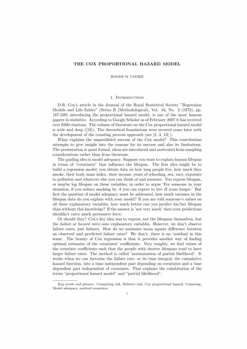
THE COX PROPORTIONAL HAZARD MODEL

ROGER M. COOKE

1. Introduction

D.R. Cox’s article in the Journal of the Royal Statistical Society ”RegressionModels and Life-Tables” (Series B (Methodological), Vol. 34, No. 2 (1972), pp.187-220) introducing the proportional hazard model, is one of the most famouspapers in statistics. According to Google Scholar as of February 2007 it has receivedover 8500 citations. The volume of literature on the Cox proportional hazard modelis wide and deep ([18]). The theoretical foundations were secured years later withthe development of the counting process approach (see [2, 3, 13] ).

What explains the unparalleled success of the Cox model? This contributionattempts to give insight into the reasons for its success and also its limitations.The presentation is quasi formal, ideas are introduced and motivated from samplingconsiderations rather than from theorems.

The guiding idea is model adequacy. Suppose you want to explain human lifespanin terms of “covariates” that influence the lifespan. The first idea might be tobuild a regression model; you obtain data on how long people live, how much theysmoke, their body mass index, their income, years of schooling, sex, race, exposureto pollution and whatever else you can think of and measure. You regress lifespan,or maybe log lifespan on these variables, in order to argue ‘For someone in yoursituation, if you reduce smoking by A you can expect to live B years longer.’ Butfirst the question of model adequacy must be addressed, how much variance in thelifespan data do you explain with your model? If you are told someone’s values onall these explanatory variables, how much better can you predict his/her lifespanthan without this knowledge? If the answer is ’not very much’ then your predictionsshouldn’t carry much persuasive force.

Or should they? Cox’s key idea was to regress, not the lifespans themselves, butthe failure or hazard rates onto explanatory variables. However, we don’t observefailure rates, just failures. How do we minimize mean square difference betweenan observed and predicted failure rates? We don’t; there is no ‘residual in thissense. The beauty of Cox regression is that it provides another way of findingoptimal estimates of the covariates’ coefficients. Very roughly, we find values ofthe covariate coefficients such that the people with shorter lifespans tend to havelarger failure rates. The method is called ’maximization of partial likelihood’. Itworks when we can factorize the failure rate, or its time integral, the cumulativehazard function, into a time independent part depending on covariates and a timedependent part independent of covariates. That explains the cohabitation of theterms “proportional hazard model” and “partial likelihood”.

Key words and phrases. Competing risk, Relative risk, Cox proportional hazard, Censoring,Model adequacy, omitted covariates.

1

2 ROGER M. COOKE

Is it all too good to be true? The goal of this contribution is to enable the readerto judge this for him/herself 1.

2. Proportional Hazard model

To simplify the presentation, we consider the case of time-invariant covariatesX, Y, Z without censoring and without ties. We consider data to be generated bythe following hazard rate

h(X,Y, Z) = Λ0(t)eXA+Y B+ZC(2.1)

where the cumulative baseline hazard function Λ0(t) =∫ t

0λ0(u)du is the time

integral of the baseline hazard rate λ0. The covariates (X, Y, Z) are considered asrandom variables. The coefficients (A,B, C) and the baseline hazard Λ0 will beestimated from life data. If this hazard function holds, then for an individual withcovariate values (x,y,z) the survivor function is

e−h(x,y,z).(2.2)

Suppose we observe times of death t1, ...tn such that ti < tj for i < j. Let thecovariates for the individual dying at time ti be denoted (xi, yi, zi). The coefficientsA,B, C are estimated by maximizing the partial likelihood

N∏

i=1

exiA+yiB+ziC

∑nj≥i exjA+yjB+zjC

(2.3)

Note that the times of death ti do not appear in (2.3). The intuitive explanationis as follows. Given that the first death in the population occurs at time t1, theprobability that it happens to individual 1 is ex1A+y1B+z1CPn

j≥1 exjA+yjB+zjC . After individual

1 is removed from the population, the same reasoning applies to the survivingpopulation; given that the second time of death t2, the probability that it happensto individual 2 is ex2A+y2B+z2CPn

j≥2 exjA+yjB+zjC , and so on. Kalbfleisch and Prentice ([16]) note

that for constant covariates, (2.3) is the likelihood for the ordering of times of death.The baseline hazard can be estimated from the data as described in ([16]p.114).

3. Model adequacy

With (x, y, z) fixed and T random, and with constant baseline hazard rate scaledto one, the survivor function (2.2), considered as a function of the random variableT is uniformly distributed on [0 , 1], that is

T ∼ −ln(U)/h.(3.1)

where U is uniform on [0, 1]. As this holds for each individual in the populationi = 1...N . If we order the values

e−tiexiA+yiB+ziC

; i = 1...N(3.2)

1The author gratefully acknowledges many helpful comments from Bo Lindqvist

THE COX PROPORTIONAL HAZARD MODEL 3

and plot them against their number, the points should lie along the diagonal if theproportional hazard model is true with coefficients A,B, C and constant baselinehazard rate. (3.2) are the exponentials of the Cox Snell residuals; equal up to aconstant to the Martingale residual, used in the counting process approach. TheCox Snell residuals are exponentially distributed if the model is correct.

This would provide an easy heuristic check of model adequacy if the baselinehazard were indeed known to be constant and scaled to one. However, if thebaseline hazard is also estimated from the data, then this simple test does notapply.

Testing model adequacy for the Cox model is not straightforward: This is asampling of statements found in the literature regarding model evaluation: ”it isnot apparent what kinds of departures one would expect to see in the residuals ifthe model is incorrect, or even to what extent agreement with the anticipated lineshould be expected” ([16], p128). ”For most purposes, you can ignore the Cox-Snell and martingale residuals. While Cox-Snell residuals were useful for assessingthe fit of the parametric models in Chapter 4, they are not very informative forthe Cox models estimated by partial likelihood” ([1], p 173). ”Unfortunately, thisdistribution theory [of the Cox Snell residuals as exponentially distributed] has notproven to be as useful for model evaluation as the theory derived from the countingprocess approach”. ([14] p. 202), ”there is not a single, simple, easy to calculate,useful, easy to interpret measure [of model performance] for a proportional hazardsmodel.” ([14] p. 229). ”the martingale residuals can not play all the roles thatlinear model residuals do; in particular the overall distribution of the residuals doesnot aid in the global assessment of fit.” ([20] p 81). In many important studies,model adequacy is not examined, and only individual coefficients for the covariateof interest are reported, with Wald confidence bounds (eg [12, 19]). The coefficientsare used to compute relative risk, and form the basis of (dis)utility calculations fordifferent risk mitigation measures.

It may well arise that data generated with a constant baseline hazard appear toacquire a time dependent baseline hazard as a result of missing covariates. Letting¦ denote values estimated from the data, we may well find that the values

e−bΛ0(ti)exiA+yiB+ziC

; i = 1...N(3.3)

plot as uniform, while the estimates do not resemble the values which generatedthe data. In particular, this may arise in the case of missing covariates. Weidentify some covariates but many others may not be represented in our model.For example, in considering the influence of airborne fine particulate matter onnon-accidental mortality [12, 19], covariates like smoking, sex, age, socio-economicstatus, air quality, and weather are studied. However time to death is obviously in-fluenced by myriad other factors like occupation, genetic disposition, stress, diseaseprevalence, medical care, diet, alcohol consumption, home environment (eg radon),travel patterns, etc.etc.

The following type of simple numerical experiment, which the reader may verifyfor him/herself will illustrate the problems with model adequacy2.

(1) Choose coefficients (A,B, C), choose a constant baseline hazard rate scaledto one, and choose a distribution for (X,Y, Z);

2The following simulations were performed with EXCEL and checked with S+.

4 ROGER M. COOKE

(2) Sample independently 100 values of (X,Y, Z) and 100 values from the uni-form distribution on [0, 1]; compute failure times using (3.1);

(3) Estimate the coefficients by maximizing (2.3), and estimate the baselinehazard.

This procedure does not require that the distributions of the covariates be cen-tered at their means; indeed, centering is not standard procedure in applications.However, the uniform distribution on [-1,1] used here is centered.

Let the model (2.1) be termed hXY Z . To study the effects of model incomplete-ness estimate the coefficient A with a model hXY using only covariates X and Y ,and with a model hX using only covariate X. For each of the models hXY Z , hXY

and hX , we repeat the above procedure 100 times with the same values for (A, B,C),with (X,Y, Z) sampled independently from the (centered) uniform distribution on[−1, 1]; however, we change (2.3) so as to estimate A in the models hXY and hX .Figure 1 plots the ordered estimates of coefficient A.

Figure 1. 100 ordered estimates of A for hXY Z , hXY , hX ,X,Y, Z ∼ U [−1, 1], (A,B, C) = (1, 1, 1); each estimate based on100 samples

Evidently, the models hXY and hX tend to underestimate the coefficient A. Atheoretical explanation of this underestimation is given in [5, 17]. Hougaard [15]shows that missing covariates sometimes result in non-proportional hazard func-tions which could be detected with sufficient replications. He concludes that ”theregression coefficients cannot be evaluated without consideration of the variabilityof neglected covariates. This is a serious drawback of relative risk models”(p.92),leading him to promote accelerated failure or frailty models. The tendency to un-derestimate becomes more pronounced in Figure (2), where the missing covariateZ has coefficient C = 5. In spite of this, the ordered values of (3.3) plot alongthe diagonal, as shown in Figure (3). If we knew that the data was created withλ0(t) ≡ 1, then we may impose this constraint on the survivor functions. FromFigure (4) we see that uniformity is lost for the incomplete models hyXY , hX ; butnot for the complete model hXY Z . This would provide an excellent diagnostic for

THE COX PROPORTIONAL HAZARD MODEL 5

completeness if we had a priori knowledge of the baseline hazard rate; unfortu-nately in practice we do not have this knowledge. We can, however, find anotherdiagnostic (see below).

Figure 2. 100 ordered estimates of A for hXY Z , hXY , hX ,X,Y, Z ∼ U [−1, 1], (A,B, C) = (1, 1, 5) each estimate based on100 samples

Figure 3. Ordered values of (3.3) for hXY Z , hXY , hX , X, Y, Z ∼U [−1, 1], (A,B, C) = (1, 1, 5)

Figure (5) shows the Wald 95% confidence bounds for A in model hX , in eachof the 100 repetitions of the experiment whose estimates are shown in Figure (2).These bounds are derived assuming asymptotic normality of the Wald statistic

A−A

σA

6 ROGER M. COOKE

Figure 4. Ordered values of (3.3) for hXY Z , hXY , hX , X, Y, Z ∼U [−1, 1], (A,B, C) = (1, 1, 5) with Λ0(t) ≡ t;

where A is the estimate of A and σA is derived from the observed information ma-trix. If the likelihood function is correct, then the Wald statistic is asymptoticallystandard normal. In as much as these 95% confidence bands contain the true valueA = 1 in only 7% of the cases, the wisdom of stating such confidence bounds whenmodel adequacy cannot be demonstrated may be questioned.

Figure 5. Wald 95% confidence bounds for A with model , hX ofFigure (2); each estimate based on 100 samples

The models hXY and hX are clearly incorrect and mis-estimate the covariateA. Relative risk coefficients based on these models would be biased. Withouta priori knowledge of the baseline hazard function, their incorrectness cannot bediagnosed using Cox-Snell or Martingale residuals, echoing the statements cited atthe beginning of this section. The problem is that the lack of fit caused by missingcovariates is compensated in the estimated baseline hazard function.

THE COX PROPORTIONAL HAZARD MODEL 7

This observation suggests that we might detect lack of fit in the covariates bycomparing the estimated baseline hazard function with the population cumulativehazard function, that is, minus the natural logarithm of the population survivorfunction. From (3.3) it is evident that adding a constant to any covariate is equiv-alent to multiplying the baseline hazard by a constant. We therefore standardizethe covariates by centering their distributions on the means (the distributions herealready centered). This standardization can be motivated as follows. If the covari-ates X, Y and Z have no effect, then their means in the set Ri of individuals atrisk at the time ti of death of the i− th individual, are just their means x, y, z. Wewrite

∑

j∈Ri

exjA+yjB+zjC ∼∑

j∈Ri

(1 + xjA)(1 + yjB)(1 + zjC).

If X,Y and Z are independent with mean zero then the mean of the right handside is just #Ri. The Breslow estimate [4] of the baseline hazard rate is

dΛ0(ti) = [∑

j∈Ri

exjA+yjB+zjC ]−1

and the population cumulative hazard rate at ti is [#Ri]−1. Hence, under theseconditions, centering the covariates at their means, then replacing covariates withtheir mean value (zero), would equate the cumulative baseline hazard function andthe population cumulative hazard function.

Figures (6, 7) show these comparisons for the two cases from Figures (1,2).Note the difference in survival times (horizontal axis); this is caused by the heavierloading of covariate Z in Figure (7). The Nelson Aalen estimator is used for thepopulation cumulative hazard function.

Figure 6. Cumulative population and baseline hazard functionsfor hXY Z , hXY , hX , X, Y, Z ∼ U [−1, 1], (A,B, C) = (1, 1, 1)

We see in Figure (7) that the cumulative baseline hazard functions for hXY andhX have moved closer to the population cumulative hazard, reflecting the heavierloading on the missing covariate Z.

8 ROGER M. COOKE

Figure 7. Cumulative population and baseline hazard functionsfor hXY Z , hyXY , hX , X, Y, Z ∼ U [−1, 1], (A,B,C) = (1, 1, 5)

If a Cox model had none of the actual covariates, this would be equivalentto having zero coefficients on all covariates; and in this case the baseline hazardwould coincide with the population cumulative hazard. A simple heuristic testof model adequacy would test the null hypothesis that the cumulative baselinehazard function is equal to the population cumulative hazard function. If the nullhypothesis cannot be rejected, then using the Cox model would not be indicated.In Figures (8, 9) the asymptotic 2-sigma bands on the asymptotic variance of theNelsen Aalen estimator of the population cumulative hazard function ([16], p.25)have been added to Figures (6, 7). We see that with this simple test we would failto reject the null hypothesis for model hX after 100 observations in both cases. Thegreater loading of missing covariate Z in Figure (9) causes the model hXY to failto reject the null hypothesis as well.

The more familiar partial likelihood ratio test calculates the test statistic G astwice the difference between the the log partial likelihood of the model containingthe covariates and the log partial likelihood for the model not containing the co-variates. G is asymptotically chi square distributed under the null hypothesis. Theabove test may have some advantage in that it does not appeal to partial likelihood.However, it is unable to detect the lack of fit in the model hXY when C = 1.

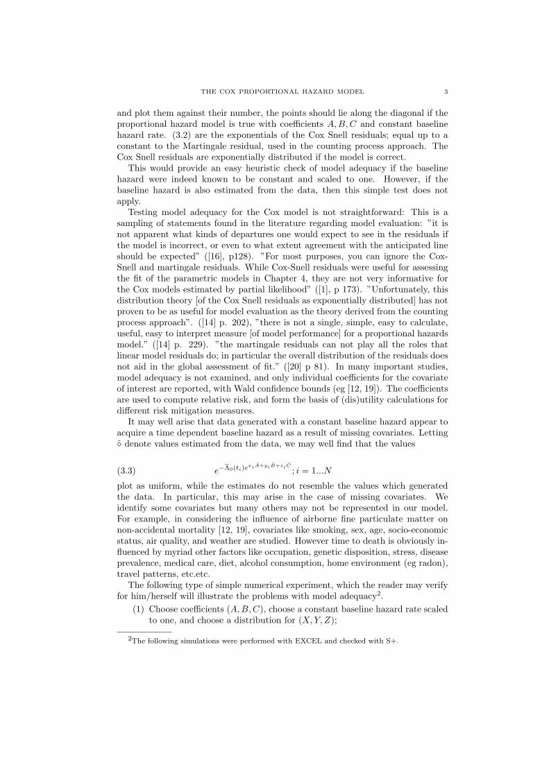
We note that for all the results mentioned above, the covariates are indepen-dent. In practice independence is not usually checked, and not always plausible.Figure (10) shows 100 estimates of the coefficient A for the models hXY Z , hyXY , hX

where the covariates are uniformly distributed on [0, 1] with correlations ρ(X, Z) =0.98, ρ(Y, Z) = 0.41 . Whereas missing covariates produce under-estimation inthe case of independence, we see that dependence in Figure(10) produces over-estimation. Note also that the spread of estimates for the complete model hXY Z isvery wide.

THE COX PROPORTIONAL HAZARD MODEL 9

Figure 8. Cumulative population and baseline hazard functionsfor hXY Z , hyXY , hX , X, Y, Z ∼ U [−1, 1], (A,B, C) = (1, 1, 5) with2-sigma confidence bands (dashed lines)

Figure 9. Cumulative population and baseline hazard functionsfor hXY Z , hyXY , hX , X, Y, Z ∼ U [−1, 1], (A,B, C) = (1, 1, 1) with2-sigma confidence bands (dashed lines)

4. Censoring and Competing Risk

The discussion of model adequacy with the proportional hazard model is some-times clouded by the role of censoring. The following statement is representative:”A perfectly adequate model may have what, at face value, seems like a terriblylow R2 due to a high percent of censored data” ([14] p. 229). The reference to R2

must be taken as metaphorical. The proportional hazard model proposes a linearregression of the log hazard function. The hazard function is not observed, andhence a measure of the difference between observed and predicted values, like R2

10 ROGER M. COOKE

Figure 10. 100 ordered estimates of A forhXY Z , hyXY , hX , X, Y, Z ∼ U [0, 1], (A,B, C) = (1, 1, 1) withdependent covariates

is not meaningful. The point is that the ability of a proportional hazard model to”explain the data” might be obscured by censoring.

Right censoring of course is a form of competing risk. In this section we reviewsome recent results from the theory of competing risk, and indicate how they mayyield diagnostic tools in proportional hazard modelling. In the competing risksapproach we model the data as a sequence of i.i.d. pairs (Ti, δi), i = 1, 2, . . ..Each T is the minimum of two or more variables, corresponding to the competingrisks. We will assume that there are two competing risks, described by two randomvariables D and C such that T = min(D,C). D will be time of death which isof primary interest, while C is a censoring time corresponding to termination ofobservation by other causes. In addition to the time T one observes the indicatorvariable δ = I(D < C) which describes the cause of the termination of observation.For simplicity we assume that P (D = C) = 0.

It is well known (Tsiatis[21]) that from observation of (T, δ) we can identify onlythe subsurvivor functions of D and C:

S∗D(t) = P (D > t, D < C) = P (T > t, δ = 1)S∗C(t) = P (C > t,C < D) = P (T > t, δ = 0),

but not in general the true survivor functions of D and C, SD(t) and SC(t). Notethat S∗D(t) depends on C, though this fact is suppressed in the notation. Note alsothat S∗D(0) = P (D < C) = P (δ = 1) and S∗C(0) = P (C < D) = P (δ = 0), so thatS∗D(0) + S∗C(0) = 1.

The conditional subsurvivor functions are defined as the survivor functions con-ditioned on the occurrence of the corresponding type of event. Assuming continuityof S∗D(t) and S∗C(t) at zero, these functions are given by

CS∗D(t) = P (D > t|D < C) = P (T > t|δ = 1) = S∗D(t)/S∗D(0)CS∗C(t) = P (C > t|C < D) = P (T > t|δ = 0) = S∗C(t)/S∗C(0).

THE COX PROPORTIONAL HAZARD MODEL 11

Closely related to the notion of subsurvivor functions is the probability of cen-soring beyond time t,

Φ(t) = P (C < D|T > t) = P (δ = 0|T > t) =S∗C(t)

S∗D(t) + S∗C(t).

This function has some diagnostic value, aiding us to choose among competing riskmodels to fit the data. Note that Φ(0) = P (δ = 0) = S∗C(0).

As mentioned above, without any additional assumptions on the joint distribu-tion of D and C, it is impossible to identify the marginal survivor functions SD(t)and SC(t). However, by making extra assumptions, one may restrict to a classof models in which the survivor functions are identifiable. A classical result oncompeting risks [21, 22] states that, assuming independence of D and C, we candetermine uniquely the survivor functions of D and C from the joint distribution of(T, δ), where at most one of the survivor functions has an atom at infinity. In thiscase the survivor functions of D and C are said to be identifiable from the censoreddata (T, δ). Hence, an independent model is always consistent with data.

If the censoring is assumed to be independent then the survivor function for T ,the minimum of D and C, can be written as

ST (t) = SD(t)SC(t)(4.1)

If we assume that D obeys a proportional hazard model, and that the censoringis independent, then we may estimate the coefficients by maximizing the partiallikelihood function adapted to account for censoring:

∏

i∈DN

exiA+yiB+ziC

∑nj≥i exjA+yjB+zjC

(4.2)

where DN is the subset of observed times t1, ...tN at which death is observed tooccur, and j runs over all times corresponding to death or censoring.

If we now substitute the survivor function with estimated coefficients into (4.1),and use the familiar Kaplan Meier estimator for SC , then we may apply the ideasof the previous section to assess model adequacy [8].

5. Conclusions

The user of the Cox proportional hazard model may be assured that if themodel is correct, then the the coefficient estimates will converge to the true values,and the confidence bands will accurately reflect sampling fluctuations around thesetrue values. If the model is not correct, however, then the coefficients’ estimatesmay not be correct, and the confidence bands may give a misleading picture. Ifthe covariates are independent, and if one or more covariates is omitted, then thecoefficients of the other covariates will be underestimated in absolute value. If thereis dependence between missing and included covariates, then nothing can be saidabout the direction of the error.

How can we check whether the model is correct? This remains the difficult point.We can test whether covariates are significantly different from zero. However, whencovariates pass this test, it does not mean that they will be estimated correctly.

12 ROGER M. COOKE

References

[1] Allison, P.D. (2003) ”Survival Analysis Using SAS a practical guide” SAS Publishing, Cary.[2] Andersen, P.K. and Gill, R.D. (1992) ”Cox’s regression model for counting processes: a large

sample study”The Annals of Statistics vol. 10, no. 4, 1100-1120.[3] Andersen, P.K., Borgan, O. Gill, R.D. and Keiding, N. (1992) Statistical Models Based on

Countinhg Processes Springer-Verlag, New York,[4] Breslow, N. (1972) Discusson on Professor cox’s paper, JRSS, B , 34, 216-217.[5] Bretagnolle, J. and Huber-Carol, C. (1988)Effects of omitting covariates in Cox’s Model for

susrvival data”Scand. J. Statist. 15, 125-138.[6] C. Bunea, R.M. Cooke, and B. Lindqvist ”Competing risk perspective over reliability data

bases” (2003), Mathematical and Statistical Methods in Relibiity (B.H. Lindqvist andK.A.Doksum eds), World Scientific Publishing, Singapore, p 355-370.

[7] C. Bunea, R.M. Cooke and B. Lindqvist,(2002) Maintenance study for components undercompeting risks, in Safety and Reliability, 1st volume, (European Safety and ReliabilityConference, ESREL 2002, Lyon, France, 18-21 March 2002), pp. 212-217.

[8] Cooke R.M. and Morales, O.(2006) ”Competing Risk and the Cox proportional hazardmodel”, Journal of Statistical Planning and Inference vol. 136, no 5 , pp. 1621-1637, 2006.

[9] R.M. Cooke, The design of reliability databases Part I and II,(1996) Reliability Engineeringand System Safety, 51, 137-146 and 209-223.

[10] R.M. Cooke and T.J. Bedford, Reliability databases in perspective (2002), IEEE Transactionson Reliability, vol. 51, no 3, (September 2002), pp. 294-310.

[11] D.R. Cox, (1972). ”Regression Models and Life-Tables” Royal Statistical Society, Series B,Vol. 34, No. 2, 1972, pp. 187-220.

[12] Dockery, D., III, C. A. P., Xu, X., Spengler, J. D., Ware, J. H., Fay, M. E., Ferris, B. G., andSpeizer, F. E. (1993). ”An association between air pollution and mortality in six U.S. cities.”New England Journal of Medicine, 329, 1753-1759.

[13] Fleming, T.R. and Harrington D.P. (1991) Counting Processes and Survival Analysis Wilely,New York.

[14] Hosmer, D.W. and Lemeshow, S. (1999) Applied Survival Analysis, Wiley, New York[15] Hougaard, P. (2000) Analysis of Multivariate Survival Data SApringer-Verlag, New York.[16] Kalbfleisch, J.D. and Prentice, R.L. (2002) The Statistical Analysis of Failure Time Data,

second edition. Wiley New York.[17] Keiding, N., Andersen, P.K., Klein, J.P. (1997) ”The role of frailty time models in describing

heterogeneity due to omitted covariates”Statistic‘s in Medicine, vol. 16, 215-224.[18] Oakes, D. (2001) ”Biometrika Centenary: Survival analysis” Biometrika 88 99-142.[19] Pope, C. A., Thun, M. J., Namboodiri, M. M., Dockery, D., Evans, J. S., Speizer, F. E., and

Heath, C. W. (1995). ”Particulate air pollution as a predictor of mortality in a prospectivestudy of U.S. adults.” American Journal of Respiratory and Critical Care Medicine, 151,669-674.

[20] Therneau, T.M. and Grambsch, P.M. (2000) Modeling Survival Data, Springer, New York.[21] A. Tsiatis, A nonidentifiability aspect of the problem of competing risks, (1975) Proceedings

of the National Academy of Sciences, USA, 72, 20-22.[22] van der Weide, J.A.M. van der, and Bedford T., “Competing risks and eternal life” (1998), in

Safety and Reliability (Proceedings of ESREL’98), S. Lydersen, G.K. Hansen, H.A. Sandtorv(eds), Vol 2, 1359-1364, Balkema, Rotterdam.

Resources for the Future, Washington DC, and Delft University of Technology,Department of Mathematics, Delft, The Netherlands

E-mail address: cooke@rff.org