A Simple Proportional Conflict Redistribution Rule

arX

iv:c

s/04

0801

0v5

[cs.

AI]

19

Sep

200

4

A Simple Proportional Conflict Redistribution Rule

Florentin Smarandache Jean DezertDept. of Mathematics ONERA/DTIM/IEDUniv. of New Mexico 29 Av. de la Division Leclerc

Gallup, NM 8730 92320 ChatillonU.S.A. France

[email protected] [email protected]

Abstract – One proposes a first alternative rule of combination to WAO (Weighted Average Operator) proposed recently by Josang,Daniel and Vannoorenberghe, called Proportional Conflict Redistribution rule (denoted PCR1). PCR1 and WAO are particular cases ofWO (the Weighted Operator) because the conflicting mass is redistributed with respect to some weighting factors. In thisfirst PCR rule,the proportionalization is done for each non-empty set withrespect to the non-zero sum of its corresponding mass matrix- instead of itsmass column average as in WAO, but the results are the same as Ph. Smets has pointed out. Also, we extend WAO (which herein givesno solution) for the degenerate case when all column sums of all non-empty sets are zero, and then the conflicting mass is transferredto the non-empty disjunctive form of all non-empty sets together; but if this disjunctive form happens to be empty, then one considersan open world (i.e. the frame of discernment might contain new hypotheses) and thus all conflicting mass is transferred tothe emptyset. In addition to WAO, we propose a general formula for PCR1(WAO for non-degenerate cases). Several numerical examples andcomparisons with other rules for combination of evidence published in literature are presented too. Another distinction between thesealternative rules is that WAO is defined on the power set, while PCR1 is on the hyper-power set (Dedekind’s lattice). A nicefeature ofPCR1, is that it works not only on non-degenerate cases but also on degenerate cases as well appearing in dynamic fusion, while WAOgives the sum of masses in this cases less than 1 (WAO does not work in these cases). Meanwhile we show that PCR1 and WAO do notpreserve unfortunately the neutrality property of the vacuous belief assignment though the fusion process. This severe drawback canhowever be easily circumvented by new PCR rules presented ina companion paper.

Keywords: WO, WAO, PCR rules, Dezert-Smarandache theory (DSmT), Datafusion, DSm hybrid rule of combination, TBM, Smets’rule, Murphy’s rule, Yager’s rule, Dubois-Prade’s rule, conjunctive rule, disjunctive rule.

1 Introduction

Due to the fact that Dempster’s rule is not mathematically defined for conflict 1 or gives counter-intuitive results for highconflict (see Zadeh’s example [22], Dezert-Smarandache-Khoshnevisan’s examples [11]), we looked for another rule,similar to Dempster’s, easy to implement due to its simple formula, and working in any case no matter the conflict. Wepresent this PCR1 rule of combination, which is an alternative of WAO for non-degenerate cases, in many examplescomparing it with other existing rules mainly: Smets’, Yager’s, Dubois-Prade’s, DSm hybride rule, Murphy’s, and ofcourse Dempster’s. PCR1 rule is commutative, but not associative nor Markovian (it is however quasi-associative andquasi-Markovian). More versions of PCR rules are proposed in a companion paper [12] to overcome the limitations ofPCR1 presented in the sequel.

2 Existing rules for combining evidence

We briefly present here the main rules proposed in the literature for combining/aggregating several independent and equi-reliable sources of evidence expressing their belief on a given finite set of exhaustive and exclusive hypotheses (Shafer’smodel). We assume the reader familiar with the Dempster-Shafer theory of evidence [10] and the recent theory of plau-sible and paradoxical reasoning (DSmT) [11]. A detailed presentation of these rules can be found in [11] and [9]. In thesequel, we consider the Shafer’s model as the valid model forthe fusion problem under consideration, unless specified.

Let Θ = {θ1, θ2, . . . , θn} be theframe of discernmentof the fusion problem under consideration havingn exhaustiveandexclusive elementaryhypothesesθi. The set of all subsets ofΘ is called thepower setof Θ and is denoted2Θ. WithinShafer’s model, abasic belief assignment(bba)m(.) : 2Θ → [0, 1] associated to a given body of evidenceB is defined by[10]

m(∅) = 0 and∑

X∈2Θ

m(X) = 1 (1)

1

http://lanl.arXiv.org/abs/cs/0408010v5

The belief (credibility) and plausibility functions ofX ⊆ Θ are defined as

Bel(X) =∑

Y ∈2Θ,Y ⊆X

m(Y ) (2)

Pl(X) =∑

Y ∈2Θ,Y ∩X 6=∅

m(Y ) = 1 − Bel(X) (3)

whereX denotes the complement ofX in Θ.

The belief functionsm(.), Bel(.) and Pl(.) are in one-to-one correspondence. The set of elementsX ∈ 2Θ having apositive basic belief assignment is called thecore/kernelof the source of evidence under consideration.

The main problem is now how to combine several belief assignments provided by a set of independent sources ofevidence. This problem is fundamental to pool correctly uncertain and imprecise information and help the decision-making. Unfortunately, no clear/unique and satisfactory answer to this problem exists since there is potentially an infinitenumber of possible rules of combination [5, 7, 9]. Our contribution here is to propose an alternative to existing ruleswhich is very easy to implement and have a legitimate behavior (not necessary the optimal one - if such optimality exists...) for practical applications.

2.1 The Dempster’s rule

The Dempster’s rule of combination is the most widely used rule of combination so far in many expert systems based onbelief functions since historically it was proposed in the seminal book of Shafer in [10]. This rule, although presentinginteresting advantages (mainly the commutativity and associativity properties) fails however to provide coherent resultsdue to the normalization procedure it involves. Discussions on the justification of the Dempster’s rule and its well-knownlimitations can be found by example in [21, 22, 23, 17]. The Dempster’s rule is defined as follows: let Bel1(.) and Bel2(.)be two belief functions provided by two independent equallyreliable sources of evidenceB1 andB2 over the sameframeΘ with corresponding belief assignmentsm1(.) andm2(.). Then the combined global belief function denotedBel(.) = Bel1(.) ⊕ Bel2(.) is obtained by combiningm1(.) andm2(.) according tom(∅) = 0 and∀(X 6= ∅) ∈ 2Θ by

m(X) =

∑

X1,X2∈2Θ

X1∩X2=X

m1(X1)m2(X2)

1 −∑

X1,X2∈2Θ

X1∩X2=∅

m1(X1)m2(X2)(4)

m(.) is a proper basic belief assignment if and only if the denominator in equation (4) is non-zero. Thedegree ofconflictbetween the sourcesB1 andB2 is defined by

k12 ,∑

X1,X2∈2Θ

X1∩X2=∅

m1(X1)m2(X2) (5)

2.2 The Murphy’s rule

The Murphy’s rule of combination [8] is a commutative but notassociative trade-off rule, denoted here with indexM ,drawn from [19, 3]. It is a special case of convex combinationof bbasm1(.) andm2(.) and consists actually in a simplearithmetic average of belief functions associated withm1(.) andm2(.). BelM (.) is then given∀X ∈ 2Θ by:

BelM (X) =1

2[Bel1(X) + Bel2(X)]

2.3 The Smets’ rule

The Smets’ rule of combination [15, 16] is the non-normalized version of the conjunctive consensus (equivalent to thenon-normalized version of Dempster’s rule). It is commutative and associative and allows positive mass on the null/emptyset∅ (i.e. open-world assumption). Smets’ rule of combination of two independent (equally reliable) sources of evidence(denoted here by indexS) is then trivially given by:

mS(∅) ≡ k12 =∑

X1,X2∈2Θ

X1∩X2=∅

m1(X1)m2(X2)

2

and∀(X 6= ∅) ∈ 2Θ, by

mS(X) =∑

X1,X2∈2Θ

X1∩X2=X

m1(X1)m2(X2)

2.4 The Yager’s rule

The Yager’s rule of combination [18, 19, 20] admits that in case of conflict the result is not reliable, so thatk12 plays therole of an absolute discounting term added to the weight of ignorance. This commutative but not associative rule, denotedhere by indexY is given1 by mY (∅) = 0 and∀X ∈ 2Θ, X 6= ∅,X 6= Θ by

mY (X) =∑

X1,X2∈2Θ

X1∩X2=X

m1(X1)m2(X2)

and whenX = Θ bymY (Θ) = m1(Θ)m2(Θ) +

∑

X1,X2∈2Θ

X1∩X2=∅

m1(X1)m2(X2)

2.5 The Dubois & Prade’s rule

The Dubois & Prade’s rule of combination [3] admits that the two sources are reliable when they are not in conflict, butone of them is right when a conflict occurs. Then if one observes a value in setX1 while the other observes this value in asetX2, the truth lies inX1 ∩X2 as longX1 ∩X2 6= ∅. If X1 ∩X2 = ∅, then the truth lies inX1 ∪ X2 [3]. According tothis principle, the commutative (but not associative) Dubois & Prade hybrid rule of combination, denoted here by indexDP , which is a reasonable trade-off between precision and reliability, is defined bymDP (∅) = 0 and∀X ∈ 2Θ, X 6= ∅by

mDP (X) =∑

X1,X2∈2Θ

X1∩X2=XX1∩X2 6=∅

m1(X1)m2(X2) +∑

X1,X2∈2Θ

X1∪X2=XX1∩X2=∅

m1(X1)m2(X2) (6)

2.6 The disjunctive rule

The disjunctive rule of combination [2, 3, 14] is a commutative and associative rule proposed by Dubois & Prade in 1986and denoted here by the index∪. m∪(.) is defined∀X ∈ 2Θ by m∪(∅) = 0 and∀(X 6= ∅) ∈ 2Θ by

m∪(X) =∑

X1,X2∈2Θ

X1∪X2=X

m1(X1)m2(X2)

The core of the belief function given bym∪ equals the union of the cores of Bel1 and Bel2. This rule reflects thedisjunctive consensus and is usually preferred when one knows that one of the sourcesB1 or B2 is mistaken but withoutknowing which one amongB1 andB2. Because we assume equi-reliability of sources in this paper, this rule will not bediscussed in the sequel.

2.7 Unification of the rules (weighted operator)

In the framework of Dempster-Shafer Theory (DST), an unifiedformula has been proposed recently by Lefevre, Colotand Vanoorenberghe in [7] to embed all the existing (and potentially forthcoming) combination rules (including the PCR1combination rule presented in the next section) involving conjunctive consensus in the same general mechanism of con-struction. We recently discovered that actually such unification formula had been already proposed 10 years before byInagaki [5] as reported in [9]. This formulation is known asthe Weighted Operator(WO) in literature [6], but since thesetwo approaches have been developed independently by Inagaki and Lefevre et al., it seems more judicious to denote itas ILCV formula instead to refer to its authors when necessary (ILCV beeing the acronym standing for Inagaki-Lefevre-Colot-Vannoorenberghe). The WO (ILCV unified fusion rule) is based on two steps.

• Step 1: Computation of the total conflicting mass based on the conjunctive consensus

k12 ,∑

X1,X2∈2Θ

X1∩X2=∅

m1(X1)m2(X2) (7)

1Θ represents here the full ignoranceθ1 ∪ θ2 ∪ . . . ∪ θn on the frame of discernment according the notation used in [10].

3

• Step 2: This step consists in the reallocation (convex combination) of the conflicting masses on(X 6= ∅) ⊆ Θ withsome given coefficientswm(X) ∈ [0, 1] such that

∑

X⊆Θ wm(X) = 1 according to

m(∅) = wm(∅) · k12

and∀(X 6= ∅) ∈ 2Θ

m(X) = [∑

X1,X2∈2Θ

X1∩X2=X

m1(X1)m2(X2)] + wm(X)k12 (8)

This WO can be easily generalized for the combination ofN ≥ 2 independent and equi-reliable sources of informationas well for step 2 by substitutingk12 by

k12...N ,∑

X1,...,XN∈2Θ

X1∩...∩XN =∅

∏

i=1,N

mi(Xi)

and for step 2 by deriving for all(X 6= ∅) ∈ 2Θ the massm(X) by

m(X) = [∑

X1,...,XN∈2Θ

X1∩...∩XN=X

∏

i=1,N

mi(Xi)] + wm(X)k12...N

The particular choice of the set of coefficientswm(.) provides a particular rule of combination. Actually this niceand important general formulation shows there exists an infinite number of possible rules of combination. Some rules arethen justified or criticized with respect to the other ones mainly on their ability to, or not to, preserve the associativityand commutativity properties of the combination. It can be easily shown in [7] that such general procedure provides allexisting rules involving conjunctive consensus developedin the literature based on Shafer’s model. We will show laterhow the PCR1 rule of combination can also be expressed as a special case of the WO.

2.8 The weighted average operator (WAO)

This operator has been recently proposed by Josang, Daniel and Vannoorenberghe in [6]. It is a particular case of WOwhere the weighting coefficientswm(A) are chosen as follows:wm(∅) = 0 and∀A ∈ 2Θ \ {∅},

wm(A) =1

N

N∑

i=1

mi(A)

whereN is the number of independent sources to combine.

2.9 The hybrid DSm rule

The hybrid DSm rule of combination is a new powerful rule of combination emerged from the recent theory of plausibleand paradoxist reasoning developed by Dezert and Smarandache, known as DSmT in literature. The foundations of DSmTare different from the DST foundations and DSmT covers potentially a wider class of applications than DST especiallyfor dealing with highly conflicting static or dynamic fusionproblems. Due to space limitations, we will not go furtherinto a detailed presentation of DSmT here. A deep presentation of DSmT can be found in [11]. The DSmT deals properlywith the granularity of information and intrinsic vague/fuzzy nature of elements of the frameΘ to manipulate. The basicidea of DSmT is to define belief assignments on hyper-power set DΘ (i.e. free Dedekind’s lattice) and to integrate allintegrity constraints (exclusivity and/or non-existential constraints) of the model, sayM(Θ), fitting with the problem intothe rule of combination. This rule, known as hybrid DSm rule works for any model (including the Shafer’s model) andfor any level of conflicting information. Mathematically, the hybrid DSm rule of combination ofN independent sourcesof evidence is defined as follows (see chap. 4 in [11]) for allX ∈ DΘ

mM(Θ)(X) , φ(X)[

S1(X) + S2(X) + S3(X)]

(9)

whereφ(X) is thecharacteristic non-emptiness functionof a setX , i.e. φ(X) = 1 if X /∈ ∅ andφ(X) = 0 otherwise,where∅ , {∅M, ∅}. ∅M is the set of all elements ofDΘ which have been forced to be empty through the constraints ofthe modelM and∅ is the classical/universal empty set.S1(X), S2(X) andS3(X) are defined by

S1(X) ,∑

X1,X2,...,XN∈DΘ

(X1∩X2∩...∩XN )=X

N∏

i=1

mi(Xi) (10)

4

S2(X) ,∑

X1,X2,...,XN∈∅

[U=X]∨[(U∈∅)∧(X=It)]

N∏

i=1

mi(Xi) (11)

S3(X) ,∑

X1,X2,...,XN∈DΘ

(X1∪X2∪...∪XN )=X

(X1∩X2∩...∩XN )∈∅

N∏

i=1

mi(Xi) (12)

with U , u(X1)∪ u(X2)∪ . . .∪ u(XN) whereu(Xi), i = 1, . . . , N , is the union of all singletonsθk, k ∈ {1, . . . , |Θ|},that composeXi andIt , θ1 ∪ θ2 ∪ . . . ∪ θn is the total ignorance.S1(X) corresponds to the conjunctive consensus onfree Dedekind’s lattice forN independent sources;S2(X) represents the mass of all relatively and absolutely empty setswhich is transferred to the total or relative ignorances;S3(X) transfers the sum of relatively empty sets to the non-emptysets.

In the case of a dynamic fusion problem, when all elements become empty because one gets new evidence on integrityconstraints (which corresponds to a specific hybrid modelM), then the conflicting mass is transferred to the total igno-rance, which also turns to be empty, therefore the empty set gets now mass which means open-world, i.e, new hypothesesmight be in the frame of discernment. For example, Let’s consider the frameΘ = {A, B} with the 2 following bbasm1(A) = 0.5, m1(B) = 0.3, m1(A ∪ B) = 0.2 andm2(A) = 0.4, m2(B) = 0.5, m2(A ∪ B) = 0.1, but one finds out

with new evidence thatA andB are truly empty, thenA ∪ B ≡ ΘM≡ ∅. Thenm(∅) = 1.

The hybrid DSm rule of combination is not equivalent to Dempter’s rule even working on the Shafer’s model. DSmTis actually a natural extension of the DST. An extension of this rule for the combination ofimprecisegeneralized (oreventually classical) basic belief functions is possible and is presented in [11].

3 The PCR1 combination rule

3.1 The PCR1 rule for 2 sources

Let Θ = {θ1, θ2} be the frame of discernment and its hyper-power setDΘ = {∅, θ1, θ2, θ1 ∪ θ2 θ1 ∩ θ2}. Two basicbelief assignments / massesm1(.) andm2(.) are defined over this hyper-power set. We assume thatm1(.) andm2(.) arenormalized belief masses following definition given by (1).The PCR1 combination rule consists in two steps:

• Step 1: Computation of the conjunctive consensus2 m∩(.) = [m1 ⊕ m2](.) and the conflicting mass according to

m∩(X) =∑

X1,X2∈DΘ

X1∩X2=X

m1(X1)m2(X2) (13)

andk12 ,

∑

X1,X2∈DΘ

X1∩X2=∅

m1(X1)m2(X2) (14)

This step coincides with the Smets’ rule of combination whenaccepting the open-world assumption. In the Smets’open-world TBM framework [13],k12 is interpreted as the massm(∅) committed to the empty set.∅ correspondsthen to all missing unknown hypotheses and the absolute impossible event.

• Step 2 (normalization): Distribution of the conflicting massk12 onto m∩(X) proportionally with the non-zerosums of their corresponding columns of non-empty sets of theeffective mass matrixM12[mij ] (index12 denotesthe list of sources entering into the mass matrix). If all sets are empty, then the conflicting mass is redistributed tothe disjunctive form of all these empty sets (which is many cases coincides with the total ignorance).

More precisely, the original mass matrixM12 is a (N = 2) × (2|Θ| − 1) matrix constructed by stacking the rowvectors {

m1 = [m1(θ1) m1(θ2) m1(θ1 ∪ θ2)]

m2 = [m2(θ1) m2(θ2) m2(θ1 ∪ θ2)]

2⊕ denotes here the generic symbol for the fusion.

5

associated with the beliefs assignmentsm1(.) andm2(.). For convenience and by convention, the row indexifollows the index of sources and the indexj for columns follows the enumeration of elements of power set2Θ

(excluding the empty set because by definition its committedmass is zero). Any permutation of rows and columnscan be arbitrarily chosen as well and it doesn’t not make any difference in the PCR1 fusion result. Thus, one hasfor the 2 sources and 2D fusion problem:

M12 =

[m1

m2

]

=

[m1(θ1) m1(θ2) m1(θ1 ∪ θ2)m2(θ1) m2(θ2) m2(θ1 ∪ θ2)

]

We denote byc12(X) the sum of the elements of the column of the mass matrix associated with elementX of thepower set, i.e

c12(X = θ1) = m1(θ1) + m2(θ1)

c12(X = θ2) = m1(θ2) + m2(θ2)

c12(X = θ1 ∪ θ2) = m1(θ1 ∪ θ2) + m2(θ1 ∪ θ2)

The conflicting massk12 is distributed proportionally with all non-zero coefficientsc12(X). For elementsX ∈ DΘ

with zero coefficientsc12(X), no conflicting mass will be distributed to them. Let’s note by w(θ1), w(θ2) andw(θ1∪θ2) the part of the conflicting mass that is respectively distributed toθ1, θ2 andθ1∪θ2 (assumingc12(θ1) > 0,c12(θ2) > 0 andc12(θ1 ∪ θ2) > 0. Then:

w(θ1)

c12(θ1)=

w(θ2)

c12(θ2)=

w(θ1 ∪ θ2)

c12(θ1 ∪ θ2)=

w(θ1) + w(θ2) + w(θ1 ∪ θ2)

c12(θ1) + c12(θ2) + c12(θ1 ∪ θ2)=

k12

d12(15)

becausec12(θ1) + c12(θ2) + c12(θ1 ∪ θ2) =

∑

X1∈DΘ\{∅}

m1(X1) +∑

X2∈DΘ\{∅}

m2(X2) = d12

Hence the proportionalized conflicting masses to transfer are given by

w(θ1) = c12(θ1) ·k12

d12

w(θ2) = c12(θ2) ·k12

d12

w(θ1 ∪ θ2) = c12(θ1 ∪ θ2) ·k12

d12

which are added respectively tom∩(θ1), m∩(θ2) andm∩(θ1 ∪ θ2).

Therefore, the general formula for the PCR1 rule for 2 sources, for |Θ| ≥ 2, is given bymPCR1(∅) = 0 and for(X 6= ∅) ∈ DΘ,

mPCR1(X) =∑

X1,X2∈DΘ

X1∩X2=X

m1(X1)m2(X2) + c12(X) ·k12

d12(16)

wherek12 is the total conflicting mass andc12(X) ,∑

i=1,2 mi(X) 6= 0, i.e. the non-zero sum of the column of themass matrixM12 corresponding to the elementX , andd12 is the sum of all non-zero column sums of all non-empty sets(in many casesd12 = 2 but in some degenerate cases it can be less).

In the degenerate case when all column sums of all non-empty sets are zero, then the conflicting mass is transferredto the non-empty disjunctive form of all sets involved in theconflict together. But if this disjunctive form happens tobe empty, then one considers an open world (i.e. the frame of discernment might contain new hypotheses) and thus allconflicting mass is transferred to the empty set.

As seen, the PCR1 combination rule works for any degree of conflict k12 ∈ [0, 1], while Dempster’s rule does notwork for k12 = 1 and gives counter-intuitive results for most of high conflicting fusion problems.

3.2 Generalization forN ≥ 2 sources

The previous PCR1 rule of combination for two sources (N = 2) can be directly and easily extended for the multi-sourcecase (N ≥ 2) as well. The general formula of the PCR1 rule is thus given bymPCR1(∅) = 0 and forX 6= ∅) ∈ DΘ

mPCR1(X) =[ ∑

X1,...,XN∈DΘ

X1∩...∩XN =X

∏

i=1,N

mi(Xi)]+ c12...N (X) ·

k12...N

d12...N

(17)

6

wherek12...N is the total conflicting mass between all theN sources which is given by

k12...N ,∑

X1,...,XN∈DΘ

X1∩...∩XN =∅

∏

i=1,N

mi(Xi) (18)

andc12...N (X) ,∑

i=1,N mi(X) 6= 0, i.e. the non-zero sum of the column of the mass matrixM12...N correspondingto the elementX , while d12...N represents the sum of all non-zero column sums of all non-empty sets (in many casesd12...N = N but in some degenerate cases it can be less).

Similarly for N sources, in the degenerate case when all column sums of all non-empty sets are zero, then the conflict-ing mass is transferred to the non-empty disjunctive form ofall sets involved in the conflict together. But if this disjunctiveform happens to be empty, then one considers an open world (i.e. the frame of discernment might contain new hypotheses)and thus all conflicting mass is transferred to the empty set.

The PCR1 rule can be seen as a cheapest, easiest implementable approximated version of the sophisticated MinC com-bination rule proposed by Daniel in [1] and [11] (chap. 10). Note also that the PCR1 rule works in the DSmT frameworkand can serve as a cheap alternative to the more sophisticated and specific DSm hybrid rule but preferentially when noneof sources is totally ignorant (see discussion in section 3.6). One applies the DSm classic rule [11] (i.e. the conjunctiveconsensus onDΘ), afterwards one identifies the model and its integrity constraints and one eventually employs the PCR1rule instead of DSm hybrid rule (depending of the dimension of the problem to solve, the number of sources involved andthe computing resources available). PCR1 can be used on the power set2Θ and within the DS Theory.

The PCR1 combination rule is commutative but not associative. It converges towards Murphy’s rule (arithmetic meanof masses) when the conflict is approaching 1, and it converges towards the conjunctive consensus rule when the conflictis approaching 0.

3.3 Implementation of the PCR1 rule

For practical use and implementation of the PCR1 combination rule, it is important to save memory space and avoiduseless computation as best as possible and especially whendealing with many sources and for frames of high dimension.To achieve this, it’s important to note that since all zero-columns of the mass matrix do not play a role in the normalization,all zero-columns (if any) of the original mass matrix can be removed tocompressthe matrix horizontally (this can be easilydone using MatLab programming language) to get an effectivemass matrix of smaller dimension for computation the setof proportionalized conflicting masses to transfer. The list of elements of power set corresponding to non-empty columsmust be maintained in parallel to this compression for implementation purpose. By example, let’s assume|Θ| = 2 andonly 2 sources providingm1(θ2) = m2(θ2) = 0 and all other masses are positive, then theeffectivemass matrix willbecome

M12 =

[m1(θ1) m1(θ1 ∪ θ2)m2(θ1) m2(θ1 ∪ θ2)

]

with now the following correspondance for column indexes:(j = 1) ↔ θ1 and(j = 2) ↔ θ1 ∪ θ2.

The computation the set of proportionalizedconflicting masses to transfer will be done using the PCR1 general formuladirectly from this previous effective mass matrix rather than from

M12 =

[m1

m2

]

=

[m1(θ1) m1(θ2) = 0 m1(θ1 ∪ θ2)m2(θ1) m2(θ2) = 0 m2(θ1 ∪ θ2)

]

3.4 PCR1 rule as a special case of WO

The PCR1 rule can be easily expressed as a special case of the WO (8) for the combination of two sources by choosing asweighting coefficients for eachX ∈ 2Θ \ {∅},

wm(X) = c12(X)/d12

For the combination ofN ≥ 2 independent and equi-reliable sources, the weighting coefficients will be given by

wm(X) = c12...N (X)/d12...N

7

3.5 Advantages of the PCR1 rule

• the PCR1 rule works in any cases, no matter what the conflict is(it may be 1 or less); Zadeh’s example, exampleswith k12 = 1 or k12 = 0.99, etc. All work;

• the implementation of PCR1 rule is very easy and thus presents a great interest for engineers who look for a cheapand an easy alternative fusion rule to existing rules;

• the PCR1 formula is simple (it is not necessary to go by proportionalization each time when fusionning);

• the PCR1 rule works quite well with respect to some other rules since the specificity of information is preserved(i.e no mass is transferred onto partial or total ignorances, neither onto the empty set as in TBM);

• the PCR1 rule reflects the majority rule;

• the PCR1 rule is convergent towards idempotence for problems with no unions or intersections of sets (we knowthat, in fact, no combination rule is idempotent, except Murphy elementary fusion mean rule);

• the PCR1 rule is similar to the classical Dempster-Shafer’srule instead of proportionalizing with respect to theresults of the conjunctive rule as is done in Dempster’s, we proportionalize with respect to the non-zero sum ofthe columns masses, the only difference is that in the DS combination rule one eliminates the denominator (whichcaused problems when the degree of conflict is 1 or close to 1);PCR1 on the power set and for non-degeneratecases gives the same results as WAO [6]; yet, for the storage proposal in a dynamic fusion when the associativityis needed, for PCR1 is needed to store only the last sum of masses, besides the previous conjunctive rules result,while in WAO it is in addition needed to store the number of thesteps and both rules become quasi-associative;

• the normalization, done proportionally with the corresponding non-zero sum of elements of the mass matrix, isnatural - because the more mass is assigned to an hypothesis by the sources the more mass that hypothesis deservesto get after the fusion.

3.6 Disadvantages of the PCR1 rule

• the PCR1 rule requires normalization/proportionalization, but the majority of rules do; rules which do not requirenormalization loose information through the transfer of conflicting mass to partial and/or total ignorances or to theempty set.

• the results of PCR1 combination rule do not bring into consideration any new set: formed by unions (uncertainties);or intersections (consensus between some hypotheses); yet, in the DSmT framework the intersections show upthrough the hyper-power set.

• the severe drawback of PCR1 and WAO rules is that they do not preserve the neutrality property of the vacuousbelief assignmentmv(.) (defined bymv(Θ) = 1) as one legitimately expects since if one or more bbasms(.),s ≥ 1, different from the vacuous belief, are combined with the vacuous belief assignment the result is not the sameas that of the combination of the bbas only (without including mv(.)), i.e. mv(.) does not act as a neutral elementfor the fusion combination.

In other words, fors ≥ 1, one gets form1(.) 6= mv(.), . . . ,ms(.) 6= mv(.):

mPCR1(.) = [m1 ⊕ . . . ms ⊕ mv](.) 6= [m1 ⊕ . . . ms](.) (19)

mWAO(.) = [m1 ⊕ . . .ms ⊕ mv](.) 6= [m1 ⊕ . . .ms](.) (20)

For the cases of the combination of only one non-vacuous belief assignmentm1(.) with the vacuous belief assign-mentmv(.) wherem1(.) has mass asigned to an empty element, saym1(∅) > 0 as in Smets’ TBM, or as in DSmTdynamic fusion where one finds out that a previous non-empty elementA, whose massm1(A) > 0, becomes emptyafter a certain time, then this mass of an empty set has to be transferred to other elements using PCR1, but for suchcase[m1 ⊕ mv](.)] is different fromm1(.).

Example: Let’s haveΘ = {A, B} and two bbas

m1(A) = 0.4 m1(B) = 0.5 m1(A ∪ B) = 0.1

m2(A) = 0.6 m2(B) = 0.2 m2(A ∪ B) = 0.2

8

together with the vacuous bbamv(Θ = A ∪ B) = 1. If one applies the PCR1 rule to combine the 3 sourcesaltogether, one gets

mPCR1|12v(A) = 0.38 + 1 ·0.38

3= 0.506667

mPCR1|12v(B) = 0.22 + 0.7 ·0.38

3= 0.308667

mPCR1|12v(A ∪ B) = 0.02 + 1.3 ·0.38

3= 0.184666

since the conjunctive consensus is given bym12v(A) = 0.38, m12v(B) = 0.22, m12v(A ∪ B) = 0.02; theconflicting mass isk12v = 0.38 and one has

x

1=

y

0.7=

z

1.3=

0.38

3

while the combination of only the sources 1 and 2 withe the PCR1 provides

mPCR1|12(A) = 0.38 + 0.19 = 0.570

mPCR1|12(B) = 0.22 + 0.133 = 0.353

mPCR1|12(A ∪ B) = 0.02 + 0.057 = 0.077

since the conjunctive consensus is given bym12(A) = 0.38, m12(B) = 0.22, m12(A ∪ B) = 0.02; the conflictingmass isk12 = 0.38 but one has now the following redistribution condition

x

1=

y

0.7=

z

0.3=

0.38

2= 0.19

Thus clearlymPCR1|12v(.) 6= mPCR1|12(.) although the third source brings no information in the fusion since itis fully ignorant. This behavior is abnormal and counter-rintuitive. WAO gives the same results in this example,therefore WAO also doesn’t satisfy the neutrality propertyof the vacuous belief assignment for the fusion. That’swhy we have improved PCR1 to PCR2-4 rules in a companion paper[12].

3.7 Comparison of the PCR1 rule with the WAO

3.7.1 The non degenerate case

Let’s compare in this section the PCR1 with the WAO for a very simple 2D general non degenerate case (none of theelements of the power set or hyper-power set of the frameΘ are known to be truly empty but the universal empty setitself) for the combination of 2 sources. Assume that the nondegenerate mass matrixM12 associated with the beliefsassignmentsm1(.) andm2(.) is given by

{

m1 = [m1(θ1) m1(θ2) m1(θ1 ∪ θ2)]

m2 = [m2(θ1) m2(θ2) m2(θ1 ∪ θ2)]

In this very simple case, the total conflict is given by

k12 = m1(θ1)m2(θ2) + m1(θ2)m2(θ1)

According to the WAO definition, one getsmWAO(∅) = wm(∅) · k12 = 0 because by definitionwm(∅) = 0. Theother weighting coefficients of WAO are given by

wm(θ1) =1

2[m1(θ1) + m2(θ1)]

wm(θ2) =1

2[m1(θ2) + m2(θ2)]

wm(θ1 ∪ θ2) =1

2[m1(θ1 ∪ θ2) + m2(θ1 ∪ θ2)]

Thus, one obtains

mWAO(θ1) = [m1(θ1)m2(θ1) + m1(θ1 ∪ θ2)m2(θ1) + m1(θ1)m2(θ1 ∪ θ2)]

+1

2[m1(θ1) + m2(θ1)] · [m1(θ1)m2(θ2) + m1(θ2)m2(θ1)]

9

mWAO(θ2) = [m1(θ2)m2(θ2) + m1(θ1 ∪ θ2)m2(θ2) + m1(θ2)m2(θ1 ∪ θ2)]

+1

2[m1(θ2) + m2(θ2)] · [m1(θ1)m2(θ2) + m1(θ2)m2(θ1)]

mWAO(θ1 ∪ θ2) = [m1(θ1 ∪ θ2)m2(θ1 ∪ θ2)] +1

2[m1(θ1 ∪ θ2) + m2(θ1 ∪ θ2)] · [m1(θ1)m2(θ2) + m1(θ2)m2(θ1)]

It is easy to verify that∑

X∈2Θ mWAO(X) = 1.

Using the PCR1 formula for 2 sources explicated in section 3.1, one hasmPCR1(∅) = 0 and the weighting coefficientsof the PCR1 rule are given by

c12(θ1) = m1(θ1) + m2(θ1)

c12(θ2) = m1(θ2) + m2(θ2)

c12(θ1 ∪ θ2) = m1(θ1 ∪ θ2) + m2(θ1 ∪ θ2)

andd12 by d12 = c12(θ1) + c12(θ2) + c12(θ1 ∪ θ2) = 2. Therefore, one finally gets:

mPCR1(θ1) = [m1(θ1)m2(θ1) + m1(θ1 ∪ θ2)m2(θ1) + m1(θ1)m2(θ1 ∪ θ2)]

+c12(θ1)

d12· [m1(θ1)m2(θ2) + m1(θ2)m2(θ1)]

mPCR1(θ2) = [m1(θ2)m2(θ2) + m1(θ1 ∪ θ2)m2(θ2) + m1(θ2)m2(θ1 ∪ θ2)]

+c12(θ2)

d12· [m1(θ1)m2(θ2) + m1(θ2)m2(θ1)]

mPCR1(θ1 ∪ θ2) = [m1(θ1 ∪ θ2)m2(θ1 ∪ θ2)] +c12(θ1 ∪ θ2)

d12· [m1(θ1)m2(θ2) + m1(θ2)m2(θ1)]

Therefore for allX in 2Θ, one hasmPCR1(X) = mWAO(X) if no singletons or unions of singletons are (or become)empty at a given time, otherwise the results are different asseen in the below three examples. This property holds for thecombination ofN > 2 sources working on an − D frame (n > 2) Θ as well if no singletons or unions of singletons are(or become) empty at a given time, otherwise the results become different.

3.7.2 The degenerate case

In the dynamic fusion, when one or more singletons or unions of singletons become empty at a certain timet whichcorresponds to a degenerate case, the WAO does not work.

Example 1: Let’s consider the Shafer’s model (exhaustivity and exclusivity of hypotheses) onΘ = {A, B, C} and thetwo following bbas

m1(A) = 0.3 m1(B) = 0.4 m1(C) = 0.3

m2(A) = 0.5 m2(B) = 0.1 m2(C) = 0.4

Then the conjunctive consensus yields

m12(A) = 0.15 m12(B) = 0.04 m12(C) = 0.12

and the conflicting massk12 = 0.69. Now assume that at timet, one finds out thatB = ∅, then the new conflict masswhich becomesk′

12 = 0.69 + 0.04 = 0.73 is re-distributed toA andB according to the WAO formula:

mWAO(B) = 0

mWAO(A) = 0.15 + (1/2)(0.3 + 0.5)(0.73) = 0.4420

mWAO(C) = 0.12 + (1/2)(0.3 + 0.4)(0.73) = 0.3755

From this WAO result, one sees clearly that the sum of the combined massesm(.) is 0.8175 < 1 while using PCR1, oneredistributes0.73 to A andB following the PCR1 formula:

mPCR1(B) = 0

mPCR1(A) = 0.15 +(0.3 + 0.5)(0.73)

(0.3 + 0.5 + 0.3 + 0.4)= 0.539333

10

mPCR1(C) = 0.12 +(0.3 + 0.4)(0.73)

(0.3 + 0.5 + 0.3 + 0.4)= 0.460667

which clearly shows that he sum of massesmPCR1(.) is 1 as expected for a proper belief assignment.

Example 2(totally degenerate case) : Let’s take exactly the same previous example with exclusive hypothesesA, B andC but assume now that at timet one finds out thatA, B andC are all truly empty, thenk′

12 = 1. In this case, the WAO isnot able to redistribute the conflict to any elementA, B, C or partial/total ignorances because they are empty. But PCR1transfers the conflicting mass to the ignoranceA∪B ∪C, which is the total ignorance herein, but this is also empty,thusthe conflicting mass is transferred to the empty set, meaningwe have an open world, i.e. new hypotheses might belong tothe frame of discernment.

Example 3 (Open-world): In the Smets’ open-world approach (when the empty set gets some mass assigned by thesources), the WAO doesn’t work either. For example, let’s considerΘ = {A, B} and the following bbasm1(∅) = 0.1,m2(∅) = 0.2 and

m1(A) = 0.4 m1(B) = 0.3 m1(A ∪ B) = 0.2

m2(A) = 0.5 m2(B) = 0.2 m2(A ∪ B) = 0.1

Then the conjunctive consensus yieldsm12(∅) = 0.28 and

m12(A) = 0.34 m12(B) = 0.13 m12(A ∪ B) = 0.02

with the conflicting massk12 = m12(A ∩ B) + m12(∅) = 0.23 + 0.28 = 0.51

Using WAO, one getsmWAO(∅) = 0

mWAO(A) = 0.34 + (1/2)(0.4 + 0.5)(0.51) = 0.5695

mWAO(B) = 0.13 + (1/2)(0.3 + 0.2)(0.51) = 0.2275

mWAO(A ∪ B) = 0.02 + (1/2)(0.2 + 0.1)(0.51) = 0.0965

The sum of massesmWAO(.) is 0.9235 < 1 while PCR1 gives:

mPCR1(∅) = 0

mPCR1(A) = 0.34 +(0.4 + 0.5)(0.51)

(0.4 + 0.5 + 0.3 + 0.2 + 0.2 + 0.1)= 0.61

mPCR1(B) = 0.13 +(0.3 + 0.2)(0.51)

(0.4 + 0.5 + 0.3 + 0.2 + 0.2 + 0.1)= 0.28

mPCR1(A ∪ B) = 0.02 +(0.2 + 0.1)(0.51)

(0.4 + 0.5 + 0.3 + 0.2 + 0.2 + 0.1)= 0.11

which shows that the sum of massesmPCR1(.) is 1.

3.7.3 Comparison of memory storages

In order to keep the associativity of PCR1 one stores the previous result of combination using the conjunctive rule, andalso the sums of mass columns [2 storages]. For the WAO one stores the previous result of combination using the con-junctive rule (as in PCR1), and the mass columns averages (but the second one is not enough in order to compute the nextaverage and that’s why one still needs to store the number of masses combined so far) [3 storages].

For example, let’sΘ = {A, B, C} and let’s suppose first that only five bbas available,m1(.), m2(.), m3(.), m4(.),m5(.), have been combined with WAO, where for examplem1(A) = 0.4, m2(A) = 0.2, m3(A) = 0.3, m4(A) = 0.6,m5(A) = 0.0. Their averagem12345(A) = 0.3 was then obtained and stored. Let’s assume now that a new bbam6(.),with m6(A) = 0.4 comes in as a new evidence. Then, how to compute with WAO the new averagem123456(A) =[m12345 ⊕ m6](A)? We need to know how many masses have been combined so far withWAO (while in PCR1 thisis not necessary). Thereforen = 5, the number of combined bbas so far, has to be stored too when using WAO insequential/iterative fusion. Whence, the new average is possible to be computed with WAO :

m123456(A) =5 · 0.3 + 0.4

5 + 1= 0.316667

11

but contrariwise to WAO, we don’t need an extra memory storage for keep in memoryn = 5 when using PCR1 tocompute3 mPCR1|123456(A) from mPCR1|12345(A) andm6(A) which is more interesting since PCR1 reduces the mem-ory storage requirement versus WAO. Indeed, using PCR1 we only store the sum of previous masses:c12345(A) =0.4 + 0.2 + 0.3 + 0.6 + 0.0 = 1.5, and when another bbam6(.) with m6(A) = 0.4 comes in as a new evidence one onlyadds it to the previous sum of masses:c123456(A) = 1.5 + 0.4 = 1.9 to get the coefficient of proportionalization for thesetA.

4 Some numerical examples

4.1 Example 1

Let’s consider a general 2D case (i.e.Θ = {θ1, θ2}) including epistemic uncertainties with the two followingbeliefassignments

m1(θ1) = 0.6, m1(θ2) = 0.3, m1(θ1 ∪ θ2) = 0.1

m2(θ1) = 0.5, m2(θ2) = 0.2, m2(θ1 ∪ θ2) = 0.3

The conjunctive consensus yields:

m∩(θ1) = 0.53, m∩(θ2) = 0.17, m∩(θ1 ∪ θ2) = 0.03

with the total conflicting massk12 = 0.27.

Applying the proportionalization from the mass matrix

M12 =

[0.6 0.3 0.10.5 0.2 0.3

]

one has

w12(θ1)

0.6 + 0.5=

w12(θ2)

0.3 + 0.2=

w12(θ1 ∪ θ2)

0.1 + 0.3=

w12(θ1) + w12(θ2) + w12(θ1 ∪ θ2)

2=

0.27

2= 0.135

and thus one deduces:

w12(θ1) = 1.1 · 0.135 = 0.1485 w12(θ2) = 0.5 · 0.135 = 0.0675 w12(θ1 ∪ θ2) = 0.4 · 0.135 = 0.0540

One addsw12(θ1) to m∩(θ1), w12(θ2) to m∩(θ2) andw12(θ1 ∪ θ2) to m∩(θ1 ∪ θ2). One finally gets the result of thePCR1 rule of combination:

mPCR1(θ1) = 0.53 + 0.1485 = 0.6785

mPCR1(θ2) = 0.17 + 0.0675 = 0.2375

mPCR1(θ1 ∪ θ2) = 0.03 + 0.0540 = 0.0840

4.2 Example 2

Let’s consider the frame of discernment with only two exclusive elements, i.e.Θ = {θ1, θ2} and consider the twofollowing Bayesianbelief assignments

m1(θ1) = 0.2, m1(θ2) = 0.8

m2(θ1) = 0.9, m2(θ2) = 0.1

The associated (effective) mass matrix will be

M12 =

[0.2 0.80.9 0.1

]

The first row ofM12 corresponds to basic belief assignmentm1(.) and the second row ofM12 corresponds to basicbelief assignmentm2(.). The columns of the mass matrixM12 correspond to focal elements ofm1(.) andm2(.) and thechoice for ordering these elements doesn’t matter. any arbitrary choice is possible. In this example the first column ofM12 is associated withθ1 and the second column withθ2.

3The notationmPCR1|12...n(.) denotes explicitly the fusion ofn bbasm1(.), m2(.), . . . ,mn(.); i.e. given the knowledge of thenbbas combined altogether.

12

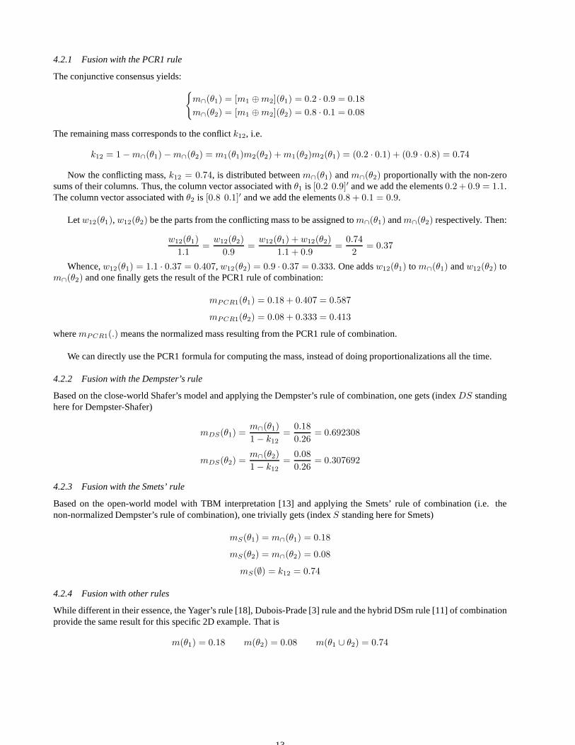
4.2.1 Fusion with the PCR1 rule

The conjunctive consensus yields:{

m∩(θ1) = [m1 ⊕ m2](θ1) = 0.2 · 0.9 = 0.18

m∩(θ2) = [m1 ⊕ m2](θ2) = 0.8 · 0.1 = 0.08

The remaining mass corresponds to the conflictk12, i.e.

k12 = 1 − m∩(θ1) − m∩(θ2) = m1(θ1)m2(θ2) + m1(θ2)m2(θ1) = (0.2 · 0.1) + (0.9 · 0.8) = 0.74

Now the conflicting mass,k12 = 0.74, is distributed betweenm∩(θ1) andm∩(θ2) proportionally with the non-zerosums of their columns. Thus, the column vector associated with θ1 is [0.2 0.9]′ and we add the elements0.2 + 0.9 = 1.1.The column vector associated withθ2 is [0.8 0.1]′ and we add the elements0.8 + 0.1 = 0.9.

Let w12(θ1), w12(θ2) be the parts from the conflicting mass to be assigned tom∩(θ1) andm∩(θ2) respectively. Then:

w12(θ1)

1.1=

w12(θ2)

0.9=

w12(θ1) + w12(θ2)

1.1 + 0.9=

0.74

2= 0.37

Whence,w12(θ1) = 1.1 · 0.37 = 0.407, w12(θ2) = 0.9 · 0.37 = 0.333. One addsw12(θ1) to m∩(θ1) andw12(θ2) tom∩(θ2) and one finally gets the result of the PCR1 rule of combination:

mPCR1(θ1) = 0.18 + 0.407 = 0.587

mPCR1(θ2) = 0.08 + 0.333 = 0.413

wheremPCR1(.) means the normalized mass resulting from the PCR1 rule of combination.

We can directly use the PCR1 formula for computing the mass, instead of doing proportionalizations all the time.

4.2.2 Fusion with the Dempster’s rule

Based on the close-world Shafer’s model and applying the Dempster’s rule of combination, one gets (indexDS standinghere for Dempster-Shafer)

mDS(θ1) =m∩(θ1)

1 − k12=

0.18

0.26= 0.692308

mDS(θ2) =m∩(θ2)

1 − k12=

0.08

0.26= 0.307692

4.2.3 Fusion with the Smets’ rule

Based on the open-world model with TBM interpretation [13] and applying the Smets’ rule of combination (i.e. thenon-normalized Dempster’s rule of combination), one trivially gets (indexS standing here for Smets)

mS(θ1) = m∩(θ1) = 0.18

mS(θ2) = m∩(θ2) = 0.08

mS(∅) = k12 = 0.74

4.2.4 Fusion with other rules

While different in their essence, the Yager’s rule [18], Dubois-Prade [3] rule and the hybrid DSm rule [11] of combinationprovide the same result for this specific 2D example. That is

m(θ1) = 0.18 m(θ2) = 0.08 m(θ1 ∪ θ2) = 0.74

13

4.3 Example 3 (Zadeh’s example)

Let’s consider the famous Zadeh’s examples [21, 22, 23, 24] with the frameΘ = {θ1, θ2, θ3}, two independent sourcesof evidence corresponding to the following Bayesian beliefassignment matrix (where columns 1, 2 and 3 correspondrespectively to elementsθ1, θ2 andθ3 and rows 1 and 2 to belief assignmentsm1(.) andm2(.) respectively), i.e.

M12 =

[0.9 0 0.10 0.9 0.1

]

In this example, one has

m∩(θ1) = [m1 ⊕ m2](θ1) = 0

m∩(θ2) = [m1 ⊕ m2](θ2) = 0

m∩(θ3) = [m1 ⊕ m2](θ3) = 0.1 · 0.1 = 0.01

and the conflict between the sources is very high and is given by

k12 = 1 − m∩(θ1) − m∩(θ2) − m∩(θ3) = 0.99


Using the PCR1 rule of combination, the conflictk12 = 0.99 is proportionally distributed tom∩(θ1), m∩(θ2), m∩(θ3)with respect to their corresponding sums of columns, i.e.0.9, 0.9, 0.2 respectively. Thus:w12(θ1)/0.9 = w12(θ2)/0.9 =w12(θ3)/0.2 = 0.99/2 = 0.495. Hence: w12(θ1) = 0.9 · 0.495 = 0.4455, w12(θ2) = 0.9 · 0.495 = 0.4455 andw12(θ3) = 0.2 · 0.495 = 0.0990. Finally the result of the PCR1 rule of combination is given by

mPCR1(θ1) = 0 + 0.4455 = 0.4455

mPCR1(θ2) = 0 + 0.4455 = 0.4455

mPCR1(θ3) = 0.01 + 0.099 = 0.109

This is an acceptable result if we don’t want to introduce thepartial ignorances (epistemic partial uncertainties). Thisresult is close to Murphy’s arithmetic mean combination rule [8], which is the following (M index standing here for theMurphy’s rule) :

mM (θ1) = (m1(θ1) + m2(θ1))/2 = (0.9 + 0)/2 = 0.45

mM (θ2) = (m1(θ2) + m2(θ2))/2 = (0 + 0.9)/2 = 0.45

mM (θ3) = (m1(θ3) + m2(θ3))/2 = (0.1 + 0.1)/2 = 0.10


The use of the Dempster’s rule of combination yields here to the counter-intuitive resultmDS(θ3) = 1. This exampleis discussed in details in [11] where several other infinite classes of counter-examples to the Dempster’s rule are alsopresented.


Based on the open-world model with TBM, the Smets’ rule of combination gives very little information, i;e.mS(θ3) =0.01 andmS(∅) = k12 = 0.99.

4.3.4 Fusion with the Yager’s rule

The Yager’s rule of combination transfers the conflicting mass k12 onto the total uncertainty and thus provides littlespecific information since one getsmY (θ3) = 0.01 andmY (θ1 ∪ θ2 ∪ θ3) = 0.99.

4.3.5 Fusion with the Dubois & Prade and DSmT rule

In zadeh’s example, the hybrid DSm rule and the Dubois-Praderule give the same result:m(θ3) = 0.01, m(θ1 ∪ θ2) =0.81, m(θ1 ∪ θ3) = 0.09 andm(θ2 ∪ θ3) = 0.09. This fusion result is more informative/specific than previous rules ofcombination and is acceptable if one wants to take into account all aggregated partial epistemic uncertainties.

4.4 Example 4 (with total conflict)

Let’s consider now the 4D case with the frameΘ = {θ1, θ2, θ3, θ4} and two independent equi-reliable sources of evidencewith the following Bayesian belief assignment matrix (where columns 1, 2, 3 and 4 correspond to elementsθ1, θ2, θ3 andθ4 and rows 1 and 2 to belief assignmentsm1(.) andm2(.) respectively)

M12 =

[0.3 0 0.7 00 0.4 0 0.6

]

14


Using the PCR1 rule of combination, one getsk12 = 1 and

m∩(θ1) = m∩(θ2) = m∩(θ3) = m∩(θ4) = 0

We distribute the conflict amongm∩(θ1), m∩(θ2), m∩(θ3) andm∩(θ4) proportionally with their sum of columns, i.e.,0.3, 0.4, 0.7 and0.6 respectively. Thus:

w12(θ1)

0.3=

w12(θ2)

0.4=

w12(θ3)

0.7=

w12(θ4)

0.6=

w12(θ1) + w12(θ2) + w12(θ3) + w12(θ4)

0.3 + 0.4 + 0.7 + 0.6=

1

2= 0.5

Thenw12(θ1) = 0.3 · 0.5 = 0.15, w12(θ2) = 0.4 · 0.5 = 0.20, w12(θ3) = 0.7 · 0.5 = 0.35 andw12(θ4) = 0.6 · 0.5 =0.30 and add them to the previous masses. One easily gets:

mPCR1(θ1) = 0.15 mPCR1(θ2) = 0.20 mPCR1(θ3) = 0.35 mPCR1(θ4) = 0.30

In this case the PCR1 combination rule gives the same result as Murphy’s arithmetic mean combination rule.


In this example, the Dempster’s rule can’t be applied since the sources are in total contradiction becausek12 = 1.Dempster’s rule is mathematically not defined because of theindeterminate form 0/0.


Using open-world assumption, the Smets’ rule provides no specific information, onlymS(∅) = 1.

4.4.4 Fusion with the Yager’s rule

The Yager’s rule gives no information either:mY (θ1 ∪ θ2 ∪ θ3 ∪ θ4) = 1 (total ignorance).

4.4.5 Fusion with the Dubois & Prade and DSmT rule

The hybrid DSm rule and the Dubois-Prade rule give here the same result:

m(θ1 ∪ θ2) = 0.12 m(θ1 ∪ θ4) = 0.18 m(θ2 ∪ θ3) = 0.28 m(θ3 ∪ θ4) = 0.42

4.5 Example 5 (convergent to idempotence)

Let’s consider now the 2D case with the frame of discernmentΘ = {θ1, θ2} and two independent equi-reliable sourcesof evidence with the following Bayesian belief assignment matrix (where columns 1 and 2 correspond to elementsθ1 andθ2 and rows 1 and 2 to belief assignmentsm1(.) andm2(.) respectively)

M12 =

[0.7 0.30.7 0.3

]

The conjunctive consensus yields here:

m∩(θ1) = 0.49 and m∩(θ2) = 0.09

with conflictk12 = 0.42.


Using the PCR1 rule of combination, one gets after distributing the conflict proportionally amongm∩(θ1) andm∩(θ2)with 0.7 + 0.7 = 1.4 and0.3 + 0.3 = 0.6 such that

w12(θ1)

1.4=

w12(θ2)

0.6=

w12(θ1) + w12(θ2)

1.4 + 0.6=

0.42

2= 0.21

whencew12(θ1) = 0.294 andw12(θ2) = 0.126 involving the following result

mPCR1(θ1) = 0.49 + 0.294 = 0.784 mPCR1(θ2) = 0.09 + 0.126 = 0.216

15


The Dempster’s rule of combination gives here:

mDS(θ1) = 0.844828 and mDS(θ2) = 0.155172


Based on the open-world model with TBM, the Smets’ rule of combination provides here:

mS(θ1) = 0.49 mS(θ2) = 0.09 mS(∅) = 0.42

4.5.4 Fusion with the other rules

The hybrid DSm rule, the Dubois-Prade rule and the Yager’s give here:

m(θ1) = 0.49 m(θ2) = 0.09 m(θ1 ∪ θ2) = 0.42

4.5.5 Behavior of the PCR1 rule with respect to idempotence

Let’s combine now with the PCR1 rule four equal sourcesm1(.) = m2(.) = m3(.) = m4(.) with mi(θ1) = 0.7 andmi(θ2) = 0.3 (i = 1, . . . , 4). The PCR1 result4 is now given by

m1234PCR1(θ1) = 0.76636 m1234

PCR1(θ2) = 0.23364

Then repeat the fusion with the PCR1 rule for eight equal sourcesmi(θ1) = 0.7 andmi(θ2) = 0.3 (i = 1, . . . , 8). Onegets now:

m1...8PCR1(θ1) = 0.717248 m1...8

PCR1(θ2) = 0.282752

ThereforemPCR1(θ1) → 0.7 andmPCR1(θ2) → 0.3. We can prove that the fusion using PCR1 rule converges towardsidempotence, i.e. fori = 1, 2

limn→∞

[m ⊕ m ⊕ . . . ⊕ m](θi)︸︷︷︸

n times

= m(θi)

in the 2D simple case with exclusive hypotheses, no unions, neither intersections (i.e. with Bayesian belief assignments).

Let Θ = {θ1, θ2} and the mass matrix

M1...n =

a 1 − aa 1 − a...

...a 1 − a

Using the general PCR1 formula, one gets for anyA 6= ∅,

limn→∞

m1...nPCR1(θ1) = an + n · a ·

k1...n

n= an + a[1 − an − (1 − a)

n] = a

becauselimn→∞ an = limn→∞ (1 − a)n

= 0 when0 < a < 1; if a = 0 or a = 1 alsolimn→∞ m1...nPCR1(θ1) = a. We

can prove similarlylimn→∞ m1...nPCR1(θ2) = 1 − a

One similarly proves the n-D,n ≥ 2, simple case forΘ = {θ1, θ2, . . . , θn} with exclusive elements when no mass ison unions neither on intersections.

4.6 Example 6 (majority opinion)Let’s consider now the 2D case with the frameΘ = {θ1, θ2} and two independent equi-reliable sources of evidence withthe following belief assignment matrix (where columns 1 and2 correspond to elementsθ1 andθ2 and rows 1 and 2 tobelief assignmentsm1(.) andm2(.) respectively)

M12 =

[0.8 0.20.3 0.7

]

Then after a while, assume that a third independent source ofevidence is introduces with belief assignmentm3(θ1) =0.3 andm3(θ2) = 0.7. The previous belief matrix is then extended/updated as follows (where the third row of matrixMcorresponds to the new sourcem3(.))

M123 =

0.8 0.20.3 0.70.3 0.7

4The verification is left to the reader.

16


The conjunctive consensus for sources 1 and 2 gives (where upper index 12 denotes the fusion of source 1 and 2)

m12∩ (θ1) = 0.24 m12

∩ (θ2) = 0.14

with conflictk12 = 0.62.

We distribute the conflict 0.62 proportionally with 1.1 and 0.9 respectively tom12∩ (θ1) andm12

∩ (θ2) such that

w12(θ1)

1.1=

w12(θ2)

0.9=

w12(θ1) + w12(θ2)

1.1 + 0.9=

0.62

2= 0.31

and thusw12(θ1) = 1.1 · 0.31 = 0.341 andw12(θ2) = 0.9 · 0.31 = 0.279.

Using the PCR1 combination rule for sources 1 and 2, one gets:

m12PCR1(θ1) = 0.24 + 0.341 = 0.581 m12

PCR1(θ2) = 0.14 + 0.279 = 0.419

Let’s combine again the previous result withm3(.) to check the majority rule (if the result’s trend is towardsm3 = m2).Consider now the following matrix (where columns 1 and 2 correspond to elementsθ1 andθ2 and rows 1 and 2 to beliefassignmentsm12

PCR1(.) andm3(.) respectively)

M12,3 =

[0.581 0.4190.3 0.7

]

The conjunctive consensus obtained fromm12PCR1(.) andm3(.) gives

m12,3∩ (θ1) = 0.1743 m12,3

∩ (θ2) = 0.2933

with conflictk12,3 = 0.5324 where the index notation 12,3 stands here for the combination of the result of the fusion ofsources 1 and 2 with the new source 3. The proportionality coefficients are obtained from

w12(θ1)

0.581 + 0.3=

w12(θ2)

0.419 + 0.7=

w12(θ1) + w12(θ2)

0.581 + 0.3 + 0.419 + 0.7=

0.5324

2= 0.2662

and thus:w12(θ1) = 0.881 · 0.2662 = 0.234522 w12(θ2) = 1.119 · 0.2662 = 0.297878

The fusion result obtained by the PCR1 after the aggregationof sources 1 and 2 with the new source 3 is:

m12,3PCR1(θ1) = 0.1743 + 0.234522 = 0.408822 m12,3

PCR1(θ2) = 0.2933 + 0.297878 = 0.591178

Thusm12,3PCR1 = [0.408822 0.591178] starts to reflect the majority opinionm2(.) = m3 = [0.3 0.7] (i.e. the mass ofθ1

becomes smaller than the mass ofθ2).

If now we apply the PCR1 rule for the 3 sources taken directly together, one gets

m123∩ (θ1) = 0.072 m123

∩ (θ2) = 0.098


Applying the proportionalization fromM123, one has

w123(θ1)

0.8 + 0.3 + 0.3=

w123(θ2)

0.2 + 0.7 + 0.7=

w123(θ1) + w123(θ2)

3=

0.83

3

Thus, the proportionalized conflicting masses to transfer ontom123∩ (θ1) andm123

∩ (θ2) are respectively given by

w123(θ1) = 1.4 ·0.83

3= 0.387333 w123(θ2) = 1.6 ·

0.83

3= 0.442667

The final result of the PCR1 rule combining all three sources together is then

m123PCR1(θ1) = 0.072 + 0.387333 = 0.459333 m123

PCR1(θ2) = 0.098 + 0.442667 = 0.540667

17

The majority opinion is reflected sincem123PCR1(θ1) < m123

PCR1(θ2). Note however that the PCR1 rule of combina-tion is clearly not associative because(m12,3

PCR1(θ1) = 0.408822) 6= (m123PCR1(θ1) = 0.459333) and(m12,3

PCR1(θ2) =0.591178) 6= (m123

PCR1(θ2) = 0.540667).

If we now combine the three previous sources altogether withthe fourth source providing the majority opinion, i.e.m4(θ1) = 0.3 andm4(θ2) = 0.7 one will get

m1234∩ (θ1) = 0.0216 m123

∩ (θ2) = 0.0686


Applying the proportionalization from mass matrix

M1234 =

0.8 0.20.3 0.70.3 0.70.3 0.7

yields

w1234(θ1) = [0.8 + 0.3 + 0.3 + 0.3] ·0.9098

4w1234(θ2) = [0.2 + 0.7 + 0.7 + 0.7] ·

0.9098

4and finally the followwing result

m1234PCR1(θ1) = 0.0216 + [0.8 + 0.3 + 0.3 + 0.3] ·

0.9098

4= 0.408265

m1234PCR1(θ2) = 0.0686 + [0.2 + 0.7 + 0.7 + 0.7] ·

0.9098

4= 0.591735

Hencem1234PCR1(θ1) is decreasing more and more whilem1234

PCR1(θ2) is increasing more and more, which reflects again themajority opinion.

4.7 Example 7 (multiple sources of information)Let’s consider now the 2D case with the frameΘ = {θ1, θ2} and 10 independent equi-reliable sources of evidence withthe following Bayesian belief assignment matrix (where columns 1 and 2 correspond to elementsθ1 andθ2 and rows 1 to10 to belief assignmentsm1(.) to m10(.) respectively)

M1...10 =

1 00.1 0.90.1 0.90.1 0.90.1 0.90.1 0.90.1 0.90.1 0.90.1 0.90.1 0.9

The conjunctive consensus operator gives here

m∩(θ1) = (0.1)9

m∩(θ2) = 0

with the conflictk1...10 = 1 − (0.1)9.


Using the general PCR1 formula (17), one gets

m1...10PCR1(θ1) = (0.1)9 + c1...10(θ1) ·

k1...10

10= (0.1)9 + (1.9) ·

1 − (0.1)9

10= (0.1)9 + (0.19) · [1 − (0.1)9]

= (0.1)9

+ 0.19 − 0.19 · (0.1)9

= (0.1)9 · 0.81 + 0.19 ≈ 0.19

m1...10PCR1(θ2) = (0.9)

9+ c1...10(θ2) ·

k1...10

10= (0.9)

9+ (8.1) ·

1 − (0.1)9

10= (0.9)

9+ (0.81) · [1 − (0.1)

9]

= (0.9)9 + 0.81 − 0.81 · (0.1)9 = (0.1)9 · 0.19 + 0.81 ≈ 0.81

The PCR1 rule’s result is converging towards the Murphy’s rule in this case, which ismM (θ1) = 0.19 andmM (θ2) =0.81.

18


In this example, the Dempster’s rule of combination givesmDS(θ1) = 1 which looks quite surprising and certainly wrongsince nine sources indicatemi(θ1) = 0.1 (i = 2, . . . , 10) and only one showsm1(θ1) = 1.


In this example when assuming open-world model, the Smets’ rule provide little specific information since one gets

mS(θ1) = (0.1)9

mS(∅) = 1 − (0.1)9

4.7.4 Fusion with the other rules

The hybrid DSm rule, the Dubois-Prade’s rule and the Yager’srule give here:

m(θ1) = (0.1)9

m(θ1 ∪ θ2) = 1 − (0.1)9

which is less specific than PCR1 result but seems more reasonable and cautious if one introduces/takes into accountepistemic uncertainty arising from the conflicting sourcesif we consider that the majority opinion does not necessaryreflect the reality of the solution of a problem. The answer tothis philosophical question is left to the reader.

4.8 Example 8 (based on hybrid DSm model)

In this last example, we show how the PCR1 rule can be applied on a fusion problem characterized by a hybrid DSmmodel rather than the Shafer’s model and we compare the result of the PCR1 rule with the result obtained from the hybridDSm rule.

Let’s consider a 3D case (i.e.Θ = {θ1, θ2, θ2}) including epistemic uncertainties with the two followingbeliefassignments

m1(θ1) = 0.4 m1(θ2) = 0.1 m1(θ3) = 0.3 m1(θ1 ∪ θ2) = 0.2

m2(θ1) = 0.6 m2(θ2) = 0.2 m2(θ3) = 0.2

We assume here ahybrid DSm model[11] (chap. 4) in which the following integrity constraintshold

θ1 ∩ θ2 = θ1 ∩ θ3 = ∅

but whereθ2 ∩ θ3 6= ∅.

The conjunctive consensus rule extended to the hyper-powersetDΘ (i.e. the Dedekind’s lattice built onΘ with unionand intersection operators) becomes now the classic DSm rule and we obtain

m∩(θ1) = 0.36 m∩(θ2) = 0.06 m∩(θ3) = 0.06 m∩(θ2 ∩ θ3) = 0.12

One works on hyper-power set (which contains, besides unions, intersections as well), not on power set as in all othertheories based on the Shafer’s model (because power set contains only unions, not intersections).

The conflicting massk12 is thus formed together by the masses ofθ1 ∩ θ2 andθ1 ∩ θ3 and is given by

k12 = m(θ1 ∩ θ2) + m(θ1 ∩ θ3) = [0.4 · 0.2 + 0.6 · 0.1] + [0.4 · 0.2 + 0.6 · 0.2] = 0.14 + 0.26 = 0.40

= 1 − m∩(θ1) − m∩(θ2) − m∩(θ3) − m∩(θ2 ∩ θ3)

The classic DSm rule (denoted here with index DSmc) providesalso

mDSmc(θ2 ∩ θ3) = 0.1 · 0.2 + 0.2 · 0.3 = 0.08 mDSmc(θ3 ∩ (θ1 ∪ θ2)) = 0.04

but sinceθ3 ∩ (θ1 ∪ θ2) = (θ3 ∩ θ1)∪ (θ3 ∩ θ2) = θ2 ∩ θ3 because integrity constraintθ1 ∩ θ3 = ∅ of the model, the totalmass committed toθ2 ∩ θ3 is finally

mDSmc(θ2 ∩ θ3) = 0.08 + 0.04 = 0.12

4.8.1 Fusion with the hybrid DSm rule

If one uses the hybrid DSm rule, one gets

mDSmh(θ1) = 0.36 mDSmh(θ2) = 0.06 mDSmh(θ3) = 0.06

mDSmh(θ1 ∪ θ2) = 0.14 mDSmh(θ1 ∪ θ3) = 0.26 mDSmh(θ2 ∩ θ3) = 0.12

19


If one uses the PCR1 rule, one has to distribute the conflicting mass 0.40 to the others according to

w12(θ1)

1.0=

w12(θ2)

0.3=

w12(θ3)

0.5=

w12(θ1 ∪ θ2)

0.2=

0.40

2= 0.20

Thus one deducesw12(θ1) = 0.20, w12(θ2) = 0.06, w12(θ3) = 0.10 andw12(θ1 ∪ θ2) = 0.04.

Nothing is distributed toθ1 ∪ θ2 because its column in the mass matrix is[0 0]′, therefore its sum is zero. Finally, onegets the following results with the PCR1 rule of combination:

mPCR1(θ1) = 0.36 + 0.20 = 0.56 mPCR1(θ2) = 0.06 + 0.06 = 0.12 mPCR1(θ3) = 0.06 + 0.10 = 0.16

mPCR1(θ1 ∪ θ2) = 0 + 0.0.4 = 0.04 mPCR1(θ2 ∩ θ3) = 0.12 + 0 = 0.12

5 Conclusion

In this paper a very simple alternative rule to WAO has been proposed for managing the transfer of epistemic uncertainty inany framework (Dempster-Shafer Theory, Dezert-Smarandache Theory) which overcomes limitations of the Dempster’srule yielding to counter-intuitive results for highly conflicting sources to combine. This rule is interesting both fromthe implementation standpoint and the coherence of the result if we don’t accept the transfer of conflicting mass topartial ignorances. It appears as an interesting compromise between the Dempster’s rule of combination and the morecomplex (but more cautious) hybrid DSm rule of combination.This first and simple Proportional Conflict Redistribution(PCR1) rule of combination works in all cases no matter how big the conflict is between sources, but when some sourcesbecome totally ignorant because in such cases, PCR1 (as WAO)does not preserve the neutrality property of the vacuousbelief assignment in the combination. PCR1 corresponds to agiven choice of proportionality coefficients in the infinitecontinuum family of possible rules of combination (i.e. weighted operator - WO) involving conjunctive consensus pointedout by Inagaki in 1991 and Lefevre, Colot and Vannoorenberghe in 2002. The PCR1 on the power set and for non-degenerate cases gives the same results as WAO; yet, for the storage proposal in a dynamic fusion when the associativityis needed, for PCR1 it is needed to store only the last sum of masses, besides the previous conjunctive rules result, whilein WAO it is in addition needed to store the number of the steps. PCR1 and WAO rules become quasi-associative. In thiswork, we extend WAO (which herein gives no solution) for the degenerate case when all column sums of all non-emptysets are zero, and then the conflicting mass is transferred tothe non-empty disjunctive form of all non-empty sets together;but if this disjunctive form happens to be empty, then one considers an open world (i.e. the frame of discernment mightcontain new hypotheses) and thus all conflicting mass is transferred to the empty set. In addition to WAO, we proposea general formula for PCR1 (WAO for non-degenerate cases). Several numerical examples and comparisons with otherrules for combination of evidence published in literature have been presented too. Another distinction between thesealternative rules is that WAO is defined on the power set2Θ, while PCR1 is on the hyper-power setDΘ. PCR1 andWAO are particular cases of the WO. In PCR1, the proportionalization is done for each non-empty set with respect to thenon-zero sum of its corresponding mass matrix - instead of its mass column average as in WAO, but the results are thesame as Ph. Smets has pointed out in non degenerate cases. In this paper, one has also proved that a nice feature of PCR1,is that it works in all cases; i.e. not only on non-degeneratecases but also on degenerate cases as well (degenerate casesmight appear in dynamic fusion problems), while the WAO doesnot work in these cases since it gives the sum of massesless than 1. WAO and PCR1 provide both however a counter-intuitive result when one or several sources become totallyignorant that why improved versions of PCR1 have been developed in a companion paper.

6 Acknowledgement

We want to thank Dr. Wu Li from NASA Langley Research Center and Dr. Philippe Smets from the Universite Libre deBruxelles for their comments, corrections, and advises.

References

[1] Daniel M., Associativity in Combination of belief functions; a derivation of minC combination, Soft Computing,7(5), pp. 288–296, 2003.

[2] Dubois D., Prade H.,A Set-Theoretic View of Belief Functions, International Journal of General Systems, pp.193-226, Vol.12, 1986.

[3] Dubois D., Prade H.,Representation and combination of uncertainty with belieffunctions and possibility measures,Computational Intelligence, 4, pp. 244-264, 1988.

20

[4] Dubois D., Prade H.,On the combination of evidence in various mathematical frameworks, Reliability Data Collec-tion and Analysis, J. Flamm and T. Luisi, Brussels, ECSC, EEC, EAFC: pp. 213-241, 1992.

[5] Inagaki T.,Interdependence between safety-control policy and multiple-senor schemes via Dempster-Shafer theory,IEEE Trans. on reliability, Vol. 40, no. 2, pp. 182-188, 1991.

[6] Josang, A., Daniel, M., Vannoorenberghe, P.,Strategies for Combining Conflicting Dogmatic Beliefs, Proceedingsof the 6th International Conference on International Fusion, Vol. 2, pp. 1133-1140, 2003.

[7] Lefevre E., Colot O., Vannoorenberghe P.,Belief functions combination and conflict management, Information Fu-sion Journal, Elsevier Publisher, Vol. 3, No. 2, pp. 149-162, 2002.

[8] Murphy C.K., Combining belief functions when evidence conflicts, Decision Support Systems, Elsevier Publisher,Vol. 29, pp. 1-9, 2000.

[9] Sentz K., Ferson S.,Combination of evidence in Dempster-Shafer Theory, SANDIA Tech. Report, SAND2002-0835,96 pages, April 2002.

[10] Shafer G.,A Mathematical Theory of Evidence, Princeton Univ. Press, Princeton, NJ, 1976.

[11] Smarandache F., Dezert J. (Editors),Applications and Advances of DSmT for Information Fusion, Am. Res. Press,Rehoboth, 2004, available athttp://www.gallup.unm.edu/˜smarandache/DSmT-book1.p df .

[12] Smarandache F., Dezert J.,Proportional Conflict Redistribution Rules for Information Fusion, 2004;The Abstract and the whole paper are available at:http://xxx.lanl.gov/abs/cs.OH/0408064 andhttp://xxx.lanl.gov/pdf/cs.OH/0408064 .

[13] Smets Ph.,The combination of evidence in the Transferable Belief Model, IEEE Trans. on Pattern Analysis andMachine Intelligence, Vol. 12, No. 5, pp. 447-458, 1990.

[14] Smets Ph.,Belief functions: the disjunctive rule of combination and the generalized Bayesian theorem, InternationalJournal of Approximate reasoning, Vol. 9, pp. 1-35, 1993.

[15] Smets Ph., Kennes R.,The transferable belief model, Artif. Intel., 66(2), pp. 191-234, 1994.

[16] Smets Ph.,Data Fusion in the Transferable Belief Model, Proc. of Fusion 2000 Intern. Conf. on Information Fusion,Paris, July 2000.

[17] Voorbraak F.,On the justification of Dempster’s rule of combination, Artificial Intelligence, 48, pp. 171-197, 1991.

[18] Yager R. R.,Hedging in the combination of evidence, Journal of Information and Optimization Science, Vol. 4, No.1, pp. 73-81, 1983.

[19] Yager R. R.,On the relationships of methods of aggregation of evidence in expert systems, Cybernetics and Systems,Vol. 16, pp. 1-21, 1985.

[20] Yager R.R.,On the Dempster-Shafer framework and new combination rules, Information Sciences, Vol. 41, pp.93–138, 1987.

[21] Zadeh L.,On the validity of Dempster’s rule of combination, Memo M 79/24, Univ. of California, Berkeley, 1979.

[22] Zadeh L.,Review of Mathematical theory of evidence, by Glenn Shafer, AI Magazine, Vol. 5, No. 3, pp. 81-83, 1984.

[23] Zadeh L.,A simple view of the Dempster-Shafer theory of evidence and its implications for the rule of combination,Berkeley Cognitive Science Report No. 33, University of California, Berkeley, CA, 1985.

[24] Zadeh L.,A simple view of the Dempster-Shafer theory of evidence and its implication for the rule of combination,AI Magazine 7, No.2, pp. 85-90, 1986.

21

A Simple Proportional Conflict Redistribution Rule

Documents

Transcript of A Simple Proportional Conflict Redistribution Rule