Rotation compatibility approach to moment redistribution for ...

Graduate Theses, Dissertations, and Problem Reports

2005

Rotation compatibility approach to moment redistribution for Rotation compatibility approach to moment redistribution for

design and rating of steel I -girders design and rating of steel I -girders

Jennifer E. Righman West Virginia University

Follow this and additional works at: https://researchrepository.wvu.edu/etd

Recommended Citation Recommended Citation Righman, Jennifer E., "Rotation compatibility approach to moment redistribution for design and rating of steel I -girders" (2005). Graduate Theses, Dissertations, and Problem Reports. 2670. https://researchrepository.wvu.edu/etd/2670

This Dissertation is protected by copyright and/or related rights. It has been brought to you by the The Research Repository @ WVU with permission from the rights-holder(s). You are free to use this Dissertation in any way that is permitted by the copyright and related rights legislation that applies to your use. For other uses you must obtain permission from the rights-holder(s) directly, unless additional rights are indicated by a Creative Commons license in the record and/ or on the work itself. This Dissertation has been accepted for inclusion in WVU Graduate Theses, Dissertations, and Problem Reports collection by an authorized administrator of The Research Repository @ WVU. For more information, please contact [email protected].

https://researchrepository.wvu.edu/

https://researchrepository.wvu.edu/

https://researchrepository.wvu.edu/etd

https://researchrepository.wvu.edu/etd?utm_source=researchrepository.wvu.edu%2Fetd%2F2670&utm_medium=PDF&utm_campaign=PDFCoverPages

https://researchrepository.wvu.edu/etd/2670?utm_source=researchrepository.wvu.edu%2Fetd%2F2670&utm_medium=PDF&utm_campaign=PDFCoverPages

mailto:[email protected]

Rotation Compatibility Approach to Moment Redistribution

for Design and Rating of Steel I-Girders

Jennifer E. Righman

Dissertation submitted to the College of Engineering and Mineral Resources

at West Virginia University

in partial fulfillment of the requirements for the degree of

Doctor of Philosophy in

Civil Engineering

Karl E. Barth, Ph.D., Chair Michael G. Barker, Ph.D.

Julio F. Davalos, Ph.D. Jacky C. Prucz, Ph.D.

John P. Zaniewski, Ph.D.

Department of Civil and Environmental Engineering

Morgantown, WV 2005

Keywords: Steel, Bridges, Design, Rating, Inelastic, Experimental Data, Finite Elements

© 2005 Jennifer E. Righman

ABSRACT

Rotation Compatibility Approach to Moment Redistribution for Design and Rating of Steel I-Girders

Jennifer E. Righman

Moment redistribution refers to the design practice where the inherent ductility of continuous-span steel bridge structures is acknowledged and consideration for the redistribution of the large negative bending moments at interior supports to the less heavily stressed positive bending regions is provided. One of the key assumptions made in moment redistribution procedures is that members have sufficient ductility to sustain a given moment capacity throughout the level of rotation required for redistribution moments to develop. However, there is presently no explicit verification that this assumption is satisfied. Instead, it is assumed that sufficient ductility can be obtained by: (1) limiting the range of girders for which moment redistribution is permissible to relatively compact members and (2) limiting the amount of moment that may be redistributed. Furthermore, the restriction of these procedures to relatively compact members has limited the potential for application of these procedures to the rating and permitting processes for existing bridge structures. The research presented herein is aimed at overcoming this limitation through a rotation compatibility approach. This method consists of direct comparison of rotation requirements for moment redistribution to available rotation (ductility) of composite or non-composite steel I-girders. An analysis procedure for determining rotation requirements is discussed along with research results illustrating the relationship between intended level of redistribution moment and required rotation for typical bridge designs. An investigation into the available rotation of typical steel I-girders is also described. It is shown that this available rotation can also be related to the intended level of redistribution moment. Thus, relating both the available and required rotations to a common parameter facilitates a direct comparison between these two quantities. The advantages of this approach compared to current design practices are also discussed. The rotation compatibility approach offers increased design economy by providing a rational basis for determining the class of sections for which moment redistribution is valid and thereby extending the applicability of the specifications. In addition to the benefits offered by this approach in new designs, there is significant potential for economic savings through application of these procedures to bridge rating.

ACKNOWLEDGEMENTS

Numerous individuals and organizations are deserving of recognition for their

contributions towards the successful completion of this dissertation. I would first like to

thank my advisor, Dr. Karl Barth, for his integral and dedicated role in helping me to

achieve my professional goals.

The experimental work performed in this project was facilitated by the assistance of

Messrs. Bill Comstock, Nate Bowe, Brandon Enochs, Laco Corder, and Alex Stinard. In

particular, the dedicated effort of Mr. Bill Comstock is sincerely appreciated.

The contributions of Ms. Lili Yang, who was instrumental in the development of many of

the tools used in the finite element analysis conducted herein, are gratefully

acknowledged. I would also like to thank Mr. Brandon Enochs for his assistance with the

final formatting of the appendices of this report.

The members of the doctoral committee for this work are Drs. Julio Davalos, Michael

Barker, Jacky Prucz, and John Zaneiwski and they are deserving of thanks for their

respective contributions to this project. I am also appreciative of Dr. David Martinelli,

Chair of the WVU Civil and Environmental Engineering Department, for his support of

this work.

Financial support for this project was provided by the West Virginia Department of

Transportation Division of Highways and is gratefully acknowledged. Fabrication of the

experimental girders included in this work was generously donated by American Bridge

Manufacturing in Coraopolis, PA. The assistance of Mr. Darko Jurkovic at American

Bridge Manufacturing is especially appreciated.

iii

I lovingly acknowledge my greatest teachers and parents, Mr. and Mrs. Jerry and Nancy

Righman, for their continuous support. And lastly, I would like to express my deep

appreciation of the countless sacrifices made by my future husband, Mr. Jesse McConnell,

who has done everything in his ability to make this task as easy as possible.

iv

TABLE OF CONTENTS

Title Page ................................................................................................................................... i

Abstract ..................................................................................................................................... ii

Acknowledgements.................................................................................................................. iii

Table of Contents..................................................................................................................... iv

List of Tables .............................................................................................................................x

List of Figures .......................................................................................................................... xi

Chapter 1: Introduction .....................................................................................1 1.1 General Theory of Moment Redistribution...............................................................5

1.2 General Theory of Rotation Compatibility ...............................................................4

1.3 Need for Current Research .........................................................................................4

1.4 Objectives......................................................................................................................6

1.5 Scope of Research ........................................................................................................7

1.6 Dissertation Organization ...........................................................................................8

Chapter 2: Literature Review..........................................................................11 2.1 Moment Redistribution Design.................................................................................11

2.1.1 Initial Inelastic Provisions (AAHSTO 1973) ......................................................11

2.1.2 Alternate Load Factor Design (AASHTO 1986).................................................12

2.1.3 Unified Autostress Method (Schilling 1989).......................................................15

2.1.4 AASHTO LRFD Specifications (AASHTO 1994 and 1998)................................15

2.1.5 AASHTO 3rd Edition LRFD Specifications (2004) .............................................16

2.2 Rating ..........................................................................................................................22

2.2.1 Elastic Rating Procedures ..................................................................................23

2.2.2 Inelastic Rating Procedures................................................................................28

2.3 Available Rotations....................................................................................................29

2.3.1 Overview of Previous Studies .............................................................................30 2.3.1.1 Experimental Studies..................................................................................................................30

v

2.3.1.2 Analytical Studies ......................................................................................................................34

2.3.2 Factors Influencing Available Rotations ............................................................38 2.3.2.1 Flange Slenderness.....................................................................................................................38

2.3.2.2 Web Slenderness ........................................................................................................................39

2.3.2.3 Lateral Bracing Distance ............................................................................................................41

2.3.2.4 Material Properties .....................................................................................................................43

2.3.2.5 Web Depth in Compression .......................................................................................................45

2.3.2.6 Relative Cross-Section Proportions............................................................................................46

2.3.2.7 Moment Gradient .......................................................................................................................46

2.3.2.8 Stiffeners ....................................................................................................................................48

2.3.2.9 Shear Force.................................................................................................................................49

2.3.2.10 Lateral Bracing Stiffness ..........................................................................................................49

2.3.2.11 Geometric Imperfections..........................................................................................................50

2.3.2.12 Axial Force...............................................................................................................................50

2.3.3 Available Rotation Prediction Equations ......................................................................51

2.4 Rotation Requirements..............................................................................................56

Chapter 3: Experimental Testing....................................................................62 3.1 General Information..................................................................................................62

3.2 Parametric Values......................................................................................................67

3.2.1 Web Slenderness .................................................................................................68

3.2.2 Compression Flange Slenderness .......................................................................69

3.2.3 Lateral Bracing...................................................................................................69

3.2.4 Cross-Section Aspect Ratio.................................................................................70

3.2.5 Material Specifications .......................................................................................70

3.2.6 Percentage of Web Depth in Compression .........................................................70

3.2.7 Comparison of Parametric Values to Previous Experimental Girders ..............71

3.3 Individual Girder Properties ....................................................................................71

3.4 Testing Procedure ......................................................................................................78

3.4.1 General Considerations ......................................................................................78

3.4.2 Data Collection...................................................................................................79

3.5 Experimental Results.................................................................................................85

3.5.1 Girder 1MG ........................................................................................................87

3.5.2 Girder 2MG ........................................................................................................89

vi

3.5.3 Girder 3MG ........................................................................................................90

3.5.4 Girder 4MG ........................................................................................................92

3.5.5 Girder 5MG ........................................................................................................93

3.5.6 Girder 6MG ........................................................................................................95

3.5.7 Girder 7MG ........................................................................................................97

3.5.8 Girder 8MG ........................................................................................................98

3.5.9 Girder 9MG ......................................................................................................101

3.5.10 Girder 10MG ..................................................................................................102

3.5.11 Girder 11MG ..................................................................................................104

3.5.12 Girder 12MG ..................................................................................................105

3.5.13 Summary of Experimental Results ..................................................................107 3.5.13.1 Moment Capacity ...................................................................................................................107

3.5.13.2 Deformed Shape.....................................................................................................................109

3.5.13.3 Deformation Capacity ............................................................................................................109

Chapter 4: Nonlinear FEA Modeling Procedures .......................................111 4.1 Mesh Density ............................................................................................................111

4.2 Element Selection.....................................................................................................112

4.2.1 Element Naming Convention ............................................................................112

4.2.2 General Purpose Shell Elements ......................................................................112

4.3 Material Modeling ...................................................................................................115

4.3.1 Von Mises Yield Criterion.................................................................................116

4.3.2 Associated Flow Rule........................................................................................117

4.3.3 Isotropic Hardening..........................................................................................117

4.3.4 Stress-Strain Relationship.................................................................................118

4.4 Geometric Imperfections.........................................................................................120

4.5 Modeling of Residual Stresses.................................................................................124

4.6 Modified Riks Algorithm ........................................................................................125

4.7 Summary...................................................................................................................130

Chapter 5: FEA of Steel I-Girders for the Determination of Moment-Rotation Characteristics.................................................................................131 5.1 FEA of Experimental Girders.................................................................................132

vii

5.2 FEA Parametric Study ............................................................................................147

5.3 FEA of Design Study Girders .................................................................................152

5.4 FEA of Extended Design Studies ............................................................................156

5.5 Discussion of FEA Results.......................................................................................160

5.6 Summary...................................................................................................................165

Chapter 6: Rotation Requirements for Steel Bridge I-Girders .................167 6.1 Background ..............................................................................................................168

6.2 Computation of Rotation Requirements................................................................169

6.2.1 Required Plastic Rotation .................................................................................169

6.2.2 Required Rotation Capacity..............................................................................175

6.3 Representative Designs............................................................................................176

6.4 Discussion of Rotation Requirements ....................................................................181

6.4.1 Moment of Inertia Considerations ....................................................................182 6.4.1.1 Influence of Ix-steel versus Ix-steel+reinforcing ....................................................................................182

6.4.1.2 Influence of Cracked Length....................................................................................................182

6.4.1.3 Influence of Material Properties...............................................................................................186

6.4.1.4 Sensitivity of Results to Ix ........................................................................................................188

6.4.2 Influence of Span Length ..................................................................................191

6.4.3 Influence of Redistribution Moment..................................................................193

6.4.4 Influence of Number of Spans ...........................................................................197

6.4.5 Required Rotation Capacity..............................................................................198

6.4.6 Development of Required Rotation Prediction Equations................................203

Chapter 7: Rotation Compatibility – Design and Rating Specifications ..................................................................207 7.1 Comparison of Available and Required Rotations ...............................................208

7.1.1 Summary of Available Rotations.......................................................................208

7.1.2 Summary of Required Rotations .......................................................................209

7.1.3 Comparison of Available and Required Rotations ...........................................210

7.1.4 Summary ...........................................................................................................218

7.2 Rotation Compatibility Design Specifications.......................................................219

viii

7.2.1 Scope .................................................................................................................219

7.2.2 Overview of Design Procedure.........................................................................219

7.2.3 Rotation Compatibility Design Specification Equations ..................................220

7.2.4 Comparison to AASHTO 2004 Moment Redistribution Procedures ................221

7.3 Rotation Compatibility Rating Specifications.......................................................224

7.3.1 Scope .................................................................................................................224

7.3.2 Overview of Rating Procedure..........................................................................224

7.3.3 Rotation Compatibility Rating Specification Equations ...................................225

7.4 Examples...................................................................................................................225

7.4.1 Design Example ................................................................................................226 7.4.1.1 Rotation Compatibility.............................................................................................................228

7.4.1.2 AASHTO 2004 – Standard Method .........................................................................................230

7.4.1.3 AASHTO 2004 – Refined Method...........................................................................................231

7.4.1.4 Comparison of Rotation Compatibility and AASHTO 2004 Designs......................................231

7.4.2 Rating Example.................................................................................................233

7.5 Summary...................................................................................................................236

Chapter 8: Summary, Conclusions, and Recommendations ......................237 8.1 Summary...................................................................................................................237

8.2 Conclusions...............................................................................................................238

8.3 Recommendations for Future Research ................................................................242

References..............................................................................................................................244

Appendix A: Nomenclature ...................................................................................................253

Appendix B: Existing Test Data ............................................................................................256

Appendix C: Material Testing Results...................................................................................296

Appendix D: FEA Moment-Rotation Curves ........................................................................302

Appendix E: Example Designs ..............................................................................................338

ix

LIST OF TABLES

Table 3-1. Stiffener Thicknesses used in Experimental Girders (in.) .........................68

Table 3-2. Parametric Values of Experimental Girders...............................................72

Table 3-3. Nominal Dimensions and Yield Strengths for Experimental Girders ......73

Table 3-4. Actual Dimensions and Yield Strengths for Experimental Girders..........74

Table 3-5. Target and Actual Parametric Values in Experimental Girders ..............75

Table 3-6. Effects of Moment Gradient Modifier, Cb ...................................................76

Table 3-7. Average Initial Imperfections in Experimental Girders ............................78

Table 3-8. Comparison of Experimental and AASHTO (2004) Capacities

(ft-kips)............................................................................................................85

Table 3-9. Deformation Capacity at M/MMAX = 0.9....................................................109

Table 5-1. Comparison of Experimental and FEA Maximum Capacities................139

Table 5-2. θRL Values in mrad (part 1) ........................................................................147

Table 5-2. θRL Values in mrad (part 2) ........................................................................148

Table 5-3. Scope of Parametric Study..........................................................................149

Table 6-1. Comparison of Rotation Requirements for Hybrid versus

Homogeneous Girders .................................................................................187

Table 6-2. Comparison of Rotation Requirements for Un-stiffened versus

Stiffened Girder ...........................................................................................189

Table 6-3. Comparison of Rotation Requirements for Sub-Optimal Girders..........190

Table 6-4. Rotation Requirements Resulting From Analysis of Experimental

Data ...............................................................................................................204

Table 7-1. Comparison of Performance Ratios from Rotation Compatibility

and Moment Redistribution Designs..........................................................232

x

LIST OF FIGURES

Figure 1-1. Illustration of Moment Redistribution Concept ...........................................2

Figure 2-1. Illustration of Effective Plastic Moment Concept.......................................13

Figure 2-2. Barth and White Moment-Rotation Model .................................................17

Figure 2-3. Strength Ratio at Mpe(30) using Eqs. 2.15 and 2.17....................................21

Figure 2-4. Strength Ratio at Mpe(9) using Eqs. 2.16 and 2.18......................................21

Figure 2-5. Strength Ratio at Mpe(30) using ALFD Mpe Equations ..............................22

Figure 2-6. Strength Ratio at Mpe(9) using ALFD Mpe Equations ................................22

Figure 2-7. Flowchart for LRFR......................................................................................25

Figure 2-8. AASHTO Legal Loads...................................................................................27

Figure 2-9. Illustration of Variable Definitions used by Kemp (1986) .........................35

Figure 2-10. Schematic Diagram of FEA Techniques used by Lääne and Lebet (2005) ..............................................................................................................38

Figure 2-11. Available Rotation versus Lateral Slenderness Ratio by Kemp and

Dekker (1991) .................................................................................................42

Figure 2-12. Diagonal Stiffener Proposed by Kemp (1986) .............................................49

Figure 2-13. Equivalent Section used by Kato (1989) ......................................................52

Figure 2-14. Available Rotation Equation Suggested by Lääne and Lebet (2005) Compared to Experimental Data .................................................................56

Figure 2-15. Definition of Rotation Capacity....................................................................57

Figure 2-16. Rotation Requirements – Kemp and Dekker (1991) ..................................59

Figure 3-1. Typical Continuous-Span Girder and Test Specimen................................62

Figure 3-2. Photograph of Experimental Setup, Viewed from Above..........................63

Figure 3-3. Photograph of Experimental Setup, Viewed from End of Girder.............64

Figure 3-4. General Test Girder Configuration, Elevation View..................................64

Figure 3-5. Lateral Bracing System used in Experimental Testing ..............................66

Figure 3-6. Lateral Frames Providing Longitudinal Restraint in Latter Stages of

Experiment .....................................................................................................67

Figure 3-7. Initial Geometric Imperfections Considered in Experimental Girders....77

Figure 3-8. Schematic Diagram of Instrumentation Used in Experimental Testing...80

Figure 3-9. Photograph of Instrumentation at Ends of Girder.....................................81

xi

Figure 3-10. Photograph of Instrumentation at Girder Centerline................................82

Figure 3-11. Photograph of Instrumentation at SL and SR ............................................83

Figure 3-12. Top Flange LVDTs ........................................................................................83

Figure 3-13. Bottom Flange LVDTs...................................................................................84

Figure 3-14. Web LVDTs....................................................................................................84

Figure 3-15. Deformed Shape of Girder 1MG..................................................................88

Figure 3-16. Load versus Displacement Data for Girder 1MG.......................................88













Figure 3-29. Deformed Shape of Girder 8MG................................................................100

Figure 3-30. Load versus Displacement Data for Girder 8MG.....................................100

Figure 3-31. Deformed Shape of Girder 9MG................................................................101

Figure 3-32. Load versus Displacement Data for Girder 9MG.....................................102

Figure 3-33. Deformed Shape of Girder 10MG..............................................................103

Figure 3-34. Load versus Displacement Data for Girder 10MG...................................104





Figure 4-1. Element Natural Coordinate System .........................................................114

Figure 4-2. Von Mises Yield Criterion...........................................................................116

Figure 4-3. Stress-Strain Relationship for Grade 50 Steel...........................................118

Figure 4-4. Stress-Strain Relationship for Grade 70 Steel...........................................119

xii

Figure 4-5. Initial Geometric Imperfections .................................................................121

Figure 4-6. Residual Stress Pattern................................................................................125

Figure 4-7. Modified Riks Algorithm ............................................................................127

Figure 5-1. FEA and Experimental Load versus Displacement Data –

Girder 1MG..................................................................................................133


Girder 2MG..................................................................................................133


Girder 3MG..................................................................................................134


Girder 4MG..................................................................................................134


Girder 5MG..................................................................................................135


Girder 6MG..................................................................................................135


Girder 7MG..................................................................................................136


Girder 8MG..................................................................................................136


Girder 9MG..................................................................................................137


Girder 10MG................................................................................................137


Girder 11MG................................................................................................138


Girder 12MG................................................................................................138

Figure 5-13. FEA and Experimental Deformed Shapes – Girder 1MG.......................140






xiii




Figure 5-22. FEA and Experimental Deformed Shapes – Girder 10MG.....................145



Figure 5-25. Moment versus Rotation – Girder CF-1-65-4-50......................................149

Figure 5-26. Moment versus Rotation – Girder SF-30-65-3-H .....................................149

Figure 5-27. Moment versus Rotation for Design Study Girders – Group 1 ...............154




Figure 5-31. Moment versus Rotation for Permutations of

Girder 120-2-E-50-20-A...............................................................................157


Girder 120-2-E-H-10-B-(S) .........................................................................158


Girder 180-2-E-50-20-B...............................................................................158


Girder 210-2-E-50-10-E...............................................................................159

Figure 5-35. θRL versus Unbraced Length for Girders Violating Current Moment

Redistribution Lateral Bracing Limits ......................................................163

Figure 5-36. Moment Rotation Model for Compact Girders (AASHTO 2004)...........164

Figure 5-37. Moment Rotation Model for Girders Violating Eq. 5.3 ...........................165

Figure 5-38. Moment versus Rotation – Girder CF-1-65-4-50......................................165

Figure 5-39. Moment versus Rotation – Girder SF-30-65-3-H .....................................166

Figure 6-1. Computation of Required Rotations in a Two-Span Continuous

Beam with Equal Span Lengths .................................................................170

Figure 6-2. Computation of Required Rotations in a Four-Span Continuous

Beam..............................................................................................................171

Figure 6-3. Definition of Variables used in Equation 6.2.............................................172

Figure 6-4. Definition of Rotation Capacity (Galambos 1968)....................................175

xiv

Figure 6-5. Representation of Negative Bending Section of Continuous-Span

Girder as Simply-Supported Beam ............................................................176

Figure 6-6. Bridge Cross-Section for Two-Span Designs.............................................177

Figure 6-7. Bridge Cross-Section for Three- and Four-Span Designs........................178

Figure 6-8. Deck Casting Sequence for Two-Span Designs .........................................179

Figure 6-9. Deck Casting Sequence for Three-Span Designs ......................................180

Figure 6-10. Deck Casting Sequence for Four-Span Designs ........................................180

Figure 6-11. Required Rotation versus Cracked Length (ft), Mrd = 20%Me,

Transition from Cracked to Composite occurs in Pier Cross-Section....184

Figure 6-12. Required Rotation versus Cracked Length (ft), Mrd = 20%Me,

Transition from Cracked to Composite occurs in Negative Bending

Region............................................................................................................185

Figure 6-13. Required Rotation versus Cracked Length (as a percentage of total

span length), Mrd = 20%Me,Transition from Cracked to Composite

occurs in Negative Bending Region............................................................186

Figure 6-14. Required Rotation for Mrd = 10%Me.........................................................191



Figure 6-17. Normalized Rotation Requirements (by percentage of redistribution

moment) for Mrd = 10%Me .........................................................................194

Figure 6-18. Normalized Rotation Requirements (by magnitude of redistribution

moment) for Mrd = 10%Me .........................................................................194

Figure 6-19. Relationship Between Percentage of Redistribution Moment and

Required Plastic Rotation ...........................................................................195

Figure 6-20. Relationship Between Magnitude of Redistribution Moment and

Required Plastic Rotation ...........................................................................196

Figure 6-21. End Rotations in Prismatic Simply-Supported Beam ..............................197

Figure 6-22. Relationship Between Percentage of Moment Redistributed and

Required Rotation Capacity .......................................................................199

Figure 6-23. Illustration of Procedure to Determine Rotation Requirements from

Experimental Moment Rotation Curves....................................................201

xv

Figure 6-24. Relationship Between Percentage of Moment Redistributed and

Required Rotation Capacity as Determined From Experimental

Results ...........................................................................................................202

Figure 6-25. Relationship Between Required Plastic Rotation and Percentage of

Redistribution Moment for Two-Span Grade 50 Designs .......................205

Figure 7-1. Moment-Rotation Models ...........................................................................209

Figure 7-2. Example Girder............................................................................................211

Figure 7-3. Comparison of Available and Required Rotations for Example

Girder with Lb satisfying Eq. 7.1 ................................................................212

Figure 7-4. Comparison of Available and Required Rotations for Example

Girder with Lb violating Eq. 7.1 .................................................................217

Figure 7-5. Design Example Bridge Cross-Section.......................................................226

Figure 7-6. Casting Sequence for Design Example.......................................................227

Figure 7-7. Rotation Compatibility and Moment Redistribution Designs .................232

Figure 7-8. Girder Elevation Rating Example..............................................................233

Figure 8-1. Moment Rotation Model .............................................................................239

xvi

Chapter 1: INTRODUCTION

This dissertation is focused on inelastic design and rating procedures for continuous-span

steel I-girder bridges. Design procedures incorporating inelastic methods are currently

incorporated in AASHTO Load and Resistance Factor Design (LRFD) Specifications (2004)

as optional provisions, termed “moment redistribution” procedures. These methods assume

that the ductility necessary for moment redistribution can be attained by implementing two

restrictions. These restrictions limit (1) the types of girders that may be used in conjunction

with moment redistribution procedures and (2) the magnitude of moment that may be

redistributed. Consequently, these requirements decrease the potential economic benefits of

inelastic design procedures. Furthermore, at the present time, moment redistribution

procedures are included in the design specifications only; these procedures are not included

in the AASHTO Load and Resistance Factor Rating (LRFR) Specifications (2003). One

primary reason for this is that the majority of existing bridge girders do not satisfy the current

requirements for use of moment redistribution provisions. Therefore, by extending the range

of girders for which moment redistribution is applicable, there is the potential for significant

economic benefits to both the design and rating processes.

To develop improved moment redistribution procedures that are valid for more slender

sections than permitted by current specifications is the primary objective of this work. This

is facilitated through a new approach to moment redistribution, termed “rotation

compatibility”. This method is founded on an explicit evaluation of the rotations required for

moment redistribution and comparison of these values to the ductility of individual girders.

The ultimate result of these procedures is design and rating specifications that do not contain

the previous restrictions on girder geometry and maximum permissible levels of

redistribution. Instead, the rotation compatibility procedures developed herein: are valid for

any girder cross-section that satisfies the cross-section proportion limits specified by

AASHTO (2004) for general steel I-girders, explicitly compute maximum levels of

redistribution, and are in a format such that the suggested procedures may be conveniently

adopted into both the AASHTO LRFD and LRFR Specifications.

1

1.1 General Theory of Moment Redistribution

In a continuous-span structure, maximum negative bending moments (at supports) typically

exceed peak positive bending moments (near midspan). Thus, as the girder is subjected to

increasing loads, yielding first occurs at the locations of peak negative moment. This

yielding (which may occur at stress levels below the yield stress of the girder due to the

presence of initial stresses resulting from the girder fabrication processes) results in

permanent inelastic rotations and residual stresses in the girder. In statically indeterminate

structures, these residual stresses are balanced by the development of residual reactions. The

moment caused by the residual reactions is termed the redistribution moment (Mrd) and is

necessarily zero at abutments and varies linearly between supports. This redistribution

moment is illustrated by the light gray line in Fig. 1-1 for a two-span continuous girder.

Figure 1-1 also illustrates the conventional elastic moment envelope for a two-span

continuous girder by the heavy black lines. Summing this elastic moment and the

redistribution moment gives the moment diagram represented by the dark gray lines in Fig.

1-1, which is the design moment used in moment redistribution procedures. Thus, in

comparison to the elastic design moments, the moment redistribution design moments are

lower in negative bending and higher in positive bending. These lower negative bending

moments are the reason that moment redistribution procedures are particularly favorable for

Distance Along Span

Mom

ent

Me

Mrd

Me + Mrd

Figure 1-1. Illustration of Moment Redistribution Concept

2

use with composite I-girder systems, which for a given cross-section have lower negative

bending capacities than positive bending capacities due to the ineffectiveness of the concrete

slab in tension. In other words, for a continuous-span composite beam of uniform cross-

section, the negative bending stresses are higher while the negative bending capacity is lower

compared to the positive bending region. Thus, moment redistribution procedures effectively

lead to a more uniform distribution between peak negative bending and positive bending

moments and a more efficient design. Because the design of the pier region of continuous-

span girders is typically controlled by bending strength requirements, designing for this

reduced level of moment has significant economic benefits. Not only does this allow for the

use of smaller cross-sections at locations of peak negative moments, but the number of flange

transitions can be reduced (which leads to both material and fabrication cost savings) and the

use of cover plates (which have unfavorable fatigue characteristics) can be eliminated. The

increased moments resulting in positive bending typically have no influence on economy as

the design of sections experiencing the highest positive bending stresses are usually not

controlled by strength requirements; instead, fatigue or serviceability considerations most

commonly govern.

In order for the assumed moment redistribution to occur, the pier section must be sufficiently

ductile such that the girder is capable of maintaining the needed moment capacity throughout

the range of rotation necessary for moment redistribution to occur. In other words, moment

redistribution will not occur without the development of inelastic rotations at the pier. The

girder must have sufficient ductility to develop the levels of inelastic rotation corresponding

to the assumed magnitude of the redistribution moments while maintaining a moment

capacity greater than or equal to the moment redistribution moments in negative bending.

Present moment redistribution specifications assume that this ductility requirement can be

satisfied by (1) limiting the range of members for which moment redistribution is permitted

to relatively compact members and (2) limiting the maximum amount of moment that may be

redistributed to 20% of the elastic moment at the piers. However, these restrictions are

conservative assumptions that limit the applicability of the moment redistribution

specifications and do not guarantee adequate ductility. Instead, adequate ductility is only

guaranteed in the present moment redistribution specifications (AASHTO 2004) by the

3

optional “refined method” for moment redistribution. Alternatively, when moment

redistribution design is performed using the more simplistic moment redistribution methods,

there is no guarantee of adequate ductility.

1.2 General Theory of Rotation Compatibility

The primary objective of the rotation compatibility procedures developed herein is to develop

a procedure to explicitly evaluate girder ductility requirements. This allows for an accurate

assessment of negative bending strength and also provides a rational means for investigating

the incorporation of more slender members in moment redistribution specifications.

Additionally, the maximum permissible level of redistribution moment can be directly

computed using this method.

The rotation compatibility approach is based on direct comparison of the ductility available

at a given level of moment for a particular girder to the required ductility for the

corresponding level of moment redistribution. This available ductility is assessed through

moment versus rotation relationships. Specifically, the moment versus rotation relationships

are obtained for a wide range of experimental and analytical girders and then compared to the

rotation required to redistribute moment from negative bending sections to positive bending

sections. In other words if the available rotation of a member is greater than that required for

moment redistribution, the intended level of moment redistribution is acceptable. Otherwise,

the intended level of moment redistribution must be reduced in accordance with the available

rotation capacity of the member.

1.3 Need for Current Research

As suggested by the above discussion, there is a need for improving the existing moment

redistribution specifications for steel I-girder bridges. The primary limitation of the existing

procedures is that the conservative assumptions made in an attempt to provide adequate

ductility restrict the range of girders for which moment redistribution is permissible and the

maximum levels of moment that may be redistributed. Not only does this decrease the

economy that may result from implementing these procedures in new designs, but also

renders the procedures too restrictive to be used in rating, as many existing bridges have

4

geometries that do not satisfy the current limits. Furthermore, as there is no explicit

evaluation of girder ductility in the basic moment redistribution provisions, there is the

potential to assume that higher levels of moment may be redistributed than that which

actually occurs, ultimately leading to failure in the pier regions of these girders. Thus a more

rational assessment of girder ductility is needed.

The current range of girders that may be used in conjunction with moment redistribution

provisions excludes many typical bridges from use unless they are specifically designed to

target these limits. These limitations are most significant in terms of required lateral bracing

distance and compression flange slenderness. The current lateral bracing limit is particularly

restrictive such that (1) many existing bridges would not satisfy this requirement, which has

implications for the rating process, and (2) the number of cross-frames necessary in new

bridge designs incorporating moment redistribution procedures is typically increased

compared to the requirements for a conventional elastic design. Thus, there is a specific need

to increase the range of applicability of the moment redistribution specification with respect

to these two limits. Research addressing extending the range of flange slenderness and

lateral bracing values applicable for moment redistribution is anticipated to have positive

economic impacts.

Additionally, there is a need to better assess the maximum levels of redistribution that are

permissible. While the current procedures assume that the same level of redistribution (20%

of the maximum negative moment) may be used for all designs, it is more rational to relate

the amount of moment that may be redistributed to the girder and bridge properties. This is

especially true if the range of girders for which moment redistribution is applicable is

increased, as a lower level of redistribution may be required for more slender members.

There are cases where the current moment redistribution procedures result in required cross-

sections in negative bending regions that are larger than those required using elastic

procedures. This occurs because, while the moment redistribution procedures allow for a

decrease in applied moment, the moment capacity is also reduced in some cases, irrespective

of the amount of moment being redistributed. Thus, because the sum of the moment capacity

5

of the girder and the redistribution moment must equal a quantity greater than the elastic

moment, in cases where the allowable moment capacity that results from the use of the

moment redistribution procedures is substantially lower than the conventional (elastic)

moment capacity and the amount of moment being redistributed is relatively small (typically

10% or less of the elastic moment), the sum of these two quantities, and therefore the elastic

moment which the girder can support, is less than the elastic moment capacity that results

from use of the elastic strength prediction equations. Consequently, moment redistribution is

of no benefit in these cases. Research is needed to address this inconsistency between the

elastic and moment redistribution procedures.

Current AASHTO (Load and Resistance Factor Rating, LRFR, 2003 and LRFD 2004)

provisions assume a consistent level of strength in both the design and rating specifications.

Therefore, it should by extension also be possible to utilize the optional moment

redistribution specifications contained in the LRFD specifications for load rating. However,

no method exists at the present time for incorporating these methods into the rating

procedures. The creation of moment redistribution specifications for bridge rating is

anticipated to have positive economic impacts as the reserve capacity of continuous-span

bridges can be accounted for during the rating process and the bridges most in need of

corrective action can then be identified.

1.4 Objectives

The primary objectives of this work are as follows.

• Explicitly evaluate the ductility requirements for moment redistribution resulting in

increased safety.

• Investigate the use of moment redistribution procedures for a broader range of girder

geometries, particularly with respect to longer unbraced lateral distances and

increased compression flange slenderness. This may also allow for the procedures to

be utilized with in-service bridges that were not necessarily designed to meet specific

compactness requirements.

• Evaluate the maximum permissible levels of moment that may be safely redistributed.

6

• Develop moment redistribution specifications for steel I-girder rating. This will result

in a more uniform level of safety throughout the bridge inventory, as suggested by

Barker and Zacher (1997).

1.5 Scope of Research

This research focuses on the inelastic behavior of steel bridge I-girders and the scope of this

project consists of four primary components: experimental testing; finite element analysis;

study of rotation requirements; and development of design and rating specifications.

Experimental testing of twelve large-scale plate girders is conducted to obtain the moment-

rotation characteristics of members that are typical of those used in the negative bending

sections of continuous-span I-girders. These girders are unique in that the slenderness

properties (i.e., flange slenderness, web slenderness, and lateral slenderness) of these girders

are higher than the values of these parameters that have been incorporated in previous

experimental programs. Because one of the primary reasons for presently limiting the range

of applicability of moment redistribution designs to relatively compact members is a lack of

experimental evidence suggesting that such procedures are appropriate for more slender

girders, such testing is necessary in order to investigate the applicability of moment

redistribution procedures to girders that are more slender than currently permitted by these

procedures.

The results of this testing are further used to validate the finite element analysis (FEA)

procedures implemented in this work. A comprehensive finite element study is conducted

where the two primary focuses are a parametric study and FEA of girders resulting from a

moment redistribution design study. From these efforts data regarding the available rotations

of a large number of typical girders is obtained.

In order to investigate rotations requirements for moment redistribution, consideration is first

given to determining an appropriate analysis procedure. This analysis procedure is then used

to calculate rotation requirements for typical moment redistribution designs and these

7

resulting rotation requirements are used to determine empirical rotation requirement

expressions.

The final component of this work is the development of the rotation compatibility procedure,

which facilitates direct comparison of the available and required rotations. The conditions

necessary to assure that the available rotations are greater than the required rotations are

investigated and this information is then synthesized into a format appropriate for

incorporation into AASHTO design and rating specifications.

1.6 Dissertation Organization

The body of this report consists of eight chapters. This first chapter, Introduction, provides

general background information of this project, discusses the need for this research, and

highlights the main objectives of this work.

The second chapter, Literature Review, discusses the previous research that has been

conducted related to the present work. Specifically, this chapter is organized into four

sections. These are: (1) an overview of inelastic bridge design methods that have previously

been proposed and/or implemented into AASHTO Specifications; (2) a description of

AASHTO rating procedures and previous studies on inelastic rating procedures; (3) a

presentation of previous research on the moment-rotation characteristics, i.e., ductility, of

steel and steel-concrete composite I-girders; and (4) a review of studies focused on the

rotation requirements for inelastic design.

The experimental testing program is described in Chapter 3, Experimental Testing. Here

information on the testing configuration and procedures is given along with a detailed

description of each of the test girders and the experimental results. The experimental results

presented include the maximum moment capacities, deformed shapes, and rotation

characteristics of each girder.

8

Chapter 4, Nonlinear FEA Modeling Procedures, discusses the finite element procedures

used in this work. Mesh densities, element types, material modeling procedures, geometric

imperfections, residual stresses, and solution algorithms are considered in this chapter.

The FEA parametric study is presented in Chapter 5, Moment – Rotation Characteristics of

Steel I-Girders. The first section of this chapter validates the FEA methods described in

Chapter 4 by presenting the results from FEA of each of the experimental girders discussed

in Chapter 3 and comparing this data to the experimental results. The ductility of negative

bending sections of continuous-span I-girders is then explored through additional FEA

studies. Specifically, this work consists of two components. First, a parametric study is

presented where the ductility of girders with high slenderness ratios are investigated.

Additionally, a series of typical bridge designs is created and FEA results of these girders

provide further insight into the moment-rotation characteristics of negative bending sections.

This chapter concludes with the development of moment-rotation models that may be used to

describe steel I-girder behavior.

Chapter 6, Rotation Requirements for Steel Bridge I-Girders, details the investigation into the

rotation requirements for moment redistribution. While there have been no previous studies

specifically focused on rotation requirements for moment redistribution, previous studies

have researched rotation requirements for other purposes; the first section of this chapter

discusses the relevance of these studies, which are presented in Chapter 2, to the present

work. The second section of this chapter then presents the analysis method used to determine

rotation requirements. Because rotation requirements for a given member are a function of

its section properties, determining representative section properties was also necessary. Thus

a series of design studies was conducted to obtain representative section properties; a

discussion of this design study is presented in the third section of Chapter 6. The final

section of this chapter discusses the affects of the various parameters investigated on rotation

requirements and concludes with the presentation of mathematical expressions to predict the

rotation requirements in continuous-span I-girders.

9

The development of the rotation compatibility procedure is the focus of Chapter 7, Rotation

Compatibility – Design and Rating Specifications. First, the expressions for available and

required rotations are used to establish the conditions necessary to assure that the available

rotation is greater than that required for moment redistribution. This information is then used

to develop the rotation compatibility specifications for design and rating. This section

concludes with the presentation of design and rating examples illustrating the use of the

suggested procedures.

Chapter 8, Summary, Conclusions, and Recommendations, summarizes the results of this

work. Recommendations for future research in this area are also given.

The body of this dissertation is followed by a list of references cited and five Appendices.

Appendix A defines the nomenclature used in this dissertation. The moment-rotation

behavior of girders tested in the present and previous experimental studies is presented in

Appendix B. Appendix C contains data resulting from tension testing performed on coupons

taken from the steel used to fabricate the experimental girders tested in this work. The

moment-rotation behavior of the girders analyzed in the FEA study is included in Appendix

D. Lastly, Appendix E contains the designs resulting from the moment redistribution design

study described in Chapter 6.

10

Chapter 2: LITERATURE REVIEW

As discussed in Chapter 1, the objective of this work is to develop moment redistribution

specifications for design and rating of steel I-girder bridges that assure the available rotation

of a cross-section is greater than the rotation required to redistribute moment. Consequently,

the literature review for this work consists of four components: a review of previous moment

redistribution design provisions; an overview of rating procedures with a specific focus on

inelastic rating methods; and a presentation of previous research related to the available and

required rotations of steel members. The available literature on each of these three subjects

is summarized in this chapter. Specifically, Section 2.1, Moment Redistribution Design,

presents a historical overview of the various inelastic design procedures that have been

incorporated into past editions of AASHTO Specifications. Section 2.2, Inelastic Rating

Methods, provides an overview of bridge rating procedures and summarizes previous

research on inelastic rating methods. In order for moment redistribution procedures to be

based on a rotation compatibility approach, both the required rotation and available rotation

must be known. Studies on the behavior of steel I-girders in negative bending, from which

conclusions can be made regarding the available rotation of these members are presented in

Section 2.3, Available Rotation. A discussion of previous research on rotation requirements

for these types of members is given in Section 2.4, Rotation Requirements.

2.1 Moment Redistribution Design

2.1.1 Initial Inelastic Provisions (AAHSTO 1973)

Past editions of the American Association of State Highway and Transportation Officials

(AASHTO) specifications have accounted for the increase in strength due to inelastic

behavior using various methods. A simple method for approximating the effects of inelastic

behavior was first incorporated in the 11th edition of the specifications (AASHTO, 1973).

Specifically, these specifications accounted for the inelastic behavior of continuous span

girders in two ways. First, the maximum moment capacity of the girder was increased from

the yield moment to the plastic moment for girders satisfying certain compactness criteria.

11

Secondly, 10% of the peak negative moment was permitted to be redistributed to the positive

bending section prior to evaluating the capacity at the maximum load level.

2.1.2 Alternate Load Factor Design (AASHTO 1986)

Comprehensive inelastic procedures were first given in the Guide Specifications for

Alternate Load Factor Design (ALFD) (AASHTO 1986), which were applicable to compact

sections. Similar to the AASHTO Load Factor Design (LFD) procedures, ALFD procedures

required a service load check, overload check, and maximum load check. The service load

checks were identical for both design philosophies but alternative methods were used for the

evaluation of the overload and maximum load checks in ALFD.

In the overload check in ALFD, which is analogous to the Service II limit state in the current

AASHTO LRFD procedures, the moment capacity at the pier was obtained using the beam-

line method. This method made use of a continuity relationship (which was a function of the

applied loading) and a moment-rotation relationship (which was based on experimental

results). A simultaneous solution of these two expressions yielded the moment capacity and

corresponding rotation at that load level.

The maximum load check in ALFD (Strength I in AASHTO LRFD) was based on a

mechanism (plastic collapse) approach. The design requirements at this load level were

simplified by using the concept of an effective plastic moment as suggested by Grubb and

Carskaddan (1981), discussed below, in that if the applied moment was less than the effective

plastic moment, then the maximum load check was assumed to be satisfied.

The concept of an effective plastic moment was first introduced by Haaijer et al. (1980).

This idea was initiated out of a desire to extend the applicability of plastic design procedures

to a broader range of cross sections and thereby increase the economical benefits that could

be achieved by using these methods. At the time, plastic design procedures for buildings

were specified by the American Institute of Steel Construction (AISC 1973), but were limited

to sections satisfying rather stringent web and compression flange slenderness ratios;

12

specifically, a cross section was required to have flange and web slenderness ratios satisfying

(adapted from Schilling et al., 1997)

/ 2 0.291 /fc fc yfb t E F≤ and (2.1)

2 / 2.3 /cp w ywD t E F≤ , (2.2)

where variable definitions for all equations are presented in Appendix A. These

requirements were based on the premise that sections need to be rather compact in order to

have sufficient rotation capacity.

However, Haaijer et al. (1980) observed that some sections that do not satisfy the

requirements of Eqs. 2.1 and 2.2 may also exhibit significant rotation capacity, although at a

reduced level of moment as shown in Fig. 2-1 where the moment-rotation behavior of

compact and non-compact girders is illustrated. Furthermore, through experimental testing

of a plate girder satisfying the above slenderness limits (Eqns. 2.1 and 2.2), Grubb and

Carskaddan (1981) found that compact sections demonstrated a minimum rotation capacity

of 63.3 mrad. Therefore, it was reasoned that any section that achieved this value of rotation

capacity at a particular level of moment would be suitable for plastic design at that moment

capacity; this level of moment was termed the effective plastic moment (Mpe) of the girder.

Therefore, Haaijer et al. (1980) concluded that a section is valid for inelastic design if its

rotation capacity at Mpe is greater than 63.3 mrad.

Plastic Rotation, θP

Rotation Capacity

Mp

Mom

ent,

M

Rotation Capacity

Mpe

Compact Girder

Noncompact Girder

Figure 2-1. Illustration of Effective Plastic Moment Concept

13

To calculate Mpe for a section that does not meet the requirements for plastic design (Eqns.

2.1 and 2.2), Haaijer et al. (1980) proposed that effective yield strengths first be calculated

for the flange (Fyfe) and web (Fywe) using the following equations.

( ) 29800 /yfe fc fc yfF t b F= ≤ (2.3)

( ) 238,300 /ywe w cp yfF t D F= ≤ (2.4)

Equations 2.3 and 2.4 are obtained by simple algebraic manipulation of the slenderness limits

in Eqs. 2.1 and 2.2, substituting Fyfe and Fywe for Fyf and Fyw, respectively, and assuming that

the modulus of elasticity (E) is equal to 29,000 ksi. These effective yield strengths are then

normalized by the actual yield strength of the compression flange to obtain the following

reduction factors.

/f yfe yfR F F= (2.5)

/w ywe yfR F F= (2.6)

The effective plastic moment is then given by the following.

pe f pf w pwM R M R M= + (2.7)

( ) 2 2

2yw w

pw cp cp

F tM D D D⎡ ⎤= − +⎣ ⎦ (2.8)

pf p pwM M M= − (2.9)

Grubb and Carskaddan (1981) confirmed the validity of using this method to calculate the

effective plastic moment by evaluating the rotation capacity obtained at Mpe (calculated using

Eqn. 2.7) in previous experimental results. The results from 49 previous tests conducted by

various researchers were analyzed. These tests included specimens having flange

slendernesses ranging from 5.0 to 14.7 and web slendernesses ranging from 29.9 to 138. It

was found that the rotation capacity at Mpe was greater than that of a compact shape

(assumed to be 63.3 mrads) in all cases, thus assuring that the above equations allow a

section to have sufficient rotation capacity at Mpe. As a result, the Guide Specifications for

ALFD (1986) prescribe that Mpe be calculated in this manner, although the procedure is

somewhat simplified by making direct use of the effective yield stresses computed in Eqns.

14

2.3 and 2.4; these effective yield stresses are used to compute the effective plastic moment in

the same manner as done with the actual yield stresses when computing the plastic moment.

2.1.3 Unified Autostress Method (Schilling 1989)

Work by Schilling (1989) aimed to extend the applicability of moment redistribution

specifications to girders with slender webs. As a result of this effort, Schilling proposed an

alternative method to ALFD that was termed the Unified Autostress Method (UAM) due to

the fact that in contrast to ALFD the same method is used in both the overload and maximum

load checks. Specifically, this method utilizes moment-rotation curves to determine the

girder capacity at both load levels.

2.1.4 AASHTO LRFD Specifications (AASHTO 1994 and 1998)

Comprehensive inelastic design procedures were first implemented in the primary

specifications with the adoption of the AASHTO Load and Resistance Factor Design

Specifications in 1994. The ALFD procedures described above serve as a foundation for the

inelastic design methods in the 1st and 2nd Editions of the AASHTO LRFD Specifications

(AASHTO 1994 and 1998). In these specifications, the Service II limit state may be

evaluated using either the beam-line (as described above for ALFD procedures) or the

unified autostress methods, both of which require the use of moment-rotation curves.

AASHTO (1994 and 1998) specifies that the ascending portion (which, as explained by

Schilling et al. (1997), is the only portion necessary for service limit states) of this response

may be expressed as:

nM M 0.7 60 P= + θ (2.10)

where M/Mn is the moment normalized by Mn, the nominal moment capacity computed per

AASHTO Specifications, and θP is the plastic rotation in radians.

The procedures described above for the maximum load check in ALFD are incorporated into

the 1st and 2nd editions of the AASHTO LRFD Specifications (1994 and 1998) for Strength I

design with only minor modifications and additions. Alternatively, Strength I requirements

may be evaluated using the unified autostress method.

15

2.1.5 AASHTO 3rd Edition LRFD Specifications (2004)

Because the ALFD based procedures required significant additional effort for engineers (i.e.,

the need to iteratively use both the girder continuity relationship and the moment-rotation

relationship) and applied only to a limited range of girder geometries, significant

improvements were made to the inelastic design specifications in the 3rd Edition of the LRFD

Specifications. These changes are based on a collaborative effort (Barth et al. 2004), where a

design approach suggested by Schilling et a. (1997) and effective plastic moment equations

developed by Barth and White (1998) are synthesized. These procedures are applicable for

straight girders satisfying the following requirements:

• Skew is no more than 10 degrees;

• Nominal yield strength of the steel does not exceed 70 ksi;

• There are no staggered crossframes in the bridge system;

• There are no holes in the tension flange within a distance equal to twice the web

depth from each side of the pier where moments are redistributed from;

• The cross-section is prismatic within the unbraced length from which moment is

redistributed;

• The shear force is less than the nominal shear capacity of the web neglecting tension

field action and post-buckling shear resistance;

• / 15wD t ≤ 0 ;

• 2 / 6.8 /≤c w ycD t E F ;

• 0.75cpD D≤ ;

• / 4.2fcD b ≤ 5 ;

• / 2 0.38 /fc fc yb t E F≤ c ; and

• [ ]1 20.1 0.06( / ) /b t ycL M M r E F≤ − .

These procedures are much easier to apply than past inelastic design procedures and are valid

for both compact and noncompact sections. Using these procedures the girder is evaluated

using shakedown (where loads less than the maximum applied load are resisted elastically

and deformations stabilize) rather than a mechanism approach. This leads to a

16

straightforward procedure where the conventional elastic moment diagram is used in

conjunction with an assumed pattern of redistribution moments.

This procedure is implemented in the evaluation of both the strength and service limit states.

It is assumed that shakedown occurs if the sum of the effective plastic moment and the

redistribution moment is less than the elastic moment (determined from conventional

moment envelopes) at the pier. Thus the redistribution moment redistribution at interior

supports is equal to:

0rd e peM M M= − ≥ (2.11)

The redistribution moment at other locations along the span is determined by connecting the

redistribution moments computed at each interior support using Eq. 2.11 with straight lines

and extending these lines to a value of zero moment at each abutment. The direction of these

redistribution moments is determined to be positive as the inelastic rotation that occurs at the

piers during moment redistribution is only possible under equivalent positive bending

moments. If the sum of the redistribution moment and the elastic moment envelope is less

than the moment capacity of the section along the entire length of the beam, then the strength

limit check is satisfied. This condition may be expressed algebraically as follows.

e rd nM M M+ ≤ (2.12)

In Barth and White (1998) and White and Barth (1998) the authors propose the moment-

plastic rotation model shown in Fig. 2-2. This model consists of a linear pre-peak region,

MpM

2100161 )RLp()RLp(nM

Mθ−θ+θ−θ−=

pMnM

θ+= p.nM

M 6070

θ0050. pθRL

Figure 2-2. Barth and White Moment-Rotation Model

17

followed by a plateau at Mn/Mp, and then a quadratic unloading portion. This suggested

moment rotation model was developed using the data obtained from a reasonably

comprehensive set of finite element parametric studies.

In this model the pre-peak region is the same as the loading portion of the moment-rotation

curve specified in the current AASHTO LRFD Specifications (1994, 1998) given in Eqn.

2.10, which is an approximate fit to experimental test data. Results from finite element

analyses in which representative girder dimensions and residual stresses have been used are

also well represented by this relationship.

The moment capacity predicted by the model is equal to the nominal moment capacity of the

girder between a plastic rotation of 0.005 rad and θRL, where θRL can be as small as 0.005 in

which case there is no plateau. For general sections θRL is expressed as

0.128 0.0119 0.0216 0.002 0.0052 2

fc fcRL

fc fc fc fc

b bD Dt b t b

θ = − − + ≥ . (2.13)

For sections having either a transverse stiffener spaced at D/2 or less on each side of the

interior support or ultracompact webs (defined as 2 2.3cp w ycD t E F≤ ), the first coefficient

in Eqn. 2.13 may be increased from 0.128 to 0.137 (Barth et al., 2004).

The unloading portion of the curve is expressed as:

21 16( ) 100( )p RL p RLn

MM

= − θ − θ + θ − θ (2.14)

In White and Barth (1998), the authors compare this moment-rotation model to the results

from nearly twenty experimental tests conducted by previous researchers (Carskaddan, 1980;

Grubb and Carskaddan, 1981; Schilling, 1985; Schilling and Morcos, 1988; Tansil, 1991; and

FHWA, 1992). The general shape of the moment rotation response of the experimental

girders is well captured by the proposed model. In addition, the model accurately predicts

the flexural capacity for all of the experimental data with the exception of two girders. There

is evidence to suggest that for one of these, the experimental results may be erroneous. For

18

the other the maximum allowable brace spacing incorporated in the development of the

model is exceeded by 16%.

The use of this moment-rotation model is implemented into the AASHTO (2004)

Specifications through a simplification where a constant value of rotation is assumed for all

girders. This idea of utilizing a constant value of rotation in design procedures was first

suggested by Schilling (1985). Schilling (1986) later conducted a series of fifty design

studies that showed the plastic rotation ranged from 0 to 29 mrads at the maximum (Strength

I) load level in these designs. Therefore, a plastic rotation of 30 mrads is assumed to be an

upper-bound value of rotation for all girders under this loading. Also, as a result of trial

designs conducted by Schilling (1989) the maximum plastic rotation under overload (Service

II) conditions for composite girders was found to be 8.9 mrads and the maximum plastic

rotation when considering only the steel girder alone was 9.6 mrads; consequently, a plastic

rotation of 9 mrads is assumed to be an upper-bound value for the Service II limit state.

These rotation values are employed to determine the effective plastic moment (Mpe) for the

girder under consideration. Effective plastic moment equations for the Strength I and Service

II limit states can be derived from Eq. 2.13 by using the assumed values of plastic rotation

discussed above. Specifically, the quadratic term of (θP – θRL) is approximated by (0.030 -

0.005 = 0.025) or (0.009 - 0.005 = 0.004) and either 0.030 or 0.009 is substituted for θP in the

linear term depending on the limit state under consideration. For general I-girders this

procedure yields:

(30)

2.63 2.3 0.35 0.39 1= − − + ≤M b F b FDpe fc yc fc yc

M t E b t En fc fc fc

Db fc

(2.15)

(9)

2.90 2.3 0.35 0.39 1M b F b FDpe fc yc fc yc

M t E b t En fc fc fc= − − + ≤

Dbfc

(2.16)

For I-girders having either a transverse stiffener spaced at D/2 or less on each side of the

interior support (over a length greater than or equal to D/2) or ultracompact webs, such that

the first coefficient in Eqn. 2.13 may be increased to 0.137, the effective plastic moments are:

19

(30)

2.78 2.3 0.35 0.39 1M b F b FDpe fc yc fc yc

M t E b t En fc fc fc= − − + ≤

Dbfc

(2.17)

(9)

1M pe

Mn= (2.18)

Barth et al. (2004) have evaluated the accuracy of Eqns. 2.15-2.18 by comparing the effective

plastic moments predicted by these equation to the measured values of moment at rotations

of 9 and 30 mrads from 68 experimental tests (Basler, 1959; Schilling, 1985; Schilling and

Morcos, 1988; Barth, 1996; Grubb and Carskaddan, 1979; Grubb and Carskaddan, 1981;

Carskaddan, 1980; Holtz and Kulak, 1973; Adams et al., 1964; Lukey et al., 1969; Hartnagel,

1997; Climenhaga and Johnson, 1972; Yakel et al., 1999; Tansil, 1991). These experimental

tests represent various loading conditions, girder geometries, and material properties. The

experiments also include steel and composite girders. Specimens from the referenced studies

in which the effective cross frame spacing exceeded the maximum allowed for inelastic

design by more than 5% were not included in the comparisons.

A strength ratio equal to the ratio of the effective plastic moment predicted by Eqns. 2.15-

2.18 to the moment measured at the corresponding rotation in the experimental work is

computed for each of the 68 girders considered. Histograms of these strength ratios at

Mpe(30) and Mpe(9) are shown in Figs. 2-3 and 2-4, respectively. These figures show that the

proposed equations are appropriately conservative for most of the girders considered. For

Mpe(30) a maximum strength ratio of 1.09, a minimum strength ratio of 0.70, and an average

strength ratio of 0.92 are obtained; for Mpe(9) a maximum strength ratio of 1.09, a minimum

strength ratio of 0.83, and an average strength ratio of 0.97 are computed.

The girders that give the lowest strength ratios typically have stockier cross sections and are

subjected to a moment gradient. This leads to moment capacities significantly exceeding Mp

for several cases. In these situations, the performance of the suggested effective plastic

moment expressions cannot be improved unless girder capacities in excess of Mp are

permitted, which would consequently complicate design specifications.

20

0

5

10

15

20

25

30

35

Frequency (%)

0.50-0.55

0.55-0.60

0.60-0.65

0.65-0.70

0.70-0.75

0.75-0.80

0.80-0.85

0.85-0.90

0.90-0.95

0.95-1.00

1.00-1.05

1.05-1.10

Strength Ratio

Figure 2-3: Strength Ratio at Mpe(30) using Eqs. 2.15 and 2.17

0

5

10

15

20

25

30

35

Frequency (%)

0.60-0.65

0.65-0.70

0.70-0.75

0.75-0.80

0.80-0.85

0.85-0.90

0.90-0.95

0.95-1.00

1.00-1.05

1.05-1.10

1.10-1.15

Strength Ratio

Figure 2-4: Strength Ratio at Mpe(9) using Eqns. 2.16 and 2.18

For comparison purposes, Barth et al. (2004) also compute the strength ratio for each of the

same experimental girders using the effective plastic moments implemented in the 1st and 2nd

Editions of the LRFD Specifications. Histograms of these strength ratios are shown in Figs.

2-5 and 2-6. For Mpe(30) these effective plastic moment expressions give a maximum

strength ratio of 1.06, minimum strength ratio of 0.53, and an average strength ratio of 0.79.

At Mpe(9) a maximum strength ratio of 1.12, a minimum ratio of 0.61, and an average

strength ratio of 0.93 result. Evaluating the two methods and comparing Fig. 2-3 to Fig. 2-5

21

0

5

10

15

20

25

30

35

Frequency (%)

0.50-0.55

0.55-0.60

0.60-0.65

0.65-0.70

0.70-0.75

0.75-0.80

0.80-0.85

0.85-0.90

0.90-0.95

0.95-1.00

1.00-1.05

1.05-1.10

Strength Ratio

Figure 2-5: Strength Ratio at Mpe(30) using ALFD Mpe Equations

0

5

10

15

20

25

30

35

Frequency (%)

0.60-0.65

0.65-0.70

0.70-0.75

0.75-0.80

0.80-0.85

0.85-0.90

0.90-0.95

0.95-1.00

1.00-1.05

1.05-1.10

1.10-1.15

Strength Ratio

Figure 2-6: Strength Ratio at Mpe(9) using ALFD Mpe Equations

and Fig. 2-4 to Fig. 2-6, it is evident that the AASHTO (2004) effective plastic moment

equations more accurately and consistently predict the behavior of the actual test girders.

2.2 Rating

In addition to the benefits inelastic design offers for new bridge designs, inelastic rating

procedures more accurately predict the strength of existing bridges, thereby increasing the

predicted capacity of bridges that may have otherwise been rated as structurally deficient.

However, rating provisions such as these have yet to be incorporated into AASHTO

22

specifications. This section will describe the current elastic AASHTO rating procedures and

present previous research on inelastic rating methods.

2.2.1 Elastic Rating Procedures

In 2003, AASHTO adopted Load and Resistance Factor Rating (LRFR) Specifications that

are consistent with the current Load and Resistance Factor Design Specifications (AASHTO

2003 and 2004, respectively). These procedures allow for a seamless transition between

design and rating using load and resistance factor procedures. The differences between the

design and rating specifications reflect the alternative philosophies associated with these

procedures; the LRFD Specifications are intended to predict the maximum load effects to

which a structure may be subjected, while the LRFR Specifications are focused on a balance

between safety and economy. These alternative approaches to design and rating are

quantitatively represented through use of a lower reliability index, generally equal to 2.5, in

LRFR compared to a reliability index of 3.5 in LRFD. The lower reliability index used in

rating is also justified by considering that during the design process there are a greater

number of uncertainties regarding geometric and material issues that must be conservatively

accounted for. However, the rating procedure is based on the actual condition of the

structure, and therefore, many of these factors can be more precisely determined leading to a

reduced need for conservatism.

The ultimate result of the LRFR procedures is obtaining one or more rating factors. These

rating factors represent the multiple of the loading being considered that can be safely

resisted by the structure or structural component under evaluation such that a rating factor

greater than or equal to one indicates adequate capacity for the considered loading, while a

rating factor less than one indicates insufficient capacity. Rating factors are computed as

DC DW P

L

C ( )(DC) ( )(DW) ( )(P)RF

( )(LL IM)− γ − γ ± γ

=λ +

(2.19)

where:

RF = rating factor

C = ϕcϕsϕRn > 0.85ϕRn for Strength Limit States and fr for Service Limit States

ϕc = condition factor (discussed below)

23

ϕs = system factor (reflecting the redundancy of a given bridge)

ϕ = LRFD resistance factor

Rn = nominal LRFD computed member resistance (using as-inspected dimensions

and material properties)

γDC = load factor for dead loads due to structural components and attachments equal to 1.25

for the Strength Limit State and 1.00 for the Service Limit State of steel structures

γDW = load factor for wearing surface and utility loads equal to 1.50 unless the wearing

surface thickness is measured, in which case the load factor equals 1.25

γp = load factor for permanent loads other than dead loads (e.g., prestressing forces) equal

to 1.00

γL = live-load factor (discussed below)

DC = dead load effect due to structural components and attachments

DW = dead load effect due to wearing surface and utilities

P = permanent loads other than dead loads

LL = live-load effect

IM = dynamic load allowance accounting for impact

Equation 2.19 may be used to determine rating factors at three primary rating levels: design-

load rating, legal-load rating, and permit-load rating. A flowchart depicting the relationship

of these three rating levels is given in Fig. 2-7. The design-load rating process is considered

to be a screening process for determining if subsequent legal-load rating is necessary. The

design-load rating is carried out at the design level of reliability and consists of two

alternative rating levels, the operating rating and the inventory rating. The inventory rating

level generally utilizes load factors equivalent to those used during design and results in a

loading that the bridge can sustain for an indefinite life-span. The operating load level uses

lower load factors, resulting in a higher rating factor; this rating factor represents the

maximum load level that the bridge may sustain, although unlimited cycles of this load may

reduce the life-span of the bridge. Furthermore, an inventory rating factor greater than or

equal to one indicates that there is adequate capacity for all AASHTO and State legal loads.

An operating rating factor greater than or equal to one indicates that there is adequate

24

START

DESIGN LOAD CHECK HL-93

INVENTORY LEVEL

RELIABILITY

RF > 1

RF < 1

DESIGN LOAD CHECK HL-93

OPERATING LEVEL

RELIABILITY

RF > 1

NO RESTRICTIVE POSTING REQUIRED

MAY BE EVALUATED FOR PERMIT VEHICLES

RF < 1

LEGAL LOAD RATING AASHTO OR STATE

LEGAL LOADS

EVALUATION LEVEL RELIABILITY

RF < 1

RF > 1

OPTIONAL HIGHER LEVEL EVALUATION

REFINED ANALYSIS LOAD TESTING SITE-SPECIFIC LOAD FACTORS DIRECT SAFETY ASSESSMENT

INITIATE LOAD POSTING AND/OR REPAIR

NO PERMIT VEHICLES ALLOWED

RF < 1 RF > 1

Figure 2-7. Flowchart for LRFR

25

capacity for all AASHTO legal loads, but adequate capacity to resist other loadings that are

considered legal by individual states is not guaranteed.

If the design-load rating results in RF less than one, legal-load rating is then performed to

assess the need for posting or strengthening of the bridge. This process is carried out using

the various AASHTO legal loads (Type 3, Type 3S3, and Type 3-3 Trucks, as well as

associated lane loads as depicted in Fig. 2-8) and other state specific legal loads as

applicable. The live-load factors for legal-load rating range between 1.4 and 1.8 as a

function of the ADTT of the subject bridge and are based on achieving a reliability index of

2.5. If the legal-load rating factor is less than one, posting or strengthening the bridge should

be considered. If the option for posting is selected, the safe posting load is computed using

Eqn 2.20,

WSafe Posting Load (RF 0.3)0.7

= − (2.20)

where W is the weight of the controlling rating vehicle and RF is the rating factor. If the

controlling rating factor is based on lane loading, W is taken as equal to 40 tons.

If the legal-load rating is greater than or equal to one the bridge may be suitable for carrying

permit vehicles. Load rating for permit vehicles is performed using the actual axle weights

and configuration of the specific permit vehicle. Live-load factors ranging between 1.1 and

1.85 are used depending on the permit type (routine or annual permits as opposed to special

or limited crossing permits) and the ADTT of the bridge.

While all members of the bridge must be periodically rated for capacity, the members

applicable to the present study on moment redistribution rating procedures are the steel

girders. The primary reasons for a change in rating factors for these members are a change in

the loads applied to the bridge or a change in cross-sectional properties due to corrosion. In

the case of section losses due to corrosion, the LRFR Specifications suggest several methods

for accounting for this change. One suggested procedure, suggested when there is uniform

corrosion throughout a member, is to decrease the original nominal capacity of the member

by the ratio of the corroded section modulus to the original section modulus to determine the

26

16 17 17 15’ 4’

(a) Type 3 Truck

10 15.5 15.5 11’ 4’

15.5 15.5 4’ 22’

(b) Type 3S2 Truck

12 12 12 15’ 4’

14 14 4’ 15’ 16’

16

(c) Type 3-3 Truck

9 9 9 15’ 4’

10.5 10.5 4’ 15’ 16’

12

(d) Lane Load for spans greater than 200 ft. and all load effects

9 9 9 15’ 4’

10.5 10.5 4’ 15’ 16’

12

(e) Lane Load for negative moment and interior pier reaction

9 9 9 15’ 4’

10.5 10.54’ 15’ 16’

12 30’

Figure 2-8. AASHTO Legal Loads

27

corroded member capacity. Alternatively, it is suggested that in areas of localized corrosion,

the capacity of tension and compression flanges can be conservatively approximated by

analyzing the flange as an independent member loaded in tension or compression.

Furthermore, condition factors, ϕc, may also be used to account for the corrosion

characteristics of members at the engineer’s discretion. For members in good or satisfactory

condition ϕc is taken as 1.0, for members in fair or poor condition ϕc is equal to 0.95 or 0.85,

respectively. Not only do these factors account for the reduced certainty in predicting the

strength of corroded members, but they also account for the increased likelihood of future

corrosion between rating cycles that may further reduce the capacity of the members.

2.2.2 Inelastic Rating Procedures

Previous research on inelastic rating methods is summarized in NCHRP Report 352

(Galambos et. al. 1993). The primary conclusions of this work are that elastic rating

procedures are very conservative for continuous-span structures and that the use of inelastic

rating procedures is justified. Two alternative inelastic procedures are thus suggested, which

are based on the same philosophy as moment redistribution. The first is a grid type of

analysis applicable for complete bridges with compact beams; the second is termed residual

damage analysis (RDA), which considers individual girders and is applicable for compact or

noncompact sections. The result from the grid analysis procedure is a rating factor at the

shakedown limit state, while the RDA provides the residual deformation of a structure at a

given rating factor.

The grid analysis method suggested by Galambos et al. (1993) for inelastic bridge rating

consists of a series of computer programs. The first of these programs acts to compute the

girder capacities and discretize the bridge into the grillage model. The second program then

performs an elastic analysis of the grillage model. The last program performs an inelastic

analysis of the grillage model and determines the redistribution moments. The inelastic

rating factor is then computed as

LL DL RD PRF(M ) M M M+ + = (2.21)

where RF is the rating factor, MLL is the elastic live load moment, MDL is the elastic dead

load moment, MRD is the redistribution moment, and Mp is the moment capacity of the beam,

28

which is equal to the full plastic moment because compact members are assumed in the

analysis. Thus the inelastic rating equation given by Eq. 2.21 is of similar format to the

elastic rating equation given by 2.19. However, a grid analysis must be performed to obtain

the redistribution moments, which adds significant complexity to the rating process.

The residual deformation method (Galambos et al. 1993, Dishongh and Galambos 1992) may

be used to determine the permanent deformations resulting from moment redistribution.

Although the method is suggested for use with rating applications, the procedure is equally

suited to design applications where it is possible to use the method to compute initial camber

recommendations. The residual deformation method is based on the conjugate beam method

of analysis; the unknowns in the analysis are the elastic rotation, inelastic rotation, moment at

each interior support, the inelastic rotation near the midspan of each span, and elastic rotation

at each end support, while the two equilibrium equations for each span and the moment-

rotation relationships at each hinge give the number of equations needed to solve for each of

the unknowns. For example, for a three-span continuous bridge there are eleven unknowns

and a system of eleven simultaneous equations. The applied loading consists of a uniformly

distributed dead load and any appropriate live-load vehicle or multiple thereof corresponding

to a particular rating factor. The loading vehicle is positioned in various positions to produce

the maximum rotation at each of the hinge locations. By using this method to compute the

inelastic rotations at each pier, the corresponding permanent deflections can also be

computed and these values can provide a rational, though rigorous, means for evaluating

permanent deformations due to the selected magnitude of live-load vehicle.

2.3 Available Rotations

There has been a substantial amount of previous research providing information on the

available rotation capacity of steel I-shaped members. These previous works are introduced

below in Section 2.3.1, Overview of Previous Studies, which is subdivided into descriptions

of experimental and analytical studies. Subsequently the results of these studies are

presented in Section 2.3.2, Factors Influencing Available Rotations, and Section 2.3.3,

Available Rotation Prediction Equations.

29

2.3.1 Overview of Previous Studies

2.3.1.1 Experimental Studies

Several investigators have previously analyzed the moment-rotation behavior of the negative

bending region of continuous-span I-girders through experimental testing. This section will

serve to introduce these works. In some cases, these studies resulted in conclusions

regarding the influence of various parameters on available rotations. These results are

subsequently presented in Section 2.3.2. In other situations, only a small number of

specimens were tested. The most significant information resulting from these tests is the

experimental moment versus rotation relationships obtained. Where available, relevant

moment versus rotation plots resulting from these works are presented in Appendix B.

Prasad and Galambos (1963) present the experimental testing of four rolled beams. These

beams contained five lateral bracing panels and were loaded such that the center three panels

were in uniform bending. The purpose of this testing was to compare the performance of

these girders to earlier, similar testing that subjected only one lateral bracing panel to

uniform moment.

Adams et al. (1964) experimentally tested beams in both uniform bending and under moment

gradient for the purpose of determining the rotation capacity of members fabricated from

ASTM A441 steel. The uniform bending tests were conducted using W10x25 rolled beams

and the moment gradient tests were conducted on 8B13 weak beam sections. Thus, within a

given series, all the beams are of uniform cross-section. The varied parameter in these tests

is the lateral bracing distance, which ranged from 25 to 45 times ry in the uniform bending

tests and 23 to 73 times ry in the moment grading tests.

An experimental study primarily aimed at investigating the relationship between flange

slenderness and rotation capacity was conducted by Lukey et al. in 1969. The secondary

influences of web slenderness, brace spacing, and moment gradient were also studied. Tests

were conducted on five-series of rolled beams with a nominal yield strength of 44 ksi. Series

A, B, and C are characterized by differing web slenderness values (of 32.7, 45.0, and 54.5,

respectively) with the flange slenderness varying between 7.0 and 9.7 for each specimen in a

30

given series. In the remaining two series a constant web slenderness of 43.6 is used and a

constant flange slenderness of 7 is used for Series D, while the flange slenderness is fixed at

9 for Series E. The varied parameters in the series D and E tests are the unbraced length

(where the Lb/ry ratio varies between 38 and 147) and the moment gradient within the

unbraced length.

Climenhaga and Johnson (1972) report the experimental testing of composite beams

conducted to assess the effects of local buckling on available rotations. The primary

variables considered in this study were flange and web slenderness, where the flange

slenderness ranged between 5.0 and 8.5 and the web slenderness ranged between 23 and 62.

The specimens were fabricated from Grade 43A structural steel; the actual yield strength of

the material ranged between 42 and 56 ksi. The use of concrete decks versus the use of an

increased tension flange producing equivalent sections properties was also investigated in as

was the use of longitudinal web stiffeners. Other variables were the force ratio, which the

authors define as the ratio between the tensile strength of the concrete reinforcement and the

tensile strength of the steel beam, and the shear ratio, which is the ratio between the applied

shear and the shear capacity. Lateral torsional buckling was prevented by providing adequate

bracing.

Two studies by Holtz and Kulak (1973 and 1975) investigate the effects of web slenderness

on available rotations. The first study (Holtz and Kulak 1973) was aimed at determining the

appropriate level of web slenderness that would assure that beams are able to reach a moment

capacity equal to Mp. The web slenderness of these specimens ranged between 2.95 yFE

and 5.35 yFE , while the flange slenderness and lateral bracing distances satisfied the

compact limits. The beams tested by Holtz and Kulak in 1975 were used to determine the

web slenderness necessary to obtain a minimum moment capacity of My. The flange

slenderness of these specimens was equal to 15 or 0.59 yFE , which is the non-compact

flange slenderness limit given in the Canadian Specifications (CSA 1969). In both cases the

beams were fabricated from 44 ksi nominal strength steel and were tested in uniform

bending.

31

Grubb and Carskaddan (1979) tested three beams with uniform cross-sections to determine

the moment-rotation characteristics. Specifically, a flange slenderness of 8 and a web

slenderness of 60 were used for all three beams. The length of the beams was variable in

order to investigate the influences of moment gradient. Lateral bracing was provided to

restrain lateral buckling modes of failure. The girders were doubly-symmetric, but a cover

plate was used to shift the elastic neutral axis such that 57% of the web was in compression.

All steel used in the specimens was nominal Grade 50.

Similar testing by Grubb and Carskaddan was reported in 1981 with a focus on evaluating

the influences of web and flange slenderness on moment-rotation behavior. The effective

flange slenderness (normalized for nominal yield strength of 50 ksi compared to the actual

flange yield strength of 53.6) of these specimens was varied between 6.00 and 7.24. The

effective web slenderness ranged between 47.8 and 63.3. All of these specimens were

proportioned to have a Dcp/D ratio equal to 0.67.

Carskaddan (1980) performed experimental testing of a two-girder system with a composite

concrete deck. The girders used were identical to those used in the testing conducted by

Grubb and Carskaddan (1979) except that the cover plate was replaced with the steel

reinforcement in the concrete deck.

In 1985, Schilling conducted moment gradient testing on three girders that were more slender

than previous experimental girders. The flange and web slenderness values of these girders

were proportioned to target the maximum allowable web slenderness for girders without

longitudinal stiffeners and the maximum allowable flange slenderness for non-compact

sections, which were 163 and 9.8, respectively, for Grade 50 steel. The varied parameters

were the span length and the percentage of the web depth in compression, with two of the

three specimens having a larger tension flange than compression flange, such that 73% of the

web was in compression at Mp.

Schilling and Morcos (1988) experimentally tested three plate girders in three-point bending

with varying web slenderness values. Specifically, the specimens had web slenderness

32

values of 81, 117, and 154. All of the girders were fabricated from Grade 50 steel, had a

flange slenderness of 6, were doubly-symmetric, had compact lateral bracing, and possessed

one-sided transverse stiffeners located a distance of one-half the web depth from midspan.

In a 1991 study, Tansil reports the experimental testing of a composite plate girder in

negative bending. The girder is designed to represent the negative bending section of a half-

scale model of a two-span continuous girder and consists of a 85 in. deep plate girder and a 9

in. deep by 156 in. wide concrete slab. The nominal yield stress of the steel is 50 ksi and the

concrete has a nominal compressive strength of 4 ksi. The girder had a compact compression

flange, web, and lateral bracing.

Six Grade 50 plate girders were tested by Barth (1996) for the purpose of studying the effects

of flange slenderness, web slenderness, lateral bracing distance, and moment gradient. These

girders were tested in three-point bending and contained single-sided transverse stiffeners

placed at one-third of the web depth on each side of the midspan location. Additional

stiffeners were placed such that the maximum shear in each panel was less than 60% of the

maximum shear capacity to avoid shear interaction effects. Furthermore, four lateral bracing

segments were used in all but one test to accurately simulate the boundary conditions of the

critical (center) lateral bracing panels. The flanges of these girders were proportioned to

have slenderness ratios equal to 7.1 and 9.0, while the web slenderness ratios were equal to

125 or 160. The lateral bracing distance was compact for all girders.

Hartnagel (1997) reports the testing of four simply-supported, compact girders, which were

ultimately used to validate inelastic design procedures suggested by the author. Three of

these girders were subjected to a monotonically increasing load, with two of these being

composite with varying reinforcement areas and the third being a non-composite girder. The

fourth girder was also a composite girder and was loaded with loads of varying magnitudes

placed at varying positions in order to simulate cyclic truck traffic.

Experimental testing of two girders in three-point bending was conducted by Yakel et al

(1999) to investigate the performance of girders fabricated from HPS-70W. Both of these

33

girders had a flange slenderness of 5.4, or 70% of the compact limit for Grade 70 steel. One

of the specimens had a web slenderness exactly equal to the compact limit using the

specifications in effect at the time of the testing, while the second girder had a web

slenderness that exceeded this limit by 18%. Compact bracing distances were used in both

specimens.

Green et al. (2001, 2002) conducted an experimental study of I-girders fabricated from

HSLA-80 steel. The experimental program consisted of beams loaded in moment gradient,

cyclic moment gradient, and uniform moment. The test specimens were designed so that

flange local buckling, web local buckling, or tension flange yielding were the predicted

failure modes. Variable flange and web slenderness ratios were investigated, with all of the

specimens having a web slenderness between 27% and 76% of the compact limit and a

flange slenderness between 41% and 128% of the compact limit. All of the specimens were

compact with respect lateral slenderness and lateral torsional buckling did not occur during

any of the experiments.

2.3.1.2 Analytical Studies

Kemp (1986) presents theoretical predictions for the available rotation at maximum moment

in beams subjected to moment gradient by computing the length of the beam in the plastic

region. For example, considering Fig. 2-9, the length of the plastic region, Lp, is the distance

over which the moment exceeds Mp. Consideration is given to the distance of Lp for the three

conventional modes of failure: flange local buckling, web local buckling, and lateral torsional

buckling, and it is assumed that the failure mode corresponding to the minimum distance of

Lp is the dominant failure mode. These three theoretical equations identify several key

factors influencing Lp, and therefore Mmax and the available rotation capacity, as will be

discussed in Section 2.3.2. Kemp also compares these theoretical predictions to experimental

results.

Kato (1989 and 1990) derives closed-form solutions for the rotation capacity of simplified

structural models as a function of the material yield ratio, which is the ratio between the yield

strength and ultimate strength of the material. This analysis is conducted for tension

34

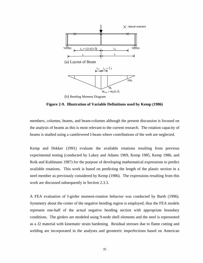
: lateral restraint

Lb

L L

(a) Layout of Beam

Lb = L[1-β(1-l)]

members, columns, beams, and beam-columns although the present discussion is focused on

the analysis of beams as this is most relevant to the current research. The rotation capacity of

beams is studied using a cantilevered I-beam where contributions of the web are neglected.

Kemp and Dekker (1991) evaluate the available rotations resulting from previous

experimental testing (conducted by Lukey and Adams 1969, Kemp 1985, Kemp 1986, and

Roik and Kuhlmann 1987) for the purpose of developing mathematical expressions to predict

available rotations. This work is based on predicting the length of the plastic section in a

steel member as previously considered by Kemp (1986). The expressions resulting from this

work are discussed subsequently in Section 2.3.3.

A FEA evaluation of I-girder moment-rotation behavior was conducted by Barth (1996).

Symmetry about the center of the negative bending region is employed, thus the FEA models

represent one-half of the actual negative bending section with appropriate boundary

conditions. The girders are modeled using 9-node shell elements and the steel is represented

as a J2 material with kinematic strain hardening. Residual stresses due to flame cutting and

welding are incorporated in the analyses and geometric imperfections based on American

Figure 2-9. Illustration of Variable Definitions used by Kemp (1986)

Lp Lp = l L

β

Mp

Mmax = Mp/(1-l)

Mp

(b) Bending Moment Diagram

35

Welding Society tolerances are also included. The varied parameters in this work include:

normalized laterally unbraced length, cross-section aspect ratio, transverse stiffener spacing,

span to depth ratio, flange slenderness, web slenderness, and percentage of the web depth in

compression. The parametric values used for each of these variables are as follows. The

alternative compact lateral bracing distances specified in the ASCE (1971) Plastic Design

Code and the longer bracing distance permitted by the original AASHTO LRFD

Specifications (1994) are the two lateral bracing distances evaluated. Cross-section aspect

ratios of d/bfc equal to 3.00 and 4.25 were selected. Stiffener configurations where the first

stiffener from midspan is located at d/3 and where the first stiffener is placed to obtain

sufficient shear capacity such that the applied shear is not greater than 60% of the shear

capacity were studied. The ratio between girder length and depth is used as a measure of the

moment gradient within the girder; L/d ratios of 20 and 30 were evaluated. Flange

slenderness values equal to the compact limit 9.2 and 7.0 were included in the study. Low,

intermediate, and high values of web slenderness, equal to 86, 125, and 163, were

incorporated. Lastly, Dcp/d ratios equal to 0.625 and 0.75 were used in this study.

Gioncu and Petcu (1997a, 1997b) present a study focused on the available rotation capacity

of steel wide-flange shapes. Specifically this work is focused on the theoretical

development, evaluation of, and parametric results obtained from a computer program

(DUCTROT 96) that calculates available rotation capacities for beams and beam-columns.

This program functions by computing the moment-rotation behavior due to the development

of in-plane and out-of-plane local buckling (Gioncu and Petcu 1997a). In a companion paper

(Gioncu and Petcu 1997b), the accuracy of the DUCTROT 96 program is evaluated against

experimental and FEA results. Compared to the results of 75 experimental tests by

independent researchers (Lukey and Adams 1969; Kemp 1985; Kuhlmann 1986 and 1989;

Spangemacher 1991; Kemp and Dekker 1991; Boeraeve et al. 1993; and Suzuki et al. 1994),

the average ratio of computed to experimental available rotation was 1.065 and the

coefficient of variation was 0.379. Thus, the average is relatively favorable; however the

authors propose a safety factor of 1.5 be applied to the results to counter the large coefficient

of variation. The DUCTROT 96 results are also compared against FEA results by

36

Spangemacher (1991), where the authors conclude that the program performs adequately in

comparison to these results.

Dinno and Birkmoe (2001) conducted an FEA study using the commercial software ANSYS

to investigate the influence of flange slenderness and web slenderness values exceeding the

compact limits. Variable material properties are also evaluated. The material properties

investigated were yield strength, ratio between elastic modulus and strain hardening

modulus, and ratio between strain hardening strain and yield strain. These girders simulated

four-point bending conditions and were modeled using four-node shell elements. All girders

had compact lateral bracing. Residual stresses and geometric imperfections are both

included in the analyses and the influences of various magnitudes and patterns of geometric

imperfections is considered.

Thomas and Earls (2003) present the results of a finite element evaluation of the available

rotation capacity of HPS70W girders. The analysis is carried out using ABAQUS software

and four-node reduced integration shell elements (ABAQUS S4R). Lateral constraints at the

midspan and support regions are assumed to be fully fixed, while the lateral constraints at

intermediate bracing locations is provided by “SPRING1” elements. Four parameters are

investigated in this study: flange slenderness, web slenderness, lateral bracing distance

between midspan and the first lateral brace, and bracing stiffness.

Lääne and Lebet (2005) present the results of a parametric study investigating the influential

parameters affecting available rotations and consequently propose an equation to calculate

the available rotation of steel plate girders. This research is conducted using ABAQUS

software to conduct FEA of analytical models of the region in the immediate vicinity of the

pier. Details of the model including loading and boundary conditions are presented in Fig. 2-

10. Here it is shown that the boundary conditions used assume that the cross-section is fully

fixed at the pier location and that rotation in the vertical (y) direction is restrained at the

opposite end of the model, where vertical and horizontal forces are applied. The length of

the girder modeled is represented by a in the figure and is equal to the height of the web in

most cases. The beam is modeled using ABAQUS S9R5 elements.

37

y

x

y

z

Flange 8x20 elements S9R5

Web 20x20 elements S9R5

Flange 8x20 elements S9R5

Stud Element B31

Distribution Beam 20 elements B32

Reinforcement Element T3D2

2.3.2 Factors Influencing Available Rotations

2.3.2.1 Flange Slenderness

It is unanimous among previous researchers that flange slenderness decidedly influences the

available rotation of steel I-girders. Furthermore, nearly all researchers to investigate this

topic (Lukey et al 1969, Kemp 1986, Barth 1996, Gioncu and Percu 1997b; Dinno and

Birkemoe 2001, Thomas and Earls 2003) agree that there is a decrease in available rotations

with increasing flange slenderness, particularly for compact flanges and when failure is

controlled by flange local buckling.

The experimental testing used to determine the current AASHTO and AISC flange

compactness limit is presented by Lukey et al. (1969) and Lukey and Adams (1969). Lukey

et al. suggest that when failure is by local buckling, the flange slenderness ratio has a

significant influence on the available rotations. However, when lateral buckling controls,

they conclude that the flange slenderness ratio is of little importance. Similarly, Dinno and

Birkemoe (2001) suggest that the interaction between flange and web slenderness has an

influence on rotation capacity when flange local buckling occurs, but that flange slenderness

has little influence on rotation capacity when web local buckling is the cause of failure.

Additionally, Lukey and Adams present data that suggests a relatively linear relationship

between flange slenderness and available rotation for flange slenderness values between 7

and 9. However, once a flange slenderness of 9 is exceeded, the influences of flange

slenderness become much less apparent.

Figure 2-10. Schematic Diagram of FEA Techniques used by Lääne and Lebet (2005)

ux = 0 φz = 0

MVV

M

V

H

Ha Intermediate Support

Fixed End

Rigid end beam 24 elements B32 φy = 0

38

As discussed above, Kemp (1986) presents the results of a study focused on the available

rotation capacity of members as a function of the length of the member that is in the plastic

region, Lp. For the limit state of flange local buckling, the following iterative equation is

proposed for computing Lp.

2

21.5 ( / )f b f f f

bt C t

=ε − π l L

(2.22)

where b is the width of the compression flange, tf is flange thickness,

0.51

fb yf

f

ls e

l⎛ ⎞

ε = ε +⎜⎜ −⎝ ⎠⎟⎟ , Cf is a boundary condition coefficient equal to 0.5 for no web or

lateral constraint or 1.0 for web and lateral restraint, lpf is Lpf/L, L is the half span length, Lpf

is Lp for the flange local buckling limit state, εyf is yield strain of the flange. This equation is

based on the assumption that the flange local buckling occurs when the length of the plastic

region is greater than the full wavelength of the flange buckle as proposed by Lay and

Galambos (1965, 1967) and is derived by rearranging the expressions and modifying the

assumptions used by Lay and Galambos, Southward (1969), and Stowell (1950).

Lääne and Lebet (2005) investigated three values of flange slenderness in their parametric

study: 8.1 (the Eurocode Class 2 limit for Grade 50 steel), 7.3 (the Eurocode Class 1 limit),

and 6 (a common value for composite bridges in Switzerland according to the authors).

Results indicate that, counter to intuition, the most compact flanges possessed the least

rotation capacity and the flanges with a slenderness of 7.3 exhibited the most rotation

capacity. Because of the significant body of evidence contradicting these conclusions, this

may be taken as a sign that the solution procedures (e.g., boundary and loading conditions)

used by Lääne and Lebet may be flawed.

2.3.2.2 Web Slenderness

Several previous researchers report increasing available rotations with decreasing web

slenderness values. For example, experimental testing of three girders with varying web

slenderness ratios ranging between 81 and 154 by Schilling and Morcos (1988) illustrates

that for these girders there is a clear decrease in both moment capacity and available rotations

with increasing web slenderness values. Thomas and Earls (2003) investigated web

39

slendernesses between 18 and 72 of HPS-70W beams, where 72 is approximately equal to

the compact limit in AASHTO (1998) of 3.76 / yE F for Fy of 70 ksi. A decreasing

relationship between rotation capacity and increasing web slenderness is evident based on

these FEA results. Lääne and Lebet (2005) investigated five different web slenderness

values ranging between 100 and 200 in increments of 25 where it was shown that increasing

web slenderness contributes to decreased rotation capacity.

Kemp and Dekker (1991) and Gioncu and Petcu (1997b) report that there is a inversely

proportional relationship between web slenderness and available rotations when the web

slenderness is above a certain limit, however, below this limit increasing rotations are

reported with increasing web slenderness. Specifically, Kemp and Dekker (1991) report that

an increase in web slenderness from 24.5 to 30 resulted in an increase in available rotation

capacity; a decrease in rotation capacity is then exhibited for beams with increasing web

slendernesses between 33 and 40. A similar trend was reported by Gioncu and Petcu

(1997b), who evaluated web slenderness values between 23 and 67. The results of this study

showed that the minimum available rotation was obtained for the beam with a web

slenderness of 38. Gioncu and Petcu attribute this behavior to the fact that beams with a

higher web slenderness will fail by elastic-plastic web buckling and beams with a lower web

slenderness will fail by plastic flange buckling.

Dinno and Birkemoe (2001) present the influences of web slenderness for 28 FEA girders.

Here it is shown that, while for low web slenderness ratio (d/tw < 30) there is a significant

increase in available rotations with decreasing web slenderness, there is typically an upper

limit of web slenderness where further increases no longer influence available rotations. This

value of web slenderness may be as low as 50 or may be greater than 70 depending on other

parameters of the girder, e.g. low flange slenderness values increase the web slenderness

value at which the moment-rotation curves converge.

These findings by Dinno and Birkemoe are consistent with the FEA results presented by

Barth (1996). Barth investigated girders with a higher web slenderness than considered by

previous researchers where the minimum web slenderness was equal to 86. These results

40

indicated even though decreased moment capacity exists for girders with higher web

slenderness values, the influence on available rotations is small as the moment-rotation

curves for girders with varying web slenderness values eventually converge.

Similar to Eq. 2.22 above, Kemp (1986) gives the following iterative equation to predict Lp

(and consequently rotation capacity) as a function of web slenderness.

21 0.97

2cp w fc w

w w w w cyw

h C h l Lt C l L C he

⎛ ⎞⎛ ⎞= ⎜⎜ ⎟ ⎜ε⎝ ⎠ ⎝ ⎠p

+ ⎟⎟ (2.23)

where hcp is the distance between the plastic neutral axis and the center of the compression

flange, tw is the web thickness, Cw = B – 0.25nw, B is 0.75 if the flange is buckled and 1 if

the flange is not buckled, nw is the ratio of applied axial force to force required to fully yield

the full web depth, ε=E/Est, εyw is yield strain of the web, lw=Lpw/L where Lpw is Lp

corresponding to the limit state of web local buckling. This equation is developed from

classical buckling theory assuming that the web depth in compression may be satisfactorily

represented by an equivalent depth subject to uniform stress equal to the yield stress. Lpw

represents the full wavelength of the web buckle using these assumptions.

2.3.2.3 Lateral Bracing Distance

It was suggested by Prasad and Galambos (1963) that lateral torsional buckling is a failure

mode with little rotation capacity available. This conclusion was based on the results of

experimental testing of beams with five lateral bracing panels loaded such that the center

three panels were in uniform bending. This is an extreme situation compared to the actual

moment conditions at the pier region of continuous beams, which approximates a linear

moment gradient. However, current researchers often cite this work and suggest that failure

by lateral torsional buckling should be prevented.

The majority of previous investigations into the influences of lateral bracing distance on

available rotations have been conducted on simply-supported beams with two lateral bracing

segments. Thus there is no torsional restraint to the critical lateral bracing panels as would

exist in actual continuous-span beams and the results from these investigations may be

unduly conservative. One such study is that of Adams et al. (1964) where it is shown that

41

there is a distinct relationship between increased lateral bracing distance and decreasing

available rotations. Similarly, Lukey et al. (1969) show that there is a significant decrease in

available rotations at Mp as the normalized unbraced length (Lb/ry) is increased from 70 to

105.

Kemp and Dekker (1991) plot the observed available rotations in 44 experimental tests

(Lukey and Adams 1969; Kemp 1985; Kemp 1986; and Roik and Kuhlmann 1987) versus

the authors’ definition of lateral slenderness ratio, Li/izcε, where Li is the distance between

locations of maximum and zero moment (which is also equal to the lateral bracing distance),

izc is the radius of gyration of the compression flange and portion of the web in compression,

and ε is 235 / yF . These experimental girders depicted in the graph reproduced in Fig. 2-11

represent relatively compact sections with lateral bracing provided at the midspan and end

supports only. Kemp and Dekker conclude that failure of beams with a lateral slenderness

greater than 60 will be dominated by lateral torsional buckling, which they term “Mode 1”

failure; conversely failure of beams with a lateral slenderness less than 60 will be dominated

by local buckling, termed “Mode 2” failure. From the data presented in Fig. 2-11, the

authors conclude that there is a quadratic relationship between lateral slenderness ratio and

available rotations. This influence appears clearer, with less scatter, for the girders with a

lateral slenderness exceeding 60.

Figure 2-11. Available Rotation versus Lateral Slenderness Ratio by Kemp and Dekker (1991)

42

Only the studies by Barth (1996) and Thomas and Earls (2003) consider multiple lateral

bracing segments such that representative boundary conditions are applied to the critical

panels. Barth illustrates through FEA and experimental testing that lateral bracing distances

less than the compact limit provide little benefit in terms of increasing available rotations.

Thomas and Earls (2003) varied the lateral bracing distance between 0.5d and 2d (d is the

depth of the cross-section) at midspan. However, it appears that a significantly larger lateral

bracing distance was used away from midspan of the girders such that the panel where failure

occurred may have been the second panel from midspan in many cases. It is hypothesized

that failure occurred in these “second panels” in all of the girders where the lateral bracing

distance at midspan is 0.5d, as all of these girders exhibited rotation capacities that were

significantly less than the rotation of corresponding girders with lateral bracing distances of

1.0d.

Kemp (1986) considers lateral torsional buckling of a compressive strut comprised of the

compression flange and the portion of the web in compression. Based on buckling theory,

Kemp gives the following iterative equation for predicting the plastic length of the beam (and

consequently rotation capacity) as a function of the lateral slenderness.

( )( ) ( )

2 (1.08 0.04 )1 0.6 0.4 1 / (0.6 0.4)

b

yf t

mLr m C e m

− β −βπ=

ε −β + β + − + (2.24)

where r is the radius of gyration of the portion of the section in compression, β is the ratio of

moment at the lateral constraint to the plastic moment, m is 1/(1-lt), and Ct is 1 if the flange

is not buckled and 0.667 if the flange is buckled.

2.3.2.4 Material Properties

Based on previous research, it is widely accepted that increased steel yield strength

corresponds to a reduction in available rotation capacity. For example, Dinno and Birkemoe

(2001) have reported members with higher yield strengths exhibit lower rotation capacity

compared to lower grade steels based on analytical results of beams subjected to four-point

bending with compact lateral bracing. Furthermore, they suggest that this trend is most

significant for cases where failure is caused by flange local buckling. Dinno and Birkemoe

also investigated the influences of varying ratios of elastic modulus to strain hardening

43

modulus, which was found to be insignificant, and ratios of strain hardening strain to yield

strain, which was insignificant for values less than or equal to 10. At ratios of strain

hardening strain to yield strain greater than 10 the available rotation was shown to decrease

in one instance.

Gioncu and Petcu (1997b) have researched the available rotation capacity of girders

comprised of steel having three different yield strengths: 33 ksi, 39 ksi, and 50 ksi. Girders

having flanges and webs with each of these materials are considered, resulting in a total of

nine girders. Comparing the rotation capacities of each of these girders shows that the yield

strength of the web has a negligible influence on the rotation capacity, but that decreased

rotation capacity results with increasing flange yield strength. A change in flange yield

strength from 33 to 50 ksi results in a 63% decrease in rotation capacity.

Green et al (2001) have investigated the available rotation capacity of high performance steel

(HSLA-80) members compared to the rotation capacity of members fabricated from A36

steel. This evaluation indicated that members fabricated from high performance steel may

have significantly less rotation capacity than A36 members with the same cross-sectional

geometry, i.e., the slenderness values are not normalized to account for the difference in yield

stress. Specifically, there is a 70 to 83% decrease in the available rotation of the high

performance steel members compared to the corresponding A36 members.

Lääne and Lebet (2005) considered two grades of steel in their parametric study: S355 and

S460, which approximately correspond to Grades 50 and 65, respectively. Results of the

study show that the higher grade steel has less ductility even though the compression flange

slenderness was decreased such that girders from both materials have the same normalized

flange slenderness (although web dimensions are equal). The authors suggest that because a

higher buckling stress develops in girders with higher yield strengths, the web is also loaded

with a higher stress and cannot support the flange as efficiently as with the lower grade steel.

Kato (1990) suggests that the widely recognized characteristic that an increase in yield

strength corresponds to a decrease in rotation capacity is actually due to the increase in yield

44

ratio that typically accompanies increased yield strengths. It is a fairly intuitive concept that

a smaller yield ratio will permit a larger extension of the plastic region and therefore

increased rotation capacity. This hypothesis is explored via a theoretical investigation

utilizing the moment-curvature relationship where steel with a yield stress of 35 ksi, YR of

0.6, E/Est=50, and εst/εy=5 is taken as the reference material. This evaluation shows that

when Fy is altered and the other three parameters are left unchanged, there is not a significant

influence on rotation capacity. However, when YR is varied and Fy, E/Est, and εst/εy are

constant, the change in rotation capacity is rather dramatic. The influences of varying E/Est

and est/ey are also presented, where it is shown that these parameters are also influential, but

to a lesser extent than the yield ratio. Thus it is proposed that the influence of material

properties on rotation capacity is best attributed to the complementary energy of the steel,

which conveniently takes into account all applicable parameters: the yield stress, modulus of

elasticity, ultimate stress, strain hardening strain, and strain hardening modulus, but that the

yield ratio is the single parameter most influential to available rotations.

2.3.2.5 Web Depth in Compression

Grubb and Carskaddan (1979) first reported the significant influences that the percentage of

the web depth in compression may have on available rotations. This observation resulted

from available rotations that were lower than expected compared to previous testing.

Because the previous tests were on doubly-symmetric sections and the tests by Grubb and

Carskaddan were singly-symmetric with 57% of the web in compression in the elastic range,

it was reasoned that the lower available rotations were due to this influence.

Subsequent research has supported that there is a relationship between increasing percentage

of depth of web in compression and available rotations, but it is suggested that this influence

is of little significance for girders with more than half of the web depth in compression and

that this behavior is better attributed to the decreased moment capacity that results with

increasing web depth in compression. For example, Barth (1996) investigated the use of

Dcp/d ratios equal to 0.625 and 0.75 and found that the primary influence of the higher ratio

was to decrease the peak moment capacity; no clear relationship exists between Dcp/d ratio

and available rotations based on the results presented in this work. Similarly, Gioncu and

45

Petcu (1997b) investigated the influence of variable tension flange area on the available

rotation capacity. The tension flange area was varied between 0 and 1.8Afc, which

corresponds to a Dcp/D ratio varying between 0.2 and 0.74 for the given beam geometry.

Results indicated that there is decreasing rotation available with increasing Dcp/D ratio,

however, for beams with a Dcp/D ratio greater than 0.5 the reduction in rotation capacity

becomes less severe. Lääne and Lebet (2005) investigated six different percentages of elastic

web depth in compression ranging between 42.8 and 63.2%, with three of these less than 0.5

and three with Dc/D greater than 0.5. They suggest that when more than half of the web is in

compression there is a negligible influence on rotation capacity, however, if the elastic

neutral axis is less than 0.5D, there is a considerable increase in ductility with decreasing

percentage of web in compression.

2.3.2.6 Relative Cross-Section Proportions

Barth (1996) studies the influence of the cross-section aspect ratio, which is defined as the

web depth divided by the compression flange width. Here it is reported that increasing d/bfc

ratios from 3 to 4.25 result in an average decrease in moment capacity of 6%. This decrease

in moment capacity correspondingly influences the available rotations at a given level of

moment.

Lääne and Lebet (2005) investigated seven combinations of relative compression flange,

tension flange, and web areas. The area of the tension flange was varied between 20 and

30% of the total area; the area of the compression flange represented between 35 and 45% of

the total girder area; and the area of the web ranged between 30 and 40% of the total area.

Results of this analysis showed that the minimum ductility results when the compression

flange area is maximized and the web area is minimized, while the maximum ductility results

when the web area is maximized and the compression flange area is minimized.

2.3.2.7 Moment Gradient

There are variable opinions regarding the influence of moment gradient on available

rotations. Grubb and Carskaddan (1979) aimed to investigate the influences of moment

gradient through experimental testing of three I-girders that were identical except for changes

46

in the span length of the specimens. At Mp the available rotations were 11 mrad for the

shortest beam, 7 mrads for the beam of intermediate length, and 0 mrads for the longest

beam. Grubb and Carskaddan also plot the available rotations from the experimental testing

conducted by Adams et al. (1964) and Lukey and Adams (1969) as a function of the L/d ratio

of the specimens, where L is half the span length and d is the total section depth. Data from

similar tests are grouped into series and it is shown that there is an increasing relationship

between available rotation and L/d ratio. The depth of all sections considered is relatively

constant, therefore it could be stated that there is an increasing relationship between span

length and available rotation. Grubb and Carskaddan hypothesize that this phenomenon

occurs because the yielding is less localized with a longer negative bending length. They

attribute the contrast between this behavior and their own experimental results to the higher

web and flange slenderness values of their own specimens and suggest that the flatter

moment gradient that exists with the longer span lengths increases the length of the web

subjected to a high compressive stress rendering the web more susceptible to buckling.

Barth (1996) examines the influence of moment gradient for L/d ratios equal to 20 and 30,

which are typical L/d ratios for continuous-span bridges. Here it is also concluded that there

is a decrease in available rotations due to lower moment gradient. However, this data

suggests that this influence is sufficiently small such that it is reasonable to neglect these

effects.

Kemp (1986) reports the results of two experimental tests that are nearly identical except that

one beam had twice the span length of the other. These results are opposite to those reported

by Grubb and Carskadan and Barth in that the increase in span length led to a drop in

available rotation capacity at the maximum moment from 7.4 to 1.4. It is suggested that this

influence is due to the fact that as the span length is increased, the yielded length remains

constant and consequently the proportion of the span that is plastic decreases resulting in a

lower rotation capacity. Similarly, Gioncu and Petcu (1997b) investigated the influence of

span length on beams ranging from 2 to 6 m in length. Consequently, it was concluded that

beams with a span length of 4 m had approximately half the available rotation capacity of

47

beams with a span length of 2 m. Beams with a span length of 6 m had approximately 75%

of the available rotation of the beams with a span length of 4 m.

2.3.2.8 Stiffeners

It was concluded by Huang (1995) that stiffeners located closer to the peak moment location,

termed inelastic restraint stiffeners, may result in greater available rotations. This behavior

occurs because these stiffeners act to restrain buckling at peak moment locations, thus

delaying the decrease in moment capacity. It is suggested that stiffeners placed at one-third

the web depth away from the pier location will result in optimal moment-rotation

characteristics.

Similarly, Lääne and Lebet (2005) observed that when the web panel length was less than the

height of the web, a substantial increase in rotation capacity was obtained. They suggest that

this may be caused by a stiffener being located where compression flange buckling would

normally occur, thus delaying or suppressing this mode of failure.

Barth (1996) subsequently investigated the influence on moment-rotation behavior due to the

inelastic restraint stiffeners suggested. Barth observed minimal benefits to the use of these

additional stiffeners and thus does not recommend their use due to the associated increased

fabrication costs.

Kemp (1986) proposes a diagonal stiffener having the configuration shown in Fig. 2-12 be

placed at sections of maximum negative moment. Test results on five pairs of experimental

girders with and without this diagonal stiffener show that the stiffened girders exhibit

approximately twice the rotation capacity of their unstiffened counterparts for cases where

failure was caused by local buckling. This stiffener arrangement is designed to stiffen the

compression flange and portion of the web in compression in order to delay buckling in the

section, however strengthening the portion of the member in tension is avoided to increase

the extent of tensile yielding in the beam, which further increases the rotation capacity.

Therefore the stiffener height, hs, should be approximately equal to the web depth in

48

Figure 2-12. Diagonal Stiffener Proposed by Kemp (1986)

compression. Based on the research by Kemp, 5% of the negative bending length is

suggested to be an optimal value for the length of the stiffener, Ls.

2.3.2.9 Shear Force

The experimental girders tested by Holtz and Kulak (1973) included three girders with

relatively high levels of shear. Specifically, the shear was approximately equal to 90% of the

shear capacity of these beams. The experimental results indicated that this had little or no

effect on the moment capacity of the beams.

Grubb and Carskaddan (1979) also conclude that the influence of shear force on available

rotation is negligible. They reason that increasing shear theoretically reduces the moment

capacity of the beam. Thus, if the available rotation is evaluated at a lower moment capacity,

higher available rotation results. Because both of these influences are small and offset one

another, Grubb and Carskaddan recommend that the effects of shear may be neglected.

2.3.2.10 Lateral Bracing Stiffness

Thomas and Earls (2003) investigated the influence of lateral bracing stiffness in their

parametric study focusing on the available rotation capacity of HPS70W girders. Here lateral

bracing was applied in the FEA in two alternative methods: rigid lateral constraints at all

lateral bracing locations or rigid lateral constraints at midspan and bearing locations and

flexible (spring element) constraints at all other lateral bracing locations. These results

49

demonstrated that the varying stiffness assigned to the spring elements contributes a

negligible influence to rotation capacity when the lateral bracing distance is between 4 and

10 times the minimum required stiffness specified in the 1999 AISC Specifications. Only

one girder is discussed where the stiffness was outside of this range and this girder had a

lateral bracing stiffness equal to the AISC specified stiffness, β. For this single girder, the

rotation capacity was approximately half the rotation capacity of similar girders with stiffness

of 4β to 10β. However, the rigid constraints (which may be thought of as having infinite

stiffness) provided a stiffness only slightly higher than the beam with stiffness equal to β.

2.3.2.11 Geometric Imperfections:

Holtz and Kulak (1973) specifically address the influence of initial out-of-flatness of the

webs of the girders tested in their experiments. They found that the six girders (out of a total

of 10 girders) that did not reach the plastic moment capacity were also the girders with the

highest values of initial web imperfections although all but one of these girders satisfied the

imperfection tolerances given by CSA Standard W29.1. It was observed that webs with the

higher imperfection values began laterally deflecting at lower levels of load, leading to

earlier buckling and reduced moment capacity.

In the FEA work conducted by Dinno and Birkmoe (1991) the influences of five different

patterns of imperfections on the available rotations were investigated. This included

imperfections that were: a function of the sine function, a function of cosine function, a

function of a combination of sine and cosine, based on buckling analysis results for the first

buckling mode, and the real imperfections mapped from similar experimental testing. It was

demonstrated that the choice of imperfection pattern is influential and should be selected to

represent the actual imperfections to the extent possible.

2.3.2.12 Axial Force

Kemp (1986) suggests that the available rotation should be a function of the parameter

h/2hcp, where h is the distance between the center of the flanges and hcp is the distance

between the plastic neutral axis and the center of the compression flange. This parameter is

said to capture the decrease in rotation capacity corresponding to axial compressive force.

50

2.3.3 Available Rotation Prediction Equations

Galambos (1968) reports the following equation for available rotation capacity of beams with

the lateral bracing distance equal to (1 0.56 )

y

y

rK h

π

ε +under uniform moment, which was

determined theoretically assuming lateral and local buckling occur simultaneously:

21 1

0.7y

y

sh KL

r

⎡ ⎤⎢ ⎥

− π⎢ ⎥⎡ ⎤ −⎢ ⎥⎢ ⎥ ⎛ ⎞⎣ ⎦ ⎢ ⎥ε ⎜ ⎟⎜ ⎟⎢ ⎥⎝ ⎠⎣ ⎦

(2.25)

where s is the ratio between the strain hardening strain and the yield strain, h is the ratio

between the strain hardening modulus and the elastic modulus, εy is the yield strain, K is the

effective length ratio, L is the unbraced length, and ry is the radius of gyration about the y

(vertical) axis. This equation was shown by Galambos (1968) to be a satisfactory

representation of the available rotation at 95% of Mp in several experimental girders. It is

noted that this equation is conservative for beams with shorter lateral bracing distances.

Similarly, the following equation was proposed to predict the available rotation (in radians)

of beams under moment gradient:

14

1

2

2.84 ( 1) 1wy

f

A Vbtsdw A V

⎛ ⎞ ⎛ ⎞ε − +⎜ ⎟ ⎜⎜ ⎟ ⎝ ⎠⎝ ⎠

⎟ (2.26)

where V1 and V2 represent the shear immediately to the left and right of the hinge locations

(Galambos 1968). The accuracy of this equation was evaluated compared to experimental

results where the test rotation was measured as the difference between the elastic rotation at

Mp and the rotation when unloading began since few tests were carried out to the point where

the girder unloaded back down to Mp. The equation was shown to be conservative for 11 out

of 13 experiments in which compact beams were used.

Kemp (1986) gives the following equation for predicting the rotation capacity at the

maximum moment based on moment curvature relationships

2 12 1m

cp

hR l s eh l

⎛= − +⎜l ⎞

⎟−⎝ ⎠ (2.27)

51

where h is the depth between the centers of the two flanges, hcp is the distance between the

plastic neutral axis and the center of the compression flange, l is Lp/L as shown in Fig. 2-9, s

is the ratio of the strain hardening strain to yield strain, and e is the ratio of elastic modulus to

strain hardening modulus. Lp is taken as the minimum Lp from the limit states of flange local

buckling, web local buckling and lateral torsional buckling as computed using Eqs. 2.22,

2.23, and 2.24, respectively. The theoretical and experimental values of Rm are compared for

11 experimental girders, where the correlation between the two is relatively good considering

the complexity of the problem. It should be pointed out that Eq. 2.27 is intended to predict

the rotation capacity at the maximum moment. Thus, the available rotation capacity after the

girder decreases to a given moment capacity will be greater than that predicted by this

equation. A general guideline is that the available rotation at Mp is equal to twice the rotation

at the maximum moment. However the accuracy of this rule of thumb varies significantly for

different beams, and may result in conservative or unconservative predictions.

Kato (1989) derives the available rotation of I-shaped steel beams by representing the I-

section as an equivalent two flange model as shown in Fig. 2-13, where the plastic moment

capacity and cross-sectional area are the same in both the original section and the equivalent

section and a web thickness of 0.6tf is further assumed. Based on the moment-curvature

relationship of this equivalent section, Eqn 2.28 is proposed to predict the available rotation

capacity of I-shaped steel beams as a function of geometric and material characteristics,

( ) ( )21 1 1st c c st

E I hR s ss E I h

⎡ ⎤ε= − + −⎢ ⎥ε⎣ ⎦

(2.28)

Figure 2-13. Equivalent Section used by Kato (1989)

52

where s is the normalized critical stress σcr/Fy and σcr is the critical stress governed by local

buckling.

To format the above equation as an expression of terms more frequently used in design, the

following equation is proposed to compute the critical stress as a function of the flange and

web slenderness

1 1.600 0.15350.6003f ws

= + +α α

(2.29)

where 2/ ( / )f yf fE F t bα = and 2/ ( / )w yw wE F t dα = . This equation is based on a linear

regression of experimental data from 68 stub-column tests. By solving Eqn. 2.28 for 1/s,

equating this with Eqn. 2.29, and incorporating a correction factor to account for the uniform

stress distribution in the experimental stub-columns as opposed to the stress gradient that

exists in beams, the following equation is obtained.

2 2

11 1.6003 0.6003

1.600 0.1535

c

f w

yf r yw r

b dt t

E EF s F s

⎛ ⎞ ⎛ ⎞⎜ ⎟ ⎜ ⎟⎜ ⎟⎝ ⎠ ⎝ ⎠+ =

⎛ ⎞ ⎛− −⎜ ⎟ ⎜

⎝ ⎠ ⎝

⎞⎟⎠

(2.30)

Then, by computing the value of 1/sr corresponding to different levels of required rotation,

the permissible flange and web slenderness can be determined. For example, by assuming

E/Est = 70, εst/εy = 10, and Fyw = Fyf=Fy, the following is obtained for a required rotation

capacity of four,

2 2

2

21

1170181

f

f w

yy

b Dt t

FF

⎛ ⎞ ⎛ ⎞⎜ ⎟ ⎜ ⎟⎜ ⎟⎝ ⎠ ⎝ ⎠+ =

⎛ ⎞⎛ ⎞⎜ ⎟⎜ ⎟ ⎜ ⎟⎜ ⎟ ⎝ ⎠⎝ ⎠

. (2.31)

Similarly, Equation 2.32 is obtained for a required rotation capacity of two,

53

2 2

2

21

200 1279

f

f w

y y

b Dt t

F F

⎛ ⎞ ⎛ ⎞⎜ ⎟ ⎜ ⎟⎜ ⎟⎝ ⎠ ⎝ ⎠

2+ =⎛ ⎞ ⎛ ⎞⎜ ⎟ ⎜ ⎟⎜ ⎟ ⎜ ⎟⎝ ⎠ ⎝ ⎠

. (2.32)

Thus, it is assumed in these equations that the required rotation capacity of a section is a

function of the interaction between flange and web slenderness and the material properties.

It has been assumed in the development of these equations that lateral torsional buckling of

the girders is prevented.

Based on his findings that the rotation capacity of beams could best be represented as a

function of the complementary energy of the steel and using the same procedure as in

previous work (Kato 1989), Kato (1990) suggested the following equation to predict the

available rotation capacity at the maximum moment

2 3

1

12 1C CR YRC YR

⎡ ⎤+ ⎛= − ⎞−⎢ ⎥⎜⎝ ⎠

⎟⎣ ⎦

. (2.33)

where C1, C2, and C3 refer to components of the complementary energy of the material, and

YR is yield ratio. The constants C1, C2, and C3 are expressed by the following equations:

21 / 2 / 2y yC E= σ = σ ε y , (2.34)

21 1 y stC

YR⎛ ⎞= − σ ε⎜ ⎟⎝ ⎠

, and (2.35)

( )2 2

3

1/ 12

y

st

YRC

E− σ

= . (2.36)

Eq. 2.33 represents the rotation capacity assuming that local buckling is prevented such that

the ultimate stress of the steel can be achieved. The possibility that the maximum stress σcr

may be less than σu is accounted for and the equations are simplified for design by utilizing

regression analysis to obtain typical values of σcr resulting in the following equation for

predicting the available rotation capacity

1 ( 1) 2 pbb

b st y

R ER RR E

⎡ ⎤ε−= − +⎢ ⎥

ε⎢ ⎥⎣ ⎦ (2.37)

54

where Rb is σcr/σy and σcr is determined using empirical equations as a function of flange

slenderness, web slenderness, and steel type and εp = εst – εy.

Kemp and Dekker (1991) expand on previous theoretical methods (Kemp 1985 and Kemp

1986) to develop the following equation for the prediction of the available rotation capacity

of steel members classified as Class 1 or Class 2 sections according to Eurocode

Specifications

1.53(60 / ) / 2 'a eR = λ α (2.38)

where

( / )e f w i zcK K L iλ = ε , ( / 2 ) / 20f f fK b t= ε , 2 / 33w w w wK K d t= = α ε for 33 / 40w wd t< α ε ≤

and ( )1 2460 / / 400w w i zc wK K L i K= = − ε⎡ ⎤⎣ ⎦ for / 3w wd t 3α ε ≤ , α’ is the percentage of the

depth of section in compression between the centers of the two flanges. This equation is

based on conservative inelastic material properties of E/Est equal to 50 and εst/εy equal to 10.

Lääne and Lebet (2005) evaluated the available rotation capacity of 30 finite element models

at a level of moment equal to 90% of My. The models included in this evaluation consisted

of girders with the following attributes: flange slenderness of either the Eurocode Class 1

limit or 6; web slenderness values of 100, 125, 150, 175, or 200; Grade S355 and Grade 460

steel; and cross-sections proportioned such that the tension flange represented 25% of the

total area of the girder, the compression flange area was 35 or 45% of the total area, and the

web was 30 or 40% of the total area. The available rotation of each of these models is then

expressed as a function of the modified reference slenderness for web buckling,

2 1.05' cp y

pw

D Ft Ek

λ = (2.39)

where k is the plate buckling coefficient of the web. Based on this data, Lääne and Lebet

proposed the Equation 2.40 to predict the available cross-section of I-girders in negative

bending,

2

15.75( ')av

p

θ =λ

. (2.40)

55

The relationship between Eq. 2.40 and experimental data for girders exceeding the Eurocode

Class 1 compactness limit is shown below in Fig 2-14. For girders with a modified reference

slenderness for web buckling less than the Class 1 compactness limit, the available rotation is

assumed to be 63 mrads based on the previous results of Grubb and Carskaddan (1981) who

found that compact sections demonstrated a minimum rotation capacity of 63 mrad. Figure

2-14 illustrates that this prediction equation is conservative in all cases and inappropriately

conservative in several cases.

2.4 Rotation Requirements

In the U. S., the majority of research on plastic design and behavior has been focused on

building-type applications. Consequently, general guidelines for rotation requirements were

suggested for this purpose, as summarized in this section, which also serve as the basis for

the AASHTO compactness limits. A more appropriate representation of AASHTO rotation

requirements would be based on an analysis of rotation requirements for continuous span

beams. A more accurate representation of rotation requirements for bridge members would

result based on the analysis of continuous-span beams. Several researchers have investigated

Figure 2-14. Available Rotation Equation Suggested by Lääne and Lebet (2005) Compared to Experimental Data

56

this issue and one particularly important aspect of this research is investigations relating

rotation requirements to intended degree of moment redistribution. These as well as other

relevant findings and theoretical considerations from these studies are summarized below.

Early work in plastic design for building applications sought to determine the approximate

degree of rotation required in order for plastic design to be valid. This requirement was

typically expressed in the non-dimensional quantity of rotation capacity equal to θ2/θ1 - 1,

where θ2 and θ1 are as shown in Fig. 2-15. Through the years, various rotation capacity

requirements have been suggested. For example, in 1963, Prasad and Galambos suggested a

rotation capacity of 10 as a rough estimate of required rotation and utilized this rotation

requirement in evaluating lateral bracing limits for plastically designed beams.

In 1974, the AISC ASD Specifications were revised and local and lateral buckling limits

were based on rotation capacity requirements of 3. Yura et al. (1978) suggested that this

level of rotation was sufficient for most civil engineering applications and this conclusion

seems to be based on research by Galambos (1968) and Neal (1963) suggesting that a

rotation capacity of 2 was generally conservative, although higher rotation requirements may

be necessary for some cases. Specifically, in a summary of rotation requirements for some

general structures, Galambos (1968) revealed that for practical structures the required

rotation capacity is less than 2, although rotation requirements may be higher for single story

Rotation, θ

Available Rotation Capacity

Mpe

Mom

ent,

M

θ1 θ2

Figure 2-15. Definition of Rotation Capacity

57

frames with very steep gables and in areas of high moment gradient. Similar findings have

been reported by Neal (1963) where it was shown that rotation capacities of 2 are adequate

for continuous beams with concentrated loads.

The rotation requirement of 3 was later adopted as the criteria for determining compact

section requirements in the AISC LRFD Specifications (Yura et al. 1978). Similarly, the

compact section criteria adopted in the current AASHTO LFRD elastic provisions are also

based on a rotation requirement of 3.

Kemp (1990) calculated required rotations by superimposing the rotations due to the applied

loads and end (redistribution) moment assuming that members are simply-supported, i.e.,

each span of continuous-span beams and beams of portal frames are analyzed as simply

supported. However, this approach results in an upper bound of the required rotation because

it assumes that a hinge is present in the structure before load has been applied and thus

neglects the increased stiffness of the structure due to continuity prior to yielding at the hinge

locations. Results of these efforts were presented in the form of graphs giving required

rotation capacity for typical three and five span bridges as a function of the ratio between

positive and negative bending moment resistance and ratio of distance to the inflection point

to the span length. Previous research by Kemp (1987) also suggested that the distance to the

inflection point was of importance as larger rotations were required for beams where the

distance to the inflection point was reduced due to low ratios between the stiffness of the

negative bending section to the stiffness of the positive bending section.

Kemp and Dekker (1991) present the required rotation of symmetrical two-span continuous

beams as shown in Fig. 2-16. As shown in the figure, the required rotation is plotted as a

function of both percentage of moment redistributed and the ratio between negative and

positive bending strength of the cross-section. It is assumed in this work that the beam is of a

uniform cross-section with uniform flexural-rigidity, but other analysis details and

assumptions are not provided. From the data presented in Fig. 2-16, it is suggested that for

an intended degree of redistribution less than 20%, a rotation capacity less than 1.0 is

58

Figure 2-16. Rotation Requirements – Kemp and Dekker (1991)

required and for moment redistribution of less than 30%, rotation capacities less than 2.0 are

required.

One of the most comprehensive studies on rotation requirements to date is presented by Li,

Choo, and Nethercot (1995). The primary purpose of this research was to determine the

rotations necessary to redistribute moment from pier sections to the midspan cross-section,

where it was assumed that the required rotation occurs at connections rather than in

members. In this work, the required rotation is quantified as the rotation necessary to

achieve moments in excess of My yet below Mp in the mid-span cross-section.

Li et al. (1995) conducted their analysis of required rotations by decomposing the rotation

into elastic and plastic components. Rotation requirements were calculated by first

representing a continuous beam as equivalent simple span beams. Thus the procedure was

similar to that used by Kemp (1990) in that the continuity at the pier prior to hinge formation

is neglected. The elastic component of rotations is that resulting in the simply-supported

beam with end moments equal to the elastic moment at each end of the span in the

continuous beam and applied loads of either a uniformly distributed load, central

concentrated load, or two third-point loads. This elastic component of rotation is calculated

as a function of: ratios between end moment(s) to the maximum span moment, the ratio of

59

the relative stiffness along the girder (cracked vs. uncracked stiffness as only beams of

uniform cross-section are considered), the maximum span moment, span length, and stiffness

of the positive moment region. The plastic rotation is considered to be that caused by plastic

deformation at midspan. Thus, by this definition of plastic rotation, if the positive bending

moment is less than My, no plastic rotation will occur regardless of the moment conditions at

the supports. The required plastic rotation is determined by the area of the curvature

diagram, where the curvature is determined using empirical formulas developed by the

authors.

Later work by the same authors (Nethercot, Li, and Choo 1995) focused on identifying the

most influential parameters affecting required rotations. Through regression analyses,

empirical equations were developed relating required rotations to percentage of moment

redistribution. Empirical equations are developed for cases of equal end moments and one

end moment equaling zero. These equations are a function of six variables: span length,

moment of inertia, modulus of elasticity, yield moment of the cross-section, plastic moment

of the cross section, and the nominal moment capacity of the beam in positive bending. The

empirical equations give results that are generally with 15% of the theoretical results for

1360 designs.

Using these empirical equations, plots are constructed of required rotation versus the ratio

between negative and positive moments (M’/Md) and required rotation versus degree of

moment redistribution. This information allowed for the determination of the maximum

degree of moment redistribution acceptable, which revealed that the maximum degree of

redistribution is typically 30% or more for semi-rigid composite frames. It is also concluded

that for a fixed amount of available rotation, span length is the most significant factor

affecting allowable degree of redistribution. The required rotations for several representative

beams to achieve their maximum moment capacity at midspan are calculated. This shows

that the required rotations are typically in the range of 36-50 mrad to achieve this purpose.

Earlier research by Hope-Gill (1979) also investigated the topic of the maximum permissible

amount of redistribution. Details of the analysis methods are not presented, but results of

60

computer analyses indicate 40% may be considered a maximum percentage of permissible

redistribution for compact sections for the case where moment is redistributed from the pier

to positive bending regions. For slender sections, a maximum allowable moment capacity

equal to 75% Mp is used in the analysis, which results in a maximum degree of redistribution

of 10 to 20%.

One important factor that must be considered in computing required rotations is the

appropriate value to use for the moment of inertia (Ix) of the pier section. The previously

mentioned studies have used various Ix quantities to represent the effectiveness of the

concrete deck in negative bending. For example, Nethercot et al (1995) assumed the moment

of inertia of negative bending sections to be equal to the average of the cracked and

uncracked moments of inertia. However, it is noted that both elastic and plastic rotations are

computed in this work, so both the cracked and uncracked sections are applicable. In work

by Hope-Gill (1979) two alternative Ix values are implemented: uncracked and cracked over

15% of the span length. It was concluded that assuming the beam to be cracked a

predetermined amount does not accurately predict actual behavior. Kemp (1990) includes

the effect of concrete cracking in negative moment regions as an additional component of

available rotation capacity equal to I/I’ – 1, where I and I’ are the uncracked and cracked

section moments of inertia, respectively.

Based on the above referenced research on rotation requirements, the following conclusions

are proposed. Approximate suggestions were developed for rotation requirements of

building members, and it was determined that these members, which are typically compact,

had more available rotation than required. Thus, American specifications have not

previously investigated rotation requirements in detail, and consequently, restrict the use of

moment redistribution procedures to relatively compact members. The findings of Li et al.

(1995), Nethercot et al. (1995), and Kemp (1990) provide information pertinent to addressing

the issue of rotation requirements for continuous-span beams. General analysis methods and

considerations of appropriate representation of the cracked pier section are of particular

interest. However, these works compute rotation requirements assuming a hinge exists at

each pier before load is placed on the girder, leading to overly conservative results.

61

Chapter 3: EXPERIMENTAL TESTING

3.1 General Information

Twelve large-scale steel I-girders were tested in three-point bending for the purpose of

obtaining moment-rotation characteristics of girders having slender geometries, which was

necessary in order to extend the applicability of moment redistribution specifications to more

slender girders. As will be detailed subsequently, these experimental girders represent the

only known series of experiments to have such geometries. The girders were designed to be

representative of the negative bending sections of continuous-span girders where the

inflection points in the continuous span girder were represented as simple supports in the test

specimen and the pier reaction is represented by an applied load in the test specimen as

shown in Fig. 3-1. This loading configuration is further suited to testing of negative bending

sections as the moment gradient produced is similar to the negative moment envelope that

exists in the negative moment regions of continuous span girders.

This chapter discusses the attributes, testing procedures, and experimental results of these

girders. Information that is consistent for all specimens is discussed in Section 3.1, General

Information. The parametric values considered in the experimental testing are given in

Section 3.2, Parametric Values. Section 3.3, Individual Girder Properties, discusses the

Figure 3-1. Typical Continuous Span Girder and Test Specimen

62

parametric values assigned to and general properties of each girder. The testing procedure

and data collection details are presented in Section 3.4, Testing Procedure. Results of these

tests are discussed in Section 3.5, where particular emphasis is placed on ultimate capacities,

moment-rotation characteristics, and failure modes.

The general experimental setup may be viewed in the photographs presented in Figs. 3-2 and

3-3, where it may be observed that the girders included in this work were of relatively large

scale. Specifically, the bearing length of the girders varied between 20 and 39 ft; the web

depth ranged between 25 and 43 in.; and the flange widths varied between 7 and 17 in. The

girder webs and flanges were fabricated from plate thicknesses of 5/16, 3/8, 1/2, 5/8, 3/4, and 7/8

in.

All girders were symmetric about the centerline of the girder. Lateral bracing was also

symmetric about the centerline of the girder and was provided at the midspan and bearing

locations of all girders in addition to two or four other locations along the span, as shown in

Figure 3-2. Photograph of Experimental Setup, Viewed from Above

63

Figure 3-3. Photograph of Experimental Setup, Viewed from End of Girder

Fig. 3-4, creating a total of either 4 (Lb3 equals zero in Fig. 3-4) or 6 lateral bracing segments.

A minimum of 4 lateral bracing segments was necessary to provide torsional restraint to the

critical (center) lateral bracing panels, while six lateral bracing panels were used in some

cases in order to increase the magnitude of moment that could be generated by providing a

longer girder length.

A constant lateral bracing distance was used when possible; however, there were two

situations where a constant lateral bracing distance was not provided. The first was the case

where using a constant lateral bracing distance would result in a total girder length greater

than 39 ft, which was the maximum bearing length of girder possible given the length of steel

Lb1 Lb2Lb2Lb3 Lb3Lb13” 3”

P

Figure 3-4. General Test Girder Configuration, Elevation View

Lateral Brace Point, Typ.

64

plate available (40 ft) and the necessity to eliminate full penetration groove welds due to the

associated increased fabrication cost. Thus, in this situation the target bracing distance was

used at the lateral bracing segments closest to midspan (Lb1 and, if possible, Lb2) and the

bracing distances in the end segments of the girder (Lb3 and, if necessary, Lb2) were reduced.

The second situation in which a constant lateral bracing distance was not provided is if 6

panels with a length equal to the target lateral bracing distance result in a total girder length

that was not sufficient to produce a maximum applied moment in the girder 10% higher than

the predicted capacity of the girder when the full capacity of the actuator (330 kips) was

applied. In this scenario, the length of the lateral bracing segments closest to the end of the

girder were increased in order to be able to generate a larger amount of moment in the girder.

When this approach was used, the capacity of each lateral bracing segment was evaluated to

assure that the segments closest to the midspan of the girder remain the critical segment

where failure will occur.

Lateral bracing for the girders was provided by a system of lateral frames having the

configuration shown in Fig. 3-5. This framing system consisted of steel cross-frames

comprised of L3x3x3/8 standard shapes, which were bolted to stiffeners welded to the girder

at each lateral bracing location. The opposite end of the cross-frames was bolted to the web

of steel WT6x29s. Each WT section had two plates, which support a 1.5 in. steel rod and

high-capacity forged steel wheels, welded onto its flange near each end of the WT, as shown

in Fig. 3-5. Lateral movement of this system was restrained by W12x72s with C10x20s

welded onto the inside face of the W sections. These vertical W12x72s were in turn bolted to

a horizontal W12x72, which was ultimately bolted to the strong floor. This same lateral

bracing system was used at the bearing locations of the girder, except that (1) the wheels

were omitted and the WT sections were bolted directly onto the vertical W12x72 members,

since there was no vertical displacement at these locations; and (2) the diagonal members of

the cross-frames were omitted as it was anticipated that the lateral forces in the ends of the

member would be significantly less than along the span of the girder.

This lateral framing system prevented lateral movement of the girder while allowing for the

vertical deflection of the beam through the presence of the steel wheels. Furthermore,

65

60"

36"

W14x132

1" Base PL

WT6x29

27.85" 27.279"

130"

16.35"

W12x72

W12x72

27.279" 27.85"

C10x20

Figure 3-5. Lateral Bracing System Used in Experimental Testing

longitudinal movement of the girders was unrestrained up to the point where the plates

supporting the steel wheels come into contact with the flanges of the channel due to

significant rotation of the girder about the vertical axis. This situation occurred in the latter

stages of several of the tests when significant lateral distortions of the girder were present

and is illustrated in Fig. 3-6. However, as will be discussed subsequently, it is possible to

calculate the amount of force (if any) being resisted by the lateral frames so that this

influence can be quantified and it is demonstrated that there is no influence on the test data

from this effect.

All girder stiffeners were designed to resist an applied load corresponding to a moment of

110% of Mp (the plastic moment capacity of the girder) based on stiffener capacities

predicted by Section 6.10.8 of the 2nd Edition of the AASHTO LRFD Bridge Design

Specifications (AASHTO 1998). There were three different types of stiffeners on each

girder: end bearing stiffeners, center bearing stiffeners, and double-sided transverse

66

Figure 3-6. Lateral Frames Providing Longitudinal Restraint in Latter Stages of Experiment

(a) Plates Supporting Wheels in Contact (b) Corresponding Girder Deformation With Channel Flanges Causing Cross-frames to Rotate About

Vertical Axis

stiffeners. The primary purpose of the double-sided transverse stiffeners was to simply

provide a connection to the lateral bracing frames and as such one set of these stiffeners was

located at each lateral bracing location. All transverse stiffeners were 5 in. wide by ½ in.

thick and were tight-fit against both the top and bottom flanges. Both the end and center

bearing stiffeners were milled-to-bear against the top and bottom flanges. These stiffeners

were also 5 in. wide in all cases; however increased thicknesses of 0.875 in., 1.125, or 1.25

in. were used in some cases in order to resist the higher concentrated loads anticipated at

these locations. Table 3-1 lists the specific stiffener thicknesses for each girder.

One-quarter inch fillet welds were used to weld all stiffeners to both the webs and flanges of

the girders. Additionally, the same size fillet welds were used at the web-flange junctions in

all girders.

3.2 Parametric Values

The primary objective of these girders was to investigate the behavior of girders designed at

several key slenderness limits, particularly slenderness limits adopted in the 3rd edition of the

AASHTO LRFD Specifications (AASHTO 2004). Specifically, two alternative web

67

Table 3-1. Stiffener Thicknesses used in Experimental Girders (in.)

SpecimenTransverse

StiffenerEnd Bearing

Stiffener

Center Bearing Stiffener

1MG 0.500 0.500 1.1252MG 0.500 0.875 1.1253MG 0.500 0.500 0.8754MG 0.500 0.500 0.8755MG 0.500 0.875 1.2506MG 0.500 0.500 0.5007MG 0.500 0.500 0.8758MG 0.500 0.500 0.8759MG 0.500 0.500 0.500

10MG 0.500 0.500 0.50011MG 0.500 0.500 0.87512MG 0.500 0.500 0.875

slenderness limits, two alternative flange slenderness limits, and three lateral bracing limits

were evaluated as discussed below. Variations in cross-section aspect ratio and material

configuration were also considered as described below based on the results of the literature

review suggesting that these are the two additional parameters most influential to available

rotations. Additionally, consideration is also given to the percentage of the web depth in

compression in the plastic range, Dcp/D.

3.2.1 Web Slenderness

The web slenderness is quantified in this work as the ratio of twice the web depth in

compression to the web thickness. The two web slenderness ratios considered were the

compact and noncompact web limits from AASHTO (2004). The web is classified as

compact (meaning that the maximum moment capacity of the girder may equal Mp provided

other compactness criteria are also satisfied) if the following equation is satisfied,

( )2

2

0.54 / 0.1yccp

pww p h y

E FDt M R M

≤ λ =−

(3.1)

where the web depth in compression (Dcp) is determined based on a fully yielded cross-

section. Alternatively, the web is considered noncompact (and the maximum moment

capacity of the girder is equal to My) if Eqn. 3.1 is violated, but Eqn. 3.2 is satisfied

68

2 5.7c w ycD t E F≤ (3.2)

where the web depth in compression (Dc) is based on elastic section properties.

3.2.2 Compression Flange Slenderness

The flange slenderness ratio is defined as the ratio between half the flange width to the flange

thickness, bfc/2tfc. The two flange slenderness ratios considered were: (1) the compact flange

slenderness ratio equal to 0.382 ycE F , where AASHTO (2004) specifies girders satisfying

this flange slenderness equation may have a maximum moment capacity of Mp and (2) the

AASHTO (2004) maximum allowable flange slenderness ratio, which is equal to 12 and is

regarded as a practical upper limit to ensure the flange will not distort excessively when

welded to the web.

3.2.3 Lateral Bracing

Three alternative lateral bracing distances were targeted in this research; these were the

compact limit, the noncompact limit, and the midpoint between these two limits. The

compact limit, Lp, is the limiting unbraced length to achieve a maximum moment capacity of

Mp, which is equal to tr E Fyc . The noncompact limit, Lr, is considered the limiting

unbraced length to achieve the onset of yielding in the flange under uniform bending and is

equal to tr E Fπ yc . The third lateral bracing limit investigated is an intermediate bracing

distance, which is equal to the average between the compact and noncompact limits, or

2.07 t yr E F c .

An additional consideration with respect to lateral bracing distances is the moment gradient

effect. The moment capacity prediction equations given in the AASHTO (2004)

Specifications are based on beams in uniform bending. Therefore, when moment gradient

conditions exist, as in these experimental girders, the computed moment capacities are

increased by the “moment gradient modifier”, which is represented by the variable Cb;

however, the maximum moment capacity is limited to a maximum of that which would result

from the use of compact brace spacing. This influence was also considered in the design of

69

the experimental girders with the goal of having several girders with moment capacities less

than the maximum allowable for lateral torsional buckling.

3.2.4 Cross-Section Aspect Ratio

The cross-sectional aspect ratio is defined as the ratio between the web depth and

compression flange width, D/bfc. This parameter was included in the experimental program

based on preliminary analyses suggesting that higher D/bfc ratios result in lower moment

capacities. It is thought that this behavior may be attributed to the decreased restraint

provided to the flange by the web, and vice versa, that occurs as the D/bfc ratio increases.

The majority of the experimental girders had a D/bfc ratio equal to 4, however one girder is

proportioned to have a D/bfc value equal to 3 and one girder with a D/bfc ratio of 5 is included

to investigate the influence of this parameter. These D/bfc values are representative of typical

bridge girder designs, with most efficient designs typically having D/bfc values in the range

between three and four.

3.2.5 Material Specifications

Both Grade 50 and HPS 70W steel were used to fabricate the girders tested in this research

and these alternative grades of steel were incorporated for two primary reasons. First, as

discussed in Chapter 2, previous studies have suggested that there is decreased rotation

capacity available for girders fabricated from higher yield strengths. Second, because HPS

70W is a relatively new material, it was of interest to include girders fabricated from this

steel. Thus, the experimental program included homogeneous girders of both grades and

hybrid girders comprised of grade 70 flanges and grade 50 webs.

3.2.6 Percentage of Web Depth in Compression

Because the percentage of the web in compression can influence girder behavior, this

parameter was also considered. Since higher Dcp/D ratios typically result in reduced

ductility, a constant value of Dcp/D equal to 0.65 was targeted for all girders. This value is a

relatively high value for the negative bending region of composite steel-concrete bridge

girders.

70

3.2.7 Comparison of Parametric Values to Previous Experimental Girders

Considering the parametric values discussed above, it is demonstrated that the focus of this

work is on girders with relatively slender geometries. These girders are unique in this respect

as few of the girders tested in previous studies represent geometries typical of the most

slender bridge girders. This is shown by comparison of the parametric values discussed

above to those of the girders contained in Appendix B, which were introduced in Chapter 2.

A review of the girders presented in Appendix B shows that the majority of these girders are

doubly-symmetric girders. In other words, the Dcp/D ratio of these girders is equal to 0.5 and

thus higher ductility is expected from these girders compared to girders with higher Dcp/D

ratios, which frequently occur in practice. The only singly-symmetric girders shown in

Appendix B are those tested by Grubb and Carskaddan (1979 and 1981), Carskaddan (1980),

Schilling (1985), Climenhaga and Johnson (1972), and Tansil (1991). Of these tests, those

by Carskaddan and Tansil are composite beam tests and insufficient information exists to

determine the slenderness properties of these girders. Similarly, the geometry of the girders

tested by Climenhaga and Johnson is not available.

The seven girders tested by Grubb and Carskaddan all have compact flanges, compact lateral

bracing distances, and D/bfc ratios less than three. Four of these girders also have compact

webs. Thus, determining the behavior of slender girders based on these results is not

possible.

The two girders tested by Schilling that are mono-symmetric have non-compact webs and

non-compact lateral bracing distance. Thus, only these two girders of the sixty-eight girders

contained in Appendix B are relevant to the current focus on slender girder behavior. This

discussion serves to emphasize the need for and importance of the experimental testing

conducted herein.

3.3 Individual Girder Properties

The test girders were designed to target as many combinations of the above parametric values

as possible while varying a minimum number of parameters in each girder in order to

71

ascertain the influence of individual variables. The target values of web slenderness, flange

slenderness, D/bfc ratio, lateral bracing distance, nominal yield strength, and Dcp/D ratio

assigned to each girder are listed in Table 3-2. The specific purpose of each girder was as

follows.

• Specimen 1MG was designed to be a baseline girder. It was a compact 50 ksi girder

with a D/bfc ratio of 3.

• Specimen 2MG was a baseline, compact, Grade 50 girder with a D/bfc ratio of 4.

• Specimen 3MG was a variation of 2MG with a noncompact web.

• Specimen 4MG was a variation of 3MG with intermediate bracing distance.

• Specimen 5MG was a variation of 4MG with a D/bfc ratio of 5.

• Specimen 6MG was a Grade 50 girder with a D/bfc ratio of 4 and maximum

slenderness ratios for web, flange, and lateral slenderness. This was also a variation

of Specimen 4MG with increased flange and lateral slenderness.

• Specimen 7MG was a variation of 4MG with a hybrid material configuration.

• Specimen 8MG was a variation of 7MG with a slender flange.

• Specimen 9MG was a variation of 7MG with noncompact bracing distance.

• Specimen 10MG was a variation of 8MG with noncompact bracing distance, a

variation of 9MG with a slender flange, and a variation of 6MG with a hybrid

material configuration.

Table 3-2. Parametric Values of Experimental Girders

Specimen Web Slenderness

Flange Slenderness D/bfc Bracing Distance Fy Dcp/D

1 MG λ pw 0.382 (E/Fy) 1/2 3 Lb = Lp 50 0.65

2 MG λ pw 0.382 (E/Fy) 1/2 4 Lb = Lp 50 0.65

3 MG 5.7 (E/Fy) 1/2 0.382 (E/Fy) 1/2 4 Lb = Lp 50 0.65

4 MG 5.7 (E/Fy) 1/2 0.382 (E/Fy) 1/2 4 Lb = Lp+0.5(Lr-Lp) 50 0.65

5 MG 5.7 (E/Fy) 1/2 0.382 (E/Fy) 1/2 5 Lb = Lp+0.5(Lr-Lp) 50 0.65

6 MG 5.7 (E/Fy) 1/2 12 4 Lb = Lr 50 0.65

7 MG 5.7 (E/Fy) 1/2 0.382 (E/Fy) 1/2 4 Lb = Lp+0.5(Lr-Lp) Hybrid (50 / 70) 0.65

8 MG 5.7 (E/Fy) 1/2 12 4 Lb = Lp+0.5(Lr-Lp) Hybrid (50 / 70) 0.65

9 MG 5.7 (E/Fy) 1/2 0.382 (E/Fy) 1/2 4 Lb = Lr Hybrid (50 / 70) 0.65

10 MG 5.7 (E/Fy) 1/2 12 4 Lb = Lr Hybrid (50 / 70) 0.65

11 MG 5.7 (E/Fy) 1/2 0.382 (E/Fy) 1/2 4 Lb = Lr 70 0.65

12 MG 5.7 (E/Fy) 1/2 12 4 Lb = Lr 70 0.65

72

• Specimen 11MG was a variation of 9MG with a homogeneous (HPS 70W) material

configuration.

• Specimen 12MG was a variation of 11MG with a slender flange and a variation of

6MG and 10MG with a homogeneous, HPS 70W material configuration.

Once this matrix of parameters was determined, the test girders were designed to satisfy

these target slenderness parameters based on the nominal material properties (yield strength

and modulus of elasticity) of the steel. The resulting dimensions were then used to determine

quantities of plate needed. Once the plate that would be used to fabricate the girders was

received, three tension coupons were taken from each plate and the actual yield strengths of

each plate were determined. The average yield strength from all of the coupons taken from

the same heat (where in some cases there were multiple plates from the same heat of steel)

were used to finalize the dimensions of the girders; however, the nominal value of elastic

modulus, 29,000 ksi, was still used in the final girder designs as there was little variation in

this parameter (the average variation in elastic modulus is only 4.5% compared to an average

variation in yield strength of 26%). The resulting dimensions specified for each girder are as

presented in Table 3-3. The reader is referred to Appendix C for additional data and

information relating to the tension testing.

Table 3-3. Nominal Dimensions and Yield Strengths for Experimental Girders Lb1 Lb2 Lb3 D tw bfc tfc bft tft Fyc Fyt Fyw

(in) (in) (in) (in) (in) (in) (in) (in) (in) (ksi) (ksi) (ksi)

1 MG 36 48 60 24.750 0.750 8.125 0.500 14.000 0.875 50.00 50.00 50.00

2 MG 30 48 66 27.000 0.750 7.250 0.500 17.000 0.875 50.00 50.00 50.00

3 MG 42 42 36 31.000 0.313 7.875 0.500 12.125 0.500 50.00 50.00 50.00

4 MG 96 96 0 30.000 0.313 7.875 0.500 12.125 0.500 50.00 50.00 50.00

5 MG 84 84 66 43.000 0.500 8.250 0.500 13.000 0.750 50.00 50.00 50.00

6 MG 132 102 0 30.000 0.313 7.500 0.313 9.500 0.500 50.00 50.00 50.00

7 MG 78 78 0 29.000 0.313 7.000 0.500 10.750 0.500 70.00 70.00 50.00

8 MG 84 84 0 28.000 0.313 8.000 0.375 9.750 0.500 70.00 70.00 50.00

9 MG 114 114 0 29.000 0.313 7.000 0.500 10.750 0.500 70.00 70.00 50.00

10 MG 126 108 0 28.000 0.313 8.000 0.375 9.750 0.500 70.00 70.00 50.00

11 MG 114 114 0 32.000 0.375 7.125 0.500 15.500 0.500 70.00 70.00 70.00

12 MG 114 114 0 32.000 0.375 8.250 0.375 14.000 0.500 70.00 70.00 70.00

Specimen

73

Once the girders were received from the fabricator each girder was carefully measured to

determine the actual dimensions of the girder. Measurements were taken at a minimum of

four cross sections along the length of the girder and then averaged. The measurements of

plate thicknesses and flange widths less than 12 in. were taken using calipers with an

accuracy of 0.001 in. Flanges with a width greater than 12 in., web depths, and lateral

distances were taken using a tape measure and these measurements were rounded to the

nearest 0.0625 in. Table 3-4 reports these actual dimensions of the test girders along with the

actual yield strengths obtained from the respective tension coupons.

As discussed above, each girder was designed based on five different geometric

requirements: web slenderness, flange slenderness, lateral slenderness, D/bfc ratio, and Dcp/D

ratio. As it was not possible to satisfy all five of these requirements simultaneously as

changing the dimensions of the girder to better satisfy one limit (such as web slenderness)

often results in the target value of another limit (e.g., percentage of web in compression)

deviating more from the desired value. However, given this difficulty and the limitation of

the six available plate thicknesses, it is believed that the intended parametric values are well

satisfied. This is demonstrated in Table 3-5, which summarizes the target parametric values

assigned to each girder and the resulting values based on the nominal and actual dimensions

for each girder. Note that the designation of “nominal value” in Table 3-5 refers to the value

Table 3-4. Actual Dimensions and Yield Strengths for Experimental Girders Lb1 Lb2 Lb3 D tw bfc tfc bft tft Fyc Fyt Fyw

(in) (in) (in) (in) (in) (in) (in) (in) (in) (ksi) (ksi) (ksi)

1 MG 36 48 60 24.750 0.750 8.262 0.505 14.000 0.878 64.6 56.0 72.6

2 MG 30 48 66 27.000 0.750 7.318 0.515 17.000 0.875 64.6 44.3 72.6

3 MG 42 42 36 30.958 0.316 8.038 0.499 12.250 0.499 64.6 64.6 62.6

4 MG 96 96 0 29.688 0.315 7.995 0.520 12.375 0.521 66.3 66.3 58.5

5 MG 84 84 66 42.980 0.503 8.401 0.502 13.175 0.764 64.6 72.6 64.6

6 MG 132 102 0 29.828 0.319 7.647 0.321 9.584 0.502 62.6 64.6 58.5

7 MG 78 78 0 28.908 0.320 7.129 0.526 10.835 0.531 88.2 88.2 58.5

8 MG 84 84 0 27.859 0.317 8.135 0.383 9.940 0.532 94.8 88.2 58.5

9 MG 114 114 0 28.750 0.322 7.047 0.526 10.750 0.526 88.2 88.2 62.6

10 MG 126 108 0 27.875 0.327 8.086 0.386 9.954 0.524 94.8 88.2 58.5

11 MG 114 114 0 31.844 0.375 7.133 0.528 15.594 0.531 88.2 88.2 94.8

1 11 1 0 3 0. 8 0 1 0 88 882 MG 4 14 2.750 390 .257 .524 4.188 .524 .2 .2 94.8

Specimen

74

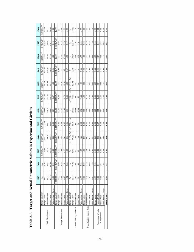
1MG

2MG

3MG

4MG

5MG

6MG

7MG

Targ

et E

quat

ion

λ pw

λ pw

5.7(

E/F

8MG

9MG

10M

G11

MG

12M

G

yc)1/

25.

7(E

/Fyc

)1/2

5.7(

E/F y

c)1/

25.

7(E/

F yc)

1/2

5.7(

E/F y

c)1/

2y

c)1/

25.

7(E/

F

75

5.7(

E/F y

c)1/

25.

7(E

/Fyc

)1/2

5.7(

E/F y

c)1/

25.

7(E

/Fy

c)1/

2

99.6

910

3.36

99.6

810

3.36

103.

36N

omin

al V

alue

43.3

746

.411

0.08

106.

799

.97

110.

3510

2.67

99.9

610

2.67

99.9

610

0.9

96.1

1A

ctua

l Val

ue43

.26

46.1

110

8.37

105.

2599

.68

106.

8510

0.17

99.2

298

.69

95.7

410

1.17

94.8

6R

atio

: Act

ual /

Tar

get

0.97

0.99

0.90

0.88

0.80

0.87

0.97

1.00

0.95

0.96

0.98

0.92

Targ

et E

quat

ion

0.38

2(E/

F

Targ

et V

alue

44

.51

46.5

912

0.77

119.

2112

3.98

122.

6810

3.36

yc)

1/2

12.0

00.

382(

E/F

yc)

1/2

12.0

00.

382(

E/F

yc)

1/2

12.0

00.

382(

E/F

yc)1/

20.

382(

E/F y

c)1/

20.

382(

E/F y

c)1/

20.

382(

E/F y

c)1/

20.

382(

E/F y

c)1/

212

.00

Targ

et V

alue

8.

098.

098.

097.

998.

3112

.00

6.93

126.

9312

6.93

12N

omin

al V

alue

8.13

7.25

7.88

7.88

8.25

12.0

07

10.6

77

10.6

77.

138.

25Ac

tual

Val

ue8.

187.

18.

057.

698.

3711

.93

6.78

10.6

16.

710

.49

6.75

7.88

Rat

io: A

ctua

l / T

arge

t1.

010.

881.

000.

961.

010.

990.

980.

880.

970.

870.

970.

66Ta

rget

Equ

atio

nL p

L pL p

L p +

0.5

(Lr -

Lp)

L p +

0.5

(Lr -

Lp)

L rL p

+ 0

.5(L

r - L

p)L p

+ 0

.5(L

r - L

p)L r

L rL r

L rTa

rget

Val

ue

36.4

630

.45

40.8

296

.35

88.7

513

5.22

75.1

182

.92

114.

613

2.34

109.

8313

0.12

Nom

inal

Val

ue36

3042

9684

132.

0078

8411

412

611

411

4A

ctua

l Val

ue36

3042

9684

132.

0078

8411

412

611

411

4R

atio

: Act

ual /

Tar

get

0.99

0.99

1.03

1.00

0.95

0.98

1.04

1.01

0.99

0.95

1.04

0.88

Targ

et V

alue

3.00

4.00

4.00

4.00

5.00

4.00

4.00

4.00

4.00

4.00

4.00

4.00

Nom

inal

Val

ue3.

053.

723.

943.

815.

214.

004.

143.

54.

143.

54.

493.

88A

ctua

l Val

ue3

3.69

3.85

3.71

5.12

3.90

4.05

3.42

4.08

3.45

4.46

3.97

Rat

io: A

ctua

l / T

arge

t0.

980.

990.

980.

970.

980.

980.

980.

980.

990.

990.

991.

02Ta

rget

Val

ue0.

650.

650.

650.

650.

650.

650.

650.

650.

650.

650.

650.

65N

omin

al V

alue

0.66

0.64

0.61

0.63

0.67

0.65

0.66

0.64

0.65

0.64

0.66

0.61

Act

ual V

alue

0.66

0.64

0.61

0.64

0.68

0.64

0.66

0.66

0.65

0.66

0.68

0.61

Rat

io: A

ctua

l / T

arge

t1.

020.

980.

940.

981.

050.

991.

021.

021.

001.

021.

050.

94Av

erag

e R

atio

0.99

0.97

0.97

0.96

0.96

0.96

1.00

0.98

0.98

0.96

1.01

0.88

Web

Sle

nder

ness

Flan

ge S

lend

erne

ss

Per

cent

age

Web

in

Com

pres

sion

Cro

ss S

ectio

n As

pect

Rat

io

Late

ral B

raci

ng D

ista

nce

Tab

le 3

-5.

Tar

get a

nd A

ctua

l Par

amet

ric

Val

ues i

n E

xper

imen

tal G

irde

rs

based on the nominal dimensions of the girder but the actual material properties of the girder

as these were known prior to designing the girders. This shows that each parametric value

assigned to the girders was typically satisfied within 5%, i.e., the ratio between the actual and

target parametric values was between 0.95 and 1.05 in most cases. Furthermore, the average

ratio is 0.97 with a standard deviation of 0.06. It will be noticed that the intended flange

slenderness ratio for Girder 12MG is not well satisfied. This is due to a fabrication error

where a flange width much narrower than the intended flange width was used. This also

affects the other performance ratios of this girder to a smaller degree. However, the

objective of Girder 12MG, to investigate a more slender flange compared to Girder 11MG,

can still be evaluated.

As discussed above, it was desired to have several girders where the lateral bracing distance

was of sufficient length so that the moment capacity computed from the lateral torsional

buckling equations would be less than the maximum allowable capacity for this limit state.

Table 3-6 demonstrates the girder characteristics with respect to moment gradient effects.

Here it is shown that 4 (6MG, 10MG, 11MG, and 12MG) of the 10 girders with lateral

bracing distances greater than the compact limit will give moment capacities less than the

maximum allowable for the lateral torsional buckling.

Table 3-6. Effects of Moment Gradient Modifier, Cb

Girder Number Cb M = MMAX-LTB

1 MG 1.13 yes2 MG 1.10 yes3 MG 1.19 yes4 MG 1.30 yes5 MG 1.20 yes6 MG 1.34 no7 MG 1.31 yes8 MG 1.30 yes9 MG 1.30 yes

10 MG 1.32 no11 MG 1.30 no12 MG 1.30 no

76

In addition to the measurements taken of the girder dimensions, the geometric imperfections

of the girders were also recorded. These initial imperfections were considered to be

comprised of three components as shown in Fig. 3-7: an out-of-flatness of the web panels

(δow), a tilt of the compression flange (δof), and a lateral sweep of the compression flanges

(δoL). The initial out-of-flatness of the web panel, illustrated in Fig. 3-7(a), was measured by

holding a straightedge with a 24 in. length flush against the surface of the web. The

maximum gap between the straightedge and the surface of the web, which typically occurs

near the midheight of the web, was then recorded as δow. The initial tilt of the compression

flange, as shown in Fig. 3-7(b), was assumed to consist of uniform rotation of the flange

about the web. This type of imperfection was observed in several of the girders; however, an

equally typical situation was that the flange was not straight across its width with the flange

deformed such that both edges of the flange were rotated towards the web. In cases where

the flange exhibited uniform rotation, δof was measured by holding a level at one edge of the

flange and measuring the difference between level and the opposite edge of the flange and

then dividing this value by two in order to obtain the average difference in height between

the web centerline and the flange edge. If both edges of the flange were rotated towards the

web, δof was measured by holding a level at the center of the flange and measuring the

distance between level and each edge of the flange then averaging these two values. The

sweep of the compression flange, shown in Fig. 3-7(c) was measured by holding a level in

Y

Z

Y

X

δowD

do

(a) Initial out-of-flatness of web panel

do

bfc

δof

δof

Z

X

(b) Initial tilt of compression flange

X Lb

δoL

Z

δoLY

X (c) Initial sweep of the compression flange

Figure 3-7. Initial Geometric Imperfections Considered in Experimental Girders

77

the vertical position against the bottom of the web and then measuring the difference between

the top of the level and the surface of the web. Each of these imperfection measurements is

taken at the center of each lateral bracing panel of each girder. For several girders, additional

measurements were also taken at other points along the girders, especially when it was

observed that more severe imperfections occurred at an alternate location. In this case, the

reported imperfection value is based on a weighted average, where a higher weight is given

to imperfection values closer to midspan as these values are assumed to have a more

significant influence of girder behavior. The accuracy of this weighted average procedure is

shown to be accurate through comparisons to FEA results. The average of the recorded

initial imperfections is given for each girder in Table 3-7.

3.4 Testing Procedure

3.4.1 General Considerations

Prior to conducting each experiment, the girders were coated with a mixture of lime and

water so that yielding in the girders could be visually detected with ease. This method

worked well to indicate the progress of yielding in the beams. Small cracks began to appear

in the lime coating as yielding initiated and as yielding in the girder progressed, so did the

size and number of cracks in the lime coating.

Table 3-7. Average Initial Imperfections in Experimental Girders Specimen δow δof δoL

1MG 0.00 0.08 0.212MG 0.00 0.10 0.093MG 0.24 0.08 0.224MG 0.11 0.09 0.135MG 0.12 0.09 0.106MG 0.06 0.06 0.197MG 0.13 0.10 0.318MG 0.20 0.19 0.209MG 0.05 0.09 0.1810MG 0.03 0.22 0.3111MG 0.09 0.11 0.2012MG 0.03 0.09 0.15

78

Load was applied to the girders using a 330-kip actuator, which was mounted on a steel

tension frame with equal capacity as viewed in Fig. 3-2. The tests were conducted in a

displacement control mode using small displacement increments and allowing for loads to

stabilize before applying the subsequent displacement increment. Specifically, displacement

increments ranging between 0.10 in. and 0.20 in. were used during the portions of the test

where a linear-elastic response is expected; smaller increments of 0.05, 0.075, or 0.1 in. were

used during portions of the test when inelastic behavior was expected. For displacement

intervals less than or equal to 0.1 in. the displacement was applied over a time interval of one

minute. A duration of up to 2 minutes was used for larger displacement increments.

At the completion of each displacement interval, the force output from the actuator was

monitored to ascertain when a stable load was achieved. In the elastic range of behavior, a

constant force reading was typically obtained after ten minutes or less. However, once

yielding of the girder began, the work input by the actuator caused plastic deformations of

the girder to occur and hence less force is subsequently required from the actuator to

maintain the prescribed amount of vertical deflection. Because time is required for these

plastic deformations to develop, approximately 20 minutes was required for the loading to

become stable in the inelastic range of the testing. Allowing for the load to become stable

before proceeding to the subsequent load step assures that the static load-deflection curve is

obtained.

3.4.2 Data Collection

A significant amount of data was recorded at each load step during the girder tests. This data

not only included load and vertical displacement measurements required to obtain moment-

rotation relationships, but also vertical and horizontal displacements at two cross-sections in

proximity to and symmetric about midspan of the girder to obtain quantitative measurements

to aid in the categorization of failure modes, i.e., flange local buckling, web local buckling,

lateral distortional buckling, or a combination of these modes. Figure 3-8 schematically

illustrates the instrumentation layout for all tests, while Figs. 3-9 through 3-14 show

photographs of these sensors.

79

CL

EL SL SR

x x

ER

(a) Instrumentation Locations

Girder

x2

X1X1

X2 Spring-Loaded

LVDT (typ.)

Girder

Clamp

Steel Angle

LVDT Stand

+/- 1” LVDT

Load Cell

(b) Instrumentation at EL and ER

Girder

LVDT Stand

+/- 5” LVDT

Welded Rod

(c) Instrumentation at CL

(d) Instrumentation at SL and SR

Figure 3-8. Schematic Diagram of Instrumentation Used in Experimental Testing

80

As shown in Fig. 3-8(a) instrumentation was placed at five cross-sections along the length of

the beam (labeled EL, SL, ER, SR, and CL, where “E” designates end locations, “S”

designates locations along the span, “L” refers to the left side of the beam, “R” refers to the

right side of the beam, and “CL” designates the centerline of the bean). Figures 3-8(b, c, and

d) show schematic diagrams of the instrumentation placed at each of these locations as

discussed below. Additionally, at each displacement increment the force and displacement

readings output from the actuator are also recorded.

Figures 3-8(b) and 3-9 depict the instrumentation installed at the left and right ends of the

beam, labeled as sections EL and ER, respectively. Specifically, at each end of the beam,

there were two linear variable differential transducers (LVDTs) for the purposes of obtaining

end rotations of the girder as well as low profile load cells for determining end reactions. The

force readings from the load cells also served as a comparison to the actuator force for

verification that the reported forces are accurate and assessment of the amount of force (if

any) resisted by the lateral frames.

Figure 3-9. Photograph of Instrumentation at Ends of Girder

81

Figure 3-8(c) illustrates the instrumentation provided at the center of the beam, labeled as

cross-section CL. At this location a small-diameter rod was welded on the bottom surface of

the girder at the longitudinal and transverse center of the beam from which a LVDT was

suspended in order to measure vertical displacement of the beam at this location. This

welded rod was necessary due to limited clearance between the bottom surface of the girder

and the testing frame (as shown in Fig. 3-10), which prohibited installation of the LVDT

directly under the centerline of the girder.

An arrangement of spring-loaded LVDTs as depicted in Figs. 3-8(d) was placed at cross-

sections SL and SR in order to measure the deformations of the cross-section. Specifically,

at each of these sections there are a total of seven LVDTs as shown in Fig. 3-11: two

measuring vertical deformation of the top flange (see Fig. 3-12), two measuring vertical

deformation of the bottom flange (see Fig. 3-13), and three measuring lateral deformation of

the web (see Fig. 3-14). Based on the readings from these sensors, the rotation of both the

top and bottom flanges can be determined in addition to the deformed shape of the web. The

use of three LVDTs on the web allowed for assessing if the web deformation was linear (as

would be expected if lateral-torsional buckling occurred) or quadratic (as would occur during

web local buckling).

Figure 3-10. Photograph of Instrumentation at Girder Centerline

82

Figure 3-11. Photograph of Instrumentation at SL and SR

Figure 3-12. Top Flange LVDTs

The pair of LVDTs on the bottom flange was centered about the web of the girder with a

typical spacing of 6 in. between the two sensors, but varied based on the width of the bottom

flange. The LVDT pair on the top flange was also centered about the web, but with a smaller

distance between these two gages of 3 in. to attempt to capture the displacement of the top

83

flange even if significant lateral movement of the top flange occurred, i.e., the LVDTs are

mounted independently of the girder such that the displacements captured by the LVDTs

represent the displacement at a fixed point in space as opposed to the displacement of a fixed

point on the girder. The three web LVDTs were placed such that they were located

Figure 3-13. Bottom Flange LVDTs

Figure 3-14. Web LVDTs

84

approximately equal distances apart to the extent permitted by the LVDT stands. The web

LVDT closest to the top flange is located at least 5 in. from the top flange to allow for a

minimum of this amount of deflection. The longitudinal location of these sensors, labeled as

x in Fig. 3-8(a), varied for each girder and was determined by conducting a finite element

analysis of the girders prior to each experiment in order to predict the location where the

most critical buckling was expected.

3.5 Experimental Results

There are three primary points of interest regarding the experimental results. These are (1)

maximum moment capacities and comparison of these strengths to those predicted by

AASHTO specifications, (2) the failure modes as determined from visual assessment of the

girder and quantitative measurements resulting from the LVDT readings, and (3) the load

versus deflection response of the girders. These three attributes of each girder are discussed

in the following sections, followed by a discussion of general conclusions formed on the

basis of these experimental results and will subsequently be used to verify the FEA

techniques implemented in later chapters.

The maximum moment capacities of each girder and the respective moment capacities

predicted by AASHTO (2004) Specifications are given below in Table 3-8. A discussion of

this data is given in the subsequent sections detailing the results of each girder individually.

Table 3-8. Comparison of Experimental and AASHTO (2004) Capacities (ft-kips)

Specimen MEXP MAASHTO

Percent Difference

1MG 1635 1640 0.32MG 1757 1805 2.83MG 985 991 0.64MG 978 971 0.85MG 1803 2026 12.46MG 519 582 12.27MG 951 1043 9.78MG 809 777 4.09MG 897 1060 18.2

10MG 834 796 4.511MG 1125 1317 17.112MG 1 1584 9.445 6

85

It is noted that the optional provisions given in Appendix A of Article 6.10 of the

specifications (AASHTO 2004), which allow for the prediction of moment capacities in

excess of My, are applicable for these girders and have been used to compute predicted

moment capacities. Furthermore, it is noted that in the current (2004) specifications the

controlling failure modes are either computed to be local buckling (which is based on the

enderness properties of the flange, i.e., flange local buckling), lateral-torsional buckling, or

te data

cases where readings from top flange LVDTs were not available due to significant lateral

sl

tension flange yielding.

The LVDT readings from the sensors located along the span of the girder are used to

generate a plot of the deformed shape of each girder, which are presented for each girder in

the following sections. The presented data is the data from the panel of the girder to the right

or left of midspan (i.e, SR or SL in Fig. 3-8(a)) experiencing the most severe distortions and,

in cases where such data is available, is the data after removing the load from the girder at

the end of the test, thus representing the final deformed shape of the girder. Where this data

is not available due to the need for removing sensors in order to avoid damage (as was done

in the testing of girders 2MG, 9MG, and 12MG), the data presented is the data from the last

available load step. Unless noted otherwise, the deformed shape presented is qualitatively

representative of the deformed shape of the girder throughout the unloading range although

the magnitude of the deformations increases as the vertical displacement applied to the girder

increases. In each plot the original undeformed shape of the girder is represented by square

data points and the deformed shape is represented by a series of diamonds. Furthermore,

filled data points represent actual test data and shaded data points represent approxima

in

movement of the flange such that the LVDT is no longer in contact with the flange.

Load versus deflection plots are subsequently presented for each of the twelve experimental

girders. It is noted that there is a linear relationship between load and moment as well as

between deflection and rotation, so the shape of the moment versus rotation curves is the

same as the shape of the load versus deflection relationships presented below. For many of

the girders, the girder was loaded multiple times and in these cases the load versus deflection

relationship of each loading cycle is presented. In most cases, the deflection data presented

86

in the load versus deflection plots represents an average of the readings obtained from the

internal LVDT contained within the actuator and the readings obtained from the external

LVDT located beneath the centerline of the girder. In this situation, the data in the load

versus deflection plots is represented by a series of squares. It is noted that the actuator

displacement data may over predict the actual displacements in the girder as the actuator has

the ability to move longitudinally and laterally in addition to vertically. Conversely, the

external LVDT may under predict the actual displacements due to lateral or longitudinal

movement of the point on the bottom flange of the girder to which the LVDT is affixed.

Thus, averaging these two values gives a realistic representation of the actual girder

deflection in most cases. However, there are instances when the external LVDT data is

deemed unreliable due to substantial movement of the bottom flange of the girder at

midspan, resulting in LVDT readings that are significantly less than the actual vertical

deflection of the girder. In these instances, the data presented in the load versus deflection

lots is the actuator data only. This is indicated by using a series of triangles to represent the p

data in the plots.

3.5.1 Girder 1MG

Table 3-8 indicates that the maximum moment capacity of girder 1MG is well predicted by

the AASHTO (2004) specifications. Specifically, the predicted moment capacity of 1640 ft-

ips matches the experimental capacity of the girder (1635 ft-kips) within 0.3% and is

of the web in

ompression. It is also observed that the top flange and the top of the web remain

the girder at a particular level of load, where the deformation capacity is computed as the

ratio between the plastic displacement (total displacement minus elastic displacement) and

k

controlled by flange local buckling.

The deformed shape of the girder is shown in Fig. 3-15, where it is shown that the

predominant deformations are in the compression flange and portion

c

approximately perpendicular to one another throughout the testing range.

As shown in Fig. 3-16, girder 1MG exhibits relatively ductile behavior as anticipated for this

compact girder. The ductility of the girder may be quantified by the deformation capacity of

87

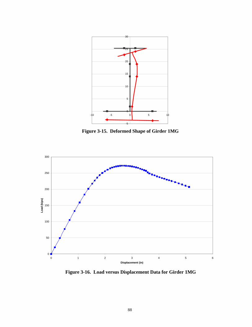
-5

0

5

10

15

20

25

30

-10 -5 0 5 10

Figure 3-15. Deformed Shape of Girder 1MG

0

50

100

150

200

250

300

0 1 2 3 4 5 6

Displacement (in)

Load

(kip

s)

Figure 3-16. Load versus Displacement Data for Girder 1MG

88

the elastic displacement. At a load equal to 246 kips (which is equal to 90% of the maximum

load), the deformation capacity of this girder is 2.0.

3.5.2. Girder 2MG

The AASHTO (2004) specifications accurately predict the moment capacity of Girder 2MG

by predicting a moment capacity of 1805 ft-kips, which differs from the experimental

capacity of 1757 ft-kips by only 2.7%. Furthermore, the specifications predict the same

moment capacity for all three strength calculations: flange local buckling, lateral torsional

buckling, and tension flange yielding.

The deformed shape of Girder 2MG is shown below in Fig. 3-17. Here it is shown that the

most significant deformations are lateral movement of the girder. However, it is important to

note that testing of this girder was terminated prior to achieving significant deformations in

the girder due to failure of one of the lateral braces, which contributed to the lateral

movement of the beam depicted in the figure. Additionally, rotation of the compression

flange about the web and web buckling are also captured by the LVDT readings presented in

Fig. 3-17.


-5

0

5

10

15

20

25

30

-10 -5 0 5 10

89

Girder 2MG also displays a ductile load versus displacement relationship typical of a

compact beam, which is shown in Fig. 3-18. At a load of 264 kips, equal to 90% of the

maximum load, the deformation capacity of girder 2MG is 2.3. Thus, comparing the

deformation capacities Girder 1MG with a D/bfc ratio of 3 (and a deformation capacity equal

to 2.0) and Girder 2MG with a D/bfc ratio of 4 (and a deformation capacity equal to 2.3)

illustrates that there is not a significant influence on girder ductility with varying D/bfc ratio

for these compact girders.

3.5.3 Girder 3MG

As shown in Table 3-8, the AASHTO (2004) Specifications accurately predict the capacity of

girder 3MG. The difference between the experimental capacity of 985 ft-kips and the

predicted capacity of 991 ft-kips is only 0.6%. The predicted capacity is computed using

Appendix A and is controlled by the computations based on flange local buckling or lateral

torsional buckling.

0

50

100

150

200

250

300

350

0 1 2 3 4 5 6

Displacement (in)

Load

(kip

s)


90

Two plots of the deformed shape of Girder 3MG are given below in Fig. 3-19. The plot on

the left represents the deformed shape of the girder at the maximum load where it is clear that

web buckling is the only deformation present. The plot on the right in Fig. 3-19 shows the

deformed shape of the girder after the testing has been completed. This plot indicates that, as

web buckling progresses, flange buckling also begins to occur due to the decreased restraint

to the flange as the web deformations increase. These experimental results support the

anticipated failure mode of web local buckling, which was assumed based on the non-

compact web, compact flanges, and compact brace spacing of this girder. Furthermore,

comparing Figs. 3-17 and 3-19, the influence of the more slender flange in Girder 3MG is

clearly observed.

Figure 3-20 illustrates the load versus deflection data for Girder 3MG. This graph shows that

there is a nearly linear relationship between load and deflection in both the loading and

unloading phases. However, the girder is still relatively ductile, with a deformation capacity

of 1.9 at 90% of the maximum load. Thus, the use of a non-compact web appears to result in

only slightly less deformation compared to the compact girders (1MG and 2MG) discussed

above.

-5

0

5

10

15

20

25

30

35

-10 -5 0 5 10

-5

0

5

10

15

20

25

30

35

-10 -5 0 5 10

Figure 3-19. Deformed Shapes of Girder 3MG

91

0

20

40

60

80

100

120

140

160

180

200

220

0 1 2 3

Displacement (in)

Load

(kip

s)


3.5.4 Girder 4MG

The AASHTO (2004) Specifications result in a predicted moment capacity of 971 ft-kips for

Girder 4MG, which is based on flange local buckling or lateral torsional buckling. This

capacity differs from the experimental moment capacity of 978 ft-kips by only 0.7%.

Figure 3-21 shows the deformed shape of Girder 4MG at the sensor locations, which are

located approximately 4 in. from the point where the most severe girder deformations

occurred. From the figure, lateral movement of the compression flange and deformation of

the web are the most prominent deformations; however significant flange local buckling also

occurred in the girder, but due to the small amplitude of this buckle, this deformation was not

well captured by the LVDTs. Comparing Figs. 3-19 and 3-21, the influence of the longer

bracing distance in Girder 4MG is shown to be increased lateral movement of the

compression flange and portion of the web in compression.

92

-5

0

5

10

15

20

25

30

35

-8 -6 -4 -2 0 2 4 6 8


The influences of longer lateral bracing distance can also be seen by analyzing the load

versus displacement graphs presented in Figs. 3-20 and 3-22. From Fig. 3-22, it can be

determined that Girder 4MG has significantly less ductility than the girders previously

discussed; at a load of 108 kips (90% of the maximum load), the deformation capacity is only

1.1. In other words, the deformation capacity decreases by 42% for Girder 4MG with an

intermediate lateral bracing distance compared to Girder 3MG with a compact lateral bracing

distance.

3.5.5 Girder 5MG

As shown by Table 3-8, the AASHTO (2004) Specifications over predict the capacity of

Girder 5MG by 12.4%. This predicted capacity is controlled by flange local buckling and

lateral torsional buckling, where both failure modes predict equal capacity.

Figure 3-23 illustrates the deformed shape of girder 5MG, where the primary deformation is

lateral movement of the compression flange accompanied by a small amount of rotation

between the compression flange and web. However, a local buckle was also present in the

compression flange of the girder, but was not well captured by the instrumentation because

93

0

20

40

60

80

100

120

140

0 1 2 3 4 5

Displacement (in)

Load

(kip

s)


-5

0

5

10

15

20

25

30

35

40

45

-10 -5 0 5 10


94

the LVDTs were located 3 in. from the center of the flange buckle. Comparing Fig. 3-23 to

Fig. 3-21, shows that the higher D/bfc ratio used in Girder 5MG does not have an influence of

the deformed shape.

The load versus displacement curve for Girder 5MG is shown below in Fig. 3-24. From this

data it is determined that at a load of 163 kips (90% of the maximum load) the deformation

capacity of the girder is 1.0. Comparing this data to the corresponding data for Girder 4MG

(deformation capacity of 1.1), it is shown that the deformation capacity of the two girders are

approximately equal. Thus it is concluded that the increased D/bfc ratio of Girder 5MG does

not have a significant influence on girder behavior.

3.5.6 Girder 6MG

The AASHTO (2004) equations also over-predict the capacity of Girder 6MG, as shown in

Table 3-8. Specifically, the predicted capacity of 582 ft-kips is 12.2% higher than the

0

20

40

60

80

100

120

140

160

180

200

0 1 2 3 4 5

Displacement (in)

Load

(kip

s)


95

experimentally observed capacity of 519 ft-kips. The predicted capacity is controlled by

flange local buckling.

Figure 3-25 shows the deformed shape of Girder 6MG. This deformed shape plot seems to

depict a lateral torsional buckling failure mode, however the LVDTs were located

approximately 6 in. from the location of the girder where the maximum deformations

occurred. At this location, significant flange and web local buckling was also observed.

Thus the deformed shape of the girder is as anticipated considering that all three slenderness

ratios were maximized in this girder.

The load versus displacement data for Girder 6MG shown below in Fig. 3-26 indicates that

this girder has the least ductility of all of the girders examined thus far, with the load

dropping relatively quickly after the maximum load is attained. Computation of the

deformation capacity of Girder 6MG supports this observation where at a load equal to 90%

of the maximum load (48 kips), the deformation capacity is determined to be 0.7.

-5

0

5

10

15

20

25

30

35

-10 -5 0 5 10


96

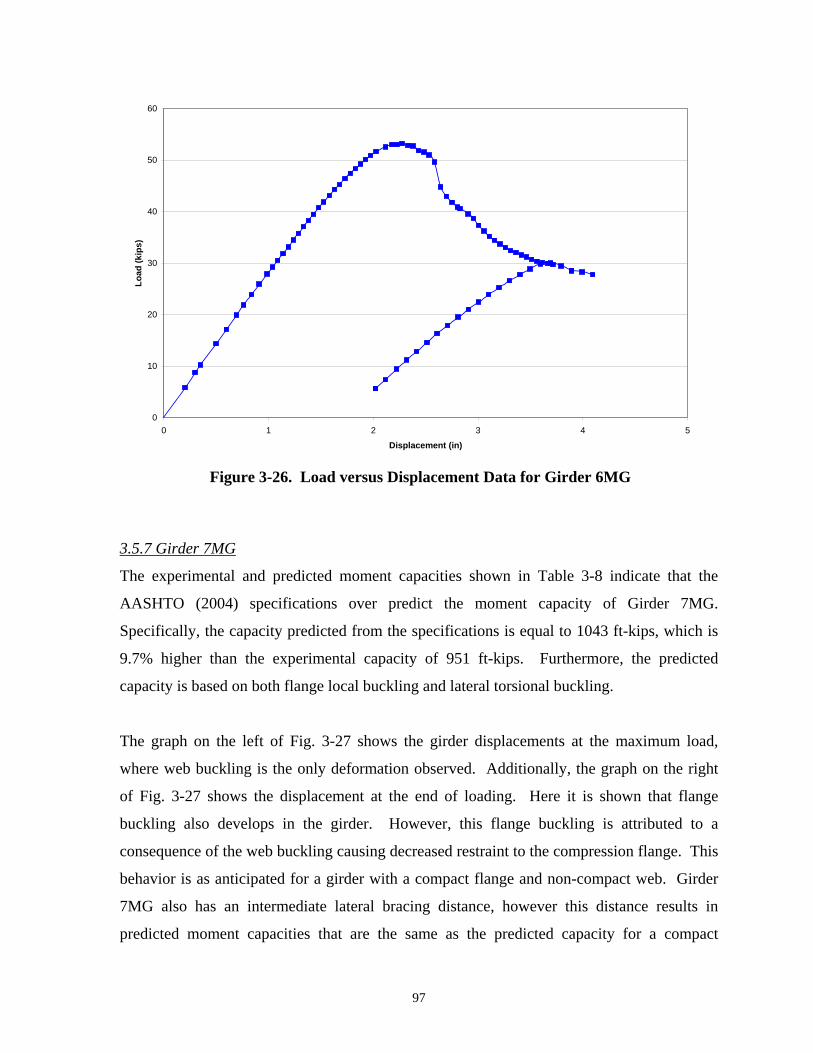
0

10

20

30

40

50

60

0 1 2 3 4 5

Displacement (in)

Load

(kip

s)


3.5.7 Girder 7MG

The experimental and predicted moment capacities shown in Table 3-8 indicate that the

AASHTO (2004) specifications over predict the moment capacity of Girder 7MG.

Specifically, the capacity predicted from the specifications is equal to 1043 ft-kips, which is

9.7% higher than the experimental capacity of 951 ft-kips. Furthermore, the predicted

capacity is based on both flange local buckling and lateral torsional buckling.

The graph on the left of Fig. 3-27 shows the girder displacements at the maximum load,

where web buckling is the only deformation observed. Additionally, the graph on the right

of Fig. 3-27 shows the displacement at the end of loading. Here it is shown that flange

buckling also develops in the girder. However, this flange buckling is attributed to a

consequence of the web buckling causing decreased restraint to the compression flange. This

behavior is as anticipated for a girder with a compact flange and non-compact web. Girder

7MG also has an intermediate lateral bracing distance, however this distance results in

predicted moment capacities that are the same as the predicted capacity for a compact

97

-5

0

5

10

15

20

25

30

35

-10 -5 0 5 10

-5

0

5

10

15

20

25

30

35

-10 -5 0 5 10


bracing distance due to moment gradient (Cb) effects. It is noted that these deformed shapes

differ from the deformed shape of Girder 4MG, where all three buckling modes were

observed, although the two girders only differ in that Girder 7MG is a hybrid girder while

Girder 4MG is a homogeneous Grade 50 girder.

Figure 3-28 indicates that Girder 7MG has a moderate amount of ductility. Evaluating the

deformation capacity at 131 kips (90% of the maximum load) gives a deformation capacity

of 1.2. Comparing these results to the deformation capacity of Girder 4MG (1.1), it is

determined that the results for the two girders are nearly equal, although slightly higher

deformation capacity results for the hybrid girder.

3.5.8 Girder 8MG

As shown in Table 3-8, the specifications predict the moment capacity of girder 8MG within

an acceptable level of accuracy. Specifically, the predicted capacity of 777 ft-kip, which is

based on the flange local buckling equations, is 4.0% conservative compared to the actual

girder capacity of 809 ft-kips.

98

0

20

40

60

80

100

120

140

160

0 1 2 3 4 5

Displacement (in)

Load

(kip

s)


The deformed shape of Girder 8MG is shown below in Fig. 3-29. This figure indicates that

the primary girder deformations are web deformations and lateral movement of the

compression flange. However, in actuality, the most significant deformations were a flange

buckle with amplitude of 3 in. that developed in the girder 15 in. from the LVDT locations.

Comparing the deformed shape of Girder 8MG to Girder 7MG, flange buckling only occurs

in Girder 7MG as a consequence to web buckling, while flange local buckling is the

predominant failure mode in Girder 8MG. Thus, the deformed shapes of these two girders

are as expected given that the two girders are similar except that Girder 8MG has a slender

flange, while Girder 7MG has a compact flange.

Figure 3-30 shows the load versus displacement relationship for Girder 8MG, where it is

observed that the load rapidly decreases once the maximum moment capacity is attained.

99

-5

0

5

10

15

20

25

30

-6 -4 -2 0 2 4 6


0

20

40

60

80

100

120

140

0 1 2 3 4 5

Displacement (in)

Load

(kip

s)


100

Computation of the deformation capacity at a load of 104 kips (90% of the maximum load)

gives a result of 0.7. Thus, compared to Girder 7MG with a deformation capacity of 1.2, the

increased flange slenderness of Girder 8MG results in a significant decrease in deformation

capacity.

3.5.9 Girder 9MG

The specifications predict a moment capacity that is highly unconservative for Girder 9MG.

Here the controlling capacity is based on both flange local buckling and lateral torsional

buckling and is equal to 1060 ft-kips, which is 18.2% higher than the actual capacity of 897

ft-kips.

Figure 3-31 shows the deformed shape of the girder is dominated by web local buckling and

lateral movement of the compression flange. This is also the predicted behavior of the girder

as the girder has a non-compact web, non-compact brace spacing and a compact flange.

Girders 7MG and 9MG differ only in that a shorter bracing distance is used in Girder 7MG

and comparing these deformed shape of Girder 9MG to the final deformed shape of Girder

7MG shown on the right side of Fig.3-27, it is observed that the two deformed shapes are

similar, although more flange deformation is observed in Girder 7MG.

-5

0

5

10

15

20

25

30

35

-6 -4 -2 0 2 4 6


101

Figure 3-32 shows the load versus displacement data for girder 9MG, where it is observed

that the load quickly reduces after the maximum load is reached and then a more gradual

unloading occurs. At 90% of the maximum load, 85.2 kips, the slope of the unloading curve

is still relatively steep, resulting in a deformation capacity of only 0.4. Comparing this

deformation capacity to the deformation capacity of Girder 7MG (1.2), it is concluded that

the increased lateral bracing distance of Girder 9MG significantly reduces the deformation

capacity. Furthermore, in comparison to the deformation capacity of Girder 8MG (0.7),

which differs from Girder 7MG in that a slender flange is used, it is concluded that, for the

values investigated, increased lateral bracing distance is more detrimental to deformation

capacity than increased flange slenderness.

3.5.10 Girder 10MG

Table 3-8 shows that the AASHTO (2004) Specifications are 4.5% conservative for Girder

10MG. The predicted capacity of 796 ft-kips is based on flange local buckling compared to

the experimental capacity of 834 ft-kips.

0

10

20

30

40

50

60

70

80

90

100

0 1 2 3 4

Displacement (in)

Load

(kip

s)

5


102

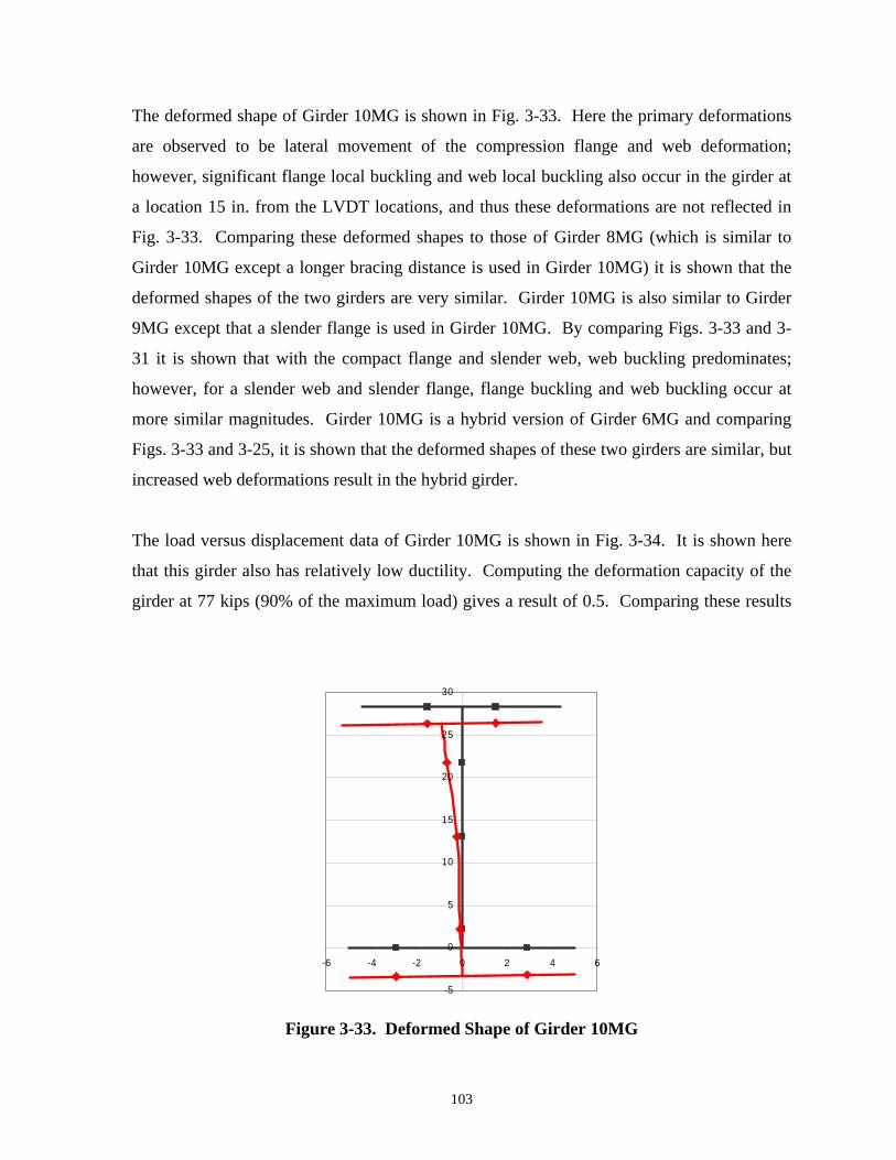
The deformed shape of Girder 10MG is shown in Fig. 3-33. Here the primary deformations

are observed to be lateral movement of the compression flange and web deformation;

however, significant flange local buckling and web local buckling also occur in the girder at

a location 15 in. from the LVDT locations, and thus these deformations are not reflected in

Fig. 3-33. Comparing these deformed shapes to those of Girder 8MG (which is similar to

Girder 10MG except a longer bracing distance is used in Girder 10MG) it is shown that the

deformed shapes of the two girders are very similar. Girder 10MG is also similar to Girder

9MG except that a slender flange is used in Girder 10MG. By comparing Figs. 3-33 and 3-

31 it is shown that with the compact flange and slender web, web buckling predominates;

however, for a slender web and slender flange, flange buckling and web buckling occur at

more similar magnitudes. Girder 10MG is a hybrid version of Girder 6MG and comparing

Figs. 3-33 and 3-25, it is shown that the deformed shapes of these two girders are similar, but

increased web deformations result in the hybrid girder.

The load versus displacement data of Girder 10MG is shown in Fig. 3-34. It is shown here

that this girder also has relatively low ductility. Computing the deformation capacity of the

girder at 77 kips (90% of the maximum load) gives a result of 0.5. Comparing these results

-5

0

5

10

15

20

25

30

-6 -4 -2 0 2 4 6


103

0

10

20

30

40

50

60

70

80

90

0 1 2 3 4 5 6

Displacement (in)

Load

(kip

s)


to the deformation capacity of Girder 8MG at the same normalized load (0.7), it is shown that

the longer bracing distance slightly reduces the deformation capacity. Similarly, comparison

with the deformation capacity of Girder 9MG (0.4), it is shown that the increased flange

slenderness of Girder 10MG does not have a detrimental influence on the girder ductility.

Lastly, comparing the deformation capacities of Girder 10MG (0.5) and Girder 6MG (0.7), it

is seen that the hybrid girder has slightly less deformation capacity.

3.5.11 Girder 11MG

The specifications predict a moment capacity of 1317 ft-kips for Girder 11MG. This

capacity is 17.1% higher than the experimental capacity of 1125 ft-kips and is based on the

lateral torsional buckling equations.

The deformed shape of Girder 11MG consists of a combination of lateral torsional buckling

and web buckling, as shown in Fig. 3-35. This deformed shape consisting predominantly of

web buckling in combination with lateral buckling is as expected behavior for this girder

104

-5

0

5

10

15

20

25

30

35

-10 -5 0 5 10


with non-compact web slenderness, non-compact bracing distance, and compact flanges.

Girder 11MG is similar to Girder 9MG except that the web of Girder 11MG is comprised of

steel having a higher yield strength. Thus, the deformed shapes of the two girders (shown in

Figs. 3-35 and 3-31) are similar, but there is less web buckling in Girder 11MG.

Figure 3-36 illustrates the load versus displacement data for Girder 11MG. It is shown here

that there is a comparatively small amount of ductility for this girder. Computing the

deformation capacity at 107 kips (90% of the maximum load) gives a deformation capacity

of 0.5, which closely corresponds to the deformation capacity of the similar hybrid girder,

Girder 9MG, which had a deformation capacity of 0.4.

3.5.12 Girder 12MG

The maximum moment capacity of Girder 12MG is 1445 ft-kips, as shown in Table 3-8. The

specifications predict a moment capacity 9.6% higher than this, 1584 ft-kips, based on flange

local buckling.

105

0

20

40

60

80

100

120

140

0 1 2 3 4 5 6

Displacement (in)

Load

(kip

s)


The deformed shape of Girder 12MG is shown in Fig. 3-37. As shown in the figure, the

main type of deformation in Girder 12MG consists of lateral movement of the compression

flange in combination with rotation of the compression flange about the web. Girder 12MG

is similar to Girder 11MG except that Girder 12MG has a slightly more slender compression

flange. The influence of the higher compression flange slenderness is shown to be that

flange and web buckling occur at approximately the same magnitude when the flange

slenderness is increased, compared to Girder 11MG where web buckling is prominent.

Girder 12MG is also similar to Girder 9MG except steel of a higher yield stress is used in

Girder 12MG. Comparing Fig. 3-37 and 3-31, it is observed that the influence of the higher

web strength is less bending in the compression region of the web. Girder 12MG is also

similar to Girder 6MG, but with two differences, which are a higher yield strength of 70 ksi

used in Girder 12MG compared to a yield strength of 50 ksi in Girder 6MG and a lower

flange slenderness is used in Girder 12MG. Comparing the deformed shapes of these two

girders shows that the deformed shapes of the two girders are very similar, especially when it

106


-10

-5

0

5

10

15

20

25

30

35

40

-10 -5 0 5 10

is considered that the deformed shape of Girder 6MG shown in Fig. 3-25 does not capture the

web and flange deformations that occurred away from the LVDT locations in this girder.

Figure 3-38 shows the load versus displacement data for Girder 12MG. The ductility of this

girder is also shown to be relatively limited, as the load rapidly descends after reaching the

maximum load. The deformation capacity of this girder is computed to be 0.6 at a load of

137 kips (90% of the maximum load). This closely corresponds to the deformation capacity

of similar girders such as Girder 11MG (0.5), Girder 9MG (0.4), and Girder 6MG (0.7).

3.5.13 Summary of Experimental Results

3.5.13.1 Moment Capacity

The above comparisons of the experimental moment capacity to that predicted by the

AASHTO (2004) Specifications reveal several trends. First, for the compact girders included

in this study (Girders 1MG and 2MG) the specifications give accurate predictions of the

moment capacities (within 3% of the experimental capacities).

107

0

20

40

60

80

100

120

140

160

0 1 2 3 4 5 6

Displacement (in)

Load

(kip

s)


Three of the girders in this work (Girders 3MG, 4MG, and 5MG) were nominal Grade 50

girders with non-compact webs and compact flanges. For two of these, the AASHTO

Specifications give accurate predictions of the experimental capacity. For the third Grade 50

girder with a non-compact web and compact flange, the predicted capacities are

unconservative by 12.4%. For the Grade 50 girder with a non-compact web, non-compact

compression flange, and non-compact lateral bracing distance (Girder 6MG), the

specifications are unconservative.

The predicted moment capacities are also unconservative for the three girders with compact

flanges incorporating Grade 70 steel (Girders 7MG, 9MG, and 11MG), but conversely, are

conservative for both girders with slender flanges incorporating Grade 70 steel (Girders 8MG

and 10MG).

108

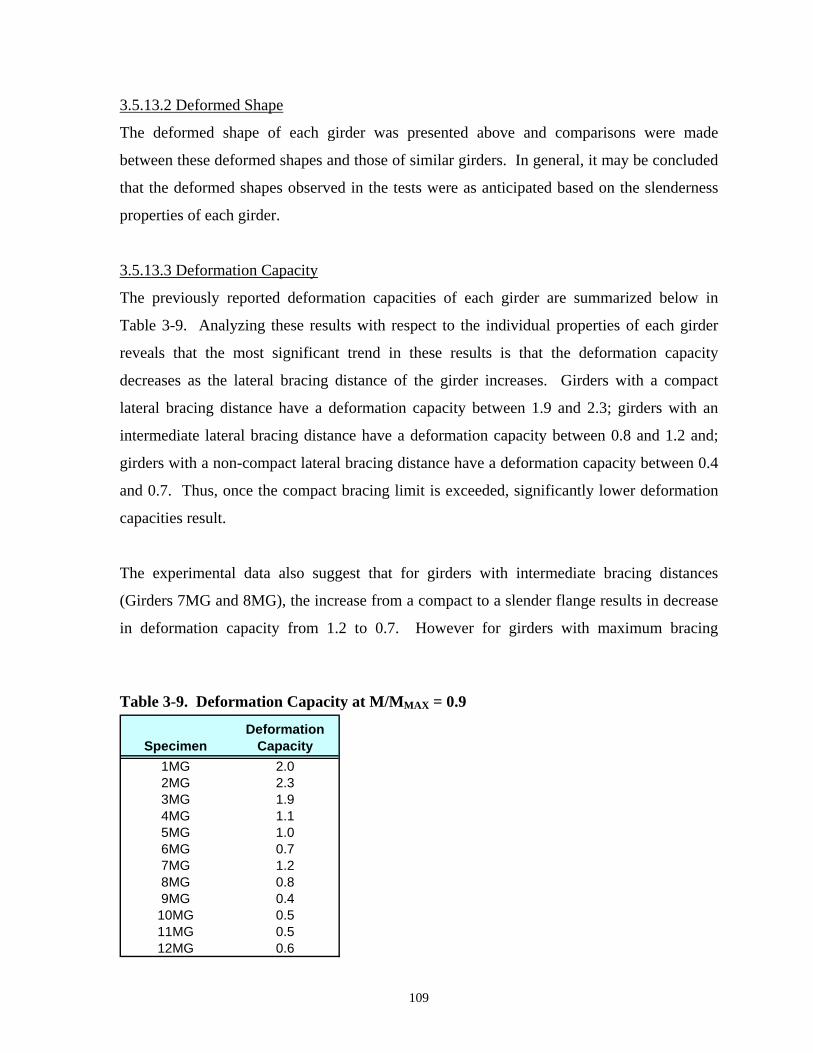
3.5.13.2 Deformed Shape

The deformed shape of each girder was presented above and comparisons were made

between these deformed shapes and those of similar girders. In general, it may be concluded

that the deformed shapes observed in the tests were as anticipated based on the slenderness

properties of each girder.

3.5.13.3 Deformation Capacity

The previously reported deformation capacities of each girder are summarized below in

Table 3-9. Analyzing these results with respect to the individual properties of each girder

reveals that the most significant trend in these results is that the deformation capacity

decreases as the lateral bracing distance of the girder increases. Girders with a compact

lateral bracing distance have a deformation capacity between 1.9 and 2.3; girders with an

intermediate lateral bracing distance have a deformation capacity between 0.8 and 1.2 and;

girders with a non-compact lateral bracing distance have a deformation capacity between 0.4

and 0.7. Thus, once the compact bracing limit is exceeded, significantly lower deformation

capacities result.

The experimental data also suggest that for girders with intermediate bracing distances

(Girders 7MG and 8MG), the increase from a compact to a slender flange results in decrease

in deformation capacity from 1.2 to 0.7. However for girders with maximum bracing

Table 3-9. Deformation Capacity at M/MMAX = 0.9

SpecimenDeformation

Capacity1MG 2.02MG 2.33MG 1.94MG 1.15MG 1.06MG 0.77MG 1.28MG 0.89MG 0.4

10MG 0.511MG 0.512MG 0.6

109

distances (Girders 9MG through 12MG), variable flange slenderness does not have an

appreciable influence of deformation capacity.

Based on the experimental data, a clear trend can not be determined between deformation

capacity and the other variables investigated (web slenderness, material properties, D/bfc

ratio). The influences of these variables will be further explored through the FEA presented

in Chapter 5.

110

Chapter 4: NONLINEAR FEA MODELING PROCEDURES

This chapter will discuss the methods and procedures employed to conduct nonlinear FEA in

this research. In summary, FEA was performed using commercially available FEA software,

namely ABAQUS version 6.3.1. Initially, FEMAP software (version 8.3) was used to create

the geometry (nodes and elements) for each girder being analyzed. FEMAP is then capable

of writing this information in the form of an ABAQUS input file. This input file is then

modified by the user to include material, load, and analysis technique information.

Additionally, the node coordinates in the input file are modified to account for initial

geometric imperfections using a FORTRAN program specially created for this purpose. The

new input file and a user-defined sub-routine specifying residual stresses are then analyzed

by ABAQUS using the modified Riks method. Thorough details of these procedures are

presented herein. The reader will notice that throughout this chapter reference is made to

specific commands used in ABAQUS; these are given by the notation *command.

4.1 Mesh Density

Initial considerations that must be correctly addressed are element size and mesh density.

The selection of relatively large elements will result in unrealistically low predicted strengths

due to the effects of stress concentrations, while relatively small elements can cause an

overestimation of the energy dissipation capacity (Bazant and Cedolin 1980). By selecting

the appropriate mesh density, these situations will be avoided, and accurate results can be

obtained. Previous research by Yang (2004) has evaluated the ideal mesh density for steel I-

girders of the type investigated in this study. This assessment included an evaluation of the

accuracy and processing time for models with three different mesh densities: a relatively

course mesh with 4 elements across the width of each flange and 6 elements throughout the

height of the web, an intermediate mesh density with 6 elements across the width of the

flange and 10 elements throughout the height of the web, and a fine mesh density with 10

elements across the flange width and 20 elements through the web height. Yang concluded

that the ideal mesh density was the combination of 10 elements across the flange width and

111

20 elements throughout the web height, which resulted in less than 1% error compared to

selected experimental results. Thus, this same element size is used in the current research.

Furthermore, the aspect ratio is minimized (made closest to 1) to the extent possible. Using

the mesh density discussed above, there are twice as many elements in the web as there are in

each flange. However, the web height is typically three to four times the width of the

compression flange. Because it is desirable for the web and flange elements to have equal

lengths so that these elements will share coincident nodes, it is not possible to choose the

element length so that the web and flange will both have an aspect ratio of 1. Instead, an

element length is selected that gives an equal aspect ratio in the compression flange and the

web, which typically results in an aspect ratio of approximately 1.4 for all elements.

4.2 Element Selection

ABAQUS/Standard provides the user with a large number of available element types.

Therefore, it is necessary to initially investigate the suitability of a selected element type for

the given problem. As proven by several researchers (White et. al. 1987; Huang 1995; Barth

1996; Earls and Shah 2000), shell elements are both sufficient and necessary for modeling

the physical behavior of the type of plate girders analyzed in this study.

4.2.1 Element Naming Convention

The element naming convention used in ABAQUS conveys the key attributes of the element.

For example, the first letter of the element name refers to the general element type, with “S”

representing a shell element. This is followed by a number indicating the number of nodes in

the element. This character may be followed by the letter “R”, which indicates that reduced

integration is used. Lastly, a “5” at the end of an element name indicates that the element

only contains five degrees of freedom (three translations and two in-plane rotations),

otherwise all six degrees of freedom are considered.

4.2.2 General-Purpose Shell Elements

Previous research on the performance of negative bending regions of steel I-girders has

shown that the S4R element results in the most accurate prediction of actual girder behavior

112

(Yang 2004). S4R is a 4-node general-purpose shell element. These elements are intended to

provide robust, accurate solutions for both thin and thick shells, using classical (Kirchhoff)

shell theory when appropriate for relatively thin shells and thick (Mindlin) shell theory as the

shell thickness increases. These elements allow for finite membrane strains and rotations of

the shell. Therefore, they are suitable for large-strain analysis involving inelastic

deformation of materials with nonzero effective Poisson’s ratio. These elements allow for

change in shell thickness as a function of the membrane strain. Transverse shear deformation

is also included. These elements are not subject to hourglass effects or transverse shear

locking.

Other popular shell elements available in the ABAQUS element library are S4, S4R5, and

S9R5. As suggested by the element labels, the difference between the S4 and S4R elements

is the number of integration points used in the analysis; “full” integration is used for S4

elements, while “reduced” integration is used for S4R elements. In full integration, a

sufficient number of integration points is selected such that integration of the element

stiffness matrix is exact, i.e., for first order elements, such as S4, each element has four

integration points. However, reduced integration elements use one order less than that

required for full integration of the element stiffness matrix. Thus, for a S4R element only

one integration point is used to form the element stiffness matrix. However, the mass matrix

and force matrix are still integrated exactly. Displacements are then computed at each node.

Linear interpolation is then used to determine the displacements at other locations using

u = Σ fi ui (4.1)

where ui are the displacements at each node and fi is the following shape function

( )(i 01f 1 14

)0= + ξ + η (4.2)

and ξ0 and η0 refer are expressed as

0 iξ = ξ ξ (4.3)

0 iη = η η (4.4)

113

where ξ and η refer to the natural coordinates of each node, as illustrated in Fig. 4-1. For

example, at node 1, ξ equals -1 and η equals -1. Thus, ξ0 equals - ξ and η0 equals - η and

Eq. 4.2 becomes

( )(11f 1 14

)= − ξ − η (4.5)

S4R elements offer several advantages over the fully integrated S4 elements. For example,

reduced integration of isoparametric elements computes strains and stresses at the locations

known to provide optimal accuracy; thus, reduced integration usually produces more accurate

results provided the elements are not disturbed or loaded in in-plane bending. Furthermore,

reduced integration typically softens the response of the elements, which also leads to

increased accuracy by counteracting the overly stiff response usually encountered in FEA.

The use of fewer integration points also benefits the user by resulting in reduced computing

time and storage requirements. The primary disadvantage of using reduced integration is that

deformation modes that cause no strain at the integration points may develop. This may lead

to inaccurate results if these zero-energy modes propagate through the structure in a

phenomenon commonly known as hourglassing. However, ABAQUS prevents hourglassing

1 2

3 4 η

ξ

η = −1

ξ = −1

η = 1

ξ =1

Figure 4-1. Element Natural Coordinate System

114

for S4R elements by introducing a small artificial stiffness associated with zero-energy

deformation modes.

S4R5 and S9R5 are three-dimensional shell elements whose behavior is governed by

classical (Kirchoff) shell theory. Thus, these elements are only appropriate for cases where

transverse shear flexibility is negligible and the shell normal remains orthogonal to the shell

reference surface, i.e, for relatively thin plates or shells. Because thin shell elements neglect

transverse shear, these elements have only five degrees of freedom (three displacement

components and two in-surface rotation components) at each node. Consequently, use of

these two elements to model thick shells may give inaccurate results. ABAQUS (2002)

suggests that thin shell elements are appropriate when the shell thickness is less than

approximately 1/15 of the characteristic length (distance between supports) of the shell.

Because of the high mesh density used in this work, the characteristic length of the elements

is relatively small (1 to 2 in. for most cases). Therefore, it is not appropriate to consider

these elements as thin shells as this would require element thicknesses less than 2/15 of an

inch, which is thinner than the plate thicknesses utilized in this work (5/16 in. or greater).

4.3 Material Modeling

An elastic-plastic constitutive law including strain hardening effects is used in this work.

From a numerical viewpoint, the implementation of a constitutive model involves the

integration of the state of the material at an integration point over a time increment.

Therefore, ABAQUS utilizes the incremental plasticity form of the elastic-plastic model, in

which the increment of plastic strain is related to the state of stress and the stress increment.

Incremental models are formulated in terms of: a yield surface, a flow rule, and a hardening

rule. Of the many material modeling options available in ABAQUS, an elastic-plastic

constitutive model with standard Mises yield surfaces, associate plastic flow rule, and

isotropic work hardening has been found to be suitable to represent rate-independent

behavior of a metal subjected to a relatively monotonic loading where creep effects are not

important (Earls and Shah 2000). Consequently, this approach is used in this study.

115

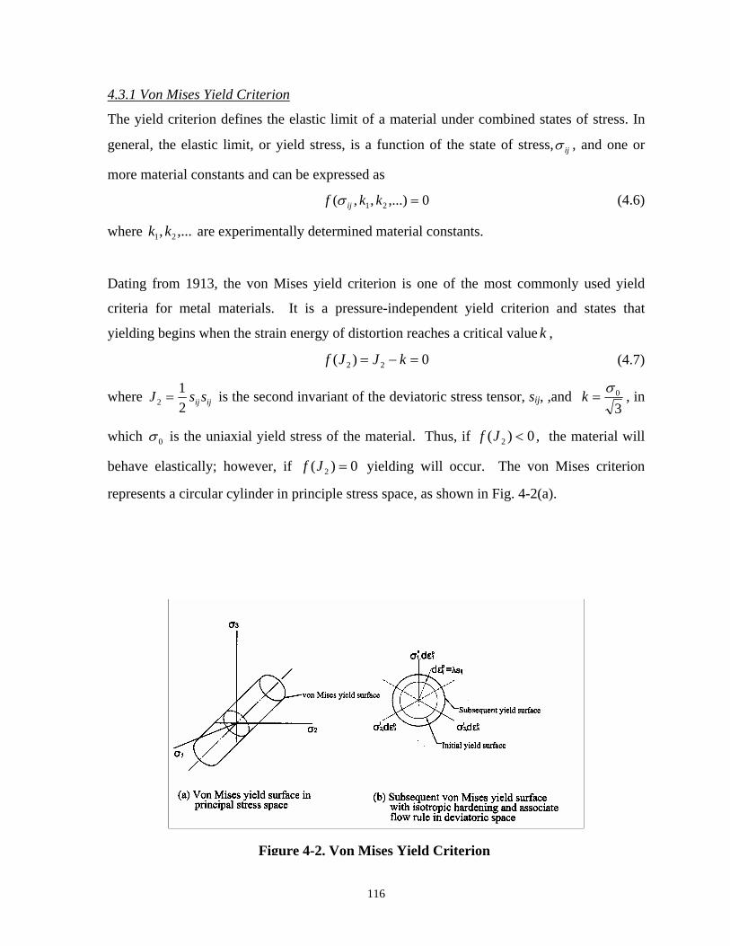
4.3.1 Von Mises Yield Criterion

The yield criterion defines the elastic limit of a material under combined states of stress. In

general, the elastic limit, or yield stress, is a function of the state of stress, ijσ , and one or

more material constants and can be expressed as

0,...),,( 21 =kkf ijσ (4.6)

where ,..., 21 kk are experimentally determined material constants.

Dating from 1913, the von Mises yield criterion is one of the most commonly used yield

criteria for metal materials. It is a pressure-independent yield criterion and states that

yielding begins when the strain energy of distortion reaches a critical value k ,

0)( 22 =−= kJJf (4.7)

where ijij ssJ21

2 = is the second invariant of the deviatoric stress tensor, sij, ,and 30σ

=k , in

which 0σ is the uniaxial yield stress of the material. Thus, if 0)( 2 <Jf , the material will

behave elastically; however, if 0)( 2 =Jf yielding will occur. The von Mises criterion

represents a circular cylinder in principle stress space, as shown in Fig. 4-2(a).

Figure 4-2. Von Mises Yield Criterion

116

4.3.2 Associated Flow Rule

The flow rule defines both the direction and the relative magnitudes of the plastic strain

increment vector pijdε once the elastic limit has been exceeded. In 1928, von Mises proposed

the concept of the plastic potential function, which is a scalar function of the stresses, )( ijg σ .

Then the plastic flow equations can be written in the form of

ij

pij

gddσ

λε∂∂

= (4.8)

where λd is a positive scalar factor of proportionality, which is nonzero only when plastic

deformations occur.

The simplest flow rule is termed associated flow rule, which means that the yield function

and the plastic potential function coincide, i.e. gf = . Thus,

ij

pij

fddσ

λε∂∂

= (4.9)

This implies that the plastic flow develops normal to the yield surface ij

fσ∂∂ . For the von

Mises criteria, the associated flow rule has the simple form:

ijij

pij sdfdd λ

σλε =

∂∂

= (4.10)

4.3.3 Isotropic Hardening

The hardening rule specifies the manner in which the initial yield surface changes during the

process of plastic flow. The most widely used flow rules are those of isotropic hardening,

kinematic hardening, and mixed hardening, which is a combination isotropic and kinematic

hardening. Isotropic hardening is the simplest hardening rule and is based on the assumption

that the initial yield surface expands uniformly without distortion or translation as plastic

flow occurs. This hardening rule generally gives realistic results except for cases where

complex loading paths with stress reversals are considered.

For isotropic hardening, the size of the yield surface is governed by the value of 2k , which is

expressed as a function of effective strain, pε , where the value of pε depends on the loading

117

history. The equation for the subsequent yield surface can be written in the general form

)()( 2 pij kF εσ = (4.11)

or for the von Mises yield function, 2)( JF ij =σ , Eqn. (4.11) becomes

)(21 2

2p

ijij kssJ ε== (4.12)

The von Mises criterion with associated plastic flow rule and isotropic work hardening is

illustrated in deviatoric space in Fig. 4-2(b).

4.3.4 Stress-Strain Relationship

A multi-linear relationship consisting of an elastic region, a yield plateau, a strain-hardening

region, and a second plateau are used to represent the stress-strain characteristics used in the

material modeling. These relationships for Grade 50 and Grade 70 steel are shown in Figs.

4-3 and 4-4, respectively. For Grade 50 steel, a typical value for the modulus of elasticity (E

0

10

20

30

40

50

60

70

0 0.01 0.02 0.03 0.04

Engineering Strain

Eng

inee

ring

Stre

ss (k

si)

E = 29,000 ksi

Est = 720 ksi

E’ = 145 ksi

εst = 0.011

Fy = 50 ksi

Fu = 65 ksi

Figure 4-3. Stress-Strain Relationship for Grade 50 Steel

118

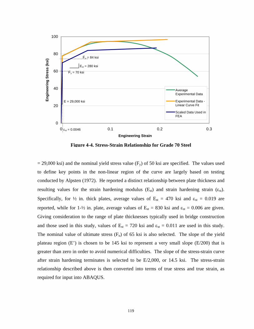
0

20

40

60

80

100

0 0.1 0.2 0.3Engineering Strain

Engi

neer

ing

Stre

ss (k

si)

AverageExperimental Data

Experimental Data -Linear Curve Fit

Scaled Data Used inFEA

E = 29,000 ksi

Est = 280 ksi

εst = 0.0046

Fy = 70 ksi

Fu = 84 ksi

Figure 4-4. Stress-Strain Relationship for Grade 70 Steel

= 29,000 ksi) and the nominal yield stress value (Fy) of 50 ksi are specified. The values used

to define key points in the non-linear region of the curve are largely based on testing

conducted by Alpsten (1972). He reported a distinct relationship between plate thickness and

resulting values for the strain hardening modulus (Est) and strain hardening strain (εst).

Specifically, for ½ in. thick plates, average values of Est = 470 ksi and εst = 0.019 are

reported, while for 1-½ in. plate, average values of Est = 830 ksi and εst = 0.006 are given.

Giving consideration to the range of plate thicknesses typically used in bridge construction

and those used in this study, values of Est = 720 ksi and εst = 0.011 are used in this study.

The nominal value of ultimate stress (Fu) of 65 ksi is also selected. The slope of the yield

plateau region (E’) is chosen to be 145 ksi to represent a very small slope (E/200) that is

greater than zero in order to avoid numerical difficulties. The slope of the stress-strain curve

after strain hardening terminates is selected to be E/2,000, or 14.5 ksi. The stress-strain

relationship described above is then converted into terms of true stress and true strain, as

required for input into ABAQUS.

119

The stress-strain model for Grade 70 steel is based on experimental testing conducted by the

Federal Highway Administration (Wright 1997). Specifically, Fig. 4-4 shows the average

experimental results from six tension tests of grade HPS70W steel, along with a multi-linear

fit to this data. Because the test specimens exhibited yield strengths greater than 70 ksi, the

data is scaled so that Fy is equal to 70 ksi. As before, the standard value of E = 29,000 ksi is

also assumed. The experimental data indicates that this material has a small yield plateau,

with εst = 1.9εy = 0.0046 (for Fy = 70 ksi) and the slope of the yield plateau is assumed to be

100 ksi. The experimental data also gives Est = 280 ksi and the slope of the stress-strain

relationship once strain hardening terminates is again approximated as 14.5 ksi. Lastly, the

test data indicates that the yield stress is 83% of the ultimate stress; using this information

along with Fy = 70 ksi, gives Fu = 84 ksi. Again, this data is converted into terms of true

stress and true strain for input into ABAQUS.

4.4 Geometric Imperfections

The nonlinearity in response due to the presence of initial imperfections of the girder has a

measurable impact on girder ductility, especially on the maximum moment capacity and

unloading shape of moment-plastic rotation curves. Furthermore, from the numerical

analysis point of view, the modified Riks method of analysis used in this work is a type of

post-buckling analysis. Thus, a continuous response is required as opposed to bifurcation.

This can be accomplished by introducing a geometric imperfection pattern in the “perfect”

geometry so that some degree of buckling occurs before the critical load is reached, as would

occur in actual girders. Therefore, introduction of geometric imperfections is a critical step in

this type of analysis, and consequently, the application of geometric imperfections is

carefully studied in this work.

In welded plate girders, initial geometric imperfections are generally generated during the

welding process and/or due to initial out-of-flatness of the long steel plates. Three types of

geometric imperfections are considered in this work in order to capture these characteristics:

an out-of-flatness of the web, a tilt of the compression flange, and a lateral sweep of the

compression flange. These imperfections were previously illustrated in Fig. 3-7 and are

reproduced here in Fig. 4-5.

120

Y Y δof

δof

The values prescribed for these three types of imperfections are based on maximum

allowable tolerances specified by the American Welding Society (AWS) and engineering

judgment. For example, AWS specifies alternative tolerances for the initial out-of-flatness of

the web, depending on if the girder is stiffened. For girders with one-sided transverse

stiffeners, the maximum allowable initial out-of-flatness of the web, δow (see Fig. 4-5), is

d/67, where d is the minimum panel dimension, either the web depth (D) or distance between

stiffeners (do). Alternatively, the maximum allowable value is D/150 for unstiffened girders.

In this study δow is prescribed to be equal to d/100, which is chosen to represent a midpoint

between the above two requirements. This maximum value of distortion occurs at the center

of each web panel and the amount of out-of-flatness at all other locations in the web panel

decreases in a half sine wave pattern, in both the X and Y-directions (see Fig. 4-5).

Furthermore, the direction of δow alternates in adjacent web panels.

The maximum allowable tilt of the flanges, δof, specified by AWS is equal to bf/100 or ¼ in.,

whichever is greater. However, it is felt that it is unlikely that the distortion of the flange

would be this severe in girders with relatively short panel lengths. Therefore, δof is assigned

to be the lesser value of bfc/150 or 0.3do/150 = do/500. This results in values slightly less

than that permitted by AWS for girders with long panel lengths (i.e., 03.0 dbfc < ), while for

Figure 4-5. Initial geometric imperfections

Z X

δowD

do

(a) Initial out-of-flatness of web panel

do

bfc Z

X

(b) Initial tilt of compression flange

δoLY

Z

δoL

X Lb

X (c) Initial sweep of the compression flange

121

short panels, δof may be significantly less than AWS tolerances. The maximum value of δof

occurs at the horizontal center of each web panel along the flange edge. The value of δof

decreases in a sine wave pattern along the length of the girder (Z-direction, in Fig. 4-5) and

decreases linearly along the width of the flange (X-direction). The direction of δof also

alternates in adjacent panels.

AWS limits the variation in straightness of welded girders to 1/960th of the girder length. In

this work, a lateral sweep of the compression flange (δoL) is specified to be somewhat less

than this limit, with a maximum value equal to Lb/1500, where Lb is the distance between

lateral bracing. This value is prescribed at the center of the lateral bracing segment at the

web-compression flange junction. The value of δoL varies in a sine wave pattern along the Z-

direction of the girder and varies linearly in the Y-direction (see Fig. 4-5). As with the other

imperfections, the direction of δoL alternates in adjacent lateral bracing segments.

Furthermore, δoL and δow are prescribed in the same direction within each web panel so that

the effects of these two imperfections are cumulative.

Several approaches may be used to implement these imperfections, all of which involve

various methods of altering the initial coordinates of each node. One commonly employed

approach is to define imperfections as a linear superposition of buckling eigenmodes from a

previous buckling or frequency analysis. This approach can be accomplished by first using

the *buckle or *frequency commands in ABAQUS to establish probable lower energy

collapse buckling modes; then specifying the output file of the buckling analysis in addition

to one or more buckling modes multiplied by the scale factor by way of *imperfection

command. A similar approach is based on the solution obtained from a previous *static

analysis. Alternatively, geometric imperfections can be directly specified in the input file.

In the initial stages of this research, the buckling analysis method was used to apply initial

geometric imperfections. However, although the buckling analysis approach is widely used

in the nonlinear analysis of plate girders, the resulting buckling mode shapes were generally

found to be too localized to represent the initial shape of the girders at a global level.

122

Furthermore, the predominant displacements resulting from buckling analyses were

associated with buckling of the relatively slender webs. In order to obtain a more suitable

buckled shape, it was deemed necessary to increase the web thickness used in the buckling

analysis (usually twice the thickness of the actual girder). At the beginning of this work, this

approach was adopted and initially worked well for girders with relatively short lateral

bracing distances. However, when girders with larger lateral bracing distances were later

studied, it was difficult to obtain buckling modes giving a desired geometric imperfection

pattern.

Other disadvantages of this method also become evident. First, it is not possible to control

the values of the three different types of imperfections simultaneously, even if several

different buckling modes are superimposed. For instance, high values are normally obtained

for out-of-flatness of the web, but it is difficult for the desired values for the tilt of the

compression flange to be obtained at the same time. Furthermore, it is not possible to

separate these three types of imperfections to study their effects on the moment-rotation

capacity of the girders independently, nor is it possible to have a uniform degree of

imperfections along the length of the girder as would be encountered in actual girders.

Instead, the imperfections are most severe near midspan of the girder and are minimal near

the supports. Lastly, this method is time consuming due to the need to first run a buckling

analysis and then carry out the separate nonlinear analysis, and also creates additional files

that occupy valuable CPU space.

Because the objective of performing the buckling analysis is to simply modify the nodal

coordinates, the same outcome can also be achieved through the use of a FORTRAN

program developed to fulfill the same function, which also eliminates the shortcomings of the

buckling analysis approach described above. The purpose of the program is to apply initial

imperfections to the girder by changing the initial global coordinates of each node to give the

desired imperfections outlined above. The program is compiled using FORTRAN2000

language and functions by reading the data from the input file generated by FEMAP and

processing user input to create a new input file with modified nodal coordinates. This

123

program was successfully implemented in all FEA conducted in this work and the basic

structure of the program is as follows.

1. Because different parts of the girder (web, flange, etc.) have different imperfection

modes, it must first be determined if a given node is a web node, a compression

flange node, or neither. The program accomplishes this by first reading the

coordinates of the “reference node”, which is defined as the node at the junction of

the web and bottom flange at one end of the girder. A given node is then determined

to be on the web if the X coordinate of the node is the same as the reference node.

The user also specifies the web depth and if the top or bottom flange is in

compression flange in order for the compression flange nodes to be identified.

2. The distance between stiffeners is given by the user and then the out-of-flatness of the

web is introduced to all nodes previously identified as web nodes according to the

value of δow provided by the user. Furthermore, the user may specify different values

of δow to be used within each panel if warranted.

3. If a node is on the compression flange, the tilt of the flange is added based on user

input for the flange width and δof. Again, the user may specify the same value of δof

for every panel or vary the values within each panel in any manner desired.

4. After completing the previous procedures, the lateral sweep of the compression flange

is superimposed within each lateral bracing segment, resulting in additional

modification of the coordinates of all web and the compression flange nodes. These

imperfections are based on user input regarding the number of lateral bracing

segments, the length of each segment, and the value of δoL for each segment.

5. Lastly, the node coordinates that have been changed and all other unchanged parts of

the original ABAQUS input file are saved as a new ABAQUS input file. A text file is

also generated for the user’s convenience that provides information on the applied

imperfection modes as a convenient check of user input.

4.5 Modeling of Residual Stress

The longitudinal residual stresses in welded I-girders are primarily caused by flame cutting

of the plates and longitudinal welding between the flanges and the web. Typically, the tensile

residual stresses are essentially equal to the yield stress of the material within a small area,

124

termed the heat affected zones, while a smaller, near-constant self-equilibrating compression

stress is developed within the other regions of the plates. The residual stress distribution may

be idealized by assuming that when the section is free of external forces, the residual stresses

over the entire cross-section must satisfy equilibrium and sum to zero.

In this study, residual stress effects are represented by specifying initial stress conditions at

the beginning of the analysis through a user-defined sub-routine, which automatically applies

a prescribed magnitude of initial (residual) stress to each element depending on the elements

location in the girder. When initial stresses are given, the initial stress state may not be in

exact equilibrium for the finite element matrix. Therefore, an initial step is included to allow

ABAQUS to check for equilibrium and iterate, if necessary, to achieve equilibrium.

Specifically, a *static step, where girder dead load is also applied, is implemented before the

Riks analysis to insure that equilibrium is satisfied once residual stresses have been included.

The residual stress pattern that is used in this study is shown in Fig. 4-6. This stress

distribution is considered a reasonable approximation of the actual residual stresses induced

by welding and flame cutting in typical plate girders.

4.6 Modified Riks Algorithm

The girders studied in this work are analyzed using the Modified Riks algorithm available in

ABAQUS. Because it was of key importance to obtain information on girder behavior once

0.59Fy

-0.07Fy

0.59Fy

0.19Fy 0.19Fy

0.34Fy

-0.17Fy -0.17Fy

(a) Residual Stress Pattern for Flanges (b) Residual Stress Pattern for Webs

Figure 4-6. Residual Stress Patttern

125

maximum loads had been exceeded for this research, it was necessary to employ a solution

method capable of capturing this response. The Modified Riks method was selected for use

because it has been shown to be one of the most versatile and efficient of such methods

(Huang 1994), capable of obtaining a complete nonlinear solution and giving information on

girder behavior in both the loading and unloading regions.

The Modified Riks method was initially introduced by Riks (1979), and later improved upon

by several researchers (Crisfield 1983, 1981; Ramm 1981; Powell and Simons 1981). In

addition to the ability to pass beyond the limit point and trace the unloading portion of the

nonlinear equilibrium path, the Riks method also allows solutions to be achieved regardless

of whether the response is stable or unstable. This method provides efficient usage of

computational resources during the nonlinear solution process. In short, the Modified Riks

method may be considered as a combination of the displacement control procedure, the arc-

length method, and Newton iteration techniques.

One basic assumption used in the Modified Riks method is that the loading is proportional,

i.e., all load magnitudes vary with a single scalar parameter. Furthermore, the load

magnitude is used as an additional unknown during the solution. Because the progress of the

solution is independent of the load increment, ABAQUS uses the “arc length”, which is the

distance along the static equilibrium path in load-displacement space, to control the

increment size. This value is initially provided by the user and is later adjusted by the

ABAQUS automatic load increment algorithm based on the convergence rate. The essence

of the method is then to find the solution of a single equilibrium path in a space that is

defined by the nodal variables and the loading parameter. The solution during each increment

is found by moving a given distance along the tangent line to the current solution point and

then searching for equilibrium in the plane that not only passes through the point thus

obtained, but also is orthogonal to the same tangent line. Once this plane is determined,

Newton’s method remains the basic algorithm to solve the equilibrium equations.

Additionally, it is assumed that the response is reasonably smooth, i.e., sudden bifurcations

do not occur. The algorithm of modified Riks method is shown in Fig. 4-7 and is briefly

described below.

126

Figure 4-7. Modified Riks Algorithm

The initial arc length increment along the static equilibrium path, inlΔ , is given in the input

file of ABAQUS. The initial load proportional factor increment, inλΔ , is computed as

period

inin l

lΔ=Δλ (4.13)

where periodl is the total arc length scale factor that is also given in the ABAQUS input file.

This value of inλΔ is only used during the first iteration of the initial increment.

For subsequent increments, suppose the solution has already been obtained at point Ai

( 00 , iiu λ ). Next the equilibrium state of the structure at the i+1 load increment is sought as

shown in Fig. 4-7. First, the arc length is used to determine ilΔ , the distance traveled along a

line tangent to the current solution point. As discussed above, Newton’s method is then used

to obtain a solution on the plane orthogonal to ki AA . The incremental equilibrium equation

after the jth iteration may be expressed as a linear system of equations:

ji

ji

ji FuK Δ=Δ (4.14)

127

where jiK is the tangent stiffness matrix for the load increment i at the end of the jth iteration;

jiuΔ is the incremental displacement vector; and j

iFΔ is a load vector which may be

described as

ji

ji

ji RPF +Δ=Δ (4.15)

in which jiPΔ is the load increment at the jth iteration of load increment i which can be

expressed as a fraction of the total applied load P as:

PP ji

ji λΔ=Δ (4.16)

where jiλΔ is the increment of the load magnitude parameter. j

iR is the out-of-balance force

vector which equals the difference between the external and internal forces at the beginning

of iteration j, i.e.

ji

ji

ji QPR −= (4.17)

where jiQ is the internal force vector. j

iR is then used to check equilibrium within the

prescribed equilibrium tolerances. If the equilibrium tolerances are satisfied, then the solution

is assumed to have converged and this process is repeated for the next load step. Otherwise

additional iterations are performed until the out-of-balance force vector (as computed using

Eq. 4.17) is within the prescribed tolerances.

The incremental load magnitude parameter can be obtained by first substituting Eqn. 4.14

and 4.16 into the equilibrium equation, Eqn. 4.15, giving

ji

ji

ji

ji RPuK +Δ=Δ λ (4.18)

Furthermore, two displacement vectors, ajiuΔ and bj

iuΔ , may be defined corresponding to the

two load vectors P and jiR ,

PuK aji

ji =Δ (4.19)

ji

bji

ji RuK =Δ (4.20)

Substituting ajiuΔ and bj

iuΔ into Eq. (4.18), gives

bji

aji

ji

ji uuu Δ+ΔΔ=Δ λ (4.21)

128

For the first iteration (j=0) at ith increment, the structure is in an equilibrium state at the

beginning of the increment. Thus, the out-of balance force vanishes at this stage, and

consequently 00 =Δ biu . Substituting this into Eqn. 4.21 gives

000 aiii uu ΔΔ=Δ λ (4.22)

Also, from Fig. 4-7, it is shown that

{ } { }00202 )( iT

ii uuli

ΔΔ+Δ=Δ λ (4.23)

The incremental load parameter for the first iteration can thus be obtained by substituting

Eqn. 4.22 into Eqn. 4.23

{ } { } 100

0

+ΔΔ

Δ±=Δ

ai

Tai

ii

uu

lλ (4.24)

Because the vector 1+ik AA must be orthogonal to ki AA , the dot product of these two vectors

must equal zero, or symbolically,

{ } { } 000 =ΔΔ+ΔΔ ji

Ti

jii uuλλ (4.25)

Substituting Eqn. 4.22 for 0iuΔ and Eqn. 4.23 for j

iuΔ into Eqn. 4.25 gives the incremental

load parameter for subsequent iterations to be

{ } { }

{ } { } 10

0

+ΔΔ

ΔΔ−=Δ

aji

Tai

bji

Taij

iuu

uuλ (4.26)

Finally, the solution point at j+1 can be expressed as

ji

j

ii

ji uuu ∑

=

+ Δ+=0

01 (4.27)

ji

j

ii

ji λλλ ∑

=

+ Δ+=0

01 (4.28)

Or, by multiplying Eqn. (4.28) by P, we may write

∑=

+ +=j

i

jii

ji PPP

0

01 (4.29)

129

The stiffness matrix is then updated and multiplied by the displacements obtained above

(Eqn. 4.27) to find the forces at the current solution point. These forces are in turn used

along with the loads obtained above (Eqn. 4.29) to calculate the out-of-balance force vector.

This iteration algorithm is repeated until the equilibrium solution is considered to have

converged for increment i+1, when all the entries in NiR are sufficiently small. Furthermore,

it is also noteworthy to point out that ABAQUS scales the above load-displacement solution

space such that the dimensions are approximately the same magnitude on each axis.

4.7 Summary

This chapter has discussed the FEA modeling procedures used in this work. Chapter 5 will

discuss the use of these modeling procedures to: (1) predict the behavior of the experimental

girders discussed in Chapters 3 and (2) obtain inelastic moment-rotation curves of the steel I-

girders used in the FEA study.

130

Chapter 5: FEA OF STEEL I-GIRDERS FOR THE DETERMINATION OF MOMENT-ROTATION CHARACTERISTICS

This chapter aims to investigate the available rotation of steel I-girders at various levels of

moment, as obtained from experimental and analytical moment versus rotation curves.

Previous research has resulted in a reasonably accurate moment-rotation model for compact

girders, which is used as the basis for the AASHTO (2004) moment redistribution provisions.

This model is applicable for girders with compact flanges, compact lateral bracing distances,

and compact or non-compact webs. Thus, the specific objective of this chapter is to

determine a similar model that is applicable for more slender classes of girders. Of particular

interest is to investigate increased flange slenderness ratios and greater unbraced lengths

compared to those permitted by the current AASHTO (2004) moment redistribution

procedures contained in Appendix B of the specifications as these are the two areas where

the current specifications are most prohibitive.

This chapter consists of five sections. In Section 5.1 FEA of the experimental girders

previously introduced in Chapter 3 is presented. Here it is shown that the FEA techniques

discussed in Chapter 4 provide an accurate prediction of girder behavior. Section 5.2 then

presents the FEA results of a parametric study focused on slender members. Because the

available rotations resulting from the analysis of these girders was relatively low, it was not

possible to make sound conclusions on the relationship between available rotations and

variations in the investigated parameters. Therefore, FEA were conducted for two additional

series of girders. The first of these is presented in Section 5.3 where the analysis of a series

of representative moment redistribution designs is discussed. Trends in girder behavior are

established on the basis of these results and then additional modeling of modified versions of

these girders is presented in Section 5.4, where increased lateral bracing distances and flange

slenderness ratios are investigated. A synthesis of the experimental and FEA data is

presented in Section 5.5. Here the available rotations of steel I-girders is examined with a

specific focus on the behavior of slender I-girders and a moment-rotation model for these

types of girders is presented. A chapter summary is included in Section 5.6.

131

5.1 FEA of Experimental Girders

To first validate the FEA procedures introduced in Chapter 4, analyses of each of the

experimental girders are presented herein. Girder geometries used in the analyses are the

average of the measured dimensions from a minimum of four cross-sections along the length

of the girder. Similarly, the material properties of each flange and web are based on the

stress-strain data resulting from the tension testing of coupons taken from the same steel plate

as the girder component under consideration. The three types of geometric imperfections

(see Section 3.3) are measured in each panel of each girder. At a minimum, the geometric

imperfections are measured at the center of each panel, and in some cases additional

measurements are recorded. Because the imperfection program used in conjunction with

these analyses applies a pattern of imperfections based on the magnitude of the imperfections

at the center of the panel, when the imperfections are measured at multiple locations, a

weighted average is used to obtain the imperfection value input into the program, where

higher weights are assigned to imperfection values closer to midspan of the girder.

Specifically, imperfection measurements taken within the third of the panel closest to

midspan are assigned a weight of 1.0, measurements within the center third of the panel are

assigned a weight of 0.8, and measurements taken from the third of the panel farthest from

midspan are assigned a weight of 0.5. To account for the small amount of flexibility and

lateral movement of the lateral constraints used in the experimental testing, the lateral

constraints used in these analyses are comprised of ABAQUS SPRING1 elements as opposed

to fully rigid constraints. The spring elements are applied at the web nodes closest to where

the lateral constraints are affixed in the actual girders and are assigned a spring constant of 40

kips/in. All other attributes of the analyses conducted of the experimental girders are the

same as those reported in Chapter 4.

The experimental load versus deflection plots previously presented in Figs. 3-16, 3-18, 3-20,

3-22, 3-24, 3-26, 3-28, 3-30, 3-32, 3-34, 3-36, and 3-38 are reproduced below in Figs. 5-1

through 5-12 presenting only the peak data, i.e., the reloading portions of the curves are

neglected, and comparing these results to the corresponding FEA results. Figures 5-1

through 5-12 show that the FEA techniques generally produce results that well represent the

experimental results. Specifically, these figures show that (1) the shape of the load versus

132

0

50

100

150

200

250

300

0 1 2 3 4 5

Displacement (in)

Load

(kip

s)

EXP

FEA

Figure 5-1. FEA and Experimental Load versus Displacement Data - Girder 1MG

0

50

100

150

200

250

300

350

0 1 2 3 4 5

Displacement (in)

Load

(kip

s)

EXP

FEA


133

0

20

40

60

80

100

120

140

160

180

200

220

0 1 2 3

Displacement (in)

Load

(kip

s)

EXP

FEA


0

20

40

60

80

100

120

140

0 1 2 3 4 5

Displacement (in)

Load

(kip

s)

EXP

FEA


134

0

50

100

150

200

250

0 1 2 3 4 5

Displacement (in)

Load

(kip

s)

EXP

FEA


0

10

20

30

40

50

60

0 1 2 3 4 5

Displacement (in)

Load

(kip

s)

FEA

EXP


135

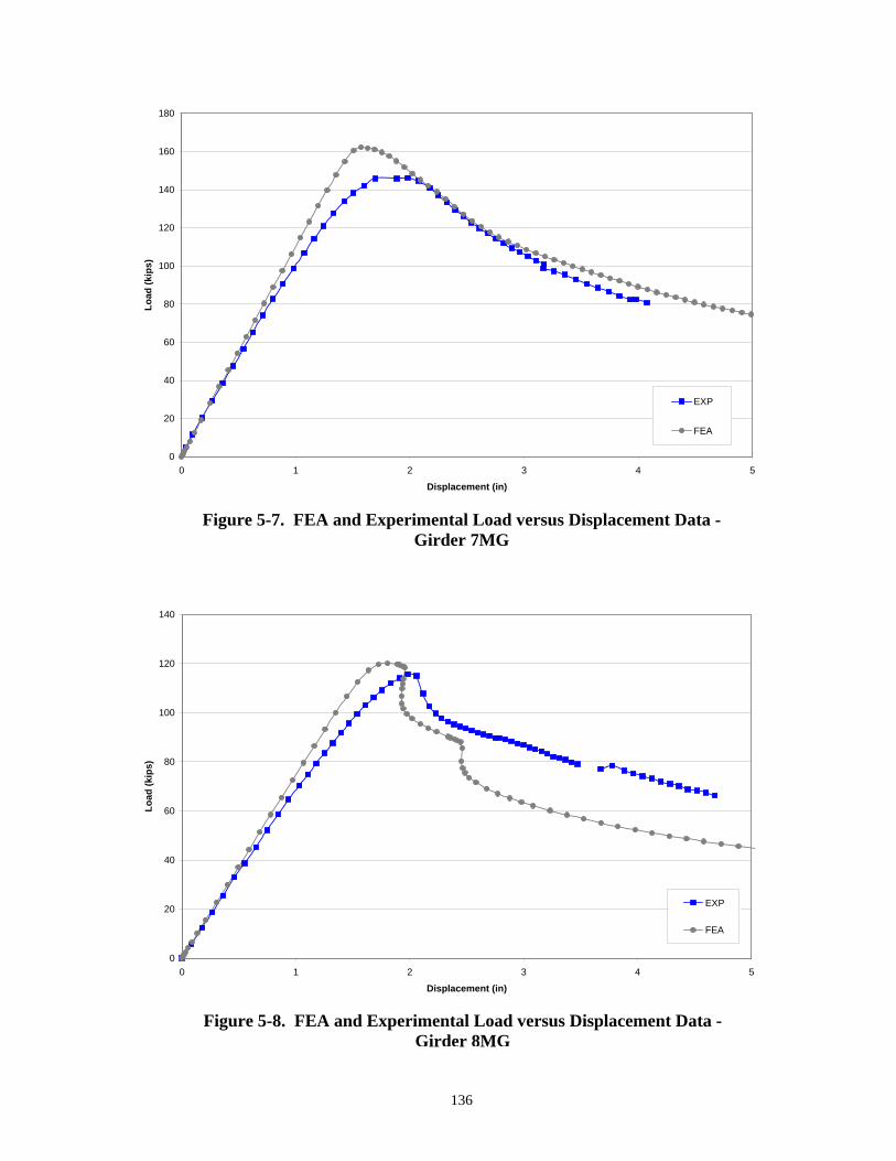
0

20

40

60

80

100

120

140

160

180

0 1 2 3 4 5

Displacement (in)

Load

(kip

s)

EXP

FEA


0

20

40

60

80

100

120

140

0 1 2 3 4 5

Displacement (in)

Load

(kip

s)

EXP

FEA


136

0

10

20

30

40

50

60

70

80

90

100

0 1 2 3 4 5

Displacement (in)

Load

(kip

s)

EXP

FEA


0

10

20

30

40

50

60

70

80

90

0 1 2 3 4 5

Displacement (in)

Load

(kip

s)

6

EXP

FEA


137

0

20

40

60

80

100

120

140

0 1 2 3 4 5 6

Displacement (in)

Load

(kip

s)

EXP

FEA


0

20

40

60

80

100

120

140

160

0 1 2 3 4 5 6

Displacement (in)

Load

(kip

s)

EXP

FEA


138

deflection response is very similar in both the experimental and analytical results and (2) the

maximum moment capacity is well predicted by the FEA. The primary differences between

the experimental and FEA results is that, in all cases, the initial stiffness of the girder is

greater in the FEA results. In some cases this results in less displacement at a given load

throughout the range of loading up to the maximum load (e.g., Girder 2MG) and in other

situations the slopes of the two curves are initially equal, but yielding initiates in the actual

girder earlier than predicted by the FEA (e.g., Girder 7MG). For some girders, the

displacements are also conservative throughout the unloading phase, but in most cases the

two curves converge during unloading. Thus, the FEA displacements (and therefore

rotations) are either conservative or accurate during the unloading phase, which is most

relevant to the present focus of determining available rotations.

Table 5-1 compares the maximum capacities from both the experimental and FEA results.

Here a positive percent difference indicates that the FEA produces conservative results. It is

shown by Table 5-1 that the FEA and experimental capacities are generally in agreement

within 5%, which is considered to be an accurate strength prediction. Of the three cases

where the deviation between the two capacities is greater than 5%, one of these is Girder

7MG; this girder was loaded to 99.7% of the maximum load, unloaded, reloaded to 39.9% of

the maximum load, and then loaded to the maximum load. Thus, there is the potential that

this may have reduced the ultimate capacity that may have otherwise been achieved as it can

Table 5-1. Comparison of Experimental and FEA Maximum Capacities (kips)

SpecimenMaximum Load Experimental

Maximum Load FEA Percent Difference

1MG 273 248 9.02MG 293 300 -2.53MG 199 200 -0.84MG 122 121 0.55MG 185 198 -6.96MG 53 55 -3.27MG 146 162 -10.98MG 116 120 -3.89MG 94 98 -3.910MG 86 85 0.411MG 118 114 3.712MG 152 145 4.7

139

be seen from Fig. 3-28 that there is a small change in the stiffness of the girder between the

2nd and 3rd loading cycles, indicating that permanent deformations have already been

introduced before attaining the maximum load. Girder 1MG has an actual capacity that is

9.0% higher than the FEA results. Thus, even though there is a relatively high percent

difference the FEA results are conservative for this case. Overall, it is believed that the

experimental capacities are well predicted by the FEA results.

Figures 5-13 through 5-24 compare the deformed shapes resulting from the experiments and

the FEA. Each of these plots shows the original (undeformed) cross section and LVDT

positions with data points, the deformed LVDT positions with data points (as previously

presented in Figs. 3-17, 3-19, 3-21, 3-23, 3-25, 3-27, 3-29, 3-31, 3-33, 3-35, 3-37, and 3-39),

and the deformed shape from the FEA (without data points). It should be noted that in cases

where such data is available the experimental data represents the deformed shape after

unloading the girder. However this data was not available for Girders 2MG, 9MG, and

12MG due to the need for removing the instrumentation prior to unloading the girder in order

to avoid damage to this equipment, and consequently, the deformed shapes presented for

-5

0

5

10

15

20

25

30

-10 -5 0 5 10

Figure 5-13. FEA and Experimental Deformed Shapes - Girder 1MG

140

-5

0

5

10

15

20

25

30

-10 -5 0 5 10

Figure 5-14. FEA and Experimental Deformed Shapes - Girder 2MG

-5

0

5

10

15

20

25

30

35

-10 -5 0 5 10

Figure 5-15. FEA and Experimental Deformed Shapes – Girder 3MG

141


-5

0

5

10

15

20

25

30

35

-10 -5 0 5 10

-5

0

5

10

15

20

25

30

35

40

45

-10 -5 0 5 10


142

-5

0

5

10

15

20

25

30

35

-10 -5 0 5 10


-5

0

5

10

15

20

25

30

35

-10 -5 0 5 10


143

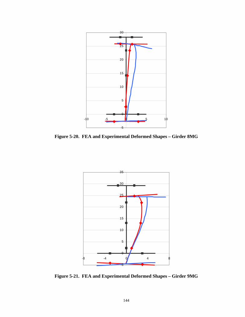
-5

0

5

10

15

20

25

30

-10 -5 0 5 10


-5

0

5

10

15

20

25

30

35

-8 -4 0 4 8


144

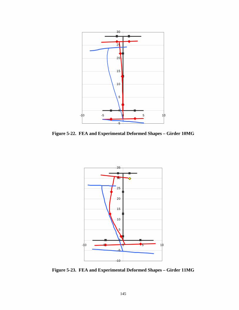
-5

0

5

10

15

20

25

30

-10 -5 0 5 10


-10

-5

0

5

10

15

20

25

30

35

-10 -5 0 5 10


145

-10

-5

0

5

10

15

20

25

30

35

40

-10 -5 0 5 10


these girders are from the last load step where data is available. The FEA data is the data

from the closest corresponding load step at the cross-section closest to the point where the

LVDTs are located. The FEA and experimental deformed shapes are shown to be quite

similar in most cases, especially within the context of the significant number of parameters

involved. For example, in most cases the girders exhibit similar modes of buckling, at the

same location along the length of the girder, and with similar magnitudes of deformations.

As the experimental deformed shapes, load versus deflection responses, and maximum

capacities are all well represented by the FEA it is concluded that the FEA procedures

adopted in this work are of reliable accuracy and may be used with confidence to investigate

the available rotations of steel I-girders.

The ductility of steel I-girders can be represented by two key parameters. These are the

rotation at which the moment level decreases below Mn (termed θRL) and the equation of the

curve representing the unloading behavior below this point. θRL is given below in Table 5-2

for each of the 12 experimental girders and the 71 hypothetical girders to be discussed in this

chapter. The θRL values presented in Table 5-2 are determined by analyzing the moment

146

Table 5-2. θRL Values in mrad (part 1)

Girder LabelActual θRL

AASHTO θRL

Actual / AASHTO

2Dcp

θRL

Actual / 2Dcp

2Dcp and Lb/rt

θRL

Actual / 2Dcp and Lb/rt

1MG 8 NA NA NA NA 5.8 1.372MG 8 11.1 0.72 5.6 1.42 5.6 1.423MG 3 7.2 0.42 5.0 0.60 5.0 0.604MG 4 NA NA NA NA 5.0 0.805MG 5 NA NA NA NA 5.0 1.006MG 6 NA NA NA NA 5.0 1.207MG 5 NA NA NA NA 5.0 1.008MG 3 NA NA NA NA 5.0 0.609MG 2 NA NA NA NA 5.0 0.4010MG 5 NA NA NA NA 5.0 1.0011MG 2 NA NA NA NA 5.0 0.4012MG 3 NA NA NA NA 5.0 0.60CF-1-65-4-50 1 5.0 0.20 5.0 0.20 5.0 0.20CF-2-65-4-50 1 NA NA NA NA 5.0 0.10CF-30-65-4-50 1 NA NA NA NA 5.0 0.20SF-1-65-4-50 1 NA NA NA NA 5.0 0.20SF-2-65-4-50 1 NA NA NA NA 5.0 0.20SF-30-65-4-50 0 NA NA NA NA 5.0 0.04SF-1-65-3-50 2 NA NA NA NA 5.0 0.38SF-2-65-3-50 2 NA NA NA NA 5.0 0.34SF-30-65-3-50 1 NA NA NA NA 5.0 0.26CF-1-65-4-H 2 5.0 0.44 5.0 0.44 5.0 0.44CF-2-65-4-H 0 NA NA NA NA 5.0 0.06CF-30-65-4-H 2 NA NA NA NA 5.0 0.40SF-1-65-4-H 1 NA NA NA NA 5.0 0.20SF-2-65-4-H 1 NA NA NA NA 5.0 0.18SF-30-65-4-H 2 NA NA NA NA 5.0 0.44CF-0.5-65-3-H 1 8.9 0.16 5.7 0.25 5.7 0.25CF-1-65-3-H 4 8.9 0.46 5.7 0.72 5.7 0.72CF-1.65-65-3-H 2 NA NA NA NA 5.0 0.48CF-30-65-3-H 2 NA NA NA NA 5.0 0.32SF-1.75-65-3-H 2 NA NA NA NA 5.0 0.34SF-30-65-3-H 1 NA NA NA NA 5.0 0.28CF-1-50-4-50 1 5.0 0.28 5.0 0.28 5.0 0.28CF-2-50-4-50 0 NA NA NA NA 5.0 0.08CF-30-50-4-50 0 NA NA NA NA 5.0 0.02SF-1-50-4-50 1 NA NA NA NA 5.0 0.24SF-2-50-4-50 1 NA NA NA NA 5.0 0.24SF-3.75-50-4-50 0 NA NA NA NA 5.0 0.00CF-1-50-4-H 1 5.0 0.22 5.0 0.22 5.0 0.22CF-2-50-4-H 0 NA NA NA NA 5.0 0.08SF-1-50-4-H 1 NA NA NA NA 5.0 0.24SF-2-50-4-H 1 NA NA NA NA 5.0 0.22SF-30-50-4-H 2 NA NA NA NA 5.0 0.42

Sec

tion

5.2

Gird

ers

Sec

tion

5.1

Gird

ers

versus rotation plots for each of the experimental and FEA girders, which are presented in

Appendices B and D, respectively. It is noted that the maximum capacity of several of the

experimental girders was less than Mn; in this case, the reported rotation is the rotation at the

maximum moment level, which is conservative in that it is the rotation before the girder

experiences any unloading.

5.2 FEA Parametric Study

A FEA parametric study was conducted to further investigate the rotation characteristics of

slender steel I-girders. The variables included are similar to those included in the

experimental testing, although increased combinations of these variables are studied

147

Table 5-2, continued. θRL Values in mrad (part 2)

Girder LabelActual θRL

AASHTO θRL

Actual / AASHTO

2Dcp

θRL

Actual / 2Dcp

2Dcp and Lb/rt

θRL

Actual / 2Dcp and Lb/rt

90-2-E-50-10-A 23 27.8 0.83 18.3 1.26 18.3 1.2690-2-E-50-20-B 29 27.8 1.03 24.1 1.19 24.1 1.19120-2-E-50-10-A 39 36.3 1.07 28.5 1.36 28.5 1.36120-2-E-50-20-A 27 31.4 0.87 22.0 1.24 22.0 1.24120-2-E-50-20-Lb=20 11 NA NA NA NA 8.5 1.29120-2-E-50-20-Lb=30 3 NA NA NA NA 5.0 0.60120-2-E-50-20-NCF 16 NA NA NA NA 5.0 3.20120-2-E-50-20-NCF-Lb=30 13 NA NA NA NA 5.0 2.60120-2-E-50-UF(30)-E 63 31.4 1.99 35.1 1.78 35.1 1.78120-2-E-50-U(30)-E 63 31.4 1.99 35.1 1.78 35.1 1.78120-2-H-10-A 61 25.7 2.38 36.6 1.67 36.6 1.67120-2-H-10-B 60 NA NA NA NA 30.3 1.98120-2-H-10-B(S) 63 25.7 2.45 37.9 1.66 37.9 1.66120-2-H-10-B(S)-16 49 NA NA NA NA 33.3 1.47120-2-H-10-B(S)-24 36 NA NA NA NA 23.5 1.53120-2-H-10-B(S)-30 23 NA NA NA NA 16.1 1.43120-2-H-10-B(S)-NCF 25 NA NA NA NA 5.0 5.00120-2-H-10-B(S)-NCF-30 32 NA NA NA NA 5.0 6.40120-2-H-20-A 48 NA NA NA NA 35.8 1.34120-2-H-20-A(S) 27 NA NA NA NA 37.0 0.73150-2-50-10-A 42 27.7 1.53 28.6 1.48 27.8 1.52150-2-50-20-C 35 27.0 1.30 25.6 1.38 24.7 1.43150-2-50-40-A 37 23.7 1.56 27.5 1.35 26.5 1.40180-2-E-50-10-A 23 27.5 0.82 22.5 1.00 22.5 1.00180-2-E-50-20-B 25 25.7 0.97 23.1 1.08 23.1 1.08180-2-E-50-20-B-22.5 10 NA NA NA NA 12.3 0.78180-2-E-50-20-B-30 4 NA NA NA NA 5.0 0.86180-2-E-50-20-NCF 9 NA NA NA NA 5.0 1.78180-2-E-50-20-NCF-Lb=30 7 NA NA NA NA 5.0 1.42210-2-E-50-10-E 10 18.8 0.54 17.8 0.57 17.8 0.57210-2-E-50-10-E-18 9 18.8 0.48 17.8 0.51 17.8 0.51210-2-E-50-10-E-26.25 3 NA NA NA NA 11.1 0.28210-2-E-50-10-E-30 3 NA NA NA NA 8.0 0.35210-2-E-50-10-NCF 19 NA NA NA NA 5.0 3.80210-2-E-50-10-NCF-30 11 NA NA NA NA 5.0 2.20210-2-E-50-20-F 14 22.1 0.62 20.2 0.68 20.2 0.68210-2-E-50-30-B 17 19.5 0.87 21.2 0.80 21.2 0.80210-2-E-50-40-C 23 17.3 1.33 19.6 1.17 19.6 1.17140-175-140-D 17 27.7 0.61 35.2 0.48 35.2 0.48

Sec

tion

5.3

and

Sec

tion

5.4

Gird

ers

compared to those feasible to include in the experimental testing. The parametric values

included in this FEA study are equal to:

• flange slenderness values equal to the compact limit, 0.38 ycE F , and the maximum

allowable flange slenderness of 12;

• homogeneous Grade 50 girders and hybrid girders comprised of Grade 50 webs and

Grade 70 flanges;

• D/bfc ratios of 3 and 4.25;

• lateral bracing distances equal to the current AASHTO 2004 Appendix B lateral

bracing limit, and various percentages of this limit, up to a maximum lateral bracing

distance of 30 ft; and

• Dcp/D ratios of 0.65 and 0.50.

148

• A constant web slenderness equal to the noncompact limit, 2 5.7=c w ycD t E F ,

was used as the variation in web slenderness results in little influence on moment

versus rotation behavior.

In order to minimize the number of analyses required while obtaining complete information

on the rotation characteristics of slender I-girders, representative combinations of the above

parameters were carefully selected. Table 5-3 summarizes the attributes of each of the 32

analyses comprising this parametric study. This table also introduces the naming convention

used for these FEA girders. The first component of the girder label refers to the flange

slenderness used; “CF” indicates that the flange is proportioned to have a slenderness equal

to the compact limit, while “SF” specifies that the maximum flange slenderness is used. The

Table 5-3. Scope of Parametric Study

Girder LabelFlange

SlendernessLateral Bracing

Distance Dcp/D Ratio D/bfc RatioMaterial

Configuration

CF-1-65-4-50 Compact 100% 65 4 50CF-2-65-4-50 Compact 200% 65 4 50CF-30-65-4-50 Compact 30 (375%) 65 4 50SF-1-65-4-50 Slender 100% 65 4 50SF-2-65-4-50 Slender 200% 65 4 50SF-30-65-4-50 Slender 30 (375%) 65 4 50SF-1-65-3-50 Slender 100% 65 3 50SF-2-65-3-50 Slender 200% 65 3 50SF-30-65-3-50 Slender 30 (400%) 65 3 50CF-1-65-4-H Compact 100% 65 4 HCF-2-65-4-H Compact 200% 65 4 HCF-30-65-4-H Compact 30 (429%) 65 4 HSF-1-65-4-H Slender 100% 65 4 HSF-2-65-4-H Slender 200% 65 4 HSF-30-65-4-H Slender 30 (500%) 65 4 HCF-0.5-65-3-H Compact 50% 65 3 HCF-1-65-3-H Compact 100% 65 3 HCF-1.65-65-3-H Compact 165% 65 3 HCF-30-65-3-H Compact 30 (230%) 65 3 HSF-1.75-65-3-H Slender 175% 65 3 HSF-30-65-3-H Slender 30 (250%) 65 3 HCF-1-50-4-50 Compact 100% 50 4 50CF-2-50-4-50 Compact 200% 50 4 50CF-30-50-4-50 Compact 30 (333%) 50 4 50SF-1-50-4-50 Slender 100% 50 4 50SF-2-50-4-50 Slender 200% 50 4 50SF-3.75-50-4-50 Slender 30 (375%) 50 4 50CF-1-50-4-H Compact 100% 50 4 HCF-2-50-4-H Compact 200% 50 4 HSF-1-50-4-H Slender 100% 50 4 HSF-2-50-4-H Slender 200% 50 4 HSF-30-50-4-H Slender 30 (500%) 50 4 H

149

second element of the girder label indicates the multiple used of the Appendix B lateral

bracing distance or that the maximum lateral bracing distance of 30 ft is used. The third label

refers to the percentage of the web depth in compression. The fourth part indicates the D/bfc

ratio. Lastly, the fifth component conveys the material configuration where “50” indicates

that the girder is a homogeneous Grade 50 girder and “H” indicates that the girder is a hybrid

girder with Grade 70 steel used for the flanges of the negative bending section and Grade 50

steel used elsewhere.

Girder designs satisfying the desired parameters were created for each of the cases presented

in Table 5-3. This was accomplished by first selecting a web depth of 60 in. for each girder.

The compression flange width was then selected to provide the desired D/bfc ratio. Next, the

compression flange thickness was selected to give the desired compression flange

slenderness. The web slenderness, tension flange width, and tension flange thickness were

then simultaneously selected to give the desired web slenderness and Dcp/D ratio. Lastly, the

lateral bracing distances were selected.

The selected web depth of 60 in. corresponds to an L/D (span length to web depth) ratio of

30 for a 150 ft span length. It was assumed that 25% of each span length was in negative

bending, resulting in a simply-supported length of 75 ft in each of the models. Thus, the

moment gradient induced into each girder is representative of actual loading conditions for

typical continuous-span bridges. A minimum of four lateral bracing segments are used to

provide warping restraint to the center two critical lateral bracing panels. Thus, for a

maximum lateral bracing distance of 30 ft, the total girder length is 120 ft. Consequently,

cantilevered ends of the girder extend beyond the simple supports. All other aspects of the

FEA are as discussed in Chapter 4.

Representative moment rotation plots resulting from these analyses are presented in Figs. 5-

25 and 5-26, while this data is presented for each of the parametric study girders in Appendix

D. Figures 5-25 and 5-26 show that these girders exhibit a relatively low degree of ductility

in that there is little rotation available at high moment levels and the slope of the descending

portion of the curve is relatively steep. The ductility resulting from the parametric study

150

0.0

0.2

0.4

0.6

0.8

1.0

1.2

0 5 10 15 20 25 30 35 40 45

Plastic Rotation (m rad)

M/M

n

Figure 5-25. Moment versus Rotation – Girder CF-1-65-4-50

0.0

0.2

0.4

0.6

0.8

1.0

1.2

1.4

0 5 10 15 20 25 30 35 40


M/M

n

Figure 5-26. Moment versus Rotation – Girder SF-30-65-3-H

designs is further represented by the data presented in Table 5-2. Here θRL is presented for

each of the parametric girders, which is determined by analyzing the moment rotation plots

(contained in Appendix D) for each of the girders. Here it shown that θRL varies between 0

and 4 for this series of parametric girders.

151

It should be noted that because the θRL value for a given girder is directly related to the

girder’s nominal moment capacity, the value of Mn of a given girder should also be

considered when comparing θRL values for different girders. For example, considering the

results presented in Table 5-2 for girders CF-1-65-4-H, CF-2-65-4-H, and CF-30-65-4-H, it

is observed that despite the significantly increased lateral bracing distance of CF-30-65-4-H

compared to CF-2-65-4-H, a higher θRL value results for the girder with the longer bracing

distance. This is somewhat counterintuitive and occurs because the AASHTO (2004)

equations predict lower moment capacities for these girders with longer lateral bracing

distances (or increasing flange slenderness, etc). Thus, the girders with longer bracing

distances exhibit less available rotation at a given magnitude of moment, but when the results

are normalized by nominal moment capacity, greater available rotations may be predicted for

girders with greater lateral bracing distances.

The relatively low θRL values of the parametric study girders is attributed to the fact that

several of the slenderness ratios are simultaneously maximized (to varying degrees) in each

of these girders. Because of the narrow range of θRL that exists for these girders, it is

necessary to perform additional FEA studies to obtain data and form conclusions on the

variation in θRL with the variation in girder geometries. The subsequent series of FEA is

performed for girders that are more typical of those that would be encountered in actual

bridge designs. Specifically, FEA was conducted of the girders resulting from the design

study subsequently presented in Chapter 6. These girders are typical of those that would

result from use of the current (AASHTO 2004) moment redistribution procedures. Analyses

of these girders are presented in the following section, Section 5.3. To then obtain moment

versus rotation behavior of girders that have slenderness properties exceeding the current

moment redistribution limits, the slenderness properties of these designs were increased and

FEA of these girders were conducted as described in Section 5.4.

5.3 FEA of Design Study Girders

Section 6.3 presents the design of a representative series of girders obtained using moment

redistribution procedures. These designs were created for the purpose of aiding in the

determination of rotation requirements as discussed in the following chapter. FEA of 21 of

152

these girders are performed here to obtain the moment versus rotation of typical girders,

which are then used to identify trends in this behavior. Girders with similar moment-rotation

behavior are subsequently identified and representative girders from each of these groups are

selected for investigation of the influences of increased slenderness parameters, which is

presented in Section 5.4.

The design criteria used for these girders are presented in Section 6.3 and Appendix E details

each design. To summarize, two-, three-, and four-span continuous homogeneous and hybrid

girders were designed targeting specific percentages of redistribution moment. FEA of the

negative bending section of representative two- and three-span designs were performed and

the moment versus rotation behavior of these girders was obtained. These girders were

modeled representing the dead load contraflexure points as the locations of simple supports

and cantilevered segments extend beyond these supports as needed to provide additional

lateral bracing panels, and consequently, warping restraint to the midspan panels. The

models were then loaded with a point load at the center of the simply-supported span,

producing the moment gradient typical of negative bending sections. Figures 5-27 through 5-

30 present the resulting data by grouping together the plots for girders with moment versus

rotation curves having similar shapes.

These figures refer to specific designs using the following naming convention. For the two

span designs, the first number in the label refers to the span length, followed by a label of “2”

indicating that the design is a two-span bridge, and the label “E” indicating that both spans

are of equal length. For the three-span designs, the first three numbers give the lengths of

each span. These span length labels are then followed by a label indicating the material

properties of the girder, where “50” represents a Grade 50 design and “H” represents a hybrid

girder with Grade 70 flanges in negative bending sections and Grade 50 elsewhere. Next, a

label indicating the targeted percentage of redistribution moment is given. In most cases

more than one design was performed for each design situation before the optimum design

was achieved; the next label in the naming convention simply references the specific design

for each situation that was selected as the optimal design. Some of the design labels are then

followed by the label “(S)”, which indicates that the girder design is a stiffened girder. In

153

cases where the design girder consists of a uniform cross-section, this is indicated by the

label “U” and in cases where the flange dimensions are uniform but the web thickness varies

at field splice locations, this is indicated by the label “UF”.

Figures 5-27 through 5-30 show that these girders exhibit significantly more ductility than

the girders previously presented in Section 5.2. This is also demonstrated by the higher qRL

values for these girders, presented in Table 5-2. This is expected as the girders in these

figures are more compact than those from the parametric study. From each of the plots in

Figs. 5-27 through 5-30, the girder with the least ductility is then selected for further study;

modified versions of girders 120-2-E-50-20-A, 120-2-E-H-10-B-(S), 180-2-E-50-20-B, and

210-2-E-50-10-E with increased lateral bracing distance and flange slenderness are designed

and analyzed as discussed below.

0

0.2

0.4

0.6

0.8

1

1.2

1.4

0 10 20 30 40 50 60 70 80 90 100

Plastic Rotation (mrad)

M/M

n

150-2-E-50-10-A

120-2-E-50-10-A

120-2-E-H-20-A(S)

120-2-E-H-20-A

120-2-E-50-20-A

Figure 5-27. Moment versus Rotation for Design Study Girders – Group 1

154

0

0.2

0.4

0.6

0.8

1

1.2

1.4

1.6

0 10 20 30 40 50 60 70 80 90 100


M/M

n120-2-E-H-10-B-(S)

120-2-E-H-10-A

120-2-E-H-10-B

120-2-E-50-U(30)/UF(30)-E


0

0.2

0.4

0.6

0.8

1

1.2

1.4

0 20 40 60 80 100 120 140


M/M

n

150-2-E-50-40-A

90-2-E-50-10-A

90-2-E-50-20-B

120-2-E-50-20-A

180-2-E-50-20-B

150-2-e-50-20-C

180-2-E-50-10-A


155

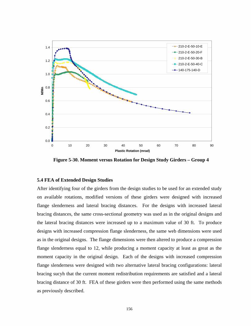
0.0

0.2

0.4

0.6

0.8

1.0

1.2

1.4

0 10 20 30 40 50 60 70 80 90


M/M

n210-2-E-50-10-E

210-2-E-50-20-F

210-2-E-50-30-B

210-2-E-50-40-C

140-175-140-D


5.4 FEA of Extended Design Studies

After identifying four of the girders from the design studies to be used for an extended study

on available rotations, modified versions of these girders were designed with increased

flange slenderness and lateral bracing distances. For the designs with increased lateral

bracing distances, the same cross-sectional geometry was used as in the original designs and

the lateral bracing distances were increased up to a maximum value of 30 ft. To produce

designs with increased compression flange slenderness, the same web dimensions were used

as in the original designs. The flange dimensions were then altered to produce a compression

flange slenderness equal to 12, while producing a moment capacity at least as great as the

moment capacity in the original design. Each of the designs with increased compression

flange slenderness were designed with two alternative lateral bracing configurations: lateral

bracing sucyh that the current moment redistribution requirements are satisfied and a lateral

bracing distance of 30 ft. FEA of these girders were then performed using the same methods

as previously described.

156

The results of these efforts are presented in the form of the moment versus rotation plots

given in Figs. 5-31 through 5-34. In these figures the girders are labeled using the naming

convention described above followed by additional descriptors indicating the alternative

lateral bracing distance used (if applicable) and if a non-compact flange (indicated by the

label “NCF”) is used. Figure 5-31 presents the data for the original and modified versions of

girder 120-2-E-50-20-A. Here it is shown that, for the designs with a compact flange,

increasing lateral bracing distances correspond to a decrease in the available rotation of the

girder. Increased lateral bracing distance also results in reduced rotations for the girders with

non-compact flanges, although this influence is much less significant for these girders. In

fact the available rotation at Mn is nearly equal for the two non-compact flange designs

shown in Fig. 5-31 even though the lateral bracing distance varies by 300%. This difference

in behavior between the compact and non-compact flange girders is consistent with the

behavior predicted by the AASHTO (2004) moment redistribution lateral bracing limit. For

the original, compact flange design for Girder 120-2-E-50-20-A the AASHTO 2004

0.0

0.2

0.4

0.6

0.8

1.0

1.2

1.4

0 20 40 60 80 100 120


M/M

n

120-2-E-50-20-A

120-2-E-50-20-Lb=20

120-2-E-50-20-Lb=30

120-2-E-50-20-NCF

120-2-E-50-20-Lb=30-NCF

Figure 5-31. Moment versus Rotation for Permutations of Girder 120-2-E-50-20-A

157

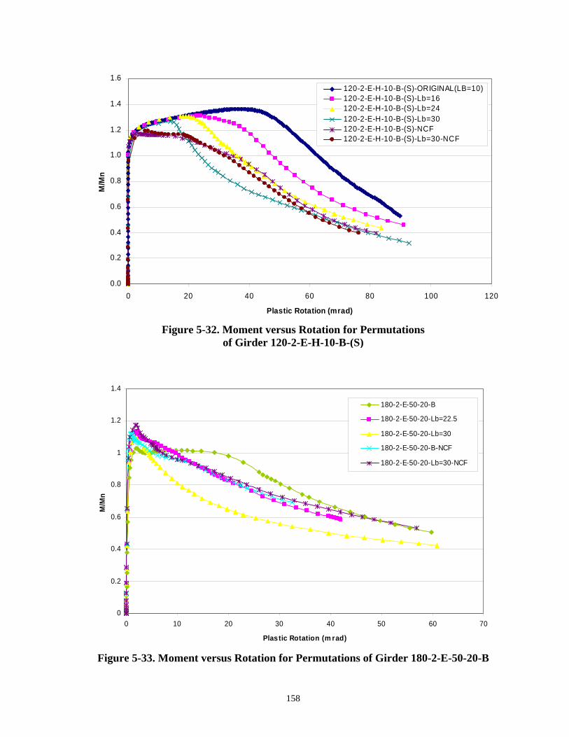
0.0

0.2

0.4

0.6

0.8

1.0

1.2

1.4

1.6

0 20 40 60 80 100


M/M

n

120

120-2-E-H-10-B-(S)-ORIGINAL(LB=10)120-2-E-H-10-B-(S)-Lb=16120-2-E-H-10-B-(S)-Lb=24120-2-E-H-10-B-(S)-Lb=30120-2-E-H-10-B-(S)-NCF120-2-E-H-10-B-(S)-Lb=30-NCF

Figure 5-32. Moment versus Rotation for Permutations of Girder 120-2-E-H-10-B-(S)

0

0.2

0.4

0.6

0.8

1

1.2

1.4

0 10 20 30 40 50 60 70


M/M

n

180-2-E-50-20-B

180-2-E-50-20-Lb=22.5

180-2-E-50-20-Lb=30

180-2-E-50-20-B-NCF

180-2-E-50-20-Lb=30-NCF

Figure 5-33. Moment versus Rotation for Permutations of Girder 180-2-E-50-20-B

158

0.0

0.2

0.4

0.6

0.8

1.0

1.2

1.4

0 10 20 30 40 50 60 70 8


M/M

n

0

210-2-E-50-10-E(Lb=10)

210-2-E-50-10-Lb=18

210-2-E-50-10-Lb=26.25

210-2-E-50-10-Lb=30

210-2-E-50-10-NCF

210-2-E-50-10-Lb=30-NCF

Figure 5-34. Moment versus Rotation for Permutations of Girder 210-2-E-50-10-E

Appendix B limit was 14 ft, while the Appendix B limit for the non-compact flange girders is

36 ft. Thus, it appears that when the AASHTO Appendix B lateral bracing limit is satisfied,

there is little influence of available rotations with varying lateral bracing distances.

Comparing the two designs having the original lateral bracing distance of 10 ft in Fig. 5-31

shows that the girder with the compact flange initially exhibits higher rotations than the

girder with the non-compact flange, however at a moment capacity of less than 90% of Mn

on the unloading portion of the curve, the girder with the non-compact flange has the greater

ductility. This is attributed to the higher value of rt characteristic of the non-compact flange

girder. Similarly, comparing the two designs with a lateral bracing distance of 30 ft, the non-

compact flange girder is again the more ductile of the two as the higher rt value of this girder

provides greater restraint to the lateral torsional buckling mode of failure.

These same trends are evident in Figs. 5-32 through 5-34, which present the data from the

modified designs of 120-2-E-H-10-B-(S), 180-2-E-50-20-B, and 210-2-E-50-10-E,

respectively. For the designs in Fig. 5-32, the Appendix B lateral bracing requirements are

10 ft for the compact flange girders and 22 ft for the non-compact flange; for the designs in

159

Fig. 5-33, these requirements are 15 ft for the compact flange girders and 37 ft for the non-

compact flange girders; and for the designs in Fig. 5-34, these requirements are 22 ft for the

compact flange girders and 42 ft for the non-compact flange girders. Thus, the data in Fig. 5-

34 further substantiates the claim that when the lateral bracing distance satisfies Appendix B

requirements, there is little influence on available rotations. Specifically, the original design

(210-2-E-50-10-E) with a lateral bracing distance of 10 ft and the modified design with a

lateral bracing distance of 18 ft have nearly identical moment-rotation characteristics as both

are below the limit of 22 ft.

5.5 Discussion of FEA Results

Table 5-2 quantitatively demonstrates that the slender girders have significantly lower levels

of available rotation at Mn than compact girders. For example, examining the θRL values for

the experimental girders, it is observed that the compact girders (1MG and 2MG) have

available rotations of 8 mrads at Mn, while the slender girders (3MG through 12MG) have

available rotations between 2 and 6 mrads at maximum moment. The available rotations of

the parametric study girders presented in Section 5.2, where the slenderness ratios of the

girders were maximized, is between 0 and 4. The design example girders presented in

Section 5.3, which have slenderness properties satisfying the current AASHTO moment

redistribution provisions, show much higher θRL values, ranging between 14 and 63 mrads.

Thus, comparing the results of the girders from Section 5.2 and Section 5.3, it appears that

increasing the allowable range of slenderness values results in a significant decrease in

available rotations. However, examining the results of the girders presented in Section 5.4

shows that for more realistic girders, where fewer slenderness parameters are simultaneously

maximized, the results are more favorable. Specifically, for the Section 5.4 girders, the θRL

values range between 3 and 49 mrads.

In addition to the actual θRL values, Table 5-2 also presents the value of θRL predicted by the

AASHTO (2004) Specifications, which is given by the equation

yc ycfc fcRL

fc fc fc fc

F Fb bD D128 143 21.6 24.1 5t E b t b E

θ = − − + ≥ . (5.1)

160

It was observed that the accuracy of this prediction equation could be improved by replacing

the quantity D in the current equation with 2Dcp, resulting in

yc cp cp ycfc fcRL

fc fc fc fc

F 2D 2D Fb b128 143 21.6 24.1 5

t E b t b Eθ = − − + ≥ (5.2)

Comparing the resulting θRL values presented in Table 5-2 using Eqs. 5.1 and 5.2, it is shown

that Eq. 5.2 results in either equal or improved predictions in most cases. For the 25 FEA

girders from Sections 5.2, 5.3, and 5.4 for which Eq. 5.1 is valid, Eq. 5.2 gives: the same θRL

as Eq. 5.1 for 4 of the girders; an improved θRL value for 16 of the girders, and less accurate

θRL values in 5 cases. An improved θRL value is defined as either closer to the actual value

when both equations are conservative, closer to the actual value when both equations are

unconservative, or a conservative prediction resulting from Eq. 5.2 compared to an

unconservative prediction resulting from Eq. 5.1. Thus, Eq. 5.2 results in θRL values either

equal to or more accurate than those predicted by Eq. 5.1 for 80% of the FEA girders. For

the experimental girders, Eq. 5.2 is more accurate than Eq. 5.1 for both of the girders for

which Eq. 5.1 is valid.

Both Eq. 5.1 and 5.2 are limited to a minimum value of 5 mrads. This is believed to be

justified, even though several of the girders presented in Table 5-3 have θRL values below

this minimum, for the following reasons. It was demonstrated in Section 5.1 that, by

comparison to the actual experimental results, the FEA results are conservative with respect

to predicting the amount of deflection (and thus rotation) at high load levels. Thus, even

though θRL values between 0 and 4 mrads were obtained from the FEA of the girders in

Section 5.2, it is believed that the actual rotations of these girders would likely exceed a

minimum of 5 mrads. This trend is not unique to the present study as other researchers have

also reported that FEA results conservatively predict available rotations. For example,

Greschik et al. (1989) also report that FEA results give conservative estimates of rotation

capacities compared to experimental results. Specifically, a rotation capacity of 5.75 was

obtained in the FEA of a beam that displayed a rotation capacity of 7.10 experimentally.

Additionally, Kemp (1990) includes the effect of concrete cracking in negative bending

161

regions as an additional component of available rotation, which is conservatively neglected

herein.

Neither Eqs. 5.1 nor 5.2 incorporates the effects of unbraced length. Such a consideration

was not previously necessary, as it has been shown that for lateral bracing distances less than

the current limit, the available rotations are very similar regardless of the value of Lb.

However, since it has also been shown that a decrease in available rotations results if the

current lateral bracing limit is violated, it is necessary to include this parameter in the θRL

prediction equation if the moment redistribution specifications are to be extended to include

girders with greater unbraced lengths. Any consideration of the influences of unbraced

length should also incorporate the radius of gyration of the compression flange and portion of

the web in compression (rt) as lateral torsional buckling is controlled by the value of this

parameter. Thus, it is considered appropriate to normalize the unbraced length by rt. The

variation in θRL with normalized unbraced length is thus shown below in Fig. 5-35 for the

designs previously presented in Section 5.4 that violate the current moment redistribution

lateral bracing limit. The unbraced lengths used in this figure are equal to the actual

unbraced length of the girders for girders that violate the current lateral bracing limit and are

equal to the maximum allowable bracing distance for girders that satisfy the limit. This is

based on the observation that if the moment redistribution lateral bracing limits are satisfied,

nearly constant θRL values result. Figure 5-35 shows that the average slope of the rotation

versus unbraced length relationship is 0.5 mrads. Thus the decrease in available rotation with

increasing lateral bracing distance is expressed as a function of 0.5Lb/rt. However, it is

desirable to incorporate this quantity in such a way as to obtain values of θRL equal to that

given by Eq. 5.2 for cases when the current lateral bracing limits are satisfied and then obtain

linearly decreasing rotations for lateral bracing distances exceeding this limit. By examining

the current lateral bracing limit equation,

y

t

2

1b F

ErMM06.010.0L ⎥

⎦

⎤⎢⎣

⎡−≤ , (5.3)

it is revealed that for typical girders this equation results in a maximum normalized lateral

bracing distance (Lb/rt) equal to 30. Thus, θRL is expressed as

162

m = -0.794

m = -0.2588

m = -0.5055

m = -0.5988

yc cp cp ycfc fc bRL

fc fc fc fc t

F 2D 2D Fb b L128 143 21.6 24.1 max 0, 0.5 30 5

t E b t b E r⎡ ⎤⎛ ⎞

θ = − − + − − ≥⎢ ⎥⎜ ⎟⎝ ⎠⎣ ⎦

(5.4)

It is suggested that Eq. 5.4 can be used to determine θRL for all girders regardless of unbraced

length. It is noted that obtaining higher θRL values than would result from Eq. 5.2 is

prevented by forcing the last term of the equation to equal zero for cases where Eq. 5.3 is

satisfied.

The θRL values resulting from the use of Eq. 5.4 are also shown in Table 5-2. Here the

acceptable accuracy of this equation is demonstrated as it is shown that there is a favorable

comparison between the accuracy of the current AASHTO (2004) θRL equation, which has an

average ratio between actual and predicted θRL values of 0.97 and the accuracy of Eq. 5.4,

which has an average ratio between actual and predicted θRL values of 0.96.

y = -0.47770

10

20

30

40

50

60

70

0 10 20 30 40 50 60 70 80 90

Lb/rt

120-2-H-10-B(S)

120-2-H-10-B(S)-NCF

120-2-E-50-20-A

180-2-E-50-20-B

210-2-E-50-10-E

RL (

mra

ds)

Figure 5-35. θRL versus Unbraced Length for Girders Violating Current Moment Redistribution Lateral Bracing Limits

163

Although it will be demonstrated in the following chapter that θRL is the only parameter

describing the moment-rotation behavior that is necessary in the rotation compatibility

procedure, the shape of the unloading curve is also needed to fully represent the moment-

rotation behavior and will be briefly discussed. It is observed that the unloading curve of the

moment-rotation model incorporated in the AASHTO (2004) Specifications, shown below in

Fig. 5-36, is accurate in predicting the behavior of compact beams. In fact, it is concluded

that the relatively flat unloading curve used in this model is accurate for all cases except

where failure is influenced by lateral torsional buckling, i.e., for cases where Eq. 5.3 is

violated. When failure is attributed wholly or in part to lateral torsional buckling, the girder

unloads more rapidly. The experimental and FEA results previously presented are used to

determine a mathematical expression for this relationship. An equation of similar format to

that given by the current AASHTO (2004) Specifications is adopted and it is determined that

the unloading behavior for girders that violate Eq. 5.3 can be expressed as

( ) 2RLpRLp

n

pe )(0012.0060.01MM

θ−θ+θ−θ−= , (5.6)

which is shown graphically in Fig. 5-37. The accuracy of this relationship is shown below

for two typical girders in Figs. 5-38 and 5-39. Additional comparisons between the proposed

moment-rotation model and actual data are shown for each of the FEA girders in Appendix D.

1

pe

n

MM

5 θRL θp

pe 2p RL p RL

n

M 1 0.016 ( ) 0.0001( )M

= − − + −θ θ θ θ

pep

n

M 0.7 0.060M

= + θ

Figure 5-36. Moment Rotation Model for Compact Girders (AASHTO 2004)

164

5.6 Summary

This chapter has investigated the moment-rotation behavior of steel I-girders, with a specific

focus on slender I-girder behavior. This study has resulted in an improved θRL prediction

equation for girders that satisfy the current AASHTO (2004) requirements for moment

redistribution and the development of a θRL equation for girders that are outside of the range

0.0

0.2

0.4

0.6

0.8

1.0

1.2

0 5 10 15 20 25 30 35 40 45


M/M

n

FEA

Barth Model

New Model

p

1

e

n

MM

5

pe 2p RL p RL

n

M1 0.060( ) 0.0012 ( )

M= − − + −θ θ θ θ

pe

n

M 0.7 0.060M

= + θp

θpθRL

Figure 5-37. Moment Rotation Model for Girders Violating Eq. 5.3

Figure 5-38. Moment versus Rotation - Girder CF-1-65-4-50

165

0.0

0.2

0.4

0.6

0.8

1.0

1.2

1.4

0 5 10 15 20 25 30 35 40


M/M

n

FEA

Barth Model

New Model

Figure 5-39. Moment versus Rotation - Girder SF-30-65-3-H

of applicability of the current moment redistribution specifications. Additionally, a moment-

rotation model for girders that are currently not applicable for use with moment redistribution

provisions has been presented and will be subsequently used in Chapter 7 to develop moment

redistribution specifications for these types of girders.

166

Chapter 6: ROTATION REQUIREMENTS FOR STEEL BRIDGE

I-GIRDERS

While the previous chapter focused on the available rotation of steel I-girders, this chapter

will determine the rotation requirements for moment redistribution to occur. Chapter 7 will

then compare these rotation requirements to the previously determined available rotations,

ultimately resulting in the development of rotation compatibility specifications for design and

rating of continuous-span steel I-girder bridges.

A literature review of previous rotation requirement studies has been previously presented in

Chapter 2. The relevance of these studies to the current work is first presented in the

background section of this chapter in Section 6.1.

The rotation requirements suggested in this chapter are determined based on a simple

structural analysis procedure, which is discussed in Section 6.2. This method is considered

to provide a conservatively accurate representation of the girder behavior that occurs during

moment redistribution. In summary, these calculations assume that all loads up to Mpe are

resisted elastically. Once a moment of Mpe is reached it is assumed that a hinge develops

instantaneously. Thus, all moments exceeding Mpe are redistribution moments. As discussed

previously, these redistribution moments then cause positive bending in the girder.

In order to obtain girder properties representative of members designed using moment

redistribution procedures it was necessary to create a series of example bridge designs. A

discussion of these designs is given in Section 6.3.

Given the analysis procedures discussed in Section 6.2 and the design examples presented in

Section 6.3, the resulting rotation requirements are evaluated in Section 6.4. First the relative

influence of the parameters affecting the required plastic rotation is explored. Resulting

rotation requirements are then presented in terms of both required plastic rotations and

required rotation capacity, with particular emphasis on required plastic rotations as these are

167

the rotation requirements that will subsequently be used in the development of the rotation

compatibility specifications. This section and this chapter conclude with the development of

rotation requirement prediction equations.

6.1 Background

As discussed previously, rotation requirements specifically applicable to AASHTO moment

redistribution procedures have not previously been investigated. Because of this, researchers

in this area frequently cite a required rotation capacity of three as the rotation requirement.

This limit was originally incorporated into AISC Specifications based on limited data and

was by extension later incorporated in AASHTO specifications (the reader is referred to

Section 2.3.1 for expanded discussion of this rotation requirement). Assuming that a

required rotation capacity of three is appropriate for plastic building design, there are several

reasons that suggest rotation requirements for bridge members will likely be significantly less

than that required for buildings. First, current inelastic bridge design specifications are

based on a shakedown approach instead of mechanism formation as assumed in building

design. Because the shakedown loading will necessarily be less than the mechanism loading,

the rotation required to achieve shakedown should be less than that required to develop a

mechanism. Second, the higher degree of indeterminacy typical of building frames, as

compared to bridge girders, dictates that more hinges must be developed in order to

redistribute moment. Because the first hinge to develop must have sufficient rotation

capacity to allow all subsequent hinges to develop, bridge girders will certainly have lower

rotation requirements because there are fewer hinges required. Lastly, experimental studies

(e.g., Hartnagel and Tran 2003) have shown that girders with rotation capacities much less

than three are still able to satisfy the ductility assumptions inherent in the current AASHTO

moment redistribution specifications.

A review of the analysis procedures previously used to determine rotation requirements was

also presented in Section 2.3.1. The analysis procedure used in this work is similar to that

used in the previous continuous-span rotation studies conducted by Kemp (1990), Li et al.

(1995), and Nethercot et al. (1995) with one important modification. This is that in the

previous works it is assumed that a hinge exists at interior support locations prior to the

168

application of load on the girder. While this approach is suitable for these previous studies

where the applied moment is not decomposed into elastic and plastic components, improved

rotation requirement predictions can be obtained when the elastic moments and plastic

(redistribution) moments are applied to the girder separately. Specifically, the analysis

approach used herein assumes that there is full continuity at piers under elastic levels of

moment (i.e., less than or equal to Mpe); plastic hinges are then assumed once Mpe is

exceeded, thus conservatively predicting the required plastic rotations.

6.2 Computation of Rotation Requirements

6.2.1 Required Plastic Rotation

The required plastic rotation can be computed using basic structural analysis methods by

representing each span of the girder as simply-supported (i.e., hinge at each pier) and then

applying end moments (equal to the redistribution moment, Mrd) at each pier location. As

discussed above, this approach is similar to methods used by Kemp (1990), Nethercot et al

(1995), and Li et al (1995), but differs in the way pier continuity is considered.

Consequently, the moments applied to compute required rotations also differ in that the end

moments are equal to the redistribution moment as opposed to the total moment. Using the

smaller redistribution moment is justified because it is assumed in this work that moments up

to Mpe are resisted elastically. Thus the component of rotation up to Mpe is elastic rotation at

the pier and the rotation corresponding to Mrd is plastic rotation.

Figure 6.1 illustrates this procedure for a two-span continuous beam with equal span lengths.

For a beam with uniform cross-section, the rotation at the end of the beam where moment is

applied is computed as

ML2 3EIθ

= . (6.1)

Thus the total rotation at the pier is equal to θ due to equal components of rotation equal to

θ/2 required in each span when equal span lengths exist. For two-span continuous girders

with unequal span lengths, the rotations in each span will not necessarily be equal; however,

the same approach of summing the required rotation from each span to obtain the total

required pier rotation may still be utilized. For continuous-span bridges with three or more

169

Mrd

Mrd

θ/2

Figure 6-1. Computation of Required Rotations in a Two-Span Continuous Beam with Equal Span Lengths

spans, it must be recognized that the rotation at a given pier subsequently influences the

rotation at all other adjacent pier locations. For example, consider the four-span structure

shown in Fig. 6-2. In this case, the required rotation at Pier 1 will be equal to the sum of θ1,

θ2, and θ4, while the required rotation at Pier 2 will equal the sum of θ3, θ3, θ6, and θ8. This

concept can be considered analogous to the formulation of the structure stiffness matrix using

matrix structural analysis in that the stiffness of individual elements (which in this case could

be represented by each span of the girder) contribute to the global stiffness matrix. Thus, for

additional spans, increased stiffness and consequently increased rotation requirements result.

Equation 6.1 shows that the influential parameters affecting required rotation are: the

magnitude of the redistribution moment, the length of the span, and the flexural rigidity of

the beam. Specifically, there is a linear increasing relationship between the required rotation

and the redistribution moment and the same relationship exists between required rotation and

girder length. The required rotation is inversely proportional to the quantity EI representing

the flexural rigidity of the member. Typically, the flexural rigidity will vary along the length

of most bridge girders due to the presence of one or more section transitions. When this

occurs the influence of the varying flexural rigidity can be expressed through polynomial

expressions. For example, Eqn. 6.2 expresses the required rotation for a span containing n

different cross-sections as

170

Mrd

L1 L2 L3

L1

θ2

θ4

θ1

L2

Mrd

L2

Mrd

L4

θ3

θ5

θ6

θ8

Mrd

L3

Mrd

L3

Abutment 1 Abutment 2 Pier 1 Pier 2 Pier 3

Figure 6-2. Computation of Required Rotations in a Four-Span Continuous Beam

( )

j 1

23 i j 1 j 1njrd 1 i 1

j i j ij 2 i 1 i 11 j j

M L 12 EI 3x x 2 2x 3

−

− −=

= = =

⎡ ⎤⎡ ⎤⎛ ⎞⎢ ⎥⎢ ⎥⎜ ⎟ ⎛ ⎞⎛ ⎞ ⎛θ ⎢ ⎥⎢ ⎥⎜ ⎟= + + + +⎜ ⎟⎜ ⎟ ⎜⎜ ⎟⎢ ⎥⎢ ⎥⎜ ⎟⎝ ⎠ ⎝⎝ ⎠⎢ ⎥⎜ ⎟⎢ ⎥⎝ ⎠⎣ ⎦⎣ ⎦

∑∑ ∑ ∑ j

2 ⎞⎟⎠

(6.2)

The variables contained in Eq. 6-2 are illustrated in Fig. 6-3 where the variable represents

171

Mrd …

x3Ix1I x2I xnI

t3L t2L t1L tnL …

L

Figure 6-3. Definition of Variables used in Equation 6.2

the ratio of the length of a particular cross-section to the total span length, x represents the

relative ratios between the moment of inertia of various cross-sections, and x1 is set equal to

one. Furthermore it is noted that when the span consists of a uniform cross-section, the

summation terms in Eqn. 6.2 will equal zero, 1 = x1 = 1, and thus Eqn. 6.2 reduces to Eqn.

6.1.

Based on Eq. 6.2, it is again shown that the required rotation is a function of span length,

magnitude of redistribution moment, modulus of elasticity, and moment(s) of inertia of

various cross-sections and the respective length of these cross-sections. For a given design

scenario, the span length is known based on the geometry of the subject bridge. The modulus

of elasticity is also known from the outset by using the conventional value of modulus of

elasticity for steel of 29,000 ksi. Thus the parameters x1, … , xn, 1, … , n, and Mrd remain

to be determined in order to obtain required rotation values. Because the objective of the

present work is to obtain typical required rotations for representative bridges designed using

the AASHTO (2004) moment redistribution provisions, a series of design studies was

conducted to obtain typical cross-section properties (moments of inertia and cross-section

lengths) and redistribution moment values resulting from use of these specifications.

Not only does the moment of inertia typically vary along the length of the beam, but

AASHTO specifications also incorporate four different methods of calculating Ix (and other

section properties) for composite girders. Therefore, some initial consideration should be

given to which of these cross-sections is most appropriate for computing rotation

172

requirements. The differences in these alternative values are related to the effectiveness of

the concrete slab, and furthermore, the assumed level of effectiveness of the concrete slab

depends on the loading type under consideration. For example, in the evaluation of positive

moment capacity under live loads, it is assumed that the full effective width of the concrete

slab is composite with the steel girder. This same cross-section is also used when performing

the initial structural analysis of the bridge. A reduced cross-section consisting of one-third of

the slab is used for the evaluation of dead loads acting on the composite positive bending

section to account for decreased strength due to creep effects in the concrete. Because the

concrete slab is in tension in negative bending sections, these sections are assumed to have a

fully cracked concrete slab when evaluating the strength of these sections; therefore, the

cross-section is represented by the steel girder plus the reinforcing steel in the concrete slab

but the slab itself is neglected. Additionally, the cross-section comprised of the girder alone

is used to evaluate construction loads prior to deck casting.

The moment of inertia values used to determine rotation requirements are selected to be

consistent with the moment of inertia values and typical practices used in the current

AASHTO Specifications (2004). Therefore, when computing elastic rotations (needed to

compute required rotation capacity, as discussed below) the full composite section is used.

The reason for this is that, as illustrated in Fig. 6-1, the redistribution moments producing the

plastic rotation are in effect positive bending moments. Thus, by using the full composite

section, the same cross-section is used as that used in AASHTO (2004) for the evaluation of

positive bending capacity. Not only is this believed to be the most suitable cross-section to

determine elastic rotations, this practice is also conservative because the full composite

cross-section also results in the highest moment of inertia of the four possible cross-sections.

Furthermore, the maximum moment of inertia will result in the minimum elastic rotation and,

as will be shown below, the minimum elastic rotation will produce the maximum required

rotation capacity.

For the computation of plastic rotations, the full composite section is used over the majority

of the span length as the redistribution moments are effectually positive bending moments.

However, it is believed that a reduced cross-section should be used in the vicinity of the

173

piers. This is due to the likely occurrence of cracking of the concrete slab in these negative

bending regions given that moments in excess of Mpe and relatively large tensile forces in the

slab will develop in these regions. Thus, it is believed that the cross-section comprised of the

steel girder plus the slab reinforcing would be most appropriate and consistent with current

AASHTO provisions as this is the cross-section used to evaluate negative bending capacity.

Alternatively, the cross-section comprised of only the steel girder was identified as being a

second valid choice for representing the cross-sections in negative bending although, use of

the steel girder alone would result in more conservative results due to the smaller moment of

inertia values resulting from the use of this cross-section. The influences of using these two

alternative Ix values on the resulting plastic rotation requirements will be subsequently

investigated.

In addition to selecting the appropriate values of moment of inertia to be used, consideration

then must also be given to the length over which these moment of inertia values should be

used in the computation of required plastic rotations. In other words, the appropriate length

over which the slab is considered to be cracked must be determined. This issue has

previously been discussed in Chapter 2 where the treatment of this issue by previous

researchers was discussed. In summary, Nethercot et al (1995) use a reduced moment of

inertia over the entire length of the section that is in negative bending; however, this reduced

moment of inertia is equal to the average of the cracked and uncracked moments of inertia,

although it is noted that both elastic and plastic rotations are computed in the same

calculation, so both the cracked and uncracked sections are applicable. In work by Hope-Gill

(1979) two alternative Ix values are evaluated: uncracked and cracked over 15% of the span

length. Thus, it was decided in the present work to explore the effects of using a cracked

cross-section over: (1) the entire length of the girder between points of dead load

contraflexure, (2) varying percentages of the span length, and (3) varying distances. The

influences of these cracked distances on rotation requirements will also be investigated

subsequently in Section 6.4.1.2.

174

6.2.2 Required Rotation Capacity

The procedures discussed above detail the method for computing the required plastic rotation

used in this work. However, it is also of interest to compute the rotation requirements in

terms of required rotation capacity. Figure 6-4 (from Galambos 1968) illustrates the

definition of rotation capacity, which is represented by the variable R in the figure. Figure 6-

4 represents the elastic rotation at Mp as θp and the total rotation at Mp on the unloading

portion of the curve is expressed as θmax=Rθp. Galambos (1968) also gives the following

equation for rotation capacity.

R = θmax/θp-1 (6.3)

By simple algebraic manipulation, Eqn. 6.3 could also be expressed by the following.

R = (θmax-θp)/ θp (6.4) Since θmax is the total rotation and θp is the elastic rotation the difference between the two is

the plastic rotation, θplastic and Eqn. 6.4 can be expressed as

R = θplastic/θp. (6.5) Realizing that θp is the elastic rotation corresponding to Mp, if the rotation capacity at an

alternative level of moment (Mpe for example) is desired, the denominator in Eqn. 6.5 should

correspond to the elastic rotation at this level of moment, θelastic, giving

R = θplastic/θelastic. (6.6)

Figure 6-4. Definition of Rotation Capacity (Galambos 1968)

175

Equation 6.6 is used to compute the required rotation capacity with the numerator (plastic

rotation) computed as outlined above in section 6.2.1 and the denominator (elastic rotation)

equal to the elastic rotation at Mpe. This computation of elastic rotation is carried out by

representing the portion of the girder between dead load contraflexure points as a simply

supported beam with the pier reaction acting as a point load at midspan as shown

schematically in Fig. 6-5. The magnitude of the point load is selected such that the moment

at midspan induced by the point load is equal to Mpe, and consequently, an equivalent

moment gradient exists in both the negative bending region of the continuous span beam and

the simply-supported beam representing the negative bending region. The deflection at

midspan is then calculated using basic structural analysis procedures, with the moment of

inertia computed using the full composite section. The chord between the deflected position

at midspan and the end supports is used to compute the rotation at midspan. Thus, rotation at

the pier under a moment equivalent to Mpe is determined, which is the elastic rotation of the

girder.

6.3 Representative Designs

As discussed above, it was necessary to obtain designs for several representative bridges in

order to determine typical moments of inertia, cross-section lengths, and magnitudes of

redistribution moments. Therefore, a series of typical designs were generated for a variety of

two-span continuous bridges having equal span lengths and a limited number of three- and

four-span continuous bridges. It was assumed in these designs that the exterior and interior

Figure 6-5. Representation of Negative Bending Section of Continuous-Span Girder as Simply-Supported Beam

176

girders are identical, and thus, the girders designed satisfy requirements for both. The bridge

girders were designed for all applicable limit states, i.e., strength, service, fatigue, and

constructibility, according to the AASTHO (2004) Specifications. While it was not

attempted to obtain the optimum (minimum weight) design, efficiency of the design was

assured by requiring that the performance ratio (applied force divided by section capacity) of

each section must be greater than or equal to 0.95. For the pier sections, the design was

typically controlled by strength requirements. Thus, the pier section design was based on

achieving the targeted percentage of moment redistribution. Consequently, the performance

ratio requirements were not directly applicable; instead a redistribution percentage as close as

possible to the targeted redistribution percentage was the goal. Flange transitions were used

in the designs when weight savings of at least 1000 lbs of steel could be obtained.

Consideration was also given to minimizing the number of plate thicknesses used in a given

design.

The cross-section of the two-span bridges is shown in Fig. 6-6 and consisted of four girders

spaced at 10 ft, which support a two-lane roadway. The roadway width of the two-span

bridges was 34 ft and the total bridge width was 37 ft. These bridges had a total slab

thickness of 8.5 in. where it was assumed that this was comprised of a structural thickness of

8 in. and an integral wearing surface thickness of 0.5 in. A 2 in. haunch (measured from the

bottom of the top flange) was also assumed.

Figure 6-6. Bridge Cross-Section for Two-Span Designs

177

3 @ 12’

9 ½” Slab w/ ½” Integral Wearing Surface

3’ – 6” 3’ – 6”

43' – 0”

3 ½ ”

F.W.S. at 25 psf

2’ – 0” 1’ – 6”

40’ – 0” Roadway

Figure 6-7. Bridge Cross-Section for Three- and Four-Span Designs

Alternatively, the cross-section of the three- and four-span bridges is shown in Fig. 6-7 where

the cross-section was slightly altered compared to the two-span designs. The reason for this

was to eliminate any influence on rotation requirements that may be related to a specific

bridge cross-section (which was found to be negligible) while continuing to use

representative bridge cross-sections. Specifically, through the use of variable bridge cross-

sections, the effective width of the composite section and the slab thickness also vary and

thus it is assured that the results presented herein are not related to a specific bridge cross-

section. From Fig. 6-7 it may be seen that these bridges consisted of four girders with a

wider girder spacing of 12 ft, a wider roadway width of 40 ft, and a wider total bridge width

of 43 ft. The three- and four-span bridges also had a larger slab thickness of 9.5 in. and a

haunch of 3.5 in.; an integral wearing surface thickness of 0.5 in. was again assumed.

In addition to the self-weight of the girders and concrete slab, the girders were also designed

to support non-composite dead loads equal to 15 psf for stay-in-place deck forms as well as

an additional 5% of the girder weight, which represented the weight of the cross-frames and

other miscellaneous steel details. These non-composite dead loads, designated as DC1 loads

in the AASHTO LRFD Specifications (2004), were assumed to be equally distributed to all

girders in accordance with recommended design practices. The composite dead load

(designated as DC2 in AASHTO LRFD Specifications) consisted of the self-weight of the

parapets, which is equal to 520 lbs/ft per parapet for edge barriers used in this study. The

178

girders were also designed for future wearing surface dead loads (designated as DW in

AASHTO LRFD Specifications) equal to 25 psf. Both the DC2 and DW loads were also

assumed to be equally distributed to all girders.

In evaluating constructibility requirements, lateral bending forces in the exterior girders due

to the deck overhang form brackets were considered. It was assumed that these loads may be

represented as a uniformly distributed load equal to 275 lbs/ft comprised of the weight of the

deck forms (40 lbs/ft), screed rail (85 lbs/ft), railing (25 lbs/ft), and walkway (125 lbs/ft) in

addition to the weight of the finishing machine, which had an assumed weight of 3000 lbs.

Additionally, the influence of the deck casting sequence was taken into consideration as

mandated by Section 6.10.3.4 of the AASHTO LRFD Specifications (2004). For the two-

span bridges, it was assumed that the first slab pours begin at the bearing locations and

continue to 50 to 70% of the span length (which coincides with the location of a section

transition in the girder for convenience in the design process) as shown in Fig. 6-8. During

the subsequent closure pour over the pier it is assumed that the end sections of each span are

composite. Similar deck casting sequences, where positive bending sections are poured prior

to negative bending sections, are considered in the three- and four-span designs, which are

depicted in Figs. 6-9 and 6-10, respectively.

The varied parameters in the designs include number of spans, span length, percentage of

redistribution moment, material yield strength, and stiffened versus unstiffened webs. The

purpose of the three- and four-span bridge designs was to investigate the influence of the

0.5L – 0.7L 0.6L – 1.0L

0.5L – 0.7L

Figure 6-8. Deck Casting Sequence for Two-Span Designs

179

C BEARING L L C BEARINGL C PIER L C PIER

number of spans only. Consequently, the influence of the other varied parameters was

carried out through the two-span designs. For the two-span designs, five different span

lengths were used: 90, 120, 150, 180, and 210 ft. For each of these span lengths, designs

were obtained for targeted levels of moment redistribution of 10% and 20% based on use of

the AASHTO (2004) moment redistribution procedures and equations. Additionally, higher

percentages of redistribution were also investigated in several cases, up to a maximum of

40% redistribution, which enabled a uniform cross-section to be utilized in some situations.

The influences of material properties were evaluated based on alternative homogeneous and

hybrid designs with span lengths of 120 ft and 210 ft. Similarly, the influences of the use of

stiffened versus un-stiffened webs were evaluated by creating alternative designs for the

girders with a span length of 120 ft. The designs resulting from these efforts are provided in

Appendix E.

1 1 2 3 3

100’ 100’ 91’ 82’ 82’

Figure 6-9. Deck Casting Sequence for Three-Span Designs

C BEARING L L C BEARINGC PIER L L C PIER

1 1 2 3 3

100’ 100’ 100’ 80’ 80’

L C PIER

4 4

100’ 100’

Figure 6-10. Deck Casting Sequence for Four-Span Designs

180

In the following sections, specific designs are referenced using the following naming

convention. For the two span designs, the first number in the label refers to the span length,

where all two span designs consist of spans of equal length, followed by a label of “2”

indicating that the design is a two-span bridge. For the three and four-span designs, the first

three or four numbers give the lengths of each span. These span length labels are then

followed by a label indicating the material properties of the girder, where “50” represents a

Grade 50 design and “H” represents a hybrid girder with Grade 70 flanges in negative

bending sections and Grade 50 elsewhere. Next, a label indicating the targeted percentage of

redistribution moment is given. In most cases more than one design was performed for each

design situation before the optimum design was achieved; the next label in the naming

convention simply references the specific design for each situation that was selected as the

optimal design. Some of the design labels are then followed by the label “(S)”, which

indicates that the girder design is a stiffened girder. In cases where the design girder consists

of a uniform cross-section, this is indicated by the label “U” and in cases where the flange

dimensions are uniform but the web thickness varies, this is indicated by the label “UF”. For

example, Girder 90-2-50-20-B is a two-span continuous, homogeneous Grade 50 girder with

90 ft. span lengths and a redistribution moment that is approximately 20% of the elastic

moment. The “B” at the end of this label refers to the specific girder design selected of the

several trial designs created for this design situation.

6.4 Discussion of Rotation Requirements

Based on the computation procedures outlined in Section 6.2 and the representative designs

discussed in Section 6.3, the required rotations for typical continuous-span steel I-girders

were obtained. This section will first discuss the influences of variable moment of inertia,

span length, redistribution moment, and number of spans on the required plastic rotation.

There are also the considerations of the effectiveness of the concrete slab, length of the

cracked section, material properties, and the optimization of the design affecting the moment

of inertia and these influences are discussed. Then in order to form comparisons between the

rotation requirements suggested in this work and the conventional rotation requirement of

three, the required rotation capacities resulting from this work are also presented. This

181

section concludes with the presentation of suggested expressions for predicting the required

rotations in continuous-span steel I-girders.

6.4.1 Moment of Inertia Considerations

6.4.1.1 Influence of Ix-steel vs. Ix-steel+reinforcing

As discussed above, two alternative values may be considered for representing the moment

of inertia of cross-sections that are assumed to have a cracked slab: the moment of inertia of

the steel girder plus the steel slab reinforcement and the moment of inertia of the steel girder

alone. The moment of inertia value for the girder plus reinforcement is considered to be the

more appropriate of the two values and is used to form conclusions on rotation requirements

in the remaining sections of this work. Furthermore, use of this value of moment of inertia is

also supported by Carskaddan (1980). However, investigation of the influence of an

alternative, more conservative moment of inertia value was also initially investigated.

Comparisons were made between the required plastic rotations resulting from the use of

these two alternative cracked moment of inertia values for each of the design examples

created in this work. This showed that the using the moment of inertia of the steel girder

alone resulted in required plastic rotations that were 0.3 to 5.0 mrads higher than the plastic

rotations required using the larger moment of inertia value of the steel girder plus the steel

reinforcement. This represents a 2 to 26% increase in the required plastic rotations. The

girders where the difference in required plastic rotations was largest were generally girders

with shorter span lengths and higher levels of redistribution.

6.4.1.2 Influence of Cracked Length

Equation 6.2 may be used not only to represent the variation in moment of inertia due to

section transitions, but also the change in moment of inertia due to cracking of the concrete

slab. Assuming that the cross-section where the transition from composite cross-section to

cracked cross-section occurs may be identified as cross-section m and c represents the

cracked length, Eq. 6.2 may be transformed into Eq. 6.7. Here the summation terms m 1

j 2

−

=∑ and

182

n

j m 1= +∑ are equivalent to the summation term as in Eq. 6.2 although consideration is given to

the fact that the cross-section may be composite (designated by the subscript “com” on the

moment of inertial terms) or cracked (subscript “cr”). Furthermore, the summation term at j

= m is represented by the last four terms of Eqn. 6.7, which account for the variable cracked

length.

( )

j 1

23 i j 1 j 1m 1jrd 1 i 1

j i j ij 2 i 1 i 11 j com j com

M L 1 2EI 3x x 2 2x 3

−

− −−=

= = =− −

⎡ ⎤⎡ ⎤⎛ ⎞⎢ ⎥⎢ ⎥⎜ ⎟ ⎛ ⎞⎛ ⎞ ⎛⎢ ⎥⎢ ⎥⎜ ⎟θ = + + + +⎜ ⎟⎜ ⎟ ⎜⎜ ⎟⎢ ⎥⎢ ⎥⎜ ⎟⎝ ⎠ ⎝⎝ ⎠⎜ ⎟⎢ ⎥⎢ ⎥⎝ ⎠⎣ ⎦⎣ ⎦

∑∑ ∑ ∑ j

⎞⎟⎠

( )

j 1

2i j 1 j 1nji 1

j i j i jj m 1 i 1 i 1j cr j cr

1 2x 2 2x 3

−

− −=

= + = =− −

⎡ ⎤⎛ ⎞⎢ ⎥⎜ ⎟ ⎛ ⎞⎛ ⎞ ⎛ ⎞⎢ ⎥⎜ ⎟+ + + +⎜ ⎟⎜ ⎟ ⎜ ⎟⎜ ⎟⎢ ⎥⎜ ⎟⎝ ⎠ ⎝ ⎠⎝ ⎠⎜ ⎟⎢ ⎥⎝ ⎠⎣ ⎦

∑∑ ∑ ∑

( ) ( )

2

m 1

i m ci 1

1 2x 3

− −

=

⎛ ⎞+ −⎜ ⎟⎝ ⎠∑

nm 1

i cin m 1i mi 1

i c i m ci m i 1m com m comx 2 2

−

==

= =− −

⎛ ⎞⎛ ⎞ −⎜ ⎟⎜ ⎟⎛ ⎞ ⎛ ⎞ ⎝ ⎠⎜ ⎟+ − + − +⎜ ⎟ ⎜ ⎟⎜ ⎟⎝ ⎠ ⎝ ⎠⎜ ⎟⎝ ⎠

∑∑∑ ∑

( ) ( ) ( ) ( )

m

2i c m mci 1

c i c ii 1 i 1m cr m cr

1x 2 2x

=

= =− −

⎛ ⎞−⎜ ⎟⎛ ⎞ ⎛⎜ ⎟+ − +⎜ ⎟ ⎜⎜ ⎟⎝ ⎠ ⎝

⎜ ⎟⎝ ⎠

∑∑ ∑ c

13

⎞− ⎟

⎠ (6.7)

It is noted that Eqn. 6.7 is valid for the case of concrete cracking at one end of the span, i.e.,

the equation is valid for the end spans of continuous girders. However, the equation is easily

modified to account for concrete cracking at both ends of internal spans. This consists of

using the first summation term for all cross-sections where a composite cross-section exists,

the second summation term for all cross-sections that are fully cracked, and the remaining

terms for the two cross-sections where the transition between composite and cracked sections

occurs.

Equation 6.7 indicates that for the transition between composite and cracked cross-sections

occurring in a particular section transition, the relationship between cracked length and

183

required plastic rotation is quadratic. This is shown graphically in Fig. 6-11 for the two-span

Grade 50 designs with a targeted redistribution of 20% of the elastic moment assuming that

the transition between composite and cracked sections occurs within the pier cross-section,

i.e., prior to the first section transition from the pier. However, Fig. 6-11 also shows that the

linear terms of the equation dominate. Specifically, a linear fit to the required rotation versus

cracked length curves for each of the five girders results in R2 values ranging between 0.9888

and 0.9994.

Extending the data shown in Fig. 6-11 to include the full range of cracked lengths considered

yields the results presented in Fig. 6-12. Here data is presented illustrating the influence of

the assumed cracked length for distances ranging between zero (i.e., composite behavior is

assumed throughout the girder) and the point of dead load contraflexure. The maximum

variation in required rotation over this range of cracked lengths is 5.1 mrads or 41% for the

data from the 20% redistribution designs presented in Fig. 6-12. When all the girder designs

are considered in this manner, the maximum variation is 10.3 mrad or 42%. When the

0

2

4

6

8

10

12

14

0 5 10 15 20 25 30 35 40

Cracked Length (ft)

Req

uire

d Pl

astic

Rot

atio

n (m

rad)

210-2-E-50-20-F

180-2-E-50-20-B

150-2-E-50-20-C

120-2-E-50-20-A

90-2-E-50-20-B

Figure 6-11. Required Rotation versus Cracked Length (ft), Mrd=20%Me, Transition from Cracked to Composite occurs in Pier Cross-Section

184

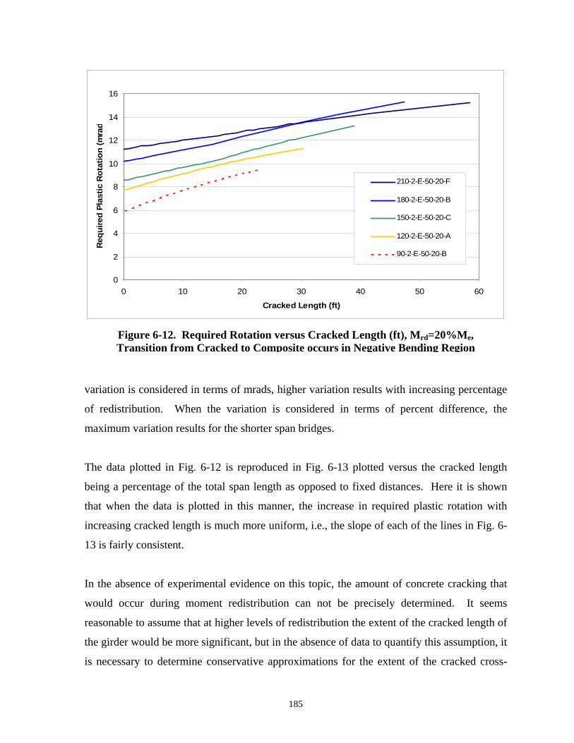
0

2

4

6

8

10

12

14

16

0 10 20 30 40 50 60

Cracked Length (ft)

Req

uire

d Pl

astic

Rot

atio

n (m

rad

210-2-E-50-20-F

180-2-E-50-20-B

150-2-E-50-20-C

120-2-E-50-20-A

90-2-E-50-20-B

Figure 6-12. Required Rotation versus Cracked Length (ft), Mrd=20%Me, Transition from Cracked to Composite occurs in Negative Bending Region

variation is considered in terms of mrads, higher variation results with increasing percentage

of redistribution. When the variation is considered in terms of percent difference, the

maximum variation results for the shorter span bridges.

The data plotted in Fig. 6-12 is reproduced in Fig. 6-13 plotted versus the cracked length

being a percentage of the total span length as opposed to fixed distances. Here it is shown

that when the data is plotted in this manner, the increase in required plastic rotation with

increasing cracked length is much more uniform, i.e., the slope of each of the lines in Fig. 6-

13 is fairly consistent.

In the absence of experimental evidence on this topic, the amount of concrete cracking that

would occur during moment redistribution can not be precisely determined. It seems

reasonable to assume that at higher levels of redistribution the extent of the cracked length of

the girder would be more significant, but in the absence of data to quantify this assumption, it

is necessary to determine conservative approximations for the extent of the cracked cross-

185

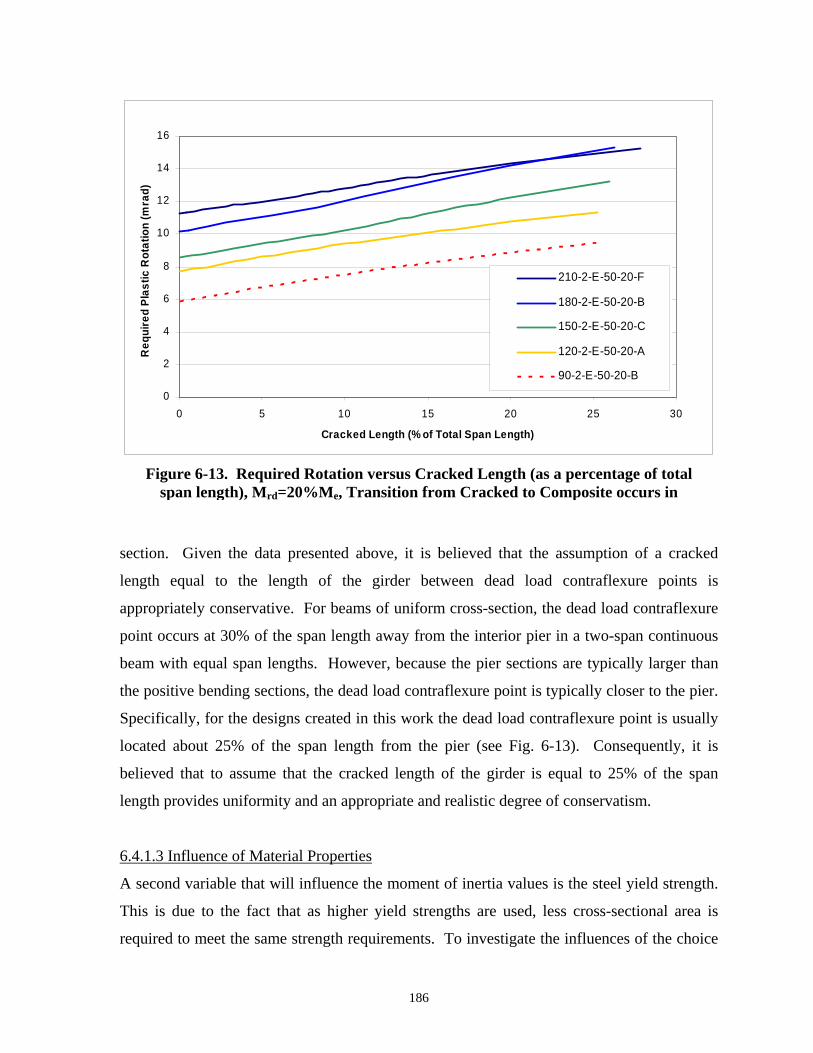
0

2

4

6

8

10

12

14

16

0 5 10 15 20 25 30

Cracked Length (% of Total Span Length)

Req

uire

d Pl

astic

Rot

atio

n (m

rad)

210-2-E-50-20-F

180-2-E-50-20-B

150-2-E-50-20-C

120-2-E-50-20-A

90-2-E-50-20-B

Figure 6-13. Required Rotation versus Cracked Length (as a percentage of total span length), Mrd=20%Me, Transition from Cracked to Composite occurs in

section. Given the data presented above, it is believed that the assumption of a cracked

length equal to the length of the girder between dead load contraflexure points is

appropriately conservative. For beams of uniform cross-section, the dead load contraflexure

point occurs at 30% of the span length away from the interior pier in a two-span continuous

beam with equal span lengths. However, because the pier sections are typically larger than

the positive bending sections, the dead load contraflexure point is typically closer to the pier.

Specifically, for the designs created in this work the dead load contraflexure point is usually

located about 25% of the span length from the pier (see Fig. 6-13). Consequently, it is

believed that to assume that the cracked length of the girder is equal to 25% of the span

length provides uniformity and an appropriate and realistic degree of conservatism.

6.4.1.3 Influence of Material Properties

A second variable that will influence the moment of inertia values is the steel yield strength.

This is due to the fact that as higher yield strengths are used, less cross-sectional area is

required to meet the same strength requirements. To investigate the influences of the choice

186

of material yield strength, designs were created using both of the two most popular material

configurations: Grade 50 steel used throughout the girder or Grade 50 steel used for positive

bending flanges and all webs in combination with Grade 70 steel used for the flanges of

negative bending sections. The results of this evaluation are shown below in Table 6-1 for

two-span designs with a span length of 120 ft at targeted redistribution levels of 10 and 20%

and a span length of 210 ft with redistribution levels of 10, 20, 30, and 40%. It is noted that

the use of a hybrid material configuration for higher levels of moment redistribution at the

120 ft span length was not practical because a uniform (Grade 50) cross-section could be

used for 30% redistribution, i.e., there would be no benefit associated with the use of a higher

yield strength in negative bending without having a smaller cross-section in negative bending

than in positive bending, which is typically regarded as poor design practice. Because, as

shown by Eqs .6.1, 6.2, and 6.7, the required rotations are directly proportional to the

magnitude of the redistribution moment, it is more appropriate to compare the required

rotation values normalized by the magnitude of the redistribution moment or the percentage

of redistribution moment. These comparisons are illustrated in Table 6-1 where the required

rotation, redistribution moment, percentage of redistribution moment, required rotation

normalized by redistribution moment, and required rotation normalized by percentage of

redistribution moment are given. The percent difference values refer to the difference in

normalized rotation values for each pair of homogeneous and hybrid girders.

The results presented in Table 6-1 show that the influence of the reduced cross-section

resulting from the hybrid designs has a significant influence on rotation requirements. In

Table 6-1. Comparison of Rotation Requirements for Hybrid v. Homogeneous Girders

θDesign θP (mrad) Mrd (ft-kips) Mrd % P / Mrd % Difference θP / Mrd% % Difference120-2-H-10-B 6.1 825 9.5 0.00739 0.645120-2-50-10-A 5.8 968 10.6 0.00596 0.546120-2-H-20-A 10.2 1364 15.6 0.00750 0.654120-2-50-20-A 11.3 1699 19.4 0.00666 0.584210-2-H-10-A 6.9 2558 9.7 0.00268 0.708210-2-50-10-E 7.1 2984 10.9 0.00237 0.651210-2-H-20-B 16.0 5141 20.0 0.00312 0.800210-2-50-20-F 15.0 5242 19.5 0.00285 0.766210-2-H-30-B 23.8 7516 29.9 0.00316 0.796210-2-50-30-B 22.0 8042 30.0 0.00273 0.731210-2-H-40-B 33.3 9936 41.1 0.00335 0.811210-2-50-40-C 29.9 10228 40.0 0.00293 0.748

12.7 12.0

24.0 18.2

13.2 8.6

9.3 4.5

15.9 8.8

14.6 8.5

187

terms of required rotation normalized by the magnitude of redistribution moment the

difference is 9 to 24% and in terms of required rotation normalized by percentage of

redistribution moment the difference is 5 to 18%. Thus, the influence of pier section material

configuration is significant enough to be considered when developing rotation requirement

equations.

6.4.1.4 Sensitivity of Results to Ix

A final consideration with respect to the influence of moment of inertia values on required

plastic rotation is the sensitivity of the results to these moment of inertia values. It is obvious

from Eqs. 6.1, 6.2, and 6.7 that the required rotations are inversely proportional to the

moment of inertia values of the girder. Thus, the objective of this section is to investigate the

sensitivity of the rotation requirements to the variation in Ix values that may occur for a given

design situation. In other words, the objective here is not to evaluate changes in rotation

requirements across a broad range of moment of inertia values, but instead, to assess the

variability in rotation requirements that occurs over the limited range of Ix values that will

efficiently satisfy the design requirements of a particular design scenario. This is of

importance because the goal of this work is to provide definitive conclusions on rotation

requirements. Thus, it is necessary to avoid the presentation of results that are linked to

specific designs. It should be recognized that for a certain design scenario (i.e., given span

lengths and level of intended redistribution) the required moment capacity at various cross-

sections along the length of the girders will be relatively constant. Consequently, the

required cross-section properties (e.g., moment of inertia values) will also be relatively

constant. However, various designers may arrive at different cross-section geometries to

satisfy the same design requirements. Thus, this influence is examined herein through

applying alternative design criteria compared to those used in the development of the initial

designs. Specifically, three of the design criteria that will most significantly affect the

resulting moment of inertia values are selected for investigation. These are: the use of

“stiffened” versus “un-stiffened” webs, employing different limits for the minimum

performance ratio that is acceptable, and implementing alternative criteria for when section

transitions are used.

188

Un-stiffened webs have a web thickness such that shear requirements are satisfied without

the need for transverse stiffeners, while stiffened webs have a reduced web thickness and

require the addition of transverse stiffeners. Results of four of the example designs illustrate

the influences on rotation requirements from the use of stiffened versus un-stiffened webs.

Specifically, the hybrid 120 ft designs with a targeted redistribution of 10% and 20% were

initially designed as un-stiffened girders and then redesigned with a web thickness 1/16 in.

less than the original un-stiffened designs, which is a typical web thickness for stiffened

girders. For the case of the designs with 20% redistribution targeted, the two designs are

identical except for the change in web thickness; however, for the designs with 10%

redistribution, it was also necessary to increase the web depth by 1 in. and change the

proportions of the top and bottom flanges in order to satisfy design requirements.

Table 6-2 compares the resulting required rotations for the stiffened and un-stiffened designs.

As before, the required rotations are normalized by the magnitude of the redistribution

moment and the percentage of the redistribution moment, and because the reduction in web

thickness also resulted in a significant increase in the redistribution moment, it is not

appropriate to directly compare the required rotations of the stiffened versus un-stiffened

designs. Table 6-2 shows that the difference in normalized required rotation is less than 2%

in all cases. Also it is shown that when the required rotation is normalized by the magnitude

of the redistribution moment, the change from stiffened to un-stiffened girders may result in

either an increase or decrease in the normalized required rotation. Thus it is concluded that

the influence of stiffened versus un-stiffened webs is negligible.

Different designers may also arrive at varying moment of inertia values for a given design

situation due to the use of alternative limits on the minimum allowable performance ratios.

As stated previously, it was required that the designs created in this work have a minimum

performance ratio of 0.95 for each section transition. Alternatively, three girders were also

Design θP (mrad) Mrd (ft-kips) Mrd % θP / Mrd % Difference θP / Mrd% % Difference120-2-H-20-A 10.2 1364 15.6 0.00750 0.654120-2-H-20-A-(S) 14.9 1953 22.5 0.00764 0.664120-2-H-10-B 6.1 825 9.5 0.00739 0.645120-2-H-10-B-(S) 11.2 1523 17.1 0.00736 0.654

1.8

0.4

1.5

1.4

Table 6-2. Comparison of Rotation Requirements for Un-stiffened v. Stiffened Girders

189

designed accepting lower performance ratios and these are compared to the more optimal

design for the same situation in Table 6-3. The performance ratios of these alternative

designs are as described below.

• In Design 140-175-140-H-B the center cross-section comprising 30% of the span

length has a maximum performance ratio of only 0.91.

• In Design 150-2-E-30-B one of the three cross-sections is slightly over-designed with

a maximum performance ratio equal to 0.94.

• Design 210-2-E-50-10-A is significantly over-designed, with all of the cross-sections

except for the pier section having performance ratios ranging between 0.79 and 0.88.

Thus it is believed that the first two examples represent alternative reasonable designs and

the third example illustrates a more extreme situation where it is unlikely that a designer

would consider this to be an appropriate design.

From the results presented in Table 6-3, it can be seen that the percent difference in

normalized required rotations is approximately 1% or less for the two designs that are

considered reasonable design alternatives. Additionally, for the significantly over-designed

girder the difference is approximately 10%.

An additional cause of variation in the moment of inertia values for a particular design

situation is the use of alternative criteria to establish when section transitions are appropriate.

This influence is also examined using Design 140-175-140-H-B, which contains a section

transition in the end span where the resulting weight savings is only 500 lbs in addition to

having a performance ratio of 0.91 along 30% of the span length. Thus, even though the

design criteria used for Design 140-175-140-H-B differs from the criteria used for Design

Table 6-3. Comparison of Rotation Requirements for Alternative Design Criteria Girders Design θP (mrad) Mrd (ft-kips) Mrd % θP / Mrd % Difference θP / Mrd% % Difference140-175-140-H-B 17.7 2635 18.7 0.00672 0.949140-175-140-H-ORIGINAL 18.1 2696 18.9 0.00671 0.957150-2-E-50-30-B 20.8 4140 31.9 0.00502 0.652150-2-E-50-30-C 21.0 4137 31.9 0.00508 0.659210-2-E-50-10-A 6.0 2786 10.0 0.00214 0.597210-2-E-50-10-E 7.1 2984 10.9 0.00237 0.651

1.2 1.1

0.3

9.8

0.9

8.4

190

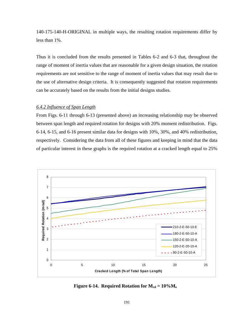
140-175-140-H-ORIGINAL in multiple ways, the resulting rotation requirements differ by

less than 1%.

Thus it is concluded from the results presented in Tables 6-2 and 6-3 that, throughout the

range of moment of inertia values that are reasonable for a given design situation, the rotation

requirements are not sensitive to the range of moment of inertia values that may result due to

the use of alternative design criteria. It is consequently suggested that rotation requirements

can be accurately based on the results from the initial designs studies.

6.4.2 Influence of Span Length

From Figs. 6-11 through 6-13 (presented above) an increasing relationship may be observed

between span length and required rotation for designs with 20% moment redistribution. Figs.

6-14, 6-15, and 6-16 present similar data for designs with 10%, 30%, and 40% redistribution,

respectively. Considering the data from all of these figures and keeping in mind that the data

of particular interest in these graphs is the required rotation at a cracked length equal to 25%

0

1

2

3

4

5

6

7

8

0 5 10 15 20 25


Req

uire

d R

otat

ion

(mra

d)

210-2-E-50-10-E

180-2-E-50-10-A

150-2-E-50-10-A

120-2-E-20-10-A

90-2-E-50-10-A

Figure 6-14. Required Rotation for Mrd = 10%Me

191

0

5

10

15

20

25

0 5 10 15 20 25


Req

uire

d R

otat

ion

(mra

d)

210-2-E-50-30-B

150-2-E-50-30-C

120-2-E-50-UF(30)-E

120-2-E-50-U(30)-E


0

5

10

15

20

25

30

35

0 5 10 15 20 25


Req

uire

d R

otat

ion

(mra

d)

210-2-E-50-40-C

150-2-E-50-40-A


192

of the total span length (as discussed above), it is shown that in general the highest rotation

requirements correspond to the girders with the longest span lengths. However, a longer

span length does not necessarily correspond to increased rotation requirements. For example,

in Fig. 6-13, a slightly higher rotation is required for the 180 ft. girder compared to the 210 ft.

girder. Also, in Fig. 6-14, approximately the same amount of rotation is required for the

bridges with the three longest span lengths (i.e., 150 ft., 180 ft., and 210 ft.) while

approximately the same amount of rotation is required for all of the designs plotted in Fig. 6-

15, where the span length varies from 120 ft to 210 ft. Thus it is believed that rotation

requirements based on the span lengths producing the greatest rotation requirements are

justified.

As with the variables previously discussed, the influence of span length on required plastic

rotation is also considered in terms of normalized required rotation. The data is normalized

by both the percentage of redistribution moment and the magnitude of the redistribution

moment in Figs. 6-17 and 6-18, respectively, for the designs with a targeted redistribution

percentage of 10%. The trend in Fig. 6-17 is similar to the results previously presented,

which is as anticipated since the previous results were grouped by common percentages of

redistribution moment. In Fig. 6-18 it is shown that significantly decreased normalized

rotation is required with increasing span length, this same trend exists for the design

examples with other levels of redistribution.

6.4.3 Influence of Redistribution Moment

The influence of the amount of moment being redistributed has been briefly addressed above

as reason for presenting rotation requirements normalized by either the magnitude of the

redistribution moment or the redistribution moment percentage (represented as a percentage

of the elastic moment). Figure 6-19 examines this influence in greater detail by presenting

the required rotation as a function of the percentage of moment being redistributed for the

two-span design examples. Here a strong linear relationship is shown between the two

variables, which is particularly true when designs of a fixed span length and material

193

0.00

0.10

0.20

0.30

0.40

0.50

0.60

0.70

0.80

0 5 10 15 20 25


Requ

ired

Rota

tion/

Mrd

%

210-2-E-50-10-E

180-2-E-50-10-A

150-2-E-50-10-A

120-2-E-20-10-A

90-2-E-50-10-A

Figure 6-17. Normalized rotation requirements (by percentage of redistribution moment) for Mrd=10%Me

0.000

0.001

0.002

0.003

0.004

0.005

0.006

0.007

0.008

0.009

0.010

0 5 10 15 20 25


Req

uire

d R

otat

ion/

Mrd

210-2-E-50-10-E 180-2-E-50-10-A

Figure 6-18. Normalized rotation requirements (by magnitude of redistribution moment) for Mrd=10%Me

150-2-E-50-10-A 120-2-E-20-10-A90-2-E-50-10-A

0

5

10

15

20

25

30

35

0 5 10 15 20 25 30 35 40 45

Mrd/Me*100

Req

uire

d Pl

astic

Rot

atio

n (m

rads

)L=90

L=120

L=120, Hybrid

L=120, Hybrid, Stiffened

L=150

L=180

L=210

Figure 6-19. Relationship Between Percentage of Redistribution Moment and Required Plastic Rotation

configuration are considered. Figure 6-20 plots the required rotation as a function of the

magnitude of the redistribution moment and shows that when the results are plotted in this

manner there is still a linear relationship within a particular series, but overall there is

considerable scatter within the results. This may be explained by the fact that girders

designed for shorter span lengths will have smaller cross-sections; therefore, a redistribution

moment of a fixed magnitude will cause greater rotations in the shorter span lengths. When

the redistribution moment is expressed as a percentage of the elastic moment, the effect of

varying span length is minimized as the larger elastic moments corresponding to increased

span length also correspond to larger cross-sections. It is concluded that it is more

appropriate to evaluate rotation requirements in terms of the percentage of the moment being

redistributed as opposed to the magnitude of this moment.

Once it was determined that the required plastic rotation is best related as a function of the

percentage of redistribution moment, the nature of this relationship is sought. As discussed

195

0

5

10

15

20

25

30

35

0 1000 2000 3000 4000 5000 6000 7000 8000 9000 10000 11000

Mrd (ft-kips)

Req

uire

d Pl

astic

Rot

atio

n (m

rads

L=90

L=120

L=120, Hybrid


L=150

L=180

L=210

Figure 6-20. Relationship Between Magnitude of Redistribution Moment and Required Plastic Rotation

above and shown by Eqn. 6-1, there is a linear relationship between Mrd and the required

rotations. However, it should be realized that this statement is true assuming that the other

variables influencing the required rotations (span length, modulus of elasticity, and moment

of inertia) are all constant; although with increasing redistribution moment, smaller pier

sections (i.e., reduced moment of inertia values) are required. Therefore, for uniform

increments of increasing redistribution, increasing increments of required rotation will result.

However, examination of the data in Fig. 6-19 indicates that this issue is negligible; a linear

fit to the data for each span length and material configuration yields R2 values between 0.995

and 1.000. As the ultimate goal is to develop rotation requirement relationships suitable for

incorporation in design and rating procedures, the simplicity offered by the use of a linear

relationship between required plastic rotation and percentage of redistribution moment is

favored over the increase in complexity with minimal increase in accuracy that would result

by incorporating non-linear equations.

196

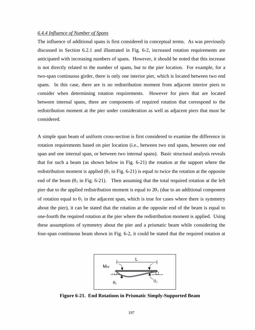
6.4.4 Influence of Number of Spans

The influence of additional spans is first considered in conceptual terms. As was previously

discussed in Section 6.2.1 and illustrated in Fig. 6-2, increased rotation requirements are

anticipated with increasing numbers of spans. However, it should be noted that this increase

is not directly related to the number of spans, but to the pier location. For example, for a

two-span continuous girder, there is only one interior pier, which is located between two end

spans. In this case, there are is no redistribution moment from adjacent interior piers to

consider when determining rotation requirements. However for piers that are located

between internal spans, there are components of required rotation that correspond to the

redistribution moment at the pier under consideration as well as adjacent piers that must be

considered.

A simple span beam of uniform cross-section is first considered to examine the difference in

rotation requirements based on pier location (i.e., between two end spans, between one end

span and one internal span, or between two internal spans). Basic structural analysis reveals

that for such a beam (as shown below in Fig. 6-21) the rotation at the support where the

redistribution moment is applied (θ1 in Fig. 6-21) is equal to twice the rotation at the opposite

end of the beam (θ2 in Fig. 6-21). Then assuming that the total required rotation at the left

pier due to the applied redistribution moment is equal to 2θ1 (due to an additional component

of rotation equal to θ1 in the adjacent span, which is true for cases where there is symmetry

about the pier), it can be stated that the rotation at the opposite end of the beam is equal to

one-fourth the required rotation at the pier where the redistribution moment is applied. Using

these assumptions of symmetry about the pier and a prismatic beam while considering the

four-span continuous beam shown in Fig. 6-2, it could be stated that the required rotation at

L

Mrd

θ1

θ2

Figure 6-21. End Rotations in Prismatic Simply-Supported Beam

197

the center pier would be equal to the sum of: (1) the required rotation at the center pier due to

application of a redistribution moment at the center pier, (2) one-fourth the required rotation

at the left pier due to application of the redistribution moment at the left pier, and (3) one-

fourth the required rotation at the right pier due to application of the redistribution moment at

the right pier.

It is desirable to investigate the accuracy of assuming that the rotation requirements at piers

adjacent to interior spans can be computed using this method of increasing the required

rotation due to the redistribution moment applied at the pier under consideration by one-

fourth of the required rotations at adjacent piers when the redistribution moment is applied at

these locations for general girders (with varying cross-sections that are not symmetric about

piers) due to the simplicity offered by this approach. This issue is investigated through trial

designs of a three-span and a four-span continuous girder. The three-span girder has a span

arrangement with lengths of 140 ft, 175 ft, and 140 ft and uses hybrid sections in negative

bending locations. The four-span girder has span lengths of 150 ft, 180 ft, 180 ft, and 150 ft

and is a homogeneous Grade 50 girder.

In these design examples the ratio between the component of required rotation that is due to

applying the redistribution moment at the adjacent pier and the component of rotation that is

due to applying the redistribution moment at adjacent piers is equal to: 24.8% for the three-

span design, 22.3% for the pier located adjacent to an end span in the four-span girder, and

26.2% for the pier located between two internal spans in the four-span girder. Thus it is

concluded that it is reasonable to compute the required rotation at a pier that is adjacent to

one or two internal spans as the sum of the rotation that would be computed assuming the

pier was adjacent to two end spans and 25% of the required rotation that is computed at each

adjacent pier assuming these piers are also adjacent to two end spans.

6.4.5 Required Rotation Capacity

Required rotation capacities were not of primary interest in this work as the rotation

requirements used in the rotation compatibility procedure are in terms of plastic rotation

(versus rotation capacity). However, a presentation of the required rotation capacities for

198

moment redistribution is presented herein as it is of interest to compare these rotation

capacity requirements with the conventional rotation capacity requirement of three (see

Section 2.4). Figure 6-22 reproduces the data presented in Fig. 6-19, but plots the rotation

requirement in non-dimensional terms of required rotation capacity. Here it is shown that the

same linearly increasing relationship exists between percentage of redistribution moment and

rotation requirements. Furthermore, for girders with redistribution moments less than the

AASHTO (2004) limit (20% of the elastic moment), it is shown that the required rotation

capacity is less than 2. However, as the redistribution moments exceed this limit, increased

rotation capacity is required. For a redistribution moment equal to 40% of the elastic

moment, which was the highest percentage of redistribution moment investigated in this

study, the required rotation capacity is approximately 4. Comparing these results to the

conventional rotation capacity requirement of three, it is shown that this requirement is very

conservative for the AASHTO (2004) moment redistribution requirements, however a

0

1

2

3

4

5

0 5 10 15 20 25 30 35 40 45

Mrd/Me*100

Requ

ired

Rota

tion

Capa

city

L=90

L=120

L=120, Hybrid


L=150

L=180

L=210

Figure 6-22. Relationship Between Percentage of Moment Redistributed and Required Rotation Capacity

199

rotation capacity of three would be unconservative if higher degrees of moment redistribution

were permitted.

An alternative approach to evaluating rotation requirements is to utilize moment versus

rotation curves from experimental testing. This method is used herein to validate the results

presented above. For this evaluation, the experimental data presented in Chapter 3 as well as

the data from all three-point bending tests presented in Appendix B is employed. Because

the rotation requirements are a function of the global stiffness of the structure and the test

specimens represent only the pier region of a continuous span structure, several assumptions

must first be made regarding the relationship between the test specimen and the structure of

which it is a component. First, it is assumed that the structure consists of a uniform cross-

section, i.e, both the positive and negative bending regions have geometry and cross-

sectional properties equal to that of the test specimen under consideration. Second, as a

consequence of assuming that a uniform cross-section is used it can be assumed that the

inflection point in the continuous-span structure occurs at a location equal to 30% of the span

length away from the pier. This leads to representing the span length of the continuous-span

structure as equal to five-thirds the length of the test specimen.

Once the stiffness of the structure is determined, the required plastic rotation can then be

related to the redistribution moment using the linear relationship given by Eq. 6.1,

ML2 3EIθ

= . (6.1)

Furthermore, the redistribution moment can be related to the experimental moment versus

rotation curve, which gives Mpe, using Eq. 2.11,

rd e peM M M= − (2.11)

and an assumed value of Me. It is initially assumed that Me is equal to 120%Mn, which

represents a redistribution of moment equal to the maximum allowable redistribution

currently permitted by AASHTO (2004) specifications. For some of the more slender

girders, this assumed level of elastic moment did not give a solution and the elastic moment

level was consequently reduced in these cases.

200

The procedure used to determine rotation requirements using experimental data is illustrated

below in Fig. 6-23, which illustrates the experimental moment versus plastic rotation curve

for Girder 4MG, introduced in Chapter 3. Figure 6-23 also shows a required rotation curve.

This curve is determined by first assuming that at the elastic moment there is no plastic

rotation. Thus, the elastic moment of 1165 ft-kips, or 98% of Mp, determines the y-intercept

of the required rotation curve. Secondly, the x-intercept of the required rotation curve is

determined by realizing that when a hinge exists at the pier, no moment can be resisted at this

location and the beam may be analyzed as a simply supported beam with an applied end

moment of magnitude equal to the elastic moment. For Girder 4MG, this results in a plastic

rotation of 34 mrads. The intersection point where the required rotation curve is less than the

available rotation curve is thus the required plastic rotation of the girder. In this case, the

required plastic rotation is then 12.40 mrads at a moment of 62% of Mp. Computing the

elastic rotation at this same level of moment using simple structural analysis procedures

gives an elastic rotation of 6.85 mrads. The ratio between the plastic and elastic rotations

0.0

0.2

0.4

0.6

0.8

1.0

1.2

0 10 20 30 4

θP (mrad)

M/M

p

0

Figure 6-23. Illustration of Procedure to Determine Rotation Requirements from Experimental Moment versus Rotation Curves

201

then gives the required rotation capacity, which is equal to 1.81 for Girder 4MG (assuming

an elastic moment of 1165 ft-kips and the global stiffness assumptions outlined above).

This same procedure is used to determine the rotation requirements for each of the 3-point

bending tests included in Appendix B and the experimental girders discussed in Chapter 3.

Plots illustrating these procedures are also included in Appendix B. This data is summarized

in Fig. 6-24, which presents the required rotation capacity for 53 experimental girders as a

function of the percentage of redistribution moment. Thus, Fig. 6.24 is analogous to Fig. 6-

22. Comparing Figs. 6-22 and 6-24, it is shown that the rotation requirements illustrated in

Fig. 6-22 resulting from the analysis procedure discussed in Section 6.2 and the design

studies presented in Section 6.3 are slightly higher than those that result from analysis of the

experimental moment versus rotation curves. This is as expected because of the nature of the

experimental specimens. Specifically, the experimental girders, except for the Chapter 3

(Righman 2005) girders, are relatively compact. This causes the available and required

rotation curves to typically intersect in the pre-peak region of the moment versus rotation

response, where the ratio between plastic and elastic rotation is relatively low. With this

0

1

2

3

4

5

6

7

0 10 20 30 40 50 6

Mrd/Me*100

Requ

ired

Rota

tion

Capa

city

0

Righman (2005)Schilling (1985)Schilling and Morcos (1988)

BarthGrubb and Carskaddan (1979, 1981)Adams, Lay, and Galambos (1964)Lukey et al. (1969)

Hartnagel (1997)Yakel et al. (1999)

Figure 6-24. Relationship Between Percentage of Moment Redistributed and Required Rotation Capacity as Determined From Experimental Results

202

consideration, it is concluded that the comparison between the two methods for computing

required rotation capacities is favorable and that the results presented in Fig. 6-22 are

appropriately conservative.

The results from determining the rotation requirements from experimental data are also

presented in Table 6-4. Here the required plastic rotations, corresponding elastic rotations,

required rotation capacities, and the corresponding percentage of the elastic moment that is

redistributed are tabulated. Thus, the data in Table 6-4 can be used to compare with the

results of Schilling (1986). Schilling reported required plastic rotations between 0 and 29

mrads using the same approach of determining the intersection of the moment versus rotation

and required rotation curves for hypothetical girders. From, Table 6-4 it is observed that the

required plastic rotation for these experimental girders is between 1 and 17 mrads.

6.4.6 Development of Required Rotation Prediction Equations

Based on evaluation of the influential variables affecting rotation requirements identified

above, it is concluded that equations to predict the required rotation should be primarily

expressed as a linear function of the percentage of redistribution moment. It is also necessary

to incorporate the effects of pier location and material properties.

The relationship between percentage of redistribution moment and required rotation is

illustrated in Fig. 6-25 for the two-span Grade 50 girders. The relationship

erdpR M/M80=θ (6.8)

is shown by the dark solid line to conservatively represent the available data.

Using Eq. 6.8 and the previously established relationship that the rotation requirements at

piers adjacent to internal spans can be computed as the sum of the required rotation at the

pier under consideration assuming the pier is located between end spans and 25% of the

required rotations at adjacent piers assuming these piers are also located between end spans,

results in the following rotation requirements:

203

Table 6-4. Rotation Requirements Resulting from Analysis of Experimental Data

Girder θ p θ e R Mrd/Me*1001MG 6.77 10.49 0.65 172MG 6.45 9.03 0.71 193MG 3.32 6.05 0.55 164MG 12.40 6.85 1.81 365MG 11.98 4.21 2.85 496MG 1.23 1.67 0.74 57MG 17.05 2.85 5.98 508MG 11.92 6.69 1.78 369MG 1.92 11.28 0.17 510MG 11.26 8.53 1.32 2911MG 16.38 5.83 2.81 4712MG 11.47 7.61 1.51 32US 2.22 5.53 0.40 17UL 2.07 10.41 0.20 20SL 1.33 10.10 0.13 15S 4.68 16.32 0.29 23M 2.93 12.36 0.24 21D 2.98 12.12 0.25 16P2 6.20 9.10 0.68 18P3 5.00 8.52 0.59 16P6 8.70 11.20 0.78 20188-3-1 1.85 9.58 0.19 12188-3-2 5.05 18.22 0.28 16188-3-3 10.48 32.24 0.33 26188-3-5 4.59 15.41 0.30 20188-3-6 4.76 16.02 0.30 19188-3-7 3.75 14.45 0.26 22188-3-8 5.60 14.51 0.39 21HT-28 3.39 18.50 0.18 10HT-43 0.70 12.70 0.06 9A-1 3.44 23.61 0.15 12A-2 4.45 18.84 0.24 17B-1 2.20 17.60 0.13 10B-2 4.30 11.21 0.38 19B-3 3.19 13.70 0.23 17B-4 3.29 14.27 0.23 22B-5 3.82 15.68 0.24 17C-1 4.67 11.16 0.42 18C-2 2.56 7.75 0.33 22C-3 2.59 10.30 0.25 14C-4 2.74 10.71 0.26 19C-5 2.85 10.54 0.27 17D-6 2.36 8.22 0.29 22E-6 1.95 11.29 0.17 20D-1 4.04 15.62 0.26 22D-2 4.48 9.59 0.47 14D-5 6.39 20.95 0.31 19E-1 3.00 24.47 0.12 13E-2 4.80 13.30 0.36 13E-5 8.42 30.32 0.28 14

Hartnagel (1997) W14x26 2.77 19.37 0.14 10A 6.34 51.85 0.12 10D 3.32 56.79 0.06 4

Schilling and Morcos (1988)

Schilling (1985)

Righman (2005)

Barth (1996)

Lukey et al. (1969)

Adams, Lay, and Galambos (1964)

Grubb and Carskaddan (1979, 1981)

Yakel et al. (1999)

204

Relationship Between Mrd and Required Plastic Rotation

0

5

10

15

20

25

30

35

0 5 10 15 20 25 30 35 40 45

Mrd/Me*100

Req

uire

d Pl

astic

Rot

atio

n (m

rads

)

L=90

L=120

L=150

L=180

L=210

θ pR = 80 Mrd/Me

Figure 6-25. Relationship Between Required Plastic Rotation and Percentage of Redistribution Moment for Two-Span Grade 50 Designs

• For homogeneous pier sections between an end span and an internal span

pR rd1 e1 rdA180 M / M 20M / Mθ = + eA1 , (6.9)

• And, for homogeneous pier sections between two internal spans

pR rd e rdA1 eA1 rdA280M / M 20 M / M 20 M / Mθ = + + eA2 , (6.10)

where Mrd/Me refers to the redistribution moment at the pier under consideration, while

MrdA1/MeA1 and MrdA2/MeA2 refer to the redistribution moment at adjacent spans.

The relationship between required plastic rotation and percentage of redistribution moment

for hybrid girders is evaluated by considering the results previously presented in Table 6-1

where the rotation requirements for homogeneous and hybrid girders are compared.

Examining the difference in θP/Mrd% ratios for each pair of hybrid and homogeneous girders

shows that the maximum difference occurs for the 120 ft designs with 10% redistribution and

205

is equal to 0.099, or approximately 0.1. Because it is shown by Eq. 6.8 that the ratio of

θP/Mrd% for homogeneous girders is equal to 0.8, increasing this value by 0.1 gives the

resulting relationship for the rotation requirements for two-span hybrid girders,

erdpR M/M90=θ . (6.11)

Using the same procedure used above to determine the rotation requirements for piers

adjacent to interior spans for homogeneous girders, the rotation requirements at piers

adjacent to interior spans in hybrid girders are determined to be:

• For hybrid pier sections between an end span and an internal span

pR rd1 e1 rdA190 M / M 22.5M / Mθ = + eA1 , (6.12)

• And, for hybrid pier sections between two internal spans

pR rd e rdA1 eA1 rdA290M / M 22.5M / M 22.5M / Mθ = + + eA2 . (6.13)

By assuming that similar levels of redistribution moment will occur at each pier, the above

equations can be reduced to,

pR rdC (M / M )eθ = (6.14)

where:

• For homogeneous pier sections:

C 80 20 n= + , and (6.15)

• For hybrid pier sections between two end spans:

C 90 22.5n= + (6.16)

and n represents the number of adjacent piers where moment redistribution occurs.

Thus the ultimate result of the rotation requirement study conducted herein is Eqs. 6.14

through 6.16. These relationships will be used in the following chapter to develop the

rotation compatibility design and rating specifications by comparing these rotation

requirements to the available rotations of steel I-girders.

206

Chapter 7: ROTATION COMPATABILITY - DESIGN AND RATING

SPECIFICATIONS

The primary focus of this chapter will be to present the development of the rotation

compatibility approach to moment redistribution and its applications for steel bridge design

and rating. This is carried out through synthesis of the available rotation/moment rotation

characteristics presented in Chapter 5 and the rotation requirements presented in Chapter 6.

It will be demonstrated herein that the suggested procedure provides a rational basis for

conveniently determining the two key parameters required for design or rating: the maximum

permissible level of redistribution and the minimum required girder capacity.

As previously discussed the rotation compatibility procedure is based on explicitly assuring

that the available rotation of a girder is greater than the rotation required for the intended

level of moment redistribution to occur. The first section of this chapter (Section 7.1) will

summarize the expressions for required and available rotations developed in previous

chapters and then proceed with evaluation of the conditions under which it can be assured

that the available rotation is greater than the required rotation.

Section 7.2 presents rotation compatibility design specifications for steel bridges. Here the

range of applicability of the specifications, an overview of the design process, and a series of

equations in a format suitable for incorporation into design specifications are presented.

Similarities and differences between the rotation compatibility design procedure and the

AASHTO (2004) moment redistribution procedure are also discussed.

As discussed in Chapter 2, rating procedures consistent with the Load and Resistance Factor

Design (LRFD) procedures were published in 2003 (AASHTO 2003). These rating

specifications utilize the moment capacity equations from LRFD for load rating. Therefore,

it should by extension also be possible to utilize the optional moment redistribution

specifications contained in the LRFD specifications for load rating. However, the limited

applicability of the AASHTO (2004) moment redistribution specifications excludes many

207

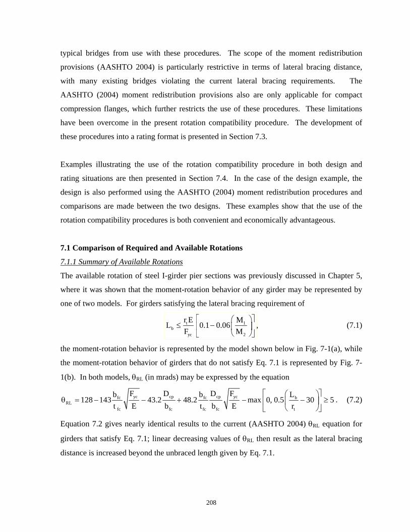
typical bridges from use with these procedures. The scope of the moment redistribution

provisions (AASHTO 2004) is particularly restrictive in terms of lateral bracing distance,

with many existing bridges violating the current lateral bracing requirements. The

AASHTO (2004) moment redistribution provisions also are only applicable for compact

compression flanges, which further restricts the use of these procedures. These limitations

have been overcome in the present rotation compatibility procedure. The development of

these procedures into a rating format is presented in Section 7.3.

Examples illustrating the use of the rotation compatibility procedure in both design and

rating situations are then presented in Section 7.4. In the case of the design example, the

design is also performed using the AASHTO (2004) moment redistribution procedures and

comparisons are made between the two designs. These examples show that the use of the

rotation compatibility procedures is both convenient and economically advantageous.

7.1 Comparison of Required and Available Rotations

7.1.1 Summary of Available Rotations

The available rotation of steel I-girder pier sections was previously discussed in Chapter 5,

where it was shown that the moment-rotation behavior of any girder may be represented by

one of two models. For girders satisfying the lateral bracing requirement of

t 1b

yc 2

r E ML 0.1 0.06

F M⎡ ⎤⎛ ⎞

≤ −⎢ ⎥⎜ ⎟⎝ ⎠

, (7.1) ⎣ ⎦

the moment-rotation behavior is represented by the model shown below in Fig. 7-1(a), while

the moment-rotation behavior of girders that do not satisfy Eq. 7.1 is represented by Fig. 7-

1(b). In both models, θRL (in mrads) may be expressed by the equation


fc fc fc fc t

F D D Fb b L128 143 43.2 48.2 max 0, 0.5 30 5

t E b t b E r⎡ ⎤⎛ ⎞

θ = − − + − − ≥⎢ ⎥⎜ ⎟⎝ ⎠⎣ ⎦

. (7.2)

Equation 7.2 gives nearly identical results to the current (AASHTO 2004) θRL equation for

girders that satisfy Eq. 7.1; linear decreasing values of θRL then result as the lateral bracing

distance is increased beyond the unbraced length given by Eq. 7.1.

208

7.1.2 Summary of Required Rotations

As discussed in Chapter 6, the required rotation is expressed as a function of the percentage

of moment to be redistributed and the pier location, with alternative expressions being

required based on the grade of material used in the pier section. In summary, rotation

requirements were formulated for homogeneous Grade 50 girders as well as hybrid girders

comprised of Grade 70 flanges in negative bending and Grade 50 steel for positive bending

flanges and webs; higher rotations are required for hybrid girders due to the smaller moment

of inertia of these girders. Additionally, higher rotation requirements are required for piers

between internal spans of the girder compared to piers adjacent to end spans due to the fact

that the redistribution moments applied at adjacent piers also influence the rotation

requirements. The alternative expressions for rotation requirements previously presented in

Chapter 6 are reproduced below in Eqs. 7.3 through 7.5 where θpR represents the required

plastic rotation, C is the rotation coefficient given by Eq. 7.4 or 7.5, Mrd/Me represents the

normalized redistribution moment, and n represents the number of adjacent piers where

redistribution moments are applied. The reader is referred to Chapter 6 for a more detailed

presentation of these equations.

pR rdC (M / M )eθ = (7.3)


C 80 20 n= + (7.4)

• For hybrid pier sections:

C 90 22.5n= + (7.5)

1

MpeMn

5 θRL θp

Mpe 21 0.060 ( ) 0.0012 ( )p RL p RLMn= − − + −θ θ θ θ

Mpe 0.7 0.060 pMn= + θ

MpeMn Mpe 21 0.016 ( ) 0.0001( )p RL p RLMn

= − − + −θ θ θ θ

Mpe 0.7 0.060 pMn= + θ

1

θp5 θRL

Figure 7-1. Moment-Rotation Models

(a) For girders satisfying Eq. 7.1 (b) For girders violating Eq. 7.1

209

7.1.3 Comparison of Available and Required Rotations

The rotation compatibility procedure is based on an explicit comparison of available and

required rotations. Moment redistribution is valid for all cases where the available rotation is

greater than or equal to that which is required, and conversely, moment redistribution may

not be used when the available rotation is less than the required rotation. The comparison of

available and required rotation is facilitated through the relationships for available and

required rotations summarized in the previous two sections in conjunction with the general

equation for moment redistribution,

Me = Mpe + Mrd. (7.6)

It may be observed that Eq. 7.3 expresses the rotation requirements in terms of Mrd/Me and

that Fig. 7-1 presents the available rotations in terms of Mpe. Thus, through algebraic

manipulation of Eq. 7.6, available and required rotations may be directly compared.

Equation 7.6 is used to express the required rotation in terms of Mpe/Mn. Because the

available rotation is already expressed in this format, a similar expression for the required

rotations will allow for direct comparison of the two rotations. This is accomplished by first

dividing Eq. 7.6 by Me.

pe rd

e e

M M1

M M+ = (7.7)

This produces the term Mrd/Me, which is also used in the rotation requirement expression

given in Eq. 7.3. This term is then subtracted from both sides of the equation, giving

pe rd

e e

M M1

M M= − . (7.8)

Multiplication by Me/Mn then results in the desired format of the equation,

pe rd e

n e

M M M1

M M⎛ ⎞

= − •⎜ ⎟⎝ ⎠ nM

. (7.9)

Examination of Eq. 7.9 reveals that the quantity Mrd/Me can be related to the required

rotation while the quantity Mpe/Me can be related to the available rotation. However, further

consideration must be given to the term Me/Mn and, as will be revealed in the following

discussion, there are two alternative cases to consider when determining the value of this

210

parameter, which are related to the relative slopes of the required rotation and available

rotation curves. These two alternative cases will be illustrated by considering the Grade 50,

two-span (90’ – 90’) continuous girder shown below in Fig. 7-2. First, Eq. 7.3 may be used

to determine the rotation requirements. Because n is equal to zero for a two-span girder (see

Section 6.4.6), the equation reduces to

pR rd80 M / Meθ = , (7.10)

such that Mrd/Me may be expressed as

Mrd/Me = 0.0125θpR . (7.11)

Substitution of Eq. 7.11 into Eq. 7.9 gives

( )pe epR

n n

M M1 0.0125

M M= − θ • (7.12)

for the present design example. In general terms, Eq. 7.12 is expressed as

Mpe/Mn = (1-θpR/C)(Me/Mn). (7.13)

It is initially assumed that the lateral bracing requirements of Eq. 7.1 are satisfied such that

θRL is computed with the last term in Eq. 7.2 equal to zero. Furthermore, it is assumed that

this girder is composite with the concrete deck resulting in Dcp = 25.91 in. and rt = 4.234 in,

giving

θRL = 18 mrads. (7.14)

Equation 7.14 is then substituted for θRL into the unloading equation in Fig. 7-1(a),

Mpe/Mn = 1 – 0.016(θp – 18) + 0.0001(θp – 18)2, (7.15)

which may also be expressed as

Mpe/Mn = 0.0001 θp2 – 0.0196 θp + 1.3204. (7.16)

63’

14 x 3/4 14 x 3/4

16 x 1-1/4 16 x 1-1/4

44 x 7/16 44 x 1/2 44 x 7/16

63’ 54’

14 x 1-1/4

16 x 1-1/4

Figure 7-2. Example Girder

211

Setting Eqs. 7.12 and 7.16 equal then gives

( )2 ep p pR

n

M0.0001 - 0.0196 + 1.3204 = 1 0.0125

Mθ θ − θ • . (7.17)

Thus, for the present example, moment redistribution is valid for any set of values of Me/Mn,

θp, and θpR that satisfy Eq. 7.17 and where θp is greater than or equal to θpR. The requirement

that the available rotation must be greater than the required rotation can thus be represented

by Eq. 7.18, which is valid for θp > θRL.

( )2 ep p pR

n

M0.0001 - 0.0196 + 1.3204 1 0.0125

Mθ θ ≥ − θ • (7.18)

A graphical representation Eq. 7.18 is given below in Fig. 7-3 where the right side of the

equation is graphed for various values of Me/Mn. Here it is shown that because the slopes of

the required rotation curves are less than the minimum slope of the available rotation curve

(which occurs at θRL), for Me/Mn ratios less than 1.29 the required rotations are less than the

0.0

0.2

0.4

0.6

0.8

1.0

1.2

1.4

1.6

0 5 10 15 20 25 30 35 40 45 50

Plastic Rotation

Mpe

/Mn

Available Rotation

Mpe/Mn (Me/Mn=1.10)

Mpe/Mn (Me/Mn=1.29)

Mpe/Mn (Me/Mn=1.40)

Figure 7-3. Comparison of Available and Required Rotations for Example Girder

with Lb satisfying Eq. 7.1

212

available rotation throughout the unloading region of the moment versus rotation response

and the curves do not intersect. Thus, the effective plastic moment capacity is equal to Mn

for Me/Mn ratios less than 1.29. Alternatively, for Me/Mn ratios greater than 1.29 the required

rotations are initially greater than the available rotation. Consequently, the effective plastic

moment in these cases is determined by the intersections of the two curves, which is shown

to be 0.7Mn for a Me/Mn ratio of 1.40 in Fig. 7-3. Lastly, it is shown by Fig. 7-3 that, for the

example girder considered, 1.29 is the maximum Me/Mn ratio, where Mpe may be taken as the

maximum allowable value (Mn).

It should be apparent from Fig. 7-3 that, above a certain limit (1.29 for this example),

increasing ratios of Me/Mn reduce the effective plastic moment capacity of the girder. In

terms of the physical girder, this represents a point where the girder can no longer sustain its

nominal moment capacity due to excessive stresses in the girder. It should also be apparent

that some maximum limit should be placed on the amount of moment that is permitted to be

redistributed. For example, in the current AASHTO (2004) Specifications this limit is 20%

of the elastic moment. However, it is suggested that a more appropriate limit would be to

limit the maximum allowable level of redistribution in accordance with the moment level at

which the moment capacity decreases below Mn. Such an approach not only establishes a

rational criterion for the maximum level of moment redistribution, but will also decrease

girder distortions compared to allowing the girder to unload to moment levels below Mn.

Thus, the objectives of the current 20% limit (to control girder deformations) are also better

satisfied. For these reasons, the maximum allowable elastic moment is limited to the

magnitude of moment at which the effective plastic moment is equal to Mn in the present

work. This maximum value of elastic moment may also be thought of as the moment level

where the available and required rotation curves intersect at a rotation value less than or

equal to θRL. Mathematical expressions for determining the maximum allowable elastic

moment are now derived based on this requirement; the ramifications of this requirement in

comparison to the values of Mpe less than Mn permissible in the current AASHTO (2004)

Specifications are subsequently discussed in Section 7.2.4.

213

The maximum allowable value of Me/Mn may be obtained mathematically by setting θpR

= θRL in Eq. 7.13. Realizing that Mpe/Mn will equal one at θRL and substituting this value

into Eq. 7.13, the maximum Me/Mn ratio can be obtained for any girder where the slope of

the required rotation is less than the slope of the available rotation.

Me/Mn < 1/(1- θRL/C) (7.19)

In order to develop the needed expressions to determine the applicable range of Eq. 7.19, (i.e.,

when the slope of the required rotation equation is less than the slope of the available rotation

equation) we now consider the respective slopes of the required rotation and available

rotation curves. From examination of Eq. 7.14 it is revealed that the slope of the required

rotation equation is

mr= -Me/CMn. (7.20)

The slope of the available rotation curves is given by taking the first derivative of the

unloading curves given in Figs. 7-1(a) and (b) with respect to θp. Expressing these equations

in the standard quadratic format of

y = ax2 + bx + c, (7.21)

the slope of the unloading curve is then expressed as

ma = -b + 2a(θp-θRL). (7.22)

Because b is negative and a is positive, the minimum slope of the available rotation curve

occurs when θp equals θRL. Thus,

ma-(min) = -b. (7.23)

By then requiring that mr < ma, from Eqs. 7.20 and 7.23, we obtain

-Me/CMn < -b, (7.24)

and thus,

Me/Mn < Cb. (7.25)

Because b is a negative quantity, Eq. 7.26 can also be expressed as

Me/Mn > C|b|. (7.26)

Equation 7.26 must be satisfied to ensure that the slope of the required rotation expression is

less than the slope of the available rotation, such that Eq. 7.19 may be used to compute the

maximum allowable ratio of Me/Mn. However, this condition alone is not sufficient to limit

214

the required rotations to be less than the available rotations; in order for Eq. 7.19 to be valid,

it must also be guaranteed that the minimum value of Me/Mn from Eq. 7.26 does not produce

a required rotation greater than the available rotation at θRL, i.e., at a moment level of Mpe/Mn

=1. If this requirement is satisfied, then it will be assured that the required rotation will be

less than the available rotation throughout the unloading range of the girder. This

requirement can be mathematically expressed by first using the basic equation of moment

redistribution, Eq. 7.6, normalized by Mn, which gives

pee

n n

MM MM M M

= + rd

n

. (7.27)

Mpe/Mn = 1 may then be substituted into Eq. 7.27 giving

e

n n

M M1

M M= + rd . (7.28)

Multiplication of Eq. 7.28 by the ratio of Mn/Me and rearranging the resulting terms gives

rdn

e e

MM1

M M= − . (7.29)

Substituting θpR/C for Mrd/Me (which may be obtained from rearranging Eq. 7.3)

subsequently results in

pRn

e

M1

M Cθ

= − (7.30)

Solving Eq. 7.30 for θpR gives

npR

e

MC 1

M⎛ ⎞

θ = −⎜⎝ ⎠

⎟ . (7.31)

Then in order to determine if a value of θpR is less than θRL for Mpe/Mn =1, the maximum

valid value of Mn/Me, which may be computed from Eq. 7.26 as

n

e

M 1(max)M C

=b

, (7.32)

is substituted into Eq. 7.31 giving

pR1(min) C 1

C b⎛ ⎞

θ = −⎜⎜⎝ ⎠

⎟⎟ , (7.33)

or,

215

pR1(min) Cb

θ = − . (7.34)

Finally, it is required that the minimum value for θpR at Mpe/Mn =1 must be less than the

available rotation at the same level of moment, i.e., θRL,

RL1Cb

− ≤ θ (7.35)

So, in conclusion, when both Eqs. 7.26 and 7.35 are satisfied, the maximum allowable value

of Me/Mn is computed using Eq. 7.19 and any value of Me/Mn satisfying both Eqs. 7.19 and

7.26 is valid.

The allowable value of Me/Mn is now examined for other situations, beginning with the case

when Eq. 7.35 is satisfied but Eq. 7.26 is violated. For this situation the available rotation

will initially be greater than the required rotation, but the two curves may eventually intersect

causing a situation where there is insufficient available rotation. This case is illustrated by

using a value of Me/Mn equal to 1.10 with the previous example girder and is shown

graphically in Fig. 7-3. The potential intersection of the two curves is found by setting the

available and required rotation curves equal to one another as follows

1-b(θ-θRL) + a(θ-θRL)2 = (1-θ/R)Me/Mn. (7.36)

Solution of Eq. 7.36 for θ gives the intersection point, which is expressed as

22 2 2e e e e

RLn n n ne

RLn

M M M M4 aR 2 bR b R 4aR 1

M M M MMb2a 2aRM 2aR

⎛ ⎞ ⎛ ⎞− θ − + + −⎜ ⎟ ⎜

⎝ ⎠ ⎝θ = θ + − ±⎟⎠ . (7.37)

Examination of the square root term in Eq. 7.37 reveals that for all cases where Me/Mn < bC

(i.e., when Eq. 7.26 is violated), this term is negative. This indicates that there is no solution

for Eq. 7.37, which signifies that the available and required rotation curves do not intersect

for any case where Eq. 7.35 is satisfied. Furthermore, we may state that the maximum

allowable ratio of Me/Mn is given by Eq. 7.19 whenever Eq. 7.35 is satisfied.

216

We now turn to the case when Eq. 7.35 is not satisfied. This situation is illustrated by

considering the previous example girder although it is now assumed that the lateral bracing is

placed at 4 equal segments per span equal to 22.5 ft, such that Eq. 7.1 is violated. Thus, θRL

is computed using Eq. 7.2 to equal 5 mrad. Substituting this value of θRL, b equal to -0.06,

and the previously computed value of C equal to 80 into Eq. 7.33 shows that the requirement

to assure that the available and required rotation curves do not interest is not satisfied. This

is shown graphically for three different Me/Mn ratios in Fig. 7-4. Here it is obvious that a

Me/Mn ratio of 1.10 (or greater) is not valid since the required rotation is greater than the

available rotation throughout the unloading region. It is also shown that for a Me/Mn ratio of

1.067 the available and required rotation curves will intersect at θRL, while for lower Me/Mn

ratios the two curves will intersect at higher rotations and lower levels of moment. Because

the most economical design situation will result when Me/Mn is maximized, it will now be

proven that a Me/Mn ratio of 1.067 will yield sufficient rotation for moment redistribution if

the rotations are limited to θRL.

0.0

0.2

0.4

0.6

0.8

1.0

1.2

1.4

0 2 4 6 8 10 12 14 16 18 20

Plastic Rotation

Mpe

/Mn

Available Rotation

Mpe/Mn (Me/Mn=1.00)

Mpe/Mn (Me/Mn=1.067)

Mpe/Mn (Me/Mn=1.10)

Figure 7-4. Comparison of Available and Required Rotations for Example Girder

with Lb violating Eq. 7.1

217

In order to assure that there is sufficient rotation available to redistribute moment when a

Me/Mn ratio of 1.067 is used, the sum of the effective plastic moment and the maximum

redistribution moment that may be developed at θRL must equal a minimum of the elastic

moment at the pier. The effective plastic moment, as determined from the available rotation

curve at θRL, is shown to be equal to Mn, i.e., Mpe/Mn = 1 and

pe pe n

e n e

M M M 11 0.9375M M M 1.067

= • = • = . (7.38)

The maximum redistribution moment (occurring at θRL), computed by rearranging Eq. 7.3, is

equal to

pRrd RL

e

M 5 0.0625M C C 80

θ θ= = = = . (7.39)

Summing Eqs. 7.38 and 7.39 gives

pe rd

e e

M M0.9375 0.0625 1

M M+ = + = . (7.40)

Thus the requirement that the effective plastic moment and redistribution moment sum to the

elastic moment is exactly satisfied and it is shown that moment redistribution is valid for the

girder under consideration for a Me/Mn ratio up to 1.067.

The maximum allowable Me/Mn ratio for the case when Eq. 7.35 is violated may then be

computed in the same manner as before, using Eq. 7.20. This is true because the intersection

point of the available and required rotation curves occurs at θRL in all cases.

7.1.4. Summary

The above discussion has compared the available and required rotations and examined the

conditions necessary to assure that the available rotation is greater than the required rotations.

All possible scenarios were investigated with regard to the various relationships that may

exist between the required and available rotation functions and the results of this analysis

show that it can be assured that the available rotation is greater than that which is required if

the intersection of the available and required rotation curves occurs at a rotation less than or

equal to θRL. Furthermore, by setting the rotation at which the two curves intersect to θRL,

the maximum allowable ratio of Me/Mn may then by computed using Eq. 7.19.

218

7.2 Rotation Compatibility Design Specifications

7.2.1 Scope

As with the AASHTO 2004 moment redistribution specifications, the moment redistribution

specifications suggested herein are limited to straight girders with skews less than 10 degrees

having neither staggered cross-frames nor holes in the top/tension flange over a distance of

two times the web depth from either side of interior-pier sections where moments are

redistributed. Also consistent with the AASHTO 2004 procedures, the current specifications

restrict the length over which the girder may be analyzed for reduced negative moments due

to moment redistribution to a distance equal to one unbraced length on each side of the pier.

However, there are no cross-section limits outside of the cross-section proportion limits for

general I-girders contained in AASHTO 2004 Section 6.10.2, which allows the rotation

compatibility specifications to be applicable for a considerably larger class of girders. The

procedures are applicable for girders having yield strengths up to 70 ksi.

7.2.2 Overview of Design Procedure

While there are no explicit requirements on lateral bracing distance in the rotation

compatibility specifications, the beneficial effects of shorter bracing spacing are incorporated

through the last term of the θRL equation (Eq. 7.2). For designs satisfying Eq. 7.1, this last

term is equal to zero. Thus, for preliminary design, the designer may wish to initially assume

that the last term of Eq. 7.2 is equal to zero when determining cross-section geometry

requirements, and then subsequently selecting the lateral bracing distance.

The rotation coefficient, C, is then used in combination with θRL to determine the maximum

permissible level of elastic moment. It was shown by Eq. 7.19 that the maximum allowable

ratio of Me/Mn is computed as

Me/Mn < 1/(1- θRL/C). (7.19)

By rearranging this equation, we arrive at the moment requirements at the pier section using

rotation compatibility moment redistribution design,

Me(1- θRL/C) < Mn, (7.41)

219

Positive bending sections must also be analyzed for the effects of moment redistribution.

This is performed by computing the redistribution moment. At the piers the redistribution

moment is equal to the difference between the applied moments and the moment capacity,

Mrd = Me – Mn. (7.42)

The redistribution moment at other locations is then determined by linear interpolation

between the redistribution moments at the ends of each span, where redistribution moments

are equal to zero at abutments as is done in the AASHTO (2004) procedures.

The following section will present the equations given above in a format suitable for

incorporation into design specifications.

7.2.3 Rotation Compatibility Design Specification Equations

• Negative bending capacity at the strength limit state may be evaluated using

Me(1- θRL/C) < Mn,, (7.41)

where:

Mn = nominal moment capacity of the girder computed using applicable AASHTO

Specifications,

θRL = yc cp cp ycfc fc b

fc fc fc fc t

F 2D 2D Fb b L128 143 21.6 24.1 max 0, 0.5 30 5

t E b t b E r⎡ ⎤⎛ ⎞

− − + − −⎢ ⎥⎜ ⎟⎝ ⎠⎣ ⎦

≥

C = 80 20 n+ for homogeneous girders with Fy < 50 ksi,

C = 90 + 22.5 n for hybrid girders with Fyf < 70 ksi, and

n = number of piers where moment redistribution occurs adjacent to the pier under

consideration.

• Positive bending capacity must then be evaluated using

Mn > Me + MrdL + (x/L)(MrdR – MrdL), (7.43)

where:

Mn = nominal moment capacity of the girder computed using applicable AASHTO

Specifications,

MrdL = redistribution moment at left end of the span under consideration, computed

using Eq. 7.42,

220

MrdR = redistribution moment at right end of the span under consideration, computed

using Eq. 7.42,

x = location where moment is being evaluated expressed as distance from left end

of span

L = span length

7.2.4 Comparison to AASHTO 2004 Moment Redistribution Procedures

The AASHTO 2004 moment redistribution procedures were previously summarized in

Chapter 2. Although the underlying theory of these procedures and the rotation compatibility

design procedures described above is the same, the resulting design equations are markedly

different. The AASHTO 2004 moment redistribution procedures are primarily based on the

computation of two quantities, the effective plastic moment (Mpe) and the redistribution

moment (Mrd). Examination of the derivation of the rotation compatibility procedures

presented in Section 7.1.3, reveals that the basis of these procedures is also the quantities Mpe

and Mrd, although the primary quantities used in the design computations in the rotation

compatibility procedure are θRL and C.

In the AASHTO 2004 procedures, Mpe for a given limit state (strength or service) is

expressed by one of two equations depending on the web slenderness and transverse stiffener

configuration. These equations express Mpe as a function of Mn and are limited to a

maximum value of Mn. This is based on the premise that compact beams will have sufficient

rotation available to redistribute moment at Mn, but that more slender beams will have

reduced rotation available at Mn and a lower level of moment must be used to achieve the

needed rotation. Furthermore, the AASHTO (2004) specifications limit the maximum

allowable level of moment redistribution to 20% of the elastic moment. Conversely, in the

present rotation compatibility procedures, the Mpe value is equal to Mn in all cases and the

maximum allowable level of redistribution varies based on the rotation requirements and

girder ductility.

To compare the consequences of these two alternative approaches to limiting maximum

levels of redistribution, a girder that has an Mpe value equal to Mn according to the AASHTO

221

(2004) specifications is first considered. Substituting Mn for Mpe in Eq. 7.6 and setting the

magnitude of redistribution moment equal to the maximum value permissible using the

AASHTO (2004) specifications, Mrd = 0.2Me, gives

Me = Mn + 0.2Me, (7.44)

which can be solved to determine the maximum allowable value of the elastic moment in

terms of Mn, giving

Me < 1.25Mn. (7.45)

In the rotation compatibility procedure, the maximum value of Mrd varies based on the

available and required rotations of the girder under consideration and can be expressed as

Mrd/Me = θRL/C. (7.39)

For illustrative purposes, a representative girder for which Mpe is equal to Mn (Girder 90-2-E-

50-20-B from Chapters 5 and 6 and also described in Appendix E) is selected and the

maximum value of normalized redistribution moment is computed using Eq. 7.39. First, Eq.

7.2 is used to compute a θRL value equal to 24.1 mrads. Then, from Eqs. 7.4 and 7.5, it is

shown that C may vary between a minimum value of 80 and a maximum value of 135.

Substituting the minimum value of C into Eq. 7.39 and rearranging the equation gives that

the maximum allowable value of redistribution moment is equal to

Mrd = (θRL/C)Me = 24.1/80Me = 0.30Me. (7.46)

Substituting Eq. 7.46 for Mrd and Mn for Mpe into Eq. 7.6 gives

Me = Mn + 0.30Me. (7.47)

The maximum allowable value for the elastic moment is then equal to

Me < 1.43Mn, (7.48)

which represents a 15% increase in the allowable value of the elastic moment compared to

the AASHTO (2004) specifications. Alternatively, substituting the maximum value of C into

Eq. 7.39 gives

Mrd = (θRL/C)Me = 24.1/135Me = 0.18Me, (7.49)

which subsequently results in a maximum allowable elastic moment of

Me < 1.22Mn. (7.50)

The above example illustrates that for girders that have a Mpe value equal to Mn in the

AASHTO (2004) procedures, the rotation compatibility procedure results in maximum

222

allowable elastic moment values that are appreciably higher (15% in this example) or slightly

lower (2% in this example) than those permitted by the AASHTO (2004) specifications.

The consequences of the alternative methodologies in the AASHTO (2004) and rotation

compatibility procedures are also illustrated for a girder that has a Mpe value less than Mn in

the AASHTO (2004) specifications. Specifically, for this consideration Girder CF-1-65-4-50

from the parametric study presented in Section 5.2 is employed. The AASHTO (2004) Mpe

equations give a value of 0.65Mn for this girder. Thus, the maximum value of the elastic

moment using the AASHTO (2004) moment redistribution procedures is

Me = 0.65Mn/0.8 = 0.81Mn. (7.51)

Alternatively, using the rotation compatibility procedures and the maximum possible value of

C (which results in the minimum allowable value of Me) gives a maximum redistribution

moment of

Mrd = (θRL/C)Me = 5/135Me = 0.04Me. (7.52)

Substituting this value of Mrd into Eq. 7.6 gives

Me = Mn + 0.04Me, (7.53)

and an allowable elastic moment of

Me < 1.04Mn, (7.54)

which is 28% higher than the allowable moment permitted by the AASHTO (2004)

specifications. Thus, it is concluded that limiting the value of Mpe to Mn in the rotation

compatibility procedures does not adversely affect the economy that may result from the use

of moment redistribution provisions.

The AASHTO 2004 moment redistribution provisions also give alternative design equations

for the strength and service limit states, where the differing equations are based on the

premise that girders will need to undergo less rotation to achieve moment redistribution at

service limit states due to the lower magnitudes of load at this limit state. Conversely, the

rotation compatibility procedures suggested above can be applied for either limit state as

these procedures directly evaluate the moment redistribution characteristics of the girder for a

given magnitude of applied loading.

223

7.3 Rotation Compatibility Rating Specifications

7.3.1 Scope

The rotation compatibility specifications are applicable to both design and rating of

continuous-span steel bridges and the scope of the rating and design procedures are identical.

The reader is referred to section 7.2.1 for a description of the scope of these specifications.

7.3.2 Overview of Rating Procedure

As discussed in Section 2.2, the LRFR procedures use the member capacities calculated from

LRFD procedures. Thus, because the effective plastic moment capacity is equal to Mn in the

rotation compatibility procedures, Mn is the girder capacity used for both inelastic and elastic

rating. However, inelastic rating procedures offer the engineer the ability to account for the

reduction in moment levels that occurs in the negative bending regions due to moment

redistribution. This effect is incorporated into the rotation compatibility rating specifications

through the use of moment redistribution load factors that decrease the applied moment in

negative bending regions and increase the applied moments in positive bending regions.

These load factors are represented by the variables γθ- and γθ+, respectively. The rating

procedure then proceeds in the same manner as would be used for an elastic design.

The load factor γθ- is easily computed as

γθ- = 1 - θRL/C. (7.55)

If this optional load factor is used in the rating analysis of negative bending regions, the

inelastic action that this assumes must be accounted for in the rating of the positive bending

sections. This is done by using Eq. 7.40 to compute the redistribution moment as a ratio of

the elastic moment at each end of the span under consideration,

Mrd/Me = θRL/C. (7.39)

Linear interpolation of the θRL/C or Mrd/Me ratio at each end of the span is used to determine

the factor by which the elastic positive bending moments should be increased in the rating

analysis, represented as γθ+. Using the subscripts “L” and “R” to refer to the left and right

ends of the span, x to represent the distance from left end of the span to the point where the

rating factor is to be computed, and L to represent the span length, Eq. 7.46 gives the

equation to compute γθ+,

224

rd rd rd

e eL R

M M Mx1M L M Mθ+

e L

⎡ ⎤⎛ ⎞ ⎛ ⎞ ⎛ ⎞γ = + + −⎢ ⎥⎜ ⎟ ⎜ ⎟ ⎜ ⎟

⎢ ⎥⎝ ⎠ ⎝ ⎠ ⎝ ⎠⎣ ⎦ (7.56)

7.3.3 Rotation Compatibility Rating Specification Equations

The rotation compatibility procedure is easily incorporated into LRFR specifications through

the addition of the load factor γθ. Specifically, the general rating equation of LRFR is given

by

DC DW P

L

C (DC) (DW) (P)RF

(LL IM)− γ − γ ± γ

=γ +

, (7.57)

which for rating using the rotation compatibility procedures may be modified as

[ ]DC DW P

L

C (DC) (DW) (RF

(LL IM)θ

θ

− γ γ + γ ± γ=

γ γ +

P). (7.58)

As discussed in the previous section, alternative formulas θγ are given for the negative and

positive bending regions, where

γθ- = 1 - θRL/C (7.55)

and

rd rd rd

e eL R

M M Mx1M L M Mθ+

e L

⎡ ⎤⎛ ⎞ ⎛ ⎞ ⎛ ⎞γ = + + −⎢ ⎥⎜ ⎟ ⎜ ⎟ ⎜ ⎟

⎢ ⎥⎝ ⎠ ⎝ ⎠ ⎝ ⎠⎣ ⎦. (7.56)

7.4 Examples

This section will illustrate the rotation compatibility procedure using both design and rating

examples. First an example bridge will be designed using the procedures outlined above; this

same bridge is then redesigned using both the standard and refined procedures given in the

AASHTO 2004 specifications and the resulting designs from the various methods are

compared. Second, a rating example is presented. This example illustrates one potential area

of application for the rotation compatibility rating procedures: a bridge initially designed

using elastic procedures experiencing section loss due to corrosion.

225

7.4.1 Design Example

This section will present the design of a two-span continuous bridge having equal 90’ spans

and the bridge cross-section shown in Fig. 7-5. The bridge is designed for all applicable limit

states, i.e., strength, service, fatigue, and constructibility. It is assumed that the girders are

comprised of Grade 50 steel and the concrete deck of the bridge is assumed to have a

minimum compressive strength of 4 ksi and standard Grade 60 steel reinforcement. In

addition to the self weight of the girders and concrete deck, the bridge is designed to support

stay-in-place forms (15 psf), cross-frames and miscellaneous steel details (with an assumed

weight equal to 5% of the girder weight), parapets weighing 520 lb/ft that are applied to the

composite sections, a future wearing surface (25 psf), and all relevant live loads (HL-93 live

loading) as prescribed by AASHTO (2004) specifications. It is also assumed that dead load

effects are equally resisted by each girder, while the AASHTO (2004) distribution factors are

used to determine the live load effects on each girder.

At the constructibility limit state, the vertical bending moments are determined by

considering the deck casting sequence illustrated in Fig. 7-6 and the variable stiffness of the

girder as sections become composite. Lateral bending forces induced by the deck form

brackets are also considered at the constructibility limit state. These form brackets are

assumed support: deck overhang weight (255 plf), overhang forms (40 plf), screed rail (85

plf), railing (25 plf), walkway (125 plf), and fininshing machine (3000 lbs).

Figure 7-5. Design Example Bridge Cross-Section

226

Given these design assumptions, the girder design u is presented in the following sections

sing the rotation compatibility and AASHTO 2004 moment redistribution (standard and

refined) procedures. For all designs, section transitions are assumed to occur at 27’ from the

pier requiring separate design of the positive and negative bending sections. Preliminary

analyses were conducted to determine the optimum L/d ratio (ratio of span length to total

super-structure depth) resulting in the most economical cross-section. This showed that the

optimum L/d ratio was equal to 20, which corresponds to a web depth of 42 in. Using a web

depth of 42 in., the web thickness was then selected to satisfy AASHTO (2004) shear

requirements without the need for intermediate transverse stiffeners. This resulted in a web

thickness of ½ in. at the pier and 7/16 in. at the abutments.

Preliminary analysis also showed that the design of positive bending section was highly

controlled by fatigue requirements. In fact, the performance ratio (applied force divided by

allowable force) for the fatigue limit state is 40% to 50% higher than the performance ratios

for the other limit states, where fatigue is governed by the welded connection between the

stiffener and bottom flange at the lateral bracing locations 50 ft. from each abutment. Thus,

in order to reduce the cross-section requirements for the positive bending section to satisfy

fatigue requirements, it is assumed that this connection is bolted, which is a Category B

fatigue detail with an allowable stress range of 8 ksi, as opposed to welded, which results in a

allowable stress range of 6 ksi.

Figure 7-6. Casting Sequence for Design Example

227

7.4.1.1 Rotation Compatibility

The girder design using the rotation compatibility procedure begins with selection of a trial

lateral bracing layout, where three lateral bracing segments of 25 ft. followed by a 15 ft.

lateral bracing segment at the pier are initially assumed. The girder geometry in the positive

bending section is then determined. Constructibility requirements dictate the geometry of the

top flange; based on a lateral bracing distance of 25 ft., a 16 in. by ¾ in. top flange is selected.

As previously stated this positive bending section design is controlled by fatigue

requirements; by utilization of a bolted stiffener to bottom flange connection, fatigue is then

governed by the stress at the termination of the web to stiffener weld, which is assumed to

terminate at a distance equal to 5 times the web thickness above the bottom flange. Given

the previously stated web and top flange dimensions, a 16 in. by 1-¼ in. bottom flange is

required to satisfy the fatigue limit state.

For the design of the negative bending section, it is initially assumed that the geometry of the

negative bending cross-section is the same as the positive bending section. Evaluation of the

pier section at the strength limit state, which typically controls the negative bending section

design, is carried out using Eq. 7.43,

Me(1- θRL/C) < Mn,, (7.41)

where

Mn = 4035 ft-kips,

θRL = 27.65 mrads using Eq. 7.2,

C = 80, and

Me = 5353 ft-kips.

Substituting the above quantities into Eq. 7.41 gives,

5353(1-27.65/80) = 3502 < 4035, (7.59)

and thus the strength requirements at the pier are satisfied with a performance ratio of 3502/

4035 = 0.86.

The negative bending section is then evaluated for strength 15’ from the pier (moment

redistribution is only permitted within one lateral bracing segment), service, fatigue, and

constructibility requirements. These design checks are performed using the same processes

228

and design equations that would be utilized in an elastic analysis and result in performance

ratios equal to 0.50, 0.92, 0.66, and 0.77, respectively. Thus, the assumed geometry of the

negative bending section results in an acceptable design using a uniform flange dimension.

It must then be verified that the positive bending section has adequate capacity to resist the

elastic positive bending moments in addition to the redistribution moments at the strength

limit state. Using Eq. 7.43 to evaluate this requirement at 36 ft from the abutment (the

critical positive bending location) gives

Mn = 6198 ft-kips > 4169 ft-kips + MrdL + (36/90)(MrdR – MrdL), (7.60)

where:

MrdL = 0 (abutment) and

MrdR = Me – Mn = 5353 – 4035 = 1318 ft-kips.

Substitition of these values into Eq. 7.43 then gives

Mn = 6198 > 4169 + 0 + (36/90)(1318 – 0) = 4696, (7.61)

resulting in a performance ratio of 0.76 (4696/6198) at the strength limit state and indicating

that the positive bending section has sufficient reserve capacity to resist redistribution

moments. The performance ratios at the service (0.70), fatigue (1.00), and constructibility

(0.78) limit states also indicate that the positive bending section design is adequate.

The high performance ratio (1.00) of the positive bending section and the desire to have a

negative bending section that is not smaller than the positive bending section indicates that

the girder geometry has been optimized for the assumed lateral bracing configuration.

However, the use of a longer lateral bracing distance at the piers will translate into a shorter

lateral bracing distance in positive bending sections and may allow for the use of a smaller

top flange. The maximum allowable bracing distance at the pier for the present girder cross-

section may be computed by first solving for the value of θRL that will result in the left and

right sides of Eq. 7.41 being equal

Me(1- θRL/C) < Mn (7.41)

Rearranging Eq. 7.41 gives

θRL > C(1- Mn/Me) (7.62)

229

and substituting the applicable values for the present design situation results in

θRL > 80(1-4035/5353) = 19.7 mrads. (7.63)

Equation 7.2 can then be used to solve for the maximum allowable brace spacing that will

give θRL equal to 19.7 mrads,

b

16 50 22.1619.7 0.128 0.143 0.04321.25 29000 16

L16 22.16 500.0482 0.0005 301.25 16 29000 4.253

≥ − −

⎛ ⎞+ − ⎜ ⎟⎝ ⎠

−

, (7.64)

resulting in Lb < 16.3 ft. Thus the lateral bracing distance in the negative bending region

cannot be appreciably altered and it is concluded that the optimal design has been obtained.

7.4.1.2 AASHTO 2004 - Standard Method

The same girder design is now evaluated using the AASHTO (2004) moment redistribution

procedures, beginning with the evaluation of the negative bending region. This begins with

computing Mpe using the AASHTO (2004) procedures, where

yc ycfc fcpe n

fc fc fc fc

F Fb bD DM 2.63 2.3 0.35 0.39 M Mt E b t b E

⎡ ⎤= − − + ≤⎢ ⎥

⎢ ⎥⎣ ⎦n . (7.65)

Substitution of the girder properties gives

[ ]pe nM 1.033 M M= n≤ , (7.66)

or,

pe nM M 4035 ft kips= = − . (7.67)

AASHTO (2004) then requires that the redistribution moment must not be greater than 20%

of the elastic moment at the pier. The redistribution moment is equal to

Mrd = Me – Mpe = 5353 – 4035 = 1318 ft –kips, (7.68)

which represents 25% of the elastic moment. Thus, the negative bending section design

obtained using the rotation compatibility procedures violates AASHTO (2004) requirements.

The thickness of the top flange of the negative bending section is consequently increased to 1

in. This gives

230

[ ]pe nM 1.033 M M= n≤ (7.69)

or,

pe nM M 4424 ft kips= = − . (7.70)

The redistribution moment is then equal to

Mrd = Me – Mpe = 5362 – 4424 = 938 ft –kips, (7.71)

This value of Mrd represents 17% of the elastic moment, and in AASHTO 2004 this is the

only strength requirement at the pier section. The negative bending section is also

satisfactory for strength 15’ from the pier, service, fatigue, and constructibility requirements,

resulting in performance ratios equal to 0.46, 0.90, 0.66, and 0.66, respectively. The positive

bending section performance ratios also indicate an acceptable design with 0.73 for strength,

0.70 for service, 1.00 for fatigue, and 0.77 for constructibility.

7.4.1.3 AASHTO 2004 – Refined Method

Because the maximum value of Mpe is equal to Mn and the maximum magnitude of the

redistribution moment is limited to 0.2Me in the AASHTO (2004) procedures, the smallest

cross-section that may satisfy the moment redistribution procedures is that presented above

for the standard method of moment redistribution design. This design is also evaluated using

the refined methods given in the AASHTO (2004) procedures, which indicates that the

design is also acceptable using these procedures. Furthermore, identical performance ratios

result whether the refined or standard methods of analysis are used as the effective plastic

moment capacity is the same using both procedures.

7.4.1.4 Comparision of Rotation Compatibility and AASHTO 2004 Designs

Figure 7-7 illustrates the alternative designs resulting from the rotation compatibility

procedures and the AASHTO (2004) moment redistribution specifications. Here it is shown

that the only difference between the two designs is that the rotation compatibility procedures

result in a top flange that is ¼ in. thinner than that required by the moment redistribution

procedures indicating that the use of the rotation compatibility procedure results in a

reasonable girder design with increased economy compared to the AASHTO (2004)

procedures.

231

63’

16 x 3/4 16 X 3/4

16 x 1-1/4 16 x 1-1/4

42 x 7/16 42 x 1/2 42 x 7/16

63’ 54’

16 x 3/4

16 x 1-1/4 16 x 1-1/4 16 x 1-1/4

63’

16 x 3/4 16 X 3/4

16 x 1-1/4 16 x 1-1/4

42 x 7/16 42 x 1/2 42 x 7/16

63’ 54’

16 x 1

16 x 1-1/4

Figure 7-7. Rotation Compatibility (left) and Moment Redistribution (right) Designs

The change to a thinner top flange allows for the use of uniform flange dimensions. This

results in the ability to eliminate either costly full-penetration groove welds of field splices

that would otherwise be required at the flange transition locations at one or more locations in

the girder. Furthermore, not only does the smaller flange result in reduced steel weight and

steel cost, but a fewer number of plate thicknesses are required for the girder fabrication,

resulting in the need for stocking less steel inventory and less scrap steel.

Table 7-1 compares the performance ratios resulting from the two designs. This shows that

the two designs result in nearly equal performance ratios. The most significant difference

between the performance ratios for the two designs results for the strength limit state in the

positive bending section. This is due to the larger redistribution moment applied in the

rotation compatibility design, which is made possible by explicitly computing the maximum

allowable level of redistribution as opposed to uniformly limiting the redistribution moment

to 20% of the elastic moment as specified in AASHTO (2004). However, even with the

Table 7-1. Comparison of Performance Ratios from Rotation Compatibility and Moment Redistribution Designs

Rotation Compatibility AAHSTO (2004) Moment Redistribution

Strength (@ 15’ from pier) 0.50 0.46 Service 0.92 0.90 Fatigue 0.66 0.66

Negative Bending

Constructibility 0.77 0.66 Strength 0.76 0.73 Service 0.70 0.70 Fatigue 1.00 1.00

Positive Bending

Constructibility 0.78 0.77

232

higher redistribution moments applied in the rotation compatibility design, the reserve

strength of the positive bending section at the strength limit state is significant.

The other primary difference between the rotation compatibility and AASHTO (2004)

procedures is that longer lateral bracing distances are permitted at interior piers in the

rotation compatibility procedures. While this only allowed for a small increase in the present

example, it is recommended that the procedure shown above to determine the maximum

allowable bracing distance be implemented in design practices.

7.4.2 Rating Example

This section illustrates the use of the rotation compatibility procedures for rating applications.

In this example, it is assumed that the subject bridge was initially designed using elastic

provisions and has since undergone corrosion at the pier location. Specifically, it is assumed

that the bottom flange of the pier section has 3/8 in. of section loss. The subject bridge for

this example is comprised of the same bridge cross-section used in the previous example

(illustrated in Fig. 7-5) and two continuous spans 120 ft in length. An elevation of the

original girder (prior to corrosion) is shown below in Fig. 7-8. Lateral bracing is provided at

four intervals of 25 ft. and one interval of 20 ft. at the pier. This girder satisfies all applicable

limit states (prior to corrosion) when designed using the same loads and design assumptions

used in the design of the examples presented in the previous sections.

84’

16 x 3/4 16 X 3/4

16 x 2 16 x2

54 x 1/2 54 x 5/8 54 x 1/2

84’ 72’

16 x 1-1/2

16 x 2

Figure 7-8. Girder Elevation Rating Example

233

Equation 7.57 is first used to perform an elastic rating for moment capacity of the pier

section,

DC DW P

L

C (DC) (DW) (P)RF

(LL IM)− γ − γ ± γ

=γ +

. (7.57)

In order to determine if posting or strengthening of the bridge is required, the rating

procedure is performed at the legal load level. Comparing the moments induced at the pier

by the various legal live loads, it is determined that the legal lane loading controls and the

distributed live load moment (including impact on axle loads only) is equal to 1571 ft-kips.

Similarly, the moments at the pier from dead loads and wearing surface loads are 3033 ft-

kips and 396 ft-kips, respectively. Assuming an ADTT greater than 5000, the applicable

load factors are γDC = 1.25, γDW = 1.50, and γL = 1.80. The girder capacity is computed using

Eq. 7.72,

C = ϕcϕsϕRn, (7.72)

where,

ϕc = 0.85 (for members in poor condition, which is appropriate for the given level

of section loss),

ϕs = 1.00

ϕ = 1.00

Rn = Mn = 8441,

resulting in

C = (0.85)(1.00)(1.00)(8441) = 7175 ft-kips. (7.74)

Substituting the above values into Eq. 7.57 gives

P7175 1.25(3033) 1.5(396) (0)RF 0.99 1

1.8(1571)− − ± γ

= = < , (7.75)

indicating that the pier section is not adequate to resist the applied moments.

To perform the same rating using the rotation compatibility procedures, the procedure is

nearly identical. The only change is the use of the moment redistribution load factors

γθ. Equation 7.55 is used to determine γθ-, which is used in the negative bending region,

γθ- = 1 - θRL/C. (7.55)

234

Using θRL equal to 9.73 and C equal to 80 gives

γθ- = 1 - 9.73/80 = 0.878. (7.76)

Equation 7.58 is then used to compute the inelastic rating factor at the pier

[ ]DC DW P

L

C (DC) (DW) (RF

(LL IM)θ

θ

− γ γ + γ ± γ=

γ γ +

P), (7.58)

which gives a rating factor of

[ ]P7175 0.878 1.25(3033) 1.5(396) (0)

RF 1.34 10.878(1.8)(1571)

− + ± γ= = > . (7.77)

indicating that the pier section is adequate to resist the legal loads and that posting or

strengthening of the bridge is not required.

Equations 7.39, 7.56, and 7.58 are then used to rate the positive bending section for moment

capacity. First Eq. 7.39 is used to determine the redistribution moment ratio,

Mrd/Me = θRL/C = 9.73/80 = 0.1216. (7.78)

Equation 7.56 is next used to determine the value of γθ,

rd rd rd

e eL R

M M Mx1M L M Mθ

e L

⎡ ⎤⎛ ⎞ ⎛ ⎞ ⎛ ⎞γ = + + −⎢ ⎥⎜ ⎟ ⎜ ⎟ ⎜ ⎟

⎢ ⎥⎝ ⎠ ⎝ ⎠ ⎝ ⎠⎣ ⎦, (7.56)

where,

(Mrd/Me)L = 0,

(Mrd/Me)R = 0.1216 (from Eq. 7.78),

x = 48 ft. (the critical positive bending location), and

L = 120 ft,

which results in

[ ]481 0 0.1216 0 1.049120θγ = + + − = . (7.68)

Lastly, using Eq. 7.58 the rating factor moment in the positive bending section is determined

to be

0.85(9473) 1.25(1.049)(1611) 1.5(1.049)(210) (0)RF 1.91 11.8(1.049)(1558)

− − ±= = > . (7.79)

Thus it is shown that this bridge rates successfully for legal loads.

235

In summary, this rating example has illustrated a rating situation where the current rating

procedures result in a rating factor less than one at the legal load level, suggesting that the

bridge should be posted or strengthened. However, by simply using the moment

redistribution load factors, γθ− and γθ+, the bridge rates successfully.

7.5 Summary

This chapter has demonstrated the development of the rotation compatibility procedure,

which was formulated through comparison of the relationships for required and available

rotations developed in previous chapters. These procedures were then further developed into

design and rating specifications and illustrative examples were presented demonstrating the

use of these specifications. The design and rating examples demonstrate that use of the

rotation compatibility procedures is convenient and results in rational economic savings.

236

Chapter 8: SUMMARY, CONCLUSIONS, & RECOMMENDATIONS

8.1 Summary

This work has resulted in the development of moment redistribution specifications that

represent a significant improvement over previous inelastic specifications in that they are

valid for an increased range of cross-sections and are based on an explicit evaluation of

girder ductility. Additionally, the procedures developed herein are convenient for use with

either design or rating of continuous-span I-girders and may be conveniently incorporated

into AASHTO specifications.

Introductory material, including general information on moment redistribution procedures,

was discussed in Chapter 1. Chapter 2 presented a detailed literature review of topics related

to this research. Components of this work included a description of previous moment

redistribution specifications, a summary of the current rating specifications and previous

work on inelastic rating of steel bridges, a review of previous studies on the available rotation

of steel I-girders, and details of previous studies on rotation requirements.

The experimental testing conducted in this work was presented in Chapter 3. Here detailed

information was given on the test girder properties, testing configurations, and experimental

procedures. Results of the experimental testing were also detailed. The most significant

conclusion resulting from this work was the decrease in girder ductility that occurs with

increasing lateral bracing distance.

Chapter 4 presented the FEA techniques used in this work. Element selection, mesh density

considerations, material modeling issues, incorporation of residual stresses, modeling of

geometric imperfections, and the solution algorithm implemented were detailed.

Results of the FEA of experimental and hypothetical girders performed in this research were

described in Chapter 5. This chapter first presented FEA of the experimental girders

discussed in Chapter 3, which illustrated that the modeling procedures described in Chapter 4

237

were accurate for predicting the behavior of steel I-girders of the type used in this work.

Chapter 5 also presented the FEA of three series of hypothetical girders: a series of

parametric designs having large slenderness ratios, a series of girders obtained from a design

study of typical moment redistribution designs, and an extended series of design study

girders with large flange slenderness values and unbraced lengths. This work along with the

experimental results was used to develop moment-rotation models to predict the available

rotations of any (straight, non-skewed) steel I-girder.

A study on the rotation requirements was presented in Chapter 6. This included a description

of the analysis method used in this work and a discussion of the relationship of this method

to those used in previous studies. In order to determine rotation requirements, it was

necessary to obtain representative section properties of moment redistribution girders. Thus,

a series of representative girders were designed. This chapter concluded with a detailed

discussion of rotation requirements for moment redistribution, including analysis of factors

influencing these requirements and the development of rotation requirement prediction

equations.

The available rotation relationships presented in Chapter 5 are then used with the required

rotation relationships introduced in Chapter 6 to develop the rotation compatibility approach

to moment redistribution. The derivation of the rotation compatibility procedures were based

on examining the conditions necessary to assure that the available rotation of a member is

greater than that required for moment redistribution and were presented in Chapter 7. This

chapter also presented methods for conveniently incorporating these procedures into design

and rating specifications and presented examples of use of the suggested rotation

compatibility specifications. These examples illustrated that use of these procedures is

convenient and results in a rational degree of economic savings.

8.2 Conclusions

The current and previous AASHTO moment redistribution specifications have aimed to

assure that adequate ductility is provided by limiting the applicability of these specifications

to a restricted class of cross-sections and requiring that rather stringent lateral bracing limits

238

be satisfied. Alternatively, by using the explicit evaluation of girder ductility inherent to the

rotation compatibility procedures suggested herein, it is no longer necessary to limit moment

redistribution procedures to the relatively compact members previous specifications have

required.

In order to extend the moment redistribution procedures to a wider class of steel I-girders, a

primary component of this research was the development of a moment-rotation model that

accurately represents the behavior of more slender members. Specifically, of interest was to

investigate increased lateral bracing distances and compression flange slenderness ratios

compared to those permitted in previous moment redistribution specifications as these are the

two areas where past methods are most restrictive. For this purpose, the experimental testing

described in Chapter 3 and the FEA modeling presented in Chapters 4 and 5 were completed.

The result of these efforts was the moment rotation model shown below in Fig. 8-1. The key

parameter in this model is the value of θRL, which represents the moment at which the

moment capacity drops below Mn and is equal to


fc fc fc fc t

F 2D 2D Fb b L128 143 21.6 24.1 max 0, 0.5 30 5

t E b t b E r⎡ ⎤⎛ ⎞

θ = − − + − − ≥⎢ ⎥⎜ ⎟⎝ ⎠⎣ ⎦

. (8.1)

Equation 8.1 is similar to the θRL equation given in the AASHTO (2004) specifications, but

differs in two respects. First Eq. 8.1 contains the quantity 2Dcp, which is used in place of D

Figure 8-1. Moment Rotation Model

p

1

e

n

MM

5 θpθRL

239

in the AASHTO θRL equation as it was found herein that improved accuracy results with this

modification. Second, the last term in Eq. 8-1 is added to incorporate the decreased ductility

that results with increasing lateral bracing distances. For lateral bracing distances that are

relatively compact, this last term equals zero, thus giving θRL values that are similar to those

resulting from the AASHTO (2004) θRL equation. However, as the compact bracing distance

is exceeded, linearly decreasing θRL values result.

The rotation compatibility approach was then founded on comparison of the ductility of steel

girders, as represented by the model shown in Fig. 8-1, to the rotations required for moment

redistribution. Thus, a second primary component of this work was to determine the rotation

requirements for moment redistribution to occur, which was presented in Chapter 6. Here it

was concluded that three parameters are needed to accurately predict the plastic rotations

required for moment redistribution. First, it is decided that the rotation requirements are

accurately represented as a linear function of the ratio between the redistribution moment and

the elastic moment of the girder. Additionally, it was found that the material properties of

the girder are also influential to the rotation requirements. Lastly, due to the increased

rotation requirements that result when redistribution moments are applied to multiple piers,

consideration was also given to the number of piers where moment redistribution occurs.

The resulting required plastic rotation, θpR, is given by Eq. 8.2.

pR rdC (M / M )eθ = (8.2)

where:


C 80 20 n= + , and (8.3)

• For hybrid pier sections between two end spans:

C 90 22.5n= + (8.4)

and n represents the number of adjacent piers where moment redistribution occurs.

Chapter 7 then compared the rotation requirements given by Eq. 8.2 and the available

rotations given by the model shown in Fig. 8.1. By requiring that the available rotations

must be greater than the required rotations, equations for inelastic design and rating were

240

developed. In summary, the rotation compatibility design equations reduce the elastic

moment of the girder at the locations of peak negative moment according to Eq. 8.5

Me(1- θRL/C) < Mn, (8.5)

where θRL is given by Eq. 8.1 and C is given by Eq. 8.3 or 8.4. The rotation compatibility

procedures are incorporated in the rating specifications through the use of the moment

redistribution load factor γθ, as shown by Eq. 8.6,

[ ]DC DW P

L

C (DC) (DW) (RF

(LL IM)θ

θ

− γ γ + γ ± γ=

γ γ +

P). (8.6)

The moment redistribution load factor acts to decrease the applied negative moments and is

given by the equation

γθ- = 1 - θRL/C. (8.7)

Conversely, γθ increases the applied positive moments and is expressed as

rd rd rd

e eL R

M M Mx1M L M Mθ+

e L

⎡ ⎤⎛ ⎞ ⎛ ⎞ ⎛ ⎞γ = + + −⎢ ⎥⎜ ⎟ ⎜ ⎟ ⎜ ⎟

⎢ ⎥⎝ ⎠ ⎝ ⎠ ⎝ ⎠⎣ ⎦ (8.8)

where Mrd/Me = θRL/C, the subscripts “L” and “R” refer to the piers at the left and right ends

of the span under consideration, x represents the distance from the left pier where the rating

analysis is being performed, and L represents the span length of the girder.

Through a direct evaluation of girder ductility, the rotation compatibility procedures

developed herein provide the needed evidence that moment redistribution is permissible for

girders more slender than those incorporated in previous moment redistribution provisions.

Specifically, the rotation compatibility procedures can be used with any steel I-girder that

satisfies the AASHTO requirements for general I-girders. Additionally, the rotation

compatibility procedures directly compute the maximum allowable levels of moment

redistribution (equal to θRL/C) based on the girder characteristics. This is also a notable

improvement over past moment redistribution specifications where either: (1) there were no

limitations on the maximum allowable level of redistribution (e.g., ALFD 1986) or (2) the

maximum amount of redistribution was limited to an assumed quantity (e.g., AASHTO

2004).

241

8.3 Recommendations for Future Research

The rotation requirements developed in this work are based on conservative assumptions

regarding the extent of concrete cracking in negative bending regions. It is possible that this

conservativism could be reduced if experimental data were available to better quantify the

concrete behavior as moment redistribution occurs. Thus, obtaining such data would be a

beneficial supplement to the existing work.

The rotation compatibility procedure presented herein is applicable to either the strength or

service limit state. However, service related issues of moment redistribution, such as the

resulting deflections under repeated occurrences of moment redistribution, investigation of

levels of concrete cracking, and quantifying appropriate limits to control this cracking,

should be investigated. Presently there is no maximum level of redistribution suggested for

the rotation compatibility procedures, but future research may suggest such a limit is rational.

With respect to the study of deflections due to the use of the suggested moment redistribution

procedures, it is suggested that the concepts used in conjunction with the residual

deformation analysis method discussed in Chapter 2 is appropriate for this purpose.

The present work is focused on moment redistribution for steel I-girders, which are currently

the most popular configuration of steel bridges. Because of the ductility offered by all steel

members, it is suggested that these procedures could be extended to other girder

configurations. Specifically, as the number of steel box girder bridges that are constructed

continues to increase, future efforts focusing on extending moment redistribution

specifications to these member types may be of benefit.

Also, the current work is focused on a girder approach to moment redistribution, i.e, only the

redistribution of moments along the length of the girder is considered. Future work

incorporating the additional transverse redistribution of moments that occurs as one over-

stressed girder redistributes moment to lesser stressed girders is also likely to have positive

economic impacts. Such a system approach to inelastic design has been studied by

Galambos et al (1993) and one suggested method of formulating this system approach to

moment redistribution would be through the use of inelastic distribution factors, which would

242

account for transverse moment redistribution through lower distribution factors. Cheung et

al (1986) provide guidelines for such distribution factors that may be of benefit to future

researchers investigating this topic.

The experimental testing conducted in this work suggests that improvements to the current

AASHTO moment capacity equations are possible. It is suggested that these specifications

may be unconservative for girders where failure is due to a combination of buckling modes

and future research is recommended to better evaluate the influences of such combined

modes of buckling. Furthermore, the moment capacities predicted for the experimental

girders in this work that had nominal yield strengths higher of 70 ksi were typically

unconservative and this data suggests that there is the potential for improving upon the

moment capacity prediction equations for these types of girders.

AASHTO Specifications do not currently include requirements for lateral bracing members.

Instead designers often adopt AISC Specifications for guidance in determining the required

stiffness of these members. Future research determining lateral bracing requirements for

bridges, with a specific focus on the additional lateral bracing demands that may be required

for moment redistribution designs, is suggested.

243

REFERENCES

AASHTO (1973). Standard Specifications for Highway Bridges, 11th ed., AASHTO,

Washington, D. C.

AASHTO (1986). Guide Specifications for Alternate Load Factor Design Procedures for

Steel Beam Bridges Using Braced Compact Sections, AASHTO, Washington, D. C.

AASHTO (1994). LRFD Bridge Design Specifications, 1st ed., Washington, D. C.

AASHTO (1998). LRFD Bridge Design Specifications, 2nd ed., Washington, D. C.

AASHTO (2003). Guide Manual for Condition Evaluation and Load and Resistance Factor

Rating (LRFR) of Highway Bridges, 1st ed., AASHTO, Washington, D. C., 2003.

AASHTO (2004). LRFD Bridge Design Specifications, 3rd ed., Washington, D. C.

ABAQUS (2002). ABAQUS/Standard User’s Manual, version 6.3, Hibbitt, Karlsson &

Sorensen, Inc.

AISC (1973). Specification for the Design, Fabrication and Erection of Structural Steel for

Buildings, AISC.

ASCE (1971). Plastic Design in Steel, ASCE, New York, NY.

AWS (1995). Bridge Welding Code, ANSI/AASHTO/AWS D1.5-95.

Adams, P. F., M. G. Lay, T. V. Galambos. (1964). “Experiments on High Strength Steel

Members”, Fritz Engineering Laboratory Report No. 297.8, Fritz Engineering

Laboratory, Lehigh University, Bethlehem, PA.

244

Alpsten, G. A. (1972). “Variation in Mechanical and Cross-Sectional Properties of Steel”,

International Conference of Planning and Design of Tall Buildings, Lehigh

University, ASCE-IABSE International Conference Preprints: Report 1b-9, 1-51.

Barker, M. G. and J. A. Zacher. (1997). “Reliability of Inelastic Capacity Rating Limits for

Steel Bridges”, Journal of Bridge Engineering, 2(2), 45-52.

Barker, M. G., B. A. Hartnagel, C. G. Schilling, and B. E. Dishongh. (2000). “Simplified

Inelastic Design of Steel Girder Bridges”, ASCE Journal of Bridge Engineering, 5(1),

58-66.

Barth, K. E. (1996). “Moment-rotation characteristics for inelastic design of steel bridge

beams and girders”, Dissertation, Purdue University, West Lafayette, Ind.

Barth, K. E., B. A. Hartnagel, D. W. White, and M. G. Barker. (2004). “Recommended

Procedures for Simplified Inelastic Design of Steel I Girder Bridges”, ASCE Journal

of Bridge Engineering, 9, 230.

Barth, K. E. and D. W. White. (1998). “Finite Element Evaluation of Moment-Rotation

Characteristics”, Engineering Structures, 20(8), 761-778.

Barth, K. E. and D. W. White. (2000). “Inelastic Design of Steel I-Girder Bridges”, Journal

of Bridge Engineering, 5(3), 179-190.

Basler, K. (1959). “Strength of Plate Girders”, Dissertation, Lehigh University, Bethlehem,

PA.

Bazant, Z. P. and L. Cedolin (1980). “Effect of Finite Element Choice in Blunt Crack Band

Analysis”, Computer Methods in Applied Mechanics and Engineering, 24(3), 305-

316.

245

Boeraeve, P. H., B. Lognard, J. Janss, J. C. Gerardy, and J. B. Schleich. (1993). “Elasto-

plastic Behaviour of Steel Frameworks”, Journal of Constructional Steel Research,

27, 3-21.

Carskaddan, P. S. (1980). “Autostress design of highway bridges, Phase 3: Initial moment

rotation tests”, Research Laboratory Report, United States Steel Corporation,

Monroeville, PA.

Cheung, M. S. Jategaonkar, and Jaeger, L. G. (1986). “Effects of Intermediate Diaphragms

in Distributing Live Loads in Beam-and-Slab Bridges”, Canadian Journal of Civil

Engineering, 13, 278-292.

Climenhaga, J. J. and Johnson, R. P. (1972). “Local buckling in continuous composite

beams”, The Structural Engineer 50(9), 367-374.

Crisfield, M. A. (1983). “An Arc-Length Method Including Line Searches and

Accelerations”, International Journal for Numerical Methods in Engineering, 19,

1269-1289.

Dinno, D. K. and P. C. Birkemoe (2001). “The Rotational Capacity of Beams Exceeding

Compact Section Slenderness Requirements”, Annual Technical Session, Structural

Stability Research Council, Proceedings, p 291-312.

Dishongh, B. E. and T. V. Galambos (1992). “Residual Deformation Analysis for Inelastic

Bridge Rating”, Journal of Structural Engineering, 118(6), 1494-1508.

Earls, C. J. and B. J. Shah (2000). “Compactness and Bracing Requirements for Use in the

Analysis and Design of High Performance Steel Highway Bridges”, Report No.

CE/ST17, Department of Civil and Environmental Engineering, University of

Pittsburgh.

246

FHWA (1992). FHWA Model Bridge Study, Volume II: Component Test Report, Publication

No. FHWA-RD-90-066, , Turner-Fairbank Highway Research Center, McLean, VA.

Galambos, T. V. (1968). “Deformation and Energy Absorption Capacity of Steel Structures

in the Inelastic Range”, American Iron and Steel Institute, Bulletin No. 8.

Galambos, T. V., R. T. Leon, C. W. French, M. Barker, B. Dishongh (1993). “Inelastic

Rating Procedures for Steel Beam and Girder Bridges”, National Cooperative

Highway Research Program, Report 352, Transportation Research Board, National

Academy Press, Washington, D. C.

Gioncu, V. and D. Petcu. (1997a). “Available Rotation Capacity of Wide-Flange Beams and

Beam-Columns, Part 1: Theoretical Approaches”, Journal of Constructional Steel

Research, 45, 161-217.

Gioncu, V. and D. Petcu. (1997b). “Available Rotation Capacity of Wide-Flange Beams

and Beam-Columns, Part 2: Experimental and Numerical Tests”, Journal of

Constructional Steel Research, 45, 219-244.

Green, P. S., Ricles, J. M., and Sause, R. (2001). “The Inelastic Behavior of High

Performance Steel Flexural Members”, Structural Stability Research Council

Proceedings, Ft. Lauderdale, FL.

Green, P. S., Sause, R., and Ricles, J.M. (2002). “Strength and Ductility of HPS Flexural

Members”, Journal of Constructional Steel Research, 58, 907-941.

Greschik, G., D. W. White, and W. McGuire (1989). “Evaluation of the rotation capacity of

wide-flange beams using shell finite elements”, Proceedings Structures Congress, San

Francisco, 590-599.

247

http://www.engineeringvillage2.org/controller/servlet/Controller?CID=quickSearchCitationFormat&searchWord1=%7bGreschik%2C+Gyula%7d&section1=AU&database=1&startYear=1969&endYear=2005&yearselect=yearrange&sort=yr

http://www.engineeringvillage2.org/controller/servlet/Controller?CID=quickSearchCitationFormat&searchWord1=%7bWhite%2C+Donald+W.%7d&section1=AU&database=1&startYear=1969&endYear=2005&yearselect=yearrange&sort=yr

http://www.engineeringvillage2.org/controller/servlet/Controller?CID=quickSearchCitationFormat&searchWord1=%7bMcGuire%2C+William%7d&section1=AU&database=1&startYear=1969&endYear=2005&yearselect=yearrange&sort=yr

Grubb, M. A. and P. S. Carskaddan. (1979). “Autostress design of highway bridges, Phase

3: Initial Moment Rotation Tests”, Research Laboratory Report, United States Steel

Corporation, Monroeville, PA.

Grubb, M. A., and P. S. Carskaddan (1981). “Autostress design of highway bridges, Phase 3:

Initial Moment Rotation Tests”, Research Laboratory Report, United States Steel

Corporation, Monroeville, PA.

Haaijer, G., P. S. Carskaddan, and M. A. Grubb. (1980). “Plastic Design with Noncompact

Sections Including Composite Bridge Members”, Structural Stability Research

Council Annual Meeting.

Hartnagel, B. A. (1997) “Inelastic design and experimental testing of compact and

noncompact steel girder bridges,” PhD dissertation, University of Missouri-

Columbia, Columbia, Mo.

Hartnagel, B. A. and A. V. Tran. (2003). “Pier Moment-Rotation of Compact and

Noncompact HPS70W I- Girders”. Published by Department of Transportation,

University Centers Program.

Holtz, N. M., and Kulak, G. L. (1973) “Web slenderness limits for compact beams”, Struct.

Engr. Rep. No. 43, Dept. of Civ. Engr., University of Alberta, Edmonton, Alberta,

Canada.

Holtz, N. M., and Kulak, G. L. (1975) “Web slenderness limits for non-compact beams”,

Struct. Engr. Rep. No. 51, Dept. of Civ. Engr., University of Alberta, Edmonton,

Alberta, Canada.

Hope-Gill, M. C. (1979). “Redistribution in Composite Beams”, Structural Engineer,

57B(1), 7-10.

248

Huang, P. C. (1994). “Finite Element Analysis of Inelastic Behavior of Structural Steel

Beams and Bridge Girders”, Ph.D. Dissertation, Cornell University, Ithaca, N. Y.

Kato, B. (1989) “Rotation Capacity of H-Section Members as Determined by Local

Buckling”, Journal of Constructional Steel Research, 13, 95-109.

Kato, B. (1990) “Deformation Capacity of Steel Structures”, Journal of Constructional Steel

Research, 17, 33-94.

Kemp, A. R. (1986). “Factors Affecting the Rotation Capacity of Plastically Designed

Members”, The Structural Engineer, 64B(2), 28-35.

Kemp, A. R. (1987). “Quantifying Ductility in Continuous Composite Beams”, Engineering

Foundation Conference on Composite Construction, Proceedings, New England

College, Henniker, NH, 107-121.

Kemp, A. R. (1990). “Quantifying Limit-States of Rotation Capacity in Flexural Members”,

Proceedings – Institution of Civil Engineers, Part 2: Research and Theory, Sept. 1990,

387-406.

Kemp, A. R. and N. W. Dekker (1991). “Available rotation capacity in steel and composite

beams”, Structural Engineer, 69(5), 88-97.

Lääne, A. and J. Lebet. (2005) “Available Rotation Capacity of Composite Bridge Plate

Girders Under Negative Moment and Shear”, Journal of Constructional Steel

Research, 61, 305-327.

Li, T. Q., B. S. Choo, and D. A. Nethercot. (1995). “Determination of Ratation Capacity

Requirements for Steel and Composite Beams”, Journal of Constructional Steel

Research, Vol. 32, p. 303-332.

249

http://www.engineeringvillage2.org/controller/servlet/Controller?CID=quickSearchCitationFormat&searchWord1=%7bKemp%2C+A.R.%7d&section1=AU&database=1&startYear=1969&endYear=2005&yearselect=yearrange&sort=yr

http://www.engineeringvillage2.org/controller/servlet/Controller?CID=quickSearchCitationFormat&searchWord1=%7bDekker%2C+N.W%7d&section1=AU&database=1&startYear=1969&endYear=2005&yearselect=yearrange&sort=yr

Lukey, A. F., and P. F. Adams. (1969). “Rotation Capacity of Beams Under Moment-

Gradient”, Journal of the Structural Division, ASCE, 95(ST6), 1173-1188.

Lukey, A. F., R. J. Smith, M. U. Hosain, P. F. Adams. (1969). “Experiments on Wide-

Flange Beams Under Moment Gradient”, WRC Bulletin No. 142.

Neal, B. G. (1963). “The Plastic Methods of Structural Analysis”, 2nd Edition, John Wiley

and Sons, New York.

Nethercot, D. A., T. Q. Li, and B. S. Choo (1995). “Required Rotations and Moment

Redistribution for composite Frames and Continuous Beams”, Journal of

Constructional Steel Research, 35, 121-163.

Prasad, J. and T. V. Galambos (1963). “The Influence of the Adjacent Spans on the Rotation

Capacity of Beams”, Fritz Engineering Laboratory Report No. 205H.12, Lehigh

University, Bethlehem, PA.

Powell, G. and J. Simons (1981). “Improved Iteration Strategy for Nonlinear Structures”,

International Journal for Numerical Methods in Engineering, 17(10), 1455-1467.

Riks, E. (1979). “An Incremental Approach to the Solution of Snapping and Buckling

Problems”, International Journal of Solids and Structures, 15, 529-551.

Schilling, C. G. (1985). “Moment-rotation tests of steel bridge girders,” Report on Project

188, American Iron and Steel Institute, Washington, D. C.

Schilling, C. G. (1986). “Exploratory Autostress Girder Designs” Report on Project 188,

American Iron and Steel Institute, Washington, D. C.

250

http://www.engineeringvillage2.org/controller/servlet/Controller?CID=quickSearchCitationFormat&searchWord1=%7bPowell%2C+Graham%7d&section1=AU&database=1&startYear=1969&endYear=2005&yearselect=yearrange&sort=yr

http://www.engineeringvillage2.org/controller/servlet/Controller?CID=quickSearchCitationFormat&searchWord1=%7bSimons%2C+Jeffrey%7d&section1=AU&database=1&startYear=1969&endYear=2005&yearselect=yearrange&sort=yr

Schilling, C. G. and S. S. Morcos. (1988). “Moment-rotation tests of steel girders with

ultracompact flanges”, Report on Project 188, American Iron and Steel Institute,

Washington, D. C.

Schilling, C. G. (1989). “A Unified Autostress Method” Report on Project 51, American

Iron and Steel Institute, Washington, D. C.

Schilling, C. G., M. G. Barker, B. E. Dishong, and B. A. Hartnagel. (1997). “Inelastic

Design Procedures and Specifications”, Final Report submitted to American Iron and

Steel Institute.

Southward, R. E. (1969). “Local Buckling in Universal Sections”, Internal Report,

University of Cambridge Engineering Department.

Spangemacher, R. (1991). “Zum Rotationsnachweisvon Stahlkonstruktion, die nach dem

traglastverfahren berechnet warden”, Dissertation, Technischen Hochshule Aachen.

Stowell, E. Z. (1950). “Compressive Strength of Flanges”, Technical Note No. 2020,

National Advisory Committee for Aeronautics.

Suzuki, T., T. Ogawa, and K. Ikarashi (1994). “A study on Local Buckling Behaviour of

Hybrid Beams”, Thin-Walled Structures, 19, 337-351.

Tansil, T. C. (1991). “Behavior of a composite plate girder in negative bending,” M. S.

Thesis, University of Texas, Austin, TX.

Thomas, S. J. and C. J. Earls. (2003). “Cross-Sectional Compactness and Bracing

Requirements for HPS483W Girders”, ASCE Journal of Structural Engineering,

129(12), 1569-1583.

White, D. W. and K. E. Barth. (1998). “Strength and Ductility of Compact-Flange I-Girders

in Negative Bending”, Journal of Constructional Steel Research, 45(3), 241-280.

251

Wright, W. J. (1997). Personal communication.

Yakel, A. J., Mans, P. and Azizinamini, A. (1999). “Flexural capacity of HPS-70W bridge

girders.” NaBRO Rep. University of Nebraska-Lincoln, Lincoln, NE.

Yang, L. (2003). “Evaulation of Moment Redistribution for Hybrid HPS 70W Bridge

Girders”, M. S. Thesis, West Virginia University, Morgantown, WV.

252

Appendix A: NOMENCLATURE

bfc = compression flange width

bft = tension flange width

Cb = moment gradient modifier

d = total section depth

do = distance between transverse stiffeners

D = web depth

Dc = web depth in compression in the elastic range

Dcp = web depth in compression at Mp

DC = dead load effect due to structural components and attachments

DW = dead load effect due to wearing surface and utilities

E = modulus of elasticity

Est = strain hardening modulus

f = shape function

Fu = ultimate stress

Fy = yield stress

Fy = yield stress

Fyc = compression flange yield stress

Fyf = flange yield stress

Fyf = effective flange yield stress

Fyt = tension flange yield stress

Fyw = web yield stress

Fywe = effective web yield stress

Ix = moment of intertia about the horizontal axis

IM = dynamic load allowance accounting for impact

l = length of constant cross-sectional area

L = span length

Lb = distance between lateral bracing locations

Lp = compact limit for lateral bracing distance

LL = live-load effect

253

mr = slope of required rotation curve

ma = slope of available rotation curve

M = moment

Me = elastic moment

MMAX = maximum moment capacity

Mn = nominal moment capacity

Mp = plastic moment capacity

Mpe = effective plastic moment capacity

Mpe(30) = moment capacity at a rotation of 30 mrads

Mpe(9) = moment capacity at a rotation of 9 mrads

Mrd = redistribution moment

My = yield moment

Mθ = moment redistribution moment capacity

n = number of piers where moment redistribution occurs

P = permanent loads other than dead loads

rt = radius of gyration of the portion of the cross-section in compression about the

vertical axis

rt = radius of gyration of the entire cross-section about the vertical axis

R = rotation capacity

Rh = hybrid girder factor

RF = rating factor

tfc = compression flange thickness

tft = tension flange thickness

tw = web thickness

u = displacement

W = rating vehicle weight

β = lateral bracing stiffness

δoF = initial tilt of the compression flange

δoL = initial lateral displacement of the compression flange relative to the tension

flange

δoW = initial out-of-flatness of the web

εy = yield strain

254

εst = strain hardening strain

γDC = load factor for dead loads due to structural components and attachments equal

to 1.25 for the Strength Limit State and 1.00 for the Service Limit State for

steel structures

γDW = load factor for wearing surface and utility loads equal to 1.50 unless the

wearing surface thickness is measured, in which case the load factor equals

1.25

γL = live-load factor

γp = load factor for permanent loads other than dead loads (e.g., prestressing

forces) equal to 1.00

γθ+ = load factor for moment redistribution in positive bending sections

γθ− = load factor for moment redistribution in negative bending sections

λpw = compact limit for web slenderness

ϕc = condition factor

ϕs = system factor (reflecting the redundancy of a given bridge)

ϕ = resistance factor

σ = stress

θ = rotation

θp = plastic rotation

θpR = required plastic rotation

θRL = rotation at which moment decreases below Mn

255

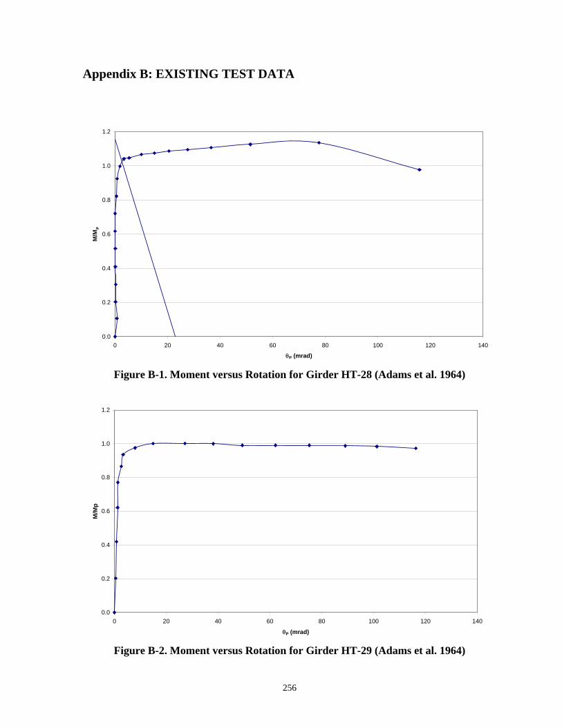
Appendix B: EXISTING TEST DATA

0.0

0.2

0.4

0.6

0.8

1.0

1.2

0 20 40 60 80 100 120

θP (mrad)

M/M

p

140

Figure B-1. Moment versus Rotation for Girder HT-28 (Adams et al. 1964)

0.0

0.2

0.4

0.6

0.8

1.0

1.2

0 20 40 60 80 100 120 140

θP (mrad)

M/M

p


256

0.0

0.2

0.4

0.6

0.8

1.0

1.2

0 10 20 30 40 50 60 70 80 90

qP (mrad)

M/M

p


0.0

0.2

0.4

0.6

0.8

1.0

1.2

0 20 40 60 80 100 120 140 160 180

θP (mrad)

M/M

p


257

0.0

0.1

0.2

0.3

0.4

0.5

0.6

0.7

0.8

0.9

1.0

0 20 40 60 80 100 120

θP (mrad)

M/M

p


0.0

0.2

0.4

0.6

0.8

1.0

1.2

0 20 40 60 80 100 120

qP (mrad)

M/M

p


258

0.0

0.2

0.4

0.6

0.8

1.0

1.2

0 20 40 60 80 100 120 140

θP (mrad)

M/M

p


0.0

0.2

0.4

0.6

0.8

1.0

1.2

0 50 100 150 200 250

θP (mrad)

M/M

p


259

0.0

0.2

0.4

0.6

0.8

1.0

1.2

0 5 10 15 20 25 30

θP (mrad)

M/M

p


0.0

0.2

0.4

0.6

0.8

1.0

1.2

0 10 20 30 40 50 60

θp (mrad)

M/M

p

Figure B-10. Moment versus Rotation for Girder P2 (Barth 1996)

260

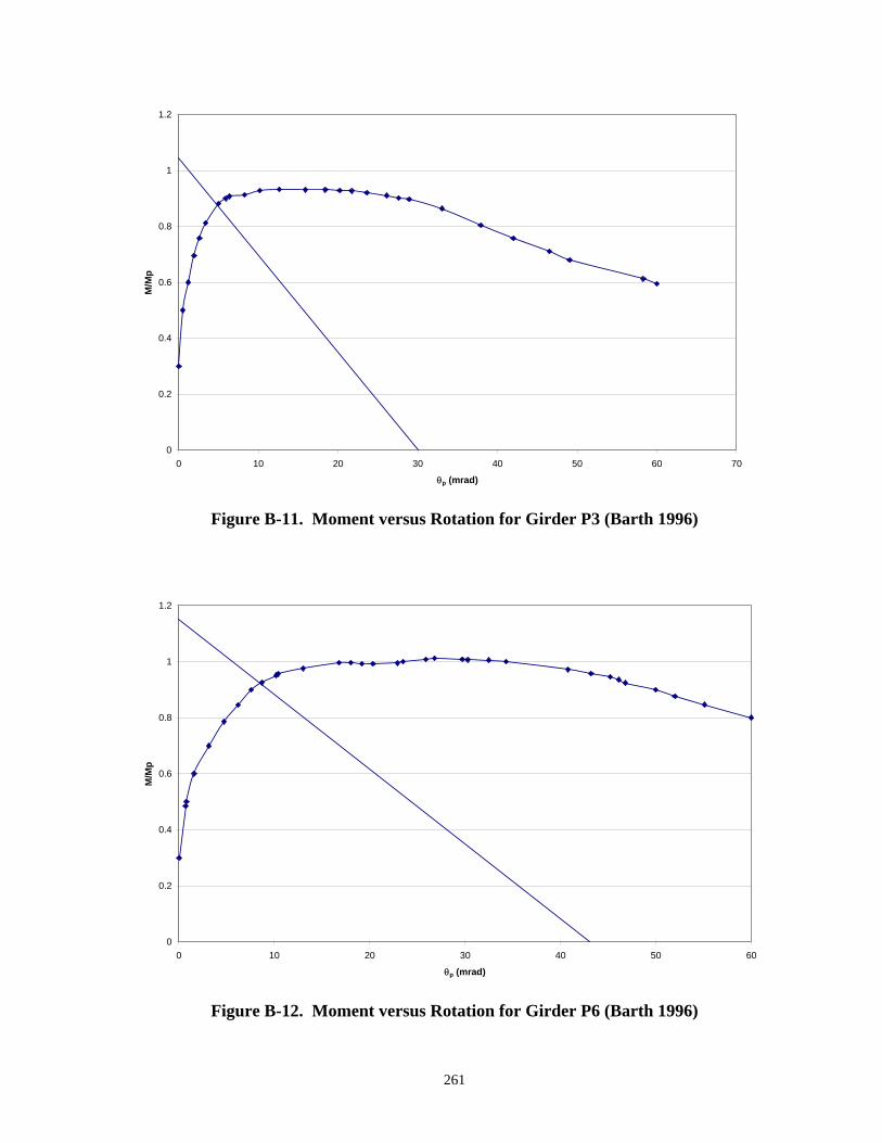
0

0.2

0.4

0.6

0.8

1

1.2

0 10 20 30 40 50 60 70

θp (mrad)

M/M

p


0

0.2

0.4

0.6

0.8

1

1.2

0 10 20 30 40 50 6

θp (mrad)

M/M

p

0


261

0

0.1

0.2

0.3

0.4

0.5

0.6

0.7

0.8

0.9

1

0 20 40 60 80 100 120

θP (mrad)

M/M

p

East

West

Figure B-13. Moment versus Rotation for Girder 188-3-4 Carskaddan (1980)

0

0.2

0.4

0.6

0.8

1

1.2

1.4

0 20 40 60 80 100

θp (mrad)

M/M

p

120

Figure B-14. Moment versus Rotation for Girder HB-40

(Climenhaga and Johnson 1972)

262

0

0.2

0.4

0.6

0.8

1

1.2

0 20 40 60 80 100

θp (mrad)

M/M

p

120

Figure B-15. Moment versus Rotation for Girder HB-41


0.0

0.2

0.4

0.6

0.8

1.0

1.2

0 20 40 60 80 100 120 140

θp (mrad)

M/M

p

Figure B-16. Moment versus Rotation for Girder SB-2 (Climenhaga and Johnson 1972)

263

0.0

0.2

0.4

0.6

0.8

1.0

1.2

1.4

0 20 40 60 80 100 120

θp (mrad)

M/M

p


0.0

0.1

0.2

0.3

0.4

0.5

0.6

0.7

0.8

0.9

1.0

0 20 40 60 80 100 120

θp (mrad)

M/M

p


264

0.0

0.1

0.2

0.3

0.4

0.5

0.6

0.7

0.8

0.9

1.0

0 20 40 60 80 100 120 140

θp (mrad)

M/M

p


0.0

0.2

0.4

0.6

0.8

1.0

1.2

0 20 40 60 80 100 120

θp (mrad)

M/M

p


265

0.0

0.2

0.4

0.6

0.8

1.0

1.2

1.4

0 20 40 60 80 100 120 140

θp (mrad)

M/M

p


0.0

0.2

0.4

0.6

0.8

1.0

1.2

0 10 20 30 40 50 60 70 80 90 100

θp (mrad)

M/M

p

Figure B-22. Moment versus Rotation for Girder SB-10


266

0.0

0.1

0.2

0.3

0.4

0.5

0.6

0.7

0.8

0.9

1.0

0 10 20 30 40 50 60 70 80 9

θp (mrad)

M/M

p

0



0.0

0.2

0.4

0.6

0.8

1.0

1.2

0 5 10 15 20 25 30 35 40 45 50

θp (mrad)

M/M

p



267

0.0

0.2

0.4

0.6

0.8

1.0

1.2

0 20 40 60 80 100 12

θP (mrad)

M/M

p

0

Figure B-25. Moment versus Rotation for Girder 188-3-1

(Grubb and Carskaddan 1979)

0.0

0.2

0.4

0.6

0.8

1.0

1.2

0 20 40 60 80 100 120

θP (mrad)

M/M

p



268

0.0

0.2

0.4

0.6

0.8

1.0

1.2

0 10 20 30 40 50 60 70 80

θP (mrad)

M/M

p



0.0

0.2

0.4

0.6

0.8

1.0

1.2

1.4

0 50 100 150 200 250

θP (mrad)

M/M

p



269

0.0

0.2

0.4

0.6

0.8

1.0

1.2

0 20 40 60 80 100 120 140 160 180

θP (mrad)

M/M

p



0.0

0.2

0.4

0.6

0.8

1.0

1.2

0 20 40 60 80 100 120 140

θP (mrad)

M/M

p



270

0.0

0.2

0.4

0.6

0.8

1.0

1.2

0 20 40 60 80 100 120 140 160

θP (mrad)

M/M

p



0.0

0.2

0.4

0.6

0.8

1.0

1.2

0 10 20 30 40 50 60

θP (mrad)

M/M

p

Figure B-32. Moment versus Rotation for Girder W14x26 (Hartnagel 1997)

271

0.0

0.2

0.4

0.6

0.8

1.0

1.2

0 10 20 30 40 50 60

θP (mrad)

M/M

p

Figure B-33. Moment versus Rotation for Girder WS-1 (Holtz and Kulak 1973)

0.0

0.2

0.4

0.6

0.8

1.0

1.2

0 5 10 15 20 25 30 35 40 45 50

θP (mrad)

M/M

p


272

0.0

0.2

0.4

0.6

0.8

1.0

1.2

0 5 10 15 20 25 30 35

θP (mrad)

M/M

p

Figure B-35. Moment versus Rotation for Girder WS-7-P (Holtz and Kulak 1973)

0.0

0.2

0.4

0.6

0.8

1.0

1.2

0 5 10 15 20 25 30 35

θP (mrad)

M/M

p

Figure B-36. Moment versus Rotation for Girder WS-8-P (Holtz and Kulak 1973)

273

0.0

0.2

0.4

0.6

0.8

1.0

1.2

0 10 20 30 40 50 60

θP (mrad)

M/M

p


0.0

0.2

0.4

0.6

0.8

1.0

1.2

1.4

0 10 20 30 40 50 60 70

θP (mrad)

M/M

p


274

0.0

0.2

0.4

0.6

0.8

1.0

1.2

1.4

0 50 100 150 200 250

θP (mrad)

M/M

p

Figure B-39. Moment versus Rotation for Girder A-1 (Lukey et al. 1969)

0.0

0.2

0.4

0.6

0.8

1.0

1.2

1.4

1.6

0 50 100 150 200 250 300

θP (mrad)

M/M

p

Figure B-40. Moment versus Rotation for Girder A-2 (Lukey et al. 1969)

275

0.0

0.2

0.4

0.6

0.8

1.0

1.2

0 10 20 30 40 50 6

θP (mrad)

M/M

p

0

Figure B-41. Moment versus Rotation for Girder B-1 (Lukey et al. 1969)

0.0

0.2

0.4

0.6

0.8

1.0

1.2

0 20 40 60 80 100 120

θP (mrad)

M/M

p

140


276

0.0

0.2

0.4

0.6

0.8

1.0

1.2

0 20 40 60 80 100 120

θP (mrad)

M/M

p

140


0.0

0.2

0.4

0.6

0.8

1.0

1.2

0 20 40 60 80 100 120 140 160

θP (mrad)

M/M

p


277

0.0

0.2

0.4

0.6

0.8

1.0

1.2

0 20 40 60 80 100 120 140 160

θP (mrad)

M/M

p


0.0

0.2

0.4

0.6

0.8

1.0

1.2

0 10 20 30 40 50 60

θP (mrad)

M/M

p

70

Figure B-46. Moment versus Rotation for Girder C-1 (Lukey et al. 1969)

278

0.0

0.2

0.4

0.6

0.8

1.0

1.2

1.4

0 20 40 60 80 100

θP (mrad)

M/M

p

120


0.0

0.2

0.4

0.6

0.8

1.0

1.2

0 10 20 30 40 50 60 70 80 90 10

θP (mrad)

M/M

p

0


279

0.0

0.2

0.4

0.6

0.8

1.0

1.2

0 10 20 30 40 50 60 70

θP (mrad)

M/M

p

80


0.0

0.2

0.4

0.6

0.8

1.0

1.2

0 20 40 60 80 100

θP (mrad)

M/M

p

120


280

0.0

0.2

0.4

0.6

0.8

1.0

1.2

0 20 40 60 80 100

θP (mrad)

M/M

p

120

Figure B-51. Moment versus Rotation for Girder D-1 (Lukey et al. 1969)

0.0

0.2

0.4

0.6

0.8

1.0

1.2

0 5 10 15 20 25 30 35

θP (mrad)

M/M

p


281

0.0

0.2

0.4

0.6

0.8

1.0

1.2

0 10 20 30 40 50 60

θP (mrad)

M/M

p

70


0.0

0.2

0.4

0.6

0.8

1.0

1.2

1.4

0 20 40 60 80 100 120 140 160

θP (mrad)

M/M

p


282

0.0

0.2

0.4

0.6

0.8

1.0

1.2

1.4

0 20 40 60 80 100

θP (mrad)

M/M

p

120

Figure B-55. Moment versus Rotation for Girder E-1 (Lukey et al. 1969)

0.0

0.2

0.4

0.6

0.8

1.0

1.2

0 10 20 30 40 5

θP (mrad)

M/M

p

0


283

0.0

0.2

0.4

0.6

0.8

1.0

1.2

0 10 20 30 40 50 60 70 80 90 10

θP (mrad)

M/M

p

0


0.0

0.2

0.4

0.6

0.8

1.0

1.2

1.4

0 10 20 30 40 50 60

θP (mrad)

M/M

p

70


284

0.0

0.2

0.4

0.6

0.8

1.0

1.2

0 20 40 60 80 100

θP (mrad)

M/M

p

120

Figure B-59. Moment versus Rotation for Girder SL (Schilling 1985)

0.0

0.2

0.4

0.6

0.8

1.0

1.2

0 20 40 60 80 100 120 140 160

θP (mrad)

M/M

p

Figure B-60. Moment versus Rotation for Girder UL (Schilling 1985)

285

0.0

0.2

0.4

0.6

0.8

1.0

1.2

0 20 40 60 80 100 120

θP (mrad)

M/M

p

Figure B-61. Moment versus Rotation for Girder US (Schilling 1985)

0.0

0.2

0.4

0.6

0.8

1.0

1.2

0 10 20 30 40 50 60 70

θP (mrad)

M/M

p

80

Figure B-62. Moment versus Rotation for Girder D (Schilling and Morcos 1988)

286

0.0

0.2

0.4

0.6

0.8

1.0

1.2

0 10 20 30 40 50 60 70 80

θP (mrad)

M/M

p

90

Figure B-63. Moment versus Rotation for Girder M (Schilling and Morcos 1988)

0.0

0.2

0.4

0.6

0.8

1.0

1.2

0 20 40 60 80 100

θP (mrad)

M/M

p

120

Figure B-64. Moment versus Rotation for Girder S (Schilling and Morcos 1988)

287

0.0

0.1

0.2

0.3

0.4

0.5

0.6

0.7

0.8

0.9

1.0

0 5 10 15 20 25 30

θP (mrad)

M/M

p

Figure B-65. Moment versus Rotation for Tansil Girder (1991)

0.0

0.2

0.4

0.6

0.8

1.0

1.2

0 10 20 30 40 50 60 70 80 90 10

θP (mrad)

M/M

p

0

Figure B-66. Moment versus Rotation for Girder A (Yakel et al. 1999)

288

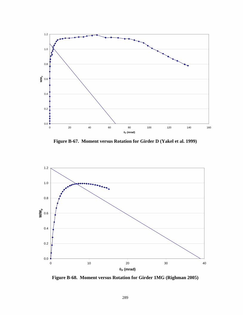
0.0

0.2

0.4

0.6

0.8

1.0

1.2

0 20 40 60 80 100 120 140 160

θP (mrad)

M/M

p

Figure B-67. Moment versus Rotation for Girder D (Yakel et al. 1999)

0.0

0.2

0.4

0.6

0.8

1.0

1.2

0 10 20 30 4

θP (mrad)

M/M

p

0

Figure B-68. Moment versus Rotation for Girder 1MG (Righman 2005)

289

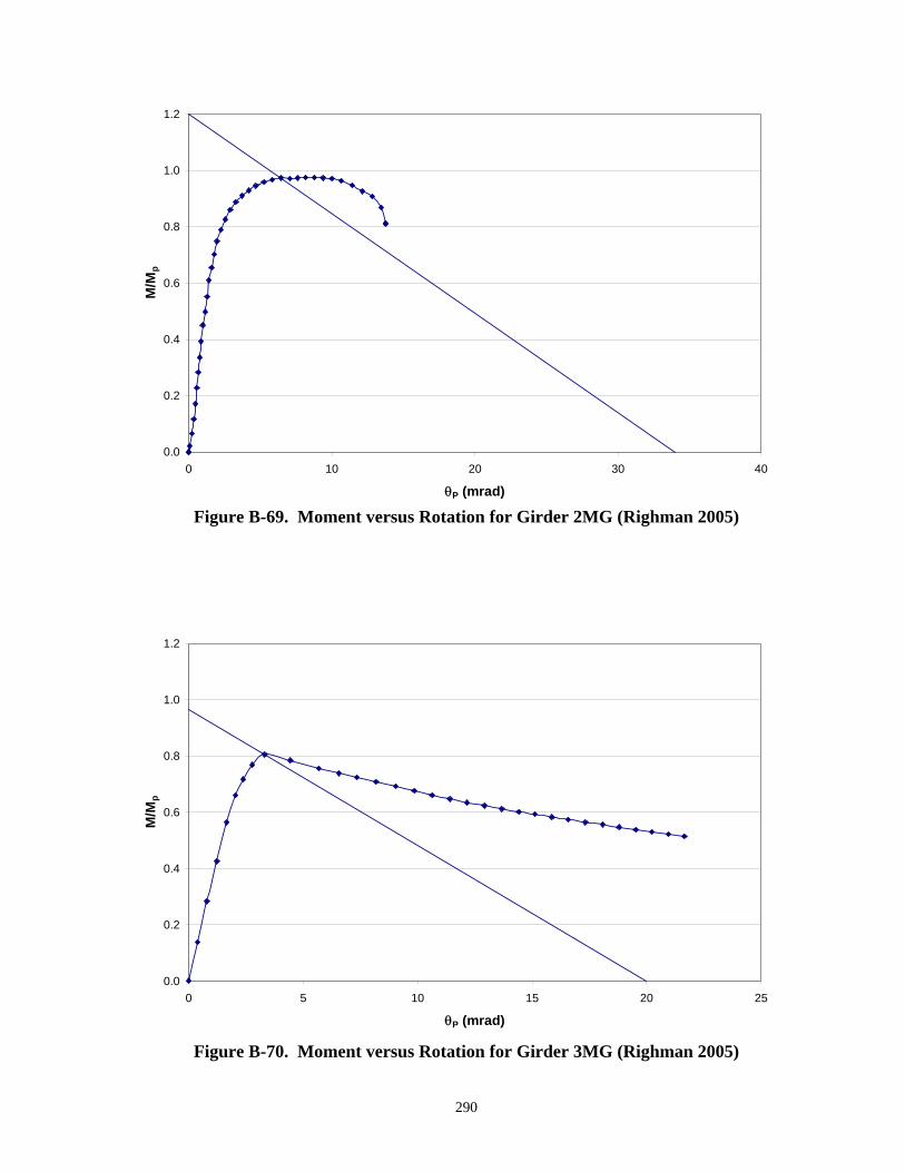
0.0

0.2

0.4

0.6

0.8

1.0

1.2

0 10 20 30 4

θP (mrad)

M/M

p

0


0.0

0.2

0.4

0.6

0.8

1.0

1.2

0 5 10 15 20 25

θP (mrad)

M/M

p


290

0.0

0.2

0.4

0.6

0.8

1.0

1.2

0 10 20 30 4

θP (mrad)

M/M

p

0


0.0

0.2

0.4

0.6

0.8

1.0

1.2

0 10 20 3

θP (mrad)

M/M

p

0


291

0.0

0.2

0.4

0.6

0.8

0 10 20 3

θP (mrad)

M/M

p

0


0.0

0.2

0.4

0.6

0.8

1.0

1.2

0 10 20 30 4

θP (mrad)

M/M

p

0


292

0.0

0.2

0.4

0.6

0.8

1.0

1.2

0 10 20 30 4

θP (mrad)

M/M

p

0


0.0

0.2

0.4

0.6

0.8

1.0

1.2

0 10 20 30 4

θP (mrad)

M/M

p

0


293

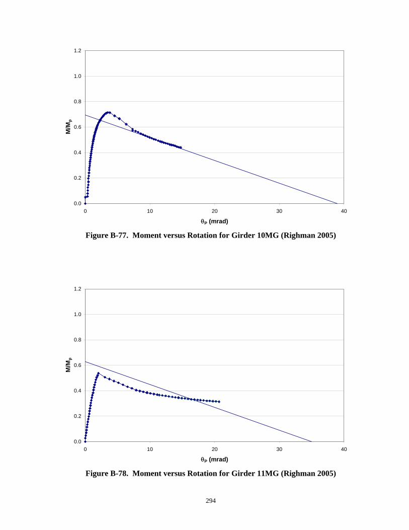
0.0

0.2

0.4

0.6

0.8

1.0

1.2

0 10 20 30 4

θP (mrad)

M/M

p

0


0.0

0.2

0.4

0.6

0.8

1.0

1.2

0 10 20 30 4

θP (mrad)

M/M

p

0


294

0.0

0.2

0.4

0.6

0.8

1.0

1.2

0 10 20 30 4

θP (mrad)

M/M

p

0


295

Appendix C: MATERIAL TESTING RESULTS

The experimental girders analyzed in this work were fabricated from nine different

combinations of plate thicknesses, material properties, and steel heats. A minimum of three

material coupons were taken from each plate of steel and tension tested to obtain material

properties. Tension testing of heats JUN and AUG was performed at West Virginia

University, while testing of heats A and B were commercially tested by Non-Destructive

Testing Group of Aliquippa, PA.

Table C-1 details the specific plates used to fabricate each girder. Each plate is labeled

according to the following naming convention: the first label indicates the plate thickness, the

second label indicates the nominal yield strength of the material, and the last label references

the heat of the material.

The stress versus strain diagrams obtained for each plate type are presented in Figs. C-1

through C-9. These diagrams depict the data resulting from the testing of each coupon with

thin lines and the average of all specimens, which is used in the FEA of the experimental

girders, by a heavy line. The inset in each graph tabulates the specific stress-strain data taken

Specimen Top Flange Bottom Flange Web 1MG 0.5" - 50 KSI - JUN 0.875" - 50KSI - B 0.75" - 50 KSI - JUN2MG 0.5" - 50 KSI - JUN 0.875" - 50KSI - A 0.75" - 50 KSI - JUN3MG 0.5" - 50 KSI - JUN 0.5" - 50 KSI - JUN 0.3125" - 50 KSI - AUG4MG 0.5" - 50 KSI - AUG 0.5" - 50 KSI - AUG 0.3125" - 50 KSI - JUN5MG 0.5" - 50 KSI - JUN 0.75" - 50 KSI - JUN 0.5" - 50 KSI - JUN6MG 0.3125" - 50 KSI - AUG 0.5" - 50 KSI - JUN 0.3125" - 50 KSI - JUN7MG 0.5" - 70 KSI - JUN 0.5" - 70 KSI - JUN 0.3125" - 50 KSI - JUN8MG 0.375" - 70 KSI - JUN 0.5" - 70 KSI - JUN 0.3125" - 50 KSI - JUN9MG 0.5" - 70 KSI - JUN 0.5" - 70 KSI - JUN 0.3125" - 50 KSI - AUG10MG 0.375" - 70 KSI - JUN 0.5" - 70 KSI - JUN 0.3125" - 50 KSI - JUN11MG 0.5" - 70 KSI - JUN 0.5" - 70 KSI - JUN 0.375" - 70 KSI - JUN12MG 0.375" - 70 KSI - JUN 0.5" - 70 KSI - JUN 0.375" - 70 KSI - JUN

Table C-1. Steel Designations for Experimental Girders

296

from the average results that is converted into true stress versus plastic strain and then input

into the ABAQUS analysis.

.3125" - 50ksi - JUN

01000020000300004000050000600007000080000

0 0.1 0.2 0.3 0.4strain (in/in)

stre

ss (p

si)

σ (psi) ε

0 057547 0.0021158048 0.0384260396 0.04562154 0.05563891 0.0765355 0.0966538 0.1466824 0.35

Figure C-1. Tension Test Data for 0.3125” – 50ksi - JUN

.3125" - 50ksi - AUG

01000020000300004000050000600007000080000

0 0.05 0.1 0.15 0.2strain (in/in)

stre

ss (p

si)

σ (psi) ε

0 062650 0.0021162755 0.0410365123 0.0437567500 0.0622169900 0.1016470350 0.1331270691 0.4

Figure C-2. Tension Test Data for 0.3125” – 50ksi - AUG

297

.500" - 50ksi - JUN

0

10000

20000

30000

40000

50000

60000

70000

80000

90000

0 0.1 0.2 0.3 0.4 0.5

strain (in/in)

stre

ss (p

si)

σ (psi) ε0 0.00

64527 0.0065381 0.0268205 0.0370848 0.0374891 0.0480106 0.0682921 0.0884980 0.1285186 0.1585751 0.50

298

Figure C-3. Tension Test Data for 0. 5” – 50ksi - JUN

.500" - 50ksi - AUG

0

10000

20000

30000

40000

50000

60000

70000

80000

90000

0.00 0.10 0.20 0.30 0.40 0.50 0.60strain (in/in)

stre

ss (p

si)

σ (psi) ε0 0.00

66298 0.0066556 0.0268487 0.0274633 0.0378378 0.0481137 0.0583127 0.0685043 0.0886119 0.0987052 0.1387438 0.40

Figure C-4. Tension Test Data for 0.5” – 50ksi - AUG

.750" - 50ksi - JUN

0100002000030000400005000060000700008000090000

100000

0 0.05 0.1 0.15 0.2

strain (in/in)

stre

ss (p

si)

σ (psi) ε0 0.0000

71968 0.002472900 0.025076600 0.031082200 0.048086150 0.072088050 0.100088557 0.130088601 0.1600


0.875" - 50ksi - A

0

10000

20000

30000

40000

50000

60000

70000

0 0.05 0.1 0.15 0.2 0.25 0.3 0.35 0.4

Strain (in/in)

Stre

ss (p

si)

σ (psi) ε0 0.0000

44267 0.001544295 0.020062167 0.100062589 0.3800

Figure C-6. Tension Test Data for 0. 875” – 50ksi - A

299

0.875" - 50ksi- B

0100002000030000400005000060000700008000090000

0.00 0.05 0.10 0.15 0.20 0.25 0.30 0.35

strain

Stre

ss (p

si)

σ (psi) ε0 0.0000

56000 0.001956053 0.006956193 0.020075000 0.100077960 0.3000

Figure C-7. Tension Test Data for 0. 875” – 50ksi - B

.375" - 70 ksi - JUN

0

20000

40000

60000

80000

100000

120000

0 0.1 0.2 0.3 0.4 0.5strain (in/in)

stre

ss (p

si)

σ (psi) ε0 0.000

95101 0.00396613 0.034

101567 0.062102740 0.088103208 0.400


300

.500" - 70ksi - JUN

0

20000

40000

60000

80000

100000

120000

0 0.05 0.1 0.15 0.2 0.25

strain (in/in)

stre

ss (p

si)

σ (psi) ε0 0.000

91207 0.00392026 0.02497346 0.05099044 0.08399220 0.200


301

Appendix D: FEA MOMENT-ROTATION CURVES

0.0

0.2

0.4

0.6

0.8

1.0

1.2

0 5 10 15 20 25 30 35 40 45


M/M

n

FEA

AASHTO Model

New Model

Figure D-1. Moment versus Rotation for Girder CF-1-65-4-50

0.0

0.2

0.4

0.6

0.8

1.0

1.2

0 5 10 15 20 25 30 35 40 45


M/M

n

FEA

AASHTO Model

New Model


302

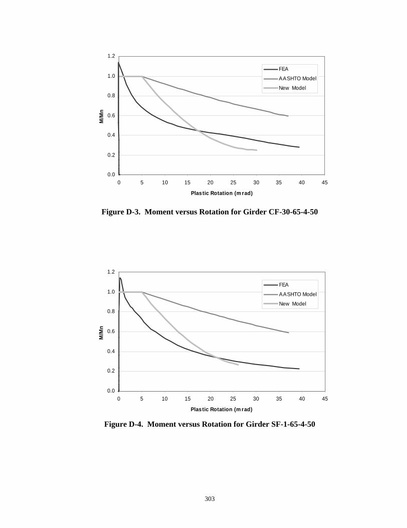
0.0

0.2

0.4

0.6

0.8

1.0

1.2

0 5 10 15 20 25 30 35 40 45


M/M

n

FEA

AASHTO Model

New Model


0.0

0.2

0.4

0.6

0.8

1.0

1.2

0 5 10 15 20 25 30 35 40 45


M/M

n

FEA

AASHTO Model

New Model

Figure D-4. Moment versus Rotation for Girder SF-1-65-4-50

303

0.0

0.2

0.4

0.6

0.8

1.0

1.2

0 5 10 15 20 25 30 35 40 45


M/M

n

FEA

AASHTO Model

New Model


0.0

0.2

0.4

0.6

0.8

1.0

1.2

0 5 10 15 20 25 30 35 40 45


M/M

n

FEA

AASHTO Model

New Model


304

0.0

0.2

0.4

0.6

0.8

1.0

1.2

1.4

0 5 10 15 20 25 30 35 40


M/M

n

FEA

AASHTO Model

New Model


0.0

0.2

0.4

0.6

0.8

1.0

1.2

1.4

0 10 20 30 40 50 60 7


M/M

n

0

FEA

AASHTO Model

New Model


305

0.0

0.2

0.4

0.6

0.8

1.0

1.2

1.4

0 5 10 15 20 25 30 35 40


M/M

n

FEA

AASHTO Model

New Model


0.0

0.2

0.4

0.6

0.8

1.0

1.2

0 5 10 15 20 25 30 35 40 45


M/M

n

FEA

AASHTO Model

New Model

Figure D-10. Moment versus Rotation for Girder CF-1-65-4-H

306

0.0

0.2

0.4

0.6

0.8

1.0

1.2

0 5 10 15 20 25 30 35 40 45


M/M

n

FEA

AASHTO Model

New Model


0.0

0.2

0.4

0.6

0.8

1.0

1.2

1.4

0 5 10 15 20 25 30 35 40 45


M/M

n

FEA

AASHTO Model

New Model


307

0.0

0.2

0.4

0.6

0.8

1.0

1.2

1.4

0 5 10 15 20 25 30 35 40


M/M

n

FEA

AASHTO Model

New Model

Figure D-13. Moment versus Rotation for Girder SF-1-65-4-H

0.0

0.2

0.4

0.6

0.8

1.0

1.2

1.4

0 5 10 15 20 25 30 35 40 45


M/M

n

FEA

AASHTO Model

New Model


308

0.0

0.2

0.4

0.6

0.8

1.0

1.2

1.4

0 5 10 15 20 25 30 35 40 45


M/M

n

FEA

AASHTO Model

New Model


0.0

0.2

0.4

0.6

0.8

1.0

1.2

0 5 10 15 20 25 30 35 40 45


M/M

n

FEA

AASHTO Model

New Model

Figure D-16. Moment versus Rotation for Girder CF-0.5-65-3-H

309

0.0

0.2

0.4

0.6

0.8

1.0

1.2

0 5 10 15 20 25 30 35 40 45


M/M

n

FEA

AASHTO Model

New Model


0.0

0.2

0.4

0.6

0.8

1.0

1.2

0 5 10 15 20 25 30 35 40 45


M/M

n

FEA

AASHTO Model

New Model

Figure D-18. Moment versus Rotation for Girder CF-1.65-65-3-H

310

0.0

0.2

0.4

0.6

0.8

1.0

1.2

0 5 10 15 20 25 30 35 40 45


M/M

n

FEA

AASHTO Model

New Model


0.0

0.2

0.4

0.6

0.8

1.0

1.2

1.4

0 5 10 15 20 25 30 35 40


M/M

n

FEA

AASHTO Model

New Model

Figure D-20. Moment versus Rotation for Girder SF-1.75-65-3-H

311

0.0

0.2

0.4

0.6

0.8

1.0

1.2

1.4

0 5 10 15 20 25 30 35 40


M/M

n

FEA

AASHTO Model

New Model


0.0

0.2

0.4

0.6

0.8

1.0

1.2

0 5 10 15 20 25 30 35 40


M/M

n

FEA

AASHTO Model

New Model


312

0.0

0.2

0.4

0.6

0.8

1.0

1.2

0 5 10 15 20 25 30 35 40 45


M/M

n

FEA

AASHTO Model

New Model


0.0

0.2

0.4

0.6

0.8

1.0

1.2

0 5 10 15 20 25 30 35 40 45


M/M

n

FEA

AASHTO Model

New Model


313

0.0

0.2

0.4

0.6

0.8

1.0

1.2

1.4

0 5 10 15 20 25 30 35 40


M/M

n

FEA

AASHTO Model

New Model


0.0

0.2

0.4

0.6

0.8

1.0

1.2

1.4

0 5 10 15 20 25 30 35 40


M/M

n

FEA

AASHTO Model

New Model


314

0.0

0.2

0.4

0.6

0.8

1.0

1.2

0 5 10 15 20 25 30 35 40 45


M/M

n

FEA

AASHTO Model

New Model


0.0

0.2

0.4

0.6

0.8

1.0

1.2

0 5 10 15 20 25 30 35 40


M/M

n

FEA

AASHTO Model

New Model


315

0.0

0.2

0.4

0.6

0.8

1.0

1.2

0 5 10 15 20 25 30 35 40 45


M/M

n

FEA

AASHTO Model

New Model


0.0

0.2

0.4

0.6

0.8

1.0

1.2

1.4

0 5 10 15 20 25 30 35 40


M/M

n

FEA

AASHTO Model

New Model


316

0.0

0.2

0.4

0.6

0.8

1.0

1.2

0 5 10 15 20 25 30 35 40


M/M

n

FEA

AASHTO Model

New Model


0.0

0.2

0.4

0.6

0.8

1.0

1.2

1.4

0 5 10 15 20 25 30 35 40 45


M/M

n

FEA

AASHTO Model

New Model


317

0.0

0.2

0.4

0.6

0.8

1.0

1.2

0 20 40 60 80 100 120 140


M/M

n

FEA

AASHTO Model

New Model

Figure D-33. Moment versus Rotation for Girder 90-2-50-10-A

0.0

0.2

0.4

0.6

0.8

1.0

1.2

0 20 40


M/M

n

60

FEA

AASHTO Model

New Model

Figure D-34. Moment versus Rotation for Girder 90-2-E-50-20-B

318

0.0

0.2

0.4

0.6

0.8

1.0

1.2

1.4

1.6

0 10 20 30 40 50 60


M/M

n

FEA

AASHTO Model

New Model

Figure D-35. Moment versus Rotation for Girder 120-2-E-50-10-A

0.0

0.2

0.4

0.6

0.8

1.0

1.2

1.4

1.6

0 10 20 30 40 50 60


M/M

n

FEA

AASHTO Model

New Model


319

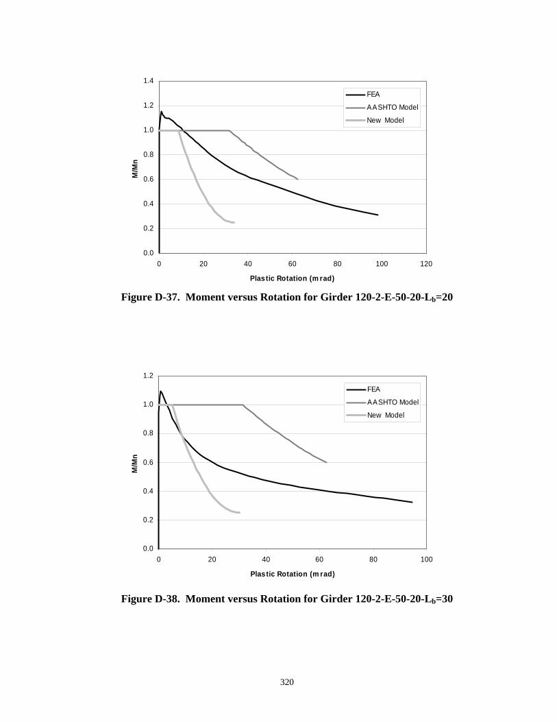
0.0

0.2

0.4

0.6

0.8

1.0

1.2

1.4

0 20 40 60 80 100 120


M/M

n

FEA

AASHTO Model

New Model

Figure D-37. Moment versus Rotation for Girder 120-2-E-50-20-Lb=20

0.0

0.2

0.4

0.6

0.8

1.0

1.2

0 20 40 60 80 100


M/M

n

FEA

AASHTO Model

New Model

Figure D-38. Moment versus Rotation for Girder 120-2-E-50-20-Lb=30

320

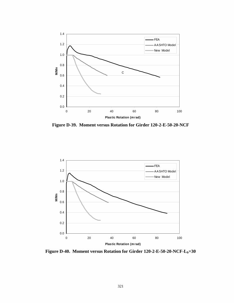
0.0

0.2

0.4

0.6

0.8

1.0

1.2

1.4

0 20 40 60 80 100


M/M

n

FEA

AASHTO Model

New Model

C

Figure D-39. Moment versus Rotation for Girder 120-2-E-50-20-NCF

0.0

0.2

0.4

0.6

0.8

1.0

1.2

1.4

0 20 40 60 80 100


M/M

n

FEA

AASHTO Model

New Model

Figure D-40. Moment versus Rotation for Girder 120-2-E-50-20-NCF-Lb=30

321

0.0

0.2

0.4

0.6

0.8

1.0

1.2

1.4

1.6

0 10 20 30 40 50 60 70 80 90


M/M

n

FEA

AASHTO Model

New Model

Figure D-41. Moment versus Rotation for Girder 120-2-E-50-UF(30)-E

0.0

0.2

0.4

0.6

0.8

1.0

1.2

1.4

1.6

0 10 20 30 40 50 60 70 80 90


M/M

n

FEA

AASHTO Model

New Model

Figure D-42. Moment versus Rotation for Girder 120-2-E-50-U(30)-E

322

0.0

0.2

0.4

0.6

0.8

1.0

1.2

1.4

1.6

0 10 20 30 40 50 60 70 80 90


M/M

n

FEA

AASHTO Model

New Model

Figure D-43. Moment versus Rotation for Girder 120-2-H-10-A

0.0

0.2

0.4

0.6

0.8

1.0

1.2

1.4

0 10 20 30 40 50 60 70 80 90


M/M

n

FEA

AASHTO Model

New Model

Figure D-44. Moment versus Rotation for Girder 120-2-H-10-B

323

0.0

0.2

0.4

0.6

0.8

1.0

1.2

1.4

1.6

0 20 40 60 80 100


M/M

n

FEA

AASHTO Model

New Model

Figure D-45. Moment versus Rotation for Girder 120-2-E-H-10-B(S)

0.0

0.2

0.4

0.6

0.8

1.0

1.2

1.4

0 20 40 60 80 100


M/M

n

FEA

AASHTO Model

New Model

Figure D-46. Moment versus Rotation for Girder 120-2-H-10-B(S)-16

324

0.0

0.2

0.4

0.6

0.8

1.0

1.2

1.4

0 20 40 60 80 100


M/M

n

FEA

AASHTO Model

New Model


0.0

0.2

0.4

0.6

0.8

1.0

1.2

1.4

0 20 40 60 80 100


M/M

n

FEA

AASHTO Model

New Model


325

0.0

0.2

0.4

0.6

0.8

1.0

1.2

1.4

0 20 40 60 80 100


M/M

n

FEA

AASHTO Model

New Model

Figure D-49. Moment versus Rotation for Girder 120-2-H-10-B(S)-NCF

0.0

0.2

0.4

0.6

0.8

1.0

1.2

1.4

0 20 40 60 80 100


M/M

n

FEA

AASHTO Model

New Model

Figure D-50. Moment versus Rotation for Girder 120-2-H-10-B(S)-NCF-30

326

0.0

0.2

0.4

0.6

0.8

1.0

1.2

1.4

1.6

0 10 20 30 40 50 60


M/M

n

FEA

AASHTO Model

New Model

Figure D-51. Moment versus Rotation for Girder 120-2-H-20-A

0.0

0.2

0.4

0.6

0.8

1.0

1.2

1.4

1.6

0 20 40 60


M/M

n

80

FEA

AASHTO Model

New Model

Figure D-52. Moment versus Rotation for Girder 120-2-H-20-A(S)

327

0.0

0.2

0.4

0.6

0.8

1.0

1.2

1.4

0 10 20 30 40 50 60


M/M

n

FEA

AASHTO Model

New Model


0.0

0.2

0.4

0.6

0.8

1.0

1.2

1.4

0 10 20 30 40 50 60 70 80 90


M/M

n

FEA

AASHTO Model

New Model

Figure D-54. Moment versus Rotation for Girder 150-2-50-20-C

328

0.0

0.2

0.4

0.6

0.8

1.0

1.2

1.4

0 20 40 60 8


M/M

n

0

FEA

AASHTO Model

New Model


0.0

0.2

0.4

0.6

0.8

1.0

1.2

0 20 40 60 8


M/M

n

0

FEA

AASHTO Model

New Model


329

0.0

0.2

0.4

0.6

0.8

1.0

1.2

1.4

0 20 40 60 8


M/M

n

0

FEA

AASHTO Model

New Model


0.0

0.2

0.4

0.6

0.8

1.0

1.2

0 20 40


M/M

n

60

FEA

AASHTO Model

New Model

Figure D-58. Moment versus Rotation for Girder 180-2-E-50-20-22.5

330

0.0

0.2

0.4

0.6

0.8

1.0

1.2

0 20 40 60 8


M/M

n

0

FEA

AASHTO Model

New Model

Figure D-59. Moment versus Rotation for Girder 180-2-E-50-20-30

0.0

0.2

0.4

0.6

0.8

1.0

1.2

0 20 40


M/M

n

60

FEA

AASHTO Model

New Model


331

0.0

0.2

0.4

0.6

0.8

1.0

1.2

1.4

0 20 40


M/M

n

60

FEA

AASHTO Model

New Model

Figure D-61. Moment versus Rotation for Girder 180-2-E-50-20-NCF-Lb=30

0.0

0.2

0.4

0.6

0.8

1.0

1.2

0 20 40 6


M/M

n

0

FEA

AASHTO Model

New Model

Figure D-62. Moment versus Rotation for Girder 210-2-E-50-10-E

332

0.0

0.2

0.4

0.6

0.8

1.0

1.2

0 20 40


M/M

n

60

FEA

AASHTO Model

New Model

Figure D-63. Moment versus Rotation for Girder 210-2-E-50-10- Lb=18

0.0

0.2

0.4

0.6

0.8

1.0

1.2

0 20 40


M/M

n

60

FEA

AASHTO Model

New Model

Figure D-64. Moment versus Rotation for Girder 210-2-E-50-10- Lb=26.25

333

0.0

0.2

0.4

0.6

0.8

1.0

1.2

0 20 40


M/M

n

60

FEA

AASHTO Model

New Model

Figure D-65. Moment versus Rotation for Girder 210-2-E-50-10- Lb=30

0.0

0.2

0.4

0.6

0.8

1.0

1.2

1.4

0 20 40


M/M

n

60

FEA

AASHTO Model

New Model


334

0.0

0.2

0.4

0.6

0.8

1.0

1.2

1.4

0 20 40


M/M

n

60

FEA

AASHTO Model

New Model

Figure D-67. Moment versus Rotation for Girder 210-2-E-50-10-NCF- Lb=30

0.0

0.2

0.4

0.6

0.8

1.0

1.2

0 20 40 6


M/M

n

0

FEA

AASHTO Model

New Model

Figure D-68. Moment versus Rotation for Girder 210-2-E-50-20-F

335

0.0

0.2

0.4

0.6

0.8

1.0

1.2

0 20 40


M/M

n

60

FEA

AASHTO Model

New Model


0.0

0.2

0.4

0.6

0.8

1.0

1.2

1.4

0 20 40


M/M

n

60

FEA

AASHTO Model

New Model

Figure D-70. Moment versus Rotation for Girder 210-2-E-50-40-C

336

0.0

0.2

0.4

0.6

0.8

1.0

1.2

1.4

1.6

0 20 40 60 80 100


M/M

n

FEA

AASHTO Model

New Model

Figure D-71. Moment versus Rotation for Girder 140-175-140-H-20-D

337

Appendix E: EXAMPLE DESIGNS

N

umbe

r of S

pans

(1-5

):2

Gird

er S

paci

ng12

0N

umbe

r of G

irder

s4

Spa

n 1

90O

verh

ang

Wid

th42

Spa

n 2

90St

ruct

ural

Sla

b Th

ickn

ess

8To

tal S

lab

Thic

knes

s8.

5H

aunc

h2

Top

Rei

nfor

cem

ent C

over

2Bo

ttom

Rei

nfor

cem

ent C

over

1R

oadw

ay W

idth

408

Span

L b1 (

ft)N

umbe

r of C

ross

- fra

mes

sp

aced

at L

b1L b

2 (ft)

Num

ber o

f Cro

ss-fr

ames

sp

aced

at L

b2L b

3 (ft)

Num

ber o

f Cro

ss-fr

ames

spa

ced

at L

b3

120

410

12

101

204

Span

Sect

ions

Cro

ss-S

ectio

nC

ross

-Sec

tion

Leng

th (f

t)bf

-top

flang

etf-

top

flang

ebf

-bot

tom

flan

getf-

botto

m fl

ange

Dtw

Fy to

pFy

bot

tom

Fy w

ebA

6314

0.75

161.

2544

0.43

7550

5050

B27

141.

2516

1.25

440.

550

5050

A27

141.

2516

1.25

440.

550

5050

B63

140.

7516

1.25

440.

4375

5050

5021

2

Cro

ss-S

ectio

n G

eom

etry

and

Ste

el P

rope

rtie

s

Long

itudi

nal B

ridge

Geo

met

ryTr

ansv

erse

Brid

ge G

eom

etry

(in)

Span

Len

gths

(ft)

Late

ral B

raci

ng G

eom

etry

2

Num

ber o

f Spa

ns (1

-5):

2G

irder

Spa

cing

120

Num

ber o

f Gird

ers

4Sp

an 1

90O

verh

ang

Wid

th42

Span

290

Stru

ctur

al S

lab

Thic

knes

s8

Tota

l Sla

b Th

ickn

ess

8.5

Hau

nch

2To

p R

einf

orce

men

t Cov

er2

Bot

tom

Rei

nfor

cem

ent C

over

1R

oadw

ay W

idth

408

Span

L b1 (

ft)N

umbe

r of C

ross

- fra

mes

sp

aced

at L

b1L b

2 (ft)

Num

ber o

f Cro

ss-fr

ames

sp

aced

at L

b2L b

3 (ft)

Num

ber o

f Cro

ss-fr

ames

spa

ced

at L

b3

120

410

12

101

204

Span

Sect

ions

Cro

ss-S

ectio

nC

ross

-Sec

tion

Leng

th (f

t)bf

-top

flang

etf-

top

flang

ebf

-bot

tom

flan

getf-

botto

m fl

ange

Dtw

Fy to

pFy

bot

tom

Fy w

ebA

6314

0.75

161.

2544

0.43

7550

5050

B27

140.

875

161.

2544

0.5

5050

50

A27

140.

875

161.

2544

0.5

5050

50B

6314

0.75

161.

2544

0.43

7550

5050

21

2

Cro

ss-S

ectio

n G

eom

etry

and

Ste

el P

rope

rtie

s

Long

itudi

nal B

ridge

Geo

met

ryTr

ansv

erse

Brid

ge G

eom

etry

(in)

Span

Len

gths

(ft)

Late

ral B

raci

ng G

eom

etry

2

Tab

le E

-1.

Gir

der

Des

ign

90-2

-E-5

0-10

-A

Tab

le E

-2.

Gir

der

Des

ign

90-2

-E-5

0-20

-B

338

Tab

le E

-3.

Gir

der

Des

ign

120-

2-E

-50-

10-A

Num

ber o

f Spa

ns (1

-5):

2G

irder

Spa

cing

120

Num

ber o

f Gird

ers

4Sp

an 1

120

Ove

rhan

g W

idth

42Sp

an 2

120

Stru

ctur

al S

lab

Thic

knes

s8

Tota

l Sla

b Th

ickn

ess

8.5

Hau

nch

2To

p R

einf

orce

men

t Cov

er2

Bot

tom

Rei

nfor

cem

ent C

over

1R

oadw

ay W

idth

408

Span

L b1 (

ft)N

umbe

r of C

ross

- fra

mes

sp

aced

at L

b1L b

2 (ft)

Num

ber o

f Cro

ss-fr

ames

sp

aced

at L

b2L b

3 (ft)

Num

ber o

f Cro

ss-fr

ames

spa

ced

at L

b3

125

410

22

102

254

Span

Sect

ions

Cro

ss-S

ectio

nC

ross

-Sec

tion

Leng

th (f

t)bf

-top

flang

etf-

top

flang

ebf

-bot

tom

flan

getf-

botto

m fl

ange

Dtw

Fy to

pFy

bot

tom

Fy w

ebA

8416

0.75

161.

625

520.

550

5050

B36

161.

625

162

520.

5625

5050

50

A36

161.

625

162

520.

5625

5050

50B

8416

0.75

161.

625

520.

550

5050

21

2

Cro

ss-S

ectio

n G

eom

etry

and

Ste

el P

rope

rtie

s

Long

itudi

nal B

ridge

Geo

met

ryTr

ansv

erse

Brid

ge G

eom

etry

(in)

Span

Len

gths

(ft)

Late

ral B

raci

ng G

eom

etry

2

Num

ber o

f Spa

ns (1

-5):

2G

irder

Spa

cing

120

Num

ber o

f Gird

ers

4Sp

an 1

120

Ove

rhan

g W

idth

42Sp

an 2

120

Stru

ctur

al S

lab

Thic

knes

s8

Tota

l Sla

b Th

ickn

ess

8.5

Hau

nch

2To

p R

einf

orce

men

t Cov

er2

Bot

tom

Rei

nfor

cem

ent C

over

1R

oadw

ay W

idth

408

Span

L b1 (

ft)N

umbe

r of C

ross

- fra

mes

sp

aced

at L

b1L b

2 (ft)

Num

ber o

f Cro

ss-fr

ames

sp

aced

at L

b2L b

3 (ft)

Num

ber o

f Cro

ss-fr

ames

spa

ced

at L

b3

125

410

22

102

254

Span

Sect

ions

Cro

ss-S

ectio

nC

ross

-Sec

tion

Leng

th (f

t)bf

-top

flang

etf-

top

flang

ebf

-bot

tom

flan

getf-

botto

m fl

ange

Dtw

Fy to

pFy

bot

tom

Fy w

ebA

8416

0.75

161.

625

520.

550

5050

B36

161.

375

161.

625

520.

5625

5050

50

A36

161.

375

161.

625

520.

5625

5050

50B

8416

0.75

161.

625

520.

550

5050

21

2

Cro

ss-S

ectio

n G

eom

etry

and

Ste

el P

rope

rtie

s

Long

itudi

nal B

ridge

Geo

met

ryTr

ansv

erse

Brid

ge G

eom

etry

(in)

Span

Len

gths

(ft)

Late

ral B

raci

ng G

eom

etry

2

Tab

le E

-4.

Gir

der

Des

ign

120-

2-E

-50-

20-A

339

Tab

le E

-5.

Gir

der

Des

ign

120-

2-E

-50-

20-N

CF

Num

ber o

f Spa

ns (1

-5):

2G

irder

Spa

cing

120

Num

ber o

f Gird

ers

4Sp

an 1

120

Ove

rhan

g W

idth

42Sp

an 2

120

Stru

ctur

al S

lab

Thic

knes

s8

Tota

l Sla

b Th

ickn

ess

8.5

Hau

nch

2

geD

twFy

top

Fy b

otto

mFy

web

1.25

520.

550

5050

520.

5625

5050

50

520.

5625

5050

501.

2552

0.5

5050

50

Long

itudi

nal B

ridge

Geo

met

ryTr

ansv

erse

Brid

ge G

eom

etry

(in)

Span

Len

gths

(ft)

Top

Rei

nfor

cem

ent C

over

2B

otto

m R

einf

orce

men

t Cov

er1

Roa

dway

Wid

th40

8

Span

L b1 (

ft)N

umbe

r of C

ross

- fra

mes

sp

aced

at L

b1L b

2 (ft)

Num

ber o

f Cro

ss-fr

ames

sp

aced

at L

b2L b

3 (ft)

Num

ber o

f Cro

ss-fr

ames

spa

ced

at L

b3

125

410

22

102

254

Span

Sect

ions

Cro

ss-S

ectio

nC

ross

-Sec

tion

Leng

th (f

t)bf

-top

flang

etf-

top

flang

ebf

-bot

tom

flan

getf-

botto

m fl

anA

8416

0.75

22B

3618

130

1.25

A36

181

301.

25B

8416

0.75

2221

2

Cro

ss-S

ectio

n G

eom

etry

and

Ste

el P

rope

rtie

s

Late

ral B

raci

ng G

eom

etry

2

Num

ber o

f Spa

ns (1

-5):

2G

irder

Spa

cing

120

Num

ber o

f Gird

ers

4Sp

an 1

120

Ove

rhan

g W

idth

42Sp

an 2

120

Stru

ctur

al S

lab

Thic

knes

s8

Tota

l Sla

b Th

ickn

ess

8.5

Hau

nch

2To

p R

einf

orce

men

t Cov

er2

Bot

tom

Rei

nfor

cem

ent C

over

1R

oadw

ay W

idth

408

Span

L b1 (

ft)N

umbe

r of C

ross

- fra

mes

sp

aced

at L

b1L b

2 (ft)

Num

ber o

f Cro

ss-fr

ames

sp

aced

at L

b2L b

3 (ft)

Num

ber o

f Cro

ss-fr

ames

spa

ced

at L

b3

120

62

206

Span

Sect

ions

Cro

ss-S

ectio

nC

ross

-Sec

tion

Leng

th (f

t)bf

-top

flang

etf-

top

flang

ebf

-bot

tom

flan

getf-

botto

m fl

ange

Dtw

Fy to

pFy

bot

tom

Fy w

ebA

8416

0.75

161.

625

520.

550

5050

B36

161.

375

161.

625

520.

5625

5050

50

A36

161.

375

161.

625

520.

5625

5050

50B

8416

0.75

161.

625

520.

550

5050

21

2

Cro

ss-S

ectio

n G

eom

etry

and

Ste

el P

rope

rtie

s

Long

itudi

nal B

ridge

Geo

met

ryTr

ansv

erse

Brid

ge G

eom

etry

(in)

Span

Len

gths

(ft)

Late

ral B

raci

ng G

eom

etry

2

Tab

le E

-6.

Gir

der

Des

ign

120-

2-E

-50-

20-L

b=20

340

341

Tab

le E

-7.

Gir

der

Des

ign

120-

2-E

-50-

20-L

b=30

Num

ber o

f Spa

ns (1

-5):

2G

irder

Spa

cing

120

Num

ber o

f Gird

ers

4Sp

an 1

120

Ove

rhan

g W

idth

42Sp

an 2

120

Stru

ctur

al S

lab

Thic

knes

s8

Tota

l Sla

b Th

ickn

ess

8.5

Hau

nch

2To

p R

einf

orce

men

t Cov

er2

Botto

m R

einf

orce

men

t Cov

er1

Roa

dway

Wid

th40

8

Span

L b1 (

ft)N

umbe

r of C

ross

- fra

mes

sp

aced

at L

b1L b

2 (ft)

Num

ber o

f Cro

ss-fr

ames

sp

aced

at L

b2L b

3 (ft)

Num

ber o

f Cro

ss-fr

ames

spa

ced

at L

b3

130

42

304

Span

Sect

ions

Cro

ss-S

ectio

nC

ross

-Sec

tion

Leng

th (f

t)bf

-top

flang

etf-

top

flang

ebf

-bot

tom

flan

getf-

botto

m fl

ange

Dtw

Fy to

pFy

bot

tom

Fy w

ebA

8416

116

1.62

552

0.5

5050

50B

3616

1.37

516

1.62

552

0.56

2550

5050

A36

161.

375

161.

625

520.

5625

5050

50B

8416

116

1.62

552

0.5

5050

5021

2

Cro

ss-S

ectio

n G

eom

etry

and

Ste

el P

rope

rtie

s

Long

itudi

nal B

ridge

Geo

met

ryTr

ansv

erse

Brid

ge G

eom

etry

(in)

Span

Len

gths

(ft)

Late

ral B

raci

ng G

eom

etry

2

Num

ber o

f Spa

ns (1

-5):

2G

irder

Spa

cing

120

Num

ber o

f Gird

ers

4Sp

an 1

120

Ove

rhan

g W

idth

42Sp

an 2

120

Stru

ctur

al S

lab

Thic

knes

s8

Tota

l Sla

b Th

ickn

ess

8.5

Hau

nch

2To

p R

einf

orce

men

t Cov

er2

Bot

tom

Rei

nfor

cem

ent C

over

1R

oadw

ay W

idth

408

Span

L b1 (

ft)N

umbe

r of C

ross

- fra

mes

sp

aced

at L

b1L b

2 (ft)

Num

ber o

f Cro

ss-fr

ames

sp

aced

at L

b2L b

3 (ft)

Num

ber o

f Cro

ss-fr

ames

spa

ced

at L

b3

130

42

304

Span

Sect

ions

Cro

ss-S

ectio

nC

ross

-Sec

tion

Leng

th (f

t)bf

-top

flang

etf-

top

flang

ebf

-bot

tom

flan

getf-

botto

m fl

ange

Dtw

Fy to

pFy

bot

tom

Fy w

ebA

8416

122

1.25

520.

550

5050

B36

181

301.

2552

0.56

2550

5050

A36

181

301.

2552

0.56

2550

5050

B84

161

221.

2552

0.5

5050

5021

2

Cro

ss-S

ectio

n G

eom

etry

and

Ste

el P

rope

rtie

s

Long

itudi

nal B

ridge

Geo

met

ryTr

ansv

erse

Brid

ge G

eom

etry

(in)

Span

Len

gths

(ft)

Late

ral B

raci

ng G

eom

etry

2

Tab

le E

-8.

Gir

der

Des

ign

120-

2-E

-50-

20-L

b=30

-NC

F

342

Num

ber o

f Spa

ns (1

-5):

2G

irder

Spa

cing

120

Num

ber o

f Gird

ers

4Sp

an 1

120

Ove

rhan

g W

idth

42Sp

an 2

120

Stru

ctur

al S

lab

Thic

knes

s8

Tota

l Sla

b Th

ickn

ess

8.5

Hau

nch

2To

p R

einf

orce

men

t Cov

er2

Bot

tom

Rei

nfor

cem

ent C

over

1R

oadw

ay W

idth

408

Span

L b1 (

ft)N

umbe

r of C

ross

- fra

mes

sp

aced

at L

b1L b

2 (ft)

Num

ber o

f Cro

ss-fr

ames

sp

aced

at L

b2L b

3 (ft)

Num

ber o

f Cro

ss-fr

ames

spa

ced

at L

b3

125

410

22

264

161

Span

Sect

ions

Cro

ss-S

ectio

nC

ross

-Sec

tion

Leng

th (f

t)bf

-top

flang

etf-

top

flang

ebf

-bot

tom

flan

getf-

botto

m fl

ange

Dtw

Fy to

pFy

bot

tom

Fy w

ebA

8416

0.75

161.

625

520.

5625

5050

50B

3616

0.75

161.

625

520.

5625

5050

50

A36

160.

7516

1.62

552

0.56

2550

5050

B84

160.

7516

1.62

552

0.56

2550

5050

21

2

Cro

ss-S

ectio

n G

eom

etry

and

Ste

el P

rope

rtie

s

Long

itudi

nal B

ridge

Geo

met

ryTr

ansv

erse

Brid

ge G

eom

etry

(in)

Span

Len

gths

(ft)

Late

ral B

raci

ng G

eom

etry

2

Long

itudi

nal B

ridge

Geo

met

ryTr

ansv

erse

Brid

ge G

eom

etry

(in)

Num

ber o

f Spa

ns (1

-5):

2G

irder

Spa

cing

120

Span

Len

gths

(ft)

Num

ber o

f Gird

ers

4Sp

an 1

120

Ove

rhan

g W

idth

42Sp

an 2

120

Stru

ctur

al S

lab

Thic

knes

s8

Tota

l Sla

b Th

ickn

ess

8.5

Hau

nch

2To

p R

einf

orce

men

t Cov

er2

Bot

tom

Rei

nfor

cem

ent C

over

1R

oadw

ay W

idth

408

Late

ral B

raci

ng G

eom

etry

Span

L b1 (

ft)N

umbe

r of C

ross

- fra

mes

sp

aced

at L

b1L b

2 (ft)

Num

ber o

f Cro

ss-fr

ames

sp

aced

at L

b2L b

3 (ft)

Num

ber o

f Cro

ss-fr

ames

spa

ced

at L

b3

125

410

22

274

121

Cro

ss-S

ectio

n G

eom

etry

and

Ste

el P

rope

rtie

sSp

anSe

ctio

nsC

ross

-Sec

tion

Cro

ss-S

ectio

n Le

ngth

(ft)

bf-to

p fla

nge

tf-to

p fla

nge

bf-b

otto

m fl

ange

tf-bo

ttom

flan

geD

twFy

top

Fy b

otto

mFy

web

12

A84

160.

7516

1.62

552

0.5

5050

50B

3616

0.75

161.

625

520.

5625

5050

50

A36

160.

7516

1.62

552

0.56

2550

5050

B84

160.

7516

1.62

552

0.5

5050

502

2

Tab

le E

-10.

Gir

der

Des

ign

120-

2-E

-50-

UF(

30)-

E

Tab

le E

-9.

Gir

der

Des

ign

120-

2-E

-50-

U(3

0)-E

343

Num

ber o

f Spa

ns (1

-5):

2G

irder

Spa

cing

120

Span

Len

gths

(ft)

Num

ber o

f Gird

ers

4Sp

an 1

120

Ove

rhan

g W

idth

42Sp

an 2

120

Stru

ctur

al S

lab

Thic

knes

s8

Tota

l Sla

b Th

ickn

ess

8.5

Hau

nch

2To

p R

einf

orce

men

t Cov

er2

Bot

tom

Rei

nfor

cem

ent C

over

1R

oadw

ay W

idth

408

Late

ral B

raci

ng G

eom

etry

Span

L b1 (

ft)N

umbe

r of C

ross

- fra

mes

sp

aced

at L

b1L b

2 (ft)

Num

ber o

f Cro

ss-fr

ames

sp

aced

at L

b2L b

3 (ft)

Num

ber o

f Cro

ss-fr

ames

spa

ced

at L

b3

125

410

22

102

254

Cro

ss-S

ectio

n G

eom

etry

and

Ste

el P

rope

rtie

sSp

anSe

ctio

nsC

ross

-Sec

tion

Cro

ss-S

ectio

n Le

ngth

(ft)

bf-to

p fla

nge

tf-to

p fla

nge

bf-b

otto

m fl

ange

tf-bo

ttom

flan

geD

twFy

top

Fy b

otto

mFy

web

12

A84

160.

7516

1.62

551

0.43

7550

5050

B36

161

161.

625

510.

570

7050

A36

161

161.

625

510.

570

7050

B84

160.

7516

1.62

551

0.43

7550

5050

Long

itudi

nal B

ridge

Geo

met

ryTr

ansv

erse

Brid

ge G

eom

etry

(in)

22

Num

ber o

f Spa

ns (1

-5):

2G

irder

Spa

cing

120

Num

ber o

f Gird

ers

4Sp

an 1

120

Ove

rhan

g W

idth

42Sp

an 2

120

Stru

ctur

al S

lab

Thic

knes

s8

Tota

l Sla

b Th

ickn

ess

8.5

Hau

nch

2To

p R

einf

orce

men

t Cov

er2

Bot

tom

Rei

nfor

cem

ent C

over

1R

oadw

ay W

idth

408

Span

L b1 (

ft)N

umbe

r of C

ross

- fra

mes

sp

aced

at L

b1L b

2 (ft)

Num

ber o

f Cro

ss-fr

ames

sp

aced

at L

b2L b

3 (ft)

Num

ber o

f Cro

ss-fr

ames

spa

ced

at L

b3

125

410

22

102

254

Span

Sect

ions

Cro

ss-S

ectio

nC

ross

-Sec

tion

Leng

th (f

t)bf

-top

flang

etf-

top

flang

ebf

-bot

tom

flan

getf-

botto

m fl

ange

Dtw

Fy to

pFy

bot

tom

Fy w

ebA

8416

0.75

161.

625

520.

4375

5050

50B

3616

0.75

181.

625

520.

570

7050

A36

160.

7518

1.62

552

0.5

7070

50B

8416

0.75

161.

625

520.

4375

5050

5021

2

Cro

ss-S

ectio

n G

eom

etry

and

Ste

el P

rope

rtie

s

Long

itudi

nal B

ridge

Geo

met

ryTr

ansv

erse

Brid

ge G

eom

etry

(in)

Span

Len

gths

(ft)

Late

ral B

raci

ng G

eom

etry

2

Tab

le E

-11.

Gir

der

Des

ign

120-

2-E

-H-1

0-(S

)-A

Tab

le E

-12.

Gir

der

Des

ign

120-

2-E

-H-1

0-(S

)-B

344

Tab

le E

-14.

Gir

der

Des

ign

120-

2-E

-H-1

0-(S

)-L

b=24

Num

ber o

f Spa

ns (1

-5):

2G

irder

Spa

cing

120

Num

ber o

f Gird

ers

4Sp

an 1

120

Ove

rhan

g W

idth

42Sp

an 2

120

Stru

ctur

al S

lab

Thic

knes

s8

Tota

l Sla

b Th

ickn

ess

8.5

Hau

nch

2To

p R

einf

orce

men

t Cov

er2

Bot

tom

Rei

nfor

cem

ent C

over

1R

oadw

ay W

idth

408

Span

L b1 (

ft)N

umbe

r of C

ross

- fra

mes

sp

aced

at L

b1L b

2 (ft)

Num

ber o

f Cro

ss-fr

ames

sp

aced

at L

b2L b

3 (ft)

Num

ber o

f Cro

ss-fr

ames

spa

ced

at L

b3

126

416

12

161

264

Span

Sect

ions

Cro

ss-S

ectio

nC

ross

-Sec

tion

Leng

th (f

t)bf

-top

flang

etf-

top

flang

ebf

-bot

tom

flan

getf-

botto

m fl

ange

Dtw

Fy to

pFy

bot

tom

Fy w

ebA

8416

0.75

161.

625

520.

4375

5050

50B

3616

0.75

181.

625

520.

570

7050

A36

160.

7518

1.62

552

0.5

7070

50B

8416

0.75

161.

625

520.

4375

5050

5021

2

Cro

ss-S

ectio

n G

eom

etry

and

Ste

el P

rope

rtie

s

Long

itudi

nal B

ridge

Geo

met

ryTr

ansv

erse

Brid

ge G

eom

etry

(in)

Span

Len

gths

(ft)

Late

ral B

raci

ng G

eom

etry

2

Num

ber o

f Spa

ns (1

-5):

2G

irder

Spa

cing

120

Num

ber o

f Gird

ers

4Sp

an 1

120

Ove

rhan

g W

idth

42Sp

an 2

120

Stru

ctur

al S

lab

Thic

knes

s8

Tota

l Sla

b Th

ickn

ess

8.5

Hau

nch

2To

p R

einf

orce

men

t Cov

er2

Bot

tom

Rei

nfor

cem

ent C

over

1R

oadw

ay W

idth

408

Span

L b1 (

ft)N

umbe

r of C

ross

- fra

mes

sp

aced

at L

b1L b

2 (ft)

Num

ber o

f Cro

ss-fr

ames

sp

aced

at L

b2L b

3 (ft)

Num

ber o

f Cro

ss-fr

ames

spa

ced

at L

b3

124

52

245

Span

Sect

ions

Cro

ss-S

ectio

nC

ross

-Sec

tion

Leng

th (f

t)bf

-top

flang

etf-

top

flang

ebf

-bot

tom

flan

getf-

botto

m fl

ange

Dtw

Fy to

pFy

bot

tom

Fy w

ebA

8416

0.75

161.

625

520.

4375

5050

50B

3616

0.75

181.

625

520.

570

7050

A36

160.

7518

1.62

552

0.5

7070

50B

8416

0.75

161.

625

520.

4375

5050

5021

2

Cro

ss-S

ectio

n G

eom

etry

and

Ste

el P

rope

rtie

s

Long

itudi

nal B

ridge

Geo

met

ryTr

ansv

erse

Brid

ge G

eom

etry

(in)

Span

Len

gths

(ft)

Late

ral B

raci

ng G

eom

etry

2

Tab

le E

-13.

Gir

der

Des

ign

120-

2-E

-H-1

0-(S

)-L

b=16

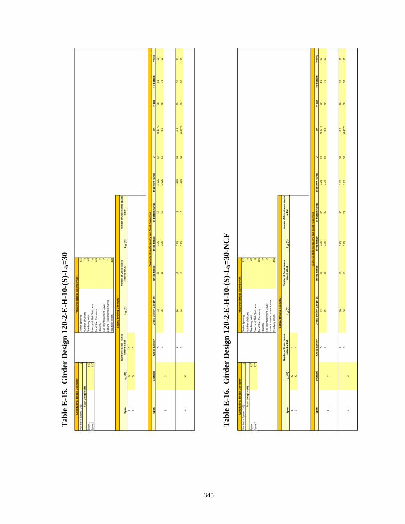
345

Num

ber o

f Spa

ns (1

-5):

2G

irder

Spa

cing

120

Num

ber o

f Gird

ers

4Sp

an 1

120

Ove

rhan

g W

idth

42Sp

an 2

120

Stru

ctur

al S

lab

Thic

knes

s8

Tota

l Sla

b Th

ickn

ess

8.5

Hau

nch

2To

p R

einf

orce

men

t Cov

er2

Bot

tom

Rei

nfor

cem

ent C

over

1R

oadw

ay W

idth

408

Span

L b1 (

ft)N

umbe

r of C

ross

- fra

mes

sp

aced

at L

b1L b

2 (ft)

Num

ber o

f Cro

ss-fr

ames

sp

aced

at L

b2L b

3 (ft)

Num

ber o

f Cro

ss-fr

ames

spa

ced

at L

b3

124

52

245

Span

Sect

ions

Cro

ss-S

ectio

nC

ross

-Sec

tion

Leng

th (f

t)bf

-top

flang

etf-

top

flang

ebf

-bot

tom

flan

getf-

botto

m fl

ange

Dtw

Fy to

pFy

bot

tom

Fy w

ebA

8416

0.75

161.

625

520.

4375

5050

50B

3616

0.75

181.

625

520.

570

7050

A36

160.

7518

1.62

552

0.5

7070

50B

8416

0.75

161.

625

520.

4375

5050

5021

2

Cro

ss-S

ectio

n G

eom

etry

and

Ste

el P

rope

rtie

s

Long

itudi

nal B

ridge

Geo

met

ryTr

ansv

erse

Brid

ge G

eom

etry

(in)

Span

Len

gths

(ft)

Late

ral B

raci

ng G

eom

etry

2

Num

ber o

f Spa

ns (1

-5):

2G

irder

Spa

cing

120

Num

ber o

f Gird

ers

4Sp

an 1

120

Ove

rhan

g W

idth

42Sp

an 2

120

Stru

ctur

al S

lab

Thic

knes

s8

Tota

l Sla

b Th

ickn

ess

8.5

Hau

nch

2To

p R

einf

orce

men

t Cov

er2

Bot

tom

Rei

nfor

cem

ent C

over

1R

oadw

ay W

idth

408

Span

L b1 (

ft)N

umbe

r of C

ross

- fra

mes

sp

aced

at L

b1L b

2 (ft)

Num

ber o

f Cro

ss-fr

ames

sp

aced

at L

b2L b

3 (ft)

Num

ber o

f Cro

ss-fr

ames

spa

ced

at L

b3

130

42

304

Span

Sect

ions

Cro

ss-S

ectio

nC

ross

-Sec

tion

Leng

th (f

t)bf

-top

flang

etf-

top

flang

ebf

-bot

tom

flan

getf-

botto

m fl

ange

Dtw

Fy to

pFy

bot

tom

Fy w

ebA

8418

0.75

241.

2552

0.43

7550

5050

B36

180.

7530

1.25

520.

570

7050

A36

180.

7530

1.25

520.

570

7050

B84

180.

7524

1.25

520.

4375

5050

5021

2

Cro

ss-S

ectio

n G

eom

etry

and

Ste

el P

rope

rtie

s

Long

itudi

nal B

ridge

Geo

met

ryTr

ansv

erse

Brid

ge G

eom

etry

(in)

Span

Len

gths

(ft)

Late

ral B

raci

ng G

eom

etry

2

Tab

le E

-16.

Gir

der

Des

ign

120-

2-E

-H-1

0-(S

)-L

b=30

-NC

F

Tab

le E

-15.

Gir

der

Des

ign

120-

2-E

-H-1

0-(S

)-L

b=30

346

Tab

le E

-17.

Gir

der

Des

ign

120-

2-E

-H-1

0-B

Num

ber o

f Spa

ns (1

-5):

2G

irder

Spa

cing

120

Num

ber o

f Gird

ers

4Sp

an 1

120

Ove

rhan

g W

idth

42Sp

an 2

120

Stru

ctur

al S

lab

Thic

knes

s8

Tota

l Sla

b Th

ickn

ess

8.5

Hau

nch

2To

p R

einf

orce

men

t Cov

er2

Bot

tom

Rei

nfor

cem

ent C

over

1R

oadw

ay W

idth

408

Span

L b1 (

ft)N

umbe

r of C

ross

- fra

mes

sp

aced

at L

b1L b

2 (ft)

Num

ber o

f Cro

ss-fr

ames

sp

aced

at L

b2L b

3 (ft)

Num

ber o

f Cro

ss-fr

ames

spa

ced

at L

b3

125

410

22

102

254

Span

Sect

ions

Cro

ss-S

ectio

nC

ross

-Sec

tion

Leng

th (f

t)bf

-top

flang

etf-

top

flang

ebf

-bot

tom

flan

getf-

botto

m fl

ange

Dtw

Fy to

pFy

bot

tom

Fy w

ebA

8416

0.75

161.

625

510.

550

5050

B36

161

161.

625

510.

5625

7070

50

A36

161

161.

625

510.

5625

7070

50B

8416

0.75

161.

625

510.

550

5050

21

2

Cro

ss-S

ectio

n G

eom

etry

and

Ste

el P

rope

rtie

s

Long

itudi

nal B

ridge

Geo

met

ryTr

ansv

erse

Brid

ge G

eom

etry

(in)

Span

Len

gths

(ft)

Late

ral B

raci

ng G

eom

etry

2

Num

ber o

f Spa

ns (1

-5):

2G

irder

Spa

cing

120

Num

ber o

f Gird

ers

4Sp

an 1

120

Ove

rhan

g W

idth

42Sp

an 2

120

Stru

ctur

al S

lab

Thic

knes

s8

Tota

l Sla

b Th

ickn

ess

8.5

Hau

nch

2To

p R

einf

orce

men

t Cov

er2

Bot

tom

Rei

nfor

cem

ent C

over

1R

oadw

ay W

idth

408

Span

L b1 (

ft)N

umbe

r of C

ross

- fra

mes

sp

aced

at L

b1L b

2 (ft)

Num

ber o

f Cro

ss-fr

ames

sp

aced

at L

b2L b

3 (ft)

Num

ber o

f Cro

ss-fr

ames

spa

ced

at L

b3

125

410

22

102

254

Span

Sect

ions

Cro

ss-S

ectio

nC

ross

-Sec

tion

Leng

th (f

t)bf

-top

flang

etf-

top

flang

ebf

-bot

tom

flan

getf-

botto

m fl

ange

Dtw

Fy to

pFy

bot

tom

Fy w

ebA

8416

0.75

161.

625

520.

550

5050

B36

160.

7516

1.62

552

0.56

2570

7050

A36

160.

7516

1.62

552

0.56

2570

7050

B84

160.

7516

1.62

552

0.5

5050

5021

2

Cro

ss-S

ectio

n G

eom

etry

and

Ste

el P

rope

rtie

s

Long

itudi

nal B

ridge

Geo

met

ryTr

ansv

erse

Brid

ge G

eom

etry

(in)

Span

Len

gths

(ft)

Late

ral B

raci

ng G

eom

etry

2

Tab

le E

-18.

Gir

der

Des

ign

120-

2-E

-H-2

0-A

Num

ber o

f Spa

ns (1

-5):

2G

irder

Spa

cing

120

Num

ber o

f Gird

ers

4Sp

an 1

120

Ove

rhan

g W

idth

42Sp

an 2

120

Stru

ctur

al S

lab

Thic

knes

s8

Tota

l Sla

b Th

ickn

ess

8.5

Hau

nch

2To

p R

einf

orce

men

t Cov

er2

Bot

tom

Rei

nfor

cem

ent C

over

1R

oadw

ay W

idth

408

Span

L b1 (

ft)N

umbe

r of C

ross

- fra

mes

sp

aced

at L

b1L b

2 (ft)

Num

ber o

f Cro

ss-fr

ames

sp

aced

at L

b2L b

3 (ft)

Num

ber o

f Cro

ss-fr

ames

spa

ced

at L

b3

125

410

22

102

254

Span

Sect

ions

Cro

ss-S

ectio

nC

ross

-Sec

tion

Leng

th (f

t)bf

-top

flang

etf-

top

flang

ebf

-bot

tom

flan

getf-

botto

m fl

ange

Dtw

Fy to

pFy

bot

tom

Fy w

ebA

8416

0.75

161.

625

520.

4375

5050

50B

3616

0.75

161.

625

520.

570

7050

A36

160.

7516

1.62

552

0.5

7070

50B

8416

0.75

161.

625

520.

4375

5050

50

2

Cro

ss-S

ectio

n G

eom

etry

and

Ste

el P

rope

rtie

s

Long

itudi

nal B

ridge

Geo

met

ryTr

ansv

erse

Brid

ge G

eom

etry

(in)

Span

Len

gths

(ft)

Late

ral B

raci

ng G

eom

etry

21

2

Num

ber o

f Spa

ns (1

-5):

2G

irder

Spa

cing

120

Num

ber o

f Gird

ers

4Sp

an 1

120

Ove

rhan

g W

idth

42Sp

an 2

120

Stru

ctur

al S

lab

Thic

knes

s8

Tota

l Sla

b Th

ickn

ess

8.5

Hau

nch

2To

p R

einf

orce

men

t Cov

er2

Bot

tom

Rei

nfor

cem

ent C

over

1R

oadw

ay W

idth

408

Span

L b1 (

ft)N

umbe

r of C

ross

- fra

mes

sp

aced

at L

b1L b

2 (ft)

Num

ber o

f Cro

ss-fr

ames

sp

aced

at L

b2L b

3 (ft)

Num

ber o

f Cro

ss-fr

ames

spa

ced

at L

b3

125

410

22

102

254

Span

Sect

ions

Cro

ss-S

ectio

nC

ross

-Sec

tion

Leng

th (f

t)bf

-top

flang

etf-

top

flang

ebf

-bot

tom

flan

getf-

botto

m fl

ange

Dtw

Fy to

pFy

bot

tom

Fy w

ebA

8416

0.75

161.

625

520.

550

5050

B36

160.

7518

1.62

552

0.56

2570

7050

A36

160.

7518

1.62

552

0.56

2570

7050

B84

160.

7516

1.62

552

0.5

5050

50

2

Cro

ss-S

ectio

n G

eom

etry

and

Ste

el P

rope

rtie

s

Long

itudi

nal B

ridge

Geo

met

ryTr

ansv

erse

Brid

ge G

eom

etry

(in)

Span

Len

gths

(ft)

Late

ral B

raci

ng G

eom

etry

21

2

Tab

le E

-19.

Gir

der

Des

ign

120-

2-E

-H-2

0-A

-(S)

Tab

le E

-20.

Gir

der

Des

ign

120-

2-E

-H-1

0-A

347

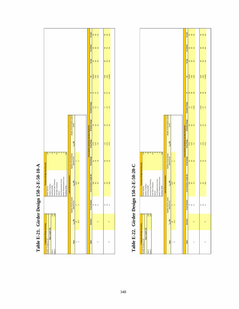
348

Tab

le E

-21.

Gir

der

Des

ign

150-

2-E

-50-

10-A

Num

ber o

f Spa

ns (1

-5):

2G

irder

Spa

cing

120

Num

ber o

f Gird

ers

4Sp

an 1

150

Ove

rhan

g W

idth

42Sp

an 2

150

Stru

ctur

al S

lab

Thic

knes

s8

Tota

l Sla

b Th

ickn

ess

8.5

Hau

nch

2To

p R

einf

orce

men

t Cov

er2

Bot

tom

Rei

nfor

cem

ent C

over

1R

oadw

ay W

idth

408

Span

L b1 (

ft)N

umbe

r of C

ross

- fra

mes

sp

aced

at L

b1L b

2 (ft)

Num

ber o

f Cro

ss-fr

ames

sp

aced

at L

b2L b

3 (ft)

Num

ber o

f Cro

ss-fr

ames

spa

ced

at L

b3

125

512

.52

212

.52

255

Span

Sect

ions

Cro

ss-S

ectio

nC

ross

-Sec

tion

Leng

th (f

t)bf

-top

flang

etf-

top

flang

ebf

-bot

tom

flan

getf-

botto

m fl

ange

Dtw

Fy to

pFy

bot

tom

Fy w

ebA

100

160.

7518

1.5

670.

5625

5050

50B

3516

0.75

181.

567

0.65

5050

50C

1516

1.5

182

670.

6550

5050

A15

161.

518

267

0.65

5050

50B

3516

0.75

181.

567

0.65

5050

50C

100

160.

7518

1.5

670.

5625

5050

5021

3

Cro

ss-S

ectio

n G

eom

etry

and

Ste

el P

rope

rtie

s

Long

itudi

nal B

ridge

Geo

met

ryTr

ansv

erse

Brid

ge G

eom

etry

(in)

Span

Len

gths

(ft)

Late

ral B

raci

ng G

eom

etry

3

Num

ber o

f Spa

ns (1

-5):

2G

irder

Spa

cing

120

Num

ber o

f Gird

ers

4Sp

an 1

150

Ove

rhan

g W

idth

42Sp

an 2

150

Stru

ctur

al S

lab

Thic

knes

s8

Tota

l Sla

b Th

ickn

ess

8.5

Hau

nch

2To

p R

einf

orce

men

t Cov

er2

Botto

m R

einf

orce

men

t Cov

er1

Roa

dway

Wid

th40

8

Span

L b1 (

ft)N

umbe

r of C

ross

- fra

mes

sp

aced

at L

b1L b

2 (ft)

Num

ber o

f Cro

ss-fr

ames

sp

aced

at L

b2L b

3 (ft)

Num

ber o

f Cro

ss-fr

ames

spa

ced

at L

b3

125

512

.52

212

.52

255

Span

Sect

ions

Cro

ss-S

ectio

nC

ross

-Sec

tion

Leng

th (f

t)bf

-top

flang

etf-

top

flang

ebf

-bot

tom

flan

getf-

botto

m fl

ange

Dtw

Fy to

pFy

bot

tom

Fy w

ebA

100

160.

7518

1.5

660.

5625

5050

50B

3516

0.75

181.

566

0.65

5050

50C

1516

1.5

181.

875

660.

6550

5050

A15

161.

518

1.87

566

0.65

5050

50B

3516

0.75

181.

566

0.65

5050

50C

100

160.

7518

1.5

660.

5625

5050

5021

3

Cro

ss-S

ectio

n G

eom

etry

and

Ste

el P

rope

rtie

s

Long

itudi

nal B

ridge

Geo

met

ryTr

ansv

erse

Brid

ge G

eom

etry

(in)

Span

Len

gths

(ft)

Late

ral B

raci

ng G

eom

etry

3

Tab

le E

-22.

Gir

der

Des

ign

150-

2-E

-50-

20-C

349

Num

ber o

f Spa

ns (1

-5):

2G

irder

Spa

cing

120

Num

ber o

f Gird

ers

4Sp

an 1

150

Ove

rhan

g W

idth

42Sp

an 2

150

Stru

ctur

al S

lab

Thic

knes

s8

Tota

l Sla

b Th

ickn

ess

8.5

Hau

nch

2To

p R

einf

orce

men

t Cov

er2

Bot

tom

Rei

nfor

cem

ent C

over

1R

oadw

ay W

idth

408

Span

Lb1

(ft)

Num

ber o

f Cro

ss- f

ram

es

spac

ed a

t Lb1

Lb2

(ft)

Num

ber o

f Cro

ss-fr

ames

sp

aced

at L

b2Lb

3 (ft

)N

umbe

r of C

ross

-fram

es s

pace

d at

Lb3

125

512

.52

212

.52

255

Span

Sect

ions

Cro

ss-S

ectio

nC

ross

-Sec

tion

Leng

th (f

t)bf

-top

flang

etf-

top

flang

ebf

-bot

tom

flan

getf-

botto

m fl

ange

Dtw

Fy to

pFy

bot

tom

Fy w

ebA

100

160.

7518

1.5

670.

5625

5050

50B

3616

0.75

181.

567

0.62

550

5050

C14

161.

518

1.5

670.

625

5050

50

A14

161.

518

1.5

670.

625

5050

50B

3616

0.75

181.

567

0.62

550

5050

C10

016

0.75

181.

567

0.56

2550

5050

21

3

Cro

ss-S

ectio

n G

eom

etry

and

Ste

el P

rope

rtie

s

Long

itudi

nal B

ridge

Geo

met

ryTr

ansv

erse

Brid

ge G

eom

etry

(in)

Span

Len

gths

(ft)

Late

ral B

raci

ng G

eom

etry

3

Num

ber o

f Spa

ns (1

-5):

2G

irder

Spa

cing

120

Num

ber o

f Gird

ers

4Sp

an 1

150

Ove

rhan

g W

idth

42Sp

an 2

150

Stru

ctur

al S

lab

Thic

knes

s8

Tota

l Sla

b Th

ickn

ess

8.5

Hau

nch

2To

p R

einf

orce

men

t Cov

er2

Bot

tom

Rei

nfor

cem

ent C

over

1R

oadw

ay W

idth

408

Span

Lb1

(ft)

Num

ber o

f Cro

ss- f

ram

es

spac

ed a

t Lb1

Lb2

(ft)

Num

ber o

f Cro

ss-fr

ames

sp

aced

at L

b2Lb

3 (ft

)N

umbe

r of C

ross

-fram

es s

pace

d at

Lb3

125

512

.52

212

.52

255

Span

Sect

ions

Cro

ss-S

ectio

nC

ross

-Sec

tion

Leng

th (f

t)bf

-top

flang

etf-

top

flang

ebf

-bot

tom

flan

getf-

botto

m fl

ange

Dtw

Fy to

pFy

bot

tom

Fy w

ebA

100

160.

875

181.

566

0.56

2550

5050

B36

160.

875

181.

625

660.

625

5050

50C

1416

0.87

518

1.62

566

0.62

550

5050

A14

160.

875

181.

625

660.

625

5050

50B

3616

0.87

518

1.62

566

0.62

550

5050

C10

016

0.87

518

1.5

660.

5625

5050

5021

3

Cro

ss-S

ectio

n G

eom

etry

and

Ste

el P

rope

rtie

s

Long

itudi

nal B

ridge

Geo

met

ryTr

ansv

erse

Brid

ge G

eom

etry

(in)

Span

Len

gths

(ft)

Late

ral B

raci

ng G

eom

etry

3

Tab

le E

-23.

Gir

der

Des

ign

150-

2-E

-50-

30-C

Tab

le E

-23.

Gir

der

Des

ign

150-

2-E

-50-

40-A

350

Num

ber o

f Spa

ns (1

-5):

2G

irder

Spa

cing

120

Num

ber o

f Gird

ers

4Sp

an 1

180

Ove

rhan

g W

idth

42Sp

an 2

180

Stru

ctur

al S

lab

Thic

knes

s8

Tota

l Sla

b Th

ickn

ess

8.5

Hau

nch

2To

p R

einf

orce

men

t Cov

er2

Bot

tom

Rei

nfor

cem

ent C

over

1R

oadw

ay W

idth

408

Span

L b1 (

ft)N

umbe

r of C

ross

- fra

mes

sp

aced

at L

b1L b

2 (ft)

Num

ber o

f Cro

ss-fr

ames

sp

aced

at L

b2L b

3 (ft)

Num

ber o

f Cro

ss-fr

ames

spa

ced

at L

b3

124

712

12

121

247

Span

Sect

ions

Cro

ss-S

ectio

nC

ross

-Sec

tion

Leng

th (f

t)bf

-top

flang

etf-

top

flang

ebf

-bot

tom

flan

getf-

botto

m fl

ange

Dtw

Fy to

pFy

bot

tom

Fy w

ebA

3716

0.75

161

730.

625

5050

50B

8316

116

273

0.62

550

5050

C45

161

222

730.

6875

5050

50D

1520

222

273

0.68

7550

5050

A15

202

222

730.

6875

5050

50B

4516

122

273

0.68

7550

5050

C83

161

162

730.

625

5050

50D

3716

0.75

161

730.

625

5050

50

21

4

Cro

ss-S

ectio

n G

eom

etry

and

Ste

el P

rope

rtie

s

Long

itudi

nal B

ridge

Geo

met

ryTr

ansv

erse

Brid

ge G

eom

etry

(in)

Span

Len

gths

(ft)

Late

ral B

raci

ng G

eom

etry

4

Num

ber o

f Spa

ns (1

-5):

2G

irder

Spa

cing

120

Num

ber o

f Gird

ers

4Sp

an 1

180

Ove

rhan

g W

idth

42Sp

an 2

180

Stru

ctur

al S

lab

Thic

knes

s8

Tota

l Sla

b Th

ickn

ess

8.5

Hau

nch

2To

p R

einf

orce

men

t Cov

er2

Bot

tom

Rei

nfor

cem

ent C

over

1R

oadw

ay W

idth

408

Span

L b1 (

ft)N

umbe

r of C

ross

- fra

mes

sp

aced

at L

b1L b

2 (ft)

Num

ber o

f Cro

ss-fr

ames

sp

aced

at L

b2L b

3 (ft)

Num

ber o

f Cro

ss-fr

ames

spa

ced

at L

b3

124

712

12

121

247

Span

Sect

ions

Cro

ss-S

ectio

nC

ross

-Sec

tion

Leng

th (f

t)bf

-top

flang

etf-

top

flang

ebf

-bot

tom

flan

getf-

botto

m fl

ange

Dtw

Fy to

pFy

bot

tom

Fy w

ebA

3016

0.75

161.

2571

0.62

550

5050

B90

161.

2516

271

0.62

550

5050

C45

161.

2520

1.75

710.

6875

5050

50D

1516

220

271

0.68

7550

5050

A15

162

202

710.

6875

5050

50B

4516

1.25

201.

7571

0.68

7550

5050

C90

161.

2516

271

0.62

550

5050

D30

160.

7516

1.25

710.

625

5050

50

21

4

Cro

ss-S

ectio

n G

eom

etry

and

Ste

el P

rope

rtie

s

Long

itudi

nal B

ridge

Geo

met

ryTr

ansv

erse

Brid

ge G

eom

etry

(in)

Span

Len

gths

(ft)

Late

ral B

raci

ng G

eom

etry

4

Tab

le E

-25.

Gir

der

Des

ign

180-

2-E

-50-

10-A

Tab

le E

-26.

Gir

der

Des

ign

180-

2-E

-50-

20-A

351

Num

ber o

f Spa

ns (1

-5):

2G

irder

Spa

cing

120

Num

ber o

f Gird

ers

4Sp

an 1

180

Ove

rhan

g W

idth

42Sp

an 2

180

Stru

ctur

al S

lab

Thic

knes

s8

Tota

l Sla

b Th

ickn

ess

8.5

Hau

nch

2To

p R

einf

orce

men

t Cov

er2

Bot

tom

Rei

nfor

cem

ent C

over

1R

oadw

ay W

idth

408

Span

L b1 (

ft)N

umbe

r of C

ross

- fra

mes

sp

aced

at L

b1L b

2 (ft)

Num

ber o

f Cro

ss-fr

ames

sp

aced

at L

b2L b

3 (ft)

Num

ber o

f Cro

ss-fr

ames

spa

ced

at L

b3

124

712

12

121

247

Span

Sect

ions

Cro

ss-S

ectio

nC

ross

-Sec

tion

Leng

th (f

t)bf

-top

flang

etf-

top

flang

ebf

-bot

tom

flan

getf-

botto

m fl

ange

Dtw

Fy to

pFy

bot

tom

Fy w

ebA

3516

0.75

161

740.

625

5050

50B

8516

116

274

0.62

550

5050

C45

161

202

740.

6875

5050

50D

1516

220

274

0.68

7550

5050

A15

162

202

740.

6875

5050

50B

4516

120

274

0.68

7550

5050

C85

161

162

740.

625

5050

50D

3516

0.75

161

740.

625

5050

50

21

4

Cro

ss-S

ectio

n G

eom

etry

and

Ste

el P

rope

rtie

s

Long

itudi

nal B

ridge

Geo

met

ryTr

ansv

erse

Brid

ge G

eom

etry

(in)

Span

Len

gths

(ft)

Late

ral B

raci

ng G

eom

etry

4

Num

ber o

f Spa

ns (1

-5):

2G

irder

Spa

cing

120

Num

ber o

f Gird

ers

4Sp

an 1

180

Ove

rhan

g W

idth

42Sp

an 2

180

Stru

ctur

al S

lab

Thic

knes

s8

Tota

l Sla

b Th

ickn

ess

8.5

Hau

nch

2To

p R

einf

orce

men

t Cov

er2

Bot

tom

Rei

nfor

cem

ent C

over

1R

oadw

ay W

idth

408

Span

L b1 (

ft)N

umbe

r of C

ross

- fra

mes

sp

aced

at L

b1L b

2 (ft)

Num

ber o

f Cro

ss-fr

ames

sp

aced

at L

b2L b

3 (ft)

Num

ber o

f Cro

ss-fr

ames

spa

ced

at L

b3

124

712

12

121

247

Span

Sect

ions

Cro

ss-S

ectio

nC

ross

-Sec

tion

Leng

th (f

t)bf

-top

flang

etf-

top

flang

ebf

-bot

tom

flan

getf-

botto

m fl

ange

Dtw

Fy to

pFy

bot

tom

Fy w

ebA

3520

122

174

0.62

550

5050

B85

201.

522

1.5

740.

625

5050

50C

4522

136

1.5

740.

6875

5050

50D

1522

1.5

361.

574

0.68

7550

5050

A15

221.

536

1.5

740.

6875

5050

50B

4522

136

1.5

740.

6875

5050

50C

8520

1.5

221.

574

0.62

550

5050

D35

201

221

740.

625

5050

50

4

Cro

ss-S

ectio

n G

eom

etry

and

Ste

el P

rope

rtie

s

Long

itudi

nal B

ridge

Geo

met

ryTr

ansv

erse

Brid

ge G

eom

etry

(in)

Span

Len

gths

(ft)

Late

ral B

raci

ng G

eom

etry

21

4

Tab

le E

-28.

Gir

der

Des

ign

180-

2-E

-50-

20-B

-NC

F

Tab

le E

-27.

Gir

der

Des

ign

180-

2-E

-50-

20-B

352

Num

ber o

f Spa

ns (1

-5):

2G

irder

Spa

cing

120

Num

ber o

f Gird

ers

4Sp

an 1

180

Ove

rhan

g W

idth

42Sp

an 2

180

Stru

ctur

al S

lab

Thic

knes

s8

Tota

l Sla

b Th

ickn

ess

8.5

Hau

nch

2To

p R

einf

orce

men

t Cov

er2

Bot

tom

Rei

nfor

cem

ent C

over

1R

oadw

ay W

idth

408

Span

L b1 (

ft)N

umbe

r of C

ross

- fra

mes

sp

aced

at L

b1L b

2 (ft)

Num

ber o

f Cro

ss-fr

ames

sp

aced

at L

b2L b

3 (ft)

Num

ber o

f Cro

ss-fr

ames

spa

ced

at L

b3

122

.58

222

.58

Span

Sect

ions

Cro

ss-S

ectio

nC

ross

-Sec

tion

Leng

th (f

t)bf

-top

flang

etf-

top

flang

ebf

-bot

tom

flan

getf-

botto

m fl

ange

Dtw

Fy to

pFy

bot

tom

Fy w

ebA

3516

0.75

161

740.

625

5050

50B

8516

116

274

0.62

550

5050

C45

161

202

740.

6875

5050

50D

1516

220

274

0.68

7550

5050

A15

162

202

740.

6875

5050

50B

4516

120

274

0.68

7550

5050

C85

161

162

740.

625

5050

50D

3516

0.75

161

740.

625

5050

50

4

Cro

ss-S

ectio

n G

eom

etry

and

Ste

el P

rope

rtie

s

Long

itudi

nal B

ridge

Geo

met

ryTr

ansv

erse

Brid

ge G

eom

etry

(in)

Span

Len

gths

(ft)

Late

ral B

raci

ng G

eom

etry

21

4

Num

ber o

f Spa

ns (1

-5):

2G

irder

Spa

cing

120

Num

ber o

f Gird

ers

4Sp

an 1

180

Ove

rhan

g W

idth

42Sp

an 2

180

Stru

ctur

al S

lab

Thic

knes

s8

Tota

l Sla

b Th

ickn

ess

8.5

Hau

nch

2To

p R

einf

orce

men

t Cov

er2

Bot

tom

Rei

nfor

cem

ent C

over

1R

oadw

ay W

idth

408

Span

L b1 (

ft)N

umbe

r of C

ross

- fra

mes

sp

aced

at L

b1L b

2 (ft)

Num

ber o

f Cro

ss-fr

ames

sp

aced

at L

b2L b

3 (ft)

Num

ber o

f Cro

ss-fr

ames

spa

ced

at L

b3

130

62

306

Span

Sect

ions

Cro

ss-S

ectio

nC

ross

-Sec

tion

Leng

th (f

t)bf

-top

flang

etf-

top

flang

ebf

-bot

tom

flan

getf-

botto

m fl

ange

Dtw

Fy to

pFy

bot

tom

Fy w

ebA

3516

1.12

516

1.12

574

0.62

550

5050

B85

161.

375

162

740.

625

5050

50C

4516

120

274

0.68

7550

5050

D15

162

202

740.

6875

5050

50

A15

162

202

740.

6875

5050

50B

4516

120

274

0.68

7550

5050

C85

161.

375

162

740.

625

5050

50D

3516

1.12

516

1.12

574

0.62

550

5050

4

Cro

ss-S

ectio

n G

eom

etry

and

Ste

el P

rope

rtie

s

Long

itudi

nal B

ridge

Geo

met

ryTr

ansv

erse

Brid

ge G

eom

etry

(in)

Span

Len

gths

(ft)

Late

ral B

raci

ng G

eom

etry

21

4

Tab

le E

-29.

Gir

der

Des

ign

180-

2-E

-50-

20-L

b=22

.5

Tab

le E

-30.

Gir

der

Des

ign

180-

2-E

-50-

Lb=

30

Num

ber o

f Spa

ns (1

-5):

2G

irder

Spa

cing

120

Num

ber o

f Gird

ers

4Sp

an 1

180

Ove

rhan

g W

idth

42Sp

an 2

180

Stru

ctur

al S

lab

Thic

knes

s8

Tota

l Sla

b Th

ickn

ess

8.5

Hau

nch

2To

p R

einf

orce

men

t Cov

er2

Bot

tom

Rei

nfor

cem

ent C

over

1R

oadw

ay W

idth

408

Span

L b1 (

ft)N

umbe

r of C

ross

- fra

mes

sp

aced

at L

b1L b

2 (ft)

Num

ber o

f Cro

ss-fr

ames

sp

aced

at L

b2L b

3 (ft)

Num

ber o

f Cro

ss-fr

ames

spa

ced

at L

b3

130

62

306

Span

Sect

ions

Cro

ss-S

ectio

nC

ross

-Sec

tion

Leng

th (f

t)bf

-top

flang

etf-

top

flang

ebf

-bot

tom

flan

getf-

botto

m fl

ange

Dtw

Fy to

pFy

bot

tom

Fy w

ebA

3522

126

1.12

574

0.62

550

5050

B85

221

261.

574

0.62

550

5050

C45

241.

125

361.

574

0.68

7550

5050

D15

241.

536

1.5

740.

6875

5050

50

A15

241.

536

1.5

740.

6875

5050

50B

4524

1.12

536

1.5

740.

6875

5050

50C

8522

126

1.5

740.

625

5050

50D

3522

126

1.12

574

0.62

550

5050

4

Cro

ss-S

ectio

n G

eom

etry

and

Ste

el P

rope

rtie

s

Long

itudi

nal B

ridge

Geo

met

ryTr

ansv

erse

Brid

ge G

eom

etry

(in)

Span

Len

gths

(ft)

Late

ral B

raci

ng G

eom

etry

21

4

Num

ber o

f Spa

ns (1

-5):

2G

irder

Spa

cing

120

Num

ber o

f Gird

ers

4Sp

an 1

210

Ove

rhan

g W

idth

42Sp

an 2

210

Stru

ctur

al S

lab

Thic

knes

s8

Tota

l Sla

b Th

ickn

ess

8.5

Hau

nch

2To

p R

einf

orce

men

t Cov

er2

Bot

tom

Rei

nfor

cem

ent C

over

1R

oadw

ay W

idth

408

Span

L b1 (

ft)N

umbe

r of C

ross

- fra

mes

sp

aced

at L

b1L b

2 (ft)

Num

ber o

f Cro

ss-fr

ames

sp

aced

at L

b2L b

3 (ft)

Num

ber o

f Cro

ss-fr

ames

spa

ced

at L

b3

125

810

12

101

258

Span

Sect

ions

Cro

ss-S

ectio

nC

ross

-Sec

tion

Leng

th (f

t)bf

-top

flang

etf-

top

flang

ebf

-bot

tom

flan

getf-

botto

m fl

ange

Dtw

Fy to

pFy

bot

tom

Fy w

ebA

5016

0.87

516

0.87

596

0.68

7550

5050

B90

160.

875

161.

375

960.

6875

5050

50C

5524

1.37

528

1.37

596

0.81

2550

5050

D15

242

282

960.

8125

5050

50

A15

242

282

960.

8125

5050

50B

5524

1.37

528

1.37

596

0.81

2550

5050

C90

160.

875

161.

375

960.

6875

5050

50D

5016

0.87

516

0.87

596

0.68

7550

5050

21

4

Cro

ss-S

ectio

n G

eom

etry

and

Ste

el P

rope

rtie

s

Long

itudi

nal B

ridge

Geo

met

ryTr

ansv

erse

Brid

ge G

eom

etry

(in)

Span

Len

gths

(ft)

Late

ral B

raci

ng G

eom

etry

4

Tab

le E

-31.

Gir

der

Des

ign

180-

2-E

-50-

20-L

b=30

-NC

F

Tab

le E

-32.

Gir

der

Des

ign

210-

2-E

-50-

10-E

353

Num

ber o

f Spa

ns (1

-5):

2G

irder

Spa

cing

120

Num

ber o

f Gird

ers

4Sp

an 1

210

Ove

rhan

g W

idth

42Sp

an 2

210

Stru

ctur

al S

lab

Thic

knes

s8

Tota

l Sla

b Th

ickn

ess

8.5

Hau

nch

2To

p R

einf

orce

men

t Cov

er2

Bot

tom

Rei

nfor

cem

ent C

over

1R

oadw

ay W

idth

408

Span

L b1 (

ft)N

umbe

r of C

ross

- fra

mes

sp

aced

at L

b1L b

2 (ft)

Num

ber o

f Cro

ss-fr

ames

sp

aced

at L

b2L b

3 (ft)

Num

ber o

f Cro

ss-fr

ames

spa

ced

at L

b3

110

126

718

12

181

267

101

Span

Sect

ions

Cro

ss-S

ectio

nC

ross

-Sec

tion

Leng

th (f

t)bf

-top

flang

etf-

top

flang

ebf

-bot

tom

flan

getf-

botto

m fl

ange

Dtw

Fy to

pFy

bot

tom

Fy w

ebA

5016

0.87

516

0.87

596

0.68

7550

5050

B90

160.

875

161.

375

960.

6875

5050

50C

5524

1.37

528

1.37

596

0.81

2550

5050

D15

242

282

960.

8125

5050

50

A15

242

282

960.

8125

5050

50B

5524

1.37

528

1.37

596

0.81

2550

5050

C90

160.

875

161.

375

960.

6875

5050

50D

5016

0.87

516

0.87

596

0.68

7550

5050

4

Cro

ss-S

ectio

n G

eom

etry

and

Ste

el P

rope

rtie

s

Long

itudi

nal B

ridge

Geo

met

ryTr

ansv

erse

Brid

ge G

eom

etry

(in)

Span

Len

gths

(ft)

Late

ral B

raci

ng G

eom

etry

21

4

Num

ber o

f Spa

ns (1

-5):

2G

irder

Spa

cing

120

Num

ber o

f Gird

ers

4Sp

an 1

210

Ove

rhan

g W

idth

42Sp

an 2

210

Stru

ctur

al S

lab

Thic

knes

s8

Tota

l Sla

b Th

ickn

ess

8.5

Hau

nch

2To

p R

einf

orce

men

t Cov

er2

Bot

tom

Rei

nfor

cem

ent C

over

1R

oadw

ay W

idth

408

Span

L b1 (

ft)N

umbe

r of C

ross

- fra

mes

sp

aced

at L

b1L b

2 (ft)

Num

ber o

f Cro

ss-fr

ames

sp

aced

at L

b2L b

3 (ft)

Num

ber o

f Cro

ss-fr

ames

spa

ced

at L

b3

126

.25

82

26.2

58

Span

Sect

ions

Cro

ss-S

ectio

nC

ross

-Sec

tion

Leng

th (f

t)bf

-top

flang

etf-

top

flang

ebf

-bot

tom

flan

getf-

botto

m fl

ange

Dtw

Fy to

pFy

bot

tom

Fy w

ebA

5016

0.87

516

0.87

596

0.68

7550

5050

B90

160.

875

161.

375

960.

6875

5050

50C

5524

1.37

528

1.37

596

0.81

2550

5050

D15

242

282

960.

8125

5050

50

A15

242

282

960.

8125

5050

50B

5524

1.37

528

1.37

596

0.81

2550

5050

C90

160.

875

161.

375

960.

6875

5050

50D

5016

0.87

516

0.87

596

0.68

7550

5050

4

Cro

ss-S

ectio

n G

eom

etry

and

Ste

el P

rope

rtie

s

Long

itudi

nal B

ridge

Geo

met

ryTr

ansv

erse

Brid

ge G

eom

etry

(in)

Span

Len

gths

(ft)

Late

ral B

raci

ng G

eom

etry

21

4

Tab

le E

-34.

Gir

der

Des

ign

210-

2-E

-50-

10-L

b=26

.25

Tab

le E

-33.

Gir

der

Des

ign

210-

2-E

-50-

10-L

b=18

354

355

Tab

le E

-35.

Gir

der

Des

ign

210-

2-E

-50-

10-L

b=30

Num

ber o

f Spa

ns (1

-5):

2G

irder

Spa

cing

120

Num

ber o

f Gird

ers

4Sp

an 1

210

Ove

rhan

g W

idth

42Sp

an 2

210

Stru

ctur

al S

lab

Thic

knes

s8

Tota

l Sla

b Th

ickn

ess

8.5

Hau

nch

2To

p R

einf

orce

men

t Cov

er2

Bot

tom

Rei

nfor

cem

ent C

over

1R

oadw

ay W

idth

408

Span

L b1 (

ft)N

umbe

r of C

ross

- fra

mes

sp

aced

at L

b1L b

2 (ft)

Num

ber o

f Cro

ss-fr

ames

sp

aced

at L

b2L b

3 (ft)

Num

ber o

f Cro

ss-fr

ames

spa

ced

at L

b3

130

72

307

Span

Sect

ions

Cro

ss-S

ectio

nC

ross

-Sec

tion

Leng

th (f

t)bf

-top

flang

etf-

top

flang

ebf

-bot

tom

flan

getf-

botto

m fl

ange

Dtw

Fy to

pFy

bot

tom

Fy w

ebA

5016

0.87

516

0.87

596

0.68

7550

5050

B90

160.

875

161.

375

960.

6875

5050

50C

5524

1.37

528

1.37

596

0.81

2550

5050

D15

242

282

960.

8125

5050

50

A15

242

282

960.

8125

5050

50B

5524

1.37

528

1.37

596

0.81

2550

5050

C90

160.

875

161.

375

960.

6875

5050

50D

5016

0.87

516

0.87

596

0.68

7550

5050

4

Cro

ss-S

ectio

n G

eom

etry

and

Ste

el P

rope

rtie

s

Long

itudi

nal B

ridge

Geo

met

ryTr

ansv

erse

Brid

ge G

eom

etry

(in)

Span

Len

gths

(ft)

Late

ral B

raci

ng G

eom

etry

21

4

Num

ber o

f Spa

ns (1

-5):

2G

irder

Spa

cing

120

Num

ber o

f Gird

ers

4Sp

an 1

210

Ove

rhan

g W

idth

42Sp

an 2

210

Stru

ctur

al S

lab

Thic

knes

s8

Tota

l Sla

b Th

ickn

ess

8.5

Hau

nch

2To

p R

einf

orce

men

t Cov

er2

Bot

tom

Rei

nfor

cem

ent C

over

1R

oadw

ay W

idth

408

Span

L b1 (

ft)N

umbe

r of C

ross

- fra

mes

sp

aced

at L

b1L b

2 (ft)

Num

ber o

f Cro

ss-fr

ames

sp

aced

at L

b2L b

3 (ft)

Num

ber o

f Cro

ss-fr

ames

spa

ced

at L

b3

130

72

307

Span

Sect

ions

Cro

ss-S

ectio

nC

ross

-Sec

tion

Leng

th (f

t)bf

-top

flang

etf-

top

flang

ebf

-bot

tom

flan

getf-

botto

m fl

ange

Dtw

Fy to

pFy

bot

tom

Fy w

ebA

5016

0.87

520

196

0.68

7550

5050

B90

161.

2520

1.75

960.

6875

5050

50C

5530

1.25

421.

7596

0.81

2550

5050

D15

301.

2542

1.75

960.

8125

5050

50

A15

301.

2542

1.75

960.

8125

5050

50B

5530

1.25

421.

7596

0.81

2550

5050

C90

161.

2520

1.75

960.

6875

5050

50D

5016

0.87

520

196

0.68

7550

5050

21

4

Cro

ss-S

ectio

n G

eom

etry

and

Ste

el P

rope

rtie

s

Long

itudi

nal B

ridge

Geo

met

ryTr

ansv

erse

Brid

ge G

eom

etry

(in)

Span

Len

gths

(ft)

Late

ral B

raci

ng G

eom

etry

4

Tab

le E

-36.

Gir

der

Des

ign

210-

2-E

-50-

10-L

b=30

-NC

F

356

Num

ber o

f Spa

ns (1

-5):

2G

irder

Spa

cing

120

Num

ber o

f Gird

ers

4Sp

an 1

210

Ove

rhan

g W

idth

42Sp

an 2

210

Stru

ctur

al S

lab

Thic

knes

s8

Tota

l Sla

b Th

ickn

ess

8.5

Hau

nch

2To

p R

einf

orce

men

t Cov

er2

Bot

tom

Rei

nfor

cem

ent C

over

1R

oadw

ay W

idth

408

Span

L b1 (

ft)N

umbe

r of C

ross

- fra

mes

sp

aced

at L

b1L b

2 (ft)

Num

ber o

f Cro

ss-fr

ames

sp

aced

at L

b2L b

3 (ft)

Num

ber o

f Cro

ss-fr

ames

spa

ced

at L

b3

125

810

12

101

258

Span

Sect

ions

Cro

ss-S

ectio

nC

ross

-Sec

tion

Leng

th (f

t)bf

-top

flang

etf-

top

flang

ebf

-bot

tom

flan

getf-

botto

m fl

ange

Dtw

Fy to

pFy

bot

tom

Fy w

ebA

5016

0.87

520

196

0.68

7550

5050

B90

161.

2520

1.75

960.

6875

5050

50C

5530

1.25

421.

7596

0.81

2550

5050

D15

301.

2542

1.75

960.

8125

5050

50

A15

301.

2542

1.75

960.

8125

5050

50B

5530

1.25

421.

7596

0.81

2550

5050

C90

161.

2520

1.75

960.

6875

5050

50D

5016

0.87

520

196

0.68

7550

5050

21

4

Cro

ss-S

ectio

n G

eom

etry

and

Ste

el P

rope

rtie

s

Long

itudi

nal B

ridge

Geo

met

ryTr

ansv

erse

Brid

ge G

eom

etry

(in)

Span

Len

gths

(ft)

Late

ral B

raci

ng G

eom

etry

4

Num

ber o

f Spa

ns (1

-5):

2G

irder

Spa

cing

120

Num

ber o

f Gird

ers

4Sp

an 1

210

Ove

rhan

g W

idth

42Sp

an 2

210

Stru

ctur

al S

lab

Thic

knes

s8

Tota

l Sla

b Th

ickn

ess

8.5

Hau

nch

2To

p R

einf

orce

men

t Cov

er2

Bot

tom

Rei

nfor

cem

ent C

over

1R

oadw

ay W

idth

408

Span

L b1 (

ft)N

umbe

r of C

ross

- fra

mes

sp

aced

at L

b1L b

2 (ft)

Num

ber o

f Cro

ss-fr

ames

sp

aced

at L

b2L b

3 (ft)

Num

ber o

f Cro

ss-fr

ames

spa

ced

at L

b3

125

810

12

101

258

Span

Sect

ions

Cro

ss-S

ectio

nC

ross

-Sec

tion

Leng

th (f

t)bf

-top

flang

etf-

top

flang

ebf

-bot

tom

flan

getf-

botto

m fl

ange

Dtw

Fy to

pFy

bot

tom

Fy w

ebA

5016

120

187

0.68

7550

5050

B90

161.

375

201.

375

870.

6875

5050

50C

5824

1.37

526

1.87

587

0.75

5050

50D

1224

1.87

526

287

0.75

5050

50

A12

241.

875

262

870.

7550

5050

B58

241.

375

261.

875

870.

7550

5050

C90

161.

375

201.

375

870.

6875

5050

50D

5016

120

187

0.68

7550

5050

21

4

Cro

ss-S

ectio

n G

eom

etry

and

Ste

el P

rope

rtie

s

Long

itudi

nal B

ridge

Geo

met

ryTr

ansv

erse

Brid

ge G

eom

etry

(in)

Span

Len

gths

(ft)

Late

ral B

raci

ng G

eom

etry

4

Tab

le E

-37.

Gir

der

Des

ign

210-

2-E

-50-

10-N

CF

Tab

le E

-38.

Gir

der

Des

ign

210-

2-E

-50-

20-F

Num

ber o

f Spa

ns (1

-5):

2G

irder

Spa

cing

120

Num

ber o

f Gird

ers

4Sp

an 1

210

Ove

rhan

g W

idth

42Sp

an 2

210

Stru

ctur

al S

lab

Thic

knes

s8

Tota

l Sla

b Th

ickn

ess

8.5

Hau

nch

2To

p R

einf

orce

men

t Cov

er2

Bot

tom

Rei

nfor

cem

ent C

over

1R

oadw

ay W

idth

408

Span

L b1 (

ft)N

umbe

r of C

ross

- fra

mes

sp

aced

at L

b1L b

2 (ft)

Num

ber o

f Cro

ss-fr

ames

sp

aced

at L

b2L b

3 (ft)

Num

ber o

f Cro

ss-fr

ames

spa

ced

at L

b3

126

714

22

142

267

Span

Sect

ions

Cro

ss-S

ectio

nC

ross

-Sec

tion

Leng

th (f

t)bf

-top

flang

etf-

top

flang

ebf

-bot

tom

flan

getf-

botto

m fl

ange

Dtw

Fy to

pFy

bot

tom

Fy w

ebA

5016

120

188

0.68

7550

5050

B90

161.

375

201.

375

880.

6875

5050

50C

7024

1.37

526

1.87

588

0.81

2550

5050

A70

241.

375

261.

875

880.

8125

5050

50B

9016

1.37

520

1.37

588

0.68

7550

5050

C50

161

201

880.

6875

5050

50

3

Cro

ss-S

ectio

n G

eom

etry

and

Ste

el P

rope

rtie

s

Long

itudi

nal B

ridge

Geo

met

ryTr

ansv

erse

Brid

ge G

eom

etry

(in)

Span

Len

gths

(ft)

Late

ral B

raci

ng G

eom

etry

21

3

Num

ber o

f Spa

ns (1

-5):

2G

irder

Spa

cing

120

Num

ber o

f Gird

ers

4Sp

an 1

210

Ove

rhan

g W

idth

42Sp

an 2

210

Stru

ctur

al S

lab

Thic

knes

s8

Tota

l Sla

b Th

ickn

ess

8.5

Hau

nch

2To

p R

einf

orce

men

t Cov

er2

Bot

tom

Rei

nfor

cem

ent C

over

1R

oadw

ay W

idth

408

Span

L b1 (

ft)N

umbe

r of C

ross

- fra

mes

sp

aced

at L

b1L b

2 (ft)

Num

ber o

f Cro

ss-fr

ames

sp

aced

at L

b2L b

3 (ft)

Num

ber o

f Cro

ss-fr

ames

spa

ced

at L

b3

126

714

22

142

267

Span

Sect

ions

Cro

ss-S

ectio

nC

ross

-Sec

tion

Leng

th (f

t)bf

-top

flang

etf-

top

flang

ebf

-bot

tom

flan

getf-

botto

m fl

ange

Dtw

Fy to

pFy

bot

tom

Fy w

ebA

5516

1.25

201.

2587

0.68

7550

5050

B85

161.

2520

1.75

870.

6875

5050

50C

5622

1.25

261.

7587

0.75

5050

50D

1422

1.25

261.

7587

0.75

5050

50

A14

221.

2526

1.75

870.

7550

5050

B56

221.

2526

1.75

870.

7550

5050

C85

161.

2520

1.75

870.

6875

5050

50D

5516

1.25

201.

2587

0.68

7550

5050

4

Cro

ss-S

ectio

n G

eom

etry

and

Ste

el P

rope

rtie

s

Long

itudi

nal B

ridge

Geo

met

ryTr

ansv

erse

Brid

ge G

eom

etry

(in)

Span

Len

gths

(ft)

Late

ral B

raci

ng G

eom

etry

21

4

Tab

le E

-40.

Gir

der

Des

ign

210-

2-E

-50-

40-C

Tab

le E

-39.

Gir

der

Des

ign

210-

2-E

-50-

30-B

357

358

Num

ber o

f Spa

ns (1

-5):

2G

irder

Spa

cing

120

Num

ber o

f Gird

ers

4Sp

an 1

210

Ove

rhan

g W

idth

42Sp

an 2

210

Stru

ctur

al S

lab

Thic

knes

s8

Tota

l Sla

b Th

ickn

ess

8.5

Hau

nch

2To

p R

einf

orce

men

t Cov

er2

Bot

tom

Rei

nfor

cem

ent C

over

1R

oadw

ay W

idth

408

Span

L b1 (

ft)N

umbe

r of C

ross

- fra

mes

sp

aced

at L

b1L b

2 (ft)

Num

ber o

f Cro

ss-fr

ames

sp

aced

at L

b2L b

3 (ft)

Num

ber o

f Cro

ss-fr

ames

spa

ced

at L

b3

125

810

12

101

258

Span

Sect

ions

Cro

ss-S

ectio

nC

ross

-Sec

tion

Leng

th (f

t)bf

-top

flang

etf-

top

flang

ebf

-bot

tom

flan

getf-

botto

m fl

ange

Dtw

Fy to

pFy

bot

tom

Fy w

ebA

5016

0.87

516

0.87

596

0.68

7550

5050

B90

161

161.

375

960.

6875

5050

50C

5520

124

1.25

960.

8125

7070

50D

1520

224

296

0.81

2570

7050

A15

202

242

960.

8125

7070

50B

5520

124

1.25

960.

8125

7070

50C

9016

116

1.37

596

0.68

7550

5050

D50

160.

875

160.

875

960.

6875

5050

50

4

Cro

ss-S

ectio

n G

eom

etry

and

Ste

el P

rope

rtie

s

Long

itudi

nal B

ridge

Geo

met

ryTr

ansv

erse

Brid

ge G

eom

etry

(in)

Span

Len

gths

(ft)

Late

ral B

raci

ng G

eom

etry

21

4

Num

ber o

f Spa

ns (1

-5):

2G

irder

Spa

cing

120

Num

ber o

f Gird

ers

4Sp

an 1

210

Ove

rhan

g W

idth

42Sp

an 2

210

Stru

ctur

al S

lab

Thic

knes

s8

Tota

l Sla

b Th

ickn

ess

8.5

Hau

nch

2To

p R

einf

orce

men

t Cov

er2

Bot

tom

Rei

nfor

cem

ent C

over

1R

oadw

ay W

idth

408

Span

L b1 (

ft)N

umbe

r of C

ross

- fra

mes

sp

aced

at L

b1L b

2 (ft)

Num

ber o

f Cro

ss-fr

ames

sp

aced

at L

b2L b

3 (ft)

Num

ber o

f Cro

ss-fr

ames

spa

ced

at L

b3

125

810

12

101

258

Span

Sect

ions

Cro

ss-S

ectio

nC

ross

-Sec

tion

Leng

th (f

t)bf

-top

flang

etf-

top

flang

ebf

-bot

tom

flan

getf-

botto

m fl

ange

Dtw

Fy to

pFy

bot

tom

Fy w

ebA

5016

120

187

0.68

7550

5050

B90

161.

375

201.

375

870.

6875

5050

50C

5520

120

287

0.75

7070

50D

1520

220

287

0.75

7070

50

A15

202

202

870.

7570

7050

B55

201

202

870.

7570

7050

C90

161.

375

201.

375

870.

6875

5050

50D

5016

120

187

0.68

7550

5050

4

Cro

ss-S

ectio

n G

eom

etry

and

Ste

el P

rope

rtie

s

Long

itudi

nal B

ridge

Geo

met

ryTr

ansv

erse

Brid

ge G

eom

etry

(in)

Span

Len

gths

(ft)

Late

ral B

raci

ng G

eom

etry

21

4

Tab

le E

-41.

Gir

der

Des

ign

210-

2-E

-H-1

0-A

Tab

le E

-42.

Gir

der

Des

ign

210-

2-E

-H-2

0-B

Num

ber o

f Spa

ns (1

-5):

2G

irder

Spa

cing

120

Num

ber o

f Gird

ers

4Sp

an 1

210

Ove

rhan

g W

idth

42Sp

an 2

210

Stru

ctur

al S

lab

Thic

knes

s8

Tota

l Sla

b Th

ickn

ess

8.5

Hau

nch

2To

p R

einf

orce

men

t Cov

er2

Bot

tom

Rei

nfor

cem

ent C

over

1R

oadw

ay W

idth

408

Span

L b1 (

ft)N

umbe

r of C

ross

- fra

mes

sp

aced

at L

b1L b

2 (ft)

Num

ber o

f Cro

ss-fr

ames

sp

aced

at L

b2L b

3 (ft)

Num

ber o

f Cro

ss-fr

ames

spa

ced

at L

b3

125

810

12

101

258

Span

Sect

ions

Cro

ss-S

ectio

nC

ross

-Sec

tion

Leng

th (f

t)bf

-top

flang

etf-

top

flang

ebf

-bot

tom

flan

getf-

botto

m fl

ange

Dtw

Fy to

pFy

bot

tom

Fy w

ebA

5016

120

188

0.68

7550

5050

B90

161.

520

1.5

880.

6875

5050

50C

5516

120

1.87

588

0.81

2570

7050

D15

161.

875

201.

875

880.

8125

7070

50

A15

161.

875

201.

875

880.

8125

7070

50B

5516

120

1.87

588

0.81

2570

7050

C90

161.

520

1.5

880.

6875

5050

50D

5016

120

188

0.68

7550

5050

4

Cro

ss-S

ectio

n G

eom

etry

and

Ste

el P

rope

rtie

s

Long

itudi

nal B

ridge

Geo

met

ryTr

ansv

erse

Brid

ge G

eom

etry

(in)

Span

Len

gths

(ft)

Late

ral B

raci

ng G

eom

etry

21

4

Num

ber o

f Spa

ns (1

-5):

2G

irder

Spa

cing

120

Num

ber o

f Gird

ers

4Sp

an 1

210

Ove

rhan

g W

idth

42Sp

an 2

210

Stru

ctur

al S

lab

Thic

knes

s8

Tota

l Sla

b Th

ickn

ess

8.5

Hau

nch

2To

p R

einf

orce

men

t Cov

er2

Bot

tom

Rei

nfor

cem

ent C

over

1R

oadw

ay W

idth

408

Span

L b1 (

ft)N

umbe

r of C

ross

- fra

mes

sp

aced

at L

b1L b

2 (ft)

Num

ber o

f Cro

ss-fr

ames

sp

aced

at L

b2L b

3 (ft)

Num

ber o

f Cro

ss-fr

ames

spa

ced

at L

b3

125

810

12

101

258

Span

Sect

ions

Cro

ss-S

ectio

nC

ross

-Sec

tion

Leng

th (f

t)bf

-top

flang

etf-

top

flang

ebf

-bot

tom

flan

getf-

botto

m fl

ange

Dtw

Fy to

pFy

bot

tom

Fy w

ebA

5016

1.12

520

1.12

587

0.68

7550

5050

B90

161.

625

201.

625

870.

6875

5050

50C

5516

1.25

201.

625

870.

7570

7050

D15

161.

625

201.

625

870.

7570

7050

A15

161.

625

201.

625

870.

7570

7050

B55

161.

2520

1.62

587

0.75

7070

50C

9016

1.62

520

1.62

587

0.68

7550

5050

D50

161.

125

201.

125

870.

6875

5050

50

4

Cro

ss-S

ectio

n G

eom

etry

and

Ste

el P

rope

rtie

s

Long

itudi

nal B

ridge

Geo

met

ryTr

ansv

erse

Brid

ge G

eom

etry

(in)

Span

Len

gths

(ft)

Late

ral B

raci

ng G

eom

etry

21

4

Tab

le E

-43.

Gir

der

Des

ign

210-

2-E

-H-3

0-B

Tab

le E

-44.

Gir

der

Des

ign

210-

2-E

-H-4

0-B

359

360

Num

ber o

f Spa

ns (1

-5):

3G

irder

Spa

cing

144

Num

ber o

f Gird

ers

4Sp

an 1

140

Ove

rhan

g W

idth

42Sp

an 2

175

Stru

ctur

al S

lab

Thic

knes

s9

Span

314

0To

tal S

lab

Thic

knes

s9.

5H

aunc

h3.

5

Long

itudi

nal B

ridge

Geo

met

ryTr

ansv

erse

Brid

ge G

eom

etry

(in)

Span

Len

gths

(ft)

Top

Rei

nfor

cem

ent C

over

2B

otto

m R

einf

orce

men

t Cov

er1

Roa

dway

Wid

th48

0

Span

L b1 (

ft)N

umbe

r of C

ross

- fra

mes

sp

aced

at L

b1L b

2 (ft)

Num

ber o

f Cro

ss-fr

ames

sp

aced

at L

b2L b

3 (ft)

Num

ber o

f Cro

ss-fr

ames

spa

ced

at L

b3

122

68

12

81

26.5

68

13

81

226

Span

Sect

ions

Cro

ss-S

ectio

nC

ross

-Sec

tion

Leng

th (f

t)bf

-top

flang

etf-

top

flang

ebf

-bot

tom

flan

getf-

botto

m fl

ange

Dtw

Fy to

pFy

bot

tom

Fy w

ebA

3516

118

0.87

567

0.5

5050

50B

6516

118

1.37

567

0.5

5050

50C

2516

0.87

518

167

0.56

2570

7050

D15

161.

518

1.87

567

0.56

2570

7050

A15

161.

518

1.87

567

0.56

2570

7050

B27

160.

875

181

670.

5625

7070

50C

9116

118

1.37

567

0.5

5050

50D

2716

0.87

518

167

0.56

2570

7050

E15

161.

518

1.87

567

0.56

2570

7050

A15

161.

518

1.87

567

0.56

2570

7050

B25

160.

875

181

670.

5625

7070

50C

6516

118

1.37

567

0.5

5050

50D

3516

118

0.87

567

0.5

5050

50

21

5

34

Cro

ss-S

ectio

n G

eom

etry

and

Ste

el P

rope

rtie

s

Late

ral B

raci

ng G

eom

etry

4

Tab

le E

-45.

Gir

der

Des

ign

140-

175-

140-

H-2

0-O

RIG

Num

ber o

f Spa

ns (1

-5):

3G

irder

Spa

cing

144

Num

ber o

f Gird

ers

4Sp

an 1

140

Ove

rhan

g W

idth

42Sp

an 2

175

Stru

ctur

al S

lab

Thic

knes

s9

Span

314

0To

tal S

lab

Thic

knes

s9.

5H

aunc

h3.

5

Long

itudi

nal B

ridge

Geo

met

ryTr

ansv

erse

Brid

ge G

eom

etry

(in)

Span

Len

gths

(ft)

Top

Rei

nfor

cem

ent C

over

2B

otto

m R

einf

orce

men

t Cov

er1

Roa

dway

Wid

th48

0

Span

L b1 (

ft)N

umbe

r of C

ross

- fra

mes

sp

aced

at L

b1L b

2 (ft)

Num

ber o

f Cro

ss-fr

ames

sp

aced

at L

b2L b

3 (ft)

Num

ber o

f Cro

ss-fr

ames

spa

ced

at L

b3

122

68

12

81

26.5

68

13

81

226

Span

Sect

ions

Cro

ss-S

ectio

nC

ross

-Sec

tion

Leng

th (f

t)bf

-top

flang

etf-

top

flang

ebf

-bot

tom

flan

getf-

botto

m fl

ange

Dtw

Fy to

pFy

bot

tom

Fy w

ebA

3516

0.75

181

660.

550

5050

B65

161

181.

566

0.5

5050

50C

2516

118

166

0.56

2570

7050

D15

161.

518

1.87

566

0.56

2570

7050

A15

161.

518

1.87

566

0.56

2570

7050

B27

161

181

660.

5625

7070

50C

9116

118

1.5

660.

550

5050

D27

161

181

660.

5625

7070

50E

1516

1.5

181.

875

660.

5625

7070

50A

1516

1.5

181.

875

660.

5625

7070

50B

2516

118

166

0.56

2570

7050

C65

161

181.

566

0.5

5050

50D

3516

0.75

181

660.

550

5050

4

Cro

ss-S

ectio

n G

eom

etry

and

Ste

el P

rope

rtie

s

Late

ral B

raci

ng G

eom

etry

21

5

34

Tab

le E

-46.

Gir

der

Des

ign

140-

175-

140-

H-2

0-B

361

Num

ber o

f Spa

ns (1

-5):

3G

irder

Spa

cing

144

Num

ber o

f Gird

ers

4Sp

an 1

140

Ove

rhan

g W

idth

42Sp

an 2

175

Stru

ctur

al S

lab

Thic

knes

s9

Span

314

0To

tal S

lab

Thic

knes

s9.

5H

aunc

h3.

5

Long

itudi

nal B

ridge

Geo

met

ryTr

ansv

erse

Brid

ge G

eom

etry

(in)

Span

Len

gths

(ft)

Top

Rei

nfor

cem

ent C

over

2B

otto

m R

einf

orce

men

t Cov

er1

Roa

dway

Wid

th48

0

Span

L b1 (

ft)N

umbe

r of C

ross

- fra

mes

sp

aced

at L

b1L b

2 (ft)

Num

ber o

f Cro

ss-fr

ames

sp

aced

at L

b2L b

3 (ft)

Num

ber o

f Cro

ss-fr

ames

spa

ced

at L

b3

122

68

12

81

26.5

68

13

81

226

Span

Sect

ions

Cro

ss-S

ectio

nC

ross

-Sec

tion

Leng

th (f

t)bf

-top

flang

etf-

top

flang

ebf

-bot

tom

flan

getf-

botto

m fl

ange

Dtw

Fy to

pFy

bot

tom

Fy w

ebA

3516

118

0.87

567

0.5

5050

50B

6516

118

1.37

567

0.5

5050

50C

2516

0.87

518

167

0.56

2570

7050

D15

161.

375

182

670.

5625

7070

50

A15

161.

375

182

670.

5625

7070

50B

2716

0.87

518

167

0.56

2570

7050

C91

161

181.

375

670.

550

5050

D27

160.

875

181

670.

5625

7070

50E

1516

1.37

518

267

0.56

2570

7050

A15

161.

375

182

670.

5625

7070

50B

2516

0.87

518

167

0.56

2570

7050

C65

161

181.

375

670.

550

5050

D35

161

180.

875

670.

550

5050

21

5

34

Cro

ss-S

ectio

n G

eom

etry

and

Ste

el P

rope

rtie

s

Late

ral B

raci

ng G

eom

etry

4

Tab

le E

-47.

Gir

der

Des

ign

140-

175-

140-

H-2

0-D

362

Num

ber o

f Spa

ns (1

-5):

4G

irder

Spa

cing

144

Num

ber o

f Gird

ers

4Sp

an 1

150

Ove

rhan

g W

idth

42Sp

an 2

180

Stru

ctur

al S

lab

Thic

knes

s9

Span

318

0To

tal S

lab

Thic

knes

s9.

5Sp

an 4

150

Hau

nch

3.5

Top

Rei

nfor

cem

ent C

over

2B

otto

m R

einf

orce

men

t Cov

er1

Roa

dway

Wid

th48

0

Span

L b1 (

ft)N

umbe

r of C

ross

- fra

mes

sp

aced

at L

b1L b

2 (ft)

Num

ber o

f Cro

ss-fr

ames

sp

aced

at L

b2L b

3 (ft)

Num

ber o

f Cro

ss-fr

ames

spa

ced

at L

b3

125

512

.52

212

.51

25.8

36

12.5

13

12.5

125

.83

612

.51

412

.52

255

Span

Sect

ions

Cro

ss-S

ectio

nC

ross

-Sec

tion

Leng

th (f

t)bf

-top

flang

etf-

top

flang

ebf

-bot

tom

flan

getf-

botto

m fl

ange

Dtw

Fy to

pFy

bot

tom

Fy w

ebA

100

161

181.

570

0.62

550

5050

B35

161

181.

570

0.68

7550

5050

C15

161.

518

270

0.68

7550

5050

A15

161.

518

270

0.68

7550

5050

B35

161

181.

570

0.68

7550

5050

C80

161

181.

570

0.62

550

5050

D35

161

181.

570

0.68

7550

5050

E15

161.

518

270

0.68

7550

5050

A15

161.

518

270

0.68

7550

5050

B35

161

181.

570

0.68

7550

5050

C80

161

181.

570

0.62

550

5050

D35

161

181.

570

0.68

7550

5050

E15

161.

518

270

0.68

7550

5050

A15

161.

518

270

0.68

7550

5050

B35

161

181.

570

0.62

550

5050

C10

016

118

1.5

700.

625

5050

50

3

43

Cro

ss-S

ectio

n G

eom

etry

and

Ste

el P

rope

rtie

s

Long

itudi

nal B

ridge

Geo

met

ryTr

ansv

erse

Brid

ge G

eom

etry

(in)

Span

Len

gths

(ft)

Late

ral B

raci

ng G

eom

etry

21

5

35

Tab

le E

-48.

4-S

pan

Gir

der

Des

ign

363

Rotation compatibility approach to moment redistribution for ...

Documents

Transcript of Rotation compatibility approach to moment redistribution for ...