HILLSLOPE REDISTRIBUTION OF SOIL ORGANIC CARBON

IN THE DEPRESSIONAL LANDSCAPE IN MINNESOTA

A DISSERTATION

SUBMITTED TO THE FACULTY OF

UNIVERSITY OF MINNESOTA

BY

AN-MIN WU

IN PARTIAL FULFILLMENT OF THE REQUIREMENTS

FOR THE DEGREE OF

DOCTOR OF PHILOSOPHY

DR. EDWARD A. NATER, CO-ADVISER

DR. JAMES C. BELL, CO-ADVISER

JULY 2014

© An-Min Wu 2014

i

Acknowledgements

I would like to express my deepest appreciation to my PhD co-advisors Dr. Jay Bell and

Dr. Ed Nater, who have inspired me to look at the big picture and to grow as an

independent scientist. I am very grateful for Dr. Bell’s insightful guidance in developing

research in my areas of interest as well as Dr. Nater’s extensive mentoring during the

entire process. I would also like to thank my committee members Dr. Carrie Jennings, Dr.

Joe Knight, and Dr. John Lamb for their encouragement and support on my dissertation

research.

My special thanks go to Three Rivers Park District, Minnesota Board of Water and Soil

Resources, and several farmers who allowed me to conduct field research on their land.

Without their kind support, my research would not have been possible. I would also like

to thank Dr. Robert DelMas, whose invaluable statistical advice has been tremendously

helpful. In addition, Dr. DelMas introduced me to the world of Shotokan karate, a sport

that has trained me to stay strong and dedicated throughout my PhD study.

Words cannot express how grateful I am for all the support from friends and family. My

heartfelt appreciation goes to my parents in my hometown Taichung, Taiwan. Their

liberal upbringing and unreserved love has made me who I am today. Last but not least, I

would like to thank my lifelong partner and husband Deepansh Kathuria for his

unconditional support while I pursued my PhD thousands of miles away. You sustained

me through the hardships, and continue to inspire me to be a better person day by day.

ii

Abstract

Agricultural tillage has been estimated to cause a loss of 30-50% of the pre-settlement

soil organic carbon (SOC) through enhanced decomposition and loss to the atmosphere or

through erosion and subsequently loss to surface waters or burial in lower landscape

positions. However, measures of whole landscape redistribution and fate of sediments

and SOC are lacking. This research seeks to estimate change in SOC storage since

agricultural settlement using soil-terrain modeling techniques in closed-depressional

landscapes. The overall quantity of SOC in depressional landscapes may have not been

lost to the atmosphere through enhanced decomposition but rather is redistributed

downslope.

I conducted field observations and soil sampling in hillslope transects in Lake Rebecca

Park Reserve in East-Central Minnesota. The thickness of re-deposited sediments (termed

post-settlement alluvium, or PSA) was identified by morphological indicators in the field.

The spatial distribution of PSA presence and its thickness were modeled with local and

regional terrain attributes using a two-stage regression approach. The current SOC

inventory (1.119 Pg) in top 1-m soil at the Lake Rebecca site was estimated by spatial

predictive models of SOC contents at four soil depths (0-10 cm, 10-30 cm, 30-60 cm, 60-

100 cm). I estimated pre-settlement SOC inventory for erosional uplands with spatial

predictive models for an uncultivated grassland in Morristown, Minnesota; for

depositional lowlands, I calculated pre-settlement SOC inventory by applying models for

soil profiles below the PSA depth at the study site. Erosional losses and depositional

gains were determined by subtracting current SOC inventory from pre-settlement values.

The results showed high SOC contents in surface soils at lower landscape positions,

especially in wetlands near the surrounding marsh. Total SOC in the uppermost meter of

this 6-ha study site was estimated as 1.528 Gg. The change in SOC density since

European settlement was highly overestimated (36.7% increase). The prediction error is

likely due to the lack of a mechanism to constrain the prediction of PSA under natural

sedimentation patterns at the very bottom of the hillslope beyond the zone where PSA

was observed. The model improvement is required to more accurately predict whole

landscape SOC distribution and change over time.

iii

Table of Contents

List of Tables……………………………………………………………………………. iv

List of Figures…………………………………………………………………………… v

Chapter 1 Introduction………………………………………………………………...... 1

Chapter 2 Spatial predictive models for post-settlement alluvium using local and regional

terrain attributes………………………………………………...................... 20

2.1 Introduction………………………………………………............................. 20

2.2 Site description…………………………………............................................ 28

2.3 Methods and materials………...................................……….......................... 32

2.4 Results and discussion………...................................……….......................... 52

2.5 Conclusion……...................................………................................................ 83

Chapter 3 The spatial prediction of soil organic carbon in Lake Rebecca Park Reserve,

Minnesota……...................................………................................................. 85

3.1 Introduction………………………………………………............................. 85

3.2 Site description…………………………………............................................ 86

3.3 Methods……………...………...................................………......................... 88

3.4 Results and discussion………...................................………........................ 102

3.5 Conclusion……...................................……….............................................. 122

Chapter 4 Spatial and temporal changes in soil carbon under the influence of agricultural

erosion……...................................……….................................................... 124

4.1 Introduction……..................................………............................................. 124

4.2 Site description.................................…….…................................................ 127

4.3 Methods.................................………............................................................ 130

4.4 Results and discussion.................................………...................................... 139

4.5 Conclusion.................................………........................................................ 156

Chapter 5 Summary and conclusion.................................………................................. 158

References.................................……….......................................................................... 164

Appendix A. Sample locations and the observed post-settlement alluvium thickness... 177

Appendix B. Soil organic carbon contents at sampling locations……………………... 179

iv

List of Tables

Table 1.1 Examples of soil carbon prediction using soil-terrain models and terrain

attributes………………………………………………………………… 14

Table 2.1 The illustration for the classification criteria of profile and plan curvature

…………………………………………………………………………... 40

Table 2.2 The usefulness of predictor variable types in regression modeling for

landscape soil processes………………………………………………… 46

Table 2.3 Descriptive statistics for the thickness of post-settlement alluvium (PSA)

at Lake Rebecca study site……………………….……………………… 53

Table 2.4 The percentage accuracy for the predictive model of PSA presence…… 70

Table 2.5 The predictive and explanatory models for the PSA presence………….. 71

Table 2.6 Summary statistics of PSA thickness for the samples spatially located

within the predicted PSA-present area. ………………………...………. 73

Table 2.7 Error analysis and validation for the PSA thickness models……………. 78

Table 3.1 Composite dry bulk density measurements used for carbon unit

conversion…….………………………………………………………… 93

Table 3.2 Soil carbon data missing criteria for source data use in regression

analysis…….……………………………………………………………. 97

Table 3.3 Descriptive statistics of soil organic carbon contents (kg · m-3) in the four

depth layers of top 1-m soils………………………..…………………. 103

Table 3.4 The multiple regression models for soil organic carbon (SOC) in current

landscapes at the Lake Rebecca site…………………………………… 111

Table 3.5 Residual analysis and cross-validation results for soil organic carbon

models at Lake Rebecca site…………………………………………… 114

Table 3.6 Summary statistics of soil organic carbon contents at the entire Lake

Rebecca study site…………………………………………………….. 117

Table 4.1 Descriptive statistics of sample soil carbon contents (kg · m-3

) at the

reference site in Morristown, Minnesota……………………………… 133

Table 4.2 The summary statistics of sample profile soil carbon (kg · m-3

) for pre-

settlement baseline carbon modeling in depositional areas…..……….. 136

Table 4.3 Regression results for baseline soil carbon contents in depressional

sites……..……………………………………………………………… 142

Table 4.4 The summary statistics of changes in soil organic carbon density

(kg C · m-2

) since European settlement………………………………... 152

v

List of Figures

Figure 1.1 Change in soil carbon storage due to agricultural land………………….. 6

Figure 1.2 Conceptual changes in soil landscapes and soil organic carbon contents in

top 1 meter before and after agricultural erosion in closed-depressional

landscapes….…………………………………………………………… 18

Figure 2.1 The conceptual model for soil organic carbon and its relevant processes on

an agricultural-influenced depressional landscape.….……………….… 22

Figure 2.2 The study site in Lake Rebecca Park Reserve is located on the recently

glaciated Des Moines lobe till region with rolling topography along its

margins……..…..………………………………………………………. 30

Figure 2.3 Aerial photos at the Lake Rebecca study site over the period of 1937 to

1984…………………………………………………………………….. 31

Figure 2.4 The schematic workflow for the spatial prediction of post-settlement

alluvium………………………………………………………………… 33

Figure 2.5 The sample locations at the Lake Rebecca study area in South-Central

Minnesota……………………………………………………….……… 35

Figure 2.6 A comparison of soil profiles with and without post-settlement alluvium

(PSA) at the Lake Rebecca site………………………………………… 37

Figure 2.7 A hillslope with the hypothetical inflection point, where a soil surface

changes from erosive (convex, steep) to potentially depositional (concave,

mildly sloping to flat) on a catena……………………………………… 41

Figure 2.8 The schematic diagram for the development of upslope dependence terrain

attributes

(UDTA) ………………………………………………………………… 42

Figure 2.9 Boxplot and the frequency distribution of post-settlement alluvium (PSA)

thickness………………………………………………………………… 53

Figure 2.10 The observed post-settlement alluvium (PSA) thickness at Rebecca site.

All PSA were found in footslope and toeslope positions in the

landscape……………….………………………………………………. 54

Figure 2.11 The distribution of relative elevation at the study area………………… 56

Figure 2.12 The spatial distribution of slope steepness at the study area…………… 56

Figure 2.13 The spatial distribution of profile curvature at the study area…………. 57

Figure 2.14 The spatial distribution of plan curvature at the study area……………. 57

Figure 2.15 The rate change of profile curvature at the study area…………………. 59

Figure 2.16 The map of flow-path length at the study area…………………………. 59

Figure 2.17 The map of specific catchment area at the study area………………….. 60

Figure 2.18 The map of compound topographic index (CTI) of the study area…….. 60

vi

Figure 2.19 The spatial database of stream power index (SPI) at the study area…… 61

Figure 2.20 An example transect of sample locations at study site (with vertical

exaggeration)…………………………………………………………… 62

Figure 2.21 The spatial distribution of the upslope areas’ slope and curvature grids at

sample locations of a hillslope transect………………………………… 63

Figure 2.22 The predicted probability map for the presence of post-settlement

alluvium…..…………………………………………………………….. 69

Figure 2.23 Samples contained in the area with over 90% probability of having PSA

present were used for Stage 2 Analysis on PSA thickness……………… 72

Figure 2.24 Residual plots for the PSA thickness models…………………………… 79

Figure 2.25 The predicted spatial distribution of post-settlement alluvium for the study

area……………………………………………………………………… 82

Figure 3.1 Sampling locations for soil carbon modeling at the Lake Rebecca study

site…..………………………………………………………………….. 89

Figure 3.2 Two distinct distributions in measured soil bulk density values at Lake

Rebecca site…………………………………………………………….. 94

Figure 3.3 The equal-area quadratic smoothing spline function (in a red line) was

used to fit a horizon-based soil carbon profile (kg·m-3) (in green

columns)………………………………………………………………… 96

Figure 3.4 Examples of carbon depth profiles for the samples 013-FOOT and 008-

TOE……………………………………………………………………. 103

Figure 3.5 Boxplots for sample soil organic carbon data…………………………. 105

Figure 3.6 The sample distribution of soil organic carbon in four depth layers…… 105

Figure 3.7 The frequency distributions of terrain attribute data at the sample locations

(n=70)………………………………………………………………….. 107

Figure 3.8 Residual plots of the soil organic carbon (SOC) regression model for the

0-10 cm layer with different transformations………………………….. 109

Figure 3.9 Spatial distribution of soil organic carbon contents in the four depth

layers….……………………………………………………………….. 116

Figure 3.10 Soil organic carbon density in the top 1 meter at Lake Rebecca site…. 120

Figure 3.11 The 95% confidence interval maps for soil carbon density in the top 1-

meter soil...…………………………………………………………….. 121

Figure 4.1 Previously estimated carbon flux and storage between soil and the

atmosphere from 4000 B.C. to A.D. 2000 in the Dijle watershed, the

Netherlands………..…………………………………………………… 125

Figure 4.2 The reference map for the Lake Rebecca study site and the Morristown

reference site.….………………………………………………………. 129

vii

Figure 4.3 A cross-sectional hillslope view for the concept of modeling baseline SOC

in buried soil profiles in the depositional site…………………………. 135

Figure 4.4 The spatial boundary for modeling baseline soil carbon at the Lake

Rebecca site….………………………………………………………... 137

Figure 4.5 The spatial distribution of baseline soil carbon storage in upland locations

of the Lake Rebecca study area……………………………………….. 141

Figure 4.6 The spatial distribution of buried soil profile carbon contents in four depth

layers..…………………………………………………………………. 146

Figure 4.7 The spatial estimation of baseline soil carbon density in depositional sites

of the Lake Rebecca site………………………………………………. 147

Figure 4.8 The spatial distribution of reference soil carbon storage at the Lake

Rebecca site.…………………………………………………………… 149

Figure 4.9 The change of soil carbon storage (in the top 1m) since European

settlement at the Lake Rebecca site…………………………………… 151

Figure 4.10 The extremely large estimates of change in SOC density are situated

beyond sample locations in the lowest landscape positions...………… 155

1

Chapter 1

Introduction

Human activities have greatly altered the global carbon (C) cycle. Land use change, fossil

fuel combustion and other anthropogenic disturbances continue to release C and result in

an unprecedented high level of carbon dioxide (CO2) in the atmosphere (Vitousek, 1994;

Foley et al., 2005; Houghton et al., 1999). Soil, as the largest terrestrial C reservoir, was

estimated to have lost 30-50% of soil organic carbon (SOC) and contributed to the

atmospheric CO2 since agriculture started (Amundson, 2001; Houghton et al., 1999;

Mann, 1986).

Agriculture affects SOC through biomass alteration, fertilization, and tillage

(McLauchlan, 2006). Agriculture replaces natural vegetation high in biomass C (e.g.

forest) with crops and removes biomass by harvest annually. Fertilization addition

promotes plant growth and increases biomass C inputs to soils, but at the same time it

increases C decomposition rate, which offsets SOC accumulation effect from increased C

inputs (Russell et al., 2009). Tillage disturbs soil and triggers soil erosion, causing a

major C loss during cultivation (Lal, 2003; Six et al., 2002). Among these agricultural

disturbances to SOC loss, the effect of tillage-induced erosion on SOC has been

controversial. Whether agricultural erosion has resulted in a soil C sink or source is

unclear (Berhe et al., 2007; van Oost et al., 2005; van Oost et al., 2007; Lal, 2003;

Houghton et al., 1999; Jacinthe et al., 2001). To understand this topic, I reviewed the

literature in the following sections.

2

Soil organic matter and its carbon protection mechanisms

Soil organic matter (SOM) stores SOC and is a key to soil functioning in the environment.

SOM positively affects soil physical, chemical, and biological properties (Brady and

Weil, 2004, Six and Jastrow, 2002), and conversely relies on soil properties to protect

itself from decomposition (Six et al., 2002). Based on stabilization mechanisms, Six et al.

(2002) identified four SOM measurable pools: 1) unprotected pool; 2) microaggregated-

protected pool; 3) silt- and clay- protected pool; and 4) biochemically-protected pool.

Unlike biochemically-quantified pools (Paul et al., 1999), the four SOM pools are

directly related to their potential rates of decomposition and can be easily related to

agricultural disturbance issues.

Among the aforementioned SOM pools, unprotected SOM is the most easily decomposed

pool (the ‘active’ pool), followed by microaggregated-protected and parts of silt- and

clay-protected pools (the ‘intermediate’ pools) and biochemically-protected pool (the

‘passive’ pool) (Tivet et al., 2013). The unprotected pool is composed of plant residues,

microbial biomass C, roots, and fungal hyphae. They are free from occlusion and are

easily attacked by soil microbes. Therefore, the unprotected SOM is labile and sensitive

for agricultural disturbances (Six et al., 2002; Stewart et al., 2007; von Lutzow et al.,

2006; von Lutzow et al., 2007).

Microaggregate-protected SOM and silt- and clay-associated SOM have intermediate

turnover time (half-life around 10 - 100 years) due to SOM occlusion and organo-mineral

interactions (Tivet et al., 2013). Macroaggregates (> 250 µm) and microaggregates (53 -

250µm) protect SOM from decomposition by physically restricting the accessibility of

3

decomposing microorganisms and their enzymes to SOM and by limiting aerobic

decomposition due to reduced oxygen diffusion (von Lutzow et al., 2006). The

stabilization of SOM also strongly relies on its binding to mineral surfaces, including fine

silt and clay surfaces and metal ions (von Lutzow et al., 2006). The dependence of SOM

stabilization in soil aggregates and particle size distribution indicates the strong

influences of soil texture and soil structure to SOC dynamics. SOM in the passive pool

has very slow turnover rate (half-life over 100 years) because of its biochemical

protection within clay microstructures (<20 µm) (Tivet et al., 2013; Six et al., 2002; von

Lutzow et al., 2007). The passive SOM can be measured by non-hydrolyzable clay and

silt fractions (Six et al., 2002).

Factors affecting soil organic carbon dynamics

Soil is a dynamic entity. Soil properties vary spatially as a function of soil forming

factors ‘clorpt’ – climate (cl), biota (o), topography (r), parent materials (p), and time (t)

(Jenny, 1941). The ‘clorpt’ model provides a framework for SOC dynamics --

decomposition, biomass C inputs, and turnover -- in various spatial scales (Trumbore,

2009). SOC dynamics are affected by climate, vegetation, topography, land use land

cover (LULC) and land use-associated management practices (Six and Jastrow, 2002;

Jenkinson and Coleman, 2008; Yadav and Malanson, 2008; Yadav and Malanson, 2009).

Climate prominently controls SOC decomposition and accumulation (Jenny et al., 1949;

Brady and Weil, 2004; Fissore et al., 2008). Areas with high precipitation levels tend to

4

store large SOM and thus contain high SOC storage (Post et al., 1982). When moisture is

not limiting, lower temperatures constrain both the rates of primary productivity and

decomposition, but favors productivity over decomposition. As a result, SOC contents

increase with lower mean annual temperatures (Fissore et al., 2008; Trumbore, 2009;

Post et al., 1982). Soils in areas with higher temperatures not only contain lower SOC

contents but also lower SOC quality, the capacity to stabilize SOC (Fissore et al., 2008).

Overall, climate effects to SOC in North American’s Great Plains consist of a ‘North-

South trend’ of decreases in SOC, due to increases in mean temperature, and a ‘West-

East trend’ of increase in SOC, due to increases in effective moisture contents (Brady and

Weil, 2004).

Vegetation affects SOC because plant residues are the main C inputs in the soil (Brady

and Weil, 2004). However, changes in vegetation types result in changes in SOC storage,

but not SOC quality (decomposition rates) (Fissore et al., 2008). Change in cover types

from grass to forest in upland positions of Aspen Parkland in Saskatchewan decreases

SOC storage due to increased leaching (Fuller and Anderson, 1993). Fissore et al. (2008)

investigated the relationship between SOC and change in forest stand types (from

hardwood to pine); the authors agreed with the alteration of SOC storage but identified no

distinct change in decomposition rates.

It can be difficult to separate the effect of vegetation from climate to SOC dynamics

because climate covaries with plant biomes (Trumbore, 2009; Jenny, 1949; Schaetzl and

Anderson, 2005). Jobbagy and Jackson (2000) recognized that climate is more significant

to the total amount of SOC, especially in the top 20 cm of soil. Vegetation, on the other

5

hand, controls the vertical distribution of SOC. For example, SOC is distributed the

deepest in shrubland (77% on the second and third meter of soil compared to the

uppermost 1m), then in forest (56%), and the shallowest in grassland (43%) (Jobbagy and

Jackson, 2000).

Topographic influences to SOC dynamics are determined by runoff and sediment

transport rates on topographic positions in a catena (Schwanghart and Jarmer, 2011). In

other words, soil erosion and redistribution affect the lateral movement and storage of

SOC in a landscape. In Saskatchewan, Pennock and Frick (2001) showed that over the

80 years of cultivation top soils (0 – 20 cm) had lost 50% of the original SOC at shoulder

positions and 30% of that at footslope positions. SOC at shoulder positions has not

reached a new equilibrium due to continuous erosion. On the other hand, SOC in

depressions remained constant (60 Mg C ha-1

) in the top 20 cm after 80 years of

cultivation, but the overall profile SOC storage in depressions was an increase as a result

of the depth addition of C-rich soil due to redistribution (Pennock and Frick, 2001).

Specific terrain attributes that affect SOC at a local scale will be discussed separately in

the ‘Soil-Terrain Modeling’ section in this chapter.

Land use is the most dominant anthropogenic effect on SOC. Research on this topic has

been focused on the impact of historical land use change to agriculture on SOC (Yadav

and Malanson, 2009; Pennock and Frick, 2001; Schulp and Verburg, 2009). At

uncultivated sites, SOC loss is mainly attributed by mineralization and turnover; however,

at cultivated sites, lateral movement induced by erosion is the main process that affects

SOC change (Martinez et al., 2010). Figure 1.1 illustrates SOC change under the

6

influence of agricultural land use. The initial SOC loss was high when agriculture started

(1840s – 1850s in the Upper Midwest); the decreasing trend of SOC slowly stabilized

until 1950s (or 1980 depending on regions) (Brady and Weil, 2004; Yadav and Malanson,

2008). Some studies pointed out that change in SOC shifted to positive (increase) since

conservational management practices started in 1950s, while some identified the

continuous decreasing trend of SOC in the landscapes (Mann 1986; Brady and Weil,

2004; Balesdent et al., 1988).

Figure 1.1 Change in soil carbon storage due to agricultural land use (adapted from

Brady and Weil, 2004; Balesdent et al., 1988; Mann, 1986).

Carb

on c

onte

nts

Initial cropping Change in practices

Net

so

il C

sto

rage

Time 1840s 1950s

7

In fact, the amount of inherent SOC loss was estimated at 50% in the top soils (0 to 15 or

20 cm) since agriculture started, and it occurred mostly during the first two decades

(Mann, 1986; Pennock and Frick, 2001). However, this large proportion of SOC loss

(1Mg·ha-1

) over the 80 years of cultivation was found in upland surface soils (Pennock

and Frick, 2001). Agricultural disturbances could have removed SOC from such location

and translocated it vertically by mixing or horizontally by erosion. In depressions and/or

wetlands, SOC has increased due to erosion-induced redistribution (Euliss et al., 2006;

Pennock and Frick, 2001) of upslope sediments. Moreover, SOC loss was found to be

more conservative (4 - 15% or 0.1-1.4 kg m-2

) when measurements were made on deeper

soil profiles (0 – 30 cm) (Mann, 1986).

Nonetheless, it is difficult to explain SOC dynamics using historical land use change

(Schulp and Verburg, 2009). High local variability of SOC is one of the reasons; in

addition, it is possible that spatial SOC flux is controlled by processes resulting from

LULC, not the spatial representation of LULC itself (Yadav and Malanson, 2008).

Management practices affect horizontal and vertical distributions of SOC in agricultural

landscapes. Tillage breaks down soil structure, mixes and aerates soils at the plough layer

(0 to ~25cm). Loose and broken soil particles are released from physical protection,

become susceptible to decomposition and can be mobilized for lateral movement (i.e.

erosion) (Grandy and Neff, 2008). Soil loss and SOC loss from surface soils (0-15cm

deep) were found to be significantly less under ridge till (32 Mg·ha-1

and 0.7 Mg·C ha-1

,

respectively) than in moldboard/disk plowed fields (243-292 Mg·ha-1

and 3.8-4.3 Mg·C

ha-1

) (Moorman et al., 2004). Similarly, no till and shallow till resulted in less SOC losses

8

than moldboard plow in the top 15 cm of soil (Viaud et al., 2011). However, for the

whole profile (0 – 40 cm), there was no significant differences on SOC storage between

fields with these tillage practices (Viaud et al., 2011).

The effects of management practices on SOC vary among SOC physiochemically-defined

pools described earlier in this chapter (Six et al., 2002). When land is cultivated,

unprotected SOC can potentially decompose within a short time (Tivet et al., 2013).

Mineral- (i.e. silt and clay) associated SOC is sensitive to disturbance (e.g. tillage) and

would be lost upon cultivation. Microaggregates can, to a certain level, physically protect

SOC from loss due to cultivation, which breaks down soil structure (Six et al., 2002; von

Lützow et al., 2007). Biochemically-protected SOM is recalcitrant from decomposition

and is therefore least affected by management practices in agricultural landscapes (Tivet

et al., 2013; Six et al., 2002).

Agricultural soil erosion and its environmental factors

Erosion comprises three stages -- detachment, transportation, and deposition. Wind

erosion and water erosion are the two types of soil erosion naturally occurred in sloping

land (so-called geologic erosion). Compared to geological erosion, anthropogenic erosion

triggered by tillage actions removes soil faster than soil formation, and its rates are often

orders of magnitude higher than those in geologic erosion (Govers et al., 1994, Toy et al.,

2002). The term ‘tillage erosion’ has been used to separate agriculture-accelerated

erosion from ‘water erosion’ (Lobb et al., 1995; van Oost et al., 2000; van Oost et al.,

2007). Because the accelerated erosion can be moved not only by tillage machinery and

9

gravity, but also by water after tillage loosens soil particles, I use a general term

‘agricultural erosion’ for overall agriculture-accelerated erosion in this study.

Environmental factors affecting agricultural erosion include topography, climate,

vegetation, and land use (Toy et al., 2002; Follain et al., 2006). Among these factors,

agricultural erosion is largely controlled by topography. Soil erosion is a function of

slope steepness and slope length (distance from the surface runoff origin) (Toy et al.,

2002; Govers et al., 1994). Besides these variables, curvature also appears to be

significant topographic variable for accelerated agricultural erosion (Govers et al., 1994).

The knowns and unknowns of erosion effect to soil carbon

Agricultural erosion affects SOC in two aspects: 1) Erosion physically redistributes SOC;

2) Erosion biologically alters C mineralization processes in the landscape due to

redistribution of soil and SOC (Gregorich et al., 1998; Lal, 2003). C mineralization is the

most dominant process of SOC loss in the first year of cultivation, whereas erosion and

deposition becomes dominant after the first year for many years (Gregorich et al., 1998).

Over 70-80% of erosion-induced soil redistribution may have redeposited in lower

hillslope positions within the same catchment or landscape (Smith et al., 2001; Stallard,

1998; van Oost et al., 2007). The fate of SOC (C sink or source to the atmosphere) under

the influence of erosion and deposition remains debatable (van Oost et al., 2005; Lal,

2003; Houghton et al., 1999; Jacinthe et al., 2001; Baker et al., 2007). The estimated net

C flux due to erosion-induced redistribution ranged from C sink (van Oost et al., 2005;

10

van Oost et al., 2007; Berhe et al., 2007) to C source (Lal, 2003; van Hemelryck et al.,

2010; Dlugoβ et al., 2012). The uncertainty lies in whether C mineralization is increased

during sediment transport and at depositional sites; in addition, SOC has high spatial

variability (Yadav and Malanson, 2008) and erosion-induced SOC change varies in

catchments/landscape types (Berhe et al. 2007). Approaches to resolve this uncertainty

issue may include the investigation of the magnitude and spatial locations of redistributed

soil at the local catchment or landscape scale, as well as the prediction of SOC change in

the redistributed soils (Dlugoβ et al., 2012; Yadav and Malanson, 2009).

Recent research has combined erosion and SOC models to simulate processes relating to

SOC dynamics in erosion-induced redistribution (Yadav and Malanson, 2009; van Oost

et al., 2007; Dlugoβ et al., 2012). The main processes relating to the fate of SOC due to

erosion-induced redistribution include: 1) dynamic replacement of eroded SOC by

increased biomass C inputs at erosional sites; 2) enhanced C mineralization due to

detachment and transport of eroded soil particles after the breakdown of soil aggregates;

and 3) SOC burial in depositional sites (van Oost et al., 2007; Harden et al., 1999; Lal,

2003; Dlugoss et al., 2012). Based on process modeling, Yadav and Malanson (2009)

found that 11 – 31% of redistributed SOC remained in the same alluvial landscape (~28

ha), and net C fluxes vary with management practices. The importance of management

practices to SOC flux was confirmed by Dlugoβ et al. (2012); the authors found that SOC

loss in a small alluvial landscape (4.2 ha) near Cologne, Germany ranged from 0.9 g C m-

2 a

-1 to 7.7 g C m

-2 a

-1, and much of the loss was due to SOC eroded out of the landscape.

Erosion-induced C sink, on the other hand, occurs in landscapes where depositional sites

11

have reduced decomposition rates, and the combined SOC from dynamic replacement at

erosional sites and reduced C loss in depositional sites compensates for the erosional

losses of SOC (Berhe et al., 2007). The examples of these C-sink landscapes include a

Tennessee Valley watershed in California, the Nelson Farm in Mississippi, and the Saeby

farm in Northern Jutland in Denmark (Berhe et al., 2007; van Oost et al., 2005).

Soil-Terrain modeling

To understand local soil variability, the prediction of soil property employs the catena

and toposequence concepts (which terms are often used interchangeably in modern soil

studies) to connect soil properties with associated soil forming processes on a chain of

hillslope (Milne, 1935; Bushnell, 1943; Jenny, 1946; Moore et al., 1993; Brown, 2006).

Based on the catena and toposequence concepts, soil-terrain models predict individual

soil properties by extending the relationships of point soil observations and digital terrain

attributes onto a spatial surface using statistical methods (McKenzie et al., 2000). The

soil-terrain relationships respond to catenary soil development, particularly for those

properties relating to water movement through and over landscapes (as subsurface and

overland flow) (Moore et al., 1993). Past studies have applied multiple statistical methods

in soil-terrain modeling, including multiple linear regression, discriminant analysis, k-

means clustering, generalized linear and addictive models, artificial neural network, and

tree-based models (Bishop and Minasny, 2006; Grunwald, 2009). Each method has its

own advantages and disadvantages. Methods involved in regression analysis, including

multiple linear regression and regression trees, are easy to use, low cost, and

12

computational efficient. General linear and addictive models and tree models can handle

quantitative and qualitative data. Neural network typically has better predictive power but

is expensive, computational complex, and not easy to interpret (Bishop and Minasny,

2006).

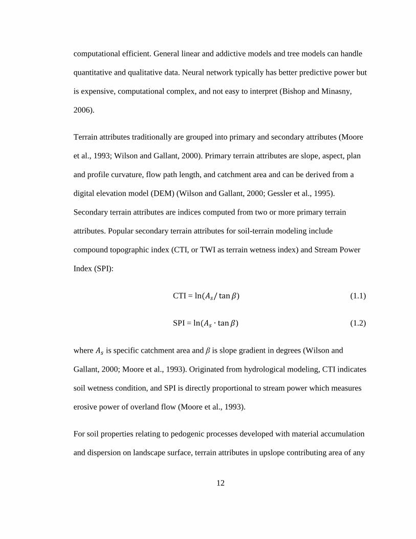
Terrain attributes traditionally are grouped into primary and secondary attributes (Moore

et al., 1993; Wilson and Gallant, 2000). Primary terrain attributes are slope, aspect, plan

and profile curvature, flow path length, and catchment area and can be derived from a

digital elevation model (DEM) (Wilson and Gallant, 2000; Gessler et al., 1995).

Secondary terrain attributes are indices computed from two or more primary terrain

attributes. Popular secondary terrain attributes for soil-terrain modeling include

compound topographic index (CTI, or TWI as terrain wetness index) and Stream Power

Index (SPI):

CTI = ) (1.1)

SPI = ) (1.2)

where is specific catchment area and β is slope gradient in degrees (Wilson and

Gallant, 2000; Moore et al., 1993). Originated from hydrological modeling, CTI indicates

soil wetness condition, and SPI is directly proportional to stream power which measures

erosive power of overland flow (Moore et al., 1993).

For soil properties relating to pedogenic processes developed with material accumulation

and dispersion on landscape surface, terrain attributes in upslope contributing area of any

13

given point location may be more significant than the location itself (Gallant and Wilson,

2000). Compared to the commonly used terrain attributes developed from local

neighborhood of the location (typically in 3-by-3-cell moving window), upslope area

terrain attributes can be viewed as ‘regional’ terrain attributes. Soil-terrain models have

applied mean slope or curvature in individual cells of upslope area, but this type of

‘regional’ terrain attribute is still far less used than the ‘local’ terrain attributes (Wilson

and Gallant, 2000). High computational cost (time and effort) has constrained

development of regional terrain attributes.

Quantitative soil spatial modeling is not limited to using terrain attributes as predictor

variables. Upgraded from Jenny’s (1941) state factor model ‘clorpt’, McBratney et al.

(2003) developed the ‘scorpan’ model – soil (s), climate (c), organism (o), topography (r),

parent materials (p), age (a), and space (n) -- that adds relevant soil properties (s) and

spatial positions for soil spatial prediction. Nevertheless, about 80% of previous studies

used topographic attributes in their final model selection (McBratney et al., 2003; Bishop

and Minasny, 2006).

Terrain attributes used for soil-terrain modeling depend on soil properties of interest.

Table 1.1 lists the selected soil-terrain modeling studies for SOC (Bishop and Minasny,

2006; Minasny et al., 2013). Overall, elevation, slope and CTI are most used predictors

for SOC prediction. Regardless of spatial resolution and areal extents, regression and

regression-based approaches (e.g. regression kriging and regression trees) are the most

popular and effective methods in the spatial prediction of SOC.

Table 1.1 Examples of soil carbon prediction using soil-terrain models and terrain attributes (adapted from Table 7.3 in Bishop

and Minasny, 2006 and Table 1.1 in Minasny et al., 2013).

Reference Terrain attribute

predictors Other predictors Methods

Resolution

(m) Geographic

Area

Area

Extent

(km2)

Arrouays et al., 1995 Distance from upstream Climate data Linear regression 1000 5,000

Bui et al., 2009 Elevation

Climate data,

lithology, moisture

index, soil class Piecewise linear

decision tree 250 Australia 2,765,000

Gessler et al., 2000

Flow direction, CA,

slope, profile & plan

curvature, CTI Linear regression 2, 4, 6, 8,

10

Santa

Barbara, CA,

USA 20.6

Grimm et al., 2008

CA, CTI, LS, slope,

hillslope positions,

profile/plan/mean

curvatures

Parent materials,

soil units, forest

history Random forest 5

Colorado

Island,

Panama

Canal 15

Marchetti et al.,

2010

Elevation, slope, plan

curvature, profile

curvature

Landsat TM

imagery (NDVI,

grain size index,

clay index)

Regression kriging

with principle

components (PCA) 40 Teramo, Italy 100

Mendonςa-Santos et

al., 2010

Elevation, slope, aspect,

plan and profile

curvature, QWETI,

slope Landsat, land cover,

lithology Regression kriging 90

Rio de

Janeiro,

Brazil 44,000

McKenzie & Ryan, Elevation, slope, aspect, Geology map, Regression tree, 25 500

14

1999 SCA, CTI, SPI,

dispersal area, erosion

index, flow direction

climate data, gamma

radiometrics GLM

Miklos et al., 2010 Elevation, plan

curvature ECa, gamma

radiometrics Decision tree 5 IA Watson,

Narrabri 4.6

Minasny et al., 2006 Elevation, slope, aspect,

CTI

Landsat (land use),

gamma radiation

(40

K); Munsell color,

soil texture (for

depth profile) Artificial Neutral

Network 25, 90

Lower

Namoi

Valley, NSW 1,500

Mishra et al., 2010 Elevation, slope

Climate, land use,

parent material

(bedrock), MODIS

NDVI

Geographically

weighted

regression 30 Midwest

USA 658,168

Moore et al., 1993 Slope, CTI Linear regression 15 0.05

Mueller and Pierce,

2003

Elevation, slope, aspect,

plan/profile/tangential

curvatures X, Y

Kriging (ordinary,

with trend model,

with external drift,

cokriging),

multivariate

regression 30.5, 100

Shiawassee

River

watershed,

Michigan 0.12

Munoz and

Kravchenko, 2011

Relative elevation,

slope, total/profile/plan

curvature, flow length,

CTI, solar radiation NIR, aerial

photograph Linear regression 1 Southeastern

Michigan 0.12

Razakamanarivo et

al., 2011 Elevation, slope Boosted regression

tree 30 Central

Madagascar 15.9

15

Kempen et al., 2011 Relative elevation

Land cover, soil

type, drainage,

paleogeography,

geomorphology Linear regression 25 Drenth, the

Netherlands 125

Simbahan et al.,

2006 Relative elevation

Eca, surface

reflectance

(IKONOS), and soil

series Regression kriging 4 Nebraska 0.48; 0.52;

0.65

Thompson and

Kolka, 2005 check Landsat Linear regression 30 Eastern

Kentucky 15

Vasques et al., 2010 Elevation Landsat images Regression kriging 30

Santa Fe

river

watershed,

Florida, USA 3,585

Zhao and Shi, 2010 Elevation, slope, CTI AVHRR, NDVI

Regression kriging,

artificial neutral

network 100 Hebei, China 187,693

16

17

Description of the study

The above literature review confirmed the important linkage between erosion and SOC in

agricultural landscapes and the uncertainty of SOC dynamics and storage under the

influence of soil redistribution at a landscape scale. Based on this review, I challenge the

widely accepted view that agricultural cultivation has led to large quantity of SOC losses

(Figure 1.1). My rejection of this hypothesis is based on two assumptions. First, whole-

landscape SOC accounting is essential in understanding true SOC dynamics. Previous

SOC storage studies focused mostly on uplands and overlooked SOC at the bottom of

hillslopes. In closed-depressional landscapes that have limited water outlets (e.g. rivers),

the quantity of SOC lost in uplands may have simply re-deposited to lower hillslope

positions. Soil redistribution might also have triggered dynamic C replacement in

erosional uplands due to exposure of "fresh" mineral surfaces as well as buried SOC in

depositional lowlands (Figure 1.2), resulting in net whole landscape SOC sequestration.

Second, many SOC studies only measured surface soils (top 5 – 25 cm) and ignored

possible SOC mixing and burial to deeper profiles due to plowing and agricultural

erosion. When measuring whole-profile SOC, change in net SOC storage due to

agriculture may be potentially more conservative than previously estimated.

18

Figure 1.2 Conceptual changes in soil landscapes and soil organic carbon (SOC)

contents in top 1 meter before and after agricultural erosion in closed-depressional

landscapes.

My goal is to understand whether soil has a positive C feedback to agriculture-induced

soil redistribution in depressional landscapes in Minnesota. To achieve this goal, I

investigate the spatial relationship of SOC and erosion-induced redeposition since

European settlement, termed post-settlement alluvium (PSA). Three overall objectives

for this study are to:

1. Identify the spatial distribution and depth and volume of PSA in a closed depressional

landscape at the Lake Rebecca Park Reserve, Minnesota;

2. Determine the spatial distribution of SOC storage change at the Lake Rebecca site; and

3. Assess the change of SOC storage due to erosion-induced redistribution since

settlement.

Erosional site

Depositional site

1m

1m

Current 1m

Current 1 m

Original surface

Original SOC content distribution

Hypothetical SOC change after erosion

SOC

SOC

Current surface (after erosion)

19

Chapter 2 focuses on spatial analysis for the PSA distribution at the Lake Rebecca site

using local and regional terrain attributes. I modeled spatial PSA availability and

thickness based on field study data and digital terrain attributes from 1-m LiDAR-derived

elevation data. In Chapter 3, I developed spatial models to predict SOC contents in four

depth layers, and obtain SOC density in the top 1m of soils. Chapter 4 synthesizes PSA

and SOC spatial information with pre-settlement baseline SOC to determine SOC change

since European settlement in the depressional landscape of Minnesota.

I hypothesize that SOC loss since European settlement is much less than 30-50% losses

observed in many other studies. With dynamic replacement and SOC burial after

agricultural erosion, I expect only a small net SOC loss in a whole depressional landscape

under the influence of PSA deposition compared to the pre-settlement condition.

20

Chapter 2

Spatial predictive models for post-settlement alluvium using

local and regional terrain attributes

2.1 Introduction

Carbon (C) emission and C storage in soil, the largest terrestrial C reservoir, are closely

connected with soil erosion (Pennock and Frick 2001; Van Oost et al., 2007; Van

Hemelryck et al., 2010; Berhe et al., 2007). In erosive agricultural landscapes, soils have

greater potentials to replenish C than in non-eroding environments (Stallard, 1998; Yadav

and Malanson, 2009; McCarty and Ritchie, 2002). The consequences of agricultural soil

erosion to net C feedback to the atmosphere have been an ongoing scientific debate since

the last decade (van Oost et al., 2005, Lal, 2003, McCarty and Ritchie 2002, Jacinthe et

al., 2001, Houghton et al., 1999). Even so, there still remains a high degree of uncertainty

regarding the fate of soil organic carbon (SOC) in erosive landscapes, and the actual C

source or sink term varies depending on the type of basins in the landscape (Berhe et al.,

2007).

In typical dendritic hydrologic networks, the majority of eroded soil materials from

uplands converge towards water channels at the bottom of hillslopes resulting in

deposition in the channels or flowing out of the watershed (van Oost et al., 2005).

However, in closed-depressional landscape, such as the late glacial, ice-marginal area of

the Des Moines lobe in east-central Minnesota, soils eroded from land surfaces are likely

to be deposited within the same landscape because of limited water outlets in this

21

hummocky landscape. Therefore, SOC in the eroded materials is likely to have

redeposited within the depressional landscape instead of moving out of the watershed.

Understanding the re-deposited eroded soil material since settlement, termed post-

settlement alluvium (PSA), in closed-depressional landscapes is essential for

understanding the fate of SOC in erosive agricultural landscapes (Ritchie et al., 2007;

Bedard-Haughn et al., 2006). If PSA accumulates in depressional wetlands, the wetlands’

high organic matter inputs and slow decomposition rates might result in SOC

sequestration in PSA. Figure 2.1 illustrated the conceptual model for SOC and its

relevant processes on an agricultural-influenced depressional landscape. Plant biomass

input, or net primary production (NPP), is the main source of soil organic matter (SOM).

The agricultural upland retains less NPP due to harvest, removal of crop residues, plant

type, and less soil moisture for plant growth. While plowing aerates soils in agricultural

uplands, prolonged saturation in the wetland results in little or no oxygen for microbial

decomposition, leading soil to accumulate SOC. The original C-rich wetland surface soils

may also be buried by PSA and preserved in the subsurface.

22

Figure 2.1 The conceptual model for soil organic carbon and its relevant

processes on an agricultural-influenced depressional landscape.

Soil erosion accelerated by agriculture is orders of magnitude faster than geological

erosion rates (Govers et al., 1994). Although the overall soil carbon storage is known to

increase in response to geological erosion and deposition (Rosenbloom et al., 2006; Yoo

et al., 2005), the effect of accelerated soil erosion on the fate of SOC remains uncertain

(Van Oost et al 2005, Berhe et al 2007). Moreover, most studies on accelerated soil

erosion and deposition were limited to uplands (vs. wetlands) due to the nature of the

typical riverine landforms (open channels at the bottom of hillslopes) and agricultural

land use (mostly in uplands) (Smith et al., 2001; Berhe et al., 2007; van Oost et al., 2007).

Studies usually consider wetlands as a separate system, even where they coexist in same

landscapes. One exceptional study in a hummocky till landscape in Saskatchewan,

Canada investigated wetland SOC storage from agricultural erosion and found the SOC

storage of 168.6 mg ha-1

for uncultivated wetlands within the agricultural area (Bedard-

Ab

Aerobic decomposition

(CO2)

Upland soil (Tilled; O

2-rich)

Erosion

Deposition PSA

NPP

Plant residues

(NPP)

CO2

Wetland soil (Saturated, O

2-limited)

PSA: Post-settlement alluvium; these are sediments redistributed by erosion in the landscape.

Ab: Original C-rich, surface soil that has been buried by PSA.

23

Haughn et al. 2006). The resulting SOC storage was small, most likely due to the short

flow path length, subtle topographic changes, small depressional areas, and relatively low

precipitation in the study site of Bedard-Haughn et al. (2006). In southwestern Minnesota,

restored wetlands were also found to play a role in carbon sequestration in small areas

near the center of the wetlands (Lennon, 2009). I predict that stronger soil redistribution

effects and a higher SOC accumulation are likely to occur in the central to eastern portion

of the Des Moines lobe till region because of the relatively greater relief and higher

precipitation.

Research has approached agricultural soil erosion and redistribution (or PSA) from

various directions. Radionuclide tracing and simulation models have been applied to

quantify erosion rates and their effect on SOC over time (de Alba et al., 2004; Yadav and

Malason, 2009; Richie and McHenry, 1990; Dlugoβ et al., 2011; Gaspa et al., 2013).

Estimation of SOC fluxes were also modeled by the simulation of soil erosion and

redistribution processes (van Oost et al., 2005; Yadav and Malason, 2009). Radionuclide

tracers Cs-137 and Pb-210 were widely applied to estimate soil redistribution that

occurred over the past 50 and 100 years, respectively (Richie and McHenry 1990,

Walling et al., 1995, McCarthy and Ritchie, 2002; Ritchie et al., 2007; Gaspa et al., 2013).

A fallout radionuclide Be-7 has also been used for assessing short-term erosion events,

but it is not suitable for the century-long erosion timeframe from settlement because of

short half-life (53 days) (Walling et al 1999). Be-10 has also been used for sediment

dating but its long half-life (1.5 million years) makes it suitable for studying geological

events rather than anthropogenic disturbances (Balco et al., 2009). Although Cs-137 and

24

Pb-210 can successfully trace medium-term soil redistribution, the equipment cost for

gamma-ray analysis is high, and data collection and processing are both resource- and

time-consuming (Yoo et al., 2006).

It is cost-effective and efficient to use soil profile observations that incorporate soil

pedogenic processes to understand the history of post-settlement alluvium. Dark colors in

surface soils are correlated to organic matter content; in typical pedogenic development a

soil has dark horizons overlying lighter-colored layers (Randall and Schaetzl, 2005).

However if external materials were introduced that covered the original surface horizon,

the darker horizon will be found at depth.

In the past two decades, terrain analysis has been widely applied to model soil property

distributions and to understand soil-landscape functions (Moore et al., 1993; Gessler et al.,

1995; Gessler et al., 2000; Thompson et al., 2006). Based on the catena concept (Milne,

1935), topographic characteristics are the primary factors that drive soil variability at

hillslopes when other soil-forming factors are similar (Grunwald 2005; Thompson et al.,

2006). Topographic relief and other terrain attributes can represent landscape

geomorphology and flow patterns that drive surficial landscape processes like soil

erosion and deposition (Ritchie and McCarty, 2003). During the last decade, more

complex statistical and data-intensive models (e.g. geostatistics, regression tree models

and fuzzy logic) have been used for soil-landscape modeling. However, modeling soil

variability with terrain analysis allows us to understand soil-landscape processes and

topographic drivers behind the dynamic changes of soil properties. Therefore, I chose to

model PSA with terrain analysis using various local and regional terrain attributes.

25

While accepted as an effective soil-landscape modeling technique, terrain analysis is

mostly limited to using ‘local’ terrain attributes. Local terrain attributes are spatial terrain

surface characteristics derived from a digital elevation model (DEM) by a fixed, small-

sized, moving window, typically 3-by-3-cell grids. Because of the small neighborhood

operation, local terrain attributes such as slope and curvature consider only local

topographic surface variations. These local terrain attributes capture the local variation at

sample locations well but do not consider upslope contributions in the entire landscape.

The vital roles of landforms and flow patterns on surficial landscape processes (e.g.

erosion) indicate that surface topography in an upslope dependence area (UA), where

flow originates, has enormous influences on soil morphological development, and thus on

the relevant soil properties (e.g. PSA). The importance of terrain attributes in the UA, or

‘regional terrain attributes’ (in contrast to local terrain attributes constructed using local

neighborhoods in typically three-by-three cell-sized moving window), has been noted

(Grunwald, 2005). However, perhaps due to the technical complexity, approaches to

incorporating true regional terrain attributes have not been developed (Wilson and

Gallant, 2000; Olaya, 2009).

In this chapter, I revisit the terrain analysis method to build a predictive model of PSA

using both local and upslope terrain attributes in a depressional landscape. My research

goals are to identify the spatial distribution and the quantity of PSA and to understand the

controls of terrain attributes on PSA development in depressional landscapes, specifically

the stagnation area of the Des Moines lobe region in Minnesota. The specific objectives

underlying the project goals include:

26

1. Observe post-settlement alluvium in a hummocky landscape with closed

depressions ;

2. Develop spatial datasets of local and regional terrain attributes for post-

settlement alluvium prediction;

3. Build a soil spatial prediction model to assess the spatial distribution of post-

settlement alluvium.

I hypothesize that regional terrain attributes significantly correlate to soil development

relating to water movement on the landscape and therefore they have strong controls on

soil re-deposition (i.e. PSA). While local terrain attributes developed by 3-by-3 moving

windows explain some soil processes, the spatial variance of PSA would be better

captured by combining local and upslope terrain attributes in a spatially-explicit model. I

expect that regional terrain attributes control erosion in upper hillslope areas; local terrain

attributes, on the other hand, drive where and how much deposition can occur.

I hypothesize that both local and regional terrain attributes can explain some of the

variance in agricultural erosion and deposition, and therefore the operative processes.

PSA is expected to accumulate on the lower part of catena, namely the footslope and

toeslope, because slope angles decrease to nearly horizontal at these positions, and water

flow becomes too slow to carry eroded materials farther. Because the UA is the source

area of the eroded materials, regional slope and regional plan curvature are expected to

influence the quantity of sediment eroded and therefore should be significant predictor

variables for the thickness of PSA. Local terrain attributes including elevation, slope

steepness, profile curvature, specific catchment areas (SCA) or compound terrain index

27

(CTI), and the rate change of profile curvature (representing the inflection point on a

catena) are expected to be important predictor variables to PSA presence. Topographic

controls for PSA thickness are expected to include stream power index (SPI), regional

slope steepness and regional plan curvature.

I developed local and regional terrain attributes from a high-resolution (1-m) LiDAR

(Light Detection and Ranging)-derived elevation model in a geographic information

systems (GIS). A two-stage regression analysis method is used with the terrain attributes

to develop spatially-explicit models. The resulting model not only predicts the spatial

distribution and the quantity of PSA in this depressional landscape, but also will help soil

pedologists understand the effects of topographic characteristics on soil processes

relevant to PSA.

28

2.2 Site description

The study site is a moderate hill surrounded by depressional wetlands at Lake Rebecca

Park Reserve in east-central Minnesota (45.05324, -93.7511) (Figure 2.2). The site is

about 6.13 hectare in area, elevation ranges from 279m to 300m above mean sea level

and slopes ranging from 0 to 28.5%. Today the Rebecca site has a typical subhumid,

midcontinental climate with a mean annual precipitation of 691mm. Native vegetation at

the Lake Rebecca site was a deciduous hardwood forest (Marschner, 1974). Conversion

of forests to cropland started in the 1840s during European settlement (Hennepin County,

1873; Dahl, P.M. 1898).

The study area is on the Pine City moraine, an irregular terminal moraine segment of the

Des Moines lobe. The Des Moines lobe retreated from this area around 11,700

radiocarbon years before present. Loamy and calcareous (unless leached) soils have

formed in the unsorted till deposits and the drainage pattern is deranged with many small

depressions and very limited water outlets (Tiner, 2003).

Situated in the prairie-forest transition zone, upland soils at the Rebecca site are

dominated by the Lester series (Mollic Hapludalfs), a forest-based soil with a thick, black

Mollic epipedon developed under prairie vegetation during the warm hypsithermal period

in the mid-Holocene. The marsh on the north of the Lake Rebecca site consists of the

Houghton soil (Typic Haplosaprists), and the wetland on the south to southeast belongs to

the Klossner soil series (Terric Haplosaprists). Soils in the midslope to footslope

29

positions between Lester and wetland soils (i.e. Houghton or Klosser series) are classified

as Hamel (Typic Argiaquolls) (Soil Survey Staff, 2013).

The Rebecca study area was converted from cropland to grassland in the early 1970s

when the current park reserve was established (Larry Gillette, personal communication,

2009). The adjacent wetland in the north, also known as Kasma Marsh, is classified as

semi-permanently flooded, and the wetland in the south-southeast is seasonally flooded

(Cowardin et al., 1979). From aerial photos (the earliest dating to 1937, a period of

drought), we can see that agricultural activities not only occurred on the rolling hills, but

also extended into the surrounding wetlands (Figure 2.3). Row crops were the main land

cover for decades indicating that tillage occurred across the entire Rebecca site. The

Kasma Marsh on the north appeared to be dry enough during the drought period in the

1930s for plowing, but has been getting wetter since that time. By 1969 to 1971, the

Kasma Marsh was no longer in agricultural production (Figure 2.3).

In this study we are interested in post-settlement deposition in depressional landscapes of

Minnesota, particularly in the hummocky margins of the Des Moines lobe in South-

Central Minnesota. The Rebecca Site represents the native environment and development

history of the region.

Figure 2.2 The study site in Lake Rebecca Park Reserve is located on the recently glaciated Des Moines lobe till region

with rolling topography along its margins.

Des Moines lobe

Superior lobe

Rainy lobe

Wadena lobe

0 1,000500KM

0 60 12030KM

30

Figure 2.3 Aerial photos at the Lake Rebecca study site over the period of 1937 to 1984.

1937 1945 1957

1969 1971 1984 31

32

2.3 Methods and materials

The schematic diagram for the approaches and logistics used in this study can be found in

Figure 2.4. I started with field data collection at the Rebecca study area. Terrain data

development was conducted at the Soil and Land Analysis Laboratory in the Department

of Soil, Water, and Climate at University of Minnesota at the same time. Terrain

attributes were used as predictor variables in linear regressions to predict post-settlement

alluvium data for the entire study site. The detailed method will be described in this

section.

33

*A detailed framework for terrain attribute developed can be found in Figure 2.9

$Digital Elevationi Model derived from Light Detection and Ranging, a remote sensing method.

^PSA: Post-settlement alluvium

Figure 2.4 The schematic workflow for the spatial prediction of post-settlement

alluvium.

Field observations and

soil data collection

GPS post-processing and

field data digitization

Stage One: PSA

presence modeling^

1-m LiDAR DEM$

Develop local & upslope

terrain attributes (TA) for

soil-landscape modeling

Terrain Data Preparation* Field Data Collection & Preparation

Stage Two: PSA

thickness modeling^

Estimated PSA volume at field site^

Important TAs for PSA presence on hillslopes

Predicted probability map for PSA presence^

Important TAs for PSA thickness^

Predicted map for PSA thickness^

Terrain Analysis and Modeling

34

Field data collection and post-processing

I described 61 soil profiles on the hillslopes of the Lake Rebecca study site during the

growing seasons of 2009 and 2010. The sampling locations were based on preliminary

observations on-site and were designed to cover a diverse range of (profile and plan)

curvatures and the distances to summit. Thirty-six of the samples were located along 6

transects and followed the stratified-gradient sampling approach of hillslope positions –

summit, shoulder, backslope, footslope, and toeslope/wetland (Figure 2.5). Twenty-five

samples were in the lower hillslope position to capture the hypothesized location of PSA

in footslope and toeslope positions. This specific sampling scheme was designed to

capture important influences of terrain characteristics on PSA accumulation and to enable

spatial PSA modeling. Detail geometry of sample locations is available in APPENDIX A.

35

Figure 2.5 The sample locations at the Lake Rebecca study area in South-Central

Minnesota.

Soil deposition (PSA) information was measured and recorded for all samples at the

Rebecca site. At each sampling location, I used an 8.25cm-diameter soil auger to recover

samples that were placed on clean, flat ground according to depth. In each sample

location, I described the presence and thickness of PSA and described the soil profile

morphology. The PSA layer can be recognized by its distinct soil morphology and color.

Even after continuous surface mixing and burial for more than 150 years, the PSA and

the underlying horizons are still identifiable in the field (Figure 2.6).

36

The boundary between PSA and the underlying original surface horizon was identified by

differences in soil texture, structure, and Munsell color. PSA has a siltier texture because

of its erosional history, a weaker structure and is lighter in color than the underlying Ab

horizon. Denoted by the subscript "b" for "buried", the buried horizon normally has a

darker soil color since it was developed at the surface of a lower, moister hillslope

position than where the PSA sediments originated. Dark colors in surface soils are

attributed to organic matter content decomposed from biomass at the surface. Regular

pedogenic development does not result in darker horizons underlying the lighter layers

unless external materials cover the original surface horizon. These abrupt changes of

horizonation may not be easily observed if PSA is less than 20 - 25 cm in depth due to

soil mixing associated with agricultural plowing.

37

Figure 2.6 A comparison of soil profiles with and without post-settlement alluvium

(PSA) at the Lake Rebecca site. (a) A soil profile in upland (Sample #029) with no PSA

shows a typical soil color change with reduced values and hues over the depth profile; (b)

A soil profile in a toeslope position (Sample #012) with PSA observed by an abrupt

darkness increase as well as soil structure and/or texture changes in the buried A horizons.

I recorded latitudes and longitudes for soil sample locations in geographic coordinates

with the datum of WGS 84 using a professional-level handheld differential Global

(a) Soil profile without PSA (b) Soil profile with PSA

38

Positioning System (GPS) (Magellan® MobileMapper™ 6). The geographic information

in the GPS device was uploaded and post-processed for differential corrections upon

return from field data collection. Using daily geodesy data for the closest base station(s)

with known GPS position(s), differential correction improves the horizontal accuracy of

sample GPS locations. The base station I used is the closest reference station in the

Minnesota Continuously Operating Reference Station (MnCORS) Networks -- either

Hollywood (44.905833, - 93.986666) or Golden Valley (45.000555, - 93.351388),

depending on availability at the time of data processing. After differential correction, the

horizontal accuracy is less than a meter (Magellan Professional, 2006).

A rough vegetation survey was also conducted at Lake Rebecca site. The coordinates of

various major wetland vegetation species, including cattails (Typha angustifolia, Typha

latifolia or hybrids), sedges (Cyperaceae) and willows (Salicaceae), were recorded using

GPS. I used the vegetation survey to estimate the spatial extent of PSA assuming that

PSA deposition ended near the wetland boundary. This boundary was difficult to

measure in the field; I assumed that PSA stopped at substantial plant barriers near

submerged surfaces and I used vegetation boundaries as the limit of PSA in the catena.

Cattails were considered to be the most effective barrier but tree species such as willows

were also counted. I recorded these vegetation locations using the differential GPS device

and re-digitized the boundary in ArcGIS after post-processing.

Development of digital terrain attributes

I downloaded the 1m-resolution LiDAR-derived Digital Elevation Model (DEM)

39

covering the spatial extent of the Lake Rebecca Park district using Filezilla, an FTP client

program. The LiDAR data in this region were collected in 2011 and acquired during the

Metro phase of a statewide Minnesota Elevation Mapping Project (Minnesota Geospatial

Information Office, 2012). The horizontal accuracy of the LiDAR DEM meets or exceeds

a RMSE of 0.6m; the vertical accuracy meets the National Digital Elevation Program

guideline requirements of a RMSE of 12.5cm, and is reported by Minnesota Department

of Natural Resources (DNR) as having a true accuracy level of ±5cm (Fugro Horizons,

Inc. and MN-DNR, 2011).

I smoothed the 1-m DEM twice using low-pass filter in the GIS software ESRI® ArcGIS

10.0. in order to fill unrealistic pits and remove artifacts resulting from mechanical errors

during data measurements and processing, Next, I used the smoothed DEM to derive the

spatial databases of local terrain attributes relevant to landscape surface processes. These

terrain attributes include both primary terrain attributes—slope steepness(%), flow path

length (m), profile curvature, plan curvature, the rate change of profile curvature,

specific catchment area (or SCA, m2)—and secondary terrain attributes—compound

topographic index (or CTI, also known as wetness index), and stream power index (or

SPI ).

Besides numerical attributes, profile and plan curvature datasets were also categorized

into three classes—concave, convex, and straight—using thresholds suggested in ArcGIS

10 (ESRI, 2013). The classification criterion was illustrated in Table 2.1. Cell with values

between -0.5 to 0.5 in both profile and plan curvature gridded data are classified in the

'straight' category. For profile curvature, values equal or less than -0.5 are classified as

40

‘convex’ and greater than +0.5 are ‘concave’. For plan curvature, the classification is

reversed on the +/- signs, where values greater than +0.5 are classified as ‘convex’ and

those equal or less than -0.5 are classified as ‘concave’ (Table 2.1).

Table 2.1 The illustration for the classification criteria of profile and plan curvature.

Convex (x) Concave (v) Straight (f)

Profile Curvature - (< -0.5) + (> 0.5) between -0.5 & 0.5

Plan Curvature + (> 0.5) - (< -0.5) between -0.5 & 0.5

I also added a new attribute, the first derivative of the profile curvature, to identify the

inflection point in a catena. This defines the rate change of profile curvature. The

inflection point of a hillslope is where surface changes from convex to concave, and I

expect the inflection point to be a critical location where erosion switches to deposition

(Figure 2.7).

41

Figure 2.7 A hillslope with the hypothetical inflection point, where a soil surface

changes from erosive (convex, steep) to potentially depositional (concave, mildly sloping

to flat) on a catena.

Because surface landscape processes in erosive uplands control the amount and the

quality of soil materials being delivered to depositional sites, topography in the UA is

potentially influential in the spatial distribution and the quantity of PSA in landscapes. So,

in addition to using local terrain attributes, I developed a procedure to generate the

upslope dependence area terrain attributes (UDTA) for soil-landscape modeling. The

raster-formatted UA, defined as the area from which water flows to a defined outlet, is

commonly used in hydrologic modeling but less so in soil-landscape modeling (Eddins,

2009). The diagram in Figure 2.8 illustrates the logistics of the UDTA development. I

created UA for all sample locations using a multiple flow-direction (MFD) algorithm in

the open-source software SAGA-GIS (Cimmery, 2010). In order to obtain UAs for the

sample locations, I defined the coordinates of my sample locations as the outlet points in

this study.

The inflection point of a catena Convex, steep in slope

Concave, flat

42

Figure 2.8 The schematic diagram for the development of upslope dependence terrain

attributes (UDTA).

43

The MFD algorithm used for calculating spatial UA grids in SAGA-GIS is modified from

the conventional single flow-direction algorithm D8. Also known as FD8, the MFD

algorithm allows water to flow from processing cells in multiple directions downslope,

which more closely simulates natural flow processes across landscapes than D8 (Freeman,

1991; Olaya and Conrad, 2009). I exported the MFD-based UA grids as ESRI ASCII files

to ArcGIS 10 and selected only cells with greater than 1% of accumulated flow

contributing to the target location for PSA modeling. The constrained UA grids were then

used as masks to extract slope, profile curvature and plan curvature using the scripting

language Python with Arcpy packages and Spatial Analyst extension in ArcGIS 10.

I created summary statistics and histograms of slope and curvature values at the UA cells

for each sample location. In order to obtain attribute tables from these floating-point

raster data, the UA slope and curvature gridded databases were converted to integer grids

before generating attribute tables and descriptive statistics. Significant digits of the

gridded UDTA cell values were preserved by multiplying the values in order of

magnitudes (i.e. 1000) prior to integer conversion. The descriptive statistics, however,

showed UA slope and curvature cells for individual sample locations were not all

normally distributed. To use a digital terrain attribute as a predictor variable in

regression analysis requires one representative value for each sample location. The

UDTA histograms for my samples did not have consistent patterns (skewed to the right,

to the left, or normally-distributed), so using the means and standard deviations of UDTA

for regression modeling would not be optimal.

During this UDTA exploratory analysis, however, I observed some relationships between

44

PSA thickness and UDTA thresholds. My preliminary data analysis showed significant

correlations between PSA thickness and area with the area (m2) and percentage area of

UA slope and UA curvature in thresholds. These were therefore used as regional terrain

attributes in spatial modeling of PSA.

The idea behind using UA slope in thresholds (e.g. the area of UA in slope greater than

6%) as regional terrain attributes is the possible control of critical slope steepness to the

flow-relevant soil properties in a specific landscape. I defined slope thresholds as 4%,

6%, 8%, 12%. These values were selected from the literature as well as the

recommendations of field soil scientists. Slope angles of 4% and 8% had been used for

soil landform classification in literature (Brabyn, 1996), and 6% of slope was suggested

by the USDA-NRCS Soil Survey team as the key slope threshold in finding soil

deposition on hillslopes in similar landscapes in this region (John Beck, personal

communications, 2012). I added 12% as a cut-off steep slope threshold.

After splitting UA grids by the above-mentioned slope thresholds, I calculated the areal

extent for each slope category (<4%, >=4%; <6%, >=6%; <8%, >=8%; <12%, and

>=12%) using Python scripts. The threshold-split UA grids are also floating-point raster

data without attribute information. I obtained the raster data area information (m2) by

converting the data to integer grids prior to getting attribute data and calculate statistics.

In addition to the previously mentioned slope categories, the sizes of UAs in the slope

ranges between 4-8% and 8-12% were also calculated as potential predictor variables in

PSA modeling. Similar steps were taken for obtaining UA in thresholds of profile

45

curvature and plan curvature. I used the three curvature categories as thresholds for UA

profile and plan curvatures: straight, concave and convex.

As previously mentioned in Section 2.1, the development of regional terrain attributes

(UDTA) is computationally challenging and thus time- and resource- consuming. While

recent GIS advances in hydrological modeling simplify UA development, I was only able

to create UDTA for sample locations. Without mapping UDTA for cells in the entire

spatial extent of the study area, the PSA models with UDTA are limited in their use to

understanding the relationships between PSA and UDTA (explanatory). I will not be able

to predict the spatial distribution of PSA at the Lake Rebecca site using the UDTA-

related PSA models. Further development of the UDTA automation will depend on the

usefulness of the attributes tested herein.

Two-stage regression analysis method

I examined summary statistics and the frequency distribution of PSA and both local and

regional terrain attributes at sample locations using the statistical language R. Since local

and regional terrain attributes were all derived from a single source, the LiDAR DEM, I

was aware of potential collinearity issues in this soil-landscape modeling. Predictor

variables were selected carefully to avoid high collinearity issue.

Forward and backward stepwise multiple linear regression was applied to fit PSA

thicknesses for all samples (n=61) at the Lake Rebecca. The best-fit models were

constructed by local and regional terrain attributes together (as ‘the mixed models’) and

46

separately. All three types of regression models (local, regional, and mixed) helped

identify topographic drivers and related soil processes for PSA. The high processing time

involved in developing UDTA for all cells, mixed and regional models does not allow the

prediction of PSA. Spatial prediction models will be built using only local terrain

attributes as predictor variables (Table 2.2).

Table 2.2 The usefulness of predictor variable types in regression modeling for

landscape soil processes.

Use Terrain attribute categories

Local

(the 3-by-3 cell

neighborhood)

Regional

(upslope areas)

Understanding soil processes √ √

Predicting soil properties √

The best local terrain variables for modeling PSA thickness are elevation, CTI, SPI, and

SlpProfile with an adjusted R2 of 58.87%. All partial correlation coefficients in the

regression model were statistically significant with the confidence interval (CI) of 90%

(p-values < 0.10). However, when evaluating the residual scatterplot of the model, I

found a clear linear pattern, indicating that the estimates from the regression model did

not capture some predictable trend. The regression was not valid because it violates the

random error requirements for linear regressions. The investigation of my data showed

that several PSA-absent samples (PSA = 0) had non-zero PSA predictions in the

regression model, and the large number of soil samples (29 out of the total 61 samples)

47

with no PSA (PSA = 0) may have destroyed the predictive power of local terrain

attributes to PSA in the regression model. To remove the linear pattern in the residuals

and predict PSA properly, I updated the PSA modeling to a two-stage regression analysis

(See diagram in Figure 2.4).

The purposes of two-stage regression analysis method were to: 1) Identify where PSA is

present, and 2) estimate PSA thickness where it occurred. At Stage 1, I used a logistic

regression to predict the probability of PSA presence. The dependent variable in the

logistic regression is ‘PSA presence’ (1= PSA present, 0=PSA absent). The binomial

distribution was fitted with local and/or regional terrain attributes in a generalized linear

model (the glm() function in R) to develop the predictive and explanatory models of PSA

presence.

Logistic regression, also known as logit function, transforms the odds of PSA presence or

absence (a range between 0 and 1) from an S-curve to a straight line by taking the natural

logarithm of the odds:

logit (p) = ln (p/(1-p)) = β0 + β1 X1 + β2 X2 +… + e (2.1)

where p is the probability of PSA presence, Xi are predictor variable with partial

regression coefficients βi, and e is the error term.

A total of 61 sample point data were used in the spatial prediction of PSA presence with

local terrain attributes using logistic regression. However, I encountered problems

generating reasonable UA grids at toeslope locations and could not apply all sample data

48

to the mixed model (using local and regional terrain attributes). The UA grids were

derived from the 1-m LiDAR DEM, at several toeslope sample locations and contain

unreasonably low cell numbers. Trivial elevation changes (less than 0.1m or even 0.01m)

in the source data between neighboring cells were likely picked up during UA

development process. Seven samples (009-DEP, 015-TOE, 020-TOE, 1E, 4E1, 4E3, and

7E) at toeslope locations with UA less than 100 cells were removed prior to the mixed

model regression.

For the logistic regression models of PSA presence, I selected predictor variables based

on stepwise regression and the regsubsets( ) function in the ‘leaps’ package in R. The

regsubsets function performs an exhaustive search on independent variable combinations

and returns the best subsets of independent variables based on estimated R2 or Bayesian

information criterion (BIC). By running the regression function glm( ), I confirmed best-

fitted model(s) that have the lowest Akaike information criterion (AIC) with 90% of

significance level (p-values < 0.10). As logistic regression is not an OLS regression but

an estimator of maximum likelihood, it does not actually have a true R2 to explain the

variance captured as a linear regression. I used AIC to select best-fitted models but

reported a pseudo R2 for the common understanding. AIC, calculated as -2 * ln(likelihood)

+ 2K (K as the number of free parameters in the model), is a criterion that seeks a model

with a good fit while considering the number of predictor variables used.

My preliminary logistic regression shows that elevation is the sole variable controlling

the presence of PSA, yet the use of absolute elevation as a predictor variable limits the

model transferability. Local elevation represents the relative potential energy in hillslope

49

positions of a catena, and therefore it is expected to be significant in landscape soil

properties like soil erosion. However, absolute elevation is not a transferable variable

outside of this study area. Each basin has different elevation ranges; the same absolute

elevation may not represent the same hillslope positions and therefore may have different

sediment accumulation capacity in different basins. To make our spatial PSA model

applicable to other areas of interest in similar geological settings, I replaced absolute

elevation with another variable, relative elevation. Typically calculated by subtracting

local minimum elevation within a defined watershed from absolute elevation for each cell,

it is difficult to define watershed boundary for closed-depressional landscapes in the GIS.

With no suitable flow algorithms for depressional landscapes, I calculated local minimum

elevation within a moving window of 200-m radius circular neighborhood using a focal

statistics function in ArcGIS. The radius was selected by trials for the Lake Rebecca area.

Local minimum elevation remains almost identical when the neighborhood processing

window in the GIS has a radius greater than 200m.

Once the best-fitted PSA presence model was selected, I evaluated the model

performance by calculating its prediction accuracy as well as by using a 10-fold cross-

validation. Then I generated a predictive probability map for PSA presence. There are

various ways to interpret logistic regression results (e.g. odds ratio, predicted probability);

because I am interested in the spatial distribution of PSA, I assessed the predicted

probability for PSA presence. The probability (p) of the PSA presence can be back-

transformed firstly to odds ratio:

p /(1-p) = Exp (β0 + β1 X1 + β2 X2 +…) (2.2)

50

then, rearranging the odds ratio Eq. (2.2) to probability as:

p = Exp (β0 + β1 X1 + β2 X2 +…) / [1+Exp (β0 + β1 X1 + β2 X2 +…) ] (2.3)

Based on Eq. (2.3), I mapped the probability distribution of PSA presence at the Lake

Rebecca site. I defined the zone of PSA presence on the map by determining the

probability threshold. Using the agreement of the observed samples, a 50% probability

(the area with 50% chance to contain PSA) would be the minimum threshold I would use

for defining the spatial distribution of PSA presence on the map, and a higher probability

is preferred.

Samples located within the PSA presence area from the result of Stage 1 analysis were

selected for Stage 2 analysis. In Stage 2 analysis, I used a multiple linear regression

method (MLR) to model the spatial distribution of PSA thickness. The number of

samples used in this stage depends on the predicted probability map of the PSA presence

and the chosen percentage probability threshold. By modeling PSA thickness without

PSA-absent samples, I expected the MLR residuals to be randomly distributed with a

mean of zero.

Similar to the procedure for Stage 1 logistic regression analysis, the selection of predictor

variables for Stage 2 MLR used stepwise regression and the regsubsets function in R. I

looked for both local and mixed models of PSA thickness with good fit. While not strictly

predictive, regional terrain attributes help illuminate the pertinent soil erosion and

deposition dynamics in this depressional landscape. A spatial map of PSA thickness was

generated for the area predicted to have PSA present at study site.

51

Model performance and validation were done after the two-stage models were chosen.

The model performance included root mean squared error (RMSE) and mean absolute

error (MAE) for the local and mixed models of PSA presence (Stage 1) and PSA

thickness (Stage 2). The residual analysis, including residual scatterplots with the locally

weighted scatterplot smoothing (LOWESS) line, normalized quantile-quantile plots

(qqplots), and density plot, were also used to evaluate if regression assumptions were met

in these models. A 10-fold cross-validation (CV) method was also applied to validate the

regression models from the two-stage regression analysis.

The k-fold CV method avoids overfitting and estimates the predicted errors for both

logistic regression and multiple linear regression. This validation technique splits the

total samples into ‘k’ equally and mutually exclusive sub-groups and trains the model k

times. In each run, one sub-group is left out as the testing dataset and the rest of

subgroups (k-1) are the training data for the model development. As a result, the model

would be tested for ‘k’ times, with all of the samples being used in the training and at

least once in the validation test. The k-fold CV method is beneficial to the small sample

size (e.g. the PSA dataset in this project) without taking away model datasets (training)

for the validation (testing) purpose. For the balance between the error variance (increase

when k is large) and the estimator bias (increase when k is small), I used 10-fold cross-

validation in this project. Ten has been proven to be an effective number of folds in this

cross-validation technique (Borra and Di Ciaccio, 2010).

52

Estimate the amount of post-settlement alluvium

Estimating the volume of PSA present at study area requires the both the areal extent (X,

Y) and depth (Z). The upper hillslope boundary of PSA is available from the predicted

probability map of PSA presence (the result of Stage 1 analysis); the depth boundary of

PSA is the PSA thickness map resulting from the Stage 2 regression analysis. In order to

close the loop for calculating the spatial area (m2) of PSA, I estimated the lower hillslope

boundary of PSA as being near the wetland edge using the field vegetation survey. The

volume of PSA was estimated as follows:

PSA volume (m3) = [PSA presence area (m

2)] * [PSA thickness (m)] (2.4)

2.4 Results and discussion

Field observations of post-settlement deposition

The observed PSA at the 61 sample locations ranges from 0 to 80 cm in depth (Table 2.3;

Figure 2.9). The average of PSA is 23.5 cm deep and 29 out of the 61 sample locations

had no observed PSA (PSA thickness = 0). As expected, the 32 PSA-present sample

locations are located at footslope and toeslope positions (Figure 2.10). The thickness of

PSA is consistently greater than 25 cm except in the wetland which was 18cm deep. The

depth (25cm) aligns with the common plowing depth in agricultural landscapes,

suggesting that active mixing by plowing (and maybe other bioturbation) at the

deposition locations has made it difficult to distinguish PSA shallower than 25cm in

depth. Mean and median of the PSA thickness (23.49cm and 20cm, respectively) do not

53

accurately reflect the actual distribution of PSA thickness at PSA-present locations

because nearly one half of the sample locations do not have PSA present (PSA=0).

Table 2.3 Descriptive statistics for the thickness of post-settlement alluvium (PSA)

at Lake Rebecca study site.

Summary Statistics PSA Thickness (cm)

Number of samples 61

Number of zero values 29

Min. 0

Max. 80

Range 80

Median 20

Mean 23.49

Standard deviation 25.70

Figure 2.9 Boxplot and the frequency distribution of post-settlement alluvium (PSA)

thickness.

54

Figure 2.10 The observed post-settlement alluvium (PSA) thickness at Rebecca site.

All PSA were found in footslope and toeslope positions in the landscape.

Local and regional terrain attributes

The spatial datasets of local terrain attributes at the study area are displayed in Figures

2.11-2.19. These local terrain attributes include relative elevation, slope, profile curvature,

plan curvature, slope of profile (the rate change of profile curvature to capture the

inflection points on catena), flow path length, specific catchment area (SCA), compound

topographic index (CTI) and stream power index (SPI). All attribute data are floating-

point raster datasets determined for 1-m cells. Relative elevation ranges from 0 to 17.1 m

55

at the Rebecca site (Figure 2.11). The values of relative elevation are highest at the ridge

top in the west and decrease slightly to the ridge extended to the east before dropping

quickly downhill to the surrounding wetlands (relative elevation ~ 0). In Figure 2.12, the

spatial distribution of slope shows that areas with slope steeper than 15% are situated in a

band on backslope positions surrounding the east-west oriented ridge across the center of

the Rebecca site, and also on a small north-south band between two summits with

different elevation in the west part of the ridge.

For the spatial distribution of profile curvature (Figure 2.13), convex profile curvature

dominates the western ridge top and the shoulder positions. About half way downslope to

the wetlands in the north, northeast, and southeast, concave profile curvature dominates.

Plan curvature shows where flow converges (at concave locations) and disperses (at

convex locations) across the hill (Figure 2.14). Convexity is more dominant at the east

and there are two main concave lines (flowlines) north of the hill. At the bottom of the

hillslope, plan curvature still displays many bumps (convexities) and dips (concavities).

These are likely very small changes captured by the high resolution DEM and may not be

meaningful if eroded sediment moves through them downhill by overland flow. Note

that the maps of plan and profile curvature both contain some striping (Figure 2.13 and

2.14). These are likely artifacts produced during the LiDAR data collection or DEM

processing. This type of error should not affect the overall analysis.

56

Figure 2.11 The distribution of relative elevation at the study area.

Figure 2.12 The spatial distribution of slope steepness at the study area.

57

Figure 2.13 The spatial distribution of profile curvature at the study area.

Figure 2.14 The spatial distribution of plan curvature at the study area.

58

The slope of profile curvature is illustrated in Figure 2.15. As expected, the patterns of

this derivative of profile curvature show a change in the curvature toward the bottom of

the hillslope. Some large rates of change of profile curvature can also be seen between

two summits on the ridge top at the west-central part of the study area. Figure 2.16 is the

flow-path-length map of the study area. The flow-path length ranges from 0 to 227 m and

displays concentric circle patterns on the map. Note that flow-path length becomes

random and problematic at the bottom of the hillslope where the flow disperses. The

specific catchment area (SCA) in Figure 2.17 clearly illustrates the overland flow patterns.

SCA ranges from 0 to 7,210 m2. The CTI and SPI, the two indices derived from slope and

SCA, are also displayed in Figure 2.18 and 2.19. The CTI, the wetness index, seems to

emphasize major flow patterns similar to the SCA. The SPI map displays the stream

power, which is very low in summit and toeslope positions.

59

Figure 2.15 The rate change of profile curvature at the study area.

Figure 2.16 The map of flow-path length at the study area.

60

Figure 2.17 The map of specific catchment area at the study area.

Figure 2.18 The map of compound topographic index (CTI) of the study area.

61

Figure 2.19 The spatial database of stream power index (SPI) at the study area.

As for regional terrain attributes, here I showcase the spatial distribution of slope and

curvature at the UA for individual sample points in one transect (Figure 2.20 and Figure

2.21). Depending on samples’ hillslope positions and landforms, upslope dependence

areas vary in size and shape. The size of the UA increases as its elevation on the hillslope

decreases. However, in Figure 2.21, the UA in a summit position is unexpectedly large.

This error may have resulted from the sensitivity of the high-resolution source DEM; tiny

surface changes on top of the hill were picked up during the UA processing.

62

Figure 2.20 An example transect of sample locations at study site (with vertical

exaggeration).

- High: 298.7 m

- Low: 281.6 m

004-TOE

023-FOOT

025-FOOT

026-BACK

027-SUM

N

Figure 2.21 The spatial distribution of the upslope areas’ slope and curvature grids at sample locations of a hillslope transect

(shown in Figure 20).

0 - 1 %

1.1 - 3 %

3.1 - 5 %

5.1 - 8 %

8.1 - 11 %

11.1 - 15 %

15.1 - 28.5 %

Concave

Straight

Convex

Concave

Straight

ConvexPla

n C

urv

atu

re

Pro

file

Cu

rvatu

re

Slo

pe

Summit (027) Backslope (026) Footslope1 (025) Footslope2 (023) Toeslope (004)

(a)

(f)

(k)

(b) (c) (d) (e)

(g) (h) (i) (j)

(l) (m) (n) (o)

63

64

As described in Section 2.3, the actual regional terrain attributes (UDTA) used in this

study were developed using the UA terrain thresholds. The regional terrain attributes,

defined by the UA slope and curvature thresholds in percentage (%) and in areas (m2),

were combined with local terrain attributes in building the explanatory PSA models.

Stage 1 analysis results: Logistic regression model for PSA presence

The best-fit logistic regression model for PSA presence prediction consists of the

variables: relative elevation, flow path length, and stream power index (SPI) and can be

defined with the following equation:

logit (PSA presence)local = 17.27 – 4.39 * [Relative elevation] – 0.08 * [Flow path length]

+ 0.97 * [SPI] (2.5)

This local PSA presence model has the lowest AIC of 29.6 and the highest pseudo R2 of

85.8% compared to models built with other combination of terrain attributes. All partial

regression coefficients and the logit model as a whole are significant at a confidence level

of 90% (p-values < 0.10). A similar amount of variance can be explained by replacing

SPI with CTI in the logistic regression model (AIC=30.342; pseudo R2 = 85.2%).

Compared to the predictive model Eq. (2.5) built with local terrain attributes, the best-fit

explanatory Logit models for PSA presence increased pseudo R2

by a mere 1.4% to

87.2%. The model for explanatory purpose is the mixed model consisting of both local

and regional terrain attributes (UDTA). The mixed model has an AIC of 23.5 and consists

65

of two predictor variables, the relative elevation and the percentage of the upslope area

with convex profile curvature:

Logit(PSA Presence)mixed = 1.83 – 5.15 * [Relative elevation] + 0.28* [%upslope area in

convex profile curvature] (2.6)

One of the mixed models that used three predictor variables (relative elevation, flow path

length and % upslope area in concave profile curvature) performed slightly better (AIC

=23.2; R2 = 89%). The mixed model in Eq. (2.6) has only two predictors so I chose it for

its simplicity and the still outstanding model performance.

As for individual predictor variables, relative elevation is the single most significant

terrain attribute for modeling the presence of PSA. When predicting PSA presence by

relative elevation alone, I obtained the logit model results with an AIC of 37.72 and a

pseudo R2 about 75.3%. Measured by elevation difference from the minimum elevation

in a 200-m radius local neighborhood, relative elevation is the quantitative measurement

for hillslope positions, and thus provides information about distinct water accumulation

and mass movement at each location on a catena. The negative relationship between

relative elevation and PSA presence indicates that a lower hillslope position has a higher

probability to contain PSA.

Besides relative elevation, flow path length and SPI are the terrain attributes controlling

the presence of PSA in the landscape. Flow path length has a small and negative

relationship with PSA presence. However, I hypothesized that the flow path length

should have positive relationship with PSA presence. Conceptually, the longer the flow

66

path, the greater the overland flow accumulates at the sample location. Investigated

visually on the spatial database, I found that the values of flow path lengths at toeslope

locations abruptly decrease and then restart from zero (Figure 2.16). This demonstrates

the inability of the current flow algorithms to handle depressional landscape properties.

When water flows to the flat bottom of a hillslope the flow should be dispersed; current

flow algorithms (e.g. F8, D-infinite, MFD and etc.) do not know how to assign values to

flat zones. Nonetheless, flow path functions correctly in uplands and this method will still

be used in the PSA modeling.

It is no surprise that SPI is one of the significant variables for predicting the spatial

distribution of PSA presence. SPI displays the rate that flowing water’s energy is

expended in the landscape, so it represents the erosive power of overland flow (Moore et

al 1993). CTI has a similar effect in combination with relative elevation and flow path

length to PSA presence too. CTI categorizes the surface saturation zones and is known as

the wetness index (Borough et al 1998). A site with a large CTI that accumulates surface

water would be expected to be where sediments (PSA) deposit.

In terms of upslope terrain control, the mixed model Eq. (2.6) indicates that upslope

profile curvature is a significant regional terrain attribute, and is a good predictor of PSA

presence in a logistic regression when coupled with relative elevation. In fact, the

regression analysis showed that the UA percentage in a convex profile curvature is the

second most important terrain attribute (next to relative elevation) that drives PSA

distribution in this landscape. Convex profile curvature in the UA is significant with a

positive partial regression coefficient when coupled with relative elevation. This suggests

67

material is eroded where profile curvature is convex and this drives the downhill

development of PSA in a catena.

This relationship can be also identified from the negative partial coefficient when

choosing ‘upslope area percentage in concave profile curvature’ as the predictor variable

(the model is not shown here). The UDTA-only models fit well using the variables UA

with slope greater than 12% and UA with concave plan curvature. The positive partial

coefficients of these predictor variables (not shown) indicate that steep slope angles and

concave plan curvature in the UA drive the development of PSA. While steep slope

triggering erosion is to be expected, I did not expect a positive relationship with concave

plan curvature in the UA. I suspect that these areas of UA with concave plan curvature

are cells right above sample locations where PSA is deposited. Further analysis is

required to understand the details of UA terrain attribute distributions and their

relationship to PSA development.

Based on the PSA presence model Eq. (2.5), I developed a probability map for the

presence of PSA (Figure 2.22). Recall that logistic regression predicts the chance of a

binary distribution (1 or 0), and the probability of the PSA presence can be predicted by

converting the resulting odds ratio to the probability Eq (2.3). The probability map

(Figure 2.22) clearly shows PSA being present at the bottom of the catena. The map also

shows that PSA was completely absent in the uplands (0-10% probability, shown in blue).

The zone with ≥ 90% probability of occurrence (shown in red) covers a broad area near

the bottom of hillslopes. In comparison, the probability of PSA presence between these

68

extremes (10-90% probability) appears to cover a very narrow band on the hillslope. I

used 90% probability as the threshold in determining where PSA is present.

Figure 2.22 The predicted probability map for the presence of post-settlement alluvium.

0 - 0.1

0.1 - 0.2

0.2 - 0.3

0.3 - 0.4

0.4 - 0.5

0.5 - 0.6

0.6 - 0.7

0.7 - 0.8

0.8 - 0.9

0.9 - 1

PSA Presence

Probability

69

70

During model evaluation, prediction accuracy and cross-validation both proved to be in

good agreement for the PSA presence model selection (Table 2.4 and Table 2.5).

Prediction accuracy was only tested for the predictive (local) model, not the explanatory

one (the mixed model). Using 90% as the minimum acceptable probability to count on

PSA presence, the overall correctness of the model is 86.9%, (Table 2.4). More

specifically, the PSA presence model correctly predicted 96.6% of the PSA-absent

samples and 78.1% of the samples with PSA present. As for the 10-fold cross-validation,

the predictive and explanatory models of PSA presence both demonstrate very high

estimated accuracies (88.5% and 90.7%, respectively) (Table 2.5).

Table 2.4 The percentage accuracy for the predictive model of PSA presence.

PSA presence Predicted (Prob. ≥ 90%)

Observed No (0) Yes (1) Total % Correct

No (0) 28 1 29 96.6

Yes(1) 7 25 32 78.1

Total 35 26 61 86.9

71

Table 2.5 The predictive and explanatory models for the PSA presence.

Stage 1

Regression

Analysis

Predictor Variables N Pseudo

R2

10-fold Cross-

Validation Estimated

Accuracy

Training Validation

PSA

Presence –

Prediction

(Local)

1) Relative Elevation

2) Stream Power

Index

3) Flow Path Length

61 85.8% 0.918 0.885

PSA

Presence –

Explanatory

(Mixed)

1) Relative Elevation

2) % Upslope Area

with Convex

Profile Curvature

54 87.2% 0.926 0.907

Stage 2 analysis results: Spatial prediction for PSA thickness

After matching sample locations with the spatial distribution of PSA presence (in the

threshold of 90% probability), I reduced the sample number to 26 for Stage 2 analysis

(Figure 2.23). The 26 samples, therefore, were all predicted to contain PSA (PSA

thickness ≠ 0). However, one of the selected samples (021-TOE) was not observed to

have PSA (PSA thickness = 0). Overall, the PSA thickness ranges from 0 to 80 cm, with

a mean of 45.81 cm and a standard deviation of 19.38 cm (Table 2.6). More than half of

the samples used during Stage 1 analysis (PSA presence) were not included in Stage 2

(PSA thickness) since they fell out of the zone that has over 90% probability of PSA

presence.

72

Figure 2.23 Samples contained in the area with over 90% probability of having PSA

present were used for Stage 2 Analysis on PSA thickness.

#* Stage 2 samples

PSA presence zone

73

Table 2.6 Summary statistics of PSA thickness for the samples spatially located

within the predicted PSA-present area.

For the mixed model analysis, only 19 samples out of the 26 were used. I filtered out

seven samples for Stage 2 analysis because their UA were too small (≤ 100) to be

reasonable. The small UA size was likely caused by the source data (1-m LiDAR DEM)

being highly sensitive to minor elevation variations in ground surface.

Using multiple linear regression, Stage 2 analysis developed the best-fit model for PSA

thickness and it had two predictor variables: plan curvature in three classes, straight,

concave and convex; and specific catchment area (in natural-log):

PSA thickness-local (cm) = 11.214 - 5.506 * [Concave Plan Curvature (categorical)] +

29.962 * [Convex Plan Curvature (categorical)] + 10.046* [Log-transformed Specific

Catchment Area] (2.7)

This local PSA thickness model has an adjusted R2 of 41.3% (p-value = 0.001975). This

means that although plan curvature and SCA are the best variable selection among local

n Mean Standard

deviation

Median Min

26 45.81 19.38 44 0

Max Range Skewness Kurtosis Standard

Error

80 0-80 0.05 -0.49 3.8

74

terrain attributes, only approximately 41% of variance in PSA thickness can be accounted

for by this set of variables.

While plan curvature is a significant predictor for PSA thickness, it is only true for

categorical values (convex, concave, and straight), not for numerical values. The

numerical curvature data are not significant; the number distributions are not as related to

PSA as when they were categorized into only three classes. A similar adjusted R2 (41.6%)

was found on another local model comprised of CTI, the rate change of profile curvature,

and plan curvature. In comparison, Eq. (2.7) only uses two predictor variables, plan

curvature and SCA. For simplicity, I chose the two-parameter model over the alternative.

Compared to the local model that has less than half of the variance accounted for (R2 <

50%), the mixed and regional models do a much better job of explaining the variance in

PSA thickness at the study site. The best-fit mixed models returned an adjusted R2 of

73.8%, a 32% increase over the regional terrain attribute model. The overall best PSA

thickness model is comprised of SCA (in natural log), the UA with 8-12 % slope, the

percentage of the UA in flat profile curvature, and the percentage of the UA in flat plan

curvature:

PSA Thickness-mixed (cm) = 52.35 + 10.11 * [Ln(SCA)] + 0.04 * [UA with 8 to 12%

Slope] - 2.61 * [% UA in Flat Profile Curvature] + 1.12 * [% UA in Flat Plan Curvature]

(2.8)

All partial regression coefficients in the mixed model are significant at the confidence

level of 90%. As for the regional model, it returned a fairly high adjusted R2 (67.5%)

75

using the predictor variables UA with medium slope steepness (6-12%), UA with straight

profile curvature and UA with straight plan curvature (not shown here). While both

regional and mixed models are significant and explained a high degree of the variance of

PSA thickness, the sample size is small (n = 19), which could affect the model reliability.

The regression results match my expectation that the mixed model better captures the

variance of PSA thickness than the local model. The adjusted R2 increased from 41.3% in

the local model to 73.8% in the mixed model. Plan curvature, both in local

neighborhoods and in upslope areas, showed a strong influence in PSA accumulation.

While the UA plan curvature was expected to be significant in predicting PSA thickness,

I did not expect the local plan curvature to be significant. Interestingly, the model results

were contrary to this speculation based on what I know of soil morphological

development. Overland flow converges where curvature is concave and I assumed that

would results in soil deposition (PSA). However, the sign of the partial regression

coefficient on plan curvature indicates the negative effect of concave plan curvature and

the positive effect of convex plan curvature on PSA thickness. What I might have

overlooked is the ‘after-event’ effect in the landscape. Soil deposition has already

occurred, changing the shape of the landform over the past one hundred and seventy

years. The positive contribution of convex plan curvature to PSA thickness reveals that

convexity could be the result of, rather than the cause of, PSA accumulation. On the other

hand, linearity and concavity in local plan curvature might just be indicators for where no

PSA has accumulated.

76

It was not surprising that SCA (specific catchment area) is one of the significant predictor

variables for PSA thickness. In fact, even though SCA was grouped as a local terrain

attribute, it carries the characteristics of upslope topography. This is important for the

purpose of PSA prediction because I cannot apply regional terrain attributes for the

spatial prediction of PSA at this time. SCA involves an understanding of the amount of

water flow along the UA; therefore, it is also an indication of how readily eroded

materials can be collected and transported through the UA. This may also indicate that

tillage erosion is not easy to separate from water erosion in the field.

The coupling of slope and CTI explained a similar amount of variance in PSA thickness

as SCA coupled with plan curvature did. The wetness index CTI, which reflects

deposition, was a significant predictor variable for PSA thickness as expected (not shown

here). Both CTI and slope had positive partial regression coefficients and therefore

positive contributions to the PSA accumulation.

The mixed model with the best goodness-of-fit for PSA thickness combined SCA as the

local terrain attributes with regional terrain attributes. The model used SCA, UA with

moderate slope (between 8 to 12%) and UA with flat curvatures (both profile and plan).

Prior to modeling, I investigated slope steepness threshold used in literature and in field

and the suggested slope, 4% or 6%, for landform changes is smaller than the resulting

slope range (8-12%) (Brabyn, 1996; John Beck, personal communication, 2012). This

slope difference may imply that the previous landform criteria should be limited to local

neighborhood application and is not suitable for regional terrain categorization. The

significance of moderately steep slope (8-12%) also suggests that slope angles in uplands

77

are most effective for erosion. While steeper slope increases soil loss, extreme steepness

in slope (greater than 12%) may have caused eroded materials to move too fast to

contribute to PSA accumulation in footslope and toeslope positions. Other significant

regional terrain attributes related to PSA thickness (UA straight profile curvature and UA

straight plan curvatures) were surprising. I suspect this is due to the definition of our

upslope area curvature and has nothing to do with the straight surface being more

important (than curved locations) in UA. As our spatial upslope curvature databases were

made by clipping local curvature gridded data by the spatial extent of the UA raster

database, the curvature values were simply calculated for individual grid cells in 1m-by-

1m resolution, not the overall curvature of the entire upslope area. The significance of

straight curvatures in UA, therefore, might simply indicate that continuous surfaces in

UA are more beneficial for PSA deposition than the small curvature changes within

individual cell extent.

As to model performance, the mixed model of PSA thickness has a higher accuracy and

results in smaller predictive errors (Table 2.7) than the local model. The MAE and

RMSE for the local model are 10.91 and 13.67, and those terms for the mixed model

were 7.03 and 8.86, respectively. Residual plots, including the scatterplot and the

normalized quantile-quantile plot (qqplot), can be found in Figure 2.24. The scatterplot

shows the model residuals were overall randomly distributed with homoscedasticity, and

qqplot shows the residuals being normally distributed. The model uncertainty may be

higher than the error statistics (MAE, RMSE) discussed here due to the small sample size

(n=26 for the local model, and n=19 for the mixed model). Model validation by the 10-

78

fold cross-validation method returned a slightly higher mean squared error (MSE) for the

local model than the mixed model. The MSE of the cross-validation dataset are 261 in the

local model and 132 in the mixed model (Table 2.7).

Table 2.7 Error analysis and validation for the PSA thickness models.

Stage 2

Regression

Analysis

Predictor variables Variances

explained MAE* RMSE^ CVMSE

+

PSA

Thickness -

Prediction

Plan curvature

Ln-transformed SCA1

41.26% 10.91 13.67 261

PSA

Thickness -

Explanatory

Ln-transformed SCA

UA with slope 8-12%2

%UA with straight profile

curvature

%UA with straight plan

curvature

72.6% 7.65 9.06 132

MAE* = mean absolute error

RMSE^= root mean squared error

CVMSE+= the average of 10 mean squared errors in 10-fold cross-validation. The MSE is used as the estimated

accuracy for the model.

1 SCA = specific catchment area; 2 UA = upslope area

79

(a) Residual scatterplots, the local model (b) Normal QQplot , the local model

(c) Residual scatterplots, the mixed model (d) Normal QQplot , the mixed model

Figure 2.24 Residual plots for the PSA thickness models.

80

From the model performance, I concluded that models based on a combination of

significant local and regional terrain attributes would predict PSA thickness better than a

model based on local terrain attributes only. The mixed model accounted for a higher

proportion of variance and was more accurate than using the local model. Because

regional terrain attributes were not developed for all cells across the entire study area, I

could not apply this mixed model for the spatial prediction of PSA thickness. However,

the mixed model demonstrated the importance of regional terrain attributes to land

surface processes. Future development of the automation of regional terrain calculation

will be beneficial to soil-landscape modeling. The automation process should help to

efficiently generate regional terrain attributes for large areas of interests, and

subsequently improve spatial prediction accuracies for soil-landscape modeling.

Spatial distribution and volume of PSA

The spatial distribution of PSA thickness was mapped in Figure 2.25. The resulting

predicted PSA thickness ranges from -4.5 cm to 99.5 cm. Of the 61,250 cells, there are 17

cells fitted with negative values for PSA thickness. Because it is impossible to have

negative values for soil thickness, I assigned these cells a PSA thickness value of 0.

Because almost all erroneous cells are spatially separate from each other, I speculate that

these negative values likely result from source data; the ill-predicted cells also have

similar landscape characteristics, flat profile curvature, flat plan curvature and a specific

catchment area smaller than 1 m2.

81

While all cells predicted with PSA present are located on lower hillslopes, Figure 2.25

shows the local variance of PSA thickness among these positions. In general, PSA

thickness is moderately high (41-60 cm thick) at footslope positions, and ranges from

moderate (21-40 cm) to low (0-20 cm) at toeslope positions. This confirms my

conceptual model that the eroded materials are first deposited on upper footslope

positions where overland flow loses its momentum due to the topography change from

steeper and convex terrain in catena above. Thicker PSA (up to 99.5 cm) is found in the

northern part of the study area. PSA accumulation is generally smaller, about 0-40 cm

thick, in the northeast of the site where the land is flat and stretches into the permanently

saturated pond. The spatial distribution of PSA in the south to southeast is more uniform;

its footslope positions are generally comprised of a higher accumulation of PSA

compared to the toeslope positions. This spatial distribution map of PSA thickness shows

that soil erosion and deposition can have significant variance even in a small depressional

landscape, and my terrain modeling allows me to predict this variance.

Based on the two-stage regression analysis results, I estimated the volume of the PSA

using the area of PSA presence and the depth of PSA accumulation. For the total area of

61,250 m2 at the Lake Rebecca site, PSA is estimated to be present in 11,798 m

2.

Combining the spatial prediction of PSA thickness at the PSA-present area, I calculated

the volume of PSA to be 8082 m3.

Figure 2.25 The predicted spatial distribution of post-settlement alluvium for the study area.

0 - 20

21 - 40

41 - 60

61 - 80

81 - 100

PSA thickness

(cm)

82

83

2.5 Conclusion

The spatial study of PSA at a study area in Lake Rebecca Park Reserve, Minnesota

demonstrates the spatial distribution of PSA, its areal extent and depth. My observations

at this site confirm that PSA is spatially present on the footslope and toeslope positions in

the catena of this landscape. This model can be applied to similar depressional landscapes

along the margins of the former Des Moines lobe in south-central Minnesota.

Regional terrain attributes, developed from terrain attributes in upslope areas, prove to be

valuable predictors for PSA thickness, and thus are effective terrain controls on the

formation of PSA. The performance of the mixed models (the combination of local and

regional terrain attributes) shows that both local and regional terrain attributes are

significant for erosional and depositional processes in a depressional landscape

Specifically, the results from this two-stage regression analysis clearly indicate that local

attributes (e.g. relative elevation) are topographic drivers for the presence (or absence) of

PSA, and regional terrain attributes are more important in predicting the thickness of PSA

in those areas where it is deposited. The development of regional terrain attributes in this

study is not only useful for PSA modeling, but it is beneficial for future soil pedology

studies in providing a better understanding of the relationships between topography and

other landscape soil properties and processes.

Unfortunately, the results of PSA modeling do not allow me to separate the influence of

erosion and deposition in determining PSA distribution. A future direction including

84

upland erosion modeling or simulation will further the understanding of landscape

evolution from erosion and deposition.

The spatial prediction of post-settlement alluvium is beneficial for earth scientists to

understand the effect of agricultural soil erosion and redistribution since settlement. The

PSA models can be coupled with soil carbon data to better predict carbon dynamics, and

to evaluate C feedback under the impact of agriculture-induced redistribution in similar

landscape settings and land history in this region.

85

Chapter 3

The spatial prediction of soil organic carbon in Lake Rebecca

Park Reserve, Minnesota

3.1 Introduction

Soil is an important carbon (C) reservoir. Globally soil organic carbon (SOC) is estimated

to be around 1500-1600 Pg in the uppermost meter of soil, and may be up to 56% more in

the top three meters (Amundson, 2001; Jobbagy & Jackson, 2000). As anthropogenic

activities continuously increase C emissions and contribute to the unprecedented high

carbon dioxide level in the atmosphere, it is essential to protect this large C reservoir and

prevent it from being destroyed (Ciais et al., 2013).

To protect C in the soil, it is essential to identify SOC distribution spatially and

quantitatively, and its fate under anthropogenic disturbances. Stallard (1998) pointed out

that the maximum C sequestration strength induced by human activities occurs in the

northern temperate zones in latitudes between 40º N to 50 º N. Within this northern

temperate region, freshwater wetlands in closed-depressional landscapes consist of high

net primary productivity (NPP) and slow C decomposition due to their long periods of

anaerobic conditions, and are expected to store a large quantity of SOC (Bedard-Haughn

et al. 2006). The majority of landscape SOC studies, however, have been concentrated

only in uplands, and excluded wetlands as a part of the catena. The goal of this study is

to predict the spatial distribution of SOC in a depressional landscape. The objectives of

this chapter are:

86

1. To develop spatial predictive models for SOC in depth layers in Lake Rebecca Park

Reserve in depressional landscapes of Minnesota;

2. To understand the spatial variability of SOC and the relationship between SOC and

terrain attributes; and

3. To estimate the quantity of SOC storage in the top 1 meter of soil at Lake Rebecca

site.

I develop a simple yet representative spatial model to capture landscape heterogeneity of

SOC in a depressional landscape in Minnesota. I hypothesize that landscape-scale SOC

distribution is driven by pedogenic processes and can be predicted by appropriate terrain

attributes using a multiple regression method. I expect the terrain attributes that best

represent landscape-scale pedogenic processes to include relative elevation, compound

terrain index (CTI) and (concave) profile and plan curvatures. Relative elevation captures

overall landscape surface process information, such as soil erosion and deposition, on a

soil hillslope, whereas CTI and curvatures indicate soil wetness and sediment

accumulation capacity (Thompson et al., 2006; Yoo et al., 2006).

3.2 Site description

The study was conducted at Lake Rebecca Park Reserve in Hennepin County, Minnesota

(Figure 2.2). The central feature of the study area is a gently rolling hill (93.752W,

45.053N) surrounded by closed depressional wetlands. The landscapes in this area were

formed by the Des Moines lobe glacier, the last major glacial advance in North America,

87

that retreated about 11,700 radiocarbon years before present (ybp). The parent material at

the Lake Rebecca site is unsorted Des Moines lobe till.

The soils at the Lake Rebecca site are loamy to fine-loamy and feature a thick, dark A

horizon with high organic matter contents. Although deciduous hardwoods like

Aceraceae and Fagaceae dominated the pre-settlement vegetation, the dry Hypsithermal

climate in the middle Holocene (~7,000 to 5,000 ybp) has likely provided a prairie

environment for the thick, dark Mollic epipedon to form in this forest soil (Anderson et

al., 1984; Wright Jr., 1976; Wright Jr., 1992). The upland soils are mainly Lester series

(Fine-loamy, mixed, superactive, mesic Molic Hapludalfs), with Hamel series (Fine-

loamy, mixed, superactive, mesic Typic Argiaquolls) in the footslope and toeslope

positions. The center of the wetland is comprised of organic matter-rich Klossner (Loamy,

mixed, euic, mesic Terric Haplosaprists) and Houghton (Euic, mesic Typic Haplosaprists)

series (Soil Survey Staff, 2013).

The Lake Rebecca site was settled and farmed in the early 1840s. It was converted from

agriculture to grassland in the early 1970s (Marschner, 1974; Larry Gillette, personal

communication, 2009) when the land was purchased as a part of the Lake Rebecca Park

Reserve for recreational use. The Kasma Marsh, the wetland north of the hill, was plowed

and farmed during the drought years of the 1930s, but returned to being seasonally

flooded after the 1950s (see the time-series of aerial photos in Figure 2.3). The elevation

range on the site is 279m to 300m above mean sea level, and the climate is a typical

subhumid, midcontinent condition with annual precipitation of 691mm. Not including the

88

Kasma Marsh or the wetland in the south, the Lake Rebecca site is around 6 hectares in

size.

3.3 Methods

Soil sampling and carbon measurement

I described soil profiles and collected bulk soil samples at a total of 71 locations at the

Lake Rebecca site (Figure 3.1). Of the total samples, 36 were taken with a stratified-

gradient approach on 6 transects, following hillslope positions – summit, shoulder,

backslope, footslope, and toeslope (or wetland) across the entire hillslope during the

growing seasons of 2009-2010. The transects were positioned to cover a diverse range of

curvatures, slope length and steepness in the landscape. Because my ultimate interest is to

understand the influence of post-settlement alluvium (or PSA, the agriculture-induced

soil redistribution) to SOC, during 2010-2011 I collected the rest of my soil samples with

the same protocol but focused only on lower hillslope positions (i.e. footslope and

toeslope positions) to better capture PSA distribution and thickness. Each sample location

was georeferenced by a differential Global Positioning System (GPS) device (Magellan®

MobileMapper™ 6) and post-processed to sub-meter accuracy as soon as I returned from

the field in the Soil and Landscape Analysis Laboratory in the Department of Soil, Water,

and Climate at University of Minnesota.

Figure 3.1 Sampling locations for soil carbon modeling at the Lake Rebecca study site.

#*

Samples

280.7 – 282.1

282.2 – 283.6

283.7 – 285.1

285.2 – 286.6

286.7 – 288

288.1 – 289.5

289.6 – 291

291.1 – 292.4

292.5 – 293.9

294 – 295.4

295.5 – 296.9

297 – 298.3

Elevation (m)

89

90

At each sampling location, a continuous soil profile was excavated by auger boring to the

first layer of carbonates. The sampling depth is typically over 1m deep, but could be less

when encountering restrictive conditions (e.g. rocks, water table or hard clayey soils).

The horizon-based profile description included soil depth, soil color, soil texture, soil

structure and consistence, rock fragment content, and a description of redoxmorphic

features. In addition to these properties, I also recorded soil morphological features that

are important to soil carbon in this landscape when available, including presence of

carbonates, depth to water table, and PSA presence and thickness. Carbonate presence

was tested by the effervescence field method using 10% hydrochloric acid (HCl), and

PSA presence was determined based on the observation of differences between PSA and

its underlying darker-colored and better-structured buried horizons (Ab). A more detailed

description of PSA identification can be found in Section 2.3.

I collected one composite soil sample for each described horizon of all sample locations,

and carefully transferred all samples to the laboratory where they were air-dried for 3

days. Soil samples were also collected in surface A and subsurface B horizons in various

hillslope positions for dry bulk density (BD) measurement. Mineral soil BD samples

were collected in the 5-cm diameter, 5-cm deep soil ring (the ring method). As to organic

soil horizons, BD samples were gathered by the ‘scoop and fill’ method. Unlike the ring

method, the ‘scoop and fill’ method obtained the sample volume by filling in the

scooped-out hole (about 200g) with standard fine sand. A graduated cylinder was used to

measure the volume of sand required to fill the hole. After sampling, I followed the

method in the Soil Survey Laboratory Methods Manual to obtain dry BD values for the

91

soil samples (Burt, 2004). The calculation of the sample BD was oven-dry sample weight

(g) divided by sample volume (cm3).

The air-dried soil samples were ground, sieved to exclude particle size fractions >2 mm,

and treated to remove carbonates in preparation for SOC measurement. The samples with

carbonates observed in the field testing were treated by acid fumigation for inorganic

carbon removal (Harris et al., 2001). Several samples contained residual carbonates after

acid fumigation and were treated with 0.5M HCl in a heated bath to completely remove

carbonates before SOC measurement.

Once the samples were free of carbonates, I measured SOC contents for all of the soil

samples using an automated dry combustion method with a CN analyzer (Elementar©

Vario MAX). The automated dry combustion is the standard, and by far the most reliable

and precise approach for soil C measurement (Chatterjee and Lal, 2009). A 10%

duplication rate was applied for C measurements. Before the CN analyzer was available

in 2010, I estimated my samples’ SOC contents from organic matter (OM) contents

measured by Loss-On-Ignition (LOI). LOI is an inexpensive method for OM

measurement by calculating mass change before and after samples are heated overnight

in a muffle furnace at 450°C (Burt, 2004). While most samples’ SOC were directly

measured again using the CN analyzer, I was unable to recover samples from a total of

six horizons at two sample locations. The SOC for these samples were estimated by the

LOI method using conversion factors calculated from the samples with both OC and OM

measurements. The conversion factor was 0.44 for surficial A horizons, 0.38 for buried A

horizons (Ab), and 0.32 for subsurface horizons. These values are lower than the

92

common conversion factor of 0.58 as well as the newly suggested factor of 0.5 for this

region (Pribyl, 2010).

Mass-based (kg/kg) SOC measurements were converted to volumetric (g/cm3) SOC

content (Mäkipää et al.,2012):

(

) (3.1)

where is the volumetric SOC content (kg C · m-3

) of a horizon, is the mass-based

SOC content (%, or kg C · kg-1

), is the composite, representative bulk density (or BD,

in g · cm-3

) at corresponding hillslope positions and horizons (Table 3.1) with a multiplier

1000 to convert to units of kg · m-3

(Kempen et al., 2011). Because of distinctive soil

characteristics in uplands versus wetlands, I grouped the BD values into these two groups

(Figure 3.2). Although it would be ideal to obtain a BD at every single sampling location,

my resources were limited. Composite BD for my samples in similar horizons and

landscape positions is the approach I could afford, and was verified with the BD values of

their matching soil types and depths in Web Soil Survey (Soil Survey Staff, 2013).

93

Table 3.1 Composite dry bulk density measurements used for carbon unit conversion.

Sampling locations and horizon

designation

Average

Dry Bulk

Density

(g/cm3)

Other Horizons Using

the Bulk Density Hillslope Position(s) Composite Layer

Upland A1 1.086

Upland A2, AB 1.364 A3, ABb and AC

Upland B and below 1.494 Bb, Cb

Upland Ab 1.24 Ab1, Ab2,...Ab(n)

Wetlands

(toeslope/depressions) Oe, Oi 0.492

Other surface layers

with C over 12%

Wetlands Oa 0.727

Wetlands A1 0.944

Wetlands A2, AB 1.234 ABb; also AC above

60cm

Wetlands Buried O

horizons 0.559*

Wetlands Ab 1.092

Wetlands B and below 1.484 Bb, Cb; also AC or ACb

below 60cm

*Estimated bulk density (BD) value. Considering post-settlement deposition (PSA) would cause

compaction of the underneath (buried) horizons and increase their BD values. I assume that the rate of

BD increase between unburied vs. buried organic horizons (OC > 12%) are the same as that between

unburied vs buried mineral horizons: (Ab-A1)/Ab = 0.136. The buried O horizon was estimated as:

0.492 * (1+0.136) = 0.559 (g/cm3).

94

Figure 3.2 Two distinct distributions in measured soil bulk density values at Lake

Rebecca site.

In order to model SOC across the entire landscape, I used equal-area quadratic smoothing

spline (EAQSS) (Malone et al. 2009, Bishop et al. 1999) to convert my horizon-based

bulk SOC measurements into fixed-depth readings in each soil profile. While the

horizon-based soil data preserves similar morphological features in a depth profile, my

intent to spatially interpolate SOC in various depths requires consistent depth

measurements across all sample locations. The EAQSS is a mass-preserving depth

function developed by Ponce-Hernandez et al. (1986) and improved by Bishop et al.

(1999) to derive continuous soil attributes in a depth profile (Malone et al., 2009). It is

assumed that true attribute values represented by a function f(x) vary smoothly with depth

x, and horizon-based measurements reflect the mean attribute value ( ) of the layer

95

with the depth interval ( , ) and the measurement error (that has the mean of 0 and

a common variance σ2):

(3.2)

Using the spline function, f(x) at any specific depth x can be minimized to

∑

∫ [ ]

(3.3)

The first part of the above spline equation is the fitted value at layer over the total of

layers in the depth profile, and the second part of the equation is the roughness of the

function f(x) (Malone et al., 2009). is the smoothing parameter that controls trade-offs

between the fitted value and the roughness penalty. The EAQSS has accurately

represented SOC in depth profiles and has been used in several recent landscape soil

property studies (Malone et al., 2009; Adhikari et al., 2012 ; Malone et al 2011, Odgers et

al., 2012).

I acquired smoothed SOC profiles using the EAQSS function with of 0.1, the value

recommended in the literature (Bishop et al., 1999; Malone et al., 2009), and retrieved the

EAQSS-estimated SOC to four fixed depths: 0-10 cm, 10-30 cm, 30-60 cm, and 60-100

cm using Spline Tool v2.0. The depth intervals were chosen based on the general vertical

distribution of soil morphological features within the study area. Modeling SOC data in

four depth layers allows me to identify the types and weights of terrain attributes

affecting SOC at each depth, and to accurately predict the 1-m SOC distribution and

quantity in the landscape. Spline Tool v2.0, a computer application developed by the

96

Commonwealth Scientific and Industrial Research Organisation (CSIRO) of Australia,

was used to fit the volumetric SOC contents (kg·m-3

) of my sample data per centimeter

for the top 1 meter, and to subsequently obtain the mean SOC for the desired depth

layers from the spline-estimated SOC (Australian Soil Resource Information, 2011).

Figure 3.3 shows an example of fitting a spline depth function to a horizon-based SOC

profile.

Figure 3.3 The equal-area quadratic smoothing spline function (in a red line) was

used to fit a horizon-based soil carbon profile (kg·m-3

) (in green columns).

The resulting database contained a SOC content value for each fixed-depth layer at each

sample location. I applied a 30% missing data allowance rule to every fixed-depth layer

data (Table 3.2). This means, that SOC observations should cover at least 70% of depth

intervals, or the splined OC contents at that layer would be eliminated prior to spatial

97

prediction. The EAQSS function generally predicts depth profiles well (most mean

squared errors (MSE) were estimated to be far less than 1 kg·m-3

), but had more

uncertainties when the attribute values (i.e. SOC) in soil profiles did not decrease over

depths (e.g. profiles with buried Ab layers, in my case). The averaged MSE in my

samples is 4.19 (kg·m-3

).

Table 3.2 Soil carbon data missing criteria for source data use in regression analysis.

After removing disqualified depth layers, the SOC data were ready for spatial modeling.

My final dataset consisted of 71 samples for the 0-10 cm layer, 68 samples for the 10-30

cm layer, 59 samples for the 30-60 cm layer, and 38 samples for the 60-100 cm layer.

Terrain modeling for soil organic carbon

Spatial modeling of SOC used multiple linear regressions with local terrain attributes for

the four fixed-depth layers:

, for (3.4)

Depth

Layer (cm)

Interval

(cm)

Missing

allowance

Missing allowance

in depth (cm)

Depth required

for analysis (cm)

0 - 10 10 0.3 3 7

10 - 30 20 0.3 6 14

30 – 60 30 0.3 9 21

60 – 100 40 0.3 12 28

98

where is the response (dependent variable) and denotes predictor variables (i.e.

terrain attributes in this study) with intercept , regression coefficients , and the

residual term . The predictor variables are local terrain attributes at the Lake Rebecca

site developed by the 1-m LiDAR (LIght Detection And Ranging)-derived digital

elevation models (DEM) in the GIS programs ArcGIS, Python and SAGA-GIS (See

Chapter 2 for the detailed description of terrain attribute development).

I included both primary and secondary terrain attributes for the regression analysis.

Primary topographic characteristics consisted of relative elevation, slope, profile

curvature (in both numerical and categorical forms), plan curvature (in both numerical

and categorical forms), rate change of profile curvature, flow path length, and specific

catchment area (SCA). Secondary topographic characteristics are comprised of

compound terrain index (CTI) and stream power index (SPI). Just like the DEM source

data, all terrain attributes are raster data formats in a 1-m resolution. A multiple flow-

direction algorithm (MFD) was used in generating the above-mentioned flow-related

primary (i.e. SCA, flow path length) and secondary terrain attributes (i.e. CTI, SPI).

Terrain attribute values were extracted to a spatial sample point database established from

the post-processed GPS locations, and joined with volumetric SOC data for the four

depth layers at all sample locations in GIS. From this joint database, I conducted

exploratory analysis to understand the distribution of SOC in the four fixed-depth layers

before regressional modeling.

99

To find multiple linear regression models for SOC with goodness-of-fit in individual soil

depth layers, I applied stepwise regression plus an exhaustive search on model parameter

selection for SOC with local terrain attributes in every depth layer. I used both backward

and forward approaches in stepwise regression, and applied a function regsubsets ( ) in

the library ‘leaps’ for the search I mentioned above in the R language. The regression

models were selected based on the amount of variance (R2) being captured with

significance levels (p-values) of the model and of partial coefficients all greater than 0.10

(90% confidence intervals).

Following model selection, I tested the regression assumptions by evaluating the residual

plots and tranformed the regression variables according to the model deficiency needs.

The key regression residual assumptions include linearity, independence,

homoscedasticity (in other words, having constant error variance), and normality. The

residual analysis including scatterplot with LOWESS, normal Q-Q plots, and density

plots were used to assess the assumptions. LOWESS is a LOcally WEighted Scatterplot

Smoothing line created based on residuals to provide visual information on residual

normality and linearity. Normal Q-Q plots is the probability plot comparing for a

‘quantile’ of one distribution (expected values) to the other ‘quantile’ distribution

(observed values), and therefore it helps to assess the residual normality. Based on

residual analysis, transformations for the selected SOC models were performed.

Model transformation is a common remedial measure for model deficiencies in the

regression models in meeting regression assumptions (Kutner et al., 2004).

Transformation can be on either dependent variable (Y) or independent variables (X), and

100

can apply different mathematical operations (square, logarithmic, or square root) to the

variable according to the model decificiency (Minasny et al., 2012; Kutner et al., 2004).

Significant terrain attributes used for predicting SOC distribution in individual depth

layers were compared. The importance of terrain control to SOC in the landscape could

be identified from the model variable selection, the partial regression coefficients and

coefficient of determination (R2) of the regression models.

The model performance of the best-fitted SOC models were reported in terms of their

adjusted R2, root mean squared error (RMSE), and mean absolute error (MAE). To

validate the SOC models, I used 10-fold cross-validation (CV) to estimate the model

accuracy objectively while maintaining the sample size as the training dataset (vs.

validation dataset). A detailed description about 10-fold CV can be found in Section 2.3.

All statistical analyses in this chapter were conducted using the open source statistical

program R.

Mapping the spatial distribution of soil carbon

The spatial distribution of SOC contents (kg · m-3

) in four depth layers were mapped

using the best-fitted SOC regression models. To avoid edge effect, I removed four cells

around the entire boundary of the resulting dataset at the Lake Rebecca site using the

mosaic database tools in ArcGIS. Terrain controls to SOC and the underlying land

surface processes in the depressional landscape were discussed.

101

The overall SOC storage, also called SOC density, in the top 1m of soils was

subsequently mapped. I developed a spatial predictive map of SOC density by summing

predictive SOC density in the four depth layers. SOC density was calculated by

multiplying the volumetric SOC contents (kg · m-3

) with the associated soil depth

(in m):

∑ (3.5)

where is the total SOC density (in kg · m-2

) from all depth layers ( = 1 – 4). The

term SOC density represents the storage of SOC per surface area; It has been commonly

used in SOC studies (Minasny et al., 2012; Kumar et al., 2012).

To assess the uncertainty of the predicted SOC storage map, I developed 95% confidence

interval (C.I.) maps. Because the SOC storage map was created from the four regression

models of SOC contents in the four depth layers, the 95% C.I. maps were also calculated

based on the 95% C.I. for SOC contents at individual depth layers:

(3.6)

where y is the 95% C.I. for the estimated SOC content , is Student’s t critical value

based on the confidence level (i.e. = 0.05) and the degree of freedom ( ) in the

regression model, and is the standard error of the estimated SOC (Belia et al., 2005).

The total amount of SOC (kg · m-2

) stored in the top 1-m soil at the Lake Rebecca site

was calculated by the spatial prediction of SOC.

102

3.4 Results and discussion

Soil carbon at the Lake Rebecca site

Soil organic carbon contents at sampling locations are listed in Appendix B. In general,

SOC decreases with depth in soil profiles. Exceptions occur in some footslope and

wetland positions where the SOC contents of some subsurface horizons are higher than

horizons above them. These inverted C depth profiles matched our observations for

samples with PSA. Figure 3.4 shows some samples’ SOC in depth profiles (in green

columns). Fitted with the spline depth function (in red lines in Figure 3.4), SOC contents

in the four fixed-depth layers (0-10 cm, 10-30 cm, 30-60 cm, and 60-100 cm) were

developed (in purple columns in Figure 3.4). Figures 3.4(a) and (b) show the original and

splined depth profiles of SOC at the sample 013-FOOT location, a typical soil profile

where SOC decreases almost exponentially with depth. Figures 3.4(c) and (d) show SOC

in the original and splined depth profiles at 008-TOE, where its SOC content initially

decreases but then increases again in the middle of the profiles. The inverted C depth

profile suggests that the subsurface horizon with the highest SOC is a buried A horizons

(Ab) underlying materials eroded from the upland (i.e. PSA). The resulting SOC contents

for the four fixed-depth layers of interest are summarized in Table 3.3.

103

Figure 3.4 Examples of carbon depth profiles for the samples 013-FOOT and 008-

TOE ((a) and (c), respectively), their fitted spline depth functions (in red lines), and the

spline-derived four depth layer profiles ((b) and (d)).

Table 3.3 Descriptive statistics of soil organic carbon contents (kg · m-3

) in the four

depth layers of top 1-m soils

Layer Depth N Mean StDev Median Min Max Range

0-10 cm 71 37.58 21.70 31.46 9.56 112.8 103.24

10-30 cm 68 24.69 14.09 21.16 9.25 74.03 64.78

30-60 cm 59 22.46 17.00 20.09 4.58 81.97 77.38

60-100 cm 38 25.13 27.77 13.07 3.84 107.79 103.95

(a) Raw C data (013-FOOT)

37.3 18.7 0 37.3 18.7 0

138.2 69.1 0 69.1 0

(c) Raw C data (008-TOE)

(b) Spline-estimated depth

layers (013-FOOT)

(d) Spline-estimated depth

layers

(008-TOE)

104

Both Dlugoβ et al (2010) and Kravchenko and Robertson (2011) reported that soil C

variability increases with soil depth, but my data shows that the lowest variability

occurred in the middle layers (10-30 cm and 30-60 cm) (Table 3.3). Soil erosion and

redistribution (PSA) may have influenced the C variability over depth (Dlugoβ et al.,

2010). This suggests that soil C storage and flux studies should consider vertical depths

for profile modeling more carefully in landscapes with soil erosion and redistribution

influences.

Due to the nature of high spatial variability in SOC (Minasny et al., 2013), some samples

had much larger SOC contents than others, producing a right-skewed SOC distribution

(Figure 3.5 and Figure 3.6). Extremely large SOC values come from samples collected

from wetland locations, where SOC is expected to accumulate due to high biomass inputs

and slow rates of decomposition. These large-value SOC samples were kept in the

regression analysis even though, from a statistical point of view, they appear to be

outliers.

105

Figure 3.5 Boxplots for sample soil organic carbon data.

Figure 3.6 The sample distribution of soil organic carbon in four depth layers.

Layer 1=0-10cm

Layer 2= 10-30cm

Layer 3 = 30-60cm

Layer 4 = 60-100cm

106

Maps of local terrain attribute databases used for SOC modeling can be found in Section

2.4. Figure 3.7 demonstrates the frequency distributions of terrain attributes at sample

locations. Although sample sizes vary in the four depth layers due to data availability,

their frequency distribution trends are similar. Among terrain attributes at sample

locations, the frequency distributions of relative elevation, slope, rate change of profile

curvature, and SCA are skewed to the right. While this behavior is very common for

measurements of natural systems, some extra concern had been raised on whether relative

elevation and slope skewed due to my intentional over-sampling at the bottom of

hillslopes for capturing PSA. The distribution of relative elevation at the entire study site

turned out to be skewed as well, but the distribution of slope was normal. This unnatural

representation of slope in sample data might reduce the robustness of my models.

107

Figure 3.7 The frequency distributions of terrain attribute data at the sample locations

(n=70).

108

Log-transformed regression models

During SOC model selection, I carefully tested model assumptions and log-transformed

the response variable SOC and one of the predictor variables (relative elevation) in a log

base e scale. The transformations were remedial measures taken for two model

deficiencies –homogeneity of variance (or homoscedasticity, constant error variance) and

linearity – in my SOC models. The residual plots in Figure 3.8 show the model-fitting

processes for SOC in the 0-10 cm layer. The residual scatterplot in Figure 3.8(a), which

was from the regression model built with significant terrain variables, including relative

elevation, flow path length, and profile curvature, showed a lack of constant error

variance. I took a natural logarithm on the response SOC to fix this homoscedasticity

issue; the residuals in the updated model (Figure 3.8(c)) look equally spread out from

zero across all levels of predicted values (from left to right). However, the LOWESS line

(in red) of the residuals from the model with log-transformed dependent variable SOC

(ln(SOC)) still has a strong bend and it falls out of 95% confidence bands (in blue dash

lines) in the middle and at the two tails of the line. I transformed the predictor variable

‘relative elevation’ to improve the curvilinear effect of the variable based on testing the

linearity of individual predictors’ relations to the response (ln(SOC)). The residuals for

the updated model have fairly constant error variance, and the LOWESS line shows

acceptable linearity (within the 95% confidence bands) of the model (Figure 3.8(d)).

109

Figure 3.8 Residual plots of the soil organic carbon (SOC) regression model for the 0-10

cm layer with different transformations. Relative elevation (relev200), flow path length, and

profile curvature are the predictor variables. When (a) both response and predictor variables

are in original scales, the error variance is not constant and the LOWESS line (in red, solid

line) falls out of 95% confidence bands (between blue, dash lines); (c) the issue of

heterogeneous error variance is fixed when transforming the response in a natural-log scale

(ln(SOC)) but the curved effect still exists; (d) the LOWESS line falls within 95% confidence

bands when both the response and one of the predictors relev200 are log-transformed. The

residual plot from the model with a predictor variable relev200 transformed in a log e scale

(ln(relev200)) is displays in (b) for a reference purpose.

Ste

p 2

: X

tra

nsf

orm

ati

on

Step 1: Y transformation

(c) (d)

(b) (a)

110

Soil carbon models for the four depth layers

I list the results of the SOC models with goodness-of-fit measures in Table 3.4. Because

of the logarithmic transformation on SOC as the response, the reported R2 values for the

regression models are also associated to SOC in a log e scale (ln(SOC)). I will explain the

model parameters’ relationships with SOC (the original scale) in a later paragraph in this

section.

Terrain characteristics explained more than half of the variances of ln(SOC) in the top 1

meter of soil in this landscape. Among the four regression models, the highest variance

of ln(SOC) accounted for is the model for the 30 - 60 cm layer. The variance explained

(R2) by the model parameters are 52.25%, 70.17%, 81.3% and 63.12% at the four depths

from top to bottom (0 - 10 cm, 10 - 30 cm, 30 - 60 cm, and 60 - 100 cm layers)

respectively. The model results confirmed my expectation that terrain attributes would

have different predictive capabilities for SOC patterns in different soil depths.

The lowest adjusted R2 among the four depths is in the surface layer (0 – 10 cm),

indicating other environmental covariates driving the amount and distribution of SOC at

soil surfaces. The environmental covariates may include climate and biological effects

(vegetation and animal disturbances) (Jenny et al., 1949; Yoo et al., 2006). For example,

rainfall, litter inputs and various bioturbations (e.g. burrow) add, transform or translocate

soil and soil properties at soil surfaces. Compared to the surface layer, biological

activities would be much lower at the subsurface layers. The moderately fair prediction

for the SOC model in the 60 – 100 cm layer suggests its weaker linkage with land surface

111

processes due to the soil depth. Because of PSA, human disturbance is likely the most

influential factor for SOC in this layer other than terrain attributes.

Table 3.4 The multiple regression models for soil organic carbon (SOC) in current

landscapes at the Lake Rebecca site.

Soil Depth

(cm) Response, Y Model Parameters, X Coefficients Adj. R

2

0 - 10 SOC*

(intercept) 4.265

0.5225

Relative Elevation* -0.401

Flow Path Length -0.003

Profile Curvature - concave -0.298

Profile Curvature - convex -0.384

10 - 30 SOC*

(intercept) 3.801

0.7017

Relative Elevation* -0.41

Flow Path Length -0.003

Profile Curvature - concave -0.141

Profile Curvature – convex -0.327

30 - 60 SOC*

(intercept) 3.692

0.813 Relative Elevation* -0.706

Flow Path Length -0.004

60 - 100 SOC*

(intercept) 3.864

0.6312 Relative elevation* -0.926

Profile Curvature - concave -0.651

Profile Curvature – convex -0.479

*variables were transformed into natural logarithmic forms.

112

The SOC models for the top two layers (0-10 cm and 10-30 cm) had the same predictor

variables – relative elevation (in a log scale), flow path length, and profile curvature (in

classes). During the model selection process, I noticed that profile curvature was

significant in categorical values but not in numerical values. The natural logarithmic term

of relative elevation is also significant to the response ln(SOC) at 30-60 cm and 60-100

cm, and the best-fitted models of the two subsurface layers only used one more predictor

(either flow path length or profile curvature) besides log-transformed relative elevation.

The partial regression coefficients for the predictor variables in all models are statistically

significant at a 90% significance level (p-value < 0.1) except for concave profile

curvature in the models for the 10-30 cm and 60-100 cm layers. The statistical

insignificance of concave profile curvature (p-values > 0.1) indicates that the null

hypothesis, which is no difference between the mean coefficient of profile concavity

(category ‘v’) and that of profile straightness (‘f’, the reference group), cannot be rejected.

Because profile curvature (in class) is essentially a single predictor variable with three

categories, or a dummy variable, the categories cannot be reported separately and profile

concavity remains in my models.

Relative elevation is the main topographic driver for SOC distribution in the landscape.

When removing all predictor variables but relative elevation (in a natural-log scale), the

regression model accounted for 40.7%, 56.92%, 75.33%, and 58.84% of the variance for

the response ln(SOC) in the 0 – 10 cm, 10 – 30 cm, 30 – 60 cm, and 60 - 100 cm layers,

respectively. The large influence of relative elevation on SOC suggests that hillslope

positions control SOC distribution in the top meter of soils. This is expected, because soil

113

water and soil drainage are distinct in each hillslope position, and carbon accumulation is

affected by soil moisture and water retention (Brady and Weil, 2004).

During model selection, I also found that SPI was a significant predictor for SOC when

coupled with relative elevation in predicting SOC, but SPI did not capture SOC variance

as well as flow path length did in the studied landscape. Both attributes (SPI and flow

path length) suggest the importance of flow accumulation for SOC contents in landscapes.

Long (average) flow path lengths means the location accumulates more flow from the top

ridge (within a sub-catchment). SPI combines both local slope gradients and flow

accumulation and is known to be related to erosive power of overland flows, soil

thickness and organic matter contents (Florinsky, 2012; Moore et al., 1993).

I evaluated SOC model performance by MAE and RMSE in Table 3.5. Residuals used in

these error-related measures were calculated by back-transforming (anti-log) the

predicted response (ln(SOC)) in order to compare with the original observations, SOC.

Based on Table 3.5, SOC is best predicted by local terrain attributes at the depth of 30-

60cm, with the smallest MAE of 5.17 kg C · m-3

and RMSE of 7.52 kg C · m-3

compared

to the other depth models. The poorest performing SOC models are for the 0-10 cm and

60-100 cm layers, which returned relatively high MAE (10.37 kg C · m-3

and 11.36 kg

C · m-3

, respectively) and RMSE (14.32 kg C · m-3

and 18.67 kg C · m-3

, respectively)

compared to the two middle soil depth layers. The residual plots (not shown here) of the

SOC models also confirmed that regression assumptions (residual randomness,

homoscedasticity, normality, and linearity) were met.

114

Table 3.5 Residual analysis and cross-validation results for soil organic carbon

models at Lake Rebecca site.

Layer MAE* RMSE^ CVMSE+

0 - 10 10.37 14.32 238.34

10 - 30 5.40 8.12 74.79

30 - 60 5.17 7.52 61.72

60 - 100 11.36 18.67 400.34

*MAE = Mean absolute error, in kg C/m3;

^RMSE = Root mean square error, in kg C/m3;

+CVMSE = Mean of squared errors in 10-fold cross validation, in kg C/m

3.

I validated the SOC models using 10-fold cross-validation (Table 3.5). The overall MSE

in the 10-fold cross-validation data (CVMSE) are relatively small in the 10-30 cm and

30-60 cm layers (74.79 kg · m-3

and 61.72 kg · m-3

, respectively), and appear to be larger

in the 0-10cm and 60-100cm layers (CVMSE = 238.34 kg · m-3

and 400.34 kg · m-3

,

respectively).

The errors of my SOC models come from various sources. First, there were errors

associated with measurements from field sampling and laboratory analysis. Second, the

spline depth function used to convert horizon-based soil sample data into fixed-depth data

also introduced errors (MSE = 4.192 kg C · m-3

). Then, when I used regression to model

SOC in depth profiles, it also introduced Type I Error (α = 0.1). The cross-validation

115

results suggest more caution should be taken when applying the models to predict the

surface and the deep subsurface soils (below 60 cm).

The spatial distribution of soil organic carbon

The spatial distributions of predicted SOC contents in four depth layers are shown in

Figure 3.9. Overall, SOC contents increase when elevation decreases. The hill tops

(summit positions) were low in SOC, especially below 30 cm in the soil profile.

Footslope and toeslope locations, particularly those reaching permanent ponded locations

at the bottom of hillslopes, were high in SOC. The mid-slope locations between summits

and wetlands have SOC contents between the two extremes. Notice that SOC contents for

maps in Figure 3.9 were displayed in the same intervals for a comparison purpose, but the

actual ranges of SOC are different in individual depth layer (Table 3.6).

Figure 3.9 Spatial distribution of soil organic carbon contents in the four depth layers.

Layer 2

(10 – 30 cm)

Layer 1

(0 – 10 cm)

< 3

3 – 8

8 – 15

15 – 22

22 – 28

28 – 35

35 – 48

48 – 61

61 – 121

> 122

SOC contents

(kg C · m-3

)

Layer 4

(60 – 100 cm)

Layer 3

(30 – 60 cm)

(a) (b)

(c) (d)

116

117

The spatial pattern and variability of SOC at Lake Rebecca study site vary with soil depth.

Table 3.6 shows the summary statistics of predicted SOC in the four depth layers at the

entire Lake Rebecca site (a total of 57,582 m2, after removing the edge buffer). The

minimum SOC decreases when soil depth increases, as expected, but the maximum SOC

did not follow the decreasing patterns and has very large values in the 30-60 and 60-100

cm layers (535.47 and 1,680.49), respectively. The large predicted SOC contents appear

to be very few cells located near the wetlands in the north and northeast. Because I

already considered the edge effect and removed edge cells in the prediction maps, these

extremely large values suggest that my samples may have not covered enough deep

subsurface data in the wetlands and could not accurately predict such environment. The

standard deviation in the 60-100 cm layer is also the highest (62.98 kg · m3) among the

four, and further confirms that the one should be careful in the use of the deep layer

model predictions.

Table 3.6 Summary statistics of soil organic carbon contents at the entire Lake

Rebecca study site.

Layer Depth

(cm)

SOC contents (kg · m-3

)

Mean Min Max StDev

1 0 - 10 36.06 12.49 253.66 25.94

2 10 - 30 24.12 8.15 164.48 17.43

3 30 - 60 23.3 4.46 535.47 32.06

4 60 - 100 27.81 1.8 1680.49 62.98

118

When visually comparing the SOC maps of the four depth layers, carbon contents are

highest in the 0-10 cm layer and decrease with depth in the profile (Figure 3.9).

Compared to spatial SOC map in 0-10 cm layer, SOC contents in the 10-30 cm layer

appear to be much smaller in the entire catena, except at the edge near the permanent

ponded area in the north and northeast part of the site. Permanent saturation is likely to

retain high organic matter (OM) contents over 30 cm in the depth profiles (and therefore

it is not uncommon to have deep, dark A or O horizons in these locations) (USDA-NRCS,

2010). In addition, I suspect that the surface wetland soils consist of relatively

undecomposed organic matter (fibric) with very low BD, resulting in lower volumetric

SOC contents than the underlying C-rich mineral soil horizon.

As to the spatial patterns of predictive SOC in the 30-60 cm layer, there is less local

variance in the map (Figure 3.9 (c)) compared to the other three depth profiles. This is

due to the choice of predictor variables. The model predicting SOC in the 30-60 cm layer

was comprised of two ‘global’ predictor variables -- relative elevation and flow path

length – that change gradually across the entire landscape, and have far less local

variability as the variable profile curvature used in the other depth layer models. For the

60-100 cm layer, as described earlier, unexpectedly high SOC are predicted for some

spots in the southern part of the site (Figure 3.9d). It is possibly due to the presence of

deep buried A horizons (by PSA) in the field, but can be also caused by the less reliable

modeling due to small sample size.

Based on the spatial prediction of SOC contents (Figure 3.9), SOC density in the four

depth layers was calculated and summed for the top 1-m soil (Figure 3.10). The predicted

119

SOC density at the entire Lake Rebecca site ranges from 5.4 kg C · m-2

to as high as 824

kg C · m-2

.

For uncertainty assessment, I developed the 95% C.I. maps for the top 1-m SOC density

(Figure 3.11). The 95% C.I. maps provide an understanding of the uncertainty in my

spatial prediction of SOC. Compared to the predicted SOC (Figure 3.10 or Figure 3.11a,

ranging from 5.4 - 825 kg C · m-2

), the upper 95% C.I. of SOC density ranges from 11.5

to 2,531.4 kg C · m-2

, and the lower 95% C.I. ranges from 2.7 to 282.9 kg C · m-2

. There

are large uncertainties in my SOC prediction toward the bottom of the hillslopes across

the entire Lake Rebecca site, especially close to the wetland edge in the north-northeast-

east where the predicted SOC density is extremely high (Figure 3.11c ).

The total quantity of SOC density in the top 1 m of soil is estimated to be 1,528,308 kg

(~1.528 Gg C) at the Lake Rebecca site in a total area of 57, 582 m2.

Figure 3.10 Soil organic carbon density in the top 1 meter at Lake Rebecca site.

< 10

11 - 15

15 - 20

20 - 30

30 - 40

40 - 50

50 - 100

100 – 200

> 200

SOC density

in top 1m

(kg C · m-2

)

120

Figure 3.11 The 95% confidence interval maps for soil carbon density in the top 1-meter soil.

Predicted

SOC density

SOC density Upper 95% C.I.

SOC density Lower 95% C.I.

< 10

11 - 15

15 - 20

20 - 30

30 - 40

40 - 50

50 - 100

100 – 200

> 200

SOC density

(kg C · m-2

)

(a) (b)

(c) 121

122

3.5 Conclusion

This study demonstrated that the spatial distribution and quantity of SOC in closed-

depressional, erosive agricultural landscapes can be predicted by terrain characteristics

using a multiple regression analysis.

The distribution of SOC and its relationship with terrain conditions vary vertically in

depths. The prediction in different depths according to soil functions and properties is

required. In this study, the spatial models of SOC were fit for four depth layers (0 - 10 cm,

10 - 30 cm, 30 - 60 cm, and 60 – 100 cm) and I could capture the differences of SOC

variances between layers. The variance of the regression response (log-transformed SOC)

captured by terrain attributes ranged from 52.25% (0 - 10 cm) to 80.1% (30 - 60 cm). My

results confirmed the need for predicting whole-profile SOC in various depths as stated in

Syswerda et al. (2011) and Kravchenko and Robertson (2011).

However, instead of decreasing predictive accuracy with depth as suggested by Syswerda

et al. (2011) and Dlugoβ et al. (2010), terrain attributes predicted the SOC distribution

most accurately at the depths of 10-30 and 30-60cm in this study. This indicates that PSA

has changed the vertical SOC distribution in the landscape. Breaking the soil profile into

depth intervals for spatial prediction of SOC should be considered in each specific

landscape according to agricultural erosion condition and soil wetness. Terrain attributes

were able to explain more variability in SOC density in the 10-30 and 30-60 cm layers

than in the 0-10 and 60-100 cm layers which indicates that variables other than

topography affect SOC density. Future modeling efforts should consider including other

123

environmental covariates especially agricultural activities and erosion-induced deposition

(PSA) to improve our understanding of SOC storage and sequestration potentials in the

modern environment.

124

Chapter 4

Spatial and temporal changes in soil carbon under the

influence of agricultural erosion

4.1 Introduction

Agricultural tillage promotes soil erosion and degrades soil quality (Gregorich et al.,

1998; Tilman et al., 2002; Mamo and Hain, 2005). Soil organic carbon (SOC) has been a

main component for studying the impact of agricultural erosion on soil quality. Previous

studies have shown that agricultural erosion altered SOC dynamics at a landscape scale

(Gregorich et al., 1998; Six et al., 2002; McCarty and Ritchie, 2002), and the erosion-

induced soil redistribution affects SOC storage (Stallard, 1998; Berhe et al., 2007).

However, the actual change in SOC storage since European settlement varies in basins

(Berhe et al., 2007).

In the past decade, studies have shown that agricultural erosion can be a net C increase or

loss (Lal, 2003; van Oost et al., 2005; Moorman et al., 2004). Depending on the fate of

eroded soils, SOC can be lost to the atmosphere as CO2, transported to rivers or lakes as

sediment, and/or re-deposited within the landscape (Figure 4.1) (van Oost et al., 2012;

Berhe et al., 2007; Harden et al., 1999). Soil that is redistributed and re-deposited within

the landscape, particularly in wetter parts of the landscape, is likely to produce an

increase in landscape SOC storage, due to slower decomposition in these landscape

positions (see the concept model in Figure 2.1). A depressional landscape, such as that on

the Des Moines lobe till plain in South-Central Minnesota, can keep eroded soils re-

125

deposited in depressional wetlands, and therefore has the potential to increase net SOC.

However, a net change in whole-landscape SOC storage for these landscapes due to

agricultural erosion is not clearly known.

Figure 4.1 Previously estimated carbon flux and storage (in Tg C, 1Tg = 1012

kg)

between soil and the atmosphere from 4000 B.C. to A.D. 2000 in the Dijle watershed, the

Netherlands. (Adapted from Figure 3 in Van Oost et al., 2012)

The goal of this project is to estimate the whole-landscape change in SOC in a

depressional landscape in Minnesota since European settlement. Here I integrate results

from the previous chapters to understand the spatial change in SOC since European

126

settlement and to determine whether PSA sediments represent a carbon sink. The spatial

distribution of PSA at the Lake Rebecca Park Reserve in South-Central Minnesota was

predicted in Chapter 2, and its current SOC distribution and inventory were estimated in

Chapter 3. In this chapter, the three objectives are to:

1. Develop a baseline SOC model representative of pre-settlement conditions at the Lake

Rebecca study site;

2. Estimate pre-settlement SOC density in the uppermost 1 meter of soil at the Lake

Rebecca site; and

3. Assess spatial and quantitative SOC changes since European settlement by comparing

current landscape SOC density to the pre-settlement baseline SOC density.

Soil organic carbon content and SOC density are the two measurement types of SOC

mentioned in this chapter. SOC content is the concentration of SOC in volume basis (in

kg · m-3

) converted from the mass-based SOC (%, or kg · kg-1

) measured in the

laboratory. On the other hand, SOC density (also known as SOC inventory or storage) is

the amount of SOC per surface area in the soil (in kg · m-2

). SOC density is the product of

volumetric SOC content and its associated soil depth (m). Of the two types, SOC density

is used to report and compare the amount of SOC in different spatial extent and temporal

scales (Minasny et al., 2013).

I estimate the pre-settlement SOC density in the top 1m of soil at the Lake Rebecca site

from predictive baseline models, and then calculate the differences in quantity and spatial

127

distribution between current SOC density (described in Chapter 4) and the pre-settlement

SOC density. The baseline model in the erosional uplands is developed by a SOC model

from a reference grassland. The baseline model for the depositional areas is developed

from soil data of the PSA-buried original soil profile at the Lake Rebecca site.

I hypothesize that erosional uplands have lost SOC due to surface soil translocation and

decomposition, even with dynamic C replacement following erosion. I expect a SOC

increase at depositional sites with the addition of PSA eroded from upland surfaces. Even

with the continuous C increase after soil redistribution, I expect the overall SOC density

to show a net loss since settlement because of the large quantities of SOC lost during

cultivation.

4.2 Site description

The study site is a hillslope in a young glaciated landscape located in the southwestern

part of Lake Rebecca Park Reserve in Hennepin County, Minnesota. The Lake Rebecca

site was converted to agriculture following European settlement (traced back to as early

as 1842). Agricultural cultivation of this site ceased in the early 1970s when the site was

transformed to prairie as a part of Lake Rebecca Park Reserve. A more detailed

description of the Lake Rebecca site can be found in Sections 2.3 and 3.3.

A relatively undisturbed site was needed to serve as a reference for pre-settlement SOC

distribution in Lake Rebecca. I selected a grassland that has been used for hay production

since the early 1920s in Morristown, Minnesota. According to the landowner, the

128

Morristown grassland has no known history of plowing, and also no such evidence is

visible in historical aerial photos of the site. While not adjacent to Lake Rebecca, this

reference site is the best grassland site I could identify for building the baseline model for

Lake Rebecca. The Morristown grassland site (44.213336, -93.429981) is also located in

the Des Moines lobe till region of Minnesota about 96 km south of the Lake Rebecca site

(Figure 4.2).

The two study areas have similar parent materials, climate, pre-settlement vegetation, and

soil types (Hobbs and Goebel 1982; Marschner, 1974; Dunevitz and Epp, 1995; Soil

Survey Staff, 2013). . Both sites are in depressional landscapes due to the geological

settings. More specifically, the Lake Rebecca site is located on the Pine City end moraine

of Des Moines Lobe. The Morristown site, on the other hand, sits on the Bemis ground

moraine and has less relief. Compared to the Lester-Hamel-Klossner or Houghton soil

series in catena of Lake Rebecca, the Morristown site has Lester-Storden complex

(Mollic Hapludalfs and Typic Eutrudepts) at summits, Hamel series (Typic Argiaquolls)

in midslope to footslope positions, and Klossner muck (Terric Haplosaprists) in at

toeslope positions (Soil Survey Staff, USDA-NRCS, 2013). The comparable natural

properties indicate the reference site was a good control location to model pre-settlement

baseline SOC.

#*Relative Elevation (m)

0 - 1.3

1.4 - 3.2

3.3 - 5.2

5.3 - 7.3

7.4 - 9.3

9.4 - 11.5

11.6 - 14.1

14.2 - 17.1

Sample Locations

Analysis Boundary

Morristown (reference)

Lake Rebecca

Figure 4.2 The reference map for the Lake Rebecca study site and the Morristown reference site. Both sites are located on

Des Moines lobe till, with Rebecca on Pine City Moraine (DPE) and Morristown on Bemis Ground Moraine (DBG).

Morristown

Lake Rebecca

DBG

DPE

DAG / DAS

129

130

4.3 Methods

Soil sampling for the reference site

Soil sample profiles at the Lake Rebecca site described in Section 4.3 were used for the

baseline SOC modeling (see Section 4.3 for more detailed description). Soil samples at

the reference grassland in Morristown, Minnesota were collected during the growing

season of 2012 for a soil research project in Southern Minnesota. Bulk soil samples at the

Morristown site were collected in a stratified-gradient following hillslope positions from

summit to footslope. Soil pits (approximately 60 - 75 cm deep) were dug in a total of 18

sample sites within three hillslope transects, and bulk soil samples were collected at 12

depths (0-5 cm, 5-10 cm, 10-15 cm, 15-20 cm, 20-25 cm, 25-30 cm, 30-40 cm, 40-50 cm,

50-75 cm, 75-100 cm, 100-125 cm and 125-150 cm) at each soil pit. At each sampling

depth between 0 and 50 cm, soil was also carefully collected with minimal compaction in

a brass cylinder (about 3.5-cm-diameter and 7-cm height) for bulk density analysis. Soils

in the 50-150 cm depth were collected with a 5-cm diameter hammer-driven corer with

plastic sleeves (AMS, Inc., American Falls, ID) to hold the soil core. Bulk density was

determined as the dry mass of soil contained in each core divided by its volume.

Geographic positions (latitude/longitude) at all sample locations were also collected using

a handheld Global Positioning System (GPS) device. After returning from field sample

collection, bulk soil samples were dried, ground, and sieved. Subsamples were taken for

organic carbon measurement and were subjected to an acid fumigation pretreatment

(Harris et al., 2001) before measurement. I measured soil organic carbon based on the

131

standard dry combustion method using an Elementar Vario Max CN Analyzer. Soil dry

bulk density was measured from soil core samples following the Soil Survey Laboratory

Methods Manual (Burt, 2004).

Presettlement baseline soil carbon estimation

The pre-settlement baseline SOC at the Lake Rebecca site was estimated by two

modeling approaches. The baseline model for the erosional uplands was developed by a

SOC model from the reference grassland, and the model for the depositional sites was

developed from original soil profiles buried under the depth of PSA at the Lake Rebecca

site.

The reference-site SOC model was only applied to erosional uplands for two reasons:

First, I was not able to test model transferability since no pre-settlement C data was

available for the Lake Rebecca site. Even with similar geological settings and climatic

conditions, transferring models have been found to lower prediction accuracy (Thompson

et al., 2006). Second, sampling at the reference site did not adequately cover toeslope

positions (where PSA is deposited) and would be inappropriate for estimating toeslope

SOC at the Lake Rebecca site. The preliminary analysis showed that the reference model

predicted negative SOC values at toeslope positions in the Morristown site. Because of

these concerns, I developed a separate reference SOC model for the bottom of the

hillslopes at the Lake Rebecca site, using sample profiles at the Lake Rebecca site with

the observed PSA depths removed (see Section 3.3 for the sample collection protocol).

132

Spatial carbon modeling for the reference site

I first prepared spatial terrain databases as potential predictor variables for reference SOC

modeling using the Geographic Information Systems (GIS) programs SAGA-GIS and

ESRI ArcGIS 10.0. Local terrain attributes were derived from a 1-m LiDAR (Light

detecting and ranging)-derived digital elevation model (DEM) (Minnesota Geospatial

Information Office, 2014). The terrain attribute datasets included relative elevation, slope,

profile and plan curvatures (in both numerical and categorical forms), flow path length,

specific catchment area (SCA), compound terrain index (CTI), and stream power index

(SPI). To remove possible artifacts from the DEM source data, the DEM was smoothed

twice using the low-pass filter method before terrain attribute development. The terrain

attribute information was then extracted by sample GPS position data so I have the terrain

properties of sample locations at the reference grassland for SOC regression modeling.

The modeling method used for mapping SOC at the Lake Rebecca site was first adopted

for the reference SOC modeling. Volumetric soil carbon content (kg·m-3

) sample data

were converted into four fixed depths (0-10 cm, 10-30 cm, 30-60 cm, and 60-100 cm)

using an equal-area spline depth function, and then joined with sample locations’ terrain

attribute information (see Chapter 3). However, preliminary statistical analysis for this

dataset revealed the inability of capturing SOC variance using terrain attributes in the

reference site. This issue could be a result of the small sample size (n=18), but was also a

signal for the lack of relationships between local terrain attributes and soil carbon in

undisturbed landscapes.

133

I updated the approach for reference SOC modeling based on the above concerns. In

order to increase the sample size, carbon data from all sample depths were pooled

together. Table 3.1 describes the summary statistics of SOC contents in this big pool of

dataset (n=190). The SOC dataset has a mean of 29.44 kg·m-3

with a standard deviation

of 17.56 kg·m-3

. In addition to terrain attributes, I added the mean sample depth as a new

potential predictor variable. Soil depth was previously found to be highly correlated to

SOC in grassland landscapes in Southeastern Minnesota (Brent Dalzell, personal

communication, 2014). Because all sample depths were collected from 18 sample

locations, the actual degrees of freedom (df) remained small, even though the sample size

increased more than 10 times.

Table 4.1 Descriptive statistics of sample soil carbon contents (kg · m-3

) at the

reference site in Morristown, Minnesota.

N mean stdev median min

190 29.44 17.56 27.63 2.12

Max range skew kurtosis se

73.96 71.84 0.41 -0.63 1.27

A multiple linear regression analysis was then applied to find the best reference SOC

model. The variable selection utilized stepwise regression and the best-fit model was

chosen with a 90% significance level followed by model evaluation. Residual scatterplots

and normality plots were used to assess whether regression assumptions were met, and if

134

variable transformation were required. I assessed model accuracy using coefficient of

determination (R2), mean absolute errors (MAE) and root mean square error (RMSE).

Spatial carbon modeling for PSA-buried profiles

In depositional areas (where PSA is present), a second, different baseline SOC model was

developed from the buried soil profile data at the Rebecca site. Figure 4.3 demonstrates

the concept framework for modeling pre-settlement baseline SOC in depositional areas

using all sample profile data below the PSA layers. I assumed that original soil surface

was buried by PSA and buried soil carbon was essentially inert with low decomposition

rates. I reconstructed baseline soil profiles by removing sample profile data above the

observed buried surface horizons (Ab1) and re-setting the soil surface (0 cm) to the top of

the buried horizon. Because the spatial distribution of erosion source in upland was

unknown, I was not able to reconstruct the pre-erosion soil profiles for the upland. But

the profile C data in erosional uplands were still included with the reconstructed baseline

depressional site profiles for modeling SOC. The erosional upland samples were used for

better capturing overall topographic trends of SOC in the landscape.

135

Figure 4.3 A cross-sectional hillslope view for the concept of modeling baseline SOC

in buried soil profiles in the depositional site.

In the depositional areas, I developed pre-settlement baseline SOC models in four fixed

depth layers (0-10 cm, 10-30cm, 30-60cm, 60-100cm) using multiple linear regression.

This is the same approach used for current Lake Rebecca SOC contents in Chapter 3.

Table 4.2 summarizes the statistics for sample profile SOC contents used for this baseline

modeling.

I converted horizon-based sample SOC content data into four depth layers using a spline

depth function and developed predictive SOC content model for individual layers using

terrain attributes. Mapping SOC in four depth layers at the PSA-present zone was not

only beneficial in predicting more accurate pre-settlement baseline SOC, but would be

Current soil landscape

Hypothetical pre-settlement landscape

136

applicable for the estimation of potential C sequestration in PSA later (Objective 3). The

variability of SOC contents was found in previous literature to decrease with depths. The

soil spatial prediction of SOC was suggested to break into various depths (Kravchenko

and Robertson, 2011; Dlugoβ et al., 2010).

Table 4.2 The summary statistics of sample profile soil carbon (kg · m-3

) for pre-

settlement baseline carbon modeling in depositional areas.

Layer N Mean StDev Median Min Max Range

0-10 cm 66 36.92 27.54 27.85 9.56 135.50 125.94

10-30 cm 60 28.02 21.31 19.64 9.25 99.08 89.83

30-60 cm 42 14.95 13.98 10.83 5.46 87.33 81.87

60-100 cm 18 6.88 2.60 6.44 3.84 11.71 7.87

Estimating pre-settlement soil carbon density

The spatial distribution of pre-settlement (baseline) SOC density (kg·m-2

) in the top 1

meter was mapped by the reference SOC model for the erosional upland and by the

buried profile SOC model for the depositional areas. The spatial boundary between the

two mutually exclusive zones (erosional vs. depositional) was defined by the PSA

presence (or absence) mapped in Chapter 3 (Figure 4.4).

137

Figure 4.4 The spatial boundary for modeling baseline soil carbon at the Lake

Rebecca site. The boundary was defined by the PSA absence (erosional upland, in orange)

and presence (depositional area, in green with stripes).

Spatial SOC density maps were first created for the entire Lake Rebecca site with the two

pre-settlement baseline regression models, and subsequently clipped to their

corresponding boundaries (Figure 4.4). In the depositional area, the spatial distribution of

baseline SOC density was developed by summing the products of predicted SOC contents

Depositional areas

Erosional upland

Analysis boundary

138

and the matching soil depths (Minasny et al., 2013), similar as SOC density calculated in

Eq. (3.5). The composite SOC storage map was then clipped to the spatial extent of PSA

presence.

The clipped SOC storage maps of both the erosional upland and the depositional area

were merged into a single 1-m spatial raster map, and the total SOC density at the Lake

Rebecca site was estimated. Because the merged map was a floating-point raster (the

gridded dataset that carries values in decimal places), the raster did not have an attribute

table for cell values (SOC) calculation. I converted the raster into integer format, and

generated an attribute table using the scripting language Python. The total baseline SOC

content of the entire landscape was calculated by combining SOC density values from all

cells in the converted raster attribute table.

The change in SOC density following settlement was determined by subtracting the

baseline SOC density map from the current SOC density map (developed in Chapter 3) at

every grid cell:

= – (4.1)

The resulting difference of SOC density between the current and baseline SOC

density ( and , respectively) showed the estimated spatial changes in

SOC storage since settlement.

139

4.4 Results and discussion

Relationship between soil carbon and soil depth in the grassland

The baseline SOC model at the reference grassland site was based on mean soil depth and

CTI:

ln( ) = 2.898 – 0.017 * + 0.13 * (4.2)

where ln( ) is volumetric SOC content in a log e scale, is average soil depth, and

is compound terrain index, or CTI. I log-transformed SOC for residual linearity required

for linear regression models. Eq. (4.2) returns an R2 of 58.6%. When back-transformed

(anti-log) the predicted values for sample SOC, I received the MAE of 8.55 and the

RMSE of 11.52.

Mean soil depth captured 40% of the SOC variance, which confirmed its significant

relationship with SOC in undisturbed landscapes (Brent Dalzell, personal communication,

2014). Unlike soil depth, terrain attributes were less correlated to SOC at the reference

site. Together with average soil depth, adding CTI increased the R2 to 58.6% . During

model selection, I found that the combination of slope and SPI in additional soil depth

resulted in a slightly higher R2 (60.7%), but predicted negative SOC contents in steep

mid-slope positions at the Lake Rebecca site, most likely due to lack of relief and slope

steepness at the reference site. The overall low correlation of terrain attributes with SOC

density supports my hypothesis, suggesting that soil materials in uncultivated grasslands

without agricultural disturbances remain stable on hillslopes.

140

Using the reference model, the spatial pattern of SOC density at the erosion upland of the

Lake Rebecca site showed a clear spatial pattern of CTI (Figure 4.5). In fact, because the

average soil depth applied for the spatial estimation of SOC density in top 1 meter of soil

is constant (=0.5 m), the baseline SOC density calculated from the model is merely a

scale shift of CTI. Even so, the overall variability of SOC density is fairly small (ranges

from 11.1 kg C m-2

to 39.2 kg C m-2

), and the prediction accuracy should not be a concern

due to this spatial pattern. Compared to current SOC density at the Lake Rebecca, low

variability in the baseline SOC in erosional upland revealed landscape stability prior to

settlement.

141

Figure 4.5 The spatial distribution of baseline soil carbon storage in upland locations

of the Lake Rebecca study area.

Baseline C density (kg · m-2

)

11 – 15

16 – 20

21 – 30

30 – 40

Analysis Boundary

142

Terrain controls of baseline soil carbon in the depressional area

As to baseline SOC models in the depressional area, the regression models for SOC

contents in four depth layers employed relative elevation, slope, and either plan curvature

or profile curvature as predictor variables (Table 4.3). The response variable in these

baseline models also transformed SOC contents in a log e scale in order to correct

heterogeneity issue in error variance.

Table 4.3 Regression results for baseline soil carbon contents in depressional sites.

Depth

(cm) Response, Y Model Parameters, X

Regression

Coefficient Adj. R

2

0 - 10 SOC+

(intercept) 4.153

27.65%

Relative Elevation -0.037

Slope -0.049

Plan Curvature – concave -0.311*

Plan Curvature – convex -0.374

10 - 30 SOC+

(intercept) 4.014

53.62%

Relative Elevation -0.062

Slope -0.058

Plan Curvature – concave -0.242*

Plan Curvature – convex -0.342

30 - 60 SOC+

(intercept) 3.434

47.94%

Relative Elevation -0.089

Slope -0.044

Profile Curvature – concave -0.325*

Profile Curvature – convex -0.248^

60 - 100 SOC+

(intercept) 2.813

35.56%

Relative Elevation -0.063

Slope -0.028*

Profile Curvature – concave -0.621

Profile Curvature – convex -0.334^

+denotes the soil organic carbon in natural logarithmic forms.

*denotes the regression coefficient significant at a 90% level (p-value < 0.10) but not at a 95% level

(p-value < 0.05).

143

^ denotes coefficients insignificant at 90% level (p-value < 0.10).

Relative elevation and slope were two dominant predictor variables in the depressional

baseline SOC models for all depths. While curvatures (in three categories: ‘straight’,

‘concave’, and ‘convex’) were found significant to SOC, the models for the top 30 cm of

soil (0-10 cm and 10-30 cm) utilized plan curvature and those for the deeper layers (30-

60cm and 60-100cm) used profile curvature in addition to relative elevation and slope.

The baseline SOC models for the depressional area returned relatively low R2 values

(Table 4.3). Nonetheless, a vertical trend in the SOC variance predicted by terrain

attributes was found in both current (in Chapter 3) and baseline (buried) soil. That is, the

R2 values for SOC models at the middle 10 -30 and 30 -60 cm depths (53.62% and

47.94%, respectively) were higher than those for the 0 - 10 and 60-100 cm depths

(27.65% and 35.56%, respectively). This trend illustrates that the variance of SOC

density captured by terrain attributes changes over depths, and confirmed the need to

separate soil profile data into multiple depths for SOC prediction (Kravchenko and

Robertson, 2011).

Among the four baseline SOC models, the smallest R2 (27.65%) occurred in the model at

the depth of 0-10 cm, which was assumed to be the original surface layer (Ab1) prior to

PSA burial. Surface soil is rich in organic matter but also is biologically active, and it can

be influenced by various environmental factors (or soil-forming factors) such as organism

(litter quality, root respiration, bioturbation) and climatic conditions (temperature and

rainfall) (Jenny, 1941, Davidson and Janssen, 2006; Kramer and Gleixner, 2007). In

addition, there are measurement errors in the field. As to deep soil (60-100 cm), the

144

relatively low R2 in the depressional baseline SOC model (35.56%) was expected, as

deep subsoils are likely to less associate with surface soil processes in the landscape.

The depositional baseline SOC models also display negative relationships between terrain

attributes and baseline SOC. That is, any increase of the predictor terrain attributes

(relative elevation, slope, and profile and plan curvatures) decreases SOC values. The

negative effects of relative elevation and slope to SOC are expected, because soil

materials, water, and thus soil carbon is likely to accumulate where elevation is lower

(toward the hillslope bottoms) and slope is smaller (in flat areas). As to the relationship

between curvatures and SOC, significant regression coefficients suggest a negative effect

of convex plan curvature to SOC in the top 30 cm of soil, and a negative effect of

concave profile curvature to SOC in the lower depths (30 - 60 and 60 - 100 cm).

The spatial distribution of baseline SOC density (kg · m-2

) predicted by the four depth

models using buried soil profile data are displayed in Figure 4.6. Overall, SOC increases

over topographic positions (from summit – midslope – footslope – toeslope) within

individual depth layers. SOC also decreases when soil depth increases (from 0 to 100 cm).

Footslope and toeslope positions (where these baseline SOC models were developed) in

the 0 – 10 cm and 10 – 30 cm layers showed higher soil carbon densities (up to 62.66 kg ·

m-2

and 54.29 kg · m-2

, respectively) and more variability than the upper hillslope

positions (Figures 4.6(a) and (b)). The estimated baseline SOC in the 30 – 60 cm layer

ranges from 2.68 kg · m-2

to 30.48 kg · m-2

(Figure 4.6 (c)), and the estimated SOC in the

60 – 100 cm layer ranges from 2.20 kg · m-2

to 16.47 kg · m-2

(Figure 4.6 (d)).

145

Based on the baseline SOC contents estimated in the four depth layers (Figure 4.6), the

spatial distribution of SOC density in the top 1m of soil in the depressional area was

predicted (Figure 4.7). The SOC density ranges from 6.4 kg · m-2

to 32.9 kg · m-2

with

the mean of 21.2 kg · m-2

and standard deviation of 4.9 kg · m-2

. Variability between cells

in Figure 4.7 suggests the 1-m DEM might be too sensitive with respect to tiny elevation

changes in local neighborhoods. Possible solutions to avoid such unrealistic local

variability include resampling, or applying a 3-m DEM as source data.

Figure 4.6 The spatial distribution of buried soil profile carbon contents in four depth layers.

2 - 5

5 - 10

10 - 20

20 - 30

30 - 50

50 - 75

SOC contents

(in kg · m-3

)

(a) (b)

(c) (d)

Depth Layer

0 – 10 cm

Depth Layer

10 – 30 cm

Depth Layer

30 – 60 cm

Depth Layer

60 – 100 cm

146

147

Figure 4.7 The spatial estimation of baseline soil carbon density in depositional sites

of the Lake Rebecca site.

SOC density in top 1m

(in kg · m-2

)

5 - 10

11 - 15

16 - 20

21 - 30

31 - 40

148

By combining Figure 4.5 and Figure 4.7, the overall baseline SOC density in the top 1

meter for the Lake Rebecca site is displayed in Figure 4.8. SOC density at the entire

spatial extent ranges from 6.4 kg · m-2

to 39.2 kg · m-2

. Because baseline SOC density

was predicted by two approaches and with different sets of terrain attributes, Figure 4.8

shows the mismatched spatial trends between erosional upland and depressional areas. A

future direction would be to improve the spatial prediction of the baseline SOC using a

more holistic approach applicable to the entire study area. The reference site in

Morristown, Minnesota was a suitable analogue for the Lake Rebecca site for its

geological settings and climatic conditions, but the lower relief at Morristown limited the

model's ability to predict SOC density on higher relief portions of the landscape .

Alternatively, using a process-based model (such as SPERO-C) to simulate the

environmental conditions (e.g. erosion) and SOC at the Lake Rebecca site in different

timeframes may provide a better estimation for the baseline SOC and subsequently for

understanding the soil carbon evolution over time (van Oost et al., 2005).

149

Figure 4.8 The spatial distribution of reference soil carbon storage at the Lake

Rebecca site.

5 - 10

11 - 15

16 - 20

21 - 30

31 - 40

41 - 50

51 - 100

SOC density (in kg · m-2

)

150

By comparing the current SOC density (Figure 3.10) for the Lake Rebecca site with the

pre-settlement baseline SOC density (Figure 4.8), the spatial change in SOC density can

be mapped (Figure 4.9). This map shows that SOC density has decreased in upland areas

following European settlement. The greatest declines in SOC density (in red in Fig. 4.9)

have occurred largely on steep hillslopes in the western portion of the site and in a

concave profile in the north-central portion of the site, where slopes are steep and CTI is

high. Moderately small SOC density losses (5 to 10 kg ·m-2, in orange-red color) occur

in the central to eastern side and small SOC density losses (0 to 5 kg · m-2, in orange)

occur along the very narrow ridge top in the same area.

The greatest change in SOC density occurs in the depositional area, which shows a large

increase (Figure 4.9). The SOC density increase in footslope positions is moderately

small (0 – 10 kg · m-2

, yellow to very light green), and gradually increases to moderate

(10 – 50 kg · m-2

, in light green) in the toeslope positions around (north – northeast – east

- southeast). In toeslope positions adjacent to permanent marsh in the north and northeast,

however, the estimated SOC density increased from 50 to several hundred kg C per m2.

151

Figure 4.9 The change of soil carbon storage (in the top 1m) since European

settlement at the Lake Rebecca site.

Change in SOC density

(kg · m-2

)

> 100

50 - 100

10 - 50

5 - 10

0 - 5

-5 - 0

-10 - -5

-30.1 - -10

152

Table 4.4 shows the summary statistics for the SOC density change at the Lake Rebecca

site. Changes in SOC density ranges from a loss of 30.06 kg C (-30.06 kg · m-2

) to a gain

of 793.6 kg C per m2 (793.6 kg · m

-2). The total mean change of SOC density for the

entire Lake Rebecca site is +7.12 kg C · m-2

with the standard deviation of 37.97 kg C ·

m-2

. I suspect that the extremely large increases in SOC density in the wetland locations

are inaccurate due to extrapolation issue (no samples were taken in the north and

northeast wetlands).

Table 4.4 The summary statistics of changes in soil organic carbon density (kg C ·

m-2

) since European settlement.

Mean StDev Min* Max* Range

7.12 37.97 -30.06 793.62 824.1

* Positive number (+) indicates carbon increase and negative

number (-) indicates carbon loss.

Although some wetland locations showed very large increases in SOC density since

settlement, the area associated with these large increases is relatively small. The

estimated whole landscape change in SOC density to 1m deep at the Lake Rebecca site

was an increase of 0.409 Gg (1 Gg = 106 kg) since settlement. The C increase was

estimated between the total quantity of baseline SOC storage (1.119 Gg) and the current

SOC storage (1.528 Gg). This result did not support my hypothesis that agricultural

erosion and deposition resulted in a net C loss since settlement. An increase in total SOC

density of 36.7% since European settlement is not realistic, even if one considers SOC

recovery after cultivation ceased in the 1970s.

153

There are a number of reasons why an increase in whole-landscape SOC density might be

observed at the Lake Rebecca site. First, SOC recovery is amplified when surface SOC is

eroded, known as ‘dynamic replacement’ (Harden et al., 1999; Liu and Bliss, 2003).

Subsoils in erosional uplands that were exposed to the surface by agricultural erosion and

tillage mixing have triggered dynamic replacement. The SOC increase due to dynamic

replacement may or may not show in the change map (Figure 4.9), but probably reduces

the magnitude of the losses from the upland. Second, conversion of the Lake Rebecca site

from agriculture to prairie in the 1970s also has contributed to an increase in SOC at the

site (Conant et al., 2001). Third, SOC storage changes in time series with a fixed depth (0

– 100 cm) in erosive landscapes account for different soil bodies within the estimated 1-

meter depth window (see Fig. 1.2). Similarly, large SOC increases found in depressional

areas have been also influenced by the result of the top 1-meter window comparison.

Although PSA contains a lower SOC than its underlying Ab horizons, PSA is likely to

still consist of higher SOC density than subsoil horizons that were accounted for within

1-m deep prior to settlement. As a result, sampling of these different depths would

underestimate losses from erosional sites as well as underestimate gains in the

depositional sites.

Last but not least, the current SOC density values in the lowest part of the depositional

sites were overestimated by the model. My spatial models predicted some extremely

large values of SOC density (i.e. up to 825 kg C · m-2

) in the lowest landscape positions.

These large predicted values occurred beyond the sampling sites on the hillslopes, and the

extrapolation of the spatial models did not accurately predict SOC for the cells close to

154

permanent wetlands (Figure 4.10). From the perspective of erosion process, PSA would

have re-deposited when the overland flow lost kinetic energy (e.g. sudden decrease in

slope steepness passing the inflection point on a hillslope) and its deposition would have

ended somewhere in the landscape when the flow no longer had sufficient energy to carry

eroded materials. The spatial models of SOC at the Lake Rebecca site, however, do not

include a mechanism to reduce PSA thickness in lower landscape positions and therefore

predict increasing thickness of PSA all the way up to the wetland boundary where the

DEM was clipped (Section 3.4). For these reasons, the change in SOC density since

European settlement in this portion of the model is highly overestimated. Therefore, the

whole landscape estimation of SOC density change is also overestimated and should be

further investigated.

Because PSA has lower SOC contents than buried original surface horizons in the

depositional area, I expect future SOC density in PSA to increase because of high net

primary productivity and low decomposition rates in the depositional areas of

depressional landscapes in humid climates. SOC in PSA at depositional surface is

unlikely to restore up to 100% of pre-settlement SOC. The new C equilibrium in PSA

depends on soil type, properties, and hydrology.

155

Figure 4.10 The extremely large estimates of change in SOC density are situated

beyond sample locations in the lowest landscape positions.

> 100

50 - 100

10 - 50

5 - 10

0 - 5

-5 - 0

-10 - -5

-30.1 - -10

Change in SOC density (kg · m-2

)

Sample locations

156

4.5 Conclusion

The reference baseline (pre-settlement) SOC density model developed from data

collected from an uncultivated grassland site in Morristown, Minnesota, used mean soil

depth and compound terrain index to predict SOC density. Baseline SOC lacked robust

relationships with terrain attributes but was highly correlated to soil depth in uncultivated

landscapes, as noted by Dalzell (2014).

The baseline SOC density map combined two approaches: (1) estimation of SOC density

for the erosional upland from the Morristown site reference model and (2) estimation of

SOC density for the depositional areas from depth layer C models using SOC data from

buried soil profiles at the Lake Rebecca site. Caution should be taken for data

interpretation as no actual pre-settlement measurement is available for verifying the

predicted accuracy of the baseline model.

The spatial distribution of change between the pre-settlement and current SOC density

confirmed that agriculture-induced redistribution had occurred at the Lake Rebecca site.

The soil redistribution has contributed to decreases in SOC density in upland locations

and increases in SOC density in depositional areas. On a whole-landscape basis, the

model predicted that total SOC density in the 0-1 m soil depth has increased by 0.409 Gg,

(36.7%) over the total area (57,527 m2) of the Lake Rebecca site since European

settlement. The increase predicted is surely an overestimation of the change in SOC

density. The increase in SOC density can arise from several causes, but is most likely due

to poor model performance in areas where SOC density was extrapolated beyond my

157

sampling locations in the very lowest parts of hillslopes at the study site. This predicted

increase in SOC density stands in stark contrast to common assertions that croplands

have lost 30-50% of their SOC since settlement.

While this result did not agree with my hypothesis that agricultural erosion results in a

net C loss in this depressional landscape, it is difficult to say whether agricultural erosion

has increased SOC density due to the uncertainties surrounding these estimates. Based on

these considerations, further investigation, more intense sampling, and model

improvement will be required in order to better estimate the change in SOC density since

agricultural settlement.

158

Chapter 5

Summary and conclusion

This study investigated the spatial distribution of post-settlement alluvium (PSA) and soil

organic carbon (SOC) in a depressional landscape in Minnesota, and the net SOC storage

change due to erosion-induced redistribution since agricultural settlement. Chapter 2

investigated the spatial presence and thickness of PSA at Lake Rebecca Park Reserve,

Minnesota, and Chapter 3 examined the spatial distribution and quantity of SOC at the

same study site. In Chapter 4, I evaluated whole-landscape SOC storage change by

synthesizing the results of previous chapters with the estimated pre-settlement SOC.

The significant findings and contribution in Chapter 2 include: First, the newly developed

regional terrain attributes showed the importance of upslope topography in soil-landscape

modeling. A spatial predictive model with a combination of selected local and regional

terrain attribute predictors explained PSA thickness much better than models built with

only local terrain attributes. Together with specific catchment area (SCA), upslope area

with moderately high slope steepness (8-12%), the percentage of upslope area (%UA)

with straight profile curvature, and %UA with straight plan curvature explained 73.8% of

the variance in PSA thickness.

Second, local terrain attributes predicted the spatial distribution of PSA presence very

well (pseudo-R2= 85.8%) and predicted PSA thickness moderately well (R

2=41.3%). The

results show that PSA was only present in lower hillslope positions (footslope and

toeslope/wetland). The PSA presence model used relative elevation, flow path length and

159

stream power index (SPI) as predictors. Relative elevation is especially important in

determining PSA presence, indicating that hillslope position is the most important control

on PSA presence in the landscape. On the other hand, SCA and plan curvature were the

best predictors used for PSA thickness. The variance explained (R2) greatly increased if

using a mix of local and regional terrain attributes as predictors, but spatial prediction

was still limited to local terrain attributes. Due to the large demand on computational

time, it was not feasible to calculate regional terrain variables across the entire study area

for PSA prediction.

Third, the spatial distribution of PSA thickness had high variability, but locations (1-m

cells) with the largest deposition (61-99.5 cm thick) were found in the north-central

footslope and the northwest toeslope positions. Moderate PSA deposition (41-80 cm thick)

was found in southern footslope positions. Finally, PSA occupied about 1/5 of the study

area (61,250 m2), with a total estimated volume of 8082.6 m

3.

There are two key conclusions in Chapter 3: First, SOC in agriculture-influenced, closed-

depressional landscapes can be accurately predicted by terrain attributes. Terrain

attributes explained 52.25% to 81.3% of SOC variability, depending on soil depth

intervals, in the top 1 m of soil.

Second, it is necessary to analyze SOC in multiple profile depths. SOC distribution

patterns were strongly related to terrain attributes at depths of 10-30 cm (R2 = 70.17%)

and 30-60 cm (R2 = 81.3%). This strong response of SOC to topography in subsoil layers

is different from previous studies that showed decreasing trends of topographic

160

influences with increasing depth, and suggests that the original surface layers have been

buried by PSA due to agricultural erosion. This model estimated that the uppermost meter

of soil in the 6-ha study site contained 1.528 Gg SOC.

Chapter 4 has three important findings: First, SOC in uncultivated grassland had no

significant correlations with terrain attributes. Topographic control of SOC distribution in

agricultural landscapes (e.g. the Lake Rebecca site) is likely attributed to erosion-induced

soil redistribution. Without observable erosion and deposition, grassland SOC is not

correlated to topography but only to depth within the soil.

Second, the spatial distribution of SOC density at the Lake Rebecca site has changed due

to erosion and deposition since European settlement. There has been an increase in SOC

density (kg m-2

) in the uppermost meter in the footslope and toeslope positions due to the

deposition of PSA. Compared to the current SOC density distribution (5.4 - 825 kg C · m-

2), the estimated pre-settlement SOC density had a much smaller range (6.4 - 39.2 kg C ·

m-2

). The smaller variability in the pre-settlement SOC density revealed landscape

stability before agriculture started. Note that the SOC density in the upper 30 cm of PSA

is still less than that of the original soil surface. As such, the total SOC in the upper 30

cm across the site is less than that of the pre-settlement surface.

Third, the net change in whole-landscape SOC storage in this depressional landscape

since European settlement is positive, but an improvement of model performance is

required. The overall increase in SOC storage (0.409 Gg, or 36.7%) is surely an

overestimation, most likely due to poor model performance in the very lowest part of the

161

hillslope beyond sample locations. The lack of mechanism in the spatial models to reduce

PSA thickness beyond the end of the zone of deposition, as a natural sediment pattern,

results in unreasonably large values of SOC density predicted in the wetlands at the edge

of the analysis boundary. Nonetheless, the prediction of increase in SOC density still

challenges the unlikely but common assertions of large SOC loss (30-50%) for the

depressional landscapes similar to the Lake Rebecca site.

Limitations and Future Research

One of the challenges faced in estimating net SOC storage change since settlement in this

and other studies is the paucity of reference data. While the spatial variability of SOC

was well predicted by terrain attributes, I could not find proper controls on temporal

changes. I used a combination of two models – one from a reference grassland and the

other from buried original soil profiles – to estimate pre-settlement SOC distribution.

These estimates are not ideal because the reference site may or may not produce an

accurate portrayal of pre-settlement conditions at the Lake Rebecca site. One of the

possibilities for filling the temporal gap is to couple with process-based tillage erosion

models (e.g. SPERO-C) to estimate the past erosion rates and associated SOC movement

in the landscape. Another approach is to use radionuclide tracers (i.e. 210

Pb, 137

Cs) to

accurately quantify erosion and redistribution and to improve the prediction of landscape

sediment distribution. Time-series data can also be generated for the future scenarios and

used for better predicting carbon sequestration potential in the future.

162

While regional terrain attributes suggest significant promise in predicting the spatial

distribution of PSA thickness, the actual spatial prediction of PSA thickness could only

be predicted with local terrain attributes. Building regional terrain attributes for every

single cell of the entire spatial extent is prohibitively time consuming. Automation for

building upslope contributing areas (UCAs) and the subsequent spatial extraction of

terrain attributes in the UCAs will accelerate the process in developing regional terrain

attributes and improves the spatial prediction of PSA. The automation process may be

beneficial in using the SAGA’s module library or API in scripting language such as

Python.

Another improvement in the future is also in the line of regional terrain attributes. This

will be to develop an algorithm to spatially quantify the trend of slope and curvatures

over the entire upslope area (of any given location). I suspect that the significance of the

‘straight’ upslope plan and profile curvatures in response to PSA thickness was a signal

for erroneously bundling upslope cells with curvatures developed per local (3x3 cells)

window basis for upslope curvature. Identifying true regional curvature through more

advanced techniques of digital terrain analysis will help to accurately quantify upslope

landforms and improve the spatial prediction of soil properties.

In summary, upscaling spatial models of SOC and PSA to a regional scale is a priority for

future direction of this research. When thinking about usability of scientific research, it is

essential to obtain results applicable at a regional or even a global scale, so they can be of

greater benefit to society. Because of similar landforms and climatic conditions,

depressional landscapes in Southern Minnesota (where the Des Moines lobe till plain is

163

located) are likely to produce spatial patterns of PSA and SOC similar to the results

obtained in this study at the Lake Rebecca site. The actual model transferability and

upscaling effects, however, require further evaluation and validation. More

environmental covariates including land cover, land use history, vegetation, and soil

properties (e.g. texture classes, soil moisture) might be required in order to obtain suitable

regional models for PSA and SOC.

Regional landscape models for SOC and agriculture-induced redistribution will provide

stakeholders, including land managers, policy makers, and farmers, with the tools to

determine the best practices and suitable regulations in preserving land resources and soil

carbon for a sustainable future. Additionally, for the purpose of future carbon credits or

taxes, the determination of possible SOC sequestration will rely on the accurate

determination of PSA distribution as well as the understanding of additional SOC

sequestration potential in PSA.

164

References

Adhikari, K., Kheir, R. B., Greve, M., Bøcher, P. K., Malone, B., Minasny, B.,

McBratney, A., & Greve, M. 2012. Progress towards GlobalSoilMap. net soil

database of denmark. Digital Soil Assessment and Beyond. CRC Press, Boca Raton,

FL, 445-451.

Amundson, R. 2001. The carbon budget in soils. Annual Review of Earth and Planetary

Sciences, 29(1), 535-562.

Anderson, J. L., Grigal, D., & Cooper, T. 1984. Soils and landscapes of minnesota

Minnesota Extension Service, University of Minnesota.

Arrouays, D., Balesdent, J., Mariotti, A., & Girardin, C. 1995. Modelling organic carbon

turnover in cleared temperate forest soils converted to maize cropping by using 13C

natural abundance measurements. Plant and Soil,173(2), 191-196.

Australian Soil Resource Information System. 2011. ASRIS - Australian Soil Resource

Information System. Retrieved from: http://www.asris.csiro.au.

Baker, J. M., Ochsner, T. E., Venterea, R. T., & Griffis, T. J. 2007. Tillage and soil

carbon sequestration—What do we really know? Agriculture, Ecosystems &

Environment, 118(1), 1-5.

Balco, G., Stone, J. O., & Jennings, C. 2005. Dating Plio-Pleistocene glacial sediments

using the cosmic-ray-produced radionuclides 10Be and 26Al. American Journal of

Science, 305(1), 1-41.

Balesdent, J., Wagner, G. H., & Mariotti, A. 1988. Soil organic matter turnover in long-

term field experiments as revealed by carbon-13 natural abundance. Soil Science

Society of America Journal, 52(1), 118-124.

Beach, T. 1994. The fate of eroded soil: Sediment sinks and sediment budgets of agrarian

landscapes in southern minnesota, 1851-1988. Annals of the Association of American

Geographers, 84(1), 5-28.

Bedard-Haughn, A., Jongbloed, F., Akkerman, J., Uijl, A., De Jong, E., Yates, T., &

Pennock, D. 2006. The effects of erosional and management history on soil organic

carbon stores in ephemeral wetlands of hummocky agricultural landscapes.

Geoderma, 135, 296-306.

Belia, S., Fidler, F., Williams, J., & Cumming, G. 2005. Researchers misunderstand

confidence intervals and standard error bars. Psychological Methods, 10(4), 389.

Berhe, A. A., Harden, J. W., Torn, M. S., Kleber, M., Burton, S. D., & Harte, J. 2012.

Persistence of soil organic matter in eroding versus depositional landform positions.

Journal of Geophysical Research: Biogeosciences (2005–2012), 117(G2)

165

Berhe, A. A., Harte, J., Harden, J. W., & Torn, M. S. 2007. The significance of the

erosion-induced terrestrial carbon sink. Bioscience, 57(4), 337-346.

Bishop, T. F. A., McBratney, A. B., & Laslett, G. M. 1999. Modelling soil attribute depth

functions with equal-area quadratic smoothing splines. Geoderma, 91(1–2), 27-45.

Bishop, T.F.A. and Minasny, B. 2006. Digital soil-terrain modeling: the predictive

potential and uncertainty. In Grunwald, S. (Eds.), Environmental soil-landscape

modeling: Geographic information technologies and pedometrics, 185-214. Boca

Raton, FL, USA: CRC Press.

Borra, S., & Di Ciaccio, A. 2010. Measuring the prediction error. A comparison of cross-

validation, bootstrap and covariance penalty methods. Computational Statistics &

Data Analysis, 54(12), 2976-2989.

Brabyn, L. 1996. Landscape classification using GIS and national digital databases.

Landscape Research, 21(3), 277-300.

Bradford, J. B., Lauenroth, W. K., & Burke, I. C. 2005. The impact of cropping on

primary production in the US great plains. Ecology, 86(7), 1863-1872.

Brady, N. C., & Weil, R. R. 2004. Elements of the nature and properties of soils. Upper

Saddle River, NJ: Pearson Educational International.

Brown, D. 2006. A historical perspective on soil-landscape modeling. In Grunwald, S.

(Eds.), Environmental soil-landscape modeling: Geographic information

technologies and pedometrics, 61-103. Boca Raton, FL, USA: CRC Press.

Bui, E., Henderson, B., & Viergever, K. 2009. Using knowledge discovery with data

mining from the Australian Soil Resource Information System database to inform

soil carbon mapping in Australia. Global biogeochemical cycles, 23(4).

Burt, R. 2004. Soil survey laboratory methods manual: Soil survey investigations report

no. 42 version 4.0. Nebraska: Natural Resources Conservation Service, United states

department of agriculture.

Bushnell, T. M. 1943. Some aspects of the soil catena concept. Soil Science Society of

America Journal, 7(C), 466-476.

Chatterjee, A., Lal, R., Wielopolski, L., Martin, M. Z., & Ebinger, M. H. 2009.

Evaluation of different soil carbon determination methods. Critical Reviews in Plant

Sciences, 28(3), 164-178.

Ciais, P., C. Sabine, G. Bala, L. Bopp, V. Brovkin, J. Canadell, A. Chhabra, R. DeFries, J.

Galloway, M. Heimann, C. Jones, C. Le Quéré, R.B. Myneni, S. Piao and P.

Thornton. 2013. Carbon and Other Biogeochemical Cycles. In: Climate Change

2013: The Physical Science Basis. Contribution of Working Group I to the Fifth

Assessment Report of the Intergovernmental Panel on Climate Change [Stocker, T.F.,

166

D. Qin, G.-K. Plattner, M. Tignor, S.K. Allen, J. Boschung, A. Nauels, Y. Xia, V.

Bex and P.M. Midgley (eds.)]. Cambridge, United Kingdom and New York, NY,

USA: Cambridge University Press.

Cimmery, V. 2010. SAGA-GIS Manual. User Guide for SAGA (version 2.0.5) Volume 1.

Retrieved from: http://sourceforge.net/projects/saga-gis/files/SAGA%20-

%20Documentation/SAGA%202%20User%20Guide/

Conant, R. T., Paustian, K., & Elliott, E. T. 2001. Grassland management and conversion

into grassland: Effects on soil carbon. Ecological Applications, 11(2), 343-355.

Cowardin, L. M., Carter, V., Golet, F. C., & LaRoe, E. T. 1979. Classification of

wetlands and deepwater habitats of the united states. Fish and Wildlife Service, US

Department of the Interior Washington, DC.

Dahl, P.M. 1898. Plat book of Hennepin County, Minnesota (Compiled and drawn from

official records and actual surveys). The Northwestern Map Publishing Co.

Dalzell, B. 2014. Personal communication.

De Alba, S., Lindstrom, M., Schumacher, T. E., & Malo, D. D. 2004. Soil landscape

evolution due to soil redistribution by tillage: A new conceptual model of soil catena

evolution in agricultural landscapes. Catena, 58(1), 77-100.

Dlugoß, V., Fiener, P., Van Oost, K., & Schneider, K. 2012. Model based analysis of

lateral and vertical soil carbon fluxes induced by soil redistribution processes in a

small agricultural catchment. Earth Surface Processes and Landforms, 37(2), 193-

208.

Dunevitz, H. and Epp, A. 1995. Natural communities and rare species of Rice County,

Minnesota. Minnesota County Biological Survey Map Series No. 8. Department of

Natural Resources.

Eddins, S. 2009. File Exchange -- Upslope area functions. Matlab® Central. Retrieved

from: http://www.mathworks.com/matlabcentral/fileexchange/15818-upslope-area-

functions.

ESRI. 2013. ArcGIS Help 10.2 – Curvature (Spatial Analyst). Retrieved from:

http://resources.arcgis.com/en/help/main/10.2/index.html#//009z000000tw000000.

Euliss Jr, N. H., Gleason, R., Olness, A., McDougal, R., Murkin, H., Robarts, R.,

Bourbonniere, R., & Warner, B. 2006. North American prairie wetlands are

important nonforested land-based carbon storage sites. Science of the Total

Environment, 361(1), 179-188.

Fissore, C., Giardina, C. P., Kolka, R. K., Trettin, C. C., King, G. M., Jurgensen, M. F.,

Barton, C. D., & McDowell, S. D. 2008. Temperature and vegetation effects on soil

167

organic carbon quality along a forested mean annual temperature gradient in North

America. Global Change Biology, 14(1), 193-205.

Florinsky, I.V. 2012. Digital Terrain Analysis In Soil Science And Geology.

Elsevier/Academic Press, Amsterdam, 379 p. ISBN 978-0-12-385036-2.

Foley, J. A., DeFries, R., Asner, G. P., Barford, C., Bonan, G., Carpenter, S. R., Chapin,

F. S., Coe, M. T., Daily, G. C., Gibbs, H. K., Helkowski, J. H., Holloway, T.,

Howard, E. A., Kucharik, C. J., Monfreda, C., Patz, J. A., Prentice, I. C.,

Ramankutty, N., & Snyder, P. K. 2005. Global consequences of land use. Science,

309(5734), 570-574.

Follain, S., Minasny, B., McBratney, A. B., & Walter, C. 2006. Simulation of soil

thickness evolution in a complex agricultural landscape at fine spatial and temporal

scales. Geoderma, 133(1), 71-86.

Freeman, T. G. 1991. Calculating catchment area with divergent flow based on a regular

grid. Computers & Geosciences, 17(3), 413-422.

Fugro Horizons, Inc. & Minnesota Department of Natural Resources (MN-DNR). 2011.

LiDAR Elevation. Twin Cities Metro Region, Minnesota. (Metadata of LiDAR

DEM) Retrieved from:

http://www.mngeo.state.mn.us/chouse/metadata/lidar_metro2011.html#Data_Qualit

y_Information.

Fuller, L. G., & Anderson, D. W. 1993. Changes in soil properties following forest

invasion of black soils of the Aspen Parkland. Canadian journal of soil

science, 73(4), 613-627.

Gallant, J. C. and Wilson, J. P. 2000.Primary topographic attributes. In: Wilson, J. P. &

Gallant, J. C. (Eds.). Terrain analysis: Principles and applications, 1-28. New York,

NY, USA: John Wiley & Sons, Inc.

Gaspar, L., Navas, A., Walling, D., Machín, J., & Gómez Arozamena, J. 2013. Using 137

Cs and 210

Pbex to assess soil redistribution on slopes at different temporal scales.

Catena, 102, 46-54.

Gessler, P., Chadwick, O., Chamran, F., Althouse, L., & Holmes, K. 2000. Modeling

soil–landscape and ecosystem properties using terrain attributes. Soil Science Society

of America Journal, 64(6), 2046-2056.

Gessler, P., Moore, I., McKenzie, N., & Ryan, P. 1995. Soil-landscape modelling and

spatial prediction of soil attributes. International Journal of Geographical

Information Systems, 9(4), 421-432.

Govers, G., Vandaele, K., Desmet, P., Poesen, J., & Bunte, K. 1994. The role of tillage in

soil redistribution on hillslopes. European Journal of Soil Science, 45(4), 469-478.

168

Grandy, A. S., & Neff, J. C. 2008. Molecular C dynamics downstream: The biochemical

decomposition sequence and its impact on soil organic matter structure and function.

Science of the Total Environment, 404(2), 297-307.

Gregorich, E., Greer, K., Anderson, D., & Liang, B. 1998. Carbon distribution and losses:

Erosion and deposition effects. Soil and Tillage Research, 47(3), 291-302.

Grimm, R., Behrens, T., Märker, M., & Elsenbeer, H. 2008. Soil organic carbon

concentrations and stocks on Barro Colorado Island—digital soil mapping using

Random Forests analysis. Geoderma, 146(1), 102-113.

Grunwald, S. 2005. Environmental soil-landscape modeling: Geographic information

technologies and pedometrics. CRC Press.

Grunwald, S. 2009. Multi-criteria characterization of recent digital soil mapping and

modeling approaches. Geoderma, 152(3), 195-207.

Grunwald, S., Thompson, J., & Boettinger, J. 2011. Digital soil mapping and modeling at

continental scales: Finding solutions for global issues. Soil Science Society of

America Journal, 75(4), 1201-1213.

Harden, J., Sharpe, J., Parton, W., Ojima, D., Fries, T., Huntington, T., & Dabney, S.

1999. Dynamic replacement and loss of soil carbon on eroding cropland. Global

Biogeochemical Cycles, 13(4), 885-901.

Harris, D., Horwath, W., & van Kessel, C. 2001. Acid fumigation of soils to remove

carbonates prior to total organic carbon or carbon-13 isotopic analysis. Soil Science

Society of America Journal, 65(6), 1853-1856.

Hennepin County, 1873. Collection of Minnesota County Atlases. 175, Roll 3, Microfilm,

Minnesota History Society.

Hobbs, H.C. and Goebel, J.E. 1982. Geologic map of Minnesota, Quaternary geology.

Minnesota Geological Survey.

Houghton, R. A., Hackler, J. L., & Lawrence, K. T. 1999. The US carbon budget:

Contributions from land-use change. Science, 285(5427), 574-578.

Jacinthe, P., & Lal, R. 2001. A mass balance approach to assess carbon dioxide evolution

during erosional events. Land Degradation & Development, 12(4), 329-339.

Jenkinson, D., & Coleman, K. 2008. The turnover of organic carbon in subsoils. part 2.

modelling carbon turnover. European Journal of Soil Science, 59(2), 400-413.

Jenny, H. 1941. Factors of Soil Formation. A System of Quantitative Pedology 1st edn.

New York: McGraw-Hill Book Co.

Jenny, H. 1946. Arrangement of soil series and types according to functions of soil-

forming factors. Soil Science, 61(5), 375-392.

169

Jenny, H. 1949. Comparative study of dcomposition rates of organic matter in temperate

and tropical regions. Soil Science, 68(6), 419-432.

Jobbagy, E. G., & Jackson, R. B. 2000. The vertical distribution of soil organic carbon

and its relation to climate and vegetation. Ecological Applications, 10(2), 423-436.

Kempen, B., Brus, D. J., & Stoorvogel, J. J. 2011. Three-dimensional mapping of soil

organic matter content using soil type–specific depth functions. Geoderma, 162(1–2),

107-123.

Kramer, C., & Gleixner, G. 2008. Soil organic matter in soil depth profiles: Distinct

carbon preferences of microbial groups during carbon transformation. Soil Biology

and Biochemistry, 40(2), 425-433.

Kravchenko, A. N., & Robertson, G. P. 2011. Whole-profile soil carbon stocks: The

danger of assuming too much from analyses of too little. Soil Science Society of

America Journal, 75(1), 235-240.

Kumar, S., Lal, R., & Liu, D. 2012. A geographically weighted regression kriging

approach for mapping soil organic carbon stock. Geoderma, 189–190(0), 627-634.

Kutner, M. H., Nachtsheim, C., & Neter, J. 2004. Applied linear regression models

McGraw-Hill/Irwin.

Lal, R. 2003. Soil erosion and the global carbon budget. Environment International,

29(4), 437-450.

Lennon, M. J. 2009. Carbon sequestration in prairie pothole wetlands. Thesis (M.S.) --

University of Minnesota, 2009.

Lobb, D., Kachanoski, R., & Miller, M. 1995. Tillage translocation and tillage erosion on

shoulder slope landscape positions measured using 137Cs as a tracer. Canadian

Journal of Soil Science, 75(2), 211-218.

Magellan Professional. 2006. MobileMapper™ Office User Manual. Magellan®.

Retrieved from:

https://www.msu.edu/~ashton/classes/428/labs/lab02/MM6_users_manual.pdf

Mäkipää, R., Liski, J., Guendehou, S., Malimbwi, R., & Kaaya, A. 2012. Soil carbon

monitoring using surveys and modelling: General description and application in the

united republic of tanzania Food and Agriculture Organization of The United

Nations.

Malone, B. P., McBratney, A. B., Minasny, B., & Laslett, G. M. 2009. Mapping

continuous depth functions of soil carbon storage and available water capacity.

Geoderma, 154(1–2), 138-152.

170

Mamo, M. and Hain, P. 2005. Erosion Control Measures: ECM for Cropped

Environments - Tillage Management. University of Nebraska, Lincoln. Plant & Soil

Sciences eLibraryPRO. Retrieved from:

http://passel.unl.edu/pages/informationmodule.php?idinformationmodule=10888010

71&topicorder=10&maxto=16.

Mann, L. K. 1986. Changes in soil carbon storage after cultivation. Soil Science, 142(5),

279-288.

Marchetti, A., Piccini, R., Francaviglia, R., Santucci, S., & Chiuchiarelli, I. 2010.

Estimating soil organic matter content by regression kriging. In: J.L. Boettinger,

D.W. Howell, A.C. Moore, A.E. Hartemink, S. Kienast-Brown (Eds.), Digital Soil

Mapping: Bridging Research, Environmental Application, and Operation, 241–254.

Progress in Soil Science, Springer, Heidelberg.

Marschner, F. 1974. The original vegetation of minnesota, a map compiled in 1930 by FJ

marschner under the direction of ML Heinselman of the U.S. Forest Service. St. Paul,

MN: Cartography Laboratory of the Department of Geography, University of

Minnesota. map (1:500,000).

Martinez, C., Hancock, G. R., & Kalma, J. D. 2010. Relationships between 137Cs and

soil organic carbon (SOC) in cultivated and never-cultivated soils: An Australian

example. Geoderma, 158(3), 137-147.

Mendonça-Santos, M. L., M.L. Mendonça-Santos, A.B. McBratney, & B. Minasny. 2006.

Soil prediction with spatially decomposed environmental factors. In: P. Lagacherie,

A.B. McBratney, M. Voltz (Eds.), Developments in Soil Science, pp. 269–278.

Elsevier.

McBratney, A. B., Mendonça Santos, M. L., & Minasny, B. 2003. On digital soil

mapping. Geoderma, 117(1–2), 3-52.

McBratney, A., Minasny, B., MacMillan, R., & Carré, F. 2011. Digital soil mapping.

Handbook of Soil Science, Volume 1: Properties and Processes (2nd

Eds.) pp. 1-44.

CRC Press.

McCarty, G., & Ritchie, J. 2002. Impact of soil movement on carbon sequestration in

agricultural ecosystems. Environmental Pollution, 116(3), 423-430.

McKenzie, N.J., Gessler, P.E., and Ryan, P.J. 2000. The role of terrain analysis in soil

mapping. In: Wilson, J. P., & Gallant, J. C. (Eds.). Terrain analysis: Principles and

applications, 245-266. New York, NY, USA: John Wiley & Sons, Inc.

McKenzie, N.J. & Ryan, P.J. 1999. Spatial prediction of soil properties using

environmental correlation. Geoderma, 89, 67–94.

171

McLauchlan, K. 2006. The nature and longevity of agricultural impacts on soil carbon

and nutrients: A review. Ecosystems, 9(8), 1364-1382.

Miklos, M., Short, M.G., McBratney, A.B. & Minasny, B. 2010. Mapping and comparing

the distribution of soil carbon under cropping and grazing management practices in

Narrabri, north-west New South Wales. Australian Journal of Soil Research 48,

248–257.

Milne, G. 1935. Some suggested units of classification and mapping for East African

soils. Soil Research, 4:183–198.

Minasny, B., McBratney, A. B., Malone, B. P., & Wheeler, I. 2013. Digital mapping of

soil carbon. Advances in Agronomy, 118, 1-47.

Minasny, B., McBratney, A.B., Mendonça-Santos, M.L., Odeh, I.O.A. & Guyon, B. 2006.

Prediction and digital mapping of soil carbon storage in the Lower Namoi Valley.

Australian Journal of Soil Research 44, 233–244

Minnesota Geospatial Information Office. 2012. LiDAR Elevation Data for Minnesota.

Retrieved from: http://www.mngeo.state.mn.us/chouse/elevation/lidar.html).

Mishra, U., Lal, R., Liu, D., & Van Meirvenne, M. 2010. Predicting the spatial variation

of the soil organic carbon pool at a regional scale. Soil Science Society of America

Journal, 74(3), 906-914.

Moore, I. D., Gessler, P., Nielsen, G. A. e., & Peterson, G. 1993. Soil attribute prediction

using terrain analysis. Soil Science Society of America Journal, 57(2), 443-452.

Moorman, T. B., Cambardella, C. A., James, D. E., Karlen, D. L., & Kramer, L. A. 2004.

Quantification of tillage and landscape effects on soil carbon in small iowa

watersheds. Soil & Tillage Research, 78(2), 225-236.

Mueller, T. G., & Pierce, F. J. 2003. Soil Carbon Maps. Soil Science Society of America

Journal, 67(1), 258-267.

Muñoz, J. D., & Kravchenko, A. 2011. Soil carbon mapping using on-the-go near

infrared spectroscopy, topography and aerial photographs. Geoderma,166(1), 102-

110.

Norton, L. D. 1986. Erosion-sedimentation in a closed drainage basin in northwest

indiana. Soil Science Society of America Journal, 50(1), 209-213.

Odgers, N. P., Libohova, Z., & Thompson, J. A. 2012. Equal-area spline functions

applied to a legacy soil database to create weighted-means maps of soil organic

carbon at a continental scale. Geoderma, 189–190(0), 153-163.

172

Olaya, V. 2009. Basic Land-Surface Parameters. In Hengl T., Reuter H. I. and

ScienceDirect (Online service) (Eds.), Geomorphometry : Concepts, software,

applications. Amsterdam ; Oxford : Elsevier.

Olaya, V., & Conrad, O. 2009. Geomorphometry in SAGA. Chapter 12 in

geomorphometry concepts, software, applications. Developments on Soil Science, 33,

293-308.

Paul, E., Harris, D., Collins, H., Schulthess, U., & Robertson, G. 1999. Evolution of CO2

and soil carbon dynamics in biologically managed, row-crop agroecosystems.

Applied Soil Ecology, 11(1), 53-65.

Pennock, D. & Frick, A. 2001. The role of field studies in landscape-scale applications of

process models: An example of soil redistribution and soil organic carbon modeling

using CENTURY. Soil and Tillage Research, 58(3), 183-191.

Ponce-Hernandez, R., Marriott, F. H. C., & Beckett, P. H. T. 1986. An improved method

for reconstructing a soil profile from analyses of a small number of samples. Journal

of Soil Science, 37(3), 455-467.

Post, W. M., Emanuel, W. R., Zinke, P. J., & Stangenberger, A. G. 1982. Soil carbon

pools and world life zones. Nature, 298, 156 - 159

Post, W. M., & Kwon, K. C. 2000. Soil carbon sequestration and land‐use change:

Processes and potential. Global Change Biology, 6(3), 317-327.

Pribyl, D. W. 2010. A critical review of the conventional SOC to SOM conversion factor.

Geoderma, 156(3), 75-83.

Razakamanarivo, R. H., Grinand, C., Razafindrakoto, M. A., Bernoux, M., & Albrecht, A.

2011. Mapping organic carbon stocks in eucalyptus plantations of the central

highlands of Madagascar: a multiple regression approach. Geoderma, 162(3), 335-

346.

Reuter, R. J., & Bell, J. C. 2003. Hillslope hydrology and soil morphology for a wetland

basin in south-central minnesota. Soil Science Society of America Journal, 67(1),

365-372.

Richardson, J., Arndt, J. L., & Freeland, J. 1994. Wetland soils of the prairie potholes.

Advances in Agronomy, 52, 121-172.

Ritchie, J. C., & McHenry, J. R. 1990. Application of radioactive fallout cesium-137 for

measuring soil erosion and sediment accumulation rates and patterns: A review.

Journal of Environmental Quality, 19(2), 215-233.

Ritchie, J. C., McCarty, G. W., Venteris, E. R., & Kaspar, T. 2007. Soil and soil organic

carbon redistribution on the landscape. Geomorphology, 89(1), 163-171.

173

Rosenbloom, N. A., Harden, J. W., Neff, J. C., & Schimel, D. S. 2006. Geomorphic

control of landscape carbon accumulation. Journal of Geophysical Research-

Biogeosciences, 111(G1), G01004.

Russell, A. E., Cambardella, C. A., Laird, D. A., Jaynes, D. B., & Meek, D. W. 2009.

Nitrogen fertilizer effects on soil carbon balances in midwestern US agricultural

systems. Ecological Applications, 19(5), 1102-1113.

Schaetzl, R. J. & Anderson, S. 2005. Soils : Genesis and geomorphology. Cambridge,

UK ; New York; New York: Cambridge University Press.

Schlesinger, W. H. 1995. An overview of the carbon cycle. Soils and Global Change, 25

Schulp, C. J. E., & Verburg, P. H. 2009. Effect of land use history and site factors on

spatial variation of soil organic carbon across a physiographic region. Agriculture,

Ecosystems & Environment, 133(1), 86-97.

Schwanghart, W., & Jarmer, T. 2011. Linking spatial patterns of soil organic carbon to

topography—a case study from south-eastern Spain. Geomorphology,126(1), 252-

263.

Simbahan, G. C., & Dobermann, A. 2006. Sampling optimization based on secondary

information and its utilization in soil carbon mapping. Geoderma,133(3), 345-362.

Six, J., & Jastrow, J. D. 2002. Organic matter turnover. Encyclopedia of soil science,

936-942.

Six, J., Conant, R., Paul, E., & Paustian, K. 2002. Stabilization mechanisms of soil

organic matter: Implications for C-saturation of soils. Plant and Soil, 241(2), 155-

176.

Smith, S. V., Renwick, W. H., Buddemeier, R. W., & Crossland, C. J. 2001. Budgets of

soil erosion and deposition for sediments and sedimentary organic carbon across the

conterminous united states. Global Biogeochemical Cycles, 15(3), 697-707.

Soil Survey Staff. 2013. Web Soil Survey. Natural Resources Conservation Service,

United States Department of Agriculture (USDA-NRCS). Retrieved from:

http://websoilsurvey.nrcs.usda.gov.

Stallard, R. F. 1998. Terrestrial sedimentation and the carbon cycle: Coupling weathering

and erosion to carbon burial. Global Biogeochemical Cycles, 12(2), 231-257.

Stewart, C. E., Paustian, K., Conant, R. T., Plante, A. F., & Six, J. 2007. Soil carbon

saturation: Concept, evidence and evaluation. Biogeochemistry, 86(1), 19-31.

Syswerda, S., Corbin, A., Mokma, D., Kravchenko, A., & Robertson, G. 2011.

Agricultural management and soil carbon storage in surface vs. deep layers. Soil

Science Society of America Journal, 75(1), 92-101.

174

Thompson, J. A., & Kolka, R. K. 2005. Soil carbon storage estimation in a forested

watershed using quantitative soil-landscape modeling. Soil Science Society of

America Journal, 69(4), 1086-1093.

Thompson, J. A., Pena-Yewtukhiw, E. M., & Grove, J. H. 2006. Soil-landscape modeling

across a physiographic region: Topographic patterns and model transportability.

Geoderma, 133(1-2), 57-70.

Tilman, D., Cassman, K. G., Matson, P. A., Naylor, R., & Polasky, S. 2002. Agricultural

sustainability and intensive production practices. Nature, 418(6898), 671-677.

Tivet, F., de Moraes Sa, Joao Carlos, Lal, R., Briedis, C., Borszowskei, P. R., dos Santos,

J. B., Farias, A., Eurich, G., Hartman, D. d. C., & Nadolny Junior, M. 2013.

Aggregate C depletion by plowing and its restoration by diverse biomass-C inputs

under no-till in sub-tropical and tropical regions of brazil. Soil and Tillage

Research, 126, 203-218.Tiner, R. W. 2003. Geographically isolated wetlands of the

united states. Wetlands, 23(3), 494-516.

Torn, M. S., Trumbore, S. E., Chadwick, O. A., Vitousek, P. M., & Hendricks, D. M.

1997. Mineral control of soil organic carbon storage and turnover. Nature,

389(6647), 170-173.

Toy, T. J., Foster, G. R., & Renard, K. G. 2002. Soil erosion: Processes, prediction,

measurement, and control. John Wiley & Sons.

Trumbore, S. 2009. Radiocarbon and soil carbon dynamics. Annual Review of Earth and

Planetary Sciences, 37, 47-66.

United States General Land Office. n.d. Original Entry Tract Books. State Archives

Microfilm 46. Minnesota History Society.

USDA- NRCS. 2010. Field Indicators of Hydric Soils in the United States: A guide for

identifying and delineating hydric soils, Version 7.0. L.M. Vasilas, G.W. Hurt, and

C.V. Noble (eds.). USDA-NRCS in cooperation with the National Technical

Committee for Hydric Soils, Fort Worth, TX.

van Hemelryck, H., Govers, G., van Oost, K., & Merckx, R. 2010. Evaluating the impact

of soil redistribution on the in situ mineralization of soil organic carbon. Earth

Surface Processes and Landforms, , n/a-n/a.

van Oost, K., Govers, G., & Desmet, P. 2000. Evaluating the effects of changes in

landscape structure on soil erosion by water and tillage. Landscape Ecology, 15(6),

577-589.

van Oost, K., Govers, G., Quine, T. A., Heckrath, G., Olesen, J. E., de Gryze, S., &

Merckx, R. 2005. Landscape-scale modeling of carbon cycling under the impact of

soil redistribution: The role of tillage erosion. Global Biogeochemical Cycles, 19(4),

GB4014.

175

van Oost, K., Quine, T. A., Govers, G., De Gryze, S., Six, J., Harden, J. W., Ritchie, J. C.,

McCarty, G. W., Heckrath, G., Kosmas, C., Giraldez, J. V., da Silva, J. R., &

Merckx, R. 2007. The impact of agricultural soil erosion on the global carbon cycle.

Science, 318(5850), 626-629.

van Oost, K., Verstraeten, G., Doetterl, S., Notebaert, B., Wiaux, F., Broothaerts, N., &

Six, J. 2012. Legacy of human-induced C erosion and burial on soil-atmosphere C

exchange. Proceedings of the National Academy of Sciences of the United States of

America, 109(47), 19492-19497.

Vasques, G. M., Grunwald, S., Comerford, N. B., & Sickman, J. O. 2010. Regional

modelling of soil carbon at multiple depths within a subtropical

watershed. Geoderma, 156(3), 326-336.

Viaud, V., Angers, D. A., Parnaudeau, V., Morvan, T., & Aubry, S. M. 2011. Response

of organic matter to reduced tillage and animal manure in a temperate loamy

soil. Soil use and management, 27(1), 84-93.

Vitousek, P. M. 1994. Beyond global warming - ecology and global change. Ecology,

75(7), 1861-1876.

von Lützow, M., Kögel-Knabner, I., Ekschmitt, K., Flessa, H., Guggenberger, G.,

Matzner, E., & Marschner, B. 2007. SOM fractionation methods: relevance to

functional pools and to stabilization mechanisms. Soil Biology and

Biochemistry, 39(9), 2183-2207.

von Lützow, M. V., Kögel-Knabner, I., Ekschmitt, K., Matzner, E., Guggenberger, G.,

Marschner, B., & Flessa, H. 2006. Stabilization of organic matter in temperate soils:

mechanisms and their relevance under different soil conditions–a review. European

Journal of Soil Science, 57(4), 426-445.

Walling, D., He, Q., & Blake, W. 1999. Use of 7Be and 137Cs measurements to

document short‐and medium‐term rates of water‐induced soil erosion on agricultural

land. Water Resources Research, 35(12), 3865-3874.

Walling, D., He, Q., & Quine, T. 1995. Use of caesium-137 and lead-210 as tracers in

soil erosion investigations. IAHS Publications-Series of Proceedings and Reports-

Intern Assoc Hydrological Sciences, 229, 163-172.

Wilson, J. P. and Gallant, J. C. 2000. Digital terrain analysis. In: Wilson, J. P. & Gallant,

J. C. (Eds.). Terrain analysis: Principles and applications, 1-28. New York, NY,

USA: John Wiley & Sons, Inc.

Wright Jr, H. 1976. The dynamic nature of holocene vegetation: A problem in

paleoclimatology, biogeography, and stratigraphic nomenclature. Quaternary

Research, 6(4), 581-596.

176

Wright Jr., H. E. 1992. Patterns of holocene climatic change in the midwestern united

states. Quaternary Research, 38(1), 129-134.

Yadav, V., & Malanson, G. 2008. Spatially explicit historical land use land cover and soil

organic carbon transformations in Southern Illinois. Agriculture, ecosystems &

environment, 123(4), 280-292.

Yadav, V., & Malanson, G. P. 2009. Modeling impacts of erosion and deposition on soil

organic carbon in the big creek basin of southern illinois. Geomorphology, 106(3-4),

304-314.

Yoo, K., Amundson, R., Heimsath, A. M., & Dietrich, W. E. 2005. Erosion of upland

hillslope soil organic carbon: Coupling field measurements with a sediment transport

model. Global Biogeochemical Cycles, 19(3), GB3003.

Yoo, K., Amundson, R., Heimsath, A. M., & Dietrich, W. E. 2006. Spatial patterns of

soil organic carbon on hillslopes: Integrating geomorphic processes and the

biological C cycle. Geoderma, 130(1-2), 47-65.

Zhao, Y,-C., Shi, X.-Z., 2010. Spatial prediction and uncertainty assessmenet of soil

organic carbon in Hebei province, China. In: Boettinger, J.L., Howell, D.W., Moore,

A.C., Hartemink, A.E., Kienast-Brown, S (Eds.), Digital Soil Mapping: Bridging

Research Environmental Application, and Operation, 227-239. Progress in Soil

Science, Springer, Netherlands.

177

Appendix A. Sample locations and the observed thickness of post-settlement alluvium.

SAMPLE ID X_UTM Y_UTM PSA Thickness (cm)

001-TOE 440866.5 4989022.241 60

002-FOOT 440870.2839 4989152.362 46

003-TOE 440871.1432 4989163.432 80

004-TOE 440862.3801 4989175.849 76

005-FOOT 440928.7035 4989162.756 0

006-TOE 440932.5668 4989167.821 36

007-TOE 440842.137 4989013.758 47

008-DEP 440861.4872 4989181.266 50

009-DEP 440940.7629 4989176.426 29

010-FOOT 440958.0774 4989121.899 49

011-TOE 440962.1411 4989125.273 64

012-TOE 440845.0991 4989007.11 69

013-FOOT 440803.6087 4989192.931 0

014-TOE 440809.4374 4989199.49 51

015-TOE 440806.7925 4989193.566 42

016-FOOT 440960.8409 4989095.054 33

017-TOE 440975.7849 4989091.311 41

018-DEP 440984.5765 4989097.357 52

019-FOOT 440955.6304 4989076.568 35

020-TOE 440974.9414 4989062.427 0

021-TOE 440973.1157 4989072.262 0

022-FOOT 440963.7571 4989074.498 53

023-FOOT 440855.7898 4989157.751 76

025-FOOT 440852.2874 4989145.015 35

026-BACK 440846.072 4989129.89 0

027-SUM 440837.9167 4989105.373 0

028-DEP 440904.6364 4989187.745 48

029-SUM 440872.0678 4989087.729 0

031-BD1 440857.1161 4989165.126 75

1A 440893.9503 4989084.271 0

178

SAMPLE ID X_UTM Y_UTM PSA Thickness (cm)

1B 440903.911 4989082.448 0

1C 440921.9454 4989069.672 0

1D 440939.8224 4989059.448 28

1E 440946.2806 4989042.633 26

2A 440708.7799 4989125.638 0

2AB 440708.4159 4989123.306 0

2B 440726.5514 4989139.264 0

2C 440741.8823 4989159.316 0

2D 440759.9967 4989182.681 0

2E 440780.3458 4989201.396 0

3A 440842.7046 4989075.699 0

3B 440847.105 4989064.809 0

3C 440850.061 4989055.412 0

3D 440858.2918 4989030.051 0

3DB 440857.2778 4989034.305 0

4C 440931.6257 4989063.646 0

4D1 440941.8649 4989052.936 33

4E1 440946.7798 4989047.732 27

4E3 440947.8578 4989045.289 31

5B 440856.8805 4989067.342 0

5C 440857.1899 4989056.505 0

5D1 440872.6552 4989032.625 33

5D2 440866.3048 4989032.786 0

5E2 440874.3504 4989028.389 36

6S1 440796.9516 4989097.863 0

7B 440874.0699 4989118.175 0

7C 440886.9006 4989129.142 0

7D1 440899.1778 4989151.709 0

7E1 440904.5538 4989159.558 18

7E2 440911.5011 4989164.466 20

7E3 440917.9121 4989176.28 34

179

Appendix B.

Soil organic carbon contents at sampling locations.

Sample ID

Upper

Depth

(cm)

Lower

Depth

(cm)

Raw C

(kg·m-3

)

1A 0 10 9.555

1A 10 55 8.595

1A 55 95 4.37

1A 95 132 4.244

1A 132 144 4.491

1A 144 170 10.588

1B 0 16 13.777

1B 16 33 7.095

1B 33 67 5.771

1B 67 80 4.635

1B 80 98 4.273

1B 98 120 3.522

1B 120 136 3.282

1B 136 146 3.045

1B 146 163 3.263

1C 0 8 23.212

1C 8 20 10.433

1C 20 40 9.04

1C 40 50 7.58

1C 50 60 7.583

1C 60 64

1C 64 75 5.528

1C 75 80 4.461

1D 0 28 17.46

1D 28 62 23.575

1D 62 71 13.407

1D 71 90 9.197

1D 90 98 6.393

1D 98 105 8.484

1D 105 125 9.738

Sample ID

Upper

Depth

(cm)

Lower

Depth

(cm)

Raw C

(kg·m-3

)

1D 125 140 8.616

1D 140 150 8.14

1D 150 160 37.488

1E 0 4 115.677

1E 4 10 62.559

1E 10 30 40.568

1E 30 43 66.365

1E 43 50

1E 50 60 17.003

2A 0 3 40.445

2A 3 26 17.108

2A 26 40 9.382

2A 40 55 8.135

2A 55 66 7.25

2A 66 85 7.606

2A 85 100 5.192

2AB 0 22 20.118

2AB 22 35 14.843

2AB 35 55 8.491

2AB 55 72 6.361

2AB 72 85 6.938

2AB 85 108 5.087

2AB 108 120

2AB 120 135 3.473

2AB 135 142 5.924

2AB 142 153 2.569

2AB 153 164 2.693

2AB 164 180 7.302

2B 1 10 27.623

2B 10 18 21.911

180

Sample ID

Upper

Depth

(cm)

Lower

Depth

(cm)

Raw C

(kg·m-3

)

2B 18 32 7.126

2B 32 48 6.017

2B 48 55 4.849

2C 0 15 32.412

2C 15 30 12.744

2C 30 38 0.867

2C 38 53 6.64

2D 0 30 12.597

2D 30 54 6.652

2D 54 90 5.85

2D 90 99 9.606

2D 99 120 5.107

2E 0 10 29.682

2E 10 43 13.176

2E 43 68 11.002

2E 68 80 7.074

2E 80 91 7.325

2E 91 95

2E 95 118 3.152

3A 0 15 20.884

3A 15 26 12.693

3A 26 50

3A 50 64

3A 64 80

3A 73 90 3.921

3B 0 10 13.809

3B 10 21 16.317

3B 21 40 9.382

3B 40 72 6.122

3C 0 7 23.032

3C 7 26 13.821

3D 0 30 13.775

3D 30 57 20.614

Sample ID

Upper

Depth

(cm)

Lower

Depth

(cm)

Raw C

(kg·m-3

)

3D 57 62

3D 62 90 11.639

3DB 0 8 15.542

3DB 8 20 13.375

3DB 35 69

3DB 69 80

3DB 80 103

3DB 103 150 6.616

4C 0 29 15.726

4C 29 59 6.483

4D1 0 33 27.756

4D1 33 60 23.539

4D1 60 86 7.725

4D1 86 150 5.68

4E1 0 27 32.474

4E1 27 70 19.105

4E1 70 90 12.115

4E1 90 97 13.147

4E1 97 130 9.621

4E1 130 145 6.727

4E1 145 152 15.603

4E3 0 3 70.175

4E3 3 24 40.875

4E3 24 34 29.863

4E3 34 60 43.68

4E3 60 75 15.616

5B 0 20 18.564

5B 20 45 6.348

5B 45 59

5B 59 74 8.905

5C 0 20 15.014

5C 20 45 9.097

5C 45 78 5.5

181

Sample ID

Upper

Depth

(cm)

Lower

Depth

(cm)

Raw C

(kg·m-3

)

5C 78 100 4.393

5C 100 130 4.931

5D1 0 20 22.088

5D1 20 33 18.207

5D1 33 52 18.096

5D1 52 80 16.41

5D1 80 90 11.743

5D1 90 115 8.023

5D2 0 14 20.254

5D2 14 30 17.436

5D2 30 70 6.107

5D2 70 80 4.496

5D2 80 95 5.092

5D2 95 128 4.849

5E2 0 30 17.893

5E2 30 40 17.082

5E2 40 98 18.194

5E2 98 110 17.122

6S1 0 24 20.224

6S1 24 50 7.075

7B 0 7 30.827

7B 7 30 12.07

7B 30 54 7.281

7C 0 7 31.938

7C 7 21 14.755

7C 21 28 8.569

7C 28 44 5.639

7C 44 54 6.031

7C 54 60 6.723

7C 60 75 4.206

7C 75 100 3.422

7D 0 44 21.651

7D 44 69 11.027

Sample ID

Upper

Depth

(cm)

Lower

Depth

(cm)

Raw C

(kg·m-3

)

7D 69 85 7.871

7D 85 97 6.891

7D 97 110 7.526

7E 0 18 28.662

7E 18 40 19.137

7E 40 58 11.988

7E2 0 5 33.195

7E2 5 20 16.412

7E2 20 33 13.197

7E3 0 3 55.754

7E3 3 23 26.863

7E3 23 34 21.416

7E3 34 48 20.128

7E3 48 69 19.192

7E3 69 85 15.09

7E3 85 100 5.483

001-TOE 0 21 26.001

001-TOE 21 43 21.184

001-TOE 43 60 20.962

001-TOE 60 78 13.986

001-TOE 78 100 14.418

001-TOE 100 116 13.571

001-TOE 116 141 12.796

002-FOOT 0 10 37.1

002-FOOT 10 32 15.585

002-FOOT 32 46 18.167

002-FOOT 46 59 24.936

002-FOOT 59 68 26.652

002-FOOT 68 90 18.817

002-FOOT 90 104 18.584

002-FOOT 104 121 15.521

002-FOOT 121 130 5.599

002-FOOT 130 150 12.886

182

Sample ID

Upper

Depth

(cm)

Lower

Depth

(cm)

Raw C

(kg·m-3

)

003-TOE 0 3 42.965

003-TOE 3 39 22.58

003-TOE 39 50 22.807

003-TOE 50 60 34.927

003-TOE 60 80 37.413

003-TOE 80 90 42.721

003-TOE 90 110 31.868

003-TOE 110 143 23.941

003-TOE 143 155 19.572

004-TOE 0 4 74.986

004-TOE 4 9 46.982

004-TOE 9 12 26.614

004-TOE 12 30 18.315

004-TOE 30 50

004-TOE 50 73

004-TOE 73 80 67.939

004-TOE 80 88 144.411

004-TOE 88 100 53.032

004-TOE 100 124 19.427

005-FOOT 0 10 44.61

005-FOOT 10 29 21.039

005-FOOT 29 41 10.986

005-FOOT 41 56 10.251

005-FOOT 56 73 5.255

005-FOOT 73 84 3.404

006-TOE 0 6 55.349

006-TOE 6 26 31.705

006-TOE 26 36 22.739

006-TOE 36 45 20.485

006-TOE 45 58 14.363

006-TOE 58 68 10.963

007-TOE 0 18 29.72

007-TOE 18 47 24.561

Sample ID

Upper

Depth

(cm)

Lower

Depth

(cm)

Raw C

(kg·m-3

)

007-TOE 47 74 25.228

007-TOE 74 90 14.896

008-DEP 0 7 85.529

008-DEP 7 11 43.398

008-DEP 11 21 25.723

008-DEP 21 31 21.894

008-DEP 31 52 20.401

008-DEP 52 57 25.562

008-DEP 57 73 134.278

008-DEP 73 78 122.257

008-DEP 78 90 45.68

008-DEP 90 100 25.849

009-DEP 0 5 105.05

009-DEP 5 13 123.139

009-DEP 13 29 52.32

009-DEP 29 49 51.175

009-DEP 49 56 43.968

009-DEP 56 67 34.08

010-FOOT 0 9 44.642

010-FOOT 9 23 22.153

010-FOOT 23 49 17.329

010-FOOT 49 59 15.477

010-FOOT 59 69 14.625

011-TOE 0 3 96.67

011-TOE 3 12 74.276

011-TOE 12 24 39.562

011-TOE 24 38 36.391

011-TOE 38 44 37.414

011-TOE 44 50 32.772

011-TOE 50 67 25.854

011-TOE 67 74 40.994

011-TOE 74 80 69.883

011-TOE 80 90 63.606

183

Sample ID

Upper

Depth

(cm)

Lower

Depth

(cm)

Raw C

(kg·m-3

)

011-TOE 90 100 20.067

012-TOE 0 1

012-TOE 1 7 35.367

012-TOE 7 27 19.762

012-TOE 27 53 17.667

012-TOE 53 69 41.889

012-TOE 69 104 52.479

012-TOE 104 120 29.289

012-TOE 120 156 43.126

013-FOOT 0 7 36.612

013-FOOT 7 36 16.24

013-FOOT 36 50 8.199

013-FOOT 50 60 6.086

013-FOOT 60 70 5.208

013-FOOT 70 79 6.007

013-FOOT 79 104 3.266

014-TOE 0 2

014-TOE 2 49 22.245

014-TOE 49 53 16.848

014-TOE 53 63 20.616

014-TOE 63 75 29.557

014-TOE 75 88 23.495

014-TOE 88 103 16.095

014-TOE 103 110 18.506

015-TOE 0 1

015-TOE 1 7 35.4

015-TOE 7 43 16.004

015-TOE 43 77 31.357

015-TOE 77 92 13.791

015-TOE 92 110 10.672

016-FOOT 0 33 25.625

016-FOOT 33 47 30.839

016-FOOT 47 55 22.056

Sample ID

Upper

Depth

(cm)

Lower

Depth

(cm)

Raw C

(kg·m-3

)

016-FOOT 55 70 12.254

016-FOOT 70 90 8.84

017-TOE 0 2

017-TOE 2 11 32.234

017-TOE 11 33 22.574

017-TOE 33 41 25.042

017-TOE 41 70 28.648

017-TOE 70 80

017-TOE 80 90

017-TOE 90 105 17.55

018-DEP 0 4 102.581

018-DEP 4 8 72.231

018-DEP 8 28 19.927

018-DEP 28 40 25.737

018-DEP 40 56 31.918

018-DEP 56 68 106.541

018-DEP 68 78 104.515

018-DEP 78 82

018-DEP 82 93 81.515

019-FOOT 0 8 31.632

019-FOOT 8 25 17.535

019-FOOT 25 35 21.48

019-FOOT 35 48 31.626

019-FOOT 48 70 27.055

019-FOOT 70 90 17.982

019-FOOT 90 100 12.104

019-FOOT 100 128

019-FOOT 128 154 12.177

020-TOE 0 1 69.68

020-TOE 1 10 44.497

020-TOE 10 25 38.304

020-TOE 25 42 24.258

021-TOE 0 22 29.413

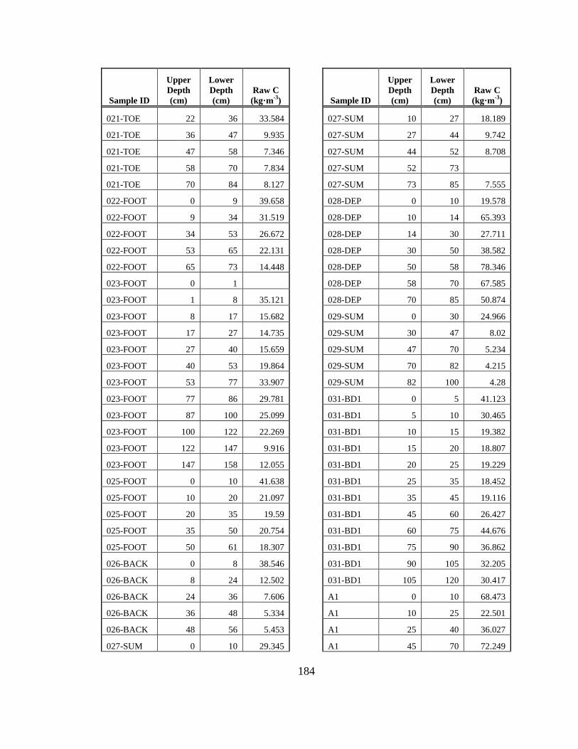
184

Sample ID

Upper

Depth

(cm)

Lower

Depth

(cm)

Raw C

(kg·m-3

)

021-TOE 22 36 33.584

021-TOE 36 47 9.935

021-TOE 47 58 7.346

021-TOE 58 70 7.834

021-TOE 70 84 8.127

022-FOOT 0 9 39.658

022-FOOT 9 34 31.519

022-FOOT 34 53 26.672

022-FOOT 53 65 22.131

022-FOOT 65 73 14.448

023-FOOT 0 1

023-FOOT 1 8 35.121

023-FOOT 8 17 15.682

023-FOOT 17 27 14.735

023-FOOT 27 40 15.659

023-FOOT 40 53 19.864

023-FOOT 53 77 33.907

023-FOOT 77 86 29.781

023-FOOT 87 100 25.099

023-FOOT 100 122 22.269

023-FOOT 122 147 9.916

023-FOOT 147 158 12.055

025-FOOT 0 10 41.638

025-FOOT 10 20 21.097

025-FOOT 20 35 19.59

025-FOOT 35 50 20.754

025-FOOT 50 61 18.307

026-BACK 0 8 38.546

026-BACK 8 24 12.502

026-BACK 24 36 7.606

026-BACK 36 48 5.334

026-BACK 48 56 5.453

027-SUM 0 10 29.345

Sample ID

Upper

Depth

(cm)

Lower

Depth

(cm)

Raw C

(kg·m-3

)

027-SUM 10 27 18.189

027-SUM 27 44 9.742

027-SUM 44 52 8.708

027-SUM 52 73

027-SUM 73 85 7.555

028-DEP 0 10 19.578

028-DEP 10 14 65.393

028-DEP 14 30 27.711

028-DEP 30 50 38.582

028-DEP 50 58 78.346

028-DEP 58 70 67.585

028-DEP 70 85 50.874

029-SUM 0 30 24.966

029-SUM 30 47 8.02

029-SUM 47 70 5.234

029-SUM 70 82 4.215

029-SUM 82 100 4.28

031-BD1 0 5 41.123

031-BD1 5 10 30.465

031-BD1 10 15 19.382

031-BD1 15 20 18.807

031-BD1 20 25 19.229

031-BD1 25 35 18.452

031-BD1 35 45 19.116

031-BD1 45 60 26.427

031-BD1 60 75 44.676

031-BD1 75 90 36.862

031-BD1 90 105 32.205

031-BD1 105 120 30.417

A1 0 10 68.473

A1 10 25 22.501

A1 25 40 36.027

A1 45 70 72.249

185

Sample ID

Upper

Depth

(cm)

Lower

Depth

(cm)

Raw C

(kg·m-3

)

A1 70 95 24.807

B2 0 10 105.003

B2 10 20 78.994

B2 20 35 27.254

B2 35 50 60.596

B2 50 65 87.728

B2 65 75 51.804

B2 75 90 34.445

B2 90 105 39.125

C3 0 5 60.995

C3 5 10 52.265

C3 10 15 62.484

C3 15 20 61.902

C3 20 25 67.049

C3 25 30 71.841

C3 30 40 52.525

C3 40 48 105.179

C3 48 58 84.613

C3 58 68 95.847

C3 68 78 93.954

C3 78 87 97.806

C3 87 97

C3 97 107 98.693

C3 107 127 54.908

D4 0 11 47.44

D4 11 22 63.604

D4 22 37 54.142

D4 37 52 67.868

Sample ID

Upper

Depth

(cm)

Lower

Depth

(cm)

Raw C

(kg·m-3

)

D4 52 67 93.688

D4 67 87 105.595

D4 87 100 117.837

E5 0 10 56.763

E5 10 25 45.261

E5 25 30 38.048

E5 30 40 39.213

E5 40 52 35.346

F6 0 10 80.465

F6 10 20 79.585

F6 20 30 69.513

F6 30 40 42.147

F6 40 60 27.647

F6 60 70 13.241

F6 70 88 8.403

G7 0 10 63.974

G7 10 22 40.071

G7 22 30 34.544

G7 30 45 54.197

I9 0 15 42.654

I9 15 22 34.114

J10 0 8 49.645

J10 8 22 33.914

L13 0 8 32.67

L13 8 22 24.886

L13 22 30 21.278

L13 30 35 17.772