The Box-Cox Transformation: Review andExtensions

Anthony C. AtkinsonThe London School of Economics, London WC2A 2AE, UK,*Marco Riani† and Aldo Corbellini‡, Dipartimento di ScienzeEconomiche e Aziendale and Interdepartmental Centre for

Robust Statistics, Universita di Parma,43100 Parma, Italy

February 16, 2020

Abstract

The Box-Cox power transformation family for non-negative responsesin linear models has a long and interesting history in both statistical practiceand theory, which we summarize. The relationship between generalized lin-ear models and log transformed data is illustrated. Extensions investigatedinclude the transform both sides model and the Yeo-Johnson transformationfor observations that can be positive or negative. The paper also describesan extended Yeo-Johnson transformation that allows positive and negativeresponses to have different power transformations. Analyses of data showthis to be necessary. Robustness enters in the fan plot for which the for-ward search provides an ordering of the data. Plausible transformations arechecked with an extended fan plot. These procedures are used to compareparametric power transformations with nonparametric transformations pro-duced by smoothing.

AMS 2000 subject classif cations: Primary 62F03, 62F35, 62J05, 62J20;secondary 68U05.

Keywords:

*e-mail: a.c.atkinson@lse.ac.uk†e-mail: mriani@unipr.it‡e-mail: aldo.corbellini@unipr.it

1

ACE; AVAS; constructed variable; extended Yeo-Johnson transformation;forward search; linked plots; robust methods.

1 IntroductionThis paper is principally concerned with the Box-Cox transformation of the re-sponse in linear regression models. The extensions include the transformation ofboth sides of the model, the transformation of responses that can be both posi-tive and negative and comparisons with nonparametric alternatives. It is taken asgiven that robust procedures are necessary, since outlying observations can havean appreciable effect on the estimated transformation.

The use of transformations in the simplif cation of distributions has a longhistory. Cox (1977) instances Fisher’s z transformation of the correlation coeff -cient (Fisher, 1915). Probit analysis for binomial proportions (Bliss, 1934) is alsoa transformation to normality. General discussions of the history, purposes anddevelopment of transformations are in the review article Cox (1977) and two re-lated articles taken from the Encyclopedia of Statistics (Atkinson and Cox, 1988;Taylor, 2004). Box and Cox (1964) emphasise the effect of transformations tonormality on the systematic part of the model. The transformation should pro-vide simple, more revealing analyses that lead to sharper inferences. An extensivesurvey of literature from the f rst quarter century of the Box-Cox transformationis Sakia (1992). Hoyle (1973) lists 19 transformations, several of which are spe-cial cases of the Box-Cox transformation. The monograph of Carroll and Ruppert(1988) ranges widely over topics in the statistical transformation of data.

The Box-Cox transformation is described in §2 together with some of the in-ferential problems arising from this seemingly simple model. The use of the Box-Cox transformation is illustrated in §3 by the analysis of data on mental illness.The results are compared with those from a generalized linear model, that is amodel in which the linear predictor, rather than the response, is transformed. Sec-tion 4 covers the transform both sides method of Carroll and Ruppert (1988) whichcan preserve the relationship between the response and a theoretical model whilstachieving homogeneity of variance. The section also describes nonparametricalternatives to the Box-Cox transformation, as well as other transformations, in-cluding extensions of the Box-Cox transformation.

These procedures are based on aggregate statistics, calculated over the wholesample. However, estimation of the transformation parameter can be particularlysensitive to outliers and an incorrect transformation can indicate spurious outliersthat disappear under the correct transformation. In §5 we discuss robust methodsand, in §6.2, recall the fan plot that illuminates the effect of individual observa-tions on the estimated transformation. Section 7 illustrates the use of these robust

2

techniques in the analysis of the illness data and compares the results with thosefrom nonparametric transformations.

Yeo and Johnson (2000) extended the Box-Cox transformation to a one-parameterfamily that allows the transformation of both positive and negative observations.§8.2 describes the further extension of this transformation by Atkinson et al.(2020) to allow different transformation parameters for positive and negative ob-servations, together with robust procedures for testing whether the different pa-rameter values are necessary. The paper concludes with an analysis of data ondifferences (John and Draper, 1980) which illustrates the need for this extendedtransformation as does the analysis in §4 of the supplementary material.

2 The Box-Cox TransformationThe Box-Cox transformation for non-negative responses is a function of the pa-rameter λ. The transformed response is

y(λ) = (yλ − 1)/λ (λ 6= 0); log y (λ = 0), (1)

with λ = 1 corresponding to no transformation, λ = 1/2 to the square root trans-formation, λ = 0 to the logarithmic transformation and λ = −1 to the reciprocaltransformation, thus avoiding a discontinuity at zero.

The development in Box and Cox (1964) is for the normal theory linear model

y(λ) = Xβ(λ) + ǫ, (2)

whereX is n×p, β(λ) is a p×1 vector of unknown parameters and the variance ofthe independent errors ǫi (i = 1, ..., n) is σ2(λ). The aim of the transformationis to produce a response for which the variance of ǫi is constant with an approx-imately normal distribution. The linear model ideally should also be simple andadditive, for example avoiding interaction and quadratic terms. All three aims aresatisf ed in the examples given by Box and Cox (1964), as they are in the analysisof numerous other data set, such as those in Atkinson and Riani (2000, Chapter 4).

To estimate λ it is necessary to allow for the change of scale of y(λ) with λ.The likelihood of the transformed observations relative to the original observa-tions y includes the Jacobian

J =

n∏

i=1

∣

∣

∣

∣

∂yi(λ)

∂yi

∣

∣

∣

∣

. (3)

For the power transformation (1), ∂yi(λ)/∂yi = yλ−1

i , so that

log J = (λ− 1)∑

log yi = n(λ− 1) log y,

3

where y is the geometric mean of the observations. A simple form for the likeli-hood is found by working with the normalized transformation

z(λ) = y(λ)/J1/n = (yλ − 1)/λyλ−1. (4)

For given λ the parameters are estimated by least squares:

β(λ) = (XTX)−1XT z(λ) and (5)

s2(λ) = {z(λ)−Xβ(λ)}T{z(λ)−Xβ(λ)}/(n− p) = R(λ)/(n− p). (6)

If an additive constant is ignored, the prof le loglikelihood, partially maximized,over β(λ) and σ2(λ), is

Lmax(λ) = −(n/2) log{R(λ)/(n− p)}, (7)

so that λ minimizes R(λ).For inference about plausible values of the transformation parameter λ, Box

and Cox suggest likelihood ratio tests using (7), that is, the statistic

TLR = 2{Lmax(λ)− Lmax(λo)} = n log{R(λ0)/R(λ)}. (8)

Although Box and Cox (1964) f nd the estimate λ that maximizes the prof leloglikelihood, they are careful to stress in their §2 that they are concerned notmerely to f nd a transformation which justif es assumptions, but rather to f nd,where possible, a metric in terms of which the f ndings may be succinctly ex-pressed. Typically in linear models, the main interest is in the factor effects, thechoice of λ being only a preliminary step. They state “we shall need to f x one,or possibly a small number, of λ’s and go ahead with the detailed estimation andinterpretation of the factor effects on this particular transformed scale. We shallchoose (the estimate λ) partly in the light of the information provided by the dataand partly from general considerations of simplicity, ease of interpretation, etc.”

This formulation has led to some controversy in the statistical literature. Bickeland Doksum (1981) and Chen et al. (2002) ignore the suggested procedure. Theyshow for regression models with response y(λ) that, when the transformation pa-rameter is poorly determined, the variability of the estimated parameters in thelinear model can be greatly increased if λ is estimated by λ rather than by λ. Boxand Cox (1982) and Hinkley and Runger (1984) query the scientif c usefulnessof such estimates of parameters on an unknown measurement scale. They furthercomment that the effects observed by Bickel and Doksum would be greatly re-duced if the investigation had been conducted in terms of z(λ) rather than y(λ).McCullagh (2002a), in comments on Chen et al., is very clear about the Box-Cox procedure for choosing λ. In the same discussion Reid (2002) comments

4

“The Box-Cox model is very useful for the theory of statistics, as a moderatelyanomalous model in the sense that blind application of conventional theory leadsto absurd results.” Details are in McCullagh (2002b) and Taylor and Liu (2007).Cox and Reid (1987) use the Box-Cox model as an example of their method forobtaining approximate parameter orthogonality, here between λ and the parame-ters of the linear model.

The practical procedure is analysis in terms of z(λ) leading to λ and hence toa, hopefully, physically interpretable estimate λ chosen from a grid of plausiblevalues. Carroll (1982) argues that the grid needs to become denser as n increases.Indeed, for the small examples of Box and Cox, inverse or logarithmic transforma-tions are indicated. But for the 509 observations on loyalty card usage in Perrottaet al. (2009), the value 1/3 is rejected when outliers are removed, but the value 0.4is acceptable. A f nal point is that, for comparisons across sets of data, parameterestimates need to be calculated using y(λ) to avoid dependence on y.

3 Mental Illness Data: Transformations and the Gen-eralized Linear Model

Kleinbaum and Kupper (1978, p.148) describe observational data on the assess-ment of mental illness of 53 patients. We compare the Box-Cox transformationwith an analysis using a generalized linear model with various Box-Cox links.

A psychiatrist assigns values for mental retardation and degree of distrust ofdoctors in newly hospitalized patients. After six months of treatment, a value isassigned for the degree of illness of each patient. We explore the Box-Cox trans-formation of degree of illness with regression on the two initial assessments. Themaximum likelihood estimate of λ is 0.046, with 95% conf dence limits from theprof le log-likelihood of -0.307, 0.404. The data support the log transformation,λ = 0. There is signif cant regression on both variables with a t value of 2.88for the relationship with the initial assessment of retardation and -2.21 for dis-trust of doctors. The QQ-plots of residuals show an appreciable improvement innormality after transformation.

In the Box-Cox model the transformed response follows a linear model. Onthe other hand, in generalized linear models the linear model is transformed by thelink function. For positive skew continuous data, an alternative to the Box-Coxtransformation is a gamma GLM. The canonical link for this GLM is the inversefunction, but the log link often provides a good f t to data. There is a strongrelationship between the linear model f tted to the logged response and the GLMwith a log link. We illustrate this relationship for the Mental Illness data.

With E(Y ) = µ and the linear predictor η = xTβ, the link function relates

5

Table 1: Mental illness data. Deviances from GLM analyses for three values ofthe parameter of the Box-Cox link

Link Deviance-1 19.180 19.561 20.12

the two by η = g(µ). For the gamma model the variance is quadratically relatedto the mean; the variance function V (µ) = µ2. We use the Box-Cox link g(µ) =(µλ − 1)/λ: for λ = −1 we obtain the reciprocal link, with the log link forλ = 0. Table 1 gives the deviances from f tting the gamma model with λ =−1, 0 and 1. Although the reciprocal link yields the smallest deviance, there is nosignif cant increase in deviance if one of the other links is used. The insensitivityof data analyses to the exact specif cation of the gamma link is well established- for example the analysis by McCullagh and Nelder (1989, p.377) of their carinsurance data. Further discussion of the relationship between the gamma andlognormal models is in McCullagh and Nelder (1989, Chapter 8). Atkinson andRiani (2000, Chapter 6) use the goodness of link test of Pregibon (1980) to providea fan plot for the parameter in the Box-Cox family of link functions.

We now consider the relationship between the two models f tted to the MentalIllness data. The coeff cient of variation of the untransformed data is taken asconstant

var(Y ) = σ2{E(Y )}2 = σ2µ2,

so that σ is the coeff cient of variation of Y . The variance-stabilizing transforma-tion is log(Y). For small σ2 the approximate moments of log(Y ) are

E{log(Y )} = log(µ)− σ2/2 and var{log(Y )} = σ2.

If the systematic part of the model is multiplicative on the original scale, coeff -cient estimates of the parameters and of their precision may be obtained by trans-forming to the log scale and using ordinary least squares. If the exact distributionof Y is known, maximum likelihood estimation for the known distribution shouldbe used. Firth (1988) compares the log-normal and gamma models under recipro-cal mis-specif cation, the gamma distribution performing slightly better.

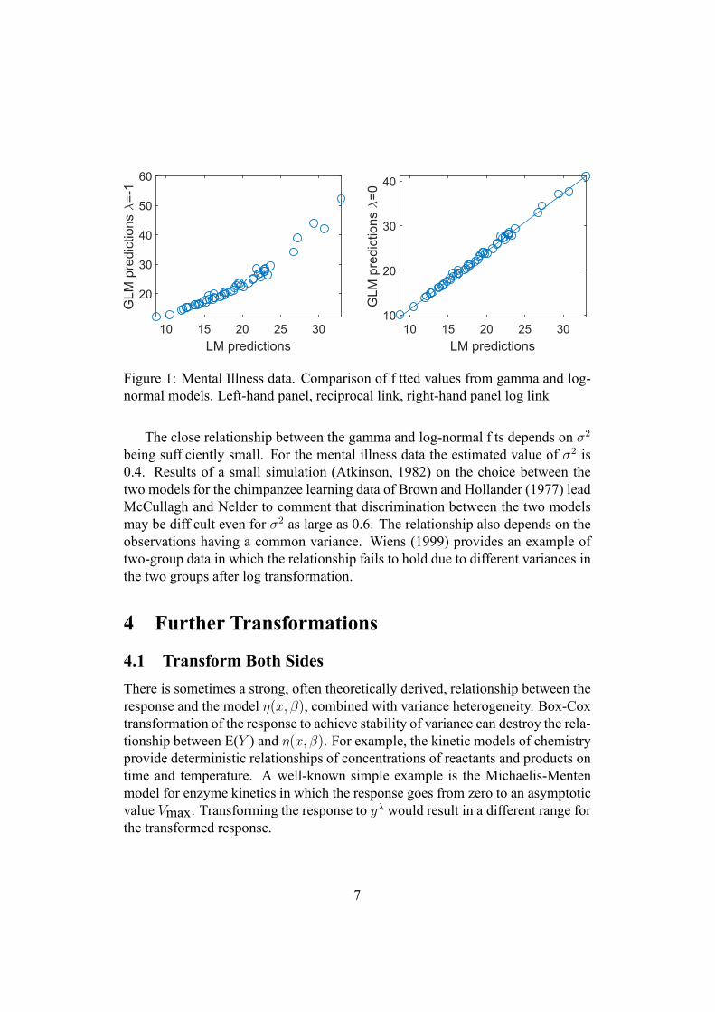
Figure 1 shows the comparison of f tted values for the linear model after logtransformation of y with those from the gamma model for two Box-Cox links. Inthe left-hand panel for the reciprocal link the relationship between the two setsof f tted values is slightly convex. The right-hand panel shows the straight-linerelationship for the log link. The plot for the identity link (λ = 1) is not shown.As is to be expected, it is slightly concave.

6

10 15 20 25 30LM predictions

20

30

40

50

60

GLM

pre

dict

ions

=-

1

10 15 20 25 30LM predictions

10

20

30

40

GLM

pre

dict

ions

=0

Figure 1: Mental Illness data. Comparison of f tted values from gamma and log-normal models. Left-hand panel, reciprocal link, right-hand panel log link

The close relationship between the gamma and log-normal f ts depends on σ2

being suff ciently small. For the mental illness data the estimated value of σ2 is0.4. Results of a small simulation (Atkinson, 1982) on the choice between thetwo models for the chimpanzee learning data of Brown and Hollander (1977) leadMcCullagh and Nelder to comment that discrimination between the two modelsmay be diff cult even for σ2 as large as 0.6. The relationship also depends on theobservations having a common variance. Wiens (1999) provides an example oftwo-group data in which the relationship fails to hold due to different variances inthe two groups after log transformation.

4 Further Transformations

4.1 Transform Both SidesThere is sometimes a strong, often theoretically derived, relationship between theresponse and the model η(x, β), combined with variance heterogeneity. Box-Coxtransformation of the response to achieve stability of variance can destroy the rela-tionship between E(Y ) and η(x, β). For example, the kinetic models of chemistryprovide deterministic relationships of concentrations of reactants and products ontime and temperature. A well-known simple example is the Michaelis-Mentenmodel for enzyme kinetics in which the response goes from zero to an asymptoticvalue Vmax. Transforming the response to yλ would result in a different range forthe transformed response.

7

Carroll and Ruppert (1988, Chapter 4) developed a transform both sides modelfor such problems, motivated by theoretical models for sockeye salmon breeding.The transformation model is

(yλ − 1)/λ = {η(x, β)λ − 1}/λ+ ǫ, (9)

where the independent errors are normally distributed. As with the Box-Cox trans-formation, the parameters λ and β are found by minimizing the residual sum ofsquares in the regression model which includes the Jacobian of the transformation,again y.

The theoretical procedure is to minimize the residual sum of squares usingy(λ)/yλ−1, or equivalently y(λ)/yλ, as the response and the similarly transformedvalue of η as the model. Carroll and Ruppert comment that, unless λ is f xed, itis not possible to use standard nonlinear regression routines for this minimizationas such routings typically do not allow the response to depend upon unknown pa-rameters. They reformulate the problem in terms of a ‘pseudo model’, estimationof which converged rapidly in our application.

15 20 25 30Gestational age (weeks)

10

20

30

40

50

Man

dibl

e le

ngth

(mm

)

15 20 25 30Gestational age (weeks)

10

20

30

40

50

Man

dibl

e le

ngth

(mm

)

Figure 2: 99% prediction intervals for back-transformed mandible length data.Left-hand panel, transform both sides, λ = 0. Right-hand panel, logarithmicBox-Cox transformation with a quadratic model.

As our example we use data on mandible length in foetuses used by Roystonand Altman (1994) to illustrate the use of fractional polynomials as explanatoryvariables in regression models. There are 158 observations on foetuses of agex less than 28 weeks. There are also nine measurements with x > 28, whichthe clinicians felt formed a different group with excessive measurement error.The plot of the data in left-hand panel of Figure 2 suggests that mandible lengthincreases linearly with gestational age and that the variance likewise increases.

8

Royston and Altman overcome the increase in variance by use of the log transfor-mation, but the relationship between log(mandible length) and age is then curved.We use the transformation of both sides to obtain a homoscedastic model in whichthe linear relationship is preserved.

Regression of all 167 observations on age assuming homoscedasticity indi-cates only two outliers, rather than 9. We proceed on the assumption that therewill be no outliers when we have allowed for heteroscedasticity. The estimatefor the Box-Cox transformation of the response suggests a value of 0.75 for λ -a compromise between preserving linearity and a transformation to homoscedas-ticity. With a logged response there is very strong evidence for inclusion of aquadratic term. The transform both sides model with regression just on age alsoindicates the log transformation with λ = −0.08.

The left-hand panel of Figure 2 shows the 99% prediction interval for theback-transformed response from the transform both sides model. The f tted modelretains the desired linearity and the prediction interval increases with gestationalage in line with the heteroscedasticity of the observations. The right-hand panelshows a similar interval for the back-transformed quadratic regression with log yas the response. This panel shows that, although the quadratic model f ts well tothe majority of the observations, there is increasing curvature for values of x > 28.

It is clear that the transform both sides model is to be preferred for predic-tions over quadratic regression. The difference from predictions using the frac-tional polynomial model of Royston and Altman is not so obvious. However,the method of transforming both sides preserves the linear relationship betweenlength and age and, more generally, the ability to combine theoretical models withtransformation to normality.

4.2 Nonparametric TransformationsThe Box-Cox transformation produces a smooth relationship between y(λ) andthe original y which is determined by the value of λ. The extended Yeo-Johnsontransformation of §8.1 for observations that can be positive or negative, likewiseproduces a smooth relationship but depending on two parameters. These paramet-ric transformations may be too restrictive. A nonparametric alternative is to usesome form of smoothing to estimate the relationship, allowing for greater f exi-bility. This may have advantages in the analysis of a specif c set of data, withdisadvantages if the aim is to compare different sets of observations which aresubject to the same transformation. Figure 9 illustrates the extra information pro-vided by one nonparametric transformation.

The general model is

g(y, κ) = η(x, β) + ǫ, (10)

9

where κ might be a vector of parameters def ning a spline transformation and ǫ isnot necessarily normally distributed.

Ramsay (1988) uses a monotone spline to estimate g(.), with the regressionparameters estimated by least squares. An advantage is that the Jacobian of thetransformation is found by straightforward differentiation of the spline. His anal-ysis of the wool data from Box and Cox produces a transformation very close tothat from the parametric analysis. The loglikelihood is not signif cantly improvedby increasing the complexity of the spline through the addition of extra knots.Song and Lu (2012) adopt a Bayesian approach. They use penalized Bayesiansplines to transform the response to approximate normality by maximizing a nor-mal likelihood with prior distributions for the parameters of η(x, β). Their plot ofthe transformation for U-shaped data1 is sigmoid, far from the convex or concaveshapes attainable from the Box-Cox transformation.

The semiparametric method of Foster et al. (2001) assumes that the Box-Coxtransformation holds, that is g(y, κ) = y(λ) but that in (10) the distribution of ǫ isunknown. An estimating equation, combined with a grid search over values of λ,provides estimates of λ and β. The covariance matrix of the parameter estimatesis found using a resampling method. The parameter estimates and their standarderrors for the wool data are virtually indistinguishable from those of Box andCox. However, the semiparametric method shows appreciable improvement forprediction when the error distribution is not normal. Cai et al. (2005) use relatedmethods for the transformation of censored survival times.

Two nonparametric methods use the “supersmoother” (Friedman and Stuet-zle, 1982) instead of the spline smoothing of Ramsay (1988). Both methods cantransform explanatory variables and response. The assumed model is a general-ized additive model, that is one with transformations of both response and ex-planatory variables but without interactions. Both rely on repeated application ofthe univariate smoother. In ACE (alternating conditional expectations) Breimanand Friedman (1985) maximize a measure of correlation between all variables;in regression the response variable is not treated as being different from the ex-planatory variables. Tibshirani (1988) describes a related method in which thetransformation for the response is intended to yield additivity and variance stabi-lization (AVAS). The asymptotic variance stabilizing transformation is estimatedfor the response. Hastie and Tibshirani (1990, Chapter 7) provide a description ofboth ACE and AVAS with an emphasis on response transformation and the math-ematical relationship to the Box-Cox transformation. Subroutine AREG of theR-package Hmisc (Harrell Jr, 2019) replaces the smoother in ACE with restrictedcubic smoothing splines, with a controllable number of knots.

1In their Figure 2 these data have a minimum of −1.5. We are assured that, for the calculationof the Box-Cox transformation in their Table 1, the data were shifted to be non-negative.

10

For the transform both sides model Wang and Ruppert (1995) assume that theobservations are normally distributed and use kernel density estimation to deter-mine g(y, κ). Since in the transform both sides model the form of the relationshipbetween y and η(x, θ) is known, least squares can be used to estimate β. A com-panion article (Nychka and Ruppert, 1995) uses splines.

We use ACE, AVAS and AREG as our nonparametric alternatives to the Box-Cox transformation, ACE and AVAS being the most studied of the nonparametrictransformations. We exclude the transformation of explanatory variables. Theoriginal progams for both ACE and AVAS are written in ‘classical’ Fortran, with-out comments and with many non-informative variable names. This Fortran codealso provides the basis of the R package acepack (Spector et al., 2016). We haverewritten the programs in Matlab. These new programs have been thoroughlycompared with the Fortran programs and validated to give identical numerical re-sults to the originals and incorporated into our toolbox for robust analysis. Theoutput of ACE and AVAS are a set of transformed responses, scaled to have unitvariance. Unlike ACE and AVAS, which are free of adjustable parameters, AREGrequires the specif cation of the number k of knots in the splines. The aggregatestatistic for comparison of models for all three is the value of R2 which Wang andMurphy (2005) convert into BIC values. Harrell provides routines for bootstrapevaluation of the variances of the estimated linear model parameters obtained fromAREG.

Marazzi et al. (2009) review papers on the Box-Cox transformation, from thestandpoint of computational feasibility and, particularly, robustness. None of themethods have high breakdown and all, for example Carroll and Ruppert (1985),breakdown for outliers at leverage points. In their discussion of Breiman andFriedman (1985), Buja and Kass (1985) comment on the need to develop diag-nostics and robust forms of ACE. Some diagnostic information can be obtainedby comparing parametric and nonparametric transformations on data before andafter the removal of outliers, which we exemplify in §10.

4.3 More TransformationsExtensions of the Box-Cox transformation

For values of λ other than zero, the distribution of y(λ) is truncated. Forλ > 0, y(λ) is bounded below at −1/λ; for λ < 0 it is bounded above at thesame value. Only exponentiation of the log normal distribution yields a normaldistribution on the whole real line. Yang (2006) introduced a dual transformationy(λ) = (yλ − y−λ)/2λ, (λ 6= 0) with the logarithmic transformations at λ = 0,which removes the bound in the Box-Cox transformation.

Zhang and Yang (2017) describe a method for applying the Box-Cox trans-formation to huge data sets. The necessity is to avoid storing all the data in the

11

computer before performing transformation calculations. For least squares re-gression the required quantities (sums of squares and products of y andX) can besequentially updated. The procedure can be extended to the Box-Cox transforma-tion to include storing sums of products of X and z(λ) for selected values of λ.Zhang and Yang (2017) choose a grid of 41 values.

Box and Cox (1964) extended their transformation to the shifted power trans-formation of (y + µ), where both µ and the transformation parameter λ are to beestimated. A diff culty is that the range of the observations now depends on µ,so that the inferential problem is non-regular. Atkinson et al. (1991) suggest agrouped likelihood approach to parameter estimation, but the estimates may de-pend on the size of the grouping interval.

In §10 we analyse data from John and Draper (1980). The normal plot of theresiduals (Atkinson, 1985, Figure 9.17) shows a long tailed symmetrical distribu-tion, which structure led John and Draper to develop the modulus transformationwith

y(λ) =

{

(|y|+ 1)λ − 1

λ

}

sign(y),

for y 6= 0. This symmetric transformation family applies the same transformationto the positive and negative tails of the distribution. The Yeo-Johnson transforma-tion, which can also be applied to observations that can be negative or positive, iseither convex or concave over the whole range of y, whereas the extended Yeo-Johnson transformation of §8.2 can be convex or concave in either tail as the datadictate.

The two transformations of Aranda-Ordaz (1981) provide invertible transfor-mations for binary data. In the symmetrical transformation in which “successes”and “failures” are interchangeable, the value λ = 0 yields the logistic model.In the asymmetrical transformation the limits are the complementary log log andlogistic models.

These methods are for independent univariate responses. The Box-Cox trans-formation was generalized to multivariate data by Andrews et al. (1971) andGnanadesikan (1977). Velilla (1995) considers robust and diagnostic aspects ofmultivariate transformations. Atkinson et al. (2004) provide examples of the anal-ysis of transformed multivariate data using the forward search.

A more general point is inference for transformed data on the original scale.The properties of predictions on the back-transformed scale are considered bymany, including Taylor (1986) and Carroll and Ruppert (1988). A second pointis that Box and Cox also develop a Bayesian procedure for transformation, whichleads to a data-dependent prior. Pericchi (1981) suggested a prior that avoideddata-dependence, which was modif ed by Sweeting (1984). Gottardo and Raftery(2009) combine Bayesian transformations with model selection.

Transformation of Explanatory Variables

12

Box and Tidwell (1962) explore power transformations of the explanatoryvariables in regression. Since the response is not transformed, residual sums ofsquares can be compared directly for different transformations.

Transformation of the response in ARIMAmodels results in transformation ofany lagged responses in the model. The constructed variables of Atkinson et al.(1997) for Box-Cox transformation of ARIMAmodels were used by Riani (2009)and Proietti and Riani (2009) in fan plots for the transformation of time series.

Transformation of ParametersThe lower left-hand panel of Figure 8.2 of McCullagh and Nelder (1989)

shows a virtually parabolic loglikelihood for a single gamma observation whenthe plot is against µ−1/3. For multiparameter problems approximate orthogonalityand a nearly quadratic form of the log likelihood will usually speed the conver-gence of iterative methods of estimation. This is a matter of numerical analysis,but approximate independence of the components of parameters combined withapproximate normality is also desirable for statistical reasons, including ease ofinterpretation in multiparameter problems. Ross (1990) includes many examples.

5 Robustness and GraphicsThe data analyses so far are based on aggregate statistics. They do not allowfor the presence of dispersed or grouped outliers, or for inf uential observations,one or a few of which may appreciably change the estimate of the transformationparameter and so the interpretation of the data. Several robust statistical methodsaddress this problem, at least for many statistical models, such as regression, if notfor data transformation. A diff culty in the intelligent application of robust meth-ods is that many require the specif cation of a parameter dependent on the amountof contamination expected in the data or the required eff ciency of estimation.

There are three general classes of approaches to robust regression: (i). SoftTrimming (downweighting). M estimation and derived methods (Huber, 1973).Observations near the centre of the distribution retain their value, but observationsfar from the centre have a weight that decreases with distance from the centre;(ii). Hard Trimming. In Least Trimmed Squares (LTS: Hampel, 1975, Rousseeuw,1984) the amount of trimming is determined by the choice of the trimming param-eter h, which is specif ed in advance. The LTS estimate is intended to minimizethe sum of squares of the residuals of h observations and (iii). Adaptive HardTrimming. In the Forward Search (FS), the observations are again hard trimmed,but the value of h is determined adaptively by the data. Starting from a small ini-tial subset of data, the number of observations used in f tting then increases untilall are included and outliers identif ed. Atkinson et al. (2010) provide a generalsurvey of the FS with discussion.

13

Two properties of these robust regression estimators are important when se-lecting a method: (i). Breakdown Point, bdp ; the asymptotic proportion of obser-vations that can go to∞without affecting the parameter estimates. This def nitionrequires both that n → ∞ and also that the distance between the contaminated anduncontaminated observations increases with n; (ii). Eff ciency of Estimation, ofthe parameters relative to least squares for uncontaminated data.

Ideally a robust estimator would have both a high breakdown point and a higheff ciency. Unfortunately this is not possible. For hard trimming, once one ofthe values, for example the breakdown point bdp, has been selected, the otheris determined. Riani et al. (2014) extended these results to S-estimation. To il-luminate the non-asymptotic properties of robust estimators Riani et al. (2014)monitor the behaviour of several extensions of M estimation, including MM esti-mation (Yohai, 1987), by analysing data over a grid of values of the eff ciency ofestimation of the parameters of the linear model. They observe that there is often apoint at which the f t switches from being robust to non-robust least squares. Thisimportant property, which at present cannot be determined analytically, dependsboth on the nominal properties of the estimator and on the particular data set beinganalysed.

The examples in Riani et al. (2014) indicate that the FS, combined with a suit-able stopping rule to avoid the inclusion of outliers, provides a robust procedurewith good properties which avoids any a priori specif cation of quantities indicat-ing the required degree of robustness. We therefore use it as the method for robustestimation of transformations. Details of the method are in §6.2.

The FS by its nature provides a series of f ts to subsets of the data of increasingsize. Forward plots of residuals, that is of residuals as the subset sizem increases,are informative about the presence of outliers. They are used both as a tool todetermine outliers and as a means of understanding the structure of the data. Theleft-hand panel of Figure 6 illustrates the outlier detection procedure. The panelsof Figure 8 show the information gained by linking plots, making clear the effectof individual observations on the estimated transformation parameter, the test foroutliers, the trajectory of residuals over the FS and the position of the observationson scatter plots. A different use of dynamic graphics in the determination of robusttransformations is in Seo (2019)

14

6 A Robust Approximate Score Test for the Trans-formation Parameter

6.1 Constructed VariablesFor inference Box and Cox (1964) rely on complete-sample likelihood inferencethrough the likelihood ratio statistic (8). A disadvantage of this likelihood ratiotest is that a numerical maximization is required to f nd the value of λ. In ourrobust procedure using the FS, we calculate almost n test statistics for the hypoth-esis that λ = λ0, typically for f ve values of λ0. There is an appreciable literatureon methods that avoid such maximizations of the likelihood: score tests (Cookand Weisberg, 1982; Atkinson, 1985) and Lagrange multiplier tests (Breusch andPagan, 1979).

We use the approximate score statistic Tp(λ), (Atkinson, 1973) derived byTaylor series expansion of z(λ) (4) about λ0. This leads to the approximate re-gression model

z(λ0) = xTβ − (λ− λ0)w(λ0) + ǫ

= xTβ + γ w(λ0) + ǫ, (11)

where γ = −(λ − λ0) and the constructed variable w(λ0) = ∂z(λ)/∂λ|λ=λ0,

which only requires calculations at the hypothesized value λ0.The approximate score statistic for testing the transformation is the t statistic

for regression on −w(λ0) , that is the test for γ = 0 in the presence of all compo-nents of β. Because Tp(λ0) is the t test for regression on −w(λ0), large positivevalues of the statistic mean that λ0 is too low and that a higher value should beconsidered.

A different approximate score statistic for the Box-Cox transformation is foundby Lawrance (1987) through an approximation to the variance of the score statis-tic, leading to an improved null distribution for the statistic. Some numerical com-parisons of the two procedures are in Atkinson and Lawrance (1989). A similarprocedure for testing the value of the parameter in the Yeo-Johnson transformationis shown in §9.

6.2 The Fan PlotThe robust transformation of regression data is complicated by the dependence ofoutliers on the value of λ. In the data of Wiens mentioned in §3, very small values,arbitrarily allocated to observations below the detection limit, have an appreciableeffect when the data are log transformed. Atkinson and Riani (2000) show howdifferent observations appear outlying for various transformations of the Poisondata of Box and Cox (1964).

15

We use the Forward Search to provide a robust plot of the approximate scorestatistic Tp(λ). We start with a f t to m0 = p + 1 observations and then succes-sively f t to larger subsets. For the subset of size m we order all observations bycloseness to the f tted model; the residuals determine closeness. The subset size isincreased by one to consist of the subset with them+1 smallest squared residualsand the model is ref tted to this new subset. The process continues with increasingsubset sizes until, f nally, all the data are f tted. The process moves from a veryrobust f t to non-robust least squares. Any outliers will enter the subset towardsthe end of the search. We thus obtain a series of f ts of the model to subsets of thedata of size m,m0 ≤ m ≤ n for each of which we ref t the model and calculatethe value of the score statistics for selected values of λ0. These are then plottedagainst the number of observations m used for estimation to give the “fan plot”.As Figure 4 shows, the ordering of the observations in a fan plot may depend onthe value of λ0.

Since the constructed variables are functions of the response, the statisticscannot exactly follow the t distribution. Atkinson and Riani (2002) provide somenumerical results on the distribution in the fan plot of the score statistic for theBox-Cox transformation. They f nd that departures from the null distribution aremost extreme towards the end of the search, where the statistic has too large avariance; increasingly strong regression relationships lead to null distributions thatare closer to t.

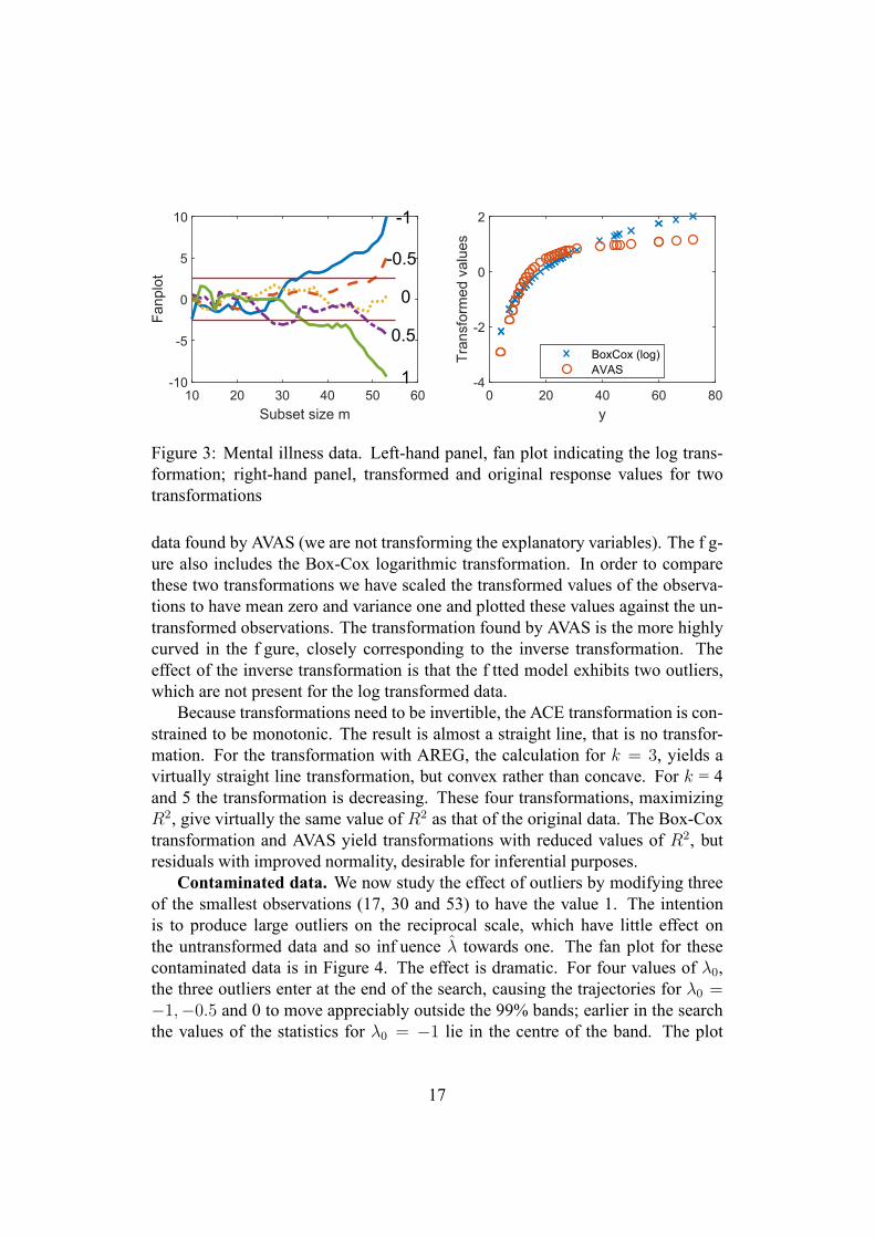
7 Mental Illness Data: A Robust AnalysisSection 3 introduced data on 53 patients and provided an analysis based on aggre-gate statistics, which indicated the log transformation of the response. Here wecompare the Box-Cox transformation with three nonparametric transformations,both on the original data and on a version contaminated with outliers, and illus-trate the use of the fan plot in the detection of outliers inf uential for the parametricdata transformation.

Original data. The left-hand panel of Figure 3 shows the fan plot for f vevalues of λ0, fanning out as the search progresses. The trajectory of values ofthe score test for the log transformation (λ0 = 0) remains within the 99% limits(±2.58) throughout the search. Other values for λ0 are rejected, −1 and +1 morestrongly than ±0.5. There are no abrupt changes in the trajectories which mightindicate the inclusion of an inf uential observation in the subset of observationsused in f tting. The log transformation is further conf rmed by a comparison of theQQ plots of residuals which is straightened by the transformation; approximatenormality has been achieved.

The right-hand panel of Figure 3 shows the monotonic transformation for these

16

10 20 30 40 50 60Subset size m

-10

-5

0

5

10

Fanp

lot

-1

-0.5

0

0.5

10 20 40 60 80

y

-4

-2

0

2

Tran

sfor

med

val

ues

BoxCox (log)AVAS

Figure 3: Mental illness data. Left-hand panel, fan plot indicating the log trans-formation; right-hand panel, transformed and original response values for twotransformations

data found by AVAS (we are not transforming the explanatory variables). The f g-ure also includes the Box-Cox logarithmic transformation. In order to comparethese two transformations we have scaled the transformed values of the observa-tions to have mean zero and variance one and plotted these values against the un-transformed observations. The transformation found by AVAS is the more highlycurved in the f gure, closely corresponding to the inverse transformation. Theeffect of the inverse transformation is that the f tted model exhibits two outliers,which are not present for the log transformed data.

Because transformations need to be invertible, the ACE transformation is con-strained to be monotonic. The result is almost a straight line, that is no transfor-mation. For the transformation with AREG, the calculation for k = 3, yields avirtually straight line transformation, but convex rather than concave. For k = 4and 5 the transformation is decreasing. These four transformations, maximizingR2, give virtually the same value of R2 as that of the original data. The Box-Coxtransformation and AVAS yield transformations with reduced values of R2, butresiduals with improved normality, desirable for inferential purposes.

Contaminated data. We now study the effect of outliers by modifying threeof the smallest observations (17, 30 and 53) to have the value 1. The intentionis to produce large outliers on the reciprocal scale, which have little effect onthe untransformed data and so inf uence λ towards one. The fan plot for thesecontaminated data is in Figure 4. The effect is dramatic. For four values of λ0,the three outliers enter at the end of the search, causing the trajectories for λ0 =−1,−0.5 and 0 to move appreciably outside the 99% bands; earlier in the searchthe values of the statistics for λ0 = −1 lie in the centre of the band. The plot

17

shows that a plausible estimate for λ based just on a f t to all the data would be0.5. However, this value is rejected earlier in the search.

10 15 20 25 30 35 40 45 50 55Subset size m

-5

0

5

10

15

20Fa

nplo

t-0.5

0

0.5

1

-1

Figure 4: Contaminated mental illness data: fan plot, showing the effect of threechanged observations

A plot similar to the right-hand panel of Figure 3 for the contaminated datashows that the curvature in the plot of transformed against original y from AVASis reduced; the transformation is close to the log transformation. Regression withthe log transformation on the contaminated data then clearly shows that the threealtered observations have large residuals. The transformation from ACE is, as pre-viously, virtually a straight line. The transformations indicated by AREG for k upto 5 are similar to those in the absence of outliers. In this example the value of k isnot clearly determined by the data. Regression using the transformation suggestedby AVAS indicates the three outliers for the contaminated data and the logarithmictransformation, but suggests an inadequate transformation for the uncontaminateddata.

Section 2 of the supplementary material for this paper includes an analysis ofthe motivating data set from Chen et al. (2002) on gasoline consumption. The dataappear to need transformation with λ around 1.5. However, application of the fanplot reveals that all evidence for this transformation comes from one observation,with by far the lowest values of both x and y. The second example in the sup-plementary material is an analysis of the Poison data from Box and Cox (1964).The fan plot, like that in Figure 3, is exemplary, with no indication of inf uentialobservations.

18

8 The Transformation of Responses that can be Neg-ative as well as Positive

8.1 The Yeo-Johnson TransformationYeo and Johnson (2000) extended the Box-Cox transformation to observationsthat can be positive or negative by using different Box-Cox transformations forthe two classes of response. For y ≥ 0 this is the generalized Box-Cox powertransformation of y + 1. For negative y the transformation is of −y + 1 to thepower 2−λ. They used a smoothness condition to combine the transformations forpositive and negative observations, so obtaining a one-parameter transformationfamily. Atkinson et al. (2020) extended the transformation to allow for distincttransformation parameters for the two response classes. They further providedconstructed variables for this extended transformation and an extended fan plotwhich permits checking the correctness of the two transformations. This sectionbrief y summarizes their results.

As with the Box-Cox transformation, analysis of data from this transformationneeds to include the Jacobian J of the transformation to allow for changes ofscale as λ varies. We continue to work with a normalized transformation z(λ) =y(λ)/J1/n in which the Jacobian is spread over all observations. If, to extend thenotation of Box and Cox, yY J is the nth root of J , it follows from equation (3.1)of Yeo and Johnson (2000) that

yY J = exp[

∑

{sgn(yi) log(|yi|+ 1)}/n]

. (12)

The normalized version of the transformation is then

y ≥ 0 :(y + 1)λ − 1

λyλ−1

Y J

(λ 6= 0); yY J log(y + 1) (λ = 0)

y < 0 : −{(−y + 1)2−λ − 1}

(2− λ)yλ−1

Y J

(λ 6= 2); − log(−y + 1)/yY J (λ = 2).

(13)

8.2 The Extended Yeo-Johnson Transformation andHomogene-ity of Transformation

Some authors, for example Weisberg (2005), query the physical interpretabilityof the constraint that positive and negative observations should be transformed bythe same value of λ, which is indeed violated by the data analysed in §10. Ac-cordingly, Atkinson et al. (2020) extended the score test to testing for the equalityof the value of λ in the two regions of y. The procedure takes the transformation

19

parameter as λ for one part and λ+α for the other and uses the score testing proce-dure for α = 0, leading to tests that positive, or negative yi need a transformationdifferent from λ.

There are now separate Jacobians, yP and yN , for positive and negative y frombreaking the summation in (12) into parts for positive and negative observations.To test for positive observations having a distinct transformation let v = y + 1.The general model for y ≥ 0 is

z(α, λ) =vλ+α − 1

(λ+ α)yλ−1

N yλ+α−1

P

, (14)

which reduces to the standard transformation when α = 0 since y = yN yP .When y < 0 let vN = −y + 1. Keeping the parameter for positive y as λ + α

the model for the negative y only depends on α through the Jacobian. Then

z(α, λ) = −v2−λN − 1

(2− λ)yλ−1

N yλ+α−1

P

. (15)

Similar expressions when the parameter for negative y is λ + α are given byAtkinson et al. (2020).

8.3 The Extended Fan Plot; Checking Postulated Transforma-tions

The original Yeo-Johnson transformation of §8.1 yields a score test and so a fanplot for a set of values of λ0. The extended Yeo-Johnson transformation of §8.2provides constructed variables for testing whether the positive and negative ob-servations also require the transformation λ0. The extended fan plot accordinglycontains three trajectories for each value of λ0. If the same transformation is ap-plied to both positive and negative responses, agreement of the three trajectoriesindicates that only one transformation is needed.

An important feature of the extended fan plot is that it provides a methodof testing a proposed transformation with different parameters, λP and λN fortransformation of the positive and negative observations. Once the data have beencorrectly transformed, the extended fan plot testing λ0 = 1 for the transformeddata should lie within the bounds for all values of m. We use this method in §§9and 10 to conf rm transformations of the data which have distinct values of λP

and λN .

20

200 400 600 800 1000Subset size m

-5

0

5

10

1

200 400 600 800 1000Subset size m

0

5

10

15 1

Figure 5: Simulated data. Extended fan plots with green (mostly upper) curvefor positive observations: left-hand panel, λ0 = 1, indicating inf uential observa-tions and the need for two transformation parameters; right-hand panel, checkingλN = 0.25 and λP = 1.5 (test of λ0 = 1 for transformed data), conf rming trans-formation parameter values and suggesting the presence of potential outliers.

9 A Simulated ExampleWe simulated 1,000 regression observations, with three explanatory variables andindependent normal errors, which were heavily contaminated with outliers. Wef rst demonstrate the use of the augmented fan plot in indicating a transformationand then use the forward search on the transformed data to detect the outliers. Wecompare this procedure with the information from using nonparametric transfor-mations on the contaminated data.

Contaminated data. Different transformations were applied to the positiveand negative observations and 200 of the observations were shifted to provideoutliers. This is a challengingly high contamination proportion unless the outliersare distinct. However, they are not evident on the scatterplots of y against theindividual x vectors (Figure 1 of the supplementary material). Linear regressiongave an R2 value of 0.31. The fan plot for these data for λ0 = 0.5, 0.75, 1, 1.25and 1.5 indicated a value of 1.25 for the overall transformation parameter, with allscore statistic values lying within the 99% interval. For other parameter values alarge number lie outside the interval; around 200 for λ0 = 1.

To investigate whether an overall transformation with λ = 1.25 is satisfactorywe calculated extended fan plots for a few values of λ. That for λ0 = 1 in theleft-hand panel of Figure 5 shows clear evidence, from m = 400 or less, thatdifferent values are needed for λN and λP . The plot also shows the effect of a setof inf uential observations entering in the last 160 steps.

21

The extended fan plot is used to f nd pairs of parameter values. The data aretransformed with pairs of values λP and λN and the extended fan plot for λ0 = 1for the transformed data inspected. The right-hand panel of Figure 5 shows theplot for λN = 0.25 and λP = 1.5. The trajectories for the positive and negativeobservations are close together and close to the trajectory for a single value of λ.In addition the inf uential observations are clearly articulated.

100 200 300 400 500 600 700 800 900Subset size m

1

1.5

2

2.5

3

3.5

4

4.5

1%

99%

50%

99.9%

99.99%

99.999%

-4 -2 0 2X1

-4

-3

-2

-1

0

1

2

y

-2 0 2X2

-2 0 2X3

Good unitsOutliers

Figure 6: Simulated data, detection of outliers using the forward search on datatransformed with λN = 0.25 and λP = 1.5. Left-hand panel, forward plot ofminimum deletion residuals. Right-hand panel, scatter plots of the transformeddata against explanatory variables; the 164 observation identif ed as outliers areplotted as open (red) circles.

To check for outliers, we perform a robust analysis on transformed data withλN = 0.25 and λP = 1.5. The left-hand panel of Figure 6 shows a plot of (ab-solute) minimum deletion residuals from the forward search on the transformeddata. For each m these are the outlier tests for the next observation to enter thesubset, which is the one closest to the already f tted model. The envelopes in theplot provide guidance as to whether the observation is outlying. The procedurefor outlier detection is that of Riani et al. (2009) adapted to regression. As a re-sult 164 outliers were identif ed. The scatter plots in the right-hand panel of thef gure show outliers as circles. The R2 for this regression is 0.518, an appreciableimprovement over the original 0.31.

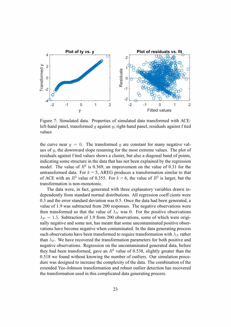
Nonparametric transformations. We now consider nonparametric transfor-mations of the response in regression. AVAS yields a virtually linear relationshipbetween the transformed and original y, that is effectively no transformation atall. The value of R2 is 0.303, slightly worse than untransformed regression. Re-sults for ACE are in the two panels of Figure 7. Now the plot of transformedagainst residual y is virtually a straight line for positive y, but there is a bend in

22

-2 -1 0 1 2y

-4

-2

0

2

4

Tran

sfor

med

y

Plot of ty vs. y

-2 -1 0 1 2Fitted values

-2

-1

0

1

2

Res

idua

ls

Plot of residuals vs. fit

Figure 7: Simulated data. Properties of simulated data transformed with ACE:left-hand panel, transformed y against y; right-hand panel, residuals against f ttedvalues

the curve near y = 0. The transformed y are constant for many negative val-ues of y, the downward slope resuming for the most extreme values. The plot ofresiduals against f tted values shows a cluster, but also a diagonal band of points,indicating some structure in the data that has not been explained by the regressionmodel. The value of R2 is 0.369, an improvement on the value of 0.31 for theuntransformed data. For k = 5, AREG produces a transformation similar to thatof ACE with an R2 value of 0.355. For k = 6, the value of R2 is larger, but thetransformation is non-monotonic.

The data were, in fact, generated with three explanatory variables drawn in-dependently from standard normal distributions. All regression coeff cients were0.3 and the error standard deviation was 0.5. Once the data had been generated, avalue of 1.9 was subtracted from 200 responses. The negative observations werethen transformed so that the value of λN was 0. For the positive observationsλP = 1.5. Subtraction of 1.9 from 200 observations, some of which were origi-nally negative and some not, has meant that some uncontaminated positive obser-vations have become negative when contaminated. In the data generating processsuch observations have been transformed to require transformation with λN ratherthan λP . We have recovered the transformation parameters for both positive andnegative observations. Regression on the uncontaminated generated data, beforethey had been transformed, gave an R2 value of 0.538, slightly greater than the0.518 we found without knowing the number of outliers. Our simulation proce-dure was designed to increase the complexity of the data. The combination of theextended Yeo-Johnson transformation and robust outlier detection has recoveredthe transformation used in this complicated data generating process.

23

10 John and Draper Difference DataSection 4 of the supplementary material contains part of an analysis of 1,405 ob-servations on the prof t or loss of individual f rms of which 407 make a loss.Further analysis is in Atkinson et al. (2020) which uses the procedure exempli-f ed in §9. Here we robustly f nd a transformation for data from John and Draper(1980), delete outliers on that scale and then compare parametric and nonpara-metric transformations on the “cleaned” data. The readings are on the subjectiveassessment of the thickness of pipe. Five inspectors assessed wall thickness atfour different locations on the pipe. The experiment was repeated three times.The sixty responses are a multiple of the difference between the inspector’s as-sessment and the ‘true’ value determined by an ultrasonic reader. If both readingswere available, the Box-Cox transformation could be applied to all 120 readingsand the differences analysed in the transformed scale. But the ultrasonic readingsare no longer known.

The fan plot of the data when the Yeo-Johnson transformation is applied showslarge increases in the values of the score statistics when the last six or seven ob-servations are included in the subset used for f tting; possible values of λ up tothis point are between 0.75 and 1.5. Since λ = 1 is a possible value, we use theuntransformed data to check for outliers.

The top left-hand panel of Figure 8 is the fan plot for λ0 = 1. The last sixobservations to enter the subset, marked by red dots in the online version, producechanges in the value of the score statistic, all in the same direction. The top right-hand panel shows the forward plot of minimum deletion residuals. The red lineshows that the six inf uential observations are also outlying, as are many otherobservations. The linked plot in the bottom-left hand panel, a forward plot ofscaled residuals, shows that the six observations (lowest, red, lines) have largenegative residuals at least from m = 30. The last panel of the f gure is a scatterplot of y against the f rst three of the explanatory variables, with the outlyingobservations again marked in red.

We “cleaned” the data by removing these six observations. Extended fan plotsfor the remaining 54 observations show that positive and negative observationsrequire distinct transformations; 1.5 for the negative observations and 0 for thepositive ones.

Table 2 gives the values of R2 for regression with four transformations of theresponse. Unconstrained ACE gives a value of 0.364, compared with 0.355 for theconstrained version. The plots of transformed against untransformed y for thesetwo transformations are similar. The value from the extended Yeo-Johnson trans-formation is slightly less at 0.336. It is surprising that AVAS performs so poorly,producing an R2 of 0.275. It is to be expected that a nonparametric transforma-tion with its f exibility of shape will produce a better transformation than one with

24

30 35 40 45 50 55 60Subset size m

2

3

4

5

6

7

Min

imum

del

etio

n re

sidu

al

1%

50%

99%

Envelope based on 60 obs.

30 35 40 45 50 55 60Subset size m

-5

-4

-3

-2

-1

0

1

2

Scal

ed re

sidu

als

1760

18383657

176018383657

0 0.5 1X1

-25

-20

-15

-10

-5

0

5

10

y1

0 0.5 1X2

0 0.5 1X3

Figure 8: Cleaned difference data; brushing linked plots from the forward searchwhen λ = 1. Upper left-hand panel, fan plot for λ0 = 1; six inf uential observa-tions are highlighted. Upper right-hand panel, forward plot of deletion residualswith the six inf uential observations highlighted. Lower left-hand panel, forwardplot of scaled residuals; the six outliers have the six lowest trajectories. Lowerright-hand panel, scatter plot of y against x1 − x3 with outliers plotted as red dots

only a few adjustable parameters. However there are only 54 observations in thecleaned data, which may be small for smoothing methods.

The top left-hand panel of Figure 9 gives the plot of transformed against orig-inal observations for the extended Yeo-Johnson transformation with λN = −1.5and λP = 0. The curve is convex for negative y and concave for positive y, re-sulting in an overall sigmoid shape. The centre panel shows the results of the un-constrained transformation with ACE. The most negative observations are trans-formed to a convex curve; there is then a series of virtually constant transformedvalues before a point of inf ection at y = 0, above which the transformation isalmost a straight line, that is no transformation. The transformation when ACEis constrained to be monotonic is found by isotonic regression on the transfor-mation in the f gure; it is similar in shape but with a horizontal central section.

25

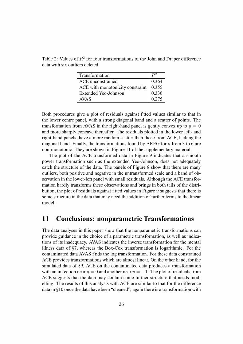
Table 2: Values of R2 for four transformations of the John and Draper differencedata with six outliers deleted

Transformation R2

ACE unconstrained 0.364ACE with monotonicity constraint 0.355Extended Yeo-Johnson 0.336AVAS 0.275

Both procedures give a plot of residuals against f tted values similar to that inthe lower centre panel, with a strong diagonal band and a scatter of points. Thetransformation from AVAS in the right-hand panel is gently convex up to y = 0and more sharply concave thereafter. The residuals plotted in the lower left- andright-hand panels, have a more random scatter than those from ACE, lacking thediagonal band. Finally, the transformations found by AREG for k from 3 to 6 arenon-monotonic. They are shown in Figure 11 of the supplementary material.

The plot of the ACE transformed data in Figure 9 indicates that a smoothpower transformation such as the extended Yeo-Johnson, does not adequatelycatch the structure of the data. The panels of Figure 8 show that there are manyoutliers, both positive and negative in the untransformed scale and a band of ob-servation in the lower-left panel with small residuals. Although the ACE transfor-mation hardly transforms these observations and brings in both tails of the distri-bution, the plot of residuals against f tted values in Figure 9 suggests that there issome structure in the data that may need the addition of further terms to the linearmodel.

11 Conclusions: nonparametric TransformationsThe data analyses in this paper show that the nonparametric transformations canprovide guidance in the choice of a parametric transformation, as well as indica-tions of its inadequacy. AVAS indicates the inverse transformation for the mentalillness data of §7, whereas the Box-Cox transformation is logarithmic. For thecontaminated data AVAS f nds the log transformation. For these data constrainedACE provides transformations which are almost linear. On the other hand, for thesimulated data of §9, ACE on the contaminated data produces a transformationwith an inf ection near y = 0 and another near y = −1. The plot of residuals fromACE suggests that the data may contain some further structure that needs mod-elling. The results of this analysis with ACE are similar to that for the differencedata in §10 once the data have been “cleaned”; again there is a transformation with

26

-5 0 5 10y

-2

-1

0

1

2

EXT

YJ ty

Plot of ty vs. y

-5 0 5 10y

-2

0

2

4

ACE

ty

Plot of ty vs. y

-5 0 5 10y

-4

-2

0

2

AVAS

ty

Plot of ty vs. y

-1 0 1Fitted values

-2

-1

0

1

2

EXT

YJ re

sidu

als

Plot of residuals vs. fit

-1 0 1Fitted values

-2

0

2

4

ACE

resi

dual

s

Plot of residuals vs. fit

-1 0 1Fitted values

-4

-2

0

2

AVAS

resi

dual

s

Plot of residuals vs. fit

Figure 9: Cleaned difference data; properties of data transformed by the extendedYeo-Johnson transformation, ACE and AVAS. Left-hand column, extended Yeo-Johnson; central column, ACE; right-hand column, AVAS. Upper row transformedy against y; lower row, residuals against f tted values

perhaps three zones and a non-random residual plot. For these examples AVASproduces respectively a virtually straight line transformation and a smooth con-cave curve. The transformations indicated by AREG for these examples are eithernon-informative, that is no transformation is indicated, or are non-monotonic.

Unlike AREG, but like the forward search, ACE and AVAS have the advantagethat the methods do not require the advance specif cation of parameters. Furtherresults in the supplementary material indicate that ACE and AVAS may behavewell for non-negative data. However, for the balance sheet data, both ACE andAVAS are inf uenced by the outliers in the data. A promising strategy is that of §10in which the fan plot, a robust method, is used to indicate a parametric transforma-tion and a scale in which the data can be cleaned. Parametric and nonparametrictransformations can then be compared on data without outliers.

27

The calculations in this paper used Matlab routines from the FSDA toolbox,available as a Matlab add-on from the Mathworks f le exchangehttps://www.mathworks.com/matlabcentral/fileexchange/.The data, the code used to reproduce all results including plots, and links to FSDAroutines are available at http://www.riani.it/ARC2019.Acknowledgements

This research benef ts from the HPC (High Performance Computing) facilityof the University of Parma. We acknowledge f nancial support from the Universityof Parma project “Statistics for fraud detection, with applications to trade dataand f nancial statements” and from the Department of Statistics, London Schoolof Economics.

ReferencesAndrews, D. F., Gnanadesikan, R., and Warner, J. L. (1971). Transformations ofmultivariate data. Biometrics, 27, 825–840.

Aranda-Ordaz, F. J. (1981). On two families of transformations to additivity forbinary response models. Biometrika, 68, 357–363.

Atkinson, A. C. (1973). Testing transformations to normality. Journal of the RoyalStatistical Society, Series B, 35, 473–479.

Atkinson, A. C. (1982). Regression diagnostics, transformations and constructedvariables (with discussion). Journal of the Royal Statistical Society, Series B,44, 1–36.

Atkinson, A. C. (1985). Plots, Transformations, and Regression. Oxford Univer-sity Press, Oxford.

Atkinson, A. C. and Cox, D. R. (1988). Transformations I. Wiley Statsref.

Atkinson, A. C. and Lawrance, A. J. (1989). A comparison of asymptoticallyequivalent tests of regression transformation. Biometrika, 76, 223–229.

Atkinson, A. C. and Riani, M. (2000). Robust Diagnostic Regression Analysis.Springer–Verlag, New York.

Atkinson, A. C. and Riani, M. (2002). Tests in the fan plot for robust, diagnostictransformations in regression. Chemometrics and Intelligent Laboratory Sys-tems, 60, 87–100.

28

Atkinson, A. C., Pericchi, L. R., and Smith, R. L. (1991). Grouped likelihoodfor the shifted power transformation. Journal of the Royal Statistical Society,Series B, 53, 473–482.

Atkinson, A. C., Koopman, S. J., and Shephard, N. (1997). Detecting shocks:Outliers and breaks in time series. Journal of Econometrics, 80, 387–422.

Atkinson, A. C., Riani, M., and Cerioli, A. (2004). Exploring Multivariate Datawith the Forward Search. Springer–Verlag, New York.

Atkinson, A. C., Riani, M., and Cerioli, A. (2010). The forward search: theoryand data analysis (with discussion). Journal of the Korean Statistical Society,39, 117–134. doi:10.1016/j.jkss.2010.02.007.

Atkinson, A. C., Riani, M., and Corbellini, A. (2020). The transformation of prof tand loss data. Applied Statistics, 69. DOI: https://doi.org/10.1111/rssc.12389.

Bickel, P. J. and Doksum, K. A. (1981). An analysis of transformations revisited.Journal of the American Statistical Association, 76, 296–311.

Bliss, C. I. (1934). The method of probits. Science, 79(2037), 38–39.

Box, G. E. P. and Cox, D. R. (1964). An analysis of transformations (with discus-sion). Journal of the Royal Statistical Society, Series B, 26, 211–252.

Box, G. E. P. and Cox, D. R. (1982). An analysis of transformations revisited,rebutted. Journal of the American Statistical Association, 77, 209–210.

Box, G. E. P. and Tidwell, P. W. (1962). Transformations of the independentvariables. Technometrics, 4, 531–550.

Breiman, L. and Friedman, J. H. (1985). Estimating optimal transformations formultiple regression and transformation (with discussion). Journal of the Amer-ican Statistical Association, 80, 580–619.

Breusch, T. S. and Pagan, A. R. (1979). A simple test for heteroscedasticity andrandom coeff cient variation. Econometrica, 47, 1287–1294.

Brown, B. W. and Hollander, M. (1977). Statistics: A Biomedical Introduction.Wiley, New York.

Buja, A. and Kass, R. E. (1985). Comment on “Estimating optimal transforma-tions for multiple regression and transformation” by Breiman and Friedman.Journal of the American Statistical Association, 80, 602–607.

29

Cai, T., Tian, L., and Wei, L. J. (2005). Semiparametric Box-Cox power transfor-mation models for censored survival observations. Biometrika, 92, 619–632.

Carroll, R. J. (1982). Prediction and power transformations when the choice ofpower is restricted to a f nite set. Journal of the American Statistical Associa-tion, 77, 908–915.

Carroll, R. J. and Ruppert, D. (1985). Transformations in regression: a robustanalysis. Technometrics, 27, 1–12.

Carroll, R. J. and Ruppert, D. (1988). Transformation and Weighting in Regres-sion. Chapman and Hall, New York.

Chen, G., Lockhart, R. A., and Stephens, M. A. (2002). Box-Cox transformationsin linear models: large sample theory and tests of normality (with discussion).The Canadian Journal of Statistics, 30, 177–234.

Cook, R. D. and Weisberg, S. (1982). Residuals and Inf uence in Regression.Chapman and Hall, London.

Cox, D. R. (1977). Nonlinear models, residuals and transformations. Mathema-tische Operationsforschung und Statistik, Serie Statistik, 8, 3–22.

Cox, D. R. and Reid, N. (1987). Parameter orthogonality and approximate con-ditional inference (with discussion). Journal of the Royal Statistical Society,Series B, 49, 1–39.

Firth, D. (1988). Multiplicative errors: Log-normal or gamma? Journal of theRoyal Statistical Society, Series B, 50, 266–268.

Fisher, R. A. (1915). Frequency distribution of the values of the correlation coef-f cient in samples from an indef nitely large population. Biometrika, 10, 507–521.

Foster, A. M., Tian, L., , and Wei, L. W. (2001). Estimation for the Box-Coxtransformation model without assuming parametric error distribution. Journalof the American Statistical Association, 96, 1097–1101.

Friedman, J. and Stuetzle, W. (1982). Smoothing of scatterplots. Technical report,Department of Statistics, Stanford University, Technical Report ORION 003.

Gnanadesikan, R. (1977). Methods for Statistical Data Analysis of MultivariateObservations. Wiley, New York.

30

Gottardo, R. and Raftery, A. (2009). Bayesian robust transformation and variableselection: a unif ed approach. Canadian Journal of Statistics, 37, 361–380.

Hampel, F. R. (1975). Beyond location parameters: robust concepts and methods.Bulletin of the International Statistical Institute, 46, 375–382.

Harrell Jr, F. E. (2019). Hmisc. R package version 4.2-0.

Hastie, T. J. and Tibshirani, R. J. (1990). Generalized Additive Models. Chapmanand Hall, London.

Hinkley, D. V. and Runger, G. (1984). The analysis of transformed data. Journalof the American Statistical Association, 79, 302–309.

Hoyle, M. H. (1973). Transformations - an introduction and a bibliography. In-ternational Statistical Review, 41, 203–223.

Huber, P. J. (1973). Robust regression: Asymptotics, conjectures and MonteCarlo. Annals of Statistics, 1, 799–821.

John, J. A. and Draper, N. R. (1980). An alternative family of transformations.Applied Statistics, 29, 190–197.

Kleinbaum, D. G. and Kupper, L. (1978). Applied Regression Analysis and OtherMultivariable Methods. Duxbury, Boston, Mass.

Lawrance, A. J. (1987). The score statistic for regression transformation.Biometrika, 74, 275–279.

Marazzi, A., Villar, A. J., and Yohai, V. J. (2009). Robust response transformationsbased on optimal prediction. Journal of the American Statistical Association,104, 360–370. DOI: 10.1198/jasa.2009.0109.

McCullagh, P. (2002a). Comment on “Box-Cox transformations in linear models:large sample theory and tests of normality” by Chen, Lockhart and Stephens.The Canadian Journal of Statistics, 30, 212–213.

McCullagh, P. (2002b). What is a statistical model? The Annals of Statistics, 30,1225—-1310.

McCullagh, P. and Nelder, J. A. (1989). Generalized Linear Models (2nd Ed.).Chapman and Hall, London.

Nychka, D. and Ruppert, D. (1995). Nonparametric transformations for both sidesof a regression model. Journal of the Royal Statistical Society, Series B, 57,519–532.

31

Pericchi, L. R. (1981). A Bayesian approach to transformations to normality.Biometrika, 68, 35–43.

Perrotta, D., Riani, M., and Torti, F. (2009). New robust dynamic plots for re-gression mixture detection. Advances in Data Analysis and Classif cation, 3,263–279. doi:10.1007/s11634-009-0050-y.

Pregibon, D. (1980). Goodness of link tests for generalized linear models. AppliedStatistics, 29, 15–23,14.

Proietti, T. and Riani, M. (2009). Transformations and seasonal adjustment. Jour-nal of Time Series Analysis, 30(1), 47–69.

Ramsay, J. O. (1988). Monotone regression splines in action. Statistical Science,3, 425–461.

Reid, N. (2002). Comment on “Box-Cox transformations in linear models: largesample theory and tests of normality” by Chen, Lockhart and Stephens. TheCanadian Journal of Statistics, 30, 211.

Riani, M. (2009). Robust transformations in univariate and multivariate time se-ries. Econometric Reviews, 28, 262 – 278.

Riani, M., Atkinson, A. C., and Cerioli, A. (2009). Finding an unknown numberof multivariate outliers. Journal of the Royal Statistical Society, Series B, 71,447–466.

Riani, M., Cerioli, A., Atkinson, A. C., and Perrotta, D. (2014). Monitoring robustregression. Electronic Journal of Statistics, 8, 642–673.

Ross, G. J. S. (1990). Nonlinear Estimation. Springer–Verlag, New York.

Rousseeuw, P. J. (1984). Least median of squares regression. Journal of theAmerican Statistical Association, 79, 871–880.

Royston, P. J. and Altman, D. G. (1994). Regression using fractional polynomialsof continuous covariates: parsimonious parametric modelling (with discussion).Applied Statistics, 43, 429–467.

Sakia, R. M. (1992). The Box-Cox transformation technique: a review. TheStatistician, 41, 169–178.

Seo, H. S. (2019). A robust method for response variable transformations usingdynamic plots. Communications for Statistical Applications and Methods, 26,463–471. DOI: https://doi.org/10.29220/CSAM.2019.26.5.463.

32

Song, X.-Y. and Lu, Z.-H. (2012). Semiparametric transformation models withBayesian P-splines. Statistics and Computing, 22, 1085–1098.

Spector, P., Friedman, J., Tibshirani, R., Lumley, T., Garbett, S., and Baron, J.(2016). acepack: ACE and AVAS for Selecting Multiple Regression Transfor-mations. R package version 1.4.1.

Sweeting, T. J. (1984). On the choice of prior distribution for the Box-Cox trans-formed linear model. Biometrika, 71, 127–134.

Taylor, J. M. G. (1986). The retransformed mean after a f tted power transforma-tion. Journal of the American Statistical Association, 81, 114–118.

Taylor, J. M. G. (2004). Transformations II. Wiley Statsref.

Taylor, J. M. G. and Liu, N. (2007). Statistical issues involved with extendingstandard models. In V. Nair, editor, Advances in Statistical Modeling and Infer-ence, pages 299–311. World Scientif c, Singapore.

Tibshirani, R. (1988). Estimating transformations for regression via additivityand variance stabilization. Journal of the American Statistical Association, 83,394–405.

Velilla, S. (1995). Diagnostics and robust estimation in multivariate data transfor-mations. Journal of the American Statistical Association, 90, 945–951.

Wang, D. and Murphy, M. (2005). Identifying nonlinear relationships in regres-sion using the ACE algorithm. Journal of Applied Statistics, 32, 243 – 258.

Wang, N. and Ruppert, D. (1995). Nonparametric estimation of the transforma-tion in the transform-both-sides regression model. Journal of the AmericanStatistical Association, 90, 522–534.

Weisberg, S. (2005). Yeo-Johnson power transformations. https://www.stat.umn.edu/arc/yjpower.pdf.

Wiens, B. L. (1999). When log-normal and gamma models give different results:a case study. The American Statistician, 53, 89–93.

Yang, Z. (2006). A modif ed family of power transformations. Economics Letters,92, 14–19. https://ink.library.smu.edu.sg/soe-research/179.

Yeo, I.-K. and Johnson, R. A. (2000). A new family of power transformations toimprove normality or symmetry. Biometrika, 87, 954–959.

33

Yohai, V. J. (1987). High breakdown-point and high eff ciency estimates for re-gression. The Annals of Statistics, 15, 642–656.

Zhang, T. and Yang, B. (2017). Box-Cox transformation in big data. Technomet-rics, 59(2), 189–201.

34