HAL Id: halshs-01261980https://halshs.archives-ouvertes.fr/halshs-01261980

Preprint submitted on 26 Jan 2016

HAL is a multi-disciplinary open accessarchive for the deposit and dissemination of sci-entific research documents, whether they are pub-lished or not. The documents may come fromteaching and research institutions in France orabroad, or from public or private research centers.

L’archive ouverte pluridisciplinaire HAL, estdestinée au dépôt et à la diffusion de documentsscientifiques de niveau recherche, publiés ou non,émanant des établissements d’enseignement et derecherche français ou étrangers, des laboratoirespublics ou privés.

Box-Cox transformations of terms nesting theTrans-Log: the example of rail infrastructure

maintenance costMarc Gaudry, Emile Quinet

To cite this version:Marc Gaudry, Emile Quinet. Box-Cox transformations of terms nesting the Trans-Log: the exampleof rail infrastructure maintenance cost. 2016. �halshs-01261980�

WORKING PAPER N° 2016 – 01

Box-Cox transformations of terms nesting the Trans-Log: the example of rail infrastructure maintenance cost

Marc Gaudry

Emile Quinet

JEL Codes: C20, C34, C87, D24, L92

Keywords: Trans-Log model, Box-Cox transformations, Generalized Flexible Quadratic model, Unrestricted Generalized Box-Cox model, railway track current maintenance cost, railway track degradation engineering models, CATRIN European project, France

PARIS-JOURDAN SCIENCES ECONOMIQUES

48, BD JOURDAN – E.N.S. – 75014 PARIS TÉL. : 33(0) 1 43 13 63 00 – FAX : 33 (0) 1 43 13 63 10

www.pse.ens.fr

CENTRE NATIONAL DE LA RECHERCHE SCIENTIFIQUE – ECOLE DES HAUTES ETUDES EN SCIENCES SOCIALES

ÉCOLE DES PONTS PARISTECH – ECOLE NORMALE SUPÉRIEURE – INSTITUT NATIONAL DE LA RECHERCHE AGRONOMIQU

1

Box-Cox transformations of terms nesting the Trans-Log:

the example of rail infrastructure maintenance cost

Marc Gaudry1 and Émile Quinet

2

1 Département de sciences économiques et

Agora Jules Dupuit (AJD), www.e-ajd.net ou http://e-ajd.mkm.de/

Université de Montréal

Montréal, marc.gaudry@umontreal.ca

2 Paris-Jourdan Sciences Économiques (PSE)

École des Ponts ParisTech (ENPC)

Paris, quinet@enpc.fr

This paper, the first September 2015 version of which was entitled «Sur la forme des équations

explicatives du coût d’entretien», was originally produced for the SNCF Réseau project «Estimation

des coûts marginaux d’entretien du réseau ferré national». The authors thank the SNCF for

financial support and for the permission to use its France-wide 1999 rail track segment maintenance

cost database produced by Michel Ikonomov.

Université de Montréal

Agora Jules Dupuit - Publication AJD-155

--------------------

Paris-Jourdan Sciences Économiques

PSE Working Paper No 2015-XXXX

Version 5, 25th

December 2015.

2

Abstract

We explore how the Trans-Log (TL) can be nested in Box-Cox transformed terms and show that a

particular specification previously defined, but not fully tested, within the European CATRIN

consortium (Gaudry & Quinet, 2010), the Unrestricted Generalized Box-Cox (U-GBC), constitutes a

proper incarnation of the Generalized Flexible Quadratic class (Blackorby et al. (1977) and nests a

number of more or less known intermediate Box-Cox-inspired partial generalizations of the TL, as

well as the target TL itself.

After a brief rail cost litterature review, our detailed references to such intermediate model

specifications making partial use of Box-Cox transformations are focused on examples developed

since 2002 using cross-sectional data, shown to differ profoundly from their ancestor aggregate time-

series firm-wide explanations of total or of current maintenance rail cost published before 2002.

Notably, the TL, devoid of prices, has since 2002 become a rail engineering degradation cost model

under an unchanged econometric terminological form garb on which we dwell.

We estimate three main rail maintenance cost model specifications strictly nesting the TL from real

1999 France-wide segment network data and compare their improved log likelihood values under

different engineering hypotheses concerning physical interactions among four rail Traffic types and

four track Quality characteristics.

We find the Trans-Log to be an inadequate model of railway damage because physical interactions

among track Quality indicators and train Traffic types are not of log-log form but of other forms better

handled by common flexible Box-Cox Transformations, twelve of which are estimated in our most

general U-GBC specification, all but one actually differing from the logarithmic case. And, of course,

not all physical interactions turn out to matter in the explanation of degradation cost: track Quality-

Quality interactions, for instance, are of nugatory importance.

Table of contents

1. Introduction .......................................................................................................................................... 3 2. The study of transport cost ................................................................................................................... 4

2.1. Relaxing fixed form single output Trans-Log constraints ............................................................ 4 2.2. Multiple rail outputs, input prices and firm-wide time-series data ............................................... 6

2.3. Multiple rail traffics, track qualities and track segment cross-section data .................................. 7 3. Nesting the Trans-Log within Box-Cox transformed terms ................................................................ 9

4. An example: joint econometric and engineering issues ..................................................................... 11 5. Conclusion ......................................................................................................................................... 15 6. Appendix 1. Detailed results of Table 4 models 4-7 ......................................................................... 15 7. References .......................................................................................................................................... 18

List of tables

Table 1. Principal Box-Cox transformation estimation pitfalls ............................................................... 5 Table 2. Nature of information available by rail line section for the French network of 1999 ............. 11

Table 3. Principal characteristics of database variables (928 observation subset) ................................ 11

Table 4. Crossing econometric form and engineering track degradation assumptions ......................... 13 Table 5. The 12 BCT power values estimated in the dominant U-GBC-2 specification (Model 4) ..... 14

Key words: Trans-Log model, Box-Cox transformations, Generalized Flexible Quadratic model,

Unrestricted Generalized Box-Cox model, railway track current maintenance cost,

railway track degradation engineering models, CATRIN European project, France.

Journal of Economic Literature Classification

C20, C34, C87, D24, L92.

3

1. Introduction Our context is the study of rail track maintenance cost and the derived calculation of the marginal cost

which forms the basis of rail infrastructure charges differentiated by type of train in countries which

apply the marginal cost pricing doctrine of the European Union: Directive 2001/14 of the European

Commission states that track access charges should be set according to direct costs of running a

vehicle on the tracks.

A particularly complete synthesis of this sort of study work is found in the 2008-2009 country reports

produced by the Cost Allocation of Transport INfrastructure Cost (CATRIN) research consortium,

summarized in Wheat et al. (2009). CATRIN studies notably provide comparable coordinated

statistical analyses1 linking annual rail maintenance expenditures to traffic and technical track

characteristics for five2 European country rail networks. The resulting cost functions rely on minimal

technical knowledge, do not use input prices as explanatory variables, but all generate cost estimates

with standard econometric model specifications such as Constant Elasticity of Substitution (CES) and

Trans-Log (TL) formulations, or their various ad hoc Box-Cox transformation (BCT) generalizations.

Recently initiated by Idström (2002), Johansson & Nilsson (2002, 2004) and Gaudry & Quinet (2003),

models of physical track damage cost are all based on single (or at most 3-4) cross sections of yearly

maintenance costs incurred by track segment of national rail infrastructure networks. They should not

be confused with former time series models of rail cost estimated from aggregate firm-wide data

panels, frequently estimated with CES and Trans-Log specifications during the previous two decades

(say 1982-2002), or even with models of only maintenance cost estimated from similarly aggregate

firm-wide time-series data (e.g. Bereskin, 2000; Sánchez, 2000), where the assumption of constant

input prices obviously cannot be made due to the length of the time-series used.

In those cases, where prices of inputs are introduced in the estimation, duly taking theory into account

adds to the main specification of maintenance cost the constraints expressing Shephard’s lemma about

the shares of inputs in the total cost, an information which entails a lot of complications in estimation

and in the calculation of derived model statistics such as elasticities. But in the cross-sectional

framework to which we will here limit the analysis of structures nesting the TL, and which is now the

most frequent procedure in rail cost analysis, prices are assumed to be constant, and the additional

constraints do not intervene. The economic models have in fact become engineering explanations of

the cost of physical track degradation.

Overall, rail maintenance cost studies then clearly belong to one of two approaches, also found in the

general literature on cost functions, depending on whether time-series or cross-sections are used. The

former must deal with price changes and Shephard’s restrictions in addition to usual specific time-

series issues: it is not easy to synthesize them or to interpret their results. The latter, more numerous,

avoid both serial correlation and price change predicaments3: analyses are simpler and more similar.

But their specifications still differ considerably, to this day without any ranking of their relative

import, notably concerning the choice among Log-Log, Trans-Log or more or less extensive Box-Cox

generalizations: a normal quandary in the absence to this day of formalized nesting among these

specifications.

We purport to fill this need, whithin the domain of cross-sectional studies and with a rail maintenance

cost application. The second section is a brief review of both panel and cross-sectional studies, but

with the emphasis on the latter. The third section proposes a complete nesting of the most frequent

cross-sectional specifications. The fourth applies this nesting to the case of current French rail

infrastructure maintenance, making it possible to conclude more rigourously than before to the

superiority of the Generalized Box-Cox formulation, either Restricted or Unrestricted, at least with

those national data.

1 In particular, Box-Cox transformations are applied by all to CES, and by some to other specifications as well.

2 Austria, France, Great Britain, Sweden, Switzerland.

3 Longer panels are beginning to appear (e.g. Odolinski & Nilsson, 2015), with those very predicaments.

4

2. The study of transport cost

2.1. Relaxing fixed form single output Trans-Log constraints The empirical litterature on transport cost functions is, as in other fields of cost estimation, dominated

by the Trans-Log which arose in production economics (Christensen et al., 1971a, 1971b) and may be

written here for our own narrower practical purposes in its simplest4 core form as:

(TL) 2

0

1 1 1 1,

ln( ) ln (ln ) ln lnj rr r i r

k k kk k ij i j

k k i j j i

y X X X X

where the formulation potentially includes multiple outputs and prices and where cross product ij

terms are distinguished as between the «squared» ii terms and the «interaction» ,ij i j terms proper.

Initially, the Xk variables included a unique output Q1 and a vector of input prices P=(P1,…,Pj), but

here we simply distinguish between «linear» k , «squared» kk and «interaction» ,ij i j coefficients.

This TL workhorse cost model of old was widely used in transport, as elsewhere, primarily to study

the total cost of production by transport firms providing transport services (e.g. buses) or such

services and their infrastructure (e.g. vertically integrated railways), etc.: the examples are legion.

It may be viewed both as a particular second order approximation of any latent true cost function and

as a particular member of the Generalized Flexible Quadratic class of such approximations:

(GFQ) 0

1 1 1

( ) ( ) ( ) ( )j rk r i r

k k k ij i i j j

k i j

C X f X f X f X

as defined, but not tested, by Blackorby et al. (1977) whose urge to make the initial TL less rigid

pertained to both allowing for more than one output (e.g. here, passenger and freight train services)

and to relaxing the logarithmic restriction on the form of variables (e.g. here, why would physical

interactions between trains and track just happen to be of logarithmic form when this is clearly not the

case for the impact of road vehicles on pavements, better explained by a Box-Tidwell formulation

(Small & Zhang, 1988; Zhang, 1989)?).

Concerning their first point, Denny & Fuss (1977) made the natural point that, if the underlying

relationship was really of TL form, product qualities of the unique output, or aggregates of distinct

outputs, also had to appear log-linearly in (TL).

But, concerning their second point, was the true form relationship as this assumed? The use of the

Box-Cox transformation ― whenceforth BCT ― in its common garb (without Tukey’s shift

parameter), namely (Box & Cox, 1964):

(BCT) ( ) [( ) 1] , 0,

ln ( ) , 0,

v

v v v v

v

v v

VarVar

Var

among Trans-Log users, as in economic modelling generally, as pointed out by Poirier (1978) and by

Davidson & MacKinnon (1085, 1993), stimulated piecemeal ad hoc generalizations and progressively

built up a layer of like-minded partial incarnations of the (GFQ) based on more or less BCT use.

It is this multiple-output BCT enriched layer that we wish to examine, and perhaps unify, in rail track

maintenance cost analysis. Doing so, we must have in mind some of the pitfalls of BCT generalization

and estimation, summarized in Table 1, which the TL avoids but which have to be taken into account

when substituting in, and enlarging the initial TL to, more general BCT specifications.

4 Economic theory proposes other constraints on the , in addition to that of symmetry retained here, which are not

physically meaningful to model material damage interactions between rail traffic and track characteristics.

5

Table 1. Principal Box-Cox transformation estimation pitfalls

Identification of BCT power estimate

P-1

if regressors include both a variable k

X transformed by a BCT and that same variable raised to a

power s and also transformed by another BCT, the model, even if theoretically valid, is not

identified and the estimates of ( )

kX

and

'( )s

kX

are strictly collinear, because a BCT estimate is

unique and invariant to any simple power transformation s of k

X even in the absence of a

regression intercept 0

. Estimated forms ( )

kX

and

'( )s

kX

, collinear due to

's , are then

mathematically and statistically undistinguishable (Gaudry & Laferrière, 1989);

Invariance of BCT power estimate

P-2 if 0

ktX , t , its BCT

kX

will not be invariant to a change in units of measurement of k

X unless

the regression has an intercept 0

(Schlesselman, 1971);

P-3

if 0kt

X , it may be transformed by a BCT k

X if and only if an associated dummy variable is

created to compensate for the shifts at 0-valued observations and to preserve invariance to units of

measurement of k

X , even if P-2 is satisfied. Replacement of zeroes by a small value (e.g.

0.0000001) induces biases that depend on its size and on the frequency of zeroes, and which are

more important in the TL than in BCT forms (Gaudry & Quinet, 2010, especially Appendix 4);

Invariance of Student’s t-statistics of coefficients of BCT transformed variables

P-4

if the t-statistics of ,...,k

coefficients of BCT transformed regressor variables k

X ,…, X are calculated in usual unconditional fashion from the first or second derivatives of the maximized Log

Likelihood, they will be dependent on the units of measurement of the regressors and therefore adjustable at will by changing these units of measurement. They recover invariance only if they are computed conditionally upon estimated BCT values (Spitzer, 1984; Dagenais & Dufour, 1994);

Global maximum of the maximized Log Likelihood

P-5

taking as reference the Likelihood maximand , as specified by Box and Cox themselves, namely:

2Tt t

22t 1 w tw

w w1exp

2 y2

,

where, under the assumptions of normality and constancy of the variance 2

w of the independent

error term wt of zero mean and y 1

t t tw / y y

denoting the Jacobian of the transformation from

wt to the observed yt, use of multiple BCT requires finding the global maximum of ln( ) because,

as long and very well known in practice, its concavity need not hold (Kouider & Chen, 1995) ;

Model fitted value of observed yt

P-6

accepting that the point of econometric modelling is the explanation of observed yt, and not of ( )y

ty

its

transformed value (including the case of the logarithmic transformation 0y

), the proper

measure of fit should be based on E(yt), the expected value of yt, preferably assumed to be

censored both downwards (due to its strictly required positivity) and even upwards (e.g. here track

maintenance cost cannot exceed regeneration cost), within a range ≤ yt ≤ , where and are

respectively the strictly positive lower and upper censoring points common to all observations. The

expected value of the doubly censored variable yt, given that ( )w is the normal density function

of w with 0 mean and variance 2w, is the same as in a Tobit model (Liem, 1979; Liem et al., 1983,

1986; Tran et al., 2008): ( ) ( )

( ) ( )( ) ( ) ( ) ( ) , ( 0)

t t

t t

w w

t tw w

E y u du y w dw w dw and

,

a familiar expression since Tobin (1958) which, in the case of 0y

, collapses to:

( )( ) exp h

t h hthE y k X

,

the particulars of which require providing an unbiased estimate of k, the sample mean of the log-

normal random variable exp(wt) for the sample (making the full previous expression preferable).

6

On top of these frequent issues5, let us mention that the forthcoming rail cost models, all gasping for

some BCT generalizability, are only rarely estimated taking heteroskedasticity into account, a

reasonable stand because the dependent variable is usually a cost per unit (of output or of segment

length, depending on model family), the range of which makes homoskedasticity almost certain.

Much more serious neglected estimation issues in the cases we report on pertain to the presence of

serial autocorrelation in times-series models, never mentioned, and to the presence of spatial

correlation of residuals in cross-sectional models, never explicitly tested6 for.

Having in mind those caveats, we first show in the following sub-section how difficult it is to choose a

specification in the case of time series data, due to the impact of price variables; in sub-section 2.3 we

study cross-sectional data models and show that the varied specifications are more clear cut, but that

up to now no study has dared to nest them all. Section 3 shows that it is indeed possible to nest them

in a general specification, the so-called Unrestricted Generalized Box-Cox-2, the test of which will be

the subject of Section 4.

2.2. Multiple rail outputs, input prices and firm-wide time-series data A few studies of cost functions with multiple rail outputs and time series data have tried to steer TL

specifications towards BCT flexibility, but with a constant concern of inclusion of input prices (a

necessity because their changes over the medium to long term induce changes in cost functions per se,

independently from changes in traffics). We retrace these efforts only within the literature on rail cost.

The smallest Box-Tidwell patch possible: a single BCT applied to traffic variables. Motivated by

the presence of zero-output observations in real problems7, the Generalized Translog Multiproduct

Cost Function (GTMCF) proposed and discussed by Burgess (1974), Brown et al. (1979) and Caves

et al. (1980b), consists in departing ever so slightly from the similar treatment of all explanatory

variables (input prices and two outputs in this case) in the TL:

“This cost function has the same form as the Trans-Log except for output levels, where the Box-Cox metric is substituted for the natural log metric. This generalization permits the inclusion of firms with zero-output levels for some products”: [… it is required] “since passenger service is zero for a substantial number of observations” (Caves et al., 1985).

This involves using a unique BCT8 on the two output variables and keeping the logarithmic form for

every other term of the GFQ specification above. We call this the Box-Tidwell-1 (BT-1) function9

because, contrary to what its overbearing name (GTMCF) states, it is general in no meaningful sense.

Actual uses of this ad hoc and retricted BT-1 to explain total rail cost did not spread beyond Caves et

al. (1980a; 1985), as it “highly complicates the interpretation of parameters” (Tovar et al., 2003,

Footnote 9) and consequently makes the imperative calculation of elasticities much more burdensome.

The interpretation of parameters might indeed be complicated by BCT generalization, but that is

expected if TL constraints are demonstrably Procrustean.

5 Note that econometric estimation programs may, like model specifications, also suffer from BCT traps: for instance,

BIOGEME (Bierlaire, 2003, 2008) violates (P-4) and many regression programs fail the (P-6) test and cannot compute a

proper measure of fit, even in the simple case of a logarithmic dependent variable: their R2 results computed on

transformed y, and not on E(y), are not duly legible, sensible, or useful. In BIOGEME, the remedy to the calculation of t-

statistics that are invariant to changes in units of measurement of the regressors consists in making an additional iteration

with the routines used (DONLP2, SOLVOPT, CFSQP, BIO (trust region)) after having fixed the BCT at their optimal

values, thereby forcing the program to recompute the variance-covariance matrix of other parameters conditionally upon

BCT estimates and producing the required conditionnal t-values. 6 Recent examples taking spatial correlation into account (Gaudry & Quinet, 2014; Gaudry et al., 2015) are not simply

assuming that maintenance cost is minimized in the short run, as in sections 2.3 and 2.4, but that it is the object of a joint

minimization with that of track renewal cost. Such joint models are not covered here: only short run maintenance cost

minimization models are. 7 Indeed, zero outputs are frequent in cost functions: think of the case of two outputs, passengers and freight traffics, and of

track segments dedicated to freight, where passenger traffic is zero, or only to High Speed Rail trains. On this issue, see

P-3 in Table 1. 8 The BCT is implicitly assumed to be positive.

9 In the literature, applying one or more BCT only to explanatory variables is simply called a Box-Tidwell (Box &

Tidwell, 1962) model because the dependent variable is not transformed as in proper Box-Cox (1964) models.

7

The BT-1 amounts to a very marginal change of the TL indeed because a single BCT is used on two

train service variables, almost the smallest Box-Tidwell patch possible: a yet smaller patch would

have used the BCT only on passenger service if all firms in the sample had offerred freight service.

Why such parsimony? The note by Caves et al., (1980a, Footnote 3) states that a generalization to

more than one BCT “needlessly complicates estimation”.

In any case, it is not clear what to make of results obtained by Caves & Co because they do not deal

correctly with zeroes10

and do not adequately calculate t-statistics11

. Winston’s (1985, p. 63) opinion

of this12

is empirically and theoretically sound but neglects estimation matters or traps.

Working with a single BCT applied to cost and to some of the price interactions. In a study of

yearly railroad operations in Belgium from 1950 to 1986, Borger (1992) extended a previous analysis

of US manufacturing by Khaled (1978) and Berndt & Khaled (1979) to multiple outputs and qualities

but otherwise retained their specification. Their strategy had partly consisted in making the usual TL

price vector13

flexible with a single BCT ( ,P iP ), yielding terms of the form ( ) ( )P P

i jP P , also applied

as ( )CC

to the dependent cost variable14

with the restriction ( ˆ ˆ / 2P C ). Their so-called Generalized

Box-Cox (GBC) estimates justified their claim that the BCT can make it possible to choose between

the TL and other competing second order fixed form approximations to an arbitrary cost function.

These were the Generalized Square Root Quadratic (GSRQ) and the Generalized Leontief (GL),

both previously introduced by Diewert (1971, 1973, 1974) and obtained as special cases by imposing

( 2; 1C P ) and ( 1; 1/ 2C P ), respectively.

Borger extended the vector of variables to two outputs T (passenger and freight traffics) and each

output was related to various network qualities Q called “operation characteristics”. Variables in these

T and Q vectors were regrouped in strictly positive “output aggregation” terms of fixed CES form

with coefficients previously estimated independently. He did not modify the asymmetric treatment of

price terms at the heart of the complicated Berndt-Khaled cost formulation, but may have considered

the prospect when he included these available exogenous estimates:

“Note that we did not estimate the parameters of the aggregator functions simultaneously with the GBC model. Although this would have been preferable from a theoretical perspective, the complexity of the GBC model forced us to use a simpler alternative. We therefore used the [log linear] aggregates constructed in Borger (1991) as independent variables in the estimation”(op. cit., 1992).

2.3. Multiple rail traffics, track qualities and track segment cross-section data An engineering model of track segment degradation. Work done with detailed track-level segment

data has a flavour totally different from that of the above time-series work, to which the previous

section was devoted, as reviews (e.g. Link et al., 2008) make clear. Essentially, track-level segment

studies must from the beginning deal with multiple outputs (traffics T), including zero-traffic values,

and multiple infrastructure characteristics and states (track qualities Q). Moreover, in practice, they do

without prices P, effectively replaced by the rich variety of rail track characteristics (to use Borger’s

wording), or qualities Q, because real rail networks consist in subsets of track of notoriously distinct

qualities by design. The TL model has effectively become a model of physical rail track degradation

measured on network infrastructure segments.

10

The papers are not duly precise on the handling of zero observations but violation of P-3 was confirmed to us in an

August 2003 email correspondence with one of Caves’ co-authors, Michael Tretheway. 11

As the t-statistic of the unique BCT parameter is computed unconditionally (Caves et al., 1980a, Table 1), the estimates

appear to violate P-4 as well. This second violation explains why imposing the logarithmic form on the output variables

«does not result in more favorable standard errors» (op. cit, p. 480) as should have been be the case. 12

“To be sure, the Trans-Log approximation runs into difficulty for zero values of output. In this case, a

transformation using the Box-Cox metric (Caves et al., 1980a) can be used to apply this functional form.” 13

Their TL is particular and contains two price vectors. The net result of this was to retain interactions between output and

prices based on their logarithmic forms, without any BCT involved: BCT applied only to the dependent cost variable and

to the interactions among prices themselves. 14

Their complex procedure, not written in the clearest manner, appears to violate P-2 and perhaps P-1 and P-4 as well. We

could find no other author than Borger willing to work his way through this complexity and apply it again, at least to rail.

8

Perhaps for that reason, on French data, but also on other national sets of data15

, the TL was soon

(Quinet, 2002; Gaudry & Quinet, 2003), and repeatedly (Gaudry & Quinet, 2010), shown to perform

very badly against a simple16

Log-Log Constant Elasticity of Substitution (CES) form, the numerous

interaction terms among types of traffic T and track qualities Q adding nothing of statistical

significance to fit, quite far from it. Whence the motivation to relax with BCT the logarithmic

constraints on these terms in particular, in the hope of finding meaningful physical interactions to

complement the documented gains from using BCT on the dependent and «linear» k terms, as

demonstrated by the coordinated CATRIN results of superiority of the Standard Box-Cox:

(SBC) Xy k

r( )

0 k k

k

y X

,

over the CES (Wheat et al., 2009) on 5 country-wide networks.

Prodding beyond TL log-log interaction terms. In practice, an important additional CATRIN-

adressed question was whether one could improve the SBC by BCT applied to the crossed interaction

terms, in particular with the Unrestricted Generalized Box-Cox

(U-GBC-1) ( )( ) ( )

0

,

( )Xy ijk

r r r

k k ij i j

k i j i j

y X X X

,

which, in the absence of squared kk terms, allowed for easy nesting of a restricted R-GBC-1 version

defined by setting all above BCT equal:

(R-GBC-1) ( ) ( ) ( )

0

,

( )r r r

k k ij i j

k i j i j

y X X X

,

Use of U-GBC or R-GBC interaction terms without squared terms in fact yielded results that

massively and decisively dominated TL and SBC results (Gaudry & Quinet, op.cit., 2010),

demonstrating that generalized interaction specifications could make a significant contribution to the

explanation of physical track degradation.

Further work on the intentionally dropped kk terms is therefore in order to complete the

demonstration of the interest of BCT flexibility for the explanation of rail track degradation.

Moreover, above mentioned comparisons were sometimes just paired comparisons and not always

involved strictly nested specifications. A more complete nesting of these various competing

specifications in a general framework is urged for a rigorous treatment. That is what we will now

address with a formal and comprehensive flexible BCT specification precisely nesting the TL and

numerous ad hoc special intermediate cases.

15

For instance, as already said, in Austria, Great Britain, Sweden and Switzerland (Wheat et al., 2009). 16

Without any adding-up constraint on the coefficients.

9

3. Nesting the Trans-Log within Box-Cox transformed terms We will now prove the nesting properties of several of the above-mentioned specifications. We

consider first U-GBC-2, a specification which will be shown to be an appropriate Box-Cox

incarnation of the GQF

(U-GBC-2) '''( ) ( )( ) ( )2

0

, ,

( ) ( )y ijk k

r r r r

k k kk k ij i j

k k i j i i j

y X X X X

,

where the squared terms are explicit, i.e. excluded from the crossed interaction terms, and identified if '

k k : if '

k k and without any restriction on these parameters, they are not identified. But other

specifications of linear and squared terms could also assure identication, for instance

1 2

1 1 2 2 1 2 2 21 1

( ) ( ) ( ) ( )2 2... ( ) ( ) ...k k kk kk

k kk k k k k k k kX X X X

for a case with two variables: we use this

type of identification below with the two sets of 4 squared terms QkQk and TkTk used jointly (in

Appendix 1, see 9kk ). More generally, the linear and squared terms are identified as long as there

is a relation between the λs of the first sum and the λs of the second one.

We also consider intermediate specifications such as the following extension to other R.H.S.

variables of the minimal Box-Tidwell-1 (BT-1) patch described earlier:

(BT-2) ( ) ( ) ( )( )2

0

,

ln( ) ( )k k k k

r r r r

k k kk k ij i j

k k i j i j

y X X X X

,

recently proposed within the SUSTRAIL European project (Wheat et al., 2014) where it is assumed to

nest the TL. We finally consider the R-GBC-2:

(R-GBC-2) ( ) ( ) 2 ( ) ( )

0

,

( ) ( )r r r r

k k kk k ij i j

k k i j i j

y X X X X

.

Our concern in this section is mathematical validity, as distinct from identifiability or other estimation

issues listed in Table 1: they will be adressed in due time if and when immediately relevant. We prove

that TL is nested in BT-2, which is nested in R-GBC-2, which itself is nested in U-GBC-2. This

assertion is evident for the L.H.S.s of the relations defining these specification, and also for the linear

terms of the R.H.S.s, so we will concentrate on the cross and squared terms.

To study them, consider the expression of cross and squared terms in (BT-2) where X≠Y for

interaction terms and X=Y for squared terms:

(1-A) 1 1Y X

C

By simple manipulation, we obtain successively:

(1-B) 1 1 1 1XYY X X Y

C

(1-C)

( ) ( ) ( )

11 1 1 1XY X YC XY X Y

which, by a limited expansion of the powers17

of Y and of X, yields if 0 :

(1-D) 1

(ln )² (ln )² (ln )² (ln )(ln )2

C XY X Y X Y .

17

The second order is necessary because the first order terms cancel out.

10

To see this last point, and using the Taylor expansion to the second order, rewrite C from (1-B)

successively as

exp( ln( ) 1 exp( ln( )) 1 exp( ln( )) 11 1 1XY XY X YX YC

,

1

ln( ) 0,5 ²(ln( ))² ln( ) 0,5 ²(ln( ))² ln( ) 0,5 ²(ln( ))²²

C XY XY X X Y Y

,

0,5 ln( ) ² (ln( ))² (ln( ))²C XY X Y ,

ln( ) ln( )C X Y ,

Comparing (1-B) and (1-C), we see that the R.H.S. of specification BT-2 is equivalent to the R.H.S. of

specification R-GCB-2; as the L.H.S. of BT-2 is nested in the L.H.S. of R-GCB-2, R-GCB-2 nests

BT-2. Relation (1-D) shows that the BT-2 specification nests the TL specification. So TL is nested in

BT-2, and BT-2 is nested in R-GCB-2, while clearly R-GCB-2 is nested in U-GBC-2. Q.E.D.

The above may be restated differently. We start from H, the hybrid specification (2-A) where squared

terms are included in the interaction terms; we show next that it can be rewritten as (2-B)18

, where the

are functions of the and of the single used, which tends to (2-C) if 0 . Namely:

(2-A) 0

,

( * ) 11*

i jkk ij

k i j

Y YYH

,

(2-B) 0

,

11 1* *

jk ik ij

k i j

YY YH

,

(2-C) 0

,

ln *ln *lnn k k ij i j

k i j

H Y Y Y .

Note that Trans-Log specification (2-C) is nested in (2-A), which does not seem to be a Trans-Log,

and in (2-B) that we have demonstrated to be the same as (2-A) in the single BCT case. Both (2-A)

and (2-B) themselves are nested in more general BCT specifications with different lambdas.

Seemingly different transformations of the same terms, i.e. ( * ) 1i jY Y

and 11

*ji

YY

,

lead to equivalent models, thereby comforting our use of the plural in the title of this paper.

18

Testing (2-B) is thefore the same as testing (2-A) and both include the TL.

11

4. An example: joint econometric and engineering issues Data for real examples. To illustrate the issues, we choose a non trivial rail track maintenance

problem with a sufficient number of traffics (Tk=4) and track qualities (Qk=4). Categories of available

variables are defined in Table 2 and descriptive statistics of the main variables are given in Table 3.

Table 2. Nature of information available by rail line section for the French network of 1999

C maintenance Cost, drawn from the analytical accounts of Société Nationale des Chemins de Fer

Français (SNCF), encompasses maintenance costs allocated to track CIV (consistance des

installations de voie) segments and represents 81% of total maintenance expenditure: the rest consists

of triages, intermodal freight platforms and service tracks, none of which can clearly be assigned to a

given track segment. It also covers catenaries, signalling, tracks, rails, sleepers, ballast, culverts and

“works of art” (ouvrages d’art, i.e. bridges and tunnels). It excludes traffic control costs and costs of

renewal (regeneration/reconstruction/renewal) but includes some Large Maintenance Operations

(Opérations de Grand Entretien, OGE) which are assigned to current maintenance accounts because

they are not full but partial renewals19

.

S technical State variables such as the number of tracks (from 1 to 18), the number of switches, the type

of control devices (automatic or not), the type of power (electrified or not), the length of the section.

Q technical Quality variables such as the age of rails, the age of sleepers, the share of concrete (vs wood)

sleepers and the maximum allowed speed in normal operation (in the absence of incidents or repairs in

progress). Maximum allowed speed is effectively both a state and a quality technical factor.

T train Traffic, measured by the number and average weight (tons) of 4 types of trains, namely Long

Distance Intercity passenger (GL = Grandes Lignes; and TGV= Trains à Grande Vitesse), Île-de-

France passenger (IdF), other20

regional passenger (TER = Trains Express Régionaux), freight (F).

Table 3. Principal characteristics of database variables (928 observation subset21

)

Variable Average Maximum Minimum

Cost of maintenance

cost per km (1999 francs) 464 801 7 604 163 480

State

switches per segment 22 345 1

length of line segments (metres) 19 197 157 924 238

power type (electrified or not) 0,68 1,00 0,00

type of traffic control (automatic or not) 0,77 1,00 0,00

Quality

age of rail (years) 26 92 4

age of sleepers (years) 27 92 4

maximal allowed speed (km/h) 127 220 60

share of concrete (vs wood) sleepers 0,58 1,00 0,00

Traffic indices by traffic category [(number of trains)x(average weight in gross tons)]

T1 : long distance passenger trains (tons) 1 116 095 16 809 701 0

T2 : regional passenger trains (tons) 426 421 4 476 021 0

T3 : Île-de-France passenger trains (tons) 878 439 32 778 126 0

T4 : freight trains (tons) 2 478 063 16 442 960 281

19

Renewal cost, incurred only every 20 or 30 years, should not be related to the current traffic but to a “proper”

cumulative amount of traffic, measured in “equivalent-tons” (depending on the specific effects, if any, of the traffic

classes), since the last renewal. Whence, yearly section repairs do not provide valuable information on the cost function for

renewal expenses which raise issues of their own, addressed in Gaudry et al. (2015). 20

The distinction between TER and IdF traffic deserves some explanation: IdF traffic is the local traffic around the Greater

Paris area (12 million inhabitants) and is mainly suburban while TER traffic corresponds to local traffic in other parts of

France (52 million inhabitants) and is a mix of suburban traffic around large agglomerations and rural traffic. 21

We will in fact use 967 observations on the classic line network (excluding the insufficiently large number of TGV-only

segments). The sub-sample of 928 observations is defined in order to allow for estimations with strictly non negative

passenger (T1+T2+T3) and freight (T4) traffic totals and easy comparison with comparable published 2-traffic results.

Research practice is severely hampered by its lack of capacity to handle zero traffic observations, as demonstrated in

Gaudry & Quinet (2010).

12

Setting up the tests. It has been shown with these very data (op. cit., 2010; p.15 and Table 9) that:

(i) among the four zero-handling rules studied, rule Z-1, consisting in the replacement of zeroes by

small values, is efficient enough (primarily because the true form is never logarithmic) and that

it is therefore not necessary in this case to resort to the strict 0-bias rule Z-3, consisting in

keeping all zeroe and adding a distinct dummy variable for each transformed variable (this may

require a large number of such dummies, up to 9 and more, depending on specification);

(ii) it is very important to go beyond 2 strictly positive traffics (e.g. passenger and freight) because

that “natural” aggregation linearizes the BCT power values associated with kT : power estimates

differ from 1 only if each train category is allowed its own BCT power. Insufficient

disaggregation and the failure to deal reasonably with observed 0-value traffics lie behind the

statement by Jansson (2002) that:

“Those studies which have tried to establish a direct link between maintenance cost and axle load have arrived at an almost linear, or slightly progressive, relationship. Although it is not possible to draw any firm conclusions about how reconstruction and maintenance costs increase with axle load, it is clear that the relationship is far less progressive than the so-called “fourth power law” in the road sector.”

On model specification. Table 4 presents the cases to be considered, where all models contain:

(a) a regression intercept 0 , as required by (P-2);

(b) a set of variables sS describing the technical state of the segment: Length and Number of

switches per segment are transformed in accordance with form specifications; dummy variables,

such as electrification, centralized control, number of tracks, etc., are not transformed;

(c) 4 track qualities denoted by Q: Maximum allowed speed, Proportion of concrete sleepers, Age

of rails and Age of sleepers;

(d) 4 kinds of trains (measured by weight) denoted by T: Long distance passenger (including TGV

trains running on classical track), Regional passenger, Île-de-France suburban Paris

passenger and Freight.

All interactions are simple products kX X of variables (or of their logarithms in TL), except for

interactions between Traffics and two of the Quality variables (Maximum allowed speed and

Proportion of concrete sleepers) which are defined as ratios; other Quality variables (Age of rails and

Age of sleepers) interact multiplicatively with Traffics. These ratios appear as such in Appendix 1.

Two kinds of intertwined issues. Two kinds of interrelated issues are adressed in the tests of Table 4:

econometric issues because mathematically valid and duly identified models are competing for

maximum likelihood fit22

; engineering issues because one needs to formulate testable rail degradation

hypotheses on the nature of interactions among traffics and infrastructure. They are crossed.

Concerning the first dimension, four econometric specifications are formulated:

1. TL Translog: ( , 0, , ,y k kk ij i j k i j );

2. BT-2 Box-Tidwell-2: ( ,ˆ ˆ0; , , ,y k ij i j k i j );

3. R-GBC-2 Restricted Generalized Box-Cox-2: ( ,ˆ ˆ ˆ , , ,y k ij i j k i j );

4. U-GBC-2 Unrestricted Generalized Box-Cox-2: ( ,ˆ ˆ ˆ ˆ , , ,y k kk ij i j k i j )

23,

and their results shown in Table 4. Starting from a simple Log-Log CES ( 0,y k k ) reference

(Model 0), the first question asked is whether BCT flexibility can do better, in turn: the TL (Model 1)

and three specifications that strictly nest it, namely the BT-2 (Model 2), the R-GBC-2 (Model 3) and

the U-GBC-2 (Model 4).

22

To compare the different cases, including eventually linear and logarithmic, as duly nested in BCT, it is implicitly

assumed that ( )E y is large relative to w

in P-6 of Table 1 (Davidson & MacKinnon, 1985, p. 501).

23 See the comment on identification made with the presentation of the (U-GBC-2): a unique

kk is used here for all four

squared qualities and squared traffic terms, ensuring that the squared terms are identified as different from the linear terms.

13

Concerning the second dimension, the engineering question is whether traffic variables interacting

among themselves and track qualities interacting among themselves make as much physical sense as

interacting traffic and track quality factors do to explain degradation: we should not be surprised to

find differences in relevance. Five specifications are examined:

A. Full squared ( , , ; 1,...,4k k k k k kQ Q Q T T T k ) and interacting ( , , ; , , 1,...,4i j i j i jQQ QT TT i j i j );

B. Limited on Qualities squared ( , ; 1,...,4k k k kQ T T T k ) and interacting ( , ; , , 1,...,4i j i jQT TT i j i j );

C. Limited on Traffics squared ( , ; 1,...,4k k k kQ Q Q T k ) and interacting ( , ; , , 1,...,4i j i jQQ QT i j i j );

D. Limited on Qualities and Traffics squared ( ; 1,...,4k kQ T k ) and interacting ( ; , , 1,...,4i jQT i j i j );

E. Limited on all interactions: squared and interacting.

Results. Estimation results are presented in Table 4 where the Y (Yes) symbol means that the full

(4x1) vectors or (4x4) products of vectors indicated at the top of the eight k , kk and ij columns

are used as regressors. In the most general U-GBC-2 specification (Model 4), the number of potential

BCT is very large, so some restrictions on their values are useful, notably because the Log Likelihood

function is flat in almost all of the 8 (squared) QkQk, and TkTk term dimensions, as can be readily

verified in Appendix 1 by looking at the t-statistics of their coefficients. The restrictions, indicated by

an underlined Y are from a model 5 variant neglecting TkTk terms (Gaudry & Quinet (2010, Table 8,

Model E (run bc10tbt:2) found in a companion file of CATRIN and Table 4 results) and containing 10

estimated BCT. Here the 9 R.H.S. estimates from that slightly less general ancestor model are used in

the estimation of the current 12-BCT Model 4 case and of the variants (the details of which are found

in Appendix 1) defined by removal of some or all interaction groups in Models 5 to 8.

Table 4. Crossing econometric form and engineering track degradation assumptions

Max. of L-1.4 run

0 Log-Log Y Y Y ― ― ― ― ― ― 19 0 -13129.3 log:2

1 TL Y Y Y Y Y Y Y Y Y 55 0 -13092.5 translog:2

2 BT-2 Y Y Y Y Y Y Y Y Y 55 1 -13062.8 ibt2:2

3 R-GBC-2 Y Y Y Y Y Y Y Y Y 55 2 -12879.2 bc:2

4 U-GBC-2 Y Y Y Y Y Y Y Y Y 55 12 -12846.8 bc10tbt:71

5 U-GBC-2 Y Y Y ― Y Y ― Y Y 45 11 -12857.5 bc10tbt:72

6 U-GBC-2 Y Y Y Y Y ― Y Y ― 45 11 -12877.2 bc10tbt:73

7 U-GBC-2 Y Y Y ― Y ― ― Y ― 35 9 -12888.3 bc10tbt:74

8 SBC Y Y Y ― ― ― ― ― ― 19 5 -12946.0 bc10tbt:77

Underline of Y denotes use of BCT estimates of a model 5 variant (not shown) estimated without TkTk terms.

The BCT of the dependent variable and of variable group names not underlined are reestimated.

C. LIMITED ON SQUARED TRAFFICS

D. LIMITED ON SQUARED QUALITIES AND TRAFFICS

E. LIMITED ON ALL INTERACTIONS

Number of

variant no

Model

A. FULL

B. LIMITED ON SQUARED QUALITIES

sS kQ kT k kQ Qk kQ T k kT T i jQ Q

i jQT i jTT ln( )

k kk ij

sS kQ kT k kQ Qk kQ T k kT T i jQ Q

i jQT i jTT ln( )

s kk ij

k kk

k kk

Concerning the Log Likelihood values obtained in Table 4, one may note:

a) Starting point: inadequacy of the Trans-Log. Recall first, as mentioned earlier, the miserable

performance of the TL (Model 1): adding 36 coefficients to the simple Log-Log (Model 0)

increases the Log-Likelihood by a mere 36.5 points.

b) Adding one or two BCT improves on the Trans-Log. It is found that, with BCT flexibility, a

single R.H.S. BCT does better than the TL (Model 2 vs Model 1) by adding 30 Log-Likelihood

points, a gain much smaller than that of 184 points contributed by the single L.H.S. BCT (Model

3 vs Model 2): with our data, the dependent variable is just not of logarithmic form and the Box-

14

Tidwell specification (BT-2) is not receivable when compared to the Restricted Generalized

Box-Cox (R-GBC-2).

c) Flexible interactions are best. Introducing flexibility of interactions to the previous

specification (Model 4 vs Model 3) still improves model fit significantly, as the 10 additional

BCT yield 32 points of Log-Likelihood.

More importantly, Model 4, designed for maximum flexibility of extant possible Quality and

Traffic interactions, infinitely dominates the nested starting point Trans-Log form (12 BCT

yield 256 Log-Likelihood point gains).

d) Not all physical interactions are useful. But are there unnecessary interactions in Model 4?

Comparison of the effects of neglecting Q*Q interactions (Model 5 vs Model 4) reduces the

Log-Likelihood by only 9 points (with 11 degrees of freedom of difference). By contrast,

neglecting T*T interactions (Model 6 vs Model 4) reduces the Log-Likelihood by some 30

points (also with 11 degrees of freedom of difference) ― so train mix has some effect on

degradation. Further removing Q*T interactions after removal of Q*Q and T*T interactions

(Model 8 vs Model 7) causes a massive reduction of 58 points: not surprisingly, the most

important interactions are between Qualities and Traffics. In toto, interactions do matter, but

they are not born equal and some of them, like the Q*Q interactions, can be ignored without

impairing fit.

Bare Model 8, devoid of any interaction, is the Standard Box-Cox model. The SBC here

dominates the Log-Log (Model 8 vs Model 0) by 158 points, on the lines of results already

found in CATRIN studies by all participating countries. Clearly, it might then have been useful

to have explored the further contribution of BCT flexibility applied to interactions in all national

CATRIN models, if the present results for France are representative.

In Table 4, the infinite statistical superiority of the Unrestricted Generalized Box-Cox (U-GBC-2)

over the Trans-Log (TL) means that all but one estimates made explicit in Table 5 differ significantly

(as Table 4 Log-Likelihood gains imply) from the restrictive TL log value 0 .

Table 5. The 12 BCT power values estimated in the dominant U-GBC-2 specification (Model 4)

C S kQ kT ,,k k i j i jQ Q QQ

Q1 Q2 Q3 Q4 Q1 0,11 T1 0,38 Q1 2,13 0,17 0,17 0,17 Cost/km

of

segment 0,32

S1 0,11 Q2 0,11 T2 1,11 Q2 2,13 0,17 0,17

S2 0,11 Q3 0,11 T3 1,11 Q3 2,13 0,17

Q4 0,11 T4 3,46 Q4 2,13

C= Cost per km

S1= Switches LEGEND ,,k k i j i jQ T QT

,,k k i j i jT T TT

S2= Length segment T1 T2 T3 T4 T1 T2 T3 T4 Q1= Rail age T1 = GL Q1 0,57 0,57 0,57 0,57 T1 2,13 0,74 0,74 0,74

Q2= Sleeper age T2 = TER Q2 0,00 0,00 0,00 0,00 T2 2,13 0,74 0,74

Q3= Maxim. speed T3 = IdF Q3 2,13 2,13 2,13 2,13 T3 2,13 0,74

Q4= % concrete ties T4 = F Q4 1,59 1,59 1,59 1,59 T4 2,13

Source: Appendix 1, Model 4, Part III.

Interactions among own quality ( ,i j i jQQ ) or traffic ( ,i j i jTT ) terms are naturally symmetric. But,

concerning the very important interactions between Qualities and Traffics ,* ,k k i j i jQ T Q T QT ,

note that the BCT parameters are the same between each given track quality and all traffic types (say

between rail age and all traffics by weight) because tests showed that the reverse (equality between a

given traffic and all qualities) had little explanatory power, as engineering intuition leads us to expect.

Such asymmetric interaction specification choices between row and column term BCT would have

been unnecessary if all interactions had (wrongly) been assumed to be of log-log type; but here, they

turn out to matter enormously.

15

5. Conclusion The Trans-Log is an inadequate model of railway damage because the physical interactions among

track Qualities and railway Traffics are not of log-log form but of specific forms that flexible BCT can

adequately represent in more general formulations nesting the TL. And not all physical interactions

matter in any case: quality-quality track characteristic interactions appear not to, but train mix has a

significant effect on degradation, albeit not as strong as the direct train weight-track quality interaction

combinations if those are properly specified.

This has been shown empirically here with a BCT transformed specification, the U-GBC-2 model,

precisely nesting the Trans-Log, as well as with middle-layer partial generalizations of the Trans-Log

all strictly nesting it, and all gasping for some bottom-up BCT generalizability, but lacking in total

flexibility as compared to the Unrestricted Generalized Box-Cox specification with a dozen BCT.

Here these known middle-layer models have been formally unified and their previous results on the

inadequacy of the TL as a physical railway degradation model set in a rigorous context showing their

mathematical validity (including their equivalence in some cases) and interrelationships, as well as the

BCT estimation traps to keep an eye open for in all cases, whether they nest the Trans-Log or not.

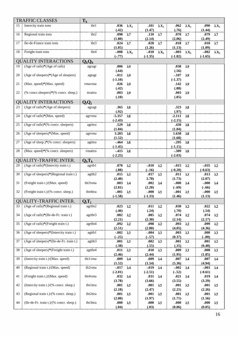
6. Appendix 1. Detailed results of Table 4 models 4-7 The table found in this appendix has three sections:

-Part I presents, for each explanatory variable, the following statistics: elasticity (for any variable including a

dummy variable), Student’s t (relative to 0) conditional on the Box-Cox transformation estimates

and a flag to recall the identity of the Box-Cox transformation applied to the variable in question;

-Part II presents estimated Box-Cox power s and their unconditional Student’s t statistics (relative to 0 and 1);

-Part III presents general statistics: value of the Log-Likelihood, sample used, measures of fit, etc.

U-GBC-2 Models from Table 4 variable Model 4 Model 5 Model 6 Model 7

PART I. Elasticities and conditional t-statistics of regression coefficients

STATE OF LINE SEGMENTS Ss 1 Number of switches apdv .228 .242 .232 .248

(9.58) (10.57) (9.98) (11.24)

2 Electrified line Dummy elec2 .105 .108 .139 .134

(2.01) (2.09) (2.59) (2.50)

3 Automatic switch control Dummy regu .072 .071 .091 .091

(1.29) (1.35) (1.56) (1.66)

4 Segment length long -.244 -.252 -.251 -.265

(-11.94) (-12.70) (-11.88) (-13.04)

5 Number of tracks = 1 (vs 2) Dummy nbv1 -.022 -.005 -.056 -.029

(-.38) (-.08) (-.93) (-.50)

6 Number of tracks = 3 (vs 2) Dummy nbv3 .104 .121 .087 .100

(.82) (.93) (0.66) (0.76)

7 Number of tracks = 4 (vs 2) Dummy nbv4 .338 .323 .260 .238

(3.62) (3.48) (3.18) (2.96)

8 Number of tracks = 5 (vs 2) Dummy nbv5 -.094 -.167 -.539 -.602

(-.23) (-.37) (-3.15) (-3.37)

9 Number of tracks = 6 (vs 2) Dummy nbv6 .693 .735 .193 .150

(3.28) (3.47) (.68) (.53)

10 Number of tracks = 10,18 (vs 2) D. nbv1018 .949 .877 -.028 -.077

(.38) (.40) (-.06) (-.16)

QUALITIES OF SEGMENTS Qk 11 Age of rails agerail 4.418 .079 1.274 .066

(2.10) (.96) (1.55) (.78)

12 Age of sleepers agetrav -3.040 .052 -1.316 .053

(-1.42) (.66) (-1.48) (0.65)

13 Maximum speed allowed vma 1.908 -.502 .030 -.476

(1.18) (-4.70) (0.04) (-4.47)

14 Proportion of concrete sleepers ttra .271 .017 .068 .017

(1.91) (1.57) (1.55) (1.45)

16

TRAFFIC CLASSES Tk 15 Intercity train tons tbt1 .036 X1 .101 X1 .062 X1 .090 X1

(.42) (1.47) (.76) (1.44)

16 Regional train tons tbt2 .098 .110 .070 .079

(1.80) (2.14) (2.06) (2.49)

17 Ile-de-France train tons tbt3 .024 .028 .018 .018

(1.05) (1.26) (1.13) (1.09)

18 Freight train tons tbt4 -.008 X -.010 X -.003 X -.002 X

(-.77) (-1.35) (-1.82) (-1.65)

QUALITY INTERACTIONS QkQk 19 (Age of rails)*(Age of rails) agragr .006 .038

(.64) (.56)

20 (Age of sleepers)*(Age of sleepers) agtagt -.011 -.107

(-1.10) (-1.37)

21 (Max. speed)*(Max. speed) vmavma .026 .142

(.42) (.88)

22 (% concr.sleepers)*(% concr. sleep.) ttrattra .003 .003

(.10) (.05)

QUALITY INTERACTIONS QiQj

23 (Age of rails)*(Age of sleepers) agragt .365 .323

(.92) (.97)

24 (Age of rails)*(Max. speed) agrvma -5.357 -2.111

(-2.43) (-2.15)

25 (Age of rails)*(% concr. sleepers) agrttra .529 .430

(1.84) (1.84)

26 (Age of sleepers)*(Max. speed) agtvma 3.283 1.638

(1.52) (1.68)

27 (Age of sleep.)*(% concr. sleepers) agtttra -.464 -.295

(-1.45) (-1.15)

28 (Max. speed)*(% concr. sleepers) vmattra -.415 -.309

(-2.25) (-2.03)

QUALITY-TRAFFIC INTER. QkTk 29 (Age of rails)*(Intercity train t.) agrtb1 .070 -.010 -.015 -.035

(.88) (-.16) (-0.20) (-0.63)

30 (Age of sleepers)*(Regional train t.) agttb2 .015 .017 .011 .013

(2.40) 2.78) (1.73) (2.07)

31 (Freight train t.)/(Max. speed) tbt3vma .003 .002 -.000 -.000

(2.81) (2.20) (-.69) (-.66)

32 (Freight train t.)/(% concr. sleep.) tbt4ttra -.001 -.000 -.001 -.000

(-1.58) (-1.33) (1.46) (1.13)

QUALITY-TRAFFIC INTER. QiTj

33 (Age of rails)*(Regional train t.) agrtbt2 .023 .011 .030 .022

(.46) (.24) (.70) (.54)

34 (Age of rails)*(Ile-de-Fr. train t.) agrtbt3 .082 .085 .074 .074

(2.21) (2.30) (2.14) (2.17)

35 (Age of rails)*(Freight train t.) agrtbt4 ,092 .098 .093 .099

(2.51) (2.80) (4.05) (4.36)

36 (Age of sleepers)*(Intercity train t.) agttb1 -.002 -.004 .003 .000

(-.25) (-.57) (0.37) (-.00)

37 (Age of sleepers)*(Ile-de-Fr. train t.) agttb3 .001 .002 .001 .001

(.38) (.55) (.35) (0.48)

38 (Age of sleepers)*(Freight train t.) agttbt4 .011 .010 .009 .008

(2.46) (2.44) (1.95) (1.85)

39 (Intercity train t.)/(Max. speed) tbt1vma .009 .009 .007 .007

(1.52) (1.54) (5.36) (4.94)

40 (Regional train t.)/(Max. speed) tb2vma -.017 -.019 -.002 -.003

(-2.01) (-2.51) (-.52) (-0.61)

41 (Freight train t.)/(Max. speed) tbt4vma .032 .031 .021 .019

(3.78) (3.66) (3.55) (3.29)

42 (Intercity train t.)/(% concr. sleep.) tbt1ttra .001 .001 .001 .001

(2.18) (2.47) (2.21) (2.26)

43 (Regional train t.)/(% concr. sleep.) tbt2ttra .001 .001 .001 .001

(2.00) (1.97) (1.71) (1.56)

44 (Ile-de-Fr. train t.)/(% concr. sleep.) tbt3ttra .000 .000 .000 .000

(.04) (.03) (0.06) (0.05)

17

TRAFFIC INTERACTIONS TkTk 45 (Intercity train t.)*(Intercity train t.) tbt1tbt1 .000 .000

(.27) (.15)

46 (Regional train t.)*(Regional train t.) tbt2tbt2 .001 .000

(2.38) (2.45)

47 (Ile-de-Fr. train t.)*(Ile-de-Fr. train t.) tbt3tbt3 -.001 -.000

(-1.11) (-.62)

48 (Freight train t.)*(Freight train t.) tbt4tbt4 .003 .002

(.32) (.68)

TRAFFIC INTERACTIONS TiTj

49 (Intercity train t.)*(Regional train t.) tbt1tbt2 -.049 -.034

(-1.34) (-0.90)

50 (Intercity train t.)*(Ile-de-Fr. train t.) tbt1tbt3 -.050 -.055

(-2.59) (-2.58)

51 (Intercity train t.)*(Freight train t.) tbt1tbt4 .014 .031

(0.44) (0.98)

52 (Regional train t.)*(Ile-de-Fr. train t.) tbt2tbt3 .013 .011

(1.06) (0.90)

53 (Regional train t.)*(Freight train t.) tbt2tbt4 .013 .008

(.47) (.29)

54 (Ile-de-Fr. train t.)*(Freight train t.) tbt3tbt4 -.022 -.026

(-2.33) (-2.63)

55 REGRESSION CONSTANT constant --- --- --- ---

(.35) (10.39) (1.64) (11.18)

PART II. Box-Cox transformations and their unconditional t-statistics with respect to 0 and 1 1 LAMBDA on Cost per km

y .319 .317 .294 .293

[22.18],[-47.37] [22.41],[-48.36] [24.02],[-57.59] [24.60],[-59.27]

2 LAMBDA (X1) X1

.377

Fixed

3 LAMBDA (X2) X2

3.458

Fixed

4 LAMBDA on Group 1 variables 1

.112

Fixed

5 LAMBDA on Group 2 variables

.574

Fixed

6 LAMBDA on Group 3 variables 3

.004

Fixed

7 LAMBDA on Group 4 variables 4

2.129

Fixed

8 LAMBDA on Group 5 variables 5

1.594

Fixed

9 LAMBDA on Group 6 variables 6

.743

Fixed

10 LAMBDA on Group 7 variables 7

1.114

Fixed

11 LAMBDA on Group 8 variables 8

.165 .357

[2.07],[-10.48] [1.00],[-1.80]

12 LAMBDA on Group 9 variables 9

2.127 2.458 1.016

[2.20],[1.16] [1.59],[0.94] [.73],[.01]

PART III. General statistics

1 LOG-LIKELIHOOD -12846.8 -12857.5 -12877.2 -12888.3

2 PSEUDO-R2 –(E) .840 .836 .799 .796

–(L) .934 .933 .930 .928

–(E) ADJ. for D.F. .829 .827 .789 .788

–(L) ADJ. for D.F. .932 .929 .926 .926

3 AVERAGE PROBABILITY OF (y = LIMIT OBS.) .000 .000 .000 .000

4 NUMBER OF OBSERVATIONS 967 967 967 967

5 PARAMETERS ESTIMATED 58 47 48 36

BETA Coefficients 55 45 45 35

BOX-COX Transformations: 9 ex previous model + 3 2 3 1

End of table.

18

7. References Berndt, E.R., Khaled, M.S. (1979). Parametric Productivity Measurement and Choice among Flexible

Functional Forms. Journal of Political Economy 87, 6, 1220-1245, December.

Bierlaire, M. (2003). BIOGEME: a free package for the estimation of discrete choice models.

Proceedings of the 3rd Swiss Transportation Research Conference, Ascona, Switzerland.

Bierlaire, M. (2008). An introduction to BIOGEME Version 1.6.

Blackorby, C., Primont, D., Russell, R.R. (1977). On Testing Separability Restrictions with Flexible

Functional Forms. Journal of Econometrics 5, 195-209.

Borger, B. de (1991). Hedonic versus homogeneous output specifications of railroad technology:

Belgian railroads 1950-1986, Transportation Research 25A, 227-238, June.

Borger, B. de (1992). Estimating a Multiple-Output Generalized Box-Cox Cost Function: Cost Structure

and Productivity Growth in Belgian Railroad Operations, 1950-86. European Economic Review 36,

pp. 1379-1398.

Box, G.E.P., Cox, D.R. (1964). An Analysis of Transformations. Journal of the Royal Statistical Society

B 26, 211-243.

Box, G.E.P., Tidwell, P.W. (1962). Transformation of the Independent Variables. Technometrics 4, 531-

550.

Brown, R.S., Caves, D.W., Christensen, L.R. (1979). Modeling the Structure and Cost of Production for

Multiproduct Firms. Southern Economic Journal 46, 256-273, July.

Burgess, D.F. (1974). A Cost Minimization Approach to Import Demand Equations. Review of

Economics and Statistics 56, 225-234.

Caves, D.W., Christensen, L.R., Swanson, J.A. (1980b). Productivity in U.S. Railroads, 1951-1974. Bell

Journal of Economics 11, 1, 168-181.

Caves, D.W., Christensen, L.R., Tretheway, M.W. (1980a). Flexible Cost Functions for Multiproduct

Firms. Review of Economics and Statistics, 477-481 (Notes Section).

Caves, D.W., Christensen, L.R., Tretheway, M.W., Windle, J. (1985). Network effects and the

measurement of returns to scale and density for U.S. railroads. Ch. 4 in A. F. Daughety (ed.),

Analytical Studies in Transport Economics, 97-120, Cambridge University Press, Cambridge.

Christensen, L.R., Jorgenson, D.W., Lau, L.J. (1971a). Conjugate Duality and the Transcendental

Logarithmic Function. Econometrica 39, 4, 255-256, July.

Christensen, L.R., Jorgenson, D.W., Lau. L.J. (1971b). Transcendental Logarithmic Production

Frontiers. Review of Economics and Statistics 55, 1, 28-45.

Dagenais, M.G., Dufour, J.-M. (1994). Pitfalls of Rescaling Regression Models with Box-Cox

Transformations. The Review of Economics and Statistics 76, 3, 571-75, August.

Davidson R., MacKinnon, J.G. (1985). Testing linear and loglinear regressions against Box-Cox

alternatives. The Canadian Journal of Economics / Revue canadienne d'Economique 18, 3, 499-517.

August.

Davidson R., MacKinnon, J.G. (1993). Transforming the Dependent Variable. Ch. 14 in Estimation and

Inference in Econometrics. Oxford University Press.

Denny, M., Fuss, M. (1977). The Use of Approximation Analysis to Test for Separability and the

Existence of Consistent Aggregates. American Economic Review 67, 3, 404-418, June.

Diewert, W.E. (1971). An Application of the Shephard Duality Theorem: A Generalized Leontief Cost

Function. Journal of Political Economy 79, 481-507.

Diewert, W.E. (1973). Separability and a Generalization of the Cobb-Douglas Cost, Production and

Indirect Utility Functions. Research Branch, Department of Manpower and Immigration, Ottawa,

January.

Diewert, W.E. (1974). Functional Forms for Revenue and Factor Requirements Functions. International

Economic Review 15, 199-130.

Gaudry, M., Laferrière, R. (1989). The Box-Cox Transformation: Power Invariance and a New

Interpretation. Economics Letters 30, 27-29.

19

Gaudry, M., Quinet, É. (2003). Rail track wear-and-tear costs by traffic class in France. Publication

AJD-66, Agora Jules Dupuit, Université de Montréal, www.e-ajd.net, et W.P. 04-02, Centre

d’Enseignement et de Recherche en Analyse Socio-économique, École Nationale des Ponts et

Chaussées (ENPC-CERAS), www.enpc.fr/ceras/labo/accueil.html, 26 pages, November.

Gaudry, M., Quinet, É. (2010). Track Wear and Tear Cost by Traffic Class: Functional Form, Zero-

Output Levels and Marginal Cost Pricing Recovery on the French Rail Network. Publication AJD-

130, Agora Jules Dupuit, Université de Montréal, et Working Paper No 2009-32, Paris-Jourdan

Sciences Économiques, 50 pages, 26 avril. www.e-ajd.net.

Gaudry, M., Quinet, É. (2014). Correlation within SNCF administrative regions among track segment

maintenance cost equation residuals of a country-wide model. In Funck, R., Rothengatter, W. (Hrsg.),

Man, Environment, Space and Time ― Economic Interactions in Four Dimensions. Karlsruhe Papers

in Economic Policy Research, Volume 34, Nomos Verlag, p. 207-232.

Gaudry, M., Lapeyre, B., Quinet, É. (2015). Infrastructure maintenance, regeneration and service

quality economics: A rail example. Publication AJD-136-E, Agora Jules Dupuit, Université de

Montréal; Working Paper No 2011-03, Paris-Jourdan Sciences Économiques, 42 p., Version 21, 25

th

January.

Idström, T. (2002). Reforming the Finnish railway infrastructure charge – an econometric analysis of

the marginal costs of rail infrastructure use. (In Finnish). Master’s Thesis. Department of Economics.

University of Jyväskylä.

Jansson, J.O. (2002). An Analysis of the Rail Transport System. In Nash, C., Wardman, M., Button, K.,

Nijkamp, P. (eds), Classics in Transport Analysis: Railways, 135-181, Edward Elgar Publishing

Limited, Cheltenham.

Johansson, P., Nilsson, J.-E. (2002). An Economic Analysis of Track Maintenance Costs. Deliverable 10

Annex A3 of UNITE (UNIfication of accounts and marginal costs for Transport Efficiency), Funded

by EU 5th Framework RTD Programme. ITS, University of Leeds, Leeds, 23 p.. Online:

http://www.its.leeds.ac.uk/projects/unite/.

Johansson, P., Nilsson, J.-E. (2004). An economic analysis of track maintenance costs. Transport Policy

11, 277-286.

Khaled, M.S. (1978). Productivity Analysis and Functional Specification. A Parametric Approach. Ph.

D. Thesis, Department of Economics, University of British Columbia, April.

Kouider, E., Chen, H. (1995). Concavity of Box-Cox log-likelihood function. Statistics and Probability

Letters 25, 171-175.

Liem, T.C. (1979). L-1: A Program for Box-Cox Transformations in Regression Models with

Heteroskedastic and Autoregressive Residuals. Publication CRT-134, Centre de recherche sur les

transports, et Cahier #7917, Département de sciences économiques, Université de Montréal, 60 p..

Refereed in The American Statistician, June 1980.

Liem, T.C., Dagenais, M.G., Gaudry, M.J.I. (1983). L-1.1: A Program for Box-Cox Transformations in

Regression Models with Heteroskedastic and Autoregressive Residuals. Publication CRT-301, Centre

de recherche sur les transports, et Cahier #8314, Département de sciences économiques, Université de

Montréal, 70 p., 1983.

Liem, T.C., Dagenais, M.G., Gaudry, M.J.I, Koblo, R. (1986). L-1.1: Ein Programm für Box-Cox

Transformationen in Regressionsmodellen mit heteroskedastischen und autoregressiven Residuen.

Publication CRT-301-D, Centre de recherche sur les transports, Université de Montréal, et Discussion

Paper 4/86, Institut für Wirtschaftspolitik und Wirtschaftsforschung, Universität Karlsruhe, 44 p..

Link, H., Stuhlemmer, A. Haraldsson, M., Abrantes, P., Wheat, P., Iwnicki, S., Nash, C., Smith, A.

(2008). CATRIN (Cost Allocation of TRansport INfrastructure cost), Deliverable D 1, Cost

allocation Practices in the European Transport Sector. Funded by Sixth Framework Programme.

VTI, Stockholm. 93 pages, March.

Odolinski, K., Nilsson, J.-E. (2015). Estimating the marginal cost of rail infrastructure maintenance

using static and dynamic models; does more data make a difference? Manuscript, Swedish National

Road and Transport Research Institute (VTI), Department of Transport Economics, 34 p..

Poirier, D. (1978). The Use of the Box-Cox Transformation in Limited Dependent Variable Models,

Journal of the American Statistical Association 73, pp. 284-287.

20

Quinet, É. (2002). Détermination des coûts marginaux sociaux du rail. Manuscrit déposé auprès de

SNCF Infrastructure, 38 pages, mars.

Quinet, É. (2015). Commentaires d’algèbre sur la transformation BC élevée au carré. Manuscrit déposé

auprès de SNCF Réseau le 29 octobre, 2 p., 12 août.

Sánchez, P.C. (2000). Vertical Relationships between Railway Operations and the Infrastructure for the

European Case. In Nash C., Niskanen, E. (eds), Helsinki Workshop on Infrastructure Charging on

Railways, VATT Discussion Papers 245, Government Institute for Economic Research, Helsinki.

Pages 71-94.

Schlesselman, J., (1971). Power families: a note on the Box and Cox transformation. Journal of the

Royal Statistical Society Series B 33, 307-311.

Small, K.A., Zhang, F. (1988). A Reanalysis of the AASHO Road Test Data: Rigid Pavements.

Department of Economics and Institute of Transportation Studies, University of California, Irvine, 34

pages.

Spitzer, J.J. (1984). Variance Estimates in Models with the Box-Cox Transformation: Implications for

Estimation and Hypothesis Testing. The Review of Economics and Statistics 66, 645-652.

Tobin, J. (1958). Estimation of Relationships for Limited Dependent Variables. Econometrica 25, 24-36.

Tovar, B., Jara-Díaz, S., Trujillo, L. (2003). Production and cost functions and their application to the

port sector: a literature survey. World Bank Policy Research Working Paper 3123, 32 pages, August.

Tran, C.-L., Gaudry, M., Dagenais, M.G. (2008). LEVEL: The L-1.6 estimation procedures for BC-

GAUHESEQ (Box-Cox Generalized AUtoregressive HEteroskedastic Single EQuation) regression

and multimoment analysis. Publication AJD-105, Agora Jules Dupuit, Université de Montréal, 59 p.,

April. www.e-ajd.net.

Wheat, P., Smith, A., Nash, C. (2009). CATRIN (Cost Allocation of TRansport INfrastructure cost),

Deliverable 8 – Rail Cost Allocation for Europe. Funded by Sixth Framework Programme. VTI,

Stockholm. 70 pages, March.

Wheat, P., Smith, A., Matthews, B. (2014). SUSTRAIL (The sustainable freight railway: Designing the

freight vehicle – track system for higher delivered tonnage with improved availability at reduced

cost). Deliverable 5.3 –Access Charge Final Report. Funded by Seventh Framework Programme,

Institute for Transpor Studies, University of Leeds, 3 November.

Winston, C. (1985). Conceptual Developments in the Economics of Transportation: An Interpretative

Survey. Journal of Economic Litterature 23, pp. 57-94, March.

Zhang, F. (1989). A Reanalysis of the AASHO Road Test Data: Flexible Pavements. Manuscript,

Department of Economics and Institute of Transportation Studies, University of California, Irvine, 34

pages.