•

•

•

•

TEST OF TREATMENT EFFECT USING THE COX PROPORTIONALHAZARDS MODEL WITH IMPUTED COVARIATE DATA

Anne Ruth Meibohrn

Department of Biostatistics, University ofNorth Carolina at Chapel Hill, NC.

Institute of Statistics Mimeo Series No. 2l09T

December 1992

..

•

•

..

TEST OP TREATMENT EFFECT

USING THE COX PROPORTIONAL HAZARDS KODEL

WITH IMPUTED COVARIATE DATA

by

Anne Ruth Keibohm

A Dissertation submitted to the faculty of The University ofNorth Carolina at Chapel Hill in partial fulfillment of therequirements for the degree of Doctor of Philosophy in theDepartment of Biostatistics.

Chapel Hill

1992

Approved by:

Advisor

•

..

Reader

Reader

Reader

Reader

ANHE RU'l'lI HEIBOBK. Test of Treatment Effect Using the Cox

Proportional Hazards Model with Imputed Covariate Data. (Under

the direction of Timothy M. Morgan.)

ABSTRACT

Missing covariate data is a common problem in clinical

trials and the analysis of survival time data. Imputing

values for the missing covariate data is equivalent to

omitting the differences between the true and imputed values

from the model. If the model for the hazard rate given the

true values is proportional hazards, then the model using

imputed values will not be. In this dissertation the

distribution of the score statistic for the test of treatment

effect using imputed data is derived for the correct and

misspecified general parametric models and for the

misspecified Cox nonparametric prop·ortional hazards model

(PHM). The robust variance estimator for the score statistic

When the Cox model is misspecified proposed by Lin and Wei

(1989) is examined for this test under the null hypothesis.

The asymptotic relative efficiency of the misspecified Cox PHM

with imputed data relative to the complete data Cox PHM and

relative to the correct parametric model for complete and

incomplete data, assuming a PHM for the complete data, is

derived. Imputing values for the missing covariate data and' ..

misspecifying the Cox PHM is very efficient unless there is a

moderate to high percentage of missing data for a covariate

with a strong effect on survival time which cannot be imputed

well and there is little censoring.

The procedure is easily implemented using standard

statistical software and a SAS macro. The implementation of

the procedure and the evaluation of its efficiency is

illustrated.

iii

..

,

ACKNOWLEDGEXENTS

First, I would like to extend special thanks to my

advisor, Dr. Tim Morgan, for his guidance and support. His

knowledge, patience, availability, and helpfulness were very

important to me and to the quality of this dissertation. I

appreciate the constructive comments of my committee, Dr. Ed

Davis, Dr. Lloyd Chambless, Dr. Paul stewart, and Dr. Gerardo

Heiss.

I am trUly thankful for my family and friends, especially

my parents and Maria, and for their love, encouragement, and

prayers. I deeply appreciate the friendship, support, and

understanding of my classmates, especially Emilia.

Finally, I am grateful to Merck Research Laboratories,

particularly the Clinical Biostatistics Department, for their

support and encouragement in the pursuit of this degree

personally and through the leave of absence, financial support

this past year, and the use of data for this dissertation.

iv

TABLB OF CONTENTS

Paqe

LIST OF TABLES •••••••••••••••••••••••••••••••••••••••••• viii

LIST OF FIGURES ••••••••••••••••••••••••••••••••••••••••.•• ix

Chapter

I. INTRODUCTION AND REVIEW OF ANALYSIS OF GENERALMODELS WHEN THERE ARE MISSING DATA••••••••••••••..•••• 1

1.1

1.2

1.3

1.4

1.5

1.6

1.7

1.8..

1.9

1.10

Introduction 1

Types of Missing Data •••..•.••••••....•••.••..... 2

Methods Utilizing the Observed Data Only••..••..• 4

Imputation Methods •••••••..••••••...••••••••••••• 6

Likelihood-based Methods •••••••••.••••.••••..•.•• 8

Methods of Factoring the Likelihood••.••.....••• 11

Iterative Methods of Computing MLEs .•...••••...• 12

Illustration of Methods of HandlingMissing Data ••••••••••••••••••••.••••..••••.•... 15

Comparison of Variances of Estimatesof the Mean••••••••••••••••••••••••••••••••••••• 20

Summary ••••••••••••••••••••••••••••••••••••••••• 28

II. SURVIVAL TIME WITH MISSING COVARIATE INFORMATION•.... 29

2 . 1 Introduction•....••............................. 29

2.2 Survival Time Models Incorporating Covariates ••. 29

2.3 Missing Covariate Data in Survival Analysis ••••• 31

2.4 Covariate Measurement Error in Failure TimeModels •••••••••••••••••••••••.•••••••••••••••••• 35

2.5 Example 1: Estimation of Hazard Function......• 39

2.6 Example 2: Test of Treatment Effect •.•••.•.•••• 52

2.7 Efficiency of Categorization of Covariates ••••.. 71

v

2.8 Summary and Research Proposal •••••••••••••.••••• 73

III. DISTRIBUTION OF COX MODEL WITH IMPUTED DATA•••••.•••• 77

3.1 Introduction 77

3.2 General Parametric Proportional Hazards Model -(:orrE!ct ~()ciE!JL••••••••••••••••••••••••••••••••••• 77

3.3 General Parametric Proportional Hazards Model -Misspecified Model •••••••••••••••••••••••••••••. 85

3.4 Normality of Score Statistic for MisspecifiedModel ••...•.•.••...••••••.••....•.....•....•.... 87

3.5 Robust Estimator of Variance for MisspecifiedCox proportional Hazards Model •.•••••••••••••••• 88

3.6 Normality of Score statistic and Robust ScoreTest ••.....•.•.....•..•......••......•.....•.... 96

3.7 ASYmptotic Relative Efficiencies of Models •••••• 97

3.8 Extension to p Covariates ••.••.•..•..•••••.•.•• 107

3.9 Imputing Values for the Missing Covariates ••... 108

3.10 Random Censoring Time •.••••••.•.••••••.••.•.••. 112

3.11 Summary .......•................................ 113

IV. IMPLEMENTATION OF METHOD •••••••••••••••••••••••••..• 115

4.1 Introduction 115

4.2 Imputing Data 115

4.3 Analysis Procedure•••••••••••••..•••••.•.••.••. 117

4.4 Estimation of ARE of Imputing Data .•.••.•...•.. 119

4.5 Summary 125

V. ILLUSTRATION OF IMPLEMENTATION AND EFFICIENCYOF METHOD ••••••••••••••••••••••••••••••••••••••••••• 126

5.1 Description of Data ••.•••••••.••••••.•.••.••.•• 126

5.2 Usual Methods of Analysis ••.•..••..•••.••.•..•• 127

5.3 Analysis of Data Imputing Values for MissingCovariates 130

5.4 Efficiency of Imputing .••••••.••••••.•••••••••• 134

vi

5.5 Summary •••••.••.••••••...•••.•••••••.•.•..••... 135

VI. SUMMARY AND SUGGESTIONS FOR FUTURE RESEARCH. • .137

APPENDICES •.••••...•••••••...•..•••.•.•...•••.••......... 142

II

A. EXPECTED VALUE OF OBSERVED ROBUST VARIANCEES~I~~()~ •.•••..•..••.•.••••••..••...•••... .142

B. SAS ~CRO TO CALCULATE SCORE TEST•••••••••• .144

C. PROGRAMS TO IMPUTE DATA AND TO CALCULATE SCORETEST .....•••••........••.........•.•....•...... 150

D. PROGRAM TO CALCULATE ARE OF IMPUTING. ..........160

..

REFERENCES. .............................................

vii

.171

..

..

LIST OF TABLES

Table 1.1: Three Random Variables and Pattern ofObservation 16

Table 1.2: Estimates of Means and Variance-covarianceMatrix from Different Methods of Analysis •••.• 19

Table 2.1: Ratio of Risk of Failure for DifferentPercentiles of the Gamma Distribution••••••••• 40

Table 2.2: ASYmptotic Relative Efficiencies of Models •... 70

Table 5.1: Patterns of Missing Data, R2 , and Alpha's ofResiduals 128

Table 5.2: Score Test of Ho: No Treatment Effect •••••..•• 133

viii

•

•

LIST OF FIGURES

Figure 2.1: Asymptotic Relative Efficiency of ModelOmitting Incomplete Observations vs.Correct Maximum Likelihood Model .•••••••••••• 59

Figure 2.2: Asymptotic Relative Efficiency of ModelOmitting covariate vs. Correct MaximumLikelihood Model 60

Figure 2.3: Asymptotic Relative Efficiency of SimpleIncorrect Model vs. Correct MaximumLikelihood Model •••••••••••••••••••••••••.••• 69

Figure 3.1: Asymptotic Relative Efficiency ofMisspecified PH Model for Incomplete Datavs. Complete Data Model .••.••••.•.••••.•.... 104

Figure 3.2: Asymptotic Relative Efficiency ofCorrect Parametric Model for IncompleteData vs. Complete Data Model ••••••••••••••.. 105

Figure 3.3: Asymptotic Relative Efficiency ofMisspecified PH Model vs. Correct ParametricModel for Incomplete Data •••••••••••••. ~ •••• 106

ix

CHAPTER 1

INTRODUCTION AND REVIEW OP ANALYSIS OP GENERAL MODELS

nEN THERB ARB MISSING DATA

1.1 Introduction

The objective in many randomized clinical trials is to

compare the length of time to an event such as healing,

relapse, or death among the treatment gro~ps. For example, a

study may compare the length of time until death for patients

with lung cancer who were treated with two different

chemotherapy regimens.

In addition to treatment, prognostic factors such as age,

severity of the disease, laboratory measurements, signs and

symptoms should be included in the model for survival time for

several reasons. First, the power of the test of the

treatment difference is increased when concomitant variables

are included in the model (Schoenfeld, 1983). Second,

randomization does not lead to asymptotically unbiased

estimates of treatment effect in all survival data models if

covariates related to survival time are omitted (Gail, Wiend,

and Piantadosi, 1984). Third, although randomization on the

average yields balanced treatment groups, it does not ensure

that the groups will be similar for every characteristic.

Thus including concomitant variables in the model may reduce

bias in the estimate and test of the difference in the

treatment effects. Fourth, examining the relationship between

survival time and prognostic factors may be an objective of

the study, for this information may help physicians develop

treatment regimens for patients individually as well as

collectively.

A common and critical problem in the analysis of clinical

trial data as well as data from other types of studies is

missing data. For various reasons, the values of the

concomitant variables and/or the response variables may be

unknown. In recent years improved methods for analyzing

datasets when some of the data are missing have been developed

for linear models. However, satisfactory methods for

analyzing survival time data when some of the concomitant

variables are missing have not been developed. The purpose of

this dissertation is to develop such a method from both

theoretical and practical viewpoints.

1.2 Types of Kissing Data

One of the factors that influences the method of analysis

when there are missing data and the interpretation of the

results is the process that caused the missing data. It is

important to try to ascertain why the data are missing and the

relationship between the observed and missing data (Rubin,

1976, Little and RUbin, 1987).

Rubin (1976) defined three conditions for the process

that causes missing data. Let 8 be the parameter of the data

and 1/1 the parameter of the missing data process which is

conditional on the given data. Rubin's definitions are:

The missing data are missing at random if for eachpossible value of the parameter 1/1, the conditionalprobability of the observed pattern of missingdata, given the missing data and the value of theobserved data, is the same for all possible valuesof the missing data.

The observed data are observed at random if foreach possible value of the missing data and theparameter 1/1, the conditional probability of theobserved pattern of missing data, given the missingdata and the observed data, is the same for allpossible values of the observed data.

The parameter 1/1 is distinct from 8 if there are no

2

...

a priori ties, via parameter space restrictions orprior distributions, between ~ and 8.

Little and Rubin (1987) defined the different types of

missing data mechanisms less formally in terms of the

relationship between the probability of response for Y and the

variables X and Y where X is observed for all observations and

Y is sUbject to nonresponse. If the probability of response

is independent of X and Y, the missing data are missing at

random (HAR) and the observed data are observed at random

(OAR). Thus the missing data are missing completely at random

(HeAR). If the probability of response depends on X but not

on Y, the missing data are missing at random (HAR). In this

case the observed data are not observed at random. If the

probability of response depends on Y and possibly on X also,

the data are neither MAR nor OAR.

In the last case when the data are neither MAR nor OAR,

the missingness cannot be ignored in any analysis. On the

other hand, if the data are MeAR, then the missing data

mechanism is ignorable. If the data are MAR but not OAR, then

the missing data mechanism is ignorable for'some methods of

analysis but not others.

In the remainder of this chapter, general methods of

handling missing data will be reviewed. Little and Rubin

(1987) reviewed methods of statistical analysis of

multivariate data when there are missing data. They presented

simple methods using observed data only or a combination of

imputed and observed values and then focused on likelihood­

based methods. Much of the following review of methods of

analyzing missing data, including terminology and notation,

comes from their review. Some of these methods will be

applied to a small dataset for illustration. Finally, the

variances for the estimates of the mean response for the

different methods will be compared for the situation when

there is one response variable and one covariate.

3

1.3 Methods utilizing the Observed Data only

The simplest and probably the most common method for

analyzing incomplete data is to base the analysis on

observations or cases with complete data. Many statistical

analysis packages, including SAS, employ this procedure. The

advantages of this procedure, subsequently referred to as

complete case analysis, are that it is simple to implement and

that the same sample contributes information to all variables

and analyses. However, usually this procedure is not very

efficient. Many observations may be eliminated reducing the

sample size and, consequently, the power. Also biases may be

introduced if the completely observed cases differ from the

cases with incomplete data. For example, if the people who

have incomplete data tend to be older than those with complete

data, the information about age and its effect on response may

be biased. Inference about the entire population not the

sUbpopulation with complete data is the objective of the

study. Complete case analysis is satisfactory only if the

amount of missing data is small and the data are missing

completely at random so that the reasons for the missing data

are ignorable.

Available case methods (Little and Rubin (1987) and Buck

(1960» utilize all available data for a variable to estimate

the mean and variance of the variable and pairwise available

data to estimate the covariance of two variables. There are

several alternative formulas for the covariance and

correlation. The covariances can be based entirely on

observations for which both variables are observed,

•

(1.1)

where n~ is the number of cases with both ~ and Yt observed

and the means y/jk) and YtGk) and the summation are calculated

over the nGk) cases. Alternatively, the estimates of the means

from all available cases, y/J) and Yt(k) , could be used to

4

calculate the covariances:

(1.2)

This is the ALLVALUE estimate of covariance in the BMDP8D

program (Dixon, 1990).The estimate of the correlation can be calculated using

the sample variances based on the n<it) cases, Sjj<it) and Stt<it), or

using the sample variances based on all available cases, SjjIDand Stt(k):

r (jk) - S (jk) IJs ljk) s ljk)jk - jk jj kk

r • - s (jlt) IJs lj) s (k)jk - jk jj kk •

(1. 3)

•

The advantage of the pairwise correlation rjr.<it) over rjr.* is that

rjr.<it) always lies in the range (-1,1) while rjr.* may be outside

this range. SAS PROC CORR (1990) with the COV option appliedto a dataset with missing data provides sjr.<it) and rjr.<it) as the

estimates of covariance and correlation, respectively.Available case methods utilize more data than complete

case methods and, consequently, should provide better

estimates. If the data are MCAR, the estimates of the means,

variances, covariances and correlations are consistent.However, the estimates have deficiencies. The covariance and

correlation matrices may not be positive. definite. Some

methods of estimating correlations may yield values outside

the range (-1,1) as noted previously. In addition, havingdifferent sample bases for different variables may make itdifficult to make comparisons and interpret the results,especially if missingness is related to the variables.

Simulation studies indicate that available case methods

tend to be better than complete case methods when the data are

MCAR and the correlations are modest. However, if the

correlations are large, complete case methods seem to be

superior (Little and RUbin, 1987).

5

1.4 Imputation ••thod.

Another common procedure is to impute or to fill in

estimates of the missing values and then apply complete data

methods of analysis which are modified to account for the

difference between observed and imputed data so that

inferences are valid. The estimates may be obtained in

different ways. Often the means of the observed data, either

unconditional or conditional, are sUbstituted for the missing

data. Medians could be used also. The imputed values may

also be the predicted values from a regression analysis of the

missing variables on the observed variables. In hot deck

imputation, recorded values from other observations in the

sample are substituted. The method of selecting the

observations varies. They could be selected randomly from all

data or from data for people with similar values for the

observed variables.

When the unconditional mean, i.e. the mean for all

available data ~ID, is imputed for observations with missing

values for Yij' the estimate of the mean is unchanged. The

estimate of the variance based on the observed and imputed

values is

(nO) _ n (j) -1 (j)Sjj - Sjjn-1

(1. 4)

where SjjID is the variance based on the available cases as

defined previously and n° indicates that some of the n

observations are imputed. Imputing values at the center of

the distribution leads to a sample variance which under­

estimates the variance by a factor of (nID-1) / (n-1). Likewise,

the sample covariance of ~ and Yt

(nO) n (jk) -1 (jk)Sjk = §jkn-1

(1.5)

underestimates the covariance by a factor of (n~-1)/(n-1).

The covariance matrix obtained is positive semi-definite.

6

Buck (1960) proposed a method for obtaining means for the

missing data conditional on the observed variables. First,

the missing values are estimated from linear regressions of

the unobserved variables on the observed variables. The

regression equations are determined from the observations with

complete data. SUbstituting the observed values for each

observation in the appropriate regression equation generates

the predicted values for the missing variables. Second,

sUbstituting the estimated values for the missing values, a

revised covariance matrix is calculated.

This procedure yields estimates of the means which are

consistent if the data are missing completely at random (HCAR)

and under mild assumptions about the moments of the

distribution (Little and Rubin, 1987). With additional

assumptions, the estimates are also consistent when the

missing data mechanism depends on the observed variables.

However, when the data are MAR but not OAR, the assumption of

a linear relationship between the completely and incompletely

observed variables may be questionable especially if it is

necessary to extrapolate beyond the range of the complete data

in order to obtain values for the incomplete data.

The sample covariance matrix from the observed and

imputed data underestimates the true variance-covariance

matrix although the estimates are better than those obtained

when unconditional means are imputed. Let D'jj.obl,i denote the

residual variance from regressing ~ on the observed variables

in case - i where the residual variance is zero if Yij is

observed. The sample variance of ~ underestimates the true

variance D'jj by the quantity (n-1) -lED'jj.obl,i. similarly, the bias

of the covariance estimate is (n-1) -lED'jk.obl,i where D'jk.obl,i is the

residual covariance of ~ and Yk from the mUltiple regression

of ~, Yk on the variables observed in case i. The residual

covariance is zero if either Yij or yilt. is observed. "A

consistent estimate of E can be constructed under the HCAR

assumption by sUbstituting consistent estimates of D'jj.obI,i and

D'jk.obl,i (such as estimates based on the sample covariance matrix

7

of the complete observations, sample sizes permitting) in the

expressions for bias and then adding the resulting quantities

to the sample covariance matrix of the filled-in data. II

(Little and Rubin, 1987, p.46)

Categorical variables can be included in the regression

models in Buck's method by replacing a variable with k

categories with k-1 indicator variables. If the original

variable is missing, then the indicator variables are

dependent variables in the regression equation along with

other missing variables. The values obtained are linear

estimates of the probabilities of falling into the categories

represented by the indicator variables. However, these

estimates can sometimes fall outside the (0,1) interval.

Using values at the center of the rlistribution of the

data such as the unconditional or conditional mean as

estimates of missing values distorts the marginal

distributions of the data. As already noted, this causes the

variance matrix to be underestimated. It also causes problems

in studying the tails of the distributions.

An alternative method of imputation, known as hot deck

imputation, randomly selects values from the entire range of

possible values for the variable. Often values from other

observations are used. It would also be possible to add a

randomly determined amount, positive or negative, to the mean

to obtain an imputed value.

1.5 Likelihood-based Methods

The procedures which Little and Rubin (1987) recommend

for analyzing incomplete data are model-based. A model for

the partially missing data is defined, and inferences are

based on the likelihood of the parameters under that model.

Parameter estimates are obtained through procedures such as

maximum likelihood.

Following the outline of Little and Rubin (1987) and

8

..

using their notation, let Y represent the data that would beobserved if there were no missing data. Partition Y into theobserved and unobserved data, Y = (Y., Ya ). The dimensions

of the subvectors and the variables comprising them may varyfrom individual to individual. The probability densityfunction of the joint distribution of Y. and Ya is

f (Y; 8) =f (Yobs ' Ymis ; 8)

where , is an unknown parameter. The marginal density of theobserved data is obtained by integrating over the missingdata:

f (Yobs ; 8) =f f (Yobs ' Ymis ; 8) dYmis • (1.6)

..

The likelihood of , based on the observed data and ignoring

the missing data mechanism, L('iY.), is proportional to the

marginal density of the observed data.Since the missing data are often not ignorably missing,

a random variable R indicating whether each component of Y isobserved or missing can be included in the model. Let Y be ann x k matrix of observations for n individuals on k variables:Y = (Yij) i=l, ••• ,n and j=1, ••• , k. Then R = (~j) where Rg=l if

Yij is observed and 0 if Yij is missing. The conditional

distribution of R given Y is the distribution for the missing

data mechanism and is a function of ~, an unknown parameterunless the missing data mechanism is known. Thus the jointdistribution of Y and R is

The data observed in a study are (Y.,R). Thedistribution of the observed data is obtained by integrating

Ya out of the joint density of Y and R:

f (Yobs ' R; 8,.) =f f (Yobs ' Ymis ; 8) f (R.: Yobs ' Ymis ;.> dYmis ' (1.7)

The likelihood of 8 and ~, L(',~iY.,R), is any function of

9

these parameters which is proportional to f(Y.,Ril,~).

If the distribution of the missing-data mechanism R is

independent of the missing values Y.., so that

(1.8)

then the data are defined to be aissinq a1: random (KAR). Thismeans that lithe probability that a particular component of Yis missing cannot depend on the value of that component whenit is missing. II (Little and RUbin, 1987, p.90) Given the data

are MAR,

f (Yobs,Ri8, t> =f (RIYobsit> If (Yobs ' Ymis i8> dYmis

=f (RlYobsit) f (Yobs i8) •

(1.9)

If there are no functional relationships between e and ~ andthe joint parameter space factors into the individualparameter spaces, i.e. e and ~ are distinct, the likelihoodsL(I,~iY.,R) and L(IiY.) differ by a factor which does notdepend on Ii and inferences for I based on them will be thesame. Therefore, the missing data mechanism ~s ignorable, and

the simpler likelihood L( I i Y.) can be used. Thus animportant advantage of likelihood-based inferences for I is

that only MAR, not MCAR, is required for the inferencesobtained from models ignoring the missing data mechanism to bevalid.

Little and Rubin (1987) claim that model based procedureshave several other advantages: flexibility, model assumptionscan be stated and evaluated, and the availability of largesample estimates of variance which take into account theincompleteness of the data. However, potential disadvantagesinclude inefficient and inconvenient implementation of methodsto obtain estimates and their variances.

10

..

1.6 .ethods of Pactorinq the Likelihood

If the assumption that the data are missing at random is

valid, then for some distributions, such as the normal

distribution and the multinomial distribution, and for some

missing data patterns, the log likelihood 1 ( , i Y.) can be

written in terms of a parameter ~ where ~ is a one-to-one

monotone function of , and such that the log likelihood

factors into components. That is,

where

1. CPt, CP2' , CP1 are distinct parameters, in thesense that the joint parameter space of ~=(cpll CPu• •• , CP1) is the product of the individual parameterspaces for ~, j=l, ••• ,J.

2. The components lj (~jiY.) correspond to loglikelihoods for complete data problems, or moregenerally, for easier incomplete data problems.

(Little and RUbin, 1987, p.97)

The components ~(~iY_) are maximized separately since

the CPj are distinct, and the MLE of ~ is ($11$2' ••• ,$1). By the

property that the maximum likelihood estimate of a one-to-one

function of a parameter is the function evaluated at the MLE

of the parameter, the MLE of , is '(~).

An approximate covariance matrix for the ML estimates can

be obtained via the decomposition also. The information

matrix based on the log likelihood l(~iY.) is block diagonal

with each block being the information matrix corresponding to

each component. The covariance matrix C(~iY.) is also block

diagonal with the inverses of the individual information

matrices as the blocks. The approximate covariance matrix of

the ML estimate of a function '='(~) can be calculated from

the formula

11

where , is expressed as a column vector and D is the matrix ofpartial derivatives of , with respect to ~: ..

J) (8) ={djk (8)} I

68whe:re djk (8) =~ .

One situation when the likelihood can be factored is whenthe data are mUltivariate normal and the missing data followa monotone pattern. That is, data for all n observations areavailable for a block of variables Y1 • For a second block of

variables, Y2 , the data are observed for ml observations. For

a subset ~ of the m1 observations, variables comprising a

third block Y3 are observed. These variables are missing forall other observations. This pattern could continue foradditional blocks of variables. Under these circumstances,the log likelihood can be factored into components which alsohave normal distributions. The maximum likelihood estimatesfor each of the components of ~ are found, and then themaximum likelihood estimate for , is obtained using the sweepoperator.

1.7 Iterative Methods of computing MLES

The method of factoring the likelihood into distinct

components which can be maximized is not always applicable.The pattern of missing data and/or the distribution may not

lead to a likelihood which can be factored, or the likelihoodmay factor but not into distinct components. Thus iterativemethods of computing maximum likelihood estimates are neededwhen explicit estimates are not available.

Assuming the data are missing at random, the objective isto maximize the likelihood L('IY~) with respect to , where

12

"

L (8;Yobs ) =Jf (YOb8 ' Ymis ;8) dYm1s '

Let ,~ be an initial estimate of , and ,00 be the estimate at

the t* iteration. Then by the Newton-Raphson algorithm,

(1.10)

where the score function S('iY.) and the observed information

I('iY.) are defined as

s (8'Y ) = 61 (8;Yobs ), obs 68

The sequence of iterates ,00 converges to the ML estimate , of

, if the log likelihood function i$ concave and unimodal. A

variation of the Newton-Raphson algorithm is the Method of

Scoring. This algorithm uses the expected information J(9)

instead of the observed information where

To obtain either the observed or the expected

information, the matrix of second derivatives of the log

likelihood must be calculated. If there are a lot of elements

in 9, then the matrix will be large. The derivatives are

likely to be complicated functions of 9 if the missing data

pattern is complex. Thu~ implementation of the algorithms

would "require careful algebraic manipulations and efficient

programming." (Little and RUbin, 1987, p.128)

An alternative, very general iterative algorithm for

obtaining MLEs when there are missing data is the EM algorithm

formalized by Dempster, Laird, and Rubin (1977). The EM

algorithm consists of two steps, Expectation and Maximization,

which are repeated until the sequence of ML estimates

13

converges.In the E step of EM, expected values of the sufficient

statistics for the parameters are calculated conditional onthe observed data (Y.) and current estimated parameters. The

expected values are substituted for the sufficient statisticswhich are functions of the missing data (Ymia) in the log

likelihood to obtain an expected log likelihood,

o(818(t» =Jl (8;Y) f (Ym1S IYobs ;8=8(t» dYmis (1.11)

where 8ro is the current estimate of the parameter 8.

The M step of EM maximizes this expected log likelihoodwith respect to 8 to determine the next estimate 8(t+l). In

general, a generalized EM algorithm (GEM) determines 8(t+l) so

that

Q (8(t+l) : 8(t» ~ Q (818(t) ), foz: all 8. (1.12)

Corollaries to thisfixed point of a GEM

The maximization is performed as if there were no missingdata.

The log likelihood based on the observed data, 1(8iY.),

increases with each iteration of the GEM,

1(8(t+l):y )~1(8(t):y )obs obs

with equality if and only if

o(8(t+l) : 8(t» =0 (8(t) : 8(t»

(Dempster, Laird, and RUbin, 1977).

theorem imply that a MLE of 8 is aalgorithm (Little and RUbin, 1987).

There are several advantages of the EM algorithm overother iterative algorithms. It is often easy to implement.It is not necessary to calculate or approximate the secondderivatives. There is a direct statistical interpretation foreach step. Also it has been shown to converge reliably

(Dempster, Laird, and Rubin (1977) and Wu (1983». However,the rate of convergence may be very slow if the proportion of

14

missing data is high or in the neighborhood of the estimate.

Another disadvantage is the estimates are not asymptotically

equivalent to ML estimates after a single iteration as are

those from the Newton-Raphson and scoring algorithms (Little

and RUbin, 1987). Schemper and smith (1990) list otherdrawbacks as "computational demands, scarce knowledge aboutsmall sample properties and an increased probability of non­

normal likelihoods" and the availability of software toimplement the algorithm for some likelihoods. In addition, itmay not even be possible to determine the solutions needed for

the EM algorithm for complicated likelihoods such as the

partial likelihood for Cox's model.

1.8 Xllustration of Hethods of Handling Hissing Data

Sixteen realizations of three independent random

variables (Y1, Y2, and Y3) were generated using the SAS RANNORfunction (1990). Y1 is from a N(7,16) distribution, Y2 froma N(5,9) distribution, and Y3 from a N(10,25) distribution.The random numbers generated were rounded to whole numbers.

The first four observations were assumed to be completely

observed. For the remaining observations, one or two of the

variables were considered to be missing. Two observations

were assigned to each pattern of missing data. The assignment

of the pattern of missing data (including no missing data) tothe observations was done before the random numbers were

generated. Table 1.1 displays the original data and the

patterns of missing data.

15

Table 1.1

..

Three Random variables and Pattern of Observation

Values of Variables Observation Pattern·

Obs. Y1 Y2 Y3 Y1 Y2 Y3

1 9 3 12 1 1 1

2 9 4 15 1 1 1

3 11 4 12 1 1 1

4 9 9 11 1 1 1

5 6 7 8 1 1 0

6 7 10 7 1 1 0

7 9 4 14 1 0 1

8 6 4 16 1 0 1

9 7 10 11 0 1 1

"10 6 7 10 0 1 1

11 10 3 13 1 0 0

12 8 5 11 1 0 0

13 2 5 19 0 1 0

14 6 0 6 0 1 0

15 8 8 8 0 0 1

16 11 5 12 0 0 1

• 1 = observed, 0 = missing

16

".

•

Estimates of the means and the variance-covariance matrix

were calculated for the data before deleting the designated

missing values and for the dataset with missing data using

methods discussed above: complete data analysis, available

data analysis, imputation of unconditional mean, imputation ofconditional mean obtained via Buck's method, and maximum

likelihood estimation using the BMDPAM program (Dixon, 1990).

Bias corrections for Buck's method were calculated using allavailable data. Table 1.2 contains the estimates from these

methods.All of the estimates of the means overestimate the sample

means based on all data except for the complete data estimateof the mean of Y2 which is an underestimate. The small total

sample size (n=16) and the relatively large proportion ofmissing data for each variable (6/16=.375) contribute to thepoor estimates of the mean.

The estimates of the variances for Y1 and Y3 sUbstantially

underestimate the sample variances based on all data. By

chance some of the values which were declared to be missing

for these variables were the more extreme ones. The estimatesof the variances from the analyses of available data, imputingeither the conditional or unconditional mean and applying a

bias correction, and using maximum likelihood estimation aresimilar and are better than the estimates based on complete

data only and imputing means without correcting for bias.

(Note that even the all data sample variances are not good

estimates of the population variances due to the small sample

size. )The sample variance estimates for Y2 based on complete

data or on imputing means without adjusting for bias areunderestimates of the all data sample variance while the

available data estimate, the bias adjusted estimates for mean

imputation, and the maximum likelihood estimate areoverestimates.

The closeness of the covariance estimates from the

different analyses of the incomplete data to the estimates

17

based on all data varies for the three pairs of variables.

For (Ytl Y2 ) and (Y21 Y3) I the estimates based on the four

observations with complete data are the closest to the all

data estimates. The other methods provide larger estimates of

the covariances. However I for (YlI Y3 ) the complete data

estimate is an underestimate as is the uncorrected estimate

from the analysis imputing the unconditional mean. The

estimates of the covariance of Yt and Y3 from the other methods

are larger then the estimate from the original sample data.

18

Table 1.2

Estimates of Means and variance-covariance Matrix

from Different Methods of Analysis

•

Mean Variance covariance

Analysis n Y1 Y2 Y3 Y1 Y2 Y3 Y1,Y2 Y1,Y3 Y2,Y3

All Data 16 7.75 5.50 11.56 5.27 7.73 11.73 -0.73 -1.05 -2.37

.... Complete Data 4 9.50 5.00 12.50 1.00 7.33 3.00 -0.67 -0.33 -2.33\D

Available Data 10· 8.40 5.90 12.10 2.71 10.77 5.66 b-2.90 -2.13 -2.97

c-2.87 -1.49 -3.05

Uncond. Mean 16 8.40 5.90 12.10 1.63 6.46 3.39 -0.96 -0.50 -1.02

Bias adj. 2.71 10.77 5.66 -2.87 -1.49 -3.05

Condo Mean 16 8.86 5.81 12.43 2.05 7.25 3.80 -1.18 -1.37 -2.78

Bias adj. 2.85 10.34 5.64 -1.72 -1. 76 -3.48

ML 16 8.66 5.94 12.42 2.73 10.09 5.60 -1.89 -1.52 -3.51

• n=10 for means and variances, n=6 for covariances

b sjk(it) in Eq. 1.1 c sjk(it) in Eq. 1.2

1.' Comparison of Variances of Estimates of the Hean

The preceding example illustrates the calculations andshows differences in estimates of means and variances fordifferent methods of analyzing missing data for one particular

dataset. It is of interest to compare the variances of theestimates of the means theoretically in order to compare theefficiency of the estimation procedures. The asymptoticrelative efficiency of two consistent statistics is

(1.13)

(Cox and Hinkley, 1974).

Let Y be a continuous response variable with expectedvalue JJ. and variance a2 • Suppose there are n independent,

identically distributed observations, Yj i=l, •.• ,n. Theestimate of the expected value is

The variance of the estimate is

a2var (~) =- .

n

(1.14)

(1.15)

If Y is observed for only c of the n observations (c<n),

then the estimate of JJ. and its variance are

(1.16)

The variance of the estimate based on c observations isgreater than the variance based on n observations since c < n.The asymptotic relative efficiency of AC to A is

20

ARE (,:tc::,:t) = var (~var (,:tc:)

= 02/n =.£02/C n

(1.17)

•If the unconditional mean of the c observed values is imputed

for the n-c missing values, the estimate of the expected value

p. and therefore its variance are the same as the values

computed from the c observed values.

Suppose a second variable X is observed for all n

observations. For the observations for which Y was not

observed, an estimate of Y can be obtained by sUbstituting X

into the regression equation of Yon' X calculated from the

observations with both X and Y observed as in Buck's

procedure:

Yi =a+~xi

t (Xi-Xc:}Yiwhere ~ =~i...;=l~ _

t(X-X)2i-l i c:

and a =Yc: - ~Xc: •

The estimate of p. is therefore

,:tR= .![tYi + t tiln i-l i-c:.l

= .![CYc: + t (a+~Xi)]n i-c:.l

= ~[CYc:+ (n-c) (Yc:-~Xc:+~~-c:)]

=Yc: - ...;,(n.;.-~....;;c...:..) ~ [XC: - Xn-c:] •

(1.18)

Letting m=n-c denote the number of observations with Y

missing, oi the variance of Y, ox2 the variance of X, Oxy the

covariance of X and Y, and p the correlation between X and Y,

the variance of ~R is

21

va:r (~R) =V(Yc) +(~rV[ (p) (Xc-Xm)]

2m - 4 - -- - oov [Yc'" (Xc -Xm>]n

=V(Yc) +(~r{[E(Xc-Xm) PV(p) + [E(P) PV(Xc-Xm)

+V (p) v (Xc -Xm>}

2m - - - 4- }- -{oov (Yc' PXc> -oov(Yc' ..Xm>n

2 [ 2 ]ay m 2 1 1 axy 2= - + (-) (- + -) - +V (p >ax

o nom a~

22m axy---no ai

=a~ (~ _.!!! [p2 _1- p2 ])n 0 0 0-3

(1.19)

where the unconditional variance of P is

V(P> = a;(1- p2> .(0 -3) a~

The asymptotic relative efficiency of AR to A is

Ignoring terms of order c-3, the variance is

2

( nR) aY(n m 2)va:r... =- - - - p .n 0 0

(1.20)

22

With two variables, X and Y, there are three possiblepatterns of observation for the variables: l} both X and Yare observed, 2} X is observed and Y is missing, and 3} X ismissing and Y is observed. Suppose that of the nobservations, nl satisfy case 1, ~ case 2, and n3 case 3.

Extending the regression approach to this situation, the

estimate of the mean of Y is

(1.21)

The variance of the estimate is

(1.22)

The efficiency of this estimate relative to Ay is obvious.The asymptotic relative efficiency of the estimate using

all available data to the estimate from the regressionapproach, ignoring the term of order (nl - 3) -I is

ARE (~i: ~~) = var (~~)var (~i)

0; n 1n +n2 (n1 +~) (1- p2)

n1n2=_..1.- -=- --.1

0;n 1 +n3

= n 1n 2 +n~n3 -n2 (n1 +n2) (n1 +n3) p2

n n 21

Thus the regression method is more efficient if

(l.23)

Assume that X and Y have a bivariate normal distribution:

23

Then the likelihood of ~ and E qiven the observed values of X

and Y is

where J'j'=(~ Yj) '. The first derivative of the loq likelihood

with respect to ~y is

where

Settinq the equation equal to zero and solvinq for ~y, the

maximum likelihood estimate of ~y is

(1.24)

If the correlation between X and Y is 0, then the estimate of

24

~y simplifies to

Asymptotically, the variance of {J.yML is the element of the

inverse of the information matrix I(~x,~y) corresponding to alif the variances a~ and al and the correlation coefficient p

are assumed to be known. The information matrix is

Therefore the variance of {J.yML is

01 +02 (1-p2)

ai(1-p2)val: (11~) =----------~

01 (01 +02+03) +0203 (1-p2)

aia;(1-p2)(1. 25)

The variance of {J.yML is greater than the variance of the

estimate if X and Y were completely observed (var({J.y)=ay2/n).

The asymptotic relative efficiency is

25

( nML. n ) _ vax (~y)ARE t"'y • t"'y - ---,;;,-vax (~~)

a;n

=-~--------='2[ n1+n2(1- p2) ]

ay 2n1n +n2n 3 (1 - P )

= n1n+n2n3(1-p2)n[~+~(1-p2)]

n[n +TL(1- p2)] -n (n-n) (1- p2)= 1 -~ 2 3

n[nl+~(1-p2)]

(1.26)

However, the variance of p,yML is smaller than the variance

if the information from the second variable were ignored and

only the observations for which Y was observed were utilized.

The asymptotic relative efficiency is

ARE (~i: ~~) =vax (~~)vax (~i)

a; n 1 +nz (1- p2)

=_...Io.-n..:.ln_+_n-=Z~n..:.3_(_1_-...;,p_2_).,.a;

n1 +n3

= (n1+n3) [n1+nz (1- p2)]

n1n +nzn3(1- p2)

= n1n +nZn3(1- p2) -nlnzp2

~n+~n3(1- p2)

(1.27)

•

The efficiency of the regression method estimate,

ignoring the term of order (n1-J)-1, relative to the maximum

likelihood estimate is

26

ARE (~~: ~~) = var (~~)var (~~)

oi ~+~ (1-p2)

n 1n +~n3 (l- p2)=-----.....;;;.--.:;~-----~

oil n 1n +n2 (n1 +n2) (l- p2) ]

n1n2

= nfn2 + nl~n2 (1-p2)

n~n2 + n 1n 2n 2 {1-p2) + n~n3{nl +n2) {1_p2)2

(1.28)

which is less than one unless n2 or n3 is zero or p is one.

Under any of these conditions, the estimates are equally

efficient.

The variance is the smallest when there are no missing

data. But given that there are missing data, the most

efficient analysis of the ones considered is the likelihood

approach assuming a bivariate normal distribution which

utilizes all available data on X and Y. The regression

approach which assumes a linear relationship between X and Y

to provide estimates of the missing Y values but does not

utilize the information on X directly is nearly as efficient

if the correlation between X and Y is large. The maximum

likelihood procedure will always give a more precise estimate

than the analysis based on the n t+n3 observations for which Y

was observed and which ignores X. The regression method will

also be more precise unless the number of observations with X

and Y observed is small. These methods are more pre<:=ise since

they incorporate information from all n observations and from

the relationship between X and Y. The least efficient

analysis is the one based on the n t complete cases only.

27

1.10 SWIIDlary

In this chapter, methods of statistical analysis forgeneral models when there are missing data have been reviewed.The efficiencies of different approaches were compared whenthere were two variables, X and Y, which could be interpreted

as an independent or explanatory variable and the dependent orresponse variable, respectively. It was shown that more

precise estimates of the variance of the estimate of the meanresponse are obtained when more observations and informationon the explanatory variable are included in the model.

Missing data are a problem for the analysis of survivaltime data also. The next chapter will review models foranalyzing survival time data which incorporate concomitantvariables and current methods of analysis when there aremissing values for some of the concomitant variables. Theefficiency of the test for treatment effect will be comparedfor some of the current methods and alternative ones.

28

•

•

CHAPTER 2

SURVXVAL TXME DATA WXTH MXSSXHG COVARXATE INFORMATXOH

2.1 Xntroduction

In this chapter models for survival time which

incorporate covariates will be reviewed. Current methods for

analyzing the data when there are missing covariate data will

be discussed. The efficiency of these methods and alternative

ones will be compared for a model which assumes an exponential

proportional hazards model for survival time and a gamma

distribution for a single continuous covariate. Based on

these results, the proposed research will be outlined •

2.2 Survival Time Models Incorporatinq Covariates

Let z· = (Zl' Z2' ••• , zp)' be a p X1 vector of concomitant

variables believed to affect survival time and 9(ZiP) be a

function of the covariates and regression parameters p. The

underlying hazard when z=o is Ao, and the hazard rate for the

j~ individual is A(tiZj). Although the relationship between

the underlying hazard Ao and the covariates may be additive

(2.1)

• (Elandt-Johnson and Johnson, 1980), typically the relationship

is modeled as mUltiplicative. The models most often used can

be classified as either an accelerated life model or a

proportional hazards model.

In the accelerated life (or failure) model, it is assumed

that the covariates alter the time to failure through a

mUltiplicative effect on t (Kalbfleisch and Prentice, 1980).

The general formula for the hazard function is

A (t; z) = Ao [tg (z; IS) ] 9 (z; IS) (2.2) •

(Cox and Oakes, 1984). In this class of models, the log of

the survival time t has a linear relationship with the

covariates z, and thus the models are known as log-linear

models. Two common choices for g {z; In are the exponential and

Weibull distributions.

The general proportional hazards model (Cox and Oakes,

1984) is

A (t; z) =Ao(t) 9 (z; IS) • (2.3)

In this model the covariates act multiplicatively on the

hazard function. The ratio of the hazards for two individuals

j and k is a constant, g(~;P)/g(Zt;P), hence the name

proportional hazards. When g(z;P) is exponential or Weibull,

the proportional hazards model and the accelerated life model

are identical (Kalbfleisch and Prentice, 1980).

The most popular form of g (z; {j} is the exponential

function. Thus the hazard rate is

l{t;z) =Ao{t) exp(IS'z) • (2.4)

This model is known as the Cox model (Cox, 1972). Often the

term proportional hazards model refers to this specific model

rather than the family of models. One advantage of this model

is that it is not necessary to specify or restrict Ao(t) in

order to make inferences about the parameters (Cox, 1972 and

Cox, 1975).

The model in equation 2.4 is the basis for the life table

regression model for analyzing survival data with covariates

proposed by Holford (1976). In this model, the period of

follow-up is divided into intervals. Within each interval

~(t) is assumed to be constant (~) which is equivalent to

assuming that the survival times within each interval have an

30

•

•

•

exponential distribution. This model is closely related tothe Cox model if the intervals are defined by the events and

there are no ties. When the covariates are categorical, log­linear models for contingency tables are applicable (Holford,

1980 and Laird and Olivier, 1981).

2.3 Kissing Covariate Data in survival Analysis

Often in clinical trials some of the covariates are not

available for all patients. Typically only those patients forwhom all the concomitant variables are available are includedin the analysis. standard computing procedures for theanalysis of survival data such as SAS PROC PHGLM (1992), BMDPprocedure P2L (Dixon, 1990), and a PC survival analysis

program COXSURV (Campos-Filho and Franco, 1990) employ thistechnique. The drawbacks of this procedure, such as loss ofpower and inference for a sUbpopulation rather than the entire

population, as discussed for the analysis of missing data in

general apply here.

Another common method for dealing with missing data in

survival analysis is to omit the covariate, especially if it

is missing for a substantial number of patients. Assuming the

correct model would include this covariate, the model would bemisspecified if the variable were omitted. Consequently,there would be a loss of power for the test of the treatment

effect; however, the aSYmptotic size of the test or alpha

level would not be affected (Schoenfeld, 1983 and Lagakos and

Schoenfeld, 19'84). If the covariate were unbalanced among the

treatment groups, then both the size and the power of the test

would be distorted. Morgan (1986) derived the aSYmptotic

relative efficiency of the proportional hazards score test of

a treatment difference of the correctly specified model to themisspecified model omitting all or subsets of the covariates.

Lee (1980) suggests two other methods for handling

missing data if omitting the incomplete observations or the

31

covariate is not adequate due to the proportion of missing

data or to nonrandomly missing data. If the covariate is

nominal or categorical, people with missing data could be

considered to be another group. If the variable is

quantitative, then the mean of the observed values could be

sUbstituted. She states that imputing the mean does not imply

that the mean is a good estimate but rather that it is a

convenient one.

Three methods for handling missing covariate information

in survival analyses have been proposed recently. The first

two are likelihood-based procedures and the third is a linear

imputation procedure. All three procedures assume that the

covariates are categorical.

Schluchter and Jackson (1989) proposed a generalized EM

algorithm and a Newton-Raphson algorithm for computing MLE's

for the parameters of log-linear models for survival analysis

when the categorical covariate information is partially

observed. The generalized EM algorithm is an extension of

work on the analysis of exponential survival data with

incomplete covariates by Whittemore and Grosser (1986).

This model has two components. First, a multinomial

model describes the probabilities in the contingency table

formed by the categorical covariates. Second, a log-linear

model describes the hazard function which is assumed,

conditional on the covariates, to be a stepwise function over

disjoint intervals of time. Thus the survival times have a

piecewise exponential distribution. It is assumed that the

censoring mechanism is independent of the survival time and is

not related to the missing covariates. Also the missing data

must be missing at random.

While this approach "can result in large gains in

efficiency over standard methods that require the exclusion of

cases with incomplete data" (Schluchter and Jackson, 1989),

there are several limitations of this likelihood-based

procedure. First, the assumption of a parametric piecewise

exponential distribution for survival times may not be

32

..

•

~.

..

•

•

appropriate for some datasets. Second, the covariates must be

categorical or continuous ones must be categorized. Third,

the survival times need to be grouped into intervals.

Ibrahim (1990) proposed a method of analyzing generalized

linear models with incomplete covariate data. Assuming the

data are missing at random and the covariates are random

variables from a discrete distribution with finite range, the

EM algorithm by the method of weights is used to obtain MLE's

of the parameters. In this procedure, the E step is expressed

as a weighted complete data log-likelihood summing over all

possible patterns of the missing data. The weight for each

pattern of observation of the covariates in each iteration is

the conditional distribution of the missing covariates given

the observed data and the current estimate of the parameter

vector. Ibrahim notes the slow convergence of the EM

algorithm as a drawback of the procedure. The convergence

rate is a function of the proportion of missing data and the

number of possible patterns of observation. Another drawback

is that the class of generalized linear models includes some

parametric survival models, but the Cox nonparametric

proportional hazards model can only be approximated by a

piecewise exponential distribution using the death times as

the interval cutpoints (Aitkin, Anderson, Francis, and Hinde,

1989). Also the covariates must be categorical.

Schemper and Smith (1990) suggested using a probability

imputation technique (PIT) to estimate missing covariate data

in survival analyses. All covariates must be dichotomous or

qualitative. In the latter case, the k categories are then

represented by k-1 indicator variables. In this procedure the

means of the non-missing covariate values are calculated

separately for each treatment group or for each subgroup

defined by the treatment group and levels of important

covariates and are imputed for the missing covariate values •

The number of variables used to define the subgroups should be

limited in order to maintain reasonably sized subgroups as the

variability of the estimates increases as the sample size

33

decreases. The imputed values can be interpreted as the

probability of being in the "1" category for each dichotomous

covariate. After the missing values are imputed, the data can

be analyzed using an appropriate model for the survival

distribution such as Cox's model. However, they do not modify

the analysis to account for having imputed some values.

This method is similar to Buck's method of conditional

imputation in that the imputation is conditional on the

observed values of other variables. The cell mean for cells

defined by treatment group and perhaps other important

covariates is determined. This is equivalent to a linear

regression model with interaction terms. Buck's procedure

would not include the interaction terms though. In the PIT

procedure, survival time, the dependent variable, is not

considered in the imputation whereas in Buck's procedure the

dependent variable is part of the regression model.

Schemper and Smith performed a Monte Carlo study

comparing three methods of handling missing data - using the

PIT method, omitting the covariate, and using complete cases

only - with the complete information in Cox's model. They did

the comparisons under different assumptions about the

relationship between missingness, treatment, and the covariate

and for different percentages of missing information. PIT had

more power for the treatment comparison than either of the

other two methods for handling missing covariate data, but its

power was less than that for the complete information.

These recently proposed methods require that the

covariates be categorical. Information is lost when

continuous variables are categorized. Morgan and Elashoff

(1986a) quantified the effect of categorizing a continuous

covariate with a gamma distribution when comparing survival

time between two treatments in a randomized clinical trial.

categorizing a continuous covariate increases the variance of

the estimated hazard ratio and decreases the efficiency of the

analysis. The efficiency of categorization decreases as the

number of categories decreases and as the strength of the

34

•

•

relationship between the covariate and survival time

increases. (See section 2.7 for more details.)When a variable is categorized, the assumption is made

that there is a stepwise relationship between the response andthe covariate. That is, it is assumed that the response is

the same for all values of the covariate included in the same

category and that the response changes when the next category

of the covariate is reached. However, an individual may bemore like individuals in an adjacent category than individuals

in the same category since on a continuous scale the distancebetween values of the covariate in adjacent categories may be

smaller than the distance between values in the same category.For example, suppose age is collapsed into 10 year age groups.

Then a 49 year old person is grouped with a 40 year old,

although he is closer in age to a 50 year old. In mostcircumstances one would expect the response of the 49 year oldto be more similar to that of the 50 year old than the 40 yearold. However, the stepwise relationship between the

categorized covariate and response assumes the opposite.

If the relationship between a continuous variable andsurvival time is continuous and not stepwise with the steps

corresponding to the categories, then by categorizing the

variable, the wrong form of the variable is used and the model

is misspecified. This results in loss of power although not

as much as there would be if the variable were omitted

(Lagakos and Schoenfeld, 1984).

2.4 covariate Measurement Error in Failure Time Models

Missing data and measurement error are essentially thesame problem. The complete data vector is equivalent to the

true data vector, and the observed data vector is a subset of

the complete or true data vector. Measurement error occurs

because not all of the variables are measured. Of course,there could also be error in the measurement of the observed

35

variables_ On the other hand, one can view measurement error

as missing the value for the error term_

Pepe, Self, and Prentice (1989) examined the impact of

covariate measurement errors on the estimation of relativerisk regression parameters_ The typical relative risk

regression model is given by

where !fo(t) is an arbitrary, unspecified baseline hazard

function, r(-) is a known relative risk function such asexp(-) or 1+(-), P is a vector of unknown regression

coefficients to be estimated,. and x·(t) is a vector-valued

function of the exposure history X(t)_

Suppose that instead of the true exposure history X(t) asurrogate measure Z(t), which is an estimate of X(t) that issUbj ect to some error, is available _ Then the hazard function

that is estimable is ~{t;Z(t)} rather than the desired hazard

function ~{t;X(t)}_ Therefore the objective is to considerhow inference on ~{t;Z(t)} can lead to inference on ~{t;X(t)}_

One approach is to specify ~{t;X(t)} by the model given above,

relate the true covariate X(t) to the observed covariate Z(t)

through some measurement error modelling assumptions, and then

derive the form of !f{t;Z(t)}_

A basic assumption required to relate these hazardfunctions is one of conditional independence (Prentice, 1982):

the observed covariate Z(t) has no predictive value given thetrue covariate X(t)_ Then the induced hazard function modelis

Although the form of the induced hazard function is the sameas the hazard function for the relative risk regression model,

it is not a member of this class because the conditional

distribution of x·(t) given ~o and Z(t) generally depends on

!fo, P, and parameters in the distribution of the covariatemeasurement errors_

36

•

If the covariates are not time dependent and under an

independent censoring assumption, an explicit form of the

induced relative risk function can be derived. The censorship

assumption asserts that

t{t;Z(t) ,no censo:ring p:rio:r to d=t{t;z(t)}

which means that a SUbject at risk at time t is representative

of the population with covariate Z(t) and without failure at

time t (Prentice, 1982). The expression for the induced

relative risk which is obtained is very complicated and would

not generally be used in practice. Thus Pepe, Self, and

Prentice described three sets of assumptions and

approximations which lead to simplifications.

First, they specified the relative risk function r to be

exponential, the distribution of the true covariate condi­

tional on the observed covariate to be given by x·=E(x·lz)+f,

and the distribution of exp(fp) to be a member of the Hougaard

family of distributions. These assumptions lead to a closed

form expression for the induced relative risk.

Second, they assumed a linear relative risk form,

r(·)=l+(·), and a regression model for x· given Z with normal

additive errors. Under these assumptions which together

violate the requirement that the relative risk be positive, an

approximate closed form for the induced relative risk is

obtained. The simpler forms of the relative risk in these two

scenarios are functions of the cumulative hazard function

~o(t), and it is necessary to be able to construct an estimate

of ~o(t) in order for these formulas to be useful. The

authors discuss several possible approaches which include

making parametric assumptions about ~o(·) or ~o(·) or to model

the dependence of the induced relative risk function on t in

a convenient ad hoc fashion. The last approach does not

require direct estimation of ~o(·), but it may require

extensive additional data to obtain estimates of parameters of

the model.

The final approximation is based on the assumption that

37

the disease is rare, i. e. the absolute risk of disease is

small for all values of the covariate x·. "If the disease is

rare, then there is little change in the conditional

distribution of x· given z over time due to the occurrence of

events in individuals with 'high risk' covariate

configurations." Thus the conditioning argument {T~t} can be

dropped with Iittle effect and the induced relative risk

E[r{p'x·}lT~t,Z] approximated by E[r{p'x·}lz] for all z.

While these assumptions and approximations lead to

simpler formulas, there are problems with them. The

independent censoring assumption is true only if the covariate

has no effect (P=O) or there are no deaths. Prentice (1982)

acknowledges that it may be more realistic to assume

independence between censoring and the t~ue covariate rather

than the observed covariate and that in the example of the

relationship between thyroid cancer incidence and gamma

radiation exposure level the assumption is violated due to

deaths without thyroid cancer. The first two scenarios which

assume exponential and linear relative risk functions,

respectively, along with assumptions about the distributions

of x· given z and the errors have simplified induced relative

risk functions. However, as discussed above, additional

assumptions or estimates are required in order for the

simplified formulas to be useful. The third scenario assumes

the disease is rare which limits its applicability. Also the

approximation of E[r{p'x·}lT~t,z] by E[r{p'x·}lz] is question­

able as it drops terms which may not go to infinity.

Since the missing data and measurement error problems are

related, measurement error models could be used when there are

missing data. However, the models discussed by Pepe, Self,

and Prentice have limitations and do not appear to be easy to

implement.

Thus current methods of analyzing survival data when

there are missing covariate data are not satisfactory.

Alternative approaches will be explored and compared to some

of the current ones in the following two examples. In these

38

•

•

•

examples, it is assumed that there is one continuous covariatewhich has a gamma distribution and that the distribution ofsurvival time given the covariate is exponential. In thefirst example, the variance of the estimate of the underlyinghazard is calculated and compared for several models. In the

second example, there are two treatment groups and thevariance of the score statistic for the treatment effect iscompared for different methods of analyzing the data.'

2.5 Example 1: Estimation of Hazard Function

In a study to estimate the hazard function of thedistribution of survival times, suppose that for each of then individuals a continuous covariate X is measured in additionto the survival time T. The observed survival time is theminimum of the survival time and the censoring time C. Forsimplicity, assume that there is a common censoring time c.

It is assumed that whether each individual was a failureor was censored and the corresponding time of failure orcensoring are known. Individuals for whom this information isnot available would only contribute information on thedistribution of the covariate and would not provide anyinformation on the relationship between the covariate andsurvival. This assumption was also made in the three recently

proposed methods discussed in the previous section.Assume that the conditional distribution of the survival

time given the covariate is exponential with mean {Ax)-l. Thus

the probability density function is

(2. 5)

Therefore the conditional survival distribution function, theprobability that the survival time is greater than t given thevalue of the covariate X, is

(2. 6)

39

Assume that X has a gamma distribution (r(Q,p» with

probability density function

(2.7)

The shape parameter Q is the effect of the covariate X on

survival time. The smaller the value of Q the stronger therelationship between the covariate and survival time. The

risk of failure is more heterogeneous for different values of

the covariate when Q is small (Table 2.1). For example, the

ratio of the risk of failure for someone at the 90· percentile

to that for someone at the 10· percentile of the gamma

distribution is 7.3 when Q=2 and 2.5 when Q=8.

Table 2.1

Ratio of Risk of Pai1ure Por Different percentiles

of the Gamma Distribution

..,g 75· : 25· 90· :' 10·

1 4.8 21.82 2.8 7.34 2.0 3.88 1.6 2.5

20 1.4 1.840 1.2 1.5

The joint distribution of the covariate and the survivaltime is

=~xllle-(lS+lt)Xreex) .

The marginal distribution of the survival time T is

40

(2.8)

•iT (t; ex, P, 1) =fin (x, t; ex, P, 1) dx

o

.. (2.9)

=.!.!(--L)_+1 .P P+lt

The unconditional survival distribution function is

t

f exl( A)_+l=1- -~ duo P P+lu

t

=l-exp-f (P+lu) -(_+1) lduo

=(--L)- .P+lt

(2.10)

In the remainder of this chapter, the probability of survivingpast the censoring time c will be denoted by S(c) where

-(--L)-s (c) - P+lc • (2.11)

There are four possible patterns of observations of data

for the covariate X and time T:

1) X is observed, T is survival time

2) X is observed, T is censoring time

3) X is missing, T is survival time

4) X is missing, T is censoring time.Let ~ denote the number of sUbjects for whom the i* pattern

is observed, and let nx.=nt +n2 and nXmiu=n3+n4. nXobl and nXmiu areassumed to be fixed, but the number of people for each pattern

of observation is random rather than constant since it isdetermined by the probability of being censored. For fixed

41

nx., the expected number of people who die is

E (n1 ) =Ilxob.E (Pr {O<T~e : X})

=nXob• E ( [l-STIX (e)] IX)

=nXoba [l-S (e)] •

Similarly the expected values of the numbers of subjects witheach of the other patterns of data are

E (Il:z) =nXob.S (e)E (n3 ) =Ilxmi•• [l-S (e)]E (n4 ) =n XJDi•• S (e) •

The likelihood function of a, p, and A given the observeddata is

(2 .12)

Combining terms and sUbstituting the values of the densities

and survival distributions CEq. 2.5 - 2.10), the likelihood is

it «l (----I!.-)&+1 It (.-lL- &)c-1T P+lt)c 1-1 P+le)

= L1 (<<,PiZ) ~(liz,t) L3(liz,t)

L4 (<< , P , Ait) Ls (<< , P, Ait) .

The asymptotic variance of the MLE A is the appropriateterm of the inverse of the expected information matrix

42

•

i •• i.~ i d

I(cz, p,l;z,y) =i.~ i~~ i~l

i d i~l ill

where

Each component of the likelihood or the log likelihood,l(a,p,A;x,t) = In L(a,p,A;x,t) can be manipulated individuallyin the process of obtaining the MLE of A and its variance.

The- information matrix for each component of the likelihood

can be calculated, and the matrices added together to obtainthe overall information matrix.

The first component L1 contains the information on the

covariate from the nx~. observations for which the covariate

X is available. The log likelihood is

The first derivatives of the log likelihood with respect tothe parameters are

~11 (cz, p;x)~p

~11(CZ,P;X)

~A.

cznXobs n~- - L, x- P i-1 i

=0.

The second partial derivatives are

43

=-nXObS ( 2;;21

)

~211 (<<, p;z) =-«nXobs

~P2 p2

~211 (<<, P ;z) _ nXobs~«~p --p-

~211(<<'P;Z) ~211(<<'P;Z) _ ~211(<<'P;Z) _~l2 = ~«~l - ~P~l -0.

Thus the information matrix for this component of the

likelihood is

( 2«+1 ) -nXobs 0nXobs 2«2 PI 1(<<,p,l)= -nXobs «nXobs 0

p p2

0 0 0

The second component of the likelihood only provides

information about A from the n t individuals who failed and for

whom X is observed. The likelihood and log likelihood are,

respectively,

L2(l;z,t) = nlXie-ltixi

i-1

The first and second partial derivatives with respect to A are

Thus the expected information matrix for this component is

44

o 0

o 0I 2 (U, ~, A.) =

o 0

oo

n Xobe [l-S (c)]A.2

The third component of the likelihood is a function of

the conditional survival distribution function for the people

who are censored at time c and for whom X is known. The

likelihood and log likelihood are, respectively,

The first and second partial derivatives with respect to A are

Thus the information matrix is a matrix of zeros. These

individuals contribute to the estimate of A but not to the

variance of A since all that is known is that the survival

time is greater than the censoring time c.

The data from the individuals who fail but for whom the

covariate X is missing contribute to the fourth component of

the likelihood which is the product of the marginal

probability density function evaluated at the individual

failure times. The likelihood and log likelihood are

I. (u, ~, A. ;x, t) =n31nu +n3 1nA. +un31n~ - (u+1) EIn (~+A.t k ) •k-l

The second partial derivatives of the log likelihood are

45

621,(<<,p,1;z,t:) =-n3

6«2 «2

62L(<<,p,1;z,t:) -«n3 En, 1_--:...-.....;...~---=-- + (<< +1)

6p2 p2 k-l (P+ltk)2

since the component of the information which is of the

most interest is the one corresponding to the second

derivative with respect to ~, the calculation of the expected

value of this component will be shown here. The calculations

of the other components are similar.

Since it is known that the individuals failed before the

censoring time c, the truncated distribution must be used:

I fT(t)fT'TSC(tlt~C)= { }

I P:r T~c

fT(t)= l-S (c) •

Recalling that n3 is a random number, the expected value

of the sum of a random number of random variables is

asymptotically the product of the expected value of the random

number and the expected value of the random variable. Thus

46

..

= (u+1) nxmiSSfC[l_-2.L +----E.-] U1(-L.)1I+1dt1 2 0 P+1t (P+1t)2 P P+1t

= u (u+1) p·~l!IS x12

C

f[(P+1t) -(.+1) -2P (P+1t) -(&+2) +p2 (P+1t) -(&+3)]ldto

= u (U+1)~ss[..!._~ + 2(i&+1 __2_12 u u «(i+1c)· (u+1) (P+lc) .+1 u+1

+ _1_ - (i.+2 ]u+2 (u+2) «(i+1c)·+2

n [ (.+1)= xmiss _2__ (u+1) 8 (c) +2u [8 (c)] -.-.1 2 u+2

- u(u+1) [8 (c)] .;2].u+2

Therefore

The last component is the contribution

individuals who were censored at time c and for

missing. The likelihood and log likelihood are

47

from the

whom X is

L s (u, p, 1;z, t) =it(~)«1-1 t' +Ae

1S (u,P,1;z,t) =un41np-u~1n(p+1e).1-1

The second partial derivative with respect to A and its

expected value are

621s (u,P,1;z,t) =U~ e 2

612 1-1 (p+1e)2

E[- 621S (U, P,1;z, t) 1= -unxmiss (s (e) -2 [S (e)] «;1 + [S (e)] «;2).

612 12

Adding together the expected values of the negatives ofthe second derivative, the terms of the information matrix forthis likelihood are

• (2u+1)n_- n~ = --xobs + Xmiaa (1-S (e»

CItClt 2u2 u 2

un un· ( ~)i = Xobs + xmus 1- [S (e)] «ISIS p2 (u+2) p2

..

..n un ( CIt+2)i =~ [1-S (e)] + xmiss 1- [S (e)] .....

u 12 (u+2) 1 2

(«+1)

i =- n Xobs - n xmiss 1- [S (e) ] -.-IS P (U+1)P

(_+1)

~ss 1- [5 (e) ] .....(u+1)1

(2.13 )

For simplicity, assume that a and P are known. Thus thevariance of A is i U -1,

var (1) = ........:.(_u_+_2...;.)_1_2 _

(u +2) n Xobs [1-S (e)] +unXD\iss(1-S (e) _:2)(2.14)

•

If a and P are unknown, then the entire information matrix

must be inverted to obtain the variance of ~.

48

When there are missing data, one approach is to use only

those observations with complete data in the analysis. In

this example, this means that only the nl individuals who

failed and for whom X is observed and the n2 individuals who

were censored and for whom X is observed contribute to the

analysis (nXoba=nl+~). The likelihood function is

The corresponding information matrix, adapted from Eq. 2.13,

is

( 2u+1 ) n Xobs 0Dxobs 2u 2

---PI xobs = n Xobs unXobs 0 (2.16)---P p2

0 0 n Xobs [l-S (c)]12

Since the information matrix is block diagonal, the inverse is

also block diagonal; and the blocks are the inverses of the

original blocks. Thus the variance of ~Xob. is the same whether

or not a and ~ are assumed to be known or not and is

..

12

var (1XObS ) =nXobs [l-S (c) ] -1 •

Xobs

(2.17)

Another approach to the analysis of survival data when

there are missing data for a covariate is to eliminate the

covariate. In this approach the analysis is based on all n

observations. The likelihood is

49

The information matrix, again adapted from Eq. 2.13, is

comprised of the following terms:

i =~ (1-5 (c»•• u2

(2.19)

If a and P are assumed to be known, the variance ofAx~ is

(u +2}.t2 ( ~)-1vax (.t ) = xomi t 1 - [5 (c)]· .

Xomit un(2.20)

If they are unknown, the information matrix must be inverted

to obtain the variance ofAx~.

The efficiency of the likelihood approach using all

available information to the current approaches of omitting

incomplete observations or omitting the covariate can be

determined by comparing the variances of the estimates of A(Eq. 1.13). The aSYmptotic relative efficiency of the

estimate of A from the analysis based only on complete

observations to that from the analysis using all data is

50

ARE (1 .1) = var (1)Xobs' 4'

var (Axob.)

= Ilxobs (l-S (c» x

1~ObS

0xobs (CI +2) (l-S (c) ) +oxmissClh - [S (c)] C;2)

12 [ (CI +2) 0xobs (l-S (c) ) ]-V- (C+2) .

Xoba (cz +2) 0Xobs (l-S (c) ) +CZ0xmiss 1- [S (c)] .-

(2.21)

Thus the analysis based on all data is more efficient.

Comparing the variance of A from the analysis utilizing

all observations but ignoring X to that from the analysis

utilizing all observations and the available information for

X, the aSYmptotic relative efficiency

( C.2)= CZO 1- [S (c)] C

( CZ + 2 ) 1iomi t

x

•

(C+2)

n Xobs (cz + 2) (1 - 5 (c) ) +n XlDiss cz 1 - [5 (c)] C

[

( C+2) ]= 12 czn 1- [5(C)]'-P c~

xomit (cz + 2) n Xobs [1 -5 (c)] + cznxmiss h - [5 (c) ] .-)

ClOxOb.(l- [S(c)] C:2)+ClOXmissh- [S(c)] C;2)

(cz +2) n Xobs (1-5 (c) ) +cznxmissh - [5 (c)] C;2)

(2.22)

shows that the latter analysis is more efficient. In both

cases, the gain in efficiency depends on the effect of the

51

covariate on survival time (a), the proportion of incomplete

observations, and the percent of censoring (S(c».

2.6 Example 2: Tes~ of TreatmeD~ Effec~

The objective of many clinical trials is to compare the

effect of two treatments on survival time. Thus it is

necessary to introduce a parameter for the effect of treatment

on survival time (111) and a variable for treatment group (ZI)

into the model used in the first example. Let ZI be a

dichotomous variable which has the value of 1 or -1 indicating

the treatment group to which the patient was randomized.

Balanced randomization will be assumed, so that the

probability of being in each group is 0.5. As a consequence

of the randomization, treatment and the covariate, x, are

assumed to be independent. As in Example 1, it is assumed

that X has a gamma distribution (Eq. 2.7) and that the

survival or censoring status and time are known.

Assume that the conditional distribution of the survival

time given the covariate X and the treatment group ZI is

exponential with mean (}.xelS1%1) -1:

•

(2.23)

The probability that the survival time is greater than t given

the covariate and the treatment is

(2.24)

The marginal distribution of survival time given treatment is

(2.25)

The corresponding survival distribution is

52

•

The likelihood function for the parameters a, P, A, and

PI given the observed data and assuming there is a common

censoring time c is

(2.27)

SUbstituting the probability density functions and the

survival distribution functions, the likelihood is

To test the null hypothesis of no treatment effect,

Ho:PI=O, versus the alternative, H1 :PI=e5 where e5 is small, an

appropriate test statistic is the total efficient score

statistic (Cox and Hinkley, 1974) which is

53

(2.28)

where P10 is the value of ~I under the null hypothesis. The

expected value of the score statistic under the null

hypothesis is zero, and its variance is the appropriate

element of the expected Fisher information Cil'll'l) evaluated at

P10 and denoted by i (P10 ) :

E[U(P 10 ) iP 10] =0

V [U ( P 10) i P 10] =i (fJ10) •

The score statistic for this model is

(2.29)

(2.30)

The elements of the expected information ,matrix under the

null hypothesis, calculated in the same manner as in Example

1, are

54

•

,

•

i = (2cz+1)nxoba + Ilxmiaa (1-5 (c»•• 2cz2 CZ2

( ••2)i = CZIlxoba + czIlxmiaa 1 - [5 (c) ] ..

U p2 (CZ+2)P2

i = Ilxoba [1-5 (c)] + czIlxmi•• (1- [5 (c)] .;2)11 12 (cz+2) 1 2

czn ( ••2)i • • =nXobs (1-5 (c) ) + xm~ss 1- [5 (c)] ..

rlrl CZ+

•where

i = - Ilxoba _ n xmiss h_[5 (c)] C;l)C' P (cz+1) P

i = n xmiaa (1- [5 (c)] C;l)d (CZ+1) 1

i • =0Crl

-czn ( C~)i lS1 = (cz+;fiiJ 1- [5 (c)] ..

i U1 =0

i 1 '1=0

(2.31)

5 (c) =(----L)C (2.32)P+1c

is the probability of survl.vl.ng past the censoring time c

under the null hypothesis of no treatment effect.

Thus the variance of the score statistic for the test of

the treatment effect using the correct model is

(C.2)

V[UCORR (P1)] =nxoba (1-5(C» +nXDlisa~2 1-5(C)-c-. (2.33)o cz+

The variance depends on three elements: the proportion of

data without the covariate observed, the strength of the

covariate (a), and the proportion of censored values (S(c».

Under the alternative hypothesis HI: 131=&, the expected

value of the score statistic is

55

(2.34)

and the variance is

(2.35)

(Cox and Hinkley, 1974). Calculations (not shown) confirm

that the expected value of the score statistic under the

alternative hypothesis for this model is approximately

[(

• +2 )] ( 2 3 6 )E [u (P1 ;~)] =~ n Xobs (1-5 (e) ) +nXmi88~ 1-5 (e) --.. •

o «+2

If test statistics are not consistent estimators of 6,then the definition of aSYmptotic relative efficiency given in

Eq. 1.13 is not appropriate. A more general definition of

aSYmptotic relative efficiency is

(2.37)

where

and

(Cox and Hinkley, 1974 and Kendall and stuart, 1967). Theratio K is the sensitivity or efficiency of the test (Randles

and Wolfe, 1979) where

(2.38)

From the expected value of the score statistic under the

alternative hypothesis (Eq. 2.34), it is easily seen that the

derivative of the expected value with respect to PI is equal

56

•

to the variance. Therefore the sensitivity K is equal to the

square root of the variance.

The two most common approaches to analyzing survival data

with missing data for covariates are to use only the

observations with complete data or to omit the covariates from

the model. If the data in this example were to be analyzed

using only the observations with complete data (X and T

observed), the variance of the score statistic under the null

hypothesis would be

(2.39)

The efficiency of this model relative to the model using all

the available data is

n Xobs (l-S (c) )=------=~---------

IlxODS (l-S (c) ) +nxmiss-u-h -S (c) _;2)u +2

(2.40)

•

The correct model using all the data is more efficient

than the model based on complete observations because it is

based on more observations (Figure 2.1). The contribution of

the complete observations is the same for both models;

however, the observations with only survival time observed

also contribute to the correct model. The gain in relative

efficiency increases as the proportion of incomplete data

increases since the difference in the number of observations

used in the analyses increases. For a given proportion of

missing data, the gain in efficiency increases as the effect

of the covariate on expected survival time decreases (a

increases). The amount of information the missing covariates

would have contributed decreases, but information on survival

time is gained from the incomplete observations. Similarly,

as the probability of being censored increases, the gain in

the efficiency also increases because little is gained from

the covariate if the person is likely to be censored (Morgan

57

and Elashoff, 1986b).

If the covariate X were omitted so that all observations

were included in the analysis, the variance of the score

statistic under the null hypothesis would be

( .+2)V [UXOmit (P1 ; P1 )] =nXOmit--!-2 1- [S (c) ] -.- •

o 0 C& +(2.41)

The efficiency of this model relative to the correct model is

C& ( .+2)Ilxomit--2 l-S (c) -.­

C&+=------.--;...~-~(--.~+2)

n Xobs (l-S (c) ) +nxmiSS --!-2 l-S (c) ...C&+

n XObS --!-2h-S (c) .=2) +nxmiSS~2 h-S (c) .=2)C&+ C&+=-......;;;;.....=--------C&......;;;;.....(=----------:.+2~)-

n Xobs (l-S (C») + n XDlis.-- l-S (c) •C& +2

(2.42)

These two models utilize the same observations, but the

correct model incorporates the covariate making it more

efficient (Figure 2.2). The contribution of the observations

with only T observed is the same for both models, but it

varies as a function of a and S(c) for the observations for

which X is observed. The smaller the proportion of incomplete

observations is the greater the gain in efficiency of the

correct model- over the model ignoring the covariate because

more observations will have data for the covariate. For a

given proportion of missing data, the gain in efficiency

increases as the effect of the covariate on expected survival

time increases (a decreases). Since the covariate does not

contribute much if the probability of censoring is high, the

relative efficiency of the model including the covariate

increases as the probability of censoring decreases.

58

•

-..

Figure 2.1

•Asymptotic Relative Efficiency of Model Omitting Incomplete

Observations vs. Correct Maximum Likelihood Model

Proportion Missing = 0.10Efficiency

1

~.::~-.~::;:,..:;'~'::.:-~::.:.;';::~,,:.:~~.:;;':;;_:-;;;.:~;:-.n;~.:.:;:;;;..:,;.:;::;,;. m,,;;;:;::_;:;:;-...............:0:..:;;;:;~oao~·_=__10.9

0.8

0.7

0.6

0.5

0.4

0.3

0.2

0.1

oL........J............L-.........J,--O-...l..-<.-L............_ ...........J.......................J

o 0.1 0.2 0.3 0.4 0.5 0.6 0.7 0.8 0.9 1

Proportion Censored

a=8a=4a=2a=l

Proportion Missing = 0.25Efficiency1,---------------,

0.9r--__

0.8

0.7

0.6

0.5

0,4

0.3

0.2

0.1

o L.......!.....<.....L-..........L..........'"-'-....L..........L-..........L_l.....o......L.-_

o 0.1 0.2 0.3 0.4 0.5 0.6 0.7 0.8 0.9 1

Proportion Censored

a=8a=4a=2a=l•

Proportion Missing = 0.50Efficiency

1

0.9

Proportion Missing = 1.0Efficiency

0.9

0.2

0.1

o L............J.......-l-.........J.~L.................-l-......................JL..........l-..-J

o 0.1 0.2 0.3 0.4 0.5 0.6 0.7 0.8 0.9 1

Proportion Censored

•

0.8

0.7

0.6

0.5

0.4

0.3

0.2

0.1

o L...........L.--l-.........J.~L..........l..-<.-l-....................'--o-...l-..-'

o 0.1 0.2 0.3 0,4 0.5 0.6 0.7 0.8 0.9 1

Proportion Censored

0.8

0.7

0.6

0.5

0.4

0.3

ARE=O

a=l a=2 a=4 a=8 a=l a=2 a=4 a=8

59

Figure 2.2

Asymptotic Relative Efficiency of Model Omitting Covariate vs.Correct Maximum Likelihood Model

•

•

0.9.- .

0.8

oL...-....J.-....L...o-l...................--'-........--...J....-.......I..-...................

o 0.1 0.2 0.3 0.4 0.5 0.6 0.7 0.8 0.9 1

Proportion Censored

Proportion Missing = 0.25Efficiency

1 r-------_._-.--.--..--..---.-..-.:.-:::.-..=-=..::~.~."'";;;:-~...:-"'"'.. ,:'l"1

........ -" -- ----------------,,-----0.9

0.8

0.7

0.6

0.5

0.4

0.3

0.2

0.1

Proportion Missing = 0.10Efficiency

1

0.6

0.5

0.4

0.3

0.2

0.1

oL.........l-......L._L-........J.....o......L..........~.J....-.......I..-........._

o 0.1 0.2 0.3 0.4 0.5 0.6 0.7 0.8 0.9 1

Proportion Censored

.. -- ...::;;:.::~~::.:-~'.- .. -:.:.:---......-- ---------------......... -".,.

0.7

a=l a=2 a=4 a=8 a=l a=2 a=4 a=8 •

Proportion Missing = 0.50Efficiency

1 r---------_-------=.:.=.-:;:""':''"'''':.:-~.;'",.",.=''':''''.. !!''''

Proportion Missing = 1.0Efficiency

--0.8 -

0.7

0.6

0.5

0.4

0.3

0.2

0.1

oL-........L-..o......L....o-l_..........-'-...........~"'_'__'_ .........~

o 0.1 0.2 0.3 0.4 0.5 0.6 0.7 0.8 0.9 1

Proportion Censored

0 ...............1--.........-'--'...................--'-..........--...........---...................

o 0.1 0.2 0.3 0.4 0.5 0.6 0.7 0.8 0.9 1

Proportion Censored

0.9 ." --- ------ 0.9

0.8

0.7

0.6

0.5

0.4

0.3

0.2

0.1 t-

ARE=1

a=l a=2 a=4 a=8 a=l a=2 a=4 a=8

60

..

When X is not observed, the correct distribution of

survival time given treatment group is given in Eq. 2.25.

However, it is unlikely that this distribution would be used

very often. Most likely, an exponential distribution, or in

general a proportional hazards model, would also be assumed

for survival time when X is unknown,

(2.43)

It is assumed here that the treatment effect Pt is the same as

for the observations with X observed.

The likelihood for this incorrect model for the

incomplete data would be

(2.44)

..

and the log likelihood is

An estimate of T can be found by setting the first

derivative of the log likelihood with respect to T equal to 0

and solving for f. The first derivative is

Therefore f is

(2.45)

The large sample expected value of f under the null

hypothesis of no treatment effect, Ho:Pt=O, is the limiting

value of f in Eq. 2.45 aSYmptotically. The limiting values of

the terms in the denominator are

61

fc fT (t)

=IlxmissPr (Tsc) t Pr (Tsc) dto

_ fC cd. (---.L)C+1-Ilxmiss t T Ji +It dt

o

C

=Ilxmi••~ f[ (13 +It) -c_Ji (13 +It) -<C+1)] 1dto

(C-1)

=nxmi J! _1_ +5 (c) - -"- [5 (C)] .....ss 1 "-1 "-1

and

E [ ~ c] =E (n4 ) E (c )1-1=Ilxmi..Pr (T>c) C

=n_. 5(C)~-~.. 1

(«-1 )

=nXDliss~ [5 (c) ] ..... -5 (c)

Thus asymptotically f is

't = 1(<<-1) [ 1-5(c) j'o 13 .!=!

1-[5(c)] «(2.46)

•

The score statistic (Eq. 2.28) for the incorrect model

for the observations for which X is missing is

The variance of the score statistic under Ho is

V [UINC.xmiss (13 10 ) ] =ET (VZ1IT [UINC,Xmiss (1310

) ] ) +

VT (EZ1IT [U1NC,Xmiss (131) ]) .

(2.47)

since under the null hypothesis of no treatment effect the

62

..

..

expected value of Zl is zero, the second part of the

expression is zero. The conditional variance is

since VZ1

(Zl) =1. Taking the expectation with respect to T and

using the correct marginal distribution for T (Eq. 2.9),

E[E (-rtk-l)2] =nXmisaP:r (T~C)!C (-r2t 2 -2-rt+l) fT(t) dt

k-1 0 P:r (T~c)

:,,-••[~:[ [(P +Atl' -2p (P +Atl +P'] f T(tl dt

C

- 2A-r![(P+At)-P]fT(t)dt

o

+[fT(tldt]

(2 2[ ( .-2) ( .-1)=~ .!.T -«- 1 - [S (c) ]... -~ 1 - [S (c) ] -.-

aa A2 «-2 «-1

+ (l-S(c)) ]

-~ [-«- (1 - [S (c)] .~1) - (1 - S (c) )1A «-1

+(l-S(c» )

for a¢1 and a¢2 and

63

22( .-2 .-1)=nxmisS~ [5 (C)] ..... -2 [5 (c)] ..... +5 (c) •

Thus the variance of the score statistic for ~1 and ~2 is

V [UINC,Xllliss (P1o) ] =nXllliss ( [1 - 5 (c) ]

+~[_1_ +5 (c) .~1 _U -1 5 (c) .~2] (2.48)(u-1)l2 u-2 u-2

- (U2~r)l[1+ (u-1)S(e) -uSee) .~1l).

Substituting To (Eq. 2.46) for T in the formula, the

variance becomes

•

V [UINC,Xllliss (P1o)] =nxmiSS ( [l-S (c)]

+2[ l-S (e~]2 x

l-S(e) •

[U-1 + (u-1)5(e) .~1 _(U-1)2 5 (e) .~2]u-2 u-2

-2[ 1-5(e~][1+(u-1)S(e) -uSee) .~l]).l-S (c) c

If there is no censoring and a>2, the variance is

v [UINC Xlllisa ( P1 ) ] =--!-2nxmias •, 0 U -

(2.49)

(2.50)

In order to calculate the efficiency of this model and

then subsequently the asymptotic relative efficiency with

respect to the correct model, it is necessary to calculate the

expected value of the score statistic under the alternative

hypothesis using the correct distribution for T given Zl (Eq.

2.25). The formula in Eq. 2.34 cannot be used because the

64

•

•

•

likelihood and, consequently, the score statistic are based onan exponential distribution (Eq. 2.43). The expected value of

the score statistic for a¢1 is

E[U1NC Xllliss(li1 ) ;li1 ] =Ez L lZ [Ez1 - EZ1 1:tk - ~Zl1:C]}• 0 1"fr 1 k-1 k k-1 k 1-1 1

=D.xmi••Ez1 {Zl [1-ST1Z1 (c I Zl)] [1-1:!tfTIZ1.T~C(t I Z11 t~c)]

-Zl1:CSTIZ1(clz1) }

=n,."..Ez,~~1 - s." I'. (c I Z,)

~e -1S1 %1 [ 1 I U I 11;1]- A --+STIZ (c I Zl) ---ST'Z (c I Zl)u-1 1 u-1' 1

n {( A)II ( A)II= xmiss _ -.t:..- +~2 Ii + Ace'1 Ii + Ace -1S1

~[ (-!.-)1I-1]- A(u-1) 1- p+Ace'l

~[ (--i.-)CI-1]}+ A (u -1) 1 - P+ Ace -1S1 •

(2.51)

At this step one could approximate the expected value

using the Taylor series expansion for eX, omitting terms of

second order and higher, and then take the derivative.

Alternatively, one could take the derivative of the expected

value with respect to Pt and then SUbstitute P10 for Pt. Since

only the derivative of the expected value is needed and not a

simpler expression for the expected value, the second approach

65

will be presented here as the calculations are shorter.

Calculations for the first approach are similar to those for

the expected value for the correct model.

The derivative of the expected value of the score

statistic is

6 _6P

1E [OINC,Xllliss (P1o) ; P] -

nX;iSS{ upalc[(P +lcelS1) -(a+1) + (P +lce-P1 ) -(a+1)]

_ (-=..pae -Pl)( lc )_(~)( lc ). 1 (P+lce Pl) • 1 (P +lce -Pl) •

~[ (-.L-)a-1] ~[ (--L-)a-1]}+ 1(u-1) 1- p+lce lS1 + 1(u-1). 1- p+lce-P1 .

Under the null hypothesis Ho:Pl=O, this simplifies to

6 { [ ~l6P1

E [UINC,xmiss (P1o) ; P1) =nxmiss u S (c) -S (c) •

+~[1 + (u -1) S (c) -uS (c) a~l l}.1(u-1)

(2.52)

SUbstituting fo (Eq. 2.46) for f,

6 { ( ~)6P1 E [UINC,XlIIiss (P1o)] =nxmiss u S (c) -5 (c) a +

( 1-5(C~)h + (u -1) S (c') -uS (c) .;1)}.l-S(c) •

(2.53)

The square of the efficiency K (Eq. 2.38) for the

incorrect model for data with X missing and for ~1 and ~2 is

66

•

•

..

'"

•

•where

6~E [UINC.XDIiss (P1o) ]

v [UINC.XDIiss (P1o ) ]

A =_.-;;l;....-.-;;S;....:(~C.:..)~.!=!

l-[S(c)] •

2

(AB +exC) 2=nxmiS8--"':"'--~---

( 1 - S) - 2AB + 2A2 D

(2.54)

.-1B =1 + (ex -1) S (c) - ex [S (c) ] .-

.+1

C =S (C) - [S (C) ] .- and

.-1 2 .-2D= ex-1 + (<<-1) [S(C)].- - (<<-1) [S(C)].-.

ex-2 «-2

If there is no censoring and a>2, this simplifies to

2 «-2'V_~ =--n i •"'''UDlC.JII1.. « XDI ss (2.56)

The asymptotic relative efficiency of the score statistic

for the simple exponential but incorrect model for the

incomplete data to the model using the correct but more

complicated marginal distribution is complicated when there is

censoring. But in the absence of censoring, the ARE is

« -2-«-nXDIiss

eff (UINC,xmiss : UCORR.XDliss) =----­« n

«+2 XDIiss (2.57)

•

Thus when alpha is large, i.e. the covariate does not have

much effect, the incorrect model for the incomplete data is

nearly as efficient as the correct model. For example, if

a=8, the efficiency is 94%.

Figure 2.3 is a graph of the asymptotic relative

efficiency of the incorrect model versus the correct model

when there is censoring and for different values of alpha.

When there is little or no censoring, the incorrect model for

67

the incomplete observations is not very efficient when the

effect of the covariate is large (small alpha). However, the

efficiency rapidly approaches one as the proportion of

censoring increases.

The complete observations are modelled by the same

distribution in both models, so the score statistics and their

expected values and variances are identical. Thus the

percentage of missing data affects the overall efficiency:

the smaller the percentage of missing data, the less the

impact of using the simpler but incorrect model for the

incomplete observations.

Table 2.2 summarizes the formulas of the aSYmptotic

relative efficiencies of the three alternative models relative

to the correct likelihood based model: omitting incomplete

observations, omitting the covariate, and assuming an

exponential distribution for survival time when the covariate

is missing.

68

•

•

•

•

tl

Figure 2.3

Asymptotic Relative Efficiency of Simple Incorrect Model vs.Correct Maximum Likelihood Model

Proportion Missing = 0.10Efficiency

1

0.9

0.8

0.7

0.6

0.5

0.4

0.3

0.2

0.1o L.........l.--o.....J-.-..J.-'--L.............J.......-l-.......J.........,JI.-,..,.................

o 0.1 0.2 0.3 0.4 0.5 0.6 0.7 0.8 0.9 1

Proportion Censored

Proportion Missing = 0.25Efficiency

1~;:.;.;.:--

0.9

0.8

0.7

0.6

0.5

0.4

0.3

0.2

0.1

o L.........l.--o.....J-......J..-,--L.............J.......-l-......J.........,JI.-,..,....J...........J

o 0.1 0.2 0.3 0.4 0.5 0.6 0.7 0.8 0.9 1

Proportion Censored

..a.=1.1

a=4

a=2.1

a=8

a=l.l

a=4

a=2.1

a=8

Proportion Missing = 0.50Efficiency

1 -- __ - - -

Proportion Missing = 1.0Efficiency

1",::;,:.._---,-0.9 ,,0.8 I

0.7

0.6

0.5

0.4

0.3

0.2 '

0.1

o ..........J-.....J.............JL..-......L..........J-.......J.~.l....o.,...I-.........L........,Jo 0.1 0.2 0.3 0.4 0.5 0.6 0.7 0.8 0.9 1

Proportion Censored

a.=1.1

a=4

a=2.1

a=8

69

a.=1.1

a=4

a.=2.1

a=8

TABLE 2.2

ASYMPTOTIC RELATIVE EFFICIENCIES OF MODELS

Model Omitting Incomplete Observations vs. Correct Model

Eff (U,..,. <Pl.) :U""" (Pl.) ) = Dxot.o( .. )nxobsA +n xmi88 -- B

Cl +2

Model Omitting covariate vs. Correct Model

• . _ n XObS ( Cl ~ 2)B +nxmiSS ( Cl ~ 2)BEff (Uxomit (P1 ) •Ucorr (P1 ) ) - __~--=:...!.- .l..::.--=~

o 0 nxobsA + nxmiSS(_Cl_)BCl +2

Simple, Misspecified Model vs. Correct Model

n A+n (CD+ClE)2Xobs xmiss A - 2CD + 2C2F

n Xobs A + n xmiss (_ex_) Bex+2

•

...

Legend

ifS(c)=O= ex (ex + 2 ) n Xobs + (ex2 - 4 ) n xmiss

ex (ex + 2 ) n Xobs + ex 2nxmiss

A=l-S(c)

C= l-S(c).!.:!

l-S (c) •

~

E=S(c) -S(c) •

.+2B=1-S(c)-2-

.-1D=l+ (Cl-1)S(c) -ClS(C) -.-

.-1 2 .-2F=Cl-1+(ex-1)S(C) .... - (Cl-1) S(c) ....

Cl-2 Cl-2

70

..

asymptotic variance of the MLE of

on the marginal distribution of

..

•

..

•

2.7 Bfficiency of cateqorization of Covariates

The three recently proposed methods for analyzing

survival data with incomplete covariate data require that the

covariates be categorical (Schluchter and Jackson, 1989,

Ibrahim, 1990, and Schemper and Smith, 1990). Morgan and

Elashoff (1986a) examined the effect of categorizing a

continuous covariate on the comparison of survival time under

the assumptions in this example: the distribution of survival

time given the covariate is exponential and the distribution

of the covariate is a member of the gamma family. They also

assumed that the SUbjects were randomly allocated to one of

two groups, as in this example, and that the SUbjects had

complete follow-up (i.e., no censoring).

Morgan and Elashoff used the asymptotic relative

efficiency (ARE) of the MLE of the treatment effect to

characterize the effect of categorization and denoted the ARE

by the efficiency of categorization, Ec ' where

Ve is the expected asymptotic variance of the MLE of treatment

effect based on the joint distribution of survival time and

the continuous covariate, and Vc is the corresponding variance

when the covariate is categorized. The efficiency of not

adjusting for the covariate is

=_cz_cz +2

where Vu is the expected

treatment effect based

survival time.

Define the categories by the cutpoints c ll ••• , CC-1 with co=O

and cc=oo. The density of survival time t given that the

covariate is in the ith category is given by

71

f(tlci _1 <X<Ci ) =['[ f(tIX)f(X)dX]/PiC1-1

where

Pi=Pr(ci -1 <X<Ci ) = '[ f(X)dX .C1-1

Then the efficiency of categorization is

where

Ei =i[ '[ (l-Xt) f (t IX) f (X) dX]2 +o C1-1

[PiCZ

1

f (t :X) f (X) dX]dt •

The efficiency of categorization ranges from the

efficiency of not adjusting for the covariate (i.e., one

category) to one when the exact value of the covariate is

known (i.e., infinite categories). The efficiency of

categorization increases with increasing numbers of categories

and with increasing efficiency of not adjusting for the

covariate. For example, when ~=0.500 (a=2) , the efficiency

of categorizing is .720, .864, and .937 for two, four, and

eight equally probable categories, respectively. When

~=0.750 (a=6) , the respective efficiencies are .883, .949,

and .978. The weaker the relationship between the covariate

and survival time (larger a), the larger the efficiency of not

adjusting for the covariate and, consequently, the larger the

efficiency of categorization. Less information is lost by not

using the covariate or its exact value when the effect of the

covariate on expected survival time is weak.

Adjusting for the continuous covariate reduces the

variance of the estimated treatment effect by l-~. The

72

•

...

..

...

..

relative efficiency of categorization,

is a measure of the efficiency recovered by categorization and

ranges from zero (covariate omitted) to one (continuous

covariate used). The relative efficiency of categorization is

approximately .50, .75, and .90 for two, four, and eight

equally probable categories, respectively.

2.8 Summary and Research Proposal

Researchers hope that there will not" be any missing data

and should try to prevent their occurrence. However, for

clinical trials this goal is often not attainable. Thus the

goal is to analyze the data in an efficient manner, both

theoretically and practically, given the available data.

In the analysis of survival data, it is important to

include relevant prognostic factors in the model. When the

covariate information is incomplete, the two most common

methods of analysis are to eliminate the observations with

incomplete data from the analysis or to omit the covariate

from the model. Software packages such as SAS and BMDP omit

the observations with incomplete data for the covariates

included in the model. Theoretical reasons as to why these

approaches are not desirable have been given.

Little and Rubin (1987) proposed likelihood based methods

for the analysis of missing data. While this approach does

have desirable statistical properties and is implemented in

some software packages such as BMDP5V (Dixon, 1990) for

certain linear models with normally distributed outcome data,

solutions may not be available for more complicated

likelihoods such as the partial likelihood for the Cox model

(Schemper and Smith, 1990). Even in situations where they are

possible, they may not be easily implemented.

73

In the two examples, different approaches to the analysis

of survival data with missing covariate information were

evaluated by comparing the aSYmptotic relative efficiencies of

the estimates of the hazard or of the score statistics for the

test of the treatment effect. For this simple model with one

continuous covariate and the distribution of the survival time

conditional on the covariate assumed to be exponential, the

approach recommended by Little and Rubin was possible and was

used as the reference for evaluating the other procedures.

The current approaches of omitting the incomplete

observations or omitting the covariate are the least

efficient. The recently proposed methods (Schluchter and

Jackson, 1989, Ibrahim, 1990, and Schemper and Smith, 1990)

suffer from a loss in efficiency due to the requirement that

continuous variables be categorized. The log-linear approach

proposed by Schluchter and Jackson also assumes a piecewise

exponential distribution which may not be appropriate for some

data.

Since missing and imputed covariate information and

covariate measurement error are interchangeable concepts,

models for covariate measurement errors in survival time

analyses could be extended to analyses with missing or imputed

covariate data. Pepe, Self, and Prentice (1989) derived three

simplified relative risk regression models when there are

covariate measurement errors. The. simpler forms of the

induced relative risk functions for the first two models are

functions of the cumulative hazard function. In order for

these functions to be useful, additional parametric

assumptions must be made or estimates of other parameters must

be obtained. The third model based on the assumption that the

disease is rare is not applicable to survival data in general.

Thus these models do not seem to be generally applicable or

easily implemented.

In the second example, the simple model which incorrectly

assumes an exponential model or, more generally a proportional

hazards model, for the incomplete data is nearly as efficient

74

•

..

•

as the correct model. It is simpler to implement and thus

from a practical viewpoint is preferable to the more

complicated correct model.

If, instead of omitting the incomplete covariates,

estimates were imputed for the missing values, assuming a

proportional hazards model would also be incorrect but may be

acceptable. If the correct model with the covariate observed

is a proportional hazards model, then the correct model when

the covariate is not available or is imputed will not be

proportional hazards except under no covariate effects or

certain pathologic distributions (Banks, 1986). However, the

use of stepwise variable selection procedures sets precedence

for making this incorrect assumption as a proportional hazards

model is assumed in all steps.

The objective of this research is to develop a method of

analyzing survival data when there are missing covariate

values that could be used with the widely used Cox

proportional hazards model. This dissertation will explore

the efficiency of imputing the covariate and assuming a

proportional hazards model relative to the correct maximum

likelihood model.

A three step approach to the analysis of survival data

when there are missing values for the covariates is proposed.

First, impute values for the missing data to obtain a complete

covariate matrix. Second, analyze the data using standard

software packages to obtain parameter estimates needed to

calculate the score statistic for treatment effect assuming a

Cox proportional hazards model. Third, calculate the score

statistic and an estimate of its variance that is appropriate

for having imputed data and misspecified a proportional

hazards model. A computer program will be written to

calculate the score statistic and the correct variance from

the results provided by standard survival analysis software.

In Chapter 3 the aSYmptotic distribution of the

misspecified proportional hazards model, inclUding the mean

and variance of the score statistic, based on the correct

75

joint distribution of survival time and the imputed covariateswill be derived. Then the asymptotic relative efficiency of

the correct general parametric model and the misspecified Cox

proportional hazards model relative to each other and to theCox proportional hazards model with complete data case will beexamined. The effect of the strength of the covariate, thepercent of censoring, and the precision of the imputationprocedure on the efficiency will be considered.

Chapter 4 will discuss numerical methods and computingprocedures. It will illustrate how existing software can beused to accomplish the first two steps. It will show how toobtain the correct score test of treatment effect using aprogram written to calculate the score statistic and its

variance from the information provided from the standardsoftware. A procedure for evaluating the impact of imputingwill be provided.

Chapter 5 will apply the proposed method and currentmethods to data from a clinical trial comparing the effect ofa new treatment versus placebo on survival time in patients

with congestive heart failure. The results of the analyseswill be compared.

The final chapter will be a discussion of the results andof areas of further research.

76

•

CHAP'l'ER 3

DIS'l'RIBU'l'IOH 01' COX HODEL WI9 IKPU'l'ED COVARIA'l'E DA'l'A

3.1 Introduction

This chapter will present the derivation of the

distribution of the score statistic when the covariate is

omitted for correct and misspecified general parametric models

and for the misspecified Cox nonparametric model. A robust

variance of the score statistic for the Cox proportional

hazards model (Lin and wei, 1989) will be examined for this

problem of omitting or imputing the covariate and

misspecifying the Cox proportional hazards model. The

aSYmptotic relative efficiency of the correct general

parametric model and misspecified Cox model when there are

missing data relative to each other and to the parametric and

Cox model with complete data will be calculated. Extensions

will be made to mUltiple covariates and imputing estimates of

missing values.

3.2 General Parametric proportional Hazards Hodel ­

Correct Hodel

Let Z be the vector of covariates with Zt representing

treatment and Z2 another covariate of interest, and let T be

survival time. Let X represent exp(P2z2)' Assume, as in

Chapter 2, that X has a r(a,p) distribution and that patients

are randomized to the two treatment groups so that treatment

and the covariate are independent.

Assume a parametric proportional hazards model with

g(z;P) assumed to be exponential (Eq. 2.4). The underlying

hazard baCt) is assumed to have a specific distribution such

as the exponential; but since it can be any distribution forwhich the hazard rate can be written explicitly, only thegeneral form needs to be given in the following equations.

The hazard rate for this model is

..

•

h (t I z) =h o ( t) e "a=ho(t) e'1Z1+'zzz

=ho (t) e'1Z1x.

The integrated or cumulative hazard function is

H ( t : z) = Ih (u I z) duo

=Ho(t) e"a

=Ho(t) e'1Z1x.

The survival distribution function is

S (t: z) =exp [-H (t I z) ]

=exp [-Ho(t) e"a]

=exp [-Ho(t) e'1Z1x] •

The probability density function is

f(tlz) =h(tlz)S(tlz)

=ho(t) ell'aexp [-Ho(t) ell'a]

=ho(t) e'1Z1xexp [-Ho(t) e'1Z1x] .

(3.1)

(3.2)

(3.3)

(3.4)

If the covariate is not observed, then the marginaldistribution of survival time given treatment is

78

•

•f(tlz1) =ff(tlz1,X)f(X)dx

o

•=fho(t) e'l%lxexp [-Ho (t) e'l%lx]

o

(3.5)

The corresponding survival distribution function is

..

The cumulative hazard function is

H(tlz1 ) =-In( p IS )-P+Ho ( t) e 1%1

=-ex [Inp -In (P +Ho (t) e IS1%1)] ,

and the hazard rate is

(3.6)

(3.7)

(3.8)

•

It is assumed that whether each individual was a failure

or was censored and the corresponding time are known. Peoplefor whom this information is not available do not provide anyinformation on the effect of treatment on survival time; sinceas a consequence of the randomization, treatment and the

covariate are independent •

The likelihood function for the parameters a, (J, PIt P2 ,

and ho(t) given the observed data and assuming there is a

common censoring time c is

79

Substituting the probability density functions and the

survival distribution functions, the likelihood is

(3.9)

The log likelihood is

80

..

..

•

•

- EHo (c) e~lZljXj +~ [ulnp -lnr(u)]j-1

~ ~+ (u -1) 1... Inxj - 1... PX j

j -1 j-1

+n)lnu + EInho (tk ) + EP1Zlk -n)ulnpk-1 k-1

The derivative of the log likelihood with respect to PI' the

parameter for treatment effect, is

To test the hypothesis of no treatment effect, 80: P1=O,

an appropriate test statistic is the score statistic. Forthis model, the score statistic is

81

(3.10)

The variance of the score statistic under the null

hypothesis is the element of the expected information matrix

corresponding to PI" The second derivative of the log

likelihood with respect to Pt is

&21 =_ i:H (t )x e'lZuz2i- EH (C)X e'lZljz2j&p.~ i-1 0 1 1 1 j -1 0 j 1

~ (A+H (t )e'lZlk)H (t )e'lZlkz2k-(H (t )e'lZlkz )2_ (u +1) L t" 0 k 0 k 10k 1k

k-1 (P +HO(t

k) e'lZlk) 2

~ (P +HO

(c) e'tZll) HO

(c) e'tZllZ~l - (HO

(c) e'tZllZ11 ) 2-elL

1-1 (P +HO

(c) e'tZll) 2

~ ~= - LHO (t1)xie'lZu z ti - LHO (c)Xje'lZ11ztj

i-1 j-1

Letting

..

•

..

define

&. ={ 11 0

if person died

if person censored,(3.11)

if a1 =1

if &1=0.(3.12 )

..

..Then the first two terms can be combined, and the expected

value calculated. Note that Zt2=1 for zt=l or Zt=-l. Thus the

82

•

•

•

expected value of the first term is

= (01 +~) EZJEx{e'lZl X [ETIX,Zl [HO(t) I t~C] Pr (T~c Ix, Zl)

+E.rIX,Zl [HO(C)] Pr (T>c lx, Zl)]}} •

But

c

=JHo (t) h o (t) e'lZlxexp [-Ho (t) e'lZlx] dto

=(e'l%lx) -1 (l-exp [-HO

(c) e'lZ lx] )

-HO (c) exp [-HO (c) e'lZlx]

=(e'lZ1x) -1 (l-STIX,Zl (C Ix, Zl) -HO(c) STIX,Zl (C Ix, Zl) .

Substituting this result in the previous equation,

{n~2 }E ~ HO (Yi)xi e'l

ZU = (01 +~)EZ {Ex [l-ST •x z (clx,zl)]}

1-1 l' , 1

= (01 +~) EZ1{1-STIZl (C I Zl)}

= (01 +~) (l-ST (C» •

(3.13 )

Under the null hypothesis the expected value of the third

term, the contribution from the individuals who failed but forwhom X was missing, is

[ .+1 .+2]=(0 +0 ) -«- -«S (c) -.- + «(<<+1) S (c)~3 4 «+2 «+2

83

The expected value of the fourth term, the contribution from

the individuals who were censored but for whom X was missing,

is

Combining these expected values,

..

~ AH (t ) ~ H (e)E{ (ex +1) l.. t' 0 t + ex l.. 0 }

t-l (P+Ho (tt» 2 1-1 (13 +Ho (e» 2(3 .14)

under the null hypothesis of no treatment effect.

Let nx.=nt+n2 and nXmiu=n3+n4 • Then the variance of

score statistic for the test of treatment effect in

parametric proportional hazards model under the

hypothesis is

the

the

null

where

( &+2)V [UCORR (13 1)] =nXobs (1-5 (e) ) +nXlniSS~2 1-5 (e) -;­

ex+

-(---.L-)&5 (e) - 13 +Ho

(e)

(3.15 )

(3 .16)

..

is the probability of surv1v1ng past the censoring time c

under the null hypothesis of no treatment effect and ignoring

the covariate.

84

•

•

3.3 General Parametric Proportional Hazards Kodel

Kisspecified Kodel

Instead of using the correct model when X is missing (Eq.

3.5 - 3.8), it is likely that a parametric proportional

hazards model would be assumed incorrectly. The hazard rate

would be assumed to be

(3.17)

The survival distribution function would be assumed to be

(3.18 )

Thus the probability density function would be assumed to be

The components of the likelihood for

observations are the same as in Eq. 3.9. The

the likelihood for the incomplete observations

(3.19 )

the complete

components of

are

•

The corresponding log likelihood is

(3.20)

..

..

The score statistic for the test of the hypothesis of no

treatment effect based on this model for the incomplete

observations is

85

(3.21)

In order to calculate the variance of the score

statistic, it is necessary to have an estimate of Ho-(t) in

terms of the parameters of the correct distribution. Let 8

represent the parameter(s) of Ho-(t). Then ~ is the solution

to the equation obtained by setting the first derivative of

the log likelihood with respect to 8 equal to zero,

.'

(3.22)

In the aSYmptotic limit and under the null hypothesis, the

equation converges to

~ 61(P;)]_ C[ 1 6h;(t) _ 6H;(t)] I66 -nXmissPr (T~c)J _ ae ae. fTIT~C (t I t~c) dt

o ho (t)

[6H; (c) ]

-nXmissPr (T>c) 6e = 0 .

(3.23)

By solving this equation, the aSYmptotic limit of B, and

subsequently Ho-(t), is obtained.

The variance of the score statistic under Ho is

V [UINC.Xmiss (Pi) ] =E.r (VZ1IT [UINC,Xmiss (Pi) ] } +

VT (EZ1IT [UINC,Xmiss (Pi) ]) •

since under the null hypothesis of no treatment effect the

expected value of Zt is zero, the second part of the

expression is zero. The conditional variance is

86

..

..

."

..

..

VZ IT [UINC.Xmi88 (Ill)] =VZ IT[E Zlk (l-H; (tk ) ) - ~H; (C) Zll]1 1 k-l 1-1

=E[l-H; (tk )] 2VZ (Zlk) + [H; (C)] 2~VZ (Zll)k-l 1 1-1 1

(3.24)

since VZ1

(Zl) =1. The unconditional variance would be obtained

by sUbstituting the asymptotic limit of 8 into the equation

and taking the expectation with respect to T using the correct

marginal distribution for T (Eq. 3.5). The calculation of the

asymptotic limit of 8 and the variance of the score statistic

was illustrated in Chapter 2 for the case· when an exponential

distribution is assumed.

3_4 Normality of Score statistic for Kisspecified Kodel

The score statistic (Eq. 3.21) is the sum of independentidentically distributed random variables,

Under the null hypothesis of no treatment effect, treatment

and survival time are independent. If there is censoring, Gk

is in the interval [-Ho-(c), 1] for treatment group 1 and in

[-1, Ho-(c)] for treatment group -1. Therefore Gk is bounded

if H(c) is finite, i.e. h(t)<~. Thus the variance is finite

if there is censoring. If there is no censoring, then the

assumption that E[l - Ho-(t)]2 is finite is required. Under

circumstances when the score statistic is a sum of independent

random variables with finite variance, the central limit

theorem is applicable and the score statistic has a normal

distribution asymptotically.

87

3.5 Ro~ust Bstimator of Variance for Hisspecified Cox

proportional Hazards Hodel

Cox (1972) showed that if one assumes a proportional

hazards effect of the covariates, inferences can be made about

the effects of the covariates without specifying the

underlying hazard rate baCt). Therefore the model is

nonparametric. The hazard rate for the Cox proportional

hazards model is given in Eq. 2.4. The partial likelihood

assuming distinct failure times (Cox, 1972 and Cox, 1975) is

(3.25 )

where D is the set of people who died or, more generally, for

whom the event was observed and Rj is the set of people at risk

at time tj. The corresponding log likelihood is

The score function for the test of the r~ covariate,

r=l, ••• , p, is

(3.26) .

The expected value under the null hypothesis is zero, and its

variance is the expected value of the information matrix where

..

(3.27)

and

(3.28 )

88

Tsiatis (1981) established the asymptotic normality of the

score statistic from the partial likelihood.

Applying the Cox proportional hazards model to the

example under consideration, the true densities for the

complete data and incomplete data are the same as in sections

3.2 and 3.3 except that ho (t), Ho (t), hoe (t) and Ho" (t) are not

specified. When the Cox model is incorrectly assumed, as it

is in this example when the covariate Z2 is omitted since the

model including Z2 is assumed to be proportional hazards, the

information matrix is no longer the appropriate variance of

the score statistic (Lin and Wei, 1989). Lin and Wei proposed

a robust estimator of variance when the Cox proportional

hazards model is misspecified.

struthers and Kalbfleisch (1986) and Lin and Wei have

shown for the univariate and mUltivariate cases, respectively,

that the estimator p converges to a well-defined constant P"when the Cox model is misspecified. Lin and Wei show that

n- IhU(p"), where U(P) is the score function (Eq. 3.26), is

asymptotically equivalent to n-Ih~~(p") where

.. W (P) =J-{z -~}dN (t)i 0 i S (0) (P ,t) i

f-Yi (t) eJl/Si

{ s (1) (A t)}d-- z-~ Fto s(O) (P,t) i s(O) (P,t) () .

(3.29)

..

Using counting process notation and letting I ( • ) be the

indicator function,

89

Ni (t) =I (Ti~t,&i =1) I

Yi (t) =I (Ti~t) I

F(t) =E[Fn(t)] I

- l~Fn (t) =- .LNi (t) I

ni-l

SCrl (P,t) =E[SCrl (P,t)] r=0,1 , 2 ,

SCrl (P,t) =n-l tYi (t)e"Slzrr.i-l

(3.30)

For a column vector a, a 82 refers to the matrix aa', a 81 refers

to the vector a, and a 80 refers to the scalar 1. Expectations

are taken with respect to the true model.Translating the counting process notation to standard

notation and also assuming fixed Type I censoring at time c,

idNi (t) =1dNi (t) +idN i (t)o 0 c

and

dF(t) =dE[Fn(t)]

=dE['! tNi (t)]ni-l

=d[.! t E [Ni (t) ]]ni-l

={d[FT(t)] if t~c

d [FT(c)] if t>c

={fT(t)dt if t~c

o if t>c.

When the covariate Z2 is omitted from the model,

90

(3.31)

(3.32)

..

..

(3.33)

Under the null hypothesis of no treatment effect, Ho:{3I=O,

and letting 13 10 denote the value of (31 under Ho,

..

and

S(Ol(R t)=E[S(O)(A t)]. "10 ' "10 '

=E [n-1 E 1]ieR(tl

=P:r [i €R ( t) ]

={ST (t) if t~c

o if t>c

S (1) (P10

' t) =E[S (ll (P10

' t)]

=E[n -1iJ7tl Zli]

=EZ1[ZlSTIZ1 (tl Zl)] if t~c

=t[STIZ1(tlz1 =1) -STIZ

1(tlz1 =-1)]

=0.

(3.34)

(3.35)

Therefore, under the null hypothesis of no treatment effect,

•

=

t i

~iZli -zlif~(t)dt ti~co

c

~iZli -Zlif~ (t) dt t 1>co

(3.36)

where Yj=min (tj, c) .

91

Lin and Wei show that the asymptotic covariance matrix

corresponding to n-~O(p·} is

(3.J7)

For this misspecified model with only treatment in the model

and under the null hypothesis 110: Pl=O,

={[l-H.r(ti )]2 ti~c, 6i =1

H.r(C)2 ti>c, ai=o.

Thus

The expected value of the first term is

(J.J8)

E{[1 - HT (ti ) ] 2} =EZ1

{ETlZ1{[1 - ~IZl (ti I Zli) ] 2}}

ZEz,V. [1 - 2lirlZ, (t i : z,,) +Iir", (t i : Z,,) 2] fT'T>o,z, (t: tsc, Z,) dt}

=Ez,{.. (T:OIZ,1 1[1-2Iir", (t i : z,,) +Iir,z, (t i IZ,,) 2] fT,z, (t: Z,) dt} .

Using the relationships between the probability

function, hazard rate, cumulative hazard, and

function and letting u =~IZl (t: Zl) ,

density

survival

Under the null hypothesis of no treatment effect, the hazard

rate is the same for both treatments. Therefore the asymptotic

variance is

92

..

•

B(P10

) =Pr (T~C)[ Pr (i~c) (l-ST(C) _~(C)2ST(C»)]+HT(C)2ST(C)

=l-ST (c) •

(3.39)

Note that this formula for the variance of the score

statistic for the test of treatment effect, under the null

hypothesis of no treatment effect, when the Cox proportionalhazards model is misspecified holds for all true underlyingdistributions. It is not dependent on the type of misspeci­fication or the distribution of the covariates, since expecta­

tions were taken with respect to the correct model withoutspecifying what the correct model is.

The covariance matrix proposed by Lin and Wei is robust

because the estimator based on the observed data does not

depend on the true distribution. BCP·) can be consistently

estimated by sCh) where

In this example with the covariate omitted, the estimate

of the variance under the null hypothesis is

93

n=n-l~

t:f.

(3041)

where ~ is the number of people in risk set ~o The notation

j<i assumes that the observations have been numbered inascending order by failure or censoring times 0 Under the nullhypothesis of no treatment effect, there will be approximatelythe same number of people from each treatment group in eachrisk set Rjo Thus aSYmptotically, as n-.co,

Then

since zt?=l and &?=&jO For large n, the number of people in

risk set j will also be large for most i and the proportion of

i •s for which nj is small will go to 0 as n-.co so that

aSYmptotically,

94

Therefore the expected value of the observed variance under

the null hypothesis of no treatment effect is

(3.42)

=1-8 (c) •

(For proof, see Appendix A.)

In summary, when the Cox proportional hazards model is

misspecified, the information matrix is no longer the

appropriate variance of the score statistic. Lin and Wei have

proposed a robust covariance matrix as an alternative. For

the score test of treatment effect in the model omitting the

covariate, the true variance and the expected value of its

estimator based on observed data is l-S (c) aSYmptotically

under the null hypothesis of no treatment effect. Lin and Wei

proved that the estimator was consistent. However, it should

be noted that the proportion of deaths is also a consistent

estimator of l-S (c), and it is a much simpler estimate.

Further research is needed to determine how these

estimators compare under different circumstances. Lin and Wei

have conducted empirical studies to evaluate the properties of

the robust score test for practical sample sizes and have

found it suitable for use in practice. For example, the size

of the test is near nominal size. An advantage of Lin's and

Wei's estimator is that it incorporates information from the

covariates. Advantages of the proportion of deaths estimator

is that it is much simpler to calculate, and its variance is

known.

95

3.6 Normality of Score Statistic and Robust Score Test

Lin and Wei proved that n-~u(p·) is asymptotically normal

since it can be expressed as a sum of n iid random vectors

(n-~~i(p·» plus terms that converge in probability to zero.

The central limit theorem can then be applied.

If the limit Pt· of Pt is zero under the null hypothesis,

then a valid test for Ho based on ~t can be constructed. Lin

and Wei give a sufficient condition for showing that this is

true. One situation in which this condition is satisfied is

when Zl is independent of the other covariates. Treatment is

independent of the other covariates in a randomized trial, so

therefore a valid test of the hypothesis of no treatment

effect can be constructed from the estimate of treatment

effect from the misspecified model.

In this example with the covariate Z2 omitted, the robust

score test for the null hypothesis of no treatment effect,

Ho: Pl=O, is

(3.43 )

...

In general, if there are covariates in the model, p can

be partitioned as CP1'~) where ~ is the vector of covariates

(Z2' ••• ,Zp). U(Pl'~)' .i(P1t~)' and i(P1t~) are partitioned

accordingly where

(3.44)

and XCP) is defined in Eg. 3.27. The robust score test for

the null hypothesis of no treatment effect, Ho:P1=O, proposed

by Lin and Wei is

96

•

(3.45)

Under the assumption of random allocation of patients to

the two treatment groups, treatment is independent of the

covariates so that A(PlI 'I)=O. Under the assumption of

independence and under the null hypothesis, the robust score

test of treatment effect simplifies to

(3.46)

Since typically the score test uses the variance under the

null hypothesis, this simpler variation of Lin's and Wei's

proposed test seems reasonable.

3.7 Asymptotic Relative Efficiencies of Hodels

Assuming the correct model when the covariate is included

is proportional hazards, the hazards for the two treatment

groups will no longer be proportional if the covariate is

omitted. When the covariate is omitted, the true

nonproportional hazards model is of the form

(3.47)

If

Lagakos and Schoenfeld (1984) stated that based on the

work of Schoenfeld (1981) the asymptotic mean and variance of

n-'hU (Pt> for the proportional hazards model when the covariate

is omitted and the true model is nonproportional are

(3.48 )

respectively, when there is equal treatment group allocation

97

and assuming PI is O(n-~). The variance is the same as that

for the score statistic for the correctly assumed Cox

proportional hazards model when the covariate Z2 is included

in the model. The loss in efficiency that results from

misspecifying the model comes from the bias from the shrinkage

of the expected value of the score statistic toward zero

rather than from any increase in the variance.

Lagakos and Schoenfeld (1984) and Morgan (1986) have

examined the aSYmptotic relative efficiency (ARE) of omitting

covariates from the proportional hazards model. Using the

definition in Eq. 2.37, the ARE of the score statistic when a

proportional hazards model is assumed instead of the correct

nonproportional hazards model when the covariate is omitted

(MISSPH) compared to the correct proportional hazards model

when the covariate is included (COMPPH) is

•

ARE(U 'U ) = [/g(t)dF(t)]2MISSPH • COMPPH [/dF ( t) ] 2 •

(3.49 )

Morgan provided the correct general formula for get)

which simplifies in the following manner when exp (132z2) is

assumed to have a gamma distribution so that Z2 is log gamma,

The components of the formula are

Thus get) is

98

..

..

cz (--L-)C.1Ho ( t) 1 P+H (t)

g(t)=l+ _ 0 _

(dmf=1 + Ho (t) (cz - (cz -1) )

P+Ho (t)

=--L-P+Ho (t)

.!=[S(t)]&

Ho(t)

cz (--L-)&.l1 P+Ho (t)

(3.50 )

..

The expected value of the score statistic is

c

=P1CZPC+1J (P +Ho (t» -1&+2l ho (t) dto

'P111~1(1-(~rl=Pl-CZ-(l-S (e) &;1).

cz+1

(3.51)

The variance of the score statistic for the misspecified modeland for the correct full model is

c

JdF (t) =l-S (e) •o

(3.52)

•

•

Therefore the ARE of the score statistic for the misspecified

proportional hazards model without the covariate (MISSPH)

compared to the proportional hazards model including the

covariate (COMPPH) in Eq. 3.49 is

99

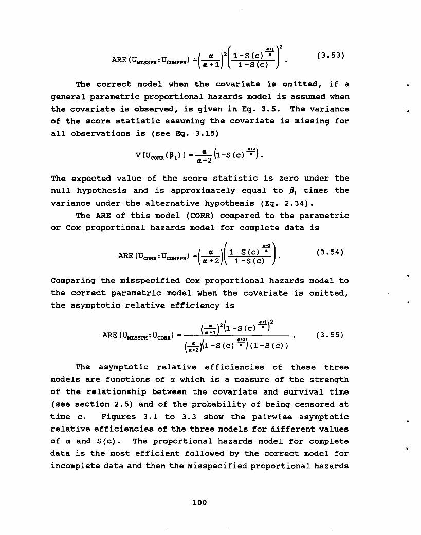
(3.53 )

The correct model when the covariate is omitted, if a

general parametric proportional hazards model is assumed whenthe covariate is observed, is given in Eq. 3.5. The varianceof the score statistic assuming the covariate is missing for

all observations is (see Eq. 3.15)

( .+2)V (UCORR (P 1 )] =_Cl_ l-S (c) - •

CI+2

The expected value of the score statistic is zero under thenull hypothesis and is approximately equal to PI times the

variance under the alternative hypothesis (Eq. 2.34).The ARE of this model (CORR) compared to the parametric

or Cox proportional hazards model for complete data is

Comparing the misspecified Cox proportional hazards model to

the correct parametric model when the covariate is omitted,

the asymptotic relative efficiency is

(.+2 )• _ CI l-S(c)-

ARE (UCORR • UCCIQIPH) -(--) ()'CI+2 l-S c

(.+1)2

. . _ (<<~1)21-S(C)-ARE (UKISSPH' UCORR ) - .+2 .

(-«)(l-S (c) -) (l-S (c) )«+2

(3.54)

(3.55 )

..

The asymptotic relative efficiencies of these three

models are functions of a which is a measure of the strength

of the relationship between the covariate and survival time

(see section 2.5) and of the probability of being censored at

time c. Figures 3.1 to 3.3 show the pairwise asymptotic

relative efficiencies of the three models for different valuesof a and S(c). The proportional hazards model for completedata is the most efficient followed by the correct model for

incomplete data and then the misspecified proportional hazards

100

..

model for incomplete data.However, incorrectly assuming a proportional hazards

model for the incomplete data is nearly as efficient as using

the more complicated correct model. In the worst case, whenthere is no censoring, the aSYmptotic relative efficiency is

_«(<<+2)ARE (UmssPH : UCORR ) - 2

(<<+1)(3.56)

•

which is 75% when a=l reflecting a strong covariate effect

where the covariate accounts for 2/3 (1 - a/(a+2» of the

variance in the survival times. For a=2, 6, and 18, i.e. thecovariate accounts for 1/2, 1/4, and 1/10 of the variance in

the survival times, "respectively, the relative efficiency is

89%, 98%, and 99.7%, respectively, even with no censoring.For small values of a when there is censoring and for largervalues of a with or without censoring, the efficiency ofmisspecifying a proportional hazards model relative to using

the correct model is nearly one.

The models omitting the covariate are not very efficient

relative to the proportional hazards model including thecovariate when there is a strong covariate effect (small a)and little or no censoring. However, when a=8 the aSYmptotic

relative efficiency of both models relative to the complete

data model is approximately 80% even with no censoring. As

the proportion of censoring increases, the efficiency of the

incomplete data models increases as the covariate does not

contribute as much information when an observation is

censored.When the covariate is observed for some observations, as

is the usual case, a proportional hazards model for complete

data would be assumed for these observations. Thus for thethree situations (complete data, using the correct parametric

model for incomplete data, and assuming a proportional hazards

model for incomplete data), the complete observations would be

modeled the same way except that the proportional hazards

model would be parametric for the second situation instead of

101

nonparametric. The efficiency of the models for incompletedata relative to the complete data model and to each other isnow a function of the proportion of missing data.

Let nXmiu be the number of observations for which the

covariate is missing and nxobI be the number of observations for

which it is observed with nXmiu+nXobI=n. If AREM is theaSYmptotic relative efficiency of using the misspecified Coxmodel for the incomplete observations versus having completedata (Eq. 3.53), the overall efficiency when p percent of the

data are missing (AR~) is

( .+1) 2. nXobs (1-5 (e) ) + nXmiSS(~) 1-5 (e) .....ARE (U .U ) = ..;n n "+1

p MISSPH • COMPPH [..;n (1 - 5 (e) ) ] 2

=[(l-p) +p~]2.

(3.57)

For example, if 50% of the data are missing and the efficiencyof omitting the covariate is .50, then ARE.50=.7286.

The ARE of the correct parametric model when p percent ofthe observations are incomplete relative to the proportionalhazards model when all observations are complete is

( " )( ~). _ nXobs (1 - 5 (e» + nxmiss Ci""+2 1 - 5 (e) •

AREp (UCORR ' UCOMPPH ) - n (1- 5 (e) )

=(l-p) +P{AREc)

(3.58 )

where AREc is given in Eq. 3.54. For the comparison of themisspecified proportional hazards model to the correctparametric model when the covariate is missing for p percent

of the observations, the aSYmptotic relative efficiency, whichdoes not simplify nicely in terms of the ARE in Eq. 3.55 butcan be written as the ratio of the AREs in Eq. 3.57 and Eq.3.58, is

102

•

..

)

• = r(l-pl (1-8 (e» +p(,,: l)h -8 (el O;,)rAREp (UMISSPH' U CORR ) -----l __

[(l-P) (l-S (e) ) +p( «:2)h -S (e) _:2)1 (l-S (e) )

= [(l-p) +pymMl2(1 -p) +p (AREc)

(3.59 )

As the proportion of missinq data decreases, the

efficiency of the models with incomplete observations relativeto the complete data model increases since more observationsare modelled correctly. with 10% missinq data, the incomplete

data models are at least 90% as efficient as the complete data

model even for small values of a and no censorinq. Likewise,the efficiency of the misspecified proportional hazards modelrelative to the correct parametric model for incomplete dataincreases as the proportion of missinq data decreases.

103

Figure 3.1

Asymptotic Relative Efficiency of Misspecified PH Model forIncomplete Data vs. Complete Data Model

t

Proportion Missing = 0.10Efficiency

1 "::':::::::-:::=:~-:::'~':'~':-::~:'~':~':~:"::;'."':" _, _._0.9 I-

0.8

0.7

0.6

0.5

0.4

0.3

0.2

0.1

oL....o-....I-.....J...........JI.-...-...l.....-I-...-J.---.J..........L-........---..l

o 0.1 0.2 0.3 0.4 0.5 0.6 0.7 0.8 0.9 1

Proportion Censored

Proportion Missing = 0.25Efficiency

1......__.__. ----------

0.9

0.8

0.7

0.6

0.5

0.4

0.3

0.2

0.1

oL....o-....I---I............J_..J......-.l-...-J. J..........L-.......J.........J

o 0.1 0.2 0.3 0.4 0.6 0.6 0.7 0.8 0.9 1

Proportion Censored

«=1 «=2 «=8 «=1 «=2 «=4 «=8

..

1.0

-------

Proportion Censored

Proportion Missing =Efficiency

1

0.4

0.3

0.2

0.1

o ........-J-........J.........J'-'-..............--I.....-.....I. ""---'--'-..........--'--'

o 0.1 0.2 0.3 0.4 0.5 0.6 0.7 0.8 0.9 1

0.9

0.8

0.7 /~//~

0.6

0.5

0.9~-

0.8

0.7

0.6

0.5

0.4

0.3

0.2

0.1

oL..........L-.......J..-,--L...........l.....--I.....-.....I._..L............I-.......L.--....J

o 0.1 0.2 0.3 0.4 0.5 0.6 0.7 0.8 0.9 1

Proportion Censored

Proportion Missing = 0.50Efficiency

1

«=1 «=2 «=4 «=8 «=1 «=2 «=4 «=8

104

Figure 3.2

Asymptotic Relative Efficiency of Correct Parametric Model forIncomplete Data vs. Complete Data Model

t

Proportion Missing = 0.10Efficiency

1 .:::::.:::::.:.::~::-:::.:::~.::.::-:~;." __ ._. _. _. - ­

0.9

0.8

0.7

0.6

0.5

0.4

0.3

0.2

0.1

oL............L...........L..-...J_...I....o.-'---.L_............L...........L..-...J

o 0.1 0.2 0.3 0.4 0.5 0.6 0.7 0.8 0.9 1

Proportion Censored

Proportion Missing = 0.25Efficiency1r-----====~"""!"'!!"'!!"""!~::::::..:===-.:--~-:-.:: --

0.9 "-----0.8

0.7

0.6

0.5

0.4

0.3

0.2

0.1

o'-'-....L........................_...1....0.-'-........-'-............................................

o 0.1 0.2 0.3 0.4 0.5 0.6 0.7 0.8 0.9 1

Proportion Censored

«=1 «=2 «=4 «=8 «=1 «=2 «=4 «=8

0.6

0.5

0.4

0.3

0.2

0.1

oL............L........................_...I....o.-'-........-'-.............L........................

o 0.1 0.2 0.3 0.4 0.5 0.6 0.7 0.8 0.9 1

Proportion Censored

1.0

.- --- :;'~'::-~~~:'

-----------

0.9.. , .

0.8

Proportion Missing =

Efficiency1

Proportion Missing = 0.50Efficiency1.----------==~~____ -:'::~~~::':::'::-~7'";,~,

0.9

0.8

0.7

0.6

0.5

0.4

0.3

0.2

0.1

oL............L...........L..-...J_...I....o.-'---.L_............................................

o 0.1 0.2 0.3 0.4 0.5 0.6 0.7 0.8 0.9 1

Proportion Censored

«=1 «=2 «=4 «=8 «=1 «=2 «=4 «=8

105

Figure 3.3

Asymptotic Relative Efficiency of Misspecified PH Model vs.Correct Parametric Model For Incomplete Data

Proportion Missing = 0.10Efficiency1e::;;::::;:!!!:~===-------,

0.9

0.8

0.7

0.6

0.5

0.4

0.3

0.2

0.1

oL.........L..o-....l..........J_.J.........J...........J.~J......-l.........L.....-....J

o 0.1 0.2 0.3 0.4 0.5 0.6 0.7 0.8 0.9 1

Proportion Censored

Proportion Missing = 0'.25Efficiency

1 .,._.__ .._._ ........ -

0.9 r:--0.8 f­

0.7

0.6

0.5 f­

0.4 f­

0.3 f­

0.2

0.1

OL.........L..o-....l..........J_...L-..-..L-............L~J......-l..............___.Jo 0.1 0.2 0.3 0.4 0.5 0.6 0.7 0.8 0.9 1

Proportion Censored

a=1 a=2 a=4 a=8 a=1 «=2 a=4 a=8

Proportion Missing = 0.50Efficiency

1 ._:::.: --- -

0.9

0.8

0.7

0.6

0.5

0.4

0.3

0.2

0.1

0L...........l-'-o!............JL.........J......~............L~.J..............I_........J..___.J

o 0.1 0.2 0.3 0.4 0.5 0.6 0.7 0.8 0.9 1

Proportion Censored

Proportion Missing = 1.0Efficiency

1 -:;;:;.. __ :-:~::.... _._ .... '-'---

0.9

0.8

0.7

0.6

0.5

0.4

0.3

0.2

0.1

0L...........l-......L..........J1..-......L-..~............L~..l..-....J...........J.___.J

o 0.1 0.2 0.3 0.4 0.5 0.6 0.7 0.8 0.9 1

Proportion Censored

•

a=1 a=2 a=4 a=8

106

a=1 a=2 a=4 a=8

t

3_8 Extension to p covariates

So far it has been assumed that there is one covariate in

addition to treatment group. Ordinarily in a clinical trialthere will be mUltiple covariates. Assuming there are p

covariates, the hazard function for the Cox proportional

hazards model is

Letting 0=132z2 + ••• + I3pzp and X=eQ, the hazard rate can

be written as

h (t I z) =ho(t) e lSlZle lSzzz + ••• + lSpzp

=ho (t) elS1ZleO

=ho (t) e lS1Z1x.

(3.60)

Now omitting X is equivalent to omitting all covariates. Theequations for variances and efficiencies derived previouslyare applicable to this situation.

Usually there is a different pattern of missing data for

each person. The likelihood needs to be expanded to account

for the different combinations of observed and missing data.

For example, if there are two covariates, Z2 and Z3' there are

four possible patterns of observation for these two variables:

both observed, neither observed, Z2 observed only, and Z3

observed only. For each of these four patterns, there couldbe people who were failures and people who were censored.

Thus the likelihood would consist of eight different products.

For each pattern of observed data, let O-={3obl- I Zobl where Zobl

is the vector of observed covariates and {3obl- is the vector of

coefficients for these variables in the model containing onlythe observed variables. Thus the error in measuring the

effect of the covariates is E=Q-{J· if only the observed

107

variables are used instead of all variables. The observed

value and the error term are assumed to be independent in this

model, known as Berkson's error model.

The hazard rate can be written as

h (t I z) =ho(t) elllZle'lllzlI+'" +llpzp

=ho (t) e'llZleO

=ho(t) e'llZleO·..

=ho (t) e'llZleO·x.

(3.61)

Now omitting X=ef is equivalent to omitting the error due to

having unobserved covariates and previous equations apply

replacing 5(c) with 5(cIQ·),

5 (c : Q.) =( P )4 .P+Ho(c)e Q

'(3.62)

Although assuming a proportional hazards model for eachpattern of missing data is more feasible than trying to use

the correct marginal distribution for each pattern, especially

if there are many covariates, this approach still requires

that mUltiple models be defined and fit. Information is also

being· lost due to the missing values for some variables.

Imputing values for the missing ones might regain some of the

lost information if the estimation can be done well and would

allow one model to be fit to all observations.

3.9 Imputing values for the'Kissing covariates

Assume that through some estimation procedure, estimatesof the missing values of the covariates are obtained. If Zj

was not observed, let ~j be the estimated value of Zj and

108

(3.63)

1

be an estimate of O. Using Berkson's model, O=Q+£ where £ is

the error in the estimation. If all of the covariates are

observed, the error is zero. If Q which is based on imputed

values, when necessary, is used instead of the true value 0,

this is equivalent to omitting the error term. Letting X=e·,

the covariate being omitted is a function of the differences

between the true, observed values and the imputed values of

the covariates and their effects on survival time,

e=Q-Q

=t (~1Z1 -~~21) •1-2

(3.64 )

SUbstituting Q for 0*, the hazard rate is the same as that for

omitting a subset of variables (Eq. 3.61). The previous

equations when X is omitted apply here SUbstituting s(cIQ) for

S(c) where

S(C:Q)=( p 0)11.~ +Ho (c) e

(3.65 )

•

The distribution of the error term is equivalent to the

conditional distribution of the true value given the imputed

value,

This can be derived easily using the change of variable

technique. Using the relationship £=0-0,

fB(e) =fOlo(Q+e:Q)I~(Q;::Q) I

=fOIO (Q+e)

since the imputed value and the error are assumed to be

independent. Thus the distribution of the error term is the

109

distribution of the true value given the observed value

shifted to have a mean of zero.

As was discussed in section 3.7, the asymptotic relative

efficiency of the misspecified proportional hazards model when

a covariate is omitted relative to the proportional hazards

model for complete data depends on a, the proportion of

censoring, and the proportion of missing data. Obviously, the

smaller the proportion of missing data is the less the impact

of imputing and omitting the error term. The size of a, a

measure of the effect of the error term on survival time, will

be determined by the accuracy of the imputation procedure and

the strength of the effect of the covariates on survival time.

In order to obtain the best estimates possible, the

values of the missing variables should be imputed conditional

on ·the values of the observed variables. The higher the

correlations among the variables are, the better the estimates

will be.

If the variables which have the strongest relationship

with survival time are observed and the variables with missing

data are strongly correlated with the observed ones, the

impact of imputing will be small. The difference between the

true and estimated values will be small since the strong

correlation should provide good estimates. Variables which

are not strongly related to survival time have small

regression coefficients also. Thus the information being

omitted will be small and should not have much variability, so

consequently a should be large.

Conversely, if values are missing for an important

covariate and the covariate is not highly correlated with any

other variables, it will not be possible to obtain good

estimates of the missing values. The regression coefficient

is large when the variable has a significant impact on

survival time. The variability in the estimates combined with

the large coefficients will result in heterogeneity in the

errors being omitted from the model and consequently a small

a. Thus, in this situation, the gain from imputation may not

110

•

be great, although it may still be better than omitting

incomplete observations or important variables.

For each pattern of missing and accuracy of imputing,

there is an efficiency of imputing,

where at is the heterogeneity of the residuals in imputing Q

for the k* pattern of missing data and St is the probability

of censoring given Q (Eq. 3.65). The relative efficiencies of

the three models when there are missing data and values are

imputed when possible are given by multinomial versions of Eq.

3.57, 3.58, and 3.59. The ARE of the score test of treatment

when the Cox model is misspecified relative to that when there

are no missing data is

(3.66 )

where AREM is defined in Eq. 3.53 and a~ for observations

with no missing data. For the comparison of the correct

parametric model with missing data to the model with complete

data, the ARE is

(3.67 )

where AREc is defined in Eq. 3.54.

For example, suppose there are four patterns of

observation: 50% of the observations have all variables

observed (a~), 30% of the observations have missing values

which are imputed well (a=50), 10% of the observations have

missing values which are imputed poorly (a=10), and 10% of the

observations are missing all of the covariates and they have

a strong effect on survival time (a=2). For simplicity,

assume there is no censoring. Then the efficiency of the

imputing the data and assuming a proportional hazards model

for all observations relative to having complete data is

111

ARE (UKISSPH : UCCMPPH ) =(.5 (1) + • 3( :~) + .1( ~~) + .1(1)t=.90572 .

Thus, in this arbitrarily chosen example, the score test of

treatment effect based on imputing values for missing data and

misspecifying the Cox proportional hazards model is 91% as

efficient as the test based on complete data. Similarly, the

efficiency of the correct parametric model relative to the

complete data model is

ARE (UCORR : UCOMPPH ) = .5 (1) + • 3( :~) + • 1( ~~) + .1H)

=.92179.

Therefore, the relative efficiency of misspecifying the Cox

proportional hazards model with imputed values versus usingthe correct parametric model which is complicated, hard to

compute, and requires an assumption about the distribution ofthe underlying hazard is

ARE (UMISSPH: UCORR

) = _._9_0_5_7_2_ = .98257 .. 92179

3.10 Random censoring Time

It has been assumed that there was fixed Type I censoring

at time c, that is, all people were followed for the same

length of time c. However, often in clinical trials, the

length of follow-up varies from person to person so that thecensoring time (ci ) is random. consequently, the probability

of being censored varies for each individual (5 (ci» • The

results given in the previous sections, which are conditional

on a given c, are easily extended to random censoring by

taking the expected value with respect to c of the mean and

variance of the score statistic. For example, when there is

112

..

random censoring, the ARE of the misspecified proportional

hazards model relative to the complete data model (Eq. 3.53)

is

•(3.68)

Similarly, the ARE of the correct parametric model relative to

the complete data model (Eq. 3.54) is

(3.69 )

•

The ARE of the misspecified proportional hazards model to the

correct parametric model is the ratio of Eq. 3.68 to Eq. 3.69.

3.11 Summary

If the hazards for the two treatment groups are assumed

to be proportional when all data are observed, then the

hazards when a covariate is omitted will be nonproportional.

If imputed values are substituted for missing values, the

error term is the covariate being omitted. Assuming a

proportional hazards model when imputed values are used is an

example of misspecifying the proportional hazards model. It

has been shown in this chapter that the misspecified

proportional hazards model is nearly as efficient as the

proportional hazards model for the complete data if the

proportion of missing data is small and/or the effect of the

covariate on survival time is small. The efficiency improves

as the proportion of censoring increases also, so that even

for a larger proportion of missing data and/ or a stronger

covariate effect the efficiency may be good. If the

imputation can be done well, the error term and its

113

relationship to survival time should be small. Thus imputingvalues for missing ones and assuming a Cox proportional

hazards model, although an incorrect assumption, is preferableto omitting incomplete observations or omitting covariates,the two most common procedures when there are missing data.with the latter procedure, it is likely that a Coxproportional hazards model will also be misspecified; and theomitted covariates are likely to be more strongly related tosurvival time than is the omitted error term.

The next chapter will discuss the implementation of thisprocedure: imputing values, analyzing the data assuming a Coxproportional hazards model, and calculating the correctvariance and test statistic. A method to determine the impactof imputing will be discussed.

114

•

•

•

..

•

CHAPTER 4

IKPLEKENTATION OF THE ANALYSIS OF SURVIVAL DATA WITH IKPUTED

COVARIATE DATA USING THE COX PROPORTIONAL HAZARDS KODEL

4.1 Introduction

In this chapter, implementation of the analysis of

survival data using the Cox proportional hazards model when

estimates are imputed for missing covariate data will be

discussed. First, methods of imputing will be reviewed

briefly. Second, the analysis of the data using a standard

Cox proportional hazards analysis program and an additional

program to make necessary adjustments to obtain the correct

score test for the test of treatment effect will be discussed.

Last, a method of determining the efficiency of imputing will

be presented.

4.2 Imputing Data

Little and Rubin (1987) have reviewed methods of imputing

data (e.g., imputing unconditional or conditional mean, hot

deck imputation) and discussed their pros and cons. Section

1.4 summarizes this information. If assumptions about the

data and computer software and hardware availability make

maximum likelihood methods of analysis feasible, Little and

Rubin recommend their use (see section 1.5).

While regression estimates are the best estimates for a

given value, the reSUlting observed variances using imputed

values are biased towards zero. One possible way to improve

estimates of the variance obtained from regression analyses is

to add a random error term to the regression model (Blackhurst

and Schluchter, 1989). A disadvantage of this procedure is

that different analysts may reach different conclusions. A

possible solution to this problem may be to use the mUltiple

imputation scheme proposed by Rubin (1978). In this procedure

each missing value is replaced by two or more values

representing a distribution of likely values. Each of the

resulting datasets is analyzed using standard complete data

methods. The analyses are combined to reflect both within and

between imputation variability.

The proposed analysis of survival data with imputed

covariate data is not dependent on the method of estimation,

but better estimates reduce the impact of imputing. In order

to obtain good estimates of the missing values and to try to

minimize the residual error, it is recommended that the

estimation be conditional on the values of the observed

variables. Various procedures are possible, and the user

should choose a method appropriate for the data to be

analyzed.

One program that estimates missing values and substitutes

the estimates in the dataset is BMDPAM (Dixon, 1990). Several

methods of estimation are available: overall or group mean,

regression on the one or two most highly correlated variables,

regression on a subset of highly correlated variables, and

regression on all available variables. The BMDP manual gives

some suggestions on which method may be the most appropriate

given the number of cases, the amount of missing data, and the

magnitude of the correlations.

SAS procedure PRINQUAL (1990) may also be used to

estimate missing data in mUltivariate data. The procedure

uses the minimum generalized variance method, an iterative

mUltiple regression algorithm which minimizes the determinant

of the covariance matrix of the transformed variables. The

example in the documentation illustrates code, which at least

for that example, estimates the missing values without

changing the nonmissing values.

116

t

4.3 Analysis Procedure

The first step of the analysis procedure is to impute

values for the missing data using a method and program of the

user's choice. The data set containing the observed and

imputed values is then used in the analysis of survival time.

The objective of the analysis is to test the null

hypothesis of no treatment effect, Ho:PI=O, using a score test

when data are imputed and the Cox proportional hazards model

is misspecified. The numerator, the score statistic, is the

same whether the data are all observed or some are imputed.

However, as seen in Chapter J, the variance of the score

statistic changes ·when the model is misspecified. Thus the

score test must be constructed. How this is accomplished

depends on the information provided by the standard Cox

proportional hazards program which the user plans to use.

If it is possible to obtain the numerator of the score

test from the standard proportional hazards analysis program,

this is the easiest way to proceed. In order to obtain the

numerator, if it is not printed, the information matrix used

in the score test must be obtainable. However, this is not

possible with either the SAS PHREG procedure (SAS, 1992) or

BMDP2L program (BMDP, 1990), two of the most commonly used

survival analysis programs. Both only provide the covariance

matrix with f11=~I. Thus it is necessary to calculate the score

statistic in addition to its variance.

The second step of the analysis procedure is to analyze

the data using a standard Cox proportional hazards program and

specifying a model that includes the covariates but not

treatment. This analysis provides the estimates of the

regression coefficients of the covariates when PI=o. These

estimates are needed to calculate the score statistic for the

test of no treatment effect.

The third step is to calculate the score statistic, its

variance, and the score test. A SAS macro which does these

calculations is provided in Appendix B. This macro utilizes

117

an output dataset created by PROC PHREG which contains pl. for

each individual. If another survival analysis program is used

which does not output this information, e.g. BMDP2L, the

program could be easily modified to calculate p' z. Thedataset must also contain treatment, the covariates, survival

time, and a status variable indicating whether the observation

was censored or not. The PHREG output dataset automatically

contains all of these variables except treatment as they were

part of the MODEL statement. Treatment can be included in thedataset via the ID statement. An identifying variable such asa patient number could also be included in the ID statement.It is not needed for the calculation of the score test, but it

is required in the efficiency program (Section 4.4).

The score statistic in Eq. 3.26 assumes that there are no

ties among the failure and censoring times. As ties do occur

in real life, the program uses Breslow's approximation to the

likelihood (Breslow, 1974) to calculate the score statistic,

(4.1)

where k is the number of distinct event times, dj is the number

of people who fail at time t j , and Sj is the sum of the vectors

Zj for the people who fail at time tj. Ties are accounted for

in the summation over the risk set also. The aSYmptotically

equivalent formula for the score statistic given by Lin and

Wei (Eq. 3.29) is also calculated accounting for ties.

Two estimates of the robust variance of the scorestatistic are calculated, the null hypothesis variation of

Lin's and wei's robust estimator, modified to account for

ties, and the proportion of deaths estimator. The score test

is

In-iU~l(O,ii o)lvar[n-iU~l (0 Iii 0) ]

118

(4.2)

•

which asymptotically has a chi-square distribution with one

degree of freedom.

Appendix C provides an example of the programs needed to

impute the data and to calculate the score test and an example

of the output from PROC PHREG and the score test macro. The

sample program was used in the example in Chapter 5 •

4.4 Bstimation of ARB of Imputinq Data

In Chapter 3, it was shown that the ARE of imputing data

and misspecifying a proportional hazards model versus having

complete data or using the correct parametric model when there

are incomplete data can be expressed in terms of the

proportion of observations with each pattern of missing data

and the ARE for each pattern of missing data. The ARE is a

function of a, the heterogeneity of the residual resulting

from imputing values for that pattern of missing data, and

S (c), the probability of being censored. The a's can be

estimated by equating the observed variances of the residual

to the theoretical variance and solving iteratively for the

a's using the Newton-Raphson algorithm.

The residual e is assumed to have a log gamma distri­

bution, since X=ef is assumed to have a gamma distribution.

The probability density function is

(4.3)

The moment generating function is

119

M.(t;u,P) =E(e tC )

=~ r(u+t)r(u) put

=A-t r(u +t)to' r(u) .

For P=l, the general form of the j~ moment for the log gamma

distribution is

M(j) (0· CI) =r(j) (u), r(u)

(Balakrishnan, 1992). In general, for P>O, the j~ moment is

..

M(j) (0; CI , P) =t (j ) ( -lnp ) j -k r (k) (CI)k-O k r (CI)

where r~{a}=r(a}. The expected value of € is

E(e) =M(ll (O;CI,P)

=r/(u) -lnpr(CI)

=v (CI) -lnp

where the psi function is

{4.4}

{4.S}

Since € is a residual, its mean is assumed to be zero. This

implies that

The variance of € is

P=e t (lIl •

120

(4.6)

..

Vee) =M(2) (0;«) - [M(l) (0;«)]2

=r"(<<) -2lnp IV(<<) + (-lnp )2_[r'(<<) _lnp]2r(<<) r(<<) r(<<)

=r" (« ) _[ r' («) ]2r(<<) r(<<)

=t' (<<) •

(4.7)

The first and second derivatives of the psi function can

be written as

t'(<<) =f (<< +k)-2It-o

tl/(<<) = -2 f (<< +k) -3,It-o

respectively. These formulas can be used in the Newton­

Raphson algorithm for determining the value of a that makes

~'(a) equate to var(e). The algorithm is

where var(e) is the observed variance of the residual. An

initial estimate of alpha is the inverse of the square root of

the variance of the residual.

The variance of the residual for each pattern of

observation or individual can be calculated from the data.

Recall that e=Q-Q where Q=P'z and Q=P'I, omitting treatment

(Zt> (Eq. 3.64). The variance of the residual for the i lb

person is

(4.8)

where ~ is the correlation between Qi and Qj. The variance of

Q is not observed, but it can be estimated. Since Q=P'z,

var(Q)=p'vp where V is the covariance matrix of z. A maximum

likelihood estimate of V which is an asymptotically unbiased

estimate can be obtained from the BMDPAM program. An estimate

121

of P can be obtained from the standard proportional hazards

analysis program, either from the analysis with imputed values

or from an analysis based on people with complete data only.

The estimate from the analysis of imputed values will be

biased since the residual is omitted from the model. While

the estimate from the analysis of complete data may be

unbiased, the subgroup of people with complete data may not be

representative of the entire sample. Also a second analysis

would have to be done to obtain this estimate.

For each individual, the correlation between Q and Q is

"

where

Ri =con: (PI!, P/Z)

A/VP=-;:;::~;::::::::;::::;:::;~;:;::J(A/VA i ) (P'VP)

(4.9)

and

Ai =D01 [I +V-1D01VDY1] P

P is the p-1 vector of coefficients for Z2' ••• 'Zp

V is the p-1 x p-1 covariance matrix of the covariates,

DOl is the p-1 x p-1 diagonal matrix ~ith l' s on the

diagonal for observed variables and O's for missing

variables,

DM1 =I-D01 is the p-1 x p-1 diagonal matrix with l's on

the diagonal for missing variables and 0' s for

observed variables.

The easiest way to show the derivation of this formula is

through an example. Consider the case where there are four

variables, Z2I Z3, Z4, and Zs. Suppose that for one individual

Z2 and Z3 are observed and Z4 and Zs are missing. Estimating Z4

and Zs through regression on Z2 and Z3,

24 =P42.3 Z 2 + P 43 .2 Z 3

2S=PS2.3Z2+PS3.2Z3 •

Then Q=P'I can be written as

122

..

•

0= P2Z2+ P3Z3+ P424+ Ps2s= P2Z2+ P3Z3+ P4(P42.3Z2+ P43 .2Z3) + Ps(PS2.3Z2+ PS3 .2Z3)= (P2+ P4P42.3 + PSPS2 .3)Z2 + (P3+ P4P43.2 + PSP S3 .2) Z3

[(P2) (P4P42.3 + Ps'PS2'3)]'[Z2]. g' + M'3.2g~5~53'2 ~:

=A'z

The first term of A can be written as Do*P where

(

1000]0100Do = 0000 .

0000

The second term is more complicated. It can be rewritten as

o 0

o 0

o 0o 0

P42.3P43.2

oo

P52.3

PS3 .2

oo

The regression coef·ficients are defined as

(P42.3 PS2.3]_ ,,_ ('" ", )A A - ~23 ~4.23 ~S.23

"43.2 "53.2

where the covariance matrix is partitioned as

v-( 1:23 1:23 .4S]1: 45 • 23 1: 45 •

Thus the second term, written in terms of V, Do, and DM, is

Combining terms, A is

123

A=DoP +Doy-1DOYDyP

=Do [I +y-1DoYDy] P ,(4.10)

A and, subsequently, R can be calculated for each person.

From the R's and the variance of Q, the variance of the

residual for each person can be calculated. The variance can

then be used to estimate a. The estimate of a will be the

same for everyone with the same pattern of observation, since

the correlation is a function of the pattern of observation

Do, the vector of coefficients P, and the covariance matrix V

but not the vector of observations z.

Also required for the calculation of the ARE is the

probability of being censored for each person,

5(CIQ)=(" p 0)-'Ii +Ho (c) e

An estimate of Ha(c), assuming fixed censoring, can be

obtained through a Newton-Raphson algorithm. An initial

estimate of Ha(c) can be obtained by using the observed

proportion of censored individuals as an estimate of 50 (c) and

the relationsbip between the cumulative hazard and the

survival function. An estimate of P can be found from its

relationship to a (Eq. 4.6). ~(a) can be approximated by

..

t (u) =lnu __1 1_ + __1_2u 12u2 120u4

1252u6

A program is provided in Appendix D to calculate

estimates of a, P, and 5 for each person and the asymptotic

relative efficiency of the misspecified proportional hazards

model with imputed data versus the correct parametric model

when there are missing data and versus the complete data

model. The program requires the input of the original data

set in order to obtain the patterns of missing data, estimates

of the vector of coefficients P and the covariance matrix of

the covariates, and the value of Q=P'z for each person (or z

124

..

...

and the program modified to calculate Q).This program to determine the ARE of the analysis with

imputed data is usually only of theoretical interest. For the

routine analysis of data sets, running a Cox proportional

hazards program on the data set with imputed values followed

by the program to calculate the correct score statistic

provides a valid test of treatment effect.

4.5 summary

The analysis of survival data with imputed covariate data

and misspecifying a Cox proportional hazards model can be

accomplished in three steps: imputing values for the missing

covariate data using a standard program, analyzing the data

using a standard proportional hazards program to obtain

estimates of the coefficients of the covariates under the null

hypothesis of no treatment effect, and running a SAS macro to

calculate the score test for the test of no treatment effect

when the proportional hazards model is misspecified.

optionally, another program can be run to evaluate the

asymptotic relative efficiency of the model with imputed data

to a model with complete data and to the correct parametric

model .

125

CHAPTER 5

ILLUSTRATION OP IMPLEMENTATION AND EPPICIENCY OP METHOD

5.1 Description of Data

A randomized, double-blind, parallel study was conducted

to evaluate the effect on mortality of an angiotensin­

converting-enzYme (ACE) inhibitor versus placebo, in addition

to conventional therapy, in patients with severe congestive

heart failure (The CONSENSUS Trial Study Group, 1987). Two

hundred fifty-three patients were enrolled in the study, 127

in the treatment group and 126 in the placebo group, prior to

its early termination due to the significant reduction in

mortality in the treatment group relative to the placebo

group.

A secondary objective of the study was "to study the

activation of hormones related to cardiovascular function and

the effect of the overall hormone response to ACE inhibition"

(Swedberg, Eneroth, Kjekhus, and Wilhemsen, 1990). In order

to do this, seven hormones were measured at baseline and at 6

weeks. Lipoprotein A (LPA) was also measured. In addition,

a ninth chemical entity, N-terminal peptide (NTERM), which was

of particular interest to one investigator was measured for

55% of the participants. (For simplicity in terminology, LPA

will be called a hormone in the following discussion.)

Blood samples were missing for 14 people. Due to

insufficient amounts of blood, not all hormones were measured

for all people. The percent of missing data for the eight

primary hormones at baseline was between 6% and 13% for each

hormone. Fifty people (20%) were missing data for at least

one of the eight hormones. Considering all nine hormones, 127

..

..

people (50%) were missing data for at least one of them. Most

people who were missing data were missing three or fewer

values. Some hormones or combinations of hormones were

missing more frequently than others suggesting that there was

a protocol for which measurements to make if there was

insufficient blood for all measurements. Excluding NTERM,

there were 11 patterns of observation for the eight hormones;

including NTERM, there were 14 patterns of observation. Table

5.1 provides the patterns of observation and the number of

people for each pattern.

These data will be used to illustrate the proposed method

of analyzing survival time data when there are missing

covariate data. The baseline hormone data, along with age and

sex, will be used as covariates. There were no missing data

for age or sex. The analyses will be done including and

excluding the additional hormone data to illustrate the method

with different proportions of missing data. The purpose of

the analyses is to illustrate the procedure and its

efficiency, not to draw conclusions from the data.

5.2 Usual Methods of Analysis

The approach taken in the analysis of the above dataset

may vary among statisticians depending on their preference to

include all variables of interest or to use a stepwise method

for the selection of variables to include in the model.

Whether the analysis is exploratory or confirmatory may be a

factor in the approach taken. Either way the missing

covariate data cause problems using the standard approaches of

either omitting the observations with incomplete data, the

default of most software programs, or omitting the covariates

with missing data.

If all nine neurohormones are included in the

proportional hazards model and incomplete observations are

omitted, the analysis is based on 126 people or 50% of the

127

Table 5.1

PATTERNS OF HISSING DATA, R2, AND ALPHA'S OF RESIDUALS

Estimating 8 Covariates

Variables Missing

None

LPA

ACE, LPA

ADR, OA, NA

ANP

ACE, ANP

ALOO, ANP

ACE, ANP, LPA

ADR, OA, LPA, NA

ACE, AOR, OA, LPA, NA

All except AGE, SEX

JL. R2

203 1.00000

2 0.89764

12 0.88586

7 0.70000

9 0.66500

1 0.66297

1 0.63538

2 0.60368

1 0.57897

1 0.55515

14 0.03504

Var. of

Residual

0.00000

0.01326

0.01478

0.03886

0.04339

0.04365

0.04723

0.05133

0.05453

0.05762

0.12498

Alpha

ao

75.55

67.80

26.11

23.43

23.29

21.57

19.88

18.74

17.77

8.45

Estimating 9 covariates

Var. of

variables Missing JL. R2 Residual Alpha

None 126 1.00000 0.00000 ao

NTERM 77 0.99999 1. 56E-6 66170.1

LPA, NTERM 2 0.89487 0.01362 73.56

ACE, LPA 8 0.88377 0.01506 66.58

ACE, LPA, NTERM 4 0.88176 0.01532 65.46

ADR, OA, NA 3 0.71812 0.03652 27.75

ADR, OA, NA, NTERM 4 0.70368 0.03839 26.42

ANP, NTERM 9 0.66420 0.04350 23.37

ACE, ANP, NTERM 1 0.66168 0.04383 23.20

ALOO, ANP, NTERM 1 0.63410 0.04740 21.49

ACE, ANP, LPA, NTERM 2 0.59989 0.05183 19.19

ADR, OA, LPA, NA 1 0.58671 0.05354 19.08

ACE, ADR, OA, LPA, NA 1 0.56136 0.05683 18.01

All except AGE, SEX 14 0.03495 0.12502 7.95

128

data. None of the variables, including treatment, have a

significant (p<0.05) effect on survival time in this sUbsample

of participants according to the Wald chi-square test for each

variable. The p-value for the score test of the null

hypothesis of no treatment effect, given the other variables

are in the model, is 0.119. Using a stepwise approach, with

an entry significance level of 0.25 and a removal significance

level of 0.15, treatment and age enter the model and remain in

it; but neither are significant. In this model, the p-value

for the score test of the null hypothesis of no treatment

effect is 0.13l.

Since overall 39% of the treatment group and 54% of the

placebo group died and the median length of time in the study

was much longer for the treatment group (216 days) than for

the placebo group (87 days), the analyst may wonder if the

subset of patients with complete hormone data is different

from those with incomplete data. The mortality picture was

better in this subsample of 126 people than in the total

sample of 253 people, but there was still a difference between

treatment groups. Twenty-six percent of the treatment group

and 37% of the placebo group died, and the median length of

time in the study was 249 days for the treatment group and 199

days for the placebo group. This suggests that the absence of

significant effects may be due to a loss of power.

This analysis points out two problems with the common

approach of omitting observations with incomplete data.

First, the subgroup of people with complete data may not be

similar to the rest of the group even though the missing data

are missing at random. Second, there is a loss of power due

to the reduction in sample size.

The statistician may decide to omit N-terminal peptide

which is missing for 45% of the people, even if it had been a

planned measurement rather than an additional one. Excluding

NTERM, 203 people have complete data, 80% of the original

sample. In this sUbsample, 41% of the treatment group and 48%

of the placebo group died, a smaller difference between the

129

groups than in the entire sample. The difference in the

median time in the study was also smaller, 216 days for the

treatment group and 132.5 days for the placebo group.

In the proportional hazards model analysis with

treatment, age, sex, and the eight remaining hormones in the

model, atrial natriuretic peptide (ANP) and treatment have

significant effects on survival time, p=0.004 and p=0.020,

respectively. The effect of noradrenaline (NA) was nearly

significant (p=O. 055). The p-values for the Wald tests of the

effects of the other covariates in this model are all greater

than 0.150. The p-value for the score test of the null

hypothesis of no treatment effect is 0.019.

Using a stepwise procedure to identify variables which

may explain some of the variation in survival time, the

variables which are identified as significant are slightly

different. The final model consists of noradrenaline

(p=0.003), atrial natriuretic peptide (p=0.004), treatment

(p=0.017), and lipoprotein A (p=0.096). The p-value for the

score test of the null hypothesis of no treatment effect,

given the other three variables are in the model, is 0.016.

Having identified significant variables, the statistician

may then rerun the model including everyone who has data for

these four variables in order to increase the power of the

analysis. However, in this case, no additional people were

included in the analysis. The 50 people who were missing data

for at least one of the eight primary neurohormones did not

have a value for at least one of the three hormones included

in the model selected through the stepwise procedure.

1990)

data.

along

5.3 Analysis of Data Imputing Values for Kissing Covariates

The regression method in the BMDP procedure AM (Dixon,

was used to estimate values for the missing hormone

Age and sex were utilized in the estimation procedure

with the neurohormones. The estimation was done twice,

130

once including N-terminal peptide and once excluding it.

Treatment was not used in the estimation procedure. In

a randomized study, treatment and baseline characteristics are

independent, at least theoretically. If, by chance, the

treatment groups are not similar at baseline with respect to

the covariates, use of treatment to estimate values to be used

in an analysis of the effect of treatment could bias the

results.

Since missing data have been estimated, the analyses are

based on all 253 people. For the model including all nine

neurohormones, age, and sex, the score test X2 of the test of

treatment effect is 12.205 using the null hypothesis variation

of Lin's and Wei's variance estimator and "12.697 using the

number of deaths estimator. For both X2 , the p-value is

<0.001.

The results are similar for the model excluding NTERM.

~he score test X2 of the test of treatment effect is 12.237

using the null hypothesis variation of Lin's and Wei's

variance estimator and 12.733 using the number of deaths

estimator. For both X2 , the p-value is <0.001.

Since the program to calculate the score test for

treatment when there are imputed data and the Cox proportional

hazards model is misspecified has not been extended yet to

include tests of the effects of the other parameters and does

not have a stepwise option, PROC PHREG with the STEPWISE

option was run on the datasets with imputed values to

determine which variables might explain some of the variation

in survival time. It is recognized that the variances used in

the Wald statistics are not correct, but they should be close

enough for the purpose of identifying variables.

For the datasets including and excluding N-terminal

peptide, the same variables were selected using the p~. 25

entry criterion and p>.15 removal criterion: treatment,

atrial natriuretic peptide, and noradrenaline. The p-value

for the score test of the null hypothesis of no treatment

effect given the other two variables are in the model is

131

<0.001 for both test statistics for both datasets. Table 5.2

summarizes the results of the analyses on the original and

imputed data.

In the analyses utilizing imputed data for the missing

neurohormone data which allows all 253 observations to be

used, the effect of treatment is highly significant (p<O.OOl

for all analyses). Using the standard approach of omitting

incomplete observations, the effect of treatment was not

significant when N-terminal peptide was included in the model

and only 126 observations or 50% of the data were used. When

this hormone, which was missing for 45% of the people, was

omitted so that the analysis utilized 80% of the observations,

the effect of treatment was significant but with a smaller

p-value (p=0.02). The differences in the test of treatment

effect for the different samples and sample sizes illustrate

the problems of decreased power and of making inferences based

on SUbgroups rather than on the entire group.

The stepwise selection of variables using the original

data and excluding N-terminal peptide as a possible variable

and using the imputed data including and excluding this

hormone yielded similar but not identical models. An

additional variable, lipoprotein A (LPA) , was included in the

model based on the 203 observations with complete data. The

question is which model better reflects the truth? LPA was

missing for 12.6% of the people, the second highest percentage

of missing data for a variable. Its coefficient of variation

was the second largest (1.135), and its squared multiple

correlation with all the other variables was among the lowest

(0.059). The variable with which LPA had the highest

correlation (rs=0.20) was NTERM which is missing for 45% of

the people. Thus it is possible that values of LPA could not

be imputed well. Decreased variability could have reduced the

significance of the relationship with survival time. On the

other hand, the additional data, observed and imputed, for LPA

and the other variables may have strengthened the true

relationships between the variables and survival time.

132

• - •

Table 5.2

SCORE TEST OF ~: NO TREATMENT EFFECT

Complete Observations

5.337 0.0186

2.430 0.1190

L- p-value

Imputed Data

L- D-value

12.2051 0.0005

12.697b 0.0004

14.4330 0.0001

12.2371 0.0005

12.733b 0.0004

14.2960 0.0002

253

..JL253

0.1312

0.0161

2.278

5.788

126

203

203

..JL126

Stepwise Selection on Original Data

Model 1 --~ Trt, Age

Model 2 --~ Trt, ANP, LPA, NA

Trt, Age, Sex, 8 Hormones (Model 2)

variables in Model

Trt, Age, Sex, 9 Hormones (Modell)

....ww

Stepwise Selection on Imputed Data

Model 1 --~ Trt, ANP, NA

Model 2 --~ Trt, ANP, NA

253

253

12.7041

13.358b

14.9710

12.6941

13.346b

14.9540

0.0004

0.0003

0.0001

0.0004

0.0003

0.00011

o

Ho variation of Lin's and Wei's variance estimate b Number of deaths variance estimate

Complete data variance estimate (from SAS PROC PHREG)

The score test calculated using the null hypothesis

variation of Lin's and Wei's variance estimator was

consistently smaller than the score test which utilized the

simple proportion of deaths estimator. The robust score test

proposed by Lin and Wei (Eq. 3.45) would yield a larger x2

than the variation under the assumptions of no treatment

effect and independence of treatment and the covariates, since

the estimate of the variance would be smaller. Further

research is needed to compare the properties of these variance

estimators and score tests.

For comparison, the score test for the test of treatment

effect assuming all the data were observed was obtained from

PROC PHREG. In this example, the score test calculated using

the usual variance formula for the Cox proportional hazards

model was larger than the score tests based on variance

estimators which account for misspecifying the Cox

proportional hazards model.

5.4 Bfficiency of Imputing

The aSYmptotic relative efficiency of imputing values for

the missing covariate data and misspecifying a Cox

proportional hazards model versus the complete data Cox

proportional hazards model and the correct parametric

proportional hazards model when there are missing data was

calculated. The estimate of P from the analysis of imputed

data was used.

Excluding NTERM, the analysis using the imputed data was

99.37% as efficient as the analysis with complete data would

have been. It was 99.99% as efficient as the correct

parametric analysis for the incomplete data would have been if

it had been feasible to calculate and program the likelihoods

for 11 different patterns of observation. For comparison, the

standard methods of omitting observations with missing data

and omitting covariates with" missing data are 80.24% and

134

•

•

•

•

..

93.04%, respectively, as efficient as the complete data

analysis. The efficiency of the proposed method of analysis is

excellent because 80% of the people had complete data and 68%

of the people with missing data were only missing a few

values. The missing values were imputed reasonably well,

despite low correlations among the covariates (Spearman

correlation < .3 except for one pair of hormones), as

indicated by the values of alpha for the different patterns of

missing data (Table 5.1).

Including NTERM, the efficiency of the imputed data

analysis relative to the complete data analysis and to the

correct parametric analysis was also 99.37% and 99.99%,

respectively. omitting incomplete observations is 50.20% as

efficient as the complete data analysis, and omitting the

hormones from the model is 92.63% as efficient. The alpha for

the residual when only NTERM was estimated was so large that

it was essentially infinity, as it is when there are no

missing data. NTERM was significantly (p<0.05) correlated

with atrial natriuretic peptide (rs=0.55), noradrenaline

(rs=0.30), and lipoprotein A (rs=0.20), so that it was imputed

very well.

The efficiency of using imputed data in the model

selected by the stepwise procedure was even higher, 99.64% as

efficient as the complete data model and 99.997% as efficient

as the correct parametric model using the dataset from the

imputation of values for eight hormones. The AREs were 99.63%

and 99.997%, respectively, using the dataset from imputing

values for all nine hormones when necessary. There were only

four patterns of observations, whether or not NTERM was

included: no missing data (n=217), NA missing (n=9), ANP

missing (n=13), and all hormones missing (n=14) •

5.5 Summary

In this clinical trial with 253 patients, 20% of the

135

people were missing data for at least one of the eight

primary hormones and considering the additional hormone, 50%

of the people were missing at least one measurement. The

standard procedure of omitting incomplete observations

resulted in a loss of power in the test of treatment effect.

The proposed method of imputing values for the missing

covariate data, misspecifying the Cox proportional hazards

model, and analyzing the data using SAS PROC PHREG and a SAS

macro was easily implemented and extremely efficient,

essentially 100% as efficient as the correct parametric model

would have been if it had been feasible to implement it.

136

"

- ..

•

•

CHAPTER 6

SUMMARY AND SUGGESTIONS POR PUTORE RESEARCH

Missing data is a common problem in clinical trials even

though researchers try to minimize the occurrence. Research

in recent years has improved the methods of analysis of linear

models when there are missing data. However, the problem of

missing covariate data when the outcome measurement is length

of survival has not received much attention until very

recently.

The two most common approaches to the analysis of

survival time data when there are missing covariate data are

to omit the observations with incomplete data from the

analysis, the default of most software programs, and to omit

the covariate{s) with missing data from the model. Disadvan­

tages of the first approach include loss of power due to

decreased sample size and inference for the subsample of

people with complete data. Omitting covariates and,

therefore, misspecifying the model also results in a loss of

power.

Several recently proposed approaches (Schluchter and

Jackson, 1989, Schemper and Smith, 1990, and Ibrahim, 1990)

require that the covariates be categorical. categorizing

continuous variables decreases the efficiency of the analysis

(Morgan and Elashoff, 1986a).

Likelihood methods as Schluchter and Jackson (1989) and

Ibrahim (1990) used are recommended, in general, by Little and

Rubin (1987) for the analysis of missing data. However,

likelihood methods are not easily implemented with survival

analysis models. First, they require that parametric

assumptions be made about the underlying hazard rate. Second,

all possible marginal distributions corresponding to the

possible patterns of observation of the data must be

calculated. Unlike the marginal distributions of the

mUltivariate normal distribution, the marginal distributions

of survival time distributions are complex. Writing a program

to calculate all possible likelihoods for a parametric model

would be a horrendous task if there are many covariates. For

the nonparametric proportional hazards model, Cox used partial

likelihood and showed that they had maximum likelihood

properties. However, if the model for complete observations

follows Cox's nonparametric proportional hazards model, data

with missing or imputed covariates do not follow Cox's model,

making nonparametric partial maximum likelihood theory

impossible.

It is desirable to have a method of analyzing survival

data when there are missing covariate data which is easy to

implement, is efficient, and is applicable to the Cox

proportional hazards model. With this goal in mind, the

distribution of the score statistic for treatment effect for

the correct and misspecified general parametric models and for

the misspecified Cox proportional hazards model with imputed

data was derived in this dissertation. The robust variance

estimator for the score statistic when the Cox model is

misspecified proposed by Lin and Wei (1989) was examined for

this specific situation under the null hypothesis of no

treatment effect and the assumption of independence of

treatment and the covariates. The asymptotic relative

efficiency of the score test for treatment effect for the

misspecified Cox proportional hazards model with imputed data

versus the complete data Cox proportional hazards model and

versus the correct parametric model for incomplete data,

assuming a proportional hazards model for the complete data,

was derived.

In this dissertation, it has been shown that imputing

values for missing covariate data, which is equivalent to

omitting the difference between the true and imputed values,

138

.,

and misspecifying the Cox proportional hazards model has many

advantages. First, the test statistic is robust to the

misspecification of the model. Second, it is very easy to

implement. The analysis can be done using standard software

packages and a SAS macro provided in the dissertation. Third,

in most situations the method is very efficient. The only

time when it would not be very efficient is when there is a

moderate to high percentage of missing data for a strong

covariate which cannot be estimated well because it is not

highly correlated with other covariates. Even under these

circumstances, the efficiency will be relatively good if there

is at least a moderate probability of being censored. In most

real life situations, the efficiency is likely to be at least

95% because correlations among biological variables are often

reasonably strong (~. 5) and there will be censored

observations in many clinical trials. Also it should be

remembered that the observed covariates contribute to the

efficiency of the analysis. So that while one unobserved

covariate would eliminate a person from an analysis based on

complete observations, one imputed value out of several

covariates per person will not affect the efficiency very much

unless the covariate with missing data has a strong effect on

survival time. In the example in Chapter 5, the efficiency of

imputing data was 99% of the unobtainable complete data

analysis and almost 100% of the impractical to implement

parametric analysis for incomplete data despite 50% of the

people missing data for at least one covariate and low

correlations among the covariates because a high proportion of

all the values were observed.

Further research needs to be done to compare the

different possible variance formulas - the robust variance

estimator as proposed by Lin and wei (1989), the null

hypothesis variation derived in this dissertation, and the

simple, but aSYmptotically equivalent, number of deaths

estimator. Lin •s and Wei •s estimator uses the observed

information matrix whereas the null hypothesis variation uses

139

the expected information matrix. Lin's and Wei's estimator

and the null hypothesis variation utilize covariate data, but

the number of deaths estimator is much simpler to calculate.

The properties of the variances need to be studied through

simulations.

The derivations in this dissertation were done under

asymptotic assumptions. There has not been much research on

the small sample properties of the Cox proportional hazards

model, but Kalbfleisch and Prentice (1980) present some

preliminary work. With only treatment in the model, the

nonparametric analysis is as efficient as the exponential

analysis for large samples if there is no treatment effect.

Even with a sample size as small as 15, 91% efficiency is

achieved. The addition of a covariate, particularly a strong

one, reduces the small sample size efficiency. Small sample

properties of the misspecified Cox proportional hazards model

are expected to be similar, but they need to investigated.

The score test for the test of the null hypothesis of

treatment effect has been derived, and its efficiency

examined. The estimate of the treatment effect may also be of

interest. It is known that when covariates are omitted from

the model, the estimate of treatment effect is biased towards

zero (Lagakos and Schoenfeld, 1984). The estimate when

imputed covariate values are used is probably also biased, but

the degree to which it is biased is not known. Future

research could investigate the bias and how to obtain an

unbiased estimate of treatment effect.

While the comparison of the effects of the treatments on

survival time is usually the primary objective of the clinical

trial, estimates and tests of the effects of covariates are

usually also of interest. The research needs to be extended

to the covariates. The theory for the test of treatment

effect relied on randomization making treatment independent of

the covariates. The theory for the tests of the effects of

the covariates would have to accommodate the correlation

between the covariates.

140

..

,

•

Another possible extension is to the situation when thereare more than two treatment groups. If there are three

treatment groups, the treatment effect could be parameterized

by two parameters. Orthogonal contrasts could be constructedto obtain two independent score tests. The theory in Chapter

3 would give the distribution of each score statistic. The

two independent statistics could be combined to obtain anoverall test of treatment effect with two degrees of freedom.

An interesting problem is time dependent covariates.Much of the theory developed would hold, but major issues

would be defining what is a missing value and deciding on howto impute values. The value of the time-dependent covariateat the time of each event is needed, but it is unlikely to beavailable as measurements are usually made at predeterminedtimes. Is this a missing value or can the most recent valuebe used if it was obtained with a specified length of time?

If the value is to be imputed, which data can be used to

estimate it - only ones from earlier points in time or anyavailable ones?

141

APPENDIX A

EXPECTED VALUE OP OBSERVED ROBUST VARIANCE ESTIMATOR

The observed robust estimator of the variance of the

score statistic for the test of treatment effect proposed by

Lin and Wei simplifies aSYmptotically and under the null

hypothesis of no treatment effect to

with Type I censoring and ordered subscripts (j<i), there are

three possible combinations for (cS'jlcS'j): (1,1), (1,0), and

(0,0). Let k denote the last death. Then

However,

is a numerical approximation for

and similarly

Using these relationships,

142

=k +2n

1 1J Inxdx+ J (lnx)2dx+ n-k(ln n-k)2It It n n

1-- 1--n n

•

where x= (nin), and the limits of integration are obtained from

the values of x when i=l and i=k and reversing the order ofintegration.

The expected value of kIn is

E(~)= ~E(k)

=l.npr (T~e)n

=1-5(e) •

Therefore the expected value of the observed variance is

11.

E[B(P1)] =(1-5(e» +2 J Inxdx+ f (lnx)2dx+5(e) (ln5(e»2S(c) S(c)

= (1 - (5 (e) ) + 2 [ -1 - 5 (e) In5 (e) +5 (e) ]

+ [2 -5 (e) (ln5 (e) ) 2 +25 (e) In5 (e) -25 (e) ]

+ 5 (e) (ln5 (e) ) 2

=1-5(e) .

143

APPENDIX B

SAS MACRO TO CALCULATB SCORB TBST

This macro calculates a score test for the test of the

null hypothesis of no treatment effect when the Cox

proportional hazards model is used to analyze survival time

data when values have been imputed for missing covariate data.

The score statistic (SCORSTAT) is calculated using Breslow's

approximation to the likelihood to account for ties (Breslow,

1974). Lin's and Wei's (1989) aSYmptotically equivalent

formula for the score statistic when the Cox model is

misspecified, modified to account for ties, is also calculated

(ASCORST). Two variances are calculated: the null hypothesis

variation of Lin's and Wei's robust variance estimator

(LWVAR SC) and the simple proportion of events estimator

(EVVAR_SC) • Each of the variance estimators is used to

calculate the score test, LWSCTEST and EVSCTEST, respectively.

The macro requires that the following information be

provided: input data set name, number of observations, number

of explanatory variables, name of the treatment group

variable, names of the covariates, name of the time variable,

and name of the status variable indicating whether the person

was censored or not. The macro is written to use an input

data set that is created by SAS PROC PHREG and contains the

data for treatment, the covariates, the time variable, the

status variable, and the SAS variable XBETA which must be

renamed as BETAZ. The SAS macro could be modif ied to input an

estimate of P and to calculate BETAZ (P'z). BETAZ or the

estimate of P must be from a model including the cQvariates

but not treatment, i.e. the model under the null hypothesis of

no treatment effect (lIo: 131=0). In addition, one of the

treatment groups must be coded as 1; and the status variable

must be coded as 1 when the event occurs.

144

•

**********************************************

*MACRO

*SCTEST *

**FUNCTION

********

CALCULATE THE SCORE STATISTIC *

FOR THE TEST OF TREATMENT *

EFFECT (HO:B1=O) USING *

BRESLOW'S MODIFICATION FOR TIES*

*CALCULATE LIN'S AND WEI'S *

VARIANCE ESTIMATE AND SIMPLE *

ESTIMATE BASED ON NO. OF DEATHS*

****FILES

***

CALCULATE SCORE TEST

OUTPUT FILE FROM PHREG WITH

ESTIMATES OF BETA'Z FOR EACH

PERSON

******

*DATE NOVEMBER 1992 *

•

•

*********************************************;

*OUTPUT DATA SET FROM PROC PHREG FOR MODEL WITHOUT TREATMENT:

DATA SET MUST CONTAIN TREATMENT WITH ONE GROUP CODED AS 1,

THE COVARIATES (NAMES SPECIFIED IN PROGRAM)

BETAZ (SAS VARIABLE XBETA),

TIME (SURVIVAL TIME),

AND STATUS (l=EVENT OCCURRED, O=CENSORED);

*INFORMATION TO SPECIFY IN MACRO:

OS = OUTPUT DATA SET NAME

N = NUMBER OF OBSERVATIONS

P = NUMBER OF COVARIATES INCLUDING TREATMENT GROUP

Zl = NAME OF TREATMENT GROUP VARIABLE

COV = NAMES OF COVARIATES EXCLUDING TREATMENT GROUP

TIME = NAME OF TIME VARIABLE

STATUS = NAME OF STATUS VARIABLE;

145

*EXAMPLE MACRO CALL STATEMENT:%SCTEST (IN. PHOUT, 200, 3, TRTN, AGE SEX, RELDAY, DIED);

*****************************************************MACRO TO CALCULATE SCORE TEST OF TREATMENT EFFECT *

***************************************************;%MACRO SCTEST(DS, N, P, Zl, COV, TIME, STATUS);PROC SORT DATA=&DS OUT=PHREGOUT;

BY DESCENDING &TIME &STATUS;RUN;

PROC IML WORKSIZE=350;USE PHREGOUT;

READ ALL VAR {&Zl &COV} INTO Z [COLNAME=COLNM];READ ALL VAR {&TIME} INTO TIME;READ ALL VAR {&STATUS} INTO STATUS;

READ ALL VAR {BETAZ} INTO BETAZ;

N={&N};

P={&P};

*BETAZ IS SUM OF BETAHAT(I) * Z(I) FOR COVARIATES;EBZ = EXP(BETAZ);

*CALCULATE EBZ*Z;EBZ_Z = EBZ#Z;

*SCORE STATISTIC BASED ON BRESLOW APPROXIMATION FOR;*LIKELIHOOD TO ACCOUNT FOR TIES;

*CALCULATE SUMS OVER RISK SET TAKING TIES INTO ACCOUNT;

SUM_EBZ = EBZ;SUM EBZZ = EBZ_Z;

146

..

•

•

..

DO I=2 TO N;SUM_EBZ[I] = SUM_EBZ[I-1] + EBZ[I];

SUM_EBZZ[I,] = SUM_EBZZ[I-1,] + EBZ_Z[I,];

J=I;

DO WHILE(TIME[J]=TIME[J-1]);J=J-1;SUM_EBZ[J] = SUM_EBZ[J] + EBZ[I];

SUM_EBZZ[J,] = SUM_EBZZ[J,] + EBZ_Z[I,];

END;

END;

SUMEBZZ1 = SUM_EBZZ[,l];

A = SUMEBZZ1/SUM_EBZ;

SCORE=J(N,l,O);

DO I=l TO N;SCORE[I] = STATUS[I]#(Z[I,l] - A[I]);

END;

*SCORE STATISTIC IS SUM OF SCORE ;SCORSTAT = SCORE[+];

*CALCULATION OF VARIANCE;

*CREATE MATRIX FROM COLUMN VECTOR - SAME VALUES IN EACH

COLUMN;

MSUM_EBZ=J(N,P,O);

DO J=l TO P;MSUM_EBZ[,J]=SUM_EBZ;

END;

*CALCULATE FIRST TERM;TERM1 = STATUS#{Z - SUM_EBZZ/MSUM_EBZ);

147

*CALCULATE SECOND TERM;

COEF=J(N,l,O);

TERM2=J(N,P,O);

DO I=l TO N;SUMTERM2=J(N,P,O);DO J=I+1 TO N;

COEF[J] = STATUS[J]#EBZ[I]/SUM_EBZ[J];

TERM2[J,] = Z[I,] - SUM_EBZZ[J,]/MSUM_EBZ[J,];SUMTERM2[J,] = SUMTERM2[J,] + COEF[J]#TERM2[J,];

END;

END;

*CALCULATE W;W=TERM1 - SUMTERM2;

*SCORE STATISTIC IS APPROXIMATED BY SUM OF WI (lxP VECTOR);SUM_W = W[+,];ASCORST = SUM W[l];

*VARIANCE IS APPROXIMATELY SUM OF W2(I) (PxP MATRIX);W2 I = J(P,P,O);

SUM W2 = J(P,P,O);

DO I=l TO N;

W2 I = W[I,]'*W[I,];

SUM W2 = SUM W2 + W2_I;

END;

*LIN'S AND WEI'S VARIANCE OF SCORE STATISTIC OF TREATMENT;

*EFFECT - MODIFIED VERSION UNDER NULL HYPOTHESIS;LWVAR_SC = SUM_W2[1,1];

*SIMPLE ESTIMATE OF VARIANCE BASED ON NUMBER OF EVENTS;

EVENTS = STATUS[+,l];

EVVAR SC = EVENTS;

148

•

•

*SCORE TEST;

LWSCTEST = SCORSTAT**2/LWVAR_SC;

EVSCTEST = SCORSTAT**2/EVVAR_SC;

PRINT 'SCORE STATISTIC', SCORSTAT,

'ASYMPTOTIC SCORE STATISTIC', ASCORST,

'HO VARIATION OF LIN"S AND WEI"S VARIANCE',

LWVAR_SC LWSCTEST,

'PROPORTION OF EVENTS VARIANCE', EVVAR SC EVSCTEST;

QUIT;

%MEND SCTEST;

149

APPENDIX C

PROGRAMS TO IMPUTB DATA AND CALCULATB SCORB TEST

The procedure of imputing estimates for missing covariate

data and calculating the score test for treatment effect when

the Cox proportional hazards model is misspecified is easily

implemented. The following programs illustrate this.

In the first program, BMDPAM was used to estimate the

missing values using the REGRESSION method and to create a

dataset containing the observed and imputed values. BMDP was

run on a mainframe computer using SAS PROC BMDP to convert the

original SAS dataset to a BMDP file and to run the BMDPAM

program. The BMDP output dataset was converted to a SAS

dataset using SAS PROC CONVERT.

After downloading the SAS dataset to a diskette, a second

program was run to merge treatment and survival time

information with the covariate data. This data management

step could be combined with the third program which calculates

the score test.

In the third program, SAS PROC PHREG was used to analyze

the data assuming a Cox proportional hazards model to obtain

an estimate of P, the vector of coefficients of the

covariates, in a model without treatment. Then the macro to

calculate the score test when the Cox model is misspecified

was run. The output from PHREG and the score test macro,

edited to fit within narrower margins, are provided.

The PHREG statements in this program are slightly

different than the ones described in Chapter 4. In addition

to providing the estimate of P which is needed for the score

test macro, this combination of statements provides the score

test of treatment assuming the data are all observed. This

test shows the impact of using the wrong estimate of variance.

150

II

•

' ..

,

"

SHOP PROGRAM TO IMPUTE DATA

Iljob cardIlpassword

II EXEC SASBMDPIILIB DO DSN=UAMBHM.SASLIB,DISP=OLD

IISYSIN DO *

*READ IN ORIGINAL DATASET AND KEEP VARIABLES NEEDED IN

ESTIMATION;

*CHANGE PAT TO A CHARACTER VARIABLE - BMDP PROGRAM WOULD NOT

RUN OTHERWISE;

DATA CNSSNUMiSET LIB.CNSSNUM;

LENGTH PATNO $ 4i

PATNO = PATiKEEP PATNO AGE SEXN ACE ADR All ALDO ANP DA LPA NAi

PROC BMDP DATA=CNSSNUM PROG=BMDPAM LABEL=PATNO UNIT=3i

VAR PATNO AGE SEXN ACE ADR All ALDO ANP DA LPA NA;

PARMCARDSiI INPUT UNIT=3.

CODE= I CNSSNUM' .

TITLE='ESTlMATION OMITTING NTERM'.

IVAR LABEL=PATNO.

ISAVE CODE='IMP8'.NEW.

UNIT=4.

CONTENT=DATA.

IESTlMATE TYPE=ML.

METHOD=REGR.

VLIM=8.

CLIM=100.

151

/PRINT MATR=PAT, FREQ, COVA, EST, CORRDICH.

/~D

/FINISH.,

*CONVERT BMDP SAVE FILE TO SAS DATASETiPROC CONVERT BMDP=FT04F001 OUT=LIB.CNSSIMP8i

PROC CONT~TS DATA=LIB.CNSSIMP8i

TITLE 'SAS DATASET CONVERTED FROM BMDP SAVE FILE'iTITLE2 'ESTIMATION OMITTING NTERM'i

PROC PRINT DATA=LIB.CNSSIMP8(OBS=25)i

152

•

8AS DATA KANAGEKENT PROGRAM

OPTIONS PS=60 LS=80 NODATE;

**********************************************PROGRAM CNSSBMDP.SAS *

It * **FUNCTION CHANGE PATNO TO NUMERIC VARIABLE*

* AND OBTAIN TRT, RELDAY, AND DIED*

* FROM ORIGINAL DATASET ** **FILES IN: C:CNSSNUM.SSD ** B:CNSSIMP8.SSD ** ** OUT: C:CNSS8IMP.SSD *********************************************;

LIBNAME DIS 'C:\MYSAS\DISSERT';LIBNAME IN 'B:';

TITLE1 ' ';TITLE2 'CONSENSUS DATASET';

*OBTAIN TRT, RELDAY, AND DIED FROM ORIGINAL DATASET;DATA CONS;

SET DIS.CNSSNUM;KEEP TRTN PAT RELDAY DIED;

PROC SORT; BY PAT ;

RUN;

..

..

*SAS DATASET WITH IMPUTED DATA (EXCLUDING NTERM) CREATED BYBMDP;*PATNO IS CHARACTER VARIABLE - CREATE NUMERIC VARIABLE PAT;

*USE IS VARIABLE CREATED BY BMDP;DATA IMP8;

SET IN.CNSSIMP8;

153

LENGTH PAT 3.;PAT=PATNO;DROP PATNO USE;

PROC SORT; BY PAT ;RUN;

*MERGE DATASETS;DATA DIS.CNSSSIMP;

MERGE CONS IMPS; BY PAT;

PROC PRINT DATA=DIS.CNSSSIMP(OBS=25);TITLE3 'SAMPLE LISTING OF DATASET WITH IMPUTED DATA';TITLE4 'FOR COVARIATES EXCLUDING NTERM'j

RUNj

154

•

SAS PROGRAM TO CALCULATB SCORB TBST

OPTIONS PS=60 LS=80 NODATE;

**********************************************FUNCTION PROPORTIONAL HAZARDS ANALYSIS *

* OF DATASET WITH IMPUTED DATA *

* FOR 8 COVARIATES *

* *

*FILES IN: C:CNSS8IMP.SSD *

* OUT: C:CNSSEST8.SSD *

* C:CNSSOUT8.SSD *

********************************************;LIBNAME DIS 'C:\MYSAS\DISSERT';

TITLEl ' ';

TITLE2 'CONSENSUS DATA WITH IMPUTED DATA FOR 8 COVARIATES';

..

*READ IN DATASET

COVARIATES, PAT ID,

VARIABLE (DIED);

DATA CONS;

SET DIS.CNSS8IMP;

PROC SORT; BY TRTN;

RUN;

WITH IMPUTED AND OBSERVED VALUES OF

TRTN, SURVIVAL TIME (RELDAY), AND STATUS

•

*STEPWISE REGRESSION FORCING ALL COVARIATES IN THE MODEL;

*PROVIDES ESTIMATES· OF EFFECTS OF COVARIATES WITHOUT TRT IN

THE MODEL;

*ALSO PROVIDES SCORE TEST OF TRT WITH THE OTHER VARIABLES IN

THE MODEL;

PROC PHREG DATA=CONS OUTEST=DIS.CNSSEST8;

MODEL RELDAY*DIED(O) = AGE SEXN ACE ADR All ALDO ANP

DA LPA NA TRTN / COVB

SELECTION = STEPWISE DETAILS INCLUDE=lO SLE=O SLS=l;

ID PAT;

OUTPUT OUT=DIS.CNSSOUT8 NUM LEFT=NUMRISK XBETA=BETAZ;

155

TITLE3 'PROPORTIONAL HAZARDS MODEL ANALYSIS';

TITLE4 'WITH IMPUTED COVARIATE DATA EXCLUDING NTERM';

RUN;

*CALCULATE SCORE TEST OF TREATMENT EFFECT;

[See Appendix B for the code for the macro to calculate the

score test.]

%SCTEST(DIS.CNSSOUTS, 253, 11, TRTN, AGE SEXN ACE ADR All ALDO

ANP DA LPA NA, RELDAY, DIED);

156

•

•

OUTPUT PROM PROC PHREG AND SCORE TEST MACRO

CONSENSUS DATA WITH IMPUTED DATA FOR 8 COVARIATES

PROPORTIONAL HAZARDS MODEL ANALYSIS

WITH IMPUTED COVARIATE DATA EXCLUDING NTERM

The PHREG Procedure

Data Set: WORK. CONS

Dependent Variable: RELDAY

Censoring Variable: DIED

Censoring Value(s): 0

Ties Handling: BRESLOW

Final Day in study

Did Patient Die? O=No l=Yes

Summary of the Number ofEvent and Censored Values

Percent

Total Event Censored Censored

253 118 135 53.36

The following variables will be included in each model:

AGE SEXN ACE ADR All

ALDO ANP DA LPA NA

Testing Global Null Hypothesis: BETA=O

•Criterion

-2 LOG L

(p=0.1712)

Score

(p=0.1067)

Wald

(p=0.1137)

without

Covariates

1172.191

with

Covariates

1158.152

157

Model Chi-Square

14.039 with 10 OF

15.761 with 10 OF

15.536 with 10 OF

CONSENSUS DATA WITH IMPUTED DATA FOR 8 COVARIATES

PROPORTIONAL HAZARDS MODEL ANALYSIS

WITH IMPUTED COVARIATE DATA EXCLUDING NTERM

Analysis of Maximum Likelihood Estimates•

Variable DF

Parameter

Estimate

Standard Wald

Error Chi-Square

Pr >

Chi-Square

AGE 1 0.004475 0.01182 0.14331 0.7050

SEXN 1 0.078623 0.21842 0.12957 0.7189

ACE 1 0.002524 0.00720 0.12291 0.7259

ADR 1 0.000545 0.0004865 1.25417 0.2628

All 1 0.000985 0.00134 0.53759 0.4634

ALDO 1 0.000050378 0.0001263 0.15898 0.6901

ANP 1 0.000580 0.0002254 6.62489 0.0101

DA 1 -0.000221 0.00118 0.03530 0.8510

LPA 1 -0.000458 0.0004420 1.07266 0.3003

NA 1 0.000256 0.0001463 3.06690 0.0799

[The risk ratio (exp(p» was deleted.]

Estimated Covariance Matrix

[Output deleted]

Analysis of Variables Not in the Model

v

Variable

TRTN

Score

Chi-Square

14.2960

Pr >

Chi-Square

0.0002 ,.

Residual Chi-square = 14.2960 with 1 DF (p=0.0002)

NOTE: No (additional) variables met the 0 level for entry into

the model.

158

."

•

Output from SCTEST macro (printed in SAS log):

498 %SCTEST(DIS.CNSSOUT8, 253, 11, TRTN, AGE SEXN ACE ADR

All ALDO

499 ANP DA LPA NA, RELDAY, DIED);

NOTE: The data set WORK.PHREGOUT has 253 observations and 16

variables.

NOTE: The PROCEDURE SORT used 5.00 seconds.

Worksize = 358400

IML Ready

SCORE STATISTIC

SCORSTAT

-38.76206

ASYMPTOTIC SCORE STATISTIC

ASCORST

-38.76206

HO VARIATION OF LIN"S AND WEI"S VARIANCE

LWVAR SC LWSCTEST

122.78704 12.236613

PROPORTION OF EVENTS VARIANCE

EVVAR SC EVSCTEST

118 12.733029

39 workspace compresses.

Exiting IML.

NOTE: The PROCEDURE IML used 9.25 minutes •

159

APPENDIX D

PROGRAM TO CALCULATE ARE OF IMPUTING

The following program calculates the asymptotic relative

efficiency of imputing values for missing covariate data and

misspecifying the Cox proportional hazards model versus the

complete data proportional hazards model (ARE_COMP) and versus

the correct parametric model when there are missing data

(ARE CORR). In addition to the efficiencies, the program

outputs the distribution of the variances of the residuals and

the values of alpha and beta associated with these variances.

The information required to run the program can be input

through %LET statements at the beginning of the program. The

program was written assuming that the patient identifying

variable is called PAT and that there is a variable called

BETAZ which is p'z. The program could be modified to input zand to calculate P' z. The program obtains the covariance

matrix V from an output dataset from BMDPAM. The statements

would need to be modified if the matrix is obtained from

another source.

The calculation of the alpha's may take a long time

depending on the number of covariates and patterns of

observation and on the size of the variances of the residuals.

For the example in Chapter 5, this part of the program took

from 42 minutes for the model with 10 covariates and 70

minutes for the model with 11 covariates.

Output from the program to calculate the asymptotic

relative efficiency of imputing for the analysis in Appendix

C is included.

160

l

•

OPTIONS PS=60 LS=80 NODATEi

********************************************PROGRAM ARE.SAS *

• * **FUNCTION ESTIMATE THE ARE OF IMPUTING *

* DATA AND MISSPECIFYING A PH *

* MODEL RELATIVE TO HAVING *

* COMPLETE DATA OR USING THE *

* CORRECT PARAMETRIC MODEL *

* **FILES ORIGINAL DATASET *

* DATASET WITH BETA'Z *

* ESTIMATE OF BETA *

* ESTIMATE OF VAR(Z) *

* **DATE NOVEMBER 1992 *

******************************************iLIBNAME DIS 'C:\MYSAS\DISSERT'i

*TITLEi%LET T1 = 'ESTIMATION OF <= 8 COVARIATES'i

*ORIGINAL DATASET WITH MISSING DATAi

%LET DSDATA = DIS.CNSSNUMi

*NUMBER OF OBSERVATIONSi

%LET N=253i

*NUMBER OF CENSORED OBSERVATIONSi

%LET NCENS=135i

*NUMBER OF COVARIATES EXCLUDING TREATMENTi

%LET P=10i

*NAMES OF COVARIATESi%LET COV=AGE SEXN ACE ADR All ALDO ANP DA LPA NAi

161

*DATASET WITH ESTIMATES OF BETA; *HARD CODED VALUES INSTEAD;

*LET DSBETA = ;

*DATASET WITH ESTIMATES OF COVARIANCE MATRIX FOR COVARIATES;

%LET DSVAR = DIS.CNSSCOV8;

*DATASET WITH VALUE OF BETAZ (OUTPUT DATSET FROM PHREG);

%LET DSBETAZ = DIS.CNSSOUT8;

PROC SORT DATA=&DSDATA OUT=ORIGDATA;

BY PAT;

RUN;

PROC IML WORKSIZE=350;

*READ IN DATA TO DETERMINE PATTERN OF MISSING;

USE ORIGDATA;

READ ALL VAR {&COV} INTO DATA[COLNAME=COVNAME];

READ ALL VAR {PAT} INTO PAT[COLNAME=PATNAME]i

N=&NiP=&P;

*ESTIMATE OF BETA FROM PHREG - ANALYSIS OF IMPUTED DATAi

B={0.004475, 0.078623, 0.002524, 0.000545, 0.000985, 0.000050,

0.000580, -0.000221, -0.000458, 0.000256}i

*ESTIMATE OF VARIANCE-COVARIANCE MATRIX OF COVARIATESi

*STATEMENTS ACCESS BMDPAM COV' OUTPUT FILE AND SELECT COV

MATRIXi

USE &DSVARi

READ ALL VAR {&COV} INTO TEMPVi

V=TEMPV[l:P,]i

VINV = INV (V) i

162

f

•

•

*CALCULATE R FOR EACH INDIVIDUAL;

R = J(N,l,O);

DO I=l TO N;

DM=J(P,P,O);

DO J=l TO P;

IF DATA[I,J]=. THEN DM[J,J]=l;

END;

*IF ALL VARIABLES MISSING, THEN DM=I, D=O AND R=O;

IF ANY(DM A= I(P» THEN DO;

D=I(P) - DM;

DV = D*V;

A = D*B + D*VINV*DV*DM*B;

NUM = A'*V*B;

R[I] = NUM/SQRT(DEN);

END;

END;

*CALCULATE R2;

R2 = R##2;

*CALCULATE VARIANCE OF RESIDUAL FOR EACH INDIVIDUAL;

VAR_RES = J(N,l,O);

DO I=l TO N;

VAR_RES[I] = ROUND«l - R2[I])*V_Q,lE-S);

163

•

ELSE IF V NE 0 THEN DO;

*INITIAL ESTIMATE OF ALPHA;

ALPHAO=l/SQRT(V);

NITER=MIN(CEIL(200/V), 20000);

*NEWTON-RAPHSON ALGORITHM TO ESTIMATE ALPHA;ARRAY ALPH {8} ALPHA1 - ALPHA8;RETAIN CUR_ALPH;CUR_ALPH = ALPHAO;

DO I=l TO 8;

*CALCULATE ESTIMATES OF F(A) AND F'(A);F=O;FP=O;DO K=O TO NITER;

AK = CUR ALPH + K;F = F + AK**(-2);FP = FP + AK**(-3);

END;

ALPH(I) = CUR_ALPH - (F - V)/(-2*FP);CUR_ALPH = ALPH(I);

END;ALPHA = CUR_ALPH;

PSI ALPH = LOG(ALPHA) - (2*ALPHA) **(-1)

- (12*ALPHA**2) **(-1) + (120*ALPHA**4) **(-1)- (252*ALPHA**6)**(-1);

BETA = EXP(PSI_ALPH);

KEEP VAR RES ALPHA BETA;

OUTPUT;END;

165

PROC PRINT;VAR VAR RES ALPHA BETA;

TITLE &T1;TITLE2 'ESTIMATION OF ALPHA AND BETA';

RUN;

*MERGE ALPHA AND BETA WITH PAT ID BY RESIDUAL;DATA ALPHARES;

MERGE VARRES ALPHA; BY VAR_RES;

*MERGE EXP(BETAHAT*Z)=QHAT WITH ALPHA, ETC;PROC SORT DATA=ALPHARES; BY PAT;RUN;

PROC SORT DATA=&DSBETAZ OUT=BETAZ(KEEP=PAT BETAZ); BY PAT;RUN;·

DATA S_C;MERGE ALPHARES BETAZ; BY PAT;

*CALCULATE HO (C) (SAME VALUE FOR ALL) AND S (C) FOR EACHINDIVIDUAL;

*S(C) IS THE VALUE OF F(K) IN THE LAST ITERATION OF THECALCULATION OF HO(C);

PROC IML WORKSIZE=100;USE S_C;READ ALL VAR {ALPHA} INTO ALPHA;READ ALL VAR {BETA} INTO BETA;READ ALL VAR {BETAZ} INTO BETAZ;

N=&N;

*NUMBER OF CENSORED OBSERVATIONS;

NO_CENS={&NCENS};

166

)

(

)

*ESTIMATE K=HO(C)j

*INITIAL ESTIMATE - CAN BE CHANGEDj

CUR_K=-LOG(NO_CENS/N)j

*CALCULATE EXP(QHAT)jEXPQ=EXP(BETAZ)j

*INITIALIZE MATRICES NEEDED IN CALCULATION OF HO AND Sj

B_KEXPQ = J(N,l,O)j

FK = J(N,l,O)j

FPK = J(N,l,O);

ALPHA_1 = ALPHA + J(N,l,l);

FPK_COEF = -ALPHA#EXPQ/BETAj

*NEWTON - RAPHSON ALGORITHM;DO J=l TO 10j

*CALCULATE ESTIMATES OF F(K) AND F'(K);DO 1=1 TO N;

IF ALPHA[I] A= • THEN DOj

B_KEXPQ[I] = BETA[I] + CUR_K#EXPQ[I];

FK[I] = (BETA[I]/B_KEXPQ[I])##ALPHA[I];

FPK[I]=FPK_COEF[I]#(BETA[I]/B_KEXPQ[I])##ALPHA_1[I];END;

ELSE DO;

FK[I] = EXP(-CUR K*EXPQ[I]);FPK[I] = -FK[I]*EXPQ[I];

END;END;

SUM_FK = FK[+];

SUM FPK = FPK[+];

167

CUR K = K;

END;

*PROBABILITY OF BEING CENSORED FOR EACH PERSON;

S C = FK;

*ARE OF IMPUTING VERSUS HAVING COMPLETE DATA;A_A1 = J(N,l,O);

A1_A = J(N,l,O);DO I=l TO N;

IF ALPHA[I] A= . THEN DO;

A_A1[I] - ALPHA[I]/ALPHA_1[I];A1_A[I] = ALPHA_1[I]/ALPHA[I];

END;

ELSE DO;

A_A1[I] =1;A1_A[I] =1;

END;END;

COMP = 1 - S_C;IMP = A_A1#(1 - S_C##A1_A);SUM_IMP = IMP[+];SUM COMP = COMP[+];ARE_COMP = SUM_IMP**2/SUM_COMP**2;

*ARE OF IMPUTING VERSUS CORRECT PARAMETRIC MODEL;

ALPHA 2 = ALPHA + J(N,1,2);A A2 = J(N,l,O);A2_A = J(N,l,O);DO I=l TO N;

IF ALPHA[I] A= • THEN DO;

A_A2[I] = ALPHA[I]/ALPHA_2[I];

A2_A[I] = ALPHA_2[I]/ALPHA[I];END;

168

,.

}

)

..

ELSE DO;

A_A2[I] =1;

A2_A[I] =1;

END;

END;

CORR = A_A2#(1 - S_C##A2_A);

SUM_CORR = CORR[+];

ARE CORR = SUM_IMP**2/(SUM_CORR*SUM_COMP);

PRINT 'ARE OF IMPUTING VS COMPLETE DATA' I ARE_ COMP I

'ARE OF IMPUTING VS CORRECT PARAMETRIC MODEL' I ARE_CORR;

QUIT;

IML Output:

ARE OF IMPUTING VS COMPLETE DATA

ARE COMP

0.9936801

ARE OF IMPUTING VS CORRECT PARAMETRIC MODEL

ARE CORR

0.9999007

169

ESTIMATING <= 8 COVARIATES

FREQUENCY OF RESIDUALS

CUmulative Cumulative

VAR RES Frequency Percent Frequency Percent

-------------------------------------------------------- ~

0 203 80.2 203 80.2

0.01325818 2 0.8 205 81.0

0.01478407 12 4.7 217 85.8

0.03885668 7 2.8 224 88.5

0.04339057 9 3.6 233 92.1

0.04365247 1 0.4 234 92.5

0.04722668 1 0.4 235 92.9

0.05133302 2 0.8 237 93.7

0.05453242 1 0.4 238 94.1

0.05761787 1 0.4 239 94.5

0.12498482 14 5.5 253 100.0

ESTIMATION OF ALPHA AND BETA

OBS VAR RES ALPHA BETA "-1 0.00000

2 0.01326 75.5507 75.0512

3 0.01478 67.8043 67.3049

4 0.03886 26.1050 25.6066

5 0.04339 23.4288 22.9306

6 0.04365 23.2912 22.7930

7 0.04723 21.5657 21.0677

8 0.05133 19.8799 19.3821

9 0.05453 18.7424 18.2447

10 0.05762 17.7650 17.2674

11 0.12498 8.4510 7.9562

170

)

..

REFERENCES

Aitkin, M., Anderson, D., Francis, B., and Hinde, J. (1989).statistical Modelling In GLIM. New York: OxfordUniversity Press.

Balakrishnan, N. (ed.) (1992). Handbook of the LogisticDistribution. New York: Marcel Dekker, Inc.

Banks, S.M. (1986). Omitted covariates in proportional hazardsregression. Presented at Society for Clinical TrialsMeeting, May 11-14, 1986. (Abstr. in Controlled ClinicalTrials 7, 247).

Blackhurst, D.W. and Schluchter, M.D. (1989). Logisticregression with a partially observed covariate.communications in statistics - simulation and Computation18 (1), 163-177.

Breslow, N.E. (1974). Covariance analysis of censored survivaldata. Biometrics 30, 89-99.

Buck, S.F. (1960). A method of estimation of missing values inmUltivariate data suitable for use with an electroniccomputer. Journal of the Royal statistical Society,series B 22, 302-306.

Campos-Filho, N. and Franco, E.L.F. (1990).. Microcomputer­assisted mUltivariate survival data analysis using Cox'sproportional hazards regression model. Computer Methodsand Programs in Biomedicine 31, 81-87.

Cox, D.R. (1972). Regression models and life tables (withdiscussion). Journal of the Royal statistical Society,series B 34, 187-220.

Cox, D.R. (1975). Partial likelihood. Biometrika 62, 269-276.

Cox, D.R. and Hinkley, D.V. (1974). Theoretical statistics.London: Chapman and Hall.

Cox, D.R. and Oakes, D. (1984). Analysis of Survival Data.New York: Chapman and Hall.

Dempster, A.P., Laird, N.M., and RUbin, D.B. (1977). Maximumlikelihood estimation from incomplete data via the EMalgorithm (with discussion). Journal of the Royalstatistical Society, series B 39, 1-38 •

Dixon, W.J. (ed.) (1990). BMDP Statistical Software. Berkeley:University of California Press.

171

Elandt-Johnson, R.C. and Johnson, N.L. (1980). Survival Modelsand Data Analysis. New York: John Wiley & Sons.

Gail, M.H., Wieand, S., and Piantadosi, S. (1984). Biasedestimates of treatment effect in randomized experimentswith nonlinear regressions and omitted covariates.Biometrika 71, 431-444.

Holford, T.R. (1976) • Life tables withinformation. Biometrics 32, 587-597.

concomitant

Holford, T.R. (1980). The analysis of rates and survivorshipusing log-linear models. Biometrics 36, 299-306.

Ibrahim, J.G. (1990). Incomplete data in generalized linearmodels. Journal of the American statistical Association85, 765-769.

Kalbfleisch, J.D. and Prentice, R.L. (1980). The StatisticalAnalysis of Failure Time Data. New York: John Wiley &Sons.

Kendall, M.G. and Stuart, A. (1967). The Advanced Theory ofstatistics. Vol. 2 (2nd ed.) New York: Hafner PUblishingCompany.

Lagakos, S.W. and Schoenfeld, D.A. (1984). Proportionalhazards tests under misspecified regression models.Biometrics 40, 1037-1048.

Laird, N. and Olivier, D. (1981). Using log-linear analysistechniques. Journal of the American statisticalAssociation 76, 231-240.

Lee, E.T. (1980). statistical Methods for Survival DataAnalysis. Belmont, CA: Lifetime Learning Publications.

Little, R.J.A. and RUbin, D.B. (1987)~ statistical Analysiswith Missing Data. New York: John Wiley & Sons.

Lin, D.Y. and Wei, L.J. (1989). The robust inference for theCox proportional hazards model. Journal of the Americanstatistical Association 84, 1074-1078.

Morgan, T.M. (1986). Omitting covariates from the proportionalhazards model. Biometrics 42, 993-995.

Morgan, T.M. and Elashoff, R.M. (1986a). Effect ofcategorizing a continuous covariate on the comparison ofsurvival time. Journal of the American statisticalAssociation 81, 917-921.

Morgan, T.M. and Elashoff, R.M. (1986b). Effect of censoringon adjusting for covariates in comparison of survival

172

\.

,.

errors andregression.

K.L. (1989). Log-linear analysisdata with partially observed

of the American statistical

j

times. communications in statistics - Theory and Methods15(6), 1837-1854.

Pepe, M.S., Self, S.G., and Prentice, R.L. (1989). Furtherresults on covariate measurement errors in cohort studieswith time to response data. statistics in Medicine 8,1167-1178.

Prentice, R.L. (1982). Covariate measurementparameter estimation in failure timeBiometrika 69, 331-342.

Randles, R.H. and Wolfe, D.A. (1979). Introduction to theTheory of Nonparametric statistics. New York: John Wiley& Sons.

RUbin, D.B. (1976). Inference and missing data. Biometrika 63,581-592.

RUbin, D.B. (1978). Multiple imputations in sample surveys ­a phenomenological Bayesian approach to nonresponse.Imputation and Editing of Faulty or Missing Survey Data,U.S. Department of Commerce, 1-23.

SAS Institute Inc. (1990). SAS User's Guide, Version 6. Cary,NC: SAS Institute Inc.

SAS Institute Inc. (1992). SAS Technical Report P-229 SAS/STATSoftware: Changes and Enhancements. Cary, NC: SASInstitute Inc.

Schluchter, M.D. and Jackson,of censored survivalcovariates. JournalAssociation 84, 42-52.

Schoenfeld, D.A. (1981). The asymptotic properties ofnonparametric tests for comparing survival distributions.Biometrika 68, 316-319.

Schoenfeld, D.A. (1983). Sample-size formula for theproportional-hazards regression model. Biometrics 39,499-503.

Schemper, M. and Smith, T.L. (1990). Efficient evaluation oftreatment effects in the presence of missing covariatevalues. statistics in Medicine 9, 777-784.

Struthers, C.A. and Kalbfleisch, J.D. (1986). Misspecifiedproportional hazard models. Biometrika 73, 363-369.

Swedberg, K., Eneroth, P., Kjekshus, J., and Wilhelmsen, L.(1990). Hormones regulating cardiovascular function inpatients with severe congestive heart failure and their

173

relation to mortality. circulation 82, 1730-1736.

The CONSENSUS Trial Study Group. (1987). Effects of enalaprilon mortality in severe congestive heart failure: Resultsof the Cooperative North Scandinavian Enalapril SurvivalStudy (CONSENSUS). New England Journal of Medicine 316,1429-1435.

Tsiatis, A.A. (1981). A large sample study of Cox's regressionmodel. The Annals of statistics 9, 93-108.

Whittemore, A.S. and Grosser, S. (1986) Regression models fordata with incomplete covariates. in Modern statisticalMethods in Chronic Disease Epidemiology, ed. S.H.Moolgavkar, New York: John Wiley & Sons, pp. 19-34.

Wu, C.F.J. (1983). On the convergence properties of the EMalgorithm. The Annals of statistics 11, 95-103.

174

·f

,.

l

1