
Incentives under list proportional representation
43
Incentives under list proportional representation * Benoit S Y Crutzen † Erasmus School of Economics Sabine Flamand ‡ Universitat Rovira i Virgili and CREIP Nicolas Sahuguet § HEC Montr´ eal and CEPR January 2019 Abstract We develop a novel moral hazard model of elections under closed- and open-list PR. Parties compete for legislative seats on the basis of their electoral output, which is a CES function of the effort choices of their candidates. Voters are well informed about these effort choices, or not. We show that, If effort choices are substitutable within parties, the cost of effort function is not too convex and voters are not well informed about the choices of individual politicians, closed lists generate higher electoral outputs than open lists. Our findings are robust to many extensions of the basic model, such as allowing for more than two parties, for ideological differences within the electorate, or for candidates to also care about their party winning control of the executive office. JEL Codes: C72; D72 Keywords: Elections; Party lists; Proportional Representation; Contests; Multiple prizes. * We gratefully acknowledge insightful and helpful comments from three anonymous referees and the editor, Kai Konrad. We are also grateful for comments and suggestions from audiences at APET 2017, CETC 2017, EPSA 2016, Lancaster GTC 2016, Laval, Mannheim, Mont Saint Anne 2018, MPSA 2016, Petralia 2016, Rotterdam, Rovira i Virgili, SAET 2017, UQAM and especially Peter Buisseret, Subhasish Chowdhury, Joan Esteban, Olle Folke, Hideo Konishi, Alexei Parakoniak, Nicola Persico, Dana Sisak, Francesco Squintani, Otto Swank, Orestis Troumpounis, Jan Zapal and Galina Zudenkova. † Department of Economics, Erasmus School of Economics Rotterdam, The Netherlands. [email protected]. ‡ Department of Economics and CREIP, Universitat Rovira i Virgili, Spain. sabine.fl[email protected]. § Department of Applied Economics, HEC Montr´ eal, Canada. [email protected]. 1
-
Upload
khangminh22 -
Category
Documents
-
view
3 -
download
0
Transcript of Incentives under list proportional representation
Incentives under list proportional representation∗
Benoit S Y Crutzen†
Erasmus School of Economics
Sabine Flamand‡
Universitat Rovira i Virgili and CREIP
Nicolas Sahuguet§
HEC Montreal and CEPR
January 2019
Abstract
We develop a novel moral hazard model of elections under closed- and open-list PR. Parties
compete for legislative seats on the basis of their electoral output, which is a CES function of the
effort choices of their candidates. Voters are well informed about these effort choices, or not. We
show that, If effort choices are substitutable within parties, the cost of effort function is not too
convex and voters are not well informed about the choices of individual politicians, closed lists
generate higher electoral outputs than open lists. Our findings are robust to many extensions
of the basic model, such as allowing for more than two parties, for ideological differences within
the electorate, or for candidates to also care about their party winning control of the executive
office.
JEL Codes: C72; D72
Keywords: Elections; Party lists; Proportional Representation; Contests; Multiple prizes.
∗We gratefully acknowledge insightful and helpful comments from three anonymous referees and the editor, Kai
Konrad. We are also grateful for comments and suggestions from audiences at APET 2017, CETC 2017, EPSA 2016,
Lancaster GTC 2016, Laval, Mannheim, Mont Saint Anne 2018, MPSA 2016, Petralia 2016, Rotterdam, Rovira i
Virgili, SAET 2017, UQAM and especially Peter Buisseret, Subhasish Chowdhury, Joan Esteban, Olle Folke, Hideo
Konishi, Alexei Parakoniak, Nicola Persico, Dana Sisak, Francesco Squintani, Otto Swank, Orestis Troumpounis, Jan
Zapal and Galina Zudenkova.†Department of Economics, Erasmus School of Economics Rotterdam, The Netherlands. [email protected].‡Department of Economics and CREIP, Universitat Rovira i Virgili, Spain. [email protected].§Department of Applied Economics, HEC Montreal, Canada. [email protected].
1

1 Introduction
Proportional representation (PR henceforth) is the democratic world’s most frequently used elec-
toral rule. As of 2015, 94 out of the 147 democracies rely on PR for their legislative elections (as
reported in Cruz, Keefer and Scartascini (2016)). In all PR systems, voters in a district elect more
than one legislator. Parties thus offer lists of candidates to the electorate. Of the 94 democracies re-
lying on PR, roughly 25 use open or flexible lists; the rest relies more heavily on closed lists. Under
closed-list PR, political parties propose an ordered list of candidates to voters. The ballot structure
allows the electorate to vote only for parties. Voters cannot express their preferences for individual
candidates. Each party’s seat share in parliament is proportional to its vote share. The legislative
seats a party won are allocated to its list candidates, following the order on that list. Thus, with
closed lists, voters do not influence which candidates within each party are elected into parliament.
Democracies that rely fully on closed-list PR include Argentina, Costa Rica, Guatemala, Israel,
Spain and Turkey.
Under open-list PR, the ballot structure allows voters to cast a preference vote for an individual
candidate on one of the party lists. The total number of preference votes received by all candidates
on a party’s list determines the party’s vote share and its number of seats in parliament. Contrary
to what happens with closed lists, the intraparty allocation of legislative seats to candidates is
determined by the number of preference votes each candidate received, as seats go to the candidates
having received the highest number of such votes.1 Thus, with open lists, voters have a direct
influence on which candidates within each party are elected into parliament. Such lists are used
for example in Austria, Brazil, Finland, Greece, Indonesia and Japan.
Under PR, electoral success requires cooperation between list members but, with open lists,
competition between party members also becomes important. Persson, Tabellini and Trebbi (2003,
p.961) offer a crisp summary of the issues at stake: ‘Politicians’ incentives are [...] diluted by two
effects. First, a free-rider problem arises among politicians on the same list. Under proportional
representation, the number of seats depends on the votes collected by the whole list, rather than
the votes for each individual candidate. Second, [if] the list is closed and voters cannot choose
their preferred candidate, an individual’s chance of re-election depends on his rank on the list,
not his individual performance”. Intuition then suggests that open lists should provide candidates
1Flexible PR systems are a mixture of these two extreme cases, possibly offering voters the right to cast more
than one vote, as in Belgium, or to cast these votes both for a party and a candidate.
2

better incentives than closed-list PR. However, because of its modelling complexity, the analysis
of incentives under various PR systems has received relatively little attention in the theoretical
literature.
To analyze these questions, we develop a model of elections under closed- and open-list PR.
We model the election as a contest between political parties. Parties are teams of candidates that
compete for multiple and indivisible prizes, the legislature’s seats. Candidates contribute to their
party’s success by exerting costly effort to improve their party’s platform, their party’s electoral
output (as in Caillaud and Tirole (2002)). An important parameter in the model is the degree
of convexity of the marginal cost function. A low degree of convexity corresponds to elections in
which the main issues are standard and candidates and their parties have a long track record and a
lot of experience dealing with these issues. Candidates can ‘simply’ repeat party arguments on the
issue. To the contrary, if the election is centered around a novel and complex issue, the intensity
and depth of the work and research required to be able to craft, propose and defend a platform is
much higher, and thus the cost of the required efforts increases more quickly.
The contest takes place at two levels, between and within parties. Between parties, under both
systems, a team contest allocates legislative seats on the basis of parties’ electoral outputs. We
use a constant elasticity of substitution (CES) function to aggregate the efforts of the different
candidates on a list into the party’s electoral output. A CES function allows to vary the degree
of complementarity between the efforts of candidates on the list and to analyze its impact on the
incentives to provide effort. A party’s electoral output will exhibit complementarity between its list
candidates when the underlying policy is multi-dimensional or multi-disciplinary. In such a case
the party needs to rely on the efforts of many of its specialists to be able to craft, propose and
defend a high quality platform.
We introduce a new binomial-Tullock mechanism to allocate the seats as a function of parties’
output. The probability that a party wins a given legislative seat follows a Tullock (1980) contest
success function based on the parties’ electoral outputs. A party’s probability of winning a certain
number of seats then follows a binomial distribution with, as key parameters, the total number of
seats in the legislature and the Tullock probability based on party electoral outputs.
Within parties, candidates’ incentives vary with the ballot structure. With closed lists, candi-
dates exert effort only to increase their party’s electoral success. As a candidate’s chance to get a
seat depends on his position on the list, he will thus exert effort to increase the number of seats
won by the party to a level where he is allocated a seat.
3
Under an open list, candidates exert effort not only to increase the number of seats won by their
party, but also to attract preference votes, as these preference votes improve a candidate’s position
in the ranking that determines how seats are allocated. To model the mapping from preference
votes to seat attribution within parties under open-list PR, we adapt the contest model of Clark
and Riis (1996).
We parametrize the sensitivity of the outcome of the intraparty contest to individual effort
with a noise parameter. A noisy contest corresponds to the case of poorly informed voters. Voters’
information may depend on the size of electoral districts or the type and the level of the election. For
example, Carey and Hix (2011 p. 385) argue that voters in “ []...] a lower magnitude multimember
district say, with magnitude of two to six” should have a relatively clear preference ordering over
the candidates or lists [...]. By contrast, in a high magnitude multimember district ”say, with
magnitude above 10” [...] voters are unlikely to have clear preference ranking over all the options
[...].”2 Similarly, there is evidence that voters in second-tier elections are not too well informed.
For example, Hobolt and Wittrock (2011, p. 39) conclude their study about voting behavior in
elections for the European Parliament by stating that “voters are likely to base their EP vote choices
on sincere preferences relating to the dominant dimension of contestation in national politics”
(emphasis added).3 With no information about individual efforts, voters randomize their preference
votes and all candidates get the same chance to go to parliament. As all candidates are on an equal
footing, we label open-list PR with uninformed voters the egalitarian rule.
Turning to our findings, we first confirm the literature’s previous finding that PR is associated
with a strong free-rider problem. Indeed, all candidates contribute to the list’s success by exerting
costly effort while the benefits are shared by all candidates. This free-riding problem is particularly
acute when lists are closed. Preference votes under open lists mitigate the issue as candidates exert
effort to also improve their ranking.
However, the two ballot structures create another important difference. With open lists, all
candidates face the same incentives and they all exert the same level of effort. If lists are closed,
the distribution of efforts is bell shaped as a function of the candidates’ positions on the list:
candidates at the top and bottom of the list exert little effort, while candidates around the median
list position are those exerting highest effort.
2More generally, Miller (1956) showed that individuals find it difficult to process and compare alternatives con-
taining more that five or seven components.3Ferraz and Finan (2008) also show that voters’ information has a first-order importance in mayoral elections in
Brazil.
4
We compare outcomes under open and closed lists to derive our main result. We find that open
lists have an advantage at dealing with the free-riding problem, especially when voters are well-
informed about candidates individual efforts and as a consequence when preference votes are very
responsive to effort. However, we show that closed-list PR can also lead to a higher electoral output
than open-list PR. This is possible when the complementarity between the efforts of candidates on
the same list are weak and when the cost of effort is not too convex. Then, high effort by a few
list members is enough to generate higher team output. This result has clear implications in terms
of constitutional design as well as in terms of the incentives of parties to adopt internal rules that
lead to incentives for their candidates that resemble closed-list or open-list systems.
We then turn to various extensions and robustness checks. In all of them, the parameter values
that determines the superiority of a ballot structure are the same as in the main result. We first
derive the set of monotonic allocation rules that maximize a party’s electoral output when voters
are ill-informed about candidates’ efforts. A monotonic rule is a mechanism that allocates seats to
candidates such that a candidate’s probability of winning a seat is increasing in the number of seats
their party won. We find that the two allocation rules that maximize a party’s electoral output
are either the closed list or the egalitarian rule. We then consider extensions to account for several
important regularities observed in elections under PR. First, we allow more than two parties; we
then analyze biased contests (in which one party is advantaged because of voters’ ideology); finally,
we solve the model when candidates also care about their party winning a majority of seats to gain
control of the executive and discuss how possible intraparty struggles for the allocation of the rents
linked to executive control impact effort provision incentives.
The rest of the paper is structured as follows. The next section reviews the related literature.
Section 3 introduces the model. Section 4 derives our main findings. Section 5 and 6 present the
extensions and robustness checks. The last section concludes and discusses possible future research.
All proofs can be found in the Appendix.
2 Related Literature
We contribute to the recent strand of research on the incentive effects of electoral rules, following
in particular the modelling philosophy of Caillaud and Tirole (2002) and Castanheira, Crutzen and
Sahuguet (2010). In these models, like in ours, candidates spend costly effort to improve electoral
5

platforms.4 The received wisdom in both economics and political science about the incentive effects
of PR is quite negative, especially PR with closed-lists; see Persson, Tabellini and Trebbi (2003) for
a crisp summary of this view. Our results show that, under some conditions, closed lists can provide
the right incentive structure to candidates and yield better outcomes than open lists.5 Crutzen and
Sahuguet (2018) also offer some cautionary tales about the negative views regarding closed-list PR
in a model where the comparison is between closed-list PR and plurality rule.
The binomial-Tullock mechanism we employ to model electoral competition between parties
is novel and is essentially a generalization of the contest success function of Tullock (1980) to
multiple indivisible prizes. The shape of the map from a party’s vote share to its seat share
that is generated by the binomial-Tullock mechanism is strikingly similar to the one Buisseret,
Folke, Prato and Rickne (2018) estimate using data on the full universe of Swedish politicians to
this date, comforting this modelling choice of ours. A classical predecessor to our mechanism is
the probabilistic voting model developed by Enelow and Hinich (1982) and Lindbeck and Weibull
(1987) and used recently by Galasso and Naniccini (2015) in their analysis of candidate selection
issues under closed-list PR. In Galasso and Naniccini (2015), the probability of winning a prize
is independent of the number of prizes a team has already won, whereas in our model the teams’
probability of winning an extra prize decreases with the number of prizes already won, a feature
that we believe is desirable, if anything simply because it is arguably more realistic.
In our model, candidates can only exert effort to improve their party’s platform. In restricting
the strategy set of candidates in such a way, we are clearly stacking the deck against closed-list
PR and in favor of open-list PR. Indeed, our modeling choices eliminate by construction a central
issue associated with open lists: they generate a tension between party and candidate strategies. A
candidate, to gain preference votes may take actions that are not in line with what the party wants
that candidate to do. For example, open-list PR generates strong incentives for candidates to cater
to subsets of the voting population to ensure they receive enough individual votes to get elected –
see for example Myerson (1993, 1999) and Ames (1995a, b, 2002). This force is shut down in our
model as the same candidates’ effort is used to determine party’s electoral success and preference
4Given that political corruption can be interpreted as the opposite of effort in our model, empirical counterparts
to our theoretical study include Persson, Tabellini and Trebbi (2003), Kunicova and Rose-Ackermann (2005) Golden
and Chang (2001), Tavits (2007) and Schleiter and Voznaya (2014).5A few other recent papers compare the various types of PR systems (closed, open, flexible), but they all focus
on selection matters; see Galasso and Naniccini (2015), Buisseret and Prato (2018a), Buisseretet al. (2018) and
Hangartner, Nelson and Tukiainen (2018).
6

votes. Intuition suggests that the ‘incentives to cultivate favored minorities’, to borrow from the
title of Myerson (1993), are strong when the electoral issue is a complex and multi-dimensional
one – because it is easier for a candidate to generate their own favored minority –, and thus when
a party’s electoral output exhibits strong complementarity between its list members. Previous
contributions have highlighted that incentives to generate personal votes imply that with open lists
candidates run more personal campaigns (Bowler and Farrell, 2011; Zittel, 2015), and – once elected
– will do more constituency service (Heitshusen, Young and Wood, 2005), introduce particularized
legislation (Crisp et al., 2004), break from the party ranks more often (Carey, 2009; Sieberer, 2006)
and have and maintain stronger local connections (Shugart, Valdini and Suominen, 2005; Tavits,
2010). Such incentives to focus on narrow, personalized campaigns and policies can even lead to
deadlocks in the political system; see for example Ames (1995b and 2002) and Myerson (1993,
1999). In closed-list systems, by contrast, candidates are more likely to concentrate exclusively
on presenting to voters the coherent policy packages that their party pledges to pursue in office
(Carey and Shugart, 1995). Also, our model highlights that voters need to be well informed about
individual candidates for an open-list PR system to generate proper incentives.
Other models focus on the incentive effects of different electoral systems to offer different policy
bundles to voters; see for example Persson and Tabellini (1999, 2000, 2003), Lizzeri and Persico
(2001, 2005), Milesi-Ferretti, Perotti and Rostagno (2002).6 Persson and Tabellini (1999, 2000,
2003) and Milesi-Ferretti, Perotti and Rostagno (2002) are positive contributions that aim to ra-
tionalize cross-country economic policy differences using differences in political institutions. Lizzeri
and Persico (2001, 2005) focus more on analyzing the conditions under which different political
systems and institutions lead to superior outcomes in terms of policy mix.
Our paper also contributes to the literature on contests.7 It offers a bridge between two different
strands of the literature: team contests and contests for multiple prizes. In team contests, several
teams compete in order to win one prize, which may be of a public or private nature, or a mix of
both. This strand of the literature focuses on incentives within teams and more specifically on the
6Buisseret and Prato (2018b) focus on the selection of politicians and compare electoral outcomes under single-
and multi-member electoral districts and pin down conditions such that multi-member electoral systems are better
than single-member ones at balancing the interests of voters and parties. As single-member districts are typical of
plurality rule and PR always comes with multi-member districts, we can interpret their results as pointing out that
under certain conditions selection under PR generates higher voter welfare than that under plurality rule.7The literature on contests is too vast to be reviewed here. We refer to Corchon (2007), Konrad (2009) and
Vojnovic (2015) for extensive reviews.
7
sharing rule that splits the single available (private part of the) prize across the winning team’s
members, so as to maximise team output. Important contributions include Nitzan (1991), Lee
(1995), Esteban and Ray (2001), Ueda (2002), Baik and Lee (2001), Nitzan and Ueda (2011), Baik
and Lee (2012) and Balart, Flamand and Troumpounis (2016).8 Another strand of this literature
uses the all-pay auction model to analyse competition between teams; see for instance Fu, Lu and
Pan (2015), Barbieri, Malueg and Topolyan (2014), Barbieri and Malueg (2016) and Eliaz and Wu
(2017). We contribute to this literature by extending it to the case of multiple indivisible prizes. We
also contribute to the group size paradox literature by showing that, depending on which optimal
intrateam allocation rule teams rely on, the group size paradox may be present or not.
We also contribute to the literature on contests for multiple prizes.9 Most of this literature
focuses on contests among individuals who can win at most one prize, Clark and Riis (1996) being
a very prominent contribution. The intrateam allocation rules we consider are not contests, as
the allocation does not depend on individual efforts.10 The tournament literature (see for instance
Nalebuff and Stiglitz (1983)) also considers the case of multiple prizes. One major advantage of our
approach is its analytical tractability. Papers using the all-pay auction model have also considered
the issue of allocating multiple prizes in contests. Moldovanu and Sela (2001) consider a contest
among individuals in which the contest designer can decide on both the number and value of the
prizes on offer. As their contest is among individuals, the issue of the intrateam prize allocation rule
is absent, by construction. Their analysis also focuses mostly on the convexity of the cost of effort
function. We have a contest model between teams and the team output exhibits different degrees of
complementarity and substitutability between individual efforts, even though the number and value
of the prizes is exogenously given. The focus of our paper is thus on the intrateam prize allocation
rule. We pin down the optimal intraparty allocation rule as a function not only of the convexity of
the individual cost of effort function, but also of the degree of complementarity between efforts in
the team production function.
Our paper also contributes to the literature on incentives in teams, and in particular to the
literature that links incentives and discrimination or non-equal treatment of ex-ante identical team
members. Winter (2004) analyses whether agents who are identical in their qualifications should
receive asymmetric rewards to improve incentives and efficiency. Winter (2004) relies on an O-Ring
technology where all agents must succeed in their task for the team to be successful. In contrast, as
8For a recent survey on sharing rules in collective rent seeking, see Flamand and Troumpounis (2015).9For a recent survey of the literature on contests with multiple prizes, see Sisak (2009).
10Crutzen and Sahuguet (2018) analyse a model in which the allocation of prizes within teams is itself a contest.
8
we use a CES production function, we parametrise complementarity in a more continuous way. Also,
Winter (2004) models effort as a binary choice and thus cannot discuss the role of the convexity of
the cost function. We also allow for a continuum of efforts to analyse the effect of the convexity of
the cost function. Bose, Pal and Sappington (2010) study the unequal treatment of identical agents
in teams. In their model, complementarity in team production leads to higher output when effort
decisions are taken sequentially as opposed to simultaneously. They find that, within each team, it
is optimal to treat differently the two team members in the presence of strategic complementarity.
Our production function is a CES, and all team members choose their efforts simultaneously. In
that case, complementarity calls for equal treatment. At least for the application we focus on, the
use of a sequential efforts does not appear to be a natural assumption.
Closer to our setup is Ray, Baland and Dagnelie (2007) who also use a CES function to model
team production. However, their model focuses on one team only and production can be shared
continuously. They find that unequal sharing rules are efficient when efforts are substitutes. Our
findings suggest that their result extends to the case of team contests for multiple indivisible
prizes. Our analysis also goes further than Ray et al. (2007), as we derive the optimal monotonic
allocation rules under contractible and non-contractible efforts, when efforts are complements as
well as substitutes.
3 Proportional representation as a contest between teams
3.1 Politicians’ efforts and parties output
Two parties are competing in an election for n legislative seats, n odd. Each party is composed of n
identical politicians who can win at most one seat. All politicians have the same effort productivity,
which we normalize to unity, and they all face the same cost of effort function, which is increasing
and convex:
C(eij) = eβij/β, with β > 1, (1)
where eij ≥ 0 is effort by politician i in party j to improve his party’s electoral output and thus
its chances of winning seats. Each seat has value V . Party j’s electoral output is denoted by Ej .
We assume that the production function aggregating individual efforts exhibits constant elasticity
of substitution:
Ej =
[n∑i=1
(eij)1−σ
] 11−σ
, with σ ∈ [0, 1) (2)
9

When σ = 0, individual efforts are perfect substitutes and a party’s electoral output is the sum
of the efforts of its list candidates. The complementarity of efforts increases with σ.
3.2 Allocation of seats between parties
The allocation of seats between parties depends on their electoral output. The distribution of
seats is random and follows a Binomial-Tullock distribution. This distribution generalizes the
Tullock contest (1980) to multiple prizes. As in a Tullock contest, the probability that party j wins
a particular seat is given by the contest success function pj =Ej
E1+E2. Seats are then awarded to
party j using independent draws from a Bernoulli distribution with parameter pj .11 The probability
that party j wins k seats follows a binomial distribution and is given by, letting Cnk = n!(n−k)!k! :
Pj(k) = Cnk (pj)k (1− pj)n−k . (3)
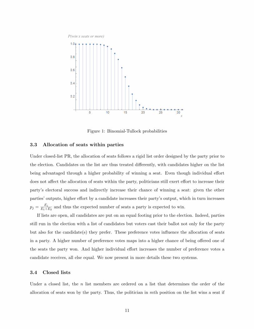
To illustrate this, figure 1 plots the probability that a party wins x seats or more in the symmetric
equilibrium in which each party expects to win half the seats (we set n = 31; this curve is just the
opposite of the CDF of our binomial-Tullock). As the figure shows, it is very likely that a party
wins the first few seats, but it is increasingly unlikely that a party wins a substantial majority of
seats, let alone the whole legislature. The inverted S-shape generated by the binomial distribution
is in line with the empirical distribution of seats won by a party, as documented by Buisseret et al.
(2018) in their analysis of party nomination strategies in Sweden (see their figure 1).
11In section 6, we generalise the formula for pj to allow for aggregate noise or different mappings from a party’s
electoral output to the number of seats it wins. Our results are not affected by these alternative specifications.
10
x
P(win x seats or more)
Figure 1: Binomial-Tullock probabilities
3.3 Allocation of seats within parties
Under closed-list PR, the allocation of seats follows a rigid list order designed by the party prior to
the election. Candidates on the list are thus treated differently, with candidates higher on the list
being advantaged through a higher probability of winning a seat. Even though individual effort
does not affect the allocation of seats within the party, politicians still exert effort to increase their
party’s electoral success and indirectly increase their chance of winning a seat: given the other
parties’ outputs, higher effort by a candidate increases their party’s output, which in turn increases
pj =Ej
E1+E2and thus the expected number of seats a party is expected to win.
If lists are open, all candidates are put on an equal footing prior to the election. Indeed, parties
still run in the election with a list of candidates but voters cast their ballot not only for the party
but also for the candidate(s) they prefer. These preference votes influence the allocation of seats
in a party. A higher number of preference votes maps into a higher chance of being offered one of
the seats the party won. And higher individual effort increases the number of preference votes a
candidate receives, all else equal. We now present in more details these two systems.
3.4 Closed lists
Under a closed list, the n list members are ordered on a list that determines the order of the
allocation of seats won by the party. Thus, the politician in mth position on the list wins a seat if
11
their party wins at least m seats. List member in mth position on the list of party j solves:
Maxemj
(V
n∑k=m
Pj(k)−eβmjβ
)(4)
Notice that the summation goes from m to n and not from 1 to n, as the list member in the
mth position on the list only gets a seat when his party wins at least m seats.
3.5 Open lists
Under an open list, like under a closed list, voters decide to vote for one of the two parties as a
function of electoral outputs E1 and E2. On top of this, voters decide to cast their ballot for a
specific candidate of the party they wish to support on the basis of the effort choices of that party’s
candidates. That is, within each party, the seats a party won are attributed on the basis of the
preference votes each of the candidates received. We model this competition for seats within a party
as a contest between n candidates for m ≤ n prizes of value V . To do this, we adapt the model of
Clark and Riis (1996) to our setting. Denote with ei the effort of politician i. The probability that
i ends up among the m candidates with the highest number of preference votes, and thus among
the m first candidates to be attributed a seat by their party, is given by:
Qi(m) = q1 +
m∑j=2
qj
(j−1∏s=1
(1− qs)
), (5)
where qj is the probability that i ends up on position m on the list. This probability is given
by a standard Tullock ratio contest success function based on individual effort choices among the
candidates who have not yet been given a seat:
qj =eri
eri +∑
k 6=i erk
,#k = n−m. (6)
One can interpret (5) as the result of a sequential process. The contestants make one contribu-
tion that is valid for the entire intraparty sequential contest. The winner of the first prize is decided
using the Tullock contest function with the contributions of all the n contestants. The winner and
his contribution are then erased and the winner of the second seat the party won is decided using
the Tullock contest function with the contributions of the remaining n−1 contestants. This process
continues until all seats a party won have been awarded.
In (6), r parametrizes the noise in the preference voting mapping. In the limit, when r = 0,
noise determines the intraparty outcome fully, for example because voters do not have (enough)
12

information about the choices of individual candidates to cast an informed vote and thus simply
randomize across all candidates. In such case, all candidates have the same probability of winning a
legislative seat. Then Qi(k) = k/n, ∀i. The intraparty seat allocation rule becomes fully egalitarian:
it treats all party candidates equally. We label this case the egalitarian rule.12
Overall, candidate i in party j chooses eij to maximize:
Vn∑
m=1
Pj(m)Qi(m)−eβijβ, (7)
where Qi(m) = q1 +∑m
j=2 qj
(∏j−1s=1(1− qs)
)and Pj(m) = CnmP
mj (1− Pj)n−m.
Under the egalitarian rule, when r = 0, for any number of seats k a party won, all politicians of
that party have the same probability k/n of winning a seat. Then, politician i in team j chooses
his level of effort to solve:
Maxeij
(V
n∑k=1
Pj(k)k
n−eβijβ
)(8)
4 Equilibrium efforts
4.1 Closed lists
Each candidate maximizes their objective function, equation (4), with respect to their individual
effort choice. Even though this problem is individual-specific as it depends on the position on the
list a candidate is in, the equilibrium is symmetric across parties. We then have:
Proposition 1 Under the closed-list, in a symmetric Nash equilibrium, a party’s electoral output
E∗CL is given by:
E∗CL =
n∑k=1
(kCnk
(1
2
)n−1) 1−σ
β+σ−1
β+σ−1β(1−σ) (
V
4
) 1β
(9)
Individual effort e∗m of list member in mth position is given by:
e∗m =
V(mCnm
(12
)n+1) ββ+σ−1
∑nk=1
(kCnk
(12
)n+1) 1−σβ+σ−1
1/β
(10)
Proof. See appendix.
12We are thankful to an anonymous referee for suggesting this interpretation of the egalitarian rule.
13

Given that the distribution of mCnm is symmetric and unimodal at the median value of m,
individual effort is bell-shaped with the candidate in the median list position exerting the highest
amount of effort. Figure 2 illustrates this finding. This property of the distribution of efforts within
parties turns out to be crucial for our result.
5 10 15 20 25 30List position
0.05
0.10
0.15
0.20
0.25
0.30
0.35
effort
Figure 2: Distribution of efforts under closed-list PR
4.2 Open lists
With open lists, the game is completely symmetric: all candidates maximize the same objective
function (7). We then have:
Proposition 2 Under the open-list, in a symmetric Nash equilibrium, a party’s electoral output
E∗OL is given by:
E∗OL = n1
1−σ
V4n
+ rVn∑
m=1
Cnm
(1
2
)n (1− m
n
) m∑j=1
1
n− j + 1
1/β
(11)
Individual effort e∗OL is given by:
e∗OL =
V4n
+ rVn∑
m=1
Cnm
(1
2
)n (1− m
n
) m∑j=1
1
n− j + 1
1/β
(12)
Proof. See appendix.
The first term within the square brackets corresponds to the incentives to work for the party to
increase the number of seats won, the second term corresponds to the incentives to get preferences
votes to improve one’s position on the list. As r goes to 0, the second term vanishes and effort
14
converges to the effort under the egalitarian allocation rule, namely(V4n
)1/β. Individual effort
increases in the value of a seat V and decreases with the number of available seats n, while a
party’s electoral output increases in both V and n.
4.3 Comparing closed lists and open lists
4.4 Effort comparison
The two systems differ in two main dimensions. The first difference comes from preference votes.
With open lists, individual effort influences both the party’s electoral success and the candidate’s
intraparty ranking (in terms of preference votes). Competing for preference votes within one’s
party is a source of incentives that does not exist with closed lists.
The second difference comes for the homogeneity (or heterogeneity) of incentives. With open
lists, all politicians face the same incentives and exert the same effort in equilibrium. With closed
lists, incentives and individual equilibrium efforts vary with a candidate’s position on the list. In
particular, the politicians located around the median position face the largest marginal benefit of
effort. To the contrary, candidates at the top and at the bottom of the list have little incentive to
exert effort.
The received wisdom in the political economy and political science literature typically views
open lists as superior to closed lists. That is mainly because preference votes under open lists
mitigate the free-riding issue. The heterogeneity of incentives also creates very weak incentives for
many candidates on the list (those near the top and near the bottom). However, if incentives are
indeed weak at the top and bottom of the list, they are much stronger for politicians in the middle
of the list.
To compare the parties’ electoral outputs under the two ballot structures, we first shut down
preference votes – setting r to zero under open lists – and compare a closed list to the egalitarian
rule. The comparison boils down to the effect of the heterogeneity of incentives on party output.
We show that the convexity of the cost function (β) and the degree of complementarity (σ), play
a central role. When the cost of effort is not too convex and efforts are not strong complements,
heterogeneous incentives lead to higher party output, and a closed list dominates the egalitarian
rule. By continuity, when voters are not too well informed about the individual efforts of candidates
(r is close enough to 0), closed lists lead to higher party outputs than open lists. We summarize
our findings in the following proposition.
15

Theorem 3 Closed lists lead to higher party output than open lists PR, E∗CL ≥ E∗OL when β ≤
2− 2σ and r is small enough. Open lists lead to higher party output than closed lists, E∗OL ≥ E∗CLwhen β ≥ 2− 2σ or when β ≤ 2− 2σ and r is large enough. The two types of ballot yield the same
party’s output E∗OL = E∗CL when β = 2− 2σ and r = 0.
Proof. See appendix.
The intuition behind this result is as follows. As we saw above, individual incentives are uniform
under the egalitarian rule and bell-shaped under closed lists. Suppose that the cost of effort function
is close to being linear (β is close to 1). If individual efforts are highly substitutable (σ close to
0), electoral output is close to equal to the sum of efforts, and this sum is what matters, not so
much the level of the different individual efforts. In this case, inducing differences in efforts can be
optimal. When efforts are complementary (σ > 1/2), inducing differences in individual efforts is
suboptimal as a party’s electoral output depends more heavily on the lowest effort decisions. What
about the convexity of the cost of effort function? Suppose for simplicity that σ = 0. When this
function is very convex (β > 2), the marginal cost is also convex. Then, asymmetric incentives are
bad for party performance. Indeed, starting from equal marginal benefits of effort, increasing the
marginal benefit of one politician and decreasing the benefit of another will have a positive effect
if the marginal cost increases more slowly for the individual with stronger incentives than for the
one with weaker incentives. However, when the marginal cost of effort is convex, this is simply not
possible.
For an example on low complementarity between party candidates, consider an election centered
around a ‘standard’ electoral issue. Then candidates expose and defend the ‘conventional’ party
line that was crafted by the party specialists who worked on the issue. Once the party platform
is finalized, most other candidates can simply stand behind their party’s official position. To the
contrary, if the central electoral issue requires parties to make use of a portfolio of skills and
competencies to develop their platform, then the efforts put in by their candidates become much
more complementary to each other, as the decision to put low effort into the contest by a single
candidate can ‘destroy’ all the efforts of their party fellows.
An increase in r increases the incentives to exert effort under an open list but not under a closed
list. When preference votes are very responsive to individual effort, exerting effort is less about
contributing to the public good and more about the individual benefit of improving one’s rank in
the allocation of seats. In what follows, we set r to zero and focus on the comparison between a
closed list system and the egalitarian rule.
16
4.5 Choice of electoral system
The design of better electoral systems is at the center of the public debate. Many countries,
including France, have thought about moving towards PR but agreement over which type of PR
to adopt is more difficult. Theorem 3 has direct implications in terms of constitutional design.
A benevolent constitution would pick the optimal electoral system in terms of society welfare. In
the model, candidates’ effort and electoral output are interpreted as a means towards improving
the quality of the party’s political platform. Effort benefits voters and a good electoral system is
a system that maximizes the party’s electoral outputs. In that case, the conditions of theorem 3
should guide the design of the optimal system. If voters are well informed about candidates efforts,
then an open-list system could be superior to a closed list system. If voters are poorly informed
about politicians’ effort, an open-list system loses its main advantage. In that case, the convexity
of the effort case and the complementarity of candidates effort become the driving forces behind
the choice of which electoral system to adopt.
In the model, effort by candidates is not only effort spent to mobilize and attract voters around
the party platform during the campaign. Effort also helps to create an appropriate and high quality
party platform. Even with closed lists, party candidates have several months between the moment
the list is announced and the election. This gives them time to improve the electoral platform that
they will defend during the campaign in the weeks before election day. For example, in Belgium,
the names of the leading candidates of all mainstream parties were announced around Christmas
2018, for the May 2019 legislative elections (together with those for the European Parliament).
This is roughly 5-6 months ahead of election day. Once parties announced their leading candidates,
these moved immediately to the preparation of their party programme, which they release a few
weeks before election day. All the leading figures of the party help craft the programme, with a
special role for the leading candidate’s garde rapprochee, a set of politicians who typically ends
up in the leading positions of the party list (within party list turnover between elections is quite
high, especially when there is a change of leadership). In this preparation phase, intraparty work
to craft and finalize the party programme is at its peak. Nevertheless, if we were to interpret effort
as advertising resources spent during the campaign to convince voters but that are not welfare
enhancing in and by themselves, the constitution should then aim at minimizing such efforts. In
that case, the condition of theorem 3 would still apply but its implications in terms of choice of
electoral system would have to be reversed.
17

If it is natural to consider the choice between closed-list and open-list at the level of constitu-
tional design, the party leadership also has its say in practice. A striking example is Colombia.
After a reform in 2003, each party can present and chose the type of ballot to use in any district:
parties can opt for closed or open lists, and the choice can differ across districts; see Shugart,
Moreno and Fajardo (2006) and Hangartner, Ruiz and Tukiainen (2018) for more on this case.
Less extreme examples can be found in many countries in which parties adopt strategies and
practices that appear to be a strategic reaction to some aspects of the electoral environment they
are embedded in. For instance, Italy before the Mani Pulite scandal of 1992 was officially using
open-list PR.13 However, in practice, many parties were using methods resembling a closed-list
system. Katz (1985) argues that the Communist party was closely controlling the list of candidates
and would give instructions to their partisans about preference votes. The final outcome would look
like that under a closed list, as the party decided the ranking of candidates and voters implemented
it.
The opposite situation also happens in countries with a closed-list system. Some parties organize
primary elections to decide the names and positions of list candidates. Even if the set of voters in
the primary and in the general election is not exactly the same, organizing a primary clearly shifts
a closed-list system towards an open-list system. For instance, in the last Israeli elections, several
parties, including Likud, Labor, the Jewish Home, and Meretz had systems in which the leadership
and most candidates on their lists were first elected in primary elections. Similarly, some small
Turkish parties use primary elections to set up their list of candidates.
To study such strategies, we add a stage to the model. In stage one, the party leadership chooses
between the egalitarian rule (open list with no preference votes) and a closed list. In the second
stage, after observing the choice of both parties, candidates choose how much effort to exert. In the
appendix, we solve for equilibrium efforts in the subgame in which parties choose different rules.
We show that a party’s electoral success follows the same condition as that of Theorem 3. This
means that in the subgame perfect equilibrium of the two-stage game, the condition driving the
parties’ choice of the allocation rule is the same as in Theorem 3.
Proposition 4 In the subgame perfect equilibrium of the two-stage game, parties choose a closed
list if β ≤ 2− 2σ and the egalitarian rule if β ≥ 2− 2σ.
13Between 1946 and 1993, parties stood in front of voters with lists of candidates in each of Italy’s 32 constituencies.
Voters could give as many as four preference votes to the candidates of their favorite party. Seats won by a party
went to the candidates with the highest number of preference votes.
18
Proof. See appendix.
Thus, for given values of β and σ, parties have a dominant strategy (strictly dominant when
β 6= 2−2σ) in the choice of allocation rule. Note that this proposition does not require that parties
have the same values of parameters β and σ. As the proof makes apparent, the choice of system
that maximizes effort does not depend on the output of the other party.
To wrap up, theorem 3 and proposition 4 show that the convexity of the marginal cost of effort,
the complementarity of the team production function and the noisiness of the election drive the
choice of the allocation rule. The noisiness of the election plays a very intuitive role. When the
marginal cost of effort is convex, giving powerful incentives to a few individuals is not productive,
as even these individuals are not going to exert much effort. With convex marginal costs, it is
thus more efficient to give all politicians within a party the same incentives and treat them in an
equal, symmetric way. When the marginal cost is not too convex or even concave, it is efficient to
provide powerful incentives to few individuals who will exert very high levels of effort. The degree
of complementarity plays a similar role. When efforts are substitutes, there is no cost in generating
very different effort levels within the team. When efforts are complementary, it is better to induce
similar effort levels, so that the egalitarian rule is optimal.
The above findings suggest that when efforts are not strong complements within each party
and/or the individual cost of effort is not too convex, the use of closed lists can be optimal.
In particular, it gives better incentives than a system which treats all candidates in an ex-ante
fair and egalitarian way. Thus, theorem 3 and proposition 4 provide an argument for the use of
closed lists PR. In the next section, we go further and show that closed lists and the egalitarian
rule are actually the two incentive mechanisms that maximize party outputs if we impose a weak
monotonicity constraint.
5 Mechanism design
For simplicity, we assume in this section that efforts are perfect substitutes, σ = 0.14 An allocation
rule can be represented as a n ∗ (n + 1) matrix of weights [λik]. Entry λik corresponds to the
probability that politician i gets a seat when his party has won k seats. Probabilities need to be
between 0 and 1, and the number of seats distributed cannot be larger than the number of seats
14The results also hold for σ > 0, but the algebra is cumbersome. The condition for proposition 4 would then be
in terms of β − 2σ (as in theorem 3).
19

won by the party. These feasibility constraints thus require 0 ≤ λik ≤ 1 and∑n
i=1 λik = k. We
focus on monotonic rules. Under a monotonic rule, the probability that a candidate wins a seat is
(weakly) increasing in the number of seats won by their party, that is λik ≤ λik+1 for any i and k.
The egalitarian allocation rule can be represented as a matrix in which each column has equal
entries λik = k/n. The closed-list can be represented as a matrix with λik = 0 if i > k and λik = 1
if i ≤ k.
Proposition 5 When β > 2, the egalitarian rule maximizes party output among all monotonic
rules. When β < 2, closed lists maximize party outputs. When β = 2, both rules maximize party
outputs.
Proof. See appendix.
The intuition behind the result is simple. The intraparty prize allocation rule determines
individual incentives and thus effort choices. When β > 2, it is optimal to equalize incentives
across politicians within a party, while when β < 2, it is optimal to make incentives as strong as
possible for some politicians. The maximization problem is similar to that of the optimal allocation
of risk. With risk-averse individuals, the allocation is as egalitarian as possible, while with risk-
loving agents, it is optimal to make the allocation as unequal as possible.
If we remove the monotonicity constraint, an allocation rule can give negative incentives to
some politicians. Negative incentives appear when an individual faces a higher probability of
getting a seat when his team gets fewer seats. Yet, the effect of these negative incentives is
limited, as effort cannot be negative. Also, negative incentives free up incentive tokens that can
be redistributed to other politicians. The combination of the zero lower bound on effort and the
possibility of redistributing incentives may then generate a higher electoral output than under the
optimal monotonic rule.
We illustrate in the appendix how this redistribution of incentives can indeed generate higher
electoral output with two examples. As the optimal rule can be non-monotonic, the politicians’
labels should no longer be given any ranking interpretation. Indeed, a politician with a lower rank
is not necessarily treated more favorably by a non-monotonic rule. In the context of elections, these
non-monotonic rules are more of a theoretical curiosity than a realistic mechanism. However, in
other contexts where team contests for multiple prizes exist, using non-monotonic incentive schemes
could be of interest.
20
6 Extensions and robustness checks
6.1 More than two parties, ideology, and noise
We now extend our model in some important directions. All formal derivations can be found
in Appendix B. We first allow for K > 2 parties as it is common to see more than two parties
competing in elections under PR. With more than two parties, the distribution of efforts under
closed lists becomes right-skewed. Indeed, in a symmetric equilibrium, each politician expects his
party to win n/K prizes. Thus, depending on the number of parties, the relevant median list
member, who exerts highest effort, is around position n/K on the party list. With two parties, the
member exerting highest effort was in the middle of the list.
Second, we extend the model to allow for biased contests. In real world elections, some parties
enjoy an ex-ante ideological advantage over their competitors. We can view such an advantage as a
bias in favour of one of the parties in the contest. Suppose party 1 is advantaged over party 2. We
assume that the probability that party 1 wins a seat given outputs E1 and E2 as λE1/ (λE1 + E2)
with λ > 1. The distribution of seats is now given by:
P1(k) = Cnk
(λE1
λE1+E2
)k (1− λE1
λE1+E2
)n−k.
Finally, we can useEγi
Eγ1 +Eγ2or γ
2 + (1 − γ) EiE1+E2
as the probability that a party wins a given
seat, where γ parametrises the responsiveness of success to effort.
These three extensions do not affect our main result and Theorem 3 still applies in those cases.
6.2 Access to government and internal party struggles
Politicians care not only about getting a seat (as we assumed so far) but also want their party to
win a majority of seats to gain control of the executive office. Assume that candidates enjoy an
additional payoff M when their party gets at least a majority of the legislative seats.
Under the egalitarian rule, candidates choose their effort to maximise:
Vn∑k=1
Pj(k)k
n+M
n∑k=n+1
2
Pj(k)− eβ
β
where∑n
k=n+12Pj(k) is the probability that the candidate’s party wins at least a majority of the
seats.
21

With a closed list, the candidate in position m on the list of party j chooses em to maximize:
Vn∑
k=m
Pj(k) +Mn∑
k=n+12
Pj(k)− eβmβ
In the appendix, we solve for the equilibrium efforts and show that theorem 3 goes through un-
changed.
We can also consider the case in which candidates have to compete within their party to secure
(some of) the benefits of their party winning control of the executive (in the spirit of Katz and
Tokatlidu, 1996).15 We do not need to model explicitly this post-election contest. From an ex-ante
perspective, internal struggles decrease the value of winning the executive office, as this ex-post
contest leads to rent dissipation. If we parametrize rent dissipation by some parameter λ < 1 the
benefits of winning office are now given by λM . The more costly this struggle is, the lower value
of λ, the less value candidates attach to their party winning a majority of seats. In the limit, the
prospect of such an intraparty struggle can totally nullify the incentive benefits of the presence of
the executive office. If the intensity of the post-election struggles does not depend on the ballot
structure (λ is the same with open lists and closed lists), then the comparison between the ballot
structures of theorem 3 remains valid. The intensity of the post-election struggles could also change
with the ballot structure. However, it is not clear which system leads to more rent dissipation. If
the closed list clearly identifies the candidates in line for the top executive positions, an open list
system could also give legitimacy to candidates that gathered the most preference votes.
6.3 Contractible efforts
We now allow parties to make the allocation of seats directly depend on the efforts of the candidates.
When efforts are contractible, allocation rules can rely not only on the incentives generated by the
number of prizes won by the party, but also directly on the effort exerted by each candidates. Under
the egalitarian rule, the contract between the party and each candidate specifies that, provided the
candidate exerts at least e∗ (that is pinned down by a candidate’s participation constraint), his
chance of getting one of the m seats won by the party is equal to m over the number of candidates
who honored their party contract. In equilibrium, this chance is thus m/n. Any deviation below
e∗ makes that probability go to zero.
Under the closed list, the contract still assigns to each politician a rank in the list, but now also
specifies a minimal effort level associated with each rank. If a politician exerts the specified effort
15We are grateful to the Editor for suggesting this extension.
22
(or more), they get a seat if the party wins a number of seats equal to at least their rank. If they
exert less effort or if the party wins fewer seats than their rank, they get no seat.16 Then, we have:
Proposition 6 When efforts are contractible, the egalitarian allocation rule leads to higher elec-
toral output than the closed-list for all values of parameters β and σ. Thus open lists dominate
closed lists for any value of r ≥ 0.
Proof. See appendix.
When efforts are observable and contractible, the level of effort is determined by the partici-
pation constraint. The contract imposes an effort level that drives each politician’s utility to their
outside option. The cost of effort enters directly in the participation constraint, whereas when
effort is not contractible, the marginal cost is what matters. Comparing electoral outputs across
the two rules, we find that the egalitarian rule generates higher output than the closed list when
β ≥ 1 − σ, which is always satisfied. Thus, with contractible effort, it is always optimal to treat
all politicians equally. This last finding suggests that the imperfect contractibility of effort is a
necessary condition for the optimality of closed lists.
Whereas the extent to which parties (and voters) are informed about the decisions of politicians
is an empirical question, it seems natural to assume that reality is in between the two extremes of
perfectly observable and perfectly unobservable efforts.
7 Conclusion
We studied the incentive effects of the two main ballot structures in proportional representation
elections: open and closed lists. We showed that the amount of information voters have about
candidate choices, the convexity of the marginal cost of effort and the degree of complementarity
between efforts within parties drive which ballot structure is best for incentives. Voters’ information
about candidates’ effort increases the responsiveness of preference votes to effort and favors the open
list system. A convex marginal cost of effort and the presence of complementarity in candidates’
efforts makes homogeneous incentives more effective than heterogeneous ones. In that case, an
open list dominates a closed one, even when voters are poorly informed. When the cost of effort is
not too convex, efforts are substitutes and voters are poorly informed, a closed list may dominate
an open one.
16For the contract to be credible, the part must have a list of at least n+1 candidates, with these extra candidates
only winnning a seat if some of the other candidates did not exert the required effort.
23

Our model is tractable and is amenable to many extensions and applications. For instance,
Crutzen and Sahuguet (2018) adapt the present set-up to compare politicians’ effort under majori-
tarian and proportional electoral systems (in particular British-style first-past-the-post and Israeli-
style closed-list PR) when political parties play an active role in the selection of their candidates.
They find that the received wisdom that suggests that majoritarian systems provide incentives more
efficiently than PR may need revisiting when parties are active players in the selection process.
The main limitation of the current paper is the symmetry imposed in the model. Politicians
have the same effort productivity (or cost of effort), and candidates are competing for prizes of
identical value (a seat in parliament). Konishi, Sahuguet, Crutzen and Flamand (2018) extend
the present model to allow for candidates with heterogeneous abilities and allow for additional
payoffs linked to minister positions. The paper then studies how parties should constitute their
lists and where on the list they should put their most able candidates. Another important puzzle
they address is: why are a party’s lead candidates teaming up with the other candidates on the
electoral list when it is anyway common knowledge that most of these candidates will take on jobs
and positions after the election that are not compatible with them sitting in parliament?
Finally, if our model is well suited for the analysis of elections under PR, it could also be
used in other contexts where contests between teams that allocate multiple indivisible prizes are
important. For instance, our model delivers stark predictions that could be empirically tested
in the context of the internal organization of firms. In some industries, complementarity among
workers are much more important than in others. In such sectors, compensation contracts should
treat workers more equally than in other sectors. Some public finance problems, especially in
federal democracies, can also be modelled as team contests for multiple indivisible prizes. Examples
include the construction of schools, hospitals and military bases for which several local governments
(municipalities) belonging to larger subnational entities (regions, states) may compete.
References
1. Ames, Barry (1995a). ”Electoral strategy under open-list proportional representation.” Amer-
ican Journal of Political Science, 406-433.
2. Ames, Barry (1995b). ”Electoral rules, constituency pressures, and pork barrel: bases of
voting in the Brazilian Congress.” The Journal of Politics, 57(2), 324-343.
3. Ames, Barry. The deadlock of democracy in Brazil. University of Michigan Press, 2002.
24

4. Baik, Kyung H. and Sanghack Lee (2001). “Strategic groups and rent dissipation,” Economic
Inquiry, 39, 672-684.
5. Baik, Kyung H. and Dongryul Lee (2012). “Do Rent-Seeking Groups Announce Their Sharing
Rules?,” Economic Inquiry, 50 (2), 348-363.
6. Balart, Pau, Subashish M. Chowdhury and Orestis Troumpounis (2015). “Linking individual
and collective contests through noise level and sharing rules,” Economics Letters, 155, 126-
130.
7. Balart, Pau, Sabine Flamand and Orestis Troumpounis (2016). “Strategic choice of sharing
rules in collective contests,” Social Choice and Welfare, 46(2), 239-62.
8. Barbieri Stefano and David Malueg (2016). “Private information group contests: best-shot
competition,” Games and Economic Behavior, 98, 219-234.
9. Barbieri Stefano, David Malueg and Iryna Topolyan (2014). “The best-shot all-pay (group)
auction with complete information,” Economic Theory, 57, 603-640.
10. Bose, Arup, Debashis Pal and David EM Sappington (2010). “Asymmetric treatment of
identical agents in teams,” European Economic Review, 54, 947-961.
11. Bowler, Shaun, and David M. Farrell, (2011). ”Electoral institutions and campaigning in
comparative perspective: Electioneering in European Parliament elections.” European Journal
of Political Research, 50(5), 668-688.
12. Buisseret, Peter and Carlo Prato (2018a). “Competing Principals? Legislative Representation
in List PR Systems,” mimeo University of Chicago Harris School of Public Policy.
13. Buisseret, Peter and Carlo Prato (2018b). “Electoral Accountability in Multi-Member Dis-
tricts,” mimeo University of Chicago Harris School of Public Policy.
14. Buisseret, Peter, Olle Folke, Carlo Prato and Johanna Rickne (2018). “Party Nomination
Strategies in Closed and Flexible List PR,” mimeo University of Chicago Harris School of
Public Policy.
15. Bose, Arup, Debashis Pal, and David E M Sappington. ”Equal pay for unequal work: Limiting
sabotage in teams.” Journal of Economics & Management Strategy, 19.1 (2010): 25-53.
25

16. Caillaud, Bernard and Tirole, Jean. 2002. “Parties as Political Intermediaries”. The Quar-
terly Journal of Economics 117: 1453-1489.
17. Carey, John M. (2009) Legislative Voting and Accountability. Cambridge University Press.
18. Carey, John M., and Simon Hix (2011). ”The electoral sweet spot: Low-magnitude propor-
tional electoral systems.” American Journal of Political Science, 55(2), 383-397.
19. Carey, John M., and Matthew S. Shugart (1995). “Incentives to Cultivate a Personal Vote:
A Rank Ordering of Electoral Formulas,” Electoral Studies 14: 417-439.
20. Castanheira, Micael, Crutzen, Benoit S Y, and Nicolas Sahuguet (2010). ”Party organization
and electoral competition.” The Journal of Law, Economics, and Organization 26(2), 212-242.
21. Clark, Derek and Christian Riis (1996). “A multi-winner nested rent-seeking contest,” Public
Choice, 87, 177-184.
22. Chang, Eric CC and Miriam A. Golden (2007). “Electoral systems, district magnitude and
corruption,” British Journal of Political Science, 37(1), 115-137.
23. Corchon, Luis (2007). “The theory of contests: a survey,” Review of Economic Design, 11,
69-100.
24. Crisp, Brian F., Maria C. Escobar-Lemmon, Bradford S. Jones, Mark P. Jones, and Michelle
M. Taylor-Robinson, (2004). ”Vote-seeking incentives and legislative representation in six
presidential democracies.” The Journal of Politics, 66(3), 823-846.
25. Cruz Cesi, Philip Keefer and Carlos Scartascini (2018). The Database of Political Institutions
2017 (DPI2017)
26. Crutzen, Benoit S. Y. and Nicolas Sahuguet (2018). “Electoral incentives: the interaction
between candidate selection and electoral rules,” Erasmus School of Economics, Erasmus
Universiteit Rotterdam.
27. Downs, Anthony (1957). An Economic Theory of Democracy. Pearson Ed.
28. Enelow, James M. and Melvin J. Hinich (1982). “Ideology, issues and the spatial theory of
elections,” American Political Science Review, 76, 493-501.
26
29. Eliaz, Kfir and Qinggong Wu (2018). “A simple model of Competition between teams,”
Journal of Economic Theory, 176, 372-392.
30. Esteban, Joan and Debraj Ray (2001). “Collective action and the group size paradox,”
American Political Science Review, 95, 663-672.
31. Ferraz, Claudio, and Frederico Finan (2008). ”Exposing corrupt politicians: the effects of
Brazil’s publicly released audits on electoral outcomes.” The Quarterly Journal of Economics
123(2), 703-745.
32. Flamand, Sabine and Orestis Troumpounis (2015). “Prize-sharing rules in collective rent
seeking,” in Companion to the Political Economy of Rent Seeking, ed. by R. D. Congleton
and A. L. Hillman, Edward Elgar Publishing, 92-112.
33. Fu, Qiang, Jingfeng Lu and Yue Pan (2015). “Team contests with mutiple pariwise battles.”
American Economic Review, 105, 2120-40.
34. Galasso, Vincenzo and Tommaso Nannicini (2015). “So closed: Political selection in propor-
tional systems,” European Journal of Political Economy, 40, 260-273.
35. Golden, Miriam A., and Eric CC Chang (2001). ”Competitive corruption: Factional conflict
and political malfeasance in postwar Italian Christian Democracy.” World Politics 53(4),
588-622.
36. Hangartner, Dominik, Nelson A. Ruiz, and Janne Tukiainen (2018). ”Open or closed: How
List Type Affects Electoral Performance,Candidate Selection, and Campaign Effort,” working
paper.
37. Heitshusen, Valerie, Garry Young, and David M. Wood (2005). ”Electoral Context and MP
Constituency Focus in Australia, Canada, Ireland, New Zealand, and the United Kingdom.”
American Journal of Political Science, 49(1), 32-45.
38. Hobolt, Sara Binzer, and Jill Wittrock (2011). ”The second-order election model revisited:
An experimental test of vote choices in European Parliament elections.” Electoral Studies,
30(1), 29-40.
39. Katz Richard (1985). ”Preference voting in Italy. Votes of opinion, belonging or exchange.”
Comparative Political Studies, 18(2), 229-249.
27

40. Konishi, Hideo, Sahuguet, Nicolas, Crutzen, Benoit S Y and Flamand, Sabine (2018). “Incen-
tivizing Team Production with Indivisible Prizes”, Erasmus School of Economics, Erasmus
Universiteit Rotterdam.
41. Konrad, Kai A. (2009). Strategy and Dynamics in Contests, Oxford UK: Oxford University
Press.
42. Kunicova, Jana, and Susan Rose-Ackerman (2005). “Electoral rules and constitutional struc-
tures as constraints on corruption,” British Journal of Political Science, 35(4), 573-606.
43. Lee, Sanghack (1995). “Endogenous sharing rules in collective-group rent-seeking,” Public
Choice, 85, 31-44.
44. Lindbeck, Assar and Jorgen W. Weibull (1987). “Balanced-budget redistribution as the
outcome of political competition,” Public Choice, 52(3), 273-297.
45. Lizzeri, A. and Persico, N., 2001. ”The provision of public goods under alternative electoral
incentives.” American Economic Review, pp.225-239.
46. Lizzeri, A. and Persico, N., 2005. ”A drawback of electoral competition.” Journal of the
European Economic Association, 3(6), pp.1318-1348.
47. Miller, George A(1956). ”The magical number seven, plus or minus two: Some limits on our
capacity for processing information.” Psychological review 63(2), 81-97.
48. Milesi-Ferretti, Gian Maria, Roberto Perotti, and Massimo Rostagno (2002). ”Electoral sys-
tems and public spending.” The Quarterly Journal of Economics, 117(2) 609-657.
49. Moldovanu Benny and Aner Sela (2001). “The Optimal Allocation of Prizes in Contests,”
American Economic Review, 91(3), 542-558.
50. Myerson, Roger B. (1993). “Incentives to Cultivate Favored Minorities Under Alternative
Electoral Systems,” American Political Science Review 87: 856-869.
51. Myerson, Roger B. (1999). “Theoretical comparisons of electoral systems,” European Eco-
nomic Review, 43(4), 671-697.
52. Nalebuff, Barry J. and Joseph E. Stiglitz (1983). “Prizes and incentives: towards a general
theory of compensation and competition,” The Bell Journal of Economics, 21-43.
28

53. Nitzan, Shmuel (1991). “Collective rent dissipation,” Economic Journal, 101, 1522-1534.
54. Nitzan, Shmuel and Kaoru Ueda (2011). “Prize sharing in collective contests,” European
Economic Review, 55, 678-687.
55. Olson, Mancur (1971). The logic of collective action. Public goods and the theory of groups.
2. print. ed., Cambridge, Mass.
56. Persson, Torsten and Guido Tabellini (1999), “The size and scope of government: Alfred
Marshall Lecture”, European Economic Review 43: 699-735.
57. Persson, Torsten and Guido Tabellini (2000). Political Economics: Explaining Economic
Policy. The MIT Press.
58. Persson, Torsten and Guido Tabellini (2003). The Economic Effect of Constitutions. The
MIT Press.
59. Persson, Torsten, Guido Tabellini and Francesco Trebbi (2003). “Electoral rules and Corrup-
tion,” The Journal of the European Economic Association, 1, 958-989.
60. Ray, Debraj, Jean-Marie Baland and Olivier Dagnelie (2007). “Inequality and inefficiency in
joint projects,” The Economic Journal, 117, 922-935.
61. Schleiter, Petra and Alisa M. Voznaya (2014). “Party system competitiveness and corrup-
tion,” Party Politics, 20(5),
62. Sieberer,Ulrich (2006) “Party unity in parliamentary democracies: A comparative analysis,”
The Journal of Legislative Studies 12: 150-178.
63. Sisak, Dana, (2009). “Multiple-prize contests: The optimal allocation of prizes,” Journal of
Economic Surveys, 23, 82-114.
64. Shugart, Matthew S., E. Moreno, and L. Fajardo (2006). Deepening democracy by renovating
political practices: The struggle for electoral reform in Colombia. unpublished paper presented
at the conference on “Democracy, human rights, and peace in Colombia”. The Kellogg
Institute, University of Notre Dame Unpublished manuscript.
65. Shugart, Matthew S., Valdini, Melody E. and Suominen, Kati (2005). “Looking for Locals:
Voter Information Demands and Personal Vote’s Earning Attributes of Legislators under
Proportional Representation,” American Journal of Political Science 49: 437-449.
29
66. Tavits, Margit (2007). “Clarity of responsibility and corruption,” American Journal of Po-
litical Science, 51(1), 218-229.
67. Tavits, Margit (2010). “Effect of Local Ties On Electoral Success and Parliamentary Be-
haviour: The Case of Estonia,” Party Politics, 16: 215a“235.
68. Tullock, Gordon (1980). “Efficient Rent Seeking,” in Toward a Theory of the Rent-Seeking
Society, ed. by J. M. Buchanan, R. D. Tollison, and G. Tullock, College Station, TX: Texas
A&M University Press, 97-112, reprinted in Roger D. Congleton, Arye L.
69. Ueda, Kaoru (2002). “Oligopolization in collective rent-seeking,” Social Choice and Welfare,
19, 613-626.
70. Vojnovic, Milan (2015). Contest Theory. Incentive Mechanisms and Ranking Methods. Cam-
bridge University Press.
71. Winter, Eyal (2004). “Incentives and Discrimination,” American Economic Review, 94, 764-
773.
72. Zittel, Thomas (2015). ”Constituency candidates in comparative perspective–How personal-
ized are constituency campaigns, why, and does it matter?.” Electoral Studies, 39, 286-294.
30

Appendix A (proofs)
Proof of proposition 1
We start by proving two useful lemmas.
Lemma 1:dEjdeij
=(Ejeij
)σProof:
Using the definition of Ej , Ej =(∑n
i=1 (eij)1−σ) 1
1−σ, we get:
dEjdeij
=1
1− σ(1− σ) (eij)
−σ
(n∑i=1
(eij)1−σ
) 11−σ−1
= (eij)−σ
(n∑i=1
(eij)1−σ
) σ1−σ
=
(Ejeij
)σ
e∗m =
(E∗
σ−1
CL mCnm
(1
2
)n+1
V
) 1β+σ−1
(13)
=
V∑nk=1
(kCnk
(12
)n+1) 1−σβ+σ−1
1/β (
mCnm
(1
2
)n+1) 1
β+σ−1
(14)
�
Lemma 2∑nk=mC
nk
(kpk−1 (1− p)n−k − (n− k) (1− p)n−k−1 pk
)= mCnmp
m−1 (1− p)n−m
Proof:
We show that terms in the sum cancel. Consider the second term within the summation
sign: (n− k)Cnk (1− p)n−k−1 pk. Using the identity (n− k)Cnk = (k + 1)Cnk+1 we can write it as
(n− k)Cnk (1− p)n−k−1 pk = (k + 1)Cnk+1 (1− p)n−k−1 pk, which corresponds exactly to the first
term within the summation sign for the index k + 1. These two terms cancel leaving only the first
and last term of the sum. The first term is mCnmpm−1 (1− p)n−m. The last term is equal to zero.
�
Under closed-list PR, the politician on the mth position on the list maximizes:
n∑k=m
Cnk
(Ej
E1 + E2
)k (1− Ej
E1 + E2
)n−kV −
eβmjβ
31

Denoting pj =Ej
E1+E2, the first-order condition is:
V
n∑k=m
dEjdeij
Ei
(E1 + E2)2Cnk
(k (pj)
k−1 (1− pj)n−k − (n− k) (pj)k (1− pj)n−k−1
)− (emj)
β−1 = 0
At a symmetric equilibrium, using Lemmas 1 and 2, the first-order condition simplifies to:
(E
em
)σ mECnm
(1
2
)n+1
V − eβ−1m = 0
Thus
(em)β+σ−1 = Eσ−1mCnm
(1
2
)n+1
V
⇐⇒
em =
(Eσ−1mCnm
(1
2
)n+1
V
) 1β+σ−1
A party’s electoral output is thus:
E =
n∑k=1
(Eσ−1kCnk
(1
2
)n+1
V
) 1−σβ+σ−1
1
1−σ
⇐⇒
Eβ
β+σ−1 =
n∑k=1
(kCnk
(1
2
)n+1
V
) 1−σβ+σ−1
1
1−σ
⇐⇒
E =
(V
4
) 1β
n∑k=1
(kCnk
(1
2
)n−1) 1−σ
β+σ−1
β+σ−1β(1−σ)
.
�
Proof of proposition 2
The first-order condition to the problem faced by candidate i (in party L, say) is:[n∑
m=1
∂PL(l)
∂eiQi(m) +
n∑m=1
PL(m)∂Qi(m)
∂ei
]V = eβ−1
i .
As all candidates face the same problem, the equilibrium is symmetric within and across parties.
As there are n candidates competing for one of the list slots, the equilibrium probability of being
32

offered slot m on the list is Q∗(m) = mn . We also have:
dPL(m)
dei=
(E1
ei
)σ E2
(E1 + E2)2Cnm (2m− n)
(1
2
)n−1
= nσ
1−σCnm4E
(2m− n)
(1
2
)n+1
Finally:dQi(m)
deiL=
r
e∗
(1− m
n
) m∑j=1
1
n− j + 1
and thus in the symmetric equilibrium, the FOC boils down to:
(e∗)β−1 = Vn∑
m=1
nσ/1−σCnm
n1/1−σe∗(2m− n)
(1
2
)n+1 m
n+ V r
n∑m=1
Cnm
(1
2
)n 1
e∗
(1− m
n
) m∑j=1
1
n− j + 1
=
V
n2
n∑m=1
Cnme∗
(2m− n)
(1
2
)n+1
m+ V r
n∑m=1
Cnm
(1
2
)n 1
e∗
(1− m
n
) m∑j=1
1
n− j + 1
Recall that (1 + x)n =
∑nm=0C
nmx
m
Taking the derivative with respect to x leads to
n(1 + x)n−1 =
n∑m=0
mCnmxm−1
and doing it again yields:
n (n− 1) (1 + x)n−2 =
n∑m=0
m (m− 1)Cnmxm−2
Setting x = 1, in these formulas yield:n∑
m=0
mCnm =
n∑m=1
mCnm = n2n−1
Similarly,n∑
m=0
m2Cnm =
n∑m=1
m2Cnm = n (n− 1) 2n−2 +
n∑m=1
mCnm
= n (n− 1) 2n−2 + n2n−1
=(n2 + n
)2n−2
Thus:n∑
m=1
Cnm(2m− n)
(1
2
)n+1
m =
(1
2
)n+1(
2n∑
m=1
m2Cnm − nn∑
m=1
mCnm
)
=
(1
2
)n+1 [2(n2 + n
)2n−2 − n22n−1
]=
n
4.
33
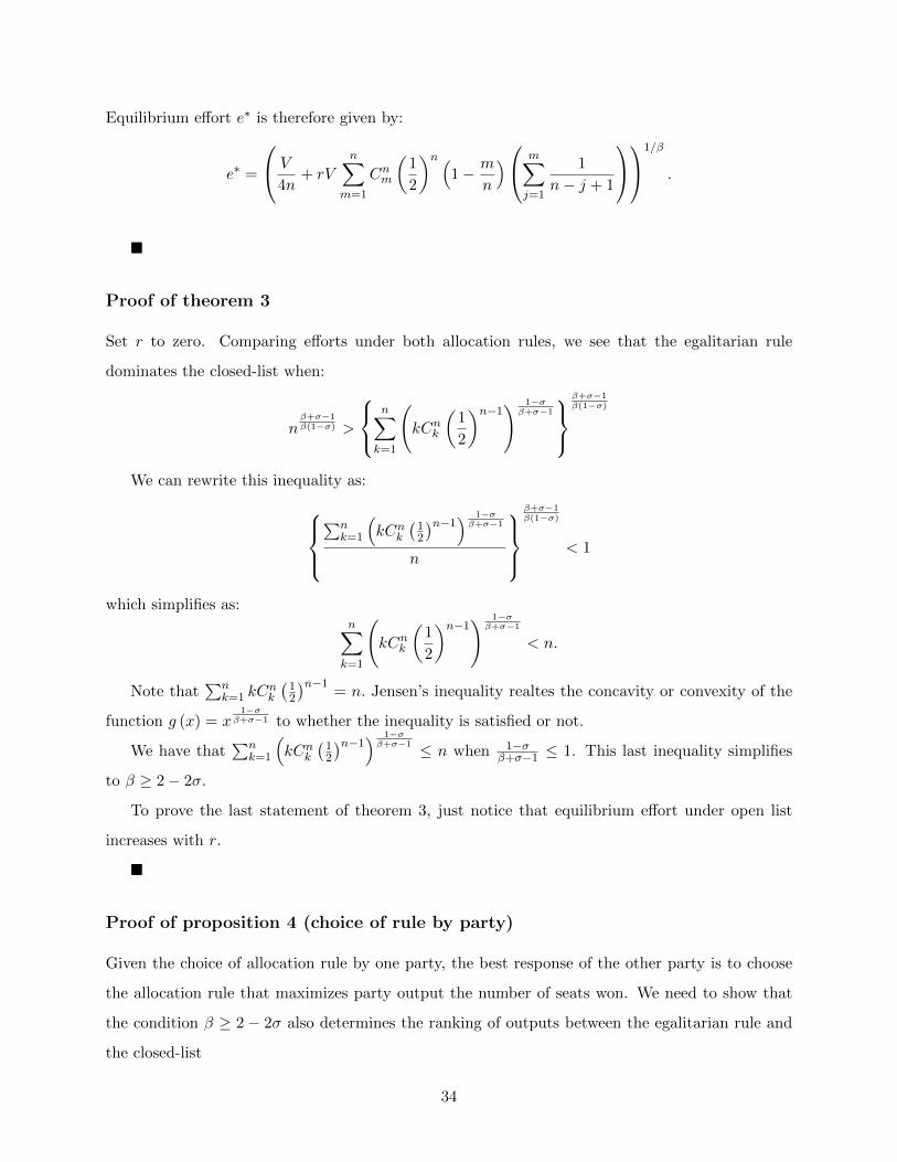
Equilibrium effort e∗ is therefore given by:
e∗ =
V
4n+ rV
n∑m=1
Cnm
(1
2
)n (1− m
n
) m∑j=1
1
n− j + 1
1/β
.
�
Proof of theorem 3
Set r to zero. Comparing efforts under both allocation rules, we see that the egalitarian rule
dominates the closed-list when:
nβ+σ−1β(1−σ) >
n∑k=1
(kCnk
(1
2
)n−1) 1−σ
β+σ−1
β+σ−1β(1−σ)
We can rewrite this inequality as:∑n
k=1
(kCnk
(12
)n−1) 1−σβ+σ−1
n
β+σ−1β(1−σ)
< 1
which simplifies as:n∑k=1
(kCnk
(1
2
)n−1) 1−σ
β+σ−1
< n.
Note that∑n
k=1 kCnk
(12
)n−1= n. Jensen’s inequality realtes the concavity or convexity of the
function g (x) = x1−σ
β+σ−1 to whether the inequality is satisfied or not.
We have that∑n
k=1
(kCnk
(12
)n−1) 1−σβ+σ−1 ≤ n when 1−σ
β+σ−1 ≤ 1. This last inequality simplifies
to β ≥ 2− 2σ.
To prove the last statement of theorem 3, just notice that equilibrium effort under open list
increases with r.
�
Proof of proposition 4 (choice of rule by party)
Given the choice of allocation rule by one party, the best response of the other party is to choose
the allocation rule that maximizes party output the number of seats won. We need to show that
the condition β ≥ 2− 2σ also determines the ranking of outputs between the egalitarian rule and
the closed-list
34
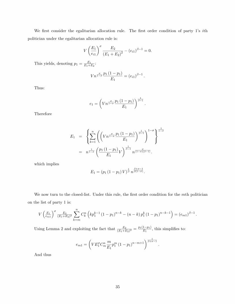
We first consider the egalitarian allocation rule. The first order condition of party 1’s ith
politician under the egalitarian allocation rule is:
V
(E1
ei1
)σ E2
(E1 + E2)2 − (ei1)β−1 = 0.
This yields, denoting p1 = E1E1+E2
:
V nσ
1−σp1 (1− p1)
E1= (ei1)β−1 .
Thus:
e1 =
(V n
σ1−σ
p1 (1− p1)
E1
) 1β−1
.
Therefore
E1 =
n∑k=1
((V n
σ1−σ
p1 (1− p1)
E1
) 1β−1
)1−σ
11−σ
= n1
1−σ
(p1 (1− p1)
E1V
) 1β−1
nσ
(1−σ)(β−1) .
which implies
E1 = (p1 (1− p1)V )1β n
β+σ−1β(1−σ) .
We now turn to the closed-list. Under this rule, the first order condition for the mth politician
on the list of party 1 is:
V(E1em1
)σE2
(E1+E2)2
n∑k=m
Cnk
(kpk−1
1 (1− p1)n−k − (n− k) pk1 (1− p1)n−k−1)
= (em1)β−1 .
Using Lemma 2 and exploiting the fact that E2(E1+E2)2
= p1(1−p1)E1
, this simplifies to:
em1 =
(V Eσ1C
nm
m
E1pm1 (1− p1)n−m+1
) 1β+σ−1
.
And thus
35

E1 =
n∑k=1
[(V Eσ1C
nk
k
E1pk1 (1− p1)n−k+1
) 1β+σ−1
]1−σ
11−σ
⇐⇒
Eβ
β+σ−1
1 =
{n∑k=1
(kCnk p
k1 (1− p1)n−k+1 V
) 1−σβ+σ−1
} 11−σ
⇐⇒
E1 =
{n∑k=1
(kCnk p
k−11 (1− p1)n−k
) 1−σβ+σ−1
} β+σ−1β(1−σ)
(p1 (1− p1)V )1β .
We need to compare the expected number of seats won under both allocation rules, given
the other party’s allocation rule. We know that if both parties choose the same allocation rule,
individual efforts are symmetric and thus party electoral outputs are equal and both parties win
on average n/2 seats. We therefore need to compare party electoral outputs when parties choose
different allocation rules.
From the calculation above, if party 1 uses the egalitarian rule and party 2 uses the closed-list,
denoting pj = E1/(Ej + E2), we get:
E1 = [p1 (1− p1)V ]1β n
β+σ−1β(1−σ) ,
E2 =
{n∑k=1
[kCnk p
k−12 (1− p2)n−k
] 1−σβ+σ−1
} β+σ−1β(1−σ)
[p2 (1− p2)V ]1β
Dividing the above two party outputs and exploiting the fact that p1 = 1 − p2 which implies
that (p1 (1− p1)V )1β = (p2 (1− p2)V )
1β , we get:
E2
E1=
∑n
k=1
[kCnk p
k−12 (1− p2)n−k
] 1−σβ+σ−1
n
β+σ−1β(1−σ)
.
We need to pin down the conditions such that E2E1
is greater or smaller than 1. Remark now that∑nk=1
(kCnk p
k−12 (1− p2)n−k
)= n. Then we use the argument based on Jensen’s inequality used
in the proof of Proposition 3 to show that the condition β > 2 − 2σ determines which party has
the highest output. This implies in turn that it is a dominant strategy for both parties to choose
the egalitarian allocation rule if and only if β > 2 − 2σ. If β = 2 − 2σ both rules yield the same
payoff. �
36
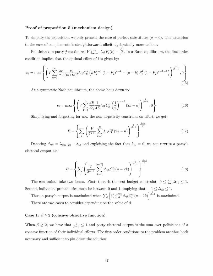
Proof of proposition 5 (mechanism design)
To simplify the exposition, we only present the case of perfect substitutes (σ = 0). The extension
to the case of complements is straightforward, albeit algebraically more tedious.
Politician i in party j maximizes V∑n
k=1 λikPj(k)− eβijβ . In a Nash equilibrium, the first order
condition implies that the optimal effort of i is given by:
ei = max
(V
n∑k=1
dEdeij
Ei(E1+E2)2
λikCnk
(kP k−1
j (1− Pj)n−k − (n− k)P kj (1− Pj)n−k−1)) 1
β−1
, 0
(15)
At a symmetric Nash equilibrium, the above boils down to:
ei = max
(V
n∑k=1
dE
dei
1
4EλikC
nk
(1
2
)n−1
(2k − n)
) 1β−1
, 0
(16)
Simplifying and forgetting for now the non-negativity constraint on effort, we get:
E =
∑i
(V
2n+1
n∑k=1
λikCnk (2k − n)
) 1β−1
β−1β
(17)
Denoting ∆ik = λi(n−k) − λik and exploiting the fact that λi0 = 0, we can rewrite a party’s
electoral output as:
E =
∑i
V
2n+1
bn/2c∑k=0
∆ikCnk (n− 2k)
1β−1
β−1β
(18)
The constraints take two forms. First, there is the seat budget constraint: 0 ≤∑
i ∆ik ≤ 1.
Second, individual probabilities must be between 0 and 1, implying that: −1 ≤ ∆ik ≤ 1.
Thus, a party’s output is maximized when∑
i
[∑bn/2ck=0 ∆ikC
nk (n− 2k)
] 1β−1
is maximized.
There are two cases to consider depending on the value of β.
Case 1: β ≥ 2 (concave objective function)
When β ≥ 2, we have that 1β−1 ≤ 1 and party electoral output is the sum over politicians of a
concave function of their individual efforts. The first order conditions to the problem are thus both
necessary and sufficient to pin down the solution.
37
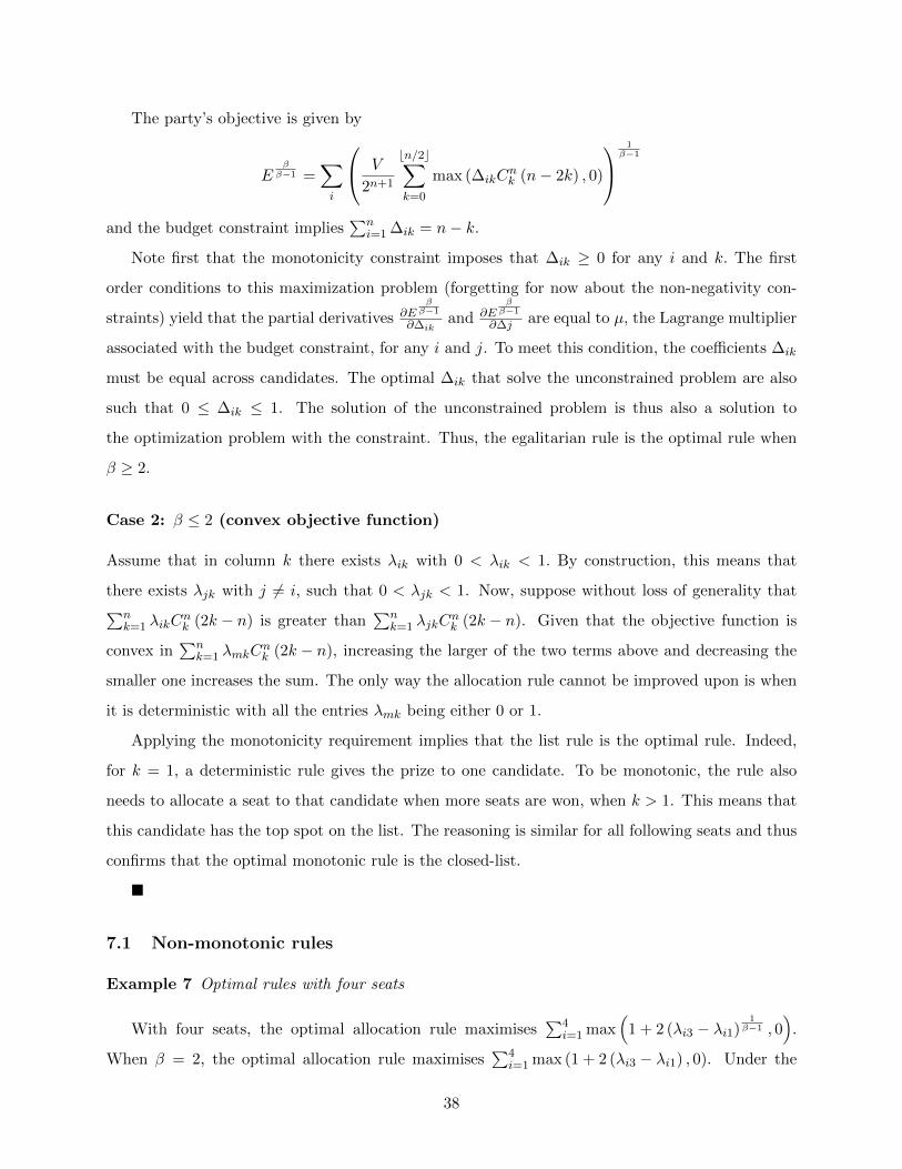
The party’s objective is given by
Eββ−1 =
∑i
V
2n+1
bn/2c∑k=0
max (∆ikCnk (n− 2k) , 0)
1β−1
and the budget constraint implies∑n
i=1 ∆ik = n− k.
Note first that the monotonicity constraint imposes that ∆ik ≥ 0 for any i and k. The first
order conditions to this maximization problem (forgetting for now about the non-negativity con-
straints) yield that the partial derivatives ∂Eββ−1
∂∆ikand ∂E
ββ−1
∂∆j are equal to µ, the Lagrange multiplier
associated with the budget constraint, for any i and j. To meet this condition, the coefficients ∆ik
must be equal across candidates. The optimal ∆ik that solve the unconstrained problem are also
such that 0 ≤ ∆ik ≤ 1. The solution of the unconstrained problem is thus also a solution to
the optimization problem with the constraint. Thus, the egalitarian rule is the optimal rule when
β ≥ 2.
Case 2: β ≤ 2 (convex objective function)
Assume that in column k there exists λik with 0 < λik < 1. By construction, this means that
there exists λjk with j 6= i, such that 0 < λjk < 1. Now, suppose without loss of generality that∑nk=1 λikC
nk (2k − n) is greater than
∑nk=1 λjkC
nk (2k − n). Given that the objective function is
convex in∑n
k=1 λmkCnk (2k − n), increasing the larger of the two terms above and decreasing the
smaller one increases the sum. The only way the allocation rule cannot be improved upon is when
it is deterministic with all the entries λmk being either 0 or 1.
Applying the monotonicity requirement implies that the list rule is the optimal rule. Indeed,
for k = 1, a deterministic rule gives the prize to one candidate. To be monotonic, the rule also
needs to allocate a seat to that candidate when more seats are won, when k > 1. This means that
this candidate has the top spot on the list. The reasoning is similar for all following seats and thus
confirms that the optimal monotonic rule is the closed-list.
�
7.1 Non-monotonic rules
Example 7 Optimal rules with four seats
With four seats, the optimal allocation rule maximises∑4
i=1 max(
1 + 2 (λi3 − λi1)1
β−1 , 0)
.
When β = 2, the optimal allocation rule maximises∑4
i=1 max (1 + 2 (λi3 − λi1) , 0). Under the
38

closed-list and the egalitarian allocation rule,∑4
i=1(λi3 − λi1) = 2. This means that∑4i=1 [(1 + 2(λi3 − λi1)] = 8.
Once we remove the monotonicity constraint, we can set some (λi3 − λi1) to be negative,
generating negative incentives for politician i who, as a consequence, chooses not to exert effort.
Yet, this also frees incentive tokens that can be strategically redistributed to the most responsive
politician(s). Exploiting this redistribution, an optimal rule is:
0 1 1 0 1
0 0 1 1 1
0 0 0 1 1
0 0 0 1 1
.
This is not the only optimal rule, as optimality puts no constraints on the value the different
λi2 can take on.
The optimal allocation rule is non-monotonic in the sense that politician 1 wins a seat if the
party wins one seat only but does not win a seat if the party wins three seats. With that rule,∑4i=1 max (1 + 2 (λi3 − λi1) , 0) = 9 > 8. Also, observe that politicians 2 to 4 are all treated equally
(the weights in columns 2 and 4 do not matter for incentives): the entries in columns 1 and 3 are
the same for these players.
This rule clearly remains optimal when β ≤ 2 since it creates even more unequal incentives
than the closed-list. For β > 2, there is a trade-off between relying on the egalitarian allocation
rule and an optimal non-monotonic rule. To pin down the value of β below which it is optimal to
depart from the egalitarian rule, one need only compare the party’s output under the egalitarian
rule,∑4
i=1(1 + 2 ∗ 1/2)1
β−1 = 4 ∗ 21
β−1 , with that under the non-monotonic list, and 3 ∗ (1 + 2 ∗
1)1
β−1 = 3 ∗ 31
β−1 , where the effort of only three politicians matter as under the non-monotonic
rule politician 1 is inactive. Then, simple algebra implies that the egalitarian rule is suboptimal
whenever 4 ∗ 21
β−1 < 3 ∗ 31
β−1 ⇐⇒ β < ln(3/2)+ln(4/3)ln(4/3) ' 2.4.
Example 8 Optimal rule with five seats
With more seats, the optimal non-monotonic rule can take different forms depending on the
value of β.
The optimal allocation rule maximises∑4
i=1 max [5 + 15 (λi4 − λi1) + 10 (λi3 − λi2) , 0]1
β−1 .
As before, when β ≤ 2 the function above is a convex function of λi4−λi1 and λi3−λi2, implying
that it is optimal to make incentives as heterogeneous as possible. Also, as all columns of the rule
matrix but the first and the last enter in the equation of party effort, the optimal non-monotonic
39

rule is this time unique. It is easy to check that it is given by
0 1 1 0 0 1
0 1 1 0 1 1
0 0 0 1 1 1
0 0 0 1 1 1
0 0 0 1 1 1
.
Thus, when β ≤ 2, it is optimal to treat differently politicians 1 and 2 and treat equally
politicians 3 to 5.
When β > 2, identifying which intra-party allocation rule is optimal is a bit more involved.
Using numerical analysis to pin down the critical values for β, it appears that there are two cases
to consider: β ≥ 3 and β ∈ (2, 3).
When β ≥ 3, the egalitarian rule is optimal: the convexity of the individual cost of effort is too
strong for the benefits of generating negative incentives to compensate for their costs.
When β ∈ (2, 3), the optimal rule gives equal incentives to four politicians and negative incen-
tives to one:
0 1 1 0 0 1
0 0 1/4 3/4 1 1
0 0 1/4 3/4 1 1
0 0 1/4 3/4 1 1
0 0 1/4 3/4 1 1
.
The last example shows that, under non-monotonicity and with a sufficient number of seats, the
space of parameter values for β can be partitioned more finely to fine tune incentives than when
the allocation rules are constrained to be monotonic.
8 Appendix B (extensions)
Number of parties
The derivation of equilibrium individual effort and party output is similar to that in the proof
of proposition 2 replacing pj = 1/2 by pj = 1/K. The proof of proposition 3 applies directly with
p = E1/∑K
j=1Ej .
�
Biased contest
The proof of proposition 3 applies directly with p = λE1/ (λE1 + E2) given that:
∂λE1
λE1+E2∂ei1
= λE2
(λE1+E2)2= p(1−p)
E1
40

�
Contest technology
Winning a majority
In what follows, we exploit lemmas 1 and 2 and the fact that at a symmetric Nash equilibrium,(Ejeij
)σ= n
σ1−σ .
The first order condition to the politician’s problem under the egalitarian rule is given by:
e∗β−1 =V
4En
σ1−σ +
M (n+ 1)
En
σ1−σCnn+1
2
(1
2
)n+2
⇐⇒
e∗ =
(V
4En
σ1−σ +
M (n+ 1)
En
σ1−σCnn+1
2
(1
2
)n+2) 1
β−1
The electoral output of each party in the symmetric equilibrium is thus:
E =
n∑k=1
( V
4En
σ1−σ +
M (n+ 1)
En
σ1−σCnn+1
2
(1
2
)n+2) 1
β−1
1−σ
11−σ
⇐⇒
Eββ−1 =
n∑k=1
(V4n
σ1−σ +M (n+ 1)n
σ1−σCnn+1
2
(1
2
)n+2) 1
β−1
1−σ
11−σ
⇐⇒
E =
n∑k=1
(V4n
σ1−σ +M (n+ 1)n
σ1−σCnn+1
2
(1
2
)n+2) 1
β−1
1−σ
β−1β(1−σ)
⇐⇒
E =
n(V
4n
σ1−σ +M (n+ 1)n
σ1−σCnn+1
2
(1
2
)n+2) 1
β−1
1−σ
β−1β(1−σ)
and thus we have that under the egalitarian rule, the output of a party is equal to:
E∗E =
{V
4+M (n+ 1)Cnn+1
2
(1
2
)n+2} 1
β
nβ+σ−1β(1−σ)
The first order condition to the politician’s problem under the closed-list is given by:
(e∗m)β−1 = V
(E
e∗m
)σ mECnm
(1
2
)n+1
+M
(E
e∗m
)σ n+ 1
2ECnn+1
2
(1
2
)n+1
41

which implies that politician m’s optimal choice is given by
e∗m =
[V Eσ
m
ECnm
(1
2
)n+1
+MEσn+ 1
2ECnn+1
2
(1
2
)n+1] 1β+σ−1
The electoral output of each party in the symmetric equilibrium is thus:
E =
n∑k=1
(V Eσ−1kCnk
(1
2
)n+1
+MEσ−1n+ 1
2Cnn+1
2
(1
2
)n+1) 1
β+σ−1
1−σ
11−σ
⇐⇒
Eβ
β+σ−1 =
n∑k=1
(V kCnk (1
2
)n+1
+Mn+ 1
2Cnn+1
2
(1
2
)n+1) 1
β+σ−1
1−σ
11−σ
and thus we have that with the closed-list, the output of a party is equal to:
E∗L =
n∑k=1
(V kCnk (1
2
)n+1
+M (n+ 1)Cnn+12
(1
2
)n+2) 1
β+σ−1
1−σ
β+σ−1β(1−σ)
To compare E∗E and E∗L, we take their ratio:
E∗LE∗E
=
∑nk=1
(V kCnk
(12
)n+1+M (n+ 1)Cnn+1
2
(12
)n+2) 1−σβ+σ−1
(V4 +M (n+ 1)Cnn+1
2
(12
)n+2) 1−σβ+σ−1
n
=
∑nk=1
(V kCnk
(12
)n+1+ M
) 1−σβ+σ−1
n(V4 + M
) 1−σβ+σ−1
.
where M = M (n+ 1)Cnn+12
(12
)n+2.
If 1−σβ+σ−1 = 1, then
∑nk=1
(V kCnk
(12
)n+1+ M
)= n
(V4 + M
)and
E∗LE∗E
is equal to one, implying
that both intra-party seat allocation rules generate the same equilibrium party output. Then,
applying Jensen’s inequality as in proposition 3 implies that a party’s output is higher under the
closed-list than under the egalitarian rule if and only if 1−σβ+σ−1 > 1 ⇐⇒ β < 2− 2σ.
�
Contractible effort
42

In a symmetric equilibrium, when both parties use the egalitarian rule, individual efforts are
given by the participation constraint:
eβ/β = V/2.
Individual effort is given by:
e = (βV/2)1/β .
This leads to party electoral output being equal to
E =
(∑e1−σ
) 11−σ
= n1
1−σ e
= n1
1−σ
(βV
2
)1/β
.
Turning to the case where both parties use the closed-list, at a symmetric equilibrium, individual
effort of the politician in mth position is given by the participation constraint:
(em)β /β =n∑
k=m
Cnk
(1
2
)nV
⇐⇒
em =
(n∑
k=m
Cnk
(1
2
)nβV
)1/β
Party output is thus equal to:
E =
(n∑
m=1
e1−σm
) 11−σ
=
n∑
m=1
(n∑
k=m
Cnk
(1
2
)nβV
) 1−σβ
1
1−σ
=
n∑
m=1
(n∑
k=m
Cnk
(1
2
)n−1) 1−σ
β
1
1−σ (βV
2
)1/β
.
The argument of proposition 3 applies but now the condition for the egalitarian rule to lead to
higher party output is that (1− σ)/β < 1 that is β > 1− σ which is always the case.
�
43