Distortions to Agricultural Incentives in Asia
606
DISTORTIONS TO AGRICULTURAL INCENTIVES IN ASIA Editors Kym Anderson • Will Martin
-
Upload
khangminh22 -
Category
Documents
-
view
1 -
download
0
Transcript of Distortions to Agricultural Incentives in Asia
DISTORTIONSTO AGRICULTURAL
INCENTIVES INASIA
EditorsKym Anderson • Will Martin

Distortions toAgriculturalIncentives in
Asia

Washington, D.C.
Distortions toAgriculturalIncentives in
Asia
Kym Andersonand Will Martin, Editors
© 2009 The International Bank for Reconstruction and Development / The World Bank1818 H Street NWWashington DC 20433Telephone: 202-473-1000Internet: www.worldbank.orgE-mail: [email protected]
All rights reserved.
1 2 3 4 12 11 10 09
This volume is a product of the staff of the International Bank for Reconstruction and Development / The WorldBank. The findings, interpretations, and conclusions expressed in this volume do not necessarily reflect the views ofthe Executive Directors of The World Bank or the governments they represent.
The World Bank does not guarantee the accuracy of the data included in this work. The boundaries, colors,denominations, and other information shown on any map in this work do not imply any judgement on the part ofThe World Bank concerning the legal status of any territory or the endorsement or acceptance of such boundaries.
Rights and PermissionsThe material in this publication is copyrighted. Copying and/or transmitting portions or all of this work without per-mission may be a violation of applicable law. The International Bank for Reconstruction and Development / TheWorld Bank encourages dissemination of its work and will normally grant permission to reproduce portions of thework promptly.
For permission to photocopy or reprint any part of this work, please send a request with complete informationto the Copyright Clearance Center Inc., 222 Rosewood Drive, Danvers, MA 01923, USA; telephone: 978-750-8400;fax: 978-750-4470; Internet: www.copyright.com.
All other queries on rights and licenses, including subsidiary rights, should be addressed to the Office of the Pub-lisher, The World Bank, 1818 H Street NW, Washington, DC 20433, USA; fax: 202-522-2422; e-mail:[email protected].
Cover design: Tomoko Hirata/World Bank.Cover photo: © Tran Thi Hoa/World Bank Photo Library.
ISBN: 978-0-8213-7662-1eISBN: 978-0-8213-7663-8DOI: 10.1596/978-0-8213-7662-1
Library of Congress Cataloging-in-Publication DataDistortions to agricultural incentives in Asia / edited by Kym Anderson and Will Martin.
p. cm.Includes bibliographical references and index.ISBN 978-0-8213-7662-1 — ISBN 978-0-8213-7663-8 (electronic)1. Agriculture—Economic aspects—Asia. 2. Agriculture and state—Asia. 3. Agriculture—Taxation—Asia. 4.
Agricultural subsidies—Asia. I. Anderson, Kym. II. Martin, Will, 1953- HD2056.Z8D57 2008338.1'85—dc22
2008029534
Dedication
To the authors of the country case studies and their assistants, especially for generating the time series of distortion estimates
that underpin the chapters, and, in particular, to Yujiro Hayami for his insights and advice during this project
and his related and influential work on Asia over several decades.


CONTENTS
Foreword xvii
Acknowledgments xxi
Contributors xxiii
Abbreviations xxvii
Map: The Focus Economies of Asia xxviii
PART I INTRODUCTION 1
1 Introduction and Summary 3Kym Anderson and Will Martin
PART II NORTHEAST ASIA 83
2 Republic of Korea and Taiwan, China 85 Masayoshi Honma and Yujiro Hayami
3 China 117Jikun Huang, Scott Rozelle, Will Martin, and Yu Liu
PART III SOUTHEAST ASIA 163
4 Indonesia 165George Fane and Peter Warr
5 Malaysia 197Prema-Chandra Athukorala and Wai-Heng Loke
6 The Philippines 223Cristina David, Ponciano Intal, and Arsenio M. Balisacan
vii
7 Thailand 255Peter Warr and Archanun Kohpaiboon
8 Vietnam 281Prema-Chandra Athukorala, Pham Lan Huong, andVo Tri Thanh
PART IV SOUTH ASIA 303
9 Bangladesh 305Nazneen Ahmed, Zaid Bakht, Paul A. Dorosh, and Quazi Shahabuddin
10 India 339Garry Pursell, Ashok Gulati, and Kanupriya Gupta
11 Pakistan 379Paul A. Dorosh and Abdul Salam
12 Sri Lanka 409Jayatilleke Bandara and Sisira Jayasuriya
Appendix A: Methodology for MeasuringDistortions to Agricultural Incentives 441Kym Anderson, Marianne Kurzweil, Will Martin,Damiano Sandri, and Ernesto Valenzuela
Appendix B: Annual Estimates of AsianDistortions to Agricultural Incentives 473Ernesto Valenzuela, Marianne Kurzweil, Johanna Croser, Signe Nelgen, and Kym Anderson
Index 563
Figures1.1 Index of Real Per Capita GDP, Asia Relative to the United States,
1950–2006 111.2 NRAs in Agriculture, Asian Focus Economies, 1980–84
and 2000–04 281.3 NRAs, by Product, Asian Focus Economies, 1980–84
and 2000–04 291.4 NRAs for Rice, Milk, and Sugar, Asian Focus Economies,
1980–84 and 2000–04 301.5 NRAs for Exportable, Import-Competing, and All Agricultural
Products, Asian Focus Economies, 1955–2004 331.6 NRAs for Agricultural and Nonagricultural Tradables and the RRA,
Asian Focus Economies, 1955–2004 51
viii Contents
1.7 RRAs in Agriculture, Asian Focus Economies, 1980–84and 2000–04 52
1.8 NRAs and RRAs, China and India, 1965–2004 531.9 NRAs and RRAs, Africa, Asia, and Latin America, 1965–2004 541.10 Income Distribution, Asian Subregions and the World, 2000 551.11 Regressions of Real GDP Per Capita and Agricultural NRAs
and RRAs, Asian Focus Economies, 1955–2005 581.12 Regressions of Real Comparative Advantage and Agricultural
NRAs and RRAs, Asian Focus Economies, 1960–2004 591.13 NRAs and International Prices, Rice, Asian Focus Economies,
1970–2005 691.14 NRAs for Rice, Malaysia, 1960–2004 711.15 RRAs and TBIs in Agriculture, Asian Focus Economies,
1980–84 and 2000–04 721.16 RRAs and Real Per Capita GDP, India, Japan, and
Northeast Asian Focus Economies, 1955–2005 751.17 NRAs for China, Japan, and the Republic of Korea and
GATT/WTO Accession, 1955–2005 762.1 RRAs for Agricultural and Nonagricultural Tradables,
Japan, Republic of Korea, and Taiwan, China, 1955–2004 1032.2 NRAs for Agricultural Products, Republic of Korea and
Taiwan, China, 1955–2004 1042.3 NRAs for Exportable, Import-Competing, and All Agricultural
Products, Taiwan, China, 1955–2002 1052.4 NRAs for Agricultural and Nonagricultural Tradables and
the RRA, Republic of Korea and Taiwan, China, 1955–2004 1062.5 NRAs for Rice, Republic of Korea and Taiwan, China, 1955–2004 1072.6 RRAs in Agriculture and Relative GDP per Agricultural Worker,
Republic of Korea and Taiwan, China, 1955–2004 1123.1 Agricultural Trade Balance, by Factor Intensity, China, 1985–2002 1283.2 The Domestic Market for Foreign Currency, China 1413.3 NRAs for Exportable, Import-Competing, and All Agricultural
Products, China, 1981–2004 1493.4 Average NRAs for Producers of Major Commodities,
China, 2000–05 1513.5 NRA Estimates in Other Studies, by Product, China, 1995–2001 1543.6 NRAs for Agricultural and Nonagricultural Tradables and
the RRA, China, 1981–2004 1554.1 Border and Domestic Prices of Import-Competing Products
Relative to the GDP Deflator, Rice and Urea Fertilizer,Indonesia, 1975–2005 174
4.2 Border and Domestic Prices of Import-Competing ProductsRelative to the GDP Deflator, Sugar, Indonesia, 1971–2005 177
Contents ix
4.3 Border and Domestic Prices of Import-Competing ProductsRelative to the GDP Deflator, Soybeans, Indonesia, 1970–2005 178
4.4 Border and Domestic Prices of Import-Competing ProductsRelative to the GDP Deflator, Maize, Indonesia, 1969–2005 179
4.5 Border and Domestic Prices of Export Crops Relative to the GDP Deflator, Indonesia, 1967–2005 181
4.6 NRAs for Exportable, Import-Competing, and All Agricultural Products, Indonesia, 1970–2004 192
4.7 NRAs for Agricultural and Nonagricultural Tradables andthe RRA, Indonesia, 1970–2004 194
5.1 Commodity Composition of Agricultural GDP, Malaysia,1965–2005 200
5.2 NRAs for Exportable, Import-Competing, and All Agricultural Products, Malaysia, 1960–2004 215
5.3 NRAs for Agricultural and Nonagricultural Tradables andthe RRA, Malaysia, 1960–2004 217
6.1 Value Shares of the Primary Production of Covered andNoncovered Commodities, the Philippines, 1966–2004 239
6.2 NRAs for Exportable, Import-Competing, and All Agricultural Products, the Philippines, 1962–2004 245
6.3 NRAs for Agricultural and Nonagricultural Tradables andthe RRA, the Philippines, 1962–2004 248
7.1 Price Comparisons and NRPs at Wholesale, Rice, Thailand,1968–2005 262
7.2 Price Comparisons and NRPs at Wholesale, Maize, Thailand,1968–2005 263
7.3 Price Comparisons and NRPs at Wholesale, Cassava, Thailand,1969–2004 264
7.4 Price Comparisons and NRPs at Wholesale, Soybeans, Thailand,1984–2005 265
7.5 Ratios, Consumer Prices to Border Prices and Miller Prices toGrower Prices, Sugar, Thailand, 1968–2005 266
7.6 Price Comparisons and NRPs at Wholesale, Sugar, Thailand,1968–2005 267
7.7 Price Comparisons and NRPs at Wholesale, Palm Oil, Thailand,1995–2004 267
7.8 Price Comparisons and NRPs at Wholesale, Rubber, Thailand,1968–2005 268
7.9 Price Comparisons and NRPs at Wholesale, Urea Fertilizer,Thailand, 1984–2005 269
7.10 NRAs for Agricultural and Nonagricultural Tradables andthe RRA, Thailand, 1970–2004 277
8.1 Agriculture, GDP, and Value Added, Vietnam, 1985–2005 284
x Contents

8.2 Commodity Shares in Agricultural Production, Vietnam,1991–2002 286
8.3 Volume, Value, and Price Indexes, Agricultural Exports,Vietnam, 1990–2004 288
8.4 Weighted Average Import Duties, Vietnam, 1990–2004 2928.5 Index, Real Exchange Rate, Vietnam, 1988–2005 2948.6 NRAs for Agricultural and Nonagricultural Tradables and
the RRA, Vietnam, 1986–2004 2989.1 Commodity Shares in Agricultural Production,
Bangladesh, 1971–2003 3159.2 NRAs and Border Prices, Rice, Bangladesh, 1974–2004 3179.3 Prices and Private Sector Imports, Rice, Bangladesh, 1997–2007 3199.4 NRAs for Exportable, Import-Competing, and All Agricultural
Products, Bangladesh, 1974–2004 3269.5 NRAs for Agricultural and Nonagricultural Tradables and
the RRA, Bangladesh, 1974–2004 32810.1 Import Tariffs, Agricultural and Nonagricultural Products, India,
2002–06 34710.2 Index, Real Effective Exchange Rate, India, 1965–2004 35010.3 NRAs for Exportable, Import-Competing, and All Agricultural
Products, India, 1965–2004 36010.4 Real Domestic Producer Prices and International
Reference Prices, Rice, India, 1965–2004 36310.5 NRAs for Agricultural and Nonagricultural Tradables and
the RRA, India, 1965–2004 36611.1 Commodity Shares in Agricultural Production, Pakistan,
1965–2005 38111.2 Import Tariffs and the Real Exchange Rate, Pakistan, 1985–2004 38511.3 NRAs for Major Covered Products, Pakistan, 1962–2005 39611.4 NRAs for Exportable, Import-Competing, and All Agricultural
Products, Pakistan, 1973–2005 39811.5 NRAs for Agricultural and Nonagricultural Tradables and
the RRA, Pakistan, 1973–2005 40112.1 Real GDP Growth, Political Episodes, and Policy Regimes,
Sri Lanka, 1951–2005 41112.2 Agriculture in GDP and Exports, Sri Lanka, 1950–2005 41412.3 Commodity Shares in Agricultural Production, Sri Lanka,
1966–2004 41412.4 Fertilizer Subsidy, Sri Lanka, 1962–2007 41912.5 NRAs for Tea, Sri Lanka, 1955–2004 42312.6 NRAs for Rubber, Sri Lanka, 1955–2004 42512.7 NRAs for Coconuts, Sri Lanka, 1955–2004 42612.8 NRAs for Rice, Sri Lanka, 1955–2004 426
Contents xi

12.9 NRAs for Exportable, Import-Competing, and All Agricultural Products, Sri Lanka, 1955–2004 428
12.10 NRAs for Agricultural and Nonagricultural Tradables andthe RRA, Sri Lanka, 1955–2004 429
A.1 A Distorted Domestic Market for Foreign Currency 445A.2 Distorted Domestic Markets for Farm Products 464
Tables1.1 Key Economic and Trade Indicators, Asian Focus Economies,
2000–04 61.2 Poverty Levels in Asia, 1981–2004 81.3 Real Growth in GDP and Exports, Asian Focus Economies,
1980–2004 101.4 Exports of Goods and Services as a Share of GDP, Asian Focus
Economies, 1965–2004 121.5 Share of Nonfood Manufactures in World Exports, Asian Focus
Economies, 1990–2006 131.6 Sectoral Shares of GDP, Asian Focus Economies, 1965–2004 141.7 Agriculture’s Share in Employment, Asian Focus Economies,
1965–2004 151.8 Sectoral Shares of Merchandise Exports, Asian Focus Economies,
1965–2004 161.9 Indexes of Comparative Advantage in Agriculture and
Processed Food, Asian Focus Economies, 1965–2004 181.10 Export Orientation, Import Dependence, and Self-Sufficiency
in Primary Agricultural Production, Asian Focus Economies,1961–2004 19
1.11 NRAs for Agricultural Products, Asian Focus Economies, 1955–2004 27
1.12 NRA Dispersion across Covered Agricultural Products,Asian Focus Economies, 1955–2004 32
1.13 NRAs for Agricultural Exportable and Import-CompetingProducts and the TBI, Asian Focus Economies, 1955–2004 34
1.14 NRAs for Covered Agricultural Products, by Policy Instrument,Asian Focus Economies, 1955–2004 38
1.15 Gross Subsidy Equivalents of Agricultural Assistance,Total and Per Farmworker, Asian Focus Economies, 1955–2004 41
1.16 NRA and Gross Subsidy Equivalents of Farmer Assistance,by Product, Asian Focus Economies, 1955–2004 45
1.17 RRAs in Agriculture, Asian Focus Economies, 1955–2004 481.18 Relative Per Capita Income, Agricultural Comparative Advantage,
and NRAs and RRAs for Agricultural Tradables, Asian FocusEconomies, 2000–04 57
xii Contents
1.19 Regressions of NRAs and Selected Determinants, Asian FocusEconomies, 1960–2004 61
1.20 CTEs for Policies Assisting the Producers of Covered Agricultural Products, Asian Focus Economies, 1960–2004 62
1.21 Value of CTEs for Policies Assisting the Producers of Covered Agricultural Products, Asian Focus Economies, 1965–2004 65
2.1 Economic Growth and Structural Transformation,Republic of Korea and Taiwan, China, 1955–2004 89
2.2 Changes in Agricultural Structure, Republic of Korea and Taiwan,China, 1955–2004 92
2.3 NRAs for Covered Agricultural Products, Republic of Korea,1955–2004 100
2.4 NRAs for Covered Agricultural Products, Taiwan, China,1955–2002 101
2.5 NRAs in Agriculture Relative to Nonagricultural Industries,Republic of Korea and Taiwan, China, 1955–2004 102
2.6 CTEs for Covered Agricultural Products, Republic ofKorea and Taiwan, China, 1955–2004 108
3.1 Real Average Annual Rates of Economic Growth, China, 1970–2004 1263.2 Structure of the Agricultural Economy, China, 1970–2005 1273.3 Rural Income Per Capita, China, 1980–2001 1303.4 NRAs for Covered Agricultural Products, China, 1981–2005 1453.5 NRAs in Agriculture Relative to Nonagricultural Industries,
China, 1981–2005 1523.6 CTEs for Covered Agricultural Products, China, 1981–2005 1534.1 Real GDP Growth and Its Sectoral Components, Indonesia,
1968–2005 1674.2 Subsector Shares of Agricultural Value Added, Indonesia,
1971–2000 1684.3 Export Sales in Total Sales and Imports in Total Usage, Indonesia,
1971–2000 1694.4 Estimated Effective Rates of Protection, Indonesia, 1987, 1995,
and 2003 1714.5 Estimates of Transmission Elasticities from Wholesale to
Farm Prices, Indonesia 1894.6 NRAs for Covered Agricultural Products, Including Fertilizer
Use Subsidies, Indonesia, 1970–2004 1914.7 NRAs in Agriculture Relative to Nonagricultural Industries,
Indonesia, 1970–2004 1935.1 Agriculture in the Economy, Malaysia, 1970–2005 2005.2 Product Shares, Agricultural Exports, Malaysia, 1970–2004 2055.3 NRAs for Covered Agricultural Products, Malaysia, 1960–2004 2145.4 NRAs in Agriculture Relative to Nonagricultural Industries,
Malaysia, 1960–2004 216
Contents xiii
6.1 Agriculture in the Economy, Growth Rates, the Philippines andOther Asian Countries, 1960–2004 224
6.2 Changes in Agricultural Structure and Trade Openness,the Philippines, 1960–2004 225
6.3 GVA Growth Rates, Major Agricultural Commodities,the Philippines, 1960–2004 227
6.4 Revealed Comparative Advantage, Major AgriculturalCommodities, the Philippines, 1960–2004 229
6.5 NRAs for Covered Agricultural Products, the Philippines,1962–2004 242
6.6 NRAs in Agriculture Relative to Nonagricultural Industries, the Philippines, 1962–2004 244
6.7 Coefficients of Variation in Real International Prices andPhilippine Wholesale Prices, Major Agricultural Commodities,1960–2004 246
7.1 Real GDP Growth and Its Sectoral Components, Thailand,1968–2005 258
7.2 Subsector Shares of Agricultural Value Added, Thailand,1975–2000 259
7.3 Estimates of Transmission Elasticities from Wholesale toFarm Prices, Thailand 272
7.4 NRAs for Covered Agricultural Products, Thailand, 1970–2004 2747.5 NRAs in Agriculture Relative to Nonagricultural Industries,
Thailand, 1970–2004 2768.1 Structure of the Agricultural Economy, Vietnam, 1986–2004 2858.2 Share of Planted Area by Crop, Vietnam, 1990–2004 2868.3 Composition of Agricultural Exports by Value, Vietnam,
1990–2004 2888.4 NRAs for Covered Agricultural Products, Vietnam, 1986–2004 2968.5 NRAs in Agriculture Relative to Nonagricultural Industries,
Vietnam, 1986–2004 2979.1 Tariff Rates on Imports, Bangladesh, 1991–2003 3139.2 Total Taxes on Agricultural Commodity Imports, Bangladesh,
1992 and 2002 3149.3 Production and Imports, Rice and Wheat, Bangladesh, 1973–2004 3169.4 NRAs for Covered Agricultural Products, Bangladesh, 1974–2004 3219.5 NRAs in Agriculture Relative to Nonagricultural Industries,
Bangladesh, 1974–2004 32710.1 Sectoral Share of GDP and Employment, India, 1950–2005 34110.2 Profile of Agricultural and Manufacturing Imports and Exports,
India, 1960–2005 34210.3 Structure of the Agricultural Economy, India, 1964–2004 35710.4 Structure of Fertilizer and Electricity Subsidies, Key Crops, India,
2004 359
xiv Contents

10.5 NRAs for Covered Agricultural Products, India, 1965–2004 36110.6 NRAs in Agriculture Relative to Nonagricultural Industries, India,
1965–2004 36210.7 Self-Sufficiency Ratios, Selected Food Products, India, 1961–2004 36511.1 Agriculture in the Economy, Pakistan, 1965–2004 38011.2 Structure of the Agricultural Economy, Major Crops, Pakistan,
2004–06 38311.3 Production and Trade, Wheat, Pakistan, 1972–2005 38711.4 NRAs for Covered Agricultural Products, Pakistan, 1962–2005 38911.5 Production and Trade, Cotton, Pakistan, 1960–2005 39111.6 NRAs in Agriculture Relative to Nonagricultural Industries,
Pakistan, 1962–2005 40012.1 Agriculture in the Economy, Sri Lanka, 1950–2005 41312.2 NRAs for Covered Agricultural Products, Sri Lanka, 1955–2004 42112.3 NRAs in Agriculture Relative to Nonagricultural Industries,
Sri Lanka, 1955–2004 422B.1 Annual Distortion Estimates, Republic of Korea, 1955–2004 475B.2 Annual Distortion Estimates, Taiwan, China, 1955–2002 481B.3 Annual Distortion Estimates, China, 1955–2005 487B.4 Annual Distortion Estimates, Indonesia, 1970–2004 490B.5 Annual Distortion Estimates, Malaysia, 1960–2004 496B.6 Annual Distortion Estimates, the Philippines, 1962–2004 502B.7 Annual Distortion Estimates, Thailand, 1970–2004 506B.8 Annual Distortion Estimates, Vietnam, 1986–2005 510B.9 Annual Distortion Estimates, Bangladesh, 1974–2004 513B.10 Annual Distortion Estimates, India, 1965–2004 517B.11 Annual Distortion Estimates, Pakistan, 1962–2005 523B.12 Annual Distortion Estimates, Sri Lanka, 1955–2004 527B.13 Annual Distortion Estimates, Asian Focus Economies, 1955–2005 533B.14 Gross Subsidy Equivalents of Assistance to Farmers, Asian Focus
Economies, 1955–2005 543B.15 Share of the Regional Value of Agricultural Production,
Asian Focus Economies, 1955–2004 546B.16 Summary of NRA Statistics, Asian Focus Economies 549B.17 Summary of NRA Statistics, by Major Product, Asian Focus
Economies, 2000–04 550B.18 Share of the Global Value of Production and Consumption,
Key Covered Products, Asian Focus Economies, 2000–04 552B.19 Share of the Global Value of Exports and Imports, Key Covered
Products, Asian Focus Economies, 2000–03 555B.20 Share of Production for Export, Consumption of Imports, and
Domestic Production, Key Covered Products, Asian Focus Economies, 2000–03 558
Contents xv

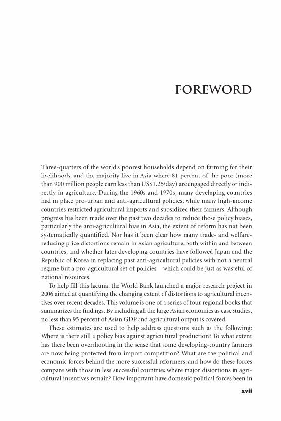
Three-quarters of the world’s poorest households depend on farming for theirlivelihoods, and the majority live in Asia where 81 percent of the poor (morethan 900 million people earn less than US$1.25/day) are engaged directly or indi-rectly in agriculture. During the 1960s and 1970s, many developing countrieshad in place pro-urban and anti-agricultural policies, while many high-incomecountries restricted agricultural imports and subsidized their farmers. Althoughprogress has been made over the past two decades to reduce those policy biases,particularly the anti-agricultural bias in Asia, the extent of reform has not beensystematically quantified. Nor has it been clear how many trade- and welfare-reducing price distortions remain in Asian agriculture, both within and betweencountries, and whether later developing countries have followed Japan and theRepublic of Korea in replacing past anti-agricultural policies with not a neutralregime but a pro-agricultural set of policies—which could be just as wasteful ofnational resources.
To help fill this lacuna, the World Bank launched a major research project in2006 aimed at quantifying the changing extent of distortions to agricultural incen-tives over recent decades. This volume is one of a series of four regional books thatsummarizes the findings. By including all the large Asian economies as case studies,no less than 95 percent of Asian GDP and agricultural output is covered.
These estimates are used to help address questions such as the following:Where is there still a policy bias against agricultural production? To what extenthas there been overshooting in the sense that some developing-country farmersare now being protected from import competition? What are the political andeconomic forces behind the more successful reformers, and how do these forcescompare with those in less successful countries where major distortions in agri-cultural incentives remain? How important have domestic political forces been in
FOREWORD
xvii

bringing about reform, compared with international forces? What explains thecross-commodity pattern of distortions within the agricultural sector of eachcountry? What policy lessons and trade implications can be drawn from these dif-fering experiences with a view to ensuring better growth-enhancing and poverty-reducing outcomes in other still-distorted developing countries during theirreforms in the future?
In Asia more than anywhere else, the reforms have been truly transformational.The world’s most populous nations, China and India, have been among the mostambitious in raising incentives for farmers, albeit from a very low base in eachcase. Vietnam also has undertaken major and rapid reforms, while in other South-east Asian economies the reforms have been more gradual (or nonexistent in thecases of Myanmar and the Democratic People’s Republic of Korea, but they werenot able to be included as case studies because of lack of access to data). Mean-while, the Republic of Korea has moved from taxing agriculture relative to othertradable sectors in the 1950s to increasingly protecting it beginning in the 1970s.This development has raised concerns that other emerging economies may followsuit and pursue the same agricultural protection growth path of more-advancedeconomies.
The new empirical indicators summarized in these case studies provide astrong evidence-based foundation for assessing the successes and failures of poli-cies of the past and for evaluating policy options for the years ahead. The analyti-cal narratives reveal that the reforms to agricultural price and trade policies weresometimes undertaken unilaterally. In other cases, they were also partly inresponse to international pressures such as the Uruguay Round (for example, theRepublic of Korea), commitments required for accession to the World TradeOrganization (WTO) (for example, China), and structural adjustment loan con-ditionality by international financial institutions (for example, the Philippines inthe 1980s).
The study is timely because the WTO is in the midst of the Doha round of mul-tilateral trade negotiations, and agricultural policy reform is one of the most con-tentious issues in those talks. Hopefully China and South and Southeast Asiancountries will not make use of the legal wiggle room they have allowed themselvesin their WTO bindings and follow Japan and the Republic of Korea into high agri-cultural protection. It might be argued, on one hand, that a laissez-faire strategycould increase rural-urban inequality and poverty and thereby generate socialunrest. On the other hand, policies that lead to high prices for staple foods, in par-ticular, involve potentially serious risks for the urban and rural poor who are netbuyers of food in developing countries. Available evidence suggests that problemsof rural-urban poverty gaps have been alleviated in parts of Asia by some of themore-mobile members of farm households finding full- or part-time work off the
xviii Foreword
farm and repatriating part of their higher earnings back to those remaining infarm households. Efficient ways of assisting any left-behind groups of poor (non-farm as well as farm) households include public investment measures that havehigh social payoffs, such as in basic education and health and in rural infrastruc-ture, as well as in agricultural research and development. As argued in the WorldBank’s World Development Report 2008, the latter also provide more sustainableand more equitable ways of securing domestic food supplies than artificiallypropping up prices.
Justin Yifu LinSenior Vice President and Chief Economist
The World Bank
Foreword xix


ACKNOWLEDGMENTS
xxi
This book provides an overview of the evolution of the distortions to agriculturalincentives caused by price and trade policies in the World Bank–defined regionsof East Asia and South Asia. The volume includes an introduction and summarychapter and commissioned studies of three Northeast Asian, five Southeast Asian,and four South Asian economies. The chapters are followed by two appendixes.The first appendix describes the methodology we have used to measure the nom-inal and relative rates of assistance for farmers and the taxes and subsidies on foodconsumption. The second appendix provides summaries of our annual estimatesof these rates of assistance across the focus economies. Together, the 12 economieswe study account for no less than 95 percent of the region’s agricultural valueadded, farm households, total population, and total gross domestic product.
To the authors of the case studies, who are listed on the following pages, we areextremely grateful for the dedicated way in which they have delivered far morethan we could have reasonably expected. We are particularly grateful to YujiroHayami for his insights and advice during this project and his influential, relatedwork over several decades. Staff at the World Bank’s East Asia and Pacific Depart-ment and South Asia Department have provided generous and insightful adviceand assistance throughout the project. This has included participation in twoBank-wide seminars that provided helpful suggestions on the draft studies. Weoffer thanks likewise to the World Bank directors in the focus economies, whoexamined and cleared the working paper versions of each chapter. We have simi-larly benefited from the feedback provided by many participants at workshopsand conferences in which drafts have been presented over the past year or so.Johanna Croser, Francesca de Nicola, Esteban Jara, Marianne Kurzweil, Signe Nelgen, Damiano Sandri, and Ernesto Valenzuela have generously assisted in
compiling material for the opening overview chapter, and Johanna Croser andMarie Damania assisted in copyediting the case study chapters.
We wish to extend our thanks to the Organisation for Economic Co-operationand Development and the International Food Policy Research Institute for sharingmethodological insights, and also to the members of the project’s Senior AdvisoryBoard, who have provided sage advice and much encouragement throughout theplanning and implementation stages. The board is comprised of Yujiro Hayami,Bernard Hoekman, Anne Krueger, John Nash, Johan Swinnen, Stefan Tangermann,Alberto Valdés, Alan Winters, and, until his untimely death in 2008, Bruce Gardner.
Our thanks go also to the Development Research Group and to the Trust Fundsof the governments of Ireland, Japan, the Netherlands, and the United Kingdomfor financial assistance. This support has made it possible for this set of economiesto be included as part of a wider study that also encompasses more than 30 otherdeveloping countries, 18 economies in transition from central planning, and 20high-income countries. Three companion volumes examine case studies of otheremerging economies in a similar way and for a similar time period (back to themid-1950s or early 1960s, except for the transition economies). Also published bythe World Bank in 2008 or 2009, they cover Africa (coedited by Kym Andersonand Will Masters), Latin America (coedited by Kym Anderson and AlbertoValdés), and Europe’s transition economies (coedited by Kym Anderson andJohan Swinnen). A global overview volume edited by Kym Anderson will be pub-lished in 2009.
Kym Anderson and Will MartinNovember 2008
xxii Acknowledgments
Nazneen Ahmed is a research fellow at the Bangladesh Institute of DevelopmentStudies, Ministry of Planning in Dhaka, Bangladesh.
Kym Anderson is George Gollin Professor of Economics at the University of Adelaide and a fellow of the Center for Economic Policy Research, London. During2004–07, he was on an extended sabbatical as lead economist (trade policy) in theDevelopment Research Group of the World Bank in Washington, DC.
Prema-Chandra Athukorala is professor of economics in the Research School ofPacific and Asian Studies at the Australian National University in Canberra.
Arsenio M. Balisacan is professor of agricultural economics and director of theSoutheast Asian Regional Center for Graduate Study and Research in Agriculturein Los Baños, Laguna, the Philippines.
Zaid Bakht is research director at the Bangladesh Institute of Development Stud-ies, Ministry of Planning in Dhaka, Bangladesh.
Jayatilleke Bandara is associate professor of economics at Griffith University inBrisbane, Australia.
Johanna Croser has been a consultant with this project and is a PhD student in theDepartment of Economics of the University of British Columbia in Vancouver,Canada.
Cristina David is a senior research fellow at the Philippine Institute for Develop-ment Studies in Makati City, the Philippines.
xxiii
CONTRIBUTORS

Paul A. Dorosh is a senior rural development economist at the Agriculture andRural Development Department (South Asia Agriculture and Rural DevelopmentGroup) at the World Bank in Washington, DC.
George Fane is an adjunct professor of economics in the Research School of Pacificand Asian Studies, Australian National University in Canberra.
Ashok Gulati is the Asian Director for the International Food Policy ResearchInstitute in New Delhi. Previously, he headed the institute’s Markets, Trade, andInstitutions Division.
Kanupriya Gupta is a senior research analyst with the International Food PolicyResearch Institute in New Delhi.
Yujiro Hayami is chairman of the graduate faculty of the Foundation forAdvanced Studies on International Development. He is also visiting professor inthe National Graduate Institute of Policy Studies, Tokyo.
Masayoshi Honma is professor of agricultural and resource economics at the University of Tokyo. He is also a member of the Board of Trustees of the Interna-tional Food Policy Research Institute in Washington, DC.
Jikun Huang is director and professor, Center for Chinese Agricultural Policy, Chinese Academy of Sciences in Beijing.
Pham Lan Huong is a researcher with the Central Institute of Economic Manage-ment in Hanoi, Vietnam.
Ponciano Intal is professor and director, Angelo King Institute for Economic andBusiness Studies, De La Salle University in Manila.
Sisira Jayasuriya was director, Asian Economics Center and associate professor inthe Department of Economics, University of Melbourne at the time of the studyand is now professor of economics at La Trobe University (Bundoora) in Victoria,Australia.
Archanun Kohpaiboon is lecturer in the economics department of ThammasatUniversity in Bangkok.
Marianne Kurzweil is a young professional at the African Development Bank inTunis. During 2006–07, she was consultant with this project at the DevelopmentResearch Group at the World Bank in Washington, DC.
xxiv Contributors
Yu Liu is researcher at the Center for Chinese Agricultural Policy, Chinese Acad-emy of Sciences in Beijing.
Wai-Heng Loke is lecturer at the Department of Economics, Faculty of Economicsand Administration at the University of Malaya in Kuala Lumpur, Malaysia.
Will Martin is lead economist in the Development Research Group at the WorldBank in Washington, DC. He specializes in trade and agricultural policy issuesglobally, especially in Asia.
Signe Nelgen has been a consultant with this project and is a PhD student in theSchool of Economics of the University of Adelaide in Australia.
Garry Pursell is visiting fellow at the Australia South Asia Research Center, Australian National University in Canberra. Previously, he was with the SouthAsia Department of the World Bank.
Scott Rozelle holds the Helen Farnsworth Endowed Professorship and is senior fellow and professor at the Freeman Spogli Institute for International Studies atStanford University in Stanford, California.
Abdul Salam is professor of economics at the Federal Urdu University and is for-mer chairman of the Agricultural Prices Commission in Islamabad, Pakistan.
Damiano Sandri is a PhD candidate in economics at Johns Hopkins University inBaltimore, Maryland. During 2006–07, he was a consultant with this project at theDevelopment Research Group at the World Bank in Washington, DC.
Quazi Shahabuddin is director general of the Bangladesh Institute of Develop-ment Studies, Ministry of Planning in Dhaka, Bangladesh.
Vo Tri Thanh is a researcher with the Central Institute of Economic Managementin Hanoi, Vietnam.
Ernesto Valenzuela is lecturer in economics and research fellow at the University ofAdelaide in Australia. During 2005–07, he was consultant at the DevelopmentResearch Group of the World Bank in Washington, DC.
Peter Warr is the John Crawford Professor of Agricultural Economics and found-ing Director of the Poverty Research Centre in the Division of Economics,Research School of Pacific and Asian Studies at the Australian National Universityin Canberra.
Contributors xxv


CTE consumer tax equivalentGDP gross domestic productGVA gross value addedIMF International Monetary FundNRA nominal rate of assistanceNRP nominal rate of protectionNTB nontariff barrierOECD Organisation for Economic Co-operation and DevelopmentRRA relative rate of assistanceTBI trade bias indexWTO World Trade Organization
Note: All dollar amounts are U.S. dollars (US$) unless otherwise indicated.
xxvii
ABBREVIATIONS

PHILIPPINES
CHINA
TAIWAN,CHINA
REP. OFKOREA
MALAYSIA
VIETNAMTHAILAND
INDIA
SRILANKA
PAKISTAN
BANGLADESH
INDONESIA
IBRD 36674DECEMBER 2008
This map was produced by the Map Design Unit of The World Bank. The boundaries, colors, denominations and any other informationshown on this map do not imply, on the part of The World BankGroup, any judgment on the legal status of any territory, or anyendorsement or acceptance of such boundaries.
0 500 1000 Kilometers
0 500 1000 Miles
The Focus Economies of Asia

Part III
INTRODUCTION

Farm earnings in developing countries have often been depressed by a pro-urban,antiagricultural bias in government policies. Progress has been made since the1980s in reducing the policy bias in many countries, however. In some cases, thechanges have been modest and intermittent, but, in China and, to a lesser extent,India, they have been transformational. Many trade-reducing price distortionsnonetheless remain within the agricultural sector in low- and middle-incomeeconomies, including in Asia. This is important for the majority of households inthe world because 45 percent of the global workforce is employed in agriculture,and 75 percent of the world’s poorest households depend directly or indirectly onfarming for livelihoods. It is even more important in Asia’s developing economies,where 60 percent of the workforce and 81 percent of the poor (625 million peopleeach earning less than US$1 a day) are engaged in agriculture (World Bank 2007;Chen and Ravallion 2007).
This study is part of a global research project seeking to understand the chang-ing scope and impact of the policy bias against agriculture and the reasons behindagricultural policy reforms in Africa, Europe’s transition economies, Latin Amer-ica and the Caribbean, and Asia.1 One purpose of the project is to obtain quanti-tative indicators of the effects of recent policy interventions. A second objective isto gain a deeper understanding of the political economy of trends in the distor-tions in agricultural incentives in various national settings. The third goal is to usethis deeper understanding to explore the prospects for reducing the distortions inagricultural incentives and discover the likely implications for agricultural com-petitiveness, equality, and poverty reduction in many countries, large and small.
3
1
INTRODUCTIONAND SUMMARY
Kym Anderson and Will Martin
The compilation of new annual time series estimates of the protection and tax-ation of farmers over the past half century is a core component of the first stage ofour research project. These estimates are used to help address questions such asthe following: Where is the policy bias against agricultural production? To whatextent has there been overshooting in that some food producers are now beingprotected from import competition in developing countries in much the sameway they were protected in Europe and Japan during earlier periods of industrial-ization? What are the political economy forces behind successful reforms in somecountries? How do they compare with the forces in other countries where reformsare less successful and major distortions in agricultural incentives remain? Overthe past two decades, how important have domestic political forces been in gener-ating reform relative to forces operating in earlier decades or international forces,such as loan conditionality, rounds of multilateral trade negotiations in the WorldTrade Organization (WTO), regional integration agreements, accession to theWTO, and the globalization of supermarkets and other firms along the valuechain? What has caused the patterns of distortion within the agricultural sectorsof individual countries? What policy lessons and trade implications may be drawnfrom these differing experiences so that we may seek to ensure growth-enhancingand poverty-reducing outcomes, including less overshooting and fewer protec-tionist regimes, during future reforms in still-distorted developing economies inAsia and elsewhere?
Our study is timely for at least four reasons. First, the WTO is in the midst of theDoha Round of multilateral trade negotiations, and agricultural policy reform isone of the most contentious issues in these talks. Second, countries are also seekingto position themselves favorably in preferential trade negotiations in the wake ofother forces in globalization, including revolutions in information, communica-tions, agricultural biotechnology, and supermarketing. Third, poorer countries andtheir development partners are striving to achieve the United Nations MillenniumDevelopment Goals by 2015, including the prime goals of alleviating hunger andreducing poverty. Fourth, the outputs of our study are timely also because worldfood prices spiked at high levels in 2008, and governments in some developingcountries, in their panic to deal with the inevitable protests from consumers, havereacted in ways that are not optimal. Spikes have occurred in the past, most notablyin 1973–74, and lessons on appropriate policy responses may be drawn from theexperiences then. The empirical estimates reported in our study reveal that govern-ments in Asia have differed in their responses to such shocks, although this is lessthe case of rice, the region’s main staple.
This study on Asia is based on a sample of 12 developing economies. Weexclude Japan, which has been a high-income country throughout our reviewperiod and, so, is analyzed separately as part of the high-income group in the
4 Distortions to Agricultural Incentives in Asia

project’s global overview volume. In Northeast Asia, we include China,the Republic of Korea (hereafter referred to as Korea), and Taiwan, China. InSoutheast Asia, we include the five large economies of Indonesia, Malaysia, thePhilippines, Thailand, and Vietnam, and, in South Asia, we include the fourlargest economies: Bangladesh, India, Pakistan, and Sri Lanka. In 2000–04, theseeconomies (all of them now WTO members) accounted for more than 95 per-cent of Asia’s agricultural value added, total farm households, total population,and total gross domestic product (GDP).2 The distortion estimates are providedfor as many years as data permit over the past five decades (an average of42 years), and they are presented for an average of eight crop and livestock prod-ucts per economy, which, in aggregate, amounts to about 70 percent of the grossvalue of agricultural production in each of these economies. The time series andcountry coverage in our study greatly exceed the data and country coverage of ear-lier studies, including Anderson and Hayami (1986); Krueger, Schiff, and Valdés(1991); Orden et al. (2007); and the Organisation for Economic Co-operationand Development (OECD 2007). The product coverage is broader in each of ourcase studies than in all earlier case studies other than the study by the OECD(2007).3
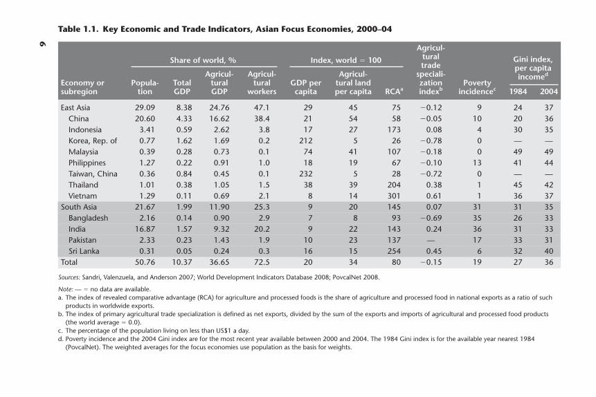
The key characteristics of these economies—accounting in 2000–04 for only10 percent of worldwide GDP, but 37 percent of global agricultural value added,51 percent of the world’s population, and 73 percent of the world’s farmers—areshown in table 1.1. The table reveals the considerable diversity within the regionin development, relative resource endowments, comparative advantage, trade spe-cialization, and the incidence of poverty and income inequality. These economiesthus provide a rich sample for comparative study.
Per capita incomes in Bangladesh, India, and Vietnam are barely 8 percentof the world average. In Indonesia, the Philippines, and Sri Lanka, they arearound 16 percent. In China, they are over 25 percent. In Thailand, they aremore than 30 percent. In Malaysia, they are about 75 percent of the world aver-age. Korea and Taiwan, China appear exceptional in that average per capitaincomes are currently twice the global average; however, in the 1950s, at thestart of the period of our study, these two economies were among the poorest inthe world.
Korea and Taiwan, China are also exceptional in the per capita endowment ofagricultural land; they have only around 5 percent of the world average endow-ment ratio. Bangladesh has a little more, followed by Sri Lanka and the Philip-pines. Even India, Indonesia, and Pakistan have only about 25 percent of theglobal average endowment, while Malaysia and Thailand have about 40 percent,and China, over 50 percent.4 Thus, these Asian economies are not relatively wellendowed with cropland or pastureland; on a per capita basis, the region has only
Introduction and Summary 5
6
Table 1.1. Key Economic and Trade Indicators, Asian Focus Economies, 2000–04
Sources: Sandri, Valenzuela, and Anderson 2007; World Development Indicators Database 2008; PovcalNet 2008.
Note: — � no data are available.a. The index of revealed comparative advantage (RCA) for agriculture and processed foods is the share of agriculture and processed food in national exports as a ratio of such
products in worldwide exports.b. The index of primary agricultural trade specialization is defined as net exports, divided by the sum of the exports and imports of agricultural and processed food products
(the world average � 0.0).c. The percentage of the population living on less than US$1 a day.d. Poverty incidence and the 2004 Gini index are for the most recent year available between 2000 and 2004. The 1984 Gini index is for the available year nearest 1984
(PovcalNet). The weighted averages for the focus economies use population as the basis for weights.
Agricul-
Share of world, % Index, world � 100 tural Gini index,trade per capita
Agricul- Agricul- Agricul- speciali- incomed
Economy or Popula- Total tural tural GDP per tural land zation Povertysubregion tion GDP GDP workers capita per capita RCAa indexb incidencec 1984 2004
East Asia 29.09 8.38 24.76 47.1 29 45 75 �0.12 9 24 37China 20.60 4.33 16.62 38.4 21 54 58 �0.05 10 20 36Indonesia 3.41 0.59 2.62 3.8 17 27 173 0.08 4 30 35Korea, Rep. of 0.77 1.62 1.69 0.2 212 5 26 �0.78 0 — —Malaysia 0.39 0.28 0.73 0.1 74 41 107 �0.18 0 49 49Philippines 1.27 0.22 0.91 1.0 18 19 67 �0.10 13 41 44Taiwan, China 0.36 0.84 0.45 0.1 232 5 28 �0.72 0 — —Thailand 1.01 0.38 1.05 1.5 38 39 204 0.38 1 45 42Vietnam 1.29 0.11 0.69 2.1 8 14 301 0.61 1 36 37
South Asia 21.67 1.99 11.90 25.3 9 20 145 0.07 31 31 35Bangladesh 2.16 0.14 0.90 2.9 7 8 93 �0.69 35 26 33India 16.87 1.57 9.32 20.2 9 22 143 0.24 36 31 33Pakistan 2.33 0.23 1.43 1.9 10 23 137 — 17 33 31Sri Lanka 0.31 0.05 0.24 0.3 16 15 254 0.45 6 32 40
Total 50.76 10.37 36.65 72.5 20 34 80 �0.15 19 27 36
34 percent of the global average. This might suggest that the comparative advan-tage of the Asian economies in agricultural goods is low, were it not for the varia-tions in these economies in the level of industrial development, the quality of landand water, and the related institutional arrangements and entitlements. As aresult, the strengths of these economies in agricultural competitiveness arediverse. The differences are reflected in the index of revealed comparative advan-tage and the agricultural trade specialization index (table 1.1). A majority of ourfocus economies have an index of revealed comparative advantage well above 100,indicating the extent to which the share of agricultural and food products in aneconomy’s merchandise trade exceeds the global average share of these products.For Korea and Taiwan, China, the index is below 30, and, for China and the Philip-pines, it is around 60. The index of agricultural trade specialization measures netexports as a ratio of exports, plus imports of farm products, and, so, it is boundedbetween �1 and �1. It is positive for half of our focus economies, but is �0.7 forBangladesh, Korea, and Taiwan, China.
Income inequality has risen slightly over the past two decades, but is still lowthroughout much of the region relative to the rest of the world. In 2004, the Ginicoefficient was between 0.40 and 0.49 in Malaysia, the Philippines, Sri Lanka, andThailand and averaged between 0.31 and 0.37 in the rest of the region. The regionalaverage of 0.36 contrasts with, for example, the average of 0.52 in Latin America.Likewise, the Gini coefficient for land distribution is relatively low in Asia, at only0.41 for China and Pakistan and below 0.50 also in Bangladesh; Indonesia; Korea;Taiwan, China; and Thailand. Even in India, the coefficient for land distribution isonly 0.58, and it is 0.50 in Vietnam. However, these coefficients imply that the distri-bution of land is more equal in Asia than it is in Latin America, where the Gini coef-ficient for land distribution is above 0.70 for major countries such as Argentina andBrazil and possibly for the region as a whole (World Bank 2007). A significant pro-portion of the rural population is landless in South Asia, however; so 31 percent ofthe population of South Asia was still living on less than US$1 a day in 2004 com-pared with only 9 percent in East Asia (table 1.1).
The extent of the decline in poverty in Asia has been unprecedented. The num-ber of people living on less than US$1 a day has been reduced by half since 1981(in 1993 purchasing power parity dollars). Most of the decline has occurred inEast Asia, especially China. In East Asia, the poverty rate declined from 58 percentto less than 10 percent of the population; but, even in South Asia, the proportionhas fallen from 50 to around 30 percent (table 1.2). During the 10 years to 2002,no less than 75 percent of the decline in the share of the poor among the popula-tion in Asia occurred in rural areas, and another 15 percent of the decline was gen-erated by a movement out of poverty among rural people who had migratedbecause of better opportunities in urban areas (Chen and Ravallion 2007).
Introduction and Summary 7
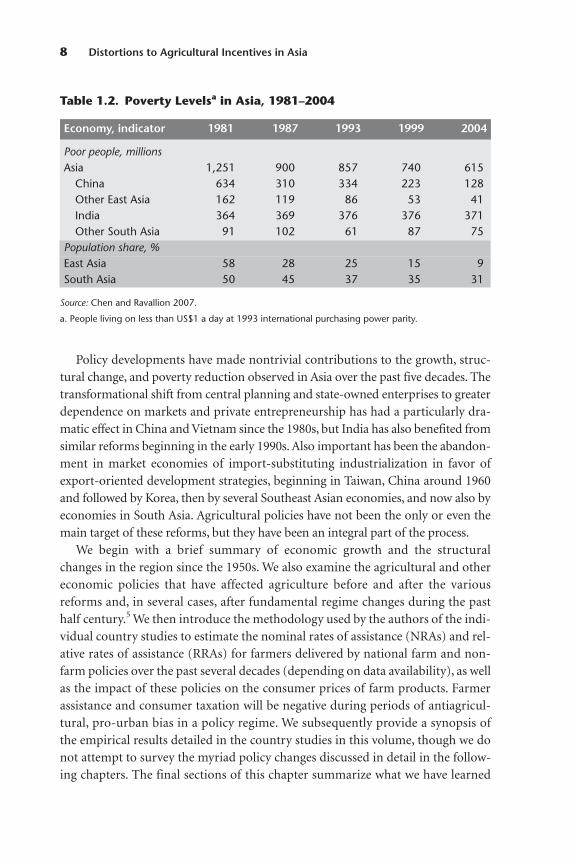
Policy developments have made nontrivial contributions to the growth, struc-tural change, and poverty reduction observed in Asia over the past five decades. Thetransformational shift from central planning and state-owned enterprises to greaterdependence on markets and private entrepreneurship has had a particularly dra-matic effect in China and Vietnam since the 1980s, but India has also benefited fromsimilar reforms beginning in the early 1990s. Also important has been the abandon-ment in market economies of import-substituting industrialization in favor ofexport-oriented development strategies, beginning in Taiwan, China around 1960and followed by Korea, then by several Southeast Asian economies, and now also byeconomies in South Asia. Agricultural policies have not been the only or even themain target of these reforms, but they have been an integral part of the process.
We begin with a brief summary of economic growth and the structuralchanges in the region since the 1950s. We also examine the agricultural and othereconomic policies that have affected agriculture before and after the variousreforms and, in several cases, after fundamental regime changes during the pasthalf century.5 We then introduce the methodology used by the authors of the indi-vidual country studies to estimate the nominal rates of assistance (NRAs) and rel-ative rates of assistance (RRAs) for farmers delivered by national farm and non-farm policies over the past several decades (depending on data availability), as wellas the impact of these policies on the consumer prices of farm products. Farmerassistance and consumer taxation will be negative during periods of antiagricul-tural, pro-urban bias in a policy regime. We subsequently provide a synopsis ofthe empirical results detailed in the country studies in this volume, though we donot attempt to survey the myriad policy changes discussed in detail in the follow-ing chapters. The final sections of this chapter summarize what we have learned
8 Distortions to Agricultural Incentives in Asia
Table 1.2. Poverty Levelsa in Asia, 1981–2004
Economy, indicator 1981 1987 1993 1999 2004
Poor people, millionsAsia 1,251 900 857 740 615
China 634 310 334 223 128Other East Asia 162 119 86 53 41India 364 369 376 376 371Other South Asia 91 102 61 87 75
Population share, %East Asia 58 28 25 15 9South Asia 50 45 37 35 31
Source: Chen and Ravallion 2007.
a. People living on less than US$1 a day at 1993 international purchasing power parity.
and draw out the implications of the findings for poverty, inequality, and the possible future direction of policies affecting agricultural incentives in Asia.
Growth and Structural Change
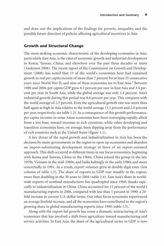
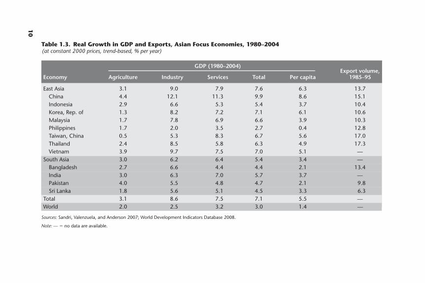
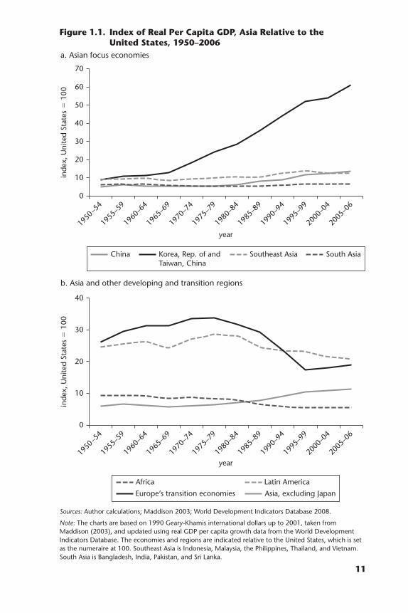
The most striking economic characteristic of the developing economies in Asia,particularly East Asia, is the rates of economic growth and industrial developmentin Korea; Taiwan, China; and elsewhere over the past three decades or more(Anderson 2008). The recent report of the Commission on Growth and Develop-ment (2008) has noted that 13 of the world’s economies have had sustainedgrowth in real per capita income of more than 7 percent for at least 25 consecutiveyears since World War II, and nine of these economies are in East Asia.6 Between1980 and 2004, per capita GDP grew 6.3 percent per year in East Asia and 3.4 per-cent per year in South Asia, while the global average was only 1.4 percent. Asia’sindustrial growth during this period was 8.6 percent per year. This compares withthe world average of 2.5 percent. Even the agricultural growth rate was more thanhalf again as high in Asia relative to the world average (3.1 percent and 2.0 percentper year, respectively; see table 1.3). As a consequence of this growth performance,per capita incomes in some Asian economies have been converging rapidly, albeitfrom a low base, toward incomes in rich countries, while other developing andtransition economies have, on average, been slipping away from the performanceof rich countries such as the United States (figure 1.1).
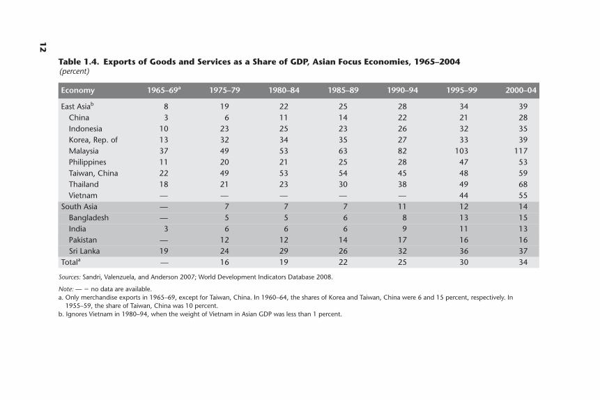
A key driver of the rapid growth and industrialization in Asia has been thedecision by many governments in the region to open up economies and abandonan import-substituting development strategy in favor of an export-orientedapproach. This shift occurred at different times in our focus economies, beginningwith Korea and Taiwan, China in the 1960s. China joined the group in the late1970s, Vietnam in the mid-1980s, and India haltingly in the early 1980s and moreconcertedly in 1991. As a result, export volumes grew at double-digit rates (lastcolumn of table 1.3). The share of exports in GDP rose steadily in the region,more than doubling in the 30 years to 2004 (table 1.4). East Asia’s share in world-wide exports of nonfood manufactures has quadrupled since 1990, thanks espe-cially to industrialization in China. China accounted for 11 percent of the world’smanufacturing exports in 2006, compared with less than 1 percent in 1990: a 20-fold increase in current U.S. dollar terms. Our other focus economies experiencedan average fivefold increase, and all the economies have contributed to the region’sgrowing share in global manufacturing exports since 1990 (table 1.5).7
Along with the export-led growth has come a dramatic restructuring of Asia’seconomies that has involved a shift from agriculture toward manufacturing andservice activities. In East Asia, the share of the agricultural sector in GDP is now
Introduction and Summary 9
10
Table 1.3. Real Growth in GDP and Exports, Asian Focus Economies, 1980–2004(at constant 2000 prices, trend-based, % per year)
GDP (1980–2004)Export volume,
Economy Agriculture Industry Services Total Per capita 1985–95
East Asia 3.1 9.0 7.9 7.6 6.3 13.7China 4.4 12.1 11.3 9.9 8.6 15.1Indonesia 2.9 6.6 5.3 5.4 3.7 10.4Korea, Rep. of 1.3 8.2 7.2 7.1 6.1 10.6Malaysia 1.7 7.8 6.9 6.6 3.9 10.3Philippines 1.7 2.0 3.5 2.7 0.4 12.8Taiwan, China 0.5 5.3 8.3 6.7 5.6 17.0Thailand 2.4 8.5 5.8 6.3 4.9 17.3Vietnam 3.9 9.7 7.5 7.0 5.1 —
South Asia 3.0 6.2 6.4 5.4 3.4 —Bangladesh 2.7 6.6 4.4 4.4 2.1 13.4India 3.0 6.3 7.0 5.7 3.7 —Pakistan 4.0 5.5 4.8 4.7 2.1 9.8Sri Lanka 1.8 5.6 5.1 4.5 3.3 6.3
Total 3.1 8.6 7.5 7.1 5.5 —World 2.0 2.5 3.2 3.0 1.4 —
Sources: Sandri, Valenzuela, and Anderson 2007; World Development Indicators Database 2008.
Note: — � no data are available.
0
10
20
30
40
50
60
70
year
inde
x, U
nite
d St
ates
� 1
00
1950
–54
1955
–59
1960
–64
1965
–69
1970
–74
1975
–79
1980
–84
1985
–89
1990
–94
1995
–99
2000
–04
2005
–06
Southeast Asia South AsiaChina Korea, Rep. of andTaiwan, China
Figure 1.1. Index of Real Per Capita GDP, Asia Relative to theUnited States, 1950–2006
a. Asian focus economies
Sources: Author calculations; Maddison 2003; World Development Indicators Database 2008.
Note: The charts are based on 1990 Geary-Khamis international dollars up to 2001, taken fromMaddison (2003), and updated using real GDP per capita growth data from the World DevelopmentIndicators Database. The economies and regions are indicated relative to the United States, which is setas the numeraire at 100. Southeast Asia is Indonesia, Malaysia, the Philippines, Thailand, and Vietnam.South Asia is Bangladesh, India, Pakistan, and Sri Lanka.
0
10
20
30
40
year
inde
x, U
nite
d St
ates
� 1
00
1950
–54
1955
–59
1960
–64
1965
–69
1970
–74
1975
–79
1980
–84
1985
–89
1990
–94
1995
–99
2000
–04
2005
–06
Europe’s transition economies Asia, excluding Japan
Africa Latin America
b. Asia and other developing and transition regions
11
12
Table 1.4. Exports of Goods and Services as a Share of GDP, Asian Focus Economies, 1965–2004(percent)
Economy 1965–69a 1975–79 1980–84 1985–89 1990–94 1995–99 2000–04
East Asiab 8 19 22 25 28 34 39China 3 6 11 14 22 21 28Indonesia 10 23 25 23 26 32 35Korea, Rep. of 13 32 34 35 27 33 39Malaysia 37 49 53 63 82 103 117Philippines 11 20 21 25 28 47 53Taiwan, China 22 49 53 54 45 48 59Thailand 18 21 23 30 38 49 68Vietnam — — — — — 44 55
South Asia — 7 7 7 11 12 14Bangladesh — 5 5 6 8 13 15India 3 6 6 6 9 11 13Pakistan — 12 12 14 17 16 16Sri Lanka 19 24 29 26 32 36 37
Totala — 16 19 22 25 30 34
Sources: Sandri, Valenzuela, and Anderson 2007; World Development Indicators Database 2008.
Note: — � no data are available.a. Only merchandise exports in 1965–69, except for Taiwan, China. In 1960–64, the shares of Korea and Taiwan, China were 6 and 15 percent, respectively. In
1955–59, the share of Taiwan, China was 10 percent.b. Ignores Vietnam in 1980–94, when the weight of Vietnam in Asian GDP was less than 1 percent.
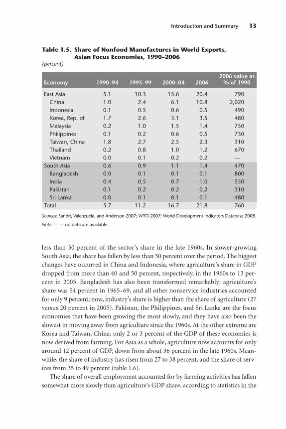
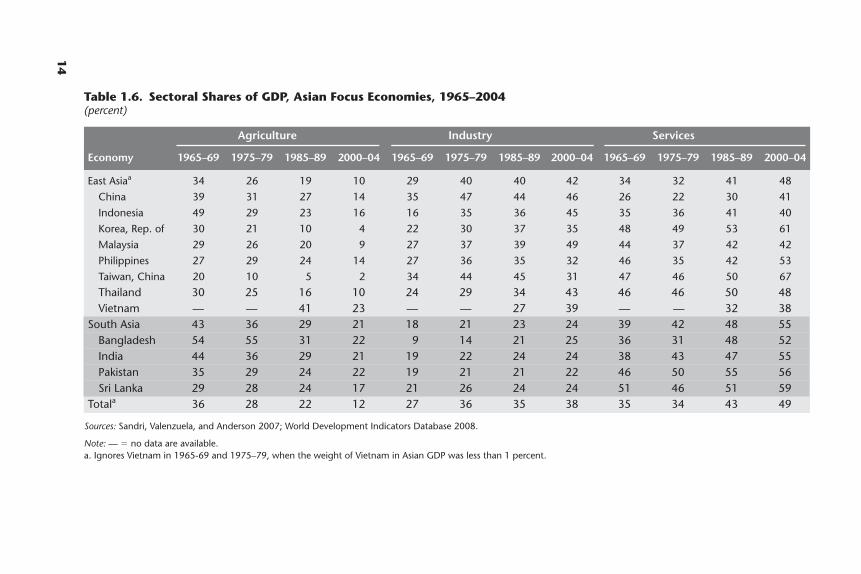
less than 30 percent of the sector’s share in the late 1960s. In slower-growingSouth Asia, the share has fallen by less than 50 percent over the period. The biggestchanges have occurred in China and Indonesia, where agriculture’s share in GDPdropped from more than 40 and 50 percent, respectively, in the 1960s to 13 per-cent in 2005. Bangladesh has also been transformed remarkably: agriculture’sshare was 54 percent in 1965–69, and all other nonservice industries accountedfor only 9 percent; now, industry’s share is higher than the share of agriculture (27versus 20 percent in 2005). Pakistan, the Philippines, and Sri Lanka are the focuseconomies that have been growing the most slowly, and they have also been theslowest in moving away from agriculture since the 1960s. At the other extreme areKorea and Taiwan, China; only 2 or 3 percent of the GDP of these economies isnow derived from farming. For Asia as a whole, agriculture now accounts for onlyaround 12 percent of GDP, down from about 36 percent in the late 1960s. Mean-while, the share of industry has risen from 27 to 38 percent, and the share of serv-ices from 35 to 49 percent (table 1.6).
The share of overall employment accounted for by farming activities has fallensomewhat more slowly than agriculture’s GDP share, according to statistics in the
Introduction and Summary 13
Table 1.5. Share of Nonfood Manufactures in World Exports,Asian Focus Economies, 1990–2006
(percent)
2006 value asEconomy 1990–94 1995–99 2000–04 2006 % of 1990
East Asia 5.1 10.3 15.6 20.4 790China 1.0 2.4 6.1 10.8 2,020Indonesia 0.1 0.5 0.6 0.5 490Korea, Rep. of 1.7 2.6 3.1 3.5 480Malaysia 0.2 1.0 1.5 1.4 750Philippines 0.1 0.2 0.6 0.5 730Taiwan, China 1.8 2.7 2.5 2.3 310Thailand 0.2 0.8 1.0 1.2 670Vietnam 0.0 0.1 0.2 0.2 —
South Asia 0.6 0.9 1.1 1.4 470Bangladesh 0.0 0.1 0.1 0.1 800India 0.4 0.5 0.7 1.0 550Pakistan 0.1 0.2 0.2 0.2 310Sri Lanka 0.0 0.1 0.1 0.1 480
Total 5.7 11.2 16.7 21.8 760
Sources: Sandri, Valenzuela, and Anderson 2007; WTO 2007; World Development Indicators Database 2008.
Note: — � no data are available.
14
Table 1.6. Sectoral Shares of GDP, Asian Focus Economies, 1965–2004(percent)
Agriculture Industry Services
Economy 1965–69 1975–79 1985–89 2000–04 1965–69 1975–79 1985–89 2000–04 1965–69 1975–79 1985–89 2000–04
East Asiaa 34 26 19 10 29 40 40 42 34 32 41 48
China 39 31 27 14 35 47 44 46 26 22 30 41
Indonesia 49 29 23 16 16 35 36 45 35 36 41 40
Korea, Rep. of 30 21 10 4 22 30 37 35 48 49 53 61
Malaysia 29 26 20 9 27 37 39 49 44 37 42 42
Philippines 27 29 24 14 27 36 35 32 46 35 42 53
Taiwan, China 20 10 5 2 34 44 45 31 47 46 50 67
Thailand 30 25 16 10 24 29 34 43 46 46 50 48Vietnam — — 41 23 — — 27 39 — — 32 38
South Asia 43 36 29 21 18 21 23 24 39 42 48 55Bangladesh 54 55 31 22 9 14 21 25 36 31 48 52India 44 36 29 21 19 22 24 24 38 43 47 55Pakistan 35 29 24 22 19 21 21 22 46 50 55 56Sri Lanka 29 28 24 17 21 26 24 24 51 46 51 59
Totala 36 28 22 12 27 36 35 38 35 34 43 49
Sources: Sandri, Valenzuela, and Anderson 2007; World Development Indicators Database 2008.
Note: — � no data are available.a. Ignores Vietnam in 1965-69 and 1975–79, when the weight of Vietnam in Asian GDP was less than 1 percent.
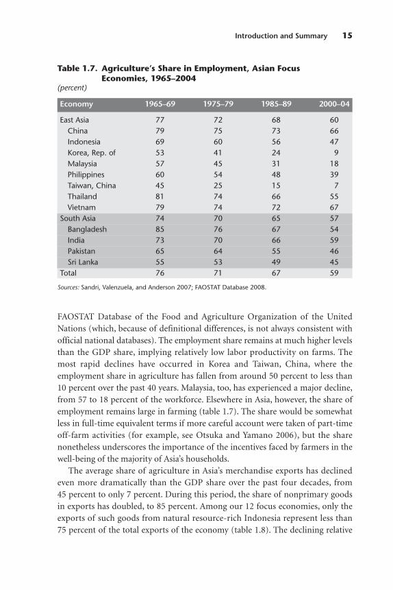
FAOSTAT Database of the Food and Agriculture Organization of the UnitedNations (which, because of definitional differences, is not always consistent withofficial national databases). The employment share remains at much higher levelsthan the GDP share, implying relatively low labor productivity on farms. Themost rapid declines have occurred in Korea and Taiwan, China, where theemployment share in agriculture has fallen from around 50 percent to less than10 percent over the past 40 years. Malaysia, too, has experienced a major decline,from 57 to 18 percent of the workforce. Elsewhere in Asia, however, the share ofemployment remains large in farming (table 1.7). The share would be somewhatless in full-time equivalent terms if more careful account were taken of part-timeoff-farm activities (for example, see Otsuka and Yamano 2006), but the sharenonetheless underscores the importance of the incentives faced by farmers in thewell-being of the majority of Asia’s households.
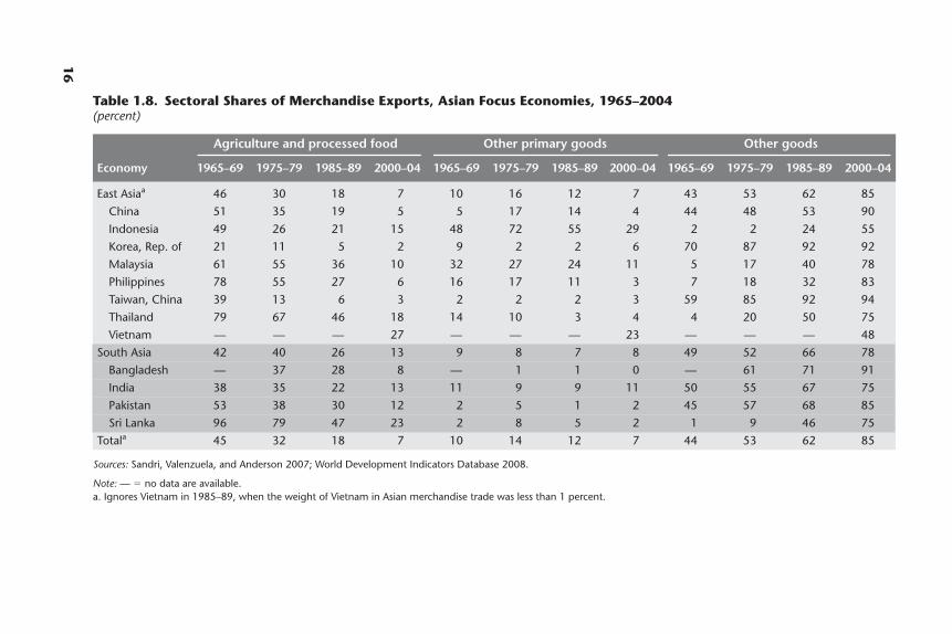
The average share of agriculture in Asia’s merchandise exports has declinedeven more dramatically than the GDP share over the past four decades, from45 percent to only 7 percent. During this period, the share of nonprimary goodsin exports has doubled, to 85 percent. Among our 12 focus economies, only theexports of such goods from natural resource-rich Indonesia represent less than75 percent of the total exports of the economy (table 1.8). The declining relative
Introduction and Summary 15
Table 1.7. Agriculture’s Share in Employment, Asian FocusEconomies, 1965–2004
(percent)
Economy 1965–69 1975–79 1985–89 2000–04
East Asia 77 72 68 60China 79 75 73 66Indonesia 69 60 56 47Korea, Rep. of 53 41 24 9Malaysia 57 45 31 18Philippines 60 54 48 39Taiwan, China 45 25 15 7Thailand 81 74 66 55Vietnam 79 74 72 67
South Asia 74 70 65 57Bangladesh 85 76 67 54India 73 70 66 59Pakistan 65 64 55 46Sri Lanka 55 53 49 45
Total 76 71 67 59
Sources: Sandri, Valenzuela, and Anderson 2007; FAOSTAT Database 2008.
16
Table 1.8. Sectoral Shares of Merchandise Exports, Asian Focus Economies, 1965–2004(percent)
Agriculture and processed food Other primary goods Other goods
Economy 1965–69 1975–79 1985–89 2000–04 1965–69 1975–79 1985–89 2000–04 1965–69 1975–79 1985–89 2000–04
East Asiaa 46 30 18 7 10 16 12 7 43 53 62 85
China 51 35 19 5 5 17 14 4 44 48 53 90
Indonesia 49 26 21 15 48 72 55 29 2 2 24 55
Korea, Rep. of 21 11 5 2 9 2 2 6 70 87 92 92
Malaysia 61 55 36 10 32 27 24 11 5 17 40 78
Philippines 78 55 27 6 16 17 11 3 7 18 32 83
Taiwan, China 39 13 6 3 2 2 2 3 59 85 92 94
Thailand 79 67 46 18 14 10 3 4 4 20 50 75
Vietnam — — — 27 — — — 23 — — — 48
South Asia 42 40 26 13 9 8 7 8 49 52 66 78
Bangladesh — 37 28 8 — 1 1 0 — 61 71 91
India 38 35 22 13 11 9 9 11 50 55 67 75
Pakistan 53 38 30 12 2 5 1 2 45 57 68 85
Sri Lanka 96 79 47 23 2 8 5 2 1 9 46 75
Totala 45 32 18 7 10 14 12 7 44 53 62 85
Sources: Sandri, Valenzuela, and Anderson 2007; World Development Indicators Database 2008.
Note: — � no data are available.a. Ignores Vietnam in 1985–89, when the weight of Vietnam in Asian merchandise trade was less than 1 percent.
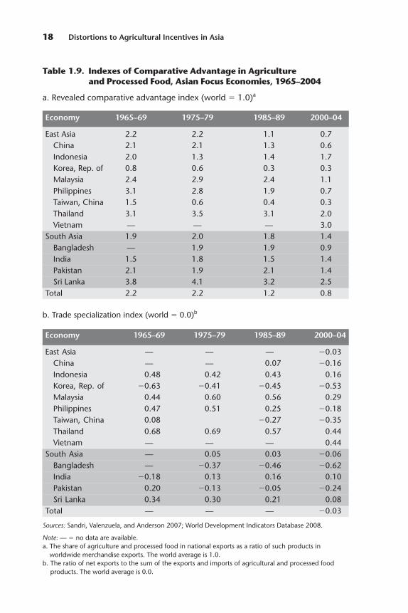
importance of farm exports has been much more rapid in Asia than in the rest ofthe world: the index of the revealed agricultural comparative advantage for Asia—defined as the share of agriculture and processed food in national exports as aratio of the share of such products in worldwide merchandise exports—has fallensince the 1980s by about two-thirds in East Asia and one-third in South Asia. Theindex of agricultural trade specialization (defined as net exports, divided by thesum of imports and exports of agricultural and processed food products) has alsofallen. The latter index, by definition, ranges from �1 to �1. It has becomeincreasingly less positive, or it has become negative in virtually all our Asian focuseconomies in recent decades (table 1.9).
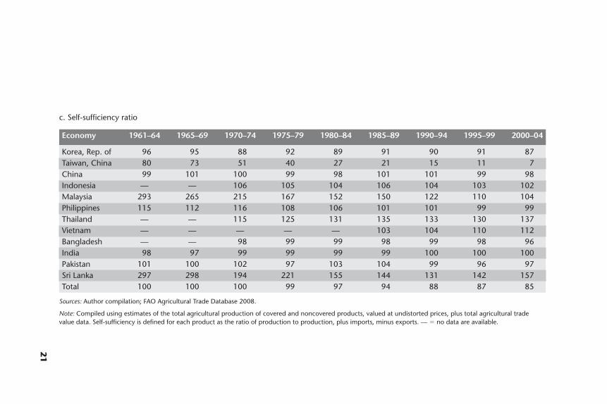
This apparent decline in agricultural comparative advantage is evident in theself-sufficiency data on primary farm products. Until 30 years ago, the region wasalmost exactly 100 percent self-sufficient in farm products; but, since then, theindicator has declined to less than 85 percent. The share of farm production thatis exported has not changed much, averaging in the 4–6 percent range. However,there have been substantial changes in individual economies, including declines inMalaysia, the Philippines, Sri Lanka, and Taiwan, China and increases in China,Thailand, and Vietnam. In contrast, since the late 1970s, the share of imports inthe domestic consumption of farm products has quadrupled, to around 20 per-cent (table 1.10).
The growing dependence on imports of farm products in Asia has occurreddespite reductions in the taxation of agricultural exports and increases in the incen-tives provided to farmers through government policy reforms (discussed below).These reforms have probably contributed to poverty reduction in Asia. Using a priceindicator that is simpler than the one developed by us below, Ravallion and Chen(2007) show that the reduction in the antiagricultural bias in farm price policies hascontributed significantly to poverty reduction in China. Rural growth is also a keycontributor to the reduction in poverty in India (Ravallion and Datt 1996). One mayrevisit these and other, similar studies using the more comprehensive measures of theextent of changes in distortions to agricultural incentives summarized below. To gen-erate these measures, a common methodology has been adopted by the authors ofthe country case studies in this volume. A summary of the methodology follows, andadditional details may be found in Anderson et al. (2008) and in appendix A.
Methodology for Measuring Ratesof Assistance or Taxation
The NRA is defined as the percentage by which government policies have raised(or lowered if the NRA is less than 0) the gross returns to producers above (or below)the gross returns they would have received without government intervention. If a
Introduction and Summary 17
(Text continues on page 22.)
18 Distortions to Agricultural Incentives in Asia
b. Trade specialization index (world � 0.0)b
Economy 1965–69 1975–79 1985–89 2000–04
East Asia — — — �0.03China — — 0.07 �0.16Indonesia 0.48 0.42 0.43 0.16Korea, Rep. of �0.63 �0.41 �0.45 �0.53Malaysia 0.44 0.60 0.56 0.29Philippines 0.47 0.51 0.25 �0.18Taiwan, China 0.08 �0.27 �0.35Thailand 0.68 0.69 0.57 0.44Vietnam — — — 0.44
South Asia — 0.05 0.03 �0.06Bangladesh — �0.37 �0.46 �0.62India �0.18 0.13 0.16 0.10Pakistan 0.20 �0.13 �0.05 �0.24Sri Lanka 0.34 0.30 0.21 0.08
Total — — — �0.03
Sources: Sandri, Valenzuela, and Anderson 2007; World Development Indicators Database 2008.
Note: — � no data are available.a. The share of agriculture and processed food in national exports as a ratio of such products in
worldwide merchandise exports. The world average is 1.0.b. The ratio of net exports to the sum of the exports and imports of agricultural and processed food
products. The world average is 0.0.
Table 1.9. Indexes of Comparative Advantage in Agricultureand Processed Food, Asian Focus Economies, 1965–2004
a. Revealed comparative advantage index (world � 1.0)a
Economy 1965–69 1975–79 1985–89 2000–04
East Asia 2.2 2.2 1.1 0.7China 2.1 2.1 1.3 0.6Indonesia 2.0 1.3 1.4 1.7Korea, Rep. of 0.8 0.6 0.3 0.3Malaysia 2.4 2.9 2.4 1.1Philippines 3.1 2.8 1.9 0.7Taiwan, China 1.5 0.6 0.4 0.3Thailand 3.1 3.5 3.1 2.0Vietnam — — — 3.0
South Asia 1.9 2.0 1.8 1.4Bangladesh — 1.9 1.9 0.9India 1.5 1.8 1.5 1.4Pakistan 2.1 1.9 2.1 1.4Sri Lanka 3.8 4.1 3.2 2.5
Total 2.2 2.2 1.2 0.8

19
Table 1.10. Export Orientation, Import Dependence, and Self-Sufficiency in Primary AgriculturalProduction, Asian Focus Economies, 1961–2004
(%, at undistorted prices)
a. Exports, as a share of production
Economy 1961–64 1965–69 1970–74 1975–79 1980–84 1985–89 1990–94 1995–99 2000–04
Korea, Rep. of 0 0 0 0 0 0 0 2 1Taiwan, China 5 9 13 14 10 10 6 5 6China 2 2 2 3 5 5 7 7 7Indonesia — — 6 5 5 6 4 5 4Malaysia 70 64 54 41 35 34 19 12 9Philippines 13 11 14 8 7 2 1 1 1Thailand — — 13 20 24 26 25 25 30Vietnam — — — — — 3 4 9 11Bangladesh — — — 3 3 3 2 1 1India 1 1 1 1 1 1 1 1 2Pakistan 7 5 5 2 5 8 4 2 1Sri Lanka 68 62 44 52 36 34 24 31 39Total 3 4 4 4 4 6 6 5 5
(Table continues on the following page.)

20
Table 1.10. Export Orientation, Import Dependence, and Self-Sufficiency in Primary AgriculturalProduction, Asian Focus Economies, 1961–2004 (continued)
b. Imports, as a share of apparent consumption
Economy 1961–64 1965–69 1970–74 1975–79 1980–84 1985–89 1990–94 1995–99 2000–04
Korea, Rep. of 4 5 12 8 11 9 11 11 13Taiwan, China 24 33 56 66 76 81 86 90 93China 2 2 2 3 5 5 7 7 7Indonesia — — 0 1 1 1 1 2 2Malaysia 13 6 3 1 1 1 2 3 6Philippines 0 0 1 0 1 0 0 2 1Thailand — — 0 0 0 0 0 2 5Vietnam — — — — — 0 0 0 0Bangladesh — — — 3 4 5 3 3 5India 3 4 2 2 1 1 1 1 2Pakistan 6 5 3 5 2 5 5 6 4Sri Lanka 7 5 1 0 1 4 1 3 5Total 3 4 4 5 7 12 17 17 19
21
c. Self-sufficiency ratio
Economy 1961–64 1965–69 1970–74 1975–79 1980–84 1985–89 1990–94 1995–99 2000–04
Korea, Rep. of 96 95 88 92 89 91 90 91 87Taiwan, China 80 73 51 40 27 21 15 11 7China 99 101 100 99 98 101 101 99 98Indonesia — — 106 105 104 106 104 103 102Malaysia 293 265 215 167 152 150 122 110 104Philippines 115 112 116 108 106 101 101 99 99Thailand — — 115 125 131 135 133 130 137Vietnam — — — — — 103 104 110 112Bangladesh — — 98 99 99 98 99 98 96India 98 97 99 99 99 99 100 100 100Pakistan 101 100 102 97 103 104 99 96 97Sri Lanka 297 298 194 221 155 144 131 142 157Total 100 100 100 99 97 94 88 87 85
Sources: Author compilation; FAO Agricultural Trade Database 2008.
Note: Compiled using estimates of the total agricultural production of covered and noncovered products, valued at undistorted prices, plus total agricultural tradevalue data. Self-sufficiency is defined for each product as the ratio of production to production, plus imports, minus exports. — � no data are available.

trade measure is the sole government intervention, then the measured NRA willalso be the consumer tax equivalent (CTE) rate at that same point in the valuechain. Where there are also domestic producer or consumer taxes or subsidies, theNRA and CTE will no longer be equal, and at least one of them will be differentfrom the price distortion at the border caused by trade measures.8
NRAs and CTEs may be used for several purposes, and the purpose affects theappropriate choice of methodology. In our project, we rely on NRAs and CTEs toachieve three purposes. One purpose is to generate a comparable set of numbersacross a wide range of countries and over a long time period. This means themethodology must be both simple and somewhat flexible. Another purpose is toprovide a single number, the NRA, to indicate the total extent of transfers to orfrom farmers because of government agricultural policies and another number,the CTE, to indicate the extent of the transfers to or from consumers. The NRAand the CTE are both expressed as a percentage of the undistorted price or in dol-lar terms. This is also the purpose of the OECD’s producer and consumer supportestimates, which may be negative if the transfers from the relevant group exceedthe transfers to the relevant group. Our research project’s agricultural NRAs andCTEs are similar in spirit to the OECD estimates, but there are also important dif-ferences, which are outlined below. Our third purpose is to enable economic mod-elers to use the NRAs as producer price wedges for individual primary and lightlyprocessed agricultural products and to use the CTEs as consumer price wedges insingle-sector, multisector, and economy-wide policy simulation models by allo-cating these wedges to particular policy instruments such as trade taxes or domes-tic producer or consumer subsidies or taxes.
The NRAs are based on our estimates of assistance to individual industries.Great care has gone into generating the NRAs for each covered agricultural indus-try, particularly in countries where trade costs are high, the pass-through alongthe value chain is affected by imperfect competition, and the markets for foreigncurrency have been highly distorted to varying degrees at various times.
Most distortions in industries producing tradables arise from trade measuressuch as quantitative trade restrictions or tariffs imposed on the import cost,insurance, and freight price or export subsidies or taxes imposed on the free onboard price at the country’s border. An ad valorem tariff or export subsidy is theequivalent of a production subsidy and a consumption tax at the same rateexpressed as a percentage of the border price. For this reason, such tariffs and sub-sidies are captured in the NRAs and CTEs at the point in the value chain at whicha product is first traded. To obtain the NRAs for farmers, the authors of the coun-try studies have estimated or guessed the extent of pass-through back to the farm-gate and added any domestic farm output subsidies. To obtain the CTEs, they have
22 Distortions to Agricultural Incentives in Asia
also added any product-specific domestic consumer taxes to the distortionscaused by border measures. Note that the NRAs and CTEs differ from the OECD’sproducer and consumer support estimates in that the latter pair is expressed as apercentage of the distorted price and, hence, will be lower (for positive protectionrates) than the former pair, which is expressed as a percentage of the undistortedprice.
We have decided not to seek estimates of the more complex effective rate ofassistance even though it is, in principle, a better single partial equilibrium measureof the distortions in producer incentives. To establish these alternative estimates,we must know, for each product, the value added and various intermediate inputshares in output. These data are not available in most developing countries even fora few years, let alone for every year in the long time series that is the focus of ourstudy. Moreover, in most countries, the distortions in farm input prices are smallcompared with the distortions in farm output prices. Nonetheless, if the product-specific distortions to input costs are significant, they may be captured by estimat-ing their equivalent values in terms of a higher output price and then including thisestimate in the NRA for individual agricultural industries wherever data allow. Wealso add any non-product-specific distortions, including distortions in farm inputprices, into the estimate for the overall sectoral NRA for agriculture.
The targeted minimum product coverage of our NRA estimates is 70 percentbased on the gross value of farm production at undistorted prices. This target cov-erage is similar to the coverage of the OECD producer support estimates. Unlikethe OECD, however, we do not routinely assume that the nominal assistance forcovered products applies equally to the farm products we do not cover. This isbecause, in developing countries, agricultural policies affecting our noncoveredproducts are often different from those affecting our covered products. For exam-ple, nontradables among noncovered farm goods—often highly perishable prod-ucts or products of low value relative to the transport cost—are frequently notsubject to direct distortionary policies. We have asked the authors of the countrycase studies to provide three sets of NRA guesstimates for noncovered farm prod-ucts, one each for the import-competing, exportable, and nontradable subsectors.Weighted averages for all agricultural products have then been generated usingthe gross values of production at unassisted prices as weights. For countries thatalso provide non-product-specific agricultural subsidies or taxes—assumed to beshared on a pro rata basis between tradables and nontradables—or assistancedecoupled from production, the net assistance from these measures is then addedto the product-specific assistance to obtain NRAs for total agriculture. We applythe same procedure to obtain NRAs also for tradable agriculture for use in gener-ating RRAs (which are defined below).
Introduction and Summary 23
How best to present regional aggregate NRA and RRA estimates depends onthe purpose for which the averages are required. We generate weighted averageNRAs for covered products for each country because only then are we able to addthe NRAs for noncovered products and the non-product-specific assistance toobtain the NRAs for all agriculture. In averaging across countries, we considereach polity as an observation of interest. So, a simple average is meaningful for thepurpose of political economy analysis. However, if one wishes to acquire a sense ofthe distortion in the agriculture of an entire region, one needs a weighted average.The weighted average NRAs for covered primary agriculture may be generated bymultiplying the share of each primary industry in the gross value of production(valued at farmgate equivalent undistorted prices) by the corresponding NRAsand adding across industries.9 The overall sectoral rate, which we denote asNRAag, may be obtained by also adding the actual or assumed information fornoncovered farm commodities and, where it exists, the aggregate value of non-product-specific and decoupled assistance in agriculture.
A weighted average can be similarly generated for the tradables part of agricul-ture, including those industries producing products such as milk and sugar thatrequire only light processing before they are traded. This is accomplished byassuming that the product’s share of non-product-specific assistance equals theproduct’s weight in the total. Call this NRAagt.
In addition to the mean, it is important also to provide a measure of the dis-persion or variability of the NRA estimates across the covered products. The costof government policy distortions in incentives in terms of resource misallocationtends to be greater, the greater the degree of substitution in production (Lloyd1974). In the case of an agricultural sector that involves a use of farmland that issector specific, but transferable among farm activities, the greater the variation ofNRAs across industries within the sector, then the higher will be the welfare costof the market interventions. A simple indicator of dispersion is the standard devi-ation in the NRAs of the covered industries.
Each industry is classified as import-competing, or as a producer of exporta-bles, or as a producer of nontradables. This status sometimes changes over time. Itis possible to generate for each year the weighted average NRAs for the two groupsof tradables (import-competing products and exportables). These NRAs are usedto generate a trade bias index (TBI), which is defined as follows:
TBI � [(1 � NRAagx�100)�(1 � NRAagm�100) � 1], (1.1)
where NRAagm and NRAagx are the average percentage NRAs for the import- competing and exportable parts of the agricultural sector. The TBI indicates, in asingle number, the extent to which the (typically) antitrade bias (negative TBI) inagricultural policies changes over time.
24 Distortions to Agricultural Incentives in Asia
Farmers are affected not only by the prices for their own outputs, but also,albeit indirectly, through changes in factor market prices and the exchange ratebecause of the incentives nonagricultural producers face. Thus, it is the relativeprices and, hence, the relative rates of government assistance that affect producerincentives. More than 70 years ago, Lerner (1936) provided the symmetry theo-rem, which proved that, in a two-sector economy, an import tax has the sameeffect as an export tax. This carries over to a model that also includes a third sec-tor producing only nontradables and to a model with imperfect competition,regardless of the economy’s size (Vousden 1990). If one assumes that there are nodistortions in the markets for nontradables and that the value shares of agricul-tural and nonagricultural nontradable products remain constant, then the economy-wide effect of distortions in agricultural incentives may be captured bymeasuring the extent to which the tradable parts of agricultural production areassisted or taxed relative to the producers of other tradables. Because we are ableto generate estimates of the average NRAs for nonagricultural tradables, we arethen able to calculate an RRA, which is defined in percentage terms as follows:
RRA � 100[(1 � NRAagt�100)�(1 � NRAnonagt�100) � 1], (1.2)
where NRAagt and NRAnonagt are the weighted average percentage NRAs for thetradable parts of the agricultural and nonagricultural sectors, respectively. Sincethe NRA cannot be less than �100 percent if producers are to earn anything, nei-ther can the RRA (assuming NRAnonagt is positive). If both of those sectors areequally assisted, the RRA is zero. This measure is useful in that, if it is below(above) zero, it provides an internationally comparable indication of the extent towhich a country’s policy regime has an anti- or proagricultural bias.
In calculating the NRAs for producers of agricultural and nonagriculturaltradables, we use the methodology outlined in appendix A to seek to includedistortions generated by dual or multiple exchange rates. Direct interventions inthe markets for foreign currency were common in some Asian countries, includ-ing China in the 1970s and 1980s. However, authors of some of the focus coun-try studies have experienced difficulty in determining an appropriate estimateof the extent of this distortion. So, the impact of such interventions on theNRAs has not been included in all the studies. The exclusion of this impact insome countries (for example, India) means that the estimated (typically) posi-tive NRAs for importables and (typically) negative NRAs for exportables aresmaller than they should be in these studies. In cases where the NRAs forimportables dominate the NRAs for exportables, this omission would lead to anunderestimate of the average (positive) NRAs for such tradables. The conversewould also be true. In either case, this leads also to an underestimate of the(anti-)TBI.
Introduction and Summary 25
To obtain U.S. dollar values for farmer assistance and consumer taxation,Valenzuela, Kurzweil, Croser, Nelgen, and Anderson (see appendix B) have multi-plied the country author NRA estimates by the gross value of production atundistorted prices to obtain an estimate, in current U.S. dollars, of the direct grosssubsidy equivalents of assistance to farmers. These estimates are then added acrossthe products of a country and across countries for all products to obtain regionalaggregate transfer estimates for the economies under study. These values are cal-culated in constant dollars and are also expressed as estimates per farmworker.
To obtain comparable U.S. dollar value estimates of consumer transfers, theCTE estimate at the point at which a product is first traded is multiplied by con-sumption (obtained from the FAO SUA-FBS Database), which is valued at undis-torted prices, to obtain an estimate in constant U.S. dollars of the tax equivalent toconsumers of primary farm products. This is then added across the products of acountry and across countries for any or all products to obtain regional aggregatetransfer estimates on the economies under study. These values are also expressedon a per capita basis.
Estimates of Asian Policy Indicators
We begin with the NRAs in agriculture and compare them with the NRAs fornonagricultural tradables. We also present constant U.S. dollar equivalents of theassistance and taxation among farmers, as well as the CTEs of policies as theyaffect the buyers of farm products.
NRAs in agriculture
Agricultural price and trade policies reduced average farmer earnings in develop-ing Asia throughout the period up to the 1980s by more than 20 percent.10 Thisimplicit taxation declined beginning in the early 1980s, and, in the mid-1990s, theNRAs switched sign and became increasingly positive. The averages hide consid-erable diversity within the region, however. The nominal assistance for farmers inKorea and Taiwan, China was positive starting in the early 1960s (although smallinitially). The NRAs were slightly above zero in Indonesia during some years inthe 1970s and 1980s, as they were in Pakistan prior to the independence ofBangladesh (East Pakistan) in 1971. The average NRAs in India and the Philip-pines became positive in the 1980s (table 1.11). A visual impression of the differ-ences across countries and the rise in average NRAs is supplied in figure 1.2, inwhich the situation in 2000–04 is compared with the situation in 1980–84. Thistrend is evident among the vast majority of the commodity NRAs for the region,too. Meat and milk were the only products for which the assistance rates were cutover 1980–2004 (figure 1.3).
26 Distortions to Agricultural Incentives in Asia
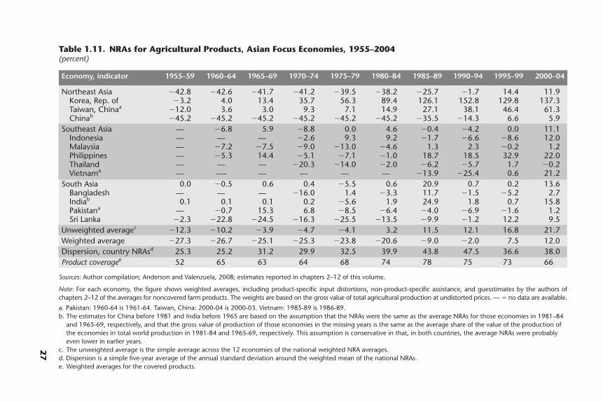
27
Table 1.11. NRAs for Agricultural Products, Asian Focus Economies, 1955–2004(percent)
Economy, indicator 1955–59 1960–64 1965–69 1970–74 1975–79 1980–84 1985–89 1990–94 1995–99 2000–04
Northeast Asia �42.8 �42.6 �41.7 �41.2 �39.5 �38.2 �25.7 �1.7 14.4 11.9Korea, Rep. of �3.2 4.0 13.4 35.7 56.3 89.4 126.1 152.8 129.8 137.3Taiwan, Chinaa �12.0 3.6 3.0 9.3 7.1 14.9 27.1 38.1 46.4 61.3Chinab �45.2 �45.2 �45.2 �45.2 �45.2 �45.2 �35.5 �14.3 6.6 5.9
Southeast Asia — �6.8 5.9 �8.8 0.0 4.6 �0.4 �4.2 0.0 11.1Indonesia — — — �2.6 9.3 9.2 �1.7 �6.6 �8.6 12.0Malaysia — �7.2 �7.5 �9.0 �13.0 �4.6 1.3 2.3 �0.2 1.2Philippines — �5.3 14.4 �5.1 �7.1 �1.0 18.7 18.5 32.9 22.0Thailand — — — �20.3 �14.0 �2.0 �6.2 �5.7 1.7 �0.2Vietnama — —- — — — — �13.9 �25.4 0.6 21.2
South Asia 0.0 �0.5 0.6 0.4 �5.5 0.6 20.9 0.7 0.2 13.6Bangladesh — — — �16.0 1.4 �3.3 11.7 �1.5 �5.2 2.7Indiab 0.1 0.1 0.1 0.2 �5.6 1.9 24.9 1.8 0.7 15.8Pakistana — �0.7 15.3 6.8 �8.5 �6.4 �4.0 �6.9 �1.6 1.2Sri Lanka �2.3 �22.8 �24.5 �16.3 �25.5 �13.5 �9.9 �1.2 12.2 9.5
Unweighted averagec �12.3 �10.2 �3.9 �4.7 �4.1 3.2 11.5 12.1 16.8 21.7Weighted average �27.3 �26.7 �25.1 �25.3 �23.8 �20.6 �9.0 �2.0 7.5 12.0Dispersion, country NRAsd 25.3 25.2 31.2 29.9 32.5 39.9 43.8 47.5 36.6 38.0Product coveragee 52 65 63 64 68 74 78 75 73 66
Sources: Author compilation; Anderson and Valenzuela, 2008; estimates reported in chapters 2–12 of this volume.
Note: For each economy, the figure shows weighted averages, including product-specific input distortions, non-product-specific assistance, and guesstimates by the authors ofchapters 2–12 of the averages for noncovered farm products. The weights are based on the gross value of total agricultural production at undistorted prices. — � no data are available.
a. Pakistan: 1960-64 is 1961-64. Taiwan, China: 2000-04 is 2000-03. Vietnam: 1985-89 is 1986-89.b. The estimates for China before 1981 and India before 1965 are based on the assumption that the NRAs were the same as the average NRAs for those economies in 1981–84
and 1965-69, respectively, and that the gross value of production of those economies in the missing years is the same as the average share of the value of the production ofthe economies in total world production in 1981-84 and 1965-69, respectively. This assumption is conservative in that, in both countries, the average NRAs were probablyeven lower in earlier years.
c. The unweighted average is the simple average across the 12 economies of the national weighted NRA averages.d. Dispersion is a simple five-year average of the annual standard deviation around the weighted mean of the national NRAs.e. Weighted averages for the covered products.

28 Distortions to Agricultural Incentives in Asia
�60
�40
�20
0
20
40
60
80
100
120
140
160
NRA
, %
economy
1980–84 2000–04
Kore
a, Re
p. o
f
Taiw
an, C
hina
Philip
pines
Vietn
am India
Indo
nesia
Sri L
anka
China
Bang
lades
h
Mala
ysia
Pakis
tan
Thail
and
Figure 1.2. NRAs in Agriculture, Asian Focus Economies,1980–84 and 2000–04
Sources: Author compilation; Anderson and Valenzuela, forthcoming; estimates reported in chapters2–12 of this volume.
Note: There are no data for Vietnam in 1980–84. The estimates for China before 1981 are based on theassumption that the NRAs were the same as the average NRAs in 1981–84 and that the gross value ofproduction in the missing years is the same as the average share of the value of production of theeconomy in total world production in 1981–84.
Figure 1.3 also illustrates the diversity of the region’s average NRAs across farmcommodities. In Asia, as in other regions, the product NRAs for rice pudding—rice, milk, and sugar—are among the highest, but, even among these three prod-ucts, there is great diversity across economies in the NRAs. The five-year averagesrange from almost zero to as much as 400 percent for rice and 140 percent formilk in Korea and to 230 percent for sugar in Bangladesh (figure 1.4). This sug-gests that the production of these products in Asia is not optimally allocated forefficient resource use.
There is a great deal of diversity across economies in the average NRAs andacross commodities within the farm sector of each economy. Measured throughthe standard deviation, the extent of both types of diversity has grown rather thandiminished over the past five decades. The cross-economy diversity of average

palm oil
coconuts
rubber
cotton
maize
beef
wheat
pig meat
milk
rice
poultry
sugar
soybeans
150100500�50
pro
duct
2000–04 1980–84
NRA, %
Figure 1.3. NRAs, by Product, Asian Focus Economies, 1980–84and 2000–04
a. Unweighted average
Sources: Author compilation; Anderson and Valenzuela, forthcoming; estimates reported inchapters 2–12 of this volume.
a. Weights are based on the gross value of total agricultural production at undistorted prices. Each NRAby economy and by product has been weighted by the value of the production in the economy of thatcommodity in a given year. Products representing less than 1 percent of the gross value of regionalproduction are excluded. These include cocoa, onions, chilies, barley, jute, sunflower seeds, garlic, peppers,cabbages, cassava, potatoes, eggs, tea, coffee, sorghum, rapeseeds, chickpeas, groundnuts, and beef.
0 50 100 150
coconuts
palm oil
rubber
pig meat
cotton
wheat
poultry
maize
soybeans
rice
milk
sugar
beef
�50
pro
duct
2000–04 1980–84
NRA, %
b. Weighted averagea
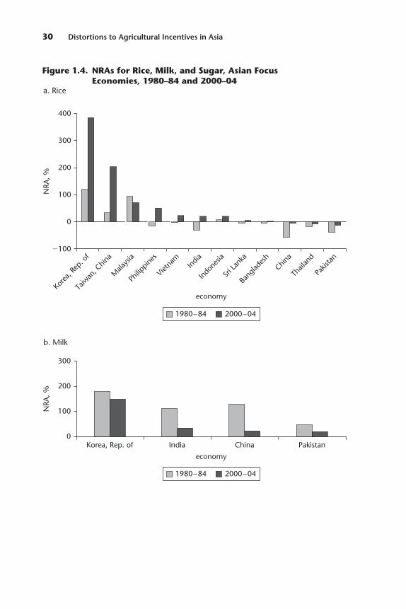
30 Distortions to Agricultural Incentives in Asia
�100
0
100
200
300
400
NRA
, %
economy
1980–84 2000–04
Kore
a, Re
p. o
f
Taiw
an, C
hina
Mala
ysia
Philip
pines
Vietn
am India
Indo
nesia
Sri L
anka
Bang
lades
hChin
a
Thail
and
Pakis
tan
Figure 1.4. NRAs for Rice, Milk, and Sugar, Asian FocusEconomies, 1980–84 and 2000–04
a. Rice
0
100
200
300
NRA
, %
economy
1980–84 2000–04
Korea, Rep. of India China Pakistan
b. Milk
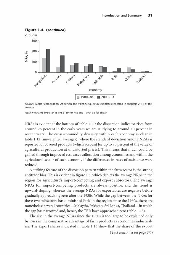
NRAs is evident at the bottom of table 1.11: the dispersion indicator rises fromaround 25 percent in the early years we are studying to around 40 percent inrecent years. The cross-commodity diversity within each economy is clear intable 1.12 (unweighted averages), where the standard deviation among NRAs isreported for covered products (which account for up to 75 percent of the value ofagricultural production at undistorted prices). This means that much could begained through improved resource reallocation among economies and within theagricultural sector of each economy if the differences in rates of assistance werereduced.
A striking feature of the distortion pattern within the farm sector is the strongantitrade bias. This is evident in figure 1.5, which depicts the average NRAs in theregion for agriculture’s import-competing and export subsectors. The averageNRAs for import-competing products are always positive, and the trend isupward-sloping, whereas the average NRAs for exportables are negative beforegradually approaching zero after the 1980s. While the gap between the NRAs forthese two subsectors has diminished little in the region since the 1960s, there arenonetheless several countries—Malaysia, Pakistan, Sri Lanka, Thailand—in whichthe gap has narrowed and, hence, the TBIs have approached zero (table 1.13).
The rise in the average NRAs since the 1980s is too large to be explained onlyby loses in the comparative advantage of farm products as economies industrial-ize. The export shares indicated in table 1.13 show that the share of the export
Introduction and Summary 31
Sources: Author compilation; Anderson and Valenzuela, 2008; estimates reported in chapters 2–12 of thisvolume.
Note: Vietnam: 1980–84 is 1986–89 for rice and 1990–95 for sugar.
Figure 1.4. (continued)c. Sugar
0
100
200
300
NRA
, %
economy
1980–84 2000–04
Bang
lades
h
Vietn
am
Pakis
tan
Philip
pines
Indo
nesia
India
China
Thail
and
(Text continues on page 37.)

32
Table 1.12. NRA Dispersion across Covered Agricultural Products, Asian Focus Economies, 1955–2004(percent)
Economy 1955–59 1960–64 1965–69 1970–74 1975–79 1980–84 1985–89 1990–94 1995–99 2000–04
Northeast Asiaa 38.5 38.5 66.8 61.7 68.6 64.0 67.1 80.5 102.3 116.6Korea, Rep. of 34.1 40.5 85.0 82.5 89.0 80.1 114.8 164.2 200.1 225.4Taiwan, Chinab 42.8 36.4 48.7 40.9 48.2 37.5 34.3 56.5 88.4 109.0China — — — — — 74.3 52.3 20.7 18.4 15.3
Southeast Asiaa — 21.1 30.4 23.9 32.7 46.2 47.9 42.5 39.7 40.4Indonesia — — — 29.1 49.4 53.6 35.0 40.5 49.0 33.3Malaysia — 19.8 10.6 11.0 34.8 58.6 90.5 71.9 33.7 40.1Philippines — 22.5 50.2 28.3 24.2 42.7 50.9 30.1 40.6 37.6Thailand — — — 27.5 22.4 30.1 29.3 25.1 22.9 16.7Vietnamb — — — — — — 33.6 44.7 52.4 74.3
South Asiaa 44.2 46.3 64.9 51.8 55.2 51.5 86.2 55.4 45.0 58.7Bangladesh — — — — 71.4 67.6 190.7 77.5 67.9 101.2India — 35.5 68.0 45.8 49.8 39.2 46.9 28.5 19.4 21.5Pakistanb — 74.6 105.8 77.6 45.0 52.2 69.4 34.4 29.4 43.1Sri Lanka 44.2 28.7 20.9 31.9 54.6 46.9 37.9 81.3 63.3 69.1
Unweighted averagea 39.0 36.8 55.5 41.5 48.0 51.1 66.9 55.9 55.6 64.4
Sources: Author compilation; Anderson and Valenzuela, 2008; estimates reported in chapters 2–12 of this volume.
Note: Dispersion for each country is a simple five-year average of the annual standard deviation around the weighted mean of the NRAs across covered products. — � no dataare available.a. The unweighted average is the simple average across the relevant economies of the simple five-year dispersion measure averages.b. Pakistan: 1960–64 is 1961–64. Taiwan, China: 2000–04 is 2000–03. Vietnam: 1985–89 is 1986–89.
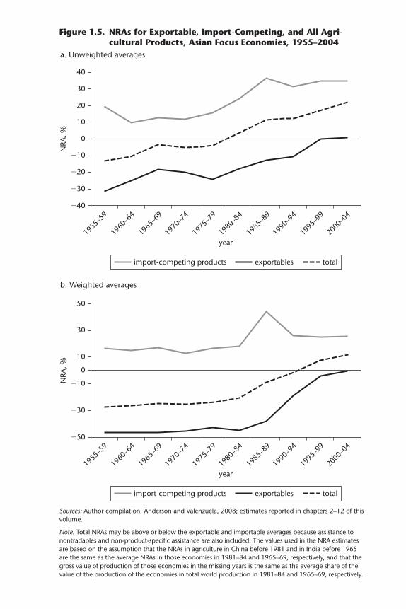
�40
year
�30
�20
10
1955
–59
1960
–64
1965
–69
1970
–74
1975
–79
1980
–84
1985
–89
1990
–94
1995
–99
2000
–04
0
20
30
�10
40N
RA, %
import-competing products exportables total
Figure 1.5. NRAs for Exportable, Import-Competing, and All Agri-cultural Products, Asian Focus Economies, 1955–2004
a. Unweighted averages
Sources: Author compilation; Anderson and Valenzuela, 2008; estimates reported in chapters 2–12 of thisvolume.
Note: Total NRAs may be above or below the exportable and importable averages because assistance tonontradables and non-product-specific assistance are also included. The values used in the NRA estimatesare based on the assumption that the NRAs in agriculture in China before 1981 and in India before 1965are the same as the average NRAs in those economies in 1981–84 and 1965–69, respectively, and that thegross value of production of those economies in the missing years is the same as the average share of thevalue of the production of the economies in total world production in 1981–84 and 1965–69, respectively.
�50
year
�30
�10
1955
–59
1960
–64
1965
–69
1970
–74
1975
–79
1980
–84
1985
–89
1990
–94
1995
–99
2000
–04
10
0
30
50
NRA
, %
import-competing products exportables total
b. Weighted averages
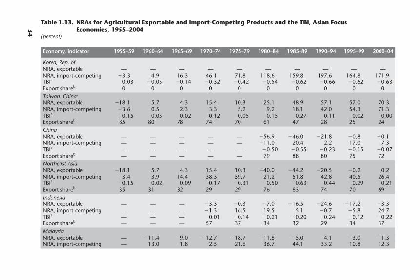
34
Table 1.13. NRAs for Agricultural Exportable and Import-Competing Products and the TBI, Asian FocusEconomies, 1955–2004
(percent)
Economy, indicator 1955–59 1960–64 1965–69 1970–74 1975–79 1980–84 1985–89 1990–94 1995–99 2000–04
Korea, Rep. ofNRA, exportable — — — — — — — — — —NRA, import-competing �3.3 4.9 16.3 46.1 71.8 118.6 159.8 197.6 164.8 171.9TBIa 0.03 �0.05 �0.14 �0.32 �0.42 �0.54 �0.62 �0.66 �0.62 �0.63Export shareb 0 0 0 0 0 0 0 0 0 0Taiwan, Chinac
NRA, exportable �18.1 5.7 4.3 15.4 10.3 25.1 48.9 57.1 57.0 70.3NRA, import-competing �3.6 0.5 2.3 3.3 5.2 9.2 18.1 42.0 54.3 71.3TBIa �0.15 0.05 0.02 0.12 0.05 0.15 0.27 0.11 0.02 0.00Export shareb 85 80 78 74 70 61 47 28 25 24ChinaNRA, exportable — — — — — �56.9 �46.0 �21.8 �0.8 �0.1NRA, import-competing — — — — — �11.0 20.4 2.2 17.0 7.3TBIa — — — — — �0.50 �0.55 �0.23 �0.15 �0.07Export shareb — — — — — 79 88 80 75 72Northeast AsiaNRA, exportable �18.1 5.7 4.3 15.4 10.3 �40.0 �44.2 �20.5 �0.2 0.2NRA, import-competing �3.4 3.9 14.4 38.3 59.7 21.2 51.8 42.8 40.5 26.4TBIa �0.15 0.02 �0.09 �0.17 �0.31 �0.50 �0.63 �0.44 �0.29 �0.21Export shareb 35 31 32 29 29 76 83 74 70 69IndonesiaNRA, exportable — — — �3.3 �0.3 �7.0 �16.5 �24.6 �17.2 �3.3NRA, import-competing — — — �1.3 16.5 19.5 5.1 �0.7 �5.8 24.7TBIa — — — 0.01 �0.14 �0.21 �0.20 �0.24 �0.12 �0.22Export shareb — — — 57 37 34 32 29 34 37MalaysiaNRA, exportable — �11.4 �9.0 �12.7 �18.7 �11.8 �5.0 �4.1 �3.0 �1.3NRA, import-competing — 13.0 �1.8 2.5 21.6 36.7 44.1 33.2 10.8 12.3
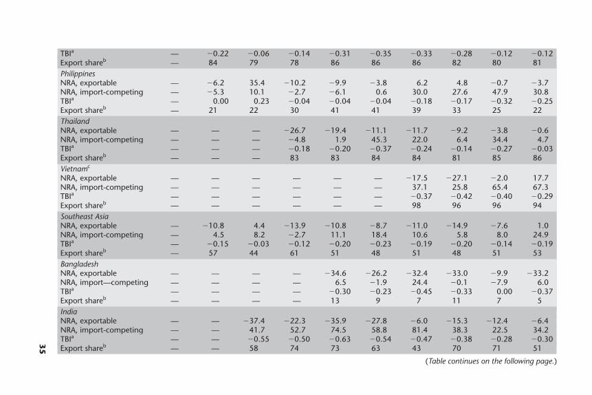
35
TBIa — �0.22 �0.06 �0.14 �0.31 �0.35 �0.33 �0.28 �0.12 �0.12Export shareb — 84 79 78 86 86 86 82 80 81PhilippinesNRA, exportable — �6.2 35.4 �10.2 �9.9 �3.8 6.2 4.8 �0.7 �3.7NRA, import-competing — �5.3 10.1 �2.7 �6.1 0.6 30.0 27.6 47.9 30.8TBIa — 0.00 0.23 �0.04 �0.04 �0.04 �0.18 �0.17 �0.32 �0.25Export shareb — 21 22 30 41 41 39 33 25 22ThailandNRA, exportable — — — �26.7 �19.4 �11.1 �11.7 �9.2 �3.8 �0.6NRA, import-competing — — — �4.8 1.9 45.3 22.0 6.4 34.4 4.7TBIa — — — �0.18 �0.20 �0.37 �0.24 �0.14 �0.27 �0.03Export shareb — — — 83 83 84 84 81 85 86Vietnamc
NRA, exportable — — — — — — �17.5 �27.1 �2.0 17.7NRA, import-competing — — — — — — 37.1 25.8 65.4 67.3TBIa — — — — — — �0.37 �0.42 �0.40 �0.29Export shareb — — — — — — 98 96 96 94Southeast AsiaNRA, exportable — �10.8 4.4 �13.9 �10.8 �8.7 �11.0 �14.9 �7.6 1.0NRA, import-competing — 4.5 8.2 �2.7 11.1 18.4 10.6 5.8 8.0 24.9TBIa — �0.15 �0.03 �0.12 �0.20 �0.23 �0.19 �0.20 �0.14 �0.19Export shareb — 57 44 61 51 48 51 48 51 53BangladeshNRA, exportable — — — — �34.6 �26.2 �32.4 �33.0 �9.9 �33.2NRA, import—competing — — — — 6.5 �1.9 24.4 �0.1 �7.9 6.0TBIa — — — — �0.30 �0.23 �0.45 �0.33 0.00 �0.37Export shareb — — — — 13 9 7 11 7 5IndiaNRA, exportable — — �37.4 �22.3 �35.9 �27.8 �6.0 �15.3 �12.4 �6.4NRA, import-competing — — 41.7 52.7 74.5 58.8 81.4 38.3 22.5 34.2TBIa — — �0.55 �0.50 �0.63 �0.54 �0.47 �0.38 �0.28 �0.30Export shareb — — 58 74 73 63 43 70 71 51
(Table continues on the following page.)
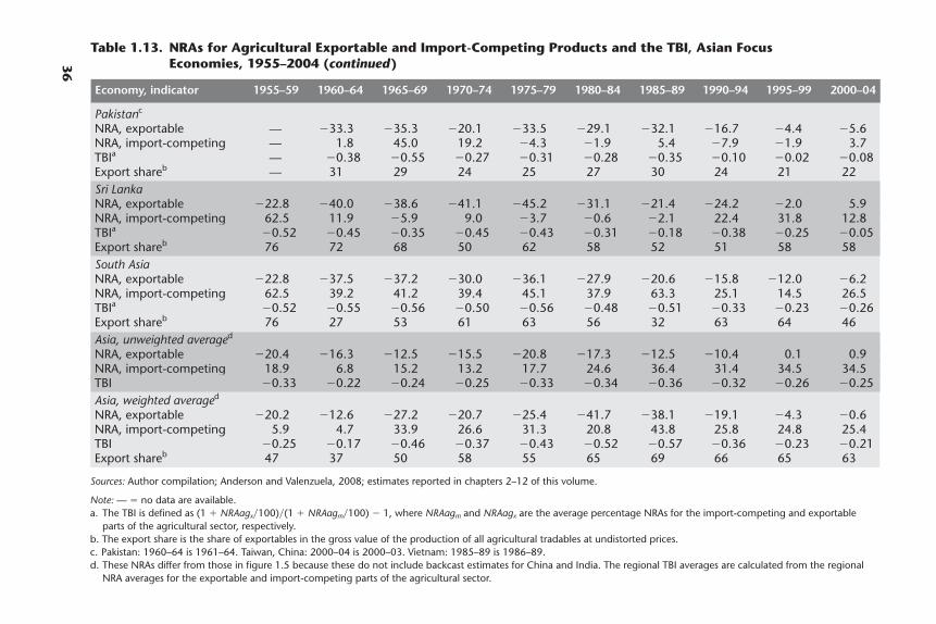
36
Pakistanc
NRA, exportable — �33.3 �35.3 �20.1 �33.5 �29.1 �32.1 �16.7 �4.4 �5.6NRA, import-competing — 1.8 45.0 19.2 �4.3 �1.9 5.4 �7.9 �1.9 3.7TBIa — �0.38 �0.55 �0.27 �0.31 �0.28 �0.35 �0.10 �0.02 �0.08Export shareb — 31 29 24 25 27 30 24 21 22Sri LankaNRA, exportable �22.8 �40.0 �38.6 �41.1 �45.2 �31.1 �21.4 �24.2 �2.0 5.9NRA, import-competing 62.5 11.9 �5.9 9.0 �3.7 �0.6 �2.1 22.4 31.8 12.8TBIa �0.52 �0.45 �0.35 �0.45 �0.43 �0.31 �0.18 �0.38 �0.25 �0.05Export shareb 76 72 68 50 62 58 52 51 58 58South AsiaNRA, exportable �22.8 �37.5 �37.2 �30.0 �36.1 �27.9 �20.6 �15.8 �12.0 �6.2NRA, import-competing 62.5 39.2 41.2 39.4 45.1 37.9 63.3 25.1 14.5 26.5TBIa �0.52 �0.55 �0.56 �0.50 �0.56 �0.48 �0.51 �0.33 �0.23 �0.26Export shareb 76 27 53 61 63 56 32 63 64 46Asia, unweighted averaged
NRA, exportable �20.4 �16.3 �12.5 �15.5 �20.8 �17.3 �12.5 �10.4 0.1 0.9NRA, import-competing 18.9 6.8 15.2 13.2 17.7 24.6 36.4 31.4 34.5 34.5TBI �0.33 �0.22 �0.24 �0.25 �0.33 �0.34 �0.36 �0.32 �0.26 �0.25Asia, weighted averaged
NRA, exportable �20.2 �12.6 �27.2 �20.7 �25.4 �41.7 �38.1 �19.1 �4.3 �0.6NRA, import-competing 5.9 4.7 33.9 26.6 31.3 20.8 43.8 25.8 24.8 25.4TBI �0.25 �0.17 �0.46 �0.37 �0.43 �0.52 �0.57 �0.36 �0.23 �0.21Export shareb 47 37 50 58 55 65 69 66 65 63
Sources: Author compilation; Anderson and Valenzuela, 2008; estimates reported in chapters 2–12 of this volume.
Note: — � no data are available.a. The TBI is defined as (1 � NRAagx�100)�(1 � NRAagm�100) � 1, where NRAagm and NRAagx are the average percentage NRAs for the import-competing and exportable
parts of the agricultural sector, respectively.b. The export share is the share of exportables in the gross value of the production of all agricultural tradables at undistorted prices.c. Pakistan: 1960–64 is 1961–64. Taiwan, China: 2000–04 is 2000–03. Vietnam: 1985–89 is 1986–89.d. These NRAs differ from those in figure 1.5 because these do not include backcast estimates for China and India. The regional TBI averages are calculated from the regional
NRA averages for the exportable and import-competing parts of the agricultural sector.
Table 1.13. NRAs for Agricultural Exportable and Import-Competing Products and the TBI, Asian FocusEconomies, 1955–2004 (continued)
Economy, indicator 1955–59 1960–64 1965–69 1970–74 1975–79 1980–84 1985–89 1990–94 1995–99 2000–04
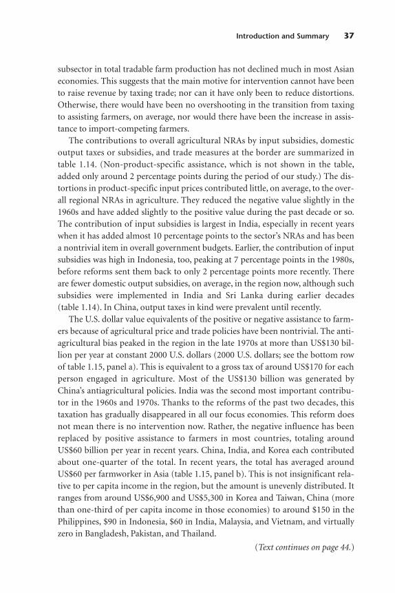
subsector in total tradable farm production has not declined much in most Asianeconomies. This suggests that the main motive for intervention cannot have beento raise revenue by taxing trade; nor can it have only been to reduce distortions.Otherwise, there would have been no overshooting in the transition from taxingto assisting farmers, on average, nor would there have been the increase in assis-tance to import-competing farmers.
The contributions to overall agricultural NRAs by input subsidies, domesticoutput taxes or subsidies, and trade measures at the border are summarized intable 1.14. (Non-product-specific assistance, which is not shown in the table,added only around 2 percentage points during the period of our study.) The dis-tortions in product-specific input prices contributed little, on average, to the over-all regional NRAs in agriculture. They reduced the negative value slightly in the1960s and have added slightly to the positive value during the past decade or so.The contribution of input subsidies is largest in India, especially in recent yearswhen it has added almost 10 percentage points to the sector’s NRAs and has beena nontrivial item in overall government budgets. Earlier, the contribution of inputsubsidies was high in Indonesia, too, peaking at 7 percentage points in the 1980s,before reforms sent them back to only 2 percentage points more recently. Thereare fewer domestic output subsidies, on average, in the region now, although suchsubsidies were implemented in India and Sri Lanka during earlier decades(table 1.14). In China, output taxes in kind were prevalent until recently.
The U.S. dollar value equivalents of the positive or negative assistance to farm-ers because of agricultural price and trade policies have been nontrivial. The anti-agricultural bias peaked in the region in the late 1970s at more than US$130 bil-lion per year at constant 2000 U.S. dollars (2000 U.S. dollars; see the bottom rowof table 1.15, panel a). This is equivalent to a gross tax of around US$170 for eachperson engaged in agriculture. Most of the US$130 billion was generated byChina’s antiagricultural policies. India was the second most important contribu-tor in the 1960s and 1970s. Thanks to the reforms of the past two decades, thistaxation has gradually disappeared in all our focus economies. This reform doesnot mean there is no intervention now. Rather, the negative influence has beenreplaced by positive assistance to farmers in most countries, totaling aroundUS$60 billion per year in recent years. China, India, and Korea each contributedabout one-quarter of the total. In recent years, the total has averaged aroundUS$60 per farmworker in Asia (table 1.15, panel b). This is not insignificant rela-tive to per capita income in the region, but the amount is unevenly distributed. Itranges from around US$6,900 and US$5,300 in Korea and Taiwan, China (morethan one-third of per capita income in those economies) to around $150 in thePhilippines, $90 in Indonesia, $60 in India, Malaysia, and Vietnam, and virtuallyzero in Bangladesh, Pakistan, and Thailand.
Introduction and Summary 37
(Text continues on page 44.)
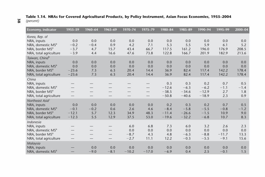
38
Table 1.14. NRAs for Covered Agricultural Products, by Policy Instrument, Asian Focus Economies, 1955–2004 (percent)
Economy, indicator 1955–59 1960–64 1965–69 1970–74 1975–79 1980–84 1985–89 1990–94 1995–99 2000–04
Korea, Rep. ofNRA, inputs 0.0 0.0 0.0 0.0 0.0 0.0 0.0 0.0 0.0 0.0NRA, domestic MSa �0.2 �0.4 0.9 4.2 7.1 5.3 5.5 5.9 6.1 5.2NRA, border MSa �3.7 4.7 15.7 43.4 66.7 117.5 161.2 196.0 176.9 208.5NRA, total agriculture �3.9 4.4 16.6 47.6 73.8 122.8 166.7 201.9 182.9 213.6Taiwan, Chinab
NRA, inputs 0.0 0.0 0.0 0.0 0.0 0.0 0.0 0.0 0.0 0.0NRA, domestic MSa 0.0 0.0 0.0 0.0 0.0 0.0 0.0 0.0 0.0 0.0NRA, border MSa �23.6 7.3 6.3 20.4 14.4 36.9 82.4 117.4 142.2 178.4NRA, total agriculture �23.6 7.3 6.3 20.4 14.4 36.9 82.4 117.4 142.2 178.4ChinaNRA, inputs — — — — — 0.3 0.3 0.2 0.7 0.5NRA, domestic MSa — — — — — �12.6 �6.3 �6.2 �1.1 �1.4NRA, border MSa — — — — — �38.5 �34.6 �12.9 2.7 1.8NRA, total agriculture — — — — — �50.8 �40.6 �18.9 2.3 0.9Northeast Asiac
NRA, inputs 0.0 0.0 0.0 0.0 0.0 0.2 0.3 0.2 0.7 0.5NRA, domestic MSa �0.1 �0.2 0.6 2.6 4.6 �8.4 �5.8 �5.5 �0.8 �1.2NRA, border MSa �12.1 5.7 12.3 34.9 48.3 �11.4 �26.6 �1.5 10.9 9.0NRA, total agriculture �12.3 5.5 12.9 37.5 53.0 �19.6 �32.2 �6.8 10.7 8.3IndonesiaNRA, inputs — — — 6.0 6.8 7.3 6.0 3.2 2.6 2.3NRA, domestic MSa — — — 0.0 0.0 0.0 0.0 0.0 0.0 0.0NRA, border MSa — — — �8.7 4.3 4.8 �6.3 �8.8 �11.7 13.3NRA, total agriculture — — — �2.7 11.1 12.2 �0.3 �5.5 �9.1 15.6MalaysiaNRA, inputs — 0.0 0.0 0.0 0.0 0.0 0.0 0.0 0.0 0.0NRA, domestic MSa — �9.0 �8.1 �10.2 �17.0 �6.9 0.4 2.5 �0.1 1.5
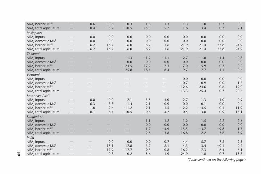
39
NRA, border MSa — 0.6 �0.6 �0.3 1.8 1.3 1.3 1.0 �0.3 0.6NRA, total agriculture — �8.4 �8.7 �10.5 �15.3 �5.7 1.8 3.4 �0.3 2.1PhilippinesNRA, inputs — 0.0 0.0 0.0 0.0 0.0 0.0 0.0 0.0 0.0NRA, domestic MSa — 0.0 0.0 0.0 0.0 0.0 0.0 0.0 0.0 0.0NRA, border MSa — �6.7 16.7 �6.0 �8.7 �1.6 21.9 21.4 37.8 24.9NRA, total agriculture — �6.7 16.7 �6.0 �8.7 �1.6 21.9 21.4 37.8 24.9ThailandNRA, inputs — — — �1.3 �1.2 �1.1 �2.7 �1.8 �1.4 �0.8NRA, domestic MSa — — — 0.0 0.0 0.0 0.0 0.0 0.0 0.0NRA, border MSa — — — �24.5 �17.2 �7.3 �7.0 �5.9 0.3 0.2NRA, total agriculture — — — �25.8 �18.4 �8.4 �9.7 �7.7 �1.1 �0.6Vietnamb
NRA, inputs — — — — — — 0.0 0.0 0.0 0.0NRA, domestic MSa — — — — — — �0.7 �0.9 0.0 1.7NRA, border MSa — — — — — — �12.6 �24.6 0.6 19.0NRA, total agriculture — — — — — — �13.3 �25.4 0.7 20.6Southeast Asiac
NRA, inputs — 0.0 0.0 2.1 3.5 4.0 2.7 1.3 1.0 0.9NRA, domestic MSa — �6.3 �3.3 �1.4 �2.1 �0.9 0.0 0.1 0.0 0.4NRA, border MSa — �1.8 9.6 �11.2 �2.1 1.5 �2.2 �4.5 �0.1 11.9NRA, total agriculture — �8.1 6.4 �10.5 �0.6 4.7 0.5 �3.0 0.9 13.1BangladeshNRA, inputs — — — — 1.1 1.2 1.2 1.5 2.2 2.6NRA, domestic MSa — — — — 0.0 0.0 0.0 0.0 0.0 0.0NRA, border MSa — — — — 1.7 �4.9 15.5 �3.7 �9.8 1.3NRA, total agriculture — — — — 2.8 �3.8 16.8 �2.2 �7.6 3.9IndiaNRA, inputs — — 0.0 0.0 0.0 0.7 4.4 5.7 7.2 9.5NRA, domestic MSa — — 18.1 17.8 3.7 2.1 4.3 3.4 �0.1 0.2NRA, border MSa — — �17.9 �17.7 �9.3 �0.8 16.2 �7.3 �6.4 6.1NRA, total agriculture — — 0.3 0.2 �5.6 1.9 24.9 1.8 0.7 15.8
(Table continues on the following page.)

40
Pakistanb
NRA, inputs — �4.5 �2.1 �1.6 4.6 3.5 2.9 2.3 1.9 1.4NRA, domestic MSa — 0.0 0.0 0.0 0.0 0.0 0.0 0.0 0.0 0.0NRA, border MSa — �1.3 23.9 10.9 �16.4 �12.8 �8.8 �12.5 �4.5 0.1NRA, total agriculture — �5.8 21.7 9.3 �11.8 �9.3 �5.9 �10.2 �2.6 1.5Sri LankaNRA, inputs 0.0 0.0 0.0 0.0 0.0 0.0 0.0 0.0 0.0 0.0NRA, domestic MSa 4.2 8.1 6.9 5.0 5.1 5.0 3.6 1.5 0.7 0.9NRA, border MSa �14.5 �38.0 �36.9 �25.4 �37.0 �24.2 �16.3 �3.1 10.8 7.8NRA, total agriculture �10.3 �29.9 �30.0 �20.3 �31.9 �19.2 �12.6 �1.7 11.5 8.6South Asiac
NRA, inputs 0.0 �1.5 �0.2 �0.1 0.4 0.9 4.0 5.0 6.3 8.3NRA, domestic MSa 4.2 8.3 16.3 16.1 3.1 1.8 3.6 2.8 �0.1 0.2NRA, border MSa �14.5 �14.7 �14.9 �15.4 �9.2 �2.5 13.5 �7.5 �6.2 5.2NRA, total agriculture �10.3 �7.8 1.2 0.6 �5.7 0.2 21.0 0.3 0.0 13.6Asia, unweighted averageNRA, inputs 0.0 �0.6 �0.3 0.3 1.1 1.1 1.0 0.9 1.1 1.3NRA, domestic MSa 1.4 0.6 2.4 1.4 �0.8 �0.9 0.1 0.0 �0.1 0.2NRA, border MSa �13.4 �6.1 1.1 �0.9 0.3 6.5 17.7 20.8 26.2 30.9NRA, total agriculture �12.0 �6.2 3.2 0.9 0.6 6.6 18.8 21.7 27.3 32.4Asia, weighted averaged
NRA, inputs 0.0 �0.5 �0.1 0.4 1.4 1.1 1.5 1.7 2.3 2.6NRA, domestic MSa 1.4 2.0 13.0 10.6 1.0 �5.3 �2.9 �2.5 �0.6 �0.7NRA, border MSa �12.4 �4.2 �10.2 �10.8 �2.8 �17.4 �13.7 �4.0 4.3 8.2NRA, total agriculture �11.1 �2.7 2.6 0.3 �0.4 �21.6 �15.2 �4.8 6.0 10.2
Sources: Author compilation; Anderson and Valenzuela, 2008; estimates reported in chapters 2–12 of this volume.
Note: — � no data are available.a. MS � market support, which is provided through domestic subsidies (or taxes) or through a border measure such as an import tariff (or subsidy) or an export subsidy (or tax).b. Pakistan: 1960–64 is 1961–64. Taiwan, China: 2000–04 is 2000–03. Vietnam: 1985–89 is 1986–1989.c. The weights for the subregional averages are based on the gross value of agricultural production at undistorted prices.d. The weight is the gross value of the production of covered products at undistorted prices.
Table 1.14. NRAs for Covered Agricultural Products, by Policy Instrument, Asian Focus Economies, 1955–2004 (continued)
Economy, indicator 1955–59 1960–64 1965–69 1970–74 1975–79 1980–84 1985–89 1990–94 1995–99 2000–04

41
Table 1.15. Gross Subsidy Equivalents of Agricultural Assistance, Total and Per Farm Worker, Asian FocusEconomies, 1955–2004
a. Total (at constant 2000 US$, millions, using the U.S. GDP deflator)
Economy 1955–59 1960–64 1965–69 1970–74 1975–79 1980–84 1985–89 1990–94 1995–99 2000–04
Korea, Rep. of �154 107 854 1,672 6,943 9,335 13,306 18,594 17,536 15,289Taiwan, Chinaa �394 133 132 439 605 1,342 2,500 3,849 4,170 3,725Chinab �52,857 �69,648 �70,671 �98,931 �124,086 �118,224 �75,780 �28,381 15,667 15,644Indonesia — — — �848 3,783 4,131 �785 �2,729 �4,101 4,286Malaysia — �250 �246 �547 �1,097 �456 75 156 3 100Philippines — �225 735 �1,082 �903 �299 1,399 1,850 3,832 1,951Thailand — — — �2,434 �2,148 �324 �645 �719 260 �14Vietnama — — — — — — �726 �1,815 �18 1,602Bangladesh — — — — 583 �672 882 �103 �448 189Indiab 46 61 �993 �7,803 �8,653 �49 21,607 1,600 281 15,433Pakistana — �91 1,089 �34 �815 �787 �380 �755 �260 95Sri Lanka �68 �461 �455 �396 �571 �344 �194 �27 245 154Total �53,426 �70,373 �69,554 �109,965 �126,359 �106,348 �38,740 �8,481 37,169 58,455All Asian
economiesc �56,836 �74,865 �73,994 �116,984 �134,424 �113,136 �41,213 �9,023 39,541 62,186
(Table continues on the following page.)

42
Table 1.15. Gross Subsidy Equivalents of Agricultural Assistance, Total and Per Farm Worker, Asian Economies,1955–2004 (continued)
b. Per person engaged in agriculture (at constant 2000 US$ using the U.S. GDP deflator)
Economy 1960–64 1965–69 1970–74 1975–79 1980–84 1985–89 1990–94 1995–99 2000–04
Korea, Rep. of 20 155 293 1,196 1,716 3,041 5,618 6,445 6,899Taiwan, Chinaa 76 76 261 390 1,045 2,077 3,699 4,795 5,329Chinab �235 �222 �281 �319 �280 �163 �57 31 31Indonesia — — �27 113 113 �19 �60 �86 86Malaysia �135 �126 �267 �515 �213 36 79 2 56Philippines �33 99 �132 �99 �30 132 163 318 155Thailand — — �163 �130 �18 �34 �36 13 �1Vietnama — — — — — �33 �73 �1 57Bangladesh — — — 20 �22 26 �3 �12 5Indiab 0 �6 �43 �43 0 97 7 1 57Pakistana �7 78 �2 �47 �41 �19 �35 �11 4Sri Lanka �217 �195 �155 �207 �116 �60 �8 66 40Total �125 �115 �166 �174 �136 �46 �9 40 61All Asian economiesc �125 �115 �166 �174 �136 �46 �9 40 61
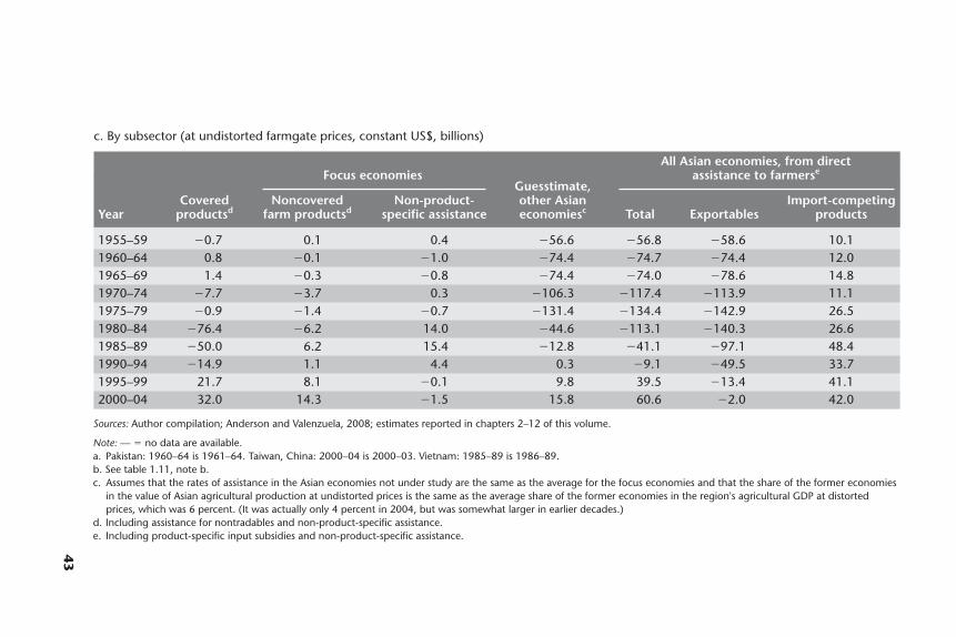
43
c. By subsector (at undistorted farmgate prices, constant US$, billions)
All Asian economies, from directFocus economies
Guesstimate,assistance to farmerse
Covered Noncovered Non-product- other Asian Import-competingYear productsd farm productsd specific assistance economiesc Total Exportables products
1955–59 �0.7 0.1 0.4 �56.6 �56.8 �58.6 10.11960–64 0.8 �0.1 �1.0 �74.4 �74.7 �74.4 12.01965–69 1.4 �0.3 �0.8 �74.4 �74.0 �78.6 14.81970–74 �7.7 �3.7 0.3 �106.3 �117.4 �113.9 11.11975–79 �0.9 �1.4 �0.7 �131.4 �134.4 �142.9 26.51980–84 �76.4 �6.2 14.0 �44.6 �113.1 �140.3 26.61985–89 �50.0 6.2 15.4 �12.8 �41.1 �97.1 48.41990–94 �14.9 1.1 4.4 0.3 �9.1 �49.5 33.71995–99 21.7 8.1 �0.1 9.8 39.5 �13.4 41.12000–04 32.0 14.3 �1.5 15.8 60.6 �2.0 42.0
Sources: Author compilation; Anderson and Valenzuela, 2008; estimates reported in chapters 2–12 of this volume.
Note: — � no data are available.a. Pakistan: 1960–64 is 1961–64. Taiwan, China: 2000–04 is 2000–03. Vietnam: 1985–89 is 1986–89.b. See table 1.11, note b.c. Assumes that the rates of assistance in the Asian economies not under study are the same as the average for the focus economies and that the share of the former economies
in the value of Asian agricultural production at undistorted prices is the same as the average share of the former economies in the region's agricultural GDP at distortedprices, which was 6 percent. (It was actually only 4 percent in 2004, but was somewhat larger in earlier decades.)
d. Including assistance for nontradables and non-product-specific assistance.e. Including product-specific input subsidies and non-product-specific assistance.
Which products contribute to the positive or negative assistance to farmersbecause of agricultural price and trade policies? Panel c in table 1.15 shows thatthe negative contribution arises mainly from policies directly affecting theexportable parts of agriculture, while most of the positive contribution arisesfrom the protection for import-competing producers. The product NRAs, shownin table 1.16, panel a, offer insights into the products that are responsible. Thisinformation is combined with information on each product’s share of the grossvalue of production to obtain the U.S. dollar contributions by product that areshown in table 1.16, panel b (also see appendix B). Rice, milk, and sugar are clearlystill the most well assisted industries. Note that, in the early 1980s, when Chinawas still heavily taxing farmers, the net contribution of rice was negative andlarge. At that time, policies affecting pig meat, fruits, and vegetables were equallyimportant contributors to the effective taxation of Asian farmers, and this wasalmost entirely because of the influence of China.
Assistance to nonfarm sectors and RRAs
The antiagricultural policy bias of past decades was not generated only by agricul-tural policies. Likewise, the significant reductions in the border protection for themanufacturing sector, which have represented the dominant intervention in thetradables part of the nonagricultural sector, have also been important in thechanges in the incentives affecting intersectorally mobile resources. Reductions inthe assistance for producers of nonfarm tradables have been even more responsi-ble for the improvement in farmer incentives than the reductions in the direct tax-ation on agricultural industries.
It has not been possible to quantify the distortions in nonfarm tradables ascarefully as we have done in agriculture. Authors have typically been obliged torely on the applied trade taxes for exports and imports rather than price compar-isons, and they therefore usually do not capture the quantitative restrictions ontrade that were once important, but have been decreasingly so through recenttimes.11 Nor do they capture distortions in services, and services are also now gen-erating tradables (or would be generating them in the absence of interventionspreventing the emergence of service tradables). As a result, the NRA estimates fornonfarm importables are smaller and decline less rapidly than the actual NRAs.The same is true of the estimated NRAs for nonfarm exportables, except that theNRAs would have sometimes been negative. Of these two elements of underesti-mation, the former bias certainly dominates. Thus, the author estimates of theoverall NRAs for nonagricultural tradables should be considered lower-boundestimates, especially in the past, and the declines are therefore less rapid than theyshould be.12
44 Distortions to Agricultural Incentives in Asia
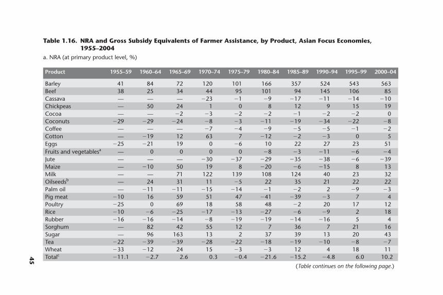
45
Table 1.16. NRA and Gross Subsidy Equivalents of Farmer Assistance, by Product, Asian Focus Economies,1955–2004
a. NRA (at primary product level, %)
Product 1955–59 1960–64 1965–69 1970–74 1975–79 1980–84 1985–89 1990–94 1995–99 2000–04
Barley 41 84 72 120 101 166 357 524 543 563Beef 38 25 34 44 95 101 94 145 106 85Cassava — — — �23 �1 �9 �17 �11 �14 �10Chickpeas — 50 24 1 0 8 12 9 15 19Cocoa — — �2 �3 �2 �2 �1 �2 �2 0Coconuts �29 �29 �24 �8 �3 �11 �19 �34 �22 �8Coffee — — — �7 �4 �9 �5 �5 �1 �2Cotton — �19 12 63 7 �12 �2 �3 0 5Eggs �25 �21 19 0 �6 10 22 27 23 51Fruits and vegetablesa — 0 0 0 0 �8 �3 �11 �6 �4Jute — — — �30 �37 �29 �35 �38 �6 �39Maize — �10 50 19 8 �20 �6 �15 8 13Milk — — 71 122 139 108 124 40 23 32Oilseedsb — 24 31 11 �5 22 35 21 22 22Palm oil — �11 �11 �15 �14 �1 �2 2 �9 �3Pig meat �10 16 59 51 47 �41 �39 �3 7 4Poultry �25 0 69 18 58 48 �2 20 17 12Rice �10 �6 �25 �17 �13 �27 �6 �9 2 18Rubber �16 �16 �14 �8 �19 �19 �14 �16 5 4Sorghum — 82 42 55 12 7 36 7 21 16Sugar — 96 163 13 2 37 39 13 20 43Tea �22 �39 �39 �28 �22 �18 �19 �10 �8 �7Wheat �33 �12 24 15 �3 �3 12 4 18 11Totalc �11.1 �2.7 2.6 0.3 �0.4 �21.6 �15.2 �4.8 6.0 10.2
(Table continues on the following page.)
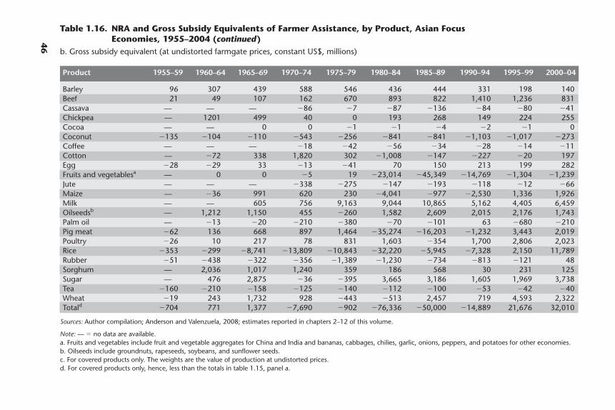
46
Table 1.16. NRA and Gross Subsidy Equivalents of Farmer Assistance, by Product, Asian FocusEconomies, 1955–2004 (continued)
b. Gross subsidy equivalent (at undistorted farmgate prices, constant US$, millions)
Product 1955–59 1960–64 1965–69 1970–74 1975–79 1980–84 1985–89 1990–94 1995–99 2000–04
Barley 96 307 439 588 546 436 444 331 198 140Beef 21 49 107 162 670 893 822 1,410 1,236 831Cassava — — — �86 �7 �87 �136 �84 �80 �41Chickpea — 1201 499 40 0 193 268 149 224 255Cocoa — — 0 0 �1 �1 �4 �2 �1 0Coconut �135 �104 �110 �543 �256 �841 �841 �1,103 �1,017 �273Coffee — — — �18 �42 �56 �34 �28 �14 �11Cotton — �72 338 1,820 302 �1,008 �147 �227 �20 197Egg �28 �29 33 �13 �41 70 150 213 199 282Fruits and vegetablesa — 0 0 �5 19 �23,014 �45,349 �14,769 �1,304 �1,239Jute — — — �338 �275 �147 �193 �118 �12 �66Maize — �36 991 620 230 �4,041 �977 �2,530 1,336 1,926Milk — — 605 756 9,163 9,044 10,865 5,162 4,405 6,459Oilseedsb — 1,212 1,150 455 �260 1,582 2,609 2,015 2,176 1,743Palm oil — �13 �20 �210 �380 �70 �101 63 �680 �210Pig meat �62 136 668 897 1,464 �35,274 �16,203 �1,232 3,443 2,019Poultry �26 10 217 78 831 1,603 �354 1,700 2,806 2,023Rice �353 �299 �8,741 �13,809 �10,843 �32,220 �5,945 �7,328 2,150 11,789Rubber �51 �438 �322 �356 �1,389 �1,230 �734 �813 �121 48Sorghum — 2,036 1,017 1,240 359 186 568 30 231 125Sugar — 476 2,875 �36 �395 3,665 3,186 1,605 1,969 3,738Tea �160 �210 �158 �125 �140 �112 �100 �53 �42 �40Wheat �19 243 1,732 928 �443 �513 2,457 719 4,593 2,322Totald �704 771 1,377 �7,690 �902 �76,336 �50,000 �14,889 21,676 32,010
Sources: Author compilation; Anderson and Valenzuela, 2008; estimates reported in chapters 2–12 of this volume.
Note: — � no data are available.a. Fruits and vegetables include fruit and vegetable aggregates for China and India and bananas, cabbages, chilies, garlic, onions, peppers, and potatoes for other economies.b. Oilseeds include groundnuts, rapeseeds, soybeans, and sunflower seeds.c. For covered products only. The weights are the value of production at undistorted prices.d. For covered products only, hence, less than the totals in table 1.15, panel a.
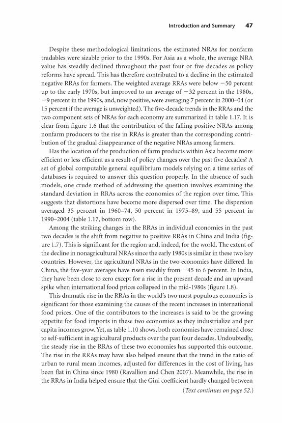
Despite these methodological limitations, the estimated NRAs for nonfarmtradables were sizable prior to the 1990s. For Asia as a whole, the average NRAvalue has steadily declined throughout the past four or five decades as policyreforms have spread. This has therefore contributed to a decline in the estimatednegative RRAs for farmers. The weighted average RRAs were below �50 percentup to the early 1970s, but improved to an average of �32 percent in the 1980s,�9 percent in the 1990s, and, now positive, were averaging 7 percent in 2000–04 (or15 percent if the average is unweighted). The five-decade trends in the RRAs and thetwo component sets of NRAs for each economy are summarized in table 1.17. It isclear from figure 1.6 that the contribution of the falling positive NRAs amongnonfarm producers to the rise in RRAs is greater than the corresponding contri-bution of the gradual disappearance of the negative NRAs among farmers.
Has the location of the production of farm products within Asia become moreefficient or less efficient as a result of policy changes over the past five decades? Aset of global computable general equilibrium models relying on a time series ofdatabases is required to answer this question properly. In the absence of suchmodels, one crude method of addressing the question involves examining thestandard deviation in RRAs across the economies of the region over time. Thissuggests that distortions have become more dispersed over time. The dispersionaveraged 35 percent in 1960–74, 50 percent in 1975–89, and 55 percent in1990–2004 (table 1.17, bottom row).
Among the striking changes in the RRAs in individual economies in the pasttwo decades is the shift from negative to positive RRAs in China and India (fig-ure 1.7). This is significant for the region and, indeed, for the world. The extent ofthe decline in nonagricultural NRAs since the early 1980s is similar in these two keycountries. However, the agricultural NRAs in the two economies have differed. InChina, the five-year averages have risen steadily from �45 to 6 percent. In India,they have been close to zero except for a rise in the present decade and an upwardspike when international food prices collapsed in the mid-1980s (figure 1.8).
This dramatic rise in the RRAs in the world’s two most populous economies issignificant for those examining the causes of the recent increases in internationalfood prices. One of the contributors to the increases is said to be the growingappetite for food imports in these two economies as they industrialize and percapita incomes grow. Yet, as table 1.10 shows, both economies have remained closeto self-sufficient in agricultural products over the past four decades. Undoubtedly,the steady rise in the RRAs of these two economies has supported this outcome.The rise in the RRAs may have also helped ensure that the trend in the ratio ofurban to rural mean incomes, adjusted for differences in the cost of living, hasbeen flat in China since 1980 (Ravallion and Chen 2007). Meanwhile, the rise inthe RRAs in India helped ensure that the Gini coefficient hardly changed between
Introduction and Summary 47
(Text continues on page 52.)

48
Table 1.17. RRAs in Agriculture, Asian Focus Economies, 1955–2004(percent)
Economy, indicator 1955–59 1960–64 1965–69 1970–74 1975–79 1980–84 1985–89 1990–94 1995–99 2000–04
Korea, Rep. ofNRA, agriculture �3.3 4.9 16.3 46.1 71.8 118.6 159.8 197.6 164.8 171.9NRA, nonagriculture 45.6 37.1 22.3 11.4 11.7 6.8 5.7 3.3 2.3 1.7RRAa �32.6 �21.4 �4.8 30.5 53.9 104.8 145.9 188.2 158.8 167.3Taiwan, Chinab
NRA, agriculture �15.8 4.7 3.9 12.0 8.9 18.7 33.8 46.3 54.9 70.9NRA, nonagriculture 8.8 9.3 8.8 7.5 7.0 5.2 4.5 2.6 1.8 1.0RRAa �22.5 �4.2 �4.5 4.2 1.7 12.9 28.0 42.5 52.2 69.0Chinac
NRA, agriculture �45.2 �45.2 �45.2 �45.2 �45.2 �45.2 �35.5 �14.3 6.6 5.9NRA, nonagriculture 41.6 41.6 41.6 41.6 41.6 41.6 28.3 24.9 9.9 5.0RRAa �60.5 �60.5 �60.5 �60.5 �60.5 �60.5 �49.9 �31.1 �3.0 0.9Northeast AsiaNRA, agriculture �43.1 �42.5 �42.2 �41.3 �40.0 �18.4 �26.2 �1.7 14.7 12.0NRA, nonagriculture 40.9 40.8 40.0 39.7 39.4 71.1 18.8 15.0 6.8 3.3RRAa �58.2 �57.7 �56.6 �55.7 �53.7 �51.9 �38.0 �14.2 7.4 8.5IndonesiaNRA, agriculture — — — �3.8 10.4 10.5 �1.9 �7.5 �9.7 13.9NRA, nonagriculture — — — 27.7 27.7 27.7 26.5 17.6 10.6 8.1RRAa — — — �24.7 �13.6 �13.5 �22.5 �21.3 �18.3 5.4MalaysiaNRA, agriculture — �7.6 �7.9 �9.4 �13.7 �4.9 1.4 2.6 �0.2 1.5NRA, nonagriculture — 7.4 7.0 7.1 6.5 5.2 3.9 2.8 2.0 0.9RRAa — �14.0 �13.9 �15.5 �18.9 �9.6 �2.4 �0.3 �2.2 0.6PhilippinesNRA, agriculture — �1.7 14.3 �6.0 �7.2 �4.0 15.8 16.7 35.7 23.5NRA, nonagriculture — 19.0 20.3 16.3 16.3 12.9 11.0 9.9 8.6 6.4RRAa — �17.4 �5.0 �19.8 �20.3 �14.9 4.3 6.1 24.9 15.9
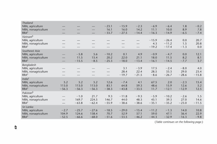
49
ThailandNRA, agriculture — — — �23.1 �15.9 �2.3 �6.9 �6.4 1.8 �0.2NRA, nonagriculture — — — 16.1 16.0 14.2 11.1 10.0 8.9 7.8RRAa — — — �33.7 �27.5 �14.4 �16.3 �14.9 �6.5 �7.4Vietnamb
NRA, agriculture — — — — — — �15.9 �26.4 0.0 20.7NRA, nonagriculture — — — — — — 4.3 �11.2 1.5 20.8RRAa — — — — — — �19.2 �17.4 �1.3 0.0Southeast AsiaNRA, agriculture — �5.8 5.6 �10.2 0.1 4.9 �0.9 �4.7 0.0 12.1NRA, nonagriculture — 11.5 15.4 20.2 22.0 21.1 18.0 11.5 8.2 8.1RRAa — �15.5 �8.5 �25.3 �18.0 �13.4 �16.1 �14.5 �7.7 3.7BangladeshNRA, agriculture — — — — 3.1 �3.9 17.5 �2.4 �8.0 4.0NRA, nonagriculture — — — — 28.4 22.4 28.5 33.3 29.0 23.4RRAa — — — — �19.7 �21.5 �8.6 �26.7 �28.6 �15.8Indiac
NRA, agriculture 5.2 5.2 5.2 12.6 �7.4 4.1 67.5 2.0 �2.3 15.4NRA, nonagriculture 113.0 113.0 113.0 83.1 64.8 59.3 48.6 15.9 12.6 5.2RRAa �56.3 �56.3 �56.3 �38.3 �43.8 �33.5 11.7 �12.1 �12.9 12.5Pakistanb
NRA, agriculture — �1.0 21.7 9.3 �11.8 �9.3 �5.9 �10.2 �2.6 1.5NRA, nonagriculture — 169.7 224.5 146.7 44.0 48.3 45.1 39.3 27.0 14.6RRAa — �63.8 �62.4 �55.9 �38.6 �38.6 �35.1 �35.2 �23.0 �11.5Sri LankaNRA, agriculture �2.7 �25.7 �27.6 �18.5 �29.0 �15.4 �11.2 �1.3 14.0 10.8NRA, nonagriculture 104.9 124.6 138.4 70.7 52.9 57.1 59.0 47.1 36.4 22.9RRAa �52.5 �66.6 �68.0 �51.6 �53.5 �46.2 �44.3 �32.9 �16.3 �9.8
(Table continues on the following page.)
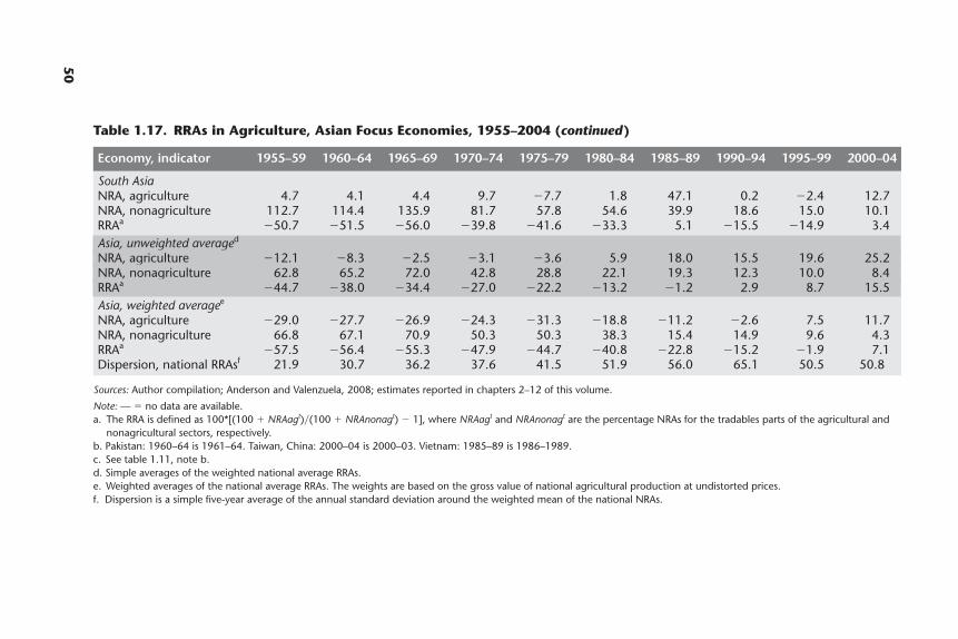
50
South AsiaNRA, agriculture 4.7 4.1 4.4 9.7 �7.7 1.8 47.1 0.2 �2.4 12.7NRA, nonagriculture 112.7 114.4 135.9 81.7 57.8 54.6 39.9 18.6 15.0 10.1RRAa �50.7 �51.5 �56.0 �39.8 �41.6 �33.3 5.1 �15.5 �14.9 3.4Asia, unweighted averaged
NRA, agriculture �12.1 �8.3 �2.5 �3.1 �3.6 5.9 18.0 15.5 19.6 25.2NRA, nonagriculture 62.8 65.2 72.0 42.8 28.8 22.1 19.3 12.3 10.0 8.4RRAa �44.7 �38.0 �34.4 �27.0 �22.2 �13.2 �1.2 2.9 8.7 15.5Asia, weighted averagee
NRA, agriculture �29.0 �27.7 �26.9 �24.3 �31.3 �18.8 �11.2 �2.6 7.5 11.7NRA, nonagriculture 66.8 67.1 70.9 50.3 50.3 38.3 15.4 14.9 9.6 4.3RRAa �57.5 �56.4 �55.3 �47.9 �44.7 �40.8 �22.8 �15.2 �1.9 7.1Dispersion, national RRAsf 21.9 30.7 36.2 37.6 41.5 51.9 56.0 65.1 50.5 50.8
Sources: Author compilation; Anderson and Valenzuela, 2008; estimates reported in chapters 2–12 of this volume.
Note: — � no data are available.a. The RRA is defined as 100*[(100 � NRAagt)�(100 � NRAnonagt) � 1], where NRAagt and NRAnonagt are the percentage NRAs for the tradables parts of the agricultural and
nonagricultural sectors, respectively.b. Pakistan: 1960–64 is 1961–64. Taiwan, China: 2000–04 is 2000–03. Vietnam: 1985–89 is 1986–1989.c. See table 1.11, note b.d. Simple averages of the weighted national average RRAs.e. Weighted averages of the national average RRAs. The weights are based on the gross value of national agricultural production at undistorted prices.f. Dispersion is a simple five-year average of the annual standard deviation around the weighted mean of the national NRAs.
Table 1.17. RRAs in Agriculture, Asian Focus Economies, 1955–2004 (continued)
Economy, indicator 1955–59 1960–64 1965–69 1970–74 1975–79 1980–84 1985–89 1990–94 1995–99 2000–04
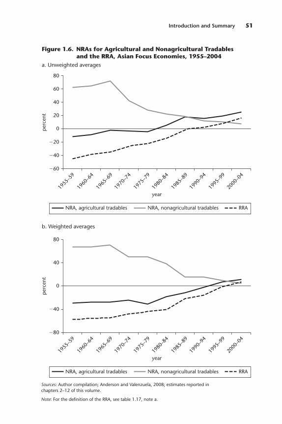
Introduction and Summary 51
�60
year
�40
20
1955
–59
1960
–64
1965
–69
1970
–74
1975
–79
1980
–84
1985
–89
1990
–94
1995
–99
2000
–04
0
40
60
�20
80
per
cent
RRANRA, nonagricultural tradablesNRA, agricultural tradables
Figure 1.6. NRAs for Agricultural and Nonagricultural Tradablesand the RRA, Asian Focus Economies, 1955–2004
a. Unweighted averages
Sources: Author compilation; Anderson and Valenzuela, 2008; estimates reported inchapters 2–12 of this volume.
Note: For the definition of the RRA, see table 1.17, note a.
�80
year
�40
1955
–59
1960
–64
1965
–69
1970
–74
1975
–79
1980
–84
1985
–89
1990
–94
1995
–99
2000
–04
0
40
80
per
cent
RRANRA, nonagricultural tradablesNRA, agricultural tradables
b. Weighted averages
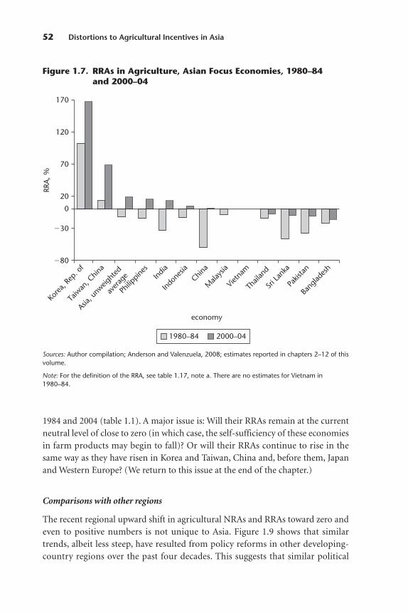
52 Distortions to Agricultural Incentives in Asia
�80
�30
20
0
70
120
170
Kore
a, Re
p. o
f
Taiw
an, C
hina
Asia, u
nweig
hted
aver
age
Philip
pines
India
Indo
nesia
China
Mala
ysia
Vietn
am
Thail
and
Sri L
anka
Pakis
tan
Bang
lades
h
RRA
, %
economy
1980–84 2000–04
Figure 1.7. RRAs in Agriculture, Asian Focus Economies, 1980–84and 2000–04
Sources: Author compilation; Anderson and Valenzuela, 2008; estimates reported in chapters 2–12 of thisvolume.
Note: For the definition of the RRA, see table 1.17, note a. There are no estimates for Vietnam in1980–84.
1984 and 2004 (table 1.1). A major issue is: Will their RRAs remain at the currentneutral level of close to zero (in which case, the self-sufficiency of these economiesin farm products may begin to fall)? Or will their RRAs continue to rise in thesame way as they have risen in Korea and Taiwan, China and, before them, Japanand Western Europe? (We return to this issue at the end of the chapter.)
Comparisons with other regions
The recent regional upward shift in agricultural NRAs and RRAs toward zero andeven to positive numbers is not unique to Asia. Figure 1.9 shows that similartrends, albeit less steep, have resulted from policy reforms in other developing-country regions over the past four decades. This suggests that similar political
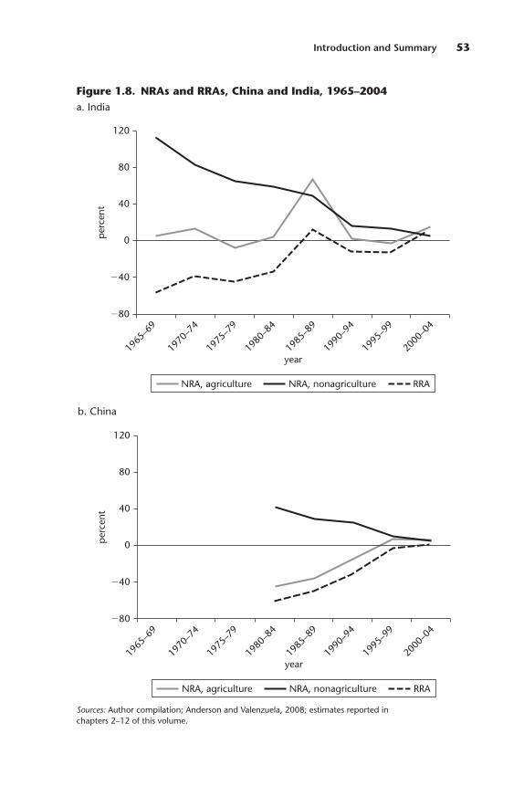
Introduction and Summary 53
�80
�40
0per
cent
40
80
120
year19
65–6
9
1970
–74
1975
–79
1980
–84
1985
–89
1990
–94
1995
–99
2000
–04
NRA, nonagricultureNRA, agriculture RRA
Figure 1.8. NRAs and RRAs, China and India, 1965–2004a. India
Sources: Author compilation; Anderson and Valenzuela, 2008; estimates reported inchapters 2–12 of this volume.
�80
�40
0per
cent
40
80
120
year19
65–6
9
1970
–74
1975
–79
1980
–84
1985
–89
1990
–94
1995
–99
2000
–04
NRA, nonagricultureNRA, agriculture RRA
b. China
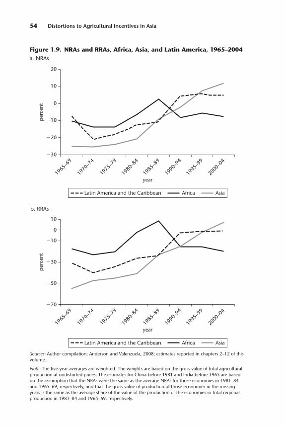
54 Distortions to Agricultural Incentives in Asia
�30
�20
�10
0
10
20
2000
–04
year
per
cent
AfricaLatin America and the Caribbean Asia
1965
–69
1970
–74
1975
–79
1980
–84
1985
–89
1990
–94
1995
–99
Figure 1.9. NRAs and RRAs, Africa, Asia, and Latin America, 1965–2004a. NRAs
Sources: Author compilation; Anderson and Valenzuela, 2008; estimates reported in chapters 2–12 of thisvolume.
Note: The five-year averages are weighted. The weights are based on the gross value of total agriculturalproduction at undistorted prices. The estimates for China before 1981 and India before 1965 are basedon the assumption that the NRAs were the same as the average NRAs for those economies in 1981–84and 1965–69, respectively, and that the gross value of production of those economies in the missingyears is the same as the average share of the value of the production of the economies in total regionalproduction in 1981–84 and 1965–69, respectively.
b. RRAs
�70
�50
�30
�10
10
0
2000
–04
year
per
cent
1965
–69
1970
–74
1975
–79
1980
–84
1985
–89
1990
–94
1995
–99
AfricaLatin America and the Caribbean Asia
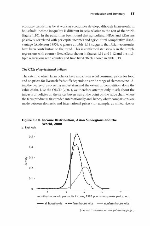
economy trends may be at work as economies develop, although farm-nonfarmhousehold income inequality is different in Asia relative to the rest of the world(figure 1.10). In the past, it has been found that agricultural NRAs and RRAs arepositively correlated with per capita incomes and agricultural comparative disad-vantage (Anderson 1995). A glance at table 1.18 suggests that Asian economieshave been contributors to the trend. This is confirmed statistically in the simpleregressions with country fixed effects shown in figures 1.11 and 1.12 and the mul-tiple regressions with country and time fixed effects shown in table 1.19.
The CTEs of agricultural policies
The extent to which farm policies have impacts on retail consumer prices for foodand on prices for livestock feedstuffs depends on a wide range of elements, includ-ing the degree of processing undertaken and the extent of competition along thevalue chain. Like the OECD (2007), we therefore attempt only to ask about theimpacts of policies on the prices buyers pay at the point on the value chain wherethe farm product is first traded internationally and, hence, where comparisons aremade between domestic and international prices (for example, as milled rice, or
Introduction and Summary 55
0
0.1
0.2
0.3
0.4
0.5
dens
ity
1 3 5 7 9
monthly household per capita income, 1993 purchasing power parity, log
nonfarm householdsfarm householdsall households
Figure 1.10. Income Distribution, Asian Subregions and theWorld, 2000
a. East Asia
(Figure continues on the following page.)
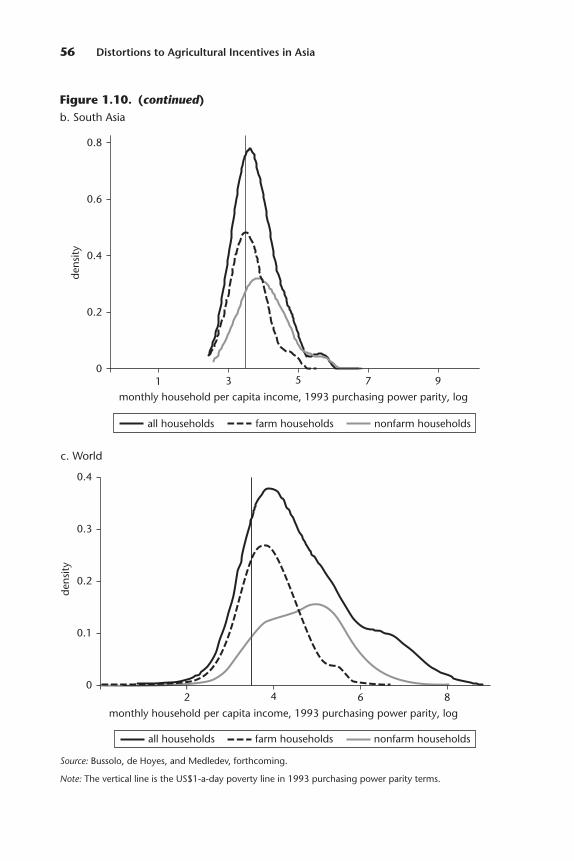
56 Distortions to Agricultural Incentives in Asia
Source: Bussolo, de Hoyes, and Medledev, forthcoming.
Note: The vertical line is the US$1-a-day poverty line in 1993 purchasing power parity terms.
Figure 1.10. (continued)b. South Asia
0
0.2
0.4
0.6
0.8
dens
ity
1 3 5 7 9
monthly household per capita income, 1993 purchasing power parity, log
nonfarm householdsfarm householdsall households
c. World
0
0.1
0.2
0.3
0.4
dens
ity
2 4 6 8
monthly household per capita income, 1993 purchasing power parity, log
nonfarm householdsfarm householdsall households
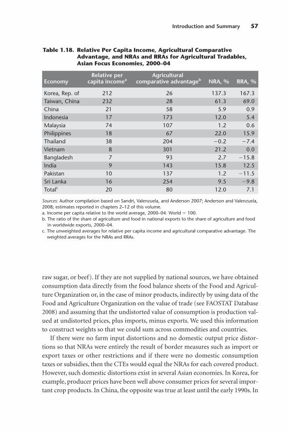
Introduction and Summary 57
Table 1.18. Relative Per Capita Income, Agricultural ComparativeAdvantage, and NRAs and RRAs for Agricultural Tradables,Asian Focus Economies, 2000–04
Relative per AgriculturalEconomy capita incomea comparative advantageb NRA, % RRA, %
Korea, Rep. of 212 26 137.3 167.3Taiwan, China 232 28 61.3 69.0China 21 58 5.9 0.9Indonesia 17 173 12.0 5.4Malaysia 74 107 1.2 0.6Philippines 18 67 22.0 15.9Thailand 38 204 �0.2 �7.4Vietnam 8 301 21.2 0.0Bangladesh 7 93 2.7 �15.8India 9 143 15.8 12.5Pakistan 10 137 1.2 �11.5Sri Lanka 16 254 9.5 �9.8Totalc 20 80 12.0 7.1
Sources: Author compilation based on Sandri, Valenzuela, and Anderson 2007; Anderson and Valenzuela,2008; estimates reported in chapters 2–12 of this volume.a. Income per capita relative to the world average, 2000–04. World � 100.b. The ratio of the share of agriculture and food in national exports to the share of agriculture and food
in worldwide exports, 2000–04.c. The unweighted averages for relative per capita income and agricultural comparative advantage. The
weighted averages for the NRAs and RRAs.
raw sugar, or beef). If they are not supplied by national sources, we have obtainedconsumption data directly from the food balance sheets of the Food and Agricul-ture Organization or, in the case of minor products, indirectly by using data of theFood and Agriculture Organization on the value of trade (see FAOSTAT Database2008) and assuming that the undistorted value of consumption is production val-ued at undistorted prices, plus imports, minus exports. We used this informationto construct weights so that we could sum across commodities and countries.
If there were no farm input distortions and no domestic output price distor-tions so that NRAs were entirely the result of border measures such as import orexport taxes or other restrictions and if there were no domestic consumptiontaxes or subsidies, then the CTEs would equal the NRAs for each covered product.However, such domestic distortions exist in several Asian economies. In Korea, forexample, producer prices have been well above consumer prices for several impor-tant crop products. In China, the opposite was true at least until the early 1990s. In

58
Sources: Author compilation based on Sandri, Valenzuela, and Anderson 2007; Anderson and Valenzuela,2008; estimates reported in chapters 2–12 of this volume.
Note: The dependent variable for the regressions is the NRAs or RRAs by country and year expressed as afraction. The results are ordinary least squares estimates. The explanatory variable is the natural log ofreal GDP per capita expressed in US$10,000s.
b. Regression of ln real GDP per capita on RRAs, with country fixed effects
�1
0
1
2
RRA
�1 0 1 2 3
ln real GDP per capita
Asia, fitted valuesAsia, RRA observations
coefficient standard error R2
0.27 0.01 0.46
�0.6
�0.3
0
0.3
0.6
NRA
�1 0 1 2 3ln real GDP per capita
Asia, fitted valuesAsia, NRA observations
Figure 1.11. Regressions of Real GDP per Capita and AgriculturalNRAs and RRAs, Asian Focus Economies, 1955–2005
a. Regression of ln real GDP per capita on NRAs, with country fixed effects
coefficient standard error R2
0.17 0.01 0.19
Introduction and Summary 59
�0.6
0
0.6
1.2
1.8
NRA
0 1 2 3 4
revealed comparative advantage
Asia, fitted valuesAsia, NRA observations
Figure 1.12. Regressions of Real Comparative Advantage and Agricul-tural NRAs and RRAs, Asian Focus Economies, 1960–2004
a. Regression of revealed comparative advantage on NRAs, with country fixed effects
coefficient standard error R2
�0.12 0.02 0.08
China, the producers of food staples were taxed more than the consumers weresubsidized even if we take into account the in-kind partial wage payment receivedby many urban workers (the iron rice bowl).13 Also, because of internationaltrade, the weights one uses to aggregate product distortion rates on the consump-tion side of the market differ from the weights one uses on the production side.Hence, aggregate CTEs differ somewhat from aggregate NRAs in each economy.This may be seen by comparing the CTEs in panel a, table 1.20 with the NRAs intable 1.11. The weighted average CTEs in the region were negative until the early1990s, but were above zero thereafter and have increased in recent years. The vari-ance in CTEs across products is even greater now than it was before the reforms ofthe past two decades (see table 1.20, panel b, including the bottom row).
In proportional and in per capita terms, the current transfers from consumersare clearly largest in Korea and Taiwan, China (panel a, table 1.20 and panel b,
(Figure continues on the following page.)
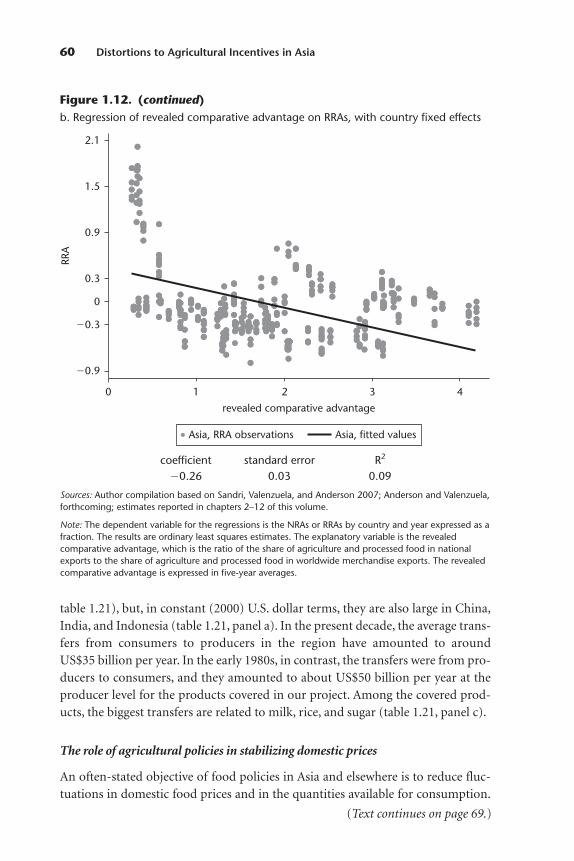
table 1.21), but, in constant (2000) U.S. dollar terms, they are also large in China,India, and Indonesia (table 1.21, panel a). In the present decade, the average trans-fers from consumers to producers in the region have amounted to aroundUS$35 bil lion per year. In the early 1980s, in contrast, the transfers were from pro-ducers to consumers, and they amounted to about US$50 billion per year at theproducer level for the products covered in our project. Among the covered prod-ucts, the biggest transfers are related to milk, rice, and sugar (table 1.21, panel c).
The role of agricultural policies in stabilizing domestic prices
An often-stated objective of food policies in Asia and elsewhere is to reduce fluc-tuations in domestic food prices and in the quantities available for consumption.
60 Distortions to Agricultural Incentives in Asia
Sources: Author compilation based on Sandri, Valenzuela, and Anderson 2007; Anderson and Valenzuela,forthcoming; estimates reported in chapters 2–12 of this volume.
Note: The dependent variable for the regressions is the NRAs or RRAs by country and year expressed as afraction. The results are ordinary least squares estimates. The explanatory variable is the revealedcomparative advantage, which is the ratio of the share of agriculture and processed food in nationalexports to the share of agriculture and processed food in worldwide merchandise exports. The revealedcomparative advantage is expressed in five-year averages.
Figure 1.12. (continued)b. Regression of revealed comparative advantage on RRAs, with country fixed effects
�0.9
�0.3
0.3
0
0.9
1.5
2.1
RRA
0 1 2 3 4
revealed comparative advantage
Asia, fitted valuesAsia, RRA observations
coefficient standard error R2
�0.26 0.03 0.09
(Text continues on page 69.)
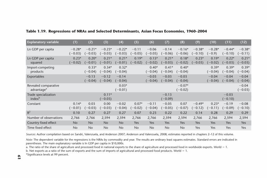
61
Table 1.19. Regressions of NRAs and Selected Determinants, Asian Focus Economies, 1960–2004
Explanatory variable (1) (2) (3) (4) (5) (6) (7) (8) (9) (10) (11) (12)
Ln GDP per capita �0.28* �0.21* �0.23* �0.22* �0.11 �0.06 �0.14 �0.16* �0.38* �0.28* �0.44* �0.38*(�0.03) (�0.03) (�0.03) (�0.03) (�0.05) (�0.05) (�0.06) (�0.06) (�0.10) (�0.9) (�0.10) (�0.11)
Ln GDP per capita 0.23* 0.20* 0.21* 0.21* 0.19* 0.15* 0.21* 0.18* 0.23* 0.19* 0.22* 0.21*squared (�0.02) (�0.01) (�0.01) (�0.01) (�0.02) (�0.02) (�0.03) (�0.02) (�0.03) (�0.02) (�0.03) (�0.03)
Import-competing 0.33* 0.34* 0.32* 0.40* 0.41* 0.40* 0.39* 0.39* 0.39*products (�0.04) (�0.04) (�0.04) (�0.04) (�0.04) (�0.04) (�0.04) (�0.04) (�0.04)
Exportables �0.13 �0.12 �0.14 �0.03 �0.03 �0.03 �0.04 �0.04 �0.04(�0.04) (�0.04) (�0.04) (�0.04) (�0.04) (�0.04) (�0.04) (�0.04) (�0.04)
Revealed comparative 0.03* �0.07* �0.04advantagea (�0.01) (�0.02) (�0.03)
Trade specialization 0.11* �0.13 �0.03indexb (�0.03) (�0.09) (�0.10)
Constant 0.14* 0.03 0.00 �0.02 0.07* �0.11 �0.05 0.07 �0.49* 0.23* �0.19 �0.08(�0.01) (�0.03) (�0.03) (�0.04) (�0.02) (�0.04) (�0.05) (�0.07) (�0.12) (�0.11) (�0.09) (�0.10)
R2 0.10 0.27 0.27 0.27 0.07 0.23 0.22 0.22 0.14 0.28 0.29 0.29
Number of observations 2,766 2,766 2,594 2,594 2,766 2,766 2,594 2,594 2,766 2,766 2,594 2,594
Country fixed effect No No No No Yes Yes Yes Yes Yes Yes Yes Yes
Time fixed effect No No No No No No No No Yes Yes Yes Yes
Sources: Author compilation based on Sandri, Valenzuela, and Anderson 2007; Anderson and Valenzuela, 2008; estimates reported in chapters 2–12 of this volume.
Note: The dependent variable for the regressions is the NRAs by commodity and year. The results are ordinary least squares estimates. Standard errors are indicated inparentheses. The main explanatory variable is ln GDP per capita in $10,000s.a. The ratio of the share of agriculture and processed food in national exports to the share of agriculture and processed food in worldwide exports. World � 1.b. Net exports as a ratio of the sum of exports and the sum of imports of agricultural and processed food products. World � 1.*Significance levels at 99 percent.
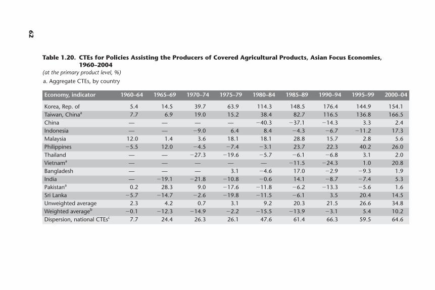
62
Table 1.20. CTEs for Policies Assisting the Producers of Covered Agricultural Products, Asian Focus Economies,1960–2004
(at the primary product level, %)
a. Aggregate CTEs, by country
Economy, indicator 1960–64 1965–69 1970–74 1975–79 1980–84 1985–89 1990–94 1995–99 2000–04
Korea, Rep. of 5.4 14.5 39.7 63.9 114.3 148.5 176.4 144.9 154.1Taiwan, Chinaa 7.7 6.9 19.0 15.2 38.4 82.7 116.5 136.8 166.5China — — — — �40.3 �37.1 �14.3 3.3 2.4Indonesia — — �9.0 6.4 8.4 �4.3 �6.7 �11.2 17.3Malaysia 12.0 1.4 3.6 18.1 18.1 28.8 15.7 2.8 5.6Philippines �5.5 12.0 �4.5 �7.4 �3.1 23.7 22.3 40.2 26.0Thailand — — �27.3 �19.6 �5.7 �6.1 �6.8 3.1 2.0Vietnama — — — — — �11.5 �24.3 1.0 20.8Bangladesh — — — 3.1 �4.6 17.0 �2.9 �9.3 1.9India — �19.1 �21.8 �10.8 �0.6 14.1 �8.7 �7.4 5.3Pakistana 0.2 28.3 9.0 �17.6 �11.8 �6.2 �13.3 �5.6 1.6Sri Lanka �5.7 �14.7 �2.6 �19.8 �11.5 �6.1 3.5 20.4 14.5Unweighted average 2.3 4.2 0.7 3.1 9.2 20.3 21.5 26.6 34.8Weighted averageb �0.1 �12.3 �14.9 �2.2 �15.5 �13.9 �3.1 5.4 10.2Dispersion, national CTEsc 7.7 24.4 26.3 26.1 47.6 61.4 66.3 59.5 64.6
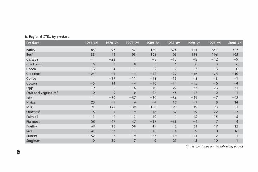
63
b. Regional CTEs, by product
Product 1965–69 1970–74 1975–79 1980–84 1985–89 1990–94 1995–99 2000–04
Barley 65 97 57 120 326 411 341 327Beef 33 43 98 106 95 156 106 105Cassava — �22 1 �8 �13 �8 �12 �9Chickpeas 5 0 0 3 5 0 3 6Cocoa �3 �4 �1 �2 �2 �3 �3 0Coconuts �24 �9 �3 �12 �22 �36 �25 �10Coffee — �17 �11 �18 �13 �8 �3 �1Cotton �5 14 �4 �16 �11 �15 �6 �4Eggs 19 0 �6 10 22 27 23 51Fruit and vegetablesd 0 0 0 �26 �45 �17 �2 �1Jute — �30 �37 �30 �36 �39 �7 �42Maize 23 �1 6 �4 17 �7 8 14Milk 71 122 139 108 123 39 23 31Oilseedse 5 �5 �9 18 32 19 22 23Palm oil �1 �9 �3 10 1 12 �15 �5Pig meat 58 49 47 �37 �38 �4 7 4Poultry 69 18 58 49 �2 21 17 12Rice �41 �37 �17 �18 �8 �9 0 16Rubber �52 �6 �19 �23 �19 �11 2 1Sorghum 9 30 7 0 23 �5 10 1
(Table continues on the following page.)

64
Sources: Author compilation; Anderson and Valenzuela, 2008; estimates reported in chapters 2–12 of this volume.
Note: The figure is based on the assumption that the CTE is the same as the NRA derived from trade measures (that is, not including any input taxes or subsidies or anydomestic producer price subsidies or taxes), except for rice, barley, wheat, and sorghum in Korea and wheat in Taiwan, China. — � no data are available.a. Pakistan: 1960–64 is 1961–64. Taiwan, China: 2000–04 is 2000–03. Vietnam: 1985–89 is 1986–89.b. The weights are consumption valued at undistorted prices, where consumption (from the FAOSTAT Database) is production, plus imports, net of exports, plus changes in the
stocks of the covered products.c. A simple five-year average of the annual standard deviation around the weighted mean of the average national CTEs.d. Fruits and vegetables include fruit and vegetable aggregates for China and India and bananas, cabbages, chilies, garlic, onions, peppers, and potatoes for other economies.e. Oilseeds include groundnuts, rapeseeds, soybeans, and sunflower seeds.f. A simple five-year average of the annual standard deviation around the weighted mean of the average regional CTEs for the covered products indicated.
Sugar 121 0 �3 32 31 8 16 27Tea �58 �29 �19 �14 �17 �10 �15 �17Wheat 8 �1 �7 5 21 14 8 2Weighted averageb �12 �15 �2 �15 �14 �3 5 10Dispersion, regional product CTEsf 53 45 44 52 85 96 76 73
Table 1.20. CTEs for Policies Assisting the Producers of Covered Agricultural Products, Asian Focus Economies,1960–2004 (continued)
b. Regional CTEs, by product
Product 1965–69 1970–74 1975–79 1980–84 1985–89 1990–94 1995–99 2000–04
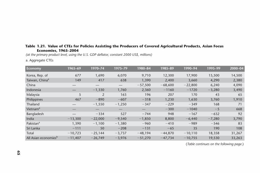
65
Table 1.21. Value of CTEs for Policies Assisting the Producers of Covered Agricultural Products, Asian FocusEconomies, 1965–2004
(at the primary product level, using the U.S. GDP deflator, constant 2000 US$, millions)
a. Aggregate CTEs
Economy 1965–69 1970–74 1975–79 1980–84 1985–89 1990–94 1995–99 2000–04
Korea, Rep. of 677 1,690 6,070 9,710 12,300 17,900 15,500 14,500Taiwan, Chinaa 149 417 638 1,390 2,400 3,660 4,290 2,380China — — — �57,500 �68,600 �22,800 6,240 4,090Indonesia — �1,330 1,760 2,360 �1160 �1720 �3,280 3,490Malaysia 5 2 163 196 207 170 43 65Philippines 467 �890 �607 �318 1,230 1,630 3,760 1,910Thailand — �1,550 �1,250 �347 �229 �349 168 71Vietnama — — — — �300 �1040 �5 668Bangladesh — �334 527 �744 948 �167 �632 92India �13,300 �22,000 �9,540 �1,850 8,800 �6,440 �7,280 3,790Pakistana 1,390 �1,100 �1,380 �960 �410 �989 �546 83Sri Lanka �111 50 �208 �131 �65 35 190 108Total �10,723 �25,144 �3,737 �48,194 �44,870 �10,110 18,358 31,267All Asian economiesb �11,407 �26,749 �3,976 �51,270 �47,734 �10,755 19,530 33,263
(Table continues on the following page.)
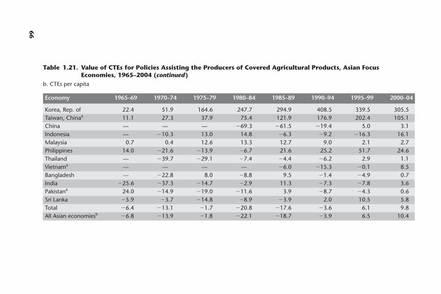
66
Table 1.21. Value of CTEs for Policies Assisting the Producers of Covered Agricultural Products, Asian FocusEconomies, 1965–2004 (continued)
b. CTEs per capita
Economy 1965–69 1970–74 1975–79 1980–84 1985–89 1990–94 1995–99 2000–04
Korea, Rep. of 22.4 51.9 164.6 247.7 294.9 408.5 339.5 305.5Taiwan, Chinaa 11.1 27.3 37.9 75.4 121.9 176.9 202.4 105.1China — — — �69.3 �61.5 �19.4 5.0 3.1Indonesia — �10.3 13.0 14.8 �6.3 �9.2 �16.3 16.1Malaysia 0.7 0.4 12.6 13.3 12.7 9.0 2.1 2.7Philippines 14.0 �21.6 �13.9 �6.7 21.6 25.2 51.7 24.6Thailand — �39.7 �29.1 �7.4 �4.4 �6.2 2.9 1.1Vietnama — — — — �6.0 �15.3 �0.1 8.5Bangladesh — �22.8 8.0 �8.8 9.5 �1.4 �4.9 0.7India �25.6 �37.3 �14.7 �2.9 11.3 �7.3 �7.8 3.6Pakistana 24.0 �14.9 �19.0 �11.6 3.9 �8.7 �4.3 0.6Sri Lanka �5.9 �3.7 �14.8 �8.9 �3.9 2.0 10.5 5.8Total �6.4 �13.1 �1.7 �20.8 �17.6 �3.6 6.1 9.8All Asian economiesb �6.8 �13.9 �1.8 �22.1 �18.7 �3.9 6.5 10.4
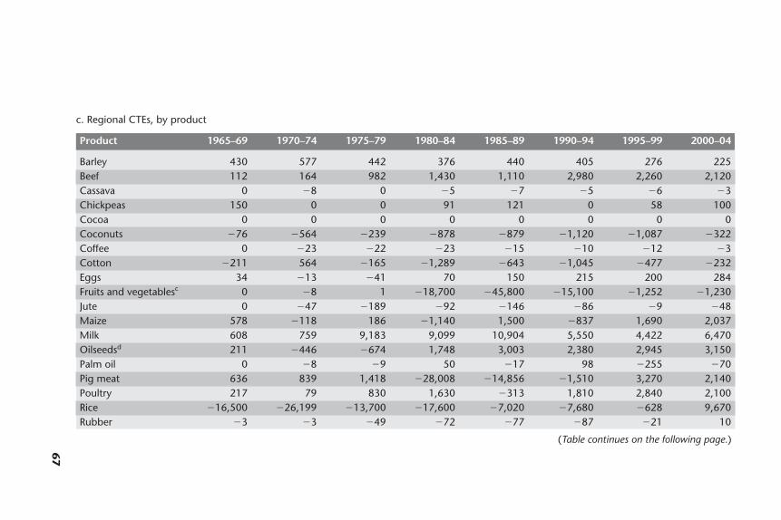
67
c. Regional CTEs, by product
Product 1965–69 1970–74 1975–79 1980–84 1985–89 1990–94 1995–99 2000–04
Barley 430 577 442 376 440 405 276 225Beef 112 164 982 1,430 1,110 2,980 2,260 2,120Cassava 0 �8 0 �5 �7 �5 �6 �3Chickpeas 150 0 0 91 121 0 58 100Cocoa 0 0 0 0 0 0 0 0Coconuts �76 �564 �239 �878 �879 �1,120 �1,087 �322Coffee 0 �23 �22 �23 �15 �10 �12 �3Cotton �211 564 �165 �1,289 �643 �1,045 �477 �232Eggs 34 �13 �41 70 150 215 200 284Fruits and vegetablesc 0 �8 1 �18,700 �45,800 �15,100 �1,252 �1,230Jute 0 �47 �189 �92 �146 �86 �9 �48Maize 578 �118 186 �1,140 1,500 �837 1,690 2,037Milk 608 759 9,183 9,099 10,904 5,550 4,422 6,470Oilseedsd 211 �446 �674 1,748 3,003 2,380 2,945 3,150Palm oil 0 �8 �9 50 �17 98 �255 �70Pig meat 636 839 1,418 �28,008 �14,856 �1,510 3,270 2,140Poultry 217 79 830 1,630 �313 1,810 2,840 2,100Rice �16,500 �26,199 �13,700 �17,600 �7,020 �7,680 �628 9,670Rubber �3 �3 �49 �72 �77 �87 �21 10
(Table continues on the following page.)
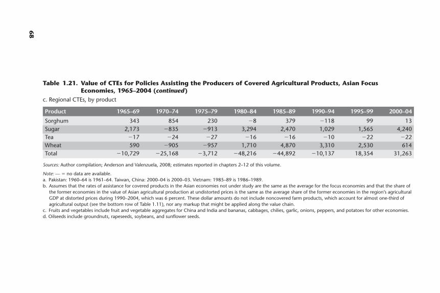
68
Sources: Author compilation; Anderson and Valenzuela, 2008; estimates reported in chapters 2–12 of this volume.
Note: — � no data are available.a. Pakistan: 1960–64 is 1961–64. Taiwan, China: 2000–04 is 2000–03. Vietnam: 1985–89 is 1986–1989.b. Assumes that the rates of assistance for covered products in the Asian economies not under study are the same as the average for the focus economies and that the share of
the former economies in the value of Asian agricultural production at undistorted prices is the same as the average share of the former economies in the region’s agriculturalGDP at distorted prices during 1990–2004, which was 6 percent. These dollar amounts do not include noncovered farm products, which account for almost one-third ofagricultural output (see the bottom row of Table 1.11), nor any markup that might be applied along the value chain.
c. Fruits and vegetables include fruit and vegetable aggregates for China and India and bananas, cabbages, chilies, garlic, onions, peppers, and potatoes for other economies.d. Oilseeds include groundnuts, rapeseeds, soybeans, and sunflower seeds.
Sorghum 343 854 230 �8 379 �118 99 13Sugar 2,173 �835 �913 3,294 2,470 1,029 1,565 4,240Tea �17 �24 �27 �16 �16 �10 �22 �22Wheat 590 �905 �957 1,710 4,870 3,310 2,530 614Total �10,729 �25,168 �3,712 �48,216 �44,892 �10,137 18,354 31,263
Table 1.21. Value of CTEs for Policies Assisting the Producers of Covered Agricultural Products, Asian FocusEconomies, 1965–2004 (continued)
c. Regional CTEs, by product
Product 1965–69 1970–74 1975–79 1980–84 1985–89 1990–94 1995–99 2000–04
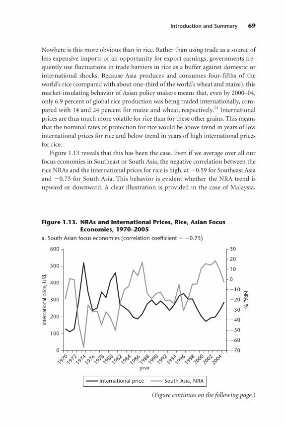
Nowhere is this more obvious than in rice. Rather than using trade as a source ofless expensive imports or an opportunity for export earnings, governments fre-quently use fluctuations in trade barriers in rice as a buffer against domestic orinternational shocks. Because Asia produces and consumes four-fifths of theworld’s rice (compared with about one-third of the world’s wheat and maize), thismarket-insulating behavior of Asian policy makers means that, even by 2000–04,only 6.9 percent of global rice production was being traded internationally, com-pared with 14 and 24 percent for maize and wheat, respectively.14 Internationalprices are thus much more volatile for rice than for these other grains. This meansthat the nominal rates of protection for rice would be above trend in years of lowinternational prices for rice and below trend in years of high international pricesfor rice.
Figure 1.13 reveals that this has been the case. Even if we average over all ourfocus economies in Southeast or South Asia, the negative correlation between therice NRAs and the international prices for rice is high, at �0.59 for Southeast Asiaand �0.75 for South Asia. This behavior is evident whether the NRA trend isupward or downward. A clear illustration is provided in the case of Malaysia,
Introduction and Summary 69
0
100
200
year
300
400
500
600
1970
1972
1974
1976
1978
1980
1982
1984
1986
1988
1990
1992
1994
1996
1998
2000
2002
2004
inte
rnat
iona
l pric
e, U
S$
�70
�60
�50
�40
�30
�20
�10
0
10
20
30
NRA, %
international price South Asia, NRA
Figure 1.13. NRAs and International Prices, Rice, Asian FocusEconomies, 1970–2005
a. South Asian focus economies (correlation coefficient � �0.75)
(Figure continues on the following page.)
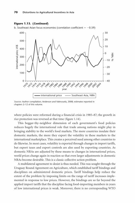
70 Distortions to Agricultural Incentives in Asia
Sources: Author compilation; Anderson and Valenzuela, 2008; estimates reported inchapters 2–12 of this volume.
Figure 1.13. (Continued)b. Southeast Asian focus economies (correlation coefficient � �0.59)
0
100
200
year
300
400
500
600
1970
1972
1974
1976
1978
1980
1982
1984
1986
1988
1990
1992
1994
1996
1998
2000
2002
2004
inte
rnat
iona
l pric
e, U
S$
�40
�30
�10
0
10
20
30
NRA, %
�20
international price Southeast Asia, NRA
where policies were reformed during a financial crisis in 1985–87; the growth inrice protection was reversed at that time (figure 1.14).
This beggar-thy-neighbor dimension of each government’s food policiesreduces hugely the international role that trade among nations might play inbringing stability to the world’s food markets. The more countries insulate theirdomestic markets, the more they export the volatility in these markets to theinternational marketplace. This creates a perceived need among other countries todo likewise. In most cases, volatility is exported through changes in import tariffs,but export taxes and export controls are also used by exporting countries. Asdomestic NRAs are adjusted by these means to changes in international prices,world prices change again in reaction so that even larger adjustments in domesticNRAs become desirable. This is a classic collective action problem.
A multilateral agreement to desist is thus needed. This was sought through theUruguay Round Agreement on Agriculture, which established tariff bindings anddisciplines on administered domestic prices. Tariff bindings help reduce theextent of the problem by imposing limits on the range of tariff increases imple-mented in response to low prices. However, the bindings are so far beyond theapplied import tariffs that the discipline facing food-importing members in yearsof low international prices is weak. Moreover, there is no corresponding WTO
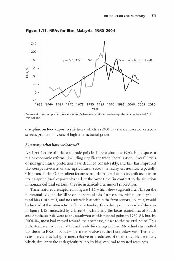
discipline on food export restrictions, which, as 2008 has starkly revealed, can be aserious problem in years of high international prices.
Summary: what have we learned?
A salient feature of price and trade policies in Asia since the 1960s is the spate ofmajor economic reforms, including significant trade liberalization. Overall levelsof nonagricultural protection have declined considerably, and this has improvedthe competitiveness of the agricultural sector in many economies, especiallyChina and India. Other salient features include the gradual policy shift away fromtaxing agricultural exportables and, at the same time (in contrast to the situationin nonagricultural sectors), the rise in agricultural import protection.
These features are captured in figure 1.15, which shows agricultural TBIs on thehorizontal axis and the RRAs on the vertical axis. An economy with no antiagricul-tural bias (RRA � 0) and no antitrade bias within the farm sector (TBI � 0) wouldbe located at the intersection of lines extending from the 0 point on each of the axesin figure 1.15 (indicated by a large �). China and the focus economies of Southand Southeast Asia were to the southwest of this neutral point in 1980–84, but, by2000–04, most had moved toward the northeast, closer to the neutral point. Thisindicates they had reduced the antitrade bias in agriculture. Most had also shiftedup, closer to RRA � 0, but some are now above rather than below zero. This indi-cates they are assisting farmers relative to producers of other tradable products,which, similar to the antiagricultural policy bias, can lead to wasted resources.
Introduction and Summary 71
Figure 1.14. NRAs for Rice, Malaysia, 1960–2004
�40
year
0
1955 1960 1965 1970 1975 1980 1985 1990 1995 2000 2005 2010
40
160
120
200
80
240
NRA
, %
y � 6.3532x � 12489 y � �6.3075x � 12681
Sources: Author compilation; Anderson and Valenzuela, 2008; estimates reported in chapters 2–12 ofthis volume.

The following features of the Asian experience over the past five decades areworth highlighting by way of a summary of the key findings of our regional study.
Since the 1950s, the region has shown a gradual shift away from the taxation offarmers relative to nonagricultural producers and the emergence, during the most
72 Distortions to Agricultural Incentives in Asia
Figure 1.15. RRAs and TBIs in Agriculture, Asian Focus Economies,1980–84 and 2000–04
a. 1980–84
�0.8�0.7 �0.6 �0.5 �0.4 �0.3 �0.2 �0.1 0 0.1 0.2
TBI
�0.3
0.20
1.2
0.7
1.7
RRA
, %
Korea, Rep. of
Taiwan, China
PhilippinesIndia
China
ThailandMalaysia
Sri Lanka PakistanBangladesh
Indonesia
b. 2000–04
�0.8�0.7 �0.6 �0.5 �0.4 �0.3 �0.2 �0.1 0 0.1 0.2
TBI
�0.3
0.20
1.2
0.7
1.7
RRA
, %
Korea, Rep. of
Taiwan, China
Bangladesh Vietnam
IndiaIndonesia
PhilippinesChina
Malaysia
Pakistan, Sri Lanka, Thailand
Sources: Author compilation; Anderson and Valenzuela, 2008; estimates reported in chapters 2–12 ofthis volume.
Note: Vietnam, 1980–84: no data are available.
recent decade, of positive assistance, on average, among farmers. The decline in theestimated (negative) RRAs in the region—from less than �50 percent until theearly 1970s to small positive rates in the past decade—has not been dissimilar tothe trends in Africa and Latin America, though it has been more dramatic. Asianfarmers were effectively taxed more than US$130 billion per year in the late 1970sand early 1980s (US$170 per person working in agriculture). Asian farmers nowenjoy support worth more than US$60 billion per year (nearly US$60 per personemployed on farms).
Despite reforms, the dispersion in the NRAs and RRAs among farmers acrossAsian economies has increased rather than diminished. This means there is stillscope for reducing the distortions in the use of resources in agriculture thoughmore intensive international relocation in production, especially rice production.This finding also suggests there are political economy forces at work amongeconomies that do not change greatly over time. In particular, the econometricresults reported above suggest that the NRAs and RRAs in agriculture tend to riseas per capita incomes rise and to be higher in economies with less agriculturalcomparative advantage.
The dispersion in NRAs among farmers has also increased rather than diminishedwithin each Asian economy under study. This means there is still scope for reducingdistortions in resource use within agriculture even in economies with averageNRAs and RRAs in agriculture close to zero. As in other regions, the products inAsia showing the highest rates of distortion and gross subsidy equivalent valuesare rice, sugar, and milk.
The antitrade bias in assistance rates within the farm sector remains strong. TheNRAs for import-competing farm industries have increased over the decades westudy, while the NRAs for agricultural exportables have become less negative. Thefact that the average NRAs for import-competing and exportable agriculturalindustries have risen almost in parallel means that the TBIs have not fallen muchfrom the peaks in the 1980s. This may be understandable from a political econ-omy viewpoint, but it means that resources are not being allocated efficientlywithin the farm sector. Because openness tends to promote economic growth(Commission on Growth and Development 2008), it also means that total factorproductivity growth in agriculture is slower than it would have been if theremaining policy interventions were ended.
Measures that restrict trade are still the most important instruments of farm assis-tance and taxation. Non-product-specific assistance and domestic taxes and subsi-dies on farm inputs and outputs made only minor contributions to the NRA esti-mates for the region as a whole. Input subsidies have played a significant role inIndia and, occasionally, in other parts of the region; but, as in Latin America, therehas been comparatively little assistance provided through public investments in
Introduction and Summary 73
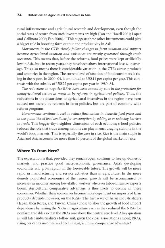
rural infrastructure and agricultural research and development, even though thesocial rates of return from such investments are high (Fan and Hazell 2001; Lopezand Gallinato 2006; Fan 2008).15 This suggests these other instruments could playa bigger role in boosting farm output and productivity in Asia.
Movements in the CTEs closely follow changes in farm taxation and supportbecause agricultural taxation and assistance are mostly generated through trademeasures. This means that, before the reforms, food prices were kept artificiallylow in Asia, but, in recent years, they have been above international levels, on aver-age. This also means there is considerable variation in the CTEs across productsand countries in the region. The current level of taxation of food consumers is ris-ing in the region. In 2000–04, it amounted to US$11 per capita per year. This con-trasts with the subsidy of US$22 per capita per year in 1980–84.
The reductions in negative RRAs have been caused by cuts in the protection fornonagricultural sectors as much as by reforms in agricultural policies. Thus, thereductions in the distortions to agricultural incentives in the region have beencaused not merely by reforms in farm policies, but are part of economy-widereform programs.
Governments continue to seek to reduce fluctuations in domestic food prices andin the quantities of food available for consumption by adding to or reducing barriersto trade. This beggar-thy-neighbor dimension of each economy’s food policiesreduces the role that trade among nations can play in encouraging stability in theworld’s food markets. This is especially the case in rice. Rice is the main staple inAsia; and Asia accounts for more than 80 percent of the global market for rice.
Where To from Here?
The expectation is that, provided they remain open, continue to free up domesticmarkets, and practice good macroeconomic governance, Asia’s developingeconomies will grow rapidly in the foreseeable future. The growth will be morerapid in manufacturing and service activities than in agriculture. In the moredensely populated economies of the region, growth will be accompanied byincreases in incomes among low-skilled workers wherever labor-intensive exportsboom. Agricultural comparative advantage is thus likely to decline in theseeconomies. Whether these economies become more dependent on imports of farmproducts depends, however, on the RRAs. The first wave of Asian industrializers(Japan, then Korea, and Taiwan, China) chose to slow the growth of food importdependence by raising the NRAs in agriculture even as they reduced the NRAs fornonfarm tradables so that the RRAs rose above the neutral zero level. A key questionis: will later industrializers follow suit, given the close associations among RRAs, rising per capita incomes, and declining agricultural comparative advantage?
74 Distortions to Agricultural Incentives in Asia
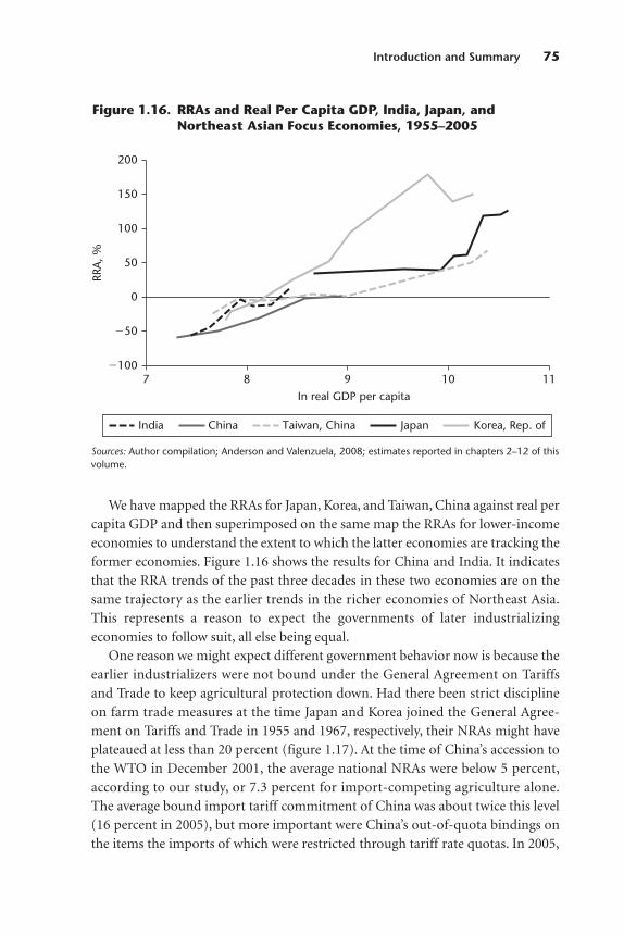
We have mapped the RRAs for Japan, Korea, and Taiwan, China against real percapita GDP and then superimposed on the same map the RRAs for lower-incomeeconomies to understand the extent to which the latter economies are tracking theformer economies. Figure 1.16 shows the results for China and India. It indicatesthat the RRA trends of the past three decades in these two economies are on thesame trajectory as the earlier trends in the richer economies of Northeast Asia.This represents a reason to expect the governments of later industrializingeconomies to follow suit, all else being equal.
One reason we might expect different government behavior now is because theearlier industrializers were not bound under the General Agreement on Tariffsand Trade to keep agricultural protection down. Had there been strict disciplineon farm trade measures at the time Japan and Korea joined the General Agree-ment on Tariffs and Trade in 1955 and 1967, respectively, their NRAs might haveplateaued at less than 20 percent (figure 1.17). At the time of China’s accession tothe WTO in December 2001, the average national NRAs were below 5 percent,according to our study, or 7.3 percent for import-competing agriculture alone.The average bound import tariff commitment of China was about twice this level(16 percent in 2005), but more important were China’s out-of-quota bindings onthe items the imports of which were restricted through tariff rate quotas. In 2005,
Introduction and Summary 75
Figure 1.16. RRAs and Real Per Capita GDP, India, Japan, andNortheast Asian Focus Economies, 1955–2005
�100
�50
0
50
100
150
200
In real GDP per capita1110987
RRA
, %
India China Taiwan, China Japan Korea, Rep. of
Sources: Author compilation; Anderson and Valenzuela, 2008; estimates reported in chapters 2–12 of thisvolume.
the latter tariff bindings were 65 percent for grains, 50 percent for sugar, and40 percent for cotton (WTO, ITC, and UNCTAD 2007). The Chinese governmentalso had bindings on product-specific domestic supports in agriculture of 8.5 per-cent and was able to provide another 8.5 percent as non-product-specific assis-tance if it so wished. This sums to an NRA of 17 percent through domestic sup-port measures alone, which is in addition to the assistance available throughout-of-quota tariff protection.
Clearly, the legal commitments the Chinese government made on acceding tothe WTO are distant from the current levels of domestic and border support itprovides to its farmers. The commitments are therefore unlikely to constrain thegovernment much in the next decade or so, and the legal commitments made bythe Asian developing economies that joined the WTO earlier (except Korea) areeven less constraining (Anderson, Martin, and Valenzuela 2008). In Bangladesh,India, and Pakistan, for example, the estimated NRAs for agricultural importablesin 2000–04 are 6, 34, and 4 percent, respectively, whereas the average bound tariffson the agricultural imports in these economies were 189, 114, and 96 percent,
76 Distortions to Agricultural Incentives in Asia
Figure 1.17. NRAs for China, Japan, and the Republic of Koreaand GATT/WTO Accession, 1955–2005
�100
�50
0
50
100
150
200
1955
–59
1960
–64
1965
–69
1970
–74
1975
–79
1980
–84
1985
–89
1990
–94
1995
–99
2000
–05
NRA
, %
year
Japan(1955 � 16.6)
Korea, Rep. of(1967 � 7.4)
China(2001 � 4.5)
Japan Korea, Rep. of China
Sources: Author compilation.
Note: WTO accession also refers to accession to the WTO predecessor organization, the GeneralAgreement on Tariffs and Trade.
respectively (WTO, ITC, and UNCTAD 2007). Also, like other developing- economy governments, the governments of these economies have significantbindings, 10 percent, on product-specific domestic supports and another 10 per-cent for non-product-specific assistance, a total of 20 extra percentage points ofNRA that legally could be applied through domestic support measures. This com-pares with the 10 percent in India and the less than 3 percent in the rest of SouthAsia (tables 1.13 and 1.14).
One can only hope that China and South and Southeast Asia will not make useof the legal wiggle room they have allowed themselves in their WTO bindings andthereby follow Japan, Korea, and Taiwan, China into substantial agricultural pro-tection.16 A much more efficient and equitable strategy would involve treatingagriculture in the same way they have been treating nonfarm tradables. Thiswould involve opening the sector to international competition and relying onmore-efficient domestic taxes (for example, taxes on income and consumption orvalue added taxes) rather than trade taxes to raise government revenue.
It might be argued that such a laissez faire strategy might increase rural-urbaninequality and poverty and thereby generate social unrest. Nonetheless, policiesthat lead to high prices for staple foods, in particular, involve potentially seriousrisks for the urban and rural poor who are net buyers of food in developing coun-tries, as has been demonstrated during the recent increases in the prices for thesegoods (Ivanic and Martin 2008). The available evidence suggests that rural-urbanpoverty gaps have been reduced in parts of Asia when more mobile members offarm households are able to find full- or part-time work off the farm and repatri-ate a portion of their higher earnings among other farm household members(Otsuka and Yamano 2006; World Bank 2007). Concerted government interven-tion through social policy measures are hugely important in reducing the gapsbetween rural and urban incomes and in raising national incomes overall (Winters, McCulloch, and McKay 2004; Hayami 2007). Efficient ways of assistingany poor (nonfarm or farm) households left behind include public investmentmeasures that have high social payoffs, such as in basic education and health care,and investments in rural infrastructure and agricultural research and develop-ment.17
What do the above lessons and implications suggest developing-country policymakers should do when confronted, as in recent years, by a sharp upward move-ment in international food prices? In the past, as illustrated for rice in figures 1.13and 1.14, many governments have simply increased export restrictions or loweredimport restrictions on food staples for the duration of the spike. What if therecent rise in international prices is more prolonged than the short-lived spikes ofthe past? Outlook projections issued by international agencies suggest that pricesmight remain high for the foreseeable future and that growth in net food imports
Introduction and Summary 77

by the rapidly industrializing economies of Asia is a significant contributor to thisphenomenon.18 Yet, as we see in figure 1.8, China and India over the past two orthree decades have steadily raised the RRAs, though these had been adequate tokeep both countries close to self-sufficiency in primary agricultural products overthe previous four decades. However, in 2000–04, China became a net importer inall trade in agriculture and processed food for the first time, while, in South Asia,the net exports of India were less than the net imports of Bangladesh and Pakistanfor the first time since the late 1960s (Sandri, Valenzuela, and Anderson 2007).19
Should these governments choose to maintain RRAs at current levels (close tozero), the import dependence of these economies in agriculture might rise. If thisoccurs, other developing economies might reconsider their current position in theWTO’s Doha Round of trade negotiations. By agreeing to lower substantially theirbound tariffs and their subsidies on agricultural products, they could extractgreater concessions from high-income countries without having to reduce theiractual applied rates in the foreseeable future.
We have dealt little in this chapter with the effects of the trends and fluctuationsin the NRAs and RRAs, especially on economic welfare, price stability, incomeequality, or poverty, and we have dealt little with the underlying causes of theseeffects. The analytical narratives in the chapters that follow touch on these issues,but more in-depth empirical analysis may now be undertaken with the help of ourassistance estimates. Some analysis will appear in our project’s publications. Specif-ically, Anderson, Valenzuela, and van der Mensbrugghe (forthcoming) provideresults from a global economy-wide model of the impacts on agricultural markets,national economic welfare, and net farm incomes of distortions to the world’sgoods markets as of 2004. They use the new agricultural distortion estimates in thisvolume and its companion volumes. How these distortions, both within an econ-omy and in the rest of the world, affect poverty and inequality are explored in aseries of country case studies brought together in Anderson, Cockburn, and Martin(forthcoming), who use national economy-wide models that have been enhancedwith detailed earning and spending information on numerous types of urban andrural households. In Anderson (Political Economy, forthcoming), a broad range oftheoretical and econometric analyses are assembled to shed light on the politicaleconomy forces that have generated the evolving pattern of inter- and intrasectoraldistortions in farmer and food consumer incentives over the past half century. Ourhope is that these and others results of this study and its companion volumes willspawn much more analysis in the years to come.
Notes
1. The other three regional studies are Anderson and Masters (forthcoming), Anderson and Swinnen (2008), and Anderson and Valdés (2008). Together with comparable studies of high-incomecountries, including Japan, they have formed the basis for a global overview volume (Anderson,A Global Perspective, forthcoming).
78 Distortions to Agricultural Incentives in Asia
2. Apart from the urban islands of Hong Kong, China and Singapore, the region’s economies that havepopulations above 1 million each and that we have omitted are Afghanistan, Cambodia, the DemocraticPeople’s Republic of Korea, the Lao People’s Democratic Republic, Mongolia, Myanmar, Nepal, and PapuaNew Guinea, which, in 2004, contributed less than 5 percent of the population, 4 percent of the agricul-tural GDP, and 2 percent of the total GDP of all the developing economies in the region.
3. Anderson and Hayami (1986) only examine Japan, the Republic of Korea, and Taiwan, Chinaand only from 1955 to 1982 (apart from the rice distortion estimates, which are provided for an addi-tional five decades). Krueger, Schiff, and Valdés (1991) analyze Korea, Malaysia, Pakistan, the Philip-pines, Sri Lanka, and Thailand, but for only four or five crops and only from 1960 to 1984. Orden et al.(2007) supply producer support estimates only for China, India, Indonesia, and Vietnam and onlysince 1985. The OECD (2007) has been covering its two Asian members, Japan and Korea, since 1986,but has also begun examining China (see OECD 2005). All these earlier studies find that the averagenominal rates of assistance (NRAs) for farmers are higher in higher-income settings and in settings inwhich agricultural comparative advantage is weaker. They find that the NRAs in each economy are alsomuch higher in the import-competing subsector than among exporters of farm products.
4. In overall land endowment per capita rather than only cropland and pastureland, China hasaround 30 percent of the global average.
5. The regime changes that have occurred during this period have included the shift from socialismto the market in China and Vietnam and the opening of India and several other economies. The regionsaw the end of colonization between the late 1940s and late 1950s. The Korean Peninsula and Taiwan,China obtained independence from Japan in 1945, India and Pakistan from Britain in 1947, Indonesiafrom the Netherlands in 1949, Indochina from France in 1954, and Malaya from Britain in 1957.
6. The nine are China; Hong Kong, China; Indonesia; Japan; Korea; Malaysia; Singapore; Taiwan,China; and Thailand. Brazil is the only other large economy in the set of 12; the other three economiesare Botswana, Malta, and Oman.
7. By contrast, the share of our focus economies in the global exports of agricultural and foodproducts grew only a little, from 11.0 to 13.5 percent between 1990 and 2006.
8. Our definition of a policy-induced price distortion follows Bhagwati (1971) and Corden (1997).It includes any policy measure at the border (such as a trade tax or subsidy, a quantitative restrictionon trade, or a dual or multiple foreign exchange rate system, assuming the country is small enough tohave no monopoly power in international markets) or any domestic producer or consumer tax, sub-sidy, or restraint on output, intermediate inputs, or primary factors of production (except where theseare needed to overcome directly an externality, or where it is set optimally across all products or fac-tors, for example as a value added tax to raise government revenue).
9. Corden (1971) proposed that the volume of free trade might be used as weights, but because thisis not observable (and an economy-wide model is needed to estimate the weights), the usual practice isto compromise by using actual distorted volumes, but undistorted unit values or, equivalently, dis-torted values, divided by (1 � NRA). If estimates of own and cross-price elasticities of demand andsupply are available, a partial equilibrium estimate of the quantity at undistorted prices might be gen-erated, but, if the estimated elasticities are unreliable, this may introduce more error to the error oneseeks to correct.
10. Recall that, unless otherwise noted, Asia is shorthand throughout this volume for our focusdeveloping economies and thus excludes Japan.
11. Also ignored are distortions in the prices for the inputs into the production of nonfarm goods,which is in contrast to the treatment of these prices in agricultural NRA estimates.
12. This bias is accentuated in cases in which distortions in exchange rates are not included, asnoted also in the section on methodology. Exchange rate distortions have been included in the studiesthat form the basis of the chapters on China, Malaysia, Pakistan, Sri Lanka, and Vietnam. Their impactwas greatest in China, where they caused the RRAs to be more negative by about 2 percentage points inthe 1970s, 6 percentage points in the 1980s, and 3 percentage points in the 1990s (see chapter 3, table3.5 in this volume).
13. It is also true that consumers in South Asia received staple foods at prices that were effectivelysubsidized through the fair price shops. However, these government handouts were sufficiently
Introduction and Summary 79

rationed to be mostly inframarginal and, so, are considered here as implicit income transfers ratherthan additional distortive consumer subsidies.
14. The number for the share of rice production represented an increase over the pre-1990s half-decade global shares, which were all less than 4.5 percent (for example, 4.1 percent in 1985–89) and isgreater than the Asian share of only 5.7 percent in 2000–04 according to our estimates.
15. Data in Pardey et al. (2006) suggest that public research and development expenditure inAsia since the late 1970s has averaged less than 0.5 percent of the gross value of production at undis-torted prices. This is trivial compared with the NRAs for the region that are generated through price-distorting measures. These NRAs are 25 to 40 times this share of the gross value of production (below�20 percent until the mid-1980s and 12 percent in 2000–04).
16. The indications in the ongoing Doha Round of multilateral trade negotiations at the WTO arenot encouraging. The Group of 33 developing countries, led by Indonesia, but strongly supported byIndia and the Philippines, among others, is arguing for additional special and differential treatment fordeveloping countries in the form of exemptions from agricultural tariff cuts for special products andfor a special safeguard mechanism that would allow these countries to impose tariffs that are evenhigher than the bound tariffs in years of likely import surges.
17. As implied by the estimates reported in note 15 above, even if only 5 percent of the currentNRAs provided to Asian farmers through farm price support policies were replaced by agriculturalresearch and development expenditure, this would more than double current public spending on thisresearch and development. The latter would increase regional economic welfare, whereas price- distortionary policies reduce welfare. Such a boost in research and development might generateanother Green Revolution, especially if it took full advantage of the new developments in biotechnol-ogy. (For rice, for example, see Anderson, Jackson, and Nielsen 2005.)
18. The World Bank’s commodity forecasts indicate that, by 2020, grain prices will still be 10 per-cent above 2006 levels in real terms (Prospects for the Global Economy Database 2008). The 2006 lev-els were 20 percent above the average for 2001–05. The International Food Policy Research Institute,the OECD, and the Food and Agriculture Organization similarly expect food prices to remain highwell into the next decade and beyond (von Braun 2007; OECD and FAO 2008).
19. The change in China was largely caused by increases in the cotton imports needed to supply theeconomy’s rising production in textiles and clothing for export.
References
Anderson, K. 1995. “Lobbying Incentives and the Pattern of Protection in Rich and Poor Countries.”Economic Development and Cultural Change 43 (2): 401–23.
———. 2008. “Distorted Agricultural Incentives and Economic Development: Asia’s Experience.”2008 World Economy Lecture, Leverhulme Center for Research on Globalization and EconomicPolicy, University of Nottingham, Semenyih, Malaysia, January 16. Forthcoming in The World Economy 32 (2009).
———, ed. forthcoming. Distortions to Agricultural Incentives: A Global Perspective, 1955 to 2007.———, ed. forthcoming. Political Economy of Distortions to Agricultural Incentives.Anderson, K., J. Cockburn, and W. Martin, eds. forthcoming. Agricultural Price Distortions, Inequality,
and Poverty.Anderson, K., and Y. Hayami, eds. 1986. The Political Economy of Agricultural Protection: East Asia in
International Perspective. London: Allen and Unwin.Anderson, K., L. A. Jackson, and C. P. Nielsen. 2005. “GM Rice Adoption: Implications for Welfare and
Poverty Alleviation.” Journal of Economic Integration 20 (4): 771–88.Anderson, K., M. Kurzweil, W. Martin, D. Sandri, and E. Valenzuela. 2008. “Measuring Distortions to
Agricultural Incentives, Revisited.” World Trade Review 7 (4): 675–704.
80 Distortions to Agricultural Incentives in Asia
Anderson, K., W. Martin, and E. Valenzuela. 2008. “Long Run Implications of WTO Accession for Agri-culture in China.” In China’s Agricultural Trade: Issues and Prospects, ed. C. Carter and I. Sheldon.London: CABI.
Anderson, K., and W. Masters, eds. forthcoming. Distortions to Agricultural Incentives in Africa. Washington, DC: World Bank.
Anderson, K., and J. Swinnen, eds. 2008. Distortions to Agricultural Incentives in Europe’s Transition.Washington, DC: World Bank.
Anderson, K., and A. Valdés, eds. 2008. Distortions to Agricultural Incentives in Latin America. Washington,DC: World Bank.
Anderson, K., and E. Valenzuela. 2008. “Estimates of Global Distortions to Agricultural Incentives,1955 to 2007.” World Bank. http://go.worldbank.org/5XY7A7LH40.
Anderson, K., E. Valenzuela, and D. van der Mensbrugghe. forthcoming. “Effects of Distortions onGlobal Welfare, Farm Incomes, and Agricultural Markets.” In Distortions to Agricultural Incentives:A Global Perspective, 1955 to 2007, ed. K. Anderson, chap. 12. London: Palgrave Macmillan; Wash-ington, DC: World Bank.
Bhagwati, J. N. 1971. “The Generalized Theory of Distortions and Welfare.” In Trade, Balance of Pay-ments and Growth: Papers In International Economics in Honor of Charles P. Kindleberger, ed. J. N.Bhagwati, R. W. Jones, R. A. Mundell, and J. Vanek, 265–86. Amsterdam: North-Holland.
Bussolo, M., R. de Hoyes, and D. Medledev. forthcoming. “Policy Impacts on Global Income Distribu-tion, Inequality, and Poverty Using Microsimulation with the Linkage Model.” In Agricultural PriceDistortions, Inequality, and Poverty, ed. K. Anderson, J. Cockburn, and W. Martin, chap. 4.
Chen, S., and M. Ravallion. 2007. “Absolute Poverty Measures for the Developing World, 1981–2004.”Policy Research Working Paper 4211, World Bank, Washington, DC.
Commission on Growth and Development. 2008. The Growth Report: Strategies For Sustained Growthand Inclusive Development. Washington, DC: Commission on Growth and Development, WorldBank.
Corden, W. M. 1971. The Theory of Protection. Oxford: Clarendon Press.———. 1997. Trade Policy and Economic Welfare. 2nd ed. Oxford: Clarendon Press.Fan, S., ed. 2008. Public Expenditures, Growth, and Poverty: Lessons from Developing Countries. Baltimore:
Johns Hopkins University Press; Washington, DC: International Food Policy Research Institute.Fan, S., and P. Hazell. 2001. “Returns to Public Investments in the Less-Favored Areas of India and
China.” American Journal of Agricultural Economics 83 (5): 1217–22.FAO Agricultural Trade Database (FAOSTAT). Food and Agriculture Organization of the United
Nations. http://faostat.fao.org/site/342/default.aspx (accessed May 2008).FAOSTAT Database. Food and Agriculture Organization of the United Nations. http://faostat.fao.org/
default.aspx (accessed May 2008).FAO SUA-FBS Database (Supply Utilization Accounts and Food Balance Sheets Database, FAOSTAT).
Food and Agriculture Organization of the United Nations. http://faostat.fao.org/site/354/default.aspx (accessed May 2008).
Hayami, Y. 2007. “An Emerging Agricultural Problem in High-Performing Asian Economies.” PolicyResearch Working Paper 4312, World Bank, Washington, DC.
Ivanic, M., and W. Martin. 2008. “Implications of Higher Global Food Prices for Poverty in Low-Income Countries.” Policy Research Working Paper 4594, World Bank, Washington, DC.
Krueger, A. O., M. Schiff, and A. Valdés. 1988. “Agricultural Incentives in Developing Countries: Meas-uring the Effect of Sectoral and Economywide Policies.” World Bank Economic Review 2 (3):255–72.
———. 1991. Asia. Vol. 2 of The Political Economy of Agricultural Pricing Policy. World Bank Compar-ative Study. Baltimore: Johns Hopkins University Press; Washington, DC: World Bank.
Lerner, A. P. 1936. “The Symmetry between Import and Export Taxes.” Economica 3 (11): 306–13.Lloyd, P. J. 1974. “A More General Theory of Price Distortions in an Open Economy.” Journal of Inter-
national Economics 4 (4): 365–86.
Introduction and Summary 81
Lopez, R., and G. I. Gallinato. 2006. “Should Governments Stop Subsidies to Public Goods? Evidencefrom Latin America.” Journal of Public Economics 91 (5–6): 1071–94.
Maddison, A. 2003. The World Economy: Historical Statistics. Paris: Development Centre, Organisationfor Economic Co-operation and Development.
OECD (Organisation for Economic Co-operation and Development). 2005. Review of AgriculturalPolicies: China. Paris: OECD.
———. 2007. Agricultural Policies in OECD Countries: Monitoring and Evaluation 2007. Paris: OECD.OECD (Organisation for Economic Co-operation and Development) and FAO (Food and Agriculture
Organization of the United Nations). 2008. OECD-FAO Agricultural Outlook 2008–2017. Paris:OECD.
OECD PSE-CSE Database (Producer and Consumer Support Estimates, OECD Database 1986–2005).Organisation for Economic Co-operation and Development. http://www.oecd.org/document/55/0,3343,en_2649_33727_36956855_1_1_1_1,00.html (accessed December 2007).
Orden, D., F. Cheng, H. Nguyen, U. Grote, M. Thomas, K. Mullen, and D. Sun. 2007. Agricultural Pro-ducer Support Estimates for Developing Countries: Measurement Issues and Evidence from India,Indonesia, China, and Vietnam. Research Report 152. Washington, DC: International Food PolicyResearch Institute.
Otsuka, K., and T. Yamano. 2006. “Introduction to the Special Issue on the Role of Nonfarm Income inPoverty Reduction: Evidence from Asia and East Africa.” Agricultural Economics 35 (3) (supple-ment): 373–97.
Pardey, P. G., N. Beintima, S. Dehmer, and S. Wood. 2006. “Agricultural Research: A Growing GlobalDivide?” Food Policy Report 17, International Food Policy Research Institute, Washington, DC.
PovcalNet. World Bank. http://go.worldbank.org/7X6J3S7K90 (accessed May 2008).Prospects for the Global Economy Database. World Bank. http://go.worldbank.org/PF6VWYXS10
(accessed May 2008).Ravallion, M., and S. Chen. 2007. “China’s (Uneven) Progress against Poverty.” Journal of Development
Economics 82 (1): 1–42.Ravallion, M., and G. Datt. 1996. “How Important to India’s Poor is the Sectoral Composition of
Economic Growth?” World Bank Economic Review 10 (1): 1–26.Sandri, D., E. Valenzuela, and K. Anderson. 2007. “Economic and Trade Indicators for Asia, 1960 to
2004.” Agricultural Distortions Working Paper 20, World Bank, Washington, DC.von Braun, J. 2007. “The World Food Situation: New Driving Forces and Required Actions.” Food
Policy Report 18, International Food Policy Research Institute, Washington, DC.Vousden, N. 1990. The Economics of Trade Protection. Cambridge, UK: Cambridge University Press.Winters, L. A., N. McCulloch, and A. McKay. 2004. “Trade Liberalization and Poverty: The Empirical
Evidence.” Journal of Economic Literature 62 (1): 72–115.World Bank. 2007. World Development Report 2008: Agriculture for Development. Washington, DC:
World Bank.World Development Indicators Database. World Bank. http://go.worldbank.org/B53SONGPA0
(accessed May 2008).WTO (World Trade Organization). International Trade Statistics 2007. Geneva: WTO.WTO (World Trade Organization), ITC (International Trade Center), and UNCTAD (United Nations
Conference on Trade and Development). 2007. World Tariff Profiles 2006. Geneva: WTO.
82 Distortions to Agricultural Incentives in Asia

Part IIII
NORTHEAST ASIA

The story of agricultural policies over the past 50 years in the Republic of Korea(the southern part of the Korean Peninsula, hereafter referred to as Korea) andTaiwan, China includes the dramatic changes in the distortions to agriculturalincentives that producers and consumers have face in the course of the develop-ment of these economies. In this study, we estimate the degree of distortions forkey agricultural products, as well as for the agricultural sector as a whole, over aperiod when these economies transitioned from low- to high-income economies(from 1955 to 2004).
Schultz (1978) established that, as economies advance from low-income tohigh-income status, price and trade policies tend to switch from taxing to subsi-dizing agriculture relative to other tradable sectors. During the 50 years of ouranalysis, Korea and Taiwan, China jumped from the status of low-income to middle-income economies and toward the status of high-income economies. Policy switching—shifting from negative to positive assistance for agriculturalproducers in the course of economic development—is clearly observable in thetime series on these two economies.
We compare the switching processes in the two economies—which grew atabout the same speed—to obtain insights into the effects of policies and theunderlying causes of the changes in the distortions in agricultural incentives. Ourfindings shed light on the process of change in agricultural distortions that occursduring the stages in economic development.
In the following sections, we first briefly describe the structure of agriculture inthe course of the development of these two economies. Next, the evolution ofagricultural policies in these economies is reviewed. Distortions to agricultural
85
2
Republic of KOREAAND TAIWAN, CHINA
Masayoshi Honma and Yujiro Hayami
incentives are measured in terms of the nominal and relative rates of assistance toagriculture (NRAs and RRAs to agriculture, respectively). We then discuss the pol-icy implications of the estimates for the two economies and draw lessons for less-developed economies that are currently experiencing structural transformation inthe course of growth.
Economic Development and Structural Change
The available choices among agricultural policies, particularly price-distortingpolicies, are closely linked to the process of economic development. As identifiedby Schultz (1978), there are two agricultural problems. The food problem under-lies the policies commonly adopted in low-income countries that exploit or taxagriculture. Such policies are in contrast to policies in many high-income coun-tries that protect or subsidize agriculture to solve the farm problem. The hypoth-esis of Schultz became an established paradigm among agricultural economistsand found support in several empirical studies (Anderson and Hayami 1986;Hayami 1988; Krueger, Schiff, and Valdés 1991). More recently, Hayami and Godo(2004) and Hayami (2005) have added the disparity problem, which is specific tomiddle-income economies. They suggest that one should examine the ways dis-tortions in agricultural incentives change in all three types of economies over thestages of development.
The most distinguishing characteristic of Korea and Taiwan, China during theperiod of analysis is the unusually rapid rates of economic growth generated bysuccess in industrial development. Indeed, during the East Asian miracle (WorldBank 1993), while Japan was first, Korea and Taiwan, China—together with HongKong, China and Singapore—comprised the runner-up group; and China andmembers of the Association of Southeast Asian Nations are now following theseeconomies. Since economic growth is a fundamental determinant of the nature ofdistortions to agricultural incentives, it is useful, in this section, to offer anoverview of development processes in Korea and Taiwan, China.
An historical perspective
Because of regular monsoon rains and the mountainous, undulated topographyin which water may be controlled relatively easily through cooperation at the fam-ily and community levels, this region is well suited to rice production on smallfamily farms organized into village communities. The agrarian structure thereforebecame characterized by a uni-modal distribution of smallholders who farmed anaverage plot of about 1 hectare. Relative to Southeast Asia, large agribusiness plan-tations based on hired labor were almost completely absent not only in Korea,
86 Distortions to Agricultural Incentives in Asia

which is located in the temperate zone, but also in Taiwan, China, where tropicalcash crops such as sugar and bananas occupy a significant agricultural subsector.The rural community was traditionally stratified across landlords, landowningcultivators, and landless tenants. Agricultural laborers subsisting on hired laborwages were not a significant component of the rural population in this region.Land reforms after World War II significantly changed the distribution oflandownership, but the distribution of operational landholdings was essentiallyintact.
There is a high degree of similarity in the agrarian structures of the twoeconomies partly because Japan brought its own institutions to its colonies: Taiwan, China was ceded by China to Japan in 1895, and the Korean Peninsulawas annexed by Japan in 1910. The biggest reform during Japanese colonizationwas the transfer of fee simple titles to landowners through cadastral surveys inreturn for the commitment of the new landowners to pay the land tax. Japaneseefforts to develop the colonies concentrated on agriculture, especially rice, whenshortages within Japan became evident after the Rice Riots of 1918. The promo-tion of rice production through agricultural research and extension systems, aswell as improvements in irrigation and drainage infrastructure, plus protectionfrom rice imports from the rest of the world (see Anderson and Tyers 1992), was amajor success from the viewpoint of the colonists in that Japan’s rice importsfrom the two colonies rose from 5 to 20 percent of the country’s consumptionbetween 1915 and 1935.
Rising exports of rice and other primary commodities and the correspondinginflows of manufactured commodities meant that dependency on agricultureremained significant in the two economies. This was especially so in the southernhalf of the Korean Peninsula because Japanese efforts in industrial development inKorea were concentrated in the north to exploit the hydroelectric power of theYalu River and feed a network of chemical industries that was larger than the onein Japan. The heavy dependency on agriculture in the south was intensified by theurban destruction during the Korean War (1950–53). In Taiwan, China, com-merce and industry were more active because the relatively larger cash crop sub-sector required larger amounts of processing and marketing relative to Koreanagriculture, which was dominated by subsistence crops such as rice and barley.Today, the wide dispersion of small and medium industries in rural areas in Taiwan, China contrasts with the concentration of Korean industry in large-scaleestablishments in urban areas and seems to be, at least in part, rooted in the cashcrop tradition.
We discuss elsewhere why Japan, Korea, and Taiwan, China were able to achieveremarkable success in economic development as forerunners to the East Asianmiracle (see Hayami and Aoki 1998; Hayami and Godo 2005). Here, it suffices to
Republic of Korea and Taiwan, China 87
say that their success was the result of borrowing technology from advancedeconomies. Gerschenkron (1962) suggested that the later the start of industrial-ization, the larger the scope for achieving economic growth by borrowing tech-nology. Why then were Korea and Taiwan, China, in particular, so successful inthis borrowing in the midst of many other late starters? One reason is that the twoeconomies were endowed with cheap, but relatively well-educated labor becauseof the diffusion of compulsory elementary education systems during the colonialperiod. This made the initial borrowing of labor-intensive industrial technologiesmore rewarding in these resource-poor economies. The accumulation of humancapital through education investments by the newly independent governmentssmoothed the way for the switch to capital- and knowledge-intensive technologiesthat occurred later. Another reason was the constant danger of Communistaggression, which compelled leaders to adopt policies to achieve economic successfor the sake of maintaining legitimacy and viability. The success of developmentbased on industrial technology borrowing by their neighbor Japan was an addedmotive for adopting this strategy.
There are many similarities, but also significant differences in the industrial-ization strategies followed by Korea and Taiwan, China. In the latter, although theNationalist Party exerted strong control over formal sectors, the government didnot attempt to intervene in the activities of small and medium entrepreneurs ininformal sectors. Informal sectors were able to grow by developing various marketing and financial links among themselves and with foreign firms. Theseenterprises were dispersed widely over urban and rural areas and were able toachieve substantial international competitive strength (Ho 1979, 1982). In contrast, government control in Korea was stronger and more complete, espe-cially under the military administration of Pak Chong-hui (1961–79). All formalcredits were channeled from nationalized banks to large industries, while foreigndirect investment was tightly controlled. The strategy was the reason for the highconcentration of industrial production in Korea in a small number of largeenterprises located predominantly in urban areas (Cole and Park 1983; Amsden1989).
Economic growth and structural transformation
We now provide a quantitative summary of economic development in Korea andTaiwan, China during the past five decades. Table 2.1 shows selected indicators ofeconomic development. The first rows provide data on real gross domestic prod-uct (GDP) per capita in 2000 constant prices in purchasing power parity dollars inKorea and Taiwan, China. Until 1960, the two economies showed a low level ofper capita GDP, at less than US$1,500. Thereafter, income levels rose rapidly,
88 Distortions to Agricultural Incentives in Asia
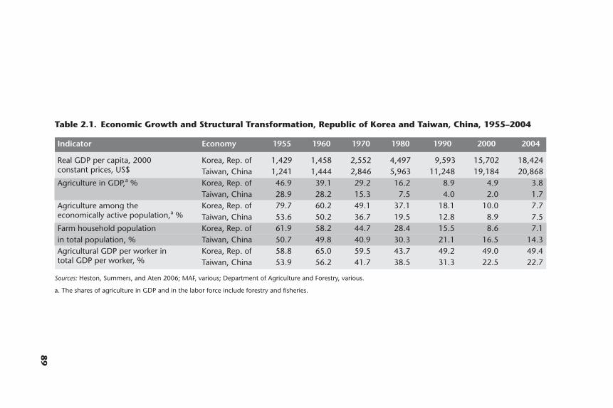
89
Table 2.1. Economic Growth and Structural Transformation, Republic of Korea and Taiwan, China, 1955–2004
Sources: Heston, Summers, and Aten 2006; MAF, various; Department of Agriculture and Forestry, various.
a. The shares of agriculture in GDP and in the labor force include forestry and fisheries.
Indicator Economy 1955 1960 1970 1980 1990 2000 2004
Real GDP per capita, 2000 Korea, Rep. of 1,429 1,458 2,552 4,497 9,593 15,702 18,424constant prices, US$ Taiwan, China 1,241 1,444 2,846 5,963 11,248 19,184 20,868Agriculture in GDP,a % Korea, Rep. of 46.9 39.1 29.2 16.2 8.9 4.9 3.8
Taiwan, China 28.9 28.2 15.3 7.5 4.0 2.0 1.7Agriculture among the Korea, Rep. of 79.7 60.2 49.1 37.1 18.1 10.0 7.7economically active population,a % Taiwan, China 53.6 50.2 36.7 19.5 12.8 8.9 7.5Farm household population Korea, Rep. of 61.9 58.2 44.7 28.4 15.5 8.6 7.1in total population, % Taiwan, China 50.7 49.8 40.9 30.3 21.1 16.5 14.3Agricultural GDP per worker in Korea, Rep. of 58.8 65.0 59.5 43.7 49.2 49.0 49.4total GDP per worker, % Taiwan, China 53.9 56.2 41.7 38.5 31.3 22.5 22.7
exceeding US$2,500 in the 1970s, US$5,000 in the 1980s, and US$10,000 in the1990s.1 The economic growth paths were largely parallel, but, after 1960, Taiwan,China went slightly ahead, with a lead of about five years.
It is convenient to review the development of the two economies in four stages,as follows:
• Low-income stage (US$1,500 or less), before 1960• Lower-middle-income stage (US$1,500–US$5,000), 1960–80• Upper-middle-income stage (US$5,000–US$10,000), 1980–90• High-income stage (US$10,000 or more), after 1990
The criteria are not applicable to all economies; they are tentatively adoptedhere for the sake of a comparison in a limited context: the development processesin these two economies.2
Although Korea and Taiwan, China experienced similar changes in real percapita GDP over the four stages, significant differences may be observed in eco-nomic structures. The GDP share of agriculture in Korea in 1955 was nearly50 percent, whereas, in Taiwan, China, it was below 30 percent. This reflectsKorea’s greater dependency on agriculture. In both economies, the share of agri-culture in GDP declined significantly (to 3.8 percent in Korea and to 1.7 percentin Taiwan, China by 2004), although Korea’s share remained at nearly double theshare in Taiwan, China.
Historical differences may be observed in the shares of agriculture in the laborforce. In 1955, up to 80 percent of workers were employed in agriculture in Koreaversus about 50 percent in Taiwan, China. The difference in the share of the laborforce employed in agriculture disappeared over time: in 2004, about 7.7 percent ofworkers were employed in agriculture in the former versus 7.5 percent in the lat-ter. Relatively more rapid declines in the labor force share compared to the GDPshare in Korea reflect the urban concentration of industry. In Taiwan, China, thereis a wide dispersion of industries over rural areas, and farmers were able toincrease their incomes through off-farm employment. While engaging in non-farm activities much of the time, they continued to be classified as farmers. Incontrast, in Korea, rural people had to quit farming and migrate to urban areas toobtain nonfarm employment. Such differences are also reflected in the muchmore rapid decrease in the share of farm household population in the total popu-lation in Korea versus Taiwan, China.
The last rows in table 2.1 report the ratios of agricultural GDP per worker tototal GDP per worker. This may be considered an indicator of the labor produc-tivity of agriculture relative to the labor productivity of the total economy innominal value. It may also be regarded as an indicator of the income gap betweenthe agricultural sector and the whole economy. This measure must be interpreted
90 Distortions to Agricultural Incentives in Asia
with care. It declined much more quickly in Taiwan, China than in Korea, whichmay appear to indicate more rapid growth in agricultural labor productivity inKorea. In fact, however, this apparently more rapid relative growth of agriculturallabor productivity in Korea was caused by more rapid relative decreases in the sizeof the farm labor force owing to steadier out-migration of farm labor to urbanoccupations. The number of agricultural workers decreased more slowly in Taiwan, China because these workers continued to farm, while increasing the allo-cation of their labor to nonfarm activities. Thus, growth in the labor productivityof farmers engaging in agricultural activities relative to that of other workerswould not have been slower and might even have been more rapid in Taiwan,China if the ratio is calculated using output per hour of labor instead of outputper worker according to the official sectoral labor force classification.
Changes in the structures of agriculture
How did the structure of agriculture in Korea and Taiwan, China change throughthe process of economic growth outlined above? Tables 2.1 and 2.2 show that, in1955, Korea had 2.2 million farm households, which accounted for 62 percent ofthe total population, while Taiwan, China had 0.73 million farm households,which accounted for 51 percent of the population. The number of farm house-holds has been relatively stable in the latter, whereas it has decreased rapidly in theformer. The number of people in farm households in Korea also declined at morerapid rates because of steadier decreases in the number of farm households andthe number of persons per farm household. These observations represent addi-tional evidence for the scarcity of nonfarm employment opportunities in ruralareas in Korea because of urban-centered industrialization. Indeed, from 1970 to2004, the share of agricultural income in the total income of farm householdsdeclined from 49 to 22 percent in Taiwan, China, whereas, in Korea, it peaked at76 percent in 1970 and was still 39 percent in 2004.
The amount of arable land increased in Korea from about 2 million hectares in1955 to 2.3 million hectares by 1970, but declined to 1.8 million hectares in 2004.In Taiwan, China, the amount increased from 0.87 million hectares in 1955 to0.91 million hectares in 1980, but declined to 0.84 million hectares in 2004.
Changes in operational farm size in Korea and Taiwan, China during the pastfive decades have resulted almost exclusively from changes in the number of farmhouseholds. In Korea, the average farm size increased from 0.9 hectares of arableland in 1955 to 1.5 hectares in 2004. Meanwhile, the farm size in Taiwan, Chinaremained close to constant at around 1.2 hectares. The much more rapid increasein farm size in Korea was the result of greater out-migration of the farm popula-tion to urban areas owing to more urban-centered industrialization.
Republic of Korea and Taiwan, China 91
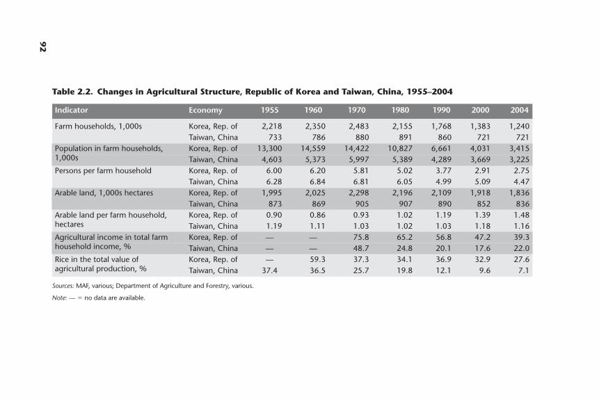
92
Table 2.2. Changes in Agricultural Structure, Republic of Korea and Taiwan, China, 1955–2004
Sources: MAF, various; Department of Agriculture and Forestry, various.
Note: — � no data are available.
Indicator Economy 1955 1960 1970 1980 1990 2000 2004
Farm households, 1,000s Korea, Rep. of 2,218 2,350 2,483 2,155 1,768 1,383 1,240Taiwan, China 733 786 880 891 860 721 721
Population in farm households, Korea, Rep. of 13,300 14,559 14,422 10,827 6,661 4,031 3,4151,000s Taiwan, China 4,603 5,373 5,997 5,389 4,289 3,669 3,225Persons per farm household Korea, Rep. of 6.00 6.20 5.81 5.02 3.77 2.91 2.75
Taiwan, China 6.28 6.84 6.81 6.05 4.99 5.09 4.47Arable land, 1,000s hectares Korea, Rep. of 1,995 2,025 2,298 2,196 2,109 1,918 1,836
Taiwan, China 873 869 905 907 890 852 836Arable land per farm household, Korea, Rep. of 0.90 0.86 0.93 1.02 1.19 1.39 1.48hectares Taiwan, China 1.19 1.11 1.03 1.02 1.03 1.18 1.16Agricultural income in total farm Korea, Rep. of — — 75.8 65.2 56.8 47.2 39.3household income, % Taiwan, China — — 48.7 24.8 20.1 17.6 22.0Rice in the total value of Korea, Rep. of — 59.3 37.3 34.1 36.9 32.9 27.6agricultural production, % Taiwan, China 37.4 36.5 25.7 19.8 12.1 9.6 7.1
This distinguishing characteristic of industrialization in Korea is clearlyreflected in the high share of agricultural income in total farm household income.The ratio fell with increases in off-farm employment among members of farmhouseholds. In Taiwan, China, the share of agricultural income was already below50 percent in 1970, when the economy was in the low-income stage, and it fell toabout 20 percent in the 1990s, when the economy approached the high-incomestage. In contrast, in Korea, the share of agricultural income in total farm house-hold income was 76 percent in 1970 and still nearly 40 percent in 2004; this wasnot only higher than the share in Taiwan, China, but also higher than the share inJapan at comparable development stages.
Major differences in the adjustments undertaken in agriculture in the face ofeconomic growth based on industrial development are also observable in thechanges in the commodity mix in farm production. Rice was traditionally themost important crop in both economies, and this importance tended to decline asper capita income rose. However, the changes in the relative importance of ricewas different in the two economies. In Korea from 1960 to 2004, the share of ricein the total value of agricultural production declined from 59 to 28 percent. InTaiwan, China, the share was initially low, at 37 percent in 1960, but fell more rap-idly, to only 7 percent in 2004. The difference reflects the greater opportunity togrow tropical cash crops there. It also reflects the economy’s success in achievinggreater agricultural diversification toward high-valued commodities such as veg-etables, fruits, chicken, and pork in response to the shift in demand toward moreincome-elastic commodities.
The Evolution of Agricultural Policy
We now outline changes in agricultural policies over the different stages of devel-opment in the two economies.
Korea
Before 1960, Korea was a low-income country, with a per capita income belowUS$1,500.3 The economy had been severely damaged during the Korean War. Theagricultural policy adopted at this stage aimed to maintain low domestic con-sumer prices for staple foods, notably rice and barley, as well as for fertilizer. TheGrain Management Law, enacted in 1950, gave the government the authority toregulate price on staple foods. However, government control was not effectiveduring the 1950s, given that the market share of government-controlled rice wasless than 10 percent. The government was supposed to purchase grain directlyfrom farmers, but it was unable to purchase sufficient amounts; there were
Republic of Korea and Taiwan, China 93
budgetary constraints, and inflation had caused grain prices to spiral upward inthe mid-1950s. Schemes to collect rice in payment of the land tax and to barterfertilizer for rice were initiated. The first type of scheme was successful, but thesecond type failed because the implicit barter price of rice was lower than themarket price. Grain imports from the United States under Public Law 480, whichamounted to 8 to 12 percent of total domestic grain in 1956–65, helped the gov-ernment keep grain prices low.
In the 1960s, under the development autocracy of Pak Chong-hui, Korealaunched an energetic policy to promote industrialization. Rather than support-ing adequate incomes among farmers, agricultural policies at the time weredesigned to keep prices on staple food crops low so as to maintain low wage ratesand a low cost of living among industrial workers. Government purchase priceswere set below market prices; this was considered necessary to raise industrialprofits and foster capital formation. The government’s price interventions gradu-ally became more intense. The market share of government-controlled rice wasexpanded to 20–25 percent during the 1960s; this was used principally to main-tain low domestic prices. These agricultural-taxing policies continued during theinitial part of the lower-middle-income stage.
The Korean economy advanced quickly toward the upper-middle-income stage.Meanwhile, the direction of agricultural policy gradually moved toward the provi-sion of support for farmers. In the early 1970s, the buffer-stock operation for non-cereal products was set in motion to counteract price declines in the subsector.Chemical fertilizers, pesticides, and farm machinery were added to the list of subsi-dized inputs (alleviating the adverse impact on farmers of the import protectionprovided to the manufacturers of these inputs). The government’s purchase pricesfor rice and barley were steadily raised with the aim of increasing food production,as well as reducing the urban-rural income gap. Although the government allowedan increase in the producer prices on staple food grains, this occurred without acomparable rise in the market prices for rice and barley, thereby preventing a rise inthe cost of living and the wage rates among industrial workers. Likewise, the gov-ernment assisted livestock producers in part by using import quotas rather thantariffs to protect them from import competition; the rents from the quotas werecaptured by the producer-managed meat import agency.4
The implementation of the two-price system, however, conflicted with the needto maintain financial and monetary stability. When the difference between the pur-chase prices and the sale prices of rice and barley widened, the deficit in the grainmanagement fund increased. Because a large portion of the deficit was financedthrough long-term overdrafts at the Bank of Korea, the policy came to represent amajor addition in inflationary pressure. The expansion in the government deficitcaused by the two-price policy became a serious constraint on the policy.
94 Distortions to Agricultural Incentives in Asia
When the economy entered the upper-middle-income stage in the 1980s, thegovernment took a step toward reducing both tariff and nontariff protection formanufacturing industries. In contrast, agricultural policies that tended to protectfarmers were strengthened. The producer prices of farm products were raised farabove border prices by means of quantitative import restrictions on most agricul-tural commodities.
After Korea entered the high-income stage in the early 1990s, significant policychanges were mostly related to the Uruguay Round Agreement on Agriculture,which was stipulated in 1995. According to the provisions of the agreement,Korea’s quantitative restrictions were converted to tariffs for all agricultural prod-ucts except rice. In the Uruguay Round negotiations, Korea retained the status ofa developing country, which assigned it special treatment in the implementationof the commitments to reduce border protection. The agricultural products undertariffication were subject to a protection reduction commitment of 24 percent,on average, within 10 years, and a minimum cut of 10 percent. The tariff rates onKorean agricultural products were over 60 percent, on average. The tariffs onproducts that were considered particularly important in Korea were cut by theminimum rate of 10 percent.
In addition, many agricultural products began to be imported under the minimum market access commitment. This commitment required that, for allagricultural products, at least 3 percent of consumption must be purchased inter-nationally during the first year, and the import share must increase annually up to5 percent of consumption within 10 years. Low tariff rates were applied to the in-quota volume so as to guarantee easy market access from exporting countries.Many key agricultural products such as rice, barley, oranges, red peppers, garlic,and onions were newly imported under this commitment.
Rice, the most important item in Korean agriculture, was temporarilyexempted from tariffication as provided in the Uruguay Round Agreement onAgriculture, annex 5.B. As an exception, rice was subject to an import quota,beginning at 1 percent of total consumption and gradually increasing up to 4 per-cent in 2004, the final implementation year. If Korean rice had not been exemptedfrom tariffication, Korea would have complied with the standard market accesscommitment, 3 to 5 percent. The temporary exemption from tariffication expiredin 2004, but Korea opted to continue invoking a rice exemption from tarifficationfor another 10 years, to 2014.
Taiwan, China
After World War II, Taiwan, China suffered high inflation rates, serious shortagesof food and other necessities, and a heavy defense burden.5 The government gave
Republic of Korea and Taiwan, China 95
the highest priority to economic stabilization, food production increases, and therepair of war damage. To alleviate the intense population pressure on the limitedland, it decided to grant incentives to farmers. Together with the land reform pro-gram implemented between 1949 and 1953, war-damaged irrigation and drainagefacilities were repaired, fertilizers and other farm inputs were made available, andfarmer organizations were strengthened.
During the recovery stage of the economy, the Sino-American Joint Commis-sion on Rural Reconstruction, established in Nanjing in 1948, played an impor-tant role. The commission served as a nonpermanent agency for the postwar ruralreconstruction of China. From 1951 to 1965, the United States provided US$1.5 bil -lion in aid in Taiwan, China through the commission. Approximately one-third ofthe aid went to agriculture, where the aid was used to build infrastructure andenhance human resources. Also, substantial imports of commodities financed byU.S. aid and increases in domestic production, especially food production, helpedrelieve demand pressure.
During the low-income stage of economic development (before 1960), agricul-tural policy in Taiwan, China was designed mainly to supply rice to the nonfarmpopulation at low, stable prices. In those days, two important taxes were imposedon farmers: the farm land tax and the hidden rice tax. Implementation wasachieved by means of compulsory rice purchases and a rice-fertilizer barter system.The compulsory purchase of paddy from landowners at official prices was anothermethod used to exert government control over rice. All paddy lands were subject tothe paddy land tax, plus the compulsory procurement of rice. The compulsory pro-curement was assessed on the basis of tax units determined according to land pro-ductivity. The difference between the government procurement prices and farmermarket prices constituted a hidden tax on paddy landowners, who, after the landreform program, were mostly farm operators. The hidden tax was graduallyreduced as per capita incomes rose, but it continued to be imposed until 1973.
The government’s rice collection by all these means during 1950–70 averaged 50to 60 percent of the total amount of rice produced, minus the home consumptionof farm families. By 1973, however, the share had declined to 20 percent. In subse-quent years, it rose again because of the launch of the guaranteed rice price policy.
The total value of the hidden rice tax was more than twice the value of the farmland tax before 1961 (except in 1954) and was larger than the total income taxbefore 1963. After 1961, when the economy moved to the lower-middle-incomestage, the hidden rice tax decreased rapidly: in 1971, the ratio of the hidden ricetax to the total income tax was only 8.5 percent (Kuo 1975).
Agricultural policy geared to exploit agriculture for the sake of supportingindustrial development (and military development) largely ended during the1970s, when the shift toward the subsidization of agriculture was initiated. This
96 Distortions to Agricultural Incentives in Asia
was the period when labor-intensive light industries were rapidly expanding inresponse to increases in export demand. Because many light industries such asgarments and footwear were located in rural areas, nonfarm incomes becameincreasingly important among farm households. Farmers were able to take advan-tage of employment in manufacturing without leaving home; and, moreover,many farmers also engaged in nonfarm self-employed activities during less busyfarm seasons. Therefore, the need for farmers to rely on agricultural protectionpolicies was less substantial in Taiwan, China than in Korea.
In 1978, Taiwan entered the upper-middle-income stage at a real GDP per capitaabove US$5,000. To help raise the incomes of farm workers to levels comparable tothe incomes of workers in the rapidly expanding industrial sector, the governmentoffered loans and subsidies to promote farm mechanization; the scheme wasdesigned to raise farm labor productivity. At this time, the growth in rice productionbegan to slow in response to renewed emphasis on livestock and fishery productsand high-value export crops. Increases in industrial employment were also pushingup the costs of farm labor. Agriculture continued to lag behind the industrial sectorin labor productivity, and the gap between farm and nonfarm per capita incomeswas widening, to the disadvantage especially of farmers who relied mainly on riceproduction. The problems faced in Taiwan, China in agriculture were similar tothose experienced by many industrial countries at comparable stages of develop-ment, especially Japan in the early 1960s and Korea in the late 1970s.
The annual per capita consumption of rice in Taiwan, China fell from 140 to74 kilograms between 1968 and 1988. The accumulation in rice reserves became aserious problem. To reduce production, farm extension workers encouragedfarmers to plant other crops in rice fields. The effort was unsuccessful because noeconomic incentive was provided. A six-year rice-crop substitution plan was inau-gurated in 1984 that involved direct subsidies of 1 metric ton of paddy rice perhectare to farmers who shifted their rice fields to corn or sorghum, or 1.5 metrictons of paddy rice per hectare to farmers who shifted to crops other than corn andsorghum. In addition, corn and sorghum were purchased by the government atguaranteed prices. Under the program, rice production declined to 1.8 millionmetric tons in 1988, which was 0.9 million metric tons less than the peak, whichhad been reached in 1976. The in-kind subsidy was altered to a cash payment in1988 to improve efficiency in the management of the program.
The economy entered the high-income stage in the late 1980s. Real GDP percapita exceeded US$10,000 beginning in 1988. The most important changes inagricultural policy during the high-income stage were related to the accession ofTaiwan, China to the World Trade Organization, which became effective on January 1, 2002. In line with the level of development of the economy, Taiwan,China agreed to adjust its tariff rates so that they were between the rates in Japan
Republic of Korea and Taiwan, China 97
and the rates in Korea. It also agreed to reduce tariffs from the average nominalrate of 20 percent in 2001 to 14 percent in the first year of accession and to 13 per-cent by 2004. The target date for tariff reductions was 2002 except for 137 itemsthat were under tariff rate quotas. Of the 41 products that were under importquota restrictions before accession to the World Trade Organization, 18 weremoved to tariffication after accession. Rice received a special exemption, and theremaining 22 items were governed by the tariff rate quota regime.
As in the case of Korea, the special treatment of rice is based on the rules of theUruguay Round Agreement on Agriculture, annex 5. The quota of rice importswas set in 2002 at 8 percent of the average domestic consumption between 1990and 1992 (144,720 tons of brown rice). By negotiation, this amount was dividedinto governmental and private import quotas. The government rice quota(65 percent of rice imports) was subject to the same treatment as rice purchasedfrom local growers. The imported rice cannot be exported for food aid, nor can itbe used for animal feed. The remainder (35 percent) was imported by privatefirms and was allocated on a first-come-first-served basis. For both private andgovernment quotas, there is a ceiling on the price markup of NT (New Taiwan)$23.26 per kilogram for rice and NT$25.59 for rice products sold on the domesticmarket. If the sale of quota rice is slow, the price markup can be cut by NT$3 everytwo weeks. The markup reduction may be continued until all quantities are sold.
The Measurement of Distortionsto Agricultural Incentives
The main focus of this study is the measurement of the extent of distortions toagricultural prices brought about by government-imposed policy measures. Themeasures examined are those that create a gap between domestic prices and pricesas they would be under free markets. Since it is not possible to understand thecharacteristics of agricultural development from a sectoral perspective alone, theproject’s methodology estimates the effects of direct agricultural policy measures(including any distortions in the foreign exchange market) and, for comparativeevaluation, also generates estimates of distortions in nonagricultural sectors.Specifically, our study computes NRAs for farmers that reflect an adjustment fordirect interventions on inputs, such as border protection for fertilizers. Via thecalculation of an RRA, it also generates NRAs for nonagricultural tradables forcomparison with the NRAs for agricultural tradables (see appendix A).
The commodities for which we calculate NRAs include rice, wheat, barley, beef,soybeans, pig meat, poultry, eggs, and milk for Korea. For Taiwan, China we esti-mate NRAs for rice, wheat, beef, pig meat, poultry, and eggs. Domestic prices havebeen converted to U.S. dollars using market rates for foreign exchange rates except
98 Distortions to Agricultural Incentives in Asia
for 1955–64 in Korea and 1955–61 in Taiwan, China. The shadow exchange ratesestimated for Korea by Frank, Kim, and Westphal (1975) and for Taiwan, China byScott (1979) are used to take into account the distortions in foreign exchangemarkets during those earlier years. Aggregate NRAs for output for each county arecalculated using weights based on the domestic production of commodities val-ued at undistorted prices.
In addition to the commodities covered in this study, three other crops—peppers, garlic, and Chinese cabbages—are included in the NRA calculations forKorea. The estimates for these products come from the producer and consumersupport estimates in the OECD PSE-CSE Database (2007). The data for thesecrops are available only beginning in 1986. We assume that the distortions affect-ing these crops prior to 1986 were equivalent to about 90 percent of the distor-tions affecting the available products that are covered.
Valued at distorted prices, the share of agricultural output surveyed in thisstudy is between 50 and 70 percent for Korea and somewhat less for Taiwan,China. It is difficult to judge the NRAs for the residual products that are not cov-ered. We assume they are made up of the following share trends (at distortedprices) between 1955 and the present: import-competing at 50 to 80 percent andnontradables at 50 to 20 percent in Korea. The distortions to the residual productsare assumed at zero for nontradables and, to import-competing products, at thesame level applied in the four products in the Organisation for EconomicCo-operation and Development study. For Taiwan, China, we assume that the dis-tortions of all the noncovered residual products are zero because most of theseproducts are nontradable or exportable.
To compute the RRAs, we estimate the NRAs for nonagricultural industries.For the latter, weighted tariffs were available for the two economies only forselected years. We linearly interpolated data for the years for which data are notavailable. For the early years, the tariff rates are estimated as the value of total tar-iff revenue, divided by the value of imports. Assuming the exportable industriesreceive no assistance, we then multiply the weighted average tariff by the share ofimport-competing industries in the value of all nonagricultural tradables. Thisprocedure undoubtedly underestimates the assistance to nonagricultural indus-tries (and thereby the implicit taxation of agriculture) in the 1950s and, to a lesserextent, the 1960s. This is so because it does not account for the nontariff importrestrictions that were rife, nor for Korea’s subsidized credit for target industries.
The estimation results for the NRAs on the covered farm products are summa-rized as five-year averages in tables 2.3 and 2.4 for Korea and Taiwan, China,respectively, while table 2.5 reports the RRAs for both economies.6 The annualmovements in the NRAs and RRAs are shown separately for the two economies infigures 2.1 to 2.6.
Republic of Korea and Taiwan, China 99
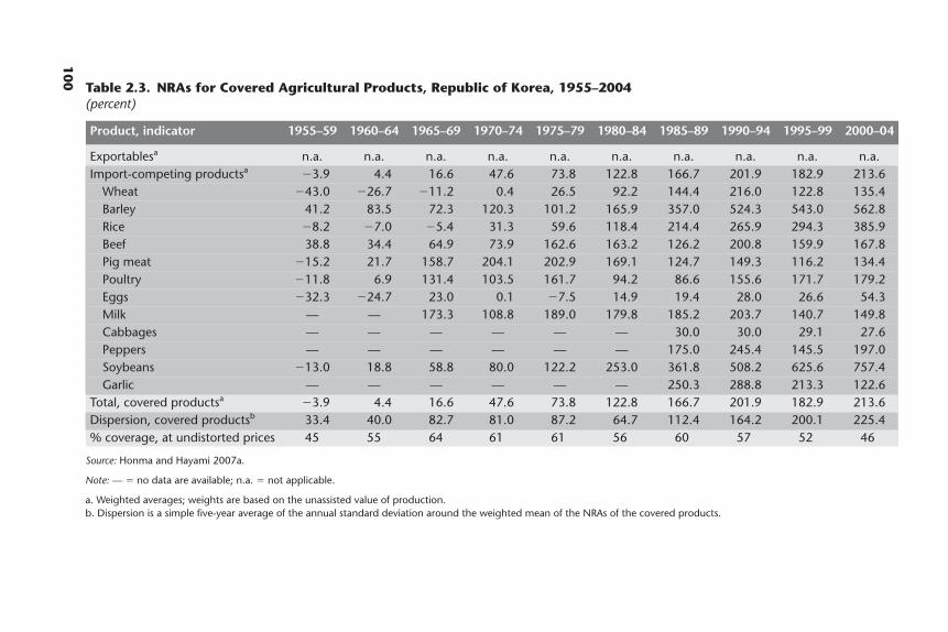
100
Table 2.3. NRAs for Covered Agricultural Products, Republic of Korea, 1955–2004(percent)
Source: Honma and Hayami 2007a.
Note: — � no data are available; n.a. � not applicable.
a. Weighted averages; weights are based on the unassisted value of production.b. Dispersion is a simple five-year average of the annual standard deviation around the weighted mean of the NRAs of the covered products.
Product, indicator 1955–59 1960–64 1965–69 1970–74 1975–79 1980–84 1985–89 1990–94 1995–99 2000–04
Exportablesa n.a. n.a. n.a. n.a. n.a. n.a. n.a. n.a. n.a. n.a.Import-competing productsa �3.9 4.4 16.6 47.6 73.8 122.8 166.7 201.9 182.9 213.6
Wheat �43.0 �26.7 �11.2 0.4 26.5 92.2 144.4 216.0 122.8 135.4Barley 41.2 83.5 72.3 120.3 101.2 165.9 357.0 524.3 543.0 562.8Rice �8.2 �7.0 �5.4 31.3 59.6 118.4 214.4 265.9 294.3 385.9Beef 38.8 34.4 64.9 73.9 162.6 163.2 126.2 200.8 159.9 167.8Pig meat �15.2 21.7 158.7 204.1 202.9 169.1 124.7 149.3 116.2 134.4Poultry �11.8 6.9 131.4 103.5 161.7 94.2 86.6 155.6 171.7 179.2Eggs �32.3 �24.7 23.0 0.1 �7.5 14.9 19.4 28.0 26.6 54.3Milk — — 173.3 108.8 189.0 179.8 185.2 203.7 140.7 149.8Cabbages — — — — — — 30.0 30.0 29.1 27.6Peppers — — — — — — 175.0 245.4 145.5 197.0Soybeans �13.0 18.8 58.8 80.0 122.2 253.0 361.8 508.2 625.6 757.4Garlic — — — — — — 250.3 288.8 213.3 122.6
Total, covered productsa �3.9 4.4 16.6 47.6 73.8 122.8 166.7 201.9 182.9 213.6Dispersion, covered productsb 33.4 40.0 82.7 81.0 87.2 64.7 112.4 164.2 200.1 225.4% coverage, at undistorted prices 45 55 64 61 61 56 60 57 52 46
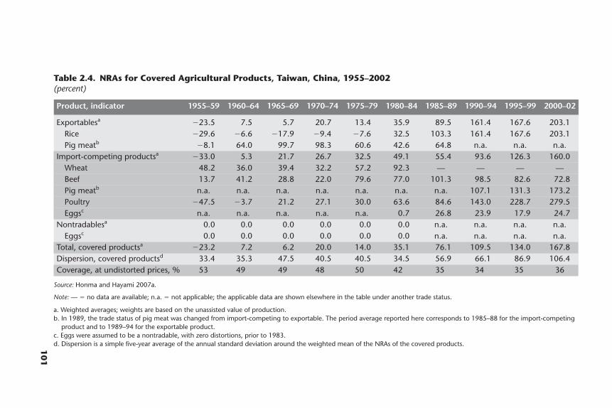
101
Table 2.4. NRAs for Covered Agricultural Products, Taiwan, China, 1955–2002(percent)
Product, indicator 1955–59 1960–64 1965–69 1970–74 1975–79 1980–84 1985–89 1990–94 1995–99 2000–02
Exportablesa �23.5 7.5 5.7 20.7 13.4 35.9 89.5 161.4 167.6 203.1Rice �29.6 �6.6 �17.9 �9.4 �7.6 32.5 103.3 161.4 167.6 203.1Pig meatb �8.1 64.0 99.7 98.3 60.6 42.6 64.8 n.a. n.a. n.a.
Import-competing productsa �33.0 5.3 21.7 26.7 32.5 49.1 55.4 93.6 126.3 160.0Wheat 48.2 36.0 39.4 32.2 57.2 92.3 — — — —Beef 13.7 41.2 28.8 22.0 79.6 77.0 101.3 98.5 82.6 72.8Pig meatb n.a. n.a. n.a. n.a. n.a. n.a. n.a. 107.1 131.3 173.2Poultry �47.5 �3.7 21.2 27.1 30.0 63.6 84.6 143.0 228.7 279.5Eggsc n.a. n.a. n.a. n.a. n.a. 0.7 26.8 23.9 17.9 24.7
Nontradablesa 0.0 0.0 0.0 0.0 0.0 0.0 n.a. n.a. n.a. n.a.Eggsc 0.0 0.0 0.0 0.0 0.0 0.0 n.a. n.a. n.a. n.a.
Total, covered productsa �23.2 7.2 6.2 20.0 14.0 35.1 76.1 109.5 134.0 167.8Dispersion, covered productsd 33.4 35.3 47.5 40.5 40.5 34.5 56.9 66.1 86.9 106.4Coverage, at undistorted prices, % 53 49 49 48 50 42 35 34 35 36
Source: Honma and Hayami 2007a.
Note: — � no data are available; n.a. � not applicable; the applicable data are shown elsewhere in the table under another trade status.
a. Weighted averages; weights are based on the unassisted value of production.b. In 1989, the trade status of pig meat was changed from import-competing to exportable. The period average reported here corresponds to 1985–88 for the import-competing
product and to 1989–94 for the exportable product.c. Eggs were assumed to be a nontradable, with zero distortions, prior to 1983.d. Dispersion is a simple five-year average of the annual standard deviation around the weighted mean of the NRAs of the covered products.
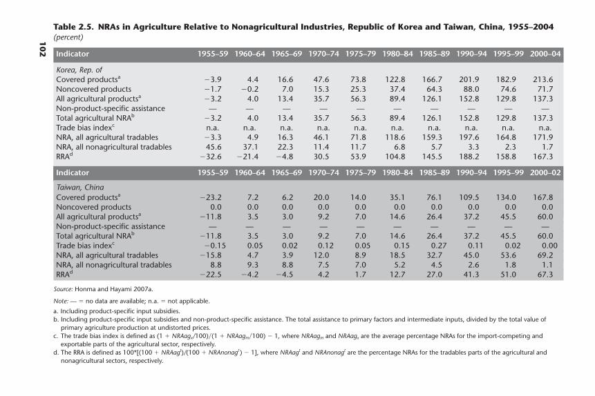
102
Table 2.5. NRAs in Agriculture Relative to Nonagricultural Industries, Republic of Korea and Taiwan, China, 1955–2004(percent)
Indicator 1955–59 1960–64 1965–69 1970–74 1975–79 1980–84 1985–89 1990–94 1995–99 2000–04
Korea, Rep. ofCovered productsa �3.9 4.4 16.6 47.6 73.8 122.8 166.7 201.9 182.9 213.6Noncovered products �1.7 �0.2 7.0 15.3 25.3 37.4 64.3 88.0 74.6 71.7All agricultural productsa �3.2 4.0 13.4 35.7 56.3 89.4 126.1 152.8 129.8 137.3Non-product-specific assistance — — — — — — — — — —Total agricultural NRAb �3.2 4.0 13.4 35.7 56.3 89.4 126.1 152.8 129.8 137.3Trade bias indexc n.a. n.a. n.a. n.a. n.a. n.a. n.a. n.a. n.a. n.a.NRA, all agricultural tradables �3.3 4.9 16.3 46.1 71.8 118.6 159.3 197.6 164.8 171.9NRA, all nonagricultural tradables 45.6 37.1 22.3 11.4 11.7 6.8 5.7 3.3 2.3 1.7RRAd �32.6 �21.4 �4.8 30.5 53.9 104.8 145.5 188.2 158.8 167.3
Indicator 1955–59 1960–64 1965–69 1970–74 1975–79 1980–84 1985–89 1990–94 1995–99 2000–02
Taiwan, ChinaCovered productsa �23.2 7.2 6.2 20.0 14.0 35.1 76.1 109.5 134.0 167.8Noncovered products 0.0 0.0 0.0 0.0 0.0 0.0 0.0 0.0 0.0 0.0All agricultural productsa �11.8 3.5 3.0 9.2 7.0 14.6 26.4 37.2 45.5 60.0Non-product-specific assistance — — — — — — — — — —Total agricultural NRAb �11.8 3.5 3.0 9.2 7.0 14.6 26.4 37.2 45.5 60.0Trade bias indexc �0.15 0.05 0.02 0.12 0.05 0.15 0.27 0.11 0.02 0.00NRA, all agricultural tradables �15.8 4.7 3.9 12.0 8.9 18.5 32.7 45.0 53.6 69.2NRA, all nonagricultural tradables 8.8 9.3 8.8 7.5 7.0 5.2 4.5 2.6 1.8 1.1RRAd �22.5 �4.2 �4.5 4.2 1.7 12.7 27.0 41.3 51.0 67.3
Source: Honma and Hayami 2007a.
Note: — � no data are available; n.a. � not applicable.
a. Including product-specific input subsidies.b. Including product-specific input subsidies and non-product-specific assistance. The total assistance to primary factors and intermediate inputs, divided by the total value of
primary agriculture production at undistorted prices.c. The trade bias index is defined as (1 � NRAagx/100)�(1 � NRAagm�100) � 1, where NRAagm and NRAagx are the average percentage NRAs for the import-competing and
exportable parts of the agricultural sector, respectively.d. The RRA is defined as 100*[(100 � NRAagt)/(100 � NRAnonagt) � 1], where NRAagt and NRAnonagt are the percentage NRAs for the tradables parts of the agricultural and
nonagricultural sectors, respectively.
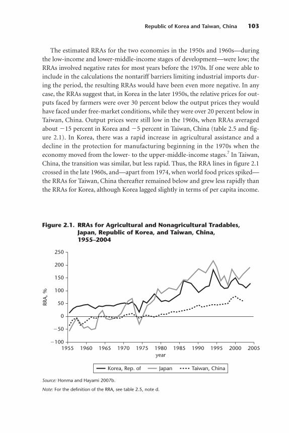
Republic of Korea and Taiwan, China 103
�100
0
�50
100
150
50
200
250
year1955 1960 1965 1970 1975 1980 1985 1990 1995 2000 2005
RRA
, %
Korea, Rep. of Japan Taiwan, China
Figure 2.1. RRAs for Agricultural and Nonagricultural Tradables,Japan, Republic of Korea, and Taiwan, China,1955–2004
Source: Honma and Hayami 2007b.
Note: For the definition of the RRA, see table 2.5, note d.
The estimated RRAs for the two economies in the 1950s and 1960s—duringthe low-income and lower-middle-income stages of development—were low; theRRAs involved negative rates for most years before the 1970s. If one were able toinclude in the calculations the nontariff barriers limiting industrial imports dur-ing the period, the resulting RRAs would have been even more negative. In anycase, the RRAs suggest that, in Korea in the later 1950s, the relative prices for out-puts faced by farmers were over 30 percent below the output prices they wouldhave faced under free-market conditions, while they were over 20 percent below inTaiwan, China. Output prices were still low in the 1960s, when RRAs averagedabout �15 percent in Korea and �5 percent in Taiwan, China (table 2.5 and fig-ure 2.1). In Korea, there was a rapid increase in agricultural assistance and adecline in the protection for manufacturing beginning in the 1970s when theeconomy moved from the lower- to the upper-middle-income stages.7 In Taiwan,China, the transition was similar, but less rapid. Thus, the RRA lines in figure 2.1crossed in the late 1960s, and—apart from 1974, when world food prices spiked—the RRAs for Taiwan, China thereafter remained below and grew less rapidly thanthe RRAs for Korea, although Korea lagged slightly in terms of per capita income.
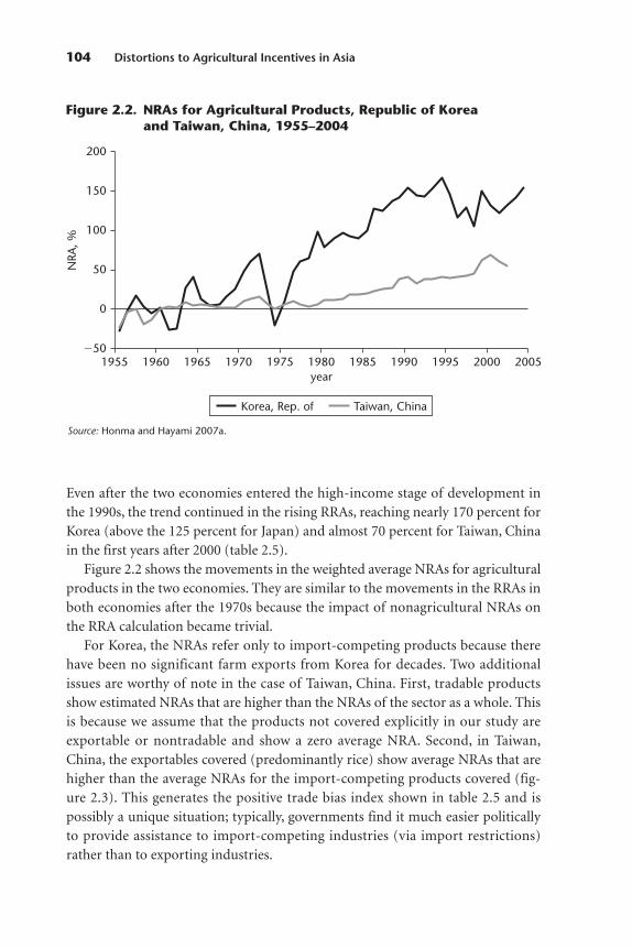
Even after the two economies entered the high-income stage of development inthe 1990s, the trend continued in the rising RRAs, reaching nearly 170 percent forKorea (above the 125 percent for Japan) and almost 70 percent for Taiwan, Chinain the first years after 2000 (table 2.5).
Figure 2.2 shows the movements in the weighted average NRAs for agriculturalproducts in the two economies. They are similar to the movements in the RRAs inboth economies after the 1970s because the impact of nonagricultural NRAs onthe RRA calculation became trivial.
For Korea, the NRAs refer only to import-competing products because therehave been no significant farm exports from Korea for decades. Two additionalissues are worthy of note in the case of Taiwan, China. First, tradable productsshow estimated NRAs that are higher than the NRAs of the sector as a whole. Thisis because we assume that the products not covered explicitly in our study areexportable or nontradable and show a zero average NRA. Second, in Taiwan,China, the exportables covered (predominantly rice) show average NRAs that arehigher than the average NRAs for the import-competing products covered (fig-ure 2.3). This generates the positive trade bias index shown in table 2.5 and is possibly a unique situation; typically, governments find it much easier politicallyto provide assistance to import-competing industries (via import restrictions)rather than to exporting industries.
104 Distortions to Agricultural Incentives in Asia
�50
50
100
0
150
200
year19601955 1965 1970 1975 1980 1985 1990 1995 2000 2005
NRA
, %
Korea, Rep. of Taiwan, China
Figure 2.2. NRAs for Agricultural Products, Republic of Koreaand Taiwan, China, 1955–2004
Source: Honma and Hayami 2007a.
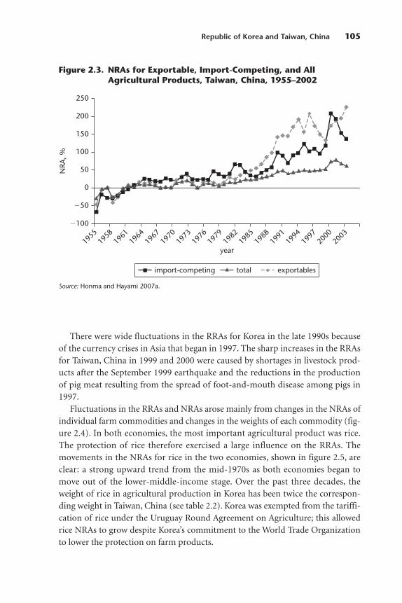
There were wide fluctuations in the RRAs for Korea in the late 1990s becauseof the currency crises in Asia that began in 1997. The sharp increases in the RRAsfor Taiwan, China in 1999 and 2000 were caused by shortages in livestock prod-ucts after the September 1999 earthquake and the reductions in the productionof pig meat resulting from the spread of foot-and-mouth disease among pigs in1997.
Fluctuations in the RRAs and NRAs arose mainly from changes in the NRAs ofindividual farm commodities and changes in the weights of each commodity (fig-ure 2.4). In both economies, the most important agricultural product was rice.The protection of rice therefore exercised a large influence on the RRAs. Themovements in the NRAs for rice in the two economies, shown in figure 2.5, areclear: a strong upward trend from the mid-1970s as both economies began tomove out of the lower-middle-income stage. Over the past three decades, theweight of rice in agricultural production in Korea has been twice the correspon-ding weight in Taiwan, China (see table 2.2). Korea was exempted from the tariffi-cation of rice under the Uruguay Round Agreement on Agriculture; this allowedrice NRAs to grow despite Korea’s commitment to the World Trade Organizationto lower the protection on farm products.
Republic of Korea and Taiwan, China 105
�100
0
�50
100
150
50
200
250
year19
5519
5819
6419
7019
7619
8219
8819
9419
6119
6719
7319
7919
8519
9119
9720
0020
03
NRA
, %
import-competing total exportables
Figure 2.3. NRAs for Exportable, Import-Competing, and AllAgricultural Products, Taiwan, China, 1955–2002
Source: Honma and Hayami 2007a.
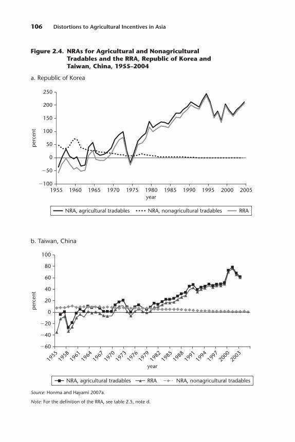
106 Distortions to Agricultural Incentives in Asia
�100
0
�50
100
150
50
200
250
year1955 1960 1965 1970 1975 1980 1985 1990 20001995 2005
per
cent
NRA, agricultural tradables NRA, nonagricultural tradables RRA
�60
�20
�40
20
40
0
60
80
100
year19
5519
5819
6419
7019
7619
8219
8819
9419
6119
6719
7319
7919
8519
9119
9720
0020
03
per
cent
NRA, agricultural tradables RRA NRA, nonagricultural tradables
Figure 2.4. NRAs for Agricultural and NonagriculturalTradables and the RRA, Republic of Korea andTaiwan, China, 1955–2004
a. Republic of Korea
Source: Honma and Hayami 2007a.
Note: For the definition of the RRA, see table 2.5, note d.
b. Taiwan, China
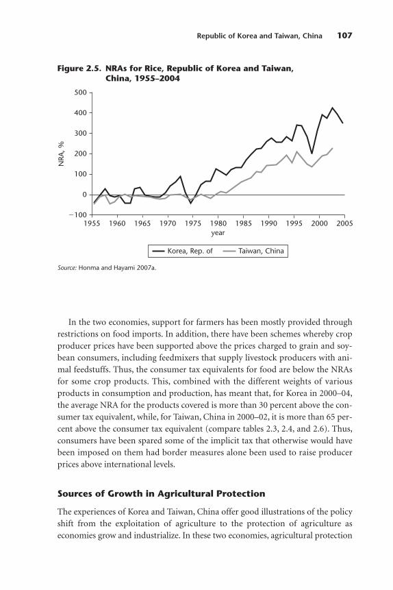
In the two economies, support for farmers has been mostly provided throughrestrictions on food imports. In addition, there have been schemes whereby cropproducer prices have been supported above the prices charged to grain and soy-bean consumers, including feedmixers that supply livestock producers with ani-mal feedstuffs. Thus, the consumer tax equivalents for food are below the NRAsfor some crop products. This, combined with the different weights of variousproducts in consumption and production, has meant that, for Korea in 2000–04,the average NRA for the products covered is more than 30 percent above the con-sumer tax equivalent, while, for Taiwan, China in 2000–02, it is more than 65 per-cent above the consumer tax equivalent (compare tables 2.3, 2.4, and 2.6). Thus,consumers have been spared some of the implicit tax that otherwise would havebeen imposed on them had border measures alone been used to raise producerprices above international levels.
Sources of Growth in Agricultural Protection
The experiences of Korea and Taiwan, China offer good illustrations of the policyshift from the exploitation of agriculture to the protection of agriculture aseconomies grow and industrialize. In these two economies, agricultural protection
Republic of Korea and Taiwan, China 107
�100
100
0
300
400
200
500
year1955 1960 1965 1970 1975 1980 1985 1990 1995 2000 2005
NRA
, %
Korea, Rep. of Taiwan, China
Figure 2.5. NRAs for Rice, Republic of Korea and Taiwan,China, 1955–2004
Source: Honma and Hayami 2007a.

108
Table 2.6. CTEs for Covered Agricultural Products, Republic of Korea and Taiwan, China, 1955–2004(percent)a. Republic of Korea
Product 1955–59 1960–64 1965–69 1970–74 1975–79 1980–84 1985–89 1990–94 1995–99 2000–04
Wheat �46.2 �22.5 �11.1 1.1 16.2 46.0 132.8 167.4 80.5 80.6Barley 40.8 77.8 64.9 96.6 57.3 119.6 325.6 411.5 341.2 327.5Rice �7.7 �5.5 �5.0 29.1 54.5 113.4 211.5 261.7 290.8 385.3Beef 38.8 34.4 64.9 73.9 162.6 163.2 122.1 200.7 153.9 167.7Pig meat �15.0 21.7 158.7 204.1 202.9 169.1 124.7 149.3 116.2 134.4Poultry �11.6 7.0 131.4 103.5 161.7 94.2 86.6 155.6 171.7 179.2Eggs �27.1 �24.7 23.0 0.1 �7.5 14.9 19.4 28.0 26.6 54.3Milk — — 130.0 108.8 189.0 179.8 185.2 203.7 140.7 149.8Soybeans �19.8 8.2 51.6 63.2 95.2 245.4 112.2 75.5 63.6 66.8Total, covered productsa — 6.6 13.6 39.2 63.3 110.6 150.8 185.9 159.6 163.9
b. Taiwan, China
Product 1955–59 1960–64 1965–69 1970–74 1975–79 1980–84 1985–89 1990–94 1995–99 2000–02
Rice �29.6 �6.6 �17.9 �9.4 �7.6 32.5 103.3 161.4 167.6 203.1Wheat 33.9 23.5 29.3 14.7 �1.1 40.3 183.4 — — —Beef 13.7 41.2 28.8 22.0 79.6 77.0 101.3 98.5 82.6 72.8Pig meat �8.1 64.0 99.7 98.3 60.6 42.6 64.8 107.1 131.3 173.2Poultry �47.5 �3.7 21.2 27.1 30.0 63.6 84.6 143.0 228.7 279.5Eggs 0.0 0.0 0.0 0.0 0.0 0.7 26.8 23.9 17.9 24.7Total, covered productsa 26.2 27.0 21.7 23.2 18.6 39.9 82.6 116.4 136.7 99.8
Source: Honma and Hayami 2007a.
Note: CTE � consumer tax equivalent. — � no data are available.a. Weighted averages; weights are based on the undistorted value of consumption. For the Republic of Korea, this includes cabbages, peppers, and garlic.

levels were negative in the 1950s and the 1960s and began to rise sharply in the late1970s following successes in industrial development.
Anderson, Hayami, and Honma (1986) found the growth of agricultural pro-tection during the three decades to the early 1980s far more rapid in theseeconomies than in the pioneers of industrialization in the West or even Japan.Moreover, the two economies were not exceptional in their bent toward growth inagricultural protection, and the growth was unusually rapid because the industrialdevelopment and the associated structural changes were also unusually rapid. Thegrowth in protection continued at the same pace to the early 1990s, when the twoeconomies were in the middle-income stage, but it began to decelerate thereafter,particularly in Korea when that economy reached the high-income stage.
The rapid growth in agricultural protection is largely explained by the shift incomparative advantage away from agriculture to industry as the result of success-ful industrialization. This shift was most pronounced during the middle-incomestage. Relative to population, the two economies are characterized by meagerendowments of natural resources, including land for cultivation. Industrializationwas the only possible route to sufficient economic growth to catch up withadvanced economies. Economic growth through the exploitation of abundantnatural resources—vent-for-surplus growth (Myint 1965)—was not an option inthese economies, unlike in Southeast Asian countries such as Malaysia and Thai-land (Douangngeune, Hayami, and Godo 2005). The decline in agriculture’s com-parative advantage because of successful industrialization increased intersectoralresource adjustment costs and led to a widening rural-urban income disparitythat, if left to the solutions of competitive markets, would have been shoulderedby farmers. This raised demands among farmers for agricultural protection.
The association between the rise in agricultural protection and the decline inagriculture’s comparative advantage was tested by Honma and Hayami (1986)using multiple regression analysis and a pooled data set on 15 countries at sixpoints of time ending in 1980. They found a strong correlation between the aggre-gate nominal rate of protection and the index of agriculture’s labor productivityrelative to the total economy’s labor productivity.8 Based on the results, Honmaand Hayami concluded that the high level of agricultural protection in East Asiawas caused not so much by factors unique to East Asia, but mainly by factors com-mon to all industrial countries.
One may argue that high rates of agricultural protection hinder adjustmentsaimed at raising agricultural productivity and thereby slow the growth in agri-culture’s comparative disadvantage. However, it is doubtful that the neededadjustments in agriculture in the face of the rapid industrial development experi-enced by East Asia’s top performers could have been achieved sufficiently quicklyunder free markets to avoid major disruptions and social instability. This is
Republic of Korea and Taiwan, China 109
particularly so because, in these economies, the agrarian structure involves a largenumber of small, independent family farms possessing unfavorable resourceendowments.
Korea and Taiwan, China were at the low-income stage of economic develop-ment in the 1950s and entered the middle-income stage in the 1960s. During themiddle-income stage, productivity growth in agriculture lagged relative to nona-griculture because of successful industrialization. Farm incomes declined relativeto the incomes of nonfarm households. Nonetheless, during the lower-middle-income stage, it was not possible for the government to secure sufficient financingto close the income gap because the share of agriculture in the national incomeand in the labor force was still large. Thus, before Korea and Taiwan, Chinareached the upper-middle-income stage, agricultural protection remained lowdespite growing rural-urban income disparity.
The basic agricultural problem confronted by middle-income economies suchas these in the 1960s and 1970s is known as the disparity problem (Hayami andGodo 2004; Hayami 2005). In this case, it revolves around the income disparitybetween farm and nonfarm households brought about by a lag in productivitygrowth in agriculture relative to nonagriculture. This lag was caused by the indus-trialization that successfully raised these economies to the middle-income stage.With respect to the low-income stage, food supply capacity rises during this stagebecause of both the productivity growth in domestic agriculture and the higherforeign exchange earnings, which enable more food imports. Meanwhile, factorscausing growth in the demand for food, such as high population growth and highdemand elasticities, are weakened. The terms of trade between agriculture andnonagriculture thus worsen.
Farmer incomes tend to decline relative to nonfarmer incomes. This reflectsthe widening intersectoral productivity gap. Observing the rapid escape of non-farm workers from poverty, farmers begin to realize the relative extent of theirpoverty even if their incomes have not fallen or have risen only slightly since theprevious stage. The dissatisfaction of these farmers who have remained poor oftenbecomes a significant source of social instability.
Thus, at the middle-income stage, preventing growth in rural-urban incomedisparity is a prime concern of policy makers. To achieve this goal, the governmentmight adopt agricultural protection measures to appease farmers so that their dis-satisfaction is not transformed into a serious antigovernmental movement.
This protection may not be sufficient, however, to close the income gapbetween farmers and urban workers until the country graduates from the lowermiddle-income stage. Because the share of agriculture in national income and inthe labor force is still large, it is difficult to raise sufficient revenue from the nonfarm sectors to close the growing farm-nonfarm income gap through direct
110 Distortions to Agricultural Incentives in Asia
support payments. It is also difficult to pass on the cost of agricultural protectionto consumers by raising food import barriers; increases in food prices erode thereal wages paid by the large number of small-scale enterprises that rely heavily oncheap labor.
Faced with the disparity problem, policy makers in middle-income countriesare forced to search for ways to protect farmers within the constraints of the foodproblem. The food problem binds because a large number of urban workers haveremained absolutely poor and food still accounts for a high share in their house-hold expenditures.
Per capita incomes rose rapidly in the late 1970s and early 1980s as Korea andTaiwan, China approached the upper-middle-income stage. Both the govern-ment and the nonagricultural sectors became capable of shouldering the cost ofagricultural protection during the upper-middle-income stage. It may be arguedthat high protection contributed to the loss in agricultural comparative advan-tage in these two economies by reducing the incentives to improve agriculturalproductivity. The effect of high protection on comparative advantage was muchsmaller than the effect of industrial productivity growth, which was unusuallyrapid among the high performers in East Asia. The conditions necessary forgrowth in agricultural protection were created by the increases in industrial productivity growth, which occurred far more quickly than agricultural productivity growth and provided the higher earnings capable of supportingagriculture.
There were also differences in the policy approaches toward agricultural pro-tection in the two economies. During the upper-middle-income stage, agricul-tural protection rose more quickly and to higher levels in Korea. This seems toreflect the differences in the cost of the intersectoral adjustments required byfarmers because of the shifts in comparative advantage. In Korea, the shift oflabor from agriculture to nonagriculture involved the migration of workersfrom rural to urban areas; whereas, in Taiwan, China, much of the shift wasabsorbed by farm households, which increased their nonfarm activities in theirhome villages and towns. The pecuniary and psychological costs of the intersec-toral labor reallocation would have been correspondingly higher in the farm sector in Korea.
The ratio of agricultural GDP per worker to total GDP per worker in nominalterms decreased more rapidly in Taiwan, China (see table 2.1). This does notmean that agricultural adjustment occurred more slowly there. One should makeallowance for the fact that output per hour of labor in agricultural activities differs from output per farm worker as carried in official statistics. Since farmersin Taiwan, China depended more heavily on earnings from nonfarm activities(table 2.2), it is likely that household incomes per capita were not lower, but
Republic of Korea and Taiwan, China 111

higher than the corresponding incomes in Korea, although, in Taiwan, China,GDP per farm worker was lower relative to GDP per worker in the total economy.
The negative relationship between the relative GDP per worker and the RRA inthe two economies in 1955–2004 is shown in figure 2.6.9 Korea intensified agricul-tural protection despite the relatively high incomes among farmers. In addition tothe high cost of intersectoral adjustment shouldered by Korean farmers, the con-stant menace of Communist aggression from the north caused citizens to feel theneed to support farmers to maintain political stability.
In their analysis, Honma and Hayami (1986) found that political power ismaximized in the agricultural sector when the share of agriculture declines to 4 to5 percent of GDP or to 5 to 8 percent of the labor force. Korea recently entered thispeak zone in terms of both GDP and labor force. Taiwan, China recently entered itin terms of the labor share (having entered this zone in 1990 in terms of GDPshare). Political economy factors may underlie the rise in agricultural protection-ism in Korea at the high-income stage since 1990, as observed through NRAs atthe farmgate, despite the lack of an apparent additional increase in agriculturalcomparative disadvantage.10
112 Distortions to Agricultural Incentives in Asia
�50
0
100
150
50
200
10 20 30 40 50 60 70
RRA
, %
Korea, Rep. of Taiwan, China
ratio of agricultural GDP per worker to total GDP per worker, %
Figure 2.6. RRAs in Agriculture and Relative GDP perAgricultural Worker, Republic of Korea andTaiwan, China, 1955–2004
Source: Honma and Hayami 2007a.
Note: Calculated at 2000 constant prices in U.S. dollars.
Concluding Remarks
This chapter examines changes in the distortions to agricultural incentives interms of price distortions in Korea and Taiwan, China in a manner consistent withthe methodology described in Anderson et al. (2008) and appendix A. Rates ofassistance to the agricultural sector are estimated for the half-century since 1955.These are based on estimates of the NRAs for selected individual commoditiesand RRAs in agriculture and industry. The estimates show that the growth of agricultural protection in Northeast Asia, together with the decline in industrialprotection rates, caused RRAs there to rise over the five postwar decades underinvestigation. The data indicate that agricultural protection rates were negative inthe two economies during the low-income stage of development and were lowduring the lower-middle-income stage, but rose sharply after the economiesreached the upper-middle-income stage. The experience seems to be explained bytwo factors common to rapidly industrializing economies: first, the strongdemand for protection among farmers, who shoulder the high cost of intersec-toral adjustments in resource allocations in a context of rapidly declining comparative advantage in agriculture; and, second, the enhanced capacity ofnonagriculture to support agriculture. The latter is associated with a growing tolerance among nonfarmers for policies to protect farmers. The first factoremerged at the beginning of the lower-middle-income stage; the second emergedwhen the economies reached the upper-middle-income stage.
Following the sharp increase in agricultural protection during the upper- middle-income stage, the two economies began to suffer from problems arisingbecause of the high level of protection. These included the misallocation ofresources and a high fiscal burden in the domestic economy, as well as seriousinternational trade frictions, which are common among high-income economies.These problems might have been less serious if the farm-nonfarm income gap hadbeen addressed properly during the middle-income stage.
The agricultural problem in the middle-income stage is known as the disparityproblem. The challenge is to balance the conflicting need to support farm incomesand the need to supply low-cost food to a large population of urban workers inview of the weak capacity of the government to raise sufficient revenue for thispurpose among nonagricultural sectors.
Contrasting patterns in agricultural and industrial growth in Korea and Taiwan, China provide a key to solving this problem. Despite their largely parallelprogress in industrial and economic development, the growth in agriculturalprotection was significantly lower in the latter. The difference seems to be largelyexplained by differences in industrial and agricultural structures. Industrialstructures have been characterized in Taiwan, China by the wide diffusion ofsmall and medium industries in rural areas and, in Korea, by urban-centered
Republic of Korea and Taiwan, China 113
industrialization. The cost of intersectoral labor reallocation that had to beshouldered by farmers was therefore considerably lower in the former. Theadvantage this represented for Taiwan, China was augmented by the success ofagricultural diversification there toward highly income-elastic commodities suchas horticultural and livestock products and away from traditional subsistencecrops, especially rice. The demand for farming assistance was thus significantlyless in Taiwan, China despite the pressures of rapid industrial expansion. Devel-oping economies currently pursuing rapid development and relying on a similarstrategy of borrowing industrial technology may benefit from closer analysis ofthe contrasting experiences in Korea and Taiwan, China.
Notes
1. Korea and Taiwan, China exceeded US$5,000 per capita GDP in 1983 and 1978, respectively, andUS$10,000 per capita GDP in 1991 and 1988, respectively.
2. In terms of real GDP per capita in 2000 constant prices, for example, China exceeded US$1,500in 1990 and US$5,000 in 2004, whereas Thailand passed the US$1,500 level in 1968 and the US$5,000level in 1991. In the high-income stage, the United Kingdom and France exceeded US$10,000 in1960 and 1964, respectively, whereas the United States had already exceeded US$10,000 in 1950.
3. This subsection draws heavily on Moon and Kang (1989).4. This drove a small wedge between the NRA for producers and the consumer tax equivalent for
beef (Anderson 1986). The scheme was similar to one operating in Japan in the 1970s. The reason thegovernment chose the scheme rather than a more efficient, equally protective tariff, plus a consumersubsidy funded with the tariff revenue, is discussed in Hayami (1979) and Anderson (1983a).
5. This section draws heavily on Mao and Schive (1995).6. Our NRAs for commodities differ from the estimates for Korea in the OECD PSE-CSE Database
(2007). There are two key differences. First, our domestic prices are wholesale prices, whereas the data-base relies on farmgate prices. Second, border prices in our calculations are based on the study inAnderson and Hayami (1986), whereas the database relies on a different set of reference prices. Thefact that producer prices were above wholesale (consumer) prices in the case of grains and soybeans inKorea is captured by setting the NRA equal to the measured consumer tax equivalent, times the ratioof the NRA to the consumer tax equivalent in Anderson (1989) for the period to 1985 and times thenegative of the ratio of producer support estimates to consumer support estimates in the OECD PSE-CSE Database (2007) for the period thereafter. Most of the differences between the database and ourmeasures arise from the differences in the border prices used. For example, our border price for rice inJapan and Korea is the world import unit value, adjusted by a quality coefficient. But the border pricefor rice in Korea in the database is China’s export price for rice, adjusted by transportation costs and,beginning in 2001, the average of the import prices for rice from China, Thailand, and the UnitedStates. This means that our NRA series for rice is more stable than the database series in recent years;and, so, this explains the stability of our NRAs for Korean rice compared with the information in thedatabase. For meat products, the border prices are also different. In the estimation of the NRAs forbeef, pork, and chicken, the database relies on border prices derived ultimately from data on borderprices for meat in Canada or the United States, while we use Japan’s import price for beef and own-country unit values for pork and chicken (or, for the 1950s, the import prices in Hong Kong, China).Our approach is preferred for estimating NRAs consistently over longer periods, particularly duringthe period when Korean imports were absent or negligible. Also, our approach is necessary if onewishes to compare the NRAs of Korea and Taiwan, China on a similar basis.
7. Fertilizer price subsidies were also being provided to farmers in Korea, but they onlypartially offset the protection from import competition that was provided to the domestic fertilizer
114 Distortions to Agricultural Incentives in Asia

manufacturing industry, which meant that farmers were effectively taxed in this respect, too, to support manufacturing (Anderson 1983b).
8. The actual data used to measure the level of agricultural protection in the regression analysis arethe nominal protection coefficients (NPC � 1 � NRP�100).
9. The average RRA in 1955–59 is paired with the agricultural GDP per worker relative to the totalGDP per worker in 1955, and so on.
10. The shares of agriculture in GDP and the labor force in Korea were 3.8 and 7.7 percent, respec-tively, in 2004, while the corresponding shares in Taiwan, China in that year were 1.7 and 7.5 percent(see table 2.1, rows 2 and 3).
References
Amsden, A. 1989. Asia’s Next Giant: South Korea and Late Industrialization. New York: Oxford Univer-sity Press.
Anderson, K. 1983a. “The Peculiar Rationality of Beef Import Quotas in Japan.” American Journal ofAgricultural Economics 65 (1): 108–12.
———. 1983b. “Fertilizer Policy in Korea.” Journal of Rural Development 6 (1): 43–57.———. 1986. “The Peculiar Rationality of Beef Import Quotas in Japan and Korea.” In The Political
Economy of Agricultural Protection: East Asia in International Perspective, ed. K. Anderson and Y.Hayami, chap. 7. London: Allen and Unwin.
———. 1989. “Korea: A Case of Agricultural Protection.” In Food Price Policies in Asia, ed. T. Sicular,chap. 4. Ithaca, NY: Cornell University Press.
Anderson, K., and Y. Hayami, eds. 1986. The Political Economy of Agricultural Protection: East Asia inInternational Perspective. London: Allen and Unwin.
Anderson, K., Y. Hayami, and M. Honma. 1986. “The Growth of Agricultural Protection.” In The Political Economy of Agricultural Protection: East Asia in International Perspective, ed. K. Andersonand Y. Hayami, chap. 2. London: Allen and Unwin.
Anderson, K., M. Kurzweil, W. Martin, D. Sandri, and E. Valenzuela. 2008. “Measuring Distortions toAgricultural Incentives, Revisited.” World Trade Review 7 (4): 675–704.
Anderson, K., and R. Tyers. 1992. “Japanese Rice Policy in the Interwar Period: Some Consequences ofImperial Self Sufficiency.” Japan and the World Economy 4 (2): 103–27.
Cole, D. C., and Y. C. Park. 1983. Financial Development in Korea, 1945–1978. Cambridge, MA: HarvardUniversity Press.
Department of Agriculture and Forestry. Various issues. Taiwan Agricultural Yearbook. Tapei: Depart-ment of Agriculture and Forestry.
Douangngeune, B., Y. Hayami, and Y. Godo. 2005. “Education and Natural Resources in EconomicDevelopment: Thailand Compared with Japan and Korea.” Journal of Asian Economics 16 (2):179–204.
Frank, C. R., K. S. Kim, and K. Westphal. 1975. Foreign Trade Regimes and Economic Development:South Korea. New York: Colombia University Press; Washington, DC: National Bureau of Eco-nomic Research.
Gerschenkron, A. 1962. Economic Backwardness in Historical Perspective. Cambridge, MA: HarvardUniversity Press.
Hayami, Y. 1979. “Trade Benefits to All: A Design of the Beef Import Liberalization in Japan.” AmericanJournal of Agricultural Economics 62 (2): 342–47.
———. 1988. Japanese Agriculture under Siege: The Political Economy of Agricultural Policies. London:Macmillan.
———. 2005. “Emerging Agricultural Problem in High-Performing Economies in Asia.” Presidentialaddress at the Fifth Conference of the Asian Society of Agricultural Economists, “Prospects ofAsian Agriculture in the New Millennium,” University of Sistan and Baluchestan, Zahedan, Iran,August 29–31.
Republic of Korea and Taiwan, China 115
Hayami, Y., and M. Aoki, eds. 1998. The Institutional Foundation of East Asian Economic Development.London: Macmillan.
Hayami, Y., and Y. Godo. 2004. “The Three Agricultural Problems in the Disequilibrium of World Agri-culture.” Asian Journal of Agriculture and Development 1 (1): 3–16.
———. 2005. Development Economics: From the Poverty to the Wealth of Nations, 3rd ed. London:Oxford University Press.
Heston, A., R. Summers, and B. Aten. 2006. “Penn World Table Version 6.2.” Center for InternationalComparisons of Production, Income and Prices, University of Pennsylvania. http://pwt.econ.upenn.edu/php_site/pwt_index.php (version of September).
Ho, S. P. S. 1979. “Decentralized Industrialization and Rural Development: Evidence from Taiwan.”Economic Development and Cultural Change 28 (1): 77–96.
———. 1982. “Economic Development and Rural Industry in South Korea and Taiwan.” World Development 10 (11): 973–90.
Honma, M., and Y. Hayami. 1986. “Determinants of Agricultural Protection Levels: An EconometricApproach.” In The Political Economy of Agricultural Protection: East Asia in International Perspec-tive, ed. K. Anderson and Y. Hayami, chap. 4. London: Allen and Unwin.
———. 2007a. “Distortions to Agricultural Incentives in Korea and Taiwan.” Agricultural DistortionsWorking Paper 30, World Bank, Washington, DC.
———. 2007b. “Distortions to Agricultural Incentives in Japan, Korea, and Taiwan.” Agricultural Distortions Working Paper 35, World Bank, Washington, DC.
Krueger, A. O., M. Schiff, and A. Valdés, eds. 1991. The Political Economy of Agricultural Pricing Policies.3 vols. Baltimore: Johns Hopkins University Press; Washington, DC: World Bank.
Kuo, S. W. Y. 1975. “Effects of Land Reform, Agricultural Pricing Policy, and Economic Growth onMultiple Crop Diversification in Taiwan.” Philippine Economic Journal 14 (1 and 2).
MAF (Ministry for Food, Agriculture, Forestry, and Fisheries, Republic of Korea). various issues.“Major Statistics of Agriculture, Forestry and Fisheries.” MAF, Seoul.
Mao, Y.-K., and C. Schive. 1995. “Agricultural and Industrial Development in Taiwan.” In Agricultureon the Road to Industrialization, ed. J. Mellor, 23–66. Baltimore: Johns Hopkins University Press.
Moon, P. Y., and B. S. Kang. 1989. Trade, Exchange Rate, and Agricultural Pricing Policies in the Republicof Korea. World Bank Comparative Study. Washington, DC: World Bank.
Myint, H. 1965. The Economic Theory of the Developing Countries. New York: Praeger.OECD PSE-CSE Database (Producer and Consumer Support Estimates, OECD Database 1986–2005).
Organisation for Economic Co-operation and Development. http://www.oecd.org/document/55/0,3343,en_2649_33727_36956855_1_1_1_1,00.html (accessed December 2007).
Schultz, T. W., ed. 1978. Distortions of Agricultural Incentives. Bloomington, IN: Indiana UniversityPress.
Scott, M. 1979. “Foreign Trade.” In Economic Growth and Structural Change in Taiwan: The PostwarExperience of the Republic of China, ed. J. Galenson, 308–83. Ithaca, NY: Cornell University Press.
Tyers, R., and K. Anderson. 1992. Disarray in World Food Markets: A Quantitative Assessment. NewYork: Cambridge University Press.
World Bank. 1993. The East Asian Miracle: Economic Growth and Public Policy. World Bank PolicyResearch Reports. New York: Oxford University Press.
116 Distortions to Agricultural Incentives in Asia
The purpose of this chapter is to present estimates of indicators of the effects onagriculture in China of direct and indirect government interventions. To put theseindicators in context, we review China’s experience with policy reforms since the1950s and measure the extent of these reforms in the agricultural sector. Becauseof data constraints, we are only able to produce quantitative measures of price dis-tortions since the early 1980s, that is, for the past 25 years, but we also summarizethe country’s agricultural experience over previous decades. Our review empha-sizes the sectoral and macroeconomic policies and the elements of the institu-tional framework that have influenced the incentive framework facing the sector’sproduct and factor markets. The changes over the past quarter century in trade,pricing, and marketing policies as these affect incentives for producing and con-suming various farm products are reflected in our estimated rates of governmentassistance to or taxation of producers and consumers.
The main finding of our study is that the nature of policy interventions haschanged dramatically in China over the past 25 years, propelling agriculture froma sector characterized by significant distortions to one that is relatively liberal.In the 1980s and early 1990s (the early reform period), there were distortions indomestic and external policies that isolated farmers and food consumers frominternational markets. Importantly, during this period, domestic marketing andpricing policies caused the prices that domestic producers and consumers facedalso to become almost independent of the effects of trade policy. Because of this,even in the case of an exportable commodity such as rice, a commodity thatappears to have been subject to little distortion at the border (meaning that theinternational price and the free-market price were nearly identical), domestic
117
3
CHINA
Jikun Huang, Scott Rozelle,Will Martin, and Yu Liu
pricing and marketing policies did not allow producers to reap the profits frominternational prices. Instead, they forced farmers to sell much of their surplus tothe state at an artificially low price. Hence, domestic policies levied a tax on farm-ers although there was little distortion at the border. Similar dynamics character-ized importable commodities such as wheat and soybeans, where, despite fairlyhigh rates of protection erected by trade policies, producers were receiving muchless protection than they would have received had there been a free domestic mar-ket for these importables.
In contrast, after the 1980s and early 1990s, the liberalization of domestic markets resulted in a reduction in the distortions arising from domestic policies.During this late reform period, the market gradually replaced the governmentprocurement system as the primary mechanism for allocating resources, and mar-ket-generated prices became the basis for production and marketing decisions byfarmers. At the same time, especially in the case of importable commodities, tradepolicy also became more liberal, and the distortions caused by border measureswere substantially reduced. As a result, we find that, since the end of the latereform period (that is, after 2000), China’s agriculture has become much less dis-torted in two ways. First, the differences between international and domestic mar-ket prices have narrowed considerably for many commodities because of tradepolicy liberalization. Second, the elimination of domestic policy distortions hasmeant that, when trade liberalization allows for increased imports or exports ofagricultural commodities, prices in the domestic market change and farmerincentives are directly affected.
In addition, we also examine the effect of input-oriented policies and exchangerate policies. We find that input-related policies have generated few distortionssince 1980. However, exchange rate policy, like changes in pricing, marketing, andtrade policies, has played an important role. In the early reform period, exchangerates were highly distorted and served to add an implicit tax on agricultural trade.By the late reform period, however, the system of exchange rates was beingreformed gradually, which reinforced the gradual shift toward a more liberal agri-cultural economy.
Despite the finding that considerable liberalization has occurred because ofpolicy reforms in the domestic and external economy, there were still distortionsin agriculture in the mid-2000s (25 years after the reforms were initiated). In somecases, the remaining distortions have arisen mainly through import tariffs, which,while low by international standards, are still providing a degree of protection fora number of importables (for example, sugar and dairy products). In the case ofother importable commodities (for example, maize), the use of export subsidieshas created a wedge between the domestic price and the international price. Thesesubsidies are mostly disguised as domestic marketing, transport, and storage
118 Distortions to Agricultural Incentives in Asia
subsidies, which are allowed under World Trade Organization (WTO) rules fordeveloping countries.
To show these results and provide the reader with a fuller discussion of recentchanges in the structure of China’s economy, the policy environment withinwhich the changes have been occurring, and the analytical approach and findingsof our analysis of price distortions, we have organized the rest of the chapter asfollows. We begin below by examining the changes in the performance of theeconomy and reviewing the policy environment and reform agenda during peri-ods of change. We examine the changes for two separate periods: the socialist era(1950–79) and the reform era (since 1980). The periods are split in this way notonly because of the differences in the performance and the policy changesbetween the two periods, but also because, in the subsequent distortion analysis,we are only able to quantify the effect of China’s liberalizing domestic and externalchanges after 1980. We discuss our quantitative approach and the sources of ourdata. The results of the distortion analysis are then presented and discussed. Thefinal section provides concluding remarks.
Growth and Structural Change in Agriculturesince 1949
The history of the Chinese economy since World War II may be clearly dividedinto a socialist era that lasted until December 1978 and the era since then duringwhich China has implemented a transition toward a market economy.
The socialist era, 1949–78
Socialist policies dominated in China from the 1950s to the 1970s. They had pro-found and complicated effects on agriculture. In this section, we briefly review theperformance of the agricultural sector during the socialist era by laying out thesector’s successes and failures. We then describe the major policies—inside andoutside agriculture—that we believe are responsible for producing the outcomesthat were realized.
Performance during the socialist eraThe record of the performance of agriculture in producing food and other rawmaterials for industry during the socialist era is mixed, although the record partlydepends on the standard against which the sector’s performance is being judged.Aggregate trends show that agriculture played an important role in increasingfood availability, especially in the staple grains (Huang et al. 2007). Between 1952and 1978, the total area sown only changed marginally, increasing 6.3 percent; the
China 119

area sown in grain also changed little, declining 2.7 percent. In contrast, grainyields increased by 91 percent from 1952 to 1978, an annual growth rate of 2.8 per-cent. In aggregate, China’s grain production rose by 86 percent, a rise of 2.5 per-cent a year. Indeed, the growth rate of grain production outpaced that of the population (1.9 percent), meaning that the agricultural sector increased per capitacalorie availability during the socialist era.
To the country’s credit, the increases in the absolute and per capita levels ofavailability of food and agricultural raw materials occurred during a time whenmany other nations were suffering from falling food production. Nonetheless, it isdifficult to argue that agriculture’s performance was sufficiently stellar to be con-sidered a transformative force in the socialist era economy. Throughout the 1950s,1960s, and 1970s, China’s consumers remained on strictly rationed diets. Coarsegrains—maize, millet, and sorghum—and sweet potatoes made up much ofthe average citizen’s staple food intake. Cooking oil, sugar, meat, and vegetableswere not available to the typical consumer on a daily basis. Most tellingly, despitethe growth, the average level of consumption in the 1970s remained low in urbanareas, at only 2,330 calories per capita, while the calorie intake of the average ruralresident was only slightly more than the United Nations average minimumrequirement of 2,100 calories. Moreover, food production systems were so fragilethat they were subject to catastrophic failure, such as occurred during the faminein 1959–61, which reportedly killed more than 30 million people (Ashton et al.1984).
Food availability became such an issue during the late 1960s and the 1970s thatChina turned to international markets to supplement domestic production.Between 1973 and 1980, China imported an average of more than 6 million tonsof grain a year, mostly wheat. In peak import years, grain accounted for a largeshare of the value of the country’s imports. At the time, planners were trying tojump-start industrialization by importing machinery and other technologies. Theinability of the agricultural sector to produce sufficient food (and foreignexchange earnings from exports) obviously represented a drag on development.
The performance of the food production subsector in the rural economy wasmixed, at best. Almost everything else about the record of structural change dur-ing agricultural development in China up to about the late 1970s is negative(Huang et al. 2007). For example, the production structure of cropping showedalmost no change at all. In 1952, grain accounted for 88 percent of the total areasown; in 1970, grain was still being sown on 83 percent of the total area sown.Likewise, there was little change in the structure of the agricultural sector accord-ing to a broader definition. The value of the cropping subsector as a share of thevalue of total agricultural output was 83 percent in 1952; it was still 75 percent in1970. Perhaps of greatest importance, the income per capita of rural farmers and
120 Distortions to Agricultural Incentives in Asia
other metrics of wealth also reflected the stagnation in the agricultural sector.Despite the rise in grain output, rural earnings per capita in the 1970s were almostthe same as they had been in the mid-1950s (Lardy 1983). Even by 1978, nearly30 years after the start of the socialist era, the annual rural per capita consumptionof almost every food item was low, amounting to only 1.1 kilograms of edible oiland 6.4 kilograms of meat (Huang and Bouis 1996). The poverty rate was between30 and 40 percent.
The stagnation in incomes, given the (even modest) rising output, suggeststhat farm productivity growth was slow. Although the data sources do not facili-tate a rigorous analysis of total factor productivity, there appears to have been acomplete absence of any gain in productivity and of any increase in allocative effi-ciency. The work of Stone and Rozelle (1995) and Wen (1993) supports such aconclusion. Using aggregate data, both studies find that total factor productivitygrowth between 1950 and 1978 was zero or close to zero.
Finally, there also was almost no sign of a shift in the structure of employmentin the economy. Other rapidly developing countries in East Asia were diversifyingthe sources of the incomes of rural populations and expanding employment inthe off-farm sector, but there was little of this in China’s rural sector (Lardy 1983).In 1957, about 84 percent of the population was in the agricultural sector; by1970, the share had risen to 85 percent; and, in 1980, it was still 83 percent. Of themore than 400 million people in China’s rural labor force in 1980, only 4 percenthad full-time off-farm employment (deBrauw et al. 2002). In fact, the share ofpeople living and working in the agricultural sector was greater in China than inany other country at a similar level of income (World Bank 1985).
Socialist policies and institutionsBlame for the poor performance of the agricultural sector may almost certainly beplaced squarely on poor policy. Even while local leaders were experimenting withprivatized land through ambitious land-to-the-tiller policies in the early 1950s,other factions in the socialist leadership were already developing policies thatwould threaten the incentives embodied in private landownership (Lardy 1983).The levels of investment believed to be required to promote industrialization werepartly obtained through transfers from the agricultural sector. During the plan-ning era, prices for agricultural products were depressed so food could be sold toconsumers at rationed prices. The scissors effect was reportedly large (that is, theextent to which the agricultural sector is taxed if the prices of agricultural goodsare set below market value and the prices of industrial goods are set above marketprice). Realized primarily through the direct taxation imposed on the prices ofagricultural goods, the estimated taxation rate was 26 percent in 1957 and 27 per-cent in 1978 (Yao 1994).
China 121

After the early 1950s, farmers were organized into collectives and then com-munes, eliminating the household farm in China. The main negative effect of thecommunization movement was the absence of incentives. The basic problem wasthat individual families were not the residual claimants of production, and deci-sion making was left to a collective leadership (Putterman 1993). Farm workerswere assigned points based on tasks that were difficult to monitor. There is adebate over the extent to which the collectives were able to motivate farmers toexert effort and attempt to increase the efficiency of production on their farms(Dong and Dow 1993; Chang and Wen 1997; Lin and Yang 2000). Most scholarsbelieve, however, that free riding and the inability to monitor agricultural laborundermined the incentives in agriculture.
Socialist era pricing and marketing policies also did little to encourage the effi-cient production and allocation of goods and services. Prices were fixed by thegovernment (Sicular 1988a). Between 1962 and 1978, the price of grain wasadjusted only three times and rose by a total of less than 20 percent. Input pricesplayed mainly an accounting function because shortages kept most producersfrom receiving the quantities they demanded. Marketing institutions—monopolizedby government parastatals—did not encourage the development of agriculture.There was little competition, and marketing officials did not have an incentive tosearch out low-cost or high-quality producers. Through plans directed via themarketing system, production was carried out based on (mostly) planned acreage,target volumes, and the quality and variety of production. Even the ratio betweenhome consumption and marketed surplus was stipulated.
The system also served to support—at least in the short run—the govern-ment’s effort at forced industrialization by keeping down the price of staples,thereby allowing wages to be kept low. Except for the amount used by farm house-holds for food, feed, and seeds at home, all production of grains, edible oils, andfiber crops was procured exclusively by the state at quota prices for a specified(compulsory) amount (Sicular 1988a). After the early 1960s, the government alsoprocured—at a somewhat higher, above-quota price (to provide an incentive toincrease production)—any surplus output beyond the quota and beyond con-sumption by farm families. The incentives, however, were targeted at collectiveleaders and not at the farmers on whose effort labor depended. To suppressthe demand for agricultural products that were in short supply (because they werepriced low), marketing policy also exercised tight control over food marketing inurban areas. Almost all major commodities were sold by government agencies tourban consumers and rural households in grain-deficit regions at low prices uponpresentation of the appropriate ration coupons.
Fertilizers, pesticides, and other material inputs, where available, were also soldduring this same period through marketing channels monopolized by the state
122 Distortions to Agricultural Incentives in Asia
(Stone 1988). The Agricultural Inputs Corporation, the government retailer forfertilizer, sold fertilizer to villages on the basis of a carefully formulated plan. Col-lective leaders needed fertilizer coupons to buy fertilizer and other inputs thatwere in short supply.
In an agricultural system dominated by either tens of millions of individualfarmers or hundreds of thousands of brigades and teams, there is a need for thegovernment to play a major role in organizing wide-ranging investments becauseindividuals have little incentive to make these investments. In several areas, the gov-ernment made such investments between 1950 and 1978. National leaders arguablyput their greatest effort into water conservation (Nickum 1998). In the early 1950s,China’s irrigation and flood control systems were a shambles. The irrigated areawas less than 20 percent of the total cultivated area (Stone 1988). By 1978, aftermore than 20 years of investment by local and national governments and the aid ofuncountable man-years of corvée labor, more than 40 percent of the country’scropland was being irrigated. By the mid-1970s, every major river system was alsoprotected by intricate networks of dikes, dams, and flood diversion projects.
In addition, led by a publicly funded research and development system, China’sagricultural scientists led the developing world in many areas and were responsiblefor generating many scientific breakthroughs. Breeders developed high-yieldingsemidwarf varieties of rice several years before the Green Revolution began inother parts of Asia (Stone 1988). Farmers were able to use hybrid maize and disease-resistant varieties of wheat in the 1960s and 1970s, long before such technologies were available elsewhere in the developing world. In 1976, YuanLongping created and commercialized the world’s first hybrid rice variety (Lin1991; Huang and Rozelle 1996). An extension system with nearly 500,000 agentswas in charge of introducing the technology to brigade technicians (Hu and Huang2001). By the mid-1970s, most of the country’s cereals were improved varieties.
The government’s approach to planning, including the placement of the ruraleconomy in the unplanned sector, also had dramatic effects on the nature ofemployment and on the structural stagnation in the country (Lyons 1987).Because the agricultural sector was large and underdeveloped, leaders decided tomake a sharp distinction between people who lived in rural areas and people wholived in urban areas. Agriculture became part of the collective sector. In return forshipments of fertilizer and small amounts of capital and other inputs, the agricul-tural sector was expected to supply food and nonfood commodities to the urban-industrial portion of the economy. The rest of the needs of the collective agriculturalsector were supposed to be satisfied by the leadership of the collectives throughtheir own resources. Farmers were not allowed to move freely from their collec-tives. The scope and magnitude of the gap in housing, education, health care, welfare, and other services between rural and urban areas widened throughout
China 123
the socialist era. Without doubt, these hukou policies—policies tied to the house-hold registration system (hukou)—and other restrictions prevented rural peoplefrom moving into manufacturing and service provision. They also artificially lim-ited structural changes during the socialist era and depressed rural incomes andrural productivity.
Two key external policies had a negative effect on agriculture in the socialistera. First, in the prereform period, agricultural trade was subject to the planningsystem (Huang and Chen 1999a, 1999b; Lardy 2001). It was used to supplementthe planning for the domestic economy. Given the nation’s commitment to self-sufficiency in all areas of the economy, imports were to be used only for procuringthose items—most of which were machinery and other productive investments—that could not be produced domestically and that facilitated realization of thegoals of the plan. Almost all trade occurred through eight state-owned tradingfirms. In the 1970s, the state agricultural trading firms monopolized nearly allfood imports and exports. Hence, it was not in the nature of the institutionalstructure of the trade apparatus to allow specialization in labor-intensive exportcrops that could be offset by imports of land-intensive staple crops. Agriculturaltrade was looked upon primarily as a means to generate foreign exchange.
Summary: socialist agriculture was a policy-driven disasterAfter nearly 30 years of development, agriculture was not effective in fulfilling anyof its roles. Although output was increasing, this was because of enormous centraland local government investments, as well as mostly corvée labor financed pre-dominantly through the sweat of farmers. Productivity and incomes were stag-nant. There had been no structural shift toward more productivity and higherefficiency. A large share of the population was locked into agriculture.
The clearest finding arising from our analysis of the socialist era is that the dis-mal performance of agriculture was mainly the result of more than two decades ofsocialist policies inside and outside the agricultural sector. Production structures,the pricing system, and marketing institutions did not provide adequate incen-tives. Some investments were effective, but there were far too few of these to offsetthe negative impact of poor incentives. Perhaps most negative was the effects of asystem that treated the rural population as second-class citizens and excludedthem from a fair share of investments, services, and opportunities. In short, theagricultural and nonagricultural policy environment failed to allow agriculture tocontribute to the establishment of a healthy modern economy.
Performance during the transition era, post-1978
We first describe the performance of the agricultural sector and the role it hasplayed since the onset of reform in the late 1970s. We then analyze in greater depth
124 Distortions to Agricultural Incentives in Asia
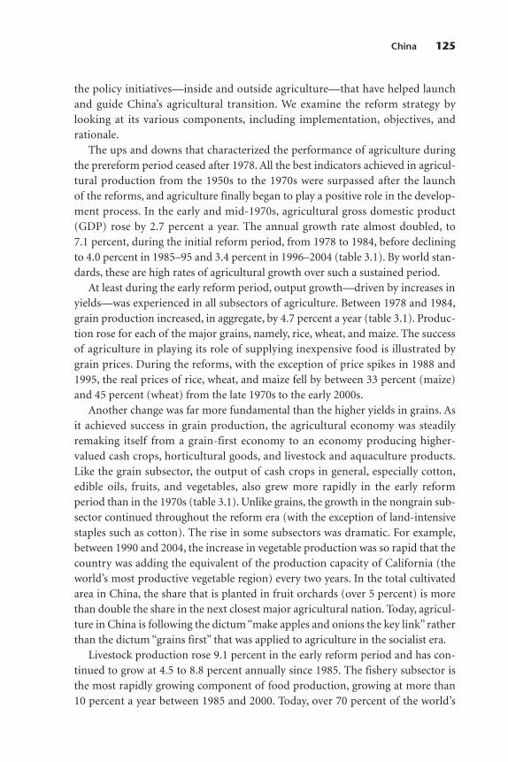
the policy initiatives—inside and outside agriculture—that have helped launchand guide China’s agricultural transition. We examine the reform strategy bylooking at its various components, including implementation, objectives, andrationale.
The ups and downs that characterized the performance of agriculture duringthe prereform period ceased after 1978. All the best indicators achieved in agricul-tural production from the 1950s to the 1970s were surpassed after the launchof the reforms, and agriculture finally began to play a positive role in the develop-ment process. In the early and mid-1970s, agricultural gross domestic product(GDP) rose by 2.7 percent a year. The annual growth rate almost doubled, to7.1 percent, during the initial reform period, from 1978 to 1984, before decliningto 4.0 percent in 1985–95 and 3.4 percent in 1996–2004 (table 3.1). By world stan-dards, these are high rates of agricultural growth over such a sustained period.
At least during the early reform period, output growth—driven by increases inyields—was experienced in all subsectors of agriculture. Between 1978 and 1984,grain production increased, in aggregate, by 4.7 percent a year (table 3.1). Produc-tion rose for each of the major grains, namely, rice, wheat, and maize. The successof agriculture in playing its role of supplying inexpensive food is illustrated bygrain prices. During the reforms, with the exception of price spikes in 1988 and1995, the real prices of rice, wheat, and maize fell by between 33 percent (maize)and 45 percent (wheat) from the late 1970s to the early 2000s.
Another change was far more fundamental than the higher yields in grains. Asit achieved success in grain production, the agricultural economy was steadilyremaking itself from a grain-first economy to an economy producing higher- valued cash crops, horticultural goods, and livestock and aquaculture products.Like the grain subsector, the output of cash crops in general, especially cotton, edible oils, fruits, and vegetables, also grew more rapidly in the early reformperiod than in the 1970s (table 3.1). Unlike grains, the growth in the nongrain sub-sector continued throughout the reform era (with the exception of land-intensivestaples such as cotton). The rise in some subsectors was dramatic. For example,between 1990 and 2004, the increase in vegetable production was so rapid that thecountry was adding the equivalent of the production capacity of California (theworld’s most productive vegetable region) every two years. In the total cultivatedarea in China, the share that is planted in fruit orchards (over 5 percent) is morethan double the share in the next closest major agricultural nation. Today, agricul-ture in China is following the dictum “make apples and onions the key link” ratherthan the dictum “grains first” that was applied to agriculture in the socialist era.
Livestock production rose 9.1 percent in the early reform period and has con-tinued to grow at 4.5 to 8.8 percent annually since 1985. The fishery subsector isthe most rapidly growing component of food production, growing at more than10 percent a year between 1985 and 2000. Today, over 70 percent of the world’s
China 125
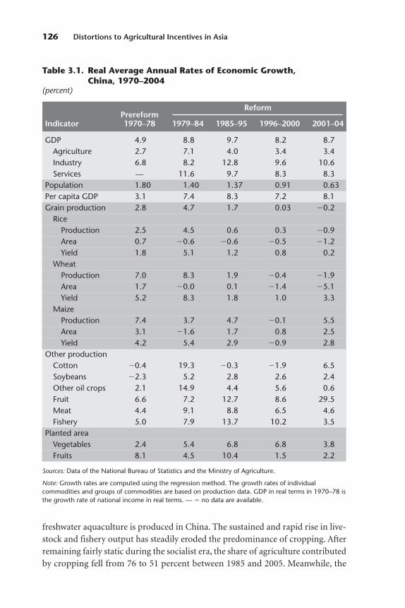
freshwater aquaculture is produced in China. The sustained and rapid rise in live-stock and fishery output has steadily eroded the predominance of cropping. Afterremaining fairly static during the socialist era, the share of agriculture contributedby cropping fell from 76 to 51 percent between 1985 and 2005. Meanwhile, the
126 Distortions to Agricultural Incentives in Asia
Table 3.1. Real Average Annual Rates of Economic Growth,China, 1970–2004
(percent)
PrereformReform
Indicator 1970–78 1979–84 1985–95 1996–2000 2001–04
GDP 4.9 8.8 9.7 8.2 8.7Agriculture 2.7 7.1 4.0 3.4 3.4Industry 6.8 8.2 12.8 9.6 10.6Services — 11.6 9.7 8.3 8.3
Population 1.80 1.40 1.37 0.91 0.63Per capita GDP 3.1 7.4 8.3 7.2 8.1Grain production 2.8 4.7 1.7 0.03 �0.2
RiceProduction 2.5 4.5 0.6 0.3 �0.9Area 0.7 �0.6 �0.6 �0.5 �1.2Yield 1.8 5.1 1.2 0.8 0.2
WheatProduction 7.0 8.3 1.9 �0.4 �1.9Area 1.7 �0.0 0.1 �1.4 �5.1Yield 5.2 8.3 1.8 1.0 3.3
MaizeProduction 7.4 3.7 4.7 �0.1 5.5Area 3.1 �1.6 1.7 0.8 2.5Yield 4.2 5.4 2.9 �0.9 2.8
Other productionCotton �0.4 19.3 �0.3 �1.9 6.5Soybeans �2.3 5.2 2.8 2.6 2.4Other oil crops 2.1 14.9 4.4 5.6 0.6Fruit 6.6 7.2 12.7 8.6 29.5Meat 4.4 9.1 8.8 6.5 4.6Fishery 5.0 7.9 13.7 10.2 3.5
Planted areaVegetables 2.4 5.4 6.8 6.8 3.8Fruits 8.1 4.5 10.4 1.5 2.2
Sources: Data of the National Bureau of Statistics and the Ministry of Agriculture.
Note: Growth rates are computed using the regression method. The growth rates of individualcommodities and groups of commodities are based on production data. GDP in real terms in 1970–78 isthe growth rate of national income in real terms. — � no data are available.
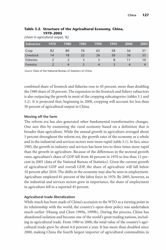
combined share of livestock and fisheries rose to 45 percent, more than doublingthe 1980 share of 20 percent. The expansion in the livestock and fishery subsectorsis also outpacing the growth in most of the cropping subcategories (tables 3.1 and3.2). It is projected that, beginning in 2008, cropping will account for less than50 percent of agricultural output in China.
Moving off the farmThe reform era has also generated other fundamental transformative changes.One sees this by examining the rural economy based on a definition that isbroader than agriculture. While the annual growth in agriculture averaged about5 percent throughout the reform era, the growth rates of the economy as a wholeand in the industrial and services sectors were more rapid (table 3.1). In fact, since1985, the growth in industry and services has been two to three times more rapidthan the growth in agriculture. Because of the differences in the sectoral growthrates, agriculture’s share of GDP fell from 40 percent in 1970 to less than 13 per-cent in 2005 (data of the National Bureau of Statistics). Given the current growthof agricultural GDP and overall GDP, the share of agriculture will fall below10 percent after 2010. The shifts in the economy may also be seen in employment.Agriculture employed 81 percent of the labor force in 1970. By 2005, however, asthe industrial and services sectors grew in importance, the share of employmentin agriculture fell to a reported 45 percent.
Agricultural trade liberalizationWhile much has been made of China’s accession to the WTO as a turning point inits relationship with the world, the country’s open-door policy was undertakenmuch earlier (Huang and Chen 1999a, 1999b). During the process, China hasabandoned isolation and become one of the world’s great trading nations, includ-ing in agricultural trade. From 1980 to 2000, the total value of the country’s agri-cultural trade grew by about 6.0 percent a year. It has more than doubled since2000, making China the fourth largest importer of agricultural commodities in
China 127
Table 3.2. Structure of the Agricultural Economy, China,1970–2005
(share in agricultural output, %)
Subsector 1970 1980 1985 1990 1995 2000 2005
Crop 82 80 76 65 58 56 51Livestock 14 18 22 26 30 30 35Fisheries 2 2 3 5 8 11 10Forestry 2 4 5 4 3 4 4
Source: Data of the National Bureau of Statistics of China.
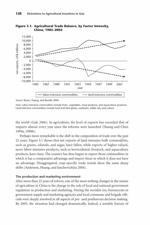
the world (Gale 2006). In agriculture, the level of exports has exceeded that ofimports almost every year since the reforms were launched (Huang and Chen1999a, 1999b).
Perhaps more remarkable is the shift in the composition of trade over the past25 years. Figure 3.1 shows that net exports of land-intensive bulk commodities,such as grains, oilseeds, and sugar, have fallen, while exports of higher-valued,more labor-intensive products, such as horticultural, livestock, and aquacultureproducts, have risen. The country has thus begun to export those commodities inwhich it has a comparative advantage and import those in which it does not havean advantage. Disaggregated, crop-specific trade trends show the same sharpshifts (Anderson, Huang, and Ianchovichina 2004).
The production and marketing environmentAfter more than 25 years of reform, one of the most striking changes in the natureof agriculture in China is the change in the role of local and national governmentregulation in production and marketing. During the socialist era, bureaucrats ingovernment supply and marketing agencies and local commune and brigade offi-cials were deeply involved in all aspects of pre- and postharvest decision making.By 2005, the situation had changed dramatically. Indeed, a notable feature of
128 Distortions to Agricultural Incentives in Asia
�10,000
�6,000�8,000
�4,000�2,000
0
net
exp
orts
, US$
mill
ions
12,000
8,00010,000
4,0006,000
2,000
1985 1987 1989 1991 1993 1995 1997 1999 2001year
labor-intensive commodities land-intensive commodities
Figure 3.1. Agricultural Trade Balance, by Factor Intensity,China, 1985–2002
Source: Rosen, Huang, and Rozelle 2004.
Note: Labor-intensive commodities include fruits, vegetables, meat products, and aquaculture products.Land-intensive commodities include food and feed grains, soybeans, edible oils, and cotton.
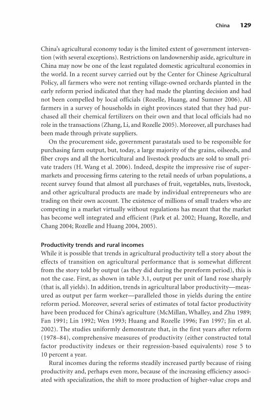
China’s agricultural economy today is the limited extent of government interven-tion (with several exceptions). Restrictions on landownership aside, agriculture inChina may now be one of the least regulated domestic agricultural economies inthe world. In a recent survey carried out by the Center for Chinese AgriculturalPolicy, all farmers who were not renting village-owned orchards planted in theearly reform period indicated that they had made the planting decision and hadnot been compelled by local officials (Rozelle, Huang, and Sumner 2006). Allfarmers in a survey of households in eight provinces stated that they had pur-chased all their chemical fertilizers on their own and that local officials had norole in the transactions (Zhang, Li, and Rozelle 2005). Moreover, all purchases hadbeen made through private suppliers.
On the procurement side, government parastatals used to be responsible forpurchasing farm output, but, today, a large majority of the grains, oilseeds, andfiber crops and all the horticultural and livestock products are sold to small pri-vate traders (H. Wang et al. 2006). Indeed, despite the impressive rise of super-markets and processing firms catering to the retail needs of urban populations, arecent survey found that almost all purchases of fruit, vegetables, nuts, livestock,and other agricultural products are made by individual entrepreneurs who aretrading on their own account. The existence of millions of small traders who arecompeting in a market virtually without regulations has meant that the markethas become well integrated and efficient (Park et al. 2002; Huang, Rozelle, andChang 2004; Rozelle and Huang 2004, 2005).
Productivity trends and rural incomesWhile it is possible that trends in agricultural productivity tell a story about theeffects of transition on agricultural performance that is somewhat differentfrom the story told by output (as they did during the prereform period), this isnot the case. First, as shown in table 3.1, output per unit of land rose sharply(that is, all yields). In addition, trends in agricultural labor productivity—meas-ured as output per farm worker—paralleled those in yields during the entirereform period. Moreover, several series of estimates of total factor productivityhave been produced for China’s agriculture (McMillan, Whalley, and Zhu 1989;Fan 1991; Lin 1992; Wen 1993; Huang and Rozelle 1996; Fan 1997; Jin et al.2002). The studies uniformly demonstrate that, in the first years after reform(1978–84), comprehensive measures of productivity (either constructed totalfactor productivity indexes or their regression-based equivalents) rose 5 to10 percent a year.
Rural incomes during the reforms steadily increased partly because of risingproductivity and, perhaps even more, because of the increasing efficiency associ-ated with specialization, the shift to more production of higher-value crops and
China 129

livestock commodities, and the expansion of off-farm work (table 3.3). Between1980 and 2001, average real rural per capita income rose by a remarkable 6 percentper year, which is as high as the growth rates experienced in Japan and the Republicof Korea during the take-off years of those economies. The amount of attentiongiven to the rural income problem by the media might seem surprising, but theattention has been generated by the more rapid rise in urban incomes relative torural incomes. Inequality is increasing between rural and urban areas, but it is alsoincreasing between those people within the rural economy who were relativelyrich at the outset of reform and those who were relatively poor. The growth rate inrural per capita income in the richest decile, at more than 8 percent annually, is farhigher than the average (3 percent annually), which means that the growth rateamong other segments of the rural population is correspondingly lower than3 percent. In relative terms, the poorest of the rural poor are falling behind.
Summary of agriculture’s performance during the transition eraWhereas the socialist era witnessed few transformations, the agricultural sectorin China has changed dramatically during the transition. The sector has grown,but the decline in its importance in employment and in the value of output in theoverall economy has been characteristic of the growth. The structure of the sec-tor itself is also changing; it is diversifying out of coarse grains into fine grains,out of staple grains into higher-valued crops, and out of cropping into livestockand aquaculture. Trade patterns are changing and are now more reflective of thecountry’s comparative advantages. One of the largest shifts has occurred in pro-duction and marketing, which have become almost laissez-faire, that is, there islittle government intervention. Although the most dramatic changes have takenplace most rapidly among wealthier households, changes are also occurringamong the poor.
130 Distortions to Agricultural Incentives in Asia
Table 3.3. Rural Income per Capita, China, 1980–2001(real 2000 yuan)
Annual growth,Income group 1980 1985 1990 1995 2000 2001 1980–2001, %
Average 711 1,248 1,305 1,702 2,253 2,347 6Bottom decile 312 448 442 493 579 578 3
(poorest)Top decile 1,530 2,486 3,253 4,763 6,805 7,159 8
(richest)
Source: Compiled based on data of the National Bureau of Statistics.

Institutions and the PolicyFoundation of Reform
Unlike leaders in the transitional economies in Europe, leaders in China did notseek to dismantle the planned economy in favor of liberalized markets during theinitial stages of reform (Rozelle and Swinnen 2004). Policy makers in China onlybegan to shift their focus toward market liberalization in 1985 after decollectiviza-tion was complete. Even then, liberalization was start-stop (Sicular 1995). Lin,Cai, and Li (1996) argue that the leaders were afraid of disruptive social effects.The institutions through which the leadership controlled the main goods in thefood economy (such as grains, fertilizers, and meat products) could not be elimi-nated before the institutions were in place that would support more efficient mar-ket exchanges. Throughout the reforms, leaders were investing in the economyand changing the rules governing those domestic producers and consumers whowere interacting with the external economy.
Pricing policies
Early during the reforms, although China’s leaders had no concrete plan to liber-alize markets, they did take steps to change the producer incentives that wereembodied in the prices producers received for their marketed surplus. Perhapsone of the least appreciated initiatives of the early reformers was their bold deci-sion to increase the administered prices received by farmers (Lardy 1983; Sicular1988a). Between 1978 and 1983, in a number of separate actions, the government-set above-quota prices (the payments farmers received for voluntary sales beyondthe mandatory deliveries) were increased by 41 percent for grain and by around50 percent for cash crops (Sicular 1988a). According to National Bureau of Statis-tics data, the price of grain relative to fertilizer rose by more than 60 percent dur-ing the first three years after the reform. During the early reform period, the rise inthe above-quota price represented a higher output price at the margin for farmers(Sicular 1995).
The important contribution of pricing policy was in the timing and breadth ofthe policy change. The first major price rise occurred in 1979, close to the momentwhen reformers were deciding to decollectivize. However, following the decisionof the leadership to implement the household responsibility system gradually,beginning first in the poorest areas of China, the price increases immediatelyaffected all farmers, regardless of whether they had been decollectivized. By 1981,the period of the second major price increase, less than half of all farmers hadbeen allowed to dismantle their communes (Lin 1992). Hence, as long as there wasa link, albeit weak, between the output price and production, the plan-based price
China 131

rise would have led to increases in farm output. Empirical studies confirm thestrong impact of these price changes on output during the first years of transition(Fan 1991; Lin 1992; Huang and Rozelle 1996; Fan and Pardey 1997).
Greater incentives
The rural economic reforms initiated in 1979 were founded on the householdresponsibility system. The reforms of this system led to the dismantlement of thecommunes. Agricultural land was contracted to households, mostly on the basisof family size and the number of people in the household labor force. Mostimportantly, after the reforms of the system, income and control rights over farm-land belonged to individual households (though the right to sell was excluded).
There is little doubt that the changes in incentives resulting from the reforms inproperty rights triggered strong growth in farm output and productivity. In themost definitive study on the subject, Lin (1992) estimates that China’s householdresponsibility system accounted for 42 to 46 percent of the total rise in outputduring 1978–84. Fan (1991) and Huang and Rozelle (1996) find that, evenaccounting for technological change, institutional change during the late 1970sand early 1980s contributed about 30 percent of output growth. Empiricalresearchers have also documented impacts that go beyond output. For example,McMillan, Whalley, and Zhu (1989) demonstrate that the early reforms raisedtotal factor productivity, accounting for 90 percent of the rise (23 percent) in1978–84. Jin et al. (2002) show that the reforms had a large effect on productivity,contributing substantially to a rise in total factor productivity that exceeded 7 per-cent annually.
Domestic market liberalization policies
In addition to pricing changes and decollectivization, another major task of thereformers was to create efficient institutions of exchange. Whether they are classicand competitive or only workable substitutes, efficient markets facilitate transac-tions among agents to allow specialization and trade and, through pricing mecha-nisms, provide information to producers and consumers about the relativescarcity of resources and products.
The major changes to agricultural commerce in the early 1980s almost exclu-sively centered on increasing crop purchase prices (Sicular 1988a; Watson 1994).The decision to raise prices should not be considered part of a strategy to liberal-ize markets. Planners in the Ministry of Commerce made the price changesadministratively, and the changes were mostly executed by the national network ofgrain procurement stations under the direction of the State Grain Bureau.
132 Distortions to Agricultural Incentives in Asia

An examination of policies and marketing activities in the early 1980s revealsthe limited changes in the marketing environment in China’s food economybefore 1985. It is true that reformers allowed farmers greater discretion in produc-ing and marketing crops in 10 planning categories, including vegetables, fruits,and coarse grains. Moreover, by 1984, the state only claimed control over 12 com-modities, including rice, wheat, maize, soybeans, peanuts, rapeseeds, and severalother cash crops (Sicular 1988a). While this may seem to represent a significantstep toward liberalization, the crops remaining almost entirely under the planningauthority of the government still accounted for more than 95 percent of the totalsown area in 1984. Hence, in policy and practice, the output of almost all the sownarea and the related marketing decisions were still directly influenced by govern-ment planners. The planners proceeded with equal caution in reducing therestrictions on free-market trade, and the process was start-stop-start at first.
Market liberalization began in earnest after 1985. Changes in the procurementsystem, additional reductions in the restrictions on commodity trading, steps tocommercialize the state trading system for grains, and calls for expansion in theestablishment of markets in rural and urban areas led to a surge in market- oriented activity (Sicular 1995). For example, only around 240,000 private and semi-private trading enterprises were registered with the State Markets Bureau in 1980; by1990, there were more than 5.2 million (deBrauw, Huang, and Rozelle 2004).
Private trading gradually expanded to include all categories of agricultural out-put remaining after contractual obligations to the government had been fulfilled.This eventually undermined the state marketing system (Rozelle et al. 2000). Thereformers eliminated the planned procurement of all agricultural products exceptrice, wheat, maize, and cotton. Government commercial departments were able tocontinue to buy and sell only if they did so through the market. Incentives wereintroduced for grains through reductions in the volume of compulsory quotasand increases in procurement prices. Even among grains, after the share of com-pulsory quota procurement reached 29 percent in 1984, it declined to 18 percentin 1985 and 13 percent in 1990. The share of negotiated procurement at marketprices rose from 3 percent in 1985 to 6 percent in 1985 and 12 percent in 1990.
Agricultural technology and water infrastructure development
Plant breeding and agricultural research are almost universally organized andmanaged by the government. Reflecting the urban bias of food policy, most cropbreeding programs emphasize fine grains (rice and wheat). The traditional focusof research has been on quantity because of concerns about food self-sufficiency,but quality improvement has recently been emphasized because of a shift indemand toward higher-quality food. There have been several joint ventures and
China 133
private domestic investment initiatives in agricultural research and development,but government policy still discriminates against the practice.
The record of the reforms in agricultural technology is mixed, and the impactof the reforms in terms of new technological development and greater crop pro-ductivity is unclear. Empirical evidence indicates that the effectiveness of thecountry’s agricultural research system is declining (Jin et al. 2002). Our previouswork has shown that, while competitive grant programs probably boosted theeffectiveness of the system, the reliance on revenues from commercialization tomake up for falling budgetary commitments weakened the system.1 It is possiblethat imperfections in the seed industry contributed to the lack of success in thereforms in research on crop breeding.
Since the late 1990s, there has been a sharp rise in spending on agriculturalresearch and development. However, government investments in the developmentof water management for irrigation and flood control swamp the investments inagricultural research. From the 1950s to the 1970s, most of the government’sefforts were focused on building dams and canals, often with the input by farmersof corvée labor. Since the end of the 1970s, greater attention has been focused onincreasing the use of the country’s massive groundwater resources (Wang, Huang,and Rozelle 2005). By 2005, China had more tube wells than any other country inthe world, with the possible exception of India. Initially, the investments weremade by local governments, which were assisted by county and provincial waterbureaus. But, by the 1990s, the government was encouraging the huge shift inownership that was already occurring, as pump sets, wells, and other irrigationequipment were being taken over by families on private farms (J. Wang et al.2005). Meanwhile, private water markets—whereby farmers would sell waterpumped from their own wells to other farmers in the village—were also encour-aged. The main policy initiative after the mid-1990s in the surface water subsectorwas a management reform that sought to raise efficiency in water use.
Trade policy
There were important changes during the 1980s and 1990s in foreign exchangepolicy that saw the nation’s currency depreciate steeply and trading rights becomemore accessible to traders. A number of other fundamental reforms were alsoundertaken in China’s international trading system. The lower agricultural tariffsand the rising imports and exports of agricultural products began to affect thedomestic terms of trade in the 1980s. During the initial reform years, most of thefall in protection was caused by a reduction in the commodities that were con-trolled by single-desk state traders (Huang and Chen 1999a, 1999b). In manyproducts, competition among nonstate foreign trade corporations started to
134 Distortions to Agricultural Incentives in Asia
stimulate imports and exports (Martin 2002). Although many major agriculturalcommodities were not included in the effort to decentralize trade, the effortspurred the export of many agricultural goods. In addition, policy shifts in the1980s and 1990s also altered the trading behavior of state traders. Thus, the policyleadership allowed state traders to boost imports during these decades.
Steps to relax restrictions on the right of access to import and export marketswere matched by steps to reduce the taxes assessed at the border. After the elimi-nation of limits on the imports and exports of many agricultural commodities, anew effort was undertaken in the early 1990s to lower the level of formal protec-tion. The simple average agricultural import tariff fell from 42 percent in 1992 to24 percent in 1998 and 21 percent in 2001 (Rosen, Huang, and Rozelle 2004).
Overall protection in the agricultural sector has declined in the past 20 years.Much of the drop has been caused by the decentralization of authority overimports and exports, a relaxation in the licensing procedures for some crops (forexample, the shift away from state trading firms in importing oil and oilseeds),and changes in the foreign exchange rate. Other trade policies have reduced thescope of nontariff barriers, relaxed the real tariff rates at the border, and changedquotas (Huang and Chen 1999a, 1999b). Despite these real and, in some areas,rapid reforms, the control over commodities that policy leaders consider ofnational strategic importance, such as rice, wheat, and maize, remains largely withgovernment officials (Nyberg and Rozelle 1999).
The accession to the WTO has been a major event in the country and will con-tinue to have a substantial impact on many sectors. Nonetheless, given the trendsin reform, the WTO accession agreement in the agricultural sector, in its most basicterms, represents a continuation of previous agricultural policies. Importantly,though, the commitments embodied in this agricultural part of the agreement—market access, domestic support, and export subsidies—are a binding confirma-tion and codification of steps the government took in the 1990s while it was negotiating the accession to the WTO.
Summary: China’s transition era agricultural policies
The scope of China’s policy efforts during the transition is impressive. Policy shiftswere realized in pricing, production management, marketing, investments, tech-nology, and trade. Although the rate of investment has risen during the reforms,the country is probably still underinvesting in agriculture relative to other sectorsand other countries. Explicit taxes and the taxes implicit in pricing and trade poli-cies have also fallen. The government is not assisting the agricultural economy inthe substantial ways that characterize the country’s neighbors in East Asia (seeHonma and Hayami 2008). However, it appears to have headed in the direction
China 135

noted by Timmer (1998), whereby developing nations, after they reach a certainpoint in development, begin to shift from making net extractions from agricultureto making net investments in the sector.
Many policies and other factors outside agriculture have affected the sector.Other rural policies, such as those that govern fiscal reform, the emergence oftownship and village enterprises, privatization, and rural governance, almost cer-tainly have a large, albeit indirect effect on agriculture. Urban employment poli-cies, residency restrictions, exchange rate management, and many other policyinitiatives also affect agriculture by influencing relative prices in the economy,access to jobs off the farm, and the overall attractiveness of staying on the farm.
Taken together, these policies have had a dramatic impact on the agriculturalsector. They have increased the output of food, driven prices down, andimproved the supplies of nongrain food and raw materials for industry. The mixof policies—pricing, enhanced property rights, market liberalization, investment,trade—has also made producers more efficient. It has freed up their labor andresources, and these have supported the structural transformation in the agricul-tural economy and the rural economy more generally. There are several pieces ofconvincing evidence that agriculture is beginning to play a more effective role inthe nation’s development: the importance of grain in the cropping subsector isshrinking; the importance of the cropping subsector in the overall agriculturalsector is shrinking; and the importance of agriculture in the general economy isshrinking. Productivity is up, and rural incomes are up. Many of the increases inwelfare, however, are being generated by individuals—there have been more than200 million of them—who have been able to shift from grain production to high-valued crops or from cropping to livestock and fisheries production or, perhapsmost importantly, who have been able to leave agriculture and the rural economyaltogether and obtain employment in cities.
Quantifying the Distortions to AgriculturalIncentives since 1980
We introduce our quantification of the policy-imposed distortions in the incen-tives faced by farmers in China by explaining our methodology and, in particular,the way we deal with distortions in the market for foreign currency. We also out-line our data sources. We then discuss our results in detail.
Methodology and data sources
The main focus of our study is government-imposed distortions that create a gapbetween domestic prices and prices as they would be under free markets. It is not
136 Distortions to Agricultural Incentives in Asia
possible to understand the characteristics of agricultural development through asectoral view alone. For comparative evaluation, the project’s methodology there-fore involves estimates of the effects of direct agricultural policy measures, includ-ing distortions in the foreign exchange market, but also estimates of distortions innonagricultural sectors. Specifically, we compute nominal rates of assistance(NRAs) to farmers that reflect an adjustment for direct interventions on tradableand nontradable inputs. We also generate NRAs for nonagricultural tradables forcomparison with the NRAs for agricultural tradables via the calculation of a rela-tive rate of assistance (RRA) (see Anderson et al. 2008 and appendix A).
This approach is not well suited to the analysis of the prereform period becauseprices played only an accounting function at the time, and key prices involving currency exchange rates were enormously distorted. During the reform period,however, the price comparison approach has provided valuable indicators of distor-tions to the incentives for production, consumption, and trade. as well as indicatorsof the income transfers associated with policy interventions. Such an approach isnecessary because of the low inframarginal procurement prices, but also because ofthe complexity and lack of transparency in the trade barriers in agriculture, includ-ing tariffs, licenses, quotas, tariff rate quotas, and government trading. Exchangerate distortions present particular measurement problems and require detailedanalysis if we expect measures based on price comparisons not to be misleading.
NRAs and CTEsNRAs are constructed in three steps. The NRAs on agricultural output are basedpartly on a comparison of the price of a commodity in the domestic economy atthe port and the international price of the commodity at that same border point(that is, including, cost, insurance, and freight in port for an import good and freeon board in port for an exportable good), taking into account inherent differencesin product quality, where appropriate. Conceptually, we need this part of the NRAon output to measure the extent, at the border, of the distortions caused by tariffs,exchange rate policies, and other nontariff barriers. A positive NRA measure indi-cates that the sector is being protected from import competition, while a negativeNRA measure indicates the sector is subject to some form of (possibly implicit)taxation at the border.
Because we have independent observations on the prices obtained by farmersin local markets, the second step involves estimating NRAs on output at the farm-gate by also taking into account any domestic distortions affecting the returns tofarmers. This part of the NRA is calculated after allowing for quality adjustments,taxes, subsidies, and the costs of domestic transport, storage, and handling indelivering products from the farm to the wholesale market. This part of the NRAon output arises from subsidy or transfer payments that cause the prices received
China 137
by farmers to differ from the prices they would receive under competitive internalmarket conditions. As we show below, these internal subsidies and tax measureshad an enormous impact on the returns to farmers, particularly during the earlyreform period.
An important component of this second part of the NRA evolved during theperiod when domestic incentives were distorted by the requirement to deliver afixed quota of output at a (low) planned price, although producers were allowed tosell above-quota output (surplus) at a higher market price. Clearly, the deliveryrequirements reduced the incomes of farm households, but the impact on the levelof output is less clear. Sicular (1988b) makes the point that, in the short run, the out-put decision of a firm is determined by the marginal return rather than the averagereturn. Under these circumstances, the inframarginal tax imposed by the plan deliv-ery requirement may not have reduced the incentive to produce. However, morerecent work on decoupled price incentives, by taking into account the incentives forfirm entry and exit, suggests that average returns may actually have a greater impacton output in the longer term (de Gorter, Just, and Kropp 2008). Nonetheless, theinability of farm households to sell their land probably reduced the extent to whichthese households exited from agriculture in response to reductions in incomes.
The third step in our NRA measurement captures distortions in farm inputmarkets. To realize this step, we provide measures that take into account directsubsidies and differences between international input prices and the input pricesthat farmers pay. While these forms of protection (or taxation) may be importantin other countries, we find that they are generally relatively small in China and socontribute little to the overall NRA.
While most of our focus is on agricultural producers, we also consider theextent to which consumers are taxed or subsidized. To achieve this, we use a meas-ure called the consumer tax equivalent (CTE). In principle, this measure com-pares the price that consumers pay for food commodities and the internationalprice at the border. As with the NRAs, differences arise between NRAs and CTEsbecause of distortions in the domestic economy, as well as at the border. Thedomestic distortions are caused by transfer policies, taxes, and subsidies that gen-erate gaps between the prices paid by consumers (adjusted to the wholesale level)and domestic market prices. If a CTE is negative, then consumers are payingprices that are below the international market prices and the consumers are beingsubsidized. (For more details on the methodology used to calculate these meas-ures, see Anderson et al. 2008 and appendix A.)
The foreign exchange regimePrior to 1981, China’s official exchange rate was seriously overvalued. While thisdid not directly affect exports and imports because decisions on these were made
138 Distortions to Agricultural Incentives in Asia

by planners, it did create serious accounting difficulties given that exports gener-ally incurred losses (Lardy 1992). If the official exchange rate is used, it will pro-vide misleading indicators of the incentives created by the foreign exchangeregime. Because it made all foreign goods appear inexpensive in terms of thedomestic currency, it overestimated the extent of protection provided to anyimportable good.
In 1981, an internal settlement rate was introduced that was intended to bealigned with the average cost of foreign exchange. This supplied at least some basisfor meaningful comparisons between domestic and international prices. Theinternal settlement rate, at 2.8 yuan per U.S. dollar for trade transactions in 1981,represented nearly a 50 percent devaluation relative to the official exchange rate. Itwas used only for nontrade transactions. This internal rate remained at Y 2.8 untilJanuary 1985, when it was merged with the official exchange rate.
During most of the reform period, the effects of the foreign exchange regimewere relatively transparent. The regime between the late 1970s and 1994 wasincluded among those found by Kiguel and O’Connell (1995) to involve differen-tial rates for different types of current account transactions. The overvalued offi-cial exchange rate was a key element of this system. Prior to 1979, enterprises hadto surrender all their foreign exchange earnings at the official rate. However,beginning in that year, exporting enterprises were allowed to retain some of theirforeign exchange earnings (Lardy 1992). Because of the pervasive shortage of for-eign exchange in the economy, the value of these retained earnings was, on aver-age, considerably above the value as measured by the official exchange rate,although there were restrictions on trading retained foreign exchange amongenterprises, which inevitably exposed the variation in the demand of enterprisesfor foreign exchange.
The restrictions on trade in retained foreign exchange were gradually liberal-ized, and a legal secondary-market exchange rate emerged that was higher (moredepreciated) than the official exchange rate. There was always a shortage of for-eign exchange at the official exchange rate, forcing importers to meet their needsfor additional foreign exchange at the secondary-market rate. Under these cir-cumstances, the exchange rate system created a distortion analogous to a tariffand an export tax. The exchange rate received by exporters was lower than thatpaid, at the margin, by importers.
To account for the effects of the exchange rate system, we construct an exporterexchange rate series by using the retention ratio to calculate a weighted average ofthe official and the secondary-market exchange rates. We use the secondary- market exchange rate as an indicator of the price paid for foreign exchange, at themargin, by importers. Following the methodology outlined in Anderson et al.(2008) and appendix A, we calculate an estimated equilibrium exchange rate as
China 139
the simple average of the importer and the exporter exchange rates. This methodarbitrarily assumes equal elasticities of demand and supply for foreign exchange,though this assumption does not affect the results for any trade impacts becausetaxes on imports and taxes on exports have the same effect (the Lerner symmetrytheorem).
The share of export earnings eligible to be retained rose gradually, and theextent to which these eligibility rights were tradable increased. Initially, there wereonly limited opportunities to trade the rights, and the shadow value varied fromfirm to firm depending upon the firm’s foreign exchange earnings and need forforeign exchange. Policy makers quickly recognized that it was important to beable to able to transfer foreign exchange among firms. Lardy (1992) notes that for-eign exchange trading outlets were first established in Guangzhou (1980) andShanghai (1981). However, the exchange rates in these markets tended to be heav-ily managed; the government was seeking to set the selling price at, for example,the internal settlement rate (Lardy 1992).
Formal foreign exchange adjustment centers were established on a large scaleafter 1985. The centers allowed firms with excess foreign exchange earnings to sellto ventures that sold their output domestically and needed foreign exchange. Overthe next few years, a large network of these centers was established, and the mar-kets became more closely integrated over time. By 1988, Lardy (1992) concludes,the price in the Shanghai market followed the strictures of supply and demand,subject to the conditions on the use of foreign exchange, including licensingrequirements and duties on imported goods. The pricing policies for importedgoods were also becoming more liberal, and, by 1990, the prices of close to 90 per-cent of all imported goods were based on the import price, plus transport costsand tariffs (Lardy 1992).
During the transition, the exchange rate regime had an extremely importantinfluence on the returns obtainable through exported goods and on the prices paidfor imported goods. Even in the absence of explicit trade policies, overvalued officialexchange rates tended to lower the returns to exported goods and increase the costsof imported goods, often by large amounts. The combination of an overvalued offi-cial exchange rate and a secondary-market exchange rate at which importers couldpurchase foreign exchange legally allows us to assess the effects of the foreignexchange regime and then to begin to assess the impacts of other trade policies.
The analytics of a multiple exchange rate system are relatively clear and are eas-ily understood in a partial equilibrium setting. Figure 3.2 shows the exchange ratesin a market that is characterized by an upward-sloping supply of foreign exchange(perhaps determined by the marginal costs of generating additional assets) and adownward-sloping demand for foreign exchange (perhaps determined by theextent of substitutability among imports and domestic goods). If there is an official
140 Distortions to Agricultural Incentives in Asia
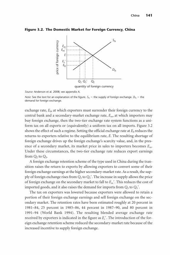
exchange rate, E0, at which exporters must surrender their foreign currency to thecentral bank and a secondary-market exchange rate, Em, at which importers maybuy foreign exchange, then the two-tier exchange rate system functions as a uni-form tax on all exports or (equivalently) a uniform tax on all imports. Figure 3.2shows the effect of such a regime. Setting the official exchange rate at E0 reduces thereturns to exporters relative to the equilibrium rate, E. The resulting shortage offoreign exchange drives up the foreign exchange’s scarcity value, and, in the pres-ence of a secondary market, its market price in sales to importers becomes Em.Under these circumstances, the two-tier exchange rate reduces export earningsfrom QE to QS.
A foreign exchange retention scheme of the type used in China during the tran-sition raises the return to exports by allowing exporters to convert some of theirforeign exchange earnings at the higher secondary-market rate. As a result, the sup-ply of foreign exchange rises from QS to QS�. The increase in supply allows the priceof foreign exchange on the secondary market to fall to Em�. This reduces the cost ofimported goods, and it also raises the demand for imports from QS to QS�.
The tax on exporters was lowered because exporters were allowed to retain aportion of their foreign exchange earnings and sell foreign exchange on the sec-ondary market. The retention rates have been estimated roughly at 20 percent in1981–84, 25 percent in 1985–86, 44 percent in 1987–90, and 80 percent in1991–94 (World Bank 1994). The resulting blended average exchange ratereceived by exporters is indicated in the figure as Es�. The introduction of the for-eign exchange retention scheme reduced the secondary-market rate because of theincreased incentive to supply foreign exchange.
China 141
QS
Sfx
Dfx
Em
E0
E
Es�
Em�
QS� QE
pric
e of
fore
ign
curr
ency
quantity of foreign currency
Figure 3.2. The Domestic Market for Foreign Currency, China
Source: Anderson et al. 2008; see appendix A.
Note: See the text for an explanation of the figure. Sfx � the supply of foreign exchange. Dfx � thedemand for foreign exchange.
We use several different series to obtain secondary-market exchange rate data:the internal settlement rate in 1981–84, an estimated secondary-market exchangerate in 1985–86, and the Foreign Exchange Adjustment Center rate in 1987–94.We use the difference between the importer exchange rate and the estimated equilibrium rate as a measure of the component of the protection for import-competing products that is represented by exchange rate distortion. Similarly, weuse the difference between the exporter exchange rate and the equilibrium rate asa measure of the exchange rate distortion affecting exportable goods. Relying onthese principles and data, we obtain the results described in Huang et al. (2007).2
The data usedIn compiling price data, we first had to make choices about our study’s coverageof commodities. We have included 11 commodities: rice, wheat, maize, soybeans,cotton, pig meat, milk, poultry, fruit (we use apples as a representative product),vegetables (we use tomatoes as a representative product), and sugar (sugar beetsand sugarcane). Over the period we study, these commodities account forbetween 75 percent (in the late 1980s) and 60 percent (during the early 2000s) ofthe total value of agricultural output (Huang et al. 2007). Because decisions onproduction and consumption were only gradually being allowed to respond todomestic market prices and because we do not have access to reliable data on sec-ondary-market exchange rates prior to 1981, we focus on data for the periodbeginning in 1981.
The data in our study have been gathered from diverse sources, depending onthe period of analysis and the commodity (see the references). We have taken com-modity balance data (production, utilization, trade, and others) from the CAPSiMdatabase of the Center for Chinese Agricultural Policy. These data have been com-piled mainly by the Ministry of Agriculture (production), the National Bureau ofStatistics (consumption and others), and the Ministry of Commerce (trade). Thedata on domestic prices are from several ministries. Specifically, farmgate outputprices have been taken from the cost of production surveys conducted by theNational Development and Reform Commission. Data on the wholesale and retailprices of most products have been collected from the Center for Price Monitoring,the National Development and Reform Commission, the Ministry of Agriculture,and the Department of Rural Survey at the National Bureau of Statistics. If whole-sale and retail prices for some commodities are not available for some years, wehave estimated the price margins from farmgate to wholesale and to retail. Muchof the data on margins, transportation costs, and other transaction costs have beentaken from extensive surveys conducted by Huang and Rozelle during the 1990sand the early 2000s. The surveys have also served to identify the commodity priceseries that provide an appropriate foundation for price comparisons. Some of this
142 Distortions to Agricultural Incentives in Asia

material has been examined in Rozelle, et al. (2000) and Huang, Rozelle, andChang (2004), who provide information on substantial quality differencesbetween imported and domestic commodities and the resulting biases in pricecomparisons as a measure of protection. Survey teams from the Center for Chinese Agricultural Policy interviewed traders in 10 cities around China in 2006,and this has provided additional data on more recent years. The data for all thecommodities are summarized in appendix B, table B.3.
International price data for all commodities except milk—free on board pricesand cost, insurance, and freight prices—represent the unit values of exports orimports, with adjustments for quality, where needed. We have taken these datafrom the Ministry of Commerce and China Customs. For the border price ofmilk, because no import prices for milk are available, we adjust the farmgate priceof milk in New Zealand according to international transportation and insurancerates to create a series for the international price of milk (cost, insurance, andfreight included), which we refer to as the reference price.
Other data used in this study include tariff rates and information on taxes andsubsidies. The tariff rates have been compiled from the Office of Tariff Regulation(1998, 2005). Agricultural tax data have been collected from cost of productionsurveys conducted by the National Development and Reform Commission. Infor-mation on subsidies (for example, recent grain subsidies) is taken from variousgovernment documents. Aggregate input subsidies are based on producer supportestimates by the Organisation for Economic Co-operation and Development(OECD), which are disaggregated into individual commodities based on shares intotal crop area (see OECD 2005 and the OECD PSE-CSE Database 1986–2005).
Results
An indirect indication of the success of China’s reform policies may be gained byexamining the domestic free-market prices for four of the country’s most impor-tant crops (Huang et al. 2007). Prices were relatively stable despite the sharp rise indemand after 1980 for all commodities because of increases in the population,rapidly rising incomes, the shift of the population from rural to urban areas, andgradual marketization. The overall self-sufficiency rate for rice, wheat, maize, andsoybeans during the 1980s and 1990s was nearly 100 percent (Huang and Chen1999a, 1999b). It is clear that domestic production was keeping up with thegrowth in demand. Many studies have found that the rise in supply, as well as intotal factor productivity, was generated by a reduction in the distortions in pro-duction incentives that was driven by reforms such as improved property rightsand more open access to new technologies (Lin 1992; Fan 1991; Huang andRozelle 1996; Jin et al. 2002).
China 143
The role of domestic price and marketing policyIt is useful to examine the relationship between the available domestic price seriesfor farmgate procurement and the urban and rural retail prices for the majorgrain crops (Huang et al. 2007). The importance and role of the government’sdomestic price and marketing policy for rice, wheat, and maize—the three largestcrops in China—may be understood through a comparison of the urban retailprice, the rural farmgate procurement price, and the rural retail price. The firsttwo are set by the government, while the third is a free-market price. Until 1992,the urban retail price for rice was usually substantially below the price on the freemarket in rural areas, despite the costs associated with transferring rice to urbanareas. This was a consequence of a procurement price system designed to provideurban residents with relatively inexpensive (that is, subsidized) food. Only urbanresidents were allowed to buy rice at these low prices, and they were allowed to doso only on the basis of ration coupons that were available in limited quantities.
The marketing and procurement system may have been the source of addi-tional distortions. In the 1980s, the relatively low selling price for grain by farmersat the farmgate shows that the food system was transferring income from rural tourban areas. The prices paid to farmers for the output they delivered based ongovernment quotas were far below free-market prices. Nonetheless, given theinframarginal nature of many of the transfers, there is some uncertainty about theeffect on the incentives for production and consumption (Sicular 1988b). This isbecause, after the mid-1980s, farmers were able to sell surplus output at highermarket prices once they had met their quota obligations. If a farmer could sell sur-plus grain at an above-quota price determined by market forces, then the farmermay have faced a less severe distortion. However, the inframarginal transfers werenot fully decoupled from incentives. It appears, for instance, that they representedan incentive to move out of agriculture (Wang, Rozelle, and Huang 1999). Thedomestic marketing and procurement system may thus have also distorted incen-tives relative to international prices.
Beginning in 1992, however, changes in the domestic marketing and procure-ment system appear to have eliminated this additional layer of regulation for pro-ducers of rice, wheat, and maize. In the early 1990s, the urban price began to riseabove the farmgate price, and urban and rural retail prices also moved closertogether. This reflects the phasing out of the implicit taxation of farmers throughthe grain procurement system. The gap between urban and rural retail priceseventually disappeared, and the gap between the rural retail price and the farm-gate price declined, suggesting that there had been an improvement in marketingefficiency (Park et al. 2002). The distortions remaining after the mid-1990s, fol-lowing the disappearance of the distortions caused by the marketing and procure-ment system, reflect only trade policies.
144 Distortions to Agricultural Incentives in Asia
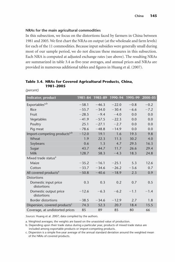
NRAs for the main agricultural commoditiesIn this subsection, we focus on the distortions faced by farmers in China between1981 and 2005. We first chart the NRAs on output (at the wholesale and farm levels)for each of the 11 commodities. Because input subsidies were generally small duringmost of our sample period, we do not discuss these measures in this subsection.Each NRA is computed at adjusted exchange rates (see above). The resulting NRAsare summarized in table 3.4 as five-year averages, and annual prices and NRAs areprovided in numerous additional tables and figures in Huang et al. (2007).
China 145
Table 3.4. NRAs for Covered Agricultural Products, China,1981–2005
(percent)
Indicator, product 1981–84 1985–89 1990–94 1995–99 2000–05
Exportablesa,b �58.1 �46.3 �22.0 �0.8 �0.2Rice �55.7 �34.0 �30.4 �6.6 �7.2Fruit �28.5 �9.4 �4.0 0.0 0.0Vegetables �41.9 �57.5 �22.3 0.0 0.0Poultry 25.1 �27.1 �2.7 0.0 0.0Pig meat �78.6 �48.8 �14.9 0.0 0.0
Import-competing productsa,b �12.0 19.1 1.6 19.3 9.8Wheat 1.9 22.3 11.3 30.2 4.0Soybeans 0.6 1.3 4.7 29.5 16.3Sugar 43.7 44.7 11.7 26.6 29.4Milk 128.7 58.3 �4.3 18.3 24.8
Mixed trade statusa
Maize �35.2 �16.1 �25.1 5.3 12.6Cotton �33.7 �34.6 �26.2 �3.6 0.7
All covered productsa �50.8 �40.6 �18.9 2.3 0.9Distortions
Domestic input price 0.3 0.3 0.2 0.7 0.5distortions
Domestic output price �12.6 �6.3 �6.2 �1.1 �1.4distortions
Border distortions �38.5 �34.6 �12.9 2.7 1.8Dispersion, covered productsc 74.3 52.3 20.7 18.4 15.5Coverage, at undistorted prices 85 89 85 80 66
Sources: Huang et al. 2007; data compiled by the authors.
a. Weighted averages; the weights are based on the unassisted value of production.b. Depending upon their trade status during a particular year, products of mixed trade status are
included among exportable products or import-competing products.c. Dispersion is a simple five-year average of the annual standard deviation around the weighted mean
of the NRAs of covered products.
Distortions in the grain economy before 1995. The distortions in the rice economyof China in the 1980s and early 1990s were characterized by two important fea-tures. First, the NRA for rice, an exportable commodity, was negative every yearbetween 1981 and 1995. Ranging between around �60 and �10 percent, the neg-ative NRA, together with the fact that China was able to export rice, suggests thatthe country was highly competitive in international rice markets during theseyears. Nonetheless, trade policy kept exporters from shipping large quantities ofrice onto world markets and kept the free-market price of rice in China’s portcities below the world price. This shows the government’s commitment to keepingdomestic market prices low. Even if there had been no other distortions in the riceeconomy, producers would have faced prices below world market prices.
The second feature demonstrates that domestic marketing and procurementrepresented an additional tax on farmers and would have insulated the domesticprice of rice from the world market price even if there had been no trade restric-tion at the border. Because of this marketing policy, which lasted to the mid-1990s, the artificially low government procurement price kept the average pricereceived for rice by farmers systematically below the free-market price.
Together, these two features meant that the producer tax on rice rangedbetween �66 in 1981 and �33 in 1991, making rice producers among the mostheavily taxed farmers in China (Huang et al. 2007).
Our NRA estimates show that, unlike the case of rice, trade policy offered someprotection to wheat between 1981 and the mid-1990s (table 3.4). During this period,the free-market price of wheat in China’s port cities ranged between 27 and 64 per-cent higher than the international price of wheat and averaged about 45 percenthigher. This alone suggests that wheat producers in China—who are known to pro-duce at a higher cost than producers in many other countries (Huang and Ma2000)—received significant protection through trade policy. However, domesticmarketing policies were having an impact in the opposite direction. The NRA resultsshow how the wheat quotas reduced the potential benefits to farmers from the highrates of protection at the country’s borders. Although protection averaged 15 percentfor wheat farmers in most years between 1981 and 1995, the rates were zero or evenslightly negative in 5 of the 15 years during this period (1981–82, 1990, and 1992–93).
The case of maize is a mix of the case of rice and the case of wheat (table 3.4).In some years, trade policy provided positive protection for maize (1983–87, 1989,and 1994), while, in other years, the domestic price of maize was lower than theworld market price. On average, trade policy protected maize only marginallybetween 1981 and 1995. As with rice and wheat, procurement policy depressed theprice of maize among farmers. Indeed, except for 1985 and 1994, the net effect ofinternational trade and domestic marketing policy from the 1980s to the early1990s was to tax maize producers.
146 Distortions to Agricultural Incentives in Asia
Distortions to the grain economy after 1995. Our analysis shows that the govern-ment’s international trade and domestic marketing policies changed strikinglyafter 1995 (table 3.4). The procurement policies that had been taxing rice, wheat,and maize farmers either by adding to the tax imposed by export policy, as in thecase of rice, or by reducing protection, as in the case of wheat, were finally elimi-nated from domestic marketing policy. The elimination of the procurement quotacontributed significantly to a reduction in the tax burden shouldered by farmers(Huang, Rozelle, and Wang 2006).
The liberalization of domestic markets in the mid-1990s was accompanied by aliberalization in trade policy at least in the case of the country’s major food grains.After 1995, the taxation and subsidization of rice and wheat were clearly beingphased out: the NRAs for rice were rising steadily (they were becoming less negative),and the NRAs for wheat were falling. Probably partly in preparation for the country’saccession to the WTO, the government liberalized trade in the main food grains soextensively that, between 1995 and 2001, most of the protection for these crops wasphased out. In 2001–05, the NRAs for both rice and wheat were almost zero.
The case of maize is a bit different from the situation among other crops. TheNRAs for maize have been positive in some of the years since 2000. This protec-tion for maize producers may be partly the result of lobbying by Jilin Province inseeking national support for its most important crop (Rozelle and Huang 2004).
Edible oils and cotton. The biggest difference in the analysis of the distortionsaffecting grain staples and the analysis of the distortions affecting cash crops (atleast for soybeans and cotton) is the smaller historical role played by domesticmarketing policy among the cash crops. Although procurement delivery quotasaimed at soybean producers existed in some counties, they were not as widespreadas the quotas for grains; in many counties, soybeans were not a target of the gov-ernment procurement system. In addition, the implicit tax on soybeans in placeswhere the soybean quotas were collected was lower than the implicit tax on staplegrain crops. There is thus little difference between the NRAs on output at thewholesale and farm levels. The same is true of cotton, although the free-marketprocurement of cotton by private traders was not allowed until the mid-1990s.When reform finally came to the cotton industry, policy makers chose not toadopt a two-tier pricing system. Instead, they opted for both private trade and pri-vate procurement through commercialized government cotton procurement sta-tions. As a result, the NRA measures of distortion on cotton output are nearly thesame at the wholesale and farm levels. This is true of all other commodities as well(livestock, horticultural commodities, milk, and sugar). For this reason, the dis-cussion in the rest of this subsection—on the 1980s, the 1990s, and the post-2000period—focuses only on trade policy.
China 147
Our analysis shows that, before 1995, soybeans were sometimes taxed andsometimes protected (table 3.4). Although the average level of protection wasclose to zero, it ranged from �20 percent to �40 percent. Rozelle and Huang(2005) show that much of this fluctuation was caused by domestic productionpolicy, which encouraged soybean production before discouraging it, and thenencouraging it again, although the trade regime permitted little trade. However,trends in the NRAs indicate that there has been some movement toward trade lib-eralization in soybeans. Beginning in the late 1990s and continuing through to2005, the protection rate for soybeans fell from around 30 percent to less than halfthat amount. This should not be a surprise given the gradual integration of Chinainto world soybean markets and the monotonic rise in imports (which exceeded25 million tons in 2005). The situation in soybeans stands in sharp contrast to thecase of maize, which enjoyed increasing protection. Maize and soybeans competefor land and other resources; it appears that, when the level of protection began torise for maize, soybean production was significantly liberalized.
The NRAs suggest that cotton and rice share similarities. The combination oftrade and monopoly procurement policy kept domestic cotton prices lower thanworld market prices in the 1980s and early 1990s. It appears that planners weretaxing cotton farmers to supply the country’s emerging textile industry with rela-tively inexpensive raw materials. The high implicit tax on cotton, along with rav-ages caused by insects, undoubtedly contributed to the stagnant and sometimesfalling share of cotton in the total planted area in many regions (data of theNational Bureau of Statistics).
Since 1995, however, (mostly) because of the liberalization in domestic mar-kets and (somewhat) because of trade liberalization, there has been a clear shift inthe level of the distortions faced by cotton producers. Although there were fluctu-ations (protection was high in 2000, but cotton was implicitly taxed in 1999 and2001), the average NRA since the mid-1990s has been close to zero (if, in choosingthe border price, one takes into account the trade status during each year).Recently, in most years, despite their authority to impose tariff rate quotas on cot-ton after a threshold amount has been imported, trade officials have essentiallyallowed the level of imports to be determined by the market.
Livestock, sugar, and horticultural commodities. With the exception of fruit forseveral years in the late 1980s and early 1990s and of poultry before 1985, the pat-terns of distortion in the livestock and horticultural subsectors are remarkablysimilar (table 3.4). In all cases during the early reform period, there was heavyimplicit taxation on livestock and horticultural commodities. As noted by Huang,Rozelle, and Chang (2004), this situation was created partly by the government’sgrain-first policy. Although China can be competitive in livestock and horticul-tural products, producers were not encouraged to produce or export these
148 Distortions to Agricultural Incentives in Asia

commodities on a large scale. Another part of the problem was the country’s ownbarriers, such as the quotas on exports to Hong Kong, China.
Since the late 1990s, the gaps between the domestic and the world pricesreceived by livestock and horticultural producers have narrowed. NRAs have risentoward zero for all these commodities, including pig meat, poultry, vegetables, andfruit. The relaxation in grain-first policies (often called structural adjustmentpolicies) has allowed producers to expand livestock and horticultural productionsignificantly. The main reason for the expansion is the rising demand inside thecountry (Rosen, Huang, and Rozelle 2004). Nonetheless, China’s accession to theWTO and the emergence of a large export-oriented livestock and horticulturalsegment in the sector have increased the interest and feasibility of participation ininternational markets.
The situation for milk and sugar contrasts with the situation for livestock andhorticultural commodities. During the 1980s, the NRAs for milk and sugar werepositive and large (table 3.4). The NRAs for milk ranged from 40 to 160 percentbetween 1980 and 1987. They fell through the early 1990s, but rose again in thelate 1990s before falling back somewhat thereafter.
The aggregate picture. After aggregating the 11 commodities in our study, wenotice a striking pattern in our results (table 3.4 and figure 3.3). In the 1980s and
China 149
�65
�45
NRA
, %
year
35
�25
�5
15
0
2003
2004
2002
2001
2000
1999
1998
1997
1996
1995
1994
1993
1992
1991
1990
1989
1988
1987
1986
1985
1984
1983
1982
1981
exportablesimport-competing products total
Figure 3.3. NRAs for Exportable, Import-Competing, and AllAgricultural Products, China, 1981–2004
Source: Huang et al. 2007.
Note: A total NRA may be above or below the exportable and import-competing averages because theassistance to nontradables and non-product-specific assistance are also included.
through to the mid-1990s, import-competing products such as wheat, soybeans,milk, and sugar were only slightly taxed, on average, at the farm level. This conclu-sion takes into account the effect of input subsidies and domestic output pricedistortions, as well as distortions at the border, the average contributions of whichare shown towards the bottom of table 3.4. The rate of protection varied consider-ably across the 11 commodities. It also varied inversely with international pricemovements, suggesting that the government was seeking to insulate the domesticmarket a little from world price fluctuations. Exported commodities such as rice,livestock, and horticultural products were subject to substantial rates of taxation,averaging 37 percent in 1981–95, though the variations from year to year werelarge and included nominal rates of taxation of more than 50 percent in severalyears. Since exported agricultural products accounted for a greater part of theeconomy than import-competing agricultural products during the early reformperiod, the agricultural distortions were negative, on average. In other words, formost of the reform period, the government was taxing farmers through interna-tional trade and domestic marketing policies.
One of the main findings of our study is evident in figure 3.3. After 1995, theNRAs of import-competing products fell from around 20 percent to less than10 percent. During this period, the average NRA for exportables rose (or theimplicit taxes on them fell) from about �40 percent to around �15 percent.
Taken together, the distortions in agriculture fell to less than 10 percent. Inmany years, the overall protection was between 0 and �5 percent. Clearly, thecombination of domestic marketing reforms and international trade liberaliza-tion generated an agricultural economy that, on average, was neither taxed norassisted. This does not mean, however, that all distortions were eliminated. In2000–05, there was still wide dispersion in the NRAs across commodities, severalof which continued to show relatively high rates of protection (figure 3.4). Forexample, the NRAs for sugar and milk were above 20 percent, and the NRAs forsoybeans and maize were nontrivial, at more than 10 percent, while the NRAs ofthe fruit, vegetable, pig meat, and poultry exportable categories were close to zero.The dispersion is much less than in earlier decades, however. This is indicated inthe decline in the standard deviation in the NRAs across our 11 commodities, butalso in the (anti)trade bias index (tables 3.4 and 3.5).
The elimination of distortions has affected food consumers as well. In the1980s and early 1990s, consumers were being taxed because of the positive protec-tion on import-competing farm products, but, at the same time, they were gainingfrom being able to consume exportables that were implicitly subsidized by mar-keting and export-restricting policies. Some consumers of rice, wheat, and maizewere also receiving additional consumer subsidies. The net effect of these inter-ventions is that, until the late 1990s, consumers were enjoying a large, implicit
150 Distortions to Agricultural Incentives in Asia
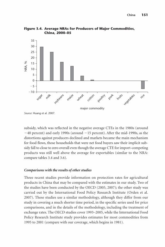
subsidy, which was reflected in the negative average CTEs in the 1980s (around�40 percent) and early 1990s (around �15 percent). After the mid-1990s, as thedistortions against producers declined and markets became the main mechanismfor food flows, those households that were net food buyers saw their implicit sub-sidy fall to close to zero overall even though the average CTE for import-competingproducts was still well above the average for exportables (similar to the NRA:compare tables 3.4 and 3.6).
Comparisons with the results of other studies
Three recent studies provide information on protection rates for agriculturalproducts in China that may be compared with the estimates in our study. Two ofthe studies have been conducted by the OECD (2005, 2007); the other study wascarried out by the International Food Policy Research Institute (Orden et al.2007). These studies use a similar methodology, although they differ from ourstudy in covering a much shorter time period, in the specific series used for pricecomparisons, and in the details of the methodology, including the treatment ofexchange rates. The OECD studies cover 1993–2005, while the International FoodPolicy Research Institute study provides estimates for most commodities from1995 to 2001 (compare with our coverage, which begins in 1981).
China 151
�10
10
5
0
�5
20
15
major commodity
NRA
, %
35
25
30
suga
rm
ilk
soyb
eans
maiz
e
wheat
cotto
n
poult
ryfru
its
vege
table
sric
epo
rk
Figure 3.4. Average NRAs for Producers of Major Commodities,China, 2000–05
Source: Huang et al. 2007.
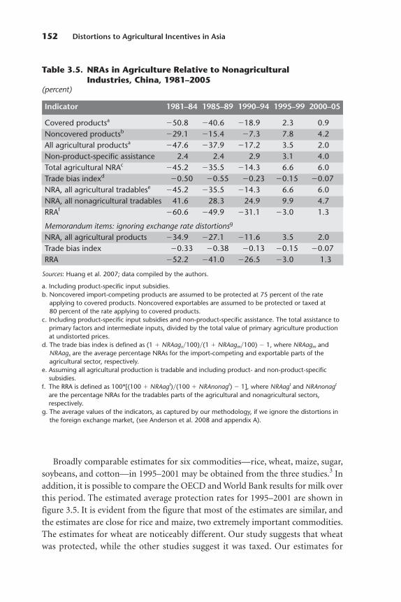
Broadly comparable estimates for six commodities—rice, wheat, maize, sugar,soybeans, and cotton—in 1995–2001 may be obtained from the three studies.3 Inaddition, it is possible to compare the OECD and World Bank results for milk overthis period. The estimated average protection rates for 1995–2001 are shown infigure 3.5. It is evident from the figure that most of the estimates are similar, andthe estimates are close for rice and maize, two extremely important commodities.The estimates for wheat are noticeably different. Our study suggests that wheatwas protected, while the other studies suggest it was taxed. Our estimates for
152 Distortions to Agricultural Incentives in Asia
Table 3.5. NRAs in Agriculture Relative to NonagriculturalIndustries, China, 1981–2005
(percent)
Indicator 1981–84 1985–89 1990–94 1995–99 2000–05
Covered productsa �50.8 �40.6 �18.9 2.3 0.9Noncovered productsb �29.1 �15.4 �7.3 7.8 4.2All agricultural productsa �47.6 �37.9 �17.2 3.5 2.0Non-product-specific assistance 2.4 2.4 2.9 3.1 4.0Total agricultural NRAc �45.2 �35.5 �14.3 6.6 6.0Trade bias indexd �0.50 �0.55 �0.23 �0.15 �0.07NRA, all agricultural tradablese �45.2 �35.5 �14.3 6.6 6.0NRA, all nonagricultural tradables 41.6 28.3 24.9 9.9 4.7RRAf �60.6 �49.9 �31.1 �3.0 1.3
Memorandum items: ignoring exchange rate distortionsg
NRA, all agricultural products �34.9 �27.1 �11.6 3.5 2.0Trade bias index �0.33 �0.38 �0.13 �0.15 �0.07RRA �52.2 �41.0 �26.5 �3.0 1.3
Sources: Huang et al. 2007; data compiled by the authors.
a. Including product-specific input subsidies.b. Noncovered import-competing products are assumed to be protected at 75 percent of the rate
applying to covered products. Noncovered exportables are assumed to be protected or taxed at80 percent of the rate applying to covered products.
c. Including product-specific input subsidies and non-product-specific assistance. The total assistance toprimary factors and intermediate inputs, divided by the total value of primary agriculture productionat undistorted prices.
d. The trade bias index is defined as (1 � NRAagx�100)�(1 � NRAagm�100) � 1, where NRAagm andNRAagx are the average percentage NRAs for the import-competing and exportable parts of theagricultural sector, respectively.
e. Assuming all agricultural production is tradable and including product- and non-product-specificsubsidies.
f. The RRA is defined as 100*[(100 � NRAagt)�(100 � NRAnonagt) � 1], where NRAagt and NRAnonagt
are the percentage NRAs for the tradables parts of the agricultural and nonagricultural sectors,respectively.
g. The average values of the indicators, as captured by our methodology, if we ignore the distortions inthe foreign exchange market, (see Anderson et al. 2008 and appendix A).
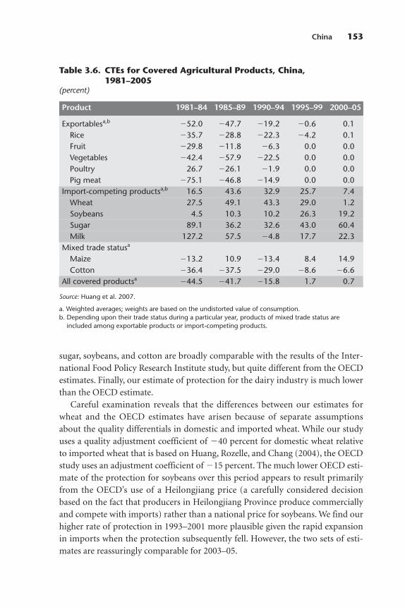
sugar, soybeans, and cotton are broadly comparable with the results of the Inter-national Food Policy Research Institute study, but quite different from the OECDestimates. Finally, our estimate of protection for the dairy industry is much lowerthan the OECD estimate.
Careful examination reveals that the differences between our estimates forwheat and the OECD estimates have arisen because of separate assumptionsabout the quality differentials in domestic and imported wheat. While our studyuses a quality adjustment coefficient of �40 percent for domestic wheat relativeto imported wheat that is based on Huang, Rozelle, and Chang (2004), the OECDstudy uses an adjustment coefficient of �15 percent. The much lower OECD esti-mate of the protection for soybeans over this period appears to result primarilyfrom the OECD’s use of a Heilongjiang price (a carefully considered decisionbased on the fact that producers in Heilongjiang Province produce commerciallyand compete with imports) rather than a national price for soybeans. We find ourhigher rate of protection in 1993–2001 more plausible given the rapid expansionin imports when the protection subsequently fell. However, the two sets of esti-mates are reassuringly comparable for 2003–05.
China 153
Table 3.6. CTEs for Covered Agricultural Products, China,1981–2005
(percent)
Product 1981–84 1985–89 1990–94 1995–99 2000–05
Exportablesa,b �52.0 �47.7 �19.2 �0.6 0.1Rice �35.7 �28.8 �22.3 �4.2 0.1Fruit �29.8 �11.8 �6.3 0.0 0.0Vegetables �42.4 �57.9 �22.5 0.0 0.0Poultry 26.7 �26.1 �1.9 0.0 0.0Pig meat �75.1 �46.8 �14.9 0.0 0.0
Import-competing productsa,b 16.5 43.6 32.9 25.7 7.4Wheat 27.5 49.1 43.3 29.0 1.2Soybeans 4.5 10.3 10.2 26.3 19.2Sugar 89.1 36.2 32.6 43.0 60.4Milk 127.2 57.5 �4.8 17.7 22.3
Mixed trade statusa
Maize �13.2 10.9 �13.4 8.4 14.9Cotton �36.4 �37.5 �29.0 �8.6 �6.6
All covered productsa �44.5 �41.7 �15.8 1.7 0.7
Source: Huang et al. 2007.
a. Weighted averages; weights are based on the undistorted value of consumption.b. Depending upon their trade status during a particular year, products of mixed trade status are
included among exportable products or import-competing products.
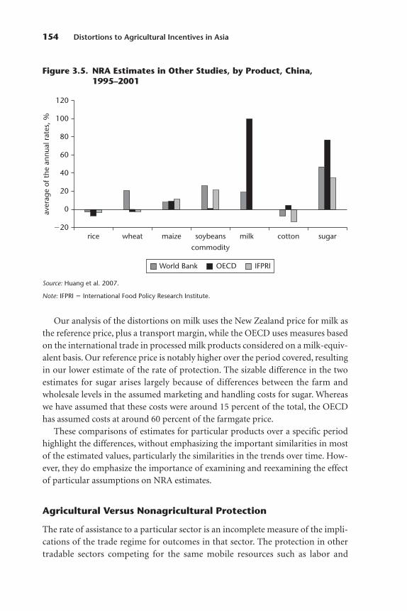
Our analysis of the distortions on milk uses the New Zealand price for milk asthe reference price, plus a transport margin, while the OECD uses measures basedon the international trade in processed milk products considered on a milk-equiv-alent basis. Our reference price is notably higher over the period covered, resultingin our lower estimate of the rate of protection. The sizable difference in the twoestimates for sugar arises largely because of differences between the farm andwholesale levels in the assumed marketing and handling costs for sugar. Whereaswe have assumed that these costs were around 15 percent of the total, the OECDhas assumed costs at around 60 percent of the farmgate price.
These comparisons of estimates for particular products over a specific periodhighlight the differences, without emphasizing the important similarities in mostof the estimated values, particularly the similarities in the trends over time. How-ever, they do emphasize the importance of examining and reexamining the effectof particular assumptions on NRA estimates.
Agricultural Versus Nonagricultural Protection
The rate of assistance to a particular sector is an incomplete measure of the impli-cations of the trade regime for outcomes in that sector. The protection in othertradable sectors competing for the same mobile resources such as labor and
154 Distortions to Agricultural Incentives in Asia
�20
0
20
40
80
60
100
120
commodity
aver
age
of t
he a
nnua
l rat
es, %
World Bank OECD IFPRI
milkmaize sugarrice wheat soybeans cotton
Figure 3.5. NRA Estimates in Other Studies, by Product, China,1995–2001
Source: Huang et al. 2007.
Note: IFPRI � International Food Policy Research Institute.

capital also matters. In a simple model with only two traded-goods sectors, agri-culture and nonagriculture, a broad idea of the total effect of the prevailing dis-tortions may be obtained using information only on the magnitude of two NRAmeasures. The distortion in the price of agricultural goods relative to nonagricul-tural goods provides the signal needed to guide the transfer of resources betweenthe two sets of trading activities. For any given level of world prices, this price sig-nal is given by the ratio:
(1 � NRAagt)�(1 � NRAnonagt). (3.1)
This may be converted into an RRA, as follows:
RRA � 100*[(100 � NRAagt)�(100 � NRAnonagt) � 1]. (3.2)
The estimates of NRAnonagt are provided in Huang et al. (2007). These esti-mates take into account the effects of the trade planning mechanism, tariffs, theexchange rate overvaluation prior to 1994, and nontariff measures such as licens-ing and quotas. While extremely simple, we believe that these estimates supply arealistic indication of the broad pattern of incentives in nonagricultural tradablesfor our sample period.
The average rates of assistance to agriculture and to nonagriculture are presentedin table 3.5 and figure 3.6. The data show that the agricultural sector was subject to
China 155
�80
�60
per
cent
year
60
40
20
�40
�20
0
2003
2004
2002
2001
2000
1999
1998
1997
1996
1995
1994
1993
1992
1991
1990
1989
1988
1987
1986
1985
1984
1983
1982
1981
NRA, agricultural tradables NRA, nonagricultural tradablesRRA
Figure 3.6. NRAs for Agricultural and NonagriculturalTradables and the RRA, China, 1981–2004
Source: Huang et al. 2007.
Note: For the definition of the RRA, see the text and table 3.5, note f.
two strong and reinforcing sets of tax measures in the early years of our sample, onedirect and the other indirect. The direct taxation through border measures and theprocurement system resulted in a negative NRA of 45 percent in 1981–84. The neg-ative NRA was only slightly lower, at 36 percent, in 1985–89. The indirect taxation ofthis sector, through support for nonagricultural activities, was similar in magnitude(42 and 28 percent) to the direct taxation during the two periods.
The first major change in the incentive environment in the agricultural sectorappears to have occurred in the mid-1980s when the rate of protection for nona-gricultural sectors declined. A sharp reduction in the taxation of manufacturingexportables resulted from the widespread availability of duty exemptions for theimported goods used in the production of exports. Protection in the nonagricul-tural sectors appears to have risen slightly during several years in the late 1980s.Increases in tariff rates and in the exchange rate distortions outweighed the reduc-tions in the effects of trade planning and nontariff barriers. However, the protec-tion for nonagricultural sectors declined steadily beginning in 1990. The declinein the direct taxation of the agricultural sector began only later; a sharp fall in theearly 1990s occurred, in large part, because of a reduction in the domestic taxationof the agricultural sector via the procurement pricing system (see above).
The declines in both the negative protection for agriculture and the positiveprotection for nonagricultural tradables since the 1990s have dramaticallychanged the distortions in agricultural incentives. Instead of facing an RRA ofclose to �50 percent as in the 1980s, farmers are now receiving slightly positiveassistance, with an average RRA of 1 percent in 2000–05. Clearly, this phasing outof farmer disincentives has been a major achievement in the government’s policyof reform and opening up.
Conclusions and Implications
The main finding of this study is that the nature and extent of government policyintervention in agriculture in China have changed dramatically over the past25 years. An agricultural sector characterized by significant distortions has beentransformed into a relatively liberal sector. Distortions in external and domesticpolicies during the early reform period—the 1980s and early 1990s—isolateddomestic producers and consumers from international markets. The prices thatdomestic farmers and consumers faced were nearly independent of trade policy.Domestic pricing and marketing policies forced farmers to sell much of their sur-plus to the government at an artificially lower price even in the case of exportablecommodities such as rice (the free-market price of which was close to the interna-tional price). Hence, although there was little trade taxation at the border, domes-tic policies levied a tax on farmers. Similar dynamics characterized the situation
156 Distortions to Agricultural Incentives in Asia
among importable commodities such as wheat and soybeans. Despite fairly highrates of protection through trade policies, producers were receiving much lessprotection than they would have received had there been a free domestic marketfor the importables. This occurred even though consumers were implicitly taxed.
In contrast, after the late 1980s and early 1990s, the liberalization of domesticmarkets reduced the distortions deriving from domestic policies. The market hasgradually replaced the state as the primary mechanism for allocating resourcesand has become the basis for the production and marketing decisions of farmers.Especially in the case of importable commodities, trade policy has also becomemore liberalized, and the distortions arising from border measures have fallensubstantially.
Thus, we find that China’s agriculture has become much less distorted in recentyears in two ways. First, the differences between international and domestic mar-ket prices have narrowed considerably for many commodities because of tradepolicy liberalization. Second, the elimination of domestic policy distortionsmeans that, as trade liberalization allows more imports or exports of agriculturalcommodities, prices in the domestic market change, and farmers are thereforemore directly affected.
There are still plenty of distortions to agricultural incentives in China. In somecases, the remaining distortions have arisen from tariffs on importable commodities(for example, wheat and soybeans). In the case of other importable commodities(for example, maize), the use of implicit export subsidies (permitted under WTOrules as domestic marketing, transport, and storage subsidies) represents a wedgebetween the domestic price and the international price. Thus, some dispersion ofNRAs among farm products remained in 2005, but much less than in the 1980s.
Notes
1. These findings are based on intensive interviews and surveys conducted by the Center for Chinese Agricultural Policy among a wide range of agricultural ministry personnel, research adminis-trators, research staff, and others involved in the agricultural research system.
2. Raw data on the official exchange rate and the several measures of the secondary-market rate arepresented in Huang et al. (2007), together with estimated foreign exchange retention rates, calculatedmeasures of the exchange rates applying, at the margin, to exporters and importers during the period,and estimated equilibrium rates.
3. We thank Andrzej Kwiecinski of the OECD for thoughtful comments that helped us understandthe differences between the sets of estimates.
References
Anderson, K., J. Huang, and E. Ianchovichina. 2004. “Will China’s WTO Accession Worsen FarmHousehold Incomes?” China Economic Review 15 (4): 443–56.
China 157

Anderson, K., M. Kurzweil, W. Martin, D. Sandri, and E. Valenzuela. 2008. “Measuring Distortions toAgricultural Incentives, Revisited.” World Trade Review 7 (4): 675–704.
Ashton, B., K. Hill, A. Piazza, and R. Zeitz. 1984. “Famine in China, 1958–1961.” Population and Devel-opment Review 10 (4): 613–45.
Center for Price Monitoring. various years. “National Major Commodity (Service) Price MonitoringData Compilation.” Unpublished data compilation, Center for Price Monitoring, National Devel-opment and Reform Commission, Beijing.
Chang, G., and G. Wen. 1997. “Communal Dining and the Chinese Famine of 1958–1961.” EconomicDevelopment and Cultural Change 46 (1): 1–34.
China Customs. various years. “Import and Export Statistics.” Statistics compilations, CustomsAdministration, Beijing.
deBrauw, A., J. Huang, and S. Rozelle. 2004. “The Sequencing of Reforms in China’s Agricultural Transition.” Economics of Transition 12 (3): 427–66.
deBrauw, A., J. Huang, S. Rozelle, L. Zhang, and Y. Zhang. 2002. “The Evolution of China’s Rural LaborMarkets during the Reforms.” Journal of Comparative Economics 30 (2): 329–53.
de Gorter, H., D. Just, and J. Kropp. 2008. “Cross-Subsidization Due to Infra-marginal Support in Agriculture: A General Theory and Empirical Evidence.” American Journal of Agricultural Economics90 (1): 42–54.
Dong, X., and G. Dow. 1993. “Monitoring Costs in Chinese Agricultural Teams.” Journal of PoliticalEconomy 101 (3): 539–53.
Fan, S. 1991. “Effects of Technological Change and Institutional Reform on Production Growth in Chinese Agriculture.” American Journal of Agricultural Economics 73 (2): 266–75.
———. 1997. “Production and Productivity Growth in Chinese Agriculture: New Measurement andEvidence.” Food Policy 22 (3): 213–28.
Fan, S., and P. Pardey. 1997. “Research Productivity and Output Growth in Chinese Agriculture.”Journal of Development Economics 53 (1): 115–37.
Fisman, R., and S. Wei. 2004. “Tax Rates and Tax Evasion: Evidence from ‘Missing Imports’ in China.”Journal of Political Economy 112 (2): 471–96.
Gale, F. 2006. “Trends in Chinese Food Demand and Trade Patterns.” Paper presented at the U.S.Department of Agriculture Agricultural Outlook Forum 2006, “Prospering in Rural America,”Arlington, VA, February 16–17.
Honma, M., and Y. Hayami. 2008. “Distortions to Agricultural Incentives in Japan, Korea, and Taiwan.”Agricultural Distortions Working Paper 35, World Bank, Washington, DC.
Hu, R., and J. Huang. 2001. “Investment in Agro-Technology Extension and Its Effect in China.”Strategy and Management 3: 25–31.
Huang, J., and H. Bouis. 1996. “Structural Changes in Demand for Food in Asia.” Food, Agriculture,and the Environment Discussion Paper 11, International Food Policy Research Institute, Washington,DC.
Huang, J., and C. Chen. 1999a. “Effects of Trade Liberalization on Agriculture in China: Institutionaland Structural Aspects.” CGPRT Centre Working Paper 42, Regional Co-ordination Center forResearch and Development of Coarse Grains, Pulses, Roots, and Tuber Crops in the Humid Tropicsof Asia and the Pacific, United Nations Economic and Social Commission for Asia and the Pacific,Bogor, Indonesia.
———. 1999b. “Effects of Trade Liberalization on Agriculture in China: Commodity Aspects.”CGPRT Centre Working Paper 43, Regional Co-ordination Center for Research and Develop-ment of Coarse Grains, Pulses, Roots, and Tuber Crops in the Humid Tropics of Asia and thePacific, United Nations Economic and Social Commission for Asia and the Pacific, Bogor,Indonesia.
Huang, J., and H. Ma. 2000. “International Comparison of Agricultural Prices.” International Trade 10:20–24.
Huang, J., and S. Rozelle. 1996. “Technological Change: Rediscovering the Engine of ProductivityGrowth in China’s Rural Economy.” Journal of Development Economics 49 (2): 337–69.
158 Distortions to Agricultural Incentives in Asia

———. 2002. “China’s Accession to WTO and Likely Shifts in the Agriculture Policy.” Working paper,Center for Chinese Agricultural Policy, Chinese Academy of Sciences, Beijing.
Huang, J., S. Rozelle, and M. Chang. 2004. “The Nature of Distortions to Agricultural Incentives inChina and Implications of WTO Accession.” World Bank Economic Review 18 (1): 59–84.
Huang, J., S. Rozelle, W. Martin, and Y. Liu. 2007. “Distortions to Agricultural Incentives in China.”Agricultural Distortions Working Paper 29, World Bank, Washington, DC.
Huang, J., S. Rozelle, and H. Wang. 2006. “Fostering or Stripping Rural China: Modernizing Agricultureand Rural to Urban Capital Flows.” Developing Economies 44 (1): 1–26.
Jin, S., J. Huang, R. Hu, and S. Rozelle. 2002. “The Creation and Spread of Technology and Total FactorProductivity in China’s Agriculture.” American Journal of Agricultural Economics 84 (4): 916–39.
Kiguel, M., and S. O’Connell. 1995. “Parallel Exchange Rates in Developing Countries.” World BankResearch Observer 10 (1): 21–52.
Lardy, N. R. 1983. Agriculture in China’s Modern Economic Development. Cambridge: Cambridge University Press.
———. 1992. Foreign Trade and Economic Reform in China, 1978–90. Cambridge: Cambridge University Press.
———. 2001. Integrating China into the Global Economy. Washington, DC: Brookings Institution.Lin, J. 1991. “Prohibitions of Factor Market Exchanges and Technological Choice in Chinese Agricul-
ture.” Journal of Development Studies 27 (4): 1–15.———. 1992. “Rural Reforms and Agricultural Growth in China.” American Economic Review 82 (1):
34–51.Lin, J., F. Cai, and Z. Li. 1996. The China Miracle: Development Strategy and Economic Reform. Hong
Kong, China: Chinese University Press.Lin, J., and D. Yang. 2000. “Food Availability, Entitlement and the Chinese Famine of 1959–61.”
Economic Journal 110 (460): 136–58.Lyons, T. 1987. Economic Integration and Planning in Maoist China. New York: Columbia University Press.Martin, W. 2002. “Implications of Reform and WTO Accession for China’s Agricultural Policies.”
Economics of Transition 9 (3): 717–42.McMillan, J., J. Whalley, and L. Zhu. 1989. “The Impact of China’s Economic Reforms on Agricultural
Productivity Growth.” Journal of Political Economy 97 (4): 781–807.Ministry of Agriculture. various years. China Agricultural Yearbook. Beijing: China Agricultural Press.———. various years. China Agricultural Development Report. Beijing: China Agricultural Press.Ministry of Commerce. various years. China Foreign Trade Yearbook. Beijing: China Foreign Economic
and Trade Press.National Bureau of Statistics of China. various years. China Rural Statistical Yearbook. Beijing: China
Statistics Press.———. various years. China Yearbook of Agricultural Price Survey. Beijing: China Statistics Press.———. various years. Statistical Yearbook of China. Beijing: China Statistics Press.National Development and Reform Commission. various years. Agricultural Production Cost and
Revenue Materials Compilation. Beijing: China Statistics Press.Nickum, J. 1998. “Is China Living on the Water Margin?” China Quarterly 156 (December): 880–98.Nyberg, A., and S. Rozelle. 1999. Accelerating China’s Rural Transformation. Washington, DC: World
Bank.OECD (Organisation for Economic Co-operation and Development). 2005. OECD Review of
Agricultural Policies: China. Paris: OECD.———. 2007. Agricultural Policies in Non-OECD Countries: Monitoring and Evaluation 2007. Paris:
OECD.OECD PSE-CSE Database (Producer and Consumer Support Estimates, OECD Database 1986–2005).
Organisation for Economic Co-operation and Development. http://www.oecd.org/document/55/0,3343,en_2649_33727_36956855_1_1_1_1,00.html (accessed December 2007).
Office of Tariff Regulation of the State Council. 1998. Import and Export Tariff Regulation of the People’sRepublic of China, 1996, 1997 and 1998. Beijing: Law Press.
China 159
———. 2005. Import Tariff and Export Tariff Rebate Compilation 2005. Beijing: Economic and Scientific Press.
Orden, D., F. Cheng, H. Nguyen, U. Grote, M. Thomas, K. Mullen, and D. Sun. 2007. Agricultural Producer Support Estimates for Developing Countries: Measurement Issues and Evidence from India,Indonesia, China, and Vietnam. Research Report 152. Washington, DC: International Food PolicyResearch Institute.
Park, A., H. Jin, S. Rozelle, and J. Huang. 2002. “Market Emergence and Transition: Arbitrage, Transi-tion Costs, and Autarky in China’s Grain Market.” American Journal of Agricultural Economics84 (1): 67–82.
Putterman, L. 1993. Continuity and Change in China’s Rural Development. New York: Oxford University Press.
Rosen, D., J. Huang, and S. Rozelle. 2004. Roots of Competitiveness: China’s Evolving Agriculture Interests. Washington, DC: Institute for International Economics.
Rozelle, S., and J. Huang. 2004. “China’s Maize Economy: Supply, Demand and Trade.” Report, U.S.Grains Council, Beijing.
———. 2005. “China’s Soybean Economy: Supply, Demand, and Trade.” Report, American SoybeanAssociation, Beijing.
Rozelle, S., J. Huang, and D. Sumner. 2006. “Supply, Demand and Trade for Horticultural Commodi-ties in China.” Working paper, Department of Agricultural and Resource Economics, University ofCalifornia Davis, Davis, CA.
Rozelle, S., A. Park, J. Huang, and H. Jin. 2000. “Bureaucrat to Entrepreneur: The Changing Role of theState in China’s Transitional Commodity Economy.” Economic Development and Cultural Change48 (2): 227–52.
Rozelle, S., and J. Swinnen. 2004. “Success and Failure of Reform: Insights from the Transition of Agri-culture.” Journal of Economic Literature 42 (2): 404–56.
Shan, W. 1989. “Reforms of China’s Foreign Trade System: Experiences and Prospects.” China Economic Review 1 (1): 33–55.
Sicular, T. 1988a. “Agricultural Planning and Pricing in the Post-Mao Period.” China Quarterly 116(December): 671–705.
———. 1988b. “Plan and Market in China’s Agricultural Commerce.” Journal of Political Economy 96(2): 283–307.
———. 1995. “Redefining State, Plan, and Market: China’s Reforms in Agricultural Commerce.” ChinaQuarterly 144 (December): 1020–46.
Stone, B. 1988. “Developments in Agricultural Technology.” China Quarterly 116 (December):767–822.
Stone, B., and S. Rozelle. 1995. Foodcrop Production Variability in China, 1931–1985. Research Notesand Studies, vol. 9. London: School of Oriental and African Studies, University of London.
Timmer, C. P. 1998. “The Agricultural Transformation.” In International Agricultural Development, 3rded., ed. C. Eicher and J. Staatz, 113–35. Baltimore: Johns Hopkins University Press.
UNCTAD (United Nations Conference on Trade and Development). 1994. Monitoring Import Regimes.Part 1 of Directory of Import Regimes. New York: United Nations.
Wang, D., S. Rozelle, and J. Huang. 1999. “The Impact of Procurement Quota on Agricultural Production in China’s Agriculture.” Working paper, Center for Chinese Agricultural Policy, Chinese Academy of Agricultural Sciences, Beijing.
Wang, H., X. Dong, J., Huang, S. Rozelle, and T. Reardon. 2006. “Producing and Procuring Horticul-tural Crops with Chinese Characteristics: A Case Study in the Greater Beijing Area.” Workingpaper, Center for Chinese Agricultural Policy, Chinese Academy of Sciences, Beijing.
Wang, J., J. Huang, and S. Rozelle. 2005. “Evolution of Tubewell Ownership and Production in theNorth China Plain.” Australian Journal of Agricultural and Resource Economics 49 (2): 177–95.
Wang, J., Z. Xu, J. Huang, and S. Rozelle. 2005. “Incentives in Water Management Reform: Assessing theEffect on Water Use, Productivity, and Poverty in the Yellow River Basin.” Environment and Devel-opment Economics 10 (6): 769–99.
160 Distortions to Agricultural Incentives in Asia

Watson, A. 1994. “China’s Agricultural Reforms: Experiences and Achievements of the AgriculturalSector in the Market Reform Process.” Working Paper 94/4, Chinese Economic Research Unit, University of Adelaide, Adelaide, Australia.
Wen, G. 1993. “Total Factor Productivity Change in China’s Farming Sector: 1952–1989.” EconomicDevelopment and Cultural Change 42 (1): 1–41.
World Bank. 1985. World Development Report 1985: International Capital and Economic Development.New York: Oxford University Press; Washington, DC: World Bank.
———. 1994. China: Foreign Trade Reform. World Bank Country Study. Washington, DC: World Bank.Yao, S. 1994. Agricultural Reforms and Grain Production in China. London: Macmillan.Zhang, L., Q. Li, and S. Rozelle. 2005. “Fertilizer Demand in China: What is Causing Farmers to Use So
Much Fertilizer?” Working paper, Center for Chinese Agricultural Policy, Chinese Academy of Sci-ences, Beijing.
China 161


Part IIIII
SOUTHEAST ASIA

In Indonesia, agricultural trade policy is a politically charged subject. Rice, the sta-ple food, is a net import, and this one commodity has been a central focus of thegovernment’s food policy throughout the postindependence period. Self- sufficiency in rice, meaning the elimination of rice imports, has been a cherishedgoal of agricultural policy for all this time. It is an emotive subject, closely linked inthe public imagination to Indonesian nationalism. When asked to name his proud-est single achievement, Soeharto, the president of Indonesia for 32 years, until1998, cited the country’s self-sufficiency in rice.1 The dominance by rice is evidentin this study, which documents the changing structure of agricultural protection inIndonesia and attempts to explain the forces that have driven the changes.
Our four central themes may be summarized as follows. First, the variations indistortion by sector have been driven by the government’s wish to (a) be self- sufficient in food, (b) stabilize food prices at acceptable levels, and (c) promotemanufacturing. (Food processing has been an important component of manufac-turing; it was even more important in the 1970s and 1980s than it is now.) Theseaims led to taxes on unprocessed exports and to subsidies for processing. Twoimport-competing industries—sugar and rice—have been significantly protected,and the rates of this protection have increased in recent years. The rate of protec-tion of the sugar industry is particularly high. Growers of rice have also receivedprotection, but, until around 2000, this occurred mainly through input subsidies
165
4
INDONESIA
George Fane and Peter Warr
The authors gratefully acknowledge the excellent research assistance of Arief Ramayandi; the helpfulcomments and data assistance of Neil McCulloch, Rina Oktaviani, Peter Rosner, and Peter Timmer; theuseful comments of workshop participants; and the significant work with spreadsheets undertaken byMarianne Kurzweil and Ernesto Valenzuela.
rather than through the price for the product. This protection may be explainedthrough our hypotheses both as the main element in food self-sufficiency and as aresult of the effect rice prices have on manufacturing wages through the cost ofliving. Since 2000, the rice industry has become more tightly protected; riceimports have been banned.
Second, during the long presidency of Soeharto, the country could afford aims(a) to (c) under good fiscal conditions, but not under bad fiscal conditions. So,good fiscal conditions meant more protection and bad trade policies, while badfiscal conditions meant less protection and good trade policies.
Third, growing evidence from around the world convinced policy makers inIndonesia and most other East Asian countries to rely more on markets and lesson government intervention. This evidence was based on theoretical arguments,statistical studies, and simple two-country comparisons such as Myanmar andThailand, the German Democratic Republic and the Federal Republic of Germany,Austria and Hungary, and the Democratic People’s Republic of Korea and theRepublic of Korea. The resulting policy shift was influenced by the collapse of thecommunist system and the victory of capitalism in the Cold War. This may havecontributed to the long-term shift worldwide toward less manufacturing protec-tion and less agricultural export taxation beginning around the mid-1980s.
Fourth, following the democratic reforms that occurred in the wake of theAsian financial crisis of the late 1990s, agricultural protectionism increased some-what in Indonesia. Aggregate measures of protection indicate that these changes,along with reduced protection in manufacturing, caused a switch in the agricul-tural sector from net taxation to net subsidization (by a narrow margin) relativeto manufacturing. However, these aggregate measures mask the fact that agricul-tural protection is concentrated in only two crucial industries: sugar and rice.
The next section describes the changing structure of the Indonesian economy,with an emphasis on the agricultural sector. The subsequent two sections provideoverviews on government economic policy in general and on government policiestoward agriculture during the period since independence. In the following sec-tions, we attempt to supply a political econometric explanation for the changingstructure and pattern in agricultural distortions over the last three decades, esti-mates of which we provide for individual farm industries and for agriculture as awhole. The final section concludes.
Economic Growth and Structural Change
From 1968 to 2005, Indonesia’s gross domestic product (GDP) grew in real termsat an average annual rate of 6.3 percent. The broad characteristics of this growthare summarized in table 4.1. For ease of comparison with other Asian economies,
166 Distortions to Agricultural Incentives in Asia
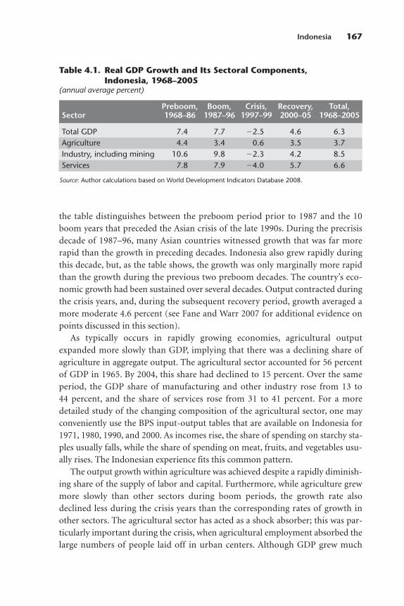
the table distinguishes between the preboom period prior to 1987 and the 10boom years that preceded the Asian crisis of the late 1990s. During the precrisisdecade of 1987–96, many Asian countries witnessed growth that was far morerapid than the growth in preceding decades. Indonesia also grew rapidly duringthis decade, but, as the table shows, the growth was only marginally more rapidthan the growth during the previous two preboom decades. The country’s eco-nomic growth had been sustained over several decades. Output contracted duringthe crisis years, and, during the subsequent recovery period, growth averaged amore moderate 4.6 percent (see Fane and Warr 2007 for additional evidence onpoints discussed in this section).
As typically occurs in rapidly growing economies, agricultural outputexpanded more slowly than GDP, implying that there was a declining share ofagriculture in aggregate output. The agricultural sector accounted for 56 percentof GDP in 1965. By 2004, this share had declined to 15 percent. Over the sameperiod, the GDP share of manufacturing and other industry rose from 13 to44 percent, and the share of services rose from 31 to 41 percent. For a moredetailed study of the changing composition of the agricultural sector, one mayconveniently use the BPS input-output tables that are available on Indonesia for1971, 1980, 1990, and 2000. As incomes rise, the share of spending on starchy sta-ples usually falls, while the share of spending on meat, fruits, and vegetables usu-ally rises. The Indonesian experience fits this common pattern.
The output growth within agriculture was achieved despite a rapidly diminish-ing share of the supply of labor and capital. Furthermore, while agriculture grewmore slowly than other sectors during boom periods, the growth rate alsodeclined less during the crisis years than the corresponding rates of growth inother sectors. The agricultural sector has acted as a shock absorber; this was par-ticularly important during the crisis, when agricultural employment absorbed thelarge numbers of people laid off in urban centers. Although GDP grew much
Indonesia 167
Table 4.1. Real GDP Growth and Its Sectoral Components,Indonesia, 1968–2005
(annual average percent)
Preboom, Boom, Crisis, Recovery, Total,Sector 1968–86 1987–96 1997–99 2000–05 1968–2005
Total GDP 7.4 7.7 �2.5 4.6 6.3Agriculture 4.4 3.4 0.6 3.5 3.7Industry, including mining 10.6 9.8 �2.3 4.2 8.5Services 7.8 7.9 �4.0 5.7 6.6
Source: Author calculations based on World Development Indicators Database 2008.
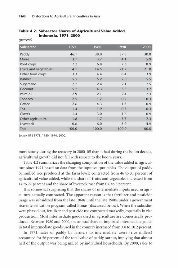
more slowly during the recovery in 2000–05 than it had during the boom decade,agricultural growth did not fall with respect to the boom years.
Table 4.2 summarizes the changing composition of the value added in agricul-ture since 1971 based on data from the input-output tables. The output of paddy(unmilled rice produced at the farm level) contracted from 46 to 31 percent ofagricultural value added, while the share of fruits and vegetables increased from14 to 22 percent and the share of livestock rose from 0.6 to 5 percent.
It is somewhat surprising that the shares of intermediate inputs used in agri-culture actually contracted. The apparent reason is that fertilizer and pesticideusage was subsidized from the late 1960s until the late 1980s under a governmentrice-intensification program called Bimas (discussed below). When the subsidieswere phased out, fertilizer and pesticide use contracted markedly, especially in riceproduction. Most intermediate goods used in agriculture are domestically pro-duced. Between 1980 and 2000, the annual share of imported intermediate goodsin total intermediate goods used in the country increased from 3.8 to 10.2 percent.
In 1971, sales of paddy by farmers to intermediate users (rice millers)accounted for 56 percent of the total value of paddy output, implying that almosthalf of the output was being milled by individual households. By 2000, sales to
168 Distortions to Agricultural Incentives in Asia
Table 4.2. Subsector Shares of Agricultural Value Added,Indonesia, 1971–2000
(percent)
Subsector 1971 1980 1990 2000
Paddy 46.1 38.0 37.5 30.8Maize 3.1 3.7 4.1 5.9Root crops 7.2 6.8 7.6 8.9Fruits and vegetables 14.1 14.5 21.7 21.8Other food crops 3.3 4.4 6.4 3.9Rubber 5.5 5.2 2.0 5.5Sugarcane 2.2 2.4 2.1 2.5Coconut 5.2 4.3 3.3 3.7Palm oil 2.9 2.1 2.4 2.3Tobacco 2.5 1.7 0.7 0.3Coffee 2.6 4.3 1.5 0.9Tea 1.4 1.9 0.5 0.3Cloves 1.4 3.0 1.6 0.9Other agriculture 1.8 1.7 3.5 7.3Livestock 0.6 6.0 5.0 4.9Total 100.0 100.0 100.0 100.0
Source: BPS 1971, 1980, 1990, 2000.

intermediate users accounted for 98 percent of the total value of the output. Sim-ilar trends occurred in maize, rubber, sugarcane, palm oil, coffee, and tea.
The international trading position of the major agricultural commodities issummarized in table 4.3. The most important import-competing agriculturalproducts are rice, sugar, maize, and soybeans. Major export-competing productsinclude coffee, rubber, tobacco, tea, palm oil, copra, shrimps, and spices. Paddy isneither exported nor imported, but milled rice has historically been a majorimport item. Since 2002, rice imports have been officially banned, but someimports have still occurred. Cassava is mainly nontraded, although there areexports of its derivatives, manioc and tapioca. Much of the livestock subsector isalso nontraded, although chickens are exported, while beef and dairy productscompete with imports.
Indonesia 169
Table 4.3. Export Sales in Total Sales and Imports in TotalUsage, Indonesia, 1971–2000
(percent)
Export share Import share
Subsector 1971 1980 1990 2000 1971 1980 1990 2000
Paddya 0.0 0.0 0.0 0.0 0.0 0.0 0.0 0.0Maize 11.4 0.3 1.8 0.3 0.0 1.1 0.2 11.3Root crops 4.7 3.7 0.7 0.3 0.0 0.1 0.0 0.1Fruits and vegetables 0.1 0.2 0.2 0.3 0.6 1.1 0.9 4.9Other food crops 4.3 0.3 1.9 0.4 0.0 22.7 18.1 47.7Rubber 57.5 58.4 6.5 0.6 0.1 0.0 0.1 0.7Sugarcane 0.0 0.0 0.0 0.0 0.0 0.0 0.0 0.0Coconut 6.6 1.2 0.3 1.5 0.0 0.0 0.0 0.1Palm oil 2.3 33.5 29.5 0.2 0.0 0.0 0.1 0.2Tobacco 7.4 12.3 7.6 0.0 1.6 7.3 15.6 0.0Coffee 21.5 58.7 13.7 0.0 0.0 0.0 0.0 0.0Tea 24.5 18.5 32.5 0.0 0.0 0.0 3.9 0.0Cloves 0.0 0.0 0.1 3.0 47.4 12.7 0.0 24.5Other agriculture 40.5 15.9 26.7 21.2 24.1 43.8 1.4 30.3Livestock 1.2 0.0 1.8 2.1 0.0 0.5 0.9 8.4Total Agriculture 7.5 9.3 2.8 2.6 1.3 2.8 2.0 8.7Milled ricea 0.0 0.8 0.0 0.0 13.5 12.5 0.2 3.9Fertilizers and 0.0 4.4 14.6 22.9 66.0 18.1 9.6 23.3pesticides
Source: BPS 1971, 1980, 1990, 2000.
a. The input-output tables classify paddy (unmilled rice) as an output of the agricultural sector andmilled rice as an output of the manufacturing sector
Over time, some sectors have shifted from one trade category to the other(import-competing or exportable). The key example is sugar, which was the mostimportant export during the colonial era, but has become one of the most highlyprotected import-competing products in the postindependence period. Anotherexample is maize, which switched from net export status to net import status duringthe 1990s. Fruits and vegetables have become major net imports, as have soybeans(which are included in the government’s input-output tables as “other food crops”).
Policy Evolution
Indonesia obtained its independence from the Netherlands in 1949. The next twodecades were chaotic. The postindependence government of President Soekarnopursued a nationalistic, quasi-socialist economic policy that produced hyperinfla-tion and economic stagnation. In 1966, Soekarno was displaced amid economicchaos by one of his generals, Soeharto, whose regime, called the New Order, lasteduntil the macroeconomic crisis of 1998. Soeharto pursued more market-orientedeconomic policies than his predecessor had. On assuming power, Soeharto speed-ily introduced a macroeconomic stabilization program and then began liberaliz-ing trade and investment policies. In 1967, foreign investors were guaranteed theright to repatriate both capital and profit, and, beginning in 1970, the capitalaccount was almost completely open. As we see below, trade policy under Soeharto’s government was much less open. It was characterized by the taxation ofexports, especially nonfood agricultural exports, and the protection of imports,including some food imports.
In the wake of the commodity boom of 1972–73 and the oil price shocks of1973–74 and 1979–80, trade policy became increasingly inward-looking. Theseexternal events tripled the ratio of Indonesia’s export prices to its import prices.Between the early 1970s and the mid-1980s, the government taxed or bannedsome traditional exports, pursued self-sufficiency in rice, and used part of theburgeoning oil revenues to establish import-substituting manufacturing indus-tries, which it then protected. In the early to mid-1980s, several traditional exportindustries were subjected to quantitative trade restrictions. The restrictionsincluded a ban on log exports that conferred high rates of effective protection onthe plywood manufacturing industry, for which raw timber is the principal input.Licensing systems were introduced for exports of vegetable oils, several spices, cof-fee, and some grades of rubber. In the case of palm oil, domestic refiners were pro-tected by a tax on exports and a requirement that growers supply these refinerswith part of their output at low, controlled prices.
In 1982, the price of petroleum began to decline. By the mid-1980s it had fallenfrom US$28 to US$10 per barrel. Many oil-exporting countries, including Nigeria
170 Distortions to Agricultural Incentives in Asia
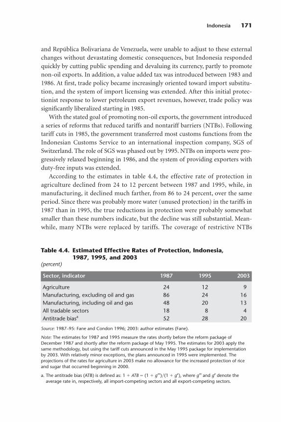
and República Bolivariana de Venezuela, were unable to adjust to these externalchanges without devastating domestic consequences, but Indonesia respondedquickly by cutting public spending and devaluing its currency, partly to promotenon-oil exports. In addition, a value added tax was introduced between 1983 and1986. At first, trade policy became increasingly oriented toward import substitu-tion, and the system of import licensing was extended. After this initial protec-tionist response to lower petroleum export revenues, however, trade policy wassignificantly liberalized starting in 1985.
With the stated goal of promoting non-oil exports, the government introduceda series of reforms that reduced tariffs and nontariff barriers (NTBs). Followingtariff cuts in 1985, the government transferred most customs functions from theIndonesian Customs Service to an international inspection company, SGS ofSwitzerland. The role of SGS was phased out by 1995. NTBs on imports were pro-gressively relaxed beginning in 1986, and the system of providing exporters withduty-free inputs was extended.
According to the estimates in table 4.4, the effective rate of protection in agriculture declined from 24 to 12 percent between 1987 and 1995, while, inmanufacturing, it declined much farther, from 86 to 24 percent, over the sameperiod. Since there was probably more water (unused protection) in the tariffs in1987 than in 1995, the true reductions in protection were probably somewhatsmaller than these numbers indicate, but the decline was still substantial. Mean-while, many NTBs were replaced by tariffs. The coverage of restrictive NTBs
Indonesia 171
Table 4.4. Estimated Effective Rates of Protection, Indonesia,1987, 1995, and 2003
(percent)
Sector, indicator 1987 1995 2003
Agriculture 24 12 9Manufacturing, excluding oil and gas 86 24 16Manufacturing, including oil and gas 48 20 13All tradable sectors 18 8 4Antitrade biasa 52 28 20
Source: 1987–95: Fane and Condon 1996; 2003: author estimates (Fane).
Note: The estimates for 1987 and 1995 measure the rates shortly before the reform package ofDecember 1987 and shortly after the reform package of May 1995. The estimates for 2003 apply thesame methodology, but using the tariff cuts announced in the May 1995 package for implementationby 2003. With relatively minor exceptions, the plans announced in 1995 were implemented. Theprojections of the rates for agriculture in 2003 make no allowance for the increased protection of riceand sugar that occurred beginning in 2000.
a. The antitrade bias (ATB) is defined as: 1 � ATB � (1 � gm)�(1 � ge), where gm and ge denote theaverage rate in, respectively, all import-competing sectors and all export-competing sectors.

declined from 44 percent of total value added in all traded industries in 1986 to23 percent in 1995. This switch from NTBs to tariffs was more extensive in man-ufacturing than in agriculture, where the coverage of NTBs declined from 67 to48 percent. In the wake of the financial crisis of 1997–98, the government wasobliged to allow free imports of both rice and sugar as a condition for borrowingfrom the International Monetary Fund (IMF). However, since the end of the IMF program, imports of rice and sugar have again been restricted by both tariffsand NTBs.
Agricultural Protection by Subsector
The distinction between import-competing products and export products is notalways entirely clear-cut, but it is nevertheless crucial to any discussion of Indone-sian agricultural policies. Whereas import-competing production has generallybeen protected by government policies, export-competing production has gener-ally been taxed. For centuries, the country’s major staple food crops have been netimports. Both the Dutch colonial government and the government of Indonesiaafter independence generally tried to control the price of rice and other importantfood crops to balance the competing interests of domestic producers and con-sumers. Except when the world prices of food crops have been unusually high,imports have been directly restricted, or subject to tariffs, or both. On the rareoccasions when world prices have been so high that growers would have had anincentive to export food crops such as rice, they have usually been prevented fromdoing so by nontax measures, including outright export bans.
In contrast, export crops have been seen by successive governments over thelast two centuries as a useful source of tax revenue. Under the cultivation system(cultuurstelsel) introduced by the Dutch in 1830, the production of cash crops forexport was stimulated by imposing taxes on villagers that could be most easilypaid in kind by handing over crops that the Dutch East India Company thenprocessed and exported. By far the most important of these exports was sugar;other important exports in the 19th century were coffee, tea, indigo, and cinna-mon. Booth (1988) reports that, in the late 1830s, 40 percent of the total incomeof the government of the Netherlands was derived from the cultivation system inthe Indonesian colonies.
Since independence, the Indonesian government’s revenue from export cropshas been obtained through export taxes that have tended to depress the domesticproduction and the exports of the relevant crops. The main reason for raisingexport revenue in this quite different way has presumably been the government’sdesire, since independence, to promote the development of the manufacturingsector, of which food processing is an important part. Rice, sugar, and soybeans
172 Distortions to Agricultural Incentives in Asia
have been protected from import competition by NTBs. The remainder ofimport-competing agriculture has been protected by tariffs and tariff surcharges.(Rice, sugar, and soybeans, along with maize, are discussed in the next four sub-sections. Import-competing and export agriculture are discussed in the subse-quent subsections.)
Rice
The most important and most enduring NTBs have been those on rice and sugar.Chart a in figure 4.1 shows estimates of the domestic wholesale prices and borderprices for rice.2 (All the price series in figures 4.1–4.4 are in rupiah per kilogram,divided by the GDP deflator indexed at 1 in 2005. The nominal rate of protection[NRP] from import competition is the percentage by which the domestic priceexceeds the border price.) While there have been enormous nominal increases inrice and sugar prices since the early 1970s, figures 4.1 and 4.2 show that any trendsin the real prices of these products have been relatively small.
It is clear from chart a in figure 4.1 that the domestic wholesale price of rice hasfluctuated much less than the border price and that domestic prices have not dif-fered greatly, on average, from the trend level of border prices. Price stabilizationwas achieved by giving the government’s food logistics agency, Bulog (Badan Urusan Logistik), a monopoly over international trade in rice and directing theagency to build up buffer stocks to smooth out fluctuations in domestic supply. Itis significant that this stabilization of domestic prices was achieved while keepingthe trend value of domestic prices roughly in line with the trend in world prices.Average rates of protection in the output market were low, but input markets wereanother matter.
Beginning in the 1970s, the Soeharto government used part of its new oilwealth to promote self-sufficiency in rice by subsidizing the adoption of high-yielding varieties that had been made available through the Green Revolution.These new varieties required greatly increased use of irrigation, fertilizers, andpesticides, which the government helped to finance. An important motivation forthis policy was the fear of a repetition of the riots precipitated by high food pricesin 1965.
Under the Bimas (bimbingan masal or massive guidance) program, which wasintroduced with the explicit goal of rice self-sufficiency, farmers received agricul-tural extension services and subsidized credit, seeds, fertilizers, and pesticides. Thegovernment also upgraded irrigation facilities and expanded irrigation coverage.The resulting rise in the profitability of rice growing, together with some coercionamong farmers who were reluctant to extend the area of rice cultivation, led to a17 percent increase in gross harvested area in the decade to 1985.3 The increase in
Indonesia 173

174
Figure 4.1. Border and Domestic Prices of Import-CompetingProducts Relative to the GDP Deflator, Rice andUrea Fertilizer, Indonesia, 1975–2005
a. Rice
Source: Fane and Warr 2007.
b. Urea fertilizer
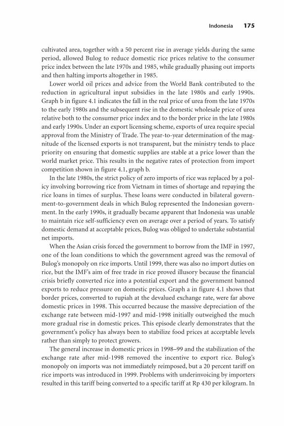
cultivated area, together with a 50 percent rise in average yields during the sameperiod, allowed Bulog to reduce domestic rice prices relative to the consumerprice index between the late 1970s and 1985, while gradually phasing out importsand then halting imports altogether in 1985.
Lower world oil prices and advice from the World Bank contributed to thereduction in agricultural input subsidies in the late 1980s and early 1990s.Graph b in figure 4.1 indicates the fall in the real price of urea from the late 1970sto the early 1980s and the subsequent rise in the domestic wholesale price of urearelative both to the consumer price index and to the border price in the late 1980sand early 1990s. Under an export licensing scheme, exports of urea require specialapproval from the Ministry of Trade. The year-to-year determination of the mag-nitude of the licensed exports is not transparent, but the ministry tends to placepriority on ensuring that domestic supplies are stable at a price lower than theworld market price. This results in the negative rates of protection from importcompetition shown in figure 4.1, graph b.
In the late 1980s, the strict policy of zero imports of rice was replaced by a pol-icy involving borrowing rice from Vietnam in times of shortage and repaying therice loans in times of surplus. These loans were conducted in bilateral govern-ment-to-government deals in which Bulog represented the Indonesian govern-ment. In the early 1990s, it gradually became apparent that Indonesia was unableto maintain rice self-sufficiency even on average over a period of years. To satisfydomestic demand at acceptable prices, Bulog was obliged to undertake substantialnet imports.
When the Asian crisis forced the government to borrow from the IMF in 1997,one of the loan conditions to which the government agreed was the removal ofBulog’s monopoly on rice imports. Until 1999, there was also no import duties onrice, but the IMF’s aim of free trade in rice proved illusory because the financialcrisis briefly converted rice into a potential export and the government bannedexports to reduce pressure on domestic prices. Graph a in figure 4.1 shows thatborder prices, converted to rupiah at the devalued exchange rate, were far abovedomestic prices in 1998. This occurred because the massive depreciation of theexchange rate between mid-1997 and mid-1998 initially outweighed the muchmore gradual rise in domestic prices. This episode clearly demonstrates that thegovernment’s policy has always been to stabilize food prices at acceptable levelsrather than simply to protect growers.
The general increase in domestic prices in 1998–99 and the stabilization of theexchange rate after mid-1998 removed the incentive to export rice. Bulog’smonopoly on imports was not immediately reimposed, but a 20 percent tariff onrice imports was introduced in 1999. Problems with underinvoicing by importersresulted in this tariff being converted to a specific tariff at Rp 430 per kilogram. In
Indonesia 175

2002, Bulog’s monopoly over imports was restored, and, since 2004, rice importshave officially been banned, although Bulog has occasionally been issued withspecial import permits.
Sugar
The Indonesian sugar industry is dominated by the state-owned mills, mainly onJava, that were acquired through the nationalization of the formerly Dutch-owned sugar estates in 1957. Investment and technical progress in this sector havebeen extremely sluggish, and the industry has languished behind protective barri-ers. The finished product of the antiquated factories—known as mill white orplantation white—is not precisely comparable to the refined sugar or the rawsugar traded on the world market. Plantation white contains more impurities,mainly molasses, than internationally traded raw sugar, but has already under-gone some of the bleaching processes that separate refined sugar from raw sugarin more technologically advanced sugar industries. Most firms in the food andbeverage subsectors are unable to use plantation white because of its relativelyhigh level of impurities; their needs are mainly met by imports of raw sugar,although a small amount of raw sugar is produced domestically.
As in the case of rice, the main motive behind government policy on sugarappears to be the desire to stabilize the domestic price at an acceptable level. Inaddition, in the case of sugar, the government has tried to protect the sugar facto-ries that it owns. This may explain why, at least since 1957, the sugar industry hasbeen more tightly regulated than any other agricultural sector: the governmenthas monopolized not only imports, but also domestic marketing. Governmentownership likewise helps to explain newspaper reports that, in the 1970s, farmersin traditional sugar-growing areas were regularly forced to grow sugar to supplylocal factories because of threats that their other crops would be burned.
Figure 4.2 compares the border price of raw sugar (after allowing for marginsbetween the free on board price and the domestic wholesale price) with thedomestic wholesale price of plantation white. The figure shows that, for much ofthe period since 1970, the domestic price was about twice the border price, imply-ing an NRP of about 100 percent. However, in 2006, this gap was narrowed appre-ciably because of the abrupt rise in world prices.
Our estimates of the NRP for sugar ignore two factors, the first of whichindicates that our estimates tend to understate the true NRP, while the secondgoes in the opposite direction. The first factor is that our estimates make noadjustment for the relatively low polarity (high level of impurities) of planta-tion white. The offsetting factor is the neglect of the cost of bleaching to obtainplantation white. Sugar industry experts have suggested that the low polarity
176 Distortions to Agricultural Incentives in Asia
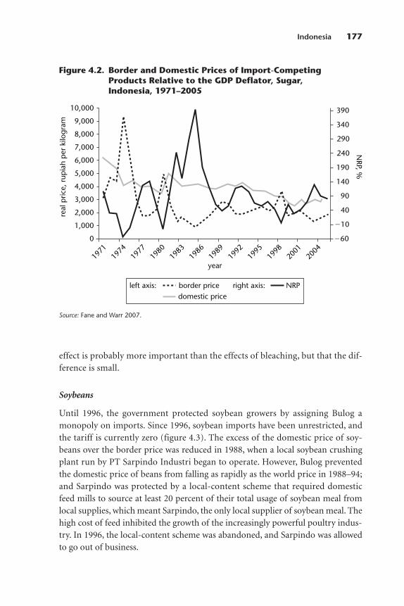
effect is probably more important than the effects of bleaching, but that the dif-ference is small.
Soybeans
Until 1996, the government protected soybean growers by assigning Bulog amonopoly on imports. Since 1996, soybean imports have been unrestricted, andthe tariff is currently zero (figure 4.3). The excess of the domestic price of soy-beans over the border price was reduced in 1988, when a local soybean crushingplant run by PT Sarpindo Industri began to operate. However, Bulog preventedthe domestic price of beans from falling as rapidly as the world price in 1988–94;and Sarpindo was protected by a local-content scheme that required domesticfeed mills to source at least 20 percent of their total usage of soybean meal fromlocal supplies, which meant Sarpindo, the only local supplier of soybean meal. Thehigh cost of feed inhibited the growth of the increasingly powerful poultry indus-try. In 1996, the local-content scheme was abandoned, and Sarpindo was allowedto go out of business.
Indonesia 177
Figure 4.2. Border and Domestic Prices of Import-CompetingProducts Relative to the GDP Deflator, Sugar,Indonesia, 1971–2005
Source: Fane and Warr 2007.
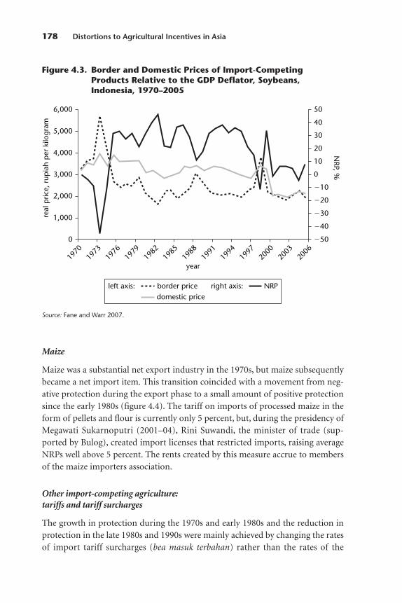
Maize
Maize was a substantial net export industry in the 1970s, but maize subsequentlybecame a net import item. This transition coincided with a movement from neg-ative protection during the export phase to a small amount of positive protectionsince the early 1980s (figure 4.4). The tariff on imports of processed maize in theform of pellets and flour is currently only 5 percent, but, during the presidency ofMegawati Sukarnoputri (2001–04), Rini Suwandi, the minister of trade (sup-ported by Bulog), created import licenses that restricted imports, raising averageNRPs well above 5 percent. The rents created by this measure accrue to membersof the maize importers association.
Other import-competing agriculture:tariffs and tariff surcharges
The growth in protection during the 1970s and early 1980s and the reduction inprotection in the late 1980s and 1990s were mainly achieved by changing the ratesof import tariff surcharges (bea masuk terbahan) rather than the rates of the
178 Distortions to Agricultural Incentives in Asia
Figure 4.3. Border and Domestic Prices of Import-CompetingProducts Relative to the GDP Deflator, Soybeans,Indonesia, 1970–2005
Source: Fane and Warr 2007.

import tariff (bea masuk).4 In terms of their economic effects, the surcharges wereequivalent to tariffs, but, unlike tariffs, the rates of the surcharges could bechanged by administrative decree without the need to amend the law. The rates ofimport duty shown in appendix table A4 in Fane and Warr (2007) are the com-bined rates of tariffs, plus tariff surcharges. A comparison of the changes in thetariffs and the changes in the tariff surcharges in appendix tables A5 and A6 inFane and Warr (2007) shows that much of the growth of protection in 1974–79and almost all of the much larger increases in protection in 1979–85 wereachieved by raising tariff surcharges rather than tariffs. When protection wasreduced in 1985–89, about half the reduction was obtained by largely eliminatingtariff surcharges, which were negligible by 1989, but had been an important partof total import duties in 1985. By 1994, tariff surcharges had been totally abol-ished, and, since then, there has been no need to distinguish between tariffs andtotal import duties.
The import duties on food processing have always been higher than those onagriculture. In every year, the average import tax rate on food processing alone
Indonesia 179
Figure 4.4. Border and Domestic Prices of Import-CompetingProducts Relative to the GDP Deflator, Maize,Indonesia, 1969–2005
Source: Fane and Warr 2007.

(Harmonized Commodity Description and Coding System, 15–24) is higher thanthe corresponding average rate on the entire agriculture and food processingproducts category (1–24). Vegetables and flowers, particularly orchids, havealways been the most highly protected of the industries within agricultural cate-gories 1–14.
Among the more traditional agricultural subsectors, livestock and estate cropshave always received relatively significant protection from imports. However,whereas livestock is mainly import-competing (but also partly nontraded), manyestate crops are mainly export-competing. In these cases, of which coffee, tea, andspices are major examples, there is a great deal of water in the tariffs. In the 1970s,the total import tax rates on tea, coffee, vanilla, cinnamon, nutmeg, and gingerwere 70 percent; by 1985, this rate had increased to 100 percent. However, by 1989,the total import duty rates on all these products had been reduced to 30 percent,and, by the mid-1990s, they had fallen to 5 percent.
The import duty rates on food crops have generally been relatively low, at leastin the period before 2000. However, these rates understate the extent of the pro-tection for food crops for two reasons: food crop producers have received inputsubsidies, and food crops have also been protected by NTBs; hence, their separatetreatment above.
Estate crops: rubber, copra, coffee, and tea
Rubber, copra, coffee, and tea are all produced by perennial plants and, in Indonesia,tend to be produced on large estates, although copra is also produced by small-holders. All have been export crops and all have been taxed, but at varying rates.The export volumes of all these commodities have declined since the 1980s. Thehigh rates of export taxation are a significant part of the explanation. Figure 4.5shows the calculations of the NRPs for each of these four commodities. For rub-ber, the export tax rate has been low, but the data show high rates of export taxa-tion for copra and tea. For coffee, the rate has declined from the high rates prior tothe 1990s.
The Political Economy of Protection:Do Good Times Produce Bad Policy,and Bad Times, Good Policy?
Key characteristics of Indonesia’s political environment provide background onthe attempts to explain the changes in trade policy summarized above. First, theconfidence of the country’s elite was boosted because of the economic successesachieved elsewhere in East and Southeast Asia starting in the 1970s. There seemed
180 Distortions to Agricultural Incentives in Asia

Indonesia 181
Figure 4.5. Border and Domestic Prices of Export Crops Relativeto the GDP Deflator, Indonesia, 1967–2005
a. Rubber
b. Copra
(Figure continues on the following page.)
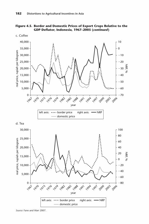
182 Distortions to Agricultural Incentives in Asia
c. Coffee
Source: Fane and Warr 2007.
d. Tea
Figure 4.5. Border and Domestic Prices of Export Crops Relative to theGDP Deflator, Indonesia, 1967–2005 (continued)
no fundamental reason why Indonesia should not succeed as well. This confi-dence meant that bolder strategies could be contemplated. This may be contrastedwith the timidity and the skepticism with regard to the international trading sys-tem that characterized most of South Asia at the time. Second, Soeharto’s politicalauthority within Indonesia was unchallenged until the end of his regime. Evenpolicies that were unpopular, at least initially, could be contemplated if Soehartoconsidered them necessary.
Observers of economic reform in Indonesia have coined the phrase “goodtimes produce bad policy, and bad times produce good policy,” where good timesmeans favorable external conditions, and good policies means deregulation andlower barriers to international trade and investment. The phrase describes muchof the history of economic reform in Indonesia. The oil price booms of the 1970swere followed by a series of trade-restricting import-substitution policies aimedat protecting at least some of the traded goods industries that could potentially beharmed by the “Dutch disease” effect of the petroleum booms, that is, the declinein the domestic competitiveness of the traded goods industries caused by a rise inthe prices of nontraded goods and services relative to traded goods and services(see Corden 1984; Warr 1986). Trade liberalization followed the adverse terms oftrade effect of the decline in petroleum prices beginning in the early 1980s. But,while good times-bad policy, bad times-good policy describes the Indonesianexperience, it does not provide an explanation. Why have good times producedbad policy, and bad times, good policy in Indonesia?
Observers of policy formation under Soeharto have reported on a contest forSoeharto’s attention between the technocrats and the nationalists (Hill 2000). Atvarious times, either of these groups might have had ascendancy, which meantthat Soeharto was heeding their messages. The technocrats, many of whom wereprofessional economists trained in the United States, favored a market-orientedeconomy, a strong emphasis on macroeconomic stability, and a relatively opentrade policy. This group dominated the Ministry of Finance and Bappenas, theNational Development Planning Agency, and had considerable influence onthe Bank of Indonesia. The World Bank used its influence directly in supportof the technocrats, and the Bank’s resources and technical expertise also assistedthe technocrats in making their case more convincing.
The economic nationalists were more diverse. They included, in particular, theengineers, led by the minister for research and technology, B. J. Habibie, a German-trained engineer with a strong preference for crash-through economicprograms based on advanced technology. This group promoted large-scale, capital-intensive projects in aeronautics, shipbuilding, steel, fertilizers, petrochemicals, andother industries. To ensure the profitability of these projects, high rates of protec-tion were advocated on infant industry grounds. This group was influential within
Indonesia 183

Dr. Habibie’s own department, as well as at the state-owned petroleum company,Pertamina. A second group of nationalists was represented by the advocates ofself-sufficiency in food, particularly rice. This group dominated the Ministry ofAgriculture and Bulog (for example, see Warr 1992; Timmer 1996). More generalsupport for policies based on import substitution was concentrated at the Min-istry of Industry.
During bad economic times, the technocrats tended to gain Soeharto’s atten-tion. During good times, he listened to the nationalists. The central dynamicderived from the role of the external shocks to the Indonesian economy thatoperated through petroleum prices. During the Soeharto period, petroleum wasboth a principal source of foreign exchange, through direct oil exports, and amajor source of government revenue, through the royalties received by the gov-ernment on the exports. Reduced oil prices implied both balance of paymentsand budgetary stresses. In addition, the majority of the country’s foreign debtwas public debt. When the price of oil fell, the fiscal burden of debt servicingbecame more painful. This increased the influence of the World Bank, whosewillingness to extend concessional loans to the country was important directlyand also as a signal to other potential foreign lenders. At such times, the govern-ment needed these loans to balance its budget. The only alternative was infla-tionary financing, the consequences of which had been experienced under Soeharto. The increased influence of the World Bank meant greater influence forthe technocrats and the policies they advocated. In addition, reduced oil pricesmeant a reduction in the influence of Pertamina because they lowered Pertam-ina’s contribution to government revenue. It also meant greater influence for theMinistry of Finance, which implemented the tax reforms—designed by tech-nocrats and like-minded foreign advisors—that helped make up for the lost oilrevenues.
In other countries, a deterioration in the terms of trade might be met byexchange controls, import licensing, and other import-substitution policies. InIndonesia, a protectionist response also occurred briefly after the oil pricedeclines of the early 1980s. But it did not last long because it did not address thesimultaneous fiscal problem. An example of the tax reforms that emerged fromthis dynamic was the introduction of a value added tax in 1986 and, at thesame time, a reduction in import duties. An import duty (tariff) is equivalent toboth a tax on consumption and a subsidy on production set at the same ad valoremrate. The tariff raises positive net revenue because the volume of consumption ofan import commodity exceeds the volume of production of that commodity. Avalue added tax is a tax on consumption alone. Moreover, it is able to raise the sameamount of revenue as a tariff, but at a lower rate of tax. This is so because it does
184 Distortions to Agricultural Incentives in Asia
not expend revenue to subsidize production. Similarly, the switch from NTBs totariffs generates revenue. NTBs may be thought of as privately levied tariffs thatmake no contribution to government revenue. A final example is the phasing outof the Bimas scheme that was designed to help rice growers achieve self- sufficiency. The budgetary cost of the fertilizer and pesticide subsidies and subsi-dized lending involved in Bimas became serious because of the fiscal deteriora-tion of the 1980s.
During times of reduced petroleum prices, such as the early to mid-1980s,illiberal trade policies were unaffordable in fiscal terms, and this reinforced theargument that trade liberalization would promote improved foreign exchangeearnings from non-oil exports. The technocrats then held sway. In contrast, during the euphoria of the 1970s that was induced by high petroleum revenues,the import-substitution schemes advocated by the nationalists seemed affordableand were politically attractive. Then, the nationalists captured Soeharto’s attention.
The Asian financial crisis of 1997–98 was the worst of times, and it producedthe best of economic policies, given that best is being used here to mean that thepolicies more closely conformed to the laissez-faire advice of neoclassical econo-mists. The Asian crisis also provides the clearest illustration of the causal linkbetween bad times and laissez-faire policies: the reforms that the governmentintroduced in the wake of the crisis were explicitly adopted to meet IMF loan conditions when all other sources of external lending had dried up.
Since Soeharto’s political demise in 1998 and the subsequent shift to a moredemocratic form of government, the president no longer holds absolute authority,and policies are therefore no longer determined simply by a contest between thetechnocrats and nationalists to influence the president. The parliament, a tokeninstitution under Soeharto, now has teeth, and the president cannot ignore itswill. Populist economic nationalism has tended to dominate in parliament; andthis has reduced, but not eliminated, the influence of the technocrats. In addition,the conspicuous reluctance of the major industrialized countries to lower the protection for their own agricultural sectors has weakened the influence of thetechnocrats who argue against Indonesian restrictions on trade. The greater protection for the rice and sugar subsectors that followed the end of the IMF pro-gram was a direct consequence of these political changes. Rice self-sufficiency andprotection for farmers are both politically attractive goals in Indonesia, and, in thepublic imagination, both are strongly associated with the national interest. Protec-tion for the rice industry is supported by all major political parties. Because ofdemocracy, rice and sugar farmers therefore now receive more protection fromimports than they did under Soeharto.
Indonesia 185
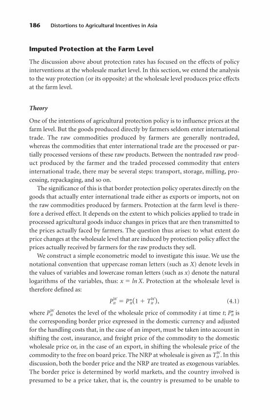
Imputed Protection at the Farm Level
The discussion above about protection rates has focused on the effects of policyinterventions at the wholesale market level. In this section, we extend the analysisto the way protection (or its opposite) at the wholesale level produces price effectsat the farm level.
Theory
One of the intentions of agricultural protection policy is to influence prices at thefarm level. But the goods produced directly by farmers seldom enter internationaltrade. The raw commodities produced by farmers are generally nontraded,whereas the commodities that enter international trade are the processed or par-tially processed versions of these raw products. Between the nontraded raw prod-uct produced by the farmer and the traded processed commodity that entersinternational trade, there may be several steps: transport, storage, milling, pro-cessing, repackaging, and so on.
The significance of this is that border protection policy operates directly on thegoods that actually enter international trade either as exports or imports, not onthe raw commodities produced by farmers. Protection at the farm level is there-fore a derived effect. It depends on the extent to which policies applied to trade inprocessed agricultural goods induce changes in prices that are then transmitted tothe prices actually faced by farmers. The question thus arises: to what extent doprice changes at the wholesale level that are induced by protection policy affect theprices actually received by farmers for the raw products they sell.
We construct a simple econometric model to investigate this issue. We use thenotational convention that uppercase roman letters (such as X) denote levels inthe values of variables and lowercase roman letters (such as x) denote the naturallogarithms of the variables, thus: x � ln X. Protection at the wholesale level istherefore defined as:
PitW � P*it(1 � Tit
W), (4.1)
where PitW denotes the level of the wholesale price of commodity i at time t; P*it is
the corresponding border price expressed in the domestic currency and adjustedfor the handling costs that, in the case of an import, must be taken into account inshifting the cost, insurance, and freight price of the commodity to the domesticwholesale price or, in the case of an export, in shifting the wholesale price of thecommodity to the free on board price. The NRP at wholesale is given as Tit
W. In thisdiscussion, both the border price and the NRP are treated as exogenous variables.The border price is determined by world markets, and the country involved is presumed to be a price taker, that is, the country is presumed to be unable to
186 Distortions to Agricultural Incentives in Asia
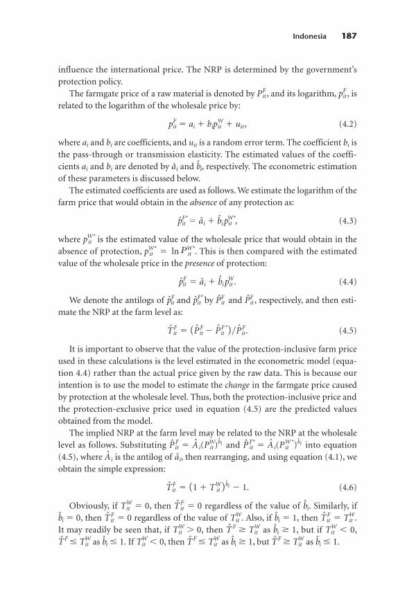
influence the international price. The NRP is determined by the government’sprotection policy.
The farmgate price of a raw material is denoted by PitF , and its logarithm, pit
F , isrelated to the logarithm of the wholesale price by:
pFit � ai � bipit
W � uit, (4.2)
where ai and bi are coefficients, and uit is a random error term. The coefficient bi isthe pass-through or transmission elasticity. The estimated values of the coeffi-cients ai and bi are denoted by ai and bi, respectively. The econometric estimationof these parameters is discussed below.
The estimated coefficients are used as follows. We estimate the logarithm of thefarm price that would obtain in the absence of any protection as:
pF*it � ai � bi p
W*it , (4.3)
where pW*it is the estimated value of the wholesale price that would obtain in the
absence of protection, pW*it � ln PW*
it . This is then compared with the estimatedvalue of the wholesale price in the presence of protection:
pFit � ai � bi p
Wit . (4.4)
We denote the antilogs of pFit and pF*
it by PFit and PF
it , respectively, and then esti-mate the NRP at the farm level as:
T Fit � (P F
it � P F*it )�P F
it. (4.5)
It is important to observe that the value of the protection-inclusive farm priceused in these calculations is the level estimated in the econometric model (equa-tion 4.4) rather than the actual price given by the raw data. This is because ourintention is to use the model to estimate the change in the farmgate price causedby protection at the wholesale level. Thus, both the protection-inclusive price andthe protection-exclusive price used in equation (4.5) are the predicted valuesobtained from the model.
The implied NRP at the farm level may be related to the NRP at the wholesalelevel as follows. Substituting P F
it � Ai(PWit )
bi and P F*it � Ai(PW
it*)bi into equation
(4.5), where Ai is the antilog of ai, then rearranging, and using equation (4.1), weobtain the simple expression:
T Fit � (1 � TW
it )bi � 1. (4.6)
Obviously, if TitW � 0, then T F
it � 0 regardless of the value of bi. Similarly, ifbi � 0, then T F
it � 0 regardless of the value of TitW. Also, if bi � 1, then T F
it � TitW.
It may readily be seen that, if TitW � 0, then T F � Tit
W as bi � 1, but if TitW � 0,
T F � TitW as bi � 1. If Tit
W � 0, then T F � TitW as bi � 1, but T F � Tit
W as bi � 1.
Indonesia 187

Econometric application
The purpose of the econometric analysis is to estimate the parameter bi for eachcommodity.5 For each commodity, we conduct the analysis using time series pricedata in which each variable is expressed in logarithms, and each is deflated by theGDP deflator for Indonesia: the farmgate price (LFP), the wholesale price (LWP),and the log of the international price, adjusted by the nominal exchange rate andtransport and handling costs (LIP). The data extend from 1976 to 2001. The sevencommodities for which these data are available are rice, maize, soybeans, sugar,rubber, coffee, and tea.
We first tested each of the series (each deflated by the GDP deflator) for theexistence of a unit root. For rice, the null hypothesis of a unit root was rejected forall three price series (recalling that they are real, not nominal, price series usingthe GDP deflator) at the 10 percent level of significance. The price series are thusconsidered stationary. For other commodities, the results are more mixed. Formaize, the null hypothesis of a unit root could not be rejected for farm prices(LFP), but was strongly rejected for the other two price series. For soybeans, thenull hypothesis of a unit root could not be rejected for the wholesale price series(LWP), but was rejected at the 10 percent level for the other two series. For sugar,the null hypothesis of a unit root could not be rejected for any of the three series,especially the farm price series (LFP). For rubber, coffee, and tea, the results weresimilar: the null hypothesis of a unit root marginally failed to be rejected for thefarm price series (LFP), but was rejected for the other two series.
We first produced ordinary least squares estimates of equation (4.2). In mostcases, autocorrelation was a problem, and an AR(1) correction term was includedto eliminate it, which was accomplished effectively. The ordinary least squaresestimates assume that LFP is endogenous and LWP is exogenous. These assump-tions were tested using Hausman’s endogeneity test, although the test has lowpower when the number of data points is small, as in this case. For each commod-ity, the null hypothesis that LWP was (weakly) exogenous to LFP failed to berejected, confirming the validity of the ordinary least squares estimates. ReverseHausman’s tests were also conducted, and the null hypothesis that LFP was exoge-nous to LWP was rejected in the cases of maize, sugar, rubber, coffee, and tea. Thishypothesis marginally failed to be rejected for rice and soybeans. The resultsroughly support the validity of the use of the ordinary least squares framework toestimate the transmission elasticity from LWP to LFP, while treating LWP asexogenous.
Usable estimates were produced for five commodities: rice, soybeans, sugar,rubber, and tea. The estimated elasticity had the expected positive sign and wassignificantly different from zero, and the estimated equation performed well.
188 Distortions to Agricultural Incentives in Asia
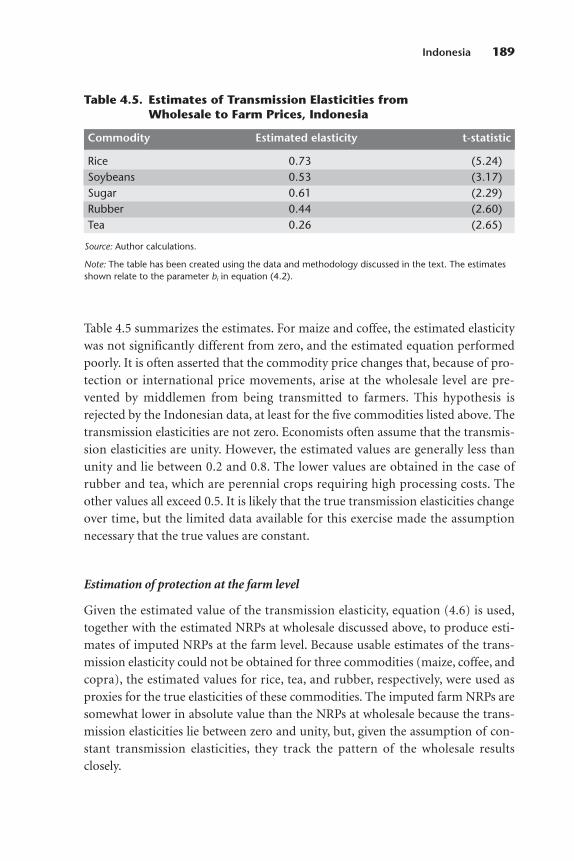
Table 4.5 summarizes the estimates. For maize and coffee, the estimated elasticitywas not significantly different from zero, and the estimated equation performedpoorly. It is often asserted that the commodity price changes that, because of pro-tection or international price movements, arise at the wholesale level are pre-vented by middlemen from being transmitted to farmers. This hypothesis isrejected by the Indonesian data, at least for the five commodities listed above. Thetransmission elasticities are not zero. Economists often assume that the transmis-sion elasticities are unity. However, the estimated values are generally less thanunity and lie between 0.2 and 0.8. The lower values are obtained in the case ofrubber and tea, which are perennial crops requiring high processing costs. Theother values all exceed 0.5. It is likely that the true transmission elasticities changeover time, but the limited data available for this exercise made the assumptionnecessary that the true values are constant.
Estimation of protection at the farm level
Given the estimated value of the transmission elasticity, equation (4.6) is used,together with the estimated NRPs at wholesale discussed above, to produce esti-mates of imputed NRPs at the farm level. Because usable estimates of the trans-mission elasticity could not be obtained for three commodities (maize, coffee, andcopra), the estimated values for rice, tea, and rubber, respectively, were used asproxies for the true elasticities of these commodities. The imputed farm NRPs aresomewhat lower in absolute value than the NRPs at wholesale because the trans-mission elasticities lie between zero and unity, but, given the assumption of con-stant transmission elasticities, they track the pattern of the wholesale resultsclosely.
Indonesia 189
Table 4.5. Estimates of Transmission Elasticities fromWholesale to Farm Prices, Indonesia
Commodity Estimated elasticity t-statistic
Rice 0.73 (5.24)Soybeans 0.53 (3.17)Sugar 0.61 (2.29)Rubber 0.44 (2.60)Tea 0.26 (2.65)
Source: Author calculations.
Note: The table has been created using the data and methodology discussed in the text. The estimatesshown relate to the parameter bi in equation (4.2).
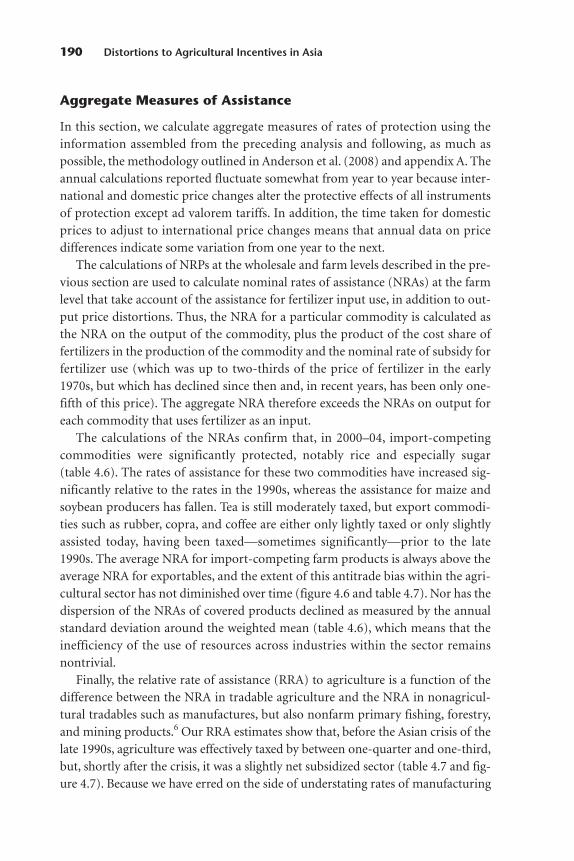
Aggregate Measures of Assistance
In this section, we calculate aggregate measures of rates of protection using theinformation assembled from the preceding analysis and following, as much aspossible, the methodology outlined in Anderson et al. (2008) and appendix A. Theannual calculations reported fluctuate somewhat from year to year because inter-national and domestic price changes alter the protective effects of all instrumentsof protection except ad valorem tariffs. In addition, the time taken for domesticprices to adjust to international price changes means that annual data on pricedifferences indicate some variation from one year to the next.
The calculations of NRPs at the wholesale and farm levels described in the pre-vious section are used to calculate nominal rates of assistance (NRAs) at the farmlevel that take account of the assistance for fertilizer input use, in addition to out-put price distortions. Thus, the NRA for a particular commodity is calculated asthe NRA on the output of the commodity, plus the product of the cost share offertilizers in the production of the commodity and the nominal rate of subsidy forfertilizer use (which was up to two-thirds of the price of fertilizer in the early1970s, but which has declined since then and, in recent years, has been only one-fifth of this price). The aggregate NRA therefore exceeds the NRAs on output foreach commodity that uses fertilizer as an input.
The calculations of the NRAs confirm that, in 2000–04, import-competingcommodities were significantly protected, notably rice and especially sugar(table 4.6). The rates of assistance for these two commodities have increased sig-nificantly relative to the rates in the 1990s, whereas the assistance for maize andsoybean producers has fallen. Tea is still moderately taxed, but export commodi-ties such as rubber, copra, and coffee are either only lightly taxed or only slightlyassisted today, having been taxed—sometimes significantly—prior to the late1990s. The average NRA for import-competing farm products is always above theaverage NRA for exportables, and the extent of this antitrade bias within the agri-cultural sector has not diminished over time (figure 4.6 and table 4.7). Nor has thedispersion of the NRAs of covered products declined as measured by the annualstandard deviation around the weighted mean (table 4.6), which means that theinefficiency of the use of resources across industries within the sector remainsnontrivial.
Finally, the relative rate of assistance (RRA) to agriculture is a function of thedifference between the NRA in tradable agriculture and the NRA in nonagricul-tural tradables such as manufactures, but also nonfarm primary fishing, forestry,and mining products.6 Our RRA estimates show that, before the Asian crisis of thelate 1990s, agriculture was effectively taxed by between one-quarter and one-third,but, shortly after the crisis, it was a slightly net subsidized sector (table 4.7 and fig-ure 4.7). Because we have erred on the side of understating rates of manufacturing
190 Distortions to Agricultural Incentives in Asia
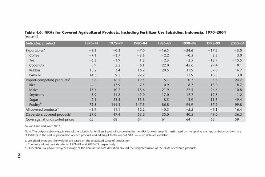
191
Table 4.6. NRAs for Covered Agricultural Products, Including Fertilizer Use Subsidies, Indonesia, 1970–2004(percent)
Indicator, product 1970–74 1975–79 1980–84 1985–89 1990–94 1995–99 2000–04
Exportablesa �3.3 �0.3 �7.0 �16.5 �24.6 �17.2 �3.0Coffee �7.1 �3.7 �8.6 �2.2 �0.5 2.3 3.0Tea �6.3 �1.9 1.8 �2.3 �2.5 �13.9 �15.5Coconuts �5.9 2.2 �6.1 �22.0 �45.6 �29.4 �8.1Rubber 15.2 �3.4 �16.2 �20.5 �31.9 37.0 16.7Palm oil �14.5 �9.2 22.2 �1.1 11.9 �18.3 �3.8
Import-competing productsa �3.6 16.5 19.5 5.1 �0.7 �5.8 24.7Rice — 13.9 7.5 �0.9 �8.7 �13.0 18.7Maize �15.4 10.2 18.6 21.9 22.5 24.6 10.8Soybeans �5.9 31.8 49.0 17.0 17.7 17.5 1.2Sugar 2.1 23.5 53.8 8.5 3.9 11.3 49.4Poultryb 72.8 144.3 147.5 86.8 94.9 87.9 99.8
All covered productsa �3.9 11.1 12.2 �0.3 �5.5 �9.1 16.4Dispersion, covered productsc 27.6 49.4 53.6 35.0 40.5 49.0 36.3Coverage, at undistorted prices 65 68 64 61 64 63 59
Source: Fane and Warr 2007.
Note: The output-subsidy equivalent of the subsidy for fertilizer input is incorporated in the NRA for each crop. It is estimated by multiplying the input subsidy by the shareof fertilizer in the cost of production of each product and adding it to the output NRA. — � no data are available.
a. Weighted averages; the weights are based on the unassisted value of production.b. The first and last periods refer to 1971–74 and 2000–03, respectively.c. Dispersion is a simple five-year average of the annual standard deviation around the weighted mean of the NRAs of covered products.

protection prior to 1987, better estimates of manufacturing protection during thisperiod would show larger negative RRAs prior to the 1990s and would therebyreinforce rather than undermine the above finding.
Conclusions and the Prospects for Reform
Having previously taxed agriculture relative to the nonfarm sectors during thepostindependence period, Indonesia’s trade policies have, on average, not taxedagriculture since around 2000. This change occurred following the Asian crisis ofthe late 1990s. The switch took the form of (a) increases in the protection of theimport-competing commodities sugar and rice; (b) declines in the taxation ofagricultural exports, especially rubber and copra; and (c) declines in manufactur-ing protection. The transition to a more democratic form of government hasweakened the influence of the country’s technocrats, who have generally favoredliberalized trade policies. Greater protection among some key agricultural com-modities has been a consequence.
Assistance for agriculture primarily takes the form of protection for theimport-competing sugar and rice subsectors. Other output subsectors receive virtually no direct assistance. Subsidies for fertilizers and other inputs were once anindirect source of assistance for agriculture, but the nominal rates of these subsi-dies have declined.
192 Distortions to Agricultural Incentives in Asia
Figure 4.6. NRAs for Exportable, Import-Competing, and AllAgricultural Products, Indonesia, 1970–2004
Source: Fane and Warr 2007.

193
Table 4.7. NRAs in Agriculture Relative to Nonagricultural Industries, Indonesia, 1970–2004(percent)
Indicator 1970–74 1975–79 1980–84 1985–89 1990–94 1995–99 2000–04
Covered productsa �3.9 11.1 12.2 �0.3 �5.5 �9.1 16.4Noncovered products �2.3 5.4 4.2 �3.8 �8.4 �7.7 7.1All agricultural productsa �3.4 9.3 9.2 �1.7 �6.6 �8.6 12.0Non-product-specific assistance 0.0 0.0 0.0 0.0 0.0 0.0 0.0Total agricultural NRAb �3.4 9.3 9.2 �1.7 �6.6 �8.6 12.0Trade bias indexc 0.03 �0.14 �0.21 �0.20 �0.24 �0.12 �0.22NRA, all agricultural tradables �3.8 10.4 10.5 �1.9 �7.5 �9.7 13.9NRA, all nonagricultural tradables 27.7 27.7 27.7 26.5 17.6 10.6 8.1RRAd �24.7 �13.6 �13.5 �22.5 �21.3 �18.3 5.4
Source: Fane and Warr 2007.
a. Including product-specific input subsidies.b. Including product-specific input subsidies and non-product-specific assistance. Represents total assistance to primary factors and intermediate inputs, divided by the total
value of primary agriculture production at undistorted prices.c. The trade bias index is defined as (1 � NRAagx�100)�(1 � NRAagm�100) � 1, where NRAagm and NRAagx are the average percentage NRAs for the import-competing and
exportable parts of the agricultural sector, respectively.d. The RRA is defined as 100*[(100 � NRAagt)�(100 � NRAnonagt) � 1], where NRAagt and NRAnonagt are the percentage NRAs for the tradables parts of the agricultural and
nonagricultural sectors, respectively.
The political explanations for the protection of sugar and the protection of riceare quite different. The protection of sugar is a consequence of the political powerof the highly concentrated refining industry, including the state-owned compo-nent of this industry, which is closely linked with large-scale sugar plantations.
In contrast, the farm production of rice (paddy) is dominated by small-scalefarm producers. The rice milling industry is much more concentrated and muchmore well organized, however, and this is relevant because rice imports competewith milled rice rather than the raw, unmilled product (paddy) produced by thefarmers. The political power of rice millers has been an important source of sup-port for the protection of the rice industry. The enhanced political power of theIndonesian parliament since the upheavals induced by the Asian crisis, togetherwith the economic nationalism that dominates among members of parliament, hasstrengthened the support for the protection of the rice industry. Since 2004, riceimports have officially been banned. In part, this policy has reflected the mistakenclaim, advanced by supporters of rice industry protection, that restricting riceimports reduces poverty. A general equilibrium analysis presented in Warr (2005)shows that the policy is more likely to have increased poverty within both rural andurban areas because the poverty-increasing effects of raising the consumer price ofrice far exceed the poverty-reducing effects of raising the producer price.
194 Distortions to Agricultural Incentives in Asia
Figure 4.7. NRAs for Agricultural and NonagriculturalTradables and the RRA, Indonesia, 1970–2004
Source: Fane and Warr 2007.
Note: For the definition of the RRA, see table 4.7, note d.
Given the politics at work, trade liberalization in the country’s sugar and riceindustries seems unlikely in the foreseeable future. Indeed, rising protectionismseems a more likely outcome, and this might conceivably extend to industriesother than sugar and rice.
Notes
1. Soeharto’s New Order began in March 1966, although Soekarno, Soeharto’s predecessor,remained nominal president for 12 more months. The statement about rice self-sufficiency wasreportedly made during Soeharto’s visit to the headquarters, in Rome, of the Food and AgricultureOrganization of the United Nations, in 1985, when Indonesia’s rice imports stood (briefly) at zero.
2. The border price of rice in chart a, figure 4.1 has been converted to make it as nearly comparableas possible to the wholesale price. The free on board price was adjusted to the cost, insurance, andfreight level by adding freight and insurance costs; the resulting price was then adjusted to the whole-sale level by adding margins to allow for the estimated handling, warehousing, and interest costs.
3. Gross indicates that each hectare that is harvested twice in a single year is counted as 2 hectares.4. The term tariff surcharge is a misnomer in the sense that the base to which the rates of the tariff
surcharge applied was not the tariff, but the border value (cost, insurance, and freight) of the importssubject to the tariff surcharge. For example, in 1985, in the case of live animals (other than pure bred),the tariff was 30 percent, and the tariff surcharge was 15 percent, giving a total import duty of 45 per-cent of the border value (cost, insurance, and freight).
5. The results are summarized here. Details of the econometric analysis are available upon request.6. The NRAs for nonagricultural tradables are estimated mainly on the basis of the effective rates of
protection for manufacturing in Fane and Condon (1996), who estimated these rates for 1987 and1995 at 48 and 20 percent, respectively. These authors also projected the corresponding effective ratefor 2003 at 13 percent based on the May 1995 tariff reduction package, which was to be implementedby 2003 and which was, in fact, largely implemented. For all years before 1987, we have used the 1987values even though some tariff reduction occurred during the few years before 1987. For 1987–95 and1995–2003, we have interpolated linearly. For 2004, we have used the 2003 value. (As noted above, thefocus of this discussion is the identification of broad long-run trends in the structure of protectionrather than annual fluctuations.)
References
Anderson, K., M. Kurzweil, W. Martin, D. Sandri, and E. Valenzuela. 2008. “Measuring Distortions toAgricultural Incentives, Revisited.” World Trade Review 7 (4): 675–704.
Booth, A. 1988. Agricultural Development in Indonesia. Sydney: Allen and Unwin.BPS (Badan Pusat Statistik, Statistics Indonesia). 1971. Input-Output Tables, Indonesia. Jakarta: BPS.———. 1980. Input-Output Tables of Indonesia. Jakarta: BPS.———. 1990. Input-Output Tables of Indonesia. Jakarta: BPS.———. 2000. Input-Output Tables of Indonesia. Jakarta: BPS.Corden, W. M. 1984. “Booming Sector and Dutch Disease Economics: A Survey.” Oxford Economic
Papers 36 (3): 359–80.Fane, G., and T. Condon. 1996. “Trade Reform in Indonesia, 1987–1995.” Bulletin of Indonesian
Economic Studies 32 (3): 33–54.Fane, G., and P. Warr. 2007. “Distortions to Agricultural Incentives in Indonesia.” Agricultural Distor-
tions Working Paper 24, World Bank, Washington, DC.Hill, H. 2000. The Indonesian Economy. 2nd ed. Cambridge: Cambridge University Press.
Indonesia 195

Timmer, C. P. 1996. “Does Bulog Stabilize Rice Prices in Indonesia? Should it Try?” Bulletin of Indonesian Economic Studies 32 (2): 45–74.
Warr, P. G. 1986. “Indonesia’s Other Dutch Disease: Economic Effects of the Petroleum Boom.” InNatural Resources and the Macroeconomy, ed. J. P. Neary and S. van Wijnbergen, 288–320. Oxford:Basil Blackwell.
———. 1992. “Comparative Advantage and Protection in Indonesia 1.” Bulletin of Indonesian Economic Studies 28 (3): 41–70.
———. 2005. “Food Policy and Poverty in Indonesia: A General Equilibrium Analysis.” AustralianJournal of Agricultural and Resource Economics 49 (4): 429–51.
World Development Indicators Database. World Bank. http://go.worldbank.org/B53SONGPA0(accessed May 2008).
196 Distortions to Agricultural Incentives in Asia

Malaysia is notable among developing countries for its long-standing commit-ment to the maintenance of a relatively open trade policy regime. It has neverrelied heavily on quantitative restrictions or other forms of nontariff protection,and its tariffs on domestic manufacturing and agriculture have been low relativeto similar tariffs in other developing countries. In the first half of the 1980s—aspart of a government-led strategy of heavy industrialization—and in the immedi-ate aftermath of the 1997–98 economic crisis, tariffs on some manufactured goodswere substantially increased, and some goods were brought under quantitativerestrictions to support selected domestic industries in the face of a massivedomestic economic contraction. However, these measures were eventually reversed,and additional tariff cuts were undertaken in the ensuing years.
Unlike its counterparts in other countries, the Malaysian government has con-sistently avoided exerting direct influence on export prices or the direct procure-ment of agricultural output through government marketing boards. Export dutieson the two major primary commodities, rubber and palm oil, were a major sourceof government revenue until the mid-1980s. However, export taxes were periodi-cally adjusted in line with world price trends to keep producer prices relatively stable. The government also plowed a significant share of this revenue into well-designed and efficiently implemented replanting schemes and productivity-enhancing research in these industries. Over the past two decades, export dutieson rubber and palm oil have decreased drastically. However, these traditionalexport industries have been under persistent domestic cost pressure, which hasarisen from the rapid structural transformation of the economy through success-ful global integration.
197
5
MALAYSIA
Prema-Chandra Athukoralaand Wai-Heng Loke
The production of paddy rice—the staple food of the country and the princi-pal domestic food crop—stands out as the single most heavily assisted economicactivity. During the immediate postwar years, assistance for this crop was intro-duced by the colonial government on the grounds of food security. After inde-pendence, particularly after the launch, in 1970, of the New Economic Policy(Dasar Ekonomi Baru), a sweeping affirmative action policy package aimed atincreasing the share of certain ethnic groups in the economy, rice became anincreasingly sensitive political crop. While the achievement of food self-suffi-ciency has continued to represent a moving target in successive developmentplans, protection for rice farmers, who are concentrated in relatively economicallybackward states, remains the overwhelmingly predominant reason behind protec-tion. Producers of subsidiary crops, horticultural products, livestock, and fishingproducts have been operating under a virtually free trade regime throughout, withthe exception of quantitative restrictions on the importation of round cabbages.High-value (processed) food products have emerged as an important dynamicexport product over the past two decades.
This chapter has two main purposes: first, to provide an analytical narrative ofthe nature and evolution of trade in Malaysia and the related and accompanyingpolicies that have had an impact on domestic agriculture (with a focus on theunderlying political economy) and, second, to examine the degree of and chang-ing patterns in the policy distortions affecting the incentives in domestic agricul-ture, including both direct (sector-specific) incentives and indirect incentivesemanating from economy-wide policies. We also aim to inform the debate inMalaysia on the future direction of national development policy as it relates todomestic agriculture. The analysis is undertaken against the backdrop of theongoing process of rapid structural transformation of the country’s economy overthe past three decades. As an integral part of the analysis, we attempt to delineatethe implications—over and above the implications of policy-induced incentives—of the process of structural transformation for the long-term viability of tradi-tional plantation crops and the new opportunities for agricultural output expan-sion in the subsidiary food-crop subsector.
Our study covers the period from 1960 (the earliest year for which reliable dataare available after independence in 1957) to 2004. We emphasize four major prod-ucts: rubber, palm oil, cocoa, and rice. The first three are exportable products,while the fourth, the main food staple, is an import-competing product. Together,the four products accounted for three-fifths to four-fifths of the value of totalagricultural gross domestic product (GDP) over the period. Because of thepaucity of data, we are unable to cover other commodities, but virtually all otheragricultural products have been facing free trade conditions throughout theperiod we study.
198 Distortions to Agricultural Incentives in Asia
The structure of the chapter is as follows. The next section provides anoverview of growth and structural change in the economy during the postinde-pendence era (since 1957), with an emphasis on the relative importance of theagricultural sector and the trends and compositional shifts in agricultural outputand trade. This is followed by a survey of the evolution of agricultural trade policyduring the era since 1957 against the backdrop of overall national developmentstrategy and macroeconomic policy. We pay particular attention to the politicaleconomy considerations that underpin policy directions. In the subsequent sec-tion, we provide estimates of the extent of and patterns in the direct and indirectdistortions in the incentives faced by domestic agriculture. The estimates arebased on indicators that have been specifically constructed for our study. The finalsection contains a summary of the key findings and policy inferences.
Agriculture in the Malaysian Economy
To aid an understanding of the policy environment in Malaysia, we explain thegrowth trends in the economy and the patterns of structural change intersec-torally and within the agricultural sector.
Economic growth trends
At independence in 1957, Malaysia was a classic agrarian economy in which agri-culture and the mineral industry were concentrated in primary production forexport (Levin 1960). Natural rubber directly accounted for 25 percent of GDP,while the second largest export, tin, accounted for 5 percent (Meerman 1979). Inaddition, a host of service activities that embraced trade, transport, and financewas dependent on the export sector. Production patterns exhibited only limitedchanges until about the mid-1970s. The structural changes since then have beendramatic, however. In particular, beginning in the late 1980s, there has been anexpansion in export-oriented manufacturing and related activities in the modernsector. The share of agriculture in GDP had declined to 19 percent by the late1980s and then plummeted to 8.5 percent in 2005 (table 5.1 and figure 5.1).
In the early 1970s, agriculture directly absorbed about half the total laboremployed in the country. This share had declined to 13.7 percent by 2005. Thecontraction in the relative importance of agriculture in total labor absorption wasparticularly marked over the two decades before 2005 (table 5.1). Despite this dra-matic structural transition, the promotion of employment opportunities in therural economy, which is roughly equivalent to the agricultural sector, has contin-ued to be an important focus of the government’s successive 10-year developmentplans. This is so particularly because of the delicate ethnic dimension involved: over
Malaysia 199
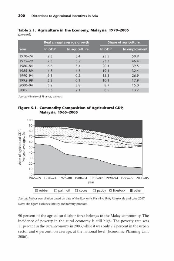
90 percent of the agricultural labor force belongs to the Malay community. Theincidence of poverty in the rural economy is still high. The poverty rate was11 percent in the rural economy in 2003, while it was only 2.2 percent in the urbansector and 6 percent, on average, at the national level (Economic Planning Unit2006).
200 Distortions to Agricultural Incentives in Asia
Table 5.1. Agriculture in the Economy, Malaysia, 1970–2005(percent)
Real annual average growth Share of agriculture
Year In GDP In agriculture In GDP In employment
1970–74 2.3 3.4 25.5 50.91975–79 7.3 5.2 23.3 46.41980–84 6.6 3.4 20.4 39.51985–89 4.8 4.3 19.1 32.41990–94 9.3 0.2 15.3 26.91995–99 5.2 0.1 10.1 17.92000–04 5.2 3.8 8.7 15.02005 5.3 2.1 8.5 13.7
Source: Ministry of Finance, various.
0
20
10
30
40
year
100
90
70
80
60
50
shar
e of
agr
icul
tura
l GD
P,fiv
e-ye
arav
erag
es, %
1965–69 1995–991990–941985–891980–841975–801970–74 2000–05
rubber palm oil cocoa paddy livestock other
Figure 5.1. Commodity Composition of Agricultural GDP,Malaysia, 1965–2005
Sources: Author compilation based on data of the Economic Planning Unit; Athukorala and Loke 2007.
Note: The figure excludes forestry and forestry products.
Over the past three decades or so, the agricultural sector has been under con-stant pressure because of the resource-pull effects of the rapid structural changesin the economy (Barlow and Jayasuriya 1987; Athukorala and Manning 1999).Widening urban-rural wage differentials and an aversion among younger peopleto engagement in agricultural pursuits has increased rural-to-urban labor migra-tion. This has caused widespread labor shortages in the rural economy and addedto the stress on agricultural wages. The area under traditional plantation crops hasshrunk in semiurban areas because of the dispersion of industrial centers acrossPeninsular Malaysia and the resulting higher demand for land for residential andindustrial expansion. In the face of severe shortages of local labor, agriculturalproducers—at first, plantation enterprises and, more recently, smallholder pro-ducers of cash crops and paddy—began to rely increasingly on foreign workers.The estimated foreign labor force in Malaysia increased from around 500,000 inthe mid-1980s to 1.8 million (23 percent of the total labor force) by 2003; abouthalf of these workers were in the agricultural sector (Athukorala 2006a). Thedependence on foreign labor is particularly high in the rubber industry because ofthe relatively high labor intensity of cultivation and harvesting. However, the rela-tively more capital-intensive palm oil industry also began to depend more on for-eign workers because fresh fruit bunch-harvesting is conducted manually. Accord-ing to a recent Malayan Agricultural Producers Association survey, 37 percent ofthe total labor force on private sector plantations in Peninsular Malaysia are for-eign workers, while the share is as high as 80 percent in East Malaysia (Khoo andChandramohan 2002).
Structural changes: plantation (cash) crops
Beginning in the 1890s, rubber was the preferred crop of the foreign-owned estatesector during the colonial period (Barlow 1978). Oil palms were first commer-cially planted in 1917 (although palm oil remained a relatively minor crop untilthe mid-1950s). During the ensuing three decades, palm oil proved to be moreprofitable than rubber and expanded in the plantation subsector at the expense ofrubber. The government policy emphasis in the plantation subsector shifted dra-matically from rubber to palm oil, and the support for the expansion of palm oilproduction increased when rubber replanting grants—grants to plant oil palmson land still under rubber—began to be distributed. The government played avigorous role in the expansion of palm oil production by embarking on a largeresettlement effort (especially though the Federal Land Development Authority)under which palm oil was the crop of choice (Pletcher 1991).1 The country’s suc-cess in promoting palm oil exports was aided by the inappropriate agriculturaland economy-wide policies of the traditional palm oil exporting countries in
Malaysia 201
Africa (MacBean 1989; Athukorala 1991). Cocoa gained importance as an alterna-tive crop in the plantation subsector starting around the beginning of the 1970s.However, about the mid-1980s, producers began to contract the area under cocoacultivation sharply because of the persistently low world prices for cocoa beans.
Around the late 1980s, the plantation subsector came under severe strainbecause of the resource-pull effects of the rapid structural changes in the econ-omy (see elsewhere above). These effects were felt more acutely in the rubber andcocoa industries, where the cultivation and harvesting processes were more laborintensive relative to the palm oil industry. Moreover, the world prices for the twoformer products were unfavorable relative to the world price of palm oil. At theend of the crop cycle, many plantation enterprises and smallholders replantedsome of the land given over to rubber with less labor-intensive crops, particularlyoil palms, or used the land for residential and industrial expansion.
Many rubber estate companies were facing hard times. They began employingforeign workers to overcome labor shortages, and then they used their technologyand their management expertise to invest in neighboring countries (particularlyIndonesia and the Philippines) in which wages and land cost less. Smallholdersalso continued to tap rubber using hired migrant labor, although the higher priceelasticity of supply among the smallholders resulted in declining output whenoutput prices fell in the early 1990s (Barlow 1997). In recent years, despite the nat-ural cushion provided by the relative capital intensity of production and the rela-tively favorable price trend, the palm oil subsector has also felt the pinch of theresource-pull effects. Many large plantation enterprises have shifted their invest-ments to neighboring land- and labor-abundant countries.
The three main plantation crops are rubber, palm oil, and cocoa. The areaunder rubber increased from 1.7 million hectares in the early 1960s to 2.0 millionhectares in the late 1970s and early 1980s. However, it has declined steadily sincethen, reaching 1.3 million hectares in 2000–04. The area under oil palm cultiva-tion rose from less than 100,000 hectares in 1960–64 to 3.8 million hectares in2000–04. The expansion in output was more rapid in both rubber and palm oilthan the expansion in area under cultivation. This reflects the widespread use ofnew high-yielding varieties and improved cultivation practices.
Since the late 1990s, the rubber and palm oil industries have benefited fromincreased world demand, especially growing demand in China, and the resultingfavorable price trends. The palm oil industry has benefited additionally in recentyears from the tight world supply of edible oils and fats and the expandingdemand for biodiesel fuel, which has pushed up palm oil prices.
In the case of rubber, the supply response to favorable prices took the form ofgreater cropping intensity in the context of the persistent decline in cultivatedarea. In contrast, the area under oil palm cultivation showed some mild positive
202 Distortions to Agricultural Incentives in Asia

response to favorable prices. In cocoa, both the output and the area under cultiva-tion have declined steadily since the early 1990s.
Meanwhile, the yield per hectare in palm oil rose throughout. In rubber, theyield increased notably in the 1960s and 1970s, but this was followed by virtualstagnation. The stability of rubber yields in the face of the decline in the total out-put of rubber occurred largely because of a contraction in the area under cultiva-tion, which suggests that marginal plantations showing poor yields were beingabandoned (Athukorala and Loke 2007).
The smallholder share of the land under rubber cultivation has always beenhigh. In 1960–2004, it grew from 50 to 93 percent. The relatively capital-intensivepalm oil industry was initially dominated by large plantations, although thesmallholder share rose from 16 percent in 1970 to around 40 percent after 1990(Athukorala and Loke 2007).2 The dominance of estate cultivation is an unusualfeature of the palm oil industry in Malaysia (and in Indonesia) because the small-holder production of palm oil is much more important in other parts of the world(Pletcher 1991).
Structural changes: food crops
Rice farming, nearly all wet paddy farming, is the major source of income for ruralhouseholds in the states of the north and east in Peninsular Malaysia and parts ofEast Malaysia. At independence, about three-quarters of the native peasant pro-ducers (predominantly rice growers and fishermen) were Malays; about 90 per-cent of the rice growers were Malays; and about one-third of the economicallyactive Malay male population represented the peasant sector (Meerman 1979).This ethnic dimension of rice farming persisted during the ensuing years, makingrice a highly sensitive political crop.
Nearly half of all peasant cultivators grow some rice. The area under paddy cul-tivation rose from 490,000 hectares in 1960–64 to 750,000 hectares in 1970–74and has remained near this level since then. Paddy production rose steadily fromthe early 1960s to the mid-1990s, however, because of increases in yield perhectare starting in the 1970s. Paddy producers were aided significantly by govern-ment policies such as sponsored irrigation schemes that permitted double crop-ping, the introduction of high-yielding varieties, the consolidation of paddy small-holdings through group farming in the eight granary areas, and direct assistance tofarmers through price supports and credit and fertilizer subsidies (see below). Bythe end of the eighth plan period in 2005, almost all farming operations in majorpaddy growing areas had been fully mechanized. As a result, the labor input perhectare declined from 47 to 15 worker days in 1995–2000 (Economic PlanningUnit 2001). At independence in 1957, about 45 percent of all rice consumed in
Malaysia 203
Malaysia was imported, but, since the mid-1970s, around 90 percent of the riceconsumed has been produced in the country.
Beginning in the mid-1990s, rice production stagnated. This has been followedby a mild, but steady decline in recent years despite the constant rise in yields perhectare (Athukorala and Loke 2007). As in the case of plantation crops, paddyfarming has been under pressure because of labor shortages arising from rural-to-urban labor migration and the aging of the farming community (Ahmad andTawang 1999). It seems that massive government support has been insufficient tomaintain paddy farming in the context of the enormous pressure emanating fromthe ongoing structural adjustment in the economy at large.
A noteworthy development in nonplantation agriculture over the past 15 yearshas been the rise in the output of subsidiary food products, such as fruits, vegeta-bles, fish, and livestock, which has been growing at a more rapid rate than paddyoutput (Economic Planning Unit 2006). While there has been some increase inthe exports of these high-value food products, the expansion in production has sofar gone predominantly to satisfying domestic demand. This is because of therapid income growth in the modern sector of the economy and the high incomeelasticity of demand for high-value food products relative to rice. The importanceof the subsidiary food subsector is bound to rise rapidly in years to come.
Figure 5.1 provides data on the composition of the value added by agriculturalproduction in the economy. The dominance of the plantation crop subsector inagriculture declined steadily, from 73 percent in the early 1970s to 53 percent in2000–05. Within this subsector, there has been a noticeable shift in the composi-tion of output from rubber toward palm oil. Cocoa accounted for around 10 per-cent of total agricultural GDP from the mid-1970s to the early 1990s, but thisshare declined thereafter, reaching negligible levels by the end of the 1990s. Thecombined share of food crops, which remained around 28 percent in the 1960sand 1970s, rose sharply during the ensuing years, reaching 47 percent in 2000–05.Within this subsector, the relative importance of paddy has declined appreciablyover the past two decades. This reflects the compositional shift toward livestock,fish, and other subsidiary food crops, mainly fruits and vegetables.
Agricultural trade
The dramatic shifts in the structure of domestic production were closely mirroredin the patterns of export. The combined share of agricultural products in totalmerchandise exports declined from 39 percent in 1970–74 to 8 percent in 2000–04(table 5.2). (The respective shares are 58 and 10 percent if timber and wood exportsare included.) Among agricultural products (excluding timber and wood), theshare of rubber declined from 62 to slightly less than 10 percent over the sameyears; this was offset by an increase in the share of palm oil from 24 to 42 percent.
204 Distortions to Agricultural Incentives in Asia

The share of Malaysia in the total world exports of natural rubber fell from62 to around 20 percent between the late 1970s and 2004, when Malaysia was thethird most important exporter of rubber in the world after Thailand and Indonesia(Athukorala and Loke 2007). In world crude palm oil exports, Malaysia was thelargest exporter until recently, accounting for a share between 65 and 80 percentfrom the mid-1970s to the late 1990s. Indonesia has since become the world’slargest exporter; it now accounts for over 50 percent of total world exports (notshown in table 5.2). This is the result of massive investment in relocation byMalaysian plantation companies in the face of mounting domestic cost pressures.
A noteworthy development in the structure of exports over the past twodecades has been the emergence of processed food as a dynamic export line. Theaverage annual growth rate of processed food exports rose from 5 to 19 percentbetween 1985–99 and 2000–04. The share of processed food in total agriculturalexports increased from 9 percent in 1970–74 to 16 percent in 1985–89 and 32 per-cent in 2000–04 (table 5.2). The rapid expansion of processed food comparedwith traditional food products (coffee, tea, sugar, cocoa, and so on) has been auniversal phenomenon in world trade over the past two decades (Athukorala andJayasuriya 2003).3 The recent performance of Malaysia in this lucrative growtharea, while impressive relative to past performance, has lagged behind that of
Malaysia 205
Table 5.2. Product Shares, Agricultural Exports, Malaysia,1970–2004
(percent)
Indicator 1970–74 1975–79 1985–89 1995–99 2000–04
Agriculture in merchandiseexports
Total 58 54 36 13 10Excluding timber and wood 39 38 24 11 8Composition, agricultural
exportsa
Rubber 62.4 52.9 33.7 12.9 9.7Palm oil 23.9 27.5 31.9 44.1 41.6Cocoa 2.1 2.3 6.4 2.5 2.6Spices 2.2 2.1 1.5 1.1 0.8Processed food 8.7 8.5 15.6 26.2 31.6World market shareRubber 62 57 37 20 19Palm oil 70 77 75 64 55Cocoa 3 3 11 4 4
Sources: Ministry of Finance, various; Bank Negara Malaysia, various.
a. Excluding timber and wood.
many other counties (particularly Thailand) with similar agricultural resourceendowments (Athukorala 2006a). An interesting issue that deserves more analysisrevolves around whether the country’s highly interventionist paddy sector sup-port policy has constrained a shift in agricultural resources to these new, moredynamic product lines.
Policy Context
The development prospects of Malaysia (then the Federation of Malaya) at inde-pendence in 1957 were mixed at best.4 On the positive side, the country’s percapita income was on a par with incomes in Hong Kong, China and Taiwan, Chinaand higher than incomes elsewhere in East Asia, save Japan. Although the rate ofpopulation growth was already rapid, the highly favorable ratio of land and othernatural resources to total population offered great potential to raise per capitaincomes. Moreover, the colonial inheritance included well-developed infrastruc-ture, efficient administrative mechanisms, and a thriving primary export sectorwith considerable potential for expansion.
The mobilization of this development potential to build the economy of thenewly independent Malaysia had to be accomplished in the face of challengesposed by a pluralistic society inherited from the colonial past. At the time, ethnicMalays, who accounted for 52 percent of the population, dominated in politics,but were relatively poor and were involved mostly in low-productivity agriculturalactivities. Ethnic Chinese (37 percent of the population) enjoyed greater eco-nomic power and dominated in the modern sector, but they did not match theethnic solidarity or political power of the Malays.5 Ethnic divisions weakened thenational fabric; the machinery of government was fragile, and the democraticpolitical leadership remained untested. In this context, there was not much roomfor optimism regarding the development policies that might be expected from thenewly elected government (World Bank 1955). The development challenges facedby the country were generally considered more problematic than the challengesbeing faced in other countries that had also newly emerged from a colonial past,particularly Ghana, India, Kenya, Myanmar, and Pakistan.6
From independence to the mid-1960s, national development policy was gener-ally in line with traditional liberal notions of the limited state. The public command of economic resources in these early years was narrow, and prevailingeconomic policies were conservative. The policy thrust basically involved contin-uing the colonial open-door policy stance relating to trade and industry, whileattempting to redress ethnic and regional economic imbalances through ruraldevelopment schemes and the provision of social and physical infrastructure(Snodgrass 1980).
206 Distortions to Agricultural Incentives in Asia

As in many other developing countries, industrialization through import sub-stitution was a key part of the Malaysian development strategy during this period.However, Malaysian policy makers, unlike their counterparts in other countries,did not seek forced industrialization through direct import restrictions and theestablishment of state-owned industrial enterprises (Lim 1992).7 Moderate tariffprotection was, by and large, the key instrument used to encourage new invest-ment in manufacturing. The average tariff rate in 1965 has been estimated at amere 13 percent, and few industries enjoyed nominal tariffs above 30 percent.Nontariff barriers were almost nonexistent (Power 1971; Lin 1984).
The race riots in Kuala Lumpur in 1969 generated a dramatic shift in develop-ment policy along ethnic lines. The leadership of the ruling National Front con-cluded that severe discrepancies in wealth had to be rapidly eliminated, partlythough public sector activity, if the country was to evolve into an integrated com-munity. The basic goals of the leadership were the eradication of poverty througha rise in incomes and the creation of more opportunities for all Malaysians irre-spective of race, as well as a rapid transformation of society to correct economicimbalances and reduce and eventually eliminate the association between race andeconomic role (Government of Malaysia 1971). However, in the language of theNew Economic Policy, a larger share of gross national product among Malays wasnot to be provided at the expense of the citizens in other ethnic groups. Giventhe delicate ethnic composition of the ruling coalition, economic equality was tobe fostered primarily by raising employment and establishing a mechanism toensure that a greater share of any newly generated assets would accrue to Malays.The redistribution of existing assets was anathema. Nationalization, land reform,and local or foreign expropriation were not considered in the New Economic Pol-icy (Ness 1967; Snodgrass 1980; Ganguly 2003).
Because of the crucial role played by foreign-owned companies in the produc-tion and marketing of plantation crops, the government took care to pursuefavorable and unambiguous policies toward direct foreign investment. Transfer-ring a progressively larger share of foreign-owned companies to local ownershipwas a declared policy objective, but the government consistently declared that thetransfer of ownership would occur through formal share trading rather thanthrough arbitrary expropriation (Myint 1984; Pletcher 1991).
In the first half of the 1980s, the promotion of heavy industries through directgovernment involvement was emphasized as part of the Look East policy ofMahathir bin Mohamad, who became prime minister in 1981. The symbol of theselective industrial policy that resulted was the Proton, the Malaysian national carproject, a joint venture of DRB-HICOM and the Mitsubishi Corporation, Japan.By 1987, there were 867 public corporate enterprises in the country, more thanone-third of which were manufacturing enterprises. Tariffs on a wide range of
Malaysia 207
manufactured goods were substantially increased in the first half of the 1980s aspart of the shift toward heavy industrialization. However, there was no significantreliance on quantitative import restrictions (Athukorala and Menon 1999).
The economic crisis of 1985–87—caused by a combination of adverse pricetrends among the country’s major export products and the budget deficits arisingfrom the shift toward heavy industrialization—put an end to the government-ledpush toward heavy industrialization. The policy package assembled to manage thecrisis placed greater emphasis on the role of the private sector and fostered morefavorable conditions for export-oriented industrialization through the greaterparticipation of foreign direct investment. The structural adjustment reformpackage that was subsequently introduced sought the gradual privatization andrestructuring of publicly owned enterprises. The reforms of the late 1980s alsoinvolved significant tariff reductions and the removal of quantitative importrestrictions. Some of the tariff increases introduced in the first half of the 1980swere reversed, and additional tariff cuts were implemented as part of the market-oriented reforms. By the early 1990s, public sector ownership in manufacturingwas limited to a modest number of politically sensitive ventures in automobilemanufacturing (the Proton project) and in the cement, petrochemical, and ironand steel industries.
The policy response to the 1997–98 Asian financial crisis involved a departurefrom the persistent trade liberalization of the previous decade (Athukorala 2002).The 1998 budget relied on higher import duties on automobiles, vans, and motor-cycles. The duties rose from 30–200 to 40–300 percent for completely assembledmotor vehicles, from 4–42 to 30–80 percent for unassembled motor vehicles, andfrom 0–35 to 5–50 percent for construction equipment. In addition, other prod-ucts were brought under nonautomatic import licensing. This included heavyequipment, construction equipment, hot-, cold-, and flat-rolled products of ironor nonalloy steel, ephedrine and ephedrine salts, chemical products, and selectedhousehold electrical appliances. The declared purpose of these measures was tobring down the current account deficit; but cushioning local producers, includingthe national car producer, Proton, against contractions in domestic demand wasalso a key motivating factor. However, there was no notable retreat from the long-standing commitment to a highly open trade regime.
Despite recent tariff increases, the average applied import duty rate—totalduty collection as a percentage of total merchandise exports—has declinedsteadily (Athukorala and Loke 2007). The underlying tariff structure is far fromuniform, however. The domestic automobile market is heavily protected throughtariff and nontariff measures. At the two-digit level of the Harmonized Commod-ity Description and Coding System, the average nominal tariff on automobiles is30 percent, while all the other tariff rates are around or below 20 percent.8 The
208 Distortions to Agricultural Incentives in Asia
overall tariff structure cascades: the tariffs on final goods are generally higher thanthe tariffs on production inputs (intermediate and capital goods) (Athukorala2005).
As part of its World Trade Organization commitments, Malaysia has bound65 percent of its tariff lines. The bound rates are much higher than the appliedmost favored nation rates (Athukorala 2002).9 This feature of the tariff structurehas given the government scope to raise applied tariffs (in 1998), thereby impart-ing a degree of uncertainty to these tariffs. There are no import quotas inMalaysia, and import prohibitions are limited to the prohibitions implementedfor national security reasons. By the mid-1990s, only 4.5 percent of all tariff linesinvolved tariffs that were not ad valorem. This share had declined to 0.7 percent by2002 because of the additional rationalization of the tariff structure following theUruguay Round agreement in 1995. There are no tariff quotas or variable importlevies (Athukorala 2002). By 2000, the coverage ratio (unweighted) of nontariffbarriers in import trade amounted to 2.3 percent, down from the 3.7 percent ofthe mid-1990s.10 Despite recent tariff increases, the average tariff rate is relativelylow by regional standards in terms of both the simple average and the import-weighted average. However, measured by the coefficient of variation, the degree ofdispersion among tariff rates is relatively high because of high tariffs for a fewproduct lines, especially motor vehicles (Athukorala 2005).
Agricultural trade policy: plantation crops
Duties on the two major primary export commodities, rubber and palm oil, werea major source of government revenue until the mid-1980s. Subsequently, dutyrates were adjusted in line with world price trends to maintain stable producerprices. Export duties were reduced sharply beginning in the mid-1980s when theviability of some industries was under severe strain because of labor shortages andrising wages, which were propelled by dramatic structural changes in the economythat were driven by export-led industrialization (Ariff and Semudram 1990). Thereduction of export duties was aided by tax buoyancy in a rapidly growing econ-omy and by increasing government revenue from petroleum exports.
The import duty rates on rubber and palm oil, which increased steadily in the1960s and 1970s, have declined over the past two decades. In 2000–04, the averageannual duty rate was 4.7 percent on rubber and 1.1 percent on palm oil. Thehigher duty rate on rubber was generated by the additional duty (cess) that con-tinued to be levied to finance the rubber replanting scheme. Duties ranging from5 to 10 percent are levied on specific grades of crude palm oil to promote domes-tic processing. By 2000, only a few other primary products, such as selected forestproducts and crude oil, were subject to export duties. Export duties contributed amere 2 percent to total government revenue (Ministry of Finance 2006).
Malaysia 209
Conventional trade policy and direct government support through fundingfor research and replanting schemes by and large lost their relevance when thestructural changes in the economy began severely to impede the long-term via-bility of plantation crops. Consequently, in recent years, the focus of policy hasshifted toward new issues such as forging links between the agricultural sectorand the rapidly growing manufacturing sectors, improving the productivity andefficiency of certain agricultural subsectors, and assisting plantation enterprisesin relocating to other countries where factor market conditions enable prof-itable production. Relaxing restrictions on labor imports both formally andinformally (that is, by turning a blind eye to illicit immigration) has alsobecome an important short-tem measure for reducing labor market pressures(Athukorala 2006a).
Agricultural trade policy: food crops
Rice is the single most highly assisted crop since the guaranteed price scheme wasintroduced by the colonial government in 1949 (Ness 1967; Meerman 1979;Pletcher 1989; Zubaidi 1992; Rudner 1994). The emphasis on assistance for paddyfarmers gained impetus after independence, particularly as part of the New Economic Policy.
The government has assisted rice producers through an all-encompassingguaranteed minimum price scheme, a price subsidy scheme, and a fertilizer sub-sidy. In 1998 (the latest year for which data are available), the total governmentexpenditure on the three schemes amounted to RM 547 million (US$150 million)or about 3 percent of the total value added for this crop. The guaranteed mini-mum price scheme was first introduced in 1949, and the minimum price was sub-sequently adjusted in 1973, 1974, 1979, 1980, 1984, and 1997. Under the scheme,Bernas (a government trading company) undertakes to buy paddy from farmersat no less than the guaranteed minimum price (since 2000, RM 5.49 per kilo-gram). Bernas procures paddy from farmers and mills rice as a business operation.It competes with private millers in the procurement of paddy and the marketingof milled rice. It purchases about 45 percent of the marketable surplus paddyavailable. Only Bernas is permitted to import rice (at zero duty) into the country.It undertakes to import rice and implement the rice price subsidy program undera long-term contract with the government. The import volume is determined byBernas according to the shortfall in production over consumption. Rice millersare required to produce 30 percent of their output at standard and premium qual-ity. Bernas is free to determine the price for its superior quality rice, and the prof-its realized on this rice are used to cross-subsidize the minimum productionrequired in standard- and medium-quality rice.
210 Distortions to Agricultural Incentives in Asia

A cash subsidy for every ton of paddy sold was introduced in 1980 and wasincreased in 1984 and 1990. Under this scheme, the government makes a fixedpayment to farmers (currently RM 2.48 per kilogram) for the paddy sold by themto any commercial rice mills. The subsidy is provided in addition to the guaran-teed minimum price received by farmers. The fertilizer subsidy scheme has beenin operation since 1985. There was also a subsidy credit scheme for paddy farmers,but this was terminated in 1996. In 2004, the total government outlay on the pricesubsidy and the fertilizer subsidy was RM 477 million (about 2 percent of thevalue added in the paddy subsector). The government also assists paddy farmersby providing drainage and irrigation facilities and management and extensionservices. The total outlay on these support measures accounted for around1.5 percent of the total value added in the paddy subsector in 2004 (WTO 2006).
Accompanying policies
Despite instances of policy slippage, government macroeconomic policy was gen-erally sound over the period under analysis. It supported growth and structuraltransition in the real sectors of the economy. Budget deficits were mostly keptwithin prudent limits, while the use of borrowed funds was minimized. The gov-ernment continued to adhere strictly to the colonial policy of avoiding loans fromthe central bank for budgetary purposes. Overall deficits arose occasionally, butthey were financed through noninflationary domestic sources, particularly theprivate savings accumulated in the Employee’s Provident Fund. Moreover, thebroadening of the tax base when the economy boomed, coupled with greater effi-ciency in tax collection, brought about a rapid increase in government revenues.For the first time in the history of the country, the government achieved a bal-anced budget in 1993, and budget balance was maintained in subsequent years.Relative to 1986–89, the public sector was a net saver in 1990–96. Fiscal balance asa share of GDP shifted from an annual average deficit of 2.5 percent to a surplus of1.5 percent between these two periods. Deficit financing reemerged, however, aspart of the policy response to the 1997–98 financial crisis. The budget deficit as ashare of GDP rose from 1.8 to 5.2 percent in 1998–2002. The share fell thereafter,reaching 3.5 percent in 2006.
By developing countrywide standards, Bank Negara Malaysia (the centralbank) has maintained an impressive track record in maintaining domestic pricestability and averting real exchange rate misalignment (Corden 1996; Athukorala2001). As part of the macroeconomic adjustment package launched in 1986,greater flexibility was introduced to the basket peg. The policy of Bank NegaraMalaysia involved allowing the exchange rate to reflect underlying trends in theeconomy, while intervening in the foreign exchange market to smooth the
Malaysia 211

excessive fluctuation in exchange rate movements that was caused by fluctuationsin short-term capital inflows. This policy was successful in achieving significantdepreciation in the overall real exchange rate from 1987 to about 1993. There wasa mild appreciation of the real exchange rate in the three years leading up to thefinancial crisis in 1997. This reflected macroeconomic imbalances in the boomingeconomy. The crisis was instrumental in reversing the appreciation. By 2000,although the exchange rate of the ringgit had been fixed against the U.S. dollar (atRM 3.8 per dollar) in September 1998 and despite the deficit financing that hadbeen undertaken as part of the crisis management package, the real exchange ratehad depreciated by almost 20 percent against precrisis levels.11 It has remainedvirtually unchanged since then.
Athukorala and Loke (2007) show that, over the past three decades, the realexchange rate in the export crop subsector has been behaving quite differentlyfrom the overall real exchange rate. Notwithstanding periodic depreciations trig-gered by increases in world commodity prices, the exchange rate in the export cropsubsector has appreciated steadily over the past 25 years. This contrast reflects theongoing structural transformation of the economy that has resulted in a deteriora-tion in the relative profitability of the traditional plantation crop subsector.
Trends and Patterns in Distortionsin Agricultural Incentives
In this section, we provide an analysis of the changing scope of and patterns indirect and indirect distortions in the incentives faced by domestic agriculture inMalaysia. We use the methodology developed by Anderson et al. (2008) anddescribed in appendix A. The main focus of the methodology in our study is government-imposed distortions that create a gap between domestic prices andprices as they would be under free-market conditions. Since it is not possible tounderstand the characteristics of agricultural development through a sectoralview alone, we estimate not only the effects of direct agricultural policy measures,but also, for comparative evaluation, the distortions in nonagricultural tradables.Specifically, we compare the nominal rates of assistance (NRAs) for tradable farmproducts with the NRAs for nonagricultural tradables by calculating indicators ofthe relative rate of assistance (RRA). In our calculations, we assume that the agri-cultural products that we do not cover have an average NRA of zero, and weassume that the shares of noncovered farm production are one-third each forexportables, importables, and nontradables.
We have been unable to avoid two important limitations in our estimatesbecause of a lack of data. First, in the case of the three plantation (cash) crops,rubber, palm oil, and cocoa, we ignore the potential differences between border
212 Distortions to Agricultural Incentives in Asia

(reference) prices and domestic prices that arise because of quality differences.This may infuse an underestimation bias into our calculations. Second, in allcases, we have assumed that there is a complete pass-through to farmgate prices ofany change in wholesale prices. This may introduce an upward bias into our esti-mates. These limitations are only important, however, in comparisons among theeffects on incentives among products or across countries at a given moment. Theyare unlikely to distort inferences based on intertemporal comparisons (changes inincentives over time) because the magnitude of the bias is less liable to vary overtime. It is also important to note that, because of our estimation method, our RRAestimates do not fully capture the distortions in agricultural incentives arisingfrom changes in the tariffs on tradable inputs. Given the cascading nature ofMalaysia’s tariff structure, this is a potentially important source of downward biasin the RRA estimates (Athukorala 2006b).
Our estimates of the direct distortions in the incentives for covered productsare reported as five-year averages in table 5.3, and they are shown as annual aver-ages in summary form in figure 5.2. The average NRAs for all covered productswere negative from 1960 to 1984, but the magnitude of the NRAs declined duringthe period. The five-year average fluctuated between 0 and 3 percent starting inthe mid-1980s. However, this aggregate picture conceals the significant assistanceprovided to paddy farmers.
NRA estimates for individual commodities point to broadly similar patterns inthe changes in the incentives faced by the two most important plantation prod-ucts, rubber and palm oil (table 5.3). In both cases, the NRAs were negativethroughout, but the absolute magnitude declined sharply over the two mostrecent decades. This reflected cuts in export duties. However, with the exceptionof some of the earlier years, the negative incentives in the palm oil industry weremuch lower in magnitude relative to the incentives in the rubber industry. For theentire period of 1960–2004, the annual average NRA for palm oil was �7.5, com-pared with �11.5 for rubber. Given that the fortunes of both products have beenpredominantly determined by domestic resource-pull effects that have arisenbecause of rapid structural adjustment in the wider economy, the generally highnegative assistance to rubber relative to palm oil remains a puzzling feature of thestructure of the incentives. Cocoa was never taxed heavily because it was alwaysconsidered a minor export crop. The NRA for this product varied between 0 and�3 percent over the period.
Among the four products under study, paddy rice is notable for a persistentlyhigh rate of assistance. The average NRA for paddy and rice in the 1960s and early1970s was 8.5 percent, although there was a high degree of annual fluctuation. Theaverage rice NRA was nearly 40 percent in 1975–79 following an upward adjustment in the guaranteed minimum price. It then reached a peak average of
Malaysia 213
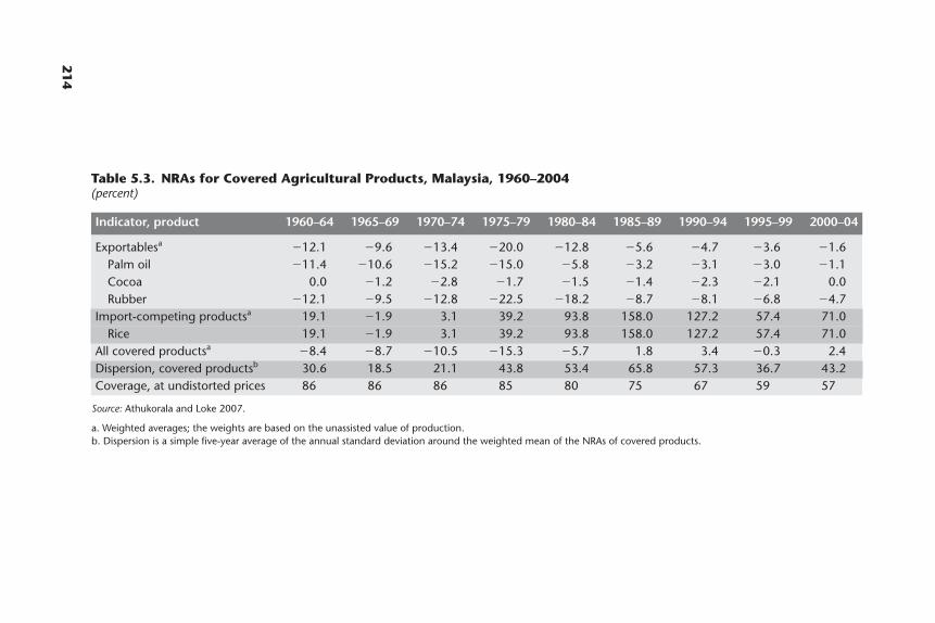
214
Table 5.3. NRAs for Covered Agricultural Products, Malaysia, 1960–2004(percent)
Indicator, product 1960–64 1965–69 1970–74 1975–79 1980–84 1985–89 1990–94 1995–99 2000–04
Exportablesa �12.1 �9.6 �13.4 �20.0 �12.8 �5.6 �4.7 �3.6 �1.6Palm oil �11.4 �10.6 �15.2 �15.0 �5.8 �3.2 �3.1 �3.0 �1.1Cocoa 0.0 �1.2 �2.8 �1.7 �1.5 �1.4 �2.3 �2.1 0.0Rubber �12.1 �9.5 �12.8 �22.5 �18.2 �8.7 �8.1 �6.8 �4.7
Import-competing productsa 19.1 �1.9 3.1 39.2 93.8 158.0 127.2 57.4 71.0Rice 19.1 �1.9 3.1 39.2 93.8 158.0 127.2 57.4 71.0
All covered productsa �8.4 �8.7 �10.5 �15.3 �5.7 1.8 3.4 �0.3 2.4Dispersion, covered productsb 30.6 18.5 21.1 43.8 53.4 65.8 57.3 36.7 43.2Coverage, at undistorted prices 86 86 86 85 80 75 67 59 57
Source: Athukorala and Loke 2007.
a. Weighted averages; the weights are based on the unassisted value of production.b. Dispersion is a simple five-year average of the annual standard deviation around the weighted mean of the NRAs of covered products.
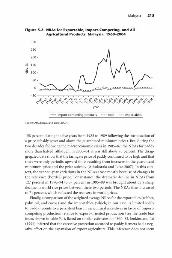
158 percent during the five years from 1985 to 1989 following the introduction ofa price subsidy (over and above the guaranteed minimum price). But, during thetwo decades following the macroeconomic crisis in 1985–87, the NRAs for paddymore than halved, although, in 2000–04, it was still above 70 percent. The disag-gregated data show that the farmgate price of paddy continued to be high and thatthere were only periodic upward shifts resulting from increases in the guaranteedminimum price and the price subsidy (Athukorala and Loke 2007). In this con-text, the year-to-year variations in the NRAs arose mostly because of changes inthe reference (border) price. For instance, the dramatic decline in NRAs from127 percent in 1990–94 to 57 percent in 1995–99 was brought about by a sharpdecline in world rice prices between these two periods. The NRAs then increasedto 71 percent, which reflected the recovery in world prices.
Finally, a comparison of the weighted average NRAs for the exportables (rubber,palm oil, and cocoa) and the importables (which, in our case, is limited solelyto paddy) points to a persistent bias in agricultural incentives in favor of import-competing production relative to export-oriented production (see the trade biasindex shown in table 5.4). Based on similar estimates for 1960–82, Jenkins and Lai(1991) inferred that the excessive protection accorded to paddy farmers had a neg-ative effect on the expansion of export agriculture. This inference does not seem
Malaysia 215
1960
1962
1964
1966
1968
1970
1972
1974
1976
1978
1980
1982
1984
1986
1988
1990
1992
1994
1996
1998
2000
2002
2004
NRA
, %
year
import-competing products total exportables
�50
0
50
100
150
200
250
300
Figure 5.2. NRAs for Exportable, Import-Competing, and AllAgricultural Products, Malaysia, 1960–2004
Source: Athukorala and Loke 2007.

216
Table 5.4. NRAs in Agriculture Relative to Nonagricultural Industries, Malaysia, 1960–2004(percent)
Indicator 1960–64 1965–69 1970–74 1975–79 1980–84 1985–89 1990–94 1995–99 2000–04
Covered productsa �8.4 �8.7 �10.5 �15.3 �5.7 1.8 3.4 �0.3 2.4Noncovered products 0.0 0.0 0.0 0.0 0.0 0.0 0.0 0.0 0.0All agricultural productsa �7.2 �7.5 �9.0 �13.0 �4.6 1.3 2.3 �0.2 1.3Non-product-specific assistance 0.0 0.0 0.0 0.0 0.0 0.0 0.0 0.0 0.0Total agricultural NRAb �7.2 �7.5 �9.0 �13.0 �4.6 1.3 2.3 �0.2 1.3Trade bias indexc �0.22 �0.06 �0.14 �0.31 �0.35 �0.33 �0.28 �0.12 �0.12NRA, all agricultural tradables �7.6 �7.9 �9.4 �13.7 �4.9 1.4 2.6 �0.2 1.5NRA, all nonagricultural tradables 7.4 7.0 7.1 6.5 5.2 3.9 2.8 2.0 0.9RRAd �14.0 �13.9 �15.5 �18.9 �9.6 �2.4 �0.3 �2.2 0.6
Source: Athukorala and Loke 2007.
a. Including product-specific input subsidies.b. Including product-specific input subsidies and non-product-specific assistance. The total assistance to primary factors and intermediate inputs, divided by the total value of
primary agriculture production at undistorted prices.c. The trade bias index is defined as (1 � NRAagx�100)�(1 � NRAagm�100) � 1, where NRAagm and NRAagx are the average percentage NRAs for the import-competing and
exportable parts of the agricultural sector, respectively.d. The RRA is defined as 100*[(100 � NRAagt)�(100 � NRAnonagt) � 1], where NRAagt and NRAnonagt are the percentage NRAs for the tradables parts of the agricultural and
nonagricultural sectors, respectively.
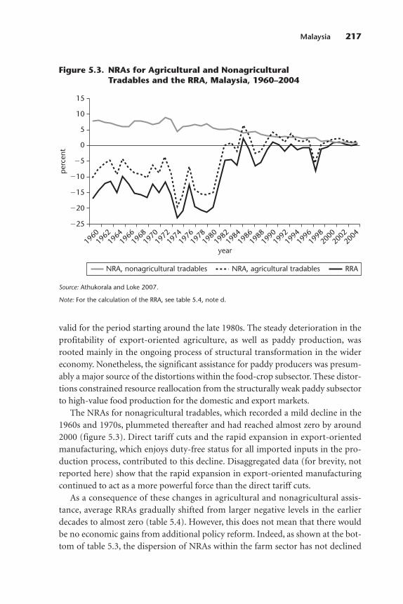
valid for the period starting around the late 1980s. The steady deterioration in theprofitability of export-oriented agriculture, as well as paddy production, wasrooted mainly in the ongoing process of structural transformation in the widereconomy. Nonetheless, the significant assistance for paddy producers was presum-ably a major source of the distortions within the food-crop subsector. These distor-tions constrained resource reallocation from the structurally weak paddy subsectorto high-value food production for the domestic and export markets.
The NRAs for nonagricultural tradables, which recorded a mild decline in the1960s and 1970s, plummeted thereafter and had reached almost zero by around2000 (figure 5.3). Direct tariff cuts and the rapid expansion in export-orientedmanufacturing, which enjoys duty-free status for all imported inputs in the pro-duction process, contributed to this decline. Disaggregated data (for brevity, notreported here) show that the rapid expansion in export-oriented manufacturingcontinued to act as a more powerful force than the direct tariff cuts.
As a consequence of these changes in agricultural and nonagricultural assis-tance, average RRAs gradually shifted from larger negative levels in the earlierdecades to almost zero (table 5.4). However, this does not mean that there wouldbe no economic gains from additional policy reform. Indeed, as shown at the bot-tom of table 5.3, the dispersion of NRAs within the farm sector has not declined
Malaysia 217
1960
1962
1964
1966
1968
1970
1972
1974
1976
1978
1980
1982
1984
1986
1988
1990
1992
1994
1996
1998
2000
2002
2004
per
cent
year
NRA, nonagricultural tradables NRA, agricultural tradables RRA
�25
�20
�15
�10
�5
0
5
10
15
Figure 5.3. NRAs for Agricultural and NonagriculturalTradables and the RRA, Malaysia, 1960–2004
Source: Athukorala and Loke 2007.
Note: For the calculation of the RRA, see table 5.4, note d.
much over time; so, there is still scope for improved resource reallocation if theassistance for paddy production is phased out.
Concluding Remarks
Malaysia stands out among developing countries because of the government’slong-standing commitment to the maintenance of a relatively open trade andinvestment policy regime. The government has persistently avoided heavy relianceon quantitative restrictions and other forms of nontariff protection. Tariffs ondomestic manufacturing and agriculture continue to be low relative to the corre-sponding tariffs in other developing countries. Export taxes, which were impor-tant sources of government revenue until about the mid-1980s, were reducedwhen the plantation subsector experienced severe cost pressure because of rapidgrowth and structural change under export-led industrialization. The averagelevel of import tariffs also declined significantly, notwithstanding the periodicupward adjustment in some tariffs and the special case of the heavy protection inthe automotive industry. The government’s record of commitment to openness isparticularly remarkable in that it reflects unilateral and voluntary policy choicesrather than pressure from major trading partners or from conditions imposed bymultilateral donor agencies or resulting from negotiations under the auspices ofthe World Trade Organization.
Nonetheless, there are notable anomalies in the incentive structure in Malaysiathat encourage the channeling of resources into inefficient activities. In particular,the tariff structure is characterized by a dualistic pattern whereby export-orientedproduction occurs within a virtual free trade regime, side-by-side with produc-tion predominantly oriented toward the domestic market in manufacturing andagriculture and assisted through tariff protection. The tariff rate structure is alsocharacterized by a high degree of dispersion because of high tariff peaks on a fewproduct lines and growing reliance on nonautomatic import licensing to regulatethe imports of a significant number of products that directly compete with thedomestic production carried out by public sector enterprises. This substantialdeparture from neutrality implies that there is ample room for policy discretion,as opposed to pure economic policy, in the effort to influence resource allocationin the economy.
The excessive assistance for paddy farmers remains a major distortion in agri-cultural incentives. In addition to the obvious welfare implications, this anomalypresumably hinders the diversification of domestic agriculture toward newdynamic product lines. Given the ongoing process of dramatic structural trans-formation in the economy that has ushered in an era of massive urban-to-rurallabor migration and generates cost pressures on traditional agriculture, the case
218 Distortions to Agricultural Incentives in Asia
for protecting paddy farmers on self-sufficiency grounds has lost relevance. Theoutright dismantling of assistance is a nonoption because of political economyconsiderations. Nonetheless, there is a strong case for replacing the existing com-plicated and costly incentives with direct income support for farmers. The fiscalburden of this support is unlikely to be high because the agricultural labor forcehas been rapidly depleting, and the incidence of rural poverty, though relativelyhigh by national standards, has been declining. This issue deserves additional sys-tematic analysis.
Notes
1. By 1984, the Federal Land Development Authority accounted for 28 percent of the 1.3 millionhectares under oil palms.
2. The bulk of the land classified as smallholding in these data involves farmers who participate inlarge government-run plantation schemes. Smallholders who do not participate in these schemesaccount for only 8 percent of the planted area measured in hectares.
3. Powerful forces on both the demand side and the supply side have underpinned this structuralshift. On the demand side, the internationalization of food habits—the growing significance ofimported processed items in consumption patterns in developed countries, as well as among large sec-tions of populations in many developing countries—appears to have played a key role. Factors such asinternational migration, the communications revolution, and tourism have contributed to the phenom-enon. This significant demand-side impetus seems to have been supported by important supply-sidedevelopments such as improvements in food technology, refrigeration facilities, and transportation thathave fostered international trade in various processed food products that are generally highly perishable.Indonesia is more well placed than Malaysia to benefit from this structural shift in world food trade givenits rich agricultural resource base and greater availability of labor (food processing and food packagingfor export are highly labor intensive).
4. The Federation of Malaya, comprising 11 states in the Malay Peninsula, secured independencefrom Britain on August 31, 1957. Sabah, Sarawak, and Singapore joined Malaya to form Malaysia onSeptember 16, 1963. Singapore left the federation in August 1965.
5. The emergence of three identifiable and mutually exclusive ethnic groups as distinct, self- conscious groups (Chinese, Indian, and Malay) stemmed in substantial part from the needs and prior-ities of British colonial policy (Ganguly 2003).
6. In the Rosentein-Rodan (1961) growth trajectory up to 1976 for 66 countries considered devel-oping countries at the time, Malaysia was classified in the low-growth category, together with Indonesia;the Republic of Korea; Singapore; Taiwan, China; and Thailand.
7. In a recent comprehensive study of the patterns and chronology of trade policy reforms, Sachsand Warner (1995) identify Malaysia as one of eight developing countries in which trade regimesremained open throughout the post–World War II period.
8. Unless otherwise noted, we have taken the tariff rates reported in this chapter from the latest(2003) tariff schedule available in the APEC Tariff Database.
9. In 2002, the simple average bound, unbound, and applied tariff rates were 19, 35, and 9.2 per-cent, respectively. All agricultural tariff lines were bound, but at much higher average levels than themanufacturing tariff lines.
10. Calculated as a percent share in total imports of the import value of the Harmonized Com-modity Description and Coding System 6 tariff lines affected by nontariff barriers.
11. The ringgit peg to the U.S. dollar was eventually abandoned in favor of a managed float system.The system went into effect on July 21, 2005.
Malaysia 219
References
Ahmad, T. M. A. T., and A. Tawang. 1999. “Effects of Trade Liberalization on Agriculture in Malaysia:Commodity Aspects.” CGPRT Centre Working Paper 46, Regional Co-ordination Center forResearch and Development of Coarse Grains, Pulses, Roots, and Tuber Crops in the Humid Trop-ics of Asia and the Pacific, United Nations Economic and Social Commission for Asia and thePacific, Bogor, Indonesia.
Anderson, K., M. Kurzweil, W. Martin, D. Sandri, and E. Valenzuela. 2008. “Measuring Distortions toAgricultural Incentives, Revisited.” World Trade Review 7 (4): 675–704.
APEC Tariff Database (Asia Pacific Economic Cooperation Tariff Database). Asia-Pacific EconomicCooperation. http://www.apectariff.org/ (accessed May 2008).
Ariff, M., and M. Semudram. 1990. “Malaysia.” In Trade, Finance, and Developing Countries: Strategiesand Constraints in the 1990s, ed. S. Page, 23–55. London: Harvester Wheatsheaf.
Athukorala, P.-C. 1991. “An Analysis of Demand and Supply Factors in Agricultural Exports fromDeveloping Asian Countries.” Weltwirtschaftliches Archiv 127 (4): 764–91.
———. 2001. Crisis and Recovery in Malaysia: The Role of Capital Controls. Cheltenham, UK: EdwardElgar.
———. 2002. “Malaysian Trade Policy and the WTO Trade Policy Review 2001.” World Economy 25(9): 1299–1317.
———. 2005. “Trade Policy in Malaysia: Liberalization Process, Structure of Protection, and ReformAgenda.” ASEAN Economic Bulletin 22 (1): 19–34.
———. 2006a. “International Labour Migration in East Asia: Trends, Patterns, and Policy Issues.”Asian-Pacific Economic Literature 20 (1): 18–39.
———. 2006b. “Post-Crisis Export Performance: The Indonesian Experience in Regional Perspective.”Bulletin of Indonesian Economic Studies 42 (2): 177–211.
Athukorala, P.-C., and S. K. Jayasuriya. 2003. “Food Safety Issues, Trade, and WTO Rules: A DevelopingCountry Perspective.” World Economy 26 (9): 141–62.
Athukorala, P.-C., and W.-H. Loke. 2007. “Distortions to Agricultural Incentives in Malaysia.” Agricul-tural Distortions Working Paper 27, World Bank, Washington, DC.
Athukorala, P.-C., and C. Manning. 1999. Structural Change and International Migration in East Asia:Adjusting to Labour Scarcity. Melbourne: Oxford University Press.
Athukorala, P.-C., and J. Menon. 1999. “Outward Orientation and Economic Performance: TheMalaysian Experience.” World Economy 22 (8): 1119–39.
Bank Negara Malaysia. various issues. Monthly Bulletin of Statistics. Kuala Lumpur: Bank NegaraMalaysia.
Barlow, C. 1978. The Natural Rubber Industry: Its Development, Technology, and Economy in Malaysia.Kuala Lumpur: Oxford University Press.
———. 1997. “Growth, Structural Change, and Plantation Tree Crops: The Case of Rubber.” WorldDevelopment 25 (10): 1589–1607.
Barlow, C., and S. Jayasuriya. 1987. “Structural Change and Its Impact on Traditional Agricultural Sectors of Rapidly Developing Countries: The Case of Natural Rubber.” Agricultural Economics1 (2): 159–74.
Corden, W. M. 1996. Pragmatic Orthodoxy: Macroeconomic Policies in Seven East Asian Economies. SanFrancisco: International Center for Economic Growth.
Economic Planning Unit. 2001. Eighth Malaysia Plan. Putrajaya, Malaysia: Economic Planning Unit,Prime Minister’s Department.
———. 2006. Ninth Malaysia Plan. Putrajaya, Malaysia: Economic Planning Unit, Prime Minister’sDepartment.
Ganguly, S. 2003. “Ethnic Policies and Political Quiescence in Malaysia and Singapore.” In GovernmentPolicies and Ethnic Relations in Asia and the Pacific, ed. M. E. Brown and S. Ganguly, 233–72. Cambridge, MA: MIT Press.
220 Distortions to Agricultural Incentives in Asia
Government of Malaysia. 1971. Second Malaysia Plan, 1971–1975. Kuala Lumpur: Government Printers.Jenkins, G. P., and A. Lai. 1989. Trade, Exchange Rate, and Agricultural Policies in Malaysia. World Bank
Comparative Study. Washington, DC: World Bank.———. 1991. “Malaysia.” In Asia. Vol. 2 of The Political Economy of Agricultural Pricing Policy, ed. A. O.
Krueger, M. Schiff, and A. Valdés, 67–106. World Bank Comparative Study. Baltimore: Johns Hopkins University Press; Washington, DC: World Bank.
Khoo, K. M., and D. Chandramohan. 2002. “Malaysian Palm Oil Industry at Crossroads and Its FutureDirection. Oil Palm Industry Economic Journal 2 (2): 10–15.
Levin, J. V. 1960. The Export Economies. New Haven, CT: Yale University Press.Lim, D. 1992. “The Dynamics of Economic Policy-Making: A Study of Malaysian Trade Policies and
Performance.” In The Dynamics of Economic Policy Reforms in South-East Asia and the South-WestPacific, ed. A. J. MacIntyre and K. Jayasuriya, 94–114. Singapore: Oxford University Press.
Lin, T. Y. 1984. “Inter-ethnic Restructuring in Malaysia, 1970–80: The Employment Perspective.” InFrom Independence to Statehood: Managing Ethnic Conflict in Five African and Asian States, ed. R. B.Goldman and J. Jayaratnam Wilson, 44–61. London: Frances Printer.
MacBean, A. I. 1989. “Agricultural Exports of Developing Countries: Market Conditions and NationalPolicies.” In The Balance between Industry and Agriculture in Economic Development, ed. N. Islam,129–64. London: Macmillan.
Meerman, J. 1979. Public Expenditure in Malaysia: Who Benefits and Why? New York: Oxford Univer-sity Press.
Ministry of Agriculture. 1997. Third National Agricultural Policy, 1998–2010. Kuala Lumpur: Ministryof Agriculture.
Ministry of Finance. 2005. Economic Report 2005/2006. Kuala Lumpur: Ministry of Finance.———. 2006. Economic Report 2006/2007. Kuala Lumpur: Ministry of Finance.———. various issues. Economic Report. Kuala Lumpur: Ministry of Finance.Myint, H. 1984. “Inward and Outward-Looking Countries Revisited: The Case of Indonesia.” Bulletin
of Indonesian Economic Studies 20 (2): 39–52.Ness, G. D. 1967. Bureaucracy and Rural Development in Malaysia. Berkeley, CA: University of California
Press.Pletcher, J. 1989. “Rice and Padi Market Management in West Malaysia, 1957–86.” Journal of Develop-
ing Areas 23 (April): 363–84.———. 1991. “Regulation with Growth: The Political Economy of Palm Oil in Malaysia.” World Devel-
opment 19 (6): 623–36.Power, J. H. 1971. “Structure of Protection in West Malaysia.” In The Structure of Protection in Develop-
ing Countries, ed. B. Balassa, 203–22. Baltimore: Johns Hopkins University Press; Washington, DC:World Bank.
Rosentein-Rodan, P. 1961. “International Aid for Underdeveloped Countries.” Review of Economics andStatistics 43 (2): 107–38.
Rudner, M. 1994. Malaysian Development: A Retrospective. Ottawa: Carleton University Press.Sachs, J. D., and A. Warner. 1995. “Economic Reforms and the Process of Global Integration.” Brookings
Papers on Economic Activity 26 (1): 1–118.Snodgrass, D. R. 1980. Inequality and Economic Development in Malaysia. Kuala Lumpur: Oxford
University Press.World Bank. 1955. The Economic Development of Malaya. Baltimore: Johns Hopkins University Press.WTO (World Trade Organization). 2006. Trade Policy Review: Malaysia. Geneva: WTO.Zubaidi, A. 1992. “The Welfare Cost of Malaysian Rice Policy under Alternative Regimes.” Malaysian
Journal of Economic Studies 29 (2): 1–12.
Malaysia 221


The economic performance of the Philippines has lagged behind that of mostother developing countries in Asia. Whereas the Philippine economy and agricul-tural sector performed moderately well in the 1960s and 1970s because of theearly advent of the Green Revolution in rice and the world commodity boom, thecountry has shown the lowest average growth rates in South and Southeast Asia ingross domestic product (GDP), gross value added (GVA) in agriculture, and agri-cultural exports over the past two decades (table 6.1).
Previous studies have argued that the country’s poor agricultural performancehas been caused largely by weaknesses in the policies and institutional frameworkgoverning the sector and less by real domestic and external market factors (David2003; Balisacan, Fuwa, and Debuque 2004). Government price and trade policieshave distorted economic incentives, and the choice of policy instruments has pro-moted rent seeking and raised the economic cost of government intervention. Thelack of market infrastructure, underinvestment in agricultural research, distor-tions in land markets because of the agrarian reform program, and other weak-nesses in governance have all contributed to the poor performance in the sector.
The declining trend in tariff protection since the 1980s through a series of uni-lateral tariff reform programs and multilateral and regional trade agreements arewell documented (Manasan and Pineda 1999; Aldaba 2005a, 2005b; Pasadilla2006). Ex ante assessments of the welfare impacts of trade liberalization that relyon computable general equilibrium models consistently report positive effects(Clarete 1991; Cororaton 2000; Habito and Cororaton 2000). International
223
6
THE PHILIPPINES
Cristina David, Ponciano Intal,and Arsenio M. Balisacan
The authors are grateful to Ernesto Valenzuela for computational assistance.
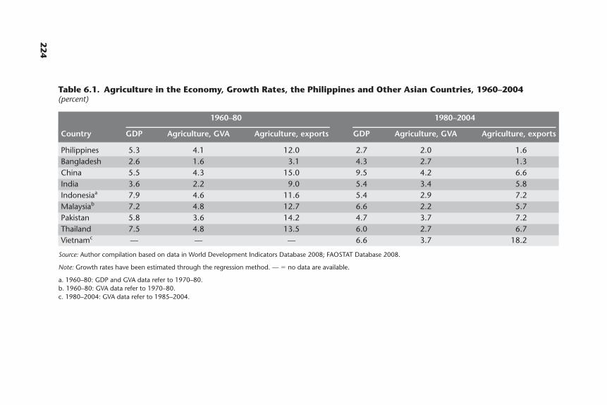
224
Table 6.1. Agriculture in the Economy, Growth Rates, the Philippines and Other Asian Countries, 1960–2004(percent)
1960–80 1980–2004
Country GDP Agriculture, GVA Agriculture, exports GDP Agriculture, GVA Agriculture, exports
Philippines 5.3 4.1 12.0 2.7 2.0 1.6Bangladesh 2.6 1.6 3.1 4.3 2.7 1.3China 5.5 4.3 15.0 9.5 4.2 6.6India 3.6 2.2 9.0 5.4 3.4 5.8Indonesiaa 7.9 4.6 11.6 5.4 2.9 7.2Malaysiab 7.2 4.8 12.7 6.6 2.2 5.7Pakistan 5.8 3.6 14.2 4.7 3.7 7.2Thailand 7.5 4.8 13.5 6.0 2.7 6.7Vietnamc — — — 6.6 3.7 18.2
Source: Author compilation based on data in World Development Indicators Database 2008; FAOSTAT Database 2008.
Note: Growth rates have been estimated through the regression method. — � no data are available.
a. 1960–80: GDP and GVA data refer to 1970–80.b. 1960–80: GVA data refer to 1970–80.c. 1980–2004: GVA data refer to 1985–2004.
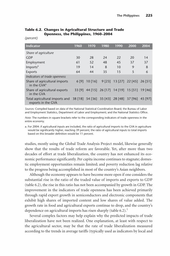
studies, mostly using the Global Trade Analysis Project model, likewise generallyshow that the results of trade reform are favorable. Yet, after more than twodecades of effort at trade liberalization, the country has not enhanced its eco-nomic performance significantly. Per capita income continues to stagnate; domes-tic employment opportunities remain limited; and poverty reduction lag relativeto the progress being accomplished in most of the country’s Asian neighbors.
Although the economy appears to have become more open if one considers thesubstantial rise in the ratio of the traded value of imports and exports to GDP(table 6.2), the rise in this ratio has not been accompanied by growth in GDP. Theimprovement in the indicators of trade openness has been achieved primarilythrough rapid export growth in semiconductors and electronic components thatexhibit high shares of imported content and low shares of value added. Thegrowth rate in food and agricultural exports continue to drop, and the country’sdependence on agricultural imports has risen sharply (table 6.2).1
Several complex factors may help explain why the predicted impacts of tradeliberalization have not been realized. One explanation, at least with respect tothe agricultural sector, may be that the rate of trade liberalization measuredaccording to the trends in average tariffs (typically used as indicators by local and
The Philippines 225
Table 6.2. Changes in Agricultural Structure and TradeOpenness, the Philippines, 1960–2004
(percent)
Indicator 1960 1970 1980 1990 2000 2004
Share of agricultureGDP 30 28 24 22 20 14Employment 61 52 48 45 37 37Importsa 19 14 8 10 9 8Exports 64 44 35 15 5 6Indicators of trade opennessShare of agricultural imports 6 [9] 10 [16] 9 [23] 13 [27] 22 [45] 26 [51]
in the GVAa
Share of agricultural exports 33 [9] 44 [15] 26 [17] 14 [19] 15 [51] 19 [46]in the GVA
Total agricultural imports and 38 [18] 54 [36] 35 [43] 28 [48] 37 [96] 45 [97]exports in the GVA
Sources: Compiled based on data of the National Statistical Coordination Board; the Bureau of Laborand Employment Statistics, Department of Labor and Employment; and the National Statistics Office.
Note: The numbers in square brackets refer to the corresponding indicators of trade openness in theentire economy.
a. For 2004: if agricultural inputs are included, the ratio of agricultural imports to the GVA in agriculturewould be significantly higher, reaching 39 percent; the ratio of agricultural inputs to total importsbased on this broader definition would be 11 percent.
international analysts) does not accurately reflect the extent or the direction ofchange in agricultural protection during recent decades.
The objective of our study is to quantify trends and patterns in agricultural dis-tortions from the early 1960s to 2004 and explain changes in these trends and pat-terns over time. In the next section, historical patterns in agricultural performanceand structural change are briefly described. The subsequent section examines theevolution of economy-wide and agriculture-specific policies that have distortedprice incentives in the sector. In the following section, we discuss the estimatedimpact of these policies on agricultural incentives. The penultimate section ana-lyzes the reasons behind policy choices, including the role of multilateral andregional trade agreements in the changes observed in recent years. Finally, we drawout the prospects for national policy reform, including the likely versus the desir-able policy direction through to 2020, the implications for the choice of policyinstruments and for the trend level in the distortions in agricultural incentives, andthe policy lessons for other developing and transition economies.
Agricultural Performance and Structural Change
Despite the relatively slow growth of the Philippine economy, the structural trans-formations that have occurred in the course of economic development have notbeen unusual. The decline in the contribution of agriculture to GDP was ratherslow from 1960 to 1980 (from 30 to 24 percent), but has become more rapid inrecent years (14 percent by 2004). The decline was accompanied by a steady dropin the share of the sector in total employment from 61 to 37 percent from 1960 to2000. The share has remained constant since then (table 6.2).
Unlike the rapid industrialization that characterized economic growth amongthe Asian tigers, however, the share of industry in the Philippines rose from 31 to39 percent in 1960–80, but then fell, reaching around 30 percent by 2004. Foodmanufacturing accounts for about 40 percent of the industrial sector. Half of thisshare consists of light processing of rice, maize, sugar, coconuts, livestock, andpoultry. Services have accounted for the largest contribution to GDP and totalemployment. While the growth in services has been driven primarily by domesticdemand for logistics, trading, and financial services, the rapid expansion in busi-ness process outsourcing has been changing the nature and the prospects forgrowth of the sector in recent years.
Growth rate and composition
Average annual growth rates in the GVA of major agricultural commodities havebeen quite erratic. The crop subsector grew rapidly prior to 1980 because of the
226 Distortions to Agricultural Incentives in Asia

Green Revolution in rice production and the world commodity boom, but it per-formed poorly thereafter, when the average growth rate was far below the growthrate of the population. The general slowdown may be observed across commodi-ties (table 6.3).
Rice is the main staple and the single most important crop. While the growthrate in rice production declined beginning in 1970, it was higher than the popula-tion growth rate. Rice continues to receive the bulk of public expenditure in thecrop subsector, and it has also benefited from increasing price protection (seebelow). Rice imports as a share of the total supply of rice have risen since the1980s, reflecting the effect of rising incomes and a shift away from maize as a foodstaple. Maize production experienced declining growth rates despite rising priceprotection and a rapid expansion in the demand for maize as feed in the pig meatand poultry industries.
The poorest performers are the traditional export crops such as coconuts,sugar, abaca, and tobacco, each of which showed a decreasing growth rate. In con-trast, nontraditional export crops such as bananas, pineapples, and mangoesshowed high growth rates. However, crop diversification, particularly towardhigh-value horticultural crops that raised the growth rates of the agricultural sec-tors in Chile, Thailand, and other developing countries, was not as pronounced inthe case of the Philippines.
The growth rate in livestock production accelerated after 1980. The contribu-tion of livestock to the GVA rose from 18 to nearly 25 percent within only25 years. This remarkable performance was generated by increasing domestic
The Philippines 227
Table 6.3. GVA Growth Rates, Major Agricultural Commodities,the Philippines, 1960–2004
(at constant 1985 prices, percent)
Product 1960–70 1970–80 1980–90 1990–2004
Crops 4.3 6.2 1.1 1.9Rice — 4.3 2.9 3.6Maize — 5.2 3.1 1.9Coconuts, including copra — 7.8 �3.9 1.1Sugar — 5.2 �1.8 4.1Bananas — 13.9 �1.8 4.0Other crops — 8.1 2.2 0.8
Livestock and poultry 3.1 3.1 5.7 4.4Livestock — 0.8 4.8 3.5Poultry — 8.5 7.5 5.7
Source: Compiled based on data of the National Statistical Coordination Board.
Note: — � no data are available.
demand, as well as productivity gains resulting from the shift to larger-scale oper-ations and the adoption of the new technologies embedded in imported breeds,veterinary medicines, and feed ingredients.
Agricultural trade and trade openness
Agriculture has historically been a net earner of foreign exchange. In the 1960s,agricultural exports accounted for nearly two-thirds of total exports, while agri-cultural imports accounted for less than 20 percent of total imports (table 6.2).The share of the sector in total exports began dropping sharply in the 1990s. By2004, the sector had ceased to be a net earner of foreign exchange; the ratio ofagricultural imports to agricultural exports rose from about one to three in the1960s and 1970s to around four to three in 2004. The relatively high growth rate ofagricultural exports in the 1970s arose mainly because of the world commodityboom and the expansion of nontraditional commodities (bananas, pineapples,and fishery products). However, world commodity prices fell sharply in the 1980sand have remained low until recently. Meanwhile, the growth in nontraditionalagricultural exports had leveled off by the 1990s. In stark contrast, neighboringcountries experienced a major export boom in cash crops during the same period.Thus, Thailand showed dramatic success in rubber, Malaysia in palm oil, andIndonesia in palm oil and cocoa.
The composition of agricultural exports has been changing in the Philippines.Coconut products has continued to be the top earner of foreign exchange,although their share in agricultural exports has decreased from nearly 70 percentin 1970 to less than 30 percent recently. The contribution of sugar to agriculturalexports, which was second only to coconuts in the 1970s (30 percent), is now only3 percent. The export value of bananas has been about twice that of sugar; andthis has been exceeded by the export value of pineapples since the 1990s. Fruitsand vegetables now account for nearly 30 percent of agricultural exports.2
The rapid growth in agricultural imports relative to agricultural exports hasstemmed from several factors. First, economic development has increased thedemand for food products exhibiting higher income elasticities. The Philippinesdoes not have a comparative advantage in many of these products, includingwheat, beef, milk, and other dairy products. Second, livestock and poultry requireagricultural inputs, such as soybean meal, maize, fishmeal, and other feed ingredi-ents, that are cheaper to import than to produce domestically. Third, agriculturalmodernization has led to greater reliance on modern manufactured inputs thatare mostly imported, such as fertilizers, agricultural chemicals, farm and agropro-cessing machinery, and veterinary medicines. Fourth, trade liberalization has gen-erated more imports of once highly protected agricultural commodities such asfruits and beef.
228 Distortions to Agricultural Incentives in Asia
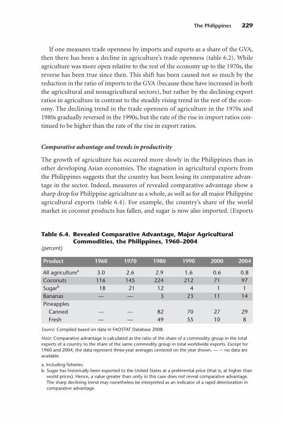
If one measures trade openness by imports and exports as a share of the GVA,then there has been a decline in agriculture’s trade openness (table 6.2). Whileagriculture was more open relative to the rest of the economy up to the 1970s, thereverse has been true since then. This shift has been caused not so much by thereduction in the ratio of imports to the GVA (because these have increased in boththe agricultural and nonagricultural sectors), but rather by the declining exportratios in agriculture in contrast to the steadily rising trend in the rest of the econ-omy. The declining trend in the trade openness of agriculture in the 1970s and1980s gradually reversed in the 1990s, but the rate of the rise in import ratios con-tinued to be higher than the rate of the rise in export ratios.
Comparative advantage and trends in productivity
The growth of agriculture has occurred more slowly in the Philippines than inother developing Asian economies. The stagnation in agricultural exports fromthe Philippines suggests that the country has been losing its comparative advan-tage in the sector. Indeed, measures of revealed comparative advantage show asharp drop for Philippine agriculture as a whole, as well as for all major Philippineagricultural exports (table 6.4). For example, the country’s share of the worldmarket in coconut products has fallen, and sugar is now also imported. (Exports
The Philippines 229
Table 6.4. Revealed Comparative Advantage, Major AgriculturalCommodities, the Philippines, 1960–2004
(percent)
Product 1960 1970 1980 1990 2000 2004
All agriculturea 3.0 2.6 2.9 1.6 0.6 0.8Coconuts 116 145 224 212 71 97Sugarb 18 21 12 4 1 1Bananas — — 3 23 11 14Pineapples
Canned — — 82 70 27 29Fresh — — 49 55 10 8
Source: Compiled based on data in FAOSTAT Database 2008.
Note: Comparative advantage is calculated as the ratio of the share of a commodity group in the totalexports of a country to the share of the same commodity group in total worldwide exports. Except for1960 and 2004, the data represent three-year averages centered on the year shown. — � no data areavailable.
a. Including fisheries.b. Sugar has historically been exported to the United States at a preferential price (that is, at higher than
world prices). Hence, a value greater than unity in this case does not reveal comparative advantage.The sharp declining trend may nonetheless be interpreted as an indicator of a rapid deterioration incomparative advantage.
have been limited to shipments to the high-priced U.S. market where they havebenefited from preferential access.) Even among nontraditional exports, such asbananas and pineapples, the shares of Philippine products on world markets havebeen declining since the mid-1980s.
The apparent loss in comparative advantage in agriculture is consistent withtrends reported in the indicators of labor and land productivity (David 2003).Labor productivity and land productivity both increased up to the late 1970s, par-ticularly during the Green Revolution in rice production. Whereas labor produc-tivity in agriculture as a whole recovered after a sharp drop in the early 1980s,labor productivity in the crop subsector has stagnated since then. Land productiv-ity in the crop subsector has grown slowly, particularly recently; yields per hectareamong traditional exports have generally remained constant or have declined.Higher growth in yields may be observed in rice, maize, and nontraditionalexports such as bananas, pineapples, and mangoes. However, productivity growthappears to have occurred in the livestock subsector, where international technol-ogy transfers, the greater scale of operations, and other management-relatedinnovations have increased production efficiencies significantly.
The Historical Evolution of Price Intervention Policies
It is helpful to describe policy trends since the 1960s. We begin with economy-wide policies and then turn to policies specific to agriculture.
Economy-wide policies
An import-substitution industrialization strategy dominated Philippine eco-nomic policies up to the late 1970s. The groundwork for the strategy involvedcomprehensive foreign exchange and import controls that were established inresponse to the severe balance of payments crisis that occurred in the late 1940s,shortly after the country’s political independence from the United States. The gov-ernment’s use of essentiality criteria in allocating foreign exchange and importlicenses during the 1950s encouraged domestic production at the final stages ofthe production of primarily nonessential and semiessential consumer goodsrather than backward integration in the production of raw materials and interme-diate and capital goods. These policies defended an overvalued peso and thusclearly penalized exports and agriculture.
A tariff system was instituted as a decontrol measure in 1957. However, the sys-tem largely preserved the bias in the incentive structure: tariffs depended onessentiality criteria. Import duties were higher for semifinished products than for
230 Distortions to Agricultural Incentives in Asia
raw materials and capital goods and even higher for finished products. Moreover,quantitative trade restrictions continued to be implemented on a substantialnumber of agricultural and nonagricultural products. Indeed, the balance of pay-ments problem encountered in the early 1960s rendered tariff protection redun-dant; import and foreign exchange controls were predominant. The adoption of amultiple exchange rate system added to the penalization of traditional agricul-tural exports.
In the early 1970s, a balance of payments crisis resulted in a major devaluationof the peso. By then, the high economic cost of the import-substitution industri-alization strategy and the detrimental effects of the strategy on export potentialwere becoming well recognized. Nonetheless, the policy response was to provideindustrial incentives directly to selected firms, including exporting enterprises,through tax holidays and the like (Bautista and Tecson 2003). No attempt wasmade to modify the highly protective tariff system. In fact, tariff protection wasraised on many import-competing products, such as primary and processed foodand agricultural products, chemical products, metal manufactures, electricalappliances, machinery, and transport equipment. During this period, the Philippines had the highest average tariff rate in Southeast Asia (Intal and Power1991). In addition, the share of imported products (based on the seven-digitPhilippine Standard Industrial Classification) subject to quantitative restrictionsrose from 26 percent in 1970 to 52 percent in 1980 (Bautista and Tecson 2003).
In the early 1980s, the government adopted various structural adjustment andstabilization measures to correct fundamental distortions in economic incentivesand imbalances in the external and public sector accounts. These measuresincluded the liberalization of the foreign exchange market, as well as trade policyreforms to remove quantitative trade restrictions and reduce the level and disper-sion of tariffs. The tariff reform program—the first of the unilateral trade liberal-ization programs—was instituted in 1981 to respond to a condition for a WorldBank structural adjustment loan package. Under the program, the dispersion oftariff rates was to be reduced by lowering the peak tariff rates of 100 and 70 per-cent to 50 percent in two stages, while the low tariff rates were to be raised to atleast 10 percent by 1985. Overall, the average tariff dropped substantially, from43 percent in 1980 to 28 percent in 1985. To complement the tariff reform pro-gram, import licensing was also to be relaxed gradually. The plan was to removeselected nontariff barriers over three years. From the original list of 1,300 importitems banned or requiring prior approval by the Central Bank of the Philippinesand other government agencies, 264 items were to be removed in 1981, another 610in early 1982, and the remainder by the end of 1983 (Bautista and Tecson 2003).
However, the balance of payments crisis of 1983, following Benigno Aquino’sassassination, stalled these initiatives. The government again adopted comprehensive
The Philippines 231

import and foreign exchange controls, rendering the tariff reductions ineffective.Commercial banks were required to turn over their foreign exchange receipts tothe central bank so that priority imports and other payments could be facilitated.A 5 percent general import tax was imposed in November 1983 to generate gov-ernment revenue and discourage imports; the rate was raised to 8 percent in April1984 and then to 10 percent two months later. Additional export duties rangingfrom 2 to 5 percent were levied on traditional export products from November1983 to December 1984, and an economic stabilization tax of 30 percent waslevied on all exports briefly in 1984.
To curtail imports and capital outflows, the peso was devalued on successiveoccasions, and, in late 1984, the exchange rate was allowed to float. Tax reforms in1983–85 gradually unified the sales tax on imports and import substitutes, remov-ing one source of import protection. The markup rate (which increases the taxbase for imports) on essential and semiessential goods was reduced to a uniform25 percent in 1985 and removed altogether in 1986.
Under the new government of Corazon Aquino, the trade liberalization pro-gram was revived in 1986. Export taxes on all commodities except logs were abol-ished. The process of lifting import licensing was accelerated: 951 import itemswere liberalized in 1986, 170 in 1987, and another 209 in 1988. Of the remaining673 restricted import items, those on list A were scheduled for immediate liberal-ization, and 94 had been liberalized by the end of 1989; those on list B were sched-uled for review. However, those on list C (114 items) continued to be restricted fornational security or health reasons.
The second tariff reform program was launched in July 1991 through an exec-utive order. This was intended to reduce the range of tariff rates to 30 percent overa five-year period. Although about 10 percent of all commodity lines were stillsubject to tariffs outside the target range, the average tariff rate had declined from33 percent in 1990 to 27 percent by the end of 1995.
As part of the second tariff reform program, an executive order was also issuedto convert the quantitative restrictions on 153 agricultural products into tariffequivalents and realign the tariffs on 48 commodities. However, the order wassoon reversed based on the Magna Carta of Small Farmers, which was passed in1991 and, among other provisions, allowed the government blanket authority torestrict agricultural imports that competed with domestic production.
The price and trade protection supplied for most major import-competingagricultural products were largely untouched by the series of unilateral trade lib-eralization measures introduced beginning in the late 1980s, however. DespiteWorld Trade Organization (WTO) and regional trade agreements, nontarifftrade barriers continue to distort the prices of some of the most important commodities.
232 Distortions to Agricultural Incentives in Asia
Agriculture-specific policies up to the mid-1980s
Although they may be generally levied on all agricultural products and inputs,import tariffs are more commonly applied only on agricultural inputs and agri-cultural products that are not locally produced in any significant quantity. Suchproducts include milk, wheat, and soybeans. Tariff protection for nontraded com-modities and for exportable products that are competitive in world markets isredundant because of prohibitive transport and other marketing costs.
Over the period under study, a wide variety of policy instruments that influ-ence price incentives were applied to major agricultural commodities. Theseincluded government monopoly control over international trade and domesticmarketing operations, import bans, quantitative trade restrictions, import licens-ing, export taxes, and export bans.3 Furthermore, despite serious efforts at unilat-eral trade liberalization, some of the policy instruments applicable to the moreimportant import-competing agricultural products were kept largely intact.Indeed, some of the interventions had a long history going back to the U.S. Com-monwealth period that began in 1935. During the martial law era under Marcos,which began in late 1972, the government had considerably more leeway in inter-vening in setting prices and in marketing in agriculture, and it exercised thispower. In the following discussion, we therefore distinguish between the evolutionof agricultural price intervention policies before and after 1986, when the Cora-zon Aquino administration took over the reins of government.
Rice and maizeWhen bad weather caused a drastic shortfall in staple food grains in 1936, theNational Rice and Corn Administration was established to ensure low, stableprices for consumers and adequate price incentives for farmers. To achieve theseconflicting objectives, the agency was granted monopoly control over the importsand exports of rice and maize, as well as budgetary support and a credit line toundertake domestic market operations to defend price floors and retail ceilingsand narrow the geographical and seasonal dispersion of prices.
Because of high world commodity prices in the early 1970s, the governmentmonopoly control over food commodities through this agency, which had beenrenamed the National Food Authority, was expanded beyond rice and maize toallow the tariff-free importation of wheat, soybeans, soybean meal, ruminant live-stock, and beef.
SugarThe sugar industry has historically been assisted more than any other industry.This is because of the preferential access assigned to Philippine sugar in theU.S. market beginning in 1902 and the authority entrusted to the Philippine
The Philippines 233
government to administer its sugar export quota to the United States through theJones-Costigan Act passed by the U.S. Congress in 1934.
Initially, the domestic quota system was established for the orderly distributionof the U.S. quota among sugar producers. In the 1960s, the quota system was alsocharged with reducing the burden on domestic consumers of the higher exportprices resulting from the 1962 devaluation and the greater U.S. quota allocationarising because of the Cuban missile crisis (given Cuba’s role as a major pro-ducer). Under this system, which is still in force, producers are paid a compositeprice derived as an average of the export price, a lower domestic wholesale price,and a reserve price weighted by the quantity allocations targeted for U.S. exports,the domestic market, and as a reserve.
When the Laurel-Langley Agreement—a trade agreement between the UnitedStates and the Philippines—expired in 1974, sugar trading was effectively nation-alized, first under Philippine Exchange Inc. and subsequently under the NationalSugar Trading Corporation. The latter was the sole Philippine wholesale buyerand seller of sugar in both the domestic and international markets until the end ofthe Marcos administration in early 1986. It also established new refineries, oper-ated sugar market outlets, and acquired leading enterprises involved in the trans-port, storage, and handling of sugar for export.
Export commoditiesExcept in the aftermath of the 1970 devaluation and the sharp increases in worldcommodity prices in the mid-1970s, there have been few attempts to intervene inthe production and trade of exportable agricultural products. Initially, as part ofstabilization measures, export taxes from 4 to 6 percent were imposed on majoragricultural exports and other primary exports; to generate revenue, these taxesremained in place until the mid-1980s. The higher rate of 6 percent was imposedon traditional exports of coconuts (copra) and centrifugal sugar to promote moreprocessing of agricultural exports. The lower rate of 4 percent was applied tococonut oil, desiccated coconuts, coconut cake and meal, molasses, abaca,bananas, and pineapple products.4
In 1974, because of the world commodity boom, additional premium dutieswere briefly imposed on exports. The duties ranged from 20 to 30 percent of thedifference between the ruling export price and a February 1974 base price. Wind-fall gains from the devaluation and the commodity boom were thus partiallysiphoned off from the producers of these agricultural and primary exportablecommodities.
The Coconut Consumers Stabilization Fund implemented an additional levyon the coconut industry in 1973 (commonly known as the coco levy). The levywas aimed partly at protecting domestic consumers from a sharp rise in the price
234 Distortions to Agricultural Incentives in Asia

for coconut oil on the world market and partly at raising funds for the develop-ment of the coconut industry.5 There was also a belief that taxing or restrictingcoconut exports might be beneficial because the Philippines was thought to pos-sess some monopoly power on the world market. (While the Philippinesaccounted for a high share of total world coconut and coconut oil exports, anymonopoly power was curtailed by the fact that coconut oil comprises only about7 percent of the world lauric oil market.) Some of the revenue from this levy wasused to buy up 80 percent of the coconut oil milling industry, which was thenreorganized under a newly created and privately owned company, UnitedCoconut Oil Mills. This company eventually acted as a monopsonist buyer ofcoconut in the farm sector. When the world prices of coconut oil fell in 1982, thelevy was lifted, only to be replaced by a ban on coconut exports to protect coconutoil mills.
Agriculture-specific policies after 1986
World commodity prices began to fall in the late 1970s. However, the policies andinstitutions established to cope with high world prices persisted because theyproved to be a convenient means of raising revenues. The related measures heavily taxed farmers so as to support private interests and cover bureaucraticinefficiencies (David 1983). In 1986, under the new Corazon Aquino govern-ment, several of the direct government price and market regulations were finallydismantled.
The reforms under Corazon AquinoExport taxes, including the coconut export ban, were abolished, and the NationalFood Authority’s monopolistic controls over international trade in wheat, soybeans, soybean meal, and meat were removed, limiting the authority’s functions to rice and maize (also the case prior to martial law). The authority’sdomestic marketing operations were also effectively reduced because financialsupport had to be provided mostly through annual budgetary allocations ratherthan profits from imports.
The National Sugar Trading Corporation was eventually replaced by the SugarRegulatory Administration, which functioned primarily as a market regulator.It mainly allocated U.S. sugar quotas, determined the allowable quantities ofimports, the importers, the amounts to be sold in the domestic market, and theamounts to be kept in reserve. It also performed developmental functions, such asresearch and extension, but it has ceased to engage in direct market operations.
Quantitative trade restrictions on fertilizers were removed, and tariffs onmajor agricultural inputs were lowered substantially. However, the monopsonist
The Philippines 235
control exercised by United Coconut Oil Mills over the coconut market has con-tinued; the government’s attempts to wrest ownership of this entity have beenbogged down in court proceedings.
Despite efforts at trade liberalization in the late 1980s, most major importableagricultural commodities that are also produced in significant volumes in thePhilippines are still subject to quantitative import restrictions, particularly thosecommodities protected by laws passed by Congress. Efforts to remove the quanti-tative restrictions were preempted by the passage of the Magna Carta of SmallFarmers in 1991, which provided blanket authority to restrict agricultural importsthat competed with domestic production. In addition, the Seed Law was passed toregulate imports of seeds and other planting materials.
The Uruguay Round Agreement on AgricultureThe country’s ratification of the Uruguay Round Agreement on Agriculture in themid-1990s promised to set a decisive path toward trade liberalization in the sec-tor. It aimed to replace all quantitative restrictions by tariffs, impose a ceiling ontariff rates, and reduce tariff protection. Unfortunately, the specific agreementsand the manner of implementation did not live up to the promise (David 1994,2003).
First, one of the most heavily regulated commodities, rice, was exempted fromtariffication until 2004, which is similar to the situation in Japan and the Republicof Korea.6
Second, the quantitative trade restrictions lifted by executive order in April1996 were replaced by tariff rate quotas that initially raised out-of-quota tariffs tothe maximum (bound) tariffs allowed under the WTO commitments, while thein-quota tariffs were set mostly at the levels existing in 1995. The initial out-of-quota tariffs of 100 percent were typically higher than the nominal protectionrates implied by the quantitative restrictions in 1990–94. They were also higherthan the book tariff rates under the executive order that set out the unilateral tar-iff reductions on a wide range of agricultural and industrial goods. Despite thereductions in the out-of-quota tariffs scheduled for no later than 2004, the tariffrates are still equal to or higher than the tariff rates in 1995, and they are higherthan the government’s target average tariff of 5 percent.
Furthermore, whereas the quantitative restrictions on primary and lightlyprocessed products were supposed to be lifted, the tariffs were raised on a numberof imported agricultural products that are considered substitutes for other com-modities (for example, feed wheat and barley as substitutes for maize). Tariffswere also increased to this same level on more heavily processed products usingthese commodities as main raw materials (for example, preserved and cannedmeat products, milled rice and maize, and roasted coffee).
236 Distortions to Agricultural Incentives in Asia
Third, the manner in which the minimum access volume provision or the tariffrate quota system of the Uruguay Round Agreement on Agriculture was adminis-tered for major import-competing commodities simply perpetuated quantitativetrade restrictions. The quantities that may be imported at the lower in-quota tariffswere sometimes changed to prevent domestic prices from rising sharply wheneverproduction shortfalls occurred. Thus, in effect, the tariffs were no different thanquantitative restrictions. For certain commodities, the right to import was assignedmostly to domestic producers of the same products (for example, pork and poul-try), and these producers have often chosen not to utilize their import allocation soas to protect their domestic production. Moreover, because most of the minimumaccess volumes were lower than the demand for imports at the in-quota tariff rateand because the right to import the minimum access volumes was not auctioned,large quota rents accrued to those entities given access to the minimum access vol-ume allocation, at least during the early period of implementation.
Finally, the agreement’s lack of provision for the market operations of paras-tatals allowed the Sugar Regulatory Administration to continue exercising its reg-ulatory authority over import levels and the market destinations of domesticsugar production. In fact, the domestic market operations of the National FoodAuthority in support of producer prices were expanded in the late 1990s toinclude sugar.7
Regional trade agreementsIn 1992, the six member countries of the Association of Southeast Asian Nationsat the time (Brunei Darussalam, Indonesia, Malaysia, the Philippines, Singapore,and Thailand) agreed to form a free trade area. The aim was to reduce tariffs tobetween 0 and 5 percent and to abolish quantitative trade restrictions and othernontariff trade barriers by 2010. Under the related Common Effective PreferentialTariff Scheme, unprocessed agricultural products were commonly included in asensitive products list that allows trade liberalization to begin later (between 2001and 2003), though the 0 to 5 percent tariff targets are still to be reached by 2010. Arecent study has indicated, however, that the effective protection rates in agricul-ture have been largely unaffected by the scheme thus far (Pimentel 2006).
Unlike other free trade areas, which usually delay or totally exclude trade liber-alization in agriculture, the agreement signed between China and the free tradearea of the Association of Southeast Asian Nations in 2002 specifically covered asignificant portion of all agricultural products through the Early Harvest Program. The agreement called for the elimination of tariffs on live animals, meatand edible meat offals, fish, dairy products, other animal products, live trees, vegetables, fruits and nuts, and a few commodities in other categories of the Harmonized Commodity Description and Coding System. The changes were to
The Philippines 237
be implemented starting in January 2004 and were to be in full operation no laterthan January 2006 in the free trade area, although exceptions were allowed insome cases depending upon negotiations with China.
The Philippines signed an Early Harvest Program Agreement with China inearly 2006. The agreement covered proportionately fewer commodities than theagreements reached by other countries of the Association of Southeast AsianNations, suggesting that there is less interest in the Philippines in engaging withChina in more open agricultural trade (Pasadilla 2006). In general, consumers willbenefit from lower prices on covered commodities, while producers of exportablebananas, pineapples, mangoes, other tropical fruits, and coconut and coconut oilare expected to gain from greater access to the vast Chinese market. However, pro-ducers of vegetables, leguminous crops, and pig meat, together with producers offruits for local markets, will be hurt, at least initially, by the entry of relativelycheap frozen meat and other meat products, potatoes, carrots, onions, garlic,peanuts, pears, apples, oranges, and other fruits and vegetables from China.
Estimates of Nominal and RelativeRates of Assistance
Measuring the distortions in incentives caused by price and trade policies has hada long history in the Philippines. The first effort was undertaken by Power (1971)in a study on the situation in 1965. This was followed by studies conducted byNorma Tan (1979), on 1974; Elizabeth Tan (1994), on the 1980s; Manasan andPineda (1999), on the 1990s; and Aldaba (2005a, 2005b), on recent years. Thesestudies estimated the effective protection rates in all industries, both agriculturaland nonagricultural. However, the main interest and analysis were concentratedon the manufacturing sector.
The first studies on agricultural protection were conducted by David (1983),Intal and Power (1991), and, more recently, David (2003). Unlike the industrialprotection studies that quantified the effects of tariffs and indirect sales taxes,these agricultural protection studies were based on domestic and border pricecomparisons. This enabled the effects of nontariff trade barriers to be measuredand redundancy in the tariffs, if any, to be taken into account. The indirectimpacts of industrial protection and other economy-wide factors on agriculturalincentives (through effects on the exchange rate) were also analyzed.
Methodology
In this study, we estimate nominal rates of assistance (NRAs) in industries. Themain focus of our study’s methodology is government-imposed distortions thatcreate a gap between domestic prices and the prices that would emerge under free
238 Distortions to Agricultural Incentives in Asia
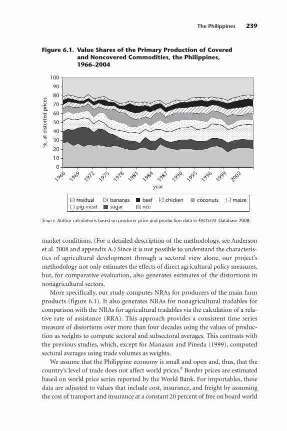
market conditions. (For a detailed description of the methodology, see Andersonet al. 2008 and appendix A.) Since it is not possible to understand the characteris-tics of agricultural development through a sectoral view alone, our project’smethodology not only estimates the effects of direct agricultural policy measures,but, for comparative evaluation, also generates estimates of the distortions innonagricultural sectors.
More specifically, our study computes NRAs for producers of the main farmproducts (figure 6.1). It also generates NRAs for nonagricultural tradables forcomparison with the NRAs for agricultural tradables via the calculation of a rela-tive rate of assistance (RRA). This approach provides a consistent time seriesmeasure of distortions over more than four decades using the values of produc-tion as weights to compute sectoral and subsectoral averages. This contrasts withthe previous studies, which, except for Manasan and Pineda (1999), computedsectoral averages using trade volumes as weights.
We assume that the Philippine economy is small and open and, thus, that thecountry’s level of trade does not affect world prices.8 Border prices are estimatedbased on world price series reported by the World Bank. For importables, thesedata are adjusted to values that include cost, insurance, and freight by assumingthe cost of transport and insurance at a constant 20 percent of free on board world
The Philippines 239
0
30
20
10
70
60
40
50
year
%,a
t di
stor
ted
pric
es
100
90
80
1966
1969
1972
1975
1978
1981
1984
1987
1990
1993
1996
1999
2002
residual bananas beef chicken coconuts maizepig meat sugar rice
Figure 6.1. Value Shares of the Primary Production of Coveredand Noncovered Commodities, the Philippines,1966–2004
Source: Author calculations based on producer price and production data in FAOSTAT Database 2008.
prices. We have not chosen the country’s officially recorded unit values forimports or exports because foreign exchange controls, export taxes, and othertaxes mean that the export unit data are significantly undervalued, particularly upto the mid-1980s. For rice, maize, and sugar, the import unit data may be eitherovervalued (in the case of imports by the National Food Authority) or underval-ued (because private importers seek to lower their tariff payments by underin-voicing). There were also no imports of some importable products during variousperiods.
Rice, maize, sugar, pig meat, beef, and poultry are consistently classified asimportables even though there were no imports of these products during someyears. In the case of sugar, the first imports occurred only in the 1990s, but, even inthe 1960s and 1970s, exports of sugar were confined to the high-priced U.S. mar-ket, where the Philippines has had preferential access, and were not competitive atthe free-market world price. Sugar is thus also treated as an importable.
In the absence of detailed time series data on marketing costs, we define thedomestic price as the wholesale price that is the closest to the same point of theborder price in the marketing chain.
For most of the agricultural commodities for which we compare the domesticand border prices, we rely on the data for the commodity that is internationallytraded and is lightly processed rather than the data on the primary product sold atthe farmgate. Thus, we take milled rice versus paddy; raw or refined sugar versussugarcane; frozen pig meat, beef, or poultry versus hog, cattle, or chicken birds. Inthe case of sugar, the rates of the protection received by farmers and millers are thesame because the revenues derived from the sale of raw and refined sugar in boththe domestic and U.S. markets are shared proportionately between the two at theratio of 70 to 30.9 The ratio of the farm price of paddy to the retail price of rice didnot change significantly, suggesting that farmers and rice millers, together withtraders, share proportionately in the protection accorded the rice industry. For rice,maize, pig meat, beef, and poultry, we assume that the NRAs of the processed prod-ucts and the farm products are equivalent. Indeed, the import tariffs on the farmproducts are generally the same as the tariffs on the lightly processed varieties.
Aside from the major agricultural commodities specified above, we have esti-mated the NRAs for other, noncovered crops within the sector. Since price com-parisons are more difficult to perform in the case of noncovered exportables,including pineapples, mangoes, abaca, and tobacco, we have assumed that the relevant average NRAs are zero or equal to the export tax whenever this applies.For products that are nontraded because of prohibitive marketing costs, such asroots and tuber crops, we have assigned zero NRA values.10 For the many import-competing vegetables, fruits, and other minor crops, we assume that the NRAs forthe group are the same as the average NRAs for covered importable products.11
240 Distortions to Agricultural Incentives in Asia

We also assume that the weights are one-third each for exportables, importables,and nontradables in the noncovered part of farm production (which, in aggre-gate, amounts to around one-fifth of the agricultural sector’s value of productionat undistorted prices).
For importable nonagricultural products, the NRAs are generally based onbook tariff rates, apart from the case of lightly processed food manufacturingindustries in which the NRAs are based on price comparisons, including rice andmaize milling, sugar milling and refining, coconut oil production and refining,and so on.12 For a number of nonagricultural primary products in fishing,forestry, and mining, we use the export taxes that applied from 1970 to 1985. Thedefinitions we use for a product’s tradability and for industry weights are the samefor the agricultural and nonagricultural sectors.
NRAs in agriculture
Our estimates of the NRAs for agricultural commodities from 1962 to 2004 aresummarized in table 6.5. Although the estimated NRAs are highly variable overtime (see the annual estimates in David, Intal, and Balisacan 2007), several generalpatterns emerge from the five-year averages shown in the table.
First, import-competing products have enjoyed much more assistance thanexportables. Coconut production has been penalized by negative NRAs over theentire period of our study, averaging around �20 to �25 percent from the 1970sto the mid-1980s. Besides the multiple exchange rate policy prior to 1970 (notmeasured here), this was caused by the imposition of several measures, includingthe export tax, the coconut levy, and the coconut export ban that were aimed atsiphoning off windfall gains from the 1970 devaluation; the subsequent worldcommodity boom of 1973–74 that was incompletely transmitted to the domesticmarket; and the lower raw material costs for the coconut oil milling industry.Despite the abolition of these policy instruments in 1986, however, coconut farm-ers continued to be implicitly taxed, albeit at a lower rate of around 15 percent ofborder prices. Evidently, the government’s failure to dismantle the ownership of70 to 80 percent of the coconut oil milling industry by United Coconut Oil Millshas allowed this entity to maintain its monopsonist power over the domestic pricefor coconuts even now.
Second, among import-competing commodities, the level of the NRAs has dif-fered significantly, and the differences have widened between two groups ofimport-competing products: the NRAs for the most important commodities—rice, maize, and sugar—have increased, while those for the many more minor, buthigher-valued commodities have declined. Each of these commodities is consid-ered in detail below.
The Philippines 241

242
Table 6.5. NRAs for Covered Agricultural Products, the Philippines, 1962–2004(percent)
Indicator, product 1962–64 1965–69 1970–74 1975–79 1980–84 1985–89 1990–94 1995–99 2000–04
Exportablesa �9.0 �7.6 �14.3 �14.6 �22.6 �16.5 �11.4 �5.4 �8.7Coconuts �24.4 �20.2 �25.3 �16.7 �27.1 �20.6 �15.3 �7.8 �14.1Bananas 0.0 0.0 �4.0 �4.0 �4.0 �0.8 0.0 0.0 0.0
Import-competing productsa �1.1 17.4 �5.6 �5.8 2.2 30.2 25.1 48.1 31.4Rice �3.4 �1.4 �9.7 �17.9 �16.3 14.5 20.9 52.7 50.7Maize 0.5 38.4 14.0 24.3 20.1 59.8 62.6 78.5 54.5Sugar �8.2 120.7 �11.7 �1.7 59.5 123.2 49.3 97.2 79.3Beef 15.0 15.0 12.0 10.0 5.0 17.0 28.0 28.0 10.0Pigs �30.0 13.6 3.2 �5.5 35.8 51.0 25.1 20.6 �8.3Chicken 8.9 67.1 28.9 28.1 38.4 42.9 56.5 42.2 52.1
All covered productsa �1.9 15.3 �6.5 �8.1 �5.1 16.1 17.5 37.9 24.9Dispersion, covered productsb 17.1 29.6 25.2 22.3 28.6 29.9 27.5 27.9 30.4Coverage, at undistorted prices 78 79 79 74 73 73 77 77 80
Source: David, Intal, and Balisacan 2007.
a. Weighted averages; the weights are based on the unassisted value of production.b. Dispersion is a simple five-year average of the annual standard deviation around the weighted mean of the NRAs of covered products.

The Philippines 243
Third, the increasingly higher NRAs observed since the 1980s may be partlycaused by the government’s efforts to reduce the burden of the adjustment of theagricultural sector to a long-term decline in world commodity prices. This declin-ing trend is visible in real domestic prices relative to real world prices for severalcommodities noted in David, Intal, and Balisacan (2007).
Fourth, the dispersion of NRAs among agricultural products within the farmsector (measured according to the standard deviation of these NRAs and reportedin table 6.5) has not diminished. The trade bias index has not diminished either(table 6.6), indicating that the NRAs for importable farm products have persist-ently remained above the NRAs for exportables. Both of these indicators implythat the efficiency of resource use within the farm sector has been substantiallycompromised by agricultural policies.
Fifth, the NRAs have fluctuated from year to year, mostly in response to worldprice changes and sometimes in response to exchange rate adjustments (see fig-ure 6.2). For example, the NRAs for import-competing agricultural products werebelow the trend in 1973–74 and 1980, when international prices were high, butabove the trend in the mid-1980s, when international prices were low. This sug-gests that domestic price stabilization has been an important objective of agricul-tural price and trade policy. Table 6.7 shows that the estimated coefficients of thevariation in domestic prices tended to be considerably lower than the correspon-ding coefficients in world prices, particularly among major import-competingcommodities.
RiceThe trends in the NRAs for rice reflect the inability of the National Food Author-ity to attain simultaneously its inherently conflicting objectives of providing lowprices to consumers and remunerative incentives to farmers. Prior to the late1980s, the domestic price of rice was, on average, about equal to the long-termlevel of the border price. The negative protection from the 1970s to the early1980s was caused by the unusually high world prices during this period. Thisdid not discourage farmers, however, because the Green Revolution in rice andthe land reform in rice farming were transforming tenant farmers to owner-operators.13
Because of the drop in the world price of rice, a sharp fall in irrigation invest-ments, and stagnation in the yield potential of newer modern varieties, growth inthe demand for rice increased more rapidly than rice production beginning inthe late 1980s. The NRAs for rice became positive; they had risen to about 50 per-cent by the early 2000s. This occurred despite the most significant rice importsever, which reflected the country’s rising comparative disadvantage in rice pro-duction.
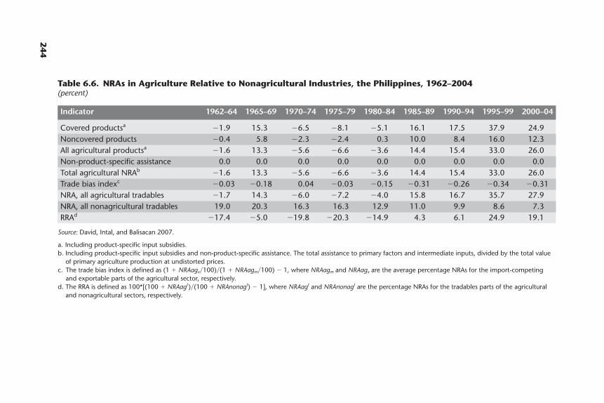
244
Table 6.6. NRAs in Agriculture Relative to Nonagricultural Industries, the Philippines, 1962–2004(percent)
Indicator 1962–64 1965–69 1970–74 1975–79 1980–84 1985–89 1990–94 1995–99 2000–04
Covered productsa �1.9 15.3 �6.5 �8.1 �5.1 16.1 17.5 37.9 24.9Noncovered products �0.4 5.8 �2.3 �2.4 0.3 10.0 8.4 16.0 12.3All agricultural productsa �1.6 13.3 �5.6 �6.6 �3.6 14.4 15.4 33.0 26.0Non-product-specific assistance 0.0 0.0 0.0 0.0 0.0 0.0 0.0 0.0 0.0Total agricultural NRAb �1.6 13.3 �5.6 �6.6 �3.6 14.4 15.4 33.0 26.0Trade bias indexc �0.03 �0.18 0.04 �0.03 �0.15 �0.31 �0.26 �0.34 �0.31NRA, all agricultural tradables �1.7 14.3 �6.0 �7.2 �4.0 15.8 16.7 35.7 27.9NRA, all nonagricultural tradables 19.0 20.3 16.3 16.3 12.9 11.0 9.9 8.6 7.3RRAd �17.4 �5.0 �19.8 �20.3 �14.9 4.3 6.1 24.9 19.1
Source: David, Intal, and Balisacan 2007.
a. Including product-specific input subsidies.b. Including product-specific input subsidies and non-product-specific assistance. The total assistance to primary factors and intermediate inputs, divided by the total value
of primary agriculture production at undistorted prices.c. The trade bias index is defined as (1 � NRAagx�100)�(1 � NRAagm�100) � 1, where NRAagm and NRAagx are the average percentage NRAs for the import-competing
and exportable parts of the agricultural sector, respectively.d. The RRA is defined as 100*[(100 � NRAagt)�(100 � NRAnonagt) � 1], where NRAagt and NRAnonagt are the percentage NRAs for the tradables parts of the agricultural
and nonagricultural sectors, respectively.
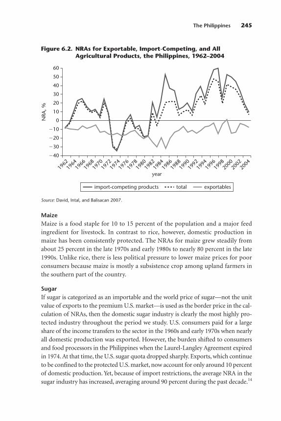
MaizeMaize is a food staple for 10 to 15 percent of the population and a major feedingredient for livestock. In contrast to rice, however, domestic production inmaize has been consistently protected. The NRAs for maize grew steadily fromabout 25 percent in the late 1970s and early 1980s to nearly 80 percent in the late1990s. Unlike rice, there is less political pressure to lower maize prices for poorconsumers because maize is mostly a subsistence crop among upland farmers inthe southern part of the country.
SugarIf sugar is categorized as an importable and the world price of sugar—not the unitvalue of exports to the premium U.S. market—is used as the border price in the cal-culation of NRAs, then the domestic sugar industry is clearly the most highly pro-tected industry throughout the period we study. U.S. consumers paid for a largeshare of the income transfers to the sector in the 1960s and early 1970s when nearlyall domestic production was exported. However, the burden shifted to consumersand food processors in the Philippines when the Laurel-Langley Agreement expiredin 1974. At that time, the U.S. sugar quota dropped sharply. Exports, which continueto be confined to the protected U.S. market, now account for only around 10 percentof domestic production. Yet, because of import restrictions, the average NRA in thesugar industry has increased, averaging around 90 percent during the past decade.14
The Philippines 245
1964
1966
1962
1968
1970
1972
1974
1976
1978
1980
1982
1984
1986
1988
1990
1992
1994
1996
1998
2000
2002
2004
NRA
, %
year
total exportablesimport-competing products
�40
�30
�20
�10
0
20
40
10
30
50
60
Figure 6.2. NRAs for Exportable, Import-Competing, and AllAgricultural Products, the Philippines, 1962–2004
Source: David, Intal, and Balisacan 2007.
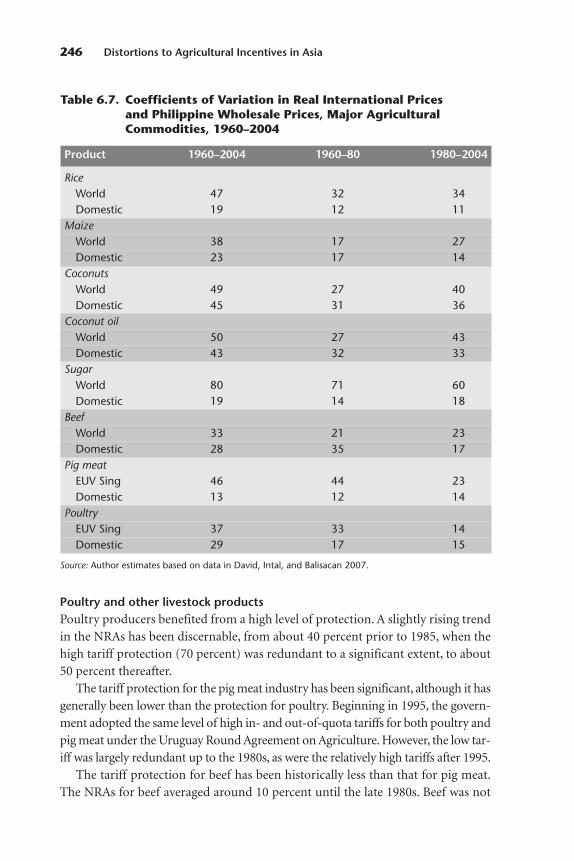
Poultry and other livestock productsPoultry producers benefited from a high level of protection. A slightly rising trendin the NRAs has been discernable, from about 40 percent prior to 1985, when thehigh tariff protection (70 percent) was redundant to a significant extent, to about50 percent thereafter.
The tariff protection for the pig meat industry has been significant, although it hasgenerally been lower than the protection for poultry. Beginning in 1995, the govern-ment adopted the same level of high in- and out-of-quota tariffs for both poultry andpig meat under the Uruguay Round Agreement on Agriculture. However, the low tar-iff was largely redundant up to the 1980s, as were the relatively high tariffs after 1995.
The tariff protection for beef has been historically less than that for pig meat.The NRAs for beef averaged around 10 percent until the late 1980s. Beef was not
246 Distortions to Agricultural Incentives in Asia
Table 6.7. Coefficients of Variation in Real International Pricesand Philippine Wholesale Prices, Major AgriculturalCommodities, 1960–2004
Product 1960–2004 1960–80 1980–2004
RiceWorld 47 32 34Domestic 19 12 11
MaizeWorld 38 17 27Domestic 23 17 14
CoconutsWorld 49 27 40Domestic 45 31 36
Coconut oilWorld 50 27 43Domestic 43 32 33
SugarWorld 80 71 60Domestic 19 14 18
BeefWorld 33 21 23Domestic 28 35 17
Pig meatEUV Sing 46 44 23Domestic 13 12 14
PoultryEUV Sing 37 33 14Domestic 29 17 15
Source: Author estimates based on data in David, Intal, and Balisacan 2007.

included among the sensitive products on which tariffs were raised following theWTO agreement. Nonetheless, an upward trend in the estimated NRAs for beefmay also be observed for the 1990s. It appears that the government’s attempt topromote activities aimed at fattening cattle, which relied on allowing duty-freeimports of young cattle from Australia, was accompanied by more restrictive non-tariff trade barriers on beef to increase incentives. The expansion of the cattle fat-tening business was short-lived, however; tariffs on beef were reduced in the late1990s, and import restrictions became untenable.15 That beef benefited from lessprotection than poultry may be explained by the prevalence of large-scale integra-tion farming operations that produced poultry through contract farming, in con-trast to the beef industry, which is dominated by backyard producers. However,the pig meat industry is also dominated by backyard producers, and this subsectorbenefited from relatively high protection rates.
Agricultural inputsTo infer the effect of price interventions on value added, David, Intal, and Balisacan (2007) report on trends in the NRAs for the major intermediate inputscommonly used in agricultural production. Until the mid-1980s, the govern-ment’s policies on industrial promotion raised the domestic prices for manufac-tured inputs in agriculture significantly. The consumer tax equivalent of theimport protection provided for agricultural inputs such as fertilizers, agriculturalchemicals, farm machinery, and even water pumps was generally higher than theNRAs for agricultural outputs, aside from the case of sugar in some years. Withthe exception of subsidies for gravity irrigation in rice, there was no significantoffsetting input assistance in agriculture. Indeed, despite price controls, tax freeimports, and direct subsidies for fertilizer companies before the mid-1980s, theconsumer tax equivalent on farm inputs was negative only during 1970–74(because of the fourfold jump in world oil prices). These data are not incorpo-rated in the aggregate NRAs for crop agriculture; but, if they had been incorpo-rated in the manner described in Anderson et al. (2008) and appendix A, theywould have lowered the estimated NRAs for crops by a few percentage points,especially in the earlier decades of the period we study. The estimated NRAs forlivestock would also be lower if the impact on the prices of feedmix deriving fromthe import restrictions on maize had been taken into account.
NRAs for nonagriculture and RRAs for agriculture
Agricultural incentives are affected indirectly by rates of assistance to nonagricul-ture. Mobile resources move across sectors or industries according to the relativeincentives. Figure 6.3 and table 6.7 show the trends in the average NRAs ofthe agricultural and nonagricultural sectors, as well as the RRAs for agriculture.
The Philippines 247
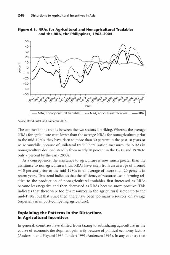
The contrast in the trends between the two sectors is striking. Whereas the averageNRAs for agriculture were lower than the average NRAs for nonagriculture priorto the mid-1980s, they have risen to more than 30 percent in the past 10 years orso. Meanwhile, because of unilateral trade liberalization measures, the NRAs innonagriculture declined steadily from nearly 20 percent in the 1960s and 1970s toonly 7 percent by the early 2000s.
As a consequence, the assistance to agriculture is now much greater than theassistance to nonagriculture; thus, RRAs have risen from an average of around�15 percent prior to the mid-1980s to an average of more than 20 percent inrecent years. This trend indicates that the efficiency of resource use in farming rel-ative to the production of nonagricultural tradables first increased as RRAsbecame less negative and then decreased as RRAs became more positive. Thisindicates that there were too few resources in the agricultural sector up to themid-1980s, but that, since then, there have been too many resources, on average(especially in import-competing agriculture).
Explaining the Patterns in the Distortionsin Agricultural Incentives
In general, countries have shifted from taxing to subsidizing agriculture in thecourse of economic development primarily because of political economy factors(Anderson and Hayami 1986; Lindert 1991; Anderson 1995). In any country that
248 Distortions to Agricultural Incentives in Asia
1964
1966
1962
1968
1970
1972
1974
1976
1978
1980
1982
1984
1986
1988
1990
1992
1994
1996
1998
2000
2002
2004
per
cent
year
NRA, nonagricultural tradables RRANRA, agricultural tradables
�50
�40
�30
�20
�10
20
40
10
0
30
50
Figure 6.3. NRAs for Agricultural and Nonagricultural Tradablesand the RRA, the Philippines, 1962–2004
Source: David, Intal, and Balisacan 2007.
would be self-sufficient in food in a world of free agricultural trade, this shift isexpected to occur when the country’s per capita income reaches 2.6 times theglobal average (Tyers and Anderson 1992). In a country that would be only65 percent self-sufficient in food under free trade, the shift would occur whenthe per capita income reaches the global average (US$4,300 in 1992). In the case ofthe Philippines, the shift from taxing to assisting agriculture directly throughprice interventions occurred at a level of economic development that was lowerthan predicted by earlier studies: per capita income in the Philippines was onlyabout US$1,200 even in the late 1990s.
Why did the switch toward higher agricultural protection occur early in thePhilippines? The explanation lies in unique historical events, political economyfactors, the local political system, and the strong nationalist sentiment for foodself-sufficiency, especially in rice. The country’s highly skewed distribution oflandownership and dualistic agrarian structure that arose from colonial land poli-cies and agroecological conditions meant that there were large landowners andplantation operators who were able to lobby effectively for their own interests.The farm producers in these groups provided the major political leaders in Con-gress and in the executive branch of government at all levels. Landed oligarchs alsorepresented the business elite, which successfully pushed for an industrial protec-tion policy that biased incentives against the agricultural sector (Hara 1994). Asthe international pressure for trade liberalization has mounted during the pasttwo decades, it has become easier to resist the opening of domestic markets forfood staples by playing up the national sentiment for food self-sufficiency. Politi-cal pressure to raise agricultural protection has been strengthened by expandedlobbying efforts undertaken by farmer organizations, large landowners, andagribusiness firms such as livestock and poultry producers, millers, seed compa-nies, and input suppliers.
There has been little resistance to the high prices for white maize as food becausewhite maize is primarily a subsistence crop. Livestock producers (including poultryproducers) and feed millers who use mostly yellow maize have chosen to lobby forgreater protection for livestock output to offset the high maize prices rather thanlobby for a more rational policy in maize and livestock. The objections to the highlyrestrictive policy on maize imports have been addressed by providing import alloca-tions at lower tariffs for the large, more well organized, and more vocal feed, poultry,and pig meat industries. The larger feed mills and livestock producers also own flourmills and are thus able to substitute low-grade wheat, which is subject to only a10 percent tariff, for the artificially high-priced maize. This policy structure provideslarge-scale feed and livestock producers with a cost advantage over smaller produc-ers who must rely on the domestic market for maize supplies.
Aside from the large size of farms and mills, the sugar subsector has historicallyhad strong political power because of its close relationship and common interest
The Philippines 249
with the government in lobbying to protect the country’s preferential marketaccess to the U.S. sugar market. In contrast, the share of sugar in direct householdexpenditure is small, and consumers have therefore generally tolerated or beenunaware of the high sugar prices. Resistance from the food processing subsectoragainst high sugar prices was mitigated by granting larger, more vocal foodprocessors the privilege to import sugar free of tariffs.
Concluding Remarks
Price intervention policies became more favorable in the agricultural sectorbeginning in the mid-1980s. The protection for major import-competing com-modities was increased, and unilateral trade liberalization measures lowered theimplicit tariffs on inputs and the protection of nonagricultural sectors. Thus,improvements in agricultural incentives occurred at the cost of the inefficiencies inresource allocation arising from widening distortions in prices within agricultureand between agriculture and nonagriculture.
Artificially raising the profitability of major import-competing commoditiesdirectly increased the cost of land for the production of other crops. It also indi-rectly reduced the competitive advantage of exportable agricultural products inworld markets. The high-price maize policy also lowered the international com-petitiveness of the pig meat industry, in which the Philippines may well have acomparative advantage. The significant protection for sugar hurts not only con-sumers, but also the food processing industry, which accounts for over 20 percentof manufacturing employment and value added. The excessive protection formajor staple food commodities reduces the welfare of rural landless and urbanpoor households and puts pressure on wages, rendering labor-intensive manufac-turing industries less competitive relative to low-wage, low-cost food economiessuch as China and Vietnam.
The economic waste caused by price intervention policies is magnified by thecontinued use of quantitative trade restrictions instead of tariffs. In particular, thegovernment’s monopoly on rice imports and domestic marketing operationsthrough the National Food Authority has been extremely costly, and it has alsofailed to achieve the basic and conflicting objectives of lowering food prices forconsumers, raising producer prices, and stabilizing both sets of prices. The use ofquantitative restrictions promotes rent seeking, reduces government revenues,incurs significant bureaucratic costs, and aggravates price uncertainties.
Unfortunately, recent policy changes in response to the WTO agreement onagriculture seem to have exacerbated rather than mitigated such problems; thenominal protection rates for major import-competing commodities have notonly been raised, but the scope of the operations of the National Food Authority
250 Distortions to Agricultural Incentives in Asia

has also been inadvertently expanded. Rice market interventions and the use ofquantitative restrictions have persisted because the economic costs and even someof the financial costs are not readily apparent to the general public. Meanwhile,the bureaucracy is being corrupted through commissions, bribes, and the otherrents typically involved in government procurement and import licensing, mak-ing it even more difficult to effect trade liberalization.
There are no indications that the government will move toward greater tradeliberalization in agriculture in the near future. In the current negotiations underthe Doha Round, efforts are being made to retain the relatively high level of tariffprotection for major import-competing agricultural commodities. Furthermore,the government is not taking any steps to dismantle the institutions and otherpolicy instruments that regulate the imports of rice, sugar, and other commodi-ties. Because of the sharp rise in world grain prices in recent years, the governmentwill be politically compelled to continue its food self-sufficiency strategy ratherthan rely on open international markets to achieve food security.
Notes
1. Because there was an acceleration in overseas labor migration, real wages did not decline. Migra-tion boosted foreign exchange earnings, and remittances began to account for at least a 10 percentshare in gross national product.
2. Fishery products, led by tuna and shrimps, have become major agricultural exports. They nowaccount for about 20 percent of total agricultural exports.
3. Even for relatively minor crops, specific laws were passed prohibiting imports. This affected, forexample, onions, garlic, potatoes, and cabbages in 1955, coffee in 1960, and cigarettes and tobacco,except for blending purposes, in 1964.
4. Export taxes were also imposed on logs at 10 percent; copper ore at 6 percent; and other metalores, shrimps, prawns, lumber, plywood, and veneer at 4 percent.
5. About 20 percent of the revenues from the tax briefly supported the direct subsidy on thedomestic consumption of coconut oil products. The remainder was supposed to be used to financedevelopment programs in the coconut industry such as replanting, vertical integration, and scholar-ships. Subsequent research showed that little benefit, if any, accrued to farmers from these expendi-tures (Clarete and Roumasset 1990).
6. The Philippines is still negotiating in the WTO’s Doha Round to keep government monopolycontrol over rice imports.
7. The government also occasionally used the WTO-sanctioned safeguard mechanism when addi-tional tariffs were imposed on poultry.
8. The country is a significant trader only in coconut products, in which it has been the world’slargest producer and exporter for most of the period we study. However, to a large extent, competingproducts such as palm oil and soybean oil may be substituted for coconut products. Coconut oil, themost important coconut product, constitutes only a small (7 percent) share of the world trade in vegetable oils.
9. According to Borrell et al. (1994), the quedan system, which allocates products to the variousmarkets in fixed proportions, reduces the incentive to increase production and invest in yield-increasing technology. This is because higher production cuts into gross revenues. Also, because exportallocation to the United States occurs at a fixed ratio, there is no incentive to improve milling qualityfor export so as to increase net returns. Meanwhile, the sugar-sharing arrangement—whereby 60 to
The Philippines 251

70 percent goes to growers, and 30 to 40 percent goes to millers (depending on the recovery rate)—thatwas instituted by law to provide millers a share of the benefits from price protection also happensto reduce the incentive of growers and millers to raise productivity. Thus, growers receive only 60 to70 percent of the benefits of productivity-enhancing investments, while millers receive only 30to 40 percent of these benefits.
10. As described in Anderson et al (2008) and appendix A, a commodity is considered nontradableif the proportion of imports and exports in the total value of production is less than 5 percent. If acommodity or commodity group is both exported and imported in significant amounts (that is, morethan 2.5 percent of the total value of output), we estimate the NRA as the average of the NRA of thecommodity as an exportable and the NRA of the commodity as an importable, weighted by the respec-tive proportions of the export and import values to the total traded value.
11. Despite the supposed removal of quantitative trade restrictions on all agricultural commodi-ties except rice, nontariff barriers appear to be significant in the case of many commodities, such asvegetables, fruits, and meat. Price comparisons are difficult to perform for many of these productsbecause of the lack of consistent world price series, difficulties in making adjustments for quality differences, and the complexity of measuring the effect the increased imports of a commodity thatmay not be grown in the country may have on the price of a highly substitutable product that is produced domestically. One clear indication of this effect, however, is the substantial smuggling ofvegetables, fruits, and nuts from China. The exports of these commodities to the Philippines reportedin Chinese trade statistics have been up to 10 times more substantial than the corresponding importsof these commodity groups reported in official Philippine trade statistics despite the already low tariffs on these smuggled products (mostly 3 percent, but, in some cases, up to 10 percent since thelate 1990s).
12. To the tariffs in the computation of NRAs, we have added the differences between the indirecttax on domestically produced goods and the indirect tax on imported products imposed from 1960 tothe early 1980s. While the tax rates on imports and the tax rate on exports were the same in most cases,the taxes were effectively greater in the case of imports because the tax base for imports was the tariff-inclusive price, augmented by a percentage markup. In 1974, the weighted average nominal tariff ratewas 22 percent for manufacturing products, but the nominal rate of protection would nonethelessbe significantly higher, 31 percent, if one takes into account the effect of the difference in the tax base(Tan 1979).
13. New seed fertilizer technologies and the accompanying expansion in irrigation increased thecountry’s comparative advantage in rice production, briefly turning the Philippines from a net riceimporter to rice self-sufficiency and, by the late 1970s, reducing the domestic price of rice in real terms.
14. Even the large margins conferred on sugar importers as a result of the high level of nominalprotection have been received mostly by sugarcane growers, who receive the major part of the importrights dispensed by the Sugar Regulatory Administration.
15. During this period, annual imports of live cattle averaged more than 200,000 head. The num-ber declined significantly thereafter, and the cattle fattening business is now limited to Del Monte andSan Miguel Corporation–Monterey Foods, which use by-products of their other businesses, that is,pineapple canning and beer manufacturing, respectively, as main cattle feed ingredients. Previously,live cattle were mostly imported for almost immediate slaughter, and the government’s policy was thusaimed at promoting the slaughtering business rather than cattle production.
References
Aldaba, R. M. 2005a. “Policy Reversals, Lobby Groups and Economic Distortions.” Discussion Paper2005–04, Philippine Institute for Development Studies, Makati City, the Philippines.
———. 2005b. “The Impact of Market Reforms on Competition, Structure and Performance of thePhilippine Economy.” Discussion Paper 2005–24, Philippine Institute for Development Studies,Makati City, the Philippines.
252 Distortions to Agricultural Incentives in Asia
Anderson, K. 1995. “Lobbying Incentives and the Pattern of Protection in Rich and Poor Countries.”Economic Development and Cultural Change 43 (2): 401–23.
Anderson, K., and Y. Hayami, eds. 1986. The Political Economy of Agricultural Protection: East Asia inInternational Perspective. London: Allen and Unwin.
Anderson, K., M. Kurzweil, W. Martin, D. Sandri, and E. Valenzuela. 2008. “Measuring Distortions toAgricultural Incentives, Revisited.” World Trade Review 7 (4): 675–704.
Balisacan, A. M., N. Fuwa, and M. H. Debuque. 2004. “The Political Economy of Philippine RuralDevelopment since the 1960s.” In Rural Development and Agricultural Growth in Indonesia, thePhilippines, and Thailand, ed. T. Akiyama and D. F. Larson, 214–93. Canberra: Asia Pacific Press.
Bautista, R. M., and G. R. Tecson. 2003. “International Dimensions.” In The Philippine Economy: Development, Policies, and Challenges, ed. A. M. Balisacan and H. Hill, 136–71. New York: OxfordUniversity Press.
Borrell, B., D. Quirke, B. de la Pena, and L. Noveno. 1994. Philippine Sugar: An Industry Finding Its Feet.Canberra: Center for International Economics.
Clarete, R. L. 1991. “E.O. 470: The Economic Effects of the 1991 Tariff Policy Reform.” Unpublishedreport, United States Agency for International Development–Philippines, Manila.
Clarete, R. L., and J. A. Roumasset. 1990. “The Relative Welfare Cost of Industrial and Agricultural Policy Distortions: A Philippine Illustration.” Oxford Economic Papers 42 (2): 462–72.
Cororaton, C. B. 2000. “Philippine Tariff Reform: A CGE Analysis.” Discussion Paper 2000–35, Philippine Institute for Development Studies, Makati City, the Philippines.
David, C. C. 1983. “Economic Policies and Philippine Agriculture.” Working Paper 83–02, PhilippineInstitute for Development Studies, Makati City, the Philippines.
———. 1994. “GATT-UR and Philippine Agriculture: Facts and Fallacies.” Journal of Philippine Devel-opment 21 (1–2): 141–78.
———. 2003. “Agriculture.” In The Philippine Economy: Development, Policies, and Challenges,ed. A. M. Balisacan and H. Hill, 175–218. New York: Oxford University Press.
David, C. C., P. Intal, and A. M. Balisacan. 2007. “Distortions to Agricultural Incentives in the Philip-pines.” Agricultural Distortions Working Paper 28, World Bank, Washington, DC.
FAOSTAT Database. Food and Agriculture Organization of the United Nations. http://faostat.fao.org/default.aspx (accessed May 2008).
GTAP Database (Global Trade Analysis Project Database). Center for Global Trade Analysis, Depart-ment of Agricultural Economics, Purdue University. https://www.gtap.agecon.purdue.edu/databases/v6/default.asp (version 6).
Habito, C. F., and C. B. Cororaton. 2000. “WTO and the Philippine Economy: An Empirical and Analytical Assessment of Post-WTO Trade Reforms in the Philippines.” Unpublished report, AgileProgram, United States Agency for International Development–Philippines, Manila.
Hara, Y. 1994. Tonan ajia shokoku no keizai hatten (The Economic Development of Southeast AsianCountries). Tokyo: Institute of Oriental Culture, University of Tokyo.
Intal, P. S., and J. H. Power. 1991. “The Philippines.” In Asia. Vol. 2 of The Political Economy of Agricul-tural Pricing Policy, ed. A. O. Krueger, M. Schiff, and A. Valdés, 149–94. World Bank ComparativeStudy. Baltimore: Johns Hopkins University Press; Washington, DC: World Bank.
Lindert, P. 1991. “Historical Patterns of Agricultural Policy.” In Agriculture and the State: Growth,Employment, and Poverty in Developing Countries, ed. C. P. Timmer, 29–83. Ithaca, NY: CornellUniversity Press.
Manasan, R. G., and V. S. Pineda. 1999. “Assessment of Philippine Tariff Reform: A 1998 Update.”Unpublished working paper, Philippine Institute for Development Studies, Makati City, the Philippines.
Pasadilla, G. O. 2006. “Preferential Trading Agreements and Agricultural Liberalization in East andSoutheast Asia.” Working Paper 11, Asia-Pacific Research and Training Network on Trade, Tradeand Investment Division, United Nations Economic and Social Commission for Asia and thePacific, Bogor, Indonesia.
The Philippines 253
Pimentel, A. 2006. “A Study on the Impact of the Philippine Tariff Reform Program: An Input-OutputModel.” Unpublished working paper, Southeast Asia Research Center for Agriculture, Los Banos,the Philippines.
Power, J. H. 1971. “The Structure of Protection in the Philippines.” In The Structure of Protection inDeveloping Countries, ed. B. Balassa, 271–80. Baltimore: Johns Hopkins University Press; Washington,DC: World Bank.
Tan, E. S. 1994. “Trade Policy Reforms in the 1990s: Effects of EO 470 and the Import LiberalizationProgram.” Research Paper 94–11, Philippine Institute for Development Studies, Makati City, thePhilippines.
Tan, N. A. 1979. “The Structure of Protection and Resource Flows in the Philippines.” In Industrial Promotion Policies in the Philippines, ed. R. M. Bautista and J. H. Power, 122–67. Makati City, thePhilippines: Philippine Institute for Development Studies.
Tyers, R., and K. Anderson. 1992. Disarray in World Food Markets: A Quantitative Assessment. NewYork: Cambridge University Press.
World Development Indicators Database. World Bank. http://go.worldbank.org/B53SONGPA0(accessed May 2008).
254 Distortions to Agricultural Incentives in Asia
Thailand is a major net agricultural exporter, and its agricultural trade policy isdominated by this fact. The list of agricultural exports includes many of the mostimportant agricultural products produced and consumed within the country,including the staple food, rice (exports of which account for between 30 and50 percent of the total output of the product), and also cassava, sugar, rubber, andpoultry products. The list of imported agricultural commodities is much shorter.Maize has been a net export in most years, but it was also a net import duringsome years in the 1990s. Soybeans were a net export for several decades, but, sincethe early 1990s, have been a net import. Palm oil has fluctuated between a netimport and a net export, but, since the late 1990s, it has been a net export.
Historically, Thailand’s large agricultural surplus has always led to a degree ofpolicy complacency regarding the agricultural sector. Agricultural importingcountries are typically concerned about food security and raising agriculturalproductivity to reduce import dependence. In Thailand, these matters have notbeen a significant concern, although stabilizing food prices for consumers hasbeen a recurrent theme of agricultural pricing policy. Until the 1980s, agriculturalexports were viewed as a source of government revenue. Unlike manufacturing,traditional agriculture was not seen as a dynamic sector of the economy thatmight contribute to rapid growth. Because the price elasticity of supply for mostagricultural products was low, at least in the short run, it was felt that the
255
7
THAILAND
Peter Warr and Archanun Kohpaiboon
The authors gratefully acknowledge the excellent research assistance of Arief Ramayandi and the help-ful comments and assistance with data of the following colleagues: Ammar Siamwalla, ChalongphobSussangkarn, and Wisarn Pupphavesa of the Thailand Development Research Institute; Isra Sarntisartof Chulalongkorn University; and Nipon Poapongsakorn, Prayong Netayarak, and SomboonSiriprachai of Thammasat University. They are also grateful for the helpful comments of workshop par-ticipants and the intensive assistance with spreadsheets by Marianne Kurzweil and Ernesto Valenzuela.
production of these products could be taxed heavily without creating a significantcontraction in output. Moreover, most agricultural producers were impoverished,poorly educated, and politically unorganized. This was particularly the caseamong rice producers; so, taxing agriculture, especially rice, was politically attractive, and rice exports were taxed until 1986 (Siamwalla, Setboonsarng, andPatamasiriwat 1993).
Because of greatly increased income per person, rapid urbanization, and theswing toward more democratic political institutions, policy has shifted from tax-ing agriculture to more neutral trade policies. This change has almost certainlyowed more to politics—the political necessity of finding ways to attract the sup-port of the huge rural electorate and the desire of the urban electorate to establishbetter economic conditions for the farm population—than to a desire to liberalizeagricultural trade for the efficiency reasons that economists emphasize. However,the transition away from taxing agriculture has not progressed much in the direc-tion of subsidizing agriculture. The key reason is that many important agricul-tural commodities are net export items, and this has made subsidizing agricultureproblematic. Had the commodities farmers produce been competing withimports and thus amenable to the imposition of tariffs, there might have beenmore political pressure to protect farmers.
Thailand is an active member of the Cairns Group of agricultural exportingcountries within the membership of the World Trade Organization. Nonetheless,while its agricultural trade is relatively liberal, the country cannot be described asa free trader with regard to agricultural commodities. Within Thailand, opposi-tion to agricultural import liberalization is strong in the case of soybeans, palmoil, rubber, rice, and sugar. The protective measures include nontariff instrumentsthat permit substantial discretion by government officials. The import controlsinclude import prohibitions, strict licensing arrangements, local content rules, anda requirement for special case-by-case approval of imports. The commodities forwhich these restrictions are applied include the five above, plus onions, garlic,potatoes, pepper, tea, raw silk, maize, coconut products, and coffee.
The inclusion of rice in this list of protected commodities may seem strange.Thailand is the world’s largest exporter of rice and is undoubtedly one of theworld’s most efficient rice producers. Why should the rice industry require pro-tection from imports? Imports of rice are, in fact, prohibited unless they are specif-ically approved by the Ministry of Commerce. The Ministry of Agriculture andCooperatives vigorously opposes any liberalization commitments with regard torice. The reasons apparently relate to the ministry’s wish to keep its options openwith respect to rice policy in the event market conditions should change unex-pectedly. Sudden changes in the price of rice can have far-reaching political conse-quences. The domestic rice market operates almost entirely without governmentintervention, but the instruments for intervention are ever ready.
256 Distortions to Agricultural Incentives in Asia

A lesser reason for the import controls on rice is that, as with most agriculturalcommodities, rice is a highly differentiated commodity. Not all grades of rice areproduced efficiently within Thailand, and the government wishes to protectdomestic producers from imports of the grades of rice that are closer substitutesfor local grades on the consumption side than they are on the production side.The lower grades of rice produced in Vietnam, but not in Thailand, are an impor-tant example.
Thailand’s general exclusion list applies to agreements in the free trade area ofthe Association of Southeast Asian Nations and includes several agriculturalindustries, among which are rice, sugar, and palm oil (both crude and refined).Within government circles, discussions about problems in the agricultural sectorrevolve overwhelmingly around the treatment of Thai exports by other countries.Thailand’s own agricultural import policy is a closed question. Problems havebeen encountered with a number of trading partners about environmental issuesand sanitary and phytosanitary issues with Thailand’s agricultural exports. Theseproblems have included a well-publicized dispute with the United States overshrimps (environmental issues) and another with Australia over precooked frozenchicken (sanitary and phytosanitary issues).
Poverty in the country is heavily concentrated in rural areas, and public opin-ion favors government support for the rural poor. Since the economic crisis of1997–98 and especially during the government of Prime Minister Thaksin Shinawatra in 2001–06, a wide range of income support programs, cash grants tovillages, and subsidized credit schemes have been introduced. Support for theseschemes was a significant component of the populist economic policy agenda ofthe Thaksin government. However, the operations of few of these schemes, if any,depended on the prices faced by agricultural producers. Because they were notlinked directly to the production of agricultural commodities, it seems that theywere not distorting resource allocations. The results of our study make an assess-ment possible of whether the price incentives facing agricultural producers were,indeed, distorted relative to international prices during the period of populistgovernment.
The following section of the chapter briefly describes the changing structure ofthe Thai economy, especially the agricultural sector. The core of the analysis, con-tained in the section thereafter, relies on comparisons between the domestic pricesand the international prices for major agricultural commodities and fertilizer andrelates the price comparisons to tariff and nontariff barriers on the same prod-ucts. It focuses on whether the relative prices for traded commodities at wholesalehave differed from the relative border prices, adjusted for transport and handlingcosts. The subsequent section extends this analysis to the farm level. The raw com-modities produced by farmers generally do not enter international trade directly.These raw commodities are inputs into the production of the processed
Thailand 257
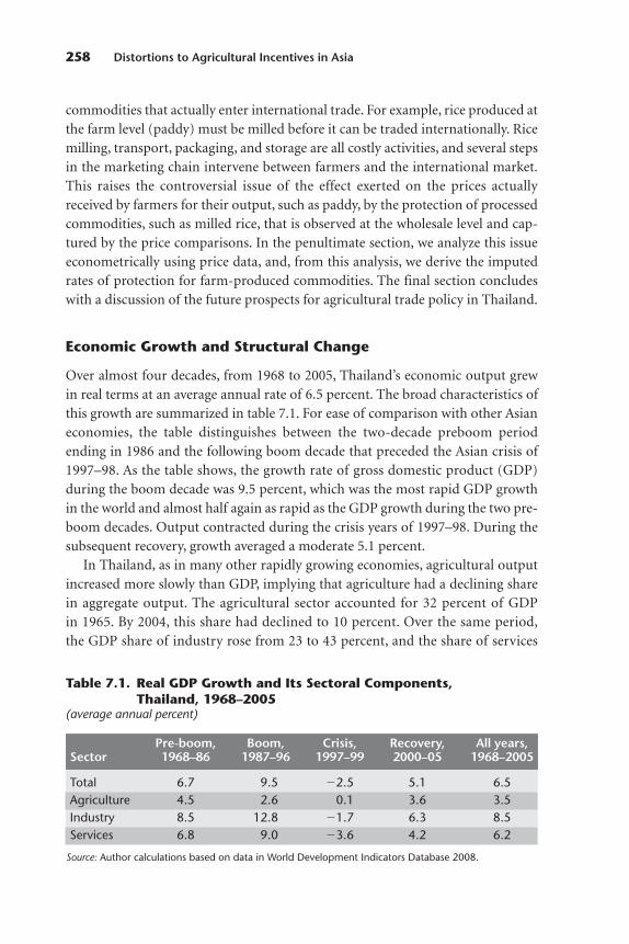
commodities that actually enter international trade. For example, rice produced atthe farm level (paddy) must be milled before it can be traded internationally. Ricemilling, transport, packaging, and storage are all costly activities, and several stepsin the marketing chain intervene between farmers and the international market.This raises the controversial issue of the effect exerted on the prices actuallyreceived by farmers for their output, such as paddy, by the protection of processedcommodities, such as milled rice, that is observed at the wholesale level and cap-tured by the price comparisons. In the penultimate section, we analyze this issueeconometrically using price data, and, from this analysis, we derive the imputedrates of protection for farm-produced commodities. The final section concludeswith a discussion of the future prospects for agricultural trade policy in Thailand.
Economic Growth and Structural Change
Over almost four decades, from 1968 to 2005, Thailand’s economic output grewin real terms at an average annual rate of 6.5 percent. The broad characteristics ofthis growth are summarized in table 7.1. For ease of comparison with other Asianeconomies, the table distinguishes between the two-decade preboom period ending in 1986 and the following boom decade that preceded the Asian crisis of1997–98. As the table shows, the growth rate of gross domestic product (GDP)during the boom decade was 9.5 percent, which was the most rapid GDP growthin the world and almost half again as rapid as the GDP growth during the two pre-boom decades. Output contracted during the crisis years of 1997–98. During thesubsequent recovery, growth averaged a moderate 5.1 percent.
In Thailand, as in many other rapidly growing economies, agricultural outputincreased more slowly than GDP, implying that agriculture had a declining sharein aggregate output. The agricultural sector accounted for 32 percent of GDPin 1965. By 2004, this share had declined to 10 percent. Over the same period,the GDP share of industry rose from 23 to 43 percent, and the share of services
258 Distortions to Agricultural Incentives in Asia
Table 7.1. Real GDP Growth and Its Sectoral Components,Thailand, 1968–2005
(average annual percent)
Pre-boom, Boom, Crisis, Recovery, All years,Sector 1968–86 1987–96 1997–99 2000–05 1968–2005
Total 6.7 9.5 �2.5 5.1 6.5Agriculture 4.5 2.6 0.1 3.6 3.5Industry 8.5 12.8 �1.7 6.3 8.5Services 6.8 9.0 �3.6 4.2 6.2
Source: Author calculations based on data in World Development Indicators Database 2008.
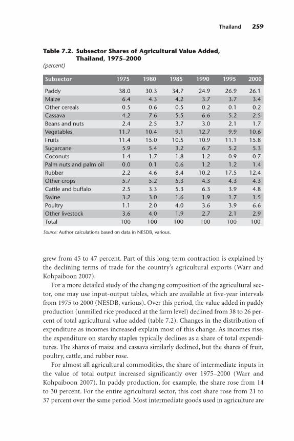
grew from 45 to 47 percent. Part of this long-term contraction is explained bythe declining terms of trade for the country’s agricultural exports (Warr and Kohpaiboon 2007).
For a more detailed study of the changing composition of the agricultural sec-tor, one may use input-output tables, which are available at five-year intervalsfrom 1975 to 2000 (NESDB, various). Over this period, the value added in paddyproduction (unmilled rice produced at the farm level) declined from 38 to 26 per-cent of total agricultural value added (table 7.2). Changes in the distribution ofexpenditure as incomes increased explain most of this change. As incomes rise,the expenditure on starchy staples typically declines as a share of total expendi-tures. The shares of maize and cassava similarly declined, but the shares of fruit,poultry, cattle, and rubber rose.
For almost all agricultural commodities, the share of intermediate inputs inthe value of total output increased significantly over 1975–2000 (Warr and Kohpaiboon 2007). In paddy production, for example, the share rose from 14to 30 percent. For the entire agricultural sector, this cost share rose from 21 to37 percent over the same period. Most intermediate goods used in agriculture are
Thailand 259
Table 7.2. Subsector Shares of Agricultural Value Added,Thailand, 1975–2000
(percent)
Subsector 1975 1980 1985 1990 1995 2000
Paddy 38.0 30.3 34.7 24.9 26.9 26.1Maize 6.4 4.3 4.2 3.7 3.7 3.4Other cereals 0.5 0.6 0.5 0.2 0.1 0.2Cassava 4.2 7.6 5.5 6.6 5.2 2.5Beans and nuts 2.4 2.5 3.7 3.0 2.1 1.7Vegetables 11.7 10.4 9.1 12.7 9.9 10.6Fruits 11.4 15.0 10.5 10.9 11.1 15.8Sugarcane 5.9 5.4 3.2 6.7 5.2 5.3Coconuts 1.4 1.7 1.8 1.2 0.9 0.7Palm nuts and palm oil 0.0 0.1 0.6 1.2 1.2 1.4Rubber 2.2 4.6 8.4 10.2 17.5 12.4Other crops 5.7 5.2 5.3 4.3 4.3 4.3Cattle and buffalo 2.5 3.3 5.3 6.3 3.9 4.8Swine 3.2 3.0 1.6 1.9 1.7 1.5Poultry 1.1 2.0 4.0 3.6 3.9 6.6Other livestock 3.6 4.0 1.9 2.7 2.1 2.9Total 100 100 100 100 100 100
Source: Author calculations based on data in NESDB, various.
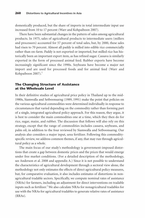
domestically produced, but the share of imports in total intermediate input useincreased from 10 to 17 percent (Warr and Kohpaiboon 2007).
There have been substantial changes in the pattern of sales among agriculturalproducts. In 1975, sales of agricultural products to intermediate users (millersand processors) accounted for 57 percent of total sales, but, by 2000, these saleshad risen to 70 percent. Almost all paddy is milled into edible rice commerciallyrather than on-farm. Paddy is not exported or imported, but milled rice has his-torically been an important export item, as has refined sugar. Cassava is similarlyexported in the form of processed animal feed. Rubber exports have becomeincreasingly significant since the 1990s. Soybeans have become a major netimport and are used for processed foods and for animal feed (Warr and Kohpaiboon 2007).1
The Changing Structure of Assistanceat the Wholesale Level
In their definitive studies of agricultural price policy in Thailand up to the mid-1980s, Siamwalla and Setboonsarng (1989, 1991) make the point that policies onthe various agricultural commodities were determined individually in response tocircumstances that varied depending on the commodity rather than forming partof a single, integrated agricultural policy approach. For this reason, they argue, itis best to consider the main commodities one at a time, which they then do forrice, sugar, maize, and rubber. The discussion that follows will also rely on thisstrategy, except that the range of commodities includes cassava, soybeans, andpalm oil, in addition to the four reviewed by Siamwalla and Setboonsarng. Ouranalysis also considers a major input, urea fertilizer. Following this commodity-specific review, we address common themes, if any, that may run through agricul-tural policy as a whole.
The main focus of our study’s methodology is government-imposed distor-tions that create a gap between domestic prices and the prices that would emergeunder free market conditions. (For a detailed description of the methodology,see Anderson et al. 2008 and appendix A.) Since it is not possible to understandthe characteristics of agricultural development through a sectoral view alone, themethodology not only estimates the effects of direct agricultural policy measures,but, for comparative evaluation, it also includes estimates of distortions in non -agricultural tradable sectors. Specifically, we compute nominal rates of assistance(NRAs) for farmers, including an adjustment for direct interventions on tradableinputs such as fertilizer.2 We also calculate NRAs for nonagricultural tradables foruse with the NRAs for agricultural tradables to generate relative rates of assistance(RRAs).
260 Distortions to Agricultural Incentives in Asia

We conduct our analysis at the wholesale level; so, in what follows, the domesticprice means the domestic wholesale price. In the calculation of the NRAs, the bor-der prices are amended by the transport and handling costs involved in adjustingthe price of imports from the cost, insurance, and freight level to the domesticwholesale level and in adjusting the price of exports from the domestic wholesalelevel to the free on board level. (The relevant transport and handling costs are sum-marized in Warr and Kohpaiboon 2007.) These adjustments are required to obtainprices that are comparable with domestic wholesale prices. The border pricesadjusted for transport and handling costs may then be interpreted as an indicationof domestic wholesale prices as they would be in the absence of protection.
Rice
From the end of World War II to 1986, the Thai government taxed rice exports.There were four individual instruments of export taxation, each with distinct legalfoundations, and each under the control of different parts of the governmentbureaucracy. The revenues these various instruments generated were directedtoward separate parts of the government. Siamwalla and Setboonsarng (1989,1991) describe these independent tax streams and point out that their combinedeffect was a rate of export taxation of around 40 percent from the late 1950s to theearly 1970s. The rate increased to around 60 percent during the commodity priceboom of 1972–74, but subsequently diminished quickly to about 20 percent.There was another peak, at about 40 percent, at the time of the second Organiza-tion of the Petroleum Exporting Countries oil price shock in 1979–80 and then asteady decline until all four forms of tax were suspended in 1986. Rice exportshave remained untaxed for the two decades since then.3
The implications of these events for actual prices are summarized in figure 7.1,which is based on the data assembled in Warr and Kohpaiboon (2007). As witheach similar figure presented thereafter on another agricultural commodity, figure 7.1 compares domestic wholesale prices with border prices for rice of com-parable quality. Since rice is a net export, border price in the figure means exportprice, adjusted for transport and handling costs between the wholesale level andthe export level. The calculations of the nominal rates of protection (NRPs) thatemerge are similar to those that would be inferred from the rates of taxationdescribed above, except that the NRPs after 1986 are not zero, but average around�6 percent. It is possible that the transport and handling costs between thewholesale and free on board locations are not fully accounted for in the data inWarr and Kohpaiboon (2007). For rice, the data in figure 7.1 support the view thatthe domestic market has received zero protection and zero subsidies; moreover,rice is also no longer taxed.
Thailand 261

Maize
Maize was a net Thai export item until the 1990s. In 1992 and 1995–2000, importsdominated. Maize subsequently reverted and is now a net export good once more.In 1965–81, the government intervened in the export market to preserve theexports to Japan and Taiwan, China, where they were used primarily for animalfeed. In both markets, season-long stability in supply was an import requirement.To ensure the fulfillment of the domestic contracts needed to ensure this stability,the government imposed quota restrictions on exports to markets other than themarkets of these two economies. The effects of this policy included an increase inthe price volatility passed on to domestic producers and average producer earn-ings that were somewhat reduced. Meanwhile, Malaysia, Singapore, and othercountries closer to Thailand had developed their own livestock industries. TheJapanese and Taiwan, China markets therefore seemed less crucial, and, by 1981,the export controls on maize were removed. The data in figure 7.2 indicate thatthere was roughly zero protection for the maize industry. Whether maize was a netimport product or a net export product, this outcome does not seem to have varied in any systematic way.
262 Distortions to Agricultural Incentives in Asia
0
4,000
2,000
6,000
8,000
year
real
pric
e, b
aht
per
met
ric t
on
NRP, %
14,000
12,000
10,000
�70
�50
�60
�40
�30
0
�10
�20
1968
1971
1974
1977
1980
1983
1986
1989
1992
1995
1998
2004
2001
NRP, %left axis: right axis:border pricedomestic price
Figure 7.1. Price Comparisons and NRPs at Wholesale, Rice,Thailand, 1968–2005
Source: Warr and Kohpaiboon 2007.
Note: NRP � 100*(domestic price � border price)�border price.

Cassava
Thailand’s cassava exports developed for the supply of animal feed to Europeanand some Asian markets, including Taiwan, China. Because of the quota restric-tions of the European Union, rents were attached to export quotas from Thailand,which, in turn, led to corruption in the allocation of the quotas. The rents associ-ated with the quotas are analogous to a privately collected export tax. As a result ofthe rents, the export price exceeded the domestic price by amounts averagingaround 10 percent (figure 7.3).
Soybeans
Soybeans were a net export item from 1960 until 1988. By 1992, they were a netimport item. During the export period, exports were taxed, but, beginning in1995, the trade regime shifted nominally to tariff quotas. The operation of the tariff quotas is described in Warr and Kohpaiboon (2007). Within the importquota volume permitted, soybeans could be imported at low or zero tariffs.Beyond the quota, the applied tariff was set at the maximum amount permitted byWorld Trade Organization obligations, which varied between 80 and 90 percent.
Thailand 263
0
1,000
2,000
3,000
year
real
pric
e, b
aht
per
met
ric t
on
NRP, %
6,000
5,000
4,000
�50
�30
�40
�20
�10
20
10
0
1968
1971
1974
1977
1980
1983
1986
1989
1992
1995
1998
2004
2001
NRP, %left axis: right axis:border pricedomestic pricefarm price
Figure 7.2. Price Comparisons and NRPs at Wholesale, Maize,Thailand, 1968–2005
Source: Warr and Kohpaiboon 2007.
Note: NRP � 100*(domestic price � border price)�border price.
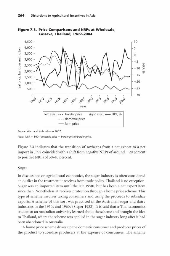
Figure 7.4 indicates that the transition of soybeans from a net export to a netimport in 1992 coincided with a shift from negative NRPs of around �20 percentto positive NRPs of 30–40 percent.
Sugar
In discussions on agricultural economics, the sugar industry is often consideredan outlier in the treatment it receives from trade policy. Thailand is no exception.Sugar was an imported item until the late 1950s, but has been a net export itemsince then. Nonetheless, it receives protection through a home price scheme. Thistype of scheme involves taxing consumers and using the proceeds to subsidizeexports. A scheme of this sort was practiced in the Australian sugar and dairyindustries in the 1950s and 1960s (Sieper 1982). It is said that a Thai economicsstudent at an Australian university learned about the scheme and brought the ideato Thailand, where the scheme was applied in the sugar industry long after it hadbeen abandoned in Australia.
A home price scheme drives up the domestic consumer and producer prices ofthe product to subsidize producers at the expense of consumers. The scheme
264 Distortions to Agricultural Incentives in Asia
0
1,000
500
1,500
2,000
year
real
pric
e, b
aht
per
met
ric t
on
NRP, %
4,500
4,000
3,000
3,500
2,500
�30
�25
�15
�20
�10
�5
10
5
0
1969
1972
1975
1978
1981
1984
1987
1990
1993
1996
1999
2002
NRP, %left axis: right axis:border pricedomestic pricefarm price
Figure 7.3. Price Comparisons and NRPs at Wholesale,Cassava, Thailand, 1969–2004
Source: Warr and Kohpaiboon 2007.
Note: NRP � 100*(domestic price � border price)�border price.

requires that leakage be prevented from the export market to the more profitabledomestic market. In most industries, this is difficult. Reimporting for domesticconsumption must also be restricted, and, as Corden (1974) points out, this maybe achieved through a restrictive tariff. Because the scheme is self-financing, it isattractive for finance ministries. However, the scheme is a protectionist device,and has a notable limitation: the capacity of the consumption tax to subsidizeexports is reduced if the volume of exports comes to represent a substantial shareof total output (exports, plus domestic consumption). This has been an issue inthe case of the sugar industry in Thailand.
Siamwalla and Setboonsarng (1989, 1991) attribute the political power of theThai sugar industry to technological changes in milling that call for large millsand the precise scheduling of sugar deliveries to the mills. Milling is highly capitalintensive, and, during the sugar processing season, processing plants must be fullyutilized. Growers and millers have bickered over prices, but they have been able tocombine their efforts to lobby the government for intervention on their behalf;other agricultural export industries in Thailand have been unable to achieve thissuccess. Sugar growers and millers are highly organized. The technological
Thailand 265
0
2,000
4,000
6,000
year
real
pric
e, b
aht
per
met
ric t
on
NRP, %
16,000
14,000
10,000
12,000
8,000
�60
�40
�20
0
20
60
40
1984
1986
1988
1990
1992
1994
1996
1998
2000
2002
2004
NRP, %left axis: right axis:border pricedomestic pricefarm price
Figure 7.4. Price Comparisons and NRPs at Wholesale,Soybeans, Thailand, 1984–2005
Source: Warr and Kohpaiboon 2007.
Note: NRP � 100*(domestic price � border price)�border price.

changes in sugar milling have also helped restrict leakage from the export marketto home consumption because the mills are large and few in number.
The scheme has stabilized consumer prices relative to export prices. Figure 7.5shows two series: the ratio of consumer prices to border prices (left axis) and theratio of miller prices to grower prices (right axis). The peak export prices of theearly 1970s were not transmitted to consumers or producers, and the NRPs forsugar (calculated as the percent deviation of the grower price from the exportprice) were negative at the time (figure 7.6). However, during most of the period ofthe operation of the scheme, consumer and producer prices were well above exportprices. Since the mid-1980s, the NRPs have averaged over 60 percent. Although it isexported, sugar is the most heavily protected agricultural subsector by far.
Palm oil
Palm oil has sometimes been a net import item and sometimes a net export item.Although the palm oil industry has been a net exporter since 1998, a system ofimport quotas remains in place (see Warr and Kohpaiboon 2007). Figure 7.7shows the NRPs for palm oil at wholesale.
266 Distortions to Agricultural Incentives in Asia
0
0.5
1.0
year
cons
umer
pric
e/bo
rder
pric
e miller p
rice/grower p
rice
3.5
3.0
2.0
2.5
1.5
0
0.2
0.6
1.0
0.4
0.8
1.2
1.4
1.8
1.6
1968
1971
1974
1977
1980
1983
1986
1989
1992
1998
1995
2004
2001
miller price/grower priceleft axis: right axis:consumer price/border price
Figure 7.5. Ratios, Consumer Prices to Border Prices andMiller Prices to Grower Prices, Sugar, Thailand,1968–2005
Source: Warr and Kohpaiboon 2007.
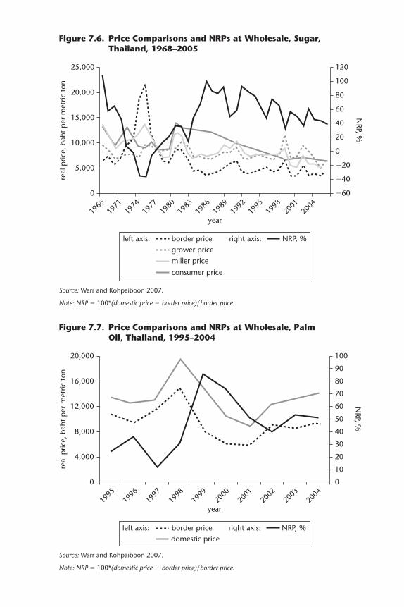
0
5,000
10,000
year
real
pric
e, b
aht
per
met
ric t
on
NRP, %
25,000
20,000
15,000
�60
�40
0
40
�20
20
60
80
120
100
1968
1971
1974
1977
1980
1983
1986
1989
1992
1998
1995
2004
2001
NRP, %left axis: right axis:border pricegrower pricemiller price
consumer price
Figure 7.6. Price Comparisons and NRPs at Wholesale, Sugar,Thailand, 1968–2005
Source: Warr and Kohpaiboon 2007.
Note: NRP � 100*(domestic price � border price)�border price.
0
4,000
8,000
year
real
pric
e, b
aht
per
met
ric t
on
NRP, %
20,000
16,000
12,000
0
50
40
30
20
10
60
70
100
90
80
1995
1996
1997
1998
1999
2000
2001
2002
2003
2004
NRP, %left axis: right axis:border pricedomestic price
Figure 7.7. Price Comparisons and NRPs at Wholesale, PalmOil, Thailand, 1995–2004
Source: Warr and Kohpaiboon 2007.
Note: NRP � 100*(domestic price � border price)�border price.
Rubber
Rubber is a net export item, and the rubber industry was subject to an export taxfor many years. The manner of calculating the tax meant that the rate driftedupwards along with inflation, and, because of the inflation in the 1970s, the exporttax rate on rubber had reached 26 percent by the early 1980s. Pressure from mem-bers of Parliament representing rubber production areas in the southern parts ofthe country led to a revision of the method of calculating the tax. This generated areturn to the lower tax rates that had been in place in the 1960s. Figure 7.8 con-firms that, since 1990, the tax rate on rubber has been close to zero.
Fertilizer
Urea is imported for use as fertilizer, the rates of tariff protection for these importshave been declining. The import taxation implies that there is disprotection (tax-ation) for the agricultural industries using this input. The decline in tariff ratesbegan in the early 1990s, and, by the early 2000s, the rates were negligible. Thispolicy change is confirmed by the price comparisons reported in figure 7.9. NRPs
268 Distortions to Agricultural Incentives in Asia
0
15,000
10,000
5,000
20,000
25,000
year
real
pric
e, b
aht
per
met
ric t
on
NRP, %
40,000
35,000
30,000
�35
�30
�25
�10
�20
�15
�5
0
15
10
5
1968
1971
1974
1977
1980
1983
1986
1989
1992
1995
1998
2004
2001
NRP, %left axis: right axis:border pricedomestic pricefarm price
Figure 7.8. Price Comparisons and NRPs at Wholesale, Rubber,Thailand, 1968–2005
Source: Warr and Kohpaiboon 2007.
Note: NRP � 100*(domestic price � border price)�border price.
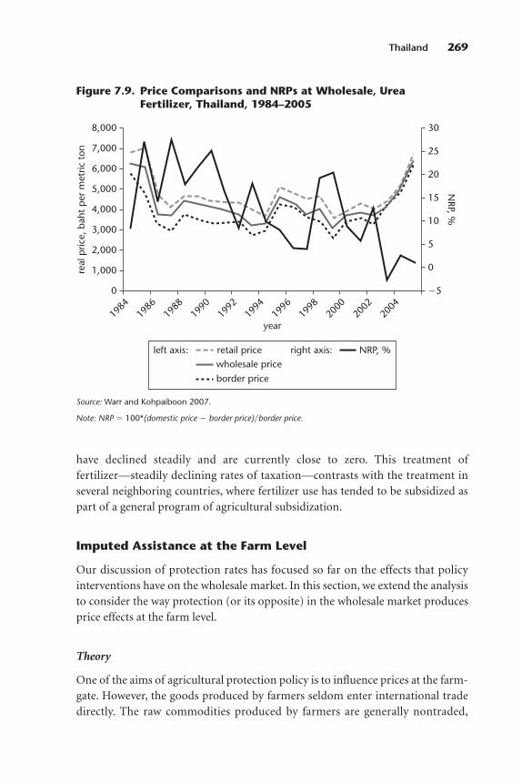
have declined steadily and are currently close to zero. This treatment of fertilizer—steadily declining rates of taxation—contrasts with the treatment inseveral neighboring countries, where fertilizer use has tended to be subsidized aspart of a general program of agricultural subsidization.
Imputed Assistance at the Farm Level
Our discussion of protection rates has focused so far on the effects that policyinterventions have on the wholesale market. In this section, we extend the analysisto consider the way protection (or its opposite) in the wholesale market producesprice effects at the farm level.
Theory
One of the aims of agricultural protection policy is to influence prices at the farm -gate. However, the goods produced by farmers seldom enter international tradedirectly. The raw commodities produced by farmers are generally nontraded,
Thailand 269
0
3,000
2,000
1,000
4,000
5,000
year
real
pric
e, b
aht
per
met
ric t
onN
RP, %
8,000
7,000
6,000
�5
5
0
10
15
30
25
20
1984
1986
1988
1990
1992
1994
1996
1998
2004
2000
2002
NRP, %left axis: right axis:retail pricewholesale priceborder price
Figure 7.9. Price Comparisons and NRPs at Wholesale, UreaFertilizer, Thailand, 1984–2005
Source: Warr and Kohpaiboon 2007.
Note: NRP � 100*(domestic price � border price)�border price.
whereas the commodities that enter international trade are the processed or par-tially processed versions of these raw products. Between the nontraded raw prod-uct produced by the farmer and the traded processed commodity that entersinternational trade, there may be several other steps, including transport, storage,milling, processing, and repackaging.
However, border protection policy operates on the goods that enter interna-tional trade either as exports or as imports. It does not operate on the raw com-modities produced by farmers. Protection at the farm level is therefore a derivedeffect. It depends on the extent to which the policies applied to the trade inprocessed agricultural goods induce changes in the prices of these goods and thentransmit the changes to the prices faced by farmers. An issue thus arises about thedegree to which price changes at wholesale that are induced by protection policyaffect the prices received by farmers for the raw products they sell.
We construct a simple econometric model to investigate this issue. We use thenotational convention that uppercase roman letters (such as X) denote the level ofthe values of variables and that lowercase roman letters (such as x) denote the nat-ural logarithms of these values. Thus, x � ln X. Protection at the wholesale level istherefore defined as:
PitW � P*it(1 � Tit
W), (7.1)
where PitW denotes the level of the wholesale price of commodity i at time t; P*it is
the corresponding border price expressed in the domestic currency and adjustedfor the handling costs involved in transferring the commodity from the cost,insurance, and freight price level to the domestic wholesale price level in the caseof an import or in transferring the commodity from the wholesale price level tothe free on board price level in the case of an export. The NRP at the wholesalelevel is given by Tit
W. In this discussion, both the border price and the NRP aretreated as exogenous variables. The border price is determined by world markets,and we presume that the country under discussion is a price taker. The NRP isdetermined by the government’s protection policy.
The farmgate price of the raw material is denoted by PFit, and its logarithm, pF
it,is related to the logarithm of the wholesale price as follows:
pFit � ai � bipit
W � uit , (7.2)
where ai and bi are coefficients, and uit is a random error term. The coefficient bi isthe pass-through or transmission elasticity. The estimated values of the coeffi-cients ai and bi are denoted by ai and bi, respectively. The econometric estimationof these parameters is discussed below.
The estimated coefficients are used as follows. We estimate the logarithm of thefarm price that would obtain in the absence of any protection as:
pF*it � ai � bipit
W*, (7.3)
270 Distortions to Agricultural Incentives in Asia
where pitW* is the estimated value of the wholesale price that would obtain in the
absence of protection so that pitW* � ln Pit
W*. This is then compared with the esti-mated value of the wholesale price in the presence of protection, as follows:
pFit � ai � bipit
W. (7.4)
We denote the antilogs of pFit and pF*
it by PFit and P F*
it , respectively, and then esti-mate the NRP at the farm level as:
TFit = (PF
it � P F*it )�PF
it . (7.5)
It is important to observe that the value of the protection-inclusive farmgateprice we use in these calculations is the price we have estimated using the econo-metric model (equation 7.4) rather than the actual price given by the raw data. Wedo this because our intention is to use the model to estimate the change in the farmgate price generated by the protection at the wholesale level. Thus, both theprotection-inclusive and the protection-exclusive prices used in (7.5) are the pre-dicted values obtained through the model.
The implied NRP at the farmgate can be related to the NRP at wholesale, as fol-lows. Substituting PF
it � Ai(PitW)bi and PF
it*
� Ai(PitW*)bi into equation (7.5), where Ai
is the antilog of ai, rearranging, and using equation (7.1), we obtain the simpleexpression:
TFit � (1 � Tit
W)bi � 1. (7.6)
Obviously, if TitW � 0, then TF
it � 0, regardless of the value of bi. Similarly, ifbi � 0, then TF
it � 0, regardless of the value of TitW. Also, if bi � 1, then TF
it = TitW. It
may be readily seen that, if TitW � 0, then TF � Tit
W as bi � 1 and TF � TitW as bi � 1.
If TitW � 0, then TF � Tit
W as bi � 1, but TF � TitW as bi � 1.
Econometric application
The purpose of the econometric analysis is to estimate the parameter bi for eachcommodity.4 We conduct the analysis for each commodity by relying on timeseries price data in which each variable is expressed in logarithms, and each isdeflated by the GDP deflator for Thailand: the farmgate price (LFP), the wholesaleprice (LWP), and the log of the international price, adjusted by the nominalexchange rate and transport and handling costs (LIP).
We first test each of the series for the existence of a unit root. The null hypoth-esis of a unit root was rejected for all price series for all commodities except soy-beans. (One should recall that the price series, relying on the GDP deflator, arereal, not nominal.) However, in the case of soybeans (the two price series forwhich the null hypothesis of a unit root could not be rejected), the series were notcointegrated. For all commodities except soybeans, the price series were thus con-sidered stationary.
Thailand 271
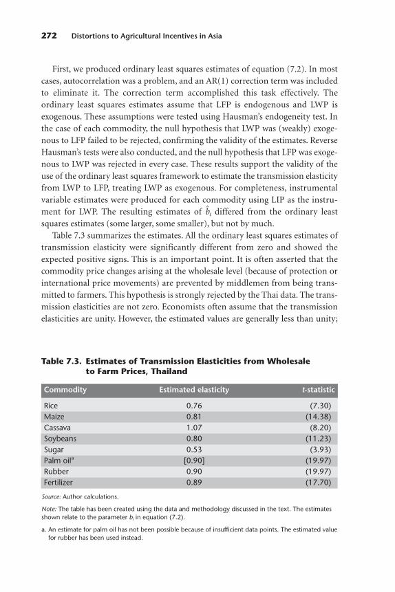
First, we produced ordinary least squares estimates of equation (7.2). In mostcases, autocorrelation was a problem, and an AR(1) correction term was includedto eliminate it. The correction term accomplished this task effectively. The ordinary least squares estimates assume that LFP is endogenous and LWP isexogenous. These assumptions were tested using Hausman’s endogeneity test. Inthe case of each commodity, the null hypothesis that LWP was (weakly) exoge-nous to LFP failed to be rejected, confirming the validity of the estimates. ReverseHausman’s tests were also conducted, and the null hypothesis that LFP was exoge-nous to LWP was rejected in every case. These results support the validity of theuse of the ordinary least squares framework to estimate the transmission elasticityfrom LWP to LFP, treating LWP as exogenous. For completeness, instrumentalvariable estimates were produced for each commodity using LIP as the instru-ment for LWP. The resulting estimates of bi differed from the ordinary leastsquares estimates (some larger, some smaller), but not by much.
Table 7.3 summarizes the estimates. All the ordinary least squares estimates oftransmission elasticity were significantly different from zero and showed theexpected positive signs. This is an important point. It is often asserted that thecommodity price changes arising at the wholesale level (because of protection orinternational price movements) are prevented by middlemen from being trans-mitted to farmers. This hypothesis is strongly rejected by the Thai data. The trans-mission elasticities are not zero. Economists often assume that the transmissionelasticities are unity. However, the estimated values are generally less than unity;
272 Distortions to Agricultural Incentives in Asia
Table 7.3. Estimates of Transmission Elasticities from Wholesaleto Farm Prices, Thailand
Commodity Estimated elasticity t-statistic
Rice 0.76 (7.30)Maize 0.81 (14.38)Cassava 1.07 (8.20)Soybeans 0.80 (11.23)Sugar 0.53 (3.93)Palm oila [0.90] (19.97)Rubber 0.90 (19.97)Fertilizer 0.89 (17.70)
Source: Author calculations.
Note: The table has been created using the data and methodology discussed in the text. The estimatesshown relate to the parameter bi in equation (7.2).
a. An estimate for palm oil has not been possible because of insufficient data points. The estimated valuefor rubber has been used instead.
most are between 0.7 and 0.9. In one case (sugar), the estimate is somewhat lower(0.53), and, in another (cassava), the estimated value slightly exceeds unity, but isnot significantly different from unity.5 It is likely that the true transmission elasticities change over time, but the limited data available for this exercise havemade it necessary to assume that the true values remain constant.
Estimation of assistance at the farm level
Given the estimated value of the transmission elasticity, we use equation (7.6),together with the estimated NRPs at the wholesale level discussed above, to pro-duce estimates of the imputed NRAs at the farm level. These are shown in Warrand Kohpaiboon (2007). Because the estimated values of the transmission elastic-ity are between zero and unity (except for the case of cassava), the imputed NRAsat the farmgate are somewhat lower in absolute value than the NRAs at the whole-sale level, but, because of the assumption of constant transmission elasticities overtime, they closely track the pattern of the results at the wholesale level.
Aggregate Measures of Agricultural Assistance
In this section, we calculate aggregate measures of rates of assistance using the infor-mation assembled from the preceding analysis and following, as much as possible,the methodology outlined in Anderson et al. (2008) and appendix A. The annualcalculations reported in this section fluctuate somewhat from year to year. Interna-tional and domestic price changes from year to year alter the protective effects of allinstruments of protection except ad valorem tariffs. In addition, the time requiredfor domestic prices to adjust to international price changes means that the annualdata on price differences produce some spurious variations from one year to thenext. Our interest is in broad trends rather than in these annual fluctuations.
Table 7.4 reports estimates of the NRAs at the farmgate for all commodities.These estimates take account of the assistance for fertilizer inputs. The NRAs arecalculated as the corresponding NRPs (discussed above), minus the product of thecost share of fertilizer in the production of the relevant commodity and the con-sumer tax equivalent of the import protection for the fertilizer industry. The con-sumer tax equivalent for fertilizer is positive every year but one, although the ratesof taxation have declined since the mid-1980s. The NRAs for covered products atwholesale are therefore below the NRAs at the farmgate for every commodity forwhich fertilizer is an input in production. The broad pattern in the NRAs forfarmers is otherwise similar to the pattern in the NRAs discussed above.
The NRAs are negative in all years for rice and in most years for maize, cassava,and rubber. For these commodities, the absolute magnitudes of these negative
Thailand 273

274
Table 7.4. NRAs for Covered Agricultural Products, Thailand, 1970–2004(percent)
Indicator, product 1970–74 1975–79 1980–84 1985–89 1990–94 1995–99 2000–04
Exportablesa �26.7 �19.4 �11.1 �11.7 �9.2 �3.8 �0.6Soybeansb — — — �19.9 n.a. n.a. n.a.Rice �30.1 �28.3 �18.0 �15.0 �16.2 �11.0 �7.6Maize �2.2 �2.6 �2.2 �7.6 �4.5 �11.5 �0.3Cassava �23.1 �0.8 �9.0 �16.6 �10.8 �13.8 �10.0Sugar 12.6 �3.2 12.7 36.8 34.0 22.4 12.6Rubber �0.5 �8.7 �17.9 �13.3 �4.4 �1.1 0.2Poultry �32.9 16.1 26.8 �7.1 �11.0 17.8 20.4Palm oil — — n.a. n.a. n.a. �12.6 �18.3
Import-competing productsa �4.8 1.9 45.3 22.0 6.4 34.4 4.7Soybeansb n.a. n.a. n.a. n.a. 27.5 21.5 30.0Pig meat �4.8 1.9 51.7 20.8 1.5 36.5 �1.8Palm oil — — �25.7 32.2 26.5 n.a. n.a.
All covered productsa �25.8 �18.4 �8.4 �9.7 �7.7 �1.1 �0.6Dispersion, covered productsc 25.0 20.8 28.5 29.3 25.1 22.9 16.7Coverage, at undistorted prices 65 65 68 71 71 75 78
Source: Warr and Kohpaiboon 2007.
Note: — � no data are available. n.a. � not applicable.
a. Weighted averages; the weights are based on the unassisted value of production.b. For exportables, 1985–89 refers to 1984–91. For import-competing products, 1990–94 refers to 1992–94, and 2000–04 refers to 2000–03.c. Dispersion is a simple five-year average of the annual standard deviation around the weighted mean of the NRAs of covered products.

rates have declined over time. For soybeans, the nominal rate was negative untilsoybeans became a net import item in the early 1990s. Since then, soybeans havebeen significantly protected. Sugar has been a protected commodity in almost allyears. The weighted average for all covered products was more than �25 percentbefore the later 1970s, but the mean rate of taxation has since fallen to virtuallyzero. The dispersion of rates for individual commodities around this mean hasnot fallen much though, suggesting that there is still considerable scope for policyreform to reduce distortions within the farm sector (bottom of table 7.4).
We have calculated the RRAs in agriculture to take into account not only theNRAs in agriculture, but also the NRAs in manufacturing and other nonfarmtradable sectors. We estimate the average NRAs for import-competing manufac-turing based on data in Nicita and Olarreaga (2006), while we assume that theaverage NRAs for other nonfarm tradable sectors are zero.6 The weighted averageof these two sets of NRAs is then calculated using weights from the input-outputtables of the National Economic and Social Development Board (NESDB, vari-ous). The estimated RRAs are negative every year, but have declined in absolutevalue from more than �30 percent in the early 1970s to around �7 percent inrecent years (table 7.5 and figure 7.10). These estimates suggest that, over the pastfour decades, agriculture has undergone a shift from a severely taxed sector to amildly taxed sector (both net).
Conclusions and Prospects for Future Reform
As Thailand has industrialized, successive governments have become more inter-ested in intervening on behalf of agricultural producers. Nonetheless, because thecountry is a major agricultural exporter, the scope for a policy of protection as ameans of influencing domestic commodity prices has been limited. This chapterhas used comparisons of the prices of agricultural commodities in domestic mar-kets and in international markets as a means of examining the magnitude of thegovernment’s interventions.
The direct taxation of agricultural exports has been gradually eliminated. Thishas been important in the case of rice, on which the high rates of export taxationbefore the mid-1980s have been abolished. Rubber exports, taxed prior to 1990,have been untaxed since then. Cassava exports have continued to be taxed to aminor extent through the system of export quotas. Fertilizer is a major input intoagricultural production, and the effective taxation of fertilizer use has beensteadily eliminated since the early 1990s. Maize exports have been consistentlyuntaxed, as have chicken exports. Most of this evolution in taxation and protec-tion has involved eliminating the price distortions that once disfavored agricul-tural export industries.
Thailand 275

276
Table 7.5. NRAs in Agriculture Relative to Nonagricultural Industries, Thailand, 1970–2004(percent)
Indicator 1970–74 1975–79 1980–84 1985–89 1990–94 1995–99 2000–04
Covered productsa �25.8 �18.4 �8.4 �9.7 �7.7 �1.1 �0.6Noncovered products �10.4 �5.8 11.3 3.4 �0.9 10.1 1.4All agricultural productsa �20.3 �14.0 �2.0 �6.2 �5.7 1.7 �0.2Non-product-specific assistance 0.0 0.0 0.0 0.0 0.0 0.0 0.0Total agricultural NRAb �20.3 �14.0 �2.0 �6.2 �5.7 1.7 �0.2Trade bias indexc �0.18 �0.20 �0.37 �0.24 �0.14 �0.27 �0.03NRA, agricultural tradables �23.1 �15.9 �2.3 �6.9 �6.4 1.8 �0.2NRA, nonagricultural tradables 16.1 16.0 14.2 11.1 10.0 8.9 7.8RRAd �33.7 �27.5 �14.4 �16.3 �14.9 �6.5 �7.4
Source: Warr and Kohpaiboon 2007.
a. Including product-specific input subsidies.b. Including product-specific input subsidies and non-product-specific assistance. Represents total assistance to primary factors and intermediate inputs, divided by the
total value of primary agriculture production at undistorted prices.c. The trade bias index is defined as (1 � NRAagx�100)�(1 � NRAagm�100) � 1, where NRAagm and NRAagx are the average percentage NRAs for the import-competing
and exportable parts of the agricultural sector, respectively.d. The RRA is defined as 100*[(100 � NRAagt)�(100 � NRAnonagt) � 1], where NRAagt and NRAnonagt are the percentage NRAs for the tradables parts of the agricultural
and nonagricultural sectors, respectively.

Three commodities depart from this general liberalization in agricultural mar-kets. Soybeans were an export before 1992 and have been a net import item sincethen. The imports have been subject to quota restrictions. The shift from a netexport item to a net import item coincided with a switch from negative to positiveNRPs. Since the early 1990s, the domestic soybean industry has benefited from anNRP of around 30–40 percent. Sugar is an export commodity, but the domesticsugar industry is protected by a system that taxes domestic consumers and trans-fers the revenue to producers. NRPs have averaged over 60 percent. The politicalpower of the highly capital-intensive sugar milling industry is behind this patternof protection. The case of palm oil is qualitatively similar to sugar, but the rates ofprotection are somewhat lower.
Government interventions on behalf of rural people have been important, butthey have generally not taken the form of interventions in agricultural commod-ity markets. Cash transfers to village organizations, subsidized loan schemes notlinked to agricultural production, and a generally good system of public infra-structure have been the main instruments. The prospects for more trade liberal-ization are not encouraging unless this occurs through bilateral preferential trad-ing arrangements such as the scheme proposed with the United States.7
Thailand 277
1970
1972
1974
1976
1978
1980
1982
1984
1986
1988
1990
1992
1994
1996
1998
2000
2002
2004
NRA
and
RRA
, %
year
�50
�40
�30
�20
�10
0
20
10
30
NRA, nonagricultural tradables RRANRA, agricultural tradables
Figure 7.10. NRAs for Agricultural and NonagriculturalTradables and the RRA, Thailand, 1970–2004
Source: Warr and Kohpaiboon 2007.
Note: For the definition of the RRA, see table 7.5, note d.

Notes
1. A full description of the trading position of the major agricultural commodities is provided inthe appendix tables in Warr and Kohpaiboon (2007).
2. The price variables and the formula used in these NRA calculations are summarized in theappendix tables in Warr and Kohpaiboon (2007). Annual price data are also included in those tables.
3. The economic effects of the rice export taxes, including the distributional effects, are explored inWarr (2001). See also the analyses of Pinthong (1976, 1984); Wong (1978); Meenaphant (1981); Barkerand Herdt (1985); Roumasset and Setboonsarng (1988); Somporn and Poapongsakorn (1995); Warrand Wollmer (1997); and Choeun, Godo, and Hayami (2006).
4. The results are summarized here. Details of the econometric analysis are available upon request.5. There is no theoretical reason to suppose that the true value of the transmission elasticity is nec-
essarily below unity. For example, if all margins between the farmgate and the wholesale level remainconstant in nominal terms as the wholesale price changes, the percent change in the derived farmgateprice would necessarily exceed the percent change in the wholesale price. The transmission elasticitywould therefore exceed unity.
6. Because the Nicita and Olarreaga (2006) data are incomplete, we have assumed that the NRAsfor manufacturing before 1982 and after 2002 are the same as the respective 1982 and 2002 NRAs cal-culated by Nicita and Olarreaga. This undoubtedly understates rates of manufacturing protection inthe 1970s and overstates them post-2002. More complete estimates for manufacturing would thereforereinforce our broad conclusions rather than undermine them.
7. A bilateral trade arrangement with the United States was under negotiation up to February 2006,but the negotiations were suspended thereafter. The protection of the soybean industry was expectedto be an important issue in these negotiations.
References
Anderson, K., M. Kurzweil, W. Martin, D. Sandri, and E. Valenzuela. 2008. “Measuring Distortions toAgricultural Incentives, Revisited.” World Trade Review 7 (4): 675–704.
Barker, R., and R. W. Herdt. 1985. The Rice Economy of Asia. With Beth Rose. Washington, DC:Resources for the Future.
Choeun, H., Y. Godo, and Y. Hayami. 2006. “The Economics and Politics of Rice Export Taxation inThailand: A Historical Simulation Analysis, 1950–1985.” Journal of Asian Economics 17 (1): 103–25.
Corden, W. M. 1974. Trade Policy and Economic Welfare. Oxford: Clarendon Press.Meenaphant, S. 1981. “An Economic Analysis of Thailand’s Rice Trade.” PhD dissertation, Rice
University, Houston.NESDB (National Economic and Social Development Board). various years. “Input-Output Table of
Thailand.” Spreadsheet, NESDB, Bangkok.Nicita, A., and M. Olarreaga. 2006. “Trade, Production, and Protection, 1976–2004.” World Bank
Economic Review 21 (1): 165–71.Pinthong, C. 1976. “A Price Analysis of the Thai Rice Marketing System.” PhD dissertation, Stanford
University, Palo Alto, CA.———. 1984. “Distribution of Benefit of Government Rice Procurement Policy in Thailand.”
[in Thai] Thammasat University Journal 13 (2): 166–87.Roumasset, J. A., and S. Setboonsarng. 1988. “Second-Best Agricultural Policy: Getting the Price of
Thai Rice Right.” Journal of Development Economics 28 (3): 323–40.Siamwalla, A., and S. Setboonsarng. 1989. Trade, Exchange Rate, and Agricultural Pricing Policies in
Thailand. Washington, DC: World Bank.———. 1991. “Thailand.” In Asia. Vol. 2 of The Political Economy of Agricultural Pricing Policy, ed. A. O.
Krueger, M. Schiff, and A. Valdés, 236–80. World Bank Comparative Study. Baltimore: Johns Hopkins University Press; Washington, DC: World Bank.
278 Distortions to Agricultural Incentives in Asia
Siamwalla, A., S. Setboonsarng, and D. Patamasiriwat. 1993. “Agriculture.” In The Thai Economy inTransition, ed. P. G. Warr, 81–117. Cambridge: Cambridge University Press.
Sieper, E. 1982. Rationalizing Rustic Regulation. Sydney: Center for Independent Studies.Somporn, I., and N. Poapongsakorn. 1995. “Rice Supply and Demand in Thailand: The Future
Outlook.” Paper presented to the Sectoral Economic Program, Thailand Development ResearchInstitute, Bangkok.
Warr, P. G. 2001. “Welfare Effects of an Export Tax: Thailand’s Rice Premium.” American Journal ofAgricultural Economics 83 (4): 903–20.
Warr, P. G., and A. Kohpaiboon. 2007. “Distortions to Agricultural Incentives in Thailand.” AgriculturalDistortions Working Paper 25, World Bank, Washington, DC.
Warr, P. G., and F. Wollmer. 1997. “Testing the Small Country Assumption: Thailand’s Rice Exports.”Journal of the Asia Pacific Economy 2 (2): 133–43.
Wong, C. M. 1978. “A Model for Evaluating the Effects of Thai Government Taxation of Rice Exportson Trade and Welfare.” American Journal of Agricultural Economics 60 (1): 65–73.
World Development Indicators Database. World Bank. http://go.worldbank.org/B53SONGPA0(accessed May 2008).
Thailand 279

Since the late 1980s, Vietnam has been making remarkable progress in its transi-tion from a closed command economy toward an open market economy and integration in the world economy. The initial progress was slow and hesitant fol-lowing the announcement of the doi moi (renovation) policy in 1986, but moresignificant reforms were undertaken in the first half of the 1990s. The process lostmomentum in 1996–98, perhaps reflecting complacency after the success of thefirst reforms, but also the economic uncertainty created by the 1997–98 Asianfinancial crisis. Since about 1999, there has been a renewed emphasis on complet-ing the unfinished reform agenda.
The key reform measures have included widespread agricultural reformsinvolving a transition from the collective regime to a system in which farmers pos-sess more freedom in making production decisions and in marketing their pro-duce. Quantitative import restrictions have been dismantled in all cases exceptsugar and petroleum products. Significant tariff reforms have led to notablereductions in the level and dispersion of effective rates of protection. Public sectorenterprises have been exposed to greater market discipline. Restrictions have beenrelaxed on foreign direct investment, particularly in export-oriented projects, andthey have been lifted on private sector participation in foreign trade and the establishment of business ventures by private individuals and companies. Theseinitiatives have been accompanied by sweeping macroeconomic policy reforms,including the unification and realignment of the exchange rate, the liberalizationof agricultural prices, the relaxation of exchange controls, and a firm commitmentto fiscal prudence.
281
8
VIETNAM
Prema-Chandra Athukorala,Pham Lan Huong, and Vo Tri Thanh

The purpose of this chapter is to examine the implications of the market- oriented policy reforms in Vietnam for the incentives faced by farmers in the con-text of the changes in the overall structure of the incentives for private sector activ-ities in the economy. We undertake the analysis against the backdrop of a narrativeon the evolution of agricultural policy and the key policy trends dating back to theera of the command economy. The empirical analysis of agricultural incentivescovers six major products—rice, sugar, pig meat, poultry, rubber, and coffee—using data from 1986 (the earliest postreform year for which the required data areavailable) to 2004. The six covered products accounted for more than two-thirds ofthe total value of agricultural production in Vietnam during the period. Our aim isto contribute to the contemporary policy debate on reforming the structure ofincentives for domestic agriculture as an integral part of the endeavor to acceleratethe country’s economic integration into the world economy.
The study has four main parts. The next section presents an overview of thegrowth and structural changes during the postreform era (since the mid-1980s). Itemphasizes the relative importance of the agricultural sector and the trends andcompositional shifts in agricultural output and trade. The subsequent sectionprovides an overview of the origins, key elements, and achievements of the effortto meet reform commitments. It highlights the political economy of the relatedpolicy making. The penultimate section—the analytical core of the chapter—examines trends and patterns in the incentives in domestic agriculture by relyingon a set of indicators based on the methodology described in Anderson et al.(2008) and appendix A. The final section summarizes the key findings and policyimplications.
Agriculture in the Vietnamese Economy
We first document the extraordinary economic growth performance of this trans-forming economy and then review the structural changes that have accompaniedthis success.
Growth trends
During the era of central planning (from the mid-1950s in the north of the coun-try and, in the south, beginning in 1975 following unification), the economy wasnot subject to forced industrialization to the same degree as the centrally plannedeconomies of China and the Soviet bloc. The prolonged military conflict with theregime in the south and with the United States caused industrial transformationto be limited to the establishment of industries that met the priorities of the wareconomy. Thus, agriculture—broadly defined to include farming, fisheries, and
282 Distortions to Agricultural Incentives in Asia
forestry—remained the dominant sector of the economy up to the 1980s. Duringthe period from 1955 to 1985, the share of agriculture in gross domestic product(GDP) fluctuated from around 38 to 52 percent without showing any clear trend(GSO 2001). By the mid-1980s, over 72 percent of the total labor force wasengaged in agricultural pursuits (Riedel 1993).
The process of the collectivization of agriculture in the northern part of thecountry had been completed by the early 1960s. The forced replacement of asemisubsistent peasant commodity production system by a regular plan usheredin an era of suppressed growth, if not stagnation, in agriculture. During most ofthe ensuing three decades, agricultural output in the north was only barely suffi-cient to meet domestic consumption requirements in that part of Vietnam.Attempts to replicate the collectivized system in the south following the adminis-trative unification of the country in 1976 resulted in a severe disruption in agri-cultural production there. Piecemeal reforms implemented in 1979–80 to loosenthe structures of central planning had only limited impact in containing outputcontraction. By the mid-1980s, large areas of the country were experiencing near-famine conditions, and food shortages were resulting in widespread suffering.National food security became a leading preoccupation (White 1985; Riedel andComer 1997; Pritchett 2003).
The response of agriculture to the market-oriented policy reforms launched inthe late 1980s was remarkably swift. Between 1988 and 1992, GDP increased by27 percent; nearly 30 percent of this increase arose directly from agriculture. Inaddition, rapid agricultural growth contributed to an expansion in rural nonagri-cultural services, input supply, and food processing. During the ensuing years, thegrowth turned out to be broadly based, and industry and services developed at apace that was more rapid than the pace of development in agriculture. Nonethe-less, the growth rate in agriculture remained impressive (3.0 to 5.2 percent peryear) relative to the precrisis experience in Vietnam and the average performancein other low-income and transition economies. Despite the notable structuralchanges over the past 15–20 years, agriculture still has a substantial weight in theVietnamese economy, contributing about 20 percent of GDP (figure 8.1) andabsorbing 57 percent of the total labor force in 2005. Slightly more than two-thirds of households in the lowest income quintile were occupied in agriculture in2004, and almost three-fifths of the incomes among households in that quintilewas generated by agricultural activities (compared with less than one-fourth ofthe incomes in the highest income quintile).
The impressive agricultural growth, especially the surge in paddy production,played a key role in winning political support for more reforms by ensuringnational food security, a source of much political anxiety in the 1980s. Agricul-tural growth was also at the heart of the success in the rapid reduction in rural
Vietnam 283
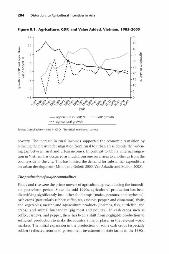
poverty. The increase in rural incomes supported the economic transition byreducing the pressure for migration from rural to urban areas despite the widen-ing gap between rural and urban incomes. In contrast to China, internal migra-tion in Vietnam has occurred as much from one rural area to another as from thecountryside to the city. This has limited the demand for substantial expenditureon urban development (Minot and Goletti 2000; Van Arkadie and Mallon 2003).
The production of major commodities
Paddy and rice were the prime movers of agricultural growth during the immedi-ate postreform period. Since the mid-1990s, agricultural production has beendiversifying significantly into other food crops (maize, peanuts, and soybeans),cash crops (particularly rubber, coffee, tea, cashews, pepper, and cinnamon), fruitsand vegetables, marine and aquaculture products (shrimps, fish, cuttlefish, andcrabs), and animal husbandry (pig meat and poultry). In cash crops such as coffee, cashews, and pepper, there has been a shift from negligible production tosufficient production to make the country a major player in the relevant worldmarkets. The initial expansion in the production of some cash crops (especiallyrubber) reflected returns to government investment in state farms in the 1980s,
284 Distortions to Agricultural Incentives in Asia
agriculture in GD
P, %
0
50
40
20
30
1985
year
10
5
25
15
35
45
1986
1987
1989
1988
1990
1992
1994
1996
1998
2000
2004
2005
2002
1991
1993
1995
1997
1999
2003
2001
2
�2
6
12
0
4
8
10
GDP growthagriculture in GDP, %agricultural growth
grow
th in
GD
P an
dag
ricul
tura
lva
lue
adde
d, %
Figure 8.1. Agriculture, GDP, and Value Added, Vietnam, 1985–2005
Source: Compiled from data in GSO, “Statistical Yearbook,” various.
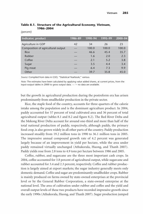
but the growth in agricultural production during the postreform era has arisenpredominantly from smallholder production in the private sector.
Rice, the staple food of the country, accounts for three-quarters of the calorieintake among the population and is the dominant agriculture product. In 2004,paddy accounted for 57 percent of total cultivated area and 36 percent of totalagricultural output (tables 8.1 and 8.2 and figure 8.2). The Red River Delta andthe Mekong River Delta account for around one-third and more than half of thetotal national production of paddy, respectively, although paddy, the primaryfood crop, is also grown widely in all other parts of the country. Paddy productionincreased steadily from 19.2 million tons in 1990 to 36.1 million tons in 2005.The impressive annual compound growth rate of 4.2 percent was generatedlargely because of an improvement in yield per hectare, while the area underpaddy remained virtually unchanged (Athukorala, Huong, and Thanh 2007).Paddy yields rose from 2.8 tons to 4.9 tons per hectare between 1986 and 2005.
Coffee, rubber, and sugarcane are the three most important cash crops. In2004, coffee accounted for 3.8 percent of agricultural output, while sugarcane andrubber accounted for 3.4 and 2.3 percent, respectively. Coffee and rubber produc-tion is largely aimed at export markets; the sugar industry generally meets onlydomestic demand. Coffee and sugar are predominantly smallholder crops. Rubberis mainly produced on farms owned by state-owned enterprises at the provinciallevel or by the General Rubber Corporation, a state-owned enterprise at thenational level. The area of cultivation under rubber and coffee and the yield andoverall output levels of these two products have recorded impressive growth sincethe early 1990s (Athukorala, Huong, and Thanh 2007). Sugar production jumped
Vietnam 285
Table 8.1. Structure of the Agricultural Economy, Vietnam,1986–2004
(percent)
Indicator, product 1986–89 1990–94 1995–99 2000–04
Agriculture in GDP 42 34 26 23Composition of agricultural output — 100.0 100.0 100.0
Rice — 46.6 45.4 35.7Rubber — 1.6 2.0 2.3Coffee — 2.1 5.2 3.8Sugar — 3.5 4.4 3.4Pig meat — 6.4 7.3 9.9Other — 39.7 35.8 45.0
Source: Compiled from data in GSO, “Statistical Yearbook,” various.
Note: The estimates have been calculated by applying value added shares, at current prices, from theinput-output tables in 2000 to gross output data. — � no data are available.
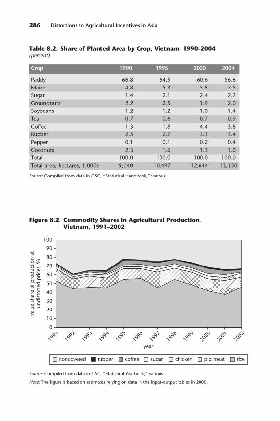
286 Distortions to Agricultural Incentives in Asia
Table 8.2. Share of Planted Area by Crop, Vietnam, 1990–2004(percent)
Crop 1990 1995 2000 2004
Paddy 66.8 64.5 60.6 56.6Maize 4.8 5.3 5.8 7.5Sugar 1.4 2.1 2.4 2.2Groundnuts 2.2 2.5 1.9 2.0Soybeans 1.2 1.2 1.0 1.4Tea 0.7 0.6 0.7 0.9Coffee 1.3 1.8 4.4 3.8Rubber 2.5 2.7 3.3 3.4Pepper 0.1 0.1 0.2 0.4Coconuts 2.3 1.6 1.3 1.0Total 100.0 100.0 100.0 100.0Total area, hectares, 1,000s 9,040 10,497 12,644 13,150
Source: Compiled from data in GSO, “Statistical Handbook,” various.
0
30
20
10
70
60
40
50
100
90
80
1991
1992
1993
1994
1995
1996
1997
1998
1999
2000
2001
2002
year
noncovered rubber coffee sugar chicken pig meat rice
valu
e sh
are
of p
rodu
ctio
nat
undi
stor
ted
pric
es, %
Figure 8.2. Commodity Shares in Agricultural Production,Vietnam, 1991–2002
Source: Compiled from data in GSO, “Statistical Yearbook,” various.
Note: The figure is based on estimates relying on data in the input-output tables in 2000.

in 1995 following the launch of the One Million Tons of Sugar Program and con-tinued to increase up to 1999. However, a mild downward trend characterized bysignificant annual fluctuations has been evident since then. Sugar yields rose from396 to 553 quintals per hectare in 1986–2005. The area under sugarcane cultiva-tion has declined in recent years because of a shift by farmers to other crops,mostly subsidiary food crops. Despite its relatively poor performance (or becauseof it), sugarcane production remains the most well assisted agricultural activity(see below). In 1995, the government launched the One Million Tons of SugarProgram, which was aimed at achieving sugar self-sufficiency by 2000 and creat-ing employment in the rural economy (Nguyen et al. 2006).
The other cash crops that have shown impressive growth during the postre-form era include cashews, groundnuts, tea, and pepper. Vietnam is the world’slargest producer of pepper, the third largest producer of cashew nuts, the fifthlargest producer of tea, and the tenth largest producer of groundnuts. However,the combined share of these products in the total agricultural GDP of the countryremains small, at less than 3 percent.
Livestock production has expanded rapidly since the early 1990s. It accountedfor about 14 percent of agricultural value added in 2000 (IAPP 2001). Pig meat isthe most important livestock product (60 percent), followed by poultry (15 per-cent) and beef (8 percent). The share of pig meat in agricultural value added rosefrom 6 percent in 1990–94 to 10 percent in 2000–04 (table 8.1). Currently, over90 percent of total pig meat production is consumed domestically, althoughexports (mainly to China) have been increasing rapidly in recent years.
Agricultural exports
Primary products accounted for nearly half of non-oil merchandise exports in themid-1980s. The share rose in the early years of the postreform period when thefirst positive response to the reforms was registered in agricultural products, espe-cially rice. In 1998, Vietnam became self-sufficient in rice and then a net exporter.In 2005, rice exports peaked at 5.3 million tons, making the country the thirdlargest rice exporter in the world (after the United States and Thailand). The com-position of agricultural exports has become increasingly diversified; pepper,cashews, rubber, coffee, and fish products have shown impressive growth. Sincethe late 1990s, manufacturing exports have been growing more rapidly, resultingin a notable shift in the composition of exports away from primary products.However, agricultural products still accounted for over one-quarter of total non-oil merchandise exports in 2004 (table 8.3).1
Until about the mid-1990s, rapid volume expansion and favorable price trendswere contributing to the growth in agricultural export earnings (figure 8.3). Prices
Vietnam 287
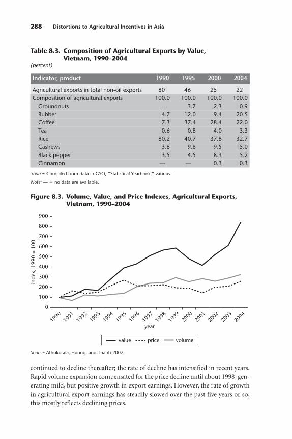
continued to decline thereafter; the rate of decline has intensified in recent years.Rapid volume expansion compensated for the price decline until about 1998, gen-erating mild, but positive growth in export earnings. However, the rate of growthin agricultural export earnings has steadily slowed over the past five years or so;this mostly reflects declining prices.
288 Distortions to Agricultural Incentives in Asia
Table 8.3. Composition of Agricultural Exports by Value,Vietnam, 1990–2004
(percent)
Indicator, product 1990 1995 2000 2004
Agricultural exports in total non-oil exports 80 46 25 22Composition of agricultural exports 100.0 100.0 100.0 100.0
Groundnuts — 3.7 2.3 0.9Rubber 4.7 12.0 9.4 20.5Coffee 7.3 37.4 28.4 22.0Tea 0.6 0.8 4.0 3.3Rice 80.2 40.7 37.8 32.7Cashews 3.8 9.8 9.5 15.0Black pepper 3.5 4.5 8.3 5.2Cinnamon — — 0.3 0.3
Source: Compiled from data in GSO, “Statistical Yearbook,” various.
Note: — � no data are available.
year
0
1990
1991
1992
1993
1994
1995
1996
1997
1998
1999
2000
2001
2002
2003
2004
inde
x, 1
990
= 10
0
pricevalue volume
900
800
700
600
500
400
300
200
100
Figure 8.3. Volume, Value, and Price Indexes, Agricultural Exports,Vietnam, 1990–2004
Source: Athukorala, Huong, and Thanh 2007.
The Reform Process: From Plan to Market
Under the collective system of agriculture instituted in the north in the early1960s, cooperatives were the key link between agricultural households and thenational economic plan. As the prime institution in the effort to replace the mar-ket by the plan, the agricultural cooperatives were responsible for organizing thedeployment of the agricultural labor force, undertaking production according toplans approved by the central authorities, selling surplus production to the state atstate-controlled prices, and implementing obligatory procurement quotas intro-duced from time to time for sales to the state of selected essential commodities(White 1981).
After the defeat of the government in the south in 1975 and the formal admin-istrative reunification of the economy in 1976, replacing the market by the plan inthe south presented a formidable challenge. Immediately after reunification, theattempt to bring southern agriculture into the collective system was fairly cau-tious. However, the rapid growth in private trade, combined with concerns aboutthe political resistance to socialist transformation among southern farmers andthe southern business community, which was dominated by ethnic Chinese, led toan attempt to accelerate the process. The Second Party Plenum, in July 1977, setambitious targets to speed the collectivization of individual farm households. Theresistance among farmers to the introduction of the collective system, coupledwith uncertainty about the future direction of reform, resulted in declines in agri-cultural output. The process of collectivization in the south was slowed. Agree-ments were then reached on the need to decentralize decision making and providebetter incentives for increasing production though private household initiatives(Duiker 1989; Fforde and de Vylder 1996; Naughton 1996).
Reforms in 1979–80 introduced production contracts under which coopera-tives subcontracted land to households and allowed households greater latitude indecision making on production issues. Under this new system, which was similarto the household responsibility system in China, households were allowed to keepor to sell on the free market any surplus above the amount stipulated for deliveryto cooperatives under the contracts. In effect, the cooperatives were limited to thesubsidiary role of allocating land, supplying inputs, and providing technical assis-tance (Woodside 1989).
These reforms had an immediate and dramatic effect: in 1994 prices, total agricultural production rose from D 37 trillion in 1979 to D 46 trillion in 1982(GSO 2001). However, rather than responding to improved production by ampli-fying reforms, as the Chinese government did, the Vietnamese governmentbackpedaled for most of the rest of the decade. The emergence in the early 1980sof severe macroeconomic imbalances, which were reflected in high and risinginflation, undermined the reform movement. The macroeconomic problems were
Vietnam 289

interpreted as a symptom of the failure of the reforms, and they also created dis-satisfaction because they led to a reduction in real wages in the civil service. Thus,the influence of hard-liners within the Communist Party of Vietnam had gainedstrength by the mid-1980s, and this added to the pressure to enforce the collec-tivization of agriculture in the south (Riedel and Comer 1997).
By the mid-1980s, the economy was stagnating because of hyperinflation and achronically poor balance of payments situation. Furthermore, it was clear by 1988that Soviet aid would soon decline. In the face of these problems, a more con-certed push toward reform was announced at the Sixth Congress of the Commu-nist Party of Vietnam in December 1986 (CPV 1994). The implementation of thisprogram of reform, referred to as doi moi, did not, however, gain much momen-tum until the collapse of the Soviet Union, which put an end to Soviet aid. Massivecontraction in agricultural output in 1988, which brought near-famine conditionsin many parts of the country, also played a role in reducing the resistance toreform. The focus of early reform was mainly on unshackling agriculture. Initially,the reform process largely ignored the private sector except in agriculture, and theprocess of establishing the institutions needed to support private sector activityoutside agriculture was undertaken only in the early 1990s after emerging signsof unrest.
Unshackling agriculture
The transition to a more decentralized, market-oriented system of agriculturalproduction was launched through the adoption of a decree by the CommunistParty of Vietnam in 1988. The decree recognized the peasant household ratherthan the cooperative as the basic unit in the agrarian structure. It recognized the rightof households to the conditional use of private land for a period of 10–15 years; toown draft animals, farm tools, and other equipment; to barter output for inputs;and to retain the income earned through production once they had paid a modesttax. However, cooperatives continued to have ultimate control over land andwater resources; and the sale of output, at prices set by the government, remainedrestricted to sales within the same district. Additional measures introduced in1989 reduced the direct involvement of the government in the allocation ofinputs. In July 1993, the duration of tenure rights over agricultural land wasextended to 20 years, and farmers were permitted to sell, lease, exchange, mort-gage, and bequeath land. Cooperatives were still meant to provide a focus for various rural activities sponsored by the government, but, in the majority of com-munes, they were reduced to only a minor role. They were to act as local tax collectors, the holders of residual property rights, and a component of the formalstate structure (Riedel 1993; Sachs and Woo 1994; Riedel and Comer 1997).
290 Distortions to Agricultural Incentives in Asia
Land tenure reforms were accompanied by sweeping domestic market pricereforms. In 1987–88, the rationing system was abolished for many commodities,and the official prices of nonessential goods were raised to a level close to free-market prices. Administered prices on most consumer goods and a large numberof agricultural and industrial inputs were abolished. In June 1990, the procure-ment of farm products by the government, usually at prices below free-marketprices, formally came to an end, allowing farmers to sell their produce at mar-ket prices. By 1990, commodity prices were largely determined by domestic mar-ket conditions, and direct subsidies had been eliminated. The sellers market wasreplaced because of the shift toward market-clearing prices. The weakening ofthe state trading system at the local level permitted private traders to developlocal markets, while many state trading enterprises became more responsive tomarket opportunities. Starting in 1989, the international trade in agriculturalproducts was also liberalized in phases, and this eventually allowed private sectorparticipation.
Trade policy reforms
Foreign trade and investment regimes were liberalized in stages in conjunctionwith the domestic market price reforms. The law on import and export dutiesintroduced in January 1988 marked the launch of the new trade tax system. Theoriginal import tariff schedule was replaced in 1992 by a detailed, consolidatedschedule based on the Harmonized Commodity Description and Coding Systemof tariff nomenclature. During the rest of the 1990s, the tariff structure was fine-tuned to mirror a policy trend toward selective protection in the case of consumergoods (cosmetics and several categories of food products), activities upstream ofthe textile and garment industry (silk, cotton, and some fiber production), andsome intermediate goods (metal products, cement, and glass). In the early andmid-2000s, following Vietnam’s accession to the free trade area of the Associationof Southeast Asian Nations in 1995 and in preparation for the country’s accessionto the World Trade Organization (WTO), the government took steps to reorgan-ize and rationalize the tariff structure (Thanh 2006).
After more than 15 years of reform, tariffs are now the major instruments usedin regulating import trade. The average (import-weighted) import duty ratedeclined from 22 percent in 1999 to 13.6 percent in 2004 (figure 8.4). The maxi-mum tariff rate (at the six-digit level of the Harmonized Commodity Descriptionand Coding System) declined from 200 percent in 1997 to 120 percent in 2001 andthen 113 percent in 2004. By October 2005, of all tariff lines, less than 1 percent(accounting for around 4 percent of total import value) were subject to tariff ratesabove 50 percent. The tariff on about one-third of the tariff lines was zero. Despite
Vietnam 291

notable efforts to rationalize the tariff structure, tariffs are still relatively high andnonuniform according to regional standards (Athukorala 2006).2
The tariff rates are generally higher for manufacturing products than for agri-cultural products and other primary products. By mid-2003, the weighted averageduty rate on manufacturing imports was 29 percent, while the correspondingrates were 11 percent on agricultural products and 3.6 percent on mineral prod-ucts. Within manufacturing, the tariff rates are particularly high for processedfoods and some consumer goods, notably garments, footwear, ceramic products,and leather goods (Athukorala 2006; Athukorala, Huong, and Thanh 2007).
By 2004, only two products, sugar and petroleum, remained subject to quanti-tative restrictions (import licensing). As part of its trade reform commitmentsunder the WTO accession agreement, the government offered to replace importlicensing on sugar by a WTO-consistent tariff trade quota system. Imports of twoproducts—poultry eggs and raw tobacco—were already subject to tariff rate quotas. The list of prohibited imports included military equipment, toxic chemi-cals, antiquities, narcotics, firecrackers, toxic toys, used consumer goods, andright-hand-drive automobiles. In addition, a considerable number of importitems (such as pharmaceuticals, some chemicals, some food items, fertilizer, andrecording and broadcasting equipment) required approval from the relevant min-istries. In 2000, in value terms, around 10 percent of imports were subject to this
292 Distortions to Agricultural Incentives in Asia
year
0
5
10
15
20
25
1990
1991
1992
1993
1994
1995
1996
1997
1998
1999
2000
2001
2002
2003
2004
imp
ort
tarif
frat
e, %
Figure 8.4. Weighted Average Import Duties, Vietnam,1990–2004
Source: Nicita and Olarreaga 2006; CIE 1998.
form of regulation. As in many other countries, these regulations are generallymaintained in Vietnam for heath and security reasons, and they do not appear todistort trade patterns substantially.
Among the early market-oriented reforms, the government introduced dutieson a number of export items. The duties were justified at the time by the need toraise revenue, protect the environment, conserve natural resources, and retaininputs for domestic production. Most of the duties were subsequently eliminated.By 1998, only a few export products—iron ore, crude oil, scrap metal, and rawcashews—were subject to duties. Export prohibitions now apply only to environ-mentally sensitive items such as agroforestry products, round wood and saw woodcut from domestic natural forests, firewood and charcoal obtained from natural-growth domestic forestry wood, and rare wild animals.
When the country began exporting rice in 1989, the exports were subject tolicensing to ensure adequate domestic supplies and reduce the price volatility inthe domestic market. Export quotas were issued only to a few state-owned enter-prises. During the next years, the number of enterprises affected ranged from 15to 40. The intense lobbying by these enterprises to share in the export quotas dur-ing the early years of the rice exports suggests that the quotas were binding andensured that the domestic price was below the relevant border price. However,starting in about 1998, the quotas became ineffective because of the rapid expan-sion in rice production and, thus, in the marketable surplus. In April 2001, the riceexport quota allocation mechanism, together with the import quota system forfertilizer, was abolished by a prime ministerial decision. Enterprises were thence-forth permitted to export rice, provided they had obtained general businesslicenses to trade in rice or other agricultural products. For rice exports to coun-tries with which the government has bilateral trade agreements, the Ministry ofTrade assigns export rights to selected enterprises in consultation with the Vietnam Food Association. However, this trade is too small to have a significantimpact on domestic rice markets.
Other reforms
The reforms in agriculture and foreign trade were accompanied by significantmacroeconomic policy reforms (Dollar 1992; Dollar and Ljunggren 1997). To fightinflation, interest rates were raised to high levels. The government also tried to curbdeficit financing, which required a large fiscal adjustment that led, for example, tothe release of 500,000 soldiers from the military and sharp cuts in the subsidies tostate-owned enterprises. These policy measures, combined with revenue windfallsfrom petroleum operations that had come on line, brought the budget deficit downfrom 11.4 to below 4 percent of GDP in 1989–92. Fiscal adjustment and monetary
Vietnam 293
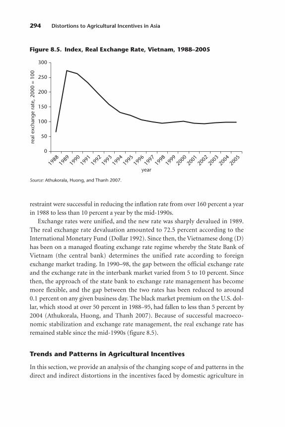
restraint were successful in reducing the inflation rate from over 160 percent a yearin 1988 to less than 10 percent a year by the mid-1990s.
Exchange rates were unified, and the new rate was sharply devalued in 1989.The real exchange rate devaluation amounted to 72.5 percent according to theInternational Monetary Fund (Dollar 1992). Since then, the Vietnamese dong (D)has been on a managed floating exchange rate regime whereby the State Bank of Vietnam (the central bank) determines the unified rate according to foreignexchange market trading. In 1990–98, the gap between the official exchange rateand the exchange rate in the interbank market varied from 5 to 10 percent. Sincethen, the approach of the state bank to exchange rate management has becomemore flexible, and the gap between the two rates has been reduced to around0.1 percent on any given business day. The black market premium on the U.S. dol-lar, which stood at over 50 percent in 1988–95, had fallen to less than 5 percent by2004 (Athukorala, Huong, and Thanh 2007). Because of successful macroeco-nomic stabilization and exchange rate management, the real exchange rate hasremained stable since the mid-1990s (figure 8.5).
Trends and Patterns in Agricultural Incentives
In this section, we provide an analysis of the changing scope of and patterns in thedirect and indirect distortions in the incentives faced by domestic agriculture in
294 Distortions to Agricultural Incentives in Asia
year
0
100
50
150
200
250
300
1988
1989
1990
1991
1992
1993
1994
1995
1996
1997
1998
1999
2000
2001
2002
2003
2005
2004
real
exc
hang
era
te, 2
000
= 10
0
Figure 8.5. Index, Real Exchange Rate, Vietnam, 1988–2005
Source: Athukorala, Huong, and Thanh 2007.
Vietnam. We rely on the methodology developed by Anderson et al. (2008) anddescribed in appendix A. The main focus of our use of the methodology is government-imposed distortions that create a gap between domestic prices andthe prices that would emerge under free market conditions. We estimate theeffects of direct agricultural policy measures, but, for comparative evaluation andbecause it is not possible to understand the characteristics of agricultural develop-ment through a sectoral view alone, we also estimate the distortions in nonagri-cultural tradables. Specifically, we compute nominal rates of assistance (NRAs)for farm producers of the six products we cover. We also calculate a relative rate ofassistance (RRA) based on the NRAs for nonagricultural tradables and the NRAsfor agricultural tradables. We assume that the NRAs for noncovered agriculturalexportable products are the same as the average NRAs for covered exportables,and we assume that the average NRA for noncovered import-competing productsis 10 percent of the NRAs for sugar. We also assume that the average NRA for nontradables is zero and that the share of nontradables in noncovered farm pro-duction is 68 percent, while the exportable share is 25 percent.
We have estimated the NRAs for nonagricultural tradables by assuming thatthe implicit duty rate on nonagricultural importables (the total tariff revenuegenerated from nonagricultural imports, divided by the value of nonagriculturalimports) is the rate of distortion in this component of nonagricultural tradablesand that nonagricultural exportables (the share of which is three-quarters as largeas the share of import-competing products) are not subject to any export taxes orsubsidies.
One should bear in mind two important caveats that arise from the paucity ofdata. First, we have ignored potential differences between border (reference)prices and domestic prices that arise from quality differences. This might haveinfused an underestimation bias into our calculations. Second, we have assumedthat there is a complete pass-through of the changes in producer (wholesale)prices to farmgate prices. This may result in an upward bias in the estimates. How-ever, these limitations are important only in comparisons of the levels of distor-tion in the incentives among products or across countries at a given time. They areunlikely to distort inferences based on intertemporal comparisons (changes inincentives over time) because the magnitude of the bias is less liable to vary overtime. Given the nature of the estimation method, our RRA estimates also do notfully capture the indirect distortions that arise in agricultural incentives fromchanges in the tariffs on tradable inputs. The tariff structure in Vietnam is cascad-ing. This may be an important source of downward bias in our RRA estimates(Athukorala 2006). We have also not captured the distortions caused by nontariffimport restrictions.
Vietnam 295
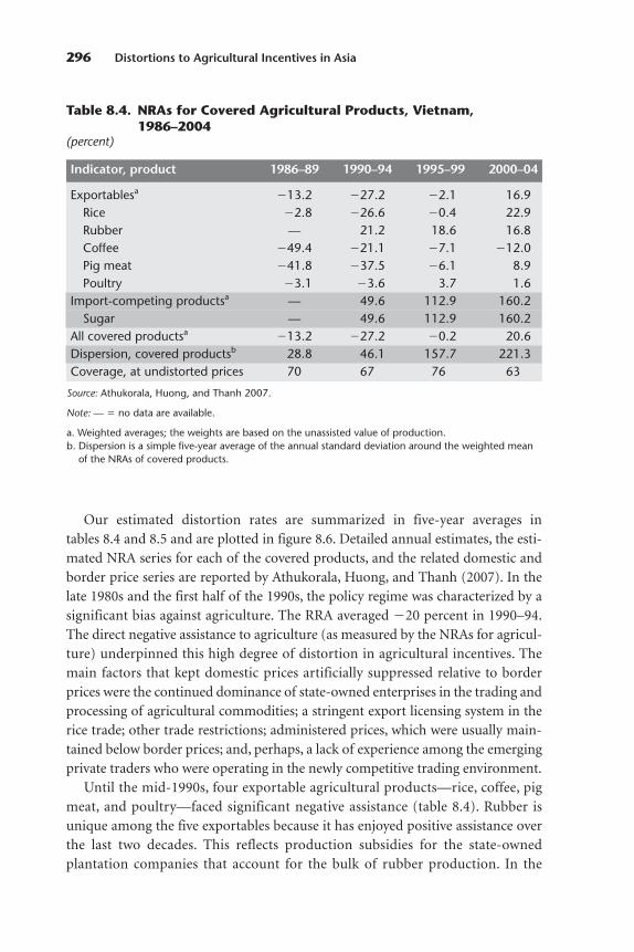
Our estimated distortion rates are summarized in five-year averages intables 8.4 and 8.5 and are plotted in figure 8.6. Detailed annual estimates, the esti-mated NRA series for each of the covered products, and the related domestic andborder price series are reported by Athukorala, Huong, and Thanh (2007). In thelate 1980s and the first half of the 1990s, the policy regime was characterized by asignificant bias against agriculture. The RRA averaged �20 percent in 1990–94.The direct negative assistance to agriculture (as measured by the NRAs for agricul-ture) underpinned this high degree of distortion in agricultural incentives. Themain factors that kept domestic prices artificially suppressed relative to borderprices were the continued dominance of state-owned enterprises in the trading andprocessing of agricultural commodities; a stringent export licensing system in therice trade; other trade restrictions; administered prices, which were usually main-tained below border prices; and, perhaps, a lack of experience among the emergingprivate traders who were operating in the newly competitive trading environment.
Until the mid-1990s, four exportable agricultural products—rice, coffee, pigmeat, and poultry—faced significant negative assistance (table 8.4). Rubber isunique among the five exportables because it has enjoyed positive assistance overthe last two decades. This reflects production subsidies for the state-owned plantation companies that account for the bulk of rubber production. In the
296 Distortions to Agricultural Incentives in Asia
Table 8.4. NRAs for Covered Agricultural Products, Vietnam,1986–2004
(percent)
Indicator, product 1986–89 1990–94 1995–99 2000–04
Exportablesa �13.2 �27.2 �2.1 16.9Rice �2.8 �26.6 �0.4 22.9Rubber — 21.2 18.6 16.8Coffee �49.4 �21.1 �7.1 �12.0Pig meat �41.8 �37.5 �6.1 8.9Poultry �3.1 �3.6 3.7 1.6
Import-competing productsa — 49.6 112.9 160.2Sugar — 49.6 112.9 160.2
All covered productsa �13.2 �27.2 �0.2 20.6Dispersion, covered productsb 28.8 46.1 157.7 221.3Coverage, at undistorted prices 70 67 76 63
Source: Athukorala, Huong, and Thanh 2007.
Note: — � no data are available.
a. Weighted averages; the weights are based on the unassisted value of production.b. Dispersion is a simple five-year average of the annual standard deviation around the weighted mean
of the NRAs of covered products.
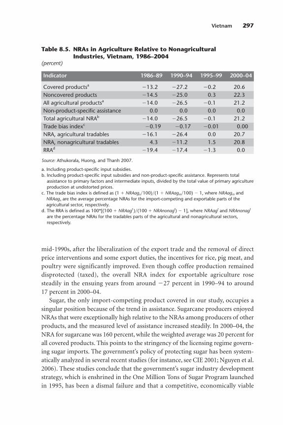
Vietnam 297
Table 8.5. NRAs in Agriculture Relative to NonagriculturalIndustries, Vietnam, 1986–2004
(percent)
Indicator 1986–89 1990–94 1995–99 2000–04
Covered productsa �13.2 �27.2 �0.2 20.6Noncovered products �14.5 �25.0 0.3 22.3All agricultural productsa �14.0 �26.5 �0.1 21.2Non-product-specific assistance 0.0 0.0 0.0 0.0Total agricultural NRAb �14.0 �26.5 �0.1 21.2Trade bias indexc �0.19 �0.17 �0.01 0.00NRA, agricultural tradables �16.1 �26.4 0.0 20.7NRA, nonagricultural tradables 4.3 �11.2 1.5 20.8RRAd �19.4 �17.4 �1.3 0.0
Source: Athukorala, Huong, and Thanh 2007.
a. Including product-specific input subsidies.b. Including product-specific input subsidies and non-product-specific assistance. Represents total
assistance to primary factors and intermediate inputs, divided by the total value of primary agricultureproduction at undistorted prices.
c. The trade bias index is defined as (1 � NRAagx�100)�(1 � NRAagm�100) � 1, where NRAagm andNRAagx are the average percentage NRAs for the import-competing and exportable parts of theagricultural sector, respectively.
d. The RRA is defined as 100*[(100 � NRAagt )�(100 � NRAnonagt) � 1], where NRAagt and NRAnonagt
are the percentage NRAs for the tradables parts of the agricultural and nonagricultural sectors,respectively.
mid-1990s, after the liberalization of the export trade and the removal of directprice interventions and some export duties, the incentives for rice, pig meat, andpoultry were significantly improved. Even though coffee production remaineddisprotected (taxed), the overall NRA index for exportable agriculture rosesteadily in the ensuing years from around �27 percent in 1990–94 to around17 percent in 2000–04.
Sugar, the only import-competing product covered in our study, occupies asingular position because of the trend in assistance. Sugarcane producers enjoyedNRAs that were exceptionally high relative to the NRAs among producers of otherproducts, and the measured level of assistance increased steadily. In 2000–04, theNRA for sugarcane was 160 percent, while the weighted average was 20 percent forall covered products. This points to the stringency of the licensing regime govern-ing sugar imports. The government’s policy of protecting sugar has been system-atically analyzed in several recent studies (for instance, see CIE 2001; Nguyen et al.2006). These studies conclude that the government’s sugar industry developmentstrategy, which is enshrined in the One Million Tons of Sugar Program launchedin 1995, has been a dismal failure and that a competitive, economically viable

sugar industry cannot be developed through isolation from world market conditions. The substantial protection provided to the sugar industry is a majorconstraint on the diversification of scarce land resources to more dynamic,export-oriented crops. Moreover, the high domestic sugar prices not only taxdomestic consumers, but also hamper the competitiveness of the domestic con-fectionary, food, and beverage industries.
Improvement in the NRAs for exportable agriculture, coupled with the mainte-nance of the high NRAs enjoyed by sugarcane producers, have generated animprovement in the RRAs for agriculture over the past 10 years. Moreover, thisimprovement in the relative incentives in agriculture has taken place against thebackdrop of a steady rise in the NRAs for nonagricultural sectors over time (table 8.5and figure 8.6). Clearly, the elimination of various direct price interventions indomestic trade, the removal of export duties on almost all agricultural products,the liberalization in import trade, and the exchange rate reforms have been instrumental in redressing the antiagricultural bias in the incentive structurewithin the economy.
298 Distortions to Agricultural Incentives in Asia
�50
�40
�30
�20
�10
0
10
20
30
40
1986
1987
1988
1989
1990
1991
1992
1993
1994
1995
1996
1997
1998
1999
2000
2001
2002
2003
2004
NRA
, %
year
NRA, nonagricultural tradables RRANRA, agricultural tradables
Figure 8.6. NRAs for Agricultural and NonagriculturalTradables and the RRA, Vietnam, 1986–2004
Source: Athukorala, Huong, and Thanh 2007.
Note: For the definition of the RRA, see table 8.5, note d.
A comparison of the weighted average NRAs for the covered exportables (rice,rubber, coffee, pig meat, and poultry) with the corresponding NRAs for sugar(an import-competing product) points to a persistent bias in agricultural incen-tives in favor of import-competing production in agriculture (table 8.4). How-ever, this comparison needs to be qualified: the NRAs for import-competingproducts refer only to the protection for sugar, which is an outlier relative toother import- competing agricultural products in Vietnam that are not coveredin this study.
Concluding Remarks
Over the past two decades, Vietnam has made significant progress in market- oriented reforms. The foreign trade regime has become more liberalized; therehas been a palpable transition from quantitative restraints to tariffs as the maininstrument in regulating imports. Export taxes on all significant products havebeen eliminated. In domestic trade, the dominance of state-owned enterprises inmost areas has ended, and price controls and restrictions on production and themovement of goods no longer exist.
The reform process is far from complete, however. The structure of trade pro-tection is still out of step with the level and the dispersion of nominal and effec-tive protection rates among Vietnam’s major trading partners in the region.Stringent quantitative import restrictions on sugar and high import duties onagricultural products in which the country has a clear comparative advantage,particularly rice, coffee, and tea, are major anomalies. The tariff rates are exces-sive on crucial agricultural inputs and other intermediate goods that are pro-duced locally by state-owned enterprises. Had information on these rates beenavailable to us in our analysis, our NRA estimates in agriculture would have beenlower. The licensing scheme for rice exports, although seemingly nonbindingfor some time now, remains an important source of uncertainty among privatesector traders.
The attempt to unshackle domestic agriculture accounted for the first of themarket-oriented reforms, and the reforms in this area have been more wide- ranging than the reforms in other areas. The predominance of agriculture in theprereform economy—its importance in determining the fortunes of the economyand ensuring the livelihoods of a majority of the population—made the sweepingagricultural reforms politically palatable. Because the vast potential of agriculturewas untapped under the command economy, the response of agriculture tothe reforms was swift. The impressive outcome played a pivotal role in sustainingthe momentum of the reforms and supporting market-oriented programs.
Vietnam 299

Our empirical analysis of trends and patterns in the incentives in agriculturehas yielded several important findings. In the first half of the 1990s, the policyregime was characterized by a significant bias against agriculture. This bias dissi-pated because of the gradual removal of the privileges enjoyed by state-ownedenterprises in procuring, processing, and trading agricultural products; the open-ing of domestic and foreign trade to the private sector; and the emergence of thenascent private sector in a competitive trade environment. By 2000–04, the NRAsin agriculture and the degree of antiagricultural bias embodied in the overall poli-cies affecting tradables represented evidence that the bias had been reversed. Theimprovement in the relative incentives for agriculture was generated predomi-nantly, if not solely, by direct reforms in agriculture. This is demonstrated by thesmall size of the increase in the NRAs for nonagricultural tradables. In this con-text, the implementation of the tariff reform commitments undertaken duringthe accession to the WTO may play a vital role in consolidating the reform effortand reducing the remaining sectoral policy bias.
According to our commodity-level estimates, the excessive assistance providedto sugar producers, mainly though stringent quantitative restrictions on sugarimports, is the major irregularity in the incentive structure. The NRAs have con-tinued to be high in recent years despite a steady decline in border prices; thisreflects the severity of the existing quantitative restrictions. The significant protec-tion provided to this industry is a major constraint on the diversification of agri-culture into dynamic export-oriented crops. High domestic sugar prices taxdomestic consumers, but also hamper the competitiveness of the domestic con-fectionary, food, and beverage industries. Redressing this anomaly in the incentivestructure remains a formidable challenge because sugarcane has long been achoice crop in the government’s rural development and agricultural diversifica-tion programs. Unfortunately, the government has missed the opportunity tomake use of the WTO accession process to face down the political resistance toreform. Instead, it has chosen the soft option of replacing the sugar import licens-ing scheme by WTO-consistent tariff rate quotas during 2008.
Notes
1. Export shares are estimated in gross terms, that is, on the basis of published trade data withoutadjusting for import content. This tends to understate the balance of payments implications of agri-cultural exports, particularly because most of the newly emerging manufactured exports greatlydepend on imported inputs.
2. By mid-2003, the average unweighted tariff rate, 16.7 percent, was aa little lower than the averagerates in China (17.5 percent) and Thailand (18.5 percent), but much higher than the rates in Indonesia(8.4 percent), Malaysia (10.2 percent), and the Philippines (7.6 percent). The degree of dispersion inthe tariff rates—measured through the coefficient of variation—is much higher in Vietnam than inChina, the Philippines, and Thailand, but lower in Vietnam than in Indonesia and Malaysia.
300 Distortions to Agricultural Incentives in Asia
References
Anderson, K., M. Kurzweil, W. Martin, D. Sandri, and E. Valenzuela. 2008. “Measuring Distortions toAgricultural Incentives, Revisited.” World Trade Review 7 (4): 675–704.
Athukorala, P.-C. 2006. “Trade Policy Reforms and the Structure of Protection in Vietnam.” WorldEconomy 29 (2): 161–87.
Athukorala, P.-C., P. L. Huong, and V. T. Thanh. 2007. “Distortions to Agricultural Incentives in Vietnam.” Agricultural Distortions Working Paper 26, World Bank, Washington, DC.
CIE (Center for International Economics). 1998. Vietnam’s Trade Policies 1998. Canberra: CIE.———. 2001. Vietnam Sugar Program: Where Next? Canberra: CIE.CPV (Communist Party of Vietnam). 1994. “Political Report of the Central Committee to the
Midterm Party Conference.” Report, CPV, Hanoi. Cited in Dollar and Ljunggren 1997, 464.Dollar, D. 1992. “Vietnam: Successes and Failures of Macroeconomic Stabilization.” In The Challenge of
Reform in Indochina, ed. B. Ljunggren, 207–31. Cambridge, MA: Harvard University Press.Dollar, D., and B. Ljunggren. 1997. “Vietnam.” In Going Global: Transition from Plan to Market in the
World Economy, ed. P. Desai, 439–71. Cambridge, MA: MIT Press.Duiker, W. J. 1989. Vietnam since the Fall of Saigon. 3rd ed. Athens, OH: Ohio University Press.Fforde, A., and S. de Vylder. 1996. From Plan to Market: The Economic Transition in Vietnam. Boulder,
CO: Westview Press.GSO (General Statistics Office). 2000. Statistical Data of Vietnam Agriculture, Forestry, and Fishery,
1975–2000. Hanoi: Statistical Publishing House.———. 2001. Vietnamese Economy during the Years of Renovation in Aggregated Economic Indicators of
the System of National Accounts. Hanoi: Statistical Publishing House.———. various years. Statistical Yearbook of Vietnam. Hanoi: Statistical Publishing House.———. various years. Statistical Handbook of Vietnam. Hanoi: Statistical Publishing House.IAPP (Institute for Agricultural Planning and Projecting). 2001. “Report on Strategy for Developing
the Livestock Sector in Vietnam until 2010.” Unpublished study, IAPP, Hanoi. Cited in Nguyen andGrote 2004, 13.
Minot, N., and F. Goletti. 2000. “Rice Market Liberalization and Poverty in Viet Nam.” Research Report114, International Food Policy Research Institute, Washington, DC.
Naughton, B. 1996. “Distinctive Features of Economic Reform in China and Vietnam.” In ReformingAsian Socialism: The Growth of Market Institutions, ed. J. McMillan and B. Naughton, 273–96. AnnArbor, MI: University of Michigan Press.
Nguyen, Hoa, and Ulrike Grote. 2004. “Agricultural Policies in Vietnam: Producer Support Estimates,1986–2002.” MTID Discussion Paper 79, Markets, Trade, and Institutions Division, InternationalFood Policy Research Institute, Washington, DC.
Nguyen M. T., D. Harris, T. Chong Thang, and N. Q. Nguyen. 2006. “Building a Roadmap for the Inter-national Integration of Vietnam’s Sugar Industry.” Unpublished study, Ministry of Agriculture andRural Development and Australian Agency for International Development, Hanoi.
Nicita, A., and M. Olarreaga. 2006. “Trade, Production, and Protection, 1976–2004.” World Bank Economic Review 21 (1): 165–71.
Pritchett, L. 2003. “A Toy Collection, a Socialist Star, and a Democratic Dud?” In In Search of Prosperity:Analytic Narratives on Economic Growth, ed. D. Rodrik, 123–51. Princeton, NJ: Princeton University Press.
Riedel, J. 1993. “Vietnam: On the Trails of the Tigers.” World Economy 16 (4): 401–22.Riedel, J., and B. Comer. 1997. “Transition to a Market Economy in Vietnam.” In Economies in Transi-
tion: Comparing Asia and Eastern Europe, ed. W. T. Woo, S. Parker, and J. D. Sachs, 189–213. Cambridge, MA: MIT Press.
Sachs, J. D., and W. T. Woo. 1994. “Experiences in the Transition to a Market Economy.” Journal ofComparative Economics 18 (3): 271–75.
Thanh, V. T. 2006. “Vietnam’s Trade Liberalization and International Economic Integration: Evolution,Problems and Challenges.” ASEAN Economic Bulletin 22 (1): 75–91.
Vietnam 301
Van Arkadie, B., and R. Mallon. 2003. Vietnam: A Transition Tiger? Canberra: Asia Pacific Press.White, C. 1981. “Agrarian Reform and National Liberation in the Vietnamese Revolution, 1920–1957.”
PhD dissertation, Cornell University, Ithaca, NY.———. 1985. “Agricultural Planning, Pricing Policy and Co-operatives in Vietnam.” World Develop-
ment 13 (1): 97–114.Woodside, A. 1989. “Peasants and the State in the Aftermath of the Vietnamese Revolution.” Journal of
Peasant Studies 16 (4): 283–97.
302 Distortions to Agricultural Incentives in Asia

Part ivII
SOUTH ASIA


The government of Bangladesh has substantially liberalized its trade and agricul-tural pricing policies since the country’s independence in 1971. The governmenthad removed most of the distortions in agricultural incentives by the mid-1990s.Although it has raised the level of trade protection for some agricultural andindustrial products sharply since 1998, the total distortions in agriculture remainsmall. In particular, relative to India and Pakistan, domestic and internationaltrade policies for the major staples—rice and wheat—are substantially more lib-eral in Bangladesh.
In the early 1970s, the government pursued highly restrictive trade andexchange rate policies through import regulations, high import tariffs, exporttaxes, pervasive quantitative restrictions, and an overvalued exchange rate. Thesepolices were similar to the policies implemented in the 1960s when Bangladeshwas part of Pakistan. The policy regime in the 1970s was especially restrictive inthe agricultural sector. The government had a monopoly on the imports of mostagricultural commodities and placed stiff export restrictions on raw jute, themajor agricultural export. Because of these distortions, agricultural price incen-tives were substantially reduced during the period (Rahman 1994).
Under pressure from donors and disenchanted by the slow economic growthand continued balance of payments problems despite the policies, the governmentinitiated reforms in the early 1980s. Broad liberalization was not undertaken untilthe early 1990s, however. The liberalization was accompanied by agriculturaltrade and pricing reforms. By the mid-1990s, distortions in the output prices forrice and wheat had been virtually eliminated, and the total distortions were mini-mal. The government raised the import tariffs on rice in response to subsidized
305
9
BANGLADESH
Nazneen Ahmed, Zaid Bakht,Paul A. Dorosh, and Quazi Shahabuddin
exports by India in 2001, but domestic rates of assistance calculated relative tointernational market prices indicate that there have been only small overall agri-cultural price distortions since around 2000.
In the next section, we describe growth and structural change in the economyof Bangladesh. We focus on the agricultural sector. In the subsequent section, weoffer an overview of the evolution of agricultural policies since independence. Wethen report our time series estimates of nominal rates of assistance (NRAs) forselected agricultural products. In the penultimate section, we discuss the changingpolitical economy of agricultural price and trade policies. We follow with someconcluding observations.
Economic Growth and Structural Change
The growth of gross domestic product (GDP) has accelerated steadily inBangladesh since the early 1980s. The average growth rate rose from 3.2 percent in1980–84 to 5.3 percent in 2000–04.1 The acceleration in per capita income growthhas been even greater, mainly because the population growth rate has declinedfrom 2.2 to 1.5 percent per year over the last 25 years. Several features of the pol-icy context during this period of growth are noteworthy, including the stablemacroeconomic environment and the emphasis on the private sector as theengine of economic growth, on economic liberalization and outward orientation,and on agriculture and rural development.
At only 2.8 percent in 1980–2004, the growth rate in the agricultural sector(including forestry and fishing) has been considerably slower than overall GDPgrowth. It was also uneven. It averaged only 1.7 percent a year during the first halfof the 1990s, when growth in the crop subsector declined slightly. During the sec-ond half of the 1990s, growth in the crop subsector surged to an average 3.8 per-cent a year, while total agriculture grew at 4.8 percent a year. Growth in the fishingsubsector was even more rapid in the 1990s, averaging 8.1 percent a year, but thenslowed substantially to 1.7 percent after 2000 (Ahmed et al. 2007).
Thus, as in most other countries, sustained economic growth in Bangladeshhas been accompanied by a structural transformation that has involved a declin-ing share of agriculture despite positive agricultural GDP growth. The GDP shareof agriculture declined from 32 percent in 1980–84 to 23 percent in 2000–04.About 7 percentage points of the growth throughout this period was accountedfor by forestry and fishing. Meanwhile, the share of industry in GDP rose from18 to 28 percent, and the share of services was steady at around 50 percent.Exports of ready-made garments have boomed in the past two decades, causingagriculture’s share in total exports to fall from more than 33 percent in the 1970sand 1980s to less than 8 percent after 2000. Nonetheless, more than 60 percent of
306 Distortions to Agricultural Incentives in Asia

the country’s labor force continues to be employed in agriculture at least parttime. Moreover, because agricultural production provides critical links for devel-opment in the rest of the economy, its performance has an important bearing onemployment generation, food security, and poverty reduction. For these reasons,agricultural growth is still a development priority.
Field crops and horticulture are the dominant activities in agriculture,accounting for four times as much agricultural value added as livestock activitiessince the early 1980s (Ahmed et al. 2007). Cropping is dominated by the produc-tion of cereals, especially rice, in which technological progress, supported by thedevelopment of irrigation infrastructure, has been the main engine of growth.Rice represented about 70 percent of the value added arising from crop produc-tion in 1973 and about 80 percent in 1999. The rapid expansion of rice produc-tion has been achieved in part at the expense of pulses and oilseeds, which remainimportant sources of protein and micronutrients. Apart from rice and wheat, theonly crops showing rapid growth over the past two decades are maize, potatoes,and vegetables.
Domestic demand factors have contributed to this structural change in theagricultural economy. They include income growth in aggregate, plus the acceler-ation in the growth in per capita income generated by the slowdown in popula-tion growth. Population growth was the dominant factor behind the growth indomestic demand for food in the 1970s, when per capita incomes were basicallystagnant. In the 1990s, income growth and the varying income elasticity ofdemand for different food items became major factors behind the pattern ofgrowth in domestic demand. Farmers have now started to respond to market sig-nals by reallocating resources to activities that are showing strong market growth(Hossain 2001).
Agricultural exports
In 1973, exports of agricultural commodities stood at slightly more than 80 per-cent of total exports. Their value grew at a modest trend rate of 4.2 percent innominal terms and 1.4 percent in real terms over the subsequent three decades.Most of the growth was recorded by fishing (shrimps). In contrast, overall exportsgrew at a trend rate of nearly 11 percent (8.4 percent in real terms), which largelyreflected rapid growth in ready-made garments. The share of ready-made gar-ments in total exports had risen to nearly 75 percent by 2004–05, while the shareof agriculture in total exports had declined from 37 to 7 percent (Ahmed et al.2007).
The composition of agricultural exports has also undergone significant changeduring the last three decades. In the 1970s, the average share of exports of raw jute
Bangladesh 307
in total agricultural exports was 70 percent, while the corresponding share ofexports of tea and shrimps were 17 and 9 percent, respectively. However, exportsof raw jute began facing stiff competition from synthetic substitutes, and the realvalue of raw jute exports declined by about two-thirds from the 1970s to the early1990s before stabilizing, although the share of the exports in total agriculturalexport earnings continued to fall as exports of shrimps and vegetables expanded.By 2004, the share of jute exports was only 15 percent (and of tea exports, less than3 percent) compared with 65 percent for shrimps and 6 percent for vegetables(from zero in the 1970s). The rising demand for vegetables by expatriateBangladeshis and various policy measures, particularly the provision of cashincentives and subsidized freight charges, facilitated the rapid growth in vegetableexports.
Agricultural imports
Similar to the case of agricultural exports, the share of major agricultural importsin total imports has declined since the 1970s. The share of these imports—wheat,raw cotton, edible oil, rice, sugar, milk and cream, pulses, spices, oilseeds, andtobacco—declined from an average of 33 percent in the 1970s to 24 percent in the1980s and only 16 percent in 2000–04 (Ahmed et al. 2007). The total real value ofmajor agricultural imports nonetheless increased over this period by an average of2.1 percent a year. This is more rapid than the increase in the value of agriculturalexports (1.4 percent a year), but slower than the increase in the value of totalimports (4.9 percent a year). In 2004, raw cotton, edible oil, wheat, rice, sugar, andmilk powder accounted (in decreasing order) for most agricultural imports.
However, the above figures cover recorded imports only. Studies have shownthat illegal imports from India constitute nearly 20 percent of Bangladesh’s totalrecorded imports (Bakht 1999). Of these illegal imports, two-thirds consist ofonly six agricultural goods: cattle (42 percent), sugar (7 percent), pulses (6 per-cent), milk powder (3 percent), spices (3 percent), and rice (2 percent).
Historically, food aid has constituted an important component of the wheatimports of Bangladesh. During the 1980s and 1990s, food aid in wheat accountedfor about two-thirds of total wheat imports; thus, average wheat food aid wasabout 1.0 million tons a year, and average total wheat imports were 1.5 milliontons a year. Government commercial imports accounted for the remainder oftotal imports. Domestic wheat procurement, food aid, private commercialimports (since the trade liberalization in the early 1990s), and government com-mercial imports have contributed wheat to the public food distribution system.The amount of food aid has dropped substantially since 1999 following large gainsin domestic grain production. Food aid never provided more than 0.5 percent of
308 Distortions to Agricultural Incentives in Asia

rice supplies, however. Before 1992–93, the public sector accounted for all com-mercial imports of rice; but, in response to market incentives, private sectorimports have increased since then to supplement domestic production and gov-ernment imports.
In most years since 2000, raw cotton has surpassed rice and wheat, combined,as the major agricultural import. The growth in the real value of raw cottonimports has been especially rapid since the early 1990s, when the governmentstarted offering a 25 percent cash subsidy for exports of ready-made garmentsproduced using domestic fabric, a policy that encouraged a surge in investment intextile spinning and composite mills (Bakht 2001a). Growth in the real value ofraw cotton imports averaged 12 percent a year in the 1990s and 15 percent a yearin 1999–2004.
The real value of imports of edible oil rose by 3.2 percent a year from the early1970s to 2004, so that the share of edible oil in total agricultural imports remainedclose to one-fifth over the period. Recorded sugar imports (not including sugarsmuggled from India) increased even more rapidly, rising from 1.4 percent of thevalue of agricultural imports in the early 1970s to 7 percent in 1999–2004.Between 1973 and 2003, the domestic production of sugar increased by onlyabout 100,000 metric tons, raising the output level from 90,000 tons in 1973 toaround 190,000 tons in 2003. In contrast, domestic demand for sugar increased bynearly 700,000 tons during this period. As a result, imports of sugar increasedfrom about 12,000 tons in 1973 to nearly 600,000 tons in 2003.
Exchange Rate and Trade Policies
The government followed inward-oriented, import-substituting trade policiesbeginning at independence in 1971 until major reforms were instituted in the1980s and especially the 1990s. This section provides a brief history of the policiesand the reforms during these years.
The 1970s: Inward-oriented policies
Faced with an imminent balance of payments crisis in 1971, the first independ-ence government continued the highly restrictive trade and exchange rate policiesthat had been in place when Bangladesh had been part of Pakistan. Quantitativerestrictions on imports, high tariff rates, and a fixed, overvalued exchange ratewere used to control imports, conserve scarce foreign exchange, and provide pro-tection for domestic industry. However, in line with the political philosophy of thegovernment, the protectionist trade regime was maintained even after the possi-bility of a balance of payments crisis had decreased substantially in the mid-1970s
Bangladesh 309
following a recovery in export earnings, an increase in foreign aid, a decline inworld prices for grains and other commodities, and the 70 percent devaluation ofthe taka (Tk) in 1975 from Tk 8.9 to Tk 15.1 per U.S. dollar.
Initially, under the fixed exchange rate system, all foreign exchange accrued tothe government and was then allocated for competing uses through a discre-tionary and cumbersome mechanism of import licensing. However, in the early1970s, in response to a crisis in foreign exchange, the government instituted a sys-tem, eventually known as the wage earner scheme, that allowed foreign exchangeearned by Bangladeshis abroad—worker remittances—to be used to import par-ticular categories of goods. At the same time, under the export performancelicense system, certain exporters were given a specified proportion of their exportearnings in the form of import entitlement certificates. The certificates could beused to import particular categories of goods, or they could be sold at a premiumso that other traders could import such goods. There was thus a de facto dualexchange rate, whereby the export performance license premium reflectedthe market price of foreign exchange to some extent. In 1977, wage earners wereallowed to sell their foreign exchange earnings directly in a market that came to beknown as the secondary exchange market. A special foreign exchange rate, calledthe wage earner scheme rate, was available to them on this market.
During the early years of restrictive trade policy, most agricultural commodi-ties were on lists of restricted or banned imports. These lists were aimed at pro-tecting producers from external competition by ensuring that producers receivedremunerative prices. There were also restrictions on agricultural exports, andsome agricultural products were subject to export duties. The goal was to ensurethat adequate stocks of agricultural commodities were available in the domesticmarket. However, fiscal incentives were also established to promote exports ofnontraditional items. According to an export policy order issued in 1976, earningsfrom exports of nontraditional items were doubled from 15–20 to 30–40 percent.2
Duty drawback schemes were undertaken to promote exports of textile productsmanufactured using imported raw materials.
The outcome of these autarkic trade and exchange rate policies was disap-pointing with regard to export development, the balance of payments situation,and overall economic growth, particularly considering the rapid growth achievedby East Asian economies that followed a more outward-oriented developmentstrategy. Disenchanted with the import-substitution strategy (and encouraged bydonor conditionalities), policy makers in Bangladesh and other South Asiancountries began to adopt more open economic policies in the late 1970s. This shiftwas facilitated by a change in government in 1975; the new government had amore positive view on the development of a mixed economy and favored a moreopen trade regime. However, the export promotion measures that were
310 Distortions to Agricultural Incentives in Asia
introduced in the late 1970s were limited in scope and were implemented onlygradually. Overall trade policies continued to be inward looking, and the econ-omy, particularly the external sector, remained overregulated.
The 1980s: Initial policy reforms
The new government that came to power in March 1982 initiated a wide-rangingpolicy reform package, the New Industrial Policy, to liberalize the economy. Alarge number of nationalized companies, especially in the jute and textile subsec-tors, were privatized within a few years, and measures to increase foreign anddomestic investment were adopted. However, only limited trade liberalizationoccurred under the New Industrial Policy or its successor, the Revised IndustrialPolicy, introduced in 1986. A cash compensatory scheme administered byBangladesh Bank was also introduced in 1986, providing cash equal to 15 percentof free on board export values for exports manufactured using local fabrics.3
Ultimately, the progress in trade liberalization was slow in the 1980s, especiallyin the reduction in import tariffs (Bakht 2001b). However, some liberalization inagricultural exports did occur. Export duties on raw jute and tea were withdrawnin 1981, and the duties on exports of dried fruit, fresh fruit, oil cakes, corianderseed, dry chilies, dry ginger, black pepper, turmeric, tobacco, vegetables, and pota-toes were withdrawn in 1986. Restrictions on exports of jute seed, wheat, pulses,shrimps other than frozen, frogs (dead or alive) and frog legs, and onions weremaintained even after 1995. Export restrictions on rice, wheat bran, and molasseswere removed only in 1998.
There were major reforms in exchange rate policy. In mid-1979, Bangladeshadopted a flexible policy, fixing the taka to a basket of the currencies of the coun-try’s major trading partners.4 Then, in 1986, the export performance license system was simplified substantially through the introduction of an export per-formance benefit. Exporters could directly cash any benefit entitlements at theirbanks at the existing wage earner scheme rate. During the 1980s, these policies,particularly the export performance benefit, contributed to rapid growth in non-traditional exports. They also contributed to rapid expansion in the secondary(wage earner scheme) market. A wide range of agricultural commodities werefavored by the export performance benefit incentives (Ahmed et al. 2007). How-ever, exports of raw jute were not included in this benefit scheme and thus suffered directly from the overvalued exchange rate.
Meanwhile, imports financed at the official exchange rate were quicklyreduced, and an increasing share of imports became subject to the secondaryexchange market, including a portion of the foreign exchange received throughcommodity aid. By 1991, 41 percent of all imports were financed through this
Bangladesh 311
means, while the share of the secondary exchange market in nonaid imports wasnearly 70 percent. The enhanced role of the secondary exchange market helpednarrow the gap between the official exchange rate and the wage earner schemerate. The two rates were finally unified in 1992, and this marked the end of theexport performance benefit arrangement (Rahman 1992).
1990s: Major trade liberalization
After a decade of half-hearted attempts at trade liberalization, the democraticgovernment that came to power in 1991 sought boldly to reform the trade regime.The reforms included tariff reductions and rationalization, the establishment of aless-complicated import tax structure, the gradual elimination of nontariffimport restrictions, and promotion for exports through income tax exemptions,bonded warehousing, and flexible exchange rate management.5
Until the 1990s, the government relied heavily on quantitative restrictions tocontrol imports, especially in agricultural commodities. About 37 percent of thetariff lines for agricultural products (21 percent of all products) were eitherbanned or restricted in 1987 (World Bank 1994). By 1984, all quantitative restric-tions on agricultural products had been removed, and only 2 percent of the tarifflines of all products were still facing quantitative restrictions. In particular, privatesector imports of rice and wheat were legalized in the early 1990s, ending the gov-ernment’s monopoly on food grain imports. The ban on exports of fine qualityrice (but not on ordinary coarse rice) was also lifted.
Trade liberalization in the early 1990s brought tariff rates down sharply. Totalprotective import duty rates, both customs duties and para-tariff measures (sur-charges, license fees, regulatory duties, value added taxes, and supplementaryduties), declined from 74 to 32 percent between 1991 and 1995 (measured accord-ing to the unweighted average of all tariff lines). Likewise, import tariffs and thetotal tax incidence on the imports of major agricultural commodities declinedrapidly during the early 1990s (table 9.1).6 Refined edible oil, sugar, milk powder,and spices were subject to relatively high duty rates, while raw cotton, wheat, rape-seeds, and lentils enjoyed lower duty rates (table 9.2).
Trade reforms have stalled in recent years, however. Although customs dutiesdeclined from 29 percent in 1995 to 19 percent in 2003, the effect of para-tariffmeasures rose sharply, mainly because of a steep increase in supplementaryduties. Average total protective import duty rates have thus remained essentiallyunchanged since the mid-1990s. For some products that were already protected,including processed fruits, cement, soap, cotton shirts and sheets, selected ceramicand steel products, batteries, bicycles, and toys, total protection rates rose by morethan 30 percent between 1997 and 2003 (World Bank 2004).
312 Distortions to Agricultural Incentives in Asia
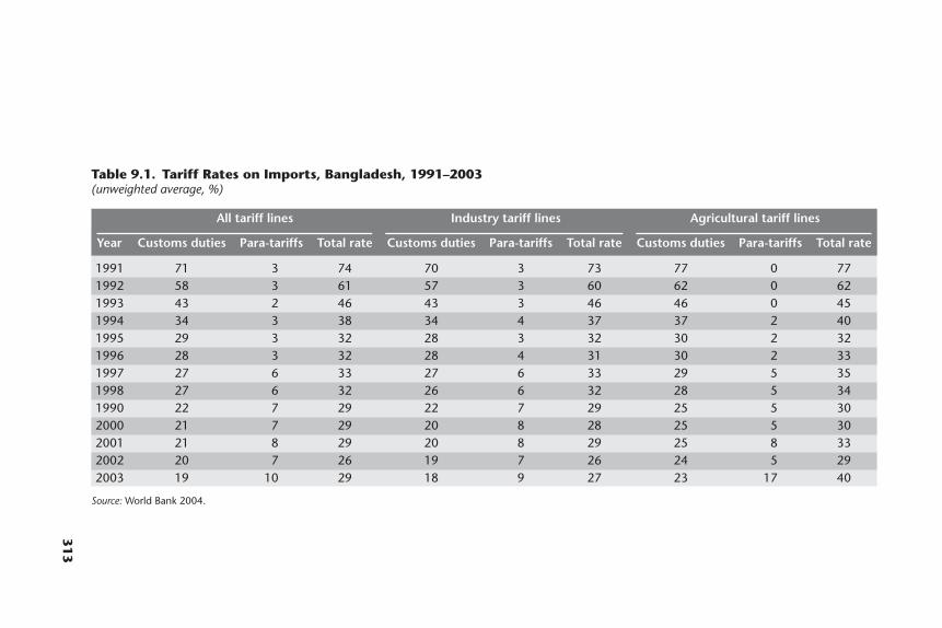
313
Table 9.1. Tariff Rates on Imports, Bangladesh, 1991–2003(unweighted average, %)
All tariff lines Industry tariff lines Agricultural tariff lines
Year Customs duties Para-tariffs Total rate Customs duties Para-tariffs Total rate Customs duties Para-tariffs Total rate
1991 71 3 74 70 3 73 77 0 771992 58 3 61 57 3 60 62 0 621993 43 2 46 43 3 46 46 0 451994 34 3 38 34 4 37 37 2 401995 29 3 32 28 3 32 30 2 321996 28 3 32 28 4 31 30 2 331997 27 6 33 27 6 33 29 5 351998 27 6 32 26 6 32 28 5 341990 22 7 29 22 7 29 25 5 302000 21 7 29 20 8 28 25 5 302001 21 8 29 20 8 29 25 8 332002 20 7 26 19 7 26 24 5 292003 19 10 29 18 9 27 23 17 40
Source: World Bank 2004.
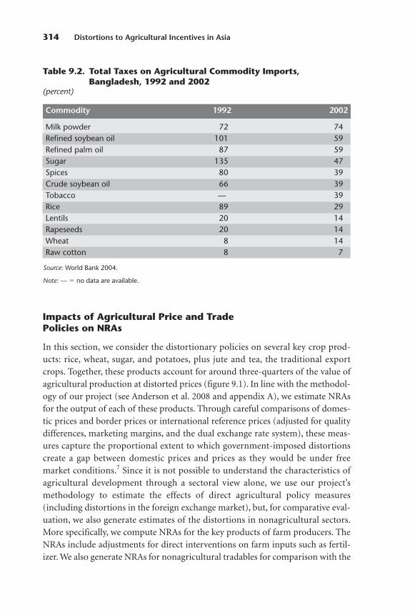
Impacts of Agricultural Price and TradePolicies on NRAs
In this section, we consider the distortionary policies on several key crop prod-ucts: rice, wheat, sugar, and potatoes, plus jute and tea, the traditional exportcrops. Together, these products account for around three-quarters of the value ofagricultural production at distorted prices (figure 9.1). In line with the methodol-ogy of our project (see Anderson et al. 2008 and appendix A), we estimate NRAsfor the output of each of these products. Through careful comparisons of domes-tic prices and border prices or international reference prices (adjusted for qualitydifferences, marketing margins, and the dual exchange rate system), these meas-ures capture the proportional extent to which government-imposed distortionscreate a gap between domestic prices and prices as they would be under free market conditions.7 Since it is not possible to understand the characteristics ofagricultural development through a sectoral view alone, we use our project’smethodology to estimate the effects of direct agricultural policy measures(including distortions in the foreign exchange market), but, for comparative eval-uation, we also generate estimates of the distortions in nonagricultural sectors.More specifically, we compute NRAs for the key products of farm producers. TheNRAs include adjustments for direct interventions on farm inputs such as fertil-izer. We also generate NRAs for nonagricultural tradables for comparison with the
314 Distortions to Agricultural Incentives in Asia
Table 9.2. Total Taxes on Agricultural Commodity Imports,Bangladesh, 1992 and 2002
(percent)
Commodity 1992 2002
Milk powder 72 74Refined soybean oil 101 59Refined palm oil 87 59Sugar 135 47Spices 80 39Crude soybean oil 66 39Tobacco — 39Rice 89 29Lentils 20 14Rapeseeds 20 14Wheat 8 14Raw cotton 8 7
Source: World Bank 2004.
Note: — � no data are available.
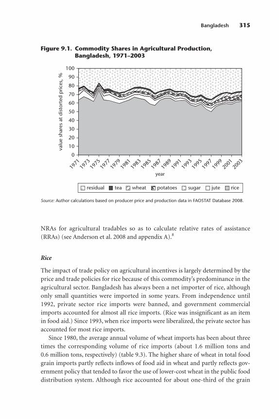
NRAs for agricultural tradables so as to calculate relative rates of assistance(RRAs) (see Anderson et al. 2008 and appendix A).8
Rice
The impact of trade policy on agricultural incentives is largely determined by theprice and trade policies for rice because of this commodity’s predominance in theagricultural sector. Bangladesh has always been a net importer of rice, althoughonly small quantities were imported in some years. From independence until1992, private sector rice imports were banned, and government commercialimports accounted for almost all rice imports. (Rice was insignificant as an itemin food aid.) Since 1993, when rice imports were liberalized, the private sector hasaccounted for most rice imports.
Since 1980, the average annual volume of wheat imports has been about threetimes the corresponding volume of rice imports (about 1.6 million tons and0.6 million tons, respectively) (table 9.3). The higher share of wheat in total foodgrain imports partly reflects inflows of food aid in wheat and partly reflects gov-ernment policy that tended to favor the use of lower-cost wheat in the public fooddistribution system. Although rice accounted for about one-third of the grain
Bangladesh 315
0
10
20
30
40
50
60
70
80
90
100
valu
e sh
ares
at d
isto
rted
pric
es, %
residual tea wheat potatoes sugar jute rice
year19
7119
7319
7519
7719
7919
8119
8319
8519
8719
8919
9119
9319
9519
9719
9920
0120
03
Figure 9.1. Commodity Shares in Agricultural Production,Bangladesh, 1971–2003
Source: Author calculations based on producer price and production data in FAOSTAT Database 2008.
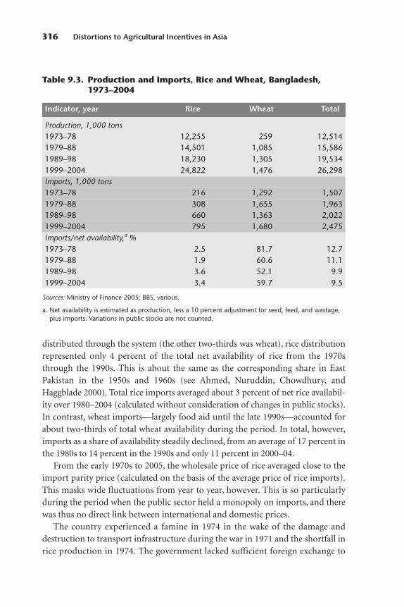
distributed through the system (the other two-thirds was wheat), rice distributionrepresented only 4 percent of the total net availability of rice from the 1970sthrough the 1990s. This is about the same as the corresponding share in East Pakistan in the 1950s and 1960s (see Ahmed, Nuruddin, Chowdhury, and Haggblade 2000). Total rice imports averaged about 3 percent of net rice availabil-ity over 1980–2004 (calculated without consideration of changes in public stocks).In contrast, wheat imports—largely food aid until the late 1990s—accounted forabout two-thirds of total wheat availability during the period. In total, however,imports as a share of availability steadily declined, from an average of 17 percent inthe 1980s to 14 percent in the 1990s and only 11 percent in 2000–04.
From the early 1970s to 2005, the wholesale price of rice averaged close to theimport parity price (calculated on the basis of the average price of rice imports).This masks wide fluctuations from year to year, however. This is so particularlyduring the period when the public sector held a monopoly on imports, and therewas thus no direct link between international and domestic prices.
The country experienced a famine in 1974 in the wake of the damage anddestruction to transport infrastructure during the war in 1971 and the shortfall inrice production in 1974. The government lacked sufficient foreign exchange to
316 Distortions to Agricultural Incentives in Asia
Table 9.3. Production and Imports, Rice and Wheat, Bangladesh,1973–2004
Indicator, year Rice Wheat Total
Production, 1,000 tons1973–78 12,255 259 12,5141979–88 14,501 1,085 15,5861989–98 18,230 1,305 19,5341999–2004 24,822 1,476 26,298Imports, 1,000 tons1973–78 216 1,292 1,5071979–88 308 1,655 1,9631989–98 660 1,363 2,0221999–2004 795 1,680 2,475Imports/net availability,a %1973–78 2.5 81.7 12.71979–88 1.9 60.6 11.11989–98 3.6 52.1 9.91999–2004 3.4 59.7 9.5
Sources: Ministry of Finance 2005; BBS, various.
a. Net availability is estimated as production, less a 10 percent adjustment for seed, feed, and wastage,plus imports. Variations in public stocks are not counted.

make up the deficit by purchasing rice imports at the high prevailing internationalprice.9 The domestic price for rice rose substantially in the 1974/75 season, butwas still below the international price. After this crisis and the 61 percent devalua-tion in the taka relative to the U.S. dollar in May 1975, the domestic wholesaleprice for rice was double the import parity price, but it went below this level againduring the subsequent six years (figure 9.2).
Rice and wheat imports represented 10 percent of the total food grain supply,but, because wheat was not a close substitute for rice in domestic consumption,the effect of wheat imports (mainly food aid) on the market price for rice waslikely to have been small. Nonetheless, in the absence of wheat imports, domesticrice prices would have been somewhat higher during this period.10
In the early 1980s, rapid increases in the domestic production of rice led togreater availability and lower real wholesale prices. International rice prices werefalling even more rapidly, however, so that, over the five-year period 1983–87, theaverage domestic price was 21 percent above the import parity price. The govern-ment monopoly on imports thus had an effect on rice tariffs similar to the effectof an import tariff under a liberalized trade environment that favors net sellers ofrice relative to net buyers. A surge in domestic rice production (mainly of winterrice [boro]) following major floods in 1987 and 1988 led to another drop in real
Bangladesh 317
100
0
200
300
400
500
600
1974
1976
1978
1980
1982
1984
1986
1988
1990
1992
1994
1996
1998
2000
2002
2004
bord
er p
rice,
U.S
. dol
lar
per
ton
−60
−40
−20
0
20
40
60
80
100
120
NRA
, %
year
border prices NRA
Figure 9.2. NRAs and Border Prices, Rice, Bangladesh, 1974–2004
Source: Ahmed et al. 2007.
Note: The Pearson correlation coefficient between the two series shown is �0.41.
wholesale rice prices in 1989, and this brought domestic prices close to par withborder prices and eliminated the implicit protection for producers. This price-sta-bilizing role of government has tended to generate a negative correlation betweenNRAs and border prices, the extent of which is evident in figure 9.2.
Trade liberalization in the early 1990s created a possible direct link betweendomestic and border prices for rice, particularly during periods following poordomestic rice harvests. Throughout the 1980s and early 1990s, Thailand was themajor source of rice imports to Bangladesh. However, the 1994 liberalization thatpermitted private sector imports in Bangladesh coincided with rice trade liberal-ization and the buildup of public rice stocks in India, which made private sectorrice imports from India legal and feasible.11 Because of lower transport costs,reduced delivery times (for private sector imports), and the possibility of smallercontracts for the delivery of imports by truck, India rapidly replaced Thailand asthe major source of rice imports in Bangladesh in the mid-1990s. Large-scale riceimports from India supplemented domestic supplies during crop shortfalls inBangladesh in 1994, 1997, and 1998.12 In 1997 and 1998, 92 percent of riceimports came from India. However, during periods following normal or above-average rice harvests (most of 1996 and 1997, in 2000, and in the first half of2001), domestic rice prices in Bangladesh were below import parity levels, elimi-nating any incentives for private sector imports (figure 9.2).13 Average domesticwholesale prices were 5 and 12 percent below average import parity prices in1990–94 and 1995–99, respectively, although there were few trade barriers duringthese years. The negative NRAs reflect periods when rice came close to being anontradable because of good domestic harvests.
Beginning in 2000, the government of India adopted increasingly aggressivemeasures to promote exports to reduce a massive public stock buildup. The meas-ures included subsidies for rice exports that involved the provision of grain fromgovernment stocks to exporters at prices that were below cost.14 Because domesticrice prices in Bangladesh were approximately equal to the full-cost import parityprices, including taxes, for below-poverty-line rice made in India, small amountsof low-quality rice were imported into Bangladesh in 2000.15 However, when theIndian government lowered its above-poverty-line sales price for fine rice from Rs11.3 per kilogram to only Rs 8.3 per kilogram in July 2001, the government ofBangladesh increased rice import tariffs and taxes from 5 to 37.5 percent.16 Thisraised the below-poverty-line import parity price, plus taxes, to 33 percent abovethe domestic price in Bangladesh, thereby essentially cutting off the incentive forprivate sector rice trade with India (figure 9.3).17 However, in mid-2002, thedomestic price again rose toward the import parity price, including taxes, leadingto relatively large-scale private sector trade with India once more. Until early2006, domestic prices were at or near below-poverty-line import parity prices,
318 Distortions to Agricultural Incentives in Asia
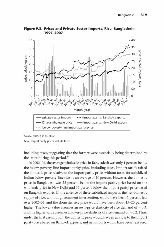
including taxes, suggesting that the former were essentially being determined bythe latter during this period.18
In 2002–04, the average wholesale price in Bangladesh was only 1 percent belowthe below-poverty-line import parity price, including taxes. Import tariffs raisedthe domestic price relative to the import parity price, without taxes, for subsidizedIndian below-poverty-line rice by an average of 10 percent. However, the domesticprice in Bangladesh was 28 percent below the import parity price based on thewholesale price in New Delhi and 15 percent below the import parity price basedon Bangkok exports. In the absence of these subsidized imports, the net domesticsupply of rice, without government intervention, would have been 5 percent lessover 2002–04, and the domestic rice price would have been about 15–25 percenthigher. The lower value assumes an own-price elasticity of rice demand of �0.3,and the higher value assumes an own-price elasticity of rice demand of �0.2. Thus,under the first assumption, the domestic price would have risen close to the importparity price based on Bangkok exports, and net imports would have been near zero.
Bangladesh 319
0
5
10
15
20
25
30
35
Jan-9
7Jul
-97
Jan-9
8Jul
-98
Jan-9
9Jul
-99
Jan-0
0Jul
-00
Jan-0
1Jul
-01
Jan-0
2Jul
-02
Jan-0
3Jul
-03
Jan-0
4Jul
-04
Jan-0
5Jul
-05
Jan-0
6Jul
-06
Jan-0
7Jul
-07
pric
e, t
aka/
kilo
gram
0
month, year
50
100
150
200
250
300
350
400
private sector im
ports, tons
private sector imports
Dhaka wholesale price import parity, New Delhi exports
below-poverty-line import parity price
import parity, Bangkok exports
Figure 9.3. Prices and Private Sector Imports, Rice, Bangladesh,1997–2007
Source: Ahmed et al. 2007.
Note: Import parity prices include taxes.

Wheat
Wheat was a minor crop in Bangladesh in the 1960s, prior to independence.Wheat production increased rapidly thereafter, from an average of about 0.1 mil-lion tons a year in 1969–74 to more than 1.8 million tons a year in 1997–99. Thisrise was associated with a sevenfold expansion in the area cultivated in wheat anda twofold expansion in wheat yields per hectare. Wheat production growth wasespecially rapid in the 1970s, increasing by an average 37 percent a year as the areaunder wheat expanded by 19 percent a year, and yields per hectare rose by 15 per-cent a year. In 1998–2003, the area under wheat declined from a peak of 967,000hectares to 704,000 hectares, while the area planted in maize, potatoes, and winterrice expanded (Dorosh 2006).
Because of the government monopoly on external trade, there was no explicitlink between the international price of wheat and the domestic price from the1970s to the early 1990s. Because food aid and government commercial importsaccounted for over half of the total supply, government policy on the net distribu-tion of wheat (there was limited domestic procurement of wheat) was the domi-nant factor determining the domestic market price.
Partly because of food aid conditionality among donors stipulating that foodaid should not generate price disincentives for domestic production, the averagedomestic price on wheat was close to the import parity price throughout thisperiod. After the devaluation in 1975, the estimated NRAs on output averagedonly 3 percent until 1993 (table 9.4).
After the liberalization of wheat imports in 1992, the import parity price ofwheat provided a price ceiling for wheat in the same way the import parity priceof rice accomplished this for rice. In most years, domestic prices were close to thisceiling, so that the average NRA on output was less than 4 percent after 1994. Onlyduring a period when international wheat prices were high (around 1996) weredomestic prices substantially below border prices (NRAs of �14 percent).
From the mid-1990s until 2000, most commercial wheat imports involvedhigh-gluten wheat for baking that was imported from major international wheatexporters such as Australia, the European Union, and the United States. Thiswheat accounted for about 10 percent of total wheat use in Bangladesh, and it didnot directly compete with soft, lower-gluten domestic wheat, which is used mostlyfor traditional breads (for example, roti and chapati). However, in 2000 and in sev-eral years since then, subsidized wheat exports from India were found on marketsin Bangladesh.
Because of the rapid increases in rice production and rice supply and the lowerreal price of rice, which tended to reduce the demand for wheat, the significantfood aid beginning in 1999, if it had been maintained, would likely have reduced
320 Distortions to Agricultural Incentives in Asia

321
Table 9.4. NRAs for Covered Agricultural Products, Bangladesh, 1974–2004(percent)
Indicator, product 1974 1975–79 1980–84 1985–89 1990–94 1995–99 2000–04
Exportablesa �28.7 �34.6 �26.2 �32.4 �33.0 �9.9 �33.2Jute �30.0 �37.1 �29.3 �35.4 �38.4 �5.6 �38.7Tea 1.4 �14.5 �10.7 �19.9 �11.9 �20.5 �20.4
Import-competing productsa �20.6 6.5 �1.9 24.4 �0.1 �7.9 6.1Riceb �25.7 6.5 �5.2 20.4 �5.3 �12.0 2.6Wheat 38.9 30.3 �5.8 11.3 4.5 2.6 �0.3Sugar 73.7 92.1 137.0 436.0 166.1 138.8 223.9
Nontradablesa
Potatoes 1.3 1.5 1.3 1.7 2.2 2.7 1.8All covered productsa �20.8 2.8 �3.8 16.8 �2.2 �7.6 3.9Dispersion, covered productsc 52.1 71.4 67.6 190.7 77.5 67.9 101.2Coverage, at undistorted prices 77 77 78 72 72 70 72
Source: Ahmed et al. 2007.
a. Weighted averages; the weights are based on the unassisted value of production.b. Calculated based on the average cost of rice imports.c. Dispersion is a simple five-year average of the annual standard deviation around the weighted mean of the NRAs of covered products.
the domestic price of wheat below the import parity price (del Ninno and Dorosh2003). However, donors substantially reduced food aid after 2001. There werethree reasons for this reduction: the government had achieved its domestic foodproduction target of 454 grams per person per day, thus eliminating the notionalfood gap; the European Union was reducing its use of in-kind food aid; and theUnited States and other countries were shifting their deliveries of food aidresources to other parts of the world. Nonetheless, wheat production has declinedsince 2000. This has largely been the result of growing competition from maize,including hybrid varieties that have been profitable and have been satisfying adomestic market for poultry feed.
Jute
After the onset of the boom in the production of ready-made garments inBangladesh in the early 1980s, jute lost its prominent share in total export earn-ings. Nonetheless, it is still an important farm export commodity. Bangladeshremains the leading exporter of raw jute in the world, and a significant number offarm households continue to depend on jute cultivation for their livelihoods.
International jute prices have been declining steadily, however, and the worlddemand for jute has been shrinking in the face of synthetic substitutes. The nominalU.S. dollar export price of jute fell by an average 1.5 percent a year from 1973 to2004. The decline in real prices has been an even steeper �4.2 percent per year(measured using the U.S. wholesale price index as a deflator for the dollar priceseries). As a result, the real 2004–05 dollar price of jute fell by two-thirds between thelate 1970s and the early 2000s. Because the quantity of raw jute exports remainedrather flat over the period, export earnings fell dramatically (Ahmed et al. 2007).
The domestic price of jute has been consistently below the export parity pricepartly because of an effort to encourage the domestic processing of jute productsfor export.19 In the 1970s and 1980s, the average domestic wholesale price of jutewas more than 30 percent below the export parity price.20 Following the trade lib-eralization of the early 1990s, the NRAs on jute output averaged only 6 percent.However, after the closing of public sector jute mills, the domestic price of rawjute again fell significantly below the export parity price, perhaps reflecting thedisruption in marketing channels and the greater differential between the qualityof raw jute for export and jute for the domestic market (table 9.4).
Tea
Like jute, tea was once a major export of East Pakistan and then Bangladesh.Between 1973 and 1983, the value of tea exports rose in nominal dollar terms
322 Distortions to Agricultural Incentives in Asia
mainly because of an increase in the international price of tea. However, from thepeak value of exports, at US$69 million in 1983, export earnings from tea declinedsteadily to only US$16 million in 2004. One factor in the decline in exports wasthe rise in the domestic demand for tea. During the last three decades, tea produc-tion has expanded at a trend rate of 2 percent, while domestic tea consumptionincreased at a trend rate of 7.5 percent, leaving a smaller exportable surplus.
The domestic price of tea, which is based on the auction at Chittagong, hasbeen consistently 10 to 20 percent below the export parity price, which is equiva-lent to the average export price in Chittagong. This may reflect handling costs atthe port. Rahman (1994) uses a border price based on the London auction price,discounted by 30 percent, less marketing and processing costs to cover the trans-fers to Chittagong port from the tea gardens in Sylhet in northeastern Bangladesh.He finds little difference between the domestic price and the border price in mostyears between 1974 and 1987 except when the border price spiked in 1976, 1983,and 1984. The gaps between the average export price and the Chittagong auctionprice or the London auction price may largely reflect quality differences ratherthan trade and domestic pricing policy distortions.
Sugar
Bangladesh produces less than 20 percent of the sugar it consumes. The remain-der is provided by official sugar imports (nearly 50 percent of consumption) andsugar smuggled from neighboring India.21 The country’s sugar industry is highlyprotected through import tariffs. Imports have been controlled through licensing(before 1992), a government monopoly (1992–2001), and a combination ofparastatals and private traders (since June 2002). As a result, the domestic price ofsugar is substantially higher than the world price. Farmers do not reap all the ben-efits of this policy, however, since sugarcane prices are fixed by the government,and sugar mills retain a monopsony on sugarcane purchases within designatedsugarcane areas near each mill.22
Official trade has generally faced high import tariffs. For example, tariffs onsugar imports were 135 percent in 1992 before major trade liberalization, but still47 percent in 2002 after the liberalization. These high tariffs on sugar have greatlyreduced imports of sugar through official channels, but have also provided majorincentives for sugar smuggling.
Our NRA estimates for output vary substantially over time largely because offluctuations in the world price of sugar, but also because milling, transport, andmarketing costs are subtracted from the border price for sugar to determine thesugarcane price at the farmgate. Our NRAs on output average more than 150 per-cent for the 1980s and 1990s and even more since 2000 (table 9.4).
Bangladesh 323
Distortions in input prices
Modern agricultural technology was introduced in East Pakistan in the early1960s. There was eventually heavy public sector involvement in the procurementand distribution of modern agricultural inputs and in investments for the devel-opment of water resources. A parastatal, the East Pakistan Agricultural Develop-ment Corporation, later known as the Bangladesh Agricultural DevelopmentCorporation, was established in 1963. The corporation held a virtual monopolyover the procurement and distribution of fertilizers, seeds, pesticides, and smallirrigation equipment, although it had to conform to pricing policies and relatedpolicies that the government formulated from time to time.23
Major reforms in the markets for fertilizer and irrigation equipment werelaunched in the late 1970s (Ahmed et al. 2007). Under the new marketing systemestablished in 1978, private sector trade in fertilizer was liberalized, leading to asubstantial expansion in the number of wholesalers and retailers operating in thefertilizer market.24 The share of private trade climbed to 75 percent in 1989 andnearly 100 percent in 1992, when the ban on private sector fertilizer imports wasremoved and the deregulation of fertilizer marketing was completed. BetweenDecember 1994 and March 1995, however, a serious shortage in the supply of urealed to a crisis in the market. The government partially reversed the reform processby initiating controls on wholesale markets, regulating pricing at the factory gate,and imposing restrictions on domestic traders who were selling outside the dis-tricts in which they had been registered (Ahmed 2001).25
Subsidies for the domestic production of nitrogenous fertilizer have beenresponsible for the greatest distortion in agricultural input prices. By 1983, fertil-izer prices at the farmgate had been deregulated throughout the country anddirect subsidies to farmers for the production of urea had been eliminated. How-ever, subsidies continued through 1991 for imports of other fertilizers—namely,triple superphosphate and muriate of potash—that were designed to improve thebalance of chemical nutrients. Subsidies for imported fertilizers such as these werereintroduced in January 2005 at the rate of 35 percent.
Government controls on urea and on the volume of urea imports and exportshave helped maintain the domestic wholesale price for urea consistently belowthe import parity border price and generally above the export parity price,despite the liberalization in marketing.26 The average domestic price for urea was37–50 percent below the import parity price in the 1970s and 1980s and 50 per-cent below the import parity price in the 1990s and 2000s. (The average domes-tic price for urea was about 40 percent above the average export parity price from1990–91 to 2004–05.) However, the average domestic price of triple superphos-phate has been only 18 percent below the import parity price since 1990, though
324 Distortions to Agricultural Incentives in Asia
it had been 47 percent below the import parity price in the 1970s and 1980s(Ahmed et al. 2007).
Given that the cost of fertilizer accounts for an average of only 5 percent of thetotal cost of paddy and even less for most other crops, the fertilizer subsidy has nothad a major effect on the overall NRAs in agriculture in recent years. Indeed, it hasadded only 1 or 2 percent during most years. This also applies to the main non-tradable food, potatoes, which would otherwise show NRAs of zero.
The total assistance to agriculture
For the agricultural sector as a whole, including both tradable and nontradablegoods, average NRAs since the mid-1970s have been low. Since 1975, the five-yearaverage NRAs for the six products we cover have ranged from �8 percent in themid-1990s, when international prices were high, to 17 percent in the later 1980s,when international prices were low (table 9.4). Three key factors have driven thisresult. First, since rice accounts for two-thirds of covered product output, theNRAs for rice largely determine the total NRAs for tradable agriculture. The prod-uct exhibiting the greatest price distortions, sugarcane, accounts for only 1 or2 percent of the total value of domestic agricultural production in most years andso has little influence on the sector’s average NRAs.
Second, the implicit taxation of agricultural exports (jute and tea) partially off-sets the protection for importables in our total NRA estimates. However, jute andtea account for only a small weight in the average NRA (less than 5 percent sincethe late 1980s).
Third, while the share of potatoes, the nontradable good shown in table 9.4,has a somewhat larger weight in the average, up to 7 percent in recent years, theonly measured assistance involved arises from the assistance for fertilizer, and, so,the NRA for potatoes is small.
Our NRA estimates suggest that, relative to import-competing agriculturalproducts, agricultural exports are discouraged. This is illustrated in figure 9.4.Our estimates also suggest that the dispersion of the NRAs for our covered prod-ucts around the mean value each year is wide and has not declined over the past30 years. One measure of this phenomenon, shown near the bottom of table 9.4, isthe standard deviation in these NRAs: it was around 70 percent or more. This lackof convergence in NRAs implies that the allocation of land and other farmresources among our covered industries continues to be inefficient.
Virtually all noncovered products, including fruits, vegetables, and meat products,receive little assistance; we therefore assume that the corresponding NRAs are zero.We also assume that they are nontradable over the period we study. Including these
Bangladesh 325

goods, which account for about one-quarter of the total value of agricultural produc-tion, the weighted average NRAs for total agriculture are closer to zero relative to theweighted average of the covered products alone (upper portion of table 9.5).
The assistance provided by government policies to nonagricultural tradablesectors is also important for the competitiveness of agriculture within the econ-omy and the ability of agriculture to contribute to the economy. The effect ofimport tariffs and import quotas on the domestic prices of nonfarm import-com-peting goods may be expressed as an implicit tariff rate. This rate is defined as theratio of domestic prices (measured at the border) to import prices. In the absenceof detailed data on domestic and import prices, we have calculated estimates ofthis implicit tariff. Our calculations provide NRAs for the import-competingparts of the nonfarm sector. We combine these with an assumed NRA of zero forthe exportable part of the same sector to generate production-weighted averageNRAs for nonagricultural tradables. Though this method may be crude, it pro-vides a reasonable measure that may be compared with the NRAs for tradableagriculture so as to derive RRAs. The RRAs indicate the extent to which the pricesreceived by farmers are depressed relative to the prices faced by the producers ofother tradables in the economy (table 9.5, note d.).
326 Distortions to Agricultural Incentives in Asia
−80
−60
−40
−20
0
20
40
60
80
NRA
, %
year
100
120
1974
1976
1978
1980
1982
1984
1986
1988
1990
1992
1994
1996
1998
2000
2002
2004
import-competing total exportables
Figure 9.4. NRAs for Exportable, Import-Competing, and All Agricultural Products, Bangladesh, 1974–2004
Source: Ahmed et al. 2007.
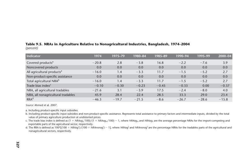
327
Table 9.5. NRAs in Agriculture Relative to Nonagricultural Industries, Bangladesh, 1974–2004(percent)
Indicator 1974 1975–79 1980–84 1985–89 1990–94 1995–99 2000–04
Covered productsa �20.8 2.8 �3.8 16.8 �2.2 �7.6 3.9Noncovered products 0.0 0.0 0.0 0.0 0.0 0.0 0.0All agricultural productsa �16.0 1.4 �3.3 11.7 �1.5 �5.2 2.7Non-product-specific assistance 0.0 0.0 0.0 0.0 0.0 0.0 0.0Total agricultural NRAb �16.0 1.4 �3.3 11.7 �1.5 �5.2 2.7Trade bias indexc �0.10 �0.30 �0.23 �0.45 �0.33 0.00 �0.37NRA, all agricultural tradables �21.6 3.1 �3.9 17.5 �2.4 �8.0 4.0NRA, all nonagricultural tradables 45.9 28.4 22.4 28.5 33.3 29.0 23.4RRAd �46.3 �19.7 �21.5 �8.6 �26.7 �28.6 �15.8
Source: Ahmed et al. 2007.
a. Including product-specific input subsidies.b. Including product-specific input subsidies and non-product-specific assistance. Represents total assistance to primary factors and intermediate inputs, divided by the total
value of primary agriculture production at undistorted prices.c. The trade bias index is defined as (1 � NRAagx�100)�(1 � NRAagm�100) � 1, where NRAagm and NRAagx are the average percentage NRAs for the import-competing and
exportable parts of the agricultural sector, respectively.d. The RRA is defined as 100*[(100 � NRAagt)�(100 � NRAnonagt) � 1], where NRAagt and NRAnonagt are the percentage NRAs for the tradables parts of the agricultural and
nonagricultural sectors, respectively.

In table 9.5, we summarize the RRA findings on the basis of annual estimatesreported in Ahmed et al. (2007). These estimates reveal that, although the NRAsfor agricultural tradables were positive in some years, they were always well belowthe NRAs for nonagricultural tradables. Hence, the RRA estimates are quite nega-tive; they suggest that the relative prices of farm products have been depressed bymore than one-fifth since independence. The value of the RRAs in the first half ofthe present decade is considerably higher than the value of the RRAs for the 1990s,however (at an average �16 percent compared with �27 percent). Additionalreform in the nonfarm sectors will be needed to eliminate the distortions inresource allocation among the sectors that produce tradables (figure 9.5).
The Political Economy of Agricultural Policies
There was a progressive shift in government agricultural policies toward privatiza-tion, deregulation, and a reduction in input subsidies. The shift began in the mid-1970s and continued in stages up to the early 1990s. There are still government
328 Distortions to Agricultural Incentives in Asia
−60
−40
−20
0
20
40
60
80
100
NRA
and
RRA
, %
1974
1976
1978
1980
1982
1984
1986
1988
1990
1992
1994
1996
1998
2000
2002
2004
year
NRA, agriculturaltradables
RRA NRA, nonagriculturaltradables
Figure 9.5. NRAs for Agricultural and Nonagricultural Tradablesand the RRA, Bangladesh, 1974–2004
Source: Ahmed et al. 2007.
Note: For the definition of the RRA, see table 9.5, note d.
controls on fertilizers, sugar production, and the wholesale trade, but these are ofrelatively minor economic significance.
The successive government administrations that formulated and implementedthese policies, like all governments, balanced a variety of objectives against arange of constraints. In the policy-making process, pressures and counterpres-sures are exerted on governments by various interest groups, and the responses ofthe governments are usually conditioned by interests held in common by the pres-sure groups and government leaders. Sometimes, if effective pressure groups havenot emerged or if they may be successfully set against one another, the govern-ment might then pursue its own agenda, which may be predatory, altruistic, or ablend of the two (Grindle 1991). Even if reform proposals are sound on the economics, the reforms will not be successful and sustainable unless they findacceptance according to minimum social and political criteria. If they do not findsuch acceptance, the government may be forced to backtrack and adopt policiesthat are less satisfactory on economic grounds.27
In Bangladesh, several factors have been especially important in determiningthe influence of various interest groups on agricultural policies and reforms sinceindependence. These include the relative political strengths of farmers versusurban groups, academic and political views on socialism and capitalism, debateswithin government ministries, and the reach of donors.
One of the most important facets of the political economy is the relative weak-ness of farmers and the rural poor in lobbying the government. These groupsinclude a large number of households, but their geographical dispersion, internaldifferences, ideological orientations, and poor resource base render them largelyineffective politically. In contrast, the working class in the urban formal sector, thebureaucracy as a pressure group within the government apparatus, and privateentrepreneurs constitute organized and powerful interest groups that few govern-ments can afford to antagonize.28
The weak political position of farmers and smallholders explains why conflictsof interest between agriculture and industry have consistently been resolved infavor of industry. Thus, for example, in the case of agricultural-based industrialraw materials such as jute, the policy has focused on keeping the price of the inputlow so that the relevant industrial product is competitive. Export taxes andrestrictions on agricultural commodity exports contributed to the discriminationagainst agriculture. The weak representation of the interests of the peasantrywithin the major political parties and the predominance of trading and industrialinterests led to an excessively protected economic regime and shaped the politicaleconomy so that government policies continued to discriminate against agricul-ture. Even in the case of policy measures such as input subsidies, farmers failed toderive much benefit because the subsidies were largely usurped by rent-seeking
Bangladesh 329
public officials who were in collusion with middlemen. Any residual benefits tofarmers were often more than offset by depressed farm output prices.
Another important factor shaping agricultural and economic policies moregenerally is the wide divergence of views among social scientists and other profes-sionals on the issue of reform. The views of some critics of market mechanismswere initially shaped by colonialism, which these critics consider a form ofexploitation by world capitalism. These critics once pointed to the apparent suc-cesses of China and the Soviet Union in economic transformation and to certainblatant examples of market failure, such as the Bengal famine in 1943. The stridestaken in China toward the market economy and the disintegration of the SovietUnion have, more recently, disillusioned many of these critics regarding thevirtues of central planning. Nonetheless, an articulate antimarket lobby still per-sists among intellectuals that effectively counters the sweeping and sometimessimplistic claims for the market made by votaries.
The policy process is also complicated by the fact that policy makers andimplementers often hold divergent views on the appropriateness of particularreform measures. Sometimes, this occurs because of differences in the social andpolitical orientation of these actors. Rivalry among ministries and the unwilling-ness of the bureaucracy to relinquish the levers of control even in cases in whichpolitical leaders are committed to deregulation may also lead to such outcomes.For example, a ministry of commerce may obstruct liberalization measures pro-posed by a ministry of finance.
Finally, donors have had a major effect on government policy in Bangladesh inpart because of the importance of foreign aid in the development budget and inbalance of payments support. Within agriculture, donor support in the fundingfor agricultural research, rural infrastructure, and food aid was especially impor-tant in the 1970s and 1980s, and this contributed to the weight of donor views inthe policy process. In particular, the Asian Development Bank, the United StatesAgency for International Development, and the World Bank exerted substantialinfluence during the formulation and implementation of agricultural policy bytying program loans and import credits to the policy reform agenda.
Major Reforms in Agricultural Pricing
The major reforms in agricultural policy in the 1980s were swayed by the policyperspectives of the dominant donor agencies as outlined in papers on agriculturaland food policy and pricing prepared by the World Bank and the United StatesAgency for International Development. The World Bank (1979) argued that thenet effect of policy interventions in developing countries was to discourage agricultural production, that higher price incentives might be an important
330 Distortions to Agricultural Incentives in Asia
instrument in increasing food production, and that input subsidies had proved aninefficient means of protecting agriculture. The World Bank also highlighted thecomplexities in the effects of food prices on various groups and advocated a grad-ual rise in food prices to avoid the hardships resulting from abrupt price increases.The United States Agency for International Development (USAID 1982) likewiseargued that government interventions in agricultural markets tended to reduceefficiency in the allocation of resources, inhibited gains in productivity, and oftendid little for the groups they were supposed to help. The U.S. aid agency advocatedpolicies that did not suppress producer prices, that did not attempt to regulateconsumer access to food, and that led to a speedy withdrawal of subsidies for agri-cultural inputs, including credit. Government interventions were to be limited toagricultural research, the construction of large-scale irrigation systems, and spe-cial feeding programs to combat malnutrition.
Thus, donors generally advocated a market-oriented agricultural policy,though they also suggested that a central role should be reserved for output pricesupports to promote self-sufficiency in food grains.29 This objective was ulti-mately achieved in 2000 (Osmani and Quasem 1990).30
Reforms in agricultural input markets, particularly those related to fertilizerprices, generally faced more opposition. In 1973, the First Five-Year Plan ofBangladesh (1973–78) underscored the need for the eventual removal of agricul-tural input subsidies and emphasized that the inputs should be sold at a profit.Indeed, urea prices were raised substantially in 1973. Sections of the bureaucracywere opposed to the elimination of input subsidies and to the privatization of thedistribution of fertilizer and irrigation equipment. This resistance was partlycaused by the bureaucracy’s reluctance to accept a curtailment in its power overmarket controls and distribution. A misplaced concern about equity also con-tributed to the opposition of bureaucrats to the proposed reforms. Donor pressureto carry out the reforms swiftly played a major role in quelling this opposition.
Fertilizer markets were liberalized again in the early 1990s. The country wit-nessed a major crisis in the fertilizer market in 1994–95. This led to a partial rever-sal of the reform in the fertilizer market. Indeed, farmers agitated so militantly thatthere were incidents involving police gunfire and several deaths. This was in sharpcontrast to the 1974 famine, which caused little uproar in rural Bangladesh, and tothe fertilizer shortage in 1993 when farmers were paying high fertilizer prices with-out much protest (Abdullah 1996). The unmet expectations about the lower pricesthat were supposed to be generated by policy reforms and a perception that therehad been injustices may explain the outrage of farmers in the mid-1990s.31
The 1974 famine had a different dynamic in the sense that it affected mainlylandless laborers. In contrast, the fertilizer shortage in 1993 mainly affected mid-level farmers, who are known to be more militant and among whom marketed
Bangladesh 331
rice surpluses are not usually sufficiently large to offset higher urea prices (Wolf1971). Because national elections were pending, the political parties in oppositionalso tried to reap dividends from the crisis by mobilizing the peasantry.
Not all reforms in agricultural input markets have been opposed by farmers.Some policy reforms seem to have benefited a majority of farmers. For example,the elimination of the standards requirement in irrigation equipment has beenpopular. This policy faced opposition from public sector employees, particularlythose active in exercising government market controls and government authorityover imports (especially the Bangladesh Agricultural Development Corporation).However, this opposition did not prove to be a major roadblock. The issue wasnever politicized, and the government and its development partners handled thematter tactfully, but also with firmness (Abdullah and Shahabuddin 1993).
Concluding Observations
Agriculture has undergone major structural changes and achieved major suc-cesses in Bangladesh over the last four decades. Despite the many problems andconstraints, a quiet agricultural revolution has taken place that has enabled thecountry to achieve its national food security targets in the production of foodgrains. Agriculture continues to evolve in response to numerous factors, includingnatural calamities, sociopolitical changes, population growth, urbanization, newtechnology, opportunities in the rural nonfarm sector, and commercialization.Government macroeconomic, trade, and agricultural pricing policies have playeda major role in shaping price incentives in production and consumption and willcontinue to be important determinants of agricultural growth.
For over 30 years, a central objective of government agricultural policy wasself-sufficiency in food grains. To achieve this objective, the governmentattempted to maintain sufficient incentives for the expansion of domestic rice andwheat production through the maintenance of remunerative output prices andfertilizer subsidies. Investments in agricultural research and technology that per-mitted large gains in productivity and a substantial increase in irrigation in thearea under rice cultivation were also crucial. Meanwhile, government policy wasalso designed to protect poor consumers through the subsidized sale of rice (untilthe early 1990s) and extensive safety nets involving food for work programs andfood transfers, particularly wheat.
Although trade liberalization has faced substantial opposition, the govern-ment nonetheless undertook major reforms in trade policy, including reducingtariffs on industrial products in the 1980s and the early 1990s and liberalizingprivate sector trade in rice and wheat in the 1990s. As a result, the domestic out-put price for wheat and rice (the main agricultural products in value) has been
332 Distortions to Agricultural Incentives in Asia
close to the border price in most years since the early 1990s. Thus, price distor-tions in agriculture have averaged less than 5 percent of the value of domestic pro-duction since 1990 despite the ongoing price distortions on a few products(notably, sugarcane) and inputs (chemical fertilizers). The country has reapedgreat benefit from trade liberalization through enhanced food security becauseprivate sector imports have helped stabilize markets following significant produc-tion shortfalls. Keeping the domestic prices of most agricultural commoditiesclose to the respective border prices has also generated overall efficiency gains inthe agricultural sector.
Reducing the remaining disincentives for agricultural production—caused bythe protection for nonagricultural producers—will be a necessary part of anyfuture strategy aimed at agricultural growth and rural poverty reduction. Even aliberalized trade policy would not guarantee higher incomes among farmers. Forexample, in the early part of this decade, the upward trend in the ratio of fertilizerprices to paddy prices that was partly driven by movements in world prices even-tually reduced the price incentive for paddy production and contributed to lowerreturns to farmers. In 2007–08, the world prices for fertilizer and rice rose sub-stantially and, combined with the limits imposed by India on rice exports toBangladesh, contributed to large increases in the domestic prices for fertilizer andrice in Bangladesh in early 2008. Policies aimed at increasing production and sta-bilizing prices need not rely mainly on price subsidies or substantial increases inpublic stocks, however. Indeed, productivity-enhancing investments in agricul-tural research and extension, improvements in postharvest management andagroprocessing, and investments in market infrastructure can complement agri-cultural price and trade policies and enable rapid agricultural growth and higherfarmer incomes even in a context of shifting world prices.
Notes
1. Throughout this chapter, crop or fiscal years are indicated by the second of the two calendaryears. For example, 2004 here refers to the year 2003/04 in official statistics.
2. By 1995, exporters were also enjoying income tax exemptions on 50 percent of their export earnings.
3. Other measures included the export policy order issued in 1986, which provided special induce-ment and promotional freight rates by the national flag carriers, Biman Bangladesh Airlines andBangladesh Shipping Corporation, for exports of fruits, vegetables, and ornamental plants.
4. Initially, the reference currency was the U.K. pound sterling; but this was changed to the U.S. dollar in early 1983 because of the large weight of the United States in the total trade of Bangladesh.
5. In 1996, the government accepted the conditions of article VIII of the Articles of Agreement ofthe International Monetary Fund by making the taka fully convertible for international currentaccount transactions. Under this arrangement, exporters may freely utilize their export earnings to payfor imports.
Bangladesh 333
6. For details on the duty structure affecting imports of major agricultural commodities in1991–2003, see Ahmed et al. 2007.
7. Our NRAs for tradables include an estimate of the trade tax effect of the overvalued exchangerate. For this estimate, we rely on the black market exchange rate premium (see Global DevelopmentNetwork Growth Database). We also assume that only half of the foreign exchange rate earnings ofexporters is sold to the government at the official rate. For details on this methodology, see Andersonet al. (2008) and appendix A.
8. Throughout this section, the term agricultural sector refers only to crop and livestock productionand excludes fishing and forestry.
9. See Ravallion (1990) and del Ninno, Dorosh, and Islam (2002) for detailed discussions of mar-kets and government policy during this period.
10. To analyze this policy fully would require a multimarket model (see Dorosh and Haggblade 1997).11. Other factors also contributed to the increase in rice exports from India, including a 27 percent
depreciation of the Indian rupee in real terms (see Dorosh 2001).12. Several successive rice harvests were poor in Bangladesh: wet season rice (aman) in 1994, 1995,
and 1997; winter rice in 1995; and severe losses in autumn (aus) rice and wet season rice following themid-1998 flood. See Dorosh et al. (2004) for a discussion of government trade and pricing policies infood grains following the 1998 flood.
13. Small amounts of nonparboiled rice were imported in 2000, mainly from Vietnam. Higher-quality (noncoarse) rice imports likely accounted for much of the rest (Dorosh 2001).
14. For example, in the targeted public distribution system in India, wheat and rice were distributedat a special, highly subsidized rate to consumers certified as living below the poverty line; in 2000, statetrading parastatals in India could buy wheat at these below-poverty-line prices and then export thewheat (USDA 2001; see also Dorosh and Shahabuddin 2005 and chapter 10, on India, in this volume).
15. Bangladesh imported 281,000 tons of rice across the land borders with India during 2000. Thiswas about the same as the 286,000 tons imported in 1999. A breakdown of the rice by quality is notavailable, but a 9 percent decline in the average price of imports from India—from Tk 12.1 per kilo-gram in 1999 to Tk 11.1 per kilogram in 2000—suggests that the average quality of imports may havedeclined over the two years.
16. The total tariffs and fees were raised from 10.5 to 43.0 percent if one includes an advancedincome tax of 3 percent and a license fee of 2.5 percent.
17. The increase in import taxes raised the above-poverty-line import parity price, including taxes,to 71 percent above the domestic price.
18. Our NRA estimates on output using the average cost of imports suggest that these NRAs werearound zero, perhaps because shipments of high-quality rice raised the average import price above theimport parity price for below-poverty-line rice.
19. For example, from 1995–96 through 2002–03, the value of manufactured jute products wasmore than three times the value of raw jute exports (calculated based on data in World Bank 2005).
20. The jute export tax equivalent in East Pakistan during the 10 years leading up to the independ-ence of Bangladesh from Pakistan in 1971 was at least as severe as and probably more severe than thejute export tax equivalent during the rest of the 1970s.
21. Pursell’s estimates (2005) for 2002 are domestic production at 177,000 tons, official importsfrom India at 349,000 tons, official imports from other countries at 93,000 tons, and sugar smuggledfrom India at 400,000 tons.
22. Until June 2002, the Trading Corporation of Bangladesh and the Bangladesh Sugar and FoodIndustries Corporation, a public enterprise, shared a monopoly on sugar imports (Pursell 2005).
23. Another parastatal, the Bangladesh Water Development Board, was established in the early1960s to implement large-scale projects in surface water irrigation, flood control, and drainage. Theinitiatives were based on recommendations contained in a master plan prepared in the aftermath ofdisastrous floods in the mid-1950s.
24. Despite privatization in the distribution of fertilizers, the public sector continued to accountfor most urea production.
334 Distortions to Agricultural Incentives in Asia
25. Like fertilizer, irrigation water was also heavily subsidized in the early years of the expansion inirrigation. There was a rapid reduction in subsidies in the late 1970s when irrigation equipment previously owned by the public sector was privatized. Since 1988, the government has eliminated allrestrictions on imports of irrigation equipment by the private sector, cancelled import duties on agri-cultural machinery, and removed restrictions aimed at standardization and quality control in the pro-duction of agricultural machinery. These policy changes have had a significant impact on the use oflow-end irrigation equipment, especially shallow tube wells, and they have led to a rapid expansion inthe total area under irrigation in the country (Ahmed 2001).
26. In most years, the country has produced urea from domestic natural gas. Net exports of urea ona large scale began in 1988 (Renfro 1992).
27. For an analysis of the oscillation of postcolonial governments between technocratic and pop-ulist policies, see Huntington and Nelson (1976).
28. In reforming the grain procurement and ration shop system in the early 1990s, the governmentwas able to avoid direct conflict with consumer groups by only gradually reducing the price subsidy onration shop grain. Without the support of consumer groups, which no longer reaped significant bene-fit from the ration shop system, millers lacked the political clout to resist the call to end the millgateprocurement system (Chowdhury and Haggblade 2000).
29. Various studies of the comparative advantage of Bangladesh in agriculture demonstrate thatthe attainment of self-sufficiency in rice production is an important sociopolitical objective and alsoan eminently sensible goal strictly from the point of view of economics (see Mahmud, Rahman, andZohir 2000; Shahabuddin 2000; Shahabuddin and Dorosh 2004).
30. Government interventions through domestic procurements were largely ineffective in main-taining floor prices for producers. A number of factors contributed to the failure of domestic procure-ment, including an inadequate coverage of production areas by procurement centers, cumbersomepayment procedures that raised the transaction costs for small farmers, the lack of financial resourcesin the public food distribution system, and collusion between traders and officials that enabled tradersto capture the margin between the market price and the procurement price (Shahabuddin 1996).
31. When the issue price of fertilizer was reduced in the 1994 budget, farmers expected that theywould be the major beneficiaries. So, their notion of a just price was outraged when they were required topay prices that were nearly double (and sometimes more) the prices the middlemen paid to the factories.
References
Abdullah, A. 1996. “Urea Market in Bangladesh, 1994–95: The Anatomy of a Crisis.” In State, Marketand Development: Essays in Honour of Rehman Sobhan, ed. A. Abdullah and A. R. Khan, chap. 12.Dhaka, Bangladesh: University Press.
Abdullah, A., and Q. Shahabuddin. 1993. “Critical Issues in Bangladesh Agriculture: Policy Responseand Unfinished Agenda.” Paper presented at the Asian Development Bank and Academy for Planning and Development conference, “Bangladesh Economy in Transition,” Dhaka,Bangladesh.
Ahmed, A. W. Nuruddin, L. H. Chowdhury, and S. Haggblade. 2000. “History of Public Food Interven-tions in Bangladesh.” In Out of the Shadow of Famine: Evolving Food Markets and Food Policy inBangladesh, ed. R. Ahmed, S. Haggblade, and T.-E. Chowdhury, 121–36. Baltimore: Johns HopkinsUniversity Press; Washington, DC: International Food Policy Research Institute.
Ahmed, N., Z. Bakht, P. A. Dorosh, and Q. Shahabuddin. 2007. “Distortions to Agricultural Incentivesin Bangladesh.” Agricultural Distortions Working Paper 32, World Bank, Washington, DC.
Ahmed, R. 2001. Retrospect and Prospects of the Rice Economy of Bangladesh. Dhaka, Bangladesh: University Press.
Ahmed, R., S. Haggblade, and T.-E. Chowdhury, eds. 2000. Out of the Shadow of Famine: Evolving FoodMarkets and Food Policy in Bangladesh. Baltimore: Johns Hopkins University Press; Washington,DC: International Food Policy Research Institute.
Bangladesh 335
Anderson, K., M. Kurzweil, W. Martin, D. Sandri, and E. Valenzuela. 2008. “Measuring Distortions toAgricultural Incentives, Revisited.” World Trade Review 7 (4): 675–704.
Bakht, Z. 1999. “Impact of SAFTA on the Official and Unofficial Trade of Bangladesh.” Unpublishedworking paper, Bangladesh Institute of Development Studies, Dhaka, Bangladesh.
———. 2001a. “Preparation of the Sixth Five-Year Plan: Background Paper on Industry.” Unpublishedworking paper, Bangladesh Institute of Development Studies, Dhaka, Bangladesh.
———. 2001b. “Trade Liberalization, Exports and Growth of Manufacturing Industries inBangladesh.” In Strategies for Industrialization: The Case of Bangladesh, ed. M. M. Huq and J. Love,chap. 5. Dhaka, Bangladesh: University Press.
BBS (Bangladesh Bureau of Statistics). various years. Statistical Yearbook of Bangladesh. Dhaka,Bangladesh: BBS.
Chowdhury, T.-E., and S. Haggblade. 2000. “Dynamics and Politics of Policy Change.” In Out ofthe Shadow of Famine: Evolving Food Markets and Food Policy in Bangladesh, ed. R. Ahmed,S. Haggblade, and T.-E. Chowdhury, 165–88. Baltimore: Johns Hopkins University Press; Washington,DC: International Food Policy Research Institute.
del Ninno, C., and P. A. Dorosh. 2003. “Impacts of In-Kind Transfers on Household Food Consump-tion: Evidence from Targeted Food Programs in Bangladesh.” Journal of Development Studies40 (1): 48–78.
del Ninno, C., P. A. Dorosh, and N. Islam. 2002. “Reducing Vulnerability to Natural Disasters: Lessonsfrom the 1998 Floods in Bangladesh.” IDS Bulletin 33 (4): 98–107.
Dorosh, P. A. 2001. “Trade Liberalization and National Food Security: Rice Trade between Bangladeshand India.” World Development 29 (4): 673–89.
———. 2006. “Accelerating Income Growth in Rural Bangladesh.” Background report, World Bank,Washington, DC.
Dorosh, P. A., N. Farid, R. Amin, and M. A. Aziz. 2004. “Policy Response to Production Shocks: The1997/98 Aman Shortfall and the 1998 Flood.” In The 1998 Floods and Beyond: Towards Comprehen-sive Food Security in Bangladesh, ed. P. A. Dorosh, C. del Ninno, and Q. Shahabuddin, 155–80.Dhaka, Bangladesh: University Press; Washington, DC: International Food Policy Research Institute.
Dorosh, P. A., and S. Haggblade. 1997. “Shifting Sands: The Changing Case for Monetizing ProjectFood Aid in Bangladesh.” World Development 25 (12): 2093–104.
Dorosh, P. A., and Q. Shahabuddin. 2005. “Trade Liberalization and Food Security in Bangladesh.” InEconomic Reforms and Food Security: The Impact of Trade and Technology in South Asia, ed. S. C.Babu and A. Gulati, 141–62. New York: Haworth Press; Washington, DC: International Food PolicyResearch Institute.
FAOSTAT Database. Food and Agriculture Organization of the United Nations. http://faostat.fao.org/default.aspx (accessed May 2008).
Global Development Network Growth Database. Development Research Institute, New York University.http://www.nyu.edu/fas/institute/dri/global%20development%20network%20growth%20database.htm (accessed June 2007).
Grindle, M. S. 1991. “The New Political Economy: Positive Economics and Negative Politics.” In Politicsand Policy Making in Developing Countries: Perspectives on the New Political Economy, ed. G. M.Meier, 41–68. Richmond, CA: ICS Press.
Hossain, M. 2001. “Recent Development and Structural Changes in Bangladesh Agriculture: Issues forReviewing Strategies and Policies.” In Changes and Challenges: A Review of Bangladesh’s Develop-ment 2000, ed. R. Sobhan, chap. 3. Dhaka, Bangladesh: University Press and Center for Policy Dialogue.
Huntington, S., and J. Nelson. 1976. No Easy Choice, Cambridge MA: Harvard University Press.Mahmud, W., S. H. Rahman, and S. Zohir. 2000. “Agricultural Diversification: A Strategic Factor for
Growth.” In Out of the Shadow of Famine: Evolving Food Markets and Food Policy in Bangladesh, ed.R. Ahmed, S. Haggblade, and T.-E. Chowdhury, 232–60. Baltimore: Johns Hopkins UniversityPress; Washington, DC: International Food Policy Research Institute.
336 Distortions to Agricultural Incentives in Asia

Ministry of Finance. 2005. Bangladesh Economic Review. Dhaka, Bangladesh: Ministry of Finance.Osmani, S. R., and A. Quasem. 1990. “Pricing and Subsidy Policies for Bangladesh Agriculture.”
Unpublished working paper, Bangladesh Institute of Development Studies, Dhaka, Bangladesh.Pursell, G. 2005. “Free Trade between India and Bangladesh: A Case Study of the Sugar Industry.”
Unpublished report, World Bank, Washington, DC.Rahman, S. H. 1992. “Trade Policies and Industrialization in Bangladesh: An Assessment.” Unpub-
lished working paper, Bangladesh Institute of Development Studies, Dhaka, Bangladesh.———. 1994. “The Impact of Trade and Exchange Rate Policies on Economic Incentives in
Bangladesh Agriculture.” Working Papers on Food Policy in Bangladesh 8, International Food Policy Research Institute, Washington, DC.
Ravallion, M. 1990. Markets and Famines. Dhaka, Bangladesh: University Press.Renfro, R. Z. 1992. “Fertilizer Price and Subsidy Policies in Bangladesh.” World Development
20 (3):437–55.Shahabuddin, Q. 1996. “Public Interventions in Food Grain Markets in Bangladesh: An Appraisal.” In
State, Market and Development: Essays in Honour of Rehman Sobhan, ed. A. Abdullah and A. R.Khan, chap. 13. Dhaka, Bangladesh: University Press.
———. 2000. “Comparative Advantage in Bangladesh Agriculture.” Bangladesh Development Studies26 (1): 37–68.
Shahabuddin, Q., and P. A. Dorosh. 2004. “Diversification of Agricultural Production: ComparativeAdvantage in Crops and Implications of the World Trade Organization.” In The 1998 Floods andBeyond: Towards Comprehensive Food Security in Bangladesh, ed. P. A. Dorosh, C. del Ninno, and Q.Shahabuddin, 313–34. Dhaka, Bangladesh: University Press; Washington, DC: International FoodPolicy Research Institute.
USAID (United States Agency for International Development) 1982. “Pricing, Subsidies and RelatedPolicies in Food and Agriculture.” Policy Paper, USAID, Washington, DC.
USDA (United States Department of Agriculture). 2001. “India: Grain and Feed Annual Report 2001.”Report, Foreign Agricultural Service, USDA, Washington, DC.
Wolf, E. 1971. “Peasant Wars of the Twentieth Century.” London: Faber and Faber.World Bank. 1979. Bangladesh Food Policy Issues. Report 2761-BD. Washington, DC: World Bank.———. 1994. Bangladesh: From Stabilization to Growth. Report 12724-BD. Washington, DC: World Bank.———. 2004. An Overview. Vol. 2 of Trade Policies in South Asia: An Overview. Report 29949.
Washington, DC: World Bank.———. 2005. Bangladesh: Growth and Export Competitiveness. Report 31394-BD. Washington, DC:
World Bank.
Bangladesh 337

This chapter analyzes the impacts on price incentives in India’s agricultural sectorthat have resulted from government price, trade, and exchange rate policies. Previ-ous studies have established that, from the 1970s to 1995, the incentive systemstrongly favored manufacturing and services over the principal agricultural crops,although the extent of the antiagricultural bias had diminished considerably by themid-1990s (Pursell 1999).1 Our study updates these earlier estimates to 2005 andincorporates estimates for agriculture going back to 1965. In addition, we extendthe previous work by considering policies affecting the incentives for the produc-tion of fresh fruits and vegetables and for dairying, which account for large sharesof the rural economy as measured by the respective contributions to gross domes-tic product (GDP). We also briefly discuss policies affecting food processing.
The chapter is organized as follows. In the next section, we provide overviewsof economic growth and structural change in the Indian economy and the evolu-tion of trade policies since independence, including the effects of current govern-ment policies on agricultural trade with the country’s neighbors in South Asia. Inthe subsequent section, we discuss the exchange rate and its interaction with tradepolicies, especially during the massive rupee devaluation of 1985–93. We thenoffer quantitative evidence on nominal rates of assistance (NRAs) in various agri-cultural subsectors, including subsidies for electricity and fertilizer inputs. We alsoestimate the distortions in the incentives for farmers relative to the incentives for
339
10
INDIA
Garry Pursell, Ashok Gulati,and Kanupriya Gupta
The authors thank the members of the central project team (especially Marianne Kurzweil and ErnestoValenzuela) for their contributions and technical help with the data spreadsheets from which several ofour tables and figures have been generated.
producers of nonagricultural tradables. We use this evidence to show that the ini-tial, notable antiagricultural bias of government policies gradually gave way to aslight bias in favor of agriculture. Finally, we discuss the political economy forcesthat are likely to influence the direction of government policies, including the possibility that a strong proagricultural bias may emerge as has occurred in more-advanced, densely populated economies in East Asia and elsewhere.
Economic Growth and Structural Change
Agriculture accounted for slightly more than 50 percent of GDP in 1950, but itsshare is now less than 20 percent.2 Most of this decline occurred in crop agricul-ture. In contrast, the livestock subsector (mainly dairying) grew more rapidly thanthe rest of the economy. The GDP share of this subsector rose from 2 percent inthe early 1980s to 4.4 percent in 2005. Forestry was important after independence,but, in 2003, it provided only around 1 percent of GDP, as did fishing, despitefairly speedy growth over a long period, mainly impelled by fish farm develop-ment. Meanwhile, mining’s contribution grew from less than 1 percent in the1950s to 2.8 percent in 2005. The steep decline in agriculture’s contribution to theeconomy since independence has been generated principally by the more rapidgrowth in the services sector, from barely 30 percent of GDP in 1950 to 63 percentin 2003. The growth of the services sector has been especially brisk since the early1990s, and it accelerated during the late 1990s and early years of the next decadebecause of swift advances in information technology and export outsourcing. Theshare of manufacturing in the economy also increased, but not nearly as quickly asit did in many other developing countries. The share of manufacturing in GDP in2005 was 16 percent (much lower than in East Asian economies). This compareswith 10 percent in 1950, shortly after independence (table 10.1).
The contribution of the rural sector to GDP has declined by almost 70 percentsince independence. However, the sector still accounted for around 60 percent ofnational employment in 2003, and this share had been declining only slowly sincethe early 1990s (partly because of slow growth in manufacturing employment).
International trade in agricultural products has always been tiny relative to thesize of the agricultural sector. In 2005, agricultural imports were equivalent toonly 0.8 percent of the value of agricultural production (or 2.1 percent if edible oilimports are included), while exports were 6.4 percent of production. Even duringearlier periods, when agriculture represented a major share of total trade (forexample, 27 and 44 percent of total imports and exports, respectively, in 1960),imports and exports still only accounted for a little more than 3 percent of agri-cultural production (table 10.2).
The most important primary agricultural import initially was wheat, followedby cotton and powdered milk. Beginning around the mid-1970s, the need for
340 Distortions to Agricultural Incentives in Asia

341
Table 10.1. Sectoral Share of GDP and Employment, India, 1950–2005(percent)
Sector 1950 1960 1970 1980 1990 2000 2003 2004 2005
All agriculturea 56.9 46.7 46.1 38.9 31.3 23.4 20.9 18.8 18.3Livestock — — — 1.9 4.7 5.4 4.6 4.8 4.4Crops — — — 33.7 23.8 15.8 14.4 12.2 12.1Forestry and logging 3.0 2.2 2.1 2.5 1.8 1.0 0.9 0.8 0.7Fishing 0.4 0.5 0.6 0.7 1.0 1.1 1.1 1.0 1.1
Mining and quarrying 0.8 1.1 1.1 1.7 2.7 2.4 2.5 3.0 2.8Manufacturing 10.6 13.8 13.8 16.3 17.1 15.6 15.2 15.9 16.0Services 31.8 38.4 39.1 43.1 48.8 58.7 61.3 62.4 62.9Agriculture’s share in employment — — — — 69 62 60 — —
Sources: Author computations based on Ministry of Finance, various; CGA Database 2008.
Note: — � no data are available.
a. Agriculture includes crop agriculture, horticulture, livestock activities, inland and ocean fisheries, and forestry activities.
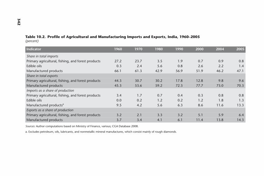
342
Table 10.2. Profile of Agricultural and Manufacturing Imports and Exports, India, 1960–2005(percent)
Indicator 1960 1970 1980 1990 2000 2004 2005
Share in total importsPrimary agricultural, fishing, and forest products 27.2 23.7 3.5 1.9 0.7 0.9 0.8Edible oils 0.3 2.4 5.6 0.8 2.6 2.2 1.4Manufactured products 66.1 61.3 42.9 56.9 51.9 46.2 47.1Share in total exportsPrimary agricultural, fishing, and forest products 44.3 30.7 30.2 17.8 12.8 9.8 9.6Manufactured products 45.3 53.6 59.2 72.3 77.7 73.0 70.3Imports as a share of productionPrimary agricultural, fishing, and forest products 3.4 1.7 0.7 0.4 0.3 0.8 0.8Edible oils 0.0 0.2 1.2 0.2 1.2 1.8 1.3Manufactured productsa 9.5 4.2 5.6 6.3 8.6 11.6 13.3Exports as a share of productionPrimary agricultural, fishing, and forest products 3.2 2.1 3.3 3.2 5.1 5.9 6.4Manufactured products 3.7 3.4 4.1 6.1 11.4 13.8 14.3
Sources: Author computations based on Ministry of Finance, various; CGA Database 2008.
a. Excludes petroleum, oils, lubricants, and nonmetallic mineral manufactures, which consist mainly of rough diamonds.
these and other agricultural imports were eliminated because of growing domes-tic production, and, since then, they have accounted for only a small share of totalimports even when they were imported during poor crop seasons, for example, inwheat and sugar.
The largest consistent imports of processed food have involved edible oils.Imports of these products expanded rapidly during the 1970s and early 1980s,triggering a major government program to replace the imports through domesticproduction. For a while, edible oil imports declined, but, despite high tariffs (an80 percent tariff on palm oil in 2006, for instance), import growth resumed in the1990s, and, by 2005, imports accounted for about 40 percent of the domestic con-sumption of these products.
During the 1950s and 1960s, agricultural products represented slightly lessthan half of the country’s total merchandise exports, but the share has steadilydeclined since then and is now around 10 percent. A diverse range of agriculturalproducts are regularly exported, including fish and fish preparations, oil cakes,cashew kernels, tea, coffee, tobacco, spices, fruits, vegetables, pulses, basmati rice,and, periodically, large quantities of sugar and common rice (more than 4 milliontons of rice in 2004/05, for example). Except for cashew kernels, the share ofexports in the total domestic production of these individual products is small.
Since the late 1980s, manufactured exports have usually accounted for 70–80percent of total merchandise exports, compared with 40–50 percent in the 1950sand 1960s. Manufactured exports have also increased in relation to total manufac-turing production, especially since the late 1980s, growing about twice as quickly,at 20–30 percent a year, in 2000–05. However, relative to many other developingcountries, these exports still constitute a small share of manufacturing sector out-put (around 15 percent in 2005).
Service sector exports have also been growing rapidly in recent years, at about25 percent annually. In 2004, net invisible exports represented 4.9 percent of GDP,compared with the negative net balances before 1990. The most dynamic compo-nents of this trade are software exports, other exports related to information tech-nology, and the outsourcing of services.
The share of food expenditure in household budgets is high in India, amount-ing to 54 percent and 42 percent of total per capita consumption expenditure inrural and urban areas, respectively. The shares of food in the budgets of the poor-est 10 percent of households is even higher, averaging 62 percent in rural areasand 58 percent in urban areas in 2003. Because of these high shares of food inhousehold budgets (the shares have been declining only slowly), it is not surpris-ing that food prices and food availability are regular news items in the local andnational press and other media, and that food prices, especially sudden increasessuch as in 2008, are highly sensitive politically. One of the most prominent
India 343

objectives of the independence movement in India was to establish institutionsand policies that would permanently eliminate catastrophic famines, such as thosethat occurred during the colonial period, and that would also ensure that basicfood items would be available to the entire population at affordable prices.
To achieve these food policy goals, the government has intervened in food grainmarkets since the late 1940s. In 1958, it established the current public distributionsystem, which sells basic foods at subsidized prices through fair price shops. (Thereare currently about 460,000 of these shops.) For most of its history, the system hasdistributed wheat, rice, sugar, and edible oils on the basis of ration cards that enti-tle the bearers to specified quantities of food items at announced low prices. InJune 1997, the system was changed by distinguishing, according to fixed criteria,between below-poverty-line and above-poverty-line buyers. The former group waseligible to benefit from especially low prices, while the latter group was eligible tobuy the food items at prices that were slightly below free-market prices. In 2001,edible oils were removed from the system, and, in 2002, the role of sugar was dras-tically reduced by allowing subsidized sales only to below-poverty-line households.The principal government food subsidy activity today is the sale of rice and wheatthrough the fair price shops to below-poverty-line households and distribution aspart of other antipoverty programs. In 2003, the total government food subsidywas estimated at Rs 258 billion (about US$5.7 billion, or 0.83 percent of GDP); thissubsidy was defined as the Food Corporation of India’s total procurement han-dling and distribution costs, less the subsidized sales value.
Trade and Exchange Rate Policies since Independence
During the second half of the 1800s and until about 1921, the British rulers ofIndia followed free trade policies that imposed few restrictions or taxes on exportsor imports.3 These free trade policies began to change in the early 1920s followingthe collapse of the post–World War I boom, and protective tariffs continued to beintroduced during the 1920s and 1930s. Then, in 1940, general controls wereimposed on all imports and exports to deal with scarcities in goods, shipping, andforeign exchange and to address wartime priorities. The general rule was thatimports would only be allowed if they were essential and could not be supplied bylocal industries.
After independence in August 1947, the government relaxed wartime importcontrols by expanding the scope of lists of goods that could be imported withoutobtaining a license (the open general license) and by raising tariffs to take pressureoff the import licensing system. However, the start of the Second Five-Year Plan in1956 coincided with a severe foreign exchange crisis, and, until 1966, the compre-hensive administration of the import licensing system was tight. These foreign
344 Distortions to Agricultural Incentives in Asia
trade policies were an extension of more general economic policies under whichthe commanding heights of the industrial economy (which excluded farming)were dominated by state enterprises, and the private sector (including agriculture)was subject to extensive controls. Collectively, these controls came to be known asthe license Raj (the Hindi word for reign or rule).
In June 1966, the rupee was devalued. This was accompanied by a brief episodeof liberalization during which import licensing was relaxed, tariffs were cut, andexport subsidies were abolished or reduced. However, the import licensing systemremained intact, and, by 1968, most liberalizing initiatives had been reversed andtight import and domestic controls had been reinstated. This remained the situa-tion until the end of the 1970s, when a new phase of slow, partial liberalizationcommenced.
The slow liberalization trend of the late 1970s and early 1980s included therelaxation of industrial licensing rules, regular additions of intermediate productsand capital goods to open general license lists, and tariff increases that succeededin capturing some of the economic rents inherent in the import licensing system.Liberalization gained momentum during the Rajiv Gandhi government adminis-tration (1985–89) when the economic growth rate accelerated above the slowaverage rate that had characterized the previous 40 years. The boom culminatedin a severe foreign exchange crisis in 1991. The government reacted by imple-menting a sharp devaluation. The devaluation was accompanied by sweeping liberalizing measures that removed many of the key domestic controls over man-ufacturing, nearly all the import licensing system for intermediate and capitalgoods, and a key export subsidy program. The initiatives also included a four-yearprogram of tariff reductions. These reductions continued into the 1990s andbrought tariffs down far below the extremely high and prohibitive rates of the1980s (when they averaged more than 100 percent), though the tariffs were stillhigh by international standards.
Domestic policies and trade policies that affected the rural sector were basi-cally untouched by the 1991 reforms. In particular, government enterprises con-tinued to dominate the domestic and international trade in cereals (notably theFood Corporation of India, which periodically imported wheat to meet domesticshortages), and agricultural products remained subject to the import licensingsystem that applied to all consumer goods. With some important exceptions,import licenses were not issued for agricultural products. The system thusamounted to an import ban on agriculture. The exceptions in agricultureincluded a few products for which imports had been open even during the mostrestrictive periods (pulses, for example) and other products, such as cotton andwool, for which unrestricted low-tariff imports of important inputs had beensuccessfully negotiated by influential industrial lobbyists. Edible oils were also
India 345

imported on a large scale (despite efforts undertaken to replace the importsthrough domestic production), first, by state trading firms holding importmonopoly rights and, later, by the private sector. However, the edible oil importswere subject to high tariffs.
It has been estimated that, in the mid-1990s, five years after the 1991 reforms,about two-thirds of tradable GDP was still protected by explicit nontariff barriers(about 36 percent in manufacturing, 84 percent in agriculture, and 40 percent inmining). During the second half of the 1990s, this situation began to change, inlarge measure in response to international pressures linked to the Uruguay Roundagreements and the negotiations associated with them. Starting in 1998, the gen-eral import licensing system began gradually to be dismantled, and, on April 1,2001, the last 715 of 2,714 tariff lines (including nearly all the agricultural tarifflines) were removed, and the system itself was abolished.
Understandably, after almost 50 years of de facto autarchy, the lifting of thesecontrols generated considerable apprehension over the ability of domestic pro-ducers of manufactured consumer goods and agricultural products to competewith imports. A war room was created at the Ministry of Commerce, and a list of300 sensitive products was drawn up so that imports of these products could bemonitored to ensure that prompt action would be taken to preempt or minimizedisruptions in local production. More substantively, during and following theUruguay Round negotiations, the government sought to protect or subsidizedomestic producers by marshaling all the techniques not explicitly forbidden bythe World Trade Organization agreements. They included techniques of uncertainlegality that the government believed might be used without attracting seriouscomplaints from trading partners.4
It became apparent soon after the final abandonment of import licensing inApril 2001 that the war room psychology had greatly exaggerated the danger repre-sented by rapidly expanding imports. During the next couple of years, existing tar-iffs and the other measures that had been introduced proved more than adequatein keeping out competing manufacturing and agricultural imports. Eventually,without a formal announcement, the sensitive products lists quietly disappearedfrom official publications and public discussion. At the same time, manufacturedexports entered a new phase of rapid expansion that continued into 2007 (ataround 20–25 percent annually). This was supplemented by similarly rapid growthin exports in services. Together with greater capital inflows, these developmentshelped create a strong balance of payments and historically high foreign exchangereserves, and they were accompanied by brisk economic growth.
Responding to the new confidence that these changes created, the governmentcommenced a program of drastic reductions in industrial tariffs in April 2003that, over the next four years, lowered the average tariff by approximately
346 Distortions to Agricultural Incentives in Asia
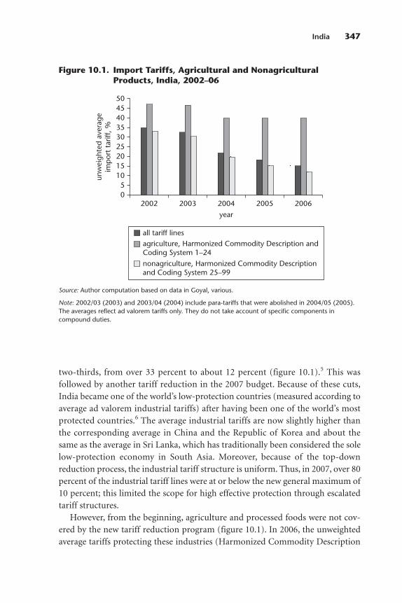
two-thirds, from over 33 percent to about 12 percent (figure 10.1).5 This was followed by another tariff reduction in the 2007 budget. Because of these cuts,India became one of the world’s low-protection countries (measured according toaverage ad valorem industrial tariffs) after having been one of the world’s mostprotected countries.6 The average industrial tariffs are now slightly higher thanthe corresponding average in China and the Republic of Korea and about thesame as the average in Sri Lanka, which has traditionally been considered the solelow-protection economy in South Asia. Moreover, because of the top-downreduction process, the industrial tariff structure is uniform. Thus, in 2007, over 80percent of the industrial tariff lines were at or below the new general maximum of10 percent; this limited the scope for high effective protection through escalatedtariff structures.
However, from the beginning, agriculture and processed foods were not cov-ered by the new tariff reduction program (figure 10.1). In 2006, the unweightedaverage tariffs protecting these industries (Harmonized Commodity Description
India 347
05
1015
30
20
40
50
year
unw
eigh
ted
aver
age
imp
ort
tarif
f, % 35
25
45
200620042002 2003 2005
agriculture, Harmonized Commodity Description andCoding System 1–24nonagriculture, Harmonized Commodity Descriptionand Coding System 25–99
all tariff lines
Figure 10.1. Import Tariffs, Agricultural and NonagriculturalProducts, India, 2002–06
Source: Author computation based on data in Goyal, various.
Note: 2002/03 (2003) and 2003/04 (2004) include para-tariffs that were abolished in 2004/05 (2005).The averages reflect ad valorem tariffs only. They do not take account of specific components incompound duties.

and Coding System, 1–24) were about 40 percent, almost four times the averageindustrial tariffs and among the highest in the world. Moreover, these tariffs arehighly dispersed; about 15 percent of the tariffs are in the 50–100 percent range.These high tariffs have been maintained despite substantial tariff redundancyamong most agricultural commodities (see elsewhere below). The domestic pricesfor many commodities are not only lower than duty-inclusive import prices, butare also frequently lower than duty-exclusive import prices. This special treatmentprovided through agricultural trade policies reflects the pressure exerted by manyfarmer and processor interest groups and mediated through and supported by theMinistry of Agriculture.
Regional trade agreements
As a by-product of the country’s highly protective agricultural trade policies, thetrade in primary and processed agricultural and livestock products between Indiaand its South Asian neighbors has been seriously hindered.7 Ironically, the mainvictim has likely been Indian exports to these countries rather than Indianimports from the region. Indian domestic prices are low, and, even under a freetrade regime, the products of neighboring countries would face difficulties com-peting there. Meanwhile, India’s high tariffs and other barriers to imports havereinforced and helped justify domestically the reluctance of other South Asiancountries to reduce their own barriers to agricultural trade either multilaterally oras part of regional and bilateral preferential trade arrangements.
Thus, for many years, the South Asian Preferential Trade Agreement had onlylimited relevance in regional agricultural trade because all agricultural imports toIndia were subject to that country’s discretionary import licensing system. Importlicensing was lifted among members of the South Asian Preferential Trade Agree-ment in 1998, three years before it was finally phased out by this group withrespect to the rest of the world. Nonetheless, since then, the combination of highredundant tariffs, low domestic prices for most agricultural products, and thecontinuing role of state trading enterprises has meant that it is impossible forthese countries to compete in the majority of India’s domestic markets. Exceptfor Bhutan and Nepal, the government of India has provided few tariff prefer-ences for agricultural products under its bilateral trade agreements, notably, in itsbilateral free trade agreement with the government of Sri Lanka. Under the SouthAsia Free Trade Agreement, most agricultural tariff lines, including the lines forprocessed foods, are on the government of India’s sensitive list of the products forwhich it has made no commitments.
The reluctance of the government to provide tariff preferences partly reflects adesire to prevent imports from third countries through preference-receiving
348 Distortions to Agricultural Incentives in Asia
countries. Reciprocally, Bangladesh, Pakistan, and Sri Lanka have been unwillingto provide tariff preferences for agricultural products under the South Asian Pref-erential Trade Agreement and have also placed most agricultural products thatthey produce on their own South Asia Free Trade Agreement sensitive productslists. This is largely a reaction to the Indian position because, even though theseagreements, in principle, involve a number of countries, the potential regionaltrade that really matters is, in practice, the bilateral trade with India. However, inBangladesh and Sri Lanka, the reciprocity also reflects a realistic assessment thatagricultural free trade with India would generate more agricultural imports fromIndia than exports to India, in the process threatening the viability of some of themore highly protected agricultural industries of these countries, such as sugar,various fresh fruits, vegetables, and a wide range of processed foods inBangladesh, and, in Sri Lanka, rice, potatoes, and onions.8
If it were opened up, India-Pakistan bilateral agricultural trade would probablybe more balanced. Recent studies suggest that there is considerable potential forwelfare-improving bilateral trade in wheat and sugar. The direction and timing ofthis trade would vary with weather and other seasonal factors and, compared totrade through the ports with countries outside the South Asia region, would benefit from large transport cost savings, especially trade between the Indiannorthwest states and Pakistan Punjab. It is also likely that the poultry and otherlivestock products of Pakistan could be profitably exported to India. However,bilateral trade between India and Pakistan is hostage to the difficult political relationship of the two countries, which is reflected in Pakistan’s positive list ofproducts that may be legally imported from India. This list includes almost noagricultural products. Moreover, rules enforced in both countries (with a fewminor exceptions) do not allow trade over the land border.
The exchange rate regime and trade policies
Trade policies must be understood in the context of exchange rate policies.9 Therupee was pegged to the pound sterling before independence in 1947, and thiscontinued until September 1975. In June 1966, the fixed rupee-pound rate wasdevalued by 57.5 percent and by the same proportion to the U.S. dollar, to Rs 7.50.In line with the fixed link with the pound, the rupee-dollar rate floated downslightly between 1966 and 1975. In September 1975, the peg to the pound sterlingwas removed, and, until 1992, the rate was fixed by the Reserve Bank of India. In1992, this system was replaced by a managed floating rate, whereby the ReserveBank of India allowed the rupee to move in relation to a basket of currencies.
A prolonged period of nominal devaluation began in 1982. The devaluation ratewas rapid at first. It slowed for three years in the mid-1980s and then accelerated
India 349
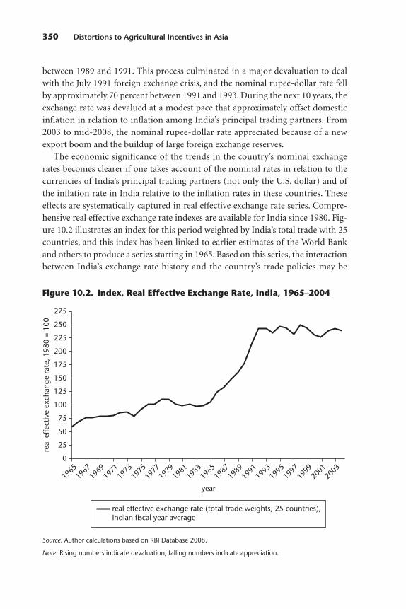
between 1989 and 1991. This process culminated in a major devaluation to dealwith the July 1991 foreign exchange crisis, and the nominal rupee-dollar rate fellby approximately 70 percent between 1991 and 1993. During the next 10 years, theexchange rate was devalued at a modest pace that approximately offset domesticinflation in relation to inflation among India’s principal trading partners. From2003 to mid-2008, the nominal rupee-dollar rate appreciated because of a newexport boom and the buildup of large foreign exchange reserves.
The economic significance of the trends in the country’s nominal exchangerates becomes clearer if one takes account of the nominal rates in relation to thecurrencies of India’s principal trading partners (not only the U.S. dollar) and ofthe inflation rate in India relative to the inflation rates in these countries. Theseeffects are systematically captured in real effective exchange rate series. Compre-hensive real effective exchange rate indexes are available for India since 1980. Fig-ure 10.2 illustrates an index for this period weighted by India’s total trade with 25countries, and this index has been linked to earlier estimates of the World Bankand others to produce a series starting in 1965. Based on this series, the interactionbetween India’s exchange rate history and the country’s trade policies may be
350 Distortions to Agricultural Incentives in Asiare
al e
ffect
ive
exch
ange
rate
, 198
0 =
100
0
25
50
75
100
125
150
175
200
225
250
275
1965
1967
1969
1971
1973
1975
1977
1979
1981
1983
1985
1987
1989
1991
1993
1995
1997
1999
2001
2003
year
real effective exchange rate (total trade weights, 25 countries),Indian fiscal year average
Figure 10.2. Index, Real Effective Exchange Rate, India, 1965–2004
Source: Author calculations based on RBI Database 2008.
Note: Rising numbers indicate devaluation; falling numbers indicate appreciation.
divided into four periods. Details of the changes in the exchange rate and therelated changes in sectoral trade policies during these periods are provided belowfollowing our discussion of the period from independence to the mid-1960s.
From 1947 to the 1966 devaluation
By 1956, inflation had begun to erode the effects of the devaluation in 1949. Theinflation accelerated during the 10 years to the mid-1960s. In effect, this amountedto a substantial real appreciation of the rupee in relation to the rates fixed to thepound sterling and the U.S. dollar. For most of the period from independence tothe mid-1960s, agricultural trade policies were characterized by stringent exportcontrols, and, when exports were allowed, by high export taxes that affected, forexample, jute and jute products, oil cakes, cotton, tea, and black pepper. Despitethese restrictions and taxes, agricultural and mineral products (the latter also subject to export taxes) accounted for about half the foreign exchange earningsfrom exports, and, because foreign exchange was becoming increasingly scarceafter 1956, the export taxes were steadily reduced and almost eliminated prior tothe 1966 devaluation. On the import side, agricultural imports by the private sectorwere effectively banned, and substantial cereal imports, mostly of wheat under theU.S. Public Law 480 food aid program, were managed by the government.
Before and immediately after independence, nearly all imports in manufactur-ing were subject to discretionary import licensing or were canalized through government monopoly trading organizations. After 1956, import licensing wasregularly tightened in response to the steadily worsening foreign exchange situa-tion. Meanwhile, tariffs were increased and had reached high levels by early 1966.These steps caused large, highly variable gaps to appear between the domestic andinternational prices of manufactured products. The other principal reaction tothe increasingly overvalued exchange rate was the government’s attempt to offsetthe resulting antiexport bias by providing substantial subsidies for manufacturedexports, mainly by allowing exporters to import otherwise restricted raw materi-als, components, and machines free of duties; the exporters then could sell in thedomestic market for premiums that reflected scarcity values.
No studies have tried to measure the effects of these policies on the relativeincentives in agriculture and manufacturing during these years. However, it isclear from the literature of the period that the economic policy thrust favoredmanufacturing. The period was therefore likely characterized by a marked anti -agricultural bias. This probably expanded along with the increasing overvaluationof the exchange rate and the countermeasures that concentrated on providinghigher incentives to manufacturers in the domestic market and in exports, whileattempting to keep agricultural prices low and stable.
India 351
From the 1966 devaluation to 1978
The nominal devaluation in June 1966 was 57.5 percent in relation to the poundsterling and the U.S. dollar, but, owing to high domestic inflation, it has been estimated at about 30 percent in real terms. In subsequent years, inflation wasgradually brought down to much lower levels, and, by 1980, the real effectiveexchange rate had declined by another 46 percent (figure 10.2). The 1966 devalu-ation helped clean up some crisis-induced trade policies, but such policies wereotherwise highly restrictive and interventionist.
In agriculture, one of the outcomes of the devaluation and, more importantly,of the suspension of U.S. Public Law 480 grain supplies from the United Statesduring the first India-Pakistan war was to reinforce the government’s determina-tion to make India self-sufficient in food grains and other basic agricultural prod-ucts. This coincided with the development and distribution of new seeds andtechniques that were instrumental in practically eliminating once substantialcereal imports by the end of 1970s and that were behind the program launched in1971 to make India self-sufficient in dairy products. To support these objectives,earlier policies were continued. With few exceptions, these allowed imports onlyof bulk agricultural commodity products, such as wheat, that were brought intothe country by parastatals according to need. In the interests of domestic avail-ability and low consumer prices, exports of most food products were not allowedalthough the domestic prices for some food products, notably rice, were usuallywell below farm-level export parity prices. Immediately after the devaluation,export taxes on nonessential exported commodities (jute, coffee, tea, cotton, oilcakes, spices) were sharply increased; the apparent purpose was to absorb some ofthe windfall gains accruing to exporters. However, because of slow export growthduring the 1970s, these taxes were steadily reduced and had practically disap-peared by the early 1980s.
In manufacturing, the 1966 devaluation was accompanied by tariff reductions,a relaxation in import licensing, and the abolition or reduction of some exportsubsidies. However, by 1968, tight import licensing had been reinstated, andimports of nearly all consumer goods, including textiles, were effectively banned;the only imports allowed were intermediate materials, components, and capitalequipment as long as the actual users could demonstrate that the goods wereessential and not otherwise locally available. Tariffs, which remained at about thesame level during the 1970s, were still being used mostly to transfer some importlicensing rents to the government and were irrelevant as protective instrumentsexcept to the extent they influenced the cost of imported intermediates and equip-ment that was not locally produced.
Empirical evidence suggests that trade policies during this period led to terms oftrade that were more highly unfavorable for agriculture relative to manufacturing
352 Distortions to Agricultural Incentives in Asia
in the domestic economy than the terms of trade prevailing in world markets (seeelsewhere below).
From 1978 to 1993
The government averted a balance of payments crisis in 1980–81 with the help ofa loan from the International Monetary Fund, while maintaining the real value ofthe rupee. However, beginning in the spring of 1985, a new policy was imple-mented that led to the steady devaluation of the currency in real terms. Thisdevaluation continued without a break for the next six years, almost on a monthlybasis, until the sharp devaluation in July 1991, which was followed by additionaldepreciation until September 1992. The real rupee devaluation was large duringthe second half of the 1980s, about 62 percent between 1985 and 1990, and it wasaround 145 percent over the whole period to 1993. Among other effects, this rad-ically changed the environment of agricultural and manufacturing trade policies.
In agriculture, the rupee depreciation after 1985 partly offset a major decline inworld agricultural prices that had started in 1981 and continued until 1987. Worldprices recovered thereafter, and the continuing rupee depreciation translated theseworld price changes into much larger increases in the border prices for some of thecountry’s major agricultural commodities. However, owing to the traditional isola-tion of the domestic market, the domestic prices for most of these commoditieswere unaffected and continued to shift independently of the changes in the borderprices. The principal exceptions were cotton, pulses, oil cakes, and the main export-oriented agricultural commodities that are sold in auction markets in whichexporters and domestic traders compete, especially tea, coffee, spices, and tobacco.Despite many complex trade policy interventions and other interventions andowing to the influence of textile producers who were acting with the support of theMinistry of Textiles, domestic cotton prices broadly tracked border prices, andpulses were (and still are) the sole major primary food product that could beimported at low or moderate tariffs without import licensing or other interven-tions. The country has consistently possessed excess supplies of oil cakes (producedin fixed proportions by the edible oil industry in conjunction with the oilseedcrushing process) because of low demand by the livestock subsector that is, in turn,associated with the vegetarian diets of a large proportion of the country’s popula-tion. However, these products account for only a small share of total agriculturalproduction, around 14 percent, and about 10 percent of total rural production iflivestock, fishing, and forestry products are included. During this period, the rest(about 90 percent of total rural production) was essentially nontraded owing togovernment import monopolies, import licensing, export controls, and other non-tariff interventions, as well as prohibitive tariffs in some cases.
India 353
In manufacturing, during the 1980s, domestic prices were similarly delinkedfrom international prices by the import licensing system and high tariffs that aver-aged over 100 percent. In addition, manufactured exports, although they weregrowing more rapidly than domestic production, were limited relative to totalmanufacturing output; the export share was only about 7 percent in the mid-1980s. Hence, overall, the massive rupee devaluation did not pass through directlyto domestic industrial prices. It affected them indirectly in a minor way throughincreases in export prices and in the prices of intermediate and capital goods thatwere allowed to be imported, which increased manufacturing costs. The devalua-tion generated big increases in border prices, which led to a steep decline in aver-age implicit manufacturing protection as measured by the excess in domesticex-factory prices relative to border prices. This had important repercussions inmanufacturing trade policies. First, it made the liberalization program that wasundertaken in 1991 quite painless, including, especially, the abolition of nearly allimport licensing for manufactured intermediate goods, machinery, and equip-ment, the removal of a major export subsidy, and the tariff reduction programthat continued into the mid-1990s.
Second, many manufacturing firms that had been vulnerable to import com-petition found that, now, following the correction of the exchange rate overvalua-tion, they could not only easily compete with imports, but could outcompete withforeign manufacturers in export markets. Combined with the new, sweepingdomestic deregulation of manufacturing that accompanied the trade policy pro-gram, this created fresh momentum in investment, productivity improvements,and output expansion in the manufacturing sector.
The devaluation’s repercussions in agriculture and manufacturing led to the endof most of the systematic antiagricultural bias in the incentive system as measuredby relative rates of assistance (RRAs). However, it did not translate into a noticeableimprovement in the domestic terms of trade in agriculture because nearly all agri-cultural prices and a large proportion of manufacturing prices, including prices onall consumer goods, remained delinked from world prices by the import licensingsystem and other nontariff barriers and were still mainly determined by domesticconditions and government policies. This situation did not begin to change untilafter the import licensing system was finally removed in 2001.
From 1993 to 2007
From 1993 until mid-2007, the exchange rate was managed by regular adjust-ments in the nominal rates that stabilized the real effective exchange rate index atthe postdevaluation level within a narrow range of about 10 percent (figure 10.2).The size of the devaluation up to 1993 probably overshot the decline needed to
354 Distortions to Agricultural Incentives in Asia
reestablish the balance in foreign exchange and support the 1991 trade policyreforms. However, by being maintained at this level for the next 14 years (by farthe longest period of real exchange rate stability in the independent economic his-tory of India), it also proved adequate in supporting the removal of the importlicensing system between 1998 and 2001 and the post-2003 tariff reduction pro-gram in manufacturing.
In agriculture, however, highly protectionist trade policies continued through-out the 1990s and were still in place in mid-2007. On the import side, high to pro-hibitive tariffs, plus technical standards and sanitary and phytosanitary controls,played the role previously played by import licensing and import monopoliesamong state trading enterprises.10 With some exceptions, the predominant view isthat international agricultural markets are unreliable and unstable and shouldonly have a residual role in agricultural policies, in particular, by providing extrasupplies in times of domestic shortages and as a means of disposing of excessstocks in times of domestic surpluses. Consistent with this view, agricultural tradepolicies on some major commodities, especially cereals and sugar, are highlyopportunistic and involve frequent and significant changes, especially in tariffsand export subsidies.11 For other products, tariffs appear to be deliberately pro-hibitive. For example, 100 percent tariffs apply to tea and coffee, both of which areexported on a large scale. The domestic prices for these two products are set inauction markets in which exporters and domestic traders operate, suggesting thatthe domestic prices are about equivalent to international prices after allowing forquality differences.
In manufacturing, after the 1991 reforms, producers of intermediate and capi-tal goods were no longer protected by import licensing, and manufacturing tariffsdeclined. Nonetheless, the devalued exchange rate, plus manufacturing tariffs(mostly in the 30–40 percent range) and other measures (notably antidumpinginitiatives), removed most competitive pressures on the import side. In addition,manufactured consumer goods, including the entire textile and garment subsec-tor, were still protected by import licensing until the gradual removal of the sys-tem was initiated in the late 1990s. Hence, during the 1990s and up to about 2004,most manufacturing remained insulated from import competition, and theimpact of world market conditions occurred mainly through manufacturedexports, which, however, began to expand at a rate that was more rapid than theoverall growth rate in manufacturing. This partial orientation toward world mar-kets only changed in about 2004 following the end of import licensing in 2001 andthe implementation of the first stages of the post-2003 manufacturing tariffreduction program. Since then, most of the manufacturing sector has beenopened to world markets either through exports or through actual or potentialimports at relatively low tariffs.
India 355
The 1985–93 devaluations removed most of the long-standing antiagriculturalbias in the incentive system as measured by RRAs. However, high formal protec-tion rates and substantial tariff redundancy in manufacturing and agricultureallowed plenty of scope for the domestic terms of trade between the two sectors toshift substantially in either direction. However, all this changed in the mid-2000s.Since then, tariffs have been a real constraint on the domestic prices for manufac-tured goods. The ongoing high formal protection of agriculture, combined withsubstantial input subsidies, has nonetheless offered considerable scope for the biasof the system against agriculture to become a bias in favor of agriculture.
The Measurement of Distortionsin Agricultural Incentives
The main focus of our study is the extent of the distortions in agricultural pricesand the government-imposed policy measures that create a gap between actualdomestic prices and prices as they would emerge under free market conditions.12
Since it is not possible to understand the characteristics of agricultural develop-ment through a sectoral view alone, we provide estimates of the effects of directagricultural policy measures, including distortions in the foreign exchange mar-ket, and we also report estimates of distortions in the prices faced by the produc-ers of nonagricultural products, especially manufactures. Specifically, we com-pute NRAs for farmers that include an adjustment for direct interventionsdirected at inputs, such as subsidies for fertilizers and electricity. For comparativepurposes, we also generate aggregate NRAs for nonagricultural tradables and foragricultural tradables so as to calculate RRAs (see Anderson et al. 2008 andappendix A).
We examine 12 products, plus the collective of fruits and vegetables. Milk isclassified as an import-competing product. The other 11 commodities—rice,wheat, maize, sorghum, groundnuts, rapeseeds, soybeans, sunflower seeds, sugar,cotton, and chickpeas—have mixed trade status, which means they are exporta-bles or nontradables in some years and import-competing products in otheryears.13 Over the period we analyze, these primary agricultural commoditiesaccount altogether for nearly 70 percent of the value of agricultural production inIndia. The 11 crops have made up approximately half this share in recent years;fruits and vegetables, one-quarter; and dairying, another one-quarter (table 10.3).
Our study builds on a considerable body of earlier work, and we use the projectmethodology to provide a consistent and internationally comparable set of esti-mates back to 1964 (or, in the case of milk, 1975). The earlier work includes pro-ducer support estimates for the major crops in India in 1984–2001 that have beenmade available by the International Food Policy Research Institute, estimates for
356 Distortions to Agricultural Incentives in Asia
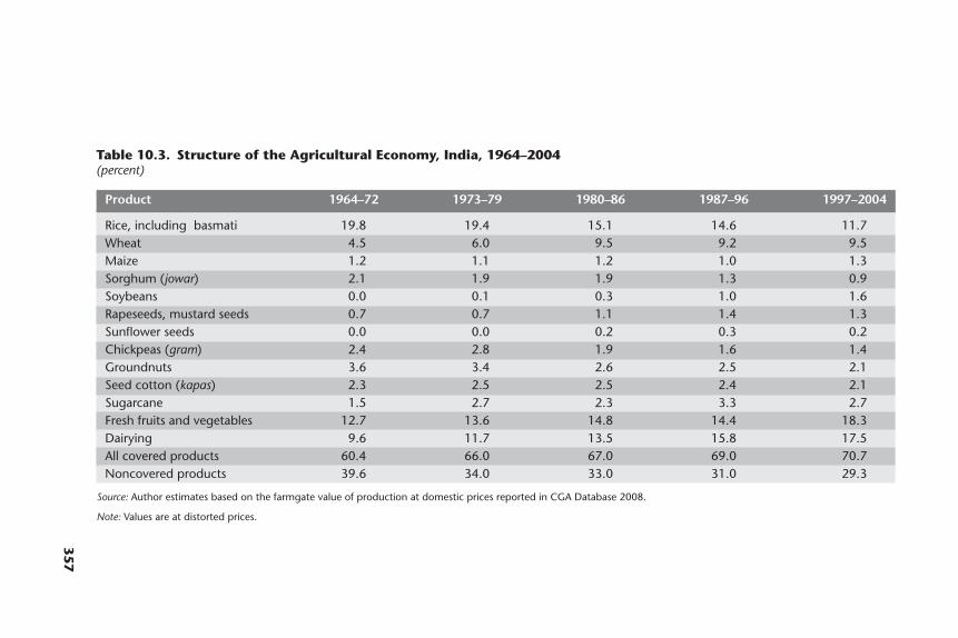
357
Table 10.3. Structure of the Agricultural Economy, India, 1964–2004(percent)
Product 1964–72 1973–79 1980–86 1987–96 1997–2004
Rice, including basmati 19.8 19.4 15.1 14.6 11.7Wheat 4.5 6.0 9.5 9.2 9.5Maize 1.2 1.1 1.2 1.0 1.3Sorghum (jowar) 2.1 1.9 1.9 1.3 0.9Soybeans 0.0 0.1 0.3 1.0 1.6Rapeseeds, mustard seeds 0.7 0.7 1.1 1.4 1.3Sunflower seeds 0.0 0.0 0.2 0.3 0.2Chickpeas (gram) 2.4 2.8 1.9 1.6 1.4Groundnuts 3.6 3.4 2.6 2.5 2.1Seed cotton (kapas) 2.3 2.5 2.5 2.4 2.1Sugarcane 1.5 2.7 2.3 3.3 2.7Fresh fruits and vegetables 12.7 13.6 14.8 14.4 18.3Dairying 9.6 11.7 13.5 15.8 17.5All covered products 60.4 66.0 67.0 69.0 70.7Noncovered products 39.6 34.0 33.0 31.0 29.3
Source: Author estimates based on the farmgate value of production at domestic prices reported in CGA Database 2008.
Note: Values are at distorted prices.
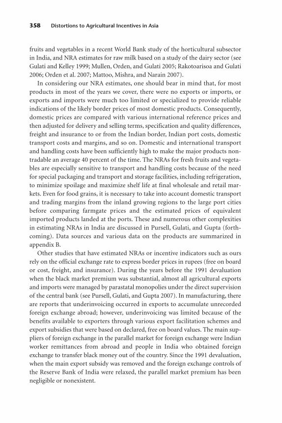
fruits and vegetables in a recent World Bank study of the horticultural subsectorin India, and NRA estimates for raw milk based on a study of the dairy sector (seeGulati and Kelley 1999; Mullen, Orden, and Gulati 2005; Rakotoarisoa and Gulati2006; Orden et al. 2007; Mattoo, Mishra, and Narain 2007).
In considering our NRA estimates, one should bear in mind that, for mostproducts in most of the years we cover, there were no exports or imports, orexports and imports were much too limited or specialized to provide reliableindications of the likely border prices of most domestic products. Consequently,domestic prices are compared with various international reference prices andthen adjusted for delivery and selling terms, specification and quality differences,freight and insurance to or from the Indian border, Indian port costs, domestictransport costs and margins, and so on. Domestic and international transportand handling costs have been sufficiently high to make the major products non-tradable an average 40 percent of the time. The NRAs for fresh fruits and vegeta-bles are especially sensitive to transport and handling costs because of the needfor special packaging and transport and storage facilities, including refrigeration,to minimize spoilage and maximize shelf life at final wholesale and retail mar-kets. Even for food grains, it is necessary to take into account domestic transportand trading margins from the inland growing regions to the large port citiesbefore comparing farmgate prices and the estimated prices of equivalentimported products landed at the ports. These and numerous other complexitiesin estimating NRAs in India are discussed in Pursell, Gulati, and Gupta (forth-coming). Data sources and various data on the products are summarized inappendix B.
Other studies that have estimated NRAs or incentive indicators such as oursrely on the official exchange rate to express border prices in rupees (free on boardor cost, freight, and insurance). During the years before the 1991 devaluationwhen the black market premium was substantial, almost all agricultural exportsand imports were managed by parastatal monopolies under the direct supervisionof the central bank (see Pursell, Gulati, and Gupta 2007). In manufacturing, thereare reports that underinvoicing occurred in exports to accumulate unrecordedforeign exchange abroad; however, underinvoicing was limited because of thebenefits available to exporters through various export facilitation schemes andexport subsidies that were based on declared, free on board values. The main sup-pliers of foreign exchange in the parallel market for foreign exchange were Indianworker remittances from abroad and people in India who obtained foreignexchange to transfer black money out of the country. Since the 1991 devaluation,when the main export subsidy was removed and the foreign exchange controls ofthe Reserve Bank of India were relaxed, the parallel market premium has beennegligible or nonexistent.
358 Distortions to Agricultural Incentives in Asia
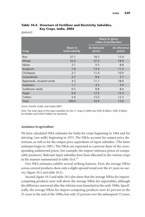
Assistance in agriculture
We have calculated NRA estimates for India for crops beginning in 1964 and fordairying (raw milk) beginning in 1975. The NRAs account for output price dis-tortions, as well as for the output price equivalents of input subsidies. (The latterestimates begin in 1983.) The NRAs are expressed as a percent share of the corre-sponding undistorted prices (for example, the import reference prices of compa-rable products). Relevant input subsidies have been allocated to the various cropsin the manner summarized in table 10.4.14
Our NRA estimates exhibit several striking features. First, the average NRAsacross covered products show only a slight upward trend over the 41 years we sur-vey (figure 10.3 and table 10.5).
Second, figure 10.3 and table 10.5 also show that the average NRAs for import-competing products were well above the average NRAs for exportables, althoughthe difference narrowed after the reforms were launched in the early 1990s. Specif-ically, the average NRAs for import-competing products were 62 percent in the25 years to the end of the 1980s, but only 32 percent over the subsequent 15 years,
India 359
Table 10.4. Structure of Fertilizer and Electricity Subsidies,Key Crops, India, 2004
(percent)
Share in grossvalue of production
Share in At domestic At referenceCrop total subsidy prices prices
Rice 37.1 18.3 15.4Wheat 35.2 27.2 18.9Maize 2.1 9.3 8.8Sorghum 1.8 12.4 11.5Chickpeas 2.7 11.4 10.9Groundnuts 2.7 8.4 5.7Rapeseeds, mustard seeds 4.5 11.7 18.0Soybeans 1.1 4.3 2.9Sunflower seeds 0.5 8.8 8.6Sugar 6.6 12.5 15.4Cotton 5.6 13.2 12.3Total 100.0 16.9 13.0
Source: Pursell, Gulati, and Gupta 2007.
Note: The total value of the input subsidies for the 11 crops in 2004 was US$7.8 billion: US$1.9 billionfor fertilizer and US$5.9 billion for electricity.

while the corresponding NRAs for exportables were �25 and �11 percent,respectively. This is captured in the average trade bias index, which was �0.53during the period before 1990 and �0.32 thereafter (table 10.6).
Third, the NRAs fluctuate widely around the trend values. Even if the NRAs areaveraged over all import-competing products or all exportables, it is clear fromfigure 10.3 that there is significant movement in the NRAs from year to year. Thisis partly because the trade status of products often changed, but there is also aclear systematic element in this finding. Before the reforms of the 1990s, the average NRAs for import-competing products and exportables were lowest in1974, when international food prices were at record highs, and highest around1987, when international food prices were at record lows in real terms. More generally, there is little year-to-year correlation between the domestic prices andthe border prices of major food products. This reflects the success of the govern-ment’s policy effort to stabilize domestic prices and insulate domestic marketsfrom fluctuations in world prices.
360 Distortions to Agricultural Incentives in AsiaN
RA, %
�70
�35
0
35
70
105
140
1965
1967
1969
1971
1973
1975
1977
1979
1981
1983
1985
1987
1989
1991
1993
1995
1997
1999
2001
2003
year
import-competing products total exportables
Figure 10.3. NRAs for Exportable, Import-Competing, and AllAgricultural Products, India, 1965–2004
Source: Pursell, Gulati, and Gupta 2007.
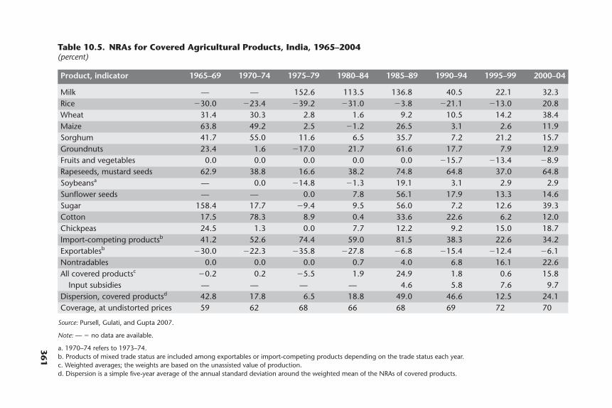
361
Table 10.5. NRAs for Covered Agricultural Products, India, 1965–2004(percent)
Product, indicator 1965–69 1970–74 1975–79 1980–84 1985–89 1990–94 1995–99 2000–04
Milk — — 152.6 113.5 136.8 40.5 22.1 32.3Rice �30.0 �23.4 �39.2 �31.0 �3.8 �21.1 �13.0 20.8Wheat 31.4 30.3 2.8 1.6 9.2 10.5 14.2 38.4Maize 63.8 49.2 2.5 �1.2 26.5 3.1 2.6 11.9Sorghum 41.7 55.0 11.6 6.5 35.7 7.2 21.2 15.7Groundnuts 23.4 1.6 �17.0 21.7 61.6 17.7 7.9 12.9Fruits and vegetables 0.0 0.0 0.0 0.0 0.0 �15.7 �13.4 �8.9Rapeseeds, mustard seeds 62.9 38.8 16.6 38.2 74.8 64.8 37.0 64.8Soybeansa — 0.0 �14.8 �1.3 19.1 3.1 2.9 2.9Sunflower seeds — — 0.0 7.8 56.1 17.9 13.3 14.6Sugar 158.4 17.7 �9.4 9.5 56.0 7.2 12.6 39.3Cotton 17.5 78.3 8.9 0.4 33.6 22.6 6.2 12.0Chickpeas 24.5 1.3 0.0 7.7 12.2 9.2 15.0 18.7Import-competing productsb 41.2 52.6 74.4 59.0 81.5 38.3 22.6 34.2Exportablesb �30.0 �22.3 �35.8 �27.8 �6.8 �15.4 �12.4 �6.1Nontradables 0.0 0.0 0.0 0.7 4.0 6.8 16.1 22.6All covered productsc �0.2 0.2 �5.5 1.9 24.9 1.8 0.6 15.8
Input subsidies — — — — 4.6 5.8 7.6 9.7Dispersion, covered productsd 42.8 17.8 6.5 18.8 49.0 46.6 12.5 24.1Coverage, at undistorted prices 59 62 68 66 68 69 72 70
Source: Pursell, Gulati, and Gupta 2007.
Note: — � no data are available.
a. 1970–74 refers to 1973–74.b. Products of mixed trade status are included among exportables or import-competing products depending on the trade status each year.c. Weighted averages; the weights are based on the unassisted value of production.d. Dispersion is a simple five-year average of the annual standard deviation around the weighted mean of the NRAs of covered products.
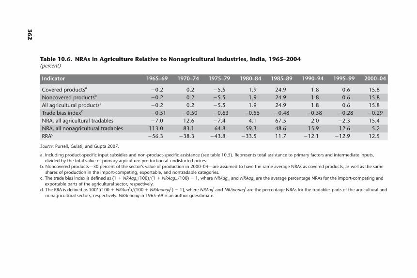
362
Table 10.6. NRAs in Agriculture Relative to Nonagricultural Industries, India, 1965–2004(percent)
Indicator 1965–69 1970–74 1975–79 1980–84 1985–89 1990–94 1995–99 2000–04
Covered productsa �0.2 0.2 �5.5 1.9 24.9 1.8 0.6 15.8Noncovered productsb �0.2 0.2 �5.5 1.9 24.9 1.8 0.6 15.8All agricultural productsa �0.2 0.2 �5.5 1.9 24.9 1.8 0.6 15.8Trade bias indexc �0.51 �0.50 �0.63 �0.55 �0.48 �0.38 �0.28 �0.29NRA, all agricultural tradables �7.0 12.6 �7.4 4.1 67.5 2.0 �2.3 15.4NRA, all nonagricultural tradables 113.0 83.1 64.8 59.3 48.6 15.9 12.6 5.2RRAd �56.3 �38.3 �43.8 �33.5 11.7 �12.1 �12.9 12.5
Source: Pursell, Gulati, and Gupta 2007.
a. Including product-specific input subsidies and non-product-specific assistance (see table 10.5). Represents total assistance to primary factors and intermediate inputs,divided by the total value of primary agriculture production at undistorted prices.
b. Noncovered products—30 percent of the sector’s value of production in 2000–04—are assumed to have the same average NRAs as covered products, as well as the sameshares of production in the import-competing, exportable, and nontradable categories.
c. The trade bias index is defined as (1 � NRAagx�100)�(1 � NRAagm�100) � 1, where NRAagm and NRAagx are the average percentage NRAs for the import-competing andexportable parts of the agricultural sector, respectively.
d. The RRA is defined as 100*[(100 � NRAagt)�(100 � NRAnonagt) � 1], where NRAagt and NRAnonagt are the percentage NRAs for the tradables parts of the agricultural andnonagricultural sectors, respectively. NRAnonag in 1965–69 is an author guesstimate.
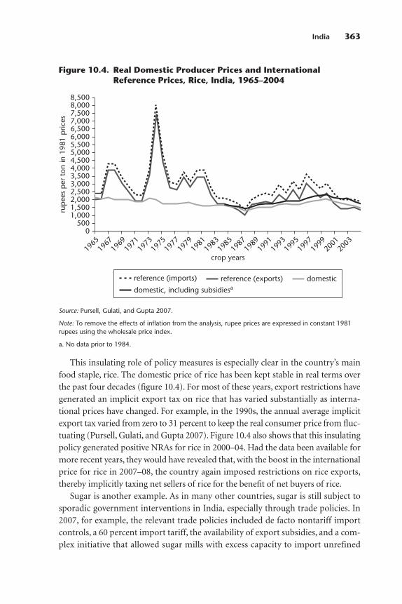
This insulating role of policy measures is especially clear in the country’s mainfood staple, rice. The domestic price of rice has been kept stable in real terms overthe past four decades (figure 10.4). For most of these years, export restrictions havegenerated an implicit export tax on rice that has varied substantially as interna-tional prices have changed. For example, in the 1990s, the annual average implicitexport tax varied from zero to 31 percent to keep the real consumer price from fluc-tuating (Pursell, Gulati, and Gupta 2007). Figure 10.4 also shows that this insulatingpolicy generated positive NRAs for rice in 2000–04. Had the data been available formore recent years, they would have revealed that, with the boost in the internationalprice for rice in 2007–08, the country again imposed restrictions on rice exports,thereby implicitly taxing net sellers of rice for the benefit of net buyers of rice.
Sugar is another example. As in many other countries, sugar is still subject tosporadic government interventions in India, especially through trade policies. In2007, for example, the relevant trade policies included de facto nontariff importcontrols, a 60 percent import tariff, the availability of export subsidies, and a com-plex initiative that allowed sugar mills with excess capacity to import unrefined
India 363
0
1,000
rup
ees
per
ton
in 1
981
pric
es
crop years
7,500
5,000
2,000
3,000
4,000
500
1,500
8,0008,500
6,0006,5007,000
5,500
2,500
3,500
4,500
2003
2001
1999
1997
1995
1993
1991
1989
1987
1985
1983
1981
1979
1977
1975
1973
1971
1969
1967
1965
domestic, including subsidiesa
domesticreference (exports)reference (imports)
Figure 10.4. Real Domestic Producer Prices and InternationalReference Prices, Rice, India, 1965–2004
Source: Pursell, Gulati, and Gupta 2007.
Note: To remove the effects of inflation from the analysis, rupee prices are expressed in constant 1981rupees using the wholesale price index.
a. No data prior to 1984.

sugar duty-free for refining and then resell in the domestic market. These measures were implemented to insulate the domestic market from wide swings ininternational sugar prices, but also to help address domestic disequilbriumsresulting from weather conditions and from production cycles imposed by thehighly politicized minimum sugarcane prices mandated by state governments.Likewise, in 2000–02, export subsidies were used to help dispose of large excesssugar stocks, whereas, in some years during the 1990s, imports were allowed duty-free to meet temporary domestic shortages.15 Similar to the case of rice, domesticsugar prices have been kept quite stable for long periods, but have steadilydeclined in real terms over time. Thus, between 1965 and 1982, they declined byabout one-third, and, between 1981 and 2004, by one-quarter.
Fourth, the dispersion of NRAs across the products we cover has been wide,although it has narrowed considerably since the reforms began in the early 1990s.Shortly before then, the average annual standard deviation around the weightedmean NRA was 45, whereas, since 1990, the average has been less than half that(see near the bottom of table 10.5).
Fifth, the contribution of farm input subsidies in the NRAs for covered prod-ucts have been steadily increasing, particularly fertilizers and electricity, which isused mainly in pumping irrigation water. In the later 1980s, input subsidies con-tributed 4 percentage points to the average NRA of 25 percent (data have not beencompiled for earlier years), but, by 2000–05, they were contributing almost10 percentage points (see near the bottom of table 10.5).16 Without input subsi-dies, the average NRA would have been negative in the 1990s, mainly because ofthe restrictions on exports of rice. (The weight of rice has been between aroundone-eighth and one-third over the past four decades; see Pursell, Gulati, andGupta 2007.) Input subsidies helped reduce the gap between the benefits to riceproducers and the export price of rice in the 1990s (figure 10.4).
Sixth, while the trade status of each crop product we cover has tended tochange frequently over the past four decades, self-sufficiency in each productnonetheless remains close to 100 percent (table 10.7). Thus, in so far as govern-ment policies on food pricing and trade have been aimed at reducing the coun-try’s dependence on food imports, they have achieved their objective.
Assistance to producers of agricultural tradables relativeto other tradables
In the absence of precise information, we have assumed that the average NRAs forcovered products are the same as the corresponding NRAs for noncovered farmproducts, which accounted for 30 percent of total agricultural production in2000–04. The incentives among farmers depend not only on agricultural NRAs,
364 Distortions to Agricultural Incentives in Asia
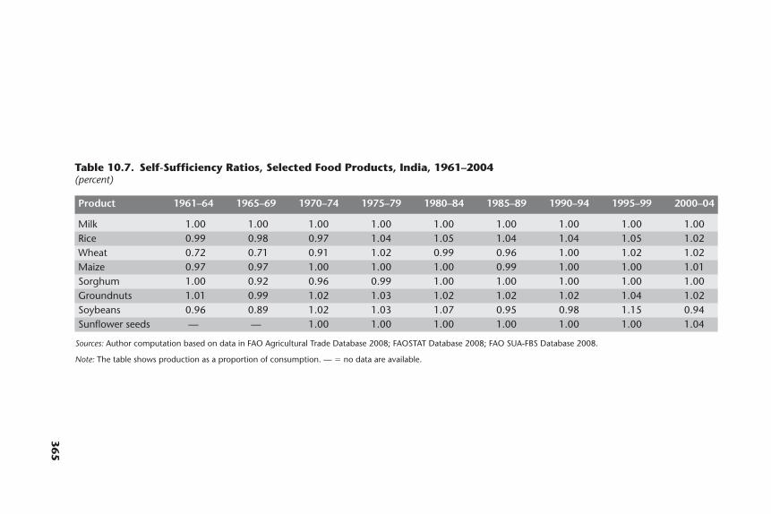
365
Table 10.7. Self-Sufficiency Ratios, Selected Food Products, India, 1961–2004(percent)
Product 1961–64 1965–69 1970–74 1975–79 1980–84 1985–89 1990–94 1995–99 2000–04
Milk 1.00 1.00 1.00 1.00 1.00 1.00 1.00 1.00 1.00Rice 0.99 0.98 0.97 1.04 1.05 1.04 1.04 1.05 1.02Wheat 0.72 0.71 0.91 1.02 0.99 0.96 1.00 1.02 1.02Maize 0.97 0.97 1.00 1.00 1.00 0.99 1.00 1.00 1.01Sorghum 1.00 0.92 0.96 0.99 1.00 1.00 1.00 1.00 1.00Groundnuts 1.01 0.99 1.02 1.03 1.02 1.02 1.02 1.04 1.02Soybeans 0.96 0.89 1.02 1.03 1.07 0.95 0.98 1.15 0.94Sunflower seeds — — 1.00 1.00 1.00 1.00 1.00 1.00 1.04
Sources: Author computation based on data in FAO Agricultural Trade Database 2008; FAOSTAT Database 2008; FAO SUA-FBS Database 2008.
Note: The table shows production as a proportion of consumption. — � no data are available.
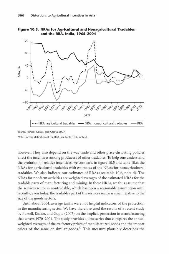
however. They also depend on the way trade and other price-distorting policiesaffect the incentives among producers of other tradables. To help one understandthe evolution of relative incentives, we compare, in figure 10.5 and table 10.6, theNRAs for agricultural tradables with estimates of the NRAs for nonagriculturaltradables. We also indicate our estimates of RRAs (see table 10.6, note d). TheNRAs for nonfarm activities are weighted averages of the estimated NRAs for thetradable parts of manufacturing and mining. In these NRAs, we thus assume thatthe services sector is nontradable, which has been a reasonable assumption untilrecently; even today, the tradables part of the services sector is small relative to thesize of the goods sectors.
Until about 2004, average tariffs were not helpful indicators of the protectionin the manufacturing sector. We have therefore used the results of a recent studyby Pursell, Kishor, and Gupta (2007) on the implicit protection in manufacturingthat covers 1970–2004. The study provides a time series that compares the annualweighted averages of the ex-factory prices of manufactured goods and the importprices of the same or similar goods.17 This measure plausibly describes the
366 Distortions to Agricultural Incentives in AsiaN
RA, %
�80
�40
0
40
80
120
1965
1967
1969
1971
1973
1975
1977
1979
1981
1983
1985
1987
1989
1991
1993
1995
1997
1999
2001
2003
year
NRA, agricultural tradables NRA, nonagricultural tradables RRA
Figure 10.5. NRAs for Agricultural and Nonagricultural Tradablesand the RRA, India, 1965–2004
Source: Pursell, Gulati, and Gupta 2007.
Note: For the definition of the RRA, see table 10.6, note d.

economic history of the period. First, the extremely high implicit nominal protec-tion of between 80 and 100 percent from the 1970s to the mid-1980s is consistentwith what we know about the restrictive import licensing system of that period.Second, the steep decline in implicit nominal protection, from around 70 percentin 1987 to almost zero in 1992, is consistent with the real rupee devaluation ofapproximately 80 percent during the same period (see figure 10.2). The decreasingvalue of the rupee during these years pushed up the border prices of importablemanufactured goods expressed in rupees, and these increases were far greater thanthe corresponding increases in the prices for domestically produced manufac-tured goods, which mirrored domestic inflation and other factors. Consequently,the average excess of the prices for domestically manufactured goods over therupee border prices for the same goods consistently declined, and it seemed nearlyto disappear altogether in 1992. After 1992, it increased for a while (between 1995and 1997, though this may have reflected the low international prices associatedwith the Asian financial crisis), but, in most years, it was well below 20 percent; theaverage rate was only 12 percent between 1992 and 2004 (the latest year for whichestimates are available). Until 2002, the apparent implicit protection rates were farbelow unweighted average industrial tariffs, for example, 45 percent in 1990 ver-sus average tariffs of 129 percent, 9 percent in 1999 versus average tariffs of 39 per-cent, and 5 percent in 2002 versus average tariffs of 33 percent. This gap narrowedsharply in 2003, however, and the possibility that domestic prices would exceedinternational prices was reduced by the cuts in manufacturing tariffs in the March2007 budget, which decreased the average tariff to below 10 percent.
The most important group of nonfarm tradable products other than manufac-tures are minerals, especially coal, iron ore, crude oil, and natural gas. Theseindustries account for about 2.5 percent of GDP. The tariffs on these items arecurrently low (in 2007, mostly zero, 2 percent, 5 percent, or 10 percent, respec-tively); except for crude oil and petroleum products, there are no major quantita-tive restrictions on imports or exports. Trade in these products is considerable;there are substantial imports (for example, coal) and exports (for instance, ironore). We have constructed for this study an NRA series that begins with an assess-ment of the situation in 2004. For coal, which accounted for about 62 percent ofdomestic mineral subsector output in 1970 and about 38 percent in 2004, theseestimates assume that domestic prices were about equal to import reference pricesin 2004 (NRA � 0); we have generated NRA estimates for earlier years using thecoal wholesale price index for India and an index of coal export prices for Aus-tralia.18 The NRAs for coal are low in many earlier years, which is consistent withthe depression of domestic coal prices, coal production, and, potentially, coalexports by Coal India, the parastatal monopoly that controls the industry. Thischanged during the late 1990s, when accelerating demand for coal pushed up
India 367
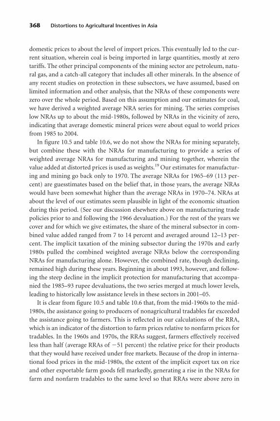
domestic prices to about the level of import prices. This eventually led to the cur-rent situation, wherein coal is being imported in large quantities, mostly at zerotariffs. The other principal components of the mining sector are petroleum, natu-ral gas, and a catch-all category that includes all other minerals. In the absence ofany recent studies on protection in these subsectors, we have assumed, based onlimited information and other analysis, that the NRAs of these components werezero over the whole period. Based on this assumption and our estimates for coal,we have derived a weighted average NRA series for mining. The series compriseslow NRAs up to about the mid-1980s, followed by NRAs in the vicinity of zero,indicating that average domestic mineral prices were about equal to world pricesfrom 1985 to 2004.
In figure 10.5 and table 10.6, we do not show the NRAs for mining separately,but combine these with the NRAs for manufacturing to provide a series ofweighted average NRAs for manufacturing and mining together, wherein thevalue added at distorted prices is used as weights.19 Our estimates for manufactur-ing and mining go back only to 1970. The average NRAs for 1965–69 (113 per-cent) are guesstimates based on the belief that, in those years, the average NRAswould have been somewhat higher than the average NRAs in 1970–74. NRAs atabout the level of our estimates seem plausible in light of the economic situationduring this period. (See our discussion elsewhere above on manufacturing tradepolicies prior to and following the 1966 devaluation.) For the rest of the years wecover and for which we give estimates, the share of the mineral subsector in com-bined value added ranged from 7 to 14 percent and averaged around 12–13 per-cent. The implicit taxation of the mining subsector during the 1970s and early1980s pulled the combined weighted average NRAs below the correspondingNRAs for manufacturing alone. However, the combined rate, though declining,remained high during these years. Beginning in about 1993, however, and follow-ing the steep decline in the implicit protection for manufacturing that accompa-nied the 1985–93 rupee devaluations, the two series merged at much lower levels,leading to historically low assistance levels in these sectors in 2001–05.
It is clear from figure 10.5 and table 10.6 that, from the mid-1960s to the mid-1980s, the assistance going to producers of nonagricultural tradables far exceededthe assistance going to farmers. This is reflected in our calculations of the RRA,which is an indicator of the distortion to farm prices relative to nonfarm prices fortradables. In the 1960s and 1970s, the RRAs suggest, farmers effectively receivedless than half (average RRAs of �51 percent) the relative price for their productsthat they would have received under free markets. Because of the drop in interna-tional food prices in the mid-1980s, the extent of the implicit export tax on riceand other exportable farm goods fell markedly, generating a rise in the NRAs forfarm and nonfarm tradables to the same level so that RRAs were above zero in
368 Distortions to Agricultural Incentives in Asia
1985–87. After the return to trend international food prices in the 1990s, the agri-cultural NRAs fell to close to zero so that, even though the NRAs for nonfarmindustries were reduced by more than half, the RRAs returned to negative values(averaging �13 percent during the decade). Although protection in manufactur-ing fell dramatically during the 1985–93 devaluations, the devaluations alsopushed up agricultural reference prices and reduced agricultural NRAs. Hence,following the devaluations and associated reforms, the antiagricultural bias in thesystem continued, but it was now far less marked. Then, beginning around 2000,more reductions in the protection for manufacturing, combined with a rise inagricultural input subsidies, boosted agricultural NRAs above the NRAs for non-farm tradables once more.
Where Are Indian Policies Heading?
Protection levels in most Indian manufacturing and also in the mining subsectorare now constrained by low tariffs. Even in a few of the industries protected byhigh tariffs, such as textile fabrics, garments, and auto assembly, expandingexports and domestic competition suggest that prices are unlikely to rise muchabove world prices in the foreseeable future. In contrast, most tariffs and otherformal instruments protecting the agricultural sector are much higher than theimplicit protection rates, and, if they are maintained at current levels, they will notstop domestic prices from rising well above world prices.
Is it probable that the government will follow a high-protection, high-subsidypath in agriculture as the Indian economy develops? The political economy of thisissue is complex. Some forces and some arguments appear to make it likely that ahigh-protection path in agriculture will be followed, while others argue againstthis outcome.
The politically important considerations favoring protection over open tradepolicies are as follows: the high share of employment in the rural sector (stillaround 60 percent), the desire to insulate farmers from the large price fluctuationsthat occur in world agricultural markets, and the feeling that the country shouldbe self-sufficient or nearly self-sufficient in the production of basic foods andother agricultural commodities. (The last argument is based on the notion thatdemand is too substantial to rely on world markets for supplies in the event ofserious crop failures or other disruptions to supplies.) These general argumentsfor protection reinforce the economic interests of farmer groups that are highlyorganized and politically effective at lobbying with the states and the central government. Within the central government, the Ministry of Agriculture repre-sents farmer interests and ensures that these views are heard in policy discussions.These are the basic reasons for the exclusion of agriculture and the food processing
India 369
industries from the liberalizing trade policy reforms in 1991, for fixing high tariffbindings during the Uruguay Round multilateral negotiations, and for leavingagriculture out of the unilateral tariff reduction program that started in 2003.They also explain the currently high agricultural tariffs, which have been deliber-ately set at prohibitive levels to keep out imports in case there is a dip in worldprices or the opening of a niche market opportunity for imports.
In contrast, because of the high share of food in household budgets in India,there is strong pressure to keep agricultural prices down. For many years, this goaldominated agricultural policies and was compatible with expanding agriculturalproduction and national self-sufficiency largely because of the successful adoptionof Green Revolution technologies in crop agriculture, in conjunction with large-scale government investment in irrigation and other rural infrastructure. Between1965 and 1988, domestic rice and wheat prices declined by 44 and 52 percent inreal terms, respectively. Because of steadily increasing farm productivity, this majorlong-term benefit to consumers was compatible with rising farmer prosperity,especially in northwestern India. There were also additional benefits arising amonglow-income households from subsidized rice and wheat supplied through the pub-lic distribution system. Moreover, the trade policy regime of the period kept theprices of the principal food grains low—directly through export restrictions andindirectly through the exchange rate overvaluations that were generated by thehigh-protection import-substitution policies in place in manufacturing. In the caseof rice, an export ban was in force in 1965–88, and average domestic rice priceswere about 23 percent below export parity prices and were lower still in relation toexport prices under counterfactual simulations of the exchange rate under freetrade.20 In these ways, food consumers benefited at the expense of farmers duringthe license Raj, although they lost as consumers of manufactured goods and, muchmore importantly, as a consequence of the missed opportunities for more rapidoverall economic growth that was forgone because of these policies.
There are no organized groups representing the interests of food consumers.Nonetheless, politicians and bureaucrats are sensitive to consumer concerns overfood prices, which are a major topic in public debates, especially debates on theefficacy of the supply of below-poverty-line groups with subsidized wheat, rice,and sugar through the public distribution system. In these ways, consumer inter-ests remain important counterforces to the producer lobbyists pressing for higheragricultural prices, usually through increases in support prices.
However, a number of factors limit the extent to which public concerns overconsumer welfare constrain lobbying groups in favor of farmers and other producers.
First, politicians and government bureaucrats are mainly sensitive to increasesin the retail prices of mass consumption staple foods, including wheat, rice, sugar,
370 Distortions to Agricultural Incentives in Asia

edible oils, milk, pulses, and selected vegetables such as onions. They are less con-cerned about the prices for other food products, especially fresh fruits, other veg-etables, and spices because consumers have long been accustomed to fluctuatingprices in retail and wholesale markets for these products.
Second, as in other countries, producer lobbying groups can be at least par-tially placated through increases in input subsidies without incurring the politicalpain that may follow output price increases. This explains the rapid rise in fertil-izer and electricity subsidies since 1985, the long-term decline in canal irrigationfees for water, and subsidized credit for farmers supplied through governmentbanks. It also explains the government’s reaction to the 2007–08 boom in worldagricultural and fertilizer prices, which included a ban on rice exports that wasaimed at protecting domestic consumers, but also raised subsidies to keep domes-tic fertilizer prices below world prices; the latter was aimed at placating farmers.However, there were limits to increases in these subsidies. For example, no addi-tional subsidy was possible if electricity was being supplied free of charge, whichwas the case in a number of Indian states. The subsidies had other consequences,notably, the effects of the farm electricity subsidies on state government budgetsand the viability and operating efficiency of state electricity boards and the effectsof the fertilizer subsidies on the central government budget (Gulati andNarayanan 2003). Until around 2005, there were signs that these limits and conse-quences may have checked the rate of growth in farm subsidies.
Third, the objective of national food self-sufficiency sometimes trumped theconcerns about consumer welfare. The clearest example is the unsuccessful attemptto replace palm oil imports by domestic production through import restrictionsinitially and through high tariffs currently (85 percent). Over long periods, dairyimport policies also involved high consumer prices without generating muchdebate on behalf of consumers. In both cases, the interests pushing for the import-substitution policies dominated public discussions, and there seems to have beenlittle, if any, public awareness that lower prices were a realistic alternative.
Fourth, the political concern about the prices for staple foods was mainly anissue of price stability, rather than about price level. If prices unexpectedly decline,producers become worried; consumers worry if prices unexpectedly increase.Although organized commodity markets and trade associations were reporting oninternational commodity prices, there was little public interest in the divergencebetween domestic prices and world prices. Thus, as long as there are no suddenlarge price changes in the current context of high redundant tariffs, it is quite plau-sible that domestic food prices might steadily rise and diverge from internationalprices, especially if general inflation is low and the exchange rate appreciates.
Fifth, producers have discovered they can be effective in blocking importswithout attracting much opposition if they act quickly and early before the
India 371
imports achieve much domestic market penetration. There is minimal establishedimporter and consumer interest to overcome if this is the approach. If imports areblocked early, there is no or little subsequent consumer and political awareness ofimports as a lower-cost alternative to domestic production. Increases in tariffs onchicken parts and garlic (from 35 to 108 percent in 2001 and in 2003, respectively)are recent examples of this strategy, and the same strategy might be applied toother products if imports threaten to overcome the already comprehensive pro-tective barriers.
This all suggests that the political interest in low consumer prices is unlikely torepresent an obstacle to increases in agricultural protection, while domestic andexternal conditions could conceivably create strong producer pressure for agricul-tural protection. Medium- or long-term scenarios that would favor a boost inprotection might include a loss in the ability of the domestic production of majorcrops such as rice and wheat to respond to domestic demand, leading to pressurefor increases in prices or in input subsidies to maintain self-sufficiency; a fall inworld prices in a context of stable or slowly rising domestic prices in real terms; areal exchange rate appreciation that reduces rupee border prices, while domesticprices remain about the same or only slowly increase; or limited progress inachieving a reduction in agricultural protection in developed countries throughnegotiations at the World Trade Organization. This last would reinforce thealready strong resistance to liberalization in the government’s agricultural tradepolicies on the argument, first, that tariff concessions should be held in reserve asa bargaining chip to exchange for substantial concessions by developed countriesand, second, that continuing the isolation of the domestic markets in developedcountries perpetuates price instability in world markets, and the government’strade policies should therefore continue to insulate domestic markets in Indiafrom world market conditions.21
Scenarios that might ease the pressures for greater protection include stableworld prices in a long-run rising trend; productivity increases, especially in yieldsand in transport, storage, and marketing, that might partially or fully offset otherfactors tending to raise domestic prices relative to border prices; productivity andproduction increases that lead to exportable surpluses and growing pressure tocut production if export subsidies are needed to profitably export surpluses; suc-cessful negotiations with the World Trade Organization on reductions in the pro-tection and the subsidies (especially export subsidies) in developed countries;greater willingness in India to implement more open agricultural trade policies;and successful negotiations through the World Trade Organization to close ortighten loopholes permitting export subsidies and more active enforcement byother countries so as to facilitate the Indian government’s no-export-subsidycommitment under the Uruguay Round Agreement on Agriculture.22
372 Distortions to Agricultural Incentives in Asia
A distinction needs to be made between changes in implicit protection andchanges in the formal protective instruments such as tariffs. Under a scenario ofgreater protection, domestic prices would rise relative to world prices. However,because of the considerable redundancy in the level of formal protection, bigincreases could occur without a boost in tariffs or tighter protection. If tariffs andother formal protective instruments are to be reduced, the initiative must comethrough the World Trade Organization; there appears to be little or no domesticpressure to achieve such a reduction.
Notes
1. Unless otherwise indicated, throughout the paper, the years are Indian financial years. For example,1996 is 1996/97, that is, the financial year from April 1, 1996 to March 31, 1997. This includes the varioustime series, except for some series that are based on crop years (for example, sugar and sugarcane).
2. Agriculture is used here and in other places in the chapter in a broad sense to include crop agri-culture, horticulture, livestock activities, inland and ocean fisheries, and forestry activities. This broaduse of the term should be apparent from the context. However, our computations of rates of assistancein agriculture include livestock, but not fisheries or forestry, which is consistent with the usagethroughout the volumes in this World Bank research project.
3. In this and the following section, the discussion of policies before 1990 relies to a large extent onPursell (1992). More information on the earlier years, especially the 1960s and 1970s, may be found inthe references cited there.
4. The techniques included modest general tariff increases through the use of para-tariff measuresand customs duties in 1997–2001; prohibitively high tariff bindings that, under the Uruguay RoundAgreement on Agriculture, may be applied to products freely within a wide range (100, 150, or300 percent); specific tariffs on most textile fabrics and garments that were implemented beginning in2001 and that are sufficiently severe to discourage any imports of these products from entering thedomestic market; local-content rules in the auto industry that were introduced in 1995 and dropped in2002 following objections by other World Trade Organization members; the widespread use ofantidumping measures that were undertaken in the early 1990s and have been applied mainly to man-ufactured intermediates; the use of state trading enterprises to control imports of cereals, fertilizers,and petroleum products; the use of tariff rate quotas to protect local producers of edible oils and pow-dered milk; new rules on technical standards introduced in 2000 within the administration of theBureau of Indian Standards; new sanitary and phytosanitary rules applicable to imports of nearly allagricultural, livestock, and food products under the general supervision of the Ministry of Agriculture;ad hoc export subsidies that are used periodically to dispose of agricultural surpluses (for example, inwheat and sugar) and that are certainly inconsistent with the spirit and, possibly, also with the letter ofthe government’s no-export subsidy commitments under the Uruguay Round Agreement on Agricul-ture; and, starting in 2005, a subsidy scheme for exports of fruits, vegetables, dairy products, and poul-try (NIAM, various). Within India, the predominant view appears to be that technical barriers to traderules and sanitary and phytosanitary measures, in addition to the legitimate roles sanctioned by theWorld Trade Organization, are instruments that may be activated or withdrawn according to whetherindividual industries are in need of nontariff protection against imports.
5. The information has been calculated from data on tariffs and other import taxes publishedannually in Goyal (various). These publications also provide detailed information on quantitativeimport restrictions, sanitary and phytosanitary measures, rules on technical barriers to trade, bilateraland regional trade agreements, and other trade policy instruments. Additional reductions in industrialtariffs appeared in the 2008 budget.
India 373
6. The main exceptions to the low industrial tariffs are specific duties on most textile fabrics andgarments and a 60 percent tariff protecting the auto industry. However, there is evidence of consider-able tariff redundancy in these industries, whereby typical domestic ex-factory prices are about equalto or even below the import prices. There are also nontariff barriers protecting domestic urea produc-ers, and the domestic prices for products derived from some of these plants are high relative to worldprices.
7. Two exceptions are the rice imports of Bangladesh from India and India’s imports of raw jutefrom Bangladesh, both of which are subject to low tariffs.
8. A World Bank study (2006) of the likely consequences of a free trade agreement betweenBangladesh and India finds that the prices for many agricultural products and processed foods arehigher in Bangladesh than in India. It concludes that, under a bilateral free trade agreement, thereappear to be few possibilities for expanded agricultural and processed food exports from Bangladeshto India, but considerable potential for increased Indian agricultural exports to Bangladesh. The latterwould involve trade diversion costs for Bangladesh, including lost customs revenue, resulting from thereplacement of duty-paying imports from the rest of the world by duty-free imports from India.
9. A comprehensive account of the Indian government’s macroeconomic policies, includingexchange rate policies, between 1964 and 1991 is offered by Joshi and Little (1994).
10. One major role of state trading enterprises in import and domestic policies was eliminated inJune 2006, when it was announced that cereal imports would no longer be a monopoly of the FoodCorporation of India. It was also announced that this entity would no longer buy wheat and rice atprocurement prices, but, instead, would rely on competitive wholesale markets to purchase the sup-plies needed for the public distribution system and general food security stocks. However, in 2006,wheat and rice tariffs, at 50 and 70–80 percent, respectively, were prohibitive.
11. Reductions in agricultural tariffs are often undertaken through special partial or completeexemptions on a particular occasion or for a particular importing organization, while the most-favored-nation tariff is formally left unchanged. Between 2001 and 2005, substantial export subsidies were paidto make it worthwhile for private traders to help dispose of large excess wheat stocks. In February 2006,it was announced that, in view of the inadequate stocks, the Food Corporation of India would import0.5 million tons of wheat at zero duty. Sugar trade policies have been especially opportunistic. Therehave been significant changes in sugar tariffs over the last 15 years or so, and, between 2001 and 2004,when about 4.3 million tons were exported, export subsidies were used extensively (Pursell 2007).
12. For the reasons discussed in appendix A, tariffs have been irrelevant as indicators of the actualdifferences between domestic and prevailing world prices for nearly all primary and processed agricul-tural products. Our estimates of the actual rates of assistance must therefore rely on painstaking directproduct-by-product comparisons of domestic prices and border prices, adjusted by port, handling,and domestic transport costs and supplemented by information on the subsidies and rates of protec-tion for inputs.
13. The trade status of each product in a given year is endogenously determined in the analysisdepending on whether the domestic price was greater than the import reference price (import- competing), less than the export reference price (exportable), or between these two (nontradable). Theimport reference price (also often called the import parity price) is the cost, insurance, and freightprice, plus port, handling, transport, and other charges. The export reference price (also known as theexport parity price) is the free on board price, minus transport, handling, and other charges incurred ingetting the product to the free on board stage. The trade status is the same in at least two-thirds of allyears for only 3 of the 13 product groups Pursell, Gulati, and Gupta (2007) cover in their analysis (seetheir appendix table A4).
14. On the complexities of calculating input subsidies in the Indian context, see Gulati andNarayanan (2003). There are implicit taxes on other tradable farm inputs because of import licensingand tariffs, but, in the second half of the 1980s, these taxes were quite small relative to fertilizer andelectricity subsidies (Gulati, Hanson, and Pursell 1990; Pursell and Gupta 1998; Gulati and Kelley1999). The implicit taxes declined, along with the decline in protection in manufacturing, during therupee devaluations in 1985–93. By 2007, most tariffs on nearly all manufactured farm inputs and also
374 Distortions to Agricultural Incentives in Asia
on trucks and specialized handling, storage, and agroprocessing equipment had declined to 7.5 per-cent. Hence, excluding these generates an upward bias in the estimated contribution of input subsidiesin crop NRAs probably by less than 1 percentage point.
Indian farmers also benefit from subsidized credit and are exempt from income taxes, but thesesubsidies are small relative to fertilizer and electricity subsidies. More importantly, farmers receivesubsidized water through canal irrigation schemes that charge fees well below the costs of operationand maintenance. Moreover, farmers do not contribute to the capital costs of the dams, canals, andother public infrastructure from which they are the principal beneficiaries. The resource allocationconsequences of the canal irrigation subsidies are especially problematic because the water suppliedthrough canal irrigation is rationed. Thus, an increase in water fees would only transfer economicrents from farmers to the recipients of the fees (mainly state governments) without directly affectingthe production of the irrigated crops. For this reason, we do not cover canal irrigation subsidies inour study.
15. Over long periods, sugar prices in India have been much lower than sugar prices in Bangladesh,where prices have been well supported, through quantitative restrictions initially and, later, throughcustoms duties and various para-tariff measures. The price differences in the two countries have gen-erated a regular legal export trade from India to Bangladesh, as well as substantial unrecorded smug-gling in exports across the porous land border to Bangladesh (Pursell 2007; see also chapter 9 in thisvolume). However, the quantities exported, though constituting large shares of the market inBangladesh, have not been sufficient to have much impact on domestic prices in India. If the govern-ment of Bangladesh were to remove or substantially reduce sugar tariffs, a principal initial impactwould probably be to divert a considerable portion of the smuggled imports from India into legalchannels. Sugar prices in Pakistan are at about the same general level as Indian prices, and there is con-siderable potential for welfare-improving trade in both directions (especially across the land border)that would help reduce seasonal and cyclical disturbances. However, except for the occasional ad hocrelaxation of restrictions, the highly restrictive bilateral trade relationship between the two countriesprevents this from happening.
16. The total input subsidy and subsidy rate appeared to have reached a plateau in 2001–05, but,since 2007, there have been large increases in the fertilizer subsidy; the government thus partially insu-lated farmers from steep rises in world fertilizer prices.
17. We have used only import reference prices in measuring the rates of assistance in manufactur-ing and aggregating them across manufacturing subsectors. Export reference prices have not been con-sidered directly partly because manufactured exports have constituted a small share of total manufac-turing production in India, but principally because the gaps between free on board and cost,insurance, and freight prices and export-import reference prices are generally quite small in the case ofthe prices for manufactured goods.
18. We cross-checked the resulting NRA series by applying the same price indexes to estimates ofthe coal protection rates in 1982 derived from an early study. The resulting series was broadly similar,although the NRAs were somewhat lower.
19. We use GDP-share value added weights because they provide a better indication of the relativesize of the manufacturing and mining sectors than do output weights. Ideally, to take account of input-output relationships, especially in manufacturing, the effective protection of the two sectors should beaveraged in a calculation that relies on the value added in world prices as weights. However, there isonly one known estimate of aggregate effective protection in manufacturing (for 1986/87), but there isno time series, and no estimates or time series exist for the mineral subsectors. In our judgment, theuse of this procedure—if it were possible to use it—would probably not change the general level ortrend of the nonagricultural NRA series much. On the one hand, the average would be reduced, espe-cially for the 1970s and 1980s, owing to the increased weight of the mineral subsectors, but, on theother hand, it would probably be increased owing to the likely excess of effective protection rates overnominal rates of protection in the manufacturing sector.
20. This does not mean that domestic rice prices would have been an average 23 percent higherwithout the export ban. This is so because Indian supply would have depressed world prices.
India 375

21. It has been suggested that one reason the government set such high agricultural tariffs was theproposal of the United States that applied tariffs rather than tariff bindings should be the startingpoint for negotiations on tariff reductions (Gulati 2004).
22. Some export subsidies in India have been justified under the World Trade Organizationrule that allows developing countries to subsidize the transport and marketing costs of agriculturalexports.
References
Anderson, K., M. Kurzweil, W. Martin, D. Sandri, and E. Valenzuela. 2008. “Measuring Distortions toAgricultural Incentives, Revisited.” World Trade Review 7 (4): 675–704.
CGA Database (Database of the Controller General of Accounts). Controller General of Accounts,Department of Expenditure, Ministry of Finance. http://cga.nic.in/ (accessed May 2008).
FAO Agricultural Trade Database (FAOSTAT). Food and Agriculture Organization of the UnitedNations. http://faostat.fao.org/site/342/default.aspx (accessed May 2008).
FAOSTAT Database. Food and Agriculture Organization of the United Nations. http://faostat.fao.org/default.aspx (accessed May 2008).
FAO SUA-FBS Database (Supply Utilization Accounts and Food Balance Sheets Database, FAOSTAT).Food and Agriculture Organization of the United Nations. http://faostat.fao.org/site/354/default.aspx (accessed May 2008).
Goyal, A., ed. various years. BIG’s Easy Reference Customs Tariff. New Delhi: Academy of Business Studies.
Gulati, A. 2004. “Trade Policies, Incentives and Institutions in Indian Agriculture.” Unpublished paper,International Food Policy Research Institute, Washington, DC.
Gulati, A., J. Hanson, and G. Pursell. 1990. “Effective Incentives in India’s Agriculture: Cotton, Ground-nuts, Wheat, and Rice.” Policy, Planning, and Research Working Paper WPS 332, World Bank,Washington, DC.
Gulati, A., and T. Kelley. 1999. Trade Liberalization and Indian Agriculture. New Delhi: Oxford Univer-sity Press.
Gulati, A., and S. Narayanan. 2003. Subsidy Syndrome in Indian Agriculture. New Delhi: Oxford University Press.
Joshi, V. J., and I. M. D. Little. 1994. India: Macroeconomics and Political Economy 1964–1991. NewDelhi: Oxford University Press.
Mattoo, A., D. Mishra, and A. Narain. 2007. From Competition at Home to Competing Abroad: A CaseStudy of India’s Horticulture. Oxford: Oxford University Press; Washington, DC: World Bank.
Ministry of Finance. 2005. Economic Survey 2004–2005. New Delhi: Ministry of Finance. http://indiabudget.nic.in.
———. Various years. Economic Survey. New Delhi: Ministry of Finance. http://indiabudget.nic.in.Mullen, K., D. Orden, and A. Gulati. 2005. “Agricultural Policies in India: Producer Support Estimates
1985–2002.” MTID Discussion Paper 82, Markets, Trade, and Institutions Division, InternationalFood Policy Research Institute, Washington, DC.
NIAM (National Institute of Agricultural Marketing). various issues. WATS, World Agro Trade Scanner.Fortnightly newsletter, NIAM, Jaipur, India.
Orden, D., F. Cheng, H. Nguyen, U. Grote, M. Thomas, K. Mullen, and D. Sun. 2007. Agricultural Pro-ducer Support Estimates for Developing Countries: Measurement Issues and Evidence from India,Indonesia, China, and Vietnam. Research Report 152. Washington, DC: International Food PolicyResearch Institute.
Pursell, G. 1992. “Trade Policies in India.” In National Trade Policies, ed. D. Salvatore, 423–58. Hand-book of Comparative Economic Policies 2. Westport, CT: Greenwood Press.
376 Distortions to Agricultural Incentives in Asia
———. 1999. “Some Aspects of the Liberalization of South Asian Agricultural Policies: How Can theWTO Help?” In Implications of the Uruguay Round Agreement for South Asia: The Case of Agricul-ture, ed. B. Blarel, G. Pursell, and A. Valdés, 29–46. New Delhi: Allied Publishers; Washington, DC:World Bank.
———. 2007. “Smuggling and the Economic Consequences of an FTA: A Case Study of India-Bangladesh Trade in Sugar.” ASARC Working Paper 2007/5, Australia South Asia Research Center,Australian National University, Canberra.
Pursell, G., A. Gulati, and K. Gupta. 2007. “Distortions to Agricultural Incentives in India.” AgriculturalDistortions Working Paper 34, World Bank, Washington, DC.
———. Forthcoming. Agricultural Trade Policies in India. Washington, DC: World Bank.Pursell, G., and A. Gupta. 1998. “Trade Policies and Incentives in Indian Agriculture: Methodology,
Background Statistics and Protection and Incentive Indicators, 1965–95; Background Paper 1,Sugar and Sugarcane.” Policy Research Working Paper 1953, World Bank, Washington, DC.
Pursell, G., N. Kishor, and K. Gupta. 2007. “Manufacturing Protection in India since Independence.”ASARC Working Paper 2007/7, Australia South Asia Research Center, Australian National Univer-sity, Canberra.
Rakotoarisoa, M., and A. Gulati. 2006. “Competitiveness and Trade Potential of the Dairy Sector inIndia.” Food Policy 31 (3): 216–27.
RBI Database (Reserve Bank of India Database on the Indian Economy). Reserve Bank of India.http://www.rbi.org.in/scripts/Statistics.aspx (accessed May 2008).
World Bank. 2006. Studies on India-Bangladesh Trade: Trade Policies and Potential FTA. 2 vols. Report37863-BD. Washington, DC: World Bank.
India 377


Trade and agricultural pricing policies, along with public investments in irrigationand agricultural research and extension, have played a crucial role in the agricul-tural development of Pakistan.1 From the 1960s to the mid-1980s, trade policies,controls on foreign exchange, and major government interventions in domesticagricultural markets created large distortions in agricultural prices. In general, theoverall effect of these policies, including the indirect effects of trade policy distor-tions on real exchange rates, was to lower the real prices of tradable agriculturalproducts (Dorosh and Valdès 1990; Hamid, Nabi, and Nasim 1990). Despite pricedisincentives, however, agricultural output rose rapidly because of the adoption ofthe Green Revolution package of inputs (improved seeds, fertilizers, irrigation)and the resulting increase in productivity (Ali and Byerlee 2002). Major invest-ments in land and, most important in the context of Pakistan, in water supply(particularly through tube wells) also allowed increases in the net area sown.
Substantial liberalization took place from the mid-1980s to the early 1990s,however, greatly reducing explicit tariffs and taxes, as well as government directinterventions in markets for most agricultural products (Nabi 1997; Salam 2001;Ahmad 2003). Nonetheless, the government continues to intervene heavily indomestic wheat markets, and significant tariffs still exist for vegetable oils andmilk products. This chapter describes these interventions and presents internallyconsistent estimates of nominal rates of assistance (NRAs), as well as estimates ofbroader trade policy effects through real exchange rate distortions.
379
11
PAKISTAN
Paul A. Dorosh and Abdul Salam
The authors are grateful to Marika Krausova for excellent research support and Garry Pursell for help-ful comments.

In the next section, we present a brief overview of agriculture in Pakistan thathighlights growth rates in the area under cultivation, yields, and production invarious crops. In the subsequent section, we describe key trade and pricing policies for major crops and measures of policy distortions (the NRAs) over time.Then, we present broader trade and exchange rate policies and estimates of theindirect effects of the distortions on the relative prices faced by agricultural pro-ducers. The final section concludes with a discussion of the political economy ofthe country’s agricultural policies.
The Agricultural Sector
Although agriculture is the primary sector of employment for nearly 50 percent ofthe national workforce, it contributes barely 20 percent of national gross domesticproduct and only around 12–13 percent of exports, even if processed foods areincluded. The decline in the relative importance of agriculture has been less rapidon Pakistan than in other South Asian countries except in exports, the share ofwhich was more than 50 percent prior to the 1970s (table 11.1). Agricultural earn-ings still account for about 70 percent of rural household incomes.
Four crops—wheat, cotton, sugarcane, and basmati and coarse rice—account foraround two-thirds of the total cropped area and the gross domestic product in cropagriculture and over one-third of total agricultural gross domestic product. Much ofthe focus of agricultural policy, research, and extension has been on these crops. Theadoption of Green Revolution technology to improve seeds and the greater use offertilizers and irrigation, especially private tube wells that provided more effectivecontrol over water, contributed to substantial increases in the yields and the volume
380 Distortions to Agricultural Incentives in Asia
Table 11.1. Agriculture in the Economy, Pakistan, 1965–2004(percent)
Indicator 1965–69 1975–79 1985–89 2000–04
Agriculture in employmentPakistan 55 53 49 45All South Asia 74 70 65 57Agriculture in gross
domestic productPakistan 35 29 24 22All South Asia 43 36 29 21Agriculture in exportsPakistan 53 38 30 12All South Asia 46 40 26 13
Sources: Sandri, Valenzuela, and Anderson 2007; World Development Indicators Database 2008.
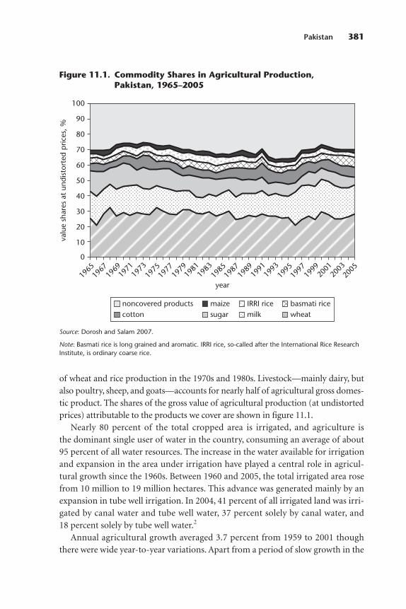
of wheat and rice production in the 1970s and 1980s. Livestock—mainly dairy, butalso poultry, sheep, and goats—accounts for nearly half of agricultural gross domes-tic product. The shares of the gross value of agricultural production (at undistortedprices) attributable to the products we cover are shown in figure 11.1.
Nearly 80 percent of the total cropped area is irrigated, and agriculture isthe dominant single user of water in the country, consuming an average of about95 percent of all water resources. The increase in the water available for irrigationand expansion in the area under irrigation have played a central role in agricul-tural growth since the 1960s. Between 1960 and 2005, the total irrigated area rosefrom 10 million to 19 million hectares. This advance was generated mainly by anexpansion in tube well irrigation. In 2004, 41 percent of all irrigated land was irri-gated by canal water and tube well water, 37 percent solely by canal water, and18 percent solely by tube well water.2
Annual agricultural growth averaged 3.7 percent from 1959 to 2001 thoughthere were wide year-to-year variations. Apart from a period of slow growth in the
Pakistan 381
0
valu
e sh
ares
at
undi
stor
ted
pric
es, %
10
20
1965
1967
1969
1971
1973
1975
1977
1979
1981
1983
1985
1987
1989
1991
1993
1995
1997
1999
2001
2003
2005
year
30
40
50
60
70
80
90
100
noncovered products maize IRRI rice basmati ricecotton sugar milk wheat
Figure 11.1. Commodity Shares in Agricultural Production,Pakistan, 1965–2005
Source: Dorosh and Salam 2007.
Note: Basmati rice is long grained and aromatic. IRRI rice, so-called after the International Rice ResearchInstitute, is ordinary coarse rice.

first half of the 1970s, average agricultural growth exceeded 3.2 percent per year ineach five-year period from 1960 to 2000, largely because of significant growth inthe crop sector in the 1970s and 1980s that is attributable to Green Revolutiontechnology (improved seeds, increased fertilizer use, and irrigation). However, theperformance of the agriculture sector, particularly the crop subsector, has sufferedin recent years because of severe droughts, rising soil salinity, and deterioratinggroundwater quality. The agricultural sector grew at a modest rate of only 2.6 per-cent per year from 1999 to 2005, however (0.5 percent per year on a per capitabasis). Real value added in the four major crops—wheat, cotton, sugarcane, andbasmati and other rice—rose by 2.6 percent per year over the period. There havebeen substantial fluctuations in recent years. Value added in the livestock subsec-tor increased somewhat more rapidly, at 3.5 percent.
Most of the increase in production in the major crops since the early 1990s hasbeen generated by higher yields. For example, from 1990 to 2005, the average annualgrowth in the area under wheat or basmati rice was 0.2 and 2.5 percent, respectively,while yields expanded by 2.2 and 3.6 percent, respectively (table 11.2). Cotton yields,in contrast, stagnated over this period, increasing by only 0.8 percent per year(although the 2004 crop was a bumper crop). Yields in sugarcane rose by only0.9 percent per year. Maize enjoyed a large expansion in yields (4.7 percent per year)and production (5.8 percent per year) over the same period.
Trade and Exchange Rate Policies
Pakistan operated a fixed nominal exchange rate regime. Only the rate relative tothe U.S. dollar changed between the year of independence and the early 1980s.3 Inthe 1960s, the government operated various export bonus schemes that substan-tially raised the rupee price of foreign exchange for exporters. The official nomi-nal exchange rate remained fixed throughout the 1960s. A major devaluation in1971–72 halved the rupee in U.S. dollar terms. Domestic inflation, coupled with afixed nominal exchange rate, steadily eroded export incentives (a real exchangerate appreciation) in the late 1970s and early 1980s, however. To restore the incen-tives for export growth, the Zia government undertook a succession of nominaldevaluations of the rupee (totaling 73 percent), from PRs 9.90 to PRs 17.2 to theU.S. dollar, between fiscal years 1981 and 1987 that achieved a real exchange ratedepreciation of 65 percent.4
There was little subsequent change in real exchange rates until 1996, when thenominal exchange rate was allowed to depreciate more rapidly. Between fiscalyears 1996 and 2001, the nominal exchange rate depreciated by 74 percent, fromPRs 33.6 to PRs 58.4 to the U.S. dollar, although, because of relatively high domes-tic inflation, the real exchange rate depreciated by only 11 percent.
382 Distortions to Agricultural Incentives in Asia
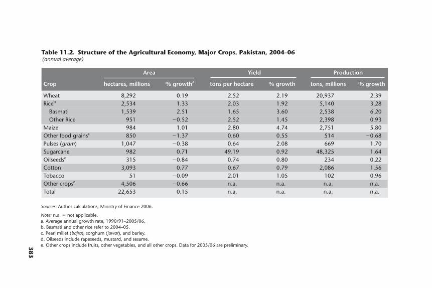
383
Table 11.2. Structure of the Agricultural Economy, Major Crops, Pakistan, 2004–06(annual average)
Sources: Author calculations; Ministry of Finance 2006.
Note: n.a. � not applicable.a. Average annual growth rate, 1990/91–2005/06.b. Basmati and other rice refer to 2004–05.c. Pearl millet (bajra), sorghum (jowar), and barley.d. Oilseeds include rapeseeds, mustard, and sesame.e. Other crops include fruits, other vegetables, and all other crops. Data for 2005/06 are preliminary.
Area Yield Production
Crop hectares, millions % growtha tons per hectare % growth tons, millions % growth
Wheat 8,292 0.19 2.52 2.19 20,937 2.39Riceb 2,534 1.33 2.03 1.92 5,140 3.28
Basmati 1,539 2.51 1.65 3.60 2,538 6.20Other Rice 951 �0.52 2.52 1.45 2,398 0.93
Maize 984 1.01 2.80 4.74 2,751 5.80Other food grainsc 850 �1.37 0.60 0.55 514 �0.68Pulses (gram) 1,047 �0.38 0.64 2.08 669 1.70Sugarcane 982 0.71 49.19 0.92 48,325 1.64Oilseedsd 315 �0.84 0.74 0.80 234 0.22Cotton 3,093 0.77 0.67 0.79 2,086 1.56Tobacco 51 �0.09 2.01 1.05 102 0.96Other cropse 4,506 �0.66 n.a. n.a. n.a. n.a.Total 22,653 0.15 n.a. n.a. n.a. n.a.

Large inflows of foreign capital (both public and private) began in late 2001.These were related to post–September 11 shifts in donor policies and the repatriation of private sector capital to Pakistan. They contributed to an 8 percentappreciation in the real exchange rate from September 2001 to October 2002. Thecapital inflows also helped the government avoid a pending balance of paymentscrisis and increase public spending. Careful macromanagement, including repay-ment of international debt, combined with a surge in public and private sectorimports, resulted in a depreciation of the real exchange rate in 2003 and 2004.More recent trends suggest that expansionary monetary and fiscal policies mayhave adversely affected the incentives for tradable goods relative to nontradablesbecause the real exchange rate appreciated by 14 percent between December 2004and November 2005.
Prior to major reforms in 1991 and 1997, the government generally followedan import-substitution trade policy aimed at promoting the industrial sector.Trade taxes were also a major source of government revenue. Under the firstNawaz Sharif government (November 1990 to July 1993), tariff rates were cutsharply in 1991 and, as a result, net tariff revenues as a share of imports fell from34 percent in 1990 to 27 percent in 1991. Unweighted average tariff rates fell from77 percent in 1988 to only 45 percent in 1994. The number of items subject toquantitative restrictions was also reduced, from 1,361 in 1988 to only 970 in 1993,although nearly 10 percent of all commodities were still subject to quantitativerestrictions in 1993 (Nabi 1997). This trade reform was accompanied by a liberal-ization in foreign exchange markets in 1992, including allowing foreign currencybank deposits (Hasan 1998).
Six years later, in March 1997, under the second Nawaz Sharif government(February 1997 to October 1999), the maximum tariff rate was reduced from 65to 45 percent; the number of tariff slabs was reduced from 13 to 5; and there was asharp reduction in the tariff rates on smuggling-prone items to between 10 and 25percent (Hasan 1998).
These changes in trade policy were reflected in net customs duties, which fellfrom an average 34 percent in 1985–89 to 22 percent in 1990–96, 12 percent in1997–2000, and 9 percent in 2001–03. The decline in the total taxes on importswas far less dramatic, however, because, as customs duties were lowered, salestaxes on imports were raised. Thus, total taxes on imports declined by only 10 per-centage points between 1990 and 2000, from 34 to 24 percent.5 The average statu-tory tariff rates were similar for agriculture and for industrial products: 21.8 and20.2 percent, respectively, in 2001 (World Bank 2004).
Along with a reduction in tariff rates, trade liberalization in the 1990s includeda gradual reduction in the number of products subject to quantitative restrictions.
384 Distortions to Agricultural Incentives in Asia
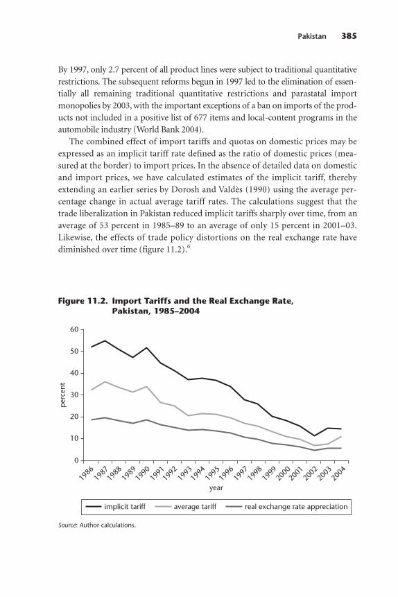
Pakistan 385
By 1997, only 2.7 percent of all product lines were subject to traditional quantitativerestrictions. The subsequent reforms begun in 1997 led to the elimination of essen-tially all remaining traditional quantitative restrictions and parastatal importmonopolies by 2003, with the important exceptions of a ban on imports of the prod-ucts not included in a positive list of 677 items and local-content programs in theautomobile industry (World Bank 2004).
The combined effect of import tariffs and quotas on domestic prices may beexpressed as an implicit tariff rate defined as the ratio of domestic prices (mea-sured at the border) to import prices. In the absence of detailed data on domesticand import prices, we have calculated estimates of the implicit tariff, therebyextending an earlier series by Dorosh and Valdès (1990) using the average per-centage change in actual average tariff rates. The calculations suggest that thetrade liberalization in Pakistan reduced implicit tariffs sharply over time, from anaverage of 53 percent in 1985–89 to an average of only 15 percent in 2001–03.Likewise, the effects of trade policy distortions on the real exchange rate havediminished over time (figure 11.2).6
0
year
10
1986
1987
1988
1989
1990
1998
1999
2000
2001
2002
2003
2004
1991
1992
1993
1994
1995
1996
1997
40
30
50
20
60
per
cent
implicit tariff average tariff real exchange rate appreciation
Figure 11.2. Import Tariffs and the Real Exchange Rate,Pakistan, 1985–2004
Source: Author calculations.
Impacts of Agricultural Price and TradePolicies on NRAs
We consider in this section distortionary policies on milk and several key cropproducts, including wheat, cotton, sugar, maize, and rice (basmati rice and IRRIrice; see the note to figure 11.1). Together, these products account for around70 percent of the value of agricultural production (figure 11.1). In line with ourproject methodology, we estimate NRAs on output for each of those products. (Fordetails on the methodology, see Anderson et al. 2008 and appendix A). Throughcareful comparisons of domestic prices and prices at the border or internationalreference prices, which we have adjusted for quality differences, marketing mar-gins, and the dual exchange rate system, we capture in these measures the propor-tional extent to which government-imposed distortions create a gap betweendomestic prices and prices as they would be under free market conditions.7
Wheat
Wheat is Pakistan’s main staple food, accounting for an average 1,040 calories perperson per day in 2001, which represents 42 percent of total caloric consumption(FAO SUA-FBS Database 2007).8 The adoption of Green Revolution technologyenabled the country to more than double wheat production from the early 1970sto the late 1990s, and the production has risen by an additional one-quarter sincethen (table 11.3).9 Nonetheless, in most years since 1960, Pakistan has been a netwheat importer.
Government wheat policyThrough its wheat policy, the government attempts to balance the competinginterests of producers and consumers. On the production side, the policy is aimedat increasing wheat productivity (yields) and output, as well as supporting farmerincomes. Increased wheat production is also considered part of an overall nationalfood security strategy of reducing dependence on food imports. On the consump-tion side, the government has attempted to enhance household food security, particularly by ensuring the availability of wheat flour at affordable prices andby maintaining price stability. The food policy options are limited, however, byoverall fiscal constraints and by a desire to minimize the fiscal subsidies on food.Moreover, the wheat procurement price has been viewed as a major determinantof overall inflation because of its role as a wage good and an indicator of overallgovernment price policy. Thus, wheat policy is to some degree constrained also byinflation targets and inflation policy.
To achieve the policy objectives, the federal and provincial governments haveemployed various instruments. Domestic procurement quantities and prices are
386 Distortions to Agricultural Incentives in Asia
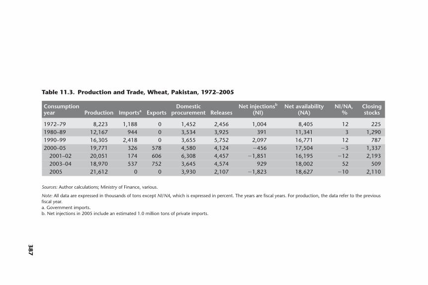
Table 11.3. Production and Trade, Wheat, Pakistan, 1972–2005
Sources: Author calculations; Ministry of Finance, various.
Note: All data are expressed in thousands of tons except NI/NA, which is expressed in percent. The years are fiscal years. For production, the data refer to the previousfiscal year.a. Government imports.b. Net injections in 2005 include an estimated 1.0 million tons of private imports.
Consumption Domestic Net injectionsb Net availability NI/NA, Closing year Production Importsa Exports procurement Releases (NI) (NA) % stocks
1972–79 8,223 1,188 0 1,452 2,456 1,004 8,405 12 2251980–89 12,167 944 0 3,534 3,925 391 11,341 3 1,2901990–99 16,305 2,418 0 3,655 5,752 2,097 16,771 12 7872000–05 19,771 326 578 4,580 4,124 �456 17,504 �3 1,337
2001–02 20,051 174 606 6,308 4,457 �1,851 16,195 �12 2,1932003–04 18,970 537 752 3,645 4,574 929 18,002 52 5092005 21,612 0 0 3,930 2,107 �1,823 18,627 �10 2,110
387
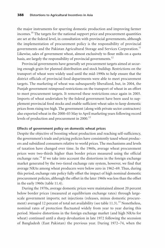
the major instruments for spurring domestic production and improving farmerincomes.10 The targets for the national support price and procurement quantitiesare set at the federal level, in consultation with provincial governments, althoughthe implementation of procurement policy is the responsibility of provincial governments and the Pakistan Agricultural Storage and Services Corporation.11
Likewise, sales of government wheat, almost exclusively to flour mills on a quotabasis, are largely the responsibility of provincial governments.12
Provincial governments have generally set procurement targets aimed at secur-ing enough grain for planned distribution and stock buildup. Restrictions on thetransport of wheat were widely used until the mid-1990s to help ensure that thedistrict officials of provincial food departments were able to meet procurementtargets. The marketing of wheat was subsequently liberalized, but, in 2004, thePunjab government reimposed restrictions on the transport of wheat in an effortto meet procurement targets. It removed these restrictions once again in 2005.Imports of wheat undertaken by the federal government have been used to sup-plement provincial food stocks and enable sufficient wheat sales to keep domesticprices from rising too high. The government (along with private sector contractors)also exported wheat in the 2000–03 May to April marketing years following recordlevels of production and procurement in 2000.13
Effects of government policy on domestic wheat pricesDespite the objective of boosting wheat production and reaching self-sufficiency,the government’s trade and pricing policies have consistently taxed wheat produc-ers and subsidized consumers relative to world prices. The mechanisms and levelsof taxation have changed over time. In the 1960s, average wheat procurementprices were two-thirds higher than border prices measured using the officialexchange rate.14 If we take into account the distortions in the foreign exchangemarket generated by the two-tiered exchange rate system, however, we find thataverage NRAs among wheat producers were below zero in 1962–69. Thus, duringthis period, exchange rate policy fully offset the impact of high nominal domesticprocurement policies, although the offset in the later 1960s was less than the offsetin the early 1960s (table 11.4).
During the 1970s, average domestic prices were maintained almost 20 percentbelow border prices (measured at equilibrium exchange rates) through large-scale government imports; net injections (releases, minus domestic procure-ment) averaged 12 percent of total net availability (see table 11.3).15 Nonetheless,nominal rates of protection fluctuated widely from year to year during thisperiod. Massive distortions in the foreign exchange market (and high NRAs forwheat) continued until a sharp devaluation in late 1972 following the secessionof Bangladesh (East Pakistan) the previous year. During 1972–74, when the
388 Distortions to Agricultural Incentives in Asia
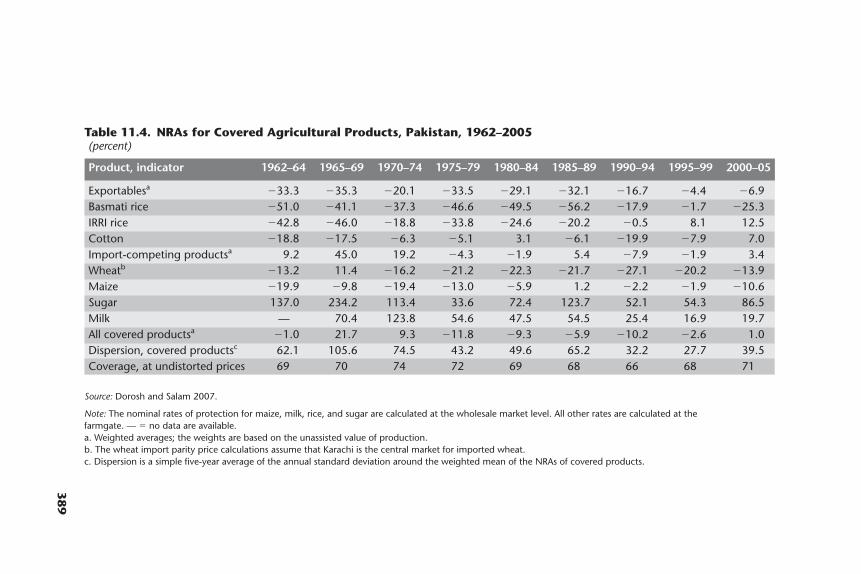
Table 11.4. NRAs for Covered Agricultural Products, Pakistan, 1962–2005(percent)
Source: Dorosh and Salam 2007.
Note: The nominal rates of protection for maize, milk, rice, and sugar are calculated at the wholesale market level. All other rates are calculated at thefarmgate. — � no data are available.a. Weighted averages; the weights are based on the unassisted value of production.b. The wheat import parity price calculations assume that Karachi is the central market for imported wheat.c. Dispersion is a simple five-year average of the annual standard deviation around the weighted mean of the NRAs of covered products.
Product, indicator 1962–64 1965–69 1970–74 1975–79 1980–84 1985–89 1990–94 1995–99 2000–05
Exportablesa �33.3 �35.3 �20.1 �33.5 �29.1 �32.1 �16.7 �4.4 �6.9Basmati rice �51.0 �41.1 �37.3 �46.6 �49.5 �56.2 �17.9 �1.7 �25.3IRRI rice �42.8 �46.0 �18.8 �33.8 �24.6 �20.2 �0.5 8.1 12.5Cotton �18.8 �17.5 �6.3 �5.1 3.1 �6.1 �19.9 �7.9 7.0Import-competing productsa 9.2 45.0 19.2 �4.3 �1.9 5.4 �7.9 �1.9 3.4Wheatb �13.2 11.4 �16.2 �21.2 �22.3 �21.7 �27.1 �20.2 �13.9Maize �19.9 �9.8 �19.4 �13.0 �5.9 1.2 �2.2 �1.9 �10.6Sugar 137.0 234.2 113.4 33.6 72.4 123.7 52.1 54.3 86.5Milk — 70.4 123.8 54.6 47.5 54.5 25.4 16.9 19.7All covered productsa �1.0 21.7 9.3 �11.8 �9.3 �5.9 �10.2 �2.6 1.0Dispersion, covered productsc 62.1 105.6 74.5 43.2 49.6 65.2 32.2 27.7 39.5Coverage, at undistorted prices 69 70 74 72 69 68 66 68 71
389
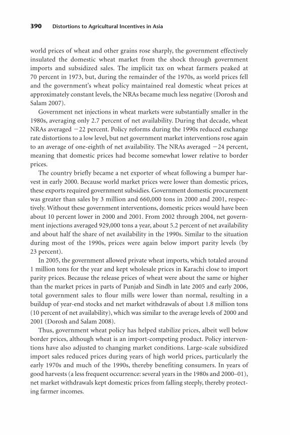
world prices of wheat and other grains rose sharply, the government effectivelyinsulated the domestic wheat market from the shock through governmentimports and subsidized sales. The implicit tax on wheat farmers peaked at70 percent in 1973, but, during the remainder of the 1970s, as world prices felland the government’s wheat policy maintained real domestic wheat prices atapproximately constant levels, the NRAs became much less negative (Dorosh andSalam 2007).
Government net injections in wheat markets were substantially smaller in the1980s, averaging only 2.7 percent of net availability. During that decade, wheatNRAs averaged �22 percent. Policy reforms during the 1990s reduced exchangerate distortions to a low level, but net government market interventions rose againto an average of one-eighth of net availability. The NRAs averaged �24 percent,meaning that domestic prices had become somewhat lower relative to borderprices.
The country briefly became a net exporter of wheat following a bumper har-vest in early 2000. Because world market prices were lower than domestic prices,these exports required government subsidies. Government domestic procurementwas greater than sales by 3 million and 660,000 tons in 2000 and 2001, respec-tively. Without these government interventions, domestic prices would have beenabout 10 percent lower in 2000 and 2001. From 2002 through 2004, net govern-ment injections averaged 929,000 tons a year, about 5.2 percent of net availabilityand about half the share of net availability in the 1990s. Similar to the situationduring most of the 1990s, prices were again below import parity levels (by23 percent).
In 2005, the government allowed private wheat imports, which totaled around1 million tons for the year and kept wholesale prices in Karachi close to importparity prices. Because the release prices of wheat were about the same or higherthan the market prices in parts of Punjab and Sindh in late 2005 and early 2006,total government sales to flour mills were lower than normal, resulting in abuildup of year-end stocks and net market withdrawals of about 1.8 million tons(10 percent of net availability), which was similar to the average levels of 2000 and2001 (Dorosh and Salam 2008).
Thus, government wheat policy has helped stabilize prices, albeit well belowborder prices, although wheat is an import-competing product. Policy interven-tions have also adjusted to changing market conditions. Large-scale subsidizedimport sales reduced prices during years of high world prices, particularly theearly 1970s and much of the 1990s, thereby benefiting consumers. In years ofgood harvests (a less frequent occurrence: several years in the 1980s and 2000–01),net market withdrawals kept domestic prices from falling steeply, thereby protect-ing farmer incomes.
390 Distortions to Agricultural Incentives in Asia
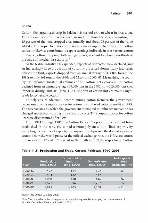
Cotton
Cotton, the largest cash crop in Pakistan, is second only to wheat in area sown.The area under cotton has averaged around 3 million hectares, accounting for15 percent of the total cropped area annually and about 25 percent of the valueadded in key crops. Domestic cotton is also a major input into textiles. The cottonsubsector likewise contributes to export earnings indirectly in that various cottonproducts (cotton lint, yarn, cloth, and garments) account for about two-thirds ofthe value of merchandise exports.16
As the textile industry has expanded, exports of raw cotton have declined, andan increasingly large proportion of cotton is processed domestically into yarn.Raw cotton (lint) exports dropped from an annual average of 414,000 tons in the1980s to only 161 tons in the 1990s and 72 tons in 2000–05. Meanwhile, the coun-try has imported substantial volumes of lint cotton; net exports in lint cottondeclined from an annual average 408,000 tons in the 1980s to �205,000 tons (netimports) during 2001–05 (table 11.5). Imports of cotton lint are mainly high-grade longer-staple cottons.
To help ensure adequate incomes among cotton farmers, the governmentbegan announcing support prices for cotton lint and seed cotton (phutti) in 1975.The mechanisms by which the government attempted to influence market priceschanged substantially during this period, however. Thus, support prices for cottonlint were discontinued after 1995.
From 1974 through 1986, the Cotton Export Corporation, which had beenestablished in the early 1970s, had a monopoly on cotton (lint) exports. Byrestricting the volume of exports, the corporation depressed the domestic price ofcotton below the world price. At the official exchange rate, the NRAs on cottonlint averaged �12 and �9 percent in the 1970s and 1980s, respectively. Cotton
Pakistan 391
Table 11.5. Production and Trade, Cotton, Pakistan, 1960–2005
Exports net of Net exports Production, imports, Domestic use, in total
Year tons, 1,000s tons, 1,000s tons, 1,000s production, %
1960–69 427 114 307 271970–79 584 132 447 211980–89 1,068 408 616 361990–99 1,627 96 1,487 52000–05 1,925 �205 2,108 �11
Source: PSD Online Database 2008.
Note: The data refer to the subsequent cotton marketing year. For example, the cotton harvest ofOctober–December 2004 is indicated as 2005.

producers nonetheless benefited from the trade protection for vegetable oils thatboosted the domestic price of cottonseed, which averaged approximately one-quarter of the value of seed cotton in 2000–04. Including the protection on cot-tonseed, the total NRAs for cotton farmers were less negative. However, if the dualexchange rate system is taken into account, the average NRAs for cotton become�18 percent in the 1960s, �6 percent in the 1970s, and �2 percent in the 1980s(see table 11.4).
Beginning in 1986 and continuing through 1993, export taxes on cotton werecalculated as a fixed percentage of the margin between the benchmark price (thetarget ex-gin price of lint, plus export incidentals) and the minimum export price,which is fixed daily by the Interagency Committee and announced by the StateBank of Pakistan. That minimum export price is based on the international pricesof lint, the domestic prices of yarn and lint, the domestic requirements of theindustry, and the global and local supply situation.17 The tax rate on this marginand the benchmark price were adjusted frequently, however, because the govern-ment was attempting to maximize export tax receipts and ensure low prices forthe domestic yarn and textile industries.18 This system of variable export taxeseffectively insulated the domestic market from movements in international prices.Nonetheless, the underinvoicing of cotton exports continued through the ship-ment of grades higher than the declared grades.
Poor domestic cotton harvests in 1993 and 1994 caused the country to becomea net importer of cotton; imports were around 100,000 tons each year. Theincreasing cotton imports and the dwindling availability of cotton for exportbrought into focus the demerits of the benchmark system, which heavily taxedcotton farmers, but provided cheap raw materials for the textile industry andencouraged inefficiency in the textile subsector. There was great resentment andopposition against the system among farmers, who demanded the elimination ofthe system. The export duty on cotton was thus abolished in 1994, and, since the1994 cotton season, domestic prices have been in line with or higher than interna-tional prices.
Since 1994, the demand for lint in the textile subsector has outpaced supply,and the country has become a net importer of cotton lint. Gross imports averaged259,000 tons per year during 2000–04. Moreover, despite the expiration of theMultifiber Agreement at the end of 2004, the country’s textile subsector has flour-ished. The imports of lint in 2005 approximated the levels in each of the previoustwo years, about 400,000 tons.
Export and import duties on cotton have been low since the mid-1990s, anddirect market interventions have likewise been minimal, except in 2004, when theTrading Corporation of Pakistan bought 270,000 tons of cotton (11 percent of pro-duction) in an effort to boost domestic prices.19 However, annual price movements
392 Distortions to Agricultural Incentives in Asia
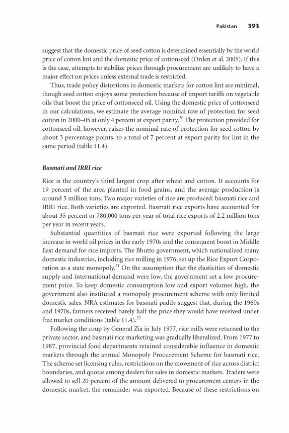
suggest that the domestic price of seed cotton is determined essentially by the worldprice of cotton lint and the domestic price of cottonseed (Orden et al. 2005). If thisis the case, attempts to stabilize prices through procurement are unlikely to have amajor effect on prices unless external trade is restricted.
Thus, trade policy distortions in domestic markets for cotton lint are minimal,though seed cotton enjoys some protection because of import tariffs on vegetableoils that boost the price of cottonseed oil. Using the domestic price of cottonseedin our calculations, we estimate the average nominal rate of protection for seedcotton in 2000–05 at only 4 percent at export parity.20 The protection provided forcottonseed oil, however, raises the nominal rate of protection for seed cotton byabout 3 percentage points, to a total of 7 percent at export parity for lint in thesame period (table 11.4).
Basmati and IRRI rice
Rice is the country’s third largest crop after wheat and cotton. It accounts for19 percent of the area planted in food grains, and the average production isaround 5 million tons. Two major varieties of rice are produced: basmati rice andIRRI rice. Both varieties are exported. Basmati rice exports have accounted forabout 35 percent or 780,000 tons per year of total rice exports of 2.2 million tonsper year in recent years.
Substantial quantities of basmati rice were exported following the largeincrease in world oil prices in the early 1970s and the consequent boost in MiddleEast demand for rice imports. The Bhutto government, which nationalized manydomestic industries, including rice milling in 1976, set up the Rice Export Corpo-ration as a state monopoly.21 On the assumption that the elasticities of domesticsupply and international demand were low, the government set a low procure-ment price. To keep domestic consumption low and export volumes high, thegovernment also instituted a monopoly procurement scheme with only limiteddomestic sales. NRA estimates for basmati paddy suggest that, during the 1960sand 1970s, farmers received barely half the price they would have received underfree market conditions (table 11.4).22
Following the coup by General Zia in July 1977, rice mills were returned to theprivate sector, and basmati rice marketing was gradually liberalized. From 1977 to1987, provincial food departments retained considerable influence in domesticmarkets through the annual Monopoly Procurement Scheme for basmati rice.The scheme set licensing rules, restrictions on the movement of rice across districtboundaries, and quotas among dealers for sales in domestic markets. Traders wereallowed to sell 20 percent of the amount delivered to procurement centers in thedomestic market; the remainder was exported. Because of these restrictions on
Pakistan 393
domestic supply, consumer prices were substantially above procurement prices.Compulsory procurement was abandoned during the 1986 harvest season. Lim-ited private sector exports were allowed, and procurement prices were raised. Thesystem of voluntary procurement at the announced support price of paddy con-tinued to 2001.
Over 60 percent of the IRRI rice produced in the country is produced inSindh, where it is also a staple food. Government policies on IRRI rice includedannounced support prices and domestic procurement, although, in the 1970s and1980s, the Rice Export Corporation did not procure IRRI rice in Punjab becausethe higher transport costs relative to Sindh, the center of procurement, madeexports of Punjab rice unprofitable. The NRAs for IRRI rice, calculated on thebasis of world rice prices, show that producer taxation in the 1980s was slightlymore than 20 percent, but that the taxation has gradually disappeared sincethen.23 In 2003, the government began announcing indicative prices for paddy,but procurement has been minimal. Currently, no export tax is levied on rice, andimports are subject to a 10 percent customs duty. This is reflected in the IRRI riceNRAs of 12.5 percent in 2000–05 (table 11.4).
Sugarcane
Sugarcane, which is cultivated exclusively on irrigated land in Pakistan, accountsfor 4 or 5 percent of the 22 million cropped hectares per year in the country.About half the area under sugarcane is represented by farms operating on lessthan 5 hectares. The geographical distribution of sugarcane production follows apattern that is similar to the pattern in other irrigated crops, that is, two-thirds ofthe crop is cultivated in Punjab, and about one-fourth in Sindh. The area plantedin sugarcane rose by 61 percent between 1979 and 1999. This was accompanied bya rise in the number of sugar mills, from 32 in 1980 to 79 in 2005, all of which arenow in the private sector. Crop production is highly variable because of changingprice incentives and fluctuations in water availability that influence the area undercultivation and the yields. Sugarcane production in Punjab ranged from 19 mil-lion to 34 million tons and, in Sindh, from 9 million to 17 million tons in1979–2005. To stabilize prices despite the variations in production, the govern-ment frequently adjusts import tariffs (set at 15 percent in 2005) and the relatedtaxes on sugar; it has also applied export bans.
The domestic marketing and processing of sugarcane were highly regulateduntil the mid-1980s. The zoning of sugar mills, whereby each farmer was requiredto sell 80 percent of the farm’s sugarcane output to mills located in the local zone,was abolished in 1987, freeing farmers to sell their sugarcane to the mills they pre-ferred. Until 2000, the government announced a support price for sugarcane each
394 Distortions to Agricultural Incentives in Asia

year; since then, support prices have been determined by provincial governments.However, there is no institutional arrangement for the public sector procurementof sugarcane if sugar mills do not pay farmers the full support price.24
Because of the wide variations in domestic production and in world prices,domestic sugar prices and the measured NRAs have also fluctuated greatly. In gen-eral, though, sugarcane and refined sugar production have been highly protected.The NRAs averaged over 100 percent in the 1960s, the early 1970s, and the later1980s, when the international prices fell again. Since then, the NRAs haveremained above 50 percent (table 11.4).
Maize
Maize is counted as a major crop, although it is sown in a total area of less than1 million hectares (one-eighth of the area given over to wheat). Production averaged2.1 million tons per year in 2002–04, which represented 8 percent of total grain pro-duction. Maize is cultivated on irrigated and nonirrigated land mainly in NorthWest Frontier Province (57 percent of the area under maize) and Punjab (41 percentof the maize area). The area under cultivation expanded by an average 1.0 percentper year from 1989 to 2005, and the adoption of hybrid maize planted in the springon irrigated land contributed to a 4.7 percent growth in yields per year. Most maizeis used as livestock and poultry feed, and this application has expanded rapidlyalong with the growth in the domestic demand for poultry products.
Apart from import duties, which have ranged from 10 to 25 percent since themid-1990s, the government has not intervened in maize production and market-ing. Maize has often been a nontradable since the 1980s because domestic priceshave been below the import parity prices (even without import tariffs), but aboveexport parity prices. Thus, the protection from import competition provided bytariffs has had little effect on domestic prices, and maize NRAs have been close tozero (table 11.4).
Milk
To protect the domestic dairy industry, the government has consistently leviedtariffs on imported milk powder. The NRAs arising from these tariffs averagedabove 70 percent in the 1960s and 1970s.25 The tariff rates for milk powder werelowered in the early 1990s and have ranged from 20 to 45 percent since the mid-1990s. The NRAs averaged 40 percent in the 1990s and 20 percent from 2000through 2005. The contrast between this high level of assistance for dairying andfor sugar and the much lower, usually negative NRAs for the other covered prod-ucts is evident in figure 11.3.
Pakistan 395
Edible oils and oilseeds
The country meets over two-thirds of its edible oil requirements throughimports, which rose from 1.1 million tons in 2000 to 1.6 million tons in 2004. Invalue terms, imports of edible oils more than doubled, from US$326 million toUS$758 million during this period. Traditional sources of domestic edible oilproduction have been cottonseed (a by-product of cotton farming), rapeseeds,and mustard.26 The area under rapeseed and mustard, sown in winter, has aver-aged 273,000 hectares in recent years. Sunflowers and soybeans were introducedin the 1980s and promoted through various development schemes and policymeasures, including attractive support prices to encourage production and pro-curement by public sector agencies and facilitate marketing. The area planted insunflowers increased rapidly, especially in southern Punjab and lower Sindh,from 108,000 hectares in 2002 to 264,000 hectares in 2004.27
There was little direct taxation of imported vegetable oils in the 1970s and 1980s.Exchange rate distortions led to an implicit subsidy on imports (and taxation ofdomestic producers) of only 3 percent in the 1970s and zero in the 1980s. Since theearly 1990s, however, vegetable oils have been consistently taxed. For example, from2000 through 2005, import tariffs on soybean oil were PRs 9,050 per ton, which was
396 Distortions to Agricultural Incentives in Asia
�60
�40
sugar milk basmati rice IRRI rice
product
wheat maize cotton
�20
0
60
40
80
20
100185
NRA
, %
1962–69 1970–79 1980–89 1990–99 2000–05
Figure 11.3. NRAs for Major Covered Products, Pakistan,1962–2005
Source: Dorosh and Salam 2007.

Pakistan 397
equivalent to an average 32 percent of the import value (using the average price ofimports for each year). Import tariffs on palm oil were equivalent to about 40 per-cent of the import value. Likewise, except for three years in which world prices wererelatively high (1994, 1995, and 1997), the domestic prices of sunflower seeds havebeen substantially higher than the estimated border prices. We have not calculatedNRAs for these products, however, because edible oils as a group constitute a tinyfraction of the value of the country’s agricultural production.
Distortions in input prices
The major distortion in nonfactor input prices in agriculture has been the subsidyfor nitrogenous fertilizer.28 The domestic producer prices of nitrogenous fertilizers,mainly urea, have been kept consistently below import parity border prices. This hasbeen achieved by using domestic natural gas inputs in domestic fertilizer produc-tion and passing on some of the savings to farmers through a discounted price.Since the early 1990s, there has been little or no subsidy for diammonium phosphateand other major fertilizers that are generally not produced domestically and there-fore must be imported. In the later 1970s and the 1980s, the domestic prices of ureaand diammonium phosphate averaged between 30 and 45 percent less than theimport parity prices. From 1990 to 2005, however, the domestic price of diammo-nium phosphate was an average of only 4 percent less than the import parity price,while the price of urea was 38 percent less than the border price.
The cost of urea and the cost of diammonium phosphate represented 8 and 10percent, respectively, of the value of wheat production according to estimates ofthe Agricultural Prices Commission for 2002. This implicit subsidy on fertilizerwas equivalent to about 3 percent (0.08 * 0.38) of the value of wheat productionfrom 1990 to 2005. Thus, the NRAs for wheat in this period should be inflated byabout 3 percentage points. For the late 1970s and the 1980s, when diammoniumphosphate was subsidized as well, the NRAs for wheat should be about 7 percent-age points (0.18 * 0.40) higher. The NRAs for paddy, cotton, and sugarcane arealso understated by similar amounts in the two periods. These calculations arerather imprecise. They do not include water subsidies, but we nonetheless addthem to the NRA time series for the various crops for completeness and becausethey are nontrivial.
Assistance for Agricultural Tradables Relativeto Nonagricultural Tradables
Using the values of production at undistorted prices as weights, we have obtaineda weighted average of the above NRA estimates. This information is provided intable 11.4, along with separate averages for the import-competing and exportable
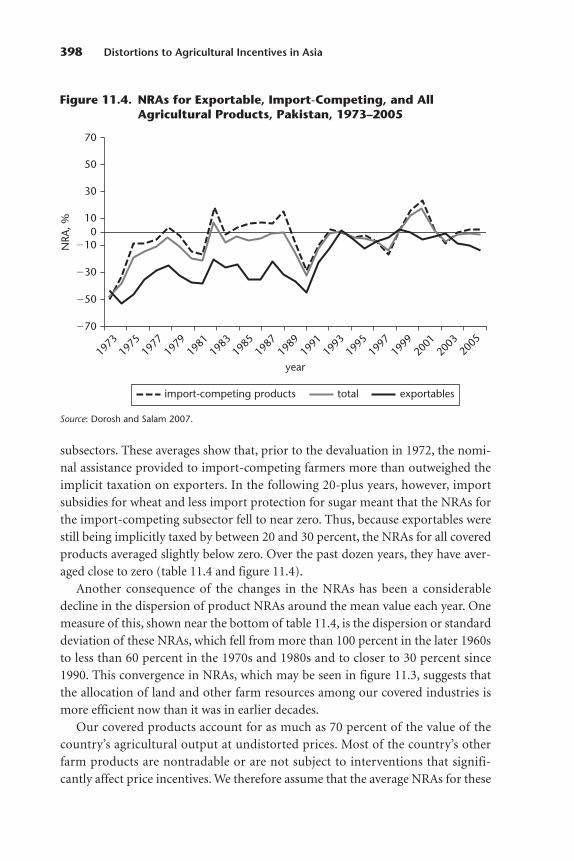
subsectors. These averages show that, prior to the devaluation in 1972, the nomi-nal assistance provided to import-competing farmers more than outweighed theimplicit taxation on exporters. In the following 20-plus years, however, importsubsidies for wheat and less import protection for sugar meant that the NRAs forthe import-competing subsector fell to near zero. Thus, because exportables werestill being implicitly taxed by between 20 and 30 percent, the NRAs for all coveredproducts averaged slightly below zero. Over the past dozen years, they have aver-aged close to zero (table 11.4 and figure 11.4).
Another consequence of the changes in the NRAs has been a considerabledecline in the dispersion of product NRAs around the mean value each year. Onemeasure of this, shown near the bottom of table 11.4, is the dispersion or standarddeviation of these NRAs, which fell from more than 100 percent in the later 1960sto less than 60 percent in the 1970s and 1980s and to closer to 30 percent since1990. This convergence in NRAs, which may be seen in figure 11.3, suggests thatthe allocation of land and other farm resources among our covered industries ismore efficient now than it was in earlier decades.
Our covered products account for as much as 70 percent of the value of thecountry’s agricultural output at undistorted prices. Most of the country’s otherfarm products are nontradable or are not subject to interventions that signifi-cantly affect price incentives. We therefore assume that the average NRAs for these
398 Distortions to Agricultural Incentives in Asia
�70
year
�50
�30
30
100
50
�10
70
NRA
, %
1973
1975
1977
1979
1981
1983
1985
1987
1989
1991
1993
1995
1997
1999
2001
2003
2005
exportablestotalimport-competing products
Figure 11.4. NRAs for Exportable, Import-Competing, and AllAgricultural Products, Pakistan, 1973–2005
Source: Dorosh and Salam 2007.
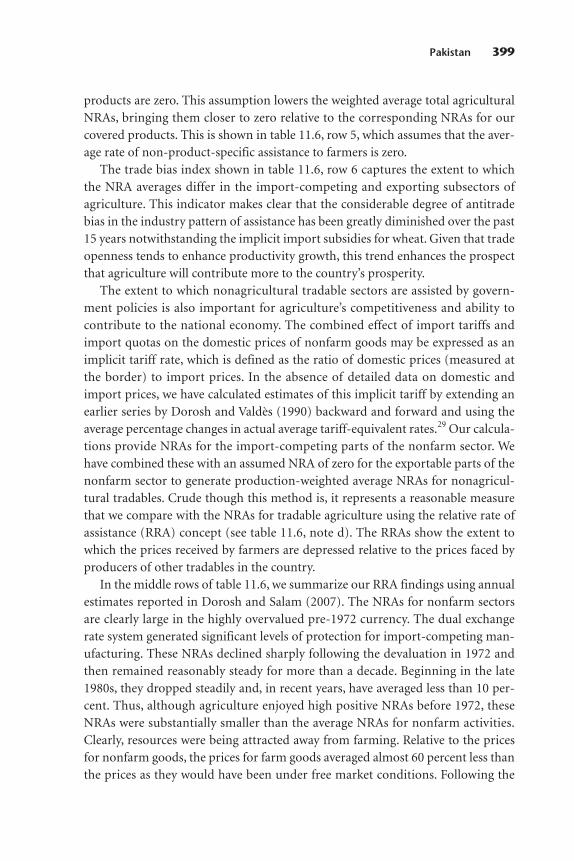
Pakistan 399
products are zero. This assumption lowers the weighted average total agriculturalNRAs, bringing them closer to zero relative to the corresponding NRAs for ourcovered products. This is shown in table 11.6, row 5, which assumes that the aver-age rate of non-product-specific assistance to farmers is zero.
The trade bias index shown in table 11.6, row 6 captures the extent to whichthe NRA averages differ in the import-competing and exporting subsectors ofagriculture. This indicator makes clear that the considerable degree of antitradebias in the industry pattern of assistance has been greatly diminished over the past15 years notwithstanding the implicit import subsidies for wheat. Given that tradeopenness tends to enhance productivity growth, this trend enhances the prospectthat agriculture will contribute more to the country’s prosperity.
The extent to which nonagricultural tradable sectors are assisted by govern-ment policies is also important for agriculture’s competitiveness and ability tocontribute to the national economy. The combined effect of import tariffs andimport quotas on the domestic prices of nonfarm goods may be expressed as animplicit tariff rate, which is defined as the ratio of domestic prices (measured atthe border) to import prices. In the absence of detailed data on domestic andimport prices, we have calculated estimates of this implicit tariff by extending anearlier series by Dorosh and Valdès (1990) backward and forward and using theaverage percentage changes in actual average tariff-equivalent rates.29 Our calcula-tions provide NRAs for the import-competing parts of the nonfarm sector. Wehave combined these with an assumed NRA of zero for the exportable parts of thenonfarm sector to generate production-weighted average NRAs for nonagricul-tural tradables. Crude though this method is, it represents a reasonable measurethat we compare with the NRAs for tradable agriculture using the relative rate ofassistance (RRA) concept (see table 11.6, note d). The RRAs show the extent towhich the prices received by farmers are depressed relative to the prices faced byproducers of other tradables in the country.
In the middle rows of table 11.6, we summarize our RRA findings using annualestimates reported in Dorosh and Salam (2007). The NRAs for nonfarm sectorsare clearly large in the highly overvalued pre-1972 currency. The dual exchangerate system generated significant levels of protection for import-competing man-ufacturing. These NRAs declined sharply following the devaluation in 1972 andthen remained reasonably steady for more than a decade. Beginning in the late1980s, they dropped steadily and, in recent years, have averaged less than 10 per-cent. Thus, although agriculture enjoyed high positive NRAs before 1972, theseNRAs were substantially smaller than the average NRAs for nonfarm activities.Clearly, resources were being attracted away from farming. Relative to the pricesfor nonfarm goods, the prices for farm goods averaged almost 60 percent less thanthe prices as they would have been under free market conditions. Following the
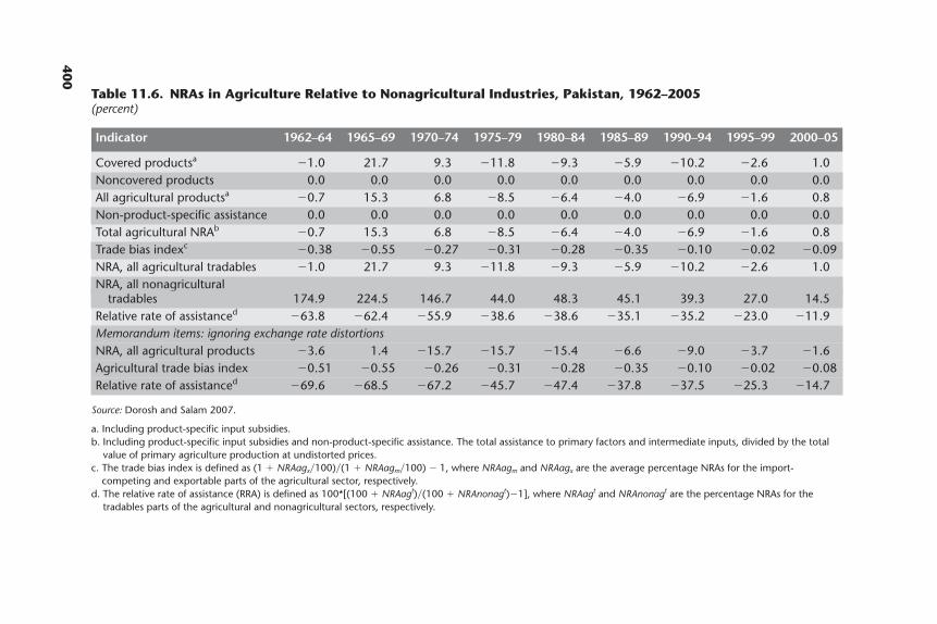
400
Table 11.6. NRAs in Agriculture Relative to Nonagricultural Industries, Pakistan, 1962–2005(percent)
Source: Dorosh and Salam 2007.
a. Including product-specific input subsidies.b. Including product-specific input subsidies and non-product-specific assistance. The total assistance to primary factors and intermediate inputs, divided by the total
value of primary agriculture production at undistorted prices.c. The trade bias index is defined as (1 � NRAagx�100)�(1 � NRAagm�100) � 1, where NRAagm and NRAagx are the average percentage NRAs for the import-
competing and exportable parts of the agricultural sector, respectively.d. The relative rate of assistance (RRA) is defined as 100*[(100 � NRAagt)�(100 � NRAnonagt)�1], where NRAagt and NRAnonagt are the percentage NRAs for the
tradables parts of the agricultural and nonagricultural sectors, respectively.
Indicator 1962–64 1965–69 1970–74 1975–79 1980–84 1985–89 1990–94 1995–99 2000–05
Covered productsa �1.0 21.7 9.3 �11.8 �9.3 �5.9 �10.2 �2.6 1.0Noncovered products 0.0 0.0 0.0 0.0 0.0 0.0 0.0 0.0 0.0All agricultural productsa �0.7 15.3 6.8 �8.5 �6.4 �4.0 �6.9 �1.6 0.8Non-product-specific assistance 0.0 0.0 0.0 0.0 0.0 0.0 0.0 0.0 0.0Total agricultural NRAb �0.7 15.3 6.8 �8.5 �6.4 �4.0 �6.9 �1.6 0.8Trade bias indexc �0.38 �0.55 �0.27 �0.31 �0.28 �0.35 �0.10 �0.02 �0.09NRA, all agricultural tradables �1.0 21.7 9.3 �11.8 �9.3 �5.9 �10.2 �2.6 1.0NRA, all nonagricultural
tradables 174.9 224.5 146.7 44.0 48.3 45.1 39.3 27.0 14.5Relative rate of assistanced �63.8 �62.4 �55.9 �38.6 �38.6 �35.1 �35.2 �23.0 �11.9Memorandum items: ignoring exchange rate distortionsNRA, all agricultural products �3.6 1.4 �15.7 �15.7 �15.4 �6.6 �9.0 �3.7 �1.6Agricultural trade bias index �0.51 �0.55 �0.26 �0.31 �0.28 �0.35 �0.10 �0.02 �0.08Relative rate of assistanced �69.6 �68.5 �67.2 �45.7 �47.4 �37.8 �37.5 �25.3 �14.7
1972 devaluation, the degree of antiagricultural bias diminished somewhat, butthe RRAs still averaged around �35 percent until the early 1990s. The RRAs beganto rise significantly then, and, since the late 1990s, they have averaged less than�10 percent (figure 11.5). So, an antiagricultural bias remains, but it is small relative to the corresponding bias that prevailed during 1970s and 1980s and,especially, during the decades before the secession of Bangladesh (East Pakistan)from Pakistan in the early 1970s.
In table 11.6, we also report how the estimated NRAs, RRAs, and trade biasindex for agriculture would differ if we had not taken into account the dualexchange rate, which added to the antitrade bias. A comparison of the two sets ofnumbers suggests that, if we had not used the dual exchange rate, we would haveoverstated the degree of direct and indirect taxation of agriculture, especially inthe later 1960s and early 1970s before the devaluation.
Political Economy and Conclusions
The government of Pakistan has a long history of intervening in agriculturalproduct markets to influence prices, production, and total supply. In major foodcommodities, particularly wheat, consumer interests have tended to outweigh
Pakistan 401
�70
year
�10
20
0
�40
80
50
110
per
cent
1973
1975
1977
1979
1981
1983
1985
1987
1989
1991
1993
1995
1997
1999
2001
2003
2005
RRANRA, nonagricultural tradablesNRA, agricultural tradables
Figure 11.5. NRAs for Agricultural and NonagriculturalTradables and the RRA, Pakistan, 1973–2005
Source: Dorosh and Salam 2007.
Note: For the definition of the RRA, see table 11.6, note d.

producer interests in determining policy, and domestic prices have generally beenkept below free trade levels. In cotton, industrialists in the spinning, weaving, andclothing industries benefited from policies to keep the domestic price of the rawmaterials low. Producers of rice, a major export, were taxed until the mid-1990sthrough restrictions on sales or through explicit export taxes and controls. Amongmajor commodities, only producers of milk and vegetable oils have consistentlygained from government trade and pricing policies (mainly import tariffs). Off-setting the negative effects on output prices to some extent, however, have beenthe implicit subsidies on canal water (irrigation fees have been lower than thecanal maintenance costs), electricity, fuel for pumps, fertilizers, and credit for thepurchase of tractors.
Competing interests and the relative strengths of various groups of stakeholdershelp explain the diversity in policies. In the case of wheat, for example, farmers, par-ticularly farmers achieving net sales, benefit from increases in procurement pricesand quantities.30 Flour millers are able to gain from low issue (sales) prices for wheatthat are typically below open market prices. Low market prices for wheat and wheatflour benefit the net buyers of this staple, who account for about 80 percent of thecountry’s population. Provincial food departments make a great effort to achievedomestic procurement targets that provide most of the grain for subsequent distri-bution. Large-scale procurement and subsidized sales create the possibility for sub-stantial economic rents. Sales of grain (at the issue price) from the surplusprovinces—typically, Punjab—to other provincial food departments involve animplicit cross-subsidization to the receiving provinces because issue prices do notcover the full cost of procurement, storage, and distribution. The provincial and fed-eral governments are also concerned to minimize fiscal subsidies and overall infla-tion. Donors have generally pushed for reductions in food subsidies and anincreased role for the private sector in wheat marketing.
In cotton and sugarcane, agricultural processors have an even stronger influ-ence on policies. Industrialists in the spinning, weaving, and clothing industrieshave a dominant voice in cotton policy debates because of the importance of thesesubsectors in terms of value added, employment, and foreign exchange earnings.The position of sugar millers is stronger than the position of the processors ofmost other crops because the high transport costs and the perishability of theinput (the yield of sugar—the rendement—produced from harvested sugarcanedrops sharply within days of the harvest) limit the competition among sugarmills. Consequently, relations between farmers and sugar mills have been tenuousat best, and this has adversely affected the development of sugarcane and relatedsubsectors. However, despite the opposing interests of processors and consumers(see above), farmers in Pakistan have more political power to defend their inter-ests than do farmers in many developing countries with more equal distribution
402 Distortions to Agricultural Incentives in Asia
of land. This is because the presence of many large farmers gives the agriculturalsector a stronger voice in political debates.
Nonetheless, macroeconomic considerations, the demonstration effect ofbroad trade liberalization in other countries, and pressure from donors haveresulted in a general reduction in the level of government interventions and theextent of policy-induced agricultural price distortions since the 1970s despite thecompeting interests of producers and consumers. During the 1970s, the Bhuttogovernment nationalized major industries and set up agricultural marketinginstitutions that played a major role in the agricultural markets for wheat, cotton,rice, and sugarcane. Broad trade and macropolicy reforms in the mid-1980sreduced overall import protection both directly and through exchange rate distor-tions. Price distortions were substantially reduced, but the agricultural marketinginstitutions of the 1970s were left in place. Reforms in the 1990s were deeper inthe sense that government direct interventions in markets (the buying and sellingof commodities) were dramatically reduced in cotton and rice; the Rice ExportCorporation of Pakistan and the Cotton Export Corporation were abolished; andprivate sector involvement in external trade was generally encouraged. Distortionswere reduced in trade overall and in the trade for agricultural products. Since2000, the price distortions in agricultural markets have remained relatively small.However, the government continues to intervene heavily in wheat markets in waysthat incur significant costs, but that have generally had little effect on marketprices, although the purchasing following the bumper wheat harvest of 2000 is anexception. The government also reentered the cotton market following thebumper cotton crop in 2004.
The government’s agricultural and trade policies are far more liberalized nowthan they were 30 years ago, and price distortions across sectors are generallysmall. Nonetheless, the pressure exerted by various stakeholders continues toinfluence government policy decisions to intervene directly in the markets for themain farm products, particularly in years of bumper harvests that threaten dra-matically to reduce producer prices or in situations of supply shortfalls in keyconsumer goods (for example, wheat and sugar). Maintaining consistent andtransparent policies is thus crucial for improvements in market efficiency. Overall,price distortions are no longer a major constraint on agricultural growth and thereal incomes of farmers, but the sector could contribute more to economic pros-perity if the dispersion in NRAs among farm products were reduced.
Notes
1. Throughout the chapter, the data and policy analysis refer to the current territory of Pakistan,which, prior to 1971, was West Pakistan. In that year, East Pakistan became the independent country ofBangladesh.
Pakistan 403
2. Throughout this chapter, crop or fiscal years are indicated by the second of the two calendaryears; for example, 2005 refers to the 2004/05 crop or fiscal year.
3. See Hamid, Nabi, and Nasim (1990) for a detailed discussion of the government’s trade andexchange rate policies from the 1960s to the mid-1980s.
4. According to economic theory, nominal devaluations alone do not cause real exchange ratechanges. However, because of import quotas, the nominal devaluations in Pakistan also directlyreduced the implicit tariff on imports, a policy shift that does affect relative prices.
5. Note that, to the extent domestic goods also pay sales taxes, these import sales taxes do not rep-resent a trade policy distortion if they are applied in lieu of sales taxes on imported products.
6. If we utilize a value of �0.41 for the omega parameter, we find that the implicit appreciationof the rupee because of trade policy fell from an average 15 percent in 1985-89 to only 5 percent in2001–03. The omega parameter is defined as the percentage change in the real exchange rate, dividedby the percentage change in trade policy, which is measured as 1, plus the equivalent tariff adjustedfor export taxes. The value of the omega parameter derives from an ordinary least squares estimateusing monthly price and trade data from 1972 to 1987 (Dorosh and Valdès 1990). Cointegration tech-niques were not utilized in the Dorosh and Valdès report, but a regression based on first differences ofvariables resulted in an omega value of �0.54. Note that black market premiums are small in Pakistan after 1985, averaging 6.4 percent from 1985 to 1993 and 12.0 percent from 1996 to 1999. Thereal exchange rate appreciation caused by trade policy, however, is conceptually different from a blackmarket premium, which largely reflects controls on foreign exchange rather than explicit trade policies. See Anderson et al. (2008) and appendix A for a discussion of this issue in the context ofour project.
7. Our NRAs for tradables include an estimate of the trade tax effect of the overvalued exchangerate. For this estimate, we rely on the black market exchange rate premium (see Global DevelopmentNetwork Growth Database). We also assume that only half the foreign exchange rate earnings ofexporters is sold to the government at the official rate. For details on this methodology, see Andersonet al. (2008) and appendix A.
8. Data of the Household Integrated Economic Survey of 2000–01 (FBS 2001) show a slightlyhigher absolute figure (1,052 calories per person per day), but a much higher caloric share (58 percentof 1,819 calories per person per day). Rural consumption per capita is 42 percent higher than urbanconsumption per capita, at 10.3 versus 7.2 kilograms per month.
9. Most wheat is harvested in March and April, which is toward the end of the fiscal year (July to June). In our discussion here, fiscal years are used unless otherwise noted, and we rely on data on production in the previous fiscal year in calculating net availability for the current fiscal year.
10. Provincial governments, particularly the government of Punjab (the largest province), inter-vene heavily in wheat markets. Government procurement averaged 4.0 million tons per year in 2002and 2003, more than 20 percent of production in those years. Punjab alone accounted for almost90 percent of this procurement, equivalent to 27 percent of its wheat production.
11. The corporation supplies wheat to food-deficit provinces, the Northern Areas, Azad Jammuand Kashmir, and the defense establishment.
12. Substantial wheat market liberalization took place in the late 1980s through the abolition ofwheat ration shops and the liberalization of private wheat imports (subsequently disallowed).
13. There are major fiscal subsidies and economic rents involved in the sale of wheat to flourmills at below market rates. Wheat issue prices (the price of wheat sales to flour mills) do not coverthe full cost of procurement (domestic or imported), storage, and handling. Provincial food subsi-dies in 2002 reached PRs 6.8 billion. The subsidies were 12 percent greater than the total Public Sector Development Program budget for the Health Division in 2004 (PRs 6.1 billion). Subsidieson the sale of imported wheat accounted for another PRs 1.2 billion that year. See Dorosh andSalam (2008).
404 Distortions to Agricultural Incentives in Asia

14. Nominal rates of protection are calculated assuming that Karachi serves as the central marketfor wheat, that is, in the absence of distortions, wheat imports would not reach northern Pakistan(Punjab). See appendix A for details on the calculation of border prices.
15. These calculations assume that private sector imports and exports were zero except in 2005;this includes an estimated 1.0 million tons of private sector imports. The data on wheat availability intable 11.3 indicate an excess of net imports over net injections. This gap, equal to 453,000 tons per yearin 1981–90, 321,000 tons per year in 1991–2000, and 204,000 tons per year in 2001–06, reflects net pri-vate sector imports, storage losses, and public stock changes (as well as possible discrepancies acrossdata sources).
16. However, the country also imports some cotton and synthetic yarn, cloth, and garments.17. This system was designed to correct a problem of underinvoicing that had lowered export tax
receipts.18. Private sector exports were allowed again beginning in 1987, but cotton lint had to be pur-
chased initially from the Cotton Export Corporation. In 1988, exporters were allowed to buy cottonfrom ginners directly.
19. The Trading Corporation of Pakistan also procured 35,000 tons (2 percent of production) in2001 to support prices.
20. The import parity price is calculated on the basis of Liverpool Cotton Price Index B; the exportparity price relies on Pakistan’s actual average export price of lint.
21. This history of the rice sector through 1987 is based on Hamid, Nabi, and Nasim (1990).22. The calculations of the border price by the Agricultural Prices Commission set a high cost for
transport and processing for basmati rice from Punjab to Karachi (the export port) of PRs 4,650 per ton,about twice the total cost of the import incidentals and transport for wheat from Karachi to the procure-ment center in Punjab (PRs 2,542 per ton) or the cost to export IRRI rice (PRs 2,300 per ton). Because ofthese high marketing margins, the border price calculated by the Agricultural Prices Commission for bas-mati rice at the farmgate is the market price.
23. For the world rice price, we use the free on board Bangkok price for white milled 5 percent bro-ken rice (IFS 57876n7M81) and a 0.71 quality adjustment factor that is equal to the average ratio of theaverage price of Pakistan rice exports (except basmati rice) to the free on board Bangkok price during1974–79.
24. In some years, provincial sugarcane commissioners must exert pressure on mills to pay farmersthe full support price.
25. We have estimated these rates using the unit import value of dry skim milk, which we haveadjusted through a conversion ratio of 1 to 8 and a quality factor of 90 percent (following Dorosh andValdès 1990).
26. Other minor oilseed crops include groundnuts, safflower, sesame, canola (an improved cultivarof rapeseeds and mustard), and linseed.
27. Soybeans are a minor crop. The area under soybeans has been steady at around 220 hectares.28. Surface irrigation water is also implicitly subsidized because the water charges (abiana) are
insufficient to cover the cost of the maintenance of dams, canals, and other water channels. The meas-urement of the economic value of these subsidies would involve an assessment of overall investmentand maintenance costs and of the distribution of these costs among the various crops. We have notattempted such a measurement in our study.
29. Dorosh and Valdès (1990) estimate an equivalent tariff of 47 percent in 1986 based on changesin relative price indexes and a base estimate of the equivalent tariff in 1980 of 55.0 percent computedby Naqvi and Kemal (1983). The calculations rely on changes in tariff rates as an index of the overallimplicit change in tariffs, instead of price indexes, to extend the (1 + tm)�(1 � tx) series reported inDorosh and Valdès (1990) because tx was zero that year.
30. Data of the Household Integrated Economic Survey, 2001–02 (FBS 2002) also indicate that wheatsales are highly concentrated. The wheat farmers who are in the top 10 percent in sales account for 47
Pakistan 405
percent of total wheat sales; the top 20 percent of wheat farmers in sales (only 5 percent of the coun-try’s households) account for 67 percent of total wheat sales. Overall, only 20 percent of householdshave a surplus in wheat production over home consumption, while 23 percent of wheat farmers are netwheat purchasers. (Net purchases are calculated on the basis of household production and an assumedper capita consumption of 140 kilograms per person per year.)
References
Ahmad, M. 2003. “Agricultural Product Markets in Pakistan.” Unpublished background paper, WorldBank, Washington, DC.
Ali, M., and D. Byerlee. 2002. “Productivity Growth and Resource Degradation in Pakistan’s Punjab:A Decomposition Analysis.” Economic Development and Cultural Change 50 (4): 839–63.
Anderson, K., M. Kurzweil, W. Martin, D. Sandri, and E. Valenzuela. 2008. “Measuring Distortions toAgricultural Incentives, Revisited.” World Trade Review 7 (4): 675–704.
Dorosh, P. A., and A. Salam. 2007. “Distortions to Agricultural Incentives in Pakistan.” AgriculturalDistortions Working Paper 33, World Bank, Washington, DC.
———. 2008. “Wheat Markets and Price Stabilization in Pakistan: An Analysis of Policy Options.”Pakistan Development Review 44 (1): 71–88.
Dorosh, P. A., and A. Valdès. 1990. Effects of Exchange Rate and Trade Policies on Agriculture in Pakistan.Research Report 84, International Food Policy Research Institute, Washington, DC.
FAO SUA-FBS Database (Supply Utilization Accounts and Food Balance Sheets Database, FAOSTAT).Food and Agriculture Organization of the United Nations. http://faostat.fao.org/site/354/default.aspx (accessed December 2007).
FBS (Federal Bureau of Statistics). 2001. Household Integrated Economic Survey, 2000–01. Islamabad:FBS.
———. 2002. Household Integrated Economic Survey, 2001–02. Islamabad: FBS.Global Development Network Growth Database. Development Research Institute, New York University.
http://www.nyu.edu/fas/institute/dri/global%20development%20network%20growth%20database.htm (accessed June 2007).
Hamid, N., I. Nabi, and A. Nasim. 1990. Trade, Exchange Rate, and Agricultural Pricing Policies in Pakistan. Washington, DC: World Bank.
Hasan, P. 1998. Pakistan’s Economy at the Crossroads: Past Policies and Present Imperatives. Islamabad:Oxford University Press.
IFS Database (International Financial Statistics Online). International Monetary Fund.http://www.imfstatistics.org/imf/ (accessed May 2008).
Ministry of Finance. 2006. Pakistan Economic Survey, 2005–2006, Islamabad: Ministry of Finance.———. various years. Pakistan Economic Survey. Islamabad: Ministry of Finance.Nabi, I. 1997. “Outward Orientation of the Economy: A Review of Pakistan’s Evolving Trade and
Exchange Rate Policy.” Journal of Asian Economics 8 (1): 143–63.Naqvi, Syed N. H., and A. R. Kemal. 1983. The Structure of Protection in Pakistan: 1980–81. Islamabad:
Pakistan Institute of Development Economics.Orden, D., A. Salam, R. Dewina, H. Nazli, and N. Minot. 2005. “The Impact of Global Cotton Markets
on Rural Poverty in Pakistan.” Pakistan Poverty Assessment Update, Background Paper Series,Asian Development Bank, Islamabad.
PSD Online Database (Production, Supply, and Distribution Online). Foreign Agricultural Service,U.S. Department of Agriculture. http://www.fas.usda.gov/psdonline/psdHome.aspx (accessed January 2008).
Salam, A. 2001. “Support Price Policy in Pakistan: Rationale, Practice and Future Options.” APComSeries 196, Agricultural Prices Commission, Islamabad.
406 Distortions to Agricultural Incentives in Asia

Sandri, D., E. Valenzuela, and K. Anderson. 2007. “Economic and Trade Indicators for Asia, 1960 to2004.” Agricultural Distortions Working Paper 20, Washington, DC, World Bank.
World Bank. 2004. An Overview. Vol. 2 of Trade Policies in South Asia: An Overview. Report 29949.Washington, DC: World Bank.
World Development Indicators Database. World Bank. http://go.worldbank.org/B53SONGPA0(accessed May 2008).
Pakistan 407


In Sri Lanka, the government’s agricultural policies since independence fromcolonial rule in 1948 have reflected changes in overall development strategy, aswell as the interplay of conflicting domestic political considerations, including theneed to balance producer and consumer interests, government revenue needs, andethnic and regional factors.
The country possessed a relatively affluent open agricultural economy in 1948.It had one of the highest levels of per capita income in Asia, a vibrant democracy,and health and education indicators that rivaled the corresponding human devel-opment indicators in many developed industrial economies. It was an oasis ofpeace, stability, and order in a turbulent region (de Silva 1981). The opportunitiesfor rapid economic development appeared rosy. To many observers, Sri Lankaseemed the country with the best prospects for development in Asia (Athukoralaand Jayasuriya 1994). However, five decades later, the country has clearly failed tolive up to its early promise. Sri Lanka remains a low-income economy; it hasslipped well below the high-performing East Asian economies in per capitaincome and is mired in violent, intractable ethnic and social conflicts.
Since independence, government administrations have experimented with awide variety of policy regimes. They have switched from noninterventionist, openfree-market policies (up to 1959) to dirigiste import-substituting industrializa-tion (1960–77) and export-oriented liberalization (after 1977). Although thecountry’s economic growth performance since the late 1970s has been satisfactoryrelative to the performance of many similar developing countries, its agriculturalsector performance—nearly stagnant per capita agricultural output—has been
409
12
SRI LANKA
Jayatilleke Bandaraand Sisira Jayasuriya
disappointing and has hampered poverty reduction. Government agriculturalpolicies have reflected the changes in the thrust and direction of the government’sbroader development strategy. However, there have also been enduring elementsin agricultural policy throughout this period.1
The agricultural sector has two main parts: the import-competing food-cropsubsector, which is dominated by rice and includes a range of subsidiary foodcrops, and the export crop subsector, which is dominated by tea—Sri Lanka is theworld’s largest tea exporter—and includes rubber, coconuts, and several minorexport crops such as cinnamon and spices.2 Fruits, vegetables, livestock, and dairyare mostly import-competing products and are generally protected althoughsmall quantities of specific commodities are exported.
Agricultural policy until well into the 1980s taxed export agriculture, whileproviding various input subsidies—irrigation, fertilizers, research and develop-ment, and extension—for protected import-competing food agriculture, particu-larly rice. Beginning in the late 1950s, the shift to inward-oriented developmentstrategies that protected import-substituting industries and the accompanyingreal exchange overvaluation (leading to exchange controls and a discriminatorydual exchange rate regime) exacerbated the burden on export crops. Despite theassistance and protection for import-competing food agriculture, the policyregime during this period probably had an overall antiagricultural bias.
The process of policy liberalization beginning in the late 1970s eroded theoverall antiagricultural bias. The direct taxation of export crops was sharplyreduced in the 1980s and largely eliminated by the early 1990s, and manufacturingtrade liberalization drastically lowered the indirect agricultural burden flowingfrom industrial protectionism. However, policy reforms have been limited andselective in the import-competing parts of the agricultural sector. Many import-competing agricultural industries, including rice, but also several other commoditiessuch as sugar, potatoes, and dairy, have continued to enjoy direct input subsidiesand, to a varying degree, protection through the trade regime. Thus, overall policies—now generally far more liberal than at any time since the late 1950s—tend to show a proagricutural bias because of the reduction in the taxes on agricultural exports.
Protection from import competition and direct assistance for food agricul-ture failed to achieve the stated goals of encouraging the adequate productionof staples and reducing the growing gap between rural and urban householdincomes. Domestic rice production increased substantially, but overall foodproduction nearly stagnated (growing less than half as quickly in Sri Lanka relative to other developing countries over the 1990s), such that food self- sufficiency has continued to decline and rural poverty reduction has been slow.A comprehensive reassessment of agricultural policies should be a priorityissue on the government’s agenda.
410 Distortions to Agricultural Incentives in Asia
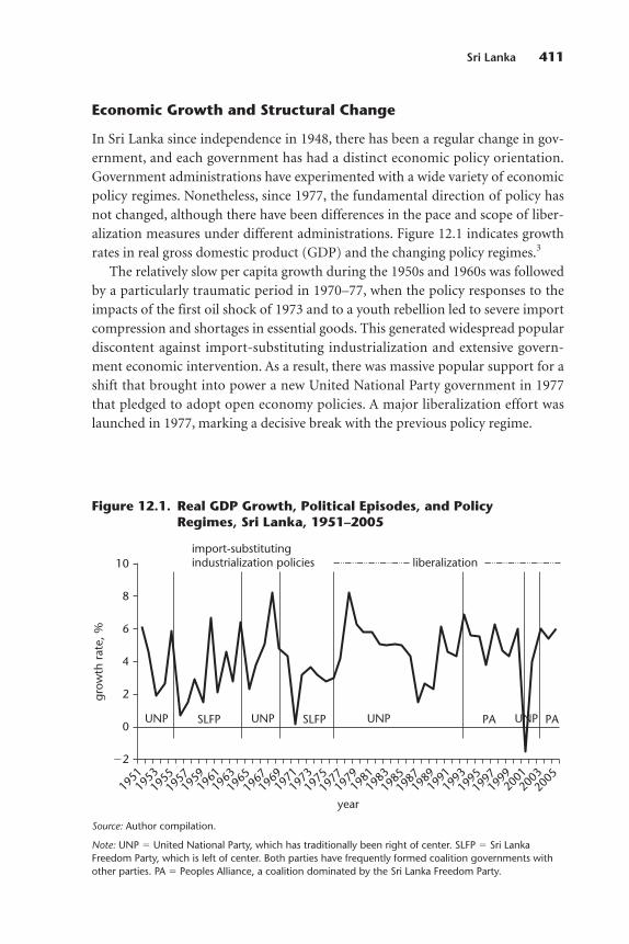
Economic Growth and Structural Change
In Sri Lanka since independence in 1948, there has been a regular change in gov-ernment, and each government has had a distinct economic policy orientation.Government administrations have experimented with a wide variety of economicpolicy regimes. Nonetheless, since 1977, the fundamental direction of policy hasnot changed, although there have been differences in the pace and scope of liber-alization measures under different administrations. Figure 12.1 indicates growthrates in real gross domestic product (GDP) and the changing policy regimes.3
The relatively slow per capita growth during the 1950s and 1960s was followedby a particularly traumatic period in 1970–77, when the policy responses to theimpacts of the first oil shock of 1973 and to a youth rebellion led to severe importcompression and shortages in essential goods. This generated widespread populardiscontent against import-substituting industrialization and extensive govern-ment economic intervention. As a result, there was massive popular support for ashift that brought into power a new United National Party government in 1977that pledged to adopt open economy policies. A major liberalization effort waslaunched in 1977, marking a decisive break with the previous policy regime.
Sri Lanka 411
�2
0
2
4
6
8
10
year
grow
th r
ate,
%
UNP
195119
5319
5519
5719
5919
6119
6319
6519
6719
6919
7119
7319
7519
7719
7919
8119
8319
8519
8719
8919
9119
9319
9519
9719
9920
0120
0320
05
SLFP SLFPUNP PA UNP
import-substitutingindustrialization policies liberalization
UNP PA
Figure 12.1. Real GDP Growth, Political Episodes, and PolicyRegimes, Sri Lanka, 1951–2005
Source: Author compilation.
Note: UNP � United National Party, which has traditionally been right of center. SLFP � Sri LankaFreedom Party, which is left of center. Both parties have frequently formed coalition governments withother parties. PA � Peoples Alliance, a coalition dominated by the Sri Lanka Freedom Party.
Because of the progressive promarket reforms in 1977 and thereafter, Sri Lankabecame the most open economy in South Asia, a distinction it probably still holds.Since 1977, the country has had a reasonably healthy real average annual GDPgrowth rate of 4.8 percent (3.5 percent per capita). An average per capita incomeof US$1,200 at the official exchange rate and over US$4,000 in purchasing powerparity dollars was reached in 2006. Despite ongoing ethnic and social conflictsthat have plagued the country for nearly two decades, the growth rate is higherthan the rates achieved since the mid-1970s by most countries at similar percapita incomes; only Botswana has recorded more rapid growth.
Performance across a wide range of human development indicators has beenabove average in Sri Lanka since the early years of independence, when the goodperformance was achieved through investments in health and education that werefinanced by taxes on plantation crop exports. Life expectancy at birth among menand women, for example, has averaged 72 and 76 years, respectively, which ishigher than the average among middle-income countries. The literacy rate is over90 percent. Nonetheless, the country’s overall developmental performance is dis-appointing relative to the case of the high-performing East Asian economies, par-ticularly because real incomes and human capital endowments were comparableor relatively higher in Sri Lanka in the 1950s and early 1960s. The poor perform-ance of Sri Lanka is at least partly the fault of the ongoing civil war and ethnicconflicts, which have caused enormous damage to the economy and the widersociopolitical environment.4
The overall position of agriculture within the national economy is outlined intable 12.1. The shares of the agricultural sector in GDP, employment, and exportshave declined progressively since the 1950s, although the sector represents a majorsource of income and employment among a large proportion of the population anda significant source of national export earnings (see table 12.1, note a). In contrast toagriculture’s share in GDP, which shrank gradually, the fall in agriculture’s share inexports was sharp in the 1970s and 1980s (figure 12.2). Until the late 1960s, agricul-tural commodities had accounted for more than 90 percent of exports, but, since theearly 1990s, their share has been below 20 percent, and manufacturing, particularlythe garment subsector, has emerged as the major export category.5
The share of various agricultural products in the value of agricultural produc-tion is shown in figure 12.3. Paddy accounted for around 25 percent of agricul-tural and fisheries output in the early 1980s, but its share is now barely half thatmuch. Likewise, the share of rice in household spending has declined by half dur-ing the same period and is currently around 10 percent.
The agricultural sector is widely considered to have contributed to the poorperformance of the economy: “In terms of sectoral contributions to growth,
412 Distortions to Agricultural Incentives in Asia

Sri Lanka 413
Table 12.1. Agriculture in the Economy, Sri Lanka, 1950–2005(percent)
Sector, subsector 1950–51 1960–61 1970–71 1980–81 1990–91 2000–02 2005
GDP, share
Agriculture 44.5 34.6 35.1 33.7 26.3 21.9 18.9
Plantationagriculture 26.3 17.8 15.8 13.9 8.1 5.2 4.4
Tea 7.7 6.5 3.2 2.6 2.4 1.4 1.2
Rubber 5.5 2.3 1.8 1.4 0.6 0.4 0.4
Coconut 7.1 4.8 4.0 3.8 2.4 1.4 1.1
Processinga 6.5 4.2 6.8 6.1 2.7 2.0 1.7
Nonplantationagriculture 14.6 14.5 16.7 15.0 14.8 12.1 11.5
Paddy 1.5 5.7 7.2 6.1 4.9 3.1 3.0
Other 13.1 8.8 9.4 8.9 9.9 9.0 8.5
Forestry 1.9 1.4 1.4 2.0 1.6 1.9 1.7
Fishing 1.2 0.9 1.2 2.7 1.8 2.7 1.3
Manufacturing 8 9 14 18 23 26 27
Services 53 55 51 48 51 52 55
Exports, share
Agriculturea �90 �90 94.6 61.6 36.3 19.3 18.2
Tea �50 �50 55.5 35.1 24.9 14.3 12.8
Rubber �20 �20 22.0 14.7 3.9 0.5 0.7
Coconut �15 �15 14.5 7.0 3.5 1.7 1.8
Other — — 3.1 4.8 4.0 2.8 2.9
Manufacturing �2 �2 1.7 31.2 56.6 77.1 80.3
Unclassified — — 3.9 2.7 7.1 1.0 1.5
Employment, share 1953 1963 1971 1981 1991 2001 2005
Agriculture 53 53 50 45 42 33 31
Manufacturing 12 12 12 15 20 22 24
Services 35 35 38 40 38 45 45
Source: CBSL, “Economic and Social Statistics,” various.
Note: — � no data are available.
a. To indicate the overall contribution of the agricultural sector to the economy, the processing of tea,rubber, and coconut products, which is usually included under manufacturing, is included in agricul-ture under GDP and export shares (but not under employment shares).
agriculture has been a continual drag,” and “the long-term average growth rate inagriculture has barely exceeded the rate of population growth, which has con-tributed to the persistence of poverty (the headcount ratio stood at 23 percent in2002, which is relatively high for Sri Lanka’s per capita income)” (IMF 2005, 5).

414 Distortions to Agricultural Incentives in Asia
0
10
20
30
40
50
60
70
80
90
100
1950
1953
1956
1959
1962
1965
1968
1971
1974
1977
1980
1983
1986
1989
1992
1995
1998
2001
2004
year
per
cent
agricultural share of GDP agricultural share of exports
Figure 12.2. Agriculture in GDP and Exports, Sri Lanka, 1950–2005
Source: CBSL, “Annual Report,” various.
0
valu
e sh
are
of p
rodu
ctio
n at
undi
stor
ted
pric
es, %
10
20
1966 1970 1974 1978 1982year
30
40
50
60
70
80
90
100
1986 1990 1994 1998 2002
residual onions chilies potatoesrubber coconuts tea rice
Figure 12.3. Commodity Shares in Agricultural Production, Sri Lanka, 1966–2004
Sources: Author calculations; Bandara and Jayasuriya 2007; FAOSTAT Database 2008.

Sri Lanka 415
Within agriculture, the output of most crops has stagnated or declined sincethe 1980s (Bandara and Jayasuriya 2007). Tea is the sole important exception. Teaoutput expanded from around 200 million kilograms per year in the early 1980sto around 300 million kilograms in 2000. An increase in the area under cultivation(primarily from an increase in smallholder cultivation in low-altitude regions)and the use of new, higher-yielding cultivars were stimulated by the higher pricesfor the stronger teas produced in lower altitudes. The production of rice andcoconuts—the two crops that dominate smallholder agriculture—has stagnated,while the output of rubber, minor crops, and subsidiary food crops, includingincome-elastic horticultural crops, has fallen significantly. This has meant thatagricultural exports (except tea) have fallen, while food imports have grown.Overall, per capita food production has dropped by over 12 percent since 1980,compared with an average rise of 48 percent in other developing countries (WorldBank 2003). This raises a question about the extent of the contribution of policydistortions to the relatively poor performance.
Policy Evolution
At independence, three plantation crops—tea, rubber, and coconuts—dominatedexports, while significant quantities of rice, wheat, and other food products wereimported. This basic distinction between exportable and import-competing agri-cultural products is critical to understanding the government’s agricultural policy.Export dependence varies greatly, however. For example, more than 80 percent ofthe coconut crop is domestically consumed, and coconuts and coconut oil areessential parts of the local diet. The share of domestic consumption is quite low inthe case of tea (less than 15 percent), while, for rubber, it is around 35 percentthanks to an expansion in rubber-based manufacturing industries.
The tea and rubber subsectors had a pronounced dualistic structure. Large foreign-owned plantations contributed a substantial share of output during theimmediate postindependence period, but these were taken over by the govern-ment in 1974. Then, beginning in the early 1990s, they were progressively handedback to the private sector, including foreign companies. Meanwhile, the shareof large plantations in output has been in gradual decline. In contrast, import-competing food crops, as well as coconuts, have always been dominated by small-holders, although a substantial portion of the coconut industry was locatedamong large plantations until the land reforms of the early 1970s.
Export taxes on agricultural crops (tea, rubber, and coconut products) wereinitially a major source of government revenue, accounting for around 30 percentof all government tax revenue during the 1950s. They helped finance expenditureson public education, health care, and food subsidies. Levies on exports also

financed agricultural research, extension, and replanting programs in plantationcrops. The structure of export taxes reduced average producer revenues, but alsohad the effect of greatly lowering the gains from any price increases. If domesticprices rose because of world price increases or currency devaluations, governmenttax revenues siphoned off the bulk of the price increases. This meant that, whileproducers had to bear the cost of increases linked to domestic inflation, they werelargely deprived of the benefit of any exchange rate adjustments that were made torestore the international competitiveness of tradables, for instance, on severaloccasions beginning in the late 1960s.
In common with governments in many developing countries, the governmentof Sri Lanka followed a food self-sufficiency policy that, more narrowly inter-preted, encouraged rice self-sufficiency. On the production side, the policyinvolved major investments in irrigation (irrigation water was supplied at no costto farmers), fertilizer subsidies, and the provision of rice and other agriculturalresearch and extension services. There was also a public distribution system forthe procurement and marketing of paddy and other commodities. The system wasaimed at making rice more affordable for consumers. Prices for food staples wereheavily regulated until the 1977 liberalization, and many of these staples remainsubject to strong government interventions, including the regulation of importvolumes, that are aimed at maintaining price stability.
Beginning in the late 1950s, the structure of incentives became additionallybiased against export crops through the adoption of import restrictions and for-eign exchange controls. These were implemented in response to growing balanceof payments problems partly caused by a secular downward movement in thecountry’s international terms of trade. The measures, rather than a currencydevaluation, led to real exchange rate overvaluation. The import restrictions (tariff measures and, increasingly, nontariff measures) and exchange controlswere subsequently strengthened after the ideological shift to an import-substitutingindustrialization development strategy. The result was high manufacturing protection; severe import compression; pervasive state controls in trade, market-ing and distribution; persistent exchange rate overvaluation; exchange controls;and a formal dual exchange rate system between 1968 and 1977.6 The dualexchange rate system included a basic official rate and the rate of the ForeignExchange Entitlement Certificate Scheme, which, initially in 1968, was set at44 percent higher (more depreciated) than the basic rate, but adjusted to 55 per-cent in 1969 and then 65 percent in 1972. Exporters of the main plantationcrops—the traditional exports of tea, rubber, and coconuts—had to convertexport earnings at the less favorable official exchange rate, while producers ofnontraditional exports were eligible for the rate available through the entitlementcertificate scheme.7 The highly overvalued official exchange rate, rather than the
416 Distortions to Agricultural Incentives in Asia
somewhat more realistic certificate rate, was also applied on some imports ofmajor agricultural products such as rice, wheat, and sugar. However, theseimports were heavily regulated and were also under direct government control.Hence, rice producers were still shielded from import competition. The high pre-mium in black market rates of exchange and other evidence indicate that substan-tial real exchange overvaluation discriminated against exportable industries andfavored import-competing products in agriculture and elsewhere.
The rice subsector was granted special incentives, and other import-competingagricultural products also gained significant protection through the import- substitution strategy. Nonetheless, Bhalla (1991) and others conclude that therewas an overall bias against agriculture because of the severity of the impact of theovervalued currency on exports, the large weight of exports in farm output, andthe high protection granted to manufacturing. This started to change only in 1977because of the policy shift away from import-substituting industrialization andtoward more liberal promarket policies.
After the 1977 policy liberalization, consumer food subsidies were sharplyreduced, and the emphasis on food self-sufficiency was enhanced.8 Public invest-ments in major irrigation systems were expanded, for example. The governmentimplemented a huge irrigation-cum-hydropower scheme, the AcceleratedMahaweli Development Project, with substantial foreign assistance. Around one-third of all government capital expenditure was devoted to this single project forseveral years beginning in 1979. The project was explicitly rationalized as a majorstep toward rice self-sufficiency, a coveted national goal. It thereby appealed to thepopular imagination, and this partially blunted the political impact of cuts infood subsidies.9
The 1977 reforms also reduced trade protection in the manufacturing sector,and explicit export taxes on plantation crops were largely eliminated in the 1980s.There were fiscal pressures and political imperatives driving the reduction ofexport taxes on plantation crops. Thus, large foreign-owned plantations werenationalized and transferred to state ownership beginning in the mid-1970s, whilethe land reforms of the early 1970s had broadened the ownership base, largelyamong Sinhalese smallholders (Moore 1985).
Trade liberalization was not uniform, however. It extended to some import-competing agricultural products, but excluded others. Crops that were widelycultivated in the north (for example, red onions, chilies, grapes) were subject toliberalization, while protection for other crops (such as potatoes) was main-tained or increased.
After the initial economic growth stimulus following the liberalization of 1977and the huge public sector investment boom (assisted by a massive flow of foreignaid), growth started to slacken, although the economy was cushioned for a while
Sri Lanka 417
by a tea price boom in the early 1980s. Simmering ethnic tensions erupted into asecessionist war following anti-Tamil riots in 1983, and social tensions in thesouth led to a highly disruptive rural youth rebellion in the late 1980s. Economicand political conditions worsened, and the economy lost steam. In 1990–91,responding to an emerging balance of payments crisis, the government devaluedthe currency and initiated a second wave of liberalization (Dunham and Kelegama 1997).
Liberalization proceeded unevenly following the initial measures. Export dutieson plantation crops, already reduced substantially in the mid-1980s, were elimi-nated in 1992, while the high rates of nominal (and effective) protection for import-competing agriculture were maintained (Edwards 1993; World Bank 1995). Bymanipulating licensing and variable tariffs, the government frequently used regula-tory controls on imports to achieve not only protection, but also price stability. Thelatter was particularly important in the case of politically sensitive commoditiessuch as rice and, sometimes, coconuts. Tariffs on agricultural imports were gradu-ally reduced until 1993, and, in January 1995, as part of the Uruguay Round Agree-ment on Agriculture, the government bound all its tariffs on agricultural goods at auniform rate of 50 percent, although this was well above the applied tariffs. Subse-quently, the government removed quantitative restrictions on all agriculturalimports except wheat and wheat flour. In fact, some of the most important changesafter the early 1990s involved not so much the level of the restrictions, but the shiftfrom various forms of nontariff barriers, including regulatory interventions, tomore transparent tariff-based import restrictions. The various indicators of assis-tance described hereafter confirm that the policy regime in recent years has gener-ally provided assistance to import-competing agriculture and that it has done this atrates similar to the rates of assistance in manufacturing.10
Despite periods of slow progress and occasional backsliding, the trend in over-all policy has been toward progressive liberalization, and the country now has perhaps the most open trade regime in South Asia. The evolution of the overallstructure of incentives may be seen by looking at changes in the manufacturingsector and the two main parts of the agricultural sector. During the reforms in1977, the implicit rates of protection for manufacturing and for many import-competing agricultural commodities were extremely high. Even after the majorreforms, in 1979, the estimated effective rate of protection in the manufacturingsector was 137 percent (Cuthbertson and Athukorala 1990). This had fallen to90 percent in 1981, and was estimated at 77 percent in 1991 and 43 percent in1994 (World Bank 2004). By 2005, liberalization had progressed in the manufac-turing sector.
There was also an important effort toward liberalizing import competition inthe food industry. Wheat imports were liberalized by ending a government-granted long-term monopoly in flour milling to Prima, a company based in
418 Distortions to Agricultural Incentives in Asia

Singapore, that had also given the company a virtual monopoly on the supply ofanimal feed. Government trading enterprises play a role in domestic distributionand in international trade, but it is minor.
Trade policy continues to protect rice and several other import-competing foodcrops, such as potatoes, through tariffs and specific duties that vary seasonally. Theinterventions respond to domestic conditions in price and supply. Furthermore,despite the shrinking share of agriculture in GDP and employment, agriculturalproducer subsidies remain important, and the government experiences intensepressure to maintain and even expand these subsidies. For example, a fertilizer sub-sidy is still used that is targeted largely, though not solely, toward import-competingcrops, particularly those cultivated by smallholders. Periodically, a fertilizer subsidyhas been a component of government assistance in agriculture, and populist gov-ernments have used the subsidy to appeal to the politically important farming com-munity. Until recently, the aggregate assistance effect of the subsidy would have notbeen large, but the amount of the subsidy was doubled in 2005–06, and the cost ofthe subsidy may have risen by an additional one-third, to SLRs 11 billion (around$100 million) or more in 2007 (figure 12.4). There are also frequent ad hoc changesin import policies, particularly in the case of subsidiary food crops such as potatoesand onions, over which small—but politically powerful—farm groups exercisemuch political clout.
Thus, the broad contours of agricultural policies in Sri Lanka appear toresemble today some aspects of the early agricultural policy evolution in more
Sri Lanka 419
0
20
40
60
80
100
120
1962
1964
1966
1968
1970
1972
1974
1976
1978
1980
1982
1984
1986
1988
1990
1992
1994
1996
1998
2000
2002
2004
2006
year
US$
, mill
ions
Figure 12.4. Fertilizer Subsidy, Sri Lanka, 1962–2007
Source: CBSL, “Economic and Social Statistics,” various.

well-developed East Asian economies: overall, the trade regime is relatively liberal, but it grants significant protection to particular import-competing agricultural industries. In the next section, we present our estimates of a numberof indicators of the incentives for major agricultural products and various categories of commodities, such as exportables and import-competing products.We also attempt to explain the changing patterns in agricultural taxation andassistance since independence that have led to the current outcome.
Direct and Indirect Distortions in Incentives
The main focus of our study’s methodology for estimating the extent of distor-tions to agricultural incentives is on government-imposed measures that create agap between actual domestic prices and these prices as they would be under freemarket conditions. (For details on the methodology, see appendix A and Andersonet al. 2008.) Because it is not possible to understand the characteristics of agricul-tural development through a sectoral view alone, our methodology estimates theeffects of direct agricultural policy measures, including distortions in the foreignexchange market, but also distortions in nonagricultural sectors that competewith farmers for mobile resources such as labor and capital. More specifically, ourstudy computes nominal rates of assistance (NRAs) for farmers. We also generateNRAs for nonagricultural tradables for comparison with NRAs for agriculturaltradables through the calculation of relative rates of assistance (RRAs).
We present, in table 12.2 our estimates of the temporal patterns in the distor-tions to agricultural incentives for seven major commodities from 1955 to 2004:three exportables (rubber, coconuts, and tea) and four import-competing prod-ucts (rice, potatoes, onions, and chilies).11 In table 12.3, we show our guesstimatesof the NRAs for noncovered farm products, which account for around one-thirdof the overall value of agricultural production. The guesstimates assume that thenoncovered products are equally divided among exportables, nontradables, andimport-competing products (one-third each of the residual value of farm produc-tion). They also assume that the NRAs are zero for nontradables and, for exporta-bles and importables, are equal to the estimated NRAs for the two subsets of cov-ered products (all of which are tradable). Farm input assistance was minor before2005, and, so, we include no estimate for such non-product-specific assistance.The NRAs for nonagricultural tradables are based on the import duty collectionrate for import-competing manufacturing and our assumption that the directassistance to nonagricultural exportables is zero.12 This method may substantiallyunderestimate the actual rate of manufacturing protection because high tariffs orbinding nontariff barriers may lead to lower import volumes and therefore lowercollection rates on import duties. We believe the nonagricultural NRAs before
420 Distortions to Agricultural Incentives in Asia
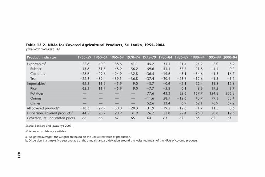
421
Table 12.2. NRAs for Covered Agricultural Products, Sri Lanka, 1955–2004(five-year averages, %)
Source: Bandara and Jayasuriya 2007.
Note: — � no data are available.
a. Weighted averages; the weights are based on the unassisted value of production.b. Dispersion is a simple five-year average of the annual standard deviation around the weighted mean of the NRAs of covered products.
Product, indicator 1955–59 1960–64 1965–69 1970–74 1975–79 1980–84 1985–89 1990–94 1995–99 2000–04
Exportablesa �22.8 �40.0 �38.6 �41.1 �45.2 �31.1 �21.4 �24.2 �2.0 5.9Rubber �15.8 �51.5 �48.9 �56.2 �59.6 �51.4 �37.7 �21.8 �4.4 �0.2Coconuts �28.6 �29.6 �24.9 �32.8 �36.5 �19.6 �5.1 �34.6 �1.3 16.7Tea �22.3 �39.4 �39.1 �36.8 �37.4 �30.4 �25.6 �12.6 �1.5 �1.2
Importablesa 62.5 11.9 �5.9 9.0 �3.7 �0.6 �2.1 22.4 31.8 12.8Rice 62.5 11.9 �5.9 9.0 �7.7 �5.8 0.1 8.6 19.2 3.7Potatoes — — — — 77.6 43.3 32.6 157.7 124.8 205.8Onions — — — — �11.6 28.7 �12.6 43.7 79.3 53.4Chilies — — — — 52.6 33.4 6.9 62.1 76.9 67.2
All covered productsa �10.3 �29.9 �30.0 �20.3 �31.9 �19.2 �12.6 �1.7 11.5 8.6Dispersion, covered productsb 44.2 28.7 20.9 31.9 26.2 22.8 22.4 25.0 20.8 12.6Coverage, at undistorted prices 66 66 67 65 64 63 67 65 62 64
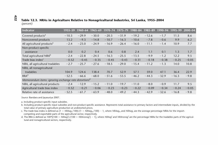
Table 12.3. NRAs in Agriculture Relative to Nonagricultural Industries, Sri Lanka, 1955–2004(percent)
Source: Bandara and Jayasuriya 2007.
a. Including product-specific input subsidies.b. Including product-specific input subsidies and non-product-specific assistance. Represents total assistance to primary factors and intermediate inputs, divided by the
total value of primary agriculture production at undistorted prices.c. The trade bias index is defined as (1 � NRAagx�100)�(1 � NRAagm�100) � 1, where NRAagm and NRAagx are the average percentage NRAs for the import-
competing and exportable parts of the agricultural sector, respectively.d. The RRA is defined as 100*[(100 � NRAagt)�(100 � NRAnonagt) � 1], where NRAagt and NRAnonagt are the percentage NRAs for the tradables parts of the agricul-
tural and nonagricultural sectors, respectively.
Indicator 1955–59 1960–64 1965–69 1970–74 1975–79 1980–84 1985–89 1990–94 1995–99 2000–04
Covered productsa �10.3 �29.9 �30.0 �20.3 �31.9 �19.2 �12.6 �1.7 11.5 8.6Noncovered products 13.2 �9.3 �14.8 �10.7 �16.3 �10.6 �7.8 �0.6 9.9 6.2All agricultural productsa �2.4 �23.0 �24.9 �16.9 �26.4 �16.0 �11.1 �1.4 10.9 7.7Non-product-specific
assistance 0.0 0.2 0.4 0.6 0.8 2.4 1.1 0.1 1.3 1.7Total agricultural NRAb �2.4 �22.8 �24.5 �16.3 �25.5 �13.5 �9.9 �1.2 12.2 9.5Trade bias indexc �0.52 �0.45 �0.35 �0.45 �0.43 �0.31 �0.18 �0.38 �0.25 �0.05NRA, all agricultural tradables �2.7 �25.7 �27.6 �18.5 �29.0 �15.4 �11.2 �1.3 14.0 10.8NRA, all nonagricultural
tradables 104.9 124.6 138.4 70.7 52.9 57.1 59.0 47.1 36.4 22.9RRAd �52.5 �66.6 �68.0 �51.6 �53.5 �46.2 �44.3 �32.9 �16.3 �9.8Memorandum items: ignoring exchange rate distortionsd
NRA, all agricultural products �2.4 �12.9 �15.2 �11.0 �19.7 �11.0 �8.0 �0.9 11.7 9.5Agricultural trade bias index �0.52 �0.21 �0.06 �0.23 �0.23 �0.22 �0.09 �0.34 �0.24 �0.05Relative rate of assistance �52.5 �61.7 �63.9 �48.0 �49.2 �44.3 �42.9 �32.6 �16.8 �9.8
422
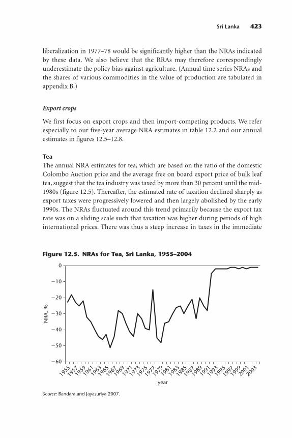
liberalization in 1977–78 would be significantly higher than the NRAs indicatedby these data. We also believe that the RRAs may therefore correspondinglyunderestimate the policy bias against agriculture. (Annual time series NRAs andthe shares of various commodities in the value of production are tabulated inappendix B.)
Export crops
We first focus on export crops and then import-competing products. We referespecially to our five-year average NRA estimates in table 12.2 and our annualestimates in figures 12.5–12.8.
TeaThe annual NRA estimates for tea, which are based on the ratio of the domesticColombo Auction price and the average free on board export price of bulk leaftea, suggest that the tea industry was taxed by more than 30 percent until the mid-1980s (figure 12.5). Thereafter, the estimated rate of taxation declined sharply asexport taxes were progressively lowered and then largely abolished by the early1990s. The NRAs fluctuated around this trend primarily because the export taxrate was on a sliding scale such that taxation was higher during periods of highinternational prices. There was thus a steep increase in taxes in the immediate
Sri Lanka 423
�60
year
�50
�40
�30
�20
�10
0
NRA
, %
1955
1957
1959
1961
196319
6519
6719
6919
7119
7319
7519
7719
7919
8119
8319
8519
8719
8919
9119
9319
9519
9719
9920
0120
03
Figure 12.5. NRAs for Tea, Sri Lanka, 1955–2004
Source: Bandara and Jayasuriya 2007.
aftermath of the 1977 reforms that was associated with the exchange rate depreci-ation accompanying the liberalization (which increased the domestic currencyprice on which the tax was based), as well as with the international tea priceincrease of the early 1980s. There is no evidence for the existence of significantmarket imperfections within the domestic market for tea production, processing,and wholesale marketing through the auction. The Colombo Tea Auction is con-sidered quite competitive, though there has been criticism of the system. Hence,the rate of export taxes and cesses provides a reasonable estimate of the NRAs. It isnot possible to use domestic and border price data to compute NRAs directlybecause of the growth in the importance of value added teas (tea bags and so on)for which reliable border prices are not available.
Not reflected in figure 12.5 is the fact that tea imports have been effectivelysubject to a near total ban until recently, ostensibly to ensure that inexpensive for-eign teas are not reexported as quality Ceylon tea. There has been some relaxationin the ban, but a prohibitive tariff has nonetheless effectively ensured that teaimports are negligible. As a result, the country has lost the chance to develop a teablending industry, and Dubai has emerged as the center of this lucrative industry,which relies on significant quantities of Sri Lankan tea and imported Sri Lankanlabor (Ganewatta 2002).
RubberThe annual NRAs for sheet rubber are based on the percentage gap between theaverage domestic Colombo Auction price for sheet rubber and the average free onboard price of rubber. They suggest that the tax on this industry was over 50 per-cent higher than the tax on the tea industry until the early 1980s. Since then, therate of taxation has declined fairly rapidly (figure 12.6). Reflecting the virtualelimination of export taxes, the NRA estimates have averaged close to zero inrecent years. They have fluctuated around the trend primarily because the exporttax rate was on a sliding scale such that taxation was higher during periods of highinternational prices. Similar to the situation in tea, the rate of export taxes andcesses provides a reasonable estimate of NRAs in recent years given that it is diffi-cult to compute reliable NRAs from available price data because of the changes inthe composition of exported rubber.
CoconutsCoconut products (copra, oil, fiber and coir products, and so on) were a majorexport product category at the time of independence. Export volumes have sincefallen. Because of the importance of coconuts as a food crop and in the produc-tion of coconut oil for household consumption (coconut oil is the most widelyused cooking oil), coconuts have attracted significant direct price and nonprice
424 Distortions to Agricultural Incentives in Asia
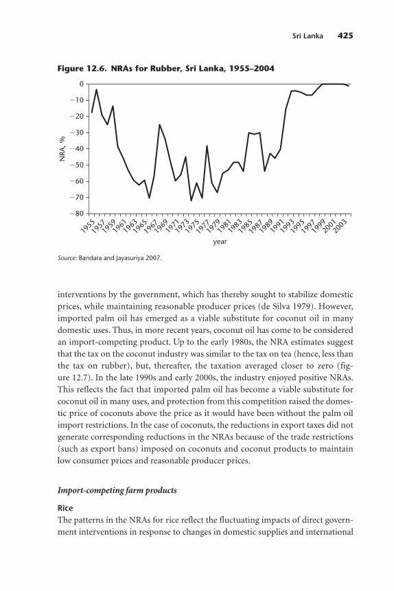
interventions by the government, which has thereby sought to stabilize domesticprices, while maintaining reasonable producer prices (de Silva 1979). However,imported palm oil has emerged as a viable substitute for coconut oil in manydomestic uses. Thus, in more recent years, coconut oil has come to be consideredan import-competing product. Up to the early 1980s, the NRA estimates suggestthat the tax on the coconut industry was similar to the tax on tea (hence, less thanthe tax on rubber), but, thereafter, the taxation averaged closer to zero (fig-ure 12.7). In the late 1990s and early 2000s, the industry enjoyed positive NRAs.This reflects the fact that imported palm oil has become a viable substitute forcoconut oil in many uses, and protection from this competition raised the domes-tic price of coconuts above the price as it would have been without the palm oilimport restrictions. In the case of coconuts, the reductions in export taxes did notgenerate corresponding reductions in the NRAs because of the trade restrictions(such as export bans) imposed on coconuts and coconut products to maintainlow consumer prices and reasonable producer prices.
Import-competing farm products
RiceThe patterns in the NRAs for rice reflect the fluctuating impacts of direct govern-ment interventions in response to changes in domestic supplies and international
Sri Lanka 425
�80
year
�70
�60
�50
�40
�20
�10
�30
0
NRA
, %
1955
1957
1959
1961
196319
6519
6719
6919
7119
7319
7519
7719
7919
8119
8319
8519
8719
8919
9119
9319
9519
9719
9920
0120
03
Figure 12.6. NRAs for Rubber, Sri Lanka, 1955–2004
Source: Bandara and Jayasuriya 2007.
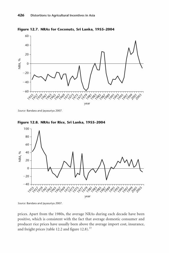
prices. Apart from the 1980s, the average NRAs during each decade have beenpositive, which is consistent with the fact that average domestic consumer andproducer rice prices have usually been above the average import cost, insurance,and freight prices (table 12.2 and figure 12.8).13
426 Distortions to Agricultural Incentives in Asia
�60
year
�40
�20
20
40
0
60
NRA
, %
1955
1957
1959
1961
196319
6519
6719
6919
7119
7319
7519
7719
7919
8119
8319
8519
8719
8919
9119
9319
9519
9719
9920
0120
03
Figure 12.7. NRAs for Coconuts, Sri Lanka, 1955–2004
Source: Bandara and Jayasuriya 2007.
�40
year
�20
0
60
40
80
20
100
NRA
, %
1955
1957
1959
1961
196319
6519
6719
6919
7119
7319
7519
7719
7919
8119
8319
8519
8719
8919
9119
9319
9519
9719
9920
0120
03
Figure 12.8. NRAs for Rice, Sri Lanka, 1955–2004
Source: Bandara and Jayasuriya 2007.
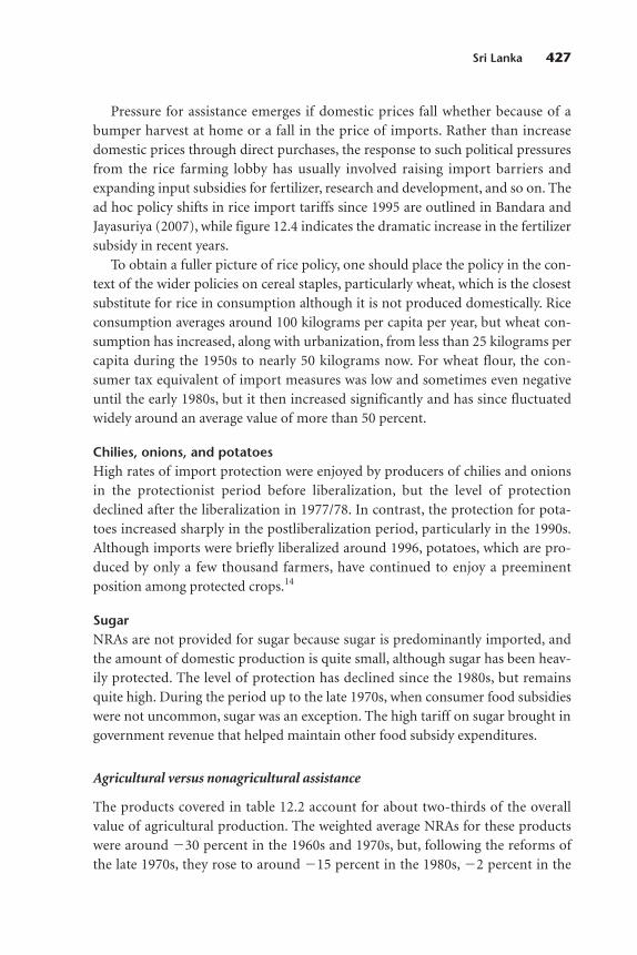
Sri Lanka 427
Pressure for assistance emerges if domestic prices fall whether because of abumper harvest at home or a fall in the price of imports. Rather than increasedomestic prices through direct purchases, the response to such political pressuresfrom the rice farming lobby has usually involved raising import barriers andexpanding input subsidies for fertilizer, research and development, and so on. Thead hoc policy shifts in rice import tariffs since 1995 are outlined in Bandara andJayasuriya (2007), while figure 12.4 indicates the dramatic increase in the fertilizersubsidy in recent years.
To obtain a fuller picture of rice policy, one should place the policy in the con-text of the wider policies on cereal staples, particularly wheat, which is the closestsubstitute for rice in consumption although it is not produced domestically. Riceconsumption averages around 100 kilograms per capita per year, but wheat con-sumption has increased, along with urbanization, from less than 25 kilograms percapita during the 1950s to nearly 50 kilograms now. For wheat flour, the con-sumer tax equivalent of import measures was low and sometimes even negativeuntil the early 1980s, but it then increased significantly and has since fluctuatedwidely around an average value of more than 50 percent.
Chilies, onions, and potatoesHigh rates of import protection were enjoyed by producers of chilies and onionsin the protectionist period before liberalization, but the level of protectiondeclined after the liberalization in 1977/78. In contrast, the protection for pota-toes increased sharply in the postliberalization period, particularly in the 1990s.Although imports were briefly liberalized around 1996, potatoes, which are pro-duced by only a few thousand farmers, have continued to enjoy a preeminentposition among protected crops.14
SugarNRAs are not provided for sugar because sugar is predominantly imported, andthe amount of domestic production is quite small, although sugar has been heav-ily protected. The level of protection has declined since the 1980s, but remainsquite high. During the period up to the late 1970s, when consumer food subsidieswere not uncommon, sugar was an exception. The high tariff on sugar brought ingovernment revenue that helped maintain other food subsidy expenditures.
Agricultural versus nonagricultural assistance
The products covered in table 12.2 account for about two-thirds of the overallvalue of agricultural production. The weighted average NRAs for these productswere around �30 percent in the 1960s and 1970s, but, following the reforms ofthe late 1970s, they rose to around �15 percent in the 1980s, �2 percent in the
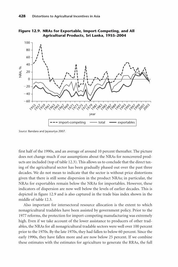
first half of the 1990s, and an average of around 10 percent thereafter. The picturedoes not change much if our assumptions about the NRAs for noncovered prod-ucts are included (top of table 12.3). This allows us to conclude that the direct tax-ing of the agricultural sector has been gradually phased out over the past threedecades. We do not mean to indicate that the sector is without price distortionsgiven that there is still some dispersion in the product NRAs; in particular, theNRAs for exportables remain below the NRAs for importables. However, theseindicators of dispersion are now well below the levels of earlier decades. This isdepicted in figure 12.9 and is also captured in the trade bias index shown in themiddle of table 12.3.
Also important for intersectoral resource allocation is the extent to whichnonagricultural tradables have been assisted by government policy. Prior to the1977 reforms, the protection for import-competing manufacturing was extremelyhigh. Even if we take account of the lower assistance to producers of other trad-ables, the NRAs for all nonagricultural tradable sectors were well over 100 percentprior to the 1970s. By the late 1970s, they had fallen to below 60 percent. Since theearly 1990s, they have fallen more and are now below 25 percent. If we combinethese estimates with the estimates for agriculture to generate the RRAs, the full
428 Distortions to Agricultural Incentives in Asia
�60
year
�40
�20
0
60
40
80
20
100
NRA
, %
1955
1957
1959
1961
1963
1965
1967
1969
1971
1973
1975
1977
1979
1981
1983
1985
1987
1989
1991
1993
1995
1997
1999
2001
2003
exportablestotalimport-competing
Figure 12.9. NRAs for Exportable, Import-Competing, and AllAgricultural Products, Sri Lanka, 1955–2004
Source: Bandara and Jayasuriya 2007.
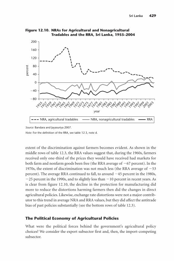
Sri Lanka 429
extent of the discrimination against farmers becomes evident. As shown in themiddle rows of table 12.3, the RRA values suggest that, during the 1960s, farmersreceived only one-third of the prices they would have received had markets forboth farm and nonfarm goods been free (the RRA average of �67 percent). In the1970s, the extent of discrimination was not much less (the RRA average of �53percent). The average RRA continued to fall, to around �45 percent in the 1980s,�25 percent in the 1990s, and to slightly less than �10 percent in recent years. Asis clear from figure 12.10, the decline in the protection for manufacturing didmore to reduce the distortions harming farmers then did the changes in directagricultural policies. Likewise, exchange rate distortions were not a major contrib-utor to this trend in average NRA and RRA values, but they did affect the antitradebias of past policies substantially (see the bottom rows of table 12.3).
The Political Economy of Agricultural Policies
What were the political forces behind the government’s agricultural policychoices? We consider the export subsector first and, then, the import-competingsubsector.
�80
year
�40
0
120
80
40
200
160
per
cent
RRANRA, nonagricultural tradablesNRA, agricultural tradables
1955
1957
1959
1961
1963
1965
1967
1969
1971
1973
1975
1977
1979
1981
1983
1985
1987
1989
1991
1993
1995
1997
1999
2001
2003
Figure 12.10. NRAs for Agricultural and NonagriculturalTradables and the RRA, Sri Lanka, 1955–2004
Source: Bandara and Jayasuriya 2007.
Note: For the definition of the RRA, see table 12.3, note d.
Export crops
At independence, relatively large-scale, foreign-owned companies dominated intea and, to a lesser extent, in rubber. Even the coconut subsector, though largelysmallholder based, still relied on a significant number of large estates. There waslittle political sympathy for the plantation subsector from the left of center coali-tions that ruled the country from 1956 to 1965 (with a brief interruption in 1960)and then again in 1970–77. The foreign plantations were under threat of national-ization beginning in 1956, and they were finally nationalized in the mid-1970swhen all large holdings were subjected to land reform. The majority of the initialworkers on the large plantations had migrated from southern India beginning inthe mid-19th century, and plantation workers were politically marginalizedthrough disenfranchisement during the first postindependence government. Mostimportantly perhaps, government revenues depended heavily on foreign tradetaxes, and export duties alone contributed nearly one-third of all government rev-enues during the first decade after independence. Because of slow economicgrowth, governments were continually under fiscal pressure and had little scope,even if they desired to do so, to reduce export taxes on plantation crops.
The combination of high taxes, secular falls in real world prices, and threats ofnationalization led to slow, but steady decline in the plantation subsector, particularly the large plantations. The subsector became based more on small-holders, a process that accelerated after the land reforms. Large foreign-ownedfirms passed into state ownership. The 1977 liberalization did not have an imme-diate positive impact on these industries, however. The exchange rate reforms,which involved a significant nominal devaluation, failed to have much of a posi-tive impact on the subsector. This was because the structure of the progressiveexport taxes, which including a sliding tax scale, effectively taxed away most of thegains of devaluation and the periodic relative price improvements.
The plantation crop subsector and its role within the economy had changed inquite fundamental ways by the mid-1980s. The subsector’s share of the nationaleconomy had shrunk, and new investments in replantings and factory moderniza-tion were clearly essential if the decline of the subsector was to be arrested. Thepolitical tensions that emerged in the aftermath of the 1977 liberalization madethe government more sensitive to the political importance of plantation crop cul-tivators. Plantation crops were cultivated almost entirely in the wetter central,western, and southern regions of the country, and the cultivators were predomi-nantly members of the majority Sinhalese community, the support of which wascritical if the governing political parties were to stay in power. Also, the exporttaxes on plantation crops directly reduced the revenues of large state-owned plan-tations. These factors combined to erode the economic and political incentives formaintaining the traditional regime of high export taxes.
430 Distortions to Agricultural Incentives in Asia

Import-competing crops
We have seen that government policies toward import-competing crops have notbeen uniform. Furthermore, in the case of key staple food crops and, most impor-tantly, in the case of rice, there has been tension between the twin objectives ofproducer support and maintenance of low consumer prices. The enduring themeof import-competing agricultural policy in the postindependence period is thisdifficult balancing act between producers and consumers in staple food crops.This is well illustrated if we examine policies in the rice sector.
Rice policyRice is the most sensitive political commodity. Aided by proceeds from high com-modity prices during the Korean War, immediate postindependence governmentswere able to maintain or expand the policy of providing inexpensive subsidizedrice to consumers through a universal rice ration that they had inherited fromBritish colonial rulers. Rationing formed a central component in a wider politicalstrategy that aimed at undercutting the potential threat from a Marxist politicalleft that had strong roots within trade unions. An attempt to reduce the rice subsidy in 1953 brought the country to the verge of revolution. Subsequentattempts to reduce the subsidy almost invariably led to the downfall or politicalhumiliation of the government administration. Subsidized rice distributedthrough the ration system became a symbol of the political power of powerfulleft-wing parties.
Rice has enormous symbolism and emotive power in Sri Lanka. Rice self-sufficiency has been a slogan that has found appeal in deep-seated nationalistaspirations, particularly among the Sinhalese, whose history has included anancient civilization based on irrigated rice cultivation and who were stirred bythe vision, irrespective of historical precision, of a golden age when Sri Lankahad exported rice to other parts of Asia and was the granary of the East. At amore mundane level, landed rice cultivators and powerful rice millers exertmuch clout in garnering electoral support for particular political parties. In SriLanka, the drive to attain rice self-sufficiency was not only a means of achiev-ing a Green Revolution on existing rice lands. Beginning already in the 1930s,the promotion of rice cultivation through land settlement schemes or colo-nization schemes was linked to the restoration of the ancient glory of the Sinhalese in the sparsely populated dry zone, which had been the cradle of theancient hydraulic empire. The restoration of old irrigation systems that wasinitiated by the British during colonial times and the construction of new,grandiose irrigation systems were seen as a vehicle for new Sinhalese farmersettlements in those parts of the country that had been largely abandoned.15 AsBruton (1992, 82) points out, “the paddy society was almost entirely Sinhalese.”
Sri Lanka 431
Thus, the rice self-sufficiency drive became associated with the rising Sinhalanationalism of the postindependence era.
In addition to the free or subsidized provision of irrigation water, fertilizers,seeds, research, extension, and other assistance for producers, the governmentpurchased paddy from farmers at a guaranteed price through a state tradingentity. It distributed varying quantities of rice rations to consumers at subsidizedprices until the late 1970s, including a period when some rationed rice was dis-tributed free of charge (1966–78). Farmers also sold rice to private buyers, whomilled it themselves or sold it to millers, who sold it on the open market. In 1972,facing rising international prices and seeking to increase domestic supplies atlower prices, the government granted monopoly procurement rights to the state-owned Paddy Marketing Board. However, the monopoly could not be enforcedand was abolished in 1975.16 The government has continued to regulate interna-tional trade and supplies to maintain stable consumer prices. This remains a cen-tral goal of food policy.17
The nonuniform pattern of trade liberalization beginning in 1977 may only beunderstood if we recognize the central political role of rice in consumption andin production. The reform government of 1977 was led by J. R. Jayewardene, whowas a lifelong opponent of the left, was strongly pro-Western in foreign policy,and had tried and failed once to dismantle the rice subsidy scheme. The Accelerated Mahaweli Development Project now played a critical political role byproviding the crucial popular political support that enabled the Jayewardene government to dismantle the rice subsidy scheme and crush the traditional polit-ical left, while implementing major liberalization measures.
However, the end of the rice subsidy scheme did not mean that the domesticprices for rice were left to the market so that rice producers would be exposed to thepressure of cheap imports. Post-1977 government policies continued to aim at con-sumer price stabilization around a reasonable price, while assisting producersthrough input subsidies and import protection. The NRAs in rice also reflect theimpact of changes in the international price and weather-related domestic supply.Because nontariff barriers insulate domestic markets from international markets,changes in domestic supply change domestic prices and, even in the absence of anychange in the policy regime, change estimated NRAs. Hence, good harvests depressdomestic prices and generate pressures for assistance and increased protection.
Its signature of the Uruguay Round Agreement on Agriculture in 1994 did notconstrain the government from exercising a high degree of discretion in changingtariffs because the applied tariffs were significantly lower than the bound tariffs.The government has frequently chosen to alter import tariffs in response todomestic pressures. For example, beginning in 1995, rice imports were subject toa tariff of 35 percent. An import licensing requirement was also imposed in
432 Distortions to Agricultural Incentives in Asia
July 2000. In July 2001, when the domestic price for rice rose because of a produc-tion shortfall, the government allowed the state-run Cooperative WholesaleEstablishment, as well as private traders, to import rice duty-free, waiving the35 percent tariff. Then, in January 2002, a specific duty, SLRs 7 per kilogram,replaced the tariff, although the Cooperative Wholesale Establishment wasallowed to import rice at a special duty of SLRs 4 per kilogram. In March 2002, thelicensing requirement was removed, and the special duty was raised to SLRs 5 perkilogram. The special duty was raised again, to SLRs 7, in March 2003, SLRs 9 inAugust 2003, and SLRs 20 in January 2006 (see IPS 2003; WTO 2004; Bandara andJayasuriya 2007).
These policy gyrations reflect the political power of the large rice producersand processors, but also the sensitivity of governments to consumer opposition toincreases in the price of the main staple food. The policy liberalization in 1977clearly reduced the high levels of protection, but protection has not been trendingdownward since then. Sri Lanka is considered a high-cost rice producer at thefringe; so, the sector would come under considerable pressure, particularly inmarginal areas, if trade were fully liberalized.18 It would be a mistake to assumethat the negative NRAs for rice observed in 2003 and 2004, for example, representa permanent policy shift. The difficult balancing act between serving producerand consumer interests will continue. The policy responses will be most sensitiveto domestic price movements. High domestic prices will tend to induce importliberalization, while low domestic prices will tend to induce import restrictions orinput subsidies (constrained, of course, by the need to control fiscal deficits).
Wheat and sugar import policiesThe changes in government policies toward wheat have been closely linked to gov-ernment rice policies. During the 1950s and 1960s, when the government wasproviding a subsidized rice ration for consumers, a significant proportion of theration rice had to be imported because domestic procurement was inadequate.The government had an incentive to encourage the substitution of wheat for ricein consumption to reduce the fiscal burden of the rice subsidy because wheat wasrelatively less expensive than rice in international markets. Meanwhile, somewheat was also provided through United States government aid. With the phase-out of the subsidized rice ration scheme starting in 1979, the incentives changed.Thus, beginning in the early 1980s, rice was implicitly protected through tougherrestrictions on wheat imports.19
Sugar imports were heavily taxed before liberalization. Tax levels have declinedsince 1977, but are still high. There is a simple explanation for the heavy taxationbefore liberalization: almost all sugar was imported; there was little domestic pro-duction; and import taxes contributed to reducing the fiscal burden imposed
Sri Lanka 433
by other food subsidies. The prevailing domestic price for sugar was accepted byconsumers although it was much higher than the international price. So long asdomestic prices were not increased too much, there was little political oppositionto the maintenance of this implicit protection. The high protection of the sugarindustry in recent years has not been maintained so much to raise governmentrevenue, but, rather, to honor an agreement signed in the early 1980s by the gov-ernment and a foreign private enterprise.20
Chilies and onionsThe liberalization of 1977 involved import liberalization that was selective anddiscriminatory. The agricultural subsectors chosen for liberalization or ongoingprotection had a clear regional dimension that also overlapped with ethnicity. Theprotectionist policies before liberalization had benefited subsidiary food cropssuch as chilies and red onions, as well as crops such as grapes. Protection hadencouraged the expansion of these crops in particular regions, such as the JaffnaPeninsula. Jaffna District produced two-thirds of the country’s entire productionof red onions. The dependency of local farmers on these high-value crops wassuch that, by 1977/78, red onions and chilies accounted for around 75 percent ofthe total area devoted to nonrice (minor food crop) cultivation in Jaffna District(DCS 1979). It was also the only dry zone district that was in a rice deficit. The1977 liberalization produced a sharp fall in protection. Despite the negativeincome effects on producers, the opposition of producers to the reform was inef-fective. The ability of Jaffna farmers to obtain any response to their demands wasconstrained by the “marginality of the Sri Lankan Tamils to the electoral system asa whole” (Moore 1985, 109).
Even so, this issue played an important role in Jaffna in the 1982 presidential elec-tions. The escalation of ethnic tensions into a full-scale secessionist war beginning in1983 has had devastating effects on the agricultural economy in the northern andeastern provinces. During the past two decades, commercial ties with the rest of thecountry have been massively disrupted. As an upshot of these developments, farm-ers in the southern regions have expanded their production of minor food crops,and this has changed the political dynamics behind government policies in minorcrops. This is most clear in the policies toward potatoes, for example. A small groupof producers was able to gather significant political clout, and the consumer resist-ance to high prices could be largely ignored. Despite occasional declines, the protection for potatoes has tended to increase over time, and this has also beenaccompanied by increases, though to a lesser degree, in crops such as red onionsand chilies (see table 12.2). From many viewpoints, a strong case can be made forremoving the assistance for potato production, particularly given its destructiveimpact on the country’s fragile ecosystems, including the most important river
434 Distortions to Agricultural Incentives in Asia
catchments and repositories of significant sources of biodiversity. As Bruton (1992,170) points out, “the strong commitment to the Sinhalese culture made it difficult todesign an economic policy that was equally appropriate for both major ethnicgroups.” There can be little doubt that the pattern of liberalization in 1977/78 is sug-gestive of a strong ethnic bias. However, the near-complete marginalization of Tamilfarmers in the north and east from mainstream political life and the collapse of theagricultural economy in these regions beginning in the mid-1980s because of warhave meant that the role of ethnicity has diminished in agricultural policy formula-tion. Tensions between producer and consumer interests have thereby become thedominant political economy issue.
Future Prospects
Our discussion of the political economy of agricultural policies has pointed to arange of factors that have influenced policy formation in agricultural crops. Thebroad sweep of trade liberalization since the late 1970s has not passed the agricultural sector by. More progress in liberalization is likely if many smallerimport-competing subsectors are unable to withstand the pressure for reform andliberalization. Liberalization will be difficult in the case of rice, the most politicallysensitive industry. The history of agricultural policy in Sri Lanka and the experi-ence of other countries in Asia suggest that this will remain the strongest bastionof protectionist pressures in the country. Even recently, whenever the rice industryhas been put under stress because of falling prices, the government has faced pres-sure to placate the industry. Almost invariably the government has ceded to thepressure and maintained the historical pattern of special treatment for rice.Arguably, the course of future agricultural trade liberalization will depend on theextent to which rice producers are able to retain their political influence. Nonethe-less, as long as rice and wheat are major items in the consumption basket, the levelof direct price protection will be constrained by the need to satisfy consumerinterests, particularly if international prices spike at high levels as they did in 2008.Fiscal pressures will also place a limit on the ability of the government to provideassistance through input subsidies. One wonders if the government will be able tomaintain the level and type of protection now being offered to the livestock,chicken, and dairy industries, the data on which have not been adequate for inclu-sion in this study.
Notes
1. For reviews of the government’s agricultural policy in Sri Lanka, see Thorbecke and Svejnar(1987); Bhalla (1991); World Bank (1995); Athukorala and Kelegama (1998); Anderson (2002);Sanderatne (2004).
Sri Lanka 435

2. The minor export crops are often referred to as nontraditional agricultural exports to distin-guish them from the traditional exports of tea, rubber, and coconuts although many of these cropshave been exported for thousands of years, while tea and rubber were introduced in the country onlyin the late 19th century.
3. For more on policy regimes and the growth experience, see Athukorala and Jayasuriya (1994);Athukorala and Rajapatirana (2000); Kelegama (2004); Weerakoon (2004); World Bank (2004).
4. The cost of the war between 1983 and 2000 has been conservatively estimated at twice the valueof the country’s GDP in 1996 (Arunatilaka, Jayasuriya, and Kelegama 2001).
5. Agriculture’s contribution to net exports is greater than implied by these gross export databecause the garment exports that dominate manufactured exports have a large import content(Athukorala and Bandara 1989).
6. See Athukorala and Jayasuriya (1994) for a description of these developments. Athukorala andRajapatirana (2000) provide an analysis of developments in the manufacturing sector.
7. The large plantation crop subsector also suffered from investor uncertainty beginning in themid-1950s and faced the threat of nationalization until the producers were finally taken over by thegovernment in the mid-1970s (Ministry of Plantation Industries, various issues).
8. To reduce the fiscal burden of the consumer rice subsidy, the government had previouslyencouraged wheat consumption over rice consumption.
9. An appeal to extend the irrigation system to Tamil farming areas was rejected, and the newly irri-gated lands were settled largely by members of the majority Sinhalese community. The project wasthus resented by sections of the minority Tamil community. This has been highlighted in numerousstudies. For example, a study for the Development Assistance Committee pointed out how the projectexacerbated ethnic tensions. The study found that the conspicuous absence of consideration of theproject’s possible negative impact on simmering tensions was striking, considering that the project hadglaring ethno-political implications: (a) there was an ethnic overlay to the geographical areas whichwould benefit (or not) from the project; and (b) the government decision to resettle displaced Sinhalese villagers in traditionally Tamil regions. The decision by the Jayawardene government to com-press and accelerate the 30-year program into 6 years further exacerbated ethnic tensions. The originalversion of the program had included irrigation projects in the Tamil-majority Northern Province; butthis was removed from the accelerated program with the argument that it would be too expensive andproblematic technically.
These facts, reported by Bush (1999), are well known, extensively documented, and not contestedby any serious scholar of Sri Lanka:
Since the 1930s and especially the 1940s resettlement projects have been implemented inSri Lanka to alleviate the growing shortage of land in the south-west, where the population islargely Sinhalese. Sri Lanka’s Tamils have opposed these projects because they threaten tochange the ethnic majority in the provinces concerned to the disadvantage of the Tamils andMuslims. With the Mahaweli project, which has been planned since the 1960s and consists of alarge number of subsidiary energy generation projects, the country’s largest scheme waslaunched, the aim being to use at least 74 percent of the settled area—where Tamils previouslyformed the majority of the population—for Sinhalese. The Sinhalese settlement projectsbecame one of the decisive motivating factors in the Tamils’ resistance. This is not least evidentfrom the many attacks on colonies of new Sinhalese settlers during the civil war. (Klingebiel2001, 10)
According to another study, the scheme was redesigned in a way that excluded the largely Tamil-populated Northern Province (also see Moore 1985):
The choice of projects to be developed also reflects the focus on Sinhalese settlement. Underthe Water Resources Development Plan, systems J, K, and L and part of system I fell within theNorthern Province and were to irrigate 232,000 acres by a Northern Central Province canal.None of these systems were included in the accelerated program. (Peebles 1990, 43)
436 Distortions to Agricultural Incentives in Asia
The World Bank, a major donor, subsequently acknowledged the problems related to the project’sperceived ethnic bias: “Donors may have missed a significant opportunity to promote equitable partici-pation through the huge Mahaweli power, irrigation, and resettlement scheme” (Kreimer at al. 1998, 22).
10. Athukorala and Kelegama (1998) suggest that the level of protection for manufacturing tendedto be overestimated given the use of gazetted tariff rates, which were often higher than actual tariffsbecause of various loopholes and exemptions. However, the same may be true of earlier estimates ofthe effective assistance to agriculture. For example, the World Bank (1995) produced estimates thatattempted to take into account the provision of free or subsidized inputs such as the irrigation waterused for many import-competing crops grown under irrigated conditions, including rice. We believethe approach used to derive the implicit subsidy associated with free irrigation water tended to overes-timate the subsidy.
11. Some commodities, such as livestock and dairying, are not included in this exercise because ofthe severe data limitations. In the livestock subsector, for example, consistent time series data on thedomestic prices of meat products are not available, and the international prices for meat products ofcomparable quality are also not available. The quality differences between domestic products andworld market products, except perhaps in the case of chickens, are sufficiently large to make compar-isons untenable.
12. Our NRAs for tradables include estimates of the trade tax effect of the overvalued exchangerate. For these estimates, we rely on the black market exchange rate premium (see Global DevelopmentNetwork Growth Database). We also assume that only half the foreign exchange rate earnings ofexporters is sold to the government at the official rate. For details on this methodology, see Andersonet al. (2008) and appendix A.
13. For readers familiar with the long history of the government’s provision of subsidized rice toconsumers, this may seem puzzling. However, the subsidies that are implemented through rationshops apply only to a small fraction of national consumption, such that the weighted average of the(low) price of government-provided rice rations and the open market consumer price is close to thelatter.
14. Tobacco also enjoys a high level of protection. According to the World Trade Organization(2004), the average tariff for the tobacco subsector was 149 percent in 1998 and 153 percent in 2003.These rates are well above the bound rate of 50 percent that was applied on most agricultural products.
15. The president and other government leaders were quite explicit about the goal of land settle-ment. For example, the minister responsible for the Accelerated Mahaweli Development Project,Gamini Dissanayake, wrote that the project represented “a return of the people to the ancient home-land . . . in the Rajarata” (Dissanayake 1983, 6, cited in Tennekoon 1988). Rajarata is the popular namefor the area, largely in North Central Province, that was the heartland of the ancient Sinhalese kingdoms.
Nimal Sanderatne, former director of economic research at the Central Bank of Sri Lanka, writes:
Colonization had another political significance in pluralist Sri Lanka. It gave the majority eth-nic community the opportunity to resettle Sinhalese in the ancient historical capitals andancient kingdoms and thereby confirm the area as a Sinhalese rather than a Tamil region. Theland settlement issue has been a most controversial issue and was an underlying cause for theethnic conflict (Sanderatne 2004, 211).
Moore (1985, 96) adds:
Dry Zone development has been explicitly viewed as a means of increasing the Sinhalese pop-ulation in the historic heartland of Sinhalese civilization. . . . Between 1946 and 1971 the Sinhalese proportion of the population of the five “frontier” districts—Amparai, Batticaloa,Polonnaruwa, Trincomalee, and Anuradhapura—increased from 33 to 51 percent. The maincause was the migration of Sinhalese settlers during new irrigation schemes.
16. The monopoly measures included procurement price increases and prohibitions on the storageand transportation of paddy in bulk. Because of high open-market prices and the activity of private
Sri Lanka 437
traders in procuring rice despite the restrictions, the state agency was unable to procure the quantitiesexpected.
17. For a recent comprehensive discussion of the paddy-rice subsector, see Weerahewa (2004).Note that numerous categories of consumer and producer prices have existed for rice and that thereare many varieties of rice. This complicates the problem of estimating average prices.
18. The extent of the country’s comparative advantage in rice production, if any, has been the subjectof studies and much debate. See Abeyratne et al. (1990); Shilpi (1995); Rafeek and Samaratunga (2000);Kikuchi et al. (2000, 2001); Weerahewa, Gunatilake, and Pitigala (2003); Thibbotuwawa (2004).
19. The state monopoly on wheat imports and the distribution of wheat that prevailed until 2001(through the Cooperative Wholesale Establishment) enabled the government to influence domesticgrain prices. Prima, a Singapore-based company, was granted a monopoly on wheat milling in 1980under a 20-year agreement signed by the government (and extended for five more years in 2000). TheCooperative Wholesale Establishment supplied wheat to this monopoly miller until 2001, when Primawas granted the right to import wheat. Prima also gained a virtual monopoly in the animal feed sectorbecause it was allowed to retain the wheat bran and other milling by-products and because it hadbought out the only viable competitor (a state agency that had been privatized). During the contractperiod, Prima could import wheat grain and mill-related equipment duty-free; it also enjoyed exemp-tions on income taxes. Prima’s monopoly in wheat imports ended in 2006, but this step is being chal-lenged in the courts. The official justification for the agreement with Prima is that the agreementhelped attract a wheat miller to Sri Lanka. This has certainly come at a large cost to the country.Clearly, the special privileges offered to a foreign-owned entity impose a burden on consumers, whilenot providing any benefits to producers—no wheat is produced in the country—or in governmentrevenues. We refrain from speculating on the reason the government supplied these special privilegesto a large foreign firm with no obvious compensating benefits for the country. For a fuller discussion,see Athukorala and Kelegama (1998).
20. The agreement is strikingly similar to the Prima wheat agreement. The sugar agreementimposes a huge cost on domestic consumers, while delivering substantial profits to the subsidiary of agiant sugar producer based in the United States. As in the case of Prima, this agreement has been justi-fied by the government on the grounds that it attracted a foreign investor. Other explanations are alsopossible. Issues that have been raised by the sugar agreement include good governance, complicity, rentextraction, and rent sharing.
References
Abeyratne, F., E. Neville, W. G. Somaratne, and P. Wickramaarachchi. 1990. “Efficiency of Rice Produc-tion and Issues Relating to Protection.” Sri Lankan Journal of Agricultural Economics 1 (1): 16–25.
Anderson, K. 2002. “Agricultural Development and Trade Reform: Their Contributions to EconomicGrowth, Poverty Alleviation, and Food Security in Sri Lanka.” Background paper, World Bank,Washington, DC.
Anderson, K., M. Kurzweil, W. Martin, D. Sandri, and E. Valenzuela. 2008. “Measuring Distortions toAgricultural Incentives, Revisited.” World Trade Review 7 (4): 675–704.
Arunatilake, N., S. Jayasuriya, and S. Kelegama. 2001. “The Economic Cost of the War in Sri Lanka.”World Development 29 (9): 1483–1500.
Athukorala, P.-C., and J. S. Bandara. 1989. “Growth of Manufactured Exports, Primary CommodityDependence, and Net Export Earnings: Sri Lanka.” World Development 17 (8): 897–903.
Athukorala, P.-C., and S. Jayasuriya. 1994. Macroeconomic Policies, Crises, and Growth in Sri Lanka,1969–90. Washington, DC: World Bank.
Athukorala, P.-C., and S. Kelegama. 1998. “The Political Economy of Agricultural Trade Policy: SriLanka in the Uruguay Round.” Contemporary South Asia 7 (1): 7–36.
Athukorala, P.-C., and S. Rajapatirana. 2000. Liberalisation and Industrial Transformation: Sri Lanka inInternational Perspective. New Delhi: Oxford University Press.
438 Distortions to Agricultural Incentives in Asia
Bandara, J., and S. Jayasuriya. 2007. “Distortions to Agricultural Incentives in Sri Lanka.” AgriculturalDistortions Working Paper 31, World Bank, Washington, DC.
Bhalla, S. 1991. “Sri Lanka.” In Asia. Vol. 2 of The Political Economy of Agricultural Pricing Policy, ed. A.O. Krueger, M. Schiff, and A. Valdés, 195–235. World Bank Comparative Study. Baltimore: JohnsHopkins University Press; Washington, DC: World Bank.
Bruton, H. J. 1992. Sri Lanka and Malaysia: The Political Economy of Poverty, Equity, and Growth. WorldBank Comparative Study. New York: Oxford University Press; Washington, DC: World Bank.
Bush, K. D. 1999. “The Limits and Scope for the Use of Development Assistance Incentives and Disin-centives for Influencing Conflict Situations: Case Study, Sri Lanka.” Unpublished report, Develop-ment Assistance Committee, Organisation for Economic Co-operation and Development, Paris.
CBSL (Central Bank of Sri Lanka). various years. Annual Report. Colombo, Sri Lanka: CBSL.———. various years. Economic and Social Statistics of Sri Lanka. Colombo, Sri Lanka: CBSL.Cuthbertson, A. G., and P.-C. Athukorala. 1990. “Sri Lanka.” In Liberalizing Foreign Trade: Indonesia,
Pakistan and Sri Lanka, ed. D. Papageorgiou, M. Michaely, and A. M. Choksi, 283–411. Oxford:Basil Blackwell.
DCS (Department of Census and Statistics). 1979. Statistical Abstract of the Democratic Socialist Repub-lic of Sri Lanka, 1979. Colombo, Sri Lanka: DCS.
de Silva, H. W. S. 1979. “The Coconut Industry in Sri Lanka: An Analysis of Government InterventionMeasures.” Masters thesis, Australian National University, Canberra.
de Silva, K. M. 1981. A History of Sri Lanka. New Delhi: Oxford University Press.Dissanayake, G. 1983. “Foreword.” In Mahaweli Projects and Programme 1984, ed. Information Service,
1–6. Colombo, Sri Lanka: Ministry of Lands and Land Development and Ministry of MahaweliDevelopment.
Dunham, D., and S. Kelegama. 1997. “Does Leadership Matter in the Economic Reform Process? Lib-eralization and Governance in Sri Lanka, 1989–1993.” World Development 25 (2): 179–90.
Edwards, C. 1993. “A Report on Protectionism and Trade Policy in Manufacturing and Agriculture inSri Lanka.” Unpublished report, Institute of Policy Studies, Colombo, Sri Lanka.
FAOSTAT Database. Food and Agriculture Organization of the United Nations. http://faostat.fao.org/default.aspx (accessed May 2008).
Ganewatta, G. 2002. The Market for Value Added Tea Products of Sri Lanka: An Economic Analysis. PhDthesis, LaTrobe University, Melbourne.
Global Development Network Growth Database. Development Research Institute, New York University.http://www.nyu.edu/fas/institute/dri/global%20development%20network%20growth%20database.htm (accessed June 2007).
IMF (International Monetary Fund). 2005. Sri Lanka: Selected Issues and Statistical Appendix. IMFCountry Report 05/337. Washington, DC: IMF.
IPS (Institute of Policy Studies). 2003. Sri Lanka: State of the Economy 2002. Colombo, Sri Lanka: IPS.Kelegama, S., ed. 2004. Economic Policy in Sri Lanka: Issues and Debates. London: Thousand Oaks.Kikuchi, M., R. Barker, M. Samad, and P. Weligamage. 2000. “Comparative Advantage of Rice Produc-
tion in an Ex-rice Importing Country: The Case of Sri Lanka.” Paper presented at the III Confer-ence of the Asian Society of Agricultural Economists, Jaipur, Sri Lanka, October 18–20.
———. 2001. “Comparative Advantage of Rice Production in Sri Lanka with Special Reference to Irrigation Costs.” Paper presented at the International Rice Research Institute’s “InternationalWorkshop on Medium- and Long-Term Prospects of Rice Supply and Demand in the 21st Century,” Los Baños, Laguna, the Philippines, December 3–5.
Klingebiel, S. 2001. “The OECD, World Bank and International Monetary Fund: Development Activi-ties in the Crisis Prevention and Conflict Management Sphere.” Unpublished report, GermanDevelopment Institute, Bonn.
Kreimer, A., J. Eriksson, R. Muscat, M. Arnold, and C. Scott. 1998. Experience with Post-Conflict Recon-struction. World Bank Operations Evaluation Study. Washington, DC: World Bank.
Ministry of Plantation Industries. various issues. Plantation Sector Pocket Book. Colombo, Sri Lanka:Ministry of Plantation Industries.
Sri Lanka 439

Moore, M. 1985. The State and Peasant Politics in Sri Lanka. Cambridge: Cambridge University Press.Peebles, P. 1990. “Colonization and Ethnic Conflict in the Dry Zone of Sri Lanka.” Journal of Asian
Studies 49 (1): 30–55.Rafeek, M. I. M., and P. A. Samaratunga. 2000. “Trade Liberalization and Its Impact on the Rice Sector
of Sri Lanka.” Sri Lankan Journal of Agricultural Economics 3 (1): 143–54.Sanderatne, N. 2004. “Agricultural Development: Controversial Issues.” In Economic Policy in Sri
Lanka: Issues and Debates, ed. S. Kelegama, 195–212. London: Thousand Oaks.Shilpi, F. 1995. “Policy Incentive, Diversification, and Comparative Advantage of Nonplantation Crops
in Sri Lanka.” Working paper, World Bank, Washington, DC.Tennekoon, S. N. 1988. “Rituals of Development: The Accelerated Mahawali Development Program of
Sri Lanka.” American Ethnologist 15 (2): 294–310.Thibbotuwawa, M. 2004. “Analysis of the Comparative Advantage and Income from Paddy Farming in
Anuradhapura, Kurunagala and Gampaha Districts with Special Emphasis on Scale of Cultiva-tion.” Unpublished project report, Department of Agricultural Economics and Business Manage-ment, Faculty of Agriculture, University of Peradeniya, Peradeniya, Sri Lanka.
Thorbecke, E., and J. Svejnar. 1987. Economic Policies and Agricultural Performance in Sri Lanka,1960–1984. Development Centre Studies. Paris: Organisation for Economic Co-operation andDevelopment.
Weerahewa, J. 2004. “Impacts of Trade Liberalization and Market Reforms on the Paddy/Rice Sector inSri Lanka.” MTID Discussion Paper 70, Markets, Trade, and Institutions Division, InternationalFood Policy Research Institute, Washington, DC.
Weerahewa, J., H. M. Gunatilake, and H. Pitigala. 2003. “Future of Paddy Farming in Sri Lanka: Scale,Comparative Advantage and Rural Poverty.” Sri Lanka Economic Journal 3 (2): 104–44.
Weerakoon, D. 2004. “The Influence of Development Ideology in Macroeconomic Policy ReformProcess.” In Economic Policy in Sri Lanka: Issues and Debates, ed. S. Kelegama, 54–70. London:Thousand Oaks.
World Bank. 1995. “Sri Lanka: Non-Plantation Crop Sector Policy Alternatives.” Report 14564-CE,World Bank, Washington, DC.
———. 2003. Sri Lanka: Promoting Agricultural and Rural Non-farm Sector Growth. 2 vols. Report25387-CE. Washington, DC: World Bank.
———. 2004. Trade Policies in South Asia: An Overview. 3 vols. Report 29949. Washington, DC:World Bank.
WTO (World Trade Organization). 2004. Trade Policy Review: Sri Lanka. Geneva: WTO.
440 Distortions to Agricultural Incentives in Asia

This appendix outlines the methodological issues associated with the task of measur-ing the impact of government policies on incentives faced by farmers and food con-sumers. The focus is on those border and domestic measures that arise exclusivelyfrom government actions, that, as such, may be altered by a political decision, andthat have an immediate effect on consumer choices, producer resource allocations,and net farm incomes. Most commonly, these measures include import or exporttaxes, subsidies, and quantitative restrictions, supplemented by domestic taxes orsubsidies for farm outputs or inputs, and consumer subsidies for food staples. Theincentives faced by farmers are affected not only by the direct protection or taxationof primary agricultural industries, but also indirectly via policies assisting nonagri-cultural industries, given that the latter may have an offsetting effect by drawingresources away from farming. This appendix begins by outlining what theorysuggests should be measured directly and indirectly. It then outlines the way thetheory is put into practice through this study.
441
Appendix A
METHODOLOGY FORMEASURING
DISTORTIONSTO AGRICULTURAL
INCENTIVES
Kym Anderson, Marianne Kurzweil, Will Martin,Damiano Sandri, and Ernesto Valenzuela
Thanks for invaluable comments are due to many project participants, including Bruce Gardner, TimJosling, Will Masters, Alan Matthews, Johan Swinnen, Alberto Valdés, and Alex Winter-Nelson, plusIbrahim Elbadawi. The information in this appendix is also available in Anderson et al. 2008a and 2008b.

What, According to Theory,Should Be Measured
The key objective of this study—obtaining a long time series on a wide range ofcountries that are at different stages of development—requires that the indicatorsbe simple. If the indicators are simple, this also means that it would be easier toupdate the indicators subsequently for policy monitoring. Throughout, we havefollowed the concept of Bhagwati (1971) and Corden (1997) whereby a marketpolicy distortion is, by definition, imposed by a government to create a gapbetween the marginal social return to a seller and the marginal social cost to abuyer in a transaction. The distortion creates an economic cost to society that maybe estimated using welfare measurement techniques such as those pioneered byHarberger (1971). As Harberger notes, this focus allows for great simplification inthe evaluation of the marginal costs of a set of distortions: changes in economiccosts may be evaluated by taking into account the changes in volumes directlyaffected by the distortions and ignoring all other changes in prices. In the absenceof divergences such as externalities, the measure of a distortion is the gap betweenthe price paid and the price received, irrespective of whether the level of theseprices is affected by the distortion.
Other developments that change the incentives facing producers and consumersmay include flow-on consequences of the distortion, but these should not be con-fused with the direct price distortion that we aim to estimate. If, for instance, a coun-try is large in world trade for a given commodity, the imposition of an export tax mayraise the price in international markets, thereby reducing the adverse impact of thedistortion on producers in the taxing country. Another flow-on consequence isthe effect of trade distortions on the real exchange rate, which is the price of tradedgoods relative to nontraded goods. Neither of these flow-on effects is of immediateconcern, however, because, if the direct distortions are accurately estimated, they maybe incorporated as price wedges into an appropriate country or global economy-wide computable general equilibrium model, which, in turn, will be able to capturethe full general equilibrium impacts (inclusive of the real exchange rate effects) of thevarious direct distortions to producer and consumer prices.
Importantly, the total effect of distortions on the agricultural sector will dependnot only on the size of the direct agricultural policy measures, but also on the mag-nitude of distortions generated by direct policy measures that alter the incentives innonagricultural sectors. It is the relative prices and, hence, the relative rates of gov-ernment assistance that affect producer incentives. In a two-sector model, an importtax has the same effect on the export sector as an export tax: this is the Lerner (1936)symmetry theorem. This carries over to a model that has many sectors and is unaf-fected if there is imperfect competition domestically or internationally or if some ofthe sectors produce only nontradables (Vousden 1990). The symmetry theorem is
442 Distortions to Agricultural Incentives in Asia

therefore also relevant in the consideration of distortions within the agriculturalsector. In particular, if import-competing farm industries are protected, such asthrough import tariffs, then this has similar effects on the incentives to produceexportables as does an explicit tax on agricultural exports; and, if both measures arein place, this represents a double imposition on farm exporters.
In what follows, we begin by focusing on direct distortions to agriculturalincentives before turning to those distortions affecting the sector indirectlythrough nonagricultural policies.
Direct agricultural distortions
Consider a small, open, perfectly competitive national economy that encompassesmany firms producing a homogeneous farm product with only primary factors.In the absence of externalities, processing, and producer-to-consumer wholesalemarketing, plus retail marketing margins, exchange rate distortions, and domesticand international trading costs, such a country would maximize national eco-nomic welfare by allowing both the domestic price of the farm product and theconsumer price of the farm product to equal E, times P, where E is the domesticcurrency price of foreign exchange, and P is the foreign currency price of the iden-tical product in the international market. Thus, any government-imposed diver-sion from this equality, in the absence of any market failures or externalities,would be welfare-reducing in the small economy.
Price-distorting trade measures at the national borderThe most common distortion is an ad valorem tax on competing imports (usuallycalled a tariff), tm. Such a tariff on imports is the equivalent of a production sub-sidy and a consumption tax, both at rate tm. If this tariff on the imported primaryagricultural product is the only distortion, its effect on producer incentives maybe measured as the nominal rate of assistance (NRA) to farm output conferred bythe border price support, (NRABS), which is the unit value of production at thedistorted price, less its value at the undistorted free-market price expressed as afraction of the undistorted price, as follows:1
NRABS � � tm. (A.1)
The effect of this import tariff on consumer incentives in this simple economyis to generate a consumer tax equivalent (CTE) on the agricultural product forfinal consumers:
CTE � tm. (A.2)
E � P(1 � tm) � E � P���
E � P
Methodology for Measuring Distortions to Agricultural Incentives 443

The effects of an import subsidy are identical to those in equations (A.1) and(A.2) for an import tax, but tm would have a negative value in that case.
Governments sometimes also intervene through an export subsidy, sx (or anexport tax, in which case sx would be negative). If this is the only intervention,then:
NRABS � CTE � sx. (A.3)
If any of these trade taxes or subsidies are specific rather than ad valorem (forexample, US$ per kilogram rather than z percent), the ad valorem equivalent maybe calculated using slight modifications of equations (A.1), (A.2), and (A.3).
Domestic producer and consumer price-distorting measuresGovernments sometimes intervene through a direct production subsidy forfarmers, sf (or a production tax, in which case sf is negative, including throughinformal taxes in kind by local and provincial governments). In that case, if onlythis distortion is present, the effect on producer incentives may be measured asthe NRA to farm output conferred by the domestic price support (NRADS),which is as above except that sf replaces tm or sx, but the CTE is zero in this case.Similarly, if the government imposes only a consumption tax, cc, on this product(or a consumption subsidy, in which case cc is negative), the CTE is as aboveexcept that cc replaces tm or sx, but the NRADS is zero in this case.
The combination of domestic and border price support provides the total rateof assistance to output and domestic consumer tax equivalent:
NRAo � NRABS � NRADS, CTE � NRABS � ct. (A.4)
What if the exchange rate system is also distorting prices?Should a multitier foreign exchange rate regime be in place, then another policy-induced price wedge exists. A simple two-tier exchange rate system creates a gapbetween the price received by all exporters and the price paid by all importers forforeign currency, thereby changing both the exchange rate received by exportersand the exchange rate paid by importers relative to the equilibrium rate, E, thatwould prevail without this distortion in the domestic market for foreign currency(Bhagwati 1978).
Exchange rate overvaluation of the type we consider here requires controls bythe government on current account transfers. A common requirement is thatexporters surrender their foreign currency earnings to the central bank for exchangeto local currency at a low official rate. This is equivalent to a tax on exports to theextent that the official rate is below the level of the exchange rate in a market withoutgovernment intervention. This implicit tax reduces the incentive of exporters to
444 Distortions to Agricultural Incentives in Asia
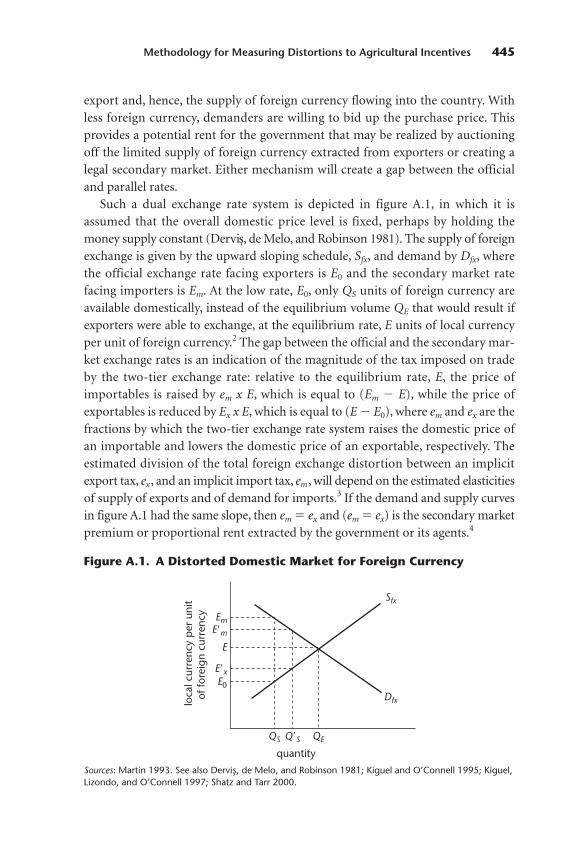
export and, hence, the supply of foreign currency flowing into the country. Withless foreign currency, demanders are willing to bid up the purchase price. Thisprovides a potential rent for the government that may be realized by auctioningoff the limited supply of foreign currency extracted from exporters or creating alegal secondary market. Either mechanism will create a gap between the officialand parallel rates.
Such a dual exchange rate system is depicted in figure A.1, in which it isassumed that the overall domestic price level is fixed, perhaps by holding themoney supply constant (Dervis, de Melo, and Robinson 1981). The supply of foreignexchange is given by the upward sloping schedule, Sfx, and demand by Dfx, wherethe official exchange rate facing exporters is E0 and the secondary market rate facing importers is Em. At the low rate, E0, only QS units of foreign currency areavailable domestically, instead of the equilibrium volume QE that would result ifexporters were able to exchange, at the equilibrium rate, E units of local currencyper unit of foreign currency.2 The gap between the official and the secondary mar-ket exchange rates is an indication of the magnitude of the tax imposed on tradeby the two-tier exchange rate: relative to the equilibrium rate, E, the price ofimportables is raised by em x E, which is equal to (Em � E), while the price ofexportables is reduced by Ex x E, which is equal to (E � E0), where em and ex are thefractions by which the two-tier exchange rate system raises the domestic price ofan importable and lowers the domestic price of an exportable, respectively. Theestimated division of the total foreign exchange distortion between an implicitexport tax, ex, and an implicit import tax, em, will depend on the estimated elasticitiesof supply of exports and of demand for imports.3 If the demand and supply curvesin figure A.1 had the same slope, then em � ex and (em � ex) is the secondary marketpremium or proportional rent extracted by the government or its agents.4
Methodology for Measuring Distortions to Agricultural Incentives 445
Figure A.1. A Distorted Domestic Market for Foreign Currency
QS
Sfx
Dfx
Em
E0
E
E�x
E�m
Q�S QE
loca
l cur
renc
y p
er u
nit
of fo
reig
n cu
rren
cy
quantity
Sources: Martin 1993. See also Dervis, de Melo, and Robinson 1981; Kiguel and O’Connell 1995; Kiguel,Lizondo, and O’Connell 1997; Shatz and Tarr 2000.

If the government chooses to allocate the limited foreign currency to differentgroups of importers at different rates, this is called a multiple exchange rate system.Some lucky importers may even be able to purchase foreign currency at the lowofficial rate. The more that is allocated and sold to demanders whose marginalvaluation is below Em, the greater the unsatisfied excess demand at Em, and, hence,the stronger the incentive for an illegal or black market to form and for less-unscrupulous exporters to lobby the government to legalize the secondary marketfor foreign exchange and to allow exporters to retain some fraction of theirexchange rate earnings for sale in the secondary market. Providing a right toexporters to retain and sell a portion of foreign exchange receipts increases theirincentives to export and thereby reduces the shortage of foreign exchange and,thus, the secondary market exchange rate (Tarr 1990). In terms of figure A.1, theavailable supply increases from QS to Q�
S, bringing down the secondary rate fromEm to E�
m, such that the weighted average of the official rate and E�m received by
exporters is E�x; the weights are the retention rate, r, and (1 � r). Again, if the
demand and supply curves in figure A.1 had the same slope, then the implicitexport tax and import tax resulting from this regime would each be equal to halfthe secondary market premium.
In the absence of a secondary market and in the presence of multiple rates forimporters below Em and for exporters below E0, a black market often emerges.The rate for buyers in this market will rise above E, the more the government sellsits foreign currency to demanders whose marginal valuation is below Em, and themore active the government is in catching and punishing exporters selling in theillegal market. If the black market were allowed to operate frictionlessly, there wouldbe no foreign currency sales to the government at the official rate, and the blackmarket rate would fall to the equilibrium rate, E. So, even though, in the lattercase, the observed premium would be positive (equal to the proportion by whichE is above the nominal official rate E0), there would be no distortion. For ourpresent purposes, since the black market is not likely to be completely friction-less, it may be considered similar to the system involving a retention scheme. Interms of figure A.1, E�
m would be the black market rate for a proportion of sales,and the weighted average of this and E0 would be the return going to exporters.Calculating E�
x in this situation (and thereby being able to estimate the implicitexport and import taxes associated with this regime) by using the same approachas in the case with no illegal market thus requires not only knowledge about E0
and the black market premium, but also a guess about the proportion, r, of salesin the black market.
In short, if a country exhibits distortions in its domestic market for foreign currency, the exchange rate relevant for calculating the NRAo or the CTE for a particular tradable product depends, in the case of a dual exchange rate system,
446 Distortions to Agricultural Incentives in Asia
on whether the product is an importable or an exportable, while, in the case ofmultiple exchange rates, it depends on the specific rate that applies to the prod-uct each year.
What about real exchange rate changes?A change in the real exchange rate alters equally the prices of exportables andimportables relative to the prices of nontradable goods and services. Such achange may arise for many different reasons, including changes in the availabilityof capital inflows, macroeconomic policy adjustments, or changes in the interna-tional terms of trade. If the economy receives a windfall, such as a greater inflow offoreign exchange from remittances, foreign aid, or a commodity boom, the com-munity moves to a higher indifference curve (Collier and Gunning 1998). Whilenet imports of tradables may change in response to this inflow of foreignexchange, the domestic supply of and demand for nontradables must balance. Theequilibrating mechanism is the price of nontradables. The price of nontradablesrises to bring forth the needed increase in the supply of nontradables and toreduce the demand for these products so as to bring the demand into line withsupply (Salter 1959).
While this type of alteration in the real exchange rate affects the incentive toproduce tradables, it is quite different in two respects from the distortions in themarket for foreign currency analyzed above. First, this real exchange rate appreci-ation reduces the incentives to produce importables and exportables to the samedegree. In contrast with the case of the multiple-tier exchange rate, the appreciationdoes not generate any change in the prices of exportables relative to importables.Second, most such changes do not involve direct economic distortions of the typemeasurable using tools such as producer surplus or consumer surplus. If thegovernment or the private sector chooses to borrow more from abroad to increasedomestic spending, this may raise the real exchange rate, but such an outcome isnot obviously a distortion. Moreover, the symmetric treatment of any such over-valuation during periods of high foreign borrowing would require that one takeinto account exchange rate undervaluation during periods of low foreign borrow-ing or the repayment of foreign debt. For these reasons, we do not follow Krueger,Schiff, and Valdés (1988) or Orden et al. (2007) in including deviations of realexchange rates from benchmark values unless these deviations arise from directexchange rate distortions such as multiple-tier exchange rates.5
What if trade costs are too high for a product to be traded internationally?Suppose the transport costs of trading are sufficient to make it unprofitable fora product to be traded internationally, such that the domestic price fluctuatesover time within the band created by the cost, insurance, and freight import
Methodology for Measuring Distortions to Agricultural Incentives 447
price and the free on board export price. Then, any trade policy measure (tm or sx)or the product-specific exchange rate distortion (for example, em or ex) is redundant.In this case, in the absence of other distortions, NRAo � 0, and the CTE � 0.However, in the presence of any domestic producer or consumer tax or subsidy(sf or tc), the domestic prices faced by both producers and consumers willbe affected. The extent of the impact depends on the price elasticities of domesticdemand and supply for the nontradable (the standard closed-economy tax incidence issue).
Thus, for example, suppose only a production tax is imposed on farmers producing a particular nontradable, so that sf � 0 and tc � 0. In this case:
NRADS � (A.5)
and
CTE � , (A.6)
where is the price elasticity of supply, and � is the (negative of the) price elasticityof demand.6
What if farm production involves primary factors, but also intermediate inputs?Where intermediate inputs are used in farm production, any taxes or subsidies onthe production, consumption, or trade of these inputs would alter farm valueadded and thereby also affect farmer incentives. Sometimes, a government willhave directly offsetting measures in place, such as a domestic subsidy for fertilizeruse by farmers, but also a tariff on fertilizer imports. In other situations, there willbe farm input subsidies, but an export tax on the final product.7 In principle, allthese items might be brought together to calculate an effective rate of direct assis-tance to farm value added (the effective rate of assistance). The nominal rate ofdirect assistance to farm output, NRAo, is a component of this, as is the sum of thenominal rates of direct assistance to all farm inputs, call it NRAi. In principle, allthree rates may be positive or negative.
The participants in this project have not been required to estimate effectiverates of assistance because to do so requires a knowledge of each product’s valueadded share of output. Such data are not available for most developing countriesfor every year in the time series nor even for every few years. And, in most devel-oping countries, distortions to farm inputs are small compared with distortions tofarm output prices, and these purchased inputs are a small fraction of the valueof output. However, where there are significant distortions to input costs, the ad
�sf�1 � �
�
�
sf�1 � �
��
�
448 Distortions to Agricultural Incentives in Asia
valorem equivalent is accounted for by summing each input’s NRA, multiplyingthis by the input-output coefficient to obtain the combined NRAi, and adding thisto the farm industry’s nominal rate of direct assistance to farm output, NRAo, toobtain the total NRA in farm production, call it simply NRA.8
NRA � NRAo � NRAi. (A.7)
What about postfarmgate costs?If a state trading corporation is charging excessively for its marketing services,thereby lowering the farmgate price of a product (for example, as a way of raisinggovernment revenue in place of an explicit tax), the extent of the excess should betreated as if it were a tax.
Some farm products, including some that are not internationally traded, areinputs into a processing industry that may also be subject to government inter-ventions. In this case, the effect of these interventions on the price received byfarmers for the primary product also needs to be taken into account. Before weexplain how, it may be helpful first to review the possible role the marketing anddistribution margins of the value chain may play in the calculation of distortionsin primary agricultural activities so as to ensure that nondistortionary pricewedges are not inadvertently included in any distortion calculations.
Nondistortionary price wedges
So far, it has been assumed that there are no divergences among farmer, processor-wholesaler, consumer, and border prices other than those arising because of sub-sidies or taxes on production, consumption, trade, or foreign currency. In practice,this is not so, and these costly value chain activities need to be explicitly recog-nized and netted out in using comparisons of domestic and border prices toderive estimates of government policy-induced distortions.9 Such recognitionalso offers the opportunity to compare the size of the NRA with wedges associatedwith, for instance, trade and processing costs (used in trade facilitation and valuechain analyses, respectively). It may also expose short-term situations where theprofits of importers or exporters are amplified by less-than-complete adjustmentby agents in the domestic value chain.
Domestic trading costsTrading costs may be nontrivial both intra- and internationally, especiallyin developing countries with poorly developed infrastructure.10 For example, domes-tic trading costs are involved in delivering farm products to port or to domesticwholesalers (assuming the latter are at the international border; otherwise, anotherset of domestic transport costs needs to be added to obtain a relevant price
Methodology for Measuring Distortions to Agricultural Incentives 449
comparison). Suppose, for instance, that domestic transport costs are equal to thefraction Tf of the price received by the farmer.
Processor-wholesaler costsDomestic processing costs and wholesale and retail distribution margins may rep-resent a large share of the final retail price. Indeed, Reardon and Timmer (2007)argue that these costs and margins are an increasingly important part of the valuechain in developing countries because consumers desire more postfarm process-ing and services added to their farm products, aided by the contribution of thesupermarket revolution to globalization.11 We denote the increases in the con-sumer price caused by these processing and wholesaling activities, over and abovethe farmgate price plus domestic trade costs, as mp and mu, respectively (or simplymu above the price of the imported processed product if the processing must bedone before the product is internationally tradable), in the absence of marketimperfections or government distortions along the value chain.
International trading costsInternational trading costs are not an issue in the distortions calculations if theinternational price used is the cost, insurance, and freight import unit value for animportable or the free on board export unit value for an exportable. But thesecosts are relevant if there is no trade (because of, say, a prohibitive trade tax on theproduct) or if the border prices are unrepresentative (because of low trade volumes,for example). In these instances, it is recommended that one select an interna-tional indicator price series (such as those of the World Bank or the InternationalMonetary Fund) and account for international trading costs (ocean or air freight,insurance, and so on).12 We denote Tm as the proportion by which the domesticprice of the import-competing product is raised above what it would otherwise beat the country’s border, or, equivalently, we denote Tx as the fraction of the free onboard price by which the price abroad of the exported product is greater.
Product quality and variety differencesThe quality of a product traded internationally is usually considered to differ fromthe quality of the domestically sold substitute, and consumers typically have ahome-country bias.13 Whenever appropriate, the domestic price should bedeflated (inflated) by the extent to which the good imported is deemed by domesticconsumers to be inferior (superior) in quality to the domestic product.14 Wedenote qm as the deflating fraction for the adjustment for product quality andvariety differences in the case of importables.
The situation is similar for exported goods. Especially if an international indicatorprice has to be used in lieu of the free on board export unit value (for example, if
450 Distortions to Agricultural Incentives in Asia
exports are close to zero and unrepresentative), the international price needs to bedeflated (inflated) by the extent to which the good is deemed by foreign con-sumers to be inferior (superior) in quality relative to the indicator good. Wedenote qx as the deflating fraction to adjust for product quality and variety differ-ences in the case of exportables.
Net effect of nondistortionary influencesIf one takes into consideration all these influences and so long as the product isstill traded internationally, the relationships between the price received by domes-tic farmers and the international price, in the absence of government-imposedprice and trade policies, are described by the following for an importable:
E � P � , (A.8)
and for an exportable it is the following:
E � P � , (A.9)
while the urban consumer price is above the producer price to the followingextent:
Pc � Pf (1 � Tf)(1 � mp)(1 � mu), (A.10)
where Pf is the farmgate price.
The impact of distortions in food processing on agricultural NRAs
Some farm products that are not internationally traded in their primary form (forexample, raw milk and cane sugar) are tradable once they have been lightlyprocessed, and the downstream processing industry may also be subject to gov-ernment interventions. In this case, the effect of the latter interventions on theprice received by farmers for the primary product also needs to be taken intoaccount, and the primary product should be classified as tradable.
Some analysts have assumed that any protection to processors, if it is passedback fully to primary agriculture (as may be the case with a farmer-owned coop-erative processing plant, for example), effectively raises the farmer price by theamount of the rise in the processor price, divided by the proportional contribu-tion of the primary product to the value of the processed product. Anotherequally extreme, but opposite assumption is that there is zero pass-through by theprocessor back down the value chain to the farmer. This is likely to be the case if
Pf (1 � Tf)(1 � mp)(1 � Tx)���
1 � qx
Pf (1 � Tf)(1 � mp)(1 � qm)���
1 � Tm
Methodology for Measuring Distortions to Agricultural Incentives 451

the raw material may be sourced internationally, but seems unlikely if the primaryproduct is nontradable and there is a positive price elasticity of farm supply (sincean assisted processor would want to expand). A more neutral assumption is thatthere is a proportional pass-through by the processor down the value chain tofarmers and their transporters or up the value chain to consumers. This would beequivalent to an equal sharing of the benefits along the value chain, which is morelikely to be the case, the more equally market power is spread among the players inthe chain.
This trio of examples illustrates the importance both of separating primary andprocessed activities for the purpose of calculating agricultural assistance ratesand of being explicit about the extent of pass-through that is occurring inpractice and, hence, the consequences for the NRAs in primary agricultural andprocessing activities.15
The above examples involving processors may also be generalized to any par-ticipants in the value chain. In particular, state trading enterprises and parastatalmarketing boards may intervene significantly, especially if they have been grantedmonopoly status by the government. Such interventions by domestic institutionsmay explain the low econometrically estimated degree of transmission of pricechanges at a border to farmgate domestic prices even following a significantreform of more-explicit price and trade policies (see Baffes and Gardner 2003 andthe references cited therein). Where reform has also involved the freeing up of pre-viously controlled parts of the marketing chain, the lowered marketing marginmay provide a benchmark against which to compare the prereform margin (as inUganda beginning in the mid-1990s; see Matthews and Opolot 2006).
The mean and standard deviation of agricultural NRAs
We need to generate a weighted average NRA for covered products in each coun-try because only then will we be able to add the NRA for noncovered products toobtain the NRA for all agriculture. If one wishes to average across countries, eachpolity is an observation of interest; so, a simple average is meaningful for the pur-pose of political economy analysis. But, if one wants a sense of the distortions inagriculture in a whole region, a weighted average is needed. The weighted averageNRA for covered primary agriculture may be generated by multiplying the valueshare of each primary industry in production (valued at farmgate equivalentundistorted prices) by the corresponding NRA and then adding across indus-tries.16 The overall sectoral rate, which we denote as NRAag, may be obtained byalso adding the actual or assumed information for the commodities not coveredand, where it exists, the aggregate value of non-product-specific assistance toagriculture.
452 Distortions to Agricultural Incentives in Asia

A weighted average may be similarly generated for the tradables part of agriculture—including those industries producing products such as milk andsugar that require only light processing before they are traded—by assuming thatthe share of the non-product-specific assistance goes to producers of tradables.Call this NRAagt.
In addition to the mean, it is important also to provide a measure of the dis-persion or variability of the NRA estimates across the covered products. The costof government policy distortions in incentives in terms of resource misallocationtends to be greater, the greater the degree of substitution in production (Lloyd1974). In the case of agriculture involving the use of farmland that is sector specific,but transferable among farm activities, the greater the variation of NRAs acrossindustries within the sector, the higher the welfare cost of these market interven-tions. A simple indicator of dispersion is the standard deviation of industry NRAswithin agriculture.17
Trade bias in agricultural assistance
A trade bias index also is needed to indicate the extent to which a country’s policyregime has an antitrade bias within the agricultural sector. This is importantbecause, as the Lerner (1936) symmetry theorem demonstrates, a tariff that assistsimport-competing farm industries has an effect on farmer incentives that is thesame as the effect of a tax on agricultural exports (see elsewhere above), and, ifboth measures are in place, this is a double imposition on farm exports. Thehigher the NRA for import-competing agricultural production (NRAagm) relativeto the NRA for exportable farm activities (NRAagx), the more incentive producersin the subsector will have to bid for mobile resources that would otherwise havebeen employed in export agriculture, all else being equal.
Once each farm industry has been classified as import-competing, as a pro-ducer of exportables, or as a producer of a nontradable (the status may sometimeschange over the years; see below), it is possible to generate, for each year, theweighted average NRAs for the two different groups of tradable farm industries.These may then be used to generate an agricultural trade bias index, TBI, which isdefined as follows:
TBI � ��11
�
�
NN
RR
AA
aagg
m
x� � 1�, (A.11)
where NRAagm and NRAagx are the average NRAs, respectively, for the import-competing and exportable parts of the agricultural sector (their weighted averageis NRAagt). This index has a value of zero whenever the import-competing andexport subsectors are equally assisted, and its lower bound approaches �1 in themost extreme case of an antitrade policy bias.
Methodology for Measuring Distortions to Agricultural Incentives 453
Indirect agricultural assistance and taxation through nonagricultural distortions
In addition to direct assistance to or taxation of farmers, the Lerner (1936) sym-metry theorem also demonstrates that farmer incentives are affected indirectly bygovernment assistance to nonagricultural production in the national economy.The higher the NRA for nonagricultural production (NRAnonag), the moreincentive producers in other sectors will have to bid up the value of mobileresources that would otherwise have been employed in agriculture, all else beingequal. If NRAag is below NRAnonag, one might expect there to be fewer resourcesin agriculture than there would be under free-market conditions in the country,notwithstanding any positive direct assistance to farmers, and, conversely, ifNRAag is greater than NRAnonag. A weighted average may be generated for thetradables part of nonagriculture, too; call it NRAnonagt.
One of the most important negative effects on farmers arises from protectionsfor industrialists from import competition. Tariffs are part of this, but so too (espe-cially in past decades) are nontariff barriers to imports. Other primary sectors (fishing, forestry, and minerals, including the extraction of energy raw materials)tend, on average, to be subject to fewer direct distortions than either agriculture ormanufacturing, but there are important exceptions. One example is a ban on logging;however, if such a ban is instituted for genuine reasons of natural resource conser-vation, it should be ignored. Another example is a resource rent tax on minerals.Unlike an export tax or quantitative restriction on the exports of such raw materials(which are clearly distortive and would need to be included in the NRA for mining),a resource rent tax, like a land tax, may be fairly benign in terms of resource real-location and, so, may be ignored (see Garnaut and Clunies Ross 1983).
The largest part of most economies is the services sector. This sector producesmostly nontradables, many of which are provided through the public sector. Dis-tortions in service markets have been extraordinarily difficult to measure, and nosystematic estimates across countries are available over time or even for a recentperiod. The only feasible way to generate time series estimates of NRAnonag inthis project has therefore involved the assumption that all services are nontrad-able, and that they, along with other nonagricultural nontradables, face no distor-tions. All the other nonagricultural products may be separated into exportablesand import-competing products for purposes of estimating correctly theirweighted average NRAs, ideally using production valued at border prices asweights (although, in practice, most of our authors have had to use shares of grossdomestic product).
Foreign exchange rate misalignment relative to the value of a country’s currency—as suggested by the fundamentals—will be ignored (see elsewhere above). This isbecause a real appreciation of the general foreign exchange rate uniformly lowers
454 Distortions to Agricultural Incentives in Asia
the price of all tradables relative to the price of nontradables; the converse is truefor a real devaluation. If a change in the exchange rate has been caused by aid orforeign investment inflows, then the excess of tradables consumption over trad-ables production leads to a new equilibrium. Certainly, such a new inflow of fundswould reduce the incentives among farmers producing tradable products, but thisis not a welfare-reducing policy distortion. Thus, it is only the exchange rate dis-tortions caused by a dual or multiple exchange rate system that need to beincluded in the calculation of the NRAs for the exportable and import-competingparts of the nonagricultural sector and, hence, of NRAnonagt, and this should beaccomplished in the same way discussed above for the inclusion of these distor-tions in the calculation of NRAagt.
Assistance to agricultural production relative to nonagricultural production
Given the calculation of NRAagt and NRAnonagt as above, it is possible to reckona relative rate of assistance (RRA), defined as follows:
RRA � ��11
�
�
N
N
RA
R
n
A
o
a
n
g
a
t
gt�� 1�. (A.12)
Since an NRA cannot be less than �1 if producers are to earn anything, thenneither can the RRA. The RRA is a useful indicator in undertaking internationalcomparisons over time of the extent to which a country’s policy regime has an anti-or proagricultural bias.
The Ways the Theory Is Put into Practice in This Study
Making the theory described above operational in the real world, where data areoften scarce, especially over a long time period, is as much an art as a science.18
Thankfully, for many countries, we have not had to start from scratch. NRAs areavailable from as early as 1955 in some cases and at least from the mid-1960s tothe early or mid-1980s for the 18 countries included in Krueger, Schiff, and Valdés(1988, 1991a) and Anderson and Hayami (1986). Much has been done to providedetailed estimates since 1986 of direct distortions in farmer incentives (thoughnot in food processing) in the high-income countries that are now members ofthe Organisation for Economic Co-operation and Development (OECD) and,since the early to mid-1990s, in selected European transition economies andBrazil, China, and South Africa (OECD 2007a, 2007b). At least for direct distor-tions, the Krueger, Schiff, and Valdés measures (1988, 1991a) have been updatedto the mid-1990s for some Latin American countries (Valdés 1996) and have also
Methodology for Measuring Distortions to Agricultural Incentives 455
been provided for some countries in Eastern Europe (Valdés 2000), and a new setof estimates of simplified producer support estimates for a few key farm productsin China, India, Indonesia, and Vietnam since 1985 is now available from theInternational Food Policy Research Institute (Orden et al. 2007). The methodol-ogy described above is, in some sense, a variation on each of these studies, and thebasic price data, at least, as well as the narratives attached to the estimates in thesestudies, are invaluable springboards for our study.19
Time period coverage of the study
For Europe’s transition economies, it is difficult to find meaningful data on thesituation prior to 1992. For the same reason, estimates are not particularly usefulbefore the 1980s for China and Vietnam. For all other countries, the target startdate has been 1955, especially if this date includes years before and after a year ofindependence so that one might examine the effects of independence, although,for numerous developing countries, the data simply are not available. The targetend date has been 2004, but, where available, 2005 data have also been included. Inmost cases, the most recent few years offer the highest quality data.
Farm product coverage of the study
The agricultural commodity coverage includes all the major food items (rice, wheat,maize or other grains, soybeans or other temperate oilseeds, palm oil or othertropical oils, sugar, beef, sheep and goat meat, pork, chickens and eggs, and milk),plus other key country-specific farm products (for example, other staples, tea, coffee or other tree crop products, tobacco, cotton, wine, and wool). Globally, as of2001, one-third of the value added in all agriculture and food industries has beenhighly processed food, beverages, and tobacco (GTAP Database; Dimaranan2006). We have also addressed these products briefly, in the same cursory way wehave addressed nonagricultural products. Fruits and vegetables are another one-sixth; so, the rest constitute the other half. Of that other half, meats are one-third;grains and oilseeds are almost another one-third; dairy products are one-sixth;and sugar, cotton, and other crops account for slightly more than one-fifth. If thehigh-income countries are excluded, these shares change quite sharply. Then,highly processed food, beverages, and tobacco are only half as important; fruitsand vegetables are somewhat more important, and, if these two groups (whichtogether account for 41 percent of the total) are excluded, the residual is equallydivided between three groups: meats, grains and oilseeds, and other crops anddairy products. By focusing on all major grain, oilseed, and livestock products,plus any key horticultural and other crop products, the coverage of our project
456 Distortions to Agricultural Incentives in Asia
reaches the target of 70 percent of the value added of most countries in agricul-ture and lightly processed food. Priority has been assigned to the most distortedindustries because the residual will then have not only a low weight, but also a lowdegree of distortion.
If highly processed food, beverages, and tobacco are excluded, then fruits andvegetables account for almost one-quarter of household food expenditure indeveloping countries. If fruits and vegetables are also excluded, three groups eachthen account for almost 30 percent of expenditure: pig and poultry products, redmeat and dairy products, and grains and oilseed products. All other crops accountfor the remaining one-eighth. So, from the consumer tax viewpoint, the desiredproduct coverage is the same as the coverage outlined above from a productionviewpoint.
Each product is explicitly identified as import-competing, exporting, or non-tradable. For many products, this categorization changes over time. In some cases,products move monotonically through these three categories, and, in others, theyfluctuate in and out of nontradability. Hence, an indication of a product’s nettrade status is given for each year rather than for only one categorization for thewhole time series. In large-area countries with high internal and coastal shippingcosts, some regions may be exporting abroad, even while other regions are netimporters from other countries. In such cases, it is necessary to estimate separateNRAs for each region and then generate a national weighted average.
Farm input coverage
The range of input subsidies considered in any particular country study in ourproject has depended on the degree of distortions in that country’s input markets.In addition to fertilizer, the large inputs and distortions are likely to involve elec-trical or diesel power, pesticides, and credit (including, occasionally, large-scaledebt forgiveness, as in Brazil and Russia, although how this is spread out beyondthe year of forgiveness is an issue).20 There are also distortions revolving aroundwater, but the task of measuring water subsidies is especially controversial and com-plex; so, these distortions have not been included in the NRA calculations. (TheOECD has also ignored them in its producer support estimates.) Similarly, distor-tions in land and labor markets have been excluded, apart from qualitative discus-sions in the analytical narratives in some of the country case studies.
Trade costs
For the calculation of distortions in international trading costs, Tm and Tx, the freeon board–cost, insurance, and freight gap in key bilateral trade in products during
Methodology for Measuring Distortions to Agricultural Incentives 457

years when the products have been traded in significant quantities is used. Bothinternational and domestic trading costs are a function of the quality of hardinfrastructure (roads, railways, ports) and soft infrastructure (business regula-tions and customs clearance procedures at state and national borders), each ofwhich may be affected by government actions. However, because it is difficult toallocate these costs between items that are avoidable and those that are unavoid-able, measuring the aggregate size of the distortions involved in a comparable wayfor a range of countries is beyond the scope of this study.21
Classifying farm products as import-competing, exportable, or nontradable
The criteria used in classifying farm industries as import-competing (M), export-ing (X), or nontrading (H) are not straightforward. Apart from the complicationsraised above about whether a product is not traded simply because of trade taxesor nontariff barriers, there will be cases where trade is minimal, or the trade statushas been reversed because of policy distortions, or the industry is characterized bysignificant imports and exports. A judgment has to be made for each sector eachyear as to whether it should be classified as M, X, or H. In the case of the two trad-able classifications (that is, leaving out nontradables), this judgment will deter-mine which exchange rate distortion to use. If trade is minimal for reasons oftrade cost rather than reasons of trade policy, then a product is classified as non-tradable if the share of production exported and the share of consumptionimported are each less than 2.5 percent, except in situations (for example, rice inChina) in which the product is clearly an exportable year after year even thoughthe self-sufficiency rate is rarely above 101 percent. Otherwise, if the share of pro-duction exported is substantially above (below) the share of consumptionimported, the product is classified as exportable (importable).
In cases in which the trade status has been reversed because of a policy distor-tion (for instance, an export subsidy, in combination with a prohibitive importtariff, is large enough to encourage sufficient production to generate an exportsurplus), the product should be given the classification of the trade status thatwould prevail without the intervention (that is, import-competing). The sameapplies if tariff preferences reverse a country’s trade status with respect to a prod-uct. The exports of many countries enjoy preferential access into the protectedmarkets of other countries. In some cases, these arrangements are based on bilat-eral or plurilateral free trade agreements or customs unions. In other cases, thepreferences are unilaterally offered by higher-income countries to developingcountries through schemes such as the generalized system of preferences, theCotonou Agreement (between the Africa, Caribbean, and Pacific group and the
458 Distortions to Agricultural Incentives in Asia
European Union), and the European Union’s Everything But Arms Initiative. Inthe few extreme cases where these preferences are such that they (in combinationwith a prohibitive import tariff) cause the developing country to become an exporterof a product that would otherwise be import-competing (such as sugar in thePhilippines), the product should nonetheless be classified as import-competingbecause the developing country’s import-restrictive policy is allowing the domesticprice of the product to equal the price reached in exporting to the preference-providing country.
If there are significant exports and imports in a given year, closer scrutiny isrequired. If, for example, there are high credit or storage costs domestically, aproduct may be exported immediately following harvest, but imported later in theyear to satisfy consumers out of season. The product would be considered anexportable for purposes of calculating the NRA because, even if there are policiesrestricting out-of-season imports (which would affect the CTE calculation), theywould not represent an encouragement for the production earlier in the year inthe presence of high credit or storage costs.
If trade or exchange rate distortions are sufficiently large to choke off interna-tional trade in a product, then they contribute to the NRA and CTE only to theextent required to drive that trade to zero: any trade taxes that exceed this require-ment have an element of redundancy. If there are trade policy distortions, but notrade passes over them (that is, they are prohibitive), there may still be policyeffects that need to be measured, but they will differ from those involved in theother cases above. An example would be a prohibitive tariff that is high enough totake the price of imported goods above the autarchy price and thus results in noimports. The NRA would therefore be less than the prohibitive tariff rate. Anothercommon example is an import tariff in a context in which the world price is suffi-ciently high so that the country is freely exporting the product at issue. In thiscase, the domestic price would be determined by the world price, less the exporttrade costs; the import tariff would be irrelevant, and there would be no distor-tion despite the presence of the import tariff.
Similar conditions apply to exportable goods in a context in which a prohibitiveexport tax creates a distortion at a level lower than the tax rate. Then, the distortionwedge would be equal to the difference between the autarchy price and the worldprice, less the export trade costs; if the country were freely importing the good, theexport tax would be irrelevant, and there would be no distortion despite the presenceof the export tax. The choice of the international price to be compared with domesticprices is therefore not based only on the actual trading status of a country (Byerleeand Morris 1993). Moreover, different prices may be needed for different regionsof a large country that simultaneously exports and imports because internal tradingcosts (including coastal shipping) are so high relative to international trading
Methodology for Measuring Distortions to Agricultural Incentives 459
costs (Koester 1986). In this case, the value of production is split according to theregional production shares in the country. If the only intervention in this sector isa tariff on imports, the tariff rate is the NRA estimate for the import-competingpart, and the NRA is zero for the other part of the sector; these different NRAs arethen included in the weighted average calculations of the NRAs for the import-competing and exportable subsectors of agriculture.
The transmission of assistance and taxation along the agricultural value chain
A crucial aspect of the NRA calculation for agricultural products is the way anypolicy measure beyond the farmgate is transmitted back to farmers and forwardto consumers. Only a few parameters and exogenous variables are needed toobtain meaningful estimates of an individual agricultural product’s NRA andCTE. Specifically, to take account of the pass-through of distortions along thevalue chain, parameters have been identified as follows (although the default is anequiproportionate pass-through):
• �f , the extent to which any distortion to a primary farm product at the wholesalelevel is passed back to farmers
• �, the extent to which any distortion to the downstream processed product ispassed back to wholesalers of a primary farm product that is nontradable
The CTEs of farm products
Many farm products are processed and are used as ingredients in the additionalprocessing of food products before the food products are purchased by final con-sumers. (For example, wheat is ground to flour and then mixed with other ingredi-ents before baking, slicing, and packaging for sale as bread.) Other farm productsare used as inputs in various farm activities, often after the farm products haveundergone some processing. (Thus, soybeans are crushed, and the meal is mixedwith maize or other feed grains for use as animal feed, while the oil is sold forcooking.) Because of these many and varied value chain paths and because, inpractice, it is difficult anyway to determine the extent to which a change in the primary farm product would be passed along any of these value chains, the OECDexpresses its consumer support estimate simply at the level at which a product isfirst traded (for example, as wheat, or soybeans, or beef). This practice has beenadopted here, too, to generate a consistent set of CTEs across countries to use in theanalysis in chapter 1 (even though our authors of individual country studies mayreport CTEs that they have estimated in a more-sophisticated way farther alongthe value chain). In the absence of any domestic production or consumption taxesor subsidies directly affecting a product, the CTE at the point at which the product
460 Distortions to Agricultural Incentives in Asia
is first traded will be the same as the NRAo. (Also recall that the NRAo in this casealso equals the NRA if NRAi is zero.)
Key required information
A template spreadsheet has been designed to aid in the management of individualcountry information and ensure a consistent comparison across regions and peri-ods. The precise ways in which parameters and exogenous variables have enteredeach country spreadsheet to generate the NRAs and CTEs endogenously aredetailed in Anderson et al. (2008a, 2008b). Most are straightforward; the mainexception is the treatment of exchange rate distortions that is described below.
The key exogenous variables needed are the agricultural quantities producedand consumed (or imported and exported if the proxy for consumption is pro-duction, plus net imports); the wholesale and border prices of primary and lightlyprocessed agricultural goods (along with, where relevant, a quality adjustment tomatch border prices); agricultural domestic input and output subsidies and taxes(the default is zero); if there are distorted farm input markets, the share of theinput in the value of farm output at border prices (and, if there are only farmgateprices rather than wholesale prices for a primary good, the proportion of the farm-gate value in the value at the wholesale level measured at the border price); thefinal domestic food consumer subsidies or taxes (the default is zero); and the officialexchange rate (and, where prevalent, the parallel exchange rate and the share ofcurrency going through the secondary or illegal market, plus the product-specificexchange rate if a multiple exchange rate system is in place).
Exchange rate distortions
The treatment of exchange rate distortions is worth spelling out since it differsfrom the method used by Krueger, Schiff, and Valdés (1988, 1991a).
If there are no exchange rate distortions, the official exchange rate is used.However, in the presence of a parallel market rate (which might be the black market rate if no legal secondary market exists), this is reported, along with anestimate of the proportion of foreign currency that is actually sold by exportersat the parallel market rate. This proportion is the formal retention rate if a for-mal dual exchange regime is in place; otherwise, it is based on a guesstimate ofthe proportion traded on the black market. (The black market premiums areprovided in Cowitt, various years; Cowitt, Edwards, and Boyce, various years;and the Global Development Network Growth Database). The spreadsheet isthen used to compute an estimate for the equilibrium exchange rate for the economy; this is the rate at which international prices are converted into localcurrency for the computation of each NRA.
Methodology for Measuring Distortions to Agricultural Incentives 461

Relevant exchange rates for importers and exporters are also then computedendogenously. If they are distorted away from the official exchange rate, the relevantexchange rate for importers and exporters are, respectively, the discounted paral-lel market rate and the weighted average of the official exchange rate and the dis-counted parallel rate according to the proportion of the exporter’s currency that issold on the parallel market. However, if a multiple exchange rate system is in placeand this system provides for a specific rate for a product that differs from the generalrates automatically calculated as above, then the automatically computed relevantexchange rate is replaced by this industry-specific rate.
Guesstimates of NRAs for agricultural products not covered
In the calculation of the weighted average rates of assistance for a subsector or sector, NRAs must be guesstimated for the agricultural products that are not covered (30 percent or so) and for which price comparisons are not calculated.The OECD, in its work on producer support estimates, assumes that the part notmeasured enjoys the same market price support as the average of the measuredpart. Another default is the assumption that the rates are zero. Orden et al. (2007)show that these two alternatives produce significantly different results for India. Itis therefore preferable to make informed judgments about the import-competing,exportable, and nontradable parts of the residual group of farm products. Anaverage applied import tariff is often the best guess for only the import-competingproducts among this set if there is no evidence of the existence of explicit produc-tion, consumption, or export taxes or subsidies. Even though this approach willmiss the nontariff trade barriers affecting these residual products, the bias will besmall if the weight is small.
Non-product-specific assistance to agriculture
If, in addition to the product-specific subsidies or taxes, there are non-product-specific forms of agricultural subsidies or taxes that one is unable to allocateamong importables, exportables, and nontradables, these are included in theNRAag using the same method (as a percentage of the total value of production)used for these types of interventions in the OECD’s calculations of its total support estimate (see OECD 2007a, 2007b).
No attempt is made to estimate the discouraging effects of underinvestmentin rural infrastructure or underdevelopment among pertinent institutions. Thestructure of the related expenditure within the rural sector is also important.This may well be a nontrivial part of the distortions in agricultural incentives,but, unfortunately, it is not captured in the measures of distortions outlinedabove.
462 Distortions to Agricultural Incentives in Asia

In some higher-income countries, governments also assist farm householdsthrough payments that are purported to be decoupled from production incentives.An example is the single farm payment in the European Union. We do not countsuch payments as part of NRAag because the latter refers specifically to measuresthat alter producer incentives. However, we do include the ad valorem equivalent ofthese payments in discussing assistance to farmers as a social group so as to be ableto compare the order of magnitude of this equivalent with the support providedthrough measures that alter production incentives.
Assistance to nonagricultural sectors
If nonagricultural sectors are assisted only through import tariffs on manufac-tures or export taxes on minerals, it is a relatively easy task to estimate aweighted average NRAnonag once the shares of import-competing, exporting,and nontradable production have been determined. In practice, however, non-tariff trade measures must also be considered among the measures affectingtradables (Dee and Ferrantino 2005; OECD 2005), and most economies havemyriad regulations affecting the many service industries. These regulations maybe complex (see Findlay and Warren 2000). Because most of the outputs of serviceindustries (including the public sector) are nontradable, the default in thisstudy is to assume that the average rate of government assistance, along withthat of nontradable nonagricultural goods, is zero. Then, the task of estimatingthe NRAnonag is reduced to obtaining only the NRAs for the producers ofimport-competing products and of export-oriented nonagricultural goods, plusthe shares of these products and goods in the undistorted value of the productionof nonagricultural tradables, so as to derive the weighted average NRAnonagt tobe entered into the RRA calculations.
The use of percentages in the chapters
To simplify the presentation in the chapters, the NRAo, NRAi, NRA, CTE, and RRAare expressed there as percentages rather than proportions.
Dollar values of farmer assistance and consumer taxation
For chapter 1, we have taken the country authors’ estimate of NRA and multipliedit by the gross value of production at undistorted prices to obtain an estimate incurrent US dollars of the direct gross subsidy equivalent of assistance to farmers(GSE). This can then simply be added up across products for a country and acrosscountries for any or all products to get regional aggregate transfer estimates for thestudied countries. To get an aggregate estimate for the rest of the region, we assumethe weighted average NRA for nonstudied countries is the same as the weighted
Methodology for Measuring Distortions to Agricultural Incentives 463
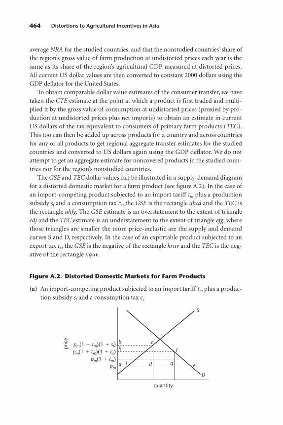
average NRA for the studied countries, and that the nonstudied countries’ share ofthe region’s gross value of farm production at undistorted prices each year is thesame as its share of the region’s agricultural GDP measured at distorted prices.All current US dollar values are then converted to constant 2000 dollars using theGDP deflator for the United States.
To obtain comparable dollar value estimates of the consumer transfer, we havetaken the CTE estimate at the point at which a product is first traded and multi-plied it by the gross value of consumption at undistorted prices (proxied by pro-duction at undistorted prices plus net imports) to obtain an estimate in currentUS dollars of the tax equivalent to consumers of primary farm products (TEC).This too can then be added up across products for a country and across countriesfor any or all products to get regional aggregate transfer estimates for the studiedcountries and converted to US dollars again using the GDP deflator. We do notattempt to get an aggregate estimate for noncovered products in the studied coun-tries nor for the region’s nonstudied countries.
The GSE and TEC dollar values can be illustrated in a supply-demand diagramfor a distorted domestic market for a farm product (see figure A.2). In the case ofan import-competing product subjected to an import tariff tm plus a productionsubsidy sf and a consumption tax cc, the GSE is the rectangle abcd and the TEC isthe rectangle ahfg. The GSE estimate is an overstatement to the extent of trianglecdj and the TEC estimate is an understatement to the extent of triangle efg, wherethose triangles are smaller the more price-inelastic are the supply and demandcurves S and D, respectively. In the case of an exportable product subjected to anexport tax tx, the GSE is the negative of the rectangle kruv and the TEC is the neg-ative of the rectangle nquv.
464 Distortions to Agricultural Incentives in Asia
Figure A.2. Distorted Domestic Markets for Farm Products
S
D
pm(1 � tm)(1 � sf)bh
a j d e
f
c
g
pm(1 � tm)(1 � cc)pm(1 � tm)
pm
pric
e
quantity
(a) An import-competing product subjected to an import tariff tm plus a produc-tion subsidy sf and a consumption tax cc

Notes
1. The NRA therefore differs from the producer support estimate calculated by the Organisationfor Economic Co-operation and Development (OECD) in that the producer support estimate isexpressed as a fraction of the distorted value (see the OECD PSE-CSE Database). It is thus tm/(1 � tm),and, so, for a positive tm, it is smaller than the NRA and is necessarily less than 100 percent.
2. Equilibrium here refers to the situation that would prevail without the distortion in the domesticmarket for foreign currency. In figure A.1 and in the discussion that follows, the equilibrium exchangerate, E, exactly balances the supply and demand for foreign currency. Taken literally, this implies a zerobalance on the current account. The approach here may readily be generalized to accommodate exoge-nous capital flows and transfers, which would shift the location of QE. With constant-elasticity supplyand demand curves, all of the results would carry through, and any exogenous change in the capitalflows or transfers would imply a shift in the Dfx or Sfx curves.
3. From the viewpoint of using the NRAo and CTE estimates later as parameters in a computablegeneral equilibrium model, it does not matter which assumptions are made here about these elastici-ties because the model’s results for real variables will not be affected. What matters for real impacts isthe magnitude of the total distortion, not its allocation between an export tax and an import tax; thisis the traditional incidence result from tax theory that also applies to trade taxes (Lerner 1936). For anexcellent general equilibrium treatment using an early version of the World Bank’s 1–2–3 model, see deMelo and Robinson (1989). There, the distinction is drawn between traded and nontraded goods(using the Armington [1969] assumption of differentiation between products sold on the domesticmarket and products sold on the international market), in contrast to the distinction between tradableand nontradable products made below in the text.
4. Note that this same type of adjustment might be made if the government forces exporters tosurrender all foreign currency earnings to the domestic commercial banking system and importersto buy all foreign currency needs from that banking system and if that system is allowed by regula-tion to charge excessive fees. This apparently occurs in, for example, Brazil, where the spread isreputedly 12 percent. If actual costs in a nondistorted competitive system are only 2 percent (as theyare in the less-distorted Chilean economy), the difference of 10 points might be treated as the equiv-alent of a 5 percent export tax and a 5 percent import tax applying to all tradables (although, as withnontariff barriers, there would be no government tariff revenue, but rather rent, which, in this case,would accrue to commercial banks instead of to the central bank). This is an illustration of thepoint made by Rajan and Zingales (2004) about the power of financial market reform to expandopportunities.
Methodology for Measuring Distortions to Agricultural Incentives 465
S
D
px
px(1 � tx)
v
ur
k n
qp
rice
quantity
Source: Authors’ derivation.
(b) An exportable product subjected to an export tax tx

5. The results of a multicountry research project that has had macropolicy as its focus are reportedin Little et al. (1993).
6. As in the case of the two-tier exchange rate, the elasticities are used merely to identify the inci-dence of these measures; as long as both the NRAo and the CTE are included in any economic modelused to assess the impact of the production tax, the real impacts will depend only on the magnitude ofthe total distortion, sf , not on the estimated NRA and CTE.
7. On this general phenomenon of offsetting distortions for outputs and inputs (and even directpayments or taxes), see Rausser (1982).
8. Bear in mind that a fertilizer plant or livestock feed mix plant might be enjoying import tariffprotection that raises the domestic price of fertilizer or feed mix to farmers by more than any con-sumption subsidy (as was the situation with respect to fertilizer in Korea; see Anderson 1983). In sucha case, the net contribution of this set of input distortions to the total NRA for agriculture would benegative.
9. This is not to say that there is no interest in comparisons across countries or over time in, forexample, the farmgate price as a proportion of the free on board export price, which summarizes theextent to which the producer price is depressed by the sum of internal transport, processing, and mar-keting costs, plus items such as explicit or implicit production or export taxes. Prominent users of thisproportion—which may be less than half in low-income countries even if there is little or no processing—include Bates (1981) and Binswanger and Scandizzo (1983). Users need to be aware, though, that thisratio understates the extent of farmer assistance (that is, it understates the rate of protection or over-states the rate of disprotection to farmers), possibly by a large margin.
10. On the basic economics of trading costs as affected by, for example, infrastructure within thecountry, at the border (ports, airports), and, in the case of landlocked countries, in transit countries, aswell as international freight costs and so on, and their impact on both the aggregate volume and productstructure of international trade, see Limão and Venables (2001), Venables and Limão (2002), and Venables (2004). See also the survey by Anderson and van Wincoop (2004), where it is reported that thetax equivalent of trading costs are estimated at more than 170 percent in high-income countries andhigher in developing and transition economies, especially those that are small, poor, and remote. By low-ering these trading costs (for example, by streamlining customs clearance procedures), trade facilitationmay be the result not only of technological changes, but also of government policy choices such as restric-tions on the ships that may be used in bilateral trade. For example, Fink, Mattoo, and Neagu (2002) esti-mate that the policy contribution to the cost of shipping goods from developing countries to the UnitedStates is greater than the border import barriers. More generally, on imperfect competition in servicesmarkets, including cartelized international shipping, see Francois and Wooten (2001, 2006).
11. The costs of processing and of wholesale and retail distribution, as well as domestic tradingcosts, change over time not only because of technological advances, but also following policy changes.For example, government investment in rural infrastructure may lower trading costs. Reardon andTimmer (2007) argue that the global supermarket revolution is, in part, driven by the opening ofdomestic markets following the relaxation of government restrictions on foreign direct investmentsince the 1980s. These types of government policies are not included in our project’s measurement ofdistortions.
12. Trading costs may be unrelated to the product price (that is, specific rather than ad valorem), inwhich case the formulas should be adjusted accordingly (for example, if Tf is in dollars per ton). If thiswere the case with international trading costs, the domestic price of importables (exportables) wouldchange less (more) than proportionately with P. The ad valorem assumption is preferable to the specificone in situations where international price and exchange rate changes are less than those that are fullypassed though the domestic value chain to the farmer and consumer because of incomplete marketintegration caused, for example, by poor infrastructure or weak institutions. Ideally, in such cases, onewould estimate econometrically the extent to which the price transmission elasticity is below unity anduse this to calculate the margin each year.
Trading costs include the storage costs that would be incurred to hold domestic products until thetime in the season when international trade takes place. Any subsidies or taxes on these or any other
466 Distortions to Agricultural Incentives in Asia
trading costs should be included in the distortion calculus. On the importance of these domestic trad-ing costs in low-income countries, see Khandker, Balkht, and Koolwal (2006) on Bangladesh; Moser,Barrett, and Minten (2005) on Madagascar; and Diop, Brenton, and Asarkaya (2005) on Rwanda.
13. On the how and the why of the variation by country of origin in the quality and variety oftraded goods, see Hummels and Klenow (2005).
14. We assume that the quality difference arises because one good provides more effective units ofservice than another, so that the relative price is a constant proportion of the value of the first good. Ifproducts are simply differentiated, without such a quality dimension (as in Armington 1969), therewill be no fixed relationship between the two prices.
15. In using the NRA and the CTE estimates later as parameters in a computable general equilib-rium model, as in the case of the incidence of the exchange rate distortion discussed elsewhere above,the assumptions made here about the extent of pass-though along the value chain may not greatlyaffect the model’s results for real variables such as prices, output, and value added.
16. Corden (1971) proposed that free trade volumes be used as weights, but, because these are notobservable (and an economy-wide model is needed to estimate them), the common practice is to com-promise by using actual distorted volumes, but undistorted unit values or, equivalently, distorted values,divided by (1 � NRA). If estimates of own-and cross-price elasticities of demand and supply are avail-able, a partial equilibrium estimate of the quantity at undistorted values might then be generated, but,if these estimated elasticities are unreliable, this may introduce additional error over and above theerror one seeks to correct.
17. The mean and standard deviations might be captured by a single measure, namely, the traderestrictiveness index developed by Anderson and Neary (2005). Calculating this index even in its sim-plest partial equilibrium mode requires that one know the own-and cross-price elasticities of demandand supply (or, at least, the elasticity of import demand, but this shortcut is only usable if the NRA andCTE are identical).
18. In addition to the methodologies of Krueger, Schiff, and Valdés (1988, 1991a) and the OECD(2007a, 2007b) for estimating agricultural distortion and producer support indicators, see the recentreview by Josling and Valdés (2004) of methodologies in earlier studies.
19. Other trade policy studies have also been of great help, particularly studies on trade andexchange rate distortions. These include various multicountry studies such as the one summarized inBhagwati (1978) and Krueger (1978) and more-recent ones summarized in Bevan, Collier, and Gunning(1989); Michaely, Papageorgiou, and Choksi (1991); Bates and Krueger (1993); and Rodrik (2003).
20. For an analysis of input subsidies in Indian agriculture, see Gulati and Narayanan (2003).21. That these costs vary hugely across countries and often dwarf trade taxes has now been clearly
established. See, for example, World Bank (2006a, 2006b), the Doing Business Database, and the gov-ernance and anticorruption indicators in the WGI Database. Also now available is a database on infor-mation and communications cost indicators for 144 countries; see the ICT at a Glance Database.In some settings, price bands induced by trading costs arising because of missing or imperfect marketsin rural areas lead poor farmers to forgo cash crops to ensure sufficient food production for survival(de Janvry, Fafchamps, and Sadoulet 1991; Fafchamps 1992). This contributes to the low supplyresponsiveness among poor producers to international price changes for the cash crops.
References
Anderson, James E., and J. Peter Neary. 2005. Measuring the Restrictiveness of International Trade Policy.Cambridge, MA: MIT Press.
Anderson, James E., and Eric van Wincoop. 2004. “Trade Costs.” Journal of Economic Literature 42 (3):691–751.
Anderson, Kym. 1983. “Fertilizer Policy in Korea.” Journal of Rural Development 6 (1): 43–57.Anderson, Kym, and Yujiro Hayami, eds. 1986. The Political Economy of Agricultural Protection: East
Asia in International Perspective. London: George Allen and Unwin.
Methodology for Measuring Distortions to Agricultural Incentives 467
Anderson, K., M. Kurzweil, W. Martin, D. Sandri, and E. Valenzuela. 2008. “Measuring Distortions toAgricultural Incentives, Revisited.” World Trade Review 7 (4): 675–704.
. 2008b. “Measuring Distortions to Agricultural Incentives, Revisited.” World Trade Review 7 (4):675–704.
Anderson, Kym, Will Martin, and Ernesto Valenzuela. 2006. “The Relative Importance of Global Agricultural Subsidies and Market Access.” World Trade Review 5 (3): 357–76.
Armington, Paul S. 1969. “A Theory of Demand for Products Distinguished by Place of Production.”IMF Staff Papers 16 (1): 159–78.
Baffes, John, and Bruce L. Gardner. 2003. “The Transmission of World Commodity Prices to DomesticMarkets under Policy Reforms in Developing Countries.” Journal of Policy Modeling 6 (3): 159–80.
Bates, Robert Hinrichs. 1981. Markets and States in Tropical Africa: The Political Basis of AgriculturalPolicies. Berkeley, CA: University of California Press.
Bates, Robert Hinrichs, and Anne O. Krueger, eds. 1993. Political and Economic Interactions in EconomicPolicy Reform: Evidence from Eight Countries. Oxford: Blackwell.
Bevan, David, Paul Collier, and Jan Willem Gunning. 1989. Peasants and Governments: An EconomicAnalysis. With Arne Bigsten and Paul Horsnell. Oxford: Clarendon Press.
Bhagwati, Jagdish N. 1971. “The Generalized Theory of Distortions and Welfare.” In Trade, Balance ofPayments and Growth: Papers in International Economics in Honor of Charles P. Kindleberger, ed.Jagdish N. Bhagwati, Ronald Jones, Robert Mundell, and Jaroslav Vanek, 69–90. Amsterdam:North-Holland.
. 1978. Foreign Trade Regimes and Economic Development: Anatomy and Consequences ofExchange Control Regimes. Cambridge, MA: Ballinger.
Binswanger, Hans P., and Pasquale L. Scandizzo. 1983. “Patterns of Agricultural Protection.” ARU Discussion Paper 15, Agricultural Research Unit, Agriculture and Rural Development Department,World Bank, Washington, DC.
Byerlee, Derek, and Michael L. Morris. 1993. “Calculating Levels of Protection: Is it Always Appropriateto Use World Reference Prices Based on Current Trading Status?” World Development 21 (5):805–15.
Collier, Paul, and Jan Willem Gunning. 1998. “Trade Shocks: Theory and Evidence.” In Africa. Vol. 1 ofTrade Shocks in Developing Countries, ed. Paul Collier and Jan Willem Gunning, 1–63. With associates.Oxford: Clarendon Press.
Corden, W. Max. 1971. The Theory of Protection. Oxford: Clarendon Press.. 1997. Trade Policy and Economic Welfare. 2nd ed. Oxford: Clarendon Press.
Cowitt, P. P., ed. Various years. World Currency Yearbook. Brooklyn: Currency Data and Intelligence, Inc.Cowitt, P. P., C. A. Edwards, and E. R. Boyce, eds. Various years. World Currency Yearbook. Brooklyn:
Currency Data and Intelligence, Inc.Dee, Philippa, and Michael Ferrantino, eds. 2005. Quantitative Methods for Assessing the Effects of
Non-Tariff Measures and Trade Facilitation. Singapore: World Scientific Publishing; Singapore:Committee on Trade and Investment, Asia-Pacific Economic Cooperation.
de Janvry, Alain, Marcel Fafchamps, and Elisabeth Sadoulet. 1991. “Peasant Household Behaviour withMissing Markets: Some Paradoxes Explained.” Economic Journal 101 (409): 1400–17.
de Melo, Jaime, and Sherman Robinson. 1989. “Product Differentiation and the Treatment of ForeignTrade in Computable General Equilibrium Models of Small Economies.” Journal of InternationalEconomics 27 (1–2): 47–67.
Dervis, Kemal, Jaime de Melo, and Sherman Robinson. 1981. “A General Equilibrium Analysis of Foreign Exchange Shortages in a Developing Economy.” Economic Journal 91 (364): 891–906.
Dimaranan, Betina V., ed. 2006. Global Trade, Assistance, and Production: The GTAP 6 Data Base. WestLafayette, IN: Center for Global Trade Analysis, Purdue University.
Diop, Ndiame, Paul Brenton, and Yakup Asarkaya. 2005. “Trade Costs, Export Development, andPoverty in Rwanda.” Policy Research Working Paper 3784, World Bank, Washington, DC.
Doing Business Database. World Bank and International Finance Corporation. http://www.doingbusiness.org/ (accessed October 2007).
468 Distortions to Agricultural Incentives in Asia
Fafchamps, Marcel. 1992. “Cash Crop Production, Food Price Volatility, and Rural Market Integrationin the Third World.” American Journal of Agricultural Economics 74 (1): 90–99.
Findlay, Christopher, and Tony Warren, eds. 2000. Impediments to Trade in Services: Measurement andPolicy Implications. Routledge Studies in the Growth Economies of Asia. London and New York:Routledge.
Fink, Carsten, Aaditya Mattoo, and Ileana Cristina Neagu. 2002. “Trade in International MaritimeServices: How Much Does Policy Matter?” World Bank Economic Review 16 (1): 81–108.
Francois, Joseph F., and Ian Wooton. 2001. “Trade in International Transport Services: The Role ofCompetition.” Review of International Economics 9 (2): 249–61.
. 2006. “Market Structure and Market Access.” Draft working paper, Erasmus School of Economics, Erasmus University, Rotterdam.
Garnaut, Ross Gregory, and Anthony I. Clunies Ross. 1983. The Taxation of Mineral Rents. Oxford:Clarendon Press.
Global Development Network Growth Database. Development Research Institute, New York University.http://www.nyu.edu/fas/institute/dri/global%20development%20network%20growth%20database.htm (accessed June 2007).
GTAP (Global Trade Analysis Project) Database. Center for Global Trade Analysis, Department of Agricul-tural Economics, Purdue University. https://www.gtap.agecon.purdue.edu/databases/v6/default.asp(version 6).
Gulati, Ashok, and Sudha Narayanan. 2003. The Subsidy Syndrome in Indian Agriculture. New Delhi:Oxford University Press.
Harberger, Arnold C. 1971. “Three Basic Postulates for Applied Welfare Economics: An InterpretativeEssay.” Journal of Economic Literature 9 (3): 785–97.
Hummels, David L., and Peter J. Klenow. 2005. “The Variety and Quality of a Nation’s Exports.” AmericanEconomic Review 95 (3): 704–23.
ICT (Information and Communication Technology) at a Glance Database. World Bank. http://go.worldbank.org/FDTYJVBR60 (accessed December 2007).
Industry Commission. 1995. Assistance to Agricultural and Manufacturing Industries. InformationPaper. Canberra: Industry Commission, Commonwealth of Australia.
Josling, Timothy E., and Alberto Valdés. 2004. “Agricultural Policy Indicators.” ESA Working Paper04–04, Agricultural and Development Economics Division, Food and Agriculture Organization ofthe United Nations, Rome.
Kee, Hiau Looi, Alessandro Nicita, and Marcelo Olarreaga. 2006. “Estimating Trade RestrictivenessIndices.” Policy Research Working Paper 3840, World Bank, Washington, DC.
Khandker, Shahidur R., Zaid Balkht, and Gayatri B. Koolwal. 2006. “The Poverty Impact ofRural Roads: Evidence from Bangladesh.” Policy Research Working Paper 3875, World Bank, Washington, DC.
Kiguel, Miguel A., and Stephen A. O’Connell. 1995. “Parallel Exchange Rates in Developing Countries.”World Bank Research Observer 10 (1): 21–52.
Kiguel, Miguel A., J. Saul Lizondo, and Stephen A. O’Connell, eds. 1997. Parallel Exchange Rates inDeveloping Countries. Basingstoke, United Kingdom: Macmillan.
Koester, Ulrich. 1986. Regional Cooperation to Improve Food Security in Southern and Eastern AfricanCountries. IFPRI Research Report 53. Washington, DC: International Food Policy Research Institute.
Krueger, Anne O. 1978. Foreign Trade Regimes and Economic Development: Liberalization Attempts andConsequences. Special Conference Series on Foreign Trade Regimes and Economic Development10. Cambridge, MA: Ballinger; Cambridge, MA: National Bureau of Economic Research.
Krueger, Anne O., Maurice Schiff, and Alberto Valdés. 1988. “Agricultural Incentives in DevelopingCountries: Measuring the Effect of Sectoral and Economywide Policies.” World Bank EconomicReview 2 (3): 255–72.
. 1991a. Latin America. Vol. 1 of The Political Economy of Agricultural Pricing Policy. Baltimore:Johns Hopkins University Press; Washington, DC: World Bank.
. 1991b. Asia. Vol. 2 of The Political Economy of Agricultural Pricing Policy. Baltimore: JohnsHopkins University Press; Washington, DC: World Bank.
Methodology for Measuring Distortions to Agricultural Incentives 469
. 1991c. Africa and the Mediterranean. Vol. 3 of The Political Economy of Agricultural PricingPolicy. Baltimore: Johns Hopkins University Press; Washington, DC: World Bank.
Lerner, Abba P. 1936. “The Symmetry between Import and Export Taxes.” Economica 3 (11): 306–13.Limão, Nuno M., and Anthony J. Venables. 2001. “Infrastructure, Geographical Disadvantage, Transport
Costs, and Trade.” World Bank Economic Review 15 (3): 451–79.Lin Yifu, Tao Ran, Liu Mingxing, and Zhang Qi. 2002. “Rural Direct Taxation and Government
Regulation in China: Economic Analysis and Policy Implications.” CCER Working Paper, August,China Center for Economic Research, Peking University, Beijing.
Little, Ian M. D., Richard N. Cooper, W. Max Corden, and Sarath Rajapatirana, eds. 1993. Boom, Crisisand Adjustment: The Macroeconomic Experience of Developing Countries. World Bank ComparativeMacroeconomic Studies. New York: Oxford University Press; Washington, DC: World Bank.
Lloyd, Peter J. 1974. “A More General Theory of Price Distortions in Open Economies.” Journal ofInternational Economics 4 (4): 365–86.
Martin, Will. 1993. “Modeling the Post-Reform Chinese Economy.” Journal of Policy Modeling 15 (5–6):545–79.
Matthews, Alan, and Jacob Opolot. 2006. “Agricultural Distortions in Uganda.” Unpublished workingpaper, Agricultural Distortions Research Project, World Bank, Washington, DC.
Michaely, Michael, Demetris Papageorgiou, and Armeane M. Choksi, eds. 1991. Lessons from Experiencein the Developing World. Vol. 7 of Liberalizing Foreign Trade. Oxford: Basil Blackwell.
Moser, Christine, Christopher B. Barrett, and Bart Minten. 2005. “Missed Opportunities and MissingMarkets: Spatio-Temporal Arbitrage of Rice in Madagascar.” Paper prepared for the AmericanAgricultural Economics Association Annual Meeting, Providence, RI, July 24–27.
OECD (Organisation for Economic Co-operation and Development). 2005. Looking Beyond Tariffs:The Role of Non-Tariff Barriers in World Trade. OECD Trade Policy Studies. Paris: OECD.
. 2007a. Agricultural Policies in Non-OECD Countries: Monitoring and Evaluation 2007. Paris:OECD.
. 2007b. Agricultural Policies in OECD Countries: Monitoring and Evaluation 2007. Paris: OECD.OECD PSE-CSE Database (Producer Support Estimate–Consumer Support Estimate Database). Organisation
for Economic Co-operation and Development. http://www.oecd.org/document/58/0,2340,en_2649_37401_32264698_1_1_1_37401,00.html (accessed October 2007).
Orden, David, Fuzhi Cheng, Hoa Nguyen, Ulrike Grote, Marcelle Thomas, Kathleen Mullen, andDongsheng Sun. 2007. Agricultural Producer Support Estimates for Developing Countries: MeasurementIssues and Evidence from India, Indonesia, China, and Vietnam. IFPRI Research Report 152. Washington, DC: International Food Policy Research Institute.
Productivity Commission. 1999. Trade and Assistance Review, 1998–99. Annual Report Series 1998–99.Canberra: Productivity Commission, Commonwealth of Australia.
Rajan, Raghuram G., and Luigi Zingales. 2004. Saving Capitalism from the Capitalists: Unleashingthe Power of Financial Markets to Create Wealth and Spread Opportunity. Princeton, NJ: PrincetonUniversity Press.
Rausser, Gordon C. 1982. “Political Economic Markets: PERTs and PESTs in Food and Agriculture.”American Journal of Agricultural Economics 64 (5): 821–33.
Reardon, Thomas, and C. Peter Timmer. 2007. “Transformation of Markets for Agricultural Output inDeveloping Countries since 1950: How Has Thinking Changed?” In Agricultural Development:Farmers, Farm Production, and Farm Markets. Vol. 3 of Handbook of Agricultural Economics, ed.Robert E. Evenson and Prabhu Pingali, 2807–55. Handbooks in Economics 18. Amsterdam: ElsevierNorth-Holland.
Rodrik, Dani, ed. 2003. In Search of Prosperity: Analytic Narratives on Economic Growth. Princeton, NJ:Princeton University Press.
Salter, W. E. G. 1959. “Internal and External Balance: The Role of Price and Expenditure Effects.”Economic Record 35 (71): 226–38.
Sandri, Damiano, Ernesto Valenzuela, and Kym Anderson. 2006. “Compendium of Economic andTrade Indicators by Region, 1960 to 2004.” Agricultural Distortions Working Paper 01, WorldBank, Washington, DC.
470 Distortions to Agricultural Incentives in Latin America
Shatz, Howard J., and David G. Tarr. 2000. “Exchange Rate Overvaluation and Trade Protection: Les-sons from Experience.” Policy Research Working Paper 2289, World Bank, Washington, DC.
Tarr, David G. 1990. “Second-Best Foreign Exchange Policy in the Presence of Domestic Price Controlsand Export Subsidies.” World Bank Economic Review 4 (2): 175–93.
Valdés, Alberto. 1996. “Surveillance of Agricultural Price and Trade Policy in Latin America duringMajor Policy Reforms.” World Bank Discussion Paper 349, World Bank, Washington, DC.
, ed. 2000. “Agricultural Support Policies in Transition Economies.” World Bank TechnicalPaper 470, World Bank, Washington, DC.
Venables, Anthony J. 2004. “Small, Remote and Poor?” World Trade Review 3 (3): 453–57.Venables, Anthony J., and Nuno M. Limão. 2002. “Geographical Disadvantage: A Heckscher-Ohlin-von
Thunen Model of International Specialization.” Journal of International Economics 58 (2): 239–63.Vousden, Neil. 1990. The Economics of Trade Protection. Cambridge: Cambridge University Press.WGI (Worldwide Governance Indicators) Database. World Bank. http://info.worldbank.org/
governance/wgi2007/home.htm (accessed October 2007).World Bank. 2006a. Assessing World Bank Support for Trade, 1987–2004: An IEG Evaluation. Washington,
DC: Knowledge Programs and Evaluation Capacity Development, Independent Evaluation Group,World Bank.
. 2006b. Information and Communications for Development 2006: Trends and Policies. Washington,DC: World Bank.
Methodology for Measuring Distortions to Agricultural Incentives 471

This appendix summarizes the estimates of the key distortion indicators definedin appendix A (see also Anderson et al. 2008). The estimates refer to our focuseconomies of Asia. Specifically, three tables are provided for each economy: (a)the nominal rates of assistance (NRAs) for the individual farm products we coverin the study, including averages weighted according to the value of production atundistorted prices; (b) the relative rates of assistance (RRAs) for producers ofagricultural tradables relative to nonagricultural tradables, including the compo-nents of the RRA calculations and averages weighted according to the value ofproduction at undistorted prices; and (c) the individual weights, shown as per-centages so they sum to 100 percent of the covered farm products and the residualnoncovered group of products.
If only the output price of a product is distorted by government policies, theNRAs represent the percentage by which the domestic producer price exceeds theprice that would prevail under free market conditions, that is, the price at the bor-der appropriately adjusted to account for differences in product quality, transportcosts, processing costs, and so on. A negative value indicates that the domesticprice is below the comparable border price. If producers of the product are alsoaffected by a distortion in product-specific input prices, this distortion isaccounted for by subtracting the ad valorem input price distortion, times therelated input-output coefficient, from the farm industry’s output NRAs to obtainthe total NRA for the production of the farm product.
473
Appendix B
ANNUAL ESTIMATESOF ASIAN DISTORTIONS
TO AGRICULTURALINCENTIVES
Ernesto Valenzuela, Marianne Kurzweil,Johanna Croser, Signe Nelgen, and Kym Anderson
The RRA is defined as follows:
100*[(100 � NRAagt)�(100 � NRAnonagt) � 1],
where NRAagt and NRAnonagt are the percentage NRAs for the tradables parts ofthe agricultural and nonagricultural sectors, respectively.
The sources of these tables are the working paper versions of the chapters inthis volume (and the associated spreadsheets), each of which is downloadable inthe working papers section of the project Web site, at http://www.worldbank.org/agdistortions. The specific references are provided following the tables.
474 Distortions to Agricultural Incentives in Asia

475
Table B.1. Annual Distortion Estimates, Republic of Korea, 1955–2004(percent)
a. NRAs for covered products
Year Barley Beef Cabbages Eggs Garlic Milk Peppers Pig meat Poultry Rice Soybeans Wheat All
1955 �11 7 — — — — — — — �42 �33 �56 �381956 36 36 — — — — — — — �6 �28 �41 �31957 90 54 — — — — — �15 — 26 �5 �32 281958 63 62 — �16 — — — 29 — �6 �11 �43 31959 27 35 — �38 — — — �8 — �12 12 �43 �71960 65 53 — �45 — — — �2 — �4 29 �41 11961 19 �3 — �50 — — — �41 �33 �44 �33 �56 �361962 19 21 — �40 — — — 16 �13 �44 �23 �45 �321963 144 61 — �13 — — — 68 12 25 61 �8 361964 171 40 — 25 — — — 67 62 32 60 16 521965 61 39 — 25 — — — 108 81 �2 44 �19 161966 43 26 — 24 — — — 114 81 �10 55 �15 71967 68 30 — 34 — 105 — 145 134 �14 104 �10 101968 85 87 — 30 — 210 — 235 203 �11 38 �6 191969 105 143 — 2 — 205 — 191 158 9 53 �6 321970 144 119 — 28 — 216 — 207 152 39 131 10 641971 149 120 — 9 — 133 — 286 153 63 76 17 821972 198 85 — �8 — 41 — 222 80 88 102 25 951973 74 18 — �7 — 60 — 193 52 11 48 �20 231974 36 28 — �21 — 94 — 112 80 �44 43 �31 �271975 59 80 — �17 — 133 — 154 107 �4 59 �20 131976 76 128 — �14 — 187 — 189 144 48 108 �4 601977 112 218 — �11 — 189 — 169 182 65 118 53 76
(Table continues on the following page.)
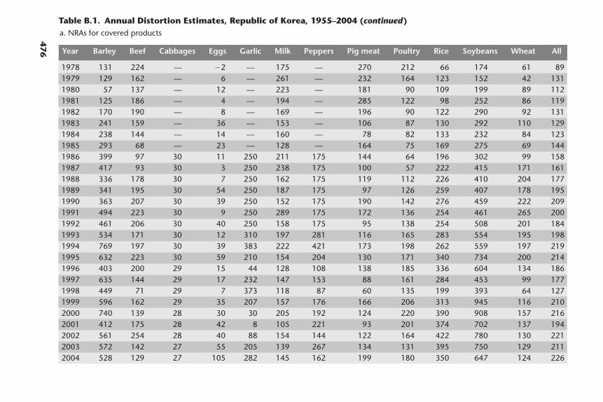
476 Year Barley Beef Cabbages Eggs Garlic Milk Peppers Pig meat Poultry Rice Soybeans Wheat All
1978 131 224 — �2 — 175 — 270 212 66 174 61 891979 129 162 — 6 — 261 — 232 164 123 152 42 1311980 57 137 — 12 — 223 — 181 90 109 199 89 1121981 125 186 — 4 — 194 — 285 122 98 252 86 1191982 170 190 — 8 — 169 — 196 90 122 290 92 1311983 241 159 — 36 — 153 — 106 87 130 292 110 1291984 238 144 — 14 — 160 — 78 82 133 232 84 1231985 293 68 — 23 — 128 — 164 75 169 275 69 1441986 399 97 30 11 250 211 175 144 64 196 302 99 1581987 417 93 30 3 250 238 175 100 57 222 415 171 1611988 336 178 30 7 250 162 175 119 112 226 410 204 1771989 341 195 30 54 250 187 175 97 126 259 407 178 1951990 363 207 30 39 250 152 175 190 142 276 459 222 2091991 494 223 30 9 250 289 175 172 136 254 461 265 2001992 461 206 30 40 250 158 175 95 138 254 508 201 1841993 534 171 30 12 310 197 281 116 165 283 554 195 1981994 769 197 30 39 383 222 421 173 198 262 559 197 2191995 632 223 30 59 210 154 204 130 171 340 734 200 2141996 403 200 29 15 44 128 108 138 185 336 604 134 1861997 635 144 29 17 232 147 153 88 161 284 453 99 1771998 449 71 29 7 373 118 87 60 135 199 393 64 1271999 596 162 29 35 207 157 176 166 206 313 945 116 2102000 740 139 28 30 30 205 192 124 220 390 908 157 2162001 412 175 28 42 8 105 221 93 201 374 702 137 1942002 561 254 28 40 88 154 144 122 164 422 780 130 2212003 572 142 27 55 205 139 267 134 131 395 750 129 2112004 528 129 27 105 282 145 162 199 180 350 647 124 226
Table B.1. Annual Distortion Estimates, Republic of Korea, 1955–2004 (continued)a. NRAs for covered products
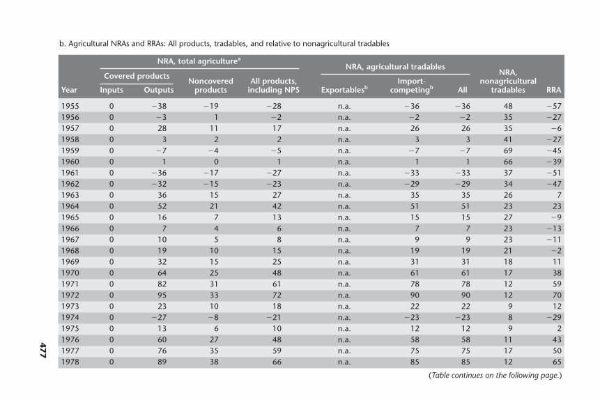
b. Agricultural NRAs and RRAs: All products, tradables, and relative to nonagricultural tradables
NRA, total agriculturea
NRA, agricultural tradablesNRA,Covered products
Noncovered All products, Import- nonagriculturalYear Inputs Outputs products including NPS Exportablesb competingb All tradables RRA
1955 0 �38 �19 �28 n.a. �36 �36 48 �571956 0 �3 1 �2 n.a. �2 �2 35 �271957 0 28 11 17 n.a. 26 26 35 �61958 0 3 2 2 n.a. 3 3 41 �271959 0 �7 �4 �5 n.a. �7 �7 69 �451960 0 1 0 1 n.a. 1 1 66 �391961 0 �36 �17 �27 n.a. �33 �33 37 �511962 0 �32 �15 �23 n.a. �29 �29 34 �471963 0 36 15 27 n.a. 35 35 26 71964 0 52 21 42 n.a. 51 51 23 231965 0 16 7 13 n.a. 15 15 27 �91966 0 7 4 6 n.a. 7 7 23 �131967 0 10 5 8 n.a. 9 9 23 �111968 0 19 10 15 n.a. 19 19 21 �21969 0 32 15 25 n.a. 31 31 18 111970 0 64 25 48 n.a. 61 61 17 381971 0 82 31 61 n.a. 78 78 12 591972 0 95 33 72 n.a. 90 90 12 701973 0 23 10 18 n.a. 22 22 9 121974 0 �27 �8 �21 n.a. �23 �23 8 �291975 0 13 6 10 n.a. 12 12 9 21976 0 60 27 48 n.a. 58 58 11 431977 0 76 35 59 n.a. 75 75 17 501978 0 89 38 66 n.a. 85 85 12 65
477
(Table continues on the following page.)
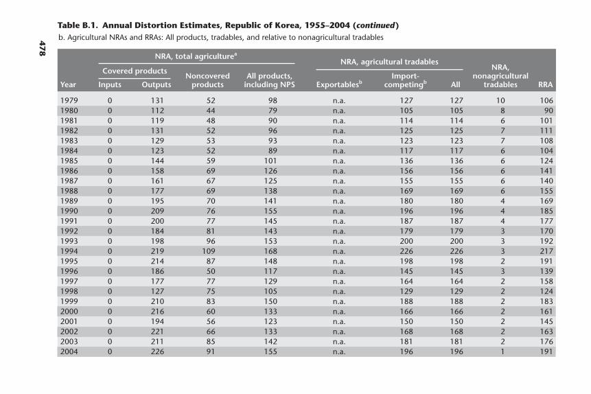
478
Table B.1. Annual Distortion Estimates, Republic of Korea, 1955–2004 (continued)b. Agricultural NRAs and RRAs: All products, tradables, and relative to nonagricultural tradables
NRA, total agriculturea
NRA, agricultural tradablesNRA,Covered products
Noncovered All products, Import- nonagriculturalYear Inputs Outputs products including NPS Exportablesb competingb All tradables RRA
1979 0 131 52 98 n.a. 127 127 10 1061980 0 112 44 79 n.a. 105 105 8 901981 0 119 48 90 n.a. 114 114 6 1011982 0 131 52 96 n.a. 125 125 7 1111983 0 129 53 93 n.a. 123 123 7 1081984 0 123 52 89 n.a. 117 117 6 1041985 0 144 59 101 n.a. 136 136 6 1241986 0 158 69 126 n.a. 156 156 6 1411987 0 161 67 125 n.a. 155 155 6 1401988 0 177 69 138 n.a. 169 169 6 1551989 0 195 70 141 n.a. 180 180 4 1691990 0 209 76 155 n.a. 196 196 4 1851991 0 200 77 145 n.a. 187 187 4 1771992 0 184 81 143 n.a. 179 179 3 1701993 0 198 96 153 n.a. 200 200 3 1921994 0 219 109 168 n.a. 226 226 3 2171995 0 214 87 148 n.a. 198 198 2 1911996 0 186 50 117 n.a. 145 145 3 1391997 0 177 77 129 n.a. 164 164 2 1581998 0 127 75 105 n.a. 129 129 2 1241999 0 210 83 150 n.a. 188 188 2 1832000 0 216 60 133 n.a. 166 166 2 1612001 0 194 56 123 n.a. 150 150 2 1452002 0 221 66 133 n.a. 168 168 2 1632003 0 211 85 142 n.a. 181 181 2 1762004 0 226 91 155 n.a. 196 196 1 191

479
c. Value shares of the primary production of coveredc and noncovered products
Year Barley Beef Cabbages Eggs Garlic Milk Peppers Pig meat Poultry Rice Soybeans Wheat Noncovered
1955 5 1 0 0 0 0 0 3 0 37 1 1 511956 6 1 0 0 0 0 0 4 0 30 1 1 571957 4 1 0 0 0 0 0 3 0 29 1 1 611958 4 1 0 1 0 0 0 3 0 34 1 1 561959 5 2 0 2 0 0 0 4 1 32 1 1 531960 4 2 0 3 0 0 0 3 1 31 1 1 541961 6 1 0 1 0 0 0 2 1 38 1 1 491962 7 1 0 2 0 0 0 1 1 37 1 1 501963 5 1 0 2 0 0 0 1 1 46 1 1 421964 9 2 0 2 0 0 0 2 1 50 2 1 311965 11 2 0 2 0 0 0 2 1 44 2 1 361966 11 2 0 2 0 0 0 2 1 46 1 1 351967 9 2 0 2 0 0 0 2 1 45 1 1 371968 10 2 0 2 0 0 0 1 1 45 2 1 361969 7 2 0 4 0 0 0 2 1 46 1 1 361970 7 2 0 4 0 0 0 2 1 39 1 1 411971 8 3 0 5 0 0 0 2 1 38 2 1 401972 7 3 0 6 0 0 0 2 2 39 2 1 381973 7 4 0 4 0 0 0 2 1 42 2 0 381974 4 2 0 3 0 0 0 1 1 51 1 0 351975 7 3 0 4 0 0 0 2 1 49 1 0 321976 7 3 0 4 0 0 0 2 1 43 1 0 371977 3 2 0 5 0 0 0 3 1 44 2 0 401978 3 2 0 4 0 1 0 3 1 41 1 0 441979 4 5 0 4 0 1 0 5 1 39 1 0 401980 3 5 0 4 0 1 0 6 2 31 1 0 471981 2 5 0 4 0 1 0 5 1 40 1 0 411982 2 4 0 4 0 1 0 6 1 36 1 0 43
(Table continues on the following page.)

480
Year Barley Beef Cabbages Eggs Garlic Milk Peppers Pig meat Poultry Rice Soybeans Wheat Noncovered
1983 2 4 0 4 0 2 0 7 2 33 1 0 461984 2 5 0 4 0 2 0 7 2 31 1 0 461985 1 7 0 4 0 2 0 6 2 28 1 0 481986 1 7 3 4 2 2 4 6 3 31 1 0 361987 1 7 4 5 1 2 3 6 3 27 1 0 381988 1 5 5 4 2 3 4 6 3 30 1 0 361989 1 4 5 4 2 3 1 6 3 26 1 0 441990 1 4 4 4 3 4 2 7 3 26 1 0 411991 1 5 4 5 3 2 3 7 3 23 0 0 451992 1 6 3 4 3 3 5 9 3 22 0 0 401993 1 6 3 4 2 3 3 10 3 19 0 0 441994 0 6 4 4 2 3 2 8 3 21 0 0 461995 0 5 3 4 4 3 4 8 3 15 0 0 521996 0 4 3 4 4 3 5 7 3 16 0 0 511997 0 5 3 4 2 3 3 9 3 19 0 0 481998 0 6 3 5 2 3 4 10 3 21 0 0 431999 0 6 3 4 2 3 3 9 3 19 0 0 472000 0 5 3 3 3 3 3 7 2 16 0 0 542001 0 4 3 4 4 4 3 8 2 16 0 0 512002 0 3 3 4 2 4 3 8 3 13 0 0 562003 0 5 4 4 1 4 2 9 3 14 0 0 55
Sources: Author compilation; Honma and Hayami 2007; chapter 2 of this volume.
Note: — � no data are available. n.a. � not applicable.
a. Including assistance for nontradables and non-product-specific assistance (NPS).b. Including product-specific input subsidies.c. The covered products are calculated at undistorted farmgate prices in U.S. dollars.
Table B.1. Annual Distortion Estimates, Republic of Korea, 1955–2004 (continued)
c. Value shares of the primary production of coveredc and noncovered products
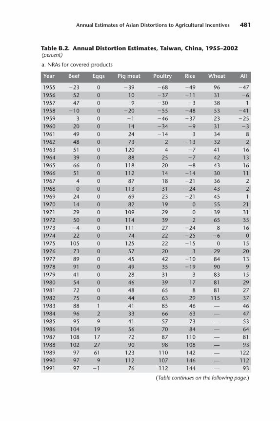
Annual Estimates of Asian Distortions to Agricultural Incentives 481
Table B.2. Annual Distortion Estimates, Taiwan, China, 1955–2002(percent)
a. NRAs for covered products
Year Beef Eggs Pig meat Poultry Rice Wheat All
1955 �23 0 �39 �68 �49 96 �471956 52 0 10 �37 �11 31 �61957 47 0 9 �30 �3 38 11958 �10 0 �20 �55 �48 53 �411959 3 0 �1 �46 �37 23 �251960 20 0 14 �34 �9 31 �31961 49 0 24 �14 3 34 81962 48 0 73 2 �13 32 21963 51 0 120 4 �7 41 161964 39 0 88 25 �7 42 131965 66 0 118 20 �8 43 161966 51 0 112 14 �14 30 111967 4 0 87 18 �21 36 21968 0 0 113 31 �24 43 21969 24 0 69 23 �21 45 11970 14 0 82 19 0 55 211971 29 0 109 29 0 39 311972 50 0 114 39 2 65 351973 �4 0 111 27 �24 8 161974 22 0 74 22 �25 �6 01975 105 0 125 22 �15 0 151976 73 0 57 20 3 29 201977 89 0 45 42 �10 84 131978 91 0 49 35 �19 90 91979 41 0 28 31 3 83 151980 54 0 46 39 17 81 291981 72 0 48 65 8 81 271982 75 0 44 63 29 115 371983 88 1 41 85 46 — 461984 96 2 33 66 63 — 471985 95 9 41 57 73 — 531986 104 19 56 70 84 — 641987 108 17 72 87 110 — 811988 102 27 90 98 108 — 931989 97 61 123 110 142 — 1221990 97 9 112 107 146 — 1121991 97 �1 76 112 144 — 93
(Table continues on the following page.)

482 Distortions to Agricultural Incentives in Asia
Year Beef Eggs Pig meat Poultry Rice Wheat All
1992 95 41 93 149 170 — 1151993 99 30 100 168 191 — 1261994 106 40 138 178 156 — 1401995 66 33 108 167 208 — 1311996 97 2 124 167 174 — 1261997 101 �1 94 195 149 — 1141998 85 11 108 242 134 — 1281999 63 44 221 372 174 — 2122000 44 33 201 347 189 — 2022001 95 22 168 254 195 — 1692002 79 19 150 237 226 — 164
Table B.2. Annual Distortion Estimates, Taiwan, China,1955–2002 (continued)
a. NRAs for covered products
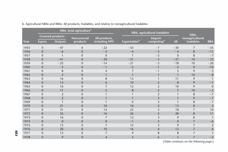
483
b. Agricultural NRAs and RRAs: All products, tradables, and relative to nonagricultural tradables
NRA, total agriculturea
NRA, agricultural tradablesNRA,Covered products
Noncovered All products, Import- nonagriculturalYear Inputs Outputs products including NPS Exportablesb competingb All tradables RRA
1955 0 �47 0 �22 �35 �7 �30 7 �351956 0 �6 0 �3 �4 �3 �4 8 �111957 0 1 0 0 1 �2 0 8 �71958 0 �41 0 �20 �31 �3 �27 10 �331959 0 �25 0 �14 �21 �3 �18 10 �261960 0 �3 0 �1 �2 �1 �2 9 �101961 0 8 0 4 7 �1 5 9 �31962 0 2 0 1 1 1 1 10 �81963 0 16 0 8 13 1 11 9 11964 0 13 0 6 10 2 8 9 �11965 0 16 0 7 12 2 10 9 01966 0 11 0 5 8 2 7 10 �21967 0 2 0 1 1 2 1 8 �71968 0 2 0 1 1 3 1 9 �71969 0 1 0 1 0 3 1 8 �71970 0 21 0 10 16 2 13 8 51971 0 31 0 14 23 3 18 7 101972 0 35 0 16 26 5 20 8 111973 0 16 0 7 12 3 9 8 11974 0 0 0 0 �1 3 0 7 �61975 0 15 0 7 12 3 9 7 21976 0 20 0 10 16 4 13 7 61977 0 13 0 7 9 8 8 7 11978 0 9 0 4 5 6 5 7 �2
(Table continues on the following page.)

484
Table B.2. Annual Distortion Estimates, Taiwan, China, 1955–2002 (continued)b. Agricultural NRAs and RRAs: All products, tradables, and relative to nonagricultural tradables
NRA, total agriculturea
NRA, agricultural tradablesNRA,Covered products
Noncovered All products, Import- nonagriculturalYear Inputs Outputs products including NPS Exportablesb competingb All tradables RRA
1979 0 15 0 7 10 5 9 7 21980 0 29 0 12 21 6 15 5 91981 0 27 0 11 17 9 14 5 81982 0 37 0 14 25 8 19 5 131983 0 46 0 19 31 12 23 5 171984 0 47 0 19 33 10 23 5 171985 0 53 0 20 37 9 25 5 191986 0 64 0 23 44 11 29 5 231987 0 81 0 26 53 13 33 5 271988 0 93 0 28 58 13 35 4 301989 0 122 0 38 53 45 47 4 411990 0 112 0 41 60 45 50 4 451991 0 93 0 34 57 34 41 3 371992 0 115 0 37 56 40 45 2 411993 0 126 0 38 61 41 46 2 431994 0 140 0 41 51 50 50 2 471995 0 131 0 39 60 43 47 2 451996 0 126 0 42 55 48 50 2 471997 0 114 0 43 58 48 50 2 481998 0 128 0 45 51 54 53 2 501999 0 212 0 63 61 79 74 2 722000 0 202 0 69 70 83 80 1 782001 0 169 0 60 66 70 69 1 672002 0 164 0 55 75 60 63 1 62

Annual Estimates of Asian Distortions to Agricultural Incentives 485
c. Value shares of the primary production of coveredc and noncovered products
Year Beef Eggs Pig meat Poultry Rice Wheat Noncovered
1955 0 0 12 1 34 0 521956 0 0 15 1 40 0 431957 0 0 16 1 35 0 481958 0 0 12 1 36 0 501959 0 1 17 1 37 0 431960 0 1 13 1 33 0 531961 0 1 13 2 35 0 491962 0 1 8 1 40 0 491963 0 1 9 2 38 0 501964 0 1 9 1 35 0 541965 0 1 9 1 36 0 531966 0 1 9 1 37 0 521967 0 1 10 2 37 0 511968 0 1 9 1 39 0 501969 0 1 11 2 35 0 501970 0 1 12 2 32 0 531971 0 1 12 2 29 0 551972 0 2 12 3 28 0 551973 0 1 12 3 29 0 541974 0 1 12 2 38 0 461975 0 2 10 2 36 0 501976 0 2 15 3 31 0 491977 0 2 17 4 26 0 511978 0 3 16 4 26 0 521979 0 2 18 4 22 0 541980 0 2 14 4 21 0 581981 0 2 14 4 21 0 591982 0 2 15 4 18 0 611983 0 3 16 5 17 — 591984 0 3 16 5 15 — 601985 0 3 16 5 14 — 621986 0 3 17 5 11 — 641987 0 2 16 5 9 — 681988 0 2 14 5 10 — 691989 0 2 14 6 9 — 691990 0 3 17 6 10 — 631991 0 3 19 5 9 — 64
(Table continues on the following page.)

486 Distortions to Agricultural Incentives in Asia
Year Beef Eggs Pig meat Poultry Rice Wheat Noncovered
1992 0 3 17 5 7 — 681993 0 3 15 5 7 — 701994 0 3 14 5 7 — 701995 0 3 16 5 6 — 701996 0 4 17 6 7 — 671997 0 5 17 7 8 — 621998 0 5 14 7 8 — 651999 0 5 11 6 8 — 702000 0 5 14 7 8 — 662001 0 5 16 7 7 — 642002 0 5 14 7 7 — 67
Sources: Author compilation; Honma and Hayami 2007; chapter 2 of this volume.
Note: — � no data are available.
a. Including assistance for nontradables and non-product-specific assistance (NPS).b. Including product-specific input subsidies.c. The covered products are calculated at undistorted farmgate prices in U.S. dollars.
Table B.2. Annual Distortion Estimates, Taiwan, China,1955–2002 (continued)
c. Value shares of the primary production of coveredc and noncovered products
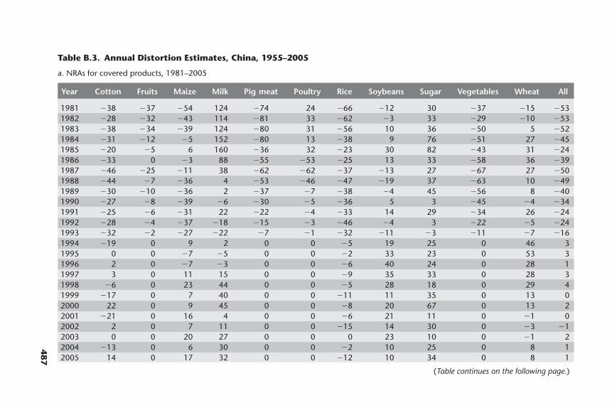
487
Table B.3. Annual Distortion Estimates, China, 1955–2005
a. NRAs for covered products, 1981–2005
Year Cotton Fruits Maize Milk Pig meat Poultry Rice Soybeans Sugar Vegetables Wheat All
1981 �38 �37 �54 124 �74 24 �66 �12 30 �37 �15 �531982 �28 �32 �43 114 �81 33 �62 �3 33 �29 �10 �531983 �38 �34 �39 124 �80 31 �56 10 36 �50 5 �521984 �31 �12 �5 152 �80 13 �38 9 76 �51 27 �451985 �20 �5 6 160 �36 32 �23 30 82 �43 31 �241986 �33 0 �3 88 �55 �53 �25 13 33 �58 36 �391987 �46 �25 �11 38 �62 �62 �37 �13 27 �67 27 �501988 �44 �7 �36 4 �53 �46 �47 �19 37 �63 10 �491989 �30 �10 �36 2 �37 �7 �38 �4 45 �56 8 �401990 �27 �8 �39 �6 �30 �5 �36 5 3 �45 �4 �341991 �25 �6 �31 22 �22 �4 �33 14 29 �34 26 �241992 �28 �4 �37 �18 �15 �3 �46 �4 3 �22 �5 �241993 �32 �2 �27 �22 �7 �1 �32 �11 �3 �11 �7 �161994 �19 0 9 2 0 0 �5 19 25 0 46 31995 0 0 �7 �5 0 0 �2 33 23 0 53 31996 2 0 �7 �3 0 0 �6 40 24 0 28 11997 3 0 11 15 0 0 �9 35 33 0 28 31998 �6 0 23 44 0 0 �5 28 18 0 29 41999 �17 0 7 40 0 0 �11 11 35 0 13 02000 22 0 9 45 0 0 �8 20 67 0 13 22001 �21 0 16 4 0 0 �6 21 11 0 �1 02002 2 0 7 11 0 0 �15 14 30 0 �3 �12003 0 0 20 27 0 0 0 23 10 0 �1 22004 �13 0 6 30 0 0 �2 10 25 0 8 12005 14 0 17 32 0 0 �12 10 34 0 8 1
(Table continues on the following page.)
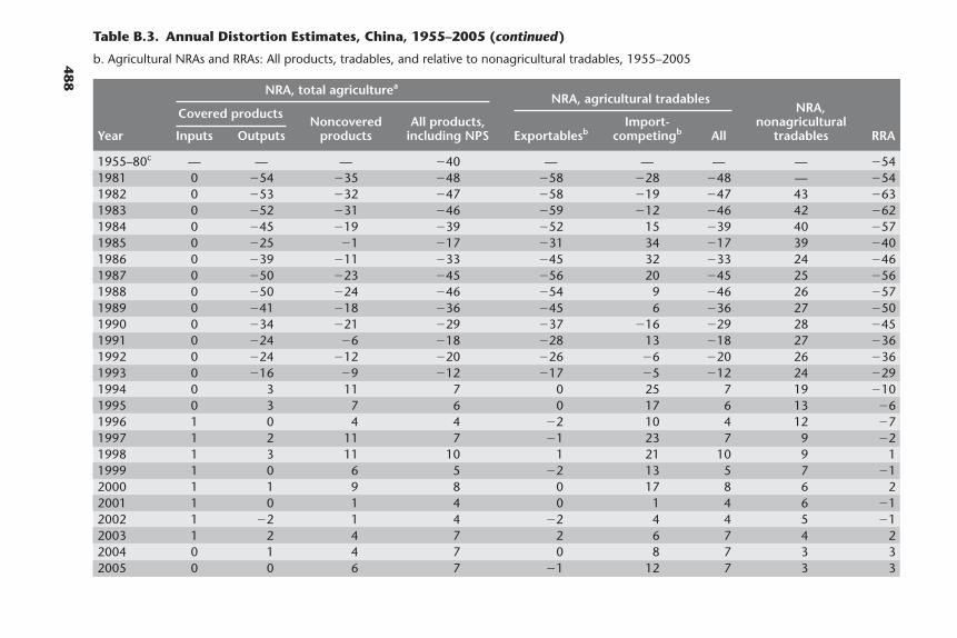
488
Table B.3. Annual Distortion Estimates, China, 1955–2005 (continued)
b. Agricultural NRAs and RRAs: All products, tradables, and relative to nonagricultural tradables, 1955–2005
NRA, total agriculturea
NRA, agricultural tradablesNRA,Covered products
Noncovered All products, Import- nonagriculturalYear Inputs Outputs products including NPS Exportablesb competingb All tradables RRA
1955–80c — — — �40 — — — — �541981 0 �54 �35 �48 �58 �28 �48 — �541982 0 �53 �32 �47 �58 �19 �47 43 �631983 0 �52 �31 �46 �59 �12 �46 42 �621984 0 �45 �19 �39 �52 15 �39 40 �571985 0 �25 �1 �17 �31 34 �17 39 �401986 0 �39 �11 �33 �45 32 �33 24 �461987 0 �50 �23 �45 �56 20 �45 25 �561988 0 �50 �24 �46 �54 9 �46 26 �571989 0 �41 �18 �36 �45 6 �36 27 �501990 0 �34 �21 �29 �37 �16 �29 28 �451991 0 �24 �6 �18 �28 13 �18 27 �361992 0 �24 �12 �20 �26 �6 �20 26 �361993 0 �16 �9 �12 �17 �5 �12 24 �291994 0 3 11 7 0 25 7 19 �101995 0 3 7 6 0 17 6 13 �61996 1 0 4 4 �2 10 4 12 �71997 1 2 11 7 �1 23 7 9 �21998 1 3 11 10 1 21 10 9 11999 1 0 6 5 �2 13 5 7 �12000 1 1 9 8 0 17 8 6 22001 1 0 1 4 0 1 4 6 �12002 1 �2 1 4 �2 4 4 5 �12003 1 2 4 7 2 6 7 4 22004 0 1 4 7 0 8 7 3 32005 0 0 6 7 �1 12 7 3 3
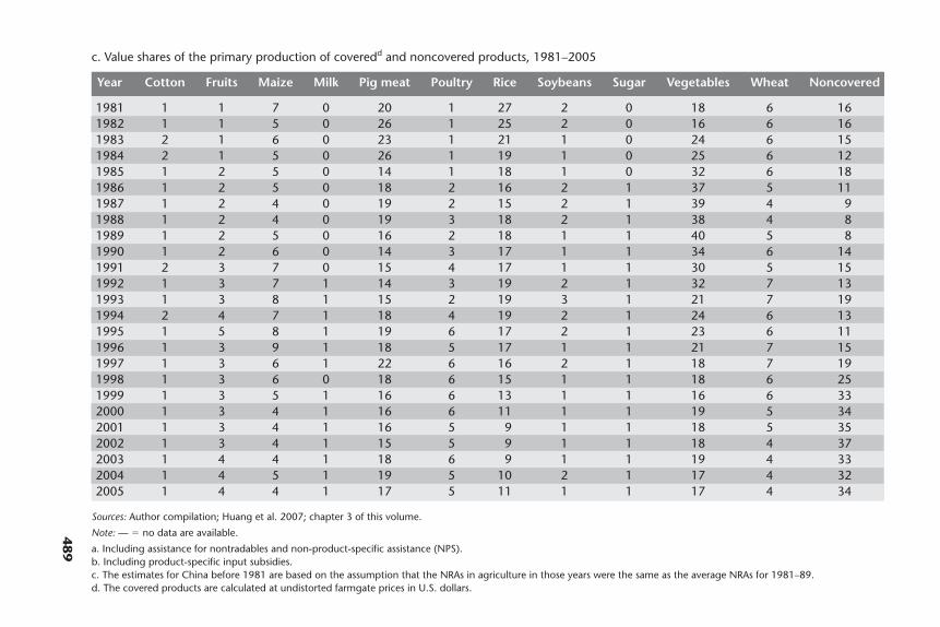
489
c. Value shares of the primary production of coveredd and noncovered products, 1981–2005
Year Cotton Fruits Maize Milk Pig meat Poultry Rice Soybeans Sugar Vegetables Wheat Noncovered
1981 1 1 7 0 20 1 27 2 0 18 6 161982 1 1 5 0 26 1 25 2 0 16 6 161983 2 1 6 0 23 1 21 1 0 24 6 151984 2 1 5 0 26 1 19 1 0 25 6 121985 1 2 5 0 14 1 18 1 0 32 6 181986 1 2 5 0 18 2 16 2 1 37 5 111987 1 2 4 0 19 2 15 2 1 39 4 91988 1 2 4 0 19 3 18 2 1 38 4 81989 1 2 5 0 16 2 18 1 1 40 5 81990 1 2 6 0 14 3 17 1 1 34 6 141991 2 3 7 0 15 4 17 1 1 30 5 151992 1 3 7 1 14 3 19 2 1 32 7 131993 1 3 8 1 15 2 19 3 1 21 7 191994 2 4 7 1 18 4 19 2 1 24 6 131995 1 5 8 1 19 6 17 2 1 23 6 111996 1 3 9 1 18 5 17 1 1 21 7 151997 1 3 6 1 22 6 16 2 1 18 7 191998 1 3 6 0 18 6 15 1 1 18 6 251999 1 3 5 1 16 6 13 1 1 16 6 332000 1 3 4 1 16 6 11 1 1 19 5 342001 1 3 4 1 16 5 9 1 1 18 5 352002 1 3 4 1 15 5 9 1 1 18 4 372003 1 4 4 1 18 6 9 1 1 19 4 332004 1 4 5 1 19 5 10 2 1 17 4 322005 1 4 4 1 17 5 11 1 1 17 4 34
Sources: Author compilation; Huang et al. 2007; chapter 3 of this volume.
Note: — � no data are available.
a. Including assistance for nontradables and non-product-specific assistance (NPS).b. Including product-specific input subsidies.c. The estimates for China before 1981 are based on the assumption that the NRAs in agriculture in those years were the same as the average NRAs for 1981–89.d. The covered products are calculated at undistorted farmgate prices in U.S. dollars.
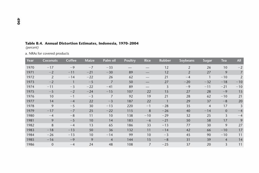
490
Table B.4. Annual Distortion Estimates, Indonesia, 1970–2004(percent)
a. NRAs for covered products
Year Coconuts Coffee Maize Palm oil Poultry Rice Rubber Soybeans Sugar Tea All
1970 �17 �9 �7 �33 — — 12 2 26 10 �21971 �2 �11 �21 �30 89 — 12 2 27 9 71972 2 �14 �22 26 62 — 21 �4 1 �10 21973 �2 1 �5 7 50 — 27 �20 �32 �18 �101974 �11 �3 �22 �41 89 — 3 �9 �11 �21 �101975 �5 �2 �24 �15 107 22 15 27 28 �9 151976 10 �1 �3 7 92 19 21 28 62 �10 211977 14 �4 22 �3 187 22 1 29 37 �8 201978 9 �5 30 �13 220 �1 �28 35 4 17 31979 �17 �7 25 �22 115 8 �26 40 �14 0 �41980 �4 �8 11 10 138 �10 �29 32 25 3 �41981 9 �5 10 14 183 �6 �21 50 58 17 91982 8 �4 13 65 186 33 �13 77 30 9 271983 �18 �13 50 36 132 11 �14 42 66 �10 171984 �26 �13 10 �14 99 10 �3 45 90 �10 111985 �16 �9 9 4 144 15 �8 31 39 4 141986 0 �4 24 48 108 7 �25 37 20 3 11

491
1987 �19 6 32 �13 58 �4 �35 14 �1 �11 �51988 �24 1 50 �33 68 �9 �19 0 �8 �4 �91989 �51 �6 �5 �12 56 �14 �15 2 �7 �3 �121990 �43 �2 �3 17 69 �10 �23 20 14 �8 �51991 �45 1 28 0 147 �16 �28 18 15 �2 �71992 �47 1 35 4 69 �8 �33 14 4 �3 �51993 �44 0 21 23 86 �4 �37 16 �6 �5 �51994 �50 �2 31 14 103 �6 �38 19 �7 6 �61995 �47 �2 37 �18 102 �12 �31 28 �7 6 �111996 �47 6 29 2 136 �15 �21 19 �12 �13 �101997 �16 5 19 �12 71 �7 56 16 �29 �23 �71998 �26 �1 36 �57 �9 �34 58 0 67 �23 �241999 �11 4 2 �6 139 4 123 24 37 �16 62000 �8 7 23 �3 107 15 56 1 60 �19 162001 �9 4 �3 12 70 21 38 �5 26 �18 172002 �10 1 1 �12 120 23 0 5 42 �15 152003 �6 0 25 �13 101 25 �4 4 68 �12 182004 — 3 9 — — 9 �6 0 51 �14 12
(Table continues on the following page.)

492
Table B.4. Annual Distortion Estimates, Indonesia, 1970–2004 (continued)b. Agricultural NRAs and RRAs: All products, tradables, and relative to nonagricultural tradables
NRA, total agriculturea
NRA, agricultural tradablesNRA,Covered products
Noncovered All products, Import- nonagriculturalYear Inputs Outputs products including NPS Exportablesb competingb All tradables RRA
1970 6 �8 �4 �3 �11 10 �8 28 �281971 6 1 6 6 �2 19 7 28 �161972 7 �5 1 2 5 �1 2 28 �201973 6 �16 �7 �9 2 �25 �10 28 �301974 5 �16 �7 �9 �11 �10 �10 28 �301975 9 6 6 12 �3 21 13 28 �111976 6 14 12 18 10 26 20 28 �61977 6 14 12 17 9 27 20 28 �61978 6 �3 2 3 1 4 3 28 �191979 7 �10 �4 �4 �18 5 �4 28 �251980 7 �10 �4 �4 �11 0 �4 28 �251981 7 2 5 8 3 12 9 28 �151982 8 20 13 22 7 34 25 28 �21983 8 9 5 12 �12 27 14 28 �111984 7 4 2 7 �21 25 9 28 �151985 7 7 4 10 �12 24 12 28 �121986 6 4 4 8 �3 15 9 28 �14
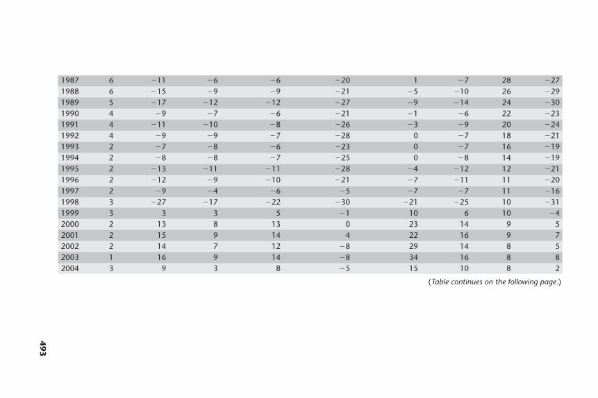
493
1987 6 �11 �6 �6 �20 1 �7 28 �271988 6 �15 �9 �9 �21 �5 �10 26 �291989 5 �17 �12 �12 �27 �9 �14 24 �301990 4 �9 �7 �6 �21 �1 �6 22 �231991 4 �11 �10 �8 �26 �3 �9 20 �241992 4 �9 �9 �7 �28 0 �7 18 �211993 2 �7 �8 �6 �23 0 �7 16 �191994 2 �8 �8 �7 �25 0 �8 14 �191995 2 �13 �11 �11 �28 �4 �12 12 �211996 2 �12 �9 �10 �21 �7 �11 11 �201997 2 �9 �4 �6 �5 �7 �7 11 �161998 3 �27 �17 �22 �30 �21 �25 10 �311999 3 3 3 5 �1 10 6 10 �42000 2 13 8 13 0 23 14 9 52001 2 15 9 14 4 22 16 9 72002 2 14 7 12 �8 29 14 8 52003 1 16 9 14 �8 34 16 8 82004 3 9 3 8 �5 15 10 8 2
(Table continues on the following page.)
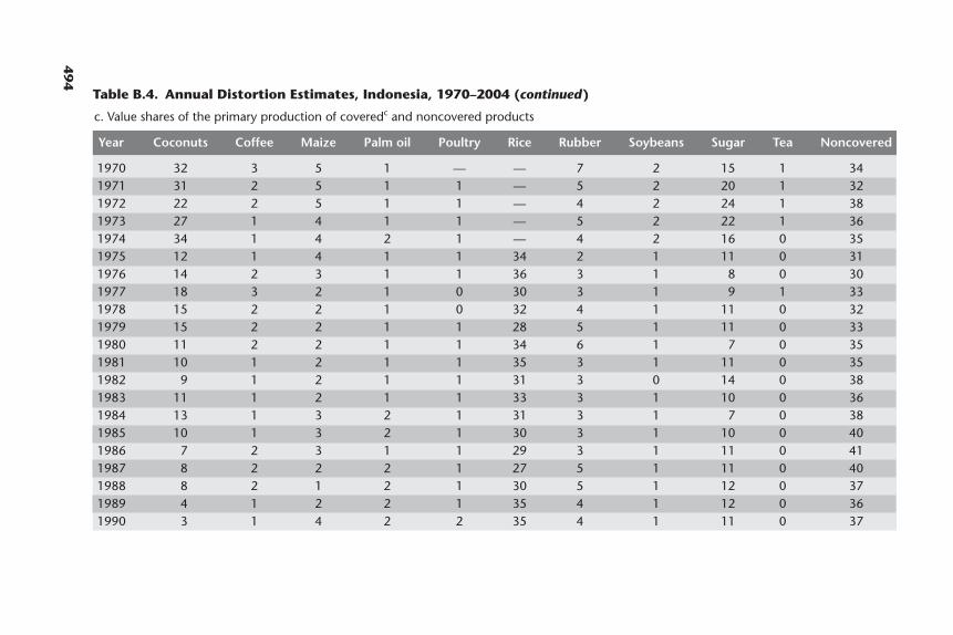
494
Table B.4. Annual Distortion Estimates, Indonesia, 1970–2004 (continued)
c. Value shares of the primary production of coveredc and noncovered products
Year Coconuts Coffee Maize Palm oil Poultry Rice Rubber Soybeans Sugar Tea Noncovered
1970 32 3 5 1 — — 7 2 15 1 341971 31 2 5 1 1 — 5 2 20 1 321972 22 2 5 1 1 — 4 2 24 1 381973 27 1 4 1 1 — 5 2 22 1 361974 34 1 4 2 1 — 4 2 16 0 351975 12 1 4 1 1 34 2 1 11 0 311976 14 2 3 1 1 36 3 1 8 0 301977 18 3 2 1 0 30 3 1 9 1 331978 15 2 2 1 0 32 4 1 11 0 321979 15 2 2 1 1 28 5 1 11 0 331980 11 2 2 1 1 34 6 1 7 0 351981 10 1 2 1 1 35 3 1 11 0 351982 9 1 2 1 1 31 3 0 14 0 381983 11 1 2 1 1 33 3 1 10 0 361984 13 1 3 2 1 31 3 1 7 0 381985 10 1 3 2 1 30 3 1 10 0 401986 7 2 3 1 1 29 3 1 11 0 411987 8 2 2 2 1 27 5 1 11 0 401988 8 2 1 2 1 30 5 1 12 0 371989 4 1 2 2 1 35 4 1 12 0 361990 3 1 4 2 2 35 4 1 11 0 37
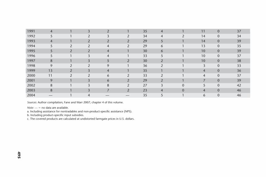
495
1991 4 1 3 2 1 35 4 1 11 0 371992 5 1 2 3 2 34 4 2 14 0 341993 4 1 2 2 2 29 5 1 14 0 391994 5 2 2 4 2 29 6 1 13 0 351995 5 2 2 4 1 30 6 1 10 0 391996 5 1 3 4 1 33 5 1 10 0 371997 8 1 3 5 2 30 2 1 10 0 381998 9 2 2 9 1 36 2 1 3 0 331999 13 2 3 4 1 35 1 1 4 0 362000 11 2 2 6 2 33 2 1 4 0 372001 9 1 3 6 2 29 2 1 7 0 392002 8 1 3 8 2 27 3 0 5 0 422003 8 1 3 7 2 23 4 0 4 0 462004 — 1 4 — — 35 5 1 6 0 46
Sources: Author compilation; Fane and Warr 2007; chapter 4 of this volume.
Note: — � no data are available.a. Including assistance for nontradables and non-product-specific assistance (NPS).b. Including product-specific input subsidies.c. The covered products are calculated at undistorted farmgate prices in U.S. dollars.
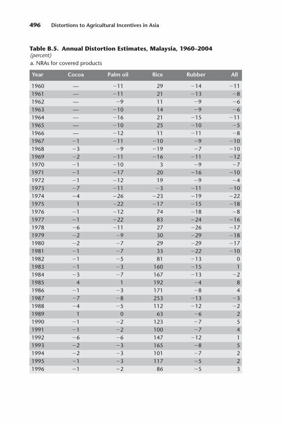
496 Distortions to Agricultural Incentives in Asia
Table B.5. Annual Distortion Estimates, Malaysia, 1960–2004(percent)a. NRAs for covered products
Year Cocoa Palm oil Rice Rubber All
1960 — �11 29 �14 �111961 — �11 21 �13 �81962 — �9 11 �9 �61963 — �10 14 �9 �61964 — �16 21 �15 �111965 — �10 25 �10 �51966 — �12 11 �11 �81967 �1 �11 �10 �9 �101968 �3 �9 �19 �7 �101969 �2 �11 �16 �11 �121970 �1 �10 3 �9 �71971 �1 �17 20 �16 �101972 �1 �12 19 �9 �41973 �7 �11 �3 �11 �101974 �4 �26 �23 �19 �221975 1 �22 �17 �15 �181976 �1 �12 74 �18 �81977 �1 �22 83 �24 �161978 �6 �11 27 �26 �171979 �2 �9 30 �29 �181980 �2 �7 29 �29 �171981 �1 �7 33 �22 �101982 �1 �5 81 �13 01983 �1 �3 160 �15 11984 �3 �7 167 �13 �21985 4 1 192 �4 81986 �1 �3 171 �8 41987 �7 �8 253 �13 �31988 �4 �5 112 �12 �21989 1 0 63 �6 21990 �1 �2 123 �7 51991 �1 �2 100 �7 41992 �6 �6 147 �12 11993 �2 �3 165 �8 51994 �2 �3 101 �7 21995 �1 �3 117 �5 21996 �1 �2 86 �5 3
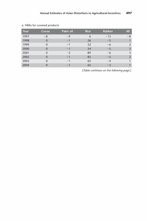
Annual Estimates of Asian Distortions to Agricultural Incentives 497
1997 �8 �9 6 �13 �81998 0 �1 26 �5 11999 0 �1 52 �6 22000 0 �1 54 �5 32001 0 �2 89 �6 32002 0 �1 82 �5 22003 0 �1 65 �4 12004 0 �1 65 �3 1
a. NRAs for covered products
Year Cocoa Palm oil Rice Rubber All
(Table continues on the following page.)
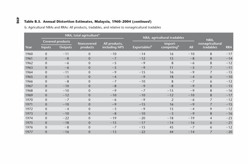
498 Table B.5. Annual Distortion Estimates, Malaysia, 1960–2004 (continued)
b. Agricultural NRAs and RRAs: All products, tradables, and relative to nonagricultural tradables
NRA, total agriculturea
NRA, agricultural tradablesNRA,Covered products
Noncovered All products, Import- nonagriculturalYear Inputs Outputs products including NPS Exportablesb competingb All tradables RRA
1960 0 �11 0 �10 �14 16 �10 8 �171961 0 �8 0 �7 �12 15 �8 8 �141962 0 �6 0 �5 �9 8 �6 8 �121963 0 �6 0 �5 �9 11 �5 7 �111964 0 �11 0 �9 �15 16 �9 7 �151965 0 �5 0 �4 �9 18 �4 6 �101966 0 �8 0 �7 �10 8 �7 6 �121967 0 �10 0 �8 �9 �8 �9 8 �151968 0 �10 0 �9 �7 �15 �9 8 �161969 0 �12 0 �10 �10 �12 �10 8 �171970 0 �7 0 �6 �9 2 �6 7 �121971 0 �10 0 �9 �15 16 �9 7 �151972 0 �4 0 �3 �9 15 �4 9 �121973 0 �10 0 �8 �10 �3 �9 8 �161974 0 �22 0 �19 �20 �18 �19 4 �231975 0 �18 0 �15 �17 �14 �16 6 �211976 0 �8 0 �7 �15 45 �7 6 �121977 0 �16 0 �13 �22 44 �14 7 �20
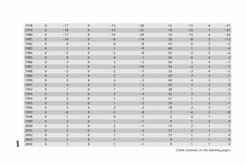
499
1978 0 �17 0 �15 �20 15 �15 6 �211979 0 �18 0 �15 �21 18 �16 7 �211980 0 �17 0 �14 �20 16 �15 6 �201981 0 �10 0 �8 �14 20 �8 5 �131982 0 0 0 0 �8 43 0 5 �51983 0 1 0 1 �9 60 1 5 �41984 0 �2 0 �2 �8 45 �2 5 �61985 0 8 0 6 �1 56 6 4 21986 0 4 0 3 �5 56 3 4 �11987 0 �3 0 �2 �10 55 �2 5 �71988 0 �2 0 �2 �7 32 �2 4 �51989 0 2 0 2 �2 22 2 3 �11990 0 5 0 4 �3 40 4 3 11991 0 4 0 3 �3 32 3 3 01992 0 1 0 1 �7 38 1 3 �21993 0 5 0 3 �4 35 3 3 11994 0 2 0 1 �3 21 1 3 �11995 0 2 0 1 �3 19 1 2 �11996 0 3 0 2 �2 18 2 3 �11997 0 �8 0 �5 �8 3 �6 2 �81998 0 1 0 0 �1 5 0 1 �11999 0 2 0 1 �1 9 1 2 02000 0 3 0 2 �1 13 2 1 12001 0 3 0 2 �2 17 2 1 12002 0 2 0 1 �1 13 1 1 02003 0 1 0 1 �1 9 1 1 02004 0 1 0 1 �1 9 1 1 0
(Table continues on the following page.)

500 Distortions to Agricultural Incentives in Asia
Table B.5. Annual Distortion Estimates, Malaysia, 1960–2004(continued)
c. Value shares of the primary production of coveredc and noncovered products
Year Cocoa Palm oil Rice Rubber Noncovered
1960 — 2 6 78 141961 — 3 11 72 141962 — 3 13 70 141963 — 4 13 69 141964 — 4 11 70 141965 — 6 12 68 141966 — 6 13 67 141967 0 7 17 62 141968 0 6 21 59 141969 0 5 16 65 141970 0 11 16 58 141971 0 16 14 56 141972 0 17 17 52 141973 0 11 17 57 141974 0 23 17 46 141975 0 29 18 37 151976 1 21 8 55 151977 0 30 6 49 151978 0 27 6 52 151979 0 26 7 51 151980 0 25 7 51 171981 1 29 9 41 191982 1 37 8 33 211983 1 30 5 41 231984 2 46 3 25 251985 2 43 3 27 251986 3 31 4 37 251987 3 29 2 41 251988 3 37 3 31 271989 2 40 5 23 291990 2 37 5 25 311991 2 39 5 21 331992 1 41 4 18 351993 1 41 3 18 371994 1 38 3 19 391995 1 42 3 14 411996 1 43 4 13 411997 0 44 5 10 41

Annual Estimates of Asian Distortions to Agricultural Incentives 501
c. Value shares of the primary production of coveredc and noncovered products
Year Cocoa Palm oil Rice Rubber Noncovered
1998 0 49 3 5 421999 0 49 3 6 422000 0 47 4 5 432001 0 44 4 9 432002 0 45 3 9 432003 0 45 2 10 432004 0 48 2 11 38
Sources: Author compilation; Athukorala and Loke 2007; chapter 5 of this volume.
Note: — � no data are available.
a. Including assistance for nontradables and non-product-specific assistance (NPS).b. Including product-specific input subsidies.c. The covered products are calculated at undistorted farmgate prices in U.S. dollars.

502 Distortions to Agricultural Incentives in Asia
Table B.6. Annual Distortion Estimates, the Philippines, 1962–2004(percent)
a. NRAs for covered products
Year Bananas Beef Coconuts Maize Pig meat Poultry Rice Sugar All
1962 0 15 �24 �14 �30 �13 �18 38 �131963 0 15 �25 8 �27 6 �6 �39 �81964 0 15 �25 8 �34 34 14 �24 11965 0 15 �25 42 �23 49 10 103 161966 0 15 �20 29 �4 48 12 157 221967 0 15 �23 39 10 66 �5 134 151968 0 15 �18 44 44 80 �14 142 141969 0 15 �16 38 40 92 �10 67 161970 �4 15 �28 �10 13 67 �8 38 51971 �4 15 �27 49 25 35 29 16 241972 �4 10 �29 43 �10 25 23 �31 41973 �4 10 �23 �8 �18 �1 �39 �48 �311974 �4 10 �19 �3 6 18 �53 �34 �321975 �4 10 �21 6 �23 13 �29 �44 �231976 �4 10 �18 22 �12 5 0 �19 �51977 �4 10 �14 41 �9 42 �4 14 11978 �4 10 �12 37 �15 42 �32 24 �111979 �4 10 �18 16 31 38 �24 16 �61980 �4 5 �25 25 48 48 �38 �18 �161981 �4 5 �21 28 42 46 �36 �15 �131982 �4 5 �31 42 30 44 3 73 121983 �4 5 �36 �2 21 27 �10 64 �31984 �4 5 �23 7 39 26 0 193 121985 �4 5 �37 41 59 50 43 273 261986 0 20 �27 62 32 40 26 114 261987 0 20 �17 96 43 44 11 126 271988 0 20 �14 46 65 43 �9 70 131989 0 20 �9 54 56 37 2 33 171990 0 20 �17 51 25 34 16 29 161991 0 30 �15 24 24 39 1 56 101992 0 30 �19 88 16 84 21 75 241993 0 30 �15 69 24 68 46 51 321994 0 30 �10 82 36 57 21 35 241995 0 30 �9 94 �2 50 55 80 361996 0 30 �4 48 31 37 71 80 471997 0 30 �22 84 53 39 63 60 451998 0 30 �5 66 �2 25 21 95 201999 0 20 2 100 23 60 53 171 412000 0 10 �23 96 6 66 73 77 392001 0 10 �23 72 0 51 69 67 362002 0 10 �5 45 �7 55 54 105 272003 0 10 �8 25 �22 49 41 84 152004 0 10 �11 35 �19 40 17 64 7

503
b. Agricultural NRAs and RRAs: All products, tradables, and relative to nonagricultural tradables
NRA, total agriculturea
NRA, agricultural tradablesNRA,Covered products
Noncovered All products, Import- nonagriculturalYear Inputs Outputs products including NPS Exportablesb competingb All tradables RRA
1962 0 �13 �3 �11 3 �15 �8 19 �231963 0 �8 �1 �6 �11 �6 �3 19 �191964 0 1 3 2 �10 5 7 19 �101965 0 16 8 14 27 12 19 19 01966 0 22 8 19 44 15 21 22 �11967 0 15 5 13 40 8 13 20 �61968 0 14 4 12 40 6 9 19 �91969 0 16 4 13 27 10 10 21 �91970 0 5 1 4 14 1 3 20 �141971 0 24 8 21 4 31 19 24 �41972 0 4 2 4 �20 17 5 15 �91973 0 �31 �11 �27 �30 �28 �27 11 �351974 0 �32 �12 �28 �19 �35 �31 10 �371975 0 �23 �8 �19 �25 �19 �20 13 �291976 0 �5 �1 �4 �14 3 �3 17 �171977 0 1 2 2 �3 5 2 18 �131978 0 �11 �3 �8 �1 �14 �8 17 �211979 0 �6 �2 �5 �6 �5 �8 17 �221980 0 �16 �7 �13 �15 �14 �17 16 �291981 0 �13 �6 �11 �12 �13 �15 13 �251982 0 12 7 11 5 17 9 13 �3
(Table continues on the following page.)
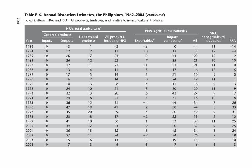
504
1983 0 �3 1 �2 �6 0 �4 11 �141984 0 12 7 11 10 13 8 12 �41985 0 26 17 24 2 44 22 12 91986 0 26 12 22 7 35 21 10 101987 0 27 11 23 11 33 21 11 91988 0 13 4 11 5 17 6 13 �61989 0 17 5 14 5 21 10 9 01990 0 16 7 14 0 24 12 11 11991 0 10 3 8 5 11 6 9 �31992 0 24 10 21 8 30 20 11 91993 0 32 13 28 6 43 27 9 171994 0 24 8 21 4 31 18 10 81995 0 36 15 31 �4 44 34 7 261996 0 47 19 41 �2 58 44 8 331997 0 45 20 39 4 60 42 9 311998 0 20 8 17 �2 25 19 8 101999 0 41 18 36 1 53 39 11 252000 0 39 17 34 �9 50 37 9 252001 0 36 15 32 �8 45 34 8 242002 0 27 11 24 �2 34 26 7 182003 0 15 6 14 �3 19 15 5 102004 0 7 3 6 5 7 6 3 3
Table B.6. Annual Distortion Estimates, the Philippines, 1962–2004 (continued)
b. Agricultural NRAs and RRAs: All products, tradables, and relative to nonagricultural tradables
NRA, total agriculturea
NRA, agricultural tradablesNRA,Covered products
Noncovered All products, Import- nonagriculturalYear Inputs Outputs products including NPS Exportablesb competingb All tradables RRA

505
c. Value shares of the primary production of coveredc and noncovered products
PigYear Bananas Beef Coconuts Maize meat Poultry Rice Sugar Noncovered
1962 5 7 2 8 11 5 37 3 221963 5 4 3 9 12 4 37 4 221964 5 4 3 9 14 4 34 5 221965 4 4 3 8 13 4 34 7 221966 4 4 2 8 14 4 36 5 221967 4 3 2 7 12 4 42 6 191968 4 3 2 7 9 3 45 6 201969 5 3 2 8 9 3 38 10 221970 4 4 3 11 11 2 31 12 221971 5 2 3 11 12 3 30 15 191972 4 3 4 9 11 2 27 17 231973 2 2 4 10 8 2 34 17 221974 3 3 5 10 6 1 41 11 211975 2 2 9 10 6 1 29 15 241976 2 2 12 10 6 1 25 15 251977 2 2 15 7 8 1 26 10 291978 3 2 15 7 9 1 28 7 281979 3 2 21 7 6 1 25 9 251980 4 3 14 6 6 1 28 10 281981 3 3 12 7 6 1 29 11 281982 4 4 15 8 8 1 25 9 271983 4 4 16 9 8 1 23 6 291984 4 3 22 9 9 1 21 5 261985 4 3 24 10 7 1 23 4 251986 5 3 14 9 9 1 24 5 301987 4 3 15 8 9 1 26 5 281988 5 3 17 9 8 1 26 6 241989 4 3 13 8 9 1 27 9 261990 4 3 14 8 12 2 23 9 261991 4 3 10 7 11 1 35 5 221992 4 3 13 7 13 1 31 6 221993 4 4 12 7 13 1 29 7 221994 4 3 10 6 12 1 35 6 221995 4 3 9 5 18 1 32 6 211996 4 3 9 7 14 2 33 6 221997 5 4 11 5 12 2 32 6 231998 4 5 10 5 16 2 28 5 251999 6 6 11 5 14 1 31 3 222000 5 7 8 5 18 1 29 5 212001 5 6 7 6 19 2 29 6 202002 5 5 9 6 21 1 30 4 192003 5 5 8 6 23 1 29 4 202004 4 4 10 6 21 1 30 4 20
Sources: Author compilation; David, Intal, and Balisacan 2007; chapter 6 of this volume.
a. Including assistance for nontradables and non-product-specific assistance (NPS).b. Including product-specific input subsidies.c. The covered products are calculated at undistorted farmgate prices in U.S. dollars.
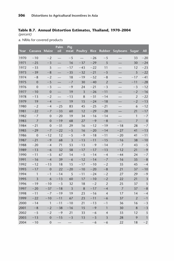
506 Distortions to Agricultural Incentives in Asia
Table B.7. Annual Distortion Estimates, Thailand, 1970–2004(percent)
a. NRAs for covered products
Palm PigYear Cassava Maize oil meat Poultry Rice Rubber Soybeans Sugar All
1970 �10 �2 — �5 — �26 �5 — 33 �20
1971 �25 �3 — 16 �37 �29 5 — 30 �24
1972 �33 5 — �17 �43 �22 11 — 12 �23
1973 �39 �8 — �35 �32 �21 �5 — 5 �22
1974 �8 �2 — 18 �19 �52 �8 — �17 �41
1975 0 �5 — �7 30 �40 2 — �11 �28
1976 0 �3 — �9 24 �21 �3 — �3 �12
1977 �10 0 — 19 3 �26 �11 — �2 �16
1978 �13 �2 — �13 8 �31 �14 — 2 �22
1979 19 �4 — 19 15 �24 �18 — �2 �13
1980 �2 �4 �25 83 45 �25 �21 — 6 �12
1981 �22 �7 �33 60 12 �29 �28 — 21 �17
1982 �7 0 �20 19 34 �16 �14 — 1 �7
1983 7 0 �19 68 27 �9 �8 — 7 0
1984 �21 0 �31 29 16 �12 �19 �18 28 �7
1985 �29 �7 �22 �5 16 �20 �14 �27 41 �13
1986 0 �12 12 �5 �9 �18 �11 �20 41 �11
1987 �21 �9 68 3 �13 �11 �15 �16 38 �10
1988 �20 �4 71 53 �13 �9 �14 �7 43 �5
1989 �13 �6 32 58 �17 �17 �13 �12 21 �9
1990 �11 �5 67 14 �5 �14 �4 �44 24 �7
1991 �16 �4 39 �6 �12 �14 �7 �16 35 �8
1992 �12 �13 18 15 �17 �10 �2 35 45 �4
1993 �17 0 22 �20 �10 �20 �8 21 37 �10
1994 1 �1 �14 5 �11 �24 �2 27 29 �9
1995 3 6 �13 60 17 �10 �2 22 21 3
1996 �19 �10 �3 32 18 �2 2 25 37 5
1997 �20 �37 �18 3 8 �17 �4 7 37 �8
1998 �11 �7 �19 19 23 �16 4 17 14 �4
1999 �22 �10 �11 67 23 �11 �6 37 2 �1
2000 �14 1 �11 �10 21 �13 �1 36 16 �3
2001 �8 �2 �38 �16 15 �9 1 30 8 �3
2002 �5 �2 �9 21 33 �6 4 33 12 5
2003 �13 0 �15 �3 13 �3 3 28 9 1
2004 �10 0 — — — �6 �6 22 18 �2
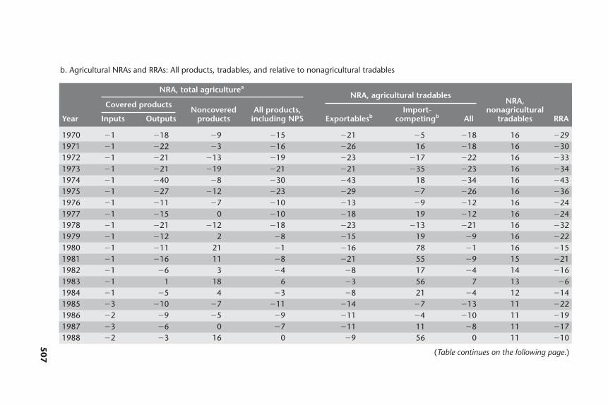
507
b. Agricultural NRAs and RRAs: All products, tradables, and relative to nonagricultural tradables
NRA, total agriculturea
NRA, agricultural tradablesNRA,Covered products
Noncovered All products, Import- nonagriculturalYear Inputs Outputs products including NPS Exportablesb competingb All tradables RRA
1970 �1 �18 �9 �15 �21 �5 �18 16 �291971 �1 �22 �3 �16 �26 16 �18 16 �301972 �1 �21 �13 �19 �23 �17 �22 16 �331973 �1 �21 �19 �21 �21 �35 �23 16 �341974 �1 �40 �8 �30 �43 18 �34 16 �431975 �1 �27 �12 �23 �29 �7 �26 16 �361976 �1 �11 �7 �10 �13 �9 �12 16 �241977 �1 �15 0 �10 �18 19 �12 16 �241978 �1 �21 �12 �18 �23 �13 �21 16 �321979 �1 �12 2 �8 �15 19 �9 16 �221980 �1 �11 21 �1 �16 78 �1 16 �151981 �1 �16 11 �8 �21 55 �9 15 �211982 �1 �6 3 �4 �8 17 �4 14 �161983 �1 1 18 6 �3 56 7 13 �61984 �1 �5 4 �3 �8 21 �4 12 �141985 �3 �10 �7 �11 �14 �7 �13 11 �221986 �2 �9 �5 �9 �11 �4 �10 11 �191987 �3 �6 0 �7 �11 11 �8 11 �171988 �2 �3 16 0 �9 56 0 11 �10
(Table continues on the following page.)

508
Table B.7. Annual Distortion Estimates, Thailand, 1970–2004 (continued)b. Agricultural NRAs and RRAs: All products, tradables, and relative to nonagricultural tradables
NRA, total agriculturea
NRA, agricultural tradablesNRA,Covered products
Noncovered All products, Import- nonagriculturalYear Inputs Outputs products including NPS Exportablesb competingb All tradables RRA
1989 �3 �7 13 �4 �13 53 �4 11 �141990 �3 �3 4 �4 �9 22 �4 10 �131991 �2 �6 �3 �7 �9 �1 �8 10 �161992 �1 �3 4 �2 �7 18 �2 10 �111993 �2 �9 �7 �9 �10 �10 �10 10 �181994 �1 �8 �2 �7 �11 4 �8 10 �161995 �1 4 18 7 �1 54 7 9 �21996 0 5 11 6 2 31 7 9 �21997 0 �8 �2 �7 �10 3 �8 9 �151998 �2 �1 4 �2 �5 19 �2 9 �101999 �3 2 19 4 �5 64 4 8 �42000 �1 �2 �3 �3 �3 �6 �3 8 �112001 �1 �3 �5 �4 �2 �14 �4 8 �112002 �2 7 8 6 4 22 7 8 �12003 0 0 0 0 1 �1 0 8 �72004 �1 �2 7 �1 �3 22 �1 8 �8

Annual Estimates of Asian Distortions to Agricultural Incentives 509
c. Value shares of the primary production of coveredc and noncovered products
Palm PigYear Cassava Maize oil meat Poultry Rice Rubber Soybeans Sugar Noncovered
1970 3 4 — 4 — 44 3 — 1 40
1971 3 4 — 3 9 40 3 — 1 37
1972 6 2 — 4 9 39 3 — 1 35
1973 4 5 — 5 7 42 4 — 2 31
1974 1 4 — 2 4 50 2 — 2 34
1975 2 5 — 3 3 47 2 — 3 35
1976 4 4 — 3 3 39 3 — 5 37
1977 6 2 — 3 5 38 4 — 7 36
1978 4 3 — 4 4 42 4 — 3 34
1979 5 4 — 3 4 39 7 — 6 33
1980 7 4 0 3 3 41 6 — 3 33
1981 6 4 0 3 4 42 5 — 5 32
1982 7 4 0 4 4 35 5 — 8 33
1983 7 5 0 3 5 36 6 — 4 33
1984 8 6 1 4 4 35 6 1 4 32
1985 6 5 1 5 4 34 7 1 3 33
1986 7 5 0 5 6 30 10 2 2 33
1987 10 3 1 5 6 28 11 1 3 31
1988 7 5 1 3 6 36 13 2 3 25
1989 6 5 1 3 6 38 10 2 4 24
1990 7 4 1 5 7 29 11 3 5 28
1991 7 4 1 6 9 30 9 1 4 28
1992 6 4 1 6 11 27 11 1 4 29
1993 5 3 1 7 11 24 12 1 4 31
1994 4 4 2 6 9 29 14 1 4 28
1995 5 4 2 4 8 28 18 1 5 25
1996 5 5 2 6 9 27 16 1 4 24
1997 4 6 2 7 9 31 12 1 4 24
1998 5 4 3 4 9 36 10 1 4 25
1999 4 5 2 4 10 33 11 1 6 25
2000 3 5 2 6 10 31 13 1 6 23
2001 4 4 2 9 12 27 12 0 5 25
2002 4 4 3 6 11 27 16 0 5 23
2003 4 4 3 6 9 24 21 0 6 21
2004 5 4 — — — 29 31 0 11 20
Sources: Author compilation; Warr and Kohpaiboon 2007; chapter 7 of this volume.
Note: — � no data are available.
a. Including assistance for nontradables and non-product-specific assistance (NPS).b. Including product-specific input subsidies.c. The covered products are calculated at undistorted farmgate prices in U.S. dollars.
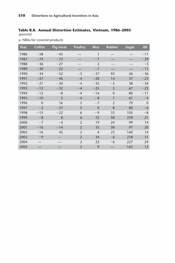
510 Distortions to Agricultural Incentives in Asia
Table B.8. Annual Distortion Estimates, Vietnam, 1986–2005(percent)
a. NRAs for covered products
Year Coffee Pig meat Poultry Rice Rubber Sugar All
1986 �58 �45 — 1 — — �111987 �74 �73 — �7 — — �291988 �36 �27 — 2 — — �31989 �30 �22 — �7 — — �111990 �34 �52 �3 �37 92 26 �361991 �27 �46 �4 �20 14 37 �231992 �21 �50 �4 �35 �5 38 �341993 �12 �32 �4 �25 5 67 �231994 �12 �8 �4 �16 0 80 �111995 �10 5 �4 �8 1 61 �41996 0 16 5 �7 2 79 01997 �2 �37 5 0 8 80 �61998 �15 �22 6 �9 33 105 �81999 �8 8 6 22 50 239 212000 �7 �4 2 19 24 99 142001 �16 �14 2 35 50 97 202002 �16 45 2 4 23 160 142003 �9 — 2 34 �6 218 312004 — — 2 22 �6 227 242005 — — 2 9 — 162 12
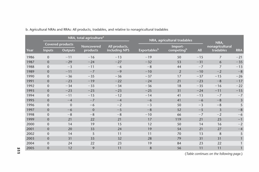
511
b. Agricultural NRAs and RRAs: All products, tradables, and relative to nonagricultural tradables
NRA, total agriculturea
NRA, agricultural tradablesNRA,Covered products
Noncovered All products, Import- nonagriculturalYear Inputs Outputs products including NPS Exportablesb competingb All tradables RRA
1986 0 �11 �16 �13 �19 50 �15 7 �211987 0 �29 �24 �27 �32 53 �31 6 �351988 0 �3 �11 �6 �8 44 �7 7 �131989 0 �11 �7 �9 �10 2 �10 �2 �81990 0 �36 �35 �36 �37 17 �37 �15 �261991 0 �23 �19 �22 �24 21 �23 �8 �171992 0 �34 �33 �34 �36 18 �35 �16 �221993 0 �23 �23 �23 �25 31 �24 �11 �151994 0 �11 �15 �12 �14 41 �13 �7 �71995 0 �4 �7 �4 �6 41 �6 �8 31996 0 0 �6 �2 �3 50 �3 �8 51997 0 �6 0 �5 �8 52 �5 3 �81998 0 �8 �8 �8 �10 66 �7 �2 �61999 0 21 22 21 17 119 21 23 �12000 0 14 19 15 12 50 14 16 �22001 0 20 33 24 19 54 21 27 �42002 0 14 5 11 11 70 13 8 52003 0 31 33 32 28 79 31 31 12004 0 24 22 23 19 84 23 22 12005 0 12 9 11 8 56 11 11 1
(Table continues on the following page.)

512 Distortions to Agricultural Incentives in Asia
Table B.8. Annual Distortion Estimates, Vietnam, 1986–2005(continued)
c. Value shares of the primary production of coveredc and noncovered products
Year Coffee Pig meat Poultry Rice Rubber Sugar Noncovered
1986 1 14 — 43 — — 421987 1 22 — 47 — — 291988 1 10 — 57 — — 321989 1 14 — 56 — — 291990 1 14 2 56 1 2 241991 1 13 3 53 1 2 281992 1 12 3 44 1 1 391993 2 13 3 45 1 1 351994 2 11 3 45 1 2 361995 5 12 3 54 1 2 231996 4 11 3 55 1 2 241997 5 18 3 46 2 2 241998 4 13 3 55 1 2 221999 5 14 3 49 1 1 262000 6 14 4 42 2 2 312001 4 16 4 37 1 3 342002 2 12 4 47 2 1 332003 2 — 5 43 4 1 452004 — — 4 47 4 1 442005 — — 3 49 — 1 47
Sources: Author compilation; Athukorala, Huong, and Thanh 2007; chapter 8 of this volume.
Note: — � no data are available.
a. Including assistance for nontradables and non-product-specific assistance (NPS).b. Including product-specific input subsidies.c. The covered products are calculated at undistorted farmgate prices in U.S. dollars.
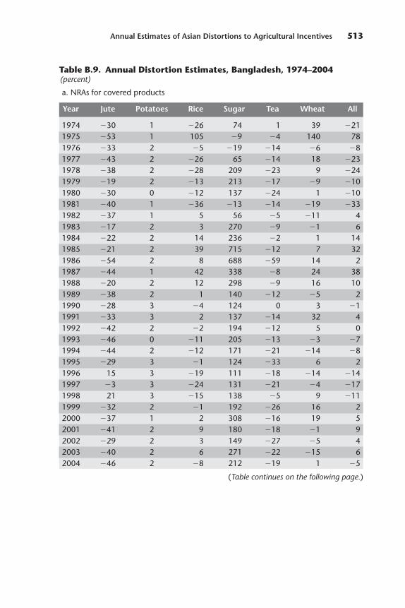
Annual Estimates of Asian Distortions to Agricultural Incentives 513
Table B.9. Annual Distortion Estimates, Bangladesh, 1974–2004(percent)
a. NRAs for covered products
Year Jute Potatoes Rice Sugar Tea Wheat All
1974 �30 1 �26 74 1 39 �211975 �53 1 105 �9 �4 140 781976 �33 2 �5 �19 �14 �6 �81977 �43 2 �26 65 �14 18 �231978 �38 2 �28 209 �23 9 �241979 �19 2 �13 213 �17 �9 �101980 �30 0 �12 137 �24 1 �101981 �40 1 �36 �13 �14 �19 �331982 �37 1 5 56 �5 �11 41983 �17 2 3 270 �9 �1 61984 �22 2 14 236 �2 1 141985 �21 2 39 715 �12 7 321986 �54 2 8 688 �59 14 21987 �44 1 42 338 �8 24 381988 �20 2 12 298 �9 16 101989 �38 2 1 140 �12 �5 21990 �28 3 �4 124 0 3 �11991 �33 3 2 137 �14 32 41992 �42 2 �2 194 �12 5 01993 �46 0 �11 205 �13 �3 �71994 �44 2 �12 171 �21 �14 �81995 �29 3 �1 124 �33 6 21996 15 3 �19 111 �18 �14 �141997 �3 3 �24 131 �21 �4 �171998 21 3 �15 138 �5 9 �111999 �32 2 �1 192 �26 16 22000 �37 1 2 308 �16 19 52001 �41 2 9 180 �18 �1 92002 �29 2 3 149 �27 �5 42003 �40 2 6 271 �22 �15 62004 �46 2 �8 212 �19 1 �5
(Table continues on the following page.)
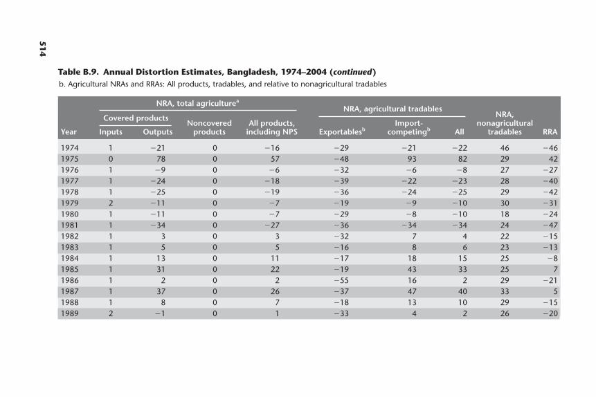
514
Table B.9. Annual Distortion Estimates, Bangladesh, 1974–2004 (continued)b. Agricultural NRAs and RRAs: All products, tradables, and relative to nonagricultural tradables
NRA, total agriculturea
NRA, agricultural tradablesNRA,Covered products
Noncovered All products, Import- nonagriculturalYear Inputs Outputs products including NPS Exportablesb competingb All tradables RRA
1974 1 �21 0 �16 �29 �21 �22 46 �461975 0 78 0 57 �48 93 82 29 421976 1 �9 0 �6 �32 �6 �8 27 �271977 1 �24 0 �18 �39 �22 �23 28 �401978 1 �25 0 �19 �36 �24 �25 29 �421979 2 �11 0 �7 �19 �9 �10 30 �311980 1 �11 0 �7 �29 �8 �10 18 �241981 1 �34 0 �27 �36 �34 �34 24 �471982 1 3 0 3 �32 7 4 22 �151983 1 5 0 5 �16 8 6 23 �131984 1 13 0 11 �17 18 15 25 �81985 1 31 0 22 �19 43 33 25 71986 1 2 0 2 �55 16 2 29 �211987 1 37 0 26 �37 47 40 33 51988 1 8 0 7 �18 13 10 29 �151989 2 �1 0 1 �33 4 2 26 �20
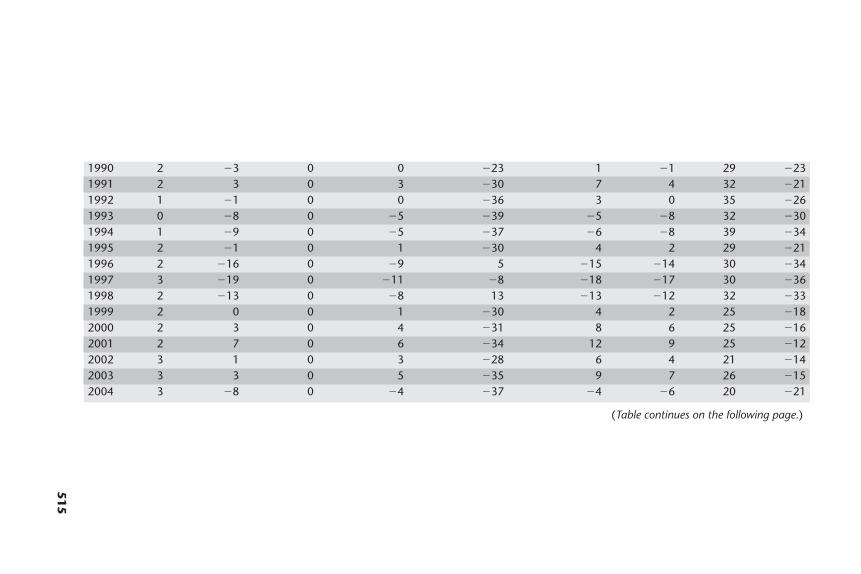
515
1990 2 �3 0 0 �23 1 �1 29 �231991 2 3 0 3 �30 7 4 32 �211992 1 �1 0 0 �36 3 0 35 �261993 0 �8 0 �5 �39 �5 �8 32 �301994 1 �9 0 �5 �37 �6 �8 39 �341995 2 �1 0 1 �30 4 2 29 �211996 2 �16 0 �9 5 �15 �14 30 �341997 3 �19 0 �11 �8 �18 �17 30 �361998 2 �13 0 �8 13 �13 �12 32 �331999 2 0 0 1 �30 4 2 25 �182000 2 3 0 4 �31 8 6 25 �162001 2 7 0 6 �34 12 9 25 �122002 3 1 0 3 �28 6 4 21 �142003 3 3 0 5 �35 9 7 26 �152004 3 �8 0 �4 �37 �4 �6 20 �21
(Table continues on the following page.)
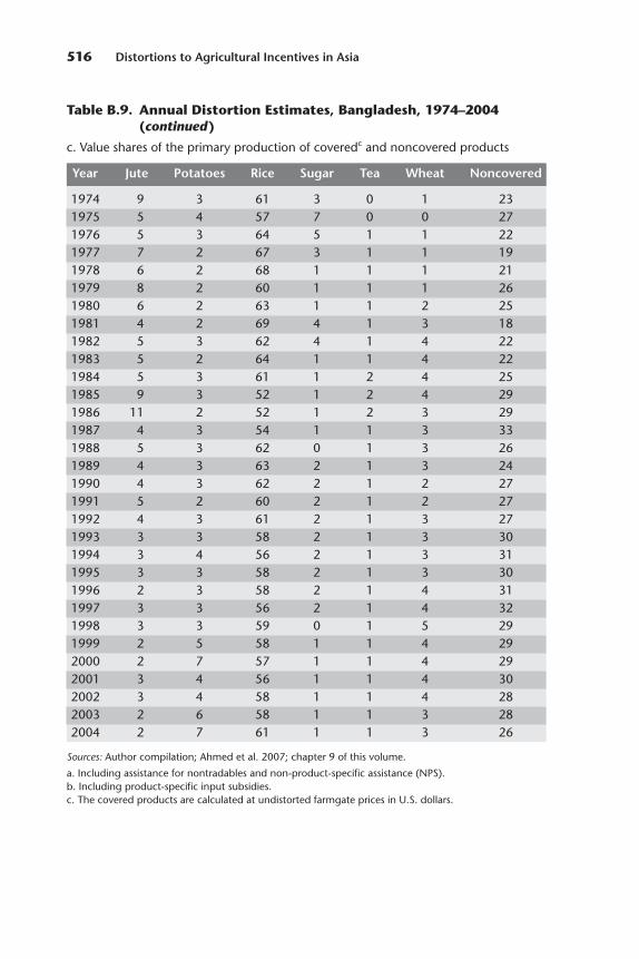
516 Distortions to Agricultural Incentives in Asia
Table B.9. Annual Distortion Estimates, Bangladesh, 1974–2004(continued)
c. Value shares of the primary production of coveredc and noncovered products
Year Jute Potatoes Rice Sugar Tea Wheat Noncovered
1974 9 3 61 3 0 1 231975 5 4 57 7 0 0 271976 5 3 64 5 1 1 221977 7 2 67 3 1 1 191978 6 2 68 1 1 1 211979 8 2 60 1 1 1 261980 6 2 63 1 1 2 251981 4 2 69 4 1 3 181982 5 3 62 4 1 4 221983 5 2 64 1 1 4 221984 5 3 61 1 2 4 251985 9 3 52 1 2 4 291986 11 2 52 1 2 3 291987 4 3 54 1 1 3 331988 5 3 62 0 1 3 261989 4 3 63 2 1 3 241990 4 3 62 2 1 2 271991 5 2 60 2 1 2 271992 4 3 61 2 1 3 271993 3 3 58 2 1 3 301994 3 4 56 2 1 3 311995 3 3 58 2 1 3 301996 2 3 58 2 1 4 311997 3 3 56 2 1 4 321998 3 3 59 0 1 5 291999 2 5 58 1 1 4 292000 2 7 57 1 1 4 292001 3 4 56 1 1 4 302002 3 4 58 1 1 4 282003 2 6 58 1 1 3 282004 2 7 61 1 1 3 26
Sources: Author compilation; Ahmed et al. 2007; chapter 9 of this volume.
a. Including assistance for nontradables and non-product-specific assistance (NPS).b. Including product-specific input subsidies.c. The covered products are calculated at undistorted farmgate prices in U.S. dollars.
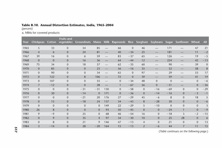
517
Table B.10. Annual Distortion Estimates, India, 1965–2004(percent)a. NRAs for covered products
Fruits andYear Chickpeas Cotton vegetables Groundnuts Maize Milk Rapeseeds Rice Sorghum Soybeans Sugar Sunflower Wheat All
1965 5 33 0 54 85 — 66 0 46 — 171 — 47 21
1966 4 6 0 24 81 — 40 �34 25 — 181 — 11 �2
1967 39 16 0 6 59 — 83 �37 65 — 126 — 19 �5
1968 0 0 0 16 36 — 64 �44 12 — 224 — 42 �13
1969 75 34 0 18 57 — 62 �35 60 — 90 — 39 0
1970 0 85 0 0 23 — 56 �16 35 — 52 — 58 8
1971 0 90 0 0 34 — 65 0 97 — 29 — 53 17
1972 0 122 0 8 106 — 72 0 39 — 59 — 41 19
1973 0 107 0 0 55 — 0 �34 48 0 0 — 0 �6
1974 7 �12 0 0 28 — 1 �67 56 0 �51 — 0 �36
1975 0 0 0 �31 �31 130 0 �58 0 �16 �69 0 0 �29
1976 0 30 0 �14 0 171 0 �36 0 �14 �16 0 �3 �1
1977 0 0 0 �21 20 176 27 �29 45 �6 8 0 18 5
1978 0 15 0 �18 24 137 34 �43 8 �28 30 0 0 �6
1979 0 0 0 0 0 149 22 �29 5 �10 0 0 0 3
1980 26 8 0 0 0 93 50 �45 0 0 �24 1 0 �9
1981 9 �9 0 25 0 68 46 �54 16 0 �18 3 �2 �15
1982 0 9 0 35 4 97 34 �30 10 0 25 28 0 6
1983 0 8 0 21 9 146 47 �13 4 0 21 0 0 13
1984 3 �14 0 28 �20 164 15 �13 2 �6 44 7 11 15
(Table continues on the following page.)
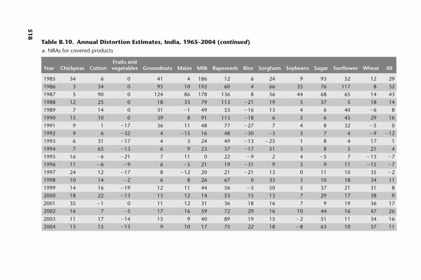
518
1985 34 6 0 41 4 186 12 6 24 9 93 52 12 29
1986 3 34 0 95 10 192 60 4 66 35 76 117 8 32
1987 5 90 0 124 86 178 136 8 56 44 68 65 14 43
1988 12 25 0 18 33 79 113 �21 19 5 37 5 18 14
1989 7 14 0 31 �1 49 53 �16 13 4 6 40 �6 8
1990 15 10 0 39 8 91 113 �18 6 5 6 45 29 16
1991 9 1 �17 36 11 48 77 �27 7 4 8 32 �5 0
1992 9 6 �32 4 �15 16 48 �30 �3 3 7 4 �9 �12
1993 6 31 �17 4 3 24 49 �13 �25 1 8 4 17 1
1994 7 65 �13 6 9 23 37 �17 51 3 8 5 21 4
1995 16 �6 �21 7 11 0 22 �9 2 4 �5 7 �13 �7
1996 11 �6 �9 6 �5 21 19 �31 9 3 9 11 �15 �7
1997 24 12 �17 8 �12 20 21 �21 13 0 11 10 35 �2
1998 10 14 �2 6 8 26 67 0 33 3 10 18 34 11
1999 14 16 �19 12 11 44 56 �5 50 5 37 21 31 8
2000 18 22 �13 13 12 14 53 15 13 7 29 17 38 9
2001 35 �1 0 11 12 31 36 18 16 7 9 19 36 17
2002 16 7 �5 17 16 59 72 29 16 10 44 16 47 26
2003 11 17 �14 15 9 40 89 19 15 �2 51 11 34 16
2004 13 15 �13 9 10 17 75 22 18 �8 63 10 37 11
Table B.10. Annual Distortion Estimates, India, 1965–2004 (continued)a. NRAs for covered products
Fruits andYear Chickpeas Cotton vegetables Groundnuts Maize Milk Rapeseeds Rice Sorghum Soybeans Sugar Sunflower Wheat All
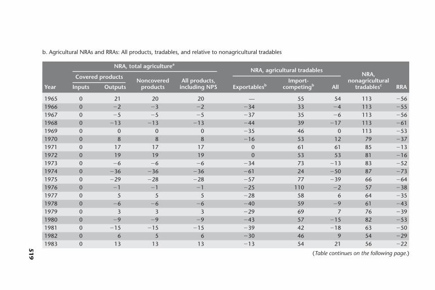
519
b. Agricultural NRAs and RRAs: All products, tradables, and relative to nonagricultural tradables
NRA, total agriculturea
NRA, agricultural tradablesNRA,Covered products
Noncovered All products, Import- nonagriculturalYear Inputs Outputs products including NPS Exportablesb competingb All tradablesc RRA
1965 0 21 20 20 — 55 54 113 �561966 0 �2 �3 �2 �34 33 �4 113 �551967 0 �5 �5 �5 �37 35 �6 113 �561968 0 �13 �13 �13 �44 39 �17 113 �611969 0 0 0 0 �35 46 0 113 �531970 0 8 8 8 �16 53 12 79 �371971 0 17 17 17 0 61 61 85 �131972 0 19 19 19 0 53 53 81 �161973 0 �6 �6 �6 �34 73 �13 83 �521974 0 �36 �36 �36 �61 24 �50 87 �731975 0 �29 �28 �28 �57 77 �39 66 �641976 0 �1 �1 �1 �25 110 �2 57 �381977 0 5 5 5 �28 58 6 64 �351978 0 �6 �6 �6 �40 59 �9 61 �431979 0 3 3 3 �29 69 7 76 �391980 0 �9 �9 �9 �43 57 �15 82 �531981 0 �15 �15 �15 �39 42 �18 63 �501982 0 6 5 6 �30 46 9 54 �291983 0 13 13 13 �13 54 21 56 �22
(Table continues on the following page.)
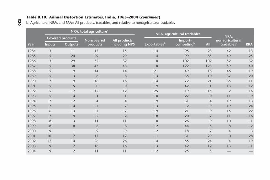
520
Table B.10. Annual Distortion Estimates, India, 1965–2004 (continued)b. Agricultural NRAs and RRAs: All products, tradables, and relative to nonagricultural tradables
NRA, total agriculturea
NRA, agricultural tradablesNRA,Covered products
Noncovered All products, Import- nonagriculturalYear Inputs Outputs products including NPS Exportablesb competingb All tradablesc RRA
1984 3 11 15 15 �14 95 23 42 �131985 5 24 29 29 4 99 85 49 251986 3 29 32 32 0 102 102 52 321987 5 38 43 43 0 122 123 59 401988 5 9 14 14 �21 49 18 46 �191989 5 3 8 8 �13 35 10 37 �201990 7 9 16 16 �14 72 21 35 �111991 5 �5 0 0 �19 42 �1 13 �121992 5 �17 �12 �12 �25 19 �15 2 �161993 5 �4 1 1 �10 27 0 11 �91994 7 �2 4 4 �9 31 4 19 �131995 7 �14 �7 �7 �13 2 �9 19 �241996 6 �13 �7 �7 �19 21 �9 15 �221997 7 �9 �2 �2 �18 20 �7 11 �161998 8 3 11 11 0 26 9 10 �11999 8 0 8 8 �12 44 5 8 �22000 9 1 9 9 �2 18 7 4 32001 10 7 17 17 �1 31 29 0 282002 12 14 26 26 �4 55 24 4 192003 9 7 16 16 �13 42 12 13 �12004 9 2 11 11 �12 25 5 — —

521
c. Value shares of the primary production of coveredd and noncovered products
Fruits and Year Chickpeas Cotton vegetables Groundnuts Maize Milk Rapeseeds Rice Sorghum Soybeans Sugar Sunflower Wheat Noncoverd
1965 3 3 15 4 2 — 1 21 3 — 2 — 4 43
1966 2 3 13 3 2 — 1 22 3 — 2 — 4 45
1967 3 3 13 3 2 — 1 28 3 — 1 — 6 39
1968 2 3 12 3 1 — 1 30 3 — 1 — 5 39
1969 2 3 16 4 1 — 1 26 2 — 2 — 6 38
1970 3 2 15 5 2 — 1 24 3 — 2 — 7 37
1971 3 3 16 5 2 — 1 22 2 — 2 — 8 36
1972 3 3 18 4 1 — 1 19 2 — 2 — 7 38
1973 2 2 13 5 1 — 1 24 2 0 3 — 5 40
1974 2 3 9 3 1 — 1 32 2 0 3 — 5 39
1975 2 2 8 3 2 4 1 31 2 0 7 0 6 32
1976 2 3 13 4 2 5 1 23 3 0 3 0 8 33
1977 2 4 13 5 1 5 1 25 3 0 3 0 7 31
1978 2 3 12 4 1 5 1 29 2 0 2 0 8 30
1979 1 4 14 4 1 5 1 21 3 0 3 0 8 34
1980 2 3 12 3 1 6 1 25 2 0 3 0 7 35
1981 2 3 11 3 1 7 1 28 2 0 4 0 6 32
1982 2 3 14 2 1 7 1 20 2 0 4 0 9 34
1983 2 3 14 4 1 6 1 20 3 0 3 0 9 34
1984 2 4 16 3 2 6 2 19 2 0 2 0 8 33
1985 3 3 19 2 1 7 1 19 2 0 2 0 9 31
(Table continues on the following page.)
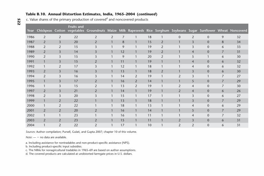
522
1986 2 2 22 2 2 7 1 18 1 0 2 0 9 32
1987 2 3 20 2 1 8 1 15 2 1 3 0 8 34
1988 2 2 15 3 1 9 1 19 2 1 3 0 6 33
1989 2 3 14 3 1 12 1 19 2 1 4 0 7 31
1990 2 3 15 3 1 9 1 20 2 1 5 1 6 30
1991 1 3 15 2 1 11 1 19 1 1 4 0 6 32
1992 1 2 17 3 1 12 1 18 1 1 4 0 6 32
1993 2 3 16 3 1 13 1 18 2 1 3 0 6 30
1994 2 3 16 3 1 14 2 19 1 2 3 1 7 27
1995 1 3 17 2 1 16 2 14 1 1 5 0 7 29
1996 1 3 15 2 1 13 2 19 1 2 4 0 7 30
1997 2 3 21 2 1 14 1 19 1 2 4 0 6 26
1998 2 3 20 3 1 15 1 17 1 1 3 0 6 27
1999 1 2 22 1 1 13 1 18 1 1 3 0 7 29
2000 1 2 22 1 1 18 1 13 1 1 4 0 6 29
2001 2 2 20 2 1 16 1 14 1 1 5 0 7 29
2002 1 1 23 1 1 16 1 11 1 1 4 0 7 32
2003 2 2 23 2 1 15 1 11 1 2 3 0 6 31
2004 1 2 22 2 1 17 1 10 1 2 2 0 6 31
Sources: Author compilation; Pursell, Gulati, and Gupta 2007; chapter 10 of this volume.
Note: — � no data are available.
a. Including assistance for nontradables and non-product-specific assistance (NPS).b. Including product-specific input subsidies.c. The NRAs for nonagricultural tradables in 1965–69 are based on author assumptions.d. The covered products are calculated at undistorted farmgate prices in U.S. dollars.
Table B.10. Annual Distortion Estimates, India, 1965–2004 (continued)c. Value shares of the primary production of coveredd and noncovered products
Fruits and Year Chickpeas Cotton vegetables Groundnuts Maize Milk Rapeseeds Rice Sorghum Soybeans Sugar Sunflower Wheat Noncoverd
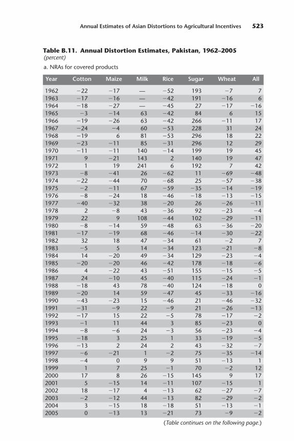
Annual Estimates of Asian Distortions to Agricultural Incentives 523
Table B.11. Annual Distortion Estimates, Pakistan, 1962–2005(percent)
a. NRAs for covered products
Year Cotton Maize Milk Rice Sugar Wheat All
1962 �22 �17 — �52 193 �7 71963 �17 �16 — �42 191 �16 61964 �18 �27 — �45 27 �17 �161965 �3 �14 63 �42 84 6 151966 �19 �26 63 �42 266 �11 171967 �24 �4 60 �53 228 31 241968 �19 6 81 �53 296 18 221969 �23 �11 85 �31 296 12 291970 �11 �11 140 �14 199 19 451971 9 �21 143 2 140 19 471972 1 19 241 6 192 7 421973 �8 �41 26 �62 11 �69 �481974 �22 �44 70 �68 25 �57 �381975 �2 �11 67 �59 �35 �14 �191976 �8 �24 18 �46 �18 �13 �151977 �40 �32 38 �20 26 �26 �111978 2 �8 43 �36 92 �23 �41979 22 9 108 �44 102 �29 �111980 �8 �14 59 �48 63 �36 �201981 �17 �19 68 �46 �14 �30 �221982 32 18 47 �34 61 �2 71983 �5 5 14 �34 123 �21 �81984 14 �20 49 �34 129 �23 �41985 �20 �20 46 �42 178 �18 �61986 4 �22 43 �51 155 �15 �51987 24 �10 45 �40 115 �24 �11988 �18 43 78 �40 124 �18 01989 �20 14 59 �47 45 �33 �161990 �43 �23 15 �46 21 �46 �321991 �31 �9 22 �9 21 �26 �131992 �17 15 22 �5 78 �17 �21993 �1 11 44 3 85 �23 01994 �8 �6 24 �3 56 �23 �41995 �18 3 25 1 33 �19 �51996 �13 2 24 2 43 �32 �71997 �6 �21 1 �2 75 �35 �141998 �4 0 9 9 51 �13 11999 1 7 25 �1 70 �2 122000 17 8 26 �15 145 9 172001 5 �15 14 �11 107 �15 12002 18 �17 4 �13 62 �27 �72003 �2 �12 44 �13 82 �29 �22004 3 �15 18 �18 51 �13 �12005 0 �13 13 �21 73 �9 �2
(Table continues on the following page.)
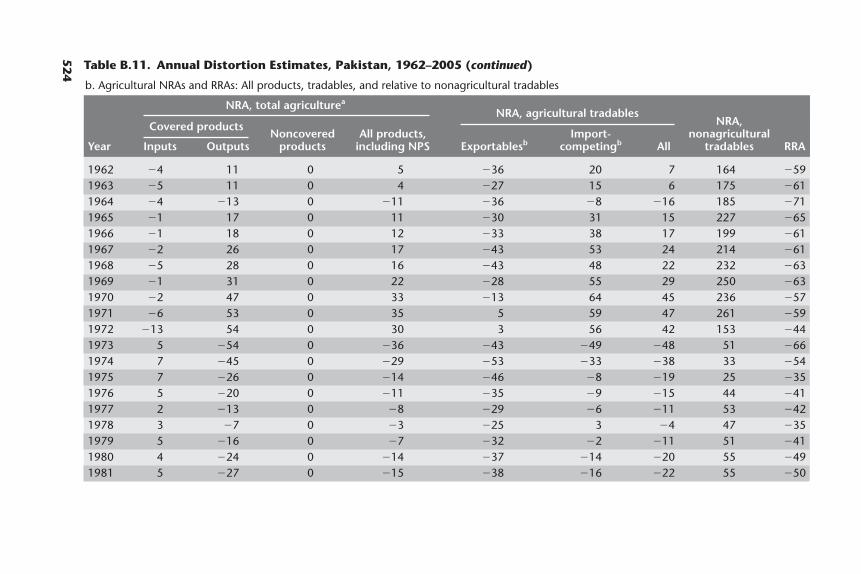
524 Table B.11. Annual Distortion Estimates, Pakistan, 1962–2005 (continued)
b. Agricultural NRAs and RRAs: All products, tradables, and relative to nonagricultural tradables
NRA, total agriculturea
NRA, agricultural tradablesNRA,Covered products
Noncovered All products, Import- nonagriculturalYear Inputs Outputs products including NPS Exportablesb competingb All tradables RRA
1962 �4 11 0 5 �36 20 7 164 �591963 �5 11 0 4 �27 15 6 175 �611964 �4 �13 0 �11 �36 �8 �16 185 �711965 �1 17 0 11 �30 31 15 227 �651966 �1 18 0 12 �33 38 17 199 �611967 �2 26 0 17 �43 53 24 214 �611968 �5 28 0 16 �43 48 22 232 �631969 �1 31 0 22 �28 55 29 250 �631970 �2 47 0 33 �13 64 45 236 �571971 �6 53 0 35 5 59 47 261 �591972 �13 54 0 30 3 56 42 153 �441973 5 �54 0 �36 �43 �49 �48 51 �661974 7 �45 0 �29 �53 �33 �38 33 �541975 7 �26 0 �14 �46 �8 �19 25 �351976 5 �20 0 �11 �35 �9 �15 44 �411977 2 �13 0 �8 �29 �6 �11 53 �421978 3 �7 0 �3 �25 3 �4 47 �351979 5 �16 0 �7 �32 �2 �11 51 �411980 4 �24 0 �14 �37 �14 �20 55 �491981 5 �27 0 �15 �38 �16 �22 55 �50
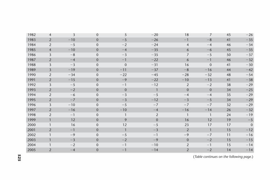
525
1982 4 3 0 5 �20 18 7 45 �261983 2 �10 0 �5 �26 �1 �8 41 �351984 2 �5 0 �2 �24 4 �4 46 �341985 4 �10 0 �4 �35 6 �6 45 �351986 3 �8 0 �3 �35 7 �5 50 �371987 2 �4 0 �1 �22 6 �1 46 �321988 3 �3 0 0 �31 16 0 41 �301989 3 �19 0 �11 �37 �8 �16 44 �421990 2 �34 0 �22 �45 �28 �32 48 �541991 2 �15 0 �9 �22 �10 �13 41 �381992 3 �5 0 �1 �12 2 �2 38 �291993 2 �2 0 0 1 0 0 34 �251994 2 �6 0 �3 �5 �4 �4 35 �291995 2 �7 0 �3 �12 �3 �5 34 �291996 3 �10 0 �5 �7 �7 �7 32 �291997 2 �16 0 �10 �4 �16 �14 26 �321998 2 �1 0 1 2 1 1 24 �191999 1 12 0 9 0 16 12 19 �52000 1 16 0 12 �5 23 17 17 02001 2 �1 0 1 �3 2 1 15 �122002 1 �9 0 �5 �1 �9 �7 11 �162003 1 �3 0 �2 �9 0 �2 15 �152004 1 �2 0 �1 �10 2 �1 15 �142005 2 �4 0 �1 �14 2 �2 14 �14
(Table continues on the following page.)

526 Distortions to Agricultural Incentives in Asia
Table B.11. Annual Distortion Estimates, Pakistan, 1962–2005(continued)
c. Value shares of the primary production of coveredc and noncovered products
Year Cotton Maize Milk Rice Sugar Wheat Noncovered
1962 9 4 — 8 7 42 311963 8 4 — 6 8 43 311964 7 4 — 14 11 34 311965 6 3 12 12 8 28 311966 7 3 14 12 5 27 311967 7 5 12 14 4 27 301968 6 3 10 14 3 33 301969 8 3 12 15 5 31 271970 8 3 10 11 7 35 261971 8 4 12 9 9 34 261972 10 3 7 9 5 39 271973 4 2 7 8 6 47 251974 7 2 6 14 6 40 261975 4 2 7 16 13 30 271976 4 2 11 12 13 30 281977 7 3 11 10 9 34 271978 5 2 10 13 6 35 291979 4 2 5 16 4 39 301980 5 2 6 14 5 38 301981 5 2 5 13 12 32 311982 4 2 8 16 8 30 311983 5 2 9 13 4 34 311984 4 2 8 14 5 33 331985 6 2 9 14 3 33 331986 5 2 9 14 3 33 331987 5 2 10 13 6 32 321988 10 2 9 14 4 31 301989 7 2 8 12 5 34 321990 9 2 9 10 5 33 331991 11 2 11 7 6 33 291992 11 2 11 6 4 31 351993 7 2 10 6 4 35 361994 7 2 12 7 5 31 361995 11 2 10 5 5 30 361996 9 2 16 5 4 29 361997 7 2 19 6 3 32 301998 6 2 19 5 6 31 30
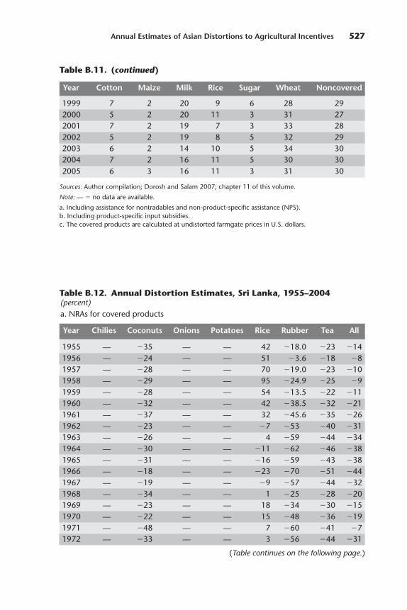
Annual Estimates of Asian Distortions to Agricultural Incentives 527
1999 7 2 20 9 6 28 292000 5 2 20 11 3 31 272001 7 2 19 7 3 33 282002 5 2 19 8 5 32 292003 6 2 14 10 5 34 302004 7 2 16 11 5 30 302005 6 3 16 11 3 31 30
Sources: Author compilation; Dorosh and Salam 2007; chapter 11 of this volume.
Note: — � no data are available.
a. Including assistance for nontradables and non-product-specific assistance (NPS).b. Including product-specific input subsidies.c. The covered products are calculated at undistorted farmgate prices in U.S. dollars.
Year Cotton Maize Milk Rice Sugar Wheat Noncovered
Table B.12. Annual Distortion Estimates, Sri Lanka, 1955–2004(percent)a. NRAs for covered products
Year Chilies Coconuts Onions Potatoes Rice Rubber Tea All
1955 — �35 — — 42 �18.0 �23 �141956 — �24 — — 51 �3.6 �18 �81957 — �28 — — 70 �19.0 �23 �101958 — �29 — — 95 �24.9 �25 �91959 — �28 — — 54 �13.5 �22 �111960 — �32 — — 42 �38.5 �32 �211961 — �37 — — 32 �45.6 �35 �261962 — �23 — — �7 �53 �40 �311963 — �26 — — 4 �59 �44 �341964 — �30 — — �11 �62 �46 �381965 — �31 — — �16 �59 �43 �381966 — �18 — — �23 �70 �51 �441967 — �19 — — �9 �57 �44 �321968 — �34 — — 1 �25 �28 �201969 — �23 — — 18 �34 �30 �151970 — �22 — — 15 �48 �36 �191971 — �48 — — 7 �60 �41 �71972 — �33 — — 3 �56 �44 �31
(Table continues on the following page.)
Table B.11. (continued)
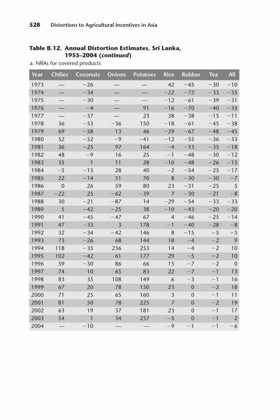
528 Distortions to Agricultural Incentives in Asia
1973 — �26 — — 42 �45 �30 �101974 — �34 — — �22 �72 �33 �351975 — �30 — — �12 �61 �39 �311976 — �4 — 91 �16 �70 �40 �351977 — �37 — 23 38 �38 �15 �111978 36 �53 �36 150 �18 �61 �45 �381979 69 �58 13 46 �29 �67 �48 �451980 52 �52 �9 �41 �12 �55 �36 �331981 36 �25 97 164 �4 �53 �35 �181982 48 �9 16 25 �1 �48 �30 �121983 35 1 11 28 �10 �48 �26 �151984 �5 �13 28 40 �2 �54 �25 �171985 22 �14 51 70 8 �30 �30 �71986 0 26 59 80 23 �31 �25 51987 �22 25 �62 �39 7 �30 �21 �81988 30 �21 �87 14 �29 �54 �33 �331989 5 �42 �25 38 �10 �43 �20 �201990 41 �45 �47 67 4 �46 �25 �141991 47 �33 3 178 �1 �40 �28 �81992 32 �34 �42 146 8 �15 �5 �51993 73 �26 68 144 18 �4 �2 91994 118 �35 236 253 14 �4 �2 101995 102 �42 61 177 29 �5 �2 101996 59 �30 86 66 15 �7 �2 01997 74 10 65 83 22 �7 �1 131998 83 35 108 149 6 �3 �1 161999 67 20 78 150 23 0 �2 182000 71 25 65 160 3 0 �1 112001 81 50 78 225 7 0 �2 192002 63 19 37 181 23 0 �1 172003 54 1 34 257 �5 0 �1 22004 — �10 — — �9 �1 �1 �6
Table B.12. Annual Distortion Estimates, Sri Lanka,1955–2004 (continued)
a. NRAs for covered products
Year Chilies Coconuts Onions Potatoes Rice Rubber Tea All
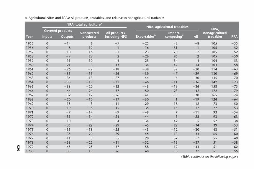
529
b. Agricultural NRAs and RRAs: All products, tradables, and relative to nonagricultural tradables
NRA, total agriculturea
NRA, agricultural tradablesNRA,Covered products
Noncovered All products, Import- nonagriculturalYear Inputs Outputs products including NPS Exportablesb competingb All tradables RRA
1955 0 �14 6 �7 �25 42 �8 105 �551956 0 �8 12 �1 �16 51 �1 105 �521957 0 �10 16 �1 �23 70 �2 105 �521958 0 �9 23 2 �26 95 2 105 �501959 0 �11 10 �4 �23 54 �4 104 �531960 0 �21 3 �13 �34 42 �14 103 �581961 0 �26 �2 �18 �38 32 �20 114 �631962 0 �31 �15 �26 �39 �7 �29 130 �691963 0 �34 �13 �27 �44 4 �30 135 �701964 0 �38 �19 �31 �46 �11 �36 142 �731965 0 �38 �20 �32 �43 �16 �36 158 �751966 0 �44 �24 �37 �50 �23 �42 172 �791967 0 �32 �17 �26 �41 �9 �30 165 �741968 0 �20 �10 �17 �30 1 �19 124 �641969 0 �15 �3 �11 �29 18 �12 73 �501970 0 �19 �6 �15 �35 15 �17 77 �531971 0 �7 �14 �9 �48 7 �11 93 �541972 0 �31 �14 �24 �44 3 �28 93 �631973 0 �10 3 �4 �34 42 �5 52 �381974 0 �35 �22 �29 �45 �22 �34 39 �531975 0 �31 �18 �25 �43 �12 �30 43 �511976 0 �35 �20 �29 �45 �13 �33 65 �601977 0 �11 3 �5 �28 37 �7 55 �401978 0 �38 �22 �31 �52 �13 �37 51 �581979 0 �45 �25 �37 �58 �17 �43 51 �621980 0 �33 �19 �26 �48 �8 �32 51 �55
(Table continues on the following page.)

530
Table B.12. Annual Distortion Estimates, Sri Lanka, 1955–2004 (continued)b. Agricultural NRAs and RRAs: All products, tradables, and relative to nonagricultural tradables
NRA, total agriculturea
NRA, agricultural tradablesNRA,Covered products
Noncovered All products, Import- nonagriculturalYear Inputs Outputs products including NPS Exportablesb competingb All tradables RRA
1981 0 �18 �10 �11 �34 5 �17 56 �471982 0 �12 �7 �8 �25 4 �12 56 �431983 0 �15 �9 �11 �22 �4 �14 56 �451984 0 �17 �9 �13 �26 0 �16 68 �501985 0 �7 �3 �4 �23 15 �7 68 �441986 0 5 4 6 �10 22 5 68 �371987 0 �8 �5 �6 �6 �10 �8 53 �401988 0 �33 �22 �29 �35 �32 �33 53 �561989 0 �20 �13 �17 �33 �5 �20 53 �481990 0 �14 �9 �13 �35 7 �14 45 �411991 0 �8 �6 �7 �32 15 �8 45 �371992 0 �5 �4 �4 �23 12 �5 52 �381993 0 9 7 8 �14 34 10 50 �271994 0 10 9 10 �18 44 11 43 �231995 0 10 9 11 �20 47 11 37 �191996 0 0 4 3 �16 29 2 40 �271997 0 13 12 14 3 32 14 36 �161998 0 16 11 16 13 20 16 35 �141999 0 18 14 18 10 32 19 33 �112000 0 11 8 11 10 14 11 21 �82001 0 19 13 19 17 22 19 23 �32002 0 17 13 17 8 32 17 23 �42003 0 2 2 4 0 6 3 25 �182004 0 �6 �5 �4 �4 �9 �6 22 �23
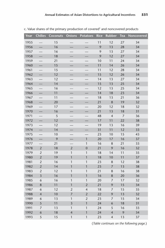
Annual Estimates of Asian Distortions to Agricultural Incentives 531
c. Value shares of the primary production of coveredc and noncovered products
Year Chilies Coconuts Onions Potatoes Rice Rubber Tea Noncovered
1955 — 15 — — 11 12 27 341956 — 16 — — 9 13 28 341957 — 16 — — 9 13 27 341958 — 18 — — 9 12 27 341959 — 21 — — 10 11 24 341960 — 15 — — 11 14 26 341961 — 15 — — 11 12 28 341962 — 12 — — 15 12 26 341963 — 12 — — 14 13 27 341964 — 14 — — 15 13 25 341965 — 16 — — 12 13 25 341966 — 11 — — 14 18 23 341967 — 11 — — 18 13 21 361968 — 20 — — 21 8 19 321969 — 17 — — 20 12 18 321970 — 16 — — 21 13 18 311971 — 5 — — 48 4 7 361972 — 12 — — 17 11 22 381973 — 12 — — 19 13 16 391974 — 14 — — 31 11 12 331975 — 10 — — 23 10 15 431976 — 9 — 1 20 17 16 371977 — 21 — 1 16 8 21 331978 2 18 2 0 21 9 16 321979 2 19 1 1 18 14 11 351980 2 19 1 1 18 10 11 371981 2 16 1 1 23 8 12 381982 2 14 1 1 23 7 13 381983 2 12 1 1 21 8 16 381984 3 16 1 1 16 8 20 361985 6 16 1 1 20 7 17 321986 8 11 1 2 21 9 15 341987 6 12 2 4 18 7 15 351988 4 10 7 2 22 9 13 321989 6 13 1 2 23 7 15 341990 5 11 3 1 24 6 18 311991 7 13 1 1 24 5 16 331992 6 18 4 1 24 4 9 341993 5 15 1 1 23 4 13 37
(Table continues on the following page.)

532 Distortions to Agricultural Incentives in Asia
1994 4 16 1 1 21 6 12 391995 4 15 1 1 21 7 11 401996 4 18 1 1 15 6 14 411997 2 19 1 1 16 5 17 401998 3 16 1 0 20 4 19 381999 3 20 2 0 22 3 16 342000 2 15 1 0 22 3 19 362001 2 14 1 1 21 3 21 372002 2 17 1 1 20 4 19 362003 2 14 1 1 23 5 18 362004 — 16 — — 22 6 21 36
Sources: Author compilation; Bandara and Jayasuriya 2007; chapter 12 of this volume.
Note: — � no data are available.a. Including assistance for nontradables and non-product-specific assistance (NPS).b. Including product-specific input subsidies.c. The covered products are calculated at undistorted farmgate prices in U.S. dollars.
Table B.12. Annual Distortion Estimates, Sri Lanka, 1955–2004(continued)
c. Value shares of the primary production of coveredc and noncovered products
Year Chilies Coconuts Onions Potatoes Rice Rubber Tea Noncovered
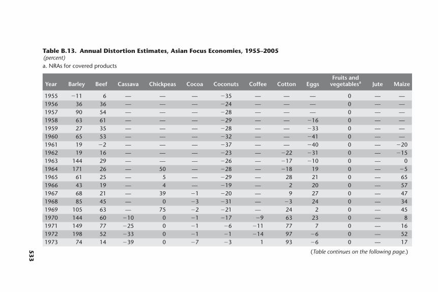
533
Table B.13. Annual Distortion Estimates, Asian Focus Economies, 1955–2005(percent)a. NRAs for covered products
Fruits andYear Barley Beef Cassava Chickpeas Cocoa Coconuts Coffee Cotton Eggs vegetablesa Jute Maize
1955 �11 6 — — — �35 — — — 0 — —1956 36 36 — — — �24 — — — 0 — —1957 90 54 — — — �28 — — — 0 — —1958 63 61 — — — �29 — — �16 0 — —1959 27 35 — — — �28 — — �33 0 — —1960 65 53 — — — �32 — — �41 0 — —1961 19 �2 — — — �37 — — �40 0 — �201962 19 16 — — — �23 — �22 �31 0 — �151963 144 29 — — — �26 — �17 �10 0 — 01964 171 26 — 50 — �28 — �18 19 0 — �51965 61 25 — 5 — �29 — 28 21 0 — 651966 43 19 — 4 — �19 — 2 20 0 — 571967 68 21 — 39 �1 �20 — 9 27 0 — 471968 85 45 — 0 �3 �31 — �3 24 0 — 341969 105 63 — 75 �2 �21 — 24 2 0 — 451970 144 60 �10 0 �1 �17 �9 63 23 0 — 81971 149 77 �25 0 �1 �6 �11 77 7 0 — 161972 198 52 �33 0 �1 �1 �14 97 �6 0 — 521973 74 14 �39 0 �7 �3 1 93 �6 0 — 17
(Table continues on the following page.)
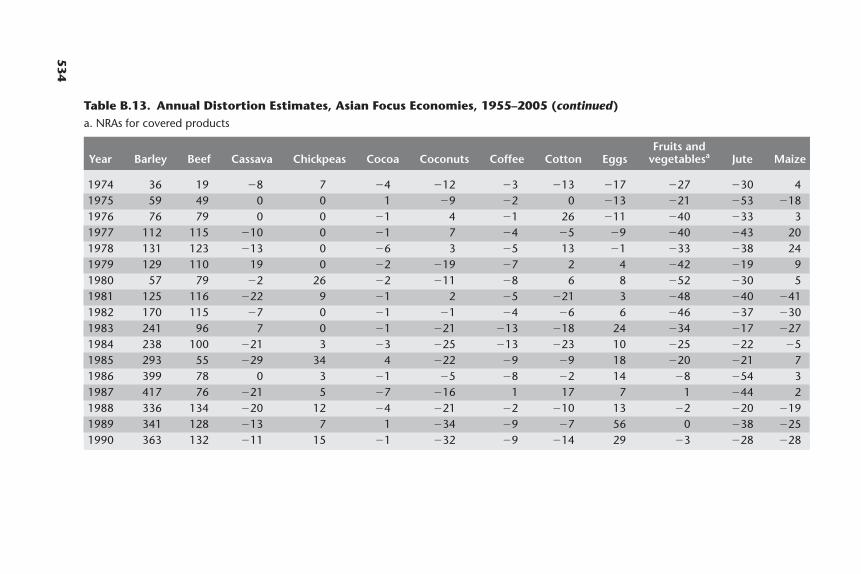
534
Table B.13. Annual Distortion Estimates, Asian Focus Economies, 1955–2005 (continued)a. NRAs for covered products
Fruits andYear Barley Beef Cassava Chickpeas Cocoa Coconuts Coffee Cotton Eggs vegetablesa Jute Maize
1974 36 19 �8 7 �4 �12 �3 �13 �17 �27 �30 41975 59 49 0 0 1 �9 �2 0 �13 �21 �53 �181976 76 79 0 0 �1 4 �1 26 �11 �40 �33 31977 112 115 �10 0 �1 7 �4 �5 �9 �40 �43 201978 131 123 �13 0 �6 3 �5 13 �1 �33 �38 241979 129 110 19 0 �2 �19 �7 2 4 �42 �19 91980 57 79 �2 26 �2 �11 �8 6 8 �52 �30 51981 125 116 �22 9 �1 2 �5 �21 3 �48 �40 �411982 170 115 �7 0 �1 �1 �4 �6 6 �46 �37 �301983 241 96 7 0 �1 �21 �13 �18 24 �34 �17 �271984 238 100 �21 3 �3 �25 �13 �23 10 �25 �22 �51985 293 55 �29 34 4 �22 �9 �9 18 �20 �21 71986 399 78 0 3 �1 �5 �8 �2 14 �8 �54 31987 417 76 �21 5 �7 �16 1 17 7 1 �44 21988 336 134 �20 12 �4 �21 �2 �10 13 �2 �20 �191989 341 128 �13 7 1 �34 �9 �7 56 0 �38 �251990 363 132 �11 15 �1 �32 �9 �14 29 �3 �28 �28

535
1991 494 163 �16 9 �1 �34 �5 �16 6 1 �33 �201992 461 163 �12 9 �6 �35 �5 �12 41 �4 �42 �241993 534 125 �17 6 �2 �32 �3 4 18 �3 �46 �161994 769 141 1 7 �2 �36 �3 23 39 1 �44 131995 632 151 3 16 �1 �36 �4 �5 49 0 �29 11996 403 133 �19 11 �1 �34 4 �4 10 �3 15 �31997 635 99 �20 24 �8 �16 2 6 9 �3 �3 101998 449 54 �11 10 0 �17 �7 3 9 1 21 221999 596 94 �22 14 0 �7 0 3 39 22 �32 92000 740 73 �14 18 0 �9 0 21 31 22 �37 132001 412 87 �8 35 0 �7 �6 �10 34 20 �41 162002 561 115 �5 16 0 �7 �4 6 32 24 �29 82003 572 78 �13 11 0 �6 �2 7 55 26 �40 192004 528 72 �10 13 0 �11 3 1 105 18 �46 72005 — 205 — — 0 �18 — 11 — 19 — 17
(Table continues on the following page.)
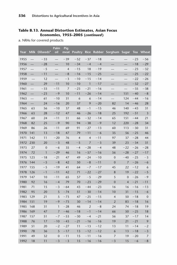
536 Distortions to Agricultural Incentives in Asia
Palm PigYear Milk Oilseedsa oil meat Poultry Rice Rubber Sorghum Sugar Tea Wheat
1955 — �33 — �39 �52 �37 �18 — — �23 �56
1956 — �28 — 10 �34 �4 �4 — — �18 �29
1957 — �5 — 4 �15 18 �19 — — �23 �32
1958 — �11 — �8 �16 �15 �25 — — �25 �22
1959 — 12 — �3 �10 �15 �14 — — �22 �26
1960 — 29 �11 10 �10 1 �17 — — �32 �27
1961 — �33 �11 7 �23 �21 �16 — — �35 �38
1962 — �23 �9 10 �11 �26 �14 — 151 �40 �8
1963 — 61 �10 31 6 6 �14 — 124 �44 �16
1964 — 24 �16 20 37 9 �20 82 14 �46 28
1965 63 56 �10 37 48 �1 �15 46 140 �43 31
1966 63 28 �12 47 46 �26 �18 25 192 �51 3
1967 60 24 �11 51 66 �32 �14 65 151 �44 21
1968 82 25 �9 90 94 �38 �9 12 220 �28 34
1969 86 26 �11 69 91 �27 �13 60 113 �30 31
1970 141 13 �18 47 79 �11 �6 35 56 �25 46
1971 142 11 �20 76 4 4 �11 97 37 �28 44
1972 230 20 �3 48 �5 7 �3 39 23 �34 31
1973 27 0 �6 35 �4 �28 �4 48 �22 �26 �28
1974 72 1 �29 46 16 �57 �16 56 �28 �27 �17
1975 123 �18 �21 47 49 �24 �10 0 �40 �25 �3
1976 144 �5 �8 42 50 �8 �11 0 7 �26 �6
1977 155 �5 �19 41 64 �7 �17 45 22 �12 6
1978 126 �1 �11 42 71 �22 �27 8 19 �22 �5
1979 147 10 �11 65 57 �5 �29 5 0 �26 �9
1980 92 16 �4 79 70 �23 �29 0 4 �21 �11
1981 71 15 �3 �64 43 �44 �23 16 16 �16 �13
1982 95 20 5 �74 51 �30 �14 10 31 �15 �6
1983 129 21 5 �73 47 �25 �15 4 50 �18 0
1984 151 19 �9 �73 30 �14 �14 2 83 �18 16
1985 168 31 1 �28 46 2 �8 24 74 �18 19
1986 169 47 7 �46 �18 �1 �14 66 50 �25 18
1987 157 51 �7 �53 �30 �4 �21 56 37 �17 14
1988 76 17 �10 �43 �21 �16 �16 19 21 �21 9
1989 51 20 �2 �27 11 �13 �12 13 11 �14 �2
1990 78 36 5 �17 13 �12 �12 6 13 �18 �3
1991 49 32 0 �11 15 �11 �16 7 19 �20 7
1992 18 11 �3 �3 15 �16 �16 �3 15 �6 �8
Table B.13. Annual Distortion Estimates, Asian FocusEconomies, 1955–2005 (continued)
a. NRAs for covered products

Annual Estimates of Asian Distortions to Agricultural Incentives 537
1993 26 8 4 4 32 �6 �19 �25 8 �5 �2
1994 26 18 2 12 23 2 �18 51 9 �3 26
1995 5 22 �8 8 16 7 �15 2 7 �5 21
1996 22 22 �1 10 20 �1 �9 9 11 �7 7
1997 19 22 �11 5 16 1 10 13 6 �9 19
1998 26 24 �22 3 12 �2 16 33 30 �7 23
1999 44 22 �3 9 20 7 24 50 46 �10 16
2000 20 22 �2 7 19 19 14 13 50 �7 20
2001 28 20 2 5 14 21 10 16 22 �8 8
2002 48 24 �6 6 17 16 1 16 45 �8 7
2003 40 26 �6 1 8 22 �1 15 50 �7 5
2004 21 18 �1 2 4 14 �5 18 49 �7 13
2005 33 19 — 0 0 �10 — — 40 �29 4
Palm PigYear Milk Oilseedsa oil meat Poultry Rice Rubber Sorghum Sugar Tea Wheat
(Table continues on the following page.)
a. NRAs for covered products
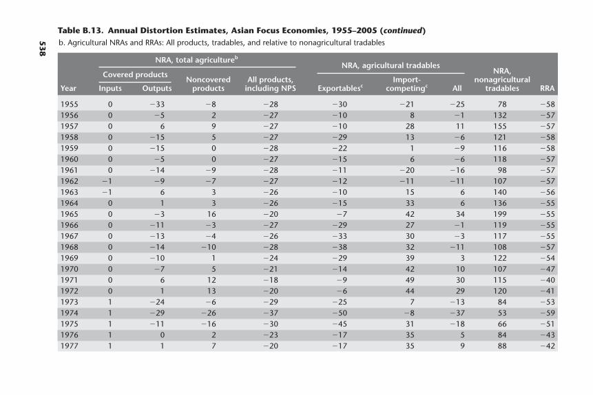
538
Table B.13. Annual Distortion Estimates, Asian Focus Economies, 1955–2005 (continued)b. Agricultural NRAs and RRAs: All products, tradables, and relative to nonagricultural tradables
NRA, total agricultureb
NRA, agricultural tradablesNRA,Covered products
Noncovered All products, Import- nonagriculturalYear Inputs Outputs products including NPS Exportablesc competingc All tradables RRA
1955 0 �33 �8 �28 �30 �21 �25 78 �581956 0 �5 2 �27 �10 8 �1 132 �571957 0 6 9 �27 �10 28 11 155 �571958 0 �15 5 �27 �29 13 �6 121 �581959 0 �15 0 �28 �22 1 �9 116 �581960 0 �5 0 �27 �15 6 �6 118 �571961 0 �14 �9 �28 �11 �20 �16 98 �571962 �1 �9 �7 �27 �12 �11 �11 107 �571963 �1 6 3 �26 �10 15 6 140 �561964 0 1 3 �26 �15 33 6 136 �551965 0 �3 16 �20 �7 42 34 199 �551966 0 �11 �3 �27 �29 27 �1 119 �551967 0 �13 �4 �26 �33 30 �3 117 �551968 0 �14 �10 �28 �38 32 �11 108 �571969 0 �10 1 �24 �29 39 3 122 �541970 0 �7 5 �21 �14 42 10 107 �471971 0 6 12 �18 �9 49 30 115 �401972 0 1 13 �20 �6 44 29 120 �411973 1 �24 �6 �29 �25 7 �13 84 �531974 1 �29 �26 �37 �50 �8 �37 53 �591975 1 �11 �16 �30 �45 31 �18 66 �511976 1 0 2 �23 �17 35 5 84 �431977 1 1 7 �20 �17 35 9 88 �42
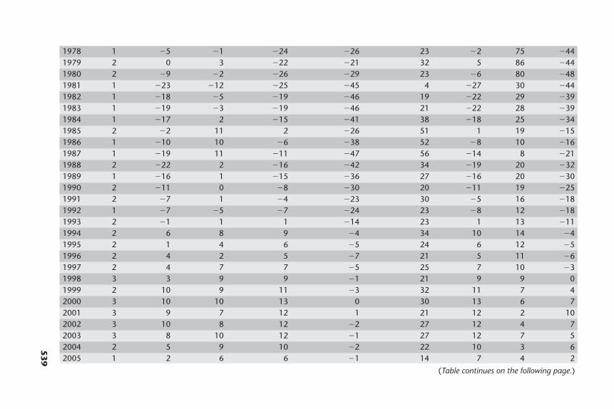
539
1978 1 �5 �1 �24 �26 23 �2 75 �441979 2 0 3 �22 �21 32 5 86 �441980 2 �9 �2 �26 �29 23 �6 80 �481981 1 �23 �12 �25 �45 4 �27 30 �441982 1 �18 �5 �19 �46 19 �22 29 �391983 1 �19 �3 �19 �46 21 �22 28 �391984 1 �17 2 �15 �41 38 �18 25 �341985 2 �2 11 2 �26 51 1 19 �151986 1 �10 10 �6 �38 52 �8 10 �161987 1 �19 11 �11 �47 56 �14 8 �211988 2 �22 2 �16 �42 34 �19 20 �321989 1 �16 1 �15 �36 27 �16 20 �301990 2 �11 0 �8 �30 20 �11 19 �251991 2 �7 1 �4 �23 30 �5 16 �181992 1 �7 �5 �7 �24 23 �8 12 �181993 2 �1 1 1 �14 23 1 13 �111994 2 6 8 9 �4 34 10 14 �41995 2 1 4 6 �5 24 6 12 �51996 2 4 2 5 �7 21 5 11 �61997 2 4 7 7 �5 25 7 10 �31998 3 3 9 9 �1 21 9 9 01999 2 10 9 11 �3 32 11 7 42000 3 10 10 13 0 30 13 6 72001 3 9 7 12 1 21 12 2 102002 3 10 8 12 �2 27 12 4 72003 3 8 10 12 �1 27 12 7 52004 2 5 9 10 �2 22 10 3 62005 1 2 6 6 �1 14 7 4 2
(Table continues on the following page.)
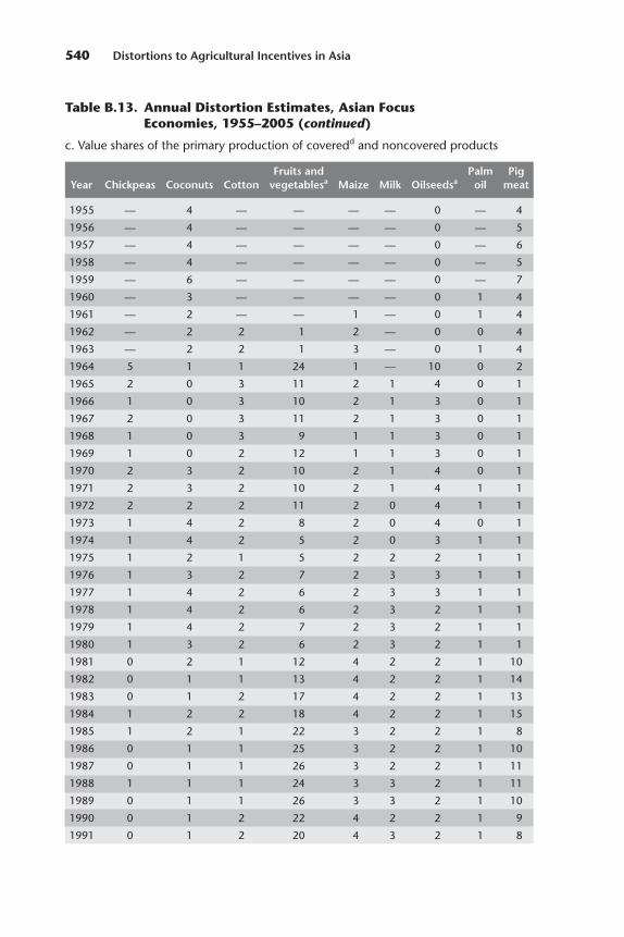
540 Distortions to Agricultural Incentives in Asia
Table B.13. Annual Distortion Estimates, Asian FocusEconomies, 1955–2005 (continued)
c. Value shares of the primary production of coveredd and noncovered products
Fruits and Palm PigYear Chickpeas Coconuts Cotton vegetablesa Maize Milk Oilseedsa oil meat
1955 — 4 — — — — 0 — 4
1956 — 4 — — — — 0 — 5
1957 — 4 — — — — 0 — 6
1958 — 4 — — — — 0 — 5
1959 — 6 — — — — 0 — 7
1960 — 3 — — — — 0 1 4
1961 — 2 — — 1 — 0 1 4
1962 — 2 2 1 2 — 0 0 4
1963 — 2 2 1 3 — 0 1 4
1964 5 1 1 24 1 — 10 0 2
1965 2 0 3 11 2 1 4 0 1
1966 1 0 3 10 2 1 3 0 1
1967 2 0 3 11 2 1 3 0 1
1968 1 0 3 9 1 1 3 0 1
1969 1 0 2 12 1 1 3 0 1
1970 2 3 2 10 2 1 4 0 1
1971 2 3 2 10 2 1 4 1 1
1972 2 2 2 11 2 0 4 1 1
1973 1 4 2 8 2 0 4 0 1
1974 1 4 2 5 2 0 3 1 1
1975 1 2 1 5 2 2 2 1 1
1976 1 3 2 7 2 3 3 1 1
1977 1 4 2 6 2 3 3 1 1
1978 1 4 2 6 2 3 2 1 1
1979 1 4 2 7 2 3 2 1 1
1980 1 3 2 6 2 3 2 1 1
1981 0 2 1 12 4 2 2 1 10
1982 0 1 1 13 4 2 2 1 14
1983 0 1 2 17 4 2 2 1 13
1984 1 2 2 18 4 2 2 1 15
1985 1 2 1 22 3 2 2 1 8
1986 0 1 1 25 3 2 2 1 10
1987 0 1 1 26 3 2 2 1 11
1988 1 1 1 24 3 3 2 1 11
1989 0 1 1 26 3 3 2 1 10
1990 0 1 2 22 4 2 2 1 9
1991 0 1 2 20 4 3 2 1 8
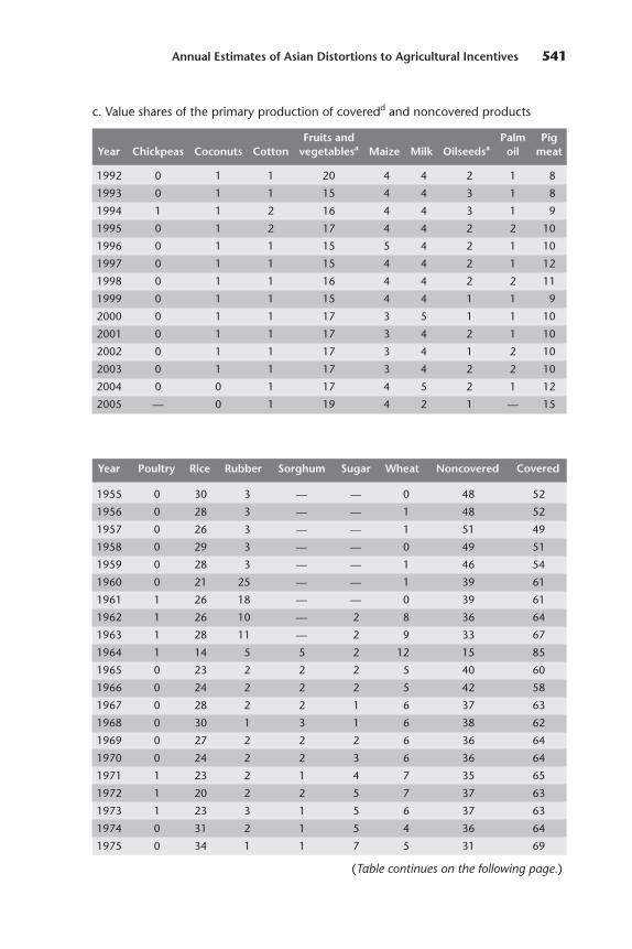
Annual Estimates of Asian Distortions to Agricultural Incentives 541
1992 0 1 1 20 4 4 2 1 8
1993 0 1 1 15 4 4 3 1 8
1994 1 1 2 16 4 4 3 1 9
1995 0 1 2 17 4 4 2 2 10
1996 0 1 1 15 5 4 2 1 10
1997 0 1 1 15 4 4 2 1 12
1998 0 1 1 16 4 4 2 2 11
1999 0 1 1 15 4 4 1 1 9
2000 0 1 1 17 3 5 1 1 10
2001 0 1 1 17 3 4 2 1 10
2002 0 1 1 17 3 4 1 2 10
2003 0 1 1 17 3 4 2 2 10
2004 0 0 1 17 4 5 2 1 12
2005 — 0 1 19 4 2 1 — 15
Fruits and Palm PigYear Chickpeas Coconuts Cotton vegetablesa Maize Milk Oilseedsa oil meat
Year Poultry Rice Rubber Sorghum Sugar Wheat Noncovered Covered
1955 0 30 3 — — 0 48 52
1956 0 28 3 — — 1 48 52
1957 0 26 3 — — 1 51 49
1958 0 29 3 — — 0 49 51
1959 0 28 3 — — 1 46 54
1960 0 21 25 — — 1 39 61
1961 1 26 18 — — 0 39 61
1962 1 26 10 — 2 8 36 64
1963 1 28 11 — 2 9 33 67
1964 1 14 5 5 2 12 15 85
1965 0 23 2 2 2 5 40 60
1966 0 24 2 2 2 5 42 58
1967 0 28 2 2 1 6 37 63
1968 0 30 1 3 1 6 38 62
1969 0 27 2 2 2 6 36 64
1970 0 24 2 2 3 6 36 64
1971 1 23 2 1 4 7 35 65
1972 1 20 2 2 5 7 37 63
1973 1 23 3 1 5 6 37 63
1974 0 31 2 1 5 4 36 64
1975 0 34 1 1 7 5 31 69
c. Value shares of the primary production of coveredd and noncovered products
(Table continues on the following page.)

542 Distortions to Agricultural Incentives in Asia
Table B.13. Annual Distortion Estimates, Asian Focus Economies,1955–2005
c. Value shares of the primary production of coveredd and noncovered products(continued)
Year Poultry Rice Rubber Sorghum Sugar Wheat Noncovered Coveredd
1976 1 29 3 2 5 5 32 68
1977 1 28 3 1 4 5 32 68
1978 1 32 3 1 4 5 31 69
1979 1 26 4 1 5 5 33 67
1980 1 29 3 1 4 5 34 66
1981 1 29 1 1 3 5 25 75
1982 1 25 1 0 3 6 25 75
1983 1 22 1 1 2 6 24 76
1984 1 21 1 1 2 6 23 77
1985 1 20 1 0 2 6 26 74
1986 1 19 1 0 2 6 23 77
1987 2 18 2 0 2 5 22 78
1988 2 21 1 0 2 4 21 79
1989 2 21 1 0 3 5 20 80
1990 2 21 1 0 3 5 23 77
1991 2 21 1 0 3 5 25 75
1992 2 21 1 0 3 5 25 75
1993 2 21 1 0 3 6 28 72
1994 3 21 2 0 3 5 25 75
1995 4 19 2 0 3 5 24 76
1996 3 21 1 0 3 6 25 75
1997 3 20 1 0 3 6 25 75
1998 4 19 1 0 2 5 28 72
1999 3 18 0 0 2 5 32 68
2000 4 15 1 0 2 5 33 67
2001 4 14 1 0 2 5 34 66
2002 4 13 1 0 2 4 36 64
2003 4 13 1 0 2 5 34 66
2004 3 14 1 0 2 4 33 67
2005 5 11 — — 1 5 34 66
Sources: Author compilation; chapters 2–12 of this volume.
Note: — � no data are available.a. Fruits and vegetables include bananas, cabbages, chilies, garlic, onions, peppers, potatoes, and fruit
and vegetable aggregates. Oilseeds include groundnuts, rapeseeds, soybeans, and sunflower seeds.b. Including assistance for nontradables and non-product-specific assistance (NPS).c. Including product-specific input subsidies.d. The covered products are calculated at undistorted farmgate prices in U.S. dollars. Products repre-
senting less than 0.5 percent of the gross value of regional production beginning in 1965 areexcluded because of the low shares. These products include barley, beef, cassava, cocoa, coffee, eggs,jute, and tea.

Table B.14. Gross Subsidy Equivalents of Assistance to Farmers, Asian Focus Economies, 1955–2005(constant 2000 US$, millions)
Korea, Taiwan,Year Bangladesh China India Indonesia Rep. of Malaysia Pakistan Philippines Sri Lanka China Thailand Vietnam
1955 — �7,101 6 — �269 — — — �40 �150 — —1956 — �11,171 10 — �14 — — — �5 �19 — —1957 — �11,081 10 — 175 — — — �7 2 — —1958 — �11,488 10 — 21 — — — 9 �134 — —1959 — �11,533 10 — �49 — — — �22 �87 — —1960 — �13,026 11 — 5 �87 — — �64 �9 — —1961 — �14,654 13 — �357 �53 — — �81 30 — —1962 — �15,694 14 — �313 �35 45 �103 �116 7 — —1963 — �16,644 15 — 315 �32 43 �58 �108 61 — —1964 — �15,061 13 — 485 �62 �149 15 �129 57 — —1965 — �14,382 3,361 — 157 �29 165 144 �141 69 — —1966 — �16,418 �463 — 86 �49 175 218 �135 53 — —1967 — �17,322 �1,158 — 119 �55 278 166 �96 9 — —1968 — �17,729 �3,203 — 233 �63 308 160 �102 13 — —1969 — �18,498 10 — 447 �102 388 186 �61 8 — —1970 — �19,674 1,802 �88 777 �53 612 52 �77 121 �366 —1971 — �20,624 3,818 230 985 �79 611 255 �124 167 �370 —1972 — �24,468 4,538 64 1,154 �30 545 64 �88 209 �439 —1973 — �37,675 �2,437 �655 487 �151 �1,081 �803 �21 141 �741 —1974 �661 �48,394 �22,142 �941 �1,144 �556 �978 �1,375 �298 0 �1,879 —1975 3,267 �47,489 �15,816 1,453 476 �391 �482 �937 �189 229 �1,332 —
(Table continues on the following page.)
543
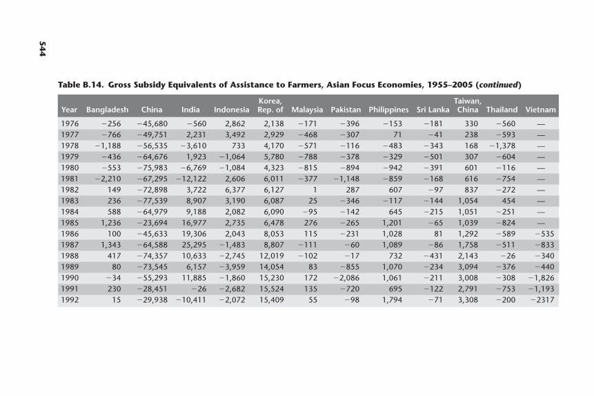
544
Table B.14. Gross Subsidy Equivalents of Assistance to Farmers, Asian Focus Economies, 1955–2005 (continued)
Korea, Taiwan,Year Bangladesh China India Indonesia Rep. of Malaysia Pakistan Philippines Sri Lanka China Thailand Vietnam
1976 �256 �45,680 �560 2,862 2,138 �171 �396 �153 �181 330 �560 —1977 �766 �49,751 2,231 3,492 2,929 �468 �307 71 �41 238 �593 —1978 �1,188 �56,535 �3,610 733 4,170 �571 �116 �483 �343 168 �1,378 —1979 �436 �64,676 1,923 �1,064 5,780 �788 �378 �329 �501 307 �604 —1980 �553 �75,983 �6,769 �1,084 4,323 �815 �894 �942 �391 601 �116 —1981 �2,210 �67,295 �12,122 2,606 6,011 �377 �1,148 �859 �168 616 �754 —1982 149 �72,898 3,722 6,377 6,127 1 287 607 �97 837 �272 —1983 236 �77,539 8,907 3,190 6,087 25 �346 �117 �144 1,054 454 —1984 588 �64,979 9,188 2,082 6,090 �95 �142 645 �215 1,051 �251 —1985 1,236 �23,694 16,977 2,735 6,478 276 �265 1,201 �65 1,039 �824 —1986 100 �45,633 19,306 2,043 8,053 115 �231 1,028 81 1,292 �589 �5351987 1,343 �64,588 25,295 �1,483 8,807 �111 �60 1,089 �86 1,758 �511 �8331988 417 �74,357 10,633 �2,745 12,019 �102 �17 732 �431 2,143 �26 �3401989 80 �73,545 6,157 �3,959 14,054 83 �855 1,070 �234 3,094 �376 �4401990 �34 �55,293 11,885 �1,860 15,230 172 �2,086 1,061 �211 3,008 �308 �1,8261991 230 �28,451 �26 �2,682 15,524 135 �720 695 �122 2,791 �753 �1,1931992 15 �29,938 �10,411 �2,072 15,409 55 �98 1,794 �71 3,308 �200 �2317
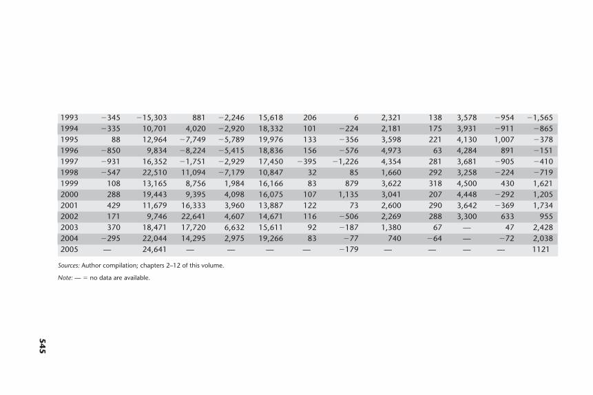
545
1993 �345 �15,303 881 �2,246 15,618 206 6 2,321 138 3,578 �954 �1,5651994 �335 10,701 4,020 �2,920 18,332 101 �224 2,181 175 3,931 �911 �8651995 88 12,964 �7,749 �5,789 19,976 133 �356 3,598 221 4,130 1,007 �3781996 �850 9,834 �8,224 �5,415 18,836 156 �576 4,973 63 4,284 891 �1511997 �931 16,352 �1,751 �2,929 17,450 �395 �1,226 4,354 281 3,681 �905 �4101998 �547 22,510 11,094 �7,179 10,847 32 85 1,660 292 3,258 �224 �7191999 108 13,165 8,756 1,984 16,166 83 879 3,622 318 4,500 430 1,6212000 288 19,443 9,395 4,098 16,075 107 1,135 3,041 207 4,448 �292 1,2052001 429 11,679 16,333 3,960 13,887 122 73 2,600 290 3,642 �369 1,7342002 171 9,746 22,641 4,607 14,671 116 �506 2,269 288 3,300 633 9552003 370 18,471 17,720 6,632 15,611 92 �187 1,380 67 — 47 2,4282004 �295 22,044 14,295 2,975 19,266 83 �77 740 �64 — �72 2,0382005 — 24,641 — — — — �179 — — — — 1121
Sources: Author compilation; chapters 2–12 of this volume.
Note: — � no data are available.
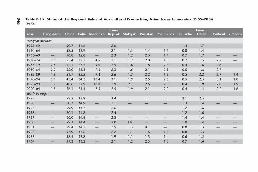
546 Table B.15. Share of the Regional Value of Agricultural Production, Asian Focus Economies, 1955–2004
(percent)
Korea, Taiwan,Year Bangladesh China India Indonesia Rep. of Malaysia Pakistan Philippines Sri Lanka China Thailand Vietnam
Five-year average1955–59 — 59.7 34.6 — 2.6 — — — 1.4 1.7 — —1960–64 — 58.5 33.9 — 2.1 1.3 1.4 1.5 0.8 1.4 — —1965–69 — 56.8 32.8 — 2.3 1.2 2.6 1.9 0.7 1.7 — —1970–74 2.0 55.4 27.7 4.5 2.1 1.2 2.0 1.8 0.7 1.5 2.7 —1975–79 2.4 52.1 23.5 9.0 2.5 1.6 1.8 2.3 0.4 1.6 2.8 —1980–84 2.0 52.0 23.3 9.6 2.3 1.6 2.1 2.1 0.5 1.8 2.7 —1985–89 1.9 51.7 22.2 9.4 2.6 1.7 2.2 1.9 0.5 2.2 2.7 1.41990–94 2.1 45.4 24.3 10.4 3.1 1.9 2.5 2.5 0.5 2.5 3.1 1.81995–99 1.7 48.6 22.9 10.0 2.9 2.1 2.5 2.3 0.4 1.9 2.8 1.92000–04 1.5 56.1 21.4 7.5 2.5 1.9 2.1 2.0 0.4 1.4 2.2 1.6Yearly average1955 — 58.2 33.8 — 3.4 — — — 2.1 2.5 — —1956 — 60.3 34.9 — 2.1 — — — 1.3 1.4 — —1957 — 59.9 34.7 — 2.6 — — — 1.2 1.6 — —1958 — 60.1 34.8 — 2.4 — — — 1.2 1.6 — —1959 — 60.0 34.8 — 2.3 — — — 1.4 1.4 — —1960 — 59.3 34.4 — 2.0 1.8 — — 1.0 1.4 — —1961 — 59.4 34.5 — 2.5 1.3 0.1 — 0.8 1.3 — —1962 — 57.9 33.6 — 2.2 1.1 1.6 1.6 0.8 1.3 — —1963 — 58.4 33.8 — 1.9 1.1 1.5 1.4 0.6 1.2 — —1964 — 57.3 33.2 — 2.1 1.2 2.3 1.6 0.7 1.6 — —
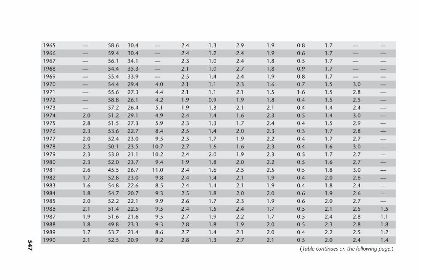
547
1965 — 58.6 30.4 — 2.4 1.3 2.9 1.9 0.8 1.7 — —1966 — 59.4 30.4 — 2.4 1.2 2.4 1.9 0.6 1.7 — —1967 — 56.1 34.1 — 2.3 1.0 2.4 1.8 0.5 1.7 — —1968 — 54.4 35.3 — 2.1 1.0 2.7 1.8 0.9 1.7 — —1969 — 55.4 33.9 — 2.5 1.4 2.4 1.9 0.8 1.7 — —1970 — 54.4 29.4 4.0 2.1 1.1 2.3 1.6 0.7 1.5 3.0 —1971 — 55.6 27.3 4.4 2.1 1.1 2.1 1.5 1.6 1.5 2.8 —1972 — 58.8 26.1 4.2 1.9 0.9 1.9 1.8 0.4 1.5 2.5 —1973 — 57.2 26.4 5.1 1.9 1.3 2.1 2.1 0.4 1.4 2.4 —1974 2.0 51.2 29.1 4.9 2.4 1.4 1.6 2.3 0.5 1.4 3.0 —1975 2.8 51.5 27.3 5.9 2.3 1.3 1.7 2.4 0.4 1.5 2.9 —1976 2.3 53.6 22.7 8.4 2.5 1.4 2.0 2.3 0.3 1.7 2.8 —1977 2.0 52.4 23.0 9.5 2.5 1.7 1.9 2.2 0.4 1.7 2.7 —1978 2.5 50.1 23.5 10.7 2.7 1.6 1.6 2.3 0.4 1.6 3.0 —1979 2.3 53.0 21.1 10.2 2.4 2.0 1.9 2.3 0.5 1.7 2.7 —1980 2.3 52.0 23.7 9.4 1.9 1.8 2.0 2.2 0.5 1.6 2.7 —1981 2.6 45.5 26.7 11.0 2.4 1.6 2.5 2.5 0.5 1.8 3.0 —1982 1.7 52.8 23.0 9.8 2.4 1.4 2.1 1.9 0.4 2.0 2.6 —1983 1.6 54.8 22.6 8.5 2.4 1.4 2.1 1.9 0.4 1.8 2.4 —1984 1.8 54.7 20.7 9.3 2.5 1.8 2.0 2.0 0.6 1.9 2.6 —1985 2.0 52.2 22.1 9.9 2.6 1.7 2.3 1.9 0.6 2.0 2.7 —1986 2.1 51.4 22.5 9.5 2.4 1.5 2.4 1.7 0.5 2.1 2.5 1.51987 1.9 51.6 21.6 9.5 2.7 1.9 2.2 1.7 0.5 2.4 2.8 1.11988 1.8 49.8 23.3 9.3 2.8 1.8 1.9 2.0 0.5 2.3 2.8 1.81989 1.7 53.7 21.4 8.6 2.7 1.4 2.1 2.0 0.4 2.2 2.5 1.21990 2.1 52.5 20.9 9.2 2.8 1.3 2.7 2.1 0.5 2.0 2.4 1.4
(Table continues on the following page.)

548
1991 2.2 46.6 23.9 10.1 3.2 1.5 2.3 2.5 0.5 2.5 3.2 1.61992 2.2 44.9 25.3 9.2 3.3 1.8 2.5 2.5 0.5 2.7 3.2 2.01993 2.1 41.1 25.8 11.7 3.3 2.1 2.6 2.5 0.5 2.9 3.2 2.11994 1.7 41.7 25.4 11.8 3.1 2.5 2.3 2.9 0.5 2.6 3.5 1.91995 1.6 44.9 23.0 11.9 3.1 2.5 2.4 2.5 0.4 2.3 3.3 1.91996 1.8 45.3 23.9 11.4 3.4 2.0 2.6 2.4 0.4 2.1 2.9 1.81997 1.7 48.7 22.1 10.8 3.0 1.7 2.7 2.4 0.4 1.8 2.8 1.91998 1.6 52.2 22.3 7.4 2.5 2.3 2.6 2.2 0.4 1.6 2.7 2.11999 1.7 51.9 23.1 8.6 2.5 2.0 2.2 2.2 0.4 1.5 2.3 1.62000 1.7 53.8 22.8 7.3 3.0 1.5 2.1 2.0 0.4 1.5 2.2 1.82001 1.5 57.4 21.5 6.3 2.6 1.5 2.1 1.8 0.3 1.3 2.1 1.62002 1.4 57.6 18.5 8.3 2.5 2.0 2.1 2.0 0.4 1.3 2.2 1.82003 1.6 53.6 22.3 9.5 2.3 2.4 2.2 2.0 0.4 — 2.3 1.52004 1.4 58.0 21.7 6.3 2.2 2.2 2.2 2.2 0.3 — 2.0 1.5
Sources: Author compilation; chapters 2–12 of this volume.
Note: — � no data are available.
Table B.15. Share of the Regional Value of Agricultural Production, Asian Focus Economies, 1955–2004 (continued)
Korea, Taiwan,Year Bangladesh China India Indonesia Rep. of Malaysia Pakistan Philippines Sri Lanka China Thailand Vietnam
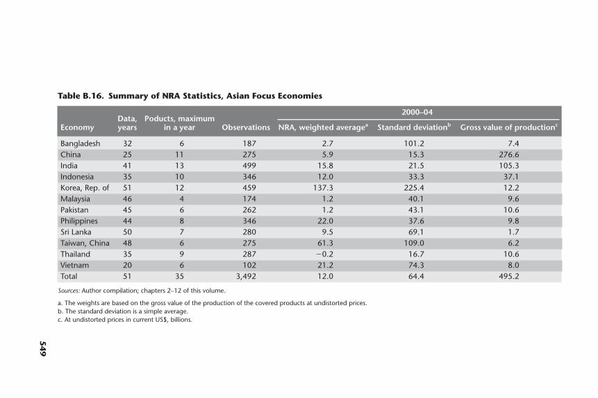
549
Table B.16. Summary of NRA Statistics, Asian Focus Economies
Data, Poducts, maximum2000–04
Economy years in a year Observations NRA, weighted averagea Standard deviationb Gross value of productionc
Bangladesh 32 6 187 2.7 101.2 7.4China 25 11 275 5.9 15.3 276.6India 41 13 499 15.8 21.5 105.3Indonesia 35 10 346 12.0 33.3 37.1Korea, Rep. of 51 12 459 137.3 225.4 12.2Malaysia 46 4 174 1.2 40.1 9.6Pakistan 45 6 262 1.2 43.1 10.6Philippines 44 8 346 22.0 37.6 9.8Sri Lanka 50 7 280 9.5 69.1 1.7Taiwan, China 48 6 275 61.3 109.0 6.2Thailand 35 9 287 �0.2 16.7 10.6Vietnam 20 6 102 21.2 74.3 8.0Total 51 35 3,492 12.0 64.4 495.2
Sources: Author compilation; chapters 2–12 of this volume.
a. The weights are based on the gross value of the production of the covered products at undistorted prices.b. The standard deviation is a simple average.c. At undistorted prices in current US$, billions.
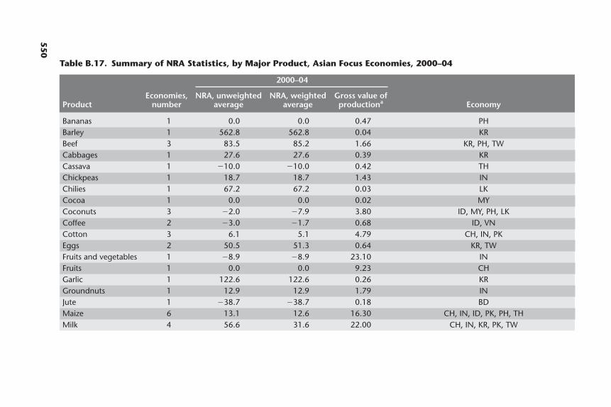
550
Table B.17. Summary of NRA Statistics, by Major Product, Asian Focus Economies, 2000–04
2000–04
Economies, NRA, unweighted NRA, weighted Gross value ofProduct number average average productiona Economy
Bananas 1 0.0 0.0 0.47 PHBarley 1 562.8 562.8 0.04 KRBeef 3 83.5 85.2 1.66 KR, PH, TWCabbages 1 27.6 27.6 0.39 KRCassava 1 �10.0 �10.0 0.42 THChickpeas 1 18.7 18.7 1.43 INChilies 1 67.2 67.2 0.03 LKCocoa 1 0.0 0.0 0.02 MYCoconuts 3 �2.0 �7.9 3.80 ID, MY, PH, LKCoffee 2 �3.0 �1.7 0.68 ID, VNCotton 3 6.1 5.1 4.79 CH, IN, PKEggs 2 50.5 51.3 0.64 KR, TWFruits and vegetables 1 �8.9 �8.9 23.10 INFruits 1 0.0 0.0 9.23 CHGarlic 1 122.6 122.6 0.26 KRGroundnuts 1 12.9 12.9 1.79 INJute 1 �38.7 �38.7 0.18 BDMaize 6 13.1 12.6 16.30 CH, IN, ID, PK, PH, THMilk 4 56.6 31.6 22.00 CH, IN, KR, PK, TW
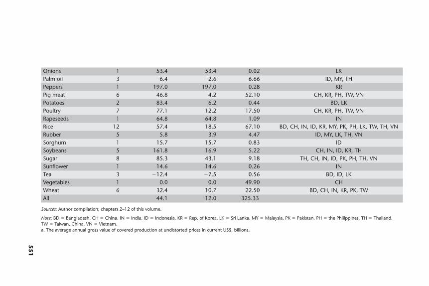
551
Onions 1 53.4 53.4 0.02 LKPalm oil 3 �6.4 �2.6 6.66 ID, MY, THPeppers 1 197.0 197.0 0.28 KRPig meat 6 46.8 4.2 52.10 CH, KR, PH, TW, VNPotatoes 2 83.4 6.2 0.44 BD, LKPoultry 7 77.1 12.2 17.50 CH, KR, PH, TW, VNRapeseeds 1 64.8 64.8 1.09 INRice 12 57.4 18.5 67.10 BD, CH, IN, ID, KR, MY, PK, PH, LK, TW, TH, VNRubber 5 5.8 3.9 4.47 ID, MY, LK, TH, VNSorghum 1 15.7 15.7 0.83 IDSoybeans 5 161.8 16.9 5.22 CH, IN, ID, KR, THSugar 8 85.3 43.1 9.18 TH, CH, IN, ID, PK, PH, TH, VNSunflower 1 14.6 14.6 0.26 INTea 3 �12.4 �7.5 0.56 BD, ID, LKVegetables 1 0.0 0.0 49.90 CHWheat 6 32.4 10.7 22.50 BD, CH, IN, KR, PK, TWAll 44.1 12.0 325.33
Sources: Author compilation; chapters 2–12 of this volume.
Note: BD � Bangladesh. CH � China. IN � India. ID � Indonesia. KR � Rep. of Korea. LK � Sri Lanka. MY � Malaysia. PK � Pakistan. PH � the Philippines. TH � Thailand.TW � Taiwan, China. VN � Vietnam.a. The average annual gross value of covered production at undistorted prices in current US$, billions.
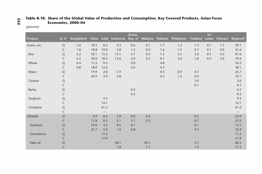
552
Table B.18. Share of the Global Value of Production and Consumption, Key Covered Products, Asian FocusEconomies, 2000–04
(percent)
Korea, SriProduct Q, Ca Bangladesh China India Indonesia Rep. of Malaysia Pakistan Philippines Thailand Lanka Vietnam Regionalb
Grains, etc. Q 1.6 18.5 8.2 4.3 0.6 0.1 1.7 1.2 1.4 0.1 1.3 39.1C 1.8 18.8 10.0 4.8 1.2 0.2 1.6 1.4 0.7 0.1 0.9 41.6
Rice Q 5.2 32.1 15.2 13.1 2.1 0.3 1.2 3.5 3.6 0.5 4.2 81.0C 5.2 30.0 18.3 13.6 2.0 0.7 0.7 3.6 1.8 0.5 3.0 79.4
Wheat Q 0.4 17.5 9.5 0.0 4.8 32.2C 0.8 18.0 12.6 2.0 4.7 38.1
Maize Q 19.9 2.0 1.9 0.3 0.9 0.7 25.7C 24.9 2.9 2.8 0.5 1.2 0.9 33.1
Cassava Q 2.0 2.0C 0.1 0.1
Barley Q 0.2 0.2C 0.5 0.5
Sorghum Q 9.5 9.5C 14.1 14.1
Chickpeas Q 61.2 61.2C — —
Oilseeds Q 4.9 6.5 3.8 0.0 6.3 0.5 22.0C 11.8 8.5 2.1 3.7 0.3 0.7 27.0
Soybeans Q 10.0 4.2 0.6 0.1 0.1 15.1C 21.7 5.0 1.6 6.8 0.7 35.9
Groundnuts Q 17.2 17.2C 17.9 17.9
Palm oil Q 28.1 49.3 3.1 80.5C 7.8 1.7 1.9 11.5
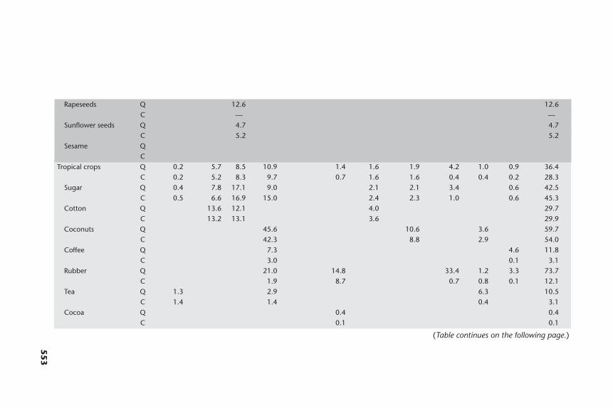
553
Rapeseeds Q 12.6 12.6C — —
Sunflower seeds Q 4.7 4.7C 5.2 5.2
Sesame QC
Tropical crops Q 0.2 5.7 8.5 10.9 1.4 1.6 1.9 4.2 1.0 0.9 36.4C 0.2 5.2 8.3 9.7 0.7 1.6 1.6 0.4 0.4 0.2 28.3
Sugar Q 0.4 7.8 17.1 9.0 2.1 2.1 3.4 0.6 42.5C 0.5 6.6 16.9 15.0 2.4 2.3 1.0 0.6 45.3
Cotton Q 13.6 12.1 4.0 29.7C 13.2 13.1 3.6 29.9
Coconuts Q 45.6 10.6 3.6 59.7C 42.3 8.8 2.9 54.0
Coffee Q 7.3 4.6 11.8C 3.0 0.1 3.1
Rubber Q 21.0 14.8 33.4 1.2 3.3 73.7C 1.9 8.7 0.7 0.8 0.1 12.1
Tea Q 1.3 2.9 6.3 10.5C 1.4 1.4 0.4 3.1
Cocoa Q 0.4 0.4C 0.1 0.1
(Table continues on the following page.)
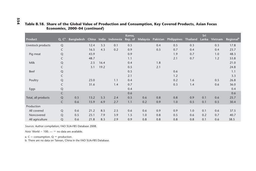
554
Livestock products Q 12.4 3.3 0.1 0.5 0.4 0.5 0.3 0.3 17.8C 16.5 4.3 0.2 0.9 0.5 0.7 0.4 0.4 23.7
Pig meat Q 43.9 0.9 1.9 0.7 1.0 48.3C 48.7 1.1 2.1 0.7 1.2 53.8
Milk Q 2.5 16.4 0.4 1.8 21.0C 3.1 19.2 0.5 2.1 24.8
Beef Q 0.5 0.6 1.1C 2.1 1.2 3.3
Poultry Q 23.0 1.1 0.4 0.2 1.6 0.5 26.8C 31.6 1.4 0.7 0.3 1.4 0.6 36.0
Eggs Q 0.4 0.4C 0.6 0.6
Total, all products Q 0.5 13.2 5.3 2.4 0.5 0.6 0.8 0.8 0.9 0.1 0.6 25.7C 0.6 15.9 6.9 2.7 1.1 0.2 0.9 1.0 0.5 0.1 0.5 30.4
ProductionAll covered Q 0.6 21.2 8.5 2.5 0.6 0.6 0.9 0.9 1.0 0.1 0.6 37.5Noncovered Q 0.5 23.1 7.9 3.9 1.5 1.0 0.8 0.5 0.6 0.2 0.7 40.7All agriculture Q 0.6 21.8 8.3 2.9 0.9 0.8 0.8 0.8 0.8 0.1 0.6 38.5
Sources: Author compilation; FAO SUA-FBS Database 2008.
Note: World � 100. — � no data are available.
a. C � consumption. Q � production.b. There are no data on Taiwan, China in the FAO SUA-FBS Database.
Table B.18. Share of the Global Value of Production and Consumption, Key Covered Products, Asian FocusEconomies, 2000–04 (continued)
Korea, SriProduct Q, Ca Bangladesh China India Indonesia Rep. of Malaysia Pakistan Philippines Thailand Lanka Vietnam Regionalb
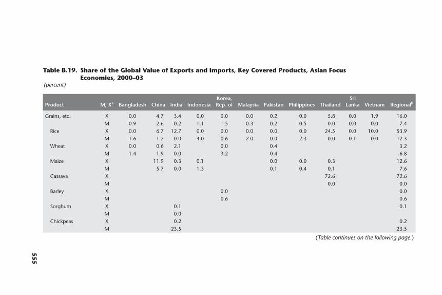
555
Table B.19. Share of the Global Value of Exports and Imports, Key Covered Products, Asian FocusEconomies, 2000–03
(percent)
Korea, SriProduct M, Xa Bangladesh China India Indonesia Rep. of Malaysia Pakistan Philippines Thailand Lanka Vietnam Regionalb
Grains, etc. X 0.0 4.7 3.4 0.0 0.0 0.0 0.2 0.0 5.8 0.0 1.9 16.0M 0.9 2.6 0.2 1.1 1.5 0.3 0.2 0.5 0.0 0.0 0.0 7.4
Rice X 0.0 6.7 12.7 0.0 0.0 0.0 0.0 0.0 24.5 0.0 10.0 53.9M 1.6 1.7 0.0 4.0 0.6 2.0 0.0 2.3 0.0 0.1 0.0 12.3
Wheat X 0.0 0.6 2.1 0.0 0.4 3.2M 1.4 1.9 0.0 3.2 0.4 6.8
Maize X 11.9 0.3 0.1 0.0 0.0 0.3 12.6M 5.7 0.0 1.3 0.1 0.4 0.1 7.6
Cassava X 72.6 72.6M 0.0 0.0
Barley X 0.0 0.0M 0.6 0.6
Sorghum X 0.1 0.1M 0.0
Chickpeas X 0.2 0.2M 23.5 23.5
(Table continues on the following page.)
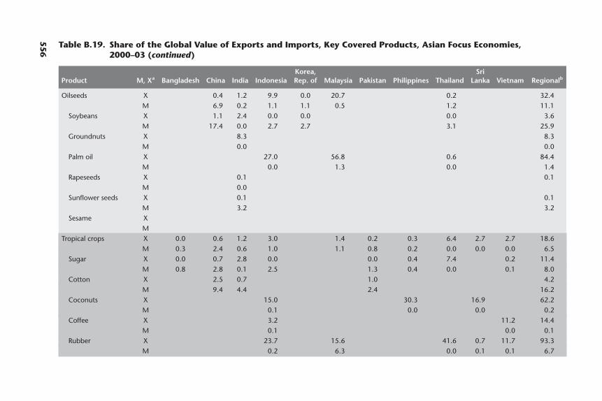
556 Table B.19. Share of the Global Value of Exports and Imports, Key Covered Products, Asian Focus Economies,
2000–03 (continued)
Korea, SriProduct M, Xa Bangladesh China India Indonesia Rep. of Malaysia Pakistan Philippines Thailand Lanka Vietnam Regionalb
Oilseeds X 0.4 1.2 9.9 0.0 20.7 0.2 32.4M 6.9 0.2 1.1 1.1 0.5 1.2 11.1
Soybeans X 1.1 2.4 0.0 0.0 0.0 3.6M 17.4 0.0 2.7 2.7 3.1 25.9
Groundnuts X 8.3 8.3M 0.0 0.0
Palm oil X 27.0 56.8 0.6 84.4M 0.0 1.3 0.0 1.4
Rapeseeds X 0.1 0.1M 0.0
Sunflower seeds X 0.1 0.1M 3.2 3.2
Sesame XM
Tropical crops X 0.0 0.6 1.2 3.0 1.4 0.2 0.3 6.4 2.7 2.7 18.6M 0.3 2.4 0.6 1.0 1.1 0.8 0.2 0.0 0.0 0.0 6.5
Sugar X 0.0 0.7 2.8 0.0 0.0 0.4 7.4 0.2 11.4M 0.8 2.8 0.1 2.5 1.3 0.4 0.0 0.1 8.0
Cotton X 2.5 0.7 1.0 4.2M 9.4 4.4 2.4 16.2
Coconuts X 15.0 30.3 16.9 62.2M 0.1 0.0 0.0 0.2
Coffee X 3.2 11.2 14.4M 0.1 0.0 0.1
Rubber X 23.7 15.6 41.6 0.7 11.7 93.3M 0.2 6.3 0.0 0.1 0.1 6.7
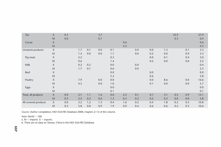
557
Tea X 0.3 3.7 23.9 27.9M 0.0 0.1 0.3 0.4
Cocoa X 0.6 0.6M 4.3 4.3
Livestock products X 1.7 0.1 0.0 0.1 0.0 0.0 1.3 0.1 3.3M 1.4 0.0 0.0 1.7 0.0 0.2 0.0 0.0 3.3
Pig meat X 2.2 0.3 0.0 0.1 0.4 3.0M 0.6 1.4 0.2 0.0 0.0 2.2
Milk X 0.2 0.2 0.0 0.0 0.4M 1.7 0.1 0.6 0.0 2.3
Beef X 0.0 0.0 0.0M 5.2 0.6 5.8
Poultry X 7.9 0.0 0.0 0.0 8.6 0.0 16.6M 4.5 0.0 1.0 0.1 0.0 0.0 5.7
Eggs X 0.0 0.0M 0.1 0.1
Total, all products X 0.0 2.1 1.1 1.6 0.0 2.5 0.1 0.1 3.1 0.5 0.9 12.1M 0.3 2.5 0.2 0.6 1.3 0.3 0.2 0.2 0.2 0.0 0.0 5.8
All covered products X 0.0 3.2 1.2 1.3 0.4 1.6 0.2 0.4 1.8 0.2 0.5 10.8M 0.3 3.8 0.8 0.9 1.9 0.9 0.4 0.6 0.6 0.2 0.3 10.6
Sources: Author compilation; FAO SUA-FBS Database 2008; chapters 2–12 of this volume.
Note: World � 100.a. M � imports. X � exports.b. There are no data on Taiwan, China in the FAO SUA-FBS Database.
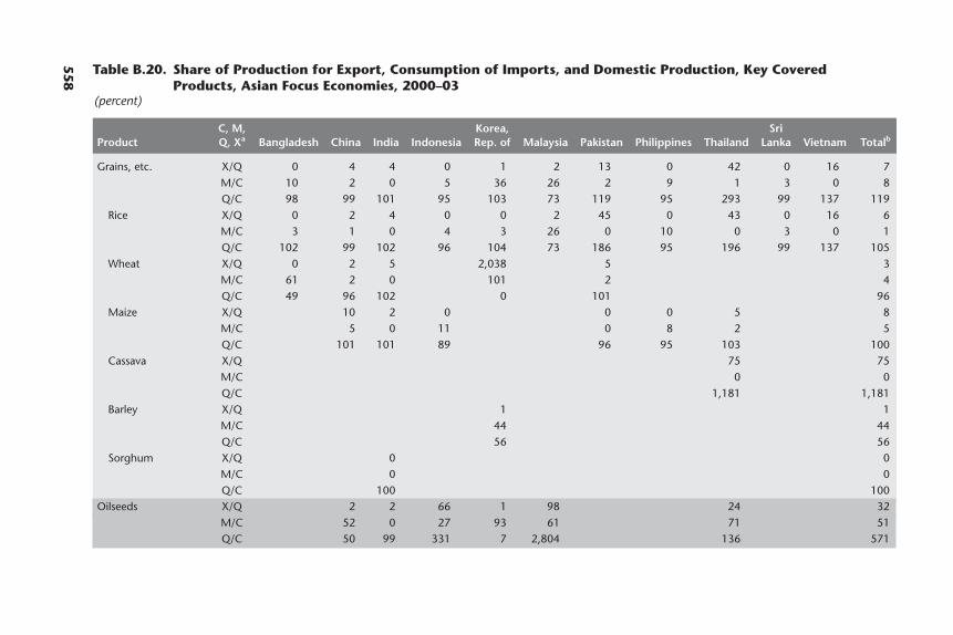
Table B.20. Share of Production for Export, Consumption of Imports, and Domestic Production, Key CoveredProducts, Asian Focus Economies, 2000–03
(percent)
C, M, Korea, SriProduct Q, Xa Bangladesh China India Indonesia Rep. of Malaysia Pakistan Philippines Thailand Lanka Vietnam Totalb
Grains, etc. X/Q 0 4 4 0 1 2 13 0 42 0 16 7M/C 10 2 0 5 36 26 2 9 1 3 0 8Q/C 98 99 101 95 103 73 119 95 293 99 137 119
Rice X/Q 0 2 4 0 0 2 45 0 43 0 16 6M/C 3 1 0 4 3 26 0 10 0 3 0 1Q/C 102 99 102 96 104 73 186 95 196 99 137 105
Wheat X/Q 0 2 5 2,038 5 3M/C 61 2 0 101 2 4Q/C 49 96 102 0 101 96
Maize X/Q 10 2 0 0 0 5 8M/C 5 0 11 0 8 2 5Q/C 101 101 89 96 95 103 100
Cassava X/Q 75 75M/C 0 0Q/C 1,181 1,181
Barley X/Q 1 1M/C 44 44Q/C 56 56
Sorghum X/Q 0 0M/C 0 0Q/C 100 100
Oilseeds X/Q 2 2 66 1 98 24 32M/C 52 0 27 93 61 71 51Q/C 50 99 331 7 2,804 136 571
558
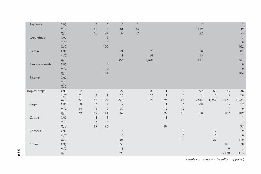
Soybeans X/Q 2 2 0 1 2 2M/C 52 0 61 93 119 49Q/C 50 94 39 7 22 53
Groundnuts X/Q 3 3M/C 0 0Q/C 102 102
Palm oil X/Q 71 98 28 85M/C 1 61 13 11Q/C 355 2,804 157 661
Sunflower seeds X/Q 0 0M/C 0 0Q/C 104 104
Sesame X/QM/CQ/C
Tropical crops X/Q 7 3 3 22 105 1 9 92 63 75 38M/C 21 9 2 18 110 7 6 1 5 5 18Q/C 97 97 107 270 192 96 107 3,855 1,250 4,171 1,024
Sugar X/Q 0 6 4 2 1 6 68 5 12M/C 34 16 0 39 12 12 1 4 9Q/C 79 97 111 62 92 93 328 102 109
Cotton X/Q 1 1 1 1M/C 4 5 3 4Q/C 97 96 99 97
Coconuts X/Q 5 12 17 9M/C 0 0 2 0Q/C 106 114 120 110
Coffee X/Q 50 101 78M/C 3 0 3Q/C 196 5,130 413
559
(Table continues on the following page.)
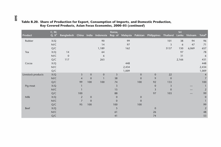
Rubber X/Q 90 99 101 38 94 96M/C 14 97 3 6 47 71Q/C 1,189 162 5137 150 6,069 657
Tea X/Q 14 64 97 78M/C 0 6 31 6Q/C 117 263 2,166 431
Cocoa X/Q 448 448M/C 2,434 2,434Q/C 1,009 1,009
Livestock products X/Q 3 0 0 3 0 0 22 4M/C 4 0 1 38 0 9 0 7Q/C 99 100 100 74 100 92 133 100
Pig meat X/Q 1 3 0 3 — 1M/C 1 15 3 0 — 2Q/C 100 88 97 103 — 99
Milk X/Q 2 0 0 0 0M/C 7 0 0 0 1Q/C 95 100 100 100 99
Beef X/Q 5 0 2M/C 61 26 48Q/C 41 74 53
560
Table B.20. Share of Production for Export, Consumption of Imports, and Domestic Production,Key Covered Products, Asian Focus Economies, 2000–03 (continued)
C, M, Korea, SriProduct Q, Xa Bangladesh China India Indonesia Rep. of Malaysia Pakistan Philippines Thailand Lanka Vietnam Totalb

Poultry X/Q 9 0 1 0 35 — 10M/C 12 1 18 3 0 — 11Q/C 96 100 83 97 153 — 99
Eggs X/Q 0 0M/C 1 1Q/C 99 99
Total, all products X/Q 0 3 2 15 2 94 8 2 51 42 25 22M/C 10 6 0 10 40 63 2 9 7 4 0 14
Q/C 98 97 101 181 84 2,256 111 96 1,234 867 762 535
Sources: Author compilation; FAO SUA-FBS Database 2008.
Note: — � no data are available.a. C � consumption. M � imports. Q � production. X � exports.b. There are no data on Taiwan, China in the FAO SUA-FBS Database.
561
References
Ahmed, N., Z. Bakht, P. A. Dorosh, and Q. Shahabuddin. 2007. “Distortions to Agricultural Incentivesin Bangladesh.” Agricultural Distortions Working Paper 32, World Bank, Washington, DC.
Anderson, K., M. Kurzweil, W. Martin, D. Sandri, and E. Valenzuela. 2008. “Measuring Distortions toAgricultural Incentives, Revisited.” World Trade Review 7 (4): 675–704.
Athukorala, P.-C., P. L. Huong, and V. T. Thanh. 2007. “Distortions to Agricultural Incentives in Vietnam.” Agricultural Distortions Working Paper 26, World Bank, Washington, DC.
Athukorala, P.-C., and W.-H. Loke. 2007. “Distortions to Agricultural Incentives in Malaysia.” Agricultural Distortions Working Paper 27, World Bank, Washington, DC.
Bandara, J., and S. Jayasuriya. 2007. “Distortions to Agricultural Incentives in Sri Lanka.” AgriculturalDistortions Working Paper 31, World Bank, Washington, DC.
David, C. C., P. Intal, and A. M. Balisacan. 2007. “Distortions to Agricultural Incentives in the Philippines.” Agricultural Distortions Working Paper 28, World Bank, Washington, DC.
Dorosh, P. A., and A. Salam. 2007. “Distortions to Agricultural Incentives in Pakistan.” AgriculturalDistortions Working Paper 33, World Bank, Washington, DC.
Fane, G., and P. Warr. 2007. “Distortions to Agricultural Incentives in Indonesia.” Agricultural Distortions Working Paper 24, World Bank, Washington, DC.
FAO SUA-FBS Database (Supply Utilization Accounts and Food Balance Sheets Database, FAOSTAT).Food and Agriculture Organization of the United Nations. http://faostat.fao.org/site/354/default.aspx (accessed May 2008).
Honma, M., and Y. Hayami. 2007. “Distortions to Agricultural Incentives in Korea and Taiwan.” Agricultural Distortions Working Paper 30, World Bank, Washington, DC.
Huang, J., S. Rozelle, W. Martin, and Y. Liu. 2007. “Distortions to Agricultural Incentives in China.”Agricultural Distortions Working Paper 29, World Bank, Washington, DC.
Pursell, G., A. Gulati, and K. Gupta. 2007. “Distortions to Agricultural Incentives in India.” AgriculturalDistortions Working Paper 34, World Bank, Washington, DC.
Warr, P. G., and A. Kohpaiboon. 2007. “Distortions to Agricultural Incentives in Thailand.” Agricultural Distortions Working Paper 25, World Bank, Washington, DC.
562 Distortions to Agricultural Incentives in Asia

AAfrica, rates of assistance
in, 52–55Agency for International
Development, 331Agricultural land per capita
Asian economies, 5–7international comparison, 7
Asia. See Economies of Asia;specific country
Association of Southeast AsianNations, 237
BBangladesh
agricultural inputs, 324–325,331, 333
agricultural NRAs, 315–326,513–515t
calculation of rates ofassistance, 314–315
economic growth, 306exchange rates, 309–310exchange rates and markets,
311–312foreign aid, 308–309, 320,
322, 330future prospects, 333illegal imports, 308importance of agricultural
sector, 307income patterns, 306industrial sector, 306labor market, 306–307
563
Index
liberalization of trade andagricultural policies,305–306, 311–312, 318,324, 332–333
nonagricultural NRAs, 326,327t, 328f, 514–515t
noncovered agriculturalproducts, 325–326
political economy, 328–330,331–332
population growth, 307pricing reforms, 330–332protectionist policies of
1970s, 305, 309–311regional trade agreements,
349, 374 n.8RRAs, 326–328, 514–515tshare of regional value of
agricultural production,546–548t
sources of NRA variation, 325structure of agricultural
sector, 306–307trade flows, 307–309value shares of primary
production, 516tSee also Economies of Asia
Black market exchange rate,446, 461
CCassava, Thailand’s production
and policies, 260, 263,273–275, 275
Chinaagricultural NRAs, 137–138,
145–154, 155–156,487t, 488t
agricultural productivity,129, 132
agricultural technologydevelopment, 123,133–134
commodity differences inrates of assistance,145, 149
comparison of agriculturaldistortion studies,151–154
economic data, 117, 142–143employment patterns,
121, 127exchange rates, 118, 138–142export subsidies, 118–119, 157gross domestic product,
125, 127growth of agricultural
assistance, 135–136,156–157
income patterns, 120–121,129–130
lessons from policy interven-tions in, 117–119, 130
manufacturing exports, 9measurement of distortions
in, 136–143, 154–155nonagricultural NRAs,
155, 488t
Figures, notes, and tables are indicated by f, n, and t, respectively.
China (continued)price policies, 122, 131–132property rights reforms, 132regional trade agreements,
237–238regulatory environment,
128–129RRAs, 47–52, 155–156, 488tshare of regional value of
agricultural production,546–548t
socialist era economicpolicies and performance,119–124
structure of agriculturaleconomy, 125–127,130, 142
tax policies, 121, 156trade policies, 118–119,
127–128, 134–135,147–149
transition to marketeconomy, 118, 124–127,131, 157
value shares of primaryproduction, 489t
water regulation, 123, 134See also Economies of Asia;
Taiwan, ChinaCocoa, Malaysia’s production
and policies, 198, 202, 213Coconut products
Philippines, 228, 234–235,236, 241
Sri Lanka, 415, 424–425, 430Coffee
Indonesia’s productionand policies, 180, 188,189, 190
Vietnam’s production andpolicies, 285, 296–297
Commodity differences, agri-cultural NRAs in Asia, 29f,30–31f, 44, 45t, 533–537t,540–542t
Comparative advantageAsian economies, 5, 7, 18tfuture prospects in Asia, 74Philippines, 229–230protection effects on,
109–110, 111rates of assistance and, 57t,
59–60frelative per capita income
and, 55, 57tshift from agriculture to
industry in Korea andTaiwan, China, 109–110
Consumer support estimates,consumer tax equivalentsand, 23
Consumer tax equivalentagricultural policy
linkage, 74application, 22calculation, 22–23, 138,
443, 460China, 151consumer support estimate
and, 23general equilibrium
modeling, 465 n.3,467 n.15
nominal rates of assistanceand, 17–22, 57–59, 460–461
patterns and trends, 55–60,62–68t, 74
U.S. dollar equivalent, 26Copra, Indonesia’s production
and policies, 180Cotton
Bangladesh’s imports, 309China’s policies and
outcomes, 148China’s production and
policies, 147, 148, 152–153India’s imports, 353Pakistan’s production and
policies, 380, 382,391–393, 402, 403
DDistortions, generally
data sources for Asianeconomies, 5
definition, 79 n.8, 442economic significance, 3estimates for nonfarm
tradables, 44, 47flow-on consequences, 442future prospects in Asia,
74–78measurement methodology,
442–443measurement methodology
in China, 136–143measurement methodology
in Korea and Taiwan,China, 98
in nonagricultural sectors,442–443
nontradable products,447–448
policy bias in Asia, 3, 44policy switching in economic
development, 85, 86
postfarmgate costs, 449–450recent reform efforts and
outcomes, 71–74research goals, 3–4sources, 22, 183, 325, 379, 441See also Nominal rates of
assistance (NRAs);Relative rates of assistance(RRAs)
Doha Round, 4
EEast Asia
economic development, 86poverty patterns, 7See also Economies of Asia;
specific countryEconomic growth
Bangladesh, 306China’s transition from
socialist economy, 125, 126t
future prospects in Asia, 74India, 340Indonesia, 166–167Korea and Taiwan, China,
85, 86–91Malaysia, 199–201patterns and trends in
Asia, 8, 9Philippines, 223policy switching and,
9, 85, 86Sri Lanka, 411–412Thailand, 258
Economies of Asiaanti-agriculture policy bias,
3, 44. See also Trade biasindex
comparative advantage,5, 7, 18t
consumer tax equivalents,patterns and trends,55–60, 62–68t, 74
countries of interest, 4–5.See also specific country
data sources, 5distribution of value of
agricultural production,546–548t
economic significance ofagriculture, 3, 5
export patterns and trends,15–17
financial crisis of 1990s,105, 166, 167, 185, 208,211, 258
future prospects, 74–78
564 Index
global share of agriculture, 5growth, 8, 9international comparison of
rates of assistance, 52–55key characteristics, 5–7,
18–21ttnonagricultural NRAs,
538–539tNRA patterns and trends,
26–44, 533–539tper capita incomes, 5policy effects on domestic
food prices, 55, 60–71recent reforms and
outcomes, 71–74RRA patterns and trends,
47–52, 538–539tsectoral shares of GDP,
9–13, 14tself-sufficiency, 17, 21tshare of global value of
exports and imports,555–561t
share of global value ofproduction andconsumption, 552–554t
structural evolution, 8, 9–17summary of NRA statistics
by country, 549tsummary of NRA statistics
by product, 550–551ttransition to market-based
economies, 166U.S. dollar equivalents of
NRAs, 26, 37, 41–43tt,463–464, 543–546t
value shares of primaryproduction, 540–542t
Education, industrialdevelopment and, 88
EmploymentBangladesh, 306–307China, 121, 127global patterns, 3India, 340, 341tMalaysia, 199–200Pakistan, 380patterns and trends in Asia,
13–15Vietnam, 283
Exchange rateBangladesh, 309–310, 311black markets, 446, 461China, 118, 137, 138–142India, 345, 349–356, 358Malaysia, 211modeling methodology and
NRA calculations, 25, 79
n.12, 444–447, 454–455,461–462
multiple rate systems,446, 462
Pakistan, 382, 384, 401Philippines, 231Sri Lanka, 410, 416–417Vietnam, 294
ExportsAsian share of value and
production, 15, 19t,555–561t
Bangladesh, 307–308, 310China, 118, 128classification of products for
analysis, 457, 458–460economic growth and, 9India, 340, 342t, 343Indonesia, 169, 170, 172–173Korea, 104Malaysia, 204–206NRA patterns and trends
and, 31–37patterns and trends in Asia,
15–17Philippines, 223, 228,
229–230share of Asian gross
domestic product, 10t, 12tSri Lanka, 412, 414f,
423–425, 430Taiwan, China, 104Thailand, 255, 256, 262,
263–264, 266Vietnam, 287–288, 292–293See also Trade policy; Trade
specialization
FFertilizers. See Input subsidies
and distortionsFishery production
in Bangladesh, 306in China, 126–127in India, 340
Food and commodity pricesBangladesh, 316–319,
320–322, 330–331,332–333
China, 117–118, 122,131–132, 143–144,146, 157
econometric modeling offarm level outcomes ofmarket level interventions,186–189, 269–273
equilibrium, 443forecasts, 80 n.18
future of Indian economy,369–371, 372
future prospects for Asianeconomies, 77–78
home price scheme, 264–265India, 339, 343–344,
360, 363, 367–368,370–371, 373
Indonesia, 165, 173,175, 176
Korea, 93–95Malaysia, 197, 210Pakistan, 379, 386–390, 391,
393–395, 397, 402, 403Philippines, 230–238, 243,
249–250policy impacts, 55, 60–71, 74recent trends, 4research goals, 8RRAs in China and India
and, 47socialist era in China, 122Sri Lanka, 416, 424–425,
426–427, 432, 433, 434Thailand, 255, 263, 266Vietnam, 287–288, 291
Food processingIndia’s trade policies,
347–348Indonesia’s production and
policies, 179–180Malaysian exports, 205modeling of farm level
outcomes of market levelinterventions, 186–189,269–273
NRA calculations, 451–452,456–457
Philippines, 226Vietnam’s support for sugar
producers and, 300Foreign aid
to Bangladesh, 308–309, 320,322, 330
to Pakistan, 384Foreign investment
in Malaysia, 207in Vietnam, 281
Forestryin Bangladesh, 306in India, 340
FruitsChina’s production and
policies, 125, 142, 148Indonesia’s production and
policies, 168Philippine production and
policies, 227, 228
Index 565
GGeneral Agreement on Tariffs
and Trade, 75Global economy and interna-
tional comparisonsagricultural land per capita,
5–7per capita income, 5, 7, 9,
11t, 55–56fprice of rice, 69–70rates of assistance, 52–55
Grain cropsChina’s production and
policies, 119–120, 125,131, 146–147
See also Maize; Rice; WheatGross domestic product
agriculture’s share, 9–13, 167,199, 226, 258–259, 283,306, 340, 380, 412
Asia’s share of global, 5Bangladesh, 306China’s agricultural, 125, 127export share, 9, 10t, 12tIndia, 340Indonesia, 166–167Malaysia’s, 199Pakistan, 380Philippines, 223, 225, 226recent growth in Asia, 10tsectoral share and political
behavior, 112sectoral shares in Asia,
13, 14tSri Lanka, 411, 412Thailand’s, 258Vietnam’s, 283See also Income/GDP, per
capita
HHabibie, B. J., 183–184Home price scheme, 264–265Horticultural commodities
China’s production andpolicies, 148, 149, 150
Philippine production andpolicies, 227
IImport-competing products,
classification, 457,458–460
ImportsAsian share of value and
production, 555–561tAsia’s agricultural imports,
17, 20t
Bangladesh, 308–309China, 118, 120, 127–128India, 340–343, 345–346, 353Indonesia, 168, 170, 172Korea, 95Malaysia, 203–204, 210Pakistan, 390Philippines, 228, 229Sri Lanka, 415, 418–419,
433–434Thailand, 255, 262,
263–264, 266trade specialization in Asia,
5, 6t, 7, 17, 18tVietnam, 292–293See also Tax and tariff
policies; Trade policyIncome/GDP, per capita
Asian economies, 5, 9, 55, 57tBangladesh, 306, 333China, 120–121, 129–130food choices and, 167, 259international comparison, 5,
9, 11f, 55–56fKorea and Taiwan, China,
88–91, 93, 97, 111–112NRAs and, 58fPhilippines, 225, 249political economy and,
248–249RRAs and, 58f, 112Sri Lanka, 411, 412See also Income inequality;
PovertyIncome inequality
in China, 130farm–nonfarm disparity,
110–111, 113implications for
protection, 113international comparison, 7,
55–56fin Malaysia, 207in middle-income countries,
110–111rural–urban poverty
gaps, 77trends and patterns in Asia,
5, 6t, 7India
agricultural NRAs, 359–364,517–520t
calculation of rates ofassistance, 356–358, 374nn.13–14, 375 nn.17–19
economic growth, 340employment patterns,
340, 341t
evolution of policy bias,339–340, 351, 354, 356
exchange rate policies, 345,349–356, 358
food prices and subsidies,339, 343–344, 348,369–371, 372
food self-sufficiency, 365t, 371
future prospects, 369–373import licensing system,
345–346, 351, 352,354, 355
input distortions, 359, 371manufacturing sector, 340,
341t, 343, 346–347, 351,354, 366–367, 368–369
mineral resources, 367–368nonagricultural NRAs, 362t,
364–368, 519–520tpolitical economy, 343–344,
369–372productivity, 372regional trade agreements,
348–349, 374 n.8rice exports, 318–319RRAs, 47–52, 362t, 366,
368–369, 519–520tservice sector, 340, 341t,
343, 346share of regional value of
agricultural production,546–548t
sources of NRAfluctuation, 360
structure of agriculturalsector, 340–344, 356, 357t
trade flows, 318–319,340–343, 345–346
trade policy evolution,344–356
value shares of primaryproduction, 511–522t
See also Economies of AsiaIndonesia
agricultural NRAs, 190, 191t,192f, 490–493t
Bimas program, 168, 173–175calculation of rates of
assistance, 190–192,195 n.6
colonial history, 172commodity differences,
168t, 169econometric modeling of
farm level outcomes ofmarket level interventions,186–189
566 Index

economic growth, 166–167effective rates of
protection, 171food prices, 165, 173,
175, 176food processing production
and policies, 179–180future prospects, 195import-competing vs. export
products, 172input subsidies, 168, 173–175nonagricultural NRAs, 190,
193t, 194f, 492–493tpetroleum economy, 170–171,
173, 175, 183, 184, 185political economy of agricul-
tural protection, 180–185,192, 194
RRAs, 190–192, 193t, 194f,492–493t
share of regional value ofagricultural production,546–548t
sources of growth in agricultural protection,165–166, 183
structure of agriculturalsector, 167–170
trade patterns, 168, 169, 170trade policies, 170–180,
184–185, 190, 192value added in agriculture, 168value shares of primary
production, 494–495tSee also Economies of Asia
Industrial sectorantiagricultural policy bias,
3, 44Asian economies, 9Bangladesh, 306educational levels of labor
force and, 88implications for agricultural
policy, 113–114India, 340, 341t, 343,
346–347, 351, 354,366–367, 368–369
Korea, 87–88, 93, 113–114Malaysia, 207–209manufacturing exports, 9, 13tNRA calculation, 454, 463Philippines, 226, 230, 231share of Asian GDP, 13Sri Lanka, 418structural trends in Asian
economies, 9–13Taiwan, China, 87–88, 93,
96–97, 113–114
technology borrowing in,87–88
Thailand, 258–259Vietnam, 292
Infrastructure investment, 462Taiwan, China, 96
Input subsidies and distortionsin Bangladesh, 324–325,
329–330, 331, 333in China, 118, 122–123contributions to NRAs, 37,
39–40tin India, 359, 364, 371in Indonesia, 165–166, 168,
173–175in Malaysia, 211modeling methodology,
448–449, 457in Pakistan, 379, 397in Philippines, 247in Sri Lanka, 419, 427in Taiwan, China, 96in Thailand, 268–269, 273in Vietnam, 299
International institutionsfuture prospects for Asian
economies, 75–77pressure for economic
reform from, 4See also specific institution
International Monetary Fund,172, 175
JJapan, 4–5, 87Jute, Bangladesh’s production
and policies, 305, 307–308,311, 322, 325
KKorea, Republic of
agricultural NRAs, 99, 100t,102t, 104, 106f, 107f,475–476t, 477–478t
agricultural policydevelopment, 93–95,107–109
agriculture’s share of GDP,90, 93
calculation of rates ofassistance, 98–99, 113
comparative advantage,109–110
exchange rate, 98–99exports, 104historical economic
development, 85, 86–91
income patterns, 88–91, 93,97, 111–112
industrial sector, 87–88, 93,109, 113–114
labor market, 88, 90–91land ownership patterns, 87lessons from policy interven-
tions in, 87–88, 113–114mechanisms of farm
support, 107nonagricultural NRAs, 102t,
106f, 477–478tregional comparison, 86RRAs, 99, 102t, 103–104, 105,
106f, 112, 113, 477–478tshare of regional value of
agricultural production,546–548t
shocks of 1990s, 105sources of growth in
agricultural protection,109–112, 113
sources of NRA/RRA fluctuations, 105
structure of agriculturalsector, 86–87, 89t, 91–93
trade bias index, 104value shares of primary
products, 479–480tSee also Economies of Asia
LLabor markets
Korea and Taiwan, Chinaeconomic development,88, 90–91
Malaysia, 204Philippines, 225See also Employment
Land ownershipChina’s property rights
reforms, 132Korea and Taiwan, China, 87Sri Lanka’s reforms, 430
Latin Americaincome inequality, 7international comparison of
rates of assistance, 52–55Livestock production and policies
China, 125–127, 148–149, 150India, 340Indonesia, 168, 169, 180NRA patterns and
trends, 26Pakistan, 381, 382Philippines, 227–228, 240,
246–247Vietnam, 287, 296–297
Index 567
MMaize production and policies
China, 125, 143, 146, 147,148, 150
Indonesia, 169, 170, 178,188, 189
Pakistan, 394–395Philippines, 233, 245, 249Thailand, 255, 262,
273–275, 275Malaysia
aggregate NRAs, 213agricultural data sources,
212–213agricultural NRAs, 213–217,
496–499tcalculation of rates of
assistance, 212–213colonial legacy, 206current tariff structure,
209, 218direct foreign investment, 207dispersion of NRAs, 217–218economic growth, 199–201employment patterns,
199, 201evolution of agricultural
assistance, 198, 209–211evolution of economic and
trade policies, 206–209exchange rate policies,
211–212financial crisis of 1990s,
208, 211food pricing policy, 210foreign workers, 201, 210future prospects, 204,
218–219industrial sector, 207–209labor supply, 204lessons from policy
interventions andoutcomes, 218
national budget, 211nonagricultural NRAs, 217,
498–499tnoncovered farm
production, 212political economy, 199–200,
203, 206, 207poverty rate, 200RRAs, 213, 498–499tshare of regional value of
agricultural production,546–548t
significant features of tradepolicy, 197
smallholder agriculture, 203
structure of agriculturalsector, 198, 200f, 201–204
subsidiary food markets, 204trade bias index, 215–217trade flows, 204–206trends in agricultural
production, 204urban migration, 201value added by agricultural
production, 204value shares of primary
production, 500–501tSee also Economies of Asia
Market economies. SeeTransition to market-based economies
Megawati Sukarnoputri, 178Milk and dairy production and
policiesChina, 143, 149, 150, 154India, 356, 358, 371NRA patterns and trends, 26,
28, 30f, 44, 45tPakistan, 395
Millennium DevelopmentGoals, 4
NNominal rate of protection
definition, 173Indonesia, 173, 176, 189, 190Thailand, 261, 264, 266
Nominal rates of assistance(NRAs)
application, 22Asian agriculture patterns
and trends, 26–31,533–539t
Bangladesh, 315–328,513–515t
calculation, 22, 190, 195 n.6,212–213, 238–241,260–261, 294–295, 314,356–358, 386, 420,443–464, 473
China, 137–138, 145–154,155–156, 487t, 488t
comparative advantage and,57t, 59f
consumer tax equivalentand, 17–22, 57–59,460–461
covered products, 456–457data sources, 455–456, 461definition, 17dispersion, 24, 32t, 73, 453estimates for nonfarm
tradables, 44, 47, 51f
exportable products, 33f,34–36t
future prospects in Asia, 74general equilibrium
modeling, 465 n.3, 467 n.15import-competing products,
33f, 34–36tIndia, 356–364, 517–520tIndonesia, 190, 191t, 192f,
490–493tinternational agreements
and, 75–77international comparison,
52–55international price of rice
and, 69–70Korea, 98–99, 100t, 102t, 104,
105, 106f, 107f, 113,475–478t
Malaysia, 212–217, 496–499tmodeling exchange rate
effects, 25multiple regressions, 61tnonagricultural, calculation
of, 454–455, 463noncovered farm products,
23, 462overall sectoral rate, 24Pakistan, 386, 388–390,
391–393, 394, 395,397–399, 523–525t
per capita income and,57t, 58f
Philippines, 238–247,502–504t
producer support estimatesand, 23
productivity and, 109, 110product variation, 29f,
30–31f, 44, 45tregional aggregates, 24research goals, 8sources of changes in, 31–37,
39–40t, 44Sri Lanka, 420–427, 432, 433,
528–530tTaiwan, China, 98–99, 101t,
102t, 104, 105, 106f, 107f,113, 481–484t
targeted minimum productcoverage, 23
Thailand, 273–275, 276t,277f, 506–508t
trade bias index, 24trade bias index and, 34–36tU.S. dollar equivalents, 26,
37, 41–43tt, 463–464,543–546t
568 Index
Vietnam, 295, 296–299,510–511t
weighted averages, 24,452–453
Nontradable products, classification of, 458, 459
Northeast Asia, 5. See alsospecific country
NRAs. See Nominal rates ofassistance
NutsIndia’s economy, 343Vietnam’s production and
policies, 287
OOils, edible
Bangladesh’s imports, 309China’s production and
policies, 147India’s imports, 343,
345–346, 353Malaysia’s production and
policies, 198, 201–203,204, 205, 209, 213
Pakistan’s production andpolicies, 396–397
Sri Lanka’s imports, 425Thailand’s production and
policies, 255, 266, 277Organisation for Economic
Co-operation andDevelopment, 22, 23, 114n.6, 151–153, 465 n.1
PPak Chong-hui, 94Pakistan
agricultural NRAs, 386,388–390, 391–393, 394,395, 397–399, 523–525t
agricultural productivity,379, 380–381
calculation of rates ofassistance, 386
dispersion of NRAs, 398employment patterns, 380exchange rate, 382, 384, 401foreign capital inflows, 384input distortions,
379, 397irrigation of farmland,
379, 381nonagricultural NRAs, 399,
524–525tnoncovered agricultural
NRAs, 398–399
political economy of agricul-tural and trade policies,401–403
regional trade agreement, 349research investment, 379RRAs, 399–401, 524–525tshare of regional value of
agricultural production,546–548t
sources of distortions inagricultural prices, 379
structure of agriculturalsector, 380–382, 383t, 386,391, 393, 394, 395, 396
trade bias index, 399, 401trade flows, 390, 391, 392,
393, 396trade policies and outcomes,
379, 382, 384–385value shares of primary
production, 526–527tSee also Economies of Asia
Palm oil. See Oils, ediblePass-through computation,
451–452, 460Pepper, Vietnam’s production
and policies, 287Philippines
agricultural input costs andsubsidies, 247
agricultural NRAs,241–247, 502t
agricultural price intervention policies,233–238, 250
agricultural productivity, 230Aquino administration
reforms, 235–236calculation of rates of
assistance, 238–241causes of poor agricultural
performance, 223, 250comparative advantage in
agricultural sector,229–230
corruption, 251dispersion of NRAs, 243economic data sources,
239–230economic growth, 223economy-wide price inter-
vention policies, 230–232employment patterns, 225exchange rates, 231future challenges, 250–251gross domestic product, 223,
225, 226income patterns, 225, 249
industrial sector, 226,230, 231
Laurel-Langley Agreement,234, 245
nonagricultural NRAs, 241,244t, 248, 503–504t
political economy, 233,249–250
poverty rate, 225quedan system, 251 n.9regional trade agreements,
237–238RRAs, 239, 244t, 247–248,
503–504tservice economy, 226share of regional value of
agricultural production,546–548t
sources of distortions inagricultural incentives,248–250
structure of agriculturalsector, 225t, 226–230
trade bias index, 243trade flows, 223, 228,
229–230trade liberalization
outcomes, 223–226, 229,231, 232, 250–251
Uruguay Round outcomes,236–237
value shares of primaryproduction, 505t
See also Economies of AsiaPolicy interventions and
outcomesagricultural import
trends, 17Bangladesh’s experience,
305–306, 330–333China’s experience,
117–119, 124, 130,135–136
econometric modeling offarm level outcomes ofmarket level interventions,186–189, 269–273
India’s experience,339–340, 344
Indonesia’s experience,165–166, 170–172,192–195
Korea’s experience, 87–88,113–114
Malaysia’s experience,197–198, 206–211, 218
Pakistan’s experiences,379, 403
Index 569
Policy interventions andoutcomes (continued)
Philippine’s experience,223–226, 241–243,248–250
poverty reduction, 17pressure for reform, 4recent history, 71–74research goals, 4socialist era in China,
121–124Sri Lanka’s experience,
409–410, 415–420Taiwan, China’s experience,
87–88, 113–114Thailand’s experience,
260–269, 273–277Vietnam’s experience,
281–282, 289–299, 300See also Distortions,
generally; Exchange rate;Tax and tariff policies;Trade policy
Political economyagricultural self-sufficiency
and, 248–249Bangladesh, 328–330,
331–332dispersion in NRAs and
RRAs, 73India, 343–344, 369–372Indonesia, 180–185, 192, 194Malaysia, 199–200, 203,
206, 207obstacles to support for
agriculture in exporteconomy, 256
Pakistan, 401–403Philippines, 233, 249–250research goals, 4rural–urban differences, 77,
328–330sectoral share of GDP
and, 112Sri Lanka, 411, 418, 429–435,
436 n.9, 437 n.15Thailand, 256, 257, 265
Povertyin China, 121in Malaysia, 200patterns and trends in Asia,
5, 6t, 7, 8tin Philippines, 225policy reform outcomes, 17rice industry protection
and, 194in rural areas, 7in Sri Lanka, 413
in Thailand, 257in Vietnam, 283–284
Prices. See Food andcommodity prices
PrivatizationBangladesh reforms of
1980s, 311China’s reforms, 132, 134
Processing costs, modeling, 450Producer support estimates,
465 n.1NRAs and, 23
Productivityagricultural protection in
Korea and Taiwan, Chinaand, 110, 111
agriculture, 15in China, 121, 129China’s property rights
reforms and, 132farm–nonfarm income
disparity and, 110future of Bangladesh’s
agricultural sector, 333Korean labor, 90–91NRA and, 109, 110Pakistan, 379, 380–381Philippines, 230Sri Lanka, 415Taiwanese labor, 90–91
QQuality of product, 153,
450–451, 467 n.14Quotas
Pakistan, 384–385Philippines, 234, 236, 237,
245, 246Thailand, 262, 263, 266, 267Vietnam, 292, 299, 312
RRegional trade agreements,
237–238, 348–349Relative rates of assistance
(RRAs)Asian agriculture patterns
and trends, 47–52,538–539t
Bangladesh, 314–315,326–328, 514–515t
calculation, 25, 190–192, 212,213, 239, 295, 454–455,474
China, 155–156, 488tcomparative advantage and,
57t, 60f
conceptual basis, 25dispersion, 73food prices and, 47future prospects in Asia,
74–75, 78India, 362t, 366, 368–369,
519–520tIndonesia, 190–192, 193t,
492–493tinternational comparison,
52–55Korea, 99, 102t, 105, 106f,
112, 113, 477–478tMalaysia, 213, 498–499tnonfarm tradables, 51fPakistan, 399–401, 524–525tpatterns and trends, 72–73per capita income and, 57t,
58f, 112Philippines, 244t, 247–248,
503–504trecent reforms and
outcomes, 74regional aggregates, 24research goals, 8significance of, in distortion
research, 25, 442significant regional
changes, 47Sri Lanka, 422t, 423,
428–429, 529–530tTaiwan, China, 99, 102t, 105,
106f, 112f, 113, 483–484tThailand, 275, 276t, 277f,
507–508ttrade bias index and,
71, 72fVietnam, 295, 296,
298, 511tResearch investment
China’s agricultural, 123,133–134
future prospects, 80 n.17in Pakistan, 379patterns and trends in Asian
economies, 73–74Revealed comparative
advantageAsian agriculture, 17definition, 17
RiceBangladesh’s imports,
308–309, 312, 315,317, 318
Bangladesh’s NRA,315–319, 325
Bangladesh’s production andpolicies, 305–306, 307
570 Index
China’s production andpolicies, 117–118, 125,143, 146, 147, 150, 152
India’s production andpolicies, 363, 370
Indonesia’s production andpolicies, 165–166,168–169, 169, 173–176,185, 188–189, 190, 194
international prices, 69–70Korea’s and Taiwan, China’s
production and policies,87, 93–94, 95, 96, 97, 98,105, 107f
Malaysia’s production andpolicies, 198, 203–204,210–211, 213–215
NRA patterns and trends, 28,30f, 44, 45t
Pakistan’s production andpolicies, 380–381, 382,393–394, 402, 403
Philippine production andpolicies, 227, 233, 240, 243
political economy, 194poverty outcomes of trade
policy, 194price volatility, 69, 70significance of, in Asian
agriculture, 74Sri Lanka’s production and
policies, 410, 415, 416,417, 419, 425–427,431–433
Thailand’s production andpolicies, 255, 256–257,260, 261, 275
Vietnam’s production andpolicies, 285, 293, 296–297
Rice pudding, 28RRAs. See Relative rates of
assistanceRubber production and policies
Indonesia, 180, 188, 189Malaysia, 198, 199, 201, 203,
204, 205, 209, 213Sri Lanka, 415, 424, 430Thailand, 260, 268,
273–275, 275Vietnam, 285, 296
Rural areasChina’s transition from
socialist economy, 127Malaysia’s policies,
199–200, 201per capita income in China,
129–130political influence, 329–330
poverty patterns, 7, 77Thailand’s transfers to, 277Vietnam, 283–284
SSelf-sufficiency, agricultural,
17, 21tBangladesh’s strategies
for, 332India’s, 365t, 371political economy and,
248–249Sri Lanka’s goals, 417, 431
Service economyIndia, 340, 341t, 343, 346NRA calculation, 454, 463Philippines, 226share of Asian GDP, 13Thailand, 258–259
Shinawatra, Thaksin, 257Size of farms
Korea, 91Malaysia, 203political influence and, 194Taiwan, China, 91
Socialist economiesChina, 119–124Vietnam, 282, 289–290
Soeharto, 165, 166, 170,183–184
Soekarno, 170South Asia, 5
poverty patterns, 7regional trade agreements,
348–349, 374 n.8See also specific country
Southeast Asia, 5regional trade agreements,
237–238See also specific country
Soybean production andpolicies
China, 143, 147, 148, 150,152–153
Indonesia, 169, 177, 188–189Thailand, 255, 260, 263–264,
275, 277Spices, Indonesia’s production
and policies, 180Sri Lanka
agricultural inputsupports, 419
agricultural NRAs, 420, 421t,423–427, 432, 433,528–530t
agricultural productivity, 415economic development,
409–410, 411–412
evolution of trade andagricultural policies,415–420
exchange rate, 410, 416–417future prospects, 435import bans, 424land reforms, 430liberalization of economic
policies, 410, 412, 417–420manufacturing sector, 418nonagricultural NRAs,
420–423, 428, 529–530tnoncovered product NRAs,
427–428political economy of agricul-
tural sector, 409, 411, 418,429–435, 436 n.9, 437 n.15
poverty rate, 413regional trade agreement, 349RRAs, 423, 428–429,
529–530tshare of regional value of
agricultural production,546–548t
structure of agriculturalsector, 410, 412–415
trade bias index, 428, 429trade flows, 412, 414f, 415trade policy, 410value shares of primary
production, 531–532tSee also Economies of Asia
Subsidies, generallycontributions to NRAs, 37,
39–40tmodeling methodology, 444,
448–449non-product-specific, 23,
462–463sources of distortion, 22U.S. dollar equivalents, 37,
41–43ttSee also Nominal rates of
assistance (NRAs);Relative rates of assistance(RRAs)
Sugar production and policiesBangladesh, 323bangladesh, 309China, 142, 148, 149, 150,
152–153, 154home price scheme, 264–265India, 363–364, 375 n.15Indonesia, 165, 169, 170,
176–177, 185, 188–189,190, 194
NRA patterns and trends, 28,31f, 44, 45t
Index 571
Sugar production and policies(continued)
Pakistan, 380, 382,394–395, 402
Philippines, 228, 233–234,235, 237, 240, 245, 249–250
Sri Lanka, 427, 433–434,438 n.20
Thailand, 264–266, 275, 277Vietnam, 285–287, 292,
297–298, 299, 300Symmetry theorem, 25, 442–443
TTaiwan, China
agricultural NRAs, 99, 101t,102t, 104, 106f, 107f,481–484t
agricultural policydevelopment, 95–98,107–109
agricultural share of GDP,90, 93
calculation of rates ofassistance, 98–99, 113
comparative advantage,109–110
covered commodities, 98exchange rate, 98–99exports, 104historical economic
development, 85, 86–91import-competing agricul-
tural products, 104, 105fincome patterns, 88–91, 93,
97, 111–112industrial sector, 87–88, 93,
96–97, 109, 113–114labor market, 88, 90–91land ownership patterns, 87lessons from policy
interventions in,87–88, 113–114
mechanisms of farmsupport, 107
nonagricultural NRAs, 102t,106f, 483–484t
regional comparison, 86,546–548t
RRAs, 99, 102t, 103–104,105, 106f, 112f, 113,483–484t
shocks of 1990s, 105sources of growth in
agricultural protection,109–112, 113
sources of NRA/RRA fluctuations, 105
structure of agriculturalsector, 86–87, 89t, 91–93
trade bias index, 104value shares of primary
production, 485–486tSee also China; Economies
of AsiaTax and tariff policies
Bangladesh, 305–306, 311,312, 323, 325, 326
China, 118, 135, 146–148,150, 156–157
contributions to NRAs, 37flow-on consequences, 442India, 344–345, 346–348,
352, 355, 363–364, 367,368, 369–370, 372, 373
Indonesia, 170, 171, 172,175–176, 177, 178–180,184–185, 190, 192
Korea, 95Malaysia, 197, 207–209, 211,
217, 218modeling methodology,
443–444non-product-specific taxes,
462–463NRA measurement, 22Pakistan, 379, 384, 385, 388,
390, 392, 394, 395,396–397, 398, 402
Philippines, 223, 230–231,232, 233, 234–235, 236,241, 249
socialist era in China, 121sources of distortion, 22Sri Lanka, 410, 415–416, 417,
418, 425, 432–434symmetry theorem, 25,
442–443Taiwan, China, 96, 97–98Thailand, 255–256, 261, 265,
268, 275Vietnam, 281, 291–292, 293,
296–297, 299, 300Tea production and policies
Bangladesh, 322–323, 325Indonesia, 180, 188, 189, 190Sri Lanka, 410, 415,
423–424, 430Technology borrowing in
industrial development,87–88
Thailandagricultural NRAs, 273–275,
276t, 277f, 506–508tcalculation of rates of
assistance, 260–261, 273
econometric modeling offarm level outcomes ofmarket level interventions,269–273
economic growth, 258evolution of wholesale-level
assistance, 260–269financial crisis of 1990s, 258future prospects, 277industrial and service
sectors, 258–259intermediate inputs in
agriculture, 259–260nominal rates of protection
at wholesale level,261–269, 277
nonagricultural NRAs, 276t,277f, 507–508t
political economy,256, 257
poverty patterns, 257regional trade relations, 257rice market regulation,
256–257, 261RRAs, 275, 276t, 277f,
507–508tshare of regional value of
agricultural production,546–548t
significant features of agricultural policy,257–258, 260, 275–277
structure of agriculturalsector, 255, 258–260
tax policies, 255–256, 261,268, 275
trade flows, 255, 256, 262,263, 264, 266
trade policy, 255, 256–257,261, 262–265, 266, 268,275, 277
value added inagriculture, 259
value shares of primaryproduction, 509t
See also Economies of AsiaTrade bias index
calculation, 24, 453Korea, 104Malaysia, 215–217NRAs and, 34–36tPakistan, 399, 401patterns and trends,
31, 71, 73Philippines, 243RRAs and, 71, 72fSri Lanka, 428, 429Taiwan, China, 104
572 Index
Trade policyagricultural import trends
and, 17Bangladesh, 305–306,
309–312China, 118, 127–128,
134–135, 147–149contributions to NRAs, 37,
39–40teconomic growth and, 9, 85farm earning outcomes, 26India, 344–356, 363–364Indonesia, 166, 170–180,
192, 194Korea, 95, 107Malaysia, 197, 207–209, 218Pakistan, 379, 384–385patterns and trends in Asia,
8, 9Philippines, 223–225, 230–238political economy of
Indonesian policies,180–185
political economy ofThailand’s policies, 256
pressure for reform, 4recent reforms and
outcomes, 73–74research goals, 4socialist era in China, 124sources of distortion, 22, 166Sri Lanka, 410Taiwan, China, 97–98, 107Thailand, 255, 256–257, 261,
262–265, 266, 268, 275, 277Uruguay Round Agreement,
70–71, 95, 236–237,246, 432
Vietnam, 281, 291–293Trade specialization in Asian
economies, 5, 6t, 7, 17, 18tTrading costs, modeling,
449–450, 457–458,466–467 nn.10–12
Transition to market-orientedeconomic policies
in Asia, 166
China’ experience, 118, 131,132–133, 157
outcomes, 8Vietnam’s experience,
281–282, 283, 299
UUnited States
dollar equivalents ofCTEs, 26
dollar equivalents of NRAs,26, 37, 41–43tt, 463–464,543–546t
per capita GDP, 11Uruguay Round Agreement,
70–71, 95, 236–237,346, 432
VVegetable production and
policiesChina, 125, 142Indonesia, 168Sri Lanka, 427, 434–435
Vietnamagricultural input tariffs, 299agricultural NRAs, 296–299,
510–511tcalculation of rates of
assistance, 294–295economic development,
282–284exchange rates, 294in-country migration, 284labor force, 283macroeconomic policy,
293–294nonagricultural NRAs, 297t,
298, 511tpolicy reforms and
outcomes, 289–294RRAs, 295, 296, 298, 511tshare of regional value of
agricultural production,546–548t
significance of agriculturalpolicy experience, 300
structure of agriculturalsector, 282, 284–287
sugar industry,285–287, 292, 297–298,299, 300
trade flows, 287–288trade policy, 281,
291–293, 299transition to market-based
economy, 281–282,283, 299
value shares of primaryproduction, 512t
See also Economies of Asia
WWater use and irrigation
Bangladesh, 335 n.25China, 123, 134modeling methodology, 457Pakistan, 379, 381
Wheat production and policiesBangladesh, 305–306, 308,
312, 317, 320–322China, 125, 143, 146, 147,
152–153India, 352, 370Pakistan, 380–381, 382,
386–390, 401–402Sri Lanka, 433, 438 n.19
Wholesaler costs,modeling, 450
World Bank, 184, 330–331World Trade Organization
China and, 127, 135future prospects for Asian
economies, 75–77India and, 373Malaysia’s membership, 209Philippine policies and, 232pressure for trade reform
from, 4Taiwan, China’s
membership, 97–98Vietnam’s membership,
292, 300See also Doha Round
Index 573
ECO-AUDITEnvironmental Benefits Statement
The World Bank is committed to preservingendangered forests and natural resources. TheOffice of the Publisher has chosen to printDistortions to Agricultural Incentives in Asiaon recycled paper with 30 percent postcon-sumer fiber in accordance with the recom-mended standards for paper usage set by theGreen Press Initiative, a nonprofit program sup-porting publishers in using fiber that is notsourced from endangered forests. For moreinformation, visit www.greenpressinitiative.org.
Saved:• 12 trees• 9 million British
thermal units oftotal energy
• 1,081 pounds of netgreenhouse gases
• 4,489 gallons ofwaste water
• 3,320 pounds ofsolid waste

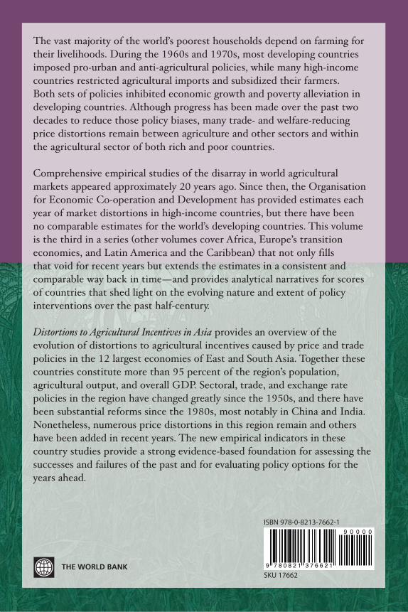
The vast majority of the world’s poorest households depend on farming for their livelihoods. During the 1960s and 1970s, most developing countries imposed pro-urban and anti-agricultural policies, while many high-income countries restricted agricultural imports and subsidized their farmers. Both sets of policies inhibited economic growth and poverty alleviation in developing countries. Although progress has been made over the past two decades to reduce those policy biases, many trade- and welfare-reducingprice distortions remain between agriculture and other sectors and within the agricultural sector of both rich and poor countries.
Comprehensive empirical studies of the disarray in world agricultural markets appeared approximately 20 years ago. Since then, the Organisation for Economic Co-operation and Development has provided estimates each year of market distortions in high-income countries, but there have been no comparable estimates for the world’s developing countries. This volume is the third in a series (other volumes cover Africa, Europe’s transition economies, and Latin America and the Caribbean) that not only fills that void for recent years but extends the estimates in a consistent and comparable way back in time—and provides analytical narratives for scores of countries that shed light on the evolving nature and extent of policy interventions over the past half-century.
Distortions to Agricultural Incentives in Asia provides an overview of the evolution of distortions to agricultural incentives caused by price and trade policies in the 12 largest economies of East and South Asia. Together these countries constitute more than 95 percent of the region’s population, agricultural output, and overall GDP. Sectoral, trade, and exchange rate policies in the region have changed greatly since the 1950s, and there have been substantial reforms since the 1980s, most notably in China and India. Nonetheless, numerous price distortions in this region remain and others have been added in recent years. The new empirical indicators in these country studies provide a strong evidence-based foundation for assessing the successes and failures of the past and for evaluating policy options for the years ahead.
ISBN 978-0-8213-7662-1
SKU 17662