Weighted DistancesBased on Neighbourhood Sequences

in Non-Standard Three-Dimensional Grids

Robin Strand

Centre for Image Analysis, Uppsala University,Box 337, SE-75105 Uppsala, Sweden

robin@cb.uu.se

Abstract. By combining weighted distances and distances based onneighbourhood sequences, a new family of distance functions with po-tentially low rotational dependency is obtained. The basic theory forthese distance functions, including functional form of the distance be-tween two points, is presented for the face-centered cubic grid and thebody-centered cubic grid. By minimizing an error function, the optimalcombination of weights and neighbourhood sequence is derived.

1 Introduction

When using non-standard grids such as the face-centered cubic (fcc) grid and thebody-centered cubic (bcc) grid for 3D images, less samples are needed to obtainthe same representation/reconstruction quality compared to the cubic grid [1].This is one reason for the increasing interest in using these grids in e.g. imageacquisition [1], image processing [2–4], and image visualization [5].

Measuring distances is of great importance in many applications. Because ofits low rotational dependency, the Euclidean distance is often used as distancefunction. There are, however, applications where other distance functions arebetter suited. For example, when minimal cost-paths are computed, a distancefunction defined as the shortest path between any two points is better suited,see e.g. [6], where the constrained distance transform is computed using the Eu-clidean distance resulting in a complex algorithm. The corresponding algorithmusing a path-based approach is simple, fast, and easy to generalize to higherdimensions [7]. Examples of path-based distances are weighted distances, whereweights define the cost (distance) between neighbouring grid points [8, 3, 2], anddistances based on neighbourhood sequences (ns-distances), where the cost isfixed but the adjacency relation is allowed to vary along the path [9, 4]. Thesepath-based distance functions are generalizations of the well-known city-blockand chessboard distance function defined for the square grid in [10]. The rota-tional dependency of weighted distances and ns-distances can be minimized byoptimizing the weights [8, 3, 2] and neighbourhood sequences [9, 4], respectively.

In this paper, weighted distances and ns-distances for the fcc and bcc grids,presented in [2, 3] and [4] respectively, are combined by defining the distance

as the shortest path between two grid points using both weights for the localdistance between neighbouring grid points and allowing the adjacency relationto vary along the path. Functional forms are given of the distance functionsfor grid points in the fcc and bcc grids. Moreover, the rotational dependency isminimized by finding the weights and neighbourhood sequence that minimize anerror function. The results are compared with results for weighted distances andns-distances, which are both special cases of the proposed distance function.

2 Basic Notions

The following definitions of the fcc and bcc grids are used:

F = {(x, y, z) : x, y, z ∈ Z and x + y + z ≡ 0 (mod 2)}. (1)B = {(x, y, z) : x, y, z ∈ Z and x ≡ y ≡ z (mod 2)}. (2)

When the result is valid for both F and B, the notation G is used. Two gridpoints p1 = (x1, y1, z1),p2 = (x2, y2, z2) ∈ G are ρ-neighbours, 1 ≤ ρ ≤ 2, if

1. |x1 − x2|+ |y1 − y2|+ |z1 − z2| ≤ 3 and2. max {|x1 − x2|, |y1 − y2|, |z1 − z2|} ≤ ρ

The points p1,p2 are adjacent if p1 and p2 are ρ-neighbours for some ρ. Theρ-neighbours which are not (ρ − 1)-neighbours are called strict ρ-neighbours.The neighbourhood relations are visualized in Figure 1 by showing the Voronoiregions (the voxels) corresponding to some adjacent grid points.

Fig. 1. The grid points corresponding to the dark and the light grey voxels are 1-neighbours. The grid points corresponding to the dark grey and white voxels are (strict)2-neighbours. Left: fcc, right: bcc.

A ns B is a sequence B = (b(i))∞i=1, where each b(i) denotes a neighbourhoodrelation in G. If B is periodic, i.e., if for some fixed strictly positive l ∈ Z+,b(i) = b(i + l) is valid for all i ∈ Z+, then we write B = (b(1), b(2), . . . , b(l)). Apath, denoted P, in a grid is a sequence p0,p1, . . . ,pn of adjacent grid points.A path is a B-path of length n if, for all i ∈ {1, 2, . . . , n}, pi−1 and pi areb(i)-neighbours. The notation 1- and (strict) 2-steps will be used for a step toa 1-neighbour and step to a (strict) 2-neighbour, respectively. The number of1-steps and strict 2-steps in a given path P is denoted 1P and 2P , respectively.

Definition 1. Given the ns B, the ns-distance d(p0,pn;B) between the pointsp0 and pn is the length of (one of) the shortest B-path(s) between the points.

Let the real numbers α and β (the weights) and a path P of length n, whereexactly l (l ≤ n) adjacent grid points in the path are strict 2-neighbours, begiven. The length of the (α, β)-weighted B-path P is (n− l)α + lβ. The B-pathP between the points p0 and pn is a shortest (α, β)-weighted B-path betweenthe points p0 and pn if no other (α, β)-weighted B-path between the points isshorter than the length of the (α, β)-weighted B-path P.

Definition 2. Given the ns B and the weights α, β, the weighted ns-distancedα,β(p0,pn; B) is the length of (one of) the shortest (α, β)-weighted B-path(s)between the points.

The following notation is used:

1kB = |{i : b(i) = 1, 1 ≤ i ≤ k}| and

2kB = |{i : b(i) = 2, 1 ≤ i ≤ k}|.

3 Distance Function in Discrete Space

We now state a functional form of the distance between two grid points (0, 0, 0)and (x, y, z), where x ≥ y ≥ z ≥ 0. We remark that by translation-invarianceand symmetry, the distance between any two grid points is given by the formulabelow. The formulas in Lemma 1 are proved (as Theorem 2 and 5) in [4].

Lemma 1. Let the ns B and the point p = (x, y, z) ∈ G, where x ≥ y ≥ z ≥ 0be given. The ns-distance between 0 and p is given by

d (0,p;B) = min{

k ∈ N : k ≥ max(

x + y + z

2, x− 2k

B

)}for p ∈ F

d (0,p;B) = min{

k ∈ N : k ≥ max(

x + y

2, x− 2k

B

)}for p ∈ B

Given a shortest B-path P of length k (obtained by the formula in Lemma 1),Lemma 2 and 3 give the number of 1-steps and 2-steps in P, i.e. 1P and 2P ,respectively.

Lemma 2. Let the point (x, y, z) ∈ F, where x ≥ y ≥ z ≥ 0, and the value of

k = min{

k : k ≥ max(

x + y + z

2, x− 2k

B

)}be given. If only the steps (1, 1, 0),

(1,−1, 0), (0, 1, 1), (1, 0, 1), and (2, 0, 0) are used for a shortest B-path between0 and (x, y, z), then

1P ={

k if x ≤ y + z

2k − x otherwise.

and

2P ={

0 if x ≤ y + z

x− k otherwise.

Proof. First of all, in the proof of Theorem 2 in [4] it is shown that there isa shortest B-path with only the steps (1, 1, 0), (1,−1, 0), (0, 1, 1), (1, 0, 1), and(2, 0, 0) when x ≥ y ≥ z ≥ 0.

For the case x ≤ y + z, the length of the shortest B-path is independent ofB and there is a shortest B-path consisting of only 1-steps, see Theorem 2 in[4]. Hence, the number of 1-steps is k and the number of 2-steps is 0.

In the proof of Theorem 2 in [4], it is shown that only the steps (2, 0, 0),(1, 1, 0), (1,−1, 0), and (1, 0, 1) are needed to find a shortest B-path between(0, 0, 0) and (x, y, z) ∈ F, where x ≥ y ≥ z ≥ 0 and x > y + z. Thus, (x, y, z) =(2, 0, 0)a1 + (1, 1, 0)a2 + (1,−1, 0)a3 + (1, 0, 1)a4 for some a1,a2,a3,a4 ∈ N.Obviously, the length k of the path is a1 + a2 + a3 + a4, 1P = a2 + a3 + a4, and2P = a1. We get:

k = a1 +a2 + a3 + a4

x = 2a1 +a2 + a3 + a4.

Thus, 1P = a2 + a3 + a4 = 2k − x and 2P = a1 = x− k. ut

Lemma 3. Let the point (x, y, z) ∈ B, where x ≥ y ≥ z ≥ 0, and the value

of k = min{

k : k ≥ max(

x + y

2, x− 2k

B

)}be given. If only the steps (1, 1, 1),

(1, 1,−1), (1,−1,−1), and (2, 0, 0) are used for a shortest B-path between 0 and(x, y, z), then

1P = 2k − x

and2P = x− k.

Proof. In the proof of Theorem 5 in [4], it is shown that only the steps (2, 0, 0),(1, 1, 1), (1, 1,−1), and (1,−1,−1) are needed to find a shortest B-path between(0, 0, 0) and (x, y, z) ∈ B, where x ≥ y ≥ z ≥ 0. Thus, (x, y, z) = (2, 0, 0)a1 +(1, 1, 1)a2 + (1, 1,−1)a3 + (1,−1 − 1)a4 for some a1,a2,a3,a4 ∈ N. Obviously,1P = a2 + a3 + a4 and 2P = a1. Using the same technique as in the proof ofLemma 2, the result follows. ut

Lemma 4. Let the ns B and the point (x, y, z) ∈ G, where x ≥ y ≥ z ≥ 0 begiven. If P is a shortest B-path between 0 and (x, y, z) consisting of only thesteps

(2, 0, 0), (1, 1, 0), (1,−1, 0), (0, 1, 1), and (1, 0, 1) (fcc)(2, 0, 0), (1, 1, 1), (1, 1,−1), and (1,−1,−1) (bcc)

such that the weights α, β ∈ R are such that 0 < α ≤ β ≤ 2α, then P is also ashortest (α, β)-weighted B-path between 0 and (x, y, z).

Proof. From [4], we know that a shortest B-path is obtained by using these stepswhen x ≥ y ≥ z ≥ 0, cf. Lemma 2 and 3.

Let n be the length of P and let l be the number of 2-steps in P. The lengthof P can then be written n = (n − l)1 + l1. The length of the (α, β)-weightedB-path is (n− l)α+ lβ. Assume that the shortest (α, β)-weighted B-path P ′ is ashorter (α, β)-weighted B-path between 0 and (x, y, z) than P. Let the length ofP ′ ((1, 1)-weighted) be n′ (n′ ≥ n since P is a shortest B-path) and the numberof 2-steps be l′. The length of the (α, β)-weighted B-path P ′ is (n′ − l′)α + l′β.By assumption,

(n′ − l′)α + l′β < (n− l)α + lβ. (3)

We get the following cases:

i l′ < lSince P ′ is a path between 0 and (x, y, z) and the only 2-step that isused is (2, 0, 0), there are at least 2(l − l′) more 1-steps in P ′ comparedto P. We get (n′ − l′) ≥ (n − l) + 2(l − l′) ⇒ (n′ − l′) − (n − l) ≥2(l−l′) ⇒ ((n′ − l′)− (n− l)) α ≥ 2(l−l′)α. By the assumption (3), we have((n′ − l′)− (n− l)) α < (l− l′)β. Thus, 2(l− l′)α ≤ ((n′ − l′)− (n− l)) α <(l − l′)β ⇒ 2α < β, which is a contradiction.

ii l′ > l(n′ − l′)α + l′β < (n− l)α + lβ by (3)(n− l′)α + l′β < (n− l)α + lβ since n′ ≥ n

(l′ − l)β < (l′ − l)αβ < α since l′ > l,

which is a contradiction.

This proves that the assumption (3) implies l′ = l. Rewriting (3) with l′ = lgives n′ < n, which contradicts the fact that P is a shortest B-path (i.e. thatn′ ≥ n). Therefore (3) is false, so

(n′ − l′)α + l′β ≥ (n− l)α + lβ.

It follows that P is a shortest (α, β)-weighted B-path. ut

The following theorems (Theorem 1 and 2) are obtained by summing up theresults from Lemma 1–4. Given a shortest B-path consisting of as many 1-stepsas possible between 0 and (x, y, z) ∈ G with x ≥ y ≥ z ≥ 0, if 0 < α ≤ β ≤ 2α,we know by Lemma 4 that the path is also a shortest (α, β)-weighted B-path.Using Lemma 2 and 3, where the number of 1-steps and 2-steps in the path aregiven, the formulas in Lemma 1 can be rewritten such that the length of thepath is given by summing the number of 1-steps and 2-steps. By multiplyingthese numbers with the corresponding weights, we get the following functionalforms of the weighted distance based on neighbourhood sequences between twopoints in the fcc and bcc grids.

Theorem 1. Let the ns B, the weights α, β s.t. 0 < α ≤ β ≤ 2α, and the point(x, y, z) ∈ F, where x ≥ y ≥ z ≥ 0, be given. The weighted ns-distance between

0 and (x, y, z) is given by

dα,β (0, (x, y, z); B) ={

k · α if x ≤ y + z(2k − x) · α + (x− k) · β otherwise,

where k = mink

: k ≥ max(

x + y + z

2, x− 2k

B

).

Theorem 2. Let the ns B, the weights α, β s.t. 0 < α ≤ β ≤ 2α, and the point(x, y, z) ∈ B, where x ≥ y ≥ z ≥ 0, be given. The weighted ns-distance between0 and (x, y, z) is given by

dα,β (0, (x, y, z); B) = (2k − x) · α + (x− k) · β

where k = mink

: k ≥ max(

x + y

2, x− 2k

B

).

To illustrate the discrete distance functions, balls of radius 20 in the fcc gridwith α = 1, β = 1.4862, and B = (1, 2) and the bcc grid with α = 1, β = 1.2199,and B = (1, 2) are shown in Figure 2.

(a) (b)

Fig. 2. Balls of radius 20 in the fcc grid with α = 1, β = 1.4862, and B = (1, 2) (a)and the bcc grid with α = 1, β = 1.2199, and B = (1, 2) (b).

4 Distance Function in Continuous Space

The optimization is carried out in R3 by finding the best shape of polyhedracorresponding to balls of constant radii using the proposed distance functions. Todo this, the distance functions presented for the fcc and bcc grids in the previoussection are stated in a more general form valid for all points (x, y, z) ∈ R3, wherex ≥ y ≥ z ≥ 0. The following distance functions are considered:

dfccα,β (0, (x, y, z); γ) =

{k · α if x ≤ y + z

(2k − x) · α + (x− k) · β otherwise,

where k = mink

: k ≥ max(

x + y + z

2, x− (1− γ)k

)

and

dbccα,β (0, (x, y, z); γ) = (2k − x) · α + (x− k) · β

where k = mink

: k ≥ max(

x + y

2, x− (1− γ)k

),

where k ∈ R and γ ∈ R, 0 ≤ γ ≤ 1 is the fraction of the steps where 2-stepsare not allowed (so 1k

B and 2kB corresponds to γk and (1− γ)k, respectively). In

this way we obtain a generalization of the distance functions in discrete spaceG valid for all points (x, y, z) where x ≥ y ≥ z ≥ 0 in continuous space R3. Byconsidering

dfccα,β (0, (x, y, z); γ) = r and dbcc

α,β (0, (x, y, z); γ) = r, (4)

the points on a sphere of constant radius are found.

Remark 1. For a fixed point (x, y, z), x+y+z2 and x+y

2 are constant and x−(1−γ)kis decreasing w.r.t. k and when k = 0, 0 ≤ max

(x+y

2 , x) ≤ max

(x+y+z

2 , x).

Therefore both k = max(

x+y+z2 , x− (1− γ)k

)and k = max

(x+y

2 , x− (1− γ)k)

has a solution k ∈ R. Thus, when k ∈ R,

k = mink

: k ≥ max(

x + y + z

2, x− (1− γ)k

)⇔ k = max

(x + y + z

2, x− (1− γ)k

)

k = mink

: k ≥ max(

x + y

2, x− (1− γ)k

)⇔ k = max

(x + y

2, x− (1− γ)k

)

4.1 Reformulation of dfcc

Using Remark 1, the expression for dfccα,β is rewritten:

dfccα,β (0, (x, y, z); γ) =

{k · α if x ≤ y + z

(2k − x) · α + (x− k) · β otherwise,

where k = max(

x + y + z

2, x− (1− γ)k

).

We get two cases:i) x+y+z

2 ≥ x− (1− γ)kk = x+y+z

2 ⇒

dfccα,β (0, (x, y, z); γ) =

{x+y+z

2 · α if x ≤ y + z

(y + z) · α +(

x−(y+z)2

)· β otherwise.

ii) x+y+z2 < x− (1− γ)k

k = x− (1− γ)k ⇒ k = x2−γ

dfccα,β (0, (x, y, z); γ) =

{ x2−γ · α if x ≤ y + z ?(

2 x2−γ − x

)· α +

(x− x

2−γ

)· β otherwise.

Observe that when x ≤ y + z, x+y+z2 ≥ x ≥ x− (1− γ)k and thus the case

? will not occur.

4.2 Reformulation of dbcc

Using Remark 1, the expression is rewritten also for dbccα,β :

dbccα,β (0, (x, y, z); γ) = (2k − x) · α + (x− k) · β

where k = max(

x + y

2, x− (1− γ)k

).

Again, there are two cases:

i) x+y2 ≥ x− (1− γ)k

k = x+y2 ⇒

dbccα,β (0, (x, y, z); γ) = (y) · α +

(x− y

2

)· β

ii) x+y2 < x− (1− γ)k

k = x− (1− γ)k ⇒ k = x2−γ

dbccα,β (0, (x, y, z); γ) =

(2

x

2− γ− x

)· α +

(x− x

2− γ

)· β

Together with (4), this describes the portions of polyhedra satisfying x ≥ y ≥z ≥ 0. By using symmetry, the entire polyhedra are described. There polyhedraare spheres with the proposed distance functions.

4.3 Optimization of the Parameters

For any triplet α, β, γ (α, β > 0 and 0 ≤ γ ≤ 1), (4) defines a polyhedron inR3. The shape of the polyhedra obtained for some values of α, β, γ are shown inFigure 3. Let A be the surface area and V the volume of the (region enclosedby the) polyhedron. The values of A and V are determined by the vertices ofthe polyhedra which are derived using (4) together with the expressions for dfcc

α,β

and dbccα,β derived in Section 4.1 and 4.2, respectively. The vertices satisfying

x ≥ y ≥ z ≥ 0 are(

2− γ

γα + β − βγ,

γ

γα + β − βγ, 0

)and

(1α

,1α

, 0)

for dfcc and(

2− γ

γα + β − βγ,

γ

γα + β − βγ,

γ

γα + β − βγ

)and

(1α

,1α

,1α

)for dbcc

The following error function (often called the compactness ratio) is used

E =A3

V 2 − 36π

36π,

which is equal to zero if and only if A is the surface area and V is the volume ofa Euclidean ball.

The values of α, β, and γ that minimize E are computed. The optimal valuesare found in Table 1 and visualized by the shape of the corresponding polyhedrain Figure 4.

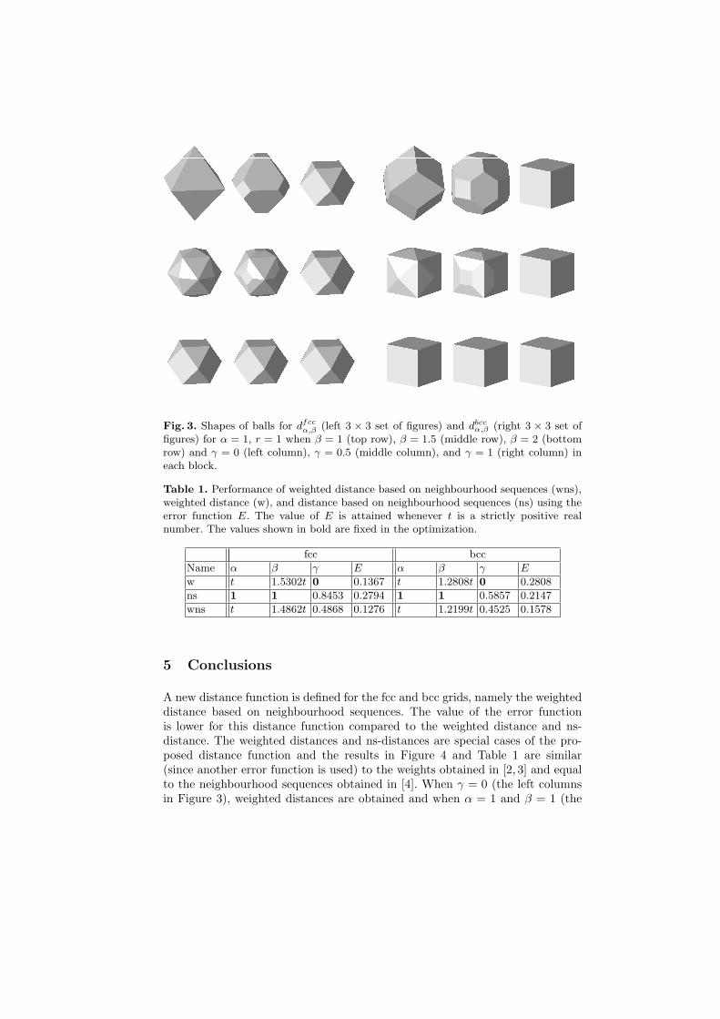
Fig. 3. Shapes of balls for dfccα,β (left 3 × 3 set of figures) and dbcc

α,β (right 3 × 3 set offigures) for α = 1, r = 1 when β = 1 (top row), β = 1.5 (middle row), β = 2 (bottomrow) and γ = 0 (left column), γ = 0.5 (middle column), and γ = 1 (right column) ineach block.

Table 1. Performance of weighted distance based on neighbourhood sequences (wns),weighted distance (w), and distance based on neighbourhood sequences (ns) using theerror function E. The value of E is attained whenever t is a strictly positive realnumber. The values shown in bold are fixed in the optimization.

fcc bcc

Name α β γ E α β γ E

w t 1.5302t 0 0.1367 t 1.2808t 0 0.2808

ns 1 1 0.8453 0.2794 1 1 0.5857 0.2147

wns t 1.4862t 0.4868 0.1276 t 1.2199t 0.4525 0.1578

5 Conclusions

A new distance function is defined for the fcc and bcc grids, namely the weighteddistance based on neighbourhood sequences. The value of the error functionis lower for this distance function compared to the weighted distance and ns-distance. The weighted distances and ns-distances are special cases of the pro-posed distance function and the results in Figure 4 and Table 1 are similar(since another error function is used) to the weights obtained in [2, 3] and equalto the neighbourhood sequences obtained in [4]. When γ = 0 (the left columnsin Figure 3), weighted distances are obtained and when α = 1 and β = 1 (the

(a) (b) (c) (d) (e) (f)

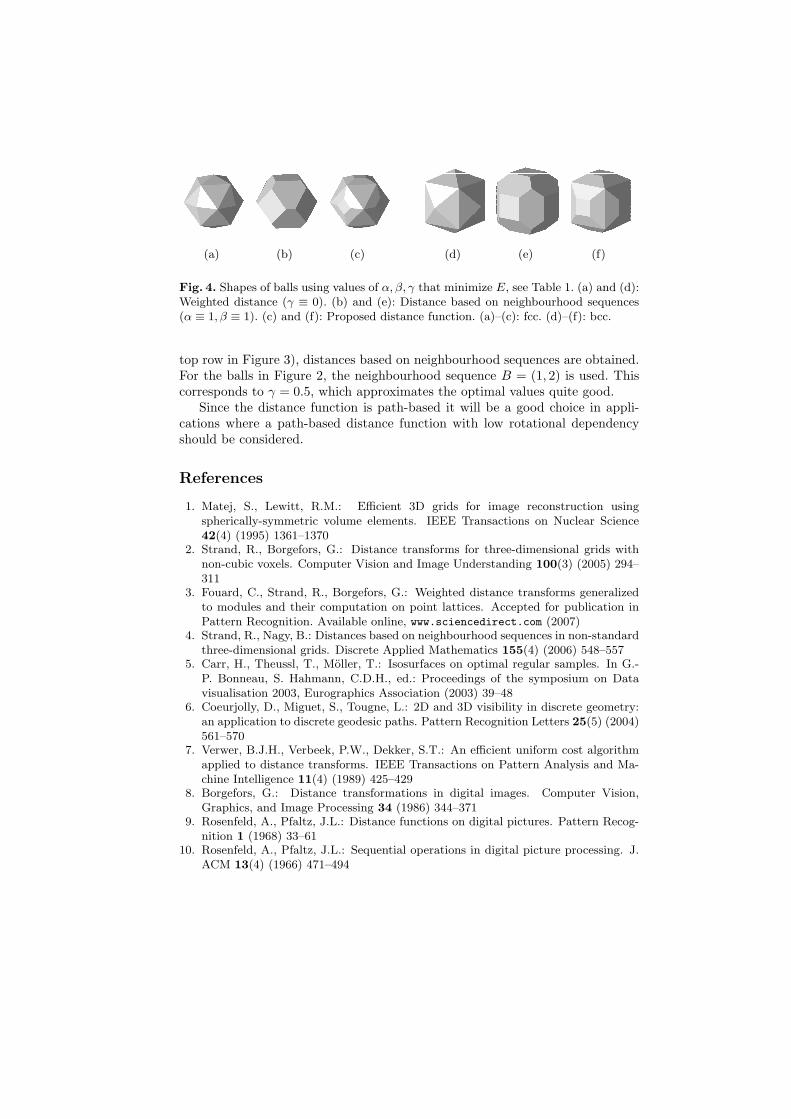
Fig. 4. Shapes of balls using values of α, β, γ that minimize E, see Table 1. (a) and (d):Weighted distance (γ ≡ 0). (b) and (e): Distance based on neighbourhood sequences(α ≡ 1, β ≡ 1). (c) and (f): Proposed distance function. (a)–(c): fcc. (d)–(f): bcc.

top row in Figure 3), distances based on neighbourhood sequences are obtained.For the balls in Figure 2, the neighbourhood sequence B = (1, 2) is used. Thiscorresponds to γ = 0.5, which approximates the optimal values quite good.

Since the distance function is path-based it will be a good choice in appli-cations where a path-based distance function with low rotational dependencyshould be considered.

References

1. Matej, S., Lewitt, R.M.: Efficient 3D grids for image reconstruction usingspherically-symmetric volume elements. IEEE Transactions on Nuclear Science42(4) (1995) 1361–1370

2. Strand, R., Borgefors, G.: Distance transforms for three-dimensional grids withnon-cubic voxels. Computer Vision and Image Understanding 100(3) (2005) 294–311

3. Fouard, C., Strand, R., Borgefors, G.: Weighted distance transforms generalizedto modules and their computation on point lattices. Accepted for publication inPattern Recognition. Available online, www.sciencedirect.com (2007)

4. Strand, R., Nagy, B.: Distances based on neighbourhood sequences in non-standardthree-dimensional grids. Discrete Applied Mathematics 155(4) (2006) 548–557

5. Carr, H., Theussl, T., Moller, T.: Isosurfaces on optimal regular samples. In G.-P. Bonneau, S. Hahmann, C.D.H., ed.: Proceedings of the symposium on Datavisualisation 2003, Eurographics Association (2003) 39–48

6. Coeurjolly, D., Miguet, S., Tougne, L.: 2D and 3D visibility in discrete geometry:an application to discrete geodesic paths. Pattern Recognition Letters 25(5) (2004)561–570

7. Verwer, B.J.H., Verbeek, P.W., Dekker, S.T.: An efficient uniform cost algorithmapplied to distance transforms. IEEE Transactions on Pattern Analysis and Ma-chine Intelligence 11(4) (1989) 425–429

8. Borgefors, G.: Distance transformations in digital images. Computer Vision,Graphics, and Image Processing 34 (1986) 344–371

9. Rosenfeld, A., Pfaltz, J.L.: Distance functions on digital pictures. Pattern Recog-nition 1 (1968) 33–61

10. Rosenfeld, A., Pfaltz, J.L.: Sequential operations in digital picture processing. J.ACM 13(4) (1966) 471–494