DISTRIBUTION OF DISTANCES AND INTERIOR DISTANCES FOR CERTAIN SELF-SIMILAR MEASURES

Christoph Bandt and Mohamed Mubarak

The Arabian Journal for Science and Engineering, Volume 29, Number 2C.December 2004 111

*To whom correspondence should be addressed.Institut für Mathematik und InformatikErnst-Moritz-Arndt-UniversitätFriedrich-Ludwig-Jahn-Str. 15aD-17487 Greifswald, Germanye-mail: [email protected]

DISTRIBUTION OF DISTANCES AND INTERIOR DISTANCES FOR CERTAIN SELF-SIMILAR

MEASURES

Christoph Bandt* and Mohamed Mubarak

Institut für Mathematik und InformatikErnst-Moritz-Arndt-Universität

Greifswald, Germany

ABSTRACT

We determine the distribution of Euclidean and interior distances in the Sierpinski gasket and the detailed structure of shortest paths in the Sierpinski carpet.

الخالصــة

سوف نقوم في هذا البحث بتعيـين توزيع المسافات األقليدية والمسافات الداخلية في مثلث سيربنسكي وأيضا توضيح مفصل لبناء أقصر المسارات داخل مربع سيربنسكي .


The Arabian Journal for Science and Engineering, Volume 29, Number 2C. December 2004112

DISTRIBUTION OF DISTANCES AND INTERIOR DISTANCES FOR CERTAINSELF-SIMILAR MEASURES

1. INTRODUCTION

When studying transport between points x, y in a fractal F, we can either go through the surrounding space,or along a “shortest path” within the fractal. For transport through the whole space, we should be interested inthe distribution of Euclidean distances |x−y| where x, y runs through F. In Section 2 we take certain self-similarmeasures µ on F as probability measures for the choice of x and y. The differences x − y, where x and y arechosen independently, are then distributed with respect to another probability measure, the correlation measureµ � µ− of µ. In Section 2, we show that the correlation measure of certain self-affine measures is self-affine, too.As a consequence, the distribution of |x− y| can easily be calculated, at least numerically, as we see in Section 3.

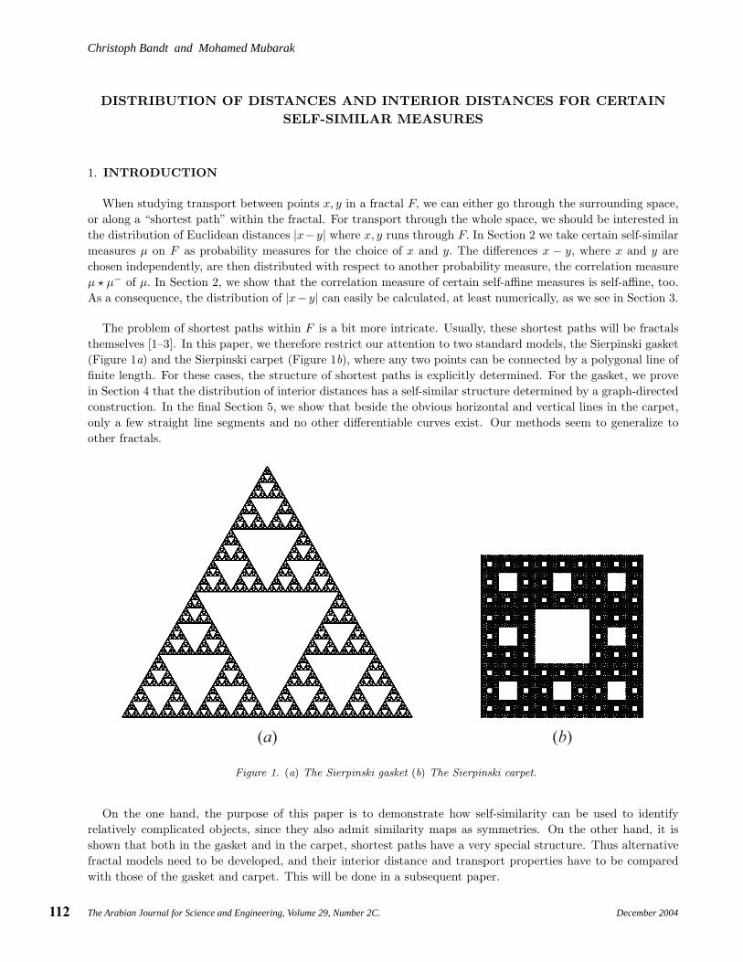
The problem of shortest paths within F is a bit more intricate. Usually, these shortest paths will be fractalsthemselves [1–3]. In this paper, we therefore restrict our attention to two standard models, the Sierpinski gasket(Figure 1a) and the Sierpinski carpet (Figure 1b), where any two points can be connected by a polygonal line offinite length. For these cases, the structure of shortest paths is explicitly determined. For the gasket, we provein Section 4 that the distribution of interior distances has a self-similar structure determined by a graph-directedconstruction. In the final Section 5, we show that beside the obvious horizontal and vertical lines in the carpet,only a few straight line segments and no other differentiable curves exist. Our methods seem to generalize toother fractals.

��

Figure 1. (a) The Sierpinski gasket (b) The Sierpinski carpet.

On the one hand, the purpose of this paper is to demonstrate how self-similarity can be used to identifyrelatively complicated objects, since they also admit similarity maps as symmetries. On the other hand, it isshown that both in the gasket and in the carpet, shortest paths have a very special structure. Thus alternativefractal models need to be developed, and their interior distance and transport properties have to be comparedwith those of the gasket and carpet. This will be done in a subsequent paper.



1.1. Basic Definitions

We try to list all prerequisites and refer to [4, 5] for details. Throughout, we work in Euclidean space IRn.

A map f : IRn → IRn is called a contraction with factor r ∈ (0, 1) if |f(x) − f(y)| ≤ r · |x − y| for all points x, y.

If equality holds, f is called similarity map with factor r. An affine map has the form f(x) = Mx + v where M

is an n×n matrix and v is a translation vector. Such an affine map is a contraction if and only if all eigenvaluesof M have modulus < 1.

Given contractions f1, ..., fm, a bounded non-empty closed set F is said to be invariant if

F = f1(F ) ∪ ... ∪ fm(F ). (1)

A well-known theorem of Hutchinson [6] says that for any finite set of contractions, there is exactly one invariantset F. If f1, ..., fm are all affine maps, F is called a self-affine set. If the fi are similarities with factor ri, then F

is called a self-similar set, and the unique number α > 0 with∑

i rαi = 1 is called the similarity dimension of F.

Sometimes, measures are more convenient and appropriate mathematical objects than sets. We shall dealwith probability measures µ on IRn which are defined on all Borel sets. Their self-similarity is defined in thesame way as above. Given contractions f1, ..., fm and positive numbers pi with

∑i pi = 1, the equation

µ = p1f1(µ) + ... + pmfm(µ) (2)

determines the uniquely determined invariant, or self-affine, or self-similar measure. Here f(µ) is defined byf(µ)(B) = µ(f−1(B)) for Borel sets B.

Figure 1 shows two well-known self-similar sets. Sierpinski’s gasket has similarity dimension log 3/ log 2, thecarpet has dimension log 8/ log 3. In both cases, the similarity dimension equals the Hausdorff dimension, and theα-dimensional Hausdorff measure is the self-similar measure for the natural weights pi = rα

i = 1/m. Note thatwe normalize the measures so that they become probability measures. Thus carpet and gasket can be consideredboth as sets and as measures.

2. SELF-SIMILAR PRODUCTS AND CONVOLUTIONS

For a probability measure µ on IRn, the distribution of x − y with respect to µ × µ is called the correlationmeasure γ of µ. In this section we determine the correlation measure of the Sierpinski gasket and similar fractals.

Product Theorem. As a first step, let us consider the distribution of (x, y) where x comes from the self-similarmeasure µ defined in (2) and y comes from a self-similar measure ν defined by ν = q1g1(ν) + ... + qkgk(ν).We shall see that the product of two self-affine measures is again a self-affine measure. First we formulate thefact for self-similar sets. For maps fi : IRn → IRn and gj : IRd → IRd, let hij : IRn+d → IRn+d be defined byhij(x, y) = (fi(x), gj(y)). Then F =

⋃fi(F ) and G =

⋃gj(G) immediately implies

F × G =⋃i,j

fi(F ) × gj(G) =⋃i,j

hij(F × G).

If the fi, gj have eigenvalues with modulus < 1, the same holds for hij which has just the eigenvalues of fi andthose of gj . However, if fi, gj are similarities then hij is a similarity only if the factors of fi and gj coincide.This proves:

Proposition 2.1. (Product of self-similar sets)

The product of two self-affine sets is a self-affine set. The product of two self-similar sets is self-similar if andonly if all factors of the similarities involved in both sets are equal.



For measures µ and ν, we can use almost the same arguments. The product measure is defined by µ×ν(A×B) =µ(A) · ν(B), and the basic equation is

µ × ν =∑i,j

pifi(µ) × qjgj(ν) =∑i,j

piqjhij(µ × ν).

Proposition 2.2. (Product of self-similar measures)

The product of two self-affine measures is a self-affine measure. The product of two self-similar measures isself-similar if and only if all factors of the similarities involved in both sets are equal. No equality condition isneeded for the weights pi, qj .

In other words, the distribution of (x, y), where x and y are chosen from self-affine probability distributions, isitself a self-affine measure. But it is hard to visualize: if µ and ν are in IR2, the product µ×ν is in IR4. However,we are interested in the distribution of x− y which is again two-dimensional. Thus we become interested in theprojection π : IR2n → IRn defined by π(x, y) = x − y.

Projection theorem. We consider the general question whether a linear projection π : IRn → IRd preservesself-similarity of sets and measures, as defined in (1) and (2). Clearly, (1) implies

G = π(F ) = π · f1(F ) ∪ ... ∪ π · fm(F ).

The question is whether π · fi(F ) can be written as gi(G) where gi is an affine map in IRd. A sufficient conditionis that fi preserves the fibers of π, that is, π(u) = π(v) implies π(fi(u)) = π(fi(v)). If this is true, we can definegi : IRd → IRd by gi(z) = π · fi · π−1(z), where it does not matter which representative of π−1(z) is taken.A condition like this should also be necessary if the fibers π−1(z) contain several points of F.

Proposition 2.3. (Projection of self-similar sets and measures)

Let F be the self-similar set and µ the self-similar measure defined on IRn by (1) and (2). Let π : IRn → IRd be alinear mapping with the property that π(u) = π(v) implies π(fi(u)) = π(fi(v)), for all u, v ∈ IRn and i = 1, ..., m.

Then G = π(F ) is a self-similar set with respect to the mappings g1, ..., gm on IRd defined by gi(z) = π ·fi ·π−1(z).Moreover, ν = π(µ) is a self-similar measure with respect to the mappings gi and the weights pi.

Correlation measure. As we noted above, we are interested in the special projection π : IR2n → IRn withπ(x, y) = x− y where both x and y come from the same self-similar measure µ defined by (2). The mappings onthe product space IR2n are hij(x, y) = (fi(x), fj(y)), and for these we have to check whether fibers are preserved.A fiber in our special case is given by the equation x − y = c for some c. So with u = (x, y) and v = (x′, y′) thecondition reads as follows:

x − y = x′ − y′ implies fi(x) − fj(y) = fi(x′) − fj(y′).

That is: x − x′ = y − y′ implies fi(x) − fi(x′) = fj(y) − fj(y′).

Now assume the fk are affine mappings: fk(x) = Mkx+vk, and let z = x−x′ = y−y′. Then fi(x)−fi(x′) = Miz

and fj(y) − fj(y′) = Mjz. Thus the condition says that Miz = Mjz for all i and j. This is true if all mappingsfk have the same matrix M = Mk. In this case, hij := fi(x)−fj(y) = M(x−y)+ vi − vj depends only on x−y.



Proposition 2.4. (When the correlation measure is self-affine)

If fk(x) = Mx + vk for k = 1, ..., m then the correlation measure γ of the self-affine measure µ in (1) is aself-affine measure with respect to the m2 mappings hij = fi−fj and the weights pij = pipj , where i, j = 1, ..., m.

Self-affine sets for such mappings fk have been studied by a number of authors, in particular in the case oftilings [7].

3. DISTRIBUTION OF EUCLIDEAN DISTANCES

3.1. Iterated Function Systems

Let us give another proof of Proposition 2.4, using iterated function systems (IFS) [8]. The measure µ isapproximated (in the sense of weak convergence of measures) by the sequence x0 ∈ F, and xk = fik

(xk−1) fork = 1, 2, ..., where each ik is chosen randomly and independently of the others from {1, ..., m}, with probabilitypi for i. The reason is that for any word u = u1...ur on {1, ..., m}, and for every k > r, the probability thatur = ik, ur−1 = ik−1, ..., u1 = ik−r+1 is pu1 · · · pur = pu. So the probability that xk is in the rth level piecefu1 · ... · fur (F ) = Fu equals pu = µ(Fu).

We take another sequence y0, y1, ... which is generated by the same procedure but with independent randomnumbers. The above argument shows that xk − yk with k = 0, 1, 2, ... will approximate the correlation measure.For any words u = u1...ur and v = v1...vr the probability that xk is in Fu and yk is in Fv is pupv = µ(Fu)µ(Fv).Thus we have an iterated function algorithm to generate the correlation measure.

Now if fk(x) = Mx + vk then this algorithm gives

xk − yk = fi(xk−1) − fj(yk−1) = M(xk−1 − yk−1) + vi − vj

where the pair (i, j) is chosen with probability pipj . Obviously, this is just the IFS algorithm for the self-similarmeasure associated with the maps hij(z) = Mz + vi − vj and the weights pij = pipj . This proves Proposition2.4.

3.2. Distances

Let x, y be points taken randomly and independently from the fractal probability measure µ defined in (1). Weare interested in the distribution of the Euclidean distance |x− y|. If, for example, µ is the uniform distributionon [0, 1], it is well known that the distance is distributed according to the density function ϕ(t) = 2(1 − t) for0 ≤ t ≤ 1.

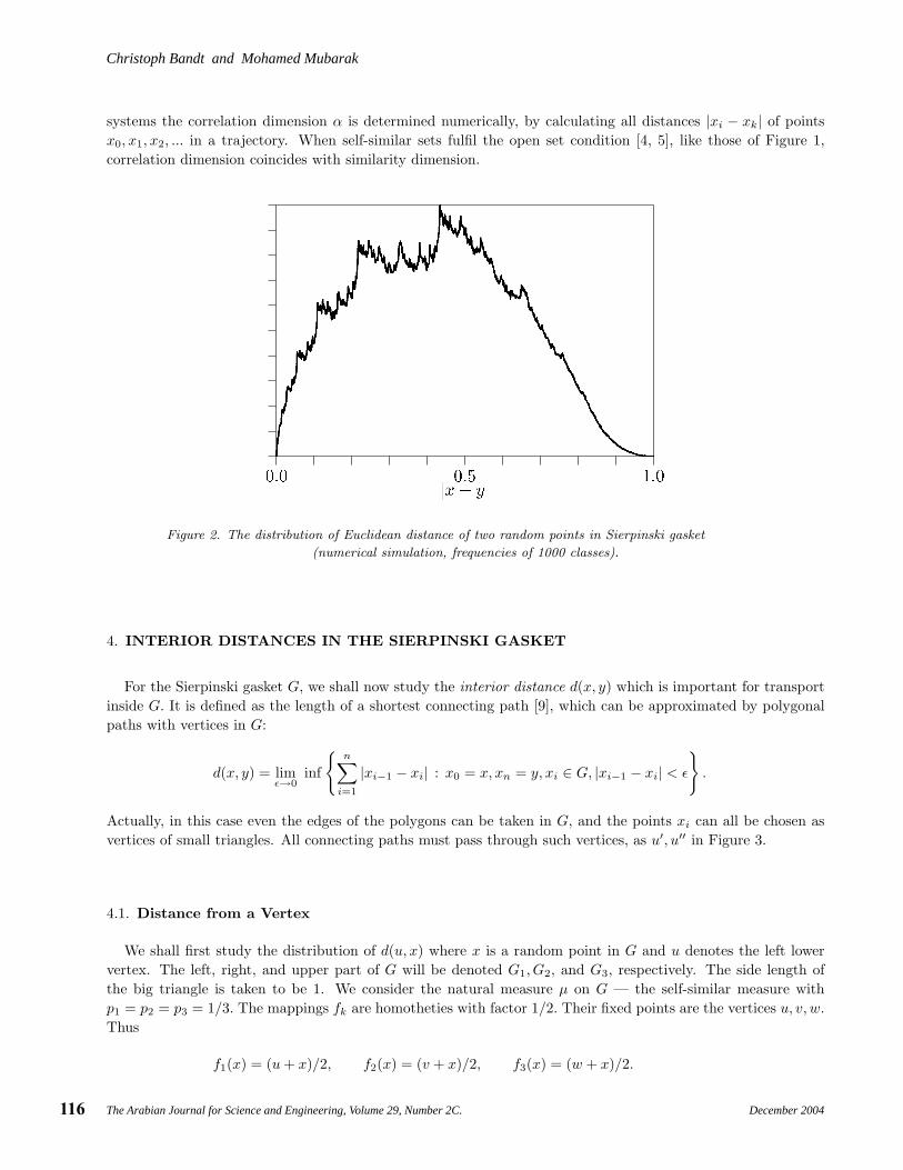
The above IFS algorithm for x − y yields a method to determine the distribution of distances numerically.The result of our numerical calculations for the Sierpinski gasket is shown in Figure 2. We have not been ableto find the distribution by analytic means. Even if x − y is distributed with respect to a self-affine measure, asin Proposition 2.4, |x − y| need not have a self-similar distribution. In other words, the map z �→ |z| does notpreserve self-similarity.

Let us mention some related work. Falconer has shown that for arbitrary subsets F of IRn with Hausdorffdimension greater than (n + 1)/2, the distance set {x − y|x, y ∈ F} contains an open set (see [5], Chapter 12).The distribution function of the distance, Φ(t) = P (|x − y| < t) was used for the definition of the correlationdimension: Φ(t) ≈ tα for small t, or more exactly α = limt→0 log Φ(t)/ log t. For so-called attractors of dynamical



systems the correlation dimension α is determined numerically, by calculating all distances |xi − xk| of pointsx0, x1, x2, ... in a trajectory. When self-similar sets fulfil the open set condition [4, 5], like those of Figure 1,correlation dimension coincides with similarity dimension.

Figure 2. The distribution of Euclidean distance of two random points in Sierpinski gasket

(numerical simulation, frequencies of 1000 classes).

4. INTERIOR DISTANCES IN THE SIERPINSKI GASKET

For the Sierpinski gasket G, we shall now study the interior distance d(x, y) which is important for transportinside G. It is defined as the length of a shortest connecting path [9], which can be approximated by polygonalpaths with vertices in G:

d(x, y) = limε→0

inf

{n∑

i=1

|xi−1 − xi| : x0 = x, xn = y, xi ∈ G, |xi−1 − xi| < ε

}.

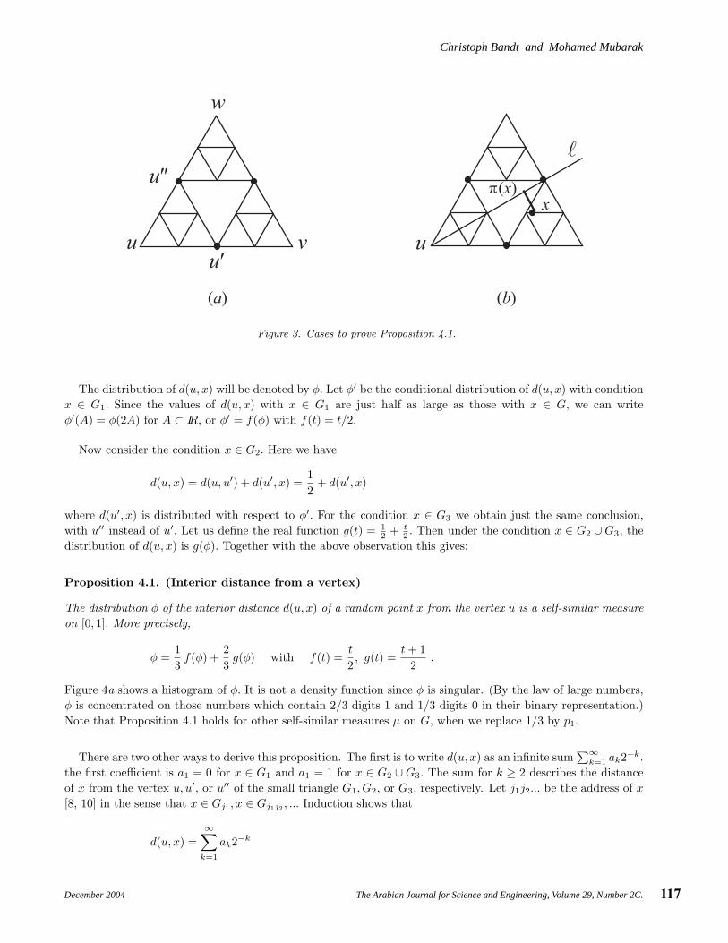
Actually, in this case even the edges of the polygons can be taken in G, and the points xi can all be chosen asvertices of small triangles. All connecting paths must pass through such vertices, as u′, u′′ in Figure 3.

4.1. Distance from a Vertex

We shall first study the distribution of d(u, x) where x is a random point in G and u denotes the left lowervertex. The left, right, and upper part of G will be denoted G1, G2, and G3, respectively. The side length ofthe big triangle is taken to be 1. We consider the natural measure µ on G — the self-similar measure withp1 = p2 = p3 = 1/3. The mappings fk are homotheties with factor 1/2. Their fixed points are the vertices u, v, w.

Thus

f1(x) = (u + x)/2, f2(x) = (v + x)/2, f3(x) = (w + x)/2.



�

�

��

�

�

��

� �

��

��

Figure 3. Cases to prove Proposition 4.1.

The distribution of d(u, x) will be denoted by φ. Let φ′ be the conditional distribution of d(u, x) with conditionx ∈ G1. Since the values of d(u, x) with x ∈ G1 are just half as large as those with x ∈ G, we can writeφ′(A) = φ(2A) for A ⊂ IR, or φ′ = f(φ) with f(t) = t/2.

Now consider the condition x ∈ G2. Here we have

d(u, x) = d(u, u′) + d(u′, x) =12

+ d(u′, x)

where d(u′, x) is distributed with respect to φ′. For the condition x ∈ G3 we obtain just the same conclusion,with u′′ instead of u′. Let us define the real function g(t) = 1

2 + t2 . Then under the condition x ∈ G2 ∪ G3, the

distribution of d(u, x) is g(φ). Together with the above observation this gives:

Proposition 4.1. (Interior distance from a vertex)

The distribution φ of the interior distance d(u, x) of a random point x from the vertex u is a self-similar measureon [0, 1]. More precisely,

φ =13

f(φ) +23

g(φ) with f(t) =t

2, g(t) =

t + 12

.

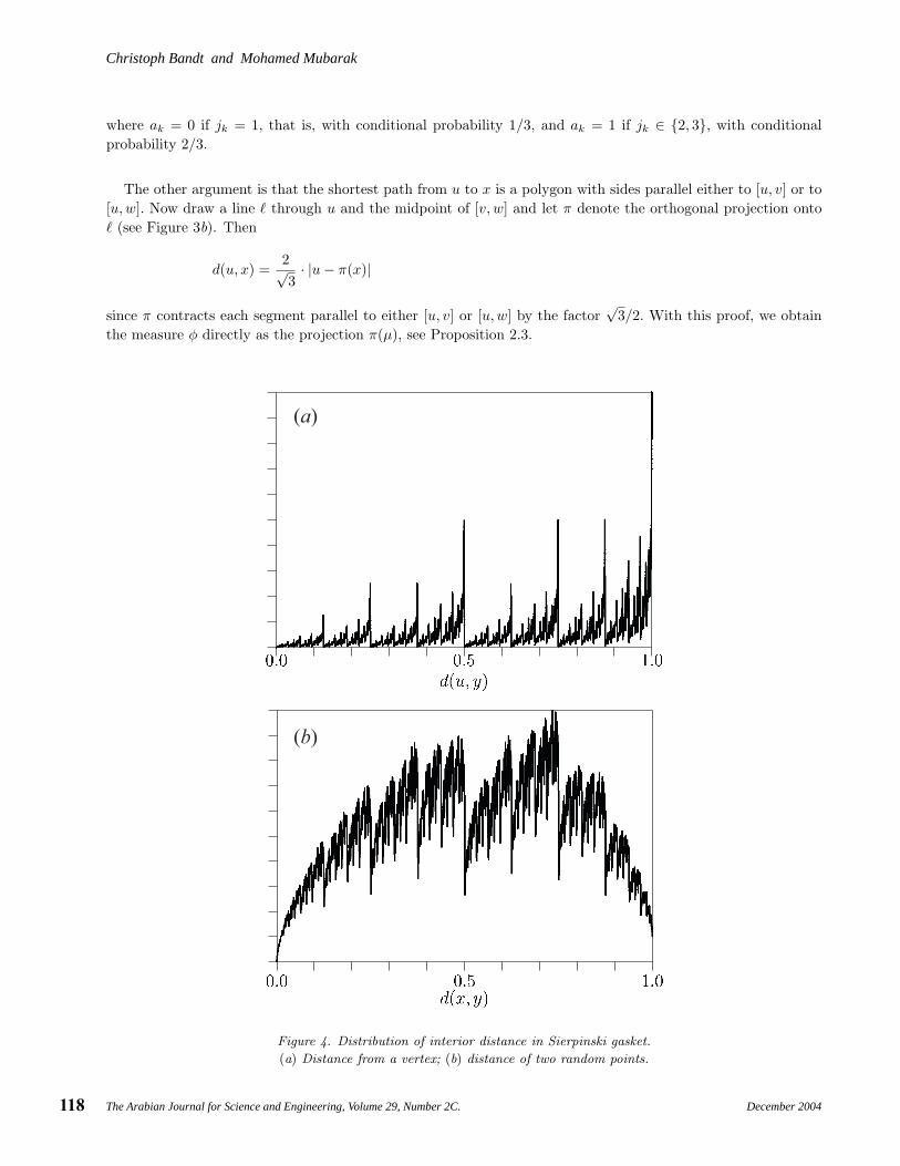
Figure 4a shows a histogram of φ. It is not a density function since φ is singular. (By the law of large numbers,φ is concentrated on those numbers which contain 2/3 digits 1 and 1/3 digits 0 in their binary representation.)Note that Proposition 4.1 holds for other self-similar measures µ on G, when we replace 1/3 by p1.

There are two other ways to derive this proposition. The first is to write d(u, x) as an infinite sum∑∞

k=1 ak2−k.

the first coefficient is a1 = 0 for x ∈ G1 and a1 = 1 for x ∈ G2 ∪ G3. The sum for k ≥ 2 describes the distanceof x from the vertex u, u′, or u′′ of the small triangle G1, G2, or G3, respectively. Let j1j2... be the address of x

[8, 10] in the sense that x ∈ Gj1 , x ∈ Gj1j2 , ... Induction shows that

d(u, x) =∞∑

k=1

ak2−k



where ak = 0 if jk = 1, that is, with conditional probability 1/3, and ak = 1 if jk ∈ {2, 3}, with conditionalprobability 2/3.

The other argument is that the shortest path from u to x is a polygon with sides parallel either to [u, v] or to[u, w]. Now draw a line through u and the midpoint of [v, w] and let π denote the orthogonal projection onto (see Figure 3b). Then

d(u, x) =2√3· |u − π(x)|

since π contracts each segment parallel to either [u, v] or [u,w] by the factor√

3/2. With this proof, we obtainthe measure φ directly as the projection π(µ), see Proposition 2.3.

��

��

Figure 4. Distribution of interior distance in Sierpinski gasket.

(a) Distance from a vertex; (b) distance of two random points.



4.2. Distance of Two Random Points

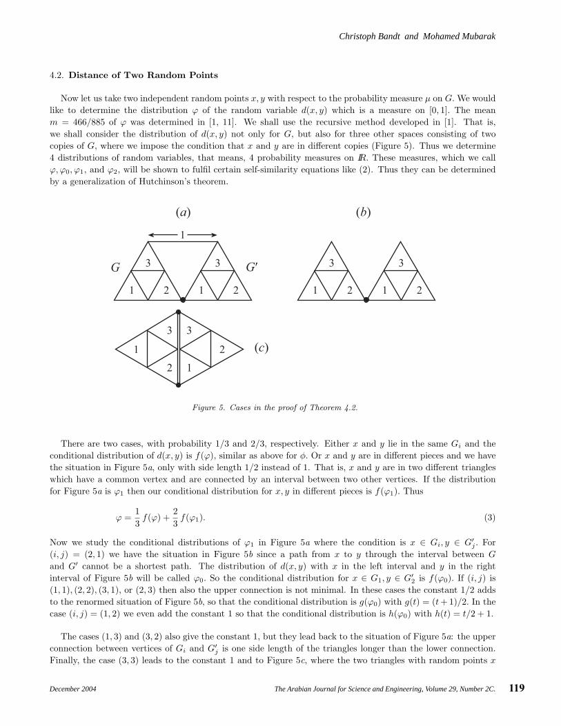
Now let us take two independent random points x, y with respect to the probability measure µ on G. We wouldlike to determine the distribution ϕ of the random variable d(x, y) which is a measure on [0, 1]. The meanm = 466/885 of ϕ was determined in [1, 11]. We shall use the recursive method developed in [1]. That is,we shall consider the distribution of d(x, y) not only for G, but also for three other spaces consisting of twocopies of G, where we impose the condition that x and y are in different copies (Figure 5). Thus we determine4 distributions of random variables, that means, 4 probability measures on IR. These measures, which we callϕ,ϕ0, ϕ1, and ϕ2, will be shown to fulfil certain self-similarity equations like (2). Thus they can be determinedby a generalization of Hutchinson’s theorem.

��

��

� �

�

� �

�

�

� �

�

� �

�

�

�

�

�

�

�

� ��

Figure 5. Cases in the proof of Theorem 4.2.

There are two cases, with probability 1/3 and 2/3, respectively. Either x and y lie in the same Gi and theconditional distribution of d(x, y) is f(ϕ), similar as above for φ. Or x and y are in different pieces and we havethe situation in Figure 5a, only with side length 1/2 instead of 1. That is, x and y are in two different triangleswhich have a common vertex and are connected by an interval between two other vertices. If the distributionfor Figure 5a is ϕ1 then our conditional distribution for x, y in different pieces is f(ϕ1). Thus

ϕ =13

f(ϕ) +23

f(ϕ1). (3)

Now we study the conditional distributions of ϕ1 in Figure 5a where the condition is x ∈ Gi, y ∈ G′j . For

(i, j) = (2, 1) we have the situation in Figure 5b since a path from x to y through the interval between G

and G′ cannot be a shortest path. The distribution of d(x, y) with x in the left interval and y in the rightinterval of Figure 5b will be called ϕ0. So the conditional distribution for x ∈ G1, y ∈ G′

2 is f(ϕ0). If (i, j) is(1, 1), (2, 2), (3, 1), or (2, 3) then also the upper connection is not minimal. In these cases the constant 1/2 addsto the renormed situation of Figure 5b, so that the conditional distribution is g(ϕ0) with g(t) = (t + 1)/2. In thecase (i, j) = (1, 2) we even add the constant 1 so that the conditional distribution is h(ϕ0) with h(t) = t/2 + 1.

The cases (1, 3) and (3, 2) also give the constant 1, but they lead back to the situation of Figure 5a: the upperconnection between vertices of Gi and G′

j is one side length of the triangles longer than the lower connection.Finally, the case (3, 3) leads to the constant 1 and to Figure 5c, where the two triangles with random points x



and y have two common vertices. If the distribution for Figure 5c is called ϕ2 we can collect our conditionaldistributions in order to obtain ϕ1.

ϕ1 =19

(f(ϕ0) + 4g(ϕ0) + h(ϕ0) + 2h(ϕ1) + h(ϕ2)) . (4)

The situation in Figure 5b is easy. d(x, y) = d(x, u) + d(u, y) implies that ϕ0 is the convolution of φ fromProposition 4.1 with itself:

ϕ0 = φ ∗ φ.

Using random sums, we can express ϕ0 as distribution of∑

k(ak + a′k)2−k where all ak and a′

k are independentrandom numbers which are 0 with probability 1/3 and 1 otherwise. Thus ak +a′

k is 0 with probability 1/9 and 2with probability 4/9, otherwise it is 1. Similar to Proposition 4.1, this implies that ϕ0 is a self-similar measure.(Compare Proposition 2.4, with x + y instead of x − y.)

ϕ0 =19f(ϕ0) +

49g(ϕ0) +

49h(ϕ0). (5)

The distribution ϕ2 of Figure 5c can be treated like ϕ1 in Figure 5a. For (2, 1), (3, 3) we get the conditionaldistribution f(ϕ0). For (1, 1), (1, 3), (2, 2), and (3, 2) we get g(ϕ1). For (2, 3), (3, 1) we get g(ϕ2) and for (1, 2) wehave h(ϕ2). Thus

ϕ2 =19

(2f(ϕ0) + 4g(ϕ1) + 2g(ϕ2) + h(ϕ2)) . (6)

Theorem 4.2. (Interior distance in the gasket)

The distribution φ of the interior distance d(x, y) of two random points x, y in G is determined from a graph-directed self-similar measure construction. More precisely, let ϕ1, ϕ0, and ϕ2 denote the distribution of d(x, y)where x and y run through G and G′ in Figure 5a, 5b, and 5c, respectively. Then the Equations (3) up to (6)are fulfilled. By these equations, ϕ,ϕ1, ϕ0, and ϕ2 are uniquely determined as probability measures on [0, 2].

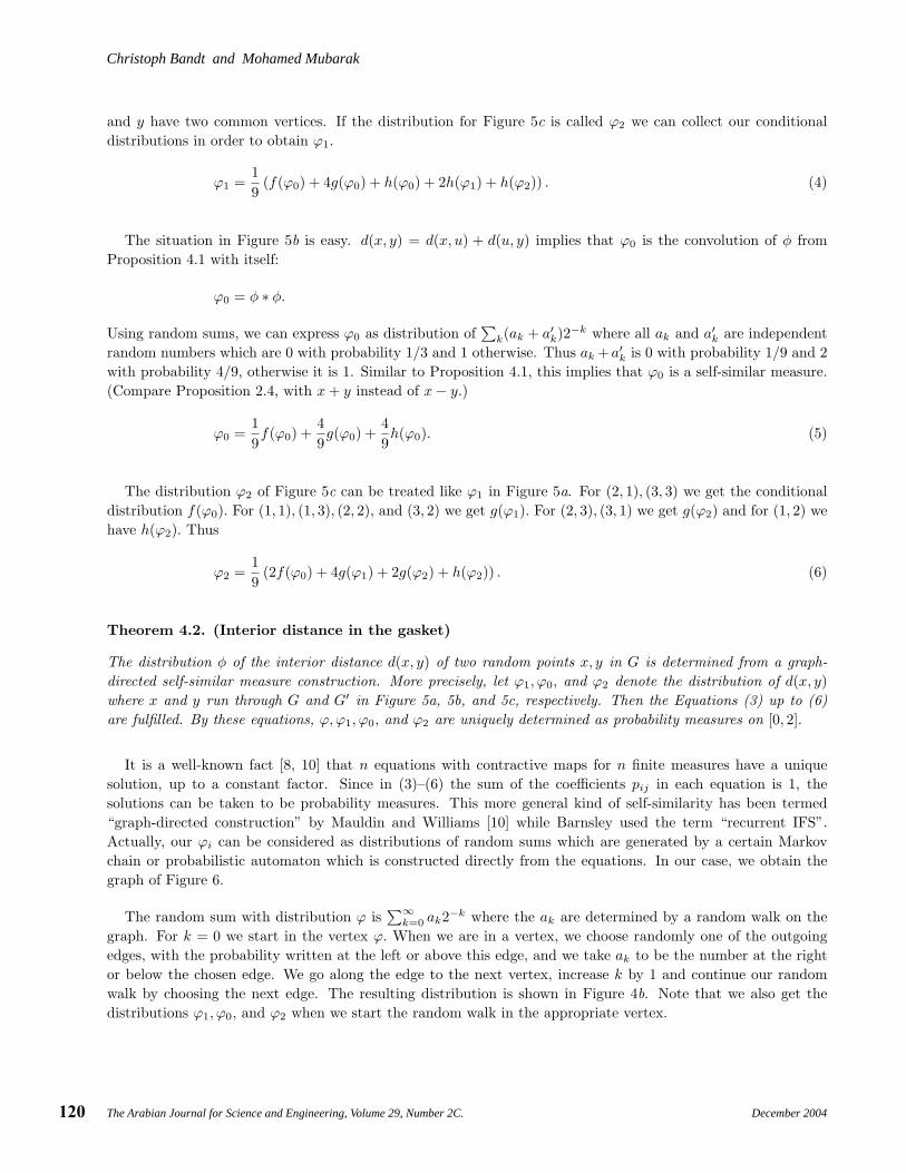
It is a well-known fact [8, 10] that n equations with contractive maps for n finite measures have a uniquesolution, up to a constant factor. Since in (3)–(6) the sum of the coefficients pij in each equation is 1, thesolutions can be taken to be probability measures. This more general kind of self-similarity has been termed“graph-directed construction” by Mauldin and Williams [10] while Barnsley used the term “recurrent IFS”.Actually, our ϕi can be considered as distributions of random sums which are generated by a certain Markovchain or probabilistic automaton which is constructed directly from the equations. In our case, we obtain thegraph of Figure 6.

The random sum with distribution ϕ is∑∞

k=0 ak2−k where the ak are determined by a random walk on thegraph. For k = 0 we start in the vertex ϕ. When we are in a vertex, we choose randomly one of the outgoingedges, with the probability written at the left or above this edge, and we take ak to be the number at the rightor below the chosen edge. We go along the edge to the next vertex, increase k by 1 and continue our randomwalk by choosing the next edge. The resulting distribution is shown in Figure 4b. Note that we also get thedistributions ϕ1, ϕ0, and ϕ2 when we start the random walk in the appropriate vertex.



Figure 6. Markov chain in the proof of Theorem 4.2.

5. SHORTEST PATHS IN THE SIERPINSKI CARPET

The Sierpinski carpet C shown in Figure 1b is more difficult to handle. We have no special vertices, like inthe gasket, which must lie on the path connecting two points. However, we have a lot of horizontal and verticalline segments in C. Let F denote the middle-third Cantor set — the self-similar subset of [0, 1] generated byg1(x) = x/3 and g2(x) = (x + 2)/3. Then the carpet contains F × [0, 1] and [0, 1] × F and all images of thesesets under the mappings f1, ..., f8 which generate the carpet, and under all images under compositions of thesefi. The union of these vertical and horizontal line segments has dimension 1 + log 2/ log 3 = log 6/ log 3 which issmaller than the dimension of C. A conclusion from our argument below, though not rigorously proved, is thattransport in C will only take place on this subset of smaller dimension. As concerns the gasket, it seems thattransport there takes place only on the sides of the small triangles, which form a subset of G of dimension 1.

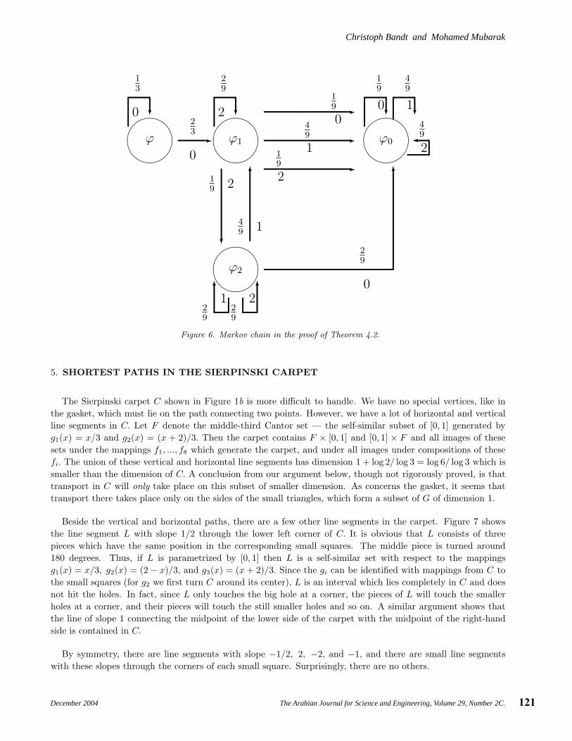
Beside the vertical and horizontal paths, there are a few other line segments in the carpet. Figure 7 showsthe line segment L with slope 1/2 through the lower left corner of C. It is obvious that L consists of threepieces which have the same position in the corresponding small squares. The middle piece is turned around180 degrees. Thus, if L is parametrized by [0, 1] then L is a self-similar set with respect to the mappingsg1(x) = x/3, g2(x) = (2 − x)/3, and g3(x) = (x + 2)/3. Since the gi can be identified with mappings from C tothe small squares (for g2 we first turn C around its center), L is an interval which lies completely in C and doesnot hit the holes. In fact, since L only touches the big hole at a corner, the pieces of L will touch the smallerholes at a corner, and their pieces will touch the still smaller holes and so on. A similar argument shows thatthe line of slope 1 connecting the midpoint of the lower side of the carpet with the midpoint of the right-handside is contained in C.

By symmetry, there are line segments with slope −1/2, 2, −2, and −1, and there are small line segmentswith these slopes through the corners of each small square. Surprisingly, there are no others.

��

ϕ

�...................................................................................................................................................

�.................................................................

23

0

13

0

��

ϕ1

�...................................................................................................................................................

29

2

�.................................................................................................................................................................................................19

2

�.................................................................................................................................................................................................49

1

�.................................................................................................................................................................................................19

0

��

ϕ0

�...................................................................................................................................................

19

0 �...................................................................................................................................

49

1

�...................................................................................................................

49

2

��

ϕ2

�.................................................................................................................................................................

19 2

�

...............

................

...............

...............

................

...............

...............

...............

................

...............

........

49 1

�

..................................................................................................................................................................................................................................................................................................................................................................................................................................................................................................................................

29

0�.................................................................................................................

................

..29

1�...................................................................................................................................

29

2



Figure 7. Other line beside the vertical and horizontal in the Sierpinski carpet.

Theorem 5.1. (Intervals and differentiable curves in the carpet)

Beside horizontal and vertical line segments, and those with slope ±1/2, ±1, and ±2 there are no other linesegments in C.

Moreover, C does not contain any differentiable curve except for these line segments.

Exact calculations will show that all other lines must hit a hole of the carpet. First, consider a line segment

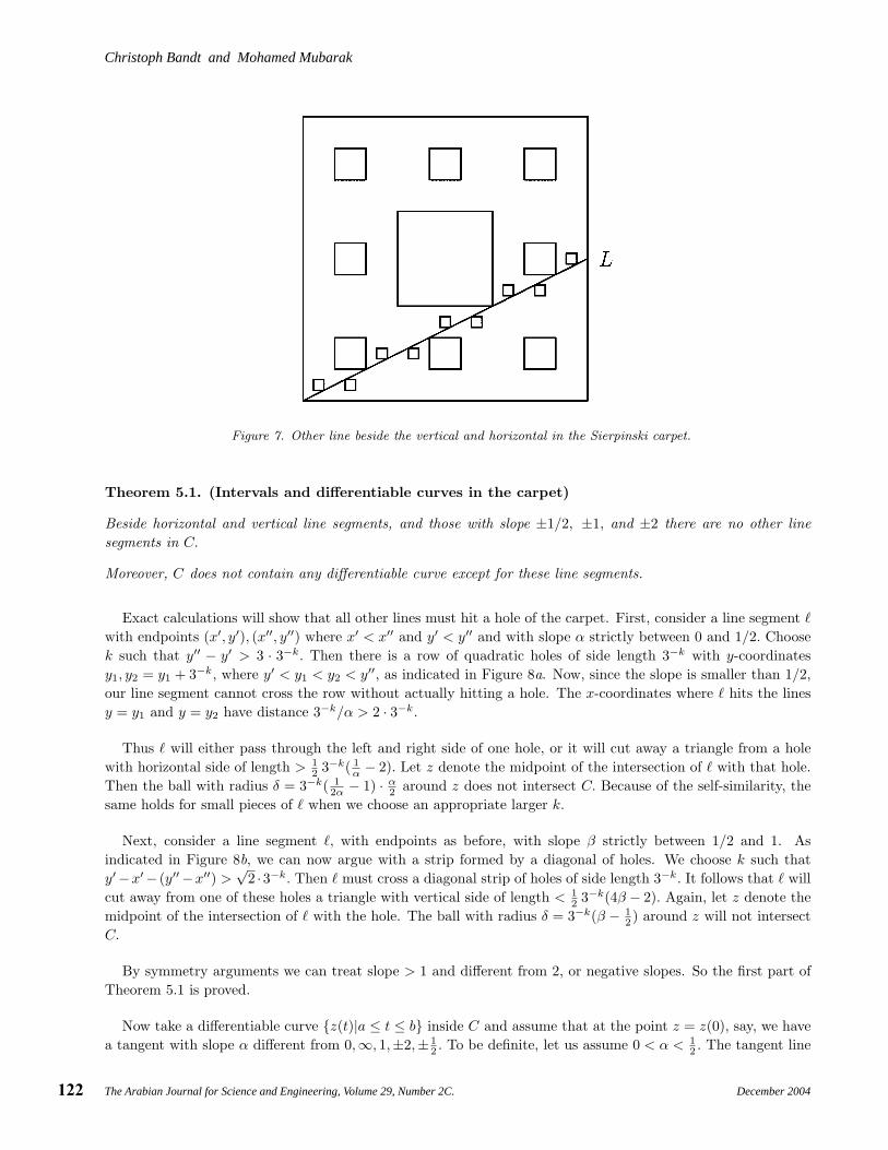
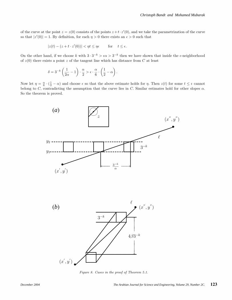
with endpoints (x′, y′), (x′′, y′′) where x′ < x′′ and y′ < y′′ and with slope α strictly between 0 and 1/2. Choosek such that y′′ − y′ > 3 · 3−k. Then there is a row of quadratic holes of side length 3−k with y-coordinatesy1, y2 = y1 + 3−k, where y′ < y1 < y2 < y′′, as indicated in Figure 8a. Now, since the slope is smaller than 1/2,

our line segment cannot cross the row without actually hitting a hole. The x-coordinates where hits the linesy = y1 and y = y2 have distance 3−k/α > 2 · 3−k.

Thus will either pass through the left and right side of one hole, or it will cut away a triangle from a holewith horizontal side of length > 1

2 3−k( 1α − 2). Let z denote the midpoint of the intersection of with that hole.

Then the ball with radius δ = 3−k( 12α − 1) · α

2 around z does not intersect C. Because of the self-similarity, thesame holds for small pieces of when we choose an appropriate larger k.

Next, consider a line segment , with endpoints as before, with slope β strictly between 1/2 and 1. Asindicated in Figure 8b, we can now argue with a strip formed by a diagonal of holes. We choose k such thaty′−x′− (y′′−x′′) >

√2 ·3−k. Then must cross a diagonal strip of holes of side length 3−k. It follows that will

cut away from one of these holes a triangle with vertical side of length < 12 3−k(4β − 2). Again, let z denote the

midpoint of the intersection of with the hole. The ball with radius δ = 3−k(β − 12 ) around z will not intersect

C.

By symmetry arguments we can treat slope > 1 and different from 2, or negative slopes. So the first part ofTheorem 5.1 is proved.

Now take a differentiable curve {z(t)|a ≤ t ≤ b} inside C and assume that at the point z = z(0), say, we havea tangent with slope α different from 0,∞, 1,±2,± 1

2 . To be definite, let us assume 0 < α < 12 . The tangent line



of the curve at the point z = z(0) consists of the points z + t · z′(0), and we take the parametrization of the curveso that |z′(0)| = 1. By definition, for each η > 0 there exists an ε > 0 such that

|z(t) − (z + t · z′(0))| < ηt ≤ ηε for t ≤ ε.

On the other hand, if we choose k with 3 · 3−k > εα > 3−k then we have shown that inside the ε-neighborhoodof z(0) there exists a point z of the tangent line which has distance from C at least

δ = 3−k

(12α

− 1)· α

2> ε · α

6·(

12− α

).

Now let η = α6 · ( 1

2 − α) and choose ε so that the above estimate holds for η. Then z(t) for some t ≤ ε cannotbelong to C, contradicting the assumption that the curve lies in C. Similar estimates hold for other slopes α.

So the theorem is proved.

��

��

Figure 8. Cases in the proof of Theorem 5.1.

(x′′, y

′′)

(x′, y

′)

........................................................................................................................................................................................................................................................................................................................................

........................................................................................................................................................................................................................................................................................................................................

...............

...............

...............

................

....................................................................................................................................................................................................... .................................................................................................................................................................................................................................................................... ...............

...............

...............

................

.......................................................................................................................................................................................................

..............................................................................................

..............................................................................................

..............................................................................................

..............................................................................................

..............................................................................................

..............................................................................................

..............................................................................................

.......................................................................................

.................................................................................................

.................................................................................................................................................................�

�

←−− 3−k

α−−→

3−k

y1

y2

�

....................................................................................................................................................................................................................................................................................................................................................................................................................................................................................................................................

...........................................................................................��z

b (x′′, y

′′)

(x′, y

′) ................................................................................

................

...............

...............

......................................................................................................................................

....................................................................................................................................................................................................................................................................

.................................................................................................................................................................................................................................................................................................................................

.................................................................................................................................................................................................................................................................................................................................

..................................................................................................................................................................................................................................................................................................................................................................................................................................................................................................................................................

.................................................................................................................................................................................................................................................................................................................................

..................................................................................................................................................................................................

.................................................................................................................................

�

�↑|||

4β3−k

|||↓

3−k

�

(a)

(b)



Remark. The proof implies that there are only countably many line segments with slope ±1/2 and ±2. Thus theunion of all these line segments has dimension one. On the other side, vertical and horizontal line segments occurin uncountable number, and their union has dimension 1 + log 2/ log 3. For the gasket, we have only countablemany line segments altogether, with three possible directions, and there are also no other smooth curves.

6. CONCLUSION

We have demonstrated how self-similarity of a measure can be used to identify more complicated objects, likethe correlation measure, and the exact distribution of interior distances in the Sierpinski gasket. Moreover, weproved that in both gasket and carpet, shortest paths have a very special structure.

These two sets are the well-established standard models for transport in fractals. Starting with the studiesof Barlow, Perkins, and Bass [12], numerous papers have appeared which investigate fine details, as for instancethe sequence of eigenvalues and eigenfunctions of the Laplace operator. Our results indicate that transportproperties of gasket and carpet are perhaps not typical for all self-similar fractals. It seems necessary to studyother fractal sets which for instance do not contain any line segments.

REFERENCES

[1] C. Bandt and T. Kuschel, “Self-Similar Sets 8. Average Interior Distance in Some Fractals”, Rendiconti Circolo Matem. Palermo,28 (1992), suppl., pp. 307–317.

[2] R. Strichartz, “Isoperimetric Estimates on Sierpinski Gasket Type Fractals”, Trans. Amer. Math. Soc., 351 (1999),pp. 1705–1752.

[3] C. Bandt and J. Stahnke, “Self-Similar Sets 6. Interior Distance in Deterministic Fractals”, Preprint, Greifswald, 1990.

[4] K. Falconer, Techniques in Fractal Geometry. Chichester: John Wiley, 1997.

[5] P. Mattila, Geometry of Sets and Measures in Euclidean Space. Cambridge: Cambridge University Press, 1995.

[6] J.E. Hutchinson, “Fractals and Self-Similarity”, Indiana Univ. Math. J., 30 (1981), pp. 713–747.

[7] J.C. Lagarias and Y. Wang, “Self-Affine Tiles in IRn”, Adv. in Math., 121 (1996), pp. 21–49.

[8] M. Barnsley, Fractals Everywhere, 2nd edn. New York: Academic Press, 1993.

[9] W. Rinow, Die innere Geometrie der metrischen Raume. Berlin: Springer, 1961.

[10] G.A. Edgar, Measure, Topology, and Fractal Geometry. Berlin: Springer, 1990.

[11] A.M. Hinz and A. Schief, “The Average Distance on the Sierpinski Gasket”, Probab. Th. Rel. Fields, 87 (1990), pp. 129–138.

[12] M.T. Barlow and R.F. Bass, “Transition Densities for Brownian Motion on the Sierpinski Carpet”, Probab. Th. Rel. Fields,91 (1992), pp. 307–330.

Paper Received 16 December 2002; Revised 1 September 2003; Accepted 26 October 2003.

DISTRIBUTION OF DISTANCES AND INTERIOR DISTANCES FOR CERTAIN SELF-SIMILAR MEASURES

Documents

Transcript of DISTRIBUTION OF DISTANCES AND INTERIOR DISTANCES FOR CERTAIN SELF-SIMILAR MEASURES