Measuring of distances of genotype strains and clustering methods.

Measures of distances of genotype strains and

clustering methods.

Andrea Scholtz

November, 2012

1 Introduction

The objective of this paper is to describe and investigate an appropriate metricfor measuring the distance between two virus strains - specifically RNA strainmutations - and then arranging these strain mutations meaningfully in order toproduce a natural fitness landscape. The problem under discussion is one wherean arbitrary number of loci and alleles, on a non-specific gene, are considered.This consideration consists of all possible mutations that may occur within thatstrain. For the sake of simplicity we consider finite strains of 4 loci and 4 allelesin the investigation of the clustering algorithm.

We discuss the possibilities of a metric which can describe the distance betweentwo genotypes by considering Mattiussi et al. (2004) and we proceed by im-plementing this metric into a MATLABr program given in the supplementarymaterial of this paper. The measure of distance used represents the dissimi-larity of strains relative to each other. We do not assume any knowledge ofthe structure of the genome. We also refer to the set of alleles as an alphabet.These distances between strains are then used to arrange the strains by methodof clustering. The method of clustering is discussed and it is motivated why thehierarchical clustering method and the specific clustering algorithm is applied.We give attention to the choice of linkage that is used in the clustering and wechoose the number of clusters formed from the clustered data, showing that itis more an intuitive step than a fixed rule.

A short discussion on the implementation and shortcomings of the applied tech-niques is given. We discuss possible difficulties that may be encountered whenapplying different clustering methods and algorithms (Vipin, 2010). The im-plementation of the outcome of this project has interesting applications in themodelling of pathogen evolution. For instance, the work done here may be im-plemented into a computer simulation to find the fitness landscape of the viralload of different genotypes over time. We must henceforth find a suitable met-ric for arranging these strains in such a way that the fitness landscape is welldefined and produces a continuous landscape given the domain of genotypesversus time. We do not take genetic drift into account and consider a genotypespace in which one genotype gives origin to another purely by method of muta-tion. Finally we conclude the investigation by summarising the steps taken tofind our results and we introduce and shortly discuss the cophenetic correlation

Genotype distance and clustering 2

coefficient and how the clustering correlates to the original distances betweenthe data.

2 Background

The problem under discussion is one where we are interested in strain mutationsrelevant to the within-host dynamics of viruses. The specific model we refer tois the model stated in Lange & Ferguson (2004), that is,

dVidt

= (1− µ)ρV sati (v, c)− ψVi − σViyi(X) (1)

dXi

dt= ξ(x0 −Xi) + ζXsat

i (Vi) (2)

dc

dt= κ(c0 − c)−

ρ

v1vsat(v, c) (3)

where each equation is applied to the i-th strain. In our case we have 256 strainsthat are results of a single strain mutating into all possible different combina-tions for a given number of loci and allelles. We note that (1) gives the rate ofchange of the viral load for the i-th strain, (2) is the immune response to thei-th strain and (3) is the level of resources which the stains need to replicate.Note that v is the total viral load that is present, hence v =

∑ni=0 Vi where

n+ 1 corresponds to the number of equations and also the number of differentstrains under consideration.

We assume that mutations are random with the first strain the origin of allothers. The parameter µ is the probability that a mutation occurs and ρ reflectsthe rate at which it occurs. Only a proportion of mutations give rise to newstrain variants or genotypes, that is δ. We refer to the space described by ρ andδ as the pathogen space.

2.1 Definitions and methodology

Given this background information, we now define a few key concepts which areof importance in this investigation.

Definition 1: The distance between two elements x1, x2 ∈ X is a functiond : X ×X → R such that for all x1, x2 and x3 ∈ X the following holds:

(M1) d(·, ·) ≥ 0, d ∈ R(M2) d(x1, x2) = 0 ⇔ x1 = x2

(M3) d(x1, x2) = d(x2, x1)

(M4) d(x1, x2) ≤ d(x1, x3) + d(x3, x2)

We call this distance function d a metric. The space (X, d) or simply X is calleda metric space. If (M4) does not hold, we call d a semimetric on X.

The objective of the research, stated broadly, is defining a metric to measure thesimilarity between objects and then grouping them together in such a way thatthese groups of objects can be said to be similar in a sense. That is, objects in

North-West University, Potchefstroom Campus


a certain group are more similar than mutually compared objects from differentgroups. The measure we use to group them according to some similarity is thedistance between the strains. We refer to groups of similar strains as a cluster.We are in search of a distance function which maps the space of the cartesianproduct of strains into the space of non-negative real numbers. It is convenientto normalise this distance by defining that strains that are completely similar,that is, not dissimilar, must have the distance d(ιi, ιj) = 0 and strains that arecompletely dissimilar, that is, not similar, must have the distance d(ιi, ιj) = 1.

Accordingly we use Cluster Analyses to decide upon a suitable clustering methodand algorithm. The idea behind the clustering method is rather easy: We definea matrix of each strain’s distance relative to each other strain, i.e. a distancematrix. To calculate the distance between each strain we need a suitable metricor distance function. This matrix is then used to group the data into clusters.This is then implemented into an algorithm that delivers a fitness landscapeof the viral load of the different genotypes over time. It will be convenient tofind m distinct clusters from the data. Another interesting question that is ad-dressed is finding the value of m - that is, into how many clusters do we haveto group the strains.

For the purpose of our investigation, we define the following concepts:

Definition 2: The specific location on a gene where different alleles may occuris referred to as a locus (pl. loci).

Definition 3: Alleles are alternative forms of a gene that may occur at a locus.That is, alleles are variants of a certain gene.

Definition 4: We refer to the change of an allele at specific loci as a mutation.

Mutations of alleles at a specific locus shall be noted and thereby a distancedefined for this mutation. It must be noted that strains aabb and abab are notidentical, because we find that the different alleles a and b on the latter arelocated at the alternate loci (a at locus 1 and 3, b at locus 2 and 4), as opposedto the former string.

Definition 5: We define a distance (proximity) matrix as a matrix which hasentries that reflect the mutual distances between objects. That is for objectsx1, x2, ..., xn :

D =

d(x1, x1) d(x1, x2) · · · d(x1, xn)d(x2, x1) d(x2, x2) · · · d(x2, xn)d(x3, x1) d(x3, x2) · · · d(x3, xn)

......

. . ....

d(xn, x1) d(xn, x2) · · · d(xn, xn)

.When the measure between the objects considered illustrates dissimilarity (sim-ilarity), we refer to the matrix as a dissimilarity (similarity) matrix.



The two basic approaches to generating hierarchical clusters are agglomerativeand divisive.

Definition 6: Divisive algorithms form clusters from one, single, all-inclusivecluster and splits the clusters until we are left with individual points.

Definition 7: Agglomerative algorithms start with the individual points andcluster them accordingly until one is left with one, all-inclusive cluster, mergingclusters in close proximity.

3 The Distance between strings

Diversity of individuals and even populations can be measured in either thegenotype or phenotype space (Mattiussi et al., 2004). In this investigation weare interested in measuring diversity in the genotype space. It is possible tomeasure the distance between strains where we have a fixed number of param-eters in n-dimensional space. However, when we work with genotypes withina variable topology and number of parameters, it is more sensible to define aspecialised distance between strains. We consider strings consisting of finitestring characters over a finite alphabet. A viable option is to use the Hammingdistance in measuring the distance between individual strains, but this deliverssome unwanted results. It is interesting to note that a generalised Hammingdistance measure may be introduced for strains of different lengths as in Sellers(1974) and Waterman et al. (1976). The metric (and semi-metric) we discussare measures of dissimilarity between strains. This is important to note whenwe implement the clustering algorithm. We proceed as follows:

Consider individuals ιj in a population Π, where sιj is the genome of the indi-vidual ιj . The population is defined as Π = {ι1, ι2, ..., ιn}. We denote the setof all substrings of an individual genome sιj , by Ψιj , and |Ψιj | the cardinalityof the set of all substrings. Hence, the set of all substrings of genomes within apopulation Π is the set of all substrings in the set {sι1 , sι2 , ..., sιn}. We denotethis set by Ψ{ι1,ι2,...,ιn}, and it is then easily seen that Ψ{ι1,ι2,...,ιn} =

⋃nj=1 Ψιj .

Before we introduce the concept of distance between individuals, we first discusspopulation diversity.

Definition 8: We define the measure of diversity of a population δ(Π) asfollows:

δ(Π) = δ({ι1, ι2, ..., ιn})

= n|Ψ{ι1,ι2,...,ιn}|∑n

j=1 |Ψιj |. (4)

That is, the diversity of the population is defined as n times the ratio of the totalnumber of substrings in the population to the cumulative number of substringsof genomes of each individual.



3.1 Substring distance

From (4) we now define the distance between individuals as the diversity betweentwo distinct individuals from the population. Since 1 ≤ δ(ιj , ιk) ≤ 2, we adjustthe inequality such that δ(ιj , ιk)− 1 = d(ιj , ιk). That is:

d(ιj , ιk) = 2|Ψ{ιj ,ιk}||Ψιj |+ |Ψιk |

− 1. (5)

We first observe that this function satisfies (M1) and (M2) for all ιj . Sec-ondly, it is easy to verify that (M3) indeed holds for all ιj and ιk such thatd(ιj , ιk) = d(ιk, ιj). Finally, we can see that due to the summation in the denom-inator of the function, it does not satisfy (M4) and therefore it is a semi-metric.We illustrate this semi-metric by considering the following example.

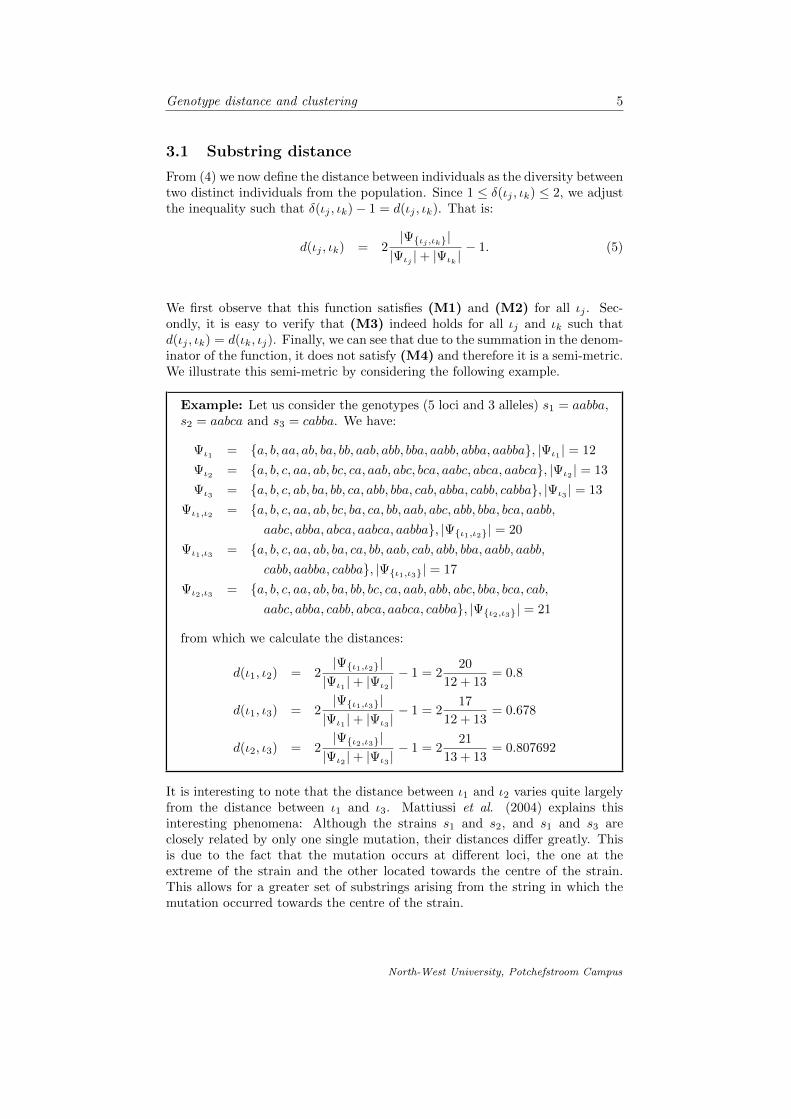
Example: Let us consider the genotypes (5 loci and 3 alleles) s1 = aabba,s2 = aabca and s3 = cabba. We have:

Ψι1 = {a, b, aa, ab, ba, bb, aab, abb, bba, aabb, abba, aabba}, |Ψι1 | = 12

Ψι2 = {a, b, c, aa, ab, bc, ca, aab, abc, bca, aabc, abca, aabca}, |Ψι2 | = 13

Ψι3 = {a, b, c, ab, ba, bb, ca, abb, bba, cab, abba, cabb, cabba}, |Ψι3 | = 13

Ψι1,ι2 = {a, b, c, aa, ab, bc, ba, ca, bb, aab, abc, abb, bba, bca, aabb,aabc, abba, abca, aabca, aabba}, |Ψ{ι1,ι2}| = 20

Ψι1,ι3 = {a, b, c, aa, ab, ba, ca, bb, aab, cab, abb, bba, aabb, aabb,cabb, aabba, cabba}, |Ψ{ι1,ι3}| = 17

Ψι2,ι3 = {a, b, c, aa, ab, ba, bb, bc, ca, aab, abb, abc, bba, bca, cab,aabc, abba, cabb, abca, aabca, cabba}, |Ψ{ι2,ι3}| = 21

from which we calculate the distances:

d(ι1, ι2) = 2|Ψ{ι1,ι2}||Ψι1 |+ |Ψι2 |

− 1 = 220

12 + 13= 0.8

d(ι1, ι3) = 2|Ψ{ι1,ι3}||Ψι1 |+ |Ψι3 |

− 1 = 217

12 + 13= 0.678

d(ι2, ι3) = 2|Ψ{ι2,ι3}||Ψι2 |+ |Ψι3 |

− 1 = 221

13 + 13= 0.807692

It is interesting to note that the distance between ι1 and ι2 varies quite largelyfrom the distance between ι1 and ι3. Mattiussi et al. (2004) explains thisinteresting phenomena: Although the strains s1 and s2, and s1 and s3 areclosely related by only one single mutation, their distances differ greatly. Thisis due to the fact that the mutation occurs at different loci, the one at theextreme of the strain and the other located towards the centre of the strain.This allows for a greater set of substrings arising from the string in which themutation occurred towards the centre of the strain.



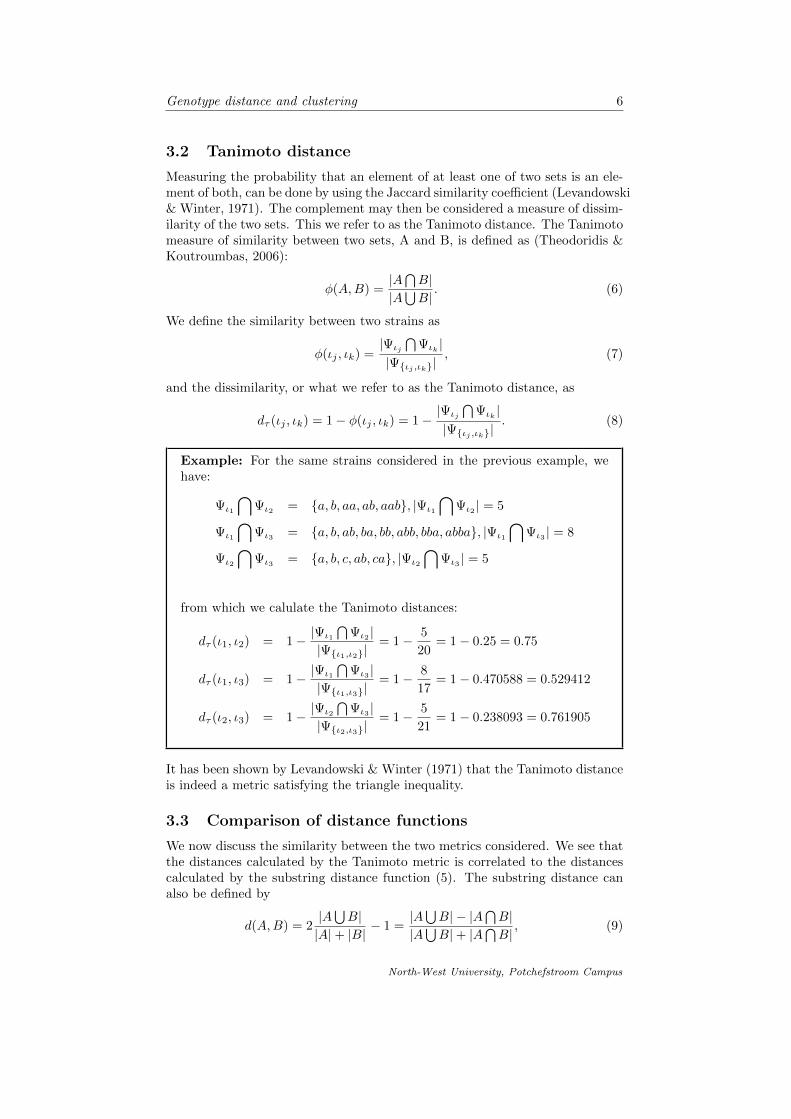
3.2 Tanimoto distance

Measuring the probability that an element of at least one of two sets is an ele-ment of both, can be done by using the Jaccard similarity coefficient (Levandowski& Winter, 1971). The complement may then be considered a measure of dissim-ilarity of the two sets. This we refer to as the Tanimoto distance. The Tanimotomeasure of similarity between two sets, A and B, is defined as (Theodoridis &Koutroumbas, 2006):

φ(A,B) =|A

⋂B|

|A⋃B|. (6)

We define the similarity between two strains as

φ(ιj , ιk) =|Ψιj

⋂Ψιk |

|Ψ{ιj ,ιk}|, (7)

and the dissimilarity, or what we refer to as the Tanimoto distance, as

dτ (ιj , ιk) = 1− φ(ιj , ιk) = 1−|Ψιj

⋂Ψιk |

|Ψ{ιj ,ιk}|. (8)

Example: For the same strains considered in the previous example, wehave:

Ψι1

⋂Ψι2 = {a, b, aa, ab, aab}, |Ψι1

⋂Ψι2 | = 5

Ψι1

⋂Ψι3 = {a, b, ab, ba, bb, abb, bba, abba}, |Ψι1

⋂Ψι3 | = 8

Ψι2

⋂Ψι3 = {a, b, c, ab, ca}, |Ψι2

⋂Ψι3 | = 5

from which we calulate the Tanimoto distances:

dτ (ι1, ι2) = 1− |Ψι1

⋂Ψι2 |

|Ψ{ι1,ι2}|= 1− 5

20= 1− 0.25 = 0.75

dτ (ι1, ι3) = 1− |Ψι1

⋂Ψι3 |

|Ψ{ι1,ι3}|= 1− 8

17= 1− 0.470588 = 0.529412

dτ (ι2, ι3) = 1− |Ψι2

⋂Ψι3 |

|Ψ{ι2,ι3}|= 1− 5

21= 1− 0.238093 = 0.761905

It has been shown by Levandowski & Winter (1971) that the Tanimoto distanceis indeed a metric satisfying the triangle inequality.

3.3 Comparison of distance functions

We now discuss the similarity between the two metrics considered. We see thatthe distances calculated by the Tanimoto metric is correlated to the distancescalculated by the substring distance function (5). The substring distance canalso be defined by

d(A,B) = 2|A

⋃B|

|A|+ |B|− 1 =

|A⋃B| − |A

⋂B|

|A⋃B|+ |A

⋂B|, (9)



which clearly shows a close similarity to the Tanimoto distance, i.e.

dτ (A,B) = 1− |A⋂B|

|A⋃B|

=|A

⋃B| − |A

⋂B|

|A⋃B|

. (10)

Here we see the factor in the denominator is slightly larger. It is interesting tonote that the distance functions which we discussed might have the underlyingproperty that they may, in addition to defining a distance between genotypes,also distinguish between the functionality between genotypes. This result isconcluded by taking into account that we consider the substrings of a string,regardless of the alleles. It should be noted that the MATLABr algorithm in-cluded in the supplementary material is computationally intense - computationof the distance matrix D for the 4 loci and 4 alleles case can take up to 120seconds on the average computer. One may attempt to optimise the code. Oncomputing the distance matrix of the objects using both the substring distanceand the Tanimoto distance, two matrices are obtained which appear to be verysimilar. Upon investigating, we find that the norm of the difference of the twomatrices is of the order 10−15. It seems that the two metrics are correlated andit is expected that similar results will be be obtained when applying either tothe clustering algorithm which we discuss in the next section.

4 Clustering of strings

Cluster analysis groups data based on information found between the data con-sidered. In short, cluster analysis is the grouping of objects into clusters basedon their similarity (Jain et al., 1999). In order to group similar objects together,we need to determine a clustering criterion (Theodoridis & Koutroumbas, 2006).Objects that are more similar are grouped together in more distinct clusters anddifferent clustering criterion may result in different clusters being formed. Theclustering criterion is a criterion selected, based on a specific property of theobjects under consideration. We define the concept of clustering in terms of apartition of a class of sets.

Definition 9: Let Φ = {ξ1, ξ2, ..., ξN} be the set of objects. We define Γ as them-clustering of Φ into m clusters γ1, γ2, ...γm, such that the following conditionsare met:

(i) γj 6= ∅, j = 1, ...,m,

(ii)

m⋃j=1

γj = Φ,

(iii) γj⋂γk = ∅ ∀ j 6= k.

It may happen that clusters are not well separated from each other. Usingcluster analysis, we may group data in a meaningful way as to reveal the naturalstructure of the data and therefore we use cluster analysis to group genes whichare similar (or dissimilar) to a certain extent. For instance, when we want togroup these genes according to their functionality (Vipin, 2010). In this paper



we wish to group genotypes according to an underlying phenomena, e.g. geneticmutation. To accomplish this we firstly discussed a suitable metric according towhich we calculate the distances between distinct genotypes. We now implementthis metric into a suitable clustering algorithm. We proceed accordingly.

4.1 Hierarchical Clustering

Hierarchical clustering is a useful clustering technique due to the fact that in-stead of selecting m clusters before applying the clustering algorithm, the datais clustered into a hierarchy of clusters from which the m clusters can then beselected. Hierarchical clustering algorithms produce a hierarchy of nested clus-ters (Theodoridis & Koutroumbas, 2006). We use MATLABr to implementthe clustering algorithm. The algorithm used is known as the agglomerativehierarchical clustering algorithm.

Basic Agglomerative Hierarchical Clustering Algorithm:

(i) Initialisation:

(a) Choose Γ0 as the initial clustering

(b) Let t = 0

(ii) Repeat the following steps until all vectors lie within a single cluster

(a) t = t+ 1

(b) Find the pair of clusters (γj , γk) such that for all possible pairs ofclusters (γr, γs) in Γt−1 it follows that

g(γj , γk) =

{minr,s g(γr, γs) if g is a dissimilarity function

maxr,s g(γr, γs) if g is a similarity function

4.1.1 Motivation

Hierarchical clustering is applied in this paper due to the frequent use thereof inbiological taxinomy and sequencing (Jain et al. 1999; Vipin, 2010). It should bekept in mind that the genotypes which we are attempting to order accordingly,do not have Euclidean distance defined between them. Therefore they cannottruly be arranged on a system of axes, because one allele can easily mutate andchange to any other allele. No alleles can be quantified numerically such thatthe distance from one is closer (or further) to the other. We defined a metric bywhich we quantify the dissimilarity of two genotypes and we use this metric asour clustering criterion. The genotypes are then ordered accordingly and thisordering occurs in the genotype space with a topology different from that ofRn. Therefore the clustering by method of a hierarchical clustering algorithmis completely plausible.

5 Three general linkages used in hierarchical clus-tering

We are interested in visualising the clustering. This is possible by using adendrogram exclusive to the hierarchical clustering method. A dendrogram is a



361315122845 416 549 3 9113542 7193410 2 61822 82914201721383125273324264140323037464439484750 14323

0.65

0.7

0.75

0.8

0.85

0.9

4032304624372733264144394847 2 61822 8282914201721383125 3 9113542 7193410 416 5491245153613504323 1

0.65

0.7

0.75

0.8

0.85

0.9

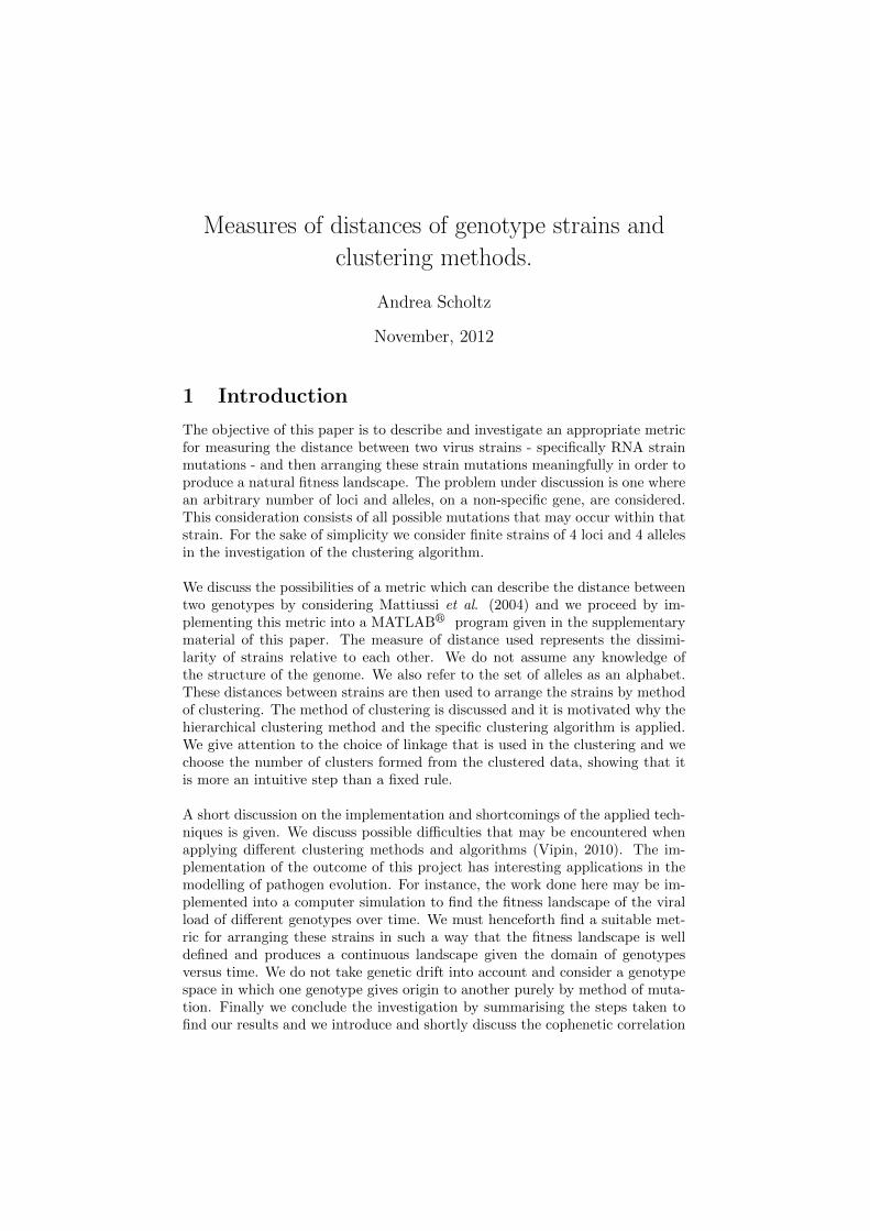
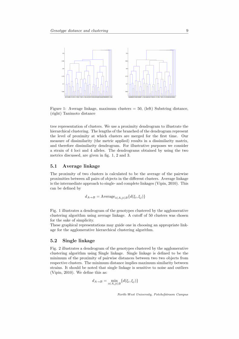
Figure 1: Average linkage, maximum clusters = 50, (left) Substring distance,(right) Tanimoto distance

tree representation of clusters. We use a proximity dendrogram to illustrate thehierarchical clustering. The lengths of the branched of the dendrogram representthe level of proximity at which clusters are merged for the first time. Ourmeasure of dissimilarity (the metric applied) results in a dissimilarity matrix,and therefore dissimilarity dendrogram. For illustrative purposes we considera strain of 4 loci and 4 alleles. The dendrograms obtained by using the twometrics discussed, are given in fig. 1, 2 and 3.

5.1 Average linkage

The proximity of two clusters is calculated to be the average of the pairwiseproximities between all pairs of objects in the different clusters. Average linkageis the intermediate approach to single- and complete linkages (Vipin, 2010). Thiscan be defined by

dA→B = Averagei∈A,j∈B{d(ξi, ξj)}

Fig. 1 illustrates a dendrogram of the genotypes clustered by the agglomerativeclustering algorithm using average linkage. A cutoff of 50 clusters was chosenfor the sake of simplicity.These graphical representations may guide one in choosing an appropriate link-age for the agglomerative hierarchical clustering algorithm.

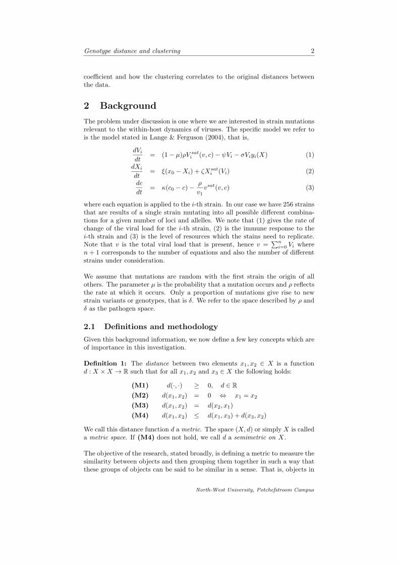
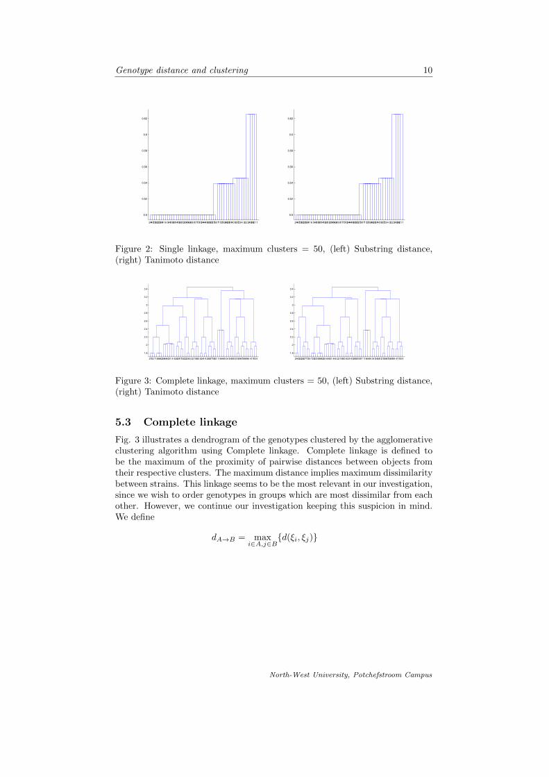
5.2 Single linkage

Fig. 2 illustrates a dendrogram of the genotypes clustered by the agglomerativeclustering algorithm using Single linkage. Single linkage is defined to be theminimum of the proximity of pairwise distances between two two objects fromrespective clusters. The minimum distance implies maximum similarity betweenstrains. It should be noted that single linkage is sensitive to noise and outliers(Vipin, 2010). We define this as:

dA→B = mini∈A,j∈B

{d(ξi, ξj)}



24472932335041 6 54818301419261320454243 817151034441639352738 711251246283140 93723 4 322 2493621 1

0.5

0.52

0.54

0.56

0.58

0.6

0.62

24472932335041 6 54818301419261320454243 817151034441639352738 711251246283140 93723 4 322 2493621 1

0.5

0.52

0.54

0.56

0.58

0.6

0.62

Figure 2: Single linkage, maximum clusters = 50, (left) Substring distance,(right) Tanimoto distance

2732 710384228464031 9 626291733222343 2211820 824141330371925 1164449 341343612153947354548 41150 5

1.8

2

2.2

2.4

2.6

2.8

3

3.2

3.4

24432226271729 7252310384228 64631 940 2211820 833141330351937 1164449 341343612153947324548 41150 5

1.8

2

2.2

2.4

2.6

2.8

3

3.2

3.4

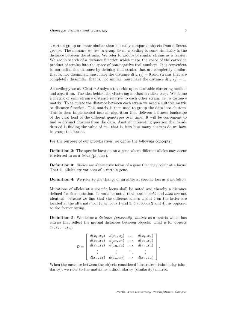
Figure 3: Complete linkage, maximum clusters = 50, (left) Substring distance,(right) Tanimoto distance

5.3 Complete linkage

Fig. 3 illustrates a dendrogram of the genotypes clustered by the agglomerativeclustering algorithm using Complete linkage. Complete linkage is defined tobe the maximum of the proximity of pairwise distances between objects fromtheir respective clusters. The maximum distance implies maximum dissimilaritybetween strains. This linkage seems to be the most relevant in our investigation,since we wish to order genotypes in groups which are most dissimilar from eachother. However, we continue our investigation keeping this suspicion in mind.We define

dA→B = maxi∈A,j∈B

{d(ξi, ξj)}



6 Implementation

These graphical representations in fig. 1 to fig. 3 may guide one in choosingan appropriate linkage for the agglomerative hierarchical clustering algorithm.The procedure for forming these clusters can be summarised in the followinginstructions:

(i) Create a matrix of all possible mutations of genotypes of 4 loci and 4alleles.

(ii) This matrix is then given as input to the MATLABr program D = GenDist(X)which computes the distance matrix D.

(iii) From this matrix D, we form a vector of pairwise distances using Y =squareform(D,’tovector’).

(iv) Now, we compute the linkages by using Z = linkage(Y,’method’)where the method is specified as single, complete or average.

(a) At this point one can plot the dendrogram of the data using theinstruction dendrogram(Z,n) where n is the number of clusterswe would like to illustrate.

(v) We continue by clustering the genotype objects using the instruction C =cluster(Z,’maxclust’,n) where n again represents the number ofclusters we would like our data to be arranged in.

(a) We can represent the clustering graphically on the XY-plane by plot-ting the genotype object against in which cluster it is be found. Thisis done as one would normally plot such a graph using scatter.

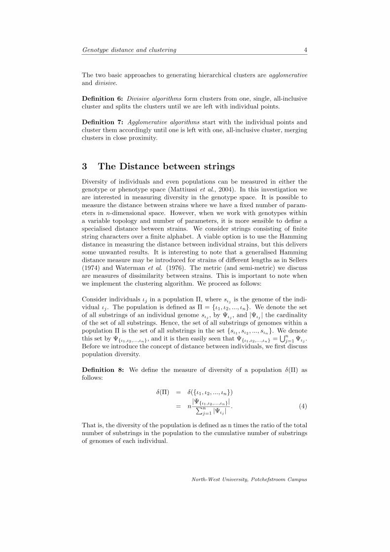
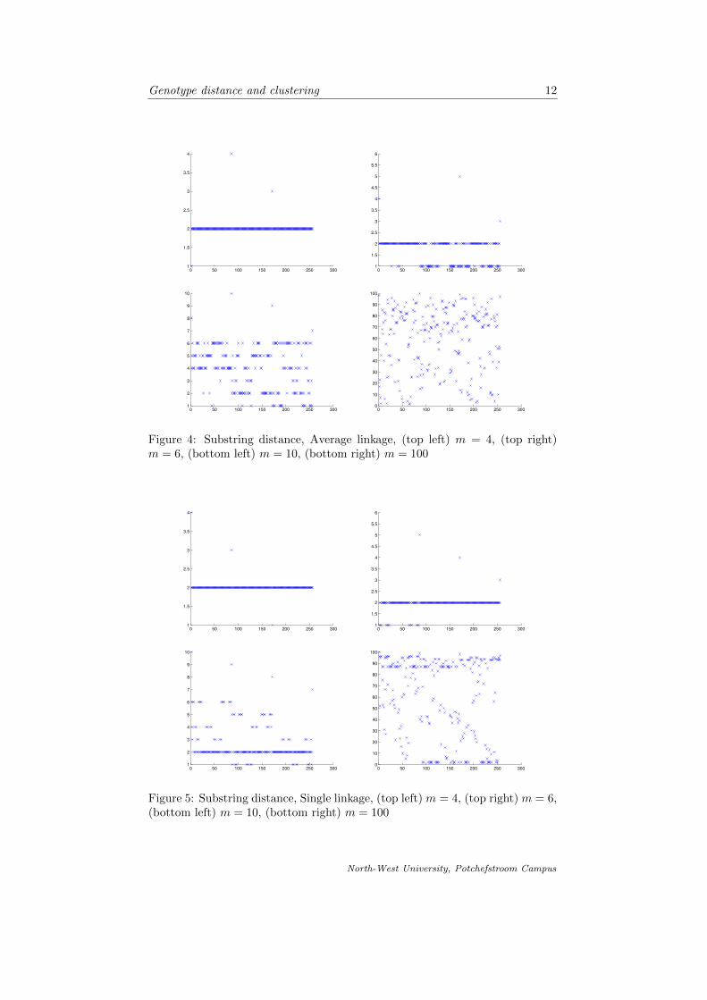
In fig. 4-9 we compare the different linkages and respective metrics that we havediscussed. For each case we cluster the genotype objects into 4, 6, 10 and 100clusters respectively.

After the clustering has been done the genotypes clustering can be implementedinto a procedure to model the fitness landscape of genotypes over time. Thisimplementation can be used for instance in the within-host model in Lange &Ferguson (2004).



0 50 100 150 200 250 3001

1.5

2

2.5

3

3.5

4

0 50 100 150 200 250 3001

1.5

2

2.5

3

3.5

4

4.5

5

5.5

6

0 50 100 150 200 250 3001

2

3

4

5

6

7

8

9

10

0 50 100 150 200 250 3000

10

20

30

40

50

60

70

80

90

100

Figure 4: Substring distance, Average linkage, (top left) m = 4, (top right)m = 6, (bottom left) m = 10, (bottom right) m = 100

0 50 100 150 200 250 3001

1.5

2

2.5

3

3.5

4

0 50 100 150 200 250 3001

1.5

2

2.5

3

3.5

4

4.5

5

5.5

6

0 50 100 150 200 250 3001

2

3

4

5

6

7

8

9

10

0 50 100 150 200 250 3000

10

20

30

40

50

60

70

80

90

100

Figure 5: Substring distance, Single linkage, (top left) m = 4, (top right) m = 6,(bottom left) m = 10, (bottom right) m = 100



0 50 100 150 200 250 3001

1.5

2

2.5

3

3.5

4

0 50 100 150 200 250 3001

1.5

2

2.5

3

3.5

4

4.5

5

5.5

6

0 50 100 150 200 250 3001

2

3

4

5

6

7

8

9

10

0 50 100 150 200 250 3000

10

20

30

40

50

60

70

80

90

100

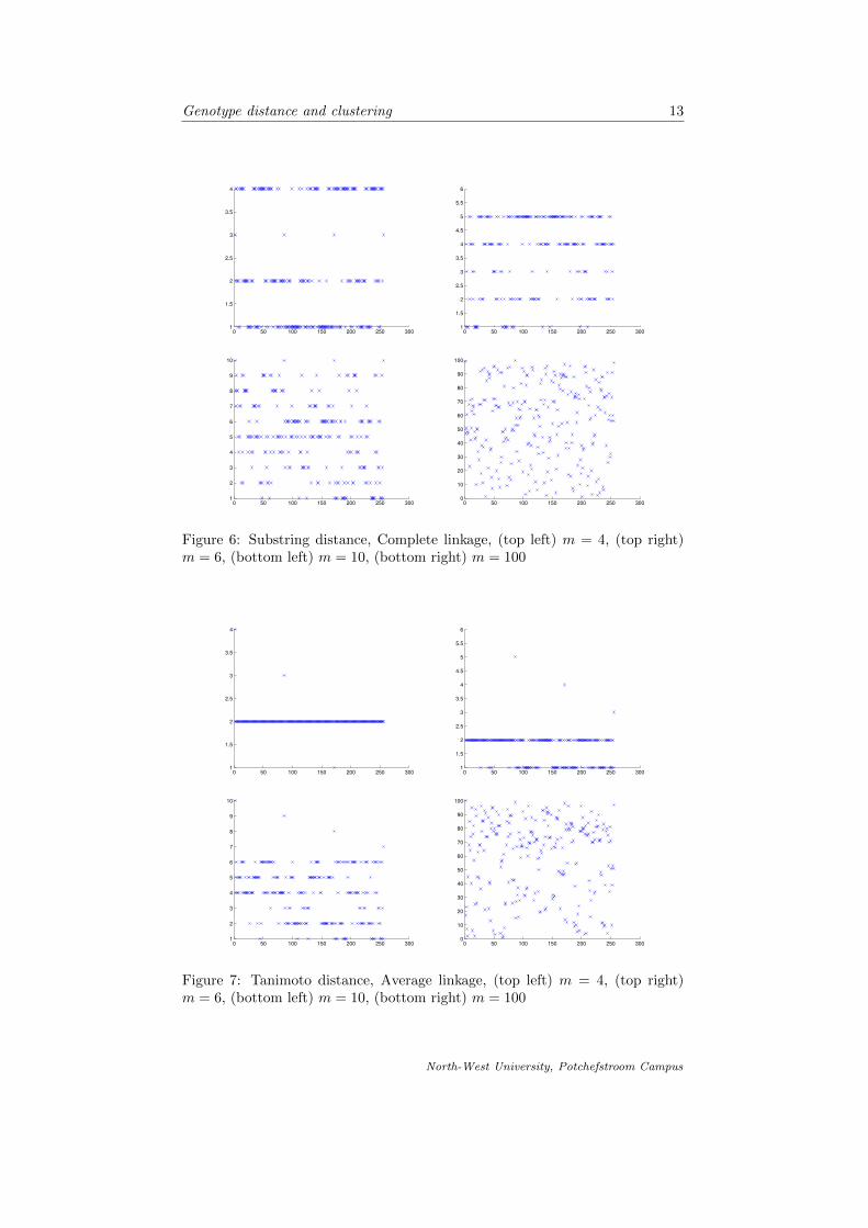
Figure 6: Substring distance, Complete linkage, (top left) m = 4, (top right)m = 6, (bottom left) m = 10, (bottom right) m = 100

0 50 100 150 200 250 3001

1.5

2

2.5

3

3.5

4

0 50 100 150 200 250 3001

1.5

2

2.5

3

3.5

4

4.5

5

5.5

6

0 50 100 150 200 250 3001

2

3

4

5

6

7

8

9

10

0 50 100 150 200 250 3000

10

20

30

40

50

60

70

80

90

100

Figure 7: Tanimoto distance, Average linkage, (top left) m = 4, (top right)m = 6, (bottom left) m = 10, (bottom right) m = 100



0 50 100 150 200 250 3001

1.5

2

2.5

3

3.5

4

0 50 100 150 200 250 3001

1.5

2

2.5

3

3.5

4

4.5

5

5.5

6

0 50 100 150 200 250 3001

2

3

4

5

6

7

8

9

10

0 50 100 150 200 250 3000

10

20

30

40

50

60

70

80

90

100

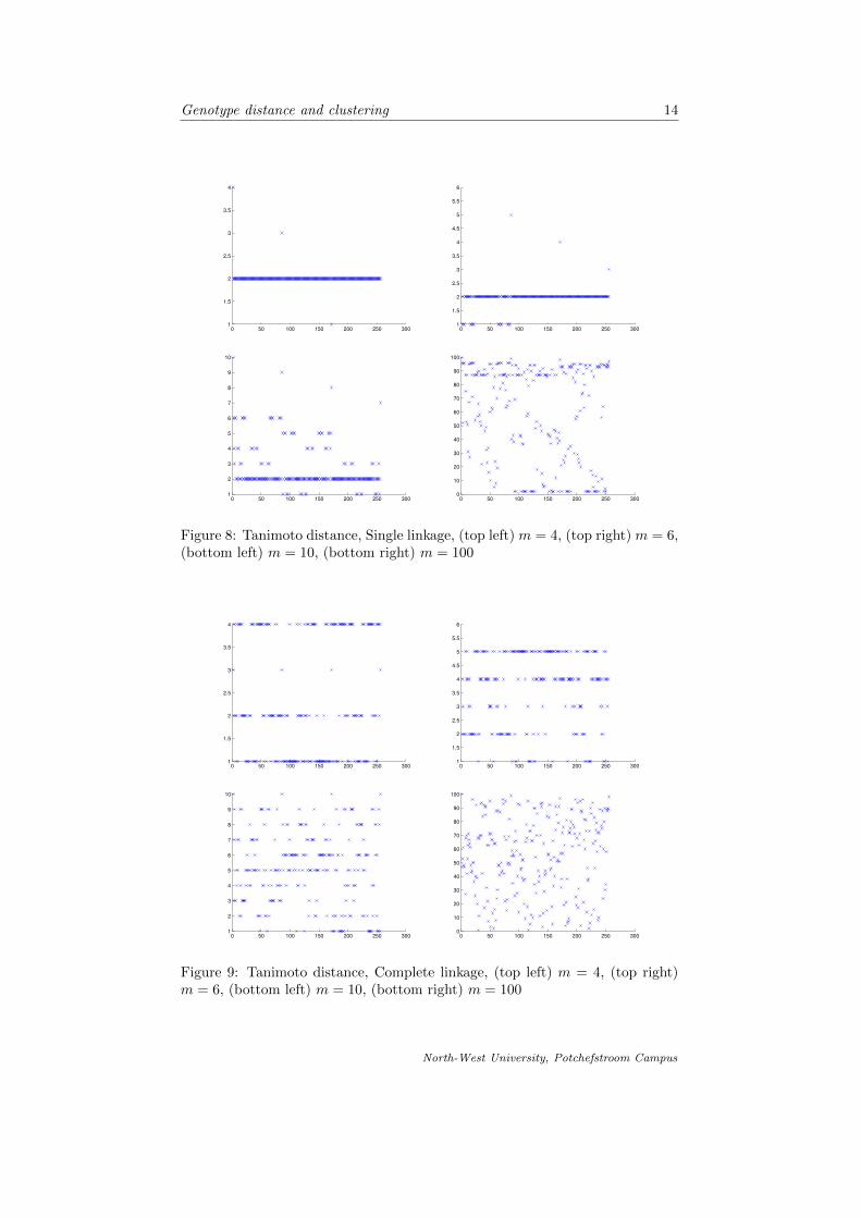
Figure 8: Tanimoto distance, Single linkage, (top left) m = 4, (top right) m = 6,(bottom left) m = 10, (bottom right) m = 100

0 50 100 150 200 250 3001

1.5

2

2.5

3

3.5

4

0 50 100 150 200 250 3001

1.5

2

2.5

3

3.5

4

4.5

5

5.5

6

0 50 100 150 200 250 3001

2

3

4

5

6

7

8

9

10

0 50 100 150 200 250 3000

10

20

30

40

50

60

70

80

90

100

Figure 9: Tanimoto distance, Complete linkage, (top left) m = 4, (top right)m = 6, (bottom left) m = 10, (bottom right) m = 100



7 Discussion

It is apparent from comparing the different linkages and distance functions tocluster the genotype objects, that the more clusters we divide the data into, theless meaningful the clustering is. Forming 100 clusters from the data (wherewe work with 256 different objects) is less striking than clustering the data intoonly 4 clusters. As suspected, the complete linkage is the best approach toclustering in this case, since we are interested in groups of objects which aresimilar to each other, but where the proximity of clusters is based on the factthat the objects in respective clusters are most dissimilar. It is also noted thatthe dendrograms formed by using the different metrics is quite similar and weconclude our suspicion that the two metrics are very similar.

Special attention is drawn to fig. 9. We conclude that the best formed clus-ters are those that make visually sense according to the representation of theclustering in fig. 4-9. The number of objects in each cluster seem more or lessuniformly spread throughout the clusters using the complete linkage, that is theclustering as in the graphs shown in fig. 9.

7.1 Correlation Coefficient

The Cophenetic Correlation Coefficient (CCC) is a means of measuring how ac-curately a dendogram represents the natural clustering of the data being clus-tered. The CCC was introduced by Sokal & Rohlf (1962). Let Γtij be theclustering at which xi and xj are merged in the same cluster for the first timeand let L(tij) be the proximity level at which the clustering Γtij is defined (thiscan be seen from the dendrogram for the specific hierarchical clustering). Wedefine the cophenetic distance between two vectors as

dC(xi, xj) = L(tij).

In other words, the cophenetic distance between two vectors is defined as theproximity level at which the two vectors are found in the same cluster for the firsttime. Now, we represent the dendrogram produced by a hierarchical clusteringalgorithm by the respective cophenetic matrix, DC . We will define statisticalindices that measure the degree of agreement between the cophenetic matrix,DC , produced by a specific hierarchical clustering algorithm, with the proximitymatrix D. The CCC measures the correlation between DC and D and is usedwhen the matrices are interval or ratio scaled. The CCC is determined as follows:

Definition 10: Let dij and cij denote the ij-th element of DC and D, respec-tively, and let M = N(N − 1)/2 be the number of upper diagonal elements ofthe matrices DC and D (N is the number of rows and columns in the matrices).Then the Cophenetic correlation coefficient is given by:

CCC =(1/M)

∑N−1i=1

∑Nj=i+1 dijcij − µPµC√

(1/M)∑N−1i=1

∑Nj=i+1 dij − µP

√(1/M)

∑N−1i=1

∑Nj=i+1 cij − µC

,



where µP and µC are the means defined by

µP = (1/M)

N−1∑i=1

N∑j=i+1

D(i, j), µC = (1/M)

N−1∑i=1

N∑j=i+1

DC(i, j).

The values of the CCC are between −1 and 1. The closer the CCC is to1, the better the agreement between the proximity and cophenetic matrices.According to the MATLABr instruction cophenet(Z,Y), the CCC, for thecase of average linkage, is computed as c = 0.576098. This indicates a reasonablecorrelation between the data and the clustering thereof.

8 Summary

We have seen that distance between strings in the genotype space are definedin terms of all possible substrings constructed from pairwise strings to be com-pared. First, we defined a measure of diversity within a population and thenwe defined the distance between two individuals as the diversity between thetwo individuals. The result was a semi-metric. This semi-metric has exactlythe properties which we require to measure the dissimilarity between strains,but we would rather use a true metric in our clustering application. We theninvestigated the Tanimoto distance which is defined in terms of the Jaccardsimilarity index. A comparison of the two metrics showed that the residue ofthe difference of two distance matrices is of the order 10−15. We concluded that,therefore the two metrics are very similar. We used both the substring distanceand the Tanimoto distance in the clustering algorithm and plotted dendrogramsof the three general linkages used in agglomerative hierarchical clustering.

We proceeded by introducing the concept of clusters in terms of partitioning ofsets and then introduced the basic agglomerative hierarchical clustering algo-rithm. We investigated the different linkages applied to the clustering and thencompared them by means of graphic representation. It was then concluded thatcomplete linkage is used to cluster the data objects. Fig. 4-9 is a graphicalrepresentation of the objects on the horizontal axes and the cluster in which itmay be found on the vertical axes.

9 Conclusion

Clustering is an effective way of grouping objects together, given a certain clus-tering criterion - in this case the measure of dissimilarity between individualstrains. Due to difficulties arising by using the Hamming distance, it wasthought to rather apply a general measure of distance to find the dissimilar-ity between strains. For this purpose the Tanimoto distance is well suited inthat it does not measure dissimilarity according to insertion, deletion and mu-tation, but rather based on the number of motifs one may find in a particularstring. Therefore the objects s1 = 0000 and s256 = 3333 (where once againwe work with 4 loci and 4 alleles) have the distance d(ι1, ι256) = 1 indicatingthat they are most dissimilar. This would be the same for the Hamming dis-tance. The difference, however, occurs for instance when two strains s2 = 0001



and s5 = 0010, have distance d(ι2, ι5) = 0.8 instead of dH = 0.5 according tothe Hamming distance. The norm of the difference of the proximity matrices,‖Dτ −DH‖ = 21.815659 indicates a great difference in the two measures for thegiven investigation.

The implementation of the metric in MATLABr and defining the proximitymatrix, though, is subject to some computational difficulty, but the optimisationof the code might result in faster computational time. On the other hand, theclustering tools included with MATLABr are implemented quite easily andgood results are obtained. The clustering of the objects into hard clusters usingthe agglomerative hierarchical clustering was easily achieved once the conceptswere implemented. Choosing the number of clusters to be used in an applicationwould now be at the discretion of the modeller. In this particular case onemight need to consider the different traits distinguished by the genotypes, thatis phenotypic properties (say, for instance, we have m distinguishable attributesphisically identifiable to each genotype) and arrange the objects into m clusters.



References

1. D’Errico, J., 2010. String subsequence tools. MATLAB Central. (online)Available at http://www.mathworks.com/ matlabcentral/fileexchange/27460-string-subsequence-tools (Accessed 25 July 2012)

2. Jain, A.K., Murty, M.N., Flynn, P.J., 1999. Data Clustering: A Review.ACM Computing Surveys, 31:3: 264-323

3. Lange, A., Ferguson, N.M., 2009, Antigenic Diversity, Transmissions Mech-anisms, and the Evolutions of Pathogens. PLoS, Computational Biology,5:10: 1-12

4. Levandowski, M & Winter, D., 1971, Distance between Sets. Nature,234(5):34-35

5. Mattiussi, C., Waibel, M., Floreano, D., 2004. Measures of Diversity forPopulations and distances Between Individuals with Highly RecognizableGenomes. Evolutionary Computation, 12:4: 495-515

6. Sellers, P. H. 1974. On the Theory and Computation of EvolutionaryDistances. SIAM Journal of Applied Mathematics, 26:4: 787-793

7. Sokal, R.R., Rohlf, F.J., 1962. The Comparison of Dendrograms by Ob-jective Methods. Taxon, 11:2: 33-40

8. Theodoridis, S., Koutroumbas, K., 2006. Pattern Recognition, AcademicPress, San Diago.

9. Vipin, K., 2010. An Extensive Survey of Clustering Methods for DataMining. University of Minnesota. (online)Available at: http://www.cs.umn.edu/h̃an/dmclass/cluster survey 1002 00.pdf (Accessed on 13 April 2012)

10. Waterman, M. S., Smith, T. F., Beyer, W. A. 1976. Some BiologicalSequence Metrics. Advances in Mathematics, 20:3: 367-387

11. Witherspoon, D.J., et al. 2007. Genetic Similarities Within and BetweenHuman Populations. Genetics, 176: 351-359



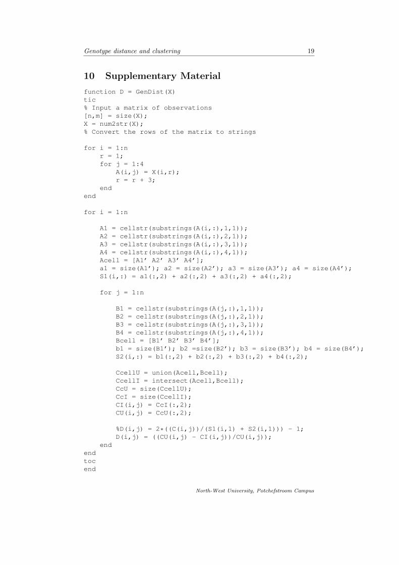
10 Supplementary Material

function D = GenDist(X)tic% Input a matrix of observations[n,m] = size(X);X = num2str(X);% Convert the rows of the matrix to strings

for i = 1:nr = 1;for j = 1:4

A(i,j) = X(i,r);r = r + 3;

endend

for i = 1:n

A1 = cellstr(substrings(A(i,:),1,1));A2 = cellstr(substrings(A(i,:),2,1));A3 = cellstr(substrings(A(i,:),3,1));A4 = cellstr(substrings(A(i,:),4,1));Acell = [A1’ A2’ A3’ A4’];a1 = size(A1’); a2 = size(A2’); a3 = size(A3’); a4 = size(A4’);S1(i,:) = a1(:,2) + a2(:,2) + a3(:,2) + a4(:,2);

for j = 1:n

B1 = cellstr(substrings(A(j,:),1,1));B2 = cellstr(substrings(A(j,:),2,1));B3 = cellstr(substrings(A(j,:),3,1));B4 = cellstr(substrings(A(j,:),4,1));Bcell = [B1’ B2’ B3’ B4’];b1 = size(B1’); b2 =size(B2’); b3 = size(B3’); b4 = size(B4’);S2(i,:) = b1(:,2) + b2(:,2) + b3(:,2) + b4(:,2);

CcellU = union(Acell,Bcell);CcellI = intersect(Acell,Bcell);CcU = size(CcellU);CcI = size(CcellI);CI(i,j) = CcI(:,2);CU(i,j) = CcU(:,2);

%D(i,j) = 2*((C(i,j))/(S1(i,1) + S2(i,1))) - 1;D(i,j) = ((CU(i,j) - CI(i,j))/CU(i,j));

endendtocend


Measuring of distances of genotype strains and clustering methods.

Documents

Transcript of Measuring of distances of genotype strains and clustering methods.