Graph Distances in the Data-Stream Model

Copyright © by SIAM. Unauthorized reproduction of this article is prohibited.

SIAM J. COMPUT. c© 2008 Society for Industrial and Applied MathematicsVol. 38, No. 5, pp. 1709–1727

GRAPH DISTANCES IN THE DATA-STREAM MODEL∗

JOAN FEIGENBAUM† , SAMPATH KANNAN‡, ANDREW MCGREGOR§ ,

SIDDHARTH SURI¶, AND JIAN ZHANG‖

Abstract. We explore problems related to computing graph distances in the data-stream model.The goal is to design algorithms that can process the edges of a graph in an arbitrary order given onlya limited amount of working memory. We are motivated by both the practical challenge of processingmassive graphs such as the web graph and the desire for a better theoretical understanding of the data-stream model. In particular, we are interested in the trade-offs between model parameters such as per-data-item processing time, total space, and the number of passes that may be taken over the stream.These trade-offs are more apparent when considering graph problems than they were in previousstreaming work that solved problems of a statistical nature. Our results include the following:(1) Spanner construction: There exists a single-pass, O(tn1+1/t)-space, O(t2n1/t)-time-per-edgealgorithm that constructs a (2t + 1)-spanner. For t = Ω(log n/log log n), the algorithm satisfies thesemistreaming space restriction of O(n polylog n) and has per-edge processing time O(polylog n).This resolves an open question from [J. Feigenbaum et al., Theoret. Comput. Sci., 348 (2005),pp. 207–216]. (2) Breadth-first-search (BFS) trees: For any even constant k, we show that anyalgorithm that computes the first k layers of a BFS tree from a prescribed node with probability atleast 2/3 requires either greater than k/2 passes or Ω(n1+1/k) space. Since constructing BFS trees isan important subroutine in many traditional graph algorithms, this demonstrates the need for newalgorithmic techniques when processing graphs in the data-stream model. (3) Graph-distance lowerbounds: Any t-approximation of the distance between two nodes requires Ω(n1+1/t) space. We alsoprove lower bounds for determining the length of the shortest cycle and other graph properties. (4)Techniques for decreasing per-edge processing: We discuss two general techniques for speeding upthe per-edge computation time of streaming algorithms while increasing the space by only a smallfactor.

Key words. stream algorithms, graph distances, spanners

AMS subject classifications. 68Q05, 68Q17, 68Q25, 68W20, 68W25

DOI. 10.1137/070683155

1. Introduction. In recent years, streaming has become an active area of re-search and an important paradigm for processing massive data sets [4, 23, 27]. Muchof the existing work has focused on computing statistics of a stream of data elements,

∗Received by the editors February 20, 2007; accepted for publication (in revised form) August 4,2008; published electronically December 19, 2008. This work was supported by the DoD UniversityResearch Initiative (URI) administered by the Office of Naval Research under grant N00014-01-1-0795. It first appeared in the Proceedings of the ACM-SIAM Symposium on Discrete Algorithms,2005 [21].

http://www.siam.org/journals/sicomp/38-5/68315.html†Department of Computer Science, Yale University, P.O. Box 208285, New Haven, CT 06520-

8285 ([email protected]). This author’s research was supported in part by ONR grantN00014-01-1-0795 and NSF grant ITR-0331548.

‡Department of Computer and Information Science, University of Pennsylvania, Philadelphia, PA19104 ([email protected]). This author’s research was supported in part by ARO grant DAAD19-01-1-0473 and NSF grant CCR-0105337.

§Department of Computer Science, University of Massachusetts, 140 Governors Drive, Amherst,MA 01003-9264. This work was done while the author was at the University of Pennsylvania andwas supported in part by NSF grant ITR-0205456.

¶Yahoo! Research, 111 West 40th Street, 17th floor, New York, NY 10018 ([email protected]).This work was done while the author was at the University of Pennsylvania and was supported inpart by NIH grant T32HG000046-05.

‖Department of Computer Science, Louisiana State University, Baton Rouge, LA 70803 ([email protected]). This work was done while the author was at Yale University and was supported by NSF grantITR-0331548.

1709


1710 FEIGENBAUM, KANNAN, MCGREGOR, SURI, AND ZHANG

e.g., frequency moments [4, 29], �p distances [23, 28], histograms [24, 26], and quan-tiles [25]. More recently, there have been extensions of the streaming research to thestudy of graph problems [6, 22, 27]. Solving graph problems in this model has raisednew challenges, because many existing approaches to the design of graph algorithmsare rendered useless by the sequential-access limitation and the space limitation ofthe streaming model.

Massive graphs arise naturally in many real-world scenarios. Two examples arethe call graph and the web graph. In the call graph, nodes represent telephone numbersand edges correspond to calls placed during some time interval. In the web graph,nodes represent web pages, and the edges correspond to hyperlinks between pages.Also, massive graphs appear in structured data mining, where the relationships amongthe data items in the data set are represented as graphs. When processing these graphsit is often appropriate to use the streaming model. For example, the graph may berevealed by a web crawler or the graph may be stored on external-memory devices,where being able to process the edges in an arbitrary order improves I/O efficiency.Indeed, the authors of [33] argue that one of the major drawbacks of standard graphalgorithms, when applied to massive graphs such as the web, is their need to haverandom access to the edge set.

In general it seems that most graph algorithms need to access the data in a veryadaptive fashion. Since we cannot store the entire graph, emulating a traditional al-gorithm may necessitate an excessive number of passes over the data. There has beensome success in estimating quantities that are of a statistical nature, e.g., countingtriangles [6, 11, 31] or estimating frequency and entropy moments of the degrees in amultigraph [12, 15]. However, it seemed for a while that more “complicated” com-putation was not possible in this model. For example, Buchsbaum, Giancarlo, andWestbrook [10] demonstrated the intrinsic difficulty of computing common neighbor-hoods in the streaming model with small space. One possible way to ameliorate thesituation is to consider algorithms that use Θ(n polylogn) space, i.e., space roughlyproportional to the number of nodes rather than the number of edges. This spacerestriction was identified as an apparent “sweet-spot” for graph streaming in a surveyarticle by Muthukrishnan [37] and dubbed the semistreaming space restriction. Thisspurred further research on algorithms for graph problems in the streaming modelsuch as distance estimation [19, 22], matchings [22, 36], and connectivity [21, 41], in-cluding the work described here. We will provide further discussion of the results ondistance estimation in the next section.

A related model is the semiexternal model. This was introduced by Abello, Buchs-baum, and Westbrook [1] for computations on massive graphs. In this model, thevertex set can be stored in memory, but the edge set cannot. However, unlike in ourmodel, random access to the edges, although expensive, was allowed. Finally, graphproblems have been considered in a model that extends the stream model by allowingthe algorithm to write to the stream during each pass [2, 16]. These annotations canthen be utilized by the algorithm during successive passes. Aggarwal et al. [2] go fur-ther and suggest a model in which sorting passes are permitted, and the data-streamis sorted according to a key encoded by the annotations.

Designing algorithms for computing graph distances is a very well studied prob-lem, and graph distances are a natural quantity to study when trying to understandproperties of massive graphs such as the diameter of the world wide web [3]. We startwith a formal definition of the relevant terms.

Definition 1.1 (graph distance, diameter, and girth). For an undirected, un-


GRAPH DISTANCES IN THE DATA-STREAM MODEL 1711

weighted graph G = (V, E), we define a distance function dG : V ×V → {0, . . . , n−1},where dG(u, v) is the length of the shortest path in G between u and v. The diameterof G is the length of the longest shortest path, i.e.,

Diam(G) = maxu,v∈V

dG(u, v).

The girth of G is the length of the shortest cycle in G, i.e.,

Girth(G) = 1 + min(u,v)∈E

dG\(u,v)(u, v).

Classic algorithms such as Dijkstra, Bellman–Ford, and Floyd–Warshall are taughtwidely [14]. Recent research has focused on computing approximate graph distances [5,7, 17, 40]. Unfortunately, these algorithms seem to be inherently unsuitable for com-puting distances in the streaming model; an important subroutine of many of theexisting algorithms is the construction of breadth-first-search (BFS) trees, and one ofour main results is a lower bound on the computational resources required to com-pute a BFS tree. For example, Thorup and Zwick provide a construction of distanceoracles for approximating distances in graphs [40]. Although all-pairs-shortest-pathdistances can be approximated using this oracle, their oracle construction requires thecomputation of shortest-path trees for certain vertices. Indeed, many constructionsof distance oracles have this requirement, i.e., they need to compute some distancesbetween certain pairs of vertices in order to build a data structure from which theall-pairs-shortest-path distances can be approximated.

A common method for approximating graph distances is via the construction ofspanners.

Definition 1.2 (spanners). A subgraph H = (V, E′) is an (α, β)-spanner ofG = (V, E) if, for any vertices x, y ∈ V ,

dG(x, y) ≤ dH(x, y) ≤ αdG(x, y) + β.

When β = 0, we call the spanner a multiplicative-spanner and refer to α as the stretchfactor of the spanner.

In [22], a simple semistreaming spanner construction is presented. That algorithmconstructs a (log n)-spanner in one pass using O(n polylog n) space. However, thisalgorithm needs O(n) time to process each edge in the input stream. Such a per-edgeprocessing time is prohibitive, especially in the streaming model when edges may bearriving in quick succession. The work of [19] studies the construction of (1 + ε, β)spanners in the streaming model. However, the algorithm of [19] requires multiplepasses over the input stream, while our construction needs only one pass.

Notation and terminology. We refer to an event’s occurring “with high probabil-ity” if the probability of the event is at least 1−1/nΩ(1). We denote the set {1, . . . , t}by [t]. Let P (S) denote the power set of S, i.e., {S′ : S′ ⊂ S}.

1.1. Our results. Our results include the following.1. Spanner construction: There exists a single-pass O(tn1+1/t log2 n) space,

O(t2n1/t log n) time-per-edge algorithm that constructs a (2t + 1)-spanner.For t = Ω(log n/log log n), the algorithm satisfies the semistreaming spacerestriction of O(n polylog n) and has per-edge processing time O(polylog n).The algorithm is presented in section 3. This result resolves an open questionfrom [22].



2. BFS trees: For any even constant k, any algorithm that computes the firstk layers of a BFS tree from a prescribed node with probability at least 2/3requires either greater than k/2 passes or Ω(n1+1/k) space. This result isproved in section 4. Since constructing BFS trees is an important subroutinein many traditional graph algorithms, this demonstrates the need for newalgorithmic techniques when processing graphs in the data-stream model.

3. Lower bounds: In section 5, we present lower bounds for the following prob-lems:(a) Connectivity and other balanced properties: We show that testing any of

a large class of graph properties, which we refer to as balanced properties,in one pass requires Ω(n) space. This class includes properties such asconnectivity and bipartiteness. This result provides a formal motivationfor the semistreaming space restriction, where algorithms are permittedO(n polylog n) space.

(b) Graph distances and graph diameter: We show that any single-pass al-gorithm that returns a t-approximation of the graph distance betweentwo given nodes with probability at least 3/4 requires Ω(n1+1/t) bits ofspace. Furthermore, this bound also applies to estimating the diame-ter of the graph. Therefore, approximating a distance using the abovespanner construction is only about a factor of 2 from optimal in termsof the approximation factor achievable for a given space restriction.

(c) Girth: Any p-pass algorithm that ascertains whether the length of theshortest cycle is longer than g requires Ω

(p−1(n/g)1+4/(3g−4)

)bits of

space.4. Techniques for decreasing per-edge processing: In section 6, we present a

method for local amortization of per-data-item complexity. We also presenta technique for adapting existing partially dynamic graph algorithms to thesemistreaming model.

The above results indicate various trade-offs between model parameters and accu-racy. These include the smooth trade-off between the space a single-pass algorithm ispermitted and the accuracy achievable when estimating graph distances. For multiple-pass algorithms, a smooth trade-off between passes and space is evident when tryingto compute the girth of a graph. This trade-off is, in a sense, fundamental as itindicates that the only way to get away with using half the amount of space is es-sentially to make half as much progress in each pass. The trade-off between spaceand passes when computing BFS trees indicates that, as we restrict the space, noalgorithm can do much better than emulating a trivial traditional graph algorithmand will consequently require an excessive number of passes.

Recent developments. Since the preliminary version of this paper appeared, im-proved spanner construction algorithms were presented by Baswana [8] and Elkin [18].Extensions of ideas in section 6 have been developed by Zelke [41, 42].

2. Preliminaries. In this section, we give a formal definition of a graph stream.Definition 2.1 (graph stream). For a data-stream A = 〈a1, a2, . . . , am〉, where

aj ∈ [n] × [n], we define a graph G on n vertices V = {v1, . . . , vn} with edges E ={(vi, vk) : aj = (i, k) for some j ∈ [m]}.

We usually assume that each aj is distinct, but this assumption is often notnecessary. When the data items are not distinct, the model can naturally be extendedto consider multigraphs; i.e., an edge (vi, vk) has multiplicity equal to |{j : aj =(i, k)}|. Similarly, we consider undirected graphs, but the definition can be generalized



to define digraph streams. Sometimes we will consider weighted graphs, and in thiscase aj ∈ [n]× [n]×N, where the third component of the data item indicates a weightassociated with the edge. Note that some authors have also considered a specialcase of the model, the adjacency-list model, in which all incident edges are groupedtogether in the stream [6]. We will be interested in the fully general model.

3. Spanners. In this section, we present a single-pass streaming algorithm thatconstructs a (2t + 1)-spanner for an unweighted, undirected graph. The algorithmuses some of the ideas from [7] and adapts them for use in the data-stream model.We then extend this algorithm to construct (1 + ε)(2t + 1)-spanners for weighted,undirected graphs using a geometric grouping technique.

Overview of the algorithm. Intuitively, we want to cover each “dense subgraph”of the graph by a tree of small depth, i.e., one of depth O(log n), rooted at some node.If there are many edges between two such dense subgraphs, only one representativeedge needs to be remembered. Edges between vertices that are not part of such densesubgraphs also need to be remembered, but we will argue that there are not too manyof them. The construction requires a delicate balance between trying to include asmany nodes as possible in a small number of dense subgraphs and ensuring that thedepth of the spanning tree covering each dense subgraph is O(log n).

Our clusters are similar to those used in [5, 7, 17]. However, the constructions ofthe clusters in [5, 7, 17] all employ an approach similar to BFS; i.e., the clusters areconstructed layer by layer. Such a layer-by-layer process is important to ensure thatthe clusters constructed in [5,7,17] have small diameters. In the streaming model, thiswould necessitate multiple passes over the input stream. Our labeling scheme employsa different strategy to control the clusters’ diameters, thus bypassing the BFS.

In more detail, in the case in which we are constructing O(log n)-spanners, weconsider log n/2 levels. Each node is present at the bottom level and is “promoted”to each successively higher level with probability 1/2. Whenever a node is present atlevel i, a cluster at level i is dynamically grown around it as we process the edges. Theexpected number of clusters at level i + 1 is half of the expected number of clustersat level i. At the top level, the expected number of clusters is

√n. As the algorithm

goes through the input stream of edges, a node in a lower-level cluster may join ahigher-level cluster. The constructed spanner consists of three types of edges: (1) asmall-diameter spanning tree for each cluster, (2) one edge between each pair of top-level clusters whose vertex sets have at least one edge between them, and (3) a smallnumber of “other” edges that do not fit into either of these two categories and arenecessary to preserve the spanner property.

The above ideas are applicable mutatis mutandis when a t-spanner is sought forother values of t. The description below is for arbitrary t.

The algorithm. A label l used in our construction is a positive integer. Giventwo parameters n and t, the set of labels L used by our algorithm is generated in thefollowing way. Initially, we have labels [n]. We denote by L0 this set of labels andcall them the level-0 labels. Independently, and with probability n−1/t, each labell ∈ L0 will be put into a set S0 and marked as selected. From each label l in S0, wegenerate a new label l′ = l + n. We denote by L1 the set of newly generated labelsand call them the level-1 labels. We then apply the above selection and new-label-generation procedure on L1 to get the set of level-2 labels L2. We continue this untilthe level-t/2 labels L�t/2� are generated. If a level-(i + 1) label l is generated froma level-i label l′, we call l the successor of l′ and denote it by Succ(l′) = l. The set oflabels we will use in our algorithm is the union of labels of levels 0, 1, 2, . . . , t/2, i.e.,



L =⋃�t/2�

0 Li. Note that L can be generated before the algorithm sees the edges inthe stream. But, in order to generate the labels in L, except in the case t = Θ(log n),the algorithm needs to know n, the number of vertices in the graph, before seeingthe edges in the input stream. For t = Θ(log n), a simple modification of the abovemethod can be used to generate L without knowing n, because the probability for alabel to be selected is constant.

At first glance, it might appear that our labeling scheme resembles the sequencesof sets initially constructed by the algorithm of Thorup and Zwick [40]. In our con-struction, the generation of the clusters of vertices depends on both the labels and theedge set. Thorup and Zwick, however, generate their sequence of sets independentlyof the edges. But, this is just the first step in their algorithm. Subsequently, theiralgorithm computes the exact distance between a fixed vertex and each of the sets ofvertices in the sequence. Computing the exact distances between a pair of verticesis difficult in the streaming model. Our algorithm takes a very different approachfrom [40] to avoid this difficulty.

While going through the stream, our algorithm will label each vertex with labelschosen from L. The algorithm may label a vertex v with multiple labels; however, vwill be labeled by at most one label from Li for i ∈ [t/2]. Moreover, if v is labeledby a label l, and l is selected, the algorithm will also label v with the label Succ(l).

Denote by li a label of level i, i.e., li ∈ Li. Let L(v) = {l0, lk1 , lk2 , . . . , lkj} be thecollection of labels that has been assigned to the vertex v, where 0 < k1 < · · · < kj ≤t/2. Let

Height(v) = max{j|lj ∈ L(v)}

and Top(v) = lk ∈ L(v) s.t. k = Height(v). Let C(l) be the collection of vertices thatare labeled with the label l.

The sets L(v) and C(l) will grow while the algorithm goes through the streamand labels the vertices. For each C(l), our algorithm stores a tree, Tree(l), on thevertices of C(l) and the tree is rooted on the first vertex that gets labeled by l. Wesay an edge (u, v) connects C(l) and C(l′) if u is labeled with l and v is labeled withl′. For some pairs of labels l, l′ ∈ L�t/2�, our algorithm will store edges that connectC(l) and C(l′). We denote by H the set of such edges stored by our algorithm. Inaddition, for each vertex v, we denote by M(v) the other edges incident to v thatare stored by our algorithm. Intuitively, the subgraph induced by ∪v∈V M(v) is thesparse part of the graph G. The spanner constructed by the algorithm is the unionof the rooted trees for all the labels, M(v) for all the vertices, and the set H . Thedetailed algorithm is given in Figure 3.1.

Analysis. We start with two preliminary lemmas showing that, with high proba-bility, the spanner construction requires only a small amount of working space. Notethat randomness is introduced in the generation of the labels in Algorithm 1; that isthe reason that the bounds stated in both lemmas are true with high probability.

Lemma 3.1. With high probability, for all v ∈ V , |M(v)| = O(tn1/t log n).Proof. Let M (i)(v) ⊆M(v) be the set of edges added to M(v) during the period

when Height(v) = i. Let L(M(v)) = ∪(u,v)∈M(v)L(u) be the set of labels that havebeen assigned to the vertices in M(v). An edge (u, v) is added to M(v) only in step2(b)ii. Note that, in this case, t

2 ≥ Height(u) ≥ Height(v). Hence, the set Lv(u)is not empty. Also, by the condition in step 2(b)ii, an edge (u, v) is added onlywhen none of the labels in Lv(u) appears in L(M(v)). Thus, if we add the edge inthis step, we will introduce/add the label(s) in Lv(u) to L(M(v)). Because Lv(u)



Algorithm 1 (efficient one pass spanner construction).The input to the algorithm is an unweighted, undirected graph G = (V, E),presented as a stream of edges, and two positive integer parameters n and t.

1. Generate the set L of labels as described. ∀ vi ∈ V , label vertex vi withlabel i ∈ L0. If i is selected, label vi with Succ(i). Continue this until weencounter a label that is not selected. Set M(vi)← ∅ and H ← ∅.

2. Upon seeing an edge (u, v) in the stream, if L(v) ∩ L(u) �= ∅, drop theedge. Otherwise, consider the following cases:(a) If Height(v) = Height(u) = t/2, and there is no edge in H that

connects C(Top(v)) and C(Top(u)), set H ← H ∪ {(u, v)}.(b) Otherwise, assume, without loss of generality, that t/2 ≥

Height(u) ≥ Height(v). Consider the collection of labels

Lv(u) = {lk1 , lk2 , . . . , lHeight(u)} ⊆ L(u),

where Height(v) ≤ k1 ≤ k2 ≤ · · · ≤ Height(u). Let l ∈ Lv(u) be theselected label whose level is the lowest among the selected labels inLv(u).

i. If such a label l exists, label the vertex v with the successorl′ = Succ(l) of l, i.e.,

L(v)← L(v) ∪ {l′}.

Incorporate the edge in the rooted tree Tree(l′). If l′ is selected,label v with l′′ = Succ(l′) and incorporate the edge in the treeTree(l′′). Continue until we see a label that is not marked asselected. (Note that Height(v) is increased by this process.)

ii. If no such label l exists and there is no edge (u′, v) in M(v) suchthat u, u′ are labeled with the same label l ∈ Lv(u), add (u, v)to M(v).

3. After seeing all the edges in the stream, output the union of the rootedtrees for all the labels, M(v) for all the vertices, and the set H as thespanner.

Fig. 3.1. An efficient, one-pass algorithm for computing sparse spanners. See the descriptionsbefore Lemma 3.1 for the definitions of H, M(v), L(v), C(l), Tree(l), Succ(l), Top(v), and Height(v).

is nonempty, it adds at least one new label to L(M(v)). This is the case for everyedge in M (i)(v). Let B be the set of distinct labels that M (i)(v) adds to L(M(v)).Furthermore, because each edge in M (i)(v) adds at least one new label, the size of Bis at least |M (i)(v)|. Note that the labels in B are not marked as selected. Otherwise,the algorithm would have taken step 2(b)i instead of step 2(b)ii. Hence, the size of Bsatisfies

Pr (|B| = k) ≤ (1− 1/n1/t)k.

Thus, with high probability, |M (i)(v)| = O(n1/t log n). Because i can take only O(t)values, with high probability,

|M(v)| =∑

i

|M (i)(v)| = O(tn1/t log n).



Lemma 3.2. With high probability, the algorithm stores O(tn1+1/t log n) edges.Proof. The algorithm stores edges in the set H , in the rooted trees for each

cluster C(l), and in the sets M(v), for all v ∈ V . By the Chernoff bound and theunion bound, with high probability the number of clusters at level t/2 is O(

√n), and

the size of the set H is O(n).For each label l, the algorithm stores a rooted tree for the set of vertices C(l).

The rooted tree is formed by the set of edges added when the vertices in C(l) getlabeled by the label l. This happens in step 2(b)i. In this step, we add an edge onlyat the time when a vertex becomes a member of C(l). Therefore, the set of edgesforms a tree on C(l). We call this tree the rooted tree of C(l). Note that two verticesu and v in C(l) may share some other label l′ of a different level. In this case, theyboth also belong to C(l′). The tree of C(l′) may have a path connecting u and v.Hence the subgraph of the spanner induced by the vertices in C(l) is not necessarilya tree. When we say “the rooted tree of C(l),” we refer only to the edges added whenthe vertices in C(l) get labeled by l.

Note that, for each level i ∈ [t/2], a vertex is labeled with at most one label inLi. Hence,

∑l∈Li |C(l)| ≤ |V |. Thus, the number of edges summed over the rooted

trees for the labels at level i is O(n), and the total number of edges in all the rootedtrees is O(tn). Finally, by Lemma 3.1, with high probability, |M(v)| = O(tn1/t log n).By the union bound, with high probability,

∑v∈V |M(v)| = O(tn1+1/t log n).

Theorem 3.3. Let G be an unweighted graph. There exists a single-passO(tn1+1/t log2 n) space algorithm that constructs a (2t + 1)-spanner of G with highprobability and processes each edge in O(t2n1/t log n) time.

Proof. Consider Algorithm 1 in Figure 3.1. At the beginning of the algorithm, forall the labels l ∈ L0, C(l) is a singleton set, and the depth of the rooted tree for C(l)is zero. We now bound, for label li, where i > 0, the depth of the rooted tree T i onthe vertices in C(li). A tree grows when an edge (u, v) is incorporated into the treein step 2(b)i. In this case, li is a successor of some label li−1 of level i− 1. Assumethat the depth dT i(v) of the vertex v in the tree is one more than the depth dT i(u) ofthe vertex u. Then u ∈ C(li−1), and the depth dT i−1(u) of u in the rooted tree T i−1

of C(li−1) is the same as dT i(u). Hence, dT i(v) = dT i−1(u) + 1, where T i is a treeof level i, and T i−1 is a tree of level i− 1. Given that dT 0(x) = 0 for all x ∈ V , thedepth of a rooted tree for C(l), where l is a label of level i, is at most i.

We proceed to show that, for any edge that the algorithm does not store, thereis a path of length at most 2t + 1 that connects the two endpoints of the edge. Thealgorithm ignores three types of edges. First, if L(u) ∩ L(v) �= ∅, the edge (u, v) isignored. In this case, let l be one of the label(s) in L(u) ∩ L(v). The nodes u andv are both on the rooted tree for C(l); hence, there is a path of length at most tconnecting u and v. Second, (u, v) will be ignored if Height(v) = Height(u) = t/2,and there is already an edge connecting C(Top(u)) and C(Top(v)). In this case, thepath connecting u and v has length at most 2t + 1. Finally, in step 2(b)ii, (u, v) willbe ignored if there is already another edge in M(v) that connects v to some u′ ∈ C(l),where l ∈ L(u). Note that u and u′ are both on the rooted tree of C(l). Hence, thereis a path of length at most t + 1 connecting u and v.

Hence, the stretch factor of the spanner constructed by Algorithm 1 is 2t + 1.By Lemma 3.2, with high probability, the algorithm stores O(tn1+1/t log n) edgesand requires O(tn1+1/t log2 n) bits of space. Also note that the bottleneck in theprocessing of each edge lies in step 2(b)ii, where, for each label in Lv(u), we need toexamine the whole set of M(v). This takes O(t2n1/t log n) time.



Extensions. Once the spanner is constructed, all-pairs-shortest-distances of thegraph can be computed from the spanner. This computation does not need to accessthe input stream and thus can be viewed as postprocessing. We also note that theabove algorithm can be used to construct a spanner of a weighted graph G = (V, E)using a geometric grouping technique [13,22]. Namely, we can round each edge weightω′ up to min{ω(1+ ε)i : i ∈ Z, ω(1+ ε)i ≥ ω′}, where ω is the weight of the first edge,and ε > 0 is a user-defined accuracy parameter. Let Gi = (V, Ei) be the graph formedfrom G by removing all edges not of weight ω(1 + ε)i. For each Gi, we construct aspanner in parallel and take the union of these spanners. This leads to the followingtheorem.

Theorem 3.4. Let G be a weighted graph and W be the ratio between the max-imum and minimum weights. There exists a single-pass O(ε−1tn1+1/t log W log2 n)space algorithm that constructs a (1 + ε)(2t + 1)-spanner of G with high probabilityand processes each edge in O(t2n1/t log n) time.

In the case where t = log n/log log n, Algorithm 1 computes a (2log n/log log n +1)-spanner in one pass using O(n log4 n) bits of space and processing each edge inO(log4 n) time. This answers an open question we posed in [22]. Finally, note thatconstructing a (2t + 1)-spanner gives a (2t + 1)-approximation for the diameter and,indirectly, a (2t + 2)/3-approximation of the girth. The diameter result is immediate.For the girth approximation, note that, if the constructed spanner is a strict subgraphof G, then the girth of G must have been between 3 and 2t + 2.

4. BFS trees lower bound. In this section, we prove a lower bound on thenumber of passes required to construct the first l layers of a BFS tree in the streamingmodel. The result is proved using a reduction from the communication-complexityproblem “multivalued pointer chasing.” This is a natural generalization of the pointer-chasing problem considered by Nisan and Wigderson [38].

Overview of proof. Nisan and Wigderson [38] considered the problem in whichAlice and Bob have functions fA : [m] → [m] and fB : [m] → [m], respectively.The k-round pointer-chasing problem is to output the result of starting from 1 andalternatively applying fA and fB a total of k times, starting with fA. Nisan andWigderson proved that, if Bob speaks first, the communication complexity of anyk-round communication protocol to solve this problem is Ω(m/k2 − k log m). Jain,Radhakrishnan, and Sen [30] gave a direct sum extension showing that, if there are dpairs of functions and the goal is to perform k-round pointer chasing as above on eachpair, the communication-complexity lower bound is approximately d times the boundof [38]. More precisely, they showed a lower bound of Ω(dm/k3 − dk log m− 2d) forthe problem.

We show how the lower bound of [30] implies a lower bound on the communicationcomplexity of pointer chasing with “d-valued functions,” i.e., functions that map i ∈[m] to a subset of [m] of size at most d. If fA and fB are such functions, then theresult of pointer chasing starting from 1 produces a set of size at most dk. The keydifference between this problem and the problem of [30] is that in the latter, one isconcerned only with chasing “like” pointers. That is, if one gets to an element j usingthe function fA,i, one can continue only with fB,i. (We will present an example afterthe formal definition of the appropriate terms.) Nevertheless, we give a reduction thatshows that the two problems have fairly similar communication complexity.

Finally, we create a an l-layered graph in which alternate layers have edges cor-responding to d-valued functions fA and fB. In order to construct the BFS tree, wemust solve the l-round, d-valued pointer-chasing problem and then apply the afore-



mentioned lower bound. This will lead to the following theorem.Theorem 4.1 (BFS lower bound). For any constant k, any algorithm that com-

putes the first k layers of a BFS tree with probability at least 2/3 requires either k/2passes or Ω(n1+1/k/(logn)1/k) space.

We now present the above argument formally. Let Fd be the set of functionsf : P ([m])→ P ([m]) such that

∀i ∈ [m], |f(i)| ≤ d and ∀A ⊂ [m], f(A) =⋃i∈A

f(i).

Throughout the rest of this section, we abuse notation and denote the singleton set{i} by i when it appears as the input or the output of a function f ∈ Fd.

Definition 4.2. Define gk,d : Fd × Fd → P ([m]) inductively as

g0,d(fA, fB) = {1} and gi,d(fA, fB) ={

fA(gi−1,d(fA, fB)) if i odd,fB(gi−1,d(fA, fB)) if i even.

Define hk,d as the d-fold direct sum of gk,1, i.e.,

hk,d(〈fA,1, . . . , fA,d〉, 〈fB,1, . . . , fB,d〉) = 〈gk,1(fA,1, fB,1), . . . , gk,1(fA,d, fB,d)〉.Example 4.3. Consider fA,1, fA,2, fB,1, fB,2 ∈ F1, where

fA,1 :1→ 1 fA,2 :1→ 2 fB,1 :1→ 1 fB,2 :1→ 32→ 2 2→ 3 2→ 2 2→ 13→ 3, 3→ 1, 3→ 3, 3→ 2.

Let fA, fB ∈ F2 be defined by fA(j) := fA,1(j)∪fA,2(j) and fB(j) := fB,1(j)∪fB,2(j).Then

h2,2(〈fA,1, fA,2〉, 〈fB,1, fB,2〉) = 〈1, 1〉, whereas g2,2(fA, fB) = {1, 2, 3}.Let Alice have function fA and Bob have function fB. Let Rr

δ(gd,k) be the r-roundrandomized communication complexity of gd,k where Bob speaks first, i.e., the numberof bits sent in the worst case (over all inputs and random coin tosses) by the bestr-round protocol Π in which, with probability at least 1− δ, both Alice and Bob learngd,k. The following theorem for hk,d was proved in [30] using an information-theoreticargument in combination with a result by Nisan and Wigderson [38].

Theorem 4.4 (see Jain, Radhakrishnan, and Sen [30]). Rk1/3(h

k,d) = Ω(dmk−3−dk log m− 2d).

We now use the above result to prove a bound on the communication complexityof gk,d.

Theorem 4.5. Rk1/3(g

k,d) = Ω(dm/(k + 1)3 − d(k + 1) log m− 2d− 6dk+1 lg m)if k is even.

Proof. The proof uses a reduction from hk,d. Let (〈fA,1, . . . , fA,d〉, 〈fB,1, . . . , fB,d〉)be an instance of hk,d. Define f∗

A and f∗B as follows:

f∗A(j) := {fA,i(j) : i ∈ [d]} and f∗

B(j) := {fB,i(j) : i ∈ [d]}.Assume that there exists a k-round protocol Π for gk,d that fails with probability atmost 1/3 and communicates o(dm/(k +1)3− d(k +1) log m− 2d− 12dk+1 lg m− km)bits in the worst case. We will show how to transform Π into a (k+1)-round protocol



Π′ for hk+1,d that fails with probability at most 1/3 and communicates o(dm/(k +1)3 − d(k + 1) log m − 2d) bits in the worst case. This contradicts Theorem 4.4 andhence shows that there is no such protocol Π.

Let Π′ be a protocol that simulates Π and, in addition, on the jth message(1 < j ≤ k + 1), sends the following set of triples:1

Tj−1 = {〈a, b, fC,a(b)〉 : b ∈ gj−2,d(f∗A, f∗

B)}, where C =

{A if j is even,B if j is odd.

Π is shown to be correct by an inductive argument and requires at most 3dj−1 log madditional bits of communication per message, because b ∈ gj−2,d(f∗

A, f∗B) and

|gj−2,d(f∗A, f∗

B)| ≤ dj−2, a ∈ [d], and each 〈a, b, fC,a(b)〉 can be encoded with at most3 logm bits. However, if Π is successful, then the player who sends the kth message(which is Alice by assumption that k is even and Bob speaks first) of Π also knowsgk,d(f∗

A, f∗B). Hence, she can also send

Tk+1 = {〈a, b, fA,a(b)〉 : b ∈ gk,d(f∗A, f∗

B)}.Hence, after (k + 1) rounds,

⋃i∈[k+1] Ti is known to both parties with probability at

least 2/3 and can be used to deduce gk+1,d. The total amount of extra communica-tion required to transmit

⋃i∈[k+1] Ti is

∑i∈[k+1] 3di log m ≤ 6dk+1 log m. Hence Π′

communicates o(dm/(k + 1)3 − d(k + 1) log m− 2d) bits in the worst case.We are now in a position to prove Theorem 4.1.Proof. The proof is a reduction from d-valued pointer chasing. Let m = n/(k+1),

and let d = c(m/ logm)1/k for some small constant c. Then, since k is constant byTheorem 4.5, Rk

1/3(gk,d) = Ω(n1+1/k/(log n)1/k).

Consider an instance (fA, fB) of gk,d. The graph described by the stream is onthe following set V of n = (k + 1)m nodes:

V =⋃

0≤i≤k

{vi1, . . . , v

im}.

For i ∈ [k], we define a set of edges E(i) between {vi−11 , . . . , vi−1

m } and {vi1, . . . , v

im}

in the following way:

E(i) ={ {(vi−1

j , vi�) : � ∈ fA(j)} if i is odd,

{(vi−1j , vi

�) : � ∈ fB(j)} if i is even.

Suppose there exists an algorithm A that computes the first k layers of the BFStree from v1

1 in p passes using memory M . Let Lr be set of nodes that are at distanceexactly r from v1

1 . Note that, for all r ∈ [k],

gr,d = Lr ∩ {vr1, . . . , v

rm}.

By simulating A on a stream starting with⋃

0≤i≤k:even E(i) and concluding with⋃i∈[k]:odd E(i) in the natural way, we deduce that there exists a (2p)-round commu-

nication protocol for gk,d that uses only 2pM communication. (Note that 2p roundsof communication rather than (2p− 1) rounds are required, because we required bothparties to learn gk,d.) Hence, either 2p > k or M = Ω(n1+1/k).

1Note that on the (k + 1)th message there is no message of Π to simulate and only Tk is trans-mitted.



5. Other lower bounds. In this section, we present lower bounds on the spacerequired to estimate graph distances, test whether a graph is connected, and computethe girth of a graph. Our lower bounds are reductions from problems in commu-nication complexity. In the Set-Disjointness problem, Alice has a length-n bi-nary string x ∈ {0, 1}n, and Bob has a length-n binary string y ∈ {0, 1}n, where∑

i∈[n] xi =∑

i∈[n] yi = n/4. If Bob is to compute

Set-Disjointness(x, y) ={

1 if x · y = 0,0 if x · y ≥ 1

(where x · y =∑

i∈[n] xiyi) with probability at least 3/4, then it is known that Ω(n)bits must be communicated between Alice and Bob [32, 39]. In the Index problem,Alice has x ∈ {0, 1}n, and Bob has j ∈ [n]. If Bob is to compute Index(x, j) = xj

with probability at least 3/4 after a single message from Alice, then it is known thatthis message must contain Ω(n) bits (e.g., [34]). To relate our graph-stream problemsto these communication problems, we use reductions based upon results from random-graph theory and extremal combinatorics.

5.1. Connectivity and balanced properties. Our first result shows that alarge class of problems, including connectivity, cannot be solved by single-pass stream-ing algorithms in small space. Specifically, we identify a general type of graph prop-erty2 and show that testing any such graph property requires Ω(n) space.

Definition 5.1 (balanced properties). We say a graph property P is balancedif there exists a constant c > 0 such that, for all sufficiently large n, there exists agraph G = (V, E) with |V | = n and u ∈ V such that

min{|{v : (V, E ∪ {(u, v)}) has P}|, |{v : (V, E ∪ {(u, v)}) has ¬P}| } ≥ cn.

In other words, there are Ω(n) vertices v such that (V, E ∪ {(u, v)}) has P and Ω(n)vertices v such that (V, E ∪ {(u, v)}) does not have P.

Many interesting properties are balanced, including connectivity, bipartiteness,and whether there exists a vertex of a certain degree.

Theorem 5.2. Testing for any balanced graph property P with probability 3/4 ina single pass requires Ω(n) space.

Proof. Let c be a constant, G = (V, E) be a graph on n vertices, and u ∈ Vbe a vertex satisfying the relevant conditions. The proof is by a reduction to thecommunication complexity of Index. Let (x, j) ∈ {0, 1}cn × [cn] be an instance ofIndex. Let G(x) be a relabeling of the vertices of G such that u = vn and, for i ∈ [cn],(V, E∪{(vn, vi)}) has P if and only if xi = 1. Such a relabeling is possible, because Pdoes not depend on the labeling of the vertices. Let e(j) = (vj , vn). Hence the graphdetermined by the edges of G(x) and e(j) has P if and only if xj = 1. Therefore,any single-pass algorithm for testing P using M bits of work space gives rise to aone-message protocol for solving Index, and this implies that M = Ω(n).

For some balanced graph properties, the above theorem can be generalized. Forexample, it is possible to show that any p-pass algorithm that determines whether agraph is connected requires Ω(np−1) bits of space [27].

2A graph property is a boolean function whose inputs are the elements of the adjacency matrixof the graph but whose output is independent of the labeling of the nodes of the graph.



5.2. Graph distances and graph diameter. If we are interested only in es-timating the distance between two nodes u and v, it may appear that constructing agraph spanner that gives no special attention to u or v, but rather approximates alldistances, is an unnecessarily crude approach. In this section, however, we show thatthe spanner-construction approach yields an approximation at most a factor 2 fromoptimal. Our result is a generalization of one in [22] that applied to the semistreamingcase. Integral to our proof is the notion of a k-critical edge.

Definition 5.3. In a graph G = (V, E), an edge e = (u, v) ∈ E is k-critical ifdG\(u,v)(u, v) ≥ k.

In Lemma 5.4, we show the existence of a graph G with a large subset of edgesE′ such that each edge in E′ is k-critical, but the removal of all edges in E′ leaves agraph with relatively small diameter. The proof uses a probabilistic method.

Lemma 5.4. For sufficiently large n and 3 ≤ k = o(log n/ log log n), there existsa set E of edges partitioned into two disjoint sets E1 and E2 on a set of n nodes Vsuch that

1. |E2| =⌈n1+1/k/144

⌉,

2. every edge in E2 is k-critical for G = (V, E), and3. Diam(G1) ≤ k + 1, where G1 = (V, E1).

Proof. Let γ = 1/k. Consider choosing a random graph G′ = (V, E′) on n nodeswhere each edge is (independently) present with probability p = 1/(2n1−γ). This iscommonly denoted as G′ ∼ Gn,p. We will then construct G1 = (V, E1) by deletingeach edge in G′ with probability 1/2. We will show that, with nonzero probability,the sets E1 and E2 = {e ∈ E′ \ E1 : e is k-critical for G′} satisfy the three requiredproperties.

The second property is satisfied by construction. It follows from the fact that, ifan edge is k-critical in a graph G, then it is also k-critical in any subgraph of G. Wenow argue that the third property is satisfied with probability at least 99/100. Firstnote that the process that generates G1 is identical to picking G1 ∼ Gn,p/2. It can beshown that, with high probability, the diameter of such a graph is less than 1/γ + 1for sufficiently large n [9, Corollary 10.12].

We now show that the first property is satisfied with probability at least 8/100.Applying the Chernoff bound and the union bound proves that, with probability atleast 99/100, the degree of every vertex in G′ is between nγ/4 and 3nγ/4.

Now consider choosing a random graph and a random edge in that graph simulta-neously, i.e., G′ = (V, E′) ∼ Gn,p and an edge (u, v) ∈R E′. We prove a lower bound onthe probability that (u, v) is k-critical in G′. Let Γi(v) = {w ∈ V : dG′\(u,v)(v, w) ≤ i}.For sufficiently large n, conditioned on the event that the maximum degree is at most3nγ/4,

|Γk(v)| ≤∑

0≤i≤k

(3n/4)iγ ≤ 1.01(3n/4)kγ ≤ 4(n− 1)/5.

As G′ varies over all possible graphs, by symmetry, each vertex is equally likely tobe in Γk(v). Thus the probability that u is not in this set is at least 1/5. By Markov’sinequality,

Pr(|{(u, v) ∈ E′ : dG′\(u,v)(u, v) ≥ k}| ≥ |E′|/9

) ≥ 1/10.

Note that, if the degree of every vertex in G′ is at least nγ/4, then |E′| ≥ n1+γ/8.Hence,

Pr(|{(u, v) ∈ E′ : dG′\(u,v)(u, v) ≥ k}| ≥ n1+γ/72

) ≥ 9/100.



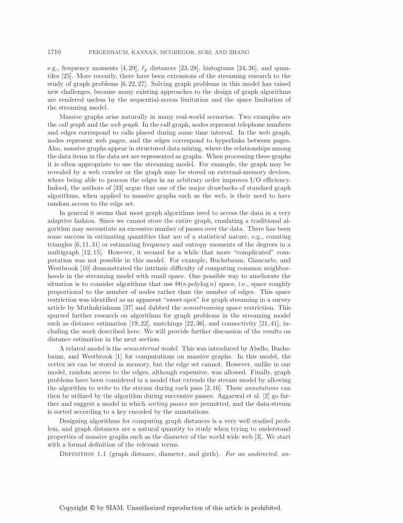
st

V2V1 Vr

...

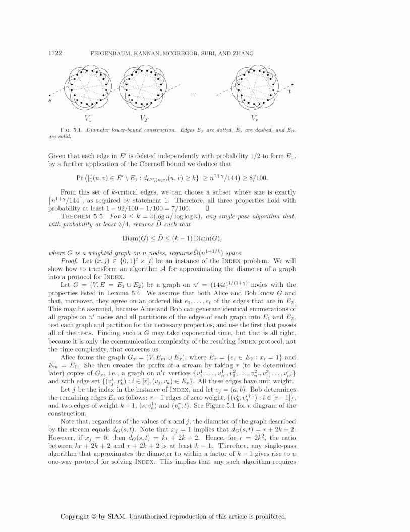
Fig. 5.1. Diameter lower-bound construction. Edges Ex are dotted, Ej are dashed, and Em

are solid.

Given that each edge in E′ is deleted independently with probability 1/2 to form E1,by a further application of the Chernoff bound we deduce that

Pr(|{(u, v) ∈ E′ \ E1 : dG′\(u,v)(u, v) ≥ k}| ≥ n1+γ/144

) ≥ 8/100.

From this set of k-critical edges, we can choose a subset whose size is exactly⌈n1+γ/144

⌉, as required by statement 1. Therefore, all three properties hold with

probability at least 1− 92/100− 1/100 = 7/100.Theorem 5.5. For 3 ≤ k = o(log n/ log log n), any single-pass algorithm that,

with probability at least 3/4, returns D such that

Diam(G) ≤ D ≤ (k − 1)Diam(G),

where G is a weighted graph on n nodes, requires Ω(n1+1/k) space.Proof. Let (x, j) ∈ {0, 1}t × [t] be an instance of the Index problem. We will

show how to transform an algorithm A for approximating the diameter of a graphinto a protocol for Index.

Let G = (V, E = E1 ∪ E2) be a graph on n′ = (144t)1/(1+γ) nodes with theproperties listed in Lemma 5.4. We assume that both Alice and Bob know G andthat, moreover, they agree on an ordered list e1, . . . , et of the edges that are in E2.This may be assumed, because Alice and Bob can generate identical enumerations ofall graphs on n′ nodes and all partitions of the edges of each graph into E1 and E2,test each graph and partition for the necessary properties, and use the first that passesall of the tests. Finding such a G may take exponential time, but that is all right,because it is only the communication complexity of the resulting Index protocol, notthe time complexity, that concerns us.

Alice forms the graph Gx = (V, Em ∪ Ex), where Ex = {ei ∈ E2 : xi = 1} andEm = E1. She then creates the prefix of a stream by taking r (to be determinedlater) copies of Gx, i.e., a graph on n′r vertices {v1

1 , . . . , v1n′ , v2

1 , . . . , v2n′ , v3

1 , . . . , vrn′}

and with edge set {(vij , v

ik) : i ∈ [r], (vj , vk) ∈ Ex}. All these edges have unit weight.

Let j be the index in the instance of Index, and let ej = (a, b). Bob determinesthe remaining edges Ej as follows: r−1 edges of zero weight, {(vi

b, vi+1a ) : i ∈ [r−1]},

and two edges of weight k + 1, (s, v1a) and (vr

b , t). See Figure 5.1 for a diagram of theconstruction.

Note that, regardless of the values of x and j, the diameter of the graph describedby the stream equals dG(s, t). Note that xj = 1 implies that dG(s, t) = r + 2k + 2.However, if xj = 0, then dG(s, t) = kr + 2k + 2. Hence, for r = 2k2, the ratiobetween kr + 2k + 2 and r + 2k + 2 is at least k − 1. Therefore, any single-passalgorithm that approximates the diameter to within a factor of k − 1 gives rise to aone-way protocol for solving Index. This implies that any such algorithm requires



... ...

V2V1 V3 Vg

Fig. 5.2. Girth lower-bound construction. Edges Ex are dotted, Ey are dashed, and Em are solid.

Ω(n1+1/k) bits of space, because the total number of nodes in the construction isn = O((144t)1/(1+1/k)k2).

5.3. Girth. In this section, we prove a lower bound on the space required by a(multipass) algorithm that tests whether a graph has girth at most g. We shall makeuse of the following result from [35].

Lemma 5.6 (see Lazebnik, Ustimenko, and Woldar [35]). Let k ≥ 1 be an oddinteger, t = k+2

4 , and q be a prime power. There exists a bipartite, q-regular graphwith at most 2qk−t+1 nodes and girth at least k + 5.

The following lower bound is established with a construction based on Lemma5.6 that yields a reduction from Set-Disjointness to girth estimation.

Theorem 5.7. For g ≥ 5, any p-pass algorithm that tests whether the girth ofan unweighted graph is at most g requires Ω

(p−1(n/g)1+4/(3g−4)

)space. If g is odd,

this can be strengthened to Ω(p−1(n/g)1+4/(3g−7)

)space.

Proof. Let q be a prime power; let k = g − 4 if g is odd, and k = g − 3 if g iseven. Let t = k+2

4 . Then,

k − t + 1 ≤ k − k + 24

+ 3/4 + 1 ≤{

(3g − 7)/4 if g is odd,(3g − 4)/4 if g is even.

Lemma 5.6 implies that there exists a q-regular graph G′ = (L ∪ R, E′) with atmost 2n′ ≤ 2qk−t+1 nodes and girth at least g + 1. Let L = {l1, . . . , ln′} and R ={r1, . . . , rn′} and, for each i ∈ [n′], Di = Γ(li).

We let (x, y) ∈ {0, 1}r × {0, 1}r be an instance of Set-Disjointness where r =n′q. It will be convenient to write x = x1 . . . xn′

and y = y1 . . . yn′, where xi, yj ∈

{0, 1}q. We will show how to transform a p-pass algorithm A for testing whether thegirth of a graph is at most g into a protocol for Set-Disjointness. IfA uses M bits ofworking memory, then the protocol will transmit O(pM) bits. Hence M = Ω(p−1n′q).

Alice and Bob construct a graph G based upon G′, x, and y as follows. For i ∈ [g],let Vi = {vi

1, . . . , vin′}. For each i ∈ [n′], let Di(x) ⊂ Di be the subset of Di whose

characteristic vector is xi. Di(y) is defined similarly. There are three sets of edges on



these nodes:

Em =g⋃

j=�g/2�+1

{(vji , v

j+1i ) : i ∈ [n′]},

Ex = {(v1i , v2

j ) : j ∈ Di(x), i ∈ [n′]}, and

Ey = {(v�g/2�j , v

�g/2�+1i ) : j ∈ Di(y), i ∈ [n′]}.

See Figure 5.2 for a diagram of the construction.Note that Girth(G) = g if there exists i such that Di(x) ∩ Di(y) �= ∅, i.e., x

and y are not disjoint. However, if x and y are disjoint, then the shortest cycle is oflength at least 4 + 2 g−2

2 ≥ g + 1. Hence, determining whether the girth is at mostg determines whether x and y are disjoint.

6. Toward fast per-item processing. In section 3, we gave a spanner con-struction that processes each edge much faster than previous spanner-constructionalgorithms. In this section, we explore two general methods for decreasing the per-edge computation time of a streaming algorithm. As a consequence, we will show howsome results from [20] give rise to efficient graph-stream algorithms.

Our first observation is that we can locally amortize per-edge processing by us-ing some of our storage space as a buffer for incoming edges. While the algorithmprocesses a time-consuming edge, subsequent edges can be buffered subject to theavailability of space. This yields a potential decrease in the minimum allowable timebetween the arrival of consecutive pairs of incoming edges.

Theorem 6.1. Consider a streaming algorithm that runs in space S(n) and usescomputation time τ(m, n) to process the entire stream. This streaming algorithm canbe simulated by a one-pass streaming algorithm that uses O(S(n) log n) storage spaceand has worst-case time per-edge τ(m, n)/S(n).

Next we turn to capitalizing on work done to speed up dynamic graph algorithms.Dynamic graph algorithms allow edges to be inserted and deleted in any order andthe current graph to be queried for a property P at any point. Partially dynamicalgorithms, on the other hand, are those that allow only edge insertions and querying.In [20], the authors describe a technique called sparsification and use it to speedup existing dynamic graph algorithms that decide whether a graph has property P .Sparsification is based on maintaining strong certificates throughout the updates tothe graph.

Definition 6.2. For any graph property P and graph G, a strong certificate forG is a graph G′ on the same vertex set such that, for any H, G ∪H has property Pif and only if G′ ∪H has it as well.

It is easy to see that strong certificates obey a transitivity property: If G′ is astrong certificate of property P for graph G, and G′′ is a strong certificate for G′,then G′′ is a strong certificate for G. Strong certificates also obey a compositionalproperty. If G′ and H ′ are strong certificates of P for G and H , then G′ ∪ H ′ is astrong certificate for G ∪H .

In order to achieve their speedup, the authors of [20] ensure that the certificatesthey maintain are not only strong but also sparse. A property is said to have sparsecertificates if there is some constant c such that for every graph G on an n-vertex set,we can find a strong certificate for G with at most cn edges. Maintaining P over asparse certificate allows an algorithm to run on a dense graph, using the (smaller)computational time required for a sparse graph.



Table 6.1

One-pass, O(npolylog n) space streaming algorithms given by Theorem 6.3.

Problem Time/edge

Bipartiteness α(n)Connected comps. α(n)

2-vertex connected comps. α(n)3-vertex connected comps. α(n)4-vertex connected comps. log n

MST log n2-edge connected comps. α(n)3-edge connected comps. α(n)4-edge connected comps. nα(n)

Constant edge connected comps. n log n

In the streaming model, we are concerned only with edge insertion and need onlyquery the property at the end of the stream. Moreover, observe that a sparse certificatefits in space O(n polylog n). The following theorem states that any algorithm thatcould be sped up via the three major techniques described in [20] yields a one-pass,O(n polylog n) space, streaming algorithm with the improved running time per inputedge.

Theorem 6.3. Let P be a property for which we can find a sparse certificate intime f(n, m). Then there exists a one-pass, semistreaming algorithm that maintainsa sparse certificate for P using f(n, O(n))/n time per edge.

Proof. Let the edges in the stream be denoted e1, e2, . . . , em. Let Gi denote thesubgraph given by e1, e2, . . . , ei. Inductively, assume we have a sparse certificate Cjn

for Gjn, where 1 ≤ j ≤ m/n, constructed in time f(n, O(n))/n per edge. Also,inductively assume that we have buffered the next n edges, ejn+1, ejn+2, . . . , e(j+1)n.Let T = Cjn∪{ejn+1, ejn+2, . . . , e(j+1)n}. By the composability of strong certificates,T is a strong certificate for G(j+1)n. Let C(j+1)n be the sparse certificate of T . By thetransitivity of strong certificates, C(j+1)n is a sparse certificate of G(j+1)n. Since Cjn

is sparse, |T | = (c+1)n. Thus, computing C(j+1)n takes time f(n, O(n)). By Theorem6.1, this results in f(n, O(n))/n time per edge, charged over ejn+1, ejn+2, . . . , e(j+1)n.This computation can be done while the next n edges are being buffered. If k =nm/n, then the final sparse certificate will be Ck ∪ {ek+1, ek+2, . . . , em}.

We note that, for f(n, m) that is linear or sublinear in m, a better speedup maybe achieved by buffering more than n edges, which is possible when we have morespace. In [20], the authors provide many algorithms for computing various graphproperties which they speed up using sparsification. Applying Theorem 6.3 to thesealgorithms yields the list of streaming algorithms outlined in Table 6.1. For l ≥ 2, thel-vertex and l-edge connectivity problems either have not been explicitly consideredin the streaming model or have algorithms with significantly slower time per edge [22].

Acknowledgments. We thank Martin Sauerhoff for helpful comments on theresults in section 4 and the anonymous referees for their comments on the presentation.

REFERENCES

[1] J. Abello, A. L. Buchsbaum, and J. Westbrook, A functional approach to external graphalgorithms, Algorithmica, 32 (2002), pp. 437–458.

[2] G. Aggarwal, M. Datar, S. Rajagopalan, and M. Ruhl, On the streaming model aug-mented with a sorting primitive, in Proceedings of the IEEE Symposium on Foundationsof Computer Science, IEEE Computer Society, Washington, DC, 2004, pp. 540–549.



[3] R. Albert, H. Jeong, and A.-L. Barabasi, The diameter of the world wide web, Nature, 401(1999), p. 130.

[4] N. Alon, Y. Matias, and M. Szegedy, The space complexity of approximating the frequencymoments, J. Comput. System Sci., 58 (1999), pp. 137–147.

[5] B. Awerbuch, B. Berger, L. Cowen, and D. Peleg, Near-linear time construction of sparseneighborhood covers, SIAM J. Comput., 28 (1998), pp. 263–277.

[6] Z. Bar-Yossef, R. Kumar, and D. Sivakumar, Reductions in streaming algorithms, with anapplication to counting triangles in graphs, in Proceedings of the ACM-SIAM Symposiumon Discrete Algorithms, ACM, New York, SIAM, Philadelphia, 2002, pp. 623–632.

[7] S. Baswana and S. Sen, A simple linear time algorithm for computing a (2k − 1)-spannerof O(n1+1/k) size in weighted graphs, in Proceedings of the International Colloquium onAutomata, Languages and Programming, Eindhoven, The Netherlands, 2003, pp. 384–396.

[8] S. Baswana, Streaming algorithm for graph spanners—single pass and constant processingtime per edge, Inform. Process. Lett., 106 (2007), pp. 110–114.

[9] B. Bollobas, Random Graphs, Academic Press, London, 1985.[10] A. L. Buchsbaum, R. Giancarlo, and J. Westbrook, On finding common neighborhoods in

massive graphs, Theoret. Comput. Sci., 299 (2003), pp. 707–718.[11] L. S. Buriol, G. Frahling, S. Leonardi, A. Marchetti-Spaccamela, and C. Sohler,

Counting triangles in data streams, in Proceedings of the ACM Symposium on Principlesof Database Systems, ACM, New York, 2006, pp. 253–262.

[12] A. Chakrabarti, G. Cormode, and A. McGregor, A near-optimal algorithm for comput-ing the entropy of a stream, in Proceedings of the ACM-SIAM Symposium on DiscreteAlgorithms, ACM, New York, SIAM, Philadelphia, 2007, pp. 328–335.

[13] E. Cohen, Fast algorithms for constructing t-spanners and paths with stretch t, SIAM J.Comput., 28 (1998), pp. 210–236.

[14] T. H. Cormen, C. E. Leiserson, R. L. Rivest, and C. Stein, Introduction to Algorithms,MIT Press, Cambridge, MA, McGraw-Hill, New York, 2001.

[15] G. Cormode and S. Muthukrishnan, Space efficient mining of multigraph streams, in Pro-ceedings of the ACM Symposium on Principles of Database Systems, ACM, New York,2005, pp. 271–282.

[16] C. Demetrescu, I. Finocchi, and A. Ribichini, Trading off space for passes in graph stream-ing problems, in Proceedings of the ACM-SIAM Symposium on Discrete Algorithms, ACM,New York, SIAM, Philadelphia, 2006, pp. 714–723.

[17] M. Elkin, Computing almost shortest paths, ACM Trans. Algorithms, 1 (2005), pp. 283–323.[18] M. Elkin, Streaming and fully dynamic centralized algorithms for constructing and main-

taining sparse spanners, in Proceedings of the International Colloquium on Automata,Languages and Programming, Wroclaw, Poland, 2007, pp. 716–727.

[19] M. Elkin and J. Zhang, Efficient algorithms for constructing (1 + ε, β)-spanners in the dis-tributed and streaming models, Distributed Computing, 18 (2006), pp. 375–385.

[20] D. Eppstein, Z. Galil, G. F. Italiano, and A. Nissenzweig, Sparsification—a technique forspeeding up dynamic graph algorithms, J. ACM, 44 (1997), pp. 669–696.

[21] J. Feigenbaum, S. Kannan, A. McGregor, S. Suri, and J. Zhang, Graph distances in thestreaming model: The value of space, in Proceedings of the ACM-SIAM Symposium onDiscrete Algorithms, ACM, New York, SIAM, Philadelphia, 2005, pp. 745–754.

[22] J. Feigenbaum, S. Kannan, A. McGregor, S. Suri, and J. Zhang, On graph problems in asemi-streaming model, Theoret. Comput. Sci., 348 (2005), pp. 207–216.

[23] J. Feigenbaum, S. Kannan, M. J. Strauss, and M. Viswanathan, An approximate L1-difference algorithm for massive data streams, SIAM J. Comput., 32 (2002), pp. 131–151.

[24] A. C. Gilbert, S. Guha, P. Indyk, Y. Kotidis, S. Muthukrishnan, and M. Strauss, Fast,small-space algorithms for approximate histogram maintenance, in Proceedings of the ACMSymposium on Theory of Computing, ACM, New York, 2002, pp. 389–398.

[25] M. Greenwald and S. Khanna, Efficient online computation of quantile summaries, in Pro-ceedings of the ACM International Conference on Management of Data, ACM, New York,2001, pp. 58–66.

[26] S. Guha, N. Koudas, and K. Shim, Approximation and streaming algorithms for histogramconstruction problems, ACM Trans. Database Syst., 31 (2006), pp. 396–438.

[27] M. R. Henzinger, P. Raghavan, and S. Rajagopalan, Computing on data streams, in Ex-ternal Memory Algorithms, AMS, Providence, RI, 1999, pp. 107–118.

[28] P. Indyk, Stable distributions, pseudorandom generators, embeddings and data stream com-putation, in Proceedings of the IEEE Symposium on Foundations of Computer Science,IEEE Computer Society, Washington, DC, 2000, pp. 189–197.



[29] P. Indyk and D. P. Woodruff, Optimal approximations of the frequency moments of datastreams, in Proceedings of the ACM Symposium on Theory of Computing, ACM, NewYork, 2005, pp. 202–208.

[30] R. Jain, J. Radhakrishnan, and P. Sen, A direct sum theorem in communication complexityvia message compression, in Proceedings of the International Colloquium on Automata,Languages and Programming, Eindhoven, The Netherlands, 2003, pp. 300–315.

[31] H. Jowhari and M. Ghodsi, New streaming algorithms for counting triangles in graphs, inProceedings of the International Conference on Computing and Combinatorics, Kunming,Yunnan, China, 2005, pp. 710–716.

[32] B. Kalyanasundaram and G. Schnitger, The probabilistic communication complexity of setintersection, SIAM J. Discrete Math., 5 (1992), pp. 545–557.

[33] R. Kumar, P. Raghavan, S. Rajagopalan, and A. Tomkins, Extracting large-scale knowledgebases from the web, in Proceedings of the International Conference on Very Large DataBases, Edinburgh, Scotland, 1999, pp. 639–650.

[34] E. Kushilevitz and N. Nisan, Communication Complexity, Cambridge University Press, Cam-bridge, UK, 1997.

[35] F. Lazebnik, V. A. Ustimenko, and A. J. Woldar, A new series of dense graphs of highgirth, Bull. AMS, 32 (1995), pp. 73–79.

[36] A. McGregor, Finding graph matchings in data streams, in Proceedings of APPROX-RANDOM, Berkeley, CA, 2005, pp. 170–181.

[37] S. Muthukrishnan, Data Streams: Algorithms and Applications, Now Publishers, Boston,2005.

[38] N. Nisan and A. Wigderson, Rounds in communication complexity revisited, SIAM J. Com-put., 22 (1993), pp. 211–219.

[39] A. A. Razborov, On the distributional complexity of disjointness, Theoret. Comput. Sci., 106(1992), pp. 385–390.

[40] M. Thorup and U. Zwick, Approximate distance oracles, in Proceedings of the ACM Sympo-sium on Theory of Computing, ACM, New York, 2001, pp. 183–192.

[41] M. Zelke, k-connectivity in the semi-streaming model, http://arxiv.org/abs/cs/0608066, 2006.[42] M. Zelke, Optimal per-edge processing times in the semi-streaming model, Inform. Process.

Lett., 104 (2007), pp. 106–112.

Graph Distances in the Data-Stream Model

Documents

Transcript of Graph Distances in the Data-Stream Model