Chapter 3Data Stream Processing

João Gama and Pedro Pereira Rodrigues

3.1 Introduction

The rapid growth in information science and technology in general and the com-plexity and volume of data in particular have introduced new challenges for the re-search community. Many sources produce data continuously. Examples include sen-sor networks, wireless networks, radio frequency identification (RFID), customerclick streams, telephone records, multimedia data, scientific data, sets of retail chaintransactions etc. These sources are called data streams. A data stream is an orderedsequence of instances that can be read only once or a small number of times usinglimited computing and storage capabilities. These sources of data are characterizedby being open-ended, flowing at high-speed, and generated by non stationary distri-butions in dynamic environments.

What distinguishes current data from earlier one is automatic data feeds. We donot just have people who are entering information into a computer. Instead, we havecomputers entering data into each other [25]. Nowadays there are applications inwhich the data are modeled best as transient data streams instead of as persistenttables. Examples of applications include network monitoring, user modeling in webapplications, sensor networks in electrical networks, telecommunications data man-agement, prediction in stock markets, monitoring radio frequency identification etc.In these applications it is not feasible to load the arriving data into a traditional database management system (DBMS) and traditional DBMS are not designed to di-rectly support the continuous queries required by these applications [3]. Carney

J. GamaLIAAD–INESC Porto L.A. and Faculty of Economics, University of Porto, Rua de Ceuta, 118-6,4050-190 Porto, Portugale-mail: jgama@fep.up.pt

P.P. RodriguesLIAAD–INESC Porto L.A. and Faculty of Sciences, University of Porto, Rua de Ceuta, 118-6,4050-190 Porto, Portugale-mail: pprodriques@fc.up.pt

26 J. Gama, P.P. Rodrigues

et al. [6] pointed out the significant differences between data bases that are pas-sive repositories of data and data bases that actually monitor applications and alerthumans when abnormal activity is detected. In the former, only the current stateof the data is relevant for analysis. Humans initiate queries, usually one-time, pre-defined queries. In the latter, data come from external sources (e.g., sensors), andrequire processing historic data. For example, in monitoring activity, queries shouldrun continuously. The answer to a continuous query is produced over time, reflect-ing the data seen so far. Moreover, if the process is not strictly stationary (as most ofreal-world applications), the target concept could gradually change over time. Forexample, the type of abnormal activity (e.g., attacks in TCP/IP networks, frauds incredit card transactions etc.) changes over time.

Organizations use decision support systems to identify potential useful patternsin data. Data analysis is complex, interactive, and exploratory over very large vol-umes of historic data, eventually stored in distributed environments. Traditional pat-tern discovery process requires online ad-hoc queries, not previously defined, thatare successively refined. Nowadays, given the current trends in decision support anddata analysis, the computer plays a much more active role, by searching hypotheses,evaluating and suggesting patterns. Due to the exploratory nature of these queries,an exact answer may not be required. A user may prefer a fast approximate answer.Range queries and selectivity estimation (the proportion of tuples that satisfya query) are two illustrative examples where fast but approximate answers are moreuseful than slow and exact ones.

Sensor networks are distributed environments producing multiple streams of data.We can consider the network as a distributed database we are interested in query-ing and mining. In this chapter we review the main techniques used for query andmining data streams that are of potential use in sensor networks.

In Sect. 3.2 we refer to the data stream models and identify its main researchchallenges. Section 3.3 presents basic stream models. Section 3.4 present basic streamalgorithms for maintaining synopsis over data streams. Section 3.5 concludes thechapter and points out future directions for research.

3.2 Data Stream Models

What makes data streams different from the conventional relational model? A keyidea is that operating in the data stream model does not preclude the use of data inconventional stored relations. Some relevant differences include [3]:

• Data elements in the stream arrive online.• The system has no control over the order in which data elements arrive, either

within a data stream or across data streams.• Data streams are potentially unbounded in size.• Once an element from a data stream has been processed it is discarded or archived.

It cannot be retrieved easily unless it is explicitly stored in memory, which issmall relative to the size of the data streams.

3 Data Stream Processing 27

In the stream model [25] the input elements a1, a2, . . . , aj , . . . arrive sequentially,item by item and describe an underlying function A. Stream models differ on howai describes A. We can distinguish between:

• Insert Only Model: once an element ai is seen, it cannot be changed.• Insert-Delete Model: elements ai can be deleted or updated.• Accumulative Model: each ai is an increment to A[j ] = A[j − 1] + ai .

Examples of stream applications for the three models include time-series gener-ated by sensor networks (Insert Only Model), radio frequency identification (Insert-Delete Model), monitoring the Max (or Min) of the sum of quantities transactionedper entity (Accumulative Model).

3.2.1 An Illustrative Problem

A simple problem that clearly illustrates the issues in stream process is finding themaximum value (MAX) or the minimum value (MIN) in a sliding window over asequence of numbers. When we can store in memory all the elements of the slidingwindow, the problem is trivial and we can find the exact solution. When the size ofthe sliding window is greater than the available memory, there is no algorithm thatprovides an exact solution, because it is not possible to store all the data elements.For example, suppose that the sequence is monotonically decreasing and the aggre-gation function is MAX. Whatever the window size, the first element in the windowis always the maximum. As the sliding window moves, the exact answer requiresmaintaining all the elements in memory.

3.2.2 Research Issues in Data Streams Management Systems

Babcock et al. [3] defined blocking query operators as query operators that are un-able to produce the first tuple of the output before they have seen the entire input.Aggregating operators, like SORT, SUM, COUNT, MAX, MIN, are blocking queryoperators. In the stream setting, continuous queries using block operators are prob-lematic. The semantics of these operators in the stream problem setting is an activeresearch area. For example, Raman et al. [26] proposed an approximate online ver-sion for Sort. Fang et al. [12] studied approximate algorithms for iceberg queriesusing data synopsis. Iceberg queries compute aggregate functions (such asCOUNT, SUM) over an attribute to find aggregate values above somespecified threshold. They process a relative large amount of data to produce resultswhere the number of above-threshold results is often very small (the tip of aniceberg).

From the point of view of a data stream management system, several researchissues emerge [3]. These issues have implications in data stream management sys-tems, like:

28 J. Gama, P.P. Rodrigues

• Approximate query processing techniques to evaluate queries that require an un-bounded amount of memory.

• Sliding window query processing, both as an approximation technique and as anoption in the query language.

• Sampling to handle situations where the flow rate of the input stream is fasterthan the query processor.

• The meaning and implementation of blocking operators (e.g., aggregation andsorting) in the presence of unending streams.

These types of queries require techniques for storing summaries or synopsis in-formation about previously seen data. There is a trade-off between the size of sum-maries and the ability to provide precise answers.

The time dimension is an important characteristic in streams. For example, intime window models, it indicates when a specific measure is valid. In single streams,the meaning of a time-stamp attribute, indicating when the tuple has arrived, hasclear semantics. When a query involves multiple streams, the semantics of timestamps is much less clear. For example, what is the time stamp of an output tuple?Research in temporal databases propose several methods to deal with time, includ-ing temporal types [27,5].

A large number of applications are distributed in nature. Sensors in electricalnetworks are geographically distributed. Data collected from these sensors have notonly a time dimension but also a space dimension. Furthermore, sensors are resourcelimited. While the time dimension is critical for synchronization aspects, the spacedimension makes bandwidth and battery power critical aspects as well.

A summary of the differences between traditional and stream data processing ispresented in Table 3.1.

Table 3.1 Differences between traditional and stream data processing

Traditional Stream

Number of passes Multiple SingleProcessing Time Unlimited RestrictedMemory Usage Unlimited RestrictedType of Result Accurate ApproximateDistributed No Yes

3.3 Basic Streaming Methods

Data streams are unbounded in length. However, this is not the only problem. Thedomain of the possible values of an attribute is also very large. A typical exampleis the domain of all IP addresses on the Internet.1 It is so huge that complete stor-

1 Actually, in the new standard protocol for the Internet, IPv6, an IP address is a number definedby 128 bits [20]. Thus, the number of all IP addresses is 2128, around 600,000 addresses for everysquare nanometer of the entire Earth’s surface.

3 Data Stream Processing 29

age is an intractable problem. The execution of queries that reference past data alsobecomes problematic. These are situations in which stream methods are applica-ble and become relevant. Stream methods provide approximate answers using thereduced resources.

It is impractical to store all data to execute queries that reference past data. Seek-ing a fast but approximate answer, however, is a valid alternative. Several techniqueshave been developed for storing summaries or synopsis information about previ-ously seen data. There is a trade-off between the size of summaries and the abilityto provide precise answers. Datar et al. [11] presented simple counting problemsthat clearly illustrate the issues in data stream research:

1. Given a stream of bits (0’s and 1’s), maintain a count of the number of 1’s in thelast N elements seen from the stream.

2. Given a stream of elements that are positive integers in the range [0, . . . , R],maintain at every instance the sum of the last N elements seen from the stream.

3. Find the number of distinct values in a stream of values with domain [1, . . . , N ].All these problems have an exact solution if we have enough memory to store allthe elements in the sliding window. That is, the exact solution requires O(N) space.Suppose we have restricted memory. How can we solve these problems using lessspace than O(N)?

Approximate answers are useful if the associated error is in an admissible bound-ary. We can define the approximation methods in the data streams as:

(ε, δ)-approximation schema: Given any positive number ε < 1 and δ < 1compute an estimate that, with probability 1 − δ, is within relative error ≤ ε.

Time and space required to compute an answer depends on ε and δ. Some results ontail inequalities provided by statistics are useful to accomplish this goal. The basicgeneral bounds on the tail probability of a random variable (that is, the probabilitythat a random variable deviates greatly from its expectation) include the Markov,and Chebyshev inequalities [24]. Two other powerful bounds derived from thoseare the Chernoff and Hoffding bounds.

Statistical Inequalities

An estimator is a function of the observable sample data that is used to estimatean unknown population parameter. We are particularly interested in interval estima-tors that compute an interval for the true value of the parameter associated with aconfidence 1 − δ. Two types of intervals are:

• Absolute approximation: X − ε ≤ μ ≤ X + ε, where ε is the absolute error; and• Relative approximation: (1 − δ)X ≤ μ ≤ (1 + δ)X, where δ is the relative error.

The following two results from statistical theory are useful in most of the cases.

Theorem 1 (Chernoff Bound). Let X1, X2, . . . , Xn be independent random vari-ables from Bernoulli experiments. Assume that P(Xi = 1) = pi . Let Xs = ∑n

i=1 Xi

be a random variable with expected value μs = ∑i=1 npi . Then for any δ > 0

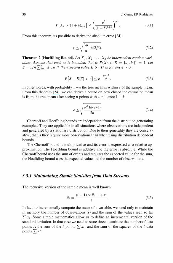
30 J. Gama, P.P. Rodrigues

P[Xs > (1 + δ)μs

] ≤(

eδ

(1 + δ)1+δ

)μs

. (3.1)

From this theorem, its possible to derive the absolute error [24]:

ε ≤√

3μ

nln(2/δ). (3.2)

Theorem 2 (Hoeffding Bound). Let X1, X2, . . . , Xn be independent random vari-ables. Assume that each xi is bounded, that is P(Xi ∈ R = [ai, bi]) = 1. LetS = 1/n

∑ni=1 Xi , with the expected value E[S]. Then for any ε > 0,

P[S − E[S] > ε

] ≤ e− 2n2ε2

R2 . (3.3)

In other words, with probability 1 − δ the true mean is within ε of the sample mean.From this theorem [24], we can derive a bound on how closed the estimated meanis from the true mean after seeing n points with confidence 1 − δ;

ε ≤√

R2 ln(2/δ)

2n. (3.4)

Chernoff and Hoeffding bounds are independent from the distribution generatingexamples. They are applicable in all situations where observations are independentand generated by a stationary distribution. Due to their generality they are conserv-ative, that is they require more observations than when using distribution dependentbounds.

The Chernoff bound is multiplicative and its error is expressed as a relative ap-proximation. The Hoeffding bound is additive and the error is absolute. While theChernoff bound uses the sum of events and requires the expected value for the sum,the Hoeffding bound uses the expected value and the number of observations.

3.3.1 Maintaining Simple Statistics from Data Streams

The recursive version of the sample mean is well known:

x̄i = (i − 1) × x̄i−1 + xi

i. (3.5)

In fact, to incrementally compute the mean of a variable, we need only to maintainin memory the number of observations (i) and the sum of the values seen so far∑

xi . Some simple mathematics allow us to define an incremental version of thestandard deviation. In that case we need to store three quantities: the number of datapoints i; the sum of the i points

∑xi ; and the sum of the squares of the i data

points∑

x2i

3 Data Stream Processing 31

σi =√

(∑x2i −

(∑xi

)2

/i

)

/(i − 1). (3.6)

Another useful measure that can be recursively computed is the correlation coef-ficient. Given two streams x and y, we need to maintain the sum of each stream(∑

xi and∑

yi), the sum of the squared values (∑

x2i and

∑y2i ), and the sum of

the cross-product (∑

(xi × yi)). The exact correlation is:

corr(a, b) =∑

(xi × yi) −∑

xi×∑yi

n√∑

x2i − (

∑xi )

2

n

√∑

y2i − (

∑yi )

2

n

. (3.7)

We have defined the sufficient statistics necessary to compute the mean, standarddeviation, and correlation on a time series. The main interest of these formulas is thatthey allow us to maintain exact statistics (mean, standard deviation, and correlation)over an eventually infinite sequence of numbers without storing in memory all thenumbers. Quantiles, median and other statistics [2] used in range queries can becomputed from histograms, and other summaries that are discussed later in thischapter. Although these statistics are used everywhere they are of limited use in thestream problem setting. In most applications recent data is the most relevant one. Tofulfill this goal, a popular approach consists of defining a time window covering themost recent data.

3.3.2 Time Windows

Time windows are a commonly used approach to solve queries in open-ended datastreams. Instead of computing an answer over the whole data stream, the query (oroperator) is computed, eventually several times, over a finite subset of tuples. In thismodel, a time stamp is associated with each tuple. The time stamp defines when aspecific tuple is valid (e.g. inside the window) or not. Queries run over the tuplesinside the window. However, in the case of joining multiple streams the semanticsof time stamps is much less clear e.g. the time stamp of an output tuple.

Several window models have been used in the literature. The following are themost relevant.

3.3.2.1 Landmark Windows

Landmark windows [14] identified relevant points (the landmarks) in the data streamand the aggregate operator uses all record seen so far after the landmark. Successivewindows share some initial points and are of growing size. In some applications,the landmarks have a natural semantic. For example, in daily basis aggregates thebeginning of the day is a landmark.

32 J. Gama, P.P. Rodrigues

3.3.2.2 Sliding Windows

Most of the time, we are not interested in computing statistics over all the past butonly in the recent past. The simplest approach are sliding windows of fixed size.These type of windows are similar to first in, first out data structures. Whenever anelement j is observed and inserted in the window, another element j − w, where w

represents the window size, is forgotten.

Fig. 3.1 Landmark and sliding windows

Suppose we want to maintain the standard deviation of the values of a datastream using only the last 100 examples, that is in a fixed time window of dimen-sion 100. After seeing observation 1,000, the observations inside the time windoware x901, . . . , x1,000, and the sufficient statistics after seeing the 1,000th observationare A = ∑1,000

i=901 xi ; B=∑1,000

i=901 x2i . Whenever the 1,001th value is observed, the

time window moves 1 observation, forgets observation 901 and the updated suffi-cient statistics are: A = A + x1,001 − x901 and B = B + x2

1,001 − x2901. Due to the

necessity to forget old observations, we need to maintain in memory all the obser-vations inside the window. The same problem applies for time windows whose sizechanges with time. In the following sections we address the problem of maintainingapproximate statistics over sliding windows in a stream, without storing in memoryall the elements inside the window.

3.3.2.3 Tilted Windows

Previous windows models use a catastrophic forget; that is, any past observation ei-ther is in the window or it is not inside the window. In tilted windows, the time scaleis compressed. The most recent data are stored inside the window at the finest detail(granularity). Oldest information is stored at a coarser detail, in an aggregated way.The level of granularity depends on the application. This window model is desig-nated a tilted time window. Tilted time windows can be designed in several ways.

3 Data Stream Processing 33

Han and Kamber [19] presented two possible variants: natural tilted time windows,and logarithm tilted windows. Illustrative examples are presented in Fig. 3.2. In thefirst case, data are stored with granularity according to a natural time taxonomy:last hour at a granularity of 15 minutes (4 points), last day in hours (24 points), lastmonth in days (32 points) and last year in months (12 points). In the case of logarith-mic tilted windows, given a maximum granularity with periods of t , the granularitydecreases logarithmically as data are older. As time goes by, the window stores thelast time period t , the one before that, and consecutive aggregates of less granularity(two periods, four periods, eight periods etc.).

Fig. 3.2 Tilted Time Windows. The top figure presents a natural tilted time window, the figure inthe bottom logarithm tilted windows

3.4 Basic Streaming Algorithms

With new data constantly arriving even as old data are being processed, the amountof computation time per data element must be low. Furthermore, since we are lim-ited to a bounded amount of memory, it may not be possible to produce exact an-swers. High-quality approximate answers can be an acceptable solution. Two typesof techniques can be used: data reduction and summaries. In both cases, queries areexecuted over a summary, a compact data-structure that captures the distribution ofthe data. In the latter approach, techniques are required for storing summaries orsynopsis information about previously seen data. Certainly, large summaries pro-vide more precise answers. So, there is a trade-off between the size of summariesand the overhead to update summaries and the ability to provide precise answers. Inboth cases, they must use data structures that can be maintained incrementally. Themost commonly used techniques for data reduction involve: sampling, synopsis andhistograms, and wavelets.

3.4.1 Sampling

Sampling involves loss of information: some tuples are selected for processing whileothers are skipped. Instead of dealing with an entire data stream, we can sample in-

34 J. Gama, P.P. Rodrigues

stances at periodic intervals. If the rate of arrival data in the stream is higher than thecapacity to process data, sampling is used as a method to slow down data. Anotheradvantage is the use of offline procedures to analyse data, eventually for differentgoals. Nevertheless, sampling must be done in a principled way in order to avoidmissing relevant information.

The most time-consuming operation in database processing is the join operation.The join operation is a blocking operator, it pairs up tuples from two sources basedon key values in some attribute(s). Sampling has been used to find approximate an-swers whenever a join between two (or more) streams is required. The main ideaconsists of executing a random sample from each input and then joining the sam-ples [10]. The output will be much smaller than the join over the full streams. Ifthe output is representative of the original, the approximate answers are represen-tative of the original output. Traditional sampling algorithms require knowledge ofthe number of tuples. They are not applicable to the streaming setting. This way,join over streams requires sequential random sampling.

The reservoir sampling technique [28] is the classic algorithm to maintain anonline random sample. The basic idea consists of maintaining a sample of size s,called the reservoir. As the stream flows, every new element has a certain probabilityof replacing an old element in the reservoir. Extensions to maintain a sample of sizek over a count-based sliding window of the n most recent data items from datastreams appear in [4]. Longbo et al. [22] presented a stratified multistage samplingalgorithm for time-based sliding window (SMS Algorithm). The SMS algorithmtakes a different sampling fraction in different strata from the time-based slidingwindow, and works even when the number of data items in the sliding windowvaries dynamically over time.

The literature contains a wealth of algorithms for computing quantiles [16] anddistinct counts [15] using samples. Sampling is a general method for solving prob-lems with huge amounts of data, and has been used in most streaming problems.Chaudhuri et al. [8] presented negative results for uniform sampling, mostly forqueries involving joins. An active research area is the design of sampling-based al-gorithms that can produce approximate answers with a guarantee on the error-bound.As a matter of fact, sampling works by providing a compact description of muchlarger data. Alternative ways to obtain compact descriptions include data synop-sis.

3.4.2 Data Synopsis

3.4.2.1 Frequency Moments

A useful mathematical tool employed to solve the above problems are the so-calledfrequency moments. A frequency moment is a number FK , defined as FK =∑v

i=1 mKi , where v is the domain size, mi is the frequency of i in the sequence,

and k >= 0. F 0 is the number of distinct values in the sequence, F 1 is the length

3 Data Stream Processing 35

Fig. 3.3 Querying schema’s: slow and exact answer vs fast but approximate answer using synopsis

of the sequence, F 2 is known as the self-join size (the repeat rate or Gini’s index ofhomogeneity). The frequency moments provide useful information about the dataand can be used in query optimizing. Alon et al. [1] showed that the second fre-quency moment of a stream of values can be approximated using logarithmic space.The authors also showed that no analogous result holds for higher frequency mo-ments.

3.4.2.2 Hash Sketches

Hash functions are another powerful tool in stream processing. They are used toproject attributes with huge domains into lower space dimensions. One of the earlierresults is the Hash sketches (aka FM) for distinct-value counting introduced by Fla-jolet and Martin [13]. The basic assumption is the existence of a hash function h(x)

that maps incoming values x ∈ [0, . . . , N − 1] uniformly across [0, . . . , 2L − 1],where L = O(log N). Let lsb(y) denote the position of the least-significant 1 bitin the binary representation of y. A value x is mapped to lsb(h(x)). The algorithmmaintains a Hash Sketch, that is a bitmap vector of L bits, initialized to zero. Foreach incoming value x, set the lsb(h(x)) to 1. At each time-stamp t , let R denotethe position of rightmost zero in the bitmap. R is an indicator of log(d), where d

denotes the number of distinct values in the stream. Flajolet and Martin [13] provedthat E[R] = log(φd), where φ = 0.7735, so d = 2R/φ. This result is based onthe uniformity of h(x): Prob[BITMAP[k] = 1] = Prob[10k] = 1/2k+1. Assum-ing d distinct values, it is expected that d/2 to map to BITMAP[0], d/4 to map toBITMAP[1], d/2r map to BITMAP[r − 1].

The FM sketches are used for estimating the number of distinct items in a data-base (or stream) in one pass while using only a small amount of space.

3.4.3 Synopsis and Histograms

Synopsis and histograms are summarization techniques that can be used to approx-imate the frequency distribution of element values in a data stream. They are com-monly used to capture attribute value distribution statistics for query optimizers (likerange queries). A histogram is defined by a set of non-overlapping intervals. Each

36 J. Gama, P.P. Rodrigues

interval is defined by the boundaries and a frequency count. The reference tech-nique is the V-Optimal histogram [18]. It defines intervals that minimize the fre-quency variance within each interval. Sketches, a special case of synopsis, provideprobabilistic guarantees on the quality of the approximate answer (e.g. the answer is10 ± 2 with probability 95%). Sketches have been used to solve the k-hot items [9].

3.4.3.1 Exponential Histograms

The exponential histogram is another histogram frequently used to solve countingproblems. Consider a simplified data stream environment where each element comesfrom the same data source and is either 0 or 1. The goal consists of counting thenumber of 1’s in a sliding window. The problem is trivial if the window can fit inmemory. The problem we address here requires O(log(N)) space, where N is thewindow size. Datar et al. [11] presented an exponential histogram strategy to solvethis problem. The basic idea consists of using buckets of different sizes to hold thedata. Each bucket has a time stamp associated with it. This time stamp is used todecide when the bucket is out of the window. Exponential histograms, other thanbuckets, use two additional variables, LAST and TOTAL. The variable LAST storesthe size of the last bucket. The variable TOTAL keeps the total size of the buckets.

When a new data element arrives, we first check the value of the element. Ifthe new data element is zero, ignore it. Otherwise create a new bucket of size 1with the current time-stamp and incrementally advance the counter TOTAL. Givena parameter ε, if there are |1/ε|/2+2 buckets of the same size, merge the two oldestbuckets of the same size into a single bucket of double size. The largest time-stampof the two buckets is used as the time-stamp of the newly created bucket. If the lastbucket gets merged, we update the size of the merged bucket to the counter LAST.

Whenever we want to estimate the moving sum, we check if the oldest bucketis within the sliding window. If not, we drop that bucket, subtract its size from thevariable TOTAL, and update the size of the current oldest bucket to the variableLAST. This procedure is repeated until all the buckets with the time stamps outsideof the sliding window are dropped. The estimate of 1’s in the sliding window isTOTAL-LAST/2.

The main property of the exponential histograms is that the size grows expo-nentially, i.e. 20, 21, 22, . . . , 2h. To store N elements (one’s) in the sliding window,only O(log(N)/ε) are needed to maintain the moving sum and the error estimating.Datar et al. [11] proved that the error is bounded within a relative error ε.

3.4.4 Wavelets

Wavelet transforms are mathematical techniques in which signals are representedas a weighted sum of simpler, fixed building waveforms at different scales and po-sitions. Wavelets attempt to capture trends in numerical functions, decomposing a

3 Data Stream Processing 37

signal into a set of coefficients. The decomposition does not preclude informationloss, because it is possible to reconstruct the signal from the full set of coefficients.Nevertheless, it is possible to eliminate small coefficients from the wavelet trans-form introducing small errors when reconstructing the original signal. The reducedset of coefficients are of great interest for streaming algorithms.

A wavelet transform decomposes a signal into several groups of coefficients. Dif-ferent coefficients contain information about characteristics of the signal at differentscales. Coefficients at a coarse scale capture global trends of the signal, while coef-ficients at fine scales capture details and local characteristics.

The simplest and most common transformation is the Haar wavelet [21]. Anysequence (x0, x1, . . . , x2n−1, x2n) of even length is transformed into a sequence oftwo-component vectors ((s0, d0), . . . , (sn, dn)). One stage of the Fast Haar-WaveletTransform consists of:

[sidi

]

= 1/2

[1 11 −1

]

×[

xi

xi+1

]

.

The process continues, by separating the sequences s and d and transforming thesequence s.

As an illustrative example, consider the sequence (4, 5, 2, 1). Applying the Haartransform:

Resolution Averages Coefficients

4 (4, 5, 2, 1)

2 (4.5, 1.5) (−0.5, 0.5)

1 (3) (1.5)

The output of the Haar transform is the sequence: (3, 1.5,−0.5, 0.5).Wavelet analysis is popular in several streaming applications because most sig-

nals can be represented using a small set of coefficients. Matias et al. [23] presentedan efficient algorithm based on multi-resolution wavelet decomposition for build-ing histograms with application to databases problems, like selectivity estimation.Along the same lines, Chakrabarti et al. [7] proposed the use of wavelet-coefficientsynopses as a general method to provide approximate answers to queries. The ap-proach uses multi-dimensional wavelets synopsis from relational tables. Guha andHarb [17] proposed one-pass wavelet construction streaming algorithms with prov-able error guarantees for minimizing a variety of error-measures including allweighted and relative Lp norms.

3.5 Emerging Challenges and Future Issues

Data stream management systems development is an emerging topic in the com-puter science community, as they offer ways to process and query massive and con-tinuous flows of data. Algorithms that process data streams deliver approximate so-lutions, providing a fast answer using few memory resources. In some applications,

38 J. Gama, P.P. Rodrigues

mostly data base oriented, an approximate answer should be within an admissibleerror margin. In general, as the range of the error decreases the space of compu-tational resources goes up, but linear or sub-linear space data-structures, in the di-mension of the inputs, are not applicable for data steams. The current trends in datastreams involve research in algorithms and data structures with narrow error bounds.Other research issues involve the semantics of block-operators in the stream sce-nario, join over multi-streams and processing distributed streams with privacy pre-serving concerns.

Today, data are distributed in nature. Detailed data for almost any task are col-lected over a broad area, and stream in at a much greater rate than ever before. Inparticular, advances in miniaturization, the advent of widely available and cheap com-puter power, and the explosion of networks of all kinds led to life within inanimatethings. Simple objects that surround us are gaining sensors, computational power,and actuators, and are changing from static, inanimate objects into adaptive, reactivesystems. Sensor networks and social networks are present everywhere.

Acknowledgements This work was developed under project Adaptive Learning Systems II(POSI/EIA/ 55340/2004).

References

[1] N. Alon, Y. Matias, M. Szegedy, The space complexity of approximating the frequency mo-ments. Journal of Computer and System Sciences, 58:137–147, 1999.

[2] A. Arasu, G.S. Manku, Approximate counts and quantiles over sliding windows. In: ACMSymposium on Principles of Database Systems (PODS), pp. 286–296. ACM Press, NewYork, 2004.

[3] B. Babcock, S. Babu, M. Datar, R. Motwani, J. Widom, Models and issues in data stream sys-tems. In: P.G. Kolaitis (Ed.), Proceedings of the 21nd Symposium on Principles of DatabaseSystems, pp. 1–16. ACM Press, New York, 2002.

[4] B. Babcock, M. Datar, Sampling from a moving window over streaming data. In: Proc. of the13th Annual ACM SIAM Symposium on Discrete Algorithms, pp. 633–634. ACM/SIAM,New York/Philadelphia, 2002.

[5] C. Bettini, S.G. Jajodia, S.X. Wang, Time Granularities in Databases, Data Mining and Tem-poral Reasoning. Springer, Berlin, 2000.

[6] D. Carney, U. Çetintemel, M. Cherniack, C. Convey, S. Lee, G. Seidman, M. Stonebraker,N. Tatbul, S.B. Zdonik, Monitoring streams—a new class of data management applications.In: VLDB, pp. 215–226, 2002.

[7] K. Chakrabarti, M. Garofalakis, R. Rastogi, K. Shim, Approximate query processing usingwavelets. VLDB Journal: Very Large Data Bases, 10(2–3):199–223, 2001.

[8] S. Chaudhuri, R. Motwani, V.R. Narasayya, On random sampling over joins. In: SIGMODConference, pp. 263–274, 1999.

[9] G. Cormode, S. Muthukrishnan, What’s hot and what’s not: tracking most frequent itemsdynamically. In: ACM Symposium on Principles of Database Systems (PODS), pp. 296–306,2003.

[10] A. Das, J. Gehrke, M. Riedewald, Approximate join processing over data streams. In: Proc.of the ACM SIGMOD International Conference on Management of Data, pp. 69–84, 2003.

3 Data Stream Processing 39

[11] M. Datar, A. Gionis, P. Indyk, R. Motwani, Maintaining stream statistics over sliding win-dows. In: Proceedings of 13th Annual ACM-SIAM Symposium on Discrete Algorithms,pp. 635–644. Society for Industrial and Applied Mathematics, 2002.

[12] M. Fang, N. Shivakumar, H. Garcia-Molina, R. Motwani, J.D. Ullman, Computing icebergqueries efficiently. In: Proc. 24th Int. Conf. Very Large Data Bases, VLDB, pp. 299–310,1998.

[13] P. Flajolet, G.N. Martin, Probabilistic counting algorithms for data base applications. Journalof Computer and System Sciences, 31(2):182–209, 1985.

[14] J. Gehrke, F. Korn, D. Srivastava, On computing correlated aggregates over continual datastreams. In: SIGMOD Conference, pp. 13–24. ACM Press, New York, 2001.

[15] P.B. Gibbons, Distinct sampling for highly-accurate answers to distinct values queries andevent reports. Very Large Data Boses Journal, 541–550, 2001.

[16] M. Greenwald, S. Khanna, Space-efficient online computation of quantile summaries. In:SIGMOD Conference, pp. 58–66, 2001.

[17] S. Guha, B. Harb, Wavelet synopsis for data streams: minimizing non-euclidean error. In:Proceeding of the Eleventh ACM SIGKDD International Conference on Knowledge Discov-ery in Data Mining, pp. 88–97. ACM Press, New York, 2005.

[18] S. Guha, K. Shim, J. Woo, Rehist: relative error histogram construction algorithms. In: VLDB04: Proceedings of the 30th International Conference on Very Large Data Bases, pp. 288–299.Morgan Kaufmann, San Mateo, 2004.

[19] J. Han, M. Kamber, Data Mining Concepts and Techniques. Morgan Kaufmann, San Mateo,2006.

[20] C. Huitema, IPv6: The New Internet Protocol. Prentice Hall, New York, 1998.[21] B. Jawerth, W. Sweldens, An overview of wavelet based multiresolution analyses. SIAM

Rev., 36(3):377–412, 1994.[22] Z. Longbo, L. Zhanhuai, Y. Min, W. Yong, J. Yun, Random sampling algorithms for slid-

ing windows over data streams. In: Proceedings of the 11th Joint International ComputerConference—JICC. World Scientific, Singapore, 2005.

[23] Y. Matias, J.S. Vitter, M. Wang, Wavelet-based histograms for selectivity estimation, In:ACM SIGMOD International Conference on Management of Data, pp. 448–459, 1998.

[24] R. Motwani, P. Raghavan, Randomized Algorithms. Cambridge University Press, Cam-bridge, 1997.

[25] S. Muthukrishnan, Data streams: algorithms and applications. Now Publishers, 2005.[26] V. Raman, B. Raman, J.M. Hellerstein, Online dynamic reordering for interactive data

processing. In: The VLDB Journal, pp. 709–720, 1999.[27] R. Snodgrass, I. Ahn, A taxonomy of time databases. In: SIGMOD ’85: Proceedings of the

ACM SIGMOD International Conference on Management of Data, pp. 236–246, USA. ACMPress, New York, 1985.

[28] J.S. Vitter, Random sampling with a reservoir. ACM Transactions on Mathematical Software,11(1):37–57, 1985.