EPP 1.1 Partnership Stream Rules - Independent Electricity ...
Upload
johannesburgCategory
view
3download
0
14 Journal of Computer Information Systems Spring 2013
A NEW DATA STREAM MINING ALGORITHMFOR INTERESTINGNESS-RICH ASSOCIATION RULES
VENU MADHAV KUTHADIUniversity of Johannesburg
South Africa
ABSTRACT
Frequent itemset mining and association rule generation is a challenging task in data stream. Even though, various algor-ithms have been proposed to solve the issue, it has been foundout that only frequency does not decides the significanceinterestingness of the mined itemset and hence the association rules. This accelerates the algorithms to mine the associationrules based on utility i.e. proficiency of the mined rules. However, fewer algorithms exist in the literature to deal with the utility as most of them deals with reducing the complexity in frequentitemset/association rules mining algorithm. Also, those few algorithms consider only the overall utility of the associationrules and not the consistency of the rules throughout a defined number of periods. To solve this issue, in this paper, an enhanced association rule mining algorithm is proposed. The algorithm introduces new weightage validation in the conventional association rule mining algorithms to validate the utility and its consistency in the mined association rules. The utility is validated by the integrated calculation of the cost/price efficiency of the itemsets and its frequency. The consistency validation is performed at every defined number of windows using the probability distribution function, assuming that the weights are normally distributed. Hence, validated and the obtained rules are frequent and utility efficient and their interestingness are distributed throughout the entire time period. The algorithm is implemented and the resultant rules are compared against the rules that can be obtained from conventional mining algorithms. Keywords: Data Stream, Data Stream Parameters-tuned Interestingness (DSPI), Algorithm, Parameters-tuned Interestingness (API), Frequency Supporters-tuned Interestingness (FSI), Interestingness
1. INTRODUCTION
Huge volumes of data are produced by several real-world applications like high-speed networking, finance logs, sensor networks, and web tracking. This data gathered from diverse sources is modeled as an unlimited data sequence incoming at the port of the system. Normally, it is impossible to store the complete data stream in main memory for online processing as the volume of a data stream is reasonably big [1]. Managing all kinds of data within a particular type of steadfast data sets is expected in conventional database management systems (DBMSs). The concept of possibly infinite data stream is more suitable than a data set for most recent applications [12]. Continuous time sensitive data exists in data stream [2]. Data sequences arrive at high speed in data streams [6]. The data stream processing has to operate subjected to the following restrictions: 1) limited usage of memory 2) linear time consideration of the continuously created new elements 3) impossibility of performing
blocking operations and 4) impossibility to inspect data more than once [7]. Several techniques have been developed for the extraction of items or patterns from data streams [8]. However, providing efficient and high-speed methods without violating the restrictions of the data stream environment has been a major problem [7] [14]. Data stream contains time series data. The columns of the data stream are records and fields; in our data stream, records hold the transaction ID and fields hold the values of items. Preserving all elements of a data stream is impossible due to these restrictions and the following conditions must be fulfilled by a data stream system [9]. Firstly, the data stream must be analyzed by inspecting each data element only once. Secondly, even though new data elements are constantly produced in a data stream, memory usage must be restricted within finite limits. Thirdly, processing of the newly created data elements should be performed in the fastest possible manner. Lastly, the latest analysis result of a data stream must be provided at once when demanded [10]. Data stream processing systems sacrifice the precision of the analysis result by admitting few errors for fulfilling these requirements [13]. Analysis of data streams is necessitated in numerous existing applications. Data streams change dynamically, huge in volume, theoretically infinite, and necessitate multi dimensional analysis. The reason for this is real-time surveillance systems, telecommunication systems, and other dynamic environments often create immense (potentially infinite) amount of stream data, so the quantity is too vast to be scanned multiple times. Much of such data resides at low level of abstraction, but most researchers are interested in relatively high-level dynamic changes (such as trends and outliers). To determine such high-level characteristics, one may need to perform on-line multi-level, multi-dimensional analytical processing of stream data [11]. Steam data is utilized by numerous applications like monitoring of network traffic, detection of fraudulent credit card, and analysis of stock market trend [4]. The real-time production systems that create huge quantity of data at exceptional rates have been a constant confrontation to the scalability of the data mining methods. Network event logs, telephone call records, credit card transactional flows, sensoring and surveillance video streams and so on are some of the examples for such data streams [5]. Processing and categorization of continuous, high volume data streams are necessitated by upcoming applications like online photo and video streaming services, economic analysis, real-time manufacturing process control, search engines, spam filters, security, and medical services [3].
1.1 The Problem Statement
Lots of researches have been performed for the successful frequent pattern mining in data streams, which are described in section 2. In the literature, it can be seen that the previous
Spring 2013 Journal of Computer Information Systems 15
research works have performed the data stream mining basedon frequency and utility of the itemsets. Many methods havebeen proposed for mining items or patterns from the datastreams. These methods use frequency for extracting patternsfrom the data streams. But, frequency based extraction will not always be successful. In addition, frequency based mining methods have some drawbacks. To overcome these drawbacks, utility (priority) based method was introduced. Utility based methods extract patterns or items based on the weight or pri-ority of the items. But, the individual performance of thesemethods over the history of data stream mining is also poor. Accordingly, many works were developed using both the frequency and utility methods, and the performance of suchworks were satisfactory in mining items from the data streams. But, these works do not provide assurance that the extracted patterns will continue to provide the same level of profit and frequency in the future. This motivates our research in developing a new efficient data stream mining algorithm for mining frequent rules from the data stream. The reason for the motivation of this work is described in the following example.
garding the date of purchase, which is represented as variable ’date’, the receipt number as ’receipt nr’, the article number as ’article nr’, the number of items purchased as ’amount’, the article price in Belgian Francs as ’price’ with 1 Euro = 40.3399 BEF, and the customer number as ’customer nr’. But, we have not considered all this information in our data stream, insteadof we used only the transaction ID and the name of the items to be purchased. The structure of the paper is as follows: The Section 2 details the recent research works and Section 3 details the proposed enhanced association rule mining algorithm with neat diagram, equations and proper explanations. Section 4 discusses the implementation results with adequate tables and figures. Section 5 concludes the paper.
2. RELATED WORK
Chun-Jung Chu et al. [15] have proposed a method called THUI (Temporal High Utility Item sets)-Mine for efficient and effective mining of temporal high utility itemsets from data streams. Moreover, it has been the first work that has been proposed for mining temporal high utility item sets from data streams. The execution time in mining all high utility item sets in data streams has been considerably decreased by THUI-Mine utilizing its ability to recognize the temporal high utility item sets effectively by creating a fewer candidate itemsets. Thus, less memory space and execution time has been required for the successfully performing the process of identification of all temporal high utility item sets in all time windows of data streams. This was satisfied the crucial requirements of data streams mining such as time and space efficiency. Experimental analysis has been performed under diverse experimental conditions have proved that the performance of THUI-mine is remarkably better than that of By the experimental analysis, it has been clearly revealed that the THUI-Mine significantly surpass the other existing methods like Two Phase algorithm. Brian Foo et al. [16] have considered the problem of optimally configuring classifier chains for real-time multimedia stream mining systems. Jointly maximizing the performance over several classifiers under minimal end-to-end processing delay has been a difficult task due to the distributed nature of analytics (e.g. utilized models or stored data sets), where changing the filtering
Product Id Frequency Profit
1 12 120
2 1 120
3 4 120
As can be seen from the above example, the existing techniques select the frequent rules based on their utility or frequency. Based on that, the product id1 have high frequency value than the others but it is not reliable when the utility value is same for all product ids. This high utility product is not consistent in the future and also there is no literature works available based on their probability distribution. The drawbacks presented in the literature have motivated to do research in this area. The proposed data stream mining algorithm utilizes a utility and consistency weightage values. The utility and consistency weightage are the values used to select the frequent rules among the generated rules. In existing association rule mining algorithm, the rules are selected based on their frequency values, but in our paper, the rules are selected based on their utility and consistency weightage values. The definitions of both values are given below.
Utility: Utility is a measure of how useful an itemset is. Consistency: The term consistency defines the probability of a frequent itemsets, where the same probability is maintained in the entire period of transaction. The sample transaction data stream format is illustrated in Table 1.
1.2 Data Stream Description
The data are gathered over three non-consecutive periods.The 1st epoch runs from half December 1999 to half January 2000. The 2nd epoch runs from 2000 to the beginning of June 2000. The 3rd and final epoch runs from the end of August 2000 to the end of November 2000. In between these periods, no data is available, regrettably. This results in almost 5 months of data. The total number of receipts being collected equals 88,163. Totally, 5,133 customers have bought at least one product in the shop during the data collection period. The author Brijs describe that each record in the dataset contains details re-
TABLE 1. Sample Transaction data stream
Transaction ID Number Items
t1 A, B, C
t2 A, F
t3 A, B, C, E
t4 A, B, D, E
t5 C, F
t6 A, B, C, D
t7 B, C, E
t8 A, C, F
t9 B, D, E
t10 B, D, E, F
t11 D, E, F
t12 A, C
16 Journal of Computer Information Systems Spring 2013
process at a single classifier can have an unpredictable effect on both the feature values of data arriving at classifiers further downstream, as well as the end-to-end processing delay. While the utility function could not be accurately modeled, they have proposed a randomized distributed algorithm that guarantees almost sure convergence to the optimal solution. They have also provided the results using speech data showing that the algorithm could perform well under highly dynamic environments. Brian Foo et al. [17] they have proposed an optimization framework for the reconfiguration of the classifier system by developing rules for selecting algorithms under such circumstances. A method to divide rules over diverse sites has been discussed, and an adaptive solution based on Markov model has been introduced for the identification of the optimal rule under stream dynamics that are initially unknown. In addition, a technique has been proposed by them for developing new rules from a set of existing rules and also they have discussed a method to decompose rules over various sites. The benefits of utilizing the rules-based framework to deal with stream dynamics have been emphasized by presenting the simulation results for a speech classification system. Chowdhury Farhan Ahmed et al. [18] have discussed that mining High utility pattern (HUP) across data streams has emerged as a challenging issue in data mining. Level-wise candidate generation and test problem are problems that have been exhibited by existing sliding window-based HUP mining algorithms over stream data. Hence, a vast quantity of execution time and memory has been necessitated by them. In additiontheir data structure has been inappropriate for interactivemining. They have proposed a tree structure, and a novel algor-ithm for sliding window-based HUP mining over data stream called as HUS-tree (High Utility Stream tree) and HUPMS(HUP Mining over Stream data) respectively to address these issues. Their HUPMS algorithm could mine all the HUPs inthe current window by capturing the important information of the stream data into an HUS-tree utilizing a pattern growth approach. In addition HUS-tree has been highly competent in interactive mining. The fact that their algorithm achieves remarkably improved performance over existing HUP mining algorithms that are based on sliding window has been proved by means of extensive performance analyses. Younghee Kim et al. [19] have described data stream as high-speed continuous generation of a huge infinite series of data elements. Algorithms that make only one scan over the stream for knowledge recovery are necessitated by this continuous characteristic of streaming data. A flexible trade-off between processing time and mining accuracy should be supported by data mining over data streams. Mining frequent item sets by considering the weights of item sets has been recommended in several application fields for the identification of important item sets. An efficient algorithm that uses normalized weight over data streams called WSFI (Weighted Support Frequent Item sets)-Mine has been proposed. In addition, a tree structure called Weighted Support FP-Tree (WSFP-Tree) has been proposed for storing compressed important information regarding frequent item sets. The superior performs of their method over other such algorithms under the windowed streaming model has been proved by experimental results. Brian Foo et al. [20] have proposed an approach for constructing cascaded classifier topologies, especially like binary classifier trees, in resource-constrained, distributed stream mining systems. Subsequent to jointly considering the misclassification
cost of each end-to-end class of interest in the tree, the resource constraints for each classifier and the confidence level of each classified data object, classifiers with optimized operating points has been configured by their approach instead of traditionalload shedding. On the basis of available resources both intelli-gent load shedding and data replication have been taken into account by their proposed method. Enormous cost savings achieved by their algorithm on load shedding alone has been evident from its evaluation on sports video concept detection application. Further, many distributed algorithms that permitlocal information exchange based reconfiguration of each classifier by itself have been proposed. In each of these algorithms, the related tradeoffs between convergence time, information overhead, and the cost efficiency of results achieved by each classier has been analyzed. Jyothi Pillai [21] have discussed that temporal rare item set utility problem has been taking the center stage as increasingly complex real-world problems are addressed. In many real-life applications, high-utility item sets have consisted of rare items. Rare item sets have provided useful information in different decision-making domains such as business transactions, medical, security, fraudulent transactions, and retail communities. For example, in a supermarket, customers purchase microwave ovens or frying pans rarely as compared to bread, washing powder, soap. But the former transactions yield more profit for the supermarket. A retail business might be interested in identifying its most valuable customers i.e. who contribute a major fraction of overall company profit. They have presented important contributions by considering these problems in analyzing market-basket data. It has been assumed that the utilities of item sets may differ and determine the high utility item sets based on both internal (transaction) and external utilities. As all the above said data stream mining algorithms describe both frequency and utility based rules/pattern mining, in this paper, we propose an enhanced association rule mining algorithm. The algorithm is enhanced by incorporating a new utility and its consistency weightage. The cost/price efficiency of the itemsets and its frequency are utilized to validate the items utility. At every defined number of windows the probability distribution function is used to perform the consistency validation, assuming that the weights are normally distributed.
3. THE PROPOSED DATASTREAM MINING ALGORITHM
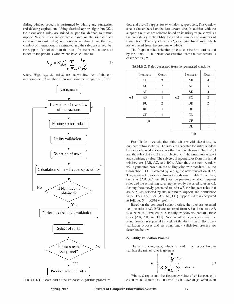
The proposed algorithm, which is illustrated as a flowchart in Figure 1, introduces a new weightage to check the utility and its consistency of the itemsets in the frequency-based minedrules. As stated earlier, the utility is validated by cost and frequency of the itemset, and the consistency is validated byusing probability distribution function (normal distribution function). Let D is the data stream and it contains a series of transactions. Each transaction is associated with an identifier, called TID and the hence the transactions can be represented as TIDn; n = 0,1,2,K, where, n varies indefinitely as the data stream is indefinite. Each transaction is a collection of items, termed as itemsets, and it can be represented as TIDn = {Im}n, where, Im represents the item i.e. Im Í {I} and ç {Im}n ç £ ç I ç . Similarto [23], the proposed algorithm utilizes sliding window opera-tion for mining rules. (For more detail about the sliding win-dow process please refer [23]). Firstly, a window with defined size of transactions is extracted from the obtained data stream. The
Spring 2013 Journal of Computer Information Systems 17
sliding window process is performed by adding one transaction and deleting expired one. Using classical apriori algorithm [22], the association rules are mined as per the defined minimum support ST (the rules are extracted based on the user defined minimum support value) and confidence value. Then, the next window of transactions are extracted and the rules are mined, but the support (for selection of the rules) for the rules that are also mined in the previous window can be calculated as
(1)
where, W cnt, Wcnt, SP and Sp are the window size of the cur- size
rent window, ID number of current window, support of pth win-
dow and overall support for pth window respectively. The window size is chosen based on the data stream size. In addition with the support, the rules are selected based on its utility value as well as the consistency of the utility for a certain number of windows of transactions. The support value is Sp calculated for all rules which are extracted from the previous windows. The frequent rules selection process can be best understood by the Table 2. The itemset construction from the data stream is described in [25].
TABLE 2: Rules generated from the generated windows
Itemsets Count
AB 4
AC 3
AD 2
w2 BC 2
BD 2
BE 1
CD 1
CF 1
DE 1
Itemsets Count
AB 2
AC 2
AE 1
w2 AF 1
BC 2
BE 1
CE 1
(i)
(ii)
FIGURE 1: Flow Chart of the Proposed Algorithm procedure.
From Table 1, we take the initial window with size 6 i.e., six numbers of transactions. The rules are generated for initial window by using classical apriori algorithm that are shown in Table 2 (i) and the rules that are £ 2, are selected with the minimum support and confidence value. The selected frequent rules from the initial window are {AB, AC, and BC}. After that, the next window w2 is generated based on the sliding window procedure i.e., the transaction ID t1 is deleted by adding the new transaction ID t7. The generated rules in window w2 are shown in Table 2 (ii). Here, the rules {AB, AC, and BC} are the previous window frequent rules and the remaining rules are the newly occurred rules in w2. Among these newly generated rules in w2, the frequent rules that are £ 2, are selected by the minimum support and confidence value. Then, the rules {AB, AC, BC} support value is computed as follows, S2 = 6(2/6) + (2/6) = 4. Based on the computed support value, the rules are selected i.e., the rules {AC, BC} are removed from w2 and the rule AB is selected as a frequent rule. Finally, window w2 contains three rules {AB, AD, and BD}. Next window is generated and the same process is repeated throughout the data stream. The utility validation process and its consistency validation process are described below.
3.1 Utility Validation Process
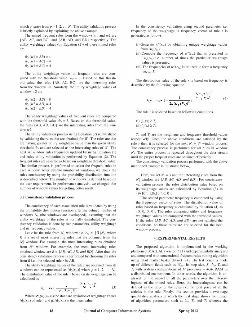
The utility weightage, which is used in our algorithm, to validate the mined rules is given as
(2)
Where, fi represents the frequency value of ith itemset, cj is
count value of item in i and W (p) is the size of pth window in size
18 Journal of Computer Information Systems Spring 2013
which p varies from p = 1, 2, . . . Ns. The utility validation process is briefly explained by exploiting the above example. The mined frequent rules form the windows w1 and w2 are {AB, AC, and BC} and {AB, AD, and BD} respectively. The utility weightage values (by Equation (2)) of these mined rules are
wp (w1 = AB) = 4 wp (w1 = AC) = 4 wp (w1 = BC) = 4
The utility weightage values of frequent rules are com-pared with the threshold value wT = 3. Based on this thresh-old value, the rules {AB, AC, BC} are the interesting rulesfrom the window w1. Similarly, the utility weightage values of window w2 are
wp (w2 = AB) = 8 wp (w2 = AD) = 4 wp (w2 = BD) = 4
The utility weightage values of frequent rules are compared with the threshold value wT = 3. Based on this threshold value, the rules {AB, AD, BD} are the interesting rules from the win-dow w2. The utility validation process using Equation (2) is initialized by validating the rules that are obtained for W1. The rules are that are having greater utility weightage value than the given utility threshold wT and are selected as the interesting rules of W1. The next W2 window rules frequency updated by using Equation (1) and rules utility validation is performed by Equation (2). The frequent rules are selected as based on weightage threshold value. The similar process is performed to select the frequent rules in each window. After definite number of windows, we check the rules consistency by using the probability distribution function is described below. The number of windows is defined based on the user requirement. In performance analysis, we changed that number of window values for getting better result.
3.2 Consistency validation process
The consistency of each association rule is validated by using the probability distribution function after the defined number of windows NS (the windows are overlapped), assuming that theutility weightage of the rules is normally distributed. The con-sistency validation is done by two parameters, utility weightage and its frequency values. Let r be the rule from NS window i.e. rNz Î {R}NS, where R is a set of most interesting rules that are obtained from theNth window. For example, the most interesting rules obtained S
from Nth window. For example, the most interesting rules S
obtained window are R = {AB, AC, AD, and BD}. After that, the consistency validation process is performed by choosing the rules from R i.e., the selected rule r be AB. The utility weightage values of the rule r are obtained from all windows can be represented as [ wp(rNs)] where p = 1, 2, . . . NS. The distribution value of the rule r based on its weightage can be calculated as
(3)
Where, sw( wp(rNs) is the standard deviation of weightage values( wp(rNs) of rule r and mw( wp(rNs) is the mean value.
In the consistency validation using second parameter i.e. frequency of the weightage, a frequency vector of rule r is generated as follows,
(i) Generate w"(rNs) by obtaining unique weightage values from ( wp(rNs).
(ii) Compute the frequency of w"(rNs) that is presented in ( wp(rNs) i.e. number of times the particular weightage
values is presented.(iii) The frequencies of w"(rNs) is utilized t o form a frequency
vector Fr.
The distribution value of the rule r is based on frequency is described by the following equation.
(4)
The rule r is selected based on following conditions.
(i) f1w(x) ≥ Tw
(ii) f1f (x) ≥ Tf
Tw and Tf are the weightage and frequency threshold values respectively. Once the above conditions are satisfied by therule r then it is selected for the next Ns + 1th window process. The consistency process is performed for all rules in windowNS. The entire process is repeated throughout the data streamuntil the proper frequent rules are obtained effectively. The consistency validation process performed with the above mentioned example is illustrated below,
Here, we set Ns = 3 and the interesting rules from theNth window are {AB, AC, AD, and BD}. For consistency S
validation process, the rules distribution value based on its weightage values are calculated by Equation (3) as{9x10¹⁴, 1.8x10¹⁵, 0, 0}. The second parameter frequency is computed by using the frequency vector of rules. The distribution value of rules based on frequency is calculated by Equation (4) as{0, 0, 0, 0}. The rules computed utility and frequency weightage values are compared with the threshold values. If the rules {AB, AC, AD, and BD} are not satisfied the conditions, so these rules are not selected for the next window process.
4. ExPERIMENTAL RESULTS
The proposed algorithm is implemented in the working platform of MATLAB (version 7.11) and experimentally analyzed and compared with conventional frequent rules mining algorithm using retail market basket dataset [24]. The test bench is made up of different fields such as Wsize, its step size, ST, wT, Tw andTf with system configurations of I7 processor – 4GB RAM ina distributed environment. In other words, the algorithm is an-alyzed for the impact of all the parameters over the interest-ingness of the mined rules. Here, the interestingness can bedefined as the price of the rules i.e. the total price of all the articles in the rule. Firstly, this section provides a two-stage quantitative analysis in which the first stage shows the impactof algorithm parameters such as wT, Tw and Tf whereas the
Spring 2013 Journal of Computer Information Systems 19
second stage shows the impact of the data stream parameterssuch as Wsize, its step size. Secondly, the interestingness iscompared between the rules that are mined using proposed algorithm as well as the conventional frequent rules mining algorithm. The existing conventional frequent mining algorithms mine the frequent rules form the database by utilizing anyone of the mining algorithm. Here, we have utilized an associ-ation rule based mining algorithm as an existing conventional frequent mining algorithm, which mine thefrequent rules from the database. The pro posed method has performed itemset mining based on utility and frequency, so the perform ance of this method is compared with conven tional frequent rules mining algorithms.
4.1 quantitative analysis
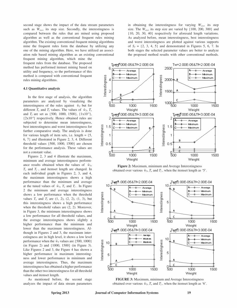
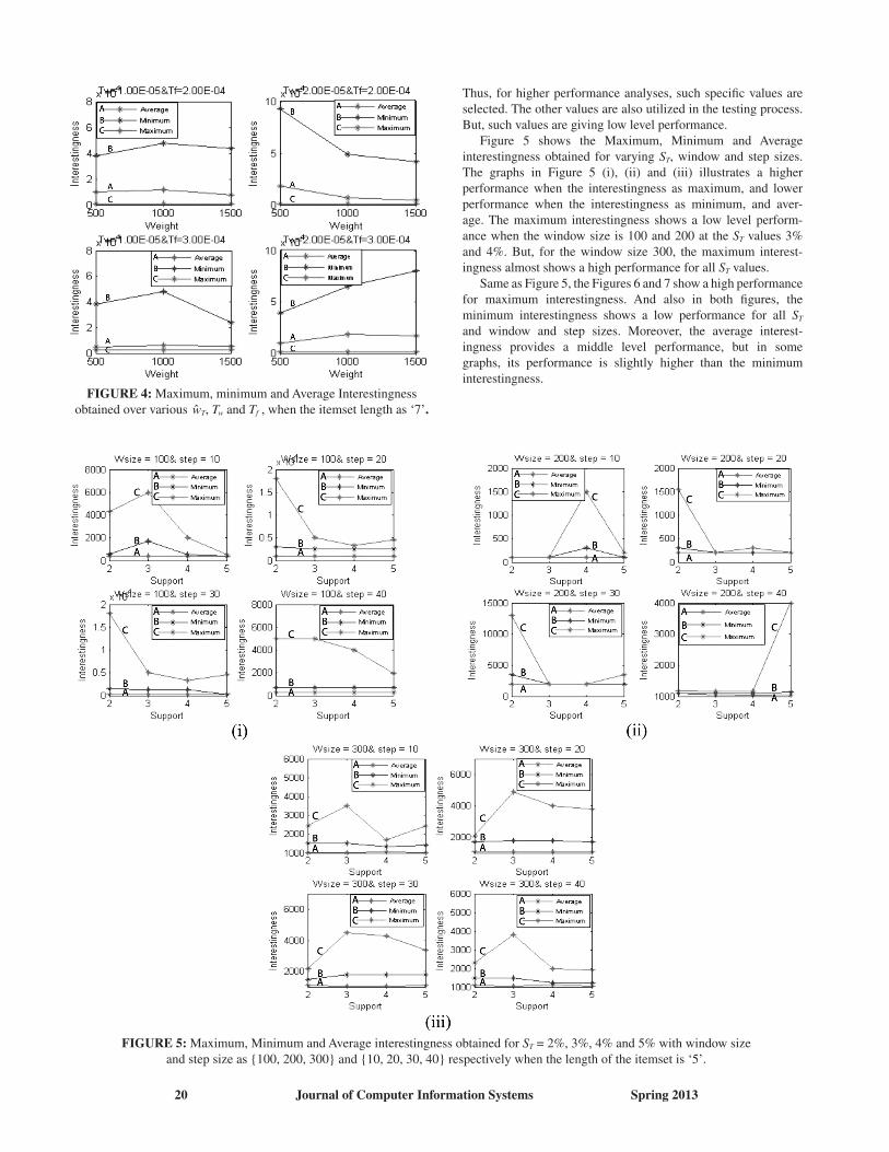
In the first stage of analysis, the algorithm parameters are analyzed by visualizing the interestingness of the rules against wT but for different Tw and Tf values. The values of wT, Tw and Tf are set as {500, 1000, 1500}, {1x10⁻⁵}, {2x10⁻⁴} respectively. Hence obtained rules are subjected to determine mean interestingness, best interestingness and worst interestingness for further comparative study. The analysis is done for various length of item sets, i.e. length = {5, 6, 7} and illustrated in Figure 2, 3, 4. Different threshold values {500, 1000, 1500} are chosen for the performance analysis. These values are not a constant value. Figures 2, 3 and 4 illustrate the maximum, minimum and average interestingness perform-ance results obtained when the values of wT, Tw and Tf , and itemset length are changed. In each individual graph in Figures 2, 3, and 4, the maximum interestingness shows a high performance than the minimum and average at the tuned values of wT, Tw and Tf . In Figure 2 the minimum and average interestingness shows a low performance when the threshold values Tw and Tf are (1, 2), (2, 2), (1, 3), but this interestingness shows a high performance when the threshold values are (2, 2). Moreover, in Figure 3, the minimum interestingness shows a low performance for all threshold values, andthe average interestingness shows slightly a higher performance than the minimum andlower than the maximum interestingness. Al-though in Figures 2 and 3, the maximum inter-estingness are in high level, it shows a low level performance when the wT values are {500, 1000} (in Figure 2) and {1000, 1500} (in Figure 3). Like Figures 2 and 3, the Figure 4 has shown a higher performance in maximum interesting-ness and lower performance in minimum and average interestingness. Thus, the maximum interestingness has obtained a higher performance than the other two interestingness for all threshold values and itemset length. As mentioned before, the second stage analyzes the impact of data stream parameters
in obtaining the interestingness for varying Wsize, its step size. The Wsize, its step size are varied by {100, 200, 300} and {10, 20, 30, 40} respectively for aforesaid length variations.As analyzed before, mean interestingness, best interestingness and worst interestingness are plotted against various supportsof ST = {2, 3, 4, 5} and demonstrated in Figures 5, 6, 7. Inboth stages the selected parameter values are better to analyze the proposed method results with other conventional methods.
FIGURE 3: Maximum, minimum and Average Interestingnessobtained over various wT, Tw and Tf , when the itemset length as ‘6’.
Figure 2: Maximum, minimum and Average Interestingnessobtained over various wT, Tw and Tf , when the itemset length as ‘5’.
20 Journal of Computer Information Systems Spring 2013
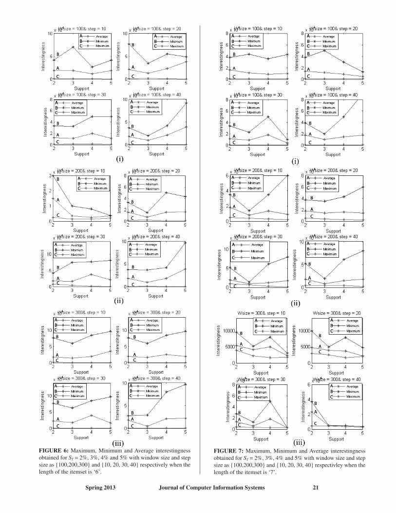
Thus, for higher performance analyses, such specific values are selected. The other values are also utilized in the testing process. But, such values are giving low level performance. Figure 5 shows the Maximum, Minimum and Average interestingness obtained for varying ST, window and step sizes. The graphs in Figure 5 (i), (ii) and (iii) illustrates a higher performance when the interestingness as maximum, and lower performance when the interestingness as minimum, and aver-age. The maximum interestingness shows a low level perform-ance when the window size is 100 and 200 at the ST values 3%and 4%. But, for the window size 300, the maximum interest-ingness almost shows a high performance for all ST values. Same as Figure 5, the Figures 6 and 7 show a high performance for maximum interestingness. And also in both figures, the minimum interestingness shows a low performance for all ST
and window and step sizes. Moreover, the average interest-ingness provides a middle level performance, but in some graphs, its performance is slightly higher than the minimum interestingness.
FIGURE 4: Maximum, minimum and Average Interestingnessobtained over various wT, Tw and Tf , when the itemset length as ‘7’.
FIGURE 5: Maximum, Minimum and Average interestingness obtained for ST = 2%, 3%, 4% and 5% with window sizeand step size as {100, 200, 300} and {10, 20, 30, 40} respectively when the length of the itemset is ‘5’.
Spring 2013 Journal of Computer Information Systems 21
FIGURE 6: Maximum, Minimum and Average interestingness obtained for ST = 2%, 3%, 4% and 5% with window size and step size as {100,200,300} and {10, 20, 30, 40} respectively when the length of the itemset is ‘6’.
FIGURE 7: Maximum, Minimum and Average interestingness obtained for ST = 2%, 3%, 4% and 5% with window size and step size as {100,200,300} and {10, 20, 30, 40} respectivley when the length of the itemset is ‘7’.
22 Journal of Computer Information Systems Spring 2013
Window Step Interestingness size size
10 1409.655
20 1185.467
100 30 1119.231
40 1076.289
10 1692.308
200 20 1747.619
30 1735.484
40 1755
10 1778.082
300 20 1768.786
30 1767.857
40 1770.142
(i)
Window Step Interestingness size size
10 1323.164
20 1157.143
100 30 1103.465
40 1071.6
10 1773.684
200 20 1745.946
30 1728.155
40 1759.055
10 1780.519
300 20 1772.778
30 1775
40 1771.028
(ii)
Window Step Interestingness size size
10 1254.774
20 1132.099
100 30 1084.652
40 1063.314
10 1840
200 20 1787.5
30 1787.963
40 1793.893
10 1782.911
300 20 1774.863
30 1776.733
40 1772.936
(iii)
Window Step Interestingness size size
10 1225.116
20 1117.109
100 30 1077.156
40 1056.92
10 1808
200 20 1775
30 1776.316
40 1783.704
10 1779.503
300 20 1772.043
30 1774.02
40 1770.455
(iv)
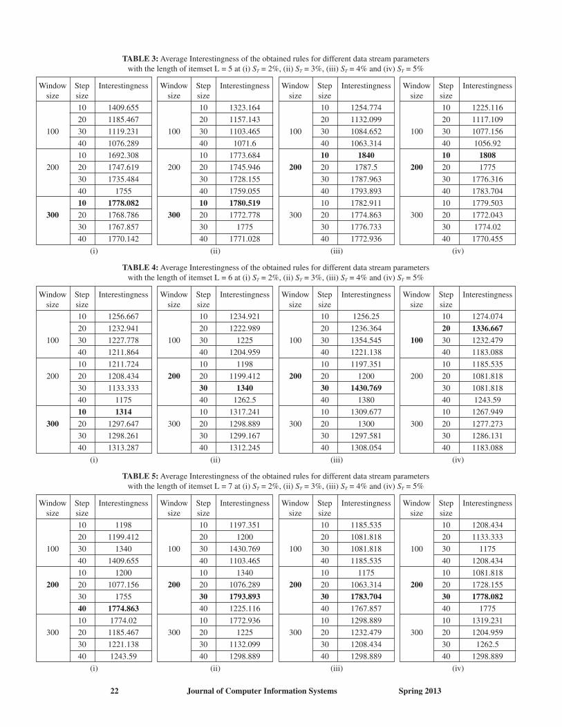
TABLE 3: Average Interestingness of the obtained rules for different data stream parameterswith the length of itemset L = 5 at (i) ST = 2%, (ii) ST = 3%, (iii) ST = 4% and (iv) ST = 5%
Window Step Interestingness size size
10 1198
20 1199.412
100 30 1340
40 1409.655
10 1200
200 20 1077.156
30 1755
40 1774.863
10 1774.02
300 20 1185.467
30 1221.138
40 1243.59
(i)
Window Step Interestingness size size
10 1197.351
20 1200
100 30 1430.769
40 1103.465
10 1340
200 20 1076.289
30 1793.893
40 1225.116
10 1772.936
300 20 1225
30 1132.099
40 1298.889
(ii)
Window Step Interestingness size size
10 1185.535
20 1081.818
100 30 1081.818
40 1185.535
10 1175
200 20 1063.314
30 1783.704
40 1767.857
10 1298.889
300 20 1232.479
30 1208.434
40 1298.889
(iii)
Window Step Interestingness size size
10 1208.434
20 1133.333
100 30 1175
40 1208.434
10 1081.818
200 20 1728.155
30 1778.082
40 1775
10 1319.231
300 20 1204.959
30 1262.5
40 1298.889
(iv)
TABLE 5: Average Interestingness of the obtained rules for different data stream parameterswith the length of itemset L = 7 at (i) ST = 2%, (ii) ST = 3%, (iii) ST = 4% and (iv) ST = 5%
Window Step Interestingness size size
10 1256.667
20 1232.941
100 30 1227.778
40 1211.864
10 1211.724
200 20 1208.434
30 1133.333
40 1175
10 1314
300 20 1297.647
30 1298.261
40 1313.287
(i)
Window Step Interestingness size size
10 1234.921
20 1222.989
100 30 1225
40 1204.959
10 1198
200 20 1199.412
30 1340
40 1262.5
10 1317.241
300 20 1298.889
30 1299.167
40 1312.245
(ii)
Window Step Interestingness size size
10 1256.25
20 1236.364
100 30 1354.545
40 1221.138
10 1197.351
200 20 1200
30 1430.769
40 1380
10 1309.677
300 20 1300
30 1297.581
40 1308.054
(iii)
Window Step Interestingness size size
10 1274.074
20 1336.667
100 30 1232.479
40 1183.088
10 1185.535
200 20 1081.818
30 1081.818
40 1243.59
10 1267.949
300 20 1277.273
30 1286.131
40 1183.088
(iv)
TABLE 4: Average Interestingness of the obtained rules for different data stream parameterswith the length of itemset L = 6 at (i) ST = 2%, (ii) ST = 3%, (iii) ST = 4% and (iv) ST = 5%
Spring 2013 Journal of Computer Information Systems 23
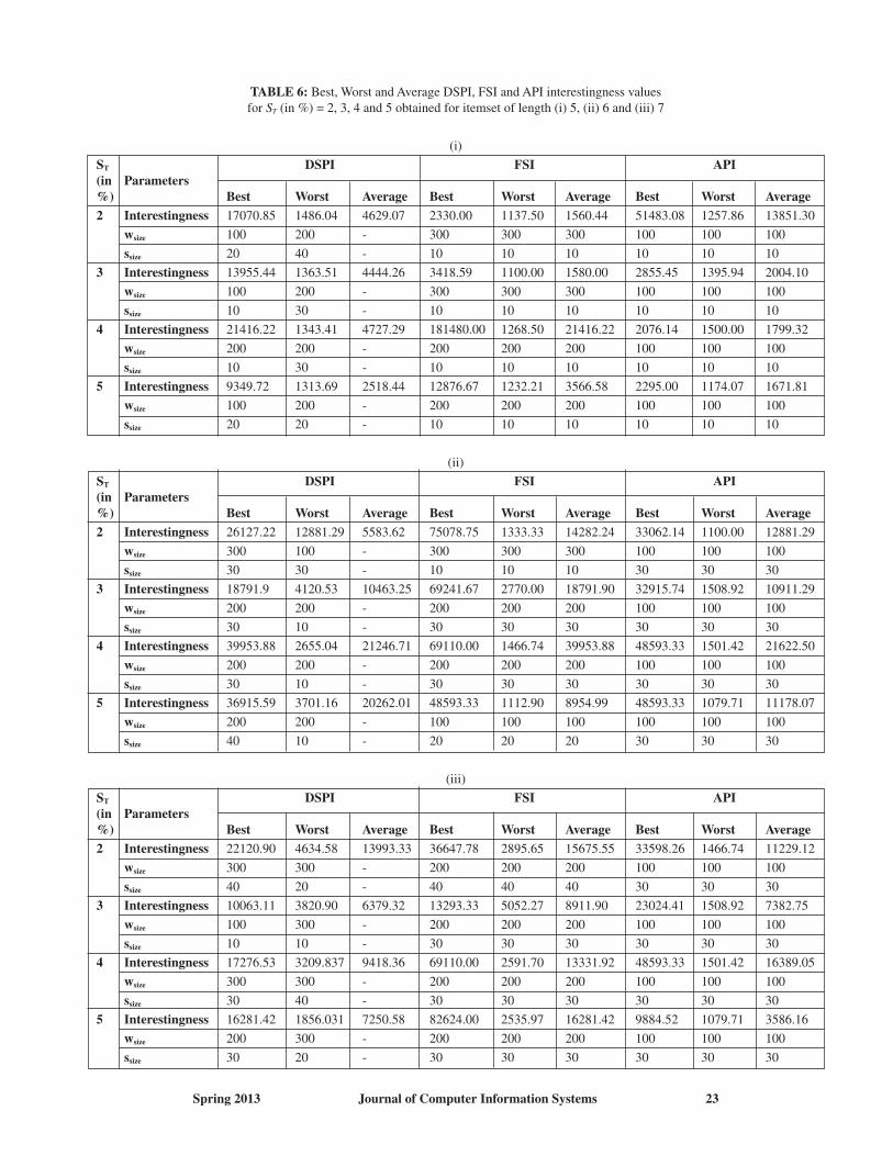
TABLE 6: Best, Worst and Average DSPI, FSI and API interestingness valuesfor ST (in %) = 2, 3, 4 and 5 obtained for itemset of length (i) 5, (ii) 6 and (iii) 7
(i)
ST DSPI FSI API(in Parameters%) Best Worst Average Best Worst Average Best Worst Average
2 Interestingness 17070.85 1486.04 4629.07 2330.00 1137.50 1560.44 51483.08 1257.86 13851.30
wsize 100 200 - 300 300 300 100 100 100
ssize 20 40 - 10 10 10 10 10 10
3 Interestingness 13955.44 1363.51 4444.26 3418.59 1100.00 1580.00 2855.45 1395.94 2004.10
wsize 100 200 - 300 300 300 100 100 100
ssize 10 30 - 10 10 10 10 10 10
4 Interestingness 21416.22 1343.41 4727.29 181480.00 1268.50 21416.22 2076.14 1500.00 1799.32
wsize 200 200 - 200 200 200 100 100 100
ssize 10 30 - 10 10 10 10 10 10
5 Interestingness 9349.72 1313.69 2518.44 12876.67 1232.21 3566.58 2295.00 1174.07 1671.81
wsize 100 200 - 200 200 200 100 100 100
ssize 20 20 - 10 10 10 10 10 10
(ii)
ST DSPI FSI API(in Parameters%) Best Worst Average Best Worst Average Best Worst Average
2 Interestingness 26127.22 12881.29 5583.62 75078.75 1333.33 14282.24 33062.14 1100.00 12881.29
wsize 300 100 - 300 300 300 100 100 100
ssize 30 30 - 10 10 10 30 30 30
3 Interestingness 18791.9 4120.53 10463.25 69241.67 2770.00 18791.90 32915.74 1508.92 10911.29
wsize 200 200 - 200 200 200 100 100 100
ssize 30 10 - 30 30 30 30 30 30
4 Interestingness 39953.88 2655.04 21246.71 69110.00 1466.74 39953.88 48593.33 1501.42 21622.50
wsize 200 200 - 200 200 200 100 100 100
ssize 30 10 - 30 30 30 30 30 30
5 Interestingness 36915.59 3701.16 20262.01 48593.33 1112.90 8954.99 48593.33 1079.71 11178.07
wsize 200 200 - 100 100 100 100 100 100
ssize 40 10 - 20 20 20 30 30 30
(iii)
ST DSPI FSI API(in Parameters%) Best Worst Average Best Worst Average Best Worst Average
2 Interestingness 22120.90 4634.58 13993.33 36647.78 2895.65 15675.55 33598.26 1466.74 11229.12
wsize 300 300 - 200 200 200 100 100 100
ssize 40 20 - 40 40 40 30 30 30
3 Interestingness 10063.11 3820.90 6379.32 13293.33 5052.27 8911.90 23024.41 1508.92 7382.75
wsize 100 300 - 200 200 200 100 100 100
ssize 10 10 - 30 30 30 30 30 30
4 Interestingness 17276.53 3209.837 9418.36 69110.00 2591.70 13331.92 48593.33 1501.42 16389.05
wsize 300 300 - 200 200 200 100 100 100
ssize 30 40 - 30 30 30 30 30 30
5 Interestingness 16281.42 1856.031 7250.58 82624.00 2535.97 16281.42 9884.52 1079.71 3586.16
wsize 200 300 - 200 200 200 100 100 100
ssize 30 20 - 30 30 30 30 30 30
24 Journal of Computer Information Systems Spring 2013
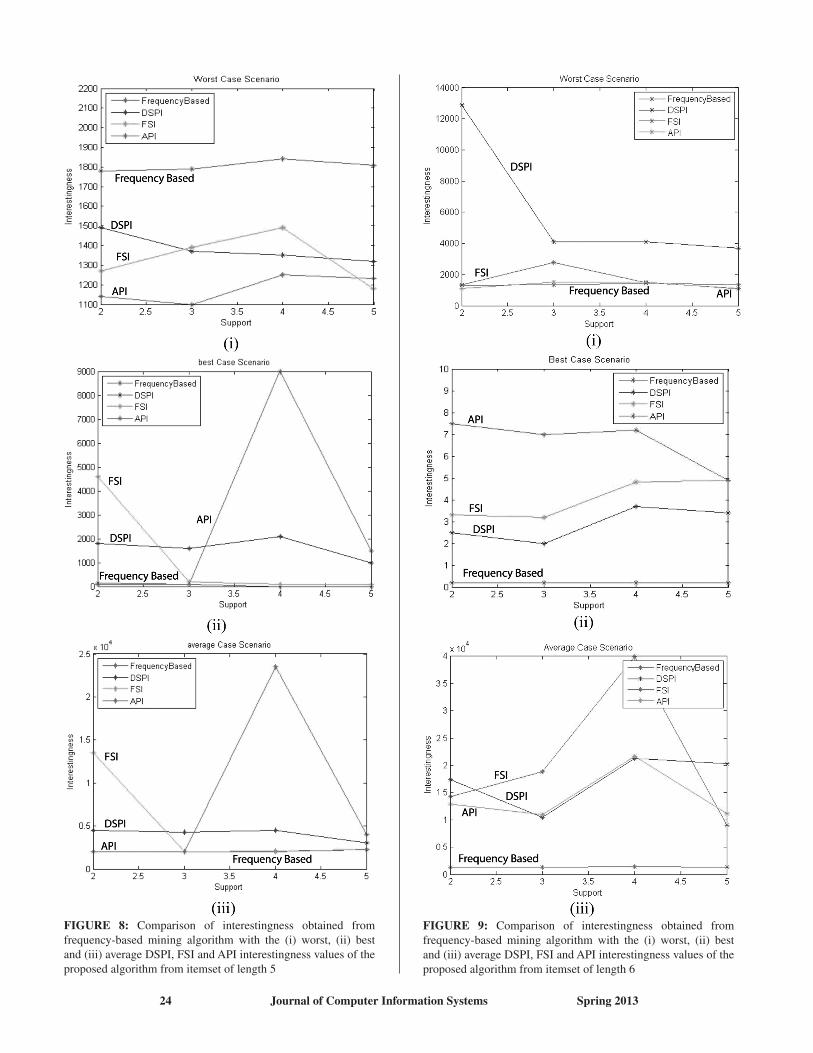
FIGURE 8: Comparison of interestingness obtained from frequency-based mining algorithm with the (i) worst, (ii) best and (iii) average DSPI, FSI and API interestingness values of the proposed algorithm from itemset of length 5
FIGURE 9: Comparison of interestingness obtained from frequency-based mining algorithm with the (i) worst, (ii) best and (iii) average DSPI, FSI and API interestingness values of the proposed algorithm from itemset of length 6
Spring 2013 Journal of Computer Information Systems 25
4.2 Comparative Analysis
In this section, the different analytical results are compared with the conventional frequent rules mining algorithm to prove that (i) only frequency-based rules are not the interesting rules for a retail shop and (ii) utility and consistency plays a major role in mining interesting rules. In order to perform this, data stream parameters’ tuning is required for proposed as well as conventional mining algorithm. The parameter tuning is nothing but finding the exact data stream parameters, Wsize, its step size, in which the algorithm achieves required interestingness. The parameter tuning process is not an automatic process. We change the parameters values for getting the best values for the performance analysis. In tuning the parameters for existing algorithm, the best Wsize and its step size, in which the maximum the interestingness are obtained for every support value. For instance in Table 3, (Wsize, step size) of {300, 10}, {300, 10}, {200, 10} and {200, 10} are identified as the best data stream parameters for ST (in %) = 2, 3, 4 and 5, respectively as they produces a maximum interestingness values of 1778, 1781, 1840 and 1808, respectively for length 5. Thus obtained maximum interestingness is compared with the interestingness of different rules that are obtained from proposed algorithm in three cases: (i) with best-case scenario, (ii) with worst-case scenario and (iii) with average-case scenario. The best, average, and worst rules are selected from the proposed algorithm. The proposed algorithm validate the consistency of the rules and select the most frequent rules, so any infrequent rules may be selected and any frequent rules may be missed. Hence, the rules results are divided into three scenarios: best case scenario, worst-case scenario, and average-case scenario. The best case scenario means the rules with high performance values; worst case scenario means the low performance rules and average case scenario means the performance values between best and worst. For each of these scenarios, three interestingness values are obtained from the proposed algorithm. Here, we have utilized the term interestingness, which is defined as follows,
Interestingness means the goal to be achieved in our process. In our paper, rules profit value is considered as the interestingness i.e., the mined frequent rules should satisfy the profit value in the future also. Based on the presented data in the dataset, the interestingness value can be varied between the dataset.
The first interestingness value for the three scenarios can be determined for every combination of data stream parameters(i) by finding the maximum interestingness among the obtained interestingness values for all the combinations of algorithm parameters, (ii) by finding the minimum interestingness among the obtained interestingness values for all the combinations of algorithm parameters and (iii) by averaging the interestingness of all the various combinations of algorithm parameters, respectively. The second interestingness value is determined by the following steps
•The algorithm parameters then can produce maximuminterestingness and minimum interestingness are selected from Figures 2, 3 and 4 for length and Figures 5, 6 and 7, respectively.
•The data stream parameters corresponds to the selectedalgorithm parameters are located
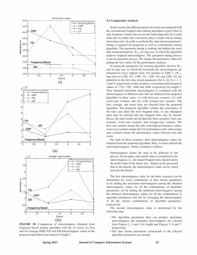
FIGURE 10: Comparison of interestingness obtained from frequency-based mining algorithm with the (i) worst, (ii) best and (iii) average DSPI, FSI and API interestingness values of the proposed algorithm from itemset of length 7
26 Journal of Computer Information Systems Spring 2013
•Themaximum,minimumandaverageinterestingnessvaluesare determined for the rules that are obtained by setting the two combination of located data stream parameters
The third interestingness value is determined by tuning thedata stream parameters that provides best performance for con-ventional algorithm. Hence the three interestingness values can be named as DSPI, API and FSI. The best, worst and averagecase DSPI, API and FSI interestingness values and the corres-ponding window size and step sizes for ST (in %) = 2, 3, 4and 5 are tabulated in Table 6 and the comparison chart of allthese parameters against frequency based conventional inter-esting rules mining algorithm are illustrated in Figures 8, 9and 10. When the comparison graphs are analyzed, even the worstDSPI, API and FSI interestingness values are more than the interestingness obtained through frequency-based mining algor-ithm. Moreover, the other scenarios achieved an interestingness value which is very higher rather than the interestingnessobtained from frequency-based mining algorithm.
5. CONCLUSION
In this paper, the conventional frequency based association rule mining algorithm for data stream was enhanced by introducing utility weightage and consistency validation factors. The en-hanced mining algorithm successfully mined the rules whichhave more interestingness that is cost benefitable. The algor-ithm was implemented and experimented in a distributed environment. The results were analyzed and derived three interestingness values called DSPI, API and FSI. Among them, best interestingness, worst interestingness and average interestingness values were obtained and compared against the interestingness values that are obtained through conventional frequency based association rule mining. The analytical results asserted that in some cases, the worst case interestingness dominates the frequency-based association rules with the 17% and off course, the average and best interestingness are 83% higher than the interestingness values obtained through conventional frequencybased data stream mining algorithms.
REFERENCES
[1] Naga K. Govindaraju, Nikunj Raghuvanshi and Dinesh Manocha, “Fast and Approximate Stream Mining of Quantiles and Frequencies Using Graphics Processors”, In Proceedings of the International Conference on Management of Data, pp. 611-622, 2005.
[2] Mohamed G. Elfeky, Walid G. Aref and Ahmed K. Elmagarmid, “STAGGER: Periodicity Mining of Data Streams using Expanding Sliding Windows”, In Proceedings of the Sixth International Conference on ICDM, Hong Kong, pp. 188-199, 2006.
[3] Hyunggon Park, Deepak S. Turaga, Olivier Verscheure and Mihaela van der Schaar, “A Framework for Distributed Multimedia Stream Mining Systems Using Coalition-Based Foresighted Strategies”, In Proceedings of the 2009 IEEE International Conference on Acoustics, Speech and Signal Processing, 2009.
[4] Fang Chu, Yizhou Wang and Carlo zaniolo, “Mining Noisy Data Streams via a Discriminative Model”, In Proceedings of Discovery Science, pp. 47-59, 2004.
[5] Haixun Wang, Wei Fan, Philip S. Yu and Jiawei Han, “Mining Concept Drifting Data Streams using Ensemble Classifiers”, In Proceedings of the ninth International Conference on Knowledge Discovery and Data Mining, pp. 226-235, 2003.
[6] Albert Bifet and Ricard Gavalda, “Mining Adaptively Frequent Closed Unlabeled Rooted Trees in Data Streams”, in Proceedings of the International Conference on Knowledge Discovery and Data Mining, pp. 34-42, 2008.
[7] Alice Marascu and Florent Masseglia, “Mining Sequential Patterns from Data Streams: a Centroid Approach”, Journal of Intelligent Information Systems, Vol. 27, No. 3, pp. 291-307, November 2006.
[8] Graham Cormode and Muthukrishnan, “What’s hot and what’s not: tracking most frequent items dynamically”, ACM Transactions on Database Systems, Vol. 30, No. 1, pp. 249-278, 2005.
[9] M. Garofalakis, J. Gehrke and R. Rastogi, “Querying and mining data streams: you only get one look”, In Proceedings of the International Conference on Management of data, Hong Kong, China, pp. 635-635, 2002.
[10] Joong Hyuk Chang and Won Suk Lee, “Finding recent frequent item sets adaptively over online data streams”, In Proceedings of the ninth International Conference on Knowledge Discovery and Data Mining, pp. 487-492, 2003.
[11] Y. Dora Cai, David Clutter, Greg Pape, Jiawei Han, Michael Welge and Loretta Auvilx, “MAIDS: Mining Alarming Incidents from Data Streams”, In Proceedings of the International Conference on Management of Data, pp. 919-920, 2004.
[12] Mayur Datar, Aristides Gionis, Piotr Indyk and Rajeev Motwani, “Maintaining Stream Statistics Over Sliding Windows”, Journal SIAM Journal on Computing, Vol. 31, No. 6, pp. 1794-1813, 2002.
[13] Nam Hun Park and Won Suk Lee, “Statistical Grid-based Clustering over Data Streams”, ACM SIGMOD Record, Vol. 33, No. 1, pp. 32-37, March 2004.
[14] Alice Marascu and Florent Masseglia, “Mining Data Streams for Frequent Sequences Extraction”, In Proceedings of the IEEE Workshop on Mining Complex Data (MCD), pp. 1-7, 2005.
[15] Chun-Jung Chu, Vincent S. Tseng and Tyne Liang, “An efficient algorithm for mining temporal high utility item sets from data streams”, Journal of Systems and Software, Vol. 81, No. 7, pp. 1105–1117, 2008.
[16] Brian Foo and Mihaela van der Schaar, “Distributed Classifier Chain Optimization for Real-Time Multimedia Stream Mining Systems”, In Proceedings of SPIE, San Jose, Calif, USA, Vol. 6820, January 2008.
[17] Brian Foo and Mihaela van der Schaar”A Rules-based Approach for Configuring Chains of Classifiers in Real-Time Stream Mining Systems,” EURASIP Journal on Advances in Signal Processing, pp. 1-37, 2009.
[18] Chowdhury Farhan Ahmed, Syed Khairuzzaman Tanbeer and Byeong-Soo Jeong, “Efficient Mining of High Utility Patterns over Data Streams with a Sliding Window Method”, Vol. 295, pp. 99-113, 2010.
[19] Younghee Kim, Wonyoung Kim and Ungmo Kim, “Mining Frequent Item sets with Normalized Weight in Continuous Data Streams”, Journal of Information Processing Systems, Vol. 6, No. 1, pp. 79-90, March 2010.
[20] Brian Foo, Deepak S. Turaga, Olivier Verscheure, Mihaela van der Schaar and Lisa Amini, “Configuring Trees of Classifiers

Spring 2013 Journal of Computer Information Systems 27
in Distributed Multimedia Stream Mining Systems”, IEEE Transactions on Circuits and Systems for Video Technology, Vol. 21, No. 3, pp. 245-258, March 2011.
[21] Jyothi Pillai, “User Centric Approach to Itemset Utility Mining in Market Basket Analysis”, International Journal on Computer Science and Engineering, Vol. 3, No. 1, pp. 393-400, January 2011.
[22] Rakesh Agrawal and Ramakrishnan Srikant, “Fast algorithms for mining association rules in large databases”,
In Proceedings of the 20th International Conference on Very Large Data Bases, VLDB, Santiago, Chile, pp. 487-499, September 1994.
[23] Chang-Hung Lee, Cheng-Ru Lin and Ming-Syan Chen, “Sliding Window Filtering: An Efficient Method for Incremental Mining on A Time-Variant Database”, Information Systems, Vol. 30, pp. 227–244, 2005.
[24] Brijs, T.: Retail Market Basket Data Set, University of Limburg, Belgium, http://fimi.cs.helsinki.fi/dat/retail.pdf .
Copyright © 2022 FDOKUMEN