Lightweight Modeling of Complex State Dependencies in

Stream Processing Systems

Anne Bouillard, Linh Phan, Samarjit Chakraborty

To cite this version:

Anne Bouillard, Linh Phan, Samarjit Chakraborty. Lightweight Modeling of Complex StateDependencies in Stream Processing Systems. 15th IEEE Real-Time and Embedded Technologyand Applications Symposium (RTAS 2009), Apr 2009, San Francisco, United States. 10 p.<inria-00429776>

HAL Id: inria-00429776

https://hal.inria.fr/inria-00429776

Submitted on 4 Nov 2009

HAL is a multi-disciplinary open accessarchive for the deposit and dissemination of sci-entific research documents, whether they are pub-lished or not. The documents may come fromteaching and research institutions in France orabroad, or from public or private research centers.

L’archive ouverte pluridisciplinaire HAL, estdestinee au depot et a la diffusion de documentsscientifiques de niveau recherche, publies ou non,emanant des etablissements d’enseignement et derecherche francais ou etrangers, des laboratoirespublics ou prives.

Lightweight Modeling of Complex State Dependenciesin Stream Processing Systems

Anne Bouillard1 Linh T.X. Phan2 Samarjit Chakraborty2

1ENS Cachan (Bretagne) / IRISA2Department of Computer Science, National University of Singapore

E-mail: Anne.Bouillard@bretagne.ens-cachan.fr {phanthix, samarjit}@comp.nus.edu.sg

Abstract

Over the last few years, Real-Time Calculus has beenused extensively to model and analyze embedded systemsprocessing continuous data/event streams. Towards this,bounds on the arrival process of streams and bounds onthe processing capacity of resources serve as inputs tothe model, which are used to calculate end-to-end delayssuffered by streams, maximum backlog, utilization of re-sources, etc. This “functional” model, although amenableto computationally inexpensive analysis methods, has lim-ited modeling capability. In particular, “state-based” pro-cessing, e.g. blocking write – where the processing dependson the “state” or fill-level of the buffer – cannot be mod-eled in a straightforward manner. This has led to a num-ber of recent proposals on using automata-theoretic modelsfor stream processing systems (e.g. Event Count Automata[RTSS 2005]). Although such models offer better modelingflexibility, they suffer from the usual state-space explosionproblem. In this paper we show that a number of complexstate-dependencies can be modeled in a lightweight man-ner, using a feedback control technique. This avoids explicitstate modeling, and hence the state-space explosion prob-lem. Our proposed modeling and analysis therefore extendthe original Real-Time Calculus-based functional modelingin a very useful way, and cover much larger problem domaincompared to what was previously possible without explicitstate-modeling. We illustrate its utility through two casestudies and also compare our analysis results with thoseobtained from detailed system simulations (which are sig-nificantly more time consuming).

1 Introduction

The escalating complexity of stream processing systemshas prompted the need for modeling and analysis techniquesthat go beyond those traditionally studied in the literature.Many of these systems process irregular data/event streamsand rely on highly dynamic resource management policies

2

B

input stream PE1 PE2 PEnα α′ α″ αout

output stream

α′β

2 β′α″

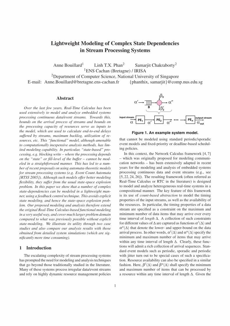
Figure 1. An example system model.

that cannot be modeled using standard periodic/sporadicevent models and fixed-priority or deadline-based schedul-ing policies.

In this context, the Network Calculus framework [4, 7]– which was originally proposed for modeling communi-cation networks – has been extensively adapted in recentyears for the modeling and analysis of embedded systemsprocessing continuous data and event streams (e.g., see[5, 22, 24, 26]). The resulting framework (often referred asReal-Time Calculus or RTC in the literature) is designedto model and analyze heterogeneous real-time systems in acompositional manner. The key feature of this frameworkis its use of count-based abstraction to model the timingproperties of the input streams, as well as the availability ofthe resources. In particular, the timing properties of a datastream are specified as a constraint on the maximum andminimum number of data items that may arrive over everytime interval of length Δ. A collection of such constraintsfor different values of Δ are captured as functions α l(Δ) andαu(Δ) that denote the lower- and upper-bound on the dataarrival process. In other words, α l(Δ) and αu(Δ) specify theminimum and maximum number of items that may arrivewithin any time interval of length Δ. Clearly, these func-tions will admit a rich collection of arrival sequences. Stan-dard event models such as periodic, sporadic and periodicwith jitter turn out to be special cases of such a specifica-tion. Resource availability can also be specified in a similarfashion. Here, β l(Δ) and β u(Δ) shall specify the minimumand maximum number of items that can be processed bya resource within any time interval of length Δ. Given the

1

functions α , denoting (α l , αu), and β denoting (β l , β u),it is possible to compute using purely algebraic techniques,the bounds on system properties such as the maximum de-lay suffered by the stream and the maximum backlog of dataitems in front of the resource. Further, it is also possible tocompute α ′ = (α l ′, αu ′) which denotes bounds on the tim-ing properties of the processed stream. α ′ may now serve asthe input to the next resource which further processes thisstream, and the output from which may be denoted as α ′′.This is repeated for all resources until the timing propertiesof the output stream αout are computed (see Figure 1).

Figure 1 shows an architecture consisting of n resourcesPE1, . . . ,PEn, which process an input stream sequentially.Each PEi has an input buffer to store incoming data itemswaiting to be processed. The service rendered by each PEi

is constrained by βi. Similar to α ′, the service function βi′

that bounds the remaining resource which can be used toprocess other data streams. Besides buffer requirements andthe delay incurred by the input stream at each resource PEi,various other performance characteristics such as the uti-lization of each resource, output jitter, the maximum end-to-end delay and the total buffer requirement in the systemcan also be obtained from the bounds α and αout .

1.1 Our contributions

Owing to the functional nature of RTC, analysis in thisframework involves algebraic manipulations which allowsfor highly efficient computation of system properties in afully compositional manner. However, modeling of com-plex state dependencies is awkward; common scenariossuch as the one where the service offered by a resource de-pends on the fill-level of a buffer cannot be modeled easily.In constrast, fine-grained modeling of state information, e.g.using timed automata [1, 9] or event count automata [6] of-ten leads to state space explosion when applied to realisticproblems.

In this paper, we present a technique to model a varietyof complex state dependencies in the existing RTC frame-work with a feedback control mechanism without resortingto explicit state-space modeling. Firstly, this technique sig-nificantly enhances the modeling power of the frameworkbut without having the problems associated with state-spacemodeling. Secondly, our model of a system is a compositionof multiple abstract components with each component cap-turing all the relevant state-dependencies as well as process-ing semantics. The properties of these components can becomputed functionally using our results and thereby attain ahigh efficiency. Thirdly, our technique enables state-basedscheduling policies to be modeled and efficiently analyzedin a modular manner.

Through case studies, we illustrate how our method canbe seamlessly integrated into the current RTC framework,and at the same time we show the effects of capturing state-

dependencies on the accuracy of the analysis. We also pro-vide experimental validation of our analysis method againstsimulation. The analysis results obtained from both meth-ods match well with each other, however our analysis is sig-nificantly faster than simulation.

1.2 Related work

The first line of related work is concerned with develop-ing task and event models that generalize classical periodicor sporadic event models, which assume fixed executiontimes for tasks. Towards this, timed automata and relatedautomata-theoretic formalisms have been recently used invarious setups to model and analyze task scheduling prob-lems (e.g., see [1,8,9]). To overcome the lack of state-basedmodeling in the RTC framework, we had proposed eventcount automata (ECAs) [6] that retain the count-based ab-straction used in RTC. Although automata-based models aremuch more expressive and capable of representing a widevariety of state-dependencies, they suffer from the state ex-plosion problem and can become inefficient when analyzinglarge system architectures.

The next line of work focuses on extending RTC tomodel complex event patterns and task activation schemes.For example, [10] presented a method to model conditionalblocking-read on an input buffer. In particular, it modeledtasks that are triggered by events on multiple input streamsusing AND/OR-activation, where an OR-task is triggeredwhenever an event is available on either of the input streamsand an AND-task is only activated when there is at leastone event from each stream. [13] proposed a way to com-pute delay and output arrival functions of data streams thatare split and joined during the system execution followingthe OR-activation and in-order activation semantics, whiletaking into account correlations in data streams and datadistribution based on different types of delay. Correlationbetween jitter and response time of individual events werealso considered in [12]. Analysis methods of more complexscheduling policies such as non-preemptive and scenario-aware scheduling of tasks were studied in [10] and [11] re-spectively. Timing properties of hierarchical event streamsthat are generated by the communication stack are modeledin [19]. Although extensive in variety, these proposed tech-niques do not handle state-modeling and control-feedbackdependencies.

The back-pressure effect with finite buffer capacities hasbeen studied in the context of data flow graphs [15]. Forinstance, in [27], an algorithm for computing the buffer ca-pacities that satisfy throughput constraints was presented.Analysis of self-time scheduling for multirate data flowwith finite buffer capacities was considered in [16]. Also,back-pressure was used in [23] as a mechanism to allow asemantics preserving implementation of synchronous mod-els on Loosely Time Triggered Architectures. The methods

2

used in this context however are not applicable into our set-ting.

There have also been hybrid frameworks that combinevarious analysis methodologies. For example, [21] unifiedthe SDF [15] and SymTA/S [2] into a single framework thatis able to model data-dependencies using SDF and to ab-stract event streams using SymTA/S. SymTA/S and RTChave been merged in [14] to capture more complex inter-actions with high accuracy. RTC and ECA can also be in-tegrated using the interfacing technique provided in [18] toachieve higher accuracy than using RTC alone while be-ing more efficient than using ECA alone. The method wepropose here can be plugged into the integrated RTC-ECAframework to further increase the efficiency of the analysis,since we can now use RTC to analyze a number of state-dependent components in the system instead of using ECAs,which will in turn reduce the total analysis time.

1.3 Organization of the paper

In the next section we describe the basic concepts ofthe RTC framework. In Section 3 we present our analy-sis method. We begin with an example that will be used toillustrate our method, followed by an overview of our anal-ysis technique in Section 3.2. Sections 3.3 and 3.4 estab-lish the theoretical results that enable the analysis of a state-dependent component, which will be applied to model state-based scheduling in Section 3.5. In Section 4 we presentexperimental results using two case studies derived froman MPEG-2 decoder to illustrate the benefits of our anal-ysis methods. Finally, we conclude with a discussion on theprospects for extending our study initiated in this paper.

2 The Real-Time Calculus BackgroundRTC is based on the (min,+) algebra [4, 7] and models

data streams and services in a network with non-decreasingnon-negative functions taking their values in the (min,+)semiring. More formally, (Rmin+,min,+), with Rmin+ =R+ ∪{∞}, is a commutative semi-ring, its zero element is∞ and its unitary element is 0.

Consider the set F = { f : R+ → Rmin+ | ∀s < t, 0 ≤f (s) ≤ f (t)}. One can define as follows two operators onF : the minimum, denoted by ⊕ and the (min,+) convolu-tion, denoted by ⊗:

for all f ,g in F , ∀t ∈ R+,

• f ⊕g(t) = min( f (t),g(t)) and

• f ⊗g(t) = inf0≤s≤t( f (s)+ g(t − s)).

The triple (F ,⊕,⊗) is also a commutative semiring andthe convolution can be seen as an analogue to the classi-cal (+,×) convolution of filtering theory, transposed in the(min,+) algebra. Its zero element is the function ε : t → ∞and its unitary element is e : 0 → 0;t → ∞.

Two other important operators for RTC are the sub-additive colsure and the (min,+) deconvolution, denoted by�: let f ,g ∈ F ,

• f ∗ =⊕∞

n=0 f n, where f 0 = e and f n+1 = f n ⊗ f .

• f �g(t) = supu≥0( f (t + u)−g(t)).

The following lemma holds for the sub-additive closure op-erator.

Lemma 1. ( [7, theorem 2.1.6]) Let f ,g,h ∈ F , and con-sider the inequation f ≤ f ⊗g⊕h. Then we have

f ≤ h⊗g∗.

2.1 Arrival and service curves

Given a data stream traversing a system that contains asingle processing element (PE), let A be its cumulative ar-rival function (i.e. A(t) is the number of data items that havearrived until time t). Here a data item can be a networkpacket or a video/audio macroblock. We say that α is an(upper) arrival curve for A (or that A is upper-constrainedby α) if ∀s, t ∈ R+, A(t + s)− A(s) ≤ α(t). This meansthat the number of items arriving between time s and t + sis never larger than α(t). An important particular case ofarrival curve is the affine functions: α(t) = σ +ρt. Then σrepresents the maximal number of items that can arrive si-multaneously (the maximal burst) and ρ the maximal long-term rate of arrivals.

Consider D the cumulative departure function of thestream, defined similarly by the number D(t) of items thathave left the system until time t. The system provides a(minimum) service curve β , D(t) ≥ A ⊗ β . Particularcases of service curves are the peak rate functions withrate r (the system can process r items per unit of time andβ (t) = rt) and the pure delay service curves with delay d:β (t) = 0 if t < d and β (t) = +∞ otherwise. The combina-tion of those two service curves gives a rate-latency func-tion β : t → R(t −T )+ where a+ denotes max(a,0).

A strict service curve β is a service curve such that forall t ∈ R+, let u be the last instant before t when there is nopacket in the system, then D(t) ≥ A(u)+ β (t −u).

2.2 Performance characteristics and bounds

The worst-case backlog and the delay can be easily char-acterized in the RTC framework as below.

Definition 1. Let A be the arrival function of a data streamthrough a system and D be its corresponding departurefunction. Then the backlog of the stream at time t is

b(t) = A(t)−D(t)

and the delay (assuming FIFO order for processing items

3

of the stream) at time t is

d(t) = inf{s ≥ 0 | A(t) ≤ D(t + s)}.Given an arrival curve and a service curve, it is possible

to compute with the RTC operations the maximal backlogand delay.

Theorem 1 ( [4, 7]). Let A be the arrival function with anarrival curve α for a stream entering a system with servicecurve β . Let D be the departure function. Then,

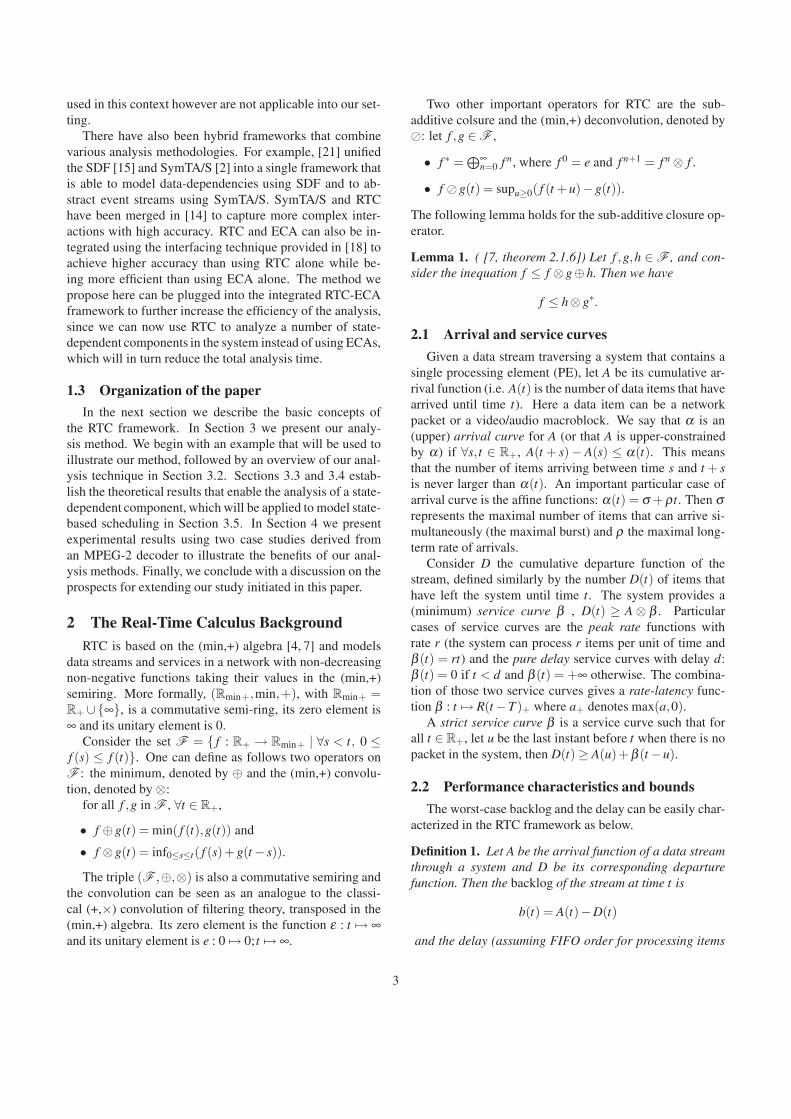
1. b(t) ≤ Bmax = sup{α(t)−β (t) | t ≥ 0},2. d(t) ≤ Dmax = inf{d ≥ 0 | ∀t ≥ 0, α(t) ≤ β (t + d)}.

The maximal backlog is the maximal vertical distancebetween α and β while the maximal delay is given by themaximal horizontal distance between those two functions.Figure 2 illustrates this fact.

Dmax

Bmax

α

β

Figure 2. Guarantee bounds on backlog anddelay.

Further, bounds on the output stream and the remainingresource of the system can be determined using Theorem 2.

Theorem 2 ( [4]). Assume a stream constrained by an ar-rival curve α entering a system with service curve β .

1. The output stream is upper-constrained by an arrivalcurve

α ′ = α �β .

2. If β is a strict service curve, the remaining resource af-ter processing the stream is bounded by a service curve

β ′ = (β −α)+.

In this paper, we assume that service curves are strict toensure for the positiveness of remaining service; however,our method is not restricted to this assumption.

From the results concerning systems with a single PE,one can obtain more general results for systems with mul-tiple PEs, using the composition of the RTC operators. Forexample, if there are two PEs in sequence, for respectiveservice curves β1 and β2, the overall service curve is β1⊗β2

(see [4, 7] for details). Such results have been based on theproperties of the (min,plus) algebra.

3 Modeling complex state-dependenciesModern stream-processing systems are usually hetero-

geneous networks of resources processing multiple datastreams using complex scheduling policies. Often, the pro-cessing of a stream depends not only on the available ser-vice but also the internal state of the system. One typicalexample is when the amount of on-chip memory is limitedand hence the internal buffers that hold the processed itemscan only accommodate up to a certain capacity. To avoidloss of data, the processor may implement blocking-writefor its output buffers, i.e it stalls whenever the buffers arefull. Otherwise, to save resource, it may proceed to processthe next data streams based on some sharing policy, in casethe output buffer that stores the currently processed streamis filled up.

Modeling and analysis of systems described above re-quire us to take into consideration the state-dependenciesthat are imposed among the different elements of a system.The original RTC framework presented in Section 2 (i) doesnot express state-information and furthermore (ii) assumesthat all buffers have infinite capacities. As a result, it isnot able to represent and correctly analyze such systems.Automata-based approaches developed recently for streamprocessing systems [6, 17] can encapsulate state informa-tion; however, their analyses become inefficient for largesystems due to the state-space explosion. In this section, wepresent a functional analysis technique, developed on top ofthe original RTC framework, which is capable of capturingthe complex state-dependencies while achieving high effi-ciency. We shall illustrate our method with an example ofstream-processing systems that is described below. Moregeneral systems can be easily modeled and analyzed usingthe same approach.

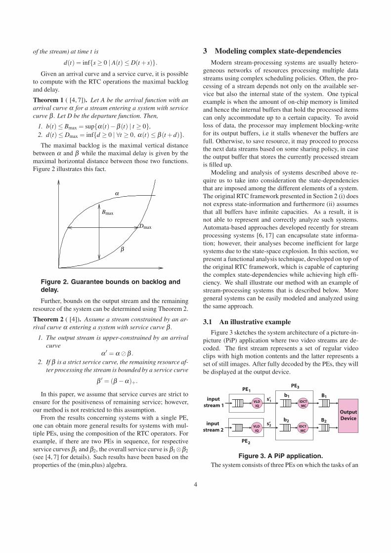
3.1 An illustrative exampleFigure 3 sketches the system architecture of a picture-in-

picture (PiP) application where two video streams are de-coded. The first stream represents a set of regular videoclips with high motion contents and the latter represents aset of still images. After fully decoded by the PEs, they willbe displayed at the output device.

VLD IQ

VLD IQ

IDCT MC

IDCT MC

input stream 1

input stream 2

b2

B1b1

B2

OutputDevice

PE

PE

PE1

2

3

s‘

s‘

1

2

Figure 3. A PiP application.The system consists of three PEs on which the tasks of an

4

MPEG-2 decoder application are partitioned and mapped.As shown in the figure, the Variable Length Decoding(VLD) and Inverse Quantization (IQ) tasks run on each ofPE1 and PE2 while the Inverse Discrete Cosine Transform(IDCT) and Motion Compensation (MC) tasks run on PE3.PE1 processes the first input video stream and PE2 pro-cesses the second input video stream. The partially decodedstreams from PE1 and PE2 (denoted by s′1 and s′2) are storedin the buffers b1 and b2 respectively, where they will furtherbe processed by PE3. The two fully decoded streams fromPE3 are then written to the playout buffers B1 and B2 beforebeing read by the output device.

PE3 schedules the two streams s′1 and s′2 using a fixed-priority scheduling policy, with s′1 having higher prioritythan s′2. Further, PE3 implements blocking-write on theplayout buffer B1; when B1 is full, the processor will pro-cess s′2 if there are some items in b2. This is done regardlessof whether there are items in b1.

Given the above system architecture, we are interestedin answering questions concerning the behavior of the sys-tem such as (1) what is the maximum backlog of a buffer?(2) what is the maximum delay experienced by a stream?(3) is the system schedulable while guaranteeing none thebuffers overflows? A correct evaluation of such propertiesare essential for designers to optimize the design of the sys-tem. As mentioned earlier, we cannot use the standard RTCframework to analyze the system since PE3 implementsstate-based scheduling scheme.

3.2 A functional analysis approach

In constructing the model for the system, we describeeach input stream to the system as an arrival curve and eachprocessing resource of the system as a service curve. Theprocessing of a stream by a resource is represented by anabstract component whose inputs are the arrival curve ofthe input stream and the service curve of the resource. Theoutputs of an abstract component are an arrival curve thatbounds the output stream and a service curve that boundsthe resource left after processing the input stream. By con-necting the abstract components following the flow of thestream (from left to right) and the order at which the dif-ferent streams are processed by a shared resource (from topto bottom), we obtain the complete abstract model of thesystem. Figure 4 depicts the abstract model of the systemarchitecture in Figure 3.

In this figure, α1 and α2 denote the arrival curves of thetwo input video streams; β1,β2 and β3 denote the servicecurves of PE1, PE2 and PE3 respectively. Similarly, β4 andβ5 are the service curves that bound the consumptions of thetwo fully processed streams. The processing of the streamsby PE1 and PE2 are represented by the abstract componentsC1 and C2, whose output arrival curves are denoted by α ′

1and α ′

2. The processing of PE3 on the output streams s′1 and

PE

PE

PE1

2

3

C1

C2

C3

C′3

C4

C5

α1

α2

α′1

α′2

α″1

α″2

β1

β2 β5

β4

OD1

OD2

β3

3β′

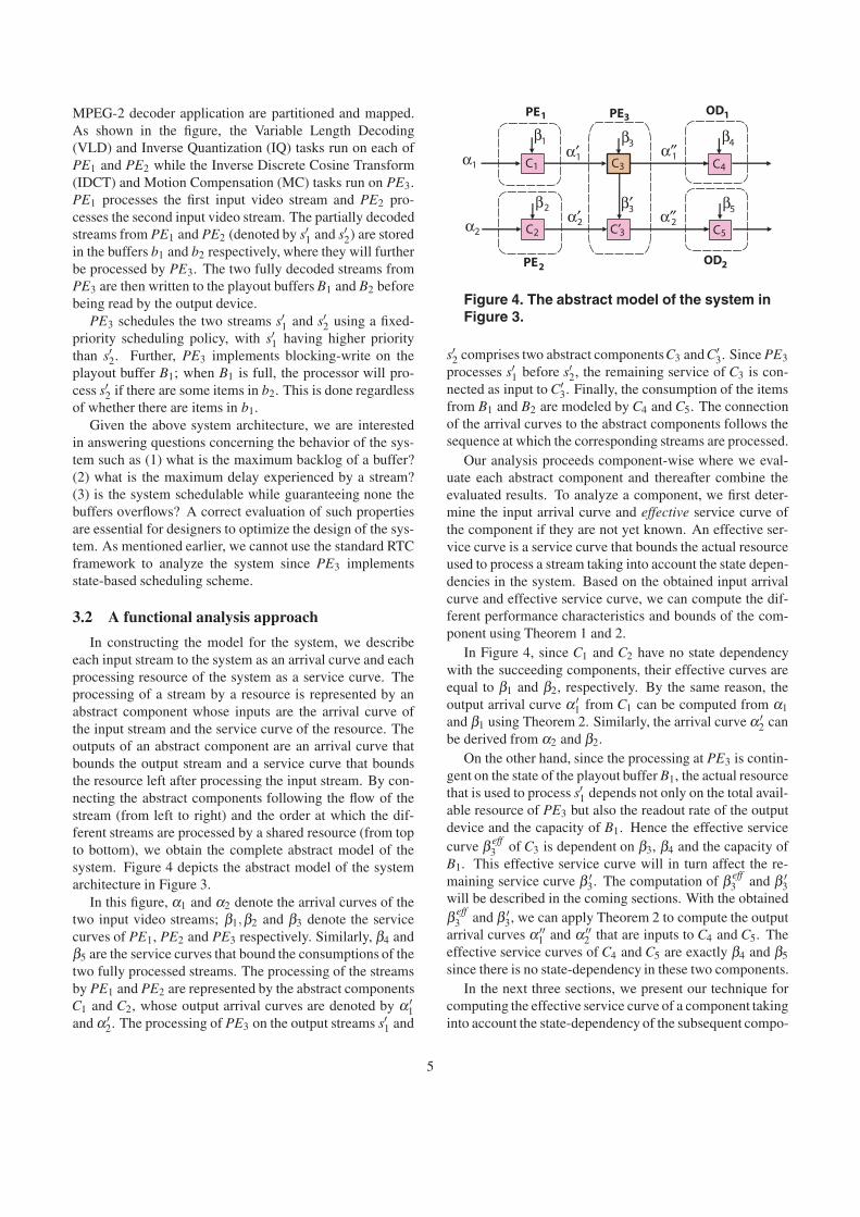
Figure 4. The abstract model of the system inFigure 3.

s′2 comprises two abstract componentsC3 and C′3. Since PE3

processes s′1 before s′2, the remaining service of C3 is con-nected as input to C′

3. Finally, the consumption of the itemsfrom B1 and B2 are modeled by C4 and C5. The connectionof the arrival curves to the abstract components follows thesequence at which the corresponding streams are processed.

Our analysis proceeds component-wise where we eval-uate each abstract component and thereafter combine theevaluated results. To analyze a component, we first deter-mine the input arrival curve and effective service curve ofthe component if they are not yet known. An effective ser-vice curve is a service curve that bounds the actual resourceused to process a stream taking into account the state depen-dencies in the system. Based on the obtained input arrivalcurve and effective service curve, we can compute the dif-ferent performance characteristics and bounds of the com-ponent using Theorem 1 and 2.

In Figure 4, since C1 and C2 have no state dependencywith the succeeding components, their effective curves areequal to β1 and β2, respectively. By the same reason, theoutput arrival curve α ′

1 from C1 can be computed from α1

and β1 using Theorem 2. Similarly, the arrival curve α ′2 can

be derived from α2 and β2.On the other hand, since the processing at PE3 is contin-

gent on the state of the playout buffer B1, the actual resourcethat is used to process s′1 depends not only on the total avail-able resource of PE3 but also the readout rate of the outputdevice and the capacity of B1. Hence the effective servicecurve β eff

3 of C3 is dependent on β3, β4 and the capacity ofB1. This effective service curve will in turn affect the re-maining service curve β ′

3. The computation of β eff3 and β ′

3will be described in the coming sections. With the obtainedβ eff

3 and β ′3, we can apply Theorem 2 to compute the output

arrival curves α ′′1 and α ′′

2 that are inputs to C4 and C5. Theeffective service curves of C4 and C5 are exactly β4 and β5

since there is no state-dependency in these two components.In the next three sections, we present our technique for

computing the effective service curve of a component takinginto account the state-dependency of the subsequent compo-

5

nents in the system. Section 3.3 looks into the case wherethe processing of the stream in the component is depen-dent on only one buffer of the next component. Section 3.4moves one step further to solve for the general case whenthe processing within the component is dependent on thebuffer state of many components in tandem. The computa-tion of the effective service curves of components that arescheduled using fixed-priority policy while being subjectedto the state of the buffers in the system is described in Sec-tion 3.5. Before going into the details, we first prove thefollowing lemma, which will be used in our formulation.

Lemma 2. Let f and g be two functions and c be a constant.Then,

1. ( f ⊗g)+ c = ( f + c)⊗g = f ⊗ (g + c)

2. ( f ⊗g∗)∗ = e + f +⊗g∗ and ( f ⊗g∗)+ = f + ⊗g∗,

where f + =⊕

n>0 f n.

Proof. 1. Let hc ∈ F , such that hc(0) = c and hc(t) = ∞,∀t > 0. Then, for every function f ∈ F , f ⊗hc = f +c. The formula follows from the associativity and thecommutativity of the ⊗ operator.

2. ( f ⊗g∗)∗ =⊕

n≥0( f ⊗g∗)n = e⊕⊕n>0( f ⊗g∗)n. As

(g∗)n = g∗, then ( f ⊗g∗)∗ = e⊕g∗⊕

n>0 f n, hence theresult.

3.3 Simple blocking-write at a single buffer

In this section, we model a setup where the process-ing of a stream is interrupted when an output buffer is full(i.e. blocking-write). This is done by extending the existingRTC framework using a feedback control mechanism. Thesystem, shown in Figure 5 consists in two PEs in tandem,where the second one has a finite capacity B2. The PEs haverespective service curves β1 and β2, and when the backlogin PE2 exceeds B2, then the service at PE1 is interrupted.The functions A1, A2 and A3 are the respective arrival pro-cesses at the entrance of the system, after serviced by thefirst PE and at the output of the system.

B2

A1 A2 A3

β2β1

Figure 5. System with two PEs in tandem, thesecond PE has a finite capacity buffer B2.

As the backlog on the second PE cannot exceed B2, onemust have A2 −A3 ≤ B2 and then A2 ≤ A3 + B2. A simplesolution to ensure this is to put a feedback control beforePE1, admitting only the amount of data that ensures that the

A2

β1 β2

A3

A3 + B2

A1

Figure 6. Feedback control to ensure non-overflow for the second buffer.

backlog constraint in PE2 is satisfied. In entrance of PE1,the arrival process then becomes A′

1 = min(A1,A3 + B2).Figure 6 represents the system that can be translated into

the following equations:{A2 ≥ min(A1,A3 + B2)⊗β1

A3 ≥ A2 ⊗β2,

which leads to the following inequation:

A2 ≥ min(A1,A2 ⊗β2 + B2)⊗β1

= min(A1 ⊗β1,A2 ⊗ (β2 + B2)⊗β1).

From Lemma 1, the solution if this inequality is:

A2 ≥ A1 ⊗β1 ⊗ [(β2 + B2)⊗β1]∗,

which proves the following lemma:

Lemma 3. The effective service curve for PE1 taking intoaccount the interruption of service when B2 is full is:

β eff1 = β1 ⊗ [(β2 + B2)⊗β1]∗.

Suppose α is the arrival curve of the input stream. Themaximal backlog and delay of the PE as well as the arrivalcurve of the output stream can be easily deduced from αand β eff

1 following Theorem 1 and 2.

3.4 Blocking-write at multiple buffers in sequenceNow suppose that there are several PEs in sequence, each

of which has a buffer with finite capacity. Then, the effec-tive service curve of the first PE (the one which has an infi-nite capacity) will depend on the capacities of all the buffersand on the other service curves: the feedback controls in-duce some cycles in the network, as shown in Figure 7.

β1

A3 + B2

A2A1

β2 β3

A3 A4

A4 + B3

βn

An+1An

An+1 + Bn

Figure 7. Line of PEs with backlog con-straints.

Consider a system with n PEs processing sequen-tially, where PE2, · · · ,PEn have respective buffer capaci-ties B2, . . . ,Bn. Theorem 3 gives the formula for computing

6

the effective service curve of PE1 considering the blocking-write at the subsequent PEs.

Theorem 3. The effective service curve β eff1 of PE1, taking

into account the feedback controls from the other PEs, isgiven by

β eff1 = β1 ⊗

nmini=0

i⊗j=1

[β j−1 ⊗ (B j + β j)]+.

Proof. The result is proved by induction. The initializationstep exactly corresponds to Lemma 3. Suppose that the re-sult holds for n PEs, and let us show it for n + 1 PEs. Thesystem obeys to the following equations:⎧⎨

⎩Ai ≥ min(Ai−1,Ai+1 + Bi)⊗βi−1

∀i ∈ {2, . . .n + 1},An+2 ≥ An+1 ⊗βn+1.

In particular, the equations concerning PEn+1 are:{An+1 ≥ min(An,An+2 + Bn+1)⊗βn

An+2 ≥ An+1 ⊗βn+1,

which is equivalent to An+1 ≥ An ⊗βn ⊗ [(βn+1 + Bn+1)⊗βn]∗. Now, one can replace the system with n + 1 PEs intandem with an equivalent system with n PEs, the n−1 firstPEs having the same service curve, and the last PE havingservice curve β ′

n = βn ⊗ [(βn+1 +Bn+1)⊗βn]∗. The capaci-ties of buffers 2 to n remain the same. Consequently, on canapply the induction hypothesis to that system and obtain aservice curve for the first PE (denoting βi ⊗ (Bi+1 + βi+1)by fi and βn−1 ⊗ (Bn + β ′

n) by f ′n−1):

β eff1 = β1⊗ [e⊕ f +

1 ⊕ f +1 ⊗ f +

2 ⊕·· ·⊕ f +1 ⊗·· ·⊗ f +

n−2⊗ f ′+n−1].

Consider only the last factor f ′+n−1 and replace β ′n by its

expression:

f ′+n−1 = [βn−1 ⊗ (Bn + βn ⊗ [(βn+1 + Bn+1)⊗βn]∗)]+

= [βn−1 ⊗ (βn + Bn)⊗ [(βn+1 + Bn+1)⊗βn]∗)]+

= [ fn−1 ⊗ f ∗n ]+ = f +n−1(e⊕ f +

n ),

which leads the desired formula and finishes the proof.

Remark that this formula takes into account the fact thatif PEi on the line has no backlog constraint (the buffer hasan infinite capacity and Bi = ∞), then the service curve doesnot depend on the service curves β j, j ≥ i. Indeed, in thatcase fi = ∞ and f +

i ⊗ ·· · ⊗ f +j = ∞. Analysis bounds on

the system can be easily computed in the same fashion asdone in the simple case when blocking-write is imposed ata single buffer.

Similar networks have been studied (see [7]), but thegoal in this reference is to compute the overall service curve.Here, we are only interested in findig the real service curveof the first server, in order to dimension the size of thebuffer, taking into account the block-writing phenomenon.

3.5 State-based scheduling policies

Recall that in the illustrative example in Figure 3 (Sec-tion 3.1), the resource of PE3 is shared between two streamss′1 and s′2. The processing policy used by PE3 is dependenton the state of the playout buffer B1 as well as the prioritiesof the streams. Specifically, PE3 will first process s′1 andonly process s′2 when b1 is empty or B1 is full.

The analysis for such a state-based scheduling policy isdivided into two phases. First, we determine the effectiveservice curve that is used to process each stream taking intoconsideration the state dependency. With the obtained ef-fective service curves, we compute the various performancecharacteristics using the results presented in Section 2.

The effective service curve β eff3 that is used to process s′1

taking into account the state dependency is computed usingLemma 3 and Theorem 3 described above. The effectiveservice curve that is used to process s′2 is also the one thatbounds the remaining resource after processing s′1, whichcan be computed using Corollary 1 below.

Corollary 1. Given a PE with service curve β processing ahigher priority stream s with arrival curve α . Assume β eff isthe effective service curve used to process the stream takinginto account the state-dependency. The remaining resourceof the PE given to the lower priority streams is bounded bythe service curve

β ′ = β − (α �β eff ).

Proof. For any given Δ > 0, the maximum number ofitems that are processed in any interval of length Δ is(α�β eff )(Δ) (Theorem 2.1). Since the PE starts processingthe lower priority streams as soon as there is no more itemsfrom s to be processed or when the output buffer is full, theamount of service given to the lower priority streams in anyinterval of length Δ is at least β (Δ)− (α � β eff )(Δ). Thisproves the corollary.

Using the computed effective service curve, the maxi-mum backlog, maximum delay the output arrival curve canbe easily computed using Theorem 1 and 2.1.

4 Experimental Case Studies

We employed two case studies to evaluate our theoreti-cal results and to illustrate the effect of state-dependency onthe behavior of a system. The first case study aims to showthe immediate ramification of processor stalling on the fill-levels of the buffers in a system. The second case studyillustrates the intermediate effect of blocking of one streamon another, at the same time demonstrates how our tech-nique can be used to evaluate systems with multiple inputstreams that are scheduled using fixed-priority schedulingpolicy with state-dependency.

7

4.1 Case study 1: Blocking-write of a stream

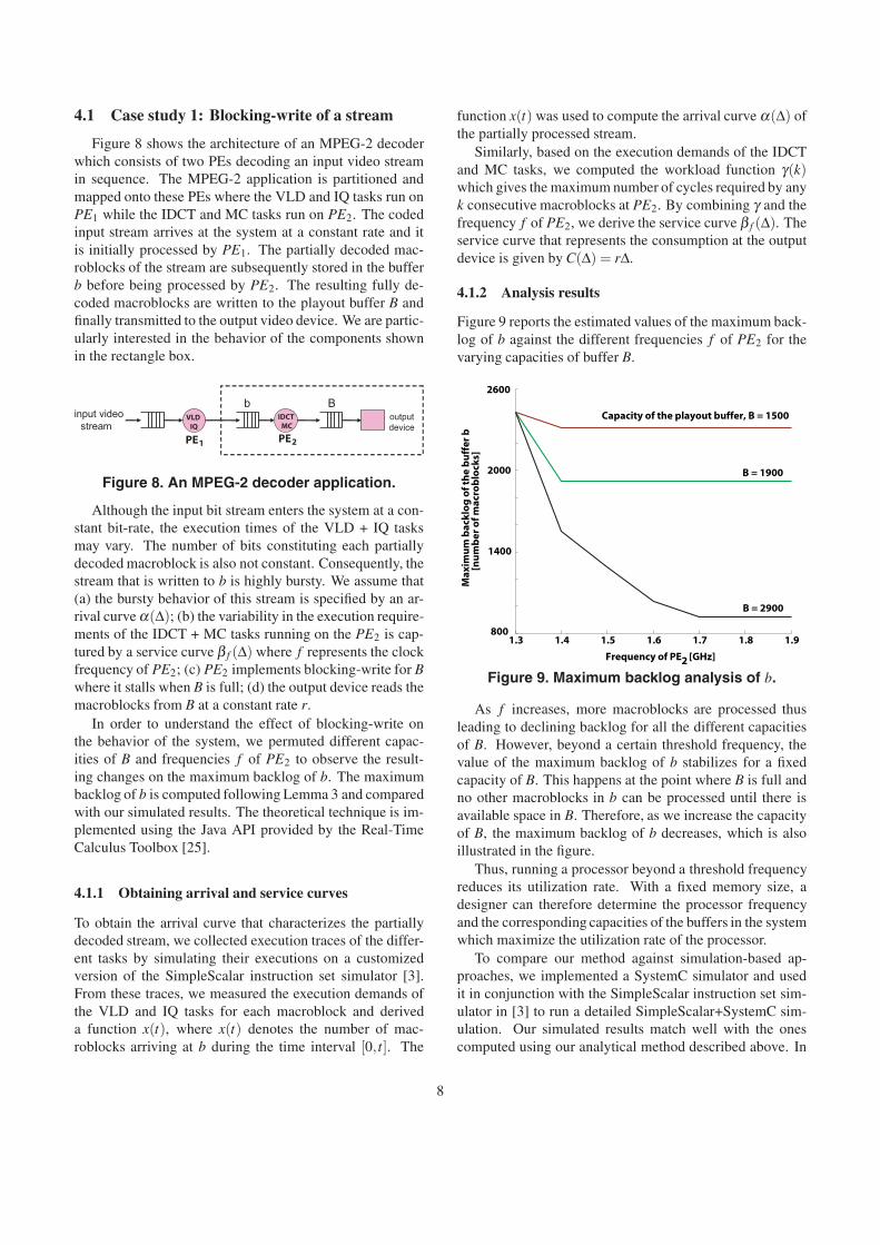
Figure 8 shows the architecture of an MPEG-2 decoderwhich consists of two PEs decoding an input video streamin sequence. The MPEG-2 application is partitioned andmapped onto these PEs where the VLD and IQ tasks run onPE1 while the IDCT and MC tasks run on PE2. The codedinput stream arrives at the system at a constant rate and itis initially processed by PE1. The partially decoded mac-roblocks of the stream are subsequently stored in the bufferb before being processed by PE2. The resulting fully de-coded macroblocks are written to the playout buffer B andfinally transmitted to the output video device. We are partic-ularly interested in the behavior of the components shownin the rectangle box.

input videostream

outputdevice

b BVLD IQ

IDCT MC

PE1 PE2

Figure 8. An MPEG-2 decoder application.

Although the input bit stream enters the system at a con-stant bit-rate, the execution times of the VLD + IQ tasksmay vary. The number of bits constituting each partiallydecoded macroblock is also not constant. Consequently, thestream that is written to b is highly bursty. We assume that(a) the bursty behavior of this stream is specified by an ar-rival curve α(Δ); (b) the variability in the execution require-ments of the IDCT + MC tasks running on the PE2 is cap-tured by a service curve β f (Δ) where f represents the clockfrequency of PE2; (c) PE2 implements blocking-write for Bwhere it stalls when B is full; (d) the output device reads themacroblocks from B at a constant rate r.

In order to understand the effect of blocking-write onthe behavior of the system, we permuted different capac-ities of B and frequencies f of PE2 to observe the result-ing changes on the maximum backlog of b. The maximumbacklog of b is computed following Lemma 3 and comparedwith our simulated results. The theoretical technique is im-plemented using the Java API provided by the Real-TimeCalculus Toolbox [25].

4.1.1 Obtaining arrival and service curves

To obtain the arrival curve that characterizes the partiallydecoded stream, we collected execution traces of the differ-ent tasks by simulating their executions on a customizedversion of the SimpleScalar instruction set simulator [3].From these traces, we measured the execution demands ofthe VLD and IQ tasks for each macroblock and deriveda function x(t), where x(t) denotes the number of mac-roblocks arriving at b during the time interval [0,t]. The

function x(t) was used to compute the arrival curve α(Δ) ofthe partially processed stream.

Similarly, based on the execution demands of the IDCTand MC tasks, we computed the workload function γ(k)which gives the maximum number of cycles required by anyk consecutive macroblocks at PE2. By combining γ and thefrequency f of PE2, we derive the service curve β f (Δ). Theservice curve that represents the consumption at the outputdevice is given by C(Δ) = rΔ.

4.1.2 Analysis results

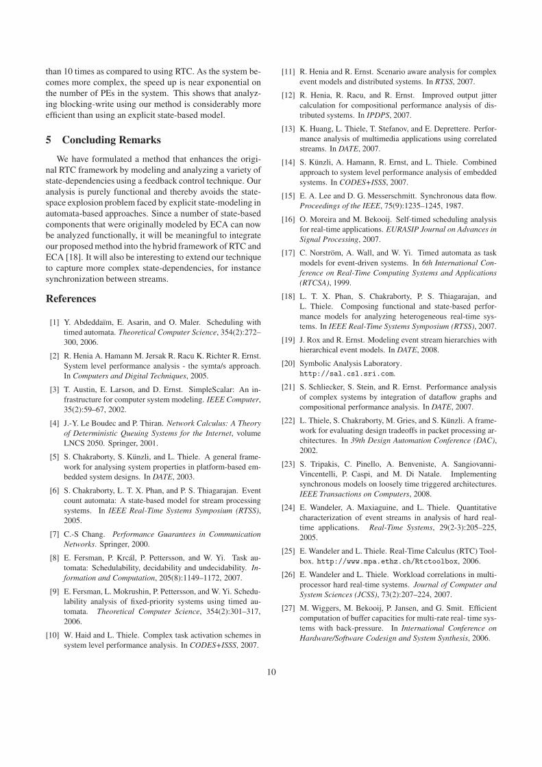
Figure 9 reports the estimated values of the maximum back-log of b against the different frequencies f of PE2 for thevarying capacities of buffer B.

1.3 1.4 1.5 1.6 1.7 1.8 1.9800

1400

2000

2600

Frequency of PE2 [GHz]

Max

imu

m b

ackl

og

of t

he

bu

ffer

b

[nu

mb

er o

f mac

rob

lock

s]

Capacity of the playout buffer, B = 1500

B = 1900

B = 2900

Figure 9. Maximum backlog analysis of b.

As f increases, more macroblocks are processed thusleading to declining backlog for all the different capacitiesof B. However, beyond a certain threshold frequency, thevalue of the maximum backlog of b stabilizes for a fixedcapacity of B. This happens at the point where B is full andno other macroblocks in b can be processed until there isavailable space in B. Therefore, as we increase the capacityof B, the maximum backlog of b decreases, which is alsoillustrated in the figure.

Thus, running a processor beyond a threshold frequencyreduces its utilization rate. With a fixed memory size, adesigner can therefore determine the processor frequencyand the corresponding capacities of the buffers in the systemwhich maximize the utilization rate of the processor.

To compare our method against simulation-based ap-proaches, we implemented a SystemC simulator and usedit in conjunction with the SimpleScalar instruction set sim-ulator in [3] to run a detailed SimpleScalar+SystemC sim-ulation. Our simulated results match well with the onescomputed using our analytical method described above. In

8

particular, the analytical bounds are always less than 5%more than those obtained from simulation. On the otherhand, performing the analysis using the RTC toolbox incor-porated with our method is significantly faster than pursuingthe pure simulation approach (less than a minute vs. severalhours). Note also that results from simulation are unable toprovide a formal guarantee on the maximum backlog thatmay incur in the system.

4.2 Case study 2: State-based scheduling of mul-tiple input streams

In this case study, we analyze the example system de-scribed in Section 3.1. We assume the two input videostreams arrive at a constant bitrate of 8 Mbps and their fullydecoded macroblocks are read by the output device at a rateof 40,000 macroblocks per second. The frequencies of PE1

and PE2 are set to be f1 = 1.3GHz and f2 = 1.25GHz, re-spectively. Given these values fixed, we are interested inthe backlog of b2 with respect to different values of the fre-quency of PE3 and capacity of B1.

First, we obtain the arrival curves α1 and α2 of the twoinput streams and the service curves β1, β2 and β3 of thethree PEs (see Section 4.1.1). From α1 and β1, we com-pute the arrival curve α ′

1 that characterizes the output streamfrom PE1. Similarly, the arrival curve α ′

2 that represents theoutput stream from PE2 is derived from α2 and β2. Basedon α ′

1, β3 and the capacity of B1, we follow Lemma 3 to

compute the effective service curve β eff3 that processes the

output stream from PE1 considering blocking-write at B1.The remaining service curve β ′

3 that is used to process the

second stream is deducted from β eff3 and α ′

1 using Corol-lary 1. The maximum backlog of b2 is then calculated fromα ′

2 and β ′3 using Theorem 1.

2.82.9

3.03.1

3.23.3

3.4 0 500

10001500

20002500

30003500

4000

0.9

1

1.1

1.2

1.3

1.4

1.5

1.6x 10

4

Capacity of the playout buffer B

[number of macroblocks]1

Bac

klo

g o

f th

e b

uff

er b

[n

um

ber

of m

acro

blo

cks]

Frequency of PE [GHz]3

2

Figure 10. Case study 2: Maximum backlogof the lower priority stream.

Figure 10 plots the maximum backlog of b2 in relationto the capacity of B1 and the frequency of PE3. Observefrom the figure that the maximum backlog of b2 is small-est around the region with highest frequencies of PE3 andlargest capacities of B2. Reversely, b2 has smallest back-logs in the area where PE3 has lowest frequencies and B2

has smallest capacities. In fact, the result shown in the fig-ure demonstrates that the maximum backlog of b2 is alwaysproportional to the frequency of PE3 and the capacity of B1.Thus the maximum backlog of the input buffer correspond-ing to the lower priority stream exhibits the same pattern asthat the higher priority stream (as seen in case study 1). Thisdemonstrates the effect of feedback control at one stream onthe other streams that share the same resource.

Table 1. Total buffer space required for PE3.

Total backlog of b1 and b2 (macroblocks)

PE3 Freq. B1 = 1000 B1 = 2000 B1 = 3000 No feedback

2.8 GHz 31170 29498 28043 14382

2.9 GHz 30490 28624 27169 12430

3.0 GHz 29619 28332 26347 10868

3.1 GHz 29359 27478 25825 9104

3.2 GHz 28603 26885 25439 7396

Table 1 reports the total maximum backlogs of the twobuffers b1 and b2 in reference to the capacity of B1 and thefrequency of PE3. The last column of the table gives the val-ues for the case when there is no state dependency. It is ob-served consistently for all frequencies that when the capac-ity of B1 is finite and blocking-write is imposed on the sys-tem, the total backlog at PE3 is much larger than the com-puted backlog in the case of no state-dependency. Thus, as-suming the buffers having infinite capacity may potentiallylead to inaccurate results, as shown in this case study. It istherefore important for us to capture the state-dependencyin the model and analysis of such systems.

For simplicity, we assume in both case studies thatblocking-write is implemented only at a single buffer in thesystem. The analysis for the case when blocking-write isimposed on multiple buffers can be done similarly, exceptthat one may additionally need to use Theorem 3 to com-pute the effective service curve offered by a processor toa stream. The same technique presented here can also beemployed to analyze systems with more than two streams.

Additionally, we have also modeled the given case stud-ies using the ECA and carried out the analysis using theSAL (Symbolic Analysis Laboratory) model checker [20].It is observed from our experiments that the analysis timewhen using ECA is much slower than when using RTC. Forexample, in case study 1, using ECA takes in average more

9

than 10 times as compared to using RTC. As the system be-comes more complex, the speed up is near exponential onthe number of PEs in the system. This shows that analyz-ing blocking-write using our method is considerably moreefficient than using an explicit state-based model.

5 Concluding Remarks

We have formulated a method that enhances the origi-nal RTC framework by modeling and analyzing a variety ofstate-dependencies using a feedback control technique. Ouranalysis is purely functional and thereby avoids the state-space explosion problem faced by explicit state-modeling inautomata-based approaches. Since a number of state-basedcomponents that were originally modeled by ECA can nowbe analyzed functionally, it will be meaningful to integrateour proposed method into the hybrid framework of RTC andECA [18]. It will also be interesting to extend our techniqueto capture more complex state-dependencies, for instancesynchronization between streams.

References

[1] Y. Abdeddaïm, E. Asarin, and O. Maler. Scheduling withtimed automata. Theoretical Computer Science, 354(2):272–300, 2006.

[2] R. Henia A. Hamann M. Jersak R. Racu K. Richter R. Ernst.System level performance analysis - the symta/s approach.In Computers and Digital Techniques, 2005.

[3] T. Austin, E. Larson, and D. Ernst. SimpleScalar: An in-frastructure for computer system modeling. IEEE Computer,35(2):59–67, 2002.

[4] J.-Y. Le Boudec and P. Thiran. Network Calculus: A Theoryof Deterministic Queuing Systems for the Internet, volumeLNCS 2050. Springer, 2001.

[5] S. Chakraborty, S. Künzli, and L. Thiele. A general frame-work for analysing system properties in platform-based em-bedded system designs. In DATE, 2003.

[6] S. Chakraborty, L. T. X. Phan, and P. S. Thiagarajan. Eventcount automata: A state-based model for stream processingsystems. In IEEE Real-Time Systems Symposium (RTSS),2005.

[7] C.-S Chang. Performance Guarantees in CommunicationNetworks. Springer, 2000.

[8] E. Fersman, P. Krcál, P. Pettersson, and W. Yi. Task au-tomata: Schedulability, decidability and undecidability. In-formation and Computation, 205(8):1149–1172, 2007.

[9] E. Fersman, L. Mokrushin, P. Pettersson, and W. Yi. Schedu-lability analysis of fixed-priority systems using timed au-tomata. Theoretical Computer Science, 354(2):301–317,2006.

[10] W. Haid and L. Thiele. Complex task activation schemes insystem level performance analysis. In CODES+ISSS, 2007.

[11] R. Henia and R. Ernst. Scenario aware analysis for complexevent models and distributed systems. In RTSS, 2007.

[12] R. Henia, R. Racu, and R. Ernst. Improved output jittercalculation for compositional performance analysis of dis-tributed systems. In IPDPS, 2007.

[13] K. Huang, L. Thiele, T. Stefanov, and E. Deprettere. Perfor-mance analysis of multimedia applications using correlatedstreams. In DATE, 2007.

[14] S. Künzli, A. Hamann, R. Ernst, and L. Thiele. Combinedapproach to system level performance analysis of embeddedsystems. In CODES+ISSS, 2007.

[15] E. A. Lee and D. G. Messerschmitt. Synchronous data flow.Proceedings of the IEEE, 75(9):1235–1245, 1987.

[16] O. Moreira and M. Bekooij. Self-timed scheduling analysisfor real-time applications. EURASIP Journal on Advances inSignal Processing, 2007.

[17] C. Norström, A. Wall, and W. Yi. Timed automata as taskmodels for event-driven systems. In 6th International Con-ference on Real-Time Computing Systems and Applications(RTCSA), 1999.

[18] L. T. X. Phan, S. Chakraborty, P. S. Thiagarajan, andL. Thiele. Composing functional and state-based perfor-mance models for analyzing heterogeneous real-time sys-tems. In IEEE Real-Time Systems Symposium (RTSS), 2007.

[19] J. Rox and R. Ernst. Modeling event stream hierarchies withhierarchical event models. In DATE, 2008.

[20] Symbolic Analysis Laboratory.http://sal.csl.sri.com.

[21] S. Schliecker, S. Stein, and R. Ernst. Performance analysisof complex systems by integration of dataflow graphs andcompositional performance analysis. In DATE, 2007.

[22] L. Thiele, S. Chakraborty, M. Gries, and S. Künzli. A frame-work for evaluating design tradeoffs in packet processing ar-chitectures. In 39th Design Automation Conference (DAC),2002.

[23] S. Tripakis, C. Pinello, A. Benveniste, A. Sangiovanni-Vincentelli, P. Caspi, and M. Di Natale. Implementingsynchronous models on loosely time triggered architectures.IEEE Transactions on Computers, 2008.

[24] E. Wandeler, A. Maxiaguine, and L. Thiele. Quantitativecharacterization of event streams in analysis of hard real-time applications. Real-Time Systems, 29(2-3):205–225,2005.

[25] E. Wandeler and L. Thiele. Real-Time Calculus (RTC) Tool-box. http://www.mpa.ethz.ch/Rtctoolbox, 2006.

[26] E. Wandeler and L. Thiele. Workload correlations in multi-processor hard real-time systems. Journal of Computer andSystem Sciences (JCSS), 73(2):207–224, 2007.

[27] M. Wiggers, M. Bekooij, P. Jansen, and G. Smit. Efficientcomputation of buffer capacities for multi-rate real- time sys-tems with back-pressure. In International Conference onHardware/Software Codesign and System Synthesis, 2006.

10