Lightweight Computation to Robust Cloud Infrastructure for ...
Upload
khangminh22Category
view
0download
0
Synthesis and Performance of Lightweight
Geopolymer Concrete
Jiting Xie
A thesis submitted in fulfilment of the requirements for the degree of
Doctor of Philosophy
School of Engineering and Information Technology
UNSW Canberra
August 2015


i
Thesis/Dissertation Sheet

ii
Statements
COPYRIGHT STATEMENT
‘I hereby grant the University of New South Wales or its agents the right to
archive and to make available my thesis or dissertation in whole or part in the
University libraries in all forms of media, now or here after known, subject to the
provisions of the Copyright Act 1968. I retain all proprietary rights, such as
patent rights. I also retain the right to use in future works (such as articles or
books) all or part of this thesis or dissertation.
I also authorise University Microfilms to use the 350 word abstract of my thesis
in Dissertation Abstract International (this is applicable to doctoral theses only).
I have either used no substantial portions of copyright material in my thesis or I
have obtained permission to use copyright material; where permission has not
been granted I have applied/will apply for a partial restriction of the digital copy
of my thesis or dissertation.’
Signed ……………………………………………………………
Date ……………………………………………………………
AUTHENTICITY STATEMENT
‘I certify that the Library deposit digital copy is a direct equivalent of the final
officially approved version of my thesis. No emendation of content has occurred
and if there are any minor variations in formatting, they are the result of the
conversion to digital format.’

iii
Signed ……………………………………………………………
Date ……………………………………………………………
ORIGINALITY STATEMENT
‘I hereby declare that this submission is my own work and to the best of my
knowledge it contains no materials previously published or written by another
person, or substantial proportions of material which have been accepted for the
award of any other degree or diploma at UNSW or any other educational
institution, except where due acknowledgement is made in the thesis. Any
contribution made to the research by others, with whom I have worked at
UNSW or elsewhere, is explicitly acknowledged in the thesis. I also declare that
the intellectual content of this thesis is the product of my own work, except to
the extent that assistance from others in the project’s design and conception or
in style, presentation and linguistic expression is acknowledged.’
Signed …………………………………………………………...
Date ……………………………………………………………
iv
Acknowledgements
The successful completion of this thesis is largely due to the great supports of
many people. I am pleased to express my acknowledgement to them here.
I give my primary appreciation to my main supervisor, A/Prof Obada Kayali, for
his enlightenment, instruction, support and encouragement in the past four
years, which have been critical and beneficial for completing this research
project.
Also, I am very thankful to my co-supervisor, Prof Evgeny Morozov, for his kind
support of my PhD study all the time.
Meanwhile, I would like to give many thanks to the China Scholarship Council
(CSC), South China University of Technology and UNSW Australia. Owing to
CSC’s policy and the cooperation program of above two universities, I have
been able to complete this research project with sufficient funding support.
Also, I am really appreciative for the technical assistance that I received during
the four-year long PhD study, including that of Mr Qingyong Ren, Dr Barry Gray,
Dr Raiden Acosta, Dr Wayne Hutchison and Prof Hans Riesen from the school
of physical, environmental and mathematical sciences in UNSW Canberra and
for their guidance and support on XRD, XRF and FTIR experiments; Dr Ulrike
Troitzsch in Australian National University for XRD experiments; Mr Jim Baxter,
Mr David Sharp, Mr Matthew Barrett and Mr Thomas Thomson for laboratory
technical support; and Dr Juan Pablo Escobedo-Diaz for his instruction and
support on optical microscopy tests.

v
Besides, I thank my colleagues, Dr Chang Lin, Dr Yuan Fang, Dr Muhammad
Junaid, Dr Mohammad Shakhaout Hossain Khan and Ms Yifei Cui, for the
knowledge acquired from the discussions with them.
And, I’d like to thank Prof. Xiaofang Hu in South China University of Technology,
who used to be my supervisor in China, and instructed me in relevant chemical
engineering skills that have been utilised in this project.
Moreover, I hope to express my sincere appreciation to Ms Denise Russel, who
volunteered to revise the English language of my thesis in the last two months.
Her job was brilliant, efficient and absolutely admirable.
Finally, I hope to thank my parents, Jing Wang and Haitian Xie, and also the
other relatives of the family, for their love, care and support which helped me go
through this PhD study. Thanks to my girlfriend, Dr Xue Gong, and other friends
in Australia, for their accompanying me in the past four year journey of my life.
vi
Abstract
A lightweight concrete (LWC) displays physical, mechanical and structural
features preferred in contemporary concrete industry. A major synthetic method
for manufacturing LWCs is to use lightweight aggregates (LWAs). A fly ash-
based LWA (FA-LWA) has been claimed as a promising material because of its
capability to produce a high-performance LWC and because of its relevant
ecological benefits. However, its manufacture requires high-powered
mechanical and thermal treatments to ensure its quality, which incurs high
energy consumption and production costs. Also, this process consumes a large
amount of fossil fuels which is likely to aggravate current resources and
environmental burdens, and does not fit with the desire for a sustainable and
eco-friendly industry. Concrete is a successful and very popular building
material because it can be used to construct strong and durable structures at a
relatively inexpensive cost. Therefore, there is a considerable concern for the
cost and quality of LWC when it is suggested to replace traditional normal
weight concrete. There has been mounting criticism directed to the cement and
concrete industries because of the large amounts of CO2 emitted by the various
activities of these industries. Therefore, it would be difficult to introduce another
high-energy LWC that could aggravate this situation whereas a low-cost, eco-
friendly LWC would likely be more acceptable. Hence, the significance of this
study is that it investigated a LWC synthesis which consumed less energy but
still possessed the desired features.
This research explored the employment of a fly ash-derived geopolymer
technology capable of generating lightweight and high-strength materials

vii
consisting of covalent-bonded aluminosilicate molecules called ‘geopolymers’
under mild-temperature (40-80oC) conditions. As this technology has been
proven to be capable of producing high-quality construction materials, such as
the well-known ‘geopolymer binder’, to replace Portland cement for
environmental reasons, it is suggested that it may be a workable solution to
reduce LWCs’ high energy consumption.
In this study, in addition to geopolymer binder, this geopolymer technology was
used to create high-quality FA-LWAs, referred to as geopolymer aggregates
(GAs), to replace the traditional high-energy methods. This way, it is expected
to realise a high-performance low-cost, eco-friendly LWC by increasing its
geopolymer material content, such as by 60-70% if only using GAs, or even by
100% using a combination of GAs and geopolymer binder.
Firstly, this study investigated whether synthesising GAs based on geopolymer
technology was practical. It examined the mechanism of geopolymerisation to
confirm that the synthesized geopolymer material was suitable for the
manufacture of GAs. The characteristics of fly ash, such as its density, particle
size and shape, carbon content, and chemical compositions, were identified
using various techniques that included electron microscopy, XRF and XRD. The
effects of the identified characteristics on fresh geopolymers were later
evaluated from a combination of workability tests, based on which a consistent
fly ash source was selected. Then, a mix design approach and procedure which
used the criteria of SiO2/Na2O, H2O/Na2O and W/G have been proposed. This
has been done so as to determine the effect of each chemical component that
was proposed and allow the final mix design to be calculated. Also, an
appropriate curing regime was researched and correlated with the geopolymer’s

viii
density, strength and microstructural development. Heat curing at 80oC for 3
days was applied to GAs and, moreover, prolonged room-temperature curing
under a low-moisture condition studied and used for a cold-bonded GA (called
RTGA). A feasible manufacturing procedure based on the outcomes of these
investigations was later designed to produce both coarse and fine GA products.
The performance of this GA was evaluated based on its grading, density, water
absorption capacity, crushing value and rebound properties which indicated that
it had adequate qualities for LWC manufacture according to the relevant
engineering standards and comparison with other FA-LWAs. Then, its porous
microstructure, which is composed of geopolymer molecules, as identified by
infrared (IR) spectroscopy, was studied based on stereo and optical microscopy
techniques. The results indicated that geopolymerisation could be a new
method for creating homogeneously distributed pores, with most less than 50
µm in size, which would facilitate the formation of the lightweight as well as
strong structure desired for GAs.
Then, the performance of LWCs after the application of GAs was examined.
The OPC-based LWC made of both coarse and fine GAs demonstrated
advanced performance with a high strength and high strength/mass ratio. Also,
the LWCs made entirely from geopolymer materials (GAs and geopolymer
binder) resulted in a medium-strength performance sufficient for structural LWC
applications. These outcomes confirmed the possibility of producing a low-cost,
eco-friendly structural LWC based on the application of the GAs created in this
research. Moreover, the fine GAs produced as a new type of artificial sand
resulted in high performance lightweight mortar materials in both OPC-based
and geopolymer binder-based systems. Furthermore, the synthesised coarse

ix
and fine RTGAs were of sufficient quality for structural LWC applications, even
though they were not as good as their heated counterparts.

x
List of Publications
Journal Paper
Jiting Xie, Obada Kayali, 2014, Effect of initial water content and curing
moisture conditions on the development of fly ash-based geopolymers in heat
and ambient temperature, Construction and Building Materials, Volume 67, Part
A, Pages 20-28.
Jiting Xie, Obada Kayali, Qingyong Ren, Wayne D. Hutchison, Yifei Cui, 2015,
Effects of variation in fly ash properties on workability and strength of
geopolymer mixes, Cement and Concrete Composites. Review process, paper
No. CCC-D-15-00238.
Conference Paper
Jiting Xie, Obada Kayali, 2013, Effect of water content on the development of fly
ash-based geopolymers in heat and ambient curing conditions, the 3rd
international conference on sustainable construction materials and technologies
(SCMT3), Kyoto, Japan.

xi
Table of Contents
Thesis/Dissertation Sheet .................................................................................... i
Statements .......................................................................................................... ii
Acknowledgements ............................................................................................ iv
Abstract .............................................................................................................. vi
List of Publications .............................................................................................. x
Table of Contents ............................................................................................... xi
List of Figures ................................................................................................... xx
List of Tables...................................................................................................xxvi
List of Abbreviations ........................................................................................xxxi
Chapter 1 Introduction and Literature Review ..................................................... 1
1.1 Background to Fly Ash-based Lightweight Aggregate (FA-LWA) .......... 2
1.1.1 Role of Aggregates in Concrete ...................................................... 2
1.1.2 Need for Artificial Aggregates .......................................................... 4
1.1.3 Lightweight Aggregates (LWAs) and Lightweight Concrete (LWC) . 6
1.1.4 Coal Fly Ash (CFA) ......................................................................... 9
1.1.5 FA-LWA ......................................................................................... 13
1.1.6 Problems of Current Manufacturing Method .................................. 17
1.2 Geopolymer Technology ...................................................................... 18
1.2.1 Brief Introduction to Geopolymer Technology ............................... 18

xii
1.2.2 Advantages of Geopolymer Technology for FA-LWA Manufacture
…………………………………………………………………………..24
1.2.3 Previous Trials using Geopolymer Technology for LWA
Manufacture ............................................................................................... 27
1.3 Scope of Thesis ................................................................................... 29
1.4 Techniques used in research ............................................................... 30
1.5 Structure of Thesis ............................................................................... 31
Chapter 2 Fly Ash and its Influence on Fresh Properties of Geopolymer ......... 38
2.1 Introduction .......................................................................................... 38
2.2 Selection and Characterisation of Fly Ash ........................................... 40
2.2.1 Selection of Fly Ash Samples ........................................................ 40
2.2.2 Density, Particle Size and Specific Surface Area .......................... 40
2.2.3 Loss on Ignition (LOI) .................................................................... 43
2.2.4 Chemical Oxide Composition (based on XRF) .............................. 44
2.2.5 Crystalline and Amorphous Contents (based on XRD) ................. 44
2.3 Geopolymer Mixes ............................................................................... 49
2.4 Fly Ash’s Influence on Fresh Properties .............................................. 51
2.4.1 Slump and Mini-flow Method ......................................................... 52
2.4.2 Vicat Plunger Penetration.............................................................. 59
2.4.3 Evaluation on Fly Ash’s Characteristics for Fresh Properties ........ 61
2.5 Fly Ash’s Effect on Hardened Properties ............................................. 65
2.6 Conclusions ......................................................................................... 71
xiii
Chapter 3 Geopolymer Mix Design ................................................................... 73
3.1 Introduction .......................................................................................... 73
3.2 Materials and Mix ................................................................................. 73
3.3 Terminology ......................................................................................... 75
3.3.1 Fly Ash/Activator Mass Ratio (F/A) ................................................ 75
3.3.2 Activator Composition Na2O·xSiO2·yH2O ...................................... 76
3.3.3 Water-to-geopolymer Solids (W/G) Ratio ...................................... 76
3.4 Mix Design Procedure.......................................................................... 77
3.5 Molarity of NaOH and Mass Ratio Na2SiO3/NaOH .............................. 89
3.6 An Alternative Mix Design Method – using NaOH Solution instead of
NaOH Flakes ................................................................................................. 94
3.7 Mix Designs used in this Thesis ......................................................... 103
3.8 Conclusions ....................................................................................... 104
Chapter 4 Curing Regime for Geopolymer Synthesis ..................................... 106
4.1 Introduction ........................................................................................ 106
4.2 Previous Research on Curing of Geopolymer Synthesis ................... 106
4.3 Curing Temperature ........................................................................... 108
4.3.1 Geopolymer Mix .......................................................................... 109
4.3.2 Curing Regime ............................................................................ 110
4.3.3 Strength ....................................................................................... 111
4.4 Curing Moisture Condition ................................................................. 112
4.4.1 Geopolymer Mix .......................................................................... 113

xiv
4.4.2 Curing Regime ............................................................................ 114
4.4.3 Strength....................................................................................... 115
4.5 Curing Period (Short-term) ................................................................ 117
4.5.1 Geopolymer Mix .......................................................................... 118
4.5.2 Curing Regime ............................................................................ 118
4.5.3 Density and Strength ................................................................... 119
4.5.4 Scanning Electron Microscopy .................................................... 123
4.6 Curing Period (Long-term) ................................................................. 126
4.6.1 Geopolymer Mix .......................................................................... 127
4.6.2 Curing Regime ............................................................................ 127
4.6.3 Density and Strength ................................................................... 127
4.7 Conclusions ....................................................................................... 131
Chapter 5 Geopolymer Aggregate (GA).......................................................... 132
5.1 Introduction ........................................................................................ 132
5.2 Mix Design used for Geopolymer Aggregate ..................................... 133
5.3 Manufacturing Procedure .................................................................. 136
5.3.1 Mixing and Casting ...................................................................... 137
5.3.2 Curing ......................................................................................... 139
5.3.3 Washing and Air Drying .............................................................. 140
5.3.4 Mechanical Crushing, Sieving and Storage................................. 142
5.4 Appearance ....................................................................................... 145
5.5 Grading .............................................................................................. 147
xv
5.5.1 Original Geopolymer Aggregate .................................................. 147
5.5.2 Refined Geopolymer Aggregate .................................................. 150
5.6 Density and Water Absorption ........................................................... 152
5.7 Internal Pores .................................................................................... 157
5.8 Crushing Value .................................................................................. 163
5.9 Rebound Test by Schmidt Hammer ................................................... 165
5.10 Infrared (IR) Spectroscopy.............................................................. 167
5.11 Evaluation of Quality of Geopolymer Aggregate ............................. 169
5.11.1 Compatibility with Standards .................................................... 170
5.11.2 Comparison with Other FA-LWAs ............................................ 172
5.12 Conclusions .................................................................................... 174
Chapter 6 OPC-based Concrete and Mortar using Geopolymer Aggregate ... 175
6.1 Introduction ........................................................................................ 175
6.2 NWC .................................................................................................. 176
6.2.1 Materials ...................................................................................... 176
6.2.2 Mix Design .................................................................................. 179
6.2.3 Concrete Preparation .................................................................. 180
6.2.4 Workability ................................................................................... 182
6.2.5 Density and Strength ................................................................... 182
6.3 OPC-GA Concrete ............................................................................. 184
6.3.1 Materials ...................................................................................... 184
6.3.2 Mix Design .................................................................................. 184
xvi
6.3.3 Concrete Preparation .................................................................. 187
6.3.4 Workability ................................................................................... 189
6.3.5 Density and Strength ................................................................... 189
6.3.6 Fracture Surface ......................................................................... 192
6.4 Comparison of OPC-GA Concrete and Other LWCs ......................... 194
6.4.1 LWC using FA-LWA .................................................................... 194
6.4.2 LWC using Geopolymer-assisted LWA ....................................... 198
6.5 OPC-GA Mortar ................................................................................. 202
6.5.1 Materials...................................................................................... 202
6.5.2 Mix Design .................................................................................. 202
6.5.3 Mortar Preparation ...................................................................... 203
6.5.4 Workability ................................................................................... 205
6.5.5 Density and Strength ................................................................... 206
6.6 Conclusions ....................................................................................... 209
Chapter 7 Geopolymer Binder-based Concrete and Mortar using Geopolymer
Aggregate ....................................................................................................... 211
7.1 Introduction ........................................................................................ 211
7.2 Mix Design Procedure for Geopolymer Binder-based Concretes ...... 212
7.2.1 Materials...................................................................................... 212
7.2.2 Geo-GA Concrete ....................................................................... 213
7.2.3 Geopolymer Concrete (GC) ........................................................ 216
7.3 Geopolymer Concrete (GC) ............................................................... 217

xvii
7.3.1 Concrete Preparation .................................................................. 217
7.3.2 Workability ................................................................................... 220
7.3.3 Density and Strength ................................................................... 221
7.4 Geo-GA Concrete .............................................................................. 223
7.4.1 Concrete Preparation .................................................................. 223
7.4.2 Density and Strength ................................................................... 223
7.4.3 Fracture Surface.......................................................................... 227
7.5 Comparison of Geo-GA Concrete and Other LWCs .......................... 229
7.5.1 Geo-GA versus OPC-GA ............................................................ 229
7.5.2 Geo-GA versus FA-LWA Geopolymer Concrete ......................... 231
7.6 Geopolymer Binder-based Mortar ...................................................... 233
7.6.1 Materials ...................................................................................... 233
7.6.2 Mix Design .................................................................................. 234
7.6.3 Mortar Preparation ...................................................................... 235
7.6.4 Workability ................................................................................... 236
7.6.5 Density and Strength ................................................................... 238
7.7 Conclusions ....................................................................................... 239
Chapter 8 Room Temperature-cured Geopolymer Aggregate (RTGA) and its
Application in Concrete ................................................................................... 241
8.1 Introduction ........................................................................................ 241
8.2 Manufacturing Procedure of RTGA .................................................... 242
8.3 Characteristics of RTGA .................................................................... 246

xviii
8.3.1 Appearance ................................................................................. 246
8.3.2 Grading ....................................................................................... 246
8.3.3 Density and Water Absorption ..................................................... 248
8.3.4 Infrared Spectroscopy ................................................................. 251
8.4 RTGA in Concrete Manufacture......................................................... 253
8.4.1 OPC-based Concrete .................................................................. 254
8.4.2 Geopolymer Binder-based Concrete ........................................... 258
8.5 Conclusion ......................................................................................... 261
Chapter 9 Conclusions and Recommendations for Future Research ............. 263
9.1 Research on Geopolymer for Manufacture of Geopolymer Aggregate
………………………………………………………………………………265
9.2 Geopolymer Aggregate ...................................................................... 268
9.3 OPC-based Concrete and Mortar using Geopolymer Aggregate ....... 270
9.4 Geopolymer Binder-based Concrete and Mortar using Geopolymer
Aggregate .................................................................................................... 272
9.5 Room Temperature-cured Geopolymer Aggregate (RTGA) .............. 274
9.6 Recommendations for Future Research ............................................ 275
Appendix A Calculation on Crystalline and Amorphous Contents in Fly Ash
based on Rietveld Quantification Data ............................................................ 279
Appendix B Design of Geopolymer Binder for Geopolymer Binder-based
Concretes and Mortars ................................................................................... 283
Bibliography .................................................................................................... 298

xix

xx
List of Figures
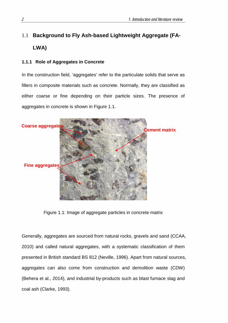
Figure 1.1: Image of aggregate particles in concrete matrix ............................... 2
Figure 1.2: Schematic of relationship between aggregates and cement matrix .. 3
Figure 1.3: SEM image of fly ash (adapted from Fang, 2013) ............................ 9
Figure 1.4: Main flowchart of processes in fly ash aggregate manufacture
(based on Chandra and Berntsson, 2002 and Bijen, 1986) .............................. 14
Figure 1.5: Images of Lytag aggregate (left) and Flashag aggregate (right, from
Kayali, 2008) ..................................................................................................... 16
Figure 1.6: Schematic of principle of geopolymer binder in concrete mix (drew
by the author based on the literature Kong, 2007, Rangan, 2007 and Bakharev,
2005a) ............................................................................................................... 20
Figure 1.7: 4-coordinated configuration of Si and Al tetrahedra in geopolymer
(Davidovits, 1976) ............................................................................................. 21
Figure 1.8: Three-dimensional network of geopolymer structure (adapted from
models proposed by Rowles et al., 2007 and Barbosa et al., 2000) ................. 22
Figure 1.9: Scheme for synthesis of fly ash-based geopolymer ........................ 22
Figure 1.10: Conceptual models for geopolymerisation proposed by Provis
(2005) (left) and Duxson (2007) (right).............................................................. 24
Figure 1.11: Schematic of relationships among thesis chapters ....................... 33
Figure 2.1: Malvern Mastersizer 2000 laser diffraction particle size analyser ... 41
Figure 2.2: Particle size distribution curves of fly ash samples ......................... 43
Figure 2.3: PANalytical Empyrean X-ray diffractometer .................................... 46
Figure 2.4: X-ray diffraction patterns and corresponding Rietveld refinement
results for fly ash samples FA1, FA2 and FA3 .................................................. 47

xxi
Figure 2.5: Preparation steps (1) Hobart mixer, (2) well-mixed fresh geopolymer,
(3) steel moulds with polyethylene cover, (4) well-compact geopolymer, (5)
geopolymer after demoulding and (6) geopolymer after heating ....................... 52
Figure 2.6: Schematic of mini-sized slump cone for slump and mini-flow testings
.......................................................................................................................... 54
Figure 2.7: Scheme of spread measurement using the mini-flow method ........ 54
Figure 2.8: Images of geopolymer flows before (left column) and once after
(right column) vibration in mini-flow test ............................................................ 56
Figure 2.9: Spread area increase by mechanical vibration of geopolymer paste
.......................................................................................................................... 58
Figure 2.10: Standard Vicat plunger for consistency testing ............................. 60
Figure 2.11: Compressive strength testing on a 3000 KN TECNOTEST machine
.......................................................................................................................... 67
Figure 3.1: Mixing procedure for fly ash-based geopolymer ............................. 75
Figure 3.2: Flowchart of procedure for geopolymer mix designs....................... 79
Figure 3.3: A modified mixing procedure for fly ash-based geopolymer ........... 95
Figure 3.4: Flowchart of procedure for an alternative geopolymer mix design
method .............................................................................................................. 97
Figure 4.1: 7-day compressive strengths of geopolymers under different curing
regimes (corresponding to the mix in Table 4.1) ............................................. 112
Figure 4.2: Compressive strengths of 14-day ambient-cured geopolymers coded
as A-14d, AS-14d and AD-14d with different W/G values ............................... 116
Figure 4.3: Density and compressive strength results for heated geopolymer
samples .......................................................................................................... 120

xxii
Figure 4.4: Density and compressive strength results of ambient-cured
geopolymer samples ....................................................................................... 121
Figure 4.5: SEM images of geopolymers with W/G=0.22: (a) A-7d, (b) A-14d
and (e) H-4h; and with W/G=0.26: (c) A-7d and (d) A-14d .............................. 124
Figure 4.6: Variations in specific density versus long-term curing period at room
temperature of fly ash-based geopolymers produced ..................................... 128
Figure 4.7: Compressive strength versus long-term curing period at room
temperature of fly ash-based geopolymer whose mix design is in Table 4.1 .. 129
Figure 4.8: Comparison of compressive strengths of geopolymers under
different curing regimes (where all samples are made from the mix design
shown in Table 4.1) ........................................................................................ 130
Figure 5.1: 7-day compressive strengths of geopolymers with different W/G
values ............................................................................................................. 135
Figure 5.2: Flowchart of manufacturing procedure for geopolymer aggregate 137
Figure 5.3: Fresh geopolymer chunks in plastic container .............................. 139
Figure 5.4: Soaking of hardened geopolymer chunks in water tank ............... 140
Figure 5.5: pH value after every day’s washing .............................................. 141
Figure 5.6: Jaw crusher used for manufacture of aggregate particles ............ 143
Figure 5.7: Grading curves of geopolymer aggregate samples after each jaw-
crushing cycle ................................................................................................. 144
Figure 5.8: Coarse (>4.75mm) (left) and fine (<4.75mm) (right) geopolymer
aggregates in air-dried condition ..................................................................... 145
Figure 5.9: Lynx stereo inspection microscope for observation of surface of
geopolymer aggregate .................................................................................... 146

xxiii
Figure 5.10: Enlarged image (40 times) of particle surface of geopolymer
aggregate (length approximately 3mm) .......................................................... 146
Figure 5.11: Grading curves of geopolymer aggregates and regularly used
crushed stone and river sand .......................................................................... 149
Figure 5.12: Grading curves of river sand, and original and refined fine
geopolymer aggregates .................................................................................. 152
Figure 5.13: Polishing procedures (1) mixing resin and hardener, (2) and (3)
soaking sample in resin, (4) covering sample in hardened resin, (5) grinder and
(6) polisher ...................................................................................................... 159
Figure 5.14: Bright field image of geopolymer aggregate sample ................... 160
Figure 5.15: Original captured image (left) and converted black-and-white image
(right) of geopolymer aggregate sample ......................................................... 161
Figure 5.16: Size distribution of detected pores in geopolymer aggregates as
obtained using an optical microscopy method ................................................ 161
Figure 5.17: Distribution of areas occupied by detected pores in geopolymer
aggregates ...................................................................................................... 162
Figure 5.18: Crushing value test of geopolymer aggregate sample ................ 164
Figure 5.19: Appearance of geopolymer aggregate sample after crushing value
test .................................................................................................................. 165
Figure 5.20: IR spectra of fly ash and geopolymer aggregate ........................ 169
Figure 6.1: Grading curves of crushed stone and river sand .......................... 177
Figure 6.2: Flowchart of preparation of OPC-based concrete ......................... 180
Figure 6.3: Steps in preparation of Con-N-OPC: (1) mixing, (2) casting, (3)
immediately after demoulding and (4) after 28-day curing .............................. 181

xxiv
Figure 6.4: Steps in preparation of concrete Con-GA-OPC (1) mixing, (2)
casting, (3) immediately after demoulding and (4) after 28-day curing ........... 188
Figure 6.5: Enlarged images (40x) of fracture surface of Con-N-OPC (left) and
Con-GA-OPC (right) (the image represents a length of approximately 3 mm) 193
Figure 6.6: Images of fresh mortar mixtures: (1) Mor-S-OPC and (2) Mor-GA-
OPC ................................................................................................................ 204
Figure 6.7: Images of 28-day cured Mor-S-OPC and Mor-GA-OPC samples . 204
Figure 6.8: Increases in spread areas of fresh Mor-S-OPC and Mor-GA-OPC
caused by mechanical vibration ...................................................................... 206
Figure 7.1: Flowchart of preparation of fly ash-based geopolymer concrete... 218
Figure 7.2: Steps in preparation of concrete Con-N-Geo (1) mixing, (2) casting,
(3) after heating and demoulding and (4) after 28-day curing ......................... 219
Figure 7.3: Steps in preparation of concrete Con-GA-Geo (1) mixing, (2) casting,
(3) after heating and demoulding and (4) after 28-day curing ......................... 224
Figure 7.4: Enlarged image (40x) of fracture surface of Con-GA-Geo (the image
represents a length of approximately 3 mm) ................................................... 228
Figure 7.5: Images on fresh mortar mixtures: (1) Mor-S-Geo and (2) Mor-GA-
Geo ................................................................................................................. 235
Figure 7.6: Images on 28-day cured Mor-S-Geo and Mor-GA-Geo samples .. 236
Figure 7.7: Increases in spread areas of fresh Mor-S-Geo and Mor-GA-Geo
caused by mechanical vibration ...................................................................... 237
Figure 8.1: Flowchart of manufacturing procedure for RTGA ......................... 243
Figure 8.2: pH value after every day’s washing .............................................. 245
Figure 8.3: Coarse (>4.75mm) (left) and fine (<4.75mm) (right) RTGAs in air-
dried condition ................................................................................................ 246

xxv
Figure 8.4: Grading curves of RTGAs and heated GAs .................................. 248
Figure 8.5: IR spectra of fly ash, heated GA and RTGA ................................. 252
Figure 8.6: Steps in preparation of Con-RTGA-OPC (1) mixing, (2) casting, (3)
immediately after demoulding and (4) after 28-day curing .............................. 256
Figure 8.7: Steps in preparation of Con-RTGA-Geo (1) mixing, (2) casting, (3)
after heating and demoulding and (4) after 28-day curing .............................. 260

xxvi
List of Tables
Table 1.1: Bulk chemical compositions of fly ashes from different coal types
(adapted from Ahmaruzzaman, 2010) .............................................................. 11
Table 1.2: Characteristics of Lytag and Flashag aggregates ............................ 16
Table 1.3: Comparison of traditional method and geopolymer technology for FA-
LWA manufacture ............................................................................................. 25
Table 2.1: Relative densities of fly ash.............................................................. 41
Table 2.2: Results of particle size distribution of the chosen fly ash batches ... 42
Table 2.3: LOI values of different fly ash samples ............................................ 43
Table 2.4: Chemical composition of each fly ash sample tested by XRF .......... 45
Table 2.5: Quantification on crystals and amorphous content in fly ash ........... 48
Table 2.6: Mixes of fly ash-based geopolymer with different fly ashes ............. 50
Table 2.7: Workability of produced fresh geopolymer mixes ............................. 55
Table 2.8: Penetration distance of Vicat plunger of fresh geopolymer mixes.... 60
Table 2.9: Air dry density and compressive strength of produced geopolymers
.......................................................................................................................... 67
Table 2.10: Quantification results on crystals and amorphous content before
and after geopolymerisation .............................................................................. 70
Table 3.1: Final mix design of the geopolymer mix example (kg/m3) ................ 89
Table 3.2: Molarity of NaOH solution and mass ratio of Na2SiO3/NaOH for
different geopolymer mix designs ..................................................................... 93
Table 3.3: Final mix design using a 16M NaOH ingredient of the geopolymer
mix example (kg/m3) ....................................................................................... 101
Table 3.4: Comparison of the molarity of NaOH solution between different mix
designs ........................................................................................................... 102

xxvii
Table 3.5: Mix designs for geopolymers used in this thesis ............................ 104
Table 4.1: Mix design of geopolymers for curing regime research .................. 109
Table 4.2: Curing regimes investigated for optimum geopolymer growth ....... 110
Table 4.3: Mix designs for geopolymer mixes with different initial water contents
........................................................................................................................ 114
Table 4.4: Specified curing moisture conditions for produced geopolymers ... 115
Table 4.5: Specified curing procedures for heat-cured and ambient-cured
geopolymers ................................................................................................... 119
Table 5.1: Geopolymer mix designs with different W/G values ....................... 134
Table 5.2: Geopolymer mix design for geopolymer aggregate manufacture ... 138
Table 5.3: Typical sieving analysis of coarse and fine geopolymer aggregates
........................................................................................................................ 148
Table 5.4: Grading requirements regulated in ASTM C330 for lightweight
concretes (printed in ASTM, 2009) ................................................................. 150
Table 5.5: Refined values of fine geopolymer aggregates based on ASTM C330
........................................................................................................................ 151
Table 5.6: Density and water absorption capacity of geopolymer aggregate .. 153
Table 5.7: Various mix designs and curing regimes for geopolymer aggregate
manufacture .................................................................................................... 155
Table 5.8: Density and water absorption values of geopolymer aggregate
samples made from various mix designs and curing regimes ......................... 156
Table 5.9: Crushing value of geopolymer aggregate sample tested ............... 165
Table 5.10: Results of Schmidt hammer rebound test .................................... 166
Table 5.11: Density values of geopolymer aggregates in relation to relevant
LWA standards ............................................................................................... 170
xxviii
Table 5.12: Grading of geopolymer aggregates in relation to relevant LWA
standards ........................................................................................................ 171
Table 5.13: Properties of geopolymer aggregates (GA), Lytag, Flashag and
NWAs (crushed stone (coarse) and river sand (fine)) ..................................... 173
Table 6.1: Typical sieving analysis of crushed stone and river sand .............. 176
Table 6.2: Characteristics of crushed stone and river sand ............................ 178
Table 6.3: Mix design of Con-N-OPC sample (SSD aggregates condition) .... 179
Table 6.4: Slump result for Con-N-OPC measured on a standard slump cone
........................................................................................................................ 182
Table 6.5: Density and strength properties of Con-N-OPC ............................. 183
Table 6.6: Masses and volumes of ingredients in mix designs of Con-N-OPC
and Con-GA-OPC (SSD aggregates condition) .............................................. 185
Table 6.7: Final mix design of Con-GA-OPC (SSD aggregates condition) ..... 187
Table 6.8: Density and strength properties of Con-GA-OPC .......................... 189
Table 6.9: Mix designs of Con-N-OPC, Con-GA-OPC, and Con-LY-OPC ...... 195
Table 6.10: Properties of fresh and hardened Con-N-OPC, Con-GA-OPC, and
Con-LY-OPC samples .................................................................................... 196
Table 6.11: Properties of Con-GA-OPC and Con-FS-OPC (Kayali, 2008)
samples .......................................................................................................... 198
Table 6.12: Mix designs of Con-GA-OPC and LWCs using geopolymer-assisted
LWAs reported in literature (adapted from Jo, 2007 and Bui, 2012) ............... 199
Table 6.13: Properties of concretes using different LWA products (some data
from Jo, 2007 and Bui, 2012) .......................................................................... 201
Table 6.14: Masses and volumes of ingredients in mix designs of Mor-S-OPC
and Mor-GA-OPC (SSD aggregates condition) .............................................. 203

xxix
Table 6.15: Slump and spread values of fresh Mor-S-OPC and Mor-GA-OPC
........................................................................................................................ 205
Table 6.16: Density and strength properties of Mor-S-OPC and Mor-GA-OPC
........................................................................................................................ 207
Table 7.1: Unit weight and ingredient proportions of mix designs of Con-GA-
OPC and Con-GA-Geo (SSD aggregates condition) ...................................... 214
Table 7.2: Mix designs of Con-GA-Geo samples (SSD aggregates condition)
........................................................................................................................ 215
Table 7.3: Mix designs of Con-N-Geo samples (SSD aggregates condition) .. 216
Table 7.4: Density and strength properties of Con-N-Geo .............................. 222
Table 7.5: Density and strength properties of Con-GA-Geo ........................... 225
Table 7.6: Density and strength properties of Con-GA-OPC and Con-GA-Geo
samples .......................................................................................................... 230
Table 7.7: Mix designs of Con-GA-Geo and Con-LY-Geo (SSD aggregates
condition) ........................................................................................................ 231
Table 7.8: Properties of Con-GA-Geo and Con-LY-Geo ................................. 232
Table 7.9: Mix designs of Mor-S-Geo and Mor-GA-Geo (SSD aggregates
condition) ........................................................................................................ 234
Table 7.10: Slump and spread values of fresh Mor-S-Geo and Mor-GA-Geo . 236
Table 7.11: Density and strength properties of Mor-S-Geo and Mor-GA-Geo 239
Table 8.1: Geopolymer mix design for RTGA manufacture ............................ 243
Table 8.2: Typical sieving analysis of coarse and fine RTGAs ....................... 247
Table 8.3: Densities and water absorption capacities of RTGA and heated GA
........................................................................................................................ 249

xxx
Table 8.4: Mix designs of Con-RTGA-OPC and Con-GA-OPC (SSD aggregates
condition) ........................................................................................................ 254
Table 8.5: Density and strength properties of Con-RTGA-OPC and Con-GA-
OPC ................................................................................................................ 257
Table 8.6: Mix designs of Con-RTGA-Geo and Con-GA-Geo (SSD aggregates
condition) ........................................................................................................ 259
Table 8.7: Density and strength properties of Con-RTGA-Geo and Con-GA-Geo
........................................................................................................................ 261
Table A.1: Rietveld quantification preliminary results (which served as the data
for the consequent calculations) of the tested samples .................................. 279
Table A.2: Quantification of crystalline and amorphous contents in the three fly
ash batches .................................................................................................... 282
Table B.1: Ingredient proportions of mix designs of OPC-GA and Geo-GA
concretes (SSD aggregates condition) ........................................................... 283
Table B.2: Densities of ingredients for binding material of Geo-GA concrete . 286
Table B.3: Final mix design of Geo-GA example (SSD aggregates condition)289
Table B.4: Final mix design of GC example (SSD aggregates condition) ....... 291
Table B.5: Ingredient proportions of mix designs of OPC-GA and Geo-GA
mortars (SSD aggregates condition) ............................................................... 292
Table B.6: Final mix design of Geo-GA mortar example (SSD aggregates
condition) ........................................................................................................ 294
Table B.7: Mix design of Geo-GA mortar ........................................................ 296
Table B.8: Mix design of geopolymer mortar .................................................. 296

xxxi
List of Abbreviations
Abbreviation Meaning
FA-LWA Fly ash-based lightweight aggregate
GA Geopolymer aggregate
CDW Construction and demolition waste
AAR Alkali-aggregate reaction
LWA Lightweight aggregate
LWC Lightweight concrete
NWA Normal weight aggregate
NWC Normal weight concrete
GC Geopolymer concrete
OPC Ordinary Portland cement
RTGA Room temperature-cured geopolymer aggregate
CFA Coal fly ash
SEM Scanning electron microscope
Mt Million tonnes
AAC Alkali-activated cement
GGBFS Ground-granulated blast furnace slag
OM Optical microscopy
XRF X-ray fluorescence
XRD X-ray diffraction
IR Infrared
ATR Attenuated total reflectance

xxxii
W/G Water-to-geopolymer solids ratio
LOI Loss on ignition
ER Controlled environment room
RH Relative humidity
SCM Supplementary cementitious material
F/A Fly ash/activator mass ratio
SSD Saturated surface dry condition
OD Oven dry condition
AD Air dry condition
MIP Mercury intrusion porosimetry
1
Chapter 1
Introduction and Literature Review
Fly ash-based lightweight aggregate (FA-LWA) has been claimed as a
promising artificial material in the concrete industry because of its advanced
lightweight property, its capability to supplement the current depletion of natural
aggregates and its efficient recycling of redundant fly ash waste. However, it is
usually considered that the high power consumption of the traditional FA-LWA
manufacturing process will significantly affect costs, resources and the
environment, and thus hinder the promotion of FA-LWA. To better address this
problem, this PhD research explores a new method for the manufacture of FA-
LWA, called ‘geopolymerisation’, to replace the traditional technique. The
aggregate produced is referred to as ‘geopolymer aggregate’ and simplified as
‘GA’. It is designed to be of the same high quality as usual FA-LWAs but
consume much less energy and, be sufficiently workable to produce a high-
performance lightweight concrete.
This chapter introduces the motivation, principle, objectives and outcomes of
this PhD research. It evaluates the need for and benefits of FA-LWA in the
concrete industry; the current development and issues to be further addressed
of FA-LWA; and the principle of geopolymer technology and its practicality in
FA-LWA manufacture. Also, the scope, techniques and structure of this thesis
are presented.
2 1. Introduction and literature review
1.1 Background to Fly Ash-based Lightweight Aggregate (FA-
LWA)
1.1.1 Role of Aggregates in Concrete
In the construction field, ‘aggregates’ refer to the particulate solids that serve as
fillers in composite materials such as concrete. Normally, they are classified as
either coarse or fine depending on their particle sizes. The presence of
aggregates in concrete is shown in Figure 1.1.
Figure 1.1: Image of aggregate particles in concrete matrix
Generally, aggregates are sourced from natural rocks, gravels and sand (CCAA,
2010) and called natural aggregates, with a systematic classification of them
presented in British standard BS 812 (Neville, 1996). Apart from natural sources,
aggregates can also come from construction and demolition waste (CDW)
(Behera et al., 2014), and industrial by-products such as blast furnace slag and
coal ash (Clarke, 1993).
Coarse aggregates
Fine aggregates
Cement matrix

3
The initial motive for using aggregates in concrete is economic as natural
aggregates are cheaper than cement. Concrete in which aggregates occupy
around three-quarters of its volume can still be well bonded by one-quarter of
cement. Therefore, using aggregates has been seen as an efficient way of
consuming less cement and, thus, reducing costs.
Figure 1.2: Schematic of relationship between aggregates and cement matrix
The role of aggregates has been further understood from developments in the
concrete industry. A schematic of the relationship between aggregates and
cement is presented in Figure 1.2. As, in a concrete structure, aggregates
provide the main framework, they should determine the concrete’s primary
mechanical properties while a fresh cement matrix fills the spaces between the
aggregate particles to bond them. Since a natural aggregate is normally harder
than cement, using it is helpful for improving the strength of concrete. Also, as it
has a better shape and volume stability that hardly transforms under severe
conditions, it is preferred for enhancing the durability of produced concrete
(Neville, 1996).
An aggregate’s characteristics, such as density, strength, hardness and
durability, are valuable to the properties of final concrete. As these
Aggregates
Cement matrix

4 1. Introduction and literature review
characteristics are mainly determined by the nature of the rocks from where the
aggregates came, strong and durable rocks are normally selected. Moreover,
an aggregate’s characteristics of shape, surface texture and open porosity,
which are created mainly by mechanical treatment during manufacture, also
play an important role in concrete since they can affect its bonding with the
cement matrix (Kayali, 2005, Zhang and Gjørv, 1990). Also, the grading of an
aggregate, which indicates its particle size distribution, can be significant. A
well-graded aggregate portion usually results in a more compact accumulation
of its particles in a concrete mix which reinforces the structure.
Sometimes, the chemical properties of aggregates will also influence the
concrete, with the alkali-aggregate reaction (AAR) being a well-known one. This
may occur in a high-silica aggregate, whereby its reactive silica contents react
with alkalis to form an alkali-silicate gel that easily expands in a hydrated
system and, subsequently, raises the internal pressure which causes harmful
swelling, cracking and disruption (Dent Glasser and Kataoka, 1981).
1.1.2 Need for Artificial Aggregates
Normally, natural aggregates of good quality and low cost are preferred in large-
scale real constructions and are still the dominant construction material in the
current market. However, artificial aggregates, which are not naturally present
but man-made, are increasingly being demanded.
One reason for this is the shortage of natural aggregates to satisfy the rising
demand for construction material by the world’s increasing population and
expanding urbanisation. Regional depletions of natural aggregates have
occurred in some places in Australia, especially the more developed cities, after

5
decades of mining (IQA, 2001), which is also reflected in continuous rises in the
prices of natural aggregates (Wu et al., 2005). A similar situation occurs in other
parts of the world, where depletions of natural resources and declines in the
amount of available quarrying land barely satisfy the increasing demand for raw
materials for construction (UEPG, 2010, Rao et al., 2007, Chen and Fang,
2005). Therefore, the application of an alternative material to natural aggregates
is being considered.
Also, artificial aggregates usually have more advanced properties in terms of
physical performance, durability and uniformity than natural ones (Bijen, 1986,
Chandra and Berntsson, 2002). They can be intentionally designed to have a
lighter or heavier specific gravity than normal natural aggregates. The
lightweight artificial aggregate with porous structure has better thermal and
acoustic insulation, and fire resistance, which is preferred for buildings in severe
environmental conditions (Clarke, 1993). Moreover, the one with anti-corrosive
property is highly required for coastal buildings (Kayali, 2005). Multi-function
artificial aggregate products are already available in the construction market
and comprise a considerable percentage of total aggregate use in Australia and
Europe (CCAA, 2008, UEPG, 2010).
Like natural aggregates, artificial ones can be sourced from natural rocks
(Clarke, 1993). Another category of artificial aggregates is the so-called
recycled ones that come from CDW, most of which are debris from concrete,
masonry and asphalt materials (Behera et al., 2014). Although they have
promising characteristics for concrete manufacture if there is a suitable concrete
design, they may have defects in strength, permeability or shrinkage compared
with natural aggregates (Rao et al., 2007, Zega and Di Maio, 2011, CCAA, 2008,
6 1. Introduction and literature review
Rakshvir and Barai, 2006). Artificial aggregates can also come from industrial
by-products, such as furnace clinker, blast furnace slag and pulverised coal ash
(Clarke, 1993, Short and Kinniburgh, 1978).
1.1.3 Lightweight Aggregates (LWAs) and Lightweight Concrete (LWC)
Lightweight aggregates (LWAs) belong to a special group of aggregates which
have a low specific gravity. They can come directly from rocks that have a
naturally low specific gravity, mostly volcanic porous ones such as pumice,
scoria and volcanic cinders but, as natural LWAs are usually limited to certain
regions, it is difficult to promote them widely. Therefore, most current LWA
products are artificially manufactured from natural rocks, such as clay, shale,
slate, vermiculite and perlite, or industrial by-products, such as furnace clinker,
blast furnace slag and pulverised coal ash (Clarke, 1993, Short and Kinniburgh,
1978).
Regularly used natural aggregates have similar densities within a narrow range
referred to as the normal weight aggregate (NWA) (Neville, 1996). However,
LWA is unique as it has a particularly low density compared with the NWA,
appropriate ranges of which are regulated in relevant engineering standards
and manuals. In Australia, LWAs must have particle dry densities of 500-2100
kg/m3 according to Australian standard AS 2758 (AS, 1998a) while the US
standard ASTM C330/C330M-09 regulates that the maximum bulk densities of
coarse and fine aggregates should be 880 kg/m3 and 1120 kg/m3 respectively
(ASTM, 2009). According to the new European standard BS EN 13055, LWAs
should have either a particle density of less than 2000 kg/m3 or loose bulk
density of less than 1200 kg/m3 (BS, 2002).

7
The low specific gravity of LWA generates different characteristics from those of
NWA. Firstly, although LWA usually has less strength than NWA, which could
weaken the mechanical performance of the subsequent concrete (Bremner and
Holm, 1986), it has a higher strength/weight ratio and better tensile strain
capacity (Topçu and Işikdaǧ, 2007, Al-Khaiat and Haque, 1998). Also, the open
pores on its surface can result in its enhanced interlocking with the cement
matrix which strengthens the interfacial zone between them, producing high-
performance concretes (Kayali, 2008, Zhang and Gjørv, 1990, Lo et al., 2004,
Wasserman and Bentur, 1996).
Also, LWA normally has high porosity which is likely to lead to a much higher
water absorption capacity than NWA (Neville, 1996). Based on the results from
a 24-hour soaking test, the general absorption capacity of a LWA ranges from
5-25% by mass of the dry aggregate (ACI, 2003). As this can cause its high
absorption during a concrete mix, special care, such as pre-wetting, is usually
suggested (ACI, 1998). And, it is better for the absorption capacity of a
structural LWA to be less than 15% (Neville, 1996).
Moreover, the unique high-porosity system in a LWA can result in the high
insulation of heat and sound in the resultant concrete products (Chandra and
Berntsson, 2002, Topçu and Işikdaǧ, 2007, Short and Kinniburgh, 1978, Lieu et
al., 2003, Al-Khaiat and Haque, 1998). The pores in a LWA may even resist
damage from external vibrations such as earthquakes (Huang et al., 2007, Kılıç
et al., 2003, Kayali, 2005). The porous system of LWA also affects the impact
on concrete of severe conditions such as freezing and thawing (ACI, 1994,
Klieger and Hanson, 1961).

8 1. Introduction and literature review
A major application of LWA is the manufacture of lightweight concrete (LWC)
which has a lower density than normal weight concrete (NWC). NWC, which is
normally made of conventional natural rocks and sand, and ordinary Portland
cement (OPC), lies within a narrow density range of 2200-2600 kg/m3 due to
the relatively consistent densities of above ingredients. However, LWC always
has a much lower density which is normally within the range of 300-2000 kg/m3
(Clarke, 1993, Neville, 1996). Using a LWA instead of NWA can effectively
reduce the weight of the aggregate proportion in a concrete which is 70-80% of
the concrete’s volume, and thus realise LWC.
Like NWC, LWC can be used in buildings to withstand external loadings and is
called structural LWC. In American standard ACI 213R-03, it is regulated that a
structural LWC made from LWAs should have an air-dry density within the
range of 1120-1920 kg/m3 and a minimum 28-day compressive strength of 17
MPa (ACI, 2003). A similar regulation in Australian standard AS 3600 states
that a LWC should have a saturated surface-dry density in the range of 1800-
2100 kg/m3 (AS, 2009).
LWC displays several advanced features due mainly to its application of LWA in
its manufacture. It has a light self-weight to reduce the material to be required
and, thereby, production costs are lowered. It also decreases the dead load,
foundation base and weight to be handled which simplifies the practical work. A
LWC also has special strength and strain behaviours (Lydon and Balendran,
1980, Zhang and Gjørv, 1991), and better resistance to heat, sound, chemicals
and earthquake devastation (Huang et al., 2007, Short and Kinniburgh, 1978,
Chandra and Berntsson, 2002).

9
1.1.4 Coal Fly Ash (CFA)
Coal fly ash (CFA), simply called fly ash, is a major source for the manufacture
of LWAs (Bijen, 1986, Kayali, 2008, Swamy and Lambert, 1981). Based on a
scanning electron microscope (SEM), it has been observed that fly ash is
mainly composed of solid spherical particles, and also a small proportion of
angular particles, as shown in Figure 1.3 (Fang, 2013).
(This figure has been removed due to copyright restrictions)
Figure 1.3: SEM image of fly ash (adapted from Fang, 2013)
Fly ash is a fine ash, part of the coal ash residue from pulverised coal
combustion, that can rise with the flue gas in contrast to the bottom ash that
does not rise (Page et al., 1979). During combustion, the combustible carbon in
the original coal is mostly burned out while the other contents, mainly
incombustible minerals such as SiO2, Al2O3, Fe2O3 and CaO, form the residual
coal ash which, after combustion, is released into the ambient temperature flue
with the flue gas. This subsequent rapid drop in temperature causes the coal
ash to condense into solids referred to as fly ash particles which are then
collected by an electrostatic precipitator or filter bag (Tomeczek and Palugniok,
10 1. Introduction and literature review
2002, Page et al., 1979). Due to the unique heating and cooling processes of
coal combustion, most fly ash particles are spherical shapes with small amounts
of irregular carbon particles. The particle size distribution of fly ash is generally
from 0.5 µm to 300 µm (Blissett and Rowson, 2012, Kutchko and Kim, 2006).
The annual production of fly ash is quite considerable since coal is the world’s
dominant energy resource. In Australia and New Zealand, approximately 13
million tonnes (Mt) of CFA were created in 2010 (ADAA, 2010) and a more
recent estimation has reported that the global annual production must be
around 750 Mt considering the rapid growth of developing countries in the last
10 years (Blissett and Rowson, 2012). However, a great deal of fly ash has not
been efficiently recycled. Current statistical data show that the utilisation of fly
ash is approximately 46% in Australia and New Zealand (ADAA, 2010), 39% in
the US and 47% in Europe (ECCPA, 2008, Blissett and Rowson, 2012). This
means that, every year, a large proportion of fly ash is unused and disposed of
as useless waste which may cause further issues in terms of environmental
pollution and land resource wastage (Kockal and Ozturan, 2010, Babbitt and
Lindner, 2005). Therefore, research on using fly ash for aggregate manufacture
could provide an efficient way of recycling and consuming this massive amount
of waste. Also, storage of abundant amounts of fly ash would guarantee
supplies of raw materials for artificial aggregate manufacture which could solve
the problem of the current depletion of natural resources.
Normally, fly ash has a very complex chemical composition which includes SiO2,
Al2O3, Fe2O3, CaO, MgO, K2O, Na2O and TiO2, with those from different
sources possibly being quite different due to the components present in the
original coal from which they were obtained (Vassilev and Vassileva, 2005).
11
This is usually more obvious for fly ashes from different coal types, as indicated
in Table 1.1 (Ahmaruzzaman, 2010) but may also occur among fly ash samples
from different places (Blissett and Rowson, 2012). Therefore, fly ash is usually
classified in several different categories for better reference (ASTM, 2012a, EN.,
2001).
Table 1.1: Bulk chemical compositions of fly ashes from different coal types (adapted from Ahmaruzzaman, 2010)
(This table has been removed due to copyright restrictions)
Apart from its chemical composition, fly ash also has various mineral contents
of which there are three major groups, carbon, an amorphous (glass) phase and
crystals. Carbon comes from incomplete coal combustion which can always be
found in fly ash although in small amounts (Benezet et al., 2008, Kutchko and
Kim, 2006, Tomeczek and Palugniok, 2002). Generally, carbon’s maximum
proportion in fly ash for construction has always been regulated (ASTM, 2012a),
because porous carbon has a high absorption rate which may be harmful to a
concrete’s durability in freezing and thawing conditions or require a more costly

12 1. Introduction and literature review
cement for workability (Pedersen et al., 2008, Raask and Bhaskar, 1975, Diaz
et al., 2010).
The amorphous phase and crystals are two different mineral phases and are
the major components in fly ash. The former is the dominant amount (Kutchko
and Kim, 2006, Ward and French, 2006), with crystals, such as quartz, mullite
and some iron oxides like hematite, magnetite and maghemite, always present
(Davidovits, 2008). These two phases are determined mainly by the
composition of the original coal (Tomeczek and Palugniok, 2002, Raask, 1985)
and the combustion and cooling processes experienced during its combustion
(Haugsten and Gustavson, 2000, Henry et al., 2004).
Generally, the amorphous phase in fly ash is very reactive and considered the
main reason for fly ash’s chemical activity. Amorphous silica (SiO2) and alumina
(Al2O3), the two dominant amorphous minerals in terms of proportion, react with
the calcium oxide in solution at ordinary temperatures to generate cementitious
products which is referred to as the fly ash’s pozzolanic property (Raask and
Bhaskar, 1975). This property has been well applied through replacing part of
the cement by fly ash to achieve a low cost and prevent AAR in order to
improve durability in concrete manufacture (Neville, 1996). The chemical activity
in the amorphous phase has also been made use of for producing new cement
materials in recent decades (Davidovits, 2008). In contrast, crystals are much
less reactive (Diaz et al., 2010, Chen-Tan et al., 2009). This thesis will
investigate the possibility of taking advantage of the mineral contents in fly ash
to initiate the geopolymerisation that is necessary to produce geopolymer
aggregates.

13
1.1.5 FA-LWA
The production of FA-LWA is normally conducted based on a series of
mechanical and thermal processes, as illustrated in the basic flowchart in Figure
1.4.
Basically, conventional FA-LWA manufacture consists of granulation and
sintering processes. Firstly, a mechanical process is carried out to bond
adjacent loose, fine fly ash particles together into consolidated large objects
appropriate for aggregate use and is normally referred to as the agglomeration
step (Bijen, 1986). To facilitate this, a bonding agent (mostly water) is usually
needed. This process is normally completed by a granulation technique based
on relevant apparatus, such as a pelletiser, which forms pellets which are still
not sufficiently hard and are referred to as ‘green pellets’ (Bijen, 1986).
Then, further hardening is required to tightly bind the agglomerated particles
and build a strong structure that can sustain an external load. This step is
traditionally completed by sintering which fuses the fly ash particles together at
an elevated temperature of >1000oC. Further mechanical crushing may also be
needed to generate particles of the right sizes for the particular aggregate
application. The above traditional manufacturing steps are discussed in relevant
literature (Chandra and Berntsson, 2002, Bijen, 1986).

14 1. Introduction and literature review
(This figure has been removed due to copyright restrictions)
Figure 1.4: Main flowchart of processes in fly ash aggregate manufacture (based on Chandra and Berntsson, 2002 and Bijen, 1986)
With developments in the area of FA-LWA, some other methods for completing
the above procedures have been proposed. As shown in Figure 1.4, some
materials which have a binding/cementitious function, such as OPC, lime and
water glass, are used with water which adds an advanced binding action to
enhance the effect of agglomeration (Bijen, 1986). Other agents that can initiate
chemical activation for agglomeration have also been discussed (Fansuri et al.,
2012, Geetha and Ramamurthy, 2010, Gesoğlu et al., 2007).

15
Mechanical compaction is also used to enhance the agglomeration of fly ash
particles by compressing these particles using an external force. Common
compaction methods are briquetting using a piston-type or roll press, pellet
milling and extrusion (Bijen, 1986).
For hardening, apart from elevated-temperature sintering, agglomerated fly ash
particles can also be hardened by an autoclaving process or cold-bonding in a
normal environment (Bijen, 1986, Gesoğlu et al., 2007). This raises the
possibility of removing elevated-temperature heat treatments from FA-LWA
manufacture. However, these methods weaken the properties of the final
aggregate products, and extra costs will be incurred in trying to reach
comparable quality (Bijen, 1986). Therefore, current mainstream FA-LWA
production still requires elevated-temperature sintering to achieve the desired
performance.
FA-LWA products are already commercially available and have been
successfully used in construction. One well-known example is the ‘Lytag’
aggregate (Figure 1.5) which has been widely promoted since its appearance in
the UK in the 1960s (Kayali, 2005, Swamy and Lambert, 1981). In its
manufacture, water is used as the bonding agent to adhere the loose fly ash
particles. A pelletisation process is applied for agglomeration and a sintering
process at a temperature of 1100-1300oC is used to harden the fly ash in order
to obtain the final aggregate product (Clarke, 1993, Swamy and Lambert, 1981).
The common characteristics of a Lytag aggregate are shown in Table 1.2.
16 1. Introduction and literature review
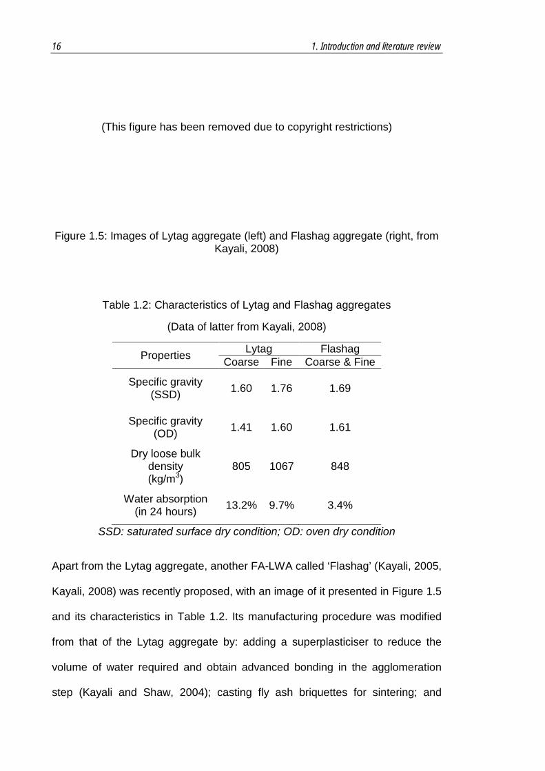
(This figure has been removed due to copyright restrictions)
Figure 1.5: Images of Lytag aggregate (left) and Flashag aggregate (right, from Kayali, 2008)
Table 1.2: Characteristics of Lytag and Flashag aggregates
(Data of latter from Kayali, 2008)
Properties Lytag Flashag Coarse Fine Coarse & Fine
Specific gravity (SSD) 1.60 1.76 1.69
Specific gravity (OD) 1.41 1.60 1.61
Dry loose bulk density (kg/m3)
805 1067 848
Water absorption (in 24 hours) 13.2% 9.7% 3.4%
SSD: saturated surface dry condition; OD: oven dry condition
Apart from the Lytag aggregate, another FA-LWA called ‘Flashag’ (Kayali, 2005,
Kayali, 2008) was recently proposed, with an image of it presented in Figure 1.5
and its characteristics in Table 1.2. Its manufacturing procedure was modified
from that of the Lytag aggregate by: adding a superplasticiser to reduce the
volume of water required and obtain advanced bonding in the agglomeration
step (Kayali and Shaw, 2004); casting fly ash briquettes for sintering; and

17
granulating the aggregate particles by crushing after, instead of pelletisation
before, sintering (Kayali, 2005). The Flashag aggregate produced is more
simply manufactured and has better properties than conventional Lytag
products, and results in a high-performance concrete (Kayali, 2005). Both Lytag
and Flashag aggregates are qualified for use in structural LWC.
1.1.6 Problems of Current Manufacturing Method
As previously stated, FA-LWA is very promising as a solution to the current
depletion of natural aggregates, for utilisation of its enhanced properties and the
consumption of large scale fly ash waste which should be reasons for it to be
applied in real construction applications. However, it is not very well promoted
because of some confronting issues. For its manufacture, it requires high-power
mechanical and thermal treatments that consume large amounts of energy to
ensure its quality. This could result in extremely high costs for its production
which, if it is used to replace natural aggregates, would add a financial burden
to the construction industry. Therefore, such a FA-LWA can only be used if its
unique features are required in a special application.
Also, as the high energy consumed in FA-LWA manufacture expends large
amounts of fossil fuels, the current depletion of fuel resources will be
aggravated despite mineral resources being saved by using recycled fly ash.
Moreover, the burning of fossil fuels could create new burdens of industrial
waste, environmental pollution and CO2 emissions.
Thus, it is necessary for establishing a firm basis that justifies the use of FA-
LWA, that the above mentioned issues be addressed. Furthermore, the author
examines the hypothesis that geopolymer technology is a promising suitable

18 1. Introduction and literature review
mechanism that may be adopted to manufacture lightweight aggregates that
could be suitable for utilisation in construction. This hypothesis, together with
the performance of such geopolymer aggregates are therefore, the subject of
this thesis.
1.2 Geopolymer Technology
1.2.1 Brief Introduction to Geopolymer Technology
It has been argued that research on ‘alkali-activated cement’ (AAC), which
originated in Europe in the 1930s, should be considered the precursor to
geopolymer technology (Roy, 1999). At first, that research concentrated on the
cementitious property that emerged in synthetic slag-based materials under the
activation of alkaline hydroxide (Roy, 1999, Komnitsas and Zaharaki, 2007,
Pacheco-Torgal et al., 2011). Later, Glukhovsky et al. (1980) investigated AAC
reaction mechanisms since the 1950s, indicating that the essential uniqueness
of such a material is its formation of amorphous alumina and silicate structures,
different from OPC materials which are composed of calcium hydrates
(Glukhovsky et al., 1980, Krivenko, 1986). This seemed to realise an improved
durability for cementitious materials (Komnitsas and Zaharaki, 2007). Although
there are still debates about the role of AAC in the development of geopolymer
since these two cementitious materials are not exactly alike, it should be
appropriate to admit that AAC is the most similar to the geopolymer in terms of
property and application.
Nowadays, the term ‘geopolymer’ specifically refers to the synthetic inorganic
polymer material developed by Davidovits since the 1970s (Davidovits, 1991).
The original geopolymer material was synthesised by activating kaolinite with an
19
alkaline solution at 100-150oC, to make use of its inorganic nature for fire-
resistant coatings in construction panels. Later, different types of, and synthetic
methods for producing, geopolymers have been developed. The resultant
geopolymer materials display advanced properties in terms of mechanics,
thermodynamics and surface chemistry which can be utilised in multiple
applications, such as adhesives, ceramics, foams, and toxic and radioactive
waste encapsulations (Davidovits, 2008).
The real breakthrough for making a geopolymer attractive was its application as
an alternative cement material to OPC. This was realised by generating fresh
geopolymer gels during concrete mixing to firstly bond the aggregates and then
harden the fresh geopolymer to form a final geopolymer concrete, which
displayed a similar cementitious property to that of OPC, as shown in Figure 1.6
(Kong et al., 2007, Rangan, 2007, Bakharev, 2005a).
Relevant research on geopolymer concrete was launched in the 1990s to
realise its considerable environmental benefits, such as extremely low CO2
emissions compared to OPC (Davidovits, 2002, CIA, 2011). Also, geopolymer
concrete possesses several superior properties, such as a higher early strength,
lower shrinkage, better thermal and chemical resistance, and more efficient
consumption of industrial by-products (such as fly ash wastes), if it has a
suitable mix and processing design (Davidovits, 2008, Duxson et al., 2007a,
Palomo et al., 1999, Rangan et al., 2005). Geopolymer concrete without any
other cement has already been created and proven by experiments to have
suitable strength and durability for use in construction (Rangan, 2007, Hardjito
and Rangan, 2005).
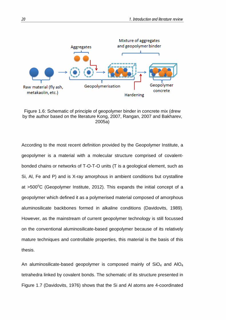
20 1. Introduction and literature review
Figure 1.6: Schematic of principle of geopolymer binder in concrete mix (drew by the author based on the literature Kong, 2007, Rangan, 2007 and Bakharev,
2005a)
According to the most recent definition provided by the Geopolymer Institute, a
geopolymer is a material with a molecular structure comprised of covalent-
bonded chains or networks of T-O-T-O units (T is a geological element, such as
Si, Al, Fe and P) and is X-ray amorphous in ambient conditions but crystalline
at >500oC (Geopolymer Institute, 2012). This expands the initial concept of a
geopolymer which defined it as a polymerised material composed of amorphous
aluminosilicate backbones formed in alkaline conditions (Davidovits, 1989).
However, as the mainstream of current geopolymer technology is still focussed
on the conventional aluminosilicate-based geopolymer because of its relatively
mature techniques and controllable properties, this material is the basis of this
thesis.
An aluminosilicate-based geopolymer is composed mainly of SiO4 and AlO4
tetrahedra linked by covalent bonds. The schematic of its structure presented in
Figure 1.7 (Davidovits, 1976) shows that the Si and Al atoms are 4-coordinated

21
and the adjacent Si/Al tetrahedra linked by sharing the O atom in the corner
position. Also, although metal cations, such as Na+, K+, Li+ and Ca2+, and water
can be present for charge balance and structural stabilisation, they are more
likely to lie around the tetrahedra backbone instead of part of it (Barbosa et al.,
2000, Davidovits, 2008). In a geopolymer, the Si and Al tetrahedra units bond
with each other to form large network backbones, as shown in Figure 1.8
(Rowles et al., 2007, Barbosa et al., 2000). The chemical composition of an
aluminosilicate-based geopolymer can be expressed as:
Mn(-(SiO2)z-AlO2)n, wH2O
where M is the alkaline element, z is 1,2 or 3 to describe the Si/Al ratios in
different units, n is the degree of polycondensation and w the degree of
hydration (Davidovits, 2008, Davidovits, 1989).
(This figure has been removed due to copyright restrictions)
Figure 1.7: 4-coordinated configuration of Si and Al tetrahedra in geopolymer (Davidovits, 1976)
The synthesis of an aluminosilicate-based geopolymer is normally based on
solid raw materials rich in alumina and silicate components, such as
metallurgical slags, fly ash and metakaolin (Duxson and Provis, 2008). A
geopolymer created from Class F fly ash has been well developed in recent
decades and is investigated in this research. A geopolymer material is
synthesised by activating raw fly ash using the alkaline activators’ sodium

22 1. Introduction and literature review
hydroxide and sodium silicate under a suitable curing regime, as depicted in
Figure 1.9 (Kong et al., 2007, Rangan et al., 2005, Rangan, 2007).
(This figure has been removed due to copyright restrictions)
Figure 1.8: Three-dimensional network of geopolymer structure (adapted from models proposed by Rowles et al., 2007 and Barbosa et al., 2000)
Figure 1.9: Scheme for synthesis of fly ash-based geopolymer
In principle, the entire geopolymerisation process used is divided into three
major stages. Firstly, the reactive contents in the raw fly ash, mainly the reactive
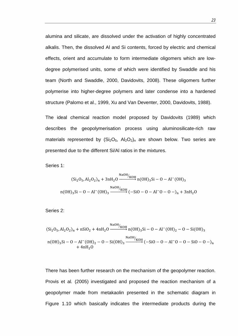
23
alumina and silicate, are dissolved under the activation of highly concentrated
alkalis. Then, the dissolved Al and Si contents, forced by electric and chemical
effects, orient and accumulate to form intermediate oligomers which are low-
degree polymerised units, some of which were identified by Swaddle and his
team (North and Swaddle, 2000, Davidovits, 2008). These oligomers further
polymerise into higher-degree polymers and later condense into a hardened
structure (Palomo et al., 1999, Xu and Van Deventer, 2000, Davidovits, 1988).
The ideal chemical reaction model proposed by Davidovits (1989) which
describes the geopolymerisation process using aluminosilicate-rich raw
materials represented by (Si2O5, Al2O2)n are shown below. Two series are
presented due to the different Si/Al ratios in the mixtures.
Series 1:
Series 2:
There has been further research on the mechanism of the geopolymer reaction.
Provis et al. (2005) investigated and proposed the reaction mechanism of a
geopolymer made from metakaolin presented in the schematic diagram in
Figure 1.10 which basically indicates the intermediate products during the
(Si2O5, Al2O2)n + nSiO2 + 4nH2ONaOH
KOH��⎯⎯⎯⎯⎯⎯⎯� n(OH)3Si − O − Al−(OH)2 − O − Si(OH)3
n(OH)3Si− O − Al−(OH)2 − O − Si(OH)3NaOH
KOH��⎯⎯⎯⎯⎯⎯⎯� (−SiO − O − Al−O − O − SiO− O −)n
+ 4nH2O
(Si2O5, Al2O2)n + 3nH2ONaOH
KOH��⎯⎯⎯⎯⎯⎯⎯� n(OH)3Si − O − Al−(OH)3
n(OH)3Si− O − Al−(OH)3NaOH
KOH��⎯⎯⎯⎯⎯⎯⎯� (−SiO− O − Al−O− O −)n + 3nH2O
24 1. Introduction and literature review
different stages of geopolymerisation. More importantly, the end-products
include not only the amorphous phase but also the nano-crystalline phase that
is also possibly present in the final geopolymer. A similar reaction model for
more generalised geopolymerisation, which provides a more specific illustration
of the secondary reactions that occur during each stage, proposed by Duxson
et al. (2007a) is also presented in Figure 1.10.
(This figure has been removed due to copyright restrictions)
Figure 1.10: Conceptual models for geopolymerisation proposed by Provis (2005) (left) and Duxson (2007) (right)
1.2.2 Advantages of Geopolymer Technology for FA-LWA Manufacture
Different from mainstream applications of geopolymers in cements, ceramics,
coatings, etc., this research makes use of geopolymer technology for the
manufacture of a FA-LWA. Its aim is to deal with the problems in the current
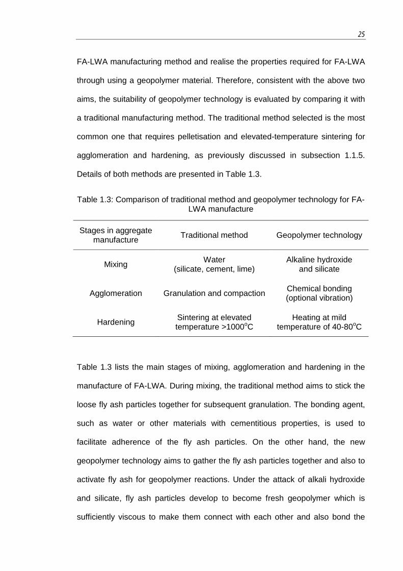
25
FA-LWA manufacturing method and realise the properties required for FA-LWA
through using a geopolymer material. Therefore, consistent with the above two
aims, the suitability of geopolymer technology is evaluated by comparing it with
a traditional manufacturing method. The traditional method selected is the most
common one that requires pelletisation and elevated-temperature sintering for
agglomeration and hardening, as previously discussed in subsection 1.1.5.
Details of both methods are presented in Table 1.3.
Table 1.3: Comparison of traditional method and geopolymer technology for FA-LWA manufacture
Stages in aggregate manufacture Traditional method Geopolymer technology
Mixing Water (silicate, cement, lime)
Alkaline hydroxide and silicate
Agglomeration Granulation and compaction Chemical bonding (optional vibration)
Hardening Sintering at elevated temperature >1000oC
Heating at mild temperature of 40-80oC
Table 1.3 lists the main stages of mixing, agglomeration and hardening in the
manufacture of FA-LWA. During mixing, the traditional method aims to stick the
loose fly ash particles together for subsequent granulation. The bonding agent,
such as water or other materials with cementitious properties, is used to
facilitate adherence of the fly ash particles. On the other hand, the new
geopolymer technology aims to gather the fly ash particles together and also to
activate fly ash for geopolymer reactions. Under the attack of alkali hydroxide
and silicate, fly ash particles develop to become fresh geopolymer which is
sufficiently viscous to make them connect with each other and also bond the

26 1. Introduction and literature review
unreacted fly ash. The mixture after geopolymerisation ends in a uniform gel-
like mixture, which looks similar to traditional cement paste although its
manufacture is based upon different principles. Furthermore, fly ash will
undergo a complex chemical reaction that renders it into a solidified geopolymer
material which is suitable to be used as aggregate for concrete production.
The different mixing conditions of the above two methods, i.e. the traditional
palletisation and sintering method versus the geopolymerisation method, also
affect their agglomeration stages. In the traditional method, a granulation
process, or even compaction process, is needed to press the bonded fly ash
particles into green pellets (Bijen, 1986, Kayali, 2008), otherwise these particles
will be likely poorly bonded. However, when using geopolymer technology, the
mixture can be tightly bonded by fresh geopolymer, and the mixing force is
sufficient to complete this bonding, with no extra mechanical means required.
The traditional granulation process can thus be saved. Sometimes, a certain
vibration process might be needed if it is planned to mould the fresh
geopolymer mixture into a suitable shape for further processing, but that would
consume much less effort than pelletisation.
Another significant difference is the hardening stage during manufacture. As
previously discussed, a major drawback of the traditional method is the high
amount of power consumed to obtain the elevated temperature of greater than
1000oC required to harden the fly ash into strong aggregate products which
could result in a high cost and significant harm to the resources and
environment. Geopolymer technology, which is capable of transferring loose,
weak fly ash particles into compact, hard objects at mild temperatures (40-
80oC), could possibly address this drawback by significantly reducing the

27
operational temperature required for hardening. Despite the hydroxide and
silicate agents needed in the geopolymer-assisted aggregate industry, their
costs would still be much less than that of the power consumed in the traditional
method.
Apart from its simple, low-cost, eco-friendly manufacture, geopolymer
technology also has several advanced features for producing a desirable FA-
LWA product. A geopolymer material usually has good mechanical properties
with a low density range (Kong and Sanjayan, 2010, Swanepoel and Strydom,
2002, Xie and Kayali, 2014) which could be suitable for a FA-LWA demanding a
high strength/weight ratio. Geopolymer normally has advanced thermal, sound
and chemical insulation that could result in better durability for future
construction use (Duxson et al., 2007a, Bakharev, 2005h) and hence it is
expected that FA-LWA will further contribute to these beneficial properties. In
addition, it has been reported that the structure of a geopolymer is incredibly
resilient in the cases of exposure to high temperatures (Barbosa, 2003). These
features appear to be able to realise the properties expected of an artificial FA-
LWA, as discussed in subsection 1.1.3. Therefore, it is estimated that the new
geopolymer technology could replace the traditional method without seriously
weakening aggregates’ properties.
1.2.3 Previous Trials using Geopolymer Technology for LWA
Manufacture
Several initial studies have been conducted to explore the possibility of using
geopolymer technology in the manufacture of LWA products. However, most of
their products are not likely to be regarded as FA-LWAs as they are not made

28 1. Introduction and literature review
solely from fly ash or fly ash derivatives, with those made from only fly ash
being weak in strength. Moreover, nearly all these research works are still in an
initial stage in terms of concrete application. Nevertheless, the experiences
gained from these applications of geopolymer technology are valuable guides
for this research.
Jo et al. (2007) proposed a kind of LWA called ‘ALFA’ made from fly ash,
cement, NaOH, Na2SiO3 and MnO2. This research aimed to initiate a
geopolymer reaction and a cement hydration and use the cementitious
materials formed later to bind all ingredients into hardened aggregate particles.
The produced ALFA aggregates had several good properties similar to normal
FA-LWAs when MnO2 was added, but very low strength when MnO2 was not
added (Jo et al., 2007). It is considered that MnO2 is necessary to produce
ALFA so as to act as the core that binds the geopolymer and hydrated cement.
In Jo’s research however, the formed geopolymer functions more as a bonding
agent which replaces water in its role in fresh mixture workability and does
away with sintering necessary in traditional FA-LWA manufacture.
Fansuri et al. (2012) investigated a method for converting a pure, fresh fly ash-
based geopolymer into pellets. This is like the pelletisation process in
conventional FA-LWA manufacture and solves the problem of granulating the
aggregates from the geopolymer material. The formed geopolymer pellets can
be later hardened by the normal geopolymer heating procedure, that is, mildly
heated for days (Fansuri et al., 2012). However, this method’s problems include
that more research is needed before it can be promoted for industrial
manufacture and the strengths of the pellets produced must be greatly
improved for structural use.

29
Bui et al. (2012) aimed to enhance the strength by adding ground-granulated
blast furnace slag (GGBFS) to a fly ash-based geopolymer mixture to produce a
LWA product that was sufficiently strong for concrete manufacture. An extra
benefit of using GGBFS was that its manufacture could be conducted at room
temperature (Bui et al., 2012). Their study agreed well with previous research
on room temperature-cured geopolymer made from a mixture of fly ash and
GGBFS (Davidovits, 2013). However, Bui et al. only researched the
manufacture of a coarse LWA product whereas, to complete a concrete mix,
natural sand is still needed and a high cement proportion (over 400 kg/m3) must
be used (Bui et al., 2012).
A study by Silva et al. which conducted research on making aggregates using
geopolymer technology was for the waste-water treatment industry not
construction (Silva et al., 2010). However, it describes a method as to produce
aggregate particles from raw materials using geopolymerisation. As expected,
the aggregate product in Silva’s research was weak in strength but, as it had
many penetrable micron pores to absorb the waste elements in water, it could
be seen as a successful example of building a micron-porosity system in a LWA
by geopolymer technology. So this method of manufacture is also consulted in
this research.
1.3 Scope of Thesis
This thesis studies a new type of artificial FA-LWA called a ‘geopolymer
aggregate’ made by geopolymer technology which is a low-cost, eco-friendly
process as it does not involve the high energy consumption of conventional FA-
LWA manufacturing methods. The geopolymer aggregate produced has

30 1. Introduction and literature review
advanced characteristics that can function as both coarse and fine aggregate
portions in concrete manufacture to produce a high-performance lightweight
concrete.
This research work consists of the principles and effects of raw materials,
activator designs and synthetic conditions for geopolymerisation; the
mechanism, manufacture and properties of geopolymer aggregates; and the
utilisation of both coarse and fine geopolymer aggregates, in either the OPC
concretes or the geopolymer binder concretes. Also, mortar material that only
uses fine geopolymer aggregates is examined.
1.4 Techniques used in research
The techniques used in this research for manufacturing, property testing and
characterisation are briefly introduced here and will be further detailed in
following chapters.
The construction materials to be manufactured include fly ash-based
geopolymer aggregate mixes, pastes, and concrete and mortar samples using
different aggregates and cementitious materials. The techniques used include
different grades of mechanical mixers, moulding facilities, vibrating table,
electric oven and controlled environment room. Also, a mechanical jaw crusher
is used to create aggregate particles in appropriate size distributions.
For property testing, techniques are applied to evaluate the physical,
mechanical, structural and compositional properties of the materials produced.
The normal physical properties, such as density and porosity, are tested on
relevant fundamental facilities, and the particle sizes and surfaces using both

31
standard sieves and a Malvern Mastersizer 2000 laser diffraction particle size
analyser.
The mechanical tests of the strength properties of relevant samples are
conducted using a TECNOTEST compression testing machine (3000 kN
capacity). On the other hand, the aggregates’ crushing value is measured using
a SHIMADZU universal testing machine (1000 kN capacity). Moreover, the
rebound index of aggregates is measured using a Schmidt hammer.
Morphology, microstructure and porosity observations are made using a
combination of scanning electron microscopy (SEM) on a HITACHI TM 3000
facility and optical microscopy (OM) on a Zeiss AxioCam MRC digital camera.
The chemical compositions of fly ash and geopolymer materials are measured
using a combination of X-ray fluorescence (XRF), which identifies the
quantitative chemical composition, and X-ray diffraction (XRD), which identifies
the crystalline phases present in the tested material, and quantifies them and
the amorphous phases in combination with Rietveld refinement method. Also,
infrared (IR) spectroscopy is applied to identify variations in the chemical
functional groups, such as Si-O-Si and Si-O-Al, both before and after
geopolymerisation using a SHIMADZU spectrophotometer equipped with an
attenuated total reflectance (ATR) accessory.
1.5 Structure of Thesis
This thesis consists of nine chapters. The first is the introduction and literature
review, the last is the conclusion chapter while the main research work is
discussed in Chapters 2 to 8. A schematic of the relationship of each chapter to
the main research work is presented in Figure 1.11.

32 1. Introduction and literature review
Chapter 1 depicts a wholistic picture of the development of the research work in
this thesis. It firstly provides the background to FA-LWA which is known as the
kind of advanced construction material highly needed in the current concrete
industry but has the shortcoming of consuming a high amount of energy during
in its manufacture. This leads to discussing the idea of making use of
geopolymer technology for low-cost, eco-friendly FA-LWA manufacture. It is
also expected that the geopolymer aggregate produced could be enhanced by
obtaining properties from advanced geopolymer materials based on previous
experiences of their use in construction. This aspect will also be explored.
This chapter then evaluates the principle of geopolymer technology, including
its history, raw materials, activating agents and conditions, reaction
mechanisms and models, and characteristics of its end-products. Based on this,
the suitability of geopolymer technology for FA-LWA manufacture is analysed
and the advantages of geopolymer materials for high-quality FA-LWA products
are highlighted.
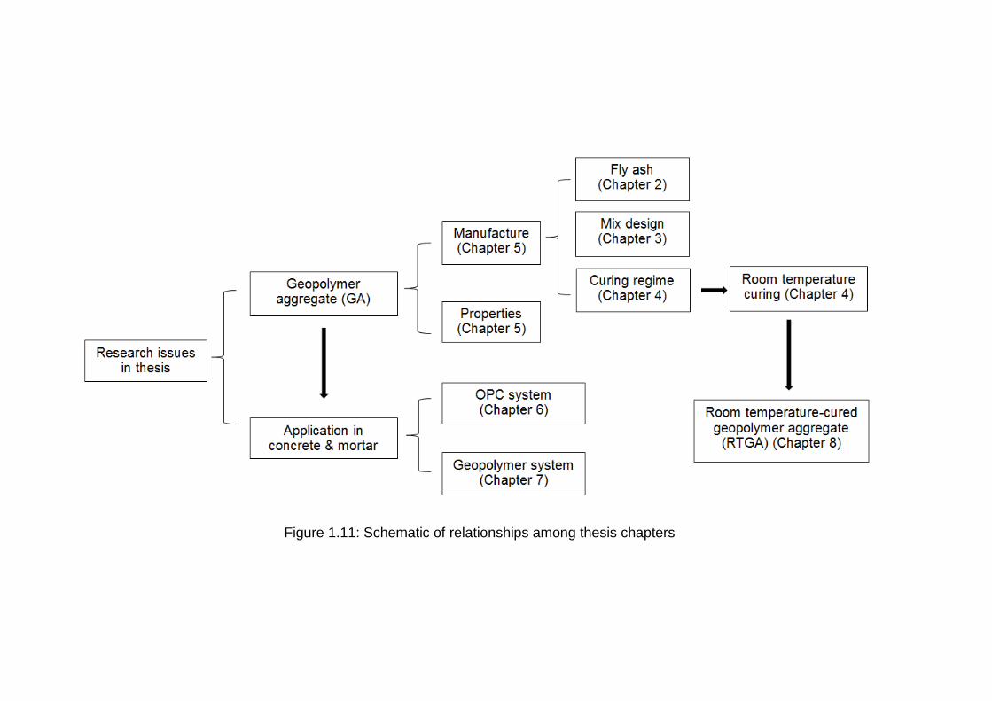
Figure 1.11: Schematic of relationships among thesis chapters

34 1. Introduction and literature review
The objectives of this research are later discussed in this chapter. The main one
is to investigate the manufacture of FA-LWA by geopolymerisation which
creates geopolymer aggregates of two types, coarse like ‘artificial stone’ and
fine like ‘artificial sand’. Another objective is to examine the suitability of the
geopolymer aggregate produced for concrete manufacture through using it in
OPC-based concretes and geopolymer binder-based concretes.
Chapter 2 launches a research work on the selection of suitable fly ash sample
for desired geopolymer synthesis. It investigates the basic characteristics of fly
ash properties, such as particle size distribution, specific surface area, loss on
ignition, chemical composition and crystalline/amorphous contents, and
examines the sensitivity of geopolymer synthesis to the minor differences
present in characteristics among different fly ash batches collected from the
same coal power station source. This was found to be more obvious in fresh
properties like workability and consistency, which is most likely to be due to the
different reaction rates of the fly ash samples containing different amorphous
SiO2, Al2O3 and CaO proportions. Thus, the author explains that to achieve
consistent manufacturing, one specific fly ash batch, which seems to be the
most suitable for geopolymer aggregates based on the testing results in
Chapter 2, is selected to create geopolymer materials for the work of this
research.
Chapter 3 concentrates on the mix design of geopolymer synthesis. A
systematic geopolymer mix design procedure is devised which uses the criteria
of SiO2/Na2O, H2O/Na2O and ‘water-to-geopolymer solids ratio’ (W/G ratio) to
distinguish between each geopolymer mix and calculate the final mix design, in
order to better reflect the relationships among the chemical components

35
involved in geopolymerisation. This mix design procedure is applied for all
geopolymer syntheses included in this thesis, including the ones for geopolymer
aggregates and the ones for the geopolymer binders in concrete and mortar
manufacture.
Chapter 4 concentrates on the curing regime of geopolymer synthesis, as a
valid factor that determines the performance of produced geopolymer materials.
The curing regime is researched by curing the fresh geopolymer made with the
selected mix design under various temperature, moisture and time conditions.
From the experimental results, it is seen that mild temperature heating is
beneficial for fresh geopolymer, that a higher temperature and a longer heating
time can facilitate growth of the geopolymer. Thus, such heating regime is first
applied for the manufacture of geopolymer aggregates and geopolymer binders
as presented and discussed in Chapters 5 to 7. On the other hand, it is found
that low-moisture curing and prolonged curing period can have a positive effect
on geopolymerisation, but these seem to be only significant for a room
temperature-cured geopolymer. Nevertheless, it is possible to make a room
temperature-cured geopolymer achieve a similar strength level as the heated
one by a well control of curing moisture and curing period. This finding is utilised
to make room temperature-cured geopolymer aggregate as detailed in Chapter
8.
Chapter 5 introduces the procedure for geopolymer aggregate manufacture.
The geopolymer material determined as suitable is synthesised based on the
research presented in Chapters 2, 3 and 4. Then, further mechanical
processing is applied to generate both coarse and fine aggregates with
appropriate particle sizes. A major feature of the manufacture of FA-LWA based

36 1. Introduction and literature review
on the method of geopolymerisation is that the traditional elevated-temperature
sintering and high-power mechanical pressing/pelletising are done away with.
The relevant properties of the geopolymer aggregate produced, such as
appearance, grading, density, water absorption, porosity, crushing value and
rebound index, are measured. The chemical structure of geopolymer aggregate
is then analysed by IR spectroscopy. It is found that the geopolymer aggregate
generated is a type of FA-LWA composed of geopolymer structure with a low
density, high porosity and high water absorption capability but possessing good
mechanical behaviour. Geopolymer aggregate therefore, can have properties
which satisfy the regulations in relevant LWA standards, and are similar or even
better than other regular FA-LWA products.
Chapters 6 and 7 are concerned with issues of utilising the geopolymer
aggregates made as explained in Chapter 5, in concrete and mortar
manufacture in relation to the type of cementitious material used. In Chapter 6,
OPC which is the most widely used cementitious material in the world, is the
sole cement material investigated in this chapter. The research in this chapter
aims to provide an evaluation of the compatibility of geopolymer aggregates
against the current mainstream cementitious system.
In Chapter 7, a fly ash-based geopolymer binder, which has been considered a
potential alternative to OPC in recent decades, is investigated. In both Chapters
6 and 7, geopolymer aggregates serve as the sole aggregate materials for
coarse and fine aggregate portions. The mix design, sample preparation,
workability, density, and increases in strength and structure of concrete mixes
using the new geopolymer aggregate are investigated. The results indicate that
this geopolymer aggregate could qualify as a good substitute for natural

37
aggregates in concrete manufacture and a concrete made of it is capable of
achieving a high-performance lightweight concrete mixture with high strength
and low self-weight. Geopolymer aggregates could also be suitable for mortar
manufacture, when treated as a special type of concrete without a coarse
aggregate portion, to produce a high-performance mortar with a similar strength
but much lower self-weight than a normal one. The mortar research also
highlights the advantage of fine geopolymer aggregate made here as new
‘artificial sand’ for structural proposes.
Chapter 8 explores the manufacture and application of a special type of
geopolymer aggregate cured at room temperature without any heat treatment,
called a room temperature-cured geopolymer aggregate (RTGA), which is
different from those discussed in Chapters 5, 6 and 7. The reason for removing
the heat treatment is to further reduce the power consumed during aggregate
manufacture, and to save on the manufacturing step of heating. The properties
of RTGA, and subsequent concrete manufacturing using either OPC or
geopolymer binder, are researched in the same way as explained in previous
chapters. The results indicate that, although RTGA is weak in strength and
more porous than the other geopolymer aggregates that experience heat
treatment, and therefore not as good, it still has certain properties which qualify
it for use in construction. Such properties make RTGA a potential
environmentally friendly construction material in the future which certainly needs
further research.

38 2. Fly ash and its influence on fresh properties of geoploymer
Chapter 2
Fly Ash and its Influence on Fresh Properties of
Geopolymer
2.1 Introduction
As introduced in Chapter 1, for the geopolymer materials discussed in this
thesis, fly ash is the major aluminosilicate source required to provide reactants
for geopolymerisation. Hence, this chapter launches a research work on the
effects of fly ash characteristics for geopolymerisation, in order to find a suitable
fly ash sample for desired geopolymer synthesis. Meanwhile, the fresh
properties, which dominate geopolymer’s performance in a mechanical
processing of geopolymer aggregates manufacturing procedure, are also
studied.
The fly ash samples from different sources are greatly varied in characteristics,
as introduced in Chapter 1, subsection 1.1.4, which were found to result in
significant differences in the properties of final geopolymer products (Diaz et al.,
2010, Rickard et al., 2011). Meanwhile, since fly ash is just a by-product rather
than an end-product, controlling uniformity and consistency to suit particular
production purposes has not been strictly applied. In real practice, a common
way to guarantee the consistency of fly ash is to select a single source of fly ash,
mostly a particular coal power station, and only use the fly ash from this source
for the entire work of geopolymer synthesis (Rickard et al., 2011).
The way of selecting fly ash from a particular coal source seems to work when
using fly ash as a supplementary cementitious material, which is relatively less

39
affected by the fly ash variability. However, through recent research, the author
finds that the fly ash samples from one particular coal source with minor
different characteristics can result in significant differences in the properties of
produced geopolymers. This is rather obvious for fresh properties like
workability and consistency, which can be significant enough to result in
inconsistent final geopolymer products.
Therefore, the author considers it necessary to strictly control the source of fly
ash, so as to assure the consistency for fresh geopolymer mix and subsequent
geopolymer aggregate products. This has been researched and is reported and
discussed in this chapter.
Three fly ash samples from different batches of one particular coal power
station are selected and investigated. It is found that all selected fly ash can
produce a fresh geopolymer mix workable for future mechanical processing.
However, the fresh properties of different mixes are quite different. This
difference is considered to be mainly due to the differences in amorphous SiO2,
Al2O3 and CaO contents in the selected fly ash samples. An evaluation is later
made on the performance of each fresh geopolymer mix against the mechanical
processing, based on which one specific batch of fly ash is preferentially
recommended to be used in later geopolymer aggregate research.
Also, the current study discovers that the hardened properties of geopolymers,
such as density and strength, are also varied for different fly ash samples. This
drives a further topic as to whether an appropriate fly ash selection may
enhance the mechanical behaviour of geopolymer aggregates. This question is
briefly discussed in this chapter. However, a further detailed discussion relating

40 2. Fly ash and its influence on fresh properties of geoploymer
to the hardened properties of geopolymer will be presented in Chapter 5, in
combination with the results of relevant testings directly related to the produced
geopolymer aggregates.
2.2 Selection and Characterisation of Fly Ash
2.2.1 Selection of Fly Ash Samples
The fly ash samples selected and discussed in this chapter were sourced from
three different production batches during the years 2012-2014 from the Eraring
thermal power station in New South Wales, Australia. The production dates are
2012-Dec-13, 2013-Jul-25 and 2014-Jan-31, which are at approximately 6
month interval. These samples are referred to as ‘FA1’, ‘FA2’ and ‘FA3’
respectively, throughout this chapter. The relevant characteristics of the
selected fly ash samples are researched and discussed in following subsections,
to distinguish each fly ash sample and later relate to the performance of the
fresh geopolymer mixes.
2.2.2 Density, Particle Size and Specific Surface Area
The relative densities of the three fly ash samples FA1, FA2 and FA3 are
measured based on Australian standard AS3583 (AS, 1991) and shown in
Table 2.1. It is seen that the selected fly ashes are not consistent in density,
very likely due to the different combustion and cooling procedures they have
been through (Kutchko and Kim, 2006).
On the other hand, particle size distribution and specific surface area of fly ash
particles were measured using a Malvern Mastersizer 2000 laser diffraction
particle size analyser (Figure 2.1), to check if the selected three fly ash samples

41
are varied in above physical properties as usually found in the fly ash from
different sources (Blissett and Rowson, 2012). The results were automatically
recorded every minute of the one hour test duration. The final results are the
average values of the last 10 records. This is to make the results accurately
reflect the situation of a well dispersed fly ash sample. The particle size and
surface information of FA1, FA2 and FA3 are shown in Table 2.2 and Figure 2.2.
Table 2.1: Relative densities of fly ash
Fly ash Density (kg/m3)
FA1 2210
FA2 2130
FA3 2060
Figure 2.1: Malvern Mastersizer 2000 laser diffraction particle size analyser
In Table 2.2, the parameter of D(x%) is used to describe the general trend in
particle size distribution, meaning the diameter where a certain percentage of
the volume distribution is below it. For example, FA1 has a D(10%)=2.93 µm,
meaning that there are 10% in volume of the total FA1 particles that are finer
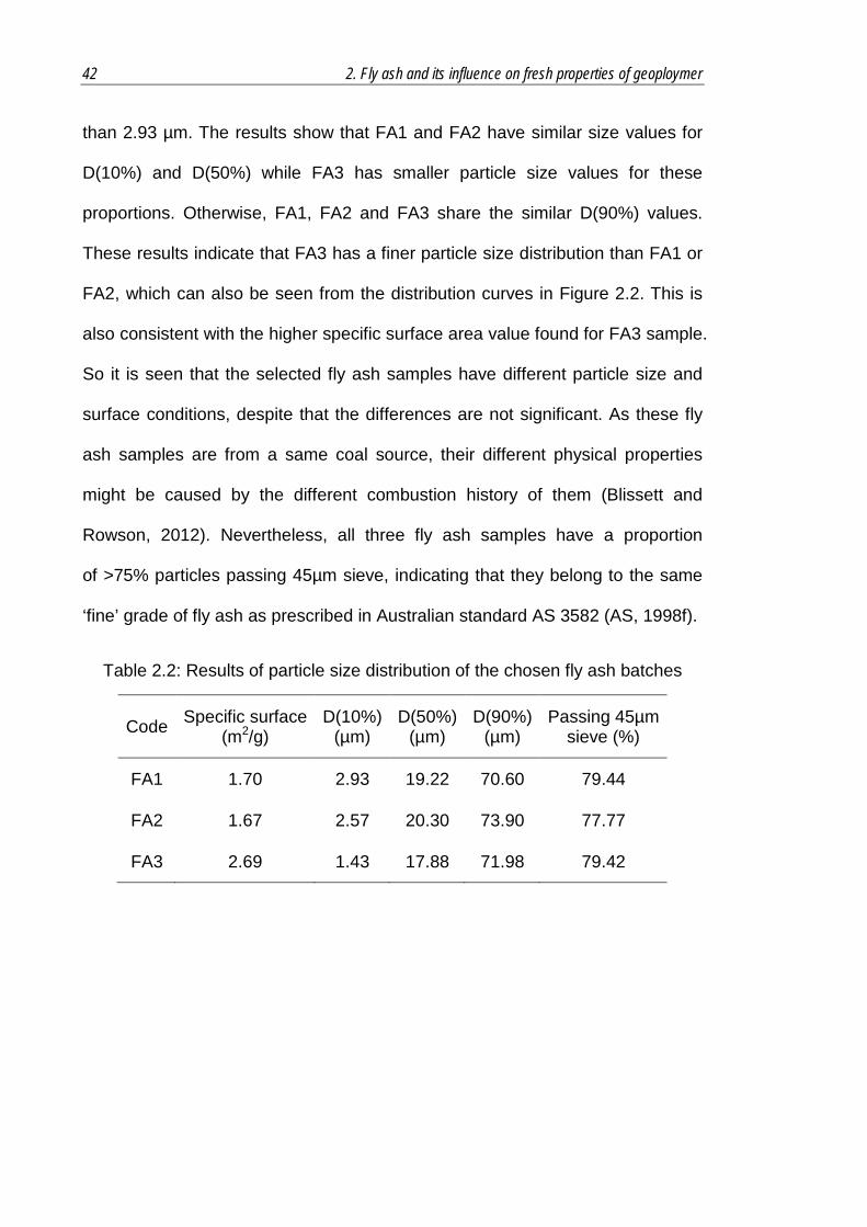
42 2. Fly ash and its influence on fresh properties of geoploymer
than 2.93 µm. The results show that FA1 and FA2 have similar size values for
D(10%) and D(50%) while FA3 has smaller particle size values for these
proportions. Otherwise, FA1, FA2 and FA3 share the similar D(90%) values.
These results indicate that FA3 has a finer particle size distribution than FA1 or
FA2, which can also be seen from the distribution curves in Figure 2.2. This is
also consistent with the higher specific surface area value found for FA3 sample.
So it is seen that the selected fly ash samples have different particle size and
surface conditions, despite that the differences are not significant. As these fly
ash samples are from a same coal source, their different physical properties
might be caused by the different combustion history of them (Blissett and
Rowson, 2012). Nevertheless, all three fly ash samples have a proportion
of >75% particles passing 45µm sieve, indicating that they belong to the same
‘fine’ grade of fly ash as prescribed in Australian standard AS 3582 (AS, 1998f).
Table 2.2: Results of particle size distribution of the chosen fly ash batches
Code Specific surface (m2/g)
D(10%) (µm)
D(50%) (µm)
D(90%) (µm)
Passing 45µm sieve (%)
FA1 1.70 2.93 19.22 70.60 79.44
FA2 1.67 2.57 20.30 73.90 77.77
FA3 2.69 1.43 17.88 71.98 79.42
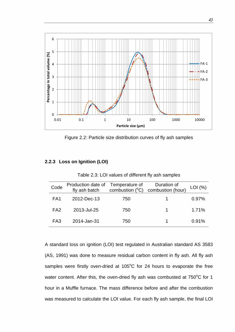
43
Figure 2.2: Particle size distribution curves of fly ash samples
2.2.3 Loss on Ignition (LOI)
Table 2.3: LOI values of different fly ash samples
Code Production date of fly ash batch
Temperature of combustion (oC)
Duration of combustion (hour) LOI (%)
FA1 2012-Dec-13 750 1 0.97%
FA2 2013-Jul-25 750 1 1.71%
FA3 2014-Jan-31 750 1 0.91%
A standard loss on ignition (LOI) test regulated in Australian standard AS 3583
(AS, 1991) was done to measure residual carbon content in fly ash. All fly ash
samples were firstly oven-dried at 105oC for 24 hours to evaporate the free
water content. After this, the oven-dried fly ash was combusted at 750oC for 1
hour in a Muffle furnace. The mass difference before and after the combustion
was measured to calculate the LOI value. For each fly ash sample, the final LOI
0
1
2
3
4
5
6
0.01 0.1 1 10 100 1000 10000
Perc
enta
ge in
tota
l vol
ume
(%)
Particle size (µm)
FA-1
FA-2
FA-3
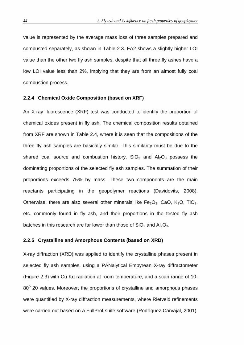
44 2. Fly ash and its influence on fresh properties of geoploymer
value is represented by the average mass loss of three samples prepared and
combusted separately, as shown in Table 2.3. FA2 shows a slightly higher LOI
value than the other two fly ash samples, despite that all three fly ashes have a
low LOI value less than 2%, implying that they are from an almost fully coal
combustion process.
2.2.4 Chemical Oxide Composition (based on XRF)
An X-ray fluorescence (XRF) test was conducted to identify the proportion of
chemical oxides present in fly ash. The chemical composition results obtained
from XRF are shown in Table 2.4, where it is seen that the compositions of the
three fly ash samples are basically similar. This similarity must be due to the
shared coal source and combustion history. SiO2 and Al2O3 possess the
dominating proportions of the selected fly ash samples. The summation of their
proportions exceeds 75% by mass. These two components are the main
reactants participating in the geopolymer reactions (Davidovits, 2008).
Otherwise, there are also several other minerals like Fe2O3, CaO, K2O, TiO2,
etc. commonly found in fly ash, and their proportions in the tested fly ash
batches in this research are far lower than those of SiO2 and Al2O3.
2.2.5 Crystalline and Amorphous Contents (based on XRD)
X-ray diffraction (XRD) was applied to identify the crystalline phases present in
selected fly ash samples, using a PANalytical Empyrean X-ray diffractometer
(Figure 2.3) with Cu Kα radiation at room temperature, and a scan range of 10-
80o 2θ values. Moreover, the proportions of crystalline and amorphous phases
were quantified by X-ray diffraction measurements, where Rietveld refinements
were carried out based on a FullProf suite software (Rodríguez-Carvajal, 2001).

45
A crystalline corundum (α-Al2O3) was added in a mass ratio of 20% of the total
scanned sample (fly ash + corundum) to serve as a spike phase to complete
the quantification (Diaz et al., 2010, Ward and French, 2006). The patterns and
related Rietveld refinements are presented in Figure 2.4.
Table 2.4: Chemical composition of each fly ash sample tested by XRF
Oxides FA1 (wt.%) FA2 (wt.%) FA3 (wt.%)
SiO2 58.60 58.00 57.36
Al2O3 20.20 22.21 22.11
Fe2O3 9.25 7.55 8.13
CaO 4.67 6.09 4.70
K2O 3.02 1.40 3.09
TiO2 2.34 2.79 2.45
SO3 1.04 0.84 1.10
SrO 0.34 0.55 0.49
ZrO2 0.30 0.29 0.26
MnO 0.16 0.14 0.19
Rb2O 0.04 - 0.04
Y2O3 0.04 0.04 0.04
V2O5 - 0.12 -
ZnO - - 0.05
SiO2 + Al2O3 78.80 80.21 79.47
SiO2 / Al2O3 2.90 2.61 2.60
Si/Al (molar) 2.47 2.22 2.21

46 2. Fly ash and its influence on fresh properties of geoploymer
Figure 2.3: PANalytical Empyrean X-ray diffractometer
In the X-ray diffraction patterns shown in Figure 2.4, the dots denote the test
results. The uppermost solid line is the plot of the theoretical calculations. The
differences between the test and the theoretical results are indicated by the
difference curve shown in the lowermost portion of the diagrams. Agreement
between the experimental and the theoretical results is generally good apart
from slight mismatch near 26.5o which is the vicinity of a number of overlapping
peaks from the different phases. The vertical short bars indicate the Bragg
positions used for refinement according to the Rietveld method, where the three
rows of these bars from top to bottom are corundum, quartz and mullite,
respectively.
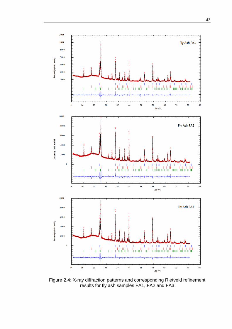
47
Figure 2.4: X-ray diffraction patterns and corresponding Rietveld refinement results for fly ash samples FA1, FA2 and FA3

48 2. Fly ash and its influence on fresh properties of geoploymer
In Figure 2.4, apart from the intentionally added corundum, distinctive amounts
of quartz and mullite are detected. A trace amount of magnetite seems to be
present but the amount is too small to be accurately quantified. The results of
the proportions of crystals and amorphous content in each fly ash sample by
Rietveld quantification are shown in Table 2.5. A complete example of the
calculations applied to the data and used to determine the crystalline and
amorphous contents, is demonstrated in the Appendix A. Fly ash FA1 has the
most crystals as 9.9% of quartz and 19.0% of mullite compared to the other two
fly ashes FA2 and FA3. The total crystalline proportions in FA2 and FA3 are
basically quite similar. Nevertheless, FA2 has a slightly higher mullite while FA3
has a slightly higher quartz.
Table 2.5: Quantification on crystals and amorphous content in fly ash
Items FA1 (wt%) FA2 (wt%) FA3 (wt%)
Quartz 9.9 6.0 6.5
Mullite 19.0 16.6 15.0
Amorphous 71.1 77.4 78.5
Total SiO2 by XRF 58.6 58.0 57.4
Total Al2O3 by XRF 20.2 22.2 22.1
Total SiO2 + Al2O3 by XRF 78.8 80.2 79.5
Amorphous SiO2 43.4 47.3 46.6
Amorphous Al2O3 6.5 10.3 11.3
Amorphous SiO2 + Al2O3 49.9 57.6 58.0
Amorphous SiO2/Al2O3 6.6 4.6 4.1

49
Moreover, considering the previous XRF composition results in combination
with the results obtained from XRD, one can also approximately calculate the
proportion of amorphous SiO2 and Al2O3 present in each fly ash sample. This is
done by subtracting the crystalline SiO2 and Al2O3 from the total amounts of
SiO2 and Al2O3 obtained from XRF results. The calculated amorphous SiO2 and
Al2O3 proportions are thus presented in Table 2.5. FA1 has the least amorphous
SiO2 and Al2O3 at around 49.9%, while the respective quantities for FA2 and
FA3 are quite similar with a value that is nearly 8% higher than FA1. Otherwise,
FA1 has the highest ratio of amorphous SiO2 to amorphous Al2O3 of about 6.6,
which is much higher than that of FA2 or FA3, which is only around 4.1 - 4.6.
2.3 Geopolymer Mixes
A blended alkali solution composed of NaOH and Na2SiO3 was used to activate
the selected fly ash samples for geopolymer synthesis. This alkali solution was
prepared by mixing the ingredients of NaOH flakes (>99% purity), Grade D
Na2SiO3 solution (29.4% SiO2, 14.7% Na2O) and deionised water in specified
proportions as designed in Table 2.6.
In Table 2.6, the mix design for all the mixes has been done such that the fly
ash quantity is maintained at a constant value of 1500 grams, and the same
activator is applied for the mixes made with the three fly ash samples FA1, FA2,
and FA3. The relevant geopolymer mixes are referred to as GEO1, GEO2 and
GEO3 correspondingly. The design of these mixes therefore, allows the
properties of the produced geopolymers to be predominantly influenced by the
unique characteristics of the used fly ash.

50 2. Fly ash and its influence on fresh properties of geoploymer
The activator was prepared through a two-step method. At first, a 14.1M NaOH
solution as designed was made by dissolving NaOH flakes into deionised water.
This was done manually, using appropriate necessary handling protective
measures. The procedure of NaOH dissolution can release large amount of
heat, hence the prepared NaOH solution was stored for one day prior to mixing
so as to cool down. Meanwhile, the NaOH solution was sealed to prevent any
contact with H2O and CO2 from the atmosphere. The second step was to
combine the solutions of NaOH and Na2SiO3 as designed with a Na2SiO3/NaOH
ratio of 3.2 just before geopolymer synthesis.
Table 2.6: Mixes of fly ash-based geopolymer with different fly ashes
Paste Fly ash Fly ash/ Activator
Mix quantities (grams)
Fly ash NaOH flakes
Na2SiO3 solution
Deionised water
GEO1 FA1 2.05 1500 68.93 556.19 105.27
GEO2 FA2 2.05 1500 68.93 556.19 105.27
GEO3 FA3 2.05 1500 68.93 556.19 105.27
Note: the NaOH flakes and deionised water present in this table are to be combined to prepare a 14.1M NaOH solution, which is used along with Na2SiO3 solution for activation purpose.
The steps of geopolymer sample preparation are displayed in Figure 2.5. The
geopolymer mixes GEO1, GEO2 and GEO3 were made by adding the prepared
activator onto the fly ash samples FA1, FA2 and FA3 respectively. A Hobart
mixer was used to mix the fly ash and activator until a uniform mixture was
achieved. A portion from the obtained fresh geopolymer mixture was tested for
fresh mix properties, and the remaining portion was used to cast samples for
density determination and strength testing. Cubic 50mm×50mm×50mm steel

51
moulds, with polyethylene sheets stuck onto the inner surface to facilitate
demoulding, were used to cast the needed samples. A vibrating table was used
to compact the fresh mixture, and the vibration continued until the surface of
fresh mixture was level and no bubbles appeared. The moulds were then
sealed with a lid and placed in a controlled environment room (ER), at 23±1oC
and 50% relative humidity (RH), for 24 hours before applying a heating curing
regime at 80oC for 72 hours in an electrical oven. After heating, the
geopolymers were demoulded once they cooled down to room temperature,
and then placed in the ER until further density and strength testing.
2.4 Fly Ash’s Influence on Fresh Properties
It is found that the variation in geopolymer mixes caused by different fly ash
batches mainly appears in fresh properties. Two aspects of fresh geopolymer
mixes, namely workability and consistency, are thus focussed on, in this section.
They are normally applied for describing fresh Portland cement, and in current
research, used to reflect the fresh properties of different geopolymer mixes.
Although geopolymer is a different mixture, it exhibits a similar cementitious
property as fresh cement paste mix (Kong and Sanjayan, 2010) and therefore is
thought suitable to resemble fresh Portland cement paste regarding the
performance of workability and consistency. The performance of each fresh mix
is evaluated for a selection of suitable fly ash for geopolymer aggregates.
Moreover, possible reasons causing the observed varied fresh properties are
analysed, to provide information needed for fly ash selection from a broader fly
ash source in future practice.

52 2. Fly ash and its influence on fresh properties of geoploymer
Figure 2.5: Preparation steps (1) Hobart mixer, (2) well-mixed fresh geopolymer, (3) steel moulds with polyethylene cover, (4) well-compact geopolymer, (5)
geopolymer after demoulding and (6) geopolymer after heating
2.4.1 Slump and Mini-flow Method
A combined slump and mini-flow method was used to evaluate the workability of
fresh geopolymer. This method is carried based on a mini-sized slump cone
(Figure 2.6) whose dimensions are: 19 mm (top diameter), 38 mm (bottom
(1) (2)
(3) (4)
(5) (6)

53
diameter) and 57 mm (height). This cone can be treated as a small-sized
version of the regular slump cone for fresh concrete regulated in Australian
standard AS 1012 (AS, 1993).
Slump value is a common factor for workability evaluation. A slump test was
measured on fresh geopolymers following the same procedure of conventional
slump testing. The result is referred to as ‘initial slump’.
On the other hand, the mini-flow method, which is usually devised for assessing
the effect of air entraining and plasticizing admixtures on Portland cement paste
(Zhor and Bremner, 1998), is to assess the flow of fresh geopolymer under
vibration. Mechanical vibration is quite widely used for geopolymer compaction
in practice (Hardjito and Rangan, 2005, Kong and Sanjayan, 2010) and will be
applied in a geopolymer aggregate manufacturing procedure (to be stated in
Chapter 5). Assessing flow under vibration is therefore needed in order to
investigate whether there is a variation of flow behaviour caused by different fly
ash samples. Apart from this, the author aims to use mini-flow result to manifest
the variations in workability of different mixes, which are relatively less obvious
in the slump test, possibly due to the high viscosity of geopolymers (Criado et
al., 2009).
For mini-flow test, the spread of the fresh geopolymer just after lifting the cone
was first measured and described as ‘initial spread’. The spread measurements
were taken along four different halves of the spread area (Figure 2.7). The
estimated spread value was calculated as the average of the four
measurements. The area of initial spread was then approximately represented
by a circular area whose diameter is the calculated average spread value.

54 2. Fly ash and its influence on fresh properties of geoploymer
Figure 2.6: Schematic of mini-sized slump cone for slump and mini-flow testings
Figure 2.7: Scheme of spread measurement using the mini-flow method

55
The mini-flow test was also performed to measure the spread of fresh
geopolymer flow upon vibration. To deal with the especially stiff geopolymer
material, a vibrating table (220-240V AC, 50HZ) was used instead of the
conventional flow table. The vibration was applied for 10 seconds. During this
period, the fresh geopolymer, immediately after slump test, was left to flow
freely on the vibrating table. The expansion of spread was measured at three
time points as (1) once the vibration stopped, (2) three minutes after the
vibration stopped, and (3) ten minutes after the vibration stopped. The spread
areas were measured in the same way as explained earlier.
The workability results of the fresh geopolymer mixes made with fly ashes FA1,
FA2 and FA3 are shown in Table 2.7, with images showing the performance of
different geopolymer mixes in Figure 2.8.
Table 2.7: Workability of produced fresh geopolymer mixes
Code
Before vibration After 10-second vibration
Initial slump (mm)
Initial spread (cm2)
Spread at once (cm2)
Spread 3 mins (cm2)
Spread 10 mins
(cm2)
GEO1 0 11.34* 12.34 13.15 13.42
GEO2 20 18.33 39.43 39.80 40.55
GEO3 10 13.50 27.74 28.19 29.19
*11.34cm2 is the bottom area of the mini-sized cone which indicates that there is no spread in this case.

56 2. Fly ash and its influence on fresh properties of geoploymer
Figure 2.8: Images of geopolymer flows before (left column) and once after (right column) vibration in mini-flow test
In Table 2.7, the geopolymer mixes GEO1, GEO2 and GEO3 display very
different slump behaviours. GEO2 has a relatively high initial slump value of 20
mm. It seems that such mix could be easily compacted with only little externally
applied compaction effort. Differently, GEO1 has almost no slump at all, and
GEO3 has a slump of 10 mm. The initial spread results show a similar trend to
GEO1 GEO1
GEO2 GEO2
GEO3 GEO3

57
that of the slump results. GEO2 has the largest spread area indicating the best
workability, followed by GEO3 which has a lower spread value than GEO2 but
still obvious initial spread. However, GEO1 results in a very stiff mixture without
detectable spread. It may therefore be concluded that geopolymer workability
could be quite different for different batches even if the fly ash used is produced
in the same power station.
Such differences in workability are further manifested after the vibration
treatment in the mini-flow test. The curves describing the increase of
geopolymer spread under vibration are shown in Figure 2.9. From this Figure, it
is seen that GEO2 shows a rapid increase in spread area from 18.33 cm2 to
40.55 cm2 in 10 minutes after vibration. Likewise, GEO3 also has an increase in
spread area from 13.50 cm2 to 29.19 cm2. However, it is found that GEO1 has a
reluctant flow after vibration, with only a slight spread increase from 11.34 cm2
to 13.42 cm2. Thus, it seems that the geopolymers made from fly ashes FA2
and FA3 can be more easily compacted by mechanical vibration.
Nevertheless, with the assistance of mechanical vibration, the geopolymer
GEO1 can also flow with an increasing spread. Although this increase is not
significant after a 10-second mechanical vibration, it is considered that a
prolonged vibration time more than 10 seconds should be useful to enlarge the
spread, and possible to make the mix of GEO1 properly compacted. For this
case, the fresh mix made with fly ash FA1 is expected to be qualified for
undertaking the required mechanical processing in geopolymer aggregate
manufacture. Indeed, this is realised as seen in Chapter 5, section 5.3 where a
prolonged vibration can work to obtain a well-cast geopolymer sample.

58 2. Fly ash and its influence on fresh properties of geoploymer
Figure 2.9: Spread area increase by mechanical vibration of geopolymer paste
On the other hand, GEO2 presents a very high fluidity, as seen in Table 2.7,
which can be easily compacted even with no need of mechanical vibration.
However, the high fluidity of GEO2 is not primary pursued in a manufacture of
geopolymer aggregates, primarily because this high fluidity may lead to a
negative effect, such as a weak end-product with loose geopolymer structure
(Rangan, 2007). Since all these fly ashes are found to be practical for
geopolymer aggregates, the fly ash FA2 is not selected for its potential risks.
Also, GEO3 seems good with a moderate workability neither too stiff nor too
fluid before vibration, but has a high spread increase after vibration, as seen in
Figure 2.9. The 10-second vibration applied seems to be too long for GEO3,
because it generates a large spread which is more than twice in area than its
original. This is not needed in a geopolymer aggregate manufacture, and a
shortened vibration time may be more appropriate.
0
5
10
15
20
25
30
35
40
45
initial spread spread at once spread in 3mins
spread in 10mins
Spre
ad a
rea
(cm
2 )
GEO1
GEO2
GEO3
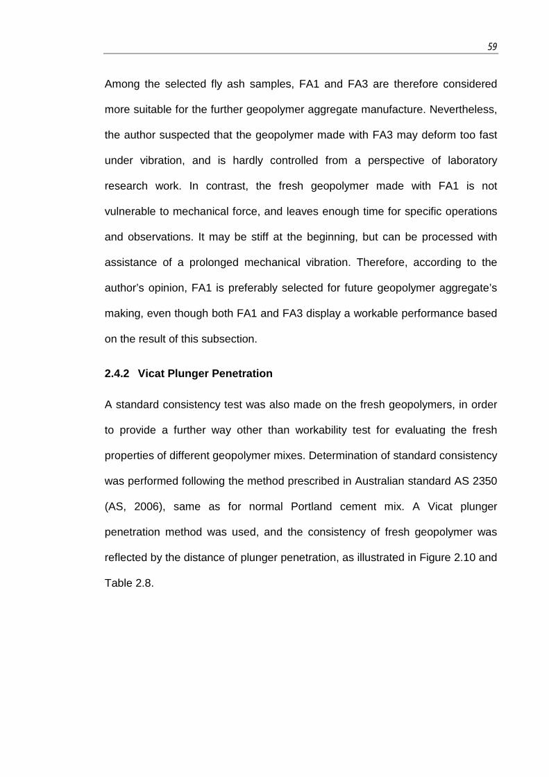
59
Among the selected fly ash samples, FA1 and FA3 are therefore considered
more suitable for the further geopolymer aggregate manufacture. Nevertheless,
the author suspected that the geopolymer made with FA3 may deform too fast
under vibration, and is hardly controlled from a perspective of laboratory
research work. In contrast, the fresh geopolymer made with FA1 is not
vulnerable to mechanical force, and leaves enough time for specific operations
and observations. It may be stiff at the beginning, but can be processed with
assistance of a prolonged mechanical vibration. Therefore, according to the
author’s opinion, FA1 is preferably selected for future geopolymer aggregate’s
making, even though both FA1 and FA3 display a workable performance based
on the result of this subsection.
2.4.2 Vicat Plunger Penetration
A standard consistency test was also made on the fresh geopolymers, in order
to provide a further way other than workability test for evaluating the fresh
properties of different geopolymer mixes. Determination of standard consistency
was performed following the method prescribed in Australian standard AS 2350
(AS, 2006), same as for normal Portland cement mix. A Vicat plunger
penetration method was used, and the consistency of fresh geopolymer was
reflected by the distance of plunger penetration, as illustrated in Figure 2.10 and
Table 2.8.
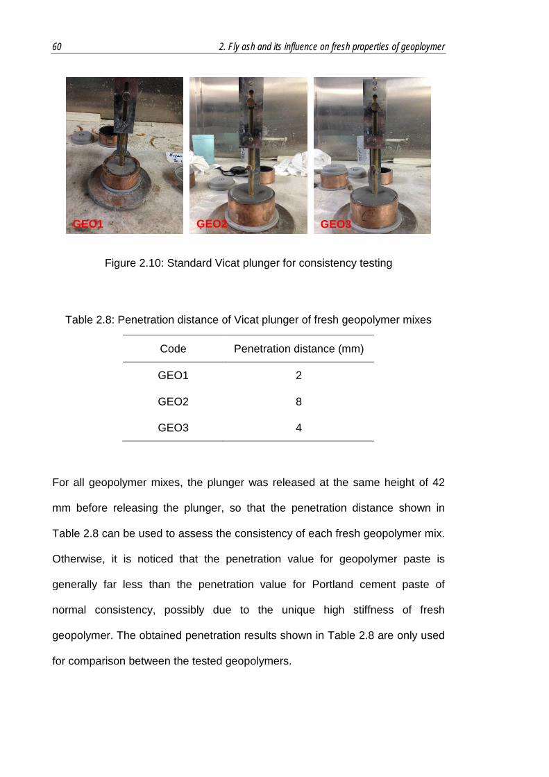
60 2. Fly ash and its influence on fresh properties of geoploymer
Figure 2.10: Standard Vicat plunger for consistency testing
Table 2.8: Penetration distance of Vicat plunger of fresh geopolymer mixes
Code Penetration distance (mm)
GEO1 2
GEO2 8
GEO3 4
For all geopolymer mixes, the plunger was released at the same height of 42
mm before releasing the plunger, so that the penetration distance shown in
Table 2.8 can be used to assess the consistency of each fresh geopolymer mix.
Otherwise, it is noticed that the penetration value for geopolymer paste is
generally far less than the penetration value for Portland cement paste of
normal consistency, possibly due to the unique high stiffness of fresh
geopolymer. The obtained penetration results shown in Table 2.8 are only used
for comparison between the tested geopolymers.
GEO1 GEO2
GEO3

61
It can be seen that the fresh geopolymers made with different fly ash samples
result in different penetration distances, where the descending order of
resistance to plunger penetration is GEO1>GEO3>GEO2. The GEO1 made
with fly ash FA1 has the highest resistance, indicating the highest stiffness,
which is in accordance with the former workability test. Besides, it is found that
the geopolymer with a higher workability shows a lower resistance to plunger
penetration. This result, on one side, proves again that the fresh properties of
geopolymer can be different when using different fly ash samples. Also, all three
fly ash samples would lead to stiff geopolymer mixes, although their effects are
slightly varied. Mechanical assistance seems to be necessary for further
processing.
2.4.3 Evaluation on Fly Ash’s Characteristics for Fresh Properties
From the above reported results, it can be concluded that the fly ash samples
sourced from different production batches of the same power station would still
result in quite different performance of the produced geopolymers. Such
differences are quite considerable for the fresh properties like workability and
consistency. Knowing that the mix design and curing condition remained the
same for all the mixes, it is reasonable to infer that such differences in
geopolymers are mainly caused by the differences in certain characteristics of
the selected fly ashes, which are researched in this subsection. The outcomes
are expected to update the knowledge of fly ash-based geopolymer, and to
provide the needed information for advising fly ash selection in future
geopolymer technology.

62 2. Fly ash and its influence on fresh properties of geoploymer
Particle Size and Specific Surface Area
Table 2.2 and Figure 2.2 indicate FA1 and FA2 have similar particle size and
surface conditions. It has been argued that the increase in specific surface area
of the fly ash may result in increased water demand in order to maintain a
certain workability level (Kohno and Komatsu, 1986). Nevertheless, it has also
been argued that due to the spherical nature of fly ash particles, workability
would in fact be enhanced (Khatri et al., 1995, Kwan and Li, 2013). Further
enhancement to the workability would occur due to efficient particle packing,
which may result in void filling leading to making water more available for
lubricating the mixture and hence improving both workability and strength
(Brouwers and Radix, 2005, Isaia et al., 2003). Therefore, based on the
detected physical fly ash characteristics, the geopolymer pastes made from FA1
and FA2 are expected to share similar workability. Such expectation is also
supported by the recent finding that the fly ash’s reactivity for geopolymerisation
is relevant to its particle size and surface information (Kumar and Kumar, 2010).
This however, has not been the case. The geopolymer mixes using FA1 and
FA2 turn out to have significant differences in workability and consistency, as
shown in the results of Table 2.7.
Examination of Table 2.2 and Figure 2.2 also shows that the fly ash FA3 clearly
has a finer particle size distribution and higher specific surface area compared
to FA1 and FA2. This is expected to provide an improved particle reactivity for
FA3 due to its broader surface contact with the activator (Kumar and Kumar,
2010). Table 2.7 shows that the geopolymer GEO3 has a better workability than
GEO1. Such better workability, at least partially, could be owing to the
enhanced particle characteristics of FA3 as discussed above. However,
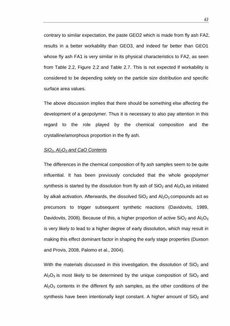
63
contrary to similar expectation, the paste GEO2 which is made from fly ash FA2,
results in a better workability than GEO3, and indeed far better than GEO1
whose fly ash FA1 is very similar in its physical characteristics to FA2, as seen
from Table 2.2, Figure 2.2 and Table 2.7. This is not expected if workability is
considered to be depending solely on the particle size distribution and specific
surface area values.
The above discussion implies that there should be something else affecting the
development of a geopolymer. Thus it is necessary to also pay attention in this
regard to the role played by the chemical composition and the
crystalline/amorphous proportion in the fly ash.
SiO2, Al2O3 and CaO Contents
The differences in the chemical composition of fly ash samples seem to be quite
influential. It has been previously concluded that the whole geopolymer
synthesis is started by the dissolution from fly ash of SiO2 and Al2O3 as initiated
by alkali activation. Afterwards, the dissolved SiO2 and Al2O3 compounds act as
precursors to trigger subsequent synthetic reactions (Davidovits, 1989,
Davidovits, 2008). Because of this, a higher proportion of active SiO2 and Al2O3
is very likely to lead to a higher degree of early dissolution, which may result in
making this effect dominant factor in shaping the early stage properties (Duxson
and Provis, 2008, Palomo et al., 2004).
With the materials discussed in this investigation, the dissolution of SiO2 and
Al2O3 is most likely to be determined by the unique composition of SiO2 and
Al2O3 contents in the different fly ash samples, as the other conditions of the
synthesis have been intentionally kept constant. A higher amount of SiO2 and

64 2. Fly ash and its influence on fresh properties of geoploymer
Al2O3 contents would be better for enhancing the geopolymer reactions.
Furthermore, a higher proportion of the amorphous phase would also be
preferred because the amorphous phase has been found to be more reactive
than the crystalline phase (van Jaarsveld et al., 2003, Chen-Tan et al., 2009,
Williams and van Riessen, 2010).
The extreme low workability of GEO1 seems to be associated with the higher
contents of quartz and mullite but lower content in amorphous SiO2 and Al2O3 of
FA1, as seen in Table 2.5. In contrast, the mixes GEO2 and GEO3, which are
from the fly ash samples containing more amorphous SiO2 and Al2O3, result in
much better workability. Whether this characteristic is in any way responsible for
the difference in workability is not certain at this time and should be further
investigated. Nevertheless, workability, which is usually decided by the
characteristics of fluidity, cohesion and viscosity of the fresh mixture, can be
influenced by the solid/liquid proportion of the mixture. A lower solid proportion
is likely to lead to an increased fluidity, and subsequent improved workability.
For the geopolymer mixes here, the initial solid/liquid proportion of the mixture
was intentionally kept the same by using the same mix design for GEO1, GEO2
and GEO3 mixes. Therefore, the workability is expected to be identical until fly
ash particles start to dissolve. When the reactive part of fly ash starts to
dissolve as a result of the activators action, the solids amount in the fresh
mixture reduces in favour of an increase in the amount of solution. The fly ash
containing more reactive contents, for example more amorphous SiO2 and
Al2O3, is therefore expected to dissolve faster and result in the mixture with an
even lower solid proportion. Such dissolution could be fast enough as to affect
the property of early stage mixture, like workability. This argument is supported
65
by the finding that the dissolution of SiO2 and Al2O3 happens almost
immediately after adding the activator (Chen-Tan et al., 2009, Li et al., 2011).
Thus, it may be reasonable to conclude that the mixture using the fly ash
containing more amorphous SiO2 and Al2O3 could quickly gain a lower
solid/liquid proportion immediately after mixing and thus impart higher
workability to the fresh mixture.
Additionally, CaO is another component in fly ash apart from SiO2 and Al2O3
that can influence the properties of fresh geopolymer mixes, like workability and
setting times (van Jaarsveld et al., 2003). Using the leaching test, it has been
found that the dissolution rate of CaO can be very fast, and sometimes even
faster than the dissolution rate of Al2O3 (Lee and Van Deventer, 2002). This
indicates that CaO may also dissolve at the early stage of mixing, increase the
proportion of liquid, and further enhancing the workability of fresh geopolymer in
a similar way as that of amorphous SiO2 and Al2O3 discussed in the previous
paragraph. It may also be supported by the relevant research on the effect of
CaO content for early cement properties (Lea, 1970), despite that more
research is clearly needed in a geopolymer system. From Table 2.4, it is seen
that FA2 has a slightly higher CaO content than the other two fly ash samples.
This may explain the better workability of GEO2 compared to GEO3, despite
the fact that FA2 and FA3 share a similar content of amorphous SiO2 and Al2O3.
2.5 Fly Ash’s Effect on Hardened Properties
Although this chapter mainly focuses on fly ash and its influence on fresh
properties, a finding on the different densities and strengths present in produced
geopolymers draws a further notice on fly ash’s effect on hardened properties.

66 2. Fly ash and its influence on fresh properties of geoploymer
For the purposes of a supplementary illustration on fly ash variability and a
secondary suggestion for fly ash selection, this finding is reported and briefly
discussed in this section. More detailed discussions on hardened geopolymers
will be made in relation to geopolymer aggregate materials in following chapters.
The density of air-dried hardened geopolymer was measured by dividing its
mass by its volume just before performing compressive strength testing, which
was done using a TECNOTEST compression testing machine (3000 kN
capacity) (Figure 2.11). The loading rate was set constant at 0.33 MPa/sec,
based on the recommended loading rate range in US standard ASTM C109
(ASTM, 2012c). The strength value for every geopolymer mix was represented
by the average value for three samples.
The density and compressive strength values are shown in Table 2.9. GEO2
and GEO3 present similar air dry density values, while GEO1 yields a higher air
dry density compared to the former two mixes. On the other hand, GEO1 has
the highest 7-day compressive strength, of nearly 53 MPa, while GEO2 and
GEO3 share the lower 7-day strength values of around 40 MPa. It is observed
that the hardened geopolymer products originated from different fly ash
samples are different in density and strength, which is likely to be caused by the
varied fly ash characteristics, since the applied mix designs and curing regimes
are same for all mixes.

67
Figure 2.11: Compressive strength testing on a 3000 KN TECNOTEST machine
Table 2.9: Air dry density and compressive strength of produced geopolymers
Code Fly ash Air dry density (kg/m3)
Compressive strength (7d) (MPa)
Standard deviation
GEO1 FA1 1690 52.94 1.59
GEO2 FA2 1630 39.22 0.41
GEO3 FA3 1630 41.05 1.27
It has been expected that a mix using a more reactive fly ash should receive an
improved formation of geopolymer structure, and therefore a more enhanced
strength. Yet the results of strength of the mixes made from FA2 and FA3 are
actually lower than that of FA1, as seen from Table 2.9. Hence, it is estimated
that some other factors may also influence the strength.
68 2. Fly ash and its influence on fresh properties of geoploymer
As seen in Table 2.5, the amorphous SiO2/Al2O3 ratios are 6.6, 4.6 and 4.1 for
FA1, FA2 and FA3 respectively. At the same time, it is noticed that the strength
values for the three ash mixes are approximately 53 MPa, 39 MPa and 41 MPa
respectively. While the difference between the strength relating to FA2 and FA3
cannot be said to be significant, it can be said quite comfortably that the
strength difference relating to FA1 when compared with that of FA2 or FA3 is
significant. The author attributes the reason for this strength superiority of FA1
to the relatively high amorphous SiO2/Al2O3 ratio. Indeed, other researchers
have found this ratio to affect the strength of geopolymers (De Silva et al., 2007,
Palomo et al., 2004).
The low strength of GEO2 may also be related in part to the high carbon
content in the original fly ash FA2, which is higher than FA1 and FA3 as seen in
Table 2.3. The unburned carbon is much more porous than the other minerals
present in fly ash (Blissett and Rowson, 2012). Too high carbon content in fly
ash is likely to absorb much of the added alkali activator and thus inhibit the
progress of geopolymerisation, which is likely to reduce the strength of
produced geopolymer (Diaz et al., 2010).
On the other hand, even though it has been once reported that CaO content
can react to form the calcium-containing hydrates and thus enhance the
strength of geopolymers (van Jaarsveld et al., 2003), the effect of CaO is not
significant in the mixes of this research, possibly due to a minor variation in
CaO proportions among the selected fly ash samples (Table 2.4).
Moreover, for the geopolymer mixes discussed here, it seems that the
proportions of amorphous and crystalline phases in fly ash may less affect the
69
hardened properties, despite that they are thought to be the major reasons for
different fresh properties in previous sections. It has been reported that less
amorphous content in fly ash would lead to relatively insufficient reactants
dissolved for geopolymerisation, and thus result in lower strength. The crystals,
which are not reactive, have been believed to almost not contribute to
geopolymer formation (Bakharev, 2006, Rickard et al., 2011). The findings in
previous sections prove the low reactivity of crystals in the fly ash. However, it is
questionable that, after a long curing period, whether these crystals do not show
evidence of having reacted efficiently enough to provide significant increase in
strength and whether the notion that crystalline formations remain more or less
inert even if the geopolymer is subjected to a long curing regime is correct.
Table 2.10 shows the difference that occurred in the crystalline phase between
its original content in the fly ash and the final content in the geopolymer, by
conducting X-ray diffraction supplemented by Rietveld quantification process.
This is illustrated by comparing the different crystalline quantities between the
pre-mixed ingredients (including fly ash and activator solids) and the final
geopolymer, as seen in Table 2.10.
The summation of crystals in the pre-mixed ingredients before
geopolymerisation is 24.1%, 18.8% and 17.9%, for GEO1, GEO2 and GEO3
respectively, which are greatly varied. Despite this, the crystalline proportions of
the final geopolymers are reduced to be 15.6%, 14.5% and 14.2%, for GEO1,
GEO2 and GEO3 respectively. These indicate that the crystals could also be
activated, which agrees a previous finding of the author that the mullite in fly
ash can be reacted if given suitable conditions (Xie and Kayali, 2014), despite
the fact that they are inert in most cases (Fernández-Jiménez and Palomo,

70 2. Fly ash and its influence on fresh properties of geoploymer
2003). The activated crystals, which are similarly composed of Si and Al
compounds, must have been transformed into geopolymer products in a
process similar to that of the amorphous phase, albeit in a relatively slow
reaction rate. This is expected to further contribute to geopolymer formation.
Table 2.10: Quantification results on crystals and amorphous content before and after geopolymerisation
Original fly ash Phase
Fly ash + activator solids
wt.%
Geopolymer wt.%
Difference wt.%
FA1
Amorphous 75.9 84.3 +8.5
Quartz 8.3 6.1
Mullite 15.8 9.5
Sum of crystals 24.1 15.6 -8.5
FA2
Amorphous 81.2 85.5 +4.3
Quartz 5.0 4.0
Mullite 13.8 10.5
Sum of crystals 18.8 14.5 -4.3
FA3
Amorphous 82.1 85.8 +3.7
Quartz 5.4 5.1
Mullite 12.5 9.1
Sum of crystals 17.9 14.2 -3.7
Besides, the degrees of crystal activation occurring in the different mixes are
different, as shown in Table 2.10 where the quantity of activated crystals is
8.5%, 4.3% and 3.7% for GEO1, GEO2 and GEO3 respectively. The fly ash
with a higher crystalline proportion results in a higher quantity of activated
crystals. This indicates that the fly ash with less amorphous content would not

71
necessarily lead to insufficient geopolymerisation, but may undergo a rather
higher degree of crystal activation that further contributes to geopolymer
formation. This would most likely be influenced by the activators’ strength and
nature as well as the curing conditions.
This research on density and strength performance of geopolymer mixes
provides advisory information for fly ash selection. As introduced in Chapter 1, a
geopolymer aggregate is designed with a low density and good strength
behaviour. In this research, the hardened geopolymers have an air dry density
of 1600-1700 kg/m3, which is in a low density range if it is used as an aggregate
(Clarke, 1993). Meanwhile, this geopolymer material can result in a
compressive strength of around 40-50 MPa, which is considered acceptable for
a load bearing material in constructions. These facts indicate that the
geopolymer materials proposed here should be suitable for producing
geopolymer aggregates.
Among the three fly ash samples, the fly ash FA1 is likely to be recommended
because of the superior strength of its geopolymer product. Nevertheless, the
geopolymers made with FA2 and FA3 are not significantly different in
mechanical properties. However, the practicality of fly ash FA1 for geopolymer
aggregates still needs a further discussion, and this will be made in Chapter 5 to
specifically examine the physical and mechanical development of the
geopolymer aggregate samples made from FA1.
2.6 Conclusions
This chapter presents an important component of the research reported in this
thesis. This component is meant to develop the current understanding of the

72 2. Fly ash and its influence on fresh properties of geoploymer
role of fly ash in geopolymerisation. It leads to the conclusion that the fresh
properties of geopolymer, such as workability and consistency, can be very
sensitive to the characteristics of fly ash batch applied, even if the ash source is
not changed. This conclusion has not been previously reported in literature
dealing with geopolymer manufacturing issues. This is however, as indicated by
the experimental results of this chapter, must be an issue of concern to be
considered before conducting the subsequent geopolymer aggregate research.
Based on the research and discussion presented in this chapter, one specific fly
ash batch is selected, for the consistency of fly ash properties, and for the
performance of its subsequent fresh geopolymer product which is considered
suitable for the further geopolymer aggregate manufacture. This fly ash is the
one produced on Dec 13th, 2012 from Eraring thermal power station. It will be
used as the fly ash precursor for geopolymerisation involved in this research
and reported and discussed in the following chapters.

73
Chapter 3
Geopolymer Mix Design
3.1 Introduction
This chapter researches a systematic mix design procedure which confirms the
proportions of fly ash, NaOH flakes, Na2SiO3 solution and water needed for a fly
ash-based geopolymer mix.
In this mix design procedure, the above mentioned ingredients are separated
into two categories as fly ash and activator. A chemical formula
Na2O·xSiO2·yH2O is used to express the activator during the mix design
procedure. Meanwhile, another parameter which is water-to-geopolymer solids
ratio (W/G ratio) is used to inter-relate the use of fly ash with that of the activator.
For this case, three criteria, namely; SiO2/Na2O, H2O/Na2O and W/G, are
proposed to distinguish each mix and to calculate the final mix design, which is
a feature of the mix design procedure presented in this chapter. Otherwise, the
factors conventionally related with a geopolymer mix, such as the molarity of
NaOH solution and the mass ratio of Na2SiO3/NaOH, can be obtained from the
outcome of this mix design procedure. This mix design procedure is able to fulfil
the need of current research and will be used for the manufacture of
geopolymer materials discussed in the remaining chapters of this thesis.
3.2 Materials and Mix
The applied ingredients for geopolymer mix include fly ash, NaOH flakes,
Na2SiO3 solution and water. Among them, fly ash is from the 2012-Dec-13 fly
ash batch obtained from the Eraring thermal power station, whose

74 3. Geopolymer mix design
characteristics are detailed in Chapter 2; ‘NaOH flakes’ is a commercial product
with a purity of >99%; Na2SiO3 is sourced from a Grade D silicate solution (29.4%
SiO2, 14.7% Na2O); water is deionised water generated from a laboratory water
purification machine. These ingredients comply with the normal synthetic
method for a fly ash-based geopolymer (Davidovits, 2008).
The geopolymer mix follows a general three-step mixing procedure (Hardjito
and Rangan, 2005, Rangan, 2007) which is shown in Figure 3.1: 1) a NaOH
solution with a certain molarity is first prepared by dissolving NaOH flakes in the
correct amount of water; 2) this NaOH solution is then combined with a Grade D
Na2SiO3 solution to form the activator; and 3) this activator is later poured on
the fly ash to activate it for geopolymerisation to take place.
Also, the following aspects need to be noticed when processing above mixing
procedure. First, the NaOH solution made from a dissolution of NaOH flakes is
not immediately used, but has to be stored in sealed condition for a certain
period before the mix is made (Arioz et al., 2012). This is because the
dissolution of NaOH flakes can release large amount of heat, and therefore
requires a certain period to cool down. On the other hand, this NaOH solution is
not pre-mixed with the Grade D Na2SiO3 solution. These two solutions are only
combined just before the start of the activation of fly ash for geopolymerisation,
i.e. the third step of above mixing procedure. This is in order to avoid a possible
transformation in the ratio of SiO2/Na2O in the used Na2SiO3 solution if earlier
pre-mixing it with NaOH solution was done (Iler, 1979, Nauman and Debye,
1951, Engelhardt et al., 1975).

75
Figure 3.1: Mixing procedure for fly ash-based geopolymer
Moreover, it needs to be stated that, the ingredients and mixing procedure
discussed in this section are for the real practical work of geopolymer mix, and
not relevant to the mix design procedure. In the mix design procedure that will
be introduced later, some other criteria are designed and used for calculations,
but they would not affect the process of practical work. After the completion of
mix design procedure, the ingredients shown in the final mix design are still
processed following the steps in Figure 3.1.
3.3 Terminology
This section introduces several terms used in a systematic geopolymer mix
design procedure for differentiating among geopolymer mixes.
3.3.1 Fly Ash/Activator Mass Ratio (F/A)
The F/A parameter is used to define the relationship between the fly ash, which
refers to the mass of fly ash particles in use, and the activator which refers to
the mass of the activator composed of NaOH and Na2SiO3 solutions. It is
provided mainly to facilitate the production of a convenient and practical mix,
and to make it easy to repeat mixes for research purposes.

76 3. Geopolymer mix design
3.3.2 Activator Composition Na2O·xSiO2·yH2O
On the other hand, the composition of the alkali activator (NaOH and Na2SiO3
solutions) is expressed in a chemistry-based way, as suggested by Provis et al.
(2009), that is, expressed in the form of mole ratios such as Na2O·xSiO2·yH2O,
where x and y stand for the mole ratios to be designed. The values of
SiO2/Na2O and H2O/Na2O can be treated as criteria which are referred by users
so as to create new geopolymer designs as required.
In the formula Na2O·xSiO2·yH2O, retaining Na2O as one mole results in x and y
being the values of the mole ratios of SiO2/Na2O and H2O/Na2O respectively.
By providing fixed values of x and y when specifying the mix design, the
composition of the activator is able to be determined while the amounts of
NaOH, Na2SiO3 and water required can be calculated later.
3.3.3 Water-to-geopolymer Solids (W/G) Ratio
A further criterion, which is the W/G ratio proposed by Rangan (2007), is used
to build another connection between the activator and fly ash apart from the F/A
to truly reflect the function of the internal components in the activator.
In the W/G ratio, water (W) refers to the mass of H2O present in the activator,
as in Na2O·xSiO2·yH2O, while geopolymer solids (G) refer to the total mass of
the materials of the geopolymer that are in the solid phase (which include the fly
ash) and the solid parts in the liquids (the solutes), that is: the solid masses of
fly ash, Na2O and SiO2.
From these definitions, it is clear that the W/G value highlights the role of H2O in
the activator Na2O·xSiO2·yH2O while the other components, Na2O and SiO2,
77
are reflected by known x and y values. The W/G ratio is used to correlate these
components with the amount of fly ash to be mixed to confirm the amounts of
ingredients required for a given mass of fly ash or given volume of the total
mixture and complete the final mix design.
For users who apply this ratio in their design, the W/G ratio needs to be
specified at the beginning, which is as significant in terms of workability and
strength as is the water to cement ratio for a regular Portland cement mix. An
appropriate W/G ratio is able to be obtained from the previous work of Hardjito
and Rangan (Rangan, 2007, Hardjito and Rangan, 2005) but needs to be
further checked in trial tests of specific raw materials.
3.4 Mix Design Procedure
A flowchart of the mix design procedure for geopolymer mix is presented in
Figure 3.2. In this figure, the mix design procedure is separated into two stages
with required steps linked by solid lines. Besides, the squares indicating the
known information by users are linked to these steps by dashed lines. In stage
1, the activator is prepared based on the designed criteria SiO2/Na2O (x value)
and H2O/Na2O (y value) for the activator Na2O·xSiO2·yH2O. Then, in stage 2,
the W/G ratio is specified, the amounts of NaOH, Na2SiO3 and water required
for the target mass of the fly ash to be activated are calculated and the value of
F/A is obtained to guide the practical work.
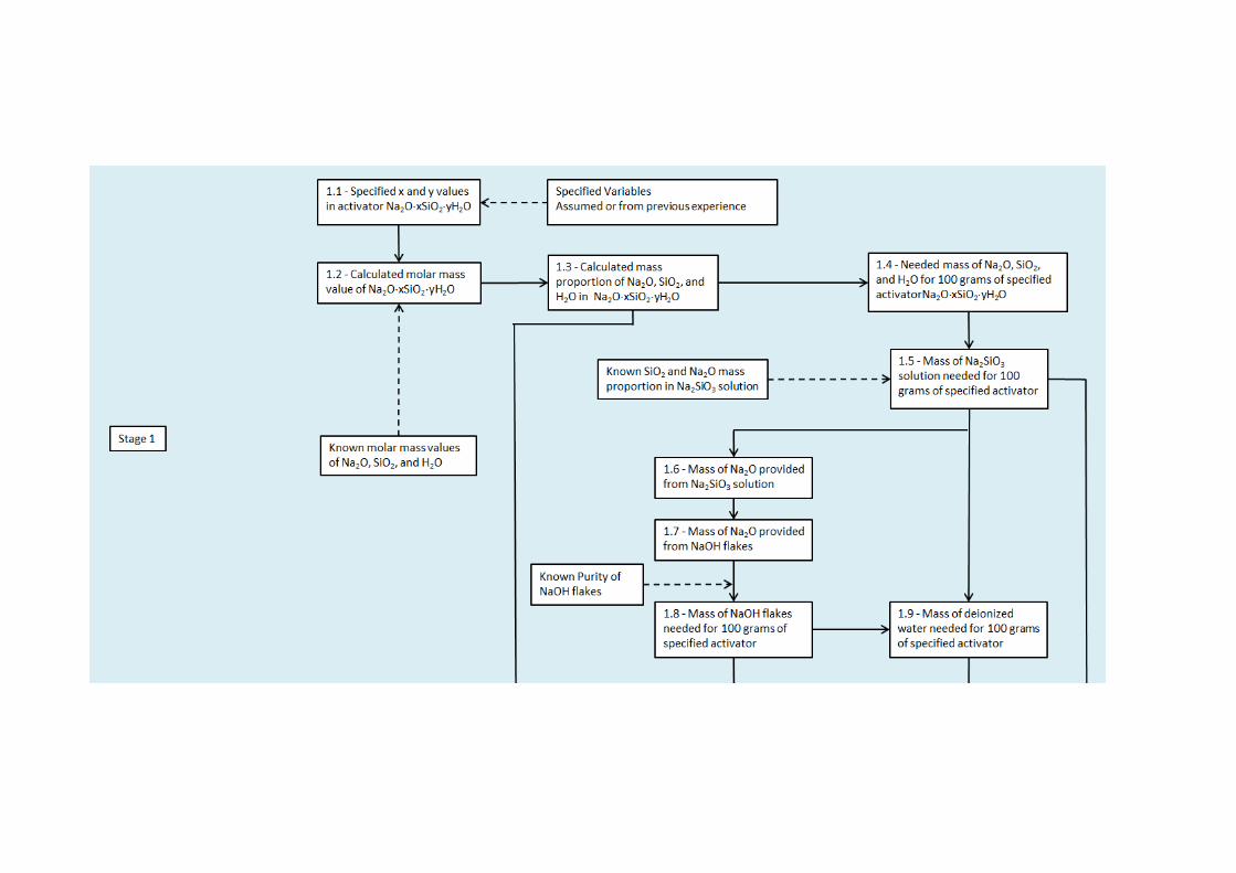
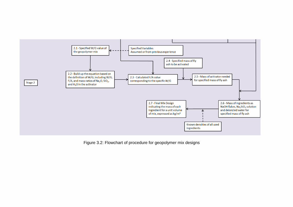
Figure 3.2: Flowchart of procedure for geopolymer mix designs
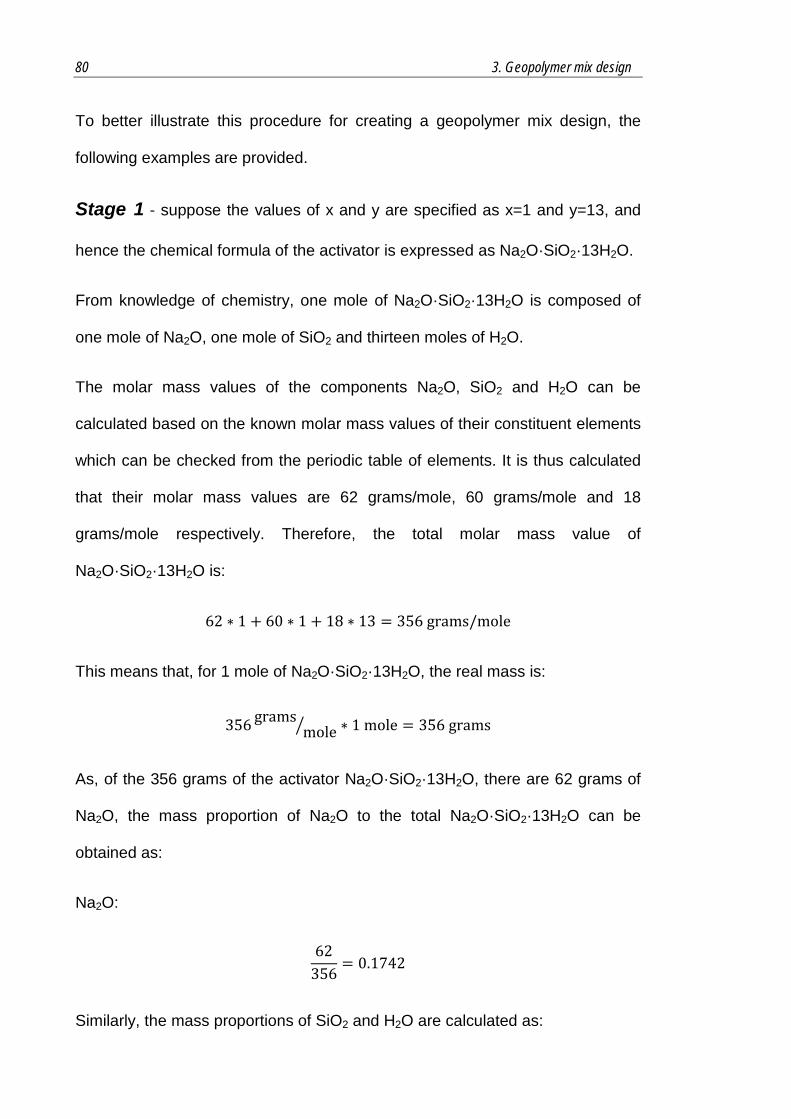
80 3. Geopolymer mix design
To better illustrate this procedure for creating a geopolymer mix design, the
following examples are provided.
Stage 1 - suppose the values of x and y are specified as x=1 and y=13, and
hence the chemical formula of the activator is expressed as Na2O·SiO2·13H2O.
From knowledge of chemistry, one mole of Na2O·SiO2·13H2O is composed of
one mole of Na2O, one mole of SiO2 and thirteen moles of H2O.
The molar mass values of the components Na2O, SiO2 and H2O can be
calculated based on the known molar mass values of their constituent elements
which can be checked from the periodic table of elements. It is thus calculated
that their molar mass values are 62 grams/mole, 60 grams/mole and 18
grams/mole respectively. Therefore, the total molar mass value of
Na2O·SiO2·13H2O is:
62 ∗ 1 + 60 ∗ 1 + 18 ∗ 13 = 356 grams/mole
This means that, for 1 mole of Na2O·SiO2·13H2O, the real mass is:
356 gramsmole� ∗ 1 mole = 356 grams
As, of the 356 grams of the activator Na2O·SiO2·13H2O, there are 62 grams of
Na2O, the mass proportion of Na2O to the total Na2O·SiO2·13H2O can be
obtained as:
Na2O:
62356
= 0.1742
Similarly, the mass proportions of SiO2 and H2O are calculated as:

81
SiO2:
60356
= 0.1685
H2O:
13 ∗ 18356
= 0.6573
The above mass proportions are corresponding to one mole of the activator
Na2O·SiO2·13H2O as 356 grams in total. Such mass proportions are not
changed once the activator’s composition is confirmed, that is, once the x and y
values are decided, even if the activator’s total amount is different. Therefore,
they can be used to calculate the required amount of each ingredient for any
specific amount of activator.
Therefore, if we need to prepare 100 grams of the activator Na2O·SiO2·13H2O,
the masses of the components Na2O, SiO2 and H2O are:
Na2O:
100 ∗ 0.1742 = 17.42 grams
SiO2:
100 ∗ 0.1685 = 16.85 grams
H2O:
100 ∗ 0.6573 = 65.73 grams
The three components Na2O, SiO2 and H2O come from the three ingredients
NaOH flakes, Na2SiO3 solution and deionised water. Among these three

82 3. Geopolymer mix design
ingredients, the Na2SiO3 solution is the only source of SiO2. Thus, the 16.85
grams of SiO2 must come solely from it. As introduced earlier, the applied
Grade D Na2SiO3 solution is composed of 29.4% SiO2, 14.7% Na2O and 55.9%
water in mass. Therefore, the amount of Na2SiO3 solution required for 100
grams of the activator is:
16.8529.4%
= 57.31 grams
There are two sources for the component Na2O; the Na2SiO3 solution and
NaOH flakes. As previously mentioned, the applied Na2SiO3 solution has a
proportion of 14.7% Na2O. Therefore, the amount of Na2O coming from it can
be calculated as:
57.31 ∗ 14.7% = 8.42 grams
Then, the remaining Na2O should come from the NaOH flakes. As 17.42 grams
of Na2O in total are required, the amount provided from the NaOH flakes is:
17.42 − 8.42 = 9 grams
The amount of NaOH flakes required to provide these 9 grams of Na2O
depends on the Na2O concentration of the specific NaOH flake product. As the
product used in this research can be treated as pure NaOH, the Na2O
concentration found above (that is the 9 grams in this example) is equivalent to
the Na2O proportion specified in the chemical formula NaOH. The chemical
formula NaOH can be rewritten as Na2O·H2O to clearly indicate the proportion
of Na2O which can be calculated based on the known molar mass values of
Na2O (62 grams/mole) and H2O (18 grams/mole) as:

83
6262 + 18
= 0.775
Then the amount of NaOH flakes required is:
90.775
= 11.61 grams
Finally, the amount of deionised water can be calculated by subtracting the
above two ingredients from 100 grams of the total activator amount as:
100 − 57.31 − 11.61 = 31.08 g
This amount of deionised water is the water that needs to be added to the 11.61
grams of NaOH flakes so that the resulting NaOH solution plus the 57.31 grams
of Na2SiO3 solution will give us the required initial 100 grams of activator whose
specified x and y were 1 and 13 respectively.
From the above we can see that, in order to prepare 100 grams of the
activator Na2O·SiO2·13H2O, the amounts of the ingredients should be
11.61 grams of NaOH flakes, 57.31 grams of Grade D silicates solution and
31.08 grams of deionised water.
The above calculations could also be used as a standard procedure for
preparing the activator for a geopolymer mix. The only variables are the values
of x and y in the activator, and the compositions of the applied ingredients which
can all be designed or acquired by users.

84 3. Geopolymer mix design
Stage 2 - suppose that a geopolymer mix with a higher workability is required.
Based on relevant knowledge 1, the W/G value is set to be 0.26 while the
activator Na2O·SiO2·13H2O introduced in the previous example is still used.
Suppose that the prepared activator aims to activate 1000 grams of fly ash for
geopolymer manufacture. From the definition of the W/G value, we can see that:
(WG� ) =
mass (H2O)mass (fly ash) + mass(Na2O) + mass(SiO2) = 0.26
(where the ‘mass (H2O)’ is the mass of the H2O in the formula
Na2O·SiO2·13H2O which is referred to here as ‘the activator’)
If we simultaneously divide the numerator and denominators in the middle
portion of this equation by ‘mass(Na2O·SiO2·13H2O)’, which is indeed the mass
of the alkali activator, this equation becomes:
�WG� �
=
mass (H2O)mass(Na2OˑSiO2ˑ13H2O)
mass (fly ash)mass(Na2OˑSiO2ˑ13H2O) + mass(Na2O)
mass(Na2OˑSiO2ˑ13H2O) + mass(SiO2)mass(Na2OˑSiO2ˑ13H2O)
= 0.26
From the definition of F/A, we can see that:
mass (fly ash)mass(Na2OˑSiO2ˑ13H2O) = (F
A� )
Therefore, one of the denominators in the equation can be simplified and the
whole equation written as:
1 Gained from author’s experience and previous report of Rangan (2007)
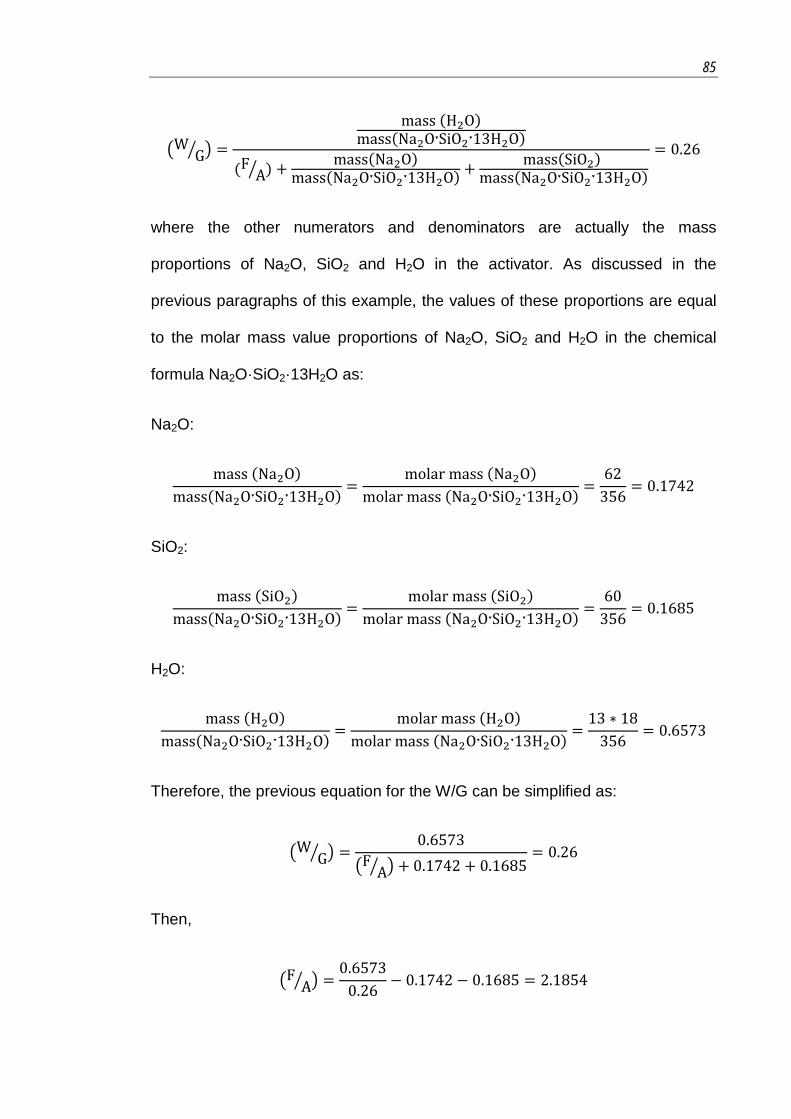
85
�WG� � =
mass (H2O)mass(Na2OˑSiO2ˑ13H2O)
(FA� ) + mass(Na2O)
mass(Na2OˑSiO2ˑ13H2O) + mass(SiO2) mass(Na2OˑSiO2ˑ13H2O)
= 0.26
where the other numerators and denominators are actually the mass
proportions of Na2O, SiO2 and H2O in the activator. As discussed in the
previous paragraphs of this example, the values of these proportions are equal
to the molar mass value proportions of Na2O, SiO2 and H2O in the chemical
formula Na2O·SiO2·13H2O as:
Na2O:
mass (Na2O)mass(Na2OˑSiO2ˑ13H2O) =
molar mass (Na2O)molar mass (Na2OˑSiO2ˑ13H2O) =
62356
= 0.1742
SiO2:
mass (SiO2)mass(Na2OˑSiO2ˑ13H2O) =
molar mass (SiO2)molar mass (Na2OˑSiO2ˑ13H2O) =
60356
= 0.1685
H2O:
mass (H2O)mass(Na2OˑSiO2ˑ13H2O) =
molar mass (H2O)molar mass (Na2OˑSiO2ˑ13H2O) =
13 ∗ 18356
= 0.6573
Therefore, the previous equation for the W/G can be simplified as:
�WG� � =
0.6573�F
A� � + 0.1742 + 0.1685= 0.26
Then,
�FA� � =
0.65730.26
− 0.1742 − 0.1685 = 2.1854
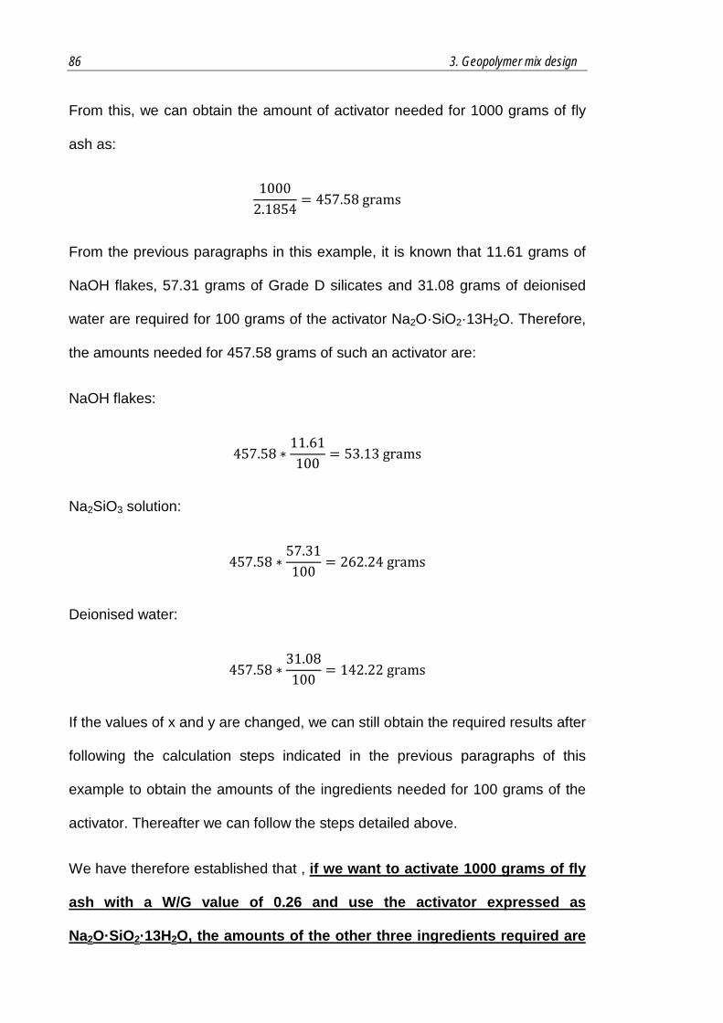
86 3. Geopolymer mix design
From this, we can obtain the amount of activator needed for 1000 grams of fly
ash as:
10002.1854
= 457.58 grams
From the previous paragraphs in this example, it is known that 11.61 grams of
NaOH flakes, 57.31 grams of Grade D silicates and 31.08 grams of deionised
water are required for 100 grams of the activator Na2O·SiO2·13H2O. Therefore,
the amounts needed for 457.58 grams of such an activator are:
NaOH flakes:
457.58 ∗11.61100
= 53.13 grams
Na2SiO3 solution:
457.58 ∗57.31100
= 262.24 grams
Deionised water:
457.58 ∗31.08100
= 142.22 grams
If the values of x and y are changed, we can still obtain the required results after
following the calculation steps indicated in the previous paragraphs of this
example to obtain the amounts of the ingredients needed for 100 grams of the
activator. Thereafter we can follow the steps detailed above.
We have therefore established that , if we want to activate 1000 grams of fly
ash with a W/G value of 0.26 and use the activator expressed as
Na2O·SiO2·13H2O, the amounts of the other three ingredients required are

87
53.13 grams of NaOH flakes, 262.24 grams of Grade D silicates and 142.22
grams of deionised water. Meanwhile, for this case, the F/A ratio is nearly
2.19.
The above calculations are then expressed in units of kg/m3 in the final mix
design which indicates the mass required per 1m3 of the mix. This is more
suitable for practical use which requires a mix design to be simple and direct.
Based on the known density values, each ingredient’s volumetric proportion can
be calculated and its mass per 1m3 volume of the mix obtained.
From known information, the densities of applied fly ash, NaOH flakes, Grade D
Na2SiO3 solution and deionised water are set to be 2210 kg/m3, 2130 kg/m3,
1520 kg/m3 and 1000 kg/m3 respectively.
The volume of 1000 grams of fly ash is:
10002210 ∗ 1000
= 4.52 ∗ 10−4 m3
The volume of 53.13 grams of NaOH flakes is:
53.132130 ∗ 1000
= 2.50 ∗ 10−5 m3
The volume of 262.24 grams of Na2SiO3 solution is:
262.241520 ∗ 1000
= 1.73 ∗ 10−4 m3
The volume of 142.22 grams deionised water is:
142.221000 ∗ 1000
= 1.42 ∗ 10−4 m3

88 3. Geopolymer mix design
Therefore, the volumetric proportion of fly ash is:
4.52 ∗ 10−4
(4.52 ∗ 10−4 + 2.50 ∗ 10−5 + 1.73 ∗ 10−4 + 1.42 ∗ 10−4)= 0.571
Similarly, the volumetric proportions of other three ingredients are:
NaOH flakes
2.50 ∗ 10−5
(4.52 ∗ 10−4 + 2.50 ∗ 10−5 + 1.73 ∗ 10−4 + 1.42 ∗ 10−4)= 0.032
Na2SiO3 solution
1.73 ∗ 10−4
(4.52 ∗ 10−4 + 2.50 ∗ 10−5 + 1.73 ∗ 10−4 + 1.42 ∗ 10−4)= 0.218
Deionised water
1.42 ∗ 10−4
(4.52 ∗ 10−4 + 2.50 ∗ 10−5 + 1.73 ∗ 10−4 + 1.42 ∗ 10−4)= 0.179
The ingredients’ volumetric proportions shown above are also their volumetric
proportions in a 1 m3 geopolymer mix. Therefore, their mass quantities in the
mix can be calculated as:
Fly ash
0.571 ∗ 2210 = 1261.91 kg/m3
NaOH flakes
0.032 ∗ 2130 = 68.16 kg/m3
Na2SiO3 solution

89
0.218 ∗ 1520 = 331.36 kg/m3
Deionised water
0.179 ∗ 1000 = 179.00 kg/m3
Hence, we can obtain a complete mix design for a geopolymer mix using
an activator Na2O·SiO2·13H2O with a W/G value of 0.26. This mix design is
shown in Table 3.1 and requires 1261.91 kg/m3 of fly ash, 68.16 kg/m3 of
NaOH flakes, 331.36 kg/m3 of Grade D Na2SiO3 solution and 179.00 kg/m3
of deionised water. The calculation steps discussed here also work for other
geopolymer mixes with various W/G values and/or activator compositions.
Therefore a systematic geopolymer mix design procedure can be established.
Table 3.1: Final mix design of the geopolymer mix example (kg/m3)
W/G value
SiO2/Na2O (x value)
H2O/Na2O (y value)
F/A value
Mix design (kg/m3)
Fly ash NaOH flakes
Na2SiO3 solution
Deionised water
0.26 1.00 13 2.19 1261.91 68.16 331.36 179.00
3.5 Molarity of NaOH and Mass Ratio Na2SiO3/NaOH
In the mix design procedure presented in the last section, the criteria used to
distinguish each geopolymer mix, and therefore required to be designed by
users, are SiO2/Na2O, H2O/Na2O and W/G values. However, in a conventional
geopolymer mix design, the factors of the molarity of NaOH solution and the
mass ratio of Na2SiO3/NaOH are often important to be defined (Rangan, 2007,
Kong and Sanjayan, 2010, Chindaprasirt et al., 2007) as they more directly
describe the solutions used in a practical mix as shown in Figure 3.1. Therefore,

90 3. Geopolymer mix design
the information of these two factors under the previous mix design procedure is
discussed in this section.
The molarity of NaOH solution and the mass ratio of Na2SiO3/NaOH can be
calculated from the final mix design made from the previous mix design
procedure, as illustrated by following example:
As introduced, a complete mix design is obtained and shown in Table 3.1 for
the example proposed in section 3.4 which, uses an activator Na2O·SiO2·13H2O
with a W/G value of 0.26. The ingredients in this mix design are 1261.91 kg/m3
of fly ash, 68.16 kg/m3 of NaOH flakes, 331.36 kg/m3 of Grade D Na2SiO3
solution and 179.00 kg/m3 of deionised water.
As displayed in Figure 3.1, the amount of NaOH solution practically used in a
geopolymer mix is a sum of the amounts of NaOH flakes and deionised water,
which is:
68.16 + 179.00 = 247.16 kg/𝑚𝑚3
Therefore, the mass proportion of NaOH solids in this NaOH solution is:
68.16247.16
∗ 100% = 27.58%
Using a chemistry manual it is able to check the molarity of a NaOH solution
which has a mass proportion of 27.58% is 8.7M (specified at a condition of 20oC
and 101.3 kPa atmospheric pressure) (ZXXK, 2012).
On the other hand, the mass ratio of Na2SiO3/NaOH can be calculated based
on the masses of Na2SiO3 (331.36 kg/m3) and NaOH (247.16 kg/m3):

91
331.36247.16
= 1.34
From the above, it is now shown that for a geopolymer mix designed with
SiO2/Na2O=1, H2O/Na2O=13 and W/G=0.26, the molarity of NaOH solution is
8.7M and the mass ratio of Na2SiO3/NaOH solutions is 1.34. These results
can describe the true nature of the used NaOH and Na2SiO3 solutions in a
practical geopolymer mix. Moreover, they can be used to compare with other
literature for scientific analysis as well as practical purposes.
Also, it is found out that the values of above factors, such as the molarity of
NaOH solution and the mass ratio of Na2SiO3/NaOH, are different for different
geopolymer mixes, as seen from some examples presented in Table 3.2 made
based on the mix design procedure in section 3.4.
In the first 5 mixes of Table 3.2, the values of SiO2/Na2O (x value) and W/G are
set constant, but the value of H2O/Na2O (y value) is varied from 11 to 15. It is
observed that a higher y value results in a higher free water usage, and a lower
molarity of NaOH solution. The mix with y=11 obtains the highest molarity as
12.5M while the mix with y=15 obtains the least molarity as 6.8M. On the other
hand, a higher y value also leads to a lower Na2SiO3/NaOH ratio, going down
from 1.76 to 1.06 for y=11 and y=15, respectively. It is thus concluded that the
molarity of NaOH solution and Na2SiO3/NaOH ratio are affected by the criterion
of H2O/Na2O used in the mix design procedure.
Moreover, for the mixes No.2, No.6 and No.7, the values of y and W/G are the
same while the value of x is varied. It is seen that a higher x value results in an
92 3. Geopolymer mix design
obvious increase in the mass ratio of Na2SiO3/NaOH, which is reasonable since
x value determines the ratio of SiO2/Na2O in the activator.
Otherwise, for the mixes No.3, No.8 and No.9, the values of x and y are kept
the same while the value of W/G is changed from 0.26 to 0.22. These three
mixes are found to have the same molarity of NaOH solution as 8.7M, and the
same mass ratio of Na2SiO3/NaOH as 1.34, despite their different W/G ratios.
This seems due to the fact that, the activator’s composition is the same
because of the same x and y values were fixed for these three mixes. So the
NaOH and Na2SiO3 solutions used to compose this activator will also be the
same for these mixes, and not affected by the variation in W/G ratio.
The above finding provides a further knowledge that the geopolymer mixes
designed with different W/G ratios could still be able to end up with the same
molarity of NaOH solution only if they use the same x and y values. For this
case, the variation in W/G ratio will only reflect on the relationship between the
fly ash and activator. Moreover, W/G can be treated as an independent factor
when studying the development of a geopolymer, where any effect on its
properties that may be observed from a change of W/G ratio, is not caused by
any change in NaOH molarity.

Table 3.2: Molarity of NaOH solution and mass ratio of Na2SiO3/NaOH for different geopolymer mix designs
No. SiO2/Na2O (x value)
H2O/Na2O (y value) W/G Fly ash
(kg/m3) NaOH flakes
(kg/m3) Na2SiO3 (kg/m3)
Water (kg/m3)
NaOH solution molarity (M)
Na2SiO3/NaOH mass ratio
1 1.0 11 0.26 1235.44 79.74 394.27 144.16 12.5 1.76
2 1.0 12 0.26 1250.08 72.85 360.00 163.34 10.4 1.52
3 1.0 13 0.26 1261.91 68.16 331.36 179.00 8.7 1.34
4 1.0 14 0.26 1272.81 62.03 306.61 193.23 7.5 1.20
5 1.0 15 0.26 1281.81 57.73 285.43 205.11 6.8 1.06
6 1.25 12 0.26 1232.49 56.19 453.21 117.77 10.8 2.61
7 1.5 12 0.26 1214.76 39.25 547.88 71.46 12.1 4.95
8 1.0 13 0.24 1311.75 63.51 313.86 170.15 8.7 1.34
9 1.0 13 0.22 1363.93 59.82 295.62 160.27 8.7 1.34

94 3. Geopolymer mix design
3.6 An Alternative Mix Design Method – using NaOH Solution
instead of NaOH Flakes
A workable mix design procedure is discussed in previous sections, which can
successfully create geopolymer mixes for research purposes. The created mix
design consists of the mass proportions of fly ash, NaOH flakes, Na2SiO3
solution and water for 1 m3 fresh geopolymer mix.
In this section, a modified mix design is proposed, which uses a NaOH solution
instead of NaOH flakes to be the source of NaOH in the final mix design, for
safety and efficiency concerns. As seen from previous sections, the practical
mix requires an activator composed of NaOH and Na2SiO3 solutions (Figure
3.1). Meanwhile, the ingredients used in the previous mix design are fly ash,
NaOH flakes, Na2SiO3 solution and water (Table 3.1). For this case, a step of
dissolving NaOH flakes by water is needed to prepare a required NaOH solution,
which is a very hazardous step, and always has to be repeated to create
different molarities for scientific or other purposes. This step of the dissolution of
NaOH flakes can even release a large amount of heat which requires a strict
protection and a long period to cool down (Xie and Kayali, 2014). Because of
the above concerns, the author proposes a modified mix design here so as to
minimise repeating this hazardous step every time a mix is made.
To clearly illustrate the above idea, a modified mixing procedure is created and
shown in Figure 3.3. This Figure is different from the old one shown in Figure
3.1, in that a NaOH solution which has a sufficiently high molarity is firstly
created from NaOH flakes by water dissolution, and acts as the source (stock)
of NaOH. Then, this high molarity NaOH solution is used along with water and
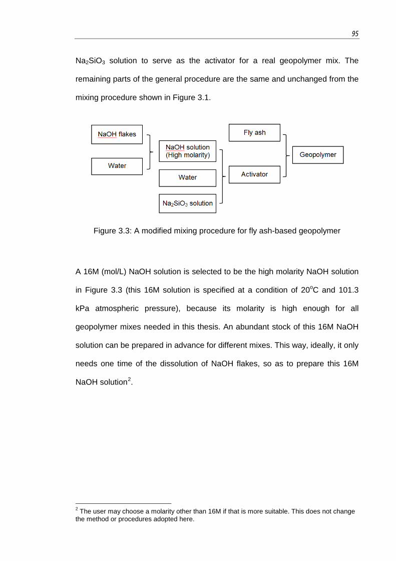
95
Na2SiO3 solution to serve as the activator for a real geopolymer mix. The
remaining parts of the general procedure are the same and unchanged from the
mixing procedure shown in Figure 3.1.
Figure 3.3: A modified mixing procedure for fly ash-based geopolymer
A 16M (mol/L) NaOH solution is selected to be the high molarity NaOH solution
in Figure 3.3 (this 16M solution is specified at a condition of 20oC and 101.3
kPa atmospheric pressure), because its molarity is high enough for all
geopolymer mixes needed in this thesis. An abundant stock of this 16M NaOH
solution can be prepared in advance for different mixes. This way, ideally, it only
needs one time of the dissolution of NaOH flakes, so as to prepare this 16M
NaOH solution2.
2 The user may choose a molarity other than 16M if that is more suitable. This does not change the method or procedures adopted here.

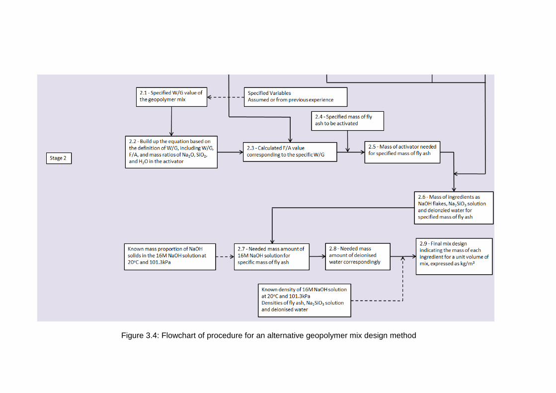
Figure 3.4: Flowchart of procedure for an alternative geopolymer mix design method

98 3. Geopolymer mix design
Correspondingly, the mix design procedure is also modified to suit the new
mixing procedure of Figure 3.3, as displayed in Figure 3.4. In this new mix
design procedure, the steps from 1.1 to 2.6 are exactly the same as those in the
old one in Figure 3.2. After these steps, the user is able to obtain the needed
masses of NaOH flakes, Na2SiO3 solution and water for activating a specified
mass of fly ash (1000 grams in the example proposed here). Based on these, it
can calculate the proportions of ingredients for the new mix design that uses a
16M NaOH solution as the source of NaOH.
This is better illustrated based on the following example:
To start with, from the example discussed in section 3.4, to activate 1000 grams
of fly ash with an activator Na2O·SiO2·13H2O and a W/G ratio of 0.26, we
required 53.13 grams of NaOH flakes, 262.47 grams of Na2SiO3 solution and
142.22 grams of deionised water.
The 262.47 grams of Na2SiO3 solution will not be changed since the required
amount of SiO2 is constant in both mix design procedures. Therefore, in the
new mix design which uses a 16M NaOH solution, all the 53.13 grams of NaOH
flakes are provided by the 16M NaOH solution.
It can be looked up that a 16M NaOH solution at 20oC and 101.3 kPa
atmospheric pressure conditions has a NaOH solid mass proportion of 43.68%
and a density of 1470 kg/m3 (ZXXK, 2012).
So, the required mass of the 16M NaOH solution is:
53.1343.68%
= 121.63 grams
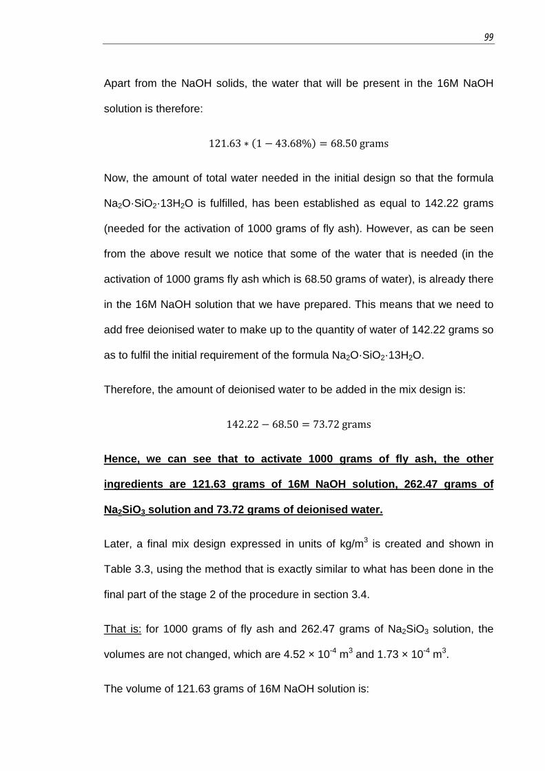
99
Apart from the NaOH solids, the water that will be present in the 16M NaOH
solution is therefore:
121.63 ∗ (1 − 43.68%) = 68.50 grams
Now, the amount of total water needed in the initial design so that the formula
Na2O·SiO2·13H2O is fulfilled, has been established as equal to 142.22 grams
(needed for the activation of 1000 grams of fly ash). However, as can be seen
from the above result we notice that some of the water that is needed (in the
activation of 1000 grams fly ash which is 68.50 grams of water), is already there
in the 16M NaOH solution that we have prepared. This means that we need to
add free deionised water to make up to the quantity of water of 142.22 grams so
as to fulfil the initial requirement of the formula Na2O·SiO2·13H2O.
Therefore, the amount of deionised water to be added in the mix design is:
142.22 − 68.50 = 73.72 grams
Hence, we can see that to activate 1000 grams of fly ash, the other
ingredients are 121.63 grams of 16M NaOH solution, 262.47 grams of
Na2SiO3 solution and 73.72 grams of deionised water.
Later, a final mix design expressed in units of kg/m3 is created and shown in
Table 3.3, using the method that is exactly similar to what has been done in the
final part of the stage 2 of the procedure in section 3.4.
That is: for 1000 grams of fly ash and 262.47 grams of Na2SiO3 solution, the
volumes are not changed, which are 4.52 × 10⁻⁴ m3 and 1.73 × 10⁻⁴ m3.
The volume of 121.63 grams of 16M NaOH solution is:

100 3. Geopolymer mix design
121.631470 ∗ 1000
= 8.27 ∗ 10−5 m3
The volume of 73.72 grams of water is:
73.721000 ∗ 1000
= 7.37 ∗ 10−5 m3
Then, the volumetric proportions of the ingredients are:
Fly ash
4.52 ∗ 10−4
(4.52 ∗ 10−4 + 8.27 ∗ 10−5 + 1.73 ∗ 10−4 + 7.37 ∗ 10−5)= 0.579
16M NaOH solution
8.27 ∗ 10−5
(4.52 ∗ 10−4 + 8.27 ∗ 10−5 + 1.73 ∗ 10−4 + 7.37 ∗ 10−5)= 0.106
Na2SiO3 solution
1.73 ∗ 10−4
(4.52 ∗ 10−4 + 8.27 ∗ 10−5 + 1.73 ∗ 10−4 + 7.37 ∗ 10−5)= 0.221
Deionised water
7.37 ∗ 10−5
(4.52 ∗ 10−4 + 8.27 ∗ 10−5 + 1.73 ∗ 10−4 + 7.37 ∗ 10−5)= 0.094
Then, the mass quantity of each ingredient for 1 m3 mix is:
Fly ash
0.579 ∗ 2210 = 1279.59 kg/m3
16M NaOH solution
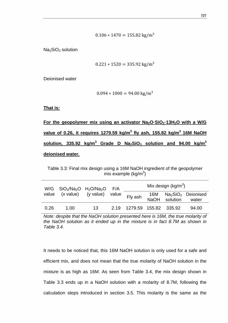
101
0.106 ∗ 1470 = 155.82 kg/m3
Na2SiO3 solution
0.221 ∗ 1520 = 335.92 kg/m3
Deionised water
0.094 ∗ 1000 = 94.00 kg/m3
That is:
For the geopolymer mix using an activator Na2O·SiO2·13H2O with a W/G
value of 0.26, it requires 1279.59 kg/m3 fly ash, 155.82 kg/m3 16M NaOH
solution, 335.92 kg/m3 Grade D Na2SiO3 solution and 94.00 kg/m3
deionised water.
Table 3.3: Final mix design using a 16M NaOH ingredient of the geopolymer mix example (kg/m3)
W/G value
SiO2/Na2O (x value)
H2O/Na2O (y value)
F/A value
Mix design (kg/m3)
Fly ash 16M NaOH
Na2SiO3 solution
Deionised water
0.26 1.00 13 2.19 1279.59 155.82 335.92 94.00
Note: despite that the NaOH solution presented here is 16M, the true molarity of the NaOH solution as it ended up in the mixture is in fact 8.7M as shown in Table 3.4.
It needs to be noticed that, this 16M NaOH solution is only used for a safe and
efficient mix, and does not mean that the true molarity of NaOH solution in the
mixture is as high as 16M. As seen from Table 3.4, the mix design shown in
Table 3.3 ends up in a NaOH solution with a molarity of 8.7M, following the
calculation steps introduced in section 3.5. This molarity is the same as the

102 3. Geopolymer mix design
molarity of NaOH solution in the mix design of Table 3.1, meaning that the two
mix design procedures proposed here and in section 3.4 would not change the
molarity of NaOH solution.
Table 3.4: Comparison of the molarity of NaOH solution between different mix designs
Mix design
using NaOH flakes
Mix design using NaOH
solution
W/G ratio 0.26 0.26
SiO2/Na2O (x value) 1 1
H2O/Na2O (y value) 13 13
F/A ratio 2.19 2.19
Fly ash (kg/m3) 1261.91 1279.59
NaOH flakes (kg/m3) 68.16 -
16M NaOH solution (kg/m3) - 155.82
Na2SiO3 solution (kg/m3) 331.36 335.92
Deionised water (kg/m3) 179.00 94.00
Molarity of NaOH solution (M) 8.7 8.7
Otherwise, the figures in the mix design of Table 3.3 are slightly different from
those of Table 3.1, despite that these two tables are made with the same values
of x, y and W/G. Nevertheless, the author considers it reasonable since the
above two mix designs are theoretically calculated based on two different
mixing procedures, where one uses NaOH flakes and the other uses a 16M
NaOH solution. The calculated figures in above mix designs are relevant to the
volumetric proportions and densities of the ingredients. However, in the case of

103
using the NaOH as flakes, when the volumes were calculated, the NaOH
volume was based on the density of the flakes. On the other hand, when the
NaOH volume was calculated in the modified method, the density of NaOH 16M
solution which was used was that sourced from the standard, hence an
inevitable discrepancy will occur, albeit slight. Moreover, in the case of
cementitious materials mix design, the actual mix design is usually obtained
after a further modification based on trial tests from the theoretically calculated
one (Neville, 1996). Therefore, it seems that a similar modification process is
required for dealing with the discrepancy in the above geopolymer mix designs.
Furthermore, the mass proportions of the chemical components involved in
geopolymerisation, such as fly ash, NaOH, Na2SiO3 and water, are not
influenced because they are only relevant to the criteria of SiO2/Na2O,
H2O/Na2O and W/G that are set to be the same in above two mix design
procedures, as introduced in sections 3.4 and 3.6.
3.7 Mix Designs used in this Thesis
The mix design researched in this chapter aims to create the mix designs for
geopolymer mixes needed in the rest of the research and discussed in following
chapters, including mixes for the geopolymer pastes, the geopolymer
aggregates, and the geopolymer binders for concrete and mortar productions.
The mix designs used in these investigations, which have been done following
the mix design procedure illustrated in this chapter, are presented in Table 3.5.
For safety and efficiency reasons, as preferred by the author, the mix designs in
Table 3.5 use a 16M NaOH solution as the stock solution according to the
principles explained in the previous paragraphs. Thus, the 16M NaOH solution

104 3. Geopolymer mix design
appears in Table 3.5 as an ingredient of the activator. The mix designs for the
binder in concrete and mortar mixes as presented in the Table 3.5, are made for
1 m3 purely geopolymer mix, but can be modulated in quantities according to
the real proportion of geopolymer binder in any specific mix.
Table 3.5: Mix designs for geopolymers used in this thesis
x y W/G F/A Fly ash (kg/m3)
16M NaOH (kg/m3)
Na2SiO3 (kg/m3)
Water (kg/m3)
Purely Geopolymer, paste mixes
1.25 11 0.23 2.16 1310.65 131.04 461.90 13.62
1.25 11 0.24 2.05 1283.42 135.00 475.88 14.03
1.25 11 0.25 1.96 1256.87 138.87 489.52 14.44
1.25 11 0.26 1.86 1230.98 142.65 502.82 14.83
1.25 11 0.22 2.28 1338.98 127.01 447.68 13.20
1.25 12 0.24 2.16 1297.98 123.12 433.97 43.42
1.25 13 0.26 2.06 1259.41 119.46 421.07 71.84
Purely Geopolymer, aggregate mixes
1.25 11 0.24 2.05 1283.42 135.00 475.88 14.03
1.25 12 0.24 2.16 1297.98 123.12 433.97 43.42
1.25 11 0.26 1.86 1230.98 142.65 502.82 14.83
Purely Geopolymer, concrete mixes
1.25 11 0.24 2.05 1283.42 135.00 475.88 14.03
1.25 11 0.26 1.86 1230.98 142.65 502.82 14.83
Purely Geopolymer, mortar mixes
1.25 11 0.26 1.86 1230.98 142.65 502.82 14.83
3.8 Conclusions
This chapter presents a mix design procedure for a fly ash-based geopolymer
made from fly ash, NaOH flakes, Na2SiO3 solution and water. This mix design
procedure distinguishes each geopolymer mix by the criteria of SiO2/Na2O,

105
H2O/Na2O and W/G, with which a final mix design can be created to satisfy the
manufacture of desired geopolymer materials. This procedure offers a
consistent and systematic method of creating the geopolymer mix designs used
in this research and presented in the following chapters of this thesis.

106 4. Curing regime for geopolymer synthesis
Chapter 4
Curing Regime for Geopolymer Synthesis
4.1 Introduction
This chapter focuses on the effect of curing regime for fly ash-based
geopolymer synthesis. Curing regime generally regulates the atmospheric
conditions applied to facilitate the development of a fresh geopolymer to obtain
the desired properties. In this chapter, the effect of curing temperature is firstly
researched. This involves a mild-temperature heat curing method (including
different heating temperature and heating time) and a room-temperature curing
method. Apart from this, the effect of moisture condition during the curing of
geopolymer is also researched, in order to enhance the properties of end-
product through a better control of the moisture condition. Moreover, the effect
of curing period for room temperature-cured (ambient-cured) geopolymer is
discussed. The outcomes of this chapter aim to provide knowledge needed for
the decision of curing regime in future geopolymer aggregate manufacture.
4.2 Previous Research on Curing of Geopolymer Synthesis
Over recent decades, there has been a great deal of research on developing
the curing regime for fly ash-based geopolymer synthesis.
A heat treatment is always preferred to attain a good and fast gain in strength of
a geopolymer, which is a thermoset inorganic polymer, and is particularly critical
for a geopolymer created from fly ash which needs relatively higher activation
energy than other raw materials (Bakharev, 2005a, Jiang and Roy, 1990). Such
heating usually proceeds at mild temperatures of 40-80oC for days after the
107
casting of a fresh geopolymer (Provis et al., 2009, Rangan, 2007, Palomo et al.,
1999, Kong et al., 2007).
Although a high curing temperature is better for the development of a fresh
geopolymer (Sindhunata et al., 2006), if it is too high, it can have a negative
effect on the end product (van Jaarsveld et al., 2002). On the other hand, a
longer heating time can improve the properties of geopolymers, but the rate of
improvement is only significant in the first 24 hours and then it becomes much
slower (Fernández-Jiménez et al., 2006). It has been suggested that,
considering the balance between outcomes and costs, an optimum curing
regime for fly ash-based geopolymer concretes is 60oC for 24 hours (Hardjito
and Rangan, 2005, Rangan, 2007). Moreover, several hours of resting before
heating is found to be beneficial for the strength gain in a geopolymer
(Bakharev, 2005a).
The idea of ambient curing held at room temperature with no heat treatment has
also been investigated (Rovnaník, 2010). Although the properties of a
geopolymer are weakened without heat treatment, to compensate for this,
several methods have been tried, such as using a prolonged curing period (Vijai
et al., 2010), reducing the fly ash’s particle size by mechanical milling (Kumar
and Kumar, 2010, Temuujin et al., 2009) or grinding (Somna et al., 2011),
adding reactive components such as GGBFS (Nath and Sarker, 2012,
Davidovits, 2013), and employing a relatively lower curing moisture (Perera et
al., 2007, Xie and Kayali, 2014). Along with heated geopolymers, a room
temperature-cured geopolymer and the relevant curing conditions that affect its
development are also researched in this chapter.

108 4. Curing regime for geopolymer synthesis
4.3 Curing Temperature
The effect of curing temperature for geopolymer manufacture is firstly
investigated. For a fly ash-based geopolymer, a mild-temperature heating from
40-80oC is always preferred in research and in practical field, where the heating
temperature and heating time are influential for final properties (Provis et al.,
2009, Rangan, 2007, Palomo et al., 1999, Kong et al., 2007). Despite this, an
ambient curing conducted at room temperature (20-23oC) can also be workable
for geopolymer synthesis (Rovnaník, 2010). Although the above literature on
the effects of heating and ambient-curing is already quite detailed, the author
still considers it necessary to examine these effects for the geopolymer mixes
included in this thesis, because these geopolymers are created from a unique
fly ash sample as seen from Chapter 2.
Applying a certain heat treatment to a fresh fly ash-based geopolymer is a
traditional method for facilitating the geopolymer’s development, and normally
consists of the following steps (Provis et al., 2009, Rangan, 2007):
a) rest the fresh geopolymer samples in sealed moulds at room
temperature for a certain period of 6-48 hours called the ‘resting time’;
b) place the geopolymer samples in an oven for a certain period (24-72
hours) and heat at a mild temperature (40-80oC);
c) remove the geopolymer samples from the oven and rest them at room
temperature for a certain period (8-24 hours) to cool down; and
d) demould the geopolymer samples and continue to rest them at a
controlled room-temperature environment for a certain period before use
for tests or applications.

109
In contrast, under the ambient-curing regime, which does not include any heat
treatment, fresh geopolymer samples are normally placed in a specified room-
temperature curing condition for a certain period. They are usually sealed in
moulds to prevent moisture loss but can also be demoulded for different
ambient conditions after they are initially hardened. Ambient-cured geopolymer
may not develop as fast as the heated one, but is also able to achieve a high
quality in end-product (Kumar and Kumar, 2010), and therefore is considered in
this section.
4.3.1 Geopolymer Mix
Table 4.1: Mix design of geopolymers for curing regime research
Fly ash batch 2012-12-13
W/G value 0.24
SiO2/Na2O (x value) 1.25
H2O/Na2O (y value) 11
Fly ash/Activator (F/A) 2.05
Fly ash (kg/m3) 1283.42
16M NaOH solution (kg/m3) 135.00
Na2SiO3 solution (kg/m3) 475.88
Water (kg/m3) 14.03
The mix design shown in Table 4.1 is applied for the geopolymer mixes used in
this section. In this mix design, SiO2/Na2O and H2O/Na2O ratios are specified as
1.25 and 11 respectively, based on the previous research of Provis et al. (2009).
Besides, the W/G ratio is set to be 0.24, based on Rangan’s research (Rangan,

110 4. Curing regime for geopolymer synthesis
2007) and the author’s trial mixes, which is suitable for making a geopolymer
mix with sufficient workability and strength. This mix design is created following
the mix design procedure proposed in Chapter 3. Cubic 50mm×50mm×50mm
geopolymer samples are manufactured following the same procedure
previously illustrated in Chapter 2, section 2.3.
4.3.2 Curing Regime
Different curing temperature and time are designed to be evaluated as
presented in Table 4.2. A heat treatment at 40-80oC for 1 or 3 days is
investigated, as suggested in previous literature (Provis et al., 2009, Rangan,
2007, Palomo et al., 1999, Kong et al., 2007). Also, an ambient curing regime
held in the ER at 20oC and 50% RH is researched. All samples go through a
specified 7-day curing regime after casting and then undergo the required
testing.
Table 4.2: Curing regimes investigated for optimum geopolymer growth
Code Resting
time (hours)
Heat (oven)
Heating time (hours)
Temperature (oC)
Testing age (days)
20ER 6 - - 20 7
H40-1d 6 Yes 24 40 7
H40-3d 6 Yes 72 40 7
H60-1d 6 Yes 24 60 7
H60-3d 6 Yes 72 60 7
H80-1d 6 Yes 24 80 7
H80-3d 6 Yes 72 80 7

111
4.3.3 Strength
The strength of hardened geopolymers cured at different conditions has been
given a special attention in this investigation. This strength performance is
represented by the compressive strength value of cubic geopolymer sample,
which has been measured using a TECNOTEST compression testing machine
(3000 kN capacity). The loading rate was set constant at 0.33 MPa/sec, based
on the recommended loading rate range in US standard ASTM C109 (ASTM,
2012c). The compressive strength result shown in Figure 4.1 is related to each
specific curing regime regulated as shown in Table 4.2, where each result is the
average of six samples from the same mixing batch.
Figure 4.1 basically demonstrates that a higher temperature and longer heating
time results in a higher strength gain, which agrees with previous finding
(Sindhunata et al., 2006). The cubic geopolymer sample which has been
through a heat curing at 80oC for 3 days achieved the highest strength of 52.94
MPa. On the other hand, the two curing regimes of 80oC for 1 day and 60oC for
3 days resulted in a comparable compressive strength. From the above, a
curing regime of 80oC for 3 days performs best in strength, and therefore is
preferred for the manufacture of geopolymer aggregates introduced in Chapter
5.
The ambient-cured geopolymer sample has the lowest compressive strength,
which is far behind those of the heated ones. This proves the general
understanding of the advantage of heating for fly ash-based geopolymer
(Sindhunata et al., 2006, Rangan, 2007). Meanwhile, it shows a significant gap
in strength between the ambient-cured and heat-cured geopolymer samples.

112 4. Curing regime for geopolymer synthesis
For a short-term curing procedure, such as 7 days, it seems that an ambient-
cured geopolymer cannot provide the needed strength for further structural use,
unless a modification on the curing regime is made.
Figure 4.1: 7-day compressive strengths of geopolymers under different curing regimes (corresponding to the mix in Table 4.1)
4.4 Curing Moisture Condition
Curing regime for geopolymers generally concentrates on curing temperature
and period, but rarely on the moisture condition. Nevertheless, an appropriate
curing moisture condition is likely to affect the developments in a fresh
geopolymer, based on the current findings (Perera et al., 2007, Xie and Kayali,
2014). Hence, in this section, research on the effect of curing moisture on the
developments in geopolymer, is presented.
2.18
12.99
28.68
39.46
24.45
38.65
52.94
0
10
20
30
40
50
60
20 40 60 80
Com
pres
sive
str
engt
h (M
Pa)
Curing temperature (oC)
ER
heat 1d
heat 3d

113
This ‘curing moisture’ research concentrates on the ambient-cured geopolymer
instead of the heated one. This is because a heated geopolymer has already
been much developed in its microstructure by heat treatment (Bakharev, 2005a,
Jiang and Roy, 1990), and therefore is considered less affected by the moisture
condition applied afterwards.
4.4.1 Geopolymer Mix
The geopolymer mixes designed here were devoted for the research into the
effects of different curing moisture conditions. These mixes were designed with
different initial water amounts so as to observe the possible effects (if any) of
the curing moisture conditions in relation to differences in the original water
content.
To fulfil this, the geopolymer mixes are intentionally designed so that they all
contain equal masses of the fly ash and activator solutes while their water
contents are different. Following the mix design procedure in Chapter 3, these
mix designs involve making the ratio of fly ash to Na2O+SiO2 constant and
varying the ratio of H2O/Na2O (the y value in Na2O·xSiO2·yH2O). The final mix
designs are presented in Table 4.3 in which all these designs are based on fly
ash content of 1000 grams in order to highlight the variation in water content.
Here, as the usages of NaOH and Na2SiO3 solutions are constant, the water
amount from these two solutions must be the same for all mixes. So, the
variation in water content among the mixes is rather realised by the quantity of
free water, as seen in Table 4.3. For 1000 grams of fly ash, 94.89 grams of 16M
NaOH and 334.34 grams of Na2SiO3 solutions remain constant, with the free

114 4. Curing regime for geopolymer synthesis
water varying from 9.82 grams to 57.05 grams. The mixing procedure for
geopolymer samples is the same as described in the last section.
Table 4.3: Mix designs for geopolymer mixes with different initial water contents
SiO2/Na2O (x value)
H2O/Na2O (y value) W/G F/A
Mix designs (grams)
Fly ash 16M NaOH
Na2SiO3 solution Water
1.25 11 0.22 2.28 1000 94.89 334.34 9.82
1.25 12 0.24 2.16 1000 94.89 334.34 33.43
1.25 13 0.26 2.06 1000 94.89 334.34 57.05
4.4.2 Curing Regime
During the first 7 days, the curing regime was the same for all samples, namely:
keeping the sample in a sealed mould and placing it inside the ER at 20oC. The
curing regimes are designed to vary the curing moisture at a certain time (7
days) after the casting of the fresh geopolymer. In this way, curing moisture
condition can be varied during the polycondensation stage which is a stage
more vulnerable to moisture change (Zuhua et al., 2009, Davidovits, 1989).
After mixing, fresh geopolymer samples were sealed in the moulds, rested for 6
hours and placed in the ER at 20oC for the first 7 days. After this 7-day ambient
curing, the geopolymer samples were demoulded, and later cured in the ER
under three different moisture conditions displayed in Table 4.4: (1) unsealed
(A); (2) sealed (AS); or (3) dried inside a desiccator over the anhydrous silica
gel (AD). The sealed curing aims to retain water during 7 to 14 days after
casting and the unsealed and desiccated aimed to release water in a semi-dry
condition with 50% RH and a dry condition respectively. A vacuum facility was
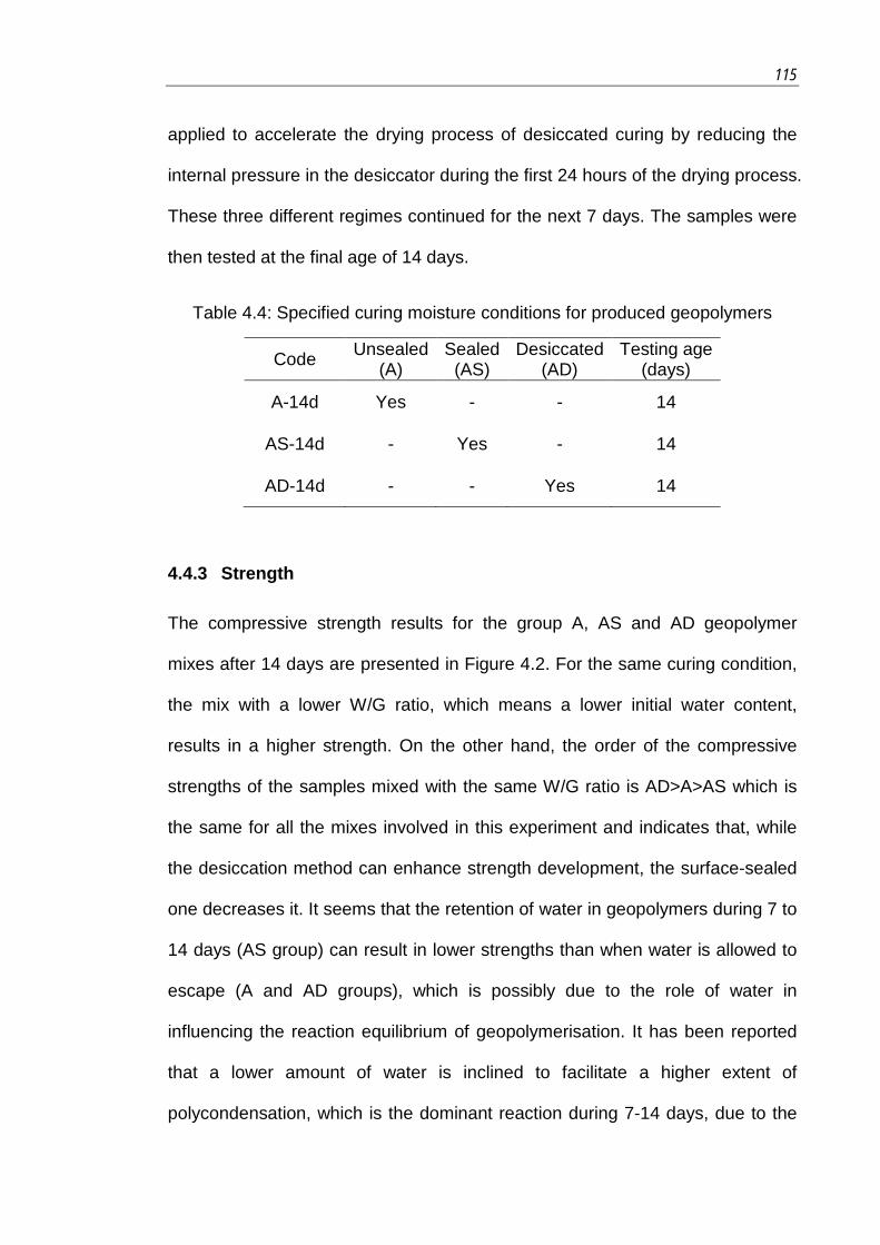
115
applied to accelerate the drying process of desiccated curing by reducing the
internal pressure in the desiccator during the first 24 hours of the drying process.
These three different regimes continued for the next 7 days. The samples were
then tested at the final age of 14 days.
Table 4.4: Specified curing moisture conditions for produced geopolymers
Code Unsealed (A)
Sealed (AS)
Desiccated (AD)
Testing age (days)
A-14d Yes - - 14
AS-14d - Yes - 14
AD-14d - - Yes 14
4.4.3 Strength
The compressive strength results for the group A, AS and AD geopolymer
mixes after 14 days are presented in Figure 4.2. For the same curing condition,
the mix with a lower W/G ratio, which means a lower initial water content,
results in a higher strength. On the other hand, the order of the compressive
strengths of the samples mixed with the same W/G ratio is AD>A>AS which is
the same for all the mixes involved in this experiment and indicates that, while
the desiccation method can enhance strength development, the surface-sealed
one decreases it. It seems that the retention of water in geopolymers during 7 to
14 days (AS group) can result in lower strengths than when water is allowed to
escape (A and AD groups), which is possibly due to the role of water in
influencing the reaction equilibrium of geopolymerisation. It has been reported
that a lower amount of water is inclined to facilitate a higher extent of
polycondensation, which is the dominant reaction during 7-14 days, due to the
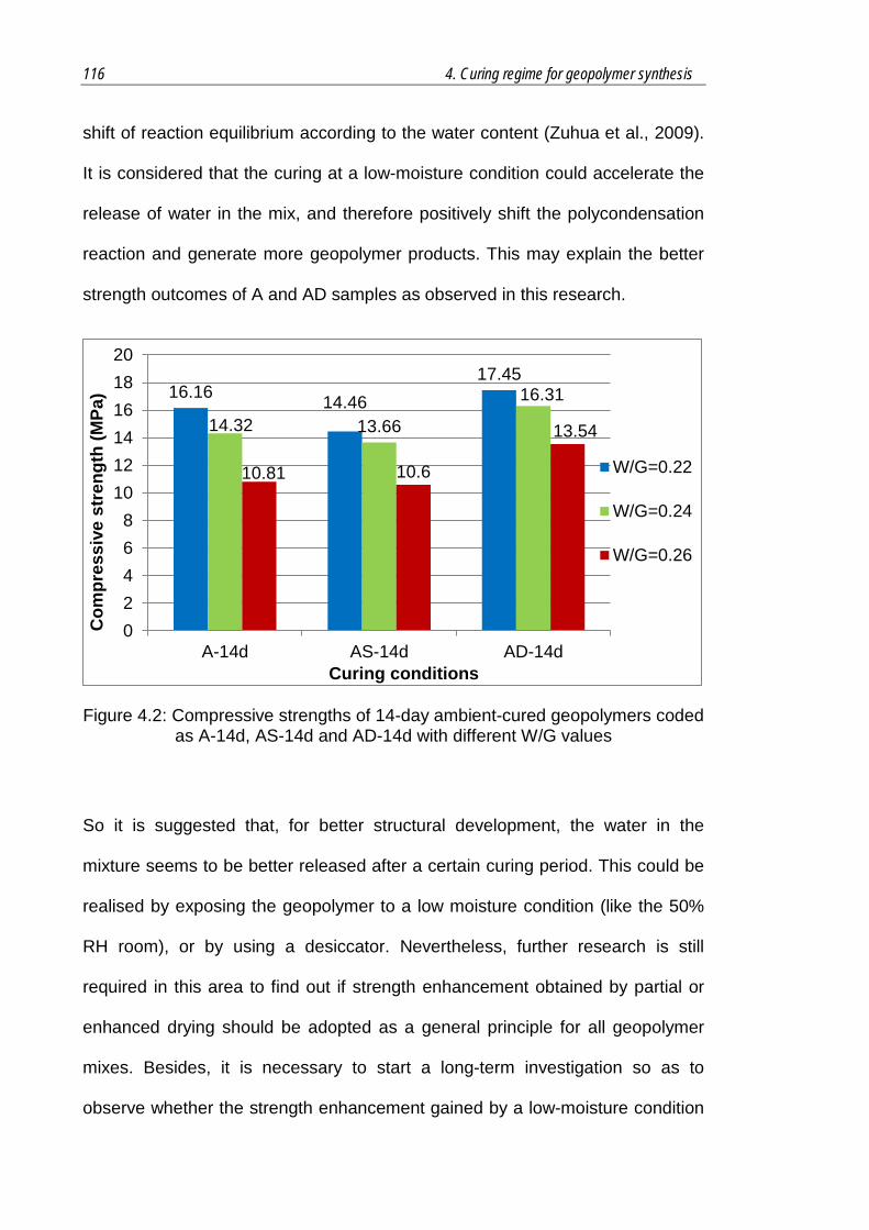
116 4. Curing regime for geopolymer synthesis
shift of reaction equilibrium according to the water content (Zuhua et al., 2009).
It is considered that the curing at a low-moisture condition could accelerate the
release of water in the mix, and therefore positively shift the polycondensation
reaction and generate more geopolymer products. This may explain the better
strength outcomes of A and AD samples as observed in this research.
Figure 4.2: Compressive strengths of 14-day ambient-cured geopolymers coded as A-14d, AS-14d and AD-14d with different W/G values
So it is suggested that, for better structural development, the water in the
mixture seems to be better released after a certain curing period. This could be
realised by exposing the geopolymer to a low moisture condition (like the 50%
RH room), or by using a desiccator. Nevertheless, further research is still
required in this area to find out if strength enhancement obtained by partial or
enhanced drying should be adopted as a general principle for all geopolymer
mixes. Besides, it is necessary to start a long-term investigation so as to
observe whether the strength enhancement gained by a low-moisture condition
16.16 14.46 17.45
14.32 13.66
16.31
10.81 10.6
13.54
02468
101214161820
A-14d AS-14d AD-14d
Com
pres
sive
str
engt
h (M
Pa)
Curing conditions
W/G=0.22
W/G=0.24
W/G=0.26

117
can be maintained for such ambient-cured geopolymers as the ones reported
above.
This section also suggests that, an early demoulding of a geopolymer sample to
make it exposed to a low-moisture condition may facilitate its strength
development. If such geopolymer is not concerned about achieving certain
shape, texture or dimensions, such as producing aggregates, then such early
demoulding may be done even slightly before the full set of the fresh
geopolymer. However, it is considered by the author that a too early demoulding
should not be suitable, because an abundant amount of water in the mix is
highly needed in an early stage (first 2-3 days of curing) for dissolution and
hydrolysis reactions (Zuhua et al., 2009). A research on an optimum
demoulding time is needed in the future.
Moreover, combined with the strength result shown in Figure 4.1, (even though
the mixes represented in Figure 4.1 are not the same as those in Figure 4.2) yet
it can be concluded when studying the two Figures that there is a remarkable
increase in strength from 7 days to 14 days of the tested ambient-cured
geopolymer samples. This phenomenon implies a possible benefit from a longer
curing time on an ambient-cured geopolymer. This phenomenon will be
discussed in the following sections that focus on the effect of curing period.
4.5 Curing Period (Short-term)
This section deals with the research on the effect of curing period for
geopolymer synthesis. Both heat curing and ambient curing regimes are
included. It is found that a heated geopolymer is stronger than an ambient-
cured geopolymer if both of them are cured for the same period. But an

118 4. Curing regime for geopolymer synthesis
ambient-cured geopolymer is likely to obtain a more obvious strength gain after
a prolonged curing period, and therefore would eventually achieve a
comparable strength with the heated one that is made with the same mix design
but heated for a short curing period. Therefore, it seems that a prolonged
ambient curing period would be workable for improving the performance of an
ambient-cured geopolymer material.
4.5.1 Geopolymer Mix
The geopolymer mixes manufactured from the same mix designs shown in the
last section (Table 4.3) are made and used for experiments regarding the curing
period. These include the mixes with different initial water contents in order to
serve the purpose of doing a satisfactorily more complete investigation.
4.5.2 Curing Regime
Two curing series are used, one is a mild-temperature heat treatment from 40-
80oC, and the other is an ambient-cured regime with samples held in the ER at
20oC and 50% relative humidity (RH). Details of the curing regimes used
throughout this section are presented in Table 4.5 and, under both, the freshly
mixed geopolymers are first sealed and rested for 6 hours in the ER, for an
enhanced geopolymer development (Bakharev, 2005a). Then, those to be
heated are placed in an electric oven at 60oC for 4 or 24 hours, and later
removed and demoulded, and stored in the ER for further testing. Also, a
controlled ambient-curing procedure is undertaken to seal fresh geopolymer
samples in moulds and keep them in the ER at 20oC. They are sealed to
achieve sufficiently uniform reactions in the first 7 days, then some are directly

119
tested at the age of 7 days while the rest are demoulded and exposed to the
atmosphere of the ER for a further 7 days.
All three geopolymer mixes detailed in Table 4.3 were manufactured and cured
at the four different curing regimes included in Table 4.5. For each specific mix
and each specific curing regime, the result is the average of three geopolymer
samples made from the same batch.
Table 4.5: Specified curing procedures for heat-cured and ambient-cured geopolymers
Code Resting time (hours)
Temperature (oC)
Heating time (hours)
Testing age (days)
H-24h
6
60 24 7
H-4h 60 4 7
A-7d 20 - 7
A-14d 20 - 14
4.5.3 Density and Strength
The density of a cubic geopolymer sample was measured by dividing its mass
by its volume, with the latter specifically measured using a water displacement
method. Also, a normal compressive strength test was conducted to represent
the mechanical property of each geopolymer produced.
The density and strength outcomes for the heated geopolymers are presented
in Figure 4.3. For all three mixes, the H-24h samples yield lower densities than
the H-4h ones which implies that heating may help to release more water into
the semi-dry atmosphere of 50% RH after demoulding and, therefore, the longer
the heating period, the lower the density.

120 4. Curing regime for geopolymer synthesis
Figure 4.3: Density and compressive strength results for heated geopolymer samples
The H-24h samples achieved higher compressive strength values than the H-4h
ones. Moreover, when the curing period is the same, a sample with a lower
1.67
1.65
1.68
1.67
1.70
1.69
1.62
1.63
1.64
1.65
1.66
1.67
1.68
1.69
1.70
1.71
H-4h H-24h
Den
sity
(g/c
m3 )
Heating period
W/G=0.22
W/G=0.24
W/G=0.26
15.71
42.07
11.05
36.25
10.18
30.32
0
5
10
15
20
25
30
35
40
45
0 4 8 12 16 20 24 28
Com
pres
sive
str
engt
h (M
Pa)
Heating period (hour)
W/G=0.22
W/G=0.24
W/G=0.26
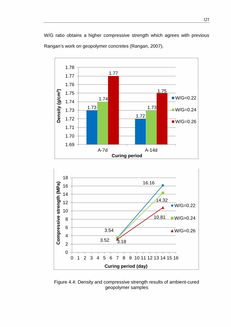
121
W/G ratio obtains a higher compressive strength which agrees with previous
Rangan’s work on geopolymer concretes (Rangan, 2007).
Figure 4.4: Density and compressive strength results of ambient-cured geopolymer samples
1.73
1.72
1.74
1.73
1.77
1.75
1.69
1.70
1.71
1.72
1.73
1.74
1.75
1.76
1.77
1.78
A-7d A-14d
Den
sity
(g/c
m3 )
Curing period
W/G=0.22
W/G=0.24
W/G=0.26
3.54
16.16
3.52
14.32
3.18
10.81
0
2
4
6
8
10
12
14
16
18
0 1 2 3 4 5 6 7 8 9 10 11 12 13 14 15 16
Com
pres
sive
str
engt
h (M
Pa)
Curing period (day)
W/G=0.22
W/G=0.24
W/G=0.26

122 4. Curing regime for geopolymer synthesis
Similarly, the density and compressive strength of an ambient-cured
geopolymer are also measured and presented in Figure 4.4. The mix with a
lower W/G ratio has a lower density. Besides, for the mix with the same W/G
ratio, A-7d sample has a higher density than the A-14d one which, it is
concluded, is the result of a mass reduction in water due to exposure to the 50%
RH atmosphere in the ER from 7 to 14 days.
It can be seen that an ambient-cured geopolymer after 7 days obtains a much
lower strength than that of a heated geopolymer cured within the same period.
This is consistent with the previous finding reported in section 4.3 of this chapter.
However, the same ambient-cured mix could end in a much higher strength
after 7 more days of ambient curing held in a 50% RH atmosphere, as seen in
Figure 4.4. Apart from a benefit from a reduced moisture condition, as
discussed in last section, a prolonged curing time also seems effective for a
strength gain in an ambient-cured geopolymer. In contrast, it has been reported
that a longer curing time at a room temperature could not significantly enhance
the strength of a heated geopolymer (Fernández-Jiménez et al., 2006). A 14-
day ambient-cured sample is observed to achieve a comparable strength with a
7-day 4-hour heated sample made from the same mix design, which is same for
all tested mixes with different W/G ratios. Therefore, it is considered that a
prolonged curing may function like a short-term heating for geopolymer
development.
Also, from this research, it is observed that a prolonged room-temperature
drying at a low humidity condition (50% RH) is likely to be an ideal curing
regime for geopolymer in terms of strength development. This is however,
different with the case of OPC, which is preferred to be cured at a room-

123
temperature and a high humidity condition (100% RH). A high water content is
required for an advanced cement hydration process in a OPC system (Lea,
1970). However, this seems not to be the case in a geopolymer one, where a
low-moisture condition after the first 7 days of curing is likely to result in a strong
end-product.
Moreover, same as the heated samples, the ambient-cured sample with a lower
W/G ratio results in a higher strength performance. From this, it is estimated
that a low initial water content may enhance the strength gain, and should be
incorporated with a prolonged curing period in geopolymer synthesis.
4.5.4 Scanning Electron Microscopy
A scanning electron microscopy (SEM) testing is used to observe the pace of
micro-structural development in the networks of produced geopolymers, and
was conducted on a HITACHI TM 3000 tabletop SEM facility at 15 kV. It was
applied on the geopolymer pieces remaining after strength tests, with four
different parts observed for each unique geopolymer mix and the dominant type
of structure seen in the SEM images chosen to be the representative image.
The images for the 7-day and 14-day ambient-cured samples with W/G=0.22
and 0.26 are presented in Figure 4.5(a) to (d). For comparison, an image of the
7-day 4-hour heat-cured sample with W/G=0.22 is presented in Figure 4.5(e).

124 4. Curing regime for geopolymer synthesis
Figure 4.5: SEM images of geopolymers with W/G=0.22: (a) A-7d, (b) A-14d and (e) H-4h; and with W/G=0.26: (c) A-7d and (d) A-14d
The ambient-cured geopolymer with W/G=0.22 displays a clear densification
process in structure from 7 to 14 days. In Figure 4.5(a), it can be seen that the
125
fly ash particles are partially dissolved and start to form small, loosely
connected blocks after 7 days of ambient curing, Then, after 14 days, they
become denser and more closely connected with a reduction in the intermediate
pores, as seen in Figure 4.5(b) tracking the structural formation pace proves
that this geopolymer can develop with a prolonged ambient curing period, which
could explain its strength gain during this period as can be seen in Figure 4.4.
The ambient-cured sample with W/G=0.26 shows a similar densification
process, but less significant than that of the sample with W/G=0.22. A higher
proportion of unreacted fly ash particles with a loose particle connections are
found as shown in Figure 4.5(c) and (d). This may be due to the lower alkali
strength caused by relatively higher water content in the W/G=0.26 sample.
Moreover, it can be noticed that there is similarity between the structure in
Figure 4.5(b), which depicts the development of a 14-day ambient-cured
geopolymer with W/G=0.22, and that in Figure 4.5(e), which represents the
same mix but heated at 60oC for 4 hours. The above two samples that have
been through different curing regimes display similar structures, and this is
consistent with their similar strength outcomes as shown in Figure 4.3 and
Figure 4.4. These similarities in micro-structural development and strength
values may indicate that the effect of heat curing (for 4 hours in this case) may
be achieved by a prolonged curing at room temperature in a relatively dry
environment.
The result of the research presented in this section, in combination with that of
section 4.4, demonstrate a possibility of applying a prolonged curing period with
a relatively dry atmosphere to enhance the strength of an ambient-cured

126 4. Curing regime for geopolymer synthesis
geopolymer. However, the research presented in this section only focuses on a
short-term period, and therefore the strengths of produced ambient-cured
geopolymers are still not very high. To deal with this, a long-term curing period
is researched and presented in the next section.
4.6 Curing Period (Long-term)
In section 4.5, it has discovered that an ambient-cured geopolymer can achieve
a strength and structural performance comparable with a heated geopolymer
when given a longer curing time. However, as this finding is arrived at during
only a very short period, the outcome of strength benefit is not very significant
yet. In this section, a long-term experiment is carried out to evaluate the
possibility of making a high-strength ambient-cured geopolymer qualified for
real structural use.
It is considered that, one shortcoming of an ambient-cured geopolymer should
be its extremely low geopolymer reaction rate, due to the absence of heat
treatment (Bakharev, 2005a, Jiang and Roy, 1990). This may explain its
extremely low-strength outcome after a short-term curing as shown in Figure
4.1. Otherwise, as a fresh ambient-cured geopolymer usually lasts longer in a
fresh stage without an early set observed, it is assumed that the extent of
geopolymer reaction can be enhanced in a longer curing period, which is the
motive of the research work in this section. This prolonged ambient-cured
geopolymer manufacture is considered appropriate for an application that does
not need a fast strength gain, such as the geopolymer aggregates. The
knowledge gained from this section will be further applied for the manufacture of
room temperature-cured geopolymer aggregates as explored in Chapter 8.

127
4.6.1 Geopolymer Mix
A mix design with a moderate water content of W/G=0.24 is selected, which is
the same as the one in Table 4.1. This mix contains a proper initial water
amount which is neither too dry nor too wet, which is considered more suitable
to represent the normal geopolymer in practical use. The geopolymer samples
are made following the same procedure presented in the last section. Three
geopolymer samples from the same batch are prepared and tested for each
specific curing regime.
4.6.2 Curing Regime
The geopolymer samples produced are placed in a container in the ER at 20oC
and 50% relative humidity for the different periods of 7, 14, 21, 28, 56 and 84
days. These samples are only sealed in the first 7 days, and later unsealed for
the rest of the curing periods. They are immediately tested once they reach their
specified curing terms.
4.6.3 Density and Strength
The specific gravities of the cubic geopolymer samples versus their different
curing periods are measured and presented in Figure 4.6. It can be seen that
the specific gravity of a geopolymer reduces in the first 14 days, slightly
increases from 14 to 28 days and reduces again from 28 to 84 days. Basically,
a longer curing period leads to a lower specific gravity.

128 4. Curing regime for geopolymer synthesis
Figure 4.6: Variations in specific density versus long-term curing period at room temperature of fly ash-based geopolymers produced
The compressive strength values of the geopolymer samples cured for different
periods are measured and presented in Figure 4.7 in which it can be seen that
longer curing periods cause higher strength gains. Despite a low strength of
less than 10 MPa in the initial days, the geopolymers tested display much
higher strengths which reach 43.96 MPa after 84 days, which is a high enough
strength as far as structural elements are concerned.
Based on the slope of the strength curve in Figure 4.7, it can be seen that the
rate of strength gain is much faster in the first 28 days, achieving almost 10
MPa increments every 7 days. Then, this rate begins to slow down, and there is
little further strength gain during 56 to 84 days, which implies that the strength
of this kind of geopolymer mix is close to the limit after 84 days of ambient
curing.
1.50
1.55
1.60
1.65
1.70
1.75
1.80
1.85
1.90
0 14 28 42 56 70 84 98
Spec
ific
grav
ity
Curing period at room temperature (days)

129
Figure 4.7: Compressive strength versus long-term curing period at room temperature of fly ash-based geopolymer whose mix design is in Table 4.1
Moreover, by comparing the geopolymer samples presented in this section with
the heated ones presented in section 4.3 using the same mix design (the
W/G=0.24 one in Table 4.1), as shown in Figure 4.8, it is found that a prolonged
curing period results in an ambient-cured geopolymer with a comparable to, or
even higher strength than those of heated geopolymers. From Figure 4.8, the
84-day ambient-cured geopolymer has a compressive strength of 43.96 MPa,
lower than only that of the geopolymer H80-3d (which undergoes heating at
80oC for 3 days) but similar to those of geopolymers H80-1d and H60-3d, and
much higher than the other heated samples.
Nevertheless, ambient curing still has a limit in terms of strength gain as it
cannot cause a fresh geopolymer to attain the same strength level that can be
realised by heat treatment. Combining Figure 4.7 and Figure 4.8, the highest
05
101520253035404550
0 14 28 42 56 70 84 98
Com
pres
sive
str
engt
h (M
Pa)
Curing period at room temperature (day)
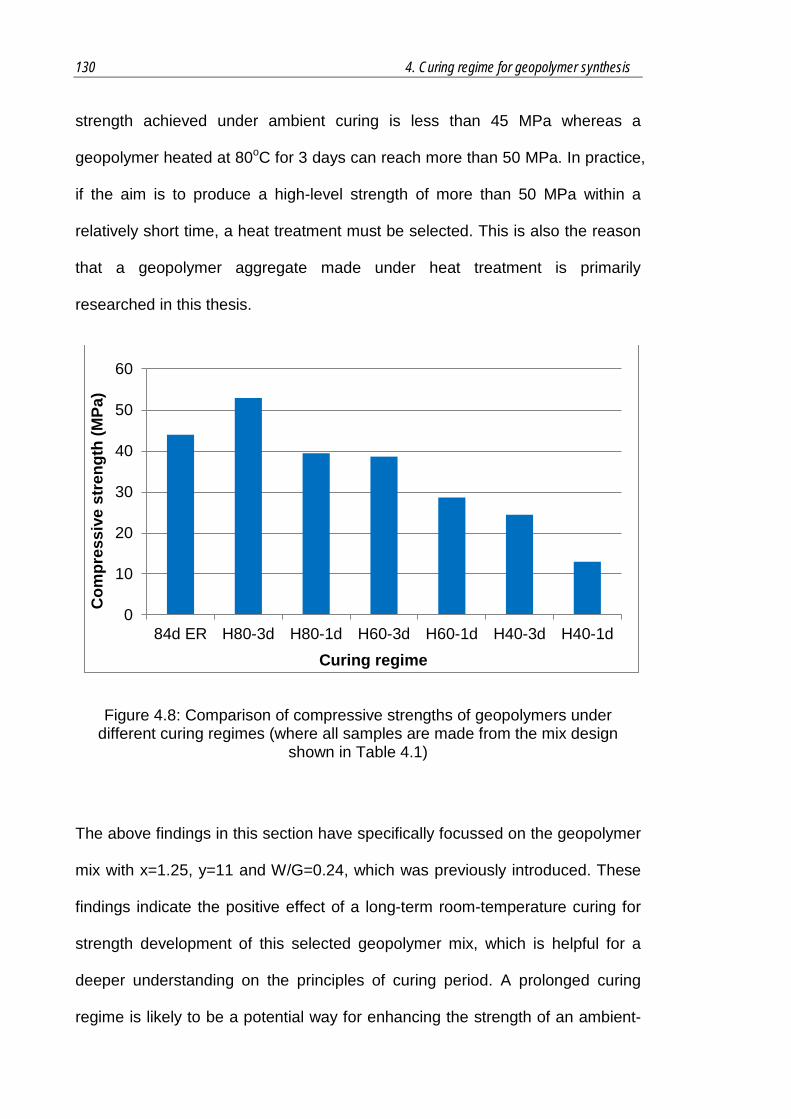
130 4. Curing regime for geopolymer synthesis
strength achieved under ambient curing is less than 45 MPa whereas a
geopolymer heated at 80oC for 3 days can reach more than 50 MPa. In practice,
if the aim is to produce a high-level strength of more than 50 MPa within a
relatively short time, a heat treatment must be selected. This is also the reason
that a geopolymer aggregate made under heat treatment is primarily
researched in this thesis.
Figure 4.8: Comparison of compressive strengths of geopolymers under different curing regimes (where all samples are made from the mix design
shown in Table 4.1)
The above findings in this section have specifically focussed on the geopolymer
mix with x=1.25, y=11 and W/G=0.24, which was previously introduced. These
findings indicate the positive effect of a long-term room-temperature curing for
strength development of this selected geopolymer mix, which is helpful for a
deeper understanding on the principles of curing period. A prolonged curing
regime is likely to be a potential way for enhancing the strength of an ambient-
0
10
20
30
40
50
60
84d ER H80-3d H80-1d H60-3d H60-1d H40-3d H40-1d
Com
pres
sive
str
engt
h (M
Pa)
Curing regime

131
cured geopolymer. This observation needs further investigation which needs to
be based on a wider selection of geopolymer mixes.
4.7 Conclusions
This chapter reports and discusses the research that deals with the effect of
curing regime on the development of fly ash-based geopolymer. The factors
studied here include curing temperature, moisture regime and curing period.
Based on the results, a heat curing method is still the better one for a fast
development in strength and structure of geopolymer mix. However, the
development of an ambient-cured geopolymer is found to be enhanced with a
reduced moisture condition and a prolonged curing period. Through this, an
ambient-cured geopolymer with a comparable strength as the heated one can
be realised, provided the time is not a constraint.
The research work reported in this chapter helps to find an optimum curing
regime used in future geopolymer aggregate manufacture. A heat curing regime
of 80oC for 3 days is selected for its advanced capability to achieve the high
strength of a fresh geopolymer, and will be applied for the manufacture of
geopolymer aggregates discussed in Chapter 5. This curing regime will also be
used for a synthesis of geopolymer binder required in concrete and mortar
mixes as presented in Chapter 7. In addition, another ambient curing regime
operating at 20oC for 84 days with a low-moisture curing condition is used for
the room temperature-cured geopolymer aggregate manufacture and will be
presented in Chapter 8.

132 5. Geopolymer aggregate (GA)
Chapter 5
Geopolymer Aggregate (GA)
5.1 Introduction
This chapter presents research on geopolymer aggregate (GA) as a new type of
FA-LWA for concrete application. It is based on the research presented in
Chapters 2, 3 and 4, which determined the fly ash, mix design procedure and
curing regime required for fly ash-based geopolymer synthesis.
Compared to traditional FA-LWA products, the manufacture of this geopolymer
aggregate is designed to be more advanced as it uses chemical bonding
instead of mechanical pressing for agglomeration, a more flexible gel-like
geopolymer for easy processing and does not involve elevated-temperature
sintering. Therefore, it aims to create a low-cost, simple and eco-friendly
artificial FA-LWA manufacturing process.
This geopolymer aggregate is composed of geopolymer materials and, based
on relevant experiments, is found to have a low specific gravity, high porosity
and high water absorption capacity but good mechanical behaviour. It is of
adequately good quality to satisfy relevant engineering standards and has
comparable properties to those of other commonly used FA-LWAs. Therefore,
this geopolymer aggregate is anticipated for the manufacture of a high-
performance lightweight concrete (LWC) with desired properties like low self-
weight and high strength/mass ratio, like the conventional FA-LWAs. And this
geopolymer aggregate may further promote this LWC industry due to its low-
cost and eco-friendly features.

133
5.2 Mix Design used for Geopolymer Aggregate
It is considered that the properties of geopolymer aggregates would be greatly
affected by the selection of geopolymer mix design. However, a complete
experimental research on the effects of different mix designs would be a huge
work requiring a long-term investigation. Instead, in this section, a desired mix
design for geopolymer aggregate manufacture is selected based on the
analysis of previous results in the literature and trial mixes by the author.
As discussed in Chapter 3, the geopolymer mix design is determined by the
criteria SiO2/Na2O, H2O/Na2O and W/G. Among them, SiO2/Na2O and
H2O/Na2O reflect the composition of the activator which is made of NaOH and
Na2SiO3 solutions. From the research of Provis et al. (2009), it was found that
usually there is an optimum range of the SiO2/Na2O ratio, which is 1.0 to 1.5, for
achieving an advanced mechanical property. Also, a H2O/Na2O ratio of 11 was
recommended in the same research (Provis et al., 2009). In addition, in the
research presented in Chapter 4, section 4.4, the mixes with a SiO2/Na2O ratio
of 1.25 and a H2O/Na2O ratio of 11-13 have been proven to be workable for
making strong geopolymer products. For these considerations, the values for
SiO2/Na2O and H2O/Na2O are specified to be respectively, 1.25 and 11 for the
geopolymer aggregate research presented in this chapter.
On the other hand, Hardjito and Rangan have studied a range of W/G ratio from
0.16 to 0.24, discovering that a lower W/G ratio in this range can result in a
higher strength performance (Hardjito and Rangan, 2005, Rangan, 2007). This
proposed range of W/G, however, is found to be not perfectly suitable for the
geopolymer mixes included in this research. Some mixes with a W/G ratio

134 5. Geopolymer aggregate (GA)
below 0.22, which should be workable according to Hardjito and Rangan’s
reports, are actually too dry to be uniformly compacted. Therefore, trial mixes
are made and tested for strength so as to find a proper W/G ratio.
The geopolymer mixes are designed with the same SiO2/Na2O (1.25) and
H2O/Na2O (11) but with different W/G ratios ranging from 0.23 to 0.26. The
resulting mix designs, which are created based on the proposed mix design
procedure in Chapter 3, are presented in Table 5.1. Cubic 50mm×50mm×50mm
geopolymer samples are manufactured following the same procedure
previously illustrated in Chapter 2, section 2.3. A heat curing regime at 80oC for
3 days is used to harden the fresh samples.
Table 5.1: Geopolymer mix designs with different W/G values
W/G value
SiO2/Na2O (x value)
H2O/Na2O (y value)
F/A value
Mix designs (kg/m3)
Fly ash 16M NaOH
Na2SiO3 solution
Deionised water
0.23 1.25 11 2.16 1310.65 131.04 461.90 13.62
0.24 1.25 11 2.05 1283.42 135.00 475.88 14.03
0.25 1.25 11 1.96 1256.87 138.87 489.52 14.44
0.26 1.25 11 1.86 1230.98 142.65 502.82 14.83
The compressive strength of the hardened geopolymer samples on the 7th day
after mixing was measured, using a TECNOTEST compression testing machine
(3000 kN capacity). The final compressive strength value for each unique
geopolymer mix is the average of six cubic samples, as displayed in Figure 5.1.
As is clear in Figure 5.1, the geopolymers made in this research can achieve
good strengths higher than 45 MPa within 7 days. Also, the geopolymer with

135
W/G=0.24 has the highest of all the mixes tested, 52.94 MPa, while that with
W/G=0.26 has the lowest of 47.16 MPa.
The difference in W/G ratio is not significant for the tested hardened samples.
This might be due to a more advanced structural growth under a high
temperature curing as 80oC, as reported in Chapter 4, section 4.3. Meanwhile, it
is found that, a lower W/G ratio does not certainly result in a higher strength, as
used to be proposed in Hardjito and Rangan’s literature (Hardjito and Rangan,
2005, Rangan, 2007). The author thinks this could be due to the unique
characteristics of the selected fly ash batch in this research. After all, the
geopolymer mix with W/G=0.24 is found to have the best strength among the
tested mixes, and therefore recommended for the geopolymer aggregate
research.
Figure 5.1: 7-day compressive strengths of geopolymers with different W/G values
49.85 52.94
49.33 47.16
0
10
20
30
40
50
60
0.23 0.24 0.25 0.26
Com
pres
sive
str
engt
h (M
Pa)
W/G value

136 5. Geopolymer aggregate (GA)
5.3 Manufacturing Procedure
This section introduces a manufacturing procedure for geopolymer aggregates
in combination with the author’s research. In Chapter 1, subsection 1.2.2, the
author illustrated the desired advantages of introducing geopolymer technology
in cost and environmental issues for creating geopolymer aggregate as a new
FA-LWA product. These advantages are expected to be realised in a real
manufacture of geopolymer aggregates presented in this section.
In principle, a desired geopolymer material is firstly created, using a normal fly
ash-based geopolymer mix with suggested fly ash, mix design and curing
regime as discussed in the previous parts of this thesis. This is to make a
hardened material with suitable performance for an aggregate product through
a low power-oriented process. Then, a mechanical processing is applied to
produce the aggregate particles from the created hard geopolymer material, to
save the mechanical pelletisation process as usually required in conventional
FA-LWA manufacture. A specific flowchart describing the manufacturing
procedure is presented in Figure 5.2 with specific steps discussed in the
following subsections.

137
Figure 5.2: Flowchart of manufacturing procedure for geopolymer aggregate
5.3.1 Mixing and Casting
In this step, a suitable geopolymer material is created from the 2012-Dec-13 fly
ash batch, as proposed in Chapter 2. The mix design specified with W/G=0.24,
SiO2/Na2O=1.25 and H2O/Na2O=11, which is recommended in this research as
of section 5.2, is now presented in Table 5.2 and used to create the needed
geopolymer material.
A normal geopolymer mixing procedure is carried out. Firstly, fly ash and an
alkali activator are mixed for 15 to 20 minutes using a 10-litre volume
mechanical mixer. Then, the uniform fresh geopolymer is cast into a flat

138 5. Geopolymer aggregate (GA)
stainless steel container, which is later fixed on a vibrating table. A vibration for
1 to 2 minutes shapes the geopolymer mixture to the internal dimensions of the
container. A steel container is used because it is sufficiently strong to be held
on a vibrating table and the sample does not stick to it in a short time. Also, it is
flat to ensure that the thickness of the produced geopolymer is less than the
size of the opening in the jaw crusher. Later, considering that the fresh
geopolymer mixture can stick to the steel surfaces especially while being
heated, the cast geopolymer is transferred to another same-sized plastic
container, and cut into the shape of chunks (Figure 5.3) for facilitating a
convenient curing and washing procedure as required and will be introduced in
next subsections. The chunks were created by cutting the geopolymer pastes
that were cast in the trays, using a large spatula when they were still fresh.
Finally, the plastic container with geopolymer chunks inside is sealed with a lid
before heating.
Table 5.2: Geopolymer mix design for geopolymer aggregate manufacture
Fly ash batch 2012-12-13
W/G value 0.24
SiO2/Na2O (x value) 1.25
H2O/Na2O (y value) 11
Fly ash/Activator (F/A) 2.05
Fly ash (kg/m3) 1283.42
16M NaOH solution (kg/m3) 135.00
Na2SiO3 solution (kg/m3) 475.88
Water (kg/m3) 14.03

139
Figure 5.3: Fresh geopolymer chunks in plastic container
5.3.2 Curing
A conventional heat-curing regime of 80oC for 3 days is applied to harden the
manufactured fresh geopolymer chunks because, based on the research
presented in Chapter 4, section 4.3, heat still seems to be the most powerful
method for enhancing the strength of a fresh geopolymer.
The fresh geopolymer chunks are sealed in a plastic container and rested in the
ER (20-23oC) for 24 hours to allow sufficient time for the initial stage
geopolymer reactions. Then, it is oven-heated at 80oC for 3 days in an electric
oven to maximise development of the geopolymer. After heating, it is returned
to the ER and de-moulded after cooling down to room temperature. The curing
moisture in the ER is set to 50% relative humidity (RH), a low-moisture
condition adapted from the research outlined in Chapter 4, section 4.4. This
post-heating period might be theoretically treated as a part of the entire curing
regime, however, it usually does not lead to obvious changes in hardened
properties of geopolymer (Rangan, 2007, Hardjito and Rangan, 2005). For

140 5. Geopolymer aggregate (GA)
consistency, in this research, it is specified that all geopolymer chunks
experience a same curing regime of 28 days in total after mixing, including the
days of heating and the days of storage in the ER, and are then subjected to
further processing.
5.3.3 Washing and Air Drying
After curing, washing is required to remove any residual caustic alkaline
activator that might be present in the pores of the hardened geopolymer
samples due to incomplete geopolymerisation process. This is for a more user-
friendly aggregate product, which is done by soaking the geopolymer samples
in a sealed water tank and changing the water every day. For thorough washing,
the soaked geopolymer samples were in a shape of small-sized chunk, as
shown in Figure 5.4. The washing continues until the pH value of water in the
tank is neutral range (pH=5-9).
Figure 5.4: Soaking of hardened geopolymer chunks in water tank
Here, the duration of washing is decided by the pH variation of the solution in
the water tank where geopolymer aggregates are soaked in. For a consistent
pH value result, which is determined by the amount of alkalis and the volume of

141
solution, it has been decided that 5 kg of geopolymer chunks are soaked in 20
litres of water in the tested water tank. This way can basically assure the
consistency of pH test and is simple to be completed in the practical work. As
seen from Figure 5.5, it takes 4-5 days of washing to reduce the pH value to a
neutral range for the geopolymer chunks produced here. Afterwards, it is
considered that most alkali content has been removed, and the final
geopolymer aggregate product is much less hazardous for users.
Figure 5.5: pH value after every day’s washing
After washing, the geopolymer chunks are dried in air. For the manufacturing
procedure proposed in this research, no additional heat is applied for drying,
because it is still unsure if a heat treatment applied on a geopolymer that has
already been hardened by heating, could lead to any further reaction and
modify its structure. Although this is a very interesting aspect that needs further
exploration, the author considers it beyond the scope of this research.
0
2
4
6
8
10
12
1 2 3 4 5
pH v
alue
Washing period (day)

142 5. Geopolymer aggregate (GA)
5.3.4 Mechanical Crushing, Sieving and Storage
Later, a mechanical crushing process is applied to reduce the dimensions of the
hardened geopolymer chunks into the proper range of aggregate particles. This
step produces aggregates after the hardening of fresh mixtures instead of prior
to it, and is likely to save a pelletisation process in usual FA-LWA manufacture
(Clarke, 1993, Swamy and Lambert, 1981). On the other hand, the aggregate
particles made this way is expected to be in an angular or irregular shape rather
than a spherical shape, which may influence the workability (Shilstone, 1999,
Kockal and Ozturan, 2010) but will be likely to enhance the strength with an
improved interlocking effect (Kayali, 2008, Zhang and Gjørv, 1990, Lo et al.,
2004, Wasserman and Bentur, 1996) of their concrete mixes.
A jaw crusher (Figure 5.6) is applied to complete this step of mechanical
crushing, which functions to squeeze particles to make them broken based on a
compressive force generated from the relative movement of two jaws (normally,
one jaw is fixed and the other jaw reciprocates). Jaw crusher is a convenient
way of breaking particles into small sizes, which has been previously used in
conventional LWA manufacture (Hu et al., 2009, Kayali, 2008), and hence is
applied here for geopolymer aggregate manufacture.
This jaw crusher can generate particles with a wide distribution of sizes which is
controlled by two factors, the gear of the jaw crusher and the cycling time of
crushing. These two factors are combined and referred to as the crushing
program. The gear number selected determines the opening size at the lower
end of the crushing chamber, which is varied between 1 mm and 30 mm with
ten different opening widths set up. Normally, one crushing program results in

143
only one particle size distribution of the produced aggregates. Therefore, an
assessment combined with trial tests is required to determine the proper
crushing program for the desired particle size.
Figure 5.6: Jaw crusher used for manufacture of aggregate particles
As, in the following chapters, a geopolymer aggregate sample with a nominal
size of 10 mm is required for concrete manufacture, the target maximum size of
jaw crushing is 10 mm. To achieve this, trial crushing processes are carried out,
with the resultant different particle size distributions tracked and shown in
Figure 5.7. It can be seen that the particle size of a sample can mostly be
reduced to less than 10 mm after two crushing cycles at gear-7 (opening size is
around 22 mm) and one at gear-5 (opening size is around 15 mm), this program
is selected for making an aggregate sample with a nominal size of 10 mm. The
obtained sample is later sieved using a 4.75 mm standard sieve, with the
portion resided on the sieve collected to be the coarse aggregates.
On the other hand, the portion of the sample passing the 4.75 mm sieve is
further crushed to make fine aggregates. Considering the usual expectation of
there being finer particles in a fine aggregate portion, a gear-1 (opening size is

144 5. Geopolymer aggregate (GA)
around 1 mm) crushing is used. However, it seems that the particle size of the
sample is hardly finer after three crushing cycles at gear-1, as seen in Figure
5.7, so the program for producing fine aggregates is set to be three times
crushing at gear-1.
Figure 5.7: Grading curves of geopolymer aggregate samples after each jaw-crushing cycle
From the above, the final crushing program for making both coarse and fine
aggregate portions is confirmed as:
• using gear-7 for 2 cycles;
• using gear-5 for 1 cycle;
• sieving and removing the coarse particles (>4.75mm); and
• using gear-1 for 3 cycles.
0.0%
10.0%
20.0%
30.0%
40.0%
50.0%
60.0%
70.0%
80.0%
90.0%
100.0%
0.01 0.1 1 10 100
Cum
ulat
ive
perc
enta
ge p
assi
ng (%
)
Sieve size (mm)
Gear 7-1st time
Gear 7-2nd time
Gear 5-1st time
Gear 1-1st time
Gear 1-2nd time
Gear 1-3rd time

145
The prepared coarse (4.75-10 mm) and fine (<4.75 mm) geopolymer aggregate
samples are maintained in an air dry condition and then stored in sealed
containers.
5.4 Appearance
The air-dried coarse and fine geopolymer aggregates produced by the
procedure in section 5.3 are displayed in Figure 5.8. The geopolymer
aggregates display a unique light-grey appearance, with angular particle shapes
formed through the step of jaw crushing. Their surfaces look smooth but feel a
little rough and are not dusty after washing.
Figure 5.8: Coarse (>4.75mm) (left) and fine (<4.75mm) (right) geopolymer aggregates in air-dried condition
An enlarged image of a geopolymer aggregate captured using a Lynx stereo
inspection microscope (Figure 5.9) is shown in Figure 5.10. A geopolymer
aggregate presents a rough and uneven surface with porous craters which can
lead to it having a lightweight property and may also strengthen its interlocking
with the cement matrix in a concrete mix (Kayali, 2008, Zhang and Gjørv, 1990).
The properties affected by these shape and surface characteristics of a
geopolymer aggregate are investigated in the following sections.

146 5. Geopolymer aggregate (GA)
Figure 5.9: Lynx stereo inspection microscope for observation of surface of geopolymer aggregate
Figure 5.10: Enlarged image (40 times) of particle surface of geopolymer aggregate (length approximately 3mm)
The pores detected in a geopolymer aggregate can be formed for several
reasons: 1) the space left by the residual activator solution; 2) the space
occupied by the air introduced during mechanical mixing and vibration; and 3)
the space caused by the curls of the polymerised structure of geopolymer, as
has been previously observed (Kriven et al., 2003, Sindhunata et al., 2006).
1 mm

147
Although these reasons might provide possible explanations for the porous
craters detected in a geopolymer aggregate (Figure 5.10), further research is
certainly needed.
5.5 Grading
Grading indicates the particle size distribution and is a significant factor for
describing the quality of a geopolymer aggregate sample. In a concrete mix,
well-graded aggregates consisting of particles in appropriate size distributions
are always preferred for densified compaction. In contrast, single-sized
aggregates, which are always not properly compacted with much space left
among the particles, may weaken the structure and require a high amount of
cement, and therefore are not preferred (Neville, 1996).
The grading of two geopolymer aggregate samples is discussed. One is a
sample collected directly from the jaw crusher and referred to as the ‘original
geopolymer aggregate’, the grading of which is determined by only the nature of
the jaw crusher and applied crushing program (subsection 5.5.1). The other is a
sample further refined after jaw crushing to meet the requirements of relevant
standards (subsection 5.5.2).
5.5.1 Original Geopolymer Aggregate
Grading of the original geopolymer aggregate sample is tested based on the
standard sieve analysis, with the results shown in Table 5.3 and subsequent
grading curves in Figure 5.11. Besides, the grading curves of the laboratory-
used crushed stone and river sand, which are two common types of natural
aggregates for concrete use, are also presented in Figure 5.11 for comparison.

148 5. Geopolymer aggregate (GA)
Table 5.3: Typical sieving analysis of coarse and fine geopolymer aggregates
Sieve size Mass retained (g)
Percentage retained (%)
Cumulative percentage retained (%)
Cumulative percentage passing (%)
Coarse
13.20 mm 0.0 0.0 0.0 100.0
9.50 mm 2.6 0.3 0.3 99.7
6.70 mm 536.5 53.0 53.3 46.7
4.75 mm 457.0 45.2 98.4 1.6
<4.75 mm 16.0 1.6 100.0 0.0
Total 1012.1
Fine
4.75 mm 0.2 0.1 0.1 99.9
2.36 mm 21.9 9.1 9.1 90.9
1.18 mm 46.5 19.4 28.6 71.4
600 µm 81.7 34.1 62.7 37.3
425 µm 67.3 28.1 90.8 9.2
300 µm 14.9 6.2 97.0 3.0
150 µm 5.9 2.5 99.5 0.5
75 µm 0.9 0.4 99.9 0.1
<75 µm 0.3 0.1 100.0 0.0
Total 239.4 Fineness modulus 3.88

149
Figure 5.11: Grading curves of geopolymer aggregates and regularly used crushed stone and river sand
The coarse geopolymer aggregates display a good grading, with an even size
distribution in the range of 4.75 to 9.50 mm, which satisfies the regulations in
the ASTM C330 standard (ASTM, 2009) and is very close to that of the normal
weight crushed stone. Therefore, it is considered that these aggregates can be
directly used in concrete with no need for further refinement.
On the other hand, the fine geopolymer aggregates do not show a good size
distribution but a high value of fineness modulus which is also not as fine as
that of the river sand, as seen in Table 5.3 and Figure 5.11. Moreover, they fail
to meet relevant regulations in the standard ASTM C330 presented in Table 5.4,
with their percentages of particles passing 300 µm too small. As this is likely
due to the limitation of the jaw crusher previously discussed, further refinement
0.0%
10.0%
20.0%
30.0%
40.0%
50.0%
60.0%
70.0%
80.0%
90.0%
100.0%
0.01 0.1 1 10 100
Cum
ulat
ive
perc
enta
ge p
assi
ng (%
)
Sieve size (mm)
Crushed stone
River sand
GA coarse
GA fine

150 5. Geopolymer aggregate (GA)
of the fine geopolymer aggregates is needed before applying them to concrete
making.
Table 5.4: Grading requirements regulated in ASTM C330 for lightweight concretes (printed in ASTM, 2009)
(This table has been removed due to copyright restrictions)
5.5.2 Refined Geopolymer Aggregate
A refinement process for modulating the grading of fine geopolymer aggregates
to make them suitable for concrete is introduced. This is done by regrouping the
sample of fine geopolymer aggregates. Firstly, the desired mass proportion
value of each size fraction is designed, based on the range of each fraction
regulated in ASTM C330 (Table 5.4), and presented in Table 5.5. Then, the
amount of aggregates required from each fraction is calculated and included in
the final geopolymer aggregate sample.
For example, suppose that 1000 grams of well-graded fine geopolymer
aggregates are needed. From Table 5.5, the mass proportions for the size
fractions 1.18-4.75 mm, 300µm-1.18 mm, 150-300 µm and 75-150 µm are 20%,
60%, 15% and 5% respectively. Therefore, the amounts of aggregates required
from each of these fractions are 200 grams, 600 grams, 150 grams and 50
grams which are included in the final fine geopolymer aggregate sample.

151
In the grading curves shown in Figure 5.12, it can be seen that the new refined
sample of fine geopolymer aggregates has an increased proportion of particles
passing 300 µm compared with that in the old sample, and is much closer to
that of river sand. After refinement, according to ASTM C330, these fine
geopolymer aggregates are qualified for application in concrete manufacture.
Therefore, the refinement procedure discussed in this subsection is applied to
prepare the fine geopolymer aggregate portion in future concrete mixes that are
discussed in the following chapters.
Table 5.5: Refined values of fine geopolymer aggregates based on ASTM C330
Sieve size Percentage retained
Cumulative percentage
retained
Cumulative percentage
passing
4.75 mm 0% 0% 100%
1.18 mm 20% 20% 80%
300 µm 60% 80% 20%
150 µm 15% 95% 5%
75 µm 5% 100% 0%
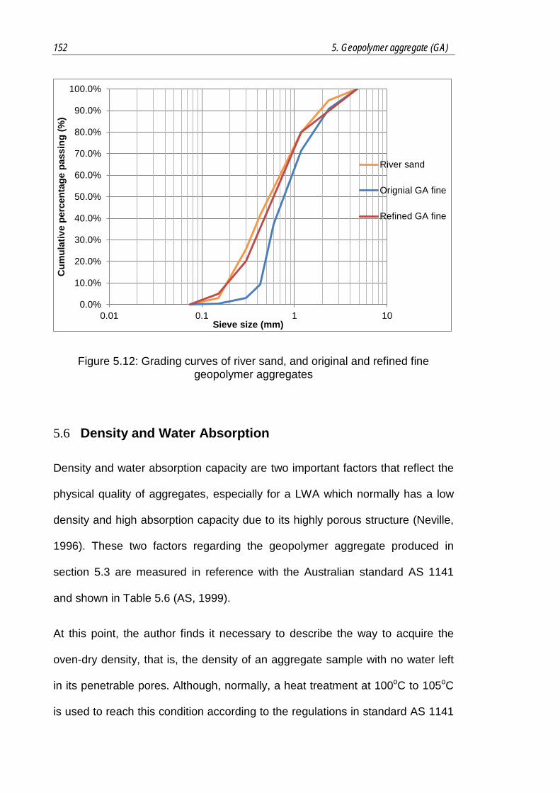
152 5. Geopolymer aggregate (GA)
Figure 5.12: Grading curves of river sand, and original and refined fine geopolymer aggregates
5.6 Density and Water Absorption
Density and water absorption capacity are two important factors that reflect the
physical quality of aggregates, especially for a LWA which normally has a low
density and high absorption capacity due to its highly porous structure (Neville,
1996). These two factors regarding the geopolymer aggregate produced in
section 5.3 are measured in reference with the Australian standard AS 1141
and shown in Table 5.6 (AS, 1999).
At this point, the author finds it necessary to describe the way to acquire the
oven-dry density, that is, the density of an aggregate sample with no water left
in its penetrable pores. Although, normally, a heat treatment at 100oC to 105oC
is used to reach this condition according to the regulations in standard AS 1141
0.0%
10.0%
20.0%
30.0%
40.0%
50.0%
60.0%
70.0%
80.0%
90.0%
100.0%
0.01 0.1 1 10
Cum
ulat
ive
perc
enta
ge p
assi
ng (%
)
Sieve size (mm)
River sand
Orignial GA fine
Refined GA fine

153
(AS, 1999), the suitability of this for a geopolymer aggregate is arguable
because, based on current knowledge it is still not clear whether a heat
treatment on a heat-hardened geopolymer can lead to any further structural
change. Therefore, another way to realise the ‘oven-dry’ condition is applied in
this section, by removing the water under a low-pressure condition in a silica-gel
desiccator assisted by a vacuum pump.
Also, it is noted that, to make the tested geopolymer aggregate sample easier to
get dried, the sample is firstly placed in the desiccator used for this type of
drying immediately after being in air-dried condition right after the jaw crushing.
For this case, the ‘oven dry mass’ is measured first, and the other parameters
required (like ‘SSD mass’) are measured later. Compared to the standard order
of measurements suggested in AS 1141, the method used in this research need
further caution to prevent any material loss during the test.
Table 5.6: Density and water absorption capacity of geopolymer aggregate
Coarse (28-day)
Fine (28-day)
Specific gravity (SSD) 1.84 2.01
Specific gravity (OD) 1.66 1.77
Dry loose bulk density (kg/m3) 876.8 1117.2
Water absorption capacity (in 24 hours) 11.0% 13.7%
SSD - saturated surface dry condition; OD - oven dry condition
From Table 5.6, a coarse geopolymer aggregate has specific gravities of 1.84
and 1.66 under saturated surface dry and oven dry conditions respectively

154 5. Geopolymer aggregate (GA)
which are lighter than those of a regular aggregate and belong to the area of
LWAs (Chandra and Berntsson, 2002). A fine geopolymer aggregate has a
similarly low specific gravity but of a slightly higher value, with specific gravities
of 2.01 and 1.77 under saturated surface dry and oven dry conditions
respectively. The dry loose bulk densities of coarse and fine geopolymer
aggregates are 876.8 kg/m3 and 1117.2 kg/m3 respectively which are also
sufficiently low to be considered LWAs (ASTM, 2009). Therefore, a geopolymer
aggregate is a type of LWA created from coal fly ash and referred to as a type
of FA-LWA product.
On the other hand, both coarse and fine geopolymer aggregates have high
water absorption capacities of above 10%, much higher than those of normal
weight aggregates (NWAs) (Neville, 1996), which is also of concern during a
concrete mix (ACI, 1998, ACI, 2003). Nevertheless, it has been seen that a
geopolymer product solely made from Class F fly ash can have a high capacity
of water absorption (Görhan and Kürklü, 2014). Several previous LWA samples
with high water absorptions are also found to end up in good quality concrete
products (Jo et al., 2007, Swamy and Lambert, 1981). So it is estimated that the
produced geopolymer aggregate may also lead to a good concrete mix if it can
be properly applied.
Furthermore, the author finds that the synthetic conditions, namely mix design
and curing regime, can greatly affect the density and water absorption capacity
of geopolymer aggregate. This is reasonable since geopolymer aggregates are
composed of geopolymer materials which can be affected by these conditions
(Duxson et al., 2007a). The variations in density and water absorption caused
by geopolymer synthetic conditions are illustrated in following paragraphs.
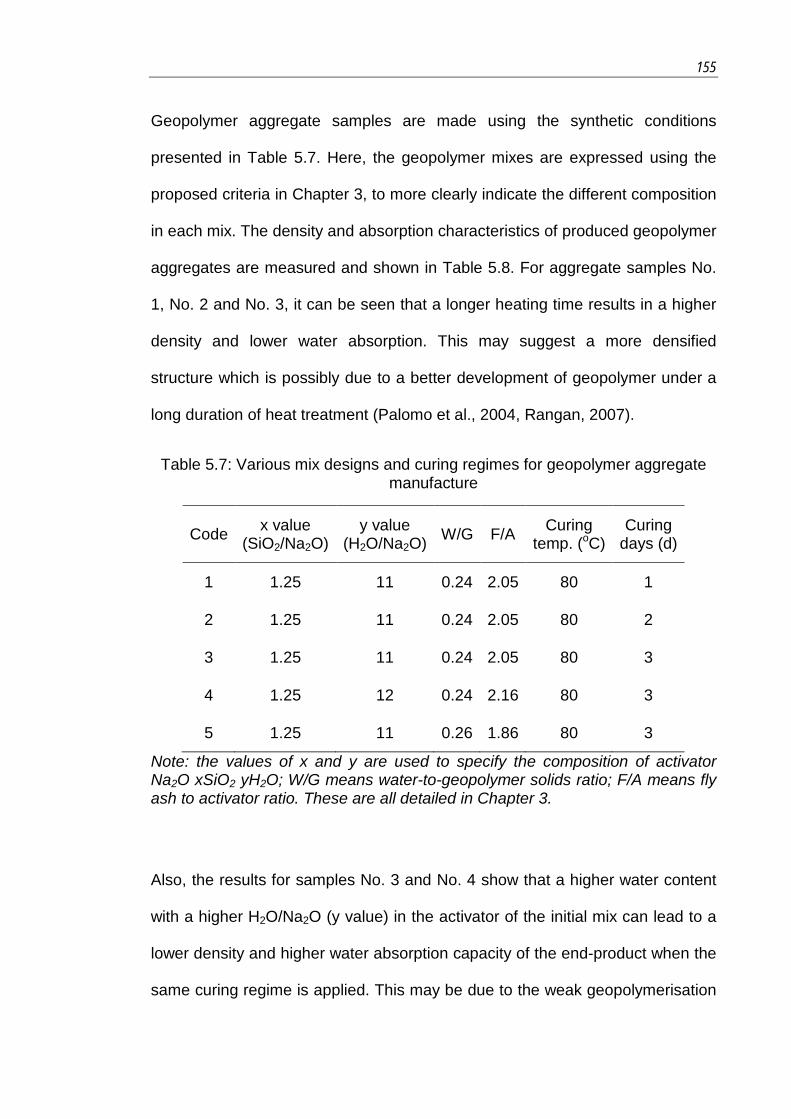
155
Geopolymer aggregate samples are made using the synthetic conditions
presented in Table 5.7. Here, the geopolymer mixes are expressed using the
proposed criteria in Chapter 3, to more clearly indicate the different composition
in each mix. The density and absorption characteristics of produced geopolymer
aggregates are measured and shown in Table 5.8. For aggregate samples No.
1, No. 2 and No. 3, it can be seen that a longer heating time results in a higher
density and lower water absorption. This may suggest a more densified
structure which is possibly due to a better development of geopolymer under a
long duration of heat treatment (Palomo et al., 2004, Rangan, 2007).
Table 5.7: Various mix designs and curing regimes for geopolymer aggregate manufacture
Code x value (SiO2/Na2O)
y value (H2O/Na2O) W/G F/A Curing
temp. (oC) Curing
days (d)
1 1.25 11 0.24 2.05 80 1
2 1.25 11 0.24 2.05 80 2
3 1.25 11 0.24 2.05 80 3
4 1.25 12 0.24 2.16 80 3
5 1.25 11 0.26 1.86 80 3
Note: the values of x and y are used to specify the composition of activator Na2O·xSiO2·yH2O; W/G means water-to-geopolymer solids ratio; F/A means fly ash to activator ratio. These are all detailed in Chapter 3.
Also, the results for samples No. 3 and No. 4 show that a higher water content
with a higher H2O/Na2O (y value) in the activator of the initial mix can lead to a
lower density and higher water absorption capacity of the end-product when the
same curing regime is applied. This may be due to the weak geopolymerisation

156 5. Geopolymer aggregate (GA)
process caused by higher water content in the initial geopolymer mix (Xie and
Kayali, 2014).
Table 5.8: Density and water absorption values of geopolymer aggregate samples made from various mix designs and curing regimes
Code Specific gravity (SSD)
Specific gravity (OD)
Water absorption capacity
1 1.76 1.52 16.0%
2 1.79 1.58 13.3%
3 1.84 1.66 11.0%
4 1.80 1.55 15.7%
5 1.94 1.68 15.8%
SSD - saturated surface dry condition; OD - oven dry condition
Sample No. 5 is based on sample No. 3 but with a higher amount of activator
added, although the composition of the added activator is unchanged.
Compared with sample No. 3, sample No. 5 has a slightly higher density, and a
much higher water absorption capacity that requires a more strict control in
concrete mix (ACI, 1998). It is considered that the extra activator in sample No.
5 should generate a higher degree of geopolymerisation and, therefore, a more
densified structure, as previously observed (Duxson et al., 2005) and reflected
by its higher density. But this variation in density is found not very obvious for
these two tested samples. On the other hand, the fact that the extra activator
added in the mix of No.5 also introduces more water and leaves more space in
the hardened structure may explain the much higher water absorption capacity
(15.8%) of this mix, which makes it less preferred in real practice.

157
In summary, the mix of No. 3 can result in satisfactory specific gravity and water
absorption capacity values, for which reasons, the author considers it preferable
for the manufacture of geopolymer aggregates.
5.7 Internal Pores
This section investigates the internal pores in the structure of a geopolymer
aggregate which is considered the main reason for its low specific gravity. The
relevant pore information is analysed using an optical microscopic (OM) method.
A geopolymer aggregate sample is mounted and polished to expose its internal
cross-section, and then an image of which is captured by a Zeiss AxioCam
MRC digital camera.
Traditionally, the information on internal pores of aggregates is analysed by
mercury intrusion porosimetry (MIP) or gas adsorption equipment. MIP uses
mercury to penetrate into the pores of tested samples and record the pressure
responses during penetration, based on which information porosity can be
obtained. MIP can cover sizes ranging from 0.0055 µm to 360 µm. However,
several of its limitations make it unsuitable for this research; for example,
mercury usually does not penetrate all the pores in a tested sample which will
underestimate the volume of pores. Also, the high pressure of mercury can
easily break the walls of the inner pores, thereby overestimating the proportion
of large pores (Korat et al., 2013, Diamond, 2000).
On the other hand, the gas adsorption method, which may use several types of
gas such as nitrogen, argon and krypton, can also be used for research on
internal pores. The principle of gas adsorption is to use the gas to penetrate and
attach to the inner surfaces of the pores, and then record variations in the

158 5. Geopolymer aggregate (GA)
volume and pressure to obtain porosity information. Although it is relatively
more accurate than MIP and has been applied in geopolymer materials (Duxson
et al., 2007e, Sindhunata et al., 2008), its maximum detectable size typically as
360 nm (Korat et al., 2013, Bouguerra et al., 1998) is considered by this author
to be not large enough for the analysis of geopolymer aggregates.
For above reasons, a microscopic method that can mostly cover micron-sized
pores is proposed in this research. The major target here is to observe the
pores present in the internal structure of geopolymer aggregates, and to
measure the size and area distributions of the pores in different sizes. Further
information on the pores of LWAs can also be conducted using a X-ray micro-
tomography (micro-CT) (Korat et al., 2013).
Geopolymer aggregate samples are selected randomly from stockpiles, washed
with water and then washed with ethanol and dried at 40oC. Afterwards, a flat
surface of the cross-section of a sample, as required by the OM method, is
created by the polishing procedures illustrated in Figure 5.13, that is: making a
mixture of epoxy resin and hardener with a mass proportion of
epoxy/hardener=25/3; soaking the aggregate sample in the fresh mixture in a
plastic mould to hold the sample; curing the sample at room temperature until
the fresh resin hardens; milling the resin with the sample inside using a grinder
on an abrasive paper with a grit size of P4000 until a flat surface appears;
polishing the sample to a 6 µm finish on the diamond plate of a polisher. Later,
the created surface is ready for microscopic observation.

159
Figure 5.13: Polishing procedures (1) mixing resin and hardener, (2) and (3) soaking sample in resin, (4) covering sample in hardened resin, (5) grinder and
(6) polisher
A bright field image of a geopolymer aggregate displaying its direct reflection of
the vertical incoming light is captured by a Zeiss AxioCam MRC digital camera,
and shown in Figure 5.14 in which the dark areas with no light reflected are the
pores and the bright areas are the surface of the cross-section. This image
(1) (2)
(3) (4)
(5) (6)

160 5. Geopolymer aggregate (GA)
shows a large range of pores of different shapes and sizes inside the
geopolymer aggregate which indicates that it has a porous internal structure
similar to its surface structure. This explains the lightweight performance of
produced geopolymer aggregates with a similar porous internal structure as the
other FA-LWAs reported before (Kayali, 2008, Swamy and Lambert, 1981).
Figure 5.14: Bright field image of geopolymer aggregate sample
Information regarding the porosity, like that of the size, area and number of
pores, is measured based on the captured bright field image assisted by the
ImageJ image-processing software. At first, a specific zone of the cross-section
of geopolymer aggregate sample is captured (like the left image in Figure 5.15).
Then, ImageJ converts the captured image into a black-and-white one to better
distinguish the pore areas from the structure, with the threshold of grey scale
set to 154. Then, it automatically measures the size, area and number of
identified pores (black areas) in the image on the right in Figure 5.15. The
minimum size of the identified pores is 1.452 µm, with the smaller pores
distorted in the captured image due to the limitation of the applied facility
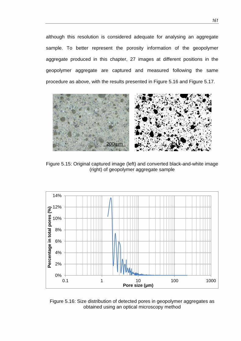
161
although this resolution is considered adequate for analysing an aggregate
sample. To better represent the porosity information of the geopolymer
aggregate produced in this chapter, 27 images at different positions in the
geopolymer aggregate are captured and measured following the same
procedure as above, with the results presented in Figure 5.16 and Figure 5.17.
Figure 5.15: Original captured image (left) and converted black-and-white image (right) of geopolymer aggregate sample
Figure 5.16: Size distribution of detected pores in geopolymer aggregates as obtained using an optical microscopy method
0%
2%
4%
6%
8%
10%
12%
14%
0.1 1 10 100 1000
Perc
enta
ge in
tota
l por
es (%
)
Pore size (µm)
200 µm

162 5. Geopolymer aggregate (GA)
Figure 5.17: Distribution of areas occupied by detected pores in geopolymer aggregates
Figure 5.16 displays the size distribution of pores detected in the geopolymer
aggregate sample, which indicates that the detected pores are in a wide size
range of 1 µm to 250 µm, and the portion within 1 µm to 10 µm is dominant. On
the other hand, Figure 5.17 shows that the pores of 10 µm to 50 µm occupy
most areas, despite there being less of this fraction than of 1 µm to 10 µm pores.
From above results, it is concluded that the pores present in the structure of
geopolymer aggregates are micron-sized, and mostly concentrated in a size
range less than 50 µm. Meanwhile, only around 0.1% of the detected pores are
larger than 100 µm as seen from Figure 5.16. This means that the pores in the
geopolymer aggregate structure are concentrated in a relatively small size
range as far as this feature of LWAs is concerned (Korat et al., 2013). Therefore,
it is envisaged that geopolymer technology may help reduce the size of pores
0.0%5.0%
10.0%15.0%20.0%25.0%30.0%35.0%40.0%45.0%50.0%
1-10µm 10-50µm 50-100µm 100-500µm
Perc
enta
ge in
tota
l por
ous
area
(%
)
Pore size (µm)

163
formed in an aggregate sample, and mitigate the defects of large-sized internal
pores.
On the other hand, based on the microscopic images in Figure 5.14, the surface
of a geopolymer aggregate’s structure is not continuous but has a large amount
of micron-sized pores. This amount of pores seems sufficient to provide the
needed porous volume to realise the lightweight of a geopolymer aggregate, as
seen from the density results in section 5.6, despite that the volume of each
single pore would be small due to its small pore size. Moreover, this type of
microstructure containing more homogeneously distributed small-sized pores is
likely to be less fragile compared to the one containing large-sized pores (Masi
et al., 2014).
5.8 Crushing Value
For a FA-LWA, its mechanical property is significant because it determines its
capability in resisting external loads in further construction applications. This is
normally reflected by the mechanical performance of a concrete made with a
specific FA-LWA product (Kayali, 2008, Lo et al., 2004) which is considered a
more convincing examination method. On the other hand, several methods that
are directly conducted on aggregate samples are also proposed, to obtain initial
estimations of their mechanical properties (Bui et al., 2012), such as the
standard crushing value test which is regulated in Australian standard AS 1141
(AS, 1999) and applied in this section.
The crushing value test assesses the capability of an aggregate sample to bear
an external mechanical pressure. As required in AS 1141, a fraction of the 9.50
mm to 13.20 mm of geopolymer aggregate particles manufactured in section

164 5. Geopolymer aggregate (GA)
5.3 is selected for the crushing value test, which is operated on a SHIMADZU
universal testing machine (1000 kN capacity) shown in Figure 5.18. The load is
made according to a certain procedure in AS 1141 for applying a force at a rate
of 40 kN per minute until 400 kN. After the test, the aggregate sample (Figure
5.19) is sieved through a 2.36 mm sieve to measure its mass proportion of
particles under a size of 2.36 mm which is its crushing value (AS, 1999). The
crushing value of the selected geopolymer aggregate sample is 23.43%, as
shown in Table 5.9.
Figure 5.18: Crushing value test of geopolymer aggregate sample
Generally, higher crushing values indicate weaker structures of the aggregates.
The crushed normal weight stone used in the locality has a crushing value of
16.90%, while usually, those of FA-LWAs are between 26% and 35% (Kayali,
2008). Therefore, the 23.43% crushing value is relatively lower, indicating a
better capability of the new geopolymer aggregate in resisting the external
pressure in a crushing value test. Based on this, geopolymer aggregate sample

165
seems to have a comparable or even slightly stronger structure than the usual
FA-LWAs, implying its potential to be undertaken for concrete manufacture.
Nevertheless, it is still weaker compared to the normal weight crushed stone.
Figure 5.19: Appearance of geopolymer aggregate sample after crushing value test
Table 5.9: Crushing value of geopolymer aggregate sample tested
Property Geopolymer aggregate
Crushing value (%) 23.43
5.9 Rebound Test by Schmidt Hammer
The mechanical performance of geopolymer aggregate is further evaluated by
rebound test based on a Schmidt hammer. Rebound test is a common way of
describing the surface hardness and penetration resistance of natural rocks
(Katz et al., 2000, Cerna and Engel, 2011). As the created geopolymer
aggregate can be treated as a new kind of ‘artificial rock’ to replace the natural
rock in a concrete mix, this rebound test is considered appropriate for providing
a supplementary knowledge on the property of geopolymer aggregate in
comparison with other natural rocks regularly used in concretes.

166 5. Geopolymer aggregate (GA)
The rebound test is conducted according to the procedure regulated in ASTM
C805 (ASTM, 2014). The tested sample is a block of synthesized ‘geopolymer
rock’ with a flat and smooth surface in the dimensions of
130mm×130mm×100mm, as required in a rebound test. This ‘geopolymer rock’
was made by normal geopolymer synthetic method with the same mix design
and curing regime as those for geopolymer aggregates, and therefore has the
same material base as the geopolymer aggregate.
Table 5.10: Results of Schmidt hammer rebound test
Hammer’s angle: -90o, vertical-down
Operation temperature: 20-23oC
Distance between each impact point: 25 mm
Rebound index (kPa)
No.1 40 No.6 39
No.2 38 No.7 37
No.3 37 No.8 38
No.4 37 No.9 37
No.5 41 No.10 42
Mean rebound index (kPa): 38.6
Standard deviation (kPa): 1.8
The rebound result is displayed in Table 5.10 in which the final rebound index is
a mean value of ten separate impacts. It is seen that the rebound index of
geopolymer aggregates is 38.6, which is much higher than the chalk (23.9),
close to limestone and sandstone (41.5-50.8), but lower than syenite and
granite (65.0-73.4) (Katz et al., 2000). From this result, it can be concluded that
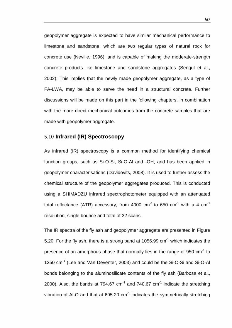
167
geopolymer aggregate is expected to have similar mechanical performance to
limestone and sandstone, which are two regular types of natural rock for
concrete use (Neville, 1996), and is capable of making the moderate-strength
concrete products like limestone and sandstone aggregates (Sengul et al.,
2002). This implies that the newly made geopolymer aggregate, as a type of
FA-LWA, may be able to serve the need in a structural concrete. Further
discussions will be made on this part in the following chapters, in combination
with the more direct mechanical outcomes from the concrete samples that are
made with geopolymer aggregate.
5.10 Infrared (IR) Spectroscopy
As infrared (IR) spectroscopy is a common method for identifying chemical
function groups, such as Si-O-Si, Si-O-Al and -OH, and has been applied in
geopolymer characterisations (Davidovits, 2008). It is used to further assess the
chemical structure of the geopolymer aggregates produced. This is conducted
using a SHIMADZU infrared spectrophotometer equipped with an attenuated
total reflectance (ATR) accessory, from 4000 cm-1 to 650 cm-1 with a 4 cm-1
resolution, single bounce and total of 32 scans.
The IR spectra of the fly ash and geopolymer aggregate are presented in Figure
5.20. For the fly ash, there is a strong band at 1056.99 cm-1 which indicates the
presence of an amorphous phase that normally lies in the range of 950 cm-1 to
1250 cm-1 (Lee and Van Deventer, 2003) and could be the Si-O-Si and Si-O-Al
bonds belonging to the aluminosilicate contents of the fly ash (Barbosa et al.,
2000). Also, the bands at 794.67 cm-1 and 740.67 cm-1 indicate the stretching
vibration of Al-O and that at 695.20 cm-1 indicates the symmetrically stretching

168 5. Geopolymer aggregate (GA)
vibration of Si-O which may all come from the mullite in the fly ash (Padmaja et
al., 2001, Fang, 2013). Moreover, the band at 777.31 cm-1 is considered to be
due to the presence of quartz (Barbosa et al., 2000, Davidovits, 2008).
On the other hand, the geopolymer aggregate sample tested has a different
spectrum to that of fly ash. It presents the same strong band in the range of 950
cm-1 to 1250 cm-1, indicating the presence of amorphous phases containing the
Si-O-Si and Si-O-Al bonds but, at the lower frequency of 999.13 cm-1, implying
an increasing proportion of the tetrahedral aluminium component which is very
possibly due to the involvement of Al components through the
geopolymerisation process (Davidovits, 2008). Moreover, this indicates that
geopolymer gels, mostly likely the N-A-S-H, could be formed in a GA sample as
supported by the findings of other researchers (Fernández-Jiménez and
Palomo, 2005, García-Lodeiro et al., 2007, Rees et al., 2007) which is
reasonable because H2O or OH is able to reside in the aluminosilicate
framework at such a relatively low-temperature (80oC) synthesising condition.
Except for this, there are several less intensive bands found in the range of 690
cm-1 to 800 cm-1 in the GA sample. These bands seem to be related to those
bands that represent crystalline phases in the IR spectrum of fly ash, but display
slightly different wavelength values and intensities. A likely reason may be that,
in a fly ash sample there are only fly ash particles, but in a GA sample there co-
exist some different phases including gels and residual solutes from the added
alkali activator (Rees et al., 2007) which may influence its framework’s
response to an IR spectroscopy. A similar phenomenon in that the detected
bands in such range (690 cm-1 to 800 cm-1) could shift from fly ash to
geopolymers has been discovered (Fang, 2013). Yet further investigation is

169
required. On the other hand, it has been discussed in Chapter 2, section 2.5,
that the mullite in fly ash is likely to be activated by the synthesising conditions
applied in this thesis. For this case, the question whether the shifted bands
observed above also imply a footprint of the activation of mullite must be further
investigated.
Figure 5.20: IR spectra of fly ash and geopolymer aggregate
5.11 Evaluation of Quality of Geopolymer Aggregate
In this chapter, a geopolymer aggregate is proposed as a new option for a FA-
LWA but at a lower cost and with a more eco-friendly manufacturing procedure,
and its relevant properties discussed in previous sections. To substitute for
conventional FA-LWA products in concrete applications, this new geopolymer
aggregate must have sufficient qualities to satisfy requirements in the relevant
standards and be comparable with the usual FA-LWAs in terms of properties
considered in this section.
20.0
30.0
40.0
50.0
60.0
70.0
80.0
90.0
100.0
110.0
500.01000.01500.02000.02500.03000.03500.04000.0
Tran
smitt
ance
(%)
Wave number (cm-1)
1056
.99
794.
67
777.
31
740.
67
777.
31
798.
53
736.
81
694.
37
999.
13
695.
20
GA
Fly ash

170 5. Geopolymer aggregate (GA)
5.11.1 Compatibility with Standards
Firstly, the compatibility of geopolymer aggregates with relevant standards is
investigated. Normally, for a FA-LWA product, density is highly significant for
determining its self-weight and strength. The regulations in the standards
introduced in Chapter 1, subsection 1.1.3, regarding the density range of LWAs
are presented in Table 5.11. Based on previous research, a coarse geopolymer
aggregate has a SSD specific gravity of 1.84, oven-dry specific gravity of 1.66
and dry loose bulk density of 876.8 kg/m3. A fine geopolymer aggregate is
heavier than a coarse one, with a SSD specific gravity of 2.01, oven-dry specific
gravity of 1.77 and dry loose bulk density of 1117.2 kg/m3. According to the
standards listed in Table 5.11, geopolymer aggregates have density values
which qualify them for use as LWAs in concrete structures.
Table 5.11: Density values of geopolymer aggregates in relation to relevant LWA standards
GA coarse
GA fine
AS 2758
ASTM C330
BS EN 13055
Specific gravity (SSD) 1.84 2.01 - - <2.0
Specific gravity (OD) 1.66 1.77 0.5-2.1 - -
Dry loose bulk density (kg/m3) 876.8 1117.2 - Coarse<880
Fine<1120 <1200
SSD - saturated surface dry condition; OD - oven dry condition
Apart from density, grading is another important factor that needs to be
evaluated. Grading of geopolymer aggregates and its requirements in relevant
standards are presented in Table 5.12 from which it has been shown that both
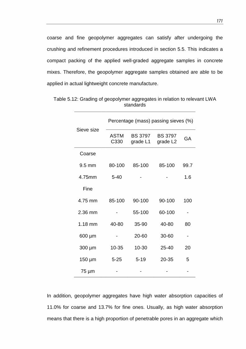
171
coarse and fine geopolymer aggregates can satisfy after undergoing the
crushing and refinement procedures introduced in section 5.5. This indicates a
compact packing of the applied well-graded aggregate samples in concrete
mixes. Therefore, the geopolymer aggregate samples obtained are able to be
applied in actual lightweight concrete manufacture.
Table 5.12: Grading of geopolymer aggregates in relation to relevant LWA standards
Sieve size
Percentage (mass) passing sieves (%)
ASTM C330
BS 3797 grade L1
BS 3797 grade L2 GA
Coarse
9.5 mm 80-100 85-100 85-100 99.7
4.75mm 5-40 - - 1.6
Fine
4.75 mm 85-100 90-100 90-100 100
2.36 mm - 55-100 60-100 -
1.18 mm 40-80 35-90 40-80 80
600 µm - 20-60 30-60 -
300 µm 10-35 10-30 25-40 20
150 µm 5-25 5-19 20-35 5
75 µm - - - -
In addition, geopolymer aggregates have high water absorption capacities of
11.0% for coarse and 13.7% for fine ones. Usually, as high water absorption
means that there is a high proportion of penetrable pores in an aggregate which

172 5. Geopolymer aggregate (GA)
can seriously affect its bonding with cement materials in concrete (Lo and Cui,
2004, Kayali, 2008, Zhang and Gjørv, 1990), this value always needs to be
considered. According to US standard ACI 213R-03, the normal capacity value
is suggested to be in the range of 5% to 25% by mass of dry aggregates (ACI,
2003) while it has also been recommended that it be less than 15% (Neville,
1996). According to the requirements of these standards, the absorption
capacity of the geopolymer aggregate is high but is still within the acceptable
range for LWA application while special care should be taken (ACI, 1998, ACI,
2003). The real effect of such a high water absorption capacity is further
investigated during presenting and discussing concrete manufacture in
Chapters 6 and 7.
5.11.2 Comparison with Other FA-LWAs
The properties of the geopolymer aggregates produced are compared with
those of other FA-LWAs, such as Lytag and Flashag aggregates introduced in
Chapter 1, subsection 1.1.5, as shown in Table 5.13. Also, the properties of
NWAs, such as crushed stone and river sand regularly used in the locality of the
author’s institution, are presented for comparison.
From Table 5.13, it is clear that NWA has a higher density and lower water
absorption capacity than the other three FA-LWA products which are detected
to be lightweight with similar specific gravities of 1.4 to 1.8. Of the FA-LWAs, the
geopolymer aggregates have the highest density values followed by the
Flashag, with the Lytag having the lowest.
The light weights of the three FA-LWA samples are related to their backbone
materials and porous structures. Lytag and Flashag share a similar backbone

173
material, sintered fly ash, and a similar porous structure formed by the voids left
from elevated-temperature sintering. Nevertheless, a geopolymer aggregate is
different as it has a unique geopolymer backbone and voids remaining after
geopolymerisation at a mild temperature, as observed by X-ray micro-
tomography (Provis et al., 2012). Therefore, the manufacture of a geopolymer
aggregate can be treated as another way of achieving the lightweight property
desired in FA-LWAs.
Table 5.13: Properties of geopolymer aggregates (GA), Lytag, Flashag and NWAs (crushed stone (coarse) and river sand (fine))
Property NWA GA Lytag Flashag
Coarse Fine Coarse Fine Coarse Fine Coarse & Fine
Specific gravity (SSD)
2.70 2.60 1.84 2.01 1.60 1.76 1.69
Specific gravity (OD)
2.68 2.57 1.66 1.77 1.41 1.60 1.61
Dry loose bulk density
(kg/m3) 1376 1640 877 1117 805 1067 848
Water absorption
(in 24 hours) 0.7% 1.2% 11% 13.7% 13.2% 9.7% 3.4%
SSD - saturated surface dry condition; OD - oven dry condition
Geopolymer aggregates and Lytag appear to have higher open porosity values
in their structures than Flashag, as deduced from their much higher water
absorption capacity values presented in Table 5.13. Compared to Lytag, the low
open porosity in Flashag seems to be due to its modified manufacture which
uses a superplasticiser to reduce the amount of water in the pre-heating mixture

174 5. Geopolymer aggregate (GA)
to mitigate the impact of void generation caused by water evaporation. In
contrast, the high open porosity in a geopolymer aggregate is considered to be
caused by the connective structure of the geopolymer material made using
current technology (Provis et al., 2012). Further research is needed to modify
geopolymer synthesis in order to reduce the connectivity of open pores in
hardened geopolymers.
5.12 Conclusions
This chapter proposes a type of artificial FA-LWA. This is a geopolymer
aggregate made based on the principle of geopolymerisation and which has
properties that qualify it for use in lightweight constructions. A practical
manufacturing procedure for it, which can be used to make both coarse and fine
aggregate samples, and can also be repeated for different designs, is proposed
and evaluated.
Also, one specifically designed geopolymer aggregate sample is produced with
its properties such as appearance, grading, density, water absorption capacity,
pore information, crushing value and hardness, measured and its chemical
structure examined using IR spectroscopy. These properties are then evaluated
by comparing them with those of regulations in the standards and other FA-
LWAs. It is found that this new geopolymer aggregate has good qualities
suitable for lightweight concrete application. Concrete and mortar practices
using the geopolymer aggregate sample created as explained in this chapter
are researched and presented in Chapters 6 and 7.

175
Chapter 6
OPC-based Concrete and Mortar using Geopolymer
Aggregate
6.1 Introduction
This chapter investigates the application of a geopolymer aggregate in a
concrete mix which, as it uses OPC as the sole cementitious material, is
referred to as an OPC-based concrete. As OPC is the most widely used
cementitious material in the world, this research on OPC-based concrete is able
to provide necessary information for evaluating the compatibility of geopolymer
aggregates with the current mainstream cementitious system.
Firstly, a normal-weight concrete (NWC) made with normal weight aggregates
(NWAs), such as crushed stone and river sand, is designed and coded as ‘Con-
N-OPC’. Then, a concrete made using geopolymer aggregates instead of
NWAs is referred to as OPC-GA concrete and coded as ‘Con-GA-OPC’. The
mix design of this new OPC-GA concrete is based on that of the Con-N-OPC
using the same volume proportions of aggregates and quantities of the other
ingredients. The research on it aims to determine a workable way of utilising
geopolymer aggregates in an OPC-based concrete mix and investigate the
capability of geopolymer aggregates to realise high-performance lightweight
concrete (LWC) as proposed in Chapter 1, subsection 1.1.3.
Also, a mortar material containing only fine aggregates and a cementitious
material, which can be treated as a special mix of concrete with no coarse
aggregates, is also examined. This aims to evaluate the practicality of a mortar
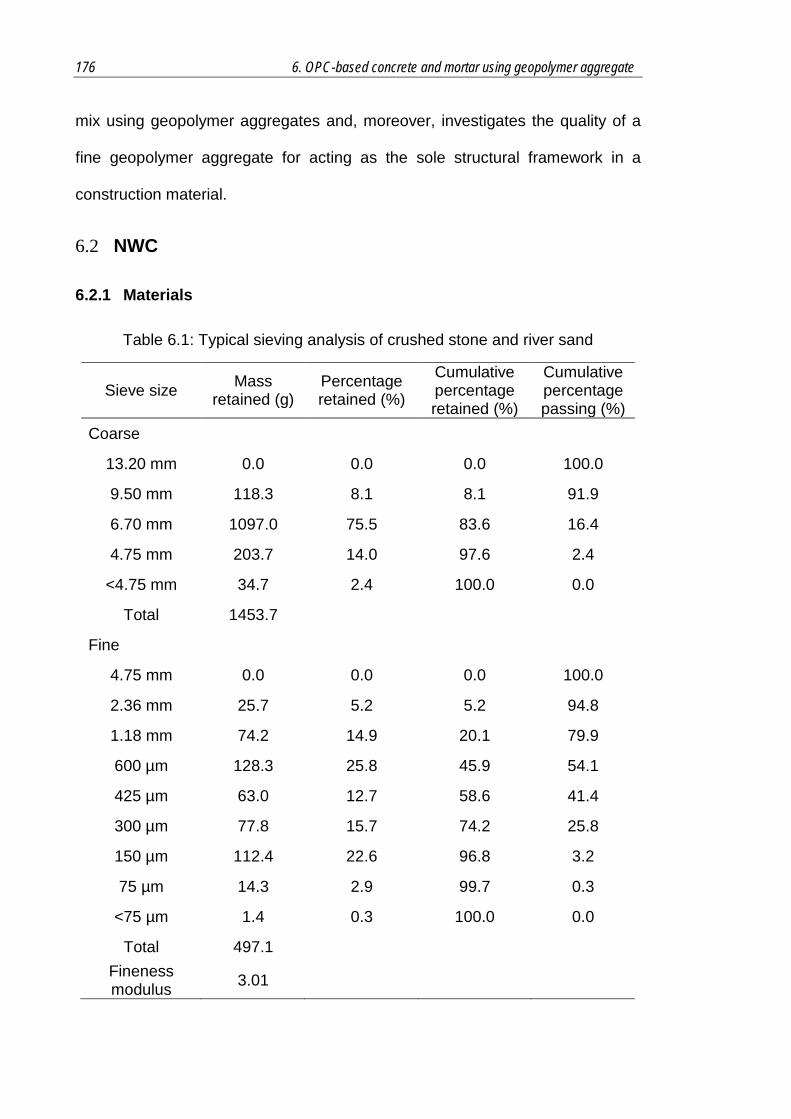
176 6. OPC-based concrete and mortar using geopolymer aggregate
mix using geopolymer aggregates and, moreover, investigates the quality of a
fine geopolymer aggregate for acting as the sole structural framework in a
construction material.
6.2 NWC
6.2.1 Materials
Table 6.1: Typical sieving analysis of crushed stone and river sand
Sieve size Mass retained (g)
Percentage retained (%)
Cumulative percentage retained (%)
Cumulative percentage passing (%)
Coarse
13.20 mm 0.0 0.0 0.0 100.0
9.50 mm 118.3 8.1 8.1 91.9
6.70 mm 1097.0 75.5 83.6 16.4
4.75 mm 203.7 14.0 97.6 2.4
<4.75 mm 34.7 2.4 100.0 0.0
Total 1453.7
Fine
4.75 mm 0.0 0.0 0.0 100.0
2.36 mm 25.7 5.2 5.2 94.8
1.18 mm 74.2 14.9 20.1 79.9
600 µm 128.3 25.8 45.9 54.1
425 µm 63.0 12.7 58.6 41.4
300 µm 77.8 15.7 74.2 25.8
150 µm 112.4 22.6 96.8 3.2
75 µm 14.3 2.9 99.7 0.3
<75 µm 1.4 0.3 100.0 0.0
Total 497.1 Fineness modulus 3.01

177
The laboratory-used crushed stone and river sand are selected to represent
NWAs in the NWC mix Con-N-OPC. The aggregates’ grading conditions are
shown in Table 6.1 and Figure 6.1 in which it can be seen that they are well-
graded with an even particle size distribution, suggesting good compaction of a
fresh concrete mix (Neville, 1996).
Figure 6.1: Grading curves of crushed stone and river sand
The density and water absorption capacities of the crushed stone and sand
selected are measured and presented in Table 6.2. The crushed stone has
specific gravities of 2.70 and 2.68 under saturated surface dry (SSD) and oven
dry (OD) conditions respectively. For the river sand, these two values are
slightly different; 2.60 and 2.57 respectively. On the other hand, the water
absorption capacity is as low as 0.7% for crushed stone and 1.2% for river sand.
These density and water absorption characteristics are in accordance with the
0.0%
10.0%
20.0%
30.0%
40.0%
50.0%
60.0%
70.0%
80.0%
90.0%
100.0%
0.01 0.1 1 10 100
Cum
ulat
ive
perc
enta
ge p
assi
ng (%
)
Sieve size (mm)
Crushed stone
River sand

178 6. OPC-based concrete and mortar using geopolymer aggregate
common understanding of the properties of NWAs (Neville, 1996) and applied
to complete the mix design procedure for Con-N-OPC.
Table 6.2: Characteristics of crushed stone and river sand
Property Crushed stone
River sand
Specific gravity (SSD) 2.70 2.60
Specific gravity (OD) 2.68 2.57
Water absorption capacity (in 24 hours) 0.7% 1.2%
SSD - saturated surface dry condition; OD - oven dry condition
Apart from aggregates, the other ingredients are cement, fly ash, water and
superplasticiser, all of which are common in a normal concrete mix. A GP
cement (Grade 45) regulated in Australian standard AS 3972 (AS, 2010)
produced by Boral Corporation is applied as the major cementitious material in
the proposed Con-N-OPC samples. Also, a fly ash sample is used as a
supplementary cementitious material (SCM) in order to make use of the
pozzolanic property of fly ash for improved durability with a hindered alkali-
aggregate reaction (AAR) (Raask and Bhaskar, 1975, Neville, 1996). This
selected fly ash sample is sourced from the 2012-Dec-13 batch from the Eraring
thermal power station, the basic characteristics of which are provided in
Chapter 2, section 2.2. Deionised water is added to trigger the cement hydration
reaction. Also, a polycarboxylate-based superplasticiser coded as ‘ADVA-142’
obtained from Grace Corporation is used to reduce the water required in a
concrete mix and enhance its fresh and final properties (Uchikawa et al., 1995,
Puertas et al., 2005).

179
6.2.2 Mix Design
The mix design of Con-N-OPC is based on a standard mix design procedure
regulated in British standard BS 5328 (Neville, 1996). Given the scope of this
study as to investigate high-performance concrete manufacture, this Con-N-
OPC mix is designed to be of good mechanical properties. Therefore, it is
specified with a characterised strength of 50 MPa and target strength of 63 MPa.
Also, fly ash is added as a 25% mass proportion of the total cementitious
material and an ADVA-142 superplasticiser applied in the proportion of 0.8 litres
per 100 kg cementitious material. According to the procedure regulated in BS
5328, the water/cement ratio of Con-N-OPC is 0.42 and the mass proportion of
fine aggregates is 43% of all the aggregates. The final mix design for 1 m3 of
fresh concrete then obtained is presented in Table 6.3. In addition, for all
concrete mix designs in this study, including that in Table 6.3, the aggregate
portion is regulated to be in a SSD condition.
Table 6.3: Mix design of Con-N-OPC sample (SSD aggregates condition)
Item Con-N-OPC (kg/m3)
Cement 351
Water 147
Crushed stone 1055
Sand 796
Fly ash 117
Superplasticiser 4
Water/Cement ratio 0.42
Water/Cementitious materials ratio 0.31

180 6. OPC-based concrete and mortar using geopolymer aggregate
6.2.3 Concrete Preparation
The preparation of concrete sample Con-N-OPC is based on a general
procedure for an OPC-based concrete mix (AS, 1993) (Figure 6.2). Firstly, the
saturated surface dry aggregate samples are prepared, by mixing the
aggregates in stock with a certain amount of water necessary for the aggregate
absorption (referred to as SSD water) in a mechanical concrete mixer for
around 2 minutes. Then, cement and fly ash are added and mixed with the wet
aggregates for a further 2 minutes to uniformly distribute the cementitious
material onto the surfaces of the aggregate particles. Following that, a dosage
of superplasticiser, which improved the workability of the fresh pastes produced,
is added along with the mixing water. Then, mixing is continued for 3-5 minutes
until a uniform fresh concrete mixture (Figure 6.3(1)) is formed.
Figure 6.2: Flowchart of preparation of OPC-based concrete

181
After mixing, a portion of the fresh concrete produced is tested for its fresh
properties, and the remaining portion used to cast samples in cubic
50mm×50mm×50mm stainless steel moulds. A vibrating table (220-240V AC,
50HZ) is applied to compact the fresh concrete mix into a well-shaped cube
(Figure 6.3(2)). The concrete sample is then sealed and cured in the ER at
20oC for 1 day, demoulded (Figure 6.3(3)), and cured in a 20oC water-spray
room. An image of a 28-day cured Con-N-OPC sample is shown in Figure
6.3(4).
Figure 6.3: Steps in preparation of Con-N-OPC: (1) mixing, (2) casting, (3) immediately after demoulding and (4) after 28-day curing
(1) (2)
(3) (4)

182 6. OPC-based concrete and mortar using geopolymer aggregate
6.2.4 Workability
The workability of a fresh concrete means that the effort needed to cast it into a
mould without any harm to its consistency (Neville, 1996), which is a significant
factor for reflecting its quality, must be carefully considered in its manufacture.
A slump test, which measures the slump distance of a conical pile of fresh
concrete, is used to describe the workability of a fresh OPC-based concrete mix.
A common slump test regulated in Australian standard AS1012 (AS, 1993) is
carried out on the fresh mix of Con-N-OPC. The slump result is shown in Table
6.4 which indicates that the fresh Con-N-OPC has moderate workability with a
slump value of 50 mm.
Table 6.4: Slump result for Con-N-OPC measured on a standard slump cone
Cone type AS1012
Cone height (mm) 300
Cone top diameter (mm) 100
Cone bottom diameter (mm) 200
Slump value (mm) 50
6.2.5 Density and Strength
The density values of fresh and hardened Con-N-OPC samples were tested
and their compressive strengths measured using a TECNOTEST compression
machine at a speed of 0.33 MPa/sec, with the final value of each mixing batch
the average of three cubic samples. Two mixing batches with the same design
and mixing procedure were produced in order to ensure that the results

183
obtained and shown in Table 6.5 can represent the properties of the designed
Con-N-OPC.
Table 6.5: Density and strength properties of Con-N-OPC
Con-N-OPC (1st batch)
Con-N-OPC (2nd batch)
Fresh density (kg/m3) 2400 2450
Density (AD) (28d) (kg/m3) 2310 2340
Density (SSD) (28d) (kg/m3) 2330 2370
Compressive strength (7d) (MPa) 52.36 (0.70)* 51.77 (1.59)*
Compressive strength (28d) (MPa) 67.70 (0.50)* 70.45 (0.63)*
SSD - saturated surface dry condition; AD - air dry condition; * the value between brackets is the standard deviation of the relevant result.
As the two batches of Con-N-OPC samples display similar density and strength
values, as seen in Table 6.5, these values are considered representative and
repeatable. The Con-N-OPC mix has a fresh density of 2400-2450 kg/m3 and
hardened densities of 2310-2340 kg/m3 (AD) and 2330-2370 kg/m3 (SSD) which
comply with the regular density ranges of NWC samples (Neville, 1996). The
hardened Con-N-OPC has compressive strengths of approximately 50 MPa and
70 MPa at 7 days and 28 days respectively. Its strength performance complies
with the target strength specified in the mix design procedure introduced in
subsection 6.2.2 and indicates that it is a type of high-strength concrete. This is
also the target strength to be achieved by the OPC-GA concrete created and
discussed in the next section.
184 6. OPC-based concrete and mortar using geopolymer aggregate
6.3 OPC-GA Concrete
6.3.1 Materials
The OPC-GA concrete uses geopolymer aggregates for both the coarse and
fine aggregate portions in its mix. The geopolymer aggregates applied here are
the ones manufactured following the procedure in Chapter 5, including the
grading refinement procedure for the fine geopolymer aggregates. Their basic
characteristics required for a concrete mix design procedure are introduced in
Chapter 5, sections 5.5 and 5.6. Apart from these, the other ingredients used
are the same as those in a NWC mix, namely, cement, fly ash, water and
superplasticiser.
6.3.2 Mix Design
Absolute Volume Principle
The mix design of Con-GA-OPC is made from that of Con-N-OPC, based on the
so-called absolute volume principle which assumes that the total volume of
fresh concrete equals the sum of the volume proportions of all its ingredients
(Neville, 1996). The specific mix design procedure for Con-GA-OPC is
explained in next paragraph in combination with the details of these two mix
designs presented in Table 6.6.
The volume proportion of each ingredient in the mix design of Con-N-OPC is
based on its known mass and density values, the sum of which is 1 m3 which
obeys the absolute volume principle, with crushed stone and river sand having
volume proportions of 0.391 m3 and 0.306 m3 respectively. In the new mix
design of Con-GA-OPC, the volume proportions of coarse and fine geopolymer
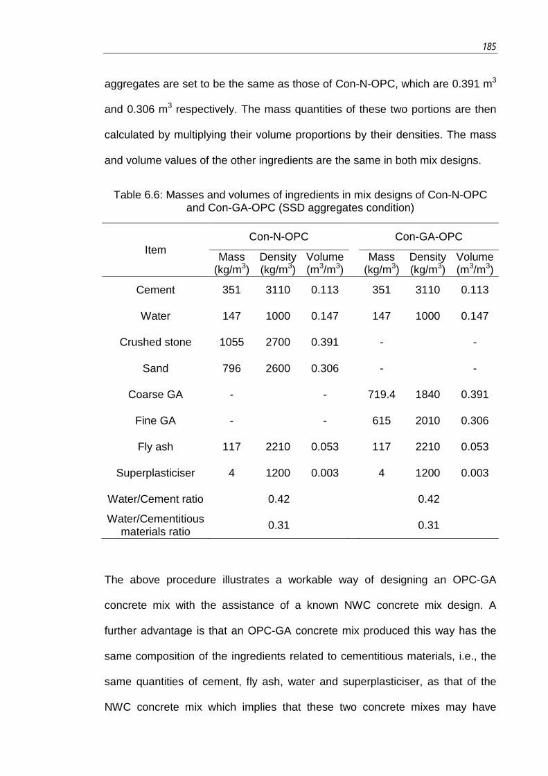
185
aggregates are set to be the same as those of Con-N-OPC, which are 0.391 m3
and 0.306 m3 respectively. The mass quantities of these two portions are then
calculated by multiplying their volume proportions by their densities. The mass
and volume values of the other ingredients are the same in both mix designs.
Table 6.6: Masses and volumes of ingredients in mix designs of Con-N-OPC and Con-GA-OPC (SSD aggregates condition)
Item Con-N-OPC Con-GA-OPC
Mass (kg/m3)
Density (kg/m3)
Volume (m3/m3) Mass
(kg/m3) Density (kg/m3)
Volume (m3/m3)
Cement 351 3110 0.113 351 3110 0.113
Water 147 1000 0.147 147 1000 0.147
Crushed stone 1055 2700 0.391 - -
Sand 796 2600 0.306 - -
Coarse GA - - 719.4 1840 0.391
Fine GA - - 615 2010 0.306
Fly ash 117 2210 0.053 117 2210 0.053
Superplasticiser 4 1200 0.003 4 1200 0.003
Water/Cement ratio 0.42 0.42
Water/Cementitious materials ratio 0.31 0.31
The above procedure illustrates a workable way of designing an OPC-GA
concrete mix with the assistance of a known NWC concrete mix design. A
further advantage is that an OPC-GA concrete mix produced this way has the
same composition of the ingredients related to cementitious materials, i.e., the
same quantities of cement, fly ash, water and superplasticiser, as that of the
NWC concrete mix which implies that these two concrete mixes may have
186 6. OPC-based concrete and mortar using geopolymer aggregate
comparable outcomes of the reactions of cementitious materials. For this case,
any variation in the properties of these two concrete mixes is considered mostly
determined by the different types of aggregates used in them.
Final Mix Design
The mix design of Con-GA-OPC presented in Table 6.6 is created by a
theoretical deduction based on that of Con-N-OPC. However, it doesn’t take
into account the different shapes and surface conditions of geopolymer
aggregates and regular NWAs which have the potential to cause workability
differences. Therefore, a further modification, whereby the quantities of water
and aggregates in the mix design are modulated to generate the same
workability as the Con-N-OPC mix, is discussed. It is specified that the
designed Con-GA-OPC and Con-N-OPC mixes have the same amounts of
cement and fly ash, and display the same workability in their fresh stages in
order to compare and assess their properties, as previously suggested (Kayali,
2005).
To realise this, trial mixes of fresh Con-GA-OPC were manufactured and tested
for their slump values, with the amount of water added modified until a mix
reaches a slump value of 50 mm, the same as that of Con-N-OPC. After
confirming the amount of water required, the quantities of the water and the
aggregates in the mix design are modified to suit a 1 m3 fresh concrete mix.
Then, this new mix design is checked by trial mixes to ensure that it results in a
slump value of 50 mm.
The final mix design of Con-GA-OPC created this way is shown in Table 6.7 in
which the water/cement ratio is higher than that in the mix design of Con-N-

187
OPC which is most likely due to the higher water requirement of the angular
geopolymer aggregate particles (Shilstone, 1999, Kockal and Ozturan, 2010).
On the other hand, the portion of fine geopolymer aggregates is divided into
several size fractions with narrower ranges, as shown in Table 6.7, to better
express the composition of this portion and help to remind users of its strict
control in practice.
Table 6.7: Final mix design of Con-GA-OPC (SSD aggregates condition)
6.3.3 Concrete Preparation
The preparation of Con-GA-OPC follows the same procedure as that for OPC-
based concrete shown in Figure 6.2. Longer time is needed to mix coarse and
fine geopolymer aggregates because they are LWAs which take a long time to
Item Con-GA-OPC (kg/m3)
Cement 351
Water 178.7
Coarse GA 686.2
Fine GA (1.18-4.75mm) 117.5
Fine GA (300µm-1.18mm) 352.5
Fine GA (150-300µm) 88.1
Fine GA (75-150µm) 29.4
Fly ash 117
Superplasticiser 4
Water/Cement ratio 0.51
Water/Cementitious materials ratio 0.38

188 6. OPC-based concrete and mortar using geopolymer aggregate
fully absorb the added SSD water. According to the author’s observation, it
usually takes 5 minutes for the surfaces of the aggregate samples to be wet
with no clear water drops. Therefore the SSD condition was first achieved with
these geopolymer aggregates, as recommended in ACI 211.2 (ACI, 1998).
Images showing the relevant steps in mixing Con-GA-OPC are presented in
Figure 6.4.
Figure 6.4: Steps in preparation of concrete Con-GA-OPC (1) mixing, (2) casting, (3) immediately after demoulding and (4) after 28-day curing
(1) (2)
(3) (4)

189
6.3.4 Workability
As discussed in subsection 6.3.2, the new Con-GA-OPC mix is intentionally
designed to be of the same workability as the Con-N-OPC mix which has a 50
mm slump value based on a standard slump cone.
6.3.5 Density and Strength
Using the same methods introduced in subsection 6.2.5, the density and
strength properties of the Con-GA-OPC samples are measured and shown in
Table 6.8. Two mixing batches made at different times are presented to ensure
that the values reported can be representative and repeatable for this type of
concrete.
Table 6.8: Density and strength properties of Con-GA-OPC
Con-GA-OPC (1st batch)
Con-GA-OPC (2nd batch)
Fresh density (kg/m3) 1856 1908
Density (AD) (28d) (kg/m3) 1770 1750
Density (SSD) (28d) (kg/m3) 1900 1900
Compressive strength (7d) (MPa) 44.20 (0.46)* 37.92 (0.09)*
Compressive strength (28d) (MPa) 59.32 (0.71)* 57.54 (0.50)*
SSD - saturated surface dry condition; AD - air dry condition; * the value between brackets is the standard deviation of the relevant result.
Table 6.8 shows that Con-GA-OPC has a fresh density of approximately 1900
kg/m3, 28-day AD density of 1750-1770 kg/m3 and 28-day SSD density of 1900
kg/m3. Clearly, these values indicate that it is much lighter than the normal-
weight Con-N-OPC whose relevant density values are more than 2300 kg/m3,
190 6. OPC-based concrete and mortar using geopolymer aggregate
as presented in Table 6.5. Due to the same amounts of cement, fly ash, water
and superplasticiser used in these two concrete mixes, this density difference is
very likely to be caused by the use of lightweight geopolymer aggregates.
Otherwise, based on its density values, Con-GA-OPC belongs in the class of
structural LWC products (ACI, 1998, Clarke, 1993) which means that
geopolymer aggregates can be a suitable option for manufacturing LWC
products, one of the main research issues in this thesis.
On the other hand, the hardened Con-GA-OPC achieves 7-day and 28-day
compressive strengths of nearly 38-44 MPa and 57-60 MPa respectively which
indicate a high-strength structure that is very likely qualified for high-
performance construction applications in practice (Hoff, 1990, Kayali, 2005).
Also, compared with the Con-N-OPC that uses NWAs, Con-GA-OPC displays a
lower strength by approximately 10 MPa. This difference in strength should be
studied when deciding which aggregate should be used in a certain construction
work. Without going too much outside the scope of this research, it must be
observed that there are expected to be several economical and structural
compensations and advantages due to reductions in the weight of structural
elements, added to that are environmental and durability advantages.
Nevertheless the difference in strength must be considered in the design of the
relevant structure. Therefore, this indicates that geopolymer aggregates are
able to produce high-quality concretes with good mechanical performances.
The author considers that two factors which make Con-GA-OPC different from
Con-N-OPC are worth discussing. One is the strength of a geopolymer
aggregate sample itself and the other the strength and performance of the
bonding between the geopolymer aggregates and cement matrix. The first

191
factor can be reflected by the results from crushing value and rebound testings
discussed in Chapter 5, sections 5.8 and 5.9. Geopolymer aggregates have a
crushing value of 23.43% which is a low value for FA-LWA products. Besides,
they have a rebound index (kPa) of 38.6 based on a Schmidt hammer,
indicating that their hardness can be comparable with several concrete-used
natural rocks. These results indicate good mechanical behaviours of
geopolymer aggregates, which may contribute to the good strength of a
concrete mix using them.
Also, regarding the second factor, the unique properties of the used aggregates,
including density, structure and absorption, can lead to different properties of
subsequent concrete products (Wasserman and Bentur, 1997, Kockal and
Ozturan, 2010). For instance, the angular shape and porous surfaces of
geopolymer aggregates are likely to lead to their enhanced interlocking with a
cement matrix to improve the strength of the bonding between them and the
cement (Kayali, 2008, Zhang and Gjørv, 1990). This may also facilitate the
development of a high-strength concrete, as reflected by the strength results in
Table 6.8.
On the other hand, several other factors can also influence the properties of the
LWA concretes, such as the aggregate proportions and water/cement ratio (Chi
et al., 2003). In this research, however, these factors are here determined by
the selected NWC mix design in section 6.2, which acts as the origin or
template of this newly created OPC-GA mix, and thus other factors that may
affect the properties of the final product are minimised.

192 6. OPC-based concrete and mortar using geopolymer aggregate
More importantly, the OPC-GA concrete made with geopolymer aggregates has
a higher strength/mass ratio than the NWC made with regular NWAs. As seen
in Table 6.5, as the NWC mix Con-N-OPC obtains a compressive strength of
67.70 MPa and AD density of 2310 kg/m3, it has a strength/mass ratio of
67.70/2310=0.0293 (MPa·m3/kg). On the other hand, as shown in Table 6.8,
Con-GA-OPC obtains a compressive strength of 59.32 MPa and AD density of
1770 kg/m3, with a strength/mass ratio of 59.32/1770=0.0335 (MPa·m3/kg).
Therefore, for a unit weight of concrete, OPC-GA has a higher strength than its
NWC counterpart; Or, for a certain strength target, OPC-GA requires less
material. These results demonstrate that OPC-GA concrete is a promising
prospect for fulfilling the concept of modern construction which prefers
reductions in unnecessary materials and foundation requirements (Clarke,
1993). However, further research is required to better understand the principle
and control of the manufacture of such high strength/mass ratio concrete
products.
6.3.6 Fracture Surface
The fracture surfaces of the OPC-GA and NWC concrete samples after
compressive strength testing are observed using a Lynx vision engineering
stereo microscope. Captured images, in which the aggregates are labelled
based on their observed shapes and sizes, are shown in Figure 6.5. The
unlabelled parts are the cement matrices which are composed of hydrated
cement, fly ash and sand.

193
Figure 6.5: Enlarged images (40x) of fracture surface of Con-N-OPC (left) and Con-GA-OPC (right) (the image represents a length of approximately 3 mm)
These images display Con-N-OPC and Con-GA-OPC fractures which represent
two series of interfacial zones, the ‘stone-cement matrix’ and ‘geopolymer
aggregate-cement matrix’. In both images, the aggregates are embedded in the
cement matrix, with a complete but not collapsed interfacial zone detected.
Moreover, little cracking is formed along their interfacial zones which indicates
that the bonding of the aggregates and cement matrices has a certain strength
to resist external pressure. This presents a strong bonding between geopolymer
aggregates and cement matrix, which may be due to an enhanced interlocking
in the interfacial zone (Kayali, 2008, Zhang and Gjørv, 1990). This is likely to be
an important factor that enhances the strength of OPC-GA concrete, along with
the strength of geopolymer aggregate itself (Wasserman and Bentur, 1996),
which may explain the high-strength of Con-GA-OPC in Table 6.8. Also, there is
no clear cracking across the aggregate observed in Con-GA-OPC, although an
LWA is normally easier to suffer a cracking due to its weak strength (Lo and Cui,
2004).
Aggregates
Aggregates

194 6. OPC-based concrete and mortar using geopolymer aggregate
6.4 Comparison of OPC-GA Concrete and Other LWCs
6.4.1 LWC using FA-LWA
The performance of OPC-GA concrete is evaluated by comparison with LWCs
made with other FA-LWAs, such as Lytag and Flashag, two high-quality ones
which have been successfully utilised to create LWCs with good mechanical
and structural properties (Kayali, 2005, Swamy and Lambert, 1981). These
OPC-based concrete mixes are expected to be appropriate references for
assessing the quality of the newly made OPC-GA concrete.
The new Lytag LWC mix is coded as ‘Con-LY-OPC’, whose mix design is
created from that of Con-N-OPC based on the same procedure illustrated in
subsection 6.3.2. The Con-LY-OPC mix is designed with the same amounts of
cementitious materials and same workability as the Con-N-OPC and Con-GA-
OPC mixes, as shown in Table 6.9. Unlike Con-GA-OPC, Con-LY-OPC can
achieve the desired workability with a lower water/cement ratio of 0.43, possibly
due to the spherical shape of Lytag aggregates that require less water to meet
the workability demand (Shilstone, 1999, Kockal and Ozturan, 2010).
The properties of the three concrete mixes are presented in Table 6.10. As
intentionally designed by the author, they all have the same workability with a
slump value of 50 mm. As previously discussed, this workability is suitable for
the normal compaction and casting of a fresh concrete mix. Also, it is found in
practice that the Con-GA-OPC and Con-LY-OPC mixes are relatively more
easily compacted by the applied mechanical vibration than the Con-N-OPC one
despite their having the same slump values. The author suggests that this is
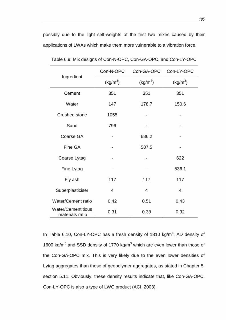
195
possibly due to the light self-weights of the first two mixes caused by their
applications of LWAs which make them more vulnerable to a vibration force.
Table 6.9: Mix designs of Con-N-OPC, Con-GA-OPC, and Con-LY-OPC
Ingredient Con-N-OPC Con-GA-OPC Con-LY-OPC
(kg/m3) (kg/m3) (kg/m3)
Cement 351 351 351
Water 147 178.7 150.6
Crushed stone 1055 - -
Sand 796 - -
Coarse GA - 686.2 -
Fine GA - 587.5 -
Coarse Lytag - - 622
Fine Lytag - - 536.1
Fly ash 117 117 117
Superplasticiser 4 4 4
Water/Cement ratio 0.42 0.51 0.43
Water/Cementitious materials ratio 0.31 0.38 0.32
In Table 6.10, Con-LY-OPC has a fresh density of 1810 kg/m3, AD density of
1600 kg/m3 and SSD density of 1770 kg/m3 which are even lower than those of
the Con-GA-OPC mix. This is very likely due to the even lower densities of
Lytag aggregates than those of geopolymer aggregates, as stated in Chapter 5,
section 5.11. Obviously, these density results indicate that, like Con-GA-OPC,
Con-LY-OPC is also a type of LWC product (ACI, 2003).

196 6. OPC-based concrete and mortar using geopolymer aggregate
Table 6.10: Properties of fresh and hardened Con-N-OPC, Con-GA-OPC, and Con-LY-OPC samples
Con-N-OPC Con-GA-OPC Con-LY-OPC
Slump (mm) 50 50 50
Fresh density (kg/m3) 2400 1856 1810
Density (AD) (28d) (kg/m3) 2310 1770 1600
Density (SSD) (28d) (kg/m3) 2330 1900 1770
Compressive strength (7d) (MPa) 52.36 (0.70)* 44.20 (0.46)* 39.97 (1.41)*
Compressive strength (28d) (MPa) 67.70 (0.50)* 59.32 (0.71)* 56.14 (0.10)*
SSD - saturated surface dry condition; AD - air dry condition; * the value between brackets is the standard deviation of the relevant result.
On the other hand, the lighter Lytag concrete has a lower strength than the
OPC-GA concrete which agrees with the common idea that a lower self-weight
may lead to a lower load-bearing capability (Neville, 1996). As long as this
finding might be convincing to a certain extent since these results are the
average of a few samples, the variations in strengths of these two concretes are
not significant and, indeed, far smaller than those in their density values, with
both capable of reaching a compressive strength level of 55-60 MPa after 28
days.
The concrete made with Lytag has a strength/mass ratio of 56.14/1600=0.0351
(MPa·m3/kg) which is higher than the 0.0335 (MPa·m3/kg) of OPC-GA concrete.
This may imply that Lytag has slightly better mechanical properties for concrete

197
than geopolymer aggregate. However, the Con-GA-OPC concrete mix can still
achieve the density and strength required for structural LWC application (ACI,
2003, Clarke, 1993). Therefore, the author considers that the variations in
mechanical properties should not be the main reason determining the selection
of either geopolymer or Lytag aggregates for LWCs but that cost, resource and
environmental issues should also be considered. A geopolymer aggregate is
likely to be preferred because of its low production cost, eco-friendly
manufacturing process and suitable properties as discussed in Chapter 5.
In this research, a concrete made with Flashag and coded as ‘Con-FS-OPC’ is
also investigated. However, due to the uniqueness of Flashag, the Con-FS-
OPC mix is made based on the mix design proposed by the inventor of Flashag
which includes using 300 kg/m3 of cement and 300 kg/m3 of fly ash (Kayali,
2008). The obtained LWC sample is considered only as a reference for the
properties of FA-LWA concrete products.
The basic properties of Con-GA-OPC and Con-FS-OPC are presented in Table
6.11. The density values of these two concrete mixes are not much varied, with
a fresh density of 1800-1850 kg/m3 and an AD density of 1770-1780 kg/m3.
Apart from this, these two concretes reach similar strength values of
approximately 60 MPa after 28 days, as seen in Table 6.11. This means that
the concrete made of geopolymer aggregates has the potential to achieve the
same strength level as that of Flashag concrete, and serve as a high-strength
concrete material in future industry (Kayali, 2008, Hoff, 1990). Besides, the new
OPC-GA concrete mix is likely to have a lower production cost compared with
the Flashag concrete, since its aggregate portion is made from a less energy
consumption procedure, as discussed in Chapter 5.
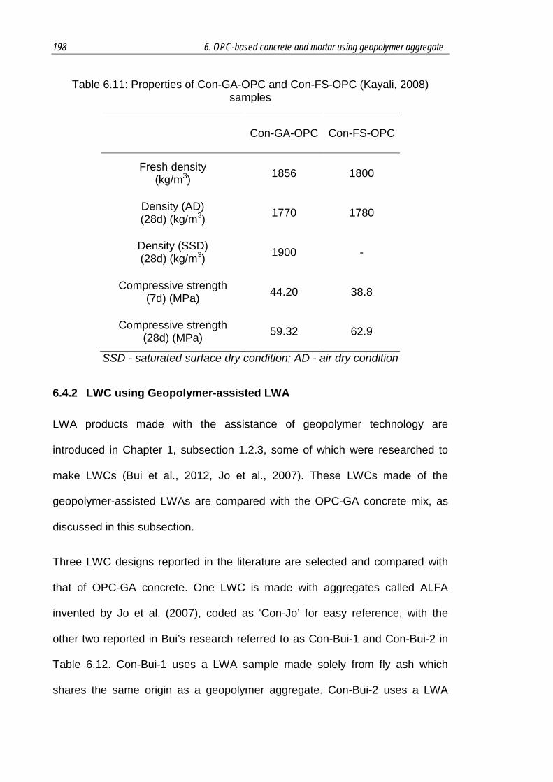
198 6. OPC-based concrete and mortar using geopolymer aggregate
Table 6.11: Properties of Con-GA-OPC and Con-FS-OPC (Kayali, 2008) samples
Con-GA-OPC Con-FS-OPC
Fresh density (kg/m3) 1856 1800
Density (AD) (28d) (kg/m3) 1770 1780
Density (SSD) (28d) (kg/m3) 1900 -
Compressive strength (7d) (MPa) 44.20 38.8
Compressive strength (28d) (MPa) 59.32 62.9
SSD - saturated surface dry condition; AD - air dry condition
6.4.2 LWC using Geopolymer-assisted LWA
LWA products made with the assistance of geopolymer technology are
introduced in Chapter 1, subsection 1.2.3, some of which were researched to
make LWCs (Bui et al., 2012, Jo et al., 2007). These LWCs made of the
geopolymer-assisted LWAs are compared with the OPC-GA concrete mix, as
discussed in this subsection.
Three LWC designs reported in the literature are selected and compared with
that of OPC-GA concrete. One LWC is made with aggregates called ALFA
invented by Jo et al. (2007), coded as ‘Con-Jo’ for easy reference, with the
other two reported in Bui’s research referred to as Con-Bui-1 and Con-Bui-2 in
Table 6.12. Con-Bui-1 uses a LWA sample made solely from fly ash which
shares the same origin as a geopolymer aggregate. Con-Bui-2 uses a LWA
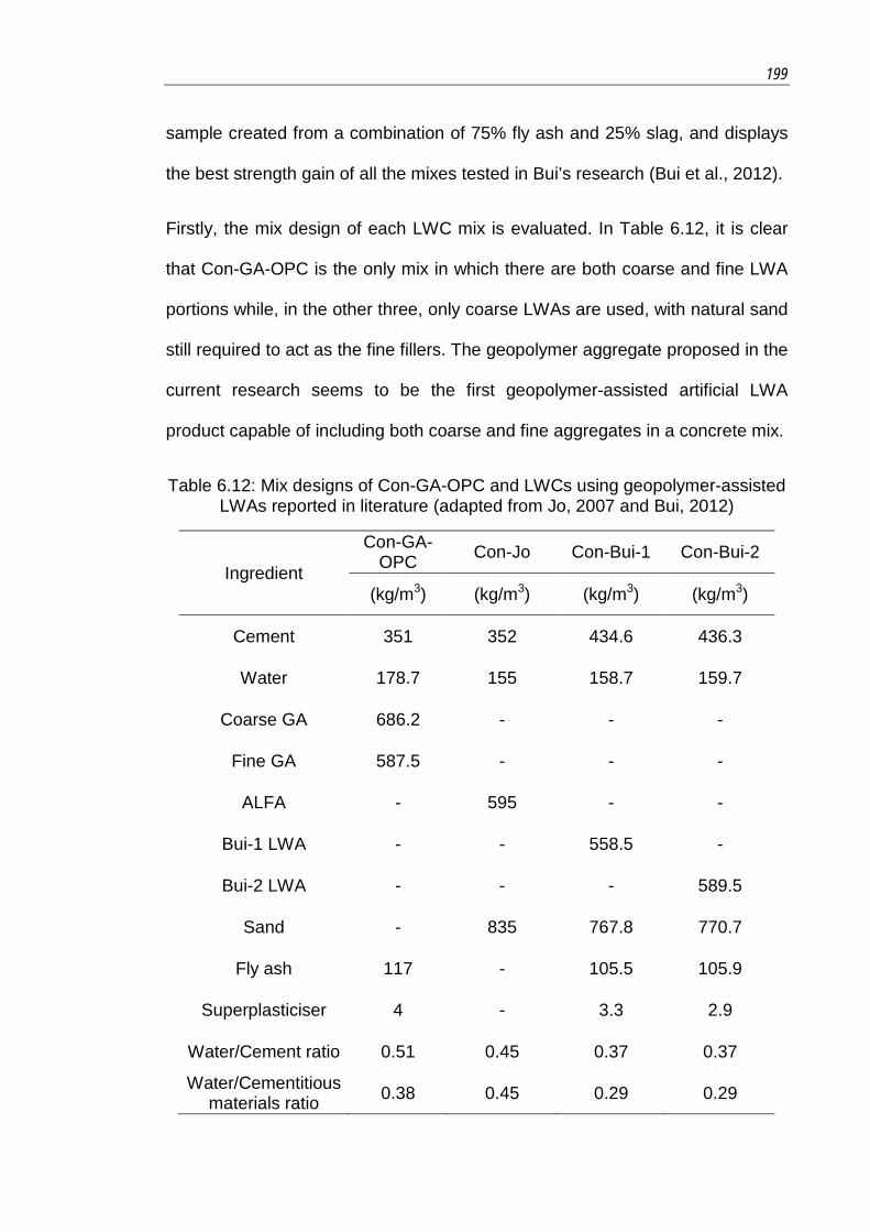
199
sample created from a combination of 75% fly ash and 25% slag, and displays
the best strength gain of all the mixes tested in Bui’s research (Bui et al., 2012).
Firstly, the mix design of each LWC mix is evaluated. In Table 6.12, it is clear
that Con-GA-OPC is the only mix in which there are both coarse and fine LWA
portions while, in the other three, only coarse LWAs are used, with natural sand
still required to act as the fine fillers. The geopolymer aggregate proposed in the
current research seems to be the first geopolymer-assisted artificial LWA
product capable of including both coarse and fine aggregates in a concrete mix.
Table 6.12: Mix designs of Con-GA-OPC and LWCs using geopolymer-assisted LWAs reported in literature (adapted from Jo, 2007 and Bui, 2012)
Ingredient
Con-GA-OPC Con-Jo Con-Bui-1 Con-Bui-2
(kg/m3) (kg/m3) (kg/m3) (kg/m3)
Cement 351 352 434.6 436.3
Water 178.7 155 158.7 159.7
Coarse GA 686.2 - - -
Fine GA 587.5 - - -
ALFA - 595 - -
Bui-1 LWA - - 558.5 -
Bui-2 LWA - - - 589.5
Sand - 835 767.8 770.7
Fly ash 117 - 105.5 105.9
Superplasticiser 4 - 3.3 2.9
Water/Cement ratio 0.51 0.45 0.37 0.37
Water/Cementitious materials ratio 0.38 0.45 0.29 0.29

200 6. OPC-based concrete and mortar using geopolymer aggregate
Bui’s concrete mixes require a higher quantity of cement (430 kg/m3) and higher
proportion of fine aggregates than the OPC-GA concrete mix. Similarly, Jo’s
concrete needs a much higher proportion of sand than OPC-GA concrete
despite using a similar cement proportion. As having more cement and fine
aggregates is beneficial for enhancing the properties of a concrete, it is of
concern that the artificial LWAs produced in Bui’s and Jo’s research might
require increased amounts of cement and fine aggregates than geopolymer
aggregates to achieve the desired quality.
Nevertheless, the mix designs of Jo’s and Bui’s concretes have lower
water/cement ratios of 0.37 to 0.45 than that of OPC-GA concrete, as usually
preferred for an enhanced strength of OPC-based concrete mix (Neville, 1996).
However, it is likely that the OPC-GA concrete cannot be designed with a
similar low water/cement ratio, as discussed earlier, because of its resultant bad
workability. Based on the outcomes of the current research, a higher
water/cement ratio is needed for OPC-GA concrete to achieve acceptable
workability for practical applications which is considered to be due to the
angular shapes of geopolymer aggregates. Or, a larger dosage of a
superplasticiser might be useful for achieving the desired workability with a low
water/cement ratio, so as to achieve an improved strength. This is indeed a
subject for future research. In contrast, the LWAs produced in Jo’s and Bui’s
research are spherical due to the application of a pelletisation process (Jo et al.,
2007, Bui et al., 2012) which can facilitate fluidity in a fresh mixture (Shilstone,
1999, Kockal and Ozturan, 2010).
The properties of these LWC mixes are measured and shown in Table 6.13.
The slump results shown in this Table are all based on a normal-sized slump

201
cone. Bui’s two mixes present slightly higher fresh density and much higher
slump values than those of Con-GA-OPC. However, these slump values may
be too high to result in the end-product having a strong structure. The density
and slump properties of Jo’s concrete mix are not known.
The hardened concretes Con-Jo and Con-Bui-1 result in low compressive
strengths of less than 30 MPa after 28 days. Although Con-Bui-2, which uses a
LWA made from a combination of fly ash and slag, has a higher compressive
strength of 38.10 MPa, this is still much lower than that of Con-GA-OPC which
is 59.32 MPa after 28 days. Obviously, the OPC-GA concrete generates a
superior high-strength performance to those of LWCs made with other
geopolymer-assisted LWAs. This is considered to be due to the advanced
characteristics of geopolymer aggregates, which have a potential to realise a
high performance geopolymer aggregate concrete manufacture.
Table 6.13: Properties of concretes using different LWA products (some data from Jo, 2007 and Bui, 2012)
Con-GA-OPC Con-Jo Con-Bui-1 Con-Bui-2
Fresh density (kg/m3) 1856 - 1931 2056
Slump (mm) 50 - 260 270
28-day compressive strength (MPa) 59.32 26.70 20.80 38.10

202 6. OPC-based concrete and mortar using geopolymer aggregate
6.5 OPC-GA Mortar
This section studies a mortar material made with fine geopolymer aggregates
which is referred to as OPC-GA mortar and coded as ‘Mor-GA-OPC’. Mortar
can be treated as a special type of concrete without a coarse aggregate portion.
Here, it is considered for making a high-performance OPC-GA mortar with a
similar strength but much lower self-weight than a normal one. Also, this
research can highlight the function of fine geopolymer aggregates working as a
new type of ‘artificial sand’ that may be needed in future construction.
6.5.1 Materials
The same fine geopolymer aggregate sample as in Con-GA-OPC (subsection
6.3.1) is used for Mor-GA-OPC, with the cement grain and water introduced in
subsection 6.2.1 completing the mix. Also, the same natural river sand used in
Con-N-OPC is applied for the manufacture of a normal mortar mix coded as
‘Mor-S-OPC’ for reference purposes.
6.5.2 Mix Design
The mix design procedure for mortars is conducted similar to that for an OPC-
GA concrete introduced in subsection 6.3.2. Firstly, a normal mortar mix (Mor-
S-OPC) using sand and cement is made with volumetric ratio of sand to cement
of 3.0 and mass ratio of water to cement of 0.45 respectively, as shown in Table
6.14. Then, the new Mor-GA-OPC mix is made by replacing the sand in Mor-S-
OPC with the same volume of fine geopolymer aggregates. The volume
proportions of other ingredients are not changed. The mix design of Mor-GA-
OPC is obtained and shown in Table 6.14, with the same cementitious material
as Mor-S-OPC. From trial tests conducted to ensure that the two mortar mixes
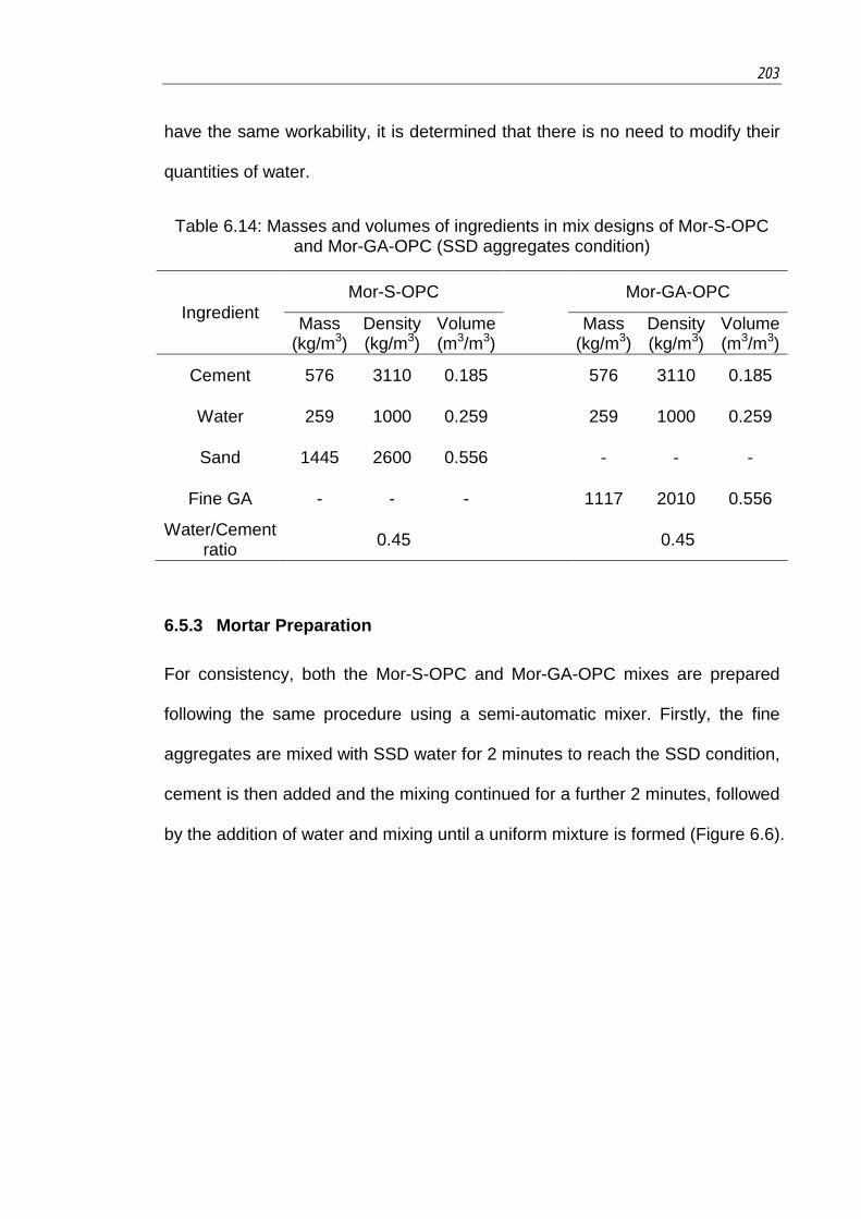
203
have the same workability, it is determined that there is no need to modify their
quantities of water.
Table 6.14: Masses and volumes of ingredients in mix designs of Mor-S-OPC and Mor-GA-OPC (SSD aggregates condition)
Ingredient Mor-S-OPC Mor-GA-OPC
Mass (kg/m3)
Density (kg/m3)
Volume (m3/m3) Mass
(kg/m3) Density (kg/m3)
Volume (m3/m3)
Cement 576 3110 0.185 576 3110 0.185
Water 259 1000 0.259 259 1000 0.259
Sand 1445 2600 0.556 - - -
Fine GA - - - 1117 2010 0.556
Water/Cement ratio 0.45 0.45
6.5.3 Mortar Preparation
For consistency, both the Mor-S-OPC and Mor-GA-OPC mixes are prepared
following the same procedure using a semi-automatic mixer. Firstly, the fine
aggregates are mixed with SSD water for 2 minutes to reach the SSD condition,
cement is then added and the mixing continued for a further 2 minutes, followed
by the addition of water and mixing until a uniform mixture is formed (Figure 6.6).

204 6. OPC-based concrete and mortar using geopolymer aggregate
Figure 6.6: Images of fresh mortar mixtures: (1) Mor-S-OPC and (2) Mor-GA-OPC
After mixing, the fresh mortar mixtures are cast into cubic 50mm×50mm×50mm
stainless steel moulds and cured at 20oC for 1 day. Then, the initially hardened
mortar samples are demoulded and placed in a water-spray room at 20oC until
further testing. This curing regime is similar to that for the concrete samples
discussed earlier. Mortar samples using regular sand and the new geopolymer
aggregates after 28 days of curing are shown in Figure 6.7. The samples have
a similar appearance possibly due to the same cement matrix formed.
Figure 6.7: Images of 28-day cured Mor-S-OPC and Mor-GA-OPC samples
(1) (2)
Mor-GA-OPC Mor-S-OPC

205
6.5.4 Workability
The workability performances of the fresh mortars discussed in this section are
evaluated based on the combined slump and mini-flow method discussed in
Chapter 2, subsection 2.4.1. The initial slumps and spreads, and spreads after
10-second vibrations of the mortar samples Mor-S-OPC and Mor-GA-OPC are
measured and presented in Table 6.15 and Figure 6.8.
As seen in Table 6.15, as both the fresh mortar mixes present the same slump
value of 20 mm based on the applied mini-sized slump cone (the cone specified
in subsection 2.4.1 with a top opening of 19 mm) and have good workability with
high fluidity, they can be easily compacted and processed. This high workability
is barely affected by the use of geopolymer aggregates or sand, but more likely
determined by the cement matrix generated in above mortar mixes.
Table 6.15: Slump and spread values of fresh Mor-S-OPC and Mor-GA-OPC
Mortar
Before vibration After 10-second vibration
Initial slump (mm)
Initial spread (cm2)
Spread at once (cm2)
Spread in 3 mins
(cm2)
Spread in 10 mins
(cm2) Mor-S-OPC 20 13.67 61.57 62.46 62.50
Mor-GA-OPC 20 13.13 82.30 82.55 82.56
On the other hand, as seen in Figure 6.8, both the fresh mortar mixes have a
high spread gain after the stimulation of mechanical vibration, with that of Mor-
GA-OPC having higher spread areas than Mor-S-OPC. This is considered to be
due to the use of fine geopolymer aggregates in the former which are much
lighter than sand, thereby reducing the weight of an entire mortar mix and

206 6. OPC-based concrete and mortar using geopolymer aggregate
possibly causing it to be less resistant to the vibration force applied. This
indicates that using lightweight geopolymer aggregates in a mortar mix could
enhance its flow against a mechanical vibration, making it easier for compaction
in practice. This has also been found when processing the previous OPC-GA
concrete samples, and can be a potential benefit for using a lightweight material.
Figure 6.8: Increases in spread areas of fresh Mor-S-OPC and Mor-GA-OPC caused by mechanical vibration
6.5.5 Density and Strength
The density and strength properties of the mortar samples produced are
presented in Table 6.16. Firstly, Mor-S-OPC has a fresh density of 2217 kg/m3
and Mor-GA-OPC has a fresh density of only 1903 kg/m3. Similarly, Mor-GA-
OPC sample has an AD density of 1750 kg/m3 and SSD density of 1900 kg/m3
which are much lower than those of Mor-S-OPC. These results show that an
application of geopolymer aggregates instead of sand can significantly reduce
0
10
20
30
40
50
60
70
80
90
initial spread spread atonce
spread in 3mins
spread in 10mins
Spre
ad a
rea
(cm
2 )
Mor-S-OPC
Mor-GA-OPC

207
the density behaviour of mortar, achieving a light self-weight mortar mix just as
what has been done in an OPC-GA concrete.
Table 6.16: Density and strength properties of Mor-S-OPC and Mor-GA-OPC
Mor-S-OPC Mor-GA-OPC
Fresh density (kg/m3) 2217 1903
Density (AD) (28d) (kg/m3) 2140 1750
Density (SSD) (28d) (kg/m3) 2220 1900
Compressive strength (7d) (MPa) 39.66 38.76
Compressive strength (28d) (MPa) 55.21 58.86
SSD - saturated surface dry condition; AD - air dry condition
On the other hand, the compressive strength results shown in Table 6.16
indicate that the Mor-GA-OPC with a much lighter density is able to achieve the
same strength level as the Mor-S-OPC mix and its 28-day compressive strength
is even slightly higher. Although this strength difference may not be significant
from a statistical viewpoint, it is at least, a very promising indication that the
utilisation of geopolymer aggregates in mortar will not compromise the strength
of the end-product. Also, as in the previous trend in concrete samples, the Mor-
GA-OPC has a higher strength/mass ratio of 0.034 (MPa·m3/kg) than that of the
Mor-S-OPC of 0.026 (MPa·m3/kg), which is considered mostly related to the
light self-weight of the former one. This indicates the advanced property of fine
geopolymer aggregates in making a high-strength but lightweight mortar

208 6. OPC-based concrete and mortar using geopolymer aggregate
material. For this case, a lightweight mortar product seems to be workable to be
used in replacement of a conventional normal weight one without a concern on
its strength loss.
Clearly, the mortar mix made with geopolymer aggregates is worth further
discussion and research because the current results show that it can be of good
quality, lightweight, a save of natural sand, and more importantly, exhibits no
corresponding strength loss. Although the OPC-GA concrete using geopolymer
aggregates can achieve a high quality, it results in an approximate 10 MPa
strength loss compared with its NWC counterpart using natural aggregates, as
shown in Table 6.5 and Table 6.8. So, the concrete mix with both coarse and
fine geopolymer aggregates seems to not function as well as the mortar mix
with only fine geopolymer aggregates. The author considers that this effect
might be partially due to the more uniform mixture of mortar which can be
treated almost as a two-phase mixture composed of sand (or artificial sand as
fine geopolymer aggregates) and a cement matrix rather than a more
complicated mixture of concrete. Also, the author wonders whether a fine
geopolymer aggregate may present better consistency than a coarse one
because it is subjected to more crushing during its manufacturing stage.
Nevertheless, the concrete mixes discussed in this chapter are not sufficient
enough to conclude that the OPC-GA concrete cannot reach the same strength
as a NWC concrete one and this makes future research in this area, highly
recommended.
209
6.6 Conclusions
In this chapter, the practicality of using geopolymer aggregates in OPC-based
concrete and mortar mixes is researched. It is found that both the concrete and
mortar made with geopolymer aggregates have certain advanced properties,
such as a light weight, high strength/mass ratio and mechanical behaviour
qualified for real-life practice. They are also successful applications of
geopolymer aggregates as a new type of FA-LWA which realise their low-cost
and eco-friendly benefits.
The concrete mix design procedure established in this chapter proves to be
suitable for creating the required mix design of OPC-GA concrete. It can also
help to correlate the OPC-GA concrete and NWC designs which have the same
ingredients for cementitious materials to provide a reference when needed to
assess the performance of the new OPC-GA concrete mix. A similar mortar mix
design procedure is also developed. Apart from being used for the mixes
discussed in this chapter, these design procedures can also be repeatedly
applied in future research for concrete and mortar designs with different
proportions of ingredients.
A workable preparation of OPC-based concrete and mortar made with
geopolymer aggregates is also illustrated, with samples measured and
analysed, and determined to have good fresh and hardened properties.
Therefore, geopolymer aggregates are found to be suited for a Portland cement
system which inspires their potential broad promotion as alternatives to current
FA-LWA products in future construction fields.

210 6. OPC-based concrete and mortar using geopolymer aggregate
Moreover, this research indicates that there might be a promising way of using
fine geopolymer aggregates in the mortar, which can have a higher
strength/mass ratio with no strength loss than the regular mortar made with
sand. It is assumed that this will make the manufacture of OPC-GA mortar of
more interest in the near future.

211
Chapter 7
Geopolymer Binder-based Concrete and Mortar using
Geopolymer Aggregate
7.1 Introduction
This chapter continues the research on the application of a geopolymer
aggregate in a concrete mix. Unlike the OPC-based concrete presented in
Chapter 6, the concrete mix researched in this chapter uses a fly ash-based
geopolymer as the sole cementitious material, and therefore it is referred to as a
geopolymer binder-based concrete. Thus, concrete mix with the aggregates and
cementitious material all made from fly ash-based geopolymer, is researched.
A concrete made with geopolymer aggregates and geopolymer binder is
designed, referred to as Geo-GA concrete and coded as ‘Con-GA-Geo’. A
workable mix design procedure is proposed to create different Geo-GA mixes
for research purposes. The research aims to evaluate the compatibility of
geopolymer aggregates with a geopolymer binder system, and the capability of
the subsequent Geo-GA concrete in realising high-performance geopolymer
LWCs.
Another kind of concrete which uses natural aggregates and geopolymer binder
is also involved in this chapter. This concrete is the one that commonly called
geopolymer concrete and has been researched for decades (Davidovits, 2008)
which is simplified as GC and coded in this chapter as ‘Con-N-Geo’. It is
researched in order to assess the designed geopolymer binders, so as to
provide information needed for a Geo-GA concrete mix. For this reason, the GC
212 7. Geopolymer binder-based concrete and mortar using geopolymer aggregate
mixes included in this chapter are made with the same geopolymer binders as
those of Geo-GA mixes.
Additionally, a mortar material made with a geopolymer binder instead of OPC
is researched. The mortar mixes in this chapter use either the regular natural
sand or fine geopolymer aggregates. It is aimed to evaluate the practicality of
using geopolymer material (both aggregates and binder) in a mortar material.
7.2 Mix Design Procedure for Geopolymer Binder-based
Concretes
7.2.1 Materials
The Geo-GA concrete uses geopolymer aggregates for both the coarse and fine
aggregate portions in its mix. These geopolymer aggregates are from the same
aggregate samples as the ones used in an OPC-GA concrete illustrated in
Chapter 6, section 6.3. On the other hand, the GC mix uses the laboratory-used
crushed stone and river sand whose relevant characteristics are presented in
Chapter 6, subsection 6.2.1.
Otherwise, the common ingredients needed for the synthesis of a fly ash-based
geopolymer, namely fly ash, NaOH solution, Na2SiO3 solution and deionised
water, are applied. The details of these ingredients are illustrated in Chapter 3.
Moreover, two chemical admixtures, which were previously reported to modify
the performance of fresh geopolymer concrete mix (Junaid et al., 2012), are
applied. One is a polycarboxylate ether base mid-range water-reducer (known
commercially as Centrox MWR), and the other is a cellulose base viscosity
modifier (known commercially as Centrox VMA). Both admixtures are added in
a dosage of 1% of the mass of fly ash.
213
7.2.2 Geo-GA Concrete
A mix design procedure is proposed here for creating different Geo-GA mixes
for research purpose. This procedure is to create Geo-GA mix design from the
known OPC-GA mix design, where the latter one can help to determine the unit
weight and aggregate proportion. From this, the proportion of binding material in
a Geo-GA mix is determined. Afterwards, this binding material can be designed
following the geopolymer mix design procedure proposed in Chapter 3. A
detailed procedure is illustrated in following paragraphs.
Firstly, the Con-GA-OPC mix discussed in Chapter 6, section 6.3 is selected as
the base to create the new Con-GA-Geo mix design. The procedure is
explained in combination with Table 7.1 in which it can be seen that Con-GA-
OPC has a unit weight of 1924.4 kg/m3, a coarse aggregate proportion of 686.2
kg/m3, a fine aggregate proportion of 587.5 kg/m3 and a binding material
proportion of 650.7 kg/m3. Since this Con-GA-OPC mix has been proved
workable with a good strength, as shown in Chapter 6, it is considered that the
above values are likely to end up in a workable mix and therefore used as a
reference for Con-GA-Geo. Then, the new mix design of Con-GA-Geo is
designed to have the same unit weight and same proportions of aggregates and
binding material as those of Con-GA-OPC, as seen in Table 7.1. Following this,
some basic information of a mix design can be quickly confirmed, as suggested
in the previous literature (Rangan, 2007).
It should be noted that, in Table 7.1, it is assumed that the 650.7 kg/m3
geopolymer binding material would occupy the same volume as that of 650.7
kg/m3 OPC in the mix. This assumption is only made for the need of mix design

214 7. Geopolymer binder-based concrete and mortar using geopolymer aggregate
procedure. A necessary modification is required and made later to obtain the
final mix design that suits 1 m3 Geo-GA concrete mix.
Table 7.1: Unit weight and ingredient proportions of mix designs of Con-GA-OPC and Con-GA-Geo (SSD aggregates condition)
Ingredient
Con-GA-OPC
Con-GA-Geo
(kg/m3) (kg/m3)
Binding material 650.7 650.7
Coarse GA 686.2 686.2
Fine GA 587.5 587.5
Unit weight 1924.4 1924.4
Aggregate mass proportion 66% 66%
Later, the ingredients used to compose this 650.7 kg/m3 binding material are
designed. In principle, since the geopolymer binder is also a kind of geopolymer
material, its mix design is completed following the mix design procedure
proposed in Chapter 3. Meanwhile, the two Centrox admixtures are also treated
as parts of this binding material, and needed to be designed for. On the other
hand, as different geopolymer binders may be required to make different Geo-
GA concretes for research purpose, some mix designs for desired geopolymer
binders in current research have been created and presented in Chapter 3,
section 3.7. The detailed mix design procedure for Geo-GA concrete mix is
illustrated in Appendix B. The final mix designs of the Geo-GA concretes
required for the current research are presented in Table 7.2. Following this
procedure, different Geo-GA mixes can be created by selecting different
SiO2/Na2O, H2O/Na2O and W/G ratios. Moreover, users may also design the

215
unit weight and aggregate proportion according to their needs, instead of based
on a known OPC-GA every time.
Table 7.2: Mix designs of Con-GA-Geo samples (SSD aggregates condition)
Concrete code Con-GA-Geo-1
Con-GA-Geo-2
Con-GA-Geo-3
Fly ash (kg/m3) 446.1 446.1 431.6
W/G value 0.24 0.26 0.26
SiO2/Na2O (x value) 1.25 1.25 1.25
H2O/Na2O (y value) 11 11 11
Fly ash/Activator (F/A) 2.05 1.86 1.86
Coarse GA (kg/m3) 666.3 652.5 663.7
Fine GA (kg/m3) 565.5 550.6 562.7
NaOH 16M (kg/m3) 47.0 51.8 50.1
Na2SiO3 (kg/m3) 165.7 182.7 176.7
Water (kg/m3) 4.9 5.4 5.2
Centrox MWR (kg/m3) 4.5 4.5 4.3
Centrox VMA (kg/m3) 4.5 4.5 4.3
Unit weight (kg/m3) 1904.5 1898.0 1898.6
Aggregate mass proportion (%) 65% 63% 65%
The expression of the mix designs presented in Table 7.2 is treated as a
standard way for all geopolymer binder-based concrete mixes included in this
thesis. As seen in Table 7.2, four sections are categorised except for the title
section. The first section is the fly ash quantity, which is to highlight the usage of
fly ash since it is the main aluminosilicate source for geopolymerisation

216 7. Geopolymer binder-based concrete and mortar using geopolymer aggregate
(Davidovits, 2008). This fly ash quantity can also be a key factor to distinguish
each mix throughout this chapter; the second section presents the factors used
to describe the design of geopolymer as detailed in Chapter 3; the third section
lists the other ingredients except fly ash in the mix design; and the last section
shows the unit weight and aggregate mass proportion. This expression of mix
design is promoted by the author since it clearly displays all information needed
for a scientific analysis.
7.2.3 Geopolymer Concrete (GC)
Table 7.3: Mix designs of Con-N-Geo samples (SSD aggregates condition)
Concrete code Con-N-Geo-1
Con-N-Geo-2
Con-N-Geo-3
Fly ash (kg/m3) 446.1 446.1 431.6
W/G value 0.24 0.26 0.26
SiO2/Na2O (x value) 1.25 1.25 1.25
H2O/Na2O (y value) 11 11 11
Fly ash/Activator (F/A) 2.05 1.86 1.86
Crushed stone (kg/m3) 977.7 957.5 973.9
River sand (kg/m3) 731.6 712.2 727.9
NaOH 16M (kg/m3) 47.0 51.8 50.1
Grade D Na2SiO3 (kg/m3) 165.7 182.7 176.7
Deionised water (kg/m3) 4.9 5.4 5.2
Centrox MWR (kg/m3) 4.5 4.5 4.3
Centrox VMA (kg/m3) 4.5 4.5 4.3
Unit weight (kg/m3) 2382.0 2364.6 2374.0
Aggregate mass proportion (%) 72% 71% 72%

217
Although the main objective of this chapter is the Geo-GA concrete, a research
on geopolymer concrete (GC) using natural aggregates is needed to be firstly
conducted, for assessing the effects of applied geopolymer binders. For this
reason, these GC mixes use the same geopolymer binders as those of Geo-GA
mixes. The mix designs of GC are presented in Table 7.3, which are made by
replacing the geopolymer aggregates in the Geo-GA mixes in Table 7.2 with the
same volume proportions of natural aggregates.
7.3 Geopolymer Concrete (GC)
The geopolymer concrete (GC) samples designed in Table 7.3 are firstly
manufactured prior to Geo-GA samples. The properties of GC samples are
measured to evaluate the performance of designed geopolymer binders, to
provide useful information for subsequent Geo-GA mixes.
7.3.1 Concrete Preparation
The preparation of concrete sample Con-N-Geo is shown in Figure 7.1, based
on the general geopolymer concrete mixing procedure (Hardjito et al., 2004,
Junaid et al., 2012, Kong and Sanjayan, 2010) with slight modification
according to the author’s experience. Firstly, the selected crushed stone and
sand are mixed with the SSD water using a mechanical concrete mixer for
around 2 minutes. Then, fly ash and Na2SiO3 solution are added and mixed with
the wet aggregates for a further 2-3 minutes. This step is to uniformly distribute
the cementitious material (which is fly ash) onto the surfaces of the aggregates,
which is like the step of adding cement to wet aggregates in an OPC-based
concrete mixing. Following that, NaOH solution, water and admixtures are
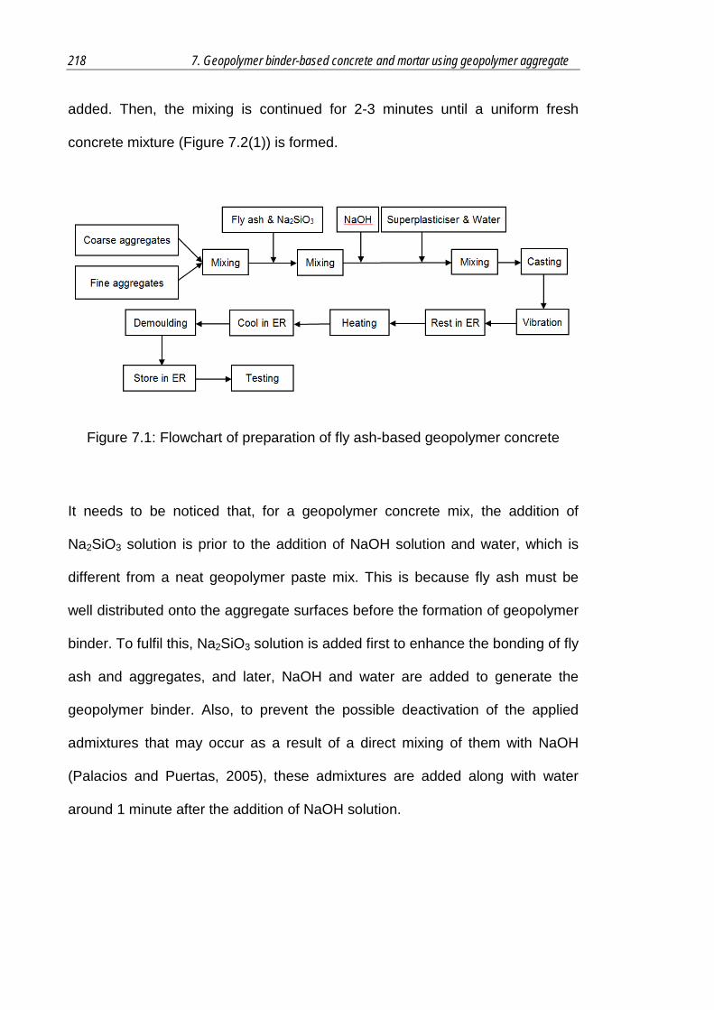
218 7. Geopolymer binder-based concrete and mortar using geopolymer aggregate
added. Then, the mixing is continued for 2-3 minutes until a uniform fresh
concrete mixture (Figure 7.2(1)) is formed.
Figure 7.1: Flowchart of preparation of fly ash-based geopolymer concrete
It needs to be noticed that, for a geopolymer concrete mix, the addition of
Na2SiO3 solution is prior to the addition of NaOH solution and water, which is
different from a neat geopolymer paste mix. This is because fly ash must be
well distributed onto the aggregate surfaces before the formation of geopolymer
binder. To fulfil this, Na2SiO3 solution is added first to enhance the bonding of fly
ash and aggregates, and later, NaOH and water are added to generate the
geopolymer binder. Also, to prevent the possible deactivation of the applied
admixtures that may occur as a result of a direct mixing of them with NaOH
(Palacios and Puertas, 2005), these admixtures are added along with water
around 1 minute after the addition of NaOH solution.

219
Figure 7.2: Steps in preparation of concrete Con-N-Geo (1) mixing, (2) casting, (3) after heating and demoulding and (4) after 28-day curing
After mixing, a portion of the fresh Con-N-Geo mix is tested for its fresh
properties, and the remaining portion used to cast samples in cubic
50mm×50mm×50mm steel moulds with polyethylene sheets stuck onto the
inner surface to facilitate demoulding. A vibrating table (220-240V AC, 50HZ) is
applied to compact the fresh mix into well-shaped cubes (Figure 7.2(2)). Since
the fresh Con-N-Geo mixes produced here are very stiff in workability, a longer
time of vibration in assistance with manual tamping is usually required. The
Con-N-Geo sample is then sealed and cured in the ER at 20oC for 1 day, and
(1) (2)
(3) (4)

220 7. Geopolymer binder-based concrete and mortar using geopolymer aggregate
later cured at 80oC for 3 days in an electric oven. After heating, the sample is
placed back in the ER, and demoulded after it cools down (Figure 7.2(3)). The
demoulded sample remains in the ER, exposed to a low-moisture atmosphere
(20oC and 50% RH), until further testing. An image of a 28-day cured Con-N-
Geo sample is shown in Figure 7.2(4).
7.3.2 Workability
The same slump test that has been used for OPC-based concretes was applied
on the fresh Con-N-Geo mixes described in this section. However, it turned out
that all tested mixes had no slump at all, displaying an extremely stiff workability.
Actually, these fresh mixes were so stiff that the mixed material could not be
properly piled in the slump cone by rodding only, but also required manual
tamping and pressing. This is considered to be due to the rather high viscosity
of geopolymer material (Criado et al., 2009). In addition, the Con-N-Geo mixes
designed here are to pursue a better strength outcome, so their W/G ratios are
set to be very low which can influence their workability (Rangan, 2007).
To deal with these viscous fresh mixes, the author also tried to use a mini-flow
test that has been introduced in Chapter 2, subsection 2.4.1, to assess their
spread increases under vibration, but based on a larger sized slump cone to
suit a concrete mix. However, there was no significant flow spread detected on
the tested Con-N-Geo samples, despite that several previously published
articles have stated the suitability of flow test for measuring the workability of
geopolymer products (Criado et al., 2009, Chindaprasirt et al., 2007, Nath and
Sarker, 2014). It is thought that the mix is too stiff, so it is hard to flow freely on
the vibrating table.

221
Obviously, this stiff workability would cause problems in a real concrete practice
situation, which is already noticed during the preparation of Con-N-Geo mixes in
this research. But for the current need of a strong geopolymer binder in the
following Geo-GA concrete manufacture, this study would rather focus on the
mechanical properties and compromise the workability requirement. Otherwise,
to well compact this concrete mix in the moulds, a long time mechanical
vibration in assistance with a certain degree of manual tamping is applied with
caution as not to affect the uniformity of the mixture.
7.3.3 Density and Strength
The density values of fresh and hardened Con-N-Geo samples were tested and
their compressive strengths measured using a TECNOTEST compression
machine at a speed of 0.33 MPa/sec, with the final value of each mixing batch
taken as the average of three cubic samples as shown in Table 7.4.
The densities of the three tested Con-N-Geo mixes are not much varied, with a
fresh density of 2300-2350 kg/m3 and an air dry density of 2150-2170 kg/m3.
For these mixes, their 28-day air dry densities are lower than their 7-day ones,
but the disparities are not significant. The density range of Con-N-Geo is close
to the range of NWC, and much higher than that of LWC (Clarke, 1993), which
is reasonable since Con-N-Geo still uses the normal weight aggregates as
crushed stone and sand.
The tested Con-N-Geo samples have 7-day compressive strengths of 55-64
MPa, which are nearly 90% of their 28-day strengths. This means that Con-N-
Geo can achieve a high early strength which agrees with the previous findings
(Rangan, 2007, Hardjito et al., 2004). Otherwise, these Con-N-Geo samples

222 7. Geopolymer binder-based concrete and mortar using geopolymer aggregate
have 28-day compressive strengths of 60-70 MPa, which are high-strength
concrete and may be preferred in real practice (Hoff, 1990).
Table 7.4: Density and strength properties of Con-N-Geo
Con-N-Geo-1 Con-N-Geo-2 Con-N-Geo-3
Fresh density (kg/m3) 2313 2338 2375
Density (AD) (7d) (kg/m3) 2170 2167 2170
Density (AD) (28d) (kg/m3) 2160 2150 2160
Compressive strength (7d) (MPa) 63.87 (0.80)* 55.54 (0.83)* 57.40 (1.10)*
Compressive strength (28d) (MPa) 70.42 (0.50)* 60.26 (0.30)* 61.65 (1.20)*
AD - air dry condition; * the value between brackets is the standard deviation of the relevant result.
Con-N-Geo-1 has a 28-day compressive strength of 70.42 MPa which is the
highest among the above three mixes. It is a high-strength concrete and
comparable to the NWC samples presented in Chapter 6, subsection 6.2.5.
Therefore, it is estimated that the geopolymer binder used in this mix must be
strong enough for a Geo-GA mix. On the other hand, Con-N-Geo-2 and Con-N-
Geo-3 result in lower 28-day strengths of around 60 MPa, very possibly due to
their higher W/G ratios (0.26) of the mix (Rangan, 2007). Nevertheless, these
two samples also have strong geopolymer binders to make them reach a high-
strength level. Moreover, they are found to have a better workability than Con-
N-Geo-1 because of their higher W/G ratios. For this case, the geopolymer

223
binders used in these two mixes are also applied for making Geo-GA concretes
described in the next section.
7.4 Geo-GA Concrete
7.4.1 Concrete Preparation
Con-GA-Geo mixes are made based on the selected mix designs shown in
Table 7.2. The preparation of Con-GA-Geo follows the same procedure as that
for GC mix shown in Figure 7.1. As the workability of these Con-GA-Geo mixes
is not much improved, a long time vibration with several manual tamping is also
required for compaction. Meanwhile, a strict control suggested in the manual
ACI 211.2 is required to assure the SSD conditions of applied lightweight
geopolymer aggregates (ACI, 1998). Images showing the relevant steps in
mixing Con-GA-Geo are presented in Figure 7.3.
7.4.2 Density and Strength
The density and strength properties of the Con-GA-Geo samples are measured
using the same methods introduced in subsection 7.3.3, and shown in Table 7.5.
Similar to the Con-N-Geo mixes, the densities of produced Con-GA-Geo
samples are not significantly varied, with a fresh density of 1870-1890 kg/m3, a
7-day air dry density of 1670-1690 kg/m3, and a 28-day air dry density of 1630-
1640 kg/m3. It can be seen that these Con-GA-Geo samples are lightweight (AS,
1998a, Clarke, 1993) after the application of lightweight geopolymer aggregates.
Through this way, one can produce a geopolymer binder-based LWC, which is
a new kind of concrete material that has been at the focus of studies in recent
years (Arellano Aguilar et al., 2010, Hu et al., 2009). Nevertheless, the LWC

224 7. Geopolymer binder-based concrete and mortar using geopolymer aggregate
proposed in this chapter is based on fly ash-based geopolymer aggregates and
binder.
Figure 7.3: Steps in preparation of concrete Con-GA-Geo (1) mixing, (2) casting, (3) after heating and demoulding and (4) after 28-day curing
Also, it can be observed that there is a slight density loss from 7-day Con-GA-
Geo samples to 28-day ones, which is possibly due to the release of water from
the geopolymer binder cured at a low-moisture condition (50% RH in the ER),
as previously discussed in Chapter 4, section 4.4.
On the other hand, the tested Con-GA-Geo samples achieve 7-day and 28-day
compressive strengths of around 25-29 MPa and 40-46 MPa respectively.
(1) (2)
(3) (4)
225
These results indicate that they can achieve a medium-strength and qualified
for structural LWC applications (ACI, 1998, Clarke, 1993). Among the samples,
Con-GA-Geo-1 has the highest compressive strength of 45.34 MPa after 28
days of curing, which is in accordance with the trend in strength results of Con-
N-Geo mixes, possibly due to its lowest W/G ratio (0.24) (Rangan, 2007).
Besides, the other two mixes with the same W/G ratio share a similar strength
result, even though they have different amounts of ingredients in the mix. For
this case, W/G ratio seems to be more important regarding the strength
development of Geo-GA concrete.
Table 7.5: Density and strength properties of Con-GA-Geo
Con-GA-Geo-1
Con-GA-Geo-2
Con-GA-Geo-3
Fresh density (kg/m3) 1890 1885 1873
Density (AD) (7d) (kg/m3) 1680 1690 1670
Density (AD) (28d) (kg/m3) 1630 1630 1640
Compressive strength (7d) (MPa)
28.67 (0.92)*
26.18 (1.39)*
25.77 (1.27)*
Compressive strength (28d) (MPa)
45.34 (1.41)*
40.04 (0.59)*
41.32 (0.75)*
AD: air dry condition; * the value between brackets is the standard deviation of the relevant result.
Compared to the Con-N-Geo samples, which are made with the same
geopolymer binders and curing regimes, Con-GA-Geo samples result in
approximately 20 MPa lower compressive strengths. Part of this strength
deficiency is considered due to using the lightweight geopolymer aggregates

226 7. Geopolymer binder-based concrete and mortar using geopolymer aggregate
instead of normal weight aggregates. Apart from this, it is not certain whether
some other factors may also affect the strength development of the concrete
using geopolymer aggregates. It can be found that the strength difference of
Geo-GA and GC (around 20 MPa) is more significant than that of OPC-GA and
NWC (around 10 MPa). It seems that the strength loss by using geopolymer
aggregates is exaggerated in a geopolymer binder system compared to that in
an OPC system. Except from the lower self-strength of geopolymer aggregate,
it is estimated that this may also be relevant to the bonding strength of
geopolymer aggregates and geopolymer binder (compared to the bonding of
geopolymer aggregates and OPC matrix), and this possibility requires further
research.
Moreover, it is not observed that Con-GA-Geo will have a high early strength
that has been found in Con-N-Geo. The 7-day strengths of Con-GA-Geo mixes
are 25-29 MPa and only achieve 62-66% of their 28-day strengths.
Nevertheless, Con-GA-Geo mixes have strength gains of approximately 15
MPa during the period of 7-28 days, where there is even no heat treatment.
This strength gain is found special because it is clearly higher than those of
Con-N-Geo mixes (4-7 MPa). It is also higher than the normal strength gain
within this period reported in the literature (Hardjito et al., 2004). As the Con-N-
Geo and Con-GA-Geo mixes share the same geopolymer binders and curing
regimes, this special strength gain is considered much relevant to the presence
of geopolymer aggregates, which needs further investigation.
The research on Geo-GA concrete in this section proves that a workable
concrete mix made with geopolymer aggregates and binder can be realised with
good mechanical properties. For this case, an ‘absolute geopolymer concrete’

227
which is almost 100% from geopolymer material is manufactured. This will
provide a new concept of concrete mix in the field of geopolymer concrete, and
a new kind of LWC material with the promising quality preferred in future
construction. However, to realise the desired mechanical properties, the
workability of Geo-GA concrete has been compromised. The Geo-GA concrete
samples produced here have stiff workability, which is even difficult to be
accurately measured by normal workability tests. The addition of admixtures
cannot significantly improve the workability, but only modify the fresh
performance to make them better compacted. This Geo-GA concrete can be
promising for its strength, but still needs further research to modify its
workability performance.
7.4.3 Fracture Surface
The fracture surface of the Geo-GA sample after compressive strength testing
is observed using a Lynx vision engineering stereo microscope. The captured
image is shown in Figure 7.4 in which the geopolymer aggregates and
geopolymer binder matrix are labelled based on their detected shapes and
sizes.
In the image, the geopolymer aggregates are embedded in the geopolymer
binder matrix, with a complete interfacial zone observed. Little cracking is
formed along the detected interfacial zone, which indicates a good strength
performance of the bonding of the aggregates and binder. Also, no cracking is
formed across the aggregates. It can be seen that Con-GA-Geo sample has a
similar fracture surface as that of Con-GA-OPC presented in Chapter 6,
subsection 6.3.6.
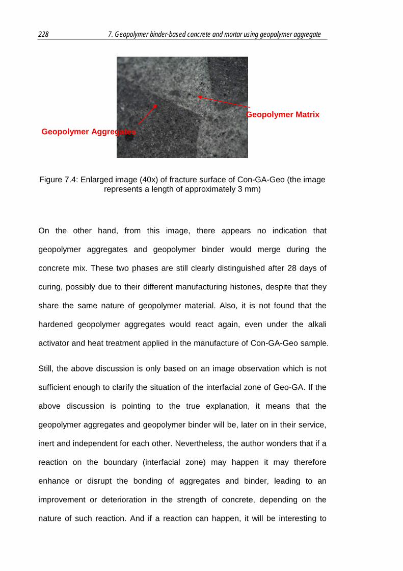
228 7. Geopolymer binder-based concrete and mortar using geopolymer aggregate
Figure 7.4: Enlarged image (40x) of fracture surface of Con-GA-Geo (the image represents a length of approximately 3 mm)
On the other hand, from this image, there appears no indication that
geopolymer aggregates and geopolymer binder would merge during the
concrete mix. These two phases are still clearly distinguished after 28 days of
curing, possibly due to their different manufacturing histories, despite that they
share the same nature of geopolymer material. Also, it is not found that the
hardened geopolymer aggregates would react again, even under the alkali
activator and heat treatment applied in the manufacture of Con-GA-Geo sample.
Still, the above discussion is only based on an image observation which is not
sufficient enough to clarify the situation of the interfacial zone of Geo-GA. If the
above discussion is pointing to the true explanation, it means that the
geopolymer aggregates and geopolymer binder will be, later on in their service,
inert and independent for each other. Nevertheless, the author wonders that if a
reaction on the boundary (interfacial zone) may happen it may therefore
enhance or disrupt the bonding of aggregates and binder, leading to an
improvement or deterioration in the strength of concrete, depending on the
nature of such reaction. And if a reaction can happen, it will be interesting to
Geopolymer Aggregates
Geopolymer Matrix

229
find out if the reactant from geopolymer aggregates is either the fly ash residue
(if any) or the hardened geopolymer structure, or both.
7.5 Comparison of Geo-GA Concrete and Other LWCs
The performance of the Geo-GA concrete produced in this research, which is a
new type of LWC, is evaluated by comparison with other LWCs. It is firstly
compared with the OPC-GA concrete discussed in Chapter 6, which uses the
same geopolymer aggregates but a different cementitious material. After this, it
is compared with a geopolymer binder-based LWC which uses a conventional
FA-LWA Lytag aggregate.
7.5.1 Geo-GA versus OPC-GA
Both Geo-GA and OPC-GA mixes are investigated in this thesis, whose
measured properties are presented in Table 7.6. The three mixes have similar
fresh densities of around 1880-1890 kg/m3. However, the two Con-GA-Geo
samples have 28-day air dry densities of 1630 kg/m3 which are around 15%
less than that of Con-GA-OPC. This difference in density is thought to be
caused by the different features of applied cementitious materials. In a Con-GA-
Geo mix, the water gets released when the concrete is cured at a low-moisture
condition after heating, which will reduce the weight and is likely to reduce the
density, as discussed in Chapter 4. However, in a Con-GA-OPC mix, water is
held in for a hydration process (Lea, 1970). Besides, further water may be
absorbed from the atmosphere during the curing of Con-GA-OPC in a water-
spray room, to take part in the cement hydration, and may increase the weight.
This may explain the higher density result of Con-GA-OPC.

230 7. Geopolymer binder-based concrete and mortar using geopolymer aggregate
Table 7.6: Density and strength properties of Con-GA-OPC and Con-GA-Geo samples
Concrete type Con-GA-OPC
Con-GA-Geo-1
Con-GA-Geo-2
Curing regime 20oC, water-spray
80oC, 3 days
80oC, 3 days
Fresh density (kg/m3) 1856 1890 1885
Density (AD) (7d) (kg/m3) - 1680 1690
Density (AD) (28d) (kg/m3) 1770 1630 1630
Compressive strength (7d) (MPa)
44.20 (0.46)*
28.67 (0.92)*
26.18 (1.39)*
Compressive strength (28d) (MPa)
59.32 (0.71)*
45.34 (1.41)*
40.04 (0.59)*
AD: air dry condition; * the value between brackets is the standard deviation of the relevant result.
On the other hand, Con-GA-Geo samples have 15-20 MPa lower compressive
strengths in comparison with the Con-GA-OPC sample which is thought quite
significant. This is considered relevant to the lower density of Con-GA-Geo,
since a concrete with a lower density is likely to have a less resistance to
external pressure (Neville, 1996). Apart from this, it is observed that geopolymer
aggregates do not perform well in a geopolymer binder system, where the
geopolymer binder-based concrete using geopolymer aggregates (Con-GA-Geo)
has a significant strength loss than the one using natural aggregates (Con-N-
Geo). This may explain the strength difference found in Con-GA-OPC and Con-
GA-Geo.
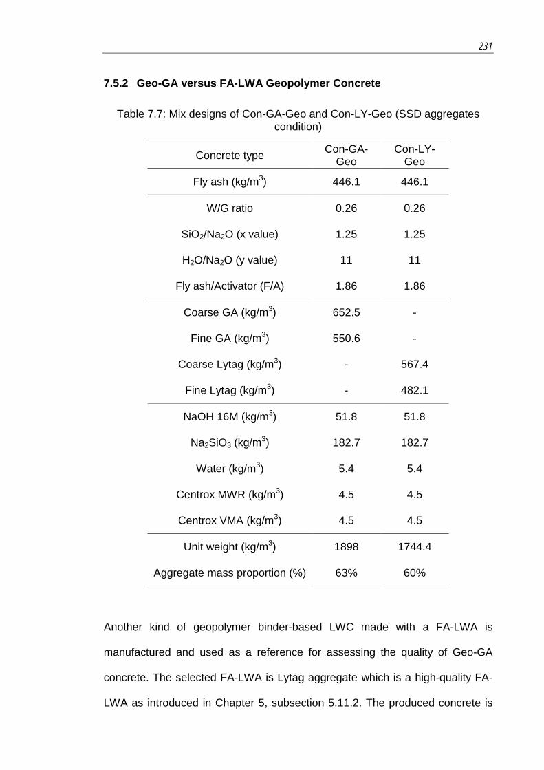
231
7.5.2 Geo-GA versus FA-LWA Geopolymer Concrete
Table 7.7: Mix designs of Con-GA-Geo and Con-LY-Geo (SSD aggregates condition)
Concrete type Con-GA-Geo
Con-LY-Geo
Fly ash (kg/m3) 446.1 446.1
W/G ratio 0.26 0.26
SiO2/Na2O (x value) 1.25 1.25
H2O/Na2O (y value) 11 11
Fly ash/Activator (F/A) 1.86 1.86
Coarse GA (kg/m3) 652.5 -
Fine GA (kg/m3) 550.6 -
Coarse Lytag (kg/m3) - 567.4
Fine Lytag (kg/m3) - 482.1
NaOH 16M (kg/m3) 51.8 51.8
Na2SiO3 (kg/m3) 182.7 182.7
Water (kg/m3) 5.4 5.4
Centrox MWR (kg/m3) 4.5 4.5
Centrox VMA (kg/m3) 4.5 4.5
Unit weight (kg/m3) 1898 1744.4
Aggregate mass proportion (%) 63% 60%
Another kind of geopolymer binder-based LWC made with a FA-LWA is
manufactured and used as a reference for assessing the quality of Geo-GA
concrete. The selected FA-LWA is Lytag aggregate which is a high-quality FA-
LWA as introduced in Chapter 5, subsection 5.11.2. The produced concrete is

232 7. Geopolymer binder-based concrete and mortar using geopolymer aggregate
coded as ‘Con-LY-Geo’ whose mix design is created based on that of Con-GA-
Geo by using the same volume proportion of aggregates, as shown in Table 7.7.
This way, the mixes of Con-GA-Geo and Con-LY-Geo use the same
geopolymer binder.
The properties of Con-GA-Geo and Con-LY-Geo samples are measured and
presented in Table 7.8. Con-LY-Geo has a fresh density of 1671 kg/m3, a 7-day
AD density of 1500 kg/m3 and a 28-day AD density of 1460 kg/m3, which are
even lower than those of lightweight Con-GA-Geo. It is assumed that this is due
to its application of Lytag aggregate, which has a lower density than the
geopolymer aggregate as stated in Chapter 5, subsection 5.11.2. The density
results of Con-LY-Geo also indicate that it is a type of LWC according to
relevant standards (AS, 1998a, ACI, 1998).
Table 7.8: Properties of Con-GA-Geo and Con-LY-Geo
Con-GA-Geo Con-LY-Geo
Fresh density (kg/m3) 1885 1671
Density (AD) (7d) (kg/m3) 1690 1500
Density (AD) (28d) (kg/m3) 1630 1460
Compressive strength (7d) (MPa) 26.18 (1.39)* 32.87 (1.77)*
Compressive strength (28d) (MPa) 40.04 (0.59)* 40.17 (0.68)*
AD: air dry condition; * the value between brackets is the standard deviation of the relevant result.

233
The two mixes end up in a similar 28-day compressive strength of
approximately 40 MPa, which is a medium-strength level and suitable for
serving as a type of structural LWC in real practice (ACI, 2003). Besides, it is
found that the geopolymer concrete using Lytag can achieve a similar strength
but an even lower self-weight compared to the one using geopolymer aggregate.
This may imply a more advanced performance of Lytag than geopolymer
aggregate. Nevertheless, as discussed in Chapter 6, subsection 6.4.1,
geopolymer aggregate can also achieve a good quality with much lower
production cost and a more eco-friendly manufacture, and therefore is
considered to be preferred compared to Lytag in future construction.
7.6 Geopolymer Binder-based Mortar
This section studies a new type of mortar material which is made of geopolymer
binder in replacement of conventional OPC. The mortars studied here include a
mortar mix using geopolymer aggregates and geopolymer binder, which is
referred to as Geo-GA mortar and coded as ‘Mor-GA-Geo’, and a mortar mix
using natural sand coded as ‘Mor-S-Geo’. The mortar using sand and
geopolymer binder has been previously researched (Chindaprasirt et al., 2007,
Kong and Sanjayan, 2010) to take advantage of geopolymer as what has been
done in concretes. In this section, apart from the geopolymer mortar using sand
(Mor-S-Geo), it also investigates the mortar mix using fine geopolymer
aggregates. The latter one is expected to be a new lightweight mortar material.
7.6.1 Materials
The same fine geopolymer aggregate sample and natural sand used in Con-
GA-Geo and Con-N-Geo mixes are used. Also, the ingredients required for a

234 7. Geopolymer binder-based concrete and mortar using geopolymer aggregate
geopolymer synthesis introduced in earlier sections, such as fly ash, NaOH
solution, Na2SiO3 solution and deionised water are applied.
7.6.2 Mix Design
The mortar mix designs are created based on the same mix design procedure
of Geo-GA and GC mixes, as illustrated in section 7.2. The mix design of Mor-
GA-Geo is firstly made based on that of Mor-GA-OPC introduced in Chapter 6,
subsection 6.5.2. Later, the mix design of Mor-S-Geo is created from Mor-GA-
Geo by replacing geopolymer aggregates with the same volume of sand. The
final mix designs of above mixes are modified to suit 1 m3 mortar mix, and
presented in Table 7.9. The detailed mix design procedure of above mortar
mixes is included in Appendix B.
Table 7.9: Mix designs of Mor-S-Geo and Mor-GA-Geo (SSD aggregates condition)
Mortar type Mor-S-Geo Mor-GA-Geo
Fly ash (kg/m3) 580.5 580.5
W/G ratio 0.26 0.26
SiO2/Na2O (x value) 1.25 1.25
H2O/Na2O (y value) 11 11
Fly ash/Activator (F/A) 1.86 1.86
River sand (kg/m3) 1372.5 -
Fine GA (kg/m3) - 1061.1
NaOH 16M (kg/m3) 67.4 67.4
Na2SiO3 (kg/m3) 237.7 237.7
Water (kg/m3) 7.0 7.0

235
7.6.3 Mortar Preparation
Both the Mor-S-Geo and Mor-GA-Geo mixes are prepared following the same
procedure, based on a semi-automatic mixer. Firstly, the fine aggregates are
mixed for 2 minutes with the amount of water necessary to make the aggregate
arrive to its SSD condition. Fly ash and Na2SiO3 solution are then added and
the mixing continues for a further 2 minutes, followed by the addition of NaOH
solution and water and mixing until a uniform mixture is formed (Figure 7.5).
Figure 7.5: Images on fresh mortar mixtures: (1) Mor-S-Geo and (2) Mor-GA-Geo
After mixing, the fresh mortar mixtures are cast into cubic 50mm×50mm×50mm
steel moulds, which have polyethylene sheets stuck onto the inner surfaces.
The samples are then cured in the ER at 20oC for 1 day, and heated at 80oC for
3 days. After heating, these samples are placed back in the ER and demoulded
to expose to the atmosphere (50%) when they cool down. This curing regime is
similar to that of Geo-GA and GC mixes, and found optimum for an enhanced
strength gain as discussed in Chapter 4. Mortar samples using sand and fine
geopolymer aggregates after 28 days of curing are shown in Figure 7.6. The
(1) (2)

236 7. Geopolymer binder-based concrete and mortar using geopolymer aggregate
samples display a similar appearance as the previous geopolymer concrete
samples.
Figure 7.6: Images on 28-day cured Mor-S-Geo and Mor-GA-Geo samples
7.6.4 Workability
The workability performances of the fresh mortars discussed in this section are
evaluated based on the combined slump and mini-flow method discussed in
Chapter 2, subsection 2.4.1. The initial slumps and spreads, and spreads after
10-second vibrations of the mortar samples; Mor-S-Geo and Mor-GA-Geo, are
measured and presented in Table 7.10 and Figure 7.7.
Table 7.10: Slump and spread values of fresh Mor-S-Geo and Mor-GA-Geo
Mortar
Before vibration After 10-second vibration
Initial slump (mm)
Initial spread (cm2)
Spread at once (cm2)
Spread in 3 mins
(cm2)
Spread in 10 mins
(cm2) Mor-S-
Geo 1 11.34* 13.58 13.92 13.92
Mor-GA-Geo 0 11.34* 14.52 14.65 14.65
*11.34cm2 is the bottom area of the mini-sized cone which indicates that there is no spread in this case.
Mor-S-Geo Mor-GA-Geo

237
Figure 7.7: Increases in spread areas of fresh Mor-S-Geo and Mor-GA-Geo caused by mechanical vibration
As seen in Table 7.10, both mortar mixes almost have no initial slump or spread
which indicates their stiff workability similar to the concrete samples reported in
previous sections. As mentioned before, this is relevant to the high viscosity of
the geopolymer binders used here. Nevertheless, as seen from Figure 7.7,
these mortars can have some detectable spreads after the stimulation of
mechanical vibration, even though these spreads are less significant than those
of OPC-based mortars presented in Chapter 6, subsection 6.5.4. The spread
results indicate that these geopolymer mortars can have better workability than
the concretes, when coarse aggregates are not present. Also, the mortar using
geopolymer aggregate results in higher spread values compared to the one
using sand, meaning that it is more vulnerable to the vibration force, possibly
due to its lower self-weight.
4
6
8
10
12
14
16
initial spread spread atonce
spread in 3mins
spread in 10mins
Spre
ad a
rea
(cm
2 )
Mor-S-Geo
Mor-GA-Geo

238 7. Geopolymer binder-based concrete and mortar using geopolymer aggregate
7.6.5 Density and Strength
The density and strength properties of the mortar samples produced are
presented in Table 7.11. Mor-GA-Geo has a fresh density of 1819 kg/m3, a 7-
day AD density of 1710 kg/m3 and a 28-day AD density of 1650 kg/m3. These
densities are much lower than those of Mor-S-Geo, which are all above 2000
kg/m3. An application of geopolymer aggregate in replacement of natural sand
can significantly reduce the density behaviour of mortar mix, as seen in Table
7.11, which is similar to the Geo-GA concrete. Meanwhile, the density range of
Mor-GA-Geo seems low enough to serve as a lightweight construction material.
On the other hand, Mor-S-Geo has a high early strength of 64.48 MPa after 7
days of curing, following the general trend that a geopolymer concrete will have
a high early strength as discussed in section 7.3. It also reaches a 28-day
compressive strength of 68.53 MPa which indicates a high-strength property.
However, Mor-GA-Geo only results in a 7-day compressive strength of 37.65
MPa, but it reaches a 28-day compressive strength of 57.58 MPa which is also
high enough for practical use, and is even comparable with the OPC-based
mortars discussed in Chapter 6, section 6.5.5 (55-59 MPa).
Otherwise, Mor-GA-Geo displays a similar trend in strength development as the
concrete sample Con-GA-Geo in that it does not have a high early strength but
receives a high strength gain at an ambient curing from 7 to 28 days after
mixing. This strength gain might be partly benefited from the low-moisture
ambient curing, as discussed in Chapter 4. But there might also be other
reasons to make this happen, considering that this strength gain is so high
(nearly 20 MPa) for an ambient-cured geopolymer. It seems that this high
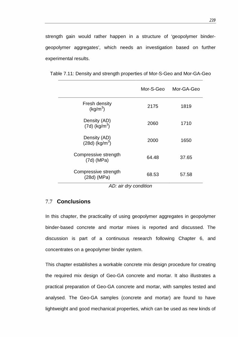
239
strength gain would rather happen in a structure of ‘geopolymer binder-
geopolymer aggregates’, which needs an investigation based on further
experimental results.
Table 7.11: Density and strength properties of Mor-S-Geo and Mor-GA-Geo
Mor-S-Geo Mor-GA-Geo
Fresh density (kg/m3) 2175 1819
Density (AD) (7d) (kg/m3) 2060 1710
Density (AD) (28d) (kg/m3) 2000 1650
Compressive strength (7d) (MPa) 64.48 37.65
Compressive strength (28d) (MPa) 68.53 57.58
AD: air dry condition
7.7 Conclusions
In this chapter, the practicality of using geopolymer aggregates in geopolymer
binder-based concrete and mortar mixes is reported and discussed. The
discussion is part of a continuous research following Chapter 6, and
concentrates on a geopolymer binder system.
This chapter establishes a workable concrete mix design procedure for creating
the required mix design of Geo-GA concrete and mortar. It also illustrates a
practical preparation of Geo-GA concrete and mortar, with samples tested and
analysed. The Geo-GA samples (concrete and mortar) are found to have
lightweight and good mechanical properties, which can be used as new kinds of
240 7. Geopolymer binder-based concrete and mortar using geopolymer aggregate
lightweight materials. The produced Geo-GA concrete can be qualified LWC
used in structural application. The Geo-GA mortar can reach a high-strength
level which is even comparable with the conventional OPC-based mortar.
However, to pursue a good strength, the workability of above Geo-GA mixes is
compromised.
A concrete/mortar mix made from 100% fly ash-based geopolymer material with
sufficient mechanical properties for structural application is realised based on
the research of this and previous chapters. The produced material is treated as
a new way of low-cost and eco-friendly concrete/mortar manufacture, since it
consumes less energy, and uses the aggregates and cementitious material both
of which originating from industrial by-products.

241
Chapter 8
Room Temperature-cured Geopolymer Aggregate
(RTGA) and its Application in Concrete
8.1 Introduction
This chapter concentrates on a special type of geopolymer aggregate (GA),
which is manufactured at a room-temperature condition (20oC) and therefore
referred to as a room temperature-cured geopolymer aggregate (RTGA).
As introduced in Chapter 1, a target of the current study is to take advantage of
geopolymer technology so as to manufacture a low-cost, eco-friendly
geopolymer aggregate. Based on the research work in previous chapters, a
geopolymer aggregate, which only requires a mild-temperature heating
operated at tens of degrees instead of a conventional elevated-temperature
heating at above a thousand degrees, is successfully created with an advanced
quality for a concrete mix. Nevertheless, this geopolymer aggregate still needs
a mild-temperature heating, whereby a concept of RTGA is promoted here to
investigate the possibility of a geopolymer aggregate made without the extra
heat treatment. Compared to the former heated geopolymer aggregates, the
development of RTGA is anticipated to be able to further reduce the energy
consumption, and also simplify the manufacturing procedure by saving the
equipment and effort for heat treatment.
A specific manufacturing procedure for RTGA, which is based on a prolonged
curing period at a low-moisture condition as suggested in Chapter 4, is firstly
illustrated in this chapter. Then, the basic properties of RTGA are measured

242 8. Room temperature-cured geopolymer aggregate (RTGA) and its application in concrete
which indicate that RTGA is a kind of FA-LWA with a low specific gravity and
high water absorption capacity. Moreover, the performance of RTGA sample in
a concrete manufacture is examined. Both OPC-based and geopolymer binder-
based concretes using the coarse and fine RTGAs are made and tested. The
results indicate that RTGA can be qualified for making a structural LWC, even
though it is not as good as its heated counterpart.
8.2 Manufacturing Procedure of RTGA
The manufacturing procedure for RTGA is similar to that for the geopolymer
aggregate manufacture previously introduced in Chapter 5, section 5.3, with
several steps changed to suit a room-temperature manufacture. For simplicity,
the previous geopolymer aggregate that has been through heat treatment is
referred to as ‘heated GA’ throughout this chapter. A flowchart of the
manufacturing procedure for RTGA is presented in Figure 8.1.
The geopolymer mix design used for the manufacture of RTGA is shown in
Table 8.1 which is the same one used for heated GA. Apart from this, the entire
mixing and casting steps for RTGA are also similar to those for the heated GA,
which are detailed in Chapter 5, subsection 5.3.1.
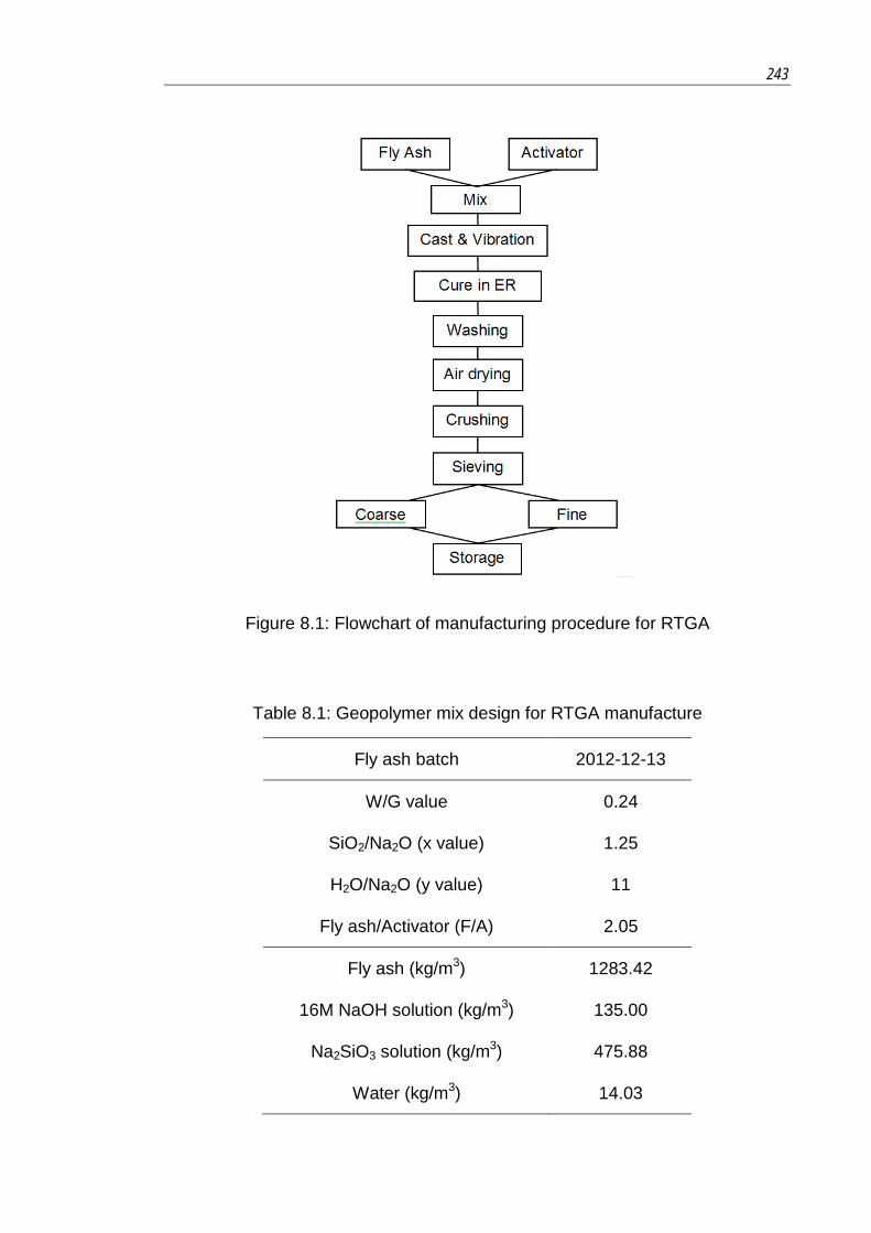
243
Figure 8.1: Flowchart of manufacturing procedure for RTGA
Table 8.1: Geopolymer mix design for RTGA manufacture
Fly ash batch 2012-12-13
W/G value 0.24
SiO2/Na2O (x value) 1.25
H2O/Na2O (y value) 11
Fly ash/Activator (F/A) 2.05
Fly ash (kg/m3) 1283.42
16M NaOH solution (kg/m3) 135.00
Na2SiO3 solution (kg/m3) 475.88
Water (kg/m3) 14.03
244 8. Room temperature-cured geopolymer aggregate (RTGA) and its application in concrete
A special step of the manufacture of RTGA is curing, which is completed in a
controlled environment room (ER) at 20oC and 50% RH. In the first 7 days, the
prepared fresh RTGA sample is sealed in the moulds to assure sufficient
moisture for the initial stage of geopolymerisation. After this, this RTGA sample
is unsealed, but still kept in the moulds to maintain its shape, and exposed to a
low-moisture condition of 50% RH in the ER for further 77 days. The total curing
time for RTGA is 84 days, as suggested in Chapter 4, where it is found that
such a long-term ambient-curing at a low-moisture atmosphere can enhance
the strength of room temperature-cured geopolymer and make it achieve a
similar strength level as the short-term heated one.
Another step of the manufacturing procedure that needs to be noticed is
washing. The washing of heated GA is needed to remove the hazardous alkalis
for a user-friendly purpose. However, this washing step in the manufacture of
RTGA has an extra mission to terminate (at the chosen time marking the end of
curing) the potential geopolymerisation that may happen in a RTGA sample.
This is done at the 84th day by removing the residual alkali content by water, so
as to clear out the reactant of geopolymer reaction. Otherwise, the residual
alkali content may continue to take part into the geopolymerisation after 84 days
(like during the period of storage) and the produced RTGA sample cannot then
be referred to as the ‘84-day room temperature-cured’ because its structure
would then be formed through a geopolymerisation process longer than 84 days.
The washing step for the RTGA sample is the same as that for the heated GA
as illustrated in Chapter 5, subsection 5.3.3. In this procedure, 5 kg of RTGA
sample is soaked in 20 litres of water in a water tank. The duration of washing is
decided by the pH variation of the solution in the water tank. As seen from
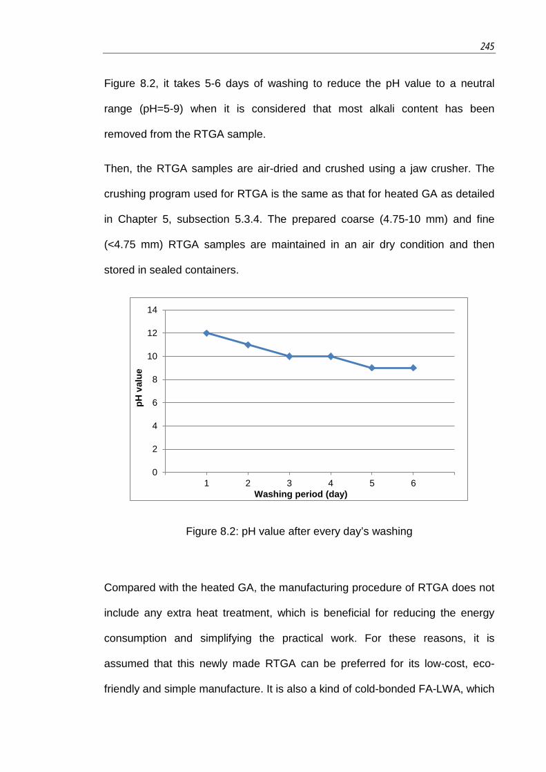
245
Figure 8.2, it takes 5-6 days of washing to reduce the pH value to a neutral
range (pH=5-9) when it is considered that most alkali content has been
removed from the RTGA sample.
Then, the RTGA samples are air-dried and crushed using a jaw crusher. The
crushing program used for RTGA is the same as that for heated GA as detailed
in Chapter 5, subsection 5.3.4. The prepared coarse (4.75-10 mm) and fine
(<4.75 mm) RTGA samples are maintained in an air dry condition and then
stored in sealed containers.
Figure 8.2: pH value after every day’s washing
Compared with the heated GA, the manufacturing procedure of RTGA does not
include any extra heat treatment, which is beneficial for reducing the energy
consumption and simplifying the practical work. For these reasons, it is
assumed that this newly made RTGA can be preferred for its low-cost, eco-
friendly and simple manufacture. It is also a kind of cold-bonded FA-LWA, which
0
2
4
6
8
10
12
14
1 2 3 4 5 6
pH v
alue
Washing period (day)
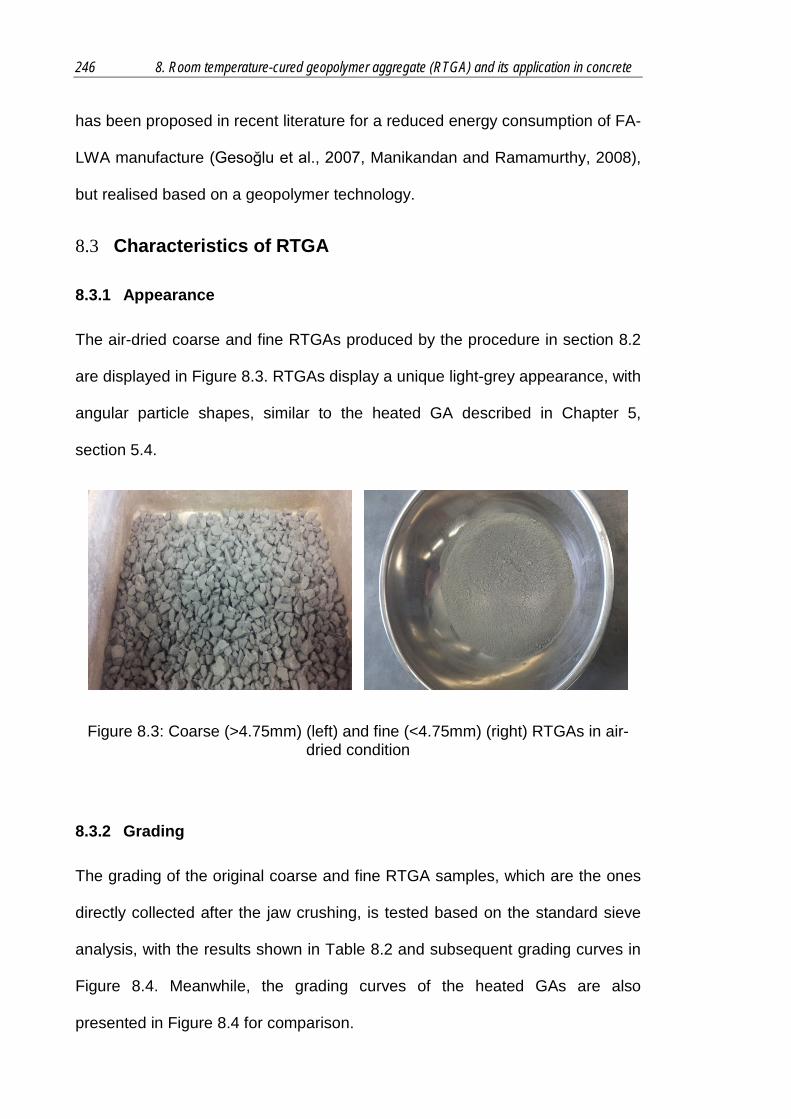
246 8. Room temperature-cured geopolymer aggregate (RTGA) and its application in concrete
has been proposed in recent literature for a reduced energy consumption of FA-
LWA manufacture (Gesoğlu et al., 2007, Manikandan and Ramamurthy, 2008),
but realised based on a geopolymer technology.
8.3 Characteristics of RTGA
8.3.1 Appearance
The air-dried coarse and fine RTGAs produced by the procedure in section 8.2
are displayed in Figure 8.3. RTGAs display a unique light-grey appearance, with
angular particle shapes, similar to the heated GA described in Chapter 5,
section 5.4.
Figure 8.3: Coarse (>4.75mm) (left) and fine (<4.75mm) (right) RTGAs in air-dried condition
8.3.2 Grading
The grading of the original coarse and fine RTGA samples, which are the ones
directly collected after the jaw crushing, is tested based on the standard sieve
analysis, with the results shown in Table 8.2 and subsequent grading curves in
Figure 8.4. Meanwhile, the grading curves of the heated GAs are also
presented in Figure 8.4 for comparison.

247
The coarse RTGA sample displays a good grading that is considered suitable
for a concrete mix. As seen from Figure 8.4, the grading curves of coarse RTGA
and coarse heated GA are almost identical. This could be reasonable since
these two aggregate samples are manufactured through the same crushing
program.
Table 8.2: Typical sieving analysis of coarse and fine RTGAs
Sieve size Mass retained (g)
Percentage retained (%)
Cumulative percentage retained (%)
Cumulative percentage passing (%)
Coarse
13.20 mm 0.0 0.0% 0.0% 100.0%
9.50 mm 3.0 0.0% 0.0% 100.0%
6.70 mm 396.2 0.4% 0.4% 99.6%
4.75 mm 270.4 58.3% 58.7% 41.3%
<4.75 mm 10.0 39.8% 98.5% 1.5%
Total 679.6
Fine
4.75 mm 1.8 0.3% 0.3% 99.7%
2.36 mm 94.7 13.5% 13.8% 86.2%
1.18 mm 127.3 18.2% 31.7% 68.3%
600 µm 223.5 31.9% 63.6% 36.4%
425 µm 55.7 7.9% 71.5% 28.5%
300 µm 64.4 9.2% 80.7% 19.3%
150 µm 116.2 16.6% 97.3% 2.7%
75 µm 15.0 2.1% 99.4% 0.6%
<75 µm 3.9 0.6% 100.0% 0.0%
Total 700.7 Fineness modulus 3.59
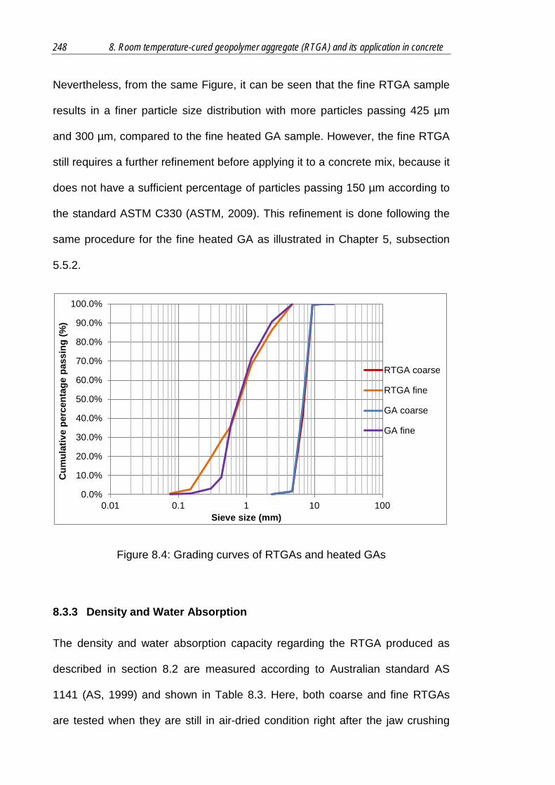
248 8. Room temperature-cured geopolymer aggregate (RTGA) and its application in concrete
Nevertheless, from the same Figure, it can be seen that the fine RTGA sample
results in a finer particle size distribution with more particles passing 425 µm
and 300 µm, compared to the fine heated GA sample. However, the fine RTGA
still requires a further refinement before applying it to a concrete mix, because it
does not have a sufficient percentage of particles passing 150 µm according to
the standard ASTM C330 (ASTM, 2009). This refinement is done following the
same procedure for the fine heated GA as illustrated in Chapter 5, subsection
5.5.2.
Figure 8.4: Grading curves of RTGAs and heated GAs
8.3.3 Density and Water Absorption
The density and water absorption capacity regarding the RTGA produced as
described in section 8.2 are measured according to Australian standard AS
1141 (AS, 1999) and shown in Table 8.3. Here, both coarse and fine RTGAs
are tested when they are still in air-dried condition right after the jaw crushing
0.0%
10.0%
20.0%
30.0%
40.0%
50.0%
60.0%
70.0%
80.0%
90.0%
100.0%
0.01 0.1 1 10 100
Cum
ulat
ive
perc
enta
ge p
assi
ng (%
)
Sieve size (mm)
RTGA coarse
RTGA fine
GA coarse
GA fine

249
procedure. Also, the relevant properties of the heated GA measured in the
same air-dried condition are presented in this Table.
Table 8.3: Densities and water absorption capacities of RTGA and heated GA
RTGA Heated GA
Coarse (84-day)
Fine (84-day) Coarse
(28-day) Fine
(28-day)
Specific gravity (SSD) 1.78 1.85 1.84 2.01
Specific gravity (OD) 1.59 1.69 1.66 1.77
Dry loose bulk density (kg/m3) 841.2 1097.5 876.8 1117.2
Water absorption capacity (in 24 hours) 10.0% 9.0% 11.0% 13.7%
SSD - saturated surface dry condition; OD - oven dry condition
From Table 8.3, a coarse RTGA has specific gravities of 1.78 and 1.59 under
saturated surface dry and oven dry conditions respectively. A fine RTGA has a
similar result but of a higher value, with specific gravities of 1.85 and 1.69 under
saturated surface dry and oven dry conditions respectively. These results
indicate that RTGA should be a type of LWAs (AS, 1998a). Meanwhile, the dry
loose bulk densities of coarse and fine RTGAs are 841.2 kg/m3 and 1137.5
kg/m3 respectively which also indicate the lightweight of RTGA as LWAs (ASTM,
2009). Therefore, RTGA is another type of FA-LWA product created by
geopolymer technology, same as the heated GA previously introduced in
Chapter 5.

250 8. Room temperature-cured geopolymer aggregate (RTGA) and its application in concrete
Also, Table 8.3 indicates that the RTGA have lower density values than the
heated GA. Considering the same mix design and mechanical crushing applied,
this detected density difference is most likely determined by the different curing
regimes of RTGA and heated GA. It is considered that the RTGA cured at room
temperature has a less densified geopolymer structure, in comparison with the
heated GA. This complies with the finding based on SEM observations in
Chapter 4, subsection 4.5.4, that a heat treatment is found beneficial for the
structural densification of fresh geopolymer. Nevertheless, the density values of
RTGA are still in the regular range of LWAs for concretes (ASTM, 2009, Clarke,
1993).
On the other hand, both coarse and fine RTGAs have high water absorption
capacities of 10% and 9% respectively. These absorption capacities, although
slightly lower than those of the heated GA, are still much higher than usual
normal weight aggregates (Neville, 1996) and should be rather noticed during
the practical concrete mix (ACI, 1998, ACI, 2003).
It was once thought that RTGA would have a higher water absorption capacity
than the heated GA. This is because a geopolymer structure cured at room
temperature usually ends up in a less densified structure than the one cured by
heating (as discussed in Chapter 4, section 4.5). This suggests that the RTGA
is expected to have a higher porosity. However, this was not the case in the
current test. The measured lower water absorption capacity of RTGA indicates
that it has a lower content of penetrable pores, compared to the heated GA,
even though RTGA may have a higher porosity. Indeed, a large proportion of
these pores must be impenetrable to water. This indicates that there must be
microstructural differences between these two aggregate samples that have

251
been caused by their different curing regimes. A rigorous study of the total
porosity as well as the pore size distribution is therefore needed to shed more
light on this phenomenon. This is, no doubt, a subject for future research.
The properties discussed in this subsection reflect the basic information of the
newly made coarse and fine RTGA samples. Moreover, these properties are
needed for completing the concrete mixes using RTGA, which will be later
researched in this chapter.
8.3.4 Infrared Spectroscopy
An infrared (IR) spectroscopy test is used to analyse the chemical structure of
the produced RTGA sample. This is conducted using a SHIMADZU infrared
spectrophotometer equipped with an attenuated total reflectance (ATR)
accessory, from 4000 cm-1 to 650 cm-1 with a 4 cm-1 resolution, single bounce
and total of 32 scans. The IR spectrum of RTGA is presented in Figure 8.5,
where the IR spectra of fly ash and heated GA are also included for comparison.

252 8. Room temperature-cured geopolymer aggregate (RTGA) and its application in concrete
Figure 8.5: IR spectra of fly ash, heated GA and RTGA
For the RTGA sample, there is a strong band at 1001.06 cm-1 which indicates
the presence of an amorphous phase that normally lies in the range of 950 cm-1
to 1250 cm-1 (Lee and Van Deventer, 2003) and could be Si-O-Si and Si-O-Al
bonds of amorphous aluminosilicate contents (Barbosa et al., 2000). This band,
as the one referring to the amorphous Si and Al contents, is also found in the
spectra of fly ash and the heated GA, but at different frequencies. Compared to
that of fly ash (1056.99 cm-1), this band shifts to a lower frequency (1001.06 cm-
1) in the spectrum of RTGA. As said in Chapter 5, section 5.10, this shift is likely
due to an increasing proportion of the tetrahedral aluminium component as a
result of geopolymerisation and is indicative of N-A-S-H formation (Fernández-
Jiménez and Palomo, 2005, Rees et al., 2007, Davidovits, 2008). Otherwise,
0.0
20.0
40.0
60.0
80.0
100.0
120.0
140.0
500.01000.01500.02000.02500.03000.03500.04000.0
Tran
smitt
ance
(%)
Wave Number (cm-1)
Fly Ash
Heated GA
RT GA
1056
.99 79
4.67
77
7.31
74
0.67
79
8.53
77
7.31
73
6.81
69
4.37
999.
13
796.
60
777.
31
694.
37
734.
88
1001
.06
695.
20
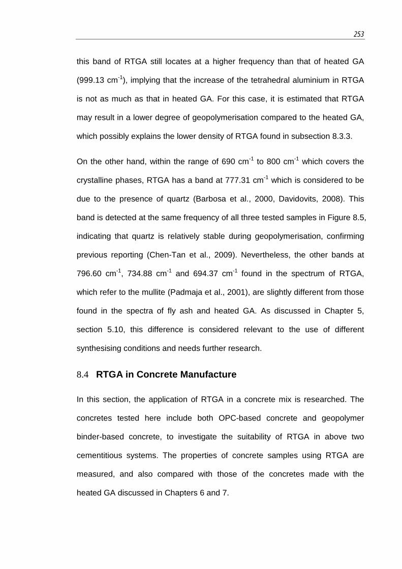
253
this band of RTGA still locates at a higher frequency than that of heated GA
(999.13 cm-1), implying that the increase of the tetrahedral aluminium in RTGA
is not as much as that in heated GA. For this case, it is estimated that RTGA
may result in a lower degree of geopolymerisation compared to the heated GA,
which possibly explains the lower density of RTGA found in subsection 8.3.3.
On the other hand, within the range of 690 cm-1 to 800 cm-1 which covers the
crystalline phases, RTGA has a band at 777.31 cm-1 which is considered to be
due to the presence of quartz (Barbosa et al., 2000, Davidovits, 2008). This
band is detected at the same frequency of all three tested samples in Figure 8.5,
indicating that quartz is relatively stable during geopolymerisation, confirming
previous reporting (Chen-Tan et al., 2009). Nevertheless, the other bands at
796.60 cm-1, 734.88 cm-1 and 694.37 cm-1 found in the spectrum of RTGA,
which refer to the mullite (Padmaja et al., 2001), are slightly different from those
found in the spectra of fly ash and heated GA. As discussed in Chapter 5,
section 5.10, this difference is considered relevant to the use of different
synthesising conditions and needs further research.
8.4 RTGA in Concrete Manufacture
In this section, the application of RTGA in a concrete mix is researched. The
concretes tested here include both OPC-based concrete and geopolymer
binder-based concrete, to investigate the suitability of RTGA in above two
cementitious systems. The properties of concrete samples using RTGA are
measured, and also compared with those of the concretes made with the
heated GA discussed in Chapters 6 and 7.

254 8. Room temperature-cured geopolymer aggregate (RTGA) and its application in concrete
8.4.1 OPC-based Concrete
Firstly, an OPC-based concrete mix made with both coarse and fine RTGAs is
researched, to assess the compatibility of RTGA with the OPC system as the
current mainstream cementitious system. This concrete is referred to as OPC-
RTGA concrete and coded as ‘Con-RTGA-OPC’.
Table 8.4: Mix designs of Con-RTGA-OPC and Con-GA-OPC (SSD aggregates condition)
Item Con-RTGA-OPC Con-GA-OPC
(kg/m3) (kg/m3)
Cement 351 351
Water 182.9 178.7
Coarse RTGA 659.7 686.2
Fine RTGA (1.18-4.75mm) 107.4 117.5
Fine RTGA (300µm-1.18mm) 322.3 352.5
Fine RTGA (150-300µm) 80.6 88.1
Fine RTGA (75-150µm) 26.9 29.4
Fly ash 117 117
Superplasticiser 4 4
Water/Cement ratio 0.52 0.51
Water/Cementitious materials ratio 0.39 0.38
The mix design of Con-RTGA-OPC is created based on the mix design of a
previous concrete mix Con-GA-OPC discussed in Chapter 6. It is specified that
Con-RTGA-OPC has the same cementitious material content and the same
workability (50 mm slump based on a standard slump test) as Con-GA-OPC.

255
This is in order to better compare the effects of RTGA and heated GA for a
OPC-based concrete mix, as previously suggested (Kayali, 2005). The final mix
design is created following the mix design procedure detailed in Chapter 6,
subsection 6.3.2, and presented in Table 8.4.
The preparation of Con-RTGA-OPC follows the normal mixing procedure of
OPC-based concrete as presented in Chapter 6, subsection 6.2.3. Same as the
preparation of Con-GA-OPC, longer time is needed to mix coarse and fine
RTGAs because they are LWAs which take a long time to fully absorb the
added SSD water. Images showing the relevant steps in mixing Con-RTGA-
OPC are presented Figure 8.6. As regulated, the fresh Con-RTGA-OPC mix
has a slump value of 50 mm based on a standard slump test (AS, 1993).
The density values of fresh and hardened Con-RTGA-OPC samples were
tested and their compressive strengths measured using a TECNOTEST
compression machine at a speed of 0.33 MPa/sec, with the final value of each
mixing batch taken as the average of three cubic samples. The density and
strength results are shown in Table 8.5. Meanwhile, the relevant results of Con-
GA-OPC are presented in the same Table for comparison.
Table 8.5 shows that Con-RTGA-OPC has a fresh density of 1921 kg/m3, 28-
day AD density of 1630 kg/m3 and 28-day SSD density of 1860 kg/m3. As using
lightweight RTGAs, Con-RTGA-OPC displays a low self-weight and belongs in
the class of structural LWC products (Clarke, 1993, ACI, 2003), which is similar
to the Con-GA-OPC.
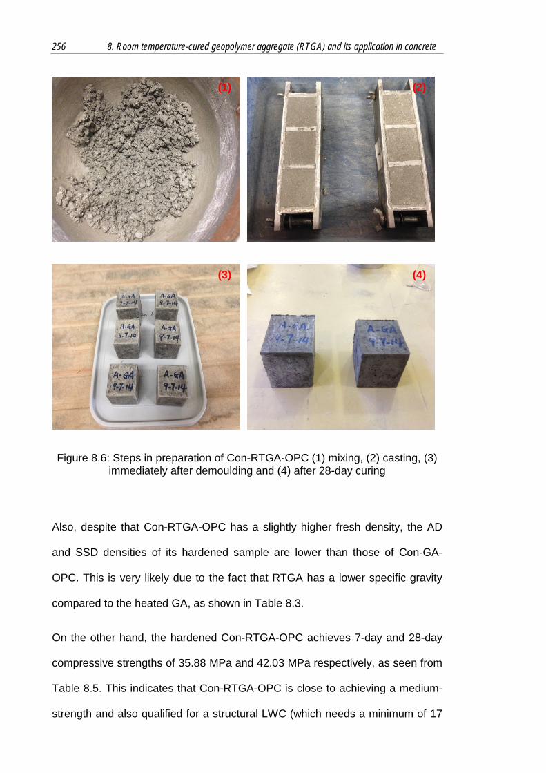
256 8. Room temperature-cured geopolymer aggregate (RTGA) and its application in concrete
Figure 8.6: Steps in preparation of Con-RTGA-OPC (1) mixing, (2) casting, (3) immediately after demoulding and (4) after 28-day curing
Also, despite that Con-RTGA-OPC has a slightly higher fresh density, the AD
and SSD densities of its hardened sample are lower than those of Con-GA-
OPC. This is very likely due to the fact that RTGA has a lower specific gravity
compared to the heated GA, as shown in Table 8.3.
On the other hand, the hardened Con-RTGA-OPC achieves 7-day and 28-day
compressive strengths of 35.88 MPa and 42.03 MPa respectively, as seen from
Table 8.5. This indicates that Con-RTGA-OPC is close to achieving a medium-
strength and also qualified for a structural LWC (which needs a minimum of 17
(1) (2)
(3) (4)

257
MPa) (ASTM, 2009, ACI, 2003). However, Con-RTGA-OPC has much lower
compressive strengths in comparison with Con-GA-OPC, where the latter one
has 7-day and 28-day compressive strengths of 44.20 MPa and 59.32 MPa
respectively. The difference in 28-day compressive strength of above two
concrete mixes is as large as 17 MPa which is considered significant. Since
these two samples are made with the same cementitious material content and
similar water/cement ratios (only varied by 0.01), and designed with the same
workability, it is considered that the above strength difference is very likely
caused by the different qualities of RTGA and heated GA.
Table 8.5: Density and strength properties of Con-RTGA-OPC and Con-GA-OPC
Con-RTGA-OPC Con-GA-OPC
Fresh density (kg/m3) 1921 1856
Density (AD) (28d) (kg/m3) 1630 1770
Density (SSD) (28d) (kg/m3) 1860 1900
Compressive strength (7d) (MPa) 35.88 (0.65)* 44.20 (0.46)*
Compressive strength (28d) (MPa) 42.03 (0.71)* 59.32 (0.71)*
SSD - saturated surface dry condition; AD - air dry condition; * the value between brackets is the standard deviation of the relevant result.
From the strength results, it is estimated that RTGA has a lower mechanical
property than the heated GA, which is likely due to a weaker structure formed
without the enhancement of heat treatment (Bakharev, 2005a, Jiang and Roy,
1990). Although the strength of RTGA should have been improved by a
prolonged curing period at a low-moisture condition, it may still be not as good
as that of the heated GA which is cured at a very effective curing regime of

258 8. Room temperature-cured geopolymer aggregate (RTGA) and its application in concrete
80oC for 3 days. This is in accordance with the previous finding in Chapter 4,
section 4.6, that a 84-day low-moisture room temperature-cured geopolymer
cubic sample results in an around 10 MPa lower compressive strength than a 7-
day geopolymer cubic sample that has been heated at 80oC for 3 days.
Therefore, although RTGA has a good quality to be suitable for making a
structural LWC product, it is still not as good as the heated GA which can
realise a high-strength LWC. Nevertheless, using RTGA instead of the heated
GA implies further low-cost and eco-friendly benefits in the manufacture of LWC
product. Also, the produced OPC-RTGA concrete can be used for the
applications that require a low-strength concrete. The exact advantages or
disadvantages of one type compared to the other depend largely on the
particular purposes and the specificities and economy of production.
8.4.2 Geopolymer Binder-based Concrete
Afterwards, a geopolymer binder-based concrete mix using both coarse and
fine RTGAs is made and researched, which is referred to as Geo-RTGA
concrete and coded as ‘Con-RTGA-Geo’. This is to evaluate the performance of
the RTGAs produced here in the fly ash-based geopolymer binder system.
The mix design of Con-RTGA-Geo is created based on one of the Con-GA-Geo
mixes introduced in Chapter 7 which is designed with a fly ash quantity of 446.1
kg/m3 and a geopolymer binder with SiO2/Na2O=1.25, H2O/Na2O=11 and
W/G=0.26. This mix design is obtained by using the same volumes of RTGAs to
replace the heated GAs in the mix design of Con-GA-Geo, as presented in
Table 8.6.

259
Table 8.6: Mix designs of Con-RTGA-Geo and Con-GA-Geo (SSD aggregates condition)
Con-RTGA-Geo Con-GA-Geo
Fly ash (kg/m3) 446.1 446.1
W/G value 0.26 0.26
SiO2/Na2O (x value) 1.25 1.25
H2O/Na2O (y value) 11 11
Fly ash/Activator (F/A) 1.96 1.96
Coarse RTGA (kg/m3) 631.3 652.5
Fine RTGA (kg/m3) 506.7 550.6
NaOH 16M (kg/m3) 51.8 51.8
Na2SiO3 (kg/m3) 182.7 182.7
Water (kg/m3) 5.4 5.4
Centrox MWR (kg/m3) 4.5 4.5
Centrox VMA (kg/m3) 4.5 4.5
Unit weight (kg/m3) 1832.9 1898.0
Aggregate mass proportion (%) 62% 63%
The preparation of concrete sample Con-RTGA-Geo follows the same
procedure as that of Con-GA-Geo illustrated in Chapter 7, subsections 7.3.1
and 7.4.1. Images showing the relevant steps in mixing Con-GA-Geo are
presented in Figure 8.7.

260 8. Room temperature-cured geopolymer aggregate (RTGA) and its application in concrete
Figure 8.7: Steps in preparation of Con-RTGA-Geo (1) mixing, (2) casting, (3) after heating and demoulding and (4) after 28-day curing
The density and strength properties of the Con-RTGA-Geo samples are
measured using the same methods introduced in subsection 8.4.1, and shown
in Table 8.7. Con-RTGA-Geo has a fresh density of 1819 kg/m3, a 7-day air dry
density of 1580 kg/m3 and a 28-day air dry density of 1540 kg/m3. As expected,
by using lightweight RTGAs, this Con-RTGA-Geo sample end up in a type of
LWC (AS, 1998a). Meanwhile, the above density values of Con-RTGA-Geo are
lower than those of Con-GA-Geo, very possibly due to the lower specific gravity
of RTGA than the heated GA.
(1) (2)
(3) (4)

261
Table 8.7: Density and strength properties of Con-RTGA-Geo and Con-GA-Geo
Con-RTGA-Geo Con-GA-Geo
Fresh density (kg/m3) 1819 1885
Density (AD) (7d) (kg/m3) 1580 1690
Density (AD) (28d) (kg/m3) 1540 1630
Compressive strength (7d) (MPa) 19.85 (0.83)* 26.18 (1.39)*
Compressive strength (28d) (MPa) 23.60 (0.43)* 40.04 (0.59)*
AD: air dry condition; * the value between brackets is the standard deviation of the relevant result.
From Table 8.7, the hardened Con-RTGA-Geo sample has 7-day and 28-day
compressive strengths of 19.85 MPa and 23.60 MPa respectively. Although this
strength is not very good based on the common knowledge of concrete
materials, it is still slightly higher than 17 MPa and therefore qualified for
structural LWC applications (ASTM, 2009, ACI, 2003).
Otherwise, the strength values of Con-RTGA-Geo are much lower than those of
Con-GA-Geo. As the situation of OPC-based concretes discussed in subsection
8.4.1, it is estimated that this detected strength difference is due to the weaker
structure of RTGA than that of the heated GA. Moreover, the strength of Con-
RTGA-Geo is so low that may hinder the promotion of this type of Geo-RTGA
concrete. Further research will be needed to make a Geo-RTGA concrete with
an improved strength quality.
8.5 Conclusion
This chapter proposes a new type of artificial geopolymer aggregate. This one
is also manufactured based on the geopolymer technology but processed at a

262 8. Room temperature-cured geopolymer aggregate (RTGA) and its application in concrete
room-temperature curing regime, and referred to as RTGA. The most dominant
difference of RTGA compared to the heated GA discussed in Chapters 5, 6 and
7 is that, there is no extra heat treatment used in the manufacture of RTGA.
In this chapter, it is aimed to produce a cold-bonded geopolymer aggregate
based on geopolymer technology, which can have sufficient properties required
for a concrete mix. This has been realised through the research reported in this
chapter, where a low-density RTGA sample is made and can be qualified for
producing structural LWCs, even though the generated LWCs only have
low/medium-strengths. Through the used methods described here, a room
temperature-cured geopolymer aggregate with further possible lower-cost and
eco-friendly benefits compared to the previous heated geopolymer aggregate
may be realised. However it must be emphasised that the latter type has a
better quality and can generate a high-strength LWC.
263
Chapter 9
Conclusions and Recommendations for Future
Research
A high-performance lightweight concrete (LWC) made with fly ash-based
lightweight aggregate (FA-LWA) is preferred because of its advanced physical,
mechanical and structural features. The promotion of FA-LWAs in LWC
manufacture is also advocated as a workable solution to problems of the
depletion of natural aggregates and recycling of large amounts of fly ash waste.
However, to ensure the quality of FA-LWAs, high-powered mechanical and
thermal treatments that consume large amounts of energy are normally required
for its manufacture which can significantly affect costs, resources and the
environment, thereby hindering the promotion of conventional FA-LWAs.
Therefore, it is of interest whether an alternative technology capable of
producing a high-quality FA-LWA, but under mild- or room-temperature
conditions to significantly reduce the amount of energy consumed during its
manufacture, is possible. Then, a new type of low-cost, eco-friendly FA-LWA
which removes the current financial and environmental burdens, and better
utilises the features of FA-LWA for a high-performance LWC in the future
concrete industry could be realised. These were the initial motivations for the
research discussed in this thesis.
The geopolymer technology adopted in this study to realise the low-cost, eco-
friendly manufacture of a FA-LWA, with the generated product called
‘geopolymer aggregate (GA)’, was introduced in Chapter 1. The advantage of
geopolymer technology is that it is capable of generating strong and durable

264 9. Conslusions and recommendations for future research
construction materials based on chemical synthesis under mild-temperature
(40-80oC) conditions. However, whether it is a suitable mechanism for making a
type of FA-LWA qualified for utilisation in construction was a promising
hypothesis worthy of the in-depth research. Another creative aspect of this
study has been how to synthesize coarse and fine GAs that are both qualified
for LWCs based on fly ash-derived geopolymer technology. A feasible
procedure for manufacturing the proposed GAs which aimed to obtain a high-
quality product was researched in this study.
Another subject addressed in this thesis was whether the GAs produced using
geopolymer technology could attain a sufficient quality for high-performance
LWC manufacture. Conventional high-quality FA-LWAs can result in LWC
products with advanced mechanical and structural properties. Therefore, it was
considered that only when the newly made GA achieved a comparable quality
to that of conventional FA-LWAs could it be promoted as an alternative with
low-cost and eco-friendly features. In this research, the quality of the GA was
evaluated according to relevant engineering standards and compared with other
commonly used FA-LWAs. Moreover, its performances in concrete and mortar
mixes, in both OPC- and geopolymer binder-based cementitious systems, were
examined.
The main findings of this thesis are summarised in sections 9.1 to 9.4, and
several recommendations for future research are presented in section 9.5.

265
9.1 Research on Geopolymer for Manufacture of Geopolymer
Aggregate
Firstly, as the GA proposed in this study was composed of a fly ash-based
geopolymer material, research was needed to produce one with features
required for a FA-LWA, as discussed in Chapters 2, 3 and 4.
The manufacture of GAs based on a fly ash-derived geopolymer technology
was investigated, with the fly ash a significant factor of concern as it is the main
aluminosilicate source for geopolymerisation. The author found that fly ash
samples from different batches could cause significant differences in the fresh
properties of their geopolymer products even though they were from the same
coal power station. This was considered to be due to the different early reaction
rates of fly ash samples caused by their slightly varied contents of amorphous
SiO2, Al2O3 and CaO. Therefore, it was necessary to strictly control the
consistency of the fly ash which was achieved by selecting one specific fly ash
sample and using it for all the geopolymer mixes. It was an ASTM F fly ash with
an air dry density of 2210 kg/m3, loss on ignition value of 0.97% and fine
particle size distribution, with 79.4% of its particles passing through a 45 µm
sieve. Furthermore, from an XRD test supplemented by a Rietveld quantification
process, it was composed of quartz (9.9%, wt.%), mullite (19.0%, wt.%) and an
amorphous content (71.1%, wt.%). Also, the fresh properties of geopolymers
affected by different fly ash samples were examined, so as to ensure that the
selected fly ash could result in a desired fresh geopolymer suitable for the
processing of GA manufacture.

266 9. Conslusions and recommendations for future research
The geopolymer synthesis in this study was undertaken by activating fly ash
with a combination of NaOH and Na2SiO3 solutions, with the final geopolymer’s
properties determined by the proportions of these ingredients. To control these
proportions and establish a systematic method for creating different geopolymer
mixes, the mix design procedure described in Chapter 3 was proposed. A
unique feature of this procedure was that, as it concentrated particularly on the
relationships among the chemical components involved in geopolymerisation, it
used the criteria of SiO2/Na2O, H2O/Na2O and W/G to distinguish between each
geopolymer mix and calculate the final mix design. In this way, it was able to
adopt previous knowledge of the effects of the chemical components for
geopolymer synthesis to help determine the geopolymer mixes needed for this
research. Then, a geopolymer mix with SiO2/Na2O=1.25, H2O/Na2O=11 and
W/G=0.24 was proposed as an optimum one for GA manufacture owing to its
high alkali and silicate, and low water contents that could enhance a GA’s
strength and structural development. Moreover, some other geopolymer mixes,
with SiO2/Na2O=1.25, H2O/Na2O=11-13 and W/G=0.22-0.26, were designed for
the geopolymer pastes, concretes and mortars investigated. The proportions of
these mixes’ ingredients were then confirmed based on the mix design
procedure in Chapter 3. Also, the factors conventionally related to a geopolymer
mix, such as the molarity of the NaOH and mass ratio of the Na2SiO3/NaOH
solutions could be obtained from the outcome of this procedure and applied to
guide the practical work.
As its curing regime is another significant factor that can influence the
development of a geopolymer, this was investigated and discussed in Chapter 4.
Firstly, the effect of a traditional heat curing regime was researched and found

267
to be better than a room-temperature one for strength and structural
development providing both methods had the same duration. As has been
reported, heat can help the development of a fly ash-based geopolymer (a
thermoset inorganic polymer) which requires high energy to activate the fly ash.
Heat curing at 80oC for 3 days, which resulted in the best strength outcome for
the geopolymer mixes tested, was selected and used for the manufacture of
GAs and geopolymer binders for concrete and mortar mixes.
This study also investigated the manufacture and development of a room
temperature-cured geopolymer, as discussed in Chapter 4. As it has generally
been agreed in recent years that heat treatment is not necessary for
geopolymerisation but is more akin to an acceleration method, the author
wondered whether a high-strength geopolymer made under room-temperature
conditions was achievable. If a geopolymer could achieve high strength with a
stable structure without heat, this would imply that it may be possible to realise
a cold-bonded GA with further low-cost, eco-friendly benefits than those of one
requiring a mild-temperature heat treatment. As the initial motivation of this
research was to lessen the amount of energy consumed in FA-LWA
manufacture, realising a cold-bonded GA was likely to be its ultimate aim. From
the study reported in Chapter 4, it was found that the strength of a room
temperature-cured geopolymer could be significantly improved with a low
moisture condition and prolonged curing period, and was able to obtain a
comparable strength to that of one heated for a short period. As a curing regime
operating at 20oC for 84 days with a low-moisture curing condition of 50% RH
enabled a cubic geopolymer sample to achieve a compressive strength of 44
268 9. Conslusions and recommendations for future research
MPa, which was considered sufficient for a LWA, this was applied to a room
temperature-cured geopolymer aggregate (RTGA), as discussed in Chapter 8.
9.2 Geopolymer Aggregate
Then, the synthesis of GAs, which aimed to successfully produce ones based
on a low-energy geopolymer technology, and enable them to maintain a
comparable quality to usual FA-LWAs, was studied (Chapter 5). This was
conducted through the feasible manufacturing procedure designed in this
research which could be used to make both coarse and fine aggregate samples,
and also be repeated for different designs.
Based on the outcomes of previous chapters, a geopolymer material was
produced with sufficient structure and strength quality to serve as the material
base for GA manufacture. For simplicity in the curing and crushing steps in this
procedure, the geopolymer material produced was cast into chunks with
dimensions of approximately 100mm×50mm×10mm. Also, to produce
aggregate particles of the desired sizes, a mechanical jaw crushing process
with a suitable crushing program was determined and applied, with both coarse
and fine GAs created. For this case, the costs, energy requirements and efforts
needed in the pelletisation process in traditional LWA manufacture were saved.
In addition, this jaw crushing was applied in order to create angular aggregate
particles which were considered beneficial for enhanced bonding with the
cement matrix in subsequent LWC manufacture. Compared with that for
conventional FA-LWAs, this manufacturing procedure was low-cost, simple and
eco-friendly, and meets the nature of geopolymer technology. This suggests a
feasible way to create GAs from fly ash based on the geopolymer technology.

269
The quality of the GA produced was assessed based on its physical and
mechanical properties to determine whether it could still achieve good quality
after undergoing the above low-energy manufacture. It displayed a lightweight
density in the range of 1660 to 1770 kg/m3 under an oven dry condition which
indicated that it was a type of FA-LWA. Also, it was of an adequately good
physical quality to satisfy relevant engineering standards and comparable with
that of conventional FA-LWAs. In addition, a standard crushing value test
indicated that it had a crushing value of 23.4%, higher than those of some
conventional FA-LWAs, which implied that it had good strength for resisting
external pressure. Also, based on a rebound test using the Schmidt hammer, it
was found that this GA had good hardness with a rebound index of 38.6 (kPa),
which is similar to those of some types of natural rocks used as aggregates in
concrete. These findings indicated that it had mechanical properties sufficiently
suitable for high-performance LWC manufacture. This meant that it could be
possible to produce a FA-LWA based on geopolymer technology with the
desired density and strength qualities but manufactured with low energy
consumption.
On the other hand, as the above density and strength performances were most
likely determined by the microstructure of the GA, as this was considered an
important aspect, it was investigated. Using a Lynx stereo inspection
microscope, it was observed that the GA had many porous craters on its
surface which were likely to generate a high number of penetrable pores, as
reflected by its detected high water absorption capacity (11.0%-14.0%). These
findings led to further research on the internal structure of the GA conducted
using an optical microscope with the assistance of image-processing software.

270 9. Conslusions and recommendations for future research
As well as its porous surface, the GA was found to have a porous internal
microstructure with a large range of pores of different shapes and sizes which
was thought to be the main reason for its lightweight property. The pores
detected were micron-sized in a range of 1 µm to 250 µm, with most less than
50 µm and only 0.1% larger than 100 µm, which is beneficial for realising a
strong structure for LWAs and could possibly explain the good mechanical
properties of GAs measured. What needs to be highlighted is that this porous
microstructure was formed mainly due to the process of geopolymerisation, as
supported by the results obtained from infrared (IR) spectroscopy which
identified that the GA’s structure contained newly formed amorphous Si-O-Si
and Si-O-Al bonds that should belong to geopolymer molecules. Therefore,
geopolymerisation was considered a new mechanism for creating an advanced
porosity system consisting of homogeneously distributed small pores, as
preferred in lightweight materials.
9.3 OPC-based Concrete and Mortar using Geopolymer
Aggregate
This study then examined whether this newly made GA could qualify for the
manufacture of high-performance LWC. As OPC is the current mainstream
cementitious system widely applied throughout the world, this research firstly
concentrated on an OPC-based concrete using GAs (OPC-GA concrete,
Chapter 6). The results showed that such a concrete had a lightweight property
with a 28-day air dry density of 1750-1770 kg/m3 and high 28-day compressive
strength of 57-60 MPa which indicated that this type of GA had a sufficiently
high quality to generate a high-strength LWC. Moreover, the OPC-GA concrete

271
mix produced, achieved a high strength/mass ratio of 0.03 (MPa·m3/kg) which
was higher than that of a normal concrete made with the same cementitious
material content and same workability but normal weight crushed stone and
sand. More importantly, both the coarse and fine aggregate portions of this
high-strength LWC were from GAs which the author considers a breakthrough
in the area of geopolymer-assisted LWA manufacture.
It was estimated that the high-strength of the lightweight OPC-GA concrete
should have come from two main aspects related to GA’s application, its self-
strength and strength of bonding with the cement matrix. The first was proven
by its good mechanical properties based on the results from crushing value and
rebound tests. To assess the second, a study of the interfacial zone of the
OPC-GA concrete’s fracture after compressive strength testing was conducted.
It was observed that the GAs were embedded in the cement matrix with a
complete and not collapsed interfacial zone. This indicated that the bonding of
GAs with the cement matrix had a certain strength for resisting external
pressure which was very likely due to their enhanced interlocking due to their
unique shape and porous surfaces.
On the other hand, as the fine GA produced in this research was found to be
qualified to serve as an aggregate portion instead of natural sand in a high-
strength LWC mix, the author undertook further research that focused on only
the performance of fine GAs. This was achieved by assessing the properties of
a mortar material using fine GAs as its sole aggregate portion (referred to as
OPC-GA mortar). The results showed that this OPC-GA mortar had a
lightweight property with a 28-day air dry density of 1750 kg/m3 and high 28-day
compressive strength of 58.86 MPa. It had a similar strength to a mortar made

272 9. Conslusions and recommendations for future research
from natural sand provided both had the same cementitious material content.
Based on this, fine GAs seem to be practical for use as a new type of eco-
friendly artificial sand capable of replacing natural sand in a mortar mix without
any strength loss.
9.4 Geopolymer Binder-based Concrete and Mortar using
Geopolymer Aggregate
Apart from the study of an OPC-GA concrete, discussed in Chapter 7, using
GAs in a geopolymer binder-based concrete (referred to as Geo-GA concrete)
was investigated. This was because, in recent decades, using a geopolymer
binder as a new green cementitious material instead of OPC in the concrete
industry has been recommended. Also, this study explored the possibility of
producing a LWC material made from a 100% fly ash-based geopolymer
material which could be considered a new type of eco-friendly concrete
because it used both aggregates and cementitious materials from industrial by-
products.
Firstly, research on the mix design of the geopolymer binder in Geo-GA
concrete was conducted based on the research work discussed in Chapter 3, to
determine workable geopolymer binders for the desired Geo-GA concrete mixes.
Also, for the better strength development of these binders, a powerful heat
curing regime of 80oC for 3 days was applied. As each of the Geo-GA concretes
produced had a lightweight property (an air dry density of 1630-1640 kg/m3) and
medium-strength (a 28-day compressive strength of 40-46 MPa), they were
suitable for structural LWC applications. Therefore, a practical ‘absolute
geopolymer LWC’ made from 100% geopolymer materials was obtained.
273
Nevertheless, the application of GAs in a geopolymer binder system could
significantly weaken the subsequent Geo-GA concretes, the strengths of which
were 20 MPa lower than those of ones using natural aggregates with the same
geopolymer binders and curing regimes. Moreover, their workability which
seemed to be necessary to obtain better strength outcomes for the samples
used in this research, was rather stiffer in the Geo-GA mixes than the
workability of the usual OPC-based ones. Based on the test results, it was
concluded that the performance of GAs in a geopolymer binder-based concrete
was not as good as that in an OPC-based one.
Later, research on a geopolymer binder-based mortar mix was investigated.
The mortar samples were made from either natural sand or fine GAs, with the
same binder, SiO2/Na2O=1.25, H2O/Na2O=11 and W/G=0.26, and same curing
regime, 80oC for 3 days. The mortar using natural sand resulted in a high 28-
day compressive strength value of 68.5 MPa which indicated that the
geopolymer mix and curing regime used were sufficient to realise a strong
geopolymer binder. The mortar using fine GAs also resulted in a high strength
with a 28-day compressive strength of 57.6 MPa and rather light weight with a
28-day air dry density of 1650 kg/m3. Apart from the strong geopolymer binder
applied, the fine GAs seemed to perform better when used alone in a mortar
mix than in combination with coarse ones. Again, this proved that the fine GAs
produced were of sufficiently high quality for use as an alternative kind of
artificial sand in future lightweight construction. Moreover, it suggested that fine
GAs may be more suitable than coarse ones for a geopolymer binder system.

274 9. Conslusions and recommendations for future research
9.5 Room Temperature-cured Geopolymer Aggregate (RTGA)
Finally, this study researched RTGAs and their applications in concretes
(Chapter 8). A RTGA is a special type of GA made under room-temperature
conditions (20oC), a type of cold-bonded FA-LWA with no extra heat treatment
applied. The idea of using a RTGA came from the promising strength results for
the room temperature-cured geopolymer samples investigated in Chapter 4 and
aimed to further reduce the energy consumption and simplify the manufacture
of GAs by eliminating the heating step. Based on this, a modified manufacturing
procedure which depended on a prolonged curing period (84 days) plus a low-
moisture curing condition (50% RH), as suggested by the research in Chapter 4,
was developed.
The RTGAs produced, ranged in density between 1590 and 1690 kg/m3 at oven
dry condition which indicated that they belonged in the class of FA-LWAs and
had a high water absorption capacity (9.0%-10.0%). Their physical properties
were similar to those of the heated GAs but with slightly lower values. Their
performances were directly evaluated based on their concrete products which
were found to be qualified structural LWCs but with much lower compressive
strengths (approximately 15-20 MPa) than those using heated GAs. This meant
that, although RTGAs must have already been improved by their prolonged
curing periods under low-moisture conditions, they were still not as good as the
GA that underwent heat curing at 80oC for 3 days. Therefore, a heated GA still
has better quality and is the primary one for generating a high-strength LWC
while a RTGA has its own benefits of being low-cost and eco-friendly, and is
suitable for low- or medium-strength LWC manufacture.

275
9.6 Recommendations for Future Research
This research investigated a low-cost, eco-friendly geopolymer aggregate (GA)
and its application in OPC-based and geopolymer binder-based lightweight
concretes and mortars. From the in-depth findings and discussions presented in
this thesis, the following issues need to be further explored in future work.
1) – the porous structure of a GA needs further research because its formation
is relevant to the geopolymerisation process, and also determines the density,
absorption and strength of a GA sample produced. In the microscopic results
obtained, it was detected that there was a large scale of micron-sized pores
present in both the surface layer and internal structure of a GA which were
thought to be a result of geopolymerisation. However, further clarification of the
mechanism of pore formation by geopolymerisation and, moreover, a technique
for controlling the porosity of a geopolymer structure to produce an acceptable
GA for the aggregate industry is required. Although several achievements of
other researchers have already revealed some information about the porosity of
a geopolymer material, further research is needed to correlate it with the quality
of a GA.
It is also recommended that a further study based on X-ray micro-tomography
(micro-CT) technology be conducted on the pore structure and tortuosity of GAs
produced in order to obtain more information on the development of porosity
under various synthetic conditions.
Moreover, further research for dealing with the high proportion of penetrable
pores in a GA, as reflected by its high water absorption capacity (around 10%
based on a standard test), is required because one that is too high may affect
276 9. Conslusions and recommendations for future research
the durability of a concrete under severe conditions (such as freezing and
thawing). The GA proposed in this research was already the one with the lowest
water absorption capacity among all designs based on the current method. In
future, improvements are needed to modify the porosity of the structures of
generated GAs so as to block their penetrable pores and prevent their
connection with the atmosphere.
A rigorous study of porosity would also reveal the different porous structures of
heated GAs and RTGAs which, it is anticipated, would better explain the
variations in water absorption capacities detected in these two aggregate
products. Also, the total porosity and proportions of penetrable and
impenetrable pores of each of these aggregates should be investigated.
2) – research is needed to explain whether a heat treatment applied on a
geopolymer that has already been hardened by heating could lead to any
further reaction and modification of its structure. As the GA considered in this
research was produced from an incomplete geopolymerisation process of fly
ash, theoretically, further heating could lead to a change in its structure which
could change its strength and porosity. This issue is important since it
determines the method of drying required for the manufacture and testing of
GAs. It is also important when it comes to assessing concretes using GA in fire
situations.
3) – further testing of the properties of concretes and mortars made with GAs is
needed. The scope of this study was limited to concentrating on only the
fundamental properties of these concretes and mortar mixes, such as
workability, fresh and hardened density, compressive strength and fracture

277
surface. Further evaluations of other properties, including tensile strength,
elasticity, shrinkage, and the durability when exposed to aggressive internal
and/or external agents, could demonstrate the benefits and/or shortcomings of
using GAs in concretes and mortars.
4) – the author considers it reasonable to propose a further investigation of the
interfacial zone between GAs and the cement matrix of a concrete. Due to the
unique nature of GAs, it is likely that a special interfacial zone in a concrete
using them would be seen which could explain their density and strength
performances.
Moreover, it is considered necessary to launch an in-depth investigation of the
interfacial zone of a ‘GA-geopolymer binder matrix’ to determine whether a
reaction could happen between these two geopolymers produced using
different manufacturing processes. This would establish whether a GA could
react during the mix of a geopolymer binder-based concrete. And if it does, how
would the reaction be and how it would affect the concrete’s performance.
A scanning electron microscope study of the interfacial zone would also be
required, to better determine the nature and composition, and physical-chemical
interaction, between the GAs and either OPC or geopolymer cementitious
matrix.
5) – The phenomenon of the specific strength gain detected in the Geo-GA
mixes in this research needs to be explained by further investigations. It
demonstrated that Geo-GA mixes (both concretes and mortars) could achieve
high strength gains of around 15-20 MPa during a period of 7-28 days after
mixing with no extra heat treatment, which were much higher than those

278 9. Conslusions and recommendations for future research
achieved by the mixes using natural aggregates. This may be better explained
by more specific monitoring of the strength development of these Geo-GA
samples. Also, it is considered that research on the changes in the chemical
and physical structures of these mixes that occur during 7-28 days after mixing
is essential.
6) - research is still required to complete the study of a RTGA based on the
initial results reported in this thesis and it is expected that a modified
manufacturing method would improve its quality. Although the RTGA made in
this study could qualify for structural LWC manufacture, the LWCs produced
had only low to medium strengths whereas the manufacture of high-strength
LWCs based on RTGAs could be a challenge but promising work in future
research.
7) – Future researches are also needed to study the mineralogical and
microstructural changes taking place during the formation process of
geopolymers. The formation of geopolymer gels (like N-A-S-H) and the
performance/change of crystalline phases during a fly ash-based
geopolymerisation process should be more deeply investigated in addition to
the XRD and FTIR performed in the work of this thesis. Such studies can be
correlated with the mechanical and physical properties of GAs analysed and
discussed in this thesis.
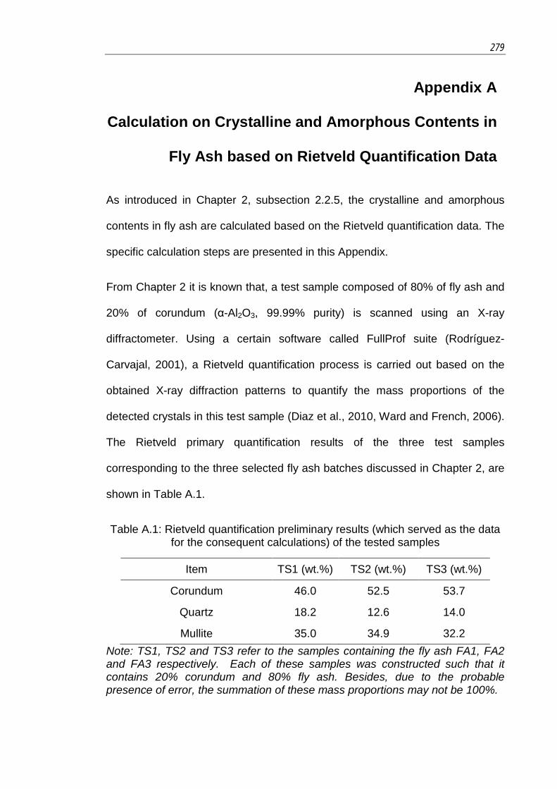
279
Appendix A
Calculation on Crystalline and Amorphous Contents in
Fly Ash based on Rietveld Quantification Data
As introduced in Chapter 2, subsection 2.2.5, the crystalline and amorphous
contents in fly ash are calculated based on the Rietveld quantification data. The
specific calculation steps are presented in this Appendix.
From Chapter 2 it is known that, a test sample composed of 80% of fly ash and
20% of corundum (α-Al2O3, 99.99% purity) is scanned using an X-ray
diffractometer. Using a certain software called FullProf suite (Rodríguez-
Carvajal, 2001), a Rietveld quantification process is carried out based on the
obtained X-ray diffraction patterns to quantify the mass proportions of the
detected crystals in this test sample (Diaz et al., 2010, Ward and French, 2006).
The Rietveld primary quantification results of the three test samples
corresponding to the three selected fly ash batches discussed in Chapter 2, are
shown in Table A.1.
Table A.1: Rietveld quantification preliminary results (which served as the data for the consequent calculations) of the tested samples
Item TS1 (wt.%) TS2 (wt.%) TS3 (wt.%)
Corundum 46.0 52.5 53.7
Quartz 18.2 12.6 14.0
Mullite 35.0 34.9 32.2 Note: TS1, TS2 and TS3 refer to the samples containing the fly ash FA1, FA2 and FA3 respectively. Each of these samples was constructed such that it contains 20% corundum and 80% fly ash. Besides, due to the probable presence of error, the summation of these mass proportions may not be 100%.

280 A. Calculation on crystalline and amorphous contents in fly ash based on Rietveld quantification data
These primary results obtained by the application of the Rietvield process are
now used to calculate the proportions of the crystalline and amorphous contents.
The calculations process is explained in the following paragraphs.
From Table A.1, three types of crystals as corundum, quartz and mullite are
distinctively detected in the X-ray diffraction patterns. Among them, quartz and
mullite are obviously derived from the original fly ash, while corundum was not
present in the fly ash as it was intentionally added. Based on the Rietveld
quantificaiton results shown in Table A.1, the proportions of crystalline and
amorphous contents in fly ash can be calculated, as illustrated by the following
example:
As chosen, in the test sample TS1, 80% in mass is fly ash FA1 and 20% in
mass is corundum. Meanwhile, the contents of quartz and mullite are totally
from the fly ash.
The mass proportions of quartz and mullite in fly ash are calculated by dividing
their masses by the mass of fly ash, as shown below:
mass proportion (quartz) =mass (quartz)mass (fly ash)
mass proportion (mullite) =mass (mullite)mass (fly ash)
Since fly ash occupies 80% in mass of the test sample, the above equations
can be trasferred into the following ones:
mass proportion (quartz) =mass (quartz)
80% ∗ mass (test sample)
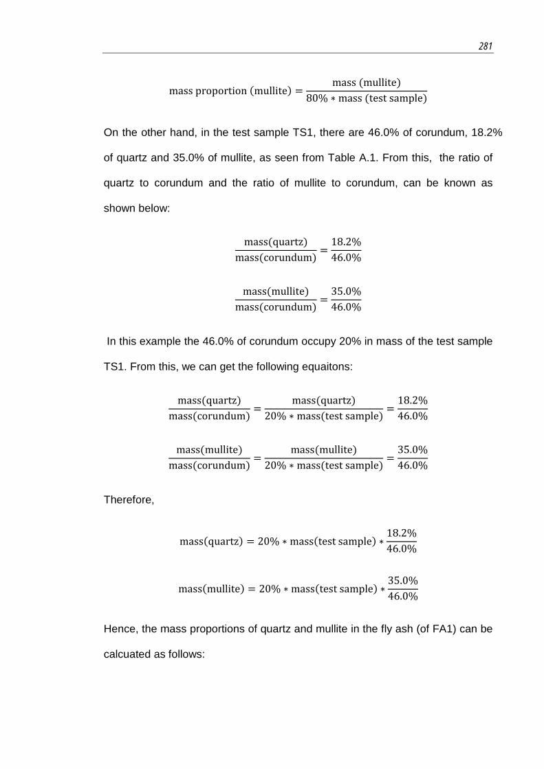
281
mass proportion (mullite) =mass (mullite)
80% ∗ mass (test sample)
On the other hand, in the test sample TS1, there are 46.0% of corundum, 18.2%
of quartz and 35.0% of mullite, as seen from Table A.1. From this, the ratio of
quartz to corundum and the ratio of mullite to corundum, can be known as
shown below:
mass(quartz)mass(corundum)
=18.2%46.0%
mass(mullite)mass(corundum)
=35.0%46.0%
In this example the 46.0% of corundum occupy 20% in mass of the test sample
TS1. From this, we can get the following equaitons:
mass(quartz)mass(corundum)
=mass(quartz)
20% ∗ mass(test sample)=
18.2%46.0%
mass(mullite)mass(corundum)
=mass(mullite)
20% ∗ mass(test sample)=
35.0%46.0%
Therefore,
mass(quartz) = 20% ∗ mass(test sample) ∗18.2%46.0%
mass(mullite) = 20% ∗ mass(test sample) ∗35.0%46.0%
Hence, the mass proportions of quartz and mullite in the fly ash (of FA1) can be
calcuated as follows:

282 A. Calculation on crystalline and amorphous contents in fly ash based on Rietveld quantification data
mass proportion (quartz) =mass (quartz)
80% ∗ mass (test sample)
=20% ∗ mass(test sample) ∗ 18.2%
46.0%80% ∗ mass (test sample)
=20% ∗ 18.2%
46.0%80%
= 9.9%
mass proportion (mullite) =mass (mullite)
80% ∗ mass (test sample)
=20% ∗ mass(test sample) ∗ 35.0%
46.0%80% ∗ mass (test sample) =
20% ∗ 35.0%46.0%
80%= 19.0%
After this, the mass proportion of the amorphous content in the fly ash (of FA1)
can be calucated as:
100% − 9.9% − 19.0% = 71.1%
Hence, it is calculated that the fly ash FA1 is composed of 9.9% of quartz, 19.0%
of mullite and 71.1% of amorphous content. Following the former calculation
steps, the crystalline and amorphous contents of fly ashes FA2 and FA3 can
also be obtained, as shown in Table A.2. These results are later used for this
research work as discussed in Chapter 2.
Table A.2: Quantification of crystalline and amorphous contents in the three fly ash batches
Item FA1 (wt.%) FA2 (wt.%) FA3 (wt.%)
Quartz 9.9 6.0 6.5
Mullite 19.0 16.6 15.0
Amorphous 71.1 77.4 78.5

283
Appendix B
Design of Geopolymer Binder for Geopolymer Binder-
based Concretes and Mortars
In Chapter 7, several geopolymer binder-based concretes and mortars are
designed for research purposes. The design of the geopolymer binder (matrix)
in these concretes and mortars is detailed in this Appendix, which is completed
based on the mix design procedure and results reported in Chapter 3.
B.1 Geo-GA concrete
In Chapter 7, subsection 7.2.2, a Geo-GA concrete is designed with the same
unit weight and aggregate mass proportion as an OPC-GA concrete proposed
in Chapter 6, as shown in Table B.1. Afterwards, the 650.7 kg/m3 binding
material in this Geo-GA concrete is required to be designed.
Table B.1: Ingredient proportions of mix designs of OPC-GA and Geo-GA concretes (SSD aggregates condition)
Ingredient OPC-GA Geo-GA
(kg/m3) (kg/m3)
Binding material 650.7 650.7
Coarse GA 686.2 686.2
Fine GA 587.5 587.5
Unit weight 1924.4 1924.4
Aggregate mass proportion 66% 66%

284 B. Design of geopolymer binder for geopolymer binder-based Concretes and mortars
As introduced in Chapter 7, this 650.7 kg/m3 binding material is composed of a
neat geopolymer mix to serve as the binder, and also two chemical admixtures.
The design of the ingredients used to compose this binding material is
explained based on the following example:
Suppose that a geopolymer mix with SiO2/Na2O=1.25, H2O/Na2O=11 and
W/G=0.24 is selected to be the binder for this Geo-GA concrete. From the mix
design results in Chapter 3, section 3.7, for 1 m3 of such geopolymer mix, it
requires 1283.42 kg/m3 of fly ash, 135.00 kg/m3 of a 16M NaOH solution,
475.88 kg/m3 of a Na2SiO3 solution and 14.03 kg/m3 of deionised water.
Suppose the amount of each chemical admixture in the mix design is a function
of ‘𝑎𝑎’. Since each chemical admixture is added in a dosage of 1% of the mass
of fly ash, it is able to define the amount of fly ash which is:
a1%
= 100a
Then, the amounts of other ingredients can be defined, based on their mass
relations with the fly ash in a 1 m3 geopolymer mix, which are:
16M NaOH solution:
100a ∗135.00
1283.42
Na2SiO3 solution:
100a ∗475.88
1283.42
Deionised water:

285
100a ∗14.03
1283.42
As this 650.7 kg/m3 binding material is composed of fly ash, 16M NaOH solution,
Na2SiO3 solution, deionised water, and two chemical admixtures, the following
equation is obtained:
100a + 100a ∗135.00
1283.42+ 100a ∗
475.881283.42
+ 100a ∗14.03
1283.42+ a + a
= 650.7 kg/m3
The value of ‘𝑎𝑎’ is solved to be:
a = 4.316 kg/m3
This value is the amount of the chemical admixture used in the mix design.
From this, the amount of fly ash is:
4.316 ∗ 100 = 431.6 kg/m3
Then, the amounts of other ingredients are:
16M NaOH solution:
4.316 ∗ 100 ∗135.00
1283.42= 45.5 kg/m3
Na2SiO3 solution:
4.316 ∗ 100 ∗475.88
1283.42= 160.3 kg/m3
Deionised water:
4.316 ∗ 100 ∗14.03
1283.42= 4.7 kg/m3

286 B. Design of geopolymer binder for geopolymer binder-based Concretes and mortars
Hence, for the 650.7 kg/m3 binding material, it requires 431.6 kg/m3 of fly ash,
45.5 kg/m3 of 16M NaOH solution, 160.3 kg/m3 of Na2SiO3 solution, 4.7 kg/m3 of
deionised water, 4.3 kg/m3 of Centrox MWR and 4.3 kg/m3 of Centrox VMA.
After this, considering that this designed geopolymer binder could have a
different volume compared to that of the OPC matrix in Table B.1, a
modification is made on the aggregate proportions to make the final mix design
fit 1 m3 Geo-GA concrete mix.
From known information, the densities of the ingredients used to compose the
binding material of Geo-GA concrete are presented in Table B.2.
Table B.2: Densities of ingredients for binding material of Geo-GA concrete
Item Density (kg/m3)
Fly ash 2210
16M NaOH 1465
Na2SiO3 solution 1520
Deionised water 1000
Centrox MWR 1030
Centrox VMA 1030
The volume of the binding material is considered equal to the summation of the
volume of each ingredient present in Table B.2, based on the absolute volume
principle, which is:
431.62210
+45.51465
+160.31520
+4.7
1000+
4.31030
+4.3
1030= 0.345 m3
On the other hand, from known information, the SSD densities of coarse and
fine geopolymer aggregates are 1840 kg/m3 and 2010 kg/m3 respectively.

287
Therefore, if the aggregate proportions are still the original ones regulated in
Table B.1, the volumes of coarse and fine geopolymer aggregates are:
Coarse geopolymer aggregate:
686.21840
= 0.373 m3
Fine geopolymer aggregate:
587.52010
= 0.292 m3
For this case, the volume of total aggregates is:
0.373 + 0.292 = 0.665 m3
Nevertheless, if the design aims to make a 1 m3 mix containing 0.345 m3
binding material, the volume left for the aggregates should be:
1 − 0.345 = 0.655 m3
From this we can see, the volume of aggregates is now 0.01 m3 more than the
ideal volume they should occupy, provided that the final mix is 1 m3. So, a slight
modification is made on the aggregates, by reducing this 0.01 m3 volume from
them.
Otherwise, the volumetric proportions of coarse and fine aggregates in the total
aggregates are not changed.
The volumetric proportion of coarse aggregates in total aggregates is:
0.3730.665
= 56.1%

288 B. Design of geopolymer binder for geopolymer binder-based Concretes and mortars
The volumetric proportion of fine aggregates in total aggregates is:
0.2920.665
= 43.9%
So, the new volumes of geopolymer aggregates are calculated as:
Coarse geopolymer aggregates:
0.655 × 56.1% = 0.368 m3
Fine geopolymer aggregates:
0.655 × 43.9% = 0.287 m3
Then, the amounts of coarse and fine geopolymer aggregates therefore, are:
Coarse geopolymer aggregates:
0.368 ∗ 1840 = 677.0 kg/m3
Fine geopolymer aggregates:
0.287 ∗ 2010 = 577.3 kg/m3
Therefore, the final mix design for this Geo-GA concrete example is made and
presented in Table B.3.
It needs to be noticed that, this mix design proposed here is based on the
theoretical calculations, and a further modification with trial tests is normally
required to confirm that the proposed mix design is actually for 1 m3 concrete
mix. Meanwhile, the effects of mixing factors, like the air content, should also be
taken into consideration during this modification. Nevertheless, the above mix
design procedure is only applied as a workable way for designing binders in

289
Geo-GA concretes included in current research. Different Geo-GA mixes can be
created by selecting different SiO2/Na2O, H2O/Na2O and W/G ratios. Moreover,
users may also design the unit weight and aggregate proportion according to
their needs or experiences, instead of based on a known OPC-GA concrete
every time. Three Geo-GA concrete mixes required for this research are
subsequently made and applied in Chapter 7, section 7.4.
Table B.3: Final mix design of Geo-GA example (SSD aggregates condition)
Fly ash (kg/m3) 431.6
W/G value 0.24
SiO2/Na2O (x value) 1.25
H2O/Na2O (y value) 11
Fly ash/Activator (F/A) 2.05
Coarse GA(kg/m3) 677.0
Fine GA (kg/m3) 577.3
NaOH 16M (kg/m3) 45.5
Na2SiO3 (kg/m3) 160.3
Water (kg/m3) 4.7
Centrox MWR (kg/m3) 4.3
Centrox VMA (kg/m3) 4.3
Unit weight (kg/m3) 1924.4
Aggregate mass proportion (%) 66%

290 B. Design of geopolymer binder for geopolymer binder-based Concretes and mortars
B.2 Geopolymer Concrete (GC)
The geopolymer concrete (GC) mix required in Chapter 7, section 7.3 is
designed based on the Geo-GA concrete, by using the same volumes of natural
aggregates, namely crushed stone and river sand, to replace the geopolymer
aggregates in the mix design of Geo-GA concrete. This is explained based on
the previous Geo-GA example (Table B.3).
From the above example, it is known that the volumes of coarse and fine
geopolymer aggregates in the mix design are 0.368 m3 and 0.287 m3
respectively.
From known information, the SSD densities of crushed stone and river sand are
2700 kg/m3 and 2600 kg/m3 respectively.
As the crushed stone and river sand in the GC mix have the same volumes as
the coarse and fine geopolymer aggregates in the Geo-GA mix, their mass
proportions can thus be calculated, which are:
Crushed stone:
0.368 ∗ 2700 = 993.4 kg/m3
River sand:
0.287 ∗ 2600 = 746.7 kg/m3
Hence, the mix design for the GC mix is obtained and presented in Table B.4.
Following the same procedure discussed in this section, the mix designs for
other GC mixes required in Chapter 7, section 7.3 can also be created.
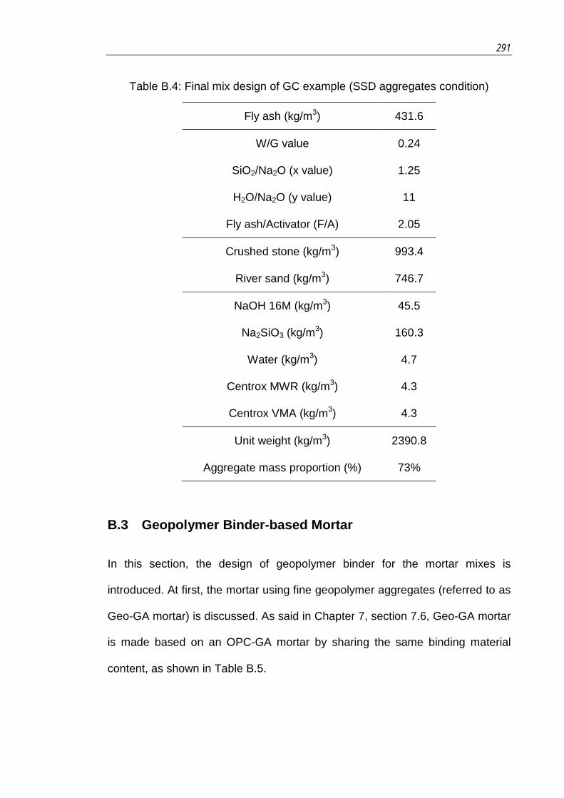
291
Table B.4: Final mix design of GC example (SSD aggregates condition)
Fly ash (kg/m3) 431.6
W/G value 0.24
SiO2/Na2O (x value) 1.25
H2O/Na2O (y value) 11
Fly ash/Activator (F/A) 2.05
Crushed stone (kg/m3) 993.4
River sand (kg/m3) 746.7
NaOH 16M (kg/m3) 45.5
Na2SiO3 (kg/m3) 160.3
Water (kg/m3) 4.7
Centrox MWR (kg/m3) 4.3
Centrox VMA (kg/m3) 4.3
Unit weight (kg/m3) 2390.8
Aggregate mass proportion (%) 73%
B.3 Geopolymer Binder-based Mortar
In this section, the design of geopolymer binder for the mortar mixes is
introduced. At first, the mortar using fine geopolymer aggregates (referred to as
Geo-GA mortar) is discussed. As said in Chapter 7, section 7.6, Geo-GA mortar
is made based on an OPC-GA mortar by sharing the same binding material
content, as shown in Table B.5.

292 B. Design of geopolymer binder for geopolymer binder-based Concretes and mortars
Table B.5: Ingredient proportions of mix designs of OPC-GA and Geo-GA mortars (SSD aggregates condition)
Ingredient OPC-GA Geo-GA
(kg/m3) (kg/m3)
Binding material 835.2 835.2
Fine GA 1116.8 1116.8
Unit weight 1951.9 1951.9
Aggregate mass proportion 57% 57%
These mixes are different from the Geo-GA concrete discussed in section B.1,
in that the 835.2 kg/m3 binding material of this Geo-GA mortar is a neat
geopolymer binder without any chemical admixture. For this reason, the design
of this binding material can be directly made from the results of Chapter 3,
section 3.7, as shown below:
Suppose that a geopolymer binder with SiO2/Na2O=1.25, H2O/Na2O=11 and
W/G=0.22 is selected for this Geo-GA mortar. From Chapter 3, it is known that
this binder has a fly ash/activator (F/A) ratio of 2.28.
Therefore, the amount of fly ash in the 835.2 kg/m3 binding material is:
835.2 ∗2.28
2.28 + 1= 580.5 kg/m3
From Chapter 3, section 3.7, for 1 m3 of the selected geopolymer binder, it
requires 1338.98 kg/m3 of fly ash, 127.01 kg/m3 of 16M NaOH solution, 447.68
kg/m3 of Na2SiO3 solution and 13.20 kg/m3 of deionised water. As the mass
proportions among the above ingredients are not changed when using this
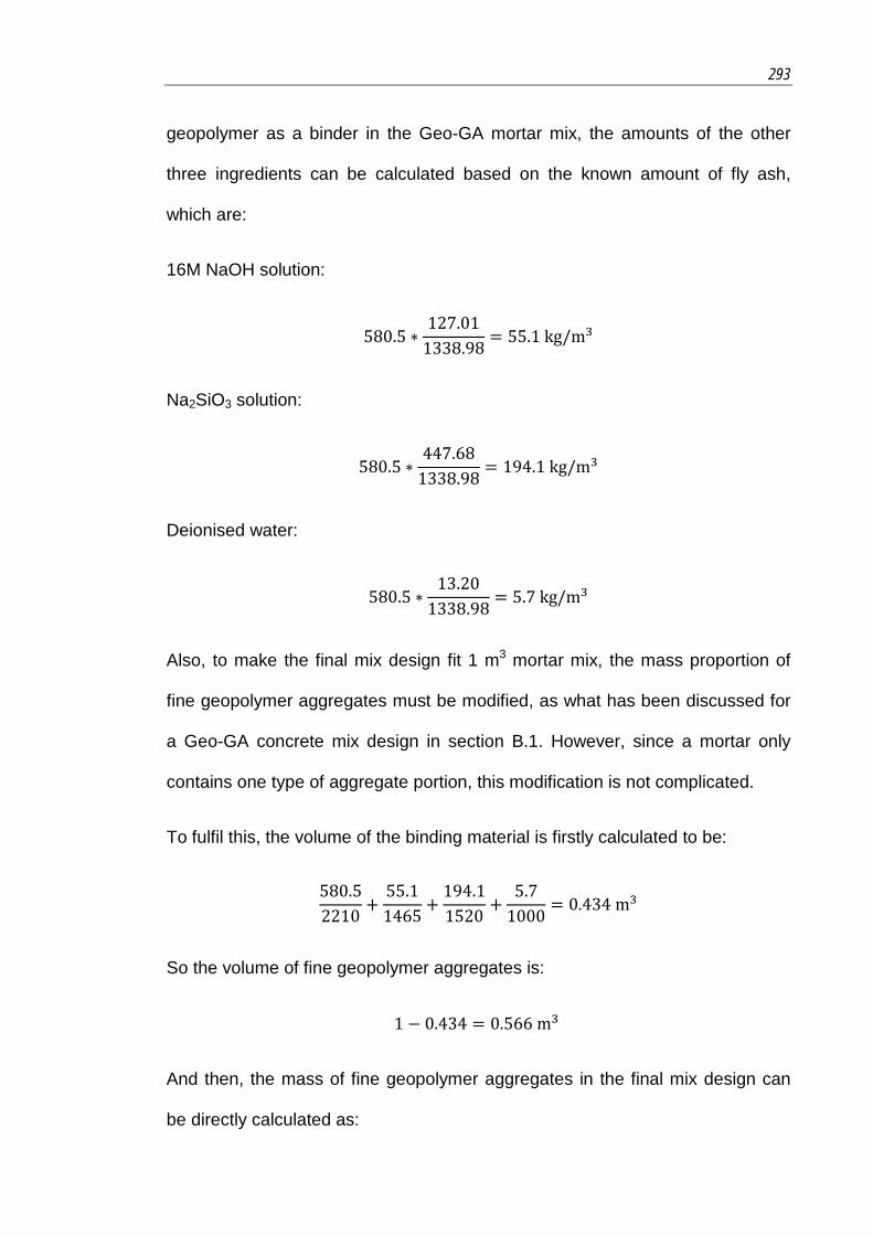
293
geopolymer as a binder in the Geo-GA mortar mix, the amounts of the other
three ingredients can be calculated based on the known amount of fly ash,
which are:
16M NaOH solution:
580.5 ∗127.01
1338.98= 55.1 kg/m3
Na2SiO3 solution:
580.5 ∗447.68
1338.98= 194.1 kg/m3
Deionised water:
580.5 ∗13.20
1338.98= 5.7 kg/m3
Also, to make the final mix design fit 1 m3 mortar mix, the mass proportion of
fine geopolymer aggregates must be modified, as what has been discussed for
a Geo-GA concrete mix design in section B.1. However, since a mortar only
contains one type of aggregate portion, this modification is not complicated.
To fulfil this, the volume of the binding material is firstly calculated to be:
580.52210
+55.11465
+194.11520
+5.7
1000= 0.434 m3
So the volume of fine geopolymer aggregates is:
1 − 0.434 = 0.566 m3
And then, the mass of fine geopolymer aggregates in the final mix design can
be directly calculated as:

294 B. Design of geopolymer binder for geopolymer binder-based Concretes and mortars
0.566 ∗ 2010 = 1137.6 kg/m3
Therefore, the final mix design of this Geo-GA mortar example is obtained and
presented in Table B.6.
Table B.6: Final mix design of Geo-GA mortar example (SSD aggregates condition)
Mortar type Geo-GA
Fly ash (kg/m3) 580.5
W/G ratio 0.22
SiO2/Na2O (x value) 1.25
H2O/Na2O (y value) 11
Fly ash/Activator (F/A) 2.28
Fine GA (kg/m3) 1137.6
NaOH 16M (kg/m3) 55.1
Na2SiO3 (kg/m3) 194.4
Water (kg/m3) 5.7
Moreover, it is possible to specify the quantity of one or more items, and use the
above steps to obtain a new mortar mix. The Geo-GA mortar mix discussed in
Chapter 7, section 7.6 is made by specifying the fly ash quantity, as introduced
below:
It is required that this Geo-GA mortar still uses 580.5 kg/m3 of fly ash as the last
example, but the geopolymer mix with SiO2/Na2O=1.25, H2O/Na2O=11 and
W/G=0.26 are now the required proportions.

295
From Chapter 3, section 3.7, it is known that for 1 m3 of the geopolymer mix
with SiO2/Na2O=1.25, H2O/Na2O=11 and W/G=0.26, it requires 1230.98 kg/m3
of fly ash, 142.65 kg/m3 of 16M NaOH solution, 502.82 kg/m3 of Na2SiO3
solution and 14.83 kg/m3 of deionised water.
Following the calculation steps of the last example, the amounts of other
ingredients can be calculated based on the amount of fly ash, which are:
16M NaOH solution:
580.5 ∗142.65
1230.98= 67.4 kg/m3
Na2SiO3 solution:
580.5 ∗502.82
1230.98= 237.7 kg/m3
Deionised water:
580.5 ∗14.83
1230.98= 7.0 kg/m3
Then, the volume of the binding material is:
580.52210
+67.41465
+237.71520
+7.0
1000= 0.472 m3
The mass proportion of fine geopolymer aggregates is thus calculated as:
(1 − 0.472) ∗ 2010 = 1061.1 kg/m3
Hence, the final mix design of the Geo-GA mortar required in Chapter 7, section
7.6 can be obtained, as shown in Table B.7.

296 B. Design of geopolymer binder for geopolymer binder-based Concretes and mortars
Table B.7: Mix design of Geo-GA mortar
Mortar type Geo-GA
Fly ash (kg/m3) 580.5
W/G ratio 0.26
SiO2/Na2O (x value) 1.25
H2O/Na2O (y value) 11
Fly ash/Activator (F/A) 1.86
Fine GA (kg/m3) 1061.1
NaOH 16M (kg/m3) 67.4
Na2SiO3 (kg/m3) 237.7
Water (kg/m3) 7.0
Table B.8: Mix design of geopolymer mortar
Mortar type Geopolymer mortar
Fly ash (kg/m3) 580.5
W/G ratio 0.26
SiO2/Na2O (x value) 1.25
H2O/Na2O (y value) 11
Fly ash/Activator (F/A) 1.86
River sand (kg/m3) 1372.5
NaOH 16M (kg/m3) 67.4
Na2SiO3 (kg/m3) 237.7
Water (kg/m3) 7.0

297
Similar to the mix design procedure for GC mix, the mix design of geopolymer
mortar using natural sand can be made based on the Geo-GA mortar in Table
B.7, by using the same volume of natural sand to replace the fine geopolymer
aggregates, as shown in Table B.8.
298 Bibliography
Bibliography
ACI 1994. Guide to durable concrete. ACI Manual of Concrete Practice, Part 1: Materials and General Properties of Concrete. Detroit: American Concrete Institute.
ACI 1998. Standard Practice for Selecting Proportions for Structural Lightweight Concrete. Detroit: American Concrete Institute.
ACI 2003. Guide for Structural Lightweight-Aggregate Concrete. Detroit: American Concrete Institute.
ADAA 2010. Annual Membership Survey Results. Sydney. AHMARUZZAMAN, M. 2010. A review on the utilization of fly ash. Progress in Energy
and Combustion Science, 36, 327-363. AL-KHAIAT, H. & HAQUE, M. N. 1998. Effect of initial curing on early strength and
physical properties of a lightweight concrete. Cement and Concrete Research, 28, 859-866.
ARELLANO AGUILAR, R., BURCIAGA DÍAZ, O. & ESCALANTE GARCÍA, J. I. 2010. Lightweight concretes of activated metakaolin-fly ash binders, with blast furnace slag aggregates. Construction and Building Materials, 24, 1166-1175.
ARIOZ, E., ARIOZ, O. & KOCKAR, O. M. 2012. An Experimental Study on the Mechanical and Microstructural Properties of Geopolymers. Procedia Engineering, 42, 121-126.
AS 1991. Methods of test for supplementary cementitious materials for use with portland cement. Sydney: Standards Association of Australia.
AS 1993. Methods of testing concrete. Sydney: Standards Association of Australia. AS 1998a. Aggregates and rock for engineering purposes. Sydney: Standards
Association of Australia. AS 1998f. Supplementary cementitious materials for use with portland and blended
cement. Sydney: Standards Association of Australia. AS 1999. Methods for sampling and testing aggregates. Sydney: Standards Association
of Australia. AS 2006. Methods of testing portland, blended and masonry cements. Sydney:
Standards Association of Australia. AS 2009. Concrete Structures. Strathfield: Standards Association of Australia. AS 2010. General purpose and blended cements. Sydney: Standards Association of
Australia. ASTM 2009. Lightweight Aggregates for Structural Concrete. United States: American
Society for Testing and Materials. ASTM 2012a. Coal Fly Ash and Raw or Calcined Natural Pozzolan for Use in Concrete.
United States: American Society for Testing and Materials. ASTM 2012c. Compressive Strength of Hydraulic Cement Mortars. United States:
American Society for Testing and Materials. ASTM 2014. Determination of Rock Hardness by Rebound Hammer. United States:
American Society for Testing and Materials. BABBITT, C. W. & LINDNER, A. S. 2005. A life cycle inventory of coal used for electricity
production in Florida. Journal of Cleaner Production, 13, 903-912.

299
BAKHAREV, T. 2005a. Geopolymeric materials prepared using Class F fly ash and elevated temperature curing. Cement and Concrete Research, 35, 1224-1232.
BAKHAREV, T. 2005h. Resistance of geopolymer materials to acid attack. Cement and Concrete Research, 35, 658-670.
BAKHAREV, T. 2006. Thermal behaviour of geopolymers prepared using class F fly ash and elevated temperature curing. Cement and Concrete Research, 36, 1134-1147.
BARBOSA, V. F. F. 2003. Synthesis and thermal behaviour of potassium sialate geopolymers. Materials Letters, 57, 1477-1482.
BARBOSA, V. F. F., MACKENZIE, K. J. D. & THAUMATURGO, C. 2000. Synthesis and characterisation of materials based on inorganic polymers of alumina and silica sodium polysialate polymers. International Journal of Inorganic Materials, 2, 309-317.
BEHERA, M., BHATTACHARYYA, S. K., MINOCHA, A. K., DEOLIYA, R. & MAITI, S. 2014. Recycled aggregate from C&D waste & its use in concrete – A breakthrough towards sustainability in construction sector: A review. Construction and Building Materials, 68, 501-516.
BENEZET, J.-C., ADAMIEC, P. & BENHASSAINE, A. 2008. Relation between silico-aluminous fly ash and its coal of origin. Particuology, 6, 85-92.
BIJEN, J. M. 1986. Manufacturing processes of artificial lightweight aggregates from fly ash. The International Journal of Cement Composites and Lightweight Concrete, 8, 191-199.
BLISSETT, R. S. & ROWSON, N. A. 2012. A review of the multi-component utilisation of coal fly ash. Fuel, 97, 1-23.
BOUGUERRA, A., LEDHEM, A., DE BARQUIN, F., DHEILLY, R. M. & QUÉNEUDEC, M. 1998. Effect of microstructure on the mechanical and thermal properties of lightweight concrete prepared from clay, cement, and wood aggregates. Cement and Concrete Research, 28, 1179-1190.
BREMNER, T. W. & HOLM, T. A. 1986. Elastic Compatibility and the Behavior of Concrete. Journal Proceedings, 83.
BROUWERS, H. J. H. & RADIX, H. J. 2005. Self-Compacting Concrete: Theoretical and experimental study. Cement and Concrete Research, 35, 2116-2136.
BS 2002. Lightweight Aggregates. UK: British Standards Institution. BUI, L. A.-T., HWANG, C.-L., CHEN, C.-T., LIN, K.-L. & HSIEH, M.-Y. 2012. Manufacture
and performance of cold bonded lightweight aggregate using alkaline activators for high performance concrete. Construction and Building Materials, 35, 1056-1062.
CCAA 2008. Use of recycled aggregates in cnostruction. Cement Concrete & Aggregates Australia.
CCAA 2010. Briefing: sustainable concrete materials. Cement Concrete & Aggregates Australia.
CERNA, B. & ENGEL, Z. 2011. Surface and sub-surface Schmidt hammer rebound value variation for a granite outcrop. Earth Surface Processes and Landforms, 36, 170-179.
CHANDRA, S. & BERNTSSON, L. 2002. Lightweight Aggregate Concrete: Science, Technology, and Applications, Norwich, NJ, Noyes Publications.21,33,119,291

300 Bibliography
CHEN-TAN, N. W., VAN RIESSEN, A., LY, C. V. & SOUTHAM, D. C. 2009. Determining the Reactivity of a Fly Ash for Production of Geopolymer. Journal of the American Ceramic Society, 92, 881-887.
CHEN, J. & FANG, Y. 2005. Present situation and problems of concrete aggregates in China. Architecture Technology, 36, 23-25.
CHI, J. M., HUANG, R., YANG, C. C. & CHANG, J. J. 2003. Effect of aggregate properties on the strength and stiffness of lightweight concrete. Cement and Concrete Composites, 25, 197-205.
CHINDAPRASIRT, P., CHAREERAT, T. & SIRIVIVATNANON, V. 2007. Workability and strength of coarse high calcium fly ash geopolymer. Cement and Concrete Composites, 29, 224-229.
CIA 2011. Recommended Practice: Geopolymer Concrete. Concrete Institute of Australia.
CLARKE, J. L. 1993. Structural Lightweight Aggregate Concrete, Glasgow, Blackie Academic & Professional.1, 5, 7, 10, 19, 20, 22
CRIADO, M., PALOMO, A., FERNÁNDEZ-JIMÉNEZ, A. & BANFILL, P. F. G. 2009. Alkali activated fly ash: effect of admixtures on paste rheology. Rheologica Acta, 48, 447-455.
DAVIDOVITS, J. Solid phase synthesis of a mineral blockpolymer by low temperature polycondensation of aluminosilicate polymers. IUPAC International Symposium on Macromolecules, 1976 Stockholm, Sweden. 3-15.
DAVIDOVITS, J. Geopolymer chemistry and properties. 1st European Conference on Soft Mineralurgy, 1988 Compiegne, France. 25-48.
DAVIDOVITS, J. 1989. Geopolymers and geopolymeric materials. Journal of Thermal Analysis and Calorimetry, 35, 429-441.
DAVIDOVITS, J. 1991. Geopolymers - inorganic polymeric new materials. Journal of Thermal Analysis, 37, 1633-1656.
DAVIDOVITS, J. 2002. 30 Years of Successes and Failures in Geopolymer Applications. Market Trends and Potential Breakthroughs. Geopolymer 2002 Conference. Melbourne.
DAVIDOVITS, J. 2008. Geopolymer Chemistry and Application, Saint-Quentin, Institut Ge ́opolyme ̀re.3, 4, 6, 24, 25, 28, 34, 63, 68, 285, 289, 302, 561
DAVIDOVITS, J. 2013. Geopolymer Cement, a review. Geopolymer Institute. DE SILVA, P., SAGOE-CRENSTIL, K. & SIRIVIVATNANON, V. 2007. Kinetics of
geopolymerization: role of Al2O3 and SiO2. Cement and Concrete Research, 37, 512-518.
DENT GLASSER, L. S. & KATAOKA, N. 1981. The chemistry of ‘alkali-aggregate’ reaction. Cement and Concrete Research, 11, 1-9.
DIAMOND, S. 2000. Mercury porosimetry: An inappropriate method for the measurement of pore size distributions in cement-based materials. Cement and Concrete Research, 30, 1517-1525.
DIAZ, E. I., ALLOUCHE, E. N. & EKLUND, S. 2010. Factors affecting the suitability of fly ash as source material for geopolymers. Fuel, 89, 992-996.
DUXSON, P., FERNÁNDEZ-JIMÉNEZ, A., PROVIS, J. L., LUKEY, G. C., PALOMO, A. & DEVENTER, J. S. J. 2007a. Geopolymer technology: the current state of the art. Journal of Materials Science, 42, 2917-2933.

301
DUXSON, P., LUKEY, G. C. & DEVENTER, J. S. J. 2007e. Physical evolution of Na-geopolymer derived from metakaolin up to 1000 °C. Journal of Materials Science, 42, 3044-3054.
DUXSON, P. & PROVIS, J. L. 2008. Designing Precursors for Geopolymer Cements. Journal of the American Ceramic Society, 91, 3864-3869.
DUXSON, P., PROVIS, J. L., LUKEY, G. C., MALLICOAT, S. W., KRIVEN, W. M. & VAN DEVENTER, J. S. J. 2005. Understanding the relationship between geopolymer composition, microstructure and mechanical properties. Colloids and Surfaces A: Physicochemical and Engineering Aspects, 269, 47-58.
ECCPA. 2008. Production and Utilisation of CCPs in 2008 in Europe [Online]. European Coal Combustion Products Association. 2015].
EN. 2001. Fly ash for concrete - Part 1: definition, specifications and conformity criteria. European Standard.
ENGELHARDT, G., ZEIGAN, D., JANCKE, H., HOEBBEL, D. & WIEKER, W. 1975. SI-29 NMR-spectroscopy of silicate solutions .2. dependence of structure of silicate anions in water solutions from Na-Si ratio. Zeitschrift fur Anorganische und Allgemeine Chemie, 418, 17-28.
FANG, Y. 2013. Structure and development of fly ash and red mud-based geopolymers. PhD, University of New South Wales.
FANSURI, H., PRASETYOKO, D., ZHANG, Z. & ZHANG, D. 2012. The effect of sodium silicate and sodium hydroxide on the strength of aggregates made from coal fly ash using the geopolymerisation method. Asia-Pacific Journal of Chemical Engineering, 7, 73-79.
FERNÁNDEZ-JIMÉNEZ, A. & PALOMO, A. 2003. Characterisation of fly ashes. Potential reactivity as alkaline cements. Fuel, 82, 2259-2265.
FERNÁNDEZ-JIMÉNEZ, A. & PALOMO, A. 2005. Mid-infrared spectroscopic studies of alkali-activated fly ash structure. Microporous and Mesoporous Materials, 86, 207-214.
FERNÁNDEZ-JIMÉNEZ, A., PALOMO, A. & LOPEZ-HOMBRADOS, C. 2006. Engineering properties of alkali-activated fly ash concrete. ACI Materials Journal, 103, 106-112.
GARCÍA-LODEIRO, I., FERNÁNDEZ-JIMÉNEZ, A., BLANCO, M. T. & PALOMO, A. 2007. FTIR study of the sol–gel synthesis of cementitious gels: C–S–H and N–A–S–H. Journal of Sol-Gel Science and Technology, 45, 63-72.
GEETHA, S. & RAMAMURTHY, K. 2010. Environmental friendly technology of cold-bonded bottom ash aggregate manufacture through chemical activation. Journal of Cleaner Production, 18, 1563-1569.
GEOPOLYMER INSTITUTE. 2012. What is a geopolymer? Introduction [Online]. Geopolymer Institute. Available: http://www.geopolymer.org/science/introduction [Accessed August 17 2012].
GESOĞLU, M., ÖZTURAN, T. & GÜNEYISI, E. 2007. Effects of fly ash properties on characteristics of cold-bonded fly ash lightweight aggregates. Construction and Building Materials, 21, 1869-1878.
GLUKHOVSKY, V., RUMYNA, G. & ROSTOVSKAJA, G. High strength slag alkaline cements. Proceedings of the seventh international congress on the chemistry of cement, 1980 Paris. 164-168.

302 Bibliography
GÖRHAN, G. & KÜRKLÜ, G. 2014. The influence of the NaOH solution on the properties of the fly ash-based geopolymer mortar cured at different temperatures. Composites Part B: Engineering, 58, 371-377.
HARDJITO, D. & RANGAN, B. V. 2005. Development and properties of low-calcium fly ash-based geopolymer concrete. Research Report GC1. Perth: Faculty of Engineering, Curtin University of Technology.
HARDJITO, D., WALLAH, S. E., SUMAJOUW, D. M. J. & RANGAN, B. V. 2004. On the development of fly ash-based geopolymer concrete. ACI Materials Journal, 101, 467-472.
HAUGSTEN, K. E. & GUSTAVSON, B. 2000. Environmental properties of vitrified fly ash from hazardous and municipal waste incineration. Waste Management, 20, 167-176.
HENRY, J., TOWLER, M. R., STANTON, K. T., QUEROL, X. & MORENO, N. 2004. Characterisation of the glass fraction of a selection of European coal fly ashes. Journal of Chemical Technology and Biotechnology, 79, 540-546.
HOFF, G. C. High strength lightweight aggregate concrete-current status and future needs. High Strength Concrete, ACI SP 121, 1990 Detroit. 619-644.
HU, S.-G., WU, J., YANG, W., HE, Y.-J., WANG, F.-Z. & DING, Q.-J. 2009. Preparation and properties of geopolymer-lightweight aggregate refractory concrete. J. Cent. South Univ. Technol., 16, 914-918.
HUANG, S.-C., CHANG, F.-C., LO, S.-L., LEE, M.-Y., WANG, C.-F. & LIN, J.-D. 2007. Production of lightweight aggregates from mining residues, heavy metal sludge, and incinerator fly ash. Journal of Hazardous Materials, 144, 52-58.
ILER, R. K. 1979. The Chemistry of Silica; Solubility, Polymerization, Colloid adn Surface Properties, adn Biochemistry, New York, John Wiley & Sons.
IQA 2001. Statistics of Australian Quarrying Industries. Institute of Quarrying Australia. ISAIA, G. C., GASTALDINI, A. L. G. & MORAES, R. 2003. Physical and pozzolanic action of
mineral additions on the mechanical strength of high-performance concrete. Cement and Concrete Composites, 25, 69-76.
JIANG, W. M. & ROY, D. M. 1990. Hydrothermal processing of new fly ash cement. Ceram. Bull., 71, 642-647.
JO, B., PARK, S. & PARK, J. 2007. Properties of concrete made with alkali-activated fly ash lightweight aggregate (AFLA). Cement and Concrete Composites, 29, 128-135.
JUNAID, M. T., KAYALI, O. & KHENNANE, A. 2012. Mix design procedure for alkali activated fly ash-based geopolymer concretes 2012 International Conference on Engineering and Applied Science. Beijing, China.
KATZ, O., RECHES, Z. & ROEGIERS, J. C. 2000. Evaluation of mechanical rock properties using a Schmidt Hammer. International Journal of Rock Mechanics and Mining Sciences, 37, 723-728.
KAYALI, O. 2005. Flashag new lightweight aggregate for high strength and durable concrete. World of Coal Ash. Lexington, KY.
KAYALI, O. 2008. Fly ash lightweight aggregates in high performance concrete. Construction and Building Materials, 22, 2393-2399.
KAYALI, O. & SHAW, K. J. 2004. Aggregate for concrete and construction.

303
KHATRI, R. P., SIRIVIVATNANON, V. & GROSS, W. 1995. Effect of different supplementary cementitious materials on mechanical properties of high performance concrete. Cement and Concrete Research, 25, 209-220.
KıLıÇ, A., ATIŞ, C. D., YAŞAR, E. & ÖZCAN, F. 2003. High-strength lightweight concrete made with scoria aggregate containing mineral admixtures. Cement and Concrete Research, 33, 1595-1599.
KLIEGER, P. & HANSON, J. A. 1961. Freezing and Thawing Tests of Lightweight Aggregate Concrete. Journal of ACI, 57, 779-796.
KOCKAL, N. U. & OZTURAN, T. 2010. Effects of lightweight fly ash aggregate properties on the behavior of lightweight concretes. Journal of Hazardous Materials, 179, 954-965.
KOHNO, K. & KOMATSU, H. Use of Ground Bottom Ash and Silica Fume in Mortar and Concrete. Proceedings of ACI Second International Conference on Fly Ash, Silica Fume, Slag and Natural Pozzolans in Concrete, 1986 Madrid. 1279-1292.
KOMNITSAS, K. & ZAHARAKI, D. 2007. Geopolymerisation: A review and prospects for the minerals industry. Minerals Engineering, 20, 1261-1277.
KONG, D. L. Y. & SANJAYAN, J. G. 2010. Effect of elevated temperatures on geopolymer paste, mortar and concrete. Cement and Concrete Research, 40, 334-339.
KONG, D. L. Y., SANJAYAN, J. G. & SAGOE-CRENTSIL, K. 2007. Comparative performance of geopolymers made with metakaolin and fly ash after exposure to elevated temperatures. Cement and Concrete Research, 37, 1583-1589.
KORAT, L., DUCMAN, V., LEGAT, A. & MIRTIČ, B. 2013. Characterisation of the pore-forming process in lightweight aggregate based on silica sludge by means of X-ray micro-tomography (micro-CT) and mercury intrusion porosimetry (MIP). Ceramics International, 39, 6997-7005.
KRIVEN, W. M., BELL, J. L. & GORDON, M. 2003. Microstructure and microchemistry of fully-reacted geopolymers and geopolymer matrix composites. In: BANSAL, N. P. S. J. P. K. W. M. S. H. (ed.) Advances in Ceramic Matrix Composites Ix.
KRIVENKO, P. V. 1986. Synthesis of Binders with Required Properties in the System R2O-RO-R2O3-SiO2-H2O. PhD, Doct. Tech. Sc.
KUMAR, S. & KUMAR, R. Tailoring Geopolymer Properties Through Mechanical Activation of Fly Ash. Second International Conference on Sustainable Construction Materials and Technologies, 2010 Italy.
KUTCHKO, B. G. & KIM, A. G. 2006. Fly ash characterization by SEM–EDS. Fuel, 85, 2537-2544.
KWAN, A. K. H. & LI, Y. 2013. Effects of fly ash microsphere on rheology, adhesiveness and strength of mortar. Construction and Building Materials, 42, 137-145.
LEA, F. M. 1970. The chemistry of cement and concrete, London, Edward Arnold Ltd. LEE, W. & VAN DEVENTER, J. 2003. Use of infrared spectroscopy to study
geopolymerization of heterogeneous amorphous aluminosilicates. Langmuir, 19, 8726-8734.
LEE, W. K. W. & VAN DEVENTER, J. S. J. 2002. Structural reorganisation of class F fly ash in alkaline silicate solutions. Colloids and Surfaces A 211, 49-66.
LI, C., LI, Y., SUN, H. & LI, L. 2011. The Composition of Fly Ash Glass Phase and Its Dissolution Properties Applying to Geopolymeric Materials. Journal of the American Ceramic Society, 94, 1773-1778.
304 Bibliography
LIEU, Y. W., CHEN, H. Q. & TAN, J. W. The insulation performance of light weight aggregate concrete. Proceeding of the 1st conference on Lightweight Aggregate and Lightweight Aggregate Concrete, 2003 Taichung, Taiwan. Taiwan Lightweight Aggregate Concrete Association, 83-98.
LO, T. Y. & CUI, H. Z. 2004. Effect of porous lightweight aggregate on strength of concrete. Materials Letters, 58, 916-919.
LO, T. Y., CUI, H. Z. & LI, Z. G. 2004. Influence of aggregate pre-wetting and fly ash on mechanical properties of lightweight concrete. Waste Management, 24, 333-338.
LYDON, F. D. & BALENDRAN, R. V. 1980. Some properties of higher strength light-weight concrete under short-term tensile stress. International Journal of Cement Composites and Lightweight Concrete, 2, 125-139.
MANIKANDAN, R. & RAMAMURTHY, K. 2008. Effect of curing method on characteristics of cold bonded fly ash aggregates. Cement and Concrete Composites, 30, 848-853.
MASI, G., RICKARD, W. D. A., VICKERS, L., BIGNOZZI, M. C. & VAN RIESSEN, A. 2014. A comparison between different foaming methods for the synthesis of light weight geopolymers. Ceramics International, 40, 13891-13902.
NATH, P. & SARKER, P. K. Geopolymer concrete for ambient curing condition. Proceedings of the Australasian Structural Engineering Conference, 11-13 July, 2012 2012 Perth, Australia.
NATH, P. & SARKER, P. K. 2014. Effect of GGBFS on setting, workability and early strength properties of fly ash geopolymer concrete cured in ambient condition. Construction and Building Materials, 66, 163-171.
NAUMAN, R. V. & DEBYE, P. 1951. Light-scattering investigations of carefully filtered sodium silicate solutions. J. Phys. Chem, 55, 1-9.
NEVILLE, A. M. 1996. Properties of Concrete, Prentice Hall. 83, 108, 109, 128, 156, 185, 189, 269, 688, 689, 745, 762
NORTH, M. R. & SWADDLE, T. W. 2000. Kinetics of silicate exchange in alkaline aluminosilicate solutions. Inorganic Chemistry, 39, 2661-2665.
PACHECO-TORGAL, F., MOURA, D., DING, Y. & JALALI, S. 2011. Composition, strength and workability of alkali-activated metakaolin based mortars. Construction and Building Materials, 25, 3732-3745.
PADMAJA, P., ANILKUMAR, G. M., MUKUNDAN, P., ARULDHAS, G. & WARRIER, K. G. K. 2001. Characterisation of stoichiometric sol-gel mullite by fourier transform infrared spectroscopy. International Journal of Inorganic Materials, 3, 693-698.
PAGE, A. L., ELSEEWI, A. & STRAUGHAN, I. R. 1979. Physical and chemical properties of fly ash from coal-fired power plants with reference to environmental impacts. In: GUNTHER, F. & GUNTHER, J. (eds.) Residue Reviews. Springer New York.
PALACIOS, M. & PUERTAS, F. 2005. Effect of superplasticizer and shrinkage-reducing admixtures on alkali-activated slag pastes and mortars. Cement and Concrete Research, 35, 1358-1367.
PALOMO, A., ALONSO, S., FERNÁNDEZ-JIMÉNEZ, A., SOBRADOS, I. & SANZ, J. 2004. Alkaline activation of fly ashes: NMR study of the reaction products. J. Am. Ceram. Soc., 87, 1141-1145.
PALOMO, A., GRUTZECK, M. W. & BLANCO, M. T. 1999. Alkali-activated fly ashes A cement for the future. Cement and Concrete Research, 29, 1323-1329.

305
PEDERSEN, K. H., JENSEN, A. D., SKJOTH-RASMUSSEN, M. S. & DAM-JOHANSEN, K. 2008. A review of the interference of carbon containing fly ash with air entrainment in concrete. Progress in Energy and Combustion Science, 34, 135-154.
PERERA, D. S., UCHIDA, O., VANCE, E. R. & FINNIE, K. S. 2007. Influence of curing schedule on the integrity of geopolymers. Journal of Materials Science, 42, 3099-3106.
PROVIS, J., DUXSON, P., VANDEVENTER, J. & LUKEY, G. 2005. The role of mathematical modelling and gel chemistry in advancing geopolymer technology. Chemical Engineering Research and Design, 83, 853-860.
PROVIS, J., MYERS, R. J., WHITE, C. E., ROSE, V. & VAN DEVENTER, J. S. J. 2012. X-ray microtomography shows pore structure and tortuosity in alkali-activated binders. Cement and Concrete Research, 42, 855-864.
PROVIS, J. L., YONG, C. Z., DUXSON, P. & VAN DEVENTER, J. S. J. 2009. Correlating mechanical and thermal properties of sodium silicate-fly ash geopolymers. Colloids and Surfaces A: Physicochemical and Engineering Aspects, 336, 57-63.
PUERTAS, F., SANTOS, H., PALACIOS, M. & MARTINEX-RAMIREZ, S. 2005. Polycarboxylate superplasticiser admixtures: effect on hydration, microstructure and rheological behaviour in cement pastes. Advances in Cement Research, 17, 77-89.
RAASK, E. 1985. Mineral Impurities in Coal Combustion: Behaviour, Problems and Remedial Measures, United States, Hemisphere Publishing Corporation.
RAASK, E. & BHASKAR, M. C. 1975. Pozzolanic activity of pulverized fuel ash. Cement and Concrete Research, 5, 363-376.
RAKSHVIR, M. & BARAI, S. V. 2006. Studies on recycled aggregates-based concrete. Waste Management & Research, 24, 225-233.
RANGAN, B. V. 2007. Low-calcium fly ash-based geopolymer concrete. In: NAWY, E. G. (ed.) Concrete Construction Engineering Handbook. 2 ed. New York: CRC Press.
RANGAN, B. V., HARDJITO D, WALLAH, S. E. & SUMAJOUW, D. M. J. Studies on fly ash-based geopolymer concrete. Geopolymer 2005 Proceedings, 2005. 133-137.
RAO, A., JHA, K. N. & MISRA, S. 2007. Use of aggregates from recycled construction and demolition waste in concrete. Resources, Conservation and Recycling, 50, 71-81.
REES, C. A., PROVIS, J., LUKEY, G. & VAN DEVENTER, J. S. J. 2007. Attenuated total reflectance fourier transform infrared analysis of fly ash geopolymer gel aging. Langmuir, 23, 8170-8179.
RICKARD, W. D. A., WILLIAMS, R., TEMUUJIN, J. & VAN RIESSEN, A. 2011. Assessing the suitability of three Australian fly ashes as an aluminosilicate source for geopolymers in high temperature applications. Materials Science and Engineering A, 528, 3390-3397.
RODRÍGUEZ-CARVAJAL, J. 2001. Recent developments of the program FULLPROF. Commission on powder diffraction (IUCr). Newsletter, 26, 12-19.
ROVNANÍK, P. 2010. Effect of curing temperature on the development of hard structure of metakaolin-based geopolymer. Construction and Building Materials, 24, 1176-1183.
ROWLES, M. R., HANNA, J. V., PIKE, K. J., SMITH, M. E. & O'CONNOR, B. H. 2007. 29Si, 27Al, 1H, and 23Na MAS NMR study of the bonding character in aluminosilicate inorganic polymers. Applied Magnetic Resonance, 32, 663-689.
306 Bibliography
ROY, D. M. 1999. Alkali-activated cements Opportunities and challenges. Cement and Concrete Research, 29, 249-254.
SENGUL, O., TASDEMIR, C. & TASDEMIR, M. A. 2002. Influence of aggregate type on mechanical behavior of normal- and high-strength concretes. Aci Materials Journal, 99, 528-533.
SHILSTONE, J. M. The aggregate: the most important value-adding component in concrete. Seventh Annual International Center for Aggregates Research Symposium, 1999 Austin, Texas.
SHORT, A. & KINNIBURGH, W. 1978. Lightweight Concrete, London, Applied Science Publishers LTD. 64, 68, 72, 78, 107
SILVA, I., CASTRO-GOMES, J. & ALBUQUERQUE, A. 2010. Geopolymeric artificial aggregates as new materials for wastewater treatment processes.
SINDHUNATA, PROVIS, J., LUKEY, G. C., XU, H. & VAN DEVENTER, J. S. J. 2008. Structural evolution of fly ash based geopolymers in alkaline environments. Ind. Eng. Chem. Res., 47, 2991-2999.
SINDHUNATA, VAN DEVENTER, J. S. J., LUKEY, G. C. & XU, H. 2006. Effect of curing temperature and silicate concentration on fly-ash-based geopolymerization. Ind. Eng. Chem. Res., 45, 3559-3568.
SOMNA, K., JATURAPITAKKUL, C., KAJITVICHYANUKUL, P. & CHINDAPRASIRT, P. 2011. NaOH-activated ground fly ash geopolymer cured at ambient temperature. Fuel, 90, 2118-2124.
SWAMY, R. N. & LAMBERT, G. H. 1981. The microstructure of Lytag aggregate. International Journal of Cement Composites and Lightweight Concrete, 3, 273-282.
SWANEPOEL, J. C. & STRYDOM, C. A. 2002. Utilisation of fly ash in a geopolymeric material. Applied Geochemistry, 17, 1143-1148.
TEMUUJIN, J., WILLIAMS, R. P. & VAN RIESSEN, A. 2009. Effect of mechanical activation of fly ash on the properties of geopolymer cured at ambient temperature. Journal of Materials Processing Technology, 209, 5276-5280.
TOMECZEK, J. & PALUGNIOK, H. 2002. Kinetics of mineral matter transformation during coal combustion. Fuel, 81, 1251-1258.
TOPÇU, I. B. & IŞIKDAǦ, B. 2007. Manufacture of high heat conductivity resistant clay bricks containing perlite. Building and Environment, 42, 3540-3546.
UCHIKAWA, H., SAWAKI, D. & HANEHARA, S. 1995. Influence of kind and added timing of organic admixture on the composition, structure and property of fresh cement paste. Cement and Concrete Research, 25, 353-364.
UEPG 2010. Planning policies and permitting procedures to ensure the sustainable supply of aggregates in Europe.
VAN JAARSVELD, J. G. S., VAN DEVENTER, J. S. J. & LUKEY, G. C. 2002. The effect of composition and temperature on the properties of fly ash- and kaolinite-based geopolymers. Chemical Engineering Journal, 89, 63-73.
VAN JAARSVELD, J. G. S., VAN DEVENTER, J. S. J. & LUKEY, G. C. 2003. The characterisation of source materials in fly ash-based geopolymers. Materials Letters, 57, 1272-1280.
VASSILEV, S. V. & VASSILEVA, C. G. 2005. Methods for characterization of composition of fly ashes from coal-fired power stations: a critical overview. Energy and Fuels, 19, 1084-1098.

307
VIJAI, K., KUMUTHA, R. & VISHNURAM, B. G. 2010. Effect of types of curing on strength of geopolymer concrete. International Journal of the Physical Sciences, 5, 1419-1423.
WARD, C. R. & FRENCH, D. 2006. Determination of glass content and estimation of glass composition in fly ash using quantitative X-ray diffractometry. Fuel, 85, 2268-2277.
WASSERMAN, R. & BENTUR, A. 1996. Interfacial interactions in lightweight aggregate concretes and their influence on the concrete strength. Cement and Concrete Composites, 18, 67-76.
WASSERMAN, R. & BENTUR, A. 1997. Effect of lightweight fly ash aggregate microstructure on the strength of concretes. Cement and Concrete Research, 27, 525-537.
WILLIAMS, R. P. & VAN RIESSEN, A. 2010. Determination of the reactive component of fly ashes for geopolymer production using XRF and XRD. Fuel, 89, 3683-3692.
WU, H., ELLIOT, A., ROSSITER, A., ZHU, J. & ZHANG, D.-K. 2005. Technology assessment report 47 Part A: Manufacturing aggregates from coal ash. Cooperative Research Centre for Coal in Sustainable Development (CCSD).
XIE, J. & KAYALI, O. 2014. Effect of initial water content and curing moisture conditions on the development of fly ash-based geopolymers in heat and ambient temperature. Construction and Building Materials, 67, Part A, 20-28.
XU, H. & VAN DEVENTER, J. S. J. 2000. The geopolymerisation of alumino-silicate minerals. Int. J. Miner. Process, 59, 247-266.
ZEGA, C. J. & DI MAIO, Á. A. 2011. Use of recycled fine aggregate in concretes with durable requirements. Waste Management, 31, 2336-2340.
ZHANG, M.-H. & GJØRV, O. E. 1990. Microstructure of the interfacial zone between lightweight aggregate and cement paste. Cement and Concrete Research, 20, 610-618.
ZHANG, M.-H. & GJØRV, O. E. 1991. Mechanical properties of high-strength lightweight concrete. ACI Materials Journal, 88, 240-247.
ZHOR, J. & BREMNER, T. W. Advances in evaluation of lignosulphonates and concrete admixtures. 4th International Conference on Recent Advances in Concrete Technology, 1998 Tokushima, Japan. 1011-1042.
ZUHUA, Z., XIAO, Y., HUAJUN, Z. & YUE, C. 2009. Role of water in the synthesis of calcined kaolin-based geopolymer. Applied Clay Science, 43, 218-223.
ZXXK. 2012. The molarity, mass proportion and density of NaOH solution [Online]. Available: www.zxxk.com/wxt/Info.aspx?InfoID=63999 [Accessed August 7 2015].
Copyright © 2022 FDOKUMEN