Green and Durable Geopolymer Composites for Sustainable ...

Green and Durable Geopolymer Composites for

Sustainable Civil Infrastructure

by

Motohiro Ohno

A dissertation submitted in partial fulfillment

of the requirements for the degree of

Doctor of Philosophy

(Civil Engineering)

in The University of Michigan

2017

Doctoral Committee:

Professor Victor C. Li, Chair

Professor Gregory A. Keoleian

Assistant Professor Aaron R. Sakulich, Worcester Polytechnic Institute

Associate Professor Jeffrey T. Scruggs

Motohiro Ohno

[email protected]

ORCID iD: 0000-0002-4995-2366

© Motohiro Ohno 2017

ii

ACKOWLEDGMENTS

This dissertation would not have been completed without the guidance and support from many

individuals. My gratitude to them is beyond description but I will try to express it here.

First and foremost, I would like to express my deepest gratitude to Professor Victor Li. I am

deeply indebted to him for his mentorship, encouragement, and patience throughout my doctoral

research. I would also like to thank Professor Gregory Keoleian, Assistant Professor Aaron

Sakulich, and Associate Professor Jeffery Scruggs for their valuable inputs, encouragement, and

kind words.

I would like to extend my gratitude to other professors and staff in the department. Especially,

experimental work in this doctoral study was possible thanks to technical advice and support

from our lab technicians – Bob Spence, Bob Fischer, and Jan Pantolin.

My gratitude also goes to my colleagues at the ACE-MRL. I have enjoyed working, discussing,

and chatting with them during my time at the University of Michigan. I would like to give

special thanks to Taeho Kim, who helped experimental studies for Chapters 5 and 6.

Finally, I am very grateful to my wife, Eunkyung, and my daughter, Hinami. Eunkyung has

always believed in me even when I did not believe in myself. The love and support of my

beloved family are always essential for my life.

After all, words alone are not enough to express my gratitude to you all.

iii

TABLE OF CONTENTS

ACKOWLEDGMENTS ................................................................................................................. ii

LIST OF TABLES ....................................................................................................................... viii

LIST OF FIGURES ....................................................................................................................... xi

LIST OF APPENDICES ............................................................................................................. xvii

ABSTRACT ............................................................................................................................... xviii

CHAPTER

PART I: INTRODUCTION ............................................................................................................ 1

CHAPTER 1: Introduction ............................................................................................................. 1

1.1 Background and motivation ............................................................................................ 1

1.2 Problem statement ........................................................................................................... 4

1.3 Research objectives ......................................................................................................... 7

1.4 Research approach and thesis organization ..................................................................... 8

PART II: DEVELOPMENT OF EGC .......................................................................................... 12

CHAPTER 2: Review of Green and Durable Concretes .............................................................. 12

2.1 Geopolymer ................................................................................................................... 12

2.1.1 History of development ......................................................................................... 13

2.1.2 Previous studies for geopolymer design ............................................................... 17

2.1.3 Unsolved problems ............................................................................................... 22

2.2 Engineered Cementitious Composite ............................................................................ 24

iv

2.2.1 History of development ......................................................................................... 24

2.2.2 Previous studies for ECC design ........................................................................... 28

2.2.3 Unsolved problems ............................................................................................... 33

2.3 Challenges for development of Engineered Geopolymer Composite ........................... 34

CHAPTER 3: Integrated Design Method ..................................................................................... 45

3.1 Framework of proposed design method ........................................................................ 45

3.2 Matrix development....................................................................................................... 49

3.2.1 Orthogonal array ................................................................................................... 49

3.2.2 Analysis of Variance ............................................................................................. 52

3.2.3 Main-effect plot and optimum conditions ............................................................. 56

3.2.4 Confirmation experiment ...................................................................................... 58

3.3 Composite Design ......................................................................................................... 60

3.3.1 Experimental characterization .............................................................................. 60

3.3.2 Analytical model ................................................................................................... 68

3.3.3 Analytical simulation ............................................................................................ 75

3.3.4 Confirmation experiment ...................................................................................... 78

3.4 Environmental assessment............................................................................................. 79

3.5 Summary........................................................................................................................ 82

CHAPTER 4: Application of Integrated Design Method ............................................................. 87

4.1 Preliminary study........................................................................................................... 87

4.2 Matrix development....................................................................................................... 90

4.2.1 Materials and testing methods .............................................................................. 90

4.2.2 Design of Experiment ........................................................................................... 92

4.2.3 Results and discussion .......................................................................................... 95

4.2.4 Optimum conditions .............................................................................................. 98

v

4.2.5 Verification experiment for compressive strength ................................................ 99

4.3 Composite design ........................................................................................................ 101

4.3.1 Experimental and analytical methods ................................................................. 101

4.3.2 Results and discussion ........................................................................................ 103

4.3.3 Verification experiment for tensile ductility ....................................................... 105

4.4 Environmental performance comparison .................................................................... 110

4.4.1 Materials and methods ........................................................................................ 110

4.4.2 Results and discussion ........................................................................................ 112

4.5 Summary and conclusions ........................................................................................... 114

PART III: CHARACTERIZATION OF EGC DURABILITY .................................................. 121

CHAPTER 5: Cracking Characteristics and Water Permeability of EGC ................................. 121

5.1 Introduction ................................................................................................................. 121

5.2 Materials and methods ................................................................................................. 123

5.2.1 Materials and mix design .................................................................................... 123

5.2.2 Specimen preparation .......................................................................................... 123

5.2.3 Preloading and crack width measurement .......................................................... 125

5.2.4 Permeability testing ............................................................................................ 126

5.3 Results and discussion ................................................................................................. 129

5.3.1 Crack patterns of EGC ........................................................................................ 129

5.3.2 Water permeability .............................................................................................. 133

5.3.3 Sealed cracks and reduction in permeability ...................................................... 139


CHAPTER 6: Feasibility Study of Self-healing EGC ................................................................ 145

6.1 Introduction ................................................................................................................. 145

6.2 Materials and methods ................................................................................................. 147

vi

6.2.1 Mix design and specimen preparation ................................................................ 147

6.2.2 Mechanical testing .............................................................................................. 148

6.2.3 SEM observation and EDS analysis ................................................................... 150


6.3.1 Visual appearance of sealed crack ...................................................................... 151

6.3.2 Stiffness recovery ................................................................................................ 152

6.3.3 Observation and elemental analysis on self-healing products ............................ 155


CHAPTER 7: Sulfuric Acid Resistance of EGC ........................................................................ 165

7.1 Introduction ................................................................................................................. 165

7.2 Material and methods .................................................................................................. 167

7.2.1 Materials and mix designs .................................................................................. 167

7.2.2 Specimen preparation .......................................................................................... 168

7.2.3 Sulfuric acid exposure ......................................................................................... 170

7.2.4 Test procedures ................................................................................................... 171


7.3.1 Visual appearance and weight change ................................................................ 172

7.3.2 Compressive strength degradation ...................................................................... 174

7.3.3 Flexural strength and deflection capacity at 28 days .......................................... 177

7.3.4 Crack patterns in preloading ............................................................................... 178

7.3.5 Residual flexural strength and deflection capacity ............................................. 179

7.3.6 Residual bending stiffness .................................................................................. 181


PART IV: APPLICATION OF EGC .......................................................................................... 187

CHAPTER 8: Application and Environmental Life Cycle Assessment ..................................... 187

vii

8.1 Introduction ................................................................................................................. 187

8.2 Target Market .............................................................................................................. 189

8.3 Technical advantage analysis ...................................................................................... 190

8.4 Life cycle environmental assessment .......................................................................... 193

8.4.1 LCA methodology .............................................................................................. 193

8.4.2 Goal and scope definition ................................................................................... 194

8.4.3 Inventory analysis ............................................................................................... 200

8.4.4 Impact assessment and interpretation ................................................................. 204


PART V: CONCLUSION........................................................................................................... 213

CHAPTER 9: Concluding Remarks ........................................................................................... 213

9.1 Research impacts and contributions ............................................................................ 213

9.2 Research findings ........................................................................................................ 215

9.3 Recommendations for future work .............................................................................. 219

APPENDICES ............................................................................................................................ 222

viii

LIST OF TABLES

Table 2.1: Summary of previous studies on material durability and structural resilience of ECC.

27

Table 3.1: L9 standard orthogonal array. Underlined tabulated values represent the coded factor

levels. 50

Table 3.2: Example data set of measured compressive strength. 53

Table 3.3: ANOVA results on the example problem. 56

Table 3.4: Pooled ANOVA results on the example problem. 58

Table 3.5: 100-year GWP values of greenhouse gasses. 81

Table 3.6: Life-cycle inventory data of EGC ingredients. 81

Table 3.7: Mix design and computed energy- and carbon-MSI of preliminary EGC. 82

Table 4.1: Mechanical properties of preliminary EGC. 88

Table 4.2: Number of cracks and crack width of preliminary EGC at various strain levels. 88

Table 4.3: Mix proportion of preliminary EGC matrix (by mass). 91

Table 4.4: Chemical compositions (mass %) and physical properties of fly ash. 91

Table 4.5: L18 orthogonal array for EGC-matrix development. 93

Table 4.6: Compressive strength of 18 EGC mixtures with 3 samples each (in MPa). 95

Table 4.7: ANOVA results on six design variables of EGC matrix (unpooled). 96

ix

Table 4.8: Mix proportion of optimum EGC matrix (by mass). 99

Table 4.9: Pooled ANOVA results on six design variables of EGC matrix. 100

Table 4.10: Measured and predicted compressive strengths of optimum EGC matrix (in MPa).

101

Table 4.11: Micromechanical parameters used as model input. 103

Table 4.12: Measured micromechanical parameters of optimum EGC matrix. 104

Table 4.13: Mechanical properties of EGC with three different fiber volume fractions. 108

Table 4.14: Life-cycle inventories of raw ingredients of concrete, ECC and EGC materials. 111

Table 4.15: Mixture proportions of EGC, concrete, and ECC materials (in kg/m3). 112

Table 5.1: Mix designs of EGC used in this study (by mass). 123

Table 5.2: Residual-crack patterns of EGC. 130

Table 5.3: Change in permeability coefficients of EGC with time. 140

Table 6.1: Mix design of EGC used in this study (by mass). 148

Table 6.2: Initial and residual stiffness and stiffness ratio for the range of 0.5 – 2.0 MPa. 153

Table 6.3: Initial and residual stiffness and stiffness ratio for the range of 0.5 – 1.0 MPa. 155

Table 7.1: Mixture proportions of cement concrete, ECC, and EGC (in kg/m3). 168

Table 7.2: Crack patterns of preloaded beam specimens. 179

Table 7.3: Flexural properties of RC, ECC, and EGC at 28 days and after acid exposure. 180

Table 8.1: Summary of assumptions and simplifications for LCA. 196

Table 8.2: Summary of inputs for life-cycle inventory analysis. 204

x

Table 8.3: Energy use of RC, ECC, and EGC pipes for each LCA phase in Scenario II (in MJ).

207

Table 8.4: GWI of RC, ECC, and EGC pipes for each LCA phase in Scenario II (in kg CO2-eq).

207

Table A-1: L4 standard orthogonal array. 223

xi

LIST OF FIGURES

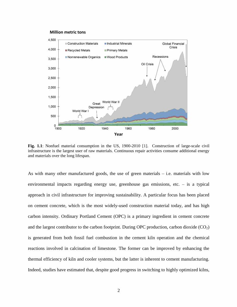
Fig. 1.1: Nonfuel material consumption in the US, 1900-2010. Construction of large-scale civil

infrastructure is the largest user of raw materials. Continuous repair activities consume additional

energy and materials over the long lifespan. 2

Fig. 1.2: Typical tensile stress-strain curve and average crack-width development of ECC. The

high ductility and tight cracking provide enhanced resilience and durability of infrastructure. 5

Fig. 1.3: Green and durable fiber-reinforced geopolymer composites through combination of

geopolymer and ECC technologies. 6

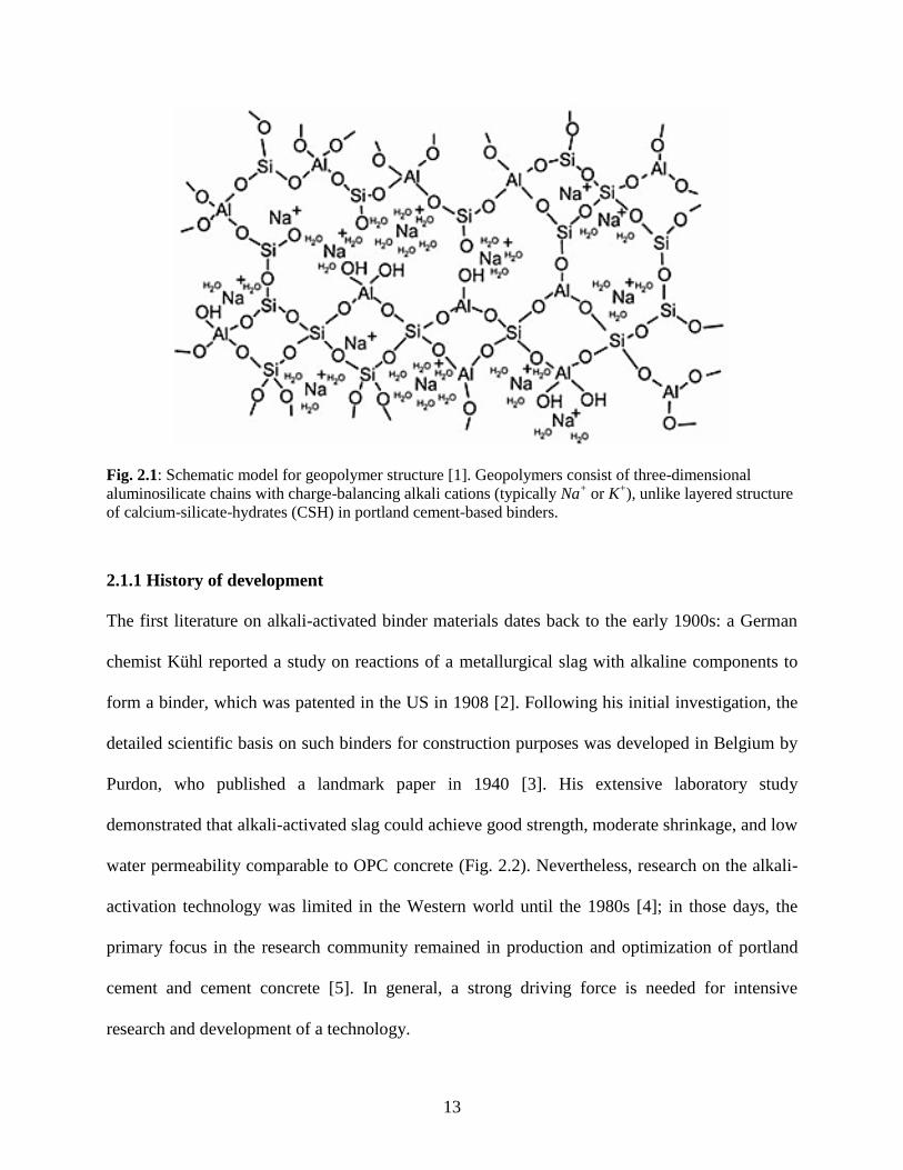
Fig. 2.1: Schematic model for geopolymer structure. Geopolymers consist of three-dimensional

aluminosilicate chains with charge-balancing alkali cations (typically Na+ or K

+), unlike layered

structure of calcium-silicate-hydrates (CSH) in portland cement-based binders. 13

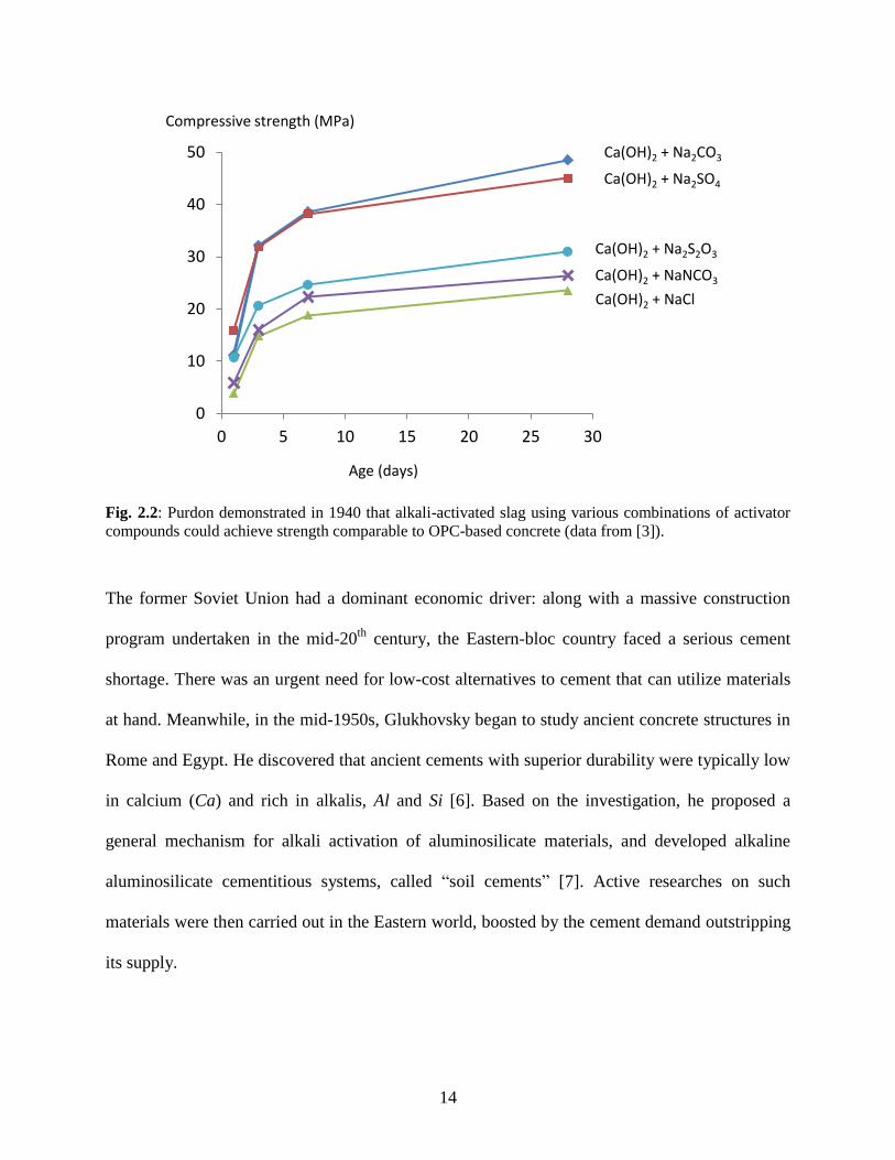
Fig. 2.2: Purdon demonstrated in 1940 that alkali-activated slag using various combinations of

activator compounds could achieve strength comparable to OPC-based concrete. 14

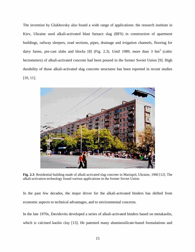
Fig. 2.3: Residential building made of alkali-activated slag concrete in Mariupol, Ukraine, 1960.

The alkali-activation technology found various applications in the former Soviet Union. 15

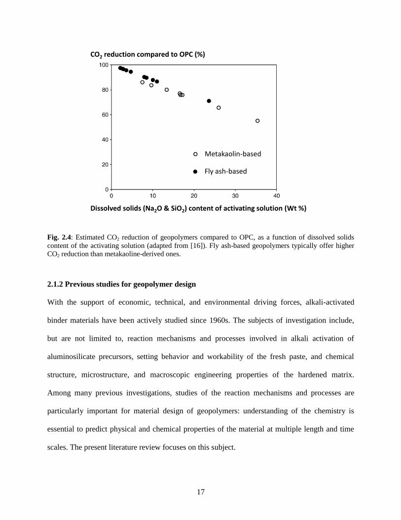
Fig. 2.4: Estimated CO2 reduction of geopolymers compared to OPC, as a function of dissolved

solids content of the activating solution. Fly ash-based geopolymers typically offer higher CO2

reduction than metakaoline-derived ones. 17

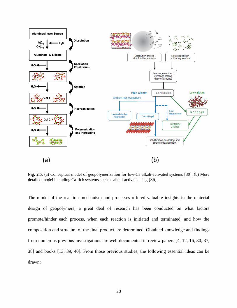
Fig. 2.5: (a) Conceptual model of geopolymerization for low-Ca alkali-activated systems. (b)

More detailed model including Ca-rich systems such as alkali-activated slag. 20

Fig. 2.6: Example of proposed mix-design methods for geopolymers. 22

xii

Fig. 2.7: Schematic illustration of brittle concrete, tension-softening FRC, and strain-hardening

HPFRCC. 25

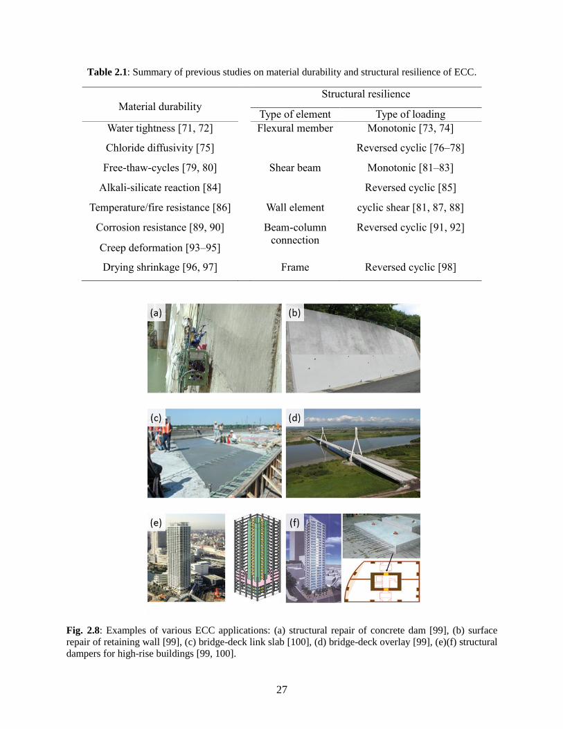
Fig. 2.8: Examples of various ECC applications: (a) structural repair of concrete dam, (b) surface

repair of retaining wall, (c) bridge-deck link slab, (d) bridge-deck overlay, (e)(f) structural

dampers for high-rise buildings. 27

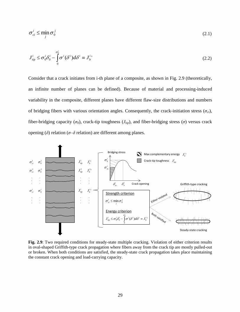
Fig. 2.9: Two required conditions for steady-state multiple cracking. Violation of either criterion

results in oval-shaped Griffith-type crack propagation where fibers away from the crack tip are

mostly pulled-out or broken. When both conditions are satisfied, the steady-state crack

propagation takes place maintaining the constant crack opening and load-carrying capacity. 29

Fig. 2.10: Schematic illustration of a bridging fiber. 31

Fig. 3.1: Design scheme of the proposed integrated design method. Three design techniques for

matrix, composite, and sustainability design phases are utilized, working synergistically to guide

the optimization. 46

Fig. 3.2: Mean compressive strength at each trial, and the total and group means. 53

Fig. 3.3: Main-effect plots showing mean compressive strength at each level of factors. 57

Fig. 3.4: (a) Specimen geometry and (b) test setup for JSCE dog bone testing. 61

Fig. 3.5: Specimen geometry for matrix fracture-toughness test. 63

Fig. 3.6: (a) Specimen geometry and (b) test setup for single-fiber pullout test. 64

Fig. 3.7: Typical singe-fiber pullout curve with slip-hardening. 65

Fig. 3.8: (a) One-way pullout case; only the short-embedment side enters the pullout stage, while

the other side remains in the debonding stage. (b) Two-way pullout case; the long-embedment

side also undergo the pullout stage for δ = uL + uS such that uS > u0S and uL > u0L. 70

Fig. 3.9: Proposed hysteresis of the debonding curve for a standard ECC (M45). 72

Fig. 3.10: Schematic illustration of matrix micro-spalling. 74

xiii

Fig. 3.11: Schematic illustration of Cook-Gordon effect. (a) Matrix crack approaching an

embedded fiber triggers debonding of the premature fiber/matrix interface, (b) which results in

additional crack opening δcg. 75

Fig. 3.12: Flow chart of numerical simulation of σ–δ curve. 76

Fig. 3.13: Simulated σ–δ curve of ECC M45. Three-dimensional uniform fiber distribution was

assumed, and both matrix micro-spalling and Cook-Gordon effect were included. 77

Fig. 3.14: Singe-crack test: (a) specimen geometry, (b) test setup, and (c) fracture plane after

testing. 78

Fig. 4.1: Stress-strain curves of preliminary EGC specimens under uniaxial tension. 88

Fig. 4.2: Strain maps obtained from the DIC analysis. Multiple-crack formation at progressively

increased imposed strain was visualized. 89

Fig. 4.3: Plots of mean responses at each level of factors to visualize the main factor effects. 97

Fig. 4.4: Computed (a) fiber-bridging capacity and (b) complementary energy with their PSH

indices. Dashed lines indicate recommended PSH values for practical design. 105

Fig. 4.5: Tensile stress-strain curves of all EGC series show strain hardening with high ductility.

107

Fig. 4.6: (a) Embodied energy and (b) global warming potential for EGC, concrete, and ECC

materials. CO2 equivalent emissions of EGC-1.5% are about half of regular concrete. 114

Fig. 5.1: Design of prism mold. 124

Fig. 5.2: Curing conditions for intact and cracked EGC specimens prior to permeability testing.

125

Fig. 5.3: Permeability-testing apparatus developed by Lepech and Li. 127

Fig. 5.4: Modified permeability-testing setup used in this study. 128

xiv

Fig. 5.5: Tensile stress-strain curves of EGC specimens under preloading. 130

Fig. 5.6: Density histograms of EGC crack width and their fitted lognormal distributions. 132

Fig. 5.7: Comparison between fitted probability distributions of Vf1.5 and Vf2.0 series. 133

Fig. 5.8: Permeability coefficient of EGC versus applied tensile strain. 134

Fig. 5.9: Comparison of permeability coefficients for EGC, ECC and reinforced cement mortar.

135

Fig. 5.10: Permeability coefficient versus maximum crack width (after unloading) for cement

concrete, reinforced cement mortar, ECC, and EGC (outliers included). 136

Fig. 5.11: Permeability coefficient versus average crack width of EGC. 139

Fig. 6.1: Test schedule and curing condition for each series of EGC. 148

Fig. 6.2: Images of EGC microcracks right after preloading and after water curing: (a)(b) a

completely-sealed microcrack; and (c)(d) a partially-sealed microcrack. 152

Fig. 6.3: Portions of stress-strain curves at preloading and reloading and chord modulus for

reloading. 154

Fig. 6.4: (a) SEM image of a microcrack and self-healing products sealing the crack; and (b)

magnified view of the healing products. 156

Fig. 6.5: EDS line-scan analysis was performed on the line that crosses a microcrack sealed with

white precipitates, including the uncracked region of the geopolymer matrix. 157

Fig. 6.6: Elemental compositions along the scanned line. The presence of efflorescence products

(Na2CO3) and calcite (CaCO3) is not confirmed. The healing products are Si- and Al-rich

substance. 159

Fig. 6.7: EDS mapping. Regions of higher concentration are shown in higher brightness. Higher

concentration of Si and Al, and lower concentration of Ca in the sealed crack can be clearly seen.

160

xv

Fig. 7.1: RC beam design and testing setup of four-point bending. 169

Fig. 7.2: Test conditions of sulfuric acid exposure. Five cycles (35-day exposure) correspond to

average corrosion damage observed in 20-year-old ordinary concrete sewer pipes. 171

Fig. 7.3: Typical appearances of specimen surface with various acid exposure periods. 173

Fig. 7.4: Slight weight gain is observed for both concrete and ECC in the first two cycles (i.e. 14

days), but the rate of subsequent weight loss is three times that of EGC. 174

Fig. 7.5: Compressive strength of concrete, ECC, and EGC before and after sulfuric acid

exposure. All the series show strength increase even after the acid attack, compared to their 28-

day compressive strength (i.e. “0d”). 175

Fig. 7.6: Strength increase due to continuous hydration is extracted by normalizing the raw

compressive strength data by those of control specimens cured in water. Continuous strength

degradation due to the acid attack is observed in concrete, while there is no significant effect on

ECC and EGC. 176

Fig. 7.7: Typical flexural stress–mid deflection curves of RC, ECC, and EGC beams. Due to

relatively high reactive fly ash, ECC beams show lower deflection capacities than expected, with

a few multiple cracks. 178

Fig. 7.8: (a) RC beam shows significant reduction in bending stiffness due to the preloading and

subsequent acid attack. The smallest stiffness reduction of (b) ECC beam is suggested to be a

result of recovery due to self-healing. 182

Fig. 8.1: Large-diameter pipe demand in the US (a) by material and (b) by application, 2011. 190

Fig. 8.2: Predicted concrete-pipe lifespan by Ohio Department of Transportation (ODOT). Years

for the pipe to reach a poor condition (based on ODOT classification) highly depend on pH of

the stream. 191

Fig. 8.3: (a) Precast geopolymer sewer pipes of 1.8 m diameter, commercially available in

Australia; (b) repair of deteriorated concrete sewer pipes in the US by spray-applied geopolymer.

192

xvi

Fig. 8.4: Schematic illustrations of comparison between RC and EGC sewer pipes. 193

Fig. 8.5: System boundary of the sewer pipe system. Use and disposal phases are omitted

because of the low contribution to the life-cycle environmental impacts. 196

Fig. 8.6: Service-life estimation procedure. 199

Fig. 8.7: Liner regressions for weight loss-exposure time relationship for acid-exposed concrete,

ECC and EGC. For concrete and ECC, the constant rate was assumed for data after 35 days. 199

Fig. 8.8: Trench design for circular RC pipe. The total trench volume for this study is 1.22 m3.

203

Fig. 8.9: Life-cycle energy use and GWI values of RC, ECC, and EGC pipes in Scenario I. 206

Fig. B-1: (a) Model of fiber debonding process; (b) a small fiber segment of the debonded zone.

225

Fig. B-2: Force equilibrium in the debonded fiber and surrounding matrix. 227

Fig. B-3: Model of fiber pullout process. 231

Fig. C-1: Pullout-debonding phase of single-fiber pullout. 234

Fig. C-2: Simulated σ–δ relations of ECC M45 by using the original and modified models. 236

Fig. C-3: Simulated fiber status at each crack opening. 236

Fig. C-4: Simulated σ–δ relations with high chemical bond of 10 J/m2 and fiber strength of 2000

MPa. 237

Fig. C-5: Simulated fiber status with high chemical bond and fiber strength. 238

Fig. D-1: Modified permeability-testing setup used in this study. 239

xvii

LIST OF APPENDICES

APPENDIX

A. Confounding of interaction effects. 223

B. Derivation of P-u relations for debonding and pullout stages. 225

C. Derivation and analysis of the proposed hysteresis for fiber debonding load. 234

D. Derivation of the modified formula for permeability coefficient. 239

xviii

ABSTRACT

Green concrete, which incorporates industrial byproducts to partially/fully replace portland

cement in normal concrete, is not as sustainable as many would like to believe. Like

conventional cement concrete, it is a brittle material with low tensile strength and ductility, and

therefore susceptible to cracking. Extensive cracking causes many types of deterioration in

concrete structures, significantly reducing their service life. Even if the structure is made of more

“environmentally-friendly” materials, the short lifespan makes it unsustainable. For establishing

sustainable infrastructure systems, a new material technology that combines high material

greenness and durability in one concrete needs to be developed.

This dissertation is focused on green and durable fiber-reinforced geopolymer composites –

Engineered Geopolymer Composites (EGCs) – for civil infrastructure applications. EGCs

combine two emerging technologies: geopolymer, which is a cement-free binder material, and

Engineered Cementitious Composite (ECC), which is a strain-hardening fiber-reinforced cement

composite with high tensile ductility and multiple-microcracking characteristics. This research

covers three aspects: development, characterization, and application of EGC.

First, a new design method for ductile fiber-reinforced geopolymer composites is proposed to

facilitate the development of EGC. It integrates three material-design techniques – Design of

Experiment (DOE), micromechanical modeling, and Material Sustainability Indices (MSI) –

each of which assists the geopolymer-matrix development, composite design, and environmental

xix

performance assessment. With the aid of the integrated design method, an optimized EGC with

good compressive strength, high tensile ductility, and enhanced material greenness is

systematically developed.

Second, fundamental durability properties of the developed EGC are experimentally

characterized. Specifically, cracking characteristics, water permeability, self-healing

functionality, and sulfuric acid resistance are investigated. Extensive crack-width measurement

and water-permeability testing on cracked EGC demonstrate the tightly-controlled multiple

cracks and higher water tightness than cracked reinforced concrete (RC). The permeability test

also observes a white substance formed inside microcracks of EGC, providing the recovery in

water tightness. Subsequent experiments also confirm the stiffness recovery, which demonstrates

the self-healing functionality of EGC. In the case of sulfuric acid resistance, acid-exposed EGC

specimens show limited surface erosion compared to cement concrete and ECC. Further, no

significant degradation in mechanical properties of EGC is observed.

Finally, this dissertation explores a promising infrastructure application of EGC. Combined with

the characterized durability properties, brief market research and technical-advantage analysis

suggest that EGC is promising for large-diameter sewer pipes. In addition, an environmental life

cycle analysis (LCA) is conducted to verify and quantify the enhanced sustainability of EGC

pipes, in comparison with RC and ECC pipes. The comparative LCA shows the 13% lower

greenhouse gas emissions of EGC than RC. Further, it is estimated that, if service life of EGC

pipes is more than 1.3 times that of RC pipes, EGC performs best in both energy consumption

and greenhouse gas emissions.

1

PART I: INTRODUCTION

CHAPTER 1: Introduction

1.1 Background and motivation

Human life is full of manufactured goods today. Manufactured goods are designed and

manufactured to improve our quality of life, but their production has some adverse impact on the

environment we live in. The same is true for civil infrastructure. However, infrastructure systems

– transportation, power, water and wastewater, and communication systems, for instance – are

different from most other products in two aspects: size and longevity. The large scale of civil

infrastructure implies huge consumption of material resources and energy in their construction

(Fig. 1.1); the long lifespan is linked to continuous repair and retrofit, which also cause

environmental impacts. Because of the large and long-lasting impacts on the environment,

sustainable design of civil infrastructure is crucial for us and future generations. This raises the

question: what does truly sustainable infrastructure look like?

2

Fig. 1.1: Nonfuel material consumption in the US, 1900-2010 [1]. Construction of large-scale civil

infrastructure is the largest user of raw materials. Continuous repair activities consume additional energy

and materials over the long lifespan.

As with many other manufactured goods, the use of green materials – i.e. materials with low

environmental impacts regarding energy use, greenhouse gas emissions, etc. – is a typical

approach in civil infrastructure for improving sustainability. A particular focus has been placed

on cement concrete, which is the most widely-used construction material today, and has high

carbon intensity. Ordinary Portland Cement (OPC) is a primary ingredient in cement concrete

and the largest contributor to the carbon footprint. During OPC production, carbon dioxide (CO2)

is generated from both fossil fuel combustion in the cement kiln operation and the chemical

reactions involved in calcination of limestone. The former can be improved by enhancing the

thermal efficiency of kiln and cooler systems, but the latter is inherent to cement manufacturing.

Indeed, studies have estimated that, despite good progress in switching to highly optimized kilns,

Million metric tons

Year

3

OPC production accounts for 5-8% of the global man-made CO2 emissions [2–5]. As a

consequence of the high carbon intensity of OPC, much effort has been made in developing

green concrete that incorporates industrial wastes to partially/fully replace OPC.

However, such concrete with lower environmental impacts does not always provide true

infrastructure sustainability. Like conventional concrete, green concrete is a brittle material with

low tensile strength and ductility, and therefore susceptible to cracking. Steel reinforcement is

typically placed in concrete structures, but often insufficient to fully control cracking under

combined mechanical and environmental loads in field applications. Cracking causes many types

of deterioration in concrete structures: it directly lowers mechanical properties of concrete, and

also accelerates the degradation by serving as pathways for aggressive agents, which penetrate

the structure and attack the concrete and steel reinforcement. The resultant poor durability of the

structure leads to frequent and/or intensive repair activities, consuming a large amount of energy

and raw materials. In the worst case scenario, full replacement of the structure is needed much

earlier than the designed service life. Thus, the approach of using green materials is inadequate

in the context of minimizing life-cycle environmental impacts of civil infrastructure.

Truly sustainable infrastructure materials should be not only green but also durable. However,

current research and development activities on sustainable construction materials are often

focused on only one aspect of the two, with little emphasis on the other. For enhancing

sustainability of infrastructure systems, a new material technology that combines high material

greenness and durability in one concrete needs to be developed. This is the motivation behind the

present doctoral research.

4

1.2 Problem statement

Recently, the research community has begun to explore green and durable concrete materials. A

promising approach is to integrate existing technologies developed for either green or durable

concrete. Out of various available ones, geopolymer and Engineered Cementitious Composite

(ECC) are emerging material technologies that have gained increasing interest in the past few

decades.

Geopolymer is a family of alkali-activated binder materials that shows promise as a green

alternative to OPC [6–8]. Geopolymer paste is formed from solid aluminosilicate sources

activated by alkaline solution. The fresh geopolymer has similar rheological and hardening

properties to those of cement binders, and can be used to produce geopolymer mortar or concrete.

Among various types of geopolymer materials, fly ash-based geopolymer is one of the most

promising candidates; it utilizes fly ash – an industrial byproduct from coal-fired power plants –

as the aluminosilicate source and relies on no OPC. Indeed, geopolymer binders have been

estimated to offer 80% or greater reduction in CO2 emissions than OPC [9]. However,

geopolymer concrete is by its nature a brittle material like cement concrete. The low ductility of

geopolymer causes cracking and corresponding performance degradation, which limits its

durability as in cement concrete.

Engineered Cementitious Composite (ECC), on the other hand, is a material technology that

imparts high tensile ductility – and therefore enhanced durability – to brittle cement concrete

[10–12]. ECC consists of OPC-based cement mortar and randomly-oriented short fibers with

moderate volume fraction (typically less than 2% by volume). Through systematic optimization

of matrix, fiber, and fiber/matrix interface properties, ECC exhibits the tensile strain-hardening

behavior with high ductility of 3-5%. Further, multiple cracking occurs in the strain-hardening

5

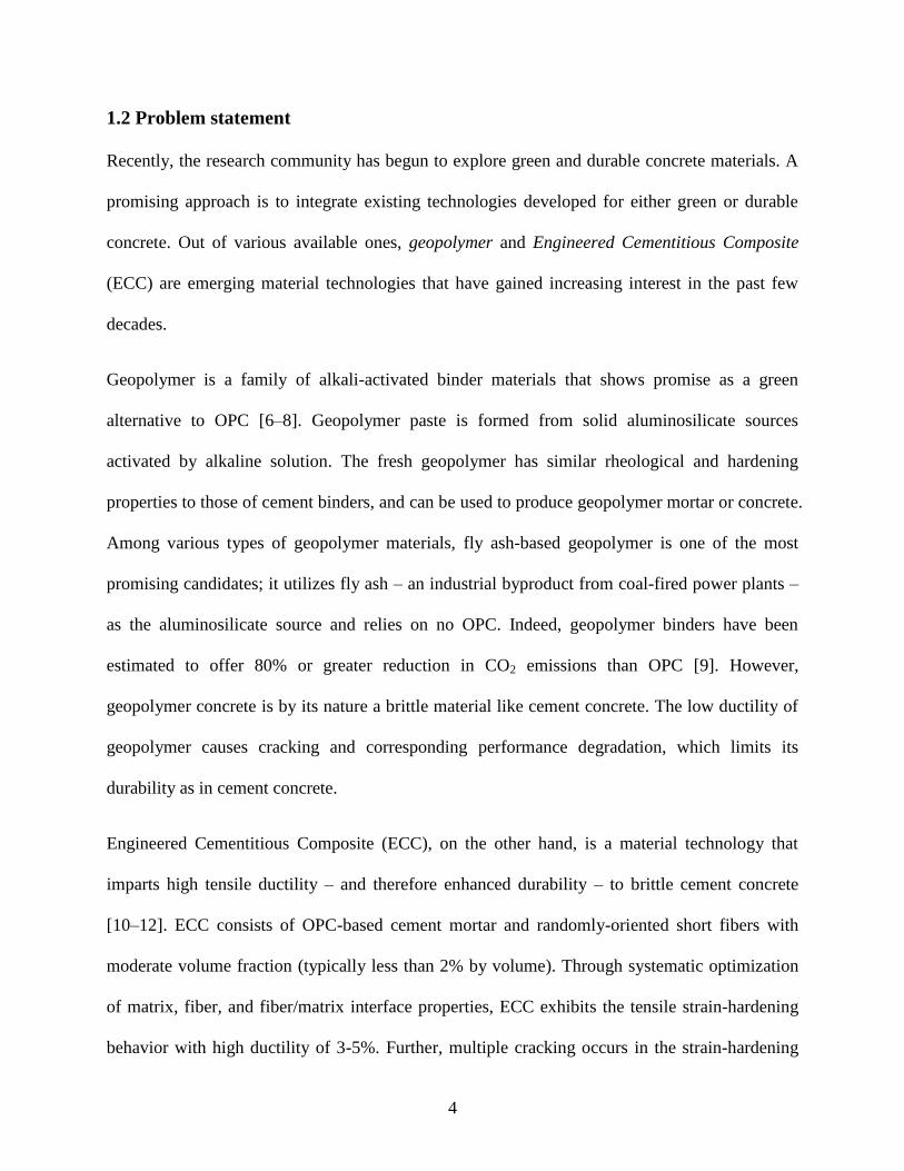
stage and the crack width is controlled to be as tight as a human hair (Fig. 1.2). These unique

features are beneficial in infrastructure applications; both laboratory and field studies have

demonstrated that the high ductility and tight cracking of ECC provide improved durability of

civil infrastructure [13–15]. However, compared to regular cement concrete, ECC has higher

carbon and energy footprints due to its use of a larger amount of OPC and petroleum-based

synthetic fibers with high embodied energy. Thus, the low material greenness of ECC is a

technical challenge to overcome for achieving true stainability of civil infrastructure.

Fig. 1.2: Typical tensile stress-strain curve and average crack-width development of ECC [16]. The high

ductility and tight cracking provide enhanced resilience and durability of infrastructure.

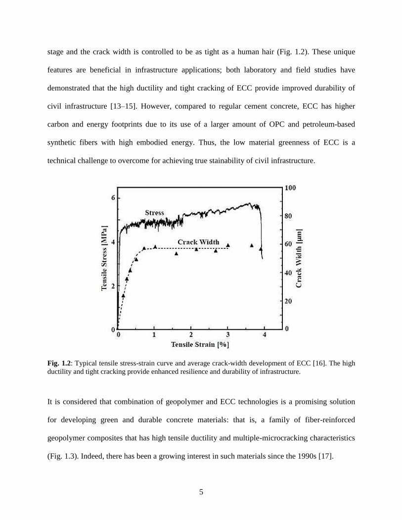
It is considered that combination of geopolymer and ECC technologies is a promising solution

for developing green and durable concrete materials: that is, a family of fiber-reinforced

geopolymer composites that has high tensile ductility and multiple-microcracking characteristics

(Fig. 1.3). Indeed, there has been a growing interest in such materials since the 1990s [17].

6

Fig. 1.3: Green and durable fiber-reinforced geopolymer composites through combination of geopolymer

and ECC technologies (diagram adapted from [17]).

While much research effort has been taken so far, scientific and technical knowledge of ductile

geopolymer composites is still in the early stage of development. Specifically, the following

major challenges remain today:

No comprehensive design method of fiber-reinforced geopolymers has been developed yet.

High tensile ductility and multiple-microcracking characteristics comparable to ECC have

not yet been achieved in such types of materials.

Much remains unknown about their durability properties.

As a result, it is difficult to quantitatively assess their sustainability in the context of

infrastructure applications throughout their service life.

Green & Durable

7

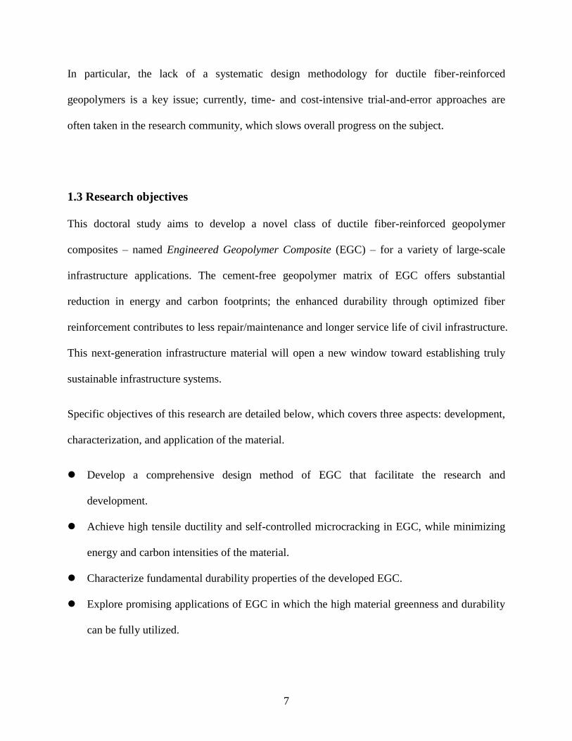
In particular, the lack of a systematic design methodology for ductile fiber-reinforced

geopolymers is a key issue; currently, time- and cost-intensive trial-and-error approaches are

often taken in the research community, which slows overall progress on the subject.

1.3 Research objectives

This doctoral study aims to develop a novel class of ductile fiber-reinforced geopolymer

composites – named Engineered Geopolymer Composite (EGC) – for a variety of large-scale

infrastructure applications. The cement-free geopolymer matrix of EGC offers substantial

reduction in energy and carbon footprints; the enhanced durability through optimized fiber

reinforcement contributes to less repair/maintenance and longer service life of civil infrastructure.

This next-generation infrastructure material will open a new window toward establishing truly

sustainable infrastructure systems.

Specific objectives of this research are detailed below, which covers three aspects: development,

characterization, and application of the material.

Develop a comprehensive design method of EGC that facilitate the research and

development.

Achieve high tensile ductility and self-controlled microcracking in EGC, while minimizing

energy and carbon intensities of the material.

Characterize fundamental durability properties of the developed EGC.

Explore promising applications of EGC in which the high material greenness and durability

can be fully utilized.

8

Conduct a case study on life-cycle environmental impacts of the example EGC application,

in comparison with conventional cement concrete and ECC.

1.4 Research approach and thesis organization

A broad range of multidisciplinary research methods are used in this thesis, including statistics,

fracture mechanics, micromechanics, materials science, and industrial ecology. The research

approach and structure of the thesis are outlined below:

Following this introductory part, Part II containing three chapters is focused on development of

green and ductile – and therefore durable – EGC materials. Chapter 2 outlines previous research

and development of both geopolymer and ECC, and also presents technical challenges in

combining the two materials technologies. Chapter 3 then proposes a new design methodology

for EGC that integrates three design techniques: Design of Experiment (DOE), micromechanical

modeling, and Material Sustainability Indices (MSI). The systematic design method enables

simultaneous optimization of multiple responses such as strength, tensile ductility (often

inversely related to strength), and energy/carbon footprints. The application of the proposed

design method is presented in Chapter 4, which systematically develops an optimized version of

EGC.

Part III describes experimental characterization on durability properties of the developed EGC,

throughout three chapters. In Chapter 5, cracking characteristics and water tightness of the

developed EGC are evaluated. Residual-crack patterns of EGC are first determined with respect

to the maximum and average crack widths, and the probability density function of crack width.

The permeability coefficients of both intact and cracked EGC are then measured by using a

9

newly-developed test setup and a formula derived based on the Darcy’s law. The effect of EGC

microcracks on the water permeability is discussed based on the measured crack patterns and

permeability coefficients. Chapter 6 focuses on the feasibility of self-healing EGC. Stiffness

recovery of EGC specimens that are preloaded to create cracks and then cured in water is

measured by uniaxial tension testing. Self-healing products are also observed by using a

Scanning Electron Microscope (SEM) equipped with an Energy Dispersive Spectroscopy (EDS)

analyzer. Chapter 7 examines the sulfuric acid resistance of EGC. Weight loss and degradation

of mechanical properties in acid-exposed EGC specimens are reported, as well as those of

regular cement concrete and ECC.

Part IV explores promising infrastructure applications of EGC. In particular, large-diameter

sewer pipes are considered in Chapter 8. The market demand, existing technology, and technical

challenges of sewer concrete pipes are first outlined. Then, a Life Cycle Assessment (LCA) on

environmental impacts of EGC sewer pipes is conducted, in comparison with reinforced-concrete

and ECC pipes.

Chapter 9 in Part V is the concluding chapter. Scientific contributions and impacts to the

research field of this dissertation are first highlighted. Major research findings are then

summarized, and recommendations for future work of this subject are provided.

10

References

[1] Center for Sustainable Systems, University of Michigan, “U.S. Material Use Factsheet,”

Pub. No. CSS05-18 , 2016.

[2] C. Chen, G. Habert, Y. Bouzidi, and A. Jullien, “Environmental impact of cement

production: detail of the difference processes and cement plant variability evaluation,” J.

Cleaner Production, vol. 18, pp. 478–485, 2010.

[3] E. Benhelal, G. Zahedi, E. Shamsaei, and A. Bahadori, “Global strategies and potential to

curb CO2 emissions in cement industry,” J. Cleanter Production, vol. 51, pp. 142–161,

2013.

[4] WBCSD, “Cement Industry Energy and CO2 Performance: Getting the Numbers Right”

[Online]. Available: http://www.wbcsdcement.org/pdf/GNR%20dox.pdf. [Accessed: 29-

August-2017].

[5] WBCSD, “Cement Sustainability Initiative Progress Report 2005,” [Online]. Available:

https://www.wbcsdcement.org/pdf/csi_progress_report_2005.pdf. [Accessed: 05-May-

2017].

[6] J. Davidovits, Geopolymer Chemistry and Applications, Third ed. Saint-Quentin (France):

Institut Geopolymere, 2008.

[7] P. Duxson, A. Fernández-Jiménez, J. L. Provis, G. C. Lukey, A. Palomo, and J. S. J. Van

Deventer, “Geopolymer technology: The current state of the art,” J. Mater. Sci., vol. 42,

no. 9, pp. 2917–2933, Dec. 2007.

[8] J. L. Provis and J. S. J. van Deventer, Geopolymers-Structure, processing, properties and

industrial applications. Cambridge (UK): Woodhead Publishing, 2009.

[9] P. Duxson, J. L. Provis, G. C. Lukey, and J. S. J. van Deventer, “The role of inorganic

polymer technology in the development of ‘green concrete,’” Cem. Concr. Res., vol. 37,

no. 12, pp. 1590–1597, Dec. 2007.

[10] V. C. Li, “Engineered Cementitious Composites (ECC) – Tailored Composites through

Micromechanical Modeling,” in Fiber reinforced concrete : present and future, N.

Banthia, A. Bentur, and A. A. Mufti, Eds. Montreal (Canada): Canadian Society for Civil

Engineering, 1998, pp. 64–97.

[11] V. C. Li, “On engineered cementitious composites (ECC). A review of the material and its

applications,” J. Adv. Concr. Technol., vol. 1, no. 3, pp. 215–230, 2003.

[12] V. C. Li, “Engineered Cementitious Composites ( ECC ) – Material , Structural , and

Durability Performance,” in Concrete Construction Engineering Handbook, E. G. Nawy,

Ed. CRC Press, 2008, pp. 1–40.

[13] M. D. Lepech and V. C. Li, “Long Term Durability Performance of Engineered

Cementitious Composites,” Restor. Build. Monum., vol. 2, no. 2, pp. 119–132, 2006.

11

[14] M. Şahmaran and V. C. Li, “Durability properties of micro-cracked ECC containing high

volumes fly ash,” Cem. Concr. Res., vol. 39, no. 11, pp. 1033–1043, Nov. 2009.

[15] M. Kunieda and K. Rokugo, “Recent Progress on HPFRCC in Japan Required

Performance and Applications,” J. Adv. Concr. Technol., vol. 4, no. 1, pp. 19–33, 2006.

[16] S. Wang, “Micromechanics based matrix design for engineered cementitious composites,”

University of Michigan, Ann Arbor, 2005.

[17] A. R. Sakulich, “Reinforced geopolymer composites for enhanced material greenness and

durability,” Sustainable Cities and Society, vol. 1, no. 4. Elsevier B.V., pp. 195–210, Dec-

2011.

12

PART II: DEVELOPMENT OF EGC

CHAPTER 2: Review of Green and Durable Concretes

This chapter provides a literature review on two material technologies: geopolymer and

Engineered Cementitious Composite (ECC). The historical development, previous research

findings, and unsolved problems of each material are outlined, with emphasis on the material

design. Based on the review, challenges in combining the two technologies are considered.

2.1 Geopolymer

In the context of this dissertation, “geopolymer” is defined as an aluminosilicate binder material

that is formed from an aluminosilicate precursor (typically supplied in a powdered form)

activated by an alkali hydroxide, alkali carbonate, and/or alkali silicate activator. As such, there

are many types of geopolymers with various physical and chemical properties, depending on the

types of precursors and activators. In general, geopolymers have three-dimensional polymeric

structure of cross-linked silicate (SiO4) and aluminate (AlO4–) tetrahedra, coupled with charge-

balancing alkali cations (Fig. 2.1).

13

Fig. 2.1: Schematic model for geopolymer structure [1]. Geopolymers consist of three-dimensional

aluminosilicate chains with charge-balancing alkali cations (typically Na+ or K

+), unlike layered structure

of calcium-silicate-hydrates (CSH) in portland cement-based binders.

2.1.1 History of development

The first literature on alkali-activated binder materials dates back to the early 1900s: a German

chemist Kühl reported a study on reactions of a metallurgical slag with alkaline components to

form a binder, which was patented in the US in 1908 [2]. Following his initial investigation, the

detailed scientific basis on such binders for construction purposes was developed in Belgium by

Purdon, who published a landmark paper in 1940 [3]. His extensive laboratory study

demonstrated that alkali-activated slag could achieve good strength, moderate shrinkage, and low

water permeability comparable to OPC concrete (Fig. 2.2). Nevertheless, research on the alkali-

activation technology was limited in the Western world until the 1980s [4]; in those days, the

primary focus in the research community remained in production and optimization of portland

cement and cement concrete [5]. In general, a strong driving force is needed for intensive

research and development of a technology.

14

Fig. 2.2: Purdon demonstrated in 1940 that alkali-activated slag using various combinations of activator

compounds could achieve strength comparable to OPC-based concrete (data from [3]).

The former Soviet Union had a dominant economic driver: along with a massive construction

program undertaken in the mid-20th

century, the Eastern-bloc country faced a serious cement

shortage. There was an urgent need for low-cost alternatives to cement that can utilize materials

at hand. Meanwhile, in the mid-1950s, Glukhovsky began to study ancient concrete structures in

Rome and Egypt. He discovered that ancient cements with superior durability were typically low

in calcium (Ca) and rich in alkalis, Al and Si [6]. Based on the investigation, he proposed a

general mechanism for alkali activation of aluminosilicate materials, and developed alkaline

aluminosilicate cementitious systems, called “soil cements” [7]. Active researches on such

materials were then carried out in the Eastern world, boosted by the cement demand outstripping

its supply.

0

10

20

30

40

50

0 5 10 15 20 25 30

Compressive strength (MPa)

Age (days)

Ca(OH)2 + Na2CO3

Ca(OH)2 + Na2SO4

Ca(OH)2 + Na2S2O3

Ca(OH)2 + NaCl

Ca(OH)2 + NaNCO3

15

The invention by Glukhovsky also found a wide range of applications: the research institute in

Kiev, Ukraine used alkali-activated blast furnace slag (BFS) in construction of apartment

buildings, railway sleepers, road sections, pipes, drainage and irrigation channels, flooring for

dairy farms, pre-cast slabs and blocks [8] (Fig. 2.3). Until 1989, more than 3 hm3 (cubic

hectometers) of alkali-activated concrete had been poured in the former Soviet Union [9]. High

durability of those alkali-activated slag concrete structures has been reported in recent studies

[10, 11].

Fig. 2.3: Residential building made of alkali-activated slag concrete in Mariupol, Ukraine, 1960 [12]. The

alkali-activation technology found various applications in the former Soviet Union.

In the past few decades, the major driver for the alkali-activated binders has shifted from

economic aspects to technical advantages, and to environmental concerns.

In the late 1970s, Davidovits developed a series of alkali-activated binders based on metakaolin,

which is calcined kaolin clay [13]. He patented many aluminosilicate-based formulations and

16

coined the term “geopolymer” for his products. The material technology was originally

developed for fire-resistant applications; shortly afterward, its high early-strength development

attracted attention from the US Army for military applications [14]. From the 1980s onwards,

research and development activities on alkali-activation technologies began to expand worldwide

because of their technical advantages such as rapid strength gain, fire resistance, chemical and

dimensional stabilities, and low permeability. However, primary use of metakaolin-based

geopolymers has been limited to small-scale niche applications to date; metakaolin is expensive

to produce in large volumes and is energy intensive due to its calcination process.

Another breakthrough came in 1993 when Wastiels et al. published the first paper on alkali-

activated binders using fly ash, which is an industrial byproduct from coal-fired power plants

[15]. Since then, research into fly ash-based geopolymers (FAGP) has been growing dramatically

because of their significant environmental benefits. Particularly, considerably lower carbon

footprints of FAGP than OPC-based binders have been highlighted in many studies (e.g. [16–

19]) (Fig. 2.4). In addition, FAGP can increases the recycling rate of fly ash; while a huge

volume of fly ash is generated around the world, most of it is just disposed of in landfills. For

instance, 1.03 billion tons of fly ash was produced in the US from 2000 to 2015, but only 40% of

it has been utilized so far [20]. The same problem of fly ash disposal is true in both China and

India, which are the top users of OPC and large contributors to the global CO2 emissions, as well

as the US. Driven by worldwide concerns of global warming, resource depletion, and waste

disposal, utilization of FAGP for large-scale construction applications is now an important

subject in both academic and industrial research institutions [16].

17

Fig. 2.4: Estimated CO2 reduction of geopolymers compared to OPC, as a function of dissolved solids

content of the activating solution (adapted from [16]). Fly ash-based geopolymers typically offer higher

CO2 reduction than metakaoline-derived ones.

2.1.2 Previous studies for geopolymer design

With the support of economic, technical, and environmental driving forces, alkali-activated

binder materials have been actively studied since 1960s. The subjects of investigation include,

but are not limited to, reaction mechanisms and processes involved in alkali activation of

aluminosilicate precursors, setting behavior and workability of the fresh paste, and chemical

structure, microstructure, and macroscopic engineering properties of the hardened matrix.

Among many previous investigations, studies of the reaction mechanisms and processes are

particularly important for material design of geopolymers: understanding of the chemistry is

essential to predict physical and chemical properties of the material at multiple length and time

scales. The present literature review focuses on this subject.

CO2 reduction compared to OPC (%)

Dissolved solids (Na2O & SiO2) content of activating solution (Wt %)

Fly ash-based

Metakaolin-based

18

Glukhovsky was the first to propose a general reaction mechanism of alkali-activation of

aluminosilicate minerals [7], which has served as a basis for subsequent studies on the chemistry

of “geopolymerization”. His model divides the reaction processes into three stages: (i)

destruction–coagulation, (ii) coagulation–condensation, and (iii) condensation–crystallization.

The first destruction process is initiated by hydroxide ions (OH–) in the alkaline activator that

sever covalent bonds of Si–O–Si and Al–O–Si in the solid aluminosilicate precursor [21]. The

severance of Si–O–Si bonds, for instance, can be expressed as:

OH

SiOOHSiSiOSiOHSiOSi

|

Silanol (≡Si–OH) and sialate (≡Si–O–) species are produced in this reaction, and the negative

charge of ≡Si–O– groups is instantly neutralized by the alkali cations (most commonly Na

+)

provided from the activator. The resultant ≡Si–O–– Na

+ complexes are chemically stable in the

alkaline media, suppressing the reverse reaction to form Si–O–Si bonds. Then, the stability

creates suitable conditions for diffusion of disaggregated units from the particle surface to the

inter-particle space, and for their subsequent coagulation. The OH– ions affect the Al–O–Si and

Al–O–Al bonds in the same way.

Following the dissolution of the solid aluminosilicate, accumulation of the disaggregated

products forms a coagulated structure that favors polycondensation. The monomer – Si(OH)4 in

the case of the silanol species – reacts with another monomer to form the following dimer:

19

33

3333

)()(

||

)()(])[()(

OHOH

OHOHSiOSiHOOHSiOSiHOOHSiOSiHO

This is followed by formation of trimers and more condensed oligomers. Aluminate species also

participate in the polycondensation process, replacing the silicate tetrahedra.

In the third stage, polymerization of silicate-aluminate species grow in all directions, producing

colloids. Lastly, the colloidal particles progressively precipitate to reconsolidate, supported by

particles in the initial solid phase working as nuclei.

The initial conceptual model developed by Glukhovsky has been extended and refined by many

other researchers (e.g. [22–29]). Based on those contributions, Duxson et al. presented an often-

reproduced schematic illustration of geopolymerization processes (Fig. 2.5-a) in their “state of

the art” review paper [30]. The illustrated reaction mechanism outlines the key processes of

dissolution, rearrangement, condensation, and re-solidification. Those processes do not proceed

fully linearly, but rather are coupled reactions occurring concurrently. The proposed process of

particle-to-gel conversion has been confirmed in subsequent studies [31–34], with advances in

experimental and analytical methods. More recently, Provis and Bernal pointed out that their

conceptual model was highly simplified and inappropriate to be used for Ca-rich alkali-activated

systems such as alkali-activated slag [35]. It does not include the formation of CSH-type

structure, which is actually the main binder phase in slag-derived alkali-activated systems. A

more detailed conceptual diagram was provided by Provis and Bernal in [36] (Fig. 2.5-b).

20

Fig. 2.5: (a) Conceptual model of geopolymerization for low-Ca alkali-activated systems [30]. (b) More

detailed model including Ca-rich systems such as alkali-activated slag [36].

The model of the reaction mechanism and processes offered valuable insights in the material

design of geopolymers; a great deal of research has been conducted on what factors

promote/hinder each process, when each reaction is initiated and terminated, and how the

composition and structure of the final product are determined. Obtained knowledge and findings

from numerous previous investigations are well documented in review papers [4, 12, 16, 30, 37,

38] and books [13, 39, 40]. From those previous studies, the following essential ideas can be

drawn:

(a) (b)

21

The dissolution process plays a critical role in controlling all subsequent reactions and the

resultant workability, setting characteristics, mechanical properties, microstructure, and

chemical stability of geopolymers.

The rate and extent of dissolution (and those of the following precipitation and

polymerization steps) depend on many factors, including temperature, pH, alkali-cation type

and soluble-silicon concentration of the alkaline activator, and particle size, morphology,

crystallinity, and chemical compositions of the solid aluminosilicate precursor.

Secondary elements in the aluminosilicate precursor (i.e. other than Si and Al – especially

Ca) can cause side reactions during geopolymerization that significantly affect material

properties of the fresh and hardened geopolymer.

Hardened geopolymers are typically X-ray amorphous, but the amorphous phase is

converted into crystalline zeolite-type structure with time. This conversion could be either

beneficial or detrimental for long term durability of geopolymers; increased compressive

strength due to the formation of crystalline zeolites has been demonstrated in some studies

[21, 41], but decreased tensile strength has been also reported in another study [42].

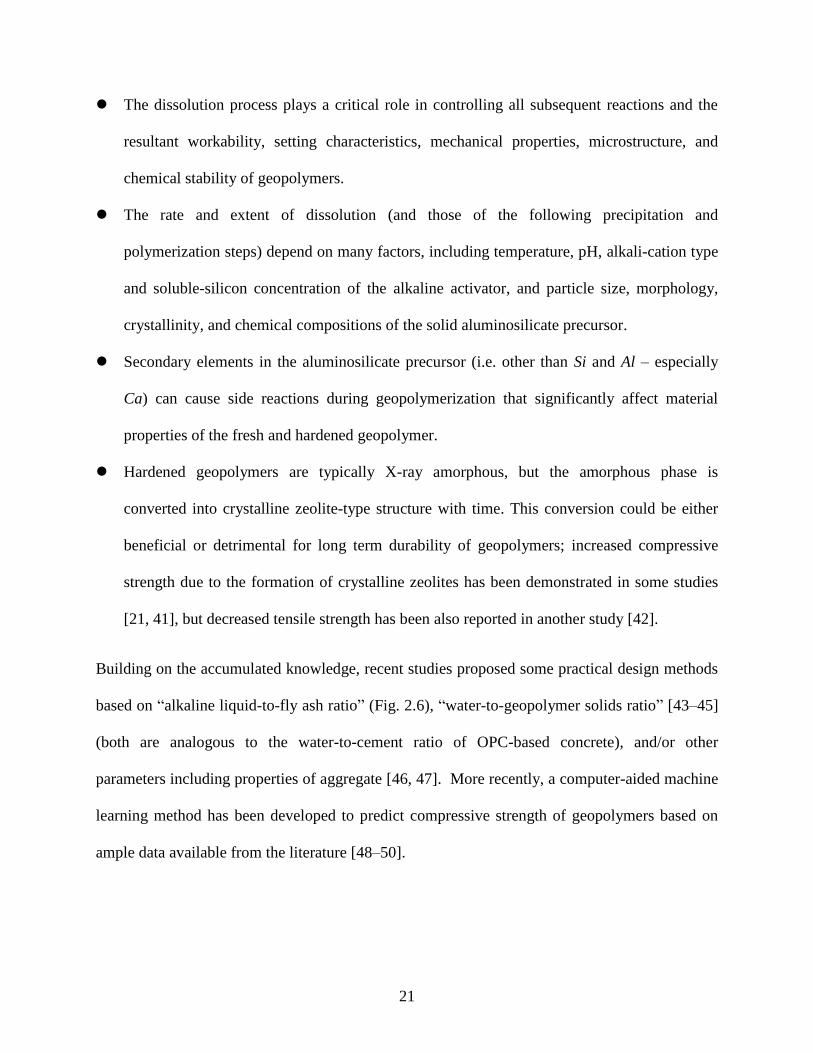
Building on the accumulated knowledge, recent studies proposed some practical design methods

based on “alkaline liquid-to-fly ash ratio” (Fig. 2.6), “water-to-geopolymer solids ratio” [43–45]

(both are analogous to the water-to-cement ratio of OPC-based concrete), and/or other

parameters including properties of aggregate [46, 47]. More recently, a computer-aided machine

learning method has been developed to predict compressive strength of geopolymers based on

ample data available from the literature [48–50].

22

Fig. 2.6: Example of proposed mix-design methods for geopolymers [45].

2.1.3 Unsolved problems

Much work has been done on the reaction mechanism/processes and their influential factors of

geopolymerization; yet much still remains unknown. Particularly, fly ash-based geopolymers

(FAGP) are the most complex system for which further understanding is needed. Indeed,

contradictory results have been sometimes reported among different studies, even when using

similar ingredients, mix proportions, and processing methods.

One of the biggest technical challenges of FAGP is large variability in fly ash properties. First of

all, since fly ash is still regarded as an industrial waste in many countries, its quality control is

not considered, unlike with blast furnace slag and metakaolin. However, the particle size,

23

morphology, composition, and reactivity of fly ash can vary to a large extent, depending on the

size and elemental compositions of feed coal, combustion conditions, and collection methods at

power plants. Even when using the same source and processing methods, a plant can produce fly

ash with a composition that varies significantly from day to day [51]. Further, crystallinity of fly

ash also affects the geopolymerization: relative amounts of crystalline and amorphous phases in

fly ash determine the dissolution behavior and resultant properties of the final product. Because

of this complexity, advanced characterization techniques are required to fully understand the

chemistry of each fly ash and predict properties of the corresponding geopolymer [52].

However, such advanced characterization methods are expensive and require high expertise. As a

result, mix design of FAGP often relies on a trial-and-error approach; several factors (type of fly

ash, alkaline liquid-to-fly ash ratio, curing temperature, etc.) are arbitrarily selected and their

effects on a property of interest (typically compressive strength or workability) are evaluated in a

series of experiments varying the levels of the design factors. As discussed above, results and

findings obtained from the extensive laboratory studies might be specific to each fly ash source.

Moreover, most of the proposed design methods for FAGP have been developed based on those

results, and might not be universally applicable. It is therefore possible that another round of

experiments needs to be done whenever a different source of fly ash is used.

In general, experiment is important to either develop a new material design or verify the existing

one. To overcome the poor repeatability of FAGP, more systematic (but practical) approaches,

instead of inefficient trial-and-error methods, to the material design need to be developed.

24

2.2 Engineered Cementitious Composite

2.2.1 History of development

Like alkali-activated binders, modern development of fiber-reinforced concrete (FRC) also

began in the early 1960s: Romualdi, Baston, and Mandel published milestone papers in 1963

[53] and 1964 [54], which demonstrated improved tensile strength of concrete through

randomly-oriented steel-wire reinforcement. Their work gained significant attention in both

academic and industrial communities, showing the great promise of FRC as a new innovative

construction material [55]. Research and development of FRC has expanded since then,

introducing a variety of other fibers (glass, carbon, synthetic, natural fibers, and their

combinations) and processing methods [56].

Fibers were originally introduced to improve the low tensile strength of concrete [57]. Their

potential in enhancing toughness – energy absorbed before rupturing – was later recognized in

the research community. The ability to suppress the brittle behavior of concrete and improve the

structural resiliency might have been attractive to engineers and asset owners. As a result, since

the early work of Aveston et al. in the early 1970s [58], considerable research and development

work has been directed toward achieving high tensile ductility in concrete. It is such high

ductility, accompanied by strain-hardening behavior, that distinguishes High Performance Fiber

Reinforced Cementitious Composite (HPFRCC) [59] from other FRC materials.

HPFRCC materials typically exhibit a strain-hardening response where sequential formation of

multiple cracks takes place, resulting in significantly higher tensile ductility than normal

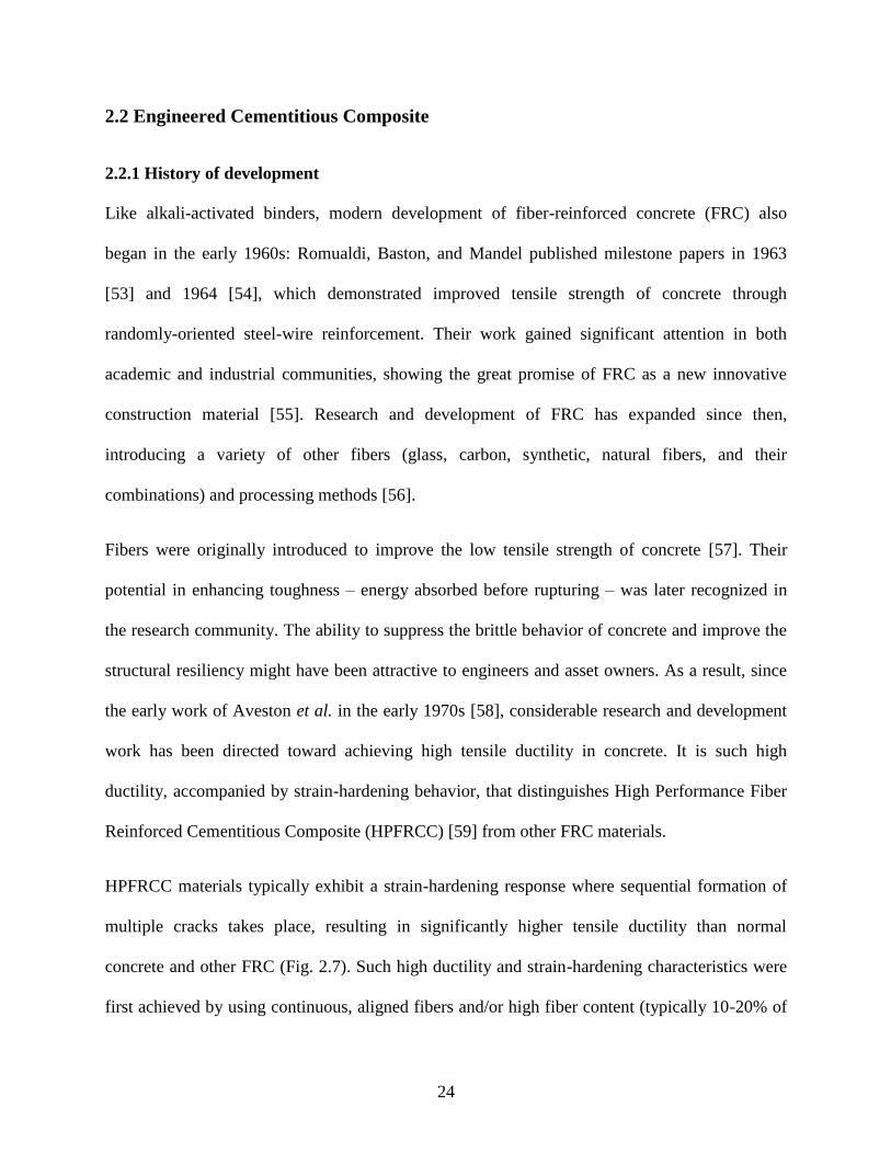
concrete and other FRC (Fig. 2.7). Such high ductility and strain-hardening characteristics were

first achieved by using continuous, aligned fibers and/or high fiber content (typically 10-20% of

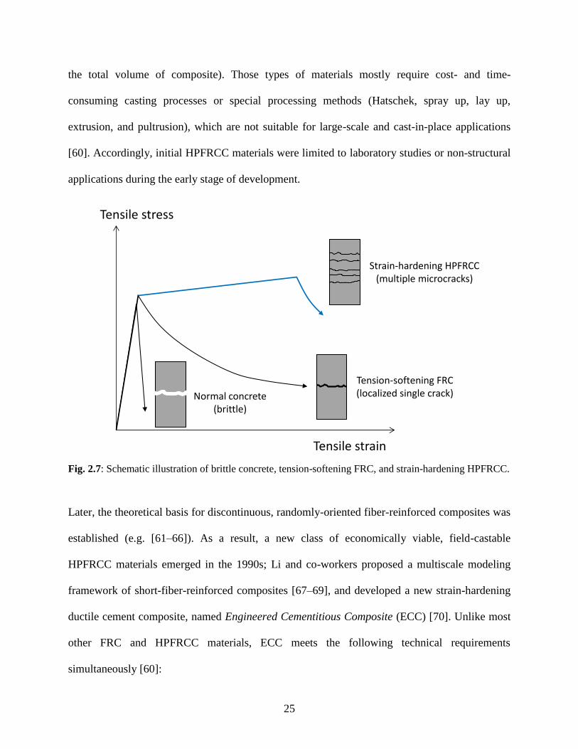
25

the total volume of composite). Those types of materials mostly require cost- and time-

consuming casting processes or special processing methods (Hatschek, spray up, lay up,

extrusion, and pultrusion), which are not suitable for large-scale and cast-in-place applications

[60]. Accordingly, initial HPFRCC materials were limited to laboratory studies or non-structural

applications during the early stage of development.

Fig. 2.7: Schematic illustration of brittle concrete, tension-softening FRC, and strain-hardening HPFRCC.

Later, the theoretical basis for discontinuous, randomly-oriented fiber-reinforced composites was

established (e.g. [61–66]). As a result, a new class of economically viable, field-castable

HPFRCC materials emerged in the 1990s; Li and co-workers proposed a multiscale modeling

framework of short-fiber-reinforced composites [67–69], and developed a new strain-hardening

ductile cement composite, named Engineered Cementitious Composite (ECC) [70]. Unlike most

other FRC and HPFRCC materials, ECC meets the following technical requirements

simultaneously [60]:

Tensile stress

Tensile strain

Normal concrete(brittle)

Tension-softening FRC(localized single crack)

Strain-hardening HPFRCC(multiple microcracks)

26

High performance – strain-hardening behavior, high tensile strength and ductility, and self-

controlled multiple microcracking, which offer structural resilience and durability.

Isotropic properties – no weak planes under multiaxial loading conditions, which ensure

robust performance.

Flexible processing – can be used in conventional concrete mixing/placing equipment,

without any special processing need.

Short fiber of lower volume fraction – directly related to the cost and weight of the material,

as well as the easy processing. ECC typically has 2% or less fiber content by volume.

The unique features of this material gained great interest in the research community, and ECC

has been intensively studied from the 1990s onwards. The extensive investigations demonstrated

various types of enhanced material durability and structural resilience of ECC (Table 2.1).

During the course of investigations, it has been discovered that the self-controlled microcracks

play an important role in the enhanced durability and resilience. In ECC materials, crack width is

typically controlled to be less than 100 μm, which is tight enough to prevent accelerated

penetration of aggressive agents through the cracks. In addition, even under a high imposed

strain, damage of the composite is not localized but distributed as multiple microcracks, which

maintains structural integrity. Consequently, degradation in mechanical properties of the

composite is limited even after cracking. Through the improved resilience and durability

confirmed in laboratory studies, ECC showed a great promise for large-scale structural

applications.

Driven by the demonstrated excellent properties, ECC has already found a number of full-scale

field applications worldwide [56] (Fig. 2.8). More importantly, enhanced durability of those

buildings and infrastructure have been confirmed.

27

Table 2.1: Summary of previous studies on material durability and structural resilience of ECC.

Material durability

Structural resilience

Type of element Type of loading

Water tightness [71, 72]

0.70

Flexural member Monotonic [73, 74]

Chloride diffusivity [75] Reversed cyclic [76–78]

Free-thaw-cycles [79, 80] Shear beam Monotonic [81–83]

Alkali-silicate reaction [84] Reversed cyclic [85]

Temperature/fire resistance [86] Wall element cyclic shear [81, 87, 88]

Corrosion resistance [89, 90] Beam-column

connection

Reversed cyclic [91, 92]

Creep deformation [93–95]

Drying shrinkage [96, 97] Frame Reversed cyclic [98]

Fig. 2.8: Examples of various ECC applications: (a) structural repair of concrete dam [99], (b) surface

repair of retaining wall [99], (c) bridge-deck link slab [100], (d) bridge-deck overlay [99], (e)(f) structural

dampers for high-rise buildings [99, 100].

28

2.2.2 Previous studies for ECC design

Since the invention of the first version of ECC in the 1990s, various types of ECC materials have

been developed to date. Added functionalities – besides the tensile strain-hardening behavior

with high ductility and multiple microcracking – of those ECC materials include self-compacting

[101], lightweight [102], sprayability [103], high early strength [104], and self-healing [105].

More recently, much effort has been placed in development of greener versions of ECC [106–

111]. Surprisingly, a wide variety of those ECC materials were developed within a decade or so.

Such rapid development was realized by a systematic micromechanics-based design method,

which is briefly reviewed here. More detailed discussion of the micromechanical modeling is

presented in Chapter 3.

It should be first mentioned that the high tensile ductility accompanied by distinct strain-

hardening of ECC is a result of sequential initiation and steady-state propagation of multiple

microcracks. When a crack initiates from a pre-existing flaw in ECC, the crack propagates in a

steady-state manner, maintaining a constant crack opening. In contrast, crack opening in normal

FRC increases with crack length as the crack propagates. As a consequence of the continuously

increasing crack opening at the site, fibers away from the crack tip are mostly pulled-out or

broken. The tension-softening behavior – i.e. decreasing load-carrying capacity – of FRC results

from the loss of bridging fibers in this “Griffith-type” cracking [112]. It is therefore important to

control the crack propagation type for achieving steady-state multiple cracking.

Marshall and Cox derived an energy-based criterion for steady-state crack propagation in fiber-

reinforced brittle matrix composites [113]. Building on their derivation, Li and Leung presented

two necessary conditions for achieving steady-state multiple cracking in randomly-distributed

short fiber-reinforced composites [69], which can be expressed as follows:

29

j

j

i

ci 0min (2.1)

')(0

0

00

i

b

iiiiii

tip JdJ

i

(2.2)

Consider that a crack initiates from i-th plane of a composite, as shown in Fig. 2.9 (theoretically,

an infinite number of planes can be defined). Because of material and processing-induced

variability in the composite, different planes have different flaw-size distributions and numbers

of bridging fibers with various orientation angles. Consequently, the crack-initiation stress (σci),

fiber-bridging capacity (σ0), crack-tip toughness (Jtip), and fiber-bridging stress (σ) versus crack

opening (δ) relation (σ–δ relation) are different among planes.

Fig. 2.9: Two required conditions for steady-state multiple cracking. Violation of either criterion results

in oval-shaped Griffith-type crack propagation where fibers away from the crack tip are mostly pulled-out

or broken. When both conditions are satisfied, the steady-state crack propagation takes place maintaining

the constant crack opening and load-carrying capacity.

1

01

ci

i

ci i

0

2

ci 2

0

.

.

.

.

.

.

.

.

.

.

.

.

'1

bJ1

tipJ

i

tipJ 'i

bJ

2

tipJ '2

bJ

.

.

.

.

.

.

.

.

.

.

.

.

Strength criterion

Energy criterion

j

j

i

ci 0min

')(0

0

00

i

b

iiiiii

tip JdJ

i

i

ss

i

ssi

o

i

0

Bridging stress

Crack opening

'i

bJ

i

tipJ

Max complementary energy

Crack-tip toughness

Griffith-type cracking

Steady-state cracking

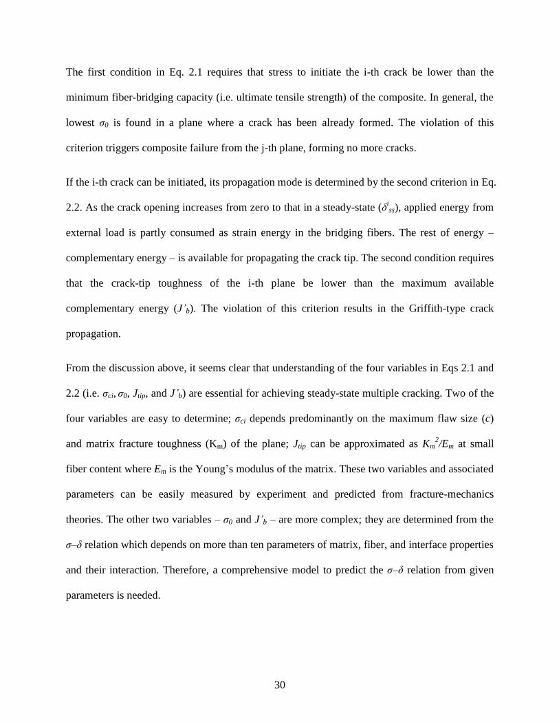
30

The first condition in Eq. 2.1 requires that stress to initiate the i-th crack be lower than the

minimum fiber-bridging capacity (i.e. ultimate tensile strength) of the composite. In general, the

lowest σ0 is found in a plane where a crack has been already formed. The violation of this

criterion triggers composite failure from the j-th plane, forming no more cracks.

If the i-th crack can be initiated, its propagation mode is determined by the second criterion in Eq.

2.2. As the crack opening increases from zero to that in a steady-state (δiss), applied energy from

external load is partly consumed as strain energy in the bridging fibers. The rest of energy –

complementary energy – is available for propagating the crack tip. The second condition requires

that the crack-tip toughness of the i-th plane be lower than the maximum available

complementary energy (J’b). The violation of this criterion results in the Griffith-type crack

propagation.

From the discussion above, it seems clear that understanding of the four variables in Eqs 2.1 and

2.2 (i.e. σci, σ0, Jtip, and J’b) are essential for achieving steady-state multiple cracking. Two of the

four variables are easy to determine; σci depends predominantly on the maximum flaw size (c)

and matrix fracture toughness (Km) of the plane; Jtip can be approximated as Km2/Em at small

fiber content where Em is the Young’s modulus of the matrix. These two variables and associated

parameters can be easily measured by experiment and predicted from fracture-mechanics

theories. The other two variables – σ0 and J’b – are more complex; they are determined from the

σ–δ relation which depends on more than ten parameters of matrix, fiber, and interface properties

and their interaction. Therefore, a comprehensive model to predict the σ–δ relation from given

parameters is needed.

31

Li et al. derived a micromechanics-based constitutive model that relates the “micromechanical

parameters” and macroscopic composite behavior [67]. The fundamental idea behind the

micromechanical model is that the composite mechanical behavior is governed by pull-out

behaviors of individual bridging fibers, while the pull-out behavior of a single fiber is

determined from properties and phenomena at mm-to-μm scales [66]. Mathematically, the

constitutive law of the σ–δ relation is expressed as follows:

cos)2/(

0

21 )()()(),()(1

0

fL

z

e

f

fdzdzppgLP

A

V (2.3)

Vf is the fiber volume fraction; Af is the cross-sectional area of fiber; φ is the inclination angle of

fiber with respect to the normal of the crack plane; Lf is the fiber length; z is the distance between

the fiber centroid and the crack plane; Le is the fiber embedment length. Figure 2.10 illustrates

those parameters.

Fig. 2.10: Schematic illustration of a bridging fiber.

P(δ, Le) represents the load carried by a single fiber aligned normal to the crack plane (i.e. φ=0).

The P-δ relation depends predominantly on the initial fiber embedment length (Le), fiber

properties (length, diameter, Young’s modulus), and chemical and frictional bonding properties

z

φ

Matrix

Fiber

Crack plane

32

of fiber/matrix interface. Besides, when a fiber is inclined from the normal to the crack plane,

additional frictional force occurs at the exit point of the fiber from the matrix [114]. This effect is

taken into account by g(φ), which is analogous to the belt friction equation. P(δ, Le) together with

g(φ) represents the pull-out behavior of a single fiber with arbitrary embedment length Le and

inclination angle φ.

p1(φ) and p2(z) are probability density functions (PDFs) of the fiber inclination angle and

location of fiber centroid, which account for the random distribution of fibers in the composite.

The double integral in Eq 2.3 calculates the total load carried by all bridging fibers in the crack

plane with various orientation angles and centroid locations. The bounds of φ integration might

be limited between φ0 and φ1 depending on the casting condition. The upper bound of z

integration is (Lf/2)cos(φ), since fibers with a larger centroid distance than that value have no

embedded part in the matrix and therefore are not counted as bridging fibers.

Vf/Af is equivalent to the number of fibers per unit area of the crack plane with φ=0. Eq. 2.3 then

gives the fiber-bridging stress at a crack plane for given parameters of matrix, fiber, and interface

properties. The complete mathematical expressions for P(δ, Le), g(φ), p1(φ), and p2(z), are

presented in Chapter 3.

In essence, the micromechanics-based constitutive law enables systematic tailoring of design

parameters for achieving desired composite tensile properties; the simulated σ–δ relation guides

modification of parameters to satisfy the strength/energy criterion for steady-state multiple

cracking, or to achieve higher tensile strength or smaller crack width of the composite. The

micromechanical modeling has been modified and extended [115–118], providing further

efficiency in materials design of ECC.

33

2.2.3 Unsolved problems

In development of ECC materials, the design process typically starts with the matrix design:

matrix ingredients, their mix proportions, and curing method are first determined to achieve a

desired function (e.g. high strength, lightweight, self-compactability, etc.). Then, an appropriate

type of fiber and its volume fraction are selected, followed by experimental characterization of

fiber/matrix interface properties. Finally, the σ–δ relation for the given matrix and fiber is

simulated, which provides guidelines for required modification on matrix, fiber, and/or interface

properties. Therefore, once the matrix with a desired property is developed, subsequent

characterization, simulation, and modification can be systematically done.

Meanwhile, matrix design for various types of ECC has been drawing on accumulated scientific

and empirical knowledge on cement materials; effects of design parameters (water-to-cement

ratio, types of cement and aggregate, curing regime, etc.) on a variety of output properties

(compressive strength, matrix toughness, workability, etc.) have been extensively studied for

OPC-based materials for over a century. Ample data and literature are thus available for guiding

the matrix design to achieve a desired property. Conversely, when the matrix is a relatively new

material with short history of development (i.e. geopolymers), the matrix development tends to

rely on exhaustive trial-and-error approaches.

Another problem is related to the requirement of multi-response optimization in ECC design. If

the matrix with a desired property could be successfully developed, it is ideal to manipulate only

fiber or interface properties in the subsequent composite design phase. In some cases, however,

the simulated σ–δ relation indicates unrealistic modification of design parameters: very high

fiber strength, too small fiber diameter, and large fiber content that needs special processing are

good examples. Matrix modification would be also required in those cases, but such modification

34

could also affect the added function achieved in the preceding matrix design stage. Therefore,

relevant parameters need to be optimized to simultaneously achieve the high tensile ductility and

added function, which adds further difficulty in the ECC design.

2.3 Challenges for development of Engineered Geopolymer Composite

The preceding discussion on geopolymer and ECC design has implications on the difficulty in

combining the two material technologies.

First and foremost, a geopolymer matrix that meets required mechanical performances, material

durability, and rheology for good fiber dispersion needs to be developed. In this matrix

development stage, there are more design variables in geopolymer than OPC-based matrix,

including types of the solid aluminosilicate source and alkaline activator, concentration of the

alkaline solution, curing temperature and duration, as well as mix proportions of ingredients.

Effects of those design factors on matrix properties need to be determined. However, because of

the relatively short history of geopolymers, accumulated knowledge on the matrix design is

limited compared to OPC-based matrix. Advanced characterization techniques are helpful in

understanding those factor effects, but the findings might be specific to each aluminosilicate

source because of the material variability, especially in fly ash. It is time and cost intensive to

explore the vast design space by trial-and-error approaches.

Development of EGC also requires design of fiber and fiber/matrix interface properties, which

adds further degrees of freedom in the material design. As in ECC design, the micromechanical

modeling is a promising tool to guide the composite design of EGC for achieving steady-state

multiple cracking with high tensile ductility. However, due to technical and economical

35

limitations on possible modification of fiber and interface properties, matrix modification might

be also required. As discussed above, such modification might diminish the matrix properties

achieved in the matrix design stage. In addition, another limitation might be put on the selection

of fiber and matrix constituents because of requirement of high material greenness. Therefore,

optimization of multiple responses in EGC design is more complicated than geopolymer and

ECC design.

The difficulty in the material design of EGC slows the overall progress in research, development,

and applications of the technology. To overcome the challenges for rapid development of EGC,

we need to develop a novel design methodology that systematically solves the multi-response

optimization problem. This is explored in the next chapter.

36

References

[1] O. B. H. Rowles M.R., Hanna J.V., Pike K.J., Smith W.E., “29Si, 27 Al, 1 H and 23 Na

MAS NMR Study of the Bonding Character in Aluminosilicate Inorganic Polymers,”

Appl.Magn.Reson, vol. 32, no. 4, pp. 663–689, 2007.

[2] H. Kühl, “Slag cement and process of making the same,” US Patent 900,939, 1908.

[3] A. O. Purdon, “The action of alkalis on blast furnace slag,” J. Soc. Chem. Ind., vol. 59, pp.

191–202, 1940.

[4] D. M. Roy, “Alkali-activated cements: Opportunities and challenges,” Cem. Concr. Res.,

vol. 29, no. 2, pp. 249–254, 1999.

[5] J. L. Provis, P. Duxson, E. Kavalerova, P. V. Krivenko, Z. Pan, F. Puertas, and J. S. J. Van

Deventer, “Historical aspects and overview,” in Alkali Activated Materials - RILEM State-

of-the-Art Reports, vol. 13, 2014, pp. 11–57.

[6] V. D. Glukhovsky, “Ancient, modern and future concretes,” in First International

Conference on Alkaline Cements and Concretes, 1994, pp. 1–8.

[7] V. D. Glukhovsky, Soil silicates. Kiev, Ukraine: Gosstroyizdat Ukrainy Publishing, 1959.

[8] P. Duxson and J. S. J. Van Deventer, “17 – Commercialization of geopolymers for

construction – opportunities and obstacles,” in Geopolymers: Structure, processing,

properties and industrial applications, J. L. Provis and J. S. J. van Deventer, Eds.

Cambridge (UK): Woodhead Publishing, 2009, pp. 379–400.

[9] P. L. Pratt, S.-D. Wang, X.-C. Pu, and K. L. Scrivener, “Alkali-activated slag cement and

concrete: a review of properties and problems,” Adv. Cem. Res., vol. 7, no. 27, pp. 93–102,

1995.

[10] X. Hua, J. L. Provis, J. S. J. Van Deventer, and P. V. Krivenko, “Characterization of Aged

Slag Concretes,” ACI Mater. J., vol. 105, no. 2, pp. 131–139, 2008.

[11] J. Deja, “Carbonation aspects of alkali activated slag mortars and concretes,” Silic. Ind.,

no. 3–4, pp. 37–42, 2002.

[12] A. Palomo, P. Krivenko, I. Garcia-Lodeiro, E. Kavalerova, O. Maltseva, and A.

Fernández-Jiménez, “A review on alkaline activation: new analytical perspectives,” Mater.

Construcción, vol. 64, no. 315, p. e022, 2014.

[13] J. Davidovits, Geopolymer Chemistry and Applications, Third ed. Saint-Quentin (France):

Institut Geopolcle analysis of geopolymers,” in Geopolymers - Structure, processing,

properties and industrial applications, J. L. Provis and J. S. J. van Deventer, Eds.

Cambridge (UK): Woodhead Publishing, 2009, pp. 194–210.

37

[18] B. C. McLellan, R. P. Williams, J. Lay, A. Van Riessen, and G. D. Corder, “Costs and

carbon emissions for geopolymer pastes in comparison to ordinary portland cement,” J.

Clean. Prod., vol. 19, no. 9–10, pp. 1080–1090, 2011.

[19] C. Ouellet-Plamondon and G. Habert, “Life cycle assessment (LCA) of alkali-activated

cements and concretes,” in Handbook of Alkali-Activated Cements, Mortars and

Concretes, F. Pacheco-Torgal, J. Labrincha, C. Leonelli, A. Palomo, and P. Chindaprasit,

Eds. Woodhead Publishing Limited, 2015, pp. 663–686.

[20] American Coal Ash Association, “American Coal Combustion Products Production & Use

Statistics.” [Online]. Available: https://www.acaa-usa.org/Publications/Production-Use-

Reports. [Accessed: 05-May-2017].

[21] A. Fernández-Jiménez and A. Palomo, “Nanostructure/microstructure of fly ash

geopolymers,” in Geopolymers - Structure, processing, properties and industrial

applications, J. L. Provis and J. S. J. van Deventer, Eds. Cambridge (UK): Woodhead

Publishing, 2009, pp. 89–117.

[22] J. Davidovits, “Geopolymers - Inorganic polymeric new matymere, 2008.

[14] P. G. Malone, C. J. Randall, and T. Kirkpatrick, Potential Applications of Alkali-Activated

alumino-silicate binders in military applications, no. Report WES/MP/GL-85-15, U.S.

Army Corps of Engineers. Vicksburg, MS, 1985.

[15] J. Wastiels, X. Wu, S. Faignet, and G. Patfoort, “Mineral polymer based on fly ash,” J.

Resour. Manag. Technol., vol. 22, no. 3, pp. 135–141, 1994.

[16] P. Duxson, J. L. Provis, G. C. Lukey, and J. S. J. van Deventer, “The role of inorganic

polymer technology in the development of ‘green concrete,’” Cem. Concr. Res., vol. 37,

no. 12, pp. 1590–1597, Dec. 2007.

[17] M. Weil, K. Dombrowski, and A. Buchwald, “Life-cyerials,” J. Therm. Anal., vol. 37, no.

8, pp. 1633–1656, 1991.

[23] H. Rahier, B. Van Mele, M. Biesemans, J. Wastiels, and X. Wu, “Low-temperature

synthesized aluminosilicate glasses Part I low-temperature reaction stoichiometry and

structure of a model compound,” J. Mater. Sci., vol. 31, no. 1, pp. 71–79, 1996.

[24] H. Rahier, B. Van Mele, and J. Wastiels, “Low-temperature synthesized aluminosilicate

glasses Part II rheological transformations during low-temperature cure and high-

temperature properties of a model compound,” J. Mater. Sci., vol. 31, no. 1, pp. 80–85,

1996.

[25] H. Rahier, W. Simons, B. Van Mele, and M. Biesemans, “Low-temperature synthesized

aluminosilicate glasses Part III influence of the composition of the silicate solution on

production, structure and properties,” J. Mater. Sci., vol. 32, no. 9, pp. 2237–2247, 1997.

[26] H. Xu and J. S. J. Van Deventer, “The geopolymerisation of alumino-silicate minerals,”

Int. J. Miner. Process., vol. 59, no. 3, pp. 247–266, 2000.

38

[27] A. Palomo, S. Alonso, and A. Fernandez-Jiménez, “Alkaline Activation of Fly Ashes :

NMR Study of the Reaction Products,” J. Am. Ceram. Soc., vol. 87, no. 6, pp. 1141–1145,

2004.

[28] A. Fernández-Jiménez, A. Palomo, and M. Criado, “Microstructure development of alkali-

activated fly ash cement: A descriptive model,” Cem. Concr. Res., vol. 35, no. 6, pp.

1204–1209, 2005.

[29] J. L. Provis and J. S. J. van Deventer, “Geopolymerisation kinetics. 2. Reaction kinetic

modelling,” Chem. Eng. Sci., vol. 62, no. 9, pp. 2318–2329, 2007.

[30] P. Duxson, A. Fernández-Jiménez, J. L. Provis, G. C. Lukey, A. Palomo, and J. S. J. Van

Deventer, “Geopolymer technology: The current state of the art,” J. Mater. Sci., vol. 42,

no. 9, pp. 2917–2933, Dec. 2007.

[31] A. Hajimohammadi, J. L. Provis, and J. S. J. Van Deventer, “Effect of alumina release rate

on the mechanism of geopolymer gel formation,” Chem. Mater., vol. 22, no. 18, pp. 5199–

5208, 2010.

[32] A. Hajimohammadi, J. L. Provis, and J. S. J. Van Deventer, “The effect of silica

availability on the mechanism of geopolymerisation,” Cem. Concr. Res., vol. 41, no. 3, pp.

210–216, 2011.

[33] C. White and J. Provis, “Molecular mechanisms responsible for the structural changes

occurring during geopolymerization: Multiscale simulation,” AIChE J., vol. 58, no. 7, pp.

2241–2253, 2012.

[34] C. E. White, J. L. Provis, B. Bloomer, N. J. Henson, and K. Page, “In situ X-ray pair

distribution function analysis of geopolymer gel nanostructure formation kinetics.,” Phys.

Chem. Chem. Phys., vol. 15, no. 22, pp. 8573–82, 2013.

[35] J. L. Provis and S. A. Bernal, “Milestones in the analysis of alkali-activated binders,” J.

Sustain. Cem. Mater., vol. 4, no. 2, pp. 74–84, 2015.

[36] J. L. Provis and S. A. Bernal, “Geopolymers and Related Alkali-Activated Materials,”

Annu. Rev. Mater. Res, vol. 44, pp. 299–327, 2014.

[37] K. Komnitsas and D. Zaharaki, “Geopolymerisation: A review and prospects for the

minerals industry,” Miner. Eng., vol. 20, no. 14, pp. 1261–1277, Nov. 2007.

[38] J. L. Provis, “Geopolymers and other alkali activated materials: why, how, and what?,”

Mater. Struct., vol. 47, no. 1–2, pp. 11–25, 2014.

[39] J. L. Provis and J. S. J. van Deventer, Geopolymers-Structure, processing, properties and

industrial applications. Cambridge (UK): Woodhead Publishing, 2009.

[40] C. Shi, P. V Krivenko, and D. Roy, Alkali-Activated Cements and Concretes. Abingdon,

UK: Taylor & Francis, 2006.

39

[41] M. Criado, M. Criado, A. Fernandez-Jimenez, A. Fernandez-Jimenez, a G. de la Torre, a

G. de la Torre, M. a G. Aranda, M. a G. Aranda, A. Palomo, and A. Palomo, “An XRD

study of the effect of the SiO2/Na2O ratio on the alkali activation of fly ash,” Cem. Concr.

Res., vol. 37, pp. 671–679, 2007.

[42] A. Mishra, D. Choudhary, N. Jain, M. Kumar, N. Sharda, and D. Dutt, “Effect of

concentration of alkaline liquid and curing time on strength and water absorption of

geopolymer concrete,” ARPN J. Eng. Appl. Sci., vol. 3, no. 1, pp. 14–18, 2008.

[43] D. Hardjito and B. V. Rangan, Development and properties of low-calcium fly ash-based

geopolymer concrete. Perth (Australia): Research report GC 1, Curtin University, 2005.

[44] N. A. Lloyd and B. V. Rangan, “Geopolymer Concrete with Fly Ash,” in Second

International Conference on Sustainable Construction Materials and Technologies, 2010.

[45] M. T. Junaid, O. Kayali, A. Khennane, and J. Black, “A mix design procedure for low

calcium alkali activated fly ash-based concretes,” Constr. Build. Mater., vol. 79, pp. 301–

310, 2015.

[46] S. V. Patankar, Y. M. Ghugal, and S. S. Jamkar, “Mix Design of Fly Ash Based

Geopolymer Concrete,” in Advances in Structural Engineering, 2015, pp. 1619–1634.

[47] T. S. Ng and S. J. Foster, “Development of a mix design methodology for high-

performance geopolymer mortars,” Struct. Concr., vol. 14, no. 2, pp. 148–156, 2013.

[48] İ. B. Topçu and M. Sarıdemir, “Prediction of compressive strength of concrete containing

fly ash using artificial neural networks and fuzzy logic,” Computational Materials Science,

vol. 41, no. 3. pp. 305–311, 2008.

[49] D. Bondar, “The Use of Artificial Neural Network To Predict Compressive Strength of

Geopolymers,” in 3rd International Conference on Sustainable Construction Materials

and Technologies, 2011.

[50] A. Nazari and F. Pacheco Torgal, “Predicting compressive strength of different

geopolymers by artificial neural networks,” Ceram. Int., vol. 39, no. 3, pp. 2247–2257,

2013.

[51] L. M. Keyte, “2 – Fly ash glass chemistry and inorganic polymer cements,” in

Geopolymers - Structure, processing, properties and industrial applications, Cambridge

(UK): Woodhead Publishing, 2009, pp. 15–36.

[52] J. S. J. van Deventer, J. L. Provis, P. Duxson, G. C. Lukey, and J. S. J. Van Deventer,

“Reaction mechanisms in the geopolymeric conversion of inorganic waste to useful

products.,” J. Hazard. Mater., vol. 139, no. 3, pp. 506–13, Jan. 2007.

[53] J. P. Romualdi and G. B. Batson, “Mechanics of Crack Arrest in Concrete,” J. Eng. Mech.

Div., vol. 89, no. 3, pp. 147–168, 1963.

40

[54] J. J. P. Romualdi and J. A. Mandel, “Tensile Strength of concrete Affected by Uniformly

Distributed and Closely Spaced Short Lengths of wire Reinforcement,” ACI J. Proc., vol.

61, no. 6, pp. 657–672, 1964.

[55] R. F. Zollo, “Fiber-reinforced concrete: an overview after 30 years of development,” Cem.

Concr. Compos., vol. 19, no. 2, pp. 107–122, 1997.

[56] V. C. Li, “Engineered Cementitious Composites ( ECC ) – Material , Structural , and

Durability Performance,” in Concrete Construction Engineering Handbook, E. G. Nawy,

Ed. CRC Press, 2008, pp. 1–40.

[57] V. Li, “Large volume, high‐performance applications of fibers in civil engineering,” J.

Appl. Polym. Sci., no. November 2000, pp. 660–686, 2002.

[58] J. . Aveston, G. A. . Cooper, and A. Kelly, “Single and multiple fracture,” in Properties of

Fiber Composites, 1971, pp. 15–24.

[59] A. E. Naaman, “High Performance Fiber Reinforced Cement Composites: Classification

and Applications,” CBM-CI Int. Work. Karachi, Pakistan, vol. 1, no. 1, pp. 389–401, 2009.





[61] J. Aveston and A. Kelly, “Theory of multiple fracture of fibrous composites,” J. Mater.

Sci., vol. 8, no. 3, pp. 352–362, 1973.

[62] A. E. Naaman, A. S. Argon, and F. Moavenzadeh, “A fracture model for fiber reinforced

cementitious materials,” Cem. Concr. Res., vol. 3, no. 4, pp. 397–411, 1973.

[63] A. E. Naaman and S. P. Shah, “Pull-out Mechanism in Steel Fiber-reinforced Concrete,” J.

Struct. Div., vol. 102, no. 8, pp. 1537–1548, 1976.

[64] V. S. Gopalaratnam and S. P. Shah, “Tensile Failure of Steel Fiber-Reinforced Mortar,” J.

Eng. Mech., vol. 113, no. 5, pp. 635–652, 1987.

[65] Y. Wang, V. C. Li, and S. Backer, “Modelling of fibre pull-out from a cement matrix,” Int.

J. Cem. Compos. Light. Concr., vol. 10, no. 3, pp. 143–149, 1988.

[66] Y. Wang, S. Backer, and V. Li, “A statistical tensile model of fibre reinforced

cementitious composites,” Composites, vol. 20, no. 3, pp. 265–274, 1989.

[67] V. C. Li, Y. Wang, and S. Backer, “A micromechanical model of tension-softening and

bridging toughening of short random fiber reinforced brittle matrix composites,” J. Mech.

Phys. Solids, vol. 39, no. 5, pp. 607–625, 1991.

[68] H. Wu and V. Li, “Conditions for pseudo strain-hardening in fiber reinforced brittle

matrix composites,” J. Appl. Mech. Rev., no. 195819, pp. 3487–3489, 1992.

41

[69] V. C. Li and C. K. Y. Leung, “Steady-State and Multiple Cracking of Short Random Fiber

Composites,” J. Eng. Mech., vol. 118, no. 11, pp. 2246–2264, 1992.

[70] V. C. Li, “From Micromechanics to Structural Engineering - The Design of Cementitious

Composites for Civil Engineering Applications,” Struct. Eng. /Earthquake Eng., vol. 10,

no. 2, pp. 37–48, 1993.

[71] M. Şahmaran and V. C. Li, “Influence of microcracking on water absorption and

sorptivity of ECC,” Mater. Struct., vol. 42, no. 5, pp. 593–603, Jul. 2008.

[72] M. D. Lepech and V. C. Li, “Water permeability of engineered cementitious composites,”

Cem. Concr. Compos., vol. 31, no. 10, pp. 744–753, Nov. 2009.

[73] M. Maalej and V. Li, “Introduction of strain-hardening engineered cementitious

composites in design of reinforced concrete flexural members for improved durability,”

ACI Struct. J., 1995.

[74] V. Li and S. Wang, “Flexural behaviors of glass fiber-reinforced polymer (GFRP)

reinforced engineered cementitious composite beams,” ACI Mater. J., 2002.

[75] M. Sahmaran, M. Li, and V. C. Li, “Transport properties of engineered cementitious

composites under chloride exposure,” ACI Mater. J., vol. 104, no. 6, pp. 604–611, 2007.

[76] G. Fischer, H. Fukuyama, and V. Li, “Effect of matrix ductility on the performance of

reinforced ECC column members under reversed cyclic loading conditions,” Proc. JCI Int.

Work. DFRCC, pp. 269–278, 2002.

[77] G. Fischer and V. C. Li, “Deformation behavior of fiber-reinforced polymer reinforced

engineered cementitious composite (ECC) flexural members under reversed cyclic loading

conditions,” ACI Struct. J., vol. 100, no. 1, pp. 25–35, 2003.

[78] G. Fischer and V. Li, “Effect of Matrix Ductility on Deformation Behavior of Steel-

Reinforced ECC Flexural Members under Reversed Cyclic Loading Conditions,” ACI

Struct. J., vol. 99, no. 6, pp. 781–790, 2002.

[79] M. Şahmaran, E. Özbay, H. E. Yücel, M. Lachemi, and V. C. Li, “Frost resistance and

microstructure of Engineered Cementitious Composites: Influence of fly ash and micro

poly-vinyl-alcohol fiber,” Cem. Concr. Compos., vol. 34, no. 2, pp. 156–165, Feb. 2012.

[80] M. Şahmaran and V. C. Li, “De-icing salt scaling resistance of mechanically loaded

engineered cementitious composites,” Cem. Concr. Res., vol. 37, no. 7, pp. 1035–1046,

Jul. 2007.

[81] T. Kanda, S. Watanabe, and V. C. Li, “Application of Pseudo Strain Hardening

Cementitious Composites to Shear Resistant Structural Elements,” in FRAMCOS-3, 1998,

pp. 1477–1490.

[82] K. Shimizu, T. Kanakubo, T. Kanda, and S. Nagai, “Shear behavior of PVA-ECC Beams,”

in Int’l RILEM Workshop HPFRCC in Structural Applications, 2006, pp. 443–451.

42

[83] P. Kabele and M. Kanakubo, “Experimental and Numerical investigation of shear

behavior of PVA-ECC in structural elements,” in Proceedings of the Fifth International

Workshop on HPFRCC (HPFRCC5), 2007, pp. 137–145.

[84] M. Sahmaran, V. C. V. Li, and M. Şahmaran, “Durability of mechanically loaded

engineered cementitious composites under highly alkaline environments,” Cem. Concr.

Compos., vol. 30, no. 2, pp. 72–81, Feb. 2008.

[85] H. Fukuyama, Y. Matsuzaki, K. Nakano, and Y. Sato, “Structural Performance of Beam

Elements with PVA-ECC,” in High Performance Fiber Reinforced Cement Composites 3

(HPFRCC 3), 1999, pp. 531–542.

[86] M. Sahmaran, M. Lachemi, and V. C. Li, “Assessing Mechanical Properties and

Microstructure of Fire-Damaged Engineered Cementitious Composites,” Aci Mater. J.,

vol. 107, no. 3, pp. 297–304, 2010.

[87] K. Kesner and S. L. Billington, “Investigation of Infill Panels Made from Engineered

Cementitious Composites for Seismic Strengthening and Retrofit,” J. Struct. Eng., vol.

131, no. 11, pp. 1712–1720, 2005.

[88] H. Fukuyama, H. Suwada, and T. Mukai, “Test on High-Performance Wall Elements With

Hpfrcc,” in Int’l RILEM Workshop HPFRCC in Structural Applications, 2006, pp. 365–

374.

[89] S. Miyazato and Y. Hiraishi, “Transport properties and steel corrosion in Ductile Fiber

Reinforced Cement Composites,” 11th Int. Conf. Fract. 2005, ICF11, vol. 2, pp. 1500–

1505, 2005.

[90] M. Sahmaran, V. C. V. Li, and C. Andrade, “Corrosion resistance performance of steel-

reinforced engineered cementitious composite beams,” ACI Mater. J., no. 105, pp. 243–

250, 2008.

[91] V. C. Li and D. K. Mishra, “Structural applications of engineered cementitious

composites,” Indian Concr. J., vol. October, pp. 561–567, 1996.

[92] G. Parra-Montesinos and James K. Wight, “Seismic Response of Exterior Rc Column-To-

Steel Beam Connections,” J. Struct. Eng, vol. 126, no. October, pp. 1113–1121, 2000.

[93] W. P. Boshoff and G. P. A. G. van Zijl, “Time-dependent response of ECC:

Characterisation of creep and rate dependence,” Cem. Concr. Res., vol. 37, no. 5, pp. 725–

734, 2007.

[94] J. M. Rouse and S. L. Billington, “Creep and shrinkage of high-performance fiber-

reinforced cementitious composites,” ACI Mater. J., vol. 104, no. 2, pp. 129–136, 2007.

[95] B. Suryanto, K. Maekawa, and K. Nagai, “Predicting the Creep Strain of PVA-ECC at

High Stress Levels based on the Evolution of Plasticity and Damage,” J. Adv. Concr.

Technol., vol. 11, no. 2, pp. 35–48, 2013.

43

[96] M. Li and V. C. Li, “Behavior of ECC-concrete layered repair system under drying

shrinkage conditions,” Restor. Build. Monum., vol. 12, no. 2, pp. 143–160, 2006.

[97] J. Zhang, C. Gong, Z. Guo, and M. Zhang, “Engineered cementitious composite with

characteristic of low drying shrinkage,” Cem. Concr. Res., vol. 39, no. 4, pp. 303–312,

2009.

[98] G. Fischer and V. Li, “Intrinsic response control of moment-resisting frames utilizing

advanced composite materials and structural elements,” ACI Struct. J., no. 100, 2003.

[99] M. Kunieda and K. Rokugo, “Recent Progress on HPFRCC in Japan Required

Performance and Applications,” J. Adv. Concr. Technol., vol. 4, no. 1, pp. 19–33, 2006.

[100] V. C. Li, “Can Concrete Be Bendable?,” Am. Sci., vol. 100, no. 6, p. 484, 2012.

[101] H.-J. Kong, S. G. Bike, and V. C. Li, “Development of a self-consolidating engineered

cementitious composite employing electrosteric dispersion/stabilization,” Cem. Concr.

Compos., vol. 25, no. 3, pp. 301–309, Apr. 2003.

[102] S. Wang, V. Li, A. Naaman, and H. Reinhardt, “Lightweight engineered cementitious

composites (ECC),” in 4th International RILEM Workshop on High Performance Fiber -

Reinforced Cement Composites (HPFRCC4), 2003, pp. 379–390.

[103] Y. Y. Kim, H. J. Kong, and V. C. Li, “Design of Engineered Cementitious Composite

Suitable for Wet-Mixture Shotcreting,” ACI Mater. J., vol. 100, no. 6, pp. 511–518, 2003.

[104] S. Wang and V. C. Li, “High-early-strength engineered cementitious composites,” ACI

Mater. J., vol. 103, no. 2, pp. 97–105, 2006.

[105] Y. Yang, M. D. Lepech, E. Yang, and V. C. Li, “Autogenous healing of engineered

cementitious composites under wet–dry cycles,” Cem. Concr. Res., vol. 39, no. 5, pp.

382–390, May 2009.

[106] V. C. Li, M. Lepech, S. Wang, M. Weimann, and G. A. Keoleian, “Development of Green

ECC for Sustainable Infrastructure Systems,” in Int’l Workshop on Sustainable

Development and Concrete Technology, 2004, pp. 181–192.

[107] E. H. Yang, Y. Yang, and V. C. Li, “Use of high volumes of fly ash to improve ECC

mechanical properties and material greenness,” ACI Mater. J., vol. 104, no. 6, pp. 620–

628, 2007.

[108] M. Lepech, G. Keoleian, S. Qian, and V. C. Li, “Design of green engineered cementitious

composites for pavement overlay applications,” in Int’l Association for Life Cycle Civil

Engineering conference (IALCCE 08), 2008, pp. 837–842.

[109] X. Huang, R. Ranade, Q. Zhang, W. Ni, and V. C. Li, “Mechanical and thermal properties

of green lightweight engineered cementitious composites,” Constr. Build. Mater., vol. 48,

pp. 954–960, Nov. 2013.

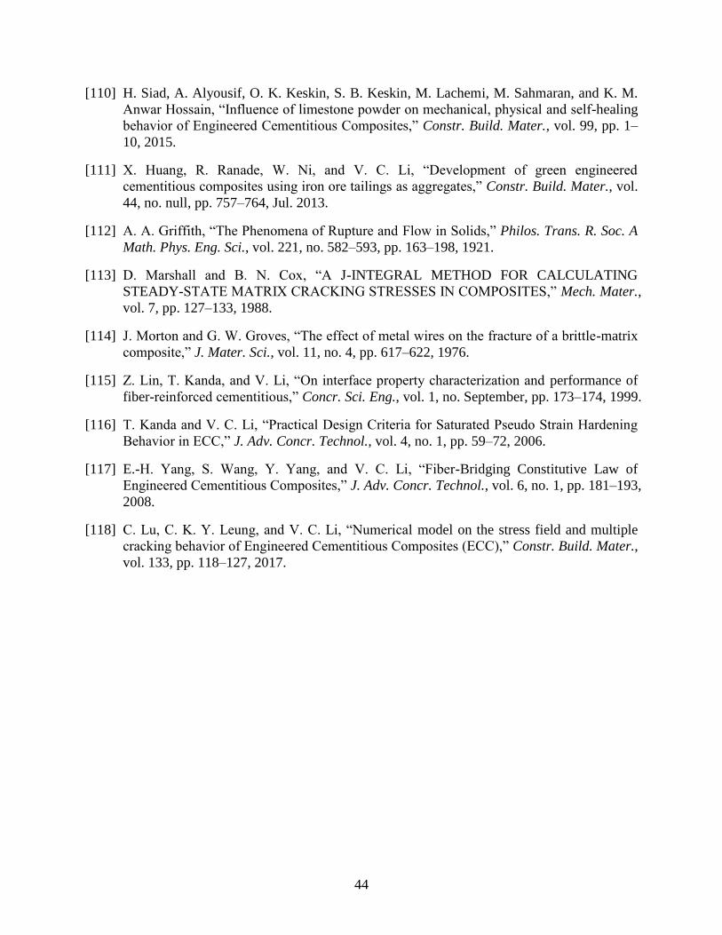
44

[110] H. Siad, A. Alyousif, O. K. Keskin, S. B. Keskin, M. Lachemi, M. Sahmaran, and K. M.

Anwar Hossain, “Influence of limestone powder on mechanical, physical and self-healing

behavior of Engineered Cementitious Composites,” Constr. Build. Mater., vol. 99, pp. 1–

10, 2015.

[111] X. Huang, R. Ranade, W. Ni, and V. C. Li, “Development of green engineered

cementitious composites using iron ore tailings as aggregates,” Constr. Build. Mater., vol.

44, no. null, pp. 757–764, Jul. 2013.

[112] A. A. Griffith, “The Phenomena of Rupture and Flow in Solids,” Philos. Trans. R. Soc. A

Math. Phys. Eng. Sci., vol. 221, no. 582–593, pp. 163–198, 1921.

[113] D. Marshall and B. N. Cox, “A J-INTEGRAL METHOD FOR CALCULATING

STEADY-STATE MATRIX CRACKING STRESSES IN COMPOSITES,” Mech. Mater.,

vol. 7, pp. 127–133, 1988.

[114] J. Morton and G. W. Groves, “The effect of metal wires on the fracture of a brittle-matrix

composite,” J. Mater. Sci., vol. 11, no. 4, pp. 617–622, 1976.

[115] Z. Lin, T. Kanda, and V. Li, “On interface property characterization and performance of

fiber-reinforced cementitious,” Concr. Sci. Eng., vol. 1, no. September, pp. 173–174, 1999.

[116] T. Kanda and V. C. Li, “Practical Design Criteria for Saturated Pseudo Strain Hardening

Behavior in ECC,” J. Adv. Concr. Technol., vol. 4, no. 1, pp. 59–72, 2006.

[117] E.-H. Yang, S. Wang, Y. Yang, and V. C. Li, “Fiber-Bridging Constitutive Law of

Engineered Cementitious Composites,” J. Adv. Concr. Technol., vol. 6, no. 1, pp. 181–193,

2008.

[118] C. Lu, C. K. Y. Leung, and V. C. Li, “Numerical model on the stress field and multiple

cracking behavior of Engineered Cementitious Composites (ECC),” Constr. Build. Mater.,

vol. 133, pp. 118–127, 2017.

45

CHAPTER 3: Integrated Design Method

An integrated design method for Engineered Geopolymer Composite (EGC) is proposed in this

chapter. The new methodology combines three material-design techniques: design of experiment,

micromechanical modeling, and material sustainability indices, which synergistically work to

solve the multi-response optimization problem in EGC design.

3.1 Framework of proposed design method

As has been discussed in Chapter 2, material design of EGC involves many design parameters

and multiple responses to be optimized. Specifically, both high tensile ductility and enhanced

material greenness need to be achieved, as well as fundamental engineering properties such as

strength. While some existing design methods are useful to partly aid the multi-response

optimization, a comprehensive framework to integrate those approaches has not been developed

yet. In the present chapter, a new integrated design methodology is proposed to facilitate the

research and development of EGC.

Figure 3.1 illustrates the design scheme of the proposed design method. It consists of three

design phases: matrix, composite, and environmental designs, each of which utilizes a specific

material-design technique. This section outlines each design phase and corresponding design

technique. The detailed theories and procedures are later presented in the following sections.

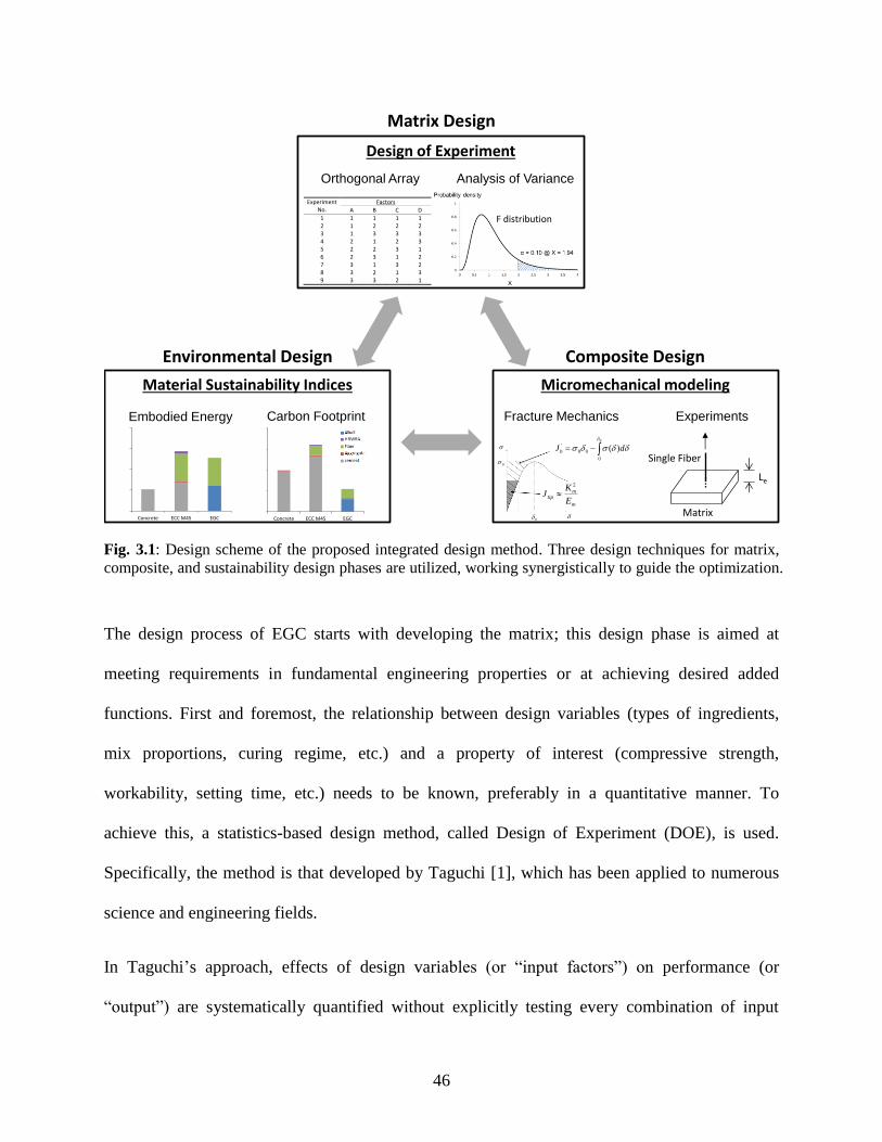
46

Fig. 3.1: Design scheme of the proposed integrated design method. Three design techniques for matrix,

composite, and sustainability design phases are utilized, working synergistically to guide the optimization.

The design process of EGC starts with developing the matrix; this design phase is aimed at

meeting requirements in fundamental engineering properties or at achieving desired added

functions. First and foremost, the relationship between design variables (types of ingredients,

mix proportions, curing regime, etc.) and a property of interest (compressive strength,

workability, setting time, etc.) needs to be known, preferably in a quantitative manner. To

achieve this, a statistics-based design method, called Design of Experiment (DOE), is used.

Specifically, the method is that developed by Taguchi [1], which has been applied to numerous

science and engineering fields.

In Taguchi’s approach, effects of design variables (or “input factors”) on performance (or

“output”) are systematically quantified without explicitly testing every combination of input

Matrix Design

Experiment No.

Factors

A B C D

1 1 1 1 1 2 1 2 2 2 3 1 3 3 3 4 2 1 2 3 5 2 2 3 1 6 2 3 1 2 7 3 1 3 2 8 3 2 1 3 9 3 3 2 1

Orthogonal Array Analysis of Variance

Design of Experiment

Material Sustainability Indices

Environmental Design Composite Design

Micromechanical modeling

Fracture Mechanics

0

0

00

' )(

dJb

m

mtip

E

KJ

2

0

0

Experiments

Single Fiber

Matrix

Le

0

2

4

6

8

Concrete ECC M45 EGC

Pri

mar

y En

erg

y (M

J/L)

0.0

0.2

0.4

0.6

0.8


CO

2Em

issi

on

s (k

g-C

O2/L

)

0

2

4

6

8


Pri

mar

y En

erg

y (M

J/L)

0.0

0.2

0.4

0.6

0.8


CO

2Em

issi

on

s (k

g-C

O2/L

)

Carbon FootprintEmbodied Energy

F distribution

47

factors. There are two key steps there. First, out of numerous possible combinations of input

factors and factor levels, only a portion of them is selected to test, based on a fractional-factorial

design using orthogonal arrays (OAs). Second, test results from the planned experiments are

statistically analyzed by using the Analysis of Variance (ANOVA) method. This step offers

quantitative evaluation on the significance of each factor and suggests optimum factor levels.

With Taguchi’s DOE technique, experimental costs can be substantially reduced, yet robust

information about the relationship between input factors and an output is obtained. The optimum

matrix design can be determined based on the information.

Once a desired EGC matrix is developed, fiber and fiber/matrix interface properties are tailored

to impart high tensile ductility and multiple-cracking characteristic to the material.

Micromechanical modeling is a design technique adopted in this composite-design phase [2],

which has been outlined in Section 2.2.2. In this design stage, micromechanical parameters –

fracture toughness and tensile strength of matrix, bonding properties between fiber and matrix,

and so forth – are first measured for the developed matrix and selected fiber. Then, the composite

tensile behavior is simulated by an analytical model that relates the measured micromechanical

parameters and macroscopic composite properties. Based on the simulation result, required

modification of micromechanical parameters are determined for achieving desired composite

properties.

The last phase is the environmental design that evaluates material sustainability of the developed

composite. Here, Material Sustainability Indices (MSI) are employed to measure the energy

consumption and carbon footprints associated with the material production [3]. MSI values

represent a partial life cycle analysis (LCA) of the material greenness that accounts for raw-

material acquisition, processing, and manufacturing, while the use and disposal phases are

48

omitted. In general, reliable life-cycle inventory data are collected from literature or database, for

all ingredients of the material. MSI values are then calculated by taking the sum of the

energy/carbon footprints of the ingredients. MSI are useful for comparing the carbon and energy

footprints of different materials on a mass or volume basis, and for quantifying the overall

environmental performance of materials, regardless of the application.

Each of the three design techniques above has been individually applied to geopolymer and

ECC development. The uniqueness of the proposed integrated design method is that those three

design stages are linked with each other and work in a synergistic manner. For example,

sustainability aspects are considered in both the matrix-design and composite-design stages by

pre-screening out energy/carbon-intensive ingredients. In addition, information from the matrix-

design stage can be utilized in the other stages; a DOE study in the matrix development may

identify some design variables as “insignificant factors” on the property of interest. Then,

without compromising the target matrix property, those design variables can be used to either

modify micromechanical parameters for the composite design or lower the energy/carbon

footprints for the environmental design. Thus, information from all three design techniques can

be fed back into each design step, systematically confining the vast design space of multi-

response optimization in EGC.

Detailed theories and procedures of the method are most easily understood through an example,

which is presented in the following sections.

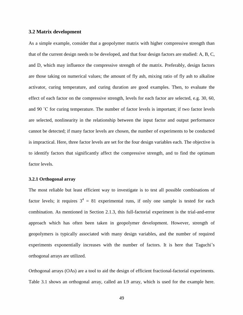
49

3.2 Matrix development

As a simple example, consider that a geopolymer matrix with higher compressive strength than

that of the current design needs to be developed, and that four design factors are studied: A, B, C,

and D, which may influence the compressive strength of the matrix. Preferably, design factors

are those taking on numerical values; the amount of fly ash, mixing ratio of fly ash to alkaline

activator, curing temperature, and curing duration are good examples. Then, to evaluate the

effect of each factor on the compressive strength, levels for each factor are selected, e.g. 30, 60,

and 90 ˚C for curing temperature. The number of factor levels is important; if two factor levels

are selected, nonlinearity in the relationship between the input factor and output performance

cannot be detected; if many factor levels are chosen, the number of experiments to be conducted

is impractical. Here, three factor levels are set for the four design variables each. The objective is

to identify factors that significantly affect the compressive strength, and to find the optimum

factor levels.

3.2.1 Orthogonal array

The most reliable but least efficient way to investigate is to test all possible combinations of

factor levels; it requires 34 = 81 experimental runs, if only one sample is tested for each

combination. As mentioned in Section 2.1.3, this full-factorial experiment is the trial-and-error

approach which has often been taken in geopolymer development. However, strength of

geopolymers is typically associated with many design variables, and the number of required

experiments exponentially increases with the number of factors. It is here that Taguchi’s

orthogonal arrays are utilized.

Orthogonal arrays (OAs) are a tool to aid the design of efficient fractional-factorial experiments.

Table 3.1 shows an orthogonal array, called an L9 array, which is used for the example here.

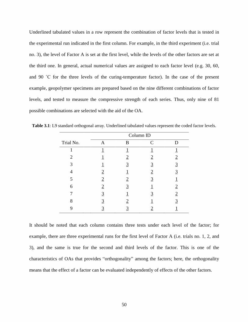
50

Underlined tabulated values in a row represent the combination of factor levels that is tested in

the experimental run indicated in the first column. For example, in the third experiment (i.e. trial

no. 3), the level of Factor A is set at the first level, while the levels of the other factors are set at

the third one. In general, actual numerical values are assigned to each factor level (e.g. 30, 60,

and 90 ˚C for the three levels of the curing-temperature factor). In the case of the present

example, geopolymer specimens are prepared based on the nine different combinations of factor

levels, and tested to measure the compressive strength of each series. Thus, only nine of 81

possible combinations are selected with the aid of the OA.

Table 3.1: L9 standard orthogonal array. Underlined tabulated values represent the coded factor levels.

Column ID

Trial No. A B C D

1 1 1 1 1

2 1 2 2 2

3 1 3 3 3

4 2 1 2 3

5 2 2 3 1

6 2 3 1 2

7 3 1 3 2

8 3 2 1 3

9 3 3 2 1

It should be noted that each column contains three tests under each level of the factor; for

example, there are three experimental runs for the first level of Factor A (i.e. trials no. 1, 2, and

3), and the same is true for the second and third levels of the factor. This is one of the

characteristics of OAs that provides “orthogonality” among the factors; here, the orthogonality

means that the effect of a factor can be evaluated independently of effects of the other factors.

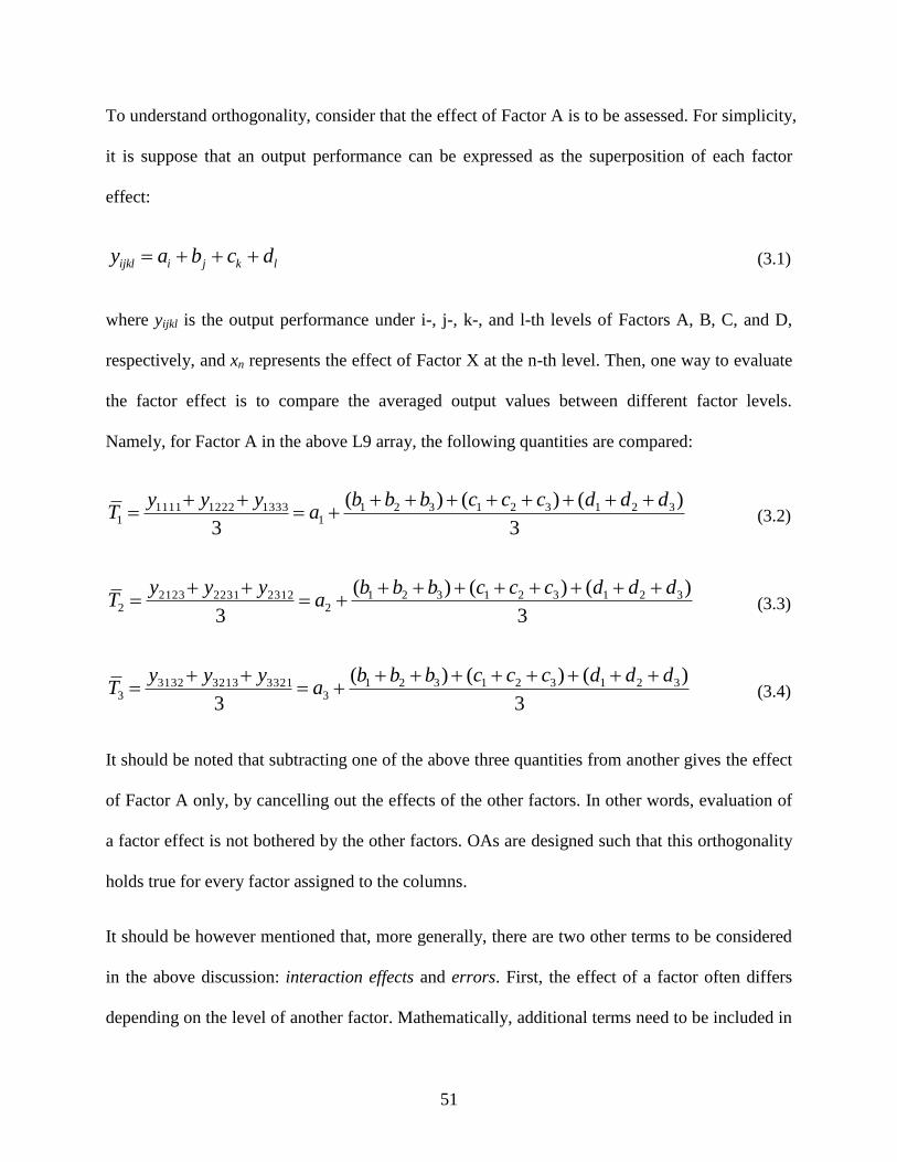
51

To understand orthogonality, consider that the effect of Factor A is to be assessed. For simplicity,

it is suppose that an output performance can be expressed as the superposition of each factor

effect:

lkjiijkl dcbay (3.1)

where yijkl is the output performance under i-, j-, k-, and l-th levels of Factors A, B, C, and D,

respectively, and xn represents the effect of Factor X at the n-th level. Then, one way to evaluate

the factor effect is to compare the averaged output values between different factor levels.

Namely, for Factor A in the above L9 array, the following quantities are compared:

3

)()()(

3

3213213211

1333122211111

dddcccbbba

yyyT

(3.2)

3

)()()(

3

3213213212

2312223121232

dddcccbbba

yyyT

(3.3)

3

)()()(

3

3213213213

3321321331323

dddcccbbba

yyyT

(3.4)

It should be noted that subtracting one of the above three quantities from another gives the effect

of Factor A only, by cancelling out the effects of the other factors. In other words, evaluation of

a factor effect is not bothered by the other factors. OAs are designed such that this orthogonality

holds true for every factor assigned to the columns.

It should be however mentioned that, more generally, there are two other terms to be considered

in the above discussion: interaction effects and errors. First, the effect of a factor often differs

depending on the level of another factor. Mathematically, additional terms need to be included in

52

Eq. 3.1. Those terms are typically not cancelled out in evaluating factor effects, and the

interaction effect is therefore mixed with main effects of factors (called “confounding”, which is

discussed in detail in Appendix A). Thus, if interaction effects are expected to be significant, an

appropriate OA that can separate the interaction effects from main-factor effects needs to be

chosen. Second, the output performance measured in experiment always contains errors to some

extent. Aside from random experimental errors, those errors could be caused by “noise factors”,

which cannot be controlled and “unknown factors”, which are not considered in the selected OA.

In either case, it might be possible to misevaluate the significance of factors if the error effect is

relatively large. To overcome this problem, it is required that the estimated factor effect be

compared with the error effect. This is the essence of Analysis of Variance, which is discussed

below.

3.2.2 Analysis of Variance

Once the fractional-factorial experiment is well planned and conducted, the obtained test data

need to be analyzed and interpreted. Analysis of Variance (ANOVA) is the most objective

method to examine the significance of factors through the test result.

As an example, Factor A is evaluated here; the following procedure is equally applicable to the

other factors. Suppose that three samples are tested for each experimental run in the L9 array.

Table 3.2 lists an example data set of the measured compressive strength. Also, Fig. 3.2 plots the

mean compressive strength at each trial, the total mean of all the data (�̅�), and the group mean

for each factor level (�̅�𝑖), which is the average of data in the same factor level. As can be seen in

the L9 array (Table 3.1), the first level of Factor A (A1) is included in the first to third trials, A2 in

the fourth to sixth, and A3 in the seventh to ninth ones.

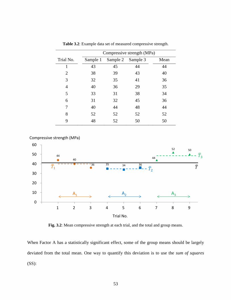
53

Table 3.2: Example data set of measured compressive strength.


Trial No. Sample 1 Sample 2 Sample 3 Mean

1 43 45 44 44

2 38 39 43 40

3 32 35 41 36

4 40 36 29 35

5 33 31 38 34

6 31 32 45 36

7 40 44 48 44

8 52 52 52 52

9 48 52 50 50

Fig. 3.2: Mean compressive strength at each trial, and the total and group means.

When Factor A has a statistically significant effect, some of the group means should be largely

deviated from the total mean. One way to quantify this deviation is to use the sum of squares

(SS):


Trial No.

44 40

36 35 34 36

44

52 50

0

10

20

30

40

50

60

0 1 2 3 4 5 6 7 8 9

A1 A2 A3

54

i

iiA TTnSS 2)( (3.5)

where ni is the sample size in the i-th level of the factor, by which the squared deviation for the

group is weighted. SS of other factors can be also calculated in the same manner. This quantity

reflects the variation caused by the factor.

Similarly, the total sum of squares can be defined as the squared deviation of each data point

from the total mean:

i j

ijT TxSS 2)( (3.6)

where xij is the data for j-th sample in the i-th trial. This quantity reflects the total variation in the

data set. In general, the total variation is larger than the sum of the variations caused by factors.

Thus, the variation due to errors (SSe) can be defined as the difference between the total variation

and variation due to factors:

)( DCBATe SSSSSSSSSSSS (3.7)

This quantity includes not only effects of random errors, but also interaction effects and

unknown-factor effects.

Then, to determine the significance of Factor A, the variation due to the factor and the variation

due to errors are compared; if the former is relatively large compared to the latter, then Factor A

is a statistically significant factor. However, the magnitude of SS depends on the number of data

points included in the calculation. Thus, direct comparison of SS might not reflect the

significance of the factor. Here, degree of freedom (DOF) is introduced to normalize SS; in the

55

present example, the total DOF (νT) is calculated as the number of all data points minus one (i.e.

27 – 1 = 26). It should be noted that one DOF is consumed by the total mean (i.e. if the total

mean is fixed, values of 26 points can be independently selected, while that of the remaining one

point is not). Similarly, since three factor levels are considered in the example, the DOF for

Factor A (νA) is 3 – 1 = 2. The same is true for the other factors. Finally, the DOF for errors (νe)

is calculated by subtracting the sum of DOF for factors from the total DOF (i.e. 26 – 2×4 = 18).

Now, each SS is normalized by the corresponding DOF, which gives the mean square (MS):

A

AA

SSMS

(3.8)

e

ee

SSMS

(3.9)

MS is also knows as variance because the formula is similar to that for the sample variance in

statistics. Also, this is the reason why the method is called Analysis of Variance. Next, a

statistical F-test is conducted on the ratio of MSA to MSe:

e

AA

MS

MSF (3.10)

The null hypothesis here is that two normally-distributed populations have the same variance. In

other words, it hypothesizes that the variation due to Factor A is not statistically significant

compared to the variation due to errors. Here, a confidence level of 5% is used for the hypothesis

test. Then, the required F-ratio to achieve the confidence level is:

55.318,2,05.0,, FFeA (3.11)

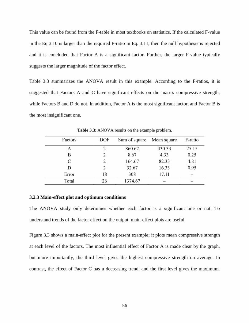
56

This value can be found from the F-table in most textbooks on statistics. If the calculated F-value

in the Eq 3.10 is larger than the required F-ratio in Eq. 3.11, then the null hypothesis is rejected

and it is concluded that Factor A is a significant factor. Further, the larger F-value typically

suggests the larger magnitude of the factor effect.

Table 3.3 summarizes the ANOVA result in this example. According to the F-ratios, it is

suggested that Factors A and C have significant effects on the matrix compressive strength,

while Factors B and D do not. In addition, Factor A is the most significant factor, and Factor B is

the most insignificant one.

Table 3.3: ANOVA results on the example problem.

Factors DOF Sum of square Mean square F-ratio

A 2 860.67 430.33 25.15

B 2 8.67 4.33 0.25

C 2 164.67 82.33 4.81

D 2 32.67 16.33 0.95

Error 18 308 17.11 –

Total 26 1374.67 – –

3.2.3 Main-effect plot and optimum conditions

The ANOVA study only determines whether each factor is a significant one or not. To

understand trends of the factor effect on the output, main-effect plots are useful.

Figure 3.3 shows a main-effect plot for the present example; it plots mean compressive strength

at each level of the factors. The most influential effect of Factor A is made clear by the graph,

but more importantly, the third level gives the highest compressive strength on average. In

contrast, the effect of Factor C has a decreasing trend, and the first level gives the maximum.

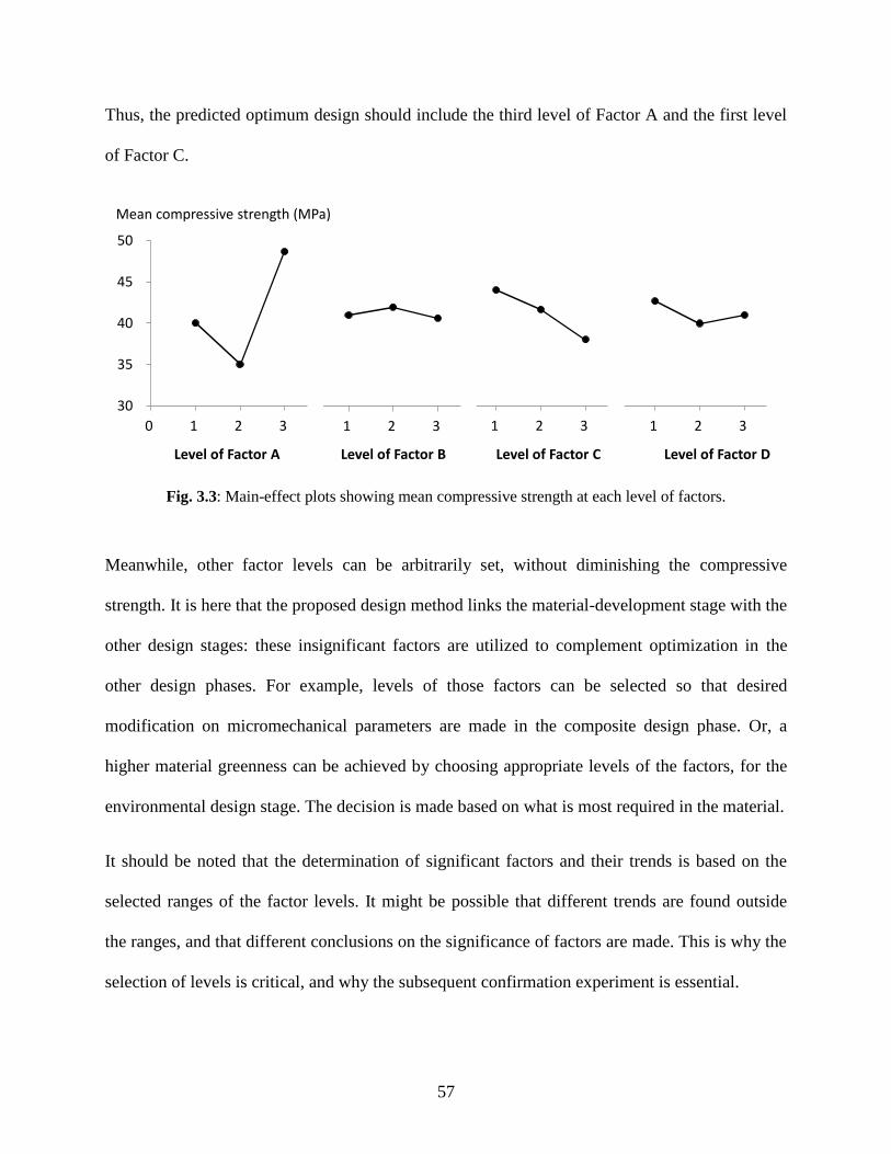
57

Thus, the predicted optimum design should include the third level of Factor A and the first level

of Factor C.

Fig. 3.3: Main-effect plots showing mean compressive strength at each level of factors.

Meanwhile, other factor levels can be arbitrarily set, without diminishing the compressive

strength. It is here that the proposed design method links the material-development stage with the

other design stages: these insignificant factors are utilized to complement optimization in the

other design phases. For example, levels of those factors can be selected so that desired

modification on micromechanical parameters are made in the composite design phase. Or, a

higher material greenness can be achieved by choosing appropriate levels of the factors, for the

environmental design stage. The decision is made based on what is most required in the material.

It should be noted that the determination of significant factors and their trends is based on the

selected ranges of the factor levels. It might be possible that different trends are found outside

the ranges, and that different conclusions on the significance of factors are made. This is why the

selection of levels is critical, and why the subsequent confirmation experiment is essential.

30

35

40

45

50

0 1 2 3

30

35

40

45

50

0 1 2 3

30

35

40

45

50

0 1 2 3

30

35

40

45

50

0 1 2 3

Mean compressive strength (MPa)

Level of Factor A Level of Factor B Level of Factor C Level of Factor D

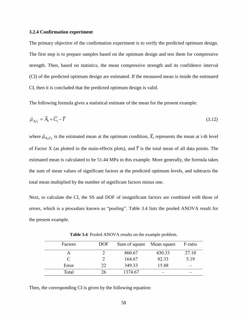
58

3.2.4 Confirmation experiment

The primary objective of the confirmation experiment is to verify the predicted optimum design.

The first step is to prepare samples based on the optimum design and test them for compressive

strength. Then, based on statistics, the mean compressive strength and its confidence interval

(CI) of the predicted optimum design are estimated. If the measured mean is inside the estimated

CI, then it is concluded that the predicted optimum design is valid.

The following formula gives a statistical estimate of the mean for the present example:

TCACA 1313̂ (3.12)

where �̂�𝐴3𝐶1 is the estimated mean at the optimum condition, �̅�𝑖 represents the mean at i-th level

of Factor X (as plotted in the main-effects plots), and �̅� is the total mean of all data points. The

estimated mean is calculated to be 51.44 MPa in this example. More generally, the formula takes

the sum of mean values of significant factors at the predicted optimum levels, and subtracts the

total mean multiplied by the number of significant factors minus one.

Next, to calculate the CI, the SS and DOF of insignificant factors are combined with those of

errors, which is a procedure known as “pooling”. Table 3.4 lists the pooled ANOVA result for

the present example.

Table 3.4: Pooled ANOVA results on the example problem.


A 2 860.67 430.33 27.10

C 2 164.67 82.33 5.19

Error 22 349.33 15.88 –

Total 26 1374.67 – –

Then, the corresponding CI is given by the following equation:

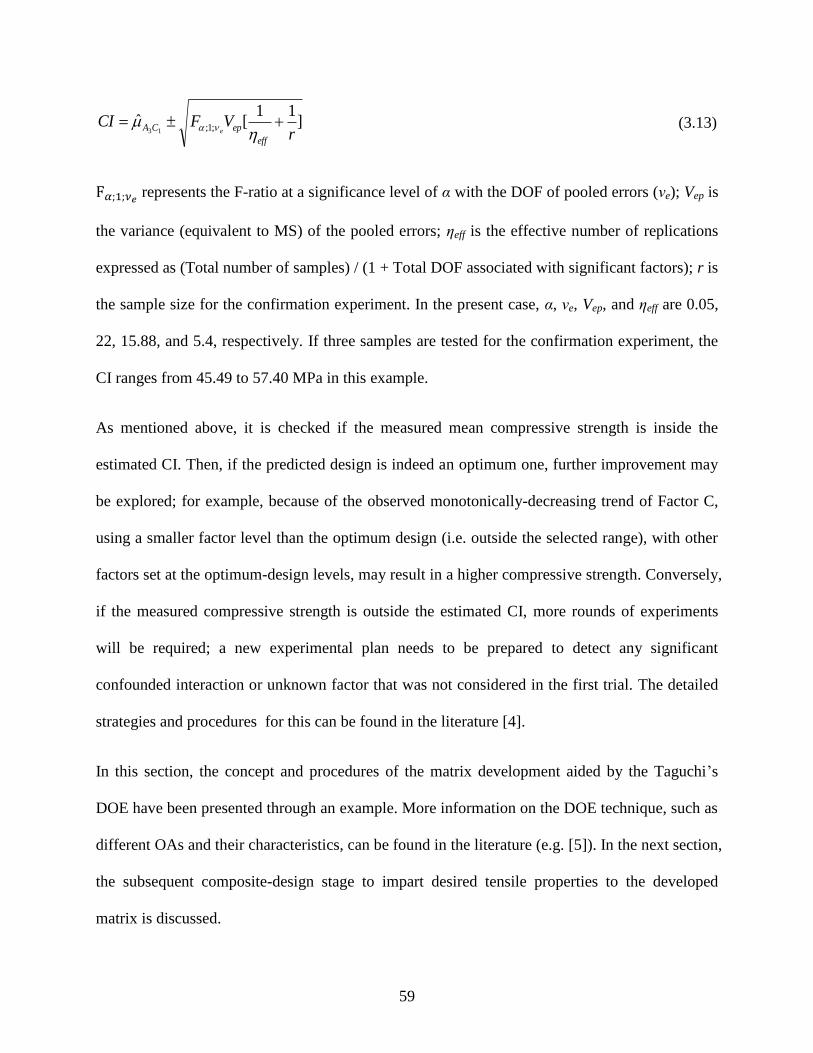
59

]11

[ˆ;1;13 r

VFCIeff

epCA e

(3.13)

F𝛼;1;𝜈𝑒 represents the F-ratio at a significance level of α with the DOF of pooled errors (νe); Vep is

the variance (equivalent to MS) of the pooled errors; ηeff is the effective number of replications

expressed as (Total number of samples) / (1 + Total DOF associated with significant factors); r is

the sample size for the confirmation experiment. In the present case, α, νe, Vep, and ηeff are 0.05,

22, 15.88, and 5.4, respectively. If three samples are tested for the confirmation experiment, the

CI ranges from 45.49 to 57.40 MPa in this example.

As mentioned above, it is checked if the measured mean compressive strength is inside the

estimated CI. Then, if the predicted design is indeed an optimum one, further improvement may

be explored; for example, because of the observed monotonically-decreasing trend of Factor C,

using a smaller factor level than the optimum design (i.e. outside the selected range), with other

factors set at the optimum-design levels, may result in a higher compressive strength. Conversely,

if the measured compressive strength is outside the estimated CI, more rounds of experiments

will be required; a new experimental plan needs to be prepared to detect any significant

confounded interaction or unknown factor that was not considered in the first trial. The detailed

strategies and procedures for this can be found in the literature [4].

In this section, the concept and procedures of the matrix development aided by the Taguchi’s

DOE have been presented through an example. More information on the DOE technique, such as

different OAs and their characteristics, can be found in the literature (e.g. [5]). In the next section,

the subsequent composite-design stage to impart desired tensile properties to the developed

matrix is discussed.

60

3.3 Composite Design

3.3.1 Experimental characterization

The first step of the composite-design stage is to select the type of reinforcing fiber. Apart from

the economical aspect, the selection may be confined by the environmental-design aspect:

energy- or carbon-intensive fibers may be pre-screened out for achieving higher material

greenness. This is another type of integration in the proposed design method that links different

design stages.

Then, the next step is to characterize micromechanical parameters of the developed matrix,

selected fiber and their interface, which govern composite tensile properties. As has been

discussed in Section 2.2.2, there are two required conditions for the steady-state multiple

cracking characteristic:

j

j

i

ci 0min (3.14)

')(0

0

00

i

b

iiiiii

tip JdJ

i

(3.15)

The variables in the left hand side of Eqs 3.14 and 3.15 represent the crack-initiation stress (σci)

and crack-tip toughness (Jtip) for a plane of the composite. These two can be determined by

experiment, which is first discussed in this section.

(i) Crack-initiation stress

For the crack-initiation stress σci, a typical measurement method is uniaxial tension testing on

composite specimens. Specifically, a dog bone test recommended by the Japan Society of Civil

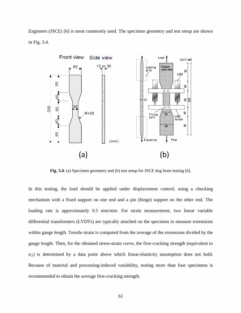
61

Engineers (JSCE) [6] is most commonly used. The specimen geometry and test setup are shown

in Fig. 3.4.

Fig. 3.4: (a) Specimen geometry and (b) test setup for JSCE dog bone testing [6].

In this testing, the load should be applied under displacement control, using a chucking

mechanism with a fixed support on one end and a pin (hinge) support on the other end. The

loading rate is approximately 0.5 mm/min. For strain measurement, two linear variable

differential transformers (LVDTs) are typically attached on the specimen to measure extensions

within gauge length. Tensile strain is computed from the average of the extensions divided by the

gauge length. Then, for the obtained stress-strain curve, the first-cracking strength (equivalent to

σci) is determined by a data point above which linear-elasticity assumption does not hold.

Because of material and processing-induced variability, testing more than four specimens is

recommended to obtain the average first-cracking strength.

(a) (b)

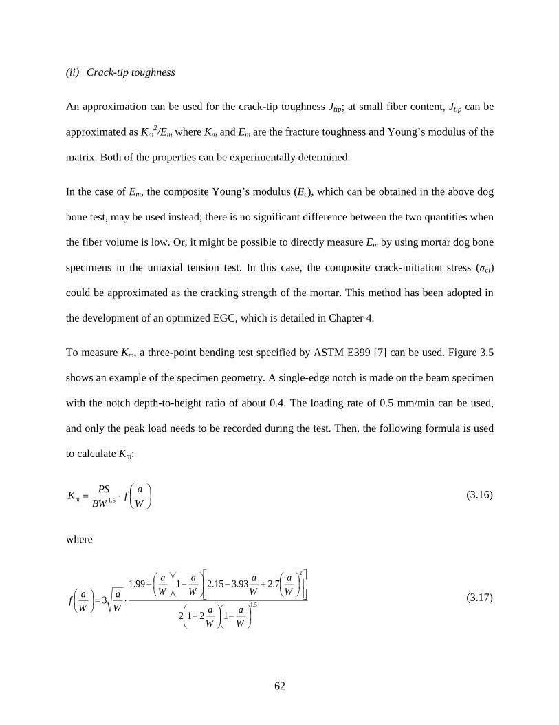
62

(ii) Crack-tip toughness

An approximation can be used for the crack-tip toughness Jtip; at small fiber content, Jtip can be

approximated as Km2/Em where Km and Em are the fracture toughness and Young’s modulus of the

matrix. Both of the properties can be experimentally determined.

In the case of Em, the composite Young’s modulus (Ec), which can be obtained in the above dog

bone test, may be used instead; there is no significant difference between the two quantities when

the fiber volume is low. Or, it might be possible to directly measure Em by using mortar dog bone

specimens in the uniaxial tension test. In this case, the composite crack-initiation stress (σci)

could be approximated as the cracking strength of the mortar. This method has been adopted in

the development of an optimized EGC, which is detailed in Chapter 4.

To measure Km, a three-point bending test specified by ASTM E399 [7] can be used. Figure 3.5

shows an example of the specimen geometry. A single-edge notch is made on the beam specimen

with the notch depth-to-height ratio of about 0.4. The loading rate of 0.5 mm/min can be used,

and only the peak load needs to be recorded during the test. Then, the following formula is used

to calculate Km:

W

af

BW

PSKm 5.1

(3.16)

where

5.1

2

1212

7.293.315.2199.1

3

W

a

W

a

W

a

W

a

W

a

W

a

W

a

W

af (3.17)

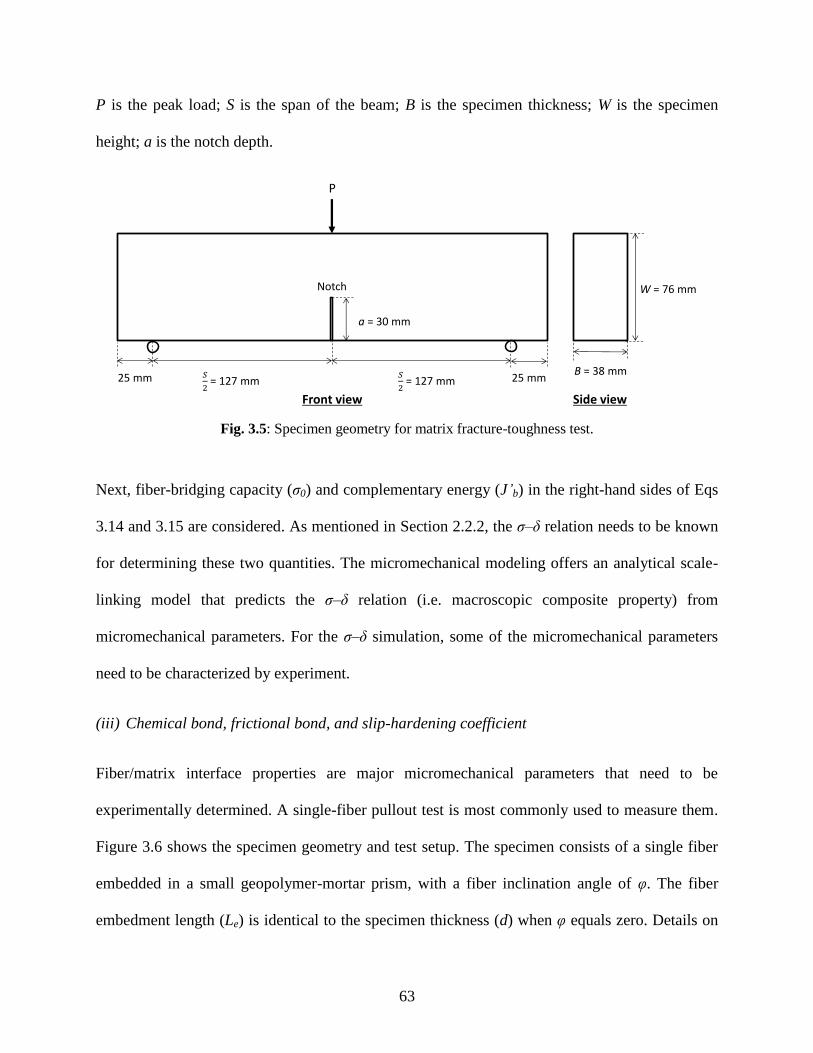
63

P is the peak load; S is the span of the beam; B is the specimen thickness; W is the specimen

height; a is the notch depth.

Fig. 3.5: Specimen geometry for matrix fracture-toughness test.

Next, fiber-bridging capacity (σ0) and complementary energy (J’b) in the right-hand sides of Eqs

3.14 and 3.15 are considered. As mentioned in Section 2.2.2, the σ–δ relation needs to be known

for determining these two quantities. The micromechanical modeling offers an analytical scale-

linking model that predicts the σ–δ relation (i.e. macroscopic composite property) from

micromechanical parameters. For the σ–δ simulation, some of the micromechanical parameters

need to be characterized by experiment.

(iii) Chemical bond, frictional bond, and slip-hardening coefficient

Fiber/matrix interface properties are major micromechanical parameters that need to be

experimentally determined. A single-fiber pullout test is most commonly used to measure them.

Figure 3.6 shows the specimen geometry and test setup. The specimen consists of a single fiber

embedded in a small geopolymer-mortar prism, with a fiber inclination angle of φ. The fiber

embedment length (Le) is identical to the specimen thickness (d) when φ equals zero. Details on

25 mm

W = 76 mm

B = 38 mm

Side view

= 127 mm = 127 mm 25 mm

Front view

Notch

a = 30 mm

P

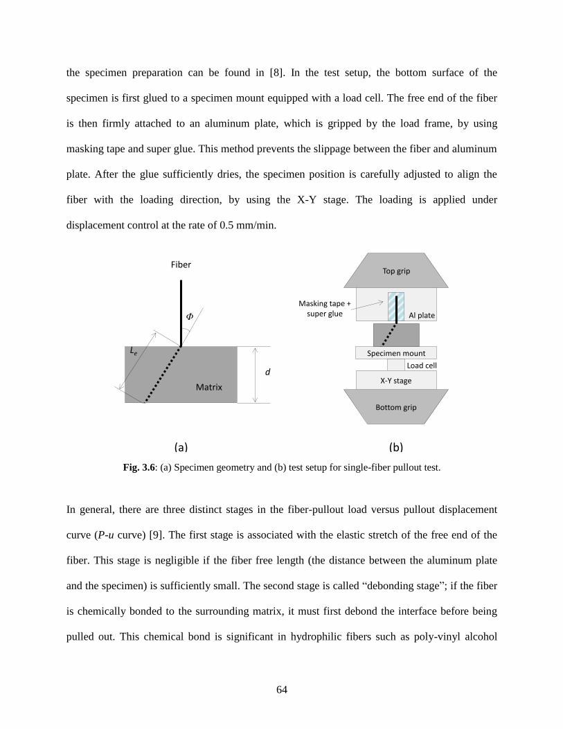
64

the specimen preparation can be found in [8]. In the test setup, the bottom surface of the

specimen is first glued to a specimen mount equipped with a load cell. The free end of the fiber

is then firmly attached to an aluminum plate, which is gripped by the load frame, by using

masking tape and super glue. This method prevents the slippage between the fiber and aluminum

plate. After the glue sufficiently dries, the specimen position is carefully adjusted to align the

fiber with the loading direction, by using the X-Y stage. The loading is applied under

displacement control at the rate of 0.5 mm/min.

Fig. 3.6: (a) Specimen geometry and (b) test setup for single-fiber pullout test.

In general, there are three distinct stages in the fiber-pullout load versus pullout displacement

curve (P-u curve) [9]. The first stage is associated with the elastic stretch of the free end of the

fiber. This stage is negligible if the fiber free length (the distance between the aluminum plate

and the specimen) is sufficiently small. The second stage is called “debonding stage”; if the fiber

is chemically bonded to the surrounding matrix, it must first debond the interface before being

pulled out. This chemical bond is significant in hydrophilic fibers such as poly-vinyl alcohol

Fiber

Matrix

Φ

Le

d

Al plate

Masking tape + super glue

Specimen mount

Top grip

Load cell

X-Y stage

Bottom grip

(a) (b)

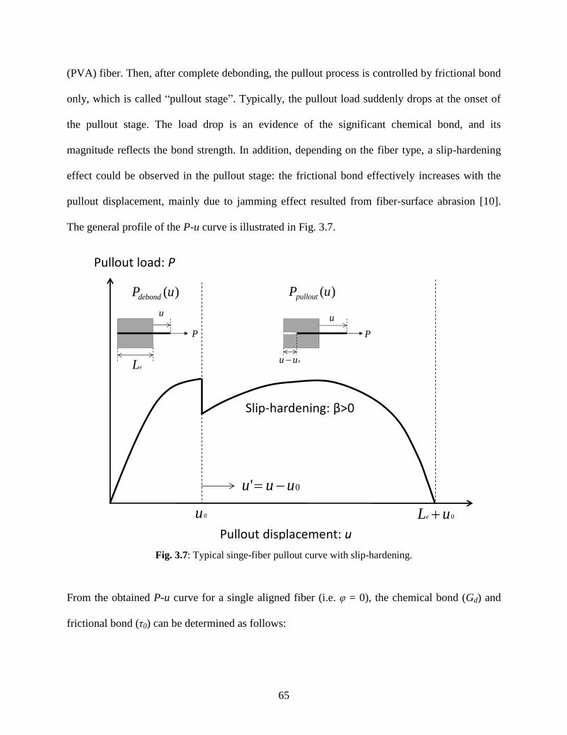
65

(PVA) fiber. Then, after complete debonding, the pullout process is controlled by frictional bond

only, which is called “pullout stage”. Typically, the pullout load suddenly drops at the onset of

the pullout stage. The load drop is an evidence of the significant chemical bond, and its

magnitude reflects the bond strength. In addition, depending on the fiber type, a slip-hardening

effect could be observed in the pullout stage: the frictional bond effectively increases with the

pullout displacement, mainly due to jamming effect resulted from fiber-surface abrasion [10].

The general profile of the P-u curve is illustrated in Fig. 3.7.

Fig. 3.7: Typical singe-fiber pullout curve with slip-hardening.

From the obtained P-u curve for a single aligned fiber (i.e. φ = 0), the chemical bond (Gd) and

frictional bond (τ0) can be determined as follows:

)(uPdebond)(uPpullout

0u

Pullout load: P

Pullout displacement: u

u

0uu

P

0uLe

Slip-hardening: β>0

u

eL

P

0' uuu

66

2

0032)()(

2uPuP

dEG pulloutdebond

ff

d

(3.18)

ef

pullout

Ld

uP

)( 0

0 (3.19)

Ef and df are the Young’s modulus and diameter of the fiber; Pdebond(u0) and Ppullout(u0) are the

pullout loads in the debonding and pullout stages, for the threshold pullout displacement (u0) at

which the full-debonding is completed and the load drop takes place. In addition, the least-square

estimation (LSE) can be used for determining the slip-hardening coefficient β; define u’ = u – u0

where u > u0 (i.e. the post-peak pullout displacement) and Pex(ui’) as the measured pullout load

at the i-th data of the post-peak pullout displacement. Then, the least square estimation of β is

obtained by:

i

iei

i

ieif

i

ieiiex

uLu

uLuduLu

uP

2''

2''

0

''' )(

ˆ (3.20)

Detailed derivations for Gd, τ0, and β can be found in Appendix B.

(iv) Snubbing coefficient and fiber-strength reduction factor

It should be noted that the formulae above are those for aligned fibers. When the inclination

angle φ is nonzero, two more parameters need to be considered: snubbing coefficient (f) and

fiber-strength reduction factor (f’).

Morton and Glove [11] and Li et al. [12] studied the fiber-inclination effect on the pullout load.

They suggested an empirical equation to express the increased fiber-bridging force P due to

inclination angle φ:

67

feuPguPuP )0,()()0,(),( (3.21)

where P(u,0) is either Pdebond(u) or Ppullout(u), depending on the pullout displacement u. To

experimentally determine f, the peak pullout load in the single-fiber pullout test is typically

compared between aligned and inclined fibers:

)0(

)(ln

1

peak

peak

P

Pf

(3.22)

In addition to the increased pullout load, Kanda and Li found the decreased in-situ strength for

both aligned and inclined fibers [13]. First, when an aligned fiber is embedded in a mortar matrix,

its strength is typically less than the nominal strength reported by the manufacturer. It is

suggested that the reduction is attributed to fiber-surface abrasion that occurs in the debonded

zone of the fiber. Further, another significant reduction is observed for inclined fibers. Based on

experimental results for PVA fiber, Kanda and Li suggested an exponential function to express

the strength-reduction effect of inclined fibers:

f

ff e )0()( (3.23)

where σf(0) and σf(φ) are the in-situ strength of aligned and inclined fibers. Then, the strength-

reduction factor f’ is determined by:

)0(

)(ln

1

f

ff

(3.24)

It is suggested that both f and f’ depend mainly on the fiber type. The snubbing coefficient f

ranges from 0.2 to 0.8 [14], and the strength-reduction factor f’ is about 0.3, for PVA fiber [9].

68

3.3.2 Analytical model

After characterizing micromechanical parameters, the composite tensile behavior is predicted by

using the analytical scale-linking model. Here, the fiber-bridging constitutive law presented by

Yang et al. [15] is used, with a slight modification to the model.

As presented in Section 2.2.2, the constitutive law is expressed as:

cos)2/(

0

21 )()()(),()(1

0

fL

z

e

f

fdzdzppgLP

A

V (3.25)

There are four functions in the double integral: P(δ, Le), g(φ), p1(φ), and p2(z). The third function

g(φ) is identical to that in Eq. 3.21. The other three functions are presented below. In addition,

two additional mechanisms that modify the σ–δ relation – matrix micro-spalling and Cook-

Gordon effect – are introduced.

(i) P(δ, Le)

P(δ, Le) represents the bridging force of a single aligned fiber for a crack opening δ. The

embedment length Le may be that for the short-embedment side, and the other side has the

embedment length of Lf – Le. It should be noted that pullout displacements for both ends of the

embedded fiber contribute to the crack opening:

SL uu (3.26)

where uL and uS are the pullout displacements for the long- and short-embedment sides. The

solution of P(δ, Le) can be obtained from Eq. 3.26 and the equilibrium of pullout loads for the

long- and short-embedment segments, which are given by either Pdebond(u) or Ppullout(u). Here,

Pdebond(u) or Ppullout(u) can be modeled by the following equations [9]:

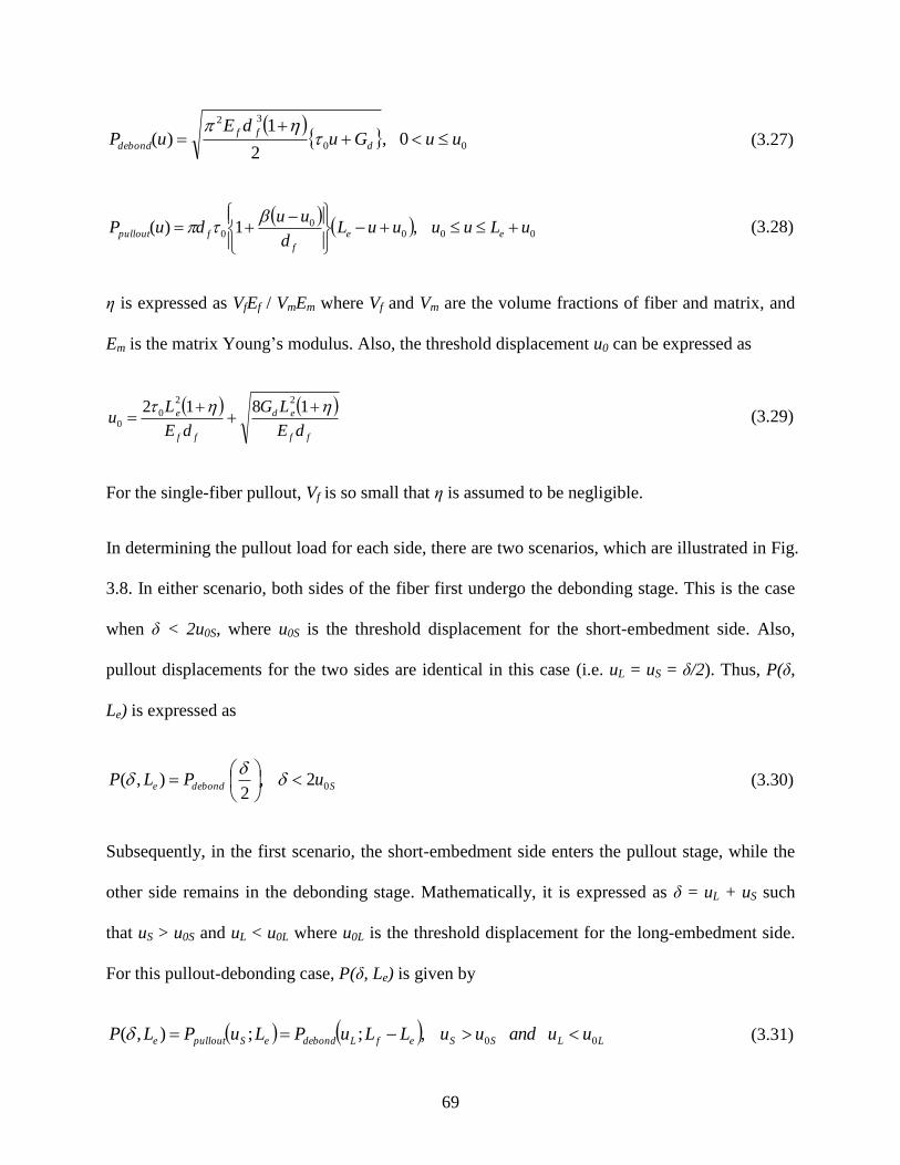
69

00

32

0,2

1)( uuGu

dEuP d

ff

debond

(3.27)

000

00 ,1)( uLuuuuL

d

uuduP ee

f

fpullout

(3.28)

η is expressed as VfEf / VmEm where Vf and Vm are the volume fractions of fiber and matrix, and

Em is the matrix Young’s modulus. Also, the threshold displacement u0 can be expressed as

ff

ed

ff

e

dE

LG

dE

Lu

181222

00

(3.29)

For the single-fiber pullout, Vf is so small that η is assumed to be negligible.

In determining the pullout load for each side, there are two scenarios, which are illustrated in Fig.

3.8. In either scenario, both sides of the fiber first undergo the debonding stage. This is the case

when δ < 2u0S, where u0S is the threshold displacement for the short-embedment side. Also,

pullout displacements for the two sides are identical in this case (i.e. uL = uS = δ/2). Thus, P(δ,

Le) is expressed as

Sdebonde uPLP 02,2

),(

(3.30)

Subsequently, in the first scenario, the short-embedment side enters the pullout stage, while the

other side remains in the debonding stage. Mathematically, it is expressed as δ = uL + uS such

that uS > u0S and uL < u0L where u0L is the threshold displacement for the long-embedment side.

For this pullout-debonding case, P(δ, Le) is given by

LLSSefLdebondeSpulloute uuanduuLLuPLuPLP 00,;;),( (3.31)

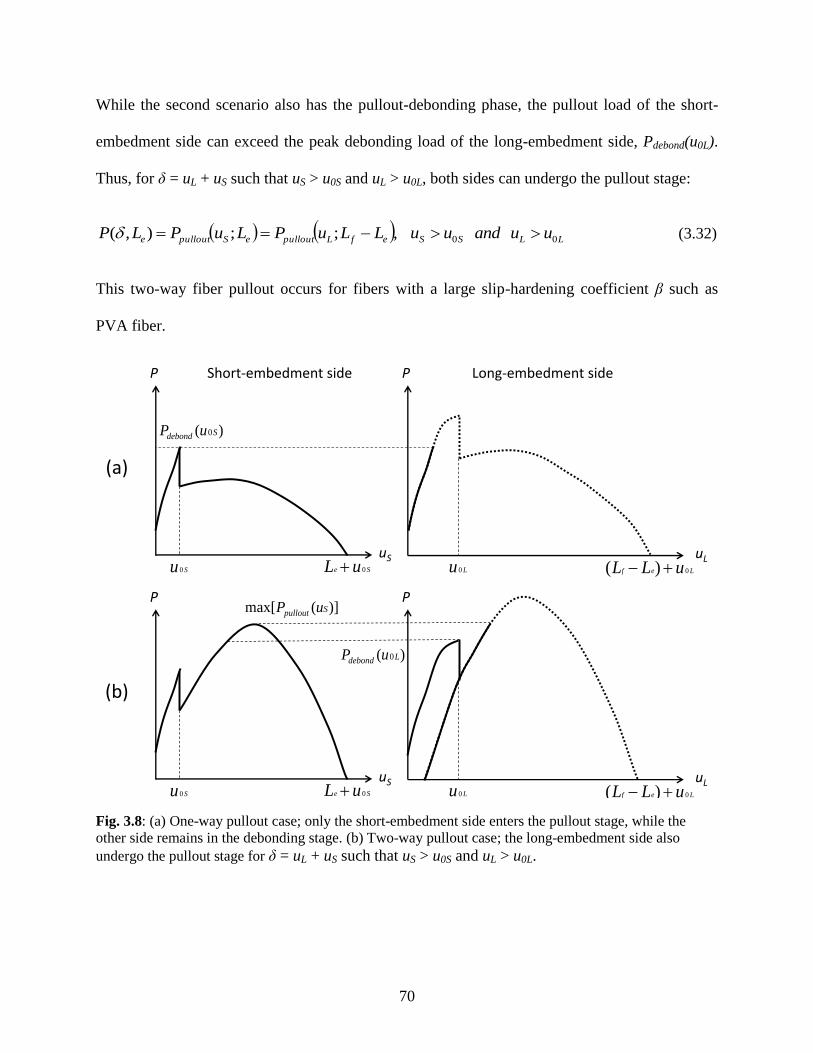
70

While the second scenario also has the pullout-debonding phase, the pullout load of the short-

embedment side can exceed the peak debonding load of the long-embedment side, Pdebond(u0L).

Thus, for δ = uL + uS such that uS > u0S and uL > u0L, both sides can undergo the pullout stage:

LLSSefLpullouteSpulloute uuanduuLLuPLuPLP 00,;;),( (3.32)

This two-way fiber pullout occurs for fibers with a large slip-hardening coefficient β such as

PVA fiber.

Fig. 3.8: (a) One-way pullout case; only the short-embedment side enters the pullout stage, while the

other side remains in the debonding stage. (b) Two-way pullout case; the long-embedment side also

undergo the pullout stage for δ = uL + uS such that uS > u0S and uL > u0L.

)( 0Sdebond uP

Su 0

P

uSSe uL 0 Lu 0

P

uLLef uLL 0)(

(a)

)( 0Ldebond uP

Su 0

P

uSSe uL 0 Lu 0

P

uLLef uLL 0)(

(b)

)](max[ Spullout uP

Long-embedment sideShort-embedment side

71

Here, a slight refinement to the above model is introduced, regarding the pullout–debonding case

(i.e. Eq. 3.31). As detailed in Appendix B, Pdebond(u) is derived by assuming the tunnel-crack

propagation along the fiber/matrix interface, which initiates from the fiber free end. Based on

this assumption, the long-embedment segment should have some debonded zone at the onset of

the pullout-debonding phase. Then, unless further tunnel-crack propagation in the long-

embedment side occurs in this phase, the P-u relationship should be modified for taking into

account the debonded zone. However, the existing model assumes no hysteresis for the P-u

relationship of the debonding side.

In this study, the following hysteresis curve is used for the debonding load in the pullout-

debonding phase:

LL

f

L

ff

L

h

debond uuad

ua

dEuP

0,

2

)1(

4)(

0

2 (3.33)

a’ is the length of the debonded zone and can be obtained by solving the following quadratic

equation:

04

)(

2

)1( 2

20

Lf

f

Ldebond

f

f uda

E

uPa

E

d (3.34)

where u’L is the maximum pullout displacement of the debonding side in the preceding loading

history. It should be noted that, during further tunnel-crack propagation (i.e. uL > u’L), the

debonding load is given by Eq. 3.27, as in the original model.

Figure 3.9 shows the proposed hysteresis in the P-u relationship. Parameters used for the plot are

those for a standard ECC (M45) [15], and a’ has been supposed to be the same as the short-

embedment length Ls, which is 4 mm here. As can be seen, the difference between Pdebond and

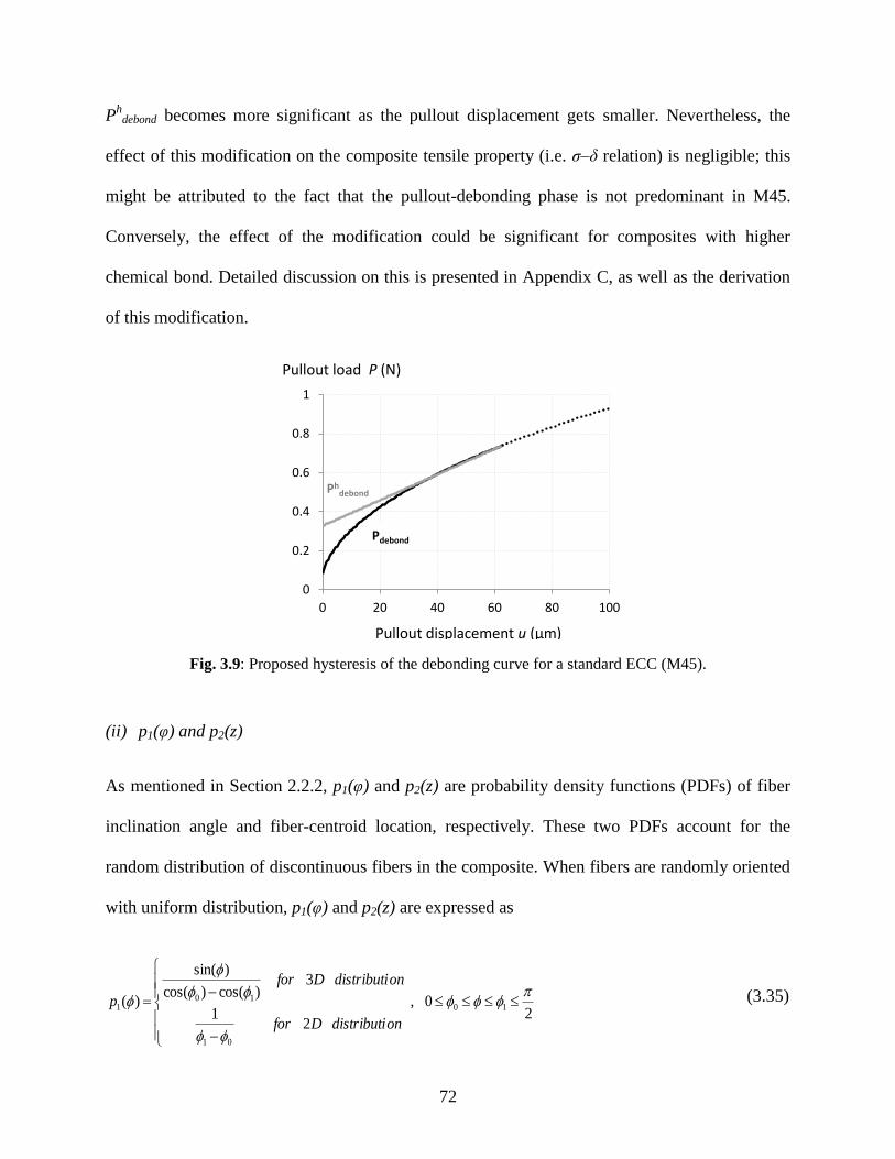
72

Ph

debond becomes more significant as the pullout displacement gets smaller. Nevertheless, the

effect of this modification on the composite tensile property (i.e. σ–δ relation) is negligible; this

might be attributed to the fact that the pullout-debonding phase is not predominant in M45.

Conversely, the effect of the modification could be significant for composites with higher

chemical bond. Detailed discussion on this is presented in Appendix C, as well as the derivation

of this modification.

Fig. 3.9: Proposed hysteresis of the debonding curve for a standard ECC (M45).

(ii) p1(φ) and p2(z)

As mentioned in Section 2.2.2, p1(φ) and p2(z) are probability density functions (PDFs) of fiber

inclination angle and fiber-centroid location, respectively. These two PDFs account for the

random distribution of discontinuous fibers in the composite. When fibers are randomly oriented

with uniform distribution, p1(φ) and p2(z) are expressed as

20,

21

3)cos()cos(

)sin(

)( 10

01

101

ondistributiDfor

ondistributiDfor

p (3.35)

0

0.2

0.4

0.6

0.8

1

0 20 40 60 80 100

Pdebond

Pullout load P (N)

Pullout displacement u (μm)

Phdebond

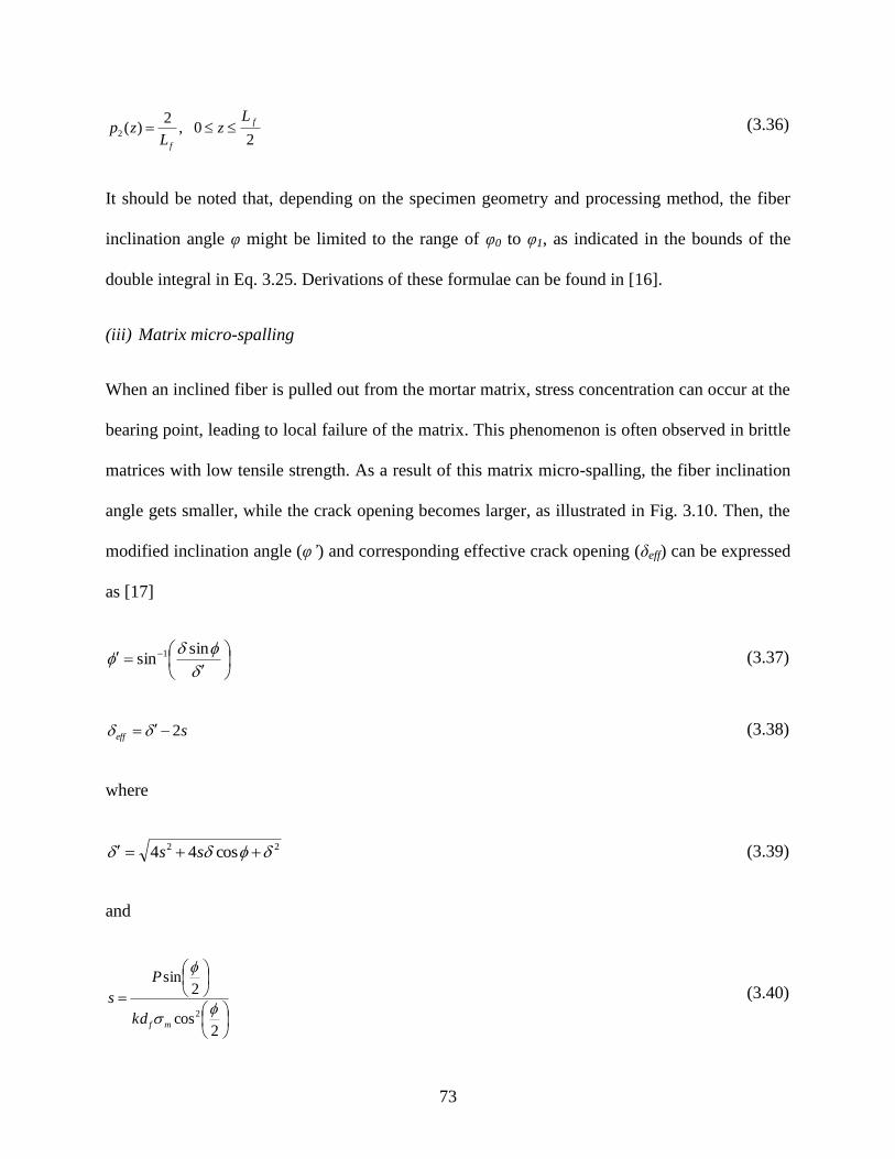
73

20,

2)(2

f

f

Lz

Lzp (3.36)

It should be noted that, depending on the specimen geometry and processing method, the fiber

inclination angle φ might be limited to the range of φ0 to φ1, as indicated in the bounds of the

double integral in Eq. 3.25. Derivations of these formulae can be found in [16].

(iii) Matrix micro-spalling

When an inclined fiber is pulled out from the mortar matrix, stress concentration can occur at the

bearing point, leading to local failure of the matrix. This phenomenon is often observed in brittle

matrices with low tensile strength. As a result of this matrix micro-spalling, the fiber inclination

angle gets smaller, while the crack opening becomes larger, as illustrated in Fig. 3.10. Then, the

modified inclination angle (φ’) and corresponding effective crack opening (δeff) can be expressed

as [17]

sinsin 1 (3.37)

seff 2 (3.38)

where

22 cos44 ss (3.39)

and

2cos

2sin

2

mfkd

P

s (3.40)

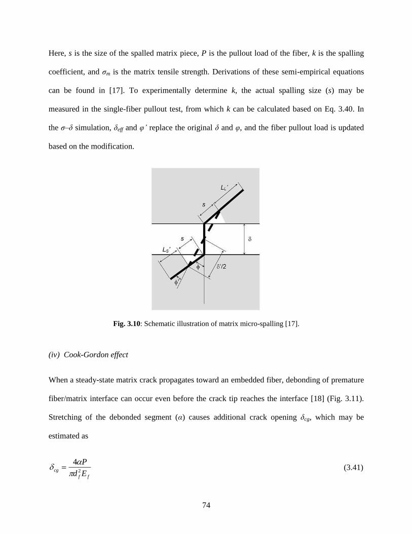
74

Here, s is the size of the spalled matrix piece, P is the pullout load of the fiber, k is the spalling

coefficient, and σm is the matrix tensile strength. Derivations of these semi-empirical equations

can be found in [17]. To experimentally determine k, the actual spalling size (s) may be

measured in the single-fiber pullout test, from which k can be calculated based on Eq. 3.40. In

the σ–δ simulation, δeff and φ’ replace the original δ and φ, and the fiber pullout load is updated

based on the modification.

Fig. 3.10: Schematic illustration of matrix micro-spalling [17].

(iv) Cook-Gordon effect

When a steady-state matrix crack propagates toward an embedded fiber, debonding of premature

fiber/matrix interface can occur even before the crack tip reaches the interface [18] (Fig. 3.11).

Stretching of the debonded segment (α) causes additional crack opening δcg, which may be

estimated as

ff

cgEd

P2

4

(3.41)

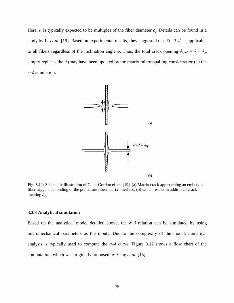
75

Here, α is typically expected to be multiples of the fiber diameter df. Details can be found in a

study by Li et al. [19]. Based on experimental results, they suggested that Eq. 3.41 is applicable

to all fibers regardless of the inclination angle φ. Thus, the total crack opening δtotal = δ + δcg

simply replaces the δ (may have been updated by the matrix micro-spalling consideration) in the

σ–δ simulation.

Fig. 3.11: Schematic illustration of Cook-Gordon effect [19]. (a) Matrix crack approaching an embedded

fiber triggers debonding of the premature fiber/matrix interface, (b) which results in additional crack

opening δcg.

3.3.3 Analytical simulation

Based on the analytical model detailed above, the σ–δ relation can be simulated by using

micromechanical parameters as the inputs. Due to the complexity of the model, numerical

analysis is typically used to compute the σ–δ curve. Figure 3.12 shows a flow chart of the

computation, which was originally proposed by Yang et al. [15].

76

Fig. 3.12: Flow chart of numerical simulation of σ–δ curve.

The computation starts with inputting micromechanical parameters and the range of crack

opening (δ), for which the composite fiber-bridging stress (σ) is computed. The maximum δ may

be half of the fiber length (Lf).

The next step is to calculate σ for a given δ in loop calculation. The loop computes and averages

pullout loads of individual fibers, varying the fiber embedment length (Le) and fiber inclination

angle (φ). Thus, there are two loops inside the loop for δ: one for Le and the other for φ. For

efficient computation, each step in the loop starts with checking the fiber status; if a single fiber

with given Le and φ has been already pulled out or broken in the preceding step, its pullout force

is not calculated in the following steps. Otherwise, P(δ, Le)g(φ) is computed based on Eqs. 3.21

and 3.26–3.34, and corresponding fiber status is determined: the computed pullout displacement

(us) is compared with Le to check the fiber pullout, and P(δ, Le)g(φ) with the in-situ fiber strength

(Eq. 3.23) to check the fiber rupture. Here, if the matrix micro-spalling is taken into account,

then δ and φ are updated based on Eqs. 3.37–3.40, and P(δ, Le) and the fiber status are modified

accordingly.

Start Micromechanical

parameters Range of δ

Input Check fiber status Calculate P(δ, Le)g(φ) (Eqs. 3.21, 3.26–3.34). Update δ and φ (Eqs. 3.37–3.40), and

modify P(δ, Le)g(φ): Matrix micro-spalling Update fiber status

Loop for Le

Loop for φ

Loop for δ

Compute σ (Eqs. 3.35, 3.36). Update δ (Eq. 3.41): Cook-Gordon effect

σ(δ)

Output

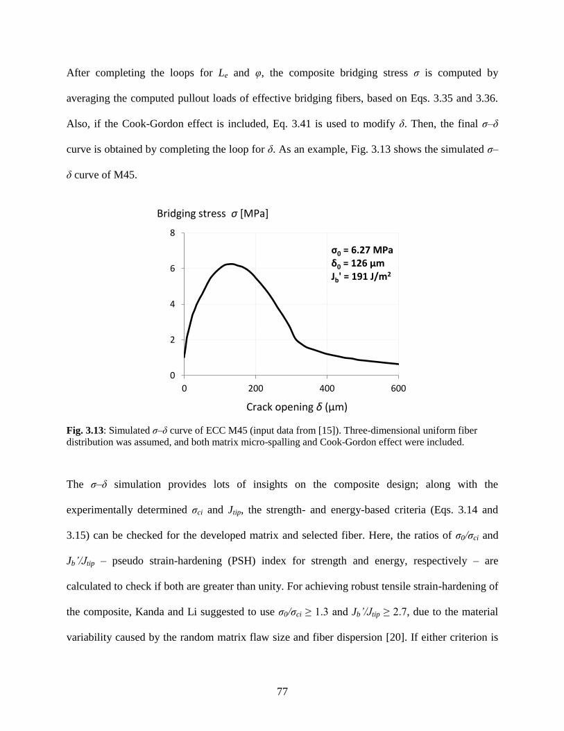
77

After completing the loops for Le and φ, the composite bridging stress σ is computed by

averaging the computed pullout loads of effective bridging fibers, based on Eqs. 3.35 and 3.36.

Also, if the Cook-Gordon effect is included, Eq. 3.41 is used to modify δ. Then, the final σ–δ

curve is obtained by completing the loop for δ. As an example, Fig. 3.13 shows the simulated σ–

δ curve of M45.

Fig. 3.13: Simulated σ–δ curve of ECC M45 (input data from [15]). Three-dimensional uniform fiber

distribution was assumed, and both matrix micro-spalling and Cook-Gordon effect were included.

The σ–δ simulation provides lots of insights on the composite design; along with the

experimentally determined σci and Jtip, the strength- and energy-based criteria (Eqs. 3.14 and

3.15) can be checked for the developed matrix and selected fiber. Here, the ratios of σ0/σci and

Jb’/Jtip – pseudo strain-hardening (PSH) index for strength and energy, respectively – are

calculated to check if both are greater than unity. For achieving robust tensile strain-hardening of

the composite, Kanda and Li suggested to use σ0/σci ≥ 1.3 and Jb’/Jtip ≥ 2.7, due to the material

variability caused by the random matrix flaw size and fiber dispersion [20]. If either criterion is

0

2

4

6

8

0 200 400 600

Bridging stress σ [MPa]

Crack opening δ (μm)

σ0 = 6.27 MPaδ0 = 126 µmJb' = 191 J/m2

78

violated, then the analytical simulation guides the required modification on micromechanical

parameters by manipulating the inputs in the computation. In addition, optimization of the

subsequent environmental design can be complemented; for example, the simulation can find the

minimum fiber volume fraction to satisfy the criteria, which is beneficial for the enhanced

environmental performance.

3.3.4 Confirmation experiment

To verify the optimum composite design predicted by the σ–δ simulation, confirmation

experiment is conducted. The simplest way is to conduct the JSCE dog bone testing (detailed in

Section 3.3.1) on composite specimens; the test checks if the desired composite tensile properties

– strain-hardening behavior, high tensile ductility, and multiple tight cracking – have been

achieved. Another way is to conduct the single-crack test proposed by Fischer and co-workers

[21–23] (Fig. 3.14). In this test, a notched uniaxial-tension specimen is loaded to deliberately

create a single crack in the notched section. The obtained stress-strain curve is a direct

measurement of the σ–δ relation. This method is useful to validate the σ–δ simulation and

identify required modification on the analysis or input data.

Fig. 3.14: Singe-crack test: (a) specimen geometry, (b) test setup, and (c) fracture plane after testing [23].

79

In this section, experimental and analytical methods used in the composite-design stage have

been detailed. With the aid of the micromechanics-based design technique, strain-hardening

ductile EGC can be systematically developed. Then, in the subsequent environmental design

stage, the material sustainability of the developed composite is evaluated.

3.4 Environmental assessment

The final stage of the proposed integrated design is the assessment of the material greenness. In

this study, Material Sustainability Indices (MSI) are used to quantify environmental impacts

associated with production of the developed composite. Here, as an example, the material

greenness of a preliminary version of EGC developed in a previous study is evaluated, with

respect to the energy and carbon intensity. The calculation of MSI values for ECC has been

detailed in [24].

The environmental impact categories to investigate are first specified. Here, embodied-energy

consumption and global warming intensity (GWI) are used. The embodied energy includes both

the process energy, which is electricity and fuel directly used in material production, and the

feedstock energy, which represents organic resource inputs that comprise the material, rather than

being used as a fuel. The feedstock energy is significant especially in plastics (i.e. organic

polymers) in which petroleum-based inputs are the primary constituent. For geopolymer

materials, GWI (i.e. carbon dioxide (CO2)-equivalent emission) is often used to show the

advantage of the materials compared to cement-based counterparts. Other impact categories –

acidification potential (AP), eutrophication potential (EP), water consumption, solid waste

generated, and so forth – may be crucial, depending on the application of the material.

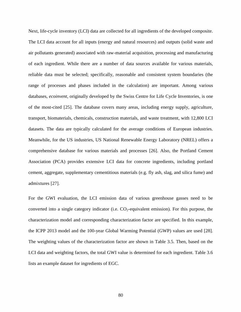
80

Next, life-cycle inventory (LCI) data are collected for all ingredients of the developed composite.

The LCI data account for all inputs (energy and natural resources) and outputs (solid waste and

air pollutants generated) associated with raw-material acquisition, processing and manufacturing

of each ingredient. While there are a number of data sources available for various materials,

reliable data must be selected; specifically, reasonable and consistent system boundaries (the

range of processes and phases included in the calculation) are important. Among various

databases, ecoinvent, originally developed by the Swiss Centre for Life Cycle Inventories, is one

of the most-cited [25]. The database covers many areas, including energy supply, agriculture,

transport, biomaterials, chemicals, construction materials, and waste treatment, with 12,800 LCI

datasets. The data are typically calculated for the average conditions of European industries.

Meanwhile, for the US industries, US National Renewable Energy Laboratory (NREL) offers a

comprehensive database for various materials and processes [26]. Also, the Portland Cement

Association (PCA) provides extensive LCI data for concrete ingredients, including portland

cement, aggregate, supplementary cementitious materials (e.g. fly ash, slag, and silica fume) and

admixtures [27].

For the GWI evaluation, the LCI emission data of various greenhouse gasses need to be

converted into a single category indicator (i.e. CO2-equivalent emission). For this purpose, the

characterization model and corresponding characterization factor are specified. In this example,

the ICPP 2013 model and the 100-year Global Warming Potential (GWP) values are used [28].

The weighting values of the characterization factor are shown in Table 3.5. Then, based on the

LCI data and weighting factors, the total GWI value is determined for each ingredient. Table 3.6

lists an example dataset for ingredients of EGC.

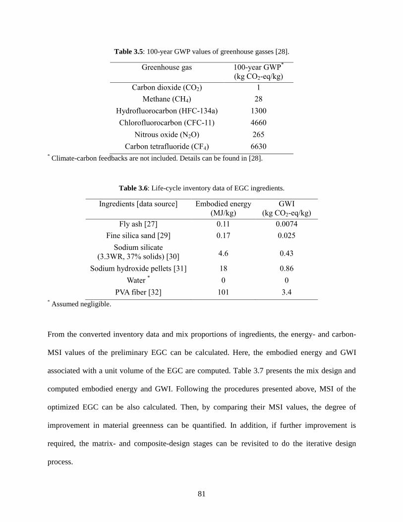
81

Table 3.5: 100-year GWP values of greenhouse gasses [28].

Greenhouse gas 100-year GWP*

(kg CO2-eq/kg)

Carbon dioxide (CO2) 1

Methane (CH4) 28

Hydrofluorocarbon (HFC-134a) 1300

Chlorofluorocarbon (CFC-11) 4660

Nitrous oxide (N2O) 265

Carbon tetrafluoride (CF4) 6630 * Climate-carbon feedbacks are not included. Details can be found in [28].

Table 3.6: Life-cycle inventory data of EGC ingredients.

Ingredients [data source] Embodied energy

(MJ/kg)

GWI

(kg CO2-eq/kg)

Fly ash [27] 0.11 0.0074

Fine silica sand [29] 0.17 0.025

Sodium silicate

(3.3WR, 37% solids) [30] 4.6 0.43

Sodium hydroxide pellets [31] 18 0.86

Water * 0 0

PVA fiber [32] 101 3.4 * Assumed negligible.

From the converted inventory data and mix proportions of ingredients, the energy- and carbon-

MSI values of the preliminary EGC can be calculated. Here, the embodied energy and GWI

associated with a unit volume of the EGC are computed. Table 3.7 presents the mix design and

computed embodied energy and GWI. Following the procedures presented above, MSI of the

optimized EGC can be also calculated. Then, by comparing their MSI values, the degree of

improvement in material greenness can be quantified. In addition, if further improvement is

required, the matrix- and composite-design stages can be revisited to do the iterative design

process.

82

Table 3.7: Mix design and computed energy- and carbon-MSI of preliminary EGC.

Ingredient Mix design

(kg/m3)

Embodied energy

(GJ/m3)

GWI

(kg CO2-eq/m3)

Fly ash 1131 0.12 8.4

Fine silica sand 340 0.06 8.5

Sodium silicate 289 1.34 125.2

Sodium hydroxide 63.5 1.15 54.6

Water 179 0 0

PVA fiber 26 2.63 88.4

Total 5.29 285

3.5 Summary

This chapter has documented the detailed procedures of the proposed integrated design method

for EGC. There are three stages in the EGC design: matrix development, composite design, and

environmental assessment.

The EGC design starts with the matrix-design stage. Here, Taguchi’s Design of Experiment

(DOE) technique is used to develop an optimum EGC matrix that meets required engineering

properties or has desired added functions. Specifically, orthogonal arrays (OA) aid the design of

efficient fractional-factorial experiments, and the Analysis of Variance (ANOVA) statistically

analyze the obtained experimental results to determine significance of design variables. Based on

the ANOVA result and complementary main-effect plots, an optimum EGC-matrix design can be

identified by choosing appropriate levels of the significant factors. Besides, factors that have

been determined to be insignificant can be used to complement optimization in other design

stages.

In the subsequent composite-design stage, the micromechanical modeling is used to

systematically tailor the fiber and fiber/matrix interface properties. First, micromechanical

83

parameters for the developed matrix, selected fiber and their interface are measured by various

experimental techniques. Then, the analytical model simulates the composite σ–δ relation by

using the measured micromechanical parameters as the inputs. The simulation result guides

required modification on the parameters to satisfy the two criteria for achieving the steady-state

multiple cracking characteristic. Also, by determining the minimum fiber volume content to

satisfy the criteria, the σ–δ simulation can complement optimization in the environmental design

stage.

For the optimized EGC, the overall material greenness is evaluated in the environmental design

stage. Here, Material Sustainability Indices (MSI) are used to quantify environmental impacts of

the material production. Particularly, embodied-energy consumption and global warming

potential are focused for EGC materials, but other impact categories may be of concern,

depending on the application. By comparing the MSI values of the optimized EGC with those of

other counterparts (preliminary EGC, normal concrete, ECC, etc.), the degree of improvement in

material greenness can be quantified. If further improvement is required, another round of

experiment/analysis can be conducted in the matrix- and composite-design stages to do the

iterative design process.

With the aid of the proposed integrated design method, EGC materials can be systematically

designed. Thus, this comprehensive design method can facilitate the research and development in

both the academic and industrial communities. To demonstrate the applicability and

effectiveness of the design method, an optimized EGC is developed in the following chapter.

84

References

[1] G. Taguchi, System of experimental design: engineering methods to optimise quality and

minimize cost. White Plains, New York: UNIPUB/Kraus International Publications, 1987.





[3] G. A. Keoleian, A. M. Kendall, M. D. Lepech, and V. C. Li, “Guiding the design and

application of new materials for enhancing sustainability performance: Framework and

infrastructure application,” Mater. Res. Soc. Symp. Proc., vol. 895, 2006.

[4] “Confirmation Experiment,” in Taguchi techniques for quality engineering:, 2nd ed., New

York, NY: McGraw Hill Professional, 1996, pp. 181–201.

[5] P. J. Ross, Taguchi techniques for quality engineering: loss function, orthogonal

experiments, parameter and tolerance design, Second. New York, NY: McGraw Hill

Professional, 1996.

[6] Japan Society of Civil Engineers, Recommendations for Design and Construction of High

Performance Fiber Reinforced Cement Composites with Multiple Fine Cracks

(HPFRCC ), vol. 82. Tokyo, Japan: JSCE, 2008.

[7] ASTM E399-12e3, Standard Test Method for Linear-Elastic Plane-Strain Fracture

Toughness K1C of Metallic Material. West Conshohocken, PA: ASTM International,

2012.

[8] A. Katz and V. Li, “A Special Technique for Detemining the Bond Strength of Carbon

Fibers in Cement Matrix by Pullout Test,” J. Mater. Sci. Lett., vol. 15, no. 20, pp. 1821–

1823, 1996.

[9] Z. Lin, T. Kanda, and V. Li, “On interface property characterization and performance of

fiber-reinforced cementitious,” Concr. Sci. Eng., vol. 1, no. September, pp. 173–174, 1999.

[10] Z. Lin and V. Li, “Crack bridging in fiber reinforced cementitious composites with slip-

hardening interfaces,” J. Mech. Phys. Solids, vol. 45, no. 5, pp. 763–787, 1997.



[12] V. C. Li, Y. Wang, and S. Backer, “Effect of inclining angle, bundling and surface

treatment on synthetic fibre pull-out from a cement matrix,” Composites, vol. 21, no. 2, pp.

132–140, 1990.

[13] T. Kanda and V. C. Li, “Interface Property and Apparent Strength of High-Strength

Hydrophilic Fiber in Cement Matrix,” Journal of Materials in Civil Engineering, vol. 10,

no. 1. pp. 5–13, 1998.

85

[14] C. Wu, “Micromechanical Tailoring of PVA-ECC for Structural Applications,” University

of Michigan, 2001.



2008.

[16] Y. Wang, S. Backer, and V. Li, “A statistical tensile model of fibre reinforced

cementitious composites,” Composites, vol. 20, no. 3, pp. 265–274, 1989.



[18] J. Cook, J. E. Gordon, C. C. Evans, and D. M. Marsh, “A mechanism for the control of

crack propagation in all-brittle systems,” Proc. R. Soc. London A Math. Phys. Eng. Sci.,

vol. 282, no. 1391, pp. 508–520, 1964.

[19] V. Li, H. Stang, and H. Krenchel, “Micromechanics of crack bridging in fibre-reinforced

concrete,” Mater. Struct., vol. 26, pp. 486–494, 1993.



[21] G. Fischer, H. Stang, and L. Dick-Nielsen, “Initiation and development of cracking in

ECC materials: Experimental Observations and modeling,” in 6th International

Conference on Fracture Mechanics of Concrete and Concrete Structures, 2007, pp. 1517–

1522.

[22] E. Pereira, G. Fischer, J. A. O. Barros, and M. Lepech, “Crack formation and tensile

stress-crack opening behavior of Fiber Reinforced Cementitious Composites (FRCC),” in

7th International Conference on Fracture Mechanics of Concrete and Concrete Structures

(FraMCoS 7), 2010, pp. 1638–1647.

[23] I. Paegle and G. Fischer, “Evaluation of test methods used to characterize fiber reinforced

cementitious composites,” Proc. Int. Conf. „Innovative Mater. Struct. Technol., pp. 122–

128, 2013.

[24] M. D. Lepech, V. C. Li, R. E. Robertson, and G. A. Keoleian, “Design of green

engineered cementitious composites for improved sustainability,” ACI Mater. J., vol. 105,

no. 6, pp. 567–575, 2008.

[25] The Swiss Centre for Life Cycle Inventories, “Ecoinvent.” [Online]. Available:

http://www.ecoinvent.org/home.html. [Accessed: 28-Jul-2017].

[26] NREL, “U.S. Life Cycle Inventory Database,” 2012. [Online]. Available:

https://www.lcacommons.gov/nrel/search. [Accessed: 28-Jul-2017].

[27] M. A. Nisbet, M. L. Marceau, and M. G. Vangeem, Environmental Life Cycle Inventory of

Portland Cement Concrete. Stokie, IL: Portland Cement Association, 2002.

86

[28] G. Myhre, D. Shindell, F. Bréon, W. Collins, J. Fuglestvedt, J. Huang, D. Koch, J.

Lamarque, D. Lee, B. Mendoza, T. Nakajima, A. Robock, G. Stephens, T. Takemura, and

H. Zhang, “Anthropogenic and natural radiative forcing,” in Climate Change 2013: The

Physical Science Basis, Working Group I Contribution to the Fifth Assessment Report of

the Intergovernmental Panel on Climate Change, T. F. Stocker, D. Qin, G.-K. Plattner, M.

Tignor, S. K. Allen, J. Boschung, A. Nauels, Y. Xia, V. Bex, and P. M. Midgley, Eds.

Cambridge (UK): Cambridge University Press, 2013, p. 714.

[29] R. Ranade, “Advanced Cementitious Composite Development for Resilient and

Sustainable Infrastructure,” University of Michigan, Ann Arbor, 2014.

[30] M. Fawer, M. Concannon, and W. Rieber, “Life cycle inventories for the production of

sodium silicates,” Int. J. Life Cycle Assess., vol. 4, no. 4, pp. 207–212, 1999.

[31] Euro Chlor, “An Eco-profile and Environmental Product Declaration of the European

Chlor-Alkali Industry,” 2013. [Online]. Available:

https://www1.ethz.ch/ifu/ESD/education/master/AESEA/Euro_Chlor_Eco-

profile_Chlorine_2014-03.pdf. [Accessed: 10-Mar-2017].

[32] R. Frazão and R. Fernandes, Comparative Analysis of the Life Cycle of AT Fibre-cement

and NT Fibre-cement. International Chrysotile Association, 2004.

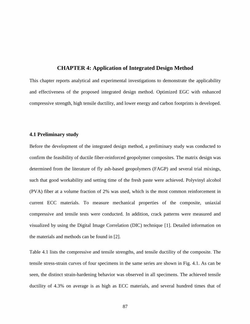
87

CHAPTER 4: Application of Integrated Design Method

This chapter reports analytical and experimental investigations to demonstrate the applicability

and effectiveness of the proposed integrated design method. Optimized EGC with enhanced

compressive strength, high tensile ductility, and lower energy and carbon footprints is developed.

4.1 Preliminary study

Before the development of the integrated design method, a preliminary study was conducted to

confirm the feasibility of ductile fiber-reinforced geopolymer composites. The matrix design was

determined from the literature of fly ash-based geopolymers (FAGP) and several trial mixings,

such that good workability and setting time of the fresh paste were achieved. Polyvinyl alcohol

(PVA) fiber at a volume fraction of 2% was used, which is the most common reinforcement in

current ECC materials. To measure mechanical properties of the composite, uniaxial

compressive and tensile tests were conducted. In addition, crack patterns were measured and

visualized by using the Digital Image Correlation (DIC) technique [1]. Detailed information on

the materials and methods can be found in [2].

Table 4.1 lists the compressive and tensile strengths, and tensile ductility of the composite. The

tensile stress-strain curves of four specimens in the same series are shown in Fig. 4.1. As can be

seen, the distinct strain-hardening behavior was observed in all specimens. The achieved tensile

ductility of 4.3% on average is as high as ECC materials, and several hundred times that of

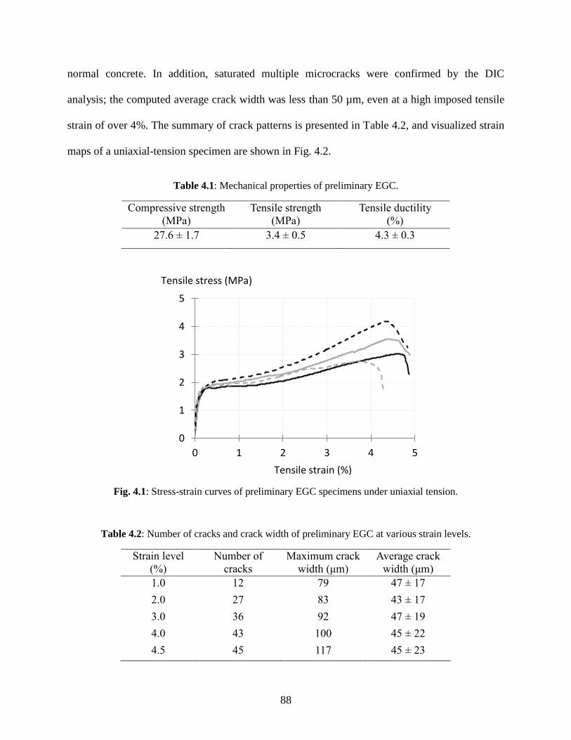
88

normal concrete. In addition, saturated multiple microcracks were confirmed by the DIC

analysis; the computed average crack width was less than 50 µm, even at a high imposed tensile

strain of over 4%. The summary of crack patterns is presented in Table 4.2, and visualized strain

maps of a uniaxial-tension specimen are shown in Fig. 4.2.

Table 4.1: Mechanical properties of preliminary EGC.

Compressive strength

(MPa)

Tensile strength

(MPa)

Tensile ductility

(%)

27.6 ± 1.7 3.4 ± 0.5 4.3 ± 0.3

Fig. 4.1: Stress-strain curves of preliminary EGC specimens under uniaxial tension.

Table 4.2: Number of cracks and crack width of preliminary EGC at various strain levels.

Strain level

(%)

Number of

cracks

Maximum crack

width (μm)

Average crack

width (μm)

1.0 12 79 47 ± 17

2.0 27 83 43 ± 17

3.0 36 92 47 ± 19

4.0 43 100 45 ± 22

4.5 45 117 45 ± 23

0

1

2

3

4

5

0 1 2 3 4 5

Tensile strain (%)

Tensile stress (MPa)

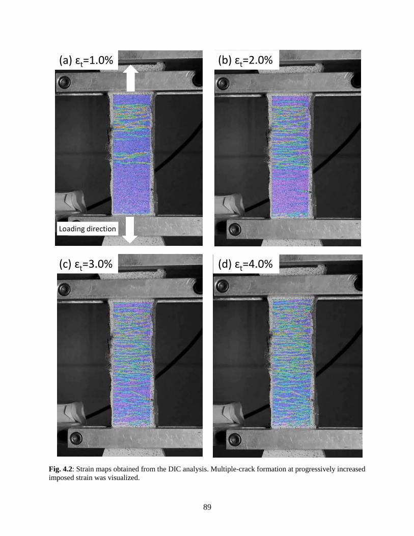
89

Fig. 4.2: Strain maps obtained from the DIC analysis. Multiple-crack formation at progressively increased

imposed strain was visualized.

(a) ɛt=1.0% (b) ɛt=2.0%

(c) ɛt=3.0% (d) ɛt=4.0%

Loading direction

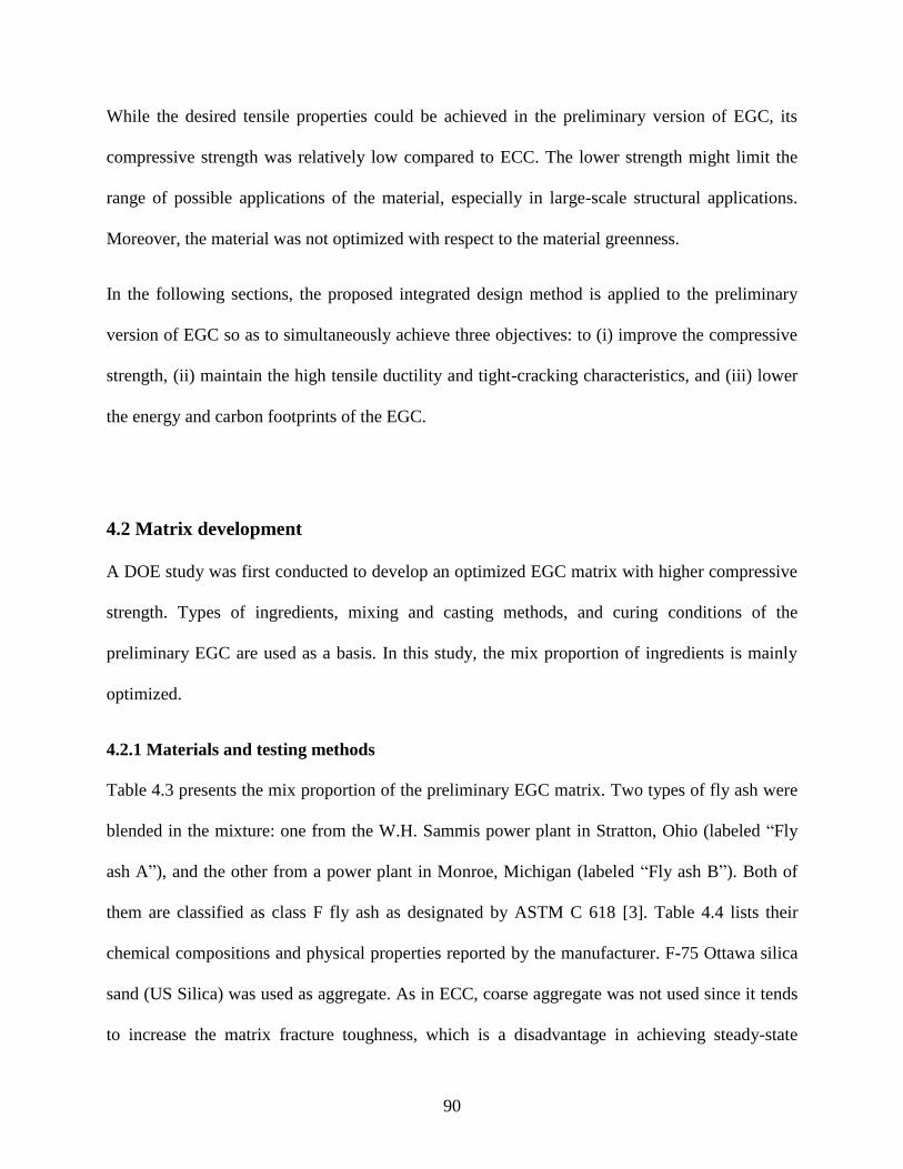
90

While the desired tensile properties could be achieved in the preliminary version of EGC, its

compressive strength was relatively low compared to ECC. The lower strength might limit the

range of possible applications of the material, especially in large-scale structural applications.

Moreover, the material was not optimized with respect to the material greenness.

In the following sections, the proposed integrated design method is applied to the preliminary

version of EGC so as to simultaneously achieve three objectives: to (i) improve the compressive

strength, (ii) maintain the high tensile ductility and tight-cracking characteristics, and (iii) lower

the energy and carbon footprints of the EGC.

4.2 Matrix development

A DOE study was first conducted to develop an optimized EGC matrix with higher compressive

strength. Types of ingredients, mixing and casting methods, and curing conditions of the

preliminary EGC are used as a basis. In this study, the mix proportion of ingredients is mainly

optimized.

4.2.1 Materials and testing methods

Table 4.3 presents the mix proportion of the preliminary EGC matrix. Two types of fly ash were

blended in the mixture: one from the W.H. Sammis power plant in Stratton, Ohio (labeled “Fly

ash A”), and the other from a power plant in Monroe, Michigan (labeled “Fly ash B”). Both of

them are classified as class F fly ash as designated by ASTM C 618 [3]. Table 4.4 lists their

chemical compositions and physical properties reported by the manufacturer. F-75 Ottawa silica

sand (US Silica) was used as aggregate. As in ECC, coarse aggregate was not used since it tends

to increase the matrix fracture toughness, which is a disadvantage in achieving steady-state

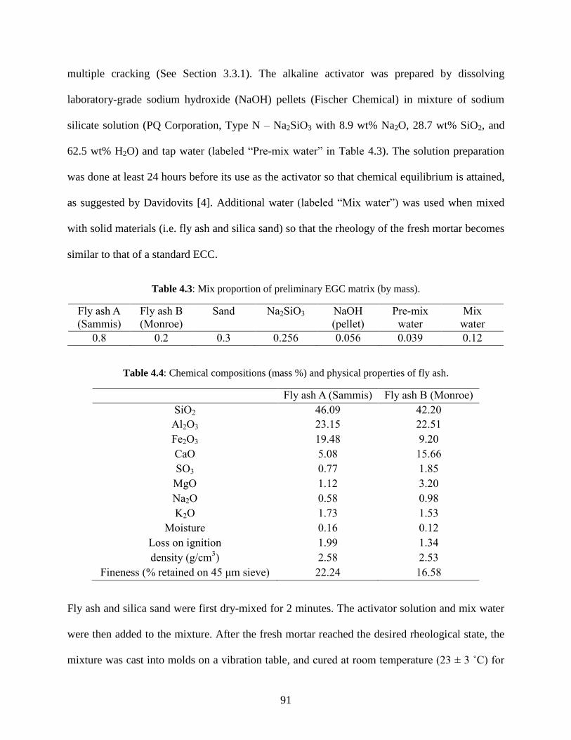
91

multiple cracking (See Section 3.3.1). The alkaline activator was prepared by dissolving

laboratory-grade sodium hydroxide (NaOH) pellets (Fischer Chemical) in mixture of sodium

silicate solution (PQ Corporation, Type N – Na2SiO3 with 8.9 wt% Na2O, 28.7 wt% SiO2, and

62.5 wt% H2O) and tap water (labeled “Pre-mix water” in Table 4.3). The solution preparation

was done at least 24 hours before its use as the activator so that chemical equilibrium is attained,

as suggested by Davidovits [4]. Additional water (labeled “Mix water”) was used when mixed

with solid materials (i.e. fly ash and silica sand) so that the rheology of the fresh mortar becomes

similar to that of a standard ECC.

Table 4.3: Mix proportion of preliminary EGC matrix (by mass).

Fly ash A

(Sammis)

Fly ash B

(Monroe)

Sand Na2SiO3 NaOH

(pellet)

Pre-mix

water

Mix

water

0.8 0.2 0.3 0.256 0.056 0.039 0.12

Table 4.4: Chemical compositions (mass %) and physical properties of fly ash.

Fly ash A (Sammis) Fly ash B (Monroe)

SiO2 46.09 42.20

Al2O3 23.15 22.51

Fe2O3 19.48 9.20

CaO 5.08 15.66

SO3 0.77 1.85

MgO 1.12 3.20

Na2O 0.58 0.98

K2O 1.73 1.53

Moisture 0.16 0.12

Loss on ignition 1.99 1.34

density (g/cm3) 2.58 2.53

Fineness (% retained on 45 μm sieve) 22.24 16.58

Fly ash and silica sand were first dry-mixed for 2 minutes. The activator solution and mix water

were then added to the mixture. After the fresh mortar reached the desired rheological state, the

mixture was cast into molds on a vibration table, and cured at room temperature (23 ± 3 ˚C) for

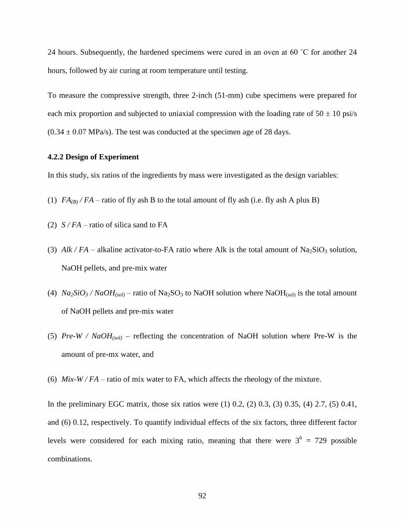
92

24 hours. Subsequently, the hardened specimens were cured in an oven at 60 ˚C for another 24

hours, followed by air curing at room temperature until testing.

To measure the compressive strength, three 2-inch (51-mm) cube specimens were prepared for

each mix proportion and subjected to uniaxial compression with the loading rate of 50 ± 10 psi/s

(0.34 ± 0.07 MPa/s). The test was conducted at the specimen age of 28 days.

4.2.2 Design of Experiment

In this study, six ratios of the ingredients by mass were investigated as the design variables:

(1) FA(B) / FA – ratio of fly ash B to the total amount of fly ash (i.e. fly ash A plus B)

(2) S / FA – ratio of silica sand to FA

(3) Alk / FA – alkaline activator-to-FA ratio where Alk is the total amount of Na2SiO3 solution,

NaOH pellets, and pre-mix water

(4) Na2SiO3 / NaOH(sol) – ratio of Na2SO3 to NaOH solution where NaOH(sol) is the total amount

of NaOH pellets and pre-mix water

(5) Pre-W / NaOH(sol) – reflecting the concentration of NaOH solution where Pre-W is the

amount of pre-mx water, and

(6) Mix-W / FA – ratio of mix water to FA, which affects the rheology of the mixture.

In the preliminary EGC matrix, those six ratios were (1) 0.2, (2) 0.3, (3) 0.35, (4) 2.7, (5) 0.41,

and (6) 0.12, respectively. To quantify individual effects of the six factors, three different factor

levels were considered for each mixing ratio, meaning that there were 36 = 729 possible

combinations.

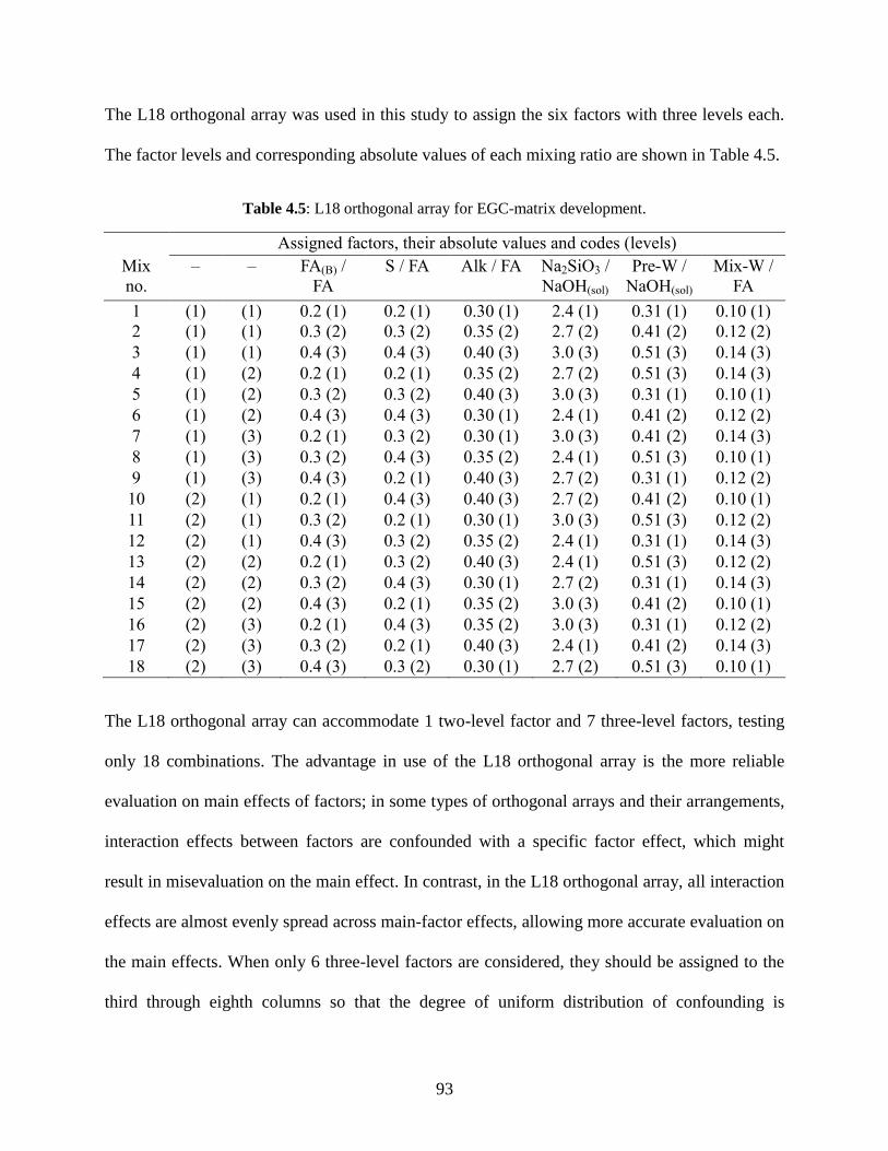
93

The L18 orthogonal array was used in this study to assign the six factors with three levels each.

The factor levels and corresponding absolute values of each mixing ratio are shown in Table 4.5.

Table 4.5: L18 orthogonal array for EGC-matrix development.

Assigned factors, their absolute values and codes (levels)

Mix

no.

– – FA(B) /

FA

S / FA Alk / FA Na2SiO3 /

NaOH(sol)

Pre-W /

NaOH(sol)

Mix-W /

FA

1 (1) (1) 0.2 (1) 0.2 (1) 0.30 (1) 2.4 (1) 0.31 (1) 0.10 (1)

2 (1) (1) 0.3 (2) 0.3 (2) 0.35 (2) 2.7 (2) 0.41 (2) 0.12 (2)

3 (1) (1) 0.4 (3) 0.4 (3) 0.40 (3) 3.0 (3) 0.51 (3) 0.14 (3)

4 (1) (2) 0.2 (1) 0.2 (1) 0.35 (2) 2.7 (2) 0.51 (3) 0.14 (3)

5 (1) (2) 0.3 (2) 0.3 (2) 0.40 (3) 3.0 (3) 0.31 (1) 0.10 (1)

6 (1) (2) 0.4 (3) 0.4 (3) 0.30 (1) 2.4 (1) 0.41 (2) 0.12 (2)

7 (1) (3) 0.2 (1) 0.3 (2) 0.30 (1) 3.0 (3) 0.41 (2) 0.14 (3)

8 (1) (3) 0.3 (2) 0.4 (3) 0.35 (2) 2.4 (1) 0.51 (3) 0.10 (1)

9 (1) (3) 0.4 (3) 0.2 (1) 0.40 (3) 2.7 (2) 0.31 (1) 0.12 (2)

10 (2) (1) 0.2 (1) 0.4 (3) 0.40 (3) 2.7 (2) 0.41 (2) 0.10 (1)

11 (2) (1) 0.3 (2) 0.2 (1) 0.30 (1) 3.0 (3) 0.51 (3) 0.12 (2)

12 (2) (1) 0.4 (3) 0.3 (2) 0.35 (2) 2.4 (1) 0.31 (1) 0.14 (3)

13 (2) (2) 0.2 (1) 0.3 (2) 0.40 (3) 2.4 (1) 0.51 (3) 0.12 (2)

14 (2) (2) 0.3 (2) 0.4 (3) 0.30 (1) 2.7 (2) 0.31 (1) 0.14 (3)

15 (2) (2) 0.4 (3) 0.2 (1) 0.35 (2) 3.0 (3) 0.41 (2) 0.10 (1)

16 (2) (3) 0.2 (1) 0.4 (3) 0.35 (2) 3.0 (3) 0.31 (1) 0.12 (2)

17 (2) (3) 0.3 (2) 0.2 (1) 0.40 (3) 2.4 (1) 0.41 (2) 0.14 (3)

18 (2) (3) 0.4 (3) 0.3 (2) 0.30 (1) 2.7 (2) 0.51 (3) 0.10 (1)

The L18 orthogonal array can accommodate 1 two-level factor and 7 three-level factors, testing

only 18 combinations. The advantage in use of the L18 orthogonal array is the more reliable

evaluation on main effects of factors; in some types of orthogonal arrays and their arrangements,

interaction effects between factors are confounded with a specific factor effect, which might

result in misevaluation on the main effect. In contrast, in the L18 orthogonal array, all interaction

effects are almost evenly spread across main-factor effects, allowing more accurate evaluation on

the main effects. When only 6 three-level factors are considered, they should be assigned to the

third through eighth columns so that the degree of uniform distribution of confounding is

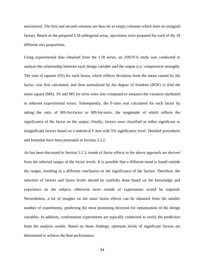
94

maximized. The first and second columns are thus set as empty columns which have no assigned

factors. Based on the prepared L18 orthogonal array, specimens were prepared for each of the 18

different mix proportions.

Using experimental data obtained from the L18 series, an ANOVA study was conducted to

analyze the relationship between each design variable and the output (i.e. compressive strength).

The sum of squares (SS) for each factor, which reflects deviation from the mean caused by the

factor, was first calculated, and then normalized by the degree of freedom (DOF) to find the

mean square (MS). SS and MS for error were also computed to measure the variation attributed

to inherent experimental errors. Subsequently, the F-ratio was calculated for each factor by

taking the ratio of MS-for-factor to MS-for-error, the magnitude of which reflects the

significance of the factor on the output. Finally, factors were classified as either significant or

insignificant factors based on a statistical F-test with 5% significance level. Detailed procedures

and formulae have been presented in Section 3.2.2.

As has been discussed in Section 3.2.3, trends of factor effects in the above approach are derived

from the selected ranges of the factor levels. It is possible that a different trend is found outside

the ranges, resulting in a different conclusion on the significance of the factors. Therefore, the

selection of factors and factor levels should be carefully done based on the knowledge and

experience on the subject; otherwise more rounds of experiments would be required.

Nevertheless, a lot of insights on the main factor effects can be obtained from the smaller

number of experiments, predicting the most promising direction for optimization of the design

variables. In addition, confirmation experiments are typically conducted to verify the prediction

from the analysis results. Based on those findings, optimum levels of significant factors are

determined to achieve the best performance.

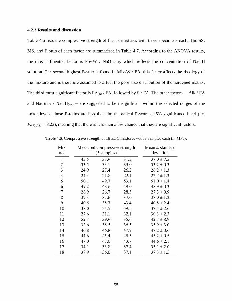
95

4.2.3 Results and discussion

Table 4.6 lists the compressive strength of the 18 mixtures with three specimens each. The SS,

MS, and F-ratio of each factor are summarized in Table 4.7. According to the ANOVA results,

the most influential factor is Pre-W / NaOH(sol), which reflects the concentration of NaOH

solution. The second highest F-ratio is found in Mix-W / FA; this factor affects the rheology of

the mixture and is therefore assumed to affect the pore size distribution of the hardened matrix.

The third most significant factor is FA(B) / FA, followed by S / FA. The other factors – Alk / FA

and Na2SiO3 / NaOH(sol) – are suggested to be insignificant within the selected ranges of the

factor levels; those F-ratios are less than the theoretical F-score at 5% significance level (i.e.

F0.05,2,41 = 3.23), meaning that there is less than a 5% chance that they are significant factors.

Table 4.6: Compressive strength of 18 EGC mixtures with 3 samples each (in MPa).

Mix

no.

Measured compressive strength

(3 samples)

Mean ± standard

deviation

1 45.5 33.9 31.5 37.0 ± 7.5

2 33.5 33.1 33.0 33.2 ± 0.3

3 24.9 27.4 26.2 26.2 ± 1.3

4 24.3 21.8 22.1 22.7 ± 1.3

5 50.1 49.7 53.1 51.0 ± 1.8

6 49.2 48.6 49.0 48.9 ± 0.3

7 26.9 26.7 28.3 27.3 ± 0.9

8 39.3 37.6 37.0 38.0 ± 1.2

9 40.5 38.7 43.4 40.8 ± 2.4

10 38.0 34.5 39.5 37.4 ± 2.6

11 27.6 31.1 32.1 30.3 ± 2.3

12 52.7 39.9 35.6 42.7 ± 8.9

13 32.6 38.5 36.5 35.9 ± 3.0

14 46.8 46.8 47.9 47.2 ± 0.6

15 44.6 45.4 45.5 45.2 ± 0.5

16 47.0 43.0 43.7 44.6 ± 2.1

17 34.1 33.8 37.4 35.1 ± 2.0

18 38.9 36.0 37.1 37.3 ± 1.5

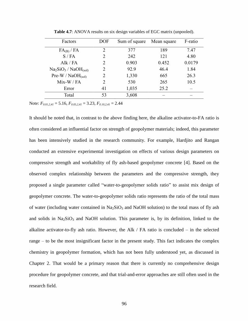
96

Table 4.7: ANOVA results on six design variables of EGC matrix (unpooled).


FA(B) / FA 2 377 189 7.47

S / FA 2 242 121 4.80

Alk / FA 2 0.903 0.452 0.0179

Na2SiO3 / NaOH(sol) 2 92.9 46.4 1.84

Pre-W / NaOH(sol) 2 1,330 665 26.3

Mix-W / FA 2 530 265 10.5

Error 41 1,035 25.2 –

Total 53 3,608 – –

Note: F0.01,2,41 = 5.16, F0.05,2,41 = 3.23, F0.10,2,41 = 2.44

It should be noted that, in contrast to the above finding here, the alkaline activator-to-FA ratio is

often considered an influential factor on strength of geopolymer materials; indeed, this parameter

has been intensively studied in the research community. For example, Hardjito and Rangan

conducted an extensive experimental investigation on effects of various design parameters on

compressive strength and workability of fly ash-based geopolymer concrete [4]. Based on the

observed complex relationship between the parameters and the compressive strength, they

proposed a single parameter called “water-to-geopolymer solids ratio” to assist mix design of

geopolymer concrete. The water-to-geopolymer solids ratio represents the ratio of the total mass

of water (including water contained in Na2SiO3 and NaOH solution) to the total mass of fly ash

and solids in Na2SiO3 and NaOH solution. This parameter is, by its definition, linked to the

alkaline activator-to-fly ash ratio. However, the Alk / FA ratio is concluded – in the selected

range – to be the most insignificant factor in the present study. This fact indicates the complex

chemistry in geopolymer formation, which has not been fully understood yet, as discussed in

Chapter 2. That would be a primary reason that there is currently no comprehensive design

procedure for geopolymer concrete, and that trial-and-error approaches are still often used in the

research field.

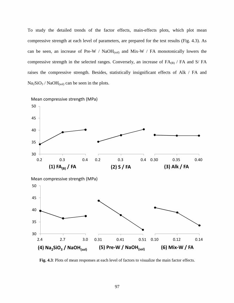
97

To study the detailed trends of the factor effects, main-effects plots, which plot mean

compressive strength at each level of parameters, are prepared for the test results (Fig. 4.3). As

can be seen, an increase of Pre-W / NaOH(sol) and Mix-W / FA monotonically lowers the

compressive strength in the selected ranges. Conversely, an increase of FA(B) / FA and S/ FA

raises the compressive strength. Besides, statistically insignificant effects of Alk / FA and

Na2SiO3 / NaOH(sol) can be seen in the plots.

Fig. 4.3: Plots of mean responses at each level of factors to visualize the main factor effects.

30

35

40

45

50

0.30 0.35 0.40

30

35

40

45

50

0.2 0.3 0.4

30

35

40

45

50

0.2 0.3 0.4


(1) FA(B) / FA (2) S / FA (3) Alk / FA

30

35

40

45

50

0.10 0.12 0.14

30

35

40

45

50

0.31 0.41 0.51

30

35

40

45

50

2.4 2.7 3.0


(4) Na2SiO3 / NaOH(sol) (5) Pre-W / NaOH(sol) (6) Mix-W / FA

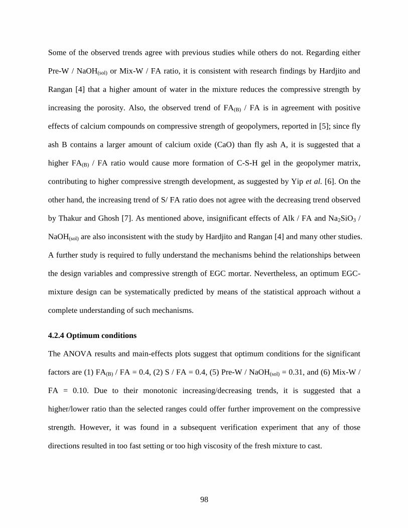
98

Some of the observed trends agree with previous studies while others do not. Regarding either

Pre-W / NaOH(sol) or Mix-W / FA ratio, it is consistent with research findings by Hardjito and

Rangan [4] that a higher amount of water in the mixture reduces the compressive strength by

increasing the porosity. Also, the observed trend of FA(B) / FA is in agreement with positive

effects of calcium compounds on compressive strength of geopolymers, reported in [5]; since fly

ash B contains a larger amount of calcium oxide (CaO) than fly ash A, it is suggested that a

higher FA(B) / FA ratio would cause more formation of C-S-H gel in the geopolymer matrix,

contributing to higher compressive strength development, as suggested by Yip et al. [6]. On the

other hand, the increasing trend of S/ FA ratio does not agree with the decreasing trend observed

by Thakur and Ghosh [7]. As mentioned above, insignificant effects of Alk / FA and Na2SiO3 /

NaOH(sol) are also inconsistent with the study by Hardjito and Rangan [4] and many other studies.

A further study is required to fully understand the mechanisms behind the relationships between

the design variables and compressive strength of EGC mortar. Nevertheless, an optimum EGC-

mixture design can be systematically predicted by means of the statistical approach without a

complete understanding of such mechanisms.

4.2.4 Optimum conditions

The ANOVA results and main-effects plots suggest that optimum conditions for the significant

factors are (1) FA(B) / FA = 0.4, (2) S / FA = 0.4, (5) Pre-W / NaOH(sol) = 0.31, and (6) Mix-W /

FA = 0.10. Due to their monotonic increasing/decreasing trends, it is suggested that a

higher/lower ratio than the selected ranges could offer further improvement on the compressive

strength. However, it was found in a subsequent verification experiment that any of those

directions resulted in too fast setting or too high viscosity of the fresh mixture to cast.

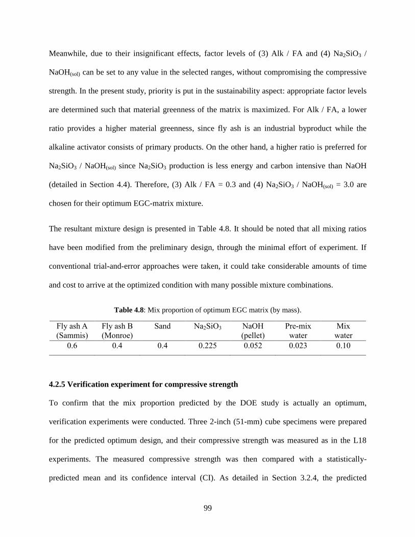
99

Meanwhile, due to their insignificant effects, factor levels of (3) Alk / FA and (4) Na2SiO3 /

NaOH(sol) can be set to any value in the selected ranges, without compromising the compressive

strength. In the present study, priority is put in the sustainability aspect: appropriate factor levels

are determined such that material greenness of the matrix is maximized. For Alk / FA, a lower

ratio provides a higher material greenness, since fly ash is an industrial byproduct while the

alkaline activator consists of primary products. On the other hand, a higher ratio is preferred for

Na2SiO3 / NaOH(sol) since Na2SiO3 production is less energy and carbon intensive than NaOH

(detailed in Section 4.4). Therefore, (3) Alk / FA = 0.3 and (4) Na2SiO3 / NaOH(sol) = 3.0 are

chosen for their optimum EGC-matrix mixture.

The resultant mixture design is presented in Table 4.8. It should be noted that all mixing ratios

have been modified from the preliminary design, through the minimal effort of experiment. If

conventional trial-and-error approaches were taken, it could take considerable amounts of time

and cost to arrive at the optimized condition with many possible mixture combinations.

Table 4.8: Mix proportion of optimum EGC matrix (by mass).

Fly ash A

(Sammis)

Fly ash B

(Monroe)

Sand Na2SiO3 NaOH

(pellet)

Pre-mix

water

Mix

water

0.6 0.4 0.4 0.225 0.052 0.023 0.10

4.2.5 Verification experiment for compressive strength

To confirm that the mix proportion predicted by the DOE study is actually an optimum,

verification experiments were conducted. Three 2-inch (51-mm) cube specimens were prepared

for the predicted optimum design, and their compressive strength was measured as in the L18

experiments. The measured compressive strength was then compared with a statistically-

predicted mean and its confidence interval (CI). As detailed in Section 3.2.4, the predicted

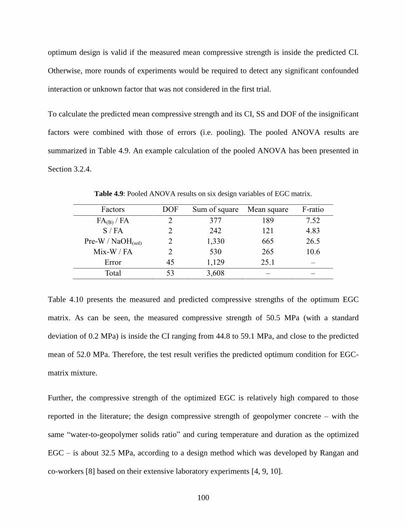
100

optimum design is valid if the measured mean compressive strength is inside the predicted CI.

Otherwise, more rounds of experiments would be required to detect any significant confounded

interaction or unknown factor that was not considered in the first trial.

To calculate the predicted mean compressive strength and its CI, SS and DOF of the insignificant

factors were combined with those of errors (i.e. pooling). The pooled ANOVA results are

summarized in Table 4.9. An example calculation of the pooled ANOVA has been presented in

Section 3.2.4.

Table 4.9: Pooled ANOVA results on six design variables of EGC matrix.


FA(B) / FA 2 377 189 7.52

S / FA 2 242 121 4.83

Pre-W / NaOH(sol) 2 1,330 665 26.5

Mix-W / FA 2 530 265 10.6

Error 45 1,129 25.1 –

Total 53 3,608 – –

Table 4.10 presents the measured and predicted compressive strengths of the optimum EGC

matrix. As can be seen, the measured compressive strength of 50.5 MPa (with a standard

deviation of 0.2 MPa) is inside the CI ranging from 44.8 to 59.1 MPa, and close to the predicted

mean of 52.0 MPa. Therefore, the test result verifies the predicted optimum condition for EGC-

matrix mixture.

Further, the compressive strength of the optimized EGC is relatively high compared to those

reported in the literature; the design compressive strength of geopolymer concrete – with the

same “water-to-geopolymer solids ratio” and curing temperature and duration as the optimized

EGC – is about 32.5 MPa, according to a design method which was developed by Rangan and

co-workers [8] based on their extensive laboratory experiments [4, 9, 10].

101

Since the achieved compressive strength in the optimized EGC matrix is sufficiently high for

various kinds of infrastructure applications, the primary objective of this matrix-development

stage has been successfully achieved.

Table 4.10: Measured and predicted compressive strengths of optimum EGC matrix (in MPa).

Measured compressive strength

(3 samples)

Measured

mean

Predicted

mean

Predicted

CI

50.2 50.9 50.5 50.5 52.0 [44.8, 59.1]

4.3 Composite design

In this design stage, the micromechanical modeling technique is used to develop strain-hardening

ductile EGC based on the optimized EGC matrix.

4.3.1 Experimental and analytical methods

Fiber/matrix interface properties were first determined by experiment. For the optimized EGC

matrix, small prismatic specimens with an embedded single fiber were prepared for conducting

the single-fiber pullout test. The specimen thickness – equivalent to the fiber embedment length

– varied from 0.9 mm to 2.7 mm. Polyvinyl alcohol (PVA) fiber with 1.2% oil coating by weight

[11] was employed, considering its preceding successful applications in ECC materials. The

embedded fiber in each specimen was uniaxially pulled out with the loading rate of 0.5 mm/min.

From the obtained single-fiber pullout curves, τ0, Gd, and β were computed based on Eqs. 3.18–

3.20 presented in Section 3.3.1.

Matrix properties were also experimentally evaluated. To determine the matrix fracture

toughness (Km), notched beam specimens with 305 mm in length, 76 mm in height and 38 mm in

thickness were prepared for conducting a three-point bending test. Four specimens with the notch

depth-to-height ratio of 0.4 were tested in accordance with ASTM E399 [12]. The loading rate

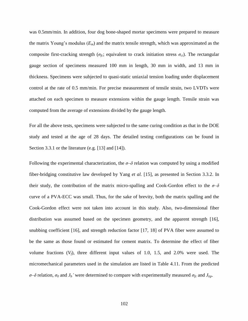
102

was 0.5mm/min. In addition, four dog bone-shaped mortar specimens were prepared to measure

the matrix Young’s modulus (Em) and the matrix tensile strength, which was approximated as the

composite first-cracking strength (σfc; equivalent to crack initiation stress σci). The rectangular

gauge section of specimens measured 100 mm in length, 30 mm in width, and 13 mm in

thickness. Specimens were subjected to quasi-static uniaxial tension loading under displacement

control at the rate of 0.5 mm/min. For precise measurement of tensile strain, two LVDTs were

attached on each specimen to measure extensions within the gauge length. Tensile strain was

computed from the average of extensions divided by the gauge length.

For all the above tests, specimens were subjected to the same curing condition as that in the DOE

study and tested at the age of 28 days. The detailed testing configurations can be found in

Section 3.3.1 or the literature (e.g. [13] and [14]).

Following the experimental characterization, the σ–δ relation was computed by using a modified

fiber-bridging constitutive law developed by Yang et al. [15], as presented in Section 3.3.2. In

their study, the contribution of the matrix micro-spalling and Cook-Gordon effect to the σ–δ

curve of a PVA-ECC was small. Thus, for the sake of brevity, both the matrix spalling and the

Cook-Gordon effect were not taken into account in this study. Also, two-dimensional fiber

distribution was assumed based on the specimen geometry, and the apparent strength [16],

snubbing coefficient [16], and strength reduction factor [17, 18] of PVA fiber were assumed to

be the same as those found or estimated for cement matrix. To determine the effect of fiber

volume fractions (Vf), three different input values of 1.0, 1.5, and 2.0% were used. The

micromechanical parameters used in the simulation are listed in Table 4.11. From the predicted

σ–δ relation, σ0 and Jb’ were determined to compare with experimentally measured σfc and Jtip.

103

Table 4.11: Micromechanical parameters used as model input.

Fiber properties Interface properties

Diameter

(μm)

Length

(mm)

Young’s

modulus

(GPa)

Apparent

strength

(MPa)

Volume

(%)

Snubbing

coefficient

Strength

reduction

coefficient

39 12 42.8 1092 a 1.0, 1.5, 2.0 0.2

b 0.33

b

a Reduced fiber strength when the fiber is embedded in cementitious matrix [11].

b Assumed values based on experiment [15].


Table 4.12 summarizes the test results of the single-fiber pullout test, matrix fracture toughness

test, and mortar dog bone uniaxial tension test. According to the test results, EGC is

characterized by the strong chemical bond and weak frictional bond and slip-hardening,

compared to ECC: the chemical bond (Gd) between the optimized EGC matrix and PVA fiber is

6.1 J/m2, which is 4-5 times higher than those found in ECC materials [11, 15]; on the other hand,

the frictional bond (τ0) of 0.7 MPa and the slip-hardening coefficient (β) of 0.33 for EGC are

both lower than τ0 of 1.11MPa and β of 1.15 reported by Li and Wu [11], or 1.31-1.91 MPa and

0.58-0.63 found by Yang et al. [15]. The strong chemical bond typically results in smaller crack

width by limiting the crack opening during the strain-hardening stage. While the weaker

frictional bond and smaller slip-hardening coefficient might cause lower bridging capacity (σ0), a

high tensile ductility can be achieved by suppressing fiber rupture and facilitating fiber pullout.

These properties have been indeed demonstrated in the preliminary version of EGC; it exhibited

smaller average crack width than ECC materials, with high tensile ductility of over 4.5% [2].

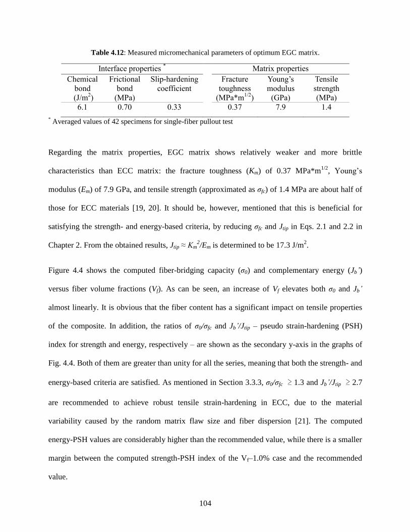
104

Table 4.12: Measured micromechanical parameters of optimum EGC matrix.

Interface properties * Matrix properties

Chemical

bond

(J/m2)

Frictional

bond

(MPa)

Slip-hardening

coefficient

Fracture

toughness

(MPa*m1/2

)

Young’s

modulus

(GPa)

Tensile

strength

(MPa)

6.1 0.70 0.33 0.37 7.9 1.4

* Averaged values of 42 specimens for single-fiber pullout test

Regarding the matrix properties, EGC matrix shows relatively weaker and more brittle

characteristics than ECC matrix: the fracture toughness (Km) of 0.37 MPa*m1/2

, Young’s

modulus (Em) of 7.9 GPa, and tensile strength (approximated as σfc) of 1.4 MPa are about half of

those for ECC materials [19, 20]. It should be, however, mentioned that this is beneficial for

satisfying the strength- and energy-based criteria, by reducing σfc and Jtip in Eqs. 2.1 and 2.2 in

Chapter 2. From the obtained results, Jtip ≈ Km2/Em is determined to be 17.3 J/m

2.

Figure 4.4 shows the computed fiber-bridging capacity (σ0) and complementary energy (Jb’)

versus fiber volume fractions (Vf). As can be seen, an increase of Vf elevates both σ0 and Jb’

almost linearly. It is obvious that the fiber content has a significant impact on tensile properties

of the composite. In addition, the ratios of σ0/σfc and Jb’/Jtip – pseudo strain-hardening (PSH)

index for strength and energy, respectively – are shown as the secondary y-axis in the graphs of

Fig. 4.4. Both of them are greater than unity for all the series, meaning that both the strength- and

energy-based criteria are satisfied. As mentioned in Section 3.3.3, σ0/σfc ≥ 1.3 and Jb’/Jtip ≥ 2.7

are recommended to achieve robust tensile strain-hardening in ECC, due to the material

variability caused by the random matrix flaw size and fiber dispersion [21]. The computed

energy-PSH values are considerably higher than the recommended value, while there is a smaller

margin between the computed strength-PSH index of the Vf–1.0% case and the recommended

value.

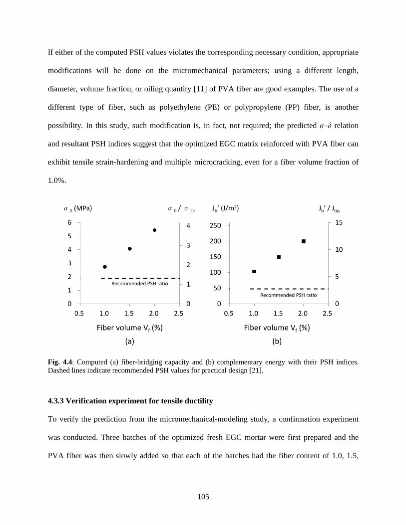
105

If either of the computed PSH values violates the corresponding necessary condition, appropriate

modifications will be done on the micromechanical parameters; using a different length,

diameter, volume fraction, or oiling quantity [11] of PVA fiber are good examples. The use of a

different type of fiber, such as polyethylene (PE) or polypropylene (PP) fiber, is another

possibility. In this study, such modification is, in fact, not required; the predicted σ–δ relation

and resultant PSH indices suggest that the optimized EGC matrix reinforced with PVA fiber can

exhibit tensile strain-hardening and multiple microcracking, even for a fiber volume fraction of

1.0%.

Fig. 4.4: Computed (a) fiber-bridging capacity and (b) complementary energy with their PSH indices.

Dashed lines indicate recommended PSH values for practical design [21].

4.3.3 Verification experiment for tensile ductility

To verify the prediction from the micromechanical-modeling study, a confirmation experiment

was conducted. Three batches of the optimized fresh EGC mortar were first prepared and the

PVA fiber was then slowly added so that each of the batches had the fiber content of 1.0, 1.5,

Fiber volume Vf (%)

σ0 (MPa)

0

1

2

3

4

0

1

2

3

4

5

6

0.5 1.0 1.5 2.0 2.5

σ0 / σfc

0

5

10

15

0

50

100

150

200

250

0.5 1.0 1.5 2.0 2.5

Jb‘ (J/m2) Jb‘ / Jtip

Fiber volume Vf (%)

Recommended PSH ratio

Recommended PSH ratio

(a) (b)

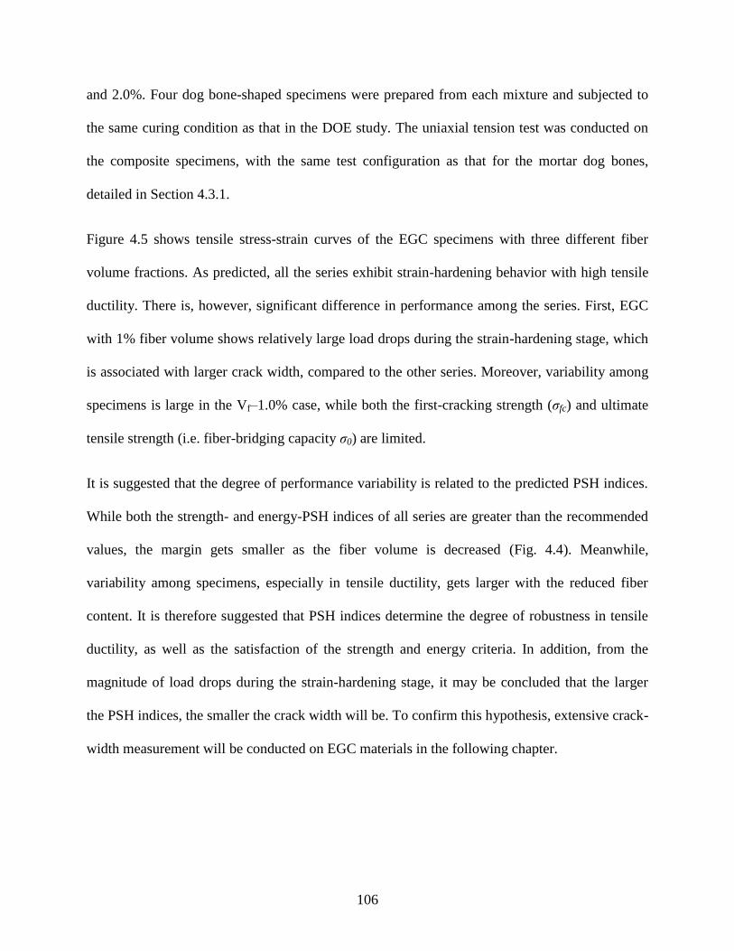
106

and 2.0%. Four dog bone-shaped specimens were prepared from each mixture and subjected to

the same curing condition as that in the DOE study. The uniaxial tension test was conducted on

the composite specimens, with the same test configuration as that for the mortar dog bones,

detailed in Section 4.3.1.

Figure 4.5 shows tensile stress-strain curves of the EGC specimens with three different fiber

volume fractions. As predicted, all the series exhibit strain-hardening behavior with high tensile

ductility. There is, however, significant difference in performance among the series. First, EGC

with 1% fiber volume shows relatively large load drops during the strain-hardening stage, which

is associated with larger crack width, compared to the other series. Moreover, variability among

specimens is large in the Vf–1.0% case, while both the first-cracking strength (σfc) and ultimate

tensile strength (i.e. fiber-bridging capacity σ0) are limited.

It is suggested that the degree of performance variability is related to the predicted PSH indices.

While both the strength- and energy-PSH indices of all series are greater than the recommended

values, the margin gets smaller as the fiber volume is decreased (Fig. 4.4). Meanwhile,

variability among specimens, especially in tensile ductility, gets larger with the reduced fiber

content. It is therefore suggested that PSH indices determine the degree of robustness in tensile

ductility, as well as the satisfaction of the strength and energy criteria. In addition, from the

magnitude of load drops during the strain-hardening stage, it may be concluded that the larger

the PSH indices, the smaller the crack width will be. To confirm this hypothesis, extensive crack-

width measurement will be conducted on EGC materials in the following chapter.

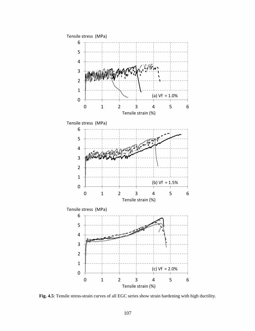
107

Fig. 4.5: Tensile stress-strain curves of all EGC series show strain hardening with high ductility.

0

1

2

3

4

5

6

0 1 2 3 4 5 6Tensile strain (%)


(a) Vf = 1.0%

0

1

2

3

4

5

6



(b) Vf = 1.5%

0

1

2

3

4

5

6



(c) Vf = 2.0%

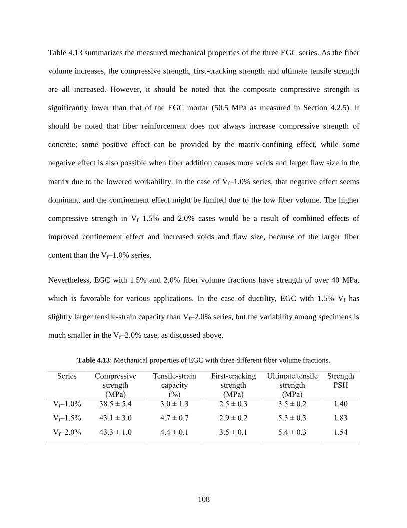
108

Table 4.13 summarizes the measured mechanical properties of the three EGC series. As the fiber

volume increases, the compressive strength, first-cracking strength and ultimate tensile strength

are all increased. However, it should be noted that the composite compressive strength is

significantly lower than that of the EGC mortar (50.5 MPa as measured in Section 4.2.5). It

should be noted that fiber reinforcement does not always increase compressive strength of

concrete; some positive effect can be provided by the matrix-confining effect, while some

negative effect is also possible when fiber addition causes more voids and larger flaw size in the

matrix due to the lowered workability. In the case of Vf–1.0% series, that negative effect seems

dominant, and the confinement effect might be limited due to the low fiber volume. The higher

compressive strength in Vf–1.5% and 2.0% cases would be a result of combined effects of

improved confinement effect and increased voids and flaw size, because of the larger fiber

content than the Vf–1.0% series.

Nevertheless, EGC with 1.5% and 2.0% fiber volume fractions have strength of over 40 MPa,

which is favorable for various applications. In the case of ductility, EGC with 1.5% Vf has

slightly larger tensile-strain capacity than Vf–2.0% series, but the variability among specimens is

much smaller in the Vf–2.0% case, as discussed above.

Table 4.13: Mechanical properties of EGC with three different fiber volume fractions.

Series Compressive

strength

(MPa)

Tensile-strain

capacity

(%)

First-cracking

strength

(MPa)

Ultimate tensile

strength

(MPa)

Strength

PSH

Vf–1.0% 38.5 ± 5.4 3.0 ± 1.3 2.5 ± 0.3 3.5 ± 0.2 1.40

Vf–1.5% 43.1 ± 3.0 4.7 ± 0.7 2.9 ± 0.2 5.3 ± 0.3 1.83

Vf–2.0% 43.3 ± 1.0 4.4 ± 0.1 3.5 ± 0.1 5.4 ± 0.3 1.54

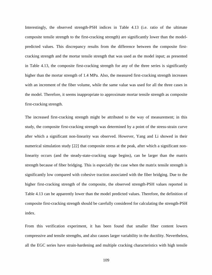
109

Interestingly, the observed strength-PSH indices in Table 4.13 (i.e. ratio of the ultimate

composite tensile strength to the first-cracking strength) are significantly lower than the model-

predicted values. This discrepancy results from the difference between the composite first-

cracking strength and the mortar tensile strength that was used as the model input; as presented

in Table 4.13, the composite first-cracking strength for any of the three series is significantly

higher than the mortar strength of 1.4 MPa. Also, the measured first-cracking strength increases

with an increment of the fiber volume, while the same value was used for all the three cases in

the model. Therefore, it seems inappropriate to approximate mortar tensile strength as composite

first-cracking strength.

The increased first-cracking strength might be attributed to the way of measurement; in this

study, the composite first-cracking strength was determined by a point of the stress-strain curve

after which a significant non-linearity was observed. However, Yang and Li showed in their

numerical simulation study [22] that composite stress at the peak, after which a significant non-

linearity occurs (and the steady-state-cracking stage begins), can be larger than the matrix

strength because of fiber bridging. This is especially the case when the matrix tensile strength is

significantly low compared with cohesive traction associated with the fiber bridging. Due to the

higher first-cracking strength of the composite, the observed strength-PSH values reported in

Table 4.13 can be apparently lower than the model predicted values. Therefore, the definition of

composite first-cracking strength should be carefully considered for calculating the strength-PSH

index.

From this verification experiment, it has been found that smaller fiber content lowers

compressive and tensile strengths, and also causes larger variability in the ductility. Nevertheless,

all the EGC series have strain-hardening and multiple cracking characteristics with high tensile

110

ductility. In addition, due to the adequate compressive strength and excellent tensile properties,

EGC with 1.5 or 2.0% Vf seems promising for large-scale infrastructure applications. In the

following section, material greenness of these two series is assessed in the final design stage.

4.4 Environmental performance comparison

4.4.1 Materials and methods

Environmental performances of the developed EGC-1.5% and EGC-2.0% were compared with

that of the preliminary version of EGC, in terms of the Material Sustainability Indices (MSI) [23].

As references, MSI of OPC concrete and ECC materials were also investigated. Specifically,

embodied-energy consumption and global warming intensity (GWI) associated with unit volume

of the materials were calculated by accounting for all required energy and generated emissions in

the cradle-to-gate phases: raw-material acquisition, processing and manufacturing. Energy and

emissions associated with temperature curing of EGC were not included; similar heat/steam-

induced accelerated curing is often employed in precast-concrete production, and the comparison

study of the materials is therefore not affected by the exclusion. For the carbon-footprint

calculations, 100-year GWP values of the ICPP 2013 report [24] were used to calculate the

carbon dioxide (CO2) equivalent emissions.

For the MSI calculation, the quality and reliability of life-cycle inventory data for ingredients are

crucial. The inventory data used in this study are listed in Table 4.14. The data were collected

from literature that uses consistent system boundaries and assumptions, report both the energy

consumption and greenhouse gas emissions, and have significance in the research field. It should

be noted, however, that some of the data are a little too old; current production of those

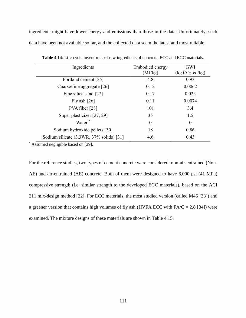
111

ingredients might have lower energy and emissions than those in the data. Unfortunately, such

data have been not available so far, and the collected data seem the latest and most reliable.

Table 4.14: Life-cycle inventories of raw ingredients of concrete, ECC and EGC materials.

Ingredients Embodied energy

(MJ/kg)

GWI

(kg CO2-eq/kg)

Portland cement [25] 4.8 0.93

Coarse/fine aggregate [26] 0.12 0.0062

Fine silica sand [27] 0.17 0.025

Fly ash [26] 0.11 0.0074

PVA fiber [28] 101 3.4

Super plasticizer [27, 29] 35 1.5

Water * 0 0

Sodium hydroxide pellets [30] 18 0.86

Sodium silicate (3.3WR, 37% solids) [31] 4.6 0.43 * Assumed negligible based on [29].

For the reference studies, two types of cement concrete were considered: non-air-entrained (Non-

AE) and air-entrained (AE) concrete. Both of them were designed to have 6,000 psi (41 MPa)

compressive strength (i.e. similar strength to the developed EGC materials), based on the ACI

211 mix-design method [32]. For ECC materials, the most studied version (called M45 [33]) and

a greener version that contains high volumes of fly ash (HVFA ECC with FA/C = 2.8 [34]) were

examined. The mixture designs of these materials are shown in Table 4.15.

112

Table 4.15: Mixture proportions of EGC, concrete, and ECC materials (in kg/m3).

Prelim

EGC

EGC-

2.0%

EGC-

1.5%

Non-AE

concrete *

AE

concrete *

ECC

M45

HVFA

ECC

Type I cement 470 547 571 324

Coarse aggregate 1079 1079

Fine aggregate 647 492

Fine silica sand 340 460 463 456 456

Fly ash 1131 1151 1157 685 906

PVA fiber 26 26 19.5 26 26

SP 6.8 5.3

Water 179 142 142 193 175 332 320

NaOH (pellet)

(pellets)

63.5 59.8 60.1

Na2SiO3 289 259 260 * Designed for compressive strength of 6000 psi (41 MPa), slump of 3 in (76 mm), maximum aggregate

size of 1 in (25 mm), fine aggregate modulus of 2.80, and absorption capacity of 0.5% and 0.7% for

coarse and fine aggregate, respectively. The air contents of Non-AE and AE concrete are 1% and 4.5%,

respectively.


Figure 4.6 shows the computed energy- and carbon-MSI of EGC, concrete, and ECC materials.

For EGC materials, the effect of optimizations during the matrix- and composite-design phases

can be quantified; the embodied energy of the preliminary EGC is reduced from 5.29 to 4.46

GJ/m3 in EGC-1.5%, while the GWI decreases from 285 to 251 kg CO2-eq/m

3. These are 16 and

12% reduction in the embodied energy and CO2 equivalent emissions, respectively.

The large contributors to the embodied energy of EGC series are the alkaline activator and PVA

fiber, which account for 45 and 51%, respectively, of the total energy for EGC-2.0%, and 51 and

44% for EGC-1.5%. While the total energy consumption of EGC is greater than that of concrete,

the geopolymer binder (i.e. fly ash plus alkaline activator) consumes comparable or even less

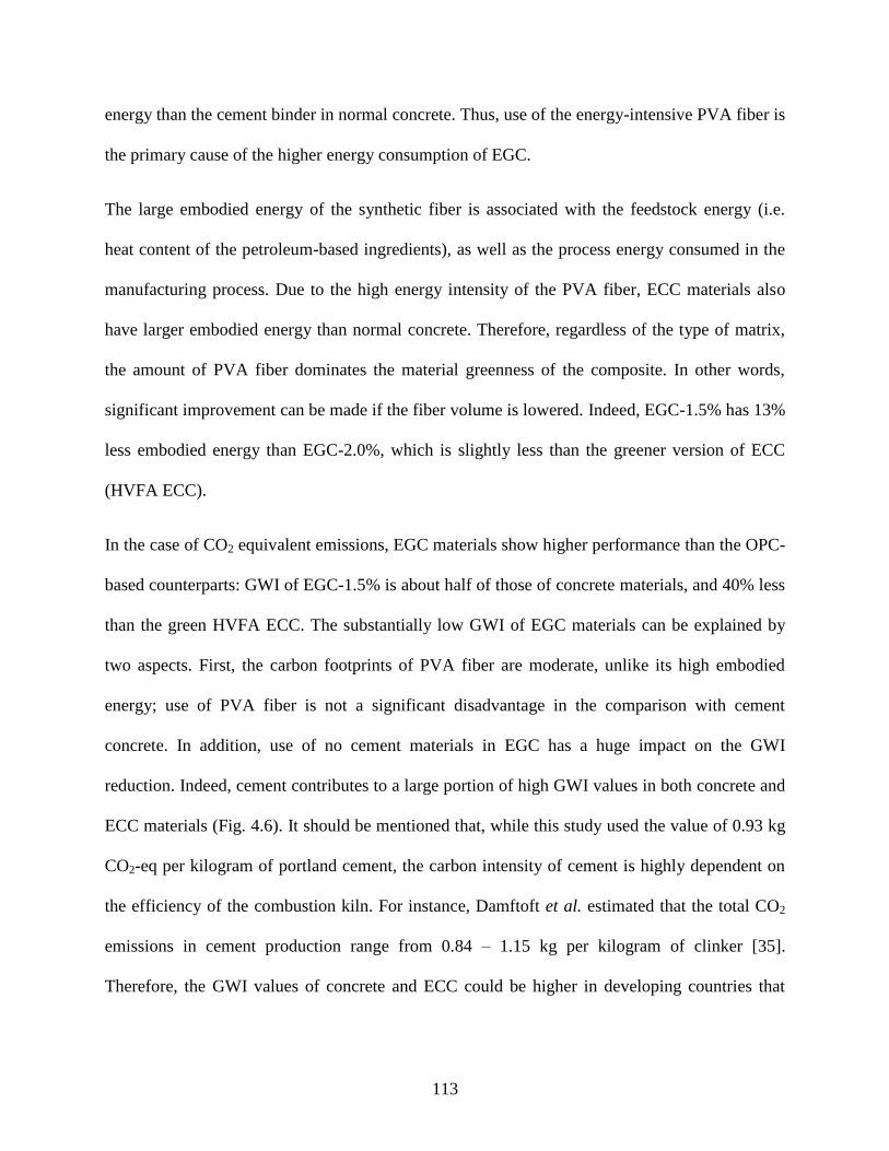
113

energy than the cement binder in normal concrete. Thus, use of the energy-intensive PVA fiber is

the primary cause of the higher energy consumption of EGC.

The large embodied energy of the synthetic fiber is associated with the feedstock energy (i.e.

heat content of the petroleum-based ingredients), as well as the process energy consumed in the

manufacturing process. Due to the high energy intensity of the PVA fiber, ECC materials also

have larger embodied energy than normal concrete. Therefore, regardless of the type of matrix,

the amount of PVA fiber dominates the material greenness of the composite. In other words,

significant improvement can be made if the fiber volume is lowered. Indeed, EGC-1.5% has 13%

less embodied energy than EGC-2.0%, which is slightly less than the greener version of ECC

(HVFA ECC).

In the case of CO2 equivalent emissions, EGC materials show higher performance than the OPC-

based counterparts: GWI of EGC-1.5% is about half of those of concrete materials, and 40% less

than the green HVFA ECC. The substantially low GWI of EGC materials can be explained by

two aspects. First, the carbon footprints of PVA fiber are moderate, unlike its high embodied

energy; use of PVA fiber is not a significant disadvantage in the comparison with cement

concrete. In addition, use of no cement materials in EGC has a huge impact on the GWI

reduction. Indeed, cement contributes to a large portion of high GWI values in both concrete and

ECC materials (Fig. 4.6). It should be mentioned that, while this study used the value of 0.93 kg

CO2-eq per kilogram of portland cement, the carbon intensity of cement is highly dependent on

the efficiency of the combustion kiln. For instance, Damftoft et al. estimated that the total CO2

emissions in cement production range from 0.84 – 1.15 kg per kilogram of clinker [35].

Therefore, the GWI values of concrete and ECC could be higher in developing countries that

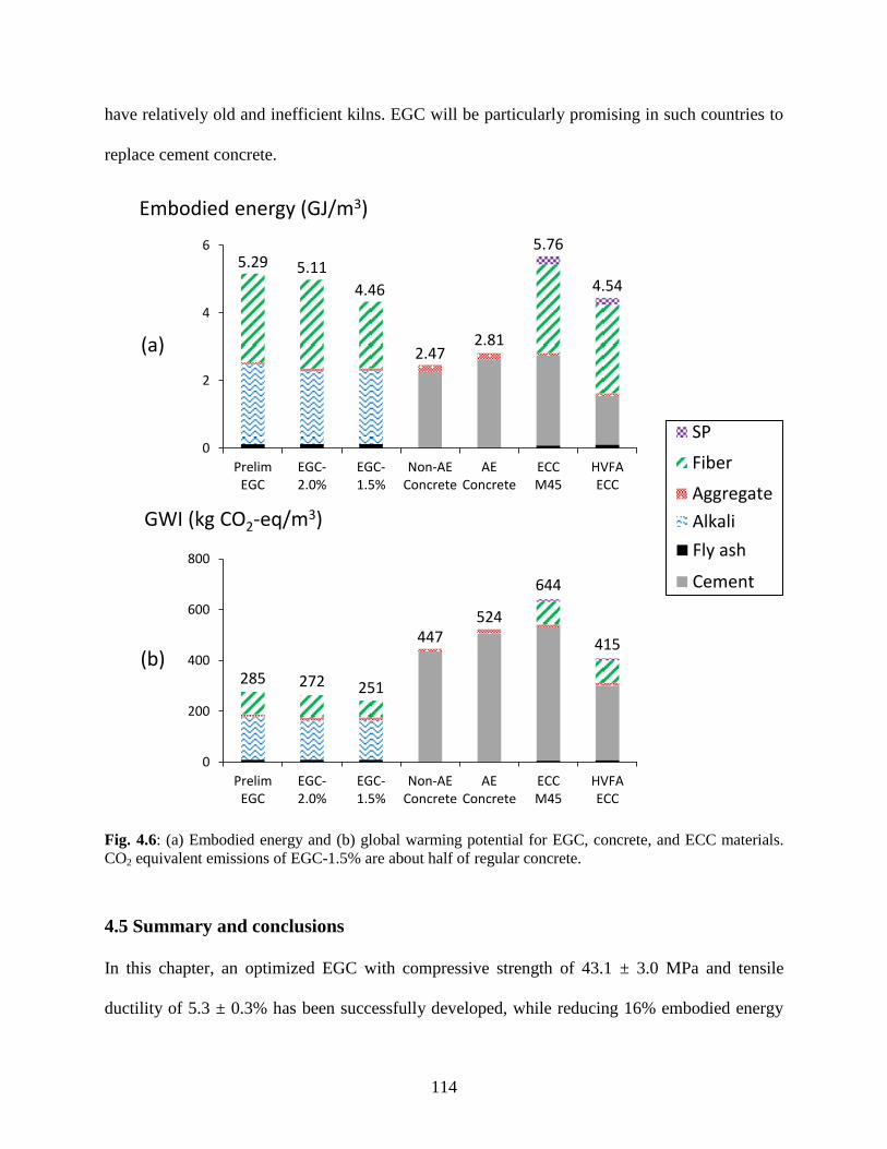
114

have relatively old and inefficient kilns. EGC will be particularly promising in such countries to

replace cement concrete.

Fig. 4.6: (a) Embodied energy and (b) global warming potential for EGC, concrete, and ECC materials.

CO2 equivalent emissions of EGC-1.5% are about half of regular concrete.

4.5 Summary and conclusions

In this chapter, an optimized EGC with compressive strength of 43.1 ± 3.0 MPa and tensile

ductility of 5.3 ± 0.3% has been successfully developed, while reducing 16% embodied energy

GWI (kg CO2-eq/m3)

0

2

4

6

Non-AEConcrete

AEConcrete

ECCM45

HVFAECC

EGC-2.0%

EGC-1.5%

EGC-1.0%

SP

Fiber

Aggregate

Cement

Fly ash

0

2

4

6

Non-AEConcrete

AEConcrete

ECCM45

HVFAECC

EGC-2.0%

EGC-1.5%

EGC-1.0%

SP

Fiber

Aggregate

Cement

Alkali0

2

4

6

Non-AEConcrete

AEConcrete

ECCM45

HVFAECC

EGC-2.0%

EGC-1.5%

EGC-1.0%

SP

Fiber

Aggregate

Cement

Fly ash0

2

4

6

Non-AEConcrete

AEConcrete

ECCM45

HVFAECC

EGC-2.0%

EGC-1.5%

EGC-1.0%

SP

Fiber

Aggregate

Cement

Alkali

Embodied energy (GJ/m3)

(a)

(b)

5.29 5.11

4.46

2.47 2.81

5.76

4.54

0

2

4

6

PrelimEGC

EGC-2.0%

EGC-1.5%

Non-AEConcrete

AEConcrete

ECCM45

HVFAECC

285 272 251

447 524

644

415

0

200

400

600

800

PrelimEGC

EGC-2.0%

EGC-1.5%

Non-AEConcrete

AEConcrete

ECCM45

HVFAECC

115

and 12% CO2 equivalent emissions compared to the preliminary EGC. The embodied energy and

GWI of the optimized EGC are 23 and 61% lower, respectively, than those of a standard version

of ECC (M45). Therefore, the applicability and effectiveness of the proposed design method

have been demonstrated through the systematic design process and the achieved results.

The proposed design method is applicable to not only fly ash-based fiber-reinforced geopolymers

but most other types of fiber-reinforced brittle matrix composites. The efficient and systematic

design process facilitates the research and development of high-performance sustainable

composite materials.

In addition, the following new findings can be derived from this study:

The alkaline activator-to-fly ash ratio is the most insignificant factor for compressive strength

of the EGC matrix, in the selected range of this study. This contrasts with previous studies

that reported the alkaline activator-to-fly ash ratio as the most significant factor.

Compressive strength of EGC matrix increases when a larger amount of fly ash with higher

calcium content is incorporated, even if the fly ash is classified as class F (i.e. low-calcium).

EGC matrix has relatively low tensile strength and more brittle behavior compared to ECC

matrix materials. This is, however, beneficial in achieving robust tensile strain-hardening and

multiple microcracking.

Interface between EGC matrix and PVA fiber has strong chemical bond, weak frictional

bond and small slip-hardening coefficient. The strong chemical bond is beneficial for

achieving smaller crack width, while increasing the chance of fiber rupture and lowering the

complementary energy (Jb’). On the other hand, weak frictional bond and small slip-

116

hardening coefficient might reduce the bridging capacity (σ0), but could contribute to a high

tensile ductility by suppressing fiber rupture and facilitating fiber pullout. In the case of the

developed EGCs, both smaller crack width and higher tensile ductility could be achieved

because of the synergistic effects of bonding properties.

The optimized EGC shows high tensile ductility of 3.0% even with the small fiber volume

fraction of 1.0%. However, due to a small margin between the first-cracking strength and

fiber-bridging capacity, variability among specimens is larger than EGC with higher fiber

contents.

EGC materials have a huge advantage in terms of the global warming intensity (GWI)

associated with the material production. Although the embodied energy of EGC is higher

than that of normal concrete, improvement is possible by reducing the volume fractions of

energy-intensive PVA fiber, or by replacing the PVA fiber with one with lower embodied

energy.

EGC with 1.5% PVA fiber shows balanced properties in tension and compression, and in

MSI. This composite has suitable mechanical properties for civil infrastructure applications

and support infrastructure sustainability through a low GWI.

As mentioned in the last finding, EGC-1.5% seems to be the most promising material because of

the high mechanical performances and material greenness. Despite the superiority of EGC-1.5%,

it might be too early to draw the conclusion; indeed, crack width of EGC-1.5% is suggested to be

larger than that of EGC-2.0%, based on their stress-strain curves. The larger crack width might

result in lower durability properties, which is detrimental to sustainability of the structure.

117

Therefore, it is necessary to evaluate durability properties of the developed EGC, which is

addressed in the next three chapters.

118

References

[1] M. Sutton, J. Orteu, and H. Schreier, Image Correlation for Shape, Motion and

Deformation Measurements: basic concepts, theory and applications. Boston, MA:

Springer US, 2009.

[2] M. Ohno and V. C. Li, “A feasibility study of strain hardening fiber reinforced fly ash-

based geopolymer composites,” Constr. Build. Mater., vol. 57, pp. 163–168, Apr. 2014.

[3] ASTM C618, Standard specification for coal fly ash and raw or calcined natural

pozzolona for use in concrete. West Conshohocken, PA: ASTM International, 2015.

[4] D. Hardjito and B. V. Rangan, Development and properties of low-calcium fly ash-based

geopolymer concrete. Perth (Australia): Research report GC 1, Curtin University, 2005.

[5] J. Temuujin, A. van Riessen, and R. Williams, “Influence of calcium compounds on the

mechanical properties of fly ash geopolymer pastes,” J. Hazard. Mater., vol. 167, no. 1–3,

pp. 82–88, 2009.

[6] C. K. Yip, G. C. Lukey, and J. S. J. Van Deventer, “The coexistence of geopolymeric gel

and calcium silicate hydrate at the early stage of alkaline activation,” Cem. Concr. Res.,

vol. 35, no. 9, pp. 1688–1697, 2005.

[7] R. N. Thakur and S. Ghosh, “Effect of mix composition on compressive strength and

microstructure of fly ash based geopolymer composites,” J. Eng. Appl. Sci., vol. 4, no. 4,

pp. 68–74, 2009.

[8] N. A. Lloyd and B. V. Rangan, “Geopolymer Concrete with Fly Ash,” in Second

International Conference on Sustainable Construction Materials and Technologies, 2010.

[9] D. Hardjito, S. E. Wallah, D. M. J. Sumajouw, and B. V. Rangan, “On the Development

of Fly Ash-Based Geopolymer Concrete,” ACI Mater. J., vol. 101, no. 6, pp. 467–472,

2004.

[10] B. V. Rangan, “Mix design and production of fly ash based geopolymer concrete,” Indian

Concr. J., vol. 82, no. 5, pp. 7–15, 2008.

[11] V. C. Li, C. Wu, S. Wang, A. Ogawa, and T. Saito, “Interface tailoring for strain-

hardening polyvinyl alcohol-engineered cementitious composite (PVA-ECC),” ACI Mater.

J., vol. 99, no. 5, pp. 463–472, 2002.

[12] ASTM E399-12e3, Standard Test Method for Linear-Elastic Plane-Strain Fracture

Toughness K1C of Metallic Material. West Conshohocken, PA: ASTM International,

2012.

[13] M. Li and V. C. Li, “Cracking and healing of engineered cementitious composites under

chloride environment,” ACI Mater. J., vol. 108, no. 3, pp. 333–340, 2011.

119

[14] B. Felekoglu, K. Tosun-Felekoglu, R. Ranade, Q. Zhang, and V. C. Li, “Influence of

matrix flowability, fiber mixing procedure, and curing conditions on the mechanical

performance of HTPP-ECC,” Compos. Part B Eng., vol. 60, pp. 359–370, Apr. 2014.



2008.

[16] T. Kanda and V. C. Li, “Interface Property and Apparent Strength of High-Strength

Hydrophilic Fiber in Cement Matrix,” Journal of Materials in Civil Engineering, vol. 10,

no. 1. pp. 5–13, 1998.



[18] V. C. Li, “Postcrack scaling relations for fiber reinforced cementitious composites,” J.

Mater. Civ. Eng., vol. 4, no. 1, pp. 41–57, 1992.

[19] S. Wang and V. C. Li, “High-early-strength engineered cementitious composites,” ACI

Mater. J., vol. 103, no. 2, pp. 97–105, 2006.

[20] E. Yang, “Designing Added Functions in Engineered Cementitious Composites,”




[22] E. Yang and V. Li, “Numerical study on steady-state cracking of composites,” Compos.

Sci. Technol., vol. 67, no. 2, pp. 151–156, Feb. 2007.

[23] G. A. Keoleian, A. M. Kendall, M. D. Lepech, and V. C. Li, “Guiding the design and

application of new materials for enhancing sustainability performance: Framework and

infrastructure application,” Mater. Res. Soc. Symp. Proc., vol. 895, 2006.








[25] M. L. Marceau, M. A. Nisbet, and M. G. Vangeem, Life Cycle Inventory of Portland

Cement Manufacture. Stokie, IL: Portland Cement Association, 2006.





120



[29] G. A. Keoleian, A. Kendall, J. E. Dettling, V. M. Smith, R. F. Chandler, M. D. Lepech,

and V. C. Li, “Life Cycle Modeling of Concrete Bridge Design: Comparison of

Engineered Cementitious Composite Link Slabs and Conventional Steel Expansion Joints,”

J. Infrastruct. Syst., vol. 11, no. 1, pp. 51–60, 2005.

[30] Euro Chlor, “An Eco-profile and Environmental Product Declaration of the European

Chlor-Alkali Industry,” 2013. [Online]. Available:





[32] ACI Committee 211, Standard Practice for Selecting Proportions for Normal

Heavyweight, and Mass Concrete (Reapproved 2009), no. Reapproved. Farmington Hills,

MI: American Concrete Institute, 2009.



[34] E. H. Yang, Y. Yang, and V. C. Li, “Use of high volumes of fly ash to improve ECC

mechanical properties and material greenness,” ACI Mater. J., vol. 104, no. 6, pp. 620–

628, 2007.

[35] J. S. Damtoft, J. Lukasik, D. Herfort, D. Sorrentino, and E. M. Gartner, “Sustainable

development and climate change initiatives,” Cem. Concr. Res., vol. 38, no. 2, pp. 115–

127, 2008.

121

PART III: CHARACTERIZATION OF EGC DURABILITY

CHAPTER 5: Cracking Characteristics and Water Permeability of EGC

This chapter describes experimental characterization of crack patterns and water tightness of the

developed EGC. Crack patterns of EGC materials with different fiber volumes are first

determined, and permeability coefficients of intact and cracked EGC are then measured. Based

on the experimental result, the relationship between the cracking characteristics and water

permeability is investigated.

5.1 Introduction

Durability of concrete materials is highly dependent on their transport properties. Buenfeld

pointed out that major deterioration mechanisms of concrete – reinforcement corrosion, sulfate

attack, frost attack, and alkali-silica reaction (ASR) – are controlled by the transport of

aggressive agents [1]. There are many transport processes within concrete, but most of them are

governed by three mechanisms: permeation, diffusion, and absorption. Their driving forces are

hydrostatic head, chemical concentration gradient, and capillary suction, respectively. Detailed

discussion on the three mechanisms can be found in the literature (e.g. [2]). In general, the

dominant mechanism is determined by the surrounding environment of the concrete structure.

122

Transport properties of concrete drastically change if cracking occurs; particularly, increase in

permeability is significant. Wang et al. reported that water permeability of cracked concrete was

five orders of magnitude higher than that of intact concrete, when the crack opening was 350 µm

[3]. Tsukamoto also found that the water flow rate in concrete scales to the third power of crack

width [4]. The severe degradation in water tightness is detrimental to concrete durability, as well

as functionality when used as hydraulic infrastructure. It should be noted that some design codes

use a maximum permissible crack width of 300 µm (e.g. [5–7]), meaning that such a degree of

damage can occur in actual concrete structures. In reality, due to the difficulty in crack-width

control, crack width in structures may far exceed the permissible value [8].

Despite the marked effect of cracking on concrete permeability, the degree of degradation is

limited when the crack opening is sufficiently small; Shah and coworkers suggested from

extensive experimental studies that approximately 100 µm is a threshold value of crack opening

under loading, below which the water permeability of concrete materials does not increase

significantly [3, 9–12]. In addition, Lepech and Li demonstrated that water permeability of

cracked ECC, which has tightly-controlled crack width of less than 80µm, is comparable to that

of uncracked ECC and cement mortar [13]. Therefore, cracking characteristics of concrete play a

key role in determining the water tightness and associated durability properties.

In this chapter, crack patterns of the developed EGC with 1.5% and 2.0% fiber volume fractions

are first investigated. The number of cracks and residual crack-width distribution are determined,

by using an optical microscope, for EGC specimens that are uniaxially strained to either 1 or 2%.

Subsequently, the preloaded EGC specimens, as well as intact specimens, are tested for their

water permeability by means of a newly-developed test setup. To calculate the permeability

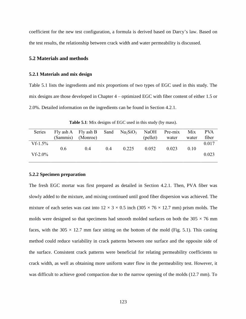
123

coefficient for the new test configuration, a formula is derived based on Darcy’s law. Based on

the test results, the relationship between crack width and water permeability is discussed.

5.2 Materials and methods

5.2.1 Materials and mix design

Table 5.1 lists the ingredients and mix proportions of two types of EGC used in this study. The

mix designs are those developed in Chapter 4 – optimized EGC with fiber content of either 1.5 or

2.0%. Detailed information on the ingredients can be found in Section 4.2.1.

Table 5.1: Mix designs of EGC used in this study (by mass).

Series Fly ash A

(Sammis)

Fly ash B

(Monroe)

Sand Na2SiO3 NaOH

(pellet)

Pre-mix

water

Mix

water

PVA

fiber

Vf-1.5% 0.6 0.4 0.4 0.225 0.052 0.023 0.10

0.017

Vf-2.0% 0.023

5.2.2 Specimen preparation

The fresh EGC mortar was first prepared as detailed in Section 4.2.1. Then, PVA fiber was

slowly added to the mixture, and mixing continued until good fiber dispersion was achieved. The

mixture of each series was cast into 12 × 3 × 0.5 inch (305 × 76 × 12.7 mm) prism molds. The

molds were designed so that specimens had smooth molded surfaces on both the 305 × 76 mm

faces, with the 305 × 12.7 mm face sitting on the bottom of the mold (Fig. 5.1). This casting

method could reduce variability in crack patterns between one surface and the opposite side of

the surface. Consistent crack patterns were beneficial for relating permeability coefficients to

crack width, as well as obtaining more uniform water flow in the permeability test. However, it

was difficult to achieve good compaction due to the narrow opening of the molds (12.7 mm). To

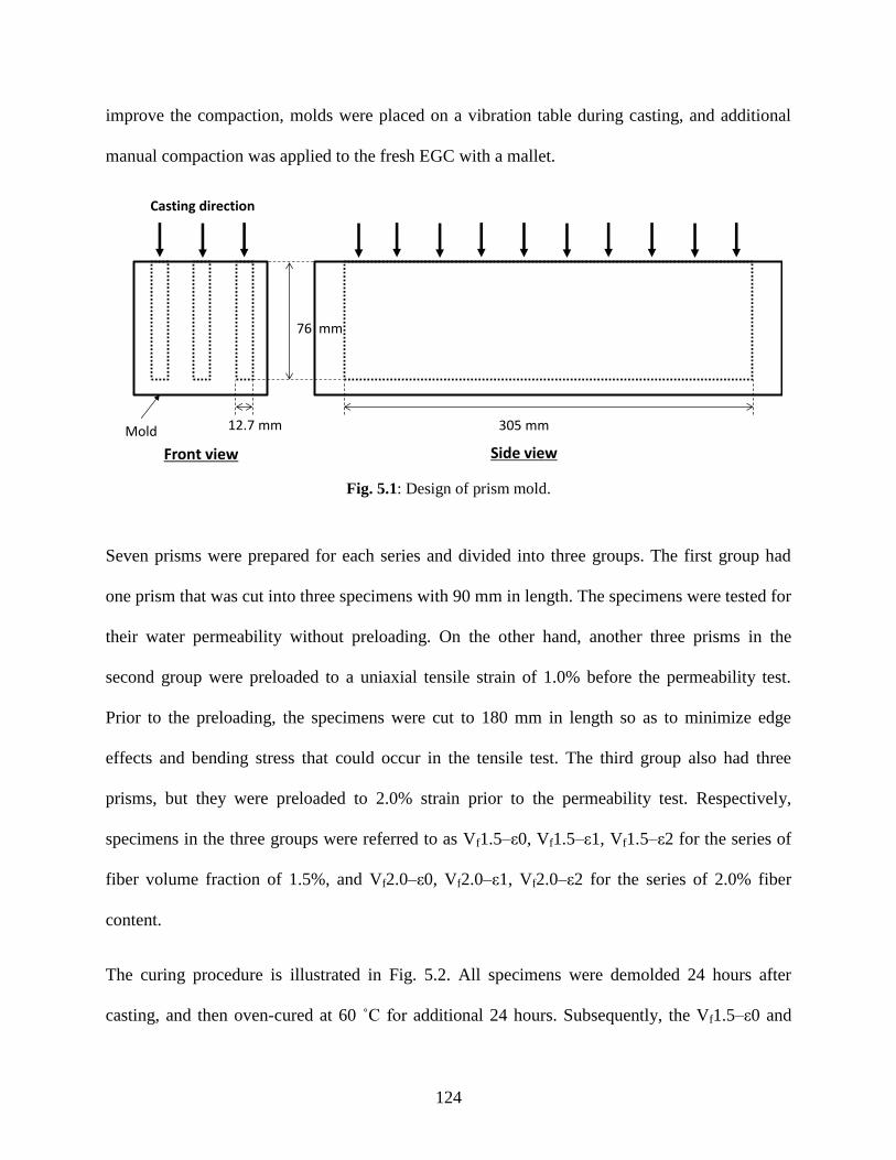
124

improve the compaction, molds were placed on a vibration table during casting, and additional

manual compaction was applied to the fresh EGC with a mallet.

Fig. 5.1: Design of prism mold.

Seven prisms were prepared for each series and divided into three groups. The first group had

one prism that was cut into three specimens with 90 mm in length. The specimens were tested for

their water permeability without preloading. On the other hand, another three prisms in the

second group were preloaded to a uniaxial tensile strain of 1.0% before the permeability test.

Prior to the preloading, the specimens were cut to 180 mm in length so as to minimize edge

effects and bending stress that could occur in the tensile test. The third group also had three

prisms, but they were preloaded to 2.0% strain prior to the permeability test. Respectively,

specimens in the three groups were referred to as Vf1.5–ε0, Vf1.5–ε1, Vf1.5–ε2 for the series of

fiber volume fraction of 1.5%, and Vf2.0–ε0, Vf2.0–ε1, Vf2.0–ε2 for the series of 2.0% fiber

content.

The curing procedure is illustrated in Fig. 5.2. All specimens were demolded 24 hours after

casting, and then oven-cured at 60 ˚C for additional 24 hours. Subsequently, the Vf1.5–ε0 and

12.7 mm

76 mm

305 mmMold

Casting direction

Front view Side view

125

Vf2.0–ε0 specimens were cured at room temperature (23 ± 3 ˚C) for 12 days, followed by water

curing at room temperature for at least 14 days (i.e. age of 28 days or older). In this curing

method, the specimens are water-saturated and at least 28 days old prior to permeability testing.

The water saturation ensures steady-state water flow through the specimens during the

permeability testing, which is a required condition for using Darcy’s law to compute the

permeability coefficient. In the case of preloaded specimens, the same oven-curing method was

applied but the subsequent room-temperature curing continued for 26 days. The specimens were

then loaded at the age of 28 days. After the preloading, the cracked specimens were sectioned

into 90 mm in length to fit the permeability test apparatus, and cured in a water bath for at least

14 days prior to the permeability test, as in the uncracked specimens.

Fig. 5.2: Curing conditions for intact and cracked EGC specimens prior to permeability testing.

5.2.3 Preloading and crack width measurement

The 1%- and 2%-strain specimens were loaded in uniaxial tension under displacement control at

the rate of 0.5 mm/min. Prior to the preloading, aluminum plates were glued to both ends of the

specimens so as to facilitate the gripping of the specimens by the load frame. Two LVDTs were

attached to each specimen for measuring extensions within gauge length of about 80 mm.

Tensile strain was computed from the average of extensions divided by the gauge length.

Specimen age (days)

0 42

Permeability testing

Preloading

Vf1.5–ε0, Vf2.0–ε0

21 14 28

Air, 23 ± 3 ˚C

Oven, 60 ˚C

Air, 23 ± 3 ˚C Water, 23 ± 3 ˚C

Permeability testingWater, 23 ± 3 ˚CAir, 23 ± 3 ˚CVf1.5–ε1, Vf1.5–ε2

Vf2.0–ε1, Vf2.0–ε2

126

Once the desired strain level was reached, the load was incrementally removed from the

specimens to obtain their unloading stress-strain curves. The unloaded specimens were then

observed by a digital optical microscope to record the number of microcracks and their crack

width. To accurately characterize the crack patterns, crack-width measurement was performed

across three lines parallel to the loaded direction, which were drawn on the center and both near-

edge sides of the specimen surface. Variability in crack width between one surface and the other

side was assumed to be small, because of the employed casting method mentioned above.

5.2.4 Permeability testing

The permeability-test setup in this study followed the falling-head test method proposed by

Wang et al. [3]. Figure 5.3 schematically illustrates the apparatus developed by Lepech and Li

[13]. The specimen was mounted and clamped between the top and bottom open-head containers,

both of which were filled with water. Water permeated from the top to bottom because of the

pressure head. The test started with filling both the inflow and outflow pipes with water, and the

water-level decrease in the inflow pipe was measured at regular time intervals. The outflow-pipe

water level was kept constant since extra water overflowed from the end of the pipe. The water-

pressure head was thus measured between the falling water level and the constant outflow-pipe

water level.

For this test configuration, Wang et al. derived the following formula to calculate the

permeability coefficient (k, in cm/sec), based on the Darcy’s law [3]:

f

in

h

h

At

Lak 0ln (5.1)

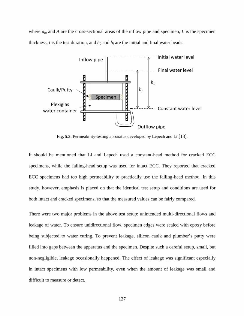
127

where ain and A are the cross-sectional areas of the inflow pipe and specimen, L is the specimen

thickness, t is the test duration, and h0 and hf are the initial and final water heads.

Fig. 5.3: Permeability-testing apparatus developed by Lepech and Li [13].

It should be mentioned that Li and Lepech used a constant-head method for cracked ECC

specimens, while the falling-head setup was used for intact ECC. They reported that cracked

ECC specimens had too high permeability to practically use the falling-head method. In this

study, however, emphasis is placed on that the identical test setup and conditions are used for

both intact and cracked specimens, so that the measured values can be fairly compared.

There were two major problems in the above test setup: unintended multi-directional flows and

leakage of water. To ensure unidirectional flow, specimen edges were sealed with epoxy before

being subjected to water curing. To prevent leakage, silicon caulk and plumber’s putty were

filled into gaps between the apparatus and the specimen. Despite such a careful setup, small, but

non-negligible, leakage occasionally happened. The effect of leakage was significant especially

in intact specimens with low permeability, even when the amount of leakage was small and

difficult to measure or detect.

Inflow pipe

Outflow pipe

Specimen

Caulk/Putty

Plexiglaswater container

Initial water level

Final water level

Constant water level

h0

hf

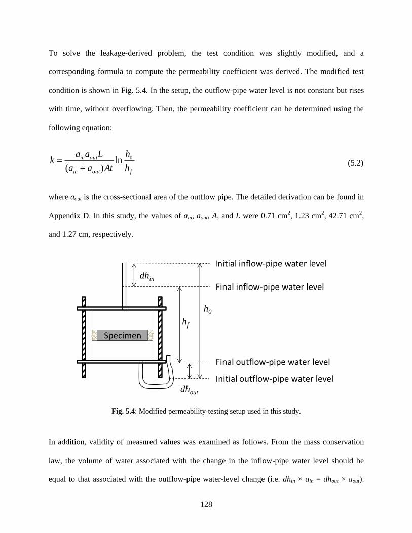
128

To solve the leakage-derived problem, the test condition was slightly modified, and a

corresponding formula to compute the permeability coefficient was derived. The modified test

condition is shown in Fig. 5.4. In the setup, the outflow-pipe water level is not constant but rises

with time, without overflowing. Then, the permeability coefficient can be determined using the

following equation:

foutin

outin

h

h

Ataa

Laak 0ln

)( (5.2)

where aout is the cross-sectional area of the outflow pipe. The detailed derivation can be found in

Appendix D. In this study, the values of ain, aout, A, and L were 0.71 cm2, 1.23 cm

2, 42.71 cm

2,

and 1.27 cm, respectively.

Fig. 5.4: Modified permeability-testing setup used in this study.

In addition, validity of measured values was examined as follows. From the mass conservation

law, the volume of water associated with the change in the inflow-pipe water level should be

equal to that associated with the outflow-pipe water-level change (i.e. dhin × ain = dhout × aout).

Specimen

Initial inflow-pipe water level

Final inflow-pipe water level

Initial outflow-pipe water level

h0

hf

Final outflow-pipe water level

dhin

dhout

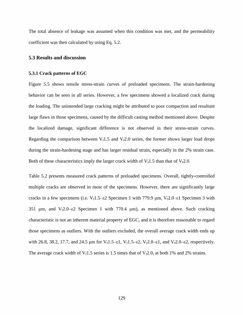
129

The total absence of leakage was assumed when this condition was met, and the permeability

coefficient was then calculated by using Eq. 5.2.

5.3 Results and discussion

5.3.1 Crack patterns of EGC

Figure 5.5 shows tensile stress-strain curves of preloaded specimens. The strain-hardening

behavior can be seen in all series. However, a few specimens showed a localized crack during

the loading. The unintended large cracking might be attributed to poor compaction and resultant

large flaws in those specimens, caused by the difficult casting method mentioned above. Despite

the localized damage, significant difference is not observed in their stress-strain curves.

Regarding the comparison between Vf1.5 and Vf2.0 series, the former shows larger load drops

during the strain-hardening stage and has larger residual strain, especially in the 2% strain case.

Both of these characteristics imply the larger crack width of Vf1.5 than that of Vf2.0.

Table 5.2 presents measured crack patterns of preloaded specimens. Overall, tightly-controlled

multiple cracks are observed in most of the specimens. However, there are significantly large

cracks in a few specimens (i.e. Vf1.5–ε2 Specimen 1 with 779.9 μm, Vf2.0–ε1 Specimen 3 with

351 μm, and Vf2.0–ε2 Specimen 1 with 770.4 μm), as mentioned above. Such cracking

characteristic is not an inherent material property of EGC, and it is therefore reasonable to regard

those specimens as outliers. With the outliers excluded, the overall average crack width ends up

with 26.8, 38.2, 17.7, and 24.5 μm for Vf1.5–ε1, Vf1.5–ε2, Vf2.0–ε1, and Vf2.0–ε2, respectively.

The average crack width of Vf1.5 series is 1.5 times that of Vf2.0, at both 1% and 2% strains.

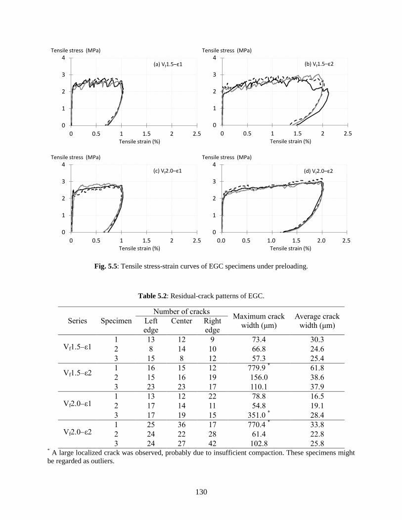
130

Fig. 5.5: Tensile stress-strain curves of EGC specimens under preloading.

Table 5.2: Residual-crack patterns of EGC.

Series Specimen

Number of cracks Maximum crack

width (μm)

Average crack

width (μm) Left

edge

Center Right

edge

Vf1.5–ε1 1 13 12 9 73.4 30.3

2 8 14 10 66.8 24.6

3 15 8 12 57.3 25.4

Vf1.5–ε2 1 16 15 12 779.9

* 61.8

2 15 16 19 156.0 38.6

3 23 23 17 110.1 37.9

Vf2.0–ε1 1 13 12 22 78.8 16.5

2 17 14 11 54.8 19.1

3 17 19 15 351.0 * 28.4

Vf2.0–ε2 1 25 36 17 770.4

* 33.8

2 24 22 28 61.4 22.8

3 24 27 42 102.8 25.8 * A large localized crack was observed, probably due to insufficient compaction. These specimens might

be regarded as outliers.

0

1

2

3

4

0 0.5 1 1.5 2 2.5Tensile strain (%)


(a) Vf1.5–ε1

0

1

2

3

4

0 0.5 1 1.5 2 2.5Tensile strain (%)


(b) Vf1.5–ε2

0

1

2

3

4

0 0.5 1 1.5 2 2.5Tensile strain (%)


(c) Vf2.0–ε1

0

1

2

3

4

0.0 0.5 1.0 1.5 2.0 2.5Tensile strain (%)


(d) Vf2.0–ε2

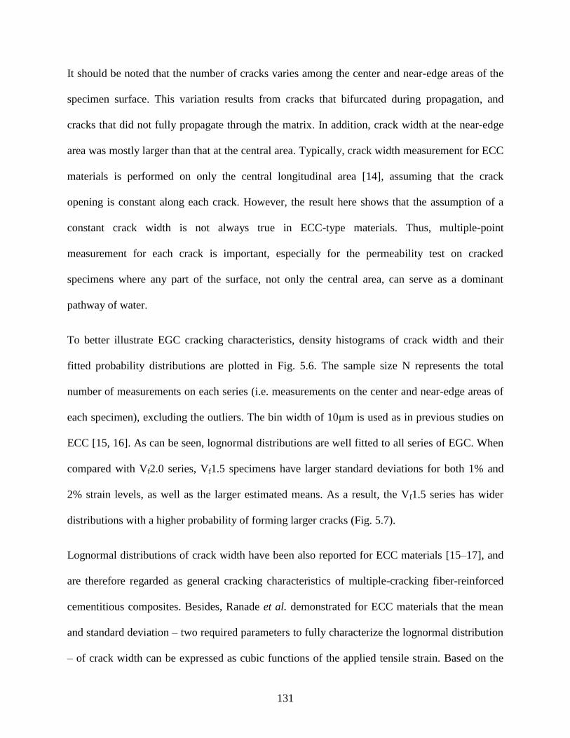
131

It should be noted that the number of cracks varies among the center and near-edge areas of the

specimen surface. This variation results from cracks that bifurcated during propagation, and

cracks that did not fully propagate through the matrix. In addition, crack width at the near-edge

area was mostly larger than that at the central area. Typically, crack width measurement for ECC

materials is performed on only the central longitudinal area [14], assuming that the crack

opening is constant along each crack. However, the result here shows that the assumption of a

constant crack width is not always true in ECC-type materials. Thus, multiple-point

measurement for each crack is important, especially for the permeability test on cracked

specimens where any part of the surface, not only the central area, can serve as a dominant

pathway of water.

To better illustrate EGC cracking characteristics, density histograms of crack width and their

fitted probability distributions are plotted in Fig. 5.6. The sample size N represents the total

number of measurements on each series (i.e. measurements on the center and near-edge areas of

each specimen), excluding the outliers. The bin width of 10μm is used as in previous studies on

ECC [15, 16]. As can be seen, lognormal distributions are well fitted to all series of EGC. When

compared with Vf2.0 series, Vf1.5 specimens have larger standard deviations for both 1% and

2% strain levels, as well as the larger estimated means. As a result, the Vf1.5 series has wider

distributions with a higher probability of forming larger cracks (Fig. 5.7).

Lognormal distributions of crack width have been also reported for ECC materials [15–17], and

are therefore regarded as general cracking characteristics of multiple-cracking fiber-reinforced

cementitious composites. Besides, Ranade et al. demonstrated for ECC materials that the mean

and standard deviation – two required parameters to fully characterize the lognormal distribution

– of crack width can be expressed as cubic functions of the applied tensile strain. Based on the

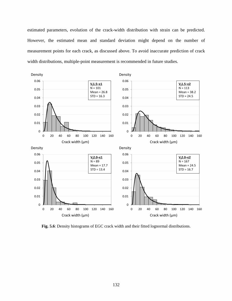
132

estimated parameters, evolution of the crack-width distribution with strain can be predicted.

However, the estimated mean and standard deviation might depend on the number of

measurement points for each crack, as discussed above. To avoid inaccurate prediction of crack

width distributions, multiple-point measurement is recommended in future studies.

Fig. 5.6: Density histograms of EGC crack width and their fitted lognormal distributions.

0

0.01

0.02

0.03

0.04

0.05

0.06

0 20 40 60 80 100 120 140 160

Density

Crack width (μm)

Vf1.5–ε1N = 101Mean = 26.8STD = 16.3

0

0.01

0.02

0.03

0.04

0.05

0.06

0 20 40 60 80 100 120 140 160

Density

Crack width (μm)

Vf1.5–ε2N = 113Mean = 38.2STD = 24.5

0

0.01

0.02

0.03

0.04

0.05

0.06

0 20 40 60 80 100 120 140 160

Density

Crack width (μm)

Vf2.0–ε1N = 89Mean = 17.7STD = 13.4

0

0.01

0.02

0.03

0.04

0.05

0.06

0 20 40 60 80 100 120 140 160

Density

Crack width (μm)

Vf2.0–ε2N = 167Mean = 24.5STD = 16.7

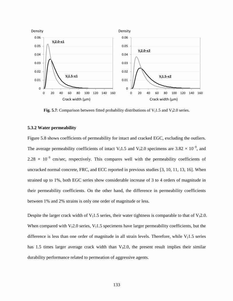
133

Fig. 5.7: Comparison between fitted probability distributions of Vf1.5 and Vf2.0 series.

5.3.2 Water permeability

Figure 5.8 shows coefficients of permeability for intact and cracked EGC, excluding the outliers.

The average permeability coefficients of intact Vf1.5 and Vf2.0 specimens are 3.82 × 10–9

, and

2.28 × 10–9

cm/sec, respectively. This compares well with the permeability coefficients of

uncracked normal concrete, FRC, and ECC reported in previous studies [3, 10, 11, 13, 16]. When

strained up to 1%, both EGC series show considerable increase of 3 to 4 orders of magnitude in

their permeability coefficients. On the other hand, the difference in permeability coefficients

between 1% and 2% strains is only one order of magnitude or less.

Despite the larger crack width of Vf1.5 series, their water tightness is comparable to that of Vf2.0.

When compared with Vf2.0 series, Vf1.5 specimens have larger permeability coefficients, but the

difference is less than one order of magnitude in all strain levels. Therefore, while Vf1.5 series

has 1.5 times larger average crack width than Vf2.0, the present result implies their similar

durability performance related to permeation of aggressive agents.

0

0.01

0.02

0.03

0.04

0.05

0.06

0 20 40 60 80 100 120 140 160

Density

Crack width (μm)

Vf1.5–ε1

Vf2.0–ε1

0

0.01

0.02

0.03

0.04

0.05

0.06

0 20 40 60 80 100 120 140 160

Density

Crack width (μm)

Vf1.5–ε2

Vf2.0–ε2

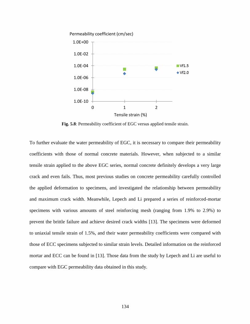
134

Fig. 5.8: Permeability coefficient of EGC versus applied tensile strain.

To further evaluate the water permeability of EGC, it is necessary to compare their permeability

coefficients with those of normal concrete materials. However, when subjected to a similar

tensile strain applied to the above EGC series, normal concrete definitely develops a very large

crack and even fails. Thus, most previous studies on concrete permeability carefully controlled

the applied deformation to specimens, and investigated the relationship between permeability

and maximum crack width. Meanwhile, Lepech and Li prepared a series of reinforced-mortar

specimens with various amounts of steel reinforcing mesh (ranging from 1.9% to 2.9%) to

prevent the brittle failure and achieve desired crack widths [13]. The specimens were deformed

to uniaxial tensile strain of 1.5%, and their water permeability coefficients were compared with

those of ECC specimens subjected to similar strain levels. Detailed information on the reinforced

mortar and ECC can be found in [13]. Those data from the study by Lepech and Li are useful to

compare with EGC permeability data obtained in this study.

1.0E-10

1.0E-08

1.0E-06

1.0E-04

1.0E-02

1.0E+00

0 1 2

Tensile strain (%)

Permeability coefficient (cm/sec)

135

Figure 5.9 shows the comparison of permeability coefficients for EGC, ECC and reinforced

cement mortar. Permeability coefficients of cracked reinforced mortars range from 3.02 × 10–6

to

4.46 × 10–2

cm/sec. Only one of the series shows a comparable permeability to cracked EGC, but

the specimen has a high amount of steel reinforcement of 2.9%, which is not economical in

practice. Therefore, when subjected to the same strain level, degradation in water permeability is

significantly limited in EGC compared to typical reinforced mortar/concrete. On the other hand,

cracked ECC shows better water tightness than cracked EGC: their permeability coefficients

range from 1.95 × 10–8

to 7.74 × 10–8

cm/sec, which are 2 to 3 orders of magnitude smaller than

those of cracked EGC, even at a tensile strain of 3%.

Fig. 5.9: Comparison of permeability coefficients for EGC, ECC and reinforced cement mortar.

The test results also show that permeability coefficients are highly dependent on crack width,

regardless of the material type. The reinforced-mortar specimen that shows comparable

permeability to EGC has similar maximum crack width and number of cracks to those of EGC.

Other reinforced mortars have fewer cracks with a large localized crack of 240 to 500 µm, and

1.0E-10

1.0E-08

1.0E-06

1.0E-04

1.0E-02

1.0E+00

0 1 2 3

Tensile strain (%)


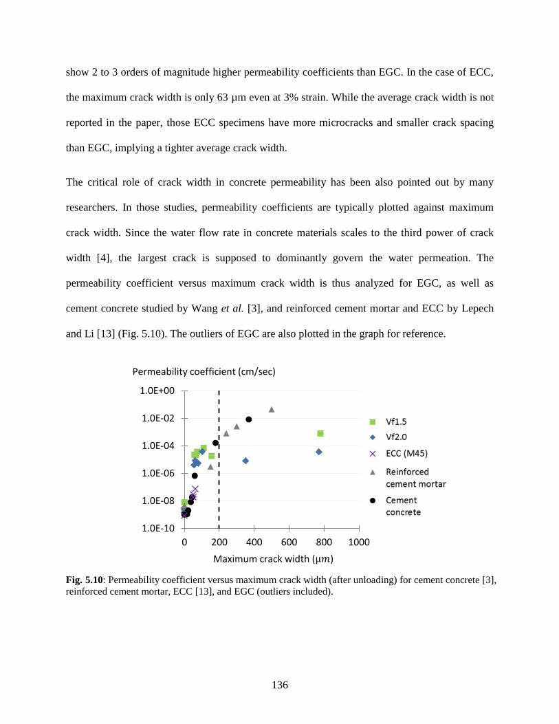
136

show 2 to 3 orders of magnitude higher permeability coefficients than EGC. In the case of ECC,

the maximum crack width is only 63 µm even at 3% strain. While the average crack width is not

reported in the paper, those ECC specimens have more microcracks and smaller crack spacing

than EGC, implying a tighter average crack width.

The critical role of crack width in concrete permeability has been also pointed out by many

researchers. In those studies, permeability coefficients are typically plotted against maximum

crack width. Since the water flow rate in concrete materials scales to the third power of crack

width [4], the largest crack is supposed to dominantly govern the water permeation. The

permeability coefficient versus maximum crack width is thus analyzed for EGC, as well as

cement concrete studied by Wang et al. [3], and reinforced cement mortar and ECC by Lepech

and Li [13] (Fig. 5.10). The outliers of EGC are also plotted in the graph for reference.

Fig. 5.10: Permeability coefficient versus maximum crack width (after unloading) for cement concrete [3],

reinforced cement mortar, ECC [13], and EGC (outliers included).

1.0E-10

1.0E-08

1.0E-06

1.0E-04

1.0E-02

1.0E+00

0 200 400 600 800 1000

Maximum crack width ( )


137

For crack width of less than 200 µm, similar increasing trends in the permeability coefficient can

be seen in all the materials. Data on EGC do not include the outliers in this range and therefore

represent the inherent property of EGC permeability. It should be noted, however, that EGC

specimens have many microcracks in the tested area, with a small variance in crack width. In

such cases, many cracks – not only the largest one – can serve as a significant pathway of water.

In contrast, concrete and reinforced mortar have fewer cracks, with damage localized in a single

crack. The largest crack has a dominant effect on the permeability in such materials. Therefore,

when related to maximum crack width, EGC permeability coefficients tend to be overestimated

compared to normal concrete materials. The same is true for ECC materials. To make a fair

comparison, Lepech and Li suggested normalizing the permeability coefficients of cracked ECC

by the number of cracks [13]. By applying this normalization, permeability coefficients of EGC

compare well to those of concrete and reinforced mortar.

A different trend can be seen in data for crack width of over 200 µm: permeability coefficients of

EGC are limited compared to those of concrete and reinforced mortar in this range. As discussed

in the preceding section, those EGC specimens have localized large cracking and do not reflect

the inherent cracking characteristics of EGC. However, if the quality of workmanship were poor

in actual applications, it might be possible for such a large crack to form in the EGC structure.

The test result implies that EGC can significantly limit the permeability increase even in the

unfavorable case. On the other hand, a large crack is not uncommon in RC structures even when

the concrete is well compacted and finished. Then, water permeability of the structure

considerably increases with crack opening, as suggested by the data of concrete and reinforced

mortar in Fig. 5.10.

138

The limited EGC permeability for crack width of over 200 µm might be attributed to the unique

distribution of damage. As mentioned in the preceding section, crack width in EGC is not

constant along each crack. The unintended large cracking mostly started from the edge of the

specimen, but the localized damage did not propagate fast and was confined to the near-edge

area. Indeed, the measured maximum crack width only represents the crack opening at a small

area. As a result, the rate of water flow in that small area might not be dominant in the total flow

rate of the tested area. This could explain the little correlation between permeability coefficient

and maximum crack width of EGC, especially for Vf2.0 series. It should be noted that ECC

materials with unintended poor compaction or fiber dispersion typically exhibit strain-softening

behavior with a localized crack that propagates through the matrix much faster. Further research

is required to understand mechanisms behind the suppressed propagation of unintended localized

cracking in EGC.

From the discussion above, the maximum crack width is not an appropriate factor to relate the

water permeability of EGC. However, when plotted against average crack width, EGC

permeability shows a distinct positive correlation even when the outliers are included (Fig. 5.11).

Particularly, a linear relationship can be seen between the average crack width and the log of

permeability coefficient of cracked EGC. While few previous studies focused on the average

crack width of the tested specimens, it might be possible to predict water permeability from

average crack width for ECC-type materials. Further research is also needed to verify this

hypothesis.

139

Fig. 5.11: Permeability coefficient versus average crack width of EGC.

5.3.3 Sealed cracks and reduction in permeability

During the course of this study, a possibility of self-healing in EGC was discovered. There was

an extra specimen that was preloaded to create microcracks and then stored in water for months.

Interestingly, white substance was formed on the specimen surface, especially within the cracks.

The same phenomenon was also reported for ECC in previous studies [13, 18]. As a result of the

sealed cracks, cracked ECC specimens showed significant decrease in permeability coefficients

(i.e. recovery in water tightness) with time. This could be another reason that permeability

coefficients of cracked ECC are significantly lower than those of EGC, apart from the difference

in crack width (discussed in the preceding section). The white substance in EGC implied that a

similar decrease in the permeability was possible. Therefore, the preloaded specimens used in the

permeability test were moved back to a water bath after the test, and cured for about 90 days

prior to the second round of the permeability measurement.

1.0E-10

1.0E-08

1.0E-06

1.0E-04

1.0E-02

1.0E+00

0 20 40 60 80

Average crack width (μ )


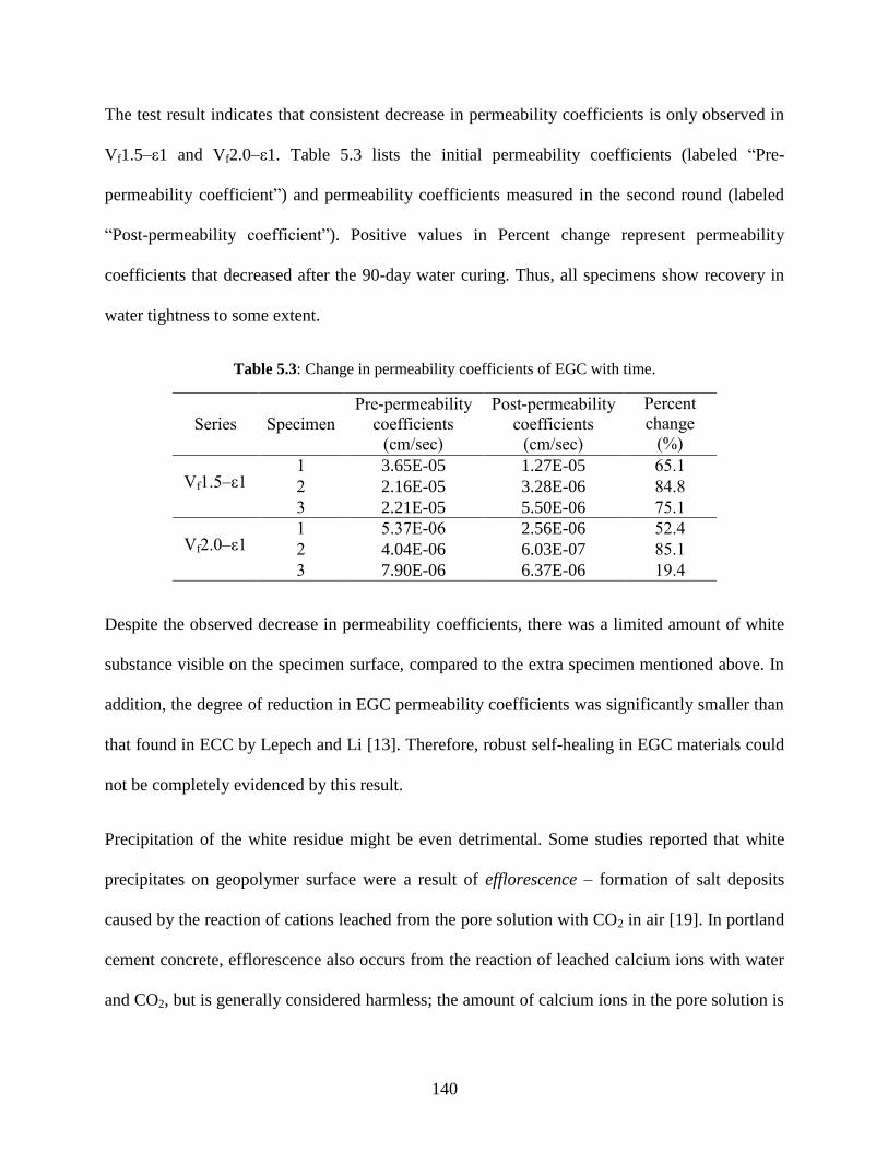
140

The test result indicates that consistent decrease in permeability coefficients is only observed in

Vf1.5–ε1 and Vf2.0–ε1. Table 5.3 lists the initial permeability coefficients (labeled “Pre-

permeability coefficient”) and permeability coefficients measured in the second round (labeled

“Post-permeability coefficient”). Positive values in Percent change represent permeability

coefficients that decreased after the 90-day water curing. Thus, all specimens show recovery in

water tightness to some extent.

Table 5.3: Change in permeability coefficients of EGC with time.

Series Specimen

Pre-permeability

coefficients

(cm/sec)

Post-permeability

coefficients

(cm/sec)

Percent

change

(%)

Vf1.5–ε1 1 3.65E-05

1.27E-05

65.1

2 2.16E-05

3.28E-06

84.8

3 2.21E-05

5.50E-06

75.1

Vf2.0–ε1 1 5.37E-06 2.56E-06

52.4

2 4.04E-06

6.03E-07

85.1

3 7.90E-06

6.37E-06

19.4

Despite the observed decrease in permeability coefficients, there was a limited amount of white

substance visible on the specimen surface, compared to the extra specimen mentioned above. In

addition, the degree of reduction in EGC permeability coefficients was significantly smaller than

that found in ECC by Lepech and Li [13]. Therefore, robust self-healing in EGC materials could

not be completely evidenced by this result.

Precipitation of the white residue might be even detrimental. Some studies reported that white

precipitates on geopolymer surface were a result of efflorescence – formation of salt deposits

caused by the reaction of cations leached from the pore solution with CO2 in air [19]. In portland

cement concrete, efflorescence also occurs from the reaction of leached calcium ions with water

and CO2, but is generally considered harmless; the amount of calcium ions in the pore solution is

141

typically limited, and the effect of efflorescence on binder degradation is thus negligible.

Conversely, efflorescence in geopolymers might be a significant issue because of the higher

concentrations of soluble alkali metal cations available [20]. Indeed, Zhang et al. found that

efflorescence had negative effects on compressive strength and stiffness of fly ash-based

geopolymers [21]. Therefore, it is important to know whether the white substance formed in

EGC results from beneficial self-healing or detrimental efflorescence. Further research to address

this question has been conducted, which is reported in the following chapter.


Cracking characteristics and water tightness have been experimentally determined for the

developed EGC with fiber contents of 1.5% and 2.0%. The test result indicates that Vf1.5 series

has 1.5 times larger crack width on average than Vf2.0 series. Nevertheless, their water

permeability is comparable at both 1% and 2% strain levels. It is therefore suggested that the

Vf1.5 series has comparable transport properties and related durability to the Vf2.0, even with

the smaller fiber content. Combined with the results on their mechanical properties and

environmental performances obtained in Chapter 4, it can be concluded that the Vf1.5 series is

preferable to Vf2.0. In addition, it has been found that degradation in water tightness of EGC is

significantly limited compared to that of normal reinforced mortar/concrete. This result suggests

better transport properties and related durability of EGC.

The other findings obtained in this study are listed below;

Residual crack width of EGC is lognormally distributed for both 1% and 2% strain levels.

142

A few specimens showed a localized large crack during the uniaxial tension test, but the

crack did not propagate through the matrix and the damage was confined to the near-edge

area. Mechanisms behind this suppressed propagation of localized cracking would be a

subject of further studies.

Crack width of EGC is not constant along each crack, and the numbers of cracks are

different between the central area and near-edge sides of the specimen surface. Measuring

multiple points for each crack is recommended to accurately evaluate the crack patterns.

Due to the nonuniform opening along each crack, maximum crack width only represents the

crack opening in a small area. As a result, there is little correlation between the maximum

crack width and permeability coefficients of EGC.

Instead, a distinct linear relationship is observed between average crack width and

permeability coefficient. It might be possible to predict EGC water permeability from the

average crack width, but further research is required to verify the hypothesis.

During the course of this study, a white substance formed on the specimen surface and

blocking the microcracks was observed. Time-dependent decrease in permeability

coefficients has been also confirmed in specimens subjected to 1% strain.

The last finding suggests a possibility of self-healing phenomenon in EGC materials. However, it

is also possible that precipitation of the white substance resulted from efflorescence, which could

be detrimental to mechanical properties of geopolymers. Thus, a further investigation on the

white precipitate is required to confirm the feasibility of self-healing EGC. The following

chapter is concerned with this.

143

References

[1] N. R. Buenfeld, “Measuring and modeling transport phenomena in concrete for life

prediction of structures,” in Prediction of concrete durability: proceedings of STATS 21st

anniversary conference, J. Glanville and A. Neville, Eds. London, UK: E & FN Spon,

1995, pp. 77–90.

[2] H. W. Reinhardt, “Transport Properties of Concrete,” in Penetration and Permeability of

Concrete: Barriers to organic and contaminating liquids, H. W. Reinhardt, Ed. London,

UK: E & FN Spon, 1997, pp. 213–264.

[3] K. Wang, D. C. Jansen, S. P. Shah, and A. F.KArr, “Permeability study of cracked

concrete,” Cem. Concr. Res., vol. 27, no. 3, pp. 381–393, 1997.

[4] M. Tsukamoto, “Tightness of fiber concrete,” Darmstadt Concr., vol. 5, no. 3, pp. 215–

225, 1990.

[5] ACI 318S, Building Code Requirements for Structural Concrete and Commentary.

Farmington Hills, MI: American Concrete Institute, 2011.

[6] AASHTO, “AASHTO LRFD Bridge Design Specifications, 7th Edition,” 2014.

[7] ASTM C76-16, Standard Specification for Reinforced Concrete Culvert, Storm Drain,

and Sewer Pipe. West Conshohocken, PA: ASTM International, 2016.

[8] V. Li and H. Stang, “Elevating FRC material ductility to infrastructure durability,” in 6th

RILEM Symposium on Fiber-Reinforced Concretes (FRC) - BEFIB 2004, 2004, pp. 1–16.

[9] C.-M. Aldea, S. P. Shah, and K. Alan, “Effect of cracking on water and chloride

permeability of concrete,” J. Mater. Civ. Eng., vol. 11, no. 3, pp. 181–187, 1999.

[10] C.-M. Aldea, S. P. Shah, and A. Karr, “Permeability of cracked concrete,” Mater. Struct.,

vol. 32, no. 5, pp. 370–376, 1999.

[11] J. Rapoport, C.-M. Aldea, S. P. Shah, B. Ankenman, and A. Karr, “Permeability of

Cracked Steel Fiber-Reinforced Concrete,” J. Mater. Civ. Eng., vol. 14, no. 4, pp. 355–

358, Aug. 2002.

[12] J. S. Lawler, D. Zampini, and S. P. Shah, “Permeability of cracked hybrid fiber-reinforced

mortar under load,” ACI Mater. J., vol. 99, no. 4, pp. 379–385, 2002.

[13] M. D. Lepech and V. C. Li, “Water permeability of engineered cementitious composites,”

Cem. Concr. Compos., vol. 31, no. 10, pp. 744–753, Nov. 2009.

[14] Japan Society of Civil Engineers, Recommendations for Design and Construction of High

Performance Fiber Reinforced Cement Composites with Multiple Fine Cracks

(HPFRCC ), vol. 82. Tokyo, Japan: JSCE, 2008.

144

[15] R. Ranade, J. Zhang, J. P. Lynch, and V. C. Li, “Influence of micro-cracking on the

composite resistivity of Engineered Cementitious Composites,” Cem. Concr. Res., vol. 58,

pp. 1–12, Apr. 2014.

[16] H. Liu, Q. Zhang, C. Gu, H. Su, and V. C. Li, “Influence of micro-cracking on the

permeability of Engineered Cementitious Composites,” Cem. Concr. Res., vol. 72, pp.

104–113, 2016.

[17] P. Wang, F. H. Wittmann, T. Zhao, and W. Huang, “EVOLUTION OF CRACK

PATTERNS ON SHCC AS FUNCTION OF IMPOSED STRAIN,” in 2nd int. RILEM

conf. on strain hardening cementitious composites, 2011, pp. 217–224.

[18] H. Liu, Q. Zhang, C. Gu, H. Su, and V. Li, “Influence of microcrack self-healing behavior

on the permeability of Engineered Cementitious Composites,” Cem. Concr. Compos., vol.

82, pp. 14–22, 2017.

[19] J. L. Provis and S. A. Bernal, “Geopolymers and Related Alkali-Activated Materials,”

Annu. Rev. Mater. Res, vol. 44, pp. 299–327, 2014.

[20] Z. Zhang, H. Wang, J. L. Provis, and A. Reid, “Efflorescence : A Critical Challenge for

Geopolymer Applications ?,” in Concrete Institute of Australia’s Biennial National

Conference, 2013.

[21] Z. H. Zhang, T. Yang, and H. Wang, “The Effect of Efflorescence on the Mechanical

Properties of Geopolymers,” in 23rd Australasian Conference on the Mechanics of

Structures and Materials, 2014, vol. I, pp. 107–112.

145

CHAPTER 6: Feasibility Study of Self-healing EGC

In this chapter, a feasibility study on self-healing functionality of EGC is documented. An

experimental investigation is conducted to measure the mechanical-performance recovery of pre-

cracked EGC due to self-healing. In addition, self-healing products are observed by scanning

electron microscopy (SEM) and examined using energy dispersive spectroscopy (EDS).

6.1 Introduction

Cement materials have inherent self-healing functionality. Indeed, autogenous healing of cracks

in cement concrete has been reported for many years, even since the 19th century [1]. Early

academic research on the phenomenon dates back to the end of 19th century [2], and active

research activities have been done in the past few decades. Based on the intensive studies, three

major mechanisms have been proposed for the self-healing phenomenon in cement-based

materials:

Hydration of unreacted cement – unhydrated cement in the hardened matrix reacts with

water in cracks, creating calcium silicate hydrates (CSH) and other hydration products.

Calcite (CaCO3) formation – binding of calcium ions on crack surfaces with carbonate ions

dissolved from atmospheric carbon dioxide (CO2).

Pozzolanic reaction – aluminate or silicate species and calcium hydroxide (CaOH) in the

matrix react with water, producing CSH and other phases.

146

Theoretically, self-healing can occur in the presence of only water and CO2 (i.e. under a normal

condition of most structures).

Recently, the concept of self-healing concrete has been gaining increasing attention. Particularly,

the technology is attractive to many developed countries facing a huge financial burden for repair

and rehabilitation of their aging infrastructure. Moreover, smart concrete structures that can

autogenously recover from damage are also promising for enhancing the resiliency for public

safety. Such societal needs are driving the active research and development of new technologies

to maximize the self-healing functionality of cement concrete. Today, various types of self-

healing concrete and relevant techniques have been developed, including encapsulation of

healing chemicals [3] or calcite-producing bacteria [4], inclusion of mineral admixtures [5], and

healing agents activated by a heating device embedded in the cement matrix [6].

ECC is another promising candidate for self-healing concrete. Yang et al. experimentally

demonstrated that ECC exhibits significant stiffness recovery (more than 80% of the initial

stiffness) even when strained up to 3% [7]. Herbert and Li also found that self-healing of ECC is

repeatable under multiple loading cycles [8]. Moreover, ECC has been demonstrated to self-heal

even under chloride or highly alkaline environments [9, 10]. More importantly, self-healing ECC

simply utilizes the intrinsic healing functionality of cement materials to achieve the high

performance recovery, repeatability, and versatility; in contrast, other technologies often require

cost-intensive additives, components, or devices to impart the self-healing capability to the

concrete material.

It is the self-controlled microcracking that realizes the enhanced self-healing in ECC. The tight

crack width is beneficial for self-healing products to precipitate and fully seal the crack.

147

Conversely, even if a material has a self-healing functionality, it cannot autogenously heal large

cracks, just as human bodies cannot cure serious wounds by themselves. Therefore, damage

control plays a key role in bringing out the healing potential of cement materials. The same may

be true for geopolymers; today, only a handful of papers have been published to report the self-

healing of geopolymers [5, 11, 12], which does not necessarily imply low/no self-healing

functionality of the material. If the crack width can be tightly controlled, robust self-healing

might also be possible in geopolymers.

The objective of this study is to demonstrate the feasibility of self-healing EGC. EGC specimens

are first uniaxially loaded to create cracks and subjected to three different conditioning regimes

prior to reloading: air-curing or water-curing for 120 days, or no curing (i.e. reloading right after

preloading). Stiffness recovery due to self-healing is evaluated by comparing the initial stiffness

of intact specimens and the residual stiffness in reloading. During the course of curing, cracks

are photographically recorded regularly, to capture the formation of healing products. In addition,

the microstructure of healing products is observed by using a scanning electron microscope

(SEM). An elemental analysis is also conducted by using an energy dispersive spectroscopy

(EDS) system.

6.2 Materials and methods

6.2.1 Mix design and specimen preparation

The mix design of EGC in this study is similar to the Vf2.0 series developed in Chapter 4. Table

6.1 presents the mix proportion of ingredients. A lower amount of sand was incorporated to

facilitate the self-healing by relatively increasing the paste volume. Also, the fiber volume

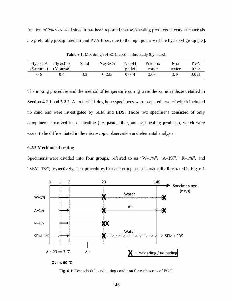
148

fraction of 2% was used since it has been reported that self-healing products in cement materials

are preferably precipitated around PVA fibers due to the high polarity of the hydroxyl group [13].

Table 6.1: Mix design of EGC used in this study (by mass).

Fly ash A

(Sammis)

Fly ash B

(Monroe)

Sand Na2SiO3 NaOH

(pellet)

Pre-mix

water

Mix

water

PVA

fiber

0.6 0.4 0.2 0.225 0.044 0.031 0.10 0.021

The mixing procedure and the method of temperature curing were the same as those detailed in

Section 4.2.1 and 5.2.2. A total of 11 dog bone specimens were prepared, two of which included

no sand and were investigated by SEM and EDS. Those two specimens consisted of only

components involved in self-healing (i.e. paste, fiber, and self-healing products), which were

easier to be differentiated in the microscopic observation and elemental analysis.

6.2.2 Mechanical testing

Specimens were divided into four groups, referred to as “W–1%”, ”A–1%”, ”R–1%”, and

“SEM–1%”, respectively. Test procedures for each group are schematically illustrated in Fig. 6.1.

Fig. 6.1: Test schedule and curing condition for each series of EGC.

Specimen age (days)

0

SEM / EDS

W–1%

21 28 148

Air, 23 ± 3 ˚C

Oven, 60 ˚C

Water

AirA–1%

R–1%

SEM–1%

X

X

X

X

Air

Water

X

X

X

X : Preloading / Reloading

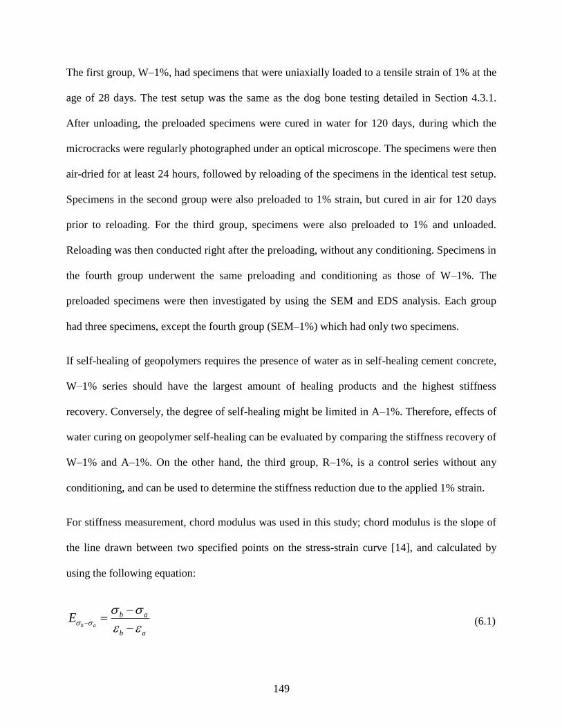
149

The first group, W–1%, had specimens that were uniaxially loaded to a tensile strain of 1% at the

age of 28 days. The test setup was the same as the dog bone testing detailed in Section 4.3.1.

After unloading, the preloaded specimens were cured in water for 120 days, during which the

microcracks were regularly photographed under an optical microscope. The specimens were then

air-dried for at least 24 hours, followed by reloading of the specimens in the identical test setup.

Specimens in the second group were also preloaded to 1% strain, but cured in air for 120 days

prior to reloading. For the third group, specimens were also preloaded to 1% and unloaded.

Reloading was then conducted right after the preloading, without any conditioning. Specimens in

the fourth group underwent the same preloading and conditioning as those of W–1%. The

preloaded specimens were then investigated by using the SEM and EDS analysis. Each group

had three specimens, except the fourth group (SEM–1%) which had only two specimens.

If self-healing of geopolymers requires the presence of water as in self-healing cement concrete,

W–1% series should have the largest amount of healing products and the highest stiffness

recovery. Conversely, the degree of self-healing might be limited in A–1%. Therefore, effects of

water curing on geopolymer self-healing can be evaluated by comparing the stiffness recovery of

W–1% and A–1%. On the other hand, the third group, R–1%, is a control series without any

conditioning, and can be used to determine the stiffness reduction due to the applied 1% strain.

For stiffness measurement, chord modulus was used in this study; chord modulus is the slope of

the line drawn between two specified points on the stress-strain curve [14], and calculated by

using the following equation:

ab

ab

abE

(6.1)

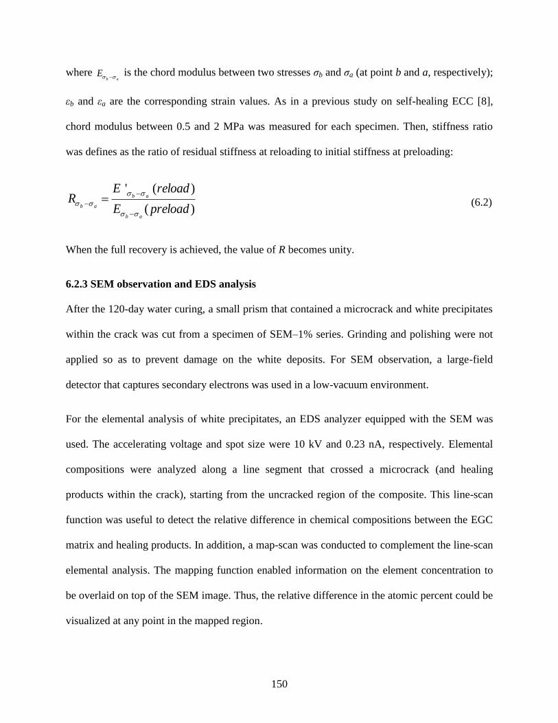
150

where ab

E is the chord modulus between two stresses σb and σa (at point b and a, respectively);

εb and εa are the corresponding strain values. As in a previous study on self-healing ECC [8],

chord modulus between 0.5 and 2 MPa was measured for each specimen. Then, stiffness ratio

was defines as the ratio of residual stiffness at reloading to initial stiffness at preloading:

)(

)('

preloadE

reloadER

ab

ab

ab

(6.2)

When the full recovery is achieved, the value of R becomes unity.

6.2.3 SEM observation and EDS analysis

After the 120-day water curing, a small prism that contained a microcrack and white precipitates

within the crack was cut from a specimen of SEM–1% series. Grinding and polishing were not

applied so as to prevent damage on the white deposits. For SEM observation, a large-field

detector that captures secondary electrons was used in a low-vacuum environment.

For the elemental analysis of white precipitates, an EDS analyzer equipped with the SEM was

used. The accelerating voltage and spot size were 10 kV and 0.23 nA, respectively. Elemental

compositions were analyzed along a line segment that crossed a microcrack (and healing

products within the crack), starting from the uncracked region of the composite. This line-scan

function was useful to detect the relative difference in chemical compositions between the EGC

matrix and healing products. In addition, a map-scan was conducted to complement the line-scan

elemental analysis. The mapping function enabled information on the element concentration to

be overlaid on top of the SEM image. Thus, the relative difference in the atomic percent could be

visualized at any point in the mapped region.

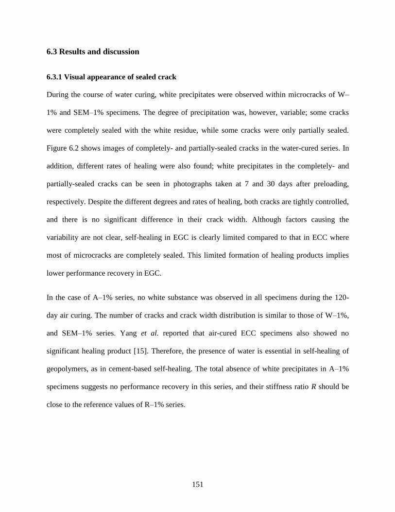
151


6.3.1 Visual appearance of sealed crack

During the course of water curing, white precipitates were observed within microcracks of W–

1% and SEM–1% specimens. The degree of precipitation was, however, variable; some cracks

were completely sealed with the white residue, while some cracks were only partially sealed.

Figure 6.2 shows images of completely- and partially-sealed cracks in the water-cured series. In

addition, different rates of healing were also found; white precipitates in the completely- and

partially-sealed cracks can be seen in photographs taken at 7 and 30 days after preloading,

respectively. Despite the different degrees and rates of healing, both cracks are tightly controlled,

and there is no significant difference in their crack width. Although factors causing the

variability are not clear, self-healing in EGC is clearly limited compared to that in ECC where

most of microcracks are completely sealed. This limited formation of healing products implies

lower performance recovery in EGC.

In the case of A–1% series, no white substance was observed in all specimens during the 120-

day air curing. The number of cracks and crack width distribution is similar to those of W–1%,

and SEM–1% series. Yang et al. reported that air-cured ECC specimens also showed no

significant healing product [15]. Therefore, the presence of water is essential in self-healing of

geopolymers, as in cement-based self-healing. The total absence of white precipitates in A–1%

specimens suggests no performance recovery in this series, and their stiffness ratio R should be

close to the reference values of R–1% series.

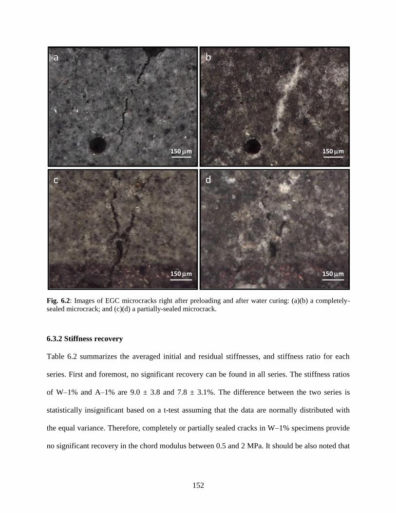
152

Fig. 6.2: Images of EGC microcracks right after preloading and after water curing: (a)(b) a completely-

sealed microcrack; and (c)(d) a partially-sealed microcrack.

6.3.2 Stiffness recovery

Table 6.2 summarizes the averaged initial and residual stiffnesses, and stiffness ratio for each

series. First and foremost, no significant recovery can be found in all series. The stiffness ratios

of W–1% and A–1% are 9.0 ± 3.8 and 7.8 ± 3.1%. The difference between the two series is

statistically insignificant based on a t-test assuming that the data are normally distributed with

the equal variance. Therefore, completely or partially sealed cracks in W–1% specimens provide

no significant recovery in the chord modulus between 0.5 and 2 MPa. It should be also noted that

150 m150 m

a b

150 m150 m

c d

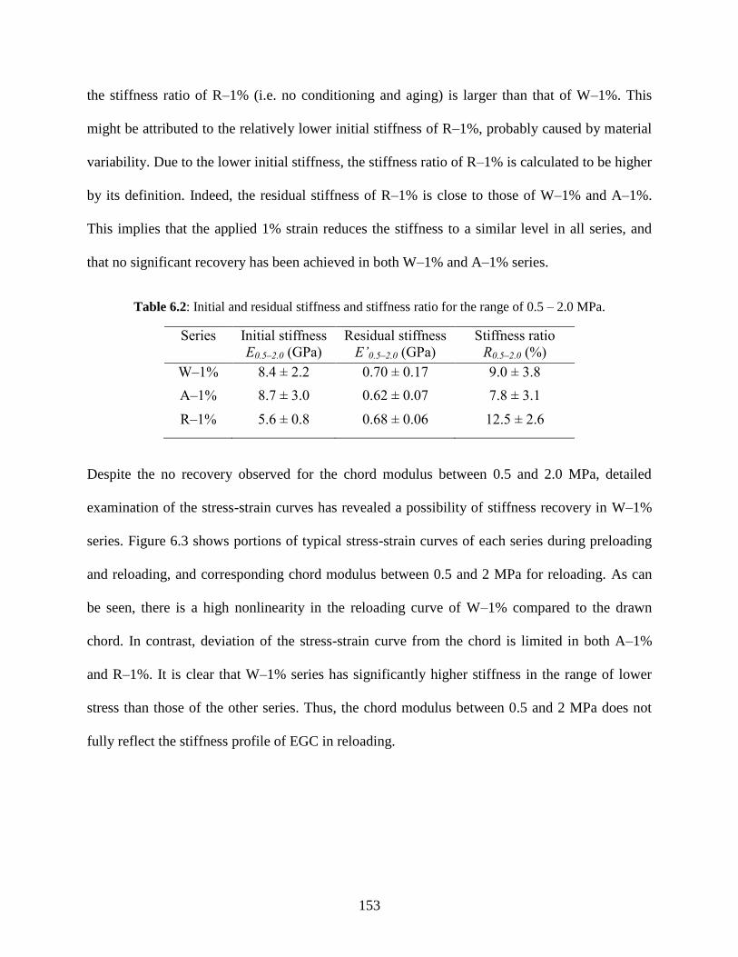
153

the stiffness ratio of R–1% (i.e. no conditioning and aging) is larger than that of W–1%. This

might be attributed to the relatively lower initial stiffness of R–1%, probably caused by material

variability. Due to the lower initial stiffness, the stiffness ratio of R–1% is calculated to be higher

by its definition. Indeed, the residual stiffness of R–1% is close to those of W–1% and A–1%.

This implies that the applied 1% strain reduces the stiffness to a similar level in all series, and

that no significant recovery has been achieved in both W–1% and A–1% series.

Table 6.2: Initial and residual stiffness and stiffness ratio for the range of 0.5 – 2.0 MPa.

Series Initial stiffness

E0.5–2.0 (GPa)

Residual stiffness

E’0.5–2.0 (GPa)

Stiffness ratio

R0.5–2.0 (%)

W–1% 8.4 ± 2.2 0.70 ± 0.17 9.0 ± 3.8

A–1% 8.7 ± 3.0 0.62 ± 0.07 7.8 ± 3.1

R–1% 5.6 ± 0.8 0.68 ± 0.06 12.5 ± 2.6

Despite the no recovery observed for the chord modulus between 0.5 and 2.0 MPa, detailed

examination of the stress-strain curves has revealed a possibility of stiffness recovery in W–1%

series. Figure 6.3 shows portions of typical stress-strain curves of each series during preloading

and reloading, and corresponding chord modulus between 0.5 and 2 MPa for reloading. As can

be seen, there is a high nonlinearity in the reloading curve of W–1% compared to the drawn

chord. In contrast, deviation of the stress-strain curve from the chord is limited in both A–1%

and R–1%. It is clear that W–1% series has significantly higher stiffness in the range of lower

stress than those of the other series. Thus, the chord modulus between 0.5 and 2 MPa does not

fully reflect the stiffness profile of EGC in reloading.

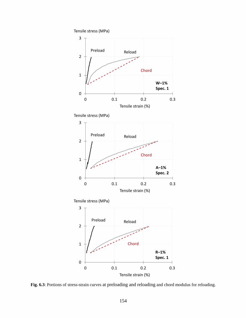
154

Fig. 6.3: Portions of stress-strain curves at preloading and reloading and chord modulus for reloading.

0

1

2

3

0 0.1 0.2 0.3

Chord

Tensile strain (%)


Preload Reload

W–1%Spec. 1

0

1

2

3

0 0.1 0.2 0.3

Chord

Tensile strain (%)


Preload Reload

A–1%Spec. 2

0

1

2

3

0 0.1 0.2 0.3

Chord

Tensile strain (%)


Preload Reload

R–1%Spec. 1

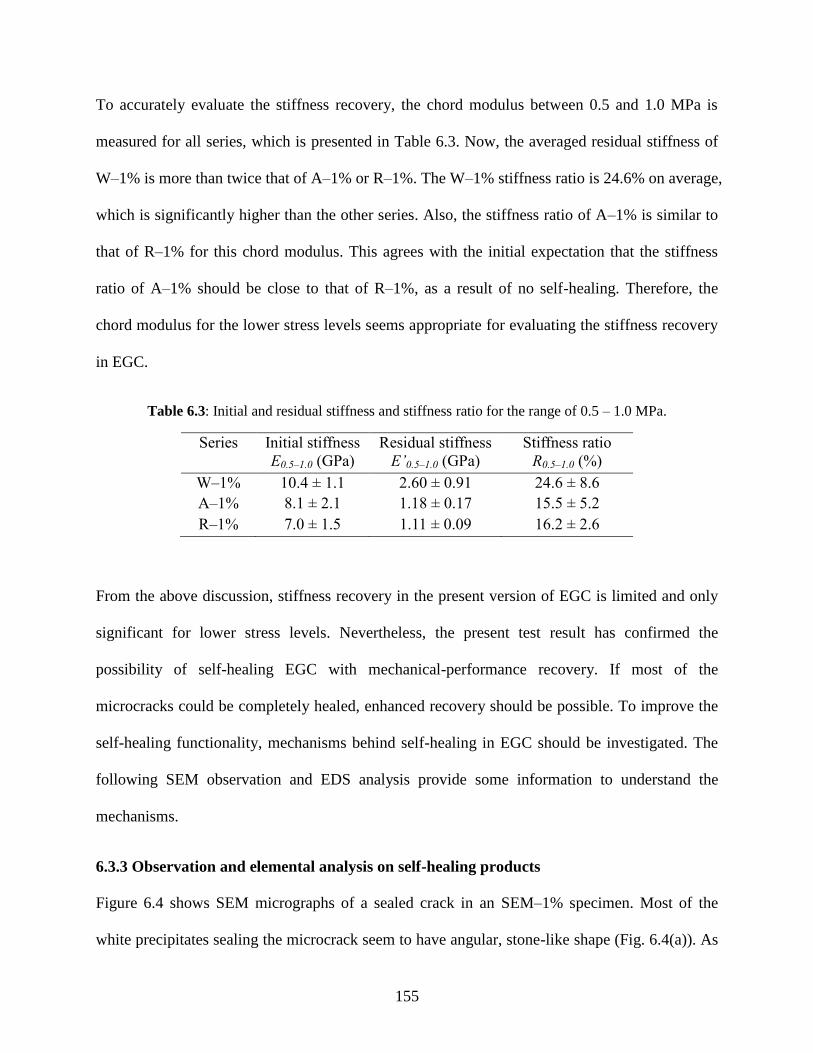
155

To accurately evaluate the stiffness recovery, the chord modulus between 0.5 and 1.0 MPa is

measured for all series, which is presented in Table 6.3. Now, the averaged residual stiffness of

W–1% is more than twice that of A–1% or R–1%. The W–1% stiffness ratio is 24.6% on average,

which is significantly higher than the other series. Also, the stiffness ratio of A–1% is similar to

that of R–1% for this chord modulus. This agrees with the initial expectation that the stiffness

ratio of A–1% should be close to that of R–1%, as a result of no self-healing. Therefore, the

chord modulus for the lower stress levels seems appropriate for evaluating the stiffness recovery

in EGC.

Table 6.3: Initial and residual stiffness and stiffness ratio for the range of 0.5 – 1.0 MPa.

Series Initial stiffness

E0.5–1.0 (GPa)

Residual stiffness

E’0.5–1.0 (GPa)

Stiffness ratio

R0.5–1.0 (%)

W–1% 10.4 ± 1.1 2.60 ± 0.91 24.6 ± 8.6

A–1% 8.1 ± 2.1 1.18 ± 0.17 15.5 ± 5.2

R–1% 7.0 ± 1.5 1.11 ± 0.09 16.2 ± 2.6

From the above discussion, stiffness recovery in the present version of EGC is limited and only

significant for lower stress levels. Nevertheless, the present test result has confirmed the

possibility of self-healing EGC with mechanical-performance recovery. If most of the

microcracks could be completely healed, enhanced recovery should be possible. To improve the

self-healing functionality, mechanisms behind self-healing in EGC should be investigated. The

following SEM observation and EDS analysis provide some information to understand the

mechanisms.

6.3.3 Observation and elemental analysis on self-healing products

Figure 6.4 shows SEM micrographs of a sealed crack in an SEM–1% specimen. Most of the

white precipitates sealing the microcrack seem to have angular, stone-like shape (Fig. 6.4(a)). As

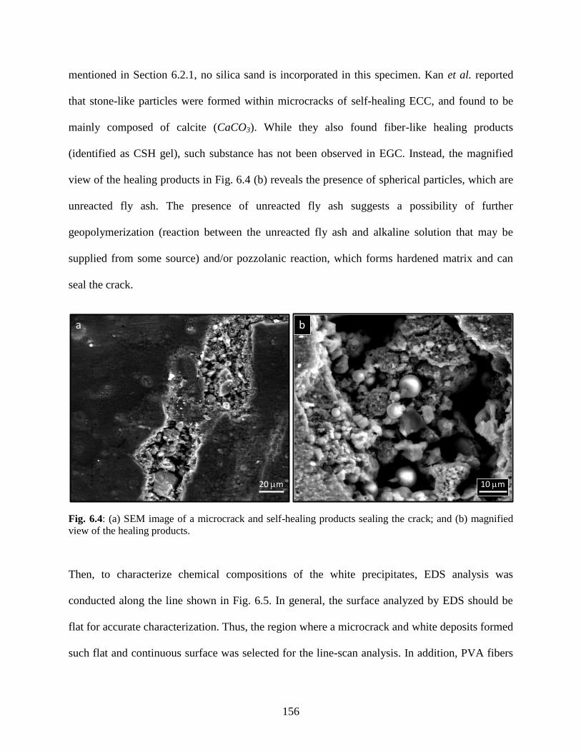
156

mentioned in Section 6.2.1, no silica sand is incorporated in this specimen. Kan et al. reported

that stone-like particles were formed within microcracks of self-healing ECC, and found to be

mainly composed of calcite (CaCO3). While they also found fiber-like healing products

(identified as CSH gel), such substance has not been observed in EGC. Instead, the magnified

view of the healing products in Fig. 6.4 (b) reveals the presence of spherical particles, which are

unreacted fly ash. The presence of unreacted fly ash suggests a possibility of further

geopolymerization (reaction between the unreacted fly ash and alkaline solution that may be

supplied from some source) and/or pozzolanic reaction, which forms hardened matrix and can

seal the crack.

Fig. 6.4: (a) SEM image of a microcrack and self-healing products sealing the crack; and (b) magnified

view of the healing products.

Then, to characterize chemical compositions of the white precipitates, EDS analysis was

conducted along the line shown in Fig. 6.5. In general, the surface analyzed by EDS should be

flat for accurate characterization. Thus, the region where a microcrack and white deposits formed

such flat and continuous surface was selected for the line-scan analysis. In addition, PVA fibers

20 m

a

10 m

b

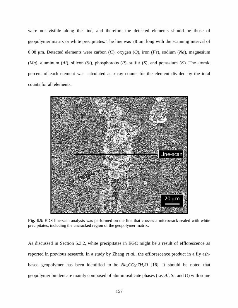
157

were not visible along the line, and therefore the detected elements should be those of

geopolymer matrix or white precipitates. The line was 78 μm long with the scanning interval of

0.08 μm. Detected elements were carbon (C), oxygen (O), iron (Fe), sodium (Na), magnesium

(Mg), aluminum (Al), silicon (Si), phosphorous (P), sulfur (S), and potassium (K). The atomic

percent of each element was calculated as x-ray counts for the element divided by the total

counts for all elements.

Fig. 6.5: EDS line-scan analysis was performed on the line that crosses a microcrack sealed with white

precipitates, including the uncracked region of the geopolymer matrix.

As discussed in Section 5.3.2, white precipitates in EGC might be a result of efflorescence as

reported in previous research. In a study by Zhang et al., the efflorescence product in a fly ash-

based geopolymer has been identified to be Na2CO3·7H2O [16]. It should be noted that

geopolymer binders are mainly composed of aluminosilicate phases (i.e. Al, Si, and O) with some

20 m

Line-scan

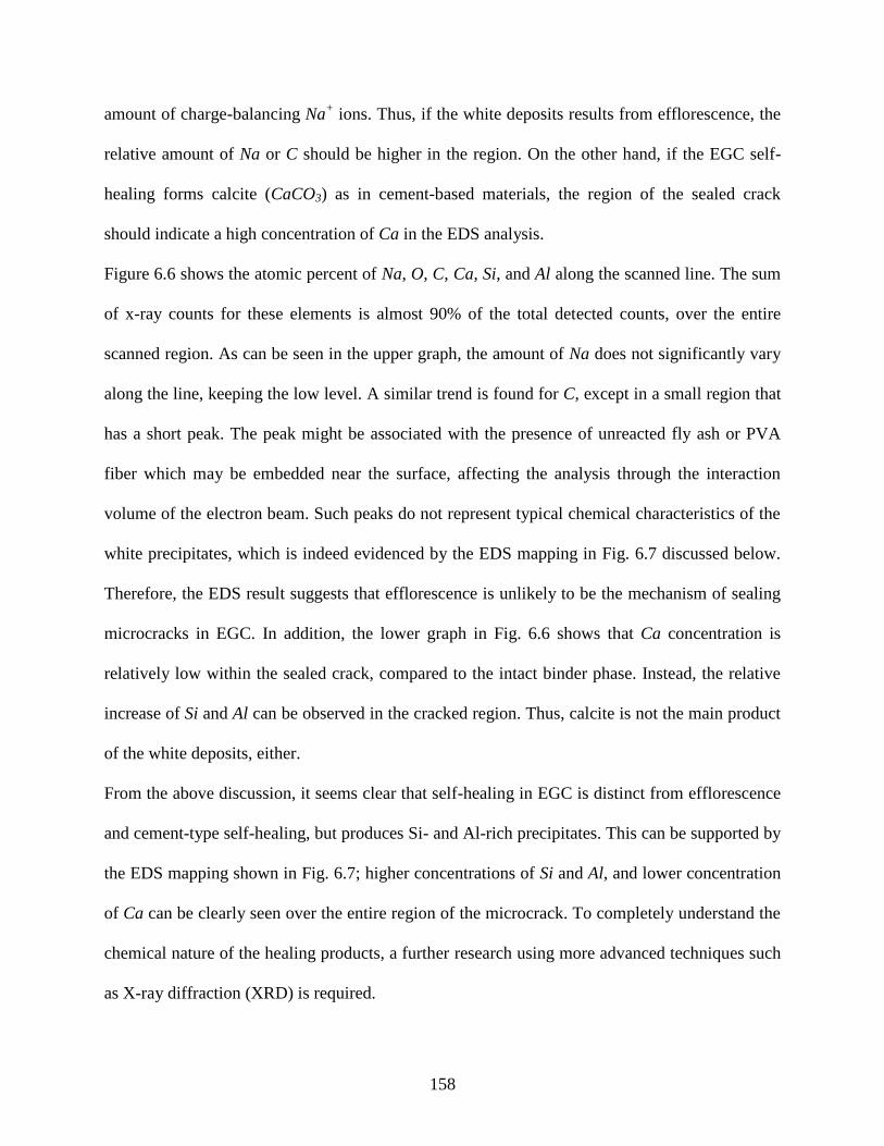
158

amount of charge-balancing Na+ ions. Thus, if the white deposits results from efflorescence, the

relative amount of Na or C should be higher in the region. On the other hand, if the EGC self-

healing forms calcite (CaCO3) as in cement-based materials, the region of the sealed crack

should indicate a high concentration of Ca in the EDS analysis.

Figure 6.6 shows the atomic percent of Na, O, C, Ca, Si, and Al along the scanned line. The sum

of x-ray counts for these elements is almost 90% of the total detected counts, over the entire

scanned region. As can be seen in the upper graph, the amount of Na does not significantly vary

along the line, keeping the low level. A similar trend is found for C, except in a small region that

has a short peak. The peak might be associated with the presence of unreacted fly ash or PVA

fiber which may be embedded near the surface, affecting the analysis through the interaction

volume of the electron beam. Such peaks do not represent typical chemical characteristics of the

white precipitates, which is indeed evidenced by the EDS mapping in Fig. 6.7 discussed below.

Therefore, the EDS result suggests that efflorescence is unlikely to be the mechanism of sealing

microcracks in EGC. In addition, the lower graph in Fig. 6.6 shows that Ca concentration is

relatively low within the sealed crack, compared to the intact binder phase. Instead, the relative

increase of Si and Al can be observed in the cracked region. Thus, calcite is not the main product

of the white deposits, either.

From the above discussion, it seems clear that self-healing in EGC is distinct from efflorescence

and cement-type self-healing, but produces Si- and Al-rich precipitates. This can be supported by

the EDS mapping shown in Fig. 6.7; higher concentrations of Si and Al, and lower concentration

of Ca can be clearly seen over the entire region of the microcrack. To completely understand the

chemical nature of the healing products, a further research using more advanced techniques such

as X-ray diffraction (XRD) is required.

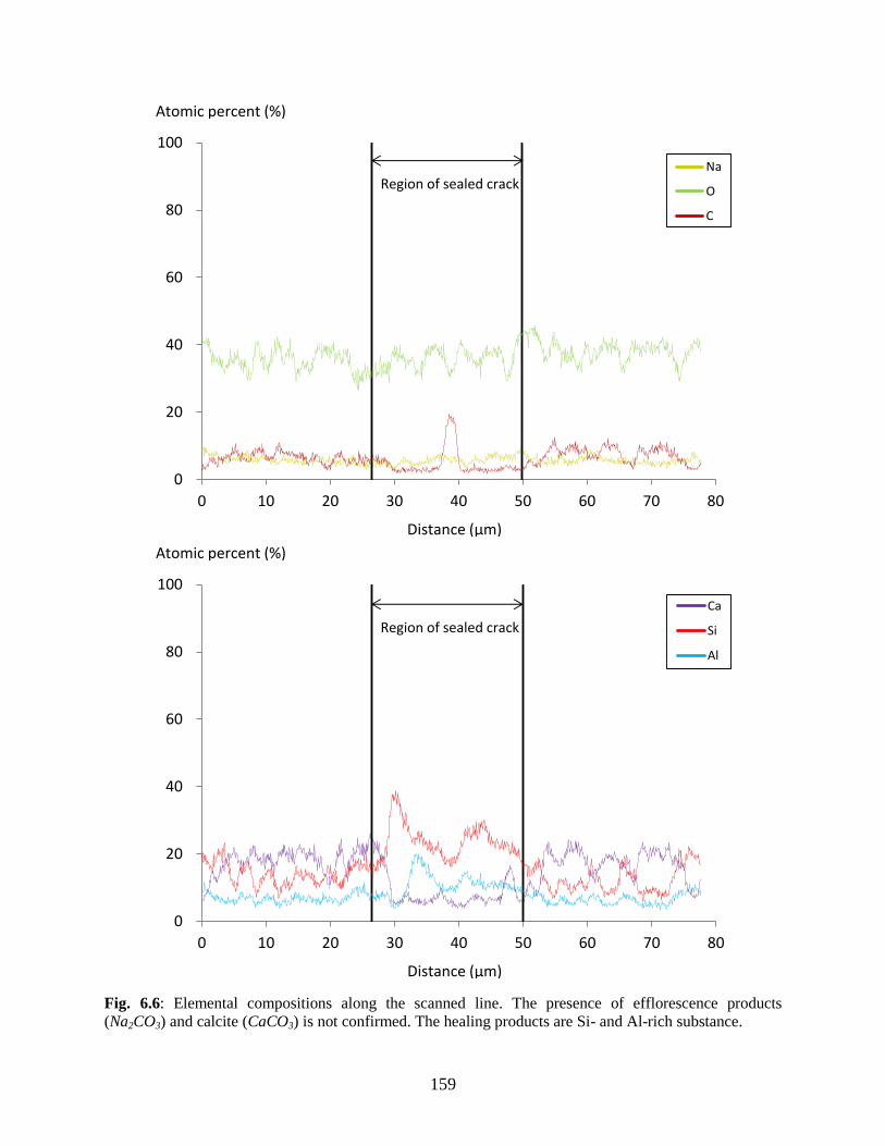
159

Fig. 6.6: Elemental compositions along the scanned line. The presence of efflorescence products

(Na2CO3) and calcite (CaCO3) is not confirmed. The healing products are Si- and Al-rich substance.

0

20

40

60

80

100

0 10 20 30 40 50 60 70 80

Atomic percent (%)

Distance (μm)

0

20

40

60

80

100

0 20 40 60 80

軸ラベル

軸ラベル

グラフタイトル

Ca

Si

Al

系列2

系列3

Region of sealed crack

0

20

40

60

80

100

0 10 20 30 40 50 60 70 80

Atomic percent (%)

Distance (μm)

0.0

0.2

0.4

0.6

0.8

1.0

0 20 40 60 80

軸ラベル

軸ラベル


Na

O

C

系列2

系列3

Region of sealed crack

160

Fig. 6.7: EDS mapping. Regions of higher concentration are shown in higher brightness. Higher

concentration of Si and Al, and lower concentration of Ca in the sealed crack can be clearly seen.

Ca

Na

Si Al

C

O

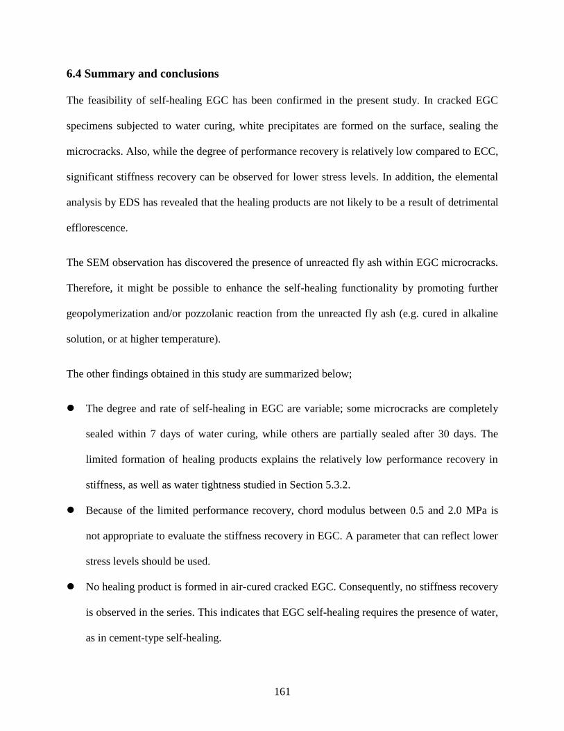
161


The feasibility of self-healing EGC has been confirmed in the present study. In cracked EGC

specimens subjected to water curing, white precipitates are formed on the surface, sealing the

microcracks. Also, while the degree of performance recovery is relatively low compared to ECC,

significant stiffness recovery can be observed for lower stress levels. In addition, the elemental

analysis by EDS has revealed that the healing products are not likely to be a result of detrimental

efflorescence.

The SEM observation has discovered the presence of unreacted fly ash within EGC microcracks.

Therefore, it might be possible to enhance the self-healing functionality by promoting further

geopolymerization and/or pozzolanic reaction from the unreacted fly ash (e.g. cured in alkaline

solution, or at higher temperature).

The other findings obtained in this study are summarized below;

The degree and rate of self-healing in EGC are variable; some microcracks are completely

sealed within 7 days of water curing, while others are partially sealed after 30 days. The

limited formation of healing products explains the relatively low performance recovery in

stiffness, as well as water tightness studied in Section 5.3.2.

Because of the limited performance recovery, chord modulus between 0.5 and 2.0 MPa is

not appropriate to evaluate the stiffness recovery in EGC. A parameter that can reflect lower

stress levels should be used.

No healing product is formed in air-cured cracked EGC. Consequently, no stiffness recovery

is observed in the series. This indicates that EGC self-healing requires the presence of water,

as in cement-type self-healing.

162

Healing products in EGC are mostly angular, stone-like substance, and relatively rich in Si

and Al but low in Ca, compared to the geopolymer matrix. Thus, calcite (CaCO3) is unlikely

to be a main healing product of EGC self-healing.

Chemical compositions of the healing products have not been completely identified in this study.

A further study is required to fully understand the chemical nature of the healing products and

corresponding reaction mechanisms. With that information, it would be possible to develop an

effective method to improve the self-healing functionality of EGC.

163

References

[1] K. Van Breugel, “Is there a market for self-healing cement-based materials,” Proc. First

Int. Conf. Self Heal. Mater., no. April, pp. 1–9, 2007.

[2] N. Hearn, “Self-sealing, autogenous healing and continued hydration: What is the

difference?,” Mater. Struct., vol. 31, no. 8, pp. 563–567, 1998.

[3] H. Huang and G. Ye, “Application of sodium silicate solution as self-healing agent in

cementitious materials,” Int. RILEM Conf. Adv. Constr. Mater. Through Sci. Eng., no.

1993, pp. 530–536, 2011.

[4] H. M. Jonkers, A. Thijssen, G. Muyzer, O. Copuroglu, and E. Schlangen, “Application of

bacteria as self-healing agent for the development of sustainable concrete,” Ecol. Eng., vol.

36, no. 2, pp. 230–235, 2010.

[5] T.-H. Ahn and T. Kishi, “Crack Self-healing Behavior of Cementitious Composites

Incorporating Various Mineral Admixtures,” J. Adv. Concr. Technol., vol. 8, no. 2, pp.

171–186, 2010.

[6] T. Nishiwaki, H. Mihashi, B.-K. Jang, and K. Miura, “Development of Self-Healing

System for Concrete with Selective Heating around Crack,” J. Adv. Concr. Technol., vol.

4, no. 2, pp. 267–275, 2006.

[7] Y. Yang, M. D. Lepech, E. Yang, and V. C. Li, “Autogenous healing of engineered

cementitious composites under wet–dry cycles,” Cem. Concr. Res., vol. 39, no. 5, pp.

382–390, May 2009.

[8] E. Herbert and V. Li, “Self-Healing of Microcracks in Engineered Cementitious

Composites (ECC) Under a Natural Environment,” Materials (Basel)., vol. 6, no. 7, pp.

2831–2845, Jul. 2013.

[9] M. Li and V. C. Li, “Cracking and healing of engineered cementitious composites under

chloride environment,” ACI Mater. J., vol. 108, no. 3, pp. 333–340, 2011.

[10] M. Sahmaran, V. C. V. Li, and M. Şahmaran, “Durability of mechanically loaded

engineered cementitious composites under highly alkaline environments,” Cem. Concr.

Compos., vol. 30, no. 2, pp. 72–81, Feb. 2008.

[11] M. K. Ali, A. I. Abu-tair, J. M. Kinuthia, and R. Babecki, “Self-healing and strength

development of geopolymer concrete made with Waste by products,” in International

Conference on Biological, Civil and Environmental Engineering, 2015, pp. 32–42.

[12] X. Liu, M. J. Ramos, S. D. Nair, H. Lee, D. N. Espinoza, and E. van Oort, “True Self-

Healing Geopolymer Cements for Improved Zonal Isolation and Well Abandonment,” in

SPE/IADC Drilling Conference and Exhibition, 2017.

164

[13] T. Nishiwaki, M. Koda, M. Yamada, H. Mihashi, and T. Kikuta, “Experimental Study on

Self-Healing Capability of FRCC Using Different Types of Synthetic Fibers,” J. Adv.

Concr. Technol., vol. 10, no. 6, pp. 195–206, 2012.

[14] ASTM E111-04, Standard Test Method for Young’s Modulus, Tangent Modulus, and

Chord Modulus. West Conshohocken, PA: ASTM International, 2010.

[15] Y. Yang, E. Yang, and V. C. Li, “Autogenous healing of engineered cementitious

composites at early age,” Cem. Concr. Res., vol. 41, no. 2, pp. 176–183, Feb. 2011.

[16] Z. Zhang, H. Wang, J. L. Provis, and A. Reid, “Efflorescence : A Critical Challenge for

Geopolymer Applications ?,” in Concrete Institute of Australia’s Biennial National

Conference, 2013.

165

CHAPTER 7: Sulfuric Acid Resistance of EGC

This chapter presents an experimental study on sulfuric acid resistance of EGC. Weight loss and

residual mechanical performances of acid-exposed EGC specimens are measured, in comparison

with OPC concrete and ECC.

7.1 Introduction

Sulfuric acid resistance is an important durability property for wastewater infrastructure. Under

sewer environments, sulfate compounds present in the wastewater are typically converted into

sulfuric acid, through metabolisms of sulfate-reducing and sulfur-oxidizing bacteria. This

sulfuric acid reacts with calcium hydroxide, calcium silicate hydrates and calcium monosulfate

in the cement matrix, forming loose and expansive gypsum and ettringite. As a result, the

structural integrity and load-bearing capacity of the sewer concrete are reduced. Detailed

information about the mechanisms of sulfuric acid formation in the wastewater can be found in

literature [1, 2].

Because of the biogenic sulfuric acid attack, unexpected early deterioration of concrete

wastewater facilities has been often reported [2, 3]. Further, much of sewer infrastructure is

outdated, reaching the end of their service life in many countries. The aging and deterioration of

wastewater infrastructure systems create an urgent need for repair and replacement; for example,

according to the US Environmental Protection Agency (EPA), $271 billion would be

166

required to maintain and upgrade the deteriorating wastewater infrastructure in the US [4]. Since

sewage treatment is essential for maintaining the quality of life of citizens and ecosystems, their

failure can result in social and environmental impacts (including drinking water contamination),

as well as economic burden. For overcoming the challenge of crumbling wastewater

infrastructure, much effort has been made to improve the vulnerability of concrete pipes under

wastewater environments [5–8].

Of those newly developed technologies, geopolymer is a promising alternative to cement

materials for sewer-infrastructure applications. Previous studies reported high sulfuric acid

resistance of geopolymer concrete, especially in terms of weight loss caused by acid exposure

[9–13]. While strength reduction due to the acid attack is observed in geopolymer concrete, the

degree and rate of degradation are considerably lower than those of portland cement concrete. It

is suggested that the better performance of geopolymers in acidic environments is attributed to

the lower calcium content involved in the matrix formation [12]. Driven by the promising acid-

resistant property, many field-demonstration projects have been conducted in the US to use

spray-applied geopolymer for repair/rehabilitation of concrete sewer pipes and culverts [14].

Further, precast geopolymer-concrete pipes have been commercially available in Australia [15].

Hence, more and more geopolymer applications for wastewater infrastructure will be expected in

the near future.

However, as has been discussed throughout this dissertation, durability performance of

geopolymers might be limited if extensive cracking takes place in field applications. Particularly,

large-diameter concrete pipes, which typically require steel reinforcement, can be seriously

damaged by corrosion that is induced by acidic media penetrating through the wide cracks. One

promising solution to this challenge is to use EGC; EGC has tightly-controlled crack width even

167

under a high imposed strain (as demonstrated in Chapter 5), and it might be even possible to

eliminate steel reinforcement in the pipe, fully relying on the ductile EGC for crack control.

Therefore, applications of EGC for large-diameter concrete pipes are worth considering; the first

step is to verify the durability of EGC under sulfuric acid attack.

This chapter reports an experimental investigation on sulfuric acid resistance of EGC in

comparison with OPC concrete and ECC; the latter two materials serve as controls. Weight loss

and residual compressive strength of cylinder specimens subjected to sulfuric acid exposure are

presented. In addition, to study the combined effects of cracking and acid attack on mechanical-

property degradation, residual flexural strength and deflection capacity are measured for beam

specimens that are preloaded to create cracks before acid exposure.

7.2 Material and methods

7.2.1 Materials and mix designs

Table 7.1 lists the ingredients and their mix proportions of portland cement concrete, ECC and

EGC used in this study. The EGC design is that of 1.5% fiber volume fraction, developed in

Chapter 4. Properties of the ingredients can be found in Section 4.2.1. For cement concrete and

ECC, Type I portland cement and ASTM class F fly ash from the Monroe power plant (Section

4.2.1), were used as their binder materials. Crushed limestone with a maximum size of 25 mm

and silica sand with a fineness modulus of 2.43 were used as coarse and fine aggregate of cement

concrete, respectively. F-75 Ottawa fine silica sand and short polyvinyl alcohol (PVA) fiber with

1.2% oil coating were used for ECC, as in EGC mixture. To obtain adequate workability,

polycarboxylate-based superplasticizer (ADVA 190, GCP Applied Technologies Inc.) was added

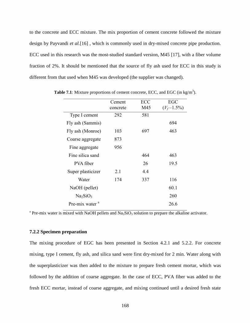
168

to the concrete and ECC mixture. The mix proportion of cement concrete followed the mixture

design by Payvandi et al.[16] , which is commonly used in dry-mixed concrete pipe production.

ECC used in this research was the most-studied standard version, M45 [17], with a fiber volume

fraction of 2%. It should be mentioned that the source of fly ash used for ECC in this study is

different from that used when M45 was developed (the supplier was changed).

Table 7.1: Mixture proportions of cement concrete, ECC, and EGC (in kg/m3).

Cement

concrete

ECC

M45

EGC

(Vf –1.5%)

Type I cement 292 581

Fly ash (Sammis) 694

Fly ash (Monroe) 103 697 463

Coarse aggregate 873

Fine aggregate 956

Fine silica sand 464 463

PVA fiber 26 19.5

Super plasticizer 2.1 4.4

Water 174 337 116

NaOH (pellet)

(pellets)

60.1

Na2SiO3

(pellets)

260

Pre-mix water a 26.6

a Pre-mix water is mixed with NaOH pellets and Na2SiO3 solution to prepare the alkaline activator.

7.2.2 Specimen preparation

The mixing procedure of EGC has been presented in Section 4.2.1 and 5.2.2. For concrete

mixing, type I cement, fly ash, and silica sand were first dry-mixed for 2 min. Water along with

the superplasticizer was then added to the mixture to prepare fresh cement mortar, which was

followed by the addition of coarse aggregate. In the case of ECC, PVA fiber was added to the

fresh ECC mortar, instead of coarse aggregate, and mixing continued until a desired fresh state

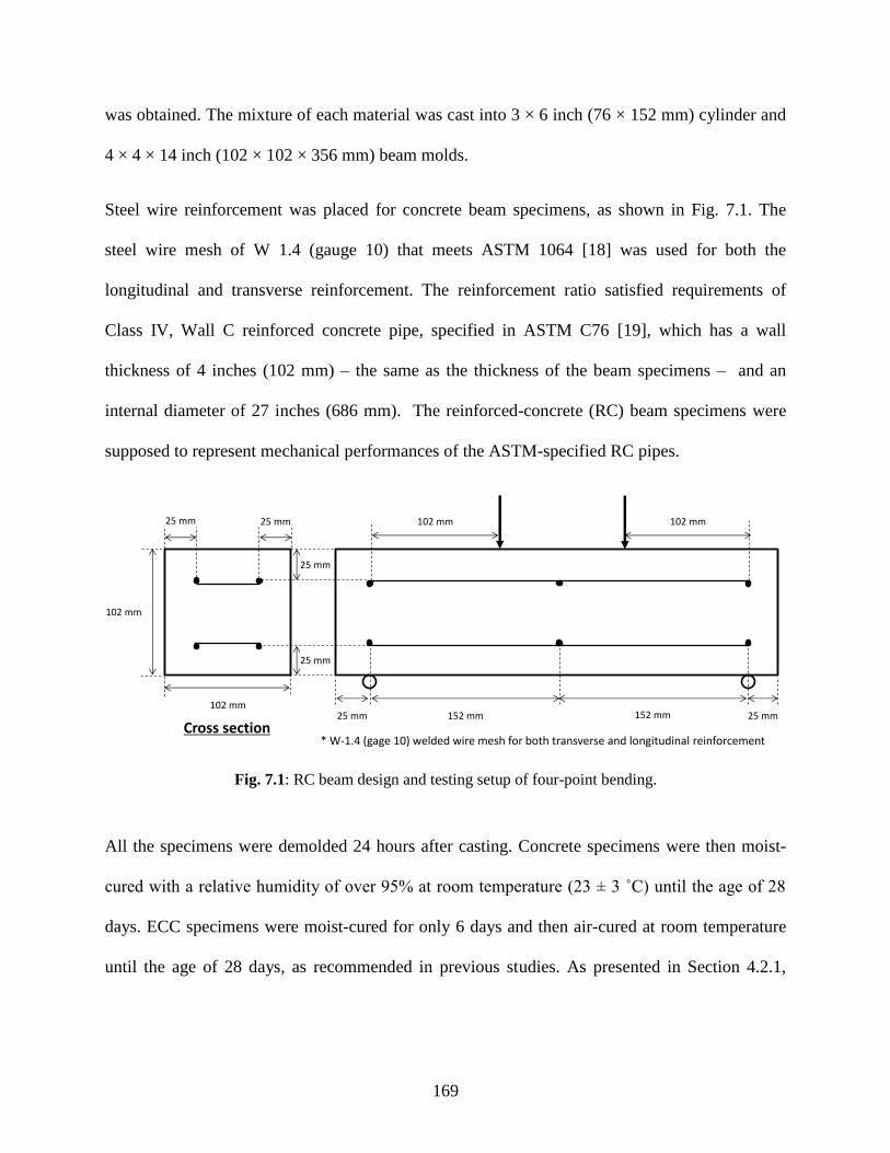
169

was obtained. The mixture of each material was cast into 3 × 6 inch (76 × 152 mm) cylinder and

4 × 4 × 14 inch (102 × 102 × 356 mm) beam molds.

Steel wire reinforcement was placed for concrete beam specimens, as shown in Fig. 7.1. The

steel wire mesh of W 1.4 (gauge 10) that meets ASTM 1064 [18] was used for both the

longitudinal and transverse reinforcement. The reinforcement ratio satisfied requirements of

Class IV, Wall C reinforced concrete pipe, specified in ASTM C76 [19], which has a wall

thickness of 4 inches (102 mm) – the same as the thickness of the beam specimens – and an

internal diameter of 27 inches (686 mm). The reinforced-concrete (RC) beam specimens were

supposed to represent mechanical performances of the ASTM-specified RC pipes.

Fig. 7.1: RC beam design and testing setup of four-point bending.

All the specimens were demolded 24 hours after casting. Concrete specimens were then moist-

cured with a relative humidity of over 95% at room temperature (23 ± 3 ˚C) until the age of 28

days. ECC specimens were moist-cured for only 6 days and then air-cured at room temperature

until the age of 28 days, as recommended in previous studies. As presented in Section 4.2.1,

25 mm 25 mm

152 mm

25 mm

25 mm

152 mm25 mm 25 mm

102 mm

102 mm

Cross section

102 mm 102 mm

* W-1.4 (gage 10) welded wire mesh for both transverse and longitudinal reinforcement

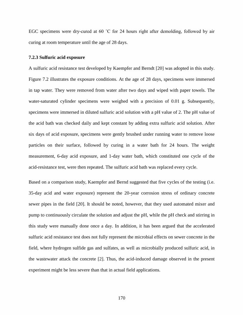
170

EGC specimens were dry-cured at 60 ˚C for 24 hours right after demolding, followed by air

curing at room temperature until the age of 28 days.

7.2.3 Sulfuric acid exposure

A sulfuric acid resistance test developed by Kaempfer and Berndt [20] was adopted in this study.

Figure 7.2 illustrates the exposure conditions. At the age of 28 days, specimens were immersed

in tap water. They were removed from water after two days and wiped with paper towels. The

water-saturated cylinder specimens were weighed with a precision of 0.01 g. Subsequently,

specimens were immersed in diluted sulfuric acid solution with a pH value of 2. The pH value of

the acid bath was checked daily and kept constant by adding extra sulfuric acid solution. After

six days of acid exposure, specimens were gently brushed under running water to remove loose

particles on their surface, followed by curing in a water bath for 24 hours. The weight

measurement, 6-day acid exposure, and 1-day water bath, which constituted one cycle of the

acid-resistance test, were then repeated. The sulfuric acid bath was replaced every cycle.

Based on a comparison study, Kaempfer and Bernd suggested that five cycles of the testing (i.e.

35-day acid and water exposure) represent the 20-year corrosion stress of ordinary concrete

sewer pipes in the field [20]. It should be noted, however, that they used automated mixer and

pump to continuously circulate the solution and adjust the pH, while the pH check and stirring in

this study were manually done once a day. In addition, it has been argued that the accelerated

sulfuric acid resistance test does not fully represent the microbial effects on sewer concrete in the

field, where hydrogen sulfide gas and sulfates, as well as microbially produced sulfuric acid, in

the wastewater attack the concrete [2]. Thus, the acid-induced damage observed in the present

experiment might be less severe than that in actual field applications.

171

Fig. 7.2: Test conditions of sulfuric acid exposure. Five cycles (35-day exposure) correspond to average

corrosion damage observed in 20-year-old ordinary concrete sewer pipes [20].

7.2.4 Test procedures

Cylinder specimens

Uniaxial compression testing was first conducted on three cylinder specimens of each material

for their 28-day compressive strength. Specimens were capped with sulfur capping compounds at

least one day prior to testing. The loading rate was 35 ± 7 psi/s (0.25 ± 0.05 MPa/s).

Nine intact cylinders for each material were subjected to the acid exposure. Out of these, three

randomly-selected ones were tested for residual compressive strength after each five cycles (i.e.

35 days of exposure). Namely, the average weight change was determined for nine specimens for

1-5 cycles, six specimens for 6-10 cycles, and three specimens for 11-15 cycles. To evaluate the

effects of continuous hydration of cementitious materials, another set of nine cylinders for

concrete and ECC were prepared as control specimens and subjected to water bath for the same

exposure periods as those of acid-exposed specimens. The control specimens were then tested for

reference compressive strength. For EGC cylinders, no significant strength increase after 28 days

was observed in preliminary studies. Thus, control specimens for EGC were not prepared here.

Specimen age (days)

28 30 36 37

Water bath Water bath

Sulfuric acid exposure (PH 2)• PH value checked daily• Acid bath replaced every cycle

Sulfuric acid exposure

Weight measurementWeight measurement

1st cycle (7 days) 2nd cycle

172

Beam specimens

A four-point bending test was first performed on three beam specimens of each material for their

28-day flexural strength – known as modulus of rupture (MOR) – and their deflection capacity

(i.e. deflection at MOR). The span length was 12 inches (305 mm) and a constant loading rate of

0.003 in/min (0.076 mm/min) was applied under displacement control of the loading head. To

measure the mid-point net deflection, two potentiometers were mounted on both sides of a

rectangular jig that surrounded the beam specimen and was clamped at mid-depth directly above

the loading supports.

Another set of three beams for each material was preloaded at the age of 28 days. The testing

configurations were identical to the above flexural strength test, except that the test was stopped

at the net mid-point deflection of 0.02 inches (0.51 mm), which was equivalent to 1/600 of the

span length. After unloading the specimens, cracks were observed by an optical digital

microscope to measure their crack width. For each crack, crack width was measured on the

center and both edges of the specimen surface (i.e. measured at three points) and averaged.

Subsequently, the preloaded specimens were immersed in tap water for two days, and subjected

to the acid exposure of 15 cycles (105 days). The acid-exposed beams were then reloaded for

their residual MOR and deflection capacity.


7.3.1 Visual appearance and weight change

Figure 7.3 shows visual appearances of specimen surfaces before and after acid exposure. As can

be seen, concrete and ECC specimens have remarkable erosion of the surface due to sulfuric acid

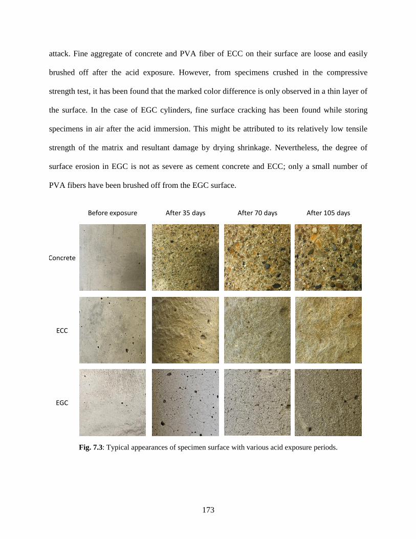
173

attack. Fine aggregate of concrete and PVA fiber of ECC on their surface are loose and easily

brushed off after the acid exposure. However, from specimens crushed in the compressive

strength test, it has been found that the marked color difference is only observed in a thin layer of

the surface. In the case of EGC cylinders, fine surface cracking has been found while storing

specimens in air after the acid immersion. This might be attributed to its relatively low tensile

strength of the matrix and resultant damage by drying shrinkage. Nevertheless, the degree of

surface erosion in EGC is not as severe as cement concrete and ECC; only a small number of

PVA fibers have been brushed off from the EGC surface.

Fig. 7.3: Typical appearances of specimen surface with various acid exposure periods.

Concrete

ECC

EGC

Before exposure After 35 days After 70 days After 105 days

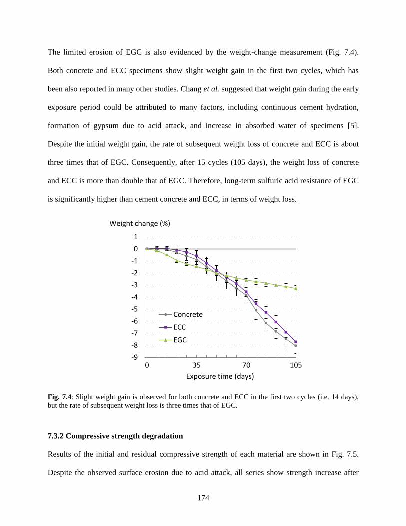
174

The limited erosion of EGC is also evidenced by the weight-change measurement (Fig. 7.4).

Both concrete and ECC specimens show slight weight gain in the first two cycles, which has

been also reported in many other studies. Chang et al. suggested that weight gain during the early

exposure period could be attributed to many factors, including continuous cement hydration,

formation of gypsum due to acid attack, and increase in absorbed water of specimens [5].

Despite the initial weight gain, the rate of subsequent weight loss of concrete and ECC is about

three times that of EGC. Consequently, after 15 cycles (105 days), the weight loss of concrete

and ECC is more than double that of EGC. Therefore, long-term sulfuric acid resistance of EGC

is significantly higher than cement concrete and ECC, in terms of weight loss.

Fig. 7.4: Slight weight gain is observed for both concrete and ECC in the first two cycles (i.e. 14 days),

but the rate of subsequent weight loss is three times that of EGC.

7.3.2 Compressive strength degradation

Results of the initial and residual compressive strength of each material are shown in Fig. 7.5.

Despite the observed surface erosion due to acid attack, all series show strength increase after

-9

-8

-7

-6

-5

-4

-3

-2

-1

0

1

0 35 70 105

Concrete

ECC

EGC

Weight change (%)

Exposure time (days)

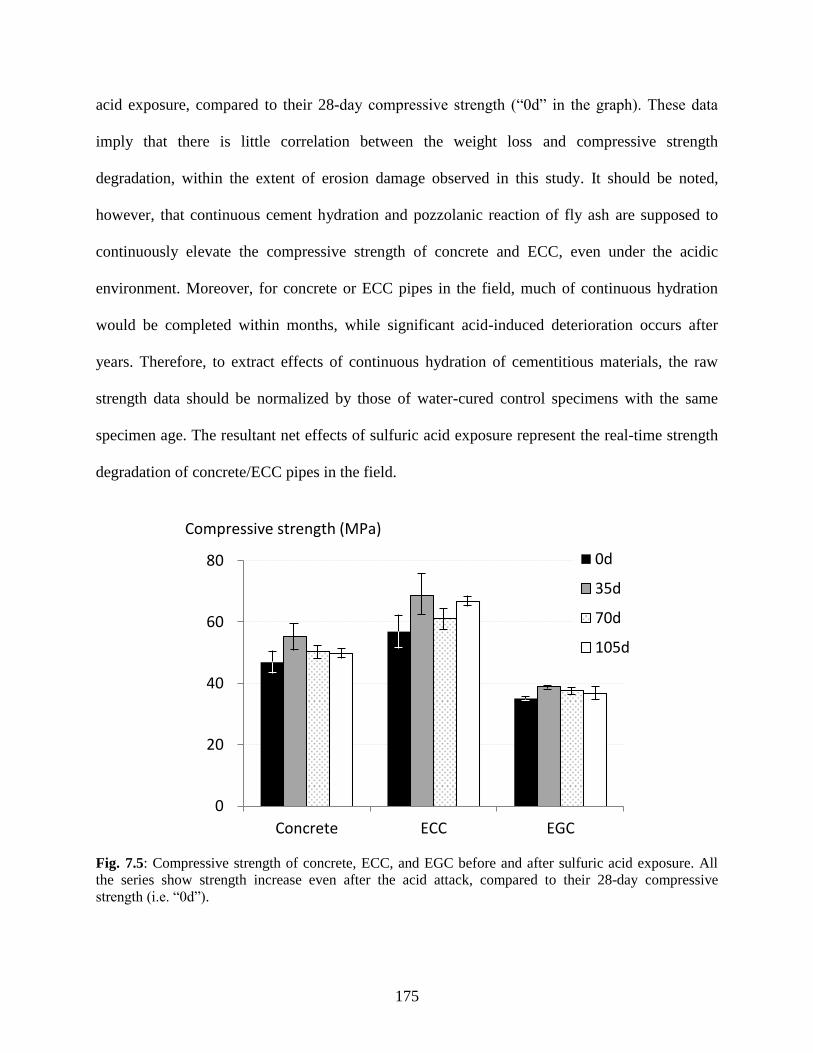
175

acid exposure, compared to their 28-day compressive strength (“0d” in the graph). These data

imply that there is little correlation between the weight loss and compressive strength

degradation, within the extent of erosion damage observed in this study. It should be noted,

however, that continuous cement hydration and pozzolanic reaction of fly ash are supposed to

continuously elevate the compressive strength of concrete and ECC, even under the acidic

environment. Moreover, for concrete or ECC pipes in the field, much of continuous hydration

would be completed within months, while significant acid-induced deterioration occurs after

years. Therefore, to extract effects of continuous hydration of cementitious materials, the raw

strength data should be normalized by those of water-cured control specimens with the same

specimen age. The resultant net effects of sulfuric acid exposure represent the real-time strength

degradation of concrete/ECC pipes in the field.

Fig. 7.5: Compressive strength of concrete, ECC, and EGC before and after sulfuric acid exposure. All

the series show strength increase even after the acid attack, compared to their 28-day compressive

strength (i.e. “0d”).

0

20

40

60

80

Concrete ECC EGC

0d

35d

70d

105d


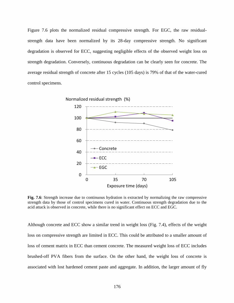
176

Figure 7.6 plots the normalized residual compressive strength. For EGC, the raw residual-

strength data have been normalized by its 28-day compressive strength. No significant

degradation is observed for ECC, suggesting negligible effects of the observed weight loss on

strength degradation. Conversely, continuous degradation can be clearly seen for concrete. The

average residual strength of concrete after 15 cycles (105 days) is 79% of that of the water-cured

control specimens.

Fig. 7.6: Strength increase due to continuous hydration is extracted by normalizing the raw compressive

strength data by those of control specimens cured in water. Continuous strength degradation due to the

acid attack is observed in concrete, while there is no significant effect on ECC and EGC.

Although concrete and ECC show a similar trend in weight loss (Fig. 7.4), effects of the weight

loss on compressive strength are limited in ECC. This could be attributed to a smaller amount of

loss of cement matrix in ECC than cement concrete. The measured weight loss of ECC includes

brushed-off PVA fibers from the surface. On the other hand, the weight loss of concrete is

associated with lost hardened cement paste and aggregate. In addition, the larger amount of fly

0

20

40

60

80

100

120

0 35 70 105

Concrete

ECC

EGC

Normalized residual strength (%)


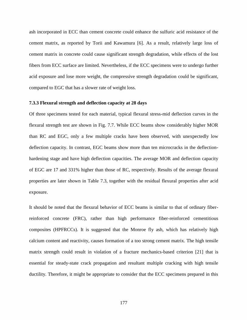
177

ash incorporated in ECC than cement concrete could enhance the sulfuric acid resistance of the

cement matrix, as reported by Torii and Kawamura [6]. As a result, relatively large loss of

cement matrix in concrete could cause significant strength degradation, while effects of the lost

fibers from ECC surface are limited. Nevertheless, if the ECC specimens were to undergo further

acid exposure and lose more weight, the compressive strength degradation could be significant,

compared to EGC that has a slower rate of weight loss.

7.3.3 Flexural strength and deflection capacity at 28 days

Of three specimens tested for each material, typical flexural stress-mid deflection curves in the

flexural strength test are shown in Fig. 7.7. While ECC beams show considerably higher MOR

than RC and EGC, only a few multiple cracks have been observed, with unexpectedly low

deflection capacity. In contrast, EGC beams show more than ten microcracks in the deflection-

hardening stage and have high deflection capacities. The average MOR and deflection capacity

of EGC are 17 and 331% higher than those of RC, respectively. Results of the average flexural

properties are later shown in Table 7.3, together with the residual flexural properties after acid

exposure.

It should be noted that the flexural behavior of ECC beams is similar to that of ordinary fiber-

reinforced concrete (FRC), rather than high performance fiber-reinforced cementitious

composites (HPFRCCs). It is suggested that the Monroe fly ash, which has relatively high

calcium content and reactivity, causes formation of a too strong cement matrix. The high tensile

matrix strength could result in violation of a fracture mechanics-based criterion [21] that is

essential for steady-state crack propagation and resultant multiple cracking with high tensile

ductility. Therefore, it might be appropriate to consider that the ECC specimens prepared in this

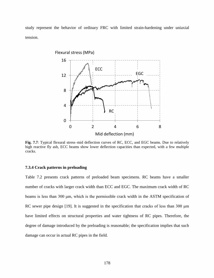
178

study represent the behavior of ordinary FRC with limited strain-hardening under uniaxial

tension.

Fig. 7.7: Typical flexural stress–mid deflection curves of RC, ECC, and EGC beams. Due to relatively

high reactive fly ash, ECC beams show lower deflection capacities than expected, with a few multiple

cracks.

7.3.4 Crack patterns in preloading

Table 7.2 presents crack patterns of preloaded beam specimens. RC beams have a smaller

number of cracks with larger crack width than ECC and EGC. The maximum crack width of RC

beams is less than 300 μm, which is the permissible crack width in the ASTM specification of

RC sewer pipe design [19]. It is suggested in the specification that cracks of less than 300 μm

have limited effects on structural properties and water tightness of RC pipes. Therefore, the

degree of damage introduced by the preloading is reasonable; the specification implies that such

damage can occur in actual RC pipes in the field.

0

4

8

12

16

0 2 4 6 8

Mid deflection (mm)

RC

Flexural stress (MPa)

ECCEGC

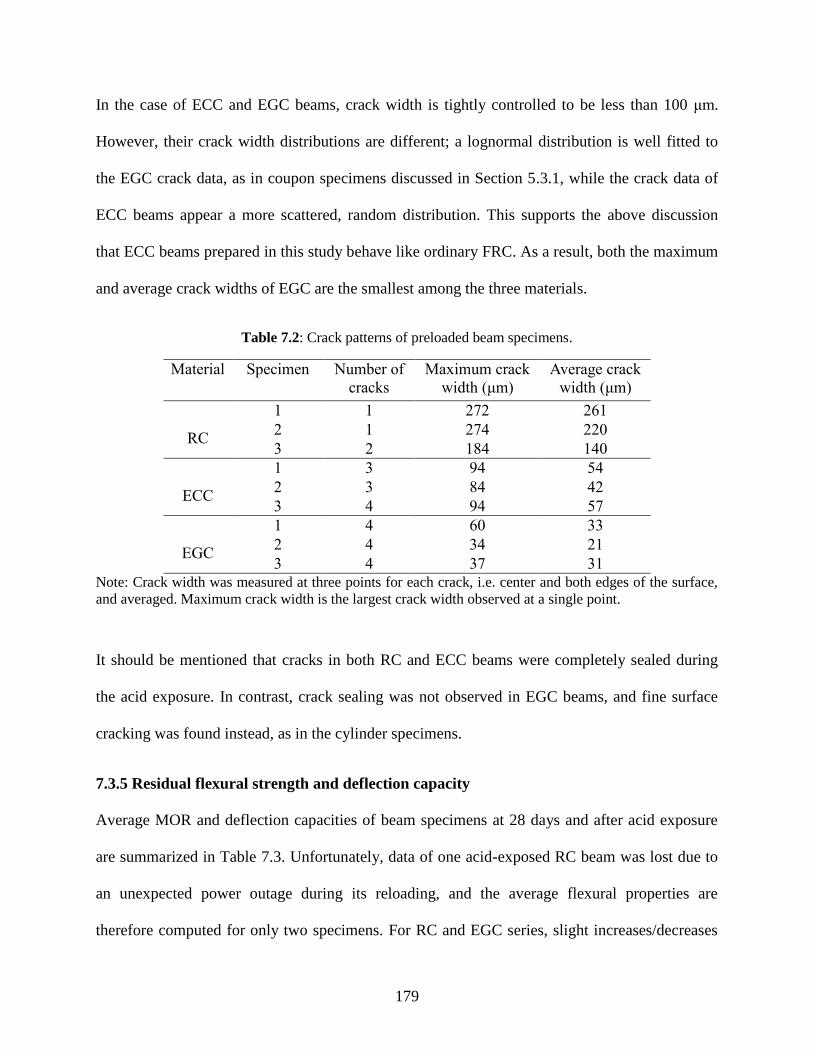
179

In the case of ECC and EGC beams, crack width is tightly controlled to be less than 100 μm.

However, their crack width distributions are different; a lognormal distribution is well fitted to

the EGC crack data, as in coupon specimens discussed in Section 5.3.1, while the crack data of

ECC beams appear a more scattered, random distribution. This supports the above discussion

that ECC beams prepared in this study behave like ordinary FRC. As a result, both the maximum

and average crack widths of EGC are the smallest among the three materials.

Table 7.2: Crack patterns of preloaded beam specimens.

Material Specimen Number of

cracks

Maximum crack

width (μm)

Average crack

width (μm)

RC

1 1 272 261

2 1 274 220

3 2 184 140

ECC

1 3 94 54

2 3 84 42

3 4 94 57

EGC

1 4 60 33

2 4 34 21

3 4 37 31 Note: Crack width was measured at three points for each crack, i.e. center and both edges of the surface,

and averaged. Maximum crack width is the largest crack width observed at a single point.

It should be mentioned that cracks in both RC and ECC beams were completely sealed during

the acid exposure. In contrast, crack sealing was not observed in EGC beams, and fine surface

cracking was found instead, as in the cylinder specimens.

7.3.5 Residual flexural strength and deflection capacity

Average MOR and deflection capacities of beam specimens at 28 days and after acid exposure

are summarized in Table 7.3. Unfortunately, data of one acid-exposed RC beam was lost due to

an unexpected power outage during its reloading, and the average flexural properties are

therefore computed for only two specimens. For RC and EGC series, slight increases/decreases

180

can be found in their residual MOR and deflection capacities, in comparison with their 28-day

performances. However, with the assumption that the data are normally distributed with the

equal variance, a statistical t-test reveals that those differences before and after acid exposure are

insignificant, compared to the observed variations among specimens. Therefore, the acid-induced

surface erosion observed in this study does not cause any remarkable degradation in the MOR

and deflection capacity of RC and EGC.

Table 7.3: Flexural properties of RC, ECC, and EGC at 28 days and after acid exposure.

28-day performance After acid exposure

MOR, f0

(MPa)

Deflection

at MOR, δ0

(mm)

MOR, f1

(MPa)

Deflection

at MOR, δ1

(mm)

f1 / f0

δ1 / δ0

RC 9.2 ± 1.4 1.25 ± 0.27 8.3 ± 0.7 1.39 ± 0.14 0.90 1.11

ECC 15.0 ± 0.4 1.23 ± 0.49 13.8 ± 0.3 2.30 ± 0.16 0.92 1.87

EGC 10.8 ± 1.0 5.39 ± 1.09 11.6 ± 1.5 5.26 ± 0.95 1.08 0.98

In contrast, effects of acid exposure on both the MOR and deflection capacity of ECC are

statistically significant. While the residual MOR has only 8% reduction from the 28-day value,

the decrease is significant when the observed small sample variance is taken into account. The

degradation could be mainly attributed to brushed-off PVA fibers due to the surface erosion;

unlike compressive strength, flexural strength of ECC beams highly depends on the number of

fibers that can bridge cracks. Thus, loss of a considerable number of PVA fibers has a direct

impact on the load-carrying capacity. Conversely, 87% increase in the deflection capacity could

be associated with the degraded cement matrix; due to the acid-induced surface erosion, first-

cracking strength of ECC could be lowered, which is beneficial for achieving a higher ductility,

as discussed in Section 2.2.2. Indeed, more multiple cracks have been observed during reloading

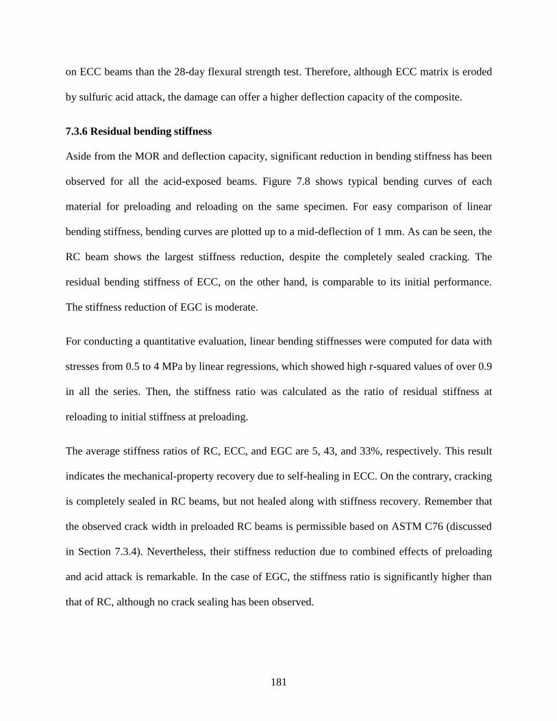
181

on ECC beams than the 28-day flexural strength test. Therefore, although ECC matrix is eroded

by sulfuric acid attack, the damage can offer a higher deflection capacity of the composite.

7.3.6 Residual bending stiffness

Aside from the MOR and deflection capacity, significant reduction in bending stiffness has been

observed for all the acid-exposed beams. Figure 7.8 shows typical bending curves of each

material for preloading and reloading on the same specimen. For easy comparison of linear

bending stiffness, bending curves are plotted up to a mid-deflection of 1 mm. As can be seen, the

RC beam shows the largest stiffness reduction, despite the completely sealed cracking. The

residual bending stiffness of ECC, on the other hand, is comparable to its initial performance.

The stiffness reduction of EGC is moderate.

For conducting a quantitative evaluation, linear bending stiffnesses were computed for data with

stresses from 0.5 to 4 MPa by linear regressions, which showed high r-squared values of over 0.9

in all the series. Then, the stiffness ratio was calculated as the ratio of residual stiffness at

reloading to initial stiffness at preloading.

The average stiffness ratios of RC, ECC, and EGC are 5, 43, and 33%, respectively. This result

indicates the mechanical-property recovery due to self-healing in ECC. On the contrary, cracking

is completely sealed in RC beams, but not healed along with stiffness recovery. Remember that

the observed crack width in preloaded RC beams is permissible based on ASTM C76 (discussed

in Section 7.3.4). Nevertheless, their stiffness reduction due to combined effects of preloading

and acid attack is remarkable. In the case of EGC, the stiffness ratio is significantly higher than

that of RC, although no crack sealing has been observed.

182

Fig. 7.8: (a) RC beam shows significant reduction in bending stiffness due to the preloading and

subsequent acid attack. The smallest stiffness reduction of (b) ECC beam is suggested to be a result of

recovery due to self-healing.

0

4

8

12

16

0 0.25 0.5 0.75 1

Mid deflection (mm)


Preload

Reload

(a) RC

0

4

8

12

16

0 0.25 0.5 0.75 1

Mid deflection (mm)


Preload Reload

(b) ECC

0

4

8

12

16

0 0.25 0.5 0.75 1

Mid deflection (mm)


PreloadReload

(c) EGC

183


This chapter has experimentally demonstrated the high sulfuric acid resistance of EGC. Acid-

induced surface erosion of EGC specimens is limited compared to cement concrete and ECC,

especially in terms of weight loss. No significant degradation has been observed for its

compressive strength, MOR and deflection capacity after acid exposure. While combined effects

of preloading and acid attack cause remarkable degradation in its linear bending stiffness, the

degree of reduction is significantly less than RC. Due to the considerably slower rate of weight

loss in EGC than concrete and ECC, differences in mechanical-property degradation among the

materials would be more remarkable when subjected to longer acid exposure or more severe

acidic environments.

The following findings have been also obtained during this study;

A limited number of PVA fibers are brushed-off in EGC due to the acid-induced surface

erosion, while acid-exposed ECC loses a significant amount of fibers. The loss of fiber does

not reduce compressive strength of both materials, but causes statistically significant

degradation in MOR of ECC.

While the deflection capacity of EGC shows insignificant reduction after acid exposure, that

of ECC can be rather increased. The increase could be attributed to the degraded cement

matrix with lower matrix tensile strength, which is beneficial for achieving a higher ductility.

Self-healing of EGC is not observed under acidic environments. Conversely, cement

materials show significant healing; cracks of preloaded RC and ECC beams have been

completely sealed during the acid exposure.

184

Significant mechanical-performance recovery due to the self-healing has been observed in

linear bending stiffness of ECC beams only. Despite the sealed cracking in preloaded RC

beams, their stiffness reduction is the largest among the materials.

As mentioned in Section 7.2.3, the chemical test method used in this study might not fully

represent the microbial effects on sewer concrete in the field. Therefore, further research would

be required to verify the durability of EGC under sewer environments. Nevertheless, the high

sulfuric acid resistance of EGC has been experimentally demonstrated, which shows the promise

of EGC for sewer-pipe applications. Then, based on the experimental result obtained here, the

next chapter conducts a life-cycle assessment on environmental performances of EGC sewer

pipes.

185

References

[1] D. J. Roberts, D. Nica, G. Zuo, and J. L. Davis, “Quantifying microbially induced

deterioration of concrete: Initial studies,” in International Biodeterioration and

Biodegradation, 2002, vol. 49, no. 4, pp. 227–234.

[2] M. O’Connell, C. McNally, and M. G. Richardson, “Biochemical attack on concrete in

wastewater applications: A state of the art review,” Cem. Concr. Compos., vol. 32, no. 7,

pp. 479–485, 2010.

[3] W. Sand and E. Bock, “Concrete corrosion in the Hamburg Sewer system,” Environ.

Technol., vol. 5, no. 12, pp. 517–528, 1984.

[4] United States Environmental Protectio Agency, “Clean Watersheds Needs Survey 2012 -

Report to Congress,” 2016.

[5] Z. T. Chang, X. J. Song, R. Munn, and M. Marosszeky, “Using limestone aggregates and

different cements for enhancing resistance of concrete to sulphuric acid attack,” Cem.

Concr. Res., vol. 35, no. 8, pp. 1486–1494, 2005.

[6] K. Torii and M. Kawamura, “Effects of fly ash and silica fume on the resistance of mortar

to sulfuric acid and sulfate attack,” Cem. Concr. Res., vol. 24, no. 2, pp. 361–370, 1994.

[7] W. De Muynck, N. De Belie, and W. Verstraete, “Effectiveness of admixtures, surface

treatments and antimicrobial compounds against biogenic sulfuric acid corrosion of

concrete,” Cem. Concr. Compos., vol. 31, no. 3, pp. 163–170, 2009.

[8] E. Vincke, E. Van Wanseele, J. Monteny, A. Beeldens, N. D. Belie, L. Taerwe, D. Van

Gemert, and W. Verstraete, “Influence of polymer addition on biogenic sulfuric acid

attack of concrete,” Int. Biodeterior. Biodegrad., vol. 49, no. 4, pp. 283–292, 2002.

[9] J. Davidovits, D. C. Comrie, J. H. Paterson, and D. J. Ritcey, “Geopolymeric concrete for

environmental protection,” Concr. Int., vol. 12, no. 7, pp. 30–40, 1990.

[10] T. Bakharev, “Resistance of geopolymer materials to acid attack,” Cem. Concr. Res., vol.

35, no. 4, pp. 658–670, 2005.

[11] X. J. Song, M. Marosszeky, M. Brungs, and R. Munn, “Durability of fly ash based

Geopolymer concrete against sulphuric acid attack,” Durab. Build. Mater., no. April, pp.

17–20, 2005.

[12] S. E. Wallah and B. V. Rangan, “Low-Calcium Fly Ash-Based Geopolymer Concrete:

Long-Term Properties,” Concrete, 2006.

[13] S. Thokchom, P. Ghosh, and S. Ghosh, “Resistance of Fly Ash Based Geopolymer

Mortars in Sulfuric Acid,” ARPN J. Eng. Appl. Sci., vol. 4, no. 1, pp. 65–70, 2009.

186

[14] D. Keaffaber, “GeoSpray: GeoPolymer Mortar System and Concrete Cloth for Structural

Rehabilitation/Repair of Sewer and Storm Infrastructure,” Milliken Infrastructure, 2015.

[Online]. Available:

http://ctt.mtu.edu/sites/ctt/files/resources/bridge2016/conference/08keaffaber.pdf.

[Accessed: 04-Jul-2017].

[15] J. T. Gourley and G. B. Johnson, “Developments in geopolymer precast concrete,” in The

worled Congress Geopolymer, 2005, pp. 139–143.

[16] A. Peyvandi, P. Soroushian, and S. Jahangirnejad, “Enhancement of the structural

efficiency and performance of concrete pipes through fiber reinforcement,” Constr. Build.

Mater., vol. 45, pp. 36–44, 2013.



[18] ASTM A1064/A1064M-16b, Standard Specification for Steel Wire and Welded Wire

Reinforcement, Plain and Deformed, for Concrete. West Conshohocken, PA: ASTM

International, 2016.



[20] Kaempfer W and M. Berndt, “Estimation of Service Life of Concrete Pipes in Sewer,” 8th

Conf. Durab. Build. Mater. Components, p. Vol. 1, p. 36–45., 1999.

[21] V. C. Li and C. K. Y. Leung, “Steady-State and Multiple Cracking of Short Random Fiber

Composites,” J. Eng. Mech., vol. 118, no. 11, pp. 2246–2264, 1992.

187

PART IV: APPLICATION OF EGC

CHAPTER 8: Application and Environmental Life Cycle Assessment

This chapter is concerned with a promising infrastructure application of EGC: large-diameter

sewer pipes. The market demand, existing technologies, and technical challenges are first

outlined. Then, an environmental life cycle analysis (LCA) is conducted to evaluate the

sustainability of the EGC pipe, in comparison with RC and ECC pipes.

8.1 Introduction

Wastewater infrastructure is facing an increasing crisis worldwide. For example, there are over

800,000 miles of public sewer mains in the US, many of which were installed in the early 20th

century [1]. Since then, repair and retrofit have been patchwork, and many of the outdated sewer

systems are susceptible to blockages and leakages; according to the US Environmental

Protection Agency (EPA), at least 23,000 to 75,000 sanitary-sewer overflows occur every year

[2], mainly caused by blockages and line breaks. It is clear that such wastewater leakages affect

the natural environment and human health. Therefore, there is an urgent need for replacement of

old sanitary pipes reaching the end of their service life. Considering the expected long lifespan of

public sewer systems, a durable piping material for new installation needs to be carefully

selected.

188

Traditionally, concrete and steel were predominantly used for underground pipes; in recent years,

plastic has emerged as a competitive alternative [3]. Plastic pipes offer a variety of advantages;

for example, polyvinyl chloride (PVC) and high-density polyethylene (HDPE) pipes are light-

weight and corrosive-resistant technologies. Lightweight is beneficial for reducing time and cost

for installation, and high corrosion resistance prevents early deterioration/failure of the pipe,

extending the service life. These technical advantages lower the life-cycle cost of plastic-pipe

applications, which is attractive to asset owners. Indeed, demand for plastic pipes in the US is

predicted to rise at the most rapid pace of all piping materials [4].

However, there are also limitations in plastic pipes. PVC pipes, for example, have relatively low

crush resistance and are prone to cracking. Unlike reinforced-concrete (RC) pipes, plastic pipes

can easily lose structural integrity if cracking is extensive. Further, the material becomes more

brittle if the temperature is below 3 °C (37 °F), and therefore is not suitable for installation

during cold temperatures [3]. Aside from the technical aspect, plastic pipes have large embodied

energy due to petroleum-based raw ingredients. Indeed, embodied energy per unit mass of PVC

or HDPE is more than 20 times that of RC [5] (it should be noted that the density of PVC or

HDPE is roughly half that of RC). Meanwhile, the high carbon intensity of cement is a

disadvantage of RC pipes. Hence, to select the best piping material, each technology should be

comprehensively evaluated depending on the application.

The objective of this chapter is to investigate the feasibility of using EGC for sewer-pipe

applications. The market size and trends are first outlined to determine the target market. Then,

technical advantages of EGC pipes are presented in comparison with existing technologies in the

market. Finally, an environmental life cycle analysis (LCA) is conducted to assess the

sustainability of EGC pipes in terms of the energy use and carbon dioxide (CO2) emissions.

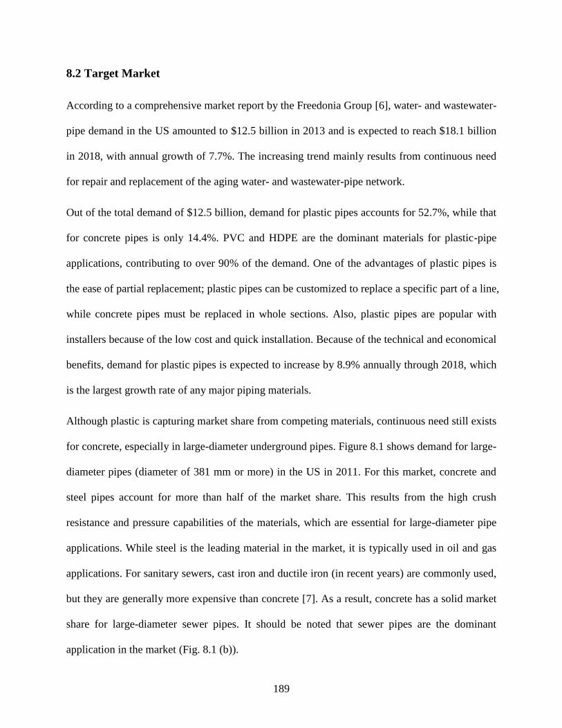
189

8.2 Target Market

According to a comprehensive market report by the Freedonia Group [6], water- and wastewater-

pipe demand in the US amounted to $12.5 billion in 2013 and is expected to reach $18.1 billion

in 2018, with annual growth of 7.7%. The increasing trend mainly results from continuous need

for repair and replacement of the aging water- and wastewater-pipe network.

Out of the total demand of $12.5 billion, demand for plastic pipes accounts for 52.7%, while that

for concrete pipes is only 14.4%. PVC and HDPE are the dominant materials for plastic-pipe

applications, contributing to over 90% of the demand. One of the advantages of plastic pipes is

the ease of partial replacement; plastic pipes can be customized to replace a specific part of a line,

while concrete pipes must be replaced in whole sections. Also, plastic pipes are popular with

installers because of the low cost and quick installation. Because of the technical and economical

benefits, demand for plastic pipes is expected to increase by 8.9% annually through 2018, which

is the largest growth rate of any major piping materials.

Although plastic is capturing market share from competing materials, continuous need still exists

for concrete, especially in large-diameter underground pipes. Figure 8.1 shows demand for large-

diameter pipes (diameter of 381 mm or more) in the US in 2011. For this market, concrete and

steel pipes account for more than half of the market share. This results from the high crush

resistance and pressure capabilities of the materials, which are essential for large-diameter pipe

applications. While steel is the leading material in the market, it is typically used in oil and gas

applications. For sanitary sewers, cast iron and ductile iron (in recent years) are commonly used,

but they are generally more expensive than concrete [7]. As a result, concrete has a solid market

share for large-diameter sewer pipes. It should be noted that sewer pipes are the dominant

application in the market (Fig. 8.1 (b)).

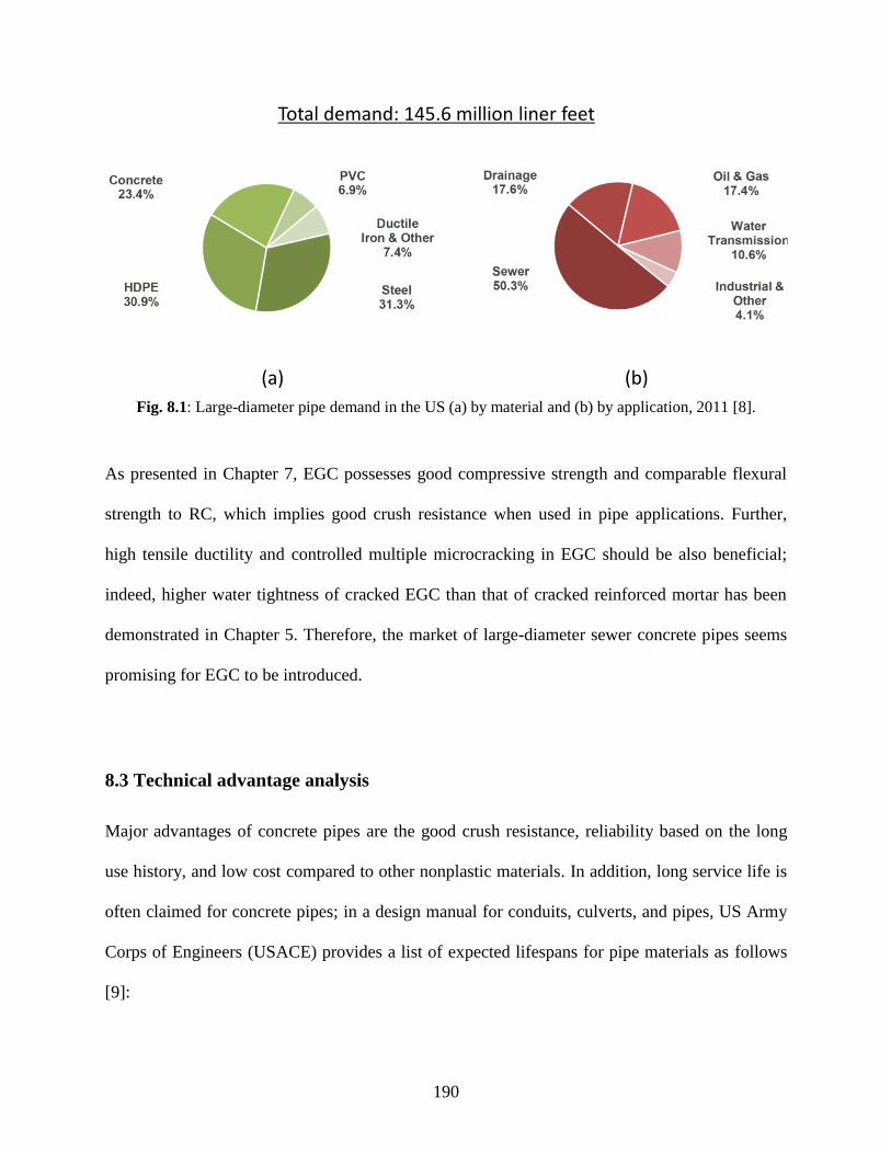
190

Fig. 8.1: Large-diameter pipe demand in the US (a) by material and (b) by application, 2011 [8].

As presented in Chapter 7, EGC possesses good compressive strength and comparable flexural

strength to RC, which implies good crush resistance when used in pipe applications. Further,

high tensile ductility and controlled multiple microcracking in EGC should be also beneficial;

indeed, higher water tightness of cracked EGC than that of cracked reinforced mortar has been

demonstrated in Chapter 5. Therefore, the market of large-diameter sewer concrete pipes seems

promising for EGC to be introduced.

8.3 Technical advantage analysis

Major advantages of concrete pipes are the good crush resistance, reliability based on the long

use history, and low cost compared to other nonplastic materials. In addition, long service life is

often claimed for concrete pipes; in a design manual for conduits, culverts, and pipes, US Army

Corps of Engineers (USACE) provides a list of expected lifespans for pipe materials as follows

[9]:

(a) (b)

Total demand: 145.6 million liner feet

191

(i) Concrete – between 70 and 100 years.

(ii) Steel – at least 50 years provided that coatings are properly applied.

(iii) Plastic – less than 50 years.

It should be noted that the design manual was published in 1997, and the recommended service

life for plastic pipes is relatively short because of the limited performance history of the material

at that time; a longer service life might be able to be claimed today.

Despite the long life expectancy for concrete pipes, the actual longevity highly depends on the

site conditions. Particularly, acidic environments significantly shorten the lifespan of concrete

pipes (Fig. 8.2). Indeed, unexpected early deterioration of concrete sewer facilities has been

reported worldwide [10, 11]. The severe deterioration is typically associated with formation of

biogenic sulfuric acid in wastewater; cement-based materials are severely eroded due to their low

sulfuric acid resistance, as discussed throughout Chapter 7. To improve the low acid resistance,

various technologies including surface coatings or plastic liners have been introduced, which

however require additional initial costs.

Fig. 8.2: Predicted concrete-pipe lifespan by Ohio Department of Transportation (ODOT) [12]. Years for

the pipe to reach a poor condition (based on ODOT classification) highly depend on pH of the stream.

1

10

100

11 2 3 4 5 6 7

1

10

100

5

50

Eq. 17 with 1.0% pipe slope [11]

Years to Poor

pH

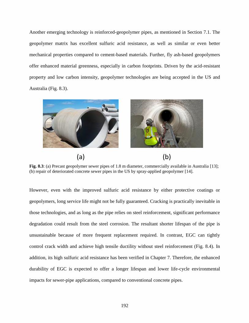
192

Another emerging technology is reinforced-geopolymer pipes, as mentioned in Section 7.1. The

geopolymer matrix has excellent sulfuric acid resistance, as well as similar or even better

mechanical properties compared to cement-based materials. Further, fly ash-based geopolymers

offer enhanced material greenness, especially in carbon footprints. Driven by the acid-resistant

property and low carbon intensity, geopolymer technologies are being accepted in the US and

Australia (Fig. 8.3).

Fig. 8.3: (a) Precast geopolymer sewer pipes of 1.8 m diameter, commercially available in Australia [13];

(b) repair of deteriorated concrete sewer pipes in the US by spray-applied geopolymer [14].

However, even with the improved sulfuric acid resistance by either protective coatings or

geopolymers, long service life might not be fully guaranteed. Cracking is practically inevitable in

those technologies, and as long as the pipe relies on steel reinforcement, significant performance

degradation could result from the steel corrosion. The resultant shorter lifespan of the pipe is

unsustainable because of more frequent replacement required. In contrast, EGC can tightly

control crack width and achieve high tensile ductility without steel reinforcement (Fig. 8.4). In

addition, its high sulfuric acid resistance has been verified in Chapter 7. Therefore, the enhanced

durability of EGC is expected to offer a longer lifespan and lower life-cycle environmental

impacts for sewer-pipe applications, compared to conventional concrete pipes.

(a) (b)

193

Fig. 8.4: Schematic illustrations of comparison between RC and EGC sewer pipes.

8.4 Life cycle environmental assessment

To verify and quantify the enhanced sustainability of EGC pipes, an environmental life-cycle

analysis (LCA) is conducted in this section. Specifically, energy consumption and carbon

emissions are inventoried here. For reference, life-cycle environmental performances of the EGC

pipe are compared with those of RC and ECC pipes.

8.4.1 LCA methodology

In general, LCA considers the entire life cycle of a product: from raw-material acquisition,

through production/manufacturing, to use and end-of-life treatment. The ISO 14040 provides

general requirements of an LCA study, defining the following four phases [15];

(i) Goal and scope definition – to state the objective(s) of the study and define the product

system(s) to be studied. The functional unit, system boundary, assumptions, and impact

categories are determined in this phase.

(ii) Inventory analysis – to collect data of relevant inputs and outputs of the product system(s)

and relate them to the functional unit.

(iii) Impact assessment – to associate the inventory data with specific environmental-impact

Can eliminate reinforcing steel

Tight cracking

EGC

Controlled CrackingPrevents Permeation

Reinforcing Steel

Cracking

Corrosion

H2SH2S

Sulfide Attack

H2SO4

Permeation

Cement Concrete

Geopolymer MatrixHigh Acid Resistance

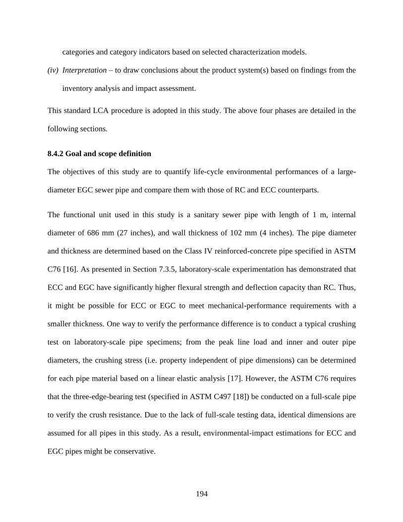
194

categories and category indicators based on selected characterization models.

(iv) Interpretation – to draw conclusions about the product system(s) based on findings from the

inventory analysis and impact assessment.

This standard LCA procedure is adopted in this study. The above four phases are detailed in the

following sections.

8.4.2 Goal and scope definition

The objectives of this study are to quantify life-cycle environmental performances of a large-

diameter EGC sewer pipe and compare them with those of RC and ECC counterparts.

The functional unit used in this study is a sanitary sewer pipe with length of 1 m, internal

diameter of 686 mm (27 inches), and wall thickness of 102 mm (4 inches). The pipe diameter

and thickness are determined based on the Class IV reinforced-concrete pipe specified in ASTM

C76 [16]. As presented in Section 7.3.5, laboratory-scale experimentation has demonstrated that

ECC and EGC have significantly higher flexural strength and deflection capacity than RC. Thus,

it might be possible for ECC or EGC to meet mechanical-performance requirements with a

smaller thickness. One way to verify the performance difference is to conduct a typical crushing

test on laboratory-scale pipe specimens; from the peak line load and inner and outer pipe

diameters, the crushing stress (i.e. property independent of pipe dimensions) can be determined

for each pipe material based on a linear elastic analysis [17]. However, the ASTM C76 requires

that the three-edge-bearing test (specified in ASTM C497 [18]) be conducted on a full-scale pipe

to verify the crush resistance. Due to the lack of full-scale testing data, identical dimensions are

assumed for all pipes in this study. As a result, environmental-impact estimations for ECC and

EGC pipes might be conservative.

195

Figure 8.5 shows the system boundary in this study. In general, assumptions and simplifications

are necessary to model the product system. First and foremost, the present LCA study omits the

use and end-of-life phases. In most products, the use phase significantly contributes to the life-

cycle environmental impacts. However, unlike pipes for drinking water, typical sewer lines are

not pressurized to transport the wastewater, but run at a slope. Consequently, the energy

consumption in the use phase is limited for a sewer pipe, compared to that for a pump-driven

water pipe [19]. In addition, Vahidi et al. concluded in their LCA study on wastewater piping

systems that maintenance and repair of a concrete pipe (15-year interval for a period of 50 years)

had almost negligible impacts in the life-cycle energy/material use and greenhouse gas emissions

[7]. Regarding the end-of-life stage, used concrete pipes are usually not recycled; the old pipes

are often abandoned in the site after their service life, and the disposal phase is therefore omitted

in many comparative LCA studies on underground pipe systems [5, 7, 19, 20]. Other

assumptions and simplifications are summarized in Table 8.1.

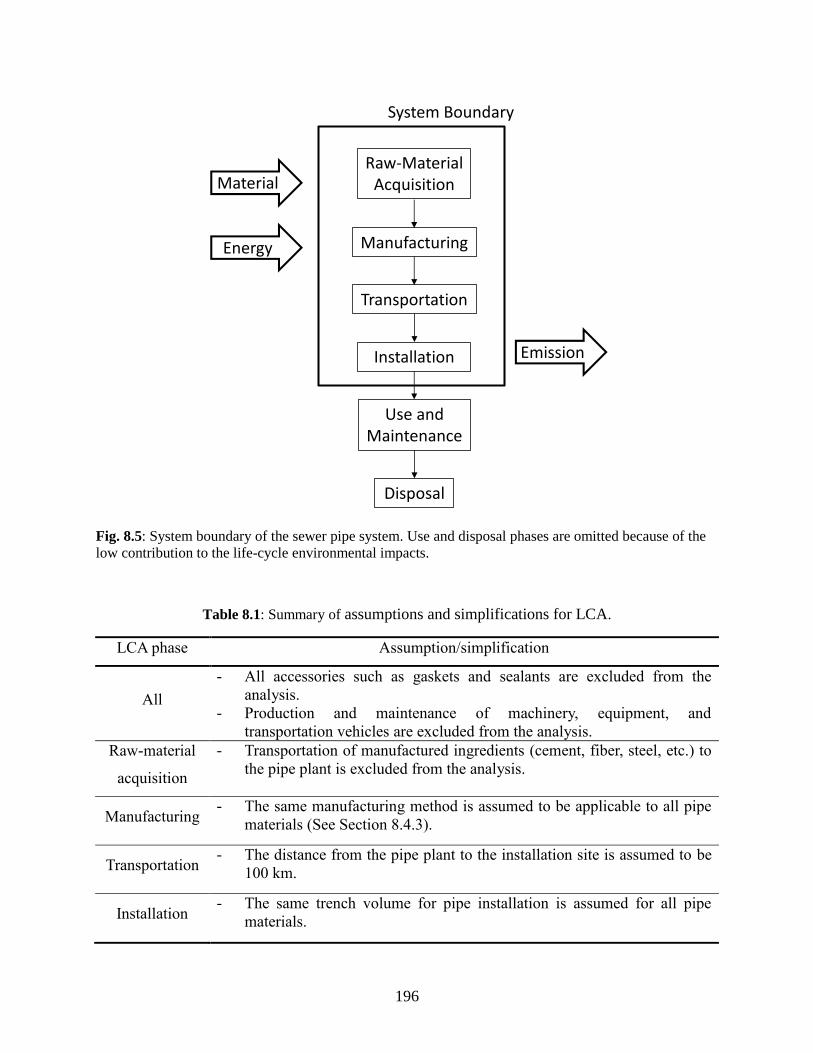
196

Fig. 8.5: System boundary of the sewer pipe system. Use and disposal phases are omitted because of the

low contribution to the life-cycle environmental impacts.

Table 8.1: Summary of assumptions and simplifications for LCA.

LCA phase Assumption/simplification

All

- All accessories such as gaskets and sealants are excluded from the

analysis.

- Production and maintenance of machinery, equipment, and

transportation vehicles are excluded from the analysis.

Raw-material

acquisition

- Transportation of manufactured ingredients (cement, fiber, steel, etc.) to

the pipe plant is excluded from the analysis.

Manufacturing - The same manufacturing method is assumed to be applicable to all pipe

materials (See Section 8.4.3).

Transportation - The distance from the pipe plant to the installation site is assumed to be

100 km.

Installation - The same trench volume for pipe installation is assumed for all pipe

materials.

Raw-Material Acquisition

Manufacturing

Use and Maintenance

Transportation

Disposal

Installation

System Boundary

Material

Energy

Emission

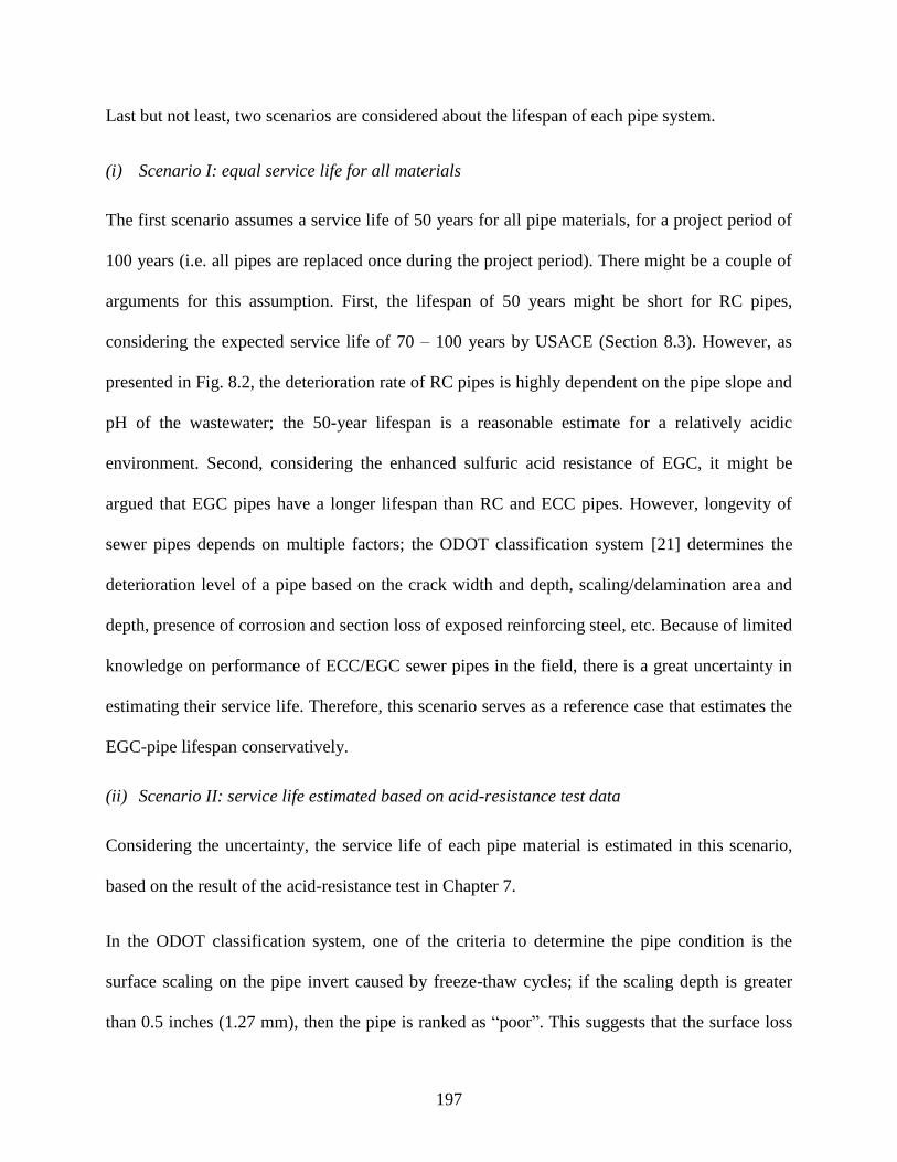
197

Last but not least, two scenarios are considered about the lifespan of each pipe system.

(i) Scenario I: equal service life for all materials

The first scenario assumes a service life of 50 years for all pipe materials, for a project period of

100 years (i.e. all pipes are replaced once during the project period). There might be a couple of

arguments for this assumption. First, the lifespan of 50 years might be short for RC pipes,

considering the expected service life of 70 – 100 years by USACE (Section 8.3). However, as

presented in Fig. 8.2, the deterioration rate of RC pipes is highly dependent on the pipe slope and

pH of the wastewater; the 50-year lifespan is a reasonable estimate for a relatively acidic

environment. Second, considering the enhanced sulfuric acid resistance of EGC, it might be

argued that EGC pipes have a longer lifespan than RC and ECC pipes. However, longevity of

sewer pipes depends on multiple factors; the ODOT classification system [21] determines the

deterioration level of a pipe based on the crack width and depth, scaling/delamination area and

depth, presence of corrosion and section loss of exposed reinforcing steel, etc. Because of limited

knowledge on performance of ECC/EGC sewer pipes in the field, there is a great uncertainty in

estimating their service life. Therefore, this scenario serves as a reference case that estimates the

EGC-pipe lifespan conservatively.

(ii) Scenario II: service life estimated based on acid-resistance test data

Considering the uncertainty, the service life of each pipe material is estimated in this scenario,

based on the result of the acid-resistance test in Chapter 7.

In the ODOT classification system, one of the criteria to determine the pipe condition is the

surface scaling on the pipe invert caused by freeze-thaw cycles; if the scaling depth is greater

than 0.5 inches (1.27 mm), then the pipe is ranked as “poor”. This suggests that the surface loss

198

of 0.5-inch depth can significantly affect the pipe performance (and possibly lose a large part of

cover depth in RC pipes). This criterion is adopted here to determine the service life of each pipe

material, combined with the relationship between weight loss and acid-exposure time for each

material, shown in Fig. 7.4 in Chapter 7.

Figure 8.6 illustrates the method for the service life estimation. Two assumptions are made here.

First, it is assumed that specimens in the acid-resistance test were uniformly eroded over the

entire surface area; namely the diameter and height of the cylinder specimen are equally reduced.

Then, the weight loss can be related to the reduced diameter and height as follows;

)2(2

2

4)1(

22

xhxdhd

y

(8.1)

where y, ρ, d, and h are the weight loss (in percent), density, diameter, and height of the cylinder,

respectively, and x represents the depth of lost surface due to erosion. It should be noted that the

diameter and height are reduced by 2x. Then, by substituting x = 0.5 (plus, d = 3 and h = 6 for

the 3 × 6 inch cylinder specimen) into Eq. 8.1, a critical value of y for which the pipe is assumed

to reach the end of the service life can be determined.

The second assumption is that the rate of weight loss does not accelerate but keeps constant after

the test duration (105 days). Figure 8.7 shows the weight-loss data presented in Chapter 7 and

their linear regressions. For concrete and ECC, data from 35 days were used for the regression

analysis. As mentioned in Section 7.3.1, a slower rate of weight loss (and even weight gain) is

typically observed for cement-based materials, mainly due to continuous cement hydration and

formation of gypsum caused by acid attack. As a result, the weight loss-exposure time

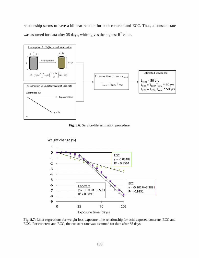
199

relationship seems to have a bilinear relation for both concrete and ECC. Thus, a constant rate

was assumed for data after 35 days, which gives the highest R2 value.

Fig. 8.6: Service-life estimation procedure.

Fig. 8.7: Liner regressions for weight loss-exposure time relationship for acid-exposed concrete, ECC and

EGC. For concrete and ECC, the constant rate was assumed for data after 35 days.

Assumption 1: Uniform surface erosion

Assumption 2: Constant weight-loss rate

Weight loss (%)

Exposure time

Acid exposure

d – 2xd

h h – 2x

)2(2

2

4)1(

22

xhxdhd

y

Tconc , TECC , TEGC

Exposure time to reach ycritical

Lconc = 50 yrsLECC = TECC/ Tconc * 50 yrsLEGC = TEGC/ Tconc * 50 yrs

Estimated service life

Aty

-9

-8

-7

-6

-5

-4

-3

-2

-1

0

1

0 35 70 105

Weight change (%)


ECCy = -0.1027t+3.2891R2 = 0.9931

Concretey = -0.1081t+3.2233R2 = 0.9893

EGCy = -0.0348tR2 = 0.9564

200

Based on the above two assumptions, the exposure time to reach the critical value of y

(equivalent to critical surface-erosion depth) can be determined for each material. Then, by

assuming that the calculated exposure time for concrete is equivalent to a service life of 50 years,

lifespans of ECC and EGC can be determined by taking the ratio of their exposure times.

The calculated lifespans are 52.6 and 156.1 years for ECC and EGC pipes, respectively. It should

be mentioned again that service life of sewer pipes is affected by many factors, and the above

estimation method is therefore much simplified. A further study is required to develop a more

comprehensive method for the service-life estimation. Considering the uncertainty in the current

method, it is assumed for a project period of 100 years that RC and ECC pipes are replaced once,

while no replacement is scheduled for the EGC pipe.

Regarding the impact categories, life-cycle energy use and carbon dioxide (CO2) equivalent

emissions are selected in this study. As in the MSI calculation in Chapter 4, 100-year GWP

values of the ICPP 2013 report [22] are used to calculate the CO2 equivalent emissions.

8.4.3 Inventory analysis

Data for the inventory analysis are collected from various sources, mainly from scientific

literatures and environmental reports from industrial bodies. The data sources are selected based

on the validity of system boundaries and assumptions, reliability, and significance in the research

field. Information on the inventory data for each LCA phase is presented below.

(i) Raw-material acquisition

For ingredients of concrete, ECC, and EGC, associated embodied energy and GWI per unit mass

of the materials have been presented in Table 4.14 in Chapter 4. For production of reinforcing

steel, the dataset developed by the International Iron and Steel Institute is adopted [23].

201

The mix design for the RC pipe is that studied in Chapter 7, which is commonly used in dry-

mixed concrete pipe production. It incorporates fly ash and is different from the OPC concrete

studied in Chapter 4. Due to the use of fly ash, the RC is suggested to have a higher sulfuric acid

resistance than normal design. Therefore, any surface coatings are not considered here. For ECC

and EGC pipes, ECC M45 and EGC Vf–1.5% are used as in Chapter 7.

(ii) Pipe manufacturing

Inventory data for production energy of RC pipes are obtained from a comprehensive LCA study

on water and wastewater pipe systems conducted by Recio et al. [19]. The study estimated that

the production energy is 0.45 kWh per kilogram of RC pipe, assuming that the energy used in the

production process is only electricity. Thus, carbon footprints of the pipe production can be

estimated from the energy intensity multiplied by a CO2-emission factor for electricity

generation. In this study, a factor of 0.611 kg CO2-eq/kWh is adopted, which is estimated from

life-cycle greenhouse gas emissions from electricity generation in the US [24]. In addition, the

same temperature-curing method (at 60 ˚C for 24 hours) is assumed to be used for all pipes. The

associated carbon intensity is obtained from a study on CO2 equivalent emissions from

geopolymer and cement-concrete production by Turner and Collins [25]. They assumed that

liquid petroleum gas (LPG) is used for the temperature curing, and used a CO2-emission factor of

1.54 kg CO2-eq/L for LPG. To calculate the energy associated with the LPG use, the higher

heating value (HHV) of 25.4 MJ/L is used for LPG.

It is assumed that the same energy and carbon intensities are applied to production of both ECC

and EGC pipes. Difference in pipe-manufacturing energy/emissions results from the different

weight per unit volume of each pipe.

202

(iii) Transportation to the installation site

LCI data for production of cement, fly ash, and aggregate – obtained from LCA studies on

portland cement concrete conducted by Portland Cement Association (PCA) [26, 27] – include

energy and emissions for transportation from the extraction site to the manufacturing plant (note

that transportation from the manufactured ingredients to the pipe manufacturing plant is excluded

in the present LCA study). The study by PCA used energy consumption of 1,060 kJ/metric ton-

km, assuming that the transportation energy efficiency was 0.024 L of diesel fuel per metric ton-

km. This was based on the heat content of 44.2 MJ/L for diesel. Also, the carbon intensity was

calculated based on a CO2-emission factor of 2.77 kg-CO2/L for diesel. In this study, the same

energy and carbon intensities were used for transportation of the pipe to the installation site,

assuming that the same transportation vehicle and fuel were used.

(iv) Installation

Energy and emissions in this phase are mainly associated with trench excavation for pipe

installation. First, the required trench volume is determined based on an installation manual for

concrete pipe and box culvert, published from the American Concrete Pipe Association [28].

According to the trench-design recommendation, the minimum trench width for an RC pipe with

686-mm diameter is 1300 mm, which is adopted in this study. Also, the class D bedding for

circular pipes is selected as shown in Fig. 8.8; the minimum depth over the top of the pipe is 150

mm, and the trench depth of 937 mm (i.e. 150 mm plus 787 mm of the outside diameter) is used

for the analysis. This class of bedding requires no special care to shape the foundation surface

and to fill all spaces under and around the pipe with granular materials. Energy and emissions

associated with the granular materials are excluded from the analysis, by assuming that the

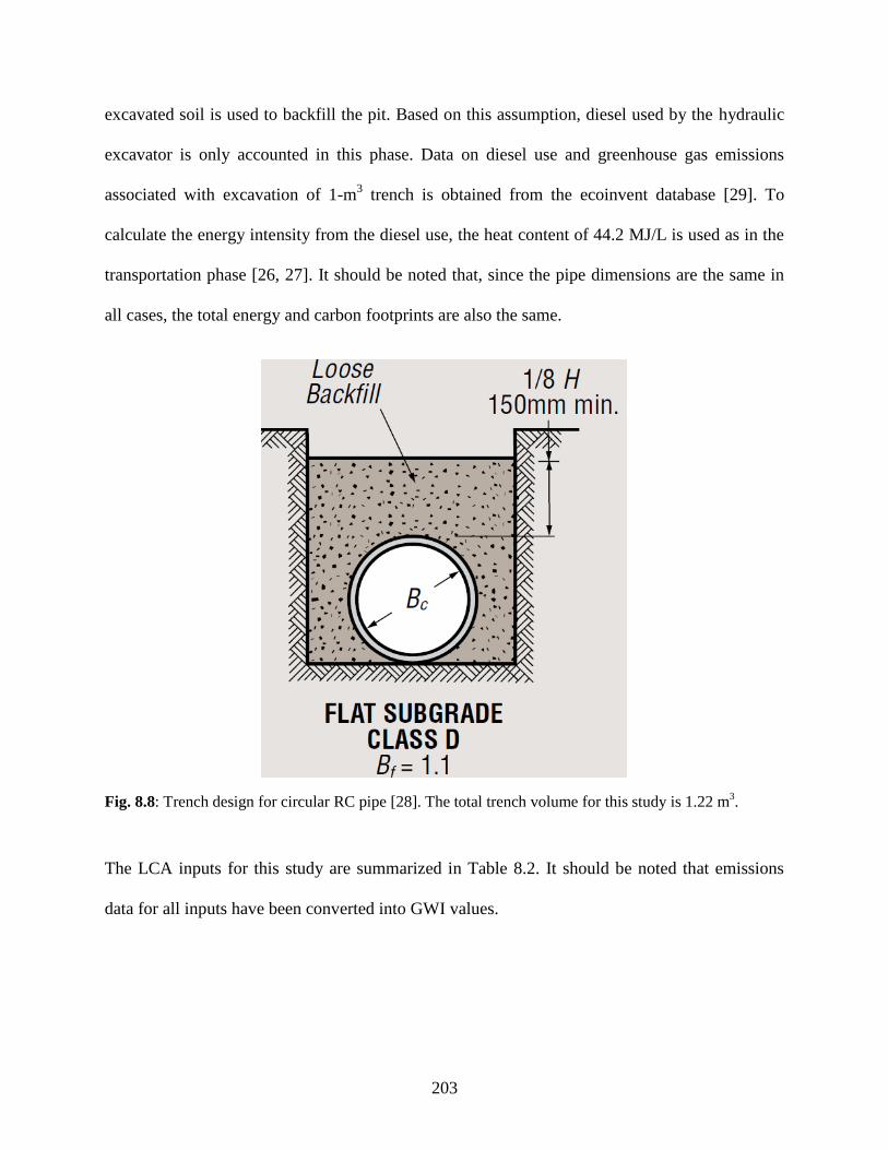
203

excavated soil is used to backfill the pit. Based on this assumption, diesel used by the hydraulic

excavator is only accounted in this phase. Data on diesel use and greenhouse gas emissions

associated with excavation of 1-m3 trench is obtained from the ecoinvent database [29]. To

calculate the energy intensity from the diesel use, the heat content of 44.2 MJ/L is used as in the

transportation phase [26, 27]. It should be noted that, since the pipe dimensions are the same in

all cases, the total energy and carbon footprints are also the same.

Fig. 8.8: Trench design for circular RC pipe [28]. The total trench volume for this study is 1.22 m3.

The LCA inputs for this study are summarized in Table 8.2. It should be noted that emissions

data for all inputs have been converted into GWI values.

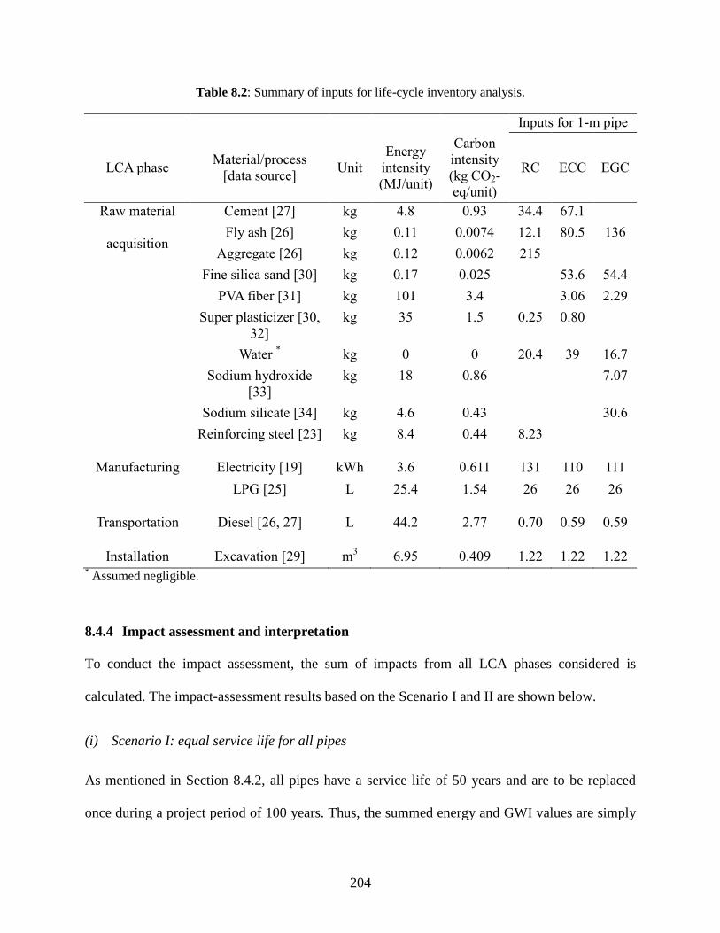
204

Table 8.2: Summary of inputs for life-cycle inventory analysis.

Inputs for 1-m pipe

LCA phase Material/process

[data source] Unit

Energy

intensity

(MJ/unit)

Carbon

intensity

(kg CO2-

eq/unit)

RC ECC EGC

Raw material

acquisition

Cement [27] kg 4.8 0.93 34.4 67.1

Fly ash [26] kg 0.11 0.0074 12.1 80.5 136

Aggregate [26] kg 0.12 0.0062 215

Fine silica sand [30] kg 0.17 0.025 53.6 54.4

PVA fiber [31] kg 101 3.4 3.06 2.29

Super plasticizer [30,

32]

kg 35 1.5 0.25 0.80

Water * kg 0 0 20.4 39 16.7

Sodium hydroxide

[33]

kg 18 0.86 7.07

Sodium silicate [34] kg 4.6 0.43 30.6

Reinforcing steel [23] kg 8.4 0.44 8.23

Manufacturing Electricity [19]

kWh 3.6 0.611 131 110 111

LPG [25] L 25.4 1.54 26 26 26

Transportation Diesel [26, 27] L 44.2 2.77 0.70 0.59 0.59

Installation Excavation [29] m

3 6.95 0.409 1.22 1.22 1.22

* Assumed negligible.

8.4.4 Impact assessment and interpretation

To conduct the impact assessment, the sum of impacts from all LCA phases considered is

calculated. The impact-assessment results based on the Scenario I and II are shown below.

(i) Scenario I: equal service life for all pipes

As mentioned in Section 8.4.2, all pipes have a service life of 50 years and are to be replaced

once during a project period of 100 years. Thus, the summed energy and GWI values are simply

205

doubled to account for the replacement.

Figure 8.9 shows the assessment results. As can be seen, the RC pipe performs best with regard

to life-cycle energy consumption. The biggest advantage of the material is its low impact from

the material-acquisition phase; energy associated with production of RC-pipe ingredients is only

30 and 39% of those for ECC and EGC, respectively. The large difference results from two

factors: the larger amount of fly ash incorporated in the RC mix design than normal concrete,

and the use of energy-intensive PVA fibers in both ECC and EGC pipes. In the case of pipe-

manufacturing energy use, the RC pipe has a slightly larger impact than ECC and EGC pipes due

to the heavier weight. However, the difference is less than 15% and relatively small compared to

that for the material-acquisition phase. The same is true for the transportation phase. In the case

of installation energy (and emissions), the impacts are almost negligible in all pipes, which is

consistent with previous LCA studies on water- and wastewater-pipe materials [5, 7, 19, 20].

On the other hand, the EGC pipe has the lowest impact for carbon emissions; the GWI for EGC

is 86 and 70% of those for RC and ECC, respectively. The difference mainly results from the

amount of cement used; EGC uses no cement and has the lower GWI for the material-acquisition

phase; conversely, ECC has the largest amount of cement and highest GWI. Due to the high

carbon intensity of cement, the material-acquisition phase has the largest contribution to the life-

cycle GWI of the ECC pipe, while the manufacturing phase is dominant in the EGC pipe. In the

case of RC, the material-acquisition phase is limited compared to ECC; the RC incorporates fly

ash substituting for a portion of cement and uses a smaller amount of cement than ECC. It should

be also noted that PVA fibers have relatively small impacts for GWI, as mentioned in Section 4.4

in Chapter 4.

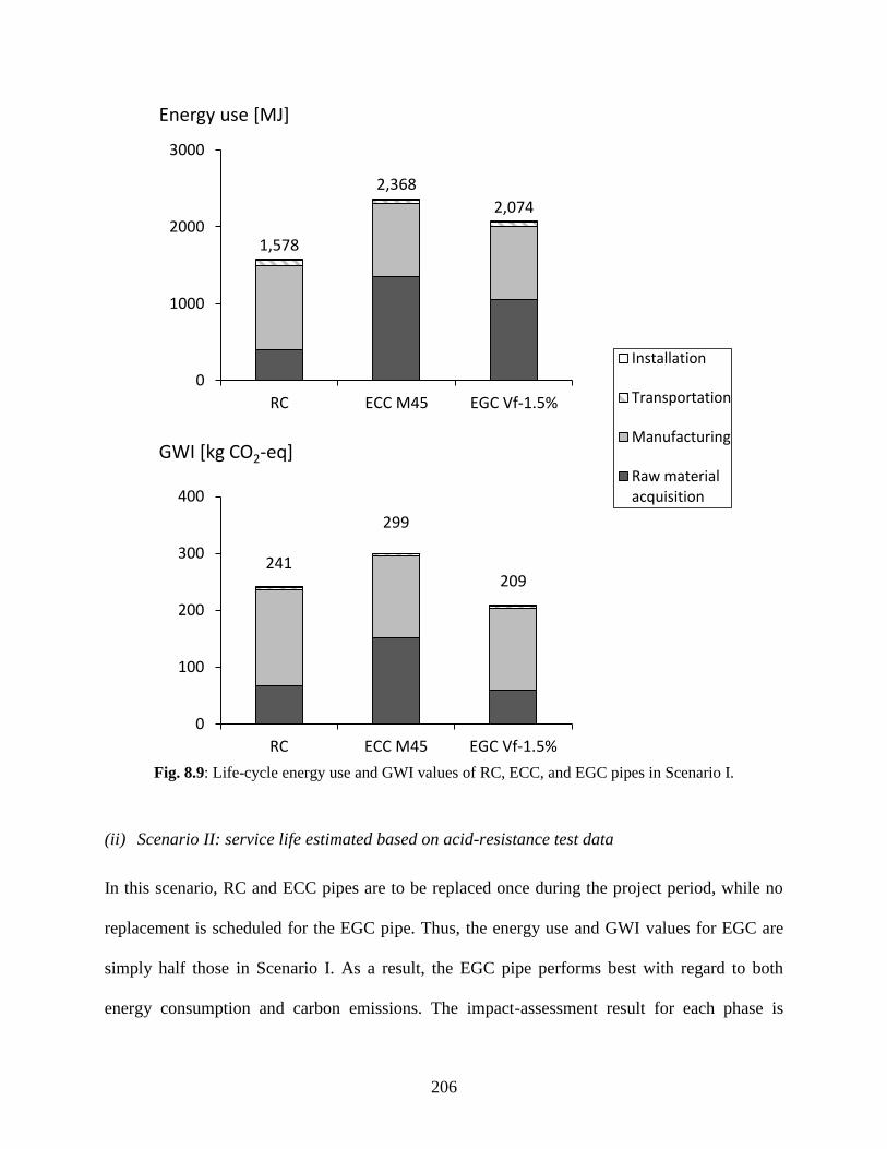
206

Fig. 8.9: Life-cycle energy use and GWI values of RC, ECC, and EGC pipes in Scenario I.

(ii) Scenario II: service life estimated based on acid-resistance test data

In this scenario, RC and ECC pipes are to be replaced once during the project period, while no

replacement is scheduled for the EGC pipe. Thus, the energy use and GWI values for EGC are

simply half those in Scenario I. As a result, the EGC pipe performs best with regard to both

energy consumption and carbon emissions. The impact-assessment result for each phase is

Energy use [MJ]

GWI [kg CO2-eq]0

1000

2000

3000

RC ECC M45EGC Vf-1.5%


Installation

Transportation

Manufacturing

Raw materialacquisition

1,578

2,368

2,074

0

1000

2000

3000

RC ECC M45 EGC Vf-1.5%

241

299

209

0

100

200

300

400

RC ECC M45 EGC Vf-1.5%

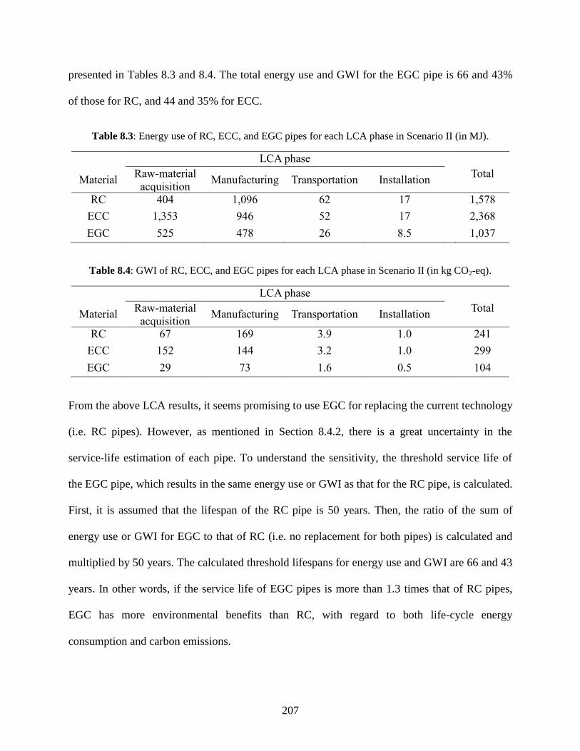
207

presented in Tables 8.3 and 8.4. The total energy use and GWI for the EGC pipe is 66 and 43%

of those for RC, and 44 and 35% for ECC.

Table 8.3: Energy use of RC, ECC, and EGC pipes for each LCA phase in Scenario II (in MJ).

LCA phase

Material Raw-material

acquisition Manufacturing Transportation Installation

Total

RC 404 1,096 62 17 1,578

ECC 1,353 946 52 17 2,368

EGC 525 478 26 8.5 1,037

Table 8.4: GWI of RC, ECC, and EGC pipes for each LCA phase in Scenario II (in kg CO2-eq).

LCA phase

Material Raw-material

acquisition Manufacturing Transportation Installation

Total

RC 67 169 3.9 1.0 241

ECC 152 144 3.2 1.0 299

EGC 29 73 1.6 0.5 104

From the above LCA results, it seems promising to use EGC for replacing the current technology

(i.e. RC pipes). However, as mentioned in Section 8.4.2, there is a great uncertainty in the

service-life estimation of each pipe. To understand the sensitivity, the threshold service life of

the EGC pipe, which results in the same energy use or GWI as that for the RC pipe, is calculated.

First, it is assumed that the lifespan of the RC pipe is 50 years. Then, the ratio of the sum of

energy use or GWI for EGC to that of RC (i.e. no replacement for both pipes) is calculated and

multiplied by 50 years. The calculated threshold lifespans for energy use and GWI are 66 and 43

years. In other words, if the service life of EGC pipes is more than 1.3 times that of RC pipes,

EGC has more environmental benefits than RC, with regard to both life-cycle energy

consumption and carbon emissions.

208


This chapter explored the feasibility of using EGC for sanitary sewer pipes. Based on the brief

reviews of the market demand and current challenges of existing technologies, it seems

promising to introduce EGC in the market of large-diameter sewer concrete pipes. In addition, to

verify and quantify the enhanced sustainability of EGC pipes, a comparative LCA study has been

conducted on three pipe materials: RC, ECC, and EGC. When equal service life is assumed for

all pipes, the LCA result indicates that the EGC pipe performs best with regard to GWI. On the

other hand, the RC pipe has the lowest life-cycle energy use. The sensitivity analysis shows that,

if service life of EGC pipes is more than 1.3 times that of RC pipes, EGC performs best in both

energy consumption and carbon emissions.

The other findings obtained in the LCA study are listed below;

Life-cycle energy use for all pipes highly depends on the material-acquisition phase.

Because of the high energy intensity of PVA fibers, the EGC pipe has 2.6 times larger

energy use than the RC pipe for this phase.

Life-cycle GWI is significantly affected by the amount of cement used. Since no cement is

used in EGC, contributions from the material-acquisition phase are limited, while the pipe-

manufacturing phase becomes dominant.

For both life-cycle energy use and GWI, transportation and installation phases have

negligible impacts.

It should be noted that, in the present LCA study, the high tensile ductility and multiple

microcracking characteristic of EGC are not taken into account for the service life estimation. As

a result, steel-reinforced geopolymer pipes would have better environmental performances than

209

EGC pipes. A further study is required to develop a more comprehensive method to estimate the

pipe lifespan based on mechanical properties, as well as sulfuric acid resistance.

In addition, life-cycle cost analysis is also important to select the best pipe material, especially

for asset owners. Considering the time and cost for manufacturing of steel cages, EGC pipes

would have significant advantages against reinforced concrete and geopolymer pipes. This will

also be a subject of future studies.

Another important aspect excluded from the present LCA study is the externalities associated

with loss of use, repair, and replacement of sewer pipes. For example, when replacement of

buried pipes under high-traffic roads requires the trench excavation, the construction activities

could cause traffic congestion or delay. This leads to time loss of drivers on the route and more

emissions from the vehicles. Such externalities are critical when frequent/extensive replacement

is required, and are thus related to the pipe lifespan. The social cost and environmental impacts

associated with those externalities should be quantified in a future study.

210

References

[1] ASCE, “Wastewater: Infrastructure Report Card 2017,” 2017. [Online]. Available:

https://www.infrastructurereportcard.org/wp-content/uploads/2017/01/Wastewater-

Final.pdf. [Accessed: 15-Aug-2017].

[2] US Environmental Protection Agency, “Sanitary Sewer Overflows: National Pollutant

Discharge Elimination System.” [Online]. Available: https://www.epa.gov/npdes/sanitary-

sewer-overflows-ssos. [Accessed: 10-Aug-2017].

[3] C. A. Taylor and J. Marr, “A Research Plan and Report on Factors A ecting Culvert Pipe

Service Life in Minnesota,” 2012.

[4] The Freedonia Group, “Plastic & Competitive Pipe,” Cleveland (OH), 2014.

[5] F. Du, G. Woods, and D. Kang, “Life Cycle Analysis for Water and Wastewater Pipe

Materials,” J. Environ. Eng., vol. 139, no. May, pp. 703–711, 2012.

[6] The Freedonia Group, “Water & Wastewater Pipe: United States,” Cleveland (OH), 2014.

[7] E. Vahidi, E. Jin, M. Das, M. Singh, and F. Zhao, “Comparative Life Cycle Analysis of

Materials in Wastewater Piping Systems,” in Procedia Engineering, 2015, vol. 118, no.

813, pp. 1177–1188.

[8] The Freedonia Group, “Large Diameter Pipe: United States,” Cleveland (OH), 2012.

[9] U.S. Army Corps of Engineers, “Engineering and Design: Coduits, Culverts, and Pipes,”

Washington, EC, 1997.

[10] M. O’Connell, C. McNally, and M. G. Richardson, “Biochemical attack on concrete in

wastewater applications: A state of the art review,” Cem. Concr. Compos., vol. 32, no. 7,

pp. 479–485, 2010.

[11] W. Sand and E. Bock, “Concrete corrosion in the Hamburg Sewer system,” Environ.

Technol., vol. 5, no. 12, pp. 517–528, 1984.

[12] D. G. Meacham, J. O. Hurd, and W. W. Shisler, “Ohio Culvert Durability Study,”

Columbs, OH, 1982.

[13] G. Johnson, “Encouraging the use of sustainable materials: Geopolymer Concrete,” Rocla,

2014. [Online]. Available:

http://www.roads.org.au/News/Publications?EntryId=54&Command=Core_Download&m

ethod=attachment. [Accessed: 17-Aug-2017].

[14] D. Keaffaber, “GeoSpray: GeoPolymer Mortar System and Concrete Cloth for Structural

Rehabilitation/Repair of Sewer and Storm Infrastructure,” Milliken Infrastructure, 2015.

[Online]. Available:

211

http://ctt.mtu.edu/sites/ctt/files/resources/bridge2016/conference/08keaffaber.pdf.

[Accessed: 04-Jul-2017].

[15] The International Standards Organisation, “Environmental management — Life cycle

assessment — Principles and framework,” Iso 14040, vol. 2006, pp. 1–28, 2006.



[17] H. Stang and V. Li, “Extrusion of ECC-Material,” in High Performance Fiber Reinforced

Cement Composites 3 (HPFRCC 3), 1999, pp. 203–212.

[18] ASTM C497-17, Standard Test Methods for Concrete Pipe, Manhole Sections, or Tile.

West Conshohocken, PA: ASTM International, 2017.

[19] J. M. B. Recio, P. J. Guerrero, M. G. Ageitos, and R. P. Narváez, “Estimate of energy

consumption and CO2 emission associated with the production, use and final disposal of

PVC, HDPE, PP, ductile iron and concrete pipes,” Barcelona (Spain), 2005.

[20] K. R. Piratla, S. M. Asce, S. T. Ariaratnam, M. Asce, and A. Cohen, “Estimation of CO 2

Emissions from the Life Cycle of a Potable Water Pipeline Project,” J. Manag. Eng., vol.

28, no. January, pp. 22–30, 2012.

[21] Ohio Department of Transportation, Ohio Culvert Design Manual. Columbs, OH, 2003.








[23] International Iron and Steel Institute, “Rebar, EAF route,” in Worldwide LCI Database for

Steel Industry Products, Brussels (Belgium), 2002.

[24] T. J. Skone, “Life Cycle Greenhouse Gas Emissions: Natural Gas and Power Production.”

[Online]. Available: https://www.eia.gov/conference/2015/pdf/presentations/skone.pdf.

[Accessed: 15-Sep-2017]..

[25] L. K. Turner and F. G. Collins, “Carbon dioxide equivalent (CO2-e) emissions: A

comparison between geopolymer and OPC cement concrete,” Constr. Build. Mater., vol.

43, pp. 125–130, Jun. 2013.



[27] M. L. Marceau, M. A. Nisbet, and M. G. Vangeem, Life Cycle Inventory of Portland

Cement Manufacture. Stokie, IL: Portland Cement Association, 2006.

212

[28] American Concrete Pipe Association, Concrete Pipe & Box Culvert Installation. Irving,

Texas.

[29] The Swiss Centre for Life Cycle Inventories, “Ecoinvent.” [Online]. Available:

http://www.ecoinvent.org/home.html. [Accessed: 28-Jul-2017].





[32] G. A. Keoleian, A. Kendall, J. E. Dettling, V. M. Smith, R. F. Chandler, M. D. Lepech,

and V. C. Li, “Life Cycle Modeling of Concrete Bridge Design: Comparison of

Engineered Cementitious Composite Link Slabs and Conventional Steel Expansion Joints,”

J. Infrastruct. Syst., vol. 11, no. 1, pp. 51–60, 2005.

[33] E. Chlor, “An Eco-profile and Environmental Product Declaration of the European Chlor-

Alkali Industry,” 2013. [Online]. Available:





213

PART V: CONCLUSION

CHAPTER 9: Concluding Remarks

This doctoral research focused on development and characterization of green and durable –

therefore, truly sustainable – fiber-reinforced geopolymer composites for civil infrastructure

applications. In this chapter, research impacts and scientific contributions achieved in this study

are first highlighted. Major research findings are then summarized, and recommended subjects

for future studies are presented in the end.

9.1 Research impacts and contributions

(i) Development of a comprehensive design method for EGC

A new design method for ductile fiber-reinforced geopolymer composites has been proposed in

this dissertation. The method integrates three design techniques – Design of Experiment (DOE),

micromechanical modeling, and Material Sustainability Indices (MSI) – to systematically

optimize the matrix, fiber, and interface properties. Fundamental engineering properties, high

tensile ductility, multiple microcracking characteristics, and enhanced material greenness can be

simultaneously achieved with the aid of the multidisciplinary integrated scheme. This design

method facilitates development of various types of EGC and promotes the overall progress in the

research community. Further, the design concept is applicable to not only fiber-reinforced

214

geopolymer composites but also many other composite materials in a variety of engineering

fields.

(ii) Development of green and durable geopolymer composites

By using the proposed integrated method, green and durable EGC materials have been developed

in Chapter 4. The optimized EGC shows tensile strain-hardening behavior with high ductility of

over 4%, and self-controls its microcracks as tight as 40 µm on average (in residual crack width).

Such excellent tensile properties have not been achieved in any other geopolymer composites.

The high tensile ductility and tight crack width can suppress the inherent brittleness of

geopolymers, leading to improved material durability. Moreover, the fiber content is limited to

1.5% by volume, which offers significant reduction in energy and carbon footprints. Because of

the high durability and enhanced material greenness, the optimized EGC is promising for a broad

range of civil infrastructure applications.

(iii) Characterization of durability properties of EGC

Fundamental durability properties of EGC have been experimentally investigated in this study.

Particularly, crack patterns and water permeability of EGC studied in Chapter 5 are crucial for its

transport properties, which govern many types of deterioration processes. The obtained

experimental results will be useful in future studies on other durability properties of EGC. In

addition, sulfuric acid resistance of EGC has been evaluated in Chapter 7, in comparison with

OPC concrete and ECC. Those data can be used to estimate service life of EGC infrastructure

under sulfuric acid attack, such as wastewater facilities.

215

(iv) Feasibility of self-healing EGC

The feasibility of achieving self-healing functionality in EGC has been demonstrated in Chapter

6. Only a handful of papers so far have reported self-healing phenomena in geopolymer materials.

Experimental results in this study confirm slight but significant stiffness recovery in preloaded

EGC due to self-healing of microcracks. Also, microstructure of healing products observed by

SEM has been presented, with elemental analysis results by using EDS. While mechanisms

behind the EGC self-healing have not been fully understood, this study will open a new window

toward developing self-healing geopolymer materials.

(v) Feasibility of introducing EGC for sewer-pipe applications

Brief market research and technical-advantage analysis in Chapter 8 suggests that EGC is

promising for large-diameter sewer pipe applications. In addition, a comparative environmental

LCA shows lower life-cycle greenhouse gas emissions of the EGC pipe than RC and ECC pipes.

The study also reveals dominant ingredients and LCA phases in their life-cycle environmental

impacts, which provides valuable insights for developing a more sustainable EGC for those

applications.

9.2 Research findings

Major research findings obtained during investigations are listed below;

216

(i) From Part II: Development of EGC

The alkaline activator-to fly ash ratio has statistically insignificant effects on compressive

strength of the EGC matrix. This is in contrast with many previous studies in the research

community.

EGC matrix has lower tensile strength and more brittle behavior than typical ECC matrix,

which is however beneficial in achieving robust multiple microcracking and resultant high

tensile ductility in the composite.

Interface properties between EGC matrix and PVA fiber are significantly different from

those for PVA-ECC; it is suggested that the stronger chemical bond, weaker frictional bond,

and smaller slip-hardening coefficient of EGC contribute to the tighter crack with and higher

tensile ductility.

The developed EGC shows tensile strain-hardening behavior with high ductility of 3% even

with a small fiber volume fraction of 1.0%. However, the performance variability is

relatively large compared to that with 1.5 or 2.0% fiber content, which might be associated

with the magnitude of PSH indices.

GWI of the optimized EGC is roughly half that of normal cement concrete; conversely, the

embodied energy of EGC is about 70% higher, which results from the use of energy-

intensive PVA fiber.

(ii) From Part III: Characterization of EGC Durability

Chapter 5: Cracking Characteristics and Water Permeability of EGC

Residual crack width of EGC is lognormally distributed as in ECC materials.

217

Some EGC specimens under uniaxial tension showed suppressed propagation of localized

cracking; a large localized crack initiated from the edge of the specimen (probably due to

unintended poor compaction and fiber dispersion), but was confined to the near-edge area,

not propagating thorough the matrix. A further research would be required to understand the

mechanism behind this phenomenon.

Multiple-point measurement is recommended to accurately characterize crack patterns of

EGC; crack width is not constant along each crack, and the numbers of crack are different

between the central area and near-edge sides of the specimen surface.

When EGC and normal reinforced mortar/concrete are subjected to the same tensile strain,

the cracked EGC shows a significantly lower permeability coefficient than the cracked

reinforced mortar/concrete. This suggests better transport properties and related durability of

EGC.

Average crack width of EGC has a stronger correlation with permeability coefficient than

maximum crack width; maximum crack width only represents the crack opening in a small

area because of the nonuniform opening along each crack.

White substance is formed on the surface of cracked EGC specimens during permeability

testing. This seals some microcracks, reducing the permeability coefficient.

Chapter 6: Feasibility Study of Self-healing EGC

The sealed microcracks also offer slight but significant stiffness recovery of EGC in uniaxial

tension testing.

However, the degree of EGC self-healing is limited compared to self-healing in ECC; some

microcracks are completely sealed, while others are only partially sealed. The limited

218

formation of healing products would be a cause of the limited performance recoveries in

water tightness and stiffness.

EGC healing products are mostly angular, stone-like substance, and relatively rich in Si and

Al but low in Ca. Unlike self-healing in cement-based materials, main healing products of

EGC are neither calcite (CaCO3) nor CSH.

Chapter 7: Sulfuric Acid Resistance of EGC

Self-healing in EGC requires the presence of water; however, no healing is observed for

EGC immersed in sulfuric acid solution. In contrast, most microcracks in ECC are

completely sealed even in the acidic environment.

Meanwhile, surface erosion of EGC due to the sulfuric acid exposure is limited compared to

that of ECC and cement concrete; the rate of weight loss for acid-exposed EGC is roughly

one third that of the cement-based materials. This verifies the high sulfuric acid resistance of

EGC.

In addition, no significant degradation in mechanical performances is observed for acid-

exposed EGC, except in linear bending stiffness. However, the stiffness reduction is

significantly lower than that for RC.

(iii) From Part IV: Application of EGC

When equal service life is assumed for large-diameter EGC, ECC, and RC sewer pipes, a

comparative LCA indicates the lowest GWI of the EGC pipe. On the other hand, the RC

pipe has the lowest life-cycle energy use.

219

If service life of the EGC pipe is more than 1.3 times that of the RC pipe, EGC performs

best in both life-cycle energy consumption and GWI.

Life-cycle energy consumption for large-diameter sewer pipes is highly dependent on the

material-acquisition phase. Particularly, PVA fiber has high energy intensity and largely

contributes to the energy use in EGC/ECC production.

Similarly, life-cycle GWI is significantly affected by the amount of cement used in the pipe

material. Since EGC incorporates no cement, the material acquisition is not the dominant

phase. Instead, the pipe manufacturing has the largest contribution to the total GWP.

For both life-cycle energy and GWI, transportation and installation phases have insignificant

impacts. This suggests that the LCA result is not so sensitive to assumptions and

simplifications in those phases.

9.3 Recommendations for future work

For continued development, characterization, and application of EGC, the following

investigations are recommended for future work:

(i) Development of natural fiber-reinforced EGC

To drastically enhance the material greenness of EGC, PVA fiber should be replaced because of

the high energy intensity. Specifically, use of natural fibers, instead of synthetic fibers produced

from petroleum-based inputs, is promising. In recent years, much effort is being made in

developing natural fiber-reinforced concrete. There is also ongoing research on natural fiber-

reinforced ECC. Knowledge and findings from those studies will be useful in developing natural

220

fiber-reinforced EGC. Also, the integrated design method proposed in this doctoral research is

applicable to the development.

(ii) Development of room temperature-cured EGC

The current EGC requires temperature curing to achieve good compressive strength. This is not

suitable for cast-in-place applications. To make a broader range of EGC applications possible,

development of room temperature-cured EGC is recommended. So far, various types of room

temperature-cured geopolymer concrete have been developed. Particularly, slag-based

geopolymers would be most promising.

(iii) Investigation on self-healing mechanisms in EGC

This doctoral research suggests that healing products of EGC are different from those of cement-

based materials. As such, they might be produced through different mechanisms. To achieve

better self-healing performance in EGC, those mechanisms should be first understood.

Particularly, more detailed chemical compositions of healing products need to be studied by

using advanced characterization techniques such as X-ray diffraction (XRD) and Fourier

transform infrared spectroscopy (FTIR).

(iv) Characterization of other durability properties

To verify the enhanced material durability of EGC, other important durability properties should

be investigated. Specifically, studies on the drying shrinkage, chloride-ion diffusivity, and fire

and frost resistance would be recommended. Many previous studies on geopolymer concrete

demonstrated comparable or better performances in such properties compared to cement concrete.

221

Thus, EGC is expected to have similar or even better performances. Verifying this hypothesis

promotes introduction of EGC into a wider variety of civil infrastructure applications.

(v) Development of a more comprehensive LCA model for sewer pipes

First and foremost, the comparative LCA method used in this study has a great uncertainty in

estimating service life of EGC pipes. Particularly, the high tensile ductility and multiple

microcracking characteristics are not taken into account in the estimation. In addition, because of

those unique characteristics, EGC pipes might be able to meet mechanical-performance

requirements with a smaller wall thickness than RC pipes. It should be also mentioned that

externalities associated with loss of use, repair, and replacement of sewer pipes might have

significant impacts on the LCA result. Conducting further experimental and analytical

investigations and data collection, a more comprehensive LCA model to account for the above

aspects needs to be developed.

(vi) Cost analysis and minimization

No cost analysis has been conducted in this doctoral study. However, the material cost is one of

the most important factors for introducing the new technology, especially into large-scale

infrastructure applications. Since EGC uses no cement but utilizes fly ash (i.e. less expensive

industrial byproduct), it has some advantage over cement concrete and ECC. On the other hand,

the cost of alkaline solution could be a significant disadvantage of EGC. It is recommended to

estimate the total material cost for EGC and compare it with those of competing materials. In

addition, a further investigation will be required to minimize the EGC cost; using less expensive

fibers or alkaline activators would be promising.

222

APPENDICES

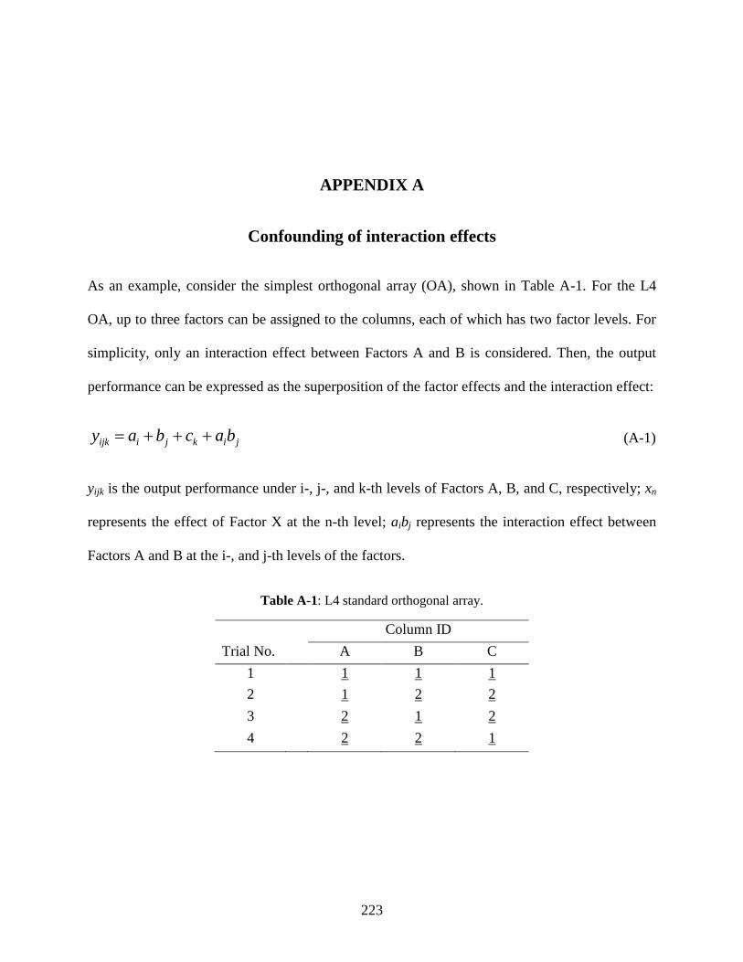
223

APPENDIX A

Confounding of interaction effects

As an example, consider the simplest orthogonal array (OA), shown in Table A-1. For the L4

OA, up to three factors can be assigned to the columns, each of which has two factor levels. For

simplicity, only an interaction effect between Factors A and B is considered. Then, the output

performance can be expressed as the superposition of the factor effects and the interaction effect:

jikjiijk bacbay (A-1)

yijk is the output performance under i-, j-, and k-th levels of Factors A, B, and C, respectively; xn

represents the effect of Factor X at the n-th level; aibj represents the interaction effect between

Factors A and B at the i-, and j-th levels of the factors.

Table A-1: L4 standard orthogonal array.

Column ID

Trial No. A B C

1 1 1 1

2 1 2 2

3 2 1 2

4 2 2 1

224

The interaction effect can be measured by the difference between the averaged outputs at the

A1B1 plus A2B2 levels and the A1B2 plus A2B1 levels. Namely, the following quantities are

compared:

22

)()(

2

22111

21212211112211

babac

bbaayyT

(A-2)

22

)()(

2

12212

21212121222112

babac

bbaayyT

(A-3)

By subtracting Eq. A-3 from Eq. A-2:

2

)()()( 12212211

2121122211

babababaccTT

(A-4)

Equation A-4 indicates that the interaction effect between Factors A and B is confounded with

the main effect of Factor C, i.e. (c1 – c2) in the equation. In other words, if no factor is assigned

to the third column, the interaction effect between assigned Factors A and B can be quantified as

the main effect of the third column. This is one way to deal with significant interaction effects in

OAs.

Following the similar derivation to that above, it can be shown that, in L9 OA discussed in

Chapter 3, the interaction effect between Factors A and B is confounded with both the third and

fourth columns (Factors C and D). Further, many other interaction effects are also confounded

with various main factor effects. This is a reason that the L9 OA is not suitable for evaluating

factors that are expected to have significant interaction effects. Conversely, in L18 OA used in

Chapter 4, all interaction effects are almost evenly confounded with main factor effects, and the

influence on the evaluation of the main factor effects is minimal.

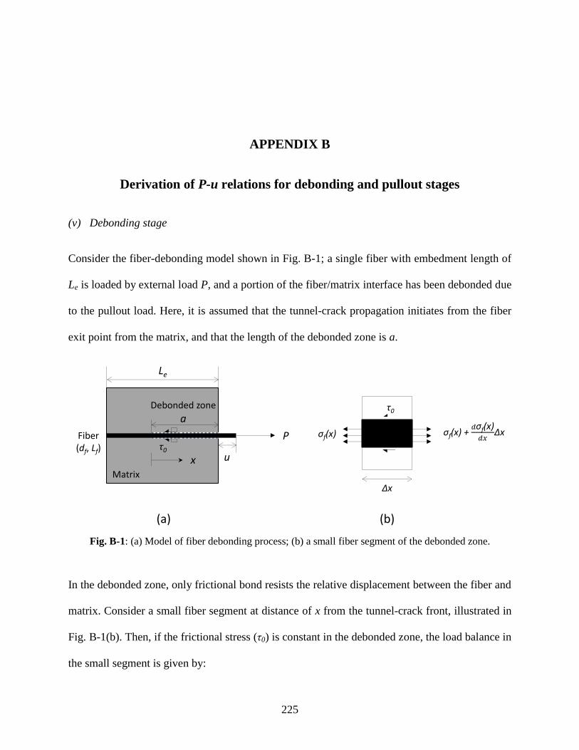
225

APPENDIX B

Derivation of P-u relations for debonding and pullout stages

(v) Debonding stage

Consider the fiber-debonding model shown in Fig. B-1; a single fiber with embedment length of

Le is loaded by external load P, and a portion of the fiber/matrix interface has been debonded due

to the pullout load. Here, it is assumed that the tunnel-crack propagation initiates from the fiber

exit point from the matrix, and that the length of the debonded zone is a.

Fig. B-1: (a) Model of fiber debonding process; (b) a small fiber segment of the debonded zone.

In the debonded zone, only frictional bond resists the relative displacement between the fiber and

matrix. Consider a small fiber segment at distance of x from the tunnel-crack front, illustrated in

Fig. B-1(b). Then, if the frictional stress (τ0) is constant in the debonded zone, the load balance in

the small segment is given by:

u

Le

Matrix

Fiber(df, Lf)

Debonded zone

P

x

a

τ0

τ0

Δx

σf(x) + Δxσf(x)

(a) (b)

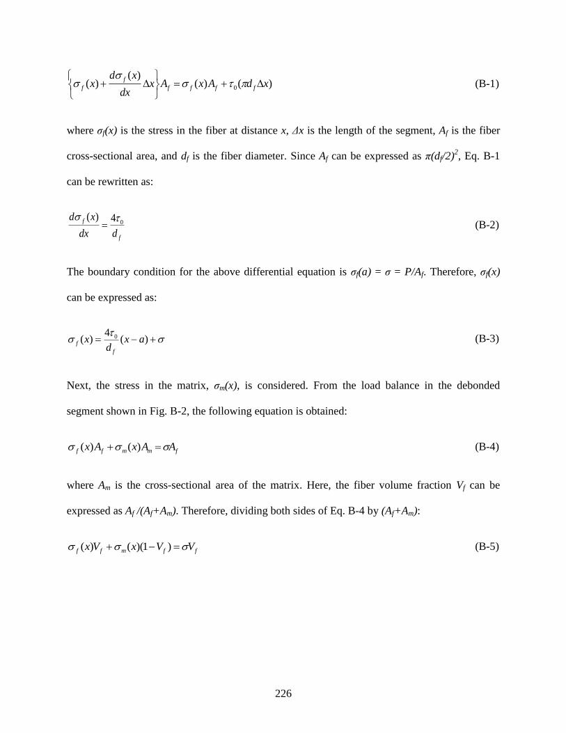
226

)()()(

)( 0 xdAxAxdx

xdx ffff

f

f

(B-1)

where σf(x) is the stress in the fiber at distance x, Δx is the length of the segment, Af is the fiber

cross-sectional area, and df is the fiber diameter. Since Af can be expressed as π(df/2)2, Eq. B-1

can be rewritten as:

f

f

ddx

xd04)(

(B-2)

The boundary condition for the above differential equation is σf(a) = σ = P/Af. Therefore, σf(x)

can be expressed as:

)(4

)( 0 axd

xf

f (B-3)

Next, the stress in the matrix, σm(x), is considered. From the load balance in the debonded

segment shown in Fig. B-2, the following equation is obtained:

fmmff AAxAx )()( (B-4)

where Am is the cross-sectional area of the matrix. Here, the fiber volume fraction Vf can be

expressed as Af /(Af+Am). Therefore, dividing both sides of Eq. B-4 by (Af+Am):

ffmff VVxVx )1)(()( (B-5)

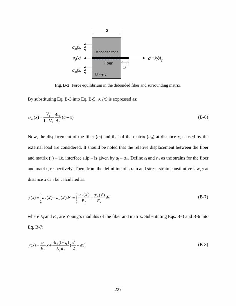
227

Fig. B-2: Force equilibrium in the debonded fiber and surrounding matrix.

By substituting Eq. B-3 into Eq. B-5, σm(x) is expressed as:

)(4

1)( 0 xa

dV

Vx

ff

f

m

(B-6)

Now, the displacement of the fiber (uf) and that of the matrix (um) at distance x, caused by the

external load are considered. It should be noted that the relative displacement between the fiber

and matrix (γ) – i.e. interface slip – is given by uf – um. Define εf and εm as the strains for the fiber

and matrix, respectively. Then, from the definition of strain and stress-strain constitutive law, γ at

distance x can be calculated as:

x

m

m

f

fx

mf xdE

x

E

xxdxxx

00

)()()()()(

(B-7)

where Ef and Em are Young’s modulus of the fiber and matrix. Substituting Eqs. B-3 and B-6 into

Eq. B-7:

)2

()1(4

)(2

0 axx

dEx

Ex

fff

(B-8)

u

a

Matrix

Fiber

Debonded zone

σ =P/Afσf(x)

σm(x)

σm(x)

228

where η is defined as VfEf /VmEm and Vm is the volume fraction of the matrix. It should be noted

that, at x = 0 (i.e. the tunnel-crack front), γ is zero since there is no interface slip in the bonded

zone. On the other hand, the interface slip at the fiber exit point (x = a) is given by:

uadE

aE

afff

20 )1(2)(

(B-9)

This is equivalent to the fiber pullout displacement u. Since a is an unknown variable, Eq. B-9

cannot be solved for the fiber pullout load P; another condition to eliminate a from the equation

is needed.

Here, an infinitesimal propagation of the tunnel crack is considered, assuming that the fiber and

matrix comprise an elastic body. Based on the linear elastic fracture mechanics (LEFM), the

energy balance in the system requires:

dAGdWdUuPd dff (B-10)

Pdu’f, dU, dWf, and GddA represent the work done by the external load, change in the stored

strain energy of the elastic system, dissipated energy by the friction at the fiber/matrix interface,

and fracture energy consumed to debond the interface, respectively. It should be noted that u’f is

the displacement of the fiber including not only the elastic stretch of the debonded zone but also

that of the bonded zone. The force equilibrium of Eq. B-5 also holds in the bonded zone, while

the elastic strains of the fiber and matrix are identical (i.e. εf = εm). Namely:

fmmffmmmfffmmfff VEVEVEVEVVV )( (B-11)

Therefore, u’f is expressed as:

229

)()(

0

aLVEVE

Vdx

E

xu e

mmff

fa

f

f

f

(B-12)

Meanwhile, regarding the friction term:

a

ff xdxdW0

0 )()( (B-13)

From Eqs. B-8 and B-13:

32

020

3

)1(4

2a

Ea

E

dW

ff

f

f

(B-14)

For the strain energy term, a theory in LEFM that the change in elastic strain energy of the

system is half the work done by external load is used. Considering the friction as surface traction,

the work term minus the friction term can be regarded as the available energy for the strain-

energy change. That is:

)(2

1ff dWuPddU (B-15)

From Eqs. B-10 and B-15:

)(2

1ffd dWuPddAG (B-16)

where dA represents the area of the extended tunnel crack and can be expressed as πdfda where

da is the length of the crack extension. Then, substituting Eqs. B-12 and B-14 into Eq. B-16, the

following equation is obtained:

230

22

002 )1(2

)1(8a

dEE

a

E

dG

ffff

f

d

(B-17)

Solve the above equation for σ > 0:

f

fd

f d

EGa

d

)1(8)1(4 0

(B-18)

By combining Eqs. B-9 and B-18, the following solution is obtained:

00 0,)()1(2

2)( uuGud

Eu d

f

f

(B-19)

Or, by converting the stress σ into the force P, the equation can be rewritten as:

00

32

0,2

1)( uuGu

dEuP d

ff

(B-20)

This is identical to the Eq. 3.27 in Chapter 3. Here, u0 is the critical pullout displacement at

which full-debonding is completed (i.e. a = Le). Therefore, from Eq. B-18:

f

fd

e

f d

EGL

du

)1(8)1(4)( 0

0

(B-21)

Also, from Eq. B-9:

2000

)1(2)()( e

ff

e

f

e LdE

LE

uLu

(B-22)

By substituting Eq. B-21 into B-22:

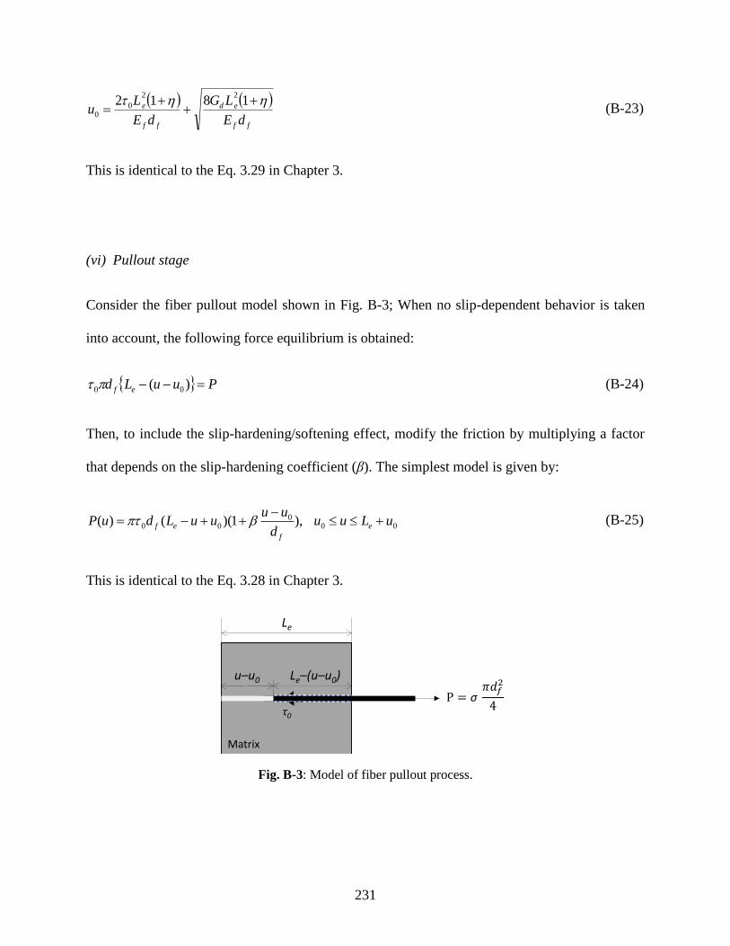
231

ff

ed

ff

e

dE

LG

dE

Lu

181222

00

(B-23)

This is identical to the Eq. 3.29 in Chapter 3.

(vi) Pullout stage

Consider the fiber pullout model shown in Fig. B-3; When no slip-dependent behavior is taken

into account, the following force equilibrium is obtained:

PuuLd ef )( 00 (B-24)

Then, to include the slip-hardening/softening effect, modify the friction by multiplying a factor

that depends on the slip-hardening coefficient (β). The simplest model is given by:

000

00 ),1)(()( uLuud

uuuuLduP e

f

ef

(B-25)


Fig. B-3: Model of fiber pullout process.

Le

Matrix

Le–(u–u0)u–u0

τ0

232

(vii) Determination of Gd, τ0, and β from results of single-fiber pullout test

First, since Vf is sufficiently small in the single-fiber pullout model, it can be assumed that η is

negligible. Then, by converting the stress σ into the force P in Eq. B-21:

2)(

3

00

ffd

efdebond

dEGLduP (B-26)

Also, when u = u0, Eq. B-25 gives:

efpullout LduP 00 )( (B-27)

From Eq. B-27, the Eq. 3.19 in Chapter 3 is obtained. In addition, by combining Eqs. B-26 and

B-27, it can be shown that:

2

0032)()(

2uPuP

dEG pulloutdebond

ff

d

(B-28)


Next, the Eq. 3.20 in Chapter 3 is derived, which gives the least square estimation (LSE) of β.

For the one-parameter LSE, the following equation needs to be solved:

0)()(2''

i

ipulloutiex uPuPd

d

(B-29)

where Pex(ui’) is the measured pullout load at the i-th data of the post-peak pullout displacement.

Then, from the chain rule in calculus:

0)()()()(2)()( ''''2'' i

ipulloutiexipulloutiex

i

ipulloutiex uPuPd

duPuPuPuP

d

d

(B-30)

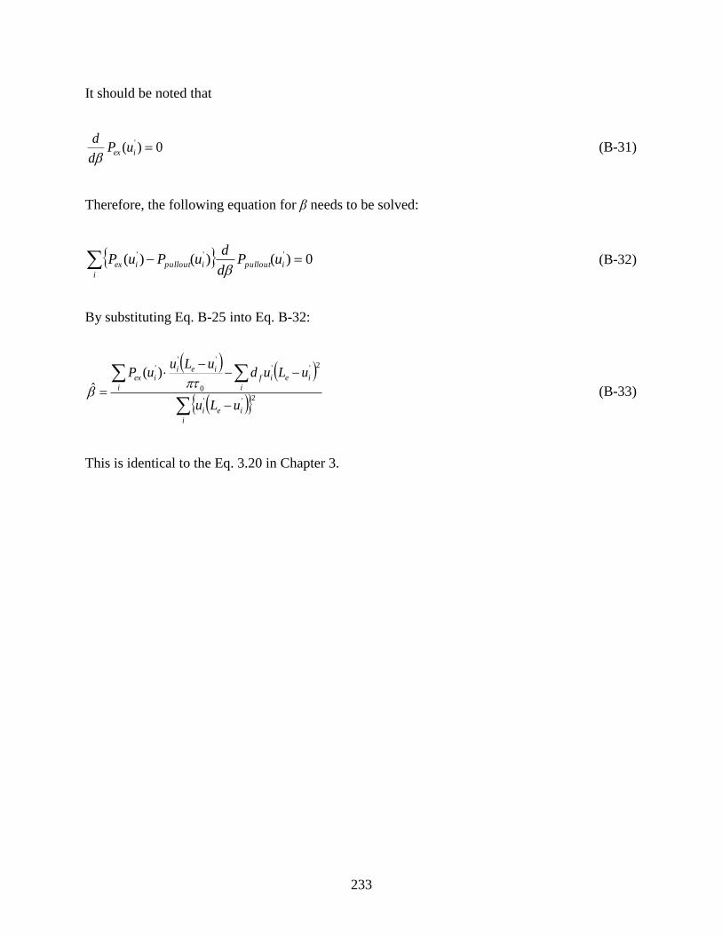
233

It should be noted that

0)( ' iex uPd

d

(B-31)

Therefore, the following equation for β needs to be solved:

0)()()( ''' i

ipulloutipulloutiex uPd

duPuP

(B-32)

By substituting Eq. B-25 into Eq. B-32:

i

iei

i

ieif

i

ieiiex

uLu

uLuduLu

uP

2''

2''

0

''' )(

ˆ (B-33)


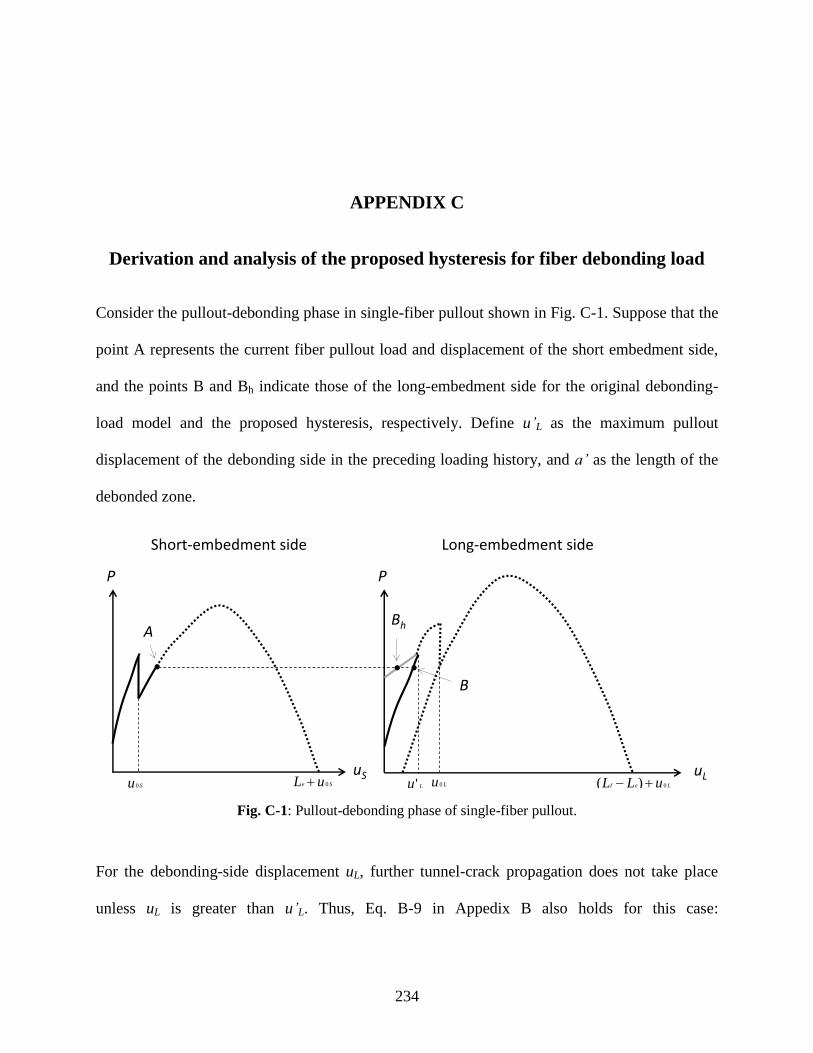
234

APPENDIX C

Derivation and analysis of the proposed hysteresis for fiber debonding load

Consider the pullout-debonding phase in single-fiber pullout shown in Fig. C-1. Suppose that the

point A represents the current fiber pullout load and displacement of the short embedment side,

and the points B and Bh indicate those of the long-embedment side for the original debonding-

load model and the proposed hysteresis, respectively. Define u’L as the maximum pullout

displacement of the debonding side in the preceding loading history, and a’ as the length of the

debonded zone.

Fig. C-1: Pullout-debonding phase of single-fiber pullout.

For the debonding-side displacement uL, further tunnel-crack propagation does not take place

unless uL is greater than u’L. Thus, Eq. B-9 in Appedix B also holds for this case:

Su 0

P

uSSe uL 0 Lu 0

P

uLLef uLL 0)(

Long-embedment sideShort-embedment side

A

B

Bh

Lu'

235

20 ')1(2

' adE

aE

ufff

L

(C-1)

Also, it should be noted that

)(4

2

L

h

debond

fuP

d

(C-2)

Then, by combining Eqs. C-1 and C-2:

LL

f

L

ff

L

h

debond uuad

ua

dEuP

0,

2

)1(

4)(

0

2 (C-3)

This is identical to the Eq. 3.33 in Chapter 3. In addition, by substituting uL = u’L into Eq. C-3,

the debonded length a’ can be obtained by solving the following equation:

ad

ua

dEuP

f

L

ff

L

h

debond

2

)1('

4)'(

0

2 (C-4)

This is equivalent to the Eq. 3.34 in Chapter 3. The comparison between Pdebond(uL) and

Ph

debond(uL) has been shown in Fig. 3.9 in Chapter 3.

Now, the effect of this modification on the composite σ–δ relation is considered. As an example,

the σ–δ curve of a standard ECC M45 is simulated by using the original and modified models.

Three-dimensional random fiber distribution is assumed, but, for simplicity, both the matrix

micro-spalling and Cook-Gordon effect (detailed in Section 3.3.2) are not taken into account.

Figure C-2 shows the simulation result. Significant difference cannot be seen between the two

curves. This might be attributed to the fact that the pullout-debonding phase is not predominant

in M45; as shown in Fig. C-3, most of fibers in the ECC are broken for large crack opening. As a

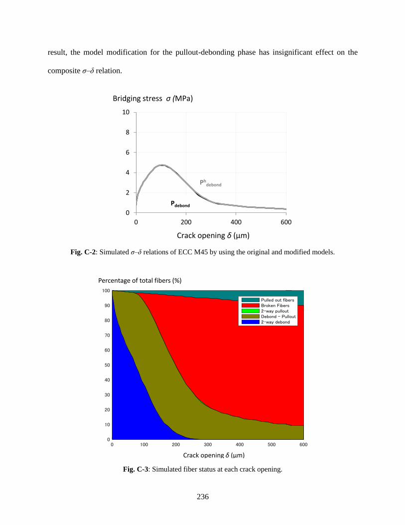
236

result, the model modification for the pullout-debonding phase has insignificant effect on the

composite σ–δ relation.

Fig. C-2: Simulated σ–δ relations of ECC M45 by using the original and modified models.

Fig. C-3: Simulated fiber status at each crack opening.

0

2

4

6

8

10

0 200 400 600

Pdebond

Bridging stress σ (MPa)


Phdebond


Percentage of total fibers (%)

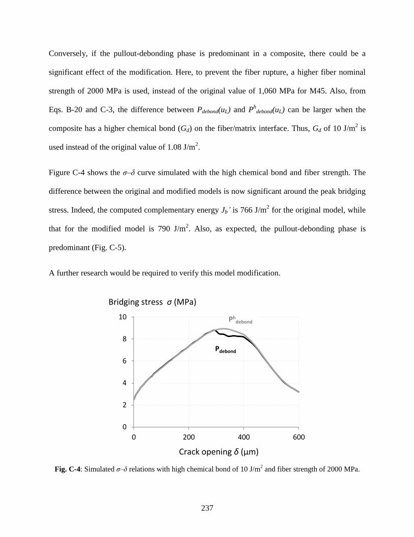
237

Conversely, if the pullout-debonding phase is predominant in a composite, there could be a

significant effect of the modification. Here, to prevent the fiber rupture, a higher fiber nominal

strength of 2000 MPa is used, instead of the original value of 1,060 MPa for M45. Also, from

Eqs. B-20 and C-3, the difference between Pdebond(uL) and Ph

debond(uL) can be larger when the

composite has a higher chemical bond (Gd) on the fiber/matrix interface. Thus, Gd of 10 J/m2 is

used instead of the original value of 1.08 J/m2.

Figure C-4 shows the σ–δ curve simulated with the high chemical bond and fiber strength. The

difference between the original and modified models is now significant around the peak bridging

stress. Indeed, the computed complementary energy Jb’ is 766 J/m2 for the original model, while

that for the modified model is 790 J/m2. Also, as expected, the pullout-debonding phase is

predominant (Fig. C-5).

A further research would be required to verify this model modification.

Fig. C-4: Simulated σ–δ relations with high chemical bond of 10 J/m2 and fiber strength of 2000 MPa.

0

2

4

6

8

10

0 200 400 600

Pdebond

Bridging stress σ (MPa)


Phdebond

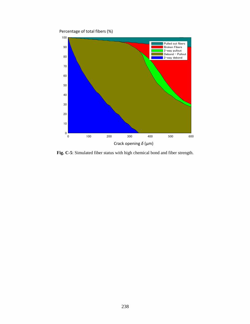
238

Fig. C-5: Simulated fiber status with high chemical bond and fiber strength.


Percentage of total fibers (%)

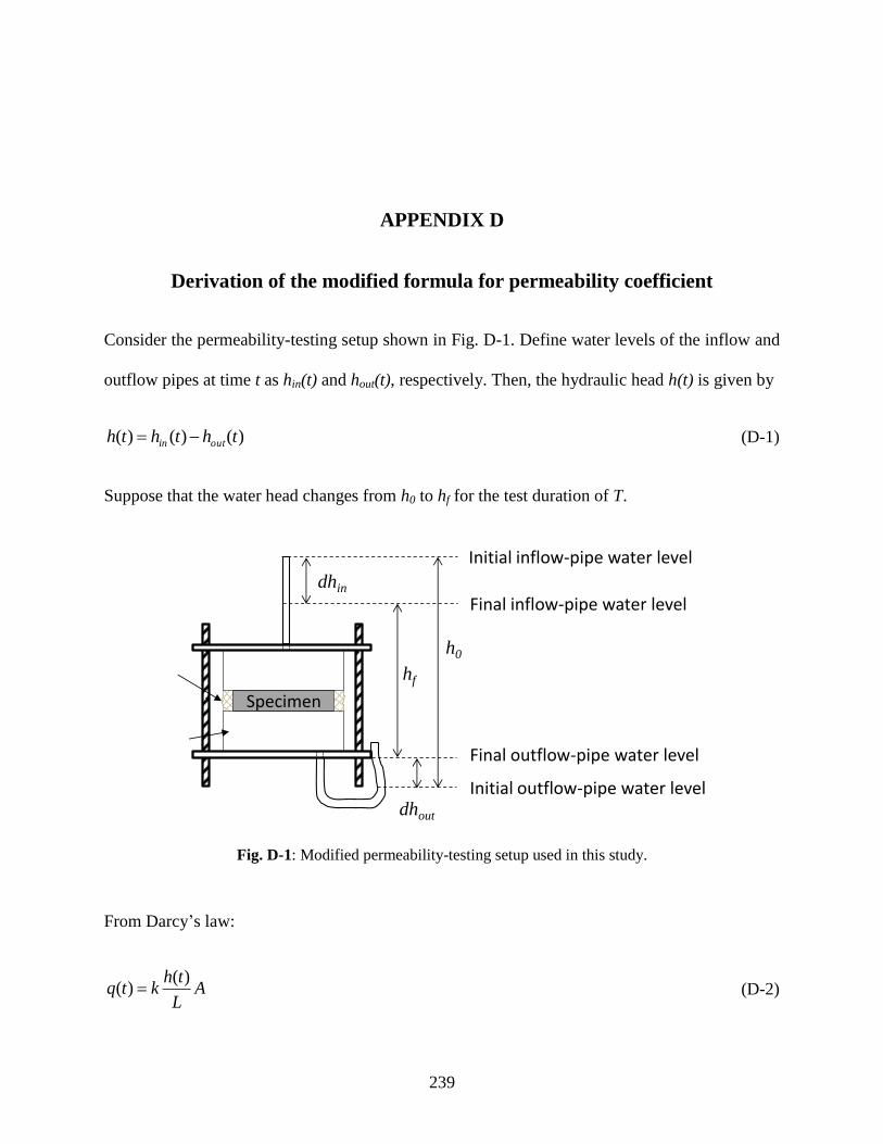
239

APPENDIX D

Derivation of the modified formula for permeability coefficient

Consider the permeability-testing setup shown in Fig. D-1. Define water levels of the inflow and

outflow pipes at time t as hin(t) and hout(t), respectively. Then, the hydraulic head h(t) is given by

)()()( ththth outin (D-1)

Suppose that the water head changes from h0 to hf for the test duration of T.

Fig. D-1: Modified permeability-testing setup used in this study.

From Darcy’s law:

AL

thktq

)()( (D-2)

Specimen

Initial inflow-pipe water level

Final inflow-pipe water level

Initial outflow-pipe water level

h0

hf

Final outflow-pipe water level

dhin

dhout

240

where q(t) represents the volumetric flow rate of water (cm3/s) permeating through the specimen

with thickness of L (cm) and cross-sectional area of A (cm2), and k is the corresponding

permeability coefficient (cm/s). Also, from the mass conservation law, the following two

equations are obtained:

tdt

tdhattq in

in )(

)( (D-3)

tdt

tdhattq out

out )(

)( (D-4)

where Δt is an infinitesimal time increment, and ain and aout are the cross-sectional areas of the

inflow and outflow pipes, respectively.

Taking the derivative of both sides in Eq. D-1 with respect to t:

dt

tdh

dt

tdh

dt

tdh outin )()()( (D-5)

Also, from Eqs. D-2 through D-4,

AL

thk

adt

tdh

in

in )(1)( (D-6)

AL

thk

adt

tdh

out

out )(1)( (D-7)

Then, substitute Eqs. D-6 and D-7 into Eq. D-5:

AL

thk

aA

L

thk

adt

tdh

outin

)(1)(1)( (D-8)

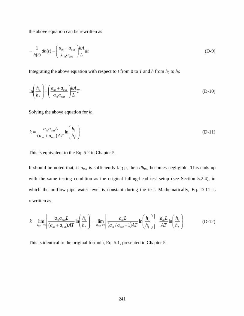
241

the above equation can be rewritten as

dtL

kA

aa

aatdh

th outin

outin

)(

)(

1 (D-9)

Integrating the above equation with respect to t from 0 to T and h from h0 to hf:

TL

kA

aa

aa

h

h

outin

outin

f

0ln (D-10)

Solving the above equation for k:

foutin

outin

h

h

ATaa

Laak 0ln

)( (D-11)

This is equivalent to the Eq. 5.2 in Chapter 5.

It should be noted that, if aout is sufficiently large, then dhout becomes negligible. This ends up

with the same testing condition as the original falling-head test setup (see Section 5.2.4), in

which the outflow-pipe water level is constant during the test. Mathematically, Eq. D-11 is

rewritten as

f

in

foutin

in

afoutin

outin

a h

h

AT

La

h

h

ATaa

La

h

h

ATaa

Laak

outout

000 lnln1/

limln)(

lim (D-12)

This is identical to the original formula, Eq. 5.1, presented in Chapter 5.

Green and Durable Geopolymer Composites for Sustainable ...

Documents

Transcript of Green and Durable Geopolymer Composites for Sustainable ...