Application of Pervious Geopolymer Concrete in Pavement ...

University of Wollongong University of Wollongong

Research Online Research Online

University of Wollongong Thesis Collection 2017+ University of Wollongong Thesis Collections

2020

Application of Pervious Geopolymer Concrete in Pavement and Piles Application of Pervious Geopolymer Concrete in Pavement and Piles

Haiqiu Zhang University of Wollongong

Follow this and additional works at: https://ro.uow.edu.au/theses1

University of Wollongong University of Wollongong

Copyright Warning Copyright Warning

You may print or download ONE copy of this document for the purpose of your own research or study. The University

does not authorise you to copy, communicate or otherwise make available electronically to any other person any

copyright material contained on this site.

You are reminded of the following: This work is copyright. Apart from any use permitted under the Copyright Act

1968, no part of this work may be reproduced by any process, nor may any other exclusive right be exercised,

without the permission of the author. Copyright owners are entitled to take legal action against persons who infringe

their copyright. A reproduction of material that is protected by copyright may be a copyright infringement. A court

may impose penalties and award damages in relation to offences and infringements relating to copyright material.

Higher penalties may apply, and higher damages may be awarded, for offences and infringements involving the

conversion of material into digital or electronic form.

Unless otherwise indicated, the views expressed in this thesis are those of the author and do not necessarily Unless otherwise indicated, the views expressed in this thesis are those of the author and do not necessarily

represent the views of the University of Wollongong. represent the views of the University of Wollongong.

Recommended Citation Recommended Citation Zhang, Haiqiu, Application of Pervious Geopolymer Concrete in Pavement and Piles, Doctor of Philosophy thesis, School of Civil and Mining Engineering, University of Wollongong, 2020. https://ro.uow.edu.au/theses1/1138

Research Online is the open access institutional repository for the University of Wollongong. For further information contact the UOW Library: [email protected]

https://ro.uow.edu.au/

https://ro.uow.edu.au/theses1

https://ro.uow.edu.au/theses1

https://ro.uow.edu.au/thesesuow

https://ro.uow.edu.au/theses1?utm_source=ro.uow.edu.au%2Ftheses1%2F1138&utm_medium=PDF&utm_campaign=PDFCoverPages

Application of Pervious Geopolymer Concrete in Pavement

and Piles

Haiqiu Zhang

BEng, MSc

Principal Supervisor:

A/Prof. Muhammad N.S. Hadi

This thesis is presented as part of the requirement for the conferral of the

degree:

Doctor of Philosophy

The University of Wollongong

School of Civil, Mining and Environmental Engineering

January 2020

ii

Abstract

Geopolymer materials (pastes, mortars and concretes) are formed through the activation

of aluminosilicate sources with an alkaline solution, and can achieve a comparatively

similar or superior performance to ordinary Portland cement (OPC). Given that these

aluminosilicate materials can be industrial by-products such as fly ash and slag,

geopolymer materials are green, economical and sustainable materials. Geopolymer

materials have also become more globally popular as an alternative to OPC by greatly

reducing the emission of CO2, as OPC requires much higher energy and temperature to

be produced. Although the properties of geopolymer concrete used in structural

members have already been relatively well researched, this study aims to investigate the

feasibility of geopolymer concrete used in pavements and piles. This study expands the

use of geopolymer materials in practice, while reducing the consumption of OPC as

much as possible. In order to fulfill the objectives of this study, three groups of

experiments have been carried out and the corresponding mathematical models were

proposed to simulate them.

The first part of this research study is concerned with the optimum mix proportion of

geopolymer pastes and concretes. Twenty-eight mixes of geopolymer paste were

conducted at ambient curing conditions to find the optimum mix proportion. The

influences of ground granulated blast furnace slag (GGBFS) content, alkaline solution

to binder (Al/Bi) mass ratio, sodium silicate solution to sodium hydroxide solution

(SS/SH) mass ratio, and additional water to binder (Aw/Bi) mass ratio on compressive

strength, setting times and workability were investigated. The optimum mix proportion

was found to have GGBFS content of 40%, Al/Bi ratio of 0.5, SS/SH ratio of 2.0, and

iii

Aw/Bi ratio of 0.15. Next, regression models by considering GGBFS content, Al/Bi,

SS/SH, Aw/Bi and artificial neural network (ANN) models by considering molar ratios

of SiO2/Al2O3, H2O/Na2O, Na2O/SiO2, CaO/SiO2 were proposed to predict the

experimental results.

The second part of this research study was concerned with the pervious geopolymer

concrete. The mix proportions of geopolymer binder and alkaline solution were selected

based on the optimum mix proportion of geopolymer paste to produce previous

geopolymer concrete (PGC) samples. The mix of PGC was proposed based on

aggregates to binder ratios (Ca/Bi), and simple a linear regression model was proposed

to simulate the compressive strength of PGC.

The third part of this research study was focused on the geosynthetics-confined pervious

geopolymer concrete (PGC) piles without or with fibre reinforced polymer (FRP)-

polyvinyl chloride (PVC)-confined concrete core (FPCC). In order to improve the

mechanical properties of piles, PGC piles were strengthened by using geogrids,

geotextiles, FRP and PVC tubes. Two groups of 12 specimens have been tested under

axial compression loading. All specimens were 160 mm in diameter and 625 mm in

height. The results from the experimental investigations show that FPCC can

significantly increase the axial load carrying capacity and ductility of PGC piles. Lastly,

analytical models were proposed to simulate their mechanical behaviour, and it was

found that the prediction results of these models are in good agreement with the


iv

List of Publications

Refereed Journal Papers:

1. Hadi, M.N.S., Zhang, H. and Parkinson, S. (2019). "Optimum mix design of

geopolymer pastes and concretes cured in ambient condition based on compressive

strength, setting time and workability." Journal of Building Engineering, 23: 301-313.

2. Zhang, H. and Hadi, M.N.S. (2019). "Geogrid-confined pervious geopolymer

concrete piles with FRP-PVC-confined concrete core: Concept and behaviour."

Construction and Building Materials, 211: 12-25.

3. Zhang, H. and Hadi, M.N.S. (2020). "Geogrid-confined pervious geopolymer

concrete piles with FRP-PVC-confined concrete core: Analytical models." Structures,

23:731-738.

v

Acknowledgments

First of all, I would like to sincerely thank my Principal Supervisor, A/Prof. Muhammad

N.S. Hadi, for his acceptance and trust, and for his patience and invaluable academic

guidance. Without his support, I would not complete this thesis. Here, no word can

exactly express my deep appreciation to him.

Sincere appreciation also goes to Mr. Ritchie McLean, Mr. Duncan Best and Mr. Alan

Grant for their technical assistances in High-bay laboratory. Your help and suggestions

were very important for me to finish my tests. I would also like to express my cordial

gratitude to Prof. Naj Aziz, Ms. Rhondalee Cambareri.

I would like to acknowledge the help and advice from my colleagues, especially, Dr

Weiqiang Wang, Dr. Jiansong Yuan, Dr. Yifei Sun, Dr. Pei Tai, Dr. Libin Gong, Dr.

Hongchao Zhao, Dr Guanyu Yang, Dr Ying Zhang, Dr. Zeya Li, Dr. Yuqin Qian. Your

professional knowledge and useful advice from the views of PhD candidates let me

make a lot of progress in my study. I really cherish the memory of every party and

activity we participated in during my study. Also, sincere appreciation goes to Dr.

Emdad K.Z. Balanji, Dr. Abbas S.A. AI-Hedad, Dr. Anh Duc Mai, Dr Mohammed

Hussein Ali Mohammed and Ms. Shelley Parkinson for their help during my study.

Lastly, I express my gratitude to my family. I sincerely thank my wife, Xin Sun, for her

support, understanding and sacrifice. My daughter’s innocent face and smiling is my

endless motivation to study and work hard. Also, the endless love given by my parents

encouraged me to overcome so many difficulties. Thank for the mental and financial

support from my parents.

vi

Certification

I, Haiqiu Zhang, declare that this thesis submitted in fulfilment of the

requirements for the conferral of Doctor of Philosophy, from the University of

Wollongong, is wholly my own work unless otherwise referenced or

acknowledged. This document has not been submitted for qualifications at any

other academic institution.

Haiqiu Zhang

9th January 2020

vii

Table of Contents

Abstract ..................................................................................................................... ii

Acknowledgments ....................................................................................................... v

Certification ................................................................................................................ vi

Table of Contents ....................................................................................................... vii

List of Tables ............................................................................................................. xii

List of Figures ........................................................................................................... xiv

CHAPTER 1

Introduction ................................................................................................................. 1

1.1 Background ...................................................................................................... 1

1.2 Research Significance ...................................................................................... 4

1.3 Objectives of this Study ................................................................................. 5

1.4 Methodologies of this Study .......................................................................... 6

1.5 Thesis Outline................................................................................................... 6

CHAPTER 2

Literature Review ........................................................................................................ 9

2.1 General .............................................................................................................. 9

2.2 Geopolymer Materials (Pastes, Mortars, and Concretes) .................................. 9

2.2.1 Factors Influencing the Mechanical Properties of Geopolymer Concrete ..

....................................................................................................... 10

2.2.2 Mix Design of Geopolymer Concrete ..................................................... 16

2.2.3 Fly Ash-based Geopolymer Materials Cured at Ambient Condition ...... 17

2.2.4 Discussion ............................................................................................... 20

2.3 Pervious Concrete ........................................................................................... 20

2.3.1 Aggregates ............................................................................................... 21

2.3.2 Cementitious Materials ........................................................................... 21

2.3.3 Mix Design of Pervious Concrete ........................................................... 23

2.3.4 Compressive Strength of Pervious Concrete ........................................... 23

2.3.5 Permeability of Pervious Concrete .......................................................... 24

2.3.6 Discussion ............................................................................................... 25

2.4 Permeable Granular Piles ................................................................................ 25

viii

2.4.1 Conventional Stone Columns .................................................................. 25

2.4.2 Confined Stone Columns ........................................................................ 26

2.4.3 Pervious Concrete Piles ........................................................................... 27

2.4.4 Discussion ............................................................................................... 28

2.5 Application of ANN in Civil Engineering ...................................................... 28

2.5.1 Predicting the Properties of Concrete, Mortar and Paste ........................ 29

2.5.2 Optimizing the Mix Proportion of Concrete, Mortar and Paste .............. 30

2.5.3 Predicting the Compressive Strength and Strain of FRP-confined

Concrete ................................................................................................... 31

2.5.4 Discussion ............................................................................................... 32

2.6 The Analytical Stress-Strain Models for FPR-Confined Concrete ................. 32

2.6.1 Types of Models ...................................................................................... 32

2.6.2 The Model Proposed by Lam and Teng (2003) ...................................... 34

2.6.3 The Model Proposed by Teng et al. (2009) ............................................. 37

2.6.4 Discussion ............................................................................................... 38

2.7 Summary ......................................................................................................... 38

CHAPTER 3

Optimum Mix Design of Geopolymer Paste and Concrete Cured in Ambient Condition

based on Compressive Strength, Setting Time and Workability ............................... 40

3.1 Introduction ..................................................................................................... 40

3.2 Experimental Programme for Geopolymer Pastes .......................................... 41

3.2.1 Materials ................................................................................................. 41

3.2.2 Mix Proportions ...................................................................................... 42

3.2.3 Mixing, Casting and Curing ................................................................... 46

3.2.4 Testing methods ...................................................................................... 48

3.2.5 Results and Discussion ........................................................................... 50

3.3 Experimental Programme for Geopolymer Concrete (GC) and OPC Concrete .

............................................................................................................... 67

3.4 The Mathematical Regression Model ............................................................. 69

3.4.1 28-day Compressive Strength Prediction Model .................................... 69

3.4.2 Initial Setting Time Model ..................................................................... 74

3.4.3 Mini Slump Test Model .......................................................................... 75

ix

3.5 Summary ......................................................................................................... 76

CHAPTER 4

Predicting the Compressive Strength of Geopolymer Materials Cured in Ambient

Condition by Using Artificial Neural Network ......................................................... 79

4.1 Introduction ..................................................................................................... 79

4.2 Experimental Database .................................................................................... 80

4.3 The ANN Model ............................................................................................. 91

4.3.1 Basic Concepts of ANN ......................................................................... 91

4.3.2 The Architecture of the ANN Model ...................................................... 95

4.3.3 Performance of ANN Model .................................................................. 99

4.3.4 Relative Importance and Relative Ranking .......................................... 100

4.4 Parametric Analysis Based on the Established ANN Model ........................ 101

4.5 Summary ....................................................................................................... 110

CHAPTER 5

Mix Design of Pervious Geopolymer Concrete ....................................................... 112

5.1 Introduction ................................................................................................... 112

5.2 Experimental Programme for PGC piles ....................................................... 113

5.2.1 Materials ............................................................................................... 113

5.2.2 Mix Proportions .................................................................................... 113

5.2.3 Mixing, Casting and Curing ................................................................. 116

5.2.4 Testing Method ..................................................................................... 118

5.2.5 Results and Discussion ......................................................................... 120

5.3 Summary ....................................................................................................... 123

CHAPTER 6

Geosynthetics-confined Pervious Geopolymer Concrete Piles with FRP-PVC-confined

Concrete Core: Experiments .................................................................................... 125

6.1 Introduction ................................................................................................... 125

6.2 Experimental Programme .............................................................................. 126

6.2.1 Preliminary Tests .................................................................................. 126

6.2.2 Main Test Matrix .................................................................................. 128

6.2.3 Preparation of Specimens ..................................................................... 132

6.2.4 Material Properties ............................................................................... 134

x

6.2.5 Instrumentation and Test Procedure ..................................................... 140

6.3 Test Results and Analysis ............................................................................. 142

6.3.1 Preliminary Tests .................................................................................. 142

6.3.2 Final States of GPGCPs and GGPGCPs .............................................. 146

6.3.3 Mechanical Behaviour of GPGCPs without FPCC and GGPGCPs without

FPCC .................................................................................................... 151

6.3.4 Mechanical Behaviour of GPGCPs with FPCC and GGPGCPs with FPCC

..................................................................................................... 160

6.3.5 Comparison between GPGCPS without FPCC and GPGCPs with FPCC .

..................................................................................................... 170

6.3.6 Comparison between GGPGCPS with and without FPCC .................. 174

6.4 Ductility ......................................................................................................... 178

6.5 Summary ....................................................................................................... 182

CHAPTER 7 Geosynthetics-confined Pervious Geopolymer Concrete Piles without

and with FRP-PVC-confined Concrete Core: Analytical Models ........................... 184

7.1 Introduction ................................................................................................... 184

7.2 Analytical Models ......................................................................................... 184

7.2.1 Equivalent Confining Pressure Provided by Geogrid tubes ................. 184

7.2.2 Equivalent Confining Pressure Provided by Geogrid-Geotextile tubes 186

7.2.3 Analytical Model for GPGCPs without FPCC and GGPGCPs without

FPCC .................................................................................................... 188

7.2.4 Analytical Model for Hollow FRP-PVC Tubes ................................... 193

7.2.5 Analytical Model for FRP-PVC-confined Geopolymer Concrete (FPCC)

194

7.2.6 Analytical Model for GPGCPs with FPCC and GGPGCPs with FPCC197

7.3 Parametric Analyses ...................................................................................... 201

7.3.1 Parametric Analyses of GPGCPs without FPCC and GGPGCPs without

FPCC .................................................................................................... 201

7.3.2 Parametric Analyses of GPGCPs with FPCC and GGPGCPs with FPCC

204

7.4 Summary ....................................................................................................... 211

CHAPTER 8 ............................................................................................................ 213

xi

Conclusions and Recommendations ........................................................................ 213

8.1 Introduction .................................................................................................. 213

8.2 Conclusions of this Research Study ............................................................. 214

8.3 Recommendations for the Future Studies .................................................... 216

References ................................................................................................................ 218

xii

List of Tables

Table 2.1 Typical range of materials proportions in pervious concrete (Kia et al. 2017).

........................................................................................................................................ 23

Table 3.1 Chemical compositions (mass%) for ground granulated blast furnace slag

(GGBFS) (Australasian Slag Association 2018), Fly ash (FA) (Eraring Power Station

Australia 2018). .............................................................................................................. 41

Table 3.2 The mix designs for the effect of GGBFS content (Hadi et al. 2019). ........... 43

Table 3.3 The mix designs for the effects of Al/Bi ratio and SS/SH ratio (Hadi et al.

2019). .............................................................................................................................. 44

Table 3.4 The mix designs for the effect of Aw/Bi ratio (Hadi et al. 2019). .................. 45

Table 3.5 The mix designs for OPC paste (Hadi et al. 2019). ........................................ 46

Table 3.6 Results of OPC paste mixes and geopolymer paste mixes (Hadi et al. 2019).51

Table 3.7 The mix design for geopolymer concrete (Hadi et al. 2019). ......................... 68

Table 3.8 The mix designs for OPC concrete (Hadi et al. 2019). ................................... 68

Table 3.9 Results of Geopolymer Concrete and OPC Concrete (Hadi et al. 2019). ....... 69


(GGBFS), Fly ash (FA). ................................................................................................. 80

Table 4.2 Chemical compositions (mass%) of sodium silicate solution (SS). ............... 81

Table 4.3 Chemical compositions (mass%) for sodium hydroxide solution. ................. 82

Table 4.4 Mix proportions of geopolymer materials. ..................................................... 83

xiii

Table 4.5 Values of SiO2/Al2O3, H2O/Na2O, Na2O/SiO2, CaO/SiO2, and

experimental and predicted 28-day compressive strength. ............................................. 87

Table 4.6 Weights of the ANN model. ........................................................................... 97

Table 4.7 Bias of the ANN model. ................................................................................. 98

Table 4.8 The values and expression of statistical parameters. .................................... 100

Table 4.9 Relative importance and relative ranking. .................................................... 101

Table 5.1 Mix design for PGC controlled by aggregate/binder mass ratio .................. 116

Table 6.1 Details of the preliminary test samples. ........................................................ 127

Table 6.2 Details of the GPGCP specimens and GGPGCP specimens. ....................... 130

Table 6.3 Mix proportions of PGC and NGC. .............................................................. 132

Table 6.4 Material properties of geotextile ................................................................... 137

Table 6.5 Average material properties of GFRP sheets. ............................................... 139

Table 6.6 Average material properties of PVC dog-bone specimens. .......................... 140

Table 6.7 Results of the preliminary tests. .................................................................... 143

Table 6.8 Test results of GPGCPs without FPCC. ....................................................... 152

Table 6.9 Test results of GGPGCPs without FPCC. .................................................... 152

Table 6.10 Test results of GPGCPs with FPCC ........................................................... 161

Table 6.11 Test results of GGPGCPs with FPCC ........................................................ 161

Table 6.12 Ductility results. .......................................................................................... 181

xiv

List of Figures

Figure 3.1 Twenty Quart Hobart Mixer (Hadi et al. 2019). ............................................ 47

Figure 3.2 The mini-size specimens cast in the mini-size moulds (Hadi et al. 2019). ... 48

Figure 3.3 Testing devices: (a) Compression testing machine; (b) Vicat apparatus; (c)

Mini-slump cone diagram(units: mm); (d) Mini-slump cone picture (Hadi et al. 2019).

........................................................................................................................................ 50

Figure 3.4 Effect of GGBFS content on the compressive strength of geopolymer pastes

(Hadi et al. 2019). ........................................................................................................... 54

Figure 3.5 Effect of GGBFS content on the initial and final setting times of geopolymer

pastes (Hadi et al. 2019). ................................................................................................ 55

Figure 3.6 Effect of GGBFS content on mini-slump tests of geopolymer pastes (Hadi et

al. 2019). ......................................................................................................................... 56

Figure 3.7 Effect of alkaline solution to binder (Al/Bi) ratio and sodium silicate solution

to sodium hydroxide solution (SS/SH) ratio on compressive strength of geopolymer

paste (Hadi et al. 2019). .................................................................................................. 58


to sodium hydroxide solution (SS/SH) ratio on initial and final setting times of

geopolymer pastes (Hadi et al. 2019). ............................................................................ 59


to sodium hydroxide solution (SS/SH) ratio on mini-slump tests of geopolymer pastes:

(a) Al/Bi=0.4; (b) Al/Bi=0.5; (c) Al/Bi=0.6; (d) Al/Bi=0.7 (Hadi et al. 2019).

(Continued) ..................................................................................................................... 60

xv

Figure 3.10 Effect of alkaline solution to binder (Al/Bi) ratio and sodium silicate

solution to sodium hydroxide solution (SS/SH) ratio on mini-slump tests of geopolymer

pastes: (a) Al/Bi=0.4; (b) Al/Bi=0.5; (c) Al/Bi=0.6; (d) Al/Bi=0.7 (Hadi et al. 2019). . 61

Figure 3.11 Effect of additional water/binder ratio (Aw/Bi) on compressive strength of

geopolymer pastes (Hadi et al. 2019). ............................................................................ 63

Figure 3.12 Effect of additional water/binder (Aw/Bi) ratio on initial and final setting

times of geopolymer pastes (Hadi et al. 2019). .............................................................. 64

Figure 3.13 Effect of additional water/binder (Aw/Bi) ratio on mini-slump tests of

geopolymer pastes: (a) Al/Bi=0.4; (b)Al/Bi=0.5; (c) Al/Bi=0.6; (d) Al/Bi=0.7 (Hadi et

al. 2019).(Continued) ...................................................................................................... 64

Figure 3.14 Effect of additional water/binder (Aw/Bi) ratio on mini-slump tests of

geopolymer pastes(a) Al/Bi=0.4; (b)Al/Bi=0.5; (c) Al/Bi=0.6; (d) Al/Bi=0.7 (Hadi et al.

2019). .............................................................................................................................. 65

Figure 3.15 Predicted results by using Equation (3.1) (Hadi et al. 2019). ..................... 70

Figure 3.16 Predicted results by using Equation (3.2) and Equation (3.4) (Hadi et al.

2019). .............................................................................................................................. 71

Figure 3.17 Predicted results by using Equation (3.6) (Hadi et al. 2019). ..................... 73

Figure 3.18 Performance of Equation (3.6) for all mixes (Hadi et al. 2019). ................. 73

Figure 3.19 Performance of Equation (3.8) for predicting initial setting time of

geopolymer paste (Hadi et al. 2019). .............................................................................. 75

Figure 3.20 Performance of Equation (3.13) for predicting mini slump test results of

geopolymer paste (Hadi et al. 2019). .............................................................................. 76

xvi

Figure 4.1 Calculation algorithm of a single neuron. ..................................................... 92

Figure 4.2 Architecture of the ANN model built by NFTOOL box in Matlab (2016b). 94

Figure 4.3 Caculation algorithm of the backpropagation feedforward ANN model built

by NFTOOL box in Matlab(2016b). ............................................................................... 94

Figure 4.4 Architecture of the proposed ANN mode ...................................................... 96

Figure 4.5 Performance of the proposed ANN model. ................................................... 99

Figure 4.6 Compressive strength vs SiO2/Al2O3 and H2O/Na2O molar ratios. ......... 103

Figure 4.7 Compressive strength vs SiO2/Al2O3 and Na2O/ SiO2 molar ratios. ........ 104

Figure 4.8 Compressive strength vs SiO2/Al2O3 and CaO/SiO2 molar ratios. ........... 106

Figure 4.9 Compressive strength vs H2O/Na2O and Na2O/ SiO2 molar ratios. ......... 107

Figure 4.10 Compressive strength vs H2O/Na2O and CaO/SiO2 molar ratios. ........... 109

Figure 4.11 Compressive strength vs Na2O/ SiO2 and CaO/SiO2 molar ratios. ......... 110

Figure 5.1 Casting the PGC samples in plastic moulds. ............................................... 117

Figure 5.2 Samples of PGC (100mm x 200mm) .......................................................... 118

Figure 5.3 Constant head water permeability apparatus (units: mm). .......................... 120

Figure 5.4 Effects of Aggregate to Binder Mass Ratio (Ca/Bi) on Compressive Strength

of PGC .......................................................................................................................... 121

Figure 5.5 Effects of Aggregate to Binder Mass Ratio (Ca/Bi) on Porosity of PGC ... 122

Figure 5.6 Effects of Aggregate to Binder Mass Ratio (Ca/Bi) on Permeability of PGC.

...................................................................................................................................... 123

xvii

Figure 6.1 Details of FPCC samples (units: mm; SG: strain gauge). ........................... 127

Figure 6.2 GPGCPs without FPCC and GGPGCPs without FPCC. ............................ 128

Figure 6.3 GPGCPs with FPCC and GGPGCPs with FPCC. ....................................... 129

Figure 6.4 Details of GPGCP specimens and GGPGCP specimens (units: mm; SG:

strain gauge): (a) GP1, GP2, GP3, GGP1, GGP2, GGP3; (b) GPC1, GPC2, GPC3.

GGPC1, GGPC2, GGPC3. ........................................................................................... 131

Figure 6.5 Geogrid used in this study: (a) Uniaxial geogrid; (b) Tensile load-axial strain

curves of the geogrid coupons. ..................................................................................... 136

Figure 6.6 White unwoven geotextile. .......................................................................... 137

Figure 6.7 Geotextile tensile test. ................................................................................. 138

Figure 6.8 Tensile load-axial strain curves of geotextile. ............................................. 138

Figure 6.9 Tensile test of the GFRP coupons. .............................................................. 139

Figure 6.10 PVC coupons used in this study: (a) Dog-bone PVC coupon; (b) Tensile

load-axial strain curves of the PVC coupons. ............................................................... 140

Figure 6.11 Axial load-axial strain curves of PGC and NGC. ..................................... 143

Figure 6.12 Failure mode of the FRP-PVC hollow tube. ............................................. 144

Figure 6.13 Axial load-axial strain curves of FRP-PVC hollow tube. ......................... 144

Figure 6.14 Failure mode of the FRP-PVC-confined concrete. ................................... 145

Figure 6.15 Axial stress-axial strain curves of the FPCCs. .......................................... 146

Figure 6.16 Axial-hoop strain responses of the FPCCs. ............................................... 146

Figure 6.17 Final states of the representative GPGCPs without FPCC: (a) GP1-1; ..... 147

xviii

Figure 6.18 Final states of the representative GGPGCPs without FPCC: (a) GGP1-1; (b)

GGP2-2; (c) GGP3-1. ................................................................................................... 149

Figure 6.19 Final state of the representative GPGCPs with FPCC: (a) GPC1-2; (b)

GPC2-2; (c) GPC3-1. .................................................................................................... 150

Figure 6.20 Final states of the representative GGPGCPs with FPCC: (a) GGPC1-2; (b)

GGPC2-2; (c) GGPC3-2. .............................................................................................. 151

Figure 6.21 Axial stress-axial strain curves of GPGCPs without FPCC. ..................... 153

Figure 6.22 Axial stress-axial strain curves of GGPGCPs without FPCC. .................. 154

Figure 6.23 Hoop strain-axial strain curves of GPGCPs without FPCC. ..................... 155

Figure 6.24 Hoop strain-axial strain curves of GGPGCPs without FPCC. .................. 156

Figure 6.25 Comparisons between GP1 and GGP1: Axial stress-axial strain curves. . 157



Figure 6.28 Comparisons between GP1 and GGP1: Hoop strain-axial strain curves. . 159



Figure 6.31 Axial stress-axial strain curves of GPGCPs with FPCC. .......................... 162

Figure 6.32 Axial stress-axial strain curves of GGPGCPs with FPCC. ....................... 162

Figure 6.33 Hoop strain-axial strain curves of GPGCPs with FPCC. .......................... 164

Figure 6.34 Hoop strain-axial strain curves of GGPGCPs with FPCC. ....................... 165

xix

Figure 6.35 Hoop strain-axial strain curves of FPCC placed in GPGCPs and GGPGCPs.

...................................................................................................................................... 166

Figure 6.36 Comparisons between GPC1 and GGPC1: Axial stress-axial strain curves.

...................................................................................................................................... 167


...................................................................................................................................... 167


...................................................................................................................................... 168

Figure 6.39 Comparisons between GPC1 and GGPC1: Hoop strain-axial strain curves.

...................................................................................................................................... 169


...................................................................................................................................... 169


...................................................................................................................................... 170

Figure 6.42 Comparisons between GP1 and GPC1: Axial stress-axial strain curves. .. 171



Figure 6.45 Comparisons between GP1 and GPC1: Hoop strain-axial strain curves. .. 173



xx

Figure 6.48 Comparisons between GGP1 and GGPC1: Axial stress-axial strain curves.

...................................................................................................................................... 175

Figure 6.49 Comparisons between GGP1 and GGPC1: Hoop strain-axial strain curves.

...................................................................................................................................... 175


...................................................................................................................................... 176


...................................................................................................................................... 177


...................................................................................................................................... 177


...................................................................................................................................... 178

Figure 6.54 Definition of u and ɛy: (a) Definition of u and y for unconfined

concrete; (b) Definition of u and y for GPGCPs without FPCC; (c) Definition of u

and y for GPGCPs with FPCC. .................................................................................. 179

Figure 7.1 Confining action of geogrid tubes. .............................................................. 186

Figure 7.2 Confining action of geogrid-geotextile tubes. ............................................. 187

Figure 7.3 Comparisons between experimental results and model predictions for

GPGCPs without FPCC: GP1. ...................................................................................... 191



xxi




GGPGCPs without FPCC: GGP1. ................................................................................ 192





Figure 7.9 Comparisons between experimental results and model predictions for FRP-

PVC tubes. .................................................................................................................... 194


FPCC. ............................................................................................................................ 197


GPGCPs with FPCC: GPC1. ........................................................................................ 198






GGPGCPs with FPCC: GGPC1. .................................................................................. 200



xxii



Figure 7.17 Axial compression behaviour of GPGCPs without FPCC for different

confinement moduli of geogrid tubes. .......................................................................... 202

Figure 7.18 Axial compression behaviour of GGPGCPs without FPCC for different

confinement moduli of geogrid-geotextile tubes. ......................................................... 202

Figure 7.19 Axial compression behaviour of GPGCPs without FPCC for different PGC

compressive strength. .................................................................................................... 203

Figure 7.20 Axial compression behaviour of GGPGCPs without FPCC for different

PGC compressive strength ............................................................................................ 204

Figure 7.21 Axial compression behaviour of GPGCPs with FPCC for different

confinement moduli of geogrid tubes. .......................................................................... 205

Figure 7.22 Axial compression behaviour of GGPGCPs with FPCC for different

confinement moduli of geogrid-geotextile tubes. ......................................................... 205

Figure 7.23 Axial compression behaviour of GPGCPs with FPCC for different PGC


Figure 7.24 Axial compression behaviour of GGPGCPs with FPCC for different PGC


Figure 7.25 Axial compression behaviour of GPGCPs with FPCC for different NGC


Figure 7.26 Axial compression behaviour of GGPGCPs with FPCC for different NGC


xxiii

Figure 7.27 Axial compression behaviour of GPGCPs with FPCC for different number

of GFRP layers. ............................................................................................................. 209


number of GFRP layers. ............................................................................................... 209

Figure 7.29 Axial compression behaviour of GPGCPs with FPCC for different ultimate

strains of GFRP. ............................................................................................................ 210


ultimate strains of GFRP ............................................................................................... 210

xxiv

Abbreviations

A cross-sectional area of PGC samples

ACI American Concrete Institute

ANN Artificial Neural Network

AS Australian Standards

ASTM American Society for Testing and Materials

An cross-sectional area of NGC

Ap the cross-sectional area of PGC

Atotal cross-sectional area of the whole PGC piles

Al/Bi Alkaline Activator to Binder Mass Ratio

Aw/Bi Additional Water to Binder Mass Ratio

a

constant obtained based on the regression analysis of test results

(Eq. (7.14))

b


(Eq. (7.14))

bs bias for the single neuron

1b bias vector of the hidden layer

b1,j element in 1b

b2 bias vector in the output layer

b2,j element in 2b

Cg the GGBFS content

Ca/Bi Coarse Aggregate to Binder Mass Ratio

CKD Cement Kiln Dust

xxv

CSH Calcium Silicate Hydrates

c


(Eq. (7.16))

D diameter of the confined concrete cylinder

d


(Eq. (7.16))

dp diameter of the GPGCPs

Ec elastic modulus of unconfined concrete

E2 slope of the linear second portion of confined concrete

EFRP elastic modulus of FRP in the hoop direction

Ele,grid lateral confinement modulus of geogrid tubes

Egt confinement modulus of geogrid-geotextile tubes

El,textile confinement modulus of geotextile

Ecm

confinement modulus of geogrid tubes for GPGCPs; or geogrid-

geotextile tubes for GGPGCPs

Ec,n elastic modulus of unconfined concrete

,'co nf unconfined compressive strength of NGC

,'cc nf confined compressive strength of NGC

F1

polynomial regression equation considering the effect of GGBFS

content

F2 polynomial regression equation considering the effect of Al/Bi

F3

polynomial regression equation considering the effect of SS/SH

ratio

xxvi

F4

polynomial regression equation considering the effect of Aw/Bi

ratio

Fp axial load carried by the PGC

Fh axial load carried by the hollow FRP-PVC tube

Fn axial load carried by the NGC

Fla,grid actual lateral confining force

Fle,grid equivalent lateral confining force

Frib force provided by one transverse geogrid rib

FA Fly Ash

FPCC FRP-PVC-confined concrete core

FRP Fibre Reinforced Polymer

f function of output neuron

f1

predicted 28-day compressive strength considering the effect of

GGBFS content

f2

predicted 28-day compressive strength considering the effects of

GGBFS content and Al/Bi

f3


GGBFS content, Al/Bi ratio and SS/SH ratio

f4


GGBFS content, Al/Bi ratio, SS/SH ratio and Aw/Bi ratio

fla,grid actual lateral confining pressure

fle,grid equivalent lateral confining pressure

fl,textile lateral confining pressure acting on concrete provided by geotextile

ftextile strength of geotextile

xxvii

'cof compressive strength of unconfined concrete

,'co nf unconfined compressive strength of NGC

,co pf compressive strength of PGC

,co pf compressive strength of PGC

,'cc nf confined compressive strength of NGC

'cuf ultimate axial stress of FRP-confined concrete

'ccf compressive strength of confined concrete

,7pgcf 7-day compressive strength of PGC

,28pgcf 28-day compressive strength of PGC

Gf specific gravities of fly ash

Gg specific gravities of GGBFS

GGBFS Ground Granulated Blast Furnace Slag

GPGCP geogrid-confined pervious geopolymer concrete pile

GGPGCP geogrid-geotextile-confined pervious geopolymer concrete pile

GSH specific gravities of sodium hydroxide solution

GSS specific gravities of sodium silicate solution

GAw specific gravities of additional water

GCa specific gravities of coarse aggregates

WH water head

H height of the GPGCPs

sI input matrix for the single neuron

xxviii

Is,j element of sI

sIW weights matrix for the single neuron

,s iIW element of sIW

IW weight matrix of the hidden layer

,j iIW element of IW

k permeability of PGC samples

L length of PGC sample

LOI Loss on Ignition

M number of neurons in hidden layer

MAPE Mean absolute percentage error

Mf mass of fly ash

Mg mass of GGBFS

MSH mass of sodium hydroxide solution

MSS mass of sodium silicate solution

MAw mass of additional water

MCa mass of coarse aggregates

m


(Eq. (7.18))

N number of inputs for one neuron

n number of transverse geogrid ribs for one GPGCP

O output of an artificial neuron

O output of the ANN

Ok element in O

xxix

OPC Ordinary Portland Cement

PGC Pervious Geopolymer Concrete

Pgrid average peak load of one geogrid rib

Q quantity of water collected over t seconds

R Coefficient of correlation

RMSE Root mean squared error

R1

polynomial regression equations for the slope of mini slump test

results versus time, considering the effects of GGBFS content,

R2


results versus time, considering the effects of Al/Bi ratio

R3


results versus time, considering the effects of SS/SH ratio

R4


results versus time, considering the effects of Aw/Bi ratio

SH Sodium Hydroxide (NaOH)

SS Sodium Silicate (Na2SiO3)

SS/SH

Sodium Silicate Solution to Sodium Hydroxide Solution Mass

Ratio

SV scaled input and target value

S1

non-linear regression equation for initial setting time considering

the effect of GGBFS content

S2

polynomial regression equation for initial setting time considering

the effect of Al/Bi ratio

xxx

S3


the effect of SS/SH ratio

S4


the effect of Aw/Bi ratio

s


(Eq. (7.18))

s4 predicted initial setting time

T time after mixing

TFRP thickness of the FRP jacket

t time (seconds)

Vtp total volume of PGC

Vf volume of fly ash in PGC

Vg volume of GGBFS in PGC

VSH volume of sodium hydroxide solution in PGC

VSS volume of sodium silicate solution in PGC

VAw volume of additional water in PGC

Vv volume of void in PGC

VCa volume of coarse aggregate in PGC

V porocity of PGC

Vol volume of PGC samples

1pW weight of PGC samples under water

2pW dry weight of PGC samples

W1 polynomial regression equations for mini slump test results at 15

xxxi

min, considering the effects of GGBFS content

W2

polynomial regression equations for mini slump test results at 15

min, considering the effects of Al/Bi ratio

W3


min, considering the effects of SS/SH ratio

W4


min, considering the effects of Aw/Bi ratio

w4 predicted mini slump test results

Y Actual input and target value

y intermediary scalar

1y intermediary vector in the hidden layer

y1,j element in 1y

2y intermediary vector between the hidden layer and the output layer

y2,j element in 2y

3y intermediary vector in the output layer

y3,k element in 3y

c axial strain

co axial strain at the peak stress of unconfined concrete

cu ultimate axial strain of confined concrete

,h rup hoop rupture strain of the FRP jacket

hp axial strain at the peak load of hollow FRP-PVC tubes

xxxii

t

transition point between the parabolic first portion and the linear

second portion of confined concrete

u axial strain at 50% of the first peak stress at descending branch

y the yield strain

,grid u average ultimate tensile strain

l lateral strain of concrete

,textile p average tensile strain of geotextile at tensile strength

,t p transition axial strain point of PGC

,co p axial strain at the peak stress of unconfined PGC

,t n transition axial strain for NGC confined by FRP-PVC tubes

,cu n ultimate axial strain of confined NGC

,co n axial strain at the peak stress of NGC

,h ult hoop ultimate tensile strain of the FRP jacket

specimen ductility

K confinement stiffness ration

strain ratio

w density of water

c axial stress of stress

,c p axial stress of PGC

,c n axial stress of confined normal geopolymer concrete

1

CHAPTER 1

Introduction

1.1 Background

Concrete is one of the most common construction materials. It is mainly produced by

using ordinary Portland cement (OPC), which is a highly energy-intensive product.

Ordinary Portland cement is made by firing a mixture of clay and limestone at

temperatures above 1300° C (Shayan 2016). This production process releases a

significant amount of greenhouse gases. There is also an increasing demand for OPC,

and the production of cement could represent nearly 10% of total anthropogenic

carbon dioxide emissions in the close future (Joosen and Blok 2001). Therefore,

many researchers try to find some methods to mitigate this problem.

Geopolymer materials can be produced from the reaction of industrial by-product

aluminosilicate materials such as slag and fly ash, together with an alkali solution

such as sodium hydroxide and sodium silicate (Hadi et al. 2019, Hadi et al. 2017,

Reddy et al. 2018, Terry et al. 2011). It has been proven that geopolymer materials

can be designed and manufactured to perform similarly to conventional OPC

materials (Hadi et al. 2019, Hadi et al. 2017, Mo et al. 2016, Reddy et al. 2018, Terry

et al. 2011). Several construction projects have previously utilized geopolymer

materials and achieved satisfactory results (Mo et al. 2016, Terry et al. 2011). Hence,

geopolymer materials (pastes, mortars and concretes) have a great potential to

replace OPC materials and can effectively reduce the amount of CO2 emissions

(Habert et al. 2010, Terry et al. 2011).

2

On the other hand, the application of geopolymer materials also facilitate the use of

by-products, such as fly ash and slag, and reduces their disposal in landfills. In 2014-

15, Australia generated around 11 million tonnes of fly ash and around 4.9 million

tonnes were recycled into products such as cement (Joe and Paul 2017). It is also

estimated that in China, 580 million tonnes of ash were generated every year and

only 67% of them were recycled (Yao et al. 2014). If the application of geopolymer

materials would be expanded, more industrial by-products would be recycled and

their disposal would be reduced significantly.

In terms of cost, some studies have compared the costs of geopolymer materials and

ordinary Portland cement materials and the results depends on some factors, such as

the mix design, grades. McLellan et. (2011) investigated some geopolymer concrete

mixes based on typical Australian feedstocks indicate potential for a 44-64%

reduction in greenhouse gas emissions while the financial costs are 7% lower to 39%

higher compared with OPC. Thaarrini and Dhivya (2016) did the cost analysis of

geopolymer concrete and OPC concrete. It was seen that the cost of production of

OPC concrete is higher than the cost of production of GPC for higher grades. For

M30 grade of GPC concrete, the cost of production is marginally (1.7%) higher than

OPC concrete of the same grade. For M50 grade, the cost of OPC concrete 11%

higher than GPC of same grade. Hence, it was concluded that the savings in cost can

be got in the production of geopolymer concretes of higher grades as well as lower

grades with only a marginal difference.

Using geopolymer materials cured in ambient condition is one of the effective ways

to expand the application to replace OPC materials (Hadi et al. 2017, Nath 2014,

3

Nath and Sarker 2014, Nath and Sarker 2015). Most of the studies regarding

geopolymer materials were conducted at high temperature condition. Although

curing at high temperatures can be used for precast concrete members, it is

considered as a great challenge for the wide application of geopolymer materials for

in-situ casting. Hence, to overcome this limitation, several recent studies investigated

the possibility of curing geopolymer materials in ambient condition (Hadi et al. 2017,

Nath 2014, Nath and Sarker 2014, Nath and Sarker 2015, Palomo et al. 2007).

Very limited studies investigated the effect of low curing temperatures. Rovnaník

(2010) investigated the effects of different curing temperatures (10, 20, 40, 60 and 80)

on the compressive and flexural strengths, pore distribution and microstructure of

alkali activated metakaolin material. The results have shown that the early-age

compressive and flexural strengths (1-day and 3-day compressive and flexural

strengths) were nearly zero due to retarded setting of geopolymer mixture. However,

the 7-day compressive strength of geopolymer mixture cured at 10 can reach 28 MPa,

and the 28-day compressive strength of geopolymer mixture cured at 10 can reach 62

MPa. It can be seen that the mixes of geopolymer materials, which have very short

setting time but high compressive strength, have a great practical potential to be used

in low temperature conditions (in winter). This is because the low temperature may

decrease the chemical reaction rate of geopolymer materials and prolong the setting

time. In the future, the geopolymer concrete cured at low temperature conditions will

be investigated.

Another way to expand the available applications of geopolymer materials is

producing pervious geopolymer concrete (PGC) for pavements and piles. Most of the

4

studies regarding geopolymer materials focused on structural members, such as

columns and beams. Only few studies investigated the feasibility of using

geopolymer materials to produce PGC for pavements and piles. It has been found

that the properties of PGC are similar to those of OPC pervious concrete. Pervious

concrete is a porous concrete material that can allow water to pass through it quickly

and easily. This characteristic of pervious concrete can provide significant

advantages when it is applied for pavements, such as requiring less maintenance and

allowing more water to pass through to the sub soil. In addition, pervious concrete

piles have been proven to yield improved mechanical properties when compared with

conventional granular piles (Suleiman et al. 2014). This new type of pile also has

some other advantages, given that it will increase the time rate of consolidation,

reduce liquefaction potential, and improve the bearing capacity in very soft clays,

peat and organic soils.

1.2 Research Significance

Geopolymer materials act as green materials, which has gained a significant attention

because the geopolymer binder can replace ordinary Portland cement (OPC) and

greatly reduce the emission of CO2. However, most studies of geopolymer materials

focused on structural concrete members (such as beam, column and slab) and at high

temperature curing condition. A very limited number of geopolymer materials

studies pay attention to ambient curing condition, pavement and piles. In this study,

to expand the application of geopolymer materials, feasibility of producing pervious

geopolymer concrete cured in ambient condition for pavement and piles has been

investigated. This study has a great potential to increase the use of geopolymer

5

materials and reduce the amount of industrial by-products and the emission of CO2.

1.3 Objectives of this Study

The main objectives of this study are to investigate the feasibility of applying

geopolymer concrete cured at ambient condition into pavements and piles. Therefore,

the research study presented in this thesis has been carried out with the following

specific objectives:

1) To find the optimum mix proportion of geopolymer pastes, based on the

test results of compressive strength, setting time and workability.

2) To propose the optimum mix proportion of normal geopolymer concrete

based on the optimum mix proportion of geopolymer pastes.

3) To develop an ANN model to predict the compressive strength of

geopolymer materials (pastes, mortars and concretes) based on

experimental data from tests of this study and tests of other literature,

which can consider more complex factors and have a better accuracy.

4) To develop the mix proportion of pervious geopolymer concrete (PGC)

based on the optimum mix proportion of geopolymer pastes.

5) To develop a new system of geosynthetics-confined pervious geopolymer

concrete piles without and with FRP-PVC-confined concrete core (FPCC),

and investigate their mechanical behaviour.

6) To propose analytical models to simulate the mechanical properties of

geosynthetics-confined pervious geopolymer concrete piles without and

with FRP-PVC-confined concrete core (FPCC), which can help to apply

this new system in practice.

6

1.4 Methodologies of this Study

This study incorporates a series of laboratory tests and theoretical methods to

investigate the feasibility of producing pervious geopolymer concrete cured in

ambient condition for pavements and piles. At first, the geopolymer paste

experiments were conducted to find the optimum mix proportion. Also, the effects of

important factors of geopolymer paste on compressive strength, setting times and

workability were investigated and discussed. After that, the ANN models were then

proposed to predict the properties of geopolymer materials based on chemical

compositions. Secondly, the mix proportion of pervious geopolymer concrete (PGC)

was proposed based on the optimum mix of geopolymer pastes. Also, the properties

of PGC were investigated and simple mathematical models were proposed to

simulate these properties. Thirdly, to improve the mechanical performance of PGC

piles, geogrid and geotextile were used to wrap them. To further strengthen the PGC

piles, the strong FRP-PVC-confined concrete was placed in the middle of PGC piles.

Finally, the simple but accurate analytical models were proposed to simulate the

mechanical behaviour of these PGC piles.

1.5 Thesis Outline

This thesis is organized in eight chapters as outlined below:

Chapter 1 introduces the background, research significance, objectives and

methodologies of this study.

Chapter 2 presents a comprehensive literature review regarding the present work.

The reaction mechanism, effects of aluminosilicate sources and alkaline solutions on

7

properties of geopolymer materials, mix proportion of geopolymer materials and

pervious concrete, the properties of pervious concrete piles and the stress-strain

models of confined concrete columns were reviewed in this section.

Chapter 3 presents the experimental details of geopolymer pastes and find the

optimum mix design of geopolymer pastes. The factors of ground granulated blast

furnace slag (GGBFS) content, alkaline solution to binder (Al/Bi) mass ratio, sodium

silicate solution to sodium hydroxide solution (SS/SH) mass ratio, and additional

water to binder (Aw/Bi) mass ratio on compressive strength, setting times and

workability were investigated. The optimum mix proportion of geopolymer pastes

was found. Then, the optimum mix proportion of geopolymer concretes was found

based on optimum mix proportion of geopolymer pastes.

Chapter 4 develops an artificial neural network (ANN) to predict the compressive

strength of geopolymer materials (pastes, mortars, and concretes) based on

experimental data from tests of this study and tests from the literature, which can

consider more complex factors and have a better accuracy.

Chapter 5 presents the experimental details and methodology of pervious

geopolymer concrete (PGC) tests based on optimum mix proportion of geopolymer

paste. Then, a simple linear regression model was proposed to simulate the

compressive strength, permeability and porosity of PGC.

Chapter 6 presents the experimental study of the geosynthetic-encased PGC piles

without and with FPCC under axial compression loading. Their mechanical

behaviour is presented and significant characteristics are concluded.

8

Chapter 7 proposes analytical models to simulate the behaviour of geosynthetic-

encased PGC piles without and with FRP-PVC-confined concrete core (FPCC). The

modelling results present the good agreement with the experimental behaviour.

Chapter 8 draws overall conclusions and clearly demonstrates all contributions of

this study. Some useful recommendations and limitations are also presented.

9

CHAPTER 2

Literature Review

2.1 General

To achieve the objectives of this thesis described in the Introduction chapter, a

review of the existing studies on various topics are presented. The literature review is

carried out in five parts. Firstly, geopolymer materials are reviewed from different

aspects, including reaction mechanism, important factors, mix design and ambient

curing conditions. Then, the characteristics of pervious concrete and pavements are

studied from existing literature. After that, the advantages of permeable granular

piles are reviewed. Next, the application of ANN in different fields of civil

engineering are studies. Lastly, the different types of analytical stress-strain models

for confined concrete are concluded. From this review, some useful suggestions and

views can be gained.

2.2 Geopolymer Materials (Pastes, Mortars, and Concretes)

Ordinary Portland Cement (OPC) is the main construction material and is made by

firing a mix of clay and limestone at temperatures above 1300 °C (Shayan 2016).

The process of manufacturing OPC produces a great amount of greenhouse gas and it

adversely affects the environment. It is estimated that the production of one tonne of

OPC can emit one tonne of CO2 (Duan et al. 2015, Wallah 2010). However,

geopolymer materials (pastes, mortars and concretes) have been proven to have

comparable properties to OPC materials (pastes, mortars and concretes) (Pacheco-

Torgal et al. 2014, Shayan 2016, Topark-Ngarm et al. 2014), and they can be made

10

by activating industrial by-products, such as slag and fly ash, with alkaline solution

Gourley et al. (2011), (Nagaraj and Babu 2018, Reddy et al. 2018). Hence,

geopolymer materials have a great potential to replace OPC materials and can

significantly reduce the emission of CO2 (Shayan 2016, Yang et al. 2013).

2.2.1 Factors Influencing the Mechanical Properties of Geopolymer Concrete

Although the polymerization process of geopolymer materials is still ambiguous,

many studies have found that the mechanical properties of the geopolymer materials

are affected significantly by the properties of aluminosilicate materials, alkaline

activators and curing conditions. These three factors are detailedly reviewed below.

Aluminosilicate Materials

The most common aluminosilicate materials used to produce geopolymer materials

are fly ash, slag and metakaolin (Pacheco-Torgal et al. 2014). Fly ash and slag are

industrial by-products and their application in geopolymer materials has gained more

and more attention. It has been proven that the chemical composition and particle

size of aluminosilicate materials had significant effects on the properties of

geopolymer materials.

Fly ash is an industrial by-product deriving from coal combustion. According to

(Pickin and Randell 2017), Australia generated 11 million tonnes of fly ash in 2014-

15. Around 5.9 million tonnes were disposed to landfills and around 4.9 million

tonnes were recycled to products such as cement. Hence, the fly ash in Australia has

wide availability. The chemical composition of fly ash varies widely, depending on

coal composition (Pacheco-Torgal et al. 2014). There are two types of fly ash: (1)

Class F fly ash with a low CaO content (under 10%); (2) Class C fly ash with a high

11

CaO content (higher than 10%). The alkaline activation of Class F fly ash induces the

precipitation of an alkaline aluminosilicate hydrate, which is known as the N-A-S-H

gel (Criado et al. 2007, Duxson et al. 2005, Fernández-Jiménez and Palomo 2005).

This kind of geopolymer materials normally have to be cured at high temperatures

due to the process of geopolymerization is slowly at ambient condition (Guo et al.

2010). Whereas, the main products of Class C fly ash-based geopolymer materials

are the calcium aluminosilicate hydrate (C-A-S-H) gel and alkaline aluminosilicate

hydrate (N-A-S-H) gel. It is possible to cure fly ash-based geopolymer materials with

high CaO content at ambient condition because the geopolymerization reaction was

improved (Phoo-ngernkham et al. 2014, Temuujin et al. 2009). The particle size of

fly ash have significant effects on the properties of geopolymer materials. Smaller

particles with higher surface area accelerate the physical and chemical reactions,

such as dissolution rate, ions transportation, forming alumina-silicate species. Hence,

the setting time was reduced and compressive strength were improved (Chindaprasirt

et al. 2010, Kumar and Kumar 2011, Somna et al. 2011).

A number of studies indicated that slag from different origins can be alkali-activated

to yield adhesive and cementitious hydration products (Bakharev et al. 1999, Shi et al.

2003). The chemical composition of slag depends on mainly on the steel-making

process and type of steel manufactured (Pacheco-Torgal et al. 2014). Except the

main components of SiO2 and Al2O3, the typical CaO content of slag is from 30% to

50% (Pacheco-Torgal et al. 2014). The main product of slag-based geopolymer

materials is the the calcium aluminosilicate hydrate (C-A-S-H) gel and alkaline

aluminosilicate hydrate (N-A-S-H) gel (Fernández-Jiménez and Palomo 2003, Myers

et al. 2013, Puertas et al. 2011, Wang and Scrivener 1995). Due to the high content

12

of CaO in aluminosilicate materials can accelerate the process of geopolymerization,

many studies added a small amount of slag into fly ash or metakaolin-based

geopolymer materials to improve their properties (Bernal et al. 2012, Hadi et al. 2017,

Lee and Lee 2013, Nath and Sarker 2014, Rao and Rao 2015). The particle size of

slag also have significant effect on properties of slay-based geopolymer materials.

Wang et al. (2005) reported that the slag with particle size over 20 microns react very

slowly and it would lead to low compressive strength. The slag with particle size

smaller than 20 microns react fast and resulted in high compressive strength.

Other materials rich in Si and Al were also used to make geopolymer materials.

Pacheco-Torgal et al. (2008) investigated the properties of geopolymer mortars made

by tungsten mine waste. It was found that the compressive strength can reach as high

as 70 MPa when a sodium hydroxide solution with a concentration of 24 M was used.

Nazari et al. (2011) used rice hush ash and fly ash to make geopolymer paste

specimens and indicated that the compressive strength can achieve 58.9 MPa.

However, the yield of these aluminosilicate materials are not as high as fly ash and

slag. Hence their applications and studies are very limited.

Alkaline Activators

The common alkaline activators used to make geopolymer materials are alkaline

hydroxide solutions (NaOH or KOH), alkaline silicate solutions (Na2SiO3 or K2SiO3)

or blends of two. Due to KOH and K2SiO3 are more expensive than NaOH and

Na2SiO3, most studies adopted NaOH and Na2SiO3 solutions as the alkaline

activators. Several properties of alkaline activators have significant effects on the

properties of geopolymer materials, including concentration of alkaline activators,

13

Some studies investigate the effects of alkaline hydroxide concentration on the

properties of geopolymer materials. For the low calcium fly ash-based geopolymer

materials, it was reported that with the increase of concentration of alkaline solution,

the compressive strength increase to some extent (Pacheco-Torgal et al. 2014,

Palomo et al. 2004). When higher concentration alkaline solution was used, the pH

value increase and promote the dissolution of Si4+ and Al3+ from fly ash, which

promote the chemical reaction and form denser microstructures. However, for slag

which has a high CaO content, it was found that much higher concentration of

sodium hydroxide failed to raise compressive strength and may increase

efflorescence and make materials more brittle. This is because the calcium from slag

become less soluble with high PH values and it had bad effects on the formation of

the calcium aluminosilicate hydrate (C-A-S-H) (Pacheco-Torgal et al. 2014).

The effects of sodium silicate solution to sodium hydroxide solution mass ratio

(SS/SH) on properties of geopolymer materials vary in different studies. It was

reported that when the SS/SH ratio increasing, the compressive strength increase but

workability and setting times decrease, due to the use of sodium silicate solution

helps to improve the geopolymerization process (Hardjito et al. 2004, Hardjito et al.

2005, Xu and Van Deventer 2000). However, some studies indicated that very high

SS/SH ratios have bad effects on the process of geopolymerization and properties of

geopolymer materials. Duxson et al. (2005) stated that a very high SS/SH ratio can

lower the pH and raises solution viscosity, inducing a decline in the degree of

geopolymerization reaction. Sindhunata et al. (2006) reported that a very high

soluble silicate content can reduce the reactivity of the geopolymerization due to the

further condensation of aluminum ions was inhibited. Nath and Sarker (2014) found

14

the best SS/SH ratio for compressive strength is 1.5 based on geopolymer mortar and

concrete tests, where the Al/Bi ratio was set as 0.45. Morsy et al. (2014) conducted a

series of geopolymer mortar tests with Al/Bi ratio of 0.4 and reported that the

optimum SS/SH ratio was 2. Bakri (Kantro 1980) conducted a series of fly-ash based

geopolymer paste tests, and the specimens were cured at elevated temperature. The

results showed that the optimum value of SS/SH ratio varied with the change of

Al/Bi ratio. Hence, the optimum SS/SH ratio for compressive strength may fluctuate,

and needs to be identified depending on different alkaline solution (Al) and binder

(Bi) materials, as well as Al/Bi mass ratios. The optimum value of SS/SH ratio are

generally referred to the alkaline activator to binder mass ratio (Al/Bi), water content

and pH level (Chatveera and Makul 2012).

Alkaline solution and geopolymer binder mass ratio (Al/Bi) has been proven to have

significant effects on the properties of geopolymer materials. Hardjito et al. (2008)

have tested the effect of Al/Bi ratio on the strength development of fly ash-based

geopolymer materials. It was observed that the compressive strength increased when

the A/FA ratio increased until it reached the optimum at around 0.40. Too high A/FA

ratio could cause the precipitation at early stage before geopolymerization and this

would result in a strength decrease as more sodium carbonate was formed and

obstructed the polymerization process (Sukmak et al. 2013). Hadi et al. (2018) used

five different types of fly ash to make geopolymer mortars with different Al/Bi ratios.

It was found that the optimum Al/Bi ratios to achieve highest compressive strength

were different for different types of fly ash.

15

Curing Conditions

The curing temperature is a significant factor in the setting of the geopolymer

materials. At ambient temperatures, fly ash reaction is extremely slow and the

pozzolanic reaction is accelerated by increasing temperature. An increase of curing

temperature in the range of 30oC to 90oC, was observed to increase the compressive

strength (Hardjito et al. 2004, Wang et al. 2004).

Khale and Chaudhary (2007) state that, processing at ambient temperature was

unfeasible due to a delayed on set of setting, and this could be avoided by the thermal

treatment. They also reported that curing at 75oC for 4 hours completed a major part

of the geopolymerization process and resulted in satisfactory properties of the

geopolymer concrete. Similarly, Swanepoel and Strydom (2002) investigated

utilization of fly ash and kaolinite clay in the geopolymeric material. The

compressive strength after 7 and 28 days was highest (6 MPa and 7 MPa respectively)

for the sample heated at 60oC for 48 h. Palomo et al. (1999) observed the

compressive strength of 60 MPa, after curing fly ash at 85oC for 5 hours, and stated

that temperature is especially important for 2 hours to 5 hours of curing. Wang et al.

(2004) reported that cement kiln dust-fly ash geopolymer cured at 24oC obtained

lower compressive strength as 6.9 MPa and 13.8 MPa at 28 and 56 days, respectively.

However, curing temperature increase up to 50oC resulted in an increase of

compressive strength by two-fold.

In addition to the curing temperature, curing time is also an important parameter, i.e.

prolonged curing time improves the polymerization process resulting in higher

compressive strength. However, literature (Hardjito et al., 2004, Swanepoel and

16

Strydom, 2002, Palomo et al., 1999) reported that an increase in strength for curing

periods beyond 48 hour is not very significant. On the other hand, Puertas et al.

(2000) noted that prolonged curing at elevated temperature breaks the granular

structure of the geopolymer. This results in dehydration and excessive shrinkage due

to contraction of gel, without transforming to a more semi-crystalline form. This

results in an adverse effect on the compressive strength of the hardened geopolymer.

Therefore, successful geopolymer concrete production can be achieved via proper

balancing of curing temperature and curing time.

2.2.2 Mix Design of Geopolymer Concrete

In order to produce the geopolymer materials with desired properties, different mix

design methods are used base on the different aluminosilicate sources and alkaline

activators. Many studies used trial and error method to find the optimum mix design

(Chindaprasirt et al. 2007, Kupaei et al. 2013, Nath and Sarker 2014, Pacheco-Torgal

et al. 2008, Ryu et al. 2013). The mix proportions used in the trial mixes were based

on the previous studies and experience.

However, some more theoretical mix design methods were proposed by some

researchers. Pavithra et al. (2016) used the method proposed by ACI to design the

mix proportions of fly ash-based geopolymer concrete. The correlation between

water to cement mass ratio and 28-day compressive strength in ACI was replaced by

the correlation between alkaline activator to fly ash mass ratio and 28-day

compressive strength. It was found that this method can effectively design the mix of

geopolymer concrete to obtain the specific 28-day compressive strength. Junaid et al.

(2015) presented a systematic mix design method for alkaline activated fly ash-based

17

geopolymer concrete. The factors of water to geopolymer solid mass ratio, alkaline

activator to fly ash mass ratio and curing conditions were considered and designing

diagrams were plotted based on test results.

The Taguchi method has been accepted to design the mix of geopolymer concrete

(Hadi et al. 2017, Olivia and Nikraz 2012, Riahi et al. 2012).The Taguchi method is

a fractional factorial design method proposed by Taguchi et al. (2005). This method

uses a special set of orthogonal array to design the experiments to study numerous

parameters with a small number of tests. Riahi et al. (2012) used Taguchi method to

investigate the 2-day and 7-day compressive strength of fly ash-based geopolymer

concrete. The effects of concentration of sodium hydroxide solution and curing

condition were considered in the Taguchi method. Olivia and Nikraz (2012) used

Taguchi method to design nine geopolymer concrete mixes by considering the

influences of aggregate content, sodium silicate solution to sodium hydroxide

solution mass ratio, alkaline activator to fly ash mass ratio, and curing method. Hadi

et al. (2017) used Taguchi method

2.2.3 Fly Ash-based Geopolymer Materials Cured at Ambient Condition

Most of the past studies investigated the properties of geopolymer materials cured at

elevated temperatures, which is considered as a great limitation for in-situ casting.

Some studies attempted to investigate the properties of geopolymer materials cured

at ambient conditions to expand their application. It was found that the properties of

geopolymer materials can be improved by increasing the fineness of fly ash (Somna

et al. 2011, Temuujin et al. 2009) and by incorporating some additional materials,

such as blast furnace slag (Hadi et al. 2017, Nath and Sarker 2014), ordinary Portland

18

cement (Nath and Sarker 2015, Palomo et al. 2007, Pangdaeng et al. 2014), calcium

hydroxide, silica fume (Nuruddin et al. 2010), and nanoparticles (Phoo-ngernkham et

al. 2014).

Increasing the fineness of particles can improve both physical and chemical reactions

of geopolymerization, such as dissolution rate of Si and Al, ions transportation,

forming aluminosilicate compounds (Chindaprasirt et al. 2010, Fernández-Jiménez

and Palomo 2003, Fu-Sheng et al. 2005, Petermann et al. 2010, Van Jaarsveld et al.

2003). The compressive strength increased but the setting times and workability

decreased with the increase of fineness (Kumar and Kumar 2011, Somna et al. 2011,

Temuujin et al. 2009).

Among many types of additives, the slag and OPC which contain a high CaO content

are most commonly used. This is because the aluminosilicate materials incorporated

with a high amount of CaO can be easily activated by alkaline solution under

ambient conditions, and calcium aluminosilicate hydrate (C-A-S-H) was formed

quickly to achieve high early age compressive strength (Kumar et al. 2010, Suwan

and Fan 2014, Temuujin et al. 2009). It was also found that the microstructure of the

geopolymers with a high CaO content was denser due to increasing formation of C-

A-S-H (Kumar et al. 2010, Nath and Sarker 2014, Nath and Sarker 2015, Suwan and

Fan 2014). Another reason is that these materials are cheap and easily available.

Slag is a type of large-yield industrial by-product. Annually, approximately 3.1

million tons of iron, steel and other slags were produced in Australia and New

Zealand (Ilyushechkin et al. 2012). Recently, numerous studies (Hadi et al. 2017,

Jang et al. 2014, Khan et al. 2016, Kumar et al. 2010, Lee and Lee 2013, Nath and

19

Sarker 2014, Wardhono et al. 2015) stated that the ground granulated blast furnace

slag (GGBFS) can be used to improve the properties of fly ash based geopolymer

materials cured at ambient conditions. It can be concluded from these studies that,

with the increase of CaO content of aluminosilicate sources, the compressive

strength of geopolymer materials increase but their setting times and workability

decrease. Also, increasing the additional water to binder mass ratio lead to the

decrease of compressive strength and increase of setting times. However, the

variation of concentration of sodium hydroxide solution, alkaline solution to binder

mass ratio, sodium silicate solution to sodium hydroxide solution mass ratios

demonstrate different effects on properties of geopolymer materials in different

studies.

Some studies used OPC as an additive to improve the properties of geopolymer

materials under ambient curing conditions. Nath and Sarker (2015) studied the

compressive strength, slump and setting times of fly ash-based geopolymer concrete

cured at ambient condition with addition of OPC (5%, 8%, 10%, 12%). It was

reported that the increase of OPC in the fly ash-based geopolmer concrete reduced

the workability and setting times, but increased the compressive strength. Aliabdo et

al. (2016) investigated the effects of OPC content on the properties of fly ash-based

geopolymer concrete. It was found that increasing the OPC content would reduce the

workability, water absorption and porosity, but improve compressive strength, tensile

strength, and modulus of elasticity. Suwan and Fan (2014) studied the influence of

mixing processes of fly-ash-OPC-blended geopolymer concrete. The test results

show the best mixing process was: Fly ash and OPC was firstly mixed with sodium

hydroxide solution for 90 s at low speed, then the mixer was stopped for 30 s to

20

remove all the paste adhered to the wall and bottom part of the bowl. The sodium

silicate solution was then added into the mixtures. After that, the mixer was restarted

and run at low speed again for a further 90 s and, then placed the homogenous slurry

in the moulds.

2.2.4 Discussion

According to this section, it can be seen that geopolymer materials (pastes, mortars

and concretes) is suitable to replace ordinary Portland cement materials (pastes,

mortars and concretes) because the properties of the former are similar to or even

better than those of the latter. However, the influence of the same factor on the

properties of geopolymer materials is different from case to case, so the optimum

mix design of geopolymer materials varies. Therefore, a series of trial tests should be

done and the detailed properties should be investigated before applying geopolymer

concrete into practice.

2.3 Pervious Concrete

Pervious concrete, which is also known as porous concrete and permeable concrete,

is a near-zero slump, open-graded material with high water permeability and porosity

(ACI, 2006) (Aoki et al. 2012). It is made by the same materials as conventional

concrete, with exceptions that most or all of the fine aggregates typically are

eliminated, and the size distribution of the coarse aggregate is kept narrow (Tennis et

al. 2004).

Pervious concrete is widely-regarded as an important cost-effective sustainable urban

system and has many advantages over conventional impervious pavement. Pervious

concrete pavement is instrumental in recharging groundwater and reducing

21

stormwater runoff by capturing rainwater and allowing it to seep into the ground.

This pavement technology creates more efficient land use by eliminating the need to

build retention ponds, swales, and other stormwater management systems (Tennis et

al. 2004). Furthermore, it was also found that the advantage of capturing and storing

rainwater can reduce the Urban Heat Island (UHI) effect, and help maintain

conducive surrounding ambience (Chandrappa and Biligiri 2016).

2.3.1 Aggregates

The particle size distribution of aggregates have great effects on properties of

pervious concrete. Blending aggregates of different sizes improves the mechanical

properties, but this is not recommended for permeable concrete because it reduces

the porosity and infiltration rates (Schaefer et al. 2006). Crouch et al. (2007)

indicated that the uniformly graded aggregate will result in a higher compressive

strength, as well as a higher void ratio. The uniformly graded aggregates are also

beneficial for field installations because it is difficult to over-compact. It is also

reported that smaller aggregates will produce a higher compressive strength than

larger aggregates, and will result in similar porosities. Ćosić et al. (2015) also proved

that a higher amount of small aggregate fractions yielded higher density, higher

compressive and flexural strength of pervious concrete. Fine aggregate is usually

excluded from pervious concrete, but addition of a small fraction (up to 7% weight of

coarse aggregate) increases compressive strength, while maintaining sufficient

permeability (Schaefer et al. 2006, Wang et al. 2006).

2.3.2 Cementitious Materials

Most of studies use ordinary Portland cement (OPC) as the main cementitious

22

materials to make pervious concrete. Some studies used supplementary cementitious

materials, such as silica fume, fly ash and slag as partial replacement for OPC.

Crouch et al. (2007), used Class F fly ash as the supplementary materials to replace

22.5% of OPC to make pervious concrete specimens and found that their

compressive strength was comparable to traditional OPC pervious concrete.

However, Aoki et al. (2012) reported that the a low-percentage replacement of OPC

with fly ash (20%) have no significant effects on compressive strength of pervious

concrete, but when a high-percentage replacement of OPC with fly ash (50%) would

lead to a great decrease of compressive strength.

Recently, geopolymer pervious concrete emerged as an alternative to traditional OPC

pervious concrete. Tho-in et al. (2012) used high-calcium fly ash as aluminosilicate

material (cementitious material) and the blend of sodium silicate solution and sodium

hydroxide solution was applied as alkaline activator. The acceptable properties of

pervious geopolymer concrete were obtained. Then, Sata et al. (2013) used the same

geopolymer binder with Tho-in et al. (2012) but different types of aggregates. It was

found that the recycled aggregate and crushed clay bricks can be used as coarse

aggregates for making pervious geopolymer concrete. Jo et al. (2015) obtained the

optimum mix of geopolymer paste cured at ambient condition and used this mix to

produce geopolymer pervious concrete. The properties of geopolymer pervious

concrete were found to be acceptable. Arafa et al. (2017) investigated the effects of

binder (fly ash) to aggregate mass ratio, aggregate size, binder to alkaline activator,

concentration of sodium hydroxide solution on compressive strength and

permeability of pervious geopolymer concrete. The optimum mix was found and its

compressive strength can reach 19.8 MPa.

23

2.3.3 Mix Design of Pervious Concrete

Materials used to make pervious concrete are the same as those for normal concrete,

but the mix proportions are different. Different mix design methods have been

investigated, and the most important requirement is to provide sufficient paste to

bind aggregates to achieve the required properties of pervious concrete (Kia et al.

2017). The absolute volume method is often used in mix design (ACI:522R-10 2010,

Deo and Neithalath 2011, Pavithra et al. 2016, Sumanasooriya and Neithalath 2011).

It was found that this method is very efficient and effective to design the mix of

geopolymer concrete. Other methods for mix design were also used. Nguyen et al.

(2014) developed a mix design method based on excess paste theory and found it

successfully optimized mix proportions of pervious concrete. The ACI:522R-10

(2010) recommended a repeated trial-and-error approach to design the mix until the

desired properties of pervious concrete were obtained. The typical proportions of

materials for pervious concrete summarized by Kia et al. (2017) are shown in Table

2.1.

Table 2.1 Typical range of materials proportions in pervious concrete (Kia et al.

2017).

Components Proportions or Ratio

Cementitious materials 150 to 700 kg/m3

Aggregate 1100 to 2800 kg/m3

Water:cement ratio (by mass) 0.2 to 0.5

Aggregate:cement ratio (by mass) 2 to 12

Fine:coarse aggregate ratio (by mass) 0 to 0.07

2.3.4 Compressive Strength of Pervious Concrete

Pervious concrete can develop 28-day compressive strengths in the range of 3.5 MPa

24

and 28 MPa (Tennis et al. 2004). However, higher pervious concrete 28-day

compressive strength are possible. Yang and Jiang (2003) reported that 28-day

compressive strength of pervious concrete can reach more than 50 MPa, with two

admixtures: silica fume and superplasticizer. Also, Lian and Zhuge (2010) conducted

a series of tests and found the 28-day compressive strength can reach 46 MPa with

silica fume and superplasticizer.

In practice, it was reported that for the pavement and footpath not exposed to

vehicles, the required compressive strength is 13.8 MPa (ACI:522R-10 2010, Crouch

et al. 2006). For the pavement exposed to traffic, the required compressive strength is

greater than 20.7 MPa, and it is usually limited to low speed and infrequent usage

(Hager 2009). In Australian Standards (AS:3727-2016), the minimum concrete grade

of pavements for pedestrians is 20 MPa, for pedestrians and light vehicles is 25 MPa,

for pedestrians and commercial vehicles is 32 MPa. It can be found that if the

pervious concrete is designed appropriately, the requirements of standards for the

pavement and pathway can be satisfied.

2.3.5 Permeability of Pervious Concrete

Permeability is an important parameter of pervious concrete as this material is

designed to act as a drainage layer in pavement structures. Normally, the

permeability of pervious concrete was tested by using constant head and falling head

method by using the similar water permeability apparatus (Aoki et al. 2012, Arafa et

al. 2017, Sata et al. 2013, Tho-in et al. 2012). An extensive survey of literature

indicated that the permeability of pervious concrete varies widely, from 0.003 to 3.3

cm/s (Kia et al. 2017).

25

2.3.6 Discussion

According to this section, it can be seen that the properties of pervious concrete are

mainly controlled by the mass ratio of aggregate to binder. Most of mix design

methodologies of pervious concrete are based on mass ratio of aggregate to binder.

The performance of pervious concrete pavement is better than impervious concrete

pavement because pervious concrete has high permeability. Also, the mechanical

properties of pervious concrete piles are better than conventional permeable granular

piles. Hence, there is a great potential to apply PGC in pavements and piles.

2.4 Permeable Granular Piles

2.4.1 Conventional Stone Columns

The concept of stone column was first applied in France in 1830 to improve a native

soil. This method has been used in many parts of world to increase the bearing

capacity, to reduce the total and differential settlements, to increase the rate of

consolidation, to improve slope stability of embankments and to improve the

resistance to liquefaction (Barksdale and Bachus 1983).

The reason why stone columns can improve the performance of foundations on soft

ground is that they cannot only reduce the settlement to an acceptable level but also

increase the bearing capacity. In addition, stone columns densify the in situ soil,

dissipate rapidly the generated pore pressures, accelerate consolidation and minimize

the post-installation settlement (Barksdale and Bachus 1983). Several studies have

investigated the failure mechanism, mechanical properties and modelling methods of

conventional stone columns (Barksdale and Bachus 1983, Black et al. 2007, Black et

al. 2011, Greenwood 1970, Greenwood 1991, Hughes et al. 1975, Najjar et al. 2010,

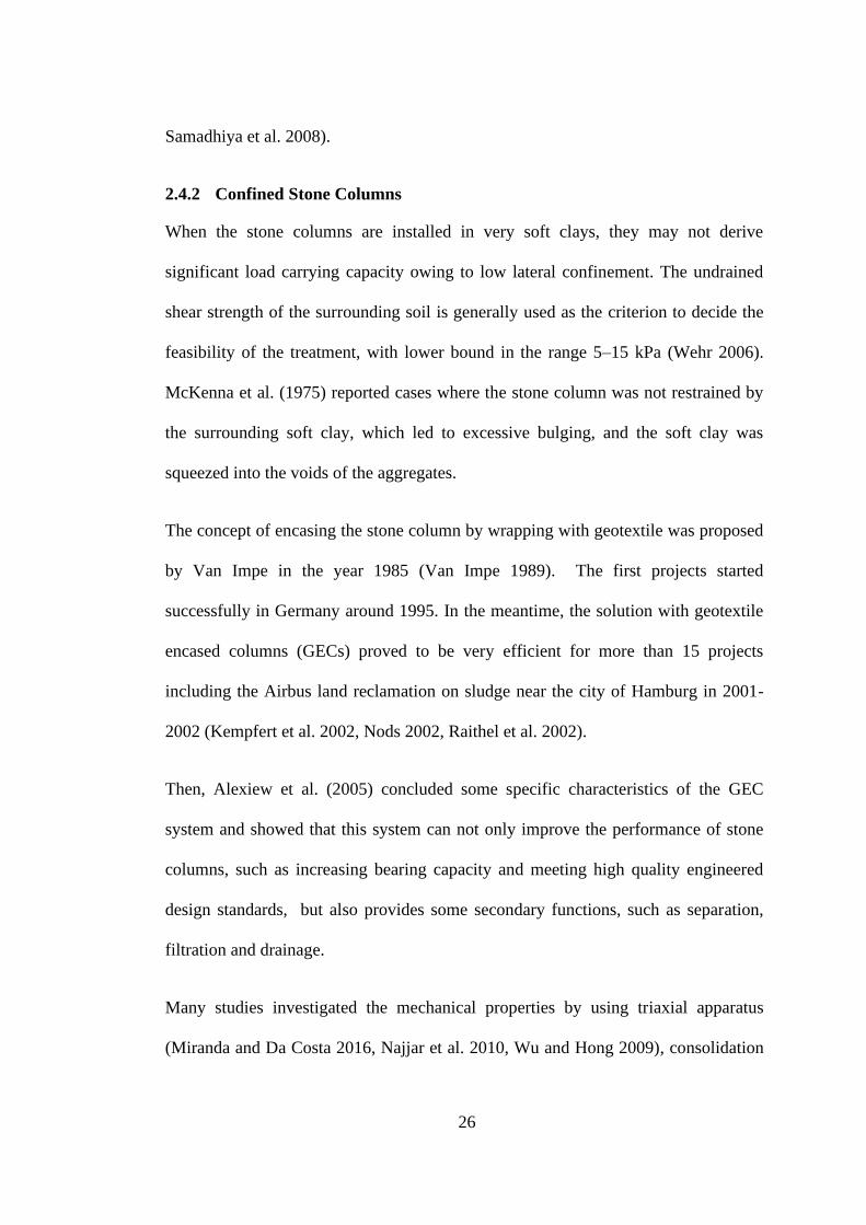
26

Samadhiya et al. 2008).

2.4.2 Confined Stone Columns

When the stone columns are installed in very soft clays, they may not derive

significant load carrying capacity owing to low lateral confinement. The undrained

shear strength of the surrounding soil is generally used as the criterion to decide the

feasibility of the treatment, with lower bound in the range 5–15 kPa (Wehr 2006).

McKenna et al. (1975) reported cases where the stone column was not restrained by

the surrounding soft clay, which led to excessive bulging, and the soft clay was

squeezed into the voids of the aggregates.

The concept of encasing the stone column by wrapping with geotextile was proposed

by Van Impe in the year 1985 (Van Impe 1989). The first projects started

successfully in Germany around 1995. In the meantime, the solution with geotextile

encased columns (GECs) proved to be very efficient for more than 15 projects

including the Airbus land reclamation on sludge near the city of Hamburg in 2001-

2002 (Kempfert et al. 2002, Nods 2002, Raithel et al. 2002).

Then, Alexiew et al. (2005) concluded some specific characteristics of the GEC

system and showed that this system can not only improve the performance of stone

columns, such as increasing bearing capacity and meeting high quality engineered

design standards, but also provides some secondary functions, such as separation,

filtration and drainage.

Many studies investigated the mechanical properties by using triaxial apparatus

(Miranda and Da Costa 2016, Najjar et al. 2010, Wu and Hong 2009), consolidation

27

cell (Ayadat and Hanna 2005, Murugesan and Rajagopal 2009), in situ tests

(Kempfert et al. 2002, Nods 2002, Raithel et al. 2002). Recently, to directly

investigate the behaviour and mechanical properties of GECs, unconfined

compression testing was conducted, which is shown in Fig 2.1 (Gniel and Bouazza

2010, Trunk et al. 2004). This testing method is similar to axial compression tests

for concrete columns.

Fig 2.1 Encased Stone Column being loaded in unconfined compression (Gniel and

Bouazza 2010)

2.4.3 Pervious Concrete Piles

The studies relevant to previous concrete piles are very limited. Compared with the

conventional stone columns, pervious concrete piles provide higher stiffness and

strength while offering similar permeability comparable to granular columns

(Suleiman et al. 2014). Suleiman et al. (2014) showed that the ultimate load of the

pervious concrete piles of the pervious piles was as much as 4.4 times that of an

28

identical granular column.

Zhang et al. (2015) studied the working mechanism of pervious concrete piles by

analysing the field test data and a numerical model was established based on the

finite-difference method and Biot’s consolidation theory. The excess pore-water

pressure, pile–soil stress ratio, lateral displacement, and settlement of the pervious

concrete piles composite foundation under the loading of the road embankment were

numerically calculated and compared with those of gravel pile and low-grade

concrete pile composite foundations. Comparisons show that the dissipation of

excess pore-water pressure in pervious concrete piles composite foundation was

fastest, which implied that pervious concrete piles can significantly mitigate the

development of excess pore-water pressure and thus enhance subsoil strength.

Furthermore, the pervious concrete piles composite foundation showed minimal

postconstruction settlement and lateral displacement.

2.4.4 Discussion

According to this section, it can be seen that the mechanical properties of pervious

concrete are better than traditional stone column. However, for some infrastructure,

the requirements may be much higher and the pervious concrete piles may not meet

them. Therefore, some kinds of reinforcing methods should be needed, and the

confinement provided by artificial materials is one of the best methods.

2.5 Application of ANN in Civil Engineering

An artificial neural network (ANN), usually called neural network, is a mathematical

model or computational model that is inspired by the structure and functional aspects

of biological neural networks. It consists of an interconnected group of artificial

29

neurons and is usually used to model the complex relationships between inputs and

outputs in experimental data, even these data are huge, noisy and incomplete. This

capability makes the ANN a very effective and powerful tool to solve complex

problems. Due to the properties of concrete and concrete members are complex and

affected by many factors, numerous studies adopted the ANN to solve these

problems, including predicting the different properties of unconfined concrete based

on a wide range of factors, optimizing the mix design of all types of concrete, and

predicting the mechanical properties of confined concrete.

2.5.1 Predicting the Properties of Concrete, Mortar and Paste

Some studies predicted the compressive strength of different types of concrete,

mortar and paste from various aspects. The types of concrete includes normal OPC

concrete (Ni and Wang 2000), high-strength concrete (Öztaş et al. 2006), self-

compacting concrete (Siddique et al. 2011), recycled aggregate concrete (Šipoš et al.

2017), and concrete containing silica fume, fly ash and slag (Bilim et al. 2009,

Sarıdemir 2009, Topcu and Sarıdemir 2008). Recently, some studies applied the

ANN model to predict the compressive strength of geopolymer materials, which is

considered as a “green material” and gain more and more attention. Due to there are

some differences between geopolymer materials and traditional OPC materials, some

special factors was considered, such as curing time and temperatures, chemical

composition, concentration of alkaline activators (Hadi et al. 2018, Kamalloo et al.

2010, Nazari and Torgal 2013, Yadollahi et al. 2015). Although the reaction

mechanism of geopolymer materials are more complex than that of OPC materials,

the preditions of ANN models can show good agreements with the experimental

results.

30

Few studies also predicted other properties of concrete, mortar and paste, such as

workability, dry shrinkage, and good predicting results were obtained. Bai et al.

(2003) used ANN to predict the workability of concrete incorporating metakaolin

and fly ash. On the basis of this ANN model, the effects of metakaolin and fly ash on

workability were analysed and diagrams used for designing the proper workability

were plotted. Bal and Buyle-Bodin (2013) proposed a multi-layer backpropagation

ANN model to predict the shrinkage of concrete. The parameters which affected

drying shrinkage of concrete were considered, including relative humidity, curing

period, volume to surface area ratio, water to cement ratio, and fine aggregate

content. Compared with other mathematical methods, it can be found that the ANN

model showed better predictions. However, until now, no studies was found to use

ANN models to predict the setting time of concrete, which is considered as a very

important parameter to make concrete in practice.

2.5.2 Optimizing the Mix Proportion of Concrete, Mortar and Paste

The ANN models combined with other mathematical methods, such as genetic

algorithm (GA) and non-linear programming, has been used to optimize the mix

proportion of concrete. The general procedure of the methodology consists of three

steps: (1) Modeling: Build an accurate model (ANN model) for targets (e.g. strength,

workability) based on experimental data; (2) Incorporating: Incorporate the ANN

model in software allowing an evaluation of the specified properties for a given mix.

(3) Optimizing: Incorporate the software in another mathematical methods allowing

a search for the optimum proportion mix design (Yeh 1999).

Yeh (1999) optimized high-performance concrete mix proportioning for a given

31

workability and compressive strength using artificial neural networks and nonlinear

programming. For performing optimum concrete mix design based on the proposed

methodology, a software package has been developed. One can conduct mix

simulations covering all the important properties of the concrete at the same time. To

demonstrate the performance of the proposed methodology, experimental results

from several different mix proportions based on various design requirements are

presented.

Kim et al. (2013) optimize the mixing proportion of recycled aggregate concrete

(RAC) using artificial neural network (ANN) based on genetic algorithm (GA) for

increasing the use of recycled aggregate (RA). The ANN and GA were used to

predict the compressive strength of the concrete at 28 days. And sensitivity analysis

of the ANN based on GA was used to find the mixing ratio of RAC. The mixing

criteria for RAC were determined and the replacement ratio of RAs was identified.

This research revealed that the proposed method, which is ANN based on GA, is

proper for optimizing appropriate mixing proportion of RAC. Also, this method

would help the construction engineers to utilize the recycled aggregate and reduce

the concrete waste in construction process.

2.5.3 Predicting the Compressive Strength and Strain of FRP-confined

Concrete

Recently, fiber-reinforced polymer (FRP) has become increasingly popular as a

confining material for the reinforced concrete columns due to its high strength-to-

weight ratio and high corrosion resistance (Jiang and Teng 2007). Numerous studies

proposed various models to predict the compressive strength and strain of FRP-

confined concrete. Among these methods, ANN model has been proven more

32

accurate than others. Pham and Hadi (2014) used ANN model to calculate the

compressive strength and strain of square/rectangular FRP-confined columns.

Compared modelling results of this ANN model with other five existing models, it

was found that the ANN model show more accurate predicting results. Mansouri et al.

(2016) studied the capability of ANN, adaptive neuro fuzzy inference system

(ANFIS), multivariate adaptive regression splines (MARS) and M5 model tress

(M5Tree) techniques to predict the compressive strength and strain of FRP-confined

concrete. The results showed that the ANN model provided the most accurate

predictions. Oreta and Kawashima (2003) applied ANN method to predict the

confined compressive strength and corresponding strain of circular concrete columns.

This study shows the importance of validating the ANN models in simulating

especially when data are limited. The ANN model was also compared to some

analytical models and the performance of ANN model was better.

2.5.4 Discussion

According to this section, it can be seen that the ANN is a very effective and

powerful tool to build the complex relationships between inputs and outputs. It has

been proven that the ANN can accurately predict the properties of geopolymer

concrete by considering various factors.

2.6 The Analytical Stress-Strain Models for FPR-Confined

Concrete

2.6.1 Types of Models

A large number of axial stress-strain design-oriented models of FRP-confined

concrete have been proposed. These models can be classified into three categories

33

based on the geometric form of the curves.

The first type of analytical models, which consists of two linear equations, were

proposed by some early studies to capture the bilinear stress-strain curves of FRP-

confined concrete (Binici 2008, Karbhari and Gao 1997, Saiid Saiidi et al. 2005,

Xiao and Wu 2000). Hence, the axial stress-strain curves consists of two lines

connected by a transition point. The first line connected the origin with the transition

point. The second line connected the transition point with ultimate point. Although

the second type models can capture the typical bilinear shape of the axial stress-strain

curves of FRP-confined concrete, these curves are different form the actual test

curves, which are smooth.

The second type of analytical models was expressed by a complex equation to

capture the bilinear shape of the axial stress-strain curves of FRP-confined concrete.

Numerous models modified the four-parameter equation proposed by Richard and

Abbott (1975) to describe the initial ascending portion of the axial stress-strain

curves of FRP-confined concrete (Campione and Miraglia 2003, Cheng et al. 2002,

Moran and Pantelides 2002, Samaan et al. 1998). In these models, the transition from

the first portion to the second portion was controlled by a shape parameter n. Some

other researchers modified the equation proposed by Sargin (1971) to capture the

bilinear shape (Ahmad et al. 1991, Ahmad and Shah 1982). Although these models

can predict the bilinear stress-strain curves accurately, the relative complexity of

these models are difficult to be used for section analysis, where integration of the

stress is required.

The more accurate third type of analytical models were proposed later, which

34

consisted of two equations. The first equation described the initial ascending region

as a curve and the second equation described the second region as a straight or

approximate straight line (Jin et al. 2003, Lam and Teng 2003, Lillistone and Jolly

2000, Miyauchi et al. 2000, Saafi et al. 1999, Teng et al. 2009, Toutanji 1999, Yu

and Teng 2010). Among these models, the one proposed by Lam and Teng (2003)

was recognized as one of the most popular and accurate models, due to its simplicity

and accuracy. This model was modified by Darby et al. (2004) and Soudki and

Alkhrdaji (2005) for design guidance. After that, Teng et al. (2009) refined the model

proposed by Lam and Teng (2003). In this refined model, more accurate ultimate

axial strain and compressive strength equations were proposed, and axial stress-strain

equations were modified to be able to presents the descending branch when the level

of confinement is low. Yu and Teng (2010) modified the model proposed by Lam

and Teng (2003) to adapt for the Chinese national code GB-50608 (Chinese Planning

Press 2010) by using new ultimate axial strain and compressive strength equations.

These equations considered the provisions in the Chinese national code GB-50010

(Chinese Architecture and Building Press 2002) and GB-50608 (Chinese Planning

Press 2010) . In the next section, the details of the three proposed models are

presented.

2.6.2 The Model Proposed by Lam and Teng (2003)

Lam and Teng (2003) proposed the design-oriented model based on five assumptions:

(1) the axial stress-strain curves of FRP-confined concrete consists of a parabolic

first portion and a straight-line second portion; (2) the initial slope of the parabola at

origin is the same as the elastic modulus of unconfined concrete Ec; (3) the first

parabola portion considered the confining effects from the FRP jacket; (4) the

35

parabolic first portion meets the linear second portion smoothly; (5) the linear second

portion ends at a point where both the compressive strength and the ultimate axial

strain are reached. These assumptions are based on the test observations of FRP-

confined concrete under axial compression.

Lam and Teng (2003) modified the simple Hognestad’s parabola (Hognestad 1951)

for the first parabolic portion of stress-strain curve of FRP-confined concrete. The

Hognestad’s parabola was used to describe the stress-strain curve of unconfined

concrete and adopted by the Lam and Teng (2003). Its expression is shown as

follows:

22' ( )c c

c co

co co

f

= −

(2.1)

where c and

c are the axial stress and axial strain, respectively, and co is the axial

strain at the peak stress of unconfined concrete, 'cof is the compressive strength of

unconfined concrete.

Based on the basic assumptions of FRP-confined concrete, the modified parabolic

equation proposed by Lam and Teng (2003) for the first portion of stress-strain curve

of FRP-confined concrete are shown as follows:

( )( )

( )

2 2

2

, 04 '

' ,

c

c c c c t

coc

co c t c cu

E EE

f

f E

− −

= +

(2.2)

where Ec is the elastic modulus of unconfined concrete, which is taken to be Ec =

4730√fco′ (in MPa) (ACI 2005); E2 is the slope of the linear second portion. In order

to let the parabolic first portion meets the linear second portion with a smooth

36

transition, the t is given by:

2

2 'co

t

c

f

E E =

−

(2.3)

The slope of the linear second portion E2 is expressed as:

2

' 'cc co

cu

f fE

−=

(2.4)

where 'ccf is the compressive strength of confined concrete. The confined concrete

compressive strength ( 'ccf ) equation takes the following equation:

( )

( )

1 3.3 , 0.07'

' 1, 0.07

K Kcc

co K

f

f

+ =

(2.5)

Based on testing results of this study, the equation to calculate the ultimate axial

strain of FRP-confined concrete proposed by Lam and Teng (2003) was used:

1.451.75 12cu

K

co

= +

(2.6)

where, the K is the confinement stiffness ratio; the is the strain ratio. The

mathematical expressions of these two ratios are as follow:

( )

2

'

FRP FRP

K

co co

E T

f D

= (2.7)

,h rup

co

=

(2.8)

where FRPE is the elastic modulus of FRP in the hoop direction; FRPT is the thickness

of the FRP jacket; ,h rup is the hoop rupture strain of the FRP jacket; D is the

diameter of the confined concrete cylinder.

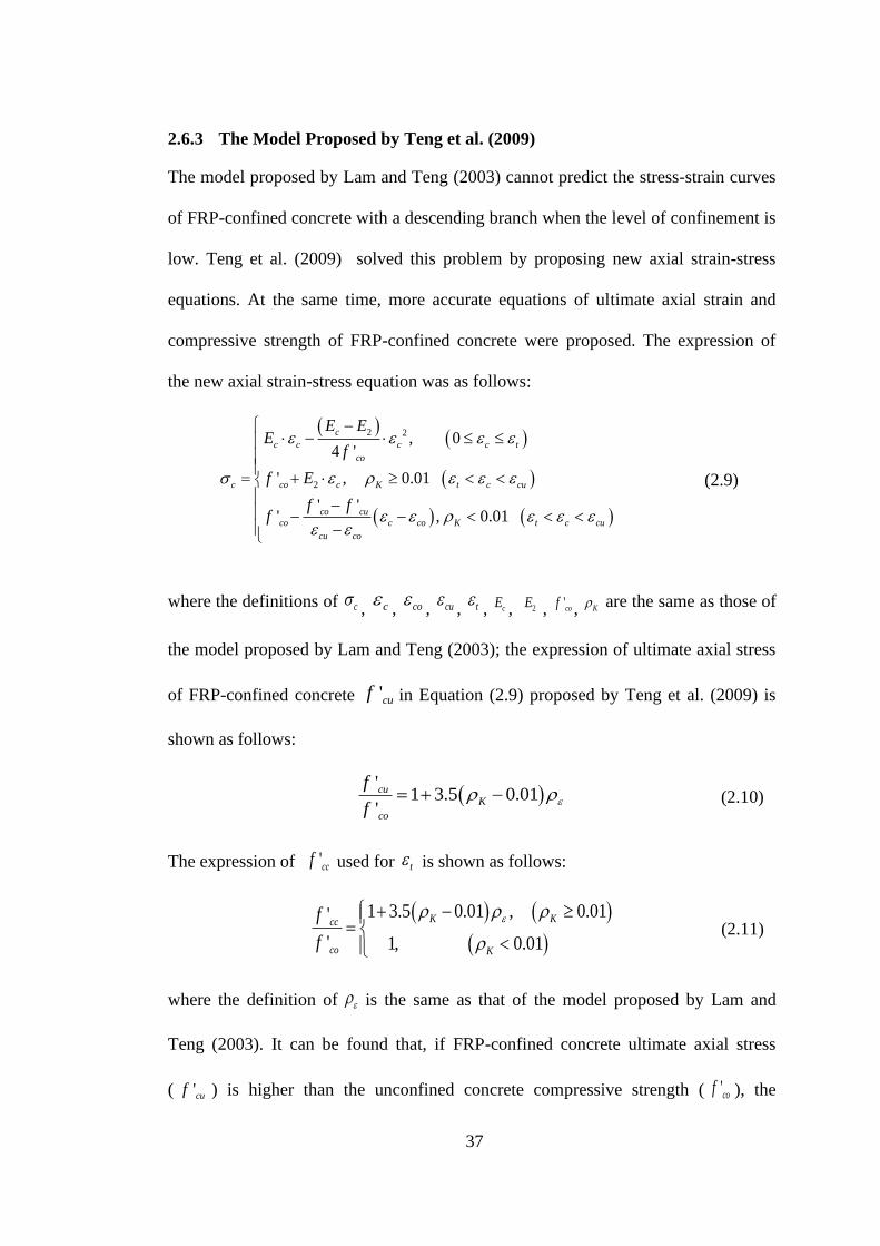
37

2.6.3 The Model Proposed by Teng et al. (2009)

The model proposed by Lam and Teng (2003) cannot predict the stress-strain curves

of FRP-confined concrete with a descending branch when the level of confinement is

low. Teng et al. (2009) solved this problem by proposing new axial strain-stress

equations. At the same time, more accurate equations of ultimate axial strain and

compressive strength of FRP-confined concrete were proposed. The expression of

the new axial strain-stress equation was as follows:

( )( )

( )

( ) ( )

2 2

2

, 04 '

' , 0.01

' '' , 0.01

c

c c c c t

co

c co c K t c cu

co cu

co c co K t c cu

cu co

E EE

f

f E

f ff

− −

= +

− − − −

(2.9)

where the definitions of c , c , co, cu

, t , cE , 2E , 'cof , K are the same as those of

the model proposed by Lam and Teng (2003); the expression of ultimate axial stress

of FRP-confined concrete 'cuf in Equation (2.9) proposed by Teng et al. (2009) is

shown as follows:

( )'

1 3.5 0.01'

cu

K

co

f

f = + −

(2.10)

The expression of 'ccf used for t is shown as follows:

( ) ( )

( )

1 3.5 0.01 , 0.01'

' 1, 0.01

K Kcc

co K

f

f

+ − =

(2.11)

where the definition of is the same as that of the model proposed by Lam and

Teng (2003). It can be found that, if FRP-confined concrete ultimate axial stress

( 'cuf ) is higher than the unconfined concrete compressive strength ( 'cof ), the

38

ultimate axial stress ( 'cuf ) is equal to the FRP-confined concrete compressive

strength ( 'ccf ).

2.6.4 Discussion

According to this section, it can be seen that for modeling the mechanical behaviour

of FRP-confined concrete, three types of models has been proposed. One of most

popular models was proposed by Teng et al. (2009), which can accurately and

rationally simulate the mechanical behaviour of FRP-confined concrete. But this

model cannot model the large axial strain confined concrete.

2.7 Summary

The PGC pavements and piles are innovative, efficient, environmentally-friendly,

and feasible ways to solve some civil engineering problems. Also, the PGC

pavement and pile can greatly expand the application of geopolymer concrete and

more industrial by-products can be recycled. However, for some infrastructure, the

requirements may be much higher and the pervious concrete piles may not meet them.

Therefore, some kinds of reinforcing methods should be needed, and the confinement

provided by artificial materials is one of the best methods. In addition, the ANN

method can be used to predict the properties of geopolymer concrete based on

various factors, and the analytical model proposed by Teng et al. (2009) can be

modified to accurately simulate the behaviour of confined PGC piles.

This Chapter leads to Chapter 3 which presents an experimental program of

geopolymer paste and geopolymer concrete. The optimum mix designs of

geopolymer paste and geopolymer concrete were determined, which will be used for

39

further study.

40

CHAPTER 3

Optimum Mix Design of Geopolymer Paste and Concrete

Cured in Ambient Condition based on Compressive

Strength, Setting Time and Workability

3.1 Introduction

In this chapter, the optimum mix design of geopolymer paste and the optimum mix

design of geopolymer concrete are determined, and regression models are proposed

to predict the properties of geopolymer pastes. At first, a series of mini-size specimen

compression tests, setting time tests and mini-slump tests were conducted at ambient

condition (23 ± 2 °C). The ground granulated blast furnace slag (GGBFS) and Class

F fly ash (FA) were used as aluminosilicate source. The alkaline activator was a

blend of sodium silicate solution and sodium hydroxide solution. Additional water

was added to improve the workability and prolong the setting time. The effects of

GGBFS content, alkaline solution to binder (Al/Bi) mass ratio, sodium silicate

solution to sodium hydroxide solution (SS/SH) mass ratio, and additional water to

binder (Aw/Bi) mass ratio on the compressive strength, setting time and workability

of geopolymer pastes were studied. Based on the test results of compressive strength,

setting time and workability, the optimum mix design of geopolymer pastes was

found. The properties of the geopolymer paste under optimum mix design were

compared with those of ordinary Portland cement (OPC) pastes to know which is

better. After that, the geopolymer concrete tests based on optimum mix design of

geopolymer paste were conducted, in comparison with OPC concrete tests. Lastly,

41

new mathematical models were proposed to predict the properties of geopolymer

pastes. In this study, all geopolymer paste specimens were cured in the indoor lab at

the ambient temperature of 23 ± 2 °C. In the future, the geopolymer paste

specimens cured at different temperatures, such as low temperature, will be

investigated.

3.2 Experimental Programme for Geopolymer Pastes

3.2.1 Materials

In this study, GGBFS and Class F FA were used as aluminosilicate sources. The

GGBFS was supplied by the Australasian Slag Association (2018) and Class F FA

was provided by Eraring Power Station Australia (2018). The FA was classified as

Class F according to AS 3582.1 (2016). The chemical compositions of GGBFS

(2018) and FA (2018) are shown in Table 3.1.

Table 3.1 Chemical compositions (mass%) for ground granulated blast furnace

slag (GGBFS) (Australasian Slag Association 2018), Fly ash (FA) (Eraring

Power Station Australia 2018).

Component GGBFS (%)

(Australasian Slag

Association 2018)

FA (%) (Eraring

Power Station

Australia 2018)

SiO2 32.4 62.2

Al2O3 14.96 27.5

Fe2O3 0.83 3.92

CaO 40.7 2.27

MgO 5.99 1.05

K2O 0.29 1.24

Na2O 0.42 0.52

TiO2 0.84 0.16

P2O5 0.38 0.30

Mn2O3 0.40 0.09

42

SO3 2.74 -

Sodium silicate solution and sodium hydroxide solution were blended together as

alkaline activator. Solid granulated caustic soda was dissolved in water to make

sodium hydroxide solution. The concentration of sodium hydroxide solution was

kept constant (14 M) for all mixes. Sodium silicate solution was provided by a local

commercial producer. The mass ratio of SiO2 to Na2O of the sodium silicate was

2.02 with chemical compositions of 29.6% SiO2 and 14.7% Na2O.

The OPC paste tests were conducted as comparative experiments. In this study, Type

general purpose (GP) cement, which is in accordance with AS 3972 (2010), was

mixed with water to make OPC paste samples. Both the compressive strength and

workability of the OPC pastes were compared with those of geopolymer pastes to see

if the latter material can have better or equivalent performance than that of OPC

pastes. For setting time, the AS 3792 (2010) was used to judge if the setting time of

geopolymer pastes can meet the requirements of setting times for Type GP cement.

3.2.2 Mix Proportions

Twenty-eight mixes of geopolymer pastes were designed to study the effects of four

factors on the compressive strength, setting time and workability of geopolymer

pastes. These four factors are GGBFS content (0%, 10%, 20%, 30%, 40%), SS/SH

ratio (1.0, 1.5, 2.0, 2.5), Al/Bi ratio (0.4, 0.5, 0.6, 0.7) and Aw/Bi ratio (0.09, 0.12,

0.15).

A labelling system was designed to clearly show the mix proportions of geopolymer

pastes. Each mix was assigned nine characters. Although the name of mix is

43

extensive, the labelling system is easy to understand.

This labelling system includes abbreviations for the four variable parameters. The

first two letters ‘Gx’ represents GGBFS content. It means the GGBFS content is x%.

For example, ‘G40’ means the binder comprised 40% GGBFS. The following two

letters “Sy” represents SS/SH ratio, where the SS/SH ratio is y. For example, ‘S2.5’

indicates a SS/SH ratio of 2.5. The third component ‘Az’ represents the Al/Bi ratio,

where the Al/Bi ratio is z. For example, ‘A.5’ means an Al/Bi ratio of 0.5. The final

component ‘Ws’ refers to the Aw/Bi ratio, where Aw/Bi ratio is s. For example,

‘W.09’ signifies an Aw/Bi ratio of 0.09.

There were three series of geopolymer paste tests in this study. In the first series, the

effect of GGBFS content on the properties of geopolymer pastes were investigated.

The values of GGBFS contents of 0%, 10%, 20%, 30%, 40% were chosen. The

values of Al/Bi ratio, SS/SH ratio, Aw/Bi ratio were kept constant at 0.5, 2.5 and

0.15, respectively. The detailed mix design can be seen in Table 3.2.

Table 3.2 The mix designs for the effect of GGBFS content (Hadi et al. 2019).

Mix GGBFS

(kg/m3)

Fly ash

(kg/m3)

GGBFS

Content

(%)

Al/

Bi

SS/

SH

Aw/

Bi

G0-S2.5-A.5-W.15 0 1061 0 0.5 2.5 0.15

G10-S2.5-A.5-W.15 107 966 10 0.5 2.5 0.15

G20-S2.5-A.5-W.15 217 868 20 0.5 2.5 0.15

G30-S2.5-A.5-W.15 329 768 30 0.5 2.5 0.15

G40-S2.5-A.5-W.15* 444 666 40 0.5 2.5 0.15

*The same mix in Table 3.3 and Table 3.4.

In the second series of geopolymer paste tests, the effects of Al/Bi ratios and SS/SH

44

ratios were investigated. The values of Al/Bi ratios of 0.4, 0.5, 0.6, 0.7, and the

values of SS/SH ratios of 1.0, 1.5, 2.0, 2.5 were used. The GGBFS content and

Aw/Bi ratio were kept at 40% and 0.15, respectively. The detailed mix proportions

are shown in Table 3.3. In this study, the mutual influence of these two factors were

investigated together, in comparison with other studies which investigated them

separately (Morsy et al. 2014, Nath and Sarker 2014).

Table 3.3 The mix designs for the effects of Al/Bi ratio and SS/SH ratio (Hadi et

al. 2019).

Mix GGBFS

(kg/m3)

Fly ash

(kg/m3)

GGBFS

Content

(%)

Al/

Bi

SS/

SH

Aw/

Bi

G40-S1.0-A.4-W.15 477 715 40 0.4 1.0 0.15

G40-S1.5-A.4-W.15 478 718 40 0.4 1.5 0.15

G40-S2.0-A.4-W.15 479 719 40 0.4 2.0 0.15

G40-S2.5-A.4-W.15* 480 720 40 0.4 2.5 0.15

G40-S1.0-A.5-W.15 441 661 40 0.5 1.0 0.15

G40-S1.5-A.5-W.15 442 663 40 0.5 1.5 0.15

G40-S2.0-A.5-W.15 443 664 40 0.5 2.0 0.15

G40-S2.5-A.5-W.15** 444 666 40 0.5 2.5 0.15

G40-S1.0-A.6-W.15 410 615 40 0.6 1.0 0.15

G40-S1.5-A.6-W.15 411 617 40 0.6 1.5 0.15

G40-S2.0-A.6-W.15 412 618 40 0.6 2.0 0.15

G40-S2.5-A.6-W.15* 413 620 40 0.6 2.5 0.15

G40-S1.0-A.7-W.15 383 574 40 0.7 1.0 0.15

G40-S1.5-A.7-W.15 384 576 40 0.7 1.5 0.15

G40-S2.0-A.7-W.15 385 578 40 0.7 2.0 0.15

G40-S2.5-A.7-W.15* 386 579 40 0.7 2.5 0.15

*The same mixes in Table 3.4.

**The same mix in Table 3.2 and Table 3.4.

The third series of geopolymer paste tests investigated the effects of Aw/Bi ratio.

45

This is because when GGBFS content was high in the geopolymer binder, additional

water had to be added to increase the setting time and improve the workability

(Chindaprasirt et al. 2007, Hadi et al. 2017, Wardhono et al. 2015). The Aw/Bi ratio

has been proven to have significant effect on the properties of geopolymer materials

(Chindaprasirt et al. 2007, Hadi et al. 2017, Wardhono et al. 2015). Hadi et al. (2017)

used 0.12 for the value of Aw/Bi. In this study, the values of the Aw/Bi ratios of 0.09,

0.12 and 0.15 were used. As mixes having Aw/Bi ratio of 0.15 were the same as

Mixes G4-S25-A4-W.15, G4-S25-A5-W.15, G4-S25-A6-W.15, G4-S25-A7-W.15 in

Table 3.3, their testing results were shared in both parts. The details of mix designs

are shown in Table 3.4.

Table 3.4 The mix designs for the effect of Aw/Bi ratio (Hadi et al. 2019).

Mix GGBFS

(kg/m3)

Fly Ash

(kg/m3)

GGBFS

Content

(%)

Al/

Bi

SS/

SH

Aw/

Bi

G40-S2.5-A.4-W.09 517 776 40 0.4 2.5 0.09

G40-S2.5-A.5-W.09 476 714 40 0.5 2.5 0.09

G40-S2.5-A.6-W.09 440 661 40 0.6 2.5 0.09

G40-S2.5-A.7-W.09 410 615 40 0.7 2.5 0.09

G40-S2.5-A.4-W.12 498 747 40 0.4 2.5 0.12

G40-S2.5-A.5-W.12 459 689 40 0.5 2.5 0.12

G40-S2.5-A.6-W.12 426 639 40 0.6 2.5 0.12

G40-S2.5-A.7-W.12 397 596 40 0.7 2.5 0.12

G40-S2.5-A.4-W.15* 480 720 40 0.4 2.5 0.15

G40-S2.5-A.5-W.15** 444 666 40 0.5 2.5 0.15

G40-S2.5-A.6-W.15* 413 620 40 0.6 2.5 0.15

G40-S2.5-A.7-W.15* 386 579 40 0.7 2.5 0.15

*The same mixes in Table 3.3.

**The same mix in Table 3.2 and Table 3.3.

46

In this study, Type general purpose (GP) cement based on AS 3972 (2010), which is

one type of ordinary Portland cement (OPC), was used to conduct OPC paste and

OPC concrete tests. Although the grade, source and classification of type GP cement

may be different, the variation of these properties must be limited in the range

required in AS 3972 (2010). Therefore, the effects of the grade, source and

classification of type GP cement are very limited. A few trial mixes were conducted

and it was found that when the w/c ratio was 0.3, the workability of OPC pastes was

very low. It was difficult to cast OPC pastes properly into the mould. When the w/c

ratio was 0.7, the problem of bleeding of OPC pastes was very obvious. Hence, w/c

ratios of 0.4, 0.5 and 0.6 were used in this study. The mix design of OPC mixes are

shown in Table 3.5. The labels used for these OPC paste tests are OPC.4, OPC.5 and

OPC.6 referring to OPC and the w/c ratios.

Table 3.5 The mix designs for OPC paste (Hadi et al. 2019).

Mix w/c Cement

(kg/m3)

Water

(kg/m3)

OPC.4 0.4 1389 556

OPC.5 0.5 1220 610

OPC.6 0.6 1087 652

3.2.3 Mixing, Casting and Curing

All tests were conducted under an ambient temperature of 23 ± 2 °C. The sodium

hydroxide solution and sodium silicate solution were mixed together for about 1 hour

before mixing with aluminosilicate source. A twenty Quart Hobart mixer

(Corporation 2018) (shown in Figure 3.1) was used to dry mix the FA and GGBFS

for 2 min.

47

Figure 3.1 Twenty Quart Hobart Mixer (Hadi et al. 2019).

Afterwards, alkaline activator was added and mixed for 1 min. In this study, the

concentration of sodium hydroxide solution was relatively high (14 M) and the

chemical reaction between aluminosilicate materials (FA and GGBFS) and alkaline

activators was relatively fast. In addition, the paste test scale was small and it is easy

to mix the geopolymer paste homogeneously. Therefore, a relatively short mixing

time was adequate to mix the paste properly. After mixing with alkaline activators,

extra water was poured into the mixer for another 2 min until the mix became well

mixed and homogeneous.

48

Figure 3.2 The mini-size specimens cast in the mini-size moulds (Hadi et al.

2019).

In this study, plastic moulds of 50 mm diameter and 100 mm height were used for

casting the geopolymer pastes (shown in Figure 3.2) to determine the compressive

strength. Six samples were cast for each mix, three of them for 7-day compressive

strength and three for 28-day compressive strength. The samples were kept in the

laboratory at an ambient condition (23 ± 2°C) for 24 hours and demoulded.

Afterwards, these specimens were cured at an ambient condition for 7 days or 28

days.

3.2.4 Testing methods

The compressive strengths of OPC pastes and geopolymer pastes were determined at

the age of 7 days and 28 days. The average of three cylinders tested under

compression was taken as the nominal compressive strength. This test was done by

using the Avery compression machine of 1800 kN loading capacity in the High Bay

49

laboratory at the University of Wollongong, Australia (shown in Figure 3.3(a)).

Initial and final setting times of OPC pastes and geopolymer pastes were measured

from the start of mixing. The procedure was in accordance with AS 2350.4 (2006) by

using Vicat apparatus (AS 2350.4 (2006)) (shown in Figure 3.3(b)). All setting time

tests were conducted under an ambient temperature of 23 ± 2 °C.

The workability of OPC pastes and geopolymer pastes was assessed by the mini-

slump tests, which were similar to previous studies (Collins et al. 2012, Collins and

Sanjayan 1998, Collins and Sanjayan 2001, Kantro 1980). The mini-slump mould

was made by using 3D print technology (shown in Figure 3.3(d)). The dimensions of

the mould are: top diameter 19 mm, bottom diameter 38 mm, and height 57 mm. The

mould was placed firmly on a flat and horizontal plastic sheet. Then, it was filled

with geopolymer paste and compacted with a small rod. The mould was removed

vertically ensuring minimal lateral disturbance. From the moment of adding alkaline

activator into binder, the mini-slump test was conducted at 15 min intervals. Mini-

slump tests were conducted for every mix at 15 min, 30 min, 45 min and 60 min.

The diameter of hardened base was measured at five locations and the average value

was used to calculate the area (Collins et al. 2012).

50

(a) Compression testing machine (b) Vicat apparatus

(c) Mini-slump cone diagram(units: mm) (d) Mini-slump cone photo

Figure 3.3 Testing devices: (a) Compression testing machine; (b) Vicat

apparatus; (c) Mini-slump cone diagram(units: mm); (d) Mini-slump cone picture

(Hadi et al. 2019).

3.2.5 Results and Discussion

Totally, four series of paste tests were conducted, including one series of OPC paste

tests and three series of geopolymer paste tests. The setting time of geopolymer

pastes were compared with the specified values in AS 3972 (2010) for Type GP

51

cement. In AS 3972 (2010), the minimum initial setting time for Type GP cement is

specified as 45 min and the maximum final setting time is specified as 360 min. All

testing results of 7-day and 28-day compressive strength, initial and final setting

times, and mini-slump base area are summarized in Table 3.6.

Table 3.6 Results of OPC paste mixes and geopolymer paste mixes (Hadi et al.

2019).

Mix

7-day

compressive

strength

(MPa)

28-day

compressive

strength

(MPa)

Initial

setting

time

(mins)

Final

setting

time

(mins)

Mini-slump base area

(103 mm2)

15

mins

30

mins

45

mins

60

mins

OPC.4 27.5 45.7 220 342 3.5 3.2 3.1 2.7

OPC.5 21.3 36.5 275 421 4.7 4.3 4.1 3.8

OPC.6 18.7 31.2 332 513 7.1 6.9 6.4 6.1

G0-S2.5-A.5-W.15 5.6 12.4 1220 1507 32.2 31.4 31.6 30.8

G10-S2.5-A.5-W.15 14.8 24.6 324 468 29.1 26.8 24.3 22.4

G20-S2.5-A.5-W.15 22.4 33.3 207 285 27.4 22.8 21.4 18.5

G30-S2.5-A.5-W.15 25.1 43.8 119 195 24.3 18.6 15.4 13.5

G40-S2.5-A.5-W.15* 28.0 47.9 66 123 22.3 14.6 10.2 7.1

G40-S1.0-A.4-W.15 22.7 37.7 76 124 16.1 11.8 5.4 -

G40-S1.5-A.4-W.15 27.0 43.0 58 106 15.4 9.7 3.8 -

G40-S2.0-A.4-W.15 30.0 51.3 50 82 14.8 8.2 - -

G40-S2.5-A.4-W.15* 29.5 49.7 41 69 14.3 7.1 - -

G40-S1.0-A.5-W.15 20.9 34.6 106 202 25.4 22.8 17.1 13.7

G40-S1.5-A.5-W.15 26.5 41.4 91 168 24.8 19.8 14.2 11.4

G40-S2.0-A.5-W.15 28.4 48.7 85 137 23.1 17.2 12.4 9.7

G40-S2.5-A.5-W.15* 28.0 47.9 66 123 22.3 14.6 10.2 7.1

G40-S1.0-A.6-W.15 15.3 26.5 140 267 29.7 26.3 23.8 21.4

G40-S1.5-A.6-W.15 19.2 33.1 118 222 28.9 25.1 21.5 16.3

G40-S2.0-A.6-W.15 22.3 40.4 103 189 27.5 23.7 19.4 14.4

G40-S2.5-A.6-W.15* 21.1 37.5 92 175 26.3 21.5 17.0 13.2

G40-S1.0-A.7-W.15 10.7 17.5 176 301 34.8 32.1 29.6 26.7

52

Table 3.6 (Continued)

G40-S1.5-A.7-W.15 11.0 21.7 149 255 33.1 29.3 26.5 24.1

G40-S2.0-A.7-W.15 13.4 25.0 127 233 31.8 28.1 25.4 22.7

G40-S2.5-A.7-W.15* 13.0 23.4 109 201 30.6 26.4 22.8 19.4

G40-S2.5-A.4-W.09 32.3 59.4 28 39 8.1 - - -

G40-S2.5-A.5-W.09 31.9 57.6 45 86 12.5 3.7 - -

G40-S2.5-A.6-W.09 25.3 48.0 69 133 18.2 11.3 4.1 -

G40-S2.5-A.7-W.09 16.6 38.9 89 169 20.5 14.6 8.3 3.6

G40-S2.5-A.4-W.12 30.0 54.5 33 58 11.4 3.6 - -

G40-S2.5-A.5-W.12 29.0 51.8 59 111 16.8 9.1 3.4 -

G40-S2.5-A.6-W.12 22.6 43.6 79 152 21.4 15.8 11.1 5.6

G40-S2.5-A.7-W.12 13.2 30.9 99 181 25.3 20.1 15.8 9.6

G40-S2.5-A.4-W.15* 29.5 49.7 41 69 14.3 7.1 - -

G40-S2.5-A.5-W.15* 28.0 47.9 66 123 22.3 14.6 10.2 7.1

G40-S2.5-A.6-W.15* 21.1 37.5 92 175 26.3 21.5 17.0 13.2

G40-S2.5-A.7-W.15* 13.0 23.4 109 201 30.6 26.4 22.8 19.4

*The same mixes in Table 3.3 and Table 3.4.

Mix G4-S20-A5-W2 marked in bold is the optimum mix proportion.

Results of OPC

The compressive strength, setting time and mini-slump areas of three OPC mixes are

shown in Table 3.6. It can be found that the highest 28-day compressive strength was

achieved by Mix OPC.4, reaching 45.7 MPa. With the increase of the water content,

the compressive strength decreased significantly. The 28-day compressive strength

of Mixes OPC.5 and OPC.6 reduced by 20% and 32%, respectively. For the three

OPC mixes, the 7-day compressive strength was about 60% of the 28-day

compressive strength.

From Table 3.6, it can be seen that the setting times of OPC pastes increased with the

53

increase of water content. Mix OPC.4 achieved initial setting time of 220 min. The

initial setting times of Mixes OPC.5 and OPC.6 increased to 275 min and 332 min,

respectively. The difference between initial and final setting time for OPC.4 was 122

min and those of Mixes OPC.5 and OPC.6 increased by 20% and 48%, respectively,

as compared to Mix OPC.4.

Mix OPC.4 had the lowest mini-slump base area. The mini-slump base areas of

Mixes OPC.5 and OPC.6 were about 35% and 110% higher than that of Mix OPC.4

at 15 min, 30 min, 45 min and 60 min. However, for the three OPC mixes, the

differences of mini-slump base area between 15 min and 60 min were only around 1

× 103 mm2.

Effect of GGBFS Content

The mixes in Table 3.2 were designed with increasing the amount of GGBFS to

investigate its effect on the properties of geopolymer pastes. All the mixes in Table

3.2 were mixed with the same Al/Bi ratio, SS/SH ratio, and Aw/Bi ratio. The testing

results of compressive strength, setting time and mini-slump base areas are shown in

Figure 3.4, Figure 3.5 and Figure 3.6, respectively.

54

Figure 3.4 Effect of GGBFS content on the compressive strength of geopolymer

pastes (Hadi et al. 2019).

The compressive strength development of geopolymer pastes with the increase of

GGBFS content are presented in Figure 3.4. It is found that Mix G0-S25-A5-W.15,

which has no slag, reacted slowly to develop compressive strength at ambient

condition. The 28-day compressive strength of Mix G0-S2.5-A.5-W.15 was only

12.4 MPa. However, when GGBFS was added, the compressive strength increased

significantly. At 28 days, the geopolymer paste mixes having 10% (G10-S2.5-A.5-

W.15), 20% (G20-S2.5-A.5-W.15), 30% (G30-S2.5-A.5-W.15) and 40% (G40-S2.5-

A.5-W.15) GGBFS of total binder achieved 98%, 169%, 253% and 293% higher

compressive strength than that of Mix G0-S2.5-A.5-W.15, respectively. This trend is

similar to those of several other research studies, such as Nath and Sarker (2014) and

Hadi et al. (2017). The reason for this trend is that the microstructure of geopolymer

pastes containing higher amount of GGBFS was denser due to increasing the

formation of C-S-H gel (Kumar et al. 2010). The variation of 7-day compressive

0

10

20

30

40

50

60

0 10 20 30 40

Com

pre

ssiv

e S

trength

(M

Pa)

GGBFS content (%)

7 days

28 days

55

strength had a similar trend to 28-day compressive strength. But the values of 7-day

compressive strength were around 60% of the 28-day compressive strength. On the

other hand, compared with the highest 28-day compressive strength of OPC mixes

(OPC.4, 45.7 MPa), only Mix G40-S2.5-A.5-W.15 had higher 28-day compressive

strength (47.9 MPa).

Figure 3.5 Effect of GGBFS content on the initial and final setting times of

geopolymer pastes (Hadi et al. 2019).

Figure 3.5 shows the initial and final setting times of geopolymer pastes with

different contents of GGBFS. For Mix G0-S2.5-A.5-W.15 with no GGBFS, the

initial and final setting times, was more than 20 hours and 25 hours, respectively.

However, when GGBFS was incorporated in the mixes, both initial and final setting

times decreased significantly. The initial setting time of Mix G10-S2.5-A.5-W.15

decreased by 73% even with a 10% addition of GGBFS in the binder. As for Mixes

G20-S2.5-A.5-W.15, G30-S2.5-A.5-W.15 and G40-S2.5-A.5-W.15, the initial setting

time decreased with the increase of GGBFS content, by 83%, 90%, and 95%

compared with that of Mix G0-S2.5-A.5-W.15, respectively. The variation of final

0

400

800

1200

1600

0 10 20 30 40

Set

tin

g T

ime

(Min

)

GGBFS content (%)

Initial Setting Time

Final Setting Time

56

setting time had a similar trend to that of initial setting time. Furthermore, the

difference between initial and final setting times reduced with the increase of

GGBFS content. Such difference of Mix G10-S2.5-A.5-W.15 was 144 min which

reduced to 78 min, 76 min and 57 min for Mixes G20-S2.5-A.5-W.15, G30-S2.5-

A.5-W.15 and G40-S2.5-A.5-W.15, respectively. These results proved the fact that

increasing the GGBFS content can greatly accelerate the setting of geopolymer

pastes (Hadi et al. 2017, Nath and Sarker 2014). Since the minimum initial setting

time allowed for Type GP cement is 45 min and the maximum final setting time is

360 min according to AS 3792 (2010), it can be found that Mixes G20-S2.5-A.5-

W.15, G30-S2.5-A.5-W.15 and G40-S2.5-A.5-W.15 met this requirement.

Figure 3.6 Effect of GGBFS content on mini-slump tests of geopolymer pastes

(Hadi et al. 2019).

Figure 3.6 shows the effect of GGBFS content on mini-slump testing results of

geopolymer pastes and the results of three OPC mixes are also included. It can be

seen that the mini-slump base areas of geopolymer pastes decreased significantly

0

5

10

15

20

25

30

35

15 30 45 60

Min

i sl

um

p b

ase

are

a (

10

3m

m2)

Time (Min)

G0-S2.5-A.5-W.15

G10-S2.5-A.5-W.15

G20-S2.5-A.5-W.15

G30-S2.5-A.5-W.15

G40-S2.5-A.5-W.15

OPC.4

OPC.5

OPC.6

57

with the increase of GGBFS content. The relationship between mini-slump base area

and time is nearly linear. It can also be found that the difference of base areas

between 15 min and 60 min became larger with the increase of GGBFS content. For

Mix G0-S2.5-A.5-W.15, the difference of base area between 15 min and 60 min was

1.4 × 103 mm2, and those of Mixes G10-S2.5-A.5-W.15, G20-S2.5-A.5-W.15, G30-

S2.5-A.5-W.15 and G40-S2.5-A.5-W.15 increased to 6.7 × 103 mm2, 8.9 × 103 mm2,

10.8 × 103 mm2 and 15.2 × 103 mm2, respectively. In other words, with the increase

of GGBFS content, the mini-slump base area decreased more rapidly. This is due to

the fact that the polymerization processes is accelerated with the increase of GGBFS

content (Nath and Sarker 2014). Within 60 min, the workability of all geopolymer

paste mixes in Figure 3.6 was better than those of OPC pastes. However, for all OPC

paste mixes, the base areas remained stable from 15 min to 60 min.

Effect of Al/Bi ratio and SS/SH ratio

In this section, the effects of both alkaline solution to binder mass (Al/Bi) ratio and

sodium silicate to sodium hydroxide mass (SS/SH) ratio on the properties of

geopolymer pastes were investigated by the mixes shown in Table 3.3. The effect of

Al/Bi ratio on the optimum SS/SH ratio was also investigated.

58


solution to sodium hydroxide solution (SS/SH) ratio on compressive strength of

geopolymer paste (Hadi et al. 2019).

Figure 3.7 shows the compressive strength development of geopolymer pastes due to

the increases of Al/Bi ratios and SS/SH ratios. Every four mixes, which had the same

SS/SH ratio but different Al/Bi ratios, are drawn into one curve. It can be seen that

with the increase of Al/Bi ratio, the compressive strengths of each curve decreased

significantly. On the other hand, it is found that the four specimens of SS/SH of 2.0

achieved the highest 28-day compressive strength compared with those of other

SS/SH ratios. Hence in this study, the optimum SS/SH ratio was 2.0 for all Al/Bi

ratios. However, the 28-day compressive strength curve of SS/SH of 2.5 was slightly

lower than the curve of SS/SH of 2.0. The lowest 28-day compressive strength was

achieved when the SS/SH was equal to 1.0. This is due to the fact that a rise in the

silica content leads to more densely packed, polymerised gels with excellent

mechanical properties (Fernández-Jiménez and Palomo 2003, Puertas et al. 2011).

0

10

20

30

40

50

60

0.4 0.5 0.6 0.7

Com

pre

ssiv

e s

trength

(M

Pa)

Al/Bi Ratio (w/c for OPC)

SS/SH=1.0 (7 days)

SS/SH=1.5 (7 days)

SS/SH=2.0 (7 days)

SS/SH=2.5 (7 days)

OPC (7 days)

SS/SH=1 (28 days)

SS/SH=1.5 (28 days)

SS/SH=2.0 (28 days)

SS/SH=2.5 (28 days)

OPC (28 days)

Optimum mix design

Mixes had higher compressive strength than

the optimum mix design

59

However, the compressive strength drops when more silicate is added, since excess

sodium silicate hinders water evaporation and structure formation (Morsy et al.

2014). The variation of 7-day compressive strength in this section had a similar trend

to that of 28-day compressive strength. In addition, compared to the OPC mixes, it

can be seen that Mixes G40-S2.0-A.4-W.15, G40-S2.5-A.4-W.15 had higher 7-day

and 28-day compressive strength than those of all OPC mixes.


solution to sodium hydroxide solution (SS/SH) ratio on initial and final setting

times of geopolymer pastes (Hadi et al. 2019).

The initial and final setting times were influenced significantly by the Al/Bi ratio and

SS/SH ratio as shown in Figure 3.8. It can be seen that the relationships between the

Al/Bi ratio and the initial and final setting times are nearly linear. With the increase

of Al/Bi ratio, the initial and final setting times increased significantly. The final

setting times increased by around 75% compared to initial setting times. This is due

0

50

100

150

200

250

300

350

400

0.4 0.5 0.6 0.7

Sett

ing T

ime

(Min

)

Al/Bi ratio (w/c ratio for OPC)

SS/SH=1.0 (Initial Setting Time)




SS/SH=1.0 (Final Setting Time)




Reference line for initial setting time

(45 min)

Reference line for final setting time

(360 min)

60

to the fact that excess alkaline solution increase the amount of water in the mix

which hindered geopolymerization (Ruiz-Santaquiteria et al. 2012). On the other

hand, it was found that initial and final setting times decreased when the SS/SH ratio

increased. This is because when the amount of soluble silica is increased, the

polymerization processes is accelerated to some extent (Nath and Sarker 2014). In

addition, it is noted that all mixes in Figure 3.8 met the requirement of final setting

time stated in AS 3972 (2010) for comparison. The initial setting time requirement

was met by all of the mixes, except Mix G4-S25-A4-W.15.


solution to sodium hydroxide solution (SS/SH) ratio on mini-slump tests of

geopolymer pastes: (a) Al/Bi=0.4; (b) Al/Bi=0.5; (c) Al/Bi=0.6; (d) Al/Bi=0.7

(Hadi et al. 2019). (Continued)

0

5

10

15

20

25

30

35

15 30 45 60

Min

i-sl

um

p B

ase

Are

a (

10

3m

m2)

Time (min)

(a) Al/Bi = 0.4

G40-S1.0-A.4-W.15G40-S1.5-A.4-W.15G40-S2.0-A.4-W.15G40-S2.5-A.4-W.15OPC.4OPC.5OPC.6

The mixes had higher compressive strength

than that of the optimum mix design

61


solution to sodium hydroxide solution (SS/SH) ratio on mini-slump tests of

geopolymer pastes: (a) Al/Bi=0.4; (b) Al/Bi=0.5; (c) Al/Bi=0.6; (d) Al/Bi=0.7

(Hadi et al. 2019).

0

5

10

15

20

25

30

35

15 30 45 60

Min

i-sl

um

p B

ase

Are

a (

10

3m

m2)

Time (min)

(b) Al/Bi = 0.5


Optimum mix design

0

5

10

15

20

25

30

35

15 30 45 60

Min

i-sl

um

p B

ase

Are

a (

10

3m

m2)

Time (min)

(c) Al/Bi = 0.6


0

5

10

15

20

25

30

35

15 30 45 60

Min

i-sl

um

p B

ase

Are

a (

10

3m

m2)

Time (min)

(d) Al/Bi = 0.7


62

Figure 3.10 shows the results of mini-slump tests influenced by Al/Bi ratios and

SS/SH ratios, and the results of OPC mixes are also included for comparison. From

Figure 3.10 (a), it is noted that over 30 min, the pastes of Mixes G40-S2.0-A.4-W.15

and G40-S2.5-A.4-W.15 became too stiff to be cast into the mini-slump cone. Over

45 min, the pastes of Mixes G40-S1.0-A.4-W.15 and G40-S1.5-A.4-W.15 could not

be cast into the mini-slump mould. In Figure 3.10 (b) (c) (d), it can be seen that all

mixes can be cast into the mould in 60 min and had higher mini-slump base areas

than those of all OPC mixes. It is found that with the increase of SS/SH ratio, the

mini-slump base areas decrease to some extent. This is because the viscosity of

sodium silicate solution is much higher than water and sodium hydroxide solution

(Nath and Sarker 2014). The viscosity would increase with the rise of SS/SH ratio.

From Figure 3.10, it can also be concluded that with the increase of Al/Bi ratio, the

mini-slump base areas increase significantly. This is because the increase of liquid

content can improve the workability of geopolymer pastes (Nath and Sarker 2014).

Effect of Additional Water

Although some studies have proven that the additional water has negative effects on

compressive strength of geopolymer concrete (Hadi et al. 2017, Wallah and Rangan

2006, Wardhono et al. 2015), sometimes additional water has to be used to improve

workability and prolong setting times (Hadi et al. 2017, Wardhono et al. 2015),

especially for geopolymer concrete containing slag. In this study, the amount of

additional water was controlled by the additional water to binder (Aw/Bi) ratio.

Mixes which investigate the effect of additional water are presented in Table 3.4.

Test results under Aw/Bi of 0.15 obtained in Section 3.2.5.3 were used here for

63

studying the influence of additional water here.

Figure 3.11 Effect of additional water/binder ratio (Aw/Bi) on compressive

strength of geopolymer pastes (Hadi et al. 2019).

As shown in Figure 3.11, the 7-day and 28-day compressive strength of geopolymer

pastes reduced when more additional water was added. Mixes with Aw/Bi of 0.09

had the highest 7-day and 28-day compressive strength.

Figure 3.12 indicates that initial and final setting times of geopolymer pastes

increased with the increase of Aw/Bi ratio. However, the three Mixes G40-S2.5-A.4-

W.09, G40-S2.5-A.4-W.12 and G40-S2.5-A.4-W.15 with Al/Bi ratio of 0.4 did not

meet the requirement of setting times for Type GP cement as stated in AS 3972

(2010), because their initial setting times were lower than the minimum required

value of 45 min. The initial and final setting times of other geopolymer paste mixes

in Figure 3.12 were considered satisfactory based on AS 3972 (2010).

0

10

20

30

40

50

60

0.4 0.5 0.6 0.7

Com

pre

ssiv

e S

trength

(M

Pa)

Al/Bi Ratio (w/c for OPC)

Aw/Bi=0.09 (7 days)

Aw/Bi=0.12 (7 days)

Aw/Bi=0.15 (7 days)

Aw/Bi=0.09 (28 days)



OPC (7 days)

OPC (28 days)

Reference line for compressive

strength of optimum mix design

Mixes had higher compressive strength than the

optimum mix design

64

Figure 3.12 Effect of additional water/binder (Aw/Bi) ratio on initial and final

setting times of geopolymer pastes (Hadi et al. 2019).

Figure 3.13 Effect of additional water/binder (Aw/Bi) ratio on mini-slump tests

of geopolymer pastes: (a) Al/Bi=0.4; (b)Al/Bi=0.5; (c) Al/Bi=0.6; (d) Al/Bi=0.7

(Hadi et al. 2019).(Continued)

0

50

100

150

200

250

300

350

400

0.4 0.5 0.6 0.7

Sett

ing T

ime

(Min

)

Al/Bi

Aw/Bi=0.09 (Initial Setting Time)

Aw/Bi=0.09 (Final Setting Time)





Reference line for minimal intial

setting time (45 min)

Reference line for maximum final

setting time (360 min)

0

5

10

15

20

25

30

35

15 30 45 60

Min

i-sl

um

p B

ase

Are

a (

10

3m

m2)

Time (min)

(a) Al/Bi = 0.4

G40-S2.5-A.4-W.09

G40-S2.5-A.4-W.12

G40-S2.5-A.4-W.15

OPC.4

OPC.5

OPC.6



65

Figure 3.14 Effect of additional water/binder (Aw/Bi) ratio on mini-slump tests

of geopolymer pastes(a) Al/Bi=0.4; (b)Al/Bi=0.5; (c) Al/Bi=0.6; (d) Al/Bi=0.7

(Hadi et al. 2019).

0

5

10

15

20

25

30

35

15 30 45 60

Min

i-sl

um

p b

ase a

rea (

10

3m

m2)

Time (min)

(b) Al/Bi = 0.5

G40-S2.5-A.5-W.09

G40-S2.5-A.5-W.12

G40-S2.5-A.5-W.15

OPC.4

OPC.5

OPC.6



0

5

10

15

20

25

30

35

15 30 45 60

Min

i-sl

um

p B

ase

Are

a (

10

3m

m2)

Time (min)

(c) Al/Bi = 0.6

G40-S2.5-A.6-W.09

G40-S2.5-A.6-W.12

G40-S2.5-A.6-W.15

OPC.4

OPC.5

OPC.6

0

5

10

15

20

25

30

35

15 30 45 60

Min

i-sl

um

p B

ase

Are

a (

10

3m

m2)

Time (min)

(d) Al/Bi = 0.7

G40-S2.5-A.7-W.09

G40-S2.5-A.7-W.12

G40-S2.5-A.7-W.15

OPC.4

OPC.5

OPC.6

66

Figure 3.14 shows the effect of additional water on the workability which was

measured in the mini-slump tests. It is found that increasing the additional water can

lead to a larger mini-slump base area. It is also noted that some geopolymer pastes

suffered flash setting. The paste of Mix G40-S2.5-A.4-W.09 (Figure 3.14 (a)) could

only be cast at 15 min. The geopolymer paste of Mixes G40-S2.5-A.4-W.12 (Figure

3.14(a)), G40-S2.5-A.4-W.15 (Figure 3.14(a)) and G40-S2.5-A.5-W.09 (Figure

3.14(b)) could be cast before 30 min. The paste of Mix G40-S2.5-A.6-W.09 could be

cast before 45 min.

Optimum Mix Design

In this study, three requirements were proposed to define the optimum mix design of

geopolymer pastes: (1) the workability (assessed by mini-slump test results) of

geopolymer pastes is same as or better than that of OPC pastes at 60 min after

mixing; (2) the initial and final setting times of geopolymer paste satisfy the

requirement of setting times for Type GP cement in AS 3792 (2010); (3) on the basis

of satisfying the first two requirements, the compressive strength of geopolymer

paste is the highest. Among all geopolymer paste mixes, Mix G40-S2.0-A.5-W.15

was determined as the optimum mix design.

The 28-day compressive strength of Mix G40-S2.0-A.5-W.15 was 48.7 MPa. It is

found that two mixes shown in Figure 3.7 and five mixes shown in Figure 3.11 had

higher 28-day compressive strength than that of Mix G40-S2.0-A.5-W.15. However,

their mini-slump tests (shown in Figure 3.10(a), Figure 3.14(a) and (b)) indicated that

they failed to be cast at 60 min after mixing. In other words, their workability did not

meet the first requirement of optimum mix design. In addition, the mini-slump base

67

area of Mix G40-S2.0-A5-W.15 was higher than those of all OPC mixes (Figure

3.10(b)) within 60 min. Mix G40-S2.0-A5-W.15 achieved the highest compressive

strength among the geopolymer pastes which meets the first requirement of optimum

mix design. At the same time, the initial and final setting times of Mix G40-S2.0-

A.5-W.15 were 85 min and 137 min, which meet the setting time requirement in AS

3792 (2010). In conclusion, geopolymer paste of Mix G40-S2.0-A.5-W.15 is the

optimum mix.

On the other hand, it was found that the 28-day compressive strength of Mix G40-

S2.0-A.5-W.15 was higher than those of all OPC mixes (Figure 3.7). Hence, the

geopolymer paste under optimum mix design is suitable to replace OPC pastes.

3.3 Experimental Programme for Geopolymer Concrete (GC) and

OPC Concrete

The geopolymer concrete tests based on optimum mix design of geopolymer paste

(Mix G40-S2.0-A.5-W.15) was conducted. The OPC concrete tests were also carried

out as references. The aim of these concrete tests was to verify whether this optimum

mix design of geopolymer paste can be applied into geopolymer concrete.

The mix of geopolymer concrete with optimum mix design was named as “GC”, and

its mix design is shown in Table 3.7. For the OPC concrete, w/c ratios of 0.4, 0.5 and

0.6 were adopted and the mixes were named as OC.4, OC.5 and OC.6. The mix

designs of OPC concrete were shown in Table 3.8.

68

Table 3.7 The mix design for geopolymer concrete (Hadi et al. 2019).

Mix GGBFS

(kg/m3)

Fly ash

(kg/m3)

Coarse

Aggregate

(kg/m3)

Sand

(kg/m3)

SS

(kg/m3)

SH

(kg/m3)

AW

(kg/m3)

GC 160 240 1039 675 133.3 66.7 60

Table 3.8 The mix designs for OPC concrete (Hadi et al. 2019).

Mix OPC (kg/m3)

Coarse

Aggregate

(kg/m3)

Sand

(kg/m3)

Water

(kg/m3)

OC.4 400 1157 752 160

OC.5 400 1092 709 200

OC.6 400 1027 667 240

A Lightburn 65 litre mixer was used to mix the concrete. Six concrete cylinders (100

mm × 200 mm) were cast for each mix of concrete. The mixing procedures for

geopolymer concrete were same as those of geopolymer paste. Due to the small scale

concrete tests, 2 min was able to mix the dry materials homogeneously (GGBFS, FA,

coarse aggregate and sand), and a total of 3 min was adequate to mix the dry

materials with alkaline activators and extra water homogeneously. The mixing time

may need to be increased when mixing larger quantities of geopolymer concrete.

The 7-day and 28-day compressive strength tests and slump tests of geopolymer

concrete and OPC concrete were conducted, and the results are shown in Table 3.9. It

can be found that the 28-day compressive strength of geopolymer concrete was

higher than those of OPC concrete. At the same time, the slump of geopolymer

concrete with the optimum mix design is larger than those of OPC concrete. Hence,

the mechanical properties of geopolymer concrete under optimum mix design are

better than those of OPC concrete. In other words, the optimum mix design of

69

geopolymer paste is suitable for the geopolymer concrete.

Table 3.9 Results of Geopolymer Concrete and OPC Concrete (Hadi et al. 2019).

Mix

7-day

compressive

strength

(MPa)

28-day

compressive

strength

(MPa)

Slump

(mm)

15

mins

30

mins

45

mins

60

mins

GC 29.1 49.2 112 101 89 70

OC.4 28.5 46.6 43 41 37 35

OC.5 21.9 38.1 58 55 51 47

OC.6 19.1 33.5 73 70 65 63

3.4 The Mathematical Regression Model

Numerous studies have used multivariable regression models to predict the

properties of paste, mortar and concrete with excellent results (Atici 2011, El-Hassan

and Ismail 2018, Kheder et al. 2003, Sobhani et al. 2010, Zain and Abd 2009). Some

of these studies applied multivariable power equation to predict the properties of

concrete (El-Hassan and Ismail 2018, Kheder et al. 2003, Zain and Abd 2009). In

this study, a new form of mathematical multivariable regression model was proposed,

which was similar to multivariable power equation. However, here the polynomial

equations was used to replace the power equations.

3.4.1 28-day Compressive Strength Prediction Model

The procedure of proposing the 28-day compressive strength prediction model can be

divided into four steps. The first step only considers one factor. Then, each step after

the first step considers one more factor. The final model considered the four factors,

including GGBFS content, Al/Bi ratio, SS/SH ratio and Aw/Bi ratio. The

70

multivariable regression models was proposed by using the CFTOOL box built in

Matlab R2016b (2016).

Firstly, the factor of GGBFS content was considered. According to the GGBFS

content shown in Table 3.2 and 28-day compressive strength results shown in Figure

3.4, the polynomial regression equation was proposed as follows:

( )2

1 1( ) 0.01 1.3 12.4G G Gf F C C C= = − + +

(3.1)

where CG is the value of GGBFS content; F1 is the polynomial regression equation

considering the effect of GGBFS content; f1 is the predicted 28-day compressive

strength considering the effect of GGBFS content. The predicted results are shown in

Figure 3.15. It can be seen that the predicted results matched well with the


Figure 3.15 Predicted results by using Equation (3.1) (Hadi et al. 2019).

After that, the factor of Al/Bi ratios was considered. The polynomial regression

equation was proposed based on the mix proportions and 28-day compressive

strength of Mixes G40-S2.5-A.4-W.15, G40-S2.5-A.5-W.15, G40-S2.5-A.6-W.15,

0

10

20

30

40

50

60

0 10 20 30 40

Co

mp

ress

ive s

tren

gth

(M

Pa)

GGBFS content (%)

28-day Compressive strength

Predicted 28-day Compressive Strength

71

and G40-S2.5-A.7-W.15 shown in Table 3.3 and Table 3.8. This equation has the

following form:

2 2 1( / ) ( )Gf F Al Bi F C= (3.2)

2

2( / ) 6.4 ( / ) 5.2 ( / )F Al Bi Al Bi Al Bi= − + (3.3)

where F2 is the polynomial regression equation considering the effect of Al/Bi; f2 is

the predicted 28-day compressive strength considering the effects of GGBFS content

and Al/Bi. The predicted results are shown in Figure 3.15. It can be found that the

predicted results matched well with the experimental results. In addition, when the

Al/Bi is equal to 0.5, the value of F2 is 1 and Equation (3.2) is equal to Equation (3.1).

This means that Equation (3.2) can also be used to predict the test results predicted

by Equation (3.1).

Figure 3.16 Predicted results by using Equation (3.2) and Equation (3.4) (Hadi et

al. 2019).

Next, the factor of SS/SH ratios was considered. The polynomial regression equation

was proposed based on the mix proportions shown in Table 3.3 and the 28-day

compressive strength results shown in Figure 3.7. This equation has the following

0

10

20

30

40

50

60

0.4 0.5 0.6 0.7

Co

mp

ress

ive s

tren

gth

(M

Pa)

Al/Bi Ratio

SS/SH=1 (28 days)

SS/SH=1.5 (28 days)

SS/SH=2.0 (28 days)

SS/SH=2.5 (28 days)

Predicted SS/SH=1 (28 days)

Predicted SS/SH=1.5 (28 days)



72

form:

3 3 2 1( / ) ( / ) ( )Gf F SS SH F Al Bi F C= (3.4)

3 2

3( / ) 0.3 ( / ) 1.4 ( / ) 1.8 ( / ) 1.4375F SS SH SS SH SS SH SS SH= − + − + (3.5)

where F3 is the polynomial regression equation considering the effect of SS/SH ratio;

f3 is the predicted 28-day compressive strength considering the effects of GGBFS

content, Al/Bi ratio and SS/SH ratio. The predicted results are shown in Figure 3.16.

It can be found that the predicted results matched well with the experimental results.

In addition, when the SS/SH is equal to 2.5, the value of F3 is 1 and Equation (3.4) is

equal to Equation (3.2). This means that Equation (3.4) can also be used to predict

the test results predicted by Equation (3.1) and Equation (3.2).

Finally, the factor of Aw/Bi ratios was considered. According to the mix proportions

shown in Table 3.4 and the 28-day compressive strength results shown in Figure 3.11,

the polynomial regression equation was proposed as follows:

4 4 3 2 1( / ) ( / ) ( / ) ( )Gf F Aw Bi F SS SH F Al Bi F C= (3.6)

2

4( / ) 22.22 ( / ) 2 ( / ) 1.2F Aw Bi Aw Bi Aw Bi= − + + (3.7)

where F4 is the polynomial regression equation considering the effect of Aw/Bi ratio;

f4 is the predicted 28-day compressive strength considering the effects of GGBFS

content, Al/Bi ratio, SS/SH ratio and Aw/Bi ratio. The predicted results are shown in

Figure 3.17. It can be found that the predicted results matched well with the

experimental results. In addition, when the Aw/Bi is equal to 0.15, the value of F4 is 1

and Equation (3.6) is equal to Equation (3.4). This means Equation (3.6) can also be

used to predict the test results predicted by Equation (3.1), Equation (3.2) and

Equation (3.4). Equation (3.6) is the final prediction model for 28-day compressive

73

strength of geopolymer paste.

Figure 3.17 Predicted results by using Equation (3.6) (Hadi et al. 2019).

To evaluate the performance of prediction model, Equation (3.6) was used to

calculate all the mixes shown in Table 3.2, Table 3.3 and Table 3.4. The comparison

between the predicted results by using Equation (3.6) and the experimental results

are shown in Figure 3.18. It was found that the value of correlation coefficient was

0.983, which means this mathematical model can predict the 28-day compressive

strength with very high accuracy due to the selection of appropriate equations.

Figure 3.18 Performance of Equation (3.6) for all mixes (Hadi et al. 2019).

0

10

20

30

40

50

60

70

0.4 0.5 0.6 0.7

Co

mp

ress

ive

Str

engt

h (

MP

a)

Al/Bi Ratio

Aw/Bi=0.09 (28-day)

Aw/Bi=0.12 (28-day)

Aw/Bi=0.15 (28-day)

Predicted Aw/Bi=0.09 (28-day)



0

10

20

30

40

50

60

70

0 10 20 30 40 50 60 70

Pre

dic

ted

Co

mp

ress

ive

Str

engt

h (

MP

a)

Experimental Compressive Strength (MPa)

R=0.983

74

3.4.2 Initial Setting Time Model

The procedure of proposing the initial setting time prediction model was similar to

that of 28-day compressive strength. The final prediction model are shown as follows:

4 4 3 2 1( / ) ( / ) ( / ) ( )Gs S Aw Bi S SS SH S Al Bi S C= (3.8)

1

4800( )

4G G

G

S C CC

= −+

(3.9)

2 ( / ) 3.5 ( / ) 0.75S Al Bi Al Bi= − (3.10)

3( / ) 0.4 ( / ) 2S SS SH SS SH= − + (3.11)

4 ( / ) 4.5 ( / ) 0.325S Aw Bi Aw Bi= + (3.12)

where S1 is the non-linear regression equation for initial setting time considering the

effect of GGBFS content; S2 is the polynomial regression equation for initial setting

time considering the effect of Al/Bi ratio; S3 is the polynomial regression equation for

initial setting time considering the effect of SS/SH ratio; S4 is the polynomial

regression equation for initial setting time considering the effect of Aw/Bi ratio; and

s4 is the predicted initial setting time.

The performance of Equation (3.8) is shown in Figure 3.19. It was found that the

value of correlation coefficient was 0.999, which means Equation (3.8) can predict

the initial setting time with very high accuracy due to the selection of appropriate

equations.

In addition, according to the test results shown in Table 3.6, it was found that the

final setting times were approximately twice the initial setting times. Therefore, the

predicted final setting times can be obtained through multiplying initial setting times

by two.

75

Figure 3.19 Performance of Equation (3.8) for predicting initial setting time of

geopolymer paste (Hadi et al. 2019).

3.4.3 Mini Slump Test Model

The procedure of proposing the mini slump test prediction model was similar to that

of 28-day compressive strength model. However, the effect of the time after mixing

should be considered. The final prediction model was proposed as follows:

4 4 3 2 1

4 3 2 1

( / ) ( / ) ( / ) ( )

( / ) ( / ) ( / ) ( ) ( 15)

G

G

w W Aw Bi W SS SH W Al Bi W C

R Aw Bi R SS SH R Al Bi R C t

=

− − (3.13)

1( ) 0.25 32G GW C C= − + (3.14)

2 ( / ) 2.4 ( / 0.27)W Al Bi Al Bi= − (3.15)

3( / ) 0.09 ( / ) 1.22W SS SH SS SH= − + (3.16)

4 ( / ) 6.3 ( / ) 0.055W Aw Bi Aw Bi= + (3.17)

1( ) 0.007 0.05G GR C C= − − (3.18)

2

2( / ) 7.4 ( / ) 10.3 ( / ) 4.3R Al Bi Al Bi Al Bi= − + (3.19)

3( / ) 0.18 ( / ) 0.55R SS SH SS SH= + (3.20)

4 ( / ) 9.4 ( / ) 2.41R Aw Bi Aw Bi= − + (3.21)

0

300

600

900

1200

1500

0 200 400 600 800 1000 1200 1400

Pre

dic

ted

Init

ial

Set

tin

g T

ime

(M

in)

Experimental Initial Setting Time (Min)

R=0.999

76

where W1, W2, W3, and W4 are the polynomial regression equations for mini slump

test results at 15 min, considering the effects of GGBFS content, Al/Bi ratio, SS/SH

ratio and Aw/Bi ratio, respectively; the R1, R2, R3, and R4 are the polynomial

regression equations for the slope of mini slump test results versus time, considering

the effects of GGBFS content, Al/Bi ratio, SS/SH ratio and Aw/Bi ratio, respectively;

T is the time after mixing; and w4 is the predicted mini slump test results.

The performance of Equation (3.13) is shown in Figure 3.20. It was found that the

value of correlation coefficient is 0.985, which means Equation (3.13) can predict the

initial setting time with very high accuracy due to the selection of appropriate

equations.

Figure 3.20 Performance of Equation (3.13) for predicting mini slump test results

of geopolymer paste (Hadi et al. 2019).

3.5 Summary

Twenty-eight geopolymer paste mixes and three OPC paste mixes were examined to

investigate the effects of GGBFS content, alkaline solution/binder (Al/Bi) mass ratio

and sodium silicate solution/sodium hydroxide solution (SS/SH) mass ratio,

0

5

10

15

20

25

30

35

0 5 10 15 20 25 30 35

Pre

dic

ted

Min

i-sl

um

p B

ase

Are

a (

10

3m

m2)

Experimental Mini-slump Base Area (103 mm2)

R=0.985

77

additional water/binder (Aw/Bi) mass ratio on the properties of geopolymer paste.

The testing results of geopolymer paste are compared with those of the ordinary

Portland cement (OPC) pastes. The results can be summarised as follows:

1. With the increase of GGBFS content in geopolymer pastes, the

compressive strength increased significantly but the setting times and

workability reduced sharply. Also, increasing the GGBFS content led to

faster decrease rate of the mini-slump base area.

2. The increase of Al/Bi ratio resulted in a decrease of the compressive

strength, but increases of workability and setting times.

3. When the SS/SH ratio increased from 1.0 to 2, the compressive strength

increased. However, when the SS/SH ratio increased from 2.0 to 2.5, the

compressive strength decreased. The optimum SS/SH ratio was 2 for all

Al/Bi ratios (0.4, 0.5, 0.6, 0.7). In addition, the increase of SS/SH ratio

resulted in the decrease of initial and final setting times and mini-slump

base area.

4. When increasing the Aw/Bi ratio, the compressive strength reduced but the

initial and final setting times and workability increased.

5. The optimum mix was found to have GGBFS content of 40%, Al/Bi ratio of

0.5, SS/SH ratio of 2.0, and Aw/Bi ratio of 0.15, from 28 geopolymer paste

mixes. It achieved not only high compressive strength, but also enough

setting times and workability. The geopolymer concrete tests based on

optimum mix design of geopolymer paste (G40-S2.0-A.5-W.15) was

78

conducted. The OPC concrete samples were also carried out as references.

It was found that the mechanical properties of geopolymer concrete under

optimum mix design are better than those of OPC concrete.

6. The multivariable regression models based on polynomial equations were

proposed to predict the 28-day compressive strength, initial setting times

and mini slump test results. It was found that the predicted results were in

good agreement with the experimental results.

It is worth noting that this chapter presented a relatively simple and fast test

methodology to obtain the optimum mix design of geopolymer paste and concrete.

At first, a series of small scale geopolymer paste tests were conducted to find the

optimum mix design. Then the geopolymer concrete tests based on this optimum mix

design were carried out, which is used to ensure this optimum mix design can also be

applied to concrete. This method can help engineers save a large amount of time and

labour.

This Chapter leads to Chapter 4 and Chapter 5. In Chapter 4, an artificial neural

network (ANN) is established to predict the experimental results of geopolymer paste

presented in this Chapter. In Chapter 5, an experimental program of pervious

geopolymer concrete (PGC) is presented based on the optimum mix design of

geopolymer paste shown in this Chapter.

79

CHAPTER 4

Predicting the Compressive Strength of Geopolymer

Materials Cured in Ambient Condition by Using Artificial

Neural Network

4.1 Introduction

Many existing studies have found that the chemical composition of aluminosilicate

materials and alkaline solution has significant effects on the properties of geopolymer

materials. However, the ordinary regression mathematical models are very difficult to

predict the compressive strength of geopolymer materials by using the chemical

composition of aluminosilicate materials and the alkaline solution. This is because the

relationships between the compressive strength of geopolymer materials and the

chemical composition are very complex. Therefore, a few studies have applied the

artificial neural network (ANN) method to predict the properties of geopolymer

materials by considering the chemical compositions. This is because ANN is able to

learn and generalize from experimental data and find the complex relationships

between inputs and outputs.

In this chapter, the artificial neural network (ANN) method is applied to predict the

compressive strength of geopolymer materials (paste, mortar and concrete) cured at

ambient condition. A total of 71 input-target sets of experimental data were used,

which are from Chapter 3 and the literature. Four factors related to chemical

composition were considered as input parameters in the ANN model, including

80

SiO2/Al2O3, H2O/Na2O, Na2O/SiO2, and CaO/SiO2 molar ratios. The 28-day

compressive strength of geopolymer materials was used as the target parameter in the

ANN model. In this Chapter, three-layer Levenberg-Marquardt backpropagation

(LMBP) feedforward ANN model was applied, which consists of one input layer, one

hidden layer and one output layer.

4.2 Experimental Database

A total of 71 input-target sets of experimental data were used in this study, which are

divided into 8 groups. Group 1 of tests was carried out by Hadi et al. (2019), including

28 geopolymer paste tests. The other 7 groups were collected from Nath (2014),

including 43 geopolymer mortar and concrete tests. All the tests of geopolymer

materials used in this study were cured at ambient condition (23 °C - 27 °C).

The aluminosilicate sources of the tests were ground granulated blast furnace slag

(GGBFS), Class F fly ash (FA) and ordinary Portland cement (OPC). The detailed

chemical composition of these aluminosilicate sources are summarised in Table 4.1.


(GGBFS), Fly ash (FA).

Component

Group 1 Group 2, 3, 4 Group 5, 6, 7, 8

Group

3, 6, 7,

8

GGBFS

(Australasian

Slag

Association

2018)

FA

(Eraring

Power

Station

Australia

2018)

GGBFS

(Nath

2014)

FA

(Nath

2014)

GGBFS

(Nath

2014)

FA

(Nath

2014)

OPC

(Nath

2014)

SiO2 32.4 62.2 32.46 50.00 29.96 53.71 21.10

Al2O3 14.96 27.5 14.30 28.25 12.25 27.20 4.70

Fe2O3 0.83 3.92 0.61 13.50 0.52 11.70 2.70

81


CaO 40.7 2.27 43.10 1.79 45.45 1.90 63.60

MgO 5.99 1.05 3.94 0.89 - - 2.60

K2O 0.29 1.24 0.33 0.46 0.38 0.54 -

Na2O 0.42 0.52 0.24 0.32 0.31 0.36 0.50

TiO2 0.84 0.16 0.55 1.54 0.46 1.62 -

P2O5 0.38 0.30 0.02 0.98 0.04 0.71 -

Mn2O3 0.40 0.09 - - - - -

SO3 2.74 - 4.58 0.38 3.62 0.30 2.50

LOI - - 0.09 0.64 2.39 0.68 2.00

The alkaline activator was the blend of sodium hydroxide solution and sodium silicate

solution. The detailed chemical composition of sodium silicate solution is summarised

in Table 4.2. For Group 7, there were three types of sodium silicate solution, which

were S3.20, S2.64 and S2.00.

Table 4.2 Chemical compositions (mass%) of sodium silicate solution (SS).

Component Group 1 Group 2, 3, 4

Group 5, 6,

7(S2.64)* ,

8

Group

7

(S3.20)

Group

7

(S2.00)

SiO2 29.6% 30.7% 30.1 30.1 29.4

Na2O 14.7% 11.4% 11.4 9.4 14.7

H2O 55.7% 57.9% 58.5 60.5 55.9

SiO2/ Na2O 2.01 2.69 2.64 3.20 2.00

* Group 7 have three different types of sodium silicate solution. The type

S2.64 was also used for Group 5, 6 and 8.

The detailed chemical composition of sodium hydroxide solution are summarised in

Table 4.3. For Group 5 and Group 6, there were four types of sodium hydroxide

solution, which were 8 M, 10 M, 12 M and 14 M.

82

Table 4.3 Chemical compositions (mass%) for sodium hydroxide solution.

Component

14 M

(Group 1, 2,

3, 4, 5, 6, 7, 8)

8 M

(Group 5,

6)

10 M

(Group 5,

6)

12 M

(Group 5,

6)

Na2O 31.31% 20.31% 24.34 27.98

H2O 68.69% 79.69% 75.66 72.02

The detailed mix proportions of all experiments used in this study are summarised in

Table 4.4. The first number of the mix name is the number of the test group. The first

number was followed by the real mix names, which are directly from Hadi et al. (2019)

and Nath (2014). For example, in the mix name 1-G0-S2.5-A.5-W.15, the first number

“1” means this mix belongs to Group 1, and G0-S2.5-A.5-W.15 corresponds to the

mix with the same name in Hadi et al. (2019).

In this study, the four molar ratios of SiO2/Al2O3, H2O/Na2O, Na2O/SiO2, CaO/SiO2

were used as the input parameters. This is because past studies have proven that these

molar ratios have significant effects on the properties of geopolymer materials

(Chindaprasirt et al. 2012, De Vargas et al. 2011, Nath 2014, Pacheco-Torgal et al.

2014, Rattanasak and Chindaprasirt 2009, Reddy et al. 2016, Zejak et al. 2013). The

values of these molar ratios of every mix were calculated based on the mix

proportions, chemical compositions of aluminosilicate sources and activator solutions.

The 28-day compressive strength was the target parameter. All input and target

parameters of every mix are summarised in Table 4.5.

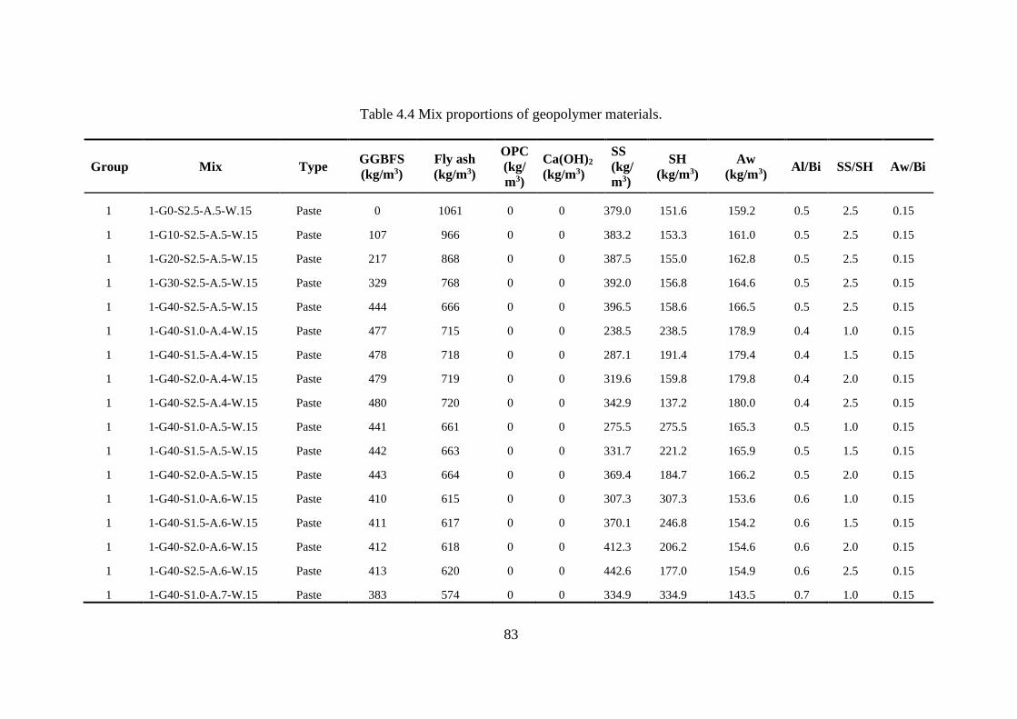
83

Table 4.4 Mix proportions of geopolymer materials.

Group Mix Type GGBFS

(kg/m3)

Fly ash

(kg/m3)

OPC

(kg/

m3)

Ca(OH)2

(kg/m3)

SS

(kg/

m3)

SH

(kg/m3)

Aw

(kg/m3) Al/Bi SS/SH Aw/Bi

1 1-G0-S2.5-A.5-W.15 Paste 0 1061 0 0 379.0 151.6 159.2 0.5 2.5 0.15

1 1-G10-S2.5-A.5-W.15 Paste 107 966 0 0 383.2 153.3 161.0 0.5 2.5 0.15

1 1-G20-S2.5-A.5-W.15 Paste 217 868 0 0 387.5 155.0 162.8 0.5 2.5 0.15

1 1-G30-S2.5-A.5-W.15 Paste 329 768 0 0 392.0 156.8 164.6 0.5 2.5 0.15

1 1-G40-S2.5-A.5-W.15 Paste 444 666 0 0 396.5 158.6 166.5 0.5 2.5 0.15

1 1-G40-S1.0-A.4-W.15 Paste 477 715 0 0 238.5 238.5 178.9 0.4 1.0 0.15

1 1-G40-S1.5-A.4-W.15 Paste 478 718 0 0 287.1 191.4 179.4 0.4 1.5 0.15

1 1-G40-S2.0-A.4-W.15 Paste 479 719 0 0 319.6 159.8 179.8 0.4 2.0 0.15

1 1-G40-S2.5-A.4-W.15 Paste 480 720 0 0 342.9 137.2 180.0 0.4 2.5 0.15

1 1-G40-S1.0-A.5-W.15 Paste 441 661 0 0 275.5 275.5 165.3 0.5 1.0 0.15

1 1-G40-S1.5-A.5-W.15 Paste 442 663 0 0 331.7 221.2 165.9 0.5 1.5 0.15

1 1-G40-S2.0-A.5-W.15 Paste 443 664 0 0 369.4 184.7 166.2 0.5 2.0 0.15

1 1-G40-S1.0-A.6-W.15 Paste 410 615 0 0 307.3 307.3 153.6 0.6 1.0 0.15

1 1-G40-S1.5-A.6-W.15 Paste 411 617 0 0 370.1 246.8 154.2 0.6 1.5 0.15

1 1-G40-S2.0-A.6-W.15 Paste 412 618 0 0 412.3 206.2 154.6 0.6 2.0 0.15

1 1-G40-S2.5-A.6-W.15 Paste 413 620 0 0 442.6 177.0 154.9 0.6 2.5 0.15

1 1-G40-S1.0-A.7-W.15 Paste 383 574 0 0 334.9 334.9 143.5 0.7 1.0 0.15

84


1 1-G40-S1.5-A.7-W.15 Paste 384 576 0 0 403.5 269.0 144.1 0.7 1.5 0.15

1 1-G40-S2.0-A.7-W.15 Paste 385 578 0 0 449.6 224.8 144.5 0.7 2.0 0.15

1 1-G40-S2.5-A.7-W.15 Paste 386 579 0 0 482.7 193.1 144.8 0.7 2.5 0.15

1 1-G40-S2.5-A.4-W.09 Paste 517 776 0 0 369.5 147.8 194.0 0.4 2.5 0.09

1 1-G40-S2.5-A.5-W.09 Paste 476 714 0 0 424.8 169.9 178.4 0.5 2.5 0.09

1 1-G40-S2.5-A.6-W.09 Paste 440 661 0 0 471.8 188.7 165.1 0.6 2.5 0.09

1 1-G40-S2.5-A.7-W.09 Paste 410 615 0 0 512.3 204.9 153.7 0.7 2.5 0.09

1 1-G40-S2.5-A.4-W.15 Paste 498 747 0 0 355.7 142.3 186.7 0.4 2.5 0.12

1 1-G40-S2.5-A.5-W.15 Paste 459 689 0 0 410.1 164.0 172.3 0.5 2.5 0.12

1 1-G40-S2.5-A.6-W.15 Paste 426 639 0 0 456.7 182.7 159.9 0.6 2.5 0.12

1 1-G40-S2.5-A.7-W.15 Paste 397 596 0 0 497.1 198.8 149.1 0.7 2.5 0.12

2 2-S00 Concrete 0 400 0 0 114.3 45.7 0 0.4 2.5 0

2 2-A40/S10/R2.5 Concrete 40 360 0 0 114.3 45.7 0 0.4 2.5 0

2 2-S20 Concrete 80 320 0 0 114.3 45.7 0 0.4 2.5 0

2 2-S30 Concrete 120 280 0 0 114.3 45.7 0 0.4 2.5 0

2 2-A35 Concrete 40 360 0 0 100 40 0 0.35 2.5 0

2 2-A45 Concrete 40 360 0 0 128.5 51.5 0 0.45 2.5 0

2 2-R1.5 Concrete 40 360 0 0 96 64 0 0.4 1.5 0

2 2-R2.0 Concrete 40 360 0 0 106.7 53.3 0 0.4 2 0

3 3-P6 Concrete 0 376 24 0 114.3 45.7 0 0.4 2.5 0

85


3 3-P8 Concrete 0 368 32 0 114.3 45.7 0 0.4 2.5 0

3 3-P10/R2.5 Concrete 0 360 40 0 114.3 45.7 0 0.4 2.5 0

3 3-P12 Concrete 0 352 48 0 114.3 45.7 0 0.4 2.5 0

3 3-R1.5 Concrete 0 360 40 0 96 64 0 0.4 1.5 0

3 3-R2.0 Concrete 0 360 40 0 106.7 53.3 0 0.4 2.0 0

4 4-A40/C2/R2.5 Concrete 0 392 0 8 114.3 45.7 0 0.4 2.5 0

4 4-C3 Concrete 0 388 0 12 114.3 45.7 0 0.4 2.5 0

4 4-A35 Concrete 0 392 0 8 100 40 0 0.35 2.5 0

4 4-R1.5 Concrete 0 392 0 8 96 64 0 0.4 1.5 0

4 4-R2.0 Concrete 0 392 0 8 106.7 53.3 0 0.4 2 0

5 5-8M Mortar 73 657 0 0 208.6 83.4 0 0.4 2.5 0

5 5-10M Mortar 73 657 0 0 208.6 83.4 0 0.4 2.5 0

5 5-12M Mortar 73 657 0 0 208.6 83.4 0 0.4 2.5 0

5 5-14M Mortar 73 657 0 0 208.6 83.4 0 0.4 2.5 0

6 6-8M Mortar 0 657 73 0 208.6 83.4 0 0.4 2.5 0

6 6-10M Mortar 0 657 73 0 208.6 83.4 0 0.4 2.5 0

6 6-12M Mortar 0 657 73 0 208.6 83.4 0 0.4 2.5 0

6 6-14M Mortar 0 657 73 0 208.6 83.4 0 0.4 2.5 0

7 7-R2.5 S3.20 Mortar 0 657 73 0 208.6 83.4 0 0.4 2.5 0

7 7-R2.5 S2.64 Mortar 0 657 73 0 208.6 83.4 0 0.4 2.5 0

86


7 7-R2.5 S2.00 Mortar 0 657 73 0 208.6 83.4 0 0.4 2.5 0

7 7-R2.0 S3.20 Mortar 0 657 73 0 194.7 97.3 0 0.4 2.0 0

7 7-R2.0 S2.64 Mortar 0 657 73 0 194.7 97.3 0 0.4 2.0 0

7 7-R2.0 S2.00 Mortar 0 657 73 0 194.7 97.3 0 0.4 2.0 0

7 7-R1.5 S3.20 Mortar 0 657 73 0 175.2 116.8 0 0.4 1.5 0

7 7-R1.5 S2.64 Mortar 0 657 73 0 175.2 116.8 0 0.4 1.5 0

8 8-S-0w Mortar 73 657 0 0 182.5 73 0 0.35 2.5 0

8 8-S-2w Mortar 73 657 0 0 182.5 73 14.6 0.35 2.5 0.02

8 8-S-4w Mortar 73 657 0 0 182.5 73 29.2 0.35 2.5 0.04

8 8-S-6w Mortar 73 657 0 0 182.5 73 43.8 0.35 2.5 0.06

8 8-P-0w Mortar 0 657 73 0 182.5 73 0 0.35 2.5 0

8 8-P-2w Mortar 0 657 73 0 182.5 73 14.6 0.35 2.5 0.02

8 8-P-4w Mortar 0 657 73 0 182.5 73 29.2 0.35 2.5 0.04

8 8-P-6w Mortar 0 657 73 0 182.5 73 43.8 0.35 2.5 0.06

87

Table 4.5 Values of SiO2/Al2O3, H2O/Na2O, Na2O/SiO2, CaO/SiO2, and experimental and predicted 28-day compressive strength.

Group Mix SiO2/Al2O3 H2O/ Na2O Na2O/SiO2 CaO/ SiO2

28-day compressive

strength (MPa)

Test Predicted

1 1-G0-S2.5-A.5-W.15 4.499 15.03 0.1362 0.0334 12.4 13.6

1 1-G10-S2.5-A.5-W.15 4.521 15.05 0.1419 0.0938 24.6 21.1

1 1-G20-S2.5-A.5-W.15 4.545 15.06 0.1481 0.1597 33.3 36.3

1 1-G30-S2.5-A.5-W.15 4.571 15.08 0.1548 0.2316 43.8 46.6

1 1-G40-S2.5-A.5-W.15 4.601 15.09 0.1623 0.3106 47.9 49.6

1 1-G40-S1.0-A.4-W.15 4.249 14.19 0.1667 0.3363 37.7 43.6

1 1-G40-S1.5-A.4-W.15 4.339 15.03 0.1521 0.3294 42.3 49.0

1 1-G40-S2.0-A.4-W.15 4.398 15.67 0.1426 0.3249 51.3 52.2

1 1-G40-S2.5-A.4-W.15 4.441 16.17 0.1361 0.3218 49.7 54.1

1 1-G40-S1.0-A.5-W.15 4.361 13.25 0.2010 0.3277 34.6 36.0

1 1-G40-S1.5-A.5-W.15 4.473 14.04 0.1824 0.3195 41.4 42.4

1 1-G40-S2.0-A.5-W.15 4.548 14.63 0.1705 0.3143 48.7 46.9

1 1-G40-S1.0-A.6-W.15 4.473 12.62 0.2336 0.3195 26.5 27.0

1 1-G40-S1.5-A.6-W.15 4.607 13.36 0.2110 0.3102 33.1 34.2

1 1-G40-S2.0-A.6-W.15 4.697 13.92 0.1966 0.3043 40.4 39.7

1 1-G40-S2.5-A.6-W.15 4.761 14.36 0.1867 0.3002 37.5 43.3

88


1 1-G40-S1.0-A.7-W.15 4.585 12.16 0.2647 0.3117 17.5 16.1

1 1-G40-S1.5-A.7-W.15 4.742 12.87 0.2380 0.3014 21.7 21.4

1 1-G40-S2.0-A.7-W.15 4.846 13.41 0.2211 0.2949 25.0 27.1

1 1-G40-S2.5-A.7-W.15 4.921 13.83 0.2095 0.2904 23.4 31.4

1 1-G40-S2.5-A.4-W.09 4.441 16.17 0.1361 0.3218 59.4 54.1

1 1-G40-S2.5-A.5-W.09 4.601 15.09 0.1623 0.3106 57.6 49.6

1 1-G40-S2.5-A.6-W.09 4.761 14.36 0.1867 0.3002 48.0 43.3

1 1-G40-S2.5-A.7-W.09 4.921 13.83 0.2095 0.2904 38.9 31.4

1 1-G40-S2.5-A.4-W.15 4.441 16.17 0.1361 0.3218 54.5 54.1

1 1-G40-S2.5-A.5-W.15 4.601 15.09 0.1622 0.3106 51.8 49.6

1 1-G40-S2.5-A.6-W.15 4.761 14.36 0.1867 0.3002 43.6 43.3

1 1-G40-S2.5-A.7-W.15 4.921 13.83 0.2095 0.2904 30.9 31.4

2 2-S00 3.537 11.74 0.1178 0.0326 26.4 30.5

2 2-A40/S10/R2.5 3.609 11.76 0.1213 0.1113 35 37.3

2 2-S20 3.690 11.77 0.1250 0.1949 45.9 44.9

2 2-S30 3.780 11.78 0.1290 0.2840 55.6 52.8

2 2-A35 3.540 11.68 0.1089 0.1134 46 43.9

2 2-A45 3.678 11.81 0.1333 0.1092 31.1 32.2

2 2-R1.5 3.521 10.64 0.1402 0.1141 35.4 34.6

2 2-R2.0 3.573 11.26 0.1290 0.1124 34.2 36.1

89


3 3-P6 3.613 11.73 0.1216 0.1033 34.3 36.7

3 3-P8 3.640 11.72 0.1229 0.1278 37 38.7

3 3-P10/R2.5 3.669 11.71 0.1242 0.1528 39.6 40.9

3 3-P12 3.698 11.71 0.1256 0.1784 36.5 43.7

3 3-R1.5 3.576 10.60 0.1436 0.1568 41.4 37.5

3 3-R2.0 3.630 11.22 0.1321 0.1544 40.3 39.4

4 4-A40/C2/R2.5 3.548 12.13 0.1160 0.0281 28.2 28.0

4 4-C3 3.553 12.14 0.1170 0.0425 32.5 29.1

4 4-A35 3.480 12.06 0.1041 0.0286 33.3 34.8

4 4-R1.5 3.461 10.98 0.1340 0.0288 33.2 29.9

4 4-R2.0 3.512 11.62 0.1234 0.0284 26.1 28.5

5 5-8M 3.964 14.99 0.0958 0.1076 30.3 33.5

5 5-10M 3.964 13.66 0.1032 0.1076 40.9 39.2

5 5-12M 3.964 12.62 0.1099 0.1076 43.7 42.7

5 5-14M 3.964 11.77 0.1161 0.1076 40.7 45.1

6 6-8M 4.023 14.94 0.0975 0.1464 34.8 33.7

6 6-10M 4.023 13.62 0.1051 0.1464 37.2 40.0

6 6-12M 4.023 12.58 0.1119 0.1464 43.2 46.7

6 6-14M 4.023 11.74 0.1181 0.1464 58.4 52.1

7 7-R2.5 S3.20 4.023 13.04 0.1088 0.1464 45.1 43.6

90


7 7-R2.5 S2.64 4.023 11.74 0.1181 0.1464 58.4 52.1

7 7-R2.5 S2.00 4.010 10.07 0.1340 0.1469 60.7 62.0

7 7-R2.0 S3.20 3.984 12.35 0.1167 0.1479 46.9 46.2

7 7-R2.0 S2.64 3.984 11.24 0.1256 0.1479 56.4 52.9

7 7-R2.0 S2.00 3.972 9.79 0.1406 0.1483 57.9 60.8

7 7-R1.5 S3.20 3.930 11.50 0.1282 0.1499 49.7 48.1

7 7-R1.5 S2.64 3.930 10.62 0.1362 0.1499 57.4 53.3

8 8-S-0w 3.893 11.68 0.1042 0.1096 58.7 53.1

8 8-S-2w 3.893 12.77 0.1042 0.1096 45.8 44.6

8 8-S-4w 3.893 13.86 0.1042 0.1096 40.2 36.9

8 8-S-6w 3.893 14.95 0.1042 0.1096 34.2 28.7

8 8-P-0w 3.950 11.65 0.1061 0.1491 57.7 57.8

8 8-P-2w 3.950 12.73 0.1061 0.1491 44.4 47.1

8 8-P-4w 3.950 13.82 0.1061 0.1491 33.7 37.4

8 8-P-6w 3.950 14.90 0.1061 0.1491 29.7 29.3

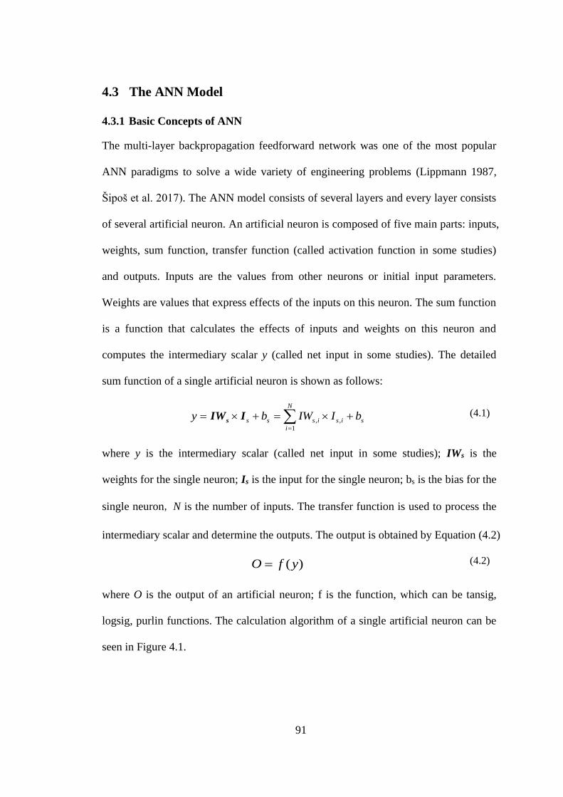
91

4.3 The ANN Model

4.3.1 Basic Concepts of ANN

The multi-layer backpropagation feedforward network was one of the most popular

ANN paradigms to solve a wide variety of engineering problems (Lippmann 1987,

Šipoš et al. 2017). The ANN model consists of several layers and every layer consists

of several artificial neuron. An artificial neuron is composed of five main parts: inputs,

weights, sum function, transfer function (called activation function in some studies)

and outputs. Inputs are the values from other neurons or initial input parameters.

Weights are values that express effects of the inputs on this neuron. The sum function

is a function that calculates the effects of inputs and weights on this neuron and

computes the intermediary scalar y (called net input in some studies). The detailed

sum function of a single artificial neuron is shown as follows:

, ,

1

N

s s s i s i s

i

y b IW I b=

= + = +sIW I

(4.1)

where y is the intermediary scalar (called net input in some studies); IWs is the

weights for the single neuron; Is is the input for the single neuron; bs is the bias for the

single neuron, N is the number of inputs. The transfer function is used to process the

intermediary scalar and determine the outputs. The output is obtained by Equation (4.2)

( )O f y= (4.2)

where O is the output of an artificial neuron; f is the function, which can be tansig,

logsig, purlin functions. The calculation algorithm of a single artificial neuron can be

seen in Figure 4.1.

92

Figure 4.1 Calculation algorithm of a single neuron.

In this study, the ANN model was developed by using NFTOOL built-in box of

MATLAB R2016b (2016) to estimate the 28-day compressive strength of geopolymer

materials. The NFTOOL built-in box established a backpropagation feedforward ANN

model. One is hidden layer and the other one is output layer. The tansig was adopted

as the transfer function between the two layers. The purlin was adopted as the transfer

function between the output layer to the final output results. The mathematical

relationship between outputs and inputs are summarized in the following part. At first,

in the hidden layer, the calculation procedures are shown as follows:

1 2= ... ... T

i NI I I II

(4.3)

= +1 1

y IW I b (4.4)

1,1 1,2 1, 1, y ... y ... yT

j My = 1y

(4.5)

1, , 1,

1

N

j j i i j

i

y IW I b=

= + (4.6)

where I is the input matrix, Ii is the element in I, and the N is the number of the input

parameters; y1 is the intermediary vector in the hidden layer, y1,j is the element in y1,

N

IWs

Input Single Neuron

b

+ f

Is

N 11 N

1 1

O

y

, ,

1

N

s s s i s i s

i

y b IW I b=

= + = +sIW I

( )O f y=

1 1

1 1

93

and the M is the number of the hidden neurons in the hidden layer; IW is the weight

matrix of the hidden layer, and IWj,i is the element of IW; b1 is the bias vector of the

hidden layer, and b1,j is the element in b1. Then, from the hidden layer to the output

layer, y1 is transformed by using tansig transfer function, which is shown as follows:

2,1 2,2 2, 2,= ... ... T

j My y y y 2y

(4.7)

1,2, 1, 2

2tan ( ) 1

1 jj j y

y sig ye−

= = −+

(4.8)

where y2 is the intermediary vector between the hidden layer and the output layer; y2,j

is the element in y2. In the output layer, the intermediary vector y3 is calculated as

follows:

= +3 2 2

y LW y b

(4.9)

3,1 3,2 3, 3, y ... y ... yT

k Sy = 3y

(4.10)

3, 2, 2,

1

M

k j j j

j

y LW y b=

= + (4.11)

where y3 is the intermediary vector in the output layer, y3,k is the element in y3, and S

is the number of output parameters; b2 is the bias vector in the output layer, and b2,j is

the element in b2. Finally, the output vector is calculated as follows:

( )purlin= =3 3

O y y (4.12)

1 2 ... ... T

k SO O O O=O (4.13)

3, 3,( )S S SO purlin y y= = (4.14)

where O is the output of the ANN, O1 is the element of O. The architecture of the

ANN model built by NFTOOL box in Matlab (2016b) is shown in Figure 4.2, and its

calculation algorithm is shown in Figure 4.3.

94

Figure 4.2 Architecture of the ANN model built by NFTOOL box in Matlab

(2016b).

Figure 4.3 Caculation algorithm of the backpropagation feedforward ANN model

built by NFTOOL box in Matlab(2016b).

The Levenberg-Marquardt backpropagation (LMBP) method was adopted as the

learning algorithm in this study. This method is recognized as one of the fastest

backpropagation algorithms and is widely accepted by many studies (Nazari and Riahi

2013, Pham and Hadi 2014, Šipoš et al. 2017). The detailed mathematical theory of

LMBP algorithms for ANN can be found in the Hagan and Menhaj (1994) and

Demuth et al. (2014).

1

2

N

Input Parameters Hidden Layer Output Layer

1

2

M

1

2

S

Feedforward

LM Backpropagation

N

IW

Input Hidden Layer Output Layer

b1

+

LW

b2

+

I

N 1M N

M 1

M 1

y3

Oy2

y1M 1

S 1

S 1

S 1S M

tan ( )sig=2 1

y y

= +3 2 2

y LW y b

( )purlin=3

O y

= +1 1

y IW I b

95

4.3.2 The Architecture of the ANN Model

The experimental database used in this study consists of 71 input-target sets of

experimental data and they were randomly divided into training sets (80%), validation

sets (10%), and test sets (10%). Prior to ANN model optimization, the input and target

parameters are better to be scaled between 0 and 1. This is because the ANN models

are very sensitive to the absolute magnitudes of input and output parameters (Oreta

and Kawashima 2003). All input and target data were scaled by using the following

equation:

min( )

max( ) min( )

Y YSV

Y Y

−=

− (4.15)

where SV is scaled value, Y is the actual value, max(Y) is the maximum value of actual

data, min(Y) is the minimum value of actual data.

In this study, four input parameters (corresponding to four molar ratios of SiO2/Al2O3,

H2O/Na2O, Na2O/SiO2, CaO/SiO2) and one output parameter (corresponding to 28-

day compressive strength) were used. The next step is to determine the number of

hidden layer neurons. The random selection of the number of hidden neurons may

arise either overfitting or underfitting of the ANN models (Sheela and Deepa 2013).

Hence, determining the appropriate number of hidden neurons to prevent overfitting

and underfitting is significant for an ANN model to predict with steady generalisation

(Šipoš et al. 2017). In this study, the optimal number of hidden neurons was obtained

by trial and error approach. Finally, the number of hidden neurons was determined as

ten.

In conclusion, the parameters of ANN model were: one input layer with four neurons;

one hidden layer with ten neurons; one output layer with one neuron; the leaning

96

method is LMBP; transfer function between the hidden layer and the output layer is

tansig. The architecture of the ANN model is illustrated in Figure 4.4. The values of

weights and bias are shown in Table 4.6 and Table 4.7, respectively.

Figure 4.4 Architecture of the proposed ANN mode

1

2

3

4

1

2

3

4

5

6

7

8

1

Input Parameters

H2O/ Na2O

Na2O/SiO2

CaO/ SiO2

SiO2/Al2O3

Hidden Layer

Output layer

9

10

N=4

M=10

S=1

97

Table 4.6 Weights of the ANN model.

Input Nodes Hidden Nodes

1 2 3 4 5 6 7 8 9 10

SiO2/Al2O3 (1) -0.7783 -1.1708 1.8575 1.2684 1.0937 -1.2055 0.6206 -1.6147 1.2592 -0.3438

H2O/ Na2O (2) 0.2451 1.5836 -0.9446 0.5000 -0.1940 -1.4972 0.5577 0.4106 -1.2479 -2.4273

Na2O/SiO2 (3) 2.5315 1.2822 0.5019 -0.8809 -2.0835 0.3318 -1.7213 -1.2331 -1.0625 -0.4366

CaO/ SiO2 (4) 0.2217 0.6870 -0.9703 -1.8169 -0.5182 -1.7847 1.1820 -1.9512 1.3043 -0.5028

Output Nodes Hidden Nodes

1 2 3 4 5 6 7 8 9 10

1 -0.9424 -0.1943 -0.8261 -0.3636 0.4309 0.4390 0.3540 -0.6691 0.1372 0.3095

98

Table 4.7 Bias of the ANN model.

Hidden Nodes

1 2 3 4 5 6 7 8 9 10

2.4803 1.9813 -1.6399 -0.9322 -0.0850 -0.2873 -0.1280 -1.0454 2.0257 -2.3676

Output Node

1

-0.0431

99

4.3.3 Performance of ANN Model

The experimental and the predicted 28-day compressive strength data are shown in

Table 4.5, and the comparison between the predicted and the experimental results are

depicted in Figure 4.5. A close agreement is seen between the proposed ANN model

and the experimental results. Furthermore, in this study, three most common statistical

parameters were used to evaluate the performance of the ANN model and its ability to

make accurate predictions. These parameters are coefficient of correlation (R), root

mean squared error (RMSE) and mean absolute percentage error (MAPE). The

detailed equations and values of them are shown in Table 4.8. For this model, the

values of R, RMSE, and MAPE are 0.95, 3.4, and 7.1%, respectively.

Figure 4.5 Performance of the proposed ANN model.

The value of R is in the range of (0, 1). Higher values of R imply that the predicted

data fit well with the experimental data (Šipoš et al. 2017). According to the

explanation for R > 0.8 proposed by Smith (Smith 1986), in this study the value of R

of 0.95 represents strong correlation between predicted compressive strength and

experimental compressive strength.

Experimental Compressive Strength (MPa)

Pre

dic

ted

Co

mp

ress

ive

Str

ength

(M

Pa)

R=0.95

100

Table 4.8 The values and expression of statistical parameters.

Statistical parameter Equation Values

Coefficient of correlation (R)

( ) ( )( )

( ) ( )

1

2 2

1 1

.

.

n

i ii

n n

i ii i

t t o oR

t t o o

=

= =

− −=

− −

0.95

Root mean squared error

(RMSE) ( )2

1

1 n

i iiRMSE t o

n == − 3.4

Mean absolute percentage error

(MAPE) 1

1 n i i

ii

t oMAPE

n t=

−= 0.071

it presents the experimental data (target values) of compressive strength; io presents the

predicted data (output values) of compressive strength; n is the number of tests; t is the

mean experimental data (target values); o is the mean predicted data (output values).

RMSE and MAPE are another effective parameters to indicate the high predictability

(Šipoš et al. 2017). Some studies predicted the compressive strength of geopolymer

materials and ordinary Portland cement materials by using some soft-computing

methods (such as ANN, ANFIS, and GP) (Nazari and Torgal 2013, Nazari et al. 2014,

Sarıdemir et al. 2009, Šipoš et al. 2017, Słoński 2010, Topcu and Sarıdemir 2008) and

indicated good modelling results. It can be concluded from these studies that the

values of RMSE and MAPE were in the range of (1.04, 4.26) and (2.21%, 12.40%),

respectively. In this study, the values of RMSE (3.4) and MAPE (7.1%) located within

these ranges, which means this ANN model indicates high predictability.

4.3.4 Relative Importance and Relative Ranking

To quantify the input parameter contribution, relative importance and relative ranking

were carried out by using Garson’s algorithm (Garson 1991). This approach has been

used in many studies (Mozumder and Laskar 2015, Oreta and Kawashima 2003,

Siddique et al. 2011), which have proven that this method can effectively estimate the

relative importance and relative ranking of input parameters in ANNs. In this study,

101

the values of weights used in Garson’s algorithm are shown in Table 4.6 and Table 4.7.

The detailed Garson’s algorithm procedures can be found in Garson (1991), Goh

(1995), Olden and Jackson (2002).

The values of relative importance for SiO2/Al2O3, H2O/Na2O, Na2O/SiO2, CaO/SiO2

molar ratios are 25.17%, 22.19%, 28.55% and 24.09%, respectively (shown in Table

4.9). It can be seen that Na2O/SiO2 has the highest relative importance and

contribution. The H2O/Na2O molar ratio has the lowest relative importance and

contribution. However, the contributions of these four molar ratios are very close. It

can be considered that these four molar ratios have significant effects on the 28-day

compressive strength of geopolymer materials.

Table 4.9 Relative importance and relative ranking.

Input

parameters

SiO2/Al2O3

(1)

H2O/ Na2O

(2)

Na2O/SiO2

(3)

CaO/ SiO2

(4)

Relative

importance 25.17% 22.19% 28.55% 24.09%

Relative

ranking 2 4 1 3

4.4 Parametric Analysis Based on the Established ANN Model

Parametric analyses have been carried out to investigate the effects of SiO2/Al2O3,

H2O/Na2O, Na2O/SiO2, CaO/SiO2 molar ratios on the compressive strength of

geopolymer materials by using the established ANN model. The influences of

parameters on the compressive strength of geopolymer materials are complex and

interdependent. In this study, the mutual influences between every two molar ratios

are presented from Figures 4.6-4.11 are discussed.

The influences between SiO2/Al2O3 and H2O/Na2O on the compressive strength are

shown in Figure 4.6. It can be seen from Figure 4.6(a), when the SiO2/Al2O3 ratio is

between 3.5 and a certain value (around 4.5), increasing the SiO2/Al2O3 ratio leads to

102

the increase of compressive strength. But when the SiO2/Al2O3 ratio is larger than a

certain value (around 4.5), increasing the SiO2/Al2O3 ratio leads to the decrease of

compressive strength. From Figure 4.6(b), when the SiO2/Al2O3 ratio is equal to 3.5, 4

and 4.5, with the increase of H2O/Na2O ratio, the compressive strength falls. Also,

when the SiO2/Al2O3 ratio increases from 3.5 to 4.5, the rate of decrease of the

compressive strength with the increase of H2O/Na2O drops. But when the SiO2/Al2O3

ratio is 5, increasing H2O/Na2O ratio leads to a slight increase of compressive strength.

(a) Effect of SiO2/Al2O3 on compressive strength with different levels of

H2O/Na2O.

Figure 4.6 Compressive strength vs SiO2/Al2O3 and H2O/Na2O molar ratios.

(Continued)

H2O/Na2O = 10

H2O/Na2O = 12

H2O/Na2O = 14

H2O/Na2O = 16

SiO2/Al2O3

Com

pre

ssiv

e st

rength

(M

Pa)

103

(b) Effect of H2O/Na2O on compressive strength with different levels of

SiO2/Al2O3

Figure 4.6 Compressive strength vs SiO2/Al2O3 and H2O/Na2O molar ratios.

The influences of SiO2/Al2O3 and Na2O/ SiO2 molar ratios on compressive strength

are depicted in Figure 4.7. It was found from Figure 4.7(a) that when the Na2O/ SiO2

ratio is equal to 0.1 and 0.15, with the increase of SiO2/Al2O3 ratio from 3.5 to a

certain value (around 4.7), the compressive strength increases. But when the Na2O/

SiO2 ratio is larger than this certain value (around 4.7), the increase of SiO2/Al2O3

ratio leads to the decrease of compressive strength. However, when the Na2O/ SiO2

ratio is between 0.2 and 0.25, increasing SiO2/Al2O3 ratio leads to a slight decrease of

compressive strength. From Figure 4.7(b), increasing the Na2O/ SiO2 ratio leads to the

decrease of compressive strength. It can also be found that when the SiO2/Al2O3 ratio

increases from 3.5 to 5, with the increase of Na2O/ SiO2 ratio, the decreasing rate of

compressive strength increases.

SiO2/Al2O3 = 3.5

SiO2/Al2O3 = 4

SiO2/Al2O3 = 4.5

SiO2/Al2O3 = 5

H2O/Na2O

Com

pre

ssiv

e st

rength

(M

Pa)

104

(a) Effect of SiO2/Al2O3 on compressive strength with different levels of Na2O/

SiO2.

(b) Effect of Na2O/ SiO2 on compressive strength with different levels of

SiO2/Al2O3.

Figure 4.7 Compressive strength vs SiO2/Al2O3 and Na2O/ SiO2 molar ratios.

The influences of SiO2/Al2O3 and CaO/SiO2 molar ratios on the compressive strength

are depicted in Figure 4.8. It can be seen from Figure 4.8(a) that when the CaO/SiO2

Na2O/SiO2 = 0.1

Na2O/SiO2 = 0.15

Na2O/SiO2 = 0.2

Na2O/SiO2 = 0.25

SiO2/Al2O3

Com

pre

ssiv

e st

rength

(M

Pa)

SiO2/Al2O3 = 3.5

SiO2/Al2O3 = 4

SiO2/Al2O3 = 4.5

SiO2/Al2O3 = 5

Na2O/SiO2

Com

pre

ssiv

e st

rength

(M

Pa)

105

ratio is equal to 0.15, 0.25 and 0.35, with the increase of SiO2/Al2O3 ratio, the

compressive strength increases first and then decreases. However, when the CaO/SiO2

ratio is equal to 0.05, the compressive strength decreases first and then increases.

From Figure 4.8(b), when the SiO2/Al2O3 ratio is equal to 3.5, 4.5 and 5, increasing

the CaO/SiO2 ratio leads to the increase of compressive strength. However, when the

the SiO2/Al2O3 ratio is equal to 4, the compressive increases sharply first and then

decreases slightly.

(a) Effect of SiO2/Al2O3 on compressive strength with different levels of

CaO/SiO2.

Figure 4.8 Compressive strength vs SiO2/Al2O3 and CaO/SiO2 molar ratios.

(Continued)

CaO/ SiO2 = 0.05

CaO/ SiO2 = 0.15

CaO/ SiO2 = 0.25

CaO/ SiO2 = 0.35

SiO2/Al2O3

Com

pre

ssiv

e st

rength

(M

Pa)

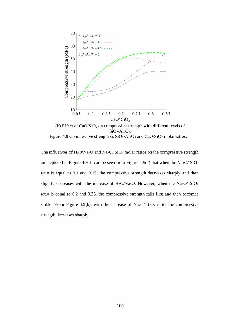
106

(b) Effect of CaO/SiO2 on compressive strength with different levels of

SiO2/Al2O3.

Figure 4.8 Compressive strength vs SiO2/Al2O3 and CaO/SiO2 molar ratios.

The influences of H2O/Na2O and Na2O/ SiO2 molar ratios on the compressive strength

are depicted in Figure 4.9. It can be seen from Figure 4.9(a) that when the Na2O/ SiO2

ratio is equal to 0.1 and 0.15, the compressive strength decreases sharply and then

slightly decreases with the increase of H2O/Na2O. However, when the Na2O/ SiO2

ratio is equal to 0.2 and 0.25, the compressive strength falls first and then becomes

stable. From Figure 4.9(b), with the increase of Na2O/ SiO2 ratio, the compressive

strength decreases sharply.

SiO2/Al2O3 = 3.5

SiO2/Al2O3 = 4

SiO2/Al2O3 = 4.5

SiO2/Al2O3 = 5

CaO/ SiO2

Com

pre

ssiv

e st

rength

(M

Pa)

107

(a) Effect of H2O/Na2O on compressive strength with different levels of Na2O/

SiO2.

(b) Effect of Na2O/ SiO2 on compressive strength with different levels of

H2O/Na2O.

Figure 4.9 Compressive strength vs H2O/Na2O and Na2O/ SiO2 molar ratios.

The effect of H2O/Na2O and CaO/SiO2 molar ratios on the compressive strength are

shown in Figure 4.10. It can be found from Figure 4.10(a) that when the CaO/SiO2

Na2O/SiO2 = 0.1

Na2O/SiO2 = 0.15

Na2O/SiO2 = 0.2

Na2O/SiO2 = 0.25

H2O/Na2O

Com

pre

ssiv

e st

rength

(M

Pa)

H2O/Na2O = 10

H2O/Na2O = 12

H2O/Na2O = 14

H2O/Na2O = 16

Na2O/SiO2

Com

pre

ssiv

e st

rength

(M

Pa)

108

molar ratio is equal to 0.05, 0.15 and 0.25, increasing the H2O/Na2O ratio leads to a

sharp decrease of compressive strength with the increase of H2O/Na2O ratio. When

the CaO/SiO2 molar ratio is equal to 0.35, the compressive strength falls sharply first

and then falls slightly with the increase of H2O/Na2O ratio. From Figure 4.10(b), when

the H2O/Na2O ratio is equal to 10 and 12, the compressive strength increases sharply

first and then decreases. When the H2O/Na2O ratio is equal to 14 and 16, the

compressive strength increases first and then keeps constant.

(a) Effect of H2O/Na2O on compressive strength with different levels of

CaO/SiO2.

Figure 4.10 Compressive strength vs H2O/Na2O and CaO/SiO2 molar ratios.

(Continued)

CaO/ SiO2 = 0.03

CaO/ SiO2 = 0.13

CaO/ SiO2 = 0.23

CaO/ SiO2 = 0.35

H2O/Na2O

Com

pre

ssiv

e st

rength

(M

Pa)

109

(b) Effect of CaO/SiO2 on compressive strength with different levels of

H2O/Na2O.

Figure 4.10 Compressive strength vs H2O/Na2O and CaO/SiO2 molar ratios.

The influences of Na2O/ SiO2 and CaO/SiO2 molar ratios on the compressive strength

are shown in Figure 4.11. It can be seen from Figure 4.11(a) that when the CaO/SiO2

ratio is between 0.05 and 0.15, the compressive strength falls sharply first and

increases slightly with increase of Na2O/ SiO2 ratio. When the CaO/SiO2 ratio is equal

to 0.25 and 0.35, the compressive strength decreases with the increase of Na2O/ SiO2

ratio. From Figure 4.11(b), with the increase of CaO/SiO2 ratio, the compressive

strength increases sharply first and then decreases slightly.

H2O/Na2O = 10

H2O/Na2O = 12

H2O/Na2O = 14

H2O/Na2O = 16

CaO/ SiO2

Com

pre

ssiv

e st

rength

(M

Pa)

110

(a) Effect of Na2O/ SiO2 on compressive strength with different levels of

CaO/SiO2.

(b) Effect of CaO/SiO2 on compressive strength with different levels of Na2O/

SiO2.

Figure 4.11 Compressive strength vs Na2O/ SiO2 and CaO/SiO2 molar ratios.

4.5 Summary

In this chapter, a backpropagation artificial neural network (ANN) was established to

predict the 28-day compressive strength of geopolymer materials cured at ambient

CaO/ SiO2 = 0.03

CaO/ SiO2 = 0.13

CaO/ SiO2 = 0.23

CaO/ SiO2 = 0.35

Na2O/SiO2

Com

pre

ssiv

e st

rength

(M

Pa)

Na2O/SiO2 = 0.1

Na2O/SiO2 = 0.15

Na2O/SiO2 = 0.2

Na2O/SiO2 = 0.25

CaO/ SiO2

Com

pre

ssiv

e st

rength

(M

Pa)

111

condition. The input parameters are SiO2/Al2O3, H2O/Na2O, Na2O/SiO2, CaO/SiO2

molar ratios. The conclusions of this Chapter are summarised as follows:

1. The results predicted by the ANN model were in good agreement with the

experimental data. The values of coefficient of correlation (R), root mean squared

error (RMSE) and mean absolute percentage error (MAPE) are 0.95, 3.4, and 7.1%,

respectively.

2. The values of relative importance of SiO2/Al2O3, H2O/Na2O, Na2O/SiO2, CaO/SiO2

molar ratios are 25.17%, 22.19%, 28.55% and 24.09%, respectively. The highest

contribution is achieved by Na2O/SiO2 ratio. However, their contributions are very

close.

3. The mutual influences of every two ratios among SiO2/Al2O3, H2O/Na2O,

Na2O/SiO2, CaO/SiO2 on compressive strength are analysed. It was found that the

effects of these ratios on the compressive strength are complex and interdependent.

This Chapter presents a more complex theoretical model for the experimental results

of geopolymer paste shown in Chapter 3. The ANN model built in this Chapter can be

easily used by engineers and researchers to predict the compressive strength. Just

input the values of four parameters into the models, and the compressive strength can

be calculated directly. Chapter 5 will present the experimental study of pervious

geopolymer concrete (PGC) based on the mix design and experimental results of

geopolymer paste.

112

CHAPTER 5

Mix Design of Pervious Geopolymer Concrete

5.1 Introduction

Pervious concrete is made by the same materials as conventional concrete, with

exceptions that most or all of the fine aggregate typically is eliminated (Tennis et al.

2004). In the last few decades, the application of pervious concrete as a pavement

material in low-volume road and a pile material in soft saturated soil area has gained

more attention (Chandrappa and Biligiri 2016, Suleiman et al. 2014). This is because

pervious concrete is a special concrete with relatively high porosity and high water

permeability compared to the conventional concrete (Zaetang et al. 2016). These

characteristics can reduce the stormwater runoff on the road surface and increase the

time rate of consolidation of pile foundation.

In this chapter, the details of pervious geopolymer concrete (PGC) tests are presented.

The mix design of PGC is based on the optimum mix design of geopolymer pastes

presented in Chapter 3. Some studies proved that high strength paste would lead to

high strength pervious concrete (Chindaprasirt et al. 2009, Zhong and Wille 2015,

Zhong and Wille 2016). In this chapter, the optimum mix of geopolymer paste (G4-

S20-A5-W2) proposed in Chapter 3 was used for making geopolymer paste in the

PGC, which cannot only achieve high strength, but also meet the requirement of

setting times in the Australian Standard (AS 2350.4-2006) and achieve higher

workability than OPC paste. The fine aggregate is not used to make PGC specimens.

The coarse aggregate size is from 5 mm to 12 mm. The coarse aggregate to binder

mass ratio (Ca/Bi ratio) was used as the main parameter to control the properties of

113

PGC, as many studies found this parameter has significant effects on the properties of

pervious concrete (Arafa et al. 2017, Tho-in et al. 2012).

The 7-day and 28-day compressive strength was measured according to the Australian

Standard. In addition, the porosity and permeability are important parameters of

pervious concrete, due to pervious concrete is designed to be used as a drainage layer

in pavement. Also, the porosity and permeability are much larger than those of normal

concrete, and have significant effects on the mechanical properties. Hence, these two

parameter were measured and the detailed procedures of measurement were presented.

Finally, the relationships between Ca/Bi ratio and compressive strength, porosity,

permeability are proposed.

5.2 Experimental Programme for PGC piles

5.2.1 Materials

In this chapter, no fine aggregate was used to make PGC. Here, the PGC is the

mixture of coarse aggregates and geopolymer paste. The aluminosilicate sources and

alkaline activator used for making the PGC specimens are the same as those of

geopolymer paste presented in Chapter 3. The coarse aggregate size used in this study

was from 5 mm to 12 mm.

5.2.2 Mix Proportions

Previous research has proven that high strength paste would lead to high strength

pervious concrete (Chindaprasirt et al. 2009, Zhong and Wille 2015, Zhong and Wille

2016). Hence, the optimum mix of geopolymer paste (G4-S20-A5-W2) proposed in

Chapter 3 was used to make pervious geopolymer concrete.

Another important factor is aggregate to binder mass ratio (Ca/Bi ratio), which has

been proven to have a significant role in controlling the compressive strength, porosity

114

and permeability of pervious concrete (Arafa et al. 2017, Tho-in et al. 2012). In this

study, four mixtures with different values of aggregate to binder mass ratio were

designed to investigate the properties of geopolymer pervious concrete. The coarse

aggregates to binder mass ratios (Ca/Bi ratio) were 5:1, 6:1, 7:1 and 8:1. The mix

proportions are calculated by absolute volume method (Pavithra et al. 2016) and

detailed procedures are shown as follows.

Ca

g f

MCa Bi

M M=

+ (5.1)

where MCa, Mg and Mf are the masses of coarse aggregates, GGBFS and fly ash,

respectively.

Firstly, the values of ground granulated blast furnace slag (GGBFS) content, alkaline

solution to binder (Al/Bi) mass ratio, sodium silicate solution to sodium hydroxide

solution (SS/SH) mass ratio, and additional water to binder (Aw/Bi) mass ratio are

fixed. Here, the optimum mix design of geopolymer pastes presented in Chapter 3 is

adopted for pervious geopolymer concrete. Therefore, the GGBFS content (Cg), Al/Bi

mass ratio, SS/SH mass ratio and Aw/Bi mass ratio of geopolymer concretes are the

same as those of optimum mix design of geopolymer pastes, which are 40%, 0.5, 2.0

and 0.15, respectively. Their expressions are shown as follows:

100%g

g

g f

MC

M M=

+ (5.2)

SS SH

f g

M MAl Bi

M M

+=

+ (5.3)

SS

SH

MSS SH

M= (5.4)

115

Aw

f g

MAw Bi

M M=

+ (5.5)

where Mg, Mf, MSS, MSH, MAw are the masses of GGBFS, fly ash, sodium silicate

solution, sodium hydroxide solution, additional water.

Secondly, the mass of coarse aggregate is determined. Based on the absolute volume

method, the total volume of PGC (Vtp) is assumed to be 1 cubic meter. The total

volume of PGC (Vtp) is the sum of volume of fly ash (Vf), volume of GGBFS (Vg),

sodium silicate solution (VSS), sodium hydroxide solution (VSH), additional water (VAw),

void (Vv) and coarse aggregate (VCa), which is shown as follows:

tp f g SS SH Aw v CaV V V V V V V V= + + + + + + (5.6)

where, Vv is assumed to be 0.15 cubic meter for PGC. The expressions of these

volume can be calculated by the following equations:

The next step is to calculate the Vf , Vg , VSS, VSH, VAw, VCa. The expressions of these

volumes can be calculated as follows:

f

f

f

MV

G= (5.7)

1

g

f

gg

g

g g

CM

CMV

G G

− = =

(5.8)

SSSS

SS

MV

G= (5.9)

SHSH

SH

MV

G= (5.10)

AwAw

Aw

MV

G= (5.11)

116

CaCa

Ca

MV

G= (5.12)

where, Cg is the GGBFS content, Mf, Mg, MSH, MSS, MAw, MCa are mass of fly ash,

GGBFS, sodium hydroxide solution, sodium silicate solution, additional water and

coarse aggregates, respectively. The Gf, Gg, GSH, GSH, GAw and GCa are the specific

gravities of fly ash, GGBFS, sodium hydroxide solution, sodium silicate solution,

additional water and coarse aggregates, respectively. In this study, Gf is 2.2, Gg is 2.85,

GSH is 1.39, GSS is 1.52, GAw is 1.0, GCa is 2.71.

Combining Equations (5.1) – (5.10), the masses of components of PGC in 1 cubic

metre can be calculated. Each mix was given a name which starts with “Ca” followed

by a number. The letter “Ca” means aggregate and the number means the values of

Ca/Bi ratio. For example, 5 means the value of Ca/Bi is 5. The detailed mix

proportions of PGC are shown in Table 5.1.

Table 5.1 Mix design for PGC controlled by aggregate/binder mass ratio

Mix

No.

Aggregates

(kg/m3)

Slag

(kg/

m3)

Fly Ash

(kg/m3)

Slag

Content

(%)

Al/

Bi

SS/

SH

Additional

Water/

Binder

Ca5 1558 122 183 40 0.5 2 0.15

Ca6 1643 108 162 40 0.5 2 0.15

Ca7 1717 96 144 40 0.5 2 0.15

Ca8 1772 87 131 40 0.5 2 0.15

5.2.3 Mixing, Casting and Curing

All tests were conducted under an ambient temperature of 23 ± 2 °C. The sodium

hydroxide solution and sodium silicate solution were mixed together for about 1 hour

before mixing with aluminosilicate source. Fly ash, GGBFS and coarse aggregates

were dry mixed in a lightburn 65 litre mixer for 2 minutes. Afterwards, alkaline

activator was added and mixed for 1 min and additional water was poured into the

117

mixer for another 2 min until the mix became well mixed and homogeneous.

After mixing, the fresh concrete was cast layer by layer into the moulds, and the depth

of each layer was approximately 50 mm. Each layer was vibrated for 10 s on a

vibration table. The plastic moulds of 100 mm in diameter and 200 mm in height were

used for casting the PGC specimens (shown in Figure 5.1) to determine the

compressive strength. Six samples (shown in Figure 5.2) were cast for each mix, three

of them for 7-day compressive strength and three for 28-day compressive strength.

The samples were kept in the laboratory at an ambient condition (23 ± 2°C) for 24

hours then demoulded. Afterwards, these specimens were cured at an ambient

condition for 7 days or 28 days.

Figure 5.1 Casting the PGC samples in plastic moulds.

118

Figure 5.2 Samples of PGC (100mm x 200mm)

5.2.4 Testing Method

Compressive Strength Tests

The compressive strengths of geopolymer pastes were determined at the age of 7 days

and 28 days in accordance with AS 1012.9 (2014). The specimens were capped with

high-strength plaster at the top and bottom ends to ensure that the axial compression

load was evenly applied to the specimen. The average of three cylinders tested under

compression was taken as the nominal compressive strength. This test was done by

using the Avery compression machine of 1800 kN loading capacity in the High Bay

laboratory at University of Wollongong, Australia.

Porosity Tests

The porosity of PGC was defined as the ratio of void volume to total volume of

concrete. In this study, the porosity of PGC was tested using 100 mm × 200 mm

cylindrical specimens. The porosity tests were carried out at the age of 7 days before

the permeability tests. At first, the dry weight of sample was measured. Then the

Ca5

Ca6

Ca7

Ca8

119

specimens were placed into a water tank filled with sufficient water to cover the whole

specimens for 2 h. After that, the weight of the specimens under the water was

measured. The porosity Equation (5.13) proposed by Park and Tia (2004) was used:

2 11 100

p p

w

W WV

Vol

− = −

(5.13)

where V is the porosity, 1pW is the weight of specimen under water,

2pW is the dry

weight of samples, w is the density of water, and the Vol is the volume of samples.

The nominal values of porosity were the average of three specimens of each mix.

Permeability Tests

After the porosity tests, the 100 mm × 200 mm cylindrical specimens used in porosity

tests were then placed in the constant head water permeability apparatus, which is

similar to the apparatus made by Sri Ravindrarajah and Aoki (2008). The schematic

diagram of constant head water permeability apparatus is shown in Figure 5.3. To

avoid the water go through the tiny gap between the specimens and tube, the PGC

specimens were wrapped with cling wrap to adjust the diameter of the tube. Hence,

the specimens can be placed tightly into the tube. The permeability coefficient was

calculated using Darcy’s law as given below:

QLk

HAt= (5.14)

where A is the cross-sectional area of specimen, Q is quantity of water collected over t

seconds, L is the length of specimen, WH is the water head, k is the permeability of

concrete samples.

120

Water level

100

Pervious concrete

specimen

20

0

42

0

Wat

er h

ead

(H

)

Quantity of Water (Q)

at time (t)

Figure 5.3 Constant head water permeability apparatus (units: mm).

5.2.5 Results and Discussion

Compressive Strength of PGC

The effects of aggregate to binder mass ratio on 7-day and 28-day compressive

strength of PGC are shown in Figure 5.4. It can be seen that the compressive strength

was significantly influenced by Ca/Bi ratio. With the increase of Ca/Bi ratio, the

compressive strength decrease. This trend is similar to those of other studies (Crouch

et al. 2007, Tho-in et al. 2012, Torres et al. 2015, Zhong and Wille 2015). The reason

of this trend is that increasing the Ca/Bi ratio resulted in the reduction of paste

thickness around the coarse aggregate, and the bonding strength would decrease

(Crouch et al. 2007, Torres et al. 2015).

121

In addition, it was found that there is a linear correlation between Ca/Bi ratio and

compressive strength. The relationship equation is shown as follows

( ),7 3.7 / 35.1pgcf Ca Bi = − +

(5.15)

( ),28 3.7 / 40.4pgcf Ca Bi = − +

(5.16)

where the ,7pgcf and ,28pgcf are 7-day compressive strength and 28-day compressive

strength of PGC, respectively. The R is the coefficient of correlation. The value of R

for predicting ,7pgcf and ,28pgcf using Equation (5.15) and Equation (5.16) are

0.9960 and 0.9985, respectively.

Figure 5.4 Effects of Aggregate to Binder Mass Ratio (Ca/Bi) on Compressive

Strength of PGC

Porosity of PGC

The effects of the Ca/Bi ratio on the porosity of PGC are presented in Figure 5.5. It

was found that increasing the Ca/Bi ratio led to the increase of porosity. This is

because when the Ca/Bi ratio increased, less voids in PGC was filled by the

geopolymer paste. This trend is consistent with other studies (Crouch et al. 2007, Tho-

0

5

10

15

20

25

5 6 7 8

Co

mp

ress

ive S

tren

gth

(M

Pa)

Aggregate to Binder Mass Ratio (Ca/Bi)

7-day Compressive Strength

28-day Compressive Strength

( ),7 3.7 / 35.1

0.9960

pgcf A Bi

R

= − +

=

( ),28 3.7 / 40.4

0.9985

pgcf A Bi

R

= − +

=

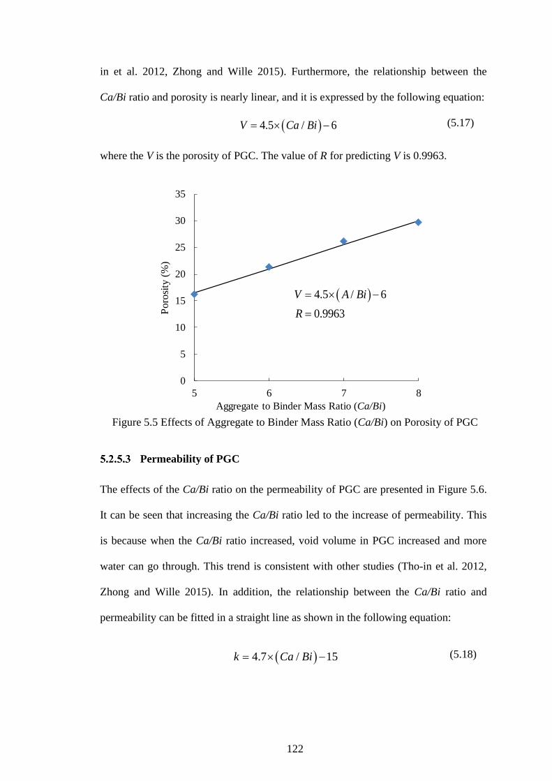
122

in et al. 2012, Zhong and Wille 2015). Furthermore, the relationship between the

Ca/Bi ratio and porosity is nearly linear, and it is expressed by the following equation:

( )4.5 / 6V Ca Bi= −

(5.17)

where the V is the porosity of PGC. The value of R for predicting V is 0.9963.

Figure 5.5 Effects of Aggregate to Binder Mass Ratio (Ca/Bi) on Porosity of PGC

Permeability of PGC

The effects of the Ca/Bi ratio on the permeability of PGC are presented in Figure 5.6.

It can be seen that increasing the Ca/Bi ratio led to the increase of permeability. This

is because when the Ca/Bi ratio increased, void volume in PGC increased and more

water can go through. This trend is consistent with other studies (Tho-in et al. 2012,

Zhong and Wille 2015). In addition, the relationship between the Ca/Bi ratio and

permeability can be fitted in a straight line as shown in the following equation:

( )4.7 / 15k Ca Bi= −

(5.18)

0

5

10

15

20

25

30

35

5 6 7 8

Poro

sity

(%

)


( )4.5 / 6

0.9963

V A Bi

R

= −

=

123

Figure 5.6 Effects of Aggregate to Binder Mass Ratio (Ca/Bi) on Permeability of

PGC.

5.3 Summary

In this Chapter, the detailed procedures and results of pervious geopolymer concrete

(PGC) tests are presented. The coarse aggregate to binder mass ratio (Ca/Bi ratio) was

used as the main parameter to design the mixes of PGC. The Ca/Bi ratios of 5, 6, 7

and 8 was selected. The results can be summarized as follows:

The coarse aggregate to binder mass ratio (Ca/Bi ratio) has a significant effect on the

properties of PGC. With increase of Ca/Bi ratio, it was found that the 7-day

compressive strength and 28-day compressive strength reduce but porosity and

permeability increase. The PGC specimens with Ca/Bi ratio of 5 reached the highest

28-day compressive strength (21.9 MPa).

It was found that relationships between Ca/Bi ratio and compressive strength, porosity

and permeability of PGC are almost linear. The linear equations can accurately predict

the properties of PGC.

This chapter leads to Chapter 6, which presents an experimental program of new

0

5

10

15

20

25

5 6 7 8

Perm

eabilit

y (

mm

/s)


( )4.7 / 15

0.9927

k A Bi

R

= −

=

124

forms of PGC piles. The mix design of PGC in Chapter 6 was based on the mix design

of PGC shown in this chapter.

125

CHAPTER 6

Geosynthetics-confined Pervious Geopolymer Concrete Piles

with FRP-PVC-confined Concrete Core: Experiments

6.1 Introduction

The use of fibre reinforced polymer (FRP) and polyvinyl chloride (PVC) as

strengthening materials have been increasingly significant in civil engineering

application, due to their high strength-to-weight ratio, high durability and high anti-

corrosion ability. Hence, for piles, which are constructed in a marine environment,

confinement by FRP and PVC is superior to steel materials.

This chapter presents an experimental investigation of geosynthetics-confined

pervious geopolymer concrete piles. Four new forms of composite piles were

proposed, including: 1. geogrid-confined pervious geopolymer concrete piles

(GPGCPs) without FRP-PVC-confined concrete core (FPCC); 2. geogrid-geotextile-

confined pervious geopolymer concrete piles (GGPGCP) without FPCC; 3. geogrid-

confined pervious geopolymer concrete piles (GPGCPs) with FPCC; 4. geogrid-

geotextile-confined pervious geopolymer concrete piles (GGPGCP) with FPCC. For

FPCC, the normal geopolymer concrete (NGC) was used to fill the FRP-PVC tubes.

The GPGCP with FPCC consists of a circular geogrid outer tube, a FPCC, and

pervious geopolymer concrete (PGC) filled in between. The GGPGCP with FPCC

consists of a circular geogrid-geotextile outer tube, a FPCC, and pervious geopolymer

concrete (PGC) filled in between. In each form of geosynthetics-confined pervious

geopolymer concrete piles, one layer, two layers, and three layers of geogrid were

used to investigate the influence of the outer tube.

126

6.2 Experimental Programme

6.2.1 Preliminary Tests

The preliminary tests examined the properties of four pairs of samples, including one

pair of plain PGCs, one pair of plain NGCs, one pair of FRP-PVC tubes, and one pair

of FPCCs. The aim of plain NGC and PGC tests is to obtain the axial stress-axial

strain curves and the ductility of the reference samples. The diameter of NGC samples

and PGC samples was 150 mm and their height was 300 mm. The aim of FRP-PVC

tube and FPCC tests is to obtain their contribution to the vertical load carrying

capacity of GPGCPs. The inner diameter and outer diameter of PVC tubes were 76

mm and 84 mm, respectively. The height of PVC tubes was 325 mm. The inner

diameter and outer diameter of FRP-PVC tubes were 76 mm and 86 mm, respectively.

The height of FRP-PVC tubes was 325 mm. The FPCC samples were made by filling

NGC into FRP-PVC tubes. One strain gauge was used for each FPCC sample to

obtain the hoop strain during the axial compression test. This strain gauge was

attached transversely onto the mid-height of the outside surface. The details of FPCC

are shown in Figure 6.1.

The four pairs of samples are named as follows: (a) P denotes plain PGC; (b) N

denotes plain NGC; (c) FP denotes FRP-PVC tubes; (d) FPCC denotes the FRP-PVC-

confined NGC; (e) the last numbers 1 or 2 are used to distinguish between the two

nominally identical specimens. The details of preliminary tests are summarised in

Table 6.1.

127

86

76

NGC

PVC-FRP tube

32

5

SG

SG

Figure 6.1 Details of FPCC samples (units: mm; SG: strain gauge).

Table 6.1 Details of the preliminary test samples.

Label Specimen Type

Outer

Diamete

r (mm)

Inner

Diameter

(mm)

P-1 Plain PGC

150 -

P-2 150 -

N-1 Plain NGC

150 -

N-2 150 -

FP-1 FRP-PVC tubes

86 76

FP-2 86 76

FPCC-1 FRP-PVC-confined

concrete (FPCC)

86 -

FPCC-2 86 -

PGC: Pervious Geopolymer Concrete.

NGC: Normal Geopolymer Concrete.

128

6.2.2 Main Test Matrix

A total of 12 GPGCP specimens and 12 GGPGCP specimens were cast and tested

under axial compression. All specimens were 160 mm in diameter and 325 mm in

height. These specimens were divided into two groups. The six specimens of GPGCPs

without FPCC and six specimens of GGPGCPs without FPCC were referred to as the

first group (shown in Figure 6.2). The six specimens of GPGCPs with FPCC and six

specimens of GGPGCPs with FPCC were referred to as the second group (shown in

Figure 6.3). To ensure more representative results, two nominally identical specimens

for each specimen configuration were tested.

Figure 6.2 GPGCPs without FPCC and GGPGCPs without FPCC.

129

Figure 6.3 GPGCPs with FPCC and GGPGCPs with FPCC.

The labelling of each specimen is named as follows: (a) GP denotes GPGCPs without

FPCC, and the number afterwards denotes the number of geogrid layers (one, two and

three layers); (b) GGP denotes GGPGCPs without FPCC, and the number afterwards

denotes the number of geogrid layers (one, two and three layers); (c) GPC denotes

GPGCPs with FPCC, and the number that follows denotes the number of geogrid

layers (one, two and three layers); (d) GGPC denotes GGPGCPs with FPCC, and the

number that follows denotes the number of geogrid layers (one, two and three layers);

(e) the last number 1 or 2 is used to distinguish between the two nominally identical

specimens. For example, Specimen GG2-2 represents the second of the two identical

GPGCPs without FPCC that were confined with two layers of geogrid. The details of

the GPGCPs specimens and GGPGCPs specimens are summarized in Table 6.2. The

detailed section configurations are shown in Figure 6.4.

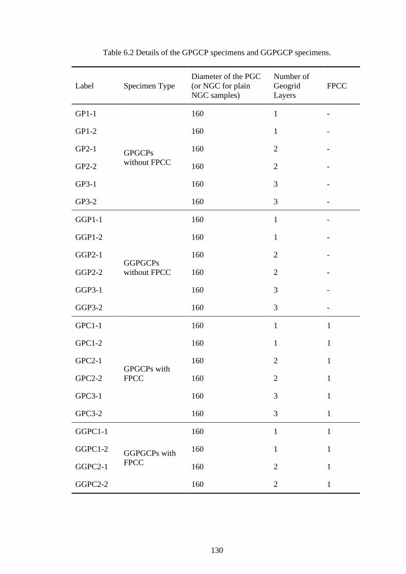
130

Table 6.2 Details of the GPGCP specimens and GGPGCP specimens.

Label Specimen Type

Diameter of the PGC

(or NGC for plain

NGC samples)

Number of

Geogrid

Layers

FPCC

GP1-1

GPGCPs

without FPCC

160 1 -

GP1-2 160 1 -

GP2-1 160 2 -

GP2-2 160 2 -

GP3-1 160 3 -

GP3-2 160 3 -

GGP1-1 160 1 -

GGP1-2 160 1 -

GGP2-1 GGPGCPs

without FPCC

160 2 -

GGP2-2 160 2 -

GGP3-1 160 3 -

GGP3-2 160 3 -

GPC1-1 160 1 1

GPC1-2 160 1 1

GPC2-1 GPGCPs with

FPCC

160 2 1

GPC2-2 160 2 1

GPC3-1 160 3 1

GPC3-2 160 3 1

GGPC1-1

GGPGCPs with

FPCC

160 1 1

GGPC1-2 160 1 1

GGPC2-1 160 2 1

GGPC2-2 160 2 1

131


GGPC3-1

160 3 1

GGPC3-2 160 3 1

GPGCP: Geogrid-confined Pervious Geopolymer Concrete Pile.

GGPGCP: Geogrid-geotextile-confined Pervious Geopolymer Concrete Pile.

FPCC: FRP-PVC-confined Concrete.

Geogrid tube

PGC

160

PGC

NGCGeogrid tube

FRP-PVC tube

160

76

86

325

325

6

10

SG

SG

SG

SG

SG

SG SG

Geogrid transverse rib

25

35

Geogrid longitudinal rib

SG

25

(a) (b)

Figure 6.4 Details of GPGCP specimens and GGPGCP specimens (units: mm; SG:

strain gauge): (a) GP1, GP2, GP3, GGP1, GGP2, GGP3; (b) GPC1, GPC2, GPC3.

GGPC1, GGPC2, GGPC3.

132

6.2.3 Preparation of Specimens

Geopolymer Concrete

The mix proportions for PGC and normal geopolymer concrete (NGC) are shown in

Table 6.3. All mixes were conducted under ambient conditions (23 ± 2 °C). In this

study, ground granulated blast furnace slag (GGBFS) and Class F fly ash (FA) were

used as an aluminosilicate source. The GGBFS was supplied by the Australasian Slag

Association, Australia (2018), and the Class F FA was provided by the Eraring Power

Station, Australia (2018). The FA was classified as Class F according to AS 3582.1

(2016). The alkaline activator was made by blending sodium hydroxide solution with

sodium silicate solution. The concentration of sodium hydroxide solution was kept

constant (14 M) for all mixtures. Sodium silicate solution was purchased from a local

commercial supplier. The mass ratio of SiO2 to Na2O of the sodium silicate was 2.02

with a chemical composition of 29.6% SiO2 and 14.7% Na2O. The sodium hydroxide

solution and sodium silicate solution were mixed together for 1 hour before being

mixed with the aluminosilicate materials. The size of the coarse aggregates ranged

from 5 mm to 12 mm.

Table 6.3 Mix proportions of PGC and NGC.

Mix

Coarse

Aggregates

(kg/m3)

Sand

(kg/m3)

Slag

(kg/m3)

Fly

Ash

(kg/m3)

Sodium

Hydroxide

Solution

(kg/m3)

Sodium

Silicate

Solution

(kg/m3)

Additional

Water

(kg/m3)

PGC 1558 - 122.0 183.0 50.8 101.7 45.8

NGC 1039 675 160.0 240.0 66.7 133.3 60.0

The mixing procedures for the normal and PGC samples were the same. The

geopolymer concrete was prepared by mixing the dry materials with the alkaline

activator in a Lightburn 65 litre mixer. The dry materials were dry mixed for 2 min,

133

then the alkaline activator was added to the mix and mixed for 1 min. Then, the

additional water was poured into the mixer and mixed for another 2 min. After mixing,

the fresh geopolymer concrete was cast layer by layer into the moulds, and the depth

of every layer was approximately 50 mm. Each layer was vibrated for 10 s on a

vibration table. The specimens were left in the laboratory at an ambient condition for

24 hours, then covered by hessian clothes to prevent losing moisture from the concrete.

Geogrid Tubes

To provide lateral confinement to the concrete specimens, the geogrid was formed

into tubular shapes, and the ends were held with plastic ties. To ensure that the

geogrid tube would not be loosened or slid under lateral expanding load, the geogrid

tube was overlapped at an approximate length of 80 mm. To maintain the same

dimensions of all concrete cores, the inner diameter of the geogrid tubes was kept at

160 mm (not including the thickness of the geogrid tube). The height of geogrid tubes

was 325 mm.

Geogrid-Geotextile Tubes

For GGPGCPs, to provide more lateral confinement and reduce the effects of geogrid

openings, geotextile tubes were put into the geogrid tubes to form geogrid-geotextile

tubes. The ends of the geotextile tubes were stitched together. To ensure the geotextile

tubes would not be loosened or slid under lateral expanding load, the end of geotextile

tubes was overlapped at a length of 100 mm. To maintain the same dimensions of all

concrete cores, the inner diameter of the geogrid tubes was kept at 160 mm (not

including the thickness of the geogrid tube). The height of geogrid tubes was 325 mm.

FRP-PVC Tubes

The PVC tubes were wrapped by GFRP to form FRP-PVC tubes using the wet layup

134

method. The inner diameter and outer diameter of PVC tubes were 76 mm and 84 mm,

respectively. The height of PVC tubes was 325 mm. At first, the GFRP sheets were

impregnated with a mixture of epoxy resin and hardener at a ratio of 3:1. After that,

the impregnated GFRP sheets were wrapped on the PVC tubes in five layers with an

overlapping length of 150 mm. The FRP-PVC tubes were then cured in the laboratory

for 1 day. These FRP-PVC tubes were used as the mould for casting the NGC. The

outer diameter and height of FRP-PVC tubes were 86 mm and 325 mm, respectively.

The inner diameter was same as that of PVC tubes (76 mm). The detailed section

configuration of FPCC is shown in Figure 6.1.

6.2.4 Material Properties

Geopolymer Concrete

The compressive strength of the plain pervious and normal geopolymer concrete was

determined according to AS 1012.9 (2014). Three NGC cylinders and three PGC

cylinders with 100 mm diameter and 200 mm height were tested to determine the 28-

day compressive strength. Because the pervious geopolymer concrete (PGC) was

produced in two batches, the compressive strengths of the PGC were different.

However, the difference was minimal. The average 28-day compressive strength of

PGC for GPGCPs without FPCC and GGPGCPs without FPCC was 22.1 MPa; that of

GPGCPs with FPCC and GGPGCPs with FPCC was 21.7 MPa. The average 28-day

compressive strength of NGC for GPGCPs with FPCC and GGPGCPs with FPCC

was 49.2 MPa. The permeability of PGC were obtained by using the method proposed

by Aoki et al. (2012), and its average value was 9.1 mm/s.

Geogrid

The uniaxial geogrid (shown in Figure 6.5(a)) were used as the outer confinement

135

material. The inner dimensions of its square openings are 25 mm × 25 mm, which was

measured by a standard ruler with an accuracy of 0.5 mm. The geogrid was

manufactured from glass fibre with a bitumen coating. The uniaxial geogrid can resist

corrosion and has a large tensile rupture strain. The widths of the transverse ribs and

the longitudinal ribs were measured by a digital vernier calliper, which are 10 mm and

6 mm, respectively. The thicknesses of the transverse rib and the longitudinal ribs

were measured by a digital vernier calliper, which are 1.5 mm and 1.0 mm,

respectively.

The mechanical properties of the uniaxial geogrid were determined by using the

ASTM D6637-M15 (2015). The length of each test transverse rib between the testing

machine clamps was 150 mm, which was measured by a standard ruler with an

accuracy of 0.5 mm. Five single transverse geogrid ribs were prepared and tested by

using the 100 kN Instron testing machine at the High Bay Laboratory, University of

Wollongong, Australia. The tensile testing rate was 5 mm/min. The tensile load-axial

strain curves of the geogrid are depicted in Figure 6.5(b). The average tensile ultimate

load of geogrid ribs was 2.8 kN and the average ultimate tensile strain was 9.2%.

136

(a)

(b)

Figure 6.5 Geogrid used in this study: (a) Uniaxial geogrid; (b) Tensile load-axial

strain curves of the geogrid coupons.

Geotextile

The white unwoven geotextile (shown in Figure 6.6) was chosen as the reinforcement

0

0.5

1

1.5

2

2.5

3

3.5

0 0.02 0.04 0.06 0.08 0.1

Tensi

le L

oad (

kN

)

Axial Strain

Coupon 1

Coupon 2

Coupon 3

Coupon 4

Coupon 5

137

material in this chapter. Tensile tests of geotextile (shown in Figure 6.7) were

conducted in accordance with AS 3706.2-2012. Each specimen was 200 mm wide and

five specimens were tested. The alumina jaws were used to clamp the geotextile and

the distance between the jaws was 100 mm. The displacement controlled tests were

carried out at a rate of 20 mm/min. The tensile load-axial strain curves of geotextile

are depicted into Figure 6.8. The properties of geotextile are summarized into Table

6.4.

Table 6.4 Material properties of geotextile

Type

Nominal

thickness,

ttextile

(mm/ply)

Tensile

strength,

ftextile (kN/m)

Tensile

stiffness, Etextile

(kN/m)

Tensile Strain at

peak strength,

ɛtextile,u (%)

Geotextile 6 59.81 282.12 0.212

Figure 6.6 White unwoven geotextile.

138

Figure 6.7 Geotextile tensile test.

Figure 6.8 Tensile load-axial strain curves of geotextile.

Fibre Reinforced Polymer

In this study, glass fibre reinforced polymer (GFRP) was chosen as the reinforcement

material. The GFRP sheets were formed from bidirectional glass fibre and had a

nominal thickness of 0.15 mm. The GFRP sheets were first impregnated with a

mixture of epoxy resin and hardener at a ratio of 3:1. Then, these sheets were cured in

0

2

4

6

8

10

12

14

16

18

0 0.1 0.2 0.3

Ten

sile

lo

ad

(k

N)

Axial Strain

Coupon 1

Coupon 2

Coupon 3

Coupon 4

Coupon 5

139

the laboratory for 1 day. Flat coupon tests were conducted according to ASTM

D7565(2010). The width of the test coupon was 25 mm and the length measured

between the testing machine clamps was 200 mm. The longitudinal strain was

measured by using three strain gauges on the two sides of the test coupon (shown in

Figure 6.9). The aforementioned 100 kN Instron testing machine was used to test the

coupons at a loading rate of 2 mm/min. Five coupons were tested. The test results

showed that the average tensile strength, elastic modulus and ultimate tensile strain

were 621.5 MPa, 33.4 GPa and 1.86%, respectively, as shown in Table 6.5.

Table 6.5 Average material properties of GFRP sheets.

Type Thickness

(mm/ply)

Tensile

Strength

(MPa)

Fracture

Stress

(MPa)

Elastic

Modulus

(GPa)

Ultimate

Tensile

Strain (%)

GFRP 0.15 621.5 - 33.4 1.86

Figure 6.9 Tensile test of the GFRP coupons.

140

PVC

The commercial PVC pipes were used in this study, with an outside diameter of 84

mm and a thickness of 4 mm. The tensile tests of PVC coupons were conducted based

on ASTM D638 (2014). Five dog-bone coupons (Figure 6.10 (a)) were cut from the

PVC tube. The width of the narrow section of the dog-bone coupon was 13 mm and

the length between the testing machine clamps was 115 mm.

(a) (b)

Figure 6.10 PVC coupons used in this study: (a) Dog-bone PVC coupon; (b)

Tensile load-axial strain curves of the PVC coupons.

Table 6.6 Average material properties of PVC dog-bone specimens.

Type Thickness

(mm/ply)

Tensile

Strength

(MPa)

Fracture

Stress

(MPa)

Elastic

Modulus

(GPa)

Ultimate

Tensile

Strain (%)

PVC

specimen 4 51.2 42.7 1.58 55.4

The tensile tests were carried out using the aforementioned 100 kN Instron testing

machine at a loading rate of 5 mm/min. Figure 6.10 (b) represents the tensile load-

0

0.5

1

1.5

2

2.5

3

3.5

0 0.2 0.4 0.6

Ten

sile

Lo

ad

(k

N)

Axial Strain

Coupon 1

Coupon 2

Coupon 3

Coupon 4

Coupon 5

141

axial strain behaviour of the PVC coupon tests. The average tensile strength, fracture

stress, elastic modulus and ultimate tensile strain were 51.2 MPa, 42.7 MPa, 1.58 GPa

and 55.4%, respectively, as shown in Table 6.6.

6.2.5 Instrumentation and Test Procedure

All of the preliminary test samples and GPGCP specimens were tested by using the

Denison 5000 kN testing machine in the High Bay Laboratory at the University of

Wollongong, Australia. The GPGCP specimens were capped with high-strength

plaster at the top and bottom ends to ensure that the axial compression load was

evenly applied onto the specimens. The axial deformation were measured using two

Linear Variable Differential Transformers (LVDTs), which were fixed at two

diagonally opposite corners between the loading and supporting steel plates. All the

specimens were axially loaded up to 50 mm displacement at a rate of 1 mm/min.

For each FRP-PVC confined concrete (FPCC) specimen, a strain gauge was attached

transversely onto the mid-height of the outside surface (shown in Figure 6.1). The

purpose of this gauge was to obtain the hoop strain during the tests.

For each GPGCP without FPCC specimen, three strain gauges were used to monitor

the hoop strain. All these strain gauges were attached transversely onto the outside

surface of the transverse ribs of the geogrid tubes. One strain gauge was attached at

the mid-height transverse rib of the geogrid tubes, and two other strain gauges were

attached at the second top and second bottom transverse ribs of the geogrid tubes.

Figure 6.4(a) clearly shows the locations of these strain gauges.

For each GPGCP with FPCC specimen, four strain gauges were used to monitor the

hoop strain. Three of them were attached transversely onto the outside surface of

transverse ribs of geogrid tubes (shown in Figure 6.4(b)). Their positions are the same

142

as those of GPGCPs without FPCC specimens described above. Another strain gauge

was attached at the mid-height of the outside surface of the FRP-PVC-confined

concrete, shown in Figure 6.1.

In general, the ultimate axial strains of confined concrete columns are no more than 5%

(Csuka and Kollár 2010, Jiang and Teng 2007, Teng et al. 2009) because after

reaching this value of axial strain, the axial stress of columns decreases significantly,

and the small remaining axial stress is not considered. Another reason is that such a

large deformation is not allowed for structural members in practice, due to the

requirement of serviceability. However, for granular piles encased by geosynthetics in

the laboratory or on site, the axial strain can reach as high as 15% (Raithel et al. 2004).

Therefore, in this study, to investigate if the GPGCPs and GGPGCPs can allow for

such high deformation, the ultimate axial deformation was set to 50 mm,

corresponding to an axial strain of 15.4%.

6.3 Test Results and Analysis

6.3.1 Preliminary Tests

The preliminary test results are summarised in Table 6.7. The axial load-axial strain

relationships of two plain PGC specimens and two plain NGC specimens are shown in

Figure 6.11. All plain PGC specimens and NGC specimens failed due to the crushing

and spalling of concrete at the mid-height of the specimens.

To estimate the contribution of FRP-PVC tubes to the axial load carrying capacity,

two specimens were axially loaded. Figure 6.12 shows that the two FRP-PVC tubes

failed due to local elephant-foot buckling and rupture of the GFRP. The axial stress-

axial strain relationships are illustrated in Figure 6.13. The compression tests were

stopped when the axial deformation reached 50 mm (the axial strain was 15.4%). The

143

axial behaviour of the FRP-PVC tubes consisted of three branches. In the first branch,

the axial stress increased rapidly to the peak stress. In the second branch, the FRP

jacket ruptured, and the axial stress decreased sharply to a low level. After that, in the

third branch, the axial stress was kept stable at a very low level.

Table 6.7 Results of the preliminary tests.

Specimen

Label

Maximum

Load (kN)

Maximum

Axial stress

(MPa)

Axial Strain

at Maximum

Load

Hoop Strain

at FRP

Rupture

P-1 373 21.1 0.0021 -

P-2 388 22.0 0.0019 -

N-1 871 49.3 0.0023 -

N-2 836 47.3 0.0021 -

FP-1 45.1 - 0.0232 -

FP-2 44.9 - 0.0215 -

FPCC-1 457 78.2 0.0264 0.0180

FPCC-2 437 75.2 0.0255 0.0183

Figure 6.11 Axial load-axial strain curves of PGC and NGC.

0

20

40

60

0 0.002 0.004 0.006 0.008 0.01

Axia

l S

tress

(M

Pa)

Axial strain

P-1

P-2

N-1

N-2

144

Figure 6.12 Failure mode of the FRP-PVC hollow tube.

Figure 6.13 Axial load-axial strain curves of FRP-PVC hollow tube.

Two FRP-PVC-confined concrete specimens were tested to determine their

compressive behaviour, and their dimensions and section configurations are shown in

0

10

20

30

40

50

0 0.04 0.08 0.12 0.16

Axia

l L

oad (

kN

)

Axial strain

FP-1

FP-2

145

Figure 6.1. After testing, the final state of the FRP-PVC-confined concrete is shown in

Figure 6.14. The FRP jacket separated from the specimens, and the PVC tubes

expanded and were distorted significantly. The axial stress-axial strain behaviour,

shown in Figure 6.15, is similar to that observed in a previous study conducted by

Fakharifar and Chen (2016). The axial stress-axial strain curve consists of a parabolic

first branch, a linear second branch and a descending third branch. The peak stress

was reached at the end of the second branch when the GFRP ruptured. Then, the axial

stress decreased rapidly and gradually stabilized. The compression tests were

continued until the specimens reached an axial deformation of 50 mm (axial strain of

0.154). Figure 6.16 represents the axial strain versus hoop strain curves of two FPCCs

from the beginning of the tests to the rupture of the GFPR jackets.

Figure 6.14 Failure mode of the FRP-PVC-confined concrete.

146

Figure 6.15 Axial stress-axial strain curves of the FPCCs.

Figure 6.16 Axial-hoop strain responses of the FPCCs.

6.3.2 Final States of GPGCPs and GGPGCPs

The typical final states of the representative composite pile specimens after the tests is

illustrated in Figure 6.17, Figure 6.18, Figure 6.19 and Figure 6.20. In this Chapter,

only two specimens failed due to the failure of the geogrid: GP1-1 and GP1-2, which

0

20

40

60

80

0 0.04 0.08 0.12 0.16

Axia

l S

tress

(M

Pa)

Axial Strain

FPCC1

FPCC2

-0.02

-0.016

-0.012

-0.008

-0.004

0

0 0.01 0.02 0.03

Ho

op

Str

ain

Axial Strain

FPCC-1

FPCC-2

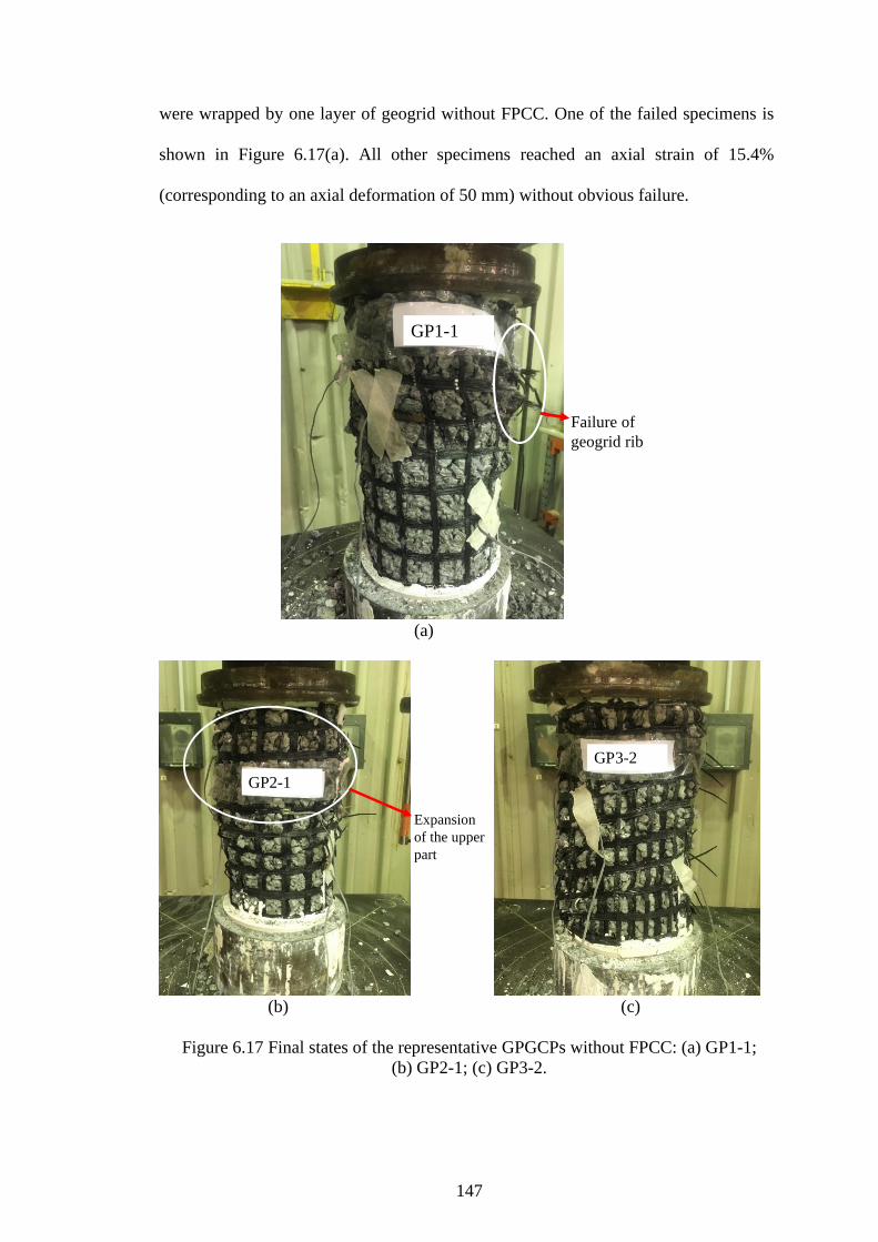
147

were wrapped by one layer of geogrid without FPCC. One of the failed specimens is

shown in Figure 6.17(a). All other specimens reached an axial strain of 15.4%

(corresponding to an axial deformation of 50 mm) without obvious failure.

(a)

(b) (c)

Figure 6.17 Final states of the representative GPGCPs without FPCC: (a) GP1-1;

(b) GP2-1; (c) GP3-2.

Failure of

geogrid rib

GP1-1

Expansion

of the upper

part

GP2-1

GP3-2

148

During the tests, for all GPGCPs without and with FPCC, only a small number of

course aggregates were squeezed out through the opening of the geogrid. Although the

expansion of specimens was large, the geogrid tubes held most of the coarse

aggregates in the pervious geopolymer concrete. Further examination of the final

states of the GPGCPs without FPCC specimens indicated that the upper half of GP2

specimens expanded more due to the non-uniform dilation of the PGC, as shown in

Figure 6.17(b). However, the GP3 specimens expanded uniformly, and no prominent

local bulging was observed, as shown in Figure 6.17(c).

For all GGPGCPs without and with FPCC, the geogrid-geotextile tubes can hold all

coarse aggregates in the pervious geopolymer concrete. Further examination of the

final states of the GGPGCPs without FPCC specimens indicated that the upper half of

GGP1 specimens expanded more due to the non-uniform dilation of the PGC, as

shown in Figure 6.18(a). However, the other GGPGCPs without FPCC specimens

expanded uniformly, and no prominent local bulging was observed, as shown in

Figure 6.18(b)(c).

149

(a)

(b) (c)

Figure 6.18 Final states of the representative GGPGCPs without FPCC: (a) GGP1-

1; (b) GGP2-2; (c) GGP3-1.

For the final states of the GPGCPs with FPCC, the GPC1 specimens expanded at the

mid-height of the specimen, as shown in Figure 6.19(a). The specimens of GPC2 and

GPC3 expanded uniformly over the entire height (shown in Figure 6.19(b)(c)).

Expansion

of the upper

part

GGP1-1

GGP2-2GGP3-1

150

(a)

(b) (c)

Figure 6.19 Final state of the representative GPGCPs with FPCC: (a) GPC1-2; (b)

GPC2-2; (c) GPC3-1.

For the final states of the GGPGCPs with FPCC, the GGPC1 specimens expanded at

the mid-height of the specimen, as shown in Figure 6.20(a). The specimens of GGPC2

and GGPC3 expanded uniformly over the entire height (shown in Figure 6.20(b)(c)).

Expansion at

the mid-height

GPC1-2

GPC2-2

GPC3-1

151

(a) (b)

(c)

Figure 6.20 Final states of the representative GGPGCPs with FPCC: (a) GGPC1-

2; (b) GGPC2-2; (c) GGPC3-2.

6.3.3 Mechanical Behaviour of GPGCPs without FPCC and GGPGCPs without

FPCC

Axial Stress-Axial Strain Behaviour

The key testing results of GPGCPs without FPCC and GGPGCPs without FPCC

are summarized in Table 6.8 and

Table 6.9, respectively. The detailed axial stress-axial strain behaviour of GPGCPs

without FPCC and GGPGCPs without FPCC is depicted in Figure 6.21 and Figure

GGPC1-2

GGPC2-2

GGPC3-2

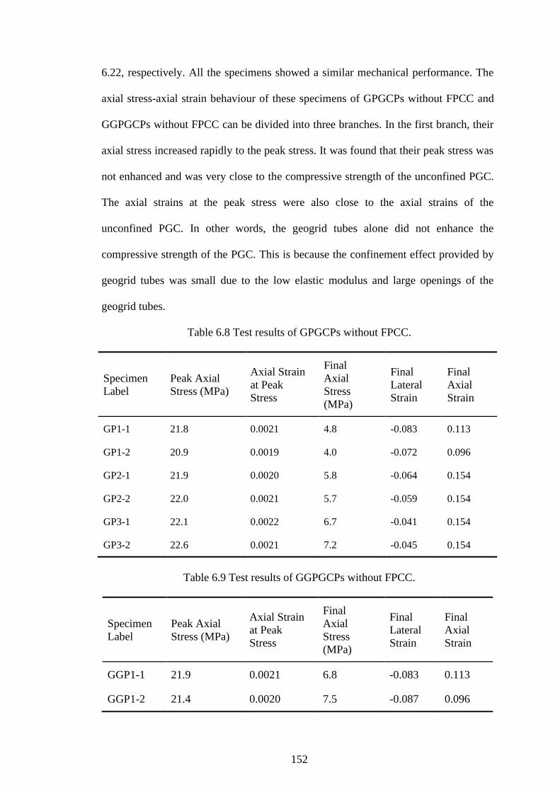
152

6.22, respectively. All the specimens showed a similar mechanical performance. The

axial stress-axial strain behaviour of these specimens of GPGCPs without FPCC and

GGPGCPs without FPCC can be divided into three branches. In the first branch, their

axial stress increased rapidly to the peak stress. It was found that their peak stress was

not enhanced and was very close to the compressive strength of the unconfined PGC.

The axial strains at the peak stress were also close to the axial strains of the

unconfined PGC. In other words, the geogrid tubes alone did not enhance the

compressive strength of the PGC. This is because the confinement effect provided by

geogrid tubes was small due to the low elastic modulus and large openings of the

geogrid tubes.

Table 6.8 Test results of GPGCPs without FPCC.

Specimen

Label

Peak Axial

Stress (MPa)

Axial Strain

at Peak

Stress

Final

Axial

Stress

(MPa)

Final

Lateral

Strain

Final

Axial

Strain

GP1-1 21.8 0.0021 4.8 -0.083 0.113

GP1-2 20.9 0.0019 4.0 -0.072 0.096

GP2-1 21.9 0.0020 5.8 -0.064 0.154

GP2-2 22.0 0.0021 5.7 -0.059 0.154

GP3-1 22.1 0.0022 6.7 -0.041 0.154

GP3-2 22.6 0.0021 7.2 -0.045 0.154

Table 6.9 Test results of GGPGCPs without FPCC.

Specimen

Label

Peak Axial

Stress (MPa)

Axial Strain

at Peak

Stress

Final

Axial

Stress

(MPa)

Final

Lateral

Strain

Final

Axial

Strain

GGP1-1 21.9 0.0021 6.8 -0.083 0.113

GGP1-2 21.4 0.0020 7.5 -0.087 0.096

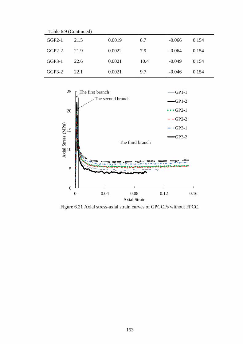
153


GGP2-1 21.5 0.0019 8.7 -0.066 0.154

GGP2-2 21.9 0.0022 7.9 -0.064 0.154

GGP3-1 22.6 0.0021 10.4 -0.049 0.154

GGP3-2 22.1 0.0021 9.7 -0.046 0.154

Figure 6.21 Axial stress-axial strain curves of GPGCPs without FPCC.

0

5

10

15

20

25

0 0.04 0.08 0.12 0.16

Axia

l Str

ess

(M

Pa)

Axial Strain

GP1-1

GP1-2

GP2-1

GP2-2

GP3-1

GP3-2

The first branch

The second branch

The third branch

154

Figure 6.22 Axial stress-axial strain curves of GGPGCPs without FPCC.

In the second branch, after the peak stress, the axial stress decreased sharply. Even

though the lateral expansion of the concrete became larger at this stage, the

confinement effect provided by the geogrid was not significant because the tensile

elastic modulus of the geogrid was relatively low and the openings were large. During

the test, although the coarse aggregates did not spall from the openings of geogrid,

these aggregates were somewhat ejected.

In the third branch, after the pronounced reduction in the axial stress, the GPGCPs

without FPCC lost approximately 70% to 80% of the load carrying capacity, and the

GGPGCPs without FPCC lost approximately 55% to 70%. However, after an axial

strain of 0.04, the axial stress stabilized without any significant change because with

increasing the axial strain, the hoop strain became more pronounced, and the

confining pressure provided by the geogrid became much higher. When the confining

pressure achieved a certain level, the axial stress of the confined concrete was held

steady even though the axial strain was large. However, Specimens GP1-1 and GP1-2,

0

5

10

15

20

25

0 0.04 0.08 0.12 0.16

Ax

ial

Str

ess

(M

Pa)

Axial strain

GGP1-1

GGP1-2

GGP2-1

GGP2-2

GGP3-1

GGP3-2

The first branchThe second branch

The third branch

155

which had only one layer of geogrid, failed before reaching an axial strain of 15.4%.

The different layers of the geogrid had a significant influence on the mechanical

behaviour in the third stage only. With additional layers of geogrid, the stable axial

stress level increased. It is estimated that the stable axial stress increased by

approximately 1.2 MPa for each additional layer of geogrid.

Axial-Hoop Strain Behaviour

Figure 6.23 and Figure 6.24 show the axial-hoop strain curves of GPGCPs without

FPCC and GGPGCPs without FPCC, respectively. The axial strains were obtained

from the measurement of the linear variable differential transformer (LVDT), while

the hoop strains were averaged from three strain gauges attached at the geogrid ribs.

When the axial strain was smaller than 0.01, the differences of the three pairs of

specimens were very close.

Figure 6.23 Hoop strain-axial strain curves of GPGCPs without FPCC.

-0.1

-0.08

-0.06

-0.04

-0.02

0

0 0.04 0.08 0.12 0.16

Av

era

ge H

oo

p S

train

Axial Strain

GP1-1

GP1-2

GP2-1

GP2-2

GP3-1

GP3-2

156

Figure 6.24 Hoop strain-axial strain curves of GGPGCPs without FPCC.

However, when the axial strain increased from 0.01 to the end, the difference between

the specimens became increasingly significant. With additional geogrid layers, the rate

of increase of the hoop strain decreased considerably. Here, more layers of geogrid

resulted in more confining pressure, leading to smaller hoop strain.

Comparison between GPGCPs without FPCC and GGPGCPs without

FPCC

Figure 6.26, Figure 6.26 and Figure 6.27 show the comparisons between the axial

stress-axial strain curves of GPGCPs without FPCC and GGPGCPs without FPCC

with the same number of geogrid layers. In each figure, the peak axial stress of

GPGCPs without FPCC and that of GGPGCPs without FPCC is nearly same. When

the axial strain increase from the beginning to around 0.005, the axial stress-axial

strain curves of GPGCPs without FPCC and GGPGCPs without FPCC are almost

same. However, when the axial strain exceeds 0.005, it can be seen that the axial

stress of GPGCPs was kept stable, and the axial stress of GGPGCPs without FPCC

increase linearly. At last, the final axial stress of GGPGCPs without FPCC is about 50%

-0.1

-0.08

-0.06

-0.04

-0.02

0

0 0.04 0.08 0.12 0.16

Av

era

ge H

oo

p S

train

Axial Strain

GGP1-1

GGP1-2

GGP2-1

GGP2-2

GGP3-1

GGP3-2

157

higher than that of GPGCPs without FPCC.

Figure 6.25 Comparisons between GP1 and GGP1: Axial stress-axial strain

curves.


curves.

0

5

10

15

20

25

0 0.04 0.08 0.12 0.16

Ax

ial

Str

ess

(M

Pa)

Axial strain

GP1-1

GP1-2

GGP1-1

GGP1-2

0

5

10

15

20

25

0 0.04 0.08 0.12 0.16

Axia

l S

tress

(M

Pa)

Axial strain

GP2-1

GP2-2

GGP2-1

GGP2-2

158


curves.

The comparisons between the hoop strain-axial strain curves of GPGCPs with FPCC

and GGPGCPs with FPCC with the same number of geogrid layers are shown in

Figure 6.28, Figure 6.29 and Figure 6.30. The hoop strain was averaged from three

strain gauges attached at the geogrid ribs, which is shown in Figure 6.4. It is found

that for GP1 and GGP1 (referred to Table 6.2), the hoop strain of GP1 was slightly

higher than GGP1. However, the hoop strain of GP2 and GP3 (referred to Table 6.2)

is higher than that of GGP2 and GGP3 (referred to Table 6.2) when the axial strain is

less than 0.10. When the axial strain exceed 0.10, the hoop strain of GGP2 and GGP3

become larger than that of GP2 and GP3.

0

5

10

15

20

25

0 0.04 0.08 0.12 0.16

Axia

l S

tress

(M

Pa)

Axial strain

GP3-1

GP3-2

GGP3-1

GGP3-2

159

Figure 6.28 Comparisons between GP1 and GGP1: Hoop strain-axial strain

curves.


curves.

-0.1

-0.08

-0.06

-0.04

-0.02

0

0 0.04 0.08 0.12 0.16

Av

era

ge H

oo

p S

train

Axial Strain

GP1-1

GP1-2

GGP1-1

GGP1-2

-0.1

-0.08

-0.06

-0.04

-0.02

0

0 0.04 0.08 0.12 0.16

Av

era

ge H

oo

p S

train

Axial Strain

GP2-1

GP2-2

GGP2-1

GGP2-2

160


curves.

6.3.4 Mechanical Behaviour of GPGCPs with FPCC and GGPGCPs with FPCC


The key test results of GPGCPs with FPCC and GGPGCPs with FPCC are

summarized in Table 6.10 and Table 6.11, respectively. The detailed axial stress-axial

strain behaviour of the three pairs of GPGCPs with FPCC specimens and GGPGCPs

with FPCC specimens are depicted in Figure 6.31 and Figure 6.32, respectively. All

specimens in this part exhibited similar mechanical performance, and the most notable

result was the presence of two peak axial stresses.

The axial behaviour of these specimens consisted of four branches. In the first branch,

the axial stress of GPGCPs with FPCC increased rapidly to the first peak axial stress,

which is similar to GPGCPs without FPCC. The axial strains at the first peak axial

stress were close to the axial strain at the peak axial stress of unconfined PGC (around

0.002). During the tests, when the specimens reached the first peak axial stress, the

-0.1

-0.08

-0.06

-0.04

-0.02

0

0 0.04 0.08 0.12 0.16

Av

era

ge H

oo

p S

train

Axial Strain

GP3-1

GP3-2

GGP3-1

GGP3-2

161

outer PGC cracked. In other words, at that moment, the outer PGC reached its peak

axial stress.

Table 6.10 Test results of GPGCPs with FPCC

Specimen

Label

First

Peak

Stress

(MPa)

Axial

Strain at

First

Peak

Stress

Second

Peak Axial

Stress

(MPa)

Axial

Strain at

Second

Peak

Stress

Final

Axial

stress

(MPa)

Final

Latera

l

Strain

Final

Axial

Strain

GPC1-1 26.2 0.0021 25.2 0.0237 7.1 -0.080 0.154

GPC1-2 26.5 0.0022 24.6 0.0249 6.3 -0.081 0.154

GPC2-1 26.6 0.0024 26.2 0.0238 8.0 -0.054 0.154

GPC2-2 26.2 0.0026 25.7 0.0254 8.9 -0.056 0.154

GPC3-1 26.4 0.0021 26.2 0.0243 9.2 -0.038 0.154

GPC3-2 25.9 0.0022 25.7 0.0256 10.0 -0.040 0.154

Table 6.11 Test results of GGPGCPs with FPCC

Specimen

Label

First

Peak

Stress

(MPa)

Axial

Strain

at First

Peak

Stress

Second

Peak

Axial

Stress

(MPa)

Axial

Strain at

Second

Peak

Stress

Final

Axial

stress

(MPa)

Final

Lateral

Strain

Final

Axial

Strain

GGPC1-1 25.8 0.0020 26.0 0.0240 9.2 -0.079 0.154

GGPC1-2 26.2 0.0021 26.1 0.0242 8.9 -0.078 0.154

GGPC2-1 26.3 0.0019 26.9 0.0236 10.6 -0.062 0.154

GGPC2-2 26.5 0.0024 26.8 0.0233 10.7 -0.059 0.154

GGPC3-1 26.6 0.0021 28.0 0.0246 12.6 -0.041 0.154

GGPC3-2 27.2 0.0022 27.4 0.0237 11.8 -0.039 0.154

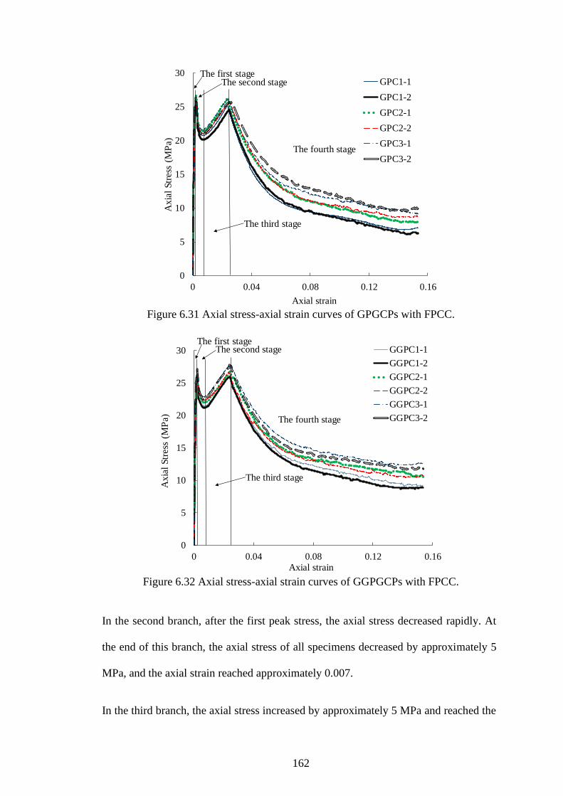
162

Figure 6.31 Axial stress-axial strain curves of GPGCPs with FPCC.

Figure 6.32 Axial stress-axial strain curves of GGPGCPs with FPCC.

In the second branch, after the first peak stress, the axial stress decreased rapidly. At

the end of this branch, the axial stress of all specimens decreased by approximately 5

MPa, and the axial strain reached approximately 0.007.

In the third branch, the axial stress increased by approximately 5 MPa and reached the

0

5

10

15

20

25

30

0 0.04 0.08 0.12 0.16

Ax

ial

Str

ess

(M

Pa)

Axial strain

GPC1-1

GPC1-2

GPC2-1

GPC2-2

GPC3-1

GPC3-2

The first stageThe second stage

The third stage

The fourth stage

0

5

10

15

20

25

30

0 0.04 0.08 0.12 0.16

Axia

l S

tress

(MP

a)

Axial strain

GGPC1-1

GGPC1-2

GGPC2-1

GGPC2-2

GGPC3-1

GGPC3-2

The first stageThe second stage

The third stage

The fourth stage

163

second peak axial stress. At the end of the third branch, the axial strain reached

approximately 0.025, at which point the GFPR jacket ruptured, as confirmed by

audible cracking of the GFRP jackets. The reason for the increase in the axial stress is

that with increasing axial strain, the PFCC provided more load carrying capacity. This

observation can be confirmed by the test results of FPCC alone in Figure 6.14,

showing that the axial stress increased until the axial strain reached approximately

0.025. It can be found from Table 6.10 and Table 6.11 that the most values of the

second peak axial stress were slightly higher than the first ones. Therefore, the second

peak axial stress was the maximum axial stress.

In the last branch, after the second peak axial stress, the axial stress decreased until the

end of the compression tests. The rate of decrease reduced with increasing the axial

strain. As the axial strain exceeded 0.14, the axial stress stabilized because when the

hoop strain became more pronounced, the confining pressure provided by the geogrid

was sufficient to stop the decrease in the axial stress. The final average axial stress of

GPGCPs with FPCC were approximately 25% to 40% of the nominal maximum

average axial stress. The final average axial stress of GGPGCPs with FPCC were

approximately 35% to 45% of the nominal maximum average axial stress. Only in the

fourth branch, the different numbers of geogrid layers had a prominent influence on

the mechanical behaviour. With additional geogrid layers, the axial stress was higher.

Axial Strain-Hoop Strain Behaviour

The axial-hoop strain curves of geogrid tubes in GPGCPs with FPCC are shown in

Figure 6.33 and Figure 6.34. The measurement methods are the same as the

measurement methods used for GPGCPs without FPCC and GGPGCPs without FPCC.

The hoop strain was averaged from three strain gauges attached at the geogrid ribs,

164

which is shown in Figure 6.4. The shape of the curves and the development trends are

the same as those of GPGCPs without FPCC and GGPGCPs without FPCC. The final

average hoop strain of Specimens GPC2 and GPC3 decreased by 31.7% and 51.6%,

respectively, relative to the final average hoop strain of Specimens GPC1. Also, The

final average hoop strain of Specimens GGPC2 and GGPC3 decreased by 22.9% and

49.0%, respectively, relative to the final average hoop strain of Specimens GGPC1. In

other words, the use of additional geogrid layers can significantly reduce the hoop

strain.

Figure 6.33 Hoop strain-axial strain curves of GPGCPs with FPCC.

-0.1

-0.08

-0.06

-0.04

-0.02

0

0 0.04 0.08 0.12 0.16

Av

era

ge H

oo

p S

train

Axial Strain

GPC1-1

GPC1-2

GPC2-1

GPC2-2

GPC3-1

GPC3-2

165

Figure 6.34 Hoop strain-axial strain curves of GGPGCPs with FPCC.

In addition, the axial-hoop strain relationships of FPCC placed in the middle of

GPGCPs and GGPGCPs were also obtained using strain gauges attached at the mid-

height of the FPCC (shown in Figure 6.1). The test results of hoop strain terminate at

the point where GFRP jackets rupture. The testing results of FPCC alone are also

included in Figure 6.35. There were no prominent differences between these sets of

results. In other words, the outer PGC and geogrid tubes have almost no influence on

the mechanical behaviour of FPCC, possibly because the confinement effect provided

by the outer PGC and geogrid tube is marginal.

-0.1

-0.08

-0.06

-0.04

-0.02

0

0 0.04 0.08 0.12 0.16

Avera

ge H

oop S

train

Axial Strain

GGPC1-1

GGPC1-2

GGPC2-1

GGPC2-2

GGPC3-1

GGPC3-2

166

Figure 6.35 Hoop strain-axial strain curves of FPCC placed in GPGCPs and

GGPGCPs.

Comparison between GPGCPs with FPCC and GGPGCPs with FPCC


stress-axial strain curves of GPGCPs with FPCC and GGPGCPs with FPCC with the

same number of geogrid layers. In each figure, the first peak axial stress of GPGCPs

with FPCC and that of GGPGCPs with FPCC is nearly the same. However, the second

peak axial stress of GPGCPs with FPCC is slightly lower than that of GGPGCPs with

FPCC. After the second peak axial stress, the axial stress of GPGCPs decrease faster

than the axial stress of GGPGCPs with FPCC. At last, the final axial stress of

GPGCPs with FPCC is about 80% of that of GGPGCPs with FPCC.

-0.024

-0.02

-0.016

-0.012

-0.008

-0.004

0

0 0.01 0.02 0.03 0.04

Hoop S

train

Axial Strain

FPCC-1 FPCC-2

GPC1-1 GPC1-2

GPC2-1 GPC2-2

GPC3-1 GPC3-2

GGPC1-1 GGPC1-2

GGPC2-1 GGPC2-2

GGPC3-1 GGPC3-2

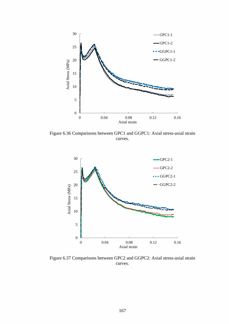
167

Figure 6.36 Comparisons between GPC1 and GGPC1: Axial stress-axial strain

curves.


curves.

0

5

10

15

20

25

30

0 0.04 0.08 0.12 0.16

Axia

l S

tress

(MP

a)

Axial strain

GPC1-1

GPC1-2

GGPC1-1

GGPC1-2

0

5

10

15

20

25

30

0 0.04 0.08 0.12 0.16

Axia

l S

tress

(MP

a)

Axial strain

GPC2-1

GPC2-2

GGPC2-1

GGPC2-2

168


curves.

The comparisons between the hoop strain-axial strain curves of GPGCPs with FPCC

and GGPGCPs with FPCC with the same number of geogrid layers are shown in

Figure 6.39, Figure 6.40 and Figure 6.41. The hoop strain was averaged from three

strain gauges attached at the geogrid ribs, which is shown in Figure 6.4. It is found

that for GPC1 and GGPC1, the hoop strain of GPC1 was slightly higher than GGPC1.

However, the hoop strain of GPC2 and GPC3 is higher than that of GGPC2 and

GGPC3 when the axial strain is less than 0.10. When the axial strain exceed 0.10, the

hoop strain of GGPC2 and GGPC3 become larger than that of GPC2 and GPC3.

0

5

10

15

20

25

30

0 0.04 0.08 0.12 0.16

Axia

l Str

ess

(MP

a)

Axial strain

GPC3-1

GPC3-2

GGPC3-1

GGPC3-2

169

Figure 6.39 Comparisons between GPC1 and GGPC1: Hoop strain-axial strain

curves.


curves.

-0.1

-0.08

-0.06

-0.04

-0.02

0

0 0.04 0.08 0.12 0.16

Av

era

ge H

oo

p S

train

Axial Strain

GPC1-1

GPC1-2

GGPC1-1

GGPC1-2

-0.1

-0.08

-0.06

-0.04

-0.02

0

0 0.04 0.08 0.12 0.16

Av

era

ge H

oo

p S

train

Axial Strain

GPC2-1

GPC2-2

GGPC2-1

GGPC2-2

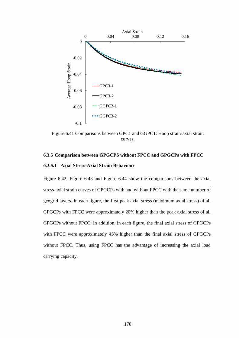
170


curves.

6.3.5 Comparison between GPGCPS without FPCC and GPGCPs with FPCC



stress-axial strain curves of GPGCPs with and without FPCC with the same number of

geogrid layers. In each figure, the first peak axial stress (maximum axial stress) of all

GPGCPs with FPCC were approximately 20% higher than the peak axial stress of all

GPGCPs without FPCC. In addition, in each figure, the final axial stress of GPGCPs

with FPCC were approximately 45% higher than the final axial stress of GPGCPs

without FPCC. Thus, using FPCC has the advantage of increasing the axial load

carrying capacity.

-0.1

-0.08

-0.06

-0.04

-0.02

0

0 0.04 0.08 0.12 0.16

Av

era

ge H

oo

p S

train

Axial Strain

GPC3-1

GPC3-2

GGPC3-1

GGPC3-2

171

Figure 6.42 Comparisons between GP1 and GPC1: Axial stress-axial strain curves.


0

5

10

15

20

25

30

0 0.04 0.08 0.12 0.16

Axia

l Str

ess

(M

Pa)

Axial strain

GP1-1

GP1-2

GPC1-1

GPC1-2

0

5

10

15

20

25

30

0 0.04 0.08 0.12 0.16

Axia

l Str

ess

(M

Pa)

Axial strain

GP2-1

GP2-2

GPC2-1

GPC2-2

172


Axial-Hoop Strain Behaviour

The comparisons between the axial-hoop strain curves of GPGCPs with and without

FPCC with the same number of geogrid layers are shown in Figure 6.45, Figure 6.46

and Figure 6.47. The hoop strain was averaged from three strain gauges attached at the

geogrid ribs, which is shown in Figure 6.4. It is found that in each figure, the hoop

strains of GPGCPs without FPCC was slightly higher than those of GPGCPs with

FPCC. However, the use of FPCC has no significant effect on the hoop strain of

GPGCPs.

0

5

10

15

20

25

30

0 0.04 0.08 0.12 0.16

Ax

ial

Str

ess

(M

Pa)

Axial strain

GP3-1

GP3-2

GPC3-1

GPC3-2

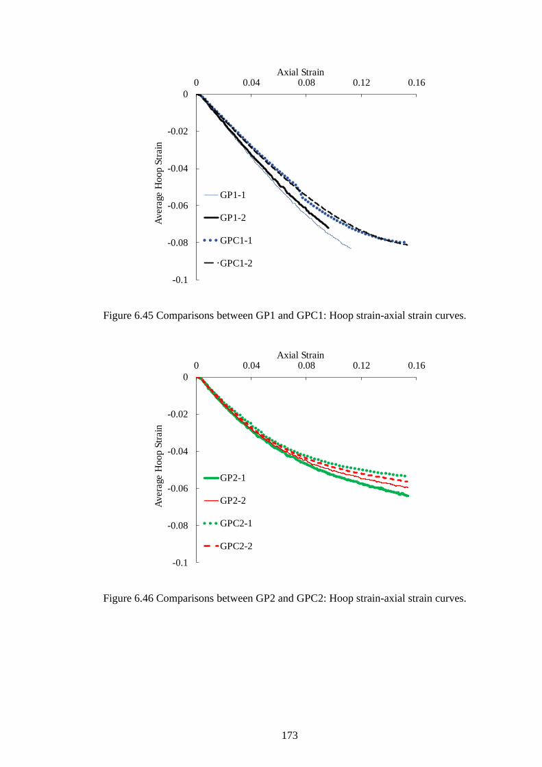
173

Figure 6.45 Comparisons between GP1 and GPC1: Hoop strain-axial strain curves.


-0.1

-0.08

-0.06

-0.04

-0.02

0

0 0.04 0.08 0.12 0.16

Av

era

ge H

oo

p S

train

Axial Strain

GP1-1

GP1-2

GPC1-1

GPC1-2

-0.1

-0.08

-0.06

-0.04

-0.02

0

0 0.04 0.08 0.12 0.16

Av

era

ge H

oo

p S

train

Axial Strain

GP2-1

GP2-2

GPC2-1

GPC2-2

174


6.3.6 Comparison between GGPGCPS with and without FPCC



stress-axial strain curves of GGPGCPs with and without FPCC with the same number

of geogrid layers. In each figure, the first peak axial stress (maximum axial stress) of

all GGPGCPs with FPCC were approximately 20% higher than the peak axial stress

of all GGPGCPs without FPCC. In addition, in each figure, the final axial stress of

GGPGCPs with FPCC were approximately 45% higher than the final axial stress of

GGPGCPs without FPCC. Thus, using FPCC has the advantage of increasing the axial

load carrying capacity.

-0.1

-0.08

-0.06

-0.04

-0.02

0

0 0.04 0.08 0.12 0.16

Av

era

ge H

oo

p S

train

Axial Strain

GP3-1

GP3-2

GPC3-1

GPC3-2

175

Figure 6.48 Comparisons between GGP1 and GGPC1: Axial stress-axial strain

curves.

Figure 6.49 Comparisons between GGP1 and GGPC1: Hoop strain-axial strain

curves.

0

5

10

15

20

25

30

0 0.04 0.08 0.12 0.16

Ax

ial

Str

ess

(MP

a)

Axial strain

GGP1-1

GGP1-2

GGPC1-1

GGPC1-2

0

5

10

15

20

25

30

0 0.04 0.08 0.12 0.16

Axia

l Str

ess

(MP

a)

Axial strain

GGP2-1

GGP2-2

GGPC2-1

GGPC2-2

176


curves.

Axial Strain-Hoop Strain Behaviour

The comparisons between the axial strain-hoop strain curves of GGPGCPs with and

without FPCC with the same number of geogrid layers are shown in Figure 6.51,

Figure 6.52 and Figure 6.53. The hoop strain was averaged from three strain gauges

attached at the geogrid ribs, which is shown in Figure 6.4. It is found that in each

figure, the hoop strains of GGPGCPs without FPCC was slightly higher than those of

GGPGCPs with FPCC. However, the use of FPCC has no significant effect on the

hoop strain of GGPGCPs.

0

5

10

15

20

25

30

0 0.04 0.08 0.12 0.16

Ax

ial

Str

ess

(MP

a)

Axial strain

GGP3-1

GGP3-2

GGPC3-1

GGPC3-2

177


curves.


curves.

-0.1

-0.08

-0.06

-0.04

-0.02

0

0 0.04 0.08 0.12 0.16

Av

era

ge H

oo

p S

train

Axial Strain

GGP1-1

GGP1-2

GGPC1-1

GGPC1-2

-0.1

-0.08

-0.06

-0.04

-0.02

0

0 0.04 0.08 0.12 0.16

Av

era

ge H

oo

p S

train

Axial Strain

GGP2-1

GGP2-2

GGPC2-1

GGPC2-2

178


curves.

6.4 Ductility

The ductility of concrete members is regarded as one of the most important design

aspects. The ductility calculation method proposed by Park (1989) was adopted in this

study, as shown in Equation (6.1):

𝜇𝜀 =𝜀𝑢𝜀𝑦

(6.1)

where is the specimen ductility. In general, u is defined as the specimen strain at

85% of the maximum stress at the descending branch (for unconfined specimens) or is

equal to the ultimate strain (for FRP-confined concrete, it is the strain at the point of

FRP rupture). The y is the yield strain, which is the axial strain at the yield stress.

-0.1

-0.08

-0.06

-0.04

-0.02

0

0 0.04 0.08 0.12 0.16

Av

era

ge H

oo

p S

train

Axial Strain

GGP3-1

GGP3-2

GGPC3-1

GGPC3-2

179

(a)

(b)

(c)

Figure 6.54 Definition of u and ɛy: (a) Definition of u and y for unconfined

concrete; (b) Definition of u and y for GPGCPs without FPCC; (c) Definition

of u and y for GPGCPs with FPCC.

Axial strain

Ax

ial

Str

ess

f y

0.75f y

0.5f y

εy εu

f y

0.75f y

0.5f y

Axial strain

εy εu

Ax

ial

Str

ess

f y

0.75f y

0.5f y

Axial strain

εy εu

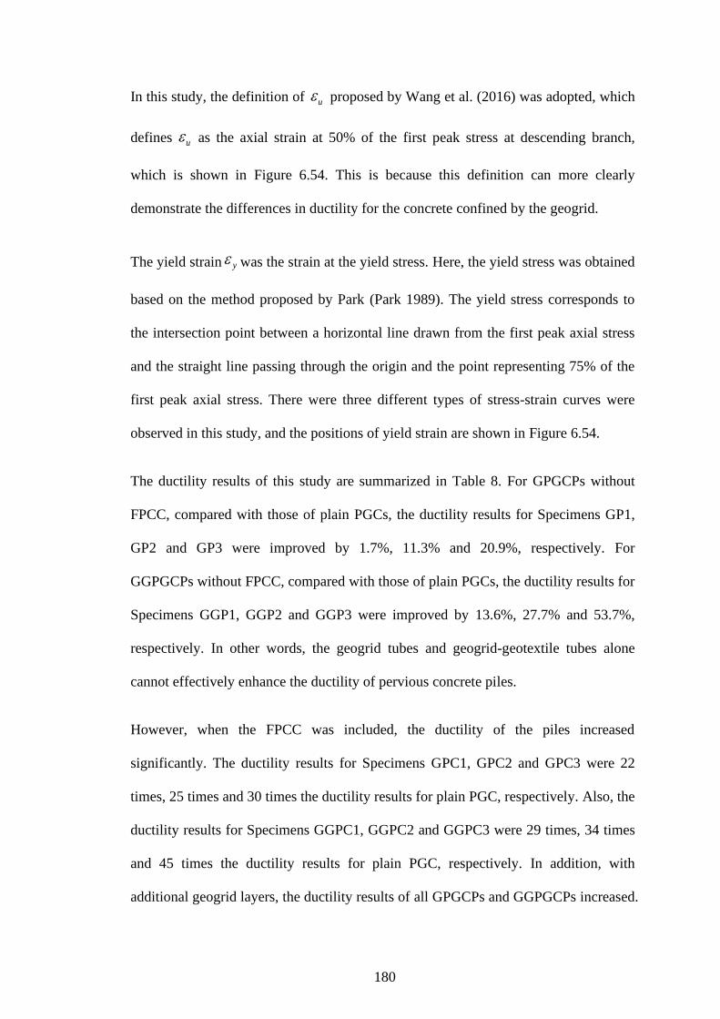
180

In this study, the definition of u proposed by Wang et al. (2016) was adopted, which

defines u as the axial strain at 50% of the first peak stress at descending branch,

which is shown in Figure 6.54. This is because this definition can more clearly

demonstrate the differences in ductility for the concrete confined by the geogrid.

The yield strain y was the strain at the yield stress. Here, the yield stress was obtained

based on the method proposed by Park (Park 1989). The yield stress corresponds to

the intersection point between a horizontal line drawn from the first peak axial stress

and the straight line passing through the origin and the point representing 75% of the

first peak axial stress. There were three different types of stress-strain curves were

observed in this study, and the positions of yield strain are shown in Figure 6.54.

The ductility results of this study are summarized in Table 8. For GPGCPs without

FPCC, compared with those of plain PGCs, the ductility results for Specimens GP1,

GP2 and GP3 were improved by 1.7%, 11.3% and 20.9%, respectively. For

GGPGCPs without FPCC, compared with those of plain PGCs, the ductility results for

Specimens GGP1, GGP2 and GGP3 were improved by 13.6%, 27.7% and 53.7%,

respectively. In other words, the geogrid tubes and geogrid-geotextile tubes alone

cannot effectively enhance the ductility of pervious concrete piles.

However, when the FPCC was included, the ductility of the piles increased

significantly. The ductility results for Specimens GPC1, GPC2 and GPC3 were 22

times, 25 times and 30 times the ductility results for plain PGC, respectively. Also, the

ductility results for Specimens GGPC1, GGPC2 and GGPC3 were 29 times, 34 times

and 45 times the ductility results for plain PGC, respectively. In addition, with

additional geogrid layers, the ductility results of all GPGCPs and GGPGCPs increased.

181

Table 6.12 Ductility results.

Specimen

Label

Yield

Strain (ɛy) ɛu Ductility

Average

Ductility

P-1 0.00193 0.0035 1.81 1.77

P-2 0.00192 0.0033 1.72

GP1-1 0.00200 0.0037 1.85 1.80

GP1-2 0.00189 0.0033 1.75

GP2-1 0.00194 0.0039 2.01 1.97

GP2-2 0.00202 0.0039 1.93

GP3-1 0.00199 0.0041 2.06 2.14

GP3-2 0.00198 0.0044 2.22

GGP1-1 0.00200 0.0039 1.95 2.01

GGP1-2 0.00194 0.0040 2.06

GGP2-1 0.00190 0.0047 2.47 2.26

GGP2-2 0.00201 0.0041 2.04

GGP3-1 0.00197 0.0053 2.69 2.72

GGP3-2 0.00200 0.0055 2.75

GPC1-1 0.00126 0.0479 38.0 38.2

GPC1-2 0.00128 0.0491 38.4

GPC2-1 0.00134 0.0596 44.5 44.9

GPC2-2 0.00132 0.0597 45.2

GPC3-1 0.00136 0.0649 47.7 53.6

GPC3-2 0.00132 0.0784 59.4

GGPC1-1 0.00129 0.0689 53.4 50.4

GGPC1-2 0.00130 0.0615 47.3

GGPC2-1 0.00132 0.0843 64.8 59.4

GGPC2-2 0.00137 0.0738 53.9

182


GGPC3-1 0.00132 0.1115 84.5 80.0

GGPC3-2 0.00125 0.0943 75.4

6.5 Summary

This Chapter presents and explains the results of axial compression tests on

geosynthetics-confined pervious geopolymer concrete piles with and without FRP-

PVC-confined concrete core (FPCC). The axial stress-axial strain behaviour, axial-

hoop strain behaviour and final state of the specimens have been discussed. According

to the test results and discussions presented above, the following conclusions can be

drawn:

1. For geogrid-confined pervious geopolymer concrete piles (GPGCPs) without FPCC

and geogrid-geotextile-confined pervious geopolymer concrete piles (GGPGCPs)

without FPCC, in comparison with plain PGC, geogrid tubes and geogrid-geotextile

tubes cannot effectively improve the maximum axial stress and axial strain at the

maximum axial stress. This is because the confinement effect provided by the geogrid

and geotextile is relatively low. Only after the maximum axial stress, the effects of the

geogrid tubes and geogrid-geotextile tubes became clear. When the number of geogrid

layers increased, the axial stress increased slightly. However, the effects of geogrid on

hoop strain was significant. When the number of geogrid layers increased, the hoop

strain decreased significantly.

2. For the GPGCPs with FPCC and GGPGCPs with FPCC, two peak axial stresses

appeared, and the values of these two peak axial stresses were close, which are

approximately 20% higher than the maximum axial stress of GPGCPs without FPCC

and GGPGCPs without FPCC. For GPGCPs with FPCC, their first peak axial stress

183

was the maximum axial stress. However, for GGPGCPs with FPCC, the first peak

axial stress is slightly lower than second peak axial stress. The effects of geogrid on

axial stress of GPGCPs with FPCC and GGPGCPs with FPCC were similar to those

of GPGCPs without FPCC and GGPGCPs without FPCC. Only after the second peak

stress the effects of geogrid tubes became clear. When the number of geogrid layers

increased, the axial stresss of GPGCPs with FPCC and GGPGCPs with FPCC

increased.

3. The incorporation of FPCC into GPGCPs and GGPGCPs did not have a significant

influence on the hoop strain of the outer geogrid tubes. The effects of geogrid on hoop

strain of GPGCPs with FPCC and GGPGCPs with FPCC is similar to those of

GPGCPs without FPCC and GGPGCPs without FPCC. When the number of geogrid

layers increased, the hoop strain of GPGCPs with FPCC and GGPGCPs with FPCC

decreased significantly.

4. All GPGCPs and GGPGCPs can bear a large axial strain due to the high ductility of

the geogrid. In comparison with the ductility of plain PGC, the ductility of GPGCPs

without FPCC and GGPGCPs without FPCC was not effectively enhanced. However,

when the FPCC was applied, the ductility of the GPGCPs with FPCC and GGPGCPs

with FPCC improved significantly.

This Chapter leads to Chapter 7, which proposes analytical models to predict the

experimental results of new forms of PGC piles shown in this Chapter.

184

CHAPTER 7

Geosynthetics-confined Pervious Geopolymer Concrete Piles

without and with FRP-PVC-confined Concrete Core:

Analytical Models

7.1 Introduction

In this chapter, to better understand the axial compressive behaviour of geosynthetics-

confined pervious geopolymer concrete piles without and with FRP-PVC-confined

concrete (FPCC), new analytical models are proposed. According to the

characteristics of the mechanical behaviour of GPGCPs without and with FPCC and

GGPGCPs without and with FPCC, the unconfined concrete model proposed by the

European Standards, and an existing popular FRP-confined concrete model are

combined here. Based on the analytical models, the influences of different parameters

on the axial compressive behaviour of GPGCPs without and with FPCC and

GGPGCPs without and with FPCC have been investigated through parametric

analyses.

7.2 Analytical Models

The research studies on the development of axial stress-axial strain models for

predicting the axial compressive behaviour of geogrid confined concrete are very

limited. Here, according to the characteristics of experimental behaviour of GPGCPs,

tailored analytical models are proposed.

7.2.1 Equivalent Confining Pressure Provided by Geogrid tubes

For GPGCPs without and with FPCC, only part of the pervious concrete surface was

185

covered by geogrid ribs, which is different from FRP and PVC wrapped concrete

(Wang et al. 2016). In this study, the actual lateral confining pressure (fla,grid) is

transferred into equivalent lateral confining pressure (fle,grid), which is assumed to

uniformly cover all lateral surface of the PGC. The confining action in geogrid-

confined PGC can be schematically illustrated in Figure 7.1. The criterion to calculate

the equivalent lateral confining pressure is that the actual lateral confining force

(Fla,grid) provided by the actual lateral confining pressure (fla,grid) is equal to the

equivalent lateral confining force (Fle,grid) provided by the equivalent lateral confining

pressure (fle,grid), which is shown as follows:

, ,la grid le gridF F=

(7.1)

The Fla,grid is the sum of forces provided by each transverse geogrid rib, which is given

by:

, 2la grid ribF n F=

(7.2)

where Frib is the force provided by one transverse geogrid rib; n is the number of

transverse geogrid ribs for one GPGCP.

The equivalent lateral confining force (Fle,grid) is expressed by:

, ,le grid le grid pF f H d=

(7.3)

where H is the height of the GPGCPs; dp is the diameter of the GPGCPs.

Combining the Equation (7.1), Equation (7.2) and Equation (7.3), the equivalent

lateral confining pressure (fle,grid) is given by:

,

2 rib

le grid

p

n Ff

d H

=

(7.4)

186

Figure 7.1 Confining action of geogrid tubes.

The next step is to calculate the lateral confinement modulus which is directly used in

the analytical model. The lateral confinement modulus (Ele,grid) is defined as the ratio

of the increment of the confining pressure and the increment of the hoop strain of

concrete:

,

,

2le grid rib

le grid

l p l

f FnE

d H

= =

(7.5)

As the tensile force-strain relationship of geogrid is nearly linear, the value of rib

l

F

can be calculated by:

,

gridrib

l grid u

PF

=

(7.6)

where the Pgrid is the average peak load of one geogrid rib; and ,grid u is the tensile

strain. For the PGC piles wrapped by two and three geogrid layers, their equivalent

lateral confinement modulus is 2Ele,grid and 3Ele,grid, respectively.

7.2.2 Equivalent Confining Pressure Provided by Geogrid-Geotextile tubes

The confining action in geogrid-geotextile-confined PGC can be schematically

illustrated in Figure 7.2. For GGPGCPs without and with FPCC, the confinement

= 160 mm

,le gridf

187

modulus of geogrid-geotextile tubes (Egt) is the sum of confinement modulus of

geogrid (Ele,grid) and confinement modulus of geotextile (El,textile), which is shown as

follows:

, ,gt le grid l textileE E E= +

(7.7)

The confinement modulus of geogrid (Ele,grid) can be calculated by Equation (7.5). The

confinement modulus of geotextile can be calculated by:

,

,

l textile

l textile

l

fE

=

(7.8)

where fl,textile is the lateral confining pressure acting on concrete provided by geotextile,

and l is the lateral strain of concrete. The expression of fl,textile is shown as follow:

,

,

2 l textile

l textile

p

Ff

Hd=

(7.9)

where Fl,textile is the lateral confining resultant force provided by geotextile.

Substituting Equation (7.9) into Equation (7.8), the elastic modulus of geotextile can

be calculated as:

,

,

2 l textile

l textile

p l

FE

Hd =

(7.10)

Figure 7.2 Confining action of geogrid-geotextile tubes.

= 160 mm

,l textilef

,l textileF ,l textileF

188

Due to the tensile force-strain relationship of geogrid is nearly linear (Figure 6.8), the

value of ,l textile

l

F

can be calculated as:

,

,

l textile textile

l textile p

F Hf

=

(7.11)

where ftextile is the strength of geotextile; ,textile p is the tensile strain of geotextile at

strength, which are shown in Table 6.4. Substituting Equation (7.11) into Equation

(7.10), the value of El,textile is given by:

,

,

,

2 2l textile textile

l textile

p l p textile p

F HfE

Hd Hd = =

(7.12)

7.2.3 Analytical Model for GPGCPs without FPCC and GGPGCPs without

FPCC

The test results of GPGCPs without FPCC and GGPGCPs without FPCC revealed that

geogrid alone do not improve the compressive strength and the axial strain at the

compressive strength of PGC. The axial stress-strain curves were divided into three

branches. The first two branches are similar to the behaviour of unconfined concrete.

Therefore, the equation used to simulate the behaviour of unconfined concrete was

adopted to describe the first two branches of the axial stress-strain curves of GPGCPs

without FPCC and GGPGCPs without FPCC. In this study, the model presented by

ENV1992-1-1 (2004) was applied for the first two branches of the axial stress-strain

curves:

2

2' c c

c co

co co

f

= −

(7.13)

where c and c are the axial stress and axial strain, respectively; co is the axial strain

189

at the peak stress of concrete; 'cof is the compressive strength of concrete.

In the third branch, the axial stress-strain behaviour of GPGCPs without FPCC and

GGPGCPs without FPCC became more gradual, and finally became stable. This can

be explained that after the significant reduction of axial stress, the lateral strain of

concrete became larger and the confinement effect provided by the geogrid became

higher (Wang et al. 2016). This characteristic is different from the axial stress-strain

behaviour of unconfined concrete, which lost all the load carrying capacity after

drastic reduction in the axial load. Through carefully interpreting the test results, it is

found that the transition axial strain point, where the axial stress-strain curves of

GPGCPs without FPCC and GGPGCPs without FPCC can be differentiated from that

of unconfined PGC, is related to the equivalent elastic modulus of geogrid tubes. This

transition axial strain point can be determined by Equation (7.14) and Equation (7.15):

,

,

cm

t p co

co p

Ea

bf

= −

(7.14)

,

le grid

cm

gt

E for GPGCPsE

E for GGPGCPs

=

(7.15)

where ,t p is transition axial strain point of PGC; ,co pf is the compressive strength of

PGC; the a and b are constants obtained based on the regression analysis of test results;

and the Ecm is the confinement modulus of geogrid tubes for GPGCPs ( ,le gridE ), or

geogrid-geotextile tubes for GGPGCPs (Egt). For the GPGCPs, the suggested values

of a and b are 1.72 and 10.0, respectively. For the GGPGCPs, the suggested values of

a and b are 1.72 and 10.7, respectively.

Based on the regression analysis of the test data shown in Figure 7.3 and Figure 7.8,

the following expression is proposed to describe the axial stress-strain curves of

190

Geogrid-confined PGC piles:

0.2

, ,

, ,

,

1' cm c

c p co p

c co p co p

co p

Ef d

c f

= +

(7.16)

where, ,c p is the axial stress of PGC. The constants c and d were obtained based on

the regression analysis of test results, which are 1.5 and 0.011, respectively.

For clarity of presentation, Equation (7.13) and Equation (7.16) are combined together

in Equation (7.17) to simulate the axial stress-strain behaviour of GPGCPs without

FPCC:

2

, ,

, ,

, 0.2

, ,

, ,

,

2' 0

1'

c c

co p c t p

co p co p

c p

cm c

co p t p c

c co p co p

co p

f for

Ef d for

c f

−

= +

(7.17)

The comparisons between the experimental results and analytical modelling results of

GPGCPs without FPCC and GGPGCPs without FPCC are shown from Figure 7.3 to

Figure 7.8, respectively. It can be seen that the analytical modelling results matched

well with the experimental results. In general, the analytical model can predict the

axial stress-strain behaviour of GPGCPs without FPCC and GGPGCPs without FPCC

with good accuracy, due to the appropriate mathematical models.

191


GPGCPs without FPCC: GP1.



0

5

10

15

20

25

0 0.04 0.08 0.12 0.16

Ax

ial

Str

ess

(M

Pa)

Axial strain

GP1-1

GP1-2

Prediction by Equation (7.17)

a=1.72

b=10

c=1.5d=0.011

Eg,eq =11.8

0

5

10

15

20

25

0 0.04 0.08 0.12 0.16

Axia

l Str

ess

(M

Pa)

Axial strain

GP2-1

GP2-2


a=1.72

b=10

c=1.5d=0.011

Eg,eq =23.6 MPa

192




GGPGCPs without FPCC: GGP1.

0

5

10

15

20

25

0 0.04 0.08 0.12 0.16

Axia

l Str

ess

(M

Pa)

Axial strain

GP3-1

GP3-2


a=1.72

b=10

c=1.5d=0.011

Eg,eq =35.4 MPa

0

5

10

15

20

25

0 0.04 0.08 0.12 0.16

Ax

ial

Str

ess

(M

Pa)

Axial strain

GGP1-1

GGP1-2


a=1.74

b=10.7

c=1.7d=0.033

Ecm =15.33 MPa

193





7.2.4 Analytical Model for Hollow FRP-PVC Tubes

Based on the regression analysis of test data of hollow FRP-PVC tubes under axial

compression loading, it can be found that the following equation can effectively

describe the compressive behaviour:

0

5

10

15

20

25

0 0.04 0.08 0.12 0.16

Axia

l S

tress

(M

Pa)

Axial strain

GGP2-1

GGP2-2


a=1.74

b=10.7

c=1.7d=0.033

Ecm =27.13 MPa

0

5

10

15

20

25

0 10 20 30 40 50

Ax

ial

Str

ess

(M

Pa)

Axial strain

GGP3-1

GGP3-2


a=1.74

b=10.7

c=1.7d=0.033

Ecm =38.93 MPa

194

( )

( )

2

3

0

pvc pvc c hp p c hp

h pvc pvc

hp c

c

E A m F for

F s E Afor

− − +

=

(7.18)

where, the Epvc is the elastic modulus of PVC materials; Apvc is the cross-sectional area

of PVC tubes; Fp is the peak load of hollow FRP-PVC tubes; hp is the axial strain at

the peak load of hollow FRP-PVC tubes; and m and s are constants.

The comparison between the experimental results and the analytical modelling results

of FRP-PVC tubes under compression loading are shown in Figure 7.9. It can be seen

that this analytical model prediction is in good agreement with experimental results.


FRP-PVC tubes.

7.2.5 Analytical Model for FRP-PVC-confined Geopolymer Concrete (FPCC)

In this section, the analytical model proposed by Teng et al. (2009) is adopted. This

analytical model is based on the following assumptions: (1) the axial stress-strain

curve consists of two parts, one is the parabolic first branch and the other one is a

linear second branch; (2) the slope of the parabola at zero axial strain is the same as

the elastic modulus of unconfined concrete; (3) the nonlinear part of the first branch is

0

10

20

30

40

50

0 0.04 0.08 0.12 0.16

Ax

ial

Lo

ad

(k

N)

Axial Strain

FP1

FP2


Epvc = 1.58GPa

Apvc = 1004.8mm2

Fp =45.1kNɛhp = 0.045

m = 0.07s = 0.005

195

affected to some degree by the confinement of the FRP jacket; (4) the parabolic first

branch meets the linear second branch smoothly; (5) the linear second branch

terminates at a point where both the compressive strength and the ultimate axial strain

of confined concrete are reached; and (6) the linear second branch intercepts the axial

stress axis at a stress value equal to the unconfined concrete strength.

Based on these assumptions, the analytical model proposed by Teng et al. (2009) is

shown as follows:

( ), 2 2

, , ,

, ,

, 2 , ,

0 4 '

'

c n

c n c c c r t n

c n co n

co n c t n c r

E EE for

f

f E for

−−

=

+

(7.19)

where ,c n is the axial stress of confined normal geopolymer concrete; c is the axial

strain of confined normal geopolymer concrete; Ec,n is the elastic modulus of

unconfined concrete, which is taken to be 4730cn coE f = (in MPa) according to ACI

318-11 (2011); E2 is the slope of the linear second branch; ,t n is the transition axial

strain for NGC. In order to let the parabolic first branch meet the linear second branch

with a smooth transition, the ,t n is given by:

,

,

, 2

2 'co n

t n

c n

f

E E =

−

(7.20)

The slope of the linear second branch E2 is expressed as:

, ,

2

,

' 'cc n co n

cu n

f fE

−=

(7.21)

where ,'cc nf is the confined compressive strength of NGC; ,'co nf is the unconfined

compressive strength of NGC; ,cu n is the ultimate axial strain of confined NGC,

which is shown in Equation (7.23). The compressive strength equation of confined

196

NGC can be calculated using the following equations:

( ),

1 3.5 0.01 0.01'

1 0.01cc n

forf

for

+ − =

(7.22)

Based on the test results of this study, the equation to calculate the ultimate axial

strain of FRP-confined concrete ( ,cu n ) proposed by Lam and Teng (2003) was used:

, 1.45

,

1.75 12cu n

co n

= +

(7.23)

where, the is the confinement stiffness ratio; the is the strain ratio. The

mathematical expressions of these two ratios are as follow:

( ), ,

2

'

FRP

co n co n p

E t

f d

=

(7.24)

,

,

h ult

co n

=

(7.25)

where EFRP is the elastic modulus of FRP in the hoop direction; TFRP is the thickness

of the FRP jacket; dp is the diameter of the GPGCPs; ,'co nf is the unconfined

compressive strength of NGC; ,co n is the axial strain at the peak stress of NGC; ,h ult

is the hoop ultimate tensile strain of the FRP jacket.

197


FPCC.

The axial load carrying capacity of FRP-PVC-confined NGC is the sum of axial loads

provided by the hollow tube and the confined NGC. The comparison between the

experimental results and the analytical modelling results of FRP-PVC-confined NGC

under axial compression loading are shown in Figure 7.10. It can be seen that the

prediction of analytical model is in good agreement with the experimental results.

7.2.6 Analytical Model for GPGCPs with FPCC and GGPGCPs with FPCC

The axial load carrying capacity can be calculated as the sum of axial loads carried by

the outer pervious geopolymer concrete (PGC), the hollow FRP-PVC tubes and the

inner normal geopolymer concrete (NGC):

p h n

total

total

F F F

A

+ +=

(7.26)

where Fp, Fh and Fn are the axial loads carried by the outer PGC, the hollow FRP-

PVC tubes and the inner NGC, respectively. The Fh is given by Equation (7.18). The

Fp and Fn can be calculated by the following expressions:

0

20

40

60

80

0 0.04 0.08 0.12 0.16

Ax

ial

Str

ess

(M

Pa)

Axial strain

FPCC1

FPCC2

Prediction by Equation(18)+Equation(19)

Efrp = 33.43GPa

Dn = 76mm

ɛh,rup = 0.0186ɛco,n = 0.0022

f = 49.2 MPa,'co nf

198

2 2

, ,4

p h

p c p p c p

d dF A

−= =

(7.27)

2

, ,4

n

n c n n c n

dF A = =

(7.28)

2

4

p

total

dA =

(7.29)

where ,c p is the axial stress of PGC; ,c n is the axial stress of NGC; Ap is the cross-

sectional area of PGC; An is the cross-sectional area of NGC; Atotal is the cross-

sectional area of the whole PGC piles; dp is the outer diameter of PGC; dh is the outer

diameter of hollow FRP-PVC tubes; and dn is the diameter of NGC. The comparison

between the experimental results and the analytical modelling results of GPGCPs with

FPCC under the compression loading are shown from Figure 7.11 to Figure 7.16,

respectively. It can be seen that this analytical model predicts results that is in good

agreement with the experimental ones.


GPGCPs with FPCC: GPC1.

0

5

10

15

20

25

30

0 0.04 0.08 0.12 0.16

Ax

ial

Str

ess

(M

Pa)

Axial strain

GPC1-1

GPC1-2


199





0

5

10

15

20

25

30

0 0.04 0.08 0.12 0.16

Axia

l S

tress

(M

Pa)

Axial strain

GPC2-1

GPC2-2


0

5

10

15

20

25

30

0 0.04 0.08 0.12 0.16

Ax

ial

Str

ess

(M

Pa)

Axial strain

GPC3-1

GPC3-2


200


GGPGCPs with FPCC: GGPC1.



0

5

10

15

20

25

30

0 0.04 0.08 0.12 0.16

Axia

l Str

ess

(M

Pa)

Axial strain

GGPC1-1

GGPC1-2


0

5

10

15

20

25

30

0 0.04 0.08 0.12 0.16

Axia

l S

tress

(M

Pa)

Axial strain

GGPC2-1

GGPC2-2


201



7.3 Parametric Analyses

Parametric analyses have been conducted to study the effects of different parameters

on the axial compression behaviour of GPGCPs. The effects of PGC compressive

strength, the confinement modulus of geogrid tubes, NGC compressive strength, the

number of plies of GFRP and the ultimate strain of GFRP have been investigated.

Equation (7.17) has been used to calculate the axial load capacity of GPGCPs without

FPCC and GGPGCPs without FPCC. Equation (7.26) has been used to calculate the

axial load capacity of GPGCPs with FPCC and GGPGCPs with FPCC.

7.3.1 Parametric Analyses of GPGCPs without FPCC and GGPGCPs without

FPCC

Effect of Confinement Modulus of Geogrid Tubes

Four values of confinement modulus of geogrid tubes grades have been considered

(20 MPa, 35 MPa, 50 MPa, and 65 MPa). Figure 7.17 and Figure 7.18 show the axial

stress-axial strain behaviour of GPGCPs without FPCC and GGPGCPs without FPCC

with different confinement modulus of geogrid tubes. It is evident that the increase in

0

5

10

15

20

25

30

0 0.04 0.08 0.12 0.16

Ax

ial

Str

ess

(M

Pa)

Axial strain

GGPC3-1

GGPC3-2


202

the confinement modulus of geogrid tubes does not enhance the peak stress of

GPGCPs without FPCC and GGPGCPs without FPCC, which were all close to the

compressive strength of the unconfined PGC. However, it is found that stable axial

stress level of the last branch increased significantly with the increase of confinement

modulus of geogrid tubes and geogrid-geotextile tubes.


confinement moduli of geogrid tubes.

Figure 7.18 Axial compression behaviour of GGPGCPs without FPCC for

different confinement moduli of geogrid-geotextile tubes.

0

5

10

15

20

25

0 0.04 0.08 0.12 0.16

Ax

ial

Str

ess

(M

Pa)

Axial Strain

Eg,eq =20 MPa

Eg,eq =35 MPa

Eg,eq =50 MPa

Eg,eq =65 MPa

Ele,grid

Ele,grid

Ele,grid

Ele,grid

0

5

10

15

20

25

0 0.04 0.08 0.12 0.16

Axia

l Str

ess

(M

Pa)

Axial Strain

Eg,eq =20 MPa

Eg,qu =35 MPa

Eg,eq =50 MPa

Eg,eq =65 MPa

Ele,grid

Ele,grid

Ele,grid

Ele,grid

203

Effect of PGC Compressive Strength

Four PGC compressive strength grades have been considered (10 MPa, 20 MPa, 30

MPa, and 40 MPa). Figure 7.19 and Figure 7.20 show the axial stress-axial strain

behaviour of GPGCPs without FPCC and GGPGCPs without FPCC with different

PGC compressive strengths. It is evident that the increase in the PGC compressive

strength significantly enhance the peak strength. However, it is found that stable axial

stress level of the last branch increased to some extent with the increase of PGC

compressive strength.


PGC compressive strength.

0

10

20

30

40

0 0.04 0.08 0.12 0.16

Ax

ial

Str

ess

(M

Pa)

Axial Strain

fpgc =10 MPa

fpgc =20 MPa

fpgc =30 MPa

fpgc =40 MPa

,'co pf

,'co pf

,'co pf

,'co pf

204

Figure 7.20 Axial compression behaviour of GGPGCPs without FPCC for

different PGC compressive strength

7.3.2 Parametric Analyses of GPGCPs with FPCC and GGPGCPs with FPCC

Effect of Confinement Modulus of Geogrid Tubes

Four values of confinement modulus of geogrid tubes grades have been considered

(20 MPa, 35 MPa, 50 MPa, and 65 MPa). Figure 7.21 and Figure 7.22 show the axial

stress-axial strain behaviour of GPGCPs with FPCC and GGPGCPs with FPCC with

different PGC compressive strengths. It is evident that the increase in the confinement

modulus of geogrid tubes strength does not enhance the first peak axial stress and

axial strain at the first peak axial stress of GPGCPs with FPCC and GGPGCPs with

FPCC. However, the increase in confinement modulus of geogrid tubes insignificantly

improve the second peak axial stress and axial strain at the second peak axial stress of

GPGCPs with FPCC and GGPGCPs with FPCC. It is also found that the axial stress

level of the last branch increased to some extent with the increase of confinement

modulus of geogrid tubes.

0

5

10

15

20

25

30

35

40

0 0.04 0.08 0.12 0.16

Ax

ial

Str

ess

(M

Pa)

Axial Strain

PGC =10 MPa

PGC =20 MPa

PGC =30 MPa

PGC =40 MPa

,'co pf

,'co pf

,'co pf

,'co pf

205


confinement moduli of geogrid tubes.


confinement moduli of geogrid-geotextile tubes.

Effect of PGC Compressive Strength

Four PGC compressive strength grades have been considered (10 MPa, 20 MPa, 30


behaviour of GPGCPs with FPCC and GGPGCPs with FPCC with different PGC

compressive strengths. It is evident that the increase in the PGC compressive strength

0

5

10

15

20

25

30

0 0.04 0.08 0.12 0.16

Ax

ial

Str

ess

(M

Pa)

Axial Strain

Eg,eq =20 MPa

Eg,eq =35 MPa

Eg,eq =50 MPa

Eg,eq =65 MPa

Ele,grid

Ele,grid

Ele,grid

Ele,grid

0

5

10

15

20

25

30

0 0.04 0.08 0.12 0.16

Ax

ial

Str

ess

(M

Pa)

Axial Strain

Eg,eq =20 MPa

Eg,eq =35 MPa

Eg,eq =50 MPa

Eg,eq =65 MPa

Ele,grid

Ele,grid

Ele,grid

Ele,grid

206

significantly enhances the first peak axial stress. It is also found that the axial stress

level of the last branch increased slightly with the increase of PGC compressive

strength. However, the axial strains at the first peak axial stress and the second peak

axial stress are not enhanced.





0

5

10

15

20

25

30

35

40

45

0 0.04 0.08 0.12 0.16

Axia

l S

tres

s (M

Pa)

Axial Strain

fpgc =10 MPa

fpgc =20 MPa

fpgc =30 MPa

fpgc =40 MPa

,'co pf

,'co pf

,'co pf

,'co pf

0

5

10

15

20

25

30

35

40

45

0 0.04 0.08 0.12 0.16

Ax

ial

Str

ess

(M

Pa)

Axial Strain

Epgc =10 MPa

Epgc =20 MPa

Epgc =30 MPa

Epgc =40 MPa

,'co pf

,'co pf

,'co pf

,'co pf

207

Effect of NGC Compressive Strength

Four NGC compressive strength grades have been considered (40 MPa, 50 MPa, 60


behaviour of GPGCPs with FPCC and GGPGCPs with FPCC with different NGC

compressive strengths. It is evident that the increase in the NGC compressive strength

significantly enhances the first and second peak axial stresses. However, it is found

that stable axial stress level of the last branch decreased to a slight extent with the

increase of NGC compressive strength. This is because the ultimate strain of GFRP

became lower with the increase of NGC compressive strength. When the GFRP

ruptures, the hoop strain and the confinement effect of PVC become lower with the

increase of NGC compressive strength. Therefore, axial stress of GPGCPs with FPCC

and GGPGCPs with FPCC reduces more quickly with the increase of NGC

compressive strength. This model can capture these characteristics of GPGCPs with

FPCC and GGPGCPs with FPCC.


NGC compressive strength.

0

5

10

15

20

25

30

35

0 0.04 0.08 0.12 0.16

Ax

ial

Str

ess

(MP

a)

Axial Strain

fc,n =40 MPa

fc,n =50 MPa

fc,n =60 MPa

fc,n =70 MPa

,'co nf

,'co nf

,'co nf

,'co nf

208


NGC compressive strength.

Effect of Number of GFRP Layers

Four different number of GFRP layers have been considered (3 layers, 5 layers, 7

layers and 9 layers). Figure 7.27 and Figure 7.28 show the axial stress-axial strain

behaviour of GPGCPs with FPCC and GGPGCPs with FPCC with different PGC

compressive strengths. It is evident that the increase in the number of GFPR layers

significantly enhances the second peak axial stress and the axial strain at the second

peak axial stress of GPGCPs with FPCC and GGPGCPs with FPCC. However, the

first peak axial stress and the axial strain at the first peak axial stress was not enhanced.

It is also found that the axial stress level of the last branch increased significantly with

the increase of confinement modulus of the geogrid tubes.

0

5

10

15

20

25

30

35

0 0.04 0.08 0.12 0.16

Axia

l Str

ess

(M

Pa)

Axial Strain

fc,ngc=40 MPa

fc,ngc=50 MPa

fc,ngc=60 MPa

fc,ngc=70 MPa

,'co nf

,'co nf

,'co nf

,'co nf

209


number of GFRP layers.


number of GFRP layers.

Effect of Ultimate Strains of GFRP

Four different ultimate tensile strains of GFRP have been considered (0.010, 0.015,

0.020 and 0.025). Figure 7.29 and Figure 7.30 show the axial stress-axial strain

behaviour of GPGCPs with FPCC with different ultimate tensile strains of GFRP. It is

evident that the increase in the ultimate tensile strains of GFRP does not enhance the

first peak strength and the axial strain at the first peak axial stress of GPGCPs with

0

5

10

15

20

25

30

35

40

0 0.04 0.08 0.12 0.16

Axia

l S

tress

(M

Pa)

Axial Strain

n =3

n =5

n =7

n =9

0

5

10

15

20

25

30

35

40

0 0.04 0.08 0.12 0.16

Axia

l Str

ess

(M

Pa)

Axial Strain

n =3

n =5

n =7

n =9

210

FPCC and GGPGCPs with FPCC. However, the increase in the number of GFPR

layers significantly enhances the second peak axial stress and the axial strain at the

second peak axial stress of GPGCPs with FPCC and GGPGCPs with FPCC. It is also

found that the axial stress level of the last branch increased to some extent with the

increase of confinement modulus of geogrid tubes.


ultimate strains of GFRP.


ultimate strains of GFRP

0

5

10

15

20

25

30

0 0.04 0.08 0.12 0.16

Ax

ial

Str

ess

(M

Pa)

Axial Strain

e = 0.010

e = 0.015

e = 0.020

e = 0.025

,h ult

,h ult

,h ult

,h ult

0

5

10

15

20

25

30

0 0.04 0.08 0.12 0.16

Ax

ial

Str

ess

(M

Pa)

Axial Strain

e =0.010

e =0.015

e =0.020

e =0.025

,h ult

,h ult

,h ult

,h ult

211

7.4 Summary

In this Chapter, analytical models for the prediction of axial compression behaviour of

GPGCPs and GGPGCPs have been developed and validated with experimental results.

Moreover, parametric analyses have been carried out to investigate the effects of

different parameters on the axial compression behaviour of GPGCPs and GGPGCPs.

The following conclusions can be drawn:

1. For the analytical model of GPGCPs without FPCC and GGPGCPs without

FPCC, the first two branches of axial stress-axial strain curves were simulated

by using the unconfined concrete model proposed by European Standards. The

third branch was simulated by a new equation. The predicted results are found

to be in good agreement with the experimental results.

2. For the prediction of hollow FRP-PVC tubes, the model was proposed by

carefully interpreting the experimental results. For the prediction of FRP-PVC-

confined normal geopolymer concrete (NGC), the model proposed by Teng et

al. (2009) was adopted to predict the first two branches of axial stress-axial

strain curves and a new equation was proposed to predict the third branch.

3. For the analytical model of GPGCPs with FPCC and GGPGCPs with FPCC, the

axial load carrying capacity was calculated as the sum of axial loads carried by

outer geogrid-confined pervious geopolymer concrete (PGC), hollow FRP-

PVC tubes and inner FRP-PVC-confined normal geopolymer concrete (NGC).

The predicted results are found to be in good agreement with the experimental

results.

4. Through the parametric analyses of analytical model of GPGCPs without FPCC

212

and GGPGCPs without FPCC, it can be concluded that the increase of

confinement modulus of geogrid tubes cannot enhance the peak axial stress of

GPGCPs without FPCC and GGPGCPs without FPCC but can increase stable

axial stress level of the last branch. However, the increase of PGC compressive

strength can significantly increase the peak axial stress of GPGCPs without

FPCC and GGPGCPs without FPCC, and increase stable axial stress level of

the last branch.

5. Through the parametric analyses of analytical model of GPGCPs with FPCC

and GGPGCPs with FPCC, it can be concluded that the first peak axial stress

can be increased by the increase of PGC compressive strength and NGC

compressive strength. The second peak axial stress can be significantly

increased by the increase of NGC compressive strength, the number of GFRP

layers, and ultimate strains of GFRP. The axial stress level of the last branch

can be significantly enhanced by the increase of number of GFRP layers and

ultimate strains of GFRP.

Finally, the proposed analytical models of GPGCPs and GGPGCPs have proven to be

effective in predicting their mechanical behaviour. The curves produced from the

parametric study can be used for the design of GPGCPs and GGPGCPs.

In Chapter 8, conclusions of this thesis are drawn. Moreover, recommendations for

further research are also presented.

213

CHAPTER 8

Conclusions and Recommendations

8.1 Introduction

This study includes experimental and theoretical investigations into geopolymer

materials, pervious geopolymer concrete (PGC) and PGC piles strengthened by

artificial materials. This can be divided into three parts.

The first part presents a series of experiments to determine the optimum mix design of

geopolymer paste and geopolymer concrete. A simple and fast methodology to obtain

the optimum mix design of geopolymer concrete can help engineers save time and

labour. Then, regression models and artificial neural network are proposed to predict

the experimental results.

The second part of this research program presents a series of PGC experiments. The

compressive strength, permeability and porosity of PGC were tested. The mix design

of PGC was proposed based on the optimum mix design of geopolymer paste

presented in the first part and the aggregates to binder ratio (Ca/Bi).

The third part presents experimental and analytical investigations of geogrid-confined

pervious geopolymer concrete piles (GPGCPs) without and with fibre reinforced

polymer (FRP)-polyvinyl chloride (PVC)-confined concrete core (FPCC), and

geogrid-geotextile-confined pervious geopolymer concrete piles (GGPGCPs) without

and with FPCC. The mix design of normal geopolymer concrete used in this part was

based on the optimum mix design of geopolymer concrete presented in the first part.

The mix design of PGC used in this part was based on the optimum mix design of

214

PGC presented in the second part.

8.2 Conclusions of this Research Study

Based on the experimental and analytical studies carried out in this study, the

following conclusions can be drawn:

1. With the increase of GGBFS content in geopolymer pastes, the compressive

strength increased significantly but the setting times and workability reduced

sharply. However, with the increase of Al/Bi ratio and Aw/Bi ratio, the

compressive strength decrease significantly and the setting times and

workability increased to some degree.

2. When the SS/SH ratio increased from 1.0 to 2, the compressive strength

increased. However, when the SS/SH ratio increased from 2.0 to 2.5, the

compressive strength decreased. The optimum SS/SH ratio was 2 for all

Al/Bi ratios (0.4, 0.5, 0.6, 0.7). In addition, the increase of SS/SH ratio

resulted in the decrease of initial and final setting times and mini-slump base

area.

3. The optimum mix was found to have GGBFS content of 40%, Al/Bi ratio of

0.5, SS/SH ratio of 2.0, and Aw/Bi ratio of 0.15, from 28 geopolymer paste

mixes. It achieved not only high compressive strength, but also enough

setting times and workability. The geopolymer concrete tests based on

optimum mix design of geopolymer paste (G40-S2.0-A.5-W.15) was

conducted. The OPC concrete samples were also carried out as references. It

was found that the mechanical properties of geopolymer concrete under

optimum mix design are better than those of OPC concrete.

215

4. The multivariable regression models based on GGBFS content, Al/Bi ratio,

SS/SH ratio, and Aw/Bi ratio were proposed to predict the 28-day

compressive strength, initial setting times and mini slump test results. It was

found that the predicted results were in good agreement with the


5. The predicting results of the ANN model based on SiO2/Al2O3, H2O/Na2O,

Na2O/SiO2, CaO/SiO2 molar ratios were in good agreement with the

experimental data. The values of coefficient of correlation (R), root mean

squared error (RMSE) and mean absolute percentage error (MAPE) are 0.95,

3.4, and 7.1%, respectively.

6. With increase of Ca/Bi ratio, it was found that the 7-day compressive strength

and 28-day compressive strength reduce but porosity and permeability

increase. It was found that relationships between Ca/Bi ratio and compressive

strength, porosity and permeability of PGC are almost linear.

7. For geogrid-confined pervious geopolymer concrete piles (GPGCPs) without

FPCC and geogrid-geotextile-confined pervious geopolymer concrete piles

(GGPGCPs) without FPCC, in comparison with plain PGC, geogrid tubes

and geogrid-geotextile tubes cannot effectively improve the maximum axial

stress and axial strain at the maximum axial stress. When the number of

geogrid layers increased, the axial stress increased slightly. However, the

effects of geogrid on hoop strain was significant. When the number of

geogrid layers increased, the hoop strain decreased significantly.

8. For the GPGCPs with FPCC and GGPGCPs with FPCC, two peak axial

stresses appeared, and the values of these two peak axial stresses were close,

216

which are approximately 20% higher than the maximum axial stress of

GPGCPs without FPCC and GGPGCPs without FPCC. For GPGCPs with

FPCC, their first peak axial stress was the maximum axial stress. However,

for GGPGCPs with FPCC, the first peak axial stress is slightly lower than

second peak axial stress. The effects of geogrid on axial stress of GPGCPs

with FPCC and GGPGCPs with FPCC were similar to those of GPGCPs

without FPCC and GGPGCPs without FPCC. Only after the second peak

stress the effects of geogrid tubes became clear. When the number of geogrid

layers increased, the axial stresss of GPGCPs with FPCC and GGPGCPs with

FPCC increased.

9. According to the characteristics of the mechanical behaviour of GPGCPs

without and with FPCC and GGPGCPs without and with FPCC, the

unconfined concrete model proposed by the European Standards and an

existing popular FRP-confined concrete model are combined here to propose

analytical models. It was found that these analytical models can accurately

predict the experimental results of GPGCPs without and with FPCC and

GGPGCPs without and with FPCC.

8.3 Recommendations for the Future Studies

Based on the results of this study, the following recommendations for future studies

are suggested:

1. As the workability of geopolymer paste reduce too quickly, some types of

superplasticizer may be used to lower the workability reducing rate of

geopolymer paste.

217

2. More valuable database can be collected from existing literature to build more

accurate and adaptable artificial neural networks to predict more properties of

geopolymer materials.

3. As the geogrid and geotextile tubes cannot effectively strengthen the PGC

piles, it is recommended to use geogrid and geotextile with much higher

confinement modulus.

4. Large scale laboratory tests or field tests are recommended to see the real

performance of the new forms of PGC piles, including the experimental

results of consolidation, lateral expansion and settlement.

5. Numerical simulation of the new forms of piles proposed in this study are

recommended to conduct, which can show the more detailed mechanism.

Also, the numerical model can be expanded to simulate the real field tests.

218

References

AS 1012.9. (2014). Methods for testing concrete. Standards Australia.

AS 2350.4. (2006). Methods of testing portland, blended and masonry cements.

Standards Australia.

AS 3582.1. (2016). Supplementary cementitious materials Part 1: Fly ash. Standards

Australia.

AS 3972. (2010). General purpose and blended cements. Standards Australia.

ASTM D638-14. (2014). Standard test method for tensile properties of plastics

American Society for Testing and Materials.

ASTM D6637-M15. (2015). Standard test method for determining tensile properties

of geogrids by the single or multi-rib tensile method. American Society for Testing

and Materials.

ASTM D7565/D7565M-10 (2010). Standard test method for determining tensile

properties of fiber reinforced polymer matrix composite used for strengthening of

civil structures. American Society for Testing and Materials.

Australasian Slag Association (2018), 41-47 Five Islands Road, Port Kembla, NSW,

Australia http://www.asa-inc.org.au/products/ground-granulated-blast-furnace-slag.

MATLAB R2016b. (2016). The Math Works, Natick, MA.

ACI:318-11 (2011). Building code requirements for structural concrete (ACI 318-11)

and commentary, American Concrete Institute, Farmington Hills, MI.

ACI:522R-10 (2010). Report on Pervious Concrete. Report number: ACI 522R-10.,

ACI Committee 522, American Concrete Institue.

http://www.asa-inc.org.au/products/ground-granulated-blast-furnace-slag

219

Ahmad, S., Khaloot, A. and Irshaid, A. (1991). Behaviour of concrete spirally

confined by fibreglass filaments. Magazine of Concrete Research, 43(156): 143-148.

Ahmad, S. H. and Shah, S. P. (1982). Complete triaxial stress-strain curves for

concrete. ASCE J Struct Div, 108(ST4): 728-742.

Alexiew, D., Brokemper, D. and Lothspeich, S. (2005). Geotextile encased columns

(GEC): load capacity, geotextile selection and pre-design graphs. Proceeding of the

Geo-Frontiers 2005 Congress, Austin, Texas.

Aliabdo, A. A., Elmoaty, A. E. M. A. and Salem, H. A. (2016). Effect of cement

addition, solution resting time and curing characteristics on fly ash based geopolymer

concrete performance. Construction and building materials, 123: 581-593.

Aoki, Y., Sri Ravindrarajah, R. and Khabbaz, H. (2012). Properties of pervious

concrete containing fly ash. Road materials and pavement design, 13(1): 1-11.

Arafa, S. A., Ali, A. Z. M., Rahmat, S. N. and Lee, Y. L. (2017). Optimum Mix for

Pervious Geopolymer Concrete (GEOCRETE) Based on Water Permeability and

Compressive Strength. MATEC Web of Conferences, EDP Sciences.

Atici, U. (2011). Prediction of the strength of mineral admixture concrete using

multivariable regression analysis and an artificial neural network. Expert Systems

with applications, 38(8): 9609-9618.

Ayadat, T. and Hanna, A. (2005). Encapsulated stone columns as a soil improvement

technique for collapsible soil. Proceedings of the Institution of Civil Engineers-

Ground Improvement, 9(4): 137-147.

220

Bai, J., Wild, S., Ware, J. and Sabir, B. (2003). Using neural networks to predict

workability of concrete incorporating metakaolin and fly ash. Advances in

Engineering Software, 34(11-12): 663-669.

Bakharev, T., Sanjayan, J. G. and Cheng, Y.-B. (1999). Alkali activation of

Australian slag cements. Cement and Concrete Research, 29(1): 113-120.

Bal, L. and Buyle-Bodin, F. (2013). Artificial neural network for predicting drying

shrinkage of concrete. Construction and Building Materials, 38: 248-254.

Barksdale, R. D. and Bachus, R. C. (1983). Design and Construction of Stone

Columns Volume I.

Bernal, S. A., Rodríguez, E. D., de Gutiérrez, R. M., Provis, J. L. and Delvasto, S.

(2012). Activation of metakaolin/slag blends using alkaline solutions based on

chemically modified silica fume and rice husk ash. Waste and Biomass Valorization,

3(1): 99-108.

Bilim, C., Atiş, C. D., Tanyildizi, H. and Karahan, O. (2009). Predicting the

compressive strength of ground granulated blast furnace slag concrete using artificial

neural network. Advances in Engineering Software, 40(5): 334-340.

Binici, B. (2008). Design of FRPs in circular bridge column retrofits for ductility

enhancement. Engineering Structures, 30(3): 766-776.

Black, J., Sivakumar, V. and McKinley, J. D. (2007). Performance of clay samples

reinforced with vertical granular columns. Canadian Geotechnical Journal, 44(1): 89-

95.

Black, J. A., Sivakumar, V. and Bell, A. (2011). The settlement performance of stone

column foundations. Géotechnique, 61(11): 909-922.

221

Campione, G. and Miraglia, N. (2003). Strength and strain capacities of concrete

compression members reinforced with FRP. Cement and Concrete Composites,

25(1): 31-41.

Chandrappa, A. K. and Biligiri, K. P. (2016). Pervious concrete as a sustainable

pavement material–Research findings and future prospects: A state-of-the-art review.


Chatveera, B. and Makul, N. (2012). Properties of geopolymer mortar produced from

fly ash and rice husk ash: Influences of fly ash-rice husk ash ratio and Na2SiO3-

NaOH ratio under curing by microwave energy. KMUTT Research and Development

Journal, 35(3): 299-310.

Cheng, H.-L., Sotelino, E. D. and Chen, W.-F. (2002). Strength estimation for FRP

wrapped reinforced concrete columns. Steel and Composite Structures, 2(1): 1-20.

China Architecture and Building Press. (2002). Code for design of concrete

structures, GB-50010, China.

Chindaprasirt, P., Chareerat, T., Hatanaka, S. and Cao, T. (2010). High-strength

geopolymer using fine high-calcium fly ash. Journal of Materials in Civil

Engineering, 23(3): 264-270.

Chindaprasirt, P., Chareerat, T. and Sirivivatnanon, V. (2007). Workability and

strength of coarse high calcium fly ash geopolymer. Cement and concrete

composites, 29(3): 224-229.

Chindaprasirt, P., De Silva, P., Sagoe-Crentsil, K. and Hanjitsuwan, S. (2012). Effect

of SiO2 and Al2O3 on the setting and hardening of high calcium fly ash-based

geopolymer systems. Journal of Materials Science, 47(12): 4876-4883.

222

Chindaprasirt, P., Hatanaka, S., Mishima, N., Yuasa, Y. and Chareerat, T. (2009).

Effects of binder strength and aggregate size on the compressive strength and void

ratio of porous concrete. International journal of minerals, metallurgy and materials,

16(6): 714-719.

Collins, F., Lambert, J. and Duan, W. H. (2012). The influences of admixtures on the

dispersion, workability, and strength of carbon nanotube–OPC paste mixtures.

Cement and Concrete Composites, 34(2): 201-207.

Collins, F. and Sanjayan, J. (1998). Early age strength and workability of slag pastes

activated by NaOH and Na2CO3. Cement and Concrete Research, 28(5): 655-664.

Collins, F. and Sanjayan, J. (2001). Early age strength and workability of slag pastes

activated by sodium silicates. Magazine of concrete research, 53(5): 321-326.

Hobart Corporation, (2018), 701 South Ridge Avenue, Troy, Ohio, USA,

https://www.hobartcorp.com/products/food-prep/mixers/legacy-countertop-mixer.

Ćosić, K., Korat, L., Ducman, V. and Netinger, I. (2015). Influence of aggregate type

and size on properties of pervious concrete. Construction and Building materials, 78:

69-76.

Criado, M., Fernández-Jiménez, A., De La Torre, A., Aranda, M. and Palomo, A.

(2007). An XRD study of the effect of the SiO2/Na2O ratio on the alkali activation

of fly ash. Cement and concrete research, 37(5): 671-679.

Crouch, L., Pitt, J. and Hewitt, R. (2007). Aggregate effects on pervious portland

cement concrete static modulus of elasticity. Journal of materials in civil engineering,

19(7): 561-568.

https://www.hobartcorp.com/products/food-prep/mixers/legacy-countertop-mixer

223

Crouch, L. K., Smith, P., Walker, E., Adam, C., Dunn, T. R. and Sparkman, A.

(2006). Determining Pervious Portland Cement Concrete Permeability with Simple

Triaxial Flexible-Wall Constant Head Permeameter.

Csuka, B. and Kollár, L. P. (2010). FRP-confined circular concrete columns

subjected to concentric loading. Journal of Reinforced Plastics and Composites,

29(23): 3504-3520.

Darby, A., Ibell, T. and Clarke, J. (2004). Design guidance for strengthening

concrete structures using fibre composite materials, Concrete Society.

De Vargas, A. S., Dal Molin, D. C., Vilela, A. C., Da Silva, F. J., Pavao, B. and Veit,

H. (2011). The effects of Na2O/SiO2 molar ratio, curing temperature and age on

compressive strength, morphology and microstructure of alkali-activated fly ash-

based geopolymers. Cement and concrete composites, 33(6): 653-660.

Demuth, H. B., Beale, M. H., De Jess, O. and Hagan, M. T. (2014). Neural network

design, Martin Hagan.

Deo, O. and Neithalath, N. (2011). Compressive response of pervious concretes

proportioned for desired porosities. Construction and Building Materials, 25(11):

4181-4189.

Duan, P., Yan, C., Zhou, W., Luo, W. and Shen, C. (2015). An investigation of the

microstructure and durability of a fluidized bed fly ash–metakaolin geopolymer after

heat and acid exposure. Materials & Design, 74: 125-137.

Duxson, P., Lukey, G., Separovic, F. and Van Deventer, J. (2005). Effect of alkali

cations on aluminum incorporation in geopolymeric gels. Industrial & Engineering

Chemistry Research, 44(4): 832-839.

224

Duxson, P., Provis, J. L., Lukey, G. C., Mallicoat, S. W., Kriven, W. M. and Van

Deventer, J. S. (2005). Understanding the relationship between geopolymer

composition, microstructure and mechanical properties. Colloids and Surfaces A:

Physicochemical and Engineering Aspects, 269(1-3): 47-58.

El-Hassan, H. and Ismail, N. (2018). Effect of process parameters on the

performance of fly ash/GGBS blended geopolymer composites. Journal of

Sustainable Cement-Based Materials, 7(2): 122-140.

Eurocode 2: Design of Concrete Structures-Part 1: General Rules and Rules for

Buildings, European Committee for Strandardization. (2004). Brussels.

Fakharifar, M. and Chen, G. (2016). Compressive behavior of FRP-confined

concrete-filled PVC tubular columns. Composite Structures, 141: 91-109.

Fernández-Jiménez, A. and Palomo, A. (2003). Characterisation of fly ashes.

Potential reactivity as alkaline cements. Fuel, 82(18): 2259-2265.

Fernández-Jiménez, A. and Palomo, A. (2005). Composition and microstructure of

alkali activated fly ash binder: Effect of the activator. Cement and concrete research,

35(10): 1984-1992.

Fu-Sheng, W., Rui-Lian, S. and Ying-Jing, C. (2005). Study on modification of the

high-strength slag cement material. Cement and concrete research, 35(7): 1344-1348.

Garson, G. D. (1991). Interpreting neural-network connection weights. Artificial

Intelligence in Engineering, 6: 47-51.

Gniel, J. and Bouazza, A. (2010). Construction of geogrid encased stone columns: A

new proposal based on laboratory testing. Geotextiles and Geomembranes, 28(1):

108-118.

225

Goh, A. (1995). Back-propagation neural networks for modeling complex systems.

Artificial Intelligence in Engineering, 9(3): 143-151.

Gourley, T., Duxson, P., Setunge, S., Lloyd, N., Dechsler, M. and South, W. (2011).

Recommended practice: geopolymer concrete. 53 Walker Street, North Sydney,

NSW, Australia, Concrete institute of Australia.

Greenwood, D. (1970). Mechanical improvement of soils below ground surface. Inst

Civil Engineers Proc, London/UK/.

Greenwood, D. A. (1991). Load tests on stone columns. Deep Foundation

Improvements: Design, Construction, and Testing, 1089: 148.

Guo, X., Shi, H., Chen, L. and Dick, W. A. (2010). Alkali-activated complex binders

from class C fly ash and Ca-containing admixtures. Journal of Hazardous Materials,

173(1-3): 480-486.

Habert, G., Billard, C., Rossi, P., Chen, C. and Roussel, N. (2010). Cement

production technology improvement compared to factor 4 objectives. Cement and

Concrete Research, 40(5): 820-826.

Hadi, M. N., Al-Azzawi, M. and Yu, T. (2018). Effects of fly ash characteristics and

alkaline activator components on compressive strength of fly ash-based geopolymer

mortar. Construction and Building Materials, 175: 41-54.

Hadi, M. N., Zhang, H. and Parkinson, S. (2019). Optimum mix design of

geopolymer pastes and concretes cured in ambient condition based on compressive

strength, setting time and workability. Journal of Building Engineering, 23: 301-313.

226

Hadi, M. N. S., Farhan, N. A. and Sheikh, M. N. (2017). Design of geopolymer

concrete with GGBFS at ambient curing condition using Taguchi method.


Hagan, M. T. and Menhaj, M. B. (1994). Training feedforward networks with the

Marquardt algorithm. IEEE transactions on Neural Networks, 5(6): 989-993.

Hager, A. S. (2009). Sustainable design of pervious concrete pavements, University

of Colorado at Denver.

Hardjito, D., Cheak, C. C. and Ing, C. L. (2008). Strength and setting times of low

calcium fly ash-based geopolymer mortar. Modern applied science, 2(4): 3-11.

Hardjito, D., Wallah, S. E., Sumajouw, D. M. and Rangan, B. (2004). Factors

influencing the compressive strength of fly ash-based geopolymer concrete. civil

engineering dimension, 6(2): 88-93.

Hardjito, D., Wallah, S. E., Sumajouw, D. M. and Rangan, B. V. (2005). Fly ash-

based geopolymer concrete. Australian Journal of Structural Engineering, 6(1): 77-

86.

Hognestad, E. (1951). Study of combined bending and axial load in reinforced

concrete members, University of Illinois at Urbana Champaign, College of

Engineering. Engineering Experiment Station.

Hughes, J., Withers, N. and Greenwood, D. (1975). A field trial of the reinforcing

effect of a stone column in soil. Geotechnique, 25(1): 31-44.

Ilyushechkin, A., Roberts, D., French, D. and Harris, D. (2012). IGCC solids

disposal and utilisation, final report for ANLEC Project 5-0710-0065, CSIRO,

Australia.

227

Jang, J., Lee, N. and Lee, H. (2014). Fresh and hardened properties of alkali-

activated fly ash/slag pastes with superplasticizers. Construction and Building

Materials, 50: 169-176.

Jiang, T. and Teng, J. (2007). Analysis-oriented stress–strain models for FRP–

confined concrete. Engineering Structures, 29(11): 2968-2986.

Jin, X., Pan, J., Liu, G. and Lai, W. (2003). Research of stress-strain curve of

concrete confined by fiber reinforced plastics under axial compression. Journal of

Building Structures, 4: 006.

Jo, M., Soto, L., Arocho, M., St John, J. and Hwang, S. (2015). Optimum mix design

of fly ash geopolymer paste and its use in pervious concrete for removal of fecal

coliforms and phosphorus in water. Construction and Building Materials, 93: 1097-

1104.

Joe, P. and Paul, R. (2017). Australian National Waste Report 2016. Suite 208, 838

Collins St, Docklands Vic 3008, Department of the Environment and Energy & Blue

Environment Pty Ltd.

Joosen, S. and Blok, K. (2001). Economic Evaluation of Sectoral Emission

Reduction Objectives for Climate Change. Economic Evaluation of Carbon Dioxide

Emission Reduction in the Household and Services Sectors in the EU. Ecofys Energy

and Environment, AEA Technology Environment and National Technical University

of Athens.

Junaid, M. T., Kayali, O., Khennane, A. and Black, J. (2015). A mix design

procedure for low calcium alkali activated fly ash-based concretes. Construction and

Building Materials, 79: 301-310.

228

Kamalloo, A., Ganjkhanlou, Y., Aboutalebi, S. H. and Noranian, H. (2010).

Modeling of compressive strength of metakaolin based geopolymers by the use of

artificial neural network research note. International Journal of Engineering-

Transactions A: Basics, 23(2): 145.

Kantro, D. L. (1980). Influence of water-reducing admixtures on properties of

cement paste—a miniature slump test. Cement, Concrete and Aggregates, 2(2): 95-

102.

Karbhari, V. M. and Gao, Y. (1997). Composite jacketed concrete under uniaxial

compression—Verification of simple design equations. Journal of materials in civil

engineering, 9(4): 185-193.

Kempfert, H., Mobius, W., Wallis, P., Raithel, M., Geduhn, M. and McClinton, R.

(2002). Reclaiming land with geotextile-encased columns. Geotechnical Fabrics

Report, 20(6): 34-39.

Khale, D. and Chaudhary, R. (2007). Mechanism of geopolymerization and factors

influencing its development: a review. Journal of materials science, 42(3): 729-746.

Khan, M. Z. N., Hao, Y. and Hao, H. (2016). Synthesis of high strength ambient

cured geopolymer composite by using low calcium fly ash. Construction and


Kheder, G., Al Gabban, A. and Abid, S. (2003). Mathematical model for the

prediction of cement compressive strength at the ages of 7 and 28 days within 24

hours. Materials and structures, 36(10): 693.

Kia, A., Wong, H. S. and Cheeseman, C. R. (2017). Clogging in permeable concrete:

A review. Journal of environmental management, 193: 221-233.

229

Kim, S., Choi, H.-B., Shin, Y., Kim, G.-H. and Seo, D.-S. (2013). Optimizing the

mixing proportion with neural networks based on genetic algorithms for recycled

aggregate concrete. Advances in Materials Science and Engineering, 2013.

Kumar, S. and Kumar, R. (2011). Mechanical activation of fly ash: Effect on

reaction, structure and properties of resulting geopolymer. Ceramics International,

37(2): 533-541.

Kumar, S., Kumar, R. and Mehrotra, S. (2010). Influence of granulated blast furnace

slag on the reaction, structure and properties of fly ash based geopolymer. Journal of

materials science, 45(3): 607-615.

Kupaei, R. H., Alengaram, U. J., Jumaat, M. Z. B. and Nikraz, H. (2013). Mix design

for fly ash based oil palm shell geopolymer lightweight concrete. Construction and


Lam, L. and Teng, J. (2003). Design-oriented stress–strain model for FRP-confined

concrete. Construction and building materials, 17(6-7): 471-489.

Lee, N. and Lee, H. (2013). Setting and mechanical properties of alkali-activated fly

ash/slag concrete manufactured at room temperature. Construction and Building

Materials, 47: 1201-1209.

Lian, C. and Zhuge, Y. (2010). Optimum mix design of enhanced permeable

concrete–an experimental investigation. Construction and Building Materials,

24(12): 2664-2671.

Lillistone, D. and Jolly, C. (2000). An innovative form of reinforcement for concrete

columns using advanced composites. Structural Engineer, 78(23/24).

230

Lippmann, R. (1987). An introduction to computing with neural nets. IEEE Assp

magazine, 4(2): 4-22.

Mansouri, I., Ozbakkaloglu, T., Kisi, O. and Xie, T. (2016). Predicting behavior of

FRP-confined concrete using neuro fuzzy, neural network, multivariate adaptive

regression splines and M5 model tree techniques. Materials and Structures, 49(10):

4319-4334.

McKenna, J., Eyre, W. and Wolstenholme, D. (1975). Performance of an

embankment supported by stone columns in soft ground. Geotechnique, 25(1): 51-

59.

McLellan, B. C., R. P. Williams, J. Lay, A. Van Riessen and G. D. Corder (2011).

Costs and carbon emissions for geopolymer pastes in comparison to ordinary

portland cement. Journal of cleaner production 19(9-10): 1080-1090.

Miranda, M. and Da Costa, A. (2016). Laboratory analysis of encased stone columns.

Geotextiles and Geomembranes, 44(3): 269-277.

Miyauchi, K., Inoue, S., Kuroda, T. and Kobayashi, A. (2000). Strengthening effects

of concrete column with carbon fiber sheet. Transactions of the Japan Concrete

Institute, 21: 143-150.

Mo, K. H., Alengaram, U. J. and Jumaat, M. Z. (2016). Structural performance of

reinforced geopolymer concrete members: A review. Construction and Building

Materials, 120: 251-264.

Moran, D. A. and Pantelides, C. P. (2002). Stress-strain model for fiber-reinforced

polymer-confined concrete. Journal of composites for construction, 6(4): 233-240.

231

Morsy, M., Alsayed, S., Al-Salloum, Y. and Almusallam, T. (2014). Effect of

sodium silicate to sodium hydroxide ratios on strength and microstructure of fly ash

geopolymer binder. Arabian Journal for Science and Engineering, 39(6): 4333-4339.

Mozumder, R. A. and Laskar, A. I. (2015). Prediction of unconfined compressive

strength of geopolymer stabilized clayey soil using artificial neural network.

Computers and Geotechnics, 69: 291-300.

Murugesan, S. and Rajagopal, K. (2009). Studies on the behavior of single and group

of geosynthetic encased stone columns. Journal of Geotechnical and

Geoenvironmental Engineering, 136(1): 129-139.

Myers, R. J., Bernal, S. A., San Nicolas, R. and Provis, J. L. (2013). Generalized

structural description of calcium–sodium aluminosilicate hydrate gels: the cross-

linked substituted tobermorite model. Langmuir, 29(17): 5294-5306.

Nagaraj, V. K. and Babu, D. L. V. (2018). Assessing the performance of molarity

and alkaline activator ratio on engineering properties of self-compacting alkaline

activated concrete at ambient temperature. Journal of Building Engineering, 20: 137-

155.

Najjar, S. S., Sadek, S. and Maakaroun, T. (2010). Effect of Sand Columns on the

Undrained Load Response of Soft Clays. Journal of Geotechnical and

Geoenvironmental Engineering, 136(9): 1263-1277.

Nath, P. (2014). Study of fly ash based geopolymer concrete cured in ambient

condition, Curtin University.

232

Nath, P. and Sarker, P. K. (2014). Effect of GGBFS on setting, workability and early

strength properties of fly ash geopolymer concrete cured in ambient condition.

Construction and Building materials, 66: 163-171.

Nath, P. and Sarker, P. K. (2015). Use of OPC to improve setting and early strength

properties of low calcium fly ash geopolymer concrete cured at room temperature.

Cement and Concrete Composites, 55: 205-214.

Nazari, A., Bagheri, A. and Riahi, S. (2011). Properties of geopolymer with seeded

fly ash and rice husk bark ash. Materials Science and Engineering: A, 528(24): 7395-

7401.

Nazari, A. and Riahi, S. (2013). Artificial neural networks to prediction total specific

pore volume of geopolymers produced from waste ashes. Neural Computing and

Applications, 22(3-4): 719-729.

Nazari, A. and Torgal, F. P. (2013). Predicting compressive strength of different

geopolymers by artificial neural networks. Ceramics International, 39(3): 2247-2257.

Nazari, A., Torgal, F. P., Cevik, A. and Sanjayan, J. (2014). Compressive strength of

tungsten mine waste-and metakaolin-based geopolymers. Ceramics International,

40(4): 6053-6062.

Nguyen, D. H., Sebaibi, N., Boutouil, M., Leleyter, L. and Baraud, F. (2014). A

modified method for the design of pervious concrete mix. Construction and Building

Materials, 73: 271-282.

Ni, H.-G. and Wang, J.-Z. (2000). Prediction of compressive strength of concrete by

neural networks. Cement and Concrete Research, 30(8): 1245-1250.

233

Nods, N. (2002). Put a sock in it: geotextile enhanced sand columns are preventing

settlement of a high-speed railway embankment in the Netherlands. Ground

Engineering, 35(2).

Nuruddin, F., Shafiq, N. and Qazi, S. (2010). Compressive strength & microstructure

of polymeric concrete incorporating fly ash & silica fume. Journal of the Canadian

Society of Civil Engineering.

Olden, J. D. and Jackson, D. A. (2002). Illuminating the “black box”: a

randomization approach for understanding variable contributions in artificial neural

networks. Ecological modelling, 154(1-2): 135-150.

Olivia, M. and Nikraz, H. (2012). Properties of fly ash geopolymer concrete designed

by Taguchi method. Materials & Design (1980-2015), 36: 191-198.

Oreta, A. W. and Kawashima, K. (2003). Neural network modeling of confined

compressive strength and strain of circular concrete columns. Journal of Structural

Engineering, 129(4): 554-561.

Öztaş, A., Pala, M., Özbay, E. a., Kanca, E., Caglar, N. and Bhatti, M. A. (2006).

Predicting the compressive strength and slump of high strength concrete using neural

network. Construction and building materials, 20(9): 769-775.

Pacheco-Torgal, F., Castro-Gomes, J. and Jalali, S. (2008). Investigations on mix

design of tungsten mine waste geopolymeric binder. Construction and Building

Materials, 22(9): 1939-1949.

Pacheco-Torgal, F., Labrincha, J., Leonelli, C., Palomo, A. and Chindaprasit, P.

(2014). Handbook of alkali-activated cements, mortars and concretes, Elsevier.

234

Palomo, A., Fernández-Jiménez, A. and Criado, M. (2004). ''Geopolymers": same

basic chemistry, different microstructures. Materiales de Construcción, 54(275): 77-

91.

Palomo, A., Fernández-Jiménez, A., Kovalchuk, G., Ordoñez, L. and Naranjo, M.

(2007). OPC-fly ash cementitious systems: study of gel binders produced during

alkaline hydration. Journal of Materials Science, 42(9): 2958-2966.

Palomo, A., Grutzeck, M. and Blanco, M. (1999). Alkali-activated fly ashes: a

cement for the future. Cement and concrete research, 29(8): 1323-1329.

Pangdaeng, S., Phoo-ngernkham, T., Sata, V. and Chindaprasirt, P. (2014). Influence

of curing conditions on properties of high calcium fly ash geopolymer containing

Portland cement as additive. Materials & Design, 53: 269-274.

Park, R. (1989). Evaluation of ductility of structures and structural assemblages from

laboratory testing. Bulletin of the New Zealand national society for earthquake

engineering, 22(3): 155-166.

Park, S.-B. and Tia, M. (2004). An experimental study on the water-purification

properties of porous concrete. Cement and Concrete Research, 34(2): 177-184.

Pavithra, P., Reddy, M. S., Dinakar, P., Rao, B. H., Satpathy, B. and Mohanty, A.

(2016). A mix design procedure for geopolymer concrete with fly ash. Journal of

Cleaner Production, 133: 117-125.

Petermann, J. C., Saeed, A. and Hammons, M. I. (2010). Alkali-activated

geopolymers: a literature review, APPLIED RESEARCH ASSOCIATES INC

PANAMA CITY FL.

235

Pham, T. M. and Hadi, M. N. (2014). Predicting stress and strain of FRP-confined

square/rectangular columns using artificial neural networks. Journal of Composites

for Construction, 18(6): 04014019.

Phoo-ngernkham, T., Chindaprasirt, P., Sata, V., Hanjitsuwan, S. and Hatanaka,

S. (2014). The effect of adding nano-SiO2 and nano-Al2O3 on properties of

high calcium fly ash geopolymer cured at ambient temperature. Materials &

Design, 55: 58-65.

Pickin, J. and Randell, P. (2017). Australian national waste report 2016. Department

of the Environment and Energy.

Press, C. P. (2010). Technical code for infrastructure application of FRP composites.

GB-50608, Beijing.

Puertas, F., Martı́nez-Ramı́rez, S., Alonso, S. and Vazquez, T. (2000). Alkali-

activated fly ash/slag cements: strength behaviour and hydration products. Cement

and concrete research, 30(10): 1625-1632.

Puertas, F., Palacios, M., Manzano, H., Dolado, J., Rico, A. and Rodríguez, J.

(2011). A model for the CASH gel formed in alkali-activated slag cements. Journal

of the European Ceramic Society, 31(12): 2043-2056.

Raithel, M., Kempfert, H. and Kirchner, A. (2002). Geotextile-encased columns

(GEC) for foundation of a dike on very soft soils. Proceedings of the seventh

international conference on geosynthetics, Nice, France.

Raithel, M., Küster, V. and Lindmark, A. (2004). Geotextile-Encased Columns-a

foundation system for earth structures, illustrated by a dyke project for a works

extension in Hamburg. Nordic Geotechnical Meeting NGM, Citeseer.

236

Rao, G. M. and Rao, T. G. (2015). Final setting time and compressive strength of fly

ash and GGBS-based geopolymer paste and mortar. Arabian Journal for Science and

Engineering, 40(11): 3067-3074.

Rattanasak, U. and Chindaprasirt, P. (2009). Influence of NaOH solution on the

synthesis of fly ash geopolymer. Minerals Engineering, 22(12): 1073-1078.

Reddy, M. S., Dinakar, P. and Rao, B. H. (2018). Mix design development of fly ash

and ground granulated blast furnace slag based geopolymer concrete. Journal of

Building Engineering, 20: 712-722.

Reddy, M. S., Dinakar, P. and Rao, B. H. (2016). A review of the influence of source

material’s oxide composition on the compressive strength of geopolymer concrete.

Microporous and Mesoporous Materials, 234: 12-23.

Riahi, S., Nazari, A., Zaarei, D., Khalaj, G., Bohlooli, H. and Kaykha, M. M. (2012).

Compressive strength of ash-based geopolymers at early ages designed by Taguchi

method. Materials & Design, 37: 443-449.

Richard, R. M. and Abbott, B. J. (1975). Versatile elastic-plastic stress-strain

formula. Journal of the Engineering Mechanics Division, 101(4): 511-515.

Rovnaník, P. (2010). Effect of curing temperature on the development of hard

structure of metakaolin-based geopolymer. Construction and Building Materials

24(7): 1176-1183

Ruiz-Santaquiteria, C., Skibsted, J., Fernández-Jiménez, A. and Palomo, A. (2012).

Alkaline solution/binder ratio as a determining factor in the alkaline activation of

aluminosilicates. Cement and Concrete Research, 42(9): 1242-1251.

237

Ryu, G. S., Lee, Y. B., Koh, K. T. and Chung, Y. S. (2013). The mechanical

properties of fly ash-based geopolymer concrete with alkaline activators.


Saafi, M., Toutanji, H. A. and Li, Z. (1999). Behavior of concrete columns confined

with fiber reinforced polymer tubes. ACI materials journal, 96(4): 500-509.

Saiid Saiidi, M., Sureshkumar, K. and Pulido, C. (2005). Simple carbon-fiber-

reinforced-plastic-confined concrete model for moment-curvature analysis. Journal

of Composites for Construction, 9(1): 101-104.

Samaan, M., Mirmiran, A. and Shahawy, M. (1998). Model of concrete confined by

fiber composites. Journal of structural engineering, 124(9): 1025-1031.

Samadhiya, N., Maheswari, P., Basu, P. and Kumar, M. B. (2008). Load-settlement

characteristics of granular piles with randomly mixed fibres. Indian Geotech. J,

38(3): 345-354.

Sargin, M. (1971). Stress-Strain relationships for concrete and analysis of structural

concrete sections. Study No. 4, Solid Mechanics Division, University of Waterloo,

Waterloo, Ontario, Canada.

Sarıdemir, M. (2009). Prediction of compressive strength of concretes containing

metakaolin and silica fume by artificial neural networks. Advances in Engineering

Software, 40(5): 350-355.

Sarıdemir, M., Topçu, İ. B., Özcan, F. and Severcan, M. H. (2009). Prediction of

long-term effects of GGBFS on compressive strength of concrete by artificial neural

networks and fuzzy logic. Construction and Building Materials, 23(3): 1279-1286.

238

Sata, V., Wongsa, A. and Chindaprasirt, P. (2013). Properties of pervious

geopolymer concrete using recycled aggregates. Construction and Building

materials, 42: 33-39.

Schaefer, V. R., Wang, K., Suleiman, M. T. and Kevern, J. T. (2006). Mix design

development for pervious concrete in cold weather climates.

Shayan, A. (2016). Specification of geopolymer concrete: general guide. 287

Elizabeth Street, Sydney, NSW, Australia, Austroads.

Sheela, K. G. and Deepa, S. N. (2013). Review on methods to fix number of hidden

neurons in neural networks. Mathematical Problems in Engineering, 2013.

Shi, C., Roy, D. and Krivenko, P. (2003). Alkali-activated cements and concretes,

CRC press.

Siddique, R., Aggarwal, P. and Aggarwal, Y. (2011). Prediction of compressive

strength of self-compacting concrete containing bottom ash using artificial neural

networks. Advances in engineering software, 42(10): 780-786.

Sindhunata, Van Deventer, J., Lukey, G. and Xu, H. (2006). Effect of curing

temperature and silicate concentration on fly-ash-based geopolymerization. Industrial

& Engineering Chemistry Research, 45(10): 3559-3568.

Šipoš, T. K., Miličević, I. and Siddique, R. (2017). Model for mix design of brick

aggregate concrete based on neural network modelling. Construction and Building

Materials, 148: 757-769.

Słoński, M. (2010). A comparison of model selection methods for compressive

strength prediction of high-performance concrete using neural networks. Computers

& structures, 88(21-22): 1248-1253.

239

Smith, G. N. (1986). Probability and statistics in civil engineering. London, Collins.

Sobhani, J., Najimi, M., Pourkhorshidi, A. R. and Parhizkar, T. (2010). Prediction of

the compressive strength of no-slump concrete: A comparative study of regression,

neural network and ANFIS models. Construction and Building Materials, 24(5): 709-

718.

Somna, K., Jaturapitakkul, C., Kajitvichyanukul, P. and Chindaprasirt, P. (2011).

NaOH-activated ground fly ash geopolymer cured at ambient temperature. Fuel,

90(6): 2118-2124.

Soudki, K. and Alkhrdaji, T. (2005). Guide for the design and construction of

externally bonded FRP systems for strengthening concrete structures (ACI 440.2 R-

02). Structures Congress 2005: Metropolis and Beyond.

Sri Ravindrarajah, R. and Aoki, Y. (2008). Environmentally friendly porous

concrete. Proceedings of the second international conference on advances in concrete

and construction.

Standards Australia (2014). AS 1012.9. Sydney, Standards Australia.

Standards Australia (2016). AS 3582.1. Supplementary cementitious materials Part

1: Fly ash. Sydney, Standards Australia.

Sukmak, P., Horpibulsuk, S., Shen, S.-L., Chindaprasirt, P. and Suksiripattanapong,

C. (2013). Factors influencing strength development in clay–fly ash geopolymer.


Suleiman, M. T., Ni, L. and Raich, A. (2014). Development of pervious concrete pile

ground-improvement alternative and behavior under vertical loading. Journal of

Geotechnical and Geoenvironmental Engineering, 140(7): 04014035.

240

Sumanasooriya, M. S. and Neithalath, N. (2011). Pore structure features of pervious

concretes proportioned for desired porosities and their performance prediction.

Cement and Concrete Composites, 33(8): 778-787.

Suwan, T. and Fan, M. (2014). Influence of OPC replacement and manufacturing

procedures on the properties of self-cured geopolymer. Construction and Building

Materials, 73: 551-561.

Swanepoel, J. and Strydom, C. (2002). Utilisation of fly ash in a geopolymeric

material. Applied geochemistry, 17(8): 1143-1148.

Taguchi, G., Chowdhury, S. and Wu, Y. (2005). Taguchi's quality engineering

handbook, John Wiley & Sons Hoboken, NJ.

Temuujin, J., Williams, R. and Van Riessen, A. (2009). Effect of mechanical

activation of fly ash on the properties of geopolymer cured at ambient temperature.

Journal of materials processing technology, 209(12-13): 5276-5280.

Temuujin, J. v., Van Riessen, A. and Williams, R. (2009). Influence of calcium

compounds on the mechanical properties of fly ash geopolymer pastes. Journal of

hazardous materials, 167(1-3): 82-88.

Teng, J., Jiang, T., Lam, L. and Luo, Y. (2009). Refinement of a design-oriented

stress–strain model for FRP-confined concrete. Journal of Composites for

Construction, 13(4): 269-278.

Tennis, P. D., Leming, M. L. and Akers, D. J. (2004). Pervious concrete pavements,

Portland Cement Association Skokie, IL.

Terry, G., Peter, D., Sujeeva, Z., Natalie, L., Mark, D. and Warren, S. (2011).

Recommended Practice- Geopolymer Concrete Z16. Concrete Institute of Australia.

241

Thaarrini, J. and S. J. I. J. o. C. E. R. Dhivya (2016). Comparative study on the

production cost of geopolymer and conventional concretes. International Journal of

Civil Engineering Research 7(2): 117-124.

Tho-in, T., Sata, V., Chindaprasirt, P. and Jaturapitakkul, C. (2012). Pervious high-

calcium fly ash geopolymer concrete. Construction and Building Materials, 30: 366-

371.

Topark-Ngarm, P., Chindaprasirt, P. and Sata, V. (2014). Setting time, strength, and

bond of high-calcium fly ash geopolymer concrete. Journal of materials in civil

engineering, 27(7): 04014198.

Topcu, I. B. and Sarıdemir, M. (2008). Prediction of compressive strength of

concrete containing fly ash using artificial neural networks and fuzzy logic.

Computational Materials Science, 41(3): 305-311.

Torres, A., Hu, J. and Ramos, A. (2015). The effect of the cementitious paste

thickness on the performance of pervious concrete. Construction and Building

Materials, 95: 850-859.

Toutanji, H. A. (1999). Stress-strain characteristics of concrete columns externally

confined with advanced fiber composite sheets. ACI materials journal, 96(3): 397-

404.

Trunk, U., Heerten, G., Paul, A. and Reuter, E. (2004). Geogrid wrapped vibro stone

columns. Third European Geosynthetics Conference, Geotechnical Engineering with

Geosynthetics: 289-294.

Van Impe, W. F. (1989). Soil improvement techniques and their evolution.

242

Van Jaarsveld, J., Van Deventer, J. and Lukey, G. (2003). The characterisation of

source materials in fly ash-based geopolymers. Materials Letters, 57(7): 1272-1280.

Wallah, S. (2010). Creep behaviour of fly ash-based geopolymer concrete. Civil

Engineering Dimension, 12(2): 73-78.

Wallah, S. and Rangan, B. V. (2006). Low-calcium fly ash-based geopolymer

concrete: Long-term properties. Perth, Australia, Faculty of Engineering, Curtin

University of Technology.

Wang, K., Schaefer, V., Kevern, J. and Suleiman, M. (2006). Development of mix

proportion for functional and durable pervious concrete. NRMCA concrete

technology forum: focus on pervious concrete.

Wang, K., Shah, S. P. and Mishulovich, A. (2004). Effects of curing temperature and

NaOH addition on hydration and strength development of clinker-free CKD-fly ash

binders. Cement and Concrete Research, 34(2): 299-309.

Wang, P., Trettin, R. and Rudert, V. (2005). Effect of fineness and particle size

distribution of granulated blast-furnace slag on the hydraulic reactivity in cement

systems. Advances in cement research, 17(4): 161-167.

Wang, S.-D. and Scrivener, K. L. (1995). Hydration products of alkali activated slag

cement. Cement and Concrete Research, 25(3): 561-571.

Wang, W., Sheikh, M. N. and Hadi, M. N. S. (2016). Axial compressive behaviour of

concrete confined with polymer grid. Materials and Structures, 49(9): 3893-3908.

Wardhono, A., Law, D. W. and Strano, A. (2015). The strength of alkali-activated

slag/fly ash mortar blends at ambient temperature. Procedia Engineering, 125: 650-

656.

243

Wehr, J. (2006). The undrained cohesion of the soil as criterion for the column

installation with a depth vibrator. Proceedings of the international symposium on

vibratory pile driving and deep soil Vibratory compaction. TRANSVIB, Paris.

Wu, C.-S. and Hong, Y.-S. (2009). Laboratory tests on geosynthetic-encapsulated

sand columns. Geotextiles and Geomembranes, 27(2): 107-120.

Xiao, Y. and Wu, H. (2000). Compressive behavior of concrete confined by carbon

fiber composite jackets. Journal of materials in civil engineering, 12(2): 139-146.

Xu, H. and Van Deventer, J. (2000). The geopolymerisation of alumino-silicate

minerals. International journal of mineral processing, 59(3): 247-266.

Yadollahi, M., Benli, A. and Demirboğa, R. (2015). Prediction of compressive

strength of geopolymer composites using an artificial neural network. Materials

Research Innovations, 19(6): 453-458.

Yang, J. and Jiang, G. (2003). Experimental study on properties of pervious concrete

pavement materials. Cement and Concrete Research, 33(3): 381-386.

Yang, K.-H., Song, J.-K. and Song, K.-I. (2013). Assessment of CO2 reduction of

alkali-activated concrete. Journal of Cleaner Production, 39: 265-272.

Yao, Z., Xia, M., Sarker, P. K. and Chen, T. (2014). A review of the alumina

recovery from coal fly ash, with a focus in China. Fuel, 120: 74-85.

Yeh, I.-C. (1999). Design of high-performance concrete mixture using neural

networks and nonlinear programming. Journal of Computing in Civil Engineering,

13(1): 36-42.

244

Yu, T. and Teng, J. (2010). Design of concrete-filled FRP tubular columns:

provisions in the Chinese technical code for infrastructure application of FRP

composites. Journal of Composites for Construction, 15(3): 451-461.

Zaetang, Y., Sata, V., Wongsa, A. and Chindaprasirt, P. (2016). Properties of

pervious concrete containing recycled concrete block aggregate and recycled

concrete aggregate. Construction and Building Materials, 111: 15-21.

Zain, M. F. M. and Abd, S. M. (2009). Multiple regression model for compressive

strength prediction of high performance concrete. Journal of applied sciences, 9(1):

155-160.

Zejak, R., Nikolic, I., Durovic, D., Mugosa, B., Blecic, D. and Radmilovic,

V. (2013). Influence of Na2O/Al2O3 and SiO2/Al2O3 ratios on the immobilization

of Pb from electric arc furnace into the fly ash based geopolymers. E3S Web

of Conferences, EDP Sciences.

Zhang, J., Cui, X., Huang, D., Jin, Q., Lou, J. and Tang, W. (2015). Numerical

simulation of consolidation settlement of pervious concrete pile composite

foundation under road embankment. International Journal of Geomechanics, 16(1):

B4015006.

Zhong, R. and Wille, K. (2016). Compression response of normal and high strength

pervious concrete. Construction and Building Materials, 109: 177-187.

Zhong, R. and Wille, K. (2015). Material design and characterization of high

performance pervious concrete. Construction and Building materials, 98: 51-60.

Application of Pervious Geopolymer Concrete in Pavement ...

Documents

Transcript of Application of Pervious Geopolymer Concrete in Pavement ...