empirical pavement design guide - ROSA P

UPDATE OF THE STATE

PAVEMENT MANAGEMENT SYSTEM AND

IMPLEMENTATION OF THE MECHANISTIC-

EMPIRICAL PAVEMENT DESIGN GUIDE

FINAL REPORT

PRINCIPAL INVESTIGATOR:

Adrian Ricardo Archilla, Ph.D.

Associate Professor

PREPARED IN COOPERATION WITH:

State of Hawaii, Department of Transportation,

Materials Testing and Research Branch and

U.S. Department of Transportation, Federal Highway Administration

Honolulu, Hawaii

March 25, 2014

i

Technical Report Documentation Page

1. Report No. FHWA/HI-15-53463

2. Government Accession No.

3. Recipient's Catalog No.

4. Title and Subtitle

Update of the State Pavement Management System and

Implementation of the Mechanistic-Empirical Pavement Design

Guide

5. Report Date

March 25, 2014

6. Performing Organization Code

7. Author(s)

Adrian Ricardo Archilla, Phillip S. Ooi, and Luis G. Diaz Vasquez 8. Performing Organization Report No.

9. Performing Organization Name and Address

Department of Civil & Environmental Engineering

University of Hawaii at Manoa

2540 Dole Street, Holmes Hall 383

Honolulu, HI, 96825

10. Work Unit No. (TRAIS)

11. Contract or Grant No.

12. Sponsoring Agency Name and Address

Hawaii Department of Transportation

Highways Division

869 Punchbowl Street, Honolulu, HI, 96813

13. Type of Report and Period Covered

FINAL

8/1/2005 to 8/1/2012

14. Sponsoring Agency Code

15. Supplementary Notes

Prepared in cooperation with the U.S. Department of Transportation,

Federal Highway Administration

16. Abstract

The Hawaii Department of Transportation (HDOT) needs to update its pavement design procedure and pavement

management system (PMS). For new pavement sections, calibration of the Mechanistic-Empirical Pavement Design Guide

(MEPDG) was performed with the help of tools developed for development of Historical Pavement Structural Information

(HPSI); development of axle load spectra (ALS), number of axles per vehicle, and lane distribution factors; and processing of

roughness. Testing of material characteristics was performed, including dynamic modulus (|E*|) of Hot Mix Asphalt (HMA),

HMA permanent deformation and fatigue cracking, resilient modulus (Mr), binder testing, permeability of permeable base

material, and coefficient of thermal expansion of Portland Cement Concrete (PCC). Local models of |E*| and Mr are

examined and the difficulties for selecting Mr, created by non-linearities and environmental effects, are analyzed. Simple

rules are presented to select Mr input values. A procedure is presented to limit the number of simulations needed for

calibration of the MEPDG for cracking and roughness. In addition, a mechanism for top-down fatigue cracking is postulated.

Overall, it is shown that the MEPDG can produce reasonable results for Hawaiian conditions. For implementation, after

personnel training, it is recommended to use the MEPDG for a few years in tandem with the current procedure to develop

calibration data and getting experience with it. Changes to the HDOT design procedure (e.g., traffic loading) are proposed.

For the PMS, it is found that although pavement condition has been collected for years, there has been a lack of consistency

in terms of the protocols used, the length and location of the pavement segments, and the calculation of the Pavement

Condition Index (PCI). The capabilities of StreetSaver©, RoadSoft©, and PAVERTM were analyzed in detail. It is found that

any of these programs (and others) can satisfy HDOT needs if some data issues discussed are overcome. This research

advanced the most with PAVERTM, for which a network of almost 2,000 pavement sections for Oahu was created and

populated. Guidelines for the use of PAVERTM that complement the Users’ Manual have been created as well as a program to

prepare the data for import into PAVERTM. Consequently, if HDOT select a low cost software for its PMS, the suggested

order or preference for adoption is 1) PAVERTM, 2) StreetSaver®, and 3) RoadSoft®.

Recommendations are provided for solving many PMS and MEPDG issues. 17. Key Words

Pavement Management, Mechanistic-Empirical

Pavement Design, Resilient Modulus, Dynamic

Modulus, Permanent Deformation, Fatigue

18. Distribution Statement

Document is available to the U.S. public through

the National Technical Information Service,

Springfield, VA 22161.

19. Security Classif. (of this report)

Unclassified

20. Security Classif. (of this page)

Unclassified

21. No. of Pages

646

22. Price

Form DOT F 1700.7 (8-72) Reproduction of completed page authorized

ii

ACKNOWLEDGEMENTS AND DISCLAIMER

The authors are grateful for the funding and support provided by the Hawaii

Department of Transportation (HDOT) and the Federal Highway Administration (FHWA).

The authors greatly appreciate the support and patience of Casey Abe (HDOT) and Steve

Ege (HDOT). Without it, some of the most useful contributions in this report could not have

been accomplished. The authors are also grateful for the many contributions and interactions at

different stages of the project of the following individuals at HDOT’s Material Testing and

Research Branch: Herbert Chu, Brandon Hee, Kwok Ming Ng, Wayne Kawahara, Joanne

Nakamura, and Loy Kuo (C&CH, formerly at HDOT).

A substantial portion of this report is based on field data provided by the HDOT Planning

Branch. The authors are thankful to Goro Sulijoadikusumo (HDOT) for his contributions, for

giving them remote access to the Road Information System and for assisting in delivering other

data not available online. The delivery of some of these latter data items by Richard Akana

(HDOT) and Jennifer Arinaga (HDOT) and the troubleshooting of RIS and Photo log connection

problems by Thomas Giguere (Intergraph Corporation) is greatly appreciated.

The authors are also grateful to the following individuals and organizations for providing

complimentary assistance to the project in the form of materials, mix design, invitations to

participate in industry meetings, advise, etc.: Richard Levins of Grace Pacific Corporation

(GPC), Jeromy Castro (GPC), Rich Gribbin of Jas W. Glover Ltd., Arist de Wolf of Alakona

Corporation, Kimo Scott of OK Hardware, Jon Young of the Hawaii Asphalt Pavement Industry

(HAPI), Wayne Kawano of the Portland Cement Concrete Industry (PCCI) and Cyndy Aylett

and James Matsusaki from the City and County of Honolulu (C&CH).

The contributions of former graduate research assistants Jayanth Kumar Rayapeddi

Kumar, Angel Panizo Espuelas, Diego Munar Castaneda, Letizia de Lannoy Kobayashi, Steve

Havel, Scott Kauai, and Chao Huang are acknowledged and appreciated. In some cases, part of

their theses directly form part of this research report and in others, their work provided a starting

iii

point for work presented in this report. The project also benefitted from the thesis and

dissertation work of the co-PI students Michelle Sagario and Dr. Yonghui Song.

Finally, the authors would like to thank the Transportation Engineering colleagues at the

UH Department of Civil and Environmental Engineering, Dr. Panos Prevedouros for helping

with a traffic survey and Dr. Constantinos Papacostas for allowing the participation on a large

number LTAP workshop trainings and advisory committee meetings, which in addition to the

knowledge acquired on them provided a venue for interacting with many of the people in the

industry.

“The contents of this report reflect the view of the authors, who are responsible for the

facts and accuracy of the data presented herein. The contents do not necessarily reflect the

official views or policies of the State of Hawaii, Department of Transportation or the Federal

Highway Administration. This report does not constitute a standard, specification or regulation.”

iv

TABLE OF CONTENTS

INTRODUCTION.................................................................................. 1

1.1 BACKGROUND ................................................................................................ 1

1.2 PROJECT SCOPE .............................................................................................. 4

1.3 REPORT ORGANIZATION .............................................................................. 8

PAVEMENT STRUCTURE INVENTORY...................................... 10

2.1 INTRODUCTION ............................................................................................ 10

2.2 NATURAL SECTIONING OF A HIGHWAY OVER TIME .......................... 11

2.3 BACKGROUND OF DATA MINING ACTIVITIES ...................................... 12

2.4 PAVEMENT STRUCTURE PROCESSING TOOL (PSPT) ........................... 18

2.4.1 General Layout ............................................................................................. 19

2.4.2 Importing Data.............................................................................................. 20

2.4.3 Editing Options ............................................................................................. 22

2.4.4 Pavement Structure Processing Tool (PSPT) Potential Improvements ........ 26

2.5 DISCUSSION AND SUMMARY .................................................................... 27

TRAFFIC LOADING ANALYSIS .................................................... 29

3.1 INTRODUCTION ............................................................................................ 29

3.2 USE OF TRAFFIC LOADING DATA IN PAVEMENT DESIGN .................. 29

3.2.1 Truck Factor ................................................................................................. 32

3.2.2 ESALC or ESAL Constants ........................................................................... 32

3.3 MEPDG TRAFFIC LOADING INFORMATION REQUIREMENTS ............ 32

3.4 ANALYSIS OF HAWAIIAN WEIGH-IN-MOTION DATA .......................... 35

3.4.1 Tools used to analyze the WIM data ............................................................. 36

3.4.2 TrafLoad ....................................................................................................... 37

3.4.3 Analysis with the customized traffic loading analysis tool and Prep-ME .... 40

v

3.4.3.1 Analyses with Prep-ME ......................................................................... 40

3.4.3.2 Analyses with a customized traffic loading analysis tool ...................... 44

3.4.3.2.1 Data issues encountered ................................................................... 46

3.4.3.2.2 ALS for Hawaiian WIM stations ..................................................... 54

3.4.3.2.3 Average Number of Axle Types per Truck Class ............................ 74

3.4.3.2.4 Monthly Adjustment Factors (MAF) ............................................... 81

3.5 DERIVATION OF ESALC .............................................................................. 88

3.5.1 HDOT Method for Calculating ESAL Constants .......................................... 89

3.6 RECOMMENDATIONS FOR USING LOCAL WIM INFORMATION ........ 96

3.6.1 Use of the WIM data with the MEPDG ........................................................ 97

3.6.2 Use of the WIM information with the HDOT design procedure ................. 102

3.7 PECENT TRUCKS IN THE DESIGN LANE ................................................ 104

PAVEMENT CONDITION .............................................................. 110

4.1 INTRODUCTION .......................................................................................... 110

4.2 INTERNATIONAL ROUGHNESS INDEX – IRI ......................................... 110

4.2.1 IRI Data Processing Tool ........................................................................... 112

4.2.1.1 Series Smoothing.................................................................................. 115

4.2.1.2 Series correction ................................................................................... 117

4.2.1.3 Segmentation into homogeneous sections............................................ 121

4.2.1.4 Additional IRI Data Processing Tool features ..................................... 125

4.2.2 Notes about the observed IRI trends ........................................................... 127

4.3 PAVEMENT CONDITION ............................................................................ 128

4.3.1 Analysis of the Historical Winshield Pavement Condition Data ................ 130

4.3.1.1 PCI Calculation and Visualization ....................................................... 133

4.3.1.1.1 Pavement Condition Index (PCI) ................................................... 133

4.3.1.1.2 Visualization of Historical PCI ...................................................... 136

4.3.1.1.3 Observations about the historical data ........................................... 139

4.3.2 Planning Branch Pavement Distress Survey .............................................. 142

vi

4.3.2.1 Some differences between LTPP and ASTM D6433

distress definitions ............................................................................... 143

4.3.2.2 Analysis of 2006, 2009, and 2010 Planning Branch Data ................... 150

4.3.2.2.1 Computation of PCI ....................................................................... 152

4.3.2.2.1.1 Asphalt Concrete Pavements .................................................. 152

4.3.2.2.1.2 PCC Pavements ...................................................................... 157

4.3.2.3 PCI Histograms .................................................................................... 160

4.3.3 General distress survey observations ......................................................... 169

4.3.4 Future distress surveys ............................................................................... 175

PAVEMENT ME DESIGN - INTRODUCTION TO

MECHANISTIC-EMPIRICAL DESIGN ....................................... 177

5.1 INTRODUCTION .......................................................................................... 177

5.2 HIERARCHICAL INPUT LEVELS ......................................................................... 180

5.3 PURPOSE OF THE HIERARCHICAL INPUT LEVELS .............................................. 180

5.3.1 Selecting the Input Level ............................................................................. 181

5.4 MECHANISTIC-EMPIRICAL ANALYSIS .................................................. 181

5.4.1 Mechanistic Analysis .................................................................................. 182

5.4.2 Empirical Analysis ...................................................................................... 201

5.4.2.1 Bottom-up fatigue cracking .................................................................. 201

5.4.2.1.1 Consideration of different traffic loads .......................................... 204

5.4.2.1.2 Consideration of changing environmental conditions ................... 206

5.4.2.1.3 Consideration of different traffic loads and environmental

conditions simultaneously .............................................................. 208

5.4.2.1.4 Summary for bottom-up fatigue cracking and consideration

of other issues ................................................................................ 210

5.4.2.1.5 Changes of environmental conditions within a season .................. 211

5.4.2.1.6 Traffic wander ................................................................................ 212

5.4.2.2 Rutting or permanent deformation ....................................................... 214

vii

5.4.2.3 Other distress types considered by the MEPDG for

flexible pavements ............................................................................... 221

5.4.2.3.1 Thermal cracking ........................................................................... 222

5.4.2.3.2 Top down fatigue cracking ............................................................ 222

5.4.2.3.3 Reflection cracking ........................................................................ 223

5.4.2.3.3.1 Existing Cracks in Pavement Surface – Prior to Overlay

Placement. .............................................................................. 223

5.4.2.3.3.2 Cracks Occurring in Existing Pavement Layers after

Overlay Placement ................................................................. 224

5.4.2.3.3.3 Smoothness (Roughness) ....................................................... 226

MATERIAL CHARACTERIZATION ........................................... 228

6.1 INTRODUCTION .......................................................................................... 228

6.2 DYNAMIC (COMPLEX) MODULUS .......................................................... 229

6.2.1 Dynamic Modulus - |E*| Definition ............................................................ 229

6.2.1.1 Description of the AMPT ..................................................................... 230

6.2.1.2 E* and |E*| definitions ......................................................................... 232

6.2.2 Determination of |E*| ................................................................................. 237

6.2.3 Dynamic Modulus Master Curve ................................................................ 239

6.2.3.1 Shift factor models ............................................................................... 242

6.2.3.1.1 Shift Factor Modeled only as Function of Temperature ................ 242

6.2.3.1.2 Shift Factor Modeled as Function of Temperature through

Binder Viscosity............................................................................. 243

6.2.3.2 Example of Dynamic Modulus Computations ..................................... 244

6.2.3.3 MEPDG Use of the Master Curve........................................................ 245

6.2.4 MEPDG Dynamic Modulus Predictions ..................................................... 247

6.2.4.1 MEPDG Levels 2 and 3 Dynamic Modulus Predictions...................... 247

6.2.4.1.1 |E*| Master Curves Models Used in the MEPDG .......................... 247

6.2.4.1.1.1 Hawaii’s Experimental |E*| Database .................................... 249

6.2.4.1.1.2 Predicted vs. Observed |E*| using the MEPDG models ......... 256

viii

6.2.4.2 Development of a local |E*| model ...................................................... 259

6.2.4.2.1 Model specification ........................................................................ 259

6.2.4.2.2 Estimation of model parameters and evaluation of results ............ 263

6.2.4.2.3 Discussion of suggested use of the local model............................. 270

6.2.4.2.4 Model Validation ........................................................................... 271

6.2.4.2.4.1 Fibers Used in the Study ........................................................ 274

6.2.4.2.4.2 |E*| model validation .............................................................. 275

6.2.4.2.5 Additional Issues ............................................................................ 280

6.2.4.2.6 Summary and Conclusions ............................................................ 281

6.3 RESILIENT MODULUS OF UNBOUND MATERIALS AND SOILS ........ 281

6.3.1 Resilient Modulus........................................................................................ 282

6.3.1.1 Modeling the effect of stress state ........................................................ 285

6.3.1.2 Predicting Mr for Pavement Design ..................................................... 287

6.3.1.2.1 Input Level 1 – Laboratory testing................................................. 287

6.3.1.2.2 Input Levels 2 & 3 ......................................................................... 289

6.3.1.2.3 Local Models of Mr ........................................................................ 290

6.3.1.2.3.1 Fine-Grained Soils .................................................................. 290

6.3.1.2.3.2 Potential application of the model in practice ........................ 295

Example 1 ................................................................................................................... 295

Example 2 ................................................................................................................... 296

6.3.1.2.3.3 Practical considerations .......................................................... 297

6.3.1.2.3.4 Resilient Modulus of Bases/Subbases .................................... 299

6.3.1.2.3.5 Test results for a few base/subbase materials ......................... 300

6.3.1.2.3.1 Additional Tests of Base Materials ........................................ 303

Material Source .......................................................................................................... 303

Base Course Material Information ............................................................................. 304

Resilient Modulus Testing .......................................................................................... 308

6.3.1.2.3.2 Developing inputs for Level 2 and Level 3 Analyses ............ 317

ix

6.4 FATIGUE CRACKING .................................................................................. 320

6.4.1 UH Flexural Fatigue Performance Tests ................................................... 320

6.4.2 Complete MEPDG Fatigue Relationship.................................................... 322

6.4.3 UH Fatigue Data Analysis .......................................................................... 325

6.5 PERMANENT DEFORMATION .................................................................. 333

6.5.1 Characterization of Permanent Deformation ............................................. 333

6.5.1.1 Parameter k3 ......................................................................................... 334

6.5.1.2 Parameter k1 ......................................................................................... 337

6.5.2 Additional Laboratory Tests ....................................................................... 340

6.6 BINDER CHARACTERIZATION ................................................................ 341

6.7 DESIGN CONSIDERATIONS FOR COMBATING MOISTURE ................ 344

6.7.1 Subdrainage Components ........................................................................... 346

6.7.2 Permeable Base .......................................................................................... 347

6.7.2.1 Permeable Layer Need ......................................................................... 348

6.7.2.2 Permeability of the Permeable Base Material ...................................... 350

6.7.2.3 Minimum Permeable Base Layer Thickness ........................................ 350

6.7.2.4 Permeable Base Material ...................................................................... 351

6.8 COEFFICIENT OF THERMAL EXPANSION OF LOCAL PCC MIXES .... 355

MEPDG CALIBRATION FOR NEW HMA PAVEMENT

SECTIONS ......................................................................................... 357

7.1 INTRODUCTION .......................................................................................... 357

7.2 PAVEMENT SECTIONS USED FOR CALIBRATION ............................... 358

7.3 CALIBRATION LIMITATIONS ................................................................... 362

7.4 UNBOUND MATERIAL MODULI .............................................................. 369

7.4.1 Temperature/Moisture Effects .................................................................... 369

7.4.2 Stress Dependency ...................................................................................... 376

7.4.3 Mr values used for calibration .................................................................... 386

7.5 CALIBRATION EFFORT FOR NEW PAVEMENTS .................................. 388

x

7.5.1 Rutting or Permanent Deformation ............................................................ 392

7.5.2 Fatigue Cracking ........................................................................................ 395

7.5.3 International Roughness Index (IRI) .......................................................... 402

7.6 TOP-DOWN FATIGUE CRACKING ............................................................ 408

7.6.1 Frequency of Loading Calculations ............................................................ 408

7.6.1.1 Effective Length Calculations .............................................................. 410

7.6.2 Temperature Gradients ............................................................................... 413

7.6.3 Combined Effect of Frequency and Temperature on |E*| .......................... 417

7.6.4 Minimum Principal Strain Distributions and Their Consequences ............ 420

7.7 SUMMARYAND A FEW OTHER OBSERVATIONS ................................. 427

PAVEMENT MANAGEMENT SYSTEM ...................................... 429

8.1 INTRODUCTION ................................................................................................ 429

8.2 MAINTENANCE AND REHABILITATION CATEGORIES ........................................ 430

8.2.1 General Definitions of Treatment Categories............................................. 430

8.2.2 Treatment Trade-offs .................................................................................. 432

8.2.3 Description of Some Maintenance Treatments ........................................... 434

8.3 COMMONLY USED PMS SOFTWARE ................................................................. 436

8.4 PMS SOFTWARE EVALUATED .......................................................................... 441

8.4.1 StreetSaver® ............................................................................................... 442

8.4.2 RoadSoft® ................................................................................................... 447

8.4.2.1 General ................................................................................................. 447

8.4.2.2 Inventory and Condition....................................................................... 450

8.4.2.3 Strategy Evaluation/Optimization ........................................................ 457

8.4.2.4 Reporting .............................................................................................. 458

8.4.2.5 Issues to Overcome for Implementation .............................................. 459

8.4.3 PAVERTM (MicroPAVER®) ......................................................................... 464

8.4.3.1 General ................................................................................................. 464

8.4.3.2 Pavement Inventory.............................................................................. 465

xi

8.4.3.2.1 Sectioning of the Oahu Network.................................................... 466

8.4.3.2.1.1 PAVERTM Tool for Creating Inventory from Shape Data ..... 467

8.4.3.2.1.2 Tools used in this study for sectioning ................................... 468

8.4.3.2.1.3 Creation of the shapefile with pavement section attributes .... 472

8.4.3.2.2 Naming Convention ....................................................................... 474

8.4.3.2.3 Inventory Import ............................................................................ 479

8.4.3.3 Pavement Condition ............................................................................. 485

8.4.3.3.1 Sampling vs. Continuous Measurements and Survey Frequency .. 486

8.4.3.3.2 Importing Pavement Distress Data Into PAVERTM ....................... 487

8.4.3.3.3 Future Distress Surveys ................................................................. 493

8.4.3.4 Pavement Deterioration Modeling ....................................................... 494

8.4.3.5 PAVERTM M&R Categories ................................................................ 499

8.4.3.6 Selection of M&R Strategies with PAVERTM ..................................... 499

8.4.3.6.1 Network-Level M&R Planning in PAVERTM ............................... 500

8.4.3.6.2 Critical PCI method for Multi-Year M&R Section Assignment ... 504

8.4.3.6.2.1 M&R Assignment for Sections Above or Equal to

The Critical PCI ...................................................................... 504

8.4.3.6.2.2 M&R Assignment for Sections Below to The Critical PCI ... 507

8.4.3.6.2.3 M&R Budget Prioritization/Optimization .............................. 508

8.4.3.6.3 Stop Gap M&R Treatments, Policies, Consequences, and Costs .. 514

8.4.3.6.3.1 Localized Repairs M&R Policy ............................................. 514

8.4.3.6.3.2 Stopgap (safety) M&R Policy ................................................ 515

8.4.3.6.3.3 Stopgap M&R Work types ..................................................... 516

8.4.3.6.3.4 Proposed pothole repair policy ............................................... 520

8.4.3.6.3.5 Stopgap M&R Costs ............................................................... 524

8.4.3.6.3.6 Stop Gap Budget Consequence .............................................. 525

8.4.3.6.3.7 Putting everything together - Stopgap M&R Families ........... 527

xii

8.4.3.6.4 Localized Preventive M&R Treatments, Policies,

Consequences, and Costs ............................................................... 529

8.4.3.6.4.1 Localized Preventive Work types ........................................... 530

8.4.3.6.4.2 Localized Preventive M&R Policy ......................................... 533

8.4.3.6.4.3 Localized Preventive Maintenance Costs ............................... 534

8.4.3.6.4.4 Localized Preventive Budget Consequence ........................... 535

8.4.3.6.4.5 Putting everything together – Localized Preventive

M&R Families ........................................................................ 536

8.4.3.6.5 Global Preventive M&R Treatments, Policies, Consequences,

and Costs ........................................................................................ 537

8.4.3.6.5.1 Global Preventive Work types ............................................... 539

8.4.3.6.5.2 Consequent Surface ................................................................ 546

8.4.3.6.5.3 Global Preventive Costs by Work Types ............................... 547

8.4.3.6.5.4 Assignment of Global Preventive Surface Treatments .......... 548

8.4.3.6.6 Major M&R Treatments, Policies, Consequences, and Costs ....... 552

8.4.3.6.6.1 Major M&R Work Types ....................................................... 552

8.4.3.6.6.2 Major M&R Costs by Work Types ........................................ 553

8.4.3.6.6.3 Major M&R Costs by PCI ...................................................... 554

8.4.3.6.6.4 Consequent Surface from Major M&R .................................. 555

8.4.3.6.6.5 Major M&R Minimum Condition Table ................................ 556

8.4.3.6.6.6 Major M&R Families ............................................................. 556

8.4.3.6.7 Summary ........................................................................................ 560

8.4.3.7 Program uses ........................................................................................ 561

8.5 OTHER PMS IMPLEMENTATION CHALLENGES .................................................. 568

FINDINGS AND RECOMMENDATIONS .................................... 569

9.1 PMS IMPLEMENTATION ................................................................................... 569

9.1.1 PMS Software.............................................................................................. 569

9.1.1.1 Comparison of some of the features of StreetSaver®,

RoadSoft®, and PAVERTM ................................................................. 570

xiii

9.1.1.2 Inventory and Distress Data ................................................................. 573

9.1.1.2.1 Inventory ........................................................................................ 573

9.1.1.2.2 Distress ........................................................................................... 575

9.1.1.3 Cost information ................................................................................... 577

9.1.2 Other issues ................................................................................................. 577

9.2 PAVEMENT ME DESIGN ................................................................................... 578

9.2.1 Traffic Loading ........................................................................................... 579

9.2.2 Material’s Characterization ....................................................................... 582

9.2.2.1 Dynamic Modulus ................................................................................ 582

9.2.2.2 Resilient Modulus of Unbound Materials ............................................ 584

9.2.3 Calibration Effort For New Pavements ...................................................... 586

9.2.3.1 Rutting or Permanent Deformation ...................................................... 587

9.2.3.2 Fatigue Cracking .................................................................................. 587

9.2.3.3 International Roughness Index (IRI) .................................................... 589

9.2.3.4 Top-Down Fatigue Cracking ................................................................ 591

9.2.3.5 General Observations ........................................................................... 592

9.3 SUGGESTED MODIFICATIONS TO THE CURRENT HDOT DESIGN PROCEDURE .. 595

9.3.1 Permeable Base .......................................................................................... 595

9.3.1.1 Permeable Base Material ...................................................................... 595

9.3.1.2 Permeable Layer Need ......................................................................... 596

9.3.1.3 Minimum Permeable Base Layer Thickness ........................................ 596

9.3.2 Structural Design ........................................................................................ 598

9.4 IMPLEMENTATION OF PAVEMENT ME DESIGN ................................................. 598

REFERENCES ............................................................................................................. 600

APPENDIX A – LITERATURE REVIEW ON PERMEABLE BASES ................. 616

A.1 Introduction ......................................................................................................... 616

A.2 Pavement Subsurface Drainage Systems ............................................................. 616

A.3 Potential Problems with Subsurface Drainage .................................................... 617

xiv

A.4 Drainage System Maintenance Activities ........................................................... 618

A.5 Drainage Layer .................................................................................................... 619

A.6 Drainage Layer Use ............................................................................................. 620

A.7 CALTRANS Highway Design Manual ............................................................... 621

A.7.1 Philosophy and Standards ............................................................................ 621

A.7.2 Drainage Layer in Caltrans Highway Design Manual

(CALTRANS Highway Design Manual) .................................................... 623

A.8 Drainage Layer Use in Other Design Guides ...................................................... 624

A.8.1 MEPDG Drainage Layer Treatment ............................................................ 624

A.8.2 Florida DOT .... ............................................................................................ 626

A.8.3 Missouri DOT . ............................................................................................ 627

A.8.4 Minnesota DOT............................................................................................ 628

A.8.5 Louisiana DOTD (Louisiana Department of Transportation and

Development) ............................................................................................ 628

A.8.6 Reported Performance Information .............................................................. 628

APPENDIX B – COEFFICIENT OF THERMAL EXPANSION OF

PORTLAND CEMENT CONCRETE MIXES IN HAWAII ....... 631

B.1 ABSTRACT ......................................................................................................... 631

B.2 INTRODUCTION ............................................................................................... 631

B.3 EXPERIMENTAL WORK .................................................................................. 633

B.3.1 Mixes .............. ............................................................................................ 633

B.3.2 Sample Preparation ...................................................................................... 636

B.4 CTE Measurement ............................................................................................... 636

B.5 CTE TEST RESULTS ......................................................................................... 639

B.6 EFFECT OF CTE ON PAVEMENT PERFORMANCE .................................... 643

B.7 CONCLUSIONS ................................................................................................. 648

B.8 RECOMMENDATIONS ..................................................................................... 649

xv

LIST OF TABLES

Table 3-1. Number of days on each month and year for which information was

available for each station and direction. ............................................................................... 58

Table 3-2. Sample sizes (number of vehicles weighed) use to obtain the ALS at each station. ... 60

Table 3-3. MEPDG default values for the average number of single, tandem, and

tridem axles per truck class. .................................................................................................. 76

Table 3-4. Average number of single, tandem, tridem, and quad axles per vehicle class

estimated from WIM Station 438. ........................................................................................ 76


estimated from WIM Station S8R......................................................................................... 77


estimated from WIM Station S9. .......................................................................................... 77


estimated from WIM Station C202B. ................................................................................... 78


estimated from WIM Station 10W. ....................................................................................... 78


estimated from WIM Station H41W. .................................................................................... 79


estimated from WIM Station C4K. ....................................................................................... 79


estimated from WIM Station C10K. ..................................................................................... 80


estimated from WIM Station C7L. ....................................................................................... 80

Table 3-13. MAF for Station S8R – Queen Kaahumanu, Big Island. .......................................... 83

Table 3-14. MAF for Station S9 – Queen Kaahumanu, Big Island. ............................................. 84

Table 3-15. MAF for Station C202B – Sand Island @ Bascule Bridge, North, Oahu. ................ 87

Table 3-16. MAF for Station C202B – Sand Island @ Bascule Bridge, South, Oahu. ................ 87

Table 3-17. MAF for Station 411 – H-3 @ MP 1.28, North-East, Oahu...................................... 88

xvi

Table 3-18. MAF for Station 411 – H-3 @ MP 1.28, South-West, Oahu. ................................... 88

Table 3-19. Nomenclature for the ESALC calculation table. ....................................................... 90

Table 3-20. ESAL Constants derived from the WIM sites. .......................................................... 95

Table 3-21. Suggested assignment of WIM station data to routes. .............................................. 98

Table 3-22. Values for the average number of single, tandem, and tridem axles per

truck class corresponding to the interpolated ALS. .............................................................. 99

Table 3-23. ESALC corresponding to the traffic loadings in Table 3-21. .................................. 103

Table 3-24. Updated ESALC values for Hawaii. ....................................................................... 104

Table 3-25. Lane distributions at WIM stations on multilane highway. .................................... 108

Table 3-26. Suggested Lane Distribution Factors....................................................................... 109

Table 6-1. Characteristics of the laboratory mixed/laboratory compacted HMA specimens. .... 254

Table 6-2. Characteristics of additional HMA specimens .......................................................... 256

Table 6-3. A and VTS values for the binders inferred from DSR measurements after

RTFO aging. ....................................................................................................................... 256

Table 6-4. Dynamic Modulus Parameter Estimation Results ..................................................... 265

Table 6-5. Characteristics of HMA specimens tested by Rayapeddi Kumar [47]. ..................... 276

Table 6-6. Parameter Estimates for equation (6-25) Mr model. ................................................. 293

Table 6-7. Type of information that can be obtained from the NCHRP 9-23b webpage. .......... 298

Table 6-8. Test results for the 3-Fine Aggregates....................................................................... 301

Table 6-9. Test results for the Coral Base at optimum water content......................................... 303

Table 6-10. Maximum Dry Density and Optimum Moisture Content values. ........................... 308

Table 6-11. NCHRP 1-37A Mr model parameter estimates in Rayapeddi Kumar’s

study [47]. ........................................................................................................................... 314

Table 6-12. Parameter estimation results for equation (6-30) obtained by Song [61] with

virgin untreated base material. ............................................................................................ 316

Table 6-13. Recommended Levels 2 and 3 Resilient Moduli at Optimum Moisture for

Unbound Aggregate Base, Subbase, Embankment, and Subgrade Soil (Source: [22]). ..... 319

Table 6-14. MEPDG Recommended Correction Values to Convert Calculated Layer Modulus

Values to an Equivalent Resilient Modulus Measured in the Laboratory (Source: [22]). .. 319

xvii

Table 6-15. Number of samples at each stress level in [71] and the corresponding

laboratory mean Air Voids, Fatigue Life, Stiffness and Strain........................................... 322

Table 6.16. Fatigue performance improvement of PMA mixture compared to the

unmodified mixture at different tensile strain levels. ......................................................... 329

Table 6-17. Multiple Linear Regression results. Nf vs. t and S model - Unmodified mix........ 331

Table 6-18. Multiple Linear Regression results. Nf vs. t and S model – PMA modified mix. . 331

Table 6-19. Parameter Estimates for log(k3). .............................................................................. 335

Table 6-20. Parameter Estimates for log(p100). .......................................................................... 338

Table 6-21. Quality of drainage based on the time to drain parameter....................................... 347

Table 6-22. MEPDG subdrainage recommendations for Wet-No freeze zone [1]. .................... 349

Table 6-23. Alternative untreated permeable base gradations. ................................................... 355

Table 7-1. Basic information for pavement sections in the calibration set. ................................ 359

Table 7-2. Vehicle class percentages for pavement sections in the calibration set. ................... 360

Table 7-3. Pavement structural information for sections in the calibration set. ......................... 361

Table 7-4. Temperatures with depth (°F) for different surface temperature scenarios. .............. 416

Table 7-5. Illustration of the procedure used to estimate |E*| as a function of frequency

and temperature. .................................................................................................................. 419

Table 7-6. HMA modulus (psi) values obtained with depth under different scenarios. ............. 420

Table 8-1. Comparison of Pavement Management Software Features (Source: [89]). .............. 438

Table 8-2. List of structural distresses used in Critical PCI method (source: [7]). ..................... 505

Table 8-3. Priority based on use/rank (source: [7]). ................................................................... 512

Table 8-4. Suggested Localized Safety (Stopgap) M&R Policy ............................................... 516

Table 8-5. Thresholds to determine crack density levels ........................................................... 532

Table A-1. Gradations of AASHTO No. 57 and HDOT and CALTRANS

stabilized permeable bases. ................................................................................................. 621

Table A-2. Untreated base gradations. ........................................................................................ 622

Table B-1. Mix Characteristics ................................................................................................... 635

Table B-2. Coefficients of thermal expansion of the testing specimens. .................................... 640

Table B-3. Characteristics of the evaluation pavement section. ................................................. 644

xviii

LIST OF FIGURES

Figure 2-1. Additional sectioning resulting from M&R activity (mill-and-fill

represented by the dashed lines). .......................................................................................... 12

Figure 2-2. Pavement history data worksheet for the Big Island. ................................................. 14

Figure 2-3. Another view of the pavement history data worksheet for the Big Island. ................ 15

Figure 2-4. Pavement history data worksheet for the Oahu. ......................................................... 16

Figure 2-5. Modified worksheet for pavement history for the Big Island. ................................... 17

Figure 2-6. Another snapshot of the modified worksheet for pavement history

for the Big Island. ................................................................................................................. 18

Figure 2-7. Initial screen of the pavement structure database editor. ........................................... 19

Figure 2-8. Structure history pane and pavement structural history chart. ................................... 21

Figure 2-9. Case where history may be dubious. .......................................................................... 23

Figure 2-10. Pavement structure after deletion operation and editing options. ............................ 25

Figure 2-11. Automatic handling of partially removed layers. ..................................................... 26

Figure 3-1. FHWA vehicle classes 4-13. ...................................................................................... 30

Figure 3-2. Locations of WIM stations as of 2012 in Hawaii. ..................................................... 35

Figure 3-3. Location of WIM stations as of 2012 in the island of Oahu. ..................................... 36

Figure 3-4. Non-informative TrafLoad error message. ................................................................ 38

Figure 3-5. TrafLoad problematic output. .................................................................................... 39

Figure 3-6. Initial quality checks with Prep-ME. ......................................................................... 42

Figure 3-7. Increasing the relaxation multiplier moves more stations into the accepted

category. ................................................................................................................................ 43

xix

Figure 3-8. Location of sensors at Station 438 in Ala Moana Blvd. ............................................ 43

Figure 3-9. Drive Tandem Axle Check as a function of GVW. ................................................... 44

Figure 3-10. ALS for tandem axles of vehicle class 9 traveling in the North-West direction on

Station 438 on Ala Moana Blvd............................................................................................ 46

Figure 3-11. Potential data coding errors in the direction field for station S8R. .......................... 49

Figure 3-12. Example where identification of problematic data was relatively simple. .............. 50

Figure 3-13. Example of a shift to the left in the GVW distributions due to a possible calibration

adjustment. ............................................................................................................................ 50

Figure 3-14. Shift in the GVW distributions for buses mimicking the shift observed for vehicle

class 9 trucks of Figure 3-13. ................................................................................................ 51

Figure 3-15. Example of the differences between a Front Axle Distribution and All Single Axles

Distribution for vehicle class 9. ............................................................................................ 55

Figure 3-16. Example of the differences between a Front Axle Distribution and All Single Axles

Distribution for vehicle class 4. ............................................................................................ 56

Figure 3-17. Correction of erroneous number of unloaded axles for buses. ................................. 57

Figure 3-18. ALS for tandem axles of vehicle class 9 on Station 438. ......................................... 64



Figure 3-21. ALS for tandem axles of vehicle class 9 on Station 10W. ....................................... 67

Figure 3-22. ALS for tandem axles of vehicle class 9 on Station C4K. ....................................... 68

Figure 3-23. ALS for tandem axles of vehicle class 9 on Station C10K. ..................................... 69

Figure 3-24. ALS for tandem axles of vehicle class 9 on Station C7L. ....................................... 70

Figure 3-25. ALS for tandem axles of vehicle class 9 on Station H41W. .................................... 71

Figure 3-26. ALS for tandem axles of vehicle class 9 on Station S9. .......................................... 72

Figure 3-27. ALS for tandem axles of vehicle class 9 on Station S8R. ........................................ 73

xx

Figure 3-28. ALS for tandem axles of vehicle class 9 on Station C202B. ................................... 74

Figure 3-29. Example of worksheet used to calculate ESALC. ................................................... 94

Figure 3-30. Interpolated ALS for tandem axles on vehicle class 9. .......................................... 100

Figure 3-31. Interpolated distribution for tridem axles on vehicle class 10. .............................. 100

Figure 3-32. Interpolated distribution on tandem axles of vehicle class 11. .............................. 101

Figure 3-33. Layout of sensors at two of the WIM Stations in Oahu. ........................................ 106

Figure 4-1. Display of IRI in maps in HDOT’s web portal. ....................................................... 111

Figure 4-2. IRI Processing Tool Menu. ...................................................................................... 112

Figure 4-3. IRI data Processing Tool – Series Adjustment Screen............................................. 113

Figure 4-4. Visualization of a single series in the IRI Data Processing Tool. ............................ 115

Figure 4-5. Visualization of two or more series in the IRI Data Processing Tool. ..................... 116

Figure 4-6. Visualization of several series in the IRI Processing Tool after zooming in. .......... 116

Figure 4-7. Use of moving averages to smooth out the series. ................................................... 117

Figure 4-8. Similar patterns for different years that are shifted longitudinally. ......................... 120

Figure 4-9. Patterns after correcting the series. .......................................................................... 120

Figure 4-10. Selecting a series to perform an automatic segmentation. ..................................... 122

Figure 4-11. Automatic segmentation into homogeneous segments. ......................................... 122

Figure 4-12. Segmentation report. .............................................................................................. 123

Figure 4-13. Change-points needing modification. .................................................................... 124

Figure 4-14. Result of dragging change-points to different locations. ....................................... 125

Figure 4-15. Comparison of IRI averages and standard deviations across years. ...................... 126

Figure 4-16. Differences between PCI calculated according to ASTM D6433 and

2006 HDOT’s approach. ..................................................................................................... 132

xxi

Figure 4-17. Deduct value curves for low, medium, and high severities of fatigue cracking in

asphalt concrete pavements (the lines represent the polynomial fits to the digitized data

points). ................................................................................................................................ 135

Figure 4-18. Determination of corrected deduct values for asphalt concrete pavements. .......... 135

Figure 4-19. Trends of average PCI vs. time for each island. .................................................... 137

Figure 4-20. PCI histogram for an island in a particular year. ................................................... 138

Figure 4-21. PCI vs. distance and time for a given route. .......................................................... 138

Figure 4-22. Identifying triggers may be difficult. ..................................................................... 140

Figure 4-23. Chart rotation facilitates visualization of the timing of different conditions. ........ 140

Figure 4-24. Unreported cracking in visual surveys. .................................................................. 141

Figure 4-25. Existing cracking over which the overlay was applied on a section of

route 7101. .......................................................................................................................... 142

Figure 4-26. Distresses collected by Mandli for asphalt concrete pavements. ........................... 144

Figure 4-27. Distresses collected by Mandli for PCC pavements. ............................................. 146

Figure 4-28. Histogram of the PCI observed on all islands in 2006. .......................................... 161

Figure 4-29. Histogram of the PCI observed on all islands in 2009. .......................................... 161

Figure 4-30. PCI distribution obtained by merging the distresses measured in 2010

with the rest of the distresses measured in 2009. ................................................................ 162

Figure 4-31. Presenting the PCI results in terms of lane-miles. ................................................. 163

Figure 4-32. PCI distribution for all roads in Oahu in 2009. ...................................................... 164

Figure 4-33. PCI distribution for all roads in Hawaii in 2009. ................................................... 164

Figure 4-34. PCI distribution for all roads in Kauai in 2009. ..................................................... 165

Figure 4-35. PCI distribution for all roads in Maui in 2009. ...................................................... 165

Figure 4-36. PCI distribution for state roads in Oahu in 2009.................................................... 166

Figure 4-37. PCI distribution for ramps in Oahu in 2009. .......................................................... 167

xxii

Figure 4-38. PCI distribution for service roads in Oahu in 2009................................................ 167

Figure 4-39. PCI distribution for frontage roads in Oahu in 2009.............................................. 168

Figure 4-40. PCI distribution for PCC pavements (all road types) on all islands in 2009. ........ 168

Figure 4-41. PCI distribution for PCC ramps on all islands in 2009. ......................................... 169

Figure 4-42. Substantial loss of aggregate (Kalanianaole Highway). ........................................ 170

Figure 4-43. Close up illustrating the disintegration of the pavement surface and the loose

aggregate. ............................................................................................................................ 171

Figure 4-44. Another example of severe raveling on Kalanianaole Highway. ........................... 171

Figure 4-45. Challenges when attempting to quantify areas with raveling. ............................... 172

Figure 4-46. Small raveled areas. ............................................................................................... 173

Figure 4-47. Longitudinal joint and raveling misclassified as fatigue cracking.

(Route 99 – MP 7.70).......................................................................................................... 173

Figure 5-1. Conceptual schematic of the three-stage design approach. Source: [1]. .................. 179

Figure 5-2. State of stresses at a point within a linear elastic layered pavement structure [34]. 183

Figure 5-3. Vertical stress distribution for a 9,000 lb. circular load on a pavement structure with a

6” HMA layer, 12” granular base with 30,000 psi modulus ( = 0.40), and a fine-grained

subgrade with 10,000 psi modulus ( = 0.45) .................................................................... 186

Figure 5-4. Radial (horizontal) stress distribution for a 9,000 lb. circular load on a pavement

structure with a 6” HMA layer ( = 0.35), 12” granular base with 30,000 psi modulus ( =

0.40), and a fine-grained subgrade with 10,000 psi modulus ( = 0.45) ............................ 187

Figure 5-5. Maximum principal stress distribution for a 9,000 lb. circular load on a pavement



xxiii

Figure 5-6. Vertical strain distribution for a 9,000 lb. circular load on a pavement structure with a

6” HMA layer, 12” granular base with 30,000 psi modulus ( = 0.40), and a fine-grained

subgrade with 10,000 psi modulus ( = 0.45) .................................................................... 190

Figure 5-7. Radial (horizontal) strain distribution for a 9,000 lb. circular load on a pavement



Figure 5-8. Minimum principal strain distribution for a 9,000 lb. circular load on a pavement



Figure 5-9. Vertical stress distribution for a 9,000 lb. circular load on a pavement structure HMA

layer (EHMA = 500,000 psi, = 0.30), 12” granular base with 30,000 psi modulus ( = 0.40),

and a fine-grained subgrade with 10,000 psi modulus ( = 0.45) ...................................... 194

Figure 5-10. Radial (horizontal) stress distribution for a 9,000 lb. circular load on a pavement

structure HMA layer (EHMA = 500,000 psi, = 0.30), 12” granular base with 30,000 psi

modulus ( = 0.40), and a fine-grained subgrade with 10,000 psi modulus ( = 0.45) ...... 195

Figure 5-11. Maximum principal stress distribution for a 9,000 lb. circular load on a pavement



Figure 5-12. Vertical strain distribution for a 9,000 lb. circular load on a pavement structure

HMA layer (EHMA = 500,000 psi, = 0.30), 12” granular base with 30,000 psi modulus ( =


Figure 5-13. Radial (horizontal) strain distribution for a 9,000 lb. circular load on a pavement



Figure 5-14. Minimum principal strain distribution for a 9,000 lb. circular load on a pavement



xxiv

Figure 5-15. Beam Fatigue Apparatus used for fatigue testing. ................................................. 202

Figure 5-16. Example of section exhibiting fatigue cracking. .................................................... 202

Figure 5-17. Consideration of temperature distributions within a season in the MEPDG. ........ 212

Figure 5-18. Treatment of Wander in the MEPDG. ................................................................... 213

Figure 5-19. Section with center and right lanes exhibiting noticeable rutting in the mix. ........ 214

Figure 5-20. Sublayering used by the MEPDG [1]..................................................................... 215

Figure 5-21. Example of the output from permanent deformation test results. .......................... 216

Figure 5-22. Simple performance tester...................................................................................... 217

Figure 5-23. Three stages of permanent deformation [1]. .......................................................... 218

Figure 5-24. Schematic of the permanent (plastic) and resilient strains occurring in a mix during

one loading cycle. ............................................................................................................... 218

Figure 6-1. Asphalt Mixture Performance Tester. ...................................................................... 230

Figure 6-2. Dynamic modulus test set up in the AMPT. ............................................................ 232

Figure 6-3. Typical Applied Stress and Associated Strain Response of HMA during |E*| Test. 233

Figure 6-4. Phase angle between stress and strain curves in viscoelastic materials. .................. 235

Figure 6-5. Dynamic Modulus Test Output from the AMPT. .................................................... 238

Figure 6-6. Example of dynamic modulus test results. ............................................................... 239

Figure 6-7. Example of shifting and curve fitting during the development of master curve

(Tref =69.8 ºF=21.0ºC). ........................................................................................................ 240

Figure 6-8. Example of the Shift Factor as a function of temperature. ...................................... 241

Figure 6-9. Simulated variations of HMA modulus over time (including the temperature

variations over time and aging) and depth. ......................................................................... 246

Figure 6-10. Gradations A and B. ............................................................................................... 250

Figure 6-11. Examples of gradations of State IV mixes used in different projects. ................... 250

xxv

Figure 6-12. Air voids distribution from quality assurance records. .......................................... 252

Figure 6-13. Observed vs. Predicted |E*| in linear scale - NCHRP 1-37A model. ..................... 258

Figure 6-14. Observed vs. Predicted |E*| in logarithmic scale - NCHRP 1-37A model. ........... 258

Figure 6-15. Observed vs. Predicted |E*| in linear scale - NCHRP 1-40D model. ..................... 259

Figure 6-16. Observed vs. Predicted |E*| in logarithmic scale - NCHRP 1-40D model. ........... 259

Figure 6-17. Observed versus fitted dynamic modulus values – linear scale. ............................ 266

Figure 6-18. Observed versus fitted dynamic modulus values – logarithmic scale................... 266

Figure 6-19. Comparison of predicted master curves for mixes with gradation “A” for three

different binders (Tref = 70ºC, Va = 5% and Pb = 5.8%). .................................................... 267

Figure 6-20. Comparison of predicted master curves for gradations A and B

(Tref = 70ºC, Va = 5% and Pb = 5.3%) ................................................................................. 268

Figure 6-21. Comparison of predicted master curves for mixes with different air voids levels

(gradation “A”, PG70-XX, Tref = 70ºC, and Pb = 5.8%). .................................................... 269

Figure 6-22. Comparison of predicted master curves for mixes with different binder contents

(gradation “A”, PG70-XX, Tref = 70ºC, and Va = 5%). ...................................................... 270

Figure 6-23. Comparison of C and D gradations with gradations A and B. ............................... 272

Figure 6-24. Gradation D. ........................................................................................................... 272

Figure 6-25. FORTA-FI HMA Fibers in its manufactured condition. ....................................... 274

Figure 6-26. Setup used to fluff the fibers. ................................................................................. 274

Figure 6-27. FORTA-FI® HMA fibers after fluffing. ................................................................ 275

Figure 6-28. Observed vs. Predicted |E*| using Rayapeddi Kumar’s data and

the local |E*| model (linear scale). ...................................................................................... 277


the local |E*| model (logarithmic scale). ............................................................................. 278

xxvi


the local |E*| model after bias correction (logarithmic scale). ............................................ 278


NCHRP 1-37A |E*| model (linear scale). ........................................................................... 279


the NCHRP 1-37A |E*| model (logarithmic scale). ............................................................ 280

Figure 6-33. Resilient modulus test specimen. ........................................................................... 282

Figure 6-34. Stress pulse and rest period in a resilient modulus test. ......................................... 283

Figure 6-35. Resilient strain (r). ................................................................................................ 283

Figure 6-36. Deviator stress vs. axial strain in the resilient modulus test. ................................. 284

Figure 6-37. Resilient Modulus Test Set-up for granular materials at UH. ................................ 289

Figure 6-38. Observed vs. predicted Mr values with Archilla et al. model [67]. ........................ 292

Figure 6-39. Estimated variation of multiplicative term in equation (6-25) with (e-eopt)

and (S-Sopt) for Hawaiian fine-grained soils. ...................................................................... 293

Figure 6-40. Resilient modulus vs. bulk stress () for 3-Fine material. ..................................... 301

Figure 6-41. Comparison of Observed vs. Predicted Resilient Moduli for the 3- and

2-parameter models with the Coral Base. ........................................................................... 304

Figure 6-42. Gradation analysis of RAP compared with HDOT requirements for

¾” maximum nominal untreated base. ............................................................................... 305

Figure 6-43. Gradation analysis of virgin aggregates from Hawaiian Cement – Halawa

Quarry compared with HDOT requirements for 1-1/2” maximum nominal

untreated base...................................................................................................................... 306

Figure 6-44. RAP Gradation and desired aggregate grading for FA

(Redrawn after Akeroyd and Hicks, 1988) ......................................................................... 307

Figure 6-45. Moisture-density relationship of base course materials. ........................................ 307

xxvii

Figure 6-46. Effect of bulk stress on resilient modulus for virgin aggregates compacted

at three different densities. .................................................................................................. 310

Figure 6-47. Effect of bulk stress on resilient modulus of FA base mixtures compacted

at three different densities. .................................................................................................. 310

Figure 6-48. Mr vs. deviator stress for specimens compacted at different densities using

virgin aggregates. ................................................................................................................ 311

Figure 6-49. Mr vs. deviator stress for specimens compacted at different densities

using virgin aggregates at low (3 psi), intermediate (5 psi), and high (20 psi)

confining stress level........................................................................................................... 312

Figure 6-50. Mr vs. deviator stress for specimens compacted at different densities

using FA mixtures. .............................................................................................................. 313

Figure 6-51. Example of fatigue test report given by UTS015 software used to

perform the test. .................................................................................................................. 321

Figure 6-52. Fatigue Test Results (Unmodified Binder) - Relationship between

Repetitions and Initial Strain grouped by Test Stress Levels. ............................................ 326

Figure 6-53. Fatigue Test Results (PMA Binder) - Relationship between Repetitions

and Initial Strain grouped by Test Stress Levels. ............................................................... 327

Figure 6-54. Fatigue performance comparison of unmodified and PMA modified mixes. ........ 328

Figure 6-55. Three-dimensional representation of fatigue performance models. ....................... 332

Figure 6-56. Viscosity () vs. temperature relationships for local binders (before

Asphalt Hawaii started to supply binder)............................................................................ 342

Figure 6-57. Repeated shear creep and recovery test results at 46 and 52°C (50th

cycle of local binders (before Asphalt Hawaii started to supply binder). ........................... 343

Figure 6-58. Time-to-drain versus permeable base permeability (pavement width = 36 ft,

shoulder with = 10 ft, longitudinal slope = 1%, cross slope = 2 %.) .................................. 348

xxviii

Figure 6-59. Laying of asphalt treated 3-Fine material for Densiphalt at the

Honolulu Airport. ................................................................................................................ 353

Figure 6-60. Layout of the Sand and Gravel Permeameter with the 3-Fine material inside. ..... 354

Figure 7-1. Fatigue Cracking for 2009 vs. Fatigue Cracking for 2006. ...................................... 362

Figure 7-2. Example of higher deterioration on the inside lane

(Route H-3, MP 0.108). ...................................................................................................... 364

Figure 7-3. Example of center lane with more deterioration than the rightmost lane

(Route 11, MP 6.478).......................................................................................................... 365

Figure 7-4. Example of left lane with more deterioration than the rightmost lane (Route H-1,

MP- 21.027). ....................................................................................................................... 365

Figure 7-5. Load associated longitudinal cracking (Route 99, MP 16.570). .............................. 366

Figure 7-6. Fatigue cracking on Route 50, MP 25.208 in 2012.................................................. 367

Figure 7-7. Fatigue cracking on Route 72, MP 15.994 in 2011.................................................. 367

Figure 7-8. Example of the line fitting process used to predict design year AADT

and growth rate. .................................................................................................................. 368

Figure 7-9. Base modulus changes in Route 83 – around MP 40. Input base modulus

at optimum water content = 17,000 psi. .............................................................................. 373

Figure 7-10. Subgrade modulus changes in Route 83 – around MP 40. Input subgrade

modulus at optimum water content = 12,608 psi (assumed water table depth = 3 ft). ....... 373

Figure 7-11. Base modulus changes in Route H1 – around MP 19.5. Input base modulus

at optimum water content = 12,000 psi (assumed water table depth = 3 ft). ...................... 374

Figure 7-12. Subgrade modulus changes in Route H-1 – around MP 19.5. Input subgrade


Figure 7-13. Base modulus changes in Route 11 – around MP 6.50. Input base modulus

at optimum water content = 28,000 psi (assumed water table depth = 3 ft). ...................... 375

xxix

Figure 7-14. Subgrade modulus changes in Route 11 – around MP 6.50. Input subgrade


Figure 7-15. Resilient modulus distributions for an aggregate base with Makakilo

characteristics (see page 314) and a weak subgrade (w > wopt) according to the

model of section 6.3.1.2.3.1. Load = 9,000 lb. ................................................................... 379


characteristics (see page 314) and a stronger subgrade according to the model

of section 6.3.1.2.3.1. Load = 9,000 lb. .............................................................................. 380


characteristics (see page 314) and a stronger subgrade according to the model

of section 6.3.1.2.3.1. Load = 14,000 lb. ............................................................................ 381

Figure 7-18. Resilient modulus distributions for a Coral Base (page 298) and weak

subgrade (w > wopt) according to the model of section 6.3.1.2.3.1. Load = 9,000 lb. ........ 382

Figure 7-19. Resilient modulus distributions for the 3-Fine aggregate (see Table 6-11

on page 312) and weak subgrade (w > wopt) according to the model of

section 6.3.1.2.3.1. Load = 9,000 lb. ................................................................................... 383

Figure 7-20. Resilient modulus distributions for the Foamed Asphalt base with

k1 = 2,955, k2 = 0.39, and k3 = -0.14 and a subgrade with k1 = 1,821, k2 = 0.42,

and k3 = -5.51. Load = 9,000 lb. ......................................................................................... 384

Figure 7-21. Resilient modulus distributions of base material tested by Bennert and

Maher [60] for the New Jersey (k1 = 992.4, k2 = 0.594, and k3 = -0.0285 and a subgrade

with k1 = 1,821, k2 = 0.42, and k3 = -5.51. Load = 9,000 lb. |E*|HMA = 100,000 psi. ......... 387

Figure 7-22. Example of HMA Dynamic Modulus input. .......................................................... 389

Figure 7-23. Example of Traffic Loading input. ......................................................................... 390

Figure 7-24. Example of Binder Dynamic Shear Modulus and Phase Angle input. .................. 390

Figure 7-25. Observed vs. Predicted Permanent Deformation after calibration. ........................ 393

Figure 7-26. Observed vs. Predicted Permanent Deformation without calibration. ................... 394

xxx

Figure 7-27. Observed vs. Predicted Permanent Deformation after calibration with

different symbols for each individual pavement section. ................................................... 395

Figure 7-28. Measured vs. Predicted Fatigue Cracking with the National Calibration

obtained at NCAT (Source: [85]). ...................................................................................... 396

Figure 7-29. Measured vs. Predicted Top-Down Cracking results obtained during

the global calibration of efforts of the NCHRP 1-40D study (Source: [86]). ..................... 397

Figure 7-30. Measured vs. Predicted Fatigue Cracking results with the default global

calibration factors................................................................................................................ 398

Figure 7-31. Measured vs. Predicted Fatigue Cracking results obtained with

1f = 1.188, C1 = 0.571, and C2 = 2.277. ............................................................................. 400

Figure 7-32. Measured vs. Predicted Fatigue Cracking results with the default

global calibration factors..................................................................................................... 402

Figure 7-33. Predicted vs. Observed results with the default global calibration factors

and IRI0 = 63. ...................................................................................................................... 404

Figure 7-34. Predicted vs. Observed results with the default global calibration factors and

actual IRI0 for sections with known values and IRI0 = 63 for the rest of the sections. ...... 405

Figure 7-35. Predicted vs. Observed results with the estimated C1, C2, and C4 and

IRI0 values estimated for each section. ............................................................................... 406

Figure 7-36. Predicted vs. Observed results with the estimated C1, C2, and C4 and

IRI0 = 78.0 in/mile for “normal” sections and IRI0 = 150.5 in/mile for fill sections. ......... 407

Figure 7-37. Effective Length Concept within the Pavement System (Source: [1]). ................. 410

Figure 7-38. Odemark’s transformation of a layered system (Source: [1]). ............................... 411

Figure 7-39. Equivalent Layer Thickness (Source: [1]). ............................................................ 412

Figure 7-40. Effective Length Calculations using Transformed Thicknesses (Source: [1]). ..... 413

Figure 7-41. Temperature profile with depth after 2, 4, 6, and 8 hours for the scenario

with variable pavement surface temperatures. .................................................................... 416

xxxi

Figure 7-42. Minimum principal strain distributions for a speed of 45 mph and

maximum surface temperature for 8 hours of a) 140°F (60°C), b) 131°F (55°C),

c) 122°F (50°C), and d) 113°F (45°C). ............................................................................... 423

Figure 7-43. Number of repetitions to failure for a speed of 45 mph and maximum

surface temperature for 8 hours of a) 140°F (60°C), b) 131°F (55°C),

c) 122°F (50°C), and d) 113°F (45°C). ............................................................................... 424

Figure 7-44. Minimum principal strain distributions for a speed of 45 mph and

varying surface temperature a) After 4 hours, b) After 6 hours,

c) After 8 hours, and d) After 8 hours – no aging. .............................................................. 425

Figure 7-45. Number of repetitions to failure for a speed of 45 mph and

variable maximum surface temperature a) After 4 hours, b) After 6 hours,

c) After 8 hours, and d) After 8 hours – no aging. .............................................................. 426

Figure 8-1. Maintenance Categories (source: [92]). ................................................................... 433

Figure 8-2. Performance of Preventive Maintenance Treatments. ............................................. 434

Figure 8-3. Surface types in StreetSaver®. ................................................................................ 443

Figure 8-4. Decision tree definition in StreetSaver®. ................................................................ 445

Figure 8-5. Definition categories in StreetSaver®. .................................................................... 446

Figure 8-6. RoadSoft® main interface. ....................................................................................... 448

Figure 8-7. RoadSoft® culver module. ....................................................................................... 449

Figure 8-8. RoadSoft® sign module. .......................................................................................... 449

Figure 8-9. Illustration of part of the RoadSoft® base map with a selection set

corresponding to the westbound direction of H-1............................................................... 450

Figure 8-10. RoadSoft® Road module with Inventory Segment tab selected. ........................... 451

Figure 8-11. RoadSoft® Road module after zooming on an area of interest with

Surface Type Segment tab selected. ................................................................................... 453

Figure 8-12. Pavement Design information form. ...................................................................... 454

xxxii

Figure 8-13. RoadSoft® Road module with Rating Segment tab selected. ................................ 455

Figure 8-14. Add/Edit Rating form. ............................................................................................ 455

Figure 8-15. Add/Edit Activity form. ......................................................................................... 455

Figure 8-16. Editing Scheduled Maintenance. ............................................................................ 456

Figure 8-17. Split Inventory Segment form. ............................................................................... 457

Figure 8-18. Surface types and treatment data in RoadSoft®. ................................................... 459

Figure 8-19. Strategy Evaluation/Optimization screen in RoadSoft®. ...................................... 460

Figure 8-20. RoadSoft® strategy evaluation results. .................................................................. 461

Figure 8-21. RoadSoft® family deterioration curve definition. ................................................. 462

Figure 8-22. RoadSoft® deterioration curve for a given section. ............................................... 462

Figure 8-23. RoadSoft® Roads Report form. ............................................................................. 463

Figure 8-24. PAVERTM Inventory Tools. ................................................................................... 468

Figure 8-25. PAVERTM Inventory Import – Selecting a Shapefile. ........................................... 469

Figure 8-26. PAVERTM Inventory Import – Connecting fields with shape file attributes. ........ 469

Figure 8-27. Collection of geometric information for each section............................................ 470

Figure 8-28. Importing latitude/longitude data into the coordinate transformation program. .... 471

Figure 8-29. Translation of latitude/longitude into UTM coordinates and computation of

cumulative distances. .......................................................................................................... 472

Figure 8-30. Shapefile’s attribute table needed for PAVERTM inventory import. ...................... 474

Figure 8-31. Inventory information for an HMA section of the Pali Hwy (Route 61). .............. 477

Figure 8-32. Inventory information for a PCC section of the Pali Hwy (Route 61). .................. 478

Figure 8-33. Example of inventory information for a ramp section (Route H-201)................... 479

Figure 8-34. Defining user defined fields to import. .................................................................. 480

Figure 8-35. Reviewing import data. .......................................................................................... 481

xxxiii

Figure 8-36. Listing of sections as they are imported. ................................................................ 482

Figure 8-37. Selection of sections after importing them into PAVERTM. .................................. 482

Figure 8-38. GIS Visualization of Pavement Surface Types in PAVERTM. ............................... 484

Figure 8-39. Chart of the Percent of Each Surface Type in PAVERTM. ..................................... 484

Figure 8-40. Chart in PAVERTM of the Percent Area vs. Age at Time of Report. ..................... 485

Figure 8-41. PAVERTM form for entering/editing distress information. .................................... 488

Figure 8-42. Example of XML file with pavement distress information for import into

PAVERTM. .......................................................................................................................... 489

Figure 8-43. PAVERTM Wizards form........................................................................................ 492

Figure 8-44. PAVERTM form to select the XML containing the distress information. .............. 492

Figure 8-45. Sections containing the sample unit being imported are highlighted

by PAVERTM. ..................................................................................................................... 493

Figure 8-46. PCI prediction modeling in PAVERTM. AAC surfaces with low traffic loading. .. 496

Figure 8-47. PCI prediction modeling in PAVERTM – AAC surfaces with high

traffic loading. ..................................................................................................................... 497

Figure 8-48. Historical times between rehabilitations/reconstructions on the Big Island. ......... 498

Figure 8-49. Localized preventive maintenance cost ($/sq.yd.) vs. PCI for individual

C&CH roads surveyed with Earthmine. ............................................................................. 502

Figure 8-50. Example of average localized preventive maintenance cost ($/sq.ft.) vs.

PCI for C&CH roads. .......................................................................................................... 503

Figure 8-51. Assignment of M&R Category Using the Critical PCI Method (Source: [7]) ....... 505

Figure 8-52. Guideline for Development of PCI vs. Unit Cost for Major M&R (source: [7])... 506

Figure 8-53. M&R Assignment of Sections above or equal to the Critical PCI (Source: [7]). .. 507

Figure 8-54. M&R Assignment of Sections above or equal to the Critical PCI (Source: [7]) ... 508

Figure 8-55. Example of M&R Input Table. .............................................................................. 515

xxxiv

Figure 8-56. Throw-and-roll pothole patch. ............................................................................... 517

Figure 8-57. Example of a semi-permanent patch. ..................................................................... 518

Figure 8-58. Recommendations for Semi-permanent patches [107]. ......................................... 519

Figure 8-59. Untreated edges in a semi-permanent patch. .......................................................... 520

Figure 8-60. Questionable smoothness of throw-and-roll patches in larger potholes. ............... 522

Figure 8-61. Ineffective throw and roll patching. ....................................................................... 523

Figure 8-62. Cost by Work Type Table ...................................................................................... 524

Figure 8-63. Stop Gap Cost by Condition Table. ....................................................................... 526

Figure 8-64. Example of Consequence of Maintenance Policy. ................................................. 526

Figure 8-65. Assumed consequence of filling potholes of low severity. .................................... 528

Figure 8-66. Stopgap (Safety) M&R Families. ........................................................................... 528

Figure 8-67. Assignment of sections to Stop-gap M&R families. .............................................. 529

Figure 8-68. Accessing the “Assign Localized Stopgap M&R Families” dialog box. ............... 529

Figure 8-69. Suggested Localized Preventive Distress Maintenance Policy. ............................. 534

Figure 8-70. Localized Preventive Cost by Condition Table. .................................................... 535

Figure 8-71. Another example of Consequence of Maintenance Policy .................................... 536

Figure 8-72. Localized Preventive M&R Families. .................................................................... 537

Figure 8-73. Assignment of sections to Preventive M&R families. ........................................... 537

Figure 8-74. Global Preventive M&R Tables and Families – Work Types table....................... 538

Figure 8-75. Unsuitable conditions for thin hot-mix overlays. ................................................... 545

Figure 8-76. Potential problems with sealed cracks ................................................................... 545

Figure 8-77. Specifying Consequent Surface types. ................................................................... 547

Figure 8-78. Costs by Work Type............................................................................................... 548

Figure 8-79. Assignment methodology for up to three different treatments. ............................. 549

xxxv

Figure 8-80. Global M&R Families. ........................................................................................... 550

Figure 8-81. Assignment of Global Preventive M&R Families. ................................................ 551

Figure 8-82. Selecting a subset of sections with the query wizard. ............................................ 552

Figure 8-83. Major M&R Work Types. ...................................................................................... 553

Figure 8-84. Costs by Work Type table. ..................................................................................... 554

Figure 8-85. Major M&R Costs by PCI for (a) Local (secondary) and (b) Primary roads. ....... 555

Figure 8-86. Specifying Consequent Surface types for Major M&R. ........................................ 556

Figure 8-87. Minimum Condition Table used in Minimum PCI analysis. ................................ 557

Figure 8-88. Major M&R Families. ............................................................................................ 558

Figure 8-89. Priorities based on section use and rank. ............................................................... 559

Figure 8-90. Section Rank Priority. ............................................................................................ 559

Figure 8-91. Branch Use Priority. ............................................................................................... 560

Figure 8-92. Total funding allocations........................................................................................ 561

Figure 8-93. Sections’ funding allocations. ................................................................................ 562

Figure 8-94. Global Preventive treatment allocation by section. ................................................ 563

Figure 8-95. GIS output example – Major M&R all years. ........................................................ 564

Figure 8-96. GIS output example – Major M&R by Year. ......................................................... 564

Figure 8-97. GIS output example – Predicted PCIs in 2013....................................................... 565



Figure 8-100. GIS output example – Grouping of sections into projects. .................................. 567

Figure B-1. Custom Water Bath Employed by UH Manoa. ....................................................... 637

Figure B-2. Temperature and displacement measurements obtained from LabVIEW

SignalExpress Version 3.0 program for one concrete specimen. ....................................... 639

xxxvi

Figure B-3. Variation of the CTE with respect to curing time of concrete specimens

for Hawaiian companies. .................................................................................................... 641

Figure B-4. Effect of CTE on the predicted time to reach 0.12 in faulting at 50%

reliability for a pavement design without dowels ............................................................... 646

Figure B-5. Effect of CTE on the predicted faulting at 50% reliability for a pavement

design with dowels. ............................................................................................................. 647

Figure B-6. Effect of CTE on the predicted percent of slabs cracked at 90% reliability

for a pavement design with dowels. .................................................................................... 648

1

INTRODUCTION

1.1 BACKGROUND

The main goal of this project was to update the Hawaii Department of Transportation

(HDOT) pavement design and pavement management practices. In particular, for pavement

design, an effort towards calibration of the recently developed Guide for Mechanistic-Empirical

Design of New and Rehabilitated Pavement Structures [1] for Hawaiian conditions was to be

performed. The guide is also widely known as the Mechanistic-Empirical Pavement Design

Guide (MEPDG), which is the term most often used in this report. The MEPDG software was

released for research purposes in 2004. The first commercial version of the software was named

DARWin ME, and as of 2013, it has been renamed Pavement ME Design [2].

The pavement design procedure currently used by HDOT for flexible pavements is based

on the Gravel Equivalent (GE) concept developed by Francis Hveem for the California

Department of Transportation (CALTRANS). The procedure relies on an empirical approach to

pavement design. It does not have an explicit mechanism to evaluate the use of new materials,

such as Stone Matrix Asphalt (SMA) mixes, Polymer Modified Asphalt (PMA) mixes, or mixes

with some other type of additives. The contribution of Hot Mix Asphalt (HMA) to the pavement

structure is taken into account through a “gravel factor”, which does not depend on the HMA

characteristics. Furthermore, the traffic loading factors (known as ESAL constants or ESALC in

the HDOT procedure, as explained later in section 3.2) were based on traffic loading from the

1970’s. Thus, there was a need to evaluate whether new values for these constants were

warranted if the procedure continues to be used.

HDOT’s personnel and consultants are very familiar with this design procedure, which

for the most part produces long lived pavement structures. However, the current HDOT design

procedure has no formal mechanism to calibrate it for local conditions. In contrast, a main

advantage of a Mechanistic-Empirical (ME) approach is that it allows for calibration to local

conditions and consideration of factors other than layer thicknesses, thus potentially allowing the

study of more cost-effective designs. Of course, these procedures also demand a better

2

understanding of pavement design, geotechnical engineering, mix design, and traffic loading

analysis. Therefore, their successful implementation requires substantially more training.

With respect to pavement management, existing data, data collection technologies, and

different software for Pavement Management Systems (PMS) needed to be evaluated.

For a PMS to function and serve the agency´s objectives, it is necessary to properly

address the obstacles and difficulties that could hamper its smooth operation. Multiple reasons

could make implementation of a PMS difficult; among those reported in the literature are

specific interests of particular stakeholders, organizational internal barriers, inappropriate

funding, poor commitment from upper management, and poorly trained personnel to run the

system to name a few ( [3], [4], [5]). The existence and success of a PMS also relies on the

information contained in a properly designed database ( [4], [6]), which ideally should contain

detailed information about Historical Pavement Structural Information (HPSI), traffic volumes,

climatic data, number of lanes, deterioration history, etc. Appropriate integration and

management of these pieces of information can provide a sound basis for determining

homogeneous pavement management sections and defining families with similar deterioration

patterns [7]. Although all information is desired for the correct functioning of the PMS,

inventory information (HPSI), condition data, and costs are critical [5].

Pavement Management at HDOT has been performed largely by use of Excel®

spreadsheets and apparently ad-hoc procedures for treatment selection and timing. As indicated

in [8], the scope and complexity of managing a network of the size managed by HDOT

(approximately 1,100 centerline-miles) require a more sophisticated system. However, no

software will be useful without feeding it with adequate and timely data. One of the obstacles for

the use of any formal procedure is the availability of data adequate for pavement management.

Currently, data are available at different locations at HDOT and they are not always readily

available for easy access or analysis. For example, some pavement structural information is

available on as-built plans (which are accessible on-line for HDOT personnel), but often these

only show the material and thickness for the latest overlay or for the layers of the last

reconstruction and little, if anything is indicated about the rest of the pavement structure.

Although the exact pavement structure is not often needed at the network level, still some

3

indication of the overall structure is useful for some analyses. The recent update to the Highway

Performance Monitoring System (HPMS) requirements for pavement thicknesses appears to be

an attempt to capture similar information for the nation’s highways [9].

Different types of performance indicators are needed for a successful implementation of a

PMS. At a minimum, some form of pavement condition indicator based on the measurement of

specific pavement distresses is needed. Typically, the indicators are obtained by measuring

individual distresses such as alligator cracking, longitudinal cracking, rutting, raveling, etc. for

flexible pavements and faulting, cracking, spalling, etc. for rigid pavements and combining them

through formal procedures into a single index. Dealing with a single index is typically easier for

communicating the results to the public although individual distresses are also used for some

other purposes such as the definition of treatment trigger values in some PMS. Examples of such

indexes are the Pavement Condition Index (PCI) standardized in ASTM D6433 and the PASER

(Pavement Surface Evaluation and Rating) system [10]. Pavement condition information is

usually complemented with roughness measurements, a kind of user serviceability index, as

provided by the International Roughness Index (IRI) and to a lesser degree by friction

measurements for safety assessment and deflection measurements for structural evaluation.

Ground Penetrating Radar has also been used for estimating as-built layer thicknesses by some

agencies.

HDOT has been routinely collecting IRI information. As with any large data collection

effort, one may find some localized problems with the data but for the most part IRI

measurements are reliable and repeatable. Another piece of information that has been collected

regularly at HDOT is pavement condition. Unfortunately, although pavement condition

information has been collected for years, there has been a lack of consistency in terms of the

protocols used to collect the information, the length and location of the pavement segments, and

the calculation of the index. For example, for years, the pavement condition was collected on one

mile segments. These segments are typically too long to be homogeneous in terms of pavement

structure, number of lanes/traffic loading, subgrade conditions, etc. For this and other reasons

that will be explained later in the report, the use of the historical information has been too limited

to develop pavement performance curves or for calibration of the MEPDG. In terms of pavement

structural information, although HDOT has a Falling Weight Deflectometer (FWD) to measure

4

pavement deflections, it is not used regularly for network monitoring. Nevertheless, not all

highway agencies use it for this purpose. However, currently the FWD is rarely used also for

structural design. If a ME design approach is adopted, it would be desirable to change this

situation (actually, this is desirable whether or not a ME design approach is used.) Friction

information is not currently collected at all.

There is a need for HDOT to select and start using a modern commercial PMS software,

to streamline the procedures and communication protocols for collecting and storing the PMS

data.

This project was intended to advance in the implementation of both the MEPDG and the

PMS. Although significant work still needs to be performed to fully implement a PMS and

calibrate the MEDPG, considerable progress has been made in several areas. This report

documents the advances made, many of the challenges that were encountered along the way, and

discusses areas that required further study.

1.2 PROJECT SCOPE

This project deals with the improvement of two very different but intrinsically related

tools. The MEPDG and the PMS in general involve different activities. Nevertheless, ideally

these two should interact with each other. PMS data should provide feedback for calibration of

the MEPDG and the MEPDG could help in predicting pavement condition. At the outset of the

project, it was recognized that much of the information available could potentially be useful for

both. Therefore, a significant effort was directed towards evaluation and processing of existing

information that could potentially help both activities.

Along the way, several tools were developed to process data to put it in a more usable

format for the intended use. In particular, tools that were created for this purpose include a

pavement inventory processing tool that allows the re-creation of the pavement structure from

spreadsheets with thickness and material information that were mined by HDOT personnel; a

roughness processing tool that allows the visualization of the voluminous roughness information,

automatic segmentation into statistically homogeneous segments, and correction

(shifting/compression/ stretching) of the roughness series to correct locational problems; a traffic

loading processing tool to obtain axle load spectra and the average number of axles of different

5

configurations (single, tandem, tridem, and quad) from Weigh-in-Motion (WIM) data; and a tool

to compute the Pavement Condition Index (PCI) outside of any specific PMS software such as

MicroPAVER® (now referred to and marketed as PAVERTM by the developer) and to transform

the distress information so that it can be imported into PAVERTM. Some of the tools, such as the

traffic loading processing tool were developed out of necessity because of issues encountered

with existing software. A new piece of software for data preparation for the MEPDG is currently

under development by University of Oklahoma researchers. Since the PI is helping HDOT in this

pool fund study, a limited evaluation of that software capabilities has also been performed.

At the outset of the project it was recognized that the existing pavement condition

information and pavement structural information was probably too limited to perform a thorough

calibration of the MEPDG. Therefore, significant effort was directed to measure material

properties needed as input. This also meant instrumenting a pavement laboratory at the

University of Hawaii at Manoa (UHM) for which a significant portion of the effort and budget of

this project was spent (complemented with funding from UHM for some equipment). In

particular, testing capabilities were added for measuring dynamic modulus, permanent

deformation, indirect tensile resilient modulus, and fatigue cracking of Hot Mix Asphalt (HMA),

viscosity, dynamic shear modulus, creep and recovery, and aging of asphalt binders, permeability

of coarse aggregate gradations (to evaluate an alternative to the existing untreated permeable

base specification), resilient modulus of base and subbase materials, and coefficient of thermal

expansion (CTE) of concrete specimens.

The equipment described above was used to carry out a thorough evaluation of 12.5-mm

Nominal Maximum Aggregate Size (NMAS) Superpave mixes with varying air voids, asphalt

contents, and binder types from which models for dynamic modulus and permanent deformation

were developed. The 12.5 NMAS mixes have basically the same gradation as the State Mix Type

IV, which appears to have been the most prevalent mix used throughout the State in recent years.

A more limited study of fatigue cracking characteristics was also conducted for these mixes.

Some limited binder testing was performed, including viscosity and dynamic shear modulus

determinations as well as creep and recovery characteristics. In addition, some unbound base

materials and foamed asphalt bases have been tested for resilient modulus. Finally, a study of the

CTE of Portland Cement Concrete (PCC) specimens of three field mixes was also performed.

6

There reasons why much more effort was put into evaluating properties of HMA than of PCC are

that first, flexible pavements currently represent about 80% of the HDOT network and second,

that until very recently no data was available for one of the most relevant distresses for Hawaiian

conditions, namely faulting. The MEPDG calibration for PCC pavements essentially requires

cracking, faulting, and roughness information. Thus, without faulting information, which is

probably the main reason that some PCC pavements have recently been retrofitted with dowels

in Oahu, calibration of the MEPDG was not really possible. If the collection of faulting

information that was started in 2010 as part of the pavement condition information survey by the

planning branch is continued, then calibration of the MEPDG for PCC pavements may be

possible in the future.

Based on the structural information available, new pavements or reconstructions were

identified to perform a calibration effort of the MEPDG for new pavement sections. Sections

have also been identified for calibration of HMA overlays of flexible pavements. Since in the

design of overlays some of the same calibration parameters derived for new pavements are used,

attention was first directed towards the calibration for new HMA pavements. Only a limited

number of sections were found with data available for this purpose. Furthermore, after some

initial unsuccessful calibration efforts, particularly of the fatigue cracking predictions, a review

of the available fatigue cracking information was deemed necessary. Fortunately, remote access

for the principal investigator (PI) to the HDOT Roadway Information System (RIS) and photo

log was restored in 20131, which was useful for accessing valuable information. A review of the

photo log allowed the estimation of new cracking data that was finally used for the calibration

effort. On the one hand, the process was so slow that it was not possible to collect the cracking

information for overlays. Because of this and the lack of reliable information about the

conditions of pavements before they were overlaid, calibration of the MEPDG for rehabilitation

projects has not been possible. On the other hand, performing this activity (obtaining cracking

information from the photo log) was very beneficial as it allowed the observation of how fatigue

cracking evolves over time for state roads, particularly those with substantial HMA thickness (10

1 The access had been lost for technical reasons.

7

to 16 inches of HMA over untreated base or subbase, which were the most common in the

sample.) Most of the fatigue cracking on these pavements appears as longitudinal cracks over a

short time span and it rarely evolves into a typical pattern of fatigue cracking. Over a long period

of time, several longitudinal cracks may appear on a wheel path which are occasionally joined by

transverse cracks. Still, the pattern does not resemble the typical alligator cracking pattern

associated with structural base failures. On the thinner pavements (on the order of 6 inches of

HMA), the same pattern is observed initially but then it is followed by the formation of

transverse cracks between both wheel paths forming a pattern that resembles that of block

cracking (note that this observation is based on a very limited number of sections). The reason

for the formation of the transverse cracks in this case it is not entirely clear, but it is believed that

the most likely cause is asphalt aging/oxidation than thermal cracking. Although this is based on

a very limited sample, many pavement sections throughout the State appear to display that type

cracking. With Hawaii’s relatively small temperature fluctuations, it is difficult to believe that

this would be related to thermal cracking, except perhaps on very thin pavements (~ 2 to 3 inches

of HMA), which provide a very small cross section to resist tensional forces caused by the

friction between the base and the HMA with thermal contractions.

With the limited available information collected, a first calibration of the MEPDG was

performed for new pavements. The initial calibration shows that with reasonable accurate inputs,

the MEPDG can produce reasonable results for Hawaiian condition. In the process, several

issues that need further study have been identified. In addition, a procedure that allows

calibration of the MEPDG with a limited number of runs has been developed.

It is recognized that full implementation of the MEPDG, if HDOT decides to do so,

would take several years. In the interim, it is necessary to continue using the HDOT design

procedure. Thus, although the procedure is left largely unchanged, a few recommended changes

are proposed. The most salient one is the use of new traffic loading factors.

The capabilities of three different PMS programs were also studied at different points in

time using available data: StreetSaver©, RoadSoft©, and PAVERTM. As indicated earlier, a PMS

is much more than just the software. It is believed that in terms of their capabilities all three of

the programs evaluated (as well as a few other that were not evaluated in detail) could be used by

8

HDOT. For reasons explained later in the report, the efforts with PAVERTM were most fruitful in

this research project. A network of almost 2,000 pavement sections for Oahu has been created

and populated with basic information within PAVERTM. Sectioning was performed based on an

analysis of several of the pieces of information described above. Also guidelines for the use of

PAVERTM that complement the Users’ Manual have been created.

Although most the effort in this project was spent on the analysis of data and software

capabilities, it has been observed that HDOT faces the same type of implementation difficulties

reported in the literature. Specifically, conflicting interests of particular stakeholders, lack of

buy-in, staffing challenges, and the need for better communication.

1.3 REPORT ORGANIZATION

The report is organized as follows. Chapter 2 describes efforts to create an inventory of

pavement structural information using mined data from as-built plans. Chapter 3 describes the

analysis of the traffic loading information from the Weigh-In-Motion (WIM) stations and how

the data were used to develop axle load spectra (ALS) for ME pavement design and derive of the

updated ESALC used in the current HDOT flexible pavement design procedure. This chapter

also presents a study of the distribution of trucks by lane at the WIM locations. Then, chapter 4

deals with the analysis of the historical pavement distress and roughness information. Distress

data are essential for both the PMS and calibration of the MEPDG. Chapter 5 provides an

overview of ME pavement design procedures in general and the MEPDG approach in particular.

The concepts discussed in this chapter provide a context for the material presented in the two

subsequent chapters. In chapter 6, the results of material characterization testing performed in

this study as well as the information from previous local studies and elsewhere are analyzed. In

chapter 7, an extensive description of the challenges found to calibrate the MEPDG are described

along with the calibration results. In particular, a procedure to reduce the number of simulations

needed during calibration for fatigue cracking is presented. Several simulations outside the

MEPDG are performed to illustrate the effects of material non-linearities and temperature

distribution with depths. The latter may help to explain the pervasive occurrence of longitudinal

fatigue cracking observed on Hawaii roads. Chapter 8 describes in detail the three PMS pieces of

9

software evaluated and provides suggestions for implementation. The last chapter summarizes

the findings and provides recommendations for implementation and future research.

10

PAVEMENT STRUCTURE INVENTORY

2.1 INTRODUCTION

As discussed in the previous chapter, Historical Pavement Structural Information (HPSI)

and pavement condition data are critical for the correct functioning of a PMS [5]. Pavement

structural information is typically an important factor in sectioning the network into

approximately homogeneous segments. This is an important consideration in the development of

deterioration models that rely on the similarity between sections to define families of pavements

with similar deterioration patterns. Obviously, pavement sections with similar pavement

structures, similar traffic loading, with the same number of lanes, same highway type (e.g.: local,

arterial, freeway), located in similar environments and constructed on similar subgrades are more

likely to behave more similarly than pavements with differences in one or more of these features.

Reliable information on traffic, number of lanes and highway type are available in

HDOT’s Planning Branch databases and therefore, with proper manipulation, these are readily

available for use in the PMS. Other information such subgrade soil is not yet readily available.

Subgrade information could be added over time as the information is obtained from new

projects. The structural information may still be useful even if HDOT decided to perform a

Ground Penetrating Radar (GPR) survey and/or a Falling Weight Deflectometer (FWD) survey

for the whole network. In the case of GPR, the historical structural information would help in the

understanding of the layering that may have been created over time with consecutive overlay

and/or mill-and-overlay activities and also provide some information of unbound layers that may

not be known without coring. An FWD study at the pavement section level should be

accompanied by some coring. However, for decisions at the network level, coring would be

prohibitively expensive. Thus, the historical information, along with traffic loading, may shed

light on places with large deflections and distress differences between sections.

At the start of this project, it was recognized that reliable pavement structural

information at the network level was not readily available. Thus, after identification of this

shortcoming, HDOT personnel undertook the mining of data on pavement structural information

11

from as-built plans. Unfortunately, for reasons beyond the control of the principal investigator,

the data were stored in spreadsheets with inconsistent formatting for the different islands. More

importantly, however, are the complications encountered for reconstructing the pavement

history.

Although the process of reconstructing the pavement structure history is in principle

simple for a given road segment, several challenges needed to be overcome to simplify the task

and make it practical at the network level. To facilitate the processing of information available in

HDOT´s archives, a Pavement Structure Processing Tool (PSPT) was developed. The present

chapter describes the development of the Pavement Structure Processing Tool (PSPT), and

describes its capabilities to generate Historical Pavement Structural Information (HPSI), along

with challenges encountered and potential room for improvements in future software versions.

Most of the information provided in this chapter was presented in Archilla & Diaz [11].

2.2 NATURAL SECTIONING OF A HIGHWAY OVER TIME

Highways are usually designed and constructed through projects of limited length.

Usually, there are differences in the structural design from project to project or even within the

length of a project due to changes in one or more factors such as changes in traffic loading (e.g.,

changes after an entry or exit ramp), changes in subgrade materials, changes from fill to cut

sections, etc. This leads to a natural sectioning of the route.

In addition to the above, further sectioning occurs when maintenance and rehabilitation

(M&R) activities are carried out on only portions of the original sections or over lengths

comprising more than one section, generating many shorter sections each with unique pavement

structural history. As illustrated in Figure 2-1, where three different pavement sections are

converted into five new structural sections after a simple mill-and-overlay operation (represented

schematically by the dash lines), situations like these are actually quite common.

In addition to changes along the alignment, changes in pavement structural history can

also occur across lanes because of either lane additions or rehabilitation activities on selected

lanes only.

12

Figure 2-1. Additional sectioning resulting from M&R activity (mill-and-fill represented by the

dashed lines).

2.3 BACKGROUND OF DATA MINING ACTIVITIES

Personnel from HDOT’s Materials Testing and Research (MT&R) Branch mined data

containing pavement structural information. The information consists mainly of material types

and layer thicknesses extracted from as-built plans. Due to personnel changes over the data

collection period, different technicians were involved in the task. As a consequence, the data

were stored in different spreadsheets for different counties with slight differences in format

among the spreadsheets.

The structure of the spreadsheets was similar for all counties. However, there were

differences and other details that made their automated or semi-automated processing

challenging such as:

Information collected on a project basis. In most cases, a project contains relatively

good information on layers that were added, some information on removed or milled

Section 1 - Layer 1Section 2 - Layer 1

Section 3 - Layer 1


Section 2 - Layer 2

Section 2 - Layer 3


Section 2 - Layer 4

NewSection

1

NewSection

2

NewSection

3

NewSection

4

NewSection

5

13

layers and often little or no information on existing layers; as a result, very often an

engineer would need to search the pavement history to get an approximation to the

existing pavement structure or obtain field cores for more detailed information.

Minor differences in the structure of the different files (e.g., different number of

columns and different layer types, differences in the convention used to designate

lanes and directions affected in a given project (e.g., identifying all lanes affected by

a project in a single column or on separate columns), placement of non-numeric fields

with potentially useful information where only numeric information should be, and

the consideration of a comments’ field often carrying other useful structural

information).

No information about the location of the layers within the pavement structure. In most

situations the application of common sense by an engineer can recreate the order of

the layers in the field (for example bound layers are above unbound layers, materials

labeled as bases should be above materials labeled as subbases, finer Hot Mix Asphalt

(HMA) mixes should be above coarser mixes (if built in the same year), etc.

However, forcing an engineer to perform such an analysis for each section would

make the process too inefficient (or it would simply not be done.)

Appropriate labeling of the materials used within the pavement structure is useful, but

identification of similar material types with different labels should be avoided. For instance, for

all practical purposes, Untreated Base Course, Untreated AB (Aggregate Base), AB, and Base

Course may all refer to very similar materials complying with the agency´s specifications; in this

case, it would be advisable to identify all of them with a standard name. Although this appears to

be a logic assumption, it is common to encounter this situation where different personnel is

involved in data gathering activities.

Each spreadsheet contains four sets of columns plus a column with comments. The first

set of columns contains general information for each project whereas the next three sets of

columns contain the layer thicknesses for existing layers (if such information was available in the

as-built plans), removed layers, and added layers, respectively. Layers names were in the first

row of the original spreadsheets.

14

Figure 2-2 shows portions of a worksheet as mined by HDOT personnel corresponding to

the Big Island illustrating the set of columns with general information and part of the set of

columns with thickness information for existing layers (which are shown in the figure with a

heading “Existing” in yellow). Notice that there is a column for each material encountered in any

project (columns were apparently added to the existing, removed, or added categories as new

materials were found in the plans). For a given project, most of the columns will be empty as

clearly illustrated in Figure 2-2. Furthermore, all valid projects should have some non-empty

“added layer” information but may or may not have “existing and removed layer” information.

Figure 2-2. Pavement history data worksheet for the Big Island.

Figure 2-3 shows another snapshot of the same worksheet illustrating the added layer

information. Clearly, the materials do not always appear in the same order for the existing,

removed and added layers. In fact, one material that may appear in the “added” category may not

be present in the “existing” or the “removed” categories. Furthermore, the headings are not

always spelled equally. The differences are even more pronounced when one compares

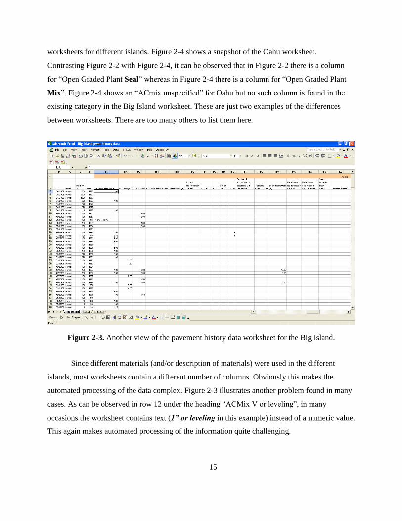
15

worksheets for different islands. Figure 2-4 shows a snapshot of the Oahu worksheet.

Contrasting Figure 2-2 with Figure 2-4, it can be observed that in Figure 2-2 there is a column

for “Open Graded Plant Seal” whereas in Figure 2-4 there is a column for “Open Graded Plant

Mix”. Figure 2-4 shows an “ACmix unspecified” for Oahu but no such column is found in the

existing category in the Big Island worksheet. These are just two examples of the differences

between worksheets. There are too many others to list them here.

Figure 2-3. Another view of the pavement history data worksheet for the Big Island.

Since different materials (and/or description of materials) were used in the different

islands, most worksheets contain a different number of columns. Obviously this makes the

automated processing of the data complex. Figure 2-3 illustrates another problem found in many

cases. As can be observed in row 12 under the heading “ACMix V or leveling”, in many

occasions the worksheet contains text (1” or leveling in this example) instead of a numeric value.

This again makes automated processing of the information quite challenging.

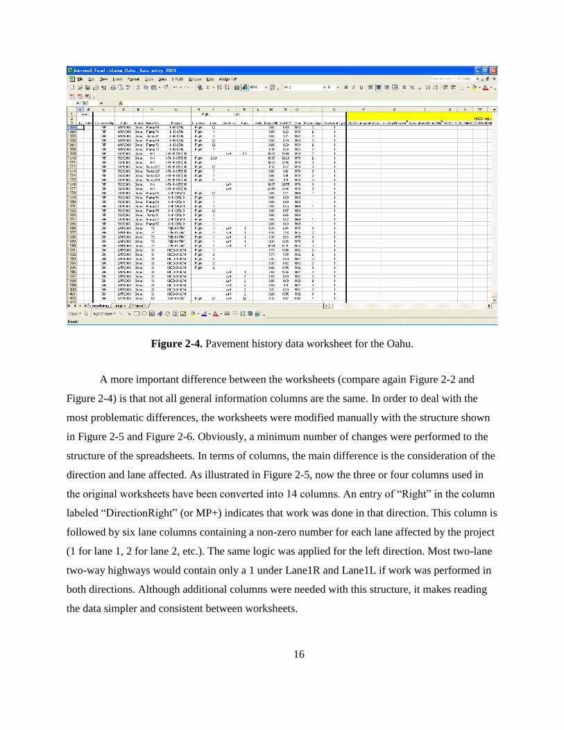
16

Figure 2-4. Pavement history data worksheet for the Oahu.

A more important difference between the worksheets (compare again Figure 2-2 and

Figure 2-4) is that not all general information columns are the same. In order to deal with the

most problematic differences, the worksheets were modified manually with the structure shown

in Figure 2-5 and Figure 2-6. Obviously, a minimum number of changes were performed to the

structure of the spreadsheets. In terms of columns, the main difference is the consideration of the

direction and lane affected. As illustrated in Figure 2-5, now the three or four columns used in

the original worksheets have been converted into 14 columns. An entry of “Right” in the column

labeled “DirectionRight” (or MP+) indicates that work was done in that direction. This column is

followed by six lane columns containing a non-zero number for each lane affected by the project

(1 for lane 1, 2 for lane 2, etc.). The same logic was applied for the left direction. Most two-lane

two-way highways would contain only a 1 under Lane1R and Lane1L if work was performed in

both directions. Although additional columns were needed with this structure, it makes reading

the data simpler and consistent between worksheets.

17

Another important modification was done to the top rows. The top-most row now

contains either a zero (nothing is also acceptable in this case) or the words “Existing”,

“Removed”, and “Added” for the different layer categories. The purpose of this modification is

to be able to discriminate the category of the layer in the column (i.e., “Existing”, “Removed”,

and “Added”) or whether the column contains other type of general information. A restriction is

that the existing layers category has to be followed by the removed layers category and this in

turn must be followed by the added layers category (that is, the order of the categories cannot be

changed). Nevertheless, the number of material types in each category can be arbitrary, which

provides significant flexibility.

Figure 2-5. Modified worksheet for pavement history for the Big Island.

Figure 2-6 provides another view of the modified spreadsheet showing some of the

existing, removed, and added layers. It also illustrates again examples of fields containing non-

numeric information.

18

In order to read the files with the PSPT, the excel file has to be exported as a comma

delimited file (CSV).

Figure 2-6. Another snapshot of the modified worksheet for pavement history for the Big Island.

It is important to note that subgrade information was not available in the recorded data;

however, this information could be added to the database over time as the information is

obtained from new projects or existing soil reports.

2.4 PAVEMENT STRUCTURE PROCESSING TOOL (PSPT)

As discussed earlier, there are many challenges that need to be overcome to process the

mined pavement structural information automatically. This section describes some of the most

important features of the Pavement Structure Processing Tool (PSPT) developed to use the

mined data to generate Historical Pavement Structural Information (HPSI), thus facilitating the

organization and interpretation of such information for the state´s Pavement Management

System.

19

2.4.1 General Layout

Figure 2-7 shows a snapshot of the main program screen, which is divided in three main

areas. On the left, a docking panel labeled “Inventory Section Selection” is located. This panel

contains three parts, identified as “Route & Direction” (for selecting a route and direction for

analysis), “Begin MP – End MP” (for selecting a mile point range for analysis from the list of

available mile points for the selected route and direction), and “Structure History” (for observing

and editing pavement structural history). Although only one of the parts is visible at a time, the

second and third panels have been overlaid in Figure 2-7 for the reader´s clarity).

On the top center of the screen there is room for a chart that shows the pavement

structural history graphically. Finally, on the top right side there is another docking panel that

contains options for the chart. A docking panel is a panel that can be docked to different

locations of the interface or be converted into a floating window. Although this is mostly a

cosmetic interface issue, it provides tremendous flexibility for the user to adopt their preferred

configuration layout.

Figure 2-7. Initial screen of the pavement structure database editor.

20

2.4.2 Importing Data

The PSPT provides a menu option for importing the pavement structure data files. After

selecting the option, the PSPT presents a standard Windows “File Open” dialog box that allows

the user to select an appropriately formatted input file (generally a comma delimited file, i.e.,

*.csv). After a confirmation message indicating that the file has been read successfully, the list of

routes will be updated with the routes imported as shown on the left panel in Figure 2-7. It must

be pointed out that this step involves a lot more than just simply reading the data file. In fact,

after reading the file, the information is sorted by route, then by direction within a route, then by

lane and finally, the information for the lane is segmented into sections with unique pavement

structural history. The segmentation for each route involves creating a list with “begin” and

“end” mile points for all the M&R and reconstruction projects related to the route (including all

lanes), sorting the mile points, eliminating all the duplicates, and then creating the segments.

The reconstruction of the pavement history is done on the fly when the user selects a

route and, within a route, a section between two mile points. Initially, no route is selected in the

list of routes. After selecting a route from the list and a direction to be analyzed from the radio

buttons at the bottom of the pane (as shown in Figure 2-7), a list of subsections available for the

route is created under the pane labeled “Begin MP – End MP”, as indicated in the left overlay in

Figure 2-7 (when the PSPT is running, activating the “Begin MP – End MP” information will

hide the list of routes).

Once the user clicks on a given “subsection”, the pavement structural history is created

on the fly based on the input information and is immediately displayed in the chart. Figure 2-8

displays the chart together with the “Structure History” pane (described later) instead of the

“Begin MP – End MP” pane (note that before selecting a subsection the chart would not be

visible). The material for each layer is displayed on the chart legend (upper corner in the right);

while the thicknesses are displayed in the data labels on each layer in whatever units were used

in the input file (inches in the examples discussed here.) The chart also displays a title with the

information for the route, direction, and begin- and end-mile points. Options for two- and three-

dimensional charts are provided as well as tooltips describing the layer names (the latter feature

being very useful when many layers appear on the legend).

21

Figure 2-8. Structure history pane and pavement structural history chart.

The “Structure History” pane displays the details of the recreated pavement structure

history (Figure 2-8). The subsection´s general information is presented at the top of the pane

(essentially the same information presented in the chart title), followed by a set of tabs created on

the fly for each year in which an M&R or reconstruction activity occurred.

Each tab contains a grid with the pavement structural information. Except for the layer

number, which is automatically assigned, all other fields are editable by the user. Notice that the

program produces an automated ordering of the layers based on some engineering common sense

rules involving a large number of substring comparisons to produce a logical ordering.

However, the ordering is produced for each year. That is, layers from different years are not

interchanged since that would produce an illogical chronological ordering. For example, in

Figure 2-8 the layer with Mix Type IV, which was constructed in 1996, is correctly shown above

the layers with Mix Type V that were created in previous years. If these same materials had been

used in the same year, the ordering would have been reversed since Mix Type V has a smaller

nominal maximum aggregate size (NMAS) than Mix Type IV, and it would be logical that a mix

with smaller NMAS be used as a surface course on top of a coarser asphalt mixture.

22

The position of the structure for each year with respect to the top of the chart also

deserves explanation. In order to explain the process, the concept of a reconstruction sequence is

introduced. A reconstruction sequence starts with a year corresponding to either new

construction or reconstruction of a pavement section and ends in the last recorded year before

another reconstruction occurs. Consider for example the case in Figure 2-8. According to the

existing records, that section was first constructed in 1949 with only 1.5 in. of AC Mix III (no

information for lower layers is available). Since the section was then reconstructed in 1969, the

first reconstruction sequence consists only of year 1949 (that is the last year with an activity

before a new reconstruction.) To date, there is no record of other reconstruction of that section;

consequently the second sequence includes all recorded years since 1969, that is, 1969, 1977,

and 1996. It is now relatively simple to explain the positioning of the layers in the chart. For a

given reconstruction sequence, the top of the thickest pavement section is arbitrarily located at

the zero depth whereas the top of the layers for the other years in the sequence are located so that

the position of the layers appearing in several years are the same for all years in the sequence.

Thus, in the example, the thickest pavement structure in the first sequence is the only pavement

structure in that sequence, that is, the one for 1949; so its top is located at zero depth. However,

the thickest structure for the second sequence occurs in 1996 and thus the top of the structure for

that year is located at the zero depth. It is clearly seen in the figure how the other layers align in

previous years. This allows the appreciation of the changes in grade occurring over time due to

overlays. Unfortunately, there is no information in the file for determining the relative grade

when reconstruction occurs, and therefore, jumps like the one shown in Figure 2-8 that are

clearly related to reconstructions should not be interpreted as changes in grade (it simply shows

that there is no information indicating the relative grade before and after the reconstruction).

Notice that in this particular example it is possible that the 1.5 in AC Mix III layers shown for

1949 and 1969 had the same grade but there is really no way of knowing this from the

information provided.

2.4.3 Editing Options

As shown before, the program is able to distinguish between reconstructions (in which

case the information from previous years is not carried forward) and overlays (in which case the

23

information from previous years is used to recreate the pavement structure when information for

existing layers is not present). However, there are occasions where the user may need to make

some changes. This section describes some features that have been added for editing the

pavement structure information.

Figure 2-9 shows a case in which the history recreation may be dubious. As shown in the

figure, a 3-in asphalt Macadam surface course on top of a 6-in stone base course was built in

1930. Then, based on the information in the input file the pavement was rehabilitated by

constructing on top of the existing structure a 6-in aggregate base (AB) and a 2-in AC Mix V.

However, although possible, the raising of the grade at once by 8 inches raises doubts of whether

the information in the input file is correct. Furthermore, it is unlikely that the aggregate base

would have been laid out directly on top of a bound material. In addition, the similarities of the

added and existing structures may also raise some concern. In fact, for this section the original

information was not entirely appropriate. This project corresponds to a selective widening as

shown in the comment section below the grids under the “Years” label in Figure 2-9.

Figure 2-9. Case where history may be dubious.

In this particular example the comment also provided the information that for this project

no new structure was added to the original section. However it must be pointed out that in this

24

particular case this part of the comment was added by the authors during a rapid check of the

plans. The point is that even if this part of the comment had not been present, a simple analysis

like the one presented above could prompt the user to double check the information in the as-

built plans. In this case, since it is known that the structure is basically unchanged, either the new

layer information or the existing layer information must be deleted and/or modified. Notice also

that apparently, the whole structure was completed in two consecutive years. Several options are

provided to make changes relatively simple. First note that the values in the grid can be edited by

simply selecting a cell and start typing the new values (standard rules, such as pressing “F2” to

start editing the information in the cell also work.)

Another option is to right click on a row that needs modification. As shown in Figure

2-10 several options are presented to the user. The selected layer can be moved up (this option

will not be active if the selected layer is the top layer), moved down (not active if the selected

layer is the bottom layer as shown in the figure), and deleted. In addition, another empty line can

be added above or below the selected layer. Added lines should then be edited to add meaningful

information.

Clearly, as illustrated in this case, the deleted layers in 1975 also need to be deleted in

subsequent years. This could become tedious and repetitive for the user if the information

propagates to several subsequent years. Thus, in order to avoid repetitive work the program

recognizes that when the user chooses to delete or move a layer in a given year, it wants to do so

in the following years as well (note that the layer information in years prior to the selected one

will not be altered). Of course, in order for a layer to be deleted or moved in several years at

once, it is required that all the layer information (except for the layer number) be identical in

subsequent years, and the layer must be in the same place with respect to the layer used as

alignment reference (only the first matching layer is used for layer alignment). It is important to

note that the layer information may not match up exactly if the user has previously edited the

information in one year.

Suppose that in the current example, the user decided to delete the 6-in stone base course

and the 3-in asphalt Macadam surface course in 1975; these two layers would also need to be

25

deleted in 1976. Figure 2-10 shows the resulting structure with those two deletions in 1975 (done

automatically by the program).

Since the HDOT may wish to standardize the layer descriptions (for example, eliminating

the “(in)” from the descriptions or combining different names that describe similar materials), a

last editing option “Select Layer Description” is provided in a pop-up menu that appears when

the user clicks a row on the “Description” column. Notice that a new option for selecting a layer

description is given at the bottom of the list. When clicked, a list with standardized names is

displayed (lower right corner of Figure 2-10). At this point, this list contains a few names just for

testing, but HDOT should develop a more comprehensive list containing most cases of interest.

Selecting a layer description from the list and pressing the OK button changes the description to

the selected standardized name.

Figure 2-10. Pavement structure after deletion operation and editing options.

When the input file contains non-numeric information in places where numeric

information is expected, this information is appended to the comments of the project by adding

three pieces of information: the first is the layer type, which is taken from the heading of the cell

where information is found; the second, labeled “Other info”, is the information found on the cell

26

being read from the input file (particularly useful when it contains some information about likely

thickness); and the third is the project number.

Whenever numeric information is provided for removed layers in the input files, this

information is taken into account automatically. Figure 2-11 shows an example in which the top

2-in of the existing layers built in 1969 are milled before being overlaid in 1990 with 2.5-in of

asphalt concrete base and 3.5-in of Mix Type IV.

Figure 2-11. Automatic handling of partially removed layers.

2.4.4 Pavement Structure Processing Tool (PSPT) Potential Improvements

Although the current version of the PSPT is already operational and can greatly reduce

time and effort in generating HPSI for the entire state´s road network, there are some areas that

need to be enhanced and further developed in order to serve its purpose in a broader way. Some

of the desired features include:

Provision of the capability for saving the changes performed by the user in a

permanent and carefully designed database.

Ability to make the number of sections more easily manageable.

27

Ability to identify and correct small errors in the locations of the “begin” or “end”

mile points of some sections while importing data, as they lead to the creation of non-

existing small sections. It would be desirable for the PSPT to be able to analyze a

significant number of sections on a given route for all lanes and directions

simultaneously, allowing the user to make decisions about sectioning the network

based on pavement structure.

Ability to create and export HPSI in formats that can readily be used in commercially

available PMS software.

Integration of HPSI with other geometric and traffic information.

Development of a process to perform periodic updates of the database without unduly

significant effort.

2.5 DISCUSSION AND SUMMARY

The existence and success of a PMS relies on the information contained in a properly

designed database with different types of data from the road network. An important piece of

information is the Historical Pavement Structural Information (HPSI). Although the process of

reconstructing the pavement structural history is in principle simple for a given road segment,

several challenges need to be overcome to simplify the task and make it practical at the network

level.

In order to generate the HPSI from as-built plans and visual surveys already available in

the Hawaii Department of Transportation, a Pavement Structure Processing Tool (PSPT) was

developed. With the PSPT, a sound basis for rational sectioning of the State of Hawaii pavement

network can be established, which is fundamental in the development of deterioration models

that rely on the similarity between sections to define families of pavements with similar

deterioration processes.

The reconstruction of the HPSI obtained with the Pavement Structure Processing Tool

(PSPT) also provides a basis for the analysis of the historical distributions of times between

maintenance and rehabilitation activities (M&R) and reconstructions for different types of

pavements, which can be useful for monitoring actual practices within the agency, for analyzing

28

potential M&R policy changes and for assuming realistic scenarios during Life Cycle Cost

Analyses (LCCA). HPSI could also be useful for interpretation of Ground Penetrating Radar

(GPR) surveys since it could assist in the understanding of the layering that may have been

created over time with consecutive overlay and/or mill-and-overlay activities, and also provide

some information of unbound layers that may not be known without coring. Additionally, the

PSPT could also be helpful for the agency in fulfilling the Highway Performance Monitoring

System (HPMS) reporting requirements, which now include pavement structural information.

Although there is significant room for improvements in future versions of the PSPT, its

current version can greatly reduce time and effort in generating HPSI for Hawaii´s road network.

29

TRAFFIC LOADING ANALYSIS

3.1 INTRODUCTION

Traffic loading information is essential for any pavement design procedure; yet, it is often

difficult to characterize accurately. Traffic loads, primarily those of heavy vehicles, cause

stresses/strains in pavement structures whose effects accumulate over time resulting in pavement

deterioration such as plastic deformation in Hot Mix Asphalt (HMA), fatigue cracking in HMA

and Portland Cement Concrete (PCC), and faulting in PCC.

This chapter presents the development of some traffic inputs required by the design

procedures using information from Weigh-In-Motion (WIM) and Automated Vehicle

Classification (AVC) stations located across the state.

3.2 USE OF TRAFFIC LOADING DATA IN PAVEMENT DESIGN

Traffic loading data are typically available for different heavy vehicle classes.

Classification of heavy vehicles is typically done following the Federal Highway Administration

(FHWA) 13 vehicle classes. Figure 3-1 shows vehicle classes 4 to 13, which represent the heavy

vehicles. Vehicle classes 1, 2 and 3 represent motorcycles, autos, and four tired trucks (pick-

ups), respectively and their effects on pavement design are negligible.

Traffic loads and their impact on pavements are quantified primarily in terms of:

number of axles of a given configuration,

configuration of these axles, and

axle load magnitudes.

Other factors that affect pavements are:

timing of load applications (time of day and season within the year),

vehicle/axle lateral placement (wander),

vehicle/axle speed, and

tire pressure.

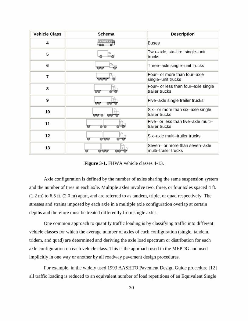
30

Figure 3-1. FHWA vehicle classes 4-13.

Axle configuration is defined by the number of axles sharing the same suspension system

and the number of tires in each axle. Multiple axles involve two, three, or four axles spaced 4 ft.

(1.2 m) to 6.5 ft. (2.0 m) apart, and are referred to as tandem, triple, or quad respectively. The

stresses and strains imposed by each axle in a multiple axle configuration overlap at certain

depths and therefore must be treated differently from single axles.

One common approach to quantify traffic loading is by classifying traffic into different

vehicle classes for which the average number of axles of each configuration (single, tandem,

tridem, and quad) are determined and deriving the axle load spectrum or distribution for each

axle configuration on each vehicle class. This is the approach used in the MEPDG and used

implicitly in one way or another by all roadway pavement design procedures.

For example, in the widely used 1993 AASHTO Pavement Design Guide procedure [12]

all traffic loading is reduced to an equivalent number of load repetitions of an Equivalent Single

FHWA Commercial Vehicle Classification

Vehicle Class Schema Description

4

Buses

5

Two–axle, six–tire, single–unit trucks

6

Three–axle single–unit trucks

7

Four– or more than four–axle single–unit trucks

8

Four– or less than four–axle single trailer trucks

9

Five–axle single trailer trucks

10

Six– or more than six–axle single trailer trucks

11

Five– or less than five–axle multi–trailer trucks

12

Six–axle multi–trailer trucks

13

Seven– or more than seven–axle multi–trailer trucks

31

Axle Load (ESAL) of 18,000 lb. In order to find that single number of ESALs, the number of

repetitions expected over the design period of each axle configuration within a load interval of

the spectrum is multiplied by a Load Equivalency Factor (LEF) appropriate for the axle

configuration/load interval combination. The LEF transforms the number of applications of the

axle configuration in the particular load interval into an equivalent number of repetitions of the

standard single axle load that would have the same effect on the pavement structure. The total

number of ESALs over the design period is then obtained by adding the contributions of each

axle configuration/load interval combination for each vehicle class over the design period.

The axle load spectrum for a given axle configuration (single, tandem, tridem, or quad) of

a particular vehicle class (4, 5, .., or 13) is defined by the percentage of the total axle applications

of the axle configuration in the particular vehicle class that fall within the particular load interval.

The definition of load intervals typically used is provided below:

Single axles – 0 to 3 kips, 3 to 4 kips,…, 39 to 40 kips (beyond 3 kips, the intervals

are of 1 kip).

Tandem axles – 0 to 6 kips, 6 to 8 kips,…, 78 to 80 kips (beyond 6 kips, the intervals

are of 2 kips).

Tridem and quad axles – 0 to 15 kips, 15 to 18 kips,…, 99 to 102 kips (beyond 15

kips, the intervals are of 3 kips).

As can be seen, computation of ESALs requires knowledge of the axle load spectrum of

each axle configuration of each vehicle class. In addition, the percentage of heavy vehicles

(commonly referred to as trucks although they include buses) in the traffic stream as well as the

percentage of each heavy vehicle class relative to the total of heavy vehicles are also needed.

Since basic traffic information typically available includes the Annual Average Daily Traffic

(AADT) or Annual Average Daily Truck Traffic (AADTT = AADT x percentage of trucks) in

both directions, a directional distribution factor as well as a lane distribution factor for multilane

facilities in one direction are also needed. Of course, traffic growth factors are also required to

properly quantify traffic over the design life.

32

3.2.1 Truck Factor

Historically, dealing with traffic loading spectra (and in turn with load equivalency

factors for each axle configuration/interval) was cumbersome for routine pavement design.

Therefore, the calculations were typically simplified using the concept of a truck factor (TF). The

TF for a given vehicle class represents the average number of ESALs applied by one passage of

the vehicle class in question. To illustrate, consider a semi-trailer truck with a single steering

axle of 12,000 lb. and LEF = 0.19 and two tandem axles each with 34,000 lbs. and LEF = 1.10.

Thus, for this hypothetical truck, the TF is simply computed as 0.19 + 1.10 +1.10 = 2.39 ESALs.

Of course, for real highway traffic, each passage of the same truck class would most likely have

different loads for the single and the tandem axles. Thus, the TF is derived by using axle load

distributions of the single and tandem axles on the vehicle class to compute the total number of

ESALs applied by a large sample of that truck and diving it by the corresponding number of

trucks in the sample. This is a calculation that is done only once in a while for a given WIM

station or stations in a region. When this TF is then used in a particular project, the implicit

assumption is that the axle load distributions at the design site are the same as those used to

obtain the truck factor.

3.2.2 ESALC or ESAL Constants

Computation of ESALs in the HDOT design procedure relies on a factor called ESALC

or ESAL Constant. The ESALC is simply the TF multiplied by 365. In other words, the value of

the ESALC represents the average number of ESALS contributed by one passage of the truck in

question on every day of the year. The only difference in the calculation of ESALs with the use

of TF or ESALC is that for the TF the value of 365 has to be used explicitly in the calculations to

convert daily loading calculations into annual calculations whereas the 365 factor is already

embedded in the ESALC.

3.3 MEPDG TRAFFIC LOADING INFORMATION REQUIREMENTS

Traffic loading information is used by the MEPDG to estimate the strains induced by the

different traffic loads and the frequency with which those strains are induced throughout the

pavement’s design life. As for other inputs in the MEPDG, traffic loading can be characterized

33

using a hierarchical approach that allows using better information for important projects and

default values for smaller projects. This is done to facilitate the use of the MEPDG regardless of

the level of detail of available traffic data. The MEPDG defines three broad levels of traffic data

input (Levels 1 through 3) based on how well future truck traffic characteristics can be estimated.

The three levels are defined in the MEPDG as:

Level 1 – There is very good knowledge of past and future traffic characteristics.

Level 2 – There is modest knowledge of past and future traffic characteristics.

Level 3 – There is poor knowledge of past and future traffic characteristics.

For Level 1, the traffic data measured at or near a site must include counting and

classifying the number of trucks traveling over the roadway, along with the breakdown by lane

and direction, and measuring the axle loads for each class to determine the truck traffic for the

first year after construction.

Level 2 requires the collection of enough truck volume information at a site to measure

truck volumes accurately. This includes being able to account for any weekday/weekend volume

variation, and any significant seasonal trends in truck loads (e.g., in areas affected by heavy,

seasonal, agricultural hauls).

Level 3 uses a regional or statewide average load distribution (or other default

distribution table).

The MEPDG requires some basic traffic (or traffic related) input data, including:

Initial two-way Annual Average Daily Truck Traffic (AADTT).

Number of lanes in the design direction.

Percent of trucks in the design direction (directional distribution factor).

Percent of trucks in the design lane (lane distribution factor).

Operational speed.

Vehicle class distribution and growth.

All these factors are site specific and should be estimated for each particular project. For

HDOT projects, AADTT (or AADT and percentage of trucks), (heavy) vehicle class distribution,

34

and an overall traffic growth factor are typically furnished by the HDOT Planning Branch.

Operational speed can be estimated from speed limits or reasonable estimates for roadways with

recurrent congestion and/or traffic signals. For the percent of trucks in the design direction,

except for special situations, the assumption of the 2002 HDOT Pavement Design Manual [13]

of 50% on each direction is still reasonable.

Currently, the most problematic parameter is the percentage of trucks in the design lane.

The 2002 Pavement Design Manual [13] assumes 100% for 2 lanes in one direction, 80% for 3

lanes in one direction and 75% for 4 lanes in one direction. These values appear to be very

conservative. Values of percentage of trucks in the design lane based on the most recent WIM

and AVC measurements are presented with the analysis of WIM data later in this chapter.

Developing an estimate of vehicle operational speed is important for flexible pavement

design using the MEPDG. As discussed later in section 6.2, frequency of loading (or

equivalently the duration of the stress pulse or load duration) directly influences the stiffness

response of the asphalt concrete layers within the pavement structure. The magnitude and

duration of the stress pulses caused by the passage of a load depend on the vehicle speed, type,

and geometry of the pavement structure, and the location of the element under consideration.

Thus, the speed of the vehicle can result in a different load frequency, resulting in different

moduli values for the HMA layers.

In addition to the basic information, the MEPDG requires the following inputs:

Traffic volume adjustment factors.

o Monthly adjustment.

o Vehicle class distribution.

o Hourly truck distribution.

o Traffic growth factors.

Axle load distribution factors.

General traffic inputs

o Number axles/trucks.

o Axle configuration.

o Wheel base.

35

Obviously, to be practical, only a few of the inputs can be project specific. The following

sections describe the efforts to determine the most important of these inputs for Hawaiian

conditions that can be used for different roads throughout the State.

3.4 ANALYSIS OF HAWAIIAN WEIGH-IN-MOTION DATA

This section describes the analysis of data from the weigh-in-motion (WIM) stations

located throughout the State. The analysis is based on millions of heavy vehicle records from 11

Weigh-In-Motion (WIM) and Automatic Vehicle Classification (AVC) stations located on the

islands of Hawaii (2 stations), Maui (1 station), and Oahu (8 stations). The data used for the

analysis were collected by the HDOT Planning Branch from 2006 to 2012 (though a variable

number of years with valid data were available for the different stations). Figure 3-2 shows the

locations of all the stations and Figure 3-3 shows the stations in Oahu only.

Figure 3-2. Locations of WIM stations as of 2012 in Hawaii.

36

Figure 3-3. Location of WIM stations as of 2012 in the island of Oahu.

The emphasis of the analysis is on those factors that are routinely required for pavement

design but that are not easy to characterize for each single project. Specifically, the analysis

concentrates on the factors needed for the characterization of the axle load spectra (axle load

weight distributions) for the new MEPDG design procedures (which are also useful in the HDOT

design procedure for new rigid pavements) and in the update of the ESAL Constants (ESALC)

used in the HDOT design procedures for new flexible pavements (the ESALC are based on the

axle weight distributions).

3.4.1 Tools used to analyze the WIM data

As described in reference [14], there are several primary causes for obtaining invalid data

from WIM stations, including: system component malfunctions, loop timeouts, weight sensor

thresholds, classification algorithms, calibration factors, rough pavement, roadway geometry,

congestion, lane closeure and alignment shift, lane changing while crossing sensors, and weather

related factors. Consequently, several data quality check procedures are recommened to be

followed by an agency’s WIM Office Data Analyst [14].

37

This section is limited to the processing of the data obtained from the WIM stations in

Hawaii as obtained from files of type “wgt” defined in the TMG [15]. The files were provided by

HDOT’s Plannning Branch. The analyses in the following sections pertain to issues observed

from the data provided and do not include other aspects that may have been performed prior to

the generation of the “wgt” files.

Given the voluminous amount of information generated by WIM stations, it is imperative

to use software to process the data. For this purpose, three different tools were used throughout

the project: TrafLoad [16], PrepME, and a third tool developed by the PI.

3.4.2 TrafLoad

TrafLoad is a product of NCHRP Project 1-39, “Traffic Data Collection, Analysis, and

Forecasting for Mechanistic Pavement Design” [16]. It was the first tool selected for analysis of

the WIM data because its output could be used directly with the MEPDG and because of its use

of rigorous data quality control checks. The program uses a rational approach to weigh

observations based on well documented procedures [16] and the software is free. TrafLoad

assumes that all input data have already been quality checked.

Unfortunately, while working on an interim report for this project, it was found that its

use was quite cumbersome. Often, one would obtain non-informative error messages such as the

one depicted in Figure 3-4, which even for someone with familiarity Structured Query Language

(SQL) queries may be too cryptic to find out what the problem is and how to resolve it.

38

Figure 3-4. Non-informative TrafLoad error message.

Although with effort many of these issues were overcome, it was also found that on some

occasions some of the output was questionable, thus also making suspicious the use of other

outputs from TrafLoad. Figure 3-5 illustrates one of these problems. The figure shows an

example of TrafLoad output with the estimated average number of single, tandem, tridem, and

quad axles for each vehicle class. Three shaded rectangles have been added to highlight the

problem. The rectangle closest to the top of the figure highlights the problems that were found

with the estimation of the number of axles per vehicle for vehicle classes 4 and 5. By definition

(see Figure 3-1), vehicle class 5 must have two single axles. Also, most class 4 vehicles (buses)

have two single axles although some may have one single axle and one tandem axle (and some

other combinations are possible for articulated buses.) Nevertheless, the average number of

single axles is typically close but lower than 2. As can be seen, the predicted average of single

axles for vehicle classes 4 and 5 were 3.78 and 3.99 in this example (which are essentially twice

what was expected.) Similarly, for vehicle class 6, the estimated values of 2 singles and 2

tandems were double of what is correct for this class of truck (this is highlighted by the second

shaded rectangle). A similar observation can be made for vehicle class 9, whose averages should

be close to 1 single and 2 tandems. As can be seen in the last rectangle, once again the values

were twice as expected. The most puzzling aspect of this error is that it occurred for only some

39

stations. It is recognized that some of these problems may have originated by lack of familiarity

with the program and questionable input data. However, in that case, the program should have

generated appropriate warnings instead of producing unreasonable output.

Figure 3-5. TrafLoad problematic output.

As mentioned before, TrafLoad uses rigorous quality controls. While this is a strength, at

the time the analysis with this program was performed some of the requirements appeared too

restrictive. Specifically, in order to be able to derive axle load spectra, TrafLoad requires a

minimum of 1 week of classification counts for 12 consecutive months. This requirement meant

that some stations with almost continuous data for 11 months could not be used. At that time,

most stations had one month (typically December) without data. Therefore, even though for most

months there were data for most of the days in the month (and typically in more than one year),

that data could not be used to derive the axle load spectra.

At the time the first analysis was performed, it was considered that a better alternative

was needed instead of using standard axle loadings from some other locations, thus discarding

some substantial local traffic loading information with potentially acceptable quality. The

rationale was that it was better to derive the axle load spectra for those months with good data

and interpolate from them for the other months than using data from other locations. Any

potential biases in the months with interpolated values are probably smaller than what one would

get from using values from other locations. As will be seen later, the data collected during the

last few years has confirmed the similarities between the different monthly axle load spectra.

40

3.4.3 Analysis with the customized traffic loading analysis tool and Prep-ME

Because of the issues described in the previous paragraphs, the PI developed a program

to estimate the axle load spectra for each axle configuration, the average number of axles by axle

type for each vehicle category, and the percentage of trucks on each lane (by vehicle class).

Since the program logic is relatively simple, it is important to feed it with information from

months with balanced numbers of the different days of the week to avoid biasing the

distributions. Considering that most of the data selected contained information for almost the

complete month, day of the week effects in the generated distributions should be minor.

More recently, the PI was also asked to represent HDOT in a pool fund study led by Dr.

Kelvin Wang at the University of Oklahoma, which is developing a program named Prep-ME to

prepare data for use with the MEPDG. Fortunately, the PI was able to use a beta version of Prep-

ME to perform some quality checks, discard months with problematic data, and visually check

that there were no significant differences between the distributions generated by the two

programs. This was important as the axle load spectra used in the calibration efforts of the

MEPDG were generated by the author’s program in part for convenience and in part because

Prep-ME could not generate the axle load spectra by direction at the time it was used (the latest

release of PrepME also permits the analysis by direction.) The following paragraphs describe

some of the analyses performed with the beta version of Prep-ME and the in-house traffic

loading analysis tool and discuss some characteristics of the axle load spectra for the HDOT’s

WIM stations.

3.4.3.1 Analyses with Prep-ME

Prep-ME uses data checks from the Traffic Monitoring Guide [15]. First, it checks the

front and drive axle weights of Class 9 trucks. The peaks of the distributions are expected to be

between 8,000 and 12,000 lb. for the front axles and between 30,000 and 36,000 lb. for the drive

tandem axles. Second, Prep-ME also checks gross vehicle weights (GVW). The GVW check is

based on the observation that most sites have two peaks in the GVW distribution. The first peak

typically occurs between 28,000 and 36,000 lb., representing unloaded tractor semitrailers [15].

The second peak in the GVW distribution corresponds to the most commonly loaded vehicle

41

condition and it falls somewhere between 72,000 lb. and 80,000 lb., although it may vary with

the type of commodities transported.

In Prep-ME, the tolerable ranges on which the above peaks are expected to fall can be

increased with a relaxation multiplier that ranges between 1 and 2. As shown in the box labeled

“Not accepted” in Figure 3-6, most of the Hawaii WIM stations did not pass all the initial

checks. Only station C202B passed all the checks2. However, after using the relaxation multiplier

for some of the requirements, some other stations could also be considered acceptable. Notice

also that the user can mark a station as “accepted” even though it did not passed all the quality

checks. This is important as the quality checks flag potential problems but they do not

necessarily indicate that the data are bad. Instead, they indicate that a more detailed analysis is

needed.

Figure 3-7 illustrates that after further analysis other stations could be moved into the

“Accepted” category. Notice that station 438 in Ala Moana Blvd. shown in Figure 3-8 is in the

accepted category in Figure 3-7 even though the same figure shows that this station failed to pass

the drive tandem axle weight check and the GVW check. It is important to note that the drive

tandem axle check in Prep-ME analyzes the relationship of the drive tandem axle weights as a

function of the GVW. This is illustrated in Figure 3-9. As can be seen in that figure, apparently

the reason why Station 438 did not pass the drive tandem axle check is that for loaded trucks ( >

72 kips GVW) the axle weights were slightly higher than the limit resulting from application of

the relaxation multiplier to the normal range. As for the GVW, apparently the program does not

identify the 2nd peak for some months of the year for this station. However, stations displaying

no loaded GVW peak or a very mild one like in this case are not uncommon. This is apparently

the case for several of the Hawaiian Stations. A possible explanation for this phenomenon is that

given the generally shorter trip lengths in Hawaii, there may be a higher than normal proportion

of trips with trucks not fully loaded and with trucks carrying very heavy loads (a justification of

why the latter is believed to be observed, as opposed to having a WIM calibration problem, is

2 In the figure, station C202B is listed as 92029 since at the time of the analysis Prep-ME only accepted

numeric station identifications.

42

provided shortly). Both, a higher proportion of partially loaded and very heavily loaded trucks

would have the effect of flattening or even eliminating the second peak. Furthermore, trucks

with intermediate loading may also explain some of the shifting of the first peak to the right. Of

course, it may also be the case the WIM station is out of calibration.

Figure 3-6. Initial quality checks with Prep-ME.

43

Figure 3-7. Increasing the relaxation multiplier moves more stations into the accepted category.

Figure 3-8. Location of sensors at Station 438 in Ala Moana Blvd.

44

Figure 3-9. Drive Tandem Axle Check as a function of GVW.

Since Prep-ME was available for evaluation during a relatively short interval of time and

there was a need to further analyze some issues that were detected for vehicle classes other 9, the

rest of the analysis was performed with the PI customized program.3

3.4.3.2 Analyses with a customized traffic loading analysis tool

Although Prep-ME was extremely useful to analyze the State WIM data, its evaluation

was limited to a relative short period of time. For this project, it was not possible to wait for a

newer version with several improvements to obtain Axle Load Spectra (ALS). At the time the

analyses were performed, Prep-ME did not have the capability to produce axle load spectra by

direction. However, previous analyses with TrafLoad and a first version of a customized

program developed by the PI showed that some of the Hawaiian stations had significantly

different loading patterns for each direction of travel. Furthermore, as explained below, several

3 A new release of Prep-ME is already available for evaluation but there was no time for testing it before

completing this report.

45

other issues, particular for other vehicle classes were also discovered in the data. Therefore, the

program initially developed by the PI was further modified and used for the analyses presented

in this section. Basically, the customized program (in reality, three programs with different

capabilities were used although they are referred here as a single program) obtains the axle load

spectra on a monthly basis from the raw “wgt” data files. The program also allows the

calculation of the distributions of GVW by vehicle class and month, the distributions of the front

axle by vehicle class and month, the distribution of the drive tandem axle by vehicle class (for

those with such axles) and month, and the percentages of vehicle class by lane for each WIM

Station. The customized program essentially counts the number of axles in each axle weight bin

for each combination of station, direction, year, month, vehicle class, and axle type. The criteria

used for discriminating between single, tandem, tridem, and quad axles are:

Single axle: single axle spaced at least 2.4 meters (8 ft.) from another axle (steering

axles are also counted as single axles even if their spacing to the next axle is less than

2.4 meters).

Tandem axle: two axles spanning no more than 2.4 meters (8 ft.).

Tridem axle: three axles spanning no more than 3 meters (10 ft.).

Quad axle: four axles spanning no more than 3.8 meters (12.5 ft.).

The program also allows the visualization of the axle load distributions for each axle

type and vehicle class combination by plotting the corresponding histograms in three

dimensional charts (with month of the year as the third dimension). Figure 3-10 shows an

example of such a chart for Station 438, vehicle class 9, and tandem axles. A rotation capability

and the ability to select which months the user wants displayed further help in the visualization

of the distributions and the analysis of problems in the data. Moreover, tooltips are provided for

each bar of the histogram when the user hovers the mouse arrow over it so that it is clear what

load range and what percentage the bar represents

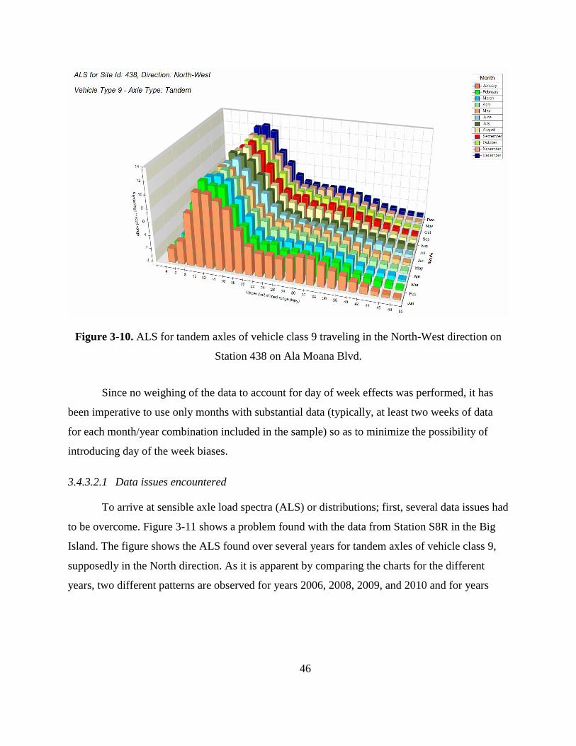
46

Figure 3-10. ALS for tandem axles of vehicle class 9 traveling in the North-West direction on

Station 438 on Ala Moana Blvd.

Since no weighing of the data to account for day of week effects was performed, it has

been imperative to use only months with substantial data (typically, at least two weeks of data

for each month/year combination included in the sample) so as to minimize the possibility of

introducing day of the week biases.

3.4.3.2.1 Data issues encountered

To arrive at sensible axle load spectra (ALS) or distributions; first, several data issues had

to be overcome. Figure 3-11 shows a problem found with the data from Station S8R in the Big

Island. The figure shows the ALS found over several years for tandem axles of vehicle class 9,

supposedly in the North direction. As it is apparent by comparing the charts for the different

years, two different patterns are observed for years 2006, 2008, 2009, and 2010 and for years

47

2007, 2011, and 20124. Aside from other data issues, it is clear that the patterns between the two

sets of years are strikingly different. A similar set of charts for the opposite direction showed that

the same patterns displayed for each year are reversed. This implies that some coding error was

intruced into the “wgt” files. The problem is relatively easy to visualize graphically but one

needs to be looking for the differences across years. Blind automatic processing of the data may

result in a totally unrealistic distribution for either direction. Also, notice how the histograms for

2008 exhibit peaks at higher load ranges when compared to the similar distributions in 2006 and

2009. In fact, both peaks for the first seven months in 2008 (around 36,000 to 40,000 lb for the

unloaded peak and 80,000 to 84,000 lb for the loaded peak) are higher than normal, which may

indicate that the WIM station may have been out of calibration for those months. This case is

known as the “Two Peaks Shifted” case.

The previous example shows that with the use of the ALS charts or GVW distribution

charts, it is relatively simple to spot years with invalid or problematic data. This is further

illustrated in Figure 3-12, which shows inconsistent distributions throughout the year unlikely to

be attributed to seasonal changes. The main challenge in these cases was to decide whether there

were any valid data or whether all data should be discarded for that particular year. This was

typically performed by several means, including observing the distributions for GVW, front and

drive tandem axles on each year, observing if there were shifts of the distributions for a given

axle/vehicle class combination or GVW across years, and observing whether any shifts in the

distributions within a given year for a given axle/vehicle class combination or GVW were

repeated for different vehicle classes and axle types on the same year. After all, the purpose of

summarizing the information monthly is to capture any seasonal changes in the axle weight

distributions. Thus, differences across months do not necessarily mean there are problems in the

4 The chart for 2010 is not shown since it only had three months of valid data. However, the pattern for

those three month was similar to those of years 2006, 2008, and 2009. After this problem was brought up to the

attention of HDOT personnel, the information for the additional months was also provided after downloading it with

FHWA’s software TMAS 2.0. At some point, the directions had been corrected for years 2008, 2009, and 2010

although it is not known to the PI when and where those coding changes occur. Now the data from 2007 to 2012 and

the first five months of 2013 are all consistent. The heavier loading for this station occurs in the South direction.

48

data. It may well be due to changes in the type/volumes of commodities being transported on a

given roadway. The reason for looking for shiftings that are common across vehicle classes on a

given year is that seasonal changes in commodity volumes more likely affect some vehicle

classes more than others. In particular, there may not be many reasons for changes in bus weights

and vehicle class 9 weights to be highly correlated. For the Hawaii data, when shiftings in the

distributions in a given year and for a given vehicle class were observed, similar shifts were

observed in the distributions for other vehicle classes as well, indicating a likely calibration

problem with the WIM station.

Figure 3-13 illustrates the above problem with GVW data for station 10W in 2006. From

the months with usable data, it can be seen that in June of that year the GVW distributions for

vehicle class 9 shifted to the left slightly. The same shift can also be observed for buses (vehicle

class 4) as shown in Figure 3-14. Thus, one is led to believe that this is more likely a

consequence of a small adjustment in the WIM calibration parameters than any real change in

the distributions. Whether some data should be retained or discarded in a case like this one is not

always easy to determine. In this case, the before and after distributions show parameters within

normal ranges. In many other situations, however, such changes pointed out to cases where the

peaks of the distributions were unreasonable.

As indicated earlier, the customized program was modified to derive front and drive

tandem axle distributions. These were useful to assess the location of the peaks of the

distributions. For many of the stations, the peaks were located slightly higher than normal.

However, considering also that for many of those stations there were several years of data

available and that the stations are regularly calibrated, it could not be always concluded that the

corresponding data were erroneous. A thorough freight study is required to determine if and why

the loads are higher than normal for some of these stations. Nevertheless, as discussed in the

following paragraphs, a significant effort was made to differentiate situations with higher than

normal loading from those with calibration problems.

49

a) Year 2006 b) Year 2007 c) Year 2008

d) Year 2009 e) Year 2011 f) Year 2012

Figure 3-11. Potential data coding errors in the direction field for station S8R.

50

Figure 3-12. Example where identification of problematic data was relatively simple.

Figure 3-13. Example of a shift to the left in the GVW distributions due to a possible calibration

adjustment.

51

Figure 3-14. Shift in the GVW distributions for buses mimicking the shift observed for vehicle

class 9 trucks of Figure 3-13.

The capability of deriving the front axle load distributions for a given vehicle class, as

opposed to the distribution of all single axles, was useful because as expected it shows narrower

distributions with better defined peaks and less noisy tails. Figure 3-15 provides an example. The

same advantage can be noted for the difference in the distributions between drive tandem axles

and all tandem axles for a given vehicle class with such axles.

As expected, the differences between the distributions for front and all single axles for

vehicle class 9 are generally minor since this vehicle class generally has a single front axle and

two tandems. The additional singles are generally the result of tandem configurations with

separation between axles in excess of the limit to be classified as tandem. Thus, those axles will

be recorded as two singles instead of one tandem. A corollary of this is that if only vehicles of

class 9 are being analyzed, similar inferences can be obtained with both distributions (front or all

singles).

52

The discrimination of the front axle distribution is much more useful for buses than for

class 9 vehicles as the former have a substantial number of non-frontal single axles with different

loading patterns. Figure 3-16 illustrates this for Station 438 in Ala Moana Blvd. In this example,

the front axle distribution has a single peak in the 11,000 lb. to 12,000 lb. range whereas the all-

singles distribution has an additional second peak in 25,000 lb. to 26,000 lb. range.

Parenthetically, that the second peak exceeds the Hawaii limit for single axles of

22,500 lb. [17] is not surprising. First, the two most common city buses, Gillig Phantom 40’ (374

vehicles) and the 60’ articulated bus New Flyer D60LF (111 vehicles) [18] have rear gross axle

weight ratings of 25,600 lb. and 26,000 lb., respectively ( [19], [20], [21])5 and second, this

Station is located in an area of Honolulu with a combination of high volume of buses and

ridership. Thus, it would be erroneous to consider the data from this station invalid because of

the higher than normal peaks on these distributions.

The above paragraphs point out many of the issues encountered when the WIM data are

analyzed carefully. Inevitably, although the literature presents extremely valuable suggestions for

verifying the quality of the data, the application of the rules are sometimes subjective and based

on judgment on the analyst helped with knowledge of local conditions. All quality controls need

to be applied carefully as there appear to be many loading situations that do not conform to what

is considered “normal”.

It is important to point out that a few other quality control checks were imposed to the

data including the separation between the front and the first loading axle and the consistency

between the number of axles counted for a given vehicle and the class it was assigned to. For

many stations, there was a non-negligible number of separations between the front axle and the

first loading axle that were too small. It is not known the cause of the problem though for some

stations, lane changing may be a contributing factor. The information for axles with the above

problem were discarded. In other situations, based on the number of axles and their separations,

some vehicles needed to be reclassified.

5 The values reported above were obtained from public records from other agencies and are just a bit higher

than the values of 23,350 lb and 25,000 lb reported by The Bus in a survey performed for this project in 2006.

53

The following section presents the best estimates of the axle load spectra (ALS) for the

different stations across the State after applying the quality controls described in this section.

Although the quality of the data was looked at for several vehicle classes (mostly classes 4, 6,

and 9), the actual selection of the month/year combinations to include were based mostly on

vehicle class 9. As will be shown, for the most part, this resulted in acceptable ALS for other

vehicle classes as well. However, unexpectedly, in a few cases the loading distributions for other

vehicle classes showed a disproportionate number of unloaded axles. This is illustrated in Figure

3-17. The left chart in the figure shows that for the North direction of Station 10W on Kalaeloa,

the percentage of single axles with less than 3,000 lb. for the month of August (the series shown

on light yellow color) is more than 10% (actually 10.44%). For the other months, the same

weight interval had percentages varying from about 0.2% to 0.8%. Clearly, something happened

on this Station on at least one of the months of August used as input that caused that single axles

on buses were not weighed properly. This is despite the fact that the single and tandem axle

distributions for class 9 vehicles did not show any problem for any of the input months

(remember the months selected were deemed to be months with good quality data) and of course

for the resulting ALS for vehicle class 9. The ALS for vehicle class 9 for this station are

presented in the following section. Furthermore, what is even more puzzling is that the resulting

distribution for tandem axles of buses did not show the same problem whereas the distributions

for both single and tandem axles on vehicles class 6 did show the problem. In other words, the

problem may be axle/vehicle dependent. There are a few options to fix this problem. One is to

find the month contributing the problematic data, eliminate it as input and regenerate the

distribution. This of course, may have the effect of eliminating valuable data for vehicle class 9

and other vehicle classes. A second viable option for this particular case in which the monthly

distributions are so similar to each other is to simply substitute the distribution for the month of

August with the distribution of one of the other months (or an average). With the similarities of

the distributions in this example and the Hawaiian climate, this should have no practical

consequence. The last option is to eliminate or reduce the percentage for the weight category and

prorate the difference among all the other weight categories according to their percentages such

that the sum of all categories adds up to 100. This is what was actually done to correct the

54

problem. As shown in part b) of Figure 3-17, the corrected series looks practically the same as

for the other months.

3.4.3.2.2 ALS for Hawaiian WIM stations

This section briefly discusses some salient features of the ALS obtained following the

quality control checks described in the previous section. Most of the discussion is based on the

distributions of tandem axles on vehicles of class 9 although for station 438 some relevant

distributions for other vehicle classes are also presented.

As a result of the quality control process, only the data corresponding to the number of

days for each month/year shown in Table 3-1 were used to obtain the ALS for the two directions

at each WIM station. The corresponding number of weighed vehicles are provided in Table 3-2.

Providing this number is important as it helps to understand why for some vehicle classes the

distributions are not very well defined. Since there are 38 weight intervals for each month of the

year, a relatively large sample size is needed for each vehicle class to reliably define the value of

each interval, particularly those with lower frequencies. Distributions with less than 15,000

vehicles weighed in a year should be looked at with caution, particularly for those axles with

lower frequencies. For those vehicle classes that are relatively rare in the State (namely, mostly

vehicle classes 7, 11 and 12 and to a lesser degree vehicle classes 8 and 10) the distributions are

simply less well defined than those observed for vehicle classes 4, 5, 6, and 9. Of course, since

they are relatively rare, they also play a minor role in the design of any particular pavement. The

values in Table 3-2 also help in the interpretation of the reliability of the average number of axles

per vehicle class presented in the following section. Unfortunately, for Stations C12E in Maui

and Station 023 on the Likelike highway the data were not of enough quality to obtain reliable

distributions and so these stations are not used in the analysis.

55

a) Front Axles b) All single axles

Figure 3-15. Example of the differences between a Front Axle Distribution and All Single Axles Distribution for vehicle class 9.

56

a) Front Axles b) All single axles

Figure 3-16. Example of the differences between a Front Axle Distribution and All Single Axles Distribution for vehicle class 4.

57

Figure 3-17. Correction of erroneous number of unloaded axles for buses.

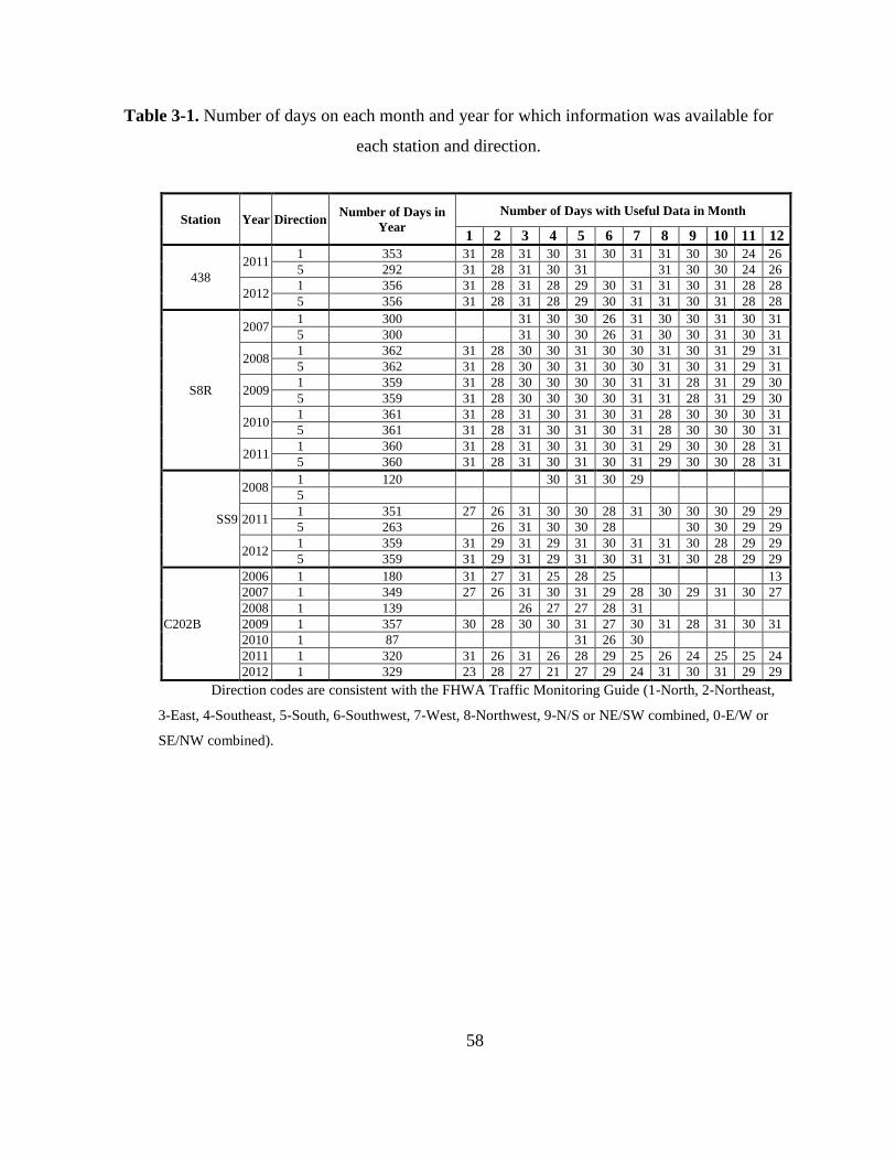
58

Table 3-1. Number of days on each month and year for which information was available for

each station and direction.

Station Year Direction Number of Days in

Year

Number of Days with Useful Data in Month

1 2 3 4 5 6 7 8 9 10 11 12

438

2011 1 353 31 28 31 30 31 30 31 31 30 30 24 26

5 292 31 28 31 30 31 31 30 30 24 26

2012 1 356 31 28 31 28 29 30 31 31 30 31 28 28

5 356 31 28 31 28 29 30 31 31 30 31 28 28

S8R

2007 1 300 31 30 30 26 31 30 30 31 30 31

5 300 31 30 30 26 31 30 30 31 30 31

2008 1 362 31 28 30 30 31 30 30 31 30 31 29 31

5 362 31 28 30 30 31 30 30 31 30 31 29 31

2009 1 359 31 28 30 30 30 30 31 31 28 31 29 30

5 359 31 28 30 30 30 30 31 31 28 31 29 30

2010 1 361 31 28 31 30 31 30 31 28 30 30 30 31

5 361 31 28 31 30 31 30 31 28 30 30 30 31

2011 1 360 31 28 31 30 31 30 31 29 30 30 28 31

5 360 31 28 31 30 31 30 31 29 30 30 28 31

SS9

2008 1 120 30 31 30 29

5

2011 1 351 27 26 31 30 30 28 31 30 30 30 29 29

5 263 26 31 30 30 28 30 30 29 29

2012 1 359 31 29 31 29 31 30 31 31 30 28 29 29

5 359 31 29 31 29 31 30 31 31 30 28 29 29

C202B

2006 1 180 31 27 31 25 28 25 13

2007 1 349 27 26 31 30 31 29 28 30 29 31 30 27

2008 1 139 26 27 27 28 31

2009 1 357 30 28 30 30 31 27 30 31 28 31 30 31

2010 1 87 31 26 30

2011 1 320 31 26 31 26 28 29 25 26 24 25 25 24

2012 1 329 23 28 27 21 27 29 24 31 30 31 29 29

Direction codes are consistent with the FHWA Traffic Monitoring Guide (1-North, 2-Northeast,

3-East, 4-Southeast, 5-South, 6-Southwest, 7-West, 8-Northwest, 9-N/S or NE/SW combined, 0-E/W or

SE/NW combined).

59

Table 3-1 (continued): Number of days on each month and year for which information was

available for each station and direction.

Station Year Direction Number of Days in

Year

Number of Days with Useful Data in Month

1 2 3 4 5 6 7 8 9 10 11 12

10W

2006 1 75 31 31 13

5 142 27 28 31 30 26

2007 1

5 120 30 30 30 30

2010 1

5 91 31 29 31

2011 1

5 352 31 28 31 30 31 30 31 25 29 30 28 28

2012 1 362 28 29 31 30 31 30 31 31 30 31 30 30

5 28 28

H41W

2006 2 227 31 28 30 31 30 31 16 30

6 227 31 28 30 31 30 31 16 30

2007 2 323 31 26 29 30 31 30 31 30 31 30 24

6 323 31 26 29 30 31 30 31 30 31 30 24

2008 2 178 30 29 28 30 31 30

6 178 30 29 28 30 31 30

C4K

2011 3 355 31 28 31 30 31 29 31 31 30 30 23 30

7 355 31 28 31 30 31 29 31 31 30 30 23 30

2012 3 359 31 28 31 30 29 30 31 31 30 30 29 29

7 359 31 28 31 30 29 30 31 31 30 30 29 29

C10K

2011 1 264 31 28 31 30 31 30 30 26 27

5 264 31 28 31 30 31 30 30 26 27

2012 1 360 31 28 31 30 31 30 31 31 30 31 28 28

5 360 31 28 31 30 31 30 31 31 30 31 28 28

CC7L

2006 3 162 31 28 30 28 24 21

7 147 28 27 30 31 31

2007 3 153 31 30 31 30 31

7 153 31 30 31 30 31

2011 3 350 30 28 31 30 31 29 31 31 30 30 23 26

7 350 30 28 31 30 31 29 31 31 30 30 23 26

2012 3 351 31 26 29 28 30 30 30 31 29 30 29 28

7 351 31 26 29 28 30 30 30 31 29 30 29 28

Direction codes are consistent with the FHWA Traffic Monitoring Guide (1-North, 2-Northeast,

3-East, 4-Southeast, 5-South, 6-Southwest, 7-West, 8-Northwest, 9-N/S or NE/SW combined, 0-E/W or

SE/NW combined).

60

Table 3-2. Sample sizes (number of vehicles weighed) use to obtain the ALS at each station.

Station Direction Vehicle Class

4 5 6 7 8 9 10 11 12 13

488 North-West 174,842 758,493 135,379 2,255 10,260 62,162 8,536 26 50 269

South-East 93,873 780,915 152,345 1,093 11,793 58,068 8,242 36 840 229

S8R North 47,101 408,105 73,841 6,776 11,682 194,988 4,859 146 268 257

South 43,844 419,997 82,054 495 11,621 209,922 5,164 1,693 1,349 222

S9 North 12,266 242,521 15,709 278 5,869 14,194 1,032 25 26 20

South 10,627 205,475 12,570 288 6,506 13,180 697 16 30 9

C202B North 11,616 544,186 449,364 4,361 27,316 485,362 20,011 1 21 6,200

South - - - - - - - - - -

10W North 68,285 439,505 155,476 6,691 29,475 211,860 18,108 553 2030 810

South 89,572 989,532 255,751 7,538 34,129 330,507 28,786 265 849 846

H41W North-East 25,153 425,803 85,072 2,812 31,046 118,561 4,562 2,245 57 488

South-West 20,760 535,369 73,984 4,595 21,018 120,343 4,475 2,672 1,015 1,385

C4K East 74,421 408,118 49,753 2,918 29,345 25,126 2,042 101 31 58

West 147,617 673,988 96,687 5,033 23,343 40,097 2,415 163 226 337

C10K North 92,489 603,211 225,562 9,563 36,050 257,953 15,865 400 2,739 1,111

South 111,062 832,137 240,514 15,569 48,853 264,850 25,457 5,522 1,322 1,430

C7L East 428,397 2,498,424 520,240 20,952 143,875 649,643 34,851 1,104 4,537 3,007

West 97,894 738,279 139,246 4,747 67,037 214,211 17,575 296 755 1,506

Figure 3-18 to Figure 3-28 show the resulting ALS for the stations with enough data to

obtain representative distributions. Notice that to make the comparisons simpler, most of the

figures are for tandem axle distributions on vehicles of class 9 although as discussed later, the

effects of other vehicle classes may be more important for some stations. The distributions for

tandem axles of vehicle class 9 on Station 438 (Figure 3-18) show a pattern in both directions

that is common to several stations. They have a very well defined unloaded peak in the 12,000

lb. to 14,000 lb. range in one direction (10,000 lb. to 12,000 lb. range in the opposite direction)

and a very mild loaded peak located, depending on the month, on either the 30,000 lb. to 32,000

lb. range or 32,000 lb. to 34,000 lb. range in one direction and almost a non-existent peak in the

opposite direction. It must be noted that even for the North-West direction, on which the soft

second peak can be observed for some months, the peaks are very mild and any minor changes in

the data can affect their location. As noted earlier, this type of distribution would not pass the

61

drive tandem check. Furthermore, their peaks are also both slightly out of what is considered

acceptable. However, with so many trucks with intermediate loading, it is reasonable to expect

that some of those could help shifting the unloaded peak to the right.

As for the flat second peak and its location or non-existence, it can be argued that both

trucks with intermediate loading and overweight trucks would tend to flatten the peak. For this

and other stations, it is also notable the long tails to the right. These may indicate a relatively

high proportion of overloaded trucks are crossing this station, which in addition to flattening the

peak would tend to shift it to the right. Of course, the difficult question to answer is whether

these tails are realistic or are the results of a calibration problem with the WIM station. This is

one of the situations in which looking at the distributions of axles for other vehicle classes and of

the distributions of the drive tandem axles can be very useful. As shown in Figure 3-19, the ALS

for tandem axles of buses at Station 438 do not exhibit long right tails. Consequently, it is logical

to infer that the long tails observed for tandem axles of vehicle class 9 are representative of the

actual loading conditions instead of being a calibration problem artifact. In fact, by observing the

distributions for drive-tandem axles (not shown) it can be further inferred that the highest loads

usually occur on the non-drive tandem axles, perhaps as a result of imbalanced loading (at this

station, the tails taper off faster for the drive tandem axles distributions than for the all tandem

distributions.)

It is also interesting to note that at this location, tandem axles on other vehicle classes can

be more damaging compared to those for vehicle class 9. As seen in Figure 3-19 for tandem

axles on buses and Figure 3-20 for tandem axles on vehicle class 6, the distributions for these

vehicle classes are concentrated on the higher side. Of course, it has to be remembered that with

each passage of a vehicle class 9 there are two tandem axle load applications but there is only

one tandem axle load application for each passage of the other vehicle classes. Thus, the relative

damaging effects cannot be inferred solely from these distributions but together with the

information about the number of axles per vehicle as well as the other axle types on each vehicle

class.

The distributions for tandem axles on vehicle class 9 at station 10W shown in Figure 3-21

exhibit a similar pattern but with better defined loaded peaks. This is not surprising as one would

62

expect a higher proportion of loaded trucks coming from and going to Campbell industrial park.

Notice, however, that for this station a detailed analysis of all the available data (2005-2012) had

to be performed to obtain these distributions. Without filtering of the data, the same type of long

right tails, as shown for station 438, were initially obtained. However, for WIM station 10W, in

many cases the distributions for the tandem axles of buses also displayed suspiciously long right

tails, indicating that much of those data may have been collected during periods with some

calibration issues. For the above reasons, as shown in Table 3-1, only some of the available data

were used to develop the ALS.

The distributions for station C4K shown in Figure 3-22 exhibit again the pattern of a very

marked unloaded peak and a very mild or non-existent loaded peak. The distributions for station

C10K shown in Figure 3-23 are more triangular as a result of a somewhat lower percentage for

the unloaded peak and a higher proportion of intermediate loads. Again, no upper peaks can be

identified. Station S9 on the big island also display a similar pattern (Figure 3-26). For the three

WIM stations mentioned, with the exception of the South direction on station C10K, the long

tails can be justified when the comparison with the tandem axles on buses explained in the

previous paragraphs are used.

The distributions for stations C7L (Figure 3-24), H41W (Figure 3-25), and S8R (Figure

3-27) have the distinctive feature of being quite different in each direction. In these cases, the

loaded and unloaded peaks of the most heavily loaded direction are about the same height with

differing degrees of intermediate loading for each of the three stations. Although differences per

direction could be noted for all WIM stations, for most, averaging the directional distributions

would have only a modest effect on designs. However, for the latter three stations the differences

are so significant that separate consideration of the heavier loaded direction is warranted. Of the

three stations, at present, the distributions derived for stations H41W and S8R are considered

reliable. Again, with reference to Table 3-1, it can be seen that only parts of three years out of the

seven year period of available data (2005-2012) were used to develop the distributions for station

H41W. Information for other years at this station produced distributions that appear to be biased

upward by about 4,000 to 6,000 lb. for the higher load ranges.

63

It must be noted that the loading for tandem axles of vehicle class 9 in the south direction

at station S8R appears high. However, the maximum loading on tandem axles of buses was

below 36,000 lb. and consistent with the 34,000 lb. limit. Thus, since no overestimation appears

to be happening for buses, it may well be that the heavy loading in this station is real.

At present the information for station C7L is considered suspect since the distributions

(Figure 3-24) present long tails that cannot be justified using the comparative approach with

tandem axles on buses described earlier. Furthermore, the distributions of tandem axles on buses

exhibited a unimodal (single peak) distribution with the peak located around 24,000 lb. to

25,000 lb. and a non-negligible percentage of loads around 50,000 lb. At this point, it cannot be

established if these are realistic loadings or that they are the result of a calibration error.

Finally, Figure 3-28 shows the distribution on Station C202B. This is the WIM station

with the longest record of good data. The pattern of loading on this station is markedly different

from all others with a very high loaded peak, which indicates, as is logical for town-bound traffic

from a port, that most trucks crossing this station are fully or intermediately loaded. Also, the

consistency of the distributions from month to month is remarkable, which is probably a result of

the enforcement efforts at this location. Despite this being the only station exhibiting a pattern

with a single identifiable peak for loaded trucks and a high proportion of intermediately loaded

trucks, traffic loading at this station is not the most damaging in the State. One of the reasons is

that the distributions for semitrailer truck, by far the most common truck at this station, do not

exhibit a long right tail seen for other stations, which again is probably attributed to the

enforcement efforts at this site. In addition, bus loads at this site are very light compared to many

other locations.

As can be seen from most figures, there seem to be little if any seasonal effects for any of

the stations. Any minor seasonal trends are probably hidden by the precision with which the data

are collected. Lastly, one of the challenges in applying the quality control checks is the risk of

eliminating valid results because they do not conform to what is expected. Although an attempt

was made to avoid this, there is always the risk of eliminating data to obtain the result that one is

expecting a priori.

64

a) North-West b) South-East

Figure 3-18. ALS for tandem axles of vehicle class 9 on Station 438.

65



66



67

a) North b) South

Figure 3-21. ALS for tandem axles of vehicle class 9 on Station 10W.

68

a) East b) West

Figure 3-22. ALS for tandem axles of vehicle class 9 on Station C4K.

69

a) North b) South

Figure 3-23. ALS for tandem axles of vehicle class 9 on Station C10K.

70

a) East b) West

Figure 3-24. ALS for tandem axles of vehicle class 9 on Station C7L.

71

a) North-East b) South-West

Figure 3-25. ALS for tandem axles of vehicle class 9 on Station H41W.

72

a) North b) South

Figure 3-26. ALS for tandem axles of vehicle class 9 on Station S9.

73

a) North b) South

Figure 3-27. ALS for tandem axles of vehicle class 9 on Station S8R.

74

Figure 3-28. ALS for tandem axles of vehicle class 9 on Station C202B.

3.4.3.2.3 Average Number of Axle Types per Truck Class

The average number of axles of each type per vehicle is an essential complement to the

ALS. In the MEPDG, these two inputs are used along with vehicle classification, AADTT,

directional distribution, lane distribution, monthly adjustment factors, and traffic growth to

estimate over time the number of repetitions of loads on different load ranges applied by the

different axle types.

This input represents the average number of axles for each truck class (classes 4 to 13)

for each axle type (single, tandem, tridem, and quad). For an example of its meaning, consider a

hypothetical situation in which the different axle types on three buses are counted. Suppose that

the first bus has two single axles (a steering axle, which is counted as single axle, and a rear

single axle), the second bus has one single and one tandem, and the third bus has three singles

(say, an articulated bus.) Therefore, if these three buses were representative of the bus loading at

the location of interest (i.e., if the proportions observed for each of these buses with respect to

the total number of buses were about 1/3), then the average number of single axles per bus would

be (2+1+3)/3 =2 and the average number of tandem axles would be (0+1+0)/3 = 0.33. On the

other hand, if at another location one observes for every articulated bus with three single axles

75

two buses with one single axle and a tandem axle and three with two single axles, then the

average number of single axles per bus at this other location would be (3×2+2×1+1×3)/6 = 1.83

and the average number of tandem axles would be (3×0+2×1+1×0)/6 = 0.33. Notice how the

average number of single axles changed. Although for this simple example the average number

of tandem axles did not change with the bus proportions with different configurations, in general,

the average number of axles for all axle types would change with changes in those proportions.

The main point of the above example is to show that the average number of axles per vehicle

class are related to the characteristics of the traffic stream observed at each location. Therefore,

slightly different number of axles per vehicle class should be expected for each WIM station.

As with most other MEPDG inputs, the number of axles types per truck class can be

input at different levels as follows:

Level 1 – values determined through direct analysis of site-specific traffic data (AVC,

WIM, or traffic counts).

Level 2 – values determined through direct analysis of regional/statewide traffic data

(AVC, WIM, or traffic counts).

Level 3 – default values based on analysis of national databases such as the LTPP

database.

Table 3-3 provides level 3 estimates of the number of axle types per truck class estimated

using LTPP data presented in NCHRP 1-37A (2004).

For locations around WIM sites, it is better to use estimates of these values from the data

for those sites. In order to obtain the average number of axles per vehicle class at each of the

WIM sites in Hawaii, the customized program to compute ALS develop by the PI was enhanced

to provide the estimates. The input data consisted of exactly the same information used to

develop the ALS (Table 3-1). Table 3-4 through Table 3-12 provide the estimates of the average

number axles per vehicle by axle type and for each direction at each of the WIM sites with useful

information in Hawaii. In general, the values obtained are within expectations. Notice that the

small sample sizes for some vehicle classes such as vehicle classes 7, 11, 12, and 13 coupled

with the fact that some of these may exhibit a wide variety of configurations resulted in wide

variations between sites for some of the axle of these truck classes.

76

Table 3-3. MEPDG default values for the average number of single, tandem, and tridem axles

per truck class.

Truck

Classification

Number of Single

Axles per Truck

Number of

Tandem Axles per

Truck

Number of

Tridem Axles

per Truck

Number of Quad

Axles per Truck

4 1.62 0.39 0.00 0.00

5 2.00 0.00 0.00 0.00

6 1.02 0.00 0.00 0.00

7 1.00 0.26 0.83 0.00

8 2.38 0.67 0.00 0.00

9 1.13 1.93 0.00 0.00

10 1.19 1.09 0.89 0.00

11 4.29 0.26 0.06 0.00

12 3.52 1.14 0.06 0.00

13 2.15 2.13 0.35 0.00

Note: The number of quad axles per truck class is 0.00, because there were too few

counted in the LTPP traffic.

The grayed cells in the following tables correspond to values estimated with samples of

less than 500, which was considered as a minimum to obtain reliable estimates of the average for

those axles that are relatively uncommon.

Table 3-4. Average number of single, tandem, tridem, and quad axles per vehicle class estimated

from WIM Station 438.

Vehicle

Class

Direction

North-West South-East

Average number per truck of: Average number per truck of:

Single

Axles

Tandem

Axles

Tridem

Axles

Quad

Axles

Single

Axles

Tandem

Axles

Tridem

Axles

Quad

Axles

4 1.903 0.230 0.000 0.000 1.524 0.521 0.000 0.000

5 2.000 0.000 0.000 0.000 2.000 0.000 0.000 0.000

6 1.000 1.000 0.000 0.000 1.000 1.000 0.000 0.000

7 1.004 0.043 0.836 0.121 1.027 0.080 0.711 0.210

8 2.260 0.729 0.000 0.000 2.118 0.873 0.000 0.000

9 1.035 1.980 0.002 0.000 1.061 1.965 0.003 0.000

10 1.003 1.041 0.958 0.000 1.006 1.037 0.961 0.001

11 1.731 0.077 0.923 0.000 1.944 0.111 0.889 0.000

12 1.160 0.880 0.980 0.000 1.033 0.996 0.985 0.005

13 1.026 0.784 1.260 0.019 1.039 0.847 1.144 0.035

77


from WIM Station S8R.

Vehicle

Class

Direction

North South


Single

Axles

Tandem

Axles

Tridem

Axles

Quad

Axles

Single

Axles

Tandem

Axles

Tridem

Axles

Quad

Axles

4 1.498 0.502 0.000 0.000 1.503 0.498 0.000 0.000

5 2.000 0.000 0.000 0.000 2.000 0.000 0.000 0.000

6 1.000 1.000 0.000 0.000 1.000 1.000 0.000 0.000

7 1.002 0.003 0.996 0.002 1.000 0.002 0.996 0.002

8 2.259 0.740 0.000 0.000 2.234 0.764 0.000 0.000

9 1.208 1.895 0.000 0.000 1.248 1.876 0.000 0.000

10 1.002 1.021 0.976 0.001 1.002 1.021 0.977 0.001

11 4.123 0.171 0.178 0.000 4.711 0.119 0.017 0.000

12 2.907 0.910 0.239 0.101 3.623 1.084 0.041 0.135

13 1.031 0.837 1.794 0.000 1.000 0.734 1.797 0.023


from WIM Station S9.

Vehicle

Class

Direction

North South


Single

Axles

Tandem

Axles

Tridem

Axles

Quad

Axles

Single

Axles

Tandem

Axles

Tridem

Axles

Quad

Axles

4 1.727 0.279 0.000 0.000 1.732 0.269 0.000 0.000

5 2.000 0.000 0.000 0.000 2.000 0.000 0.000 0.000

6 1.000 1.000 0.000 0.000 1.000 1.000 0.000 0.000

7 1.004 0.007 0.993 0.000 1.000 0.003 0.812 0.184

8 2.517 0.481 0.000 0.000 2.302 0.698 0.000 0.000

9 1.298 1.849 0.001 0.000 1.277 1.860 0.001 0.000

10 1.000 1.030 0.967 0.000 1.003 1.030 0.970 0.000

11 3.960 0.160 0.240 0.000 2.375 0.000 0.875 0.000

12 2.846 1.077 0.192 0.000 1.767 0.633 0.567 0.167

13 3.750 0.600 0.700 0.000 1.444 0.222 1.55 0.111

78


from WIM Station C202B.

Vehicle

Class

Direction

North South


Single

Axles

Tandem

Axles

Tridem

Axles

Quad

Axles

Single

Axles

Tandem

Axles

Tridem

Axles

Quad

Axles

4 1.848 0.152 0.000 0.000 - - - -

5 2.000 0.000 0.000 0.000 - - - -

6 1.000 1.000 0.00 0.00 - - - -

7 1.001 0.082 0.916 0.002 - - - -

8 2.000 0.995 0.000 0.000 - - - -

9 1.037 1.981 0.000 0.000 - - - -

10 1.007 1.051 0.947 0.001 - - - -

11 2.000 0.000 1.000 0.000 - - - -

12 1.238 1.857 0.095 0.000 - - - -

13 1.481 0.913 0.448 0.615 - - - -


from WIM Station 10W.

Vehicle

Class

Direction

North-West South-East


Single

Axles

Tandem

Axles

Tridem

Axles

Quad

Axles

Single

Axles

Tandem

Axles

Tridem

Axles

Quad

Axles

4 1.908 0.268 0.000 0.000 1.932 0.268 0.000 0.000

5 2.000 0.000 0.000 0.000 2.000 0.000 0.000 0.000

6 1.000 1.000 0.000 0.000 1.000 1.000 0.000 0.000

7 1.009 0.131 0.469 0.400 1.005 0.069 0.762 0.169

8 2.207 0.785 0.000 0.000 2.295 0.686 0.000 0.000

9 1.169 1.912 0.002 0.000 1.171 1.910 0.003 0.000

10 1.016 1.019 0.976 0.004 1.014 1.028 0.968 0.002

11 3.603 0.260 0.246 0.000 2.260 0.498 0.543 0.000

12 1.086 0.989 0.936 0.026 1.334 0.908 0.735 0.118

13 1.400 0.522 0.785 0.383 1.226 0.907 0.859 0.223

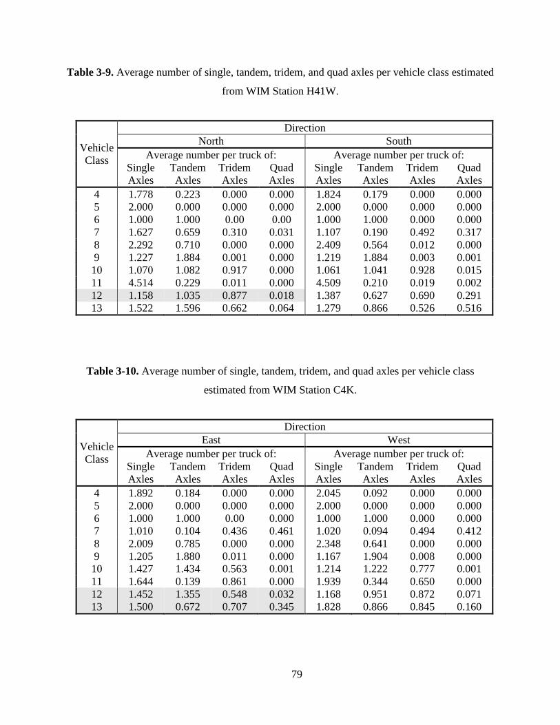
79


from WIM Station H41W.

Vehicle

Class

Direction

North South


Single

Axles

Tandem

Axles

Tridem

Axles

Quad

Axles

Single

Axles

Tandem

Axles

Tridem

Axles

Quad

Axles

4 1.778 0.223 0.000 0.000 1.824 0.179 0.000 0.000

5 2.000 0.000 0.000 0.000 2.000 0.000 0.000 0.000

6 1.000 1.000 0.00 0.00 1.000 1.000 0.000 0.000

7 1.627 0.659 0.310 0.031 1.107 0.190 0.492 0.317

8 2.292 0.710 0.000 0.000 2.409 0.564 0.012 0.000

9 1.227 1.884 0.001 0.000 1.219 1.884 0.003 0.001

10 1.070 1.082 0.917 0.000 1.061 1.041 0.928 0.015

11 4.514 0.229 0.011 0.000 4.509 0.210 0.019 0.002

12 1.158 1.035 0.877 0.018 1.387 0.627 0.690 0.291

13 1.522 1.596 0.662 0.064 1.279 0.866 0.526 0.516


estimated from WIM Station C4K.

Vehicle

Class

Direction

East West


Single

Axles

Tandem

Axles

Tridem

Axles

Quad

Axles

Single

Axles

Tandem

Axles

Tridem

Axles

Quad

Axles

4 1.892 0.184 0.000 0.000 2.045 0.092 0.000 0.000

5 2.000 0.000 0.000 0.000 2.000 0.000 0.000 0.000

6 1.000 1.000 0.00 0.000 1.000 1.000 0.000 0.000

7 1.010 0.104 0.436 0.461 1.020 0.094 0.494 0.412

8 2.009 0.785 0.000 0.000 2.348 0.641 0.000 0.000

9 1.205 1.880 0.011 0.000 1.167 1.904 0.008 0.000

10 1.427 1.434 0.563 0.001 1.214 1.222 0.777 0.001

11 1.644 0.139 0.861 0.000 1.939 0.344 0.650 0.000

12 1.452 1.355 0.548 0.032 1.168 0.951 0.872 0.071

13 1.500 0.672 0.707 0.345 1.828 0.866 0.845 0.160

80


estimated from WIM Station C10K.

Vehicle

Class

Direction

North South


Single

Axles

Tandem

Axles

Tridem

Axles

Quad

Axles

Single

Axles

Tandem

Axles

Tridem

Axles

Quad

Axles

4 1.926 0.278 0.000 0.000 1.874 0.282 0.000 0.000

5 2.000 0.000 0.000 0.000 2.000 0.000 0.000 0.000

6 1.000 1.000 0.000 0.000 1.000 1.000 0.000 0.000

7 1.017 0.113 0.531 0.356 1.011 0.075 0.665 0.260

8 2.153 0.829 0.001 0.000 2.196 0.754 0.001 0.000

9 1.162 1.914 0.003 0.000 1.182 1.891 0.011 0.000

10 1.124 1.083 0.895 0.021 1.056 1.086 0.909 0.003

11 3.073 0.423 0.283 0.000 2.472 0.448 0.501 0.000

12 1.057 0.970 0.963 0.028 1.408 1.063 0.753 0.029

13 1.139 0.758 1.012 0.219 1.464 1.064 1.003 0.046


estimated from WIM Station C7L.

Vehicle

Class

Direction

East West


Single

Axles

Tandem

Axles

Tridem

Axles

Quad

Axles

Single

Axles

Tandem

Axles

Tridem

Axles

Quad

Axles

4 2.054 0.133 0.000 0.000 2.016 0.122 0.000 0.000

5 2.000 0.000 0.000 0.000 2.000 0.000 0.000 0.000

6 1.000 1.000 0.000 0.000 1.000 1.000 0.000 0.000

7 1.022 0.097 0.496 0.407 1.006 0.122 0.734 0.145

8 2.309 0.682 0.000 0.000 2.282 0.710 0.000 0.000

9 1.117 1.937 0.003 0.000 1.113 1.940 0.002 0.000

10 1.089 1.105 0.891 0.002 1.039 1.061 0.938 0.000

11 2.836 0.173 0.516 0.000 1.966 0.544 0.632 0.000

12 1.060 0.998 0.958 0.015 1.362 0.864 0.768 0.117

13 1.377 1.533 0.725 0.049 1.504 1.261 0.919 0.013

81

3.4.3.2.4 Monthly Adjustment Factors (MAF)

The MEPDG ( [1], [2]) uses monthly adjustment factors (MAF) to account for seasonal

traffic fluctuations. The MAF, as used in the MEPDG [1], is simply 12 times the proportion of

the annual truck traffic for a given truck class that occurs in a specific month. Thus, for uniform

traffic throughout the year, the factor for each month is equal to 1. A factor greater than 1 implies

that traffic for that month is higher than average and a factor less than 1 implies that traffic is

lower than average. Naturally, the sum the MAF for the 12 months of the year must equal 12.

The importance of accurate estimation of these factors is that the effects of traffic loading

is dependent on climatic conditions that affect material characteristics, and in turn, the strains in

the pavement. Thus, the same traffic loading can have very different damaging effects depending

of the month of year on which it is applied. For States with wide variarions in temperature or

precipation, the effects can be substantial. Large changes in temperature significantly affect the

moduli of bound materials, thus affecting the overall pavement stiffness and the load induced

strains. Furthermore, in colder climates, prolonged freezing conditions substantially increase the

moduli of unbound layers for some time and when above freezing temperatures return, the water

in those bound layers melt and significantly reduce the moduli of unboud layers and the

subgrade. These freeze/thaw cycles can have a substantial detrimental effect on the pavement

performance. Precipitation causes moisture changes in the materials of unbound layers and the

subgrade, also affecting their moduli.

In Hawaii, the temperature differentials between summer and winter are relatively minor

and freezing conditions are practically non-existent. The most likely adverse factor is that of

changes in moisture conditions throughout the year. Althoguh in Hawaii there are indeed

differences in precipitation throughout the year, signigicant monthly precipitation can occur

almost all year round. The weather stations in the state report more than 200 wets days per year.

Thus, for Hawaiian conditions use of the default MAF (= 1 for each month and each vehicle

class) is expected to have only a relatively minor effect on the predictions of the pavement

deterioration process.

A study of the MAF conducted in 2007 as part of this project using classification and

weight data from the available WIM stations at that time showed that there were generally no

substantial variations of the factors. Furthermore, the factors did not appear to follow a seasonal

82

pattern clearly identifiable. Although the study had some limitations in terms of data quality, its

resutls, together with the relatively minor seasonal climatic differences in the State, lead to the

conclusion that derivation of the factors was not of first priority and thus the MAF were not

studied further. With the new version of Prep-ME soon to be realeased, the factors should be

relatively simple to compute with the data that pass the quality checks.

The following paragraphs present the derivation of the MAF previously performed with

data from 2002 to 2006.

As mentioned before, the information available at the time did not lend itself to the

derivation of reliable estimates of the MAF for all stations. Despite the limitations in the data, the

AVC (Automatic Vehicle Classification) data were used to derive monthly adjustment factors for

the same locations as the WIM stations. Although as indicated before the estimates may not have

been entirely reliable, they did provide an indication of the variability around the default value

and provided a basis to study their potential effects on the predictions. Based on the type of AVC

information available, the stations could be classified according to NCHRP 1-39 [16] as:

LEVEL 1

Station C12E – Hoonapiilani, Maui

Station S8R – Queen Kaahumanu, Big Island

Station S9 – Queen Kaahumanu, Big Island

LEVEL 2

Station 10W – Kalaeloa @ Palailai Interchange, Oahu

Station C202B – Sand Island @ Bascule Bridge, Oahu

Station H41W – H-3 @ MP 1.28, Oahu

Station C7L – H-1, Waimalu Viaduct, Oahu

Level 1 stations are required to have at least one week of data for at least 12 consecutive

months. Since this requirement was imposed by TrafLoad, it was not possible to use that

software to derive MAF for Level 2 stations. TrafLoad was then used to derive MAF only for the

Level 1 stations.

Table 3-13 and

83

Table 3-14 present the monthly adjustment factors (MAF) obtained with TrafLoad for

stations S8R and S9, respectively. A similar table was also derived for station C12E. Although

the latter passed the quality checks, there was less confidence on its results due to the lower

traffic volumes and therefore they are not presented.

The results for vehicle class 9 at station S8R show relatively minor variations around 1 of

the MFA (maximum variation of about 13 %.) The same can be noted for station S9. From these

two tables, it can be noted that for other vehicle classes such as classes 4 and 6, the variations are

in some cases larger. However, the higher MAF do not occur when more rain is to be expected

(around December and January). Other vehicle classes play only a minor role either because they

represent a small percentage of the traffic stream (vehicle classes 7, 8, and 10-13) or because

they impose relatively small loads (vehicle class 5).

Consequently, using default MAFs is not expected to have significant effects on

pavement design for Hawaii.

Table 3-13. MAF for Station S8R – Queen Kaahumanu, Big Island.

Month Vehicle Class

4 5 6 7 8 9 10 11 12 13*

1 1.105 1.004 0.946 0.793 0.953 0.940 0.961 1.298 0.895 1.000

2 1.227 1.133 0.977 0.956 0.919 0.952 0.851 1.481 1.000 1.000

3 1.053 1.183 1.061 1.011 0.924 1.040 0.916 1.351 1.000 1.000

4 1.203 1.288 0.994 0.902 1.081 1.134 0.916 1.376 1.052 1.000

5 1.245 1.326 0.977 1.039 1.081 1.129 1.061 1.559 1.264 1.000

6 0.911 0.793 0.961 1.093 1.182 1.126 1.012 0.312 1.264 1.000

7 0.773 0.770 1.019 1.011 1.062 0.956 0.723 0.598 0.737 1.000

8 0.869 0.817 1.084 0.793 1.025 0.983 0.948 0.649 1.105 1.000

9 0.842 0.770 1.030 0.902 0.991 0.953 1.077 0.649 0.790 1.000

10 1.185 1.242 0.966 1.011 1.025 0.924 1.334 1.325 1.052 1.000

11 1.001 0.926 0.985 1.176 0.929 0.918 1.077 0.832 1.052 1.000

12 0.585 0.746 1.002 1.311 0.829 0.946 1.124 0.571 0.790 1.000 * MAF set equal to 1 because estimates were unreliable.

84

Table 3-14. MAF for Station S9 – Queen Kaahumanu, Big Island.

Month Vehicle Class

4 5 6 7 8 9 10 11* 12 13*

1 1.076 1.051 1.035 1.049 1.015 0.977 0.989 1.000 1.112 1.000

2 1.288 1.254 1.011 1.312 1.203 1.064 0.954 1.000 1.033 1.000

3 1.272 1.182 1.008 0.655 1.287 1.007 0.954 1.000 0.794 1.000

4 1.380 1.164 0.990 1.115 1.235 1.144 0.818 1.000 0.636 1.000

5 1.206 1.037 0.909 0.918 1.110 0.996 0.920 1.000 1.113 1.000

6 0.768 0.961 0.969 1.246 1.020 1.072 1.091 1.000 0.954 1.000

7 0.666 0.943 1.036 0.787 0.957 0.952 1.057 1.000 1.192 1.000

8 0.936 0.868 1.055 0.984 0.957 0.941 0.954 1.000 1.033 1.000

9 0.774 0.923 0.980 0.852 0.602 0.880 0.750 1.000 0.874 1.000

10 0.811 1.039 1.103 1.902 0.592 1.065 1.261 1.000 0.954 1.000

11 0.833 0.731 0.864 0.460 0.796 0.865 0.887 1.000 1.112 1.000

12 0.990 0.846 1.039 0.721 1.225 1.038 1.363 1.000 1.192 1.000 * MAF set equal to 1 because estimates were unreliable.

The above results were based on stations located on the Big Island but it was also

desirable to estimate the MAF for Oahu.

Even though the information from the Level 2 stations could not be used to derive MAF

with TrafLoad, two of those stations, namely stations “10W” and “C202B”, contained a

significant amount of information. Consequently, the information from stations “10W” and

“C202B” was used to derive the factors. The analysis was performed manually using Microsoft

Excel. The following paragraphs explain the process.

Traffic typically exhibits hourly and day of week variations that if not accounted for

when using data for less than the whole month could bias the estimates of the MAF.

The following procedure works well if all the days of the week have a relatively similar

volume or if the ratio between the number of hours of weekdays, number of hours on Saturdays,

and number of hours on Sundays is about 5:1:1. In this case, one can simply average the hourly

volumes for each vehicle class and for each hour of the day and then add these averages to obtain

an estimate of the average daily traffic (ADT) in the month for that vehicle class. Then, the

month ADT divided by AADT for the vehicle class in question provides an estimate of the MAF

for that vehicle class. For example, for a given vehicle class, say Class 4, average daily traffic =

average number of class 4 vehicles in hour 0 (0:01 A.M. to 1:00 A.M.) + average number of

85

class 4 vehicles in hour 1 (1:01 A.M. to 2:00 A.M.) + … + average number of class 4 vehicles in

hour 23 (11:01 P.M. to 12:00 P.M.).

When the conditions for the above procedure are not met, the estimates would be biased.

For example, suppose that for a given hour of the day the average weekday traffic volume is 100,

whereas the Saturday and Sunday traffic volumes for the same hour of the day are both 50. In

this case the average hourly volume is (5 × 100 + 2 × 50)/7 = 86 vehicle/h. However, if for the

given hour there are 2 weekday observations, 1 Saturday observation and 1 Sunday observation

and one simply average these observations, the estimated hourly volume would be (100 + 100 +

50 + 50)/4 = 75, which in this case is biased towards the weekend volumes. The solution in such

cases is to calculate the average weekday and the average weekend separately and then calculate

a weighted average of these two values (with a weight of 5 for weekdays and a weight of 2 for

weekends).

In the case of station “10W”, the processing of the data was not very complicated since

there were data for most of the days on each month. The only problem found was the lack of data

for hour “0” for many of the months in the southwest direction, second lane. However, since

traffic volume for hour “0” is very low, just about 0.33% of the total in the day, a proportionality

rule was adopted to estimate that hourly volume for this particular situation. In addition, since

data were available for most of the days on each month with data (i.e. in general a fair

representation of weekday and weekend traffic was available for each month) both procedures

described above produced similar results. The MAF presented below were obtained without

separating between weekday and weekend traffic.

In the case of station “C200B” a few more complications were found.

For many months a separation of weekend and weekday traffic was required. Also, it

was not possible to discriminate between Saturday and Sunday traffic since there

were many months without data for one of those days.

In some cases there were missing data for one or two hours (usually “0” or “23”).

Since the hours missing represent hours with low volumes, the volumes for those

hours were estimated based on proportions from the other days with 24 hours of

data.

86

For some months there were days with many consecutive hours with zero volume.

These hours were not taken into account as it appears they are the result of problems

during the data collection.

Finally, results that appear to be highly suspect were also eliminated. For example,

the average number of Class 7 vehicles in March 2002 was 79.1 while from April

2002 to December 2002 the monthly average for that vehicle class oscillated

between 0 and 4.9.

For the analysis, the classes were grouped as follows:

Class 4

Class 5

Class 6

Classes 7 and 8

Classes 9 and 11

Classes 10, 12, and 13

Table 3-15 through Table 3-18 present the monthly adjustment factors (MAF) obtained

with the manual procedures outlined above for each direction at stations 10W and C202B. Again,

for vehicle class 9, with the exception of two values for the North direction at Station C202B, the

factors do not deviate too much from 1. The maximum values were again observed in the

summer months. Thus, use of a value of 1 for the winter months would result in slightly

conservative designs. Nevertheless, for some of the reasons exposed and other that will be

discussed later, the use of default MAF is not expected to be of much consequence. Therefore,

until newer MAF are derived with the more recent data it is recommended to use the defaults.

87

Table 3-15. MAF for Station C202B – Sand Island @ Bascule Bridge, North, Oahu.

Month Vehicle Class

4 5 6 7* 8* 9* 10* 11* 12* 13*

1 1.073 1.020 0.872 1.148 1.148 0.798 1.054 0.798 1.054 1.054

2 1.330 1.103 0.854 1.307 1.307 0.740 1.062 0.740 1.062 1.062

3 0.554 0.941 0.793 0.660 0.660 0.536 0.578 0.536 0.578 0.578

4 0.642 1.066 0.881 0.857 0.857 0.926 1.031 0.926 1.031 1.031

5 0.704 1.037 0.864 0.880 0.880 0.865 0.890 0.865 0.890 0.890

6 1.236 1.103 1.166 1.088 1.088 1.273 1.199 1.273 1.199 1.199

7 1.242 1.099 1.208 1.043 1.043 1.233 1.139 1.233 1.139 1.139

8 1.081 0.985 1.103 1.024 1.024 1.111 1.001 1.111 1.001 1.001

9 0.895 0.868 0.995 0.967 0.967 0.979 0.954 0.979 0.954 0.954

10 1.241 1.029 1.224 1.082 1.082 1.336 1.115 1.336 1.115 1.115

11 1.088 0.929 1.034 0.910 0.910 1.127 0.964 1.127 0.964 0.964

12 0.913 0.820 1.005 1.034 1.034 1.074 1.014 1.074 1.014 1.014 * MAF were combined for vehicle classes 7 and 8, 9 and 11, and 10, 12, and 13.

Table 3-16. MAF for Station C202B – Sand Island @ Bascule Bridge, South, Oahu.

Month Vehicle Class

4 5 6 7* 8* 9* 10* 11* 12* 13*

1 1.190 1.023 0.913 1.144 1.144 0.955 0.985 0.955 0.985 0.985

2 1.253 1.033 0.970 1.207 1.207 0.953 0.973 0.953 0.973 0.973

3 1.084 1.415 1.162 1.086 1.086 1.091 1.077 1.091 1.077 1.077

4 1.128 1.177 1.026 1.103 1.103 1.098 1.124 1.098 1.124 1.124

5 0.871 1.142 1.027 1.051 1.051 1.049 1.051 1.049 1.051 1.051

6 0.923 0.887 0.901 0.950 0.950 0.973 0.971 0.973 0.971 0.971

7 0.664 0.898 0.956 1.006 1.006 1.034 1.091 1.034 1.091 1.091

8 0.818 0.851 0.964 0.908 0.908 0.934 0.832 0.934 0.832 0.832

9 1.079 1.110 1.108 0.985 0.985 1.099 1.064 1.099 1.064 1.064

10 0.614 0.714 0.922 0.871 0.871 0.890 0.869 0.890 0.869 0.869

11 1.075 0.858 1.040 0.860 0.860 0.948 0.908 0.948 0.908 0.908


88

Table 3-17. MAF for Station 411 – H-3 @ MP 1.28, North-East, Oahu.

Month Vehicle Class

4 5 6 7* 8* 9* 10* 11* 12* 13*

1 0.916 0.974 0.972 1.018 1.018 0.930 0.769 0.930 0.769 0.769

2 0.928 0.954 0.935 0.961 0.961 0.937 0.857 0.937 0.857 0.857

3 0.941 0.959 1.123 1.069 1.069 1.010 0.938 1.010 0.938 0.938

4 0.889 0.993 1.048 1.054 1.054 1.031 1.061 1.031 1.061 1.061

5 1.020 1.086 1.087 1.134 1.134 1.162 1.427 1.162 1.427 1.427

6 0.876 1.027 0.940 1.037 1.037 1.040 1.187 1.040 1.187 1.187

7 1.015 1.069 1.026 1.086 1.086 1.162 1.146 1.162 1.146 1.146

8 1.044 0.985 1.025 1.048 1.048 1.026 0.947 1.026 0.947 0.947

9 1.070 0.980 1.042 1.021 1.021 0.982 1.041 0.982 1.041 1.041

10 1.184 0.966 0.916 0.818 0.818 0.816 0.767 0.816 0.767 0.767

11 1.118 0.985 0.948 0.827 0.827 0.864 0.961 0.864 0.961 0.961


Table 3-18. MAF for Station 411 – H-3 @ MP 1.28, South-West, Oahu.

Month Vehicle Class

4 5 6 7* 8* 9* 10* 11* 12* 13*

1 0.997 0.945 0.959 0.893 0.893 0.970 0.901 0.970 0.901 0.901

2 1.018 0.984 0.934 0.883 0.883 0.947 0.859 0.947 0.859 0.859

3 1.133 0.941 1.064 0.977 0.977 1.004 1.322 1.004 1.322 1.322

4 0.982 0.959 1.025 0.989 0.989 1.033 1.343 1.033 1.343 1.343

5 0.990 1.082 1.080 1.063 1.063 1.163 1.159 1.163 1.159 1.159

6 0.846 0.996 1.004 1.054 1.054 1.049 0.882 1.049 0.882 0.882

7 1.064 1.022 1.071 1.139 1.139 1.177 0.901 1.177 0.901 0.901

8 0.977 0.986 1.062 1.066 1.066 1.031 0.954 1.031 0.954 0.954

9 0.972 1.055 1.061 1.066 1.066 0.967 0.942 0.967 0.942 0.942

10 1.181 1.205 0.938 1.008 1.008 0.779 0.799 0.779 0.799 0.799

11 0.982 0.985 0.876 0.966 0.966 0.835 1.083 0.835 1.083 1.083


3.5 DERIVATION OF ESALC

Although one of the main goals of this project is advancing towards implementation of

the MEPDG, it is recognized that the current procedure used by HDOT to design pavements will

continue to be used for some time. Therefore, an update of some pavement design parameters

with newer information is desirable. In particular, relating to traffic loading, HDOT’s design

procedure utilizes Equivalent Single Axle Load Constants (ESALC) to convert the traffic

89

information into equivalent repetitions of a standard single axle of 18,000 lb. (80 kN). This

section presents the development of updated values of those ESALC from the WIM information

presented earlier. The current ESALC values were derived from data obtained from 1972 to

1974. The derivation of updated values with more current information (2006 - 2012) is important

for several reasons. As mentioned above, even though the use of mechanistic-empirical (M-E)

procedures will eventually replace the old procedures, the transition will take effect over several

years and therefore updated values more representative of current conditions are still needed.

Moreover, in many occasions, the starting point for an M-E analysis will be the result of a design

with old procedures using ESALC. Finally, the values will also be useful for the counties when

using other design procedures (ESALC can be easily converted to truck factors (TF) as used in

other design procedures such as the Asphalt Institute by simply dividing them by 365.)

The ESALC are derived separately for each vehicle class. The addition of ESALC for

buses is considered an important improvement to the procedures since in many situations this

vehicle class produces a substantial amount of the damage to the pavement structure. This may

be particularly significant for some city and county roads. In past analyses, it appears that buses

were pooled together with class 5 vehicles for which the ESALC value was relatively low. As

shown below, the new ESALC for buses are significantly higher than for vehicle class 5 trucks.

Other differences are noted in the values for other vehicles classes as well.

3.5.1 HDOT Method for Calculating ESAL Constants

The procedure used by HDOT for calculating the ESALC was documented by Scott

Kauai, which in turn was reproduced from an HDOT’s internal document. Basically, the same

procedure is documented here but with a slight modification because the input data is provided in

terms of a distribution of loads instead of an actual count for each vehicle class and axle type.

The procedure is explained with reference to Figure 3-29, which shows the ESALC

derivation for vehicle class 9 at station 438, direction 2 (Northeast). In the table, the columns for

each axle type are labeled a, b, etc. just above the numeric information. The nomenclature is

given in Table 3-19.

90

Table 3-19. Nomenclature for the ESALC calculation table.

Column Description

A Lower limit of axle load range (lb.)

B Upper limit of axle load range (lb.)

C Average axle load in range adjusted for axle type (lb.)

D ESAL for the average single axle load

e

Frequency of axles in the axle load range (the sum of values in this

column must be 1).

f

Frequency (column e) times the average number of axles of the

axle type in question for the truck (the values of average number of

single, tandem, tridem, and quad axles per truck are shown at the

top right of the table)

G ESAL contribution by axle type in load range.

The values in each column are calculated as follows:

1. Column c: Determine the average single axle loads for each axle load range

adjusted for axle type. The adjustment factor is 1.0 for single axles, 1.1 for

tandem axles, 1.2 for tridem, and 1.2 for quad axles6. The calculation is

accomplished with the following equation:

6 A possible justification for the adjustment factors is that the loading on multi-axle configurations may not

be evenly distributed. For example, a tandem axle with a 32 kip load may have a load configuration of 16/16 kip

loading or 14/18 kip loading. When calculating the load equivalency factor (LEF), these different load

configurations produce different values:

LEF 1: 2 * (16/18)4.2 = 2.44

LEF 2: (14/18)4.2 + (18/18)4.2 = 2.70

91

factor Adjustment typeaxlein axles ofNumber

load axle AveragecColumn

which for each axle configuration specializes as follows:

Single axles:

1.01

2bColumn aColumn

cColumn

Tandem axles:

1.12

2bColumn aColumn

cColumn

Tridem axles:

1.23

2bColumn aColumn

cColumn

Quad axles:

1.24

2bColumn aColumn

cColumn

2. Column d: Determine the ESAL of one axle of the axle type (single, tandem,

tridem, or quad) for each axle load range, column d:

24

kips18

kipsc,Column typeaxlein axles ofNumber dColumn

.

For example for a tridem axle this equation is:

24

kips18

kipsc,Column 3dColumn

.

The example shows that the LEF values are higher when the load is not distributed evenly between the

axles in the axle configuration. Some of the evidence from the WIM data indeed indicates unevenness of the load on

multi-axle configurations.

92

3. Column f: Multiply the frequency in column e by the average number of axle

types per vehicle (for the vehicle class in question):

The value in column e provides the frequency with which the load range appears

for the given axle type. For example, the value in Figure 3-29 for the load range

40,000-42,000 lb. in column e for tandem axles is 0.0142. This means that for

every 1,000 applications of tandem axles of vehicle class 9, about 14 applications

will be in the 40,000 lb-42,000 lb. load range.

Now consider 1,000 passages of vehicle class 9. Based on the average

number of tandem axles per truck passage shown at the top right of the table, on

average, each passage of a truck will contribute with 1.980 applications of tandem

axles and thus for 1,000 vehicles the number of tandem axle load applications will

be 1,980. Out of these, (0.0142) (1,980) ≈ 28 will be in the load range of 40,000-

42,000 lb. The computation was presented in terms of 1,000 vehicles just to make

it easier its understanding. However, in column f of the table number of

applications of the axle type in question is computed for one truck instead of

1,000. Thus, the value appearing on the table is basically the value computed

above divided by 1,000, which gives the normalized number of applications in the

load range for the axle type per vehicle passage. The explanations for other axle

types are entirely analogous.

Notice that the sum of the values in columns f is approximately equal to

the average number of axles (as defined by the axle types) per truck shown on the

top right corner of the worksheet. In the example of Figure 3-29, the sum is about

3.02, which agrees well with what is normally expected for vehicle class 9, whose

most common configurations consists of 1 single and 2 tandem axles (that is

about 3 axle types)7.

7 The fact that vehicle class 9 shows in general a number of single axles greater than 1 and of tandem axle

less than 2 appear to be related to the definition of single and tandem axles. Many axles are being classified as single

simply because their measured axle separation to adjacent axles is slightly more 2.4 m.

93

4. Column g: Determine the ESAL contribution for the axle in the load range. This is

accomplished by simply multiplying the values in columns d and f.

5. Truck factor (TF): add up the values in all columns g. This value provides the

average effect of a single vehicle passage in terms of equivalent single axle loads

of 18,000 lb. This is known as the truck factor (TF) in other design procedures.8

6. ESALC: Determine the ESALC for use in the Traffic Index (TI) calculation by

multiplying the TF obtained in the previous step by 365. The ESAL constant

essentially provides the ESAL/truck in a whole year. Recall that for the TI

calculation in the HDOT pavement design procedure the number of trucks is

given in trucks per day and the design life is given in years. The transformation

from daily to yearly effects is already incorporated in the ESALC.

The procedure described above was used with the data from each WIM station

that passed the quality checks described in section 3.4.3 (This was done for each direction

and for each vehicle class.) Table 3-20 summarizes the results for the most prevalent

vehicle classes 4, 5, 6, and 9.

The values in this table show substantial differences from location to location or

even for both directions at the same location. For example, the ESALC value for buses in

the North-West direction at station 438 is almost three times the value for the opposite

direction. The same type of unbalance by direction can be noted for example for vehicle

class 9 at Station H41W. Notice that identifying the reasons for such unbalances is not

simple since they can be related to generally higher loads being transported in one

direction than in the other, or even with the same loading per direction having the loading

concentrated on fewer vehicles (e.g., buses with a well-defined peak period and another

peak that is more spread out during the day), or a combination of these.

8 This value could be useful for those wishing to use other design procedures. It must be noted however that

the truck factors presented here are based on a 4.2 exponent for the calculation of the load equivalency factors

instead of the 4.0 exponent or load equivalency tables used in some other procedures (e.g., AASHTO, 1993).

94

Figure 3-29. Example of worksheet used to calculate ESALC.

95

Table 3-20. ESAL Constants derived from the WIM sites.

Station Direction Vehicle Class

4 5 6 9

C202B North 178 51 218 978

10W North 808 58 406 867

South 439 31 401 501

438 North West 1,904 50 687 728

South East 705 49 560 610

C7L East 1,497 103 710 1,213

West 1,181 83 842 1,418

C4K East 1,463 184 920 1,280

West 951 91 728 1,127

C10K North 772 40 288 557

South 647 88 854 899

H41W North East 359 46 334 454

South West 340 30 480 1233

S9 North 455 18 391 656

South 508 25 931 793

S8R North 446 32 735 648

South 359 29 435 1,324

Interpolated

10W, S9, &

C10K North

591 34 488 674

The values at station C4K for vehicle class 9 are about twice those at station 438 for the

same vehicle class. In this case, the difference appears to be mostly related to the long right tails

of the distributions observed on some of the freeway stations such as C4K. Notice that some of

the values for the stations C4K, C7L, and H41W located on Oahu freeways are even higher than

those at station C202B, for which the proportion of loaded trucks is higher than at any other

station. This illustrates that, barring errors in the data used to develop the distributions, changes

in weight limit enforcement or special overweight heavy loading permitting could have

important benefits in extending the life of pavements. As discussed in section 3.4.3.2.2, out of

these three stations only the data for station C7L had suspiciously long right tails for several

vehicle classes. However, that did not appear to be the case for the other two stations and

therefore it is believed the above observations are valid.

96

It can also be observed that for most locations, the ESALC derived for buses are much

higher than 65, which is the ESALC used in the last HDOT pavement design manual (HDOT,

2002) for class 5 vehicles (the class that was typically used to account for bus effects). On the

other hand, the derived values for class 5 vehicles are generally lower than 65. The net change

thus depends on the proportions of vehicles on every particular project under consideration but in

general it is expected to result in higher values of ESALs.

3.6 RECOMMENDATIONS FOR USING LOCAL WIM INFORMATION

An important aspect in the analysis of WIM data is to form truck weight road groups

based on a combination of known geographic, industrial, agricultural, and commercial patterns

along with knowledge of trucking patterns that occur on specific roads [15] so that designers can

select the appropriate group for each particular situation. The Traffic Monitoring Guide [15]

specifies criteria to test the quality of selected truck weight groups and determine the precision of

estimates from those groups. Obviously, the quality and precision estimates are based on

statistical analysis. Typically, at least six stations are needed per group. Thus, with only 9 WIM

sites with usable data across the State, it is not possible to perform a rigorous statistical

evaluation of groupings since it is clear that at least two or three groups are needed to represent

loading conditions within the State.

As was shown in Figure 3-2, the WIM stations in the State are located on either

freeways, principal arterials, or port/industrial roads. Thus, it is difficult to know solely from

WIM data what the loading is on other roads, particularly those on the Windward side of the

island of Oahu and Hawaii. Furthermore, since station C12E in Maui did not provide reliable

data and there is no WIM station in Kauai, axle load spectra for those islands are not yet well

defined. Yet, pavements still need to be designed in those locations. Therefore, based on the

observations provided in the previous section, the following recommendations for using the

information from the local WIM data are proposed.

First, recommendations are provided for use of the WIM data with the MEPDG and then

with the HDOT design procedure.

97

3.6.1 Use of the WIM data with the MEPDG

Obviously, for locations around the WIM sites, the corresponding distributions for those

sites should be used unless a dramatic change in loading conditions at some nearby intersection

or interchange is possible. Table 3-21 shows the suggested assignment of stations to routes. For

simplicity, except for station C4K, only the direction with heavier traffic is suggested for design.

For all other pavement segments, the data from stations C202B, 10W, S9, S8R, H41W,

438, and the North direction of station C10K were averaged. The reason for choosing these

stations is that they do not include the unreliable data of station C7L and the south direction of

station C10K (unreliable in the sense that they had long right tails that could not be justified from

the quality control checks and thus they were not considered representative of normal

conditions.) Station C4K was not included in the average as it does not appear that such high

loads are observed in other locations.

It is believed that the distributions selected to compute the average are more

representative of the likely loading conditions to be found on most roads throughout the State.

Although the data from stations C12E and 023 were questionable, they nevertheless provided

some indication that the loading at those sites are less severe than the average from the other

stations.

As an exception to the assignment in Table 3-21, it is recommended that for those

roadway sections with known heavily unbalanced loading (such access roads to quarries), the

loading corresponding to the heavy direction at station S8R (the north direction) be used. This

would provide heavy vehicle class 9 loading and moderate bus loading.

In order to simplify the use of these guidelines, Table 3-21 provides the name of the file

containing axle load spectra information corresponding to each case. Thus, to follow these

recommendations when using the MEPDG, the designer would only need to decide which file to

use based on Table 3-21 and then import the corresponding file into the Pavement ME Design

software, which is a relatively simple process. Note that the average number of axles per truck

should be selected consistently from the appropriate table in Section 3.4.3.2.3 (page 74) (i.e.,

corresponding to the site selected for the ALS input.) Table 3-22 provides the number of axles

per vehicle corresponding to the interpolated ALS.

98

Table 3-21. Suggested assignment of WIM station data to routes.

Station Routes ALS file name

C202B North

64

11 MP 0.00-10.00

19 MP 0.00-10.00

C202B_North_ALS_MEPDG.alf

10W North 95 10W_North_ALS_MEPDG.alf

438 North-West

92,

7412,

7413 MP 0.00-0.35

438_North-West_ALS_MEPDG.alf

C4K East

H-1 East MP 8.00-

22.00,

H-201 East,

7310

C4K_East_ALS_MEPDG.alf

C4K West

H-1 West MP. 8.00-

22.00,

H-201 West

C4K_West_ALS_MEPDG.alf

C10K North H-1 MP 0.00-8.00

H-1 MP 22.00-27.16 C10K_North_MEPDG.alf

H41W South-West H-3, H-2 H41W_South-West_ALS_MEPDG.alf

S9 South 11 10.00-121.98 S9_South_ALS_MEPDG.alf

S8R North 19 MP.66.5-99.52 S8R_North_ALS_MEPDG.alf

Interpolated All other roads Interpolated_All_ALS_MEPDG.alf

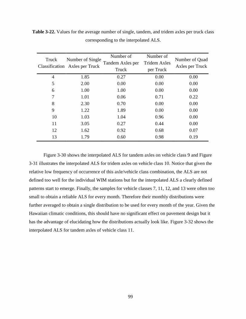
99

Table 3-22. Values for the average number of single, tandem, and tridem axles per truck class

corresponding to the interpolated ALS.

Truck

Classification

Number of Single

Axles per Truck

Number of

Tandem Axles per

Truck

Number of

Tridem Axles

per Truck

Number of Quad

Axles per Truck

4 1.85 0.27 0.00 0.00

5 2.00 0.00 0.00 0.00

6 1.00 1.00 0.00 0.00

7 1.01 0.06 0.71 0.22

8 2.30 0.70 0.00 0.00

9 1.22 1.89 0.00 0.00

10 1.03 1.04 0.96 0.00

11 3.05 0.27 0.44 0.00

12 1.62 0.92 0.68 0.07

13 1.79 0.60 0.98 0.19

Figure 3-30 shows the interpolated ALS for tandem axles on vehicle class 9 and Figure

3-31 illustrates the interpolated ALS for tridem axles on vehicle class 10. Notice that given the

relative low frequency of occurrence of this axle/vehicle class combination, the ALS are not

defined too well for the individual WIM stations but for the interpolated ALS a clearly defined

patterns start to emerge. Finally, the samples for vehicle classes 7, 11, 12, and 13 were often too

small to obtain a reliable ALS for every month. Therefore their monthly distributions were

further averaged to obtain a single distribution to be used for every month of the year. Given the

Hawaiian climatic conditions, this should have no significant effect on pavement design but it

has the advantage of elucidating how the distributions actually look like. Figure 3-32 shows the

interpolated ALS for tandem axles of vehicle class 11.

100

Figure 3-30. Interpolated ALS for tandem axles on vehicle class 9.

Figure 3-31. Interpolated distribution for tridem axles on vehicle class 10.

101

Figure 3-32. Interpolated distribution on tandem axles of vehicle class 11.

It is interesting to note that only about 2.4% of traffic on non-freeway (primary) roads is

heavy or commercial vehicles, and Classes 4 and 5 comprise 87% of the heavy vehicles. About

3.3% of traffic on freeways is heavy or commercial vehicles, and Classes 4, 5, 6 and 9 comprise

94% of the heavy vehicles. These statistics support the emphasis put on these vehicle classes and

the simplifications performed for vehicle classes 7, 11, 12, and 13, though as discussed earlier, it

is not just the frequency of loading but also the magnitude that affects pavement design.

Nevertheless, from the derived distributions, most of the damage on most state roads is most

likely caused by vehicle class 4, 5, 6, and 9.

102

3.6.2 Use of the WIM information with the HDOT design procedure

In principle, the same ideas described for the use of the WIM data with the MEPDG are

applicable to designs with the HDOT design procedure. That is, one could use the ESALC most

appropriate for each site as presented in Table 3-23. However, the HDOT design procedure is

rather conservative and relatively insensitive to traffic loading since the latter is converted into a

traffic index (TI) using the following equation:

𝑻𝑰 = 𝟗 (𝑬𝑺𝑨𝑳

𝟏, 𝟎𝟎𝟎, 𝟎𝟎𝟎)

𝟎.𝟏𝟏𝟗

(3-1)

Given the very low exponent on equation (3-1), a doubling of traffic results in an increase

of TI of only 8.6%. Even if traffic is tripled, the TI is increased by only 14%. In the HDOT

design procedure, the final thicknesses of the different layers would be directly proportional to

the value of the TI were it not for the rounding that is generally performed during layer

thicknesses selection, the application of a safety factor, and the use of a factor known as the

“gravel factor” to determine the layer thicknesses (which is not constant for asphalt concrete).

The reason is that the TI enters in a multiplicative form in the equation to compute a gravel

equivalent (GE) needed to protect each layer. The GEs are in turn used to compute the layer

thicknesses. The point of the discussion is that layer thicknesses would increase approximately

proportional to the TI, though not exactly. Thus, a 10% increase in TI would represent an

approximate 10% increase of layer thickness. As mentioned before, some of the rounding of

layer thicknesses, the application of a safety factor that increases the thickness of asphalt

concrete, or even the requirement of determining the TI to the nearest 0.5, can have a similar or

in many cases a larger effect than the inaccuracies in the ESAL computations.

In order to evaluate the potential impact of consolidating the sets of ESALC in Table 3-23

into two or three groups, the number ESALs were computed with the average ESALC values

corresponding to different trial groupings. For this, several different traffic streams with varying

vehicle class distributions were used. The vehicle class distributions were selected from those

used during the calibration efforts of the MEPDG (explained in chapter 7). The ratios of the

number of ESALs for different load groupings were then evaluated to estimate the potential effect

103

on thickness design (remember that a factor of 2 translate in about 8% change in total pavement

thickness in terms of gravel equivalent.)

Based on the above analysis, three different groups were created as presented in Table

3-24. The first group is recommended for the design of freeways. The second group is

recommended for the design of roads with moderately heavy truck loading and heavy bus

loading such as routes 92 (Ala Moana Blvd./Nimitz Hwy), 95, parts of 99, and 19 in the Kona

area on the Big Island. The third group is recommended for all other roads. These groupings

permit some differentiation based on some known characteristics of the roads. It must be noted

that the ratio of ESALs computed with the ESALC from group 1 to that computed with the

ESALC from group 3 varied from about 1.40 to 2.35. Therefore, the differences in thicknesses

between designs with these two groups are expected to be at most 10%. The ESALC from group

2 would in general result in an intermediate design. Notice that the actual variations in the

resulting thicknesses depends on the heavy traffic loading composition.

Table 3-23. ESALC corresponding to the traffic loadings in Table 3-21.

Station Vehicle Class

4 5 6 7 8 9 10 11 12 13

C202B North 178 51 218 824 241 976 863 1,375 245 793

10W North 808 58 406 964 728 867 1,452 556 2,068 4,235

438 North-West 1,904 50 687 1,391 170 728 2,145 145 2,587 4,429

C4K East 1,461 184 920 1,717 1,490 1,280 1,142 1,054 3,110 2,333

C4K West 951 91 728 1,255 308 1,127 1,290 810 2,657 1,597

C10K North 772 40 288 829 318 557 754 738 1,081 2120

H41W South-West 340 30 480 1,136 154 1,233 870 1,596 1,571 1,021

S9 South 508 25 931 1,119 781 793 1,267 61 1,362 3,849

S8R South 359 29 435 1,223 677 1,324 2,141 2,179 2,415 9,359

104

Table 3-24. Updated ESALC values for Hawaii.

ESALC Groups Vehicle Class

4 5 6 7 8 9 10 11 12 13

1: Freeways 1,206 138 824 1,486 899 1,204 1,216 932 2,884 1,965

2: Intermediate loading

(92, 95, 19, 99 MP

16.00-23.83)

1,024 46 509 1,193 525 973 1,913 960 2,357 6007

3: All other roads 343 38 575 972 511 885 1,065 718 804 2,321

3.7 PECENT TRUCKS IN THE DESIGN LANE

This section presents the analysis of the percent trucks in the design lane, which is also

commonly known as the lane distribution factor. This factor accounts for the distribution of truck

traffic between lanes in one direction [1]. It is usually computed as the percentage of trucks in

the design lane relative to all truck traffic in the design direction.

In the MEPDG, a slightly different definition is used [22]; it is defined by the primary

truck class for the roadway, where the primary truck class is defined in [22] as “the truck class

with the majority of applications using the roadway.” The MEPDG Manual of Practice [22]

further states “In other words, the percentage of trucks in the design lane is estimated for each

truck class, and the predominant truck class is used to estimate this value.”

Unfortunately, the above statements in quotes contain some vague language. It is

probably safe to assume that by “applications” the MEPDG Manual of Practice means “number

of trucks”; but depending on lane usage by different vehicle classes, it may be more problematic

to know what is meant by “predominat truck class”. Interpreting it as the truck class with the

highest volume could result in an underestimation of traffic loading effects. The reason is that for

Hawaiian conditions the “predominant truck” would most often be a class 5 truck which has

relatively minor damaging power compared to the other truck classes. Thus, for example, for a

section with 30% class 5 trucks, 20% buses (class 4) and 20% of class 9 trucks the latter two are

likely to have much more damaging power than that of class 5 trucks.

105

For Hawaii, it is recommended to estimate what truck class has the most damaging power

and use it as the predominant truck class. A simple way proposed here to estimate which vehicle

class has the most damaging power is to simply multiply the percentage of vehicles in each class

by the corresponding ESALC appropriate for the section and selecting the class with the largest

product. In cases where the numbers for the two top classes are close (say, withing 20% of each

other), an average of the lane distribution factors for those two classes could be used instead of

simply selecting the one for the largest.

The lane distribition factor (LDF) (or design lane factor in HDOT’s procedure) has not

received much attention in the recent past for pavement design in Hawaii probably because its

value is specified in the design procedure. However, use of unrealistic LDF’s or Design Lane

Factors could have almost as much of an adverse effect (over or under design of a pavement) as

any other traffic loading input. As discussed in the previous sections, the use of the different sets

of ESALC could affect the calculations of ESALs by a factor of about 2. An effect of almost the

same order of magnitude would be produced by using a factor of 0.8 if a factor of 0.5 were more

representative of actual conditions (a 60% overestimation of the loading in this example.)

A motivation for studying this factor in some detail is that while collecting cracking

information from HDOT’s video logs over several years for calibration of the MEPDG, it was

noted that on multilane highways, cracking often started earlier and/or was present on a larger

extent on the inside rather than the outside lanes even though these were constructed at the same

time. No apparent reason other than perhaps different loading on each lane could be found. In

addition, the LDF specified in the current HDOT pavement design procedure [13] (LDF = 1.00

or 100% for 1 and 2 lanes, 0.80 or 80% for 3 lanes, and 0.75 or 75% for 4 lanes in one direction)

were in some cases quite different from those suggested in the MEPDG [1] (LDF=1.00 for 1

lane, LDF = 0.90 for 2 lanes, LDF = 0.60 for 3 lanes, and LDF = 0.45 for 4 lanes.) Notice that

for the four lanes case, traffic estimated with HDOT’s recommendation would be 1.67 times the

one obtained following the MEPDG recommendations. Neither document provided guidance

about cases with more than four lanes.

Actually, the MEPDG Manual of Practice [22] states that the percent trucks in the design

lane may be estimated from AVC (automated vehicle classification) data or manual vehicle

count data. The same recommendation is provided here since AVC data can be obtained for

106

design from HDOT’s Planning Branch. Although it would be desirable that for every pavement

design on existing facilities the LDF were based on traffic information at the site, it is recognized

that this may not always be the case. Furthermore, for widening cases, some guidance is still

needed.

In order to gain some understanding of the lane usage by heavy vehicles in the State, the

information from the WIM stations on multilane highways was analyzed. For this purpose, the

PI’s program discussed in previous sections was enhanced to compute the percentages by lane

for each vehicle class at the different stations. Figure 3-33 shows the layout of the sensors at two

of the WIM sites. As can be observed, one of the sections in Oahu have a large number of lanes

in each direction. Notice that lane 1 at all WIM sites is the leftmost lane, which differs from the

numbering used in the TMG [15].

Figure 3-33. Layout of sensors at two of the WIM Stations in Oahu.

Table 3-25 shows the lane distribution by vehicle class on each direction at the WIM

stations on multi-lane highways. The first three stations in the table have two lanes in each

direction, the following three have three lanes and the last one, station C7L, has six lanes in each

direction. In this table, the values provided for vehicle classes 7, 11, 12, and 13 should be look at

with caution since they are generally based on a much smaller number of observations than for

the other vehicle classes.

107

For the cases with two lanes in one direction, it can be observed that the percentage by

lane can be quite variable from station to station, but at least for this limited number of sites, it

never goes much higher than 80% for the vehicle classes most likely to represent the primary

trucks in Hawaii (4, 5, 6, 8, 9, or 10). It is important to note that when traveling north at station

10W, the station is located just after an important intersection on which some heavy traffic may

be diverted and just before an interchange. Therefore, the higher LDF value at this site, as

compared to the values at the other sites, appears to be more related to the trip destination than to

lane selection. This, however, is always a possibility that should be accounted for.

It is also interesting to note that lane 1 (the inside lane) at these stations often carries a

higher percentage of trucks than the outside lane, which is contrary what is often expected.

On the facilities with three lanes in one direction, it can be observed that the LDF is

highly variable and that the lane with the largest percentage varies by location. The LFD varies

from 42.5 to 76%. It is interesting to note that three locations have different characteristics.

Station C10K is located just before or after a ramp entry/exit from an interchange. Thus, some

effect from the interchange may be expected (although at this location, existing pavement

condition may have also been a factor). Station C4K is further away from ramp entries and exits.

Station 438 is on an arterial with piers to the right of the Southeast bound traffic and with other

important truck destinations on the left for the Northbound traffic, which in part may explain

why the LDF is the highest for outside lane for traffic traveling in the Southeast direction and the

highest in the inside lane for traffic traveling in the opposite direction. The above discussion

highlights the need to use actual traffic observations whenever possible.

Finally the values for station C7L suggest that heavy traffic tends to be concentrated on

the center lanes when several lanes are available. For six lanes, the maximum percentage

observed is 33%.

Given all the above observations, it is suggested to use the values in Table 3-26 (page

109) for design when field data collection is not possible or when AVC data are not available.

These LDF or Design Lane Factor values represent a compromise between the highly

conservative values in the current HDOT design procedure [13] and the values in the MEPDG.

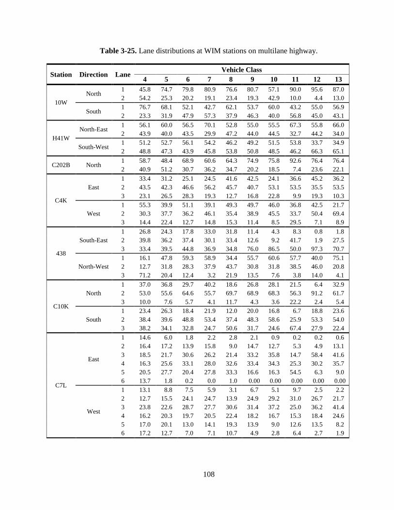
108

Table 3-25. Lane distributions at WIM stations on multilane highway.

Station Direction Lane Vehicle Class

4 5 6 7 8 9 10 11 12 13

10W

North 1 45.8 74.7 79.8 80.9 76.6 80.7 57.1 90.0 95.6 87.0

2 54.2 25.3 20.2 19.1 23.4 19.3 42.9 10.0 4.4 13.0

South 1 76.7 68.1 52.1 42.7 62.1 53.7 60.0 43.2 55.0 56.9

2 23.3 31.9 47.9 57.3 37.9 46.3 40.0 56.8 45.0 43.1

H41W

North-East 1 56.1 60.0 56.5 70.1 52.8 55.0 55.5 67.3 55.8 66.0

2 43.9 40.0 43.5 29.9 47.2 44.0 44.5 32.7 44.2 34.0

South-West 1 51.2 52.7 56.1 54.2 46.2 49.2 51.5 53.8 33.7 34.9

2 48.8 47.3 43.9 45.8 53.8 50.8 48.5 46.2 66.3 65.1

C202B North 1 58.7 48.4 68.9 60.6 64.3 74.9 75.8 92.6 76.4 76.4

2 40.9 51.2 30.7 36.2 34.7 20.2 18.5 7.4 23.6 22.1

C4K

East

1 33.4 31.2 25.1 24.5 41.6 42.5 24.1 36.6 45.2 36.2

2 43.5 42.3 46.6 56.2 45.7 40.7 53.1 53.5 35.5 53.5

3 23.1 26.5 28.3 19.3 12.7 16.8 22.8 9.9 19.3 10.3

West

1 55.3 39.9 51.1 39.1 49.3 49.7 46.0 36.8 42.5 21.7

2 30.3 37.7 36.2 46.1 35.4 38.9 45.5 33.7 50.4 69.4

3 14.4 22.4 12.7 14.8 15.3 11.4 8.5 29.5 7.1 8.9

438

South-East

1 26.8 24.3 17.8 33.0 31.8 11.4 4.3 8.3 0.8 1.8

2 39.8 36.2 37.4 30.1 33.4 12.6 9.2 41.7 1.9 27.5

3 33.4 39.5 44.8 36.9 34.8 76.0 86.5 50.0 97.3 70.7

North-West

1 16.1 47.8 59.3 58.9 34.4 55.7 60.6 57.7 40.0 75.1

2 12.7 31.8 28.3 37.9 43.7 30.8 31.8 38.5 46.0 20.8

3 71.2 20.4 12.4 3.2 21.9 13.5 7.6 3.8 14.0 4.1

C10K

North

1 37.0 36.8 29.7 40.2 18.6 26.8 28.1 21.5 6.4 32.9

2 53.0 55.6 64.6 55.7 69.7 68.9 68.3 56.3 91.2 61.7

3 10.0 7.6 5.7 4.1 11.7 4.3 3.6 22.2 2.4 5.4

South

1 23.4 26.3 18.4 21.9 12.0 20.0 16.8 6.7 18.8 23.6

2 38.4 39.6 48.8 53.4 37.4 48.3 58.6 25.9 53.3 54.0

3 38.2 34.1 32.8 24.7 50.6 31.7 24.6 67.4 27.9 22.4

C7L

East

1 14.6 6.0 1.8 2.2 2.8 2.1 0.9 0.2 0.2 0.6

2 16.4 17.2 13.9 15.8 9.0 14.7 12.7 5.3 4.9 13.1

3 18.5 21.7 30.6 26.2 21.4 33.2 35.8 14.7 58.4 41.6

4 16.3 25.6 33.1 28.0 32.6 33.4 34.3 25.3 30.2 35.7

5 20.5 27.7 20.4 27.8 33.3 16.6 16.3 54.5 6.3 9.0

6 13.7 1.8 0.2 0.0 1.0 0.00 0.00 0.00 0.00 0.00

West

1 13.1 8.8 7.5 5.9 3.1 6.7 5.1 9.7 2.5 2.2

2 12.7 15.5 24.1 24.7 13.9 24.9 29.2 31.0 26.7 21.7

3 23.8 22.6 28.7 27.7 30.6 31.4 37.2 25.0 36.2 41.4

4 16.2 20.3 19.7 20.5 22.4 18.2 16.7 15.3 18.4 24.6

5 17.0 20.1 13.0 14.1 19.3 13.9 9.0 12.6 13.5 8.2

6 17.2 12.7 7.0 7.1 10.7 4.9 2.8 6.4 2.7 1.9

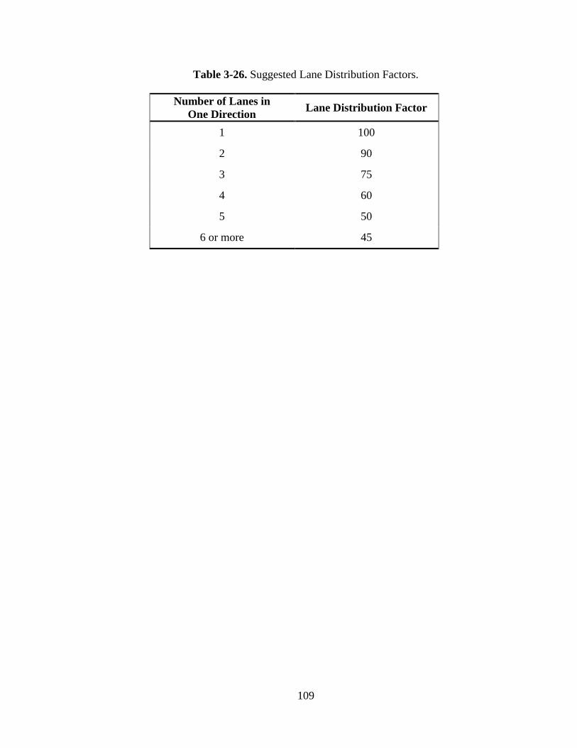
109

Table 3-26. Suggested Lane Distribution Factors.

Number of Lanes in

One Direction Lane Distribution Factor

1 100

2 90

3 75

4 60

5 50

6 or more 45

110

PAVEMENT CONDITION

4.1 INTRODUCTION

As indicated by Haas, Hudson, & Zaniewski [3], four types of pavement outputs are

periodically used by highway agencies for pavement evaluation. These include measures of

structurally adequacy (e.g., structural number and deflection with a Falling Weight

Deflectometer (FWD), Benkelman beam, etc.), rideability or serviceability (e.g., international

roughness index (IRI)), surface distress (cracking, rutting, raveling…), and surface friction.

These measures provide the means for assessing and updating if necessary design predictions,

scheduling rehabilitation measures, improving design models, construction and maintenance

practices, and updating network programs [3].

This chapter describes the pavement outputs currently collected by HDOT, the efforts to

visualize, transform, and interpret them, and areas of potential improvement.

4.2 INTERNATIONAL ROUGHNESS INDEX – IRI

Pavement roughness contributes significantly to the perceived serviceability of road

users. The most widely used measure of pavement roughness is the International Roughness

Index (IRI) developed by Sayers, Gillespie, & Queiroz [23] in a study conducted for the World

Bank. In order to measure it, road profilers equipped with laser sensors and accelerometers are

used to measure the vertical profile of the road. Then, the IRI is estimated using a mathematical

algorithm that simulates the up and down movement per unit distance traveled by a quarter of car

with certain characteristics while travelling the road at 80 km/h.

A main advantage of IRI is that its value has the same scale9 and meaning anywhere in

the world. This is because the quarter car characteristics (tire spring constant, suspension spring

constant, suspension damper/dashpot constant, mass of the suspension and mass of the car) and

9 Of course, different units are used in different parts of the world. In the US, IRI is expressed in inches/mi

whereas in countries using the SI system of units it is expressed in m/km or mm/m (1 mm/m = 1 m/km = 63.35

in/mi).

111

the vehicle speed (80 km/h) are all specified. Thus, no matter how a profile is obtained, as long

as it provides an accurate representation of the road, then IRI can be computed accurately too.

IRI has now been collected by HDOT for several years. For this project, data for 2003,

2004, 2005, 2007, 2009, and 2010 were used. The 2003, 2004, and 2005 data were collected with

an ARAN van by HDOT personnel. The rest of the data were collected by Mandli, Inc. for

HDOT’s Planning Branch. There were also some data available for 2001 collected by Roadware

and for 2003 by Mandli but due to some difficulties, these data were not analyzed. All the data

are reported every 0.01 mi (52.8 ft.). Therefore, the amount of information is voluminous,

particularly for those years on which every lane of multi-lane highways were surveyed.

Early on, it was realized that visualization of such vast amount of information was

desirable. HDOT’s has the capability in its Road Information System (RIS) web portal of

displaying the IRI information in color coded maps (Figure 4-1), which is very useful.

Figure 4-1. Display of IRI in maps in HDOT’s web portal.

Other software such as ProVAL (Profile Viewing and Analysis Software) [24] is an

excellent and free software tool for visualization and analysis of road profiles but it is geared

more towards project level analysis than network level analysis. In addition, the available data

112

sets contained only IRI values instead of road profiles, which is reasonable at the network level

considering the substantially larger storage capacity needed for storing profiles.

A tool was created to store and visualize the roughness information in charts. The tool is

intended to complement the mapping in the web portal. The purpose was to be able to observe

the IRI trends for a road for several years all at once and to be able to see the trends for each road

and easily zoom in to (or zoom out from) sections of interest. Although such types of analyses

can be done with a spreadsheet program, zooming in or our can quickly become tedious and time

consuming. As the analysis progressed, several capabilities were added including zooming and

scrolling in charts, correction of data series (shifting and or compression/expansion of series),

segmentation of roads into statistically homogeneous sections, user editing of the automatically

generated segment change-points, and reporting of the segmented information into comma

delimited files. In addition, the tool allows the visual comparison of series by lanes for a given

year or by year for a given lane and provides visual cues for data obtained at low speeds or with

IRI above user specified thresholds, which are excluded from the reported averages. The

following section provides more details of the program and, more importantly, about some of the

issues identified with the data.

4.2.1 IRI Data Processing Tool

At present, the tool developed for processing the IRI data has a very basic menu.

Essentially, it has three options for data analysis and three for database utilities as shown in

Figure 4-2.

Figure 4-2. IRI Processing Tool Menu.

113

Selecting the “Series Correction” option under “DataIRI” takes the user to the screen

shown on Figure 4-3. Notice that the screen has been configured specifically for Hawaii.10 As

shown in the figure, a list box is already populated with the routes with available information for

the selected island and source of data. Note that the first route is selected by default and for this

route the list box labeled “Lanes” lists all the lanes for which information is available for that

route and in the direction selected.

Figure 4-3. IRI data Processing Tool – Series Adjustment Screen.

The details of the interface above already help to illustrate some of the challenges found

when automatically processing information from different sources without following a particular

standard. First, notice that the direction is labeled as either “+MP” or “-MP”. This was adopted

from the convention used in the data collected for the Planning Branch. However, even for that

data source, the direction field for one of the years had a “+” or a “-” instead. For the data

collected by the Materials and Testing Research Branch (MT&R), the lanes were designated left

10 In retrospect, using radio buttons and check boxes on this interface is not the best option. If the program

is improved in the future, other controls that allow a more easy customization should be considered.

114

and right instead. Thus, some processing of the data was needed before performing the import

operation into the database.

A more difficult problem to address is the convention used for lane designation. The

testing branch uses CTR for the center lane, C+1 for the lane adjacent to the right of the center

lane, C+2 for the next lane to the right, and so on. It also uses SIN (shoulder in) for the rightmost

lane before the shoulder and a few other designations that address other particular situations that

are not described here. Unless there is some problem with the collected data, the series for the

CTR lane is continuous and of the same length as the route. For roads with at least some portion

with two lanes in one direction, there will be data for a lane designated as SIN. In contrast, the

data collected by the MT&R branch used the convention of designating the lanes as 1, 2, 3, etc.,

starting from the leftmost lane. Data for lane 1 were collected continuously. That is, the series for

lane 1 has the same length as the route. Notice that conversion of the data is then not always as

simple as changing the lane designation for a whole series since the data for the SIN lane in the

Planning Branch designation could be stored in lane 2, lane 3, etc. in the MT&R branch

database depending on the number of lanes on different portions of the highway. Since these

conversions were needed to be done only once, they were performed manually with all the risk

for introducing errors that this operation carries. Therefore, it is highly recommended that all

branches use the same lane designation. Use of the RIS web portal should be make adoption of

the planning branch designation relatively simple11.

Now, returning to the processing and visualization of the data, as soon as the user selects

a year among those available for the selected route/lane/direction combination, the corresponding

series is plotted on the chart. The user can select to display more than one year if so desired.

Figure 4-4 shows a typical situation. In this example, the series corresponding to the CTR lane of

H-1 is shown for the slightly more than the 27-mi length of the route.

Although the noise in the series is very high (which is the most typical situation), long

segments with high IRIs are easily identifiable. Note also that the changes in the background

colors indicate sections with different number of lanes. The user can easily observe the number

11 Of course, conversion of other older sources for data (not necessarily for roughness or distresses) could

still be challenging.

115

of lanes on a given section by simply hovering the mouse over one of the background areas and

waiting for a tooltip like the one shown in the figure to appear. Similar, tooltips containing the

mile point and the IRI value for each point of the series are provided when the user hovers the

mouse over them.

Figure 4-4. Visualization of a single series in the IRI Data Processing Tool.

4.2.1.1 Series Smoothing

When additional years are selected, the corresponding series are shown and the vertical

scale is changed to accomodate the range of the new series, if needed. If the range increases

significantly, details of interest may be more difficult to visualize, as illustrated in Figure 4-5.

The series in this figure now overlap considerably and it is very difficult to visually assess if IRI

is inceasing or not or by how much. As shown by a shaded area on the right side of Figure 4-5,

the program has the capability for zooming in an area of interest. The result of the zooming

operation is shown in Figure 4-6. A comparison of the series over this area is now easier.

Nevertheless, depending on the noise in the data, their quality, and number of series in the chart

such comparisons may still be challenging in some situations. Therefore, the capability to

smooth the data by applying a moving average to each series was added. The moving average is

applied by selecting the number of points to use in its calculation in the list box below the chart.

116

For example, for an 11 point moving average instead of diplaying the IRI value correspoding a

given location, the series contains the average of that value, the five points before, and the five

points after.

Figure 4-5. Visualization of two or more series in the IRI Data Processing Tool.

Figure 4-6. Visualization of several series in the IRI Processing Tool after zooming in.

117

Figure 4-7 shows how the smoothing with a moving average allows for a much more

clear comparison between series. Now, for the example in the figure, the fast deterioration

occurring approximately between mile points 19.2 and 19.7 in the years 2003 and 2004 is

evident and it is also apparent that by 2005 the section had been rehabilitated. Rehabilitation

after mile point 19.7 does not appear to have occurred until 2006.

Figure 4-7. Use of moving averages to smooth out the series.

4.2.1.2 Series correction

Figure 4-8 also illustrates how consistent the series can be from year to year. This is

actually quite remarkable considering that the measurements were performed with equipment

from two different vendors and by different personnel. However, it is important to point out that

although the consistency between series is real, the original data contained some shifting that

needed to be corrected as shown in Figure 4-9. The shifting can occur in some cases simply

because of the start of the data collection is shifted slightly longitudinally. In other cases,

however, it was evident that the series, although exhibiting almost the same pattern than in other

years, was either compressed or stretched. This was perhaps the result of inaccurate calibration

of the distance measuring instrument. It is important to note that for roads of length in the order

118

of 100 mi such as routes 11 and 19 in the Big Island, the differences at the end of the road were

as much as 0.5 mi.

The problem described above is a more difficult problem to deal with because a simple

shifting cannot solve it. One possible correction is to shift parts of the series by different amounts

on different locations. If the series is being stretched, this would result in holes being introduced

to the series. On the other hand, if a series needs to be compressed, some information where the

different sections overlap would need to be either discarded or averaged.

It is interesting to note that the series for 2006 in Figure 4-8 presented holes or small

distances without IRI information as illustrated by the breaks in the corresponding line. This was

observed for many routes on that year and was noted mainly because it created some

programming challenges. It is not known what caused these breaks, but these breaks are

consistent with a need for stretching the series. Another potential reason is that the data on those

locations were collected at low speeds and therefore eliminated from the database.

In order to overcome the shifting, the capability of compressing or stretching a data series

was implemented. Obviously, without the original road profile, a new IRI computation cannot be

run. However, an approximation can be obtained under the assumption that the total up and

down movement would be approximately the same before and after the correction but that this

movement would occur over a longer or shorter distance resulting in slightly smaller or larger

IRI values. The actual computations are as follows. For simplicity, and without loss of

generality, the explanation is made assuming that the origin of the series is not moved; however

the algorithm is implemented so that it works when both end points are moved.

The cumulative area under the curve of IRI is computed for each point of the original

series. After this, the end point is moved to its estimated correct new location, thus stretching or

compressing the original series. Therefore, the x-coordinates of each point of the new series

would now be separated by less or more than 0.01 mi. Now, the corrected series is generated by

assigning x-coordinates to its points that are separated exactly 0.01 mi. For each of these new

points, a cumulative area under the curve is assigned by interpolating from the cumulative area

under the curve of the original series after the stretching/compressing. Finally, the IRI for each

point is obtained by reversing the cumulative operation. That is, for the first point, its IRI is the

cumulative IRI divided by the 0.01 mi interval; for the second point, the IRI is computed by first

119

subtracting from its cumulative IRI the cumulative IRI of the first point and then diving the

difference by 0.01 mi; and similarly for the third and the rest of the points.

As shown in Figure 4-8, to perform the series correction the user needs to select the series

to be corrected (which is grayed out) and then enter the values of the before and after begin mile

points (BMP) and end mile points (EMP). The tooltips of the series are useful to determine

appropriate values. Figure 4-9 shows the result of applying the above algorithm to the series in

Figure 4-8. Again, the patterns on the left part of the figure are remarkable similar. The

algorithm can also be applied to only part of a series.

It must be noted that for about the last three miles, this facility has either concrete

pavement (which at the time had a rough ride because of faulting) or a viaduct, which explains

the lower consistency of the trends between years.

It is also important to note that simply moving the points of the original series

horizontally and interpolating the new points from them typically results in a highly smoothed

series. That is, the high and low values are significantly compressed as a result of the

interpolation. Therefore, use of such approach is not recommended.

Although the method presented above still produces a slight smoothing, it is usually very

minor and the series retains most of its original features. Also, when the series is stretched, the

resulting IRI values are reduced slightly and when the series is compressed they are increased

slightly.

120

Figure 4-8. Similar patterns for different years that are shifted longitudinally.

Figure 4-9. Patterns after correcting the series.

121

4.2.1.3 Segmentation into homogeneous sections

A recurrent issue in pavement management is the segmentation of the network into

homogeneous pavement segments. Many different pieces of information can be used to

accomplish this, including pavement structural information, FWD deflections, number of lanes,

traffic, etc. coupled with engineering judgment to avoid sections that are too long or too short.

Roughness can also be used to help define homogeneous pavement sections.

For this purpose, an algorithm developed by Dr. Fridtjof Thomas ( [25], [26], [27]) that

combines a Bayesian identification of transitions (change–points) between two homogeneous road

sections with a heuristic approach to find multiple homogeneous sections was implemented in the

program. The segmentation algorithm identifies changes in the level, in the variance, or in the

autocorrelation of the series of measurements. Therefore, the homogenous segments identified need

not have a constant level of IRI.

To create a segmentation, the user needs to select the Automatic Segmentation option in

the main menu (Figure 4-2) and then select the route/lane/direction/year combination of interest.

The series to be segment needs to be selected by clicking on it as shown in Figure 4-10. The

selected series is highlighted with small circular dots. The segmentation is simply performed by

pressing the “Automatic Segmentation” button. After only a few seconds a segmentation such as

that shown in Figure 4-11 is displayed.

122

Figure 4-10. Selecting a series to perform an automatic segmentation.

Figure 4-11. Automatic segmentation into homogeneous segments.

As mentioned before, change-points between segments can be generated not only by

differences in the mean values but also by changes in the variability of the data as illustrated for

123

the change point close to MP 25 in Figure 4-11. Notice that the average values before and after

this change-point are very similar but the standard deviations is more than double before the

change-point than after the change-point.

A segmentation report can be easily generated by simply pressing the “Segmentation

Report” button, which brings up the window shown in Figure 4-12. If an automatic segmentation

was generated before pressing the button the BMP and EMP on the report will correspond to the

change points of the segmentation. Otherwise, the program selects a default interval and reports

the associated values. For each interval, the average, standard deviation, and number of points

used to compute them are reported for each of the series selected in the segmentation screen. All

the information can be exported into comma delimited files for further analysis or report

generation with spreadsheet software. The number of intervals as well as their end points can

also be changed easily by the user. Notice that unlike other fields, the background of the BMP

field is white, which indicates that the field can be edited by the user. When the user changes a

given BMP, the software automatically changes the EMP of the previous segment and

recalculates the appropriate statistics for affected segments.

Figure 4-12. Segmentation report.

124

Occasionally, the user may find the location of some change-points unsatisfactory. In

such situations, selecting the “Modify Change-Points” button in Figure 4-11 allows dragging

change-points to more desirable locations. Change-points can also be inserted or deleted. Figure

4-13 illustrates an interval (from MP 14.07 to MP 15.32) where the user may desire to change

the locations of its change-points. As shown in Figure 4-14, the statistics for the affected

intervals are automatically updated after each change point is moved, inserted or deleted.

Figure 4-13. Change-points needing modification.

125

Figure 4-14. Result of dragging change-points to different locations.

4.2.1.4 Additional IRI Data Processing Tool features

A common need when analyzing pavement performance is the comparison of IRI levels

(or other indicators) for a given section of interest over time. Although this can be done with a

spreadsheet by using the export option in a segmentation report described in the previous section,

it is convenient to have an option within the program to do this. Such option is accessed by

selecting “Roughness Comparison” in the main menu (Figure 4-15). This bring up a window

where the end points of the analysis interval can be selected. Figure 4-15 shows a bar chart that

is generated once the analysis interval is selected and the “Update” button is clicked. Notice that

the analysis interval is marked with a yellow background in the top chart. The bar chart provides

a very quick way to visualize the trends on different segments of a route.

126

Figure 4-15. Comparison of IRI averages and standard deviations across years.

The figure also illustrates that a “Low Speed Cut Off” value and an “IRI Cut Off” value

can be defined. The low speed cut off is used to exclude in the computation the values that were

collected at very low speeds, which tend to be problematic. The IRI cut off is used to exclude

very high values of IRI.

The rest of the menu options not yet described (Figure 4-2) are related to database

utilities. The first of these options is self-explanatory. It simply allows the user to select which

data base to work with. At this point, the database is an Access database and because of the

speed limitations with large tables in Access, the information is spread out in different tables so

that the interface is responsive. This requires that the data be imported following certain rules,

which the second option under “Database Utilities” enforces by formatting the tables

appropriately.

Note that in all examples provided in the previous sections, series were available only up

year 2007. The reason for this is related to a problem that has been recurrent in dealing with data

for this project; namely, that the formats on which the data are provided have not been consistent

over time. In order to import data, a common format also needs to be used. The program was

originally created to read comma delimited files but it soon became evident that using a database

was more efficient for dealing with the whole network. Thus, a format based on the database

127

used for the 2006 data was created and the data from years 2003, 2004, 2005 was reconfigured

into that same format. When the 2007 data were received, a new “Prefix” field had been added,

which created problems for importing the data. Since the “Prefix” field indicates whether a road

is a state road, county road, etc., it was felt necessary to include it. In order to deal with this, the

input format was changed again and an option was added to change the old formats.

After 2007, the data were delivered in yet a slightly different format and since the PI had

to devote time to other project activities, there was no time to modify the program once again. If

HDOT desires to use this program, future work should specify either the format in which

vendors should provide the data or the format of an ASCII or comma delimited file that should

be followed to facilitate the import operation. The data for 2007 and 2009 were used for

calibration of the guide but the 2009 data were not processed with this program.

In addition to the above, the program still needs some improvements to avoid a few

known bugs that may halt its use and make the chart scrolling more responsive.

4.2.2 Notes about the observed IRI trends

The figures presented in the previous sections illustrate some features that are

representative of many other situations in the State. In general, IRI increases with time as the

pavement ages but it tends to do so at a relatively slow rate with very consistent trends in time. A

notable exception is for significantly deteriorated pavements on which IRI may increase quite

rapidly. Typically, once that condition is reached, application of a preventive maintenance

treatment is no longer cost-effective. In addition, this typically results in difficulties during

calibration of IRI predictions models, as predicted changes in cracking and rutting, which are

used to predict IRI, are usually gradual.

Therefore, use of roughness alone may not be conducive to obtaining cost effective

maintenance strategies at the network level.

Note also that it is common to observe changes in the averages that jump from less than

100 in/mi to more than 200 in/mi and that in many situations such dramatic changes cannot be

attributed solely to changes in the surface condition of the pavement. Sections on high fills and

embankments before or after bridges typically display much higher IRI’s than other sections.

Notice that the previous statement does not refer just to the short transition between a bridge and

128

its approach/exit but to longer sections sometimes as long as 0.1 mi to 0.3 mi. Confirming this

observation may be important to determine whether specifications for embankments need to be

updated. As discussed in the chapter of calibration of the MEPDG, for new sections, the IRI on

sections on high fills is about 50 in/mi higher than on other sections.

Finally, referring back to Figure 4-15, it can be seen that the average IRI reported for

2006 is smaller than that reported for 200512. Typically, unless it is known that some

maintenance activity was conducted on the section, such a reduction would be attributed to noise

in the data. However, in this particular situation, it is important to point out that systematic

reductions occur for too many sections from 2005 to 2006. The reason is that, despite the

consistency of the IRI trends, different equipment and personnel were used to perform the survey

on these years. Thus, the reduction is apparently in big part due to biases of one equipment

versus the other. Thus, it is important to remember that whenever changes are made on

equipment and/or technology such differences are to be expected. The point here is that although

changes are needed as technology evolves, performing them too often also involves additional

risks.

4.3 PAVEMENT CONDITION

As pointed out by Shahin [7], an important feature of a pavement management system

(PMS) is the ability to determine both the current condition of the pavement network and predict

its future condition. According to Haas, Hudson, & Zaniewski [3], surface distress surveys are

directed in large part towards assesing the maintenace needs to prevent accelerated future

distress or the rehabilitation measures needed to improve the pavement.

This section describes the analysis of the surface pavement condition data available at

HDOT. Reliable distress information is essential for implementation of a PMS and for

calibration of the mechansitic-empirical pavement design procedures.

As dicussed below, at HDOT several different procedures have been used by different

people following different distress definition protocols to collect pavement surface distress

12 The IRI’s in previous years are higher. However, this section was rehabilitated before the 2005 data

collection cycle.

129

information over time. Furthermore, the lengths used for sampling are also quite different

between the different surveys. The end result is that despite that a significant amount of

information was collected over time, its use at present is limited. The following list provides

some general descriptions of the different pavement distress surveys (as best undertood by the

PI):

1986 – 2004: Visual (winshield) survey of pavement condition by raters from the

Materials Testing & Research Branch (MT&R) sitting in a van traveling at about 30

mph down the road. Sampling sections were generally one mile long. Low, medium

and high severity of the following distress types were recorded on each lane: alligator

cracking, block cracking, transverse cracking, longitudinal cracking, reveling, and

potholes. In addition, a field for percent of rutting was also included in the data.

Portland Cement Concrete (PCC) pavements sections were not surveyed.

2005-2006: Basically, it was the same type of winshield survey as the previous one

but conducted by different personnel from the MT&R branch. The same of type of

distresses were collected but over pavement segments of variable length. Segment

lengths were as short as 0.03 mi and as long as 9 mi. The criteria used to define the

segments are unknown, though it appears that at least in part they were based on

easily identifiable features such as number of lanes and the location of intersections

and interchanges. Oddly, on PCC segments, “equivalent” asphalt concrete distresses

were recorded. Again, it is not known how that “equivalence” was defined.

Nevertheless, even if it were known, use of such an approach is discouraged as there

is no such thing as an equivalence of distresses between these types of pavements.

2006, 2009, 2010: Distresses measured by Mandli Communications, Inc. (Mandli)

from forward videolog images on 0.1 mi long segments. The 2006 and the 2009/2010

data correspond to two different data collection cycles. The 2010 data collection was

limited in some respects discussed later. The following details corresponds to the

2009 data collection cycle. The sampling rate was 500 frames per mile, or one frame

every 0.002 mi (10.6 ft) at speeds between 0 and 60 mph. The camera resolution was

2048 x 1152 pixels. The measuring vehicle was equipped with a distance measuring

instrument (DMI) capable of measuring distance accurate to within +/- one thousand

130

(0.001) mile per mile and an Applanix POS LV 220 Position Orientation System.

Latitude, longitude, and elevation with an accuracy level of (+/-) 1-5 meters were also

recorded. Rut depths and roughness (IRI) were measured with a Dynatest RSP Mark-

III 5-point laser road surface profiler and were reported every 0.01 mi. Both were

included on a Roughness table within the delivery database. For IRI, data collected at

speeds below 13 mi/h were flagged and not included. Rutting was reported for the left

and right wheel paths as well as their average. Other distresses were collected

following the Strategic Highway Research Program (SHRP) distress identification

manual as a guide. These were summarized and reported every tenth of a mile (0.1

mi). Two different tables were delivered for Asphalt and Concrete pavements. Data

were collected also in 2007 but for Oahu they included only ramps, service roads and

frontage roads.

2010: Visual survey performed by MT&R branch personnel. In this case, an attempt

to simplify the data collection was made. Essentially, data were collected again

visually. The MT&R brach personnel made an attempt to improve the data collection

effort by obtaining a video with audio at the same time the survey was performed.

Unfortunately, an all or nothing criterion for each distress was used for each 0.1 mi

segment. In other words, the distresses were recorded as either being present or not (0

or 100%). Except perhaps for very long homogeneous segments (for which

aggregation of these data could be performed), they are not useful for predicting

pavement deterioration, computing an agregate index or for calibration of

deterioration models.

Clearly, effective use of such disparate information is challanging. Some of the data were

more difficult to analyze than others. In particular, the data for 2010 had less information

content. In addition, the 2010 information was available in paper forms instead of electronically.

Although some effort was made to save the information in computer files; in the end, it was

considered that such effort was not worthwhile to be continued.

4.3.1 Analysis of the Historical Winshield Pavement Condition Data

An effort was made to evaluate the potential of the historical pavement distress data for

suitability to develop deterioration models and for use with PMS software. Given some concerns

131

with the nature of the data, the calculation of a condition index combining all the distress

information for a section into a single index was considered. Although many decisions may need

to be taken based on individual distresses, the summary of the pavement condition in an index is

also beneficial as it allows the rapid visualization of the condition over time and summarizing

information for upper management and the public. Several different indexes have been used for

PMS, but here, particular attention was paid to the Pavement Condition Index (PCI) as defined in

ASTM D6433. This is the only index that has an ASTM standard. Also, it is used by PAVERTM,

which is one of the PMS programs that was evaluated. Furthermore, in 2006, HDOT personnel

started reporting pavement condition in terms of PCI.

Unfortunately, the computation of the PCI’s used in 2006 did not strictly follow the

ASTM D6433 procedure. Thus, substantially different values from those using the ASTM

procedure were reported, as shown in Figure 4-16 for a sample of sections. When Figure 4-16

was created, it was not clear whether the interpretation, by the PI, of the reported distress values

was incorrect or whether the problem was in the calculation procedure. Later on it was

determined that it was the latter. A procedure unknown to the PI and certainly unrelated to

ASTM D6433 had been used but not documented13. The use of the different procedure led to

such different results. What this example demonstrates is the importance of clearly defining how

data are collected, what the values in the different data fields mean, and how they are being

processed so that evaluation of condition over time is consistent. Misinterpretations of any of

these factors may be problematic. As seen in Figure 4-16, another person using the same exact

data could have reached very different conclusions about the network condition and its evolution.

13 The assertion that the problem was in the calculation procedure is based on the equation used on

spreadsheet with the calculations. The ASTM PCI computation uses deduct values and in the spreadsheet these

appeared to be correct. The only difference was found in the actual computation of the PCI from the deduct values.

132

Figure 4-16. Differences between PCI calculated according to ASTM D6433 and 2006 HDOT’s

approach.

It is speculated that the reason why a simplified approach had been used is that the actual

PCI calculation, although not mathematically difficult, is somewhat involved. As mentioned

before, PAVERTM and other PMS programs can calculate the PCI. However, manual input of the

data into PAVERTM with the only purpose of visualization would have been tedious and

extremely time consuming. Furthermore, since the PCI sampling requirements were not met14,

some additional tweaking of the data would have been needed, making the data input process

even more time consuming and prone to error. Since it was not clear whether these data would be

used, it was preferred to implement the PCI computation procedure in a computer algorithm.

As with many of the software tools developed during this project, what started as a

program to simply compute PCI with the historical data was later improved to create charts to

visualize the data, and then it was enhanced to read the Mandli data, make appropriate

transformations, and save the data into an appropriate format to import into PAVERTM. The

14 The recommended sample unit size is 2,500±1,000 ft2. In contrast, HDOT data were usually available for

1 lane-mi = 63,360 ft2 (assuming 12 ft lanes).

PCI Values Comparison

y = -0.0049x2 + 1.0851x + 39.678

R2 = 0.9638

0

20

40

60

80

100

0 20 40 60 80 100

ASTM Standard Method

HD

OT

Meth

od

133

following section briefly discusses the PCI visualization capabilities originally develop to

visualize the historical information.

4.3.1.1 PCI Calculation and Visualization

This section provides a very brief description of the efforts to calculate and visualize the

Pavement Condition Index (PCI) according to ASTM D6433.

4.3.1.1.1 Pavement Condition Index (PCI)

ASTM D6433 defines the pavement condition index as a numerical rating of the

pavement condition that ranges from 0 to 100 with 0 being the worst possible condition and 100

being the best possible condition. Furthermore, ASTM D6433 indicates that the PCI provides a

measure of the present condition of the pavement based on the distresses observed on the surface

of the pavement, which also indicates the structural integrity and surface operational condition.

The PCI cannot measure structural capacity.

The PCI calculation involves the subdivision of the network into branches (routes for

HDOT), the branches into sections, and the sections into sampling units. According to ASTM

D6433, the calculation of PCI is done at the sampling unit level. Each sampling unit should be

2,500 ft2 ± 1,000 ft2. This requirement is problematic for the interpretation of HDOT historical

information since the data has been collected visually mostly for every one lane-mile (1 lane-mi

= 63,360 ft2 for 12 ft. lanes). Shahin [7] has investigated the effect of the sampling unit size and

from his results it can be inferred that samples much larger than the recommended size would

lead to an underestimation of the PCI. Unfortunately, the magnitude of the underestimation for

such big sample sizes cannot be inferred from his results. Nevertheless, considering that the

information is obtained at highway speeds, this type of error is likely less important than the

error incurred during the actual evaluation.

The PCI can be computed following these simple steps: 1) calculate deduct values

corresponding to each of the distresses observed in a pavement sampling section, 2) obtain a total

134

deduct value from the individual deducts15, 3) compute a corrected total deduct, and 4) subtract

the corrected total deduct value from 100.

The calculation of the deduct value is based on the “density” of each distress type16.

ASTM provides charts for the calculation of the deduct values for each distress type and severity

such as the one shown Figure 4-17 for fatigue cracking. As mentioned above, the calculation of

PCI requires computing a corrected total deduct from the total deduct. The corrected total deduct

value depends on the number of distresses used in its computation17. Figure 4-18 shows the

correction curves as a function of the number of deduct values (q).

15 The total deduct is not necessarily the sum of the individual deducts. The PCI calculation recognizes that

a distress may not have the same effect in combination with other distresses. An iterative procedure must be

followed in which distresses are ordered in decreasing order of deducts and only some of these are used to compute

the total deduct. This is the only real involved and somewhat confusing step in the PCI calculation.

16 Depending on the type of distress, density refers to 100 multiplied by either: the area with the distress

(e.g., area of fatigue cracking) divided by the sampling area, linear feet with the distress (e.g., length of longitudinal

cracking) divided by the sampling area, or number of occurrences (e.g., number of potholes) divided by the

sampling area. Notice the peculiar use of the word density, since it conforms to the usual meaning only for distresses

for which an area is measured.

17 What makes things a bit more confusing is that to determine the number of deducts, an iterative

procedure must be followed. Thus, the number of deducts is not necessarily the same as the number of distresses.

135

Figure 4-17. Deduct value curves for low, medium, and high severities of fatigue cracking in

asphalt concrete pavements (the lines represent the polynomial fits to the digitized data points).

Figure 4-18. Determination of corrected deduct values for asphalt concrete pavements.

0

10

20

30

40

50

60

70

80

90

100

0.1 1.0 10.0 100.0

Distress Density (%)

De

du

ct

Va

lue

H

M

L

0

10

20

30

40

50

60

70

80

90

100

0 10 20 30 40 50 60 70 80 90 100 110 120 130 140 150 160 170 180 190 200

CO

RR

EC

TE

D D

ED

UC

T V

AL

UE

(C

DV

)

TOTAL DEDUCT VALUE (TDV)

q = 1

q = 2

q = 3

q = 4

q = 5

q = 6

q = 7

136

4.3.1.1.2 Visualization of Historical PCI

A customized program was created to visualize the PCI computed from the historical

data. The program simply reads a comma delimited file (essentially as provided by HDOT in the

1986-2004 data file) and proceeds to compute the Pavement Condition Index for each section

and year available. The information is sorted by section and then by year.

For each section and year, the PCI is computed by first calculating the deduct value

corresponding to each distress type-severity-extent combination and then following the

procedures recommended in ASTM D6433 for computing the appropriate number of deducts and

in turn, the total deduct value and PCI.

In order to compute the deduct values; ASTM D6433 deduct curves had to be

incorporated into the program. To do this, the curves were first digitized and then polynomials

were fitted to the data. In Figure 4-17 and Figure 4-18, the lines correspond to the polynomial

fits and the points represent the digitized data. Once the parameters of the equations for

calculating deduct values and corrected deduct values in the aforementioned charts (the

polynomial fits) were estimated, the implementation of the algorithm for computing PCI was

relatively simple. The algorithm was implemented in Visual Basic.

Although the program follows the ASTM D6433 standard in most respects, due to the

type of data available, it was not possible to follow the sample size recommendations.

Furthermore, given the very approximate nature of the data, the potential effect of severity level

definitions (discussed in more detail in the next section) were not considered since while driving

at 30 mph, these are very approximate anyway.

Several charting capabilities were provided to visualize the data either at the route level

(over distance and time) or at the network level. Figure 4-19 to Figure 4-21 provide examples of

the type of charts that can be generated.

The trends in Figure 4-19 allow a quick comparison of the evolution of the average

condition on the islands. As with any chart displaying aggregate data, one must be careful in the

analysis as there may be some artificial differences caused by some of the characteristics of the

data instead of the real condition of the network. For example, notice the big drop in average

condition for Oahu in 2003. It is not clear whether on that year there was a real big drop in the

137

average network condition or that only a subset of the network was surveyed. As shown Figure

4-19 for one of the points, the program provides tooltips indicating the lane-miles on which the

average for each point is based. Interestingly, the average on Oahu for 2001 was based on 807.52

lane-miles while the average for 2003 was based on only 205.62 lane-miles.

In addition to averages, it is also important to know the distributions of pavement

condition for each island and for the whole state. Histograms such as the one in Figure 4-20 are

useful to evaluate the overall condition of the network on a particular year.

Finally, charts such as the one in Figure 4-21 allow a quick review of the condition of a

route over distance and time. Notice that areas with no PCI reported in the chart are areas with

either concrete pavements or in viaducts.

Figure 4-19. Trends of average PCI vs. time for each island.

138

Figure 4-20. PCI histogram for an island in a particular year.

Figure 4-21. PCI vs. distance and time for a given route.

139

A capability has been added to select begin and end mile points for the charts as well as

the periods to be displayed. Figure 4-22 shows an example in which the end points have been

changed to focus on a given section of the road. In addition, as illustrated in Figure 4-23, the user

can interactively rotate the chart by clicking and dragging it and also can control its dimensions

with the three scrollbars shown on the right of the figure.

4.3.1.1.3 Observations about the historical data

Except for issues such as the one discussed for Oahu’s average pavement condition in

2003, the historical data appears to have been collected quite consistently. The main concern

with these data are the coarseness with which they were collected (length of sampling sections)

which may not be useful for dealing with localized problems and the level at which some

distresses can be observed.

Because of either the nature of the data collection or the nature of the actual pavement

deterioration, it may be difficult to use PCIs from the distress data collected in the same way to

proactively find appropriate timing of maintenance activities. To illustrate this, consider again

Figure 4-22. Notice that there is a relatively sudden drop in condition from 100 to nearly 40.

After that, the condition increases again. The structural data mining information indicates that

this section was overlaid with 3.5” of AC Mix IV in 1997, which is consistent with the

improvement observed after that year. Before that, between MP 8.07 and 8.68, it had been

overlaid with 2.5 of AC Mix V in 1981 over a pavement originally constructed on 1968. After

MP 8.81, it had been overlaid with 2.5” of AC Mix V in 1986 over the pavement built also in

1968. Finally, from MP 8.68 to 8.81, the 1997 overlay of 3.5” of AC Mix IV had been laid on

top of a 2.5” ACB (Asphalt Concrete Base) course constructed in 1997 directly on top of the

1968 pavement.

According to the figure, the pavement condition was nearly 100 until about 1990. That is,

depending on the section within the mile, it stayed in excellent condition between 4 or 9 years (or

22 for the short segment from 8.68 to 8.81). After that, the condition dropped to slightly more

than 80 in 3 years and then it dropped dramatically to about 40 in a period of just 3 years. This

behavior may well be consequence of the cracking of the old pavement reflecting through the

overlay. However, it may also be partly a consequence of missing some of the initial stages of

cracking while surveying visually at 30 mph.

140

Figure 4-22. Identifying triggers may be difficult.

Figure 4-23. Rotation of the chart facilitates visualization of the timing of different conditions.

141

There is at least some evidence that some early stages of cracking may not be captured

during the visual surveys. Consider the situation shown on Figure 4-24 on route 7101. This

highway was rehab in 2006 and the picture was obtained from the 2009 photo log. In 2010, no

distresses had been reported for this route. If early stages of cracking are unreported, once

cracking becomes evident, the rate of decreased in PCI may be artificially increased.

The above observation notwithstanding, it is also quite likely that the drop in PCI for

overlays over cracked pavements is quite sudden. Figure 4-25 was taken also on route 7101 on

the day it was being overlaid. It is not surprising that such wide cracks would reflect through the

overlay relatively quickly (however, it must be noted the two photos were not taken at the same

spot.)

In summary, the historical distress information was collected consistently throughout the

years and, in combination with the pavement structural information, can then be useful for

assessing the effectiveness of past pavement rehabilitation/maintenance strategies because

pavements in excellent condition will be rated as such and pavements in poor condition will be

rated as poor. However, given the observed sudden drops in condition, there are concerns about

whether the surveys conducted at 30 mph can really identify appropriately the timing for

preventive maintenance activities. Also, data collection on mostly 1-mile long segments does not

lend itself to using the data with a more refined network.

Figure 4-24. Unreported cracking in visual surveys.

142

Figure 4-25. Existing cracking over which the overlay was applied on a section of route 7101.

4.3.2 Planning Branch Pavement Distress Survey

The data collected by Mandli Communications, Inc. (Mandli) for the Planning Branch

presents the advantage of being collected over 0.1-mi long segments. Thus, these data are much

more adaptable to whatever sectioning is chosen in the end for the PMS network. In addition, the

0.1 mi segments are about twice the size recommended for PCI calculation, which limits the

potential bias in PCI to about 5% based on Shahin’s evaluation of the sample size effects [7].

Furthermore, distresses are collected for both asphalt concrete and PCC pavements. Therefore,

the whole network can be considered when selecting maintenance strategies.

Figure 4-26 and Figure 4-27 show the distress types collected by Mandli and their rating

method. These are supposed to be collected according to the SHRP or LTPP Stress Identification

Manual [28], which is probably the most commonly used rating protocol in the US. However,

the crack width of ½-in used to differentiate medium from high severity cracking is different

from the ¾-in criteron in LTPP.

It is also important to note that some distress and severity level definitions in the LTPP

Stress Identification Manual are different from those in ASTM D6433. Therefore, calculation of

143

the PCI according to ASTM D6433 with distresses collected according to LTPP requires making

data transformations which involve assumptions and create some challenges.

4.3.2.1 Some differences between LTPP and ASTM D6433 distress definitions

Although the LTPP and ASTM D6433 protocols generally deal with similar distresses,

there are some important differences. For example, in LTPP, the lengths of longitudinal and

transverse cracking are measured separately. Furthermore, two types of longitudinal cracking are

considered: wheel path and non-wheel path longitudinal cracking. Wheel path longitudinal

cracking is typically a load associated distress whereas non-wheel path longitudinal cracking is

not typically considered to be associated with traffic loading (although as it will be discussed

later, loading may also be a factor in non-wheel path longitudinal cracking in Hawaii.) In

contrast, in ASTM D6433, the length of longitudinal and transverse cracking are combined into a

single measure, presumably because they are associated with either poorly constructed joints;

shrinkage of the Hot Mix Asphalt (HMA) layer due to low temperatures or hardening of the

asphalt and/or daily temperature cycling; or reflective cracks from cracking beneath the the

surface course (but not from PCC joints.) In ASTM D6433, fatigue cracking is considered to

start as a series of parallel longitudinal cracks, which, is similar to the recommendation in LTPP

of rating as fatigue cracking any wheel path longitudinal cracks with associated random cracking

or meandering with a quantifyable area.18

The difference in the treatment of longitudinal cracking in ASTM D6433 and the LTPP

Distress Identification Manual would not be too problematic if data collected according to LTPP

were used to compute PCI according to ASTM D6433 (and if cracking extent were the only

thing to be considered). The reason is that Longitudinal and Transverse cracking can be easily

combined.

18 The relevance of the discussion of fatigue cracking here is that with both methods, longitudinal cracks in

the wheel path are likely to be classified as fatigue cracking. However, there is a higher chance for raters using

ASTM D6433 to classify these as longitudinal.

144

Figure 4-26. Distresses collected by Mandli for asphalt concrete pavements.

145

Figure 4-26 (Continued) Distresses collected by Mandli for asphalt concrete pavements

146

Figure 4-27. Distresses collected by Mandli for PCC pavements.

147

Figure 4-27 (Continued) Distresses collected by Mandli for PCC pavements.

148

However, a difficulty to translate the distresses arises from the different definitions of

severity levels in each protocol. In LTPP, the severity levels for longitudinal cracks are:

Low severity: A crack with a mean width ≤ 6 mm (1/4 in); or a sealed crack with

sealant material in good condition and with a width that cannot be determined.

Moderate severity: Any crack with a mean width > 6 mm (1/4 in) and ≤ 19 mm

(3/4 in); or any crack with mean width ≤ 19 mm (3/4 in) and adjacent low

severity random cracking.

High severity: Any crack with a mean width > 19 mm; or any crack with a mean

width ≤ 19 mm and adjacent moderate to high severity random cracking.

In contrast, the severerity levels in ASTM D6433 are defined as:

Low severity: One of the following conditions exists:

o Non-filled crack with less than 3/8 in (100 mm).

o Filled crack of any with (filler in satisfactory condition.

Medium severity: One of the following conditions exists:

o Non-filled crack width is 3/8 in to 3 in. (10 to 76 mm).

o Non-filled is up to 3 in (76 mm) sorrounded by light and random

cracking.

o Filled crack is of any width sorrounded by light random cracking.

High severity: One of the following conditions exists:

o Any crack filled or non-filled sorounded by medium or high severity

random cracking.

o Non-filled crack over 3 in. (76 mm).

o A crack of any width where a few inches of pavement around the is

severely broken.

Clearly, there is no single one-to-one equivalence between these disparate definitions of

severity. Some differences for other distresses could also be noted. Therefore, when data are

149

collected according to LTPP, different PCI values will be obtained depending on how the

translations from LTPP distresses to ASTM D6433 distresses are made. If the data are translated

differently by different people on different years (or worse yet, if the distress identification

protocol is changed) then PCI values would also change.

A 1999 LTPP distress data variability study ( [29], [30]) investigated, among other

things, the effects of the variability within distress types and severity levels on the PCI. When

comparing the variability on PCI vs. the variability in individual distresses, the authors of the

study found that there was a general improvement in the agreement among individual raters, the

means of different groups of raters evaluated on different workshops, and a reference value. This

was an expected result as the PCI computational procedure tends to supress the sensitivity of the

PCI to variability in individual distress ratings. The authors acknowledged that distress types had

to be combined and that a few minor assumptions had to be made (e.g., severity levels were

assumed to be the same for a few distress types.)

Thus, it is apparent that as long as the same set of assumptions for data translation are

used, one would get relatively consistent PCI values over time. Now, this says nothing about

how the computed PCI would differ from a PCI computed collecting the distresses according to

the ASTM D6433 procedure instead of the LTPP procedure. For the example of

longitudinal/transverse cracking mentioned earlier, the deduct value for a given distress density

of high severity cracking is about twice the corresponding value for medium severity. For a more

specific example, consider a situation with 2,000 ft/mile of longitudinal cracking. According to

the ASTM distress density definition for a 12 ft lane, this corresponds to a density of

2000/(5280×12) ×100 = 3.2%, which in turn corresponds to deduct values of about 18 and 36 for

medium and high severity cracking, respectively. Since more than one distress would typically

be present and some proportion of each distress severity would be correctly classified, the

differences are not expected to be as large as in the above example. Nevertheless, what the

example demonstrates is that the differences can be substantial in some situations. Many factors

are involved so there is no single rule to estimate the effect on PCI. However, the PCI obtained

with distresses measured with a different protocols would generally be different from the PCI

computed with distresses measured according to ASTM D6433. Also, the relative weighing of

the different distresses could also change.

150

In conclusion, for PCI calculation and use in PMS, it is desirable to measure distresses

according to ASTM D6433. This would result in “true” PCI values in the spirit of the developers

of the index. However, an important consideration for selecting a particular method for the

distress survey is its intended use. The distress information at HDOT has at least two other

potential uses for which the SHRP method is more compatible. One is the calibration of the

MEPDG and the other is reporting for the Highway Performance Monotoring System (HMPS).

In both of these cases, distresses collected with the SHRP protocol are easier to use. Thus, if

ASTM D6433 is adopted, minor adaptations would have to made to measure the information

needed for HPMS and calibration of the MEPDG.

If HDOT continues the use of the LTPP protocol, it must do so consistenly over time so

that PCI from different years can be used to study trends without introducing artificial noise19. It

must also document any adaptation of the protocol and the reasons for it (for example, use of a

½ in instead of a ¾ in criterion to discriminate between medium and high severity cracks. It must

also specify how to convert distresses in one protocol to the other for the calculation of PCI.

Finally, it may also be necessary to adjust threshold values used in PMS decisions to account for

the fact that the values computed are not “true” PCI values. It must be recognized that once

translation of distresses are performed the resulting index is really a modified index. This report

later describes how the conversions were made with the 2006/2009 Planning Branch data.

In summary, collecting data according to ASTM D6433 is recommended for PCI

calculations but using the SHRP or LTPP Distress Identification Manual would still be

acceptable as long as the same method is used in all future surveys and the use of data

transformations and other assumptions are consistently used over time. It is also extremly

important that all transformations and assumptions are well documented.

4.3.2.2 Analysis of 2006, 2009, and 2010 Planning Branch Data

The data collected by Mandli for the Planning Branch in 2006 and 2009 were also used to

assess PCI. The data for 2006 and 2009 were available for practically the whole network. Data

were collected also in 2010 but they were more limited because only distresses required for

19 This is, of course, if HDOT decides that using a condition index to summarize the distresses is desirable.

151

HPMS reporting were collected. Therefore, the 2010 data by themselves could not be used to

compute PCI. Assuming little changes from 2009 to 2010 in the other distresses, a PCI could be

computed but given that this procedure is questionable, some results are only mentioned briefly

in the next section. The following paragraphs describe the characteristics of the 2006 and 2009

data.

As explained earlier, Mandli delivered distress data collected from forward videolog

images mostly in 0.1 mi long segments20. The actual data were collected for each frame, every

0.002 mi (10.56 ft). Although much more voluminous, use of these data would have been more

convenient for the assignment of distresses to pavement management sections. Assignment of

the data collected in 0.1 mi segments to pavement management sections of varying lengths and

with beginning and end points not necessarily located in 0.1 mi multiples still poses some

challenges, particularly for relatively short sections. Although the database delivered by Mandli

contains a table with the raw data for each frame, there was no information to link the records in

this table with the appropriate milepoint. Therefore, only the processed 0.1 mi segment

information was used. Each 0.1 lane-mile segment can be considered a sampling unit.

The program created to visualize the historical HDOT pavement condition data was

adapted to process the information from Mandli with two purposes. One was the computation of

PCI outside any PMS program for variance reporting and the second was to feed distress

information to PAVERTM (one of the PMS programs being evaluated) in an appropriate format.

Once the data were translated into distress densities for PCI calculation, computing distress

quantities to input in PAVERTM was straightforward (for those distresses not already in the

appropriate format).

20 At route ends, there are sections smaller than 0.1 mi long. In other situations, some sections were longer

than 0.1 mi. As in any large data collection effort, some errors (mostly human errors) can be expected. In a few

cases, some sections were clearly miscoded, as the section lengths were much larger than 0.1 mi (sometimes these

were tenths or hundredths of miles long) and overlapped the normal 0.1 mile segments. Detecting these problem was

essential for proper interpretation of the data and importing it into PMS software.

152

4.3.2.2.1 Computation of PCI

4.3.2.2.1.1 Asphalt Concrete Pavements

To compute PCI using the data collected by Mandli for the planning branch, translation

of the reported distresses into those in ASTM D6433 was required. To accomplish this, several

assumptions were needed and they are documented in this section. In the rest of this subsection,

ASTM D6433 will be referred to simple as ASTM for short. Several equations are developed to

compute the distress densities required to calculate the corresponding deduct values. Many of

these equations are unit dependent so care should be taken to use the indicated units.

Distresses for which an area is required to be measured such as fatigue cracking,

patching, and raveling required no transformation. The percentages reported in the database for

all these correspond directly to their corresponding distress densities.

Both, LTPP and ASTM, require reporting the length of longitudinal cracking. However,

as discussed before, LTPP differentiates between wheel path (load associated) and non-wheel

path (non-load associated) longitudinal cracking. In contrast, in ASTM, longitudinal cracking is

combined with transverse cracking because they are both presumed to be non-load associated. In

the database provided by Mandli, longitudinal cracking (both wheel path and non-wheel path)

was given as percentage, with 100% representing twice the length of the section. Thus, for

longitudinal wheel path cracking, 100% is equivalent to both wheel paths being cracked in their

full length and 50% is equivalent one wheel path being cracked entirely. These percentages can

be easily converted into length for sections of known dimensions.

To compute the PCI, it was assumed that wheel path longitudinal cracking was caused by

loading (which is the typical cause) and thus longitudinal wheel path cracking was considered as

fatigue cracking. Since the extent of fatigue cracking in ASTM is measured by the area affected,

a conversion from length (or percentage as given in the database) to area was required. For the

conversion, the recommendation in the guide for local calibration of the MEPDG [31] of

multiplying the cracking lengh by 1 ft was used. Then, the area of wheel path longitudinal

cracking so computed was added to the area of fatigue cracking for each segment (equivalently,

the distress densities were added.)

153

Since the wheel path longitudinal cracking was expressed in percentage with 100%

representing both wheel paths entirely cracked, its contribution to the distress density of fatigue

cracking (identified with the subscript AC for Alligator Cracking) was computed for standard 12

ft lanes as:

6

12

2

12

12__

Percentage

Percentage

WidthLaneLengthSegment

PercentageftLengthSegment

AreaSegment

PercentageftLengthSegmentDD LWPCfromAC

(4-1)

In the above equation, the part of the subscript LWPC stands for Longitudinal Wheel Path

Cracking. Notice that the same equation is valid when using SI units since the 1 ft. in the

numerator and the lane width in the denominator would both be affected by exactly the same

factor. The value obtained with equation (4-1) was added to the reported percentage for fatigue

cracking to obtain the total distress density from which the corresponding deduct value was

obtained for fatigue cracking.

The above transformation was done for each severity level. Since the definitions of

severity levels in LTPP and ASTM are different, consideration was given to converting the part

of the reported values from one severity level into other severity levels. For example, the value

reported for high severity cracks in LTPP (crack width > 19 mm or any crack width < 19 mm

and adjacent moderate to high severity random cracking) would typically include some moderate

cracking (say 70%) and some high severity cracking (say, 30%) as defined in ASTM. However,

any such proportioning of the distress would have been arbitrary and debatable without data to

back it up. Furthermore, since the distresses are collected visually, judgment of severity levels is

quite approximate anyway. Therefore, it was decided to calculate the index with the severity

definitions in LTPP recognizing that the resulting PCI does not conform to the ASTM standard.

This is important because if HDOT changes to ASTM or some other distress survey protocol, the

computed PCI value would also be affected. The same assumption was made for all distresses on

154

which severity levels were identified. For a few distresses, no severity was identified. The

assumption made in each of those cases is discussed for each particular situation.

Edge cracking was reported as a percentage with 100% representing the section length.

Since the distress density (DD) definition in ASTM for distresses that are measured in length is

DD = length/area × 100, the value corresponding to edge cracking was computed as:

ft

Percentage


PercentageLengthSegment

AreaSegment

PercentageLengthSegmentDDEC

1

12

(4-2)

Unlike the equation for computing the distress density contributed by longitudinal

cracking, equation (4-2) is only valid for US units (notice that the resulting value has units of

1/ft.). A different equation and resulting values must be used for SI units. Nevertheless, the

computed deduct values are the same no matter the system of units used because different charts

(deduct value curves) are applicable for US and SI units. In this report, US customary units have

been used, but it is important to have this fact in mind if other units are used.

Essentially the same conversion, Equation (4-2), was needed for computing the distress

density for Lane/Shoulder Drop-Off.

The distress density for longitudinal non-wheel path cracking was computed as:

ft

Percentage


PercentageLengthSegment

AreaSegment

PercentageLengthSegmentDDLNWPC

1

6

2

2

(4-3)

Although the result in equation (4-3) appears identical to that in equation (4-1), this is

only because in equation (4-1) a width of 1 ft. was assumed to convert linear cracking into area.

For a different width, the numerical values provided by the equations would not be same. In

155

addition, as for equation (4-2), equation (4-3) is unit dependent, so the results should be used

only with charts or deduct value curves in US units.

Transverse cracking was reported by Mandli as the number of occurrences in a segment.

In order to convert these into a distress density as defined in ASTM, each transverse crack was

assumed to be as long as the lane width, which was further assumed to be 12 ft. With this

assumption, the distress density for transverse cracking (TC) can be computed as:

)(

100

12)(

12100

10012

ftLengthSection

sOccurrence

ftftLengthSegment

Occurencesft

AreaSegment

ftsOccurrenceDDTC

(4-4)

Notice that the assumption of 12 ft. lane widths is immaterial since the value appears in

the numerator and the denominator. Equation (4-4) (as any of the equations for computing

distress densities for distresses measured in length) is once again unit dependent. Furthermore, to

use the deduct values from the charts in US customary units in ASTM, the section length must be

expressed in ft. With the results from equations (4-3) and (4-4), the distress density for

longitudinal and transverse cracking was computed as DDL&T = DDLNWPC + DDTC.

Joint reflection cracking is also measured as the number of occurrences in a segment.

Again, assuming that these cracks go across the whole lane width (assumed to be 12 ft.), then

equation (4-4) can also be used to compute their distress density (DDJRC).

The distress density for Potholes (DDPH), which is measured in number of occurrences

was computed as:

156

)(

33.8

12)(

100

100

ftLengthSection

sOccurrence

ftftLengthSegment

Occurences

AreaSegment

sOccurrenceDDPH

(4-5)

Shoving was also measured in terms of number of occurrences. However, ASTM requires

the area with shoving. Thus, it was assumed that each occurrence of shoving had an area of 12

sq. ft. Furthermore, since no severity level was identified, it was further assumed that all shoving

had medium severity. Therefore, the distress density for shoving (DDShove) was computed as:

ftftLengthSection

sOccurrence

ftftLengthSegment

Occurencesft

AreaSegment

ftsOccurrenceDDShove

)(

100

12)(

12100

10012

2

2

(4-6)

Bleeding presents yet another situation. Again, no severity was identified so for this

distress a low severity was assumed in each case. Further, for each occurrence it was assumed

that the area of bleeding was equal to the area covered by the corresponding frame, i.e.,

10.56 ft. x 12 ft. With this assumption, the distress density for bleeding is computed as:

ftftLengthSection

sOccurrence

ftftLengthSegment

Occurencesft

AreaSegment

ftsOccurrenceDDBleed

)(

1056

12)(

1256.10100

1001256.10

2

2

(4-7)

The distress density for Polished Aggregate (PA) was also computed using equation (4-7)

with DDPA instead of DDBleed. A medium severity was assumed for this distress.

157

To include rutting in the PCI calculations, additional processing of the data was needed.

Unlike the other asphalt concrete distresses, rutting was provided in a different table with

different data intervals. Rutting was reported every 0.01 mi instead of every 0.10 mi. Thus, the

data needed to be consolidated. In addition, ASTM indicates that for each severity level, rutting

should be measured in squared feet of surface area. Low severity ruts are defined as those with a

mean rut depth between 1/3 in. and ½ in., medium severity ruts are greater than ½ in. and up to

1 in., and high severity ruts are greater than 1 in. The ASTM D6433 standard is silent about how

the area should be measured.

In order to include rutting in the computation of PCI, the following transformations of the

data were performed. The rut depth for each wheel path for every 0.01 mile data interval was

analyzed to determine its severity level based on the mean rut depth. Whenever a rut at a given

severity level was detected, a width of 2 ft. was assigned to it. Then for each segment, the sum of

the areas of rutting at each severity level were obtained (2ft × 10.56ft for one wheel path or twice

this product for both wheel paths with rutting at the given severity level.) With these areas on

hand, computing the distress densities is straightforward. Unlike the previous transformations,

which were done with a Visual Basic program, these were performed with a query in Access.

One last data manipulation step involved creating another query to join the rutting information

with the other distress information.

Although the descriptions are probably quite tedious to follow, it was considered

important to document the assumptions made to interpret the data. It is very common to find very

loose definitions of how data are obtained and processed. That alone can introduce significant

noise and/or biases in trends. Although technological advances are making data collection at the

network level more practical, these changes also create challenges and keep the documentation

of details as relevant as ever.

4.3.2.2.1.2 PCC Pavements

The analysis of the PCC distress survey data was similar to that used for HMA

pavements. Again, to conform to the requirements for PCI calculation, several transformations of

the data and assumptions were required. The following paragraphs described the transformations

and assumptions used for individual distresses.

158

In ASTM, blow-ups are rated as low, medium, or high severity depending on the effect

they have on ride quality. In contrast, in LTPP only the number of blow-ups are recorded. Since

this distress is almost non-existent in Hawaiian PCC pavements, for the few cases in which they

were observed they were assumed to be of low severity. The information for this distress type is

already provided in the appropriate format so no translation is required. ASTM requires counting

the number of slabs affected by blow-ups, which is what is reported in the database created by

Mandli.

Corner breaks, divided slabs, longitudinal cracks, durability cracking, polished

aggregates, and pumping are also counted by the number of slabs affected by them. For example,

if a slab has two or more corner breaks it is still quantified as one slab affected. A joint with

pumping affects the two adjacent slabs21. The distress density is then computed by dividing this

number by the number of slabs in the sampling unit.

From the information provided in the database by Mandli and assuming an average slab

length of 15 ft., the computation of the distress density for blow-ups (DDBU), corner breaks

(DDCB), and durability cracks (DDDC) can be performed with the following equation:

ftftLengthSection

affectedSlabs

ftftLengthSegment

affectedSlabs

AreaSamplinginSlabsofNumber

affectedSlabsDD

)(

67.6

15/)(

100

100

(4-8)

A divided slab is one divided by cracks into four or more pieces due to overloading

and/or inadequate support. LTTP does not include divided slab as distress and thus it is not

available in the database. However, the database contains the number of slabs affected by

transverse cracking, which has been used here as proxy for divided slabs. Equation (4-8) can be

used to compute its distress density. Actually, a more appropriate assignment of transverse

cracks would be to the linear cracking discussed next since it includes longitudinal, transverse

21 It is assumed that the proper number of slabs is provided. Notice that two transverse joints with pumping

do not necessarily mean that four slabs were affected. If the joins are consecutive, only three slabs are affected.

159

and diagonal cracks. However, since for a given distress density the deduct values for divided

slab are higher than for linear cracking, the assignment as divided slabs is a bit more severe.

As mentioned before, linear cracking includes longitudinal, transverse, and diagonal

cracks. The number of slabs affected by these should be counted. Again, once a slab has one or

more of these cracks, it is counted as one slab affected (unless they divide the slab into four or

more pieces, in which case it is counted as a divided slab). Since the number of transverse cracks

were conservatively counted as divided slabs, only slabs with longitudinal and diagonal cracks

should be included as slabs with linear cracks. The database contains information for only

longitudinal cracking and apparently, the same approach used to quantify longitudinal cracks in

asphalt concrete pavements was used. It is not known what the logic for that decision was but it

would have been desirable to count slabs with the distress instead. This is indeed recommended

for future surveys. In order to use the longitudinal cracking information, the percentage of linear

cracking in the database was assumed to give directly the percentage of slabs in the section with

longitudinal cracks or the distress density. As discussed in chapter 8, to enter the information

into PAVERTM, the distress density was converted into a number of slabs with longitudinal

cracks.

The number of slabs with joint seal damage were used to compute deduct values for joint

seal damage. This is the only distress in which ASTM does not require computing a density of

distress. Instead, the deduct values are computed directly from the severity level, which is based

on the overall sealant’s condition for a particular sample unit. Deduct values of 8, 4 or 2 are

assigned for high, medium, and low severity levels, respectively. Since overall sealant’s

condition cannot be determined from the information provided, the following approximation was

used. For segments with some seal damage reported, the severity level with the largest reported

number of transverse joints with seal damage was used as the overall sealant’s condition.

The percentage of patching in the database provided by Mandli gives an indication of the

sample area patched. This is not necessarily the same as the percentage of slabs cracked, which is

what ASTM computes as the distress density. Nevertheless, for lack of a better indicator, it was

assumed the percent area cracked was the same as the percentage of slabs cracked. This value

was used to estimate the distress density of the ASTM distress “Patching, Large (More Than 5

sq. ft.) and Utility Cuts”.

160

Faulting was not collected until the 2010 survey, thus it could not be included in the PCI

computation from the 2006 and 2009 surveys. This is a very important distress that should

continue to be included in future surveys of PCC pavements. Its consideration in the 2010 survey

was a welcomed addition. In the 2010 survey, faulting was reported for each 0.01 mi interval.

Therefore, calculation at 0.1 mi intervals would require data manipulations to aggregate the data

similar to those described for rutting in asphalt concrete pavements.

Similarly to what was done for asphalt concrete pavements, every 0.1 lane-mi segment

was considered a sampling unit for PCI calculation.

4.3.2.3 PCI Histograms

After carrying out the data translations explained in the previous section, the PCIs were

computed using the procedure described in ASTM D6433. This section presents a few

observations about the histograms created with these data.

First, consider a general comparison between the 2006 and 2009 data. Figure 4-28 shows

the histogram of PCI for all islands in 2006 and all types of roads: state roads (SR), ramps

(RMP), service roads (SVR), frontage (FRO), and intermodal connectors (IMC). Figure 4-29

presents the same histogram but for 2009.

The left tails of the distributions are almost identical below a PCI of 50 but there are

significant differences in the distributions for PCI values above 50. The mode, which in both

cases is in the range of 90 to 100, is much higher for 2006 than for 2009. Correspondingly, the

heights of the intermediate bars are higher for 2009. The magnitude of the change for the whole

network in only three years appear quite substantial. Without information for the maintenance

and rehabilitation work performed during those years22, it is difficult to ascertain whether this is

due to a lack of consistency of the data collected on these two years or whether it represents a

real change in the network condition. The magnitude of the change appears too severe to be due

solely to the latter. Nevertheless, the differences could have been caused, at least in part, by an

22 The mining data available for the project contained information only until about 2006. Since several

issues were detected with the reliability of original information, the data are currently been verified and updated.

This will hopefully shed some light into the reasons for the substantial change from 2006 to 2009.

161

asphalt shortage that started on the islands in 2006 because one of the two local refineries

stopped producing asphalt and by the significant economic slowdown during that period. The

shortage affected asphalt paving in Hawaii until Asphalt Hawaii opened its Kalaeloa asphalt

terminal in 2009. Therefore, at least partly, the above factor may have played a role in the

substantial change between the two data collection surveys. In addition, as shown in the chart

titles, the histograms are based on different mileages of the network; however, it is also unlikely

that the additional mileage surveyed in 2009 could have caused such an important effect.

Figure 4-28. Histogram of the PCI observed on all islands in 2006.

Figure 4-29. Histogram of the PCI observed on all islands in 2009.

162

As indicated earlier, pavement condition data were also obtained in 2010. However, only

the distresses required for HPMS reporting were collected (longitudinal cracking, transverse

cracking, fatigue cracking and rutting for asphalt concrete pavements and fatigue cracking

(percent slabs cracked) and faulting for PCC pavements) [9].

The above distresses have in general an important effect on the calculation of PCI. Thus,

they were merged with the rest of the distresses measured in 2009 to obtain a gross estimate of

the PCI distribution in 2010. Since preservation type treatments have not been used much in the

past in Hawaii, the resulting PCIs would provide an upper bound of the pavement condition,

except for roads rehabilitated between 2009 and 2010, for which the computed PCI value would

represent a lower bound. Figure 4-30 shows the resulting distribution. Despite the fact that many

of the same (non-load-associated) distresses were used from 2009, this distribution looks a lot

closer to the 2006 distribution than the one for 2009, which would indicate that substantial

rehabilitation work was performed in 2009. This would need to be confirmed by HDOT records

with updated pavement structural information from data mining activities.

Figure 4-30. PCI distribution obtained by merging the distresses measured in 2010 with the rest

of the distresses measured in 2009.

163

As shown Figure 4-31 for the 2009 data, the histogram can also be presented in terms of

lane-miles in the vertical axis, which for some purposes may be more useful. Notice that except

for the vertical scale, this is the same chart presented in Figure 4-29.

Figure 4-31. Presenting the PCI results in terms of lane-miles.

It is also convenient to be able to compare the histograms for the different islands and for

the different road types. Figure 4-32 through Figure 4-35 show the histograms for all roads in

2009 obtained for the islands of Oahu, Hawaii, Kauai, and Maui, respectively. The figures are

presented in the order of improving conditions in the highest PCI range. Clearly, the 2009 data

indicate that the average condition in Maui is better than that in Oahu.

164

Figure 4-32. PCI distribution for all roads in Oahu in 2009.

Figure 4-33. PCI distribution for all roads in Hawaii in 2009.

165

Figure 4-34. PCI distribution for all roads in Kauai in 2009.

Figure 4-35. PCI distribution for all roads in Maui in 2009.

This type of analysis combined with reliable and up-to-date maintenance and

rehabilitation records, if repeated in time, can be useful for reviewing budget allocations to

166

different districts as well as for reviewing the effectiveness of maintenace and rehabilitation

practices.

Another convenient way of displaying information is by road types. For Oahu in 2009,

Figure 4-36 through Figure 4-39, show the distributions of the PCI on state roads (SR), ramps

(RMP), service road (SRV) and frontage roads (FRO), respectively. IMC roads are not displayed

as the data for these added up to less than 5 miles. As most of the mileage in Oahu is contributed

by state roads, not surprisingly, the PCI distribution for this type of roads look similar to that

obtained for all roads (Figure 4-32.) The distribution for ramps also looks very similar but with a

lower percentage in the top PCI range. Service and frontage roads exhibit generally lower

conditions.

Finally, Figure 4-40 and Figure 4-41 show the distributions of PCI for PCC pavements in

Oahu in 2009 for all roads and for ramps, respectively. It can be seen that PCC ramps are in

generally worse condition than other PCC roads.

Figure 4-36. PCI distribution for state roads in Oahu in 2009.

167

Figure 4-37. PCI distribution for ramps in Oahu in 2009.

Figure 4-38. PCI distribution for service roads in Oahu in 2009.

168

Figure 4-39. PCI distribution for frontage roads in Oahu in 2009.

Figure 4-40. PCI distribution for PCC pavements (all road types) on all islands in 2009.

169

Figure 4-41. PCI distribution for PCC ramps on all islands in 2009.

4.3.3 General distress survey observations

The detailed study of the survey information available from previous years has helped

identify a few issues that should be considered in future surveys. These are described in this

section.

A distress type that is suspected to be under reported is raveling and weathering. At least

for several roads in Oahu, raveling seems to be a common distress. Regardless of the PMS

procedure finally adopted by HDOT, raveling can be an important factor in determining

candidate sections for preservation treatments, which are most effective for climate/aging related

distresses. Yet, in the 2009 data survey, out of 25,331 records for state roads, there were only 86

records with 1% or more low severity raveling reported, 12 records with 1% or more medium

severity raveling reported (2 of which are included in the previous 86), and only 2 records with

1% or more high severity raveling reported. In other words, less than 0.35% of the network is

reported as having some raveling. Furthermore, the percentages reported in those records are

generally low.

Figure 4-42 shows a condition found on many roads in Hawaii. A substantial loss of

aggregate can be noted on the surface of the road. In the most severe spots, the surface is

disintegrating as illustrated in Figure 4-43. When this distress is present, oftentimes it appears on

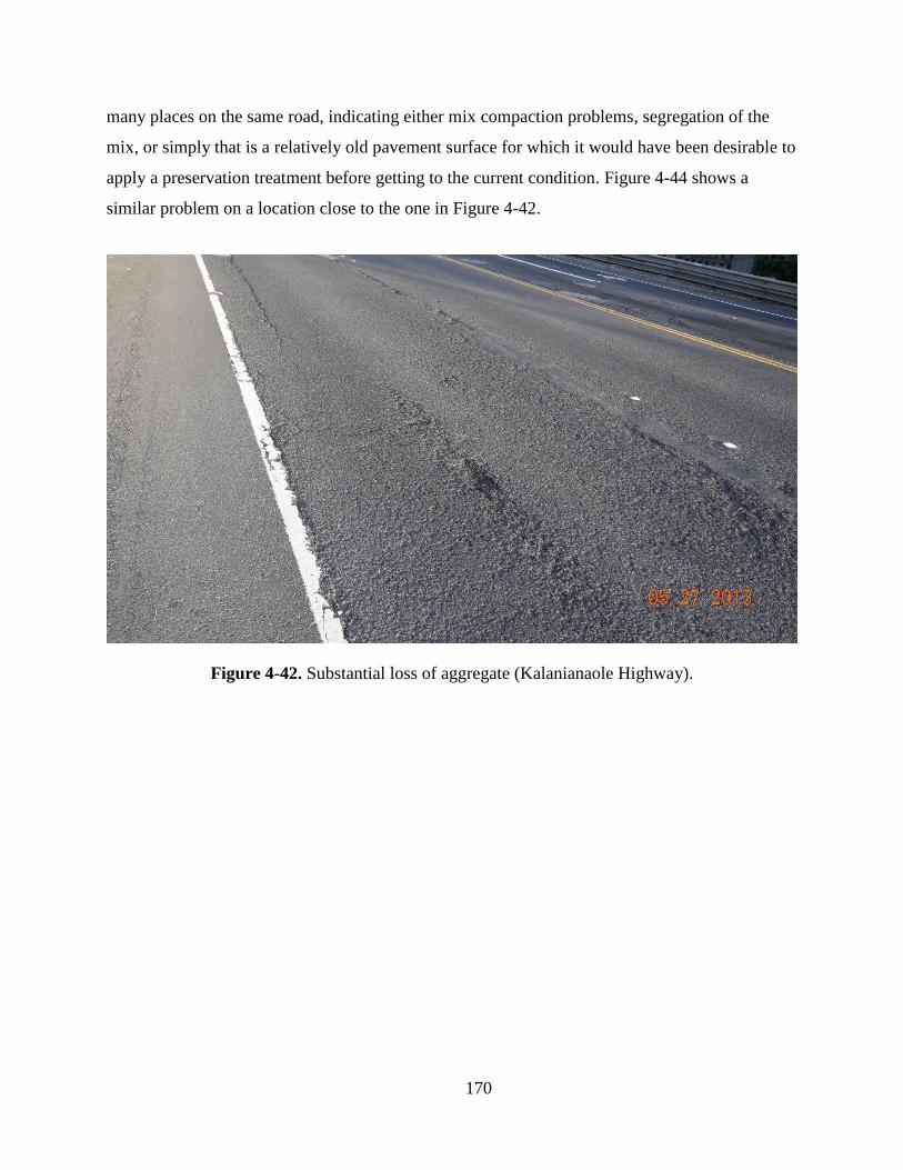
170

many places on the same road, indicating either mix compaction problems, segregation of the

mix, or simply that is a relatively old pavement surface for which it would have been desirable to

apply a preservation treatment before getting to the current condition. Figure 4-44 shows a

similar problem on a location close to the one in Figure 4-42.

Figure 4-42. Substantial loss of aggregate (Kalanianaole Highway).

171

Figure 4-43. Close up illustrating the disintegration of the pavement surface and the loose

aggregate.

Figure 4-44. Another example of severe raveling on Kalanianaole Highway.

172

Identification of raveling from forward pictures may be challenging, as it may be difficult

to discern whether one is observing raveling or a coarse pavement texture. Furthermore, as

illustrated in Figure 4-45, in those ocassions that raveling is observed, delimiting the affected

area can be subjective and also difficult in locations further away from the point of view of a

particular frame or when it appears mixed with other distresses. Moreover, often only some parts

of an area are affected and their limits are not well defined. Finally, as shown in Figure 4-46, for

some sections raveling manifests over small areas pehaps as a result of segregation and/or poor

mix compaction. On large data collection efforts, it may be tempting to neglect such small areas.

On occasions, some raveling may be confused with cracking, as on forward pictures the

lost aggregates may look as cracks. Oftentimes, raveling will be combined with some cracking.

Figure 4-47 shows a section for which cracking appears to be significantly over reported.

Apparently, the longitudinal joint and raveling were considered as fatigue cracking.

Figure 4-45. Challenges when attempting to quantify areas with raveling.

173

Figure 4-46. Small raveled areas.

Figure 4-47. Longitudinal joint and raveling misclassified as fatigue cracking.

(Route 99 – MP 7.70).

The following paragraphs describe a few other issues that were detected in the data that

should be checked as part of a quality asssurance process. Many of these are relatively easy to

solve but it is still worth pointing them out for future reference.

174

On the 2010 roughness table delivered by Mandli, both rutting and faulting are reported

on every 0.01 mi data intervals. Unless one of these intervals straddles a change in pavement

type, only one of these two distresses can be present. Thus, for most sections only one of these

distresses would be different from zero. However, several 0.01 mi long intervals were found

where both rutting and faulting were different from zero even though there was no pavement

type change within the interval. This is a relatively minor problem but it can also be solved

relatively easily.

On ocassions, there seem to be a potential for double counting of cracking. For example,

a few segments were found for which the sum of percentages of fatigue cracking at the different

severity levels were much high than 100%. Something similar was noted when adding the

percentages of say, fatigue cracking and block cracking.

Although the data is supposedly reported every 0.1 mi (except for smaller segments),

there are some fields with much larger differences between the begin mile point (BMP) and the

end mile point (EMP) (larger than 100 mi in one case.) The data should be QA for this kind of

problem, flagging any overlapping of intervals for review. As described in a later chapter, when

preparing the data to be imported into PAVERTM, these overlapping sections created several

problems and thus, the problematic intervals were ignored. However, ignoring them is not the

best solution as the problem most of the time appears to be caused by mistyping of one of the

end points, which is also an easy problem to fix if the proper interval can be identified.

Several cells with distress information have negative numbers that appear to be result of

some error. These should also be detected and fixed or eliminated.

Also, as indicated before, it may be easier to aggregate the data given in the raw data file

(the file that contains the information collected for each frame on 0.002 mi intervals) as this will

help avoid having to prorate the data for 0.1-mi segments when they straddle a PMS section.

However, for this, a key should be provided in the raw distress data table that allows linking the

frame information with mile points (or if enough information is already available in the delivered

database, instructions about how to perform the linking should be provided).

It is suggested to continue collecting longitudinal and transverse cracking separately to

facilitate HPMS reporting (i.e., longitudinal non-wheel path cracking as one distress and

175

transverse cracking (HPMS item 53) as the other). They can be combined later on for PCI

calculations or for other purposes.

4.3.4 Future distress surveys

It is important to pause here to analyze what would be appropriate for the future distress

surveys. From a consistency point of view, the first thought would be to maintain the method

currently used. However, as far as the PI knows, the next distress data collection cycle would be

performed by Mandli using an automated analysis of downward pictures (at least for cracking

distresses). Thus, even if the same protocols are followed, some important differences should be

expected, particularly in the levels of cracking. Thus, the data will not be entirely consistent for

one more cycle. However, it is highly recommended that if succesful, the technology used in the

next cycle be continued in the future with as few changes as possible. It is also important to

follow the protocol selected for performing the distress survey with as few changes as possible.

If for any reason there is a need to change some aspect of the protocol, this should be well

documented and highlighted.

It is expected that some of the cracking that before went undetected will be caught earlier

with the downward imaging. It is also expected that the lengths and areas of cracking (depending

on the type being measured) will be more repeatable. Finally, some differences should also be

expected in the classification of cracks into the different categories. Raters tend to classify some

cracks differently from those obtained by a computer algorithm.

It is also important for HDOT to decide and maintain the protocol used to perform the

distress surveys. A careful study of the distress definitions in the two most widely used distress

identification protocols, SHRP/LTPP [28] and ASTM D6433, reveals several differences that

would translate into differences on the computed PCI values.

The above paragraphs nonwithstanding, it is important to point that some highway

agencies are starting to change the methodologies for classifying and quantifying cracking of

flexible pavements. This is because the LTPP and ASTM D6433 survey methodologies were

developed mostly for field walking surveys, which are not practical at the network level.

A good example is provided by California. As reported by [32], the California

Department of Transportation (Caltrans) is considering a method in which cracks are classified

176

into one of four categories: transverse cracking (non-load-associated), longitudinal cracking

(non-load-associated outside the wheel path), wheel path cracking (load-associated), and XF

cracking (intended to identify cracking caused by reflection of underlying cracks and joints).

Each of these are related to broad but distinct cracking mechnisms. These authors have proposed

a protocol to quantify them from automated distress surveys. A main advantage of their method

is that it relies only on cracking length, which is determined relatively accurately by automated

procedures instead of relying on crack widths, which are not easy to determine. The procedure is

intended to eliminate as much as possible subjective ratings. In addition, these authors also

define wheel path areas that are wider than those defined in AASHTO R55-10. The wider areas

appear to be more realistic given the typical heavy vehicle wheel widths and wander. If HDOT

starts using downward imaging continuously to perform the distress surveys, consideration

should be given to these procedures as they have the potential to significantly reduce subjective

ratings.

Finally, as mentioned earlier, raveling is a difficult distress to quantify from photographs

and appears to be currently under-reported. However, significant technological advances have

been made in recent years that may help measuring indicators of raveling at the network level.

Specifically, a Raveling Index (RI) indicator has been proposed to detect and quantify raveling

conditions [33]. RI is obtained by measuring the volume of aggregate loss (holes due to missing

aggregates) per unit of surface area. HDOT should consider testing the use of 3D Laser

technology to quantify RI, particularly since 3D Laser technology is already been used by

HDOT. It is important to note that Mandli Communications, Inc., the vendor currently providing

the distress survey services, will be using 3D Laser technology from Pavemetrics Systems, Inc.

for automated cracking detection. Pavemetric Systems, Inc. has been involved in developing the

RI index. Thus, except perhaps for cost considerations, evaluation of the technology locally

appears feasible. Furthermore, the same technology can also provide measurements of a Road

Porosity Index, which is a pavement macro-texture indicator similar to what is obtained with the

sand patch method typically used to evaluate pavement macro-texture. Among other things,

pavement macrotexture affects safety (tire/road friction level, water runoff and aquaplanning

conditions) and noise.

177

PAVEMENT ME DESIGN

Introduction to Mechanistic-Empirical Design

5.1 INTRODUCTION

A main objective of this study is to advance in the calibration of the MEPDG or,

as it is now known, the AASHTO Pavement ME Design. As indicated in Chapter 1, a

main advantage of a mechanistic-empirical approach over entirely empirical approaches

is that, in addition to being a more rational and scientifically substantiated approach, it

provides mechanisms for calibration to local conditions. The mechanistic-empirical (ME)

approach has been used in different forms for pavement design for decades and thus its

principles are well known.

This chapter gives an overview of some of the main ME principles to provide a

framework for some of the discussions about material characterization and traffic and

climate inputs that follow as well as for the discussion of calibration of the design guide.

Emphasis is given to issues that are more relevant to the most prevalent Hawaiian

conditions. Thus, for example, subjects such as creep compliance used for thermal

cracking calculations are not discussed. For a detailed and general introduction to the ME

approach, reference is made to the book of Huang [34]. Other general references

providing good introductory concepts to the subject are those of Mallick & El-Korchi

[35] and Papagiannakis & Masad [36].

The best source for detailed discussion of the concepts used in the MEPDG is the

report from the National Cooperative Highway Research Program (NCHRP) research

study 1-37A that resulted in its creation [1]. A shorter description of inputs and issues

with the MEPDG is provided in the MEPDG Manual of Practice [22]. For those already

with some familiarity with the ME pavement design approach, the MEPDG Manual of

Practice should probably be the first reference to be consulted for further details.

The MEPDG documentation [1] is voluminous and intimidating for those without

background on mechanistic-empirical procedures. On the other hand, although the

178

MEPDG Manual of Practice [22] provides an excellent overview, it may leave some

readers without familiarity on ME design hanging on some details. Thus, the purpose of

this chapter is to provide a very basic introduction to the ME approach to pavement

design as well as the importance of the design inputs and interpretation of its outputs so

that the basic ideas can be understood. The goal is to complement the MEPDG

documentation referenced above.

In this chapter, an effort has been made to avoid as much as possible duplication

with the MEPDG documentation. Nevertheless, some duplication is unavoidable and

therefore some sections have been paraphrased and others reproduced from it. This is

made clear at the outset so that lengthy sections within quotation marks are avoided.

The mechanistic-empirical design and analysis procedure calculates pavement

responses (stresses, strains, and deflections) and uses those responses to compute

incremental damage over time. The procedure empirically relates the cumulative damage

to observed pavement distresses. This ME based procedure is shown in flowchart form in

Figure 5-1 [1]. “MEPDG”, as is used in this report, refers to the documentation and

software package” ( [1], [2]).

As with any other design procedure, the first design stage consists in evaluating

the conditions for the new or existing pavement. The evaluation portion provides inputs

required for design. These consist of environmental conditions, material characteristics,

and traffic loading. As part of the design, levels of reliability for each distress type

analyzed also need to be chosen. The second stage involves the selection of a trial design,

which is analyzed for adequacy against the user input performance criteria and reliability

values through the prediction of distresses and smoothness. If the design does not meet

the desired performance criteria at the specified reliability level, it is revised and the

evaluation process repeated as necessary. If inadequate, other trial designs (involving

design features such as layer thicknesses and materials) are analyzed until one is found

meeting all the design criteria. This approach differs with traditional design procedures

that resulted in a set of thicknesses for the given material characteristics. As shown in

Figure 5-1, the ME approach is iterative in nature. After one or more competing

alternatives are selected, the third stage (which is beyond the scope of this introduction)

179

proceeds to the selection of a strategy by considering life cycle costs and other

considerations.

Figure 5-1. Conceptual schematic of the three-stage design approach. Source: [1].

It is important to note at the outset that the basic premise of the mechanistic-

empirical approach for pavement design is conceptually simple. The difficulties lie in

180

understanding how things are integrated and in feeding the procedures with adequate

information. Most of the rest of this chapter focuses on these two aspects.

5.2 Hierarchical Input Levels

The MEPDG uses a hierarchical input level scheme to categorize the designer’s

knowledge of the input parameters. This hierarchical input structure allows users with

minimal experience in ME based procedures to use the method with little initial

investment. Three levels are available for determining the input values for most of the

material and traffic parameters:

Input Level 1 – Input parameter is measured directly; it is site- or project

specific. This level represents the greatest knowledge about the input

parameter for a specific project but has the highest testing and data collection

costs to determine the input value. Level 1 should be used for pavement

designs having unusual site features, materials, or traffic conditions that are

outside the inference space used to develop the correlations and defaults

included for input levels 2 and 3.

Input Level 2 – Input parameter is estimated from correlations or regression

equations. In other words, the input value is calculated from other site-specific

data or parameters that are less costly to measure. Input level 2 may also

represent measured regional values that are not project-specific.

Input Level 3 – Input parameter is based on “best-estimated” or default

values. Level three inputs are based on global or regional default values – the

median value from a group of data with similar characteristics. This input

level has the least knowledge about the input parameter for the specific project

but has the lowest testing and data collection costs.

5.3 Purpose of the Hierarchical Input Levels

With the exception of the HMA transverse or thermal cracking prediction

methodology, input level has no effect other than knowledge of the input parameter

(which is important for critical inputs). This approach provides the designer with a lot of

181

flexibility in obtaining the inputs for a design project based on the criticality of the

project and the available resources. The hierarchical input structure allows the user with

limited experience in ME based design procedures and only standard test equipment for

measuring material properties to use the MEPDG. On the other extreme, it allows an

experienced user to measure many inputs for a design-build type of project, or for the

forensic evaluation of an existing pavement.

5.3.1 Selecting the Input Level

For a given design project, inputs can be obtained using a mix of levels, such as

dynamic modulus from level 1, traffic load spectra from level 2, and subgrade resilient

modulus from level 3. No matter what input design levels are used, the computational

algorithms for damage and distress are the same. The same models and procedures are

used to predict distresses and smoothness. Of course, the highest the level the more

reliable the predictions are expected to be.

The MEPDG recommends that the designer use the highest level of inputs

available at the time of design.

5.4 MECHANISTIC-EMPIRICAL ANALYSIS

As the name implies, the mechanistic-empirical design procedure involves both

mechanistic and empirical components. The mechanistic component determines the

pavement responses in terms of stresses, strains, and deflections on some points within

the pavement structure caused by a given traffic loading condition and for the material

characteristics prevailing under the environmental conditions at the time the loading is

applied.

The highlighted words in the above descriptions are important. Traffic loading

always consists of a distribution of traffic load magnitudes on different heavy vehicle’s

axle load configurations (single, tandem, tridem, and quad axles). The environment and

in turn the characteristics of the materials in the different layers of the pavement structure

are constantly changing and thus, the effect of a given load depends on when it is applied.

The empirical component relates empirically the pavement responses computed in

the mechanistic analysis to different pavement distresses such as cracking and rutting.

182

This is the weakest link of the methodology. A brief explanation of the mechanistic

component is given in the following section followed by a section on the empirical

components for bottom up fatigue cracking and rutting, which are the two traditionally

considered mechanisms in ME design of flexible pavements. The MEPDG also calculates

top-down fatigue cracking, thermal cracking, reflection cracking, and smoothness. More

discussion about the consideration of these distresses for Hawaii is provided later in the

sequel.

5.4.1 Mechanistic Analysis

The structural response model is a mechanistic model based on fundamental

engineering principles. It is used to calculate critical pavement responses (deflections,

stresses, and strains). The MEPDG uses internally the JULEA program as the structural

response model used for flexible pavements. JULEA is one of many computer programs

that are available for computing the state of stresses, strains and deflections caused by

loads on pavement systems. The linear layer elastic theory assumes that each layer i is

homogeneous, isotropic, and linear elastic with elastic modulus (Ei) and Poisson ratio

(i), that the material is weightless and infinite in areal extent and that each layer has a

finite thickness hi, except for the lowest layer, which is infinite in thickness [34]. Other

assumptions include continuity conditions at layer interfaces (including friction between

layers) and that the load is applied with uniform pressure over circular areas. A stress

dependent finite element program was also available in the MEPDG for flexible

pavement analyses using input level 1 for unbound materials, but it was not included in

the global calibration effort [1]. The use of the finite element program for flexible

pavements was intended for research purposes only. This option is disabled in the current

version of Pavement ME Design [2].

To fix ideas about the mechanistic analysis, consider a pavement structure such as

the one shown in Figure 5-2. The pavement structure is a layered system and is typically

modeled using linear layered elastic analysis. In the example of Figure 5-2, the structure

is loaded by a single load of magnitude P over a circular area with radius a. Since the

materials are assumed linear elastic, the superposition principle can be used to determine

the pavement responses for any number of loads applied with uniform pressure over

183

circular areas. In particular, the loading configurations usually applied by vehicular

traffic are easily accommodated. Most computer programs available allow the analysis of

multiple-wheel loading configurations.

Clearly, some of the above assumptions are not applicable in practice. For

example, most geomaterials are non-linear (i.e., the modulus of each layer is not constant

but depends on the state of stresses) and the load is not really applied over a circular area.

Nevertheless, the theory has served well for many years for its simplicity and ease of use.

As indicated before, to date, the more advanced modeling techniques such as finite

element analysis that can cope with nonlinearities, dynamic effects, anisotropy, etc., are

used mostly for research purposes.

Figure 5-2. State of stresses at a point within a linear elastic layered pavement structure

[34].

Now, with reference to Figure 5-2, consider a differential element located at a

depth z below the pavement surface, at a distance r from the center of the load and of

dimensions dz, dr, and r d. The state of stresses at such point will be defined by the six

components z, r, t, rz (=zr), tz (=zt), and zr (rz). Most linear layer elastic analysis

programs report these stresses along with the associated (normal) principal stresses 1,

z1

z2

zn-2

H

z

E1 , 1

E2 , 2

En-1 , n-1

En , n rt tr

zt

tz rz

P

d

dz

dr

r

A B

z

zr

z

t

r

184

2, and 323. In addition, these programs also report the state of strains at the point either

in the normal, tangential and vertical directions (z, r, z, rz, tz, and zr) or in the

principal directions 1, 2, and 3 or both. Deflections at any selected point within the

pavement structure can also be computed. The differential element can be located

anywhere within the pavement structure such as points A or B in Figure 5-2.

In order to illustrate how different pavement properties affect the distribution of

stresses and strains, the following paragraphs describe the changes with the help of

several figures. The figures illustrate some of the distribution of stresses and strains that

can be computed for a pavement structure. They were all created for a 9,000-lb load

applied over a circular area with a 5.91-in radius (a typical loading configuration used

with the Falling Weight Deflectometer (FWD) to simulate the loading of a standard

single axle load). In each figure, two different scenarios are analyzed for comparison.

Part a) of each figure considers that a load is applied on a pavement structure consisting

of 6 inches of Hot Mix Asphalt (HMA) with a modulus of 500,000 psi, an unbound

granular base layer 12 inches thick with modulus of 30,000 psi, and a fine grained

subgrade with a modulus of 10,000 psi. The Poisson ratios were assumed to be 0.30, 0.4,

and 0.45 for the HMA, base, and subbase layers, respectively. The value of 0.30 for

HMA is approximately the value that the MEPDG would calculate based on the modulus

of the HMA. In part b) of each Figure, either the thickness of HMA is maintained at 6

inches and its modulus is changed 2,500,000 psi to simulate a lower temperature of the

HMA or the modulus is maintained at 500,000 psi and the thickness of the HMA layer is

changed to 12” to compare the distributions with a thicker pavement structure. For the

2,500,000 psi case, the Poisson ratio of the HMA is changed to 0.15, which is the value

that would be estimated by the MEPDG. In order to interpret the figures, it is important to

point out that the center of the load is always located on the left side of each chart and the

edge of the load is located at a distance from the center of 5.91 inches. Only the first 30

23 Recall the principal stresses for the differential element are those located at the same point but

with a different orientation of the element such that 1 is the maximum normal stress, 3 is the minimum

normal stress and there are no shear stresses acting on the faces of the element.

185

inches of the pavement structure are shown in depth and laterally. In all cases, axial

stresses/strains with positive signs are compressive and those with negative signs are

tensile. Finally, since the color pallets are the same for the different scenarios in a given

stress or strain distribution chart, it is important to look carefully at the legend of each

figure as in most situations a similar color would represent different stress/strain levels on

different charts.

Figure 5-3 illustrates how the distribution of vertical stresses for the base case (6

inches of HMA and 500,000 psi HMA modulus) compares with that obtained when the

modulus of the HMA is changed to 2.500.000 psi. As one would expect, the vertical

stresses dissipate faster with depth for the stiffer HMA layer. Of course, the faster

dissipation of vertical stresses comes at the cost of much higher tensile stresses in the

HMA layer, as can be observed in the distributions of radial stresses in Figure 5-4. Note

that although the coloring in the two parts of Figure 5-4 is similar, the stresses are much

higher in part (b). As an aside, Figure 5-4 also helps to illustrate a somewhat vexing issue

with the use of linear layer elastic analysis, which is the prediction of tensile stresses in

granular base layers. Unless some cementation occurs in these layers, these tensile

stresses are typically not realistic. However, this problem is not significant for thicker

bound layers.

Figure 5-5 shows the corresponding principal stress distributions. Although not as

easy visualize, the figure shows how that the stiffer layer spreads the stresses over a

wider area. In this figure, the short segments indicate the direction in which the principal

stresses act. As can be seen, these lines are generally more horizontal in part (b) than in

part (a), which illustrates the slab action effect typically associated with concrete

pavements (the modulus of concrete is higher than that assumed for part (b)). It may also

be surprising to see that immediately below the load; the stresses are higher in the

horizontal direction than in the vertical direction. Nevertheless, this a perfectly valid

outcome.

186

(a) (b)

Figure 5-3. Vertical stress distribution for a 9,000 lb. circular load on a pavement structure with a 6” HMA layer, 12” granular base

with 30,000 psi modulus ( = 0.40), and a fine-grained subgrade with 10,000 psi modulus ( = 0.45)

(a) EHMA = 500,000 psi and = 0.30 and (b) EHMA = 2,500,000 psi and = 0.15.

187

(a) (b)

Figure 5-4. Radial (horizontal) stress distribution for a 9,000 lb. circular load on a pavement structure with a 6” HMA layer ( =

0.35), 12” granular base with 30,000 psi modulus ( = 0.40), and a fine-grained subgrade with 10,000 psi modulus ( = 0.45)

(a) EHMA = 500,000 psi and (b) EHMA = 2,500,000 psi.

188

(a) (b)

Figure 5-5. Maximum principal stress distribution for a 9,000 lb. circular load on a pavement structure with a 6” HMA layer ( =


(a) EHMA = 500,000 psi and (b) EHMA = 2,500,000 psi.

189

Since the distress transfer functions used in ME analyses typically involve strains,

it is also illustrative to compare their distributions. Figure 5-6 shows the distribution of

vertical strains for the same two scenarios discussed before. Notice how the strains are

more than halved for the stiffer 2,500,000 psi HMA layer with respect to the 500,000 psi

HMA layer. On the other hand, it is interesting to note that the predicted vertical strains

immediately below the load are tensile instead of compressive for the lower HMA

modulus! Although this may appear counterintuitive, it is related in part to the effect of

the Poisson ratio for the HMA layer.

The results in Figure 5-7, which show the distributions of radial strains, clearly

illustrate why fatigue cracking is typically associated with the maximum horizontal

tensile strain at the bottom of the asphalt concrete layer. It is typically at this location

where tensile strains are a maximum. Once again, it is important to look at the chart

legends to see that the tensile strains are significantly lower for the stiffer HMA layer.

Finally, it is also illustrative to see the distribution of the minimum principal

strains. These are shown in Figure 5-8 for the same two scenarios. Consistent with the

results in Figure 5-4, the minimum tensile principal stains occur at the bottom of the

HMA and the stiffer layer reduces them substantially. However, note that for the scenario

with the EHMA = 500,000 psi, there is a significant area where tensile strains near the

surface are not negligible. This effect is accentuated for even lower moduli (higher

temperatures) and may be a relevant factor in the explanation why the typical cracking

occurring on Hawaii State Roads appear to be top-down longitudinal cracking. A more

thorough discussion of this issue is presented later in the report.

190

(a) (b)

Figure 5-6. Vertical strain distribution for a 9,000 lb. circular load on a pavement structure with a 6” HMA layer, 12” granular base

with 30,000 psi modulus ( = 0.40), and a fine-grained subgrade with 10,000 psi modulus ( = 0.45)


191

(a) (b)

Figure 5-7. Radial (horizontal) strain distribution for a 9,000 lb. circular load on a pavement structure with a 6” HMA layer ( =



192

(a) (b)

Figure 5-8. Minimum principal strain distribution for a 9,000 lb. circular load on a pavement structure with a 6” HMA layer ( =



193

The following figures illustrate the effect of layer thickness on the distribution of

stresses and strains. In each of the following six figures, scenario (a) is the same as

scenario (a) in Figure 5-3 to Figure 5-8. In other words, the left sides of the new figures

are the same as those presented in those figures. The difference is presented for scenario

(b), which considers an HMA layer thickness of 12 inches but with a modulus of 500,000

psi and = 0.3. That is, except for the HMA layer thickness, there is no other difference

between the two scenarios.

Figure 5-9 shows how a thicker layer of HMA helps the reduction of compressive

vertical stresses in the base and subbase. Although, it may not be obvious, the reductions

are substantial (a factor of about two.)

The same applies to the radial (horizontal) stresses illustrated in Figure 5-10.

Again, attention must be paid to the legend of each chart to appreciate the significant

reduction in horizontal stresses for the thicker HMA layer. Figure 5-11 shows the

distribution of principal stresses for which the same observations as for the two previous

figures can be made.

Figure 5-12 to Figure 5-14 show the comparison of the distributions of vertical,

horizontal, and minimum principal strains, respectively. Again, by paying attention to the

chart legends, it can be noted the substantial reduction of strains caused by the thicker

layer. Figure 5-14 shows that for the thicker HMA layer (scenario b), there exists tensile

strains near the surface of the layer that are similar in magnitude to the maximum of the

maximum tensile strain at the bottom of the HMA (in this particular example they are

about 60% of the maximum). With a lower modulus of the HMA layer, the tensile strain

near the surface can become equal or higher than that at the bottom of the HMA. This

again may provide an explanation for the prevalent longitudinal cracking observed on

state roads. These typically consists of thick structures and the top is subjected to high

temperatures throughout the year, which are the two factors that may results in higher

tensile strains at the top relative to those at the bottom. Section 7.6 (page 408) provides a

more detailed discussion of the load induced tensile strains near the surface.

194

(a) (b)

Figure 5-9. Vertical stress distribution for a 9,000 lb. circular load on a pavement structure HMA layer (EHMA = 500,000 psi,

= 0.30), 12” granular base with 30,000 psi modulus ( = 0.40), and a fine-grained subgrade with 10,000 psi modulus ( = 0.45)

(a) hHMA = 6 inches and (b) hHMA = 12 inches.

195

(a) (b)

Figure 5-10. Radial (horizontal) stress distribution for a 9,000 lb. circular load on a pavement structure HMA layer (EHMA = 500,000

psi, = 0.30), 12” granular base with 30,000 psi modulus ( = 0.40), and a fine-grained subgrade with 10,000 psi modulus ( = 0.45)


196

(a) (b)

Figure 5-11. Maximum principal stress distribution for a 9,000 lb. circular load on a pavement structure HMA layer (EHMA = 500,000



197

(a) (b)

Figure 5-12. Vertical strain distribution for a 9,000 lb. circular load on a pavement structure HMA layer (EHMA = 500,000 psi, =



198

(a) (b)

Figure 5-13. Radial (horizontal) strain distribution for a 9,000 lb. circular load on a pavement structure HMA layer (EHMA = 500,000



199

(a) (b)

Figure 5-14. Minimum principal strain distribution for a 9,000 lb. circular load on a pavement structure HMA layer (EHMA = 500,000



200

The theory behind linear layered elastic analysis is beyond the scope of this report.

For those interested in learning more about it [34] provides an excellent introduction. In any

case, to use a linear elastic analysis program one does not need to know the details of the

theory but only the main assumptions and limitations. The computer programs can be used in

the same way geotechnical engineers typically use charts or equations for determining state

of stresses based on Boussinesq theory. In fact, the MEPDG does all the pavement response

calculations in the background and the designer never even sees these intermediate results.

Nevertheless, an understanding of the main concepts is important to appreciate the ME design

approach and avoid its use as a black box.

Different pavement responses have been used for different distress types. In what

follows most of the discussion will be centered on bottom up fatigue cracking (i.e., cracking

initiating at the bottom of the asphalt concrete layer) and rutting (the longitudinal depressions

in the wheel path of the pavement). Therefore, only the responses associated with these

distresses are discussed.

Fatigue cracking is typically associated with the maximum horizontal tensile strain at

the bottom of the asphalt concrete layer whereas rutting is associated in the MEPDG to the

maximum vertical compressive strain at the midpoint of each sublayer (for rutting analysis,

the pavement structural layers are subdivided more finely). Other pavement responses are

used in mechanistic-empirical analysis for other purposes. Specifically, deflections are used

for back-calculation of layer moduli on rehabilitation projects. In addition, in the research

release of the MEPDG stresses were used for non-linear materials whose moduli depend on

them.

In summary, the pavement response results of the mechanistic analysis for a given

load and environmental condition that are used to predict distresses are:

Bottom-up fatigue cracking: the maximum tensile strain at the bottom of the

asphalt concrete layer.

Rutting: the maximum vertical compressive strains at the mid-depth of each

sublayer.

These pavement responses are then related to the distresses as explained in the

following section.

201

5.4.2 Empirical Analysis

In the empirical part of the analysis, the pavement responses are related empirically to

the different distresses.

5.4.2.1 Bottom-up fatigue cracking

For bottom-up fatigue cracking, the allowable number of repetitions of the load under

consideration is related to the maximum tensile strain at the bottom of the asphalt concrete

layer and the modulus of the asphalt concrete by:

32 *1

kk

t EKN

(5-1)

where

N = allowable number of load repetitions,

|E*| = dynamic complex modulus of the asphalt concrete mixture (psi),

t = tensile strain at the bottom of the asphalt concrete layer

(microstrain = = 10-6 in/in), and

K1, k2, and k3 = empirically derived parameters24.

This equation is derived from laboratory fatigue cracking experiments. Figure 5-15

shows a beam fatigue apparatus (BFA), one of the pieces of equipment used to carry out this

type of experiments. In order to predict cracking in the field, the parameters K1, k2, and k3 are

adjusted for a given level of cracking (i.e., the model is calibrated for field conditions). The

MEPDG has been calibrated for a level of cracking of 50% of total lane area when N loads

are applied. The values of K1, k2 and k3 used in the MEPDG for 7% air voids and 11% asphalt

content by volume are 1.793×10-3, 3.949, and 1.281 respectively. These values are used in the

examples below. Figure 5-16 illustrates a case of a section exhibiting significant fatigue

cracking.

24 The value of K1 is provided in the guide as function of air voids, volumetric asphalt content and

another parameter k1, which explains why a capital letter was used for this first parameter.

202

Figure 5-15. Beam Fatigue Apparatus used for fatigue testing.

Figure 5-16. Example of section exhibiting fatigue cracking.

If all the traffic loads were identical and the environmental conditions were constant

over time (i.e., constant material characteristics over time), equation (5-1) could be used

directly for verification of the adequacy of a trial pavement structure. To illustrate this,

consider the following simple example. Let n be the predicted (expected) number of

repetitions of the constant load magnitude over the design or performance period. The value

of n is derived from traffic loading information. For example, consider the evaluation of a

pavement for a section with constant traffic of two identical heavy vehicles per day. Further,

assume that all heavy vehicles have two axles with exactly the same loads. For those

conditions, the predicted value of n for a design period of say, 20 years, would be

Beam

S

pecimen

Actuator

Clamps

203

n = (20 years) × (365 days/year) × (2 repetitions/veh) × (2 veh/day) = 29,200 repetitions.

Thus, if N (the allowable number of repetitions corresponding to the strain level caused by

the load in question) were greater than 29,200 repetitions then the design would be adequate

from a bottom-up fatigue cracking perspective because the pavement would be able to

withstand this number of repetitions without reaching the threshold of unacceptable level of

fatigue cracking25. On the other hand, if N were lower than 29,200, the design would be

inadequate since the cracking would become unacceptably high before reaching the end of

the design period.

To illustrate the use of equation (5-1), suppose that the modulus of the mix is

1,000,000 psi (and for now assume this is constant throughout the year) and that the load

produces a 150×10-6 (150 ) tensile strain at the bottom of the asphalt concrete layer. Then,

the allowable number of repetitions is

281194933 0000001000150107931..

,,..N = 46,580

Therefore, in this case the pavement would reach the end of the design period with an

acceptable level of cracking26. Had the computed allowable number of repetitions being

much higher, say 2,000,000, the pavement would have been grossly over designed and then a

weaker (and more economical) pavement structure should have been tried for the loading

conditions under consideration.

For a larger load producing a 180×10-6 tensile strain the allowable number of

repetitions is

281194933 0000001000180107931..

,,..N = 22,673

In this case, the pavement structure is clearly inadequate to withstand the predicted

traffic loading of 29,200 repetitions over the design period.

As indicated before, many linear elastic layered analysis programs would make

calculation of the tensile strains and in turn this type analysis very simple. The problem is

that the assumptions made in the above examples are clearly unrealistic. Traffic loading is

25 For simplicity, the example assumes that 50% of the total lane area cracking is an acceptable

threshold criterion. In reality, 50% of the total lane area cracked is too high a value.

26 Again 50% of the total lane area is a very high value, but it is used here to simplify the exposition.

204

always variable (with different vehicle classes, different axle configurations, and different

axle loads as illustrated in chapter 3) and the environmental conditions are never constant,

even for Hawaii that has relatively stable whether conditions compared to other parts of the

country. In fact, near the pavement surface, variations of the HMA modulus of an intact layer

of more than 500,000 psi could be expected from winter to summer in Hawaii.

5.4.2.1.1 Consideration of different traffic loads

When conditions are not constant, how should one evaluate the adequacy of the

pavement? To illustrate the answer to this question, consider another simple (and still

unrealistic) example. Suppose again the design period is 20 years and that the two axles of

the heavy vehicles have different load levels L1 and L2. Let t1 and t2 be the maximum tensile

strains at the bottom of the asphalt concrete layer caused by loads L1 and L2, respectively.

Then, equation (5-1) could be used to compute Nf1 and Nf2 for load levels L1 and L2,

respectively. Each of these values represents the number of repetitions of the respective load

that the pavement could withstand if each of the loads were applied without the presence of

the other. However, the loads are actually intermingled. In this particular example, an

application of load L1 is followed by an application of load L2, then L1 again, L2 again and so

on. Obviously, because of the presence of the two different loads, the pavement would reach

an unacceptable level of cracking before Nf1 or Nf2 repetitions of load magnitudes L1 and L2

are applied. An important question is whether the pavement would survive the application of

the loading predicted over the design period. Using again the simplified example of constant

traffic consisting of two identical heavy vehicles per day, the predicted number of repetitions

of loads L1 and L2 would be n1 = n2 = (20 years) × (365 days/year) × (1 repetition of load

Li/veh) × (2 veh/day) = 14,600 repetitions (Li = L1 or L2 for n1 or n2, respectively).

Now suppose that (using a linear layer elastic computer program) the predicted tensile

strains for loads L1 and L2 are 150×10-6 and 180×10-6 respectively. The corresponding

allowable number of repetitions would then be

2811949331 0000001000150107931

..,,..

N = 46,580

and

2811949332 0000001000180107931

..,,..

N = 22,673

205

The answer to put all these pieces of information together is given by what is known

as Miner’s hypothesis or Miner’s law [1], which states that fatigue damage of the asphalt

concrete layer is given by the following relationship.

M

i i

i

N

nD

1

(5-2)

where:

D = damage,

M = total number of load magnitudes,

ni = actual predicted load repetitions for load magnitude Li, and

Ni = load repetitions allowed under conditions prevailing in i.

Miner’s hypothesis is simply a practical relationship that provides a mechanism to

combine the effects of different traffic loads, though some question their validity.

As indicated before, the MEPDG has been calibrated so that when the damage is

100% (D=1) the predicted cracking is 50% of the total lane area (which in turn approximates

100% of the wheel path areas).

Thus returning to the example, the application of Miner’s law in this case indicates

that at the end of the design period the damage would be:

67322

60014

58046

60014

,

,

,

,D = 0.313 + 0.644 = 0.957

Since D < 1, then the pavement would not have reached the 50% of the total lane area

cracked, although it would be very close to doing so.

It is important to reiterate that 50% of the total lane area is a very high value of

cracking. Typically a smaller threshold value is used. The equation used to translate damage

into the percentage cracking used in the MEPDG for bottom-up fatigue cracking is27:

27 A more complicated equation equivalent to equation (5-3) is presented in the MEPDG. However,

knowledge of the more complicated equation is needed mostly for those involved in the calibration of the

MEPDG cracking model. The complete expression is presented in section 7.5.2.

206

10010log2'21

100

DC

Bottom

eFC (5-3)

where

FCbottom

= bottom-up fatigue cracking, percent lane area,

D = bottom-up fatigue damage, and

85622 174839408742

...'

AChC

and where:

hAC

= total thickness of the asphalt layers, in.

In the above example, the predicted level of cracking (assuming hAC = 5 inches) is

100957010264721

100

.log.e

FCBottom = 48.7 %

The thickness of the asphalt concrete layer is included to account for the longer time it

takes for a crack to propagate on a thick layer than on a thin layer.

With a cracking criterion of 50%, the pavement design would be acceptable28.

5.4.2.1.2 Consideration of changing environmental conditions

In the ME approach, the effects of changes in environmental conditions can be taken

into account in the same way as changes in load magnitudes; that is, using Miner’s law. In the

case of a single load magnitude but different environmental conditions, the law takes the

form:

28 Once again, in reality, a lower criterion (of about 20%) is more reasonable; 50% represents an

excessive level. Reconstruction would is typically warranted before reaching such a high level.

207

T

i i

i

N

nD

1

(5-4)

where:

D = damage,

T = total number of periods with different environmental conditions.

ni = actual predicted load repetitions for period i.

Ni = load repetitions allowed under conditions prevailing in period i.

The reason why the predicted N changes from period to period is that the

environmental conditions affect the moduli of the different pavement layers and as illustrated

earlier this in turn changes the state of stresses and strains within the pavement structure.

Thus, there are changes in both the strain and the modulus in equation (5-1). Temperature

changes significantly affect the moduli of hot mix asphalt layers (as well as the moduli of

unbound materials under freezing conditions) and changes in moisture affect the moduli of

unbound materials. Consequently, even under identical loading conditions, the strains

produced within the pavement structure are different on different periods and this in turn

yields different values of N (see again equation (5-1)). Even the daily temperature changes

affect the moduli of HMA.

For illustration, consider once again an example of a design for a 20-year period with

traffic consisting of heavy vehicles with two axles with exactly the same loads. Assume the

year has two distinct seasons (e.g., a dry, hotter season and a rainy, colder season) such that

the pavement structure is overall stronger in the first season which last nine months (~ 274

days) than during the second season that last three months (~ 91 days). Suppose that the main

reason for the pavement structure being stronger in the first season than in the second season

is that during the second season moisture severely weakens the subgrade material.

Nonetheless, during the first season (which is hotter), the HMA modulus is 900,000 psi and

during the second season (colder) is 1,100,000 psi. Further, suppose that using the

corresponding moduli, the computed maximum tensile strains at the bottom of the asphalt

concrete layer are 120×10-6 and 170×10-6 for seasons 1 and 2 respectively. Under these

conditions, the calculation of damage proceeds as follows:

208

Season 1:

n1 = (20 years) × (274 days/year) × (2 repetitions/veh) × (2 veh/day) = 21,920

2811949331 000900000120107931

..,..

N = 128,679

Season 2:

n2 = (20 years) × (91 days/year) × (2 repetitions/veh) × (2 veh/day) = 7,280

2811949332 0001001000170107931

..,,..

N = 25,148

Application of Miner’s law then results in:

14825

2807

679128

92021

,

,

,

,D = 0.170 + 0.289 = 0.459

Using equation (2.3) (again assuming an asphalt concrete layer thickness of 5 in) the

computed damage results in the following percentage of bottom-up fatigue cracking in the

total lane area:

100459010264721

100

.log.e

FCBottom = 29.0 %

This value can then be directly compared against the agency threshold to assess

whether the trial pavement structure is adequate. If a 20% threshold is used, then the trial

pavement structure needs strengthening.

5.4.2.1.3 Consideration of different traffic loads and environmental conditions

simultaneously

Different loads and environmental conditions are accommodated simultaneously in

the ME approach with the following form of Miner’s law:

T

j

M

i ij

ij

N

nD

1

(5-5)

where:

D = damage,

M = total number of load magnitudes,

T = total number of periods with different environmental conditions,

209

nij

= actual predicted load repetitions for load magnitude Li during period j, and

Nij

= load repetitions allowed for load Li under conditions prevailing in j.

To illustrate the use of equation (5-5), assume as in the previous example that the year

has two distinct seasons (e.g., a dry, hotter season and a rainy, colder season) such that the

pavement structure is overall stronger in the first season which last nine months (~ 274 days)

than during the second season that last three months (~ 91 days). Suppose again that during

the first season (which is hotter) the HMA modulus is 900,000 psi and during the second

season (which is colder) is 1,100,000 psi. Further, assume traffic loading consisting on

average of 1.4 veh/day of a vehicle class with two axles (say, a local bus operating with low

frequency on weekdays only) and 0.6 veh/days of another vehicle class with two axles (e.g., a

2-axle garbage truck). Assume the axle loads on the bus are L1 and L2 and those on the truck

are L3 and L4 and that they produce tensile strains at the bottom of the HMA of 80×10-6,

105×10-6, 65×10-6 and 115×10-6, respectively during season 1 and 100×10-6, 120×10-6,

80×10-6 and 140×10-6 respectively during season 2.

Under these conditions, application of Miner’s law proceeds as follows:

Season 1:

n11 = (20 years) (274 days/year) (1 repetition/veh) (1.4 veh/day) = 7,672

28119493311 000900000080107931

..,..

N = 638,107


28119493321 0009000001050107931

..,..

N = 218,031


28119493331 0009000000650107931

..,..

N = 1,448,774


28119493341 0009000001150107931

..,..

N = 152,230

Season 2:


28119493312 000100100010107931

..,,..

N = 204,435

210


28119493322 0001001000120107931

..,,..

N = 99,511


28119493332 0001001000080107931

..,,..

N = 493,462


28119493342 0001001000140107931

..,,..

N = 54,137

Damage:

13754

0921

462493

0921

51199

5482

435204

5482

230152

2883

7744481

2883

031218

6727

107638

6727

,

,

,

,

,

,

,

,

,

,

,,

,

,

,

,

,D

= 0.0120 + 0.0352 + 0.0023 + 0.0216 + 0.0124 + 0.0256 + 0.0022 + 0.0202

= 0.1315

Bottom-up fatigue cracking (for hAC = 5 in.):

1001315.010log2647.21

100

e

FCBottom = 8.8 %

5.4.2.1.4 Summary for bottom-up fatigue cracking and consideration of other issues

Careful reading of the previous sections should provide those readers not familiar

with ME procedures with a good idea of how different loading and environmental conditions

are integrated in the bottom-up fatigue cracking procedures through Miner’s law. As

indicated at the beginning, the ideas and calculations are relatively simple. However, actual

axle loads are typically different for different vehicle classes and vary over a wide range of

magnitudes even for a single vehicle class. Furthermore the loads are applied through

different axle configurations (single, tandem, tridem, and quad axles), which complicates

matters further.

In all cases, the procedure involves the same computations for a given axle load

magnitude and axle configuration and environmental conditions:

Prediction of the expected number of repetitions of the axle in question under the

given set of environmental conditions over the design period;

211

Prediction of the maximum horizontal tensile strain at the bottom of the asphalt

concrete layer produced by the axle in question under the given set of environmental

conditions;

Prediction of the corresponding allowable number of repetitions; and

Computation of the damage (ratio of n/N) for the axle in question under the given set

of environmental conditions.

The addition of the damage induced by each axle load magnitude and configuration

for all different environmental conditions yields the total damage over the design period,

which in turn is converted to a percentage of cracking over the total lane area.

Although the procedure in concept is simple, the bookkeeping of all these calculations

becomes unmanageable with a large number of loads and environmental conditions. All these

repetitive tasks are ideal for implementation in digital computers and fortunately, all the

calculations are performed transparently to the user by the MEPDG, allowing the user to

concentrate on the inputs to the problem and on the analysis of the outputs from the program.

In fact, the MEPDG considers two more issues not yet discussed for fatigue cracking that

make the bookkeeping even more complicated. The two issues are the environmental

variations occurring within a period and the effects of traffic wander. Detailed discussion of

these is beyond the scope of this report. Only a brief discussion is presented in subsequent

text.

5.4.2.1.5 Changes of environmental conditions within a season

All the examples presented above assume that environmental conditions within a

season were constant. In reality, there are always monthly and even daily variations. Seasonal

effects within the MEPDG are considered on a monthly basis29. In order to reduce the number

of computations, the MEPDG subdivides the distribution of temperatures expected during the

month into five quintiles and computes the corresponding damage for each assuming that

traffic is distributed equally during each quintile. The subdivision of the temperature

distribution is illustrated in Figure 5-17 in terms of the normalized variable z = (t – )/,

29 Under freezing and thawing conditions, the MEPDG uses half-month periods but this is not

applicable for most of Hawaii.

212

where t = temperature, = mean temperature during the season and = standard deviation of

temperature during the season.

Figure 5-17. Consideration of temperature distributions within a season in the MEPDG.

5.4.2.1.6 Traffic wander

The discussions in the previous sections assumed that each traffic load is located in

the same position within the transverse pavement section. Actual traffic loading, however,

typically exhibits a distribution of lateral positions known as wander as illustrated in part C of

Figure 5-18 below. A normal distribution is typically assumed for traffic wander.

In all the previous examples, the damage was estimated using the maximum tensile

strain at the bottom of the asphalt concrete layer and the location of the point where that

maximum occurs was assumed to be the same for each load repetition. However, the

maximum damage does not occur always at the same point for consecutive load applications.

As indicated in part B of the figure, a single passage of a load produces variable damage

laterally. For the dual wheel configuration shown in the figure, the maximum damage appears

to be close to the center of each wheel. The shape of this damage curve actually depends on

the thickness of the asphalt concrete layer among other things, so this is not always the case.

Wander makes the determination of the location with maximum damage difficult. In

order to solve the problem, the MEPDG evaluates the damage at different points at the

bottom of the asphalt concrete layer as shown by points 1 through 5 in part A of the figure

(actually, a larger number of points is analyzed by the MEPDG). As with the temperature

effects described in the previous section and in order to simplify the analysis, the wander

distribution (assumed to be normally distributed) is split into five quintiles and the loads are

located at a representative point of the quintile to evaluate the damage. For example, consider

z = -1.2816 z = -0.5244 z = 0 z = 0.5244 z = 1.2816

20 % 20 % 20 % 20 % 20 %

f(x)

z = (t – )/

213

the damage D1 caused at point 3 by a load located as shown in part D of the figure. In this

case the damage at point 3 is practically zero. When the load is located as in part E, the

damage at point 3 is D2. Similar observations can be made for the other three quintiles. Then

the total damage caused on average at point 3 is simply D = 0.2 D1 + 0.2 D2 + 0.2 D3 + 0.2 D4

+ 0.2 D5 since there is an equal chance of 20% of the load being located on any of these

positions.

Figure 5-18. Treatment of Wander in the MEPDG.

A

B

C

D

E

F

G

H

20% of Traffic

20% of Traffic

z 1=

-1.2

81

z 1=

-1.2

81

z 2=

-0.5

24

z 2=

-0.5

24

z 3=

0.0

00

z 3=

0.0

00

z 4=

0.5

24

z 4=

0.5

24

z 5=

1.2

81

z 5=

1.2

81

214

The analysis is a bit more complex for tandem, tridem, and quad axles since the

search of the point with the highest damage also needs to be performed longitudinally. The

details are beyond the scope of this introduction.

Again, this description is provided only so that the designer is aware of the effects of

wander and understands the importance of the related input in the MEPDG, which consists of

a single value. All the calculations are done transparently by the MEPDG.

5.4.2.2 Rutting or permanent deformation

Rutting is a surface depression in the wheel paths normally accompanied by small

upheavals to the sides. It is caused by inelastic or plastic deformations in any or all of the

pavement layers and subgrade. As indicated in the MEPDG, these plastic deformations are

typically the result of:

Densification or one-dimensional compression and consolidation, and

Lateral movements or plastic flow of materials (HMA, aggregate base, and

subgrade soils) from wheel loads.

Figure 5-19 illustrates rutting apparently originating mostly in the asphalt concrete by

plastic flow in the HMA.

Figure 5-19. Section with center and right lanes exhibiting noticeable rutting in the mix.

As indicated in [1], “The width and depth of the rutting profile is highly dependent

upon the pavement structure (layer thickness and quality), traffic loading and the

environment at the design site. In the transverse profile, rutting along the wheel path modifies

215

drainage characteristics and reduces runoff capability. Water can accumulate in traffic lanes,

creating conditions for aquaplaning of vehicles, reduced skid resistance of the surface course,

and unsafe traffic conditions. In the longitudinal profile, differential permanent deformations

due to variability of materials and/or construction increase roughness and reduce the overall

serviceability of the road.”

A major objective of the MEPDG is to ensure that asphalt mix design is definitely

linked to the structural design process. The MEPDG evaluates the permanent deformation

within all rut susceptible layers (generally asphaltic and all unbound material layers) in the

pavement within the analysis period. The contribution to the total rut depths from each layer

are predicted as a function of time and traffic repetition. As for fatigue cracking, the approach

presented in the MEPDG for permanent deformation is based upon calculating incremental

distortion or rutting within each sublayer. First, for the mechanistic analysis the pavement

structure is subdivided in sublayers as shown in Figure 5-20:

Figure 5-20. Sublayering used by the MEPDG [1].

Asphalt Concrete

Asphalt Base

Unbound Base

Compacted Subgrade

Unbound Subbase

Natural Subgrade

Bedrock

0.5”

0.5”

1” increments until depth of 4”

4” till 8” Whatever is left

2” {if hB ≥ 6”}

"6for

4

2int

B

BB h

hn

"8for4

int

SB

SBSB h

hn

"12for12

int

CSB

CSBCSB h

hn

"12for12

int

SG

SGSG h

hn

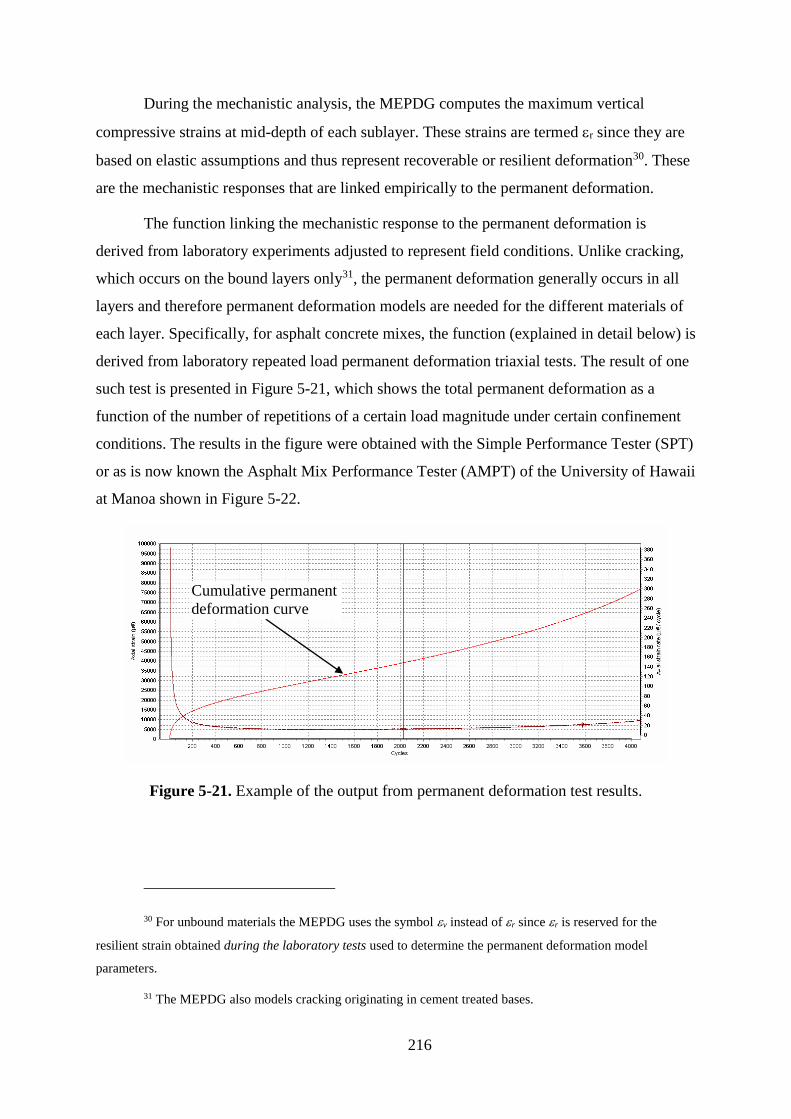
216

During the mechanistic analysis, the MEPDG computes the maximum vertical

compressive strains at mid-depth of each sublayer. These strains are termed r since they are

based on elastic assumptions and thus represent recoverable or resilient deformation30. These

are the mechanistic responses that are linked empirically to the permanent deformation.

The function linking the mechanistic response to the permanent deformation is

derived from laboratory experiments adjusted to represent field conditions. Unlike cracking,

which occurs on the bound layers only31, the permanent deformation generally occurs in all

layers and therefore permanent deformation models are needed for the different materials of

each layer. Specifically, for asphalt concrete mixes, the function (explained in detail below) is

derived from laboratory repeated load permanent deformation triaxial tests. The result of one

such test is presented in Figure 5-21, which shows the total permanent deformation as a

function of the number of repetitions of a certain load magnitude under certain confinement

conditions. The results in the figure were obtained with the Simple Performance Tester (SPT)

or as is now known the Asphalt Mix Performance Tester (AMPT) of the University of Hawaii

at Manoa shown in Figure 5-22.

Figure 5-21. Example of the output from permanent deformation test results.

30 For unbound materials the MEPDG uses the symbol v instead of r since r is reserved for the

resilient strain obtained during the laboratory tests used to determine the permanent deformation model

parameters.

31 The MEPDG also models cracking originating in cement treated bases.

Cumulative permanent

deformation curve

217

Figure 5-22. Simple performance tester.

The test results shown in Figure 5-21 exhibit the three stages typically observed under

axial repeated loading permanent deformation tests. These are illustrated schematically in

Figure 5-23. The first stage exhibits high rates of deformation mostly due to rearrangement of

the structure of the mix under the new loading conditions. During the second stage, the

deformation rate is approximately constant. Finally, the third stage is where the rate of

deformation increases with each load repetition until complete failure occurs.

The total permanent deformation in Figure 5-23 after N loading cycles is the

accumulation of the permanent deformation that occurs during each loading cycle. Figure

5-24 illustrates schematically the permanent (plastic) and resilient strains occurring in a mix

during one cycle.

The MEPDG models only the first two stages of permanent deformation with the first

stage being considered only as an extrapolation of the secondary stage. Specifically, the

laboratory-derived model in the MEPDG for asphalt concrete mixes is:

39937.0734.115552.310 NT

r

p

(5-6)

In this equation, p is the total permanent deformation accumulated up to cycle N, T is

the temperature of the mix during the test in °F and r is the resilient strain corresponding to

Test specimen

Simple performance

tester

218

the state of stresses applied during the test. It has been found experimentally that during the

permanent deformation test the resilient strain is approximately constant.

Figure 5-23. Three stages of permanent deformation [1].

Figure 5-24. Schematic of the permanent (plastic) and resilient strains occurring in a mix

during one loading cycle.

The above equation was calibrated for field conditions by the MEPDG research team.

The final expression used to compute permanent deformation within an HMA sublayer is

Loading Unloading

Resilient strain, r

Plastic strain, p

Loading cycle

Load Repetitions

Strain

Permanent Strain, p

Load Repetitions, N

Primary Secondary Tertiary

Flow Point

219

essentially equation (5-6) calibrated for field conditions multiplied by the thickness of the

sublayer in question. Specifically32,

HMAr

βkk

rzHMAHMApHMAp hεnTβkhεΔrβk

r33

221101 (5-7)

where

p (HMA) = Accumulated permanent or plastic vertical deformation in the HMA

layer/sublayer, in.

p (HMA) = accumulated permanent or plastic axial strain in the HMA layer/sublayer,

in/in.

r (HMA) = resilient or elastic calculated by the structural response model at the mid-

depth of each HMA sublayer, in/in.

hHMA = thickness of the HMA layer/sublayer, in.

n = number of axle load repetitions.

T = mix or pavement temperature, °F.

kz = depth confinement factor.

k1,k2, k3 = global field calibration parameters33 (from the NCHRP 1-40D

recalibration; k1r = -3.35412, k2r = 1.5606, k3r = 0.4791)

428277331101720

342174868210390

3281960

22

21

21

...

...

.

acac

acac

depthz

hhC

hhC

depthCCk

r1, r2, r3 = local calibration factors

Note that the factor kz was incorporated to correct for confining pressure at different

depths. The parameters r1, r2, and r3 can be used to calibrate the rutting model for local

32 In [22], hHMA is missing from the term on the right of the second equal sign.

33 There is an inconsistency in the treatment of the parameters k2r and k3r between the Interim MEPDG

Manual of Practice documentation [22] and the MEPDG software help and Pavement ME software. The

notation above agrees with the software.

220

conditions provided a historical PMS database is available with rutting information as well

pavement structural (including rehabilitation), loading, and mix characteristics information.

For unbound materials, the following field-calibrated mathematical equation is used

to calculate plastic vertical deformation within all unbound sublayers and the foundation or

embankment soil:

soilv

n

ρ

r

sssoilp hεeε

εkβΔ

β

0

11 (5-8)

where

p(soil) = permanent or plastic deformation for the layer/sublayer, in.

n = number of axle load applications.

0 = intercept determined from laboratory repeated load permanent deformation

tests, in/in.

r = resilient strain imposed in laboratory test to obtain material properties 0,

b, and r, in/in.

v = average vertical resilient or elastic strain in the layer/sublayer and

calculated by the structural response model, in/in.

hsoil = thickness of the unbound layer/sublayer, in.

ksl = global calibration coefficients; ksl = 1.673 for granular materials and 1.35

for fine grained materials.

s1 = local calibration constant for the rutting in the unbound layers; the local

calibration constant was set to 1.0 for the global calibration effort.

log = -0.61119 – 0.017638 (Wc)

β

β

C

1

9

09

101

10

(2.9)

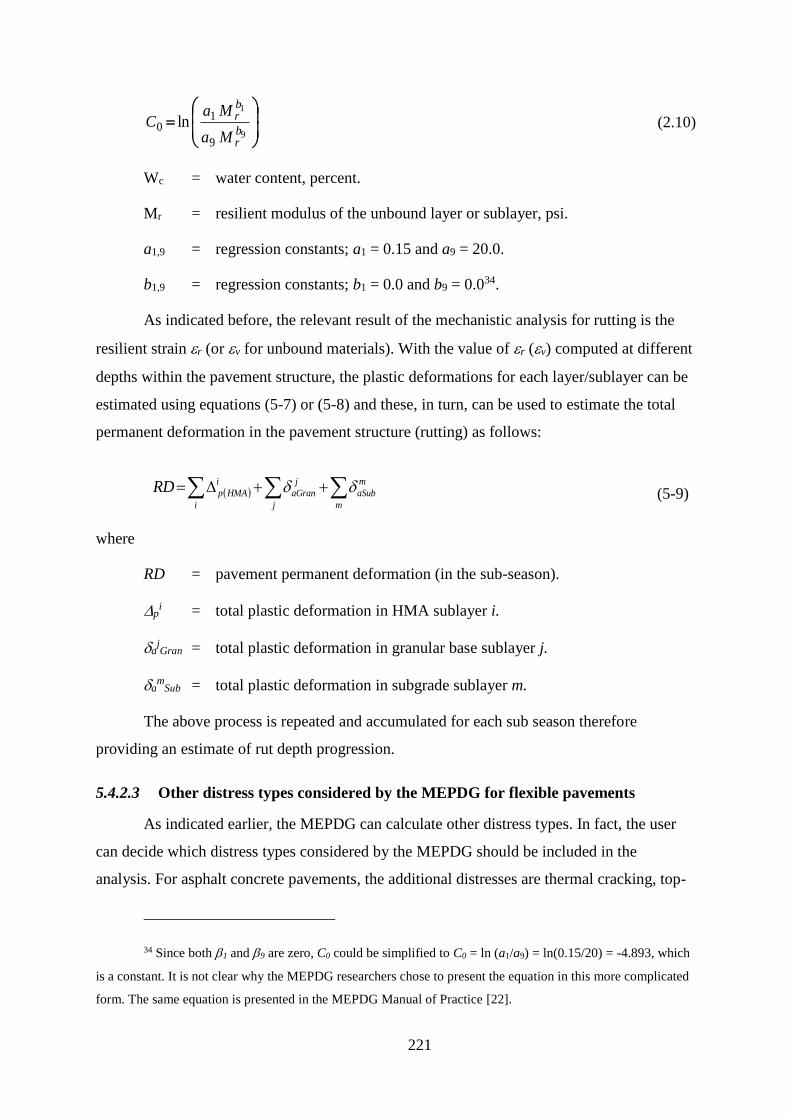
221

9

1

9

10 ln

br

br

Ma

MaC (2.10)

Wc = water content, percent.

Mr = resilient modulus of the unbound layer or sublayer, psi.

a1,9 = regression constants; a1 = 0.15 and a9 = 20.0.

b1,9 = regression constants; b1 = 0.0 and b9 = 0.034.

As indicated before, the relevant result of the mechanistic analysis for rutting is the

resilient strain r (or v for unbound materials). With the value of r (v) computed at different

depths within the pavement structure, the plastic deformations for each layer/sublayer can be

estimated using equations (5-7) or (5-8) and these, in turn, can be used to estimate the total

permanent deformation in the pavement structure (rutting) as follows:

m

m

aSub

j

j

aGran

i

i

HMApRD (5-9)

where

RD = pavement permanent deformation (in the sub-season).

pi = total plastic deformation in HMA sublayer i.

ajGran = total plastic deformation in granular base sublayer j.

am

Sub = total plastic deformation in subgrade sublayer m.

The above process is repeated and accumulated for each sub season therefore

providing an estimate of rut depth progression.

5.4.2.3 Other distress types considered by the MEPDG for flexible pavements

As indicated earlier, the MEPDG can calculate other distress types. In fact, the user

can decide which distress types considered by the MEPDG should be included in the

analysis. For asphalt concrete pavements, the additional distresses are thermal cracking, top-

34 Since both 1 and 9 are zero, C0 could be simplified to C0 = ln (a1/a9) = ln(0.15/20) = -4.893, which

is a constant. It is not clear why the MEPDG researchers chose to present the equation in this more complicated

form. The same equation is presented in the MEPDG Manual of Practice [22].

222

down fatigue cracking, and reflection cracking. In addition, the MEPDG can also calculate

smoothness (roughness) as a function of the distresses.

5.4.2.3.1 Thermal cracking

Because of the narrow range of relatively high temperatures prevalent in Hawaii,

thermal cracking is not a major concern on the State’s roads. As expected, when performing

the calibration it was found that no thermal cracking is predicted for state roads regardless of

how much the corresponding calibration parameter was changed. This is not surprising since

the thermal cracking model is based on temperatures below freezing. Therefore, its

consideration for pavement design in Hawaii is not recommended. This simplifies somewhat

the number of inputs that must be considered in detail.

5.4.2.3.2 Top down fatigue cracking

The approach used by the MEPDG for top-down fatigue cracking is almost identical

to the one presented above for bottom-up fatigue cracking. The main differences are that the

location of the critical strain is at the surface of the asphalt concrete layer instead of at the

bottom and that there are some differences in the empirical equations and the measurement of

cracking (top-down fatigue cracking is calibrated with longitudinal cracking, which is

measured in ft./mile).

As described later in the calibration portion of this report (section 7.5, page 388), this

is probably the main mechanism by which cracking starts on state roads with thick pavement

structures.

As stated in the MEPDG “the engineer should recognize that given a choice between

surface longitudinal [top-down] cracking and alligator [bottom-up] cracking, it will normally

be advisable to select the longitudinal surface cracking distress over alligator cracking. The

reason for this is due to the fact that the eventual presence of surface (top down) cracks as

well as permanent deformation in the upper HMA layers, can always be milled in future

rehabilitations strategies. However, if alligator cracking is present, the chances of full “slab-

layer” damage for the total HMA layer(s) are quite high. If this is the case, it is apparent that

complete removals of the HMA layer or very thick overlays are the only preferred

rehabilitation option.”

At this point it is recommended to limit longitudinal cracking to 2000 ft./mi as

recommended in the MEPDG. More research is needed to find out if 1) most of the observed

223

longitudinal cracking really corresponds to top-down cracking and 2) if so, at what level the

cracks start to propagate through the whole layer thickness (if they do). If cracking is allowed

to reach this point, then whether it started from the top or the bottom does not make much

difference since the structural integrity is lost anyway.

5.4.2.3.3 Reflection cracking

Despite the limitations for modeling reflection cracking in the current MEPDG

procedures, its consideration for overlay design represents a move in the right direction since

this is a major distress mode in HMA overlays of both flexible and PCC pavements. The rest

of this section is mostly reproduced from the MEPDG documentation.

Reflection cracking refers to the propagation of cracks through the overlay due to

movements near cracks and joints in the existing pavement. This movement may be vertical

due to loading, horizontal due to temperature changes, or more probably a combination of

both. Load-induced movements are influenced by the thickness of the overlay and the

thickness, modulus, and load transfer in the existing pavement. Temperature induced

movements are influenced by daily and seasonal temperature variations, the coefficient of

thermal expansion of the existing HMA and PCC layers and the spacing of cracks.

The complex combination of tensile and shear strains at the bottom of the overlay

cause cracks to initiate at the bottom of the HMA layer. With time, the cracks propagate

upward through the HMA overlay. As the process continues, multiple reflection cracks will

form and eventually portions of the HMA overlay will spall and dislodge from the pavement

surface. Even with periodic or routine maintenance (crack sealing), reflection cracks

eventually lead to a reduction of pavement smoothness and shorten the life of the overlay.

The overlay design procedure allows the designer to consider two types of reflection cracks:

reflection of cracks that exist on the surface prior to overlay placement and those that develop

in the existing surface after overlay placement.

5.4.2.3.3.1 Existing Cracks in Pavement Surface – Prior to Overlay Placement.

The MEPDG uses a simplified empirical model to predict the percentage of cracks in

the overlaid pavement that propagate through the overlay. Specifically, it considers the

percentage of cracks as a function of time using a sigmoidal function:

224

tbaeRC

1

100 (5-10)

where:

RC = Percent of cracks reflected, %.

t = Time, years.

a and b = Fitting parameters.

The parameters a and b for HMA overlays of flexible pavements are given by

a = 3.5 + 0.75 hAC

and

b = -0.688584 -3.37302 hAC(-0..915469)

where

hAC = thickness of the overlay, in.

Clearly, this model is very limited as it does not consider the influence of traffic

loading or environment (although this could be achieved by making the parameters a and b to

vary with these variables). Furthermore, it requires further local calibration. For this,

however, a database will be required containing at a minimum information on cracking

condition before placement (and if applicable after milling), cracking after overlay placement

(preferable at several points in time), overlay thickness and mix type, and traffic loading.

The empirical model for reflective cracking is used for estimating the amount of

cracking from a non-surface layer that has reflected to the surface after a certain period of

time. Although the model is limited, it represents a first effort to include this important

distress type in rehabilitation designs.

5.4.2.3.3.2 Cracks Occurring in Existing Pavement Layers after Overlay Placement

Even after overlay placement, the underlying bound layers (including all asphalt

bound and chemically stabilized layers) undergo additional fatigue damage with continued

traffic loading, and eventually crack. The continual fatigue damage accumulation of these

layers is considered in the MEPDG overlay analysis procedures.

225

For any given month m, the total fatigue damage is estimated by the following

equation:

m

i

im DD1

(2.13)

where:

Dm

= Damage for month m.

∆Di = Increment of damage in month i.

The area of fatigue cracking for the underlying layer at month m (CAm) is given by

equation (2.14).

mDm

eCA

661

100

(5-11)

For each month i, there will be an increment of damage ∆Di (calculated using similar

procedures to the ones explained earlier) which will cause an increment of cracking area

∆CAi to the stabilized layer. To estimate the amount of cracking reflected from the stabilized

layer to the surface of the pavement for month m, the reflective cracking model is applied

incrementally, as follows:

m

i

iimm CARCTRA1

(5-12)

where:

TRA = Total reflected area for month m.

RCm-i

= Percent cracking reflected for Age = m – i; (Age in years).

∆CAi

= Increment of fatigue cracking for month i.

The reflective cracking model is applied to each increment of fatigue cracking area

because the time elapsed for each of these increments is different. The model included in the

MEPDG is based on engineering judgment and a limited amount of published data from

Georgia [1].

226

5.4.2.3.3.3 Smoothness (Roughness)

Functional adequacy is quantified in the MEPDG by pavement smoothness. The

parameter used to define pavement smoothness (or roughness which is the lack of

smoothness) in the MEPDG is the International Roughness Index (IRI). Rough roads lead to

user discomfort and higher vehicle operating costs.

In the MEPDG, IRI is predicted empirically as a function of pavement distresses, site

factors that represent the foundation’s shrink/swell and frost heave potential, and an estimate

of the IRI at the time of construction. The design premise included in the MEPDG for

predicting smoothness degradation is that the occurrence of surface distress will result in

increased roughness (increasing IRI value), or in other words, a reduction in smoothness. The

unit of smoothness calculated by the MEPDG is inches per mile (meters per kilometer).

The MEPDG uses equation (5-13) to predict IRI development on new HMA

pavements and HMA overlays:

RDTCFCSFIRIIRI Total 0.40080.0400.00150.00 (5-13)

where

IRI0 = initial IRI after construction, in/mi.

SF = site factor, refer to equation (5-14) below.

FCTotal = area of fatigue cracking (combined alligator, longitudinal, and reflection

cracking in the wheel path), percent of total lane area. All load related

cracks are combined on an area basis – length of cracks is multiplied by 1

foot to convert length into an area basis.

TC = length of transverse cracking (includes the reflection of transverse cracks

in existing HMA pavements), ft./mi.

RD = average rut depth, in.

The site factor (SF) is calculated by:

1000636.01Precip007947.0102003.0 FIPIAgeSF (5-14)

where

Age = pavement age, years.

227

PI = percent plasticity index of the soil.

FI = average annual freezing index, degree F days.

Precip = average annual precipitation or rainfall, in.

These equations are used by the MEPDG to predict IRI over time (as the predictions

of cracking and rutting also change over time).

228

MATERIAL CHARACTERIZATION

6.1 INTRODUCTION

As discussed in chapter 5, material properties such as modulus and Poisson ratio play

a fundamental role in the prediction of pavement responses. In addition, some of the

parameters of the fatigue and permanent deformation models also depend on material

characteristics. Other material properties such as the coefficient of thermal expansion (COE)

and flexural strength of concrete are fundamental for PCC pavement design. Binder viscosity

and dynamic shear modulus, thermal conductivity and heat capacity of different materials,

soil characteristic curves (which affect the water content variations over time), unbound

material gradations, and permeability are other properties playing a role in pavement

performance.

A major challenge to the use of a mechanistic-empirical (ME) pavement design

procedure is obtaining reliable inputs. The hierarchical input level scheme in the MEPDG

provides the user a lot of flexibility for obtaining the inputs based on the criticality of the

project and the available resources [22]. For practical reasons, material testing for most

projects is limited to some properties that are relatively easy to measure. Furthermore, it is

common to measure properties, such as CBR or R-value of unbound materials that are related

to the properties of interest only through correlations.

Even for very important projects, some properties would need to be estimated.

Clearly, accurate estimates of actual material properties would result in designs that are more

representative of the actual pavement performance. Consequently, it is desirable to have a

library of local material properties, at least for those properties that may affect the designs the

most.

This chapter describes available information on material properties as well as the

efforts that as part of this and other related projects were performed to characterize them. The

material properties discussed include dynamic modulus, permanent deformation, and fatigue

cracking of HMA mixtures, viscosity and dynamic shear modulus of asphalt binders, resilient

modulus of granular materials, resilient modulus of soils, and coefficient of thermal

expansion of concrete. The permeability of a coarse-grained base material considered as an

alternative to the untreated permeable base material currently used is also presented. In order

229

to limit the length of the chapter, only the most relevant aspects are described on it. A lengthy

discussion is provided on layer moduli (dynamic modulus of asphalt concrete mixes and

resilient modulus of unbound materials) as these are essential for the computation of stresses

and strains. Several assumptions are needed for estimation of these properties. Other details

are relegated to appendices.

6.2 DYNAMIC (COMPLEX) MODULUS

The description of the ME approach in the preceding chapter highlights the

importance of the determination of the moduli of the different layers. These are used for the

computation of the resilient strains by the structural response model (mechanistic analysis,

Figure 5-2). Then, the resilient strains are used for calculating distresses and roughness using

empirical functions (section 5.4.2).

The Mechanistic-Empirical Pavement Design Guide (MEPDG) uses the dynamic

modulus (|E*|) as the design stiffness parameter of Hot Mix Asphalt (HMA) and the resilient

modulus as the stiffness parameter of granular bases, subbases, and subgrades. The following

paragraphs describe the information available about the dynamic modulus. Resilient modulus

of unbound materials and soils is discussed in section 6.3.

6.2.1 Dynamic Modulus - |E*| Definition

Dynamic modulus (|E*|) is the absolute value of another quantity known as the

complex modulus, E*. The complex modulus E* is used in the theory of viscoelasticity to

predict time dependent (but recoverable deformations). The MEPDG does not use

viscoelastic calculations to predict stresses and strains caused by loads. Nevertheless, |E*| has

been adopted as the elastic modulus of HMA for stress and strain computations.

Before presenting their formal definitions, it is convenient to describe briefly the

equipment and procedure used to measure them.

Several pieces of equipment capable of applying cyclic compressive loading with or

without confinement could be used for dynamic modulus determination. However, because of

some complexities with these pieces of equipment, a major component of NCHRP Project 9-

29, Simple Performance Tester for Superpave Mix Design [37], was the design and

manufacture of a simple performance tester capable of performing among others, the

dynamic modulus test. As a result, what is now known as the Asphalt Mixture Performance

230

Tester (AMPT) was developed35. Details on the development of the AMPT can be found in

Chapter 3 of [38]. The final equipment specification for the AMPT is included as Appendix E

in [39].

6.2.1.1 Description of the AMPT

The AMPT is a bottom loading dynamic testing machine with a triaxial cell that

doubles as environmental conditioning chamber due to a fully integrated refrigeration and

heating unit, a hydraulic dynamic actuator with its associated hydraulic power supply, and a

high response control and data acquisition system (Figure 6-1).

Figure 6-1. Asphalt Mixture Performance Tester.

The loading frame, consisting of three vertical columns and two heavy-duty circular

crossheads, is specifically designed to limit deflection and vibrations which might influence

the accuracy of measurements during dynamic testing of Hot Mix Asphalt (HMA). The

internal dimensions of the system allow the evaluation of 150 mm tall specimens with a

35 The original name of the AMPT was Simple Performance Tester (SPT) and much of the literature

refers to it as such.

231

diameter of 100 mm. The AMPT test specimens are usually obtained after coring and sawing

mixes compacted with the Superpave Gyratory Compactor (SGC), although specimens

obtained from field coring activities can also be used, provided the HMA is thick enough.

Figure 6-2 shows the test set up with the Asphalt Mixture Performance Tester

(AMPT) with a sample inside. The dynamic loading is applied to the HMA specimen by

means of a low friction, double acting, high-speed hydraulic force actuator, which also

includes a co-axial displacement transducer. For dynamic modulus testing, axial deformations

are measured by means of specimen-mounted LVDTs.

Considering the particular characteristics of asphalt mixtures, the AMPT features an

environmental chamber with temperature control of ± 0.5 °C between 4 °C and 60 °C that

doubles as a confining cell if triaxial testing of the specimens is required. Dynamic modulus

tests are typically performed under unconfined conditions. Nevertheless, the ability to apply

confinement to the specimens with the AMPT is particularly useful for permanent

deformation testing, where stress levels that more closely replicate those observed in the field

are required. There is also evidence that confinement affects dynamic modulus, particularly at

high temperatures and low frequencies [40].

As required by the AASHTO TP79 specification [41], control of the systems and data

acquisition and processing of all the relevant signals before and during the tests are

performed electronically by means of fully automated pre-programmed routines. Although

many variations of the test procedure to determine |E*| can be found worldwide, arguably the

most common methods are the recently released AASHTO T342 [42] (which is based on the

formerly known AASHTO TP62) and AASHTO TP79, which is the standard test procedure

established specifically to determine the dynamic modulus of HMA with the AMPT [41].

The two test protocols are used to determine the dynamic modulus of asphalt mixtures

in axial loading mode at various combinations of temperature and loading frequency. In both

methods a dynamic compressive axial stress is applied perpendicular to the parallel flat faces

of a cylindrical HMA specimen, producing a deformation small enough to ensure that the

asphalt material behaves elastically. From a testing point of view, the two procedures are very

similar, except that a reduced number of temperatures and an expanded range of frequencies

are prescribed in AASHTO TP79 (specifically, testing at temperatures of 4.4, 21.1, and

46.1°C and at loading frequencies of 10, 1.0, 0.1, and 0.01 Hz). As reported by Bonaquist in

232

[38], the use of a reduced number of temperatures and frequencies in developing a dynamic

modulus master curve for asphalt mixtures was found to be appropriate.

Figure 6-2. Dynamic modulus test set up in the AMPT.

6.2.1.2 E* and |E*| definitions

The complex modulus (E*) and dynamic modulus (|E*|) are some of the parameters

that can be used to predict the time dependent behavior of viscoelastic materials. The details

of how that is accomplished is beyond the scope of this report. However, it is important to

provide a brief description and interpretation of |E*|, as this is used as the elastic modulus of

HMA in the MEPDG.

In order to unambiguously define E* and |E*|, it is convenient to explain how and

are varied with time during the test.

In the AMPT, after application of a contact stress of around 5% of the maximum axial

stress (contact), a bottom ram transmits through the bottom platen a cyclic sinusoidal axial

Specimen

(inside rubber

membrane)

Linear

Variable

Differential

Transducer

(LVDT)

Temperature

controlled

chamber

Reaction

frame

Loading

platens

233

load while Linear Variable Differential Transducers (LVDTs) simultaneously measure the

resulting vertical deformations. In the configuration shown in Figure 6-2, three LVDTs

located 120° apart on the cylindrical specimen are used.

The application of a sinusoidal stress results in strains that also follow an approximate

sinusoidal pattern. Figure 6-3 shows the applied sinusoidal axial stress and the corresponding

strain response of a typical bituminous mixture. In this figure, scales have been chosen so that

the two curves have the same vertical separation between peaks. The figure also illustrates a

characteristic time shift (t) of viscoelastic materials between the loading curve and the

deformation curve.

Figure 6-3. Typical Applied Stress and Associated Strain Response of HMA during |E*|

Test.

The time dependency of the stress () (the sinusoidal load) is conveniently described

by a complex number that provides the deviation around the mean stress value over the

cycle.

tite ti

sin2

cos22

000 (6-1)

where 0 is the peak-to-peak stress difference in , is the angular velocity and t is time.

Similarly, the time dependency of the resulting strain is conveniently described by a

complex number that provides the deviation around the mean strain value over the cycle.

234

tite ti sin2

cos22

00)(0 (6-2)

where 0 is the peak-to-peak strain difference in , is the phase angle, and the other

variables are as defined before. An interpretation of the phase angle is provided shortly.

Actually, with the mechanical models typically used to model viscoelastic materials (spring

and dashpots connected in series and parallel), it can be shown that the strain follows

equation (6-2) when the stress is given by equation (6-1).

The sinusoids in both cases are represented by the real parts of the complex numbers

in equations (6-1) and (6-2).

With the above stress and strain quantities defined, it is now relatively simple to

define the complex modulus E*. As any other modulus, it is given by a ratio of stress to

strain. More specifically, with the notation above, it is given by:

sincos

2

2*0

0

0

0

0

0

)(0

0

iee

eE i

ti

ti

(6-3)

In equation (6-3), the real component of E*, typically denoted E’, is known as the

storage modulus. In contrast, the imaginary part, denoted E”, is called the loss modulus. The

ratio of the loss modulus to the storage modulus, E”/E’ is equal to tan

It is important to note that under viscoelastic theory all deformations are recoverable.

There are no permanent deformations.

At low temperatures and high frequencies of loading, HMA tends to behave more

elastically and therefore its storage modulus tends to zero and consequently the phase angle

also tends to zero (tan → 0). On the other hand, at high temperatures and low frequencies

of loading, HMA is more viscous (higher loss modulus) and thus the phase angle increases

(tan → ∞). The phase angle is always a quantity between 0 and 90°.

Now, it can be seen that E*, being the ratio of two complex quantities, is itself a

complex quantity. Remembering that the magnitude of a complex number is given by the

square root of the Cartesian coordinates of the real and imaginary components, the dynamic

modulus |E*| is then given by:

235

0

02

2

0

02

2

0

0 sincos|*|

E (6-4)

Since concepts involving complex numbers are somewhat abstract, it is useful to

visualize how the stress and strain quantities are related to a complex number. The

explanation is done with reference to Figure 6-4, which also helps to illustrate the

relationship between the phase angle and the time lag between the curves.

Figure 6-4. Phase angle between stress and strain curves in viscoelastic materials.

The left side of the figure illustrates the position at time t of two vectors, one for stress

and one for strain, rotating counterclockwise in a complex space at an angular velocity .

The vectors have magnitudes of 0/2 and 0/2 for stress and strain, respectively. For

convenience, the real part of the vector is oriented up in the vertical direction and the

imaginary part is oriented in the horizontal direction to the left. At time t, the real part of the

location of the tip of the stress vector is the same as the stress at time t, as shown by the dot

on the stress curve. Now, imagine that as the vector rotates counterclockwise at angular

velocity (i.e., as time t increases), other points on the stress curve are generated such that

the abscissa is the time t and the ordinate is equal to the real part of the stress vector. In other

words, the location of the tip of the vector provides the vertical position of the sinusoid at any

time t. The strain sinusoid is generated in exactly the same way by the strain vector which is

rotating at the same angular velocity but behind the stress vector by the angle .

Hopefully, the visualization of the sinusoids being generated by the trace of the tips of

two rotating vectors helps to understand the usefulness of using complex numbers to

Stress sinusoid

Strain sinusoid

Real component

t t -

Time

Imaginary

component

t

236

represent the stresses and strains in this test. More importantly, the Euler (exponential)

representation of complex numbers make the calculation of the ratio of the complex stress

and strain quite simple.

Finally, the visualization above is also useful for explaining the relationship between

the time shift between the curves (see t in Figure 6-3) and the phase angle . Note that both

rotating vectors in the complex plane are separated angularly by . Since both vectors rotate

at the same speed, if the peak stress is reached at a time T (which implies cos(T) = 1 for the

stress sinusoid), then the peak strain will be reached at a later time T+t (which implies that

cos( (T+t)-) = 1 for the strain sinusoid.) In both cases, since the sinusoids are at their

peaks, the argument of the cosine function must be 0 (or 2, 4, etc.). If, without loss of

generality, T = 0 in the stress sinusoid, then t – must also be 0 in the strain sinusoid

for cos( (T+t)-) = 1 to be true. Thus, the peak of the strain sinusoid will happen with a

time lag of t = with respect to the peak of the stress sinusoid, as illustrated in Figure

6-4. Thus, the phase lag is directly related to the phase angle and it is inversely related to the

angular velocity.

The AMPT software requires entering a frequency of loading (cycles/sec or Hz)

instead of angular velocity. The frequency f is related to the angular velocity by: = 2 π f

Unlike in Figure 6-3, the vertical scales of stress and strain curves were not selected in

Figure 6-4 so that the sinusoids have the same height. This makes the discussion more

general.

It is important to note that with a stress amplitude of 0 as depicted in Figure 6-3, the

average stress during the test, avg, is avg = contact + 0/2. Therefore, the total time dependent

stress is given by = avg + . Similarly, with a strain amplitude of 0 as depicted in Figure

6-3, the average strain during the test, avg, is avg = contact + 0/2 (where contact is the strain

corresponding to contact). Therefore, the total time dependent strain is given by = avg + .

For materials tested in the linear viscoelastic range, the contact stress has little influence in

the determination of |E*|.

The theory of the complex modulus can be derived from mechanical models

(combinations of spring and dashpots) that provide justification for some of the assumptions.

Huang [34] provides a good introduction to the subject.

237

6.2.2 Determination of |E*|

Dynamic modulus depends on mix characteristics, which is why testing of particular

mixes or the use of models that include mix characteristics are needed for modelling HMA

responses to loading. However, even for a single mix, dynamic modulus is substantially

affected by several factors. The two single most important factors that are currently

considered in the MEPDG are frequency (or its inverse, time of loading) and temperature.

Variations in any of these two factors can result in dynamic modulus changes of orders of

magnitude. Consequently, the results of dynamic modulus testing typically consist of a set of

dynamic modulus values obtained at different temperatures and time of loading (or

equivalently frequency of loading).

In order to perform a test, test frequencies, conditioning time, target temperature,

target confining stress, initial modulus, axial gauge length, and specimen dimensions need to

be defined in the software setup menu36. Some of these inputs, such as frequencies, are used

directly for control of the test while others, such as the conditioning time, are included only

for informational purposes. The conditioning time is the time allowed for the sample to reach

the target test temperature uniformly within the specimen.

Initial modulus is important for the machine to select an appropriate initial load for

testing. Although the load is automatically controlled, an initial modulus that is too different

from the actual modulus can cause control problems. The initial modulus can be easily

estimated with the tuning feature of the software before performing the test.

Figure 6-5 shows the AMPT software output after applying a cyclic stress to a given

sample at a temperature of 70°F (21.1°C) for a load frequency of 1 Hz along with the

resulting cyclic strains. A careful look at the figure reveals the characteristic phase shift of

viscoelastic materials between the loading curve and the deformation curves described

earlier.

The applied stress, confining pressure (if any), temperature and resulting axial strain

from the three on-specimen displacement transducers are measured as a function of time and

then used to calculate the dynamic modulus and other required values, such as phase angle,

36 These descriptions, of course, are for the equipment currently available at UH.

238

average temperature, average confining pressure and a number of data quality measurements,

as illustrated in Figure 6-5.

The values of dynamic modulus shown in the first row of the table within the Figure

6-5 illustrate the substantial effect that frequency, f (or equivalently time of loading, t = 1/f)

has on the dynamic modulus. The higher the frequency (the shorter the time of loading) the

higher is the measured dynamic modulus. Since temperature also has a substantial effect on

the measured dynamic modulus, the test is performed at several temperatures to cover the

range of pavement temperatures expected in the field.

Figure 6-5. Dynamic Modulus Test Output from the AMPT.

Figure 6-6 illustrates the results from a complete set of measurements on an HMA

specimen for temperatures ranging from 39.9F (4C) to 129.2F (54C) and time of loading

ranging from 0.04 s to 10 s (or equivalently frequencies ranging from 25 Hz to 0.1 Hz). As

illustrated in this figure, the dynamic modulus is affected substantially by both temperature

and time of loading (note that both chart scales are logarithmic so the differences are indeed

significant; in this example the modulus varied from about 526,000 psi (3,629 MPa) to about

1,650,000 psi (11,382 MPa)!)

239

6.2.3 Dynamic Modulus Master Curve

For mechanistic-empirical pavement design, the dynamic modulus |E*| is needed for

any given temperature and time of loading. Therefore, an interpolation model is required to

predict |E*| for any condition. Such interpolation is achieved with the use of the time-

temperature superposition principle, which allows superposition of a series of curves (each

for a constant value of temperature and varying frequencies of loading) by horizontal shifts in

the frequency domain to form what is known as a “Master Curve”.

Figure 6-6. Example of dynamic modulus test results.

The time-temperature superposition principle assumes that the effect of time of

loading (or frequency) on the material properties can be replaced by the effect of temperature,

and vice versa. In this way, the master curve can be defined as a function that describes

simultaneously the dependency of |E*| on both the temperature and the time of loading.

Although estimation of the master curve model parameters can be accomplished in a

single step, it is easier to explain it and visualize it as a two-step process in which first, the

curves obtained by varying loading time (or frequency) at each temperature are shifted

horizontally until a smooth curve is obtained and second, a smooth function is fitted to the

resulting data points. Figure 6-7 illustrates the shifting and the resulting fitted |E*| master

curve for a particular mix (reference temperature of 21.1 ºC = 70.0 ºF).

10,000

100,000

1,000,000

10,000,000

0.00001 0.0001 0.001 0.01 0.1 1 10 100 1000 10000 100000

Time of loading (s)

|E*|

(p

si)

129.2F

113.0F

100.4F

69.8F

39.9F

240

The amount of shifting along the time of loading axis (i.e., horizontal) is related to

what is known as the shift factor, which is defined, in logarithmic terms by the equation:

Tattr logloglog

(6-5)

Figure 6-7. Example of shifting and curve fitting during the development of master curve

(Tref =69.8 ºF=21.0ºC).

In equation (6-5), a(T) is the shift factor (which is a function of temperature, as

illustrated in Figure 6-8), t is the time of loading at the desired temperature, tr is the reduced

time of loading at a reference temperature, and T is the temperature of interest37. As can be

deduced from equation (6-5), the shifts shown in Figure 6-7 are equal to the negative of the

log(a(T)) (note that the time of loading is given in logarithmic scale in Figure 6-7). For

example, as shown in Figure 6-8 the shift factor for 100 ºF is about -2. Correspondingly, the

37 tr, the reduced time of loading, is a fictitious time of loading. Its interpretation is as follows. The

same modulus |E*| would be measured whether a sample is tested at any given temperature T and time of

loading t or whether it is tested at the reference temperature (typically 70 ºF) and time of loading tr.

10,000

100,000

1,000,000

10,000,000

0.00001 0.0001 0.001 0.01 0.1 1 10 100 1000 10000 100000

Time of loading (s)

|E*|

(p

si)

129.2F

113.0F

100.4F

69.8F

39.9F

Master Curve

241

points for the 100 ºF temperature are shifted about two log cycles to the right in Figure 6-7.

These shifted points are the ones used to fit the master curve.

Figure 6-8. Example of the Shift Factor as a function of temperature.

Although different continuous functions could be used for the |E*| master curve, the

sigmoidal function presented in equation (6-6) is perhaps one of the most commonly used

these days, as it is the form used by the Pavement ME Design software [2].

rteE

log

*

101

||log

(6-6)

In equation (6-6), tr is the reduced time of loading at the reference temperature, α is

the minimum value of log |E*|, δ+α corresponds to the maximum value of log |E*|, and β and

γ are parameters describing the shape of the sigmoidal function. This equation describes the

time dependency of the modulus at the reference temperature whereas the shift factors

describe the temperature dependency of the modulus; both are essential ingredients of the

master curve.

-4

-3

-2

-1

0

1

2

3

0.0 20.0 40.0 60.0 80.0 100.0 120.0 140.0

Temperature, ºF

log

a(T

)

242

6.2.3.1 Shift factor models

Different approaches are available to establish the relationship between the shift

factors and temperature. Some of these are discussed next.

6.2.3.1.1 Shift Factor Modeled only as Function of Temperature

The parameters of the master curve can be estimated using equation (6-6) along with

the following equation to model the shift factor as a function of temperature:

CTBTATa ii 2log (6-7)

where A, B and C are model parameters and Ti is the temperature in °F. All seven parameters

(A, B, C and the parameters of the sigmoid) are estimated simultaneously by the MEPDG.

The only information required for their estimation is the dynamic modulus test results.

Since the computations are done internally by the MEPDG, there is generally no need

for users to determine the parameters of these equations. The master curve and shift factors

are part of the output in the MEPDG.

Still, if so desired, different computer applications are available at the moment to

process data from AMPT |E*| tests and generate master curves. Advanced dedicated software

that can perform this task include the licensed Rheology Analysis Software (RHEA) from

Abatech [43]. Other software that can be used towards this end include Matlab and Excel,

although it is important to note that users need accessibility to the software and possess a

basic understanding of programming macros within these particular applications. In addition,

interested users can obtain the MasterSolver Excel worksheet, which was prepared as part of

NCHRP Report 9-29, and is available for free from the Transportation Research Board

website [37].

In addition, the PI has also developed a software application to automatically generate

the mixture’s modulus master curve using the output files generated by IPC Global’s AMPT.

This tool can potentially facilitate the use of perceived complex results from asphalt dynamic

modulus tests into routine pavement engineering practice. It allows, among other things,

direct reading of the summary files generated by the AMPT in SI units and compute the

master curve parameters using US customary units, thus avoiding unit conversions. The

details of the tool are presented in [44]. This software is also available for free to HDOT.

243

6.2.3.1.2 Shift Factor Modeled as Function of Temperature through Binder Viscosity

As the asphalt binder ages, the binder and the mix become stiffer. In order to account

for the stiffening of the mix with time, the MEPDG currently uses two different procedures:

one developed under project NCHRP 1-37A [1] and the other under NCHRP 1-40D . Only

the first one is explained in detail in this report since the second procedure has not yet been

nationally calibrated.

In the procedure developed under project NCHRP 1-37A, the MEPDG uses equation

(6-8) below to compute the shift factor instead of equation (6-7).

RTηηcTa logloglog (6-8)

where

= binder viscosity, cP (centipoise)38,

RTη = binder viscosity at reference temperature, cP

c = model parameter estimated simultaneously with , , , and of equation

(6-6) for given mix |E*| values and binder viscosity data.

Equation (6-8) appears to require two less parameters than equation (6-7). However, it

also requires prediction of the binder viscosity as function of temperature. This is achieved in

the MEPDG through the following two-parameter equation:

RTVTSAη logloglog (6-9)

where

= binder viscosity, cP (centipoises),

TR = temperature, Rankine (= temperature in °F + 459.67)

38 For this particular equation use of any unit of viscosity is acceptable as long as the same units are

used for both viscosity values. Recall that

R

RT

Tη

ηηη logloglog , which does not depends on the units.

This is not true however for most other equations in the MEPDG, so analysts need to be careful with units when

making calculations using MEPDG equations outside the MEPDG.

244

A = regression intercept;

VTS = regression slope of viscosity temperature susceptibility.

Parameters A and VTS are estimated by the guide based on the binder characterization

data required as input by the MEDPG for levels 1 and 2 or are provided based on the binder

grade for level 3.

6.2.3.2 Example of Dynamic Modulus Computations

As indicated before, for pavement design the dynamic modulus |E*| is needed for any

given temperature and time of loading. Equations (6-5), (6-6), and (6-7) are now used along

with a specific set of parameters , , , , A, B, and C to illustrate how this is accomplished.

Note that there is no need for users of the guide to perform computations like the ones

presented here. Nevertheless, understanding of these promotes a more informed use of the

procedure.

Suppose that = 4.186, = 2.465, = -0.871, = 0.457, A = 0.000204, B = -0.100,

and C = 6.00. First notice that for the reference temperature of 70°F equation (6-7) yields

log(a(T)) = 0.000204 (70)2 -0.100 (70) + 6.00 ≈ 0 or a(T) = 1

as it should be for the reference temperature (this restriction is imposed during estimation of

the parameters of the equation).

If an estimate of the dynamic modulus is required for a temperature of say, 85°F, and

a time of loading of 8 seconds, then the calculations proceed as follows. From equation (6-7):

log(a(T)) = 0.000204 (85)2 – 0.100 (85) + 6.00 = -1.025 or a(T) = 0.0942

Therefore from equation (6-5), the reduced time (i.e., the time of loading that would

yield the same modulus at the reference temperature as the modulus obtained at the given

temperature of 85°F and loading time of 8s) is:

tr = t/a(T) = (8 s)/(0.0942) = 84.96 s

Then, using equation (6-6), the |E*| is calculated as:

96.84log457.0871.0

*

10101

465.2186.4||log

e

E = 5.412

or

|E*| = 258,188 psi.

245

which agrees with the value of |E*| obtained for tr ≈ 85 s in Figure 6-8. The same procedure

can be used for any other temperature and time of loading.

6.2.3.3 MEPDG Use of the Master Curve

Seven parameters are required to completely characterize the mix master curve

whether equation (6-7) is used (in which case the parameters are , , , of equation (6-6)

and A, B, and C of equation (6-7)) or whether equations (6-8) and (6-9) are used (in which

case the parameters are , , , of equation (6-6), c of equation (6-8) and A and VTS of

equation (6-9)39). Both approaches are used within the MEPDG [1].

The estimation of these parameters is done by the MEPDG from the appropriate

inputs for each case. Then, the MEPDG can use the master curve to estimate the dynamic

modulus of HMA layers for any pavement temperature and frequency of loading.

The main advantage of the use of equations (6-8) and (6-9) over the use of equation

(6-7) is that binder aging can be taken directly into account by changing the binder viscosity

with age.

Binder aging is modeled internally in the MEPDG by a system known as Global

Aging System, which includes four sub-models for binder aging occurring on different

stages:

Original to mix/lay-down model to account for short term aging occurring during

mixing and lay-down.

Surface aging model to predict the viscosity of the binder at the surface of the

pavement after any period of time using the viscosity at mix/lay-down.

Air voids adjustment to adjust for different air voids in the mix.

Viscosity-depth model.

The details of the Global Aging System are beyond the scope of this report. It is

important to realize, however, that binder characterization inputs required by the MEPDG are

used to obtain binder viscosity with equation (6-9) at any temperature and that these are used

39 The parameter A of the quadratic equation (6-7) should not be confused with the binder parameter A

used in equation (6-9).

246

(after being modified by the Global Aging System to account for aging) in equation (6-8) to

predict the dynamic modulus at any temperature and age.

Figure 6-9 illustrates the effects of the seasonal variations and aging on HMA

sublayers of a 10-in thick HMA combination of layers for the Honolulu environment as

reported by the MEPDG40. The yearly fluctuations in temperature (from winter to summer)

are apparent in the figure. Notice also that the modulus increases in the first few years and

then stabilizes. This last effect is more pronounced for those layers closer to the surface

(more exposed to aging) than deeper in the pavement structure (in this particular example the

order of the lines in the graph correspond exactly with their position from top to bottom in the

pavement structure). The differences of modulus between sublayers is caused by the different

loading times experienced by the HMA at different depths41.

Figure 6-9. Simulated variations of HMA modulus over time (including the temperature

variations over time and aging) and depth.

40 In the example, there are three layers AC1 (AC Mix IV), AC2 (AC Mix III), and AC3 (ACB) of

thicknesses of 1.5, 2.5, and 6 inches, respectively. Each of these, are subdivided into sublayers with the

thicknesses shown in the figure legend. The software numbers these sublayers automatically with the numbers

shown in parenthesis in the legend.

41 Since very early after the release of the MEPDG, there were concerns about the possibility of the

loading time/frequency effect overriding the temperature effect [53]. Although the MEPDG research team

agreed with this concern, the latest version of the Pavement ME Design software (used to generate Figure 6-9)

has not addressed this issue yet. As discussed later, this may indeed be an important consideration for Hawaii.

247

6.2.4 MEPDG Dynamic Modulus Predictions

Different models are used in the MEPDG to estimate the master curve for new HMA

layers depending on the inputs level. For input level 1, the MEPDG derives the master curve

parameters directly from values of |E*| obtained by testing with the AMPT the mix expected

to be used in the project.

For input levels 2 and 3, the MEPDG makes use of either Witczak’s model adopted in

project NCHRP 1-37A [1] or the enhanced Witczak’s model adopted in project NCHRP 1-

40D [22].

The next section evaluates the adequacy of the level 2 and 3 predictions of |E*| for

some Hawaiian mixes. It is shown that although the predictions are generally reasonable, they

are somewhat biased for the mixes tested locally. Therefore, Section 6.2.4.2 considers the use

of pseudo-level 1 data generated from a model developed with Superpave 12.5 mm mixes

prepared with local materials. Most of the concepts in these two sections are from [45], [46]

and [47].

6.2.4.1 MEPDG Levels 2 and 3 Dynamic Modulus Predictions

The two Witczak’s models used by the MEPDG were developed with extensive

databases and provide a good fit to the data used in their development. They use information

about gradation, mixture volumetrics, and binder characteristics. The only difference in the

use of the models for levels 2 and 3 is that specific laboratory test data are required for binder

characteristics for level 2 but only the grade of the binder (Superpave, conventional viscosity

or conventional penetration) is required for level 3.

6.2.4.1.1 |E*| Master Curves Models Used in the MEPDG

Bari and Witczak [48] provide a summary of the models developed over the last 50

years as well as the two models used by the MEPDG. These last two models are now briefly

described.

For levels 2 and 3, the parameters of the |E*| model adopted in the NCHRP 1-37A

study [1] were obtained by fitting the model to a data set containing 2,750 test data points

from 205 Hot Mix Asphalt (HMA) un-aged laboratory blended mixtures. This version of the

Witczak |E*| predictive model is as follows:

248

log3935.0log3133.06033.0

34

2

38384

4

2

200200

*

10

1

0055.0000017.0004.00021.0872.3

822.00048.00028.0

0018.0029.025.1||log

f

abeff

beff

a

e

VV

VV

E

(6-10)

where

|E*| = dynamic modulus of the mix, 105 psi

= viscosity of the binder, 106 Poise

f = loading frequency, Hz

200 = % passing No. 200 (0.075 mm) sieve

4 = cumulative % retained on No. 4 (4.76 mm) sieve

38 = cumulative % retained on 3/8 in (9.5 mm) sieve

34 = air voids, % by volume

Vbeff = effective binder content, % by volume

The model adopted in project NCHRP 1-40D, developed also by Bari and Witczak

[48], expresses the dynamic modulus |E*| as:

bb

eff

eff

eff

eff

G

ab

b

a

ab

b

a

e

VV

VV

VV

VV

GE

log8834.0|)*log(|5785.07814.0

34

2

3838

2

3838

2

44

2

200200

0052.0*

10

1

001.00001.0012.071.003.056.2

06.108.000014.0006.0

0001.0011.0)(0027.032.065.6

|*|754.0349.0||log

(6-11)

where

|E*| = dynamic modulus, psi

200 = aggregates (by aggregates weight) passing through No. 200 sieve, %

4 = cumulative aggregates (by aggregates weight) retained on the No. 4 sieve, %

249

38 = cumulative aggregates (by aggregates weight) retained on the 3/8 in. sieve, %

34 = cumulative aggregates (by aggregates weight) retained on the ¾ in. sieve, %

Va = air voids (by volume of the mix), %

Vbeff = effective binder content (by volume of the mix), %

|Gb*| = dynamic shear modulus of binder, psi

b = phase angle of binder associated with |Gb*|, degree

This model was fitted by Bari and Witczak to 7,400 dynamic modulus data points

with an R2 = 0.80 and Se/Sy = 0.45 in arithmetic scale and R2 = 0.90 and Se/Sy = 0.32 in log

scale. R2 and Se/Sy are statistical measures of goodness of fit such that the closer are the R2

to 1 and the Se/Sy ratio to 0 the better the fit. Based on these measures, the model provides an

excellent fit to their data though unfortunately, no information is provided for either model

about the significance of each individual model parameter.

6.2.4.1.1.1 Hawaii’s Experimental |E*| Database

A data set was created at UH with HMA dynamic modulus (|E*|) test results for 79

laboratory-mixed/laboratory compacted specimens. The specimens were prepared with two

different gradations, three binder types, and varying asphalt contents and air voids. All these

mixes were prepared with aggregate from the Makakilo quarry in Oahu.

Figure 6-10 illustrates in a 0.45-power gradation chart the two Superpave 12.5 mm

Nominal Maximum Aggregate Size (NMAS) gradations included in the database. Gradation

B was selected as representative of gradations that had been used in actual paving projects

whereas gradation A was selected to represent a gradation that could result from gradation B

due to changes in the stockpiles or feeding of aggregates at the plant. Based on a later

analysis of quality assurance records in the island of Oahu, it was found that these gradations

are representative not only of Superpave gradations but also of many State Mix Type 4

gradations, which fall between gradations A and B or slightly outside, and that are commonly

used throughout the island. This is illustrated in Figure 6-11, which shows a sample of State

Mix IV gradations from different projects along with gradations A and B.

250

Figure 6-10. Gradations A and B.

Figure 6-11. Examples of gradations of State IV mixes used in different projects.

Of the three binders used in the preparation of the specimens, one is a virgin

(unmodified) PG64-16 and the other two are polymer modified binders. Of the modified

25

19

12

.5

9.5

4.7

5

2.3

6

1.1

8

0.6

0.3

0.1

50

.07

52

00

10

0

50

30

16

8 4 3/8

"

1/2

"

3/4

"

1"

0

10

20

30

40

50

60

70

80

90

100

Sieve Size (mm)

Perc

en

t P

ass

ing

Upper Spec. Limit Lower Spec. Limit Gradation A Gradation B

251

binders, one was a commercially available SBS modified PG70-2242, whereas the other,

labeled PG70-XX, was obtained by modifying a PG64-16 binder with a commercially

available reactive elastomeric terpolymer mixed with polyphosphoric acid as catalyst.

The specimens were prepared with varying air voids and asphalt contents to study the

potential differences with the binders not only under optimum conditions but under the

conditions that can be expected in the field as well. Asphalt contents at the estimated

optimum and at 0.5% below and 0.5% above the estimated optimum were selected for each

gradation. In addition, the air voids in the samples varied from slightly below 3% to almost

10%. From an analysis of quality assurance records for Oahu, it was found that these values

were in fact quite representative of the range of air voids found for Type IV and Superpave

12.5 mm NMAS mixes. Figure 6-12 shows the cumulative distribution of air voids for these

types of mixes based on 512 observations from the quality assurance records mentioned

above along with a Weibull distribution fitted to the data.

Incidentally, it must be noted that the hypothesis that the distribution of air voids is

Normal, which is the most common assumption used in practice, had to be rejected at a 5%

significance level when using a Chi-squared goodness of fit test. However, the hypothesis

that the distribution follows a Weibull distribution could not be rejected at the same

significance level.

42 The PG70-22 binder modified with SBS is the same used in a section of the Moanalua Freeway in

2004.

252

Figure 6-12. Air voids distribution from quality assurance records.

The laboratory mixes were aged for four hours before compaction. Table 6-1 shows

the volumetric characteristics of the laboratory prepared specimens.

The dataset also contains |E*| information for five more specimens corresponding to

three different mixes. The mix for two of these specimens is a Superpave 12.5 NMAS

collected from a pavement preventive maintenance project on the H-3 freeway in Oahu. This

mix was prepared with PG64-16 binder and aggregate from the Kappa quarry also in Oahu.

The mix for two other specimens is a State Mix Type IV collected from another rehabilitation

project on the Farrington Highway in Oahu. This is a warm mix asphalt (WMA) project that

was prepared with aggregate from the Makakilo quarry, PG64-16 binder, and Sasobit™. A

final specimen was compacted with a 12.5 mm NMAS Superpave mix collected at an asphalt

plant also with a PG64-16 binder and aggregates from the Kappa quarry in Oahu (retained in

4.75 mm) and Ameron Maui (passing 4.75 mm) in Maui. Table 6-2 provides the volumetric

characteristics of these mixes.

In total, 2,447 valid |E*| measurements were obtained for the 84 specimens. It is

important to notice that despite the large number of observations, there is very limited

variability in gradations for a statistical analysis of the type required for local calibration of

either of the Witczak equations. In fact, there are only five different gradations. Similarly,

0

0.1

0.2

0.3

0.4

0.5

0.6

0.7

0.8

0.9

1

1.00 2.00 3.00 4.00 5.00 6.00 7.00 8.00 9.00 10.00

F(x

) =

Pro

b (V

a <

x)

Air Voids (Va) (%)

Weibull Fit

Empirical Distribution

253

there are only three binders in the database, which also restricts the types of analysis that can

be performed with this information.

In addition to volumetric and |E*| testing, some limited binder testing was performed

on unaged binder and on binder aged in the Rolling Thin Film Oven (RTFO). The binders

were tested at several temperatures for viscosity with a Brookfield rotational viscometer and

for dynamic shear modulus and phase angle with a Dynamic Shear Rheometer.

Values of A and VTS were estimated from both sets of measurements. In the following

analyses, only the A and VTS values from the DSR measurements are used. These are

presented in Table 6-3.

254

Table 6-1. Characteristics of the laboratory mixed/laboratory compacted HMA specimens.

Aggregate

Gradation Binder Specimen ID

Va

(%)

Pb

(%)

Pbe,

%

(vol.)

Unit

Weight

(pcf)

Gmm Gmb VMA VFA

A

PG64-16

ADM001B 3.4 5.7 10.22 162.6 2.696 2.605 13.6 75.2

ADM001C 2.7 5.7 10.29 163.7 2.696 2.623 13.0 79.2

ADM001D 3.3 5.7 10.22 162.6 2.696 2.606 13.6 75.4

ADM002 5.5 5.7 10.00 159.1 2.696 2.549 15.5 64.7

ADM002B 4.6 5.7 10.09 160.4 2.696 2.571 14.7 68.5

ADM002C 5.2 5.7 10.03 159.5 2.696 2.556 15.2 65.9

ADM003 5.1 5.7 10.04 159.7 2.696 2.559 15.1 66.4

ADM003B 7.4 5.7 9.80 155.8 2.696 2.497 17.2 57.0

ADM003C 6.8 5.7 9.86 156.9 2.696 2.514 16.6 59.4

ADM004 10.1 5.7 9.51 151.3 2.696 2.425 19.6 48.6

ADM004B 9.3 5.7 9.60 152.6 2.696 2.446 18.9 50.9

ADM005 9.3 5.7 9.60 152.6 2.696 2.446 18.9 50.9

ADM006 4.3 5.7 10.12 161.1 2.696 2.581 14.4 70.4

ADM007 2.7 6.2 11.49 162.2 2.673 2.6 14.2 80.8

ADM008 2.2 6.2 11.55 163.1 2.673 2.614 13.8 84.0

ADM025 7.4 5.2 8.61 157.1 2.72 2.518 16.0 53.7

ADM026 7.4 5.2 8.61 157.2 2.72 2.519 16.0 53.8

ADM027 9.1 5.2 8.45 154.3 2.72 2.472 17.6 48.1

ADM028 9.4 5.2 8.42 153.7 2.72 2.463 17.9 47.1

PG70-XX

ADM009 3.0 5.7 10.39 163.0 2.692 2.612 13.4 77.8

ADM010 3.3 5.7 10.36 162.5 2.692 2.604 13.6 76.0

ADM011 7.4 5.7 9.91 155.5 2.692 2.492 17.3 57.2

ADM012 7.1 5.7 9.94 156.0 2.692 2.5 17.1 58.2

ADM013 9.7 5.7 9.67 151.8 2.692 2.432 19.3 50.0

ADM014 9.7 5.7 9.67 151.6 2.692 2.43 19.4 49.8

ADM015 7.3 5.2 8.75 157.2 2.716 2.519 16.0 54.7

ADM016 7.0 5.2 8.77 157.6 2.716 2.525 15.8 55.5

ADM017 7.0 6.2 11.10 154.9 2.669 2.482 18.1 61.3

ADM018 5.7 6.2 11.26 157.0 2.669 2.516 17.0 66.3

PG70-22

ADM019 2.7 5.7 11.13 162.1 2.67 2.597 13.9 80.3

ADM020 2.4 5.7 11.17 162.7 2.67 2.607 13.5 82.6

ADM021 6.9 5.7 10.65 155.1 2.67 2.486 17.5 60.7

ADM022 6.9 5.7 10.65 155.1 2.67 2.485 17.6 60.6

ADM023 9.1 5.7 10.40 151.4 2.67 2.427 19.5 53.3

ADM024 9.6 5.7 10.35 150.7 2.67 2.415 19.9 52.0

255

Table 6-1 (continued) Characteristics of the laboratory mixed/laboratory compacted HMA

specimens.

Aggregate

Gradation Binder Specimen ID

Va

(%)

Pb

(%)

Pbe,

%

(vol.)

Unit

Weight

(pcf)

Gmm Gmb VMA VFA

B

PG64-16

BDM001 3.2 5.3 10.11 162.7 2.695 2.608 13.3 75.8

BDM001B 2.3 5.3 10.21 164.2 2.695 2.632 12.5 81.4

11CH53 2.5 5.3 10.19 163.9 2.695 2.627 12.7 80.1

BDM002 5.7 5.3 9.86 158.6 2.695 2.542 15.5 63.5

BDM002B 5.3 5.3 9.90 159.2 2.695 2.552 15.2 65.1

BDM002C 5.2 5.3 9.91 159.5 2.695 2.556 15.1 65.8

BDM003 5.1 5.3 9.92 159.6 2.695 2.557 15.0 65.9

BDM004 9.6 5.3 9.45 152.1 2.695 2.437 19.0 49.7

BDM005 10.1 5.3 9.40 151.2 2.695 2.423 19.5 48.2

BDM006 3.6 5.3 10.08 162.2 2.695 2.599 13.6 73.9

BDM007 2.8 5.8 11.36 162.1 2.672 2.597 14.2 80.2

BDM007B 2.1 5.8 11.44 163.2 2.672 2.616 13.5 84.5

BDM008 2.4 5.8 11.40 162.7 2.672 2.607 13.8 82.4

BDM009 7.8 4.8 8.49 156.3 2.718 2.505 16.3 52.0

BDM010 7.8 4.8 8.49 156.4 2.718 2.507 16.3 52.2

BDM011 9.9 5.8 10.53 150.3 2.672 2.408 20.4 51.6

BDM011B 5.5 5.8 11.04 157.5 2.672 2.524 16.6 66.6

BDM012 9.7 5.8 10.56 150.6 2.672 2.414 20.2 52.2

BDM012B 6.1 5.8 10.97 156.6 2.672 2.509 17.1 64.3

BDM013 9.5 5.3 9.46 152.3 2.695 2.44 18.9 50.0

BDM013B 10.1 4.8 8.25 152.6 2.719 2.445 18.3 45.0

BDM014 9.3 5.3 9.48 152.6 2.695 2.445 18.8 50.5

BDM014B 10.2 4.8 8.24 152.4 2.719 2.442 18.4 44.7

PG70-XX

BDM015 10.4 5.8 10.79 148.7 2.661 2.383 21.2 50.8

BDM015B 5.2 5.8 11.42 157.4 2.661 2.522 16.6 68.6

BDM016 6.7 5.8 11.25 155.0 2.661 2.484 17.9 62.8

BDM017 8.8 5.3 9.87 152.8 2.684 2.449 18.6 53.0

BDM018 7.9 5.3 9.97 154.3 2.684 2.473 17.8 55.9

BDM019 7.2 4.8 8.89 156.7 2.707 2.512 16.1 55.2

BDM020 6.8 4.8 8.93 157.4 2.707 2.523 15.7 56.8

BDM021 8.6 4.8 8.75 154.3 2.707 2.473 17.4 50.3

BDM022 8.3 4.8 8.78 154.9 2.707 2.482 17.1 51.4

BDM023 5.4 5.3 10.23 158.4 2.684 2.538 15.7 65.3

BDM024 5.5 5.3 10.22 158.3 2.684 2.537 15.7 65.1

BDM025 2.1 5.3 10.59 163.9 2.684 2.627 12.7 83.3

BDM026 2.2 5.8 11.78 162.4 2.661 2.603 14.0 84.4

BDM027 2.5 5.3 10.55 163.4 2.684 2.618 13.0 81.1

11EL53 2.3 5.3 10.57 163.7 2.684 2.623 12.8 82.3

BDM028 2.3 5.8 11.78 162.3 2.661 2.601 14.0 83.9

PG70-22

BDM029 5.1 4.8 8.93 160.7 2.712 2.575 14.0 63.9

BDM030 5.2 5.3 10.13 159.1 2.688 2.549 15.3 66.2

BDM031 8.3 4.8 8.63 155.2 2.712 2.487 16.9 51.0

BDM033 2.1 5.8 11.67 162.9 2.665 2.610 13.7 85.0

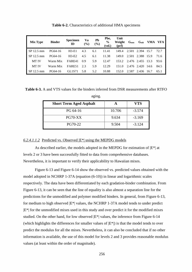
256

Table 6-2. Characteristics of additional HMA specimens

Mix Type Binder Specimen

ID

Va

(%)

Pb

(%)

Pbe,

%

(vol.)

Unit

Weight

(pcf)

Gmm Gmb VMA VFA

SP 12.5 mm PG64-16 H3-E1 4.3 6.1 11.41 149.4 2.501 2.394 15.7 72.7

SP 12.5 mm PG64-16 H3-E2 4.5 6.1 11.38 149.0 2.501 2.388 15.9 71.6

MT IV Warm Mix FARE41 0.9 5.9 12.47 153.2 2.476 2.455 13.3 93.6

MT IV Warm Mix FARE51 2.3 5.9 12.29 151.0 2.476 2.420 14.6 84.5

SP 12.5 mm PG64-16 GL1S71 5.8 5.2 10.88 152.0 2.587 2.436 16.7 65.1

Table 6-3. A and VTS values for the binders inferred from DSR measurements after RTFO

aging.

Short Term Aged Asphalt A VTS

PG 64-16 10.706 -3.574

PG70-XX 9.634 -3.169

PG70-22 9.504 -3.124

6.2.4.1.1.2 Predicted vs. Observed |E*| using the MEPDG models

As described earlier, the models adopted in the MEPDG for estimation of |E*| at

levels 2 or 3 have been successfully fitted to data from comprehensive databases.

Nevertheless, it is important to verify their applicability to Hawaiian mixes.

Figure 6-13 and Figure 6-14 show the observed vs. predicted values obtained with the

model adopted in NCHRP 1-37A (equation (6-10)) in linear and logarithmic scales

respectively. The data have been differentiated by each gradation-binder combination. From

Figure 6-13, it can be seen that the line of equality is also almost a separation line for the

predictions for the unmodified and polymer modified binders. In general, from Figure 6-13,

for medium to high observed |E*| values, the NCHRP 1-37A model tends to under predict

|E*| for the unmodified mixes used in this study and over predict it for the modified mixes

studied. On the other hand, for low observed |E*| values, the inference from Figure 6-14

(which highlights the differences for smaller values of |E*|) is that the model tends to over

predict the modulus for all the mixes. Nevertheless, it can also be concluded that if no other

information is available, the use of this model for levels 2 and 3 provides reasonable modulus

values (at least within the order of magnitude).

257

In order to compare the observed values with the predictions of the model adopted in

project NCHRP 1-40D (equation (6-11)), values of |G*| and are needed at several

frequencies. Thus, instead of directly using the DSR measurements of |G*| and (which were

obtained at a single frequency of 1.59 Hz (10 rad/s)), these were used to determine A and

VTS, and then the estimated A and VTS values were used to compute estimates of |G*| and

using the equations developed by Bari and Witczak [49]. Figure 6-15 and Figure 6-16 show

the observed vs. predicted values in linear and logarithmic scales respectively.

Although for a given observed |E*| value the range of predictions is about the same as

or smaller than the range of predictions with the NCHRP 1-37A model, contrary to a priori

expectations, the enhanced model shows a bias for all types of mixes analyzed in this study

for high values of |E*|. It tends to always over predict the |E*| values.

The above observation could be a consequence of the fact that several conversions are

required to predict |G*| and for any frequency and temperature. Recall that although some

values of |G*| and were available at a single frequency, they were used to predict A and VTS

and from these, the |G*| and were predicted for any frequency and temperature. In any case,

for level 3 analyses, these are the types of predictions that would be needed to use the model.

Both models are quite sensitive to the binder characteristics.

In summary, the models adopted in the MEPDG for estimation of |E*| produce

reasonable but apparently somewhat biased results for some of the mixes in this study. For

those cases in which level 2 or 3 must be used, the models in the MEPDG would give

reasonable modulus estimates, provided reasonably accurate volumetric properties are used.

258

Figure 6-13. Observed vs. Predicted |E*| in linear scale - NCHRP 1-37A model.

Figure 6-14. Observed vs. Predicted |E*| in logarithmic scale - NCHRP 1-37A model.

0

1,000,000

2,000,000

3,000,000

4,000,000

0 1,000,000 2,000,000 3,000,000 4,000,000

Pre

dic

ted

|E*

| (p

si)

Observed |E*| (psi)

Grad. A - PG64-16

Grad. B - PG64-16

Grad. A - PG70-XX

Grad. B - PG70-XX

Grad. A - PG70-22

Grad. B - PG 70-22

Other mixes

"Equality Line"

1,000

10,000

100,000

1,000,000

10,000,000

1,000 10,000 100,000 1,000,000 10,000,000

Pre

dic

ted

|E*

| (p

si)

Observed |E*| (psi)

Grad. A - PG64-16

Grad. B - PG64-16

Grad. A - PG70-XX

Grad. B - PG70-XX

Grad. A - PG70-22

Grad. B - PG70-22

Other Mixes

"Equality Line"

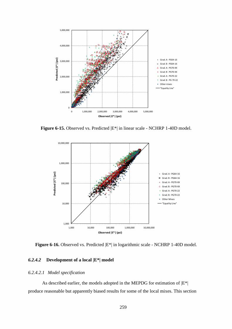
259

Figure 6-15. Observed vs. Predicted |E*| in linear scale - NCHRP 1-40D model.

Figure 6-16. Observed vs. Predicted |E*| in logarithmic scale - NCHRP 1-40D model.

6.2.4.2 Development of a local |E*| model

6.2.4.2.1 Model specification

As described earlier, the models adopted in the MEPDG for estimation of |E*|

produce reasonable but apparently biased results for some of the local mixes. This section

0

1,000,000

2,000,000

3,000,000

4,000,000

5,000,000

0 1,000,000 2,000,000 3,000,000 4,000,000 5,000,000

Pre

dic

ted

|E*

| (p

si)

Observed |E*| (psi)

Grad. A - PG64-16

Grad. B - PG64-16

Grad. A - PG70-XX

Grad. B - PG70-XX

Grad. A - PG70-22

Grad. B - PG 70-22

Other mixes

"Equality Line"

1,000

10,000

100,000

1,000,000

10,000,000

1,000 10,000 100,000 1,000,000 10,000,000

Pre

dic

ted

|E*

| (p

si)

Observed |E*| (psi)

Grad. A - PG64-16

Grad. B - PG64-16

Grad. A - PG70-XX

Grad. B - PG70-XX

Grad. A - PG70-22

Grad. B - PG70-22

Other Mixes

"Equality Line"

260

describes the development of a model similar to those used in the MEPDG that uses local mix

information.

Similarly to the approach used by Witczak, the point of departure for the formulation

of the model is equation (6-6) but making the parameters of this equation functions of mix

characteristics.

As discussed earlier, equations (6-5) (page 240) through (6-7) (page 242) can be used

to describe the changes in dynamic modulus with changes in frequency of loading and

temperature. For this, a total of seven parameters (, A, B, and C) are needed.

A comparison of equations (6-6) (page 241) and (6-11) (page 248) shows that the first

three lines in equation (6-11) are equivalent to in equation (6-6), that the numerator in the

fourth line of equation (6-11) is equivalent to in equation (6-6), and that the exponent of e

in equation (6-11) (-0.7814 -0.5785 log |Gb*| + 0.8834 log b) is equivalent to ( + log10 tr)

in equation (6-6).

At first, the last comparison may not appear entirely clear since there is no such thing

as a reduced time in equation (6-11) as there is for equation (6-6). In reality, tr appears

implicitly in (6-11) as well given that similar master curves can be derived for |G*| and b as

it was done here for |E*|. What is important to notice is that and were considered both

functions of mixture volumetrics and aggregate structure. Furthermore, based on the

comparisons of the exponents of e; and are in essence considered functions of binder

characteristics.

The estimation of the model presented below is based on these observations plus

some experimenting. The model finally selected is one that provided the largest number of

statistical significant parameter estimates at a 95% confidence level. The following equation

shows the model finally selected:

261

)(log)(

6354321

7365

4321

*

10

1021654321

1

||log

rEBWEabeff

beff

a

eff

eff

eff

eff

tDDDDVV

VV

FHWE

ab

b

FHW

E

ab

b

a

e

DDDDVV

V

DDD

DVV

VVE

(6-12)

where

CTBTA

2

rt

tlog log(a(T)) (6-13)

EDAA 21A (6-14)

EDBB 21B (6-15)

)(C BATT refref (6-16)

and where

T = temperature, ºF

Tref = reference temperature, ºF (usually 70 ºF),

Va = air voids (by volume of the mix), %

Vbeff = effective binder content (by volume of the mix), %

DE = 1 if mix prepared with PG70-XX binder and 0 otherwise

DW = 1 if mix prepared with PG70-22 binder and 0 otherwise

DH3 = 1 if Superpave Mix used in H3 project and 0 otherwise

DF = 1 if Mix Type IV used in Project 7101 A -01-04M and 0 otherwise

DB = 1 if mix prepared with gradation B and 0 otherwise

262

At first, equations (6-12) through (6-16) may appear to be complex. However, they

are simple extensions of equations (6-10) and (6-11). The following text explains the

differences followed by a presentation of the estimation results.

First, notice that the first two lines of equation (6-12) are equivalent to in equation

(6-6).The difference is that the term is made a function of air voids (Va), voids filled with

asphalt expressed in decimal (VFA/100 = Vbeff/(Vbeff+Va) ), and other variables that indicate

whether the mix is modified and the type of modifier or if the mix is one of the additional

mixes presented above. The new term is:

FHWE

ab

b

a DDDDVV

VV

eff

eff

73654321

(6-17)

Notice that these indicator variables DE, DW, DH3 and DF are useful to determine

differences in mixes when limited information is available. For example, if a mix was

prepared with PG70-XX, the value would be given by

4321

ab

b

aVV

VV

eff

eff (6-18)

since DE = 1, DW = 0 (the mix is not prepared with PG70-22), DH3 = 0, and DF = 0. Thus, the

assumption is that the term will change depending on type of binder or mixture but that the

effects of air voids and VFA are the same for all types of mixes. This is similar to the more

detailed use of gradation information in the MEPDG default models.

Similarly, the numerator of the third line of equation (6-12) provides the value of as

a function of mix characteristics, i.e.

FHWE

ab

bDDDD

VV

V

eff

eff

6354321

(6-19)

The only difference between this expression and the one for is that air voids is not

included in equation (6-19) since it was not found significant. As for the term, it becomes:

263

BWE

abeff

beff

a DDDVV

VV 654321

(6-20)

This is again a very similar expression to the ones for and . The main difference is

that it contains an indicator variable (DB) that differentiates specimens with gradation B from

other specimens. As described later, this is the only place where an effect of gradation was

specifically detected. This function further differs from the one adopted in the MEPDG in

that it is a function of volumetric characteristics. Thus, in this model, not only the maximum

and minimum values of the sigmoidal function depend on mixture volumetrics but the shape

as well.

The term is the simplest one and has the following form:

ED21 (6-21)

This term is considered to be different for the mixes with PG70-XX, as are the

expressions (6-14) and (6-15) for the A and B terms, respectively, in equation (6-13). Notice

that the term C is made a function of A, B, the reference temperature (70 ºF) such that the

shift factor is equal to 1 at the reference temperature of 70ºF. In other words, no new

parameters are needed to compute C.

6.2.4.2.2 Estimation of model parameters and evaluation of results

As indicated before, the variables included in the model are the ones that produced

statistical significant results. The parameters of these equations were estimated using the non-

linear mixed effects approach available in S-Plus. Table 6-4 shows the estimation results

(parameter estimates are shown with three significant figures). Based on the t-statistics and

the p-values for the individual parameters, it can be observed that most parameter estimates

are statistically significant at a 95% confidence level.

The R2 for the fit is 0.985 in linear scale, which indicates an excellent fit. Figure 6-17

presents a comparison of the observed versus fitted values in linear scale and Figure 6-18

shows the comparison in logarithmic scales.

It can be observed that the predictions are now clearly unbiased for all the mixes.

Also, by comparing Figure 6-18 with Figure 6-14 and Figure 6-16, it can be seen that the

variation for low |E*| conditions is reduced greatly.

264

An important consideration in the estimation of parameters of statistical models is not

only the overall goodness of fit and the achievement of overall unbiased results but also the

statistical significance of individual parameters or set of parameters and the analysis of the

reasonableness of the results in terms of the signs of the parameters. However, for non-linear

regression models this latter task is more difficult than for linear models, particularly when

some of the variables may be correlated and appear in more than one term. This is exactly the

case with this model since Va and VFA are negatively correlated and many of the indicator

variables (such DE) appear in many terms. Nevertheless, an attempt is made here to analyze

some of the most important aspects of the model.

First, notice that the parameter estimate for DE (4) in the term (equation (6-18)) is

positive, which indicates that other things being equal, the mixes prepared with PG70-XX

binder have a higher lower bound for |E*| than mixes prepared with PG64-16 unmodified

binders. On the other hand, the parameter for DE (3) in the term is negative (equation (6-

19)), which indicates that other things being equal, the mixes prepared with PG70-XX binder

have a lower range for |E*| than mixes prepared with PG64-16 unmodified binders. From the

fact that the estimate of |3| > 4, it can be inferred that the modified mix will be softer than

the unmodified mix at low temperatures and high frequencies. Thus, the use of the PG70-XX

binder results in stiffer mixes at high temperatures and low frequencies of loading, which is

beneficial for resisting rutting, and results in slightly softer mixes at low temperatures and

high frequencies of loading, which is beneficial for cracking.

The analysis for the corresponding parameters (5 and 4) for the modified PG70-22

binder leads to exactly the same conclusion. The only difference is that the absolute values of

the parameters for the PG70-22 binder are smaller than those for the PG70-XX binder. This

indicates that both modified binders reduce the range of variation of |E*| with temperature

and frequency, but that the PG70-XX does it a little bit more than the PG70-22. This is

illustrated in Figure 6-19 which shows the estimated master curves for gradation A and for

specimens with air voids Va = 5% and binder content Pb = 5.8% (the VFA is computed based

on Pb and the Gse determined in the laboratory for each mix). Notice that the figure shows

|E*| as function of the reduced frequency in Hz, which in the MEPDG is computed as the

inverse of the reduced time in s (fr = 1/tr). The effect of binder type is evident.

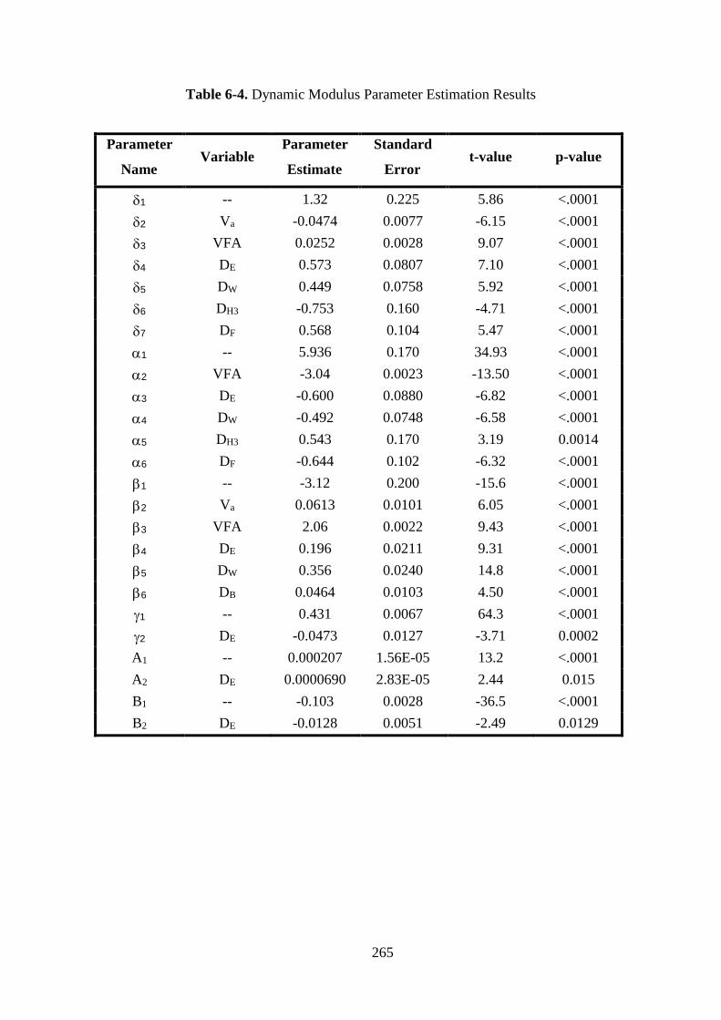
265

Table 6-4. Dynamic Modulus Parameter Estimation Results

Parameter

Name Variable

Parameter

Estimate

Standard

Error t-value p-value

1 -- 1.32 0.225 5.86 <.0001

2 Va -0.0474 0.0077 -6.15 <.0001

3 VFA 0.0252 0.0028 9.07 <.0001

4 DE 0.573 0.0807 7.10 <.0001

5 DW 0.449 0.0758 5.92 <.0001

6 DH3 -0.753 0.160 -4.71 <.0001

7 DF 0.568 0.104 5.47 <.0001

1 -- 5.936 0.170 34.93 <.0001

2 VFA -3.04 0.0023 -13.50 <.0001

3 DE -0.600 0.0880 -6.82 <.0001

4 DW -0.492 0.0748 -6.58 <.0001

5 DH3 0.543 0.170 3.19 0.0014

6 DF -0.644 0.102 -6.32 <.0001

1 -- -3.12 0.200 -15.6 <.0001

2 Va 0.0613 0.0101 6.05 <.0001

3 VFA 2.06 0.0022 9.43 <.0001

4 DE 0.196 0.0211 9.31 <.0001

5 DW 0.356 0.0240 14.8 <.0001

6 DB 0.0464 0.0103 4.50 <.0001

1 -- 0.431 0.0067 64.3 <.0001

2 DE -0.0473 0.0127 -3.71 0.0002

A1 -- 0.000207 1.56E-05 13.2 <.0001

A2 DE 0.0000690 2.83E-05 2.44 0.015

B1 -- -0.103 0.0028 -36.5 <.0001

B2 DE -0.0128 0.0051 -2.49 0.0129

266

Figure 6-17. Observed versus fitted dynamic modulus values – linear scale.

Figure 6-18. Observed versus fitted dynamic modulus values – logarithmic scale.

It should be clear that the shape of the master curves presented in Figure 6-19 are also

affected by parameters related to binder type, namely, 4, 5, 2, A2, and B2.

Other parameter estimates with similar interpretations to the s and s described

above that were found to be statistically significant are 6, 7, 5, and 6.

0

1,000,000

2,000,000

3,000,000

4,000,000

5,000,000

0 1,000,000 2,000,000 3,000,000 4,000,000 5,000,000

Pre

dic

ted

|E*

| (p

si)

Observed |E*| (psi)

Grad. A - PG64-16

Grad. B - PG64-16

Grad. A - PG70-XX

Grad. B - PG70-XX

Grad. A - PG70-22

Grad. B - PG 70-22

Other mixes

"Equality Line"

1,000

10,000

100,000

1,000,000

10,000,000

1,000 10,000 100,000 1,000,000 10,000,000

Pre

dic

ted

|E*

| (p

si)

Observed |E*| (psi)

Grad. A - PG64-16

Grad. B - PG64-16

Grad. A - PG70-XX

Grad. B - PG70-XX

Grad. A - PG70-22

Grad. B - PG70-22

Other Mixes

"Equality Line"

267

6 and 5 are parameters related to a field mix used in a particular pavement

preservation project on the H-3 freeway. In this case, the signs are reversed, which indicates

that this mix (other things being equal) is softer at high temperatures and low frequencies and

stiffer at low temperatures and high frequencies. This mix appears to perform much poorer

than other mixes analyzed in this study. It should be noted however that although the model

accounts for air voids and voids filled with asphalt, the H-3 mixes were compacted in the lab

with too low air voids and too high VFA, which may have affected to some degree the

results. Further information is required to ascertain whether the results from those two

specimens are just outliers or whether there is some other type of problems with those mixes.

Figure 6-19. Comparison of predicted master curves for mixes with gradation “A” for three

different binders (Tref = 70ºC, Va = 5% and Pb = 5.8%).

The parameters for the Farrington Highway preservation project, 7 and 6, are

similar to those for the PG70-XX. Thus, the performance of this mix (in terms of its |E*|

value) appears to be similar to that of the polymer modified mix. Interestingly, despite this

apparently good response, this project showed some early signs of distress after only 1½

years. The picture in Figure 4-24 (page 141) is from the same highway section. As mentioned

in Section 4.3.1.1.2 (page 136), some of the paving was performed on a section that still

showed severe fatigue cracking after milling, which may explain the poor field performance.

1,000

10,000

100,000

1,000,000

10,000,000

1.00E-08 1.00E-06 1.00E-04 1.00E-02 1.00E+00 1.00E+02 1.00E+04

Reduced Frequency (Hz)

|E*|

(p

si)

PG 64-16

PG70-XX

PG70-22

268

This example stresses the point that to achieve the benefits of good mixes not only the mix

characteristics but also the structural integrity of the pavement need to be adequate.

No variable differentiating between the behavior of gradations A and B were found to

be significant in the and terms. Apparently, the two gradations perform similarly when

the volumetric variables Va and VFA are the same. Parameter 6 is the only one that captures

some difference between the two gradations. Figure 6-20 illustrates the effect of this

parameter for mixes with and without modified binder. In general, although statistically

significant, the differences between the two gradations are relatively minor when compared

to the effects of other variables.

The effects of air voids and voids filled with asphalt are intricately related; thus, the

end effects are analyzed instead of analyzing the individual parameters. Figure 6-21 shows

the effect of air voids for a mix with asphalt content Pb = 5.8% and the PG70-XX binder. The

effect of air voids is quite apparent, with higher air voids resulting in lower dynamic moduli.

Notice also that keeping the binder content constant while varying the air voids (as assumed

in this figure) requires varying the VFA as well.

Figure 6-20. Comparison of predicted master curves for gradations A and B

(Tref = 70ºC, Va = 5% and Pb = 5.3%)

1,000

10,000

100,000

1,000,000

10,000,000

1.00E-05 1.00E-04 1.00E-03 1.00E-02 1.00E-01 1.00E+00 1.00E+01 1.00E+02 1.00E+03 1.00E+04


|E*|

(p

si)

PG64-16 - Gradation A

PG70-XX - Gradation A

PG64-16 - Gradation B

PG70-XX - Gradation B

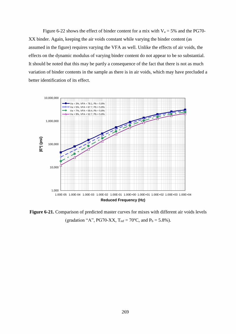
269

Figure 6-22 shows the effect of binder content for a mix with Va = 5% and the PG70-

XX binder. Again, keeping the air voids constant while varying the binder content (as

assumed in the figure) requires varying the VFA as well. Unlike the effects of air voids, the

effects on the dynamic modulus of varying binder content do not appear to be so substantial.

It should be noted that this may be partly a consequence of the fact that there is not as much

variation of binder contents in the sample as there is in air voids, which may have precluded a

better identification of its effect.

Figure 6-21. Comparison of predicted master curves for mixes with different air voids levels

(gradation “A”, PG70-XX, Tref = 70ºC, and Pb = 5.8%).

1,000

10,000

100,000

1,000,000

10,000,000

1.00E-05 1.00E-04 1.00E-03 1.00E-02 1.00E-01 1.00E+00 1.00E+01 1.00E+02 1.00E+03 1.00E+04


|E*|

(p

si)

Va = 3%, VFA = 78.1, Pb = 5.8%

Va = 5%, VFA = 67.7, Pb = 5.8%

Va = 7%, VFA = 59.4, Pb = 5.8%

Va = 9%, VFA = 52.7, Pb = 5.8%

270

Figure 6-22. Comparison of predicted master curves for mixes with different binder contents

(gradation “A”, PG70-XX, Tref = 70ºC, and Va = 5%).

6.2.4.2.3 Discussion of suggested use of the local model

As the use of the MEPDG progresses, ideally, the best option for individual states

should be the calibration of one of Witczak’s equations or similar equations for their

particular conditions. However, this may demand a substantial database with very detailed

information, which may be difficult to obtain locally.

The results of the locally calibrated model can be used to generate |E*| values for

selected temperature and frequencies for input into the MEPDG as pseudo-level 1 data. This

is the approach used in this study for calibration of the guide for State Type IV and

Superpave 12.5 mm NMAS mixes. Since a similar model has not yet been developed for

State Type III and Type V mixes, the inputs for those mixes was performed at a level 2.

As the previous sections have shown, relatively accurate results can be achieved with

this approach because although the data may be less detailed, the model is still based on

observations of local materials and thus may account for unobserved factors that cannot

possibly be included or that may be difficult to include in a universal model. Thus, although

the values generated by the model are not really level 1 data, they provide an alternative to

the use of level 2 or 3 inputs, which are based solely on gradation and binder characteristics.

1,000

10,000

100,000

1,000,000

10,000,000

1.00E-05 1.00E-04 1.00E-03 1.00E-02 1.00E-01 1.00E+00 1.00E+01 1.00E+02 1.00E+03 1.00E+04


|E*|

(p

si)

Va = 5%, VFA = 61.7, Pb = 4.8%

Va = 5%, VFA = 65.0, Pb = 5.3%

Va = 5%, VFA = 67.7, Pb = 5.8%

Va = 5%, VFA = 70.0, Pb = 6.3%

271

It is also important to point out that the sole prediction of |E*| is not enough to predict

accurately distresses such as permanent deformation. As illustrated in [50] and [51] (the

results in [50] were based on a subsample of the sample used in this report), the predictions

with the MEPDG without any adjustments in the calibration parameters of the permanent

deformation model for modified mixes do not appear to give enough credit to polymer

modified mixes and under some conditions, the MEPDG may even indicate that the modified

mixes perform worse than the unmodified mixes. Additional permanent deformation testing

and modeling together with the model presented in this section tend to confirm those findings

[52]. Permanent deformation of HMA is discussed in section 6.5 (page 333) of this report.

6.2.4.2.4 Model Validation

As part of a more limited study, additional HMA specimens were compacted and

tested for dynamic modulus and permanent deformation. Testing was performed on two sets

of six specimens of a control unmodified mix, a polymer modified mix, and a fiber reinforced

mix. For each mix, two specimens were compacted at three different target air voids. The mix

design adopted had been used by Grace Pacific Corporation (GPC) in a paving project

performed around the time of the study. GPC provided the samples of the same aggregates

and the same asphalt binder used in that project, which were used in the preparation of

specimens in the laboratory. In addition, testing was performed on six specimens (2 replicates

at three target air voids) of another unmodified mix produced at a local asphalt plant.

Figure 6-23 shows the gradations of the mixes used by Rayapeddi Kumar [47]. For lack

of a better name, they were designated C and D. The figure also shows for comparison

gradations A and B used in the development of the local model. In addition, for

limits of 12.5 mm NMAS are also shown. Gradation C meets the gradation

Superpave (SP) 12.5 mm NMAS mix. It also meets the State Mix IV gradation

On the other hand, Gradation D meets the SP 19.0 mm NMAS requirements.

Figure 6-24 shows gradation D along with the SP 19 mm gradation limits.

272

Figure 6-23. Comparison of C and D gradations with gradations A and B.

Figure 6-24. Gradation D.

1"

3/4

"

1/2

"

3/8

"

#4

#8

#16

#30

#50

#100

#200

0

10

20

30

40

50

60

70

80

90

100

Perc

en

t P

assin

g

Sieve Designation

Gradation for Plant Produced Mix

19.0 mm SuperPave Control Points - Lower

19.0 mm SuperPave Control Points - Upper

273

The aggregates used in the preparation of HMA samples in the laboratory were from

the Ameron Kapa’a quarry in the island of Oahu, Hawaii. For the plant produced mixes, the

coarse aggregates were also from the Ameron Kapa’a quarry in Oahu, Hawaii but the fine

aggregates were from Ameron Puunene quarry from the island of Maui, Hawaii.

The control, PMA, and fiber reinforced mixes were prepared with gradation C. The

other unmodified mix was prepared with gradation D.

The unmodified binder was a PG64-22 now supplied by Asphalt Hawaii. Although

the high temperature grade is the same as that used in the previous study, the source of the

binder is different. Therefore, differences in some binder characteristics may be expected.

From informal conversations with for some people in the field, there seems to be a feeling

that the new binder (source: Saudi Arabia) is a bit softer.

Similarly to the previous study, to prepare the polymer modified asphalt (PMA)

specimens, the unmodified binder from Asphalt Hawaii was modified with 1% of DuPont’s

Elvaloy®RET and mixed with 0.3% (by weight of binder) polyphosphoric acid. The latter is

added to act as a catalyst of the reaction between Elvaloy RET and the binder. An additional

set of specimens were prepared with the unmodified binder but introducing into the mix

HMA Forta-FI Fibers® in a proportion of 1 lb/ton.

In summary, the four types of mixtures tested in this study and the notation used by

Rayapeddi Kumar [47] to identify them were:

1. Laboratory produced mixtures with gradation C prepared using virgin asphalt

binder (VLPM).

2. Laboratory produced mixtures using gradation C prepared using polymer

modified asphalt binder (PMALPM).

3. Laboratory produced mixtures with gradation C prepared using unmodified binder

and fibers (FRACLPM).

4. Plant produced mixtures with gradation D prepared using virgin asphalt binder

(VPPM).

Other details on the preparation of the specimens and their characteristics are

described in [47]. Before discussing the |E*| model validation, the next subsection provides

some additional information about the procedure used by Rayapeddi Kumar [47] to disperse

the fibers in the mix.

274

6.2.4.2.4.1 Fibers Used in the Study

FORTA-FI® HMA blend fibers were used in this study. In its manufactured

condition, the fibers are clasped together. The fibers were fluffed using a makeshift procedure

prior to mixing them with hot aggregates. This is done to enhance the effect of fibers and

improve the distribution of fibers in the HMA mixture. The procedure involved placing

packaged fibers inside a hollow cylinder, the top of which was then covered using a

perforated disc. Next, compressed air was blown from the top to achieve the desired result.

Figure 6-25 through Figure 6-27 show the fibers in its manufactured condition, the fluffing

setup, and the resulting fluffed fibers. The fluffed fibers were then weighed as required and

mixed with hot aggregates before asphalt was introduced into the mixing bowl.

Figure 6-25. FORTA-FI HMA Fibers in its manufactured condition.

Figure 6-26. Setup used to fluff the fibers.

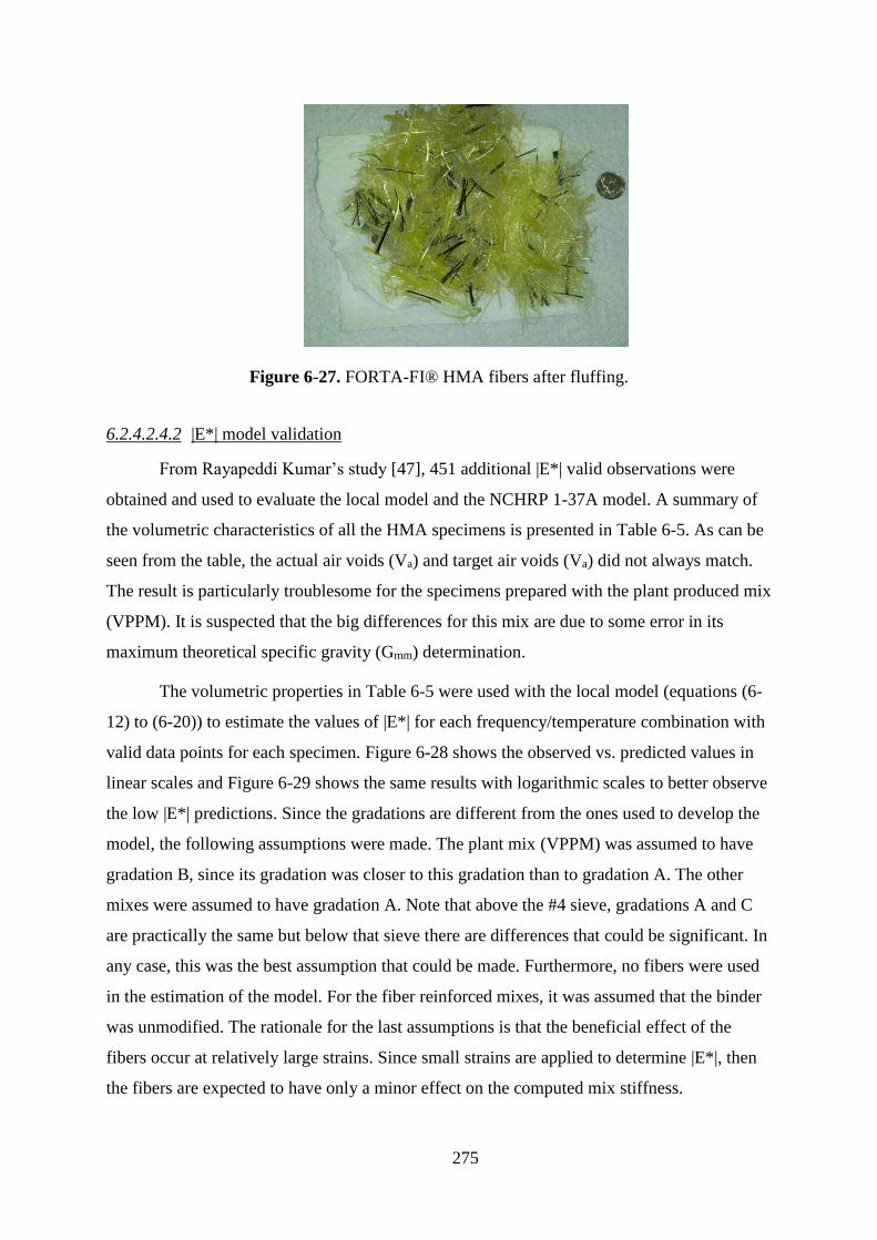
275

Figure 6-27. FORTA-FI® HMA fibers after fluffing.

6.2.4.2.4.2 |E*| model validation

From Rayapeddi Kumar’s study [47], 451 additional |E*| valid observations were

obtained and used to evaluate the local model and the NCHRP 1-37A model. A summary of

the volumetric characteristics of all the HMA specimens is presented in Table 6-5. As can be

seen from the table, the actual air voids (Va) and target air voids (Va) did not always match.

The result is particularly troublesome for the specimens prepared with the plant produced mix

(VPPM). It is suspected that the big differences for this mix are due to some error in its

maximum theoretical specific gravity (Gmm) determination.

The volumetric properties in Table 6-5 were used with the local model (equations (6-

12) to (6-20)) to estimate the values of |E*| for each frequency/temperature combination with

valid data points for each specimen. Figure 6-28 shows the observed vs. predicted values in

linear scales and Figure 6-29 shows the same results with logarithmic scales to better observe

the low |E*| predictions. Since the gradations are different from the ones used to develop the

model, the following assumptions were made. The plant mix (VPPM) was assumed to have

gradation B, since its gradation was closer to this gradation than to gradation A. The other

mixes were assumed to have gradation A. Note that above the #4 sieve, gradations A and C

are practically the same but below that sieve there are differences that could be significant. In

any case, this was the best assumption that could be made. Furthermore, no fibers were used

in the estimation of the model. For the fiber reinforced mixes, it was assumed that the binder

was unmodified. The rationale for the last assumptions is that the beneficial effect of the

fibers occur at relatively large strains. Since small strains are applied to determine |E*|, then

the fibers are expected to have only a minor effect on the computed mix stiffness.

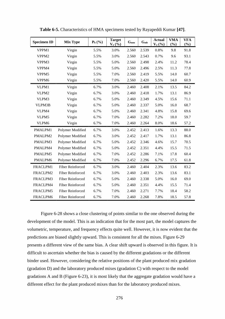
276

Table 6-5. Characteristics of HMA specimens tested by Rayapeddi Kumar [47].

Specimen ID Mix Type Pb (%) Target

Va (%) Gmm Gmb

Actual

Va (%)

VMA

(%)

VFA

(%)

VPPM1 Virgin 5.5% 3.0% 2.560 2.539 0.8% 9.8 91.8

VPPM2 Virgin 5.5% 3.0% 2.560 2.543 0.7% 9.6 93.1

VPPM3 Virgin 5.5% 5.0% 2.560 2.498 2.4% 11.2 78.4

VPPM4 Virgin 5.5% 5.0% 2.560 2.496 2.5% 11.3 77.8

VPPM5 Virgin 5.5% 7.0% 2.560 2.419 5.5% 14.0 60.7

VPPM6 Virgin 5.5% 7.0% 2.560 2.420 5.5% 14.0 60.9

VLPM1 Virgin 6.7% 3.0% 2.460 2.408 2.1% 13.5 84.2

VLPM2 Virgin 6.7% 3.0% 2.460 2.418 1.7% 13.1 86.9

VLPM3 Virgin 6.7% 5.0% 2.460 2.349 4.5% 15.6 71.1

VLPM3B Virgin 6.7% 5.0% 2.460 2.337 5.0% 16.0 68.7

VLPM4 Virgin 6.7% 5.0% 2.460 2.341 4.8% 15.8 69.6

VLPM5 Virgin 6.7% 7.0% 2.460 2.282 7.2% 18.0 59.7

VLPM6 Virgin 6.7% 7.0% 2.460 2.264 8.0% 18.6 57.2

PMALPM1 Polymer Modified 6.7% 3.0% 2.452 2.413 1.6% 13.3 88.0






FRACLPM1 Fiber Reinforced 6.7% 3.0% 2.460 2.404 2.3% 13.6 83.2






Figure 6-28 shows a close clustering of points similar to the one observed during the

development of the model. This is an indication that for the most part, the model captures the

volumetric, temperature, and frequency effects quite well. However, it is now evident that the

predictions are biased slightly upward. This is consistent for all the mixes. Figure 6-29

presents a different view of the same bias. A clear shift upward is observed in this figure. It is

difficult to ascertain whether the bias is caused by the different gradations or the different

binder used. However, considering the relative positions of the plant produced mix gradation

(gradation D) and the laboratory produced mixes (gradation C) with respect to the model

gradations A and B (Figure 6-23), it is most likely that the aggregate gradation would have a

different effect for the plant produced mixes than for the laboratory produced mixes.

277

Therefore, it is suspected that the difference is caused mainly by the binder. Note that if the

above speculation is correct, it implies that the reason why the model over-predicts the values

of |E*| is because the binder currently supplied is somewhat softer than before. It is important

to note, however, that the differences are relatively minor and that |E*| alone is not a good

indicator of mix performance.

The bias above can be easily corrected for these mixes by subtracting 0.3 from

(equation (6-17)) and adding 0.22 to (equation (6-19)). These two factors are not the result

of a re-estimation of the model. Instead, they were simply derived by trial and error. The fit in

Figure 6-30 resulting from these corrections is acceptable for all practical purposes.

Figure 6-28. Observed vs. Predicted |E*| using Rayapeddi Kumar’s data and the local |E*|

model (linear scale).

-

1,000,000

2,000,000

3,000,000

4,000,000

0 1,000,000 2,000,000 3,000,000 4,000,000

Pre

dic

ted

|E

*| (p

si)

Observed |E*| (psi)

SP 12.5 mm - Unmodified

SP 12.5 mm - PMA 1% Elvaloy

SP 12.5 mm - Fiber Reinforced


Equality Line

278


model (logarithmic scale).


model after bias correction (logarithmic scale).

10,000

100,000

1,000,000

10,000,000

10,000 100,000 1,000,000 10,000,000

Pre

dic

ted

|E

*| (p

si)

Observed |E*| (psi)


SP 12.5 mm - PMA 1%

Elvaloy

SP 12.5 mm - Fiber

Reinforced

10,000

100,000

1,000,000

10,000,000

10,000 100,000 1,000,000 10,000,000

Pre

dic

ted

|E

*| (p

si)

Observed |E*| (psi)





Equality Line

279

Rayapeddi Kumar’s data were also used to evaluate the NCHRP 1-37A model. Figure

6-31 and Figure 6-32 show the results in linear and logarithmic scales, respectively. The

predictions for the unmodified control mix are acceptable but they deviate more for the other

mixes. Still, if no other information is available, the model provides reasonable values with

some minimal information.

Figure 6-31. Observed vs. Predicted |E*| using Rayapeddi Kumar’s data and NCHRP 1-37A

|E*| model (linear scale).

0

1,000,000

2,000,000

3,000,000

4,000,000

0 1,000,000 2,000,000 3,000,000 4,000,000

Pre

dic

ted

|E

*| (p

si)

Observed |E*| (psi)





Equality Line

280

Figure 6-32. Observed vs. Predicted |E*| using Rayapeddi Kumar’s data and the

NCHRP 1-37A |E*| model (logarithmic scale).

6.2.4.2.5 Additional Issues

Despite the significant understanding about HMA dynamic modulus that has been

developed over decades, there are still a few issues that need further study. As mentioned in

section 6.2.1.1 (page 230), there is evidence that confinement affects dynamic modulus,

particularly at high temperatures and low frequencies [40] but more research is needed to

develop models that determine |E*| as a function of confinement level. Without confinement,

the |E*| values at high temperatures and low frequencies of loading appear to be

conspicuously low for some mixes. Another related issue is that all the |E*| testing is

performed in compression, where the aggregate and the binder contribute to the modulus.

However, in tension, the modulus would depend mostly on the binder. Thus, constitutive

models that account for the state of stresses should be developed. A possible reason that these

issues have not been studied in more detail is that their modeling requires the use of non-

linear finite element analysis.

Despite the widely use of |E*|, there are still controversies about the frequency

determination in the field [53]. As discussed in the next chapter (section 7.6.1), solving this

issue may be of particular interest to Hawaii since it seems that in the MEPDG the effect of

frequency is always dominating the effect of temperature.

10,000

100,000

1,000,000

10,000,000

10,000 100,000 1,000,000 10,000,000

Pre

dic

ted

|E

*| (p

si)

Observed |E*| (psi)





Equality Line

281

6.2.4.2.6 Summary and Conclusions

The main objectives of this section were to evaluate the adequacy of the |E*| models

used in the MEPDG for levels 2 and 3 designs, and to estimate a simplified version of those

models to provide more accurate data as pseudo-level 1 data. The following conclusions are

provided based on the finding:

1) The two models currently used in the MEPDG for levels 2 and 3 provide in general

reasonable estimates of |E*| for those levels of analysis, although for the mixes

analyzed, the results appear to be biased.

2) The NCHRP 1-37A model tends to under predict the |E*| of the Hawaii unmodified

mixes and over predict the |E*| of the polymer modified mixes.

3) The NCHRP 1-40D model tends to over predict the |E*| for both the unmodified and

polymer modified mixes analyzed.

4) An alternative model using the same sigmoidal function of the MEPDG model but

using indicator variables to account for some of the differences between mixes for

which no detailed information is available was developed and estimated. The

developed model shows excellent statistical results even though the number of

observations in the database is substantial. Thus it is believed to capture the behavior

of the mixes studied quite well.

5) A limited validation of the model with mixes prepared with new binder supplied on

the state indicates that the local model produces reasonable but somewhat bias

estimates. A small correction to two of the terms of the model corrects the bias. If

mixes that are too different from the ones analyzed here are considered, the NCHRP

1-37A model still provides reasonably estimates of |E*|.

6.3 RESILIENT MODULUS OF UNBOUND MATERIALS AND SOILS

The moduli of unbound bases, subbases, and subgrade soils are essential inputs for

mechanistic-empirical pavement design.

For these materials, time of loading is not as important as for HMA. However, their

moduli are significantly affected by many other factors that make their determination non-

trivial. Among these are the stress level, which depends on the position of the element within

the pavement structure, the load magnitude, material conditions such as moisture content, etc.

Furthermore, since moisture content can vary throughout the year, so does the modulus. A

282

basic understanding of the interaction of these terms becomes important to select reasonable

input values.

This section, after a brief introduction to the models used to predict modulus of

unbound materials and soils, provides a summary of the information locally available.

Although the Pavement ME Design software [2] currently uses a single modulus value for

each layer for a given set of environmental conditions, the discussions in this section about

the modulus dependence on stress provide the background to make informed decision when

selecting Mr values.

6.3.1 Resilient Modulus

For unbound base and subbase materials and soils, the elastic modulus used in the

mechanistic analysis is the resilient modulus.

The resilient modulus test for fine-grained materials is typically performed on

cylindrical specimens of a height h = 8 in. and a diameter = 4 in. For coarse-grained

materials, due to their larger maximum aggregate sizes, the diameter of the test specimen is

increased to = 6 in. and correspondingly the height is increased to h = 12 in. to maintain the

height to diameter ratio to a minimum of 2 (Figure 6-33).

Figure 6-33. Resilient modulus test specimen.

h 3 3

3

3

d

d

283

The resilient modulus test is basically a “confined uniaxial”43 repeated loaded test in

which a haversine deviator stress pulse (d) followed by a rest period is applied repeatedly to

a sample already subjected to an all-around confinement stress (3). During the test, the

resilient (recoverable) strains are also measured. Figure 6-34 illustrates the stress pulse and

Figure 6-35 the resulting resilient strains.

Figure 6-34. Stress pulse and rest period in a resilient modulus test.

Figure 6-35. Resilient strain (r).

Since unbound materials are stress-dependent, the test is performed at different stress

levels (different combination of confinement and deviator stresses.) Figure 6-35 also

illustrates that with each cycle some permanent deformation is typically accumulated. At

relatively small stress levels and after several repetitions of the load pulse, as shown in Figure

6-36, the permanent deformation accumulated per cycle becomes smaller and the slope of the

d-r curve relatively constant. All resilient modulus test protocols require the measurement

43 As stated by Muir Wood [156]: “The most widely used apparatus for investigating the stress:strain

behaviour of soils is, in origin, a ‘confined uniaxial’ testing device known (misleadingly) as the triaxial

apparatus.”

Str

ess

puls

e

Time

Time

Str

ain

r

284

of Mr after a certain number of repetitions at each stress level to capture this mostly elastic

response.

The slope of the d-r curve after a large number of cycles is by definition the resilient

modulus:

r

drM

(6-22)

Figure 6-36. Deviator stress vs. axial strain in the resilient modulus test.

It is important to recognize that a resilient modulus test does not result in a single

modulus for the material tested but instead in a set of several resilient modulus values at the

different stress levels. The influence of stress state is significant on the resilient moduli of

both cohesive and cohesionless soils.

Li and Selig [54] identified three factors that influence the resilient modulus:

(1) loading condition or stress state, (2) soil type and structure, and (3) soil physical state

(combination of molding water content and dry unit weight). For a specific sample tested in

the lab, the last two factors are fixed but the effect of stress state still needs to be modeled.

This is considered in the next section. For designs on which testing is not performed or when

changes in Mr over time are required, models that incorporate the last two factors in addition

to state stress are needed. These are covered in Section 6.3.1.2.3.

Axial Strain

Dev

iato

r S

tres

s

Mr = Resilient Modulus

1

285

6.3.1.1 Modeling the effect of stress state

Several models have been proposed to predict the stress dependency of Mr. A

description, as well as some limitations of some of the models, is found in Ooi et al. [55]. The

list of models described in that reference is not exhaustive but it provides a good description

of some of some important modeling issues. In the following, only the model adopted in the

MEPDG [1] is described in detail.

The MEPDG uses a generalized constitutive model for resilient modulus. The

generalized model used in the design procedure is as follows:

32

11

k

a

oct

k

a

aoptrp

τ

p

θpkM

(6-23)

where

Mr opt = resilient modulus at optimum water content, psi,

= bulk stress = 1 + 2 + 3,

1 = major principal stress,

2 = intermediate principal stress = 3 for Mr tests on cylindrical specimens,

3 = minor principal stress/confining pressure,

oct = octahedral shear stress,

2322

312

213

1σσσσσσ

pa = normalizing stress (atmospheric pressure) (14.7 psi),

k1, k2, k3 = regression parameters (obtained by fitting resilient modulus test data to

equation).

The constitutive model coefficients (the parameters k1, k2, and k3) are estimated from

data through linear or non-linear regression (they can be estimated very easily using linear

regression by taking logarithms of both sides of the equation). A typical requirement is that

the values determined for each test specimen should be such that the multiple correlation

coefficient, R2, exceeds 0.90.

286

Regarding the signs of the parameters k1, k2, and k3, the MEPDG documentation [1]

states:

“Coefficient k1 is proportional to Young’s modulus. Thus, the values of k1 should be positive since Mr

can never be negative. Increasing the bulk stress, , should produce stiffening or hardening of the

material, which results in a higher Mr. Therefore, the exponent k2, of the bulk stress term for the above

constitutive equation should also be positive. Coefficient k3 is the exponent of the octahedral shear

stress term. The values for k3 should be negative since increasing the shear stress will produce a

softening of the material (i.e., a lower Mr).”

Witczak and Uzan (1988) found that for granular materials tested in a triaxial stress

state, the deviator stress has two contrary effects on the stiffness of the material; they argue

that an increase in deviator stress will result in an increase in bulk stress (θ=3σ3+σd), which

leads to increase in the stiffness of the material and that an increase in deviator stress also

increases the octahedral shear stress, which tends to decrease the modulus. Hicks and

Monismith (1971) on the other hand reported a “slight softening of the granular material at

low deviator stress levels and a slight stiffening behavior at higher levels of deviator stress.”

There is a widely held belief that, for unbound materials, the coefficient k3 should be

negative ( [1], [56], [57], and [58]). However, the sign of k3 has been reported to be positive

by other researchers including references [59] and [60]. Furthermore, a study by Song ( [61]

and [62]) conducted at the UH pavement laboratory with virgin and recycled granular

materials tested using the AASHTO T307 procedure also revealed positive k3 values for the

octahedral shear stress term in the MEPDG model (equation (6-23)). Song obtained k3 values

as high as 0.82, which is uncommon. Nevertheless, values as high as 1.595 have been

reported [63]. Unfortunately, the last two references misreported the value of k1, which

appears to be smaller than usual by a factor of 1,000. This is a common occurrence because

the state of stresses are commonly expressed in kPa whereas the modulus is expressed in

MPa.

In the MEPDG, once Mropt is obtained, the resilient modulus at any moisture content

(Mr) is then estimated internally as follows:

ropt

SSkβexp1

r M10M opts

aba

(6-24)

where Mropt is the resilient modulus of the soil at optimum water content, S is the degree of

saturation, Sopt is the degree of saturation at optimum, a and b are constants representing the

287

minimum and maximum values, respectively, of log(Mr/Mropt), is a location parameter

defined as ln(-b/a) so that the ratio Mr/Mropt is equal to one at optimum, and ks is a regression

parameter. The exponent of the number 10 in equation (6-24) represents a sigmoidal function

that approximates a linear relationship between log(Mr/Mropt) and S - Sopt within a narrow

range of saturation values, beyond which, log(Mr/ Mropt) approaches a or b. Mropt is estimated

using equation (6-23).

6.3.1.2 Predicting Mr for Pavement Design

With the above background on resilient modulus, attention is now turned to the

prediction of resilient modulus for pavement design. This is again a challenging task because

for unbound materials the theory used to model pavement performance does not match the

actual material response but it is instead a useful compromise to make the calculations

practical. This is in addition to all the uncertainties typically associated with sampling and

testing. More specifically, in the current version of the Pavement ME design software [2],

unbound materials are assumed to be linear elastic, homogeneous and isotropic, when in fact

neither of these assumptions are generally satisfied.

This section first describes the options for obtaining Mr values in Hawaii and provides

a discussion of how to use them to derive inputs for the MEPDG. In addition to providing

background for selecting Mr values for design, this section provides a framework for later

discussion of some important issues, including correction factors for back-calculated layer

moduli, effects of non-linearities, changes of Mr with layer thickness/depth, and consideration

of environmental effects.

6.3.1.2.1 Input Level 1 – Laboratory testing

The current version of the Pavement ME Design software [2] does not allow to input

information at level 1, as the option to use Finite Element analysis to account for unbound

materials non-linearities is disabled. Nevertheless, as indicated and illustrated later, it is

important for pavement analysts to understand the stress dependency of Mr when selecting

appropriate input moduli. Thus, the level 1 testing is discussed next.

Level 1 resilient modulus values for unbound granular materials, subgrade and

bedrock are determined from cyclic triaxial tests on prepared representative samples. The

MEPDG recommended standard methods for modulus testing are:

288

NCHRP 1-28A, “Harmonized Test Methods for Laboratory Determination of

Resilient Modulus for Flexible Pavement Design.”

AASHTO T307, “Determining the Resilient Modulus of Soil and Aggregate

Materials.”

These test methods describe the laboratory preparation, testing, and computation of

test results. As described earlier, the state of stresses substantially affects the resilient

modulus measurements. Therefore, stress states used for modulus testing are based upon the

depth at which the material will be located within the pavement structure. Consequently, the

test protocols specify different stress levels depending on whether the material will be used as

a base/subbase or as a subgrade.

There are some differences between the two test protocols. One difference is that

AASHTO T-307 uses LVDT’s that measure the deformation between end platens whereas

NCHRP 1-28A utilizes on-specimen clamp mounted LVDT’s. Another major difference is in

the state of stress testing sequences. In this respect, the NCHRP 1-28A testing sequences are

considered superior because they try to avoid shear failure of the specimen early in the

sequence, which is a more likely possibility under AASHTO T-307 sequences.

Figure 6-37 illustrates the resilient modulus test set up for coarse-grained materials

available in the pavement laboratory at UH. Since the measurement of vertical strains is

performed through Linear Variable Differential Transducers (LVDT) located outside the

triaxial cell, the test set-up matches better the requirements of AASHTO T307. The testing

sequence can be configured to match either protocol. Equipment for performing resilient

modulus of fine-grained materials with clamp mounted internal LVDTs is available at the

geotechnical laboratory at UH.

289

Figure 6-37. Resilient Modulus Test Set-up for granular materials at UH.

The results obtained to date for granular materials in this research were obtained with

the equipment set up shown in Figure 6-37.

6.3.1.2.2 Input Levels 2 & 3

At input level 2, the Pavement ME Design software [2] allows entering the resilient

modulus directly or values that allow its computation from correlations. Other inputs

accepted include CBR, R-Value, Layer coefficient [12], DCP Penetration, and plasticity and

gradation information. At level 3, only resilient modulus can be input. Regardless of the input

level, the user can allow the program to modify the input values by temperature and moisture

or enter a single resilient modulus value to use throughout the year. In addition, at level 2, the

user also has the option to enter monthly representative values.

Although the correlations with CBR, R-Value, etc. are widely used, it must be

remembered that these are very approximate at best and that they do not account for potential

different behavior of local materials. This is particularly relevant for fine-grained tropical

residual soils, which are known to exhibit characteristics that are different from those of soils

of temperate regions on the U.S. continent. According to Mitchell and Sitar [64], tropical

residual soils including those in Hawaii are likely to be less dense, less plastic, less

compressible, stronger, and more permeable than temperate soils of comparable liquid limit.

Therefore, estimating the resilient modulus from models developed locally should be

290

preferred to relying on correlations developed elsewhere. Notice that this is not judgment on

the reliability of the measurements of CBR, R-Value, etc. but on the applicability of the

correlations to local conditions.

6.3.1.2.3 Local Models of Mr

In this subsection, information that may be useful to estimate local resilient modulus

values is presented.

6.3.1.2.3.1 Fine-Grained Soils

Sandefur [65] developed an extensive database of resilient modulus values for several

Hawaiian fine-grained soils in the island of Oahu, tested at different density levels and

moisture conditions. Index properties of these soils are summarized in [65]. All these soils

plot below the A-line and are classified as silts. Mr tests were performed in accordance with

Long-Term Pavement Performance (LTPP) Protocol P46 [66]. Testing was performed at six

target dry densities and molding water contents or physical states: 100% and 95% relative

compaction (ASTM D 698 Procedure C) and at each relative compaction, samples were

compacted at approximately three different water contents: wopt – 2%, wopt and wopt + 2%,

where wopt = the optimum water content.

A total of 78 Mr tests were performed. Each soil was tested at three confining stresses

(2, 4 and 6 psi) and five deviator stresses (2, 4, 6, 8 and 10 psi) giving more than 1,100 Mr

values.

Using these data, the parameters of several models were estimated by Ooi et al. [55].

All the models in this reference had functional forms similar to that of equation (6-23).

Unfortunately, equation (6-23) itself was not included among those estimated in that paper.

Archilla et al. [67] used the same database together with LTPP resilient modulus data for

fine-grained soils to estimate a model using two advanced statistical techniques known as

joint estimation and mixed effects. Although the model form was a bit more involved, it can

be used directly to estimate the parameters k1, k2, and k3 of equation (6-23). In addition, since

the model was estimated jointly with LTPP data (continental US data), bias parameters were

also derived. These bias parameters allow the estimation of the differences in behavior of

continental fine-grained soils vis-à-vis the tropical Hawaiian fine-grained soils. This may

allow correcting the values reported in a database developed at the national level [68] for

291

local use when no other information is available. The data from the aforementioned database

is available at: http://nchrp923b.lab.asu.edu/index.html. (last accessed: July 2013).

For the joint estimation with Hawaiian soils, sections with Mr information on fine-

grained soils (more than 50% percent passing the #200 sieve) were extracted from the LTPP

database. The Mr and soil information from 31 different sections (yielding 465 Mr

observations) were extracted from the database.

Using the two databases, the following model was estimated44:

32

optoptseopteoptsL

L_LTPP

K

oct

K

eeSSkeekSSkβexp1

βexp11LTPPβ1

1r

p

τ1

p

θ

p10M

aa

a

a a

K (6-25)

Silt_LTPP_PkPk

opt_LTPP_wk_wk_LTPPkk

1PLTPPββ

wLTPPββLTPPββ000,1K

Silt1Silt1_

opt1opt111

(6-26)

opt_wk_LTPPkk2 wβLTPPββKopt222

(6-27)

opt_LTPP_wkwk

opt_LTPP_ek_ek_LTPPkk3

w-w LTPPββ

e - eLTPPββLTPPββK

33_

3333

(6-28)

where LTPP is an indicator variable = 1 for LTPP observations and = 0 for observations for

the Hawaiian soils, wopt is the percent optimum water content of the soil, PSilt is the percent

silt, w is the as-compacted water content of the sample, e is the voids ratio of the sample, eopt

is the voids ratio corresponding to wopt, S is the saturation of the sample, Sopt is the saturation

corresponding to wopt and the s are model parameters. The parameter estimates of the model

are given in Table 6-6.

Figure 6-38 shows the observed vs. predicted values for both data sources.

44 Unfortunately, the 1,000 factor in the equation for K1, which is essential to obtain reasonable

answers, was missing in [67].

http://nchrp923b.lab.asu.edu/index.html

292

Essentially the same model was used for both databases with_LTPPβa

, _LTPPk1

β ,

opt1_LTPP_wkβ ,Silt1_LTPP_Pkβ ,

_LTPPK2β ,

_LTPPK3β ,

_LTPP_eK3β and

_LTPP_wK3β representing bias

parameters of the joint estimation to account for the different behavior between Hawaiian and

mainland soils. These parameters were not arbitrarily added. Rather, they were included

when they were statistically significant based on log-likelihood ratio tests.

Note that the MEPDG model only accounts for the effects of saturation levels

(moisture content) but not for the effect of compaction (voids ratio). Instead, equation (6-25)

also permits to account for compaction level and the interaction with saturation. Figure 6-39

shows the variation of the first term multiplying K1 in equation (6-25), which has an

important influence in the computed resilient modulus. It can be observed that high saturation

and/or high void ratios lead to low Mr values. Conversely, at low saturation and low void

ratios, the term is at its maximum and is insensitive to small changes in e and S. At conditions

in between, Mr is very sensitive to changes in saturation and void ratio. These results appear

reasonable for the ranges of e and S analyzed and are intuitively correct.

I

Figure 6-38. Observed vs. predicted Mr values with Archilla et al. model [67].

100

200

300

400

50 100 150 200 250 300 350

Hawaiian Soils

50 100 150 200 250 300 350

LTPP

Fitted values

MrM

Pa

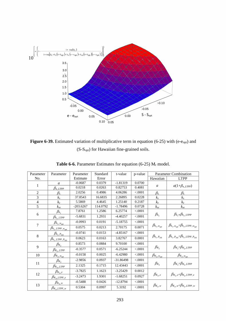
293

Figure 6-39. Estimated variation of multiplicative term in equation (6-25) with (e-eopt) and

(S-Sopt) for Hawaiian fine-grained soils.

Table 6-6. Parameter Estimates for equation (6-25) Mr model.

Parameter

No.

Parameter

Parameter

Estimate

Standard

Error

t-value

p-value

Parameter Combination

Hawaiian LTPP

1 a -0.0687 0.0379 -1.81319 0.0700

a a(1+a_LTPP) a_LTPP 0.0218 0.0263 0.82753 0.4081

2 L 2.0256 0.4986 4.06286 <.0001 L L

3 ks 37.8543 16.6835 2.26895 0.0228 ks ks

4 ke 5.5869 4.4645 1.25140 0.2187 ke ke

5 kse -203.6267 114.0792 -1.78496 0.0728 kse

kse

6 k1

7.8761 1.2586 6.25774 <.0001 k1

k1+k1_LTPP k1_LTPP -5.6831 1.2931 -4.40257 <.0001

7 k1_wopt

-0.0993 0.0191 -5.18755 <.0001 k1_wopt

k1_wopt+k1_LTPP_wopt

k1_LTPP_wopt

0.0575 0.0213 2.70175 0.0071

8 k1_PSilt

-0.0741 0.0153 -4.85167 <.0001 k1_PSilt

k1_PSilt+k1_LTPP_PSilt

k1_LTPP_PSilt

0.0623 0.0163 3.82767 0.0001

9 K2

0.8573 0.0884 9.70100 <.0001 K2

K2+K2_LTPP

K2_LTPP -0.3577 0.0571 -6.25244 <.0001

10 K2_wopt -0.0158 0.0025 -6.42980 <.0001 K2_wopt

K2_wopt

11 K3

-2.9856 0.0937 -31.86498 <.0001 K3

K3+K3_LTPP

K3_LTPP 2.1325 0.1715 12.43443 <.0001

12 K3_e -3.7825 1.1623 -3.25429 0.0012

K3_e K3_e+K3_LTPP_e K3_LTPP_e -3.2473 1.9301 -1.68251 0.0927

13 K3_w -0.5488 0.0426 -12.8794 <.0001

K3_w K3_w+K3_LTPP_w K3_LTPP_w 0.5304 0.0997 5.3192 <.0001

e - eopt S - Sopt

-0.10

-0.05

0.00

0.05 0.10

0.05

0.00

-0.05

0.5

1.0

1.5

2.5

2.0

3.0

3.5

optee

a

optSSsekopteeekoptSSskLβexp1

Lβexp11

10

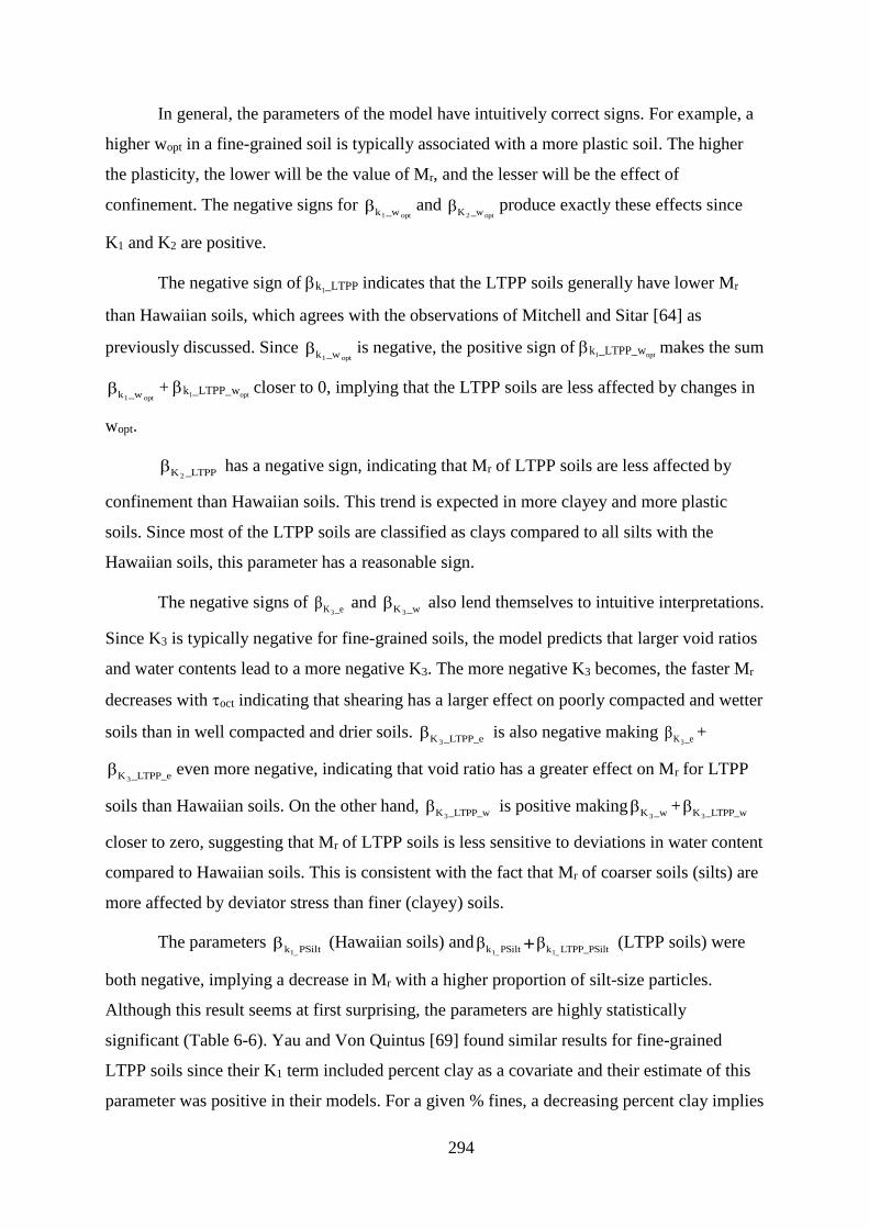
294

In general, the parameters of the model have intuitively correct signs. For example, a

higher wopt in a fine-grained soil is typically associated with a more plastic soil. The higher

the plasticity, the lower will be the value of Mr, and the lesser will be the effect of

confinement. The negative signs for opt1_wkβ and

opt2 _wKβ produce exactly these effects since

K1 and K2 are positive.

The negative sign of k1_LTPP indicates that the LTPP soils generally have lower Mr

than Hawaiian soils, which agrees with the observations of Mitchell and Sitar [64] as

previously discussed. Since opt1_wkβ is negative, the positive sign of k1_LTPP_wopt

makes the sum

opt1_wkβ + k1_LTPP_wopt closer to 0, implying that the LTPP soils are less affected by changes in

wopt.

_LTPPK2β has a negative sign, indicating that Mr of LTPP soils are less affected by

confinement than Hawaiian soils. This trend is expected in more clayey and more plastic

soils. Since most of the LTPP soils are classified as clays compared to all silts with the

Hawaiian soils, this parameter has a reasonable sign.

The negative signs of _eK3

β and _wK3

β also lend themselves to intuitive interpretations.

Since K3 is typically negative for fine-grained soils, the model predicts that larger void ratios

and water contents lead to a more negative K3. The more negative K3 becomes, the faster Mr

decreases with oct indicating that shearing has a larger effect on poorly compacted and wetter

soils than in well compacted and drier soils. _LTPP_eK3

β is also negative making _eK3

β +

_LTPP_eK3β even more negative, indicating that void ratio has a greater effect on Mr for LTPP

soils than Hawaiian soils. On the other hand, _LTPP_wK3

β is positive making_wK3

β +_LTPP_wK3

β

closer to zero, suggesting that Mr of LTPP soils is less sensitive to deviations in water content

compared to Hawaiian soils. This is consistent with the fact that Mr of coarser soils (silts) are

more affected by deviator stress than finer (clayey) soils.

The parameters PSiltk1_

β (Hawaiian soils) andLTPP_PSiltkPSiltk 1_1_

ββ (LTPP soils) were

both negative, implying a decrease in Mr with a higher proportion of silt-size particles.

Although this result seems at first surprising, the parameters are highly statistically

significant (Table 6-6). Yau and Von Quintus [69] found similar results for fine-grained

LTPP soils since their K1 term included percent clay as a covariate and their estimate of this

parameter was positive in their models. For a given % fines, a decreasing percent clay implies

295

an increasing PSilt, which explains the consistency with the Yau and Von Quintus study but

not the rationale. In reality, when PSilt increases, the soil plasticity decreases and therefore,

wopt also decreases. The net effect is typically an increase in Mr. However, the parameter for

PSilt governs the change caused by changing the percent silt maintaining all else constant

(including wopt), which as mentioned before is practically impossible. It may well be the case

that if such a change in PSilt with all else constant were possible the net effect would be a

reduction in Mr.

6.3.1.2.3.2 Potential application of the model in practice

In practice, Equation (6-25) could be easily utilized in a spreadsheet program. One

just needs to specify the values of the 13 model parameters associated with one of the two

databases and the seven soil parameters (eopt, wopt, Sopt, e, w, S and Psilt). To obtain the soil

parameters, results from three common geotechnical tests are required: (1) Proctor test (eopt =

Gsw/dmax – 1, wopt); (2) specific gravity (to obtain eopt and Sopt = Gswopt/eopt); and (3) grain

size analyses (Psilt). The design void ratio, e, is related to the relative compaction (RC) as

provided in the specifications (e = Gsw/[RC*dmax] – 1). The design water content, w, is

specified by the designer in relation to the compaction curve and climatic factors. The degree

of saturation is S = Gsw/e.

The calculations can then be performed for any state stresses as discussed in the

following example. Perhaps the most challenging aspect of the calculation is the estimation of

the state of stresses, and more importantly, which among the many state of stresses that could

be selected is the most representative. An explanation of this issue is presented after the

examples.

Example 1

As an example, consider a Hawaiian soil with wopt = 27.4%, w = 29.0%, PSilt = 45.0%,

eopt = 0.93, e = 0.93, Sopt = 0.85, S = 0.90, and Gs = 2.90. Also, recall that in US units,

pa = 14.7 psi. For a Hawaiian soil the LTPP variable is zero. Therefore, the parameters with

LTPP in their subscripts disappear from equations (6-25) through (6-28). Therefore, with the

parameters provided in Table 6-6, K1, K2, and K3 are:

821,1)0.450741.04.270993.07.8761(000,1K1

424.04.270158.08573.0K2

296

864.3)4.270.29(5488.0)93.093.0(7825.39856.2K3

The factor multiplying K1 is:

874.01010 )8523.0)(0687.0(93.00.9385.00.90203.627 -93.00.93k85.00.9037.8542.0256exp1

2.0256exp110687.0

e

With the above values in hand, it is now easy to compute the resilient modulus for any

state of stress. Consider for example a case where 3 = 2 psi and d = 8 psi, which implies

that 1 = 10 psi, = (2 + 2 + 10) psi = 14 psi, and 77.3102210223

1 222oct psi.

Then, from equation (6-25), the resilient modulus for this state of stress is:

-3.8640.424

r14.7

3.771

14.7

14.07.14874.0821,1M psi 9,500 psi

Example 2

Consider the same information as in example 1, but now estimate the resilient modulus

for a mainland soil. As before, wopt = 27.4%, w = 29.0%, PSilt = 45.0%, eopt = 0.93, e = 0.93,

Sopt = 0.85, S = 0.90, and Gs = 2.90. Now the LTPP variable is one. Therefore, with the

parameters provided in Table 6-6, K1, K2, and K3 are:

517]0.45)0623.00741.0(

4.27)0575.00993.0(5.6831)-7.8761[(000,1K1

067.04.270158.0)3577.08573.0(K2

883.0)4.270.29()5304.05488.0(

)93.093.0()2473.37825.3()1325.29856.2(K3

Notice that based on these results, a soil on the US continent is generally less stiff

(lower K1 value) and is less sensitive to changes in and oct than a Hawaiian soil of similar

characteristics. The factor multiplying K1 is now:

912.01010 )8523.0)(0469.0(93.00.9385.00.90203.627 -93.00.93k85.00.9037.8542.0256exp1

2.0256exp110218.00687.0

e

Again, for 3 = 2 psi and d = 8 psi (1 = 10 psi, = 14 psi, and oct = 3.77 psi),

equation (6-25) now yields:

297

-0.8830.067

r14.7

3.771

14.7

14.07.14912.0517M psi 5,650 psi

Comparing the result in example 2 with that in example 1, it can be seen that for the

particular soil characteristics considered, the estimated resilient modulus for the Hawaiian soil

is (9,500-5,650)/5,650 × 100 = 68% higher than the Mr for the soil with the same

characteristics in the continental US. In fact, considering all the state of stresses at which the

Hawaiian soils were tested, this difference ranges from about 50% to 210% higher!

This provides a good illustration of the dangers of using models and correlations

developed in other places without much scrutiny. When there are no other options, analysts

will often have to resort to such correlations. However, for cases like this one, where a local

model has been estimated, preference should be given to the use of the local model provided

that data to use it are available.

Although correlations between Mr and other soils characteristics (CBR, R-Value, DCP

penetration, etc.) may provide in some situations acceptable inputs, these correlations are

typically valid under specific conditions that are not always well specified (moisture content,

compaction level, exudation pressure, etc.). To date, it is not known to what extent the

commonly used correlation equations are applicable for Hawaiian conditions. It is important to

note however that two relationships between CBR and Mr and between R-Value and Mr have

been implicitly used in the HDOT procedure for years. Equation 1.1a in the current HDOT

manual [13] is nothing more than the combination of the two well know equations

Mr(psi) = 1,500 CBR and Mr(psi) = 555 R-Value + 1,155. For the reasons discussed below,

unless there is no other choice the use of such relationships is discouraged.

6.3.1.2.3.3 Practical considerations

For input level 3, the analyst still needs to estimate the resilient modulus Mr. Although

such estimate of Mr could be obtained from the website http://nchrp923b.lab.asu.edu/

developed under NCHRP project 9-23B [68]; for the same reasons discussed before, this may

result in a gross underestimation of Mr.

Table 6-7 is an example of the type of information that can be obtained from the

website. To simplify the exposition, the rows for some additional layers were deleted from the

table. Clearly, when information for more than one layer is available, some judgment will be

needed to select which one would be more representative of the likely subgrade.

http://nchrp923b.lab.asu.edu/

298

Table 6-7. Type of information that can be obtained from the NCHRP 9-23b webpage.

Map Character Map Unit Key Map Unit Name Component Name

3B7 677310 Pulehu-Mokuleia-Kawaihapai-Haleiwa (s9464) Kawaihapai

AASHTO

Classification

AASHTO

Group

Index

Top

Depth (in)

Bottom

Depth (in)

Thickness

(in) % Component

Water Table Depth

Annual Min (ft)

Depth to

Bedrock (ft)

A-6 14 0 22 22 29 N/A N/A

CBR from

Index

Properties

Resilient Modulus

from

Index Properties

(psi)

Passing

#4

(%)

Passing

#10

(%)

Passing

#40

(%)

Passing

#200

(%)

Passing

0.002

mm (%)

Liquid

Limit

(%)

6.3 8291 95 95 95 75 40 40

Plasticity

Index

(%)

Saturated

Volumetric

Water Content (%)

Saturated

Hydraulic

Conductivity

(ft/hr)

Parameter

af

(psi)

Parameter

bf

Parameter

cf

Parameter

hr

(psi)

20 48 0.10836 2.5641 0.918 0.3949 3000.05

Suppose that the information is as given in Table 6-7. Note that the table already

contains an estimate of the resilient modulus and CBR. Unfortunately, the resilient modulus

estimate is based on data from the continental US, which as seen earlier results in estimates

that are biased downward for Hawaiian fined-grained soils. Parenthetically, notice that the

estimate is provided irrespective of the actual pavement structure or traffic load. Clearly, both

the pavement structure and magnitude of the load influence the state of stresses and thus the

resilient modulus. However, incorporating the effect of the load magnitude is considered

impractical since a single representative Mr value for the whole load spectrum has to be

selected anyway in the current MEPDG implementation. As a simplification, one could

obtain an estimate of the state of stresses at the subgrade level for a standard axle load (i.e., a

single load of 9,000 lb on one side of the axle) using one of the several linear layer elastic

analysis programs available and perform the same type of analysis of the previous two

examples. A difficulty with this approach is that Table 6-7 does not contain all the

information needed to perform the analysis.

One alternative is to complement the information in Table 6-7 with additional

information from the National Cooperative Soil Survey, National Cooperative Soil

Characterization Database, available online at http://ncsslabdatamart.sc.egov.usda.gov. This

is an excellent resource but this would add to the workload.

http://ncsslabdatamart.sc.egov.usda.gov/

299

A perhaps more practical alternative is to enter the information in Table 6-7 into the

MEPDG which, based on regression models, can estimate some of the missing information

(other than entering the data into the MEPDG, no real additional work is needed). Then, an

analysis similar to that presented in the previous two examples could be carried out.

Still, given all the simplifications, it is not worth to devote this much effort into the

determination of Mr. Instead, a reasonable value is needed. At this time, for those projects on

which no other information can be obtained (either through sampling or FWD) it is

recommended as a practical alternative to use the NCHRP 9-23B website to obtain a first

estimate of the resilient modulus and increase it by 100% (i.e., multiply by 2). As shown in

example 2 above, a 100% increase is a reasonably good compromise value.

6.3.1.2.3.4 Resilient Modulus of Bases/Subbases

This section presents the results of resilient modulus tests performed on coarse-

grained materials at UH.

Testing has been performed on a limited number of samples of different materials. No

particular plan was followed to sample the materials. Instead, they were obtained as samples

of convenience. For example, samples from a full depth reclamation project were requested

when the PI had the opportunity to visit one such project in the island of Kauai. Also,

significant testing was performed on foamed asphalt base material to evaluate its potential for

local use. Although eventually the equipment used to prepare this material was shipped out of

the state, significant understanding of the material has been gained should interest to use it

arises in the future. More importantly, testing was performed simultaneously on an unbound

subbase material from the Hawaiian Cement Halawa quarry for comparison. Finally, some

testing was also performed on 3-Fine aggregates from the Makakilo quarry, which are

typically used as one of the components in HMA. Interest in the resilient modulus of 3-Fine

materials arose because this aggregate meets the widely used Wisconsin OGBC gradation

(see Table A-2 in Appendix A) and may provide an alternative for permeable base material.

Unless stated otherwise, the test were performed for 100% relative compaction (AASHTO T-

180) and optimum moisture content.

The discussion about the stress dependency of the resilient modulus for fine-grained

soils is also applicable to coarse-grained materials. In fact, since these are typically subjected

to higher state of stresses, the stress dependency has a larger effect. Thus, this issue will be

revisited later in the chapter.

300

6.3.1.2.3.5 Test results for a few base/subbase materials

As for fine-grained soils, the test results consist of a series of resilient modulus values

for different state of stresses.

Table 6-8 presents the result for the 3-Fine Aggregates from the Makakilo quarry

following the AASHTO T-307 loading sequence. These results correspond to the specimen

shown in Figure 6-37. The specimen was prepared with material with a gradation with 99.9%

passing the 3/4” (19 mm) sieve, 66.4% passing the 1/2” (12.5 mm) sieve, 27.7% passing the

3/8” (9.5 mm) sieve, and only 1.7% passing the No. 4 sieve (4.75 mm). The material is so

open graded and permeable that compaction moisture content has a negligible effect on the

resulting density for a given compaction level.45

It is well known that for some coarse grained materials, the following simplified

constitutive equation provides a good fit:

(6-29)

As shown in Figure 6-40, the 3-Fine material is a good example where this equation

provides an excellent fit with estimated parameters k1 = 1,230 and k2 = 0.495.

The simplification of equation (6-29) does not always provide the desired results.

Consider the data presented in Table 6-9 for a specimen from a coral base material used

sometimes as base. Fitting equation (6-29) to these data produces a moderate fit with

k1 = 1,998, k2 = 0.426, and an R2 of only 0.845. When the full model is used, repeated for

convenience below as equation (6-30), a much better fit is obtained with an R2 of 0.967.

32

11

k

a

oct

k

a

arp

τ

p

θpkM

(6-30)

45 Note that the table includes values for the contact stress and the cyclic stress. Their sum is the

deviator stress, which is used for computing the and oct. However, the resilient strain measured during the test

is due only to the cyclic stress. Therefore, the resilient modulus must be computed as Mr = cyclic/r.

2

1

k

a

arp

θpkM

301

Table 6-8. Test results for the 3-Fine Aggregates.

Confining

Stress

(psi)

Contact

Stress

(psi)

Cyclic

Stress

(psi)

Bulk

Stress

(psi)

Octahedral

Stress

(psi)

Resilient

Modulus

(psi)

3.0 0.4 2.7 12.1 1.4 17,143

3.0 0.7 5.4 15.1 2.9 17,748

3.0 1.0 8.1 18.1 4.3 19,679

5.0 0.6 4.5 20.1 2.4 21,203

5.0 1.1 9.0 25.1 4.8 23,543

5.0 1.6 13.5 30.1 7.1 25,289

10.0 1.3 9.0 40.2 4.8 30,196

10.0 2.3 18.0 50.2 9.5 33,706

10.0 3.3 26.9 60.1 14.2 35,154

15.0 1.4 9.0 55.3 4.9 34,358

15.0 1.9 13.5 60.3 7.2 37,237

15.0 3.4 26.9 75.3 14.3 40,942

20.0 2.0 13.5 75.4 7.3 40,148

20.0 2.5 18.0 80.4 9.7 42,925

20.0 4.5 35.9 100.4 19.1 46,790

Figure 6-40. Resilient modulus vs. bulk stress () for 3-Fine material.

Mr = 1,230.3 (/pa)0.4954

R2 = 0.996

10,000

100,000

10 100 1,000

Res

ilie

nt

Mo

du

lus (

ps

i)

Bulk Stress (psi)

302

The parameter estimates of equation (6-30) for the coral base material are k1 = 1,760,

k2 = 0.181, and k3 = 0.932. The t-statistics of the log(k1), k2, and k3 are 215, 4.13, and 6.63

respectively46, which indicate that they are all statistical significantly different from zero at a

significance level less than 1% (all p-values are almost zero). This material provides an

example in which restricting k3 to be negative would have clearly produced an inferior fit.

The comparison of observed vs. fitted values for both models in Figure 6-41 provides a

clearer picture of how much better the fit is with the 3-parameter model than with the 2-

parameter model for the coral base material.

In general, it can be seen that for similar stress levels, the coral material is stiffer than

the 3-Fine material.

The results for a specimen from a reclamation project, the Ala Kinoiki reclamation

project in Kauai, also resulted in a positive k3 and a slightly negative but statistically

insignificant k2. Specifically, the parameter estimates are: k1 = 1,187.2, k2 = -0.008, and k3 =

1.557. The R2 is 0.978. The corresponding t-statistics are 264, -0.23, and 13.3. Therefore,

parameters k1 and k3 are statistically significantly different from zero but k2 is not. Thus, re-

estimation of the model with k2 set equal to zero should produce a similar fit. The R2 of the

regression after re-estimation with k2 = 0 is 0.97847, which is essentially the same fit. From a

statistical point of view, this fit is excellent. The estimates of the parameters changed slightly

to k1 = 1187.4 and k3 = 1.535. Notice again the very high value of k3, which is somewhat

unusual and needs to be analyzed further.

Forcing k3 to be non-positive and k2 to be non-negative for the Ala Kinoidi sample

resulted in a much lower fit with an R2 of only 0.655. As mentioned before, other researchers

have estimated positive values for k3 and there does not appear to be a good justification of

why it should always be negative but the high values of k3 above were a bit concerning at

first.

46 Since logs are taken to perform the regression, the parameter estimated in the regression is not k1 but

the log(k1) from which k1 can be computed easily. This is the reason why the t-statistic correspond to log(k1).

47 A difference in R2 was noticed only in the fourth decimal.

303

Table 6-9. Test results for the Coral Base at optimum water content.

Confining

Stress

(psi)

Contact

Stress

(psi)

Cyclic

Stress

(psi)

Bulk

Stress

(psi)

Octahedral

Stress

(psi)

Resilient

Modulus

(psi)

3.0 0.4 2.7 12.1 1.4 31,541

3.0 0.7 5.4 15.1 2.9 29,963

3.0 1.0 8.1 18.1 4.3 31,937

5.0 0.6 4.5 20.1 2.4 31,805

5.0 1.1 9.0 25.1 4.8 35,661

5.0 1.6 13.5 30.1 7.1 40,618

10.0 1.3 9.0 40.2 4.8 38,812

10.0 2.3 18.0 50.2 9.6 52,444

10.0 3.3 27.0 60.2 14.3 60,430

15.0 1.4 9.0 55.4 4.9 40,691

15.0 1.9 13.5 60.4 7.3 48,401

15.0 3.4 26.9 75.3 14.3 68,135

20.0 2.0 13.5 75.5 7.3 51,967

20.0 2.5 18.0 80.5 9.7 61,172

20.0 4.7 36.0 100.6 19.2 81,279

6.3.1.2.3.1 Additional Tests of Base Materials

This subsection focuses on additional resilient modulus laboratory tests performed on

base materials by Rayapeddi Kumar [47] as part of this project and Song [61] as part of a

project on recycled materials. First, the results by Rayapeddi Kumar are explained in some

detail followed by a summary of Song’s results.

The laboratory tests performed on base course materials by Rayapeddi Kumar [47]

include: (a) Gradation analysis, (b) Modified Proctor test, and (c) Resilient Modulus test.

Material Source

A small experimental plan for base course materials included 2 different types of

aggregates namely, (a) virgin and (b) recycled. Virgin aggregates (Type B) were collected

from the Hawaiian Cement – Halawa Quarry in Aiea, Honolulu, Hawaii. A limited amount of

recycled material (foamed asphalt mixture) (~300 lbs) was delivered to the University of

Hawaii at Manoa pavement engineering laboratory by Alakona Corporation, Honolulu,

Hawaii.

304

Figure 6-41. Comparison of Observed vs. Predicted Resilient Moduli for the 3- and 2-

parameter models with the Coral Base.

The foamed asphalt (FA) base mixture used in this study was produced using 100%

RAP, stabilized using 2% of foamed (expanded) asphalt, and 1% of Portland cement as filler.

Base Course Material Information

In this section, the details of two tests performed on base course materials are

provided. First, the gradation analysis of aggregates is presented. Next, the Modified Proctor

test performed to determine the optimum moisture content and maximum dry density is

explained.

Gradation Analysis of Aggregates

The gradation analysis of RAP was performed using the AASHTO T27 procedure.

According to AASHTO T27, the aggregate sample used for sieve analysis is dried at 110 °C.

However, the RAP sample used for gradation analysis in this study was oven dried at only

60 °C for 48 hours prior to sieving. The reason for using a lower temperature to dry the RAP

material is because it contains asphalt binder, which could soften and help create lumps. The

presence of lumps could result in misrepresentation of actual gradation if the lumps are not

broken during sieving. For virgin aggregates, the gradation analysis provided by Hawaiian

20,000

30,000

40,000

50,000

60,000

70,000

80,000

90,000

20,000 40,000 60,000 80,000

Pre

dic

ted

Res

ilie

nt

Mo

du

lus (

ps

i)

Observed Resilient Modulus (psi)

3 Parameter Model

2 Parameter Model

Equality Line

305

Cement Halawa – Quarry was used. The gradation analysis results for RAP along with the

minimum and maximum requirements for 3/4” maximum nominal aggregate size allowed by

the HDOT for untreated base course materials is presented in Figure 6-42.

The gradation provided by Hawaiian Cement – Halawa (HCH) quarry along with the

minimum and maximum requirements for 1-1/2” maximum nominal aggregate size allowed

by the HDOT for untreated base course materials is presented in Figure 6-43. This figure also

includes the results of a gradation analysis performed using the AASHTO T11 procedure

(wet sieve analysis) to determine the actual percentage of virgin material passing the #200

sieve. Based on the dry sieve analysis results, both virgin material and RAP gradation fall

within the HDOT requirements for untreated base course material. However, for the virgin

material, the wet sieve analysis results indicate that the material is out of specifications.

Figure 6-42. Gradation analysis of RAP compared with HDOT requirements for ¾”

maximum nominal untreated base.

2"

1-1

/2"

1"

3/4

"

1/2

"

#4

#8

#16

#20

#40

#50

#100

#200

0

10

20

30

40

50

60

70

80

90

100

Perc

en

t P

assin

g

Sieve Designation

Reclaimed Asphalt Pavement

HDOT Minimum Specif ication

HDOT Maximum Specif ication

306

Figure 6-43. Gradation analysis of virgin aggregates from Hawaiian Cement – Halawa

Quarry compared with HDOT requirements for 1-1/2” maximum nominal untreated base.

The RAP material used in this study is also compared with the gradation requirements

recommended by Akeroyd and Hicks [70], which is widely considered by several researchers

to provide the limits of desired gradation of RAP for producing foamed asphalt mixtures.

Figure 6-44 illustrates the gradation analysis of RAP superimposed on the grading

requirements recommended by Akeroyd and Hicks. As can be seen from the figure, the

material falls within Zone A, which indicates the material is in the “ideal” grading limits for

foamed asphalt stabilization.

Maximum Dry Density and Optimum Moisture Content

The maximum dry density (γdmax) and optimum moisture content (OMC) of both

materials were determined using the standard AASHTO T180 – Method D procedure. The

OMC and maximum dry density values are presented in Figure 6-45. Table 6-10 summarizes

the test results.

2"

1-1

/2"

1"

3/4

"

1/2

"

3/8

"48

16

30

50

100

200

0

10

20

30

40

50

60

70

80

90

100P

erc

en

t P

assin

g

Sieve Designation

Hawaiian Cement - Halawa Quarry

Hawaiian Cement - Halawa Quarry (wet sieve analysis)

HDOT Minimum Specif ication

HDOT Maximum Specif ication

307

Figure 6-44. RAP Gradation and desired aggregate grading for FA

(Redrawn after Akeroyd and Hicks, 1988)

Figure 6-45. Moisture-density relationship of base course materials.

2"

1"

3/4

"

1/2

"

3/8

"

1/4

"

No.4

No.8

No.1

6

No.2

0

No.3

0

No.4

0

No.5

0

No.1

00

No.2

00

50.0

25

.0

19.0

12.5

9.5

6.3

4.7

50

2.3

60

1.1

80

0.8

50

0.6

00

0.4

25

0.3

00

0.1

50

0.0

75

0

10

20

30

40

50

60

70

80

90

100

Perc

en

t P

assin

g

Sieve Size (mm)

RAP

1,900

1,925

1,950

1,975

2,000

2,025

2,050

2,075

2,100

2,125

4.00 5.00 6.00 7.00 8.00 9.00 10.00 11.00 12.00 13.00 14.00 15.00 16.00 17.00 18.00

Dry

Den

sit

y (

kg

/m3)

Moisture Content (%)

Reclaimed Asphalt Pavement

Hawaiian Cement - Halawa Quarry

Zone C

Zone A

Zone B

Zone A: Ideal Materials

Zone B: Suitable Materials

Zone C: Unsuitable Materials

308

Table 6-10. Maximum Dry Density and Optimum Moisture Content values.

Material

Maximum Dry

Density

(kg/m3)

Maximum Dry

Density

(lb/f3)

Optimum

Moisture

Content (%)

Hawaiian Cement – Halawa 2098 131.0 11.2

Reclaimed Asphalt Pavement (RAP) 2032 126.9 8.1

Test Specimen Preparation for Resilient Modulus Testing

Resilient modulus testing included compaction and testing the materials at three

different densities; 98%, 100%, and 102% of the maximum dry density. The specimens were

tested using the repeated load triaxial resilient modulus in accordance with AASHTO T307;

except that the number of load repetitions applied during each testing sequence was reduced.

The nominal maximum size of the virgin aggregates and RAP, which is used to produce

foamed asphalt mixtures, was found to be 50 mm and 19.0 mm respectively. Based on

AASHTO T307, the dimensions of the cylindrical test specimen for testing the virgin

material and FA base was required to be compacted using a vibratory hammer in a split mold

with a target diameter of a 150 mm and a height between 305 mm and 318 mm.

Further, since there was no prior experience with the characterization of foamed

asphalt mixtures, and because of limited availability of FA, it was decided to reduce the size

of the test specimens so as to compact two replicates at three target densities. Accordingly,

each specimen using FA base was compacted using a vibratory hammer in a split mold with a

target diameter of 100 mm and a height of 203.2 mm. All the specimens compacted using FA

mixtures were cured at 40 °C for 2 days. They were compacted in accordance with the

AASHTO T307 procedure prior to testing.

Resilient Modulus Testing

The resilient modulus testing was performed using the IPC Global Universal Testing

System (UTS) consisting of a hydraulic axial stress and a pneumatic confining stress loading

system, and a computer-controlled data acquisition system (CDAS) connected to a personal

computer. The machine is capable of applying repeated cycles of a haversine-shaped load

pulse of 0.1 seconds with a 0.9 seconds rest period. The deformation produced in the sample

309

during testing is captured by two external sample Linear Variable Differential Transducers

(LVDTs) and a system LVDT that is attached to the actuator that provides the system

deformation. A test specimen placed inside the testing chamber along with sample LVDTs is

shown in Figure 6-37.

The stress state testing sequence of the AASHTO T307 procedure was used. A total

of 15 combinations (from Table 2 of AASHTO T307) of deviator and confining stresses were

applied to the compacted sample. The two stages of the resilient modulus test are:

(a) Conditioning and (b) Measuring stress and strains to calculate Mr.

Conditioning: AASHTO T307 requires between 500 and 1000 repetitions of the

conditioning deviator stress. The reason for applying the conditioning sequence is to

eliminate the effects of the initial loading versus reloading. Further, the conditioning also

helps in reducing the effects of any imperfect contact between the top platen, base plate, and

the test specimen.

Measuring stress and strains to calculate Mr: Following the conditioning cycles, the

resilient modulus testing was performed by applying 50 cycles at each combination of

confining stress and deviator stress. Repeated cycles of haversine-shaped load pulse of 0.1s

with a rest period of 0.9s were applied for both conditioning and testing. Mr was calculated as

the average of the ratios of the deviator stress to resilient strain for the last five cycles (46-

50).

The repeated load triaxial resilient modulus tests were performed to evaluate the

behavior of virgin aggregates and FA base mixtures when compacted at three different

density levels. The effect of bulk stress at each combination of the loading sequence on the

resilient modulus of virgin aggregates and FA base specimens compacted at three different

densities was observed. For brevity, the results of one specimen from each of the three

densities are presented in Figure 6-46 and Figure 6-47. The figures show resilient modulus of

three specimens plotted against the bulk stress (θ = 3σ3 + σd) on a log-log graph, where

σ3 = the confining pressure and σd = the deviator stress. As can be seen from the figure, Mr

increases with increase in density.

310

Figure 6-46. Effect of bulk stress on resilient modulus for virgin aggregates compacted at

three different densities.

Figure 6-47. Effect of bulk stress on resilient modulus of FA base mixtures compacted at

three different densities.

Figure 6-48 shows the effect that deviator stress has on the resilient modulus of

specimens compacted at 98%, 100%, and 102% of the maximum dry density using virgin

aggregates. The figure was constructed using the average values of Mr and deviator stress

from two replicate specimens. For these specimens, regardless of the level of confinement, it

1000

10000

100000

10 100 1000

Resi

lient

Mod

ulus

(ps

i)

Bulk Stress (psi)

Hawaiian Cement - Halawa Quarry @ 98% of Max. Dry Density

Hawaiian Cement - Halawa -Quarry @ 100% of Max. Dry Density

Hawaiian Cement - Halawa Quarry @ 102% of Max. Dry Density

10000

100000

10 100 1000

Resi

lient

Mod

ulus

(ps

i)

Bulk Stress (psi)

FA @ 98% of Max. Dry Density



311

is clear that a higher compaction level translates into a higher resilient modulus for the same

deviator stress level. The effect of deviator stress on Mr for each specimen of virgin

aggregates is presented individually in Appendix A of [47], where the same trends observed

in Figure 6-48 are present.


virgin aggregates.

Figure 6-49 shows the same information as Figure 6-48 except that data for two of the

confining stresses are not included. This figure is presented to illustrate why the estimation

results for this material indicate that confining stress has little effect on the modulus of virgin

aggregates. As can be observed in Figure 6-49, the points corresponding to a given density

level follow a similar trend regardless of level of confinement. This is not obvious from

Figure 6-48. As for the effect of shear, note that except at the low level of confining stress (3

psi) for specimens compacted at 102% of maximum dry density, where the modulus shows a

“slight” softening behavior, the Mr values increase with deviator stress for specimens

compacted at all densities.

5000

10000

15000

20000

25000

30000

35000

40000

45000

50000

0 5 10 15 20 25 30 35 40 45 50

Resil

ien

t M

od

ulu

s (

psi)

Deviator Stress (psi)

HCH @ 98%

HCH @ 100%

HCH @ 102%

312


virgin aggregates at low (3 psi), intermediate (5 psi), and high (20 psi) confining stress level.

Figure 6-50 shows the variation of resilient modulus with deviator stress at each

confining stress level for foamed asphalt mixture specimens compacted at 98, 100, and 102%

percent of maximum dry density. This figure is again constructed using the average values of

Mr and deviator stress from two replicate specimens. For these specimens, an increase in the

modulus is observed with increase in deviator stress at all confining stress levels for

specimens compacted at 98% of maximum dry density. For the specimens compacted at

100% of maximum dry density, a slight increase in modulus with deviator stress is observed.

Furthermore, for the specimens compacted at 102% of maximum dry density, it is observed

that the resilient modulus decreases with increase in deviator stress at all confining levels.

For the specimens compacted at 102% of maximum dry density, at low and

intermediate level of confining stress (σ3 = 3, 5, and 10 psi), the modulus values show a

“slight” softening behavior and subsequently increase marginally with increase in deviator

stress. It is also observed from the figure that at the higher confining stresses (10, 15 and 20

psi) the trend lines with deviator stress tend to cross for the 100% and 102% compaction

levels. The relative position of the crossing point also appears to depend on the confining

stress.

5000

10000

15000

20000

25000

30000

35000

40000

45000

50000

0 5 10 15 20 25 30 35 40 45 50

Resil

ien

t M

od

ulu

s (

psi)


HCH @ 98%; Confining stress = 3 psi









313

Figure 6-50. Mr vs. deviator stress for specimens compacted at different densities using FA

mixtures.

To evaluate the effects of deviator stress and octahedral shear stress on Mr of virgin

aggregates and FA based mixtures, the coefficients of the three-parameter model of equation

(6-30) was estimated using linear regression with the data from each specimen. Table 6-11

presents the statistical estimation results.

From the summary of regression coefficients presented in Table 6-11, Rayapeddi

Kumar [47] made several observations (for readability of this document, the last observation

is slightly modified in the following list):

1. The resilient modulus of virgin aggregates and FA mixtures show an increasing

trend with increase in bulk stress at increasing levels of compaction.

10000

20000

30000

40000

50000

60000

70000

80000

90000

100000

110000

120000

0 5 10 15 20 25 30 35 40 45 50

Resil

ien

t M

od

ulu

s (

psi)


FA @ 98%; Conf ining stress = 3 psi















314

Table 6-11. NCHRP 1-37A Mr model parameter estimates in Rayapeddi Kumar’s study [47].

Specimen ID k1 p-value (k1) k2 p-value (k2) k3 p-value (k3) R2

FA1 @ 98 2887.61 2.03E-27 0.39 2.04E-09 -0.09 3.42E-01 0.97

FA2 @ 98 3022.21 1.25E-26 0.39 1.31E-08 -0.18 1.14E-01 0.96

Average FA @ 98 2954.91 0.39 -0.14

FA1 @100 3312.90 3.22E-26 0.47 3.67E-09 -0.29 2.79E-02 0.97

FA2 @ 100 3362.65 8.75E-27 0.39 1.01E-08 -0.26 3.14E-02 0.96

Average FA @ 100 3337.77 0.43 -0.27

FA1 @ 102 3662.43 1.14E-24 0.44 2.20E-07 -0.57 2.94E-03 0.91

FA2 @ 102 3645.89 5.15E-26 0.43 1.96E-08 -0.43 4.08E-03 0.95

Average FA @ 102 3654.16 0.44 -0.50

HCH1 @ 98 575.57 8.46E-22 0.09 1.34E-01 1.75 9.81E-07 0.95

HCH2 @ 98 595.97 2.54E-25 0.08 2.57E-02 1.54 2.91E-09 0.98

Average HCH @ 98 585.77 0.09 1.65

HCH1 @ 100 667.78 4.90E-23 0.16 5.03E-03 1.42 1.10E-06 0.96

HCH2 @ 100 694.08 6.36E-23 0.09 1.05E-01 1.62 3.46E-07 0.96

Average HCH @ 100 680.93 0.13 1.52

HCH1 @ 102 1051.43 1.70E-24 0.07 9.67E-02 1.34 2.53E-07 0.96

HCH2 @ 102 1091.80 6.28E-25 0.06 1.34E-01 1.33 1.18E-07 0.96

Average HCH @ 102 1071.6 0.07 1.34

315

2. For virgin aggregates, a higher compaction level translates into a higher resilient

modulus for the same deviator stress. However, for FA base mixture specimens, an

increase in the modulus is observed with increase in deviator stress at all confining

stress levels for specimens compacted at 98% of maximum dry density. For the

specimens compacted at 100% of maximum dry density, a slight increase in modulus

with deviator stress is observed. Furthermore, for the specimens compacted at 102%

of maximum dry density, it is observed that the resilient modulus decreases with

increase in deviator stress at all confining levels.

3. The parameter k2 in the NCHRP 1-37A equation, which is the exponent for the bulk

stress term, is positive. This indicates increase in bulk stress increases the stiffness of

virgin aggregates and FA base mixtures.

4. The parameter k3 in the NCHRP 1-37A equation, which is the exponent for the

octahedral shear stress term, is negative for FA base mixtures, suggesting the stiffness

of FA base mixtures decreases with increase in octahedral shear stress. This behavior

is analogous to the observations made by Witczak and Uzan (1988) as explained

earlier. Further, it can be seen from the p-values of parameter k3 that the octahedral

shear stress is not statistically significant for FA base specimens compacted at 98% of

maximum dry density.

5. The sign of the parameter k3 in the NCHRP 1-37A equation is positive for specimens

compacted using virgin aggregates, which means an increase in octahedral shear

stress increases the resilient modulus of the material.

The positive sign for k3 is contrary to the widely held belief that, for unbound materials,

the coefficient k3 should be negative ( [1], [56], [57], and [58]). Nevertheless, as indicated

before, the sign of parameter k3 has been reported to be positive by several researchers including

Heydinger et al. [59] and Bennert and Maher [60]. There is really no fundamental reason why k3

should always be negative. However, the estimated values of k3 described above are higher than

those in [59] and [60], which is somewhat unique. As mentioned before, Stolle et al. [63]

reported values as high as 1.595, which is comparable to those values obtained by Rayapeddi

Kumar. Note that since Rayapeddi Kumar used a smaller number of repetitions at each stress

316

level, there may be some concern about whether that affected the results. Interestingly, the

foamed asphalt specimens, which were also tested with the smaller number of repetitions did not

exhibit the same behavior.

Fortunately, Song [61], also performed resilient modulus tests on virgin aggregates

meeting HDOT specifications for base requirements according to AASHTO T-307. In this case,

the recommended number of repetitions were used. The gradations were similar to those used by

Rayapeddi Kumar but the source of the aggregates was the Makakilo quarry. Table 6-12 shows

the parameters estimated by Song [61]48.

Table 6-12. Parameter estimation results for equation (6-30) obtained by Song [61] with virgin

untreated base material.

w

(%)

Density

(kg/m3)

Density

(lb/ft3) k1 k2 k3 R2

8.7 1,743 107.65 980 0.68 0.02 0.99

9.0 1,798 111.04 1,120 0.29 0.79 0.98

9.5 1,821 112.46 640 0.69 0.52 0.99

9.3 1,825 112.71 1,240 0.46 0.32 1.00

12.6 1,713 105.79 550 0.76 0.32 0.99

11.5 1,822 112.53 870 0.40 0.82 0.99

14.0 1,723 106.41 620 0.68 0.30 1.00

14.2 1,800 111.17 640 0.73 0.35 1.00

13.2 1,827 112.84 680 0.75 0.19 1.00

Although the values are not as high as those of Rayapeddi Kumar, they are still higher

than those reported in much of the literature. Note, however, that the trends with density for

virgin aggregates are more consistent in Rayapeddi Kumar’s result. For example, it is clear that

increasing density result in lower k3. Further research is needed to ascertain whether this is a

phenomenon attributable to these combinations of source of aggregate and gradations.

48 In Table 6-12 the parameter k1 was corrected by a factor of 1,000 since they were originally misreported.

317

Nevertheless, as indicated earlier, values almost as high as those of Rayapeddi Kumar have been

reported by other researchers [63]. In particular, these authors state49:

“The parameter k3, similar to K3, can be negative or positive, ranging from -0.432 to 1.595.” … “As

described by Eqs. (2) and (4), the resilient moduli of base/subbase aggregates are generally affected by both

the bulk and the deviatoric (or the octahedral) stresses. The resilient moduli data, however, clearly show

that the Mr values of most materials are dominated by the bulk stress , with the effect of deviatoric stress

being negligible.” … “On the other hand, for materials that are less pressure sensitive and consequently

have smaller K2 (or k2) values, the application of shear stress within the range in this study appears to cause

an increase in resilient modulus.”

In summary, the resilient modulus of some local base materials appear to increase with

deviator stress.

6.3.1.2.3.2 Developing inputs for Level 2 and Level 3 Analyses

For input level 3, the Pavement ME Design software (MEPDG) [2] requires the input of a

single value of Mr. The user has the option of allowing the program to modify the value

according to the temperature and moisture predictions or to use the value entered as an annual

representative value. For input level 2, the software adds an option of entering monthly

representative values instead of a single value. Furthermore, for level 2, the user can select

whether to input resilient modulus or another property that is correlated with Mr. In addition to

resilient modulus, the properties accepted are CBR, R-Value, AASHTO Layer coefficient ai,

DCP Penetration, and Plasticity Index (PI) and gradation. As discussed in previous sections,

using some of these options can be dangerous and it is discouraged. In particular, the use of

gradation and PI, as shown earlier, can grossly underestimate the value of Mr.

Note that the gradation and PI information is not used only when the user selects the

option to compute Mr from them. When the program is allowed to modify the Mr values

according to the temperature and moisture predictions at levels 2 and 3, it utilizes equation (6-24)

together with moisture predictions with the Enhanced Integrated Climatic Model (EICM) to

49 The parameters with uppercase K in their statement are related to another model.

318

modify the Mr values with changes in moisture50. During the local calibration efforts, it was

noted that regardless of the resilient modulus values input, the program very quickly converged

to a modulus corresponding to an “equilibrium”. The reason is that, as just mentioned, the

program uses the EICM to compute moisture and temperature changes throughout the design

life. This is one of the attractive features of the MEPDG over other design procedures.

For levels 2 and 3, the MEPDG Manual of Practice [22] recommends using the values

shown in Table 6-13 for new designs. For rehabilitation or reconstruction designs, the same

reference indicates that the resilient modulus of each unbound layer and embankment may be

back-calculated from deflection basin data. The MEPDG Manual of Practice also indicates that

the back-calculated values need to be adjusted to laboratory conditions with the correction

factors listed in Table 6-14. For reasons that will be discussed in Section 7.4 (page 369), this

practice is discouraged in this report.

With respect to new pavement sections, the values for resilient modulus at optimum

water content in Table 6-13 should be used with caution. Notice that they depend on the soil

type, location within the pavement (base/subbase or embankment), and pavement type (flexible

or rigid). The location within the pavement accounts to some extent for the state of stresses.

However, it must be recognized that the state of stresses on a given unbound material element

can vary widely depending on other factors not considered in this table such as the thickness of

the HMA layer, stiffness of the HMA layer, stiffness parameters of other layers in the pavement,

and thicknesses of other layers in the pavement. A more thorough discussion of this topic is

presented in section 7.4.

50 In locations with freezing conditions, the MEPDG further modifies the values based on computations of

the freezing zone within the pavement structure. Since for most of the State freezing is inexistent, the issue is not

discussed further here.

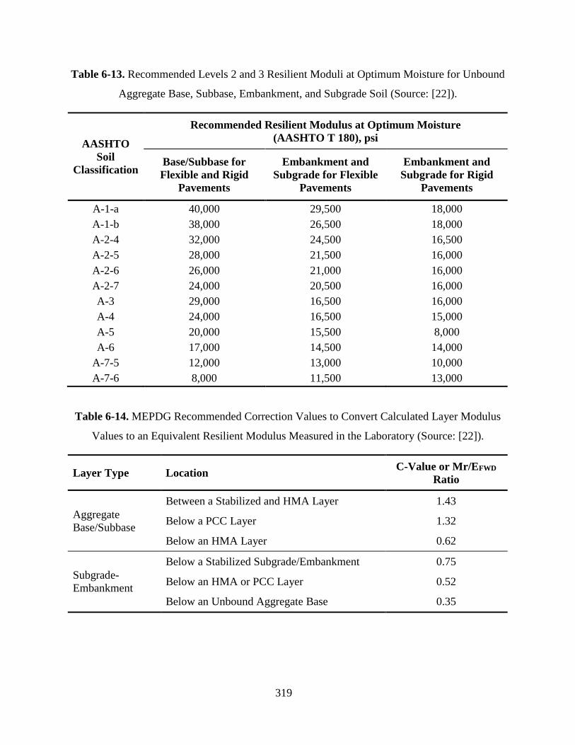
319

Table 6-13. Recommended Levels 2 and 3 Resilient Moduli at Optimum Moisture for Unbound

Aggregate Base, Subbase, Embankment, and Subgrade Soil (Source: [22]).

AASHTO

Soil

Classification

Recommended Resilient Modulus at Optimum Moisture

(AASHTO T 180), psi

Base/Subbase for

Flexible and Rigid

Pavements

Embankment and

Subgrade for Flexible

Pavements

Embankment and

Subgrade for Rigid

Pavements

A-1-a 40,000 29,500 18,000

A-1-b 38,000 26,500 18,000

A-2-4 32,000 24,500 16,500

A-2-5 28,000 21,500 16,000

A-2-6 26,000 21,000 16,000

A-2-7 24,000 20,500 16,000

A-3 29,000 16,500 16,000

A-4 24,000 16,500 15,000

A-5 20,000 15,500 8,000

A-6 17,000 14,500 14,000

A-7-5 12,000 13,000 10,000

A-7-6 8,000 11,500 13,000

Table 6-14. MEPDG Recommended Correction Values to Convert Calculated Layer Modulus

Values to an Equivalent Resilient Modulus Measured in the Laboratory (Source: [22]).

Layer Type Location C-Value or Mr/EFWD

Ratio

Aggregate

Base/Subbase

Between a Stabilized and HMA Layer 1.43

Below a PCC Layer 1.32

Below an HMA Layer 0.62

Subgrade-

Embankment

Below a Stabilized Subgrade/Embankment 0.75

Below an HMA or PCC Layer 0.52

Below an Unbound Aggregate Base 0.35

320

6.4 FATIGUE CRACKING

A limited study on fatigue cracking of local mixes was performed by Munar-Castaneda

[71]. Munar-Castaneda tested thirty (30) unmodified-mix specimens and forty two (42) Elvaloy-

modified-mix specimens at 1% concentration by mass of binder under stress-controlled

conditions. Most of the specimens had air voids close to 7%.

These results are useful as they provide an estimate of how much additional fatigue life

can be obtained from polymer modification. It is important to mention, however, that the results

are limited in terms of the number of conditions tested (only one temperature) and the

compaction conditions of the specimens. It is suspected that on some occasions the aggregates in

the mix may have been crushed during compaction, thus adding some noise to the data.

6.4.1 UH Flexural Fatigue Performance Tests

Under stress-controlled conditions, the stress is maintained constant and the resulting

strain and flexural stiffness are continuously monitored. A report was created for each test that

shows the variation of flexural stiffness and tensile strain as the load repetitions increase as well

as the initial and final values of the test variables (Figure 6-51).

Flexural stiffness followed the expected 90°-rotated S shape of typical fatigue

performance in stress-controlled tests. The rate of decrease of stiffness is initially very high, then

it reaches an approximate constant value and finally it increases again until the specimen fails.

The stiffness value decreases dramatically due to the continuous increase in tensile strain and the

accumulation of permanent strain (creep). This creep is caused by the presence of higher

stiffness in compression than in tension, and by the hysteretic heating due to the viscoelasticity

of the asphalt mix during cyclic loading [72].

In the fatigue flexural test, each specimen was tested with a sinusoidal load at one

controlled stress in the range of 1,000 kPa to 1,850 kPa, peak to peak. The frequency of the test

is 10 Hz (i.e. loading pulse width 100 msec) and the temperature of the tests was targeted at

20°C. The initial tensile strain was measured at the 50th cycle of the test, and the failure by

fatigue was defined to occur when the stiffness of the beam presented a reduction of 80% of the

initial value measured at the 50th load repetition. The samples included in the analysis have an air

void content close to 7% and an asphalt content of 5.3%.

321

Figure 6-51. Example of fatigue test report given by UTS015 software used to perform the test.

From all the beams tested, seventeen (17) unmodified and thirty (30) Elvaloy-modified

were included in the analysis after removing specimens due to problems during the testing, not

compliance with air void content in the allowable range (6% - 8%), or fatigue life greater than

1,000,000 cycles (to avoid large errors associated with high fatigue performances). The complete

database with the fatigue tests results is presented reference [71]. Table 6-15 shows for each type

of mix and stress level the number of samples and the mean of air voids, fatigue life, initial

stiffness of the mix, and initial strain. 51

51 The information in Table 6-15 needs to be interpreted with caution. For some stress levels, the

unmodified mix appears to perform better than the modified mix. However, the fatigue equations are based on strain

322

Table 6-15. Number of samples at each stress level in [71] and the corresponding

laboratory mean Air Voids, Fatigue Life, Stiffness and Strain.

Type of

mixture

Stress

Level

(kPa)

Number

of

Samples

Mean Air

Voids (%)

Average Number of

Cycles Termination @

20% stiffness

Average Initial

Stiffness @ 50th

cycle (MPa)

Average Initial

strain (m€ )

peak to peak

Unmodified 1000 1 7.16 909,130 3659 273

Unmodified 1200 3 7.04 314,837 4798 251

Unmodified 1350 3 6.63 299,630 5594 242

Unmodified 1500 4 6.57 102,998 5318 287

Unmodified 1700 3 6.27 39,803 4679 372

Unmodified 1850 3 6.54 34,317 5179 363

Number of samples 17

Modified 1% 1100 1 6.63 849,070 4222 260

Modified 1% 1200 6 7.04 368,733 4359 278

Modified 1% 1350 6 7.43 139,190 4296 324

Modified 1% 1500 7 6.97 61,917 4125 368

Modified 1% 1700 6 7.23 41,952 4363 394

Modified 1% 1850 4 6.91 34,988 4355 433

Number of samples 30

In general, in Munar-Castaneda’s study [71], the values of flexural stiffness for the

unmodified mix specimens are about 17% higher on average than the stiffness for the Elvaloy-

modified samples. This can be explained by the reduction in stiffness effect that polymer

modification has in asphalt mixtures. A more flexible mix under cyclic loading delays the

appearance of tension cracking, leading to higher fatigue performance.

6.4.2 Complete MEPDG Fatigue Relationship

As discussed in section 5.4.2.1, fatigue cracking is modeled in the MEPDG with a three-

parameter model that predicts the allowable number of load repetitions for a given strain level on

a mix with a given flexural stiffness (see equation (5-1) on page 201). Equation (5-1) is nothing

but a modification of a similar equation developed from beam fatigue laboratory tests similar to

the ones discussed in the previous section. The laboratory model takes the form:

not stress. As discussed below, the modified mixes provide a longer fatigue life for a given strain level. Note also

that in Table 6-15 the first stress level for the unmodified mix is higher than for the unmodified mix.

323

32

1

kk

tf SkN

(6-31)

where:

Nf = number of repetitions to failure (fatigue life),

S = flexural stiffness, /t, ( = extreme fiber stress and t = extreme fiber tensile strain),

k1, k2 and k3 = experimentally determined regression parameters.

It is important to clarify the meaning of flexural stiffness since the literature is not always

very precise about it and stiffness has a different meaning in strength of materials. As defined

above, S is nothing more than a normal modulus of elasticity. However, often, a correction is

introduced to consider the shear deformation on the extreme one thirds of the beam. The

correction depends on the beam specimen and ranges from 1.04 to 1.16 for the specimens sizes

that have been traditionally used [34]. For the tests perform at UH, the factor is about 1.07. The

second important consideration is that the flexural stiffness measured in a beam fatigue test is

substantially smaller than the dynamic modulus obtained in the AMPT for a given frequency and

temperature combination. For the tests performed at UH, the ratio of S/|E*| is about 0.7. Several

differences between these tests such as specimen geometry, sinusoidal loading vs. pulse loading

with rest periods, shape of the load pulse, etc. help to explain this discrepancy. The most

significant, however, is the fact that in the dynamic modulus test the sample is subjected to

compression whereas in the beam fatigue test it is subjected to tension and compression. Thus,

the modulus derived from the beam fatigue test is really a combined modulus for these two

conditions. Since both the asphalt binder and the aggregate contribute to the modulus in

compression but for the most part only the asphalt binder contributes in tension, it follows that

the stiffness in the beam fatigue test appears to be always smaller than |E*|.

The above observations notwithstanding, whether S or |E*| has been used in a particular

model is of not much practical consequence since use of one or the other translate only in a

different value of k1 when S = constant × |E*|. Estimation of the parameters k1, k2, k3 with linear

regression leaves the parameters k2 and k3 unaltered. Furthermore, k1 is multiplied, among other

things, by a calibration factor to account for the differences between laboratory and field

conditions. Thus, use of S or |E*| would only affect that calibration factor.

324

The complete expression used by the MEPDG to compute the allowable number of

repetitions for a given tensile strain is [22]:

3322

1|*|1

ffff k

HMA

k

tfHfHMAf ECCkN

(6-32)

where:

Nf-HMA = Allowable number of axle-load applications for a flexible pavement and

HMA overlays,

t = Tensile strain at critical locations and calculated by the structural

response model, in/in,

|E*HMA| = Dynamic modulus of the HMA measured in compression, psi,

kf1, kf2, kf3 = Global field calibration parameters (from NCHRP 1-40D recalibration;

kf1 = 0.007566, kf2 = -3.9492, and kf3 = -1.281), and

f1, f2, f3 = Local or mixture specific field calibration constants; for the global

calibration effort, these constants were set to 1.0.

MC 10 (6-33)

69.084.4

bea

be

VV

VM (6-34)

where:

Vbe = Effective asphalt content by volume, %,

Va = Percent air voids in the HMA mixture, and

CH = Thickness correction term, dependent on type of cracking.

For bottom-up or alligator cracking:

325

)49.302.11(

1

003602.0000398.0

1

HMAH

H

e

C

(6-35)

For top-down or longitudinal cracking:

)8186.2676.15(

1

00.1201.0

1

HMAH

H

e

C

(6-36)

where:

HHMA = Total HMA thickness, in.

6.4.3 UH Fatigue Data Analysis

Figure 6-52 shows the relationship between initial tensile strain and number of repetitions

to failure for the unmodified mixes. Figure 6-53 shows the same relationship for the PMA mixes.

Both figures are plotted using logarithmic scales for both axes. As expected, both log-log plots

show an approximate linear trend between the two variables. Thus, even without consideration of

the mix stiffness, the strain level gives a good indication of the fatigue life. The linear

relationships in the figures are expressed mathematically as:

Unmodified Mix:

tf LogNLog 1010 610.4445.16 (6-37)

610.4161079.2

tfN (6-38)

Elvaloy-modified Mix:

326

tf LogNLog 1010 872.4286.17 (6-39)

872.4171093.1

tfN (6-40)

The exponent of strain is similar in both cases, though the modified mix is a bit more

sensitive to the strain level. Both values agree quite well with reported values in the literature.

Figure 6-52. Fatigue Test Results (Unmodified Binder) - Relationship between Repetitions and

Initial Strain grouped by Test Stress Levels.

R² = 0.717

100

1000

10,000 100,000 1,000,000

Init

ial

Ten

sile S

train

( t

) (1

e-4

€)

Number of Repetitions to Failure at 20% of initial Stiffness (N)

1000 kPa

1200 kPa

1350 kPa

1500 kPa

1700 kPa

1850 kPa

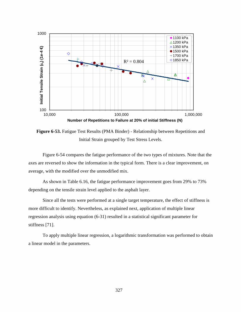
327

Figure 6-53. Fatigue Test Results (PMA Binder) - Relationship between Repetitions and

Initial Strain grouped by Test Stress Levels.

Figure 6-54 compares the fatigue performance of the two types of mixtures. Note that the

axes are reversed to show the information in the typical form. There is a clear improvement, on

average, with the modified over the unmodified mix.

As shown in Table 6.16, the fatigue performance improvement goes from 29% to 73%

depending on the tensile strain level applied to the asphalt layer.

Since all the tests were performed at a single target temperature, the effect of stiffness is

more difficult to identify. Nevertheless, as explained next, application of multiple linear

regression analysis using equation (6-31) resulted in a statistical significant parameter for

stiffness [71].

To apply multiple linear regression, a logarithmic transformation was performed to obtain

a linear model in the parameters.

R² = 0.804

100

1000

10,000 100,000 1,000,000

Init

ial

Ten

sile S

train

(

t) (

1e

-4 €

)

Number of Repetitions to Failure at 20% of initial Stiffness (N)

1100 kPa

1200 kPa

1350 kPa

1500 kPa

1700 kPa

1850 kPa

328

Figure 6-54. Fatigue performance comparison of unmodified and PMA modified mixes.

R² = 0.7173

R² = 0.8043

10,000

100,000

1,000,000

100 1000

Nu

mb

er o

f R

epet

itio

ns

to F

ail

ure

(N

f)

Initial Tensile Strain (t) (microstrain)

Unmodified Mix

PMA Mix

Nf = 2.79 ×1016 (t)-4.610

Nf = 1.93 × 1017 (t)-4.872

329

Table 6.16. Fatigue performance improvement of PMA mixture compared to the unmodified

mixture at different tensile strain levels.

Strain Level

(1 ×10-6)

Estimated average fatigue

life (Nf) unmodified

Estimated average

fatigue life (Nf) PMA Difference

Improvement

(%)

200 688,424 1,188,336 499,912 73

250 246,094 400676 154,582 63

300 106,188 164,825 58,637 55

350 52,174 77,778 25,605 49

400 28191 40,581 12,390 44

450 16,379 22,862 6,482 40

500 10,077 13,683 3,605 36

550 6,494 8,600 2,106 32

600 4,348 5,629 1,280 29

SkkkN tf 10310211010 loglogloglog (6-41)

Applying regression analysis to equation (6-41) with log10(Nf) as the dependent variable

and log10(t) and log10(S) as the independent variables produces estimates of log(k1), k2, and k3.

All the parameter estimates are statistically significant as indicated by the low p-values. The

fatigue performance model for the PMA mixes has a R2 value of 0.842, whereas for the

unmodified mixes the coefficient of determination reaches the 0.957 value.

From the results of the regression analysis, linear relationships for the two types of mixes

can be created. Transformation of the linear associations using the antilogarithm function can be

made in order to define every model in terms of the original variables.

Table 6-17 and Table 6-18 present the results of the regressions performed on the data set

for unmodified and the PMA mixes, respectively.

From the results of the regression analysis, linear relationships for the two types of mixes

can be created. Transformation of the linear associations using the antilogarithm function can be

made in order to define every model in terms of the original variables.

330

Unmodified Mix:

SLogLogNLog tf 101010 197.4157.6788.35 (6-42)

197.4157.6351014.6

SN tf (6-43)

PMA Mix:

SLogLogNLog tf 101010 128.2726.5175.27 (6-44)

128.2726.5211050.1

SN tf (6-45)

The testing results from the unmodified mixture revealed that fatigue life occurrence

between 10,000 and 1,000,000 load repetitions corresponds to a range of initial tensile strain

between 220 to 420 microstrain (1x10-6 in./in.), whereas the range for the polymer-modified

asphalt mix ranges from 240 to 550 microstrain. Therefore, there is a noticeable difference

regarding fatigue behavior between these two mixes.

The empirical relationship between the number of load repetitions (Nf) and initial tensile

strain (t) gives acceptable results for both mixtures analyzed. The fitted models have reasonably

high coefficients of determination (i.e. R2) and are statistically significant.

As expected, a reduction in flexural stiffness generates higher fatigue performances for

both mixtures.

Equations (6-43) and (6-45) can be visualized in a three-dimensional graph as shown in

Figure 6-55 for both asphalt mixtures. The planes illustrated in the graph present different slopes

in the strain and stiffness directions.

331

Table 6-17. Multiple Linear Regression results. Nf vs. t and S model - Unmodified mix.

Table 6-18. Multiple Linear Regression results. Nf vs. t and S model – PMA modified mix.

REGRESSION ANALYSIS

R Square 0.957

Adjusted R Square 0.951

Standard Error 0.106

Observations 17

ANOVA

df SS MS FSignificance

F

Regression 2 3.528 1.764 157.559 2.52E-10

Residual 14 0.157 0.011

Total 16 3.685

REGRESSION ANALYSIS

Variable CoefficientsStandard

Errort Stat P-value

Intercept 35.788 2.298 15.572 3.10E-10

Log (t) -6.157 0.347 -17.752 5.38E-11

Log (S) -4.197 0.472 -8.891 3.92E-07

REGRESSION ANALYSIS

R Square 0.842

Adjusted R Square 0.830

Standard Error 0.197

Observations 30

ANOVA

df SS MS FSignificance

F

Regression 2 5.576 2.788 71.780 1.56E-11

Residual 27 1.049 0.039

Total 29 6.625

REGRESSION ANALYSIS

Variable CoefficientsStandard

Errort Stat P-value

Intercept 27.175 4.056 6.700 3.42E-07

Log (t) -5.726 0.536 -10.679 3.40E-11

Log (S) -2.128 0.843 -2.525 1.77E-02

332

Figure 6-55. Three-dimensional representation of fatigue performance models.

In summary, the modified asphalt mixture presented on average better fatigue

performance than the unmodified mix.

PMA Mixes

Unmodified mixes

333

6.5 PERMANENT DEFORMATION

As discussed in section 5.4.2.2, in the MEPDG the vertical compressive strains computed

by the pavement response model at mid-depth of each sublayer of the pavement structure are

used to predict rutting over time. Specifically, for each Hot Mix Asphalt (HMA) sublayer, the

field calibrated form of the permanent deformation model, equation (5-7) (shown in page 219), is

used to predict the sublayer contribution to rutting for each period. Equation (5-7) was originally

derived from the permanent deformation test in the form of equation (5-6) described in section

5.4.2.2.

In addition, the MEPDG estimates the contribution of unbound layers to rutting in a

similar fashion, as described also in section 5.4.2.2. However, it has been reported that the

MEPDG tends to overestimate rutting originating in these layers. An example for Kansas is

provided in [31]. Given the thick HMA layers used in HDOT designs for new sections, rutting

originating in unbound layers appears to be minimal. Most of the rutting in new pavement

sections on state roads in Hawaii appear to be originating in the HMA. As explained chapter 7 in

relation to the calibration of the MEPDG; for this study, rutting originating in unbound layers has

been limited to a small value. Therefore, the rest of this section concentrates on the rutting

originating in HMA layers.

6.5.1 Characterization of Permanent Deformation

A substantial amount of work has been done to characterize local Superpave 12.5 mm

mixes (with gradations also meeting State Mix IV requirements) for permanent deformation.

Much of that work has been documented in another research report [46] and journal papers

( [50], [52], and [73]). Therefore, the discussion here is limited.

In the MEPDG, the prediction of permanent deformation uses results from both the

dynamic modulus test (|E*|) and repeated axial load permanent deformation tests. However, their

use is asymmetric in the sense that project specific |E*| values can be considered (measured or as

a function of other mix properties), whereas the permanent deformation parameters enter only

through the permanent deformation model, which is calibrated to local conditions at best. It is

assumed that the effects of mixture properties such as air void content, effective binder content,

and binder grade are already adequately incorporated into the permanent deformation simulation

334

through |E*| values. Mixture properties are accounted for only by the elastic response (i.e., r).

As a result, it is possible that only a portion (instead of the full extent) of the variability induced

from some mixture properties is being taken into account.

Limitations arising from the use of |E*| alone for rutting characterization have been

reported in the literature. A summary of the literature that is critical in this respect is presented in

reference [52], on which it is also concluded that predicting rutting performance by means of

elastic response alone (universal values for permanent deformation model parameters, regardless

of mixture properties) does not fully take into account mixture-specific contributions to rutting.

Thus, Archilla and Diaz [52] describe the development of models that make the parameters k1

and k3 of equation (5-6) functions of mix characteristics. The data for the same specimens used

for the development of the |E*| model presented in section 6.2.4.2 were used for the development

of this model. Therefore, the description of the gradations and binders presented in that section

are still applicable. The functions for k1 and k3 can be useful for the calibration of the permanent

deformation model as these are the parameters that more often need modification.

6.5.1.1 Parameter k3

The function for k3 is:

)log()log()log()log(

)log(

987

70226702257047036416213

beffVolabeffVola

BAXXBXXAB

PVPV

DDDDDk

(6-46)

where

DB6416 = 1 if Gradation B and binder is PG 64-16 and 0 otherwise,

DA70XX = 1 if Gradation A and binder is PG 70-XX and 0 otherwise,

DB70XX = 1 if Gradation B and binder is PG 70-XX and 0 otherwise,

DA7022 = 1 if Gradation A and binder is PG 70-22 and 0 otherwise,

DB7022 = 1 if Gradation B and binder is PG 70-22 and 0 otherwise,

Va = air void content (%), and

PbeffVol = effective binder content by volume (%).

335

In addition to considering the effects of air void content, effective binder content, and

their interaction, Equation (6-46) allows for different intercepts for the different binders and

gradations for log(k3) (1 for Gradation A with PG 64-16, 1 2 for Gradation B and PG 64-16,

1 3 for Gradation A and PG 70-XX, 1 4 for Gradation B and PG 70-XX, 1 5 for

Gradation A and PG 70-22, and 1 6 for Gradation B and PG 70-22).

Table 6-19. Parameter Estimates for log(k3).

Parameter

Name Variable ID Value

Standard


No of

observations

associated

with the

parameter

1 Intercept -2.223 0.692 -3.21 0.002 63

2 DB6416 0.018 0.017 1.04 0.302 16

3 DA70XX -0.118 0.019 -6.08 0.000 10

4 DB70XX -0.106 0.018 -5.91 0.000 14

5 DA7022 -0.111 0.025 -4.37 0.000 5

6 DB7022 -0.033 0.027 -1.22 0.228 4

7 log10(Va) 2.369 0.793 2.99 0.004 63

8 log10(PbeffVol) 2.355 0.670 3.52 0.001 63

9 log10(Va) log10(PbeffVol) -1.907 0.773 -2.47 0.017 63

Residual standard error: 0.04625 on 54 degrees of freedom.

Multiple R-Squared: 0.8362

F-statistic: 34.45 on 8 and 54 degrees of freedom, the p-value is zero. Sample size = 63

Except for parameters 2 and 6, the parameter estimates are statistically significant at a

95% confidence level. The very low p-values for 7, 8, and 9 statistically confirm the

significance of the effects of air voids, effective binder content, and their interaction on k3.

336

The fact that the estimate of 2 is not statistically significantly different from zero simply

indicates that there is no discernible difference between mixes with unmodified binder prepared

with either gradation.

A somewhat surprising result is that the estimate of parameter 6 is not statistically

significant, which would indicate that there is no difference between a mix prepared with

gradation A and the PG64-16 binder (or given that 2 was not statistically significantly different

from zero, a mix with gradation B and PG64-16 binder) and another mix prepared with gradation

B and the PG70-22 binder. It is believed that this is just an anomaly in one or more of the only

four data points available for the combination of gradation B and the PG70-22 binder. (It is

recognized that by following the same logic (i.e. low number of data points), the conclusion

drawn for the combination of gradation A and PG70-22 binder could be challenged; however, it

is important to note that these results indicate that the performance of the mixture with the

modified binder is better than the one observed in the unmodified mixture, which is logical

according to extensive literature reports, and consistent with the results obtained with the

mixtures prepared with PG70-XX binder, which have more experimental observations).

The estimates for the other three parameters (3, 4, and 5) are all statistically

significantly different from zero, which indicates that all these mixes performed better than the

unmodified mixes. The three parameter estimates are similar, thus indicating that these mixes

accumulate permanent deformation at comparable rates. The R2 is 0.836, which indicates an

acceptable fit.

The finding that the parameter k3 is a function of mix characteristics is quite important.

Currently, the MEPDG assumes that the elastic response alone (r), which is a function of |E*|,

can take completely into account all the effects that individual mixture characteristics have on

the permanent deformation response and thus, it assumes that k3 is a constant. The above results

indicate that this may not be the case.

337

6.5.1.2 Parameter k1

The procedure to estimate parameter k1 proposed in [50] is a little more involved. It

requires first the estimation of the permanent deformation (p100) after 100 load repetitions52. The

model developed for p100 for the loading conditions in [50] is:

log(p100) = 1 + 2 DB6416+ 3 DA70XX + 4 DB70XX + 5 DA7022 + 6 DB7022

+ 7 log(Va) + 8 log(PbeffVol) + 9 log(Va) log(PbeffVol) (6-47)

where,

DB6416 = 1 if gradation B and binder is PG64-16 and zero otherwise,

DA70XX = 1 if gradation A and binder is PG70-XX and zero otherwise,

DB70XX = 1 if gradation B and binder is PG70-XX and zero otherwise,

DA7022 = 1 if gradation A and binder is PG70-22 and zero otherwise,

DB7022 = 1 if gradation B and binder is PG70-22 and zero otherwise,

Va = air voids (%), and

PbeffVol = effective binder content by volume (%).

The parameters of the model described in Equation (6-47), including the results from the

regression analysis, are summarized in Table 6-20.

52 Loading consisted of an axial deviator stress of 828 kPa (120 psi), a contact stress of 41.4 kPa (5.1 psi),

and a confining stress of 138 kPa (20 psi).

338

Table 6-20. Parameter Estimates for log(p100).

Parameter

Name Variable ID Value

Standard


No of

observations

associated with

the parameter

1 Intercept -5.169 1.690 -3.06 0.004 63

2 DB6416 -0.050 0.041 -1.21 0.232 16

3 DA70XX -0.364 0.048 -7.66 0.000 10

4 DB70XX -0.353 0.044 -8.09 0.000 14

5 DA7022 -0.133 0.062 -2.14 0.037 5

6 DB7022 -0.117 0.065 -1.80 0.078 4

7 Log10(Va) 10.001 1.937 5.16 0.000 63

8 Log10(PbeffVol) 28.394 1.635 5.14 0.000 63

9 log10(Va) log10(PbeffVol) -8.604 1.887 -4.56 0.000 63

Residual standard error: 0.1129 on 54 degrees of freedom.

Multiple R-Squared: 0.8872

F-statistic: 53.11 on 8 and 54 degrees of freedom, the p-value is zero. Sample size = 63

Interpretation of the results is analogous to the interpretation of the results for k3. Again,

the parameters for DB6416 and DB7022, 2 and 6, are not statistically significant at a 95%

confidence level. The fact that the estimate of 2 is not statistically significantly different from

zero simply indicates that there is no discernible difference between mixes with unmodified

binder prepared with either gradation. As for 6, the same potential anomaly described earlier for

6 may effect this parameter estimate.

The essentially zero p-values for 7, 8, and 9 statistically confirm the significance of

the effects of air voids, effective binder content, and their interaction on p100.

The estimates for the other three parameters (3, 4, and 5) are all statistically

significantly different from zero and negative, which indicates that all these mixes performed

339

better than the unmodified mixes (i.e., they show smaller permanent deformations after 100

cycles). 3 and 4 have similar magnitudes, indicating that the mixes with PG70-XX performed

similarly regardless of whether gradation A or gradation B was used. On the other hand, the

absolute value of 5 is smaller than either 3 or 4, which indicates that the mixes prepared with

PG70-22 binder and gradation A performed slightly worse than those with PG70-XX but still

better than those PG64-16. The R2 of almost 0.89 indicates again an acceptable fit for p100.

With p100, the value of k1 can be estimated by

Tkkkr

plog100loglog 2103

100

101

(6-48)

where

p100 = cumulative permanent deformation after 100 loading repetitions,

r = resilient strain for the state of stresses, loading frequency and temperature

conditions during the test (10Hz and 54°C = 129.2°F),

k3 = parameter k3 as estimated by equation (6-47);

k2 = parameter for temperature (see below),

T = test temperature expressed in °F (129.2°F).

Due to the limitation of having only one temperature level (i.e. 54ºC=129.2°F), the

parameter k2 was assigned a value of 1.734, which is the laboratory based value used to calibrate

the MEPDG rutting prediction model [1]. This assumption only affects the laboratory estimates

of k1 but it has little effect on the main conclusions. A more detailed description of the rationale

for the above equations is presented in [50]. Reference [74] shows that adjusting the permanent

deformation model parameters of the polymer modified mixes relative to the unmodified mixes

produce more reasonable results. Otherwise, the MEPDG could even predict a lower

performance with the modified mixes, which is not logical.

340

6.5.2 Additional Laboratory Tests

Rayapeddi Kumar [47] performed additional repeated load permanent deformation tests.

These tests were performed on the same samples used to measure |E*| described in section

6.2.4.2.4. His most relevant conclusions were:

1. The Flow Number (FN)53

values of mixes prepared using polymer modified mixes at low and

medium air voids are higher compared to the FN values for other types of laboratory prepared

mixes at the same approximate air voids. For higher air voids (~7%), the FN for PMA mixes

are higher than the FN for the mixes prepared using unmodified binder.

2. The FN values for all specimens prepared using fibers are relatively constant at all air voids.

3. The average slope (k3) for polymer modified asphalt concrete mixtures is the lowest

compared to virgin and fiber reinforced concrete mixtures at low air voids (~3%). At

intermediate and higher air voids, the fiber reinforced asphalt concrete mixtures had the

lowest k3 value.

4. The average k3 values for fiber reinforced asphalt concrete mixes show a relatively lower

strain rate compared to mixtures prepared using virgin binder at corresponding target air

voids.

5. The plant produced and laboratory produced mixes using unmodified binder do not show a

particular trend with respect to the rate of accumulation of permanent strain.

53 The flow number is the number of load repetitions needed for the permanent deformation curve to reach

the inflexion point or flow point (see Figure 5-23, page 216). It is used as an indicator of mix resistance to

permanent deformation. The higher the number the more resistant the mix.

341

6.6 BINDER CHARACTERIZATION

Limited binder characterization of PG64-16 binder was performed in terms of its

rotational (Brookfiled) viscosity and dynamic shear modulus (|G*|) [46]. In addition, a few

repeated creep and recovery tests were also performed. These tests were performed before

Asphalt Hawaii started supplying most of the binder used in the state. Therefore, they may not be

entirely representative of current conditions. Nevertheless, as discussed before, relatively minor

changes in dynamic moduli and permanent deformation were observed with the Asphalt Hawaii

binder. Moreover, simulations with the MEPDG with level 1 or pseudo-level 1 data as generated

with the local |E*| models described in section 6.2.4.2 do not produce appreciably different

results with variations in binder characteristics when compared with the effects of other variables

analyzed. This is not surprising, since when using level 1 dynamic modulus inputs, the binder

characteristics are used only in a global aging model to determine the effect of aging of the

binder in |E*|. Except for the effect of aging, the master curve is defined mostly by the input |E*|

values. With respect to permanent deformation, as discussed in section [50], it is believed that

different calibration factors should be developed for significantly different binders (modified vs.

unmodified.)

Figure 6-56 shows the viscosity characteristics of Rolling Thin Film Oven (RTFO) aged

samples of the PG64-16 and the PG70-XX binders54. The viscosities were obtained with a

rotational viscometer (Brookfield viscometer) over a wide range of temperatures and also

estimated from dynamic shear modulus (|G*|) and phase angle ( measurements at 10 rad/s

obtained with a Dynamic Shear Rheometer (Bohlin CVO-100) using the following conversion

equation from the MEPDG [1]:

54 The PG70-XX binder is the PG64-16 binder modified with 1% of Elvaloy RET®. As discussed in

previous sections, polymer modification appears to have a similar effect on the performance of mixes with the

binder supplied by Asphalt Hawaii.

342

8628.4

sin

1

10

*

G (6-49)

where

|G*| = binder shear modulus, Pa

= binder phase angle, º

= viscosity, cP

Figure 6-56. Viscosity () vs. temperature relationships for local binders (before Asphalt Hawaii

started to supply binder).

Two samples of each binder were tested with the DSR. One test was performed with

8 mm plates and the other three with 25 mm plates. For the PG64-16 binder the estimated

viscosity trends with both instruments are very similar when both sets of DSR measurements are

included as shown in the figure. The estimated A and VTS parameters (the intercept and slope

respectively of the log log vs. log TR equation, where is the viscosity in cP and TR is the

temperature in Rankine as used in the MEPDG) differ somewhat when each individual DSR

series for the PG64-16 binder is considered separately. Nevertheless the trends with both

instruments for the PG64-16 still show relatively good agreement.

20 40 60

1.0E+02

1.0E+03

1.0E+04

1.0E+05

1.0E+06

1.0E+07

1.0E+08

1.0E+11

0

1.0E+10

1.0E+12

80 100 120 140 160 180 200

1.0E+09

log log = -3.5823 log TR + 10.725

log log = -3.7641log TR + 11.307

log (TR) (numbers in axis represent the temperature in ºC)

log

lo

g (

nu

mb

ers

in

axis

rep

rese

nt

vis

co

sit

y i

n c

P)

PG64-16 - Brookfield

PG64-16 - DSR 8mm - MEPDG conv.

PG64-16 - DSR 25mm MEPDG conv.

PG70-XX - Brookfield

PG70-XX - DSR 25mm - S1 - MEPDG conv.

PG70-XX - DSR 25mm - S1 - MEPDG conv.

PG70-XX - DSR 25mm - S1 - Modified conv.

PG70-XX - DSR 25mm - S2 - Modified conv.

log log = -2.9922 log TR + 9.1296

log log = -3.5696 log TR + 10.6940

log log = -3.1687 log TR + 9.6337

343

On the other hand, the trend of the viscosities estimated for the modified binder with |G*|

and using equation (6-49) (labeled “MEPDG conv.” in the figure) differs significantly from the

trend obtained with the rotational viscometer. Despite the differences that result in the A and

VTS parameters from both instruments, simulations with the MEPDG with level 1 data for the

modified binder did not produce appreciably different results when these variations in A and

VTS where considered when compared with the effects of other variables analyzed.

The binder performance was also evaluated with the repeated shear creep and recovery

tests. The tests were performed with 100 cycles each composed of a loading period of 1 second

with a shear stress of 300 kPa followed by a rest period of 9 seconds at different temperatures.

Figure 6-57 shows the results for the 50th cycle at two relevant temperatures. The improvements

in rutting resistance and elastic recovery of the modified binder over the unmodified binder are

notable. As described in previous sections, these binder improvements translate in performance

improvements of the mix.

Figure 6-57. Repeated shear creep and recovery test results at 46 and 52°C (50th cycle of

local binders (before Asphalt Hawaii started to supply binder).

Although the binder properties are important, for modeling with the MEPDG with pseudo

level 1 data (i.e., using the locally developed model as proposed here) they do not play a

substantial role. Furthermore, as discussed in chapter 7, other factors such as the resilient

0.00

0.02

0.04

0.06

0.08

0.10

0.12

0 1 2 3 4 5 6 7 8 9 10

Time (s)

To

tal S

hear

Str

ain

PG64-16 @ 52C

PG64-16 @ 46C

PG70-XX @ 52C

PG70-XX @ 46C

344

modulus of unbound materials can have a more substantive effect on the predictions. Therefore,

for MEPDG use, it is recommended to use input values based on the results of this section. Using

default binder characteristics is also considered acceptable.

6.7 DESIGN CONSIDERATIONS FOR COMBATING MOISTURE

One of the tasks for this project included evaluation of the use of the permeable base

requirement in HDOT’s existing pavement design guideline and to consider alternative solutions.

This issue was studied near the beginning of the project and was reported an interim report. This

section provides an overview of the findings and recommendations.

Water can enter into the pavement as surface water through cracks, joints, asphalt

concrete infiltration, and groundwater from infiltrated aquifers, such as a high water table or a

localized spring. The saturation of, or the presence of, water in the pavement structural section

decreases the supporting strength, or load-carrying capacity, of succeeding untreated layers

underlying the asphalt concrete. This results in increased deflection under traffic loads, thereby

leading to structural cracking and pumping action which accelerates the fatigue failure of asphalt

concrete.

Both sources of water must be considered and provisions must be made to handle both.

The structural section drainage system, which is designed to handle surface water inflow, is

generally separate from the subsurface drainage system that is designed to accommodate

encroaching groundwater.

The discussions herein are intended only for surface water inflow and not encroaching

groundwater. The estimated groundwater inflow should be determined separately by a

combination of field investigations, analytical techniques and graphical methods.

Because of the problems associated with high moisture levels within the pavement

structure, the pavement designer must try to keep the base, subbase, subgrade, and other

susceptible paving materials from becoming saturated or being exposed to high moisture levels

over long periods of time. As indicated in [1], four approaches commonly employed to control or

reduce moisture problems are:

345

Prevent moisture from entering the pavement system.

o Pavement geometry – surface drainage: Adequate cross-slopes and longitudinal

slopes.

o Joint and crack sealing.

Use materials that are less sensitive to the effects of moisture.

o Treated bases.

Incorporate design features to minimize moisture damage.

o Dowel bars at transverse joints of sufficient size and spacing.

o Widened slabs 2 ft to reduce deflections, faulting, and cracking.

o Tied concrete shoulders to keep the lane/shoulder joint tight and reduce the

potential for pumping by reducing the edge deflections.

o Provision of a granular layer between the subgrade and stabilized base course to

reduce erosion beneath the base course and to allow bottom seepage.

o Provision of adequate side ditches with flow lines beneath the pavement structure.

o Full-width paving to eliminate the lane/shoulder cold joint.

Quickly remove moisture that enters the pavement system.

Typically, a combination of approaches are needed to combat the detrimental effects of

moisture on the pavement structure. Salient aspects of each of these approaches are discussed

in [1]. Here, the design of the drainage system to quickly remove the moisture entering the

pavement system is discussed starting with the consideration of whether such a system is

warranted in the first place.

Appendix A of this manual presents a literature review about the use of permeable bases

in pavement structures, including materials and thicknesses. As shown in that appendix, there is

no general consensus about the cost-effectiveness of the use permeable layers. As expressed in

[75] “In recent years, many state highway agencies have become less enthused about subsurface

pavement drainage because of concerns about construction difficulties, the need to conduct

frequent maintenance of edgedrains and their outlets, and scant evidence of performance benefits

that justify the costs of drainage system installation and maintenance.”

The same authors also conclude “While subsurface drainage systems may still be needed

to achieve good performance for some pavements built in some places, it appears to be far less

true than it was twenty or more years ago that subsurface drainage systems are needed to achieve

good performance for most pavements in most places” [76].

346

This view also appears to be reflected in the MEPDG manual of practice which indicates

“The current state of the art is such that conclusive remarks regarding the effectiveness of

pavement subsurface drainage or the need for subsurface drainage are not possible” [22].

Nevertheless, the MEPDG recommends that water not be allowed to accumulate within the

pavement structure for reasons similar to those expressed at the beginning of this section.

Given this inconclusive evidence, it would be extremely risky to eliminate the use of

subdrainage altogether. Therefore, it is recommended to adopt many of the MEPDG

recommendations which are less demanding (in terms of when a permeable base is needed) than

the 2002 HDOT Pavement design guidelines [13] but that still require the use of a permeable

base in most heavily trafficked roads and in some roads with moderate traffic loadings. The

following subsections summarize the MEPDG recommendations tailored for Hawaiian

conditions.

6.7.1 Subdrainage Components

Rapid drainage of a pavement structural section can be achieved by placing a highly

permeable drainage layer system under the full width of the pavement surface during initial

construction. The basic components of the drainage system include [77]:

a permeable base layer,

a geotextile separator,

a collector system (edgedrain structures and outlet pipes) to transport the intercepted

water within the pavement structure to an outside drainage ditch, or water sewer

system, and

vents and cleanouts

The essential components of an edgedrain structure include [77]:

a trench filled with open graded aggregate wrapped with a geotextile filter;

a longitudinal conduit consisting of a perforated pipe.

The rest of this section concentrates on the permeable base layer component only. It

should be understood that if subsurface drainage is provided, the other components have to be

present as well to provide an effective drainage system.

347

6.7.2 Permeable Base

As indicated in [1], the primary function of the permeable base layer is to dissipate water

infiltrating the pavement surface by moving it laterally towards the edge of the pavement within

an acceptable time frame. Acceptability is measured with the time-to-drain parameter, which is

the time to drain 50 percent of the drainable (free) water starting with a fully saturated material

(i.e., the time it takes to go from S = 1 to S = 0.50, where S is the saturation of the material as

defined in geotechnical engineering, in decimal). Based on this parameter, AASHTO rates the

permeable base quality of drainage from “Excellent” to “Poor as shown in Table 6-21.

For Interstate highways and freeways, draining 50 percent of the drainable water in

approximately 2 hours is desired [78]. For other roads, “good” drainage (i.e., time-to-drain < 24

hours) is acceptable. Using the computer software DRIP developed by Applied Research

Associates for FHWA and available with the research version of the MEPDG software, it was

determined that a material with a permeability of about 5,000 ft/day would exhibit excellent

drainage for all roads with three lanes or less in one direction (a slightly higher permeability is

required for a higher number of lanes in one direction all draining to the same side of the road).

Figure 3-2 shows how the time-to-drain typically changes with permeability. The figure also

illustrates that a permeability of 1,000 ft/day provides good drainage (< 24 hours) for the

conditions cited in the figure.

Table 6-21. Quality of drainage based on the time to drain parameter.

Quality of Drainage Water Removed Within

Excellent 2 hours

Good 1 day

Fair 1 week

Poor 1 month

Very Poor Does not drain

348

Figure 6-58. Time-to-drain versus permeable base permeability (pavement width = 36 ft,

shoulder with = 10 ft, longitudinal slope = 1%, cross slope = 2 %.)

6.7.2.1 Permeable Layer Need

The 2002 HDOT pavement design manual [13] essentially requires a permeable layer for

all pavements with the exception of locations with rainfall less than 5 inches or where the

basement soil is free draining (a permeability greater than or equal to 100 ft/day). Other

exceptions must be justified in the structural section submittal.

On the other hand, the MEPDG provides different recommendations about the need of

subdrainage for four different climatic zones of the country. Much of Hawaii falls within the

Wet-No freeze climatic conditions defined in the MEPDG (Annual precipitation > 508 mm (20

in) and annual freezing index < 83 °C-days (150 °F-days)). For these conditions, the MEPDG

provides the recommendations in Table 6-22. These are less restrictive than the current HDOT

requirements and leave more room to the designer to determine when a permeable layer is

needed.

With respect to the need for a permeable layer, it is recommended to adopt the MEPDG

guidelines in reference [1]. Specifically, the use of a permeable base would be required only for

higher traffic loadings (greater than 12 million 20-year design lane heavy trucks) and subgrade

permeability lower than 100 ft/day (30 m/day). For intermediate traffic loadings (between 2.5

and 12 million 20-year design lane heavy trucks), the MEPDG recommendations would require

the use of a permeable layer for subgrades with permeability of 10 ft/day (3 m/day) or less. With

349

less than 2.5 million 20-year design lane heavy trucks, subsurface drainage would not be

required for subgrades with coefficients of permeability of 10 ft/day (3 ft/day) and above. These

recommendations relax the requirements of the current pavement design guide but still require a

drainage layer for the conditions when it can be most cost-effective. The MEPDG also indicates

that additional factors must be considered in the decision for installing permeable bases over

subgrades with higher permeability.

Table 6-22. MEPDG subdrainage recommendations for Wet-No freeze zone [1].

ksubgrade

< 10 ft/day

(< 3 m/s)

ksubgrade

10 to 100 ft/day

(3 to 30m/s)

ksubgrade

> 100 ft/day

(> 30m/s)

Greater than 12 million 20-years design lane

heavy vehicles R R F

Between 2.5 and 12 million 20-years design

lane heavy vehicles R F F

Less than 2.5 million 20-years design lane

heavy vehicles F NR NR

ksubgrade = subgrade permeability.

R= some form of subdrainage or other design features are recommended to combat potential moisture problems.

F= Providing subdrainage is feasible. The following additional factors need to be considered in the decision making:

Past pavement performance and experience in similar conditions if any.

Cost differential and anticipated increase in service life through the use of various drainage alternatives

Anticipated durability and/or erodability of paving materials

NR = subsurface drainage is not required in these conditions.

Heavy vehicles include FHWA classes 4 through 13.

When lava rock formations are present, permeable bases shall be used to properly drain

pavement structures regardless of the above recommendations. Lava bedrock depends on

fractures within the rock formation to drain water through the material. Fine material can fill the

cracks to prevent water from penetrating freely through the rock formation. This has been

observed in actual construction activities.

350

6.7.2.2 Permeability of the Permeable Base Material

The 2002 HDOT pavement design manual [13] states that permeability of untreated

permeable base materials should be above 10,000 ft/day [13]. This is in contrast with the

requirements in other design manuals, most notable the new Mechanistic-Empirical pavement

design guide [1], which requires a minimum of 1,000 ft/day for treated or untreated permeable

base layers. Obviously, the MEPDG recommendation is a minimum and a higher permeability is

desirable. However, higher permeability is usually associated with low stability, which may also

be detrimental for the pavement structure. Therefore, there are tradeoffs that need to be carefully

evaluated involving the use of a drainage layer, materials used to construct it if needed, and the

thickness of the layer.

The permeability of the various drainage layers should consider the long term alterations

the material will undergo. It is conceivable that in the permeable base, fine material will cake

around the aggregate which will eventually reduce the permeability. Also, degradation of the

layer as it undergoes repeated traffic loading is possible. These and other long term effects

should be considered in determining the design permeability. In this respect, it must be noted that

based on an analysis in Figure 6-58, the permeability must drop below 500 ft/day for the quality

of drainage to fall into the fair category. Thus, proper selection of a geotextile separator should

be carried out to minimize these potential problems.

In this report, it is recommended that a permeable base be defined as an open-graded

drainage layer with a minimum laboratory permeability value of 5,000 ft/day for interstate

highways and primary arterials and 1,000 ft/day for all other roads. Notice that these values

differ from the 10,000 ft/day required in the current 2002 HDOT guidelines [13]. However, as

mentioned before, these lower permeability values are adequate from a drainage standpoint with

the advantage that a more stable layer could be obtained in most situations.

6.7.2.3 Minimum Permeable Base Layer Thickness

Another issue with permeable bases is related to their thickness. The Hawaii Pavement

design guide provides a methodology to calculate the thickness of permeable base needed to

drain the water infiltrating the pavement from the surface but it currently requires a minimum of

6” of permeable base over a geotextile permeable separator on a 6” layer granular material to

protect the permeable layer from infiltration of fines from the subgrade. In contrast, the design

351

guides of several states (e.g., CA, FL, and MO) do not use a variable thickness of the drainage

layer but rather a fixed value governed by local experience and constructability issues. Layer

thickness has the least effect on the “time-to-drain” parameter in a permeable base, which

determines in part its effectiveness, while permeability has the greatest effect, as the time to

drain decreases exponentially with an increase in permeability. Based on this, the MEPDG

recommends 4 inches as an appropriate permeable base layer thickness (maximum and

minimum), allowing compaction without segregation while providing an acceptable hydraulic

conduit. This justification makes good engineering sense and it is practical. As indicated in the

MEPDG, the main assumptions for the hydraulic design of permeable bases are [1]:

“Water infiltrates the pavement until the permeable base is saturated.

Excess runoff will not enter the pavement section after it is saturated.

After the rainfall event ceases, water is drained to the side ditches or storm drains

through edgedrains or by daylighting.”

A thickness of 4 inches for the permeable base is adequate to satisfy those assumptions.

However, selection of an appropriate minimum thickness should also depend on the material

used for constructing the permeable layer. Untreated permeable bases (UPB) with gradations in

accordance with Section 306 of the Hawaii Standard Specifications for Roads and Bridge

Construction should be constructed with a thickness of 6 inches to accommodate the large

aggregate sizes. For other materials with maximum aggregate sizes of 1 inch, a thickness of 4

inches is recommended.

The previous practice of fixing the subbase to a thickness of 6 inches and designing a

drainage layer to absorb as much water as it can infiltrate the pavement surface is discourage

since the additional permeable material may lead to stability problems and not much benefit is

obtained in terms of time-to-drain.

6.7.2.4 Permeable Base Material

The permeable layer could be asphalt-treated, cement-treated, or untreated, depending on

structural requirements.

The 2005 Hawaii Standard Specifications for Road and Bridge Construction [79] require

a gradation for the coarse fraction of untreated permeable bases to have 100% passing the 2-in

352

sieve and between 75 and 100% passing the 1.5-inch sieve. For untreated permeable bases, the

use of a filler material with 100% passing the ½-inch sieve is also required [79]. Based on this

and the information in Appendix A, it is seen that Hawaii uses one of the coarser gradations

since the filler changes the gradation only in the upper part of the permeable layer, which may

explain some of the construction difficulties with permeable layers in Hawaii and may lead to

low stability values as well. In fact, Appendix SS in the MEPDG [1] states “To guarantee

reasonable stability, a minimum coefficient of uniformity value, Cu, of 3.5 is required for an

untreated permeable base. If this cannot be achieved, the base should be treated with either

asphalt or Portland cement.” It should be noted that although HDOT’s gradation requirements for

the coarse fraction of the permeable base material could potentially produce a Cu > 3.5, it does

not guarantee it and it is quite possible to have lower values and consequently associated low

stabilities.

As discussed in Appendix A, other states allow other gradations that provide both

adequate permeability and stability. It is worth mentioning that aggregates such as 3-Fine

commonly used in Hawaii as one of the HMA aggregates may fell within the gradation limits for

the Wisconsin OGBC No. 155, one of the commonly accepted gradations for permeable bases.

Therefore, it was decided to test samples of 3-Fine material from the Makakilo quarry for

permeability. This same material was used in 2006 at the Honolulu Airport to pave with

Densiphalt. It is permeable enough that allows the penetration of a cement slurry into the

aggregate and this may also indicate its possible use in treated permeable bases. Figure 6-59

shows how the material can be laid down with a paver.)

55 OGBC = Open Graded Base Course

353

Figure 6-59. Laying of asphalt treated 3-Fine material for Densiphalt at the Honolulu Airport.

A 6” diameter Sand and Gravel Permeameter (Figure 6-60) was used to obtain the

permeability of 3-Fine material to assess its potential use in the construction of untreated

permeable layers. This device meets the requirements listed in ASTM D 2434-68.

The permeability values observed during laboratory tests of the 3-Fine material ranged

between 36,000 and 140,000 ft/day, well above the minimum values recommended by the

HDOT current design guide. This indicates that the material tested is extremely permeable. The

capacity of the material to allow water to pass through was so high that in most instances

laboratory measurements were difficult (as illustrated by the wide range of values measured)

since the loss of energy (i.e. head loss) between the two manometers along the permeameter was

very small. Thus small errors in the readings translated into large errors in permeability values. It

is clear though that the permeability of the material was higher than required.

As discussed in Section 6.3.1.2.3.5, the resilient modulus of the 3-Fine material is not

much lower than that of other base materials. The main point of this discussion, however, is not

so much about the adequacy of the 3-Fine material for use in permeable base construction but

instead in the need to allow the use of alternative materials if the proper engineering tests are

performed (permeability, resilient modulus, and crushed faces). That is, if a material provides

adequate permeability and its modulus can be evaluated with confidence (the modulus is used

directly in M-E design) then there should be no reason from a mechanistic point of view to

354

restrict its use. Smaller maximum aggregate sizes may allow better compaction of the permeable

base and thus reduce problems during construction.

Thus, alternative gradations composed of 100 percent crushed stone should be acceptable

if testing results show that they have adequate stability and permeability of at least 5,000 ft/day

for interstate and primary arterials or at least 1,000 ft/day for other highways. Table 6-23 shows

gradations that provide a careful trade-off of constructability/stability and permeability. The New

Jersey gradation provides satisfactory permeability for many roads (greater than 1,000 ft/day)

and good stability during construction [80]. The coefficient of permeability of the AASHTO No.

67 gradation is at least 5,000 ft/day. It should be noted that what is locally known as 3-Fine

aggregate usually meets the gradations requirement of the AASHTO No. 67 gradation and results

in much higher permeability values as described in the previous page. The New Jersey gradation

may provide a viable alternative for those cases labeled F in Table 6-22.

The thickness of the untreated permeable base layer constructed with these alternative

suggested gradations should be 4 inches. As discussed before, this ensures an adequate hydraulic

channel for the free flow of water and places an upper limit on the thickness of this potentially

unstable layer [1].

Figure 6-60. Layout of the Sand and Gravel Permeameter with the 3-Fine material inside.

As for the separator layer between the permeable base and the subgrade, the minimum

thickness recommended in the MEPDG is also 4” instead of 6” and a geotextile is not always

required if the separator layer meets the filter criteria with subgrade material and the permeable

base. The research team’s view is that if a permeable base layer is deemed necessary, the

355

geotextile is an insurance against its potential premature failure that protects the additional

investment. Thus, it is recommended to continue using geotextiles to avoid contamination of the

permeable base with fines.

Table 6-23. Alternative untreated permeable base gradations.

Sieve Size Percent Passing By Weight

New Jersey Gradation AASHTO No. 67

1.5” 100

1” 95 – 100 100

0.75” 90 – 100

0.5” 60 – 80

0.375” 20 – 55

No. 4 40 – 55 0 – 10

No. 8 5 – 25 0 – 5

No. 16 0 – 8

No. 50 0 – 5

6.8 COEFFICIENT OF THERMAL EXPANSION OF LOCAL PCC MIXES

The coefficient of thermal expansion (CTE) of Portland Cement Concrete (PCC) mixes

plays a fundamental role in the mechanistic-empirical design of PCC pavements. As indicated

before, no data was available for calibration of the MEPDG for PCC pavements. Nevertheless,

much of the information analyzed for flexible pavements such as the traffic loading

characterization and the subgrade and unbound material properties are useful for their analyses.

Thus, it was considered important to determine some additional parameters that will facilitate the

implementation of the MEPDG for PCC pavements in the future. Since strength characteristics

of PCC (from which stiffness can be estimated) are relatively well understood, efforts were

directed at estimating the CTE because of its important effect on PCC faulting, which appears to

be the distress that has triggered rehabilitations of PCC pavements in the recent past. Appendix B

provides the details of this effort. Only a brief description of the study is presented here.

The primary objective of the study was to determine CTE values of PCC mixes used in

Hawaiian pavements. A secondary objective was to study the effect of curing time on the CTE.

356

To achieve these objectives, 45 concrete specimens were prepared onsite at three Hawaiian

concrete companies using local basaltic aggregates. For each site, 15 replicate test specimens

(five sets of three) were cured in a 100% humidity room for 3, 7, 14, 28, and 56 days before

determining their CTEs following AASHTO T-336. It was found that CTE values vary

significantly with curing time. It was also observed that the CTEs at 28 days computed in this

study, ranging from 6.1×10-6/℉ to 6.6×10-6/℉ (11.0×10-6/°C to 11.9×10-6/°C ), differ

significantly from the value recommended in the MEPDG Manual of Practice for concrete

specimens with basaltic rock as a constituent (5.2×10-6/˚F or 9.4×10-6/˚C), which can lead to

designs with overestimated performance. The variation caused by curing time is similar in

magnitude to the variation caused by the use of different mixes for a giving curing time. Thus,

the study results support the need to establish a standard curing time when determining an

appropriate CTE for design. Furthermore, use of a non-representative default value can have a

higher effect than that produced by differences between mixes or curing times, which highlights

the importance of performing research to establish local CTE values. Based on the results, it is

recommended to use the CTE obtained after 28 days of curing for design.

357

MEPDG CALIBRATION FOR NEW HMA

PAVEMENT SECTIONS

7.1 INTRODUCTION

This chapter describes the efforts to calibrate the MEPDG for flexible pavements. It

attempts to integrate and use much of the information described and analyzed in previous

chapters, i.e.: traffic loading, material characterization, and pavement condition. Calibration of

the MEPDG for PCC pavements was not attempted because of the lack of appropriate historical

distress information. Furthermore, even for flexible pavements calibration had to be limited to

new pavement sections because of the limitations in the available distress information.

The chapter is organized is follows. Section 7.2 briefly describes the pavement sections

used for the calibration effort. Section 7.3 describes the factors that limits the calibration in more

detail. Even with the significant amount of information available, several issues had to be

addressed for calibration of the MEPDG including usability of the distress information and

unbound material moduli. Section 7.4 provides what in the view of the writer is a very interesting

and challenging issue for use of mechanistic-empirical procedures, which is the selection of

adequate unbound material moduli when non-linear effects are significant. Section 7.5 discusses

the results of the calibration effort and describes a procedure to reduce the number of simulations

required for calibration. Then, section 7.6 analyzes the issue of top down fatigue cracking and

presents a hypothesis that may explain the widespread appearance of longitudinal fatigue

cracking on Hawaii’s roads. The chapter closes with a summary and other observations for use of

the MEPDG.

358

7.2 PAVEMENT SECTIONS USED FOR CALIBRATION

The pavement structure processing tool described in chapter 2 was used with information

updated by personnel from the Material Testing and Research Branch to estimate the pavement

structural information for a set of routes in the State. These data, which were provided in 2012 in

an excel spreadsheet, were used to identify candidate sections for calibration.

A set of sections that could be considered new sections or reconstructions were identified.

This, by itself, was challenging since at present most construction work involves pavement

rehabilitations. Consequently, only 29 sections were identified on that part of the network for

which pavement structural information had been developed. Table 7-1 provides a summary of

basic information for the sections in the calibration set. Annual Average Daily Truck Traffic

(AADTT) was estimated from the Annual Average Daily Traffic (AADT) and percentage of

trucks on HDOT’s Road Information System (RIS) for the construction year by extrapolating

backwards the historical AADT information available in the RIS. The lane distribution

percentages are assumed values based on the number of lanes on the section and the analysis of

section 3.7. These values differ slightly from the values recommended in section 3.7 as they are

intended to represent average conditions whereas the ones suggested there are intended to be

used in designs with the old design procedure.

Table 7-2 provides the vehicle class distribution for each section. These distributions

were obtained from data for 2011 provided by the Planning Branch. The implicit assumption

with the use of these values is that the distributions have not changed much over the years.

Table 7-3 provides the structural information. In this table, Mix III, IV, and V are

standard State mixes type III, IV, and V respectively, GCB is Glassphalt Concrete Base, ACB is

Asphalt Concrete Base, ATB is Asphalt Treated Base, AB is Aggregate Base, ASB is Aggregate

Subbase and UPB is Untreated Permeable Base. For one of the pavement sections (section 26),

the subgrade material varies after a depth of 22 in. Thus, the pavement structure was modeled

with a layer of 22 in with the characteristics of that subgrade material (labeled as SB1) on top of

another subgrade material. The information for section 18 (Route 50, MP 21.71-21.81) was not

used for calibration as it appear to show abnormal deterioration with a pattern that resembles

more reflection cracking from an old PCC pavement instead of the patterns typically observed on

conventional flexible pavements.

359

Table 7-1. Basic information for pavement sections in the calibration set.

Section Route Begin

MP

End

MP

Construction

Year

No. of

Lanes

(One-way)

AADTT Lane

distribution

Operational

speed Island

1 H-1 19.37 19.65 2003 3 17,551 50 20 Oahu

2 H-2 0.21 0.39 1997 2 2,004 70 50 Oahu

3 H-3 0.06 0.26 1995 2 665 70 50 Oahu

4 11 0.75 1.00 1997 3 1,299 50 45 Hawaii

5 11 6.45 6.65 1985 2 1,006 70 45 Hawaii

6 19 1.32 1.42 1988 2 1,666 70 35 Hawaii

7 19 9.80 9.90 2004 1 301 100 45 Hawaii

8 19 31.76 31.91 2002 1 585 100 55 Hawaii

9 19 32.07 32.22 2002 1 585 100 55 Hawaii

10 19 96.89 97.17 2000 1 1,240 100 55 Hawaii

11 31 0.00 0.35 2006 2 858 70 45 Maui

12 32 0.40 0.51 2000 1 390 100 25 Maui

13 311 0.00 0.50 2002 2 665 70 35 Maui

14 380 1.50 2.00 2000 2 780 70 35 Maui

15 50 0.00 0.13 1998 2 489 70 35 Kauai

16 50 15.08 15.69 2006 1 188 100 35 Kauai

17 50 18.93 19.10 2000 1 144 100 35 Kauai

18 50 21.71 21.81 2001 1 148 100 35 Kauai

19 50 25.19 25.35 1993 1 216 100 35 Kauai

20 56 8.23 8.49 2007 1 302 100 25 Kauai

21 72 14.90 15.40 1993 3 1,158 50 35 Oahu

22 83 1.86 2.11 1991 1 425 100 30 Oahu

23 83 16.09 14.19 1998 1 470 100 30 Oahu

24 83 16.22 16.30 1998 1 470 100 30 Oahu

25 83 40.24 40.44 1994 2 1,162 70 35 Oahu

26 93 9.00 9.20 1996 2 1,039 70 35 Oahu

27 95 0.60 1.00 1988 2 505 70 35 Oahu

28 95 0.60- 1.00- 1988 2 505 70 35 Oahu

29 99 16.30 16.60 1995 2 1,140 70 35 Oahu

360

Table 7-2. Vehicle class percentages for pavement sections in the calibration set.

Section Route Begin

MP

End

MP

Growth

(%)

Vehicle Class Percentage (by volume of trucks)

4 5 6 7 8 9 10 11 12 13

1 H-1 19.37 19.65 0.34 3.99 83.52 4.3 0.41 1.44 5.83 0.41 0.00 0.00 0.10

2 H-2 0.21 0.39 3.89 2.96 65.63 9.81 0.00 0.56 9.85 0.00 6.98 0.00 4.21

3 H-3 0.06 0.26 5.00 4.96 62.28 11.64 1.72 3.88 14.66 0.43 0.00 0.21 0.21

4 11 0.75 1.00 0.62 5.56 75.36 6.28 1.93 2.42 8.21 0.24 0.00 0.00 0.00

5 11 6.45 6.65 2.16 4.88 73.95 9.53 0.47 4.19 6.28 0.47 0.23 0.00 0.00

6 19 1.32 1.42 0.00 4.17 59.55 7.06 0.64 3.69 24.57 0.32 0.00 0.00 0.00

7 19 9.80 9.90 0.19 19.08 26.32 13.82 1.31 5.59 29.28 1.31 0.66 0.33 2.30

8 19 31.76 31.91 2.25 4.17 59.55 7.06 0.64 3.69 24.57 0.32 0.00 0.00 0.00

9 19 32.07 32.22 2.25 4.17 59.55 7.06 0.64 3.69 24.57 0.32 0.00 0.00 0.00

10 19 96.89 97.17 4.28 4.26 79.66 4.82 0.10 2.62 8.13 0.39 0.00 0.01 0.01

11 31 0.00 0.35 3.19 11.41 66.67 9.61 0.60 5.71 4.20 1.20 0.00 0.00 0.60

12 32 0.40 0.51 -1.86 12.37 75.26 6.19 0.00 2.58 2.58 0.51 0.00 0.00 0.51

13 311 0.00 0.50 -0.3 7.17 32.67 26.69 0.80 10.36 15.14 2.39 3.19 0.00 1.59

14 380 1.50 2.00 3.11 5.26 31.93 27.02 10.88 4.03 10.18 6.49 0.00 0.00 4.21

15 50 0.00 0.13 0.51 1.55 18.04 20.1 4.12 30.93 10.31 5.67 6.19 1.03 2.06

16 50 15.08 15.69 1.04 10.07 23.02 24.46 1.44 7.19 28.06 2.88 0.72 0.00 2.16

17 50 18.93 19.10 2.44 10.07 23.02 24.46 1.44 7.19 28.06 2.88 0.72 0.00 2.16

18 50 21.71 21.81 2.44 10.07 23.02 24.46 1.44 7.19 28.06 2.88 0.72 0.00 2.16

19 50 25.19 25.35 1.31 10.45 34.57 19.33 2.28 6.51 22.10 2.19 1.41 0.00 1.16

20 56 8.23 8.49 1.50 21.34 13.39 33.47 3.77 17.15 2.09 2.51 4.50 0.84 0.84

21 72 14.90 15.40 1.24 14.62 50.94 12.74 0.94 11.32 6.14 0.94 0.00 0.00 2.36

22 83 1.86 2.11 2.65 22.89 48.95 8.42 0.26 6.32 12.10 0.80 0.00 0.00 0.26

23 83 16.09 14.19 1.32 24.78 58.26 4.24 0.22 3.57 7.81 0.45 0.00 0.00 0.67

24 83 16.22 16.30 1.32 24.78 58.26 4.24 0.22 3.57 7.81 0.45 0.00 0.00 0.67

25 83 40.24 40.44 2.05 13.58 39.43 32.38 1.57 5.22 5.74 1.04 0.00 0.00 1.04

26 93 9.00 9.20 0.90 15.84 40.17 13.49 0.29 17.60 9.68 1.17 0.00 0.00 1.76

27 95 0.60 1.00 1.25 8.15 28.83 22.73 0.74 4.38 30.88 3.96 0.00 0.00 0.33

28 95 0.60- 1.00- 1.25 8.15 28.83 22.73 0.74 4.38 30.88 3.96 0.00 0.00 0.33

29 99 16.30 16.60 0.49 26.67 31.11 17.46 2.22 9.53 6.98 1.59 0.00 0.00 4.44

361

Table 7-3. Pavement structural information for sections in the calibration set.

Section Route Begin

MP

End

MP

Layer Type – Thickness (in)

1 2 3 4

1 H-1 19.37 19.65 Mix IV – 2.5 GCB – 14.0 AB – 4.0 ASB – 12.0

2 H-2 0.21 0.39 Mix IV – 3.5 ACB – 2.5 ATB – 4.75 ASB – 14.0

3 H-3 0.06 0.26 Mix IV – 2.5 Mix III – 3.0 ATB – 6.5 ASB – 18.5

4 11 0.75 1.00 Mix IV – 1.5 ACB – 6.5 UPB – 6.0

5 11 6.45 6.65 Mix V – 3.0 ACB – 5.0 ASB – 6.0

6 19 1.32 1.42 Mix V – 6.0 AB – 8.0

7 19 9.80 9.90 Mix IV – 4.0 ACB – 8.0 UPB – 6.0 ASB – 6.0

8 19 31.76 31.91 Mix IV – 3.5 ACB – 7.0 UPB – 6.0 ASB – 6.0

9 19 32.07 32.22 Mix IV – 3.5 ACB – 7.0 UPB – 6.0 ASB – 6.0

10 19 96.89 97.17 Mix IV – 3.5 ACB – 7.0 UPB – 6.0 ASB – 6.0

11 31 0.00 0.35 Mix IV – 3.5 ACB – 8.0 UPB – 6.0 ASB – 6.0

12 32 0.40 0.51 Mix IV – 3.0 ACB – 9.0 Broken Stone – 2.0

13 311 0.00 0.50 Mix IV – 3.5 ACB – 8.0 UPB – 6.0 ASB – 6.0

14 380 1.50 2.00 Mix IV – 3.5 ACB – 8.0 UPB – 6.0 ASB – 6.0

15 50 0.00 0.13 Mix IV – 5.5 ACB – 8.0 UPB – 6.0 ASB – 6.0

16 50 15.08 15.69 Mix IV – 2.0 ACB – 12.0 ASB – 6.0

17 50 18.93 19.10 Mix IV – 2.0 ACB – 12.0 ASB – 6.0

18 50 21.71 21.81 Mix IV – 2.25 ACB – 7.75 ASB – 1.25

19 50 25.19 25.35 Mix V – 1.5 ACB – 4.0 ASB – 6.0

20 56 8.23 8.49 Mix IV – 1.5 ACB – 6.5 AB – 1.5

21 72 14.90 15.40 Mix IV – 1.5 Mix III – 2.5 ATB – 6.5 ASB – 18.5

22 83 1.86 2.11 Mix V – 3.5 ACB – 6.0 ASB – 18.5

23 83 16.09 14.19 Mix IV – 4.0 GCB – 6.0 AB – 6.0 ASB – 20.0

24 83 16.22 16.30 Mix IV – 4.0 GCB – 6.0 AB – 6.0 ASB – 20.0

25 83 40.24 40.44 Mix IV – 4.0 ACB – 9.0 UPB – 10.0 ASB – 6.0

26 93 9.00 9.20 Mix IV – 4.0 ACB – 9.0 SB1 – 22.0

27 95 0.60 1.00 Mix V – 2.5 ACB – 5.0 ASB – 6.0

28 95 0.60- 1.00- Mix V – 2.5 ACB – 5.0 ASB – 6.0

29 99 16.30 16.60 Mix IV – 3.0 ACB – 12.0

362

7.3 CALIBRATION LIMITATIONS

As described in chapter 4, significant effort was directed towards the processing and

visualization of the existing distress information for use in PMS and the MEPDG calibration. In

addition to the issues discussed in that chapter, there were some concerns about the approximate

nature of how the cracking data were obtained. In fact, some inconsistencies were found in the

information about cracking during this MEPDG calibration phase. In general, as shown in Figure

7-1 for those sections with information in both 2006 and 2009, the fatigue cracking in 2009 was

much higher than the fatigue cracking in 2006. The 2006 data provided almost no useful

information for calibration of the MEPDG. Although for a few sections a high increase in

cracking in a three year period is feasible, it is simply not realistic to observe this for all sections.

It was very suspect that not a single point was closer to a 45° line in this graph.

Figure 7-1. Fatigue Cracking for 2009 vs. Fatigue Cracking for 2006.

0

5

10

15

20

25

0 5 10 15 20 25

20

09

Fat

igu

e C

rack

ing

(% o

f la

ne

area

)

2006 Fatigue Cracking (% of lane area)

363

The above observation prompted a more thorough review of HDOT’s RIS photo logs. It

soon became evident that the cracking information, particularly for 2006, was not always

reliable. This, coupled with the fact that the number of observations available was small, led the

research team to perform an additional effort to collect cracking information from the historical

video logs. Cracking information was collected for the rightmost lane for each of the sections

selected on years ranging from 2003 to 2012. The number of sections with 2, 3, 4, 5, and 6

observations are 2, 6, 9, 3, and 8, respectively. Thus, the data set contains a total of 121 cracking

observations. Although this is a significant improvement over the information originally

available, it still represents only a starting point for calibration of the MEPDG since many of

these observations are zero. In addition, the unbalance of the panel data set (i.e., the different

number of observations per section) is generally problematic. However, as discussed below other

issues are considered even more limiting at this point.

The data collection process was extremely slow and time consuming as a frame by frame

analysis was performed to quantify cracking.56 Consequently, it was possible to collect the

information only for new pavement sections. Collecting cracking information for rehabilitated

pavement sections following the same procedure is possible but to make such effort worthwhile

for calibration of the MEPDG it is also desirable that is accompanied by FWD testing to limit the

uncertainties in the calibration process.

The rightmost lane was selected for the data collection, as this is typically the lane for

which pavements are designed. In most States, the rightmost lane typically carries the heaviest

traffic loads. In retrospect, this may not have been the best choice in Hawaii. On multi-lane

highways, it was often observed that adjacent lanes exhibited larger deterioration levels than the

rightmost lane. As was shown in Table 3-25 (page 108) in section 3.7; in Hawaii, it is often the

case that lanes other than the rightmost lane carry the heaviest traffic loading. Unfortunately, the

analysis of the lane distribution was performed relatively late and thus there was not time to

56 The photolog is collected with one frame for every 0.002 mi or 500 frames per mile. Thus, for example,

reviewing a 0.5 mi section on given year involved the observation of 250 frames. Since the network connection

speed was at times very slow, reviewing a single section for a given year sometimes was a process that took hours.

364

collect distress information for other lanes. Doing this in a future study may result in better

calibration results.

Figure 7-2 shows an example on the H-3 freeway that displays cracking on the inside

lane not existent on the rightmost lane. Figure 7-3 shows a similar example for route 11 in the

Big Island, where the center lane has deterioration not seen in the other lanes. This phenomenon

appears to be quite prevalent in multilane highways in Hawaii. This is illustrated in yet another

example on the H-1 freeway which is not part of the calibration sample. Of course, looking at

only one screenshot, as in these figures, may be misleading. However, although it was not

quantified, the observation that often higher deterioration occurs in lanes other than the rightmost

lane is based on what was noted over the length of the segments during the data collection.

One of the patterns that were detected during the data collection process was that most of

the cracking in State roads appear as longitudinal cracks in the wheel paths. The cracking shown

in Figure 7-4 is in a relatively advanced state. Figure 7-5 shows other typical situations. On the

left wheel path, there is a very straight longitudinal crack. Although on a few occasions a

longitudinal joint was the cause of similar cracking, in many cases this type of cracks could not

be attributed to a joint since oftentimes the location of the longitudinal joint was also visible in

the photographs. Notice also the position of the pickup truck in the photo with its wheel almost

on top of the crack.

Figure 7-2. Example of higher deterioration on the inside lane (Route H-3, MP 0.108).

365

Figure 7-3. Example of center lane with more deterioration than the rightmost lane (Route 11,

MP 6.478).

Figure 7-4. Example of left lane with more deterioration than the rightmost lane (Route H-1,

MP- 21.027).

The crack on the right on Figure 7-5 also shows a typical situation. The crack orientation

is generally longitudinal but often times it jumps from one side of the wheel path to the other.

This may be simply related to heterogeneities in the pavement. In the particular example of

Figure 7-5, the cracking pattern may also be affected by the traffic entering from the intersection.

Note also how the crack on the right moves towards the center of the lane on the bottom of the

photograph. It is not unusual to observe this on Hawaii roads. Normally, cracking between the

wheel paths would be associated with environmental effects but in most of these cases it was

apparent that most of the observed cracking was load associated.

366

Figure 7-5. Load associated longitudinal cracking (Route 99, MP 16.570).

It was also observed that cracking rarely developed into the typical alligator cracking

pattern associated with bottom up fatigue cracking. Figure 7-6 shows an example for a pavement

with one of the thinnest HMA layers in the samples (about 6 inches of HMA) and Figure 7-7

shows an example for a thicker HMA layer (~11 inches). In general, on pavements with thinner

HMA layers the cracking pattern is more random than on the thicker HMA layers. Still, in both

situations, a more typical alligator cracking pattern such as the one shown in Figure 4-24 (page

141) was seldom observed. Instead, on pavements with thick HMA layers, as cracking

progresses a second longitudinal crack may be observed on the same wheel path with occasional

secondary cracking. On pavements with thinner layers but with relatively good support (as the

one in Figure 7-6 apparently has) secondary transverse cracks between the two wheel paths or

across lanes were also observed. It is important to note that in the example of Figure 7-6, the

longitudinal cracking appeared before the transverse cracking. For someone who has not seen

how this cracking developed the pattern may look like block cracking. Although the reason for

the secondary transverse cracking is not known, clearly the main cause of the longitudinal

cracking is load associated.

Since it is difficult to quantify areas of cracking from forward photographs, the length of

longitudinal cracking that was considered to be load associated was quantified instead. Note that

367

this means that when both wheel paths are completely cracked, the measured length is 10,560

ft/mi. To estimate the percent of the lane area with fatigue cracking the length of cracking was

conservatively multiplied by 2 ft. This is twice the value suggested in the MEPDG Manual of

Practice to translate longitudinal cracking into fatigue cracking [22]. Note that when cracks start

meandering, they can easily affect 2 ft of pavement. This also account for occasional small

secondary transverse cracking. Although 2 ft may lead to a slight over estimation of cracking for

low deterioration levels, it is a more conservative conversion. That is, with 2ft a given threshold

of percent of area cracked will be achieved earlier. The best solution to this problem would be to

use a technology capable of measuring the actual areas.

Figure 7-6. Fatigue cracking on Route 50, MP 25.208 in 2012.

Figure 7-7. Fatigue cracking on Route 72, MP 15.994 in 2011.

368

As indicated earlier, the AADTT was obtained from historical AADT information and

percentage of trucks. The historical AADT was extrapolated backwards by fitting the function:

)(

1001

cx

cx

rAADTAADT

(7-1)

where:

AADTx = AADT in year x

AADTc = AADT in the construction year c, and

r = growth rate (%).

The fitting process produced the parameters AADTc and r. Figure 7-8 shows as an

example the line fitted for the section between mile points 0.06 and 0.26 on the H-3 freeway. The

construction year for this section is 1995. As observed in the figure, the estimated AADT for that

year is 14,315 and since the percentage of trucks on this section was estimated as 4.64%, the

AADTT for 1995 was estimated as 665 as reported in Table 7-1. At the same time, the growth

rate for this section was estimated as r = 5%. This type of analysis was performed for each

section in the sample.

Figure 7-8. Example of the line fitting process used to predict design year AADT and growth

rate.

0

5,000

10,000

15,000

20,000

25,000

30,000

35,000

40,000

1980 1985 1990 1995 2000 2005 2010 2015

AA

DT

Year

369

7.4 UNBOUND MATERIAL MODULI

As discussed in Section 6.3, the laboratory resilient modulus, Mr, of unbound materials

and soils are almost always stress dependent (see equation (6-23) on page 285). However, in the

current version of the Pavement ME Design software the option of entering the nonlinear

parameters is not available. Thus, users of the software are forced to select a single modulus

value for each layer.

The user is also given the option of allowing the software to modify the Mr input value by

temperature/moisture, to enter monthly representative values, or to enter an annual representative

value. Entering monthly representative values may be reasonable only if an extensive Falling

Weight Deflectometer study is performed, which is not currently the situation in Hawaii. Thus,

either the first or the third options must be considered. The following section discusses this issue

in more detail.

7.4.1 Temperature/Moisture Effects

One of the big advances of the MEPDG over other design methodologies is the

integration of the Enhanced Integrated Climatic Model (EICM), which allows the computation of

evolution of temperature and moisture within the pavement structure over time. The EICM

makes the computation of these climatic variables and then the MEPDG uses them to predict the

changes in moduli of the different layers. In regions with freezing and thawing, modeling the

climatic effects on unbound materials is extremely important since it allows accounting for the

dramatic changes in modulus occurring from freezing conditions, saturated conditions produced

by thawing, and normal conditions. Freezing and thawing, however, have little relevance to

Hawaiian conditions. For Hawaii, the changes due to precipitation are the most relevant for

unbound materials.

Clearly, if the MEPDG were able to provide accurate estimates of the changes of

modulus with moisture, then using the option to allow the program to modify the Mr values with

temperature/moisture would be the most logical one.

The MEPDG requires entering the modulus at optimum moisture content and 100%

relative compaction. This value is then modified internally to account for whether the unbound

material element is in a frozen state, recovering from a frozen state, or unfrozen.

370

For the unfrozen state, the modulus is changed with the moisture content or more

specifically with the saturation level as described in equation (6-24) on page 286. For most

Hawaiian conditions, this is really the only relevant factor in the MEPDG affecting the modulus.

It is important to note that for fine grained materials, for which the MEPDG uses a = -0.5934, b

= 0.4, and km = 6.1324; the change of the modular ratio Mrmax/Mropt implied by equation (6-24) is

100.4 ≈ 2.5. Based on the local model for fine grained soils described in section 6.3.1.2.3.1 (page

290), a modular ratio of 2 to 2.5, depending on the state of stresses, can be achieved with a

reduction of moisture content of just about 2% (molding moisture contents of the samples used

to develop the model were varied by at most ±2%). According to the local model, for drier soils,

the increase in modulus could be even higher (as high as 6). However, predictions for moisture

contents more than 2% below optimum represent extrapolations beyond the range for which the

local model was developed. Thus, they should be used with caution. Furthermore, the local

model was developed with different molding moisture contents as opposed to compacting

specimens at optimum and letting the moisture content change to something different from

optimum. Nevertheless, it provides a check of the reasonableness of the MEPDG assumptions.

Without other information, use of the MEPDG assumptions seem a reasonable first

approximation.

For coarse grained materials, for which the MEPDG uses a = -0.3123, b = 0.3, and km =

6.8157; the change of the modular ratio Mrmax/Mropt implied by equation (6-24) is 100.3 ≈ 2.0.

Unfortunately, there is no local model to check this assumption for these materials.

According to the MEPDG [1], the parameter b was chosen to “conservatively” produce

the aforementioned modular ratios for fine and coarse grained materials. It is believed that by

conservatively it is meant that the modular ratio could actually be higher, which is what the local

model for fine grained soils imply. The word conservatively should be used with caution since

limiting the modulus of a layer artificially may not always result in reduced distresses. For

example, the predicted bottom up fatigue cracking would be increased with a lower modulus but

the predicted top down fatigue cracking would tend to decrease. Depending on which distress is

most prevalent, this may not be desirable.

371

In summary, the information available for fine grained soils supports the modeling in the

MEPDG, although the MEPDG may underestimate the values for some dry of optimum

conditions for fine grained soils.

The following section presents a discussion of the challenges to select reasonable values

of resilient modulus at optimum water content. Before turning attention to that important topic, it

is convenient to illustrate how the MEPDG internally changes the input values according to its

predictions of changes in the moisture content. Such predictions are highly dependent on the

prediction of the depth to the water table, which is an input into the MEPDG simulations. Very

rough estimates can be obtained of the water table depths from the Soil Conservation Service

Web Soil Survey site. Note, however, that these may be not be representative depending on the

grade of the road with respect to where the information was obtained. Since many HDOT

pavement justification reports include description of soil borings that in many cases indicate the

depth of the water table or if water table was not observed to a certain depth, it would be

important to perform an additional study to determine if such information is useful for mapping

water table depths along state roads and to start including the information from any new study in

a database.

For most of the simulations, a water table depths of 3 ft was assumed. For illustration

purposes, figures for only three cases are presented below. The reasonableness of the input

values will be discussed in the next section. Figure 7-9 shows the predicted granular base moduli

over time for Route 83 around mile point 40. This section had a 10 inch base on top of a 6 in

subbase. The resilient modulus at optimum moisture content and 100% relative compaction for

the base was assumed to be 17,000 psi and the one for the subbase was assumed to be 20,000 psi.

The MEPDG subdivides thick layers into sublayers. In this particular example, the 10-inch

granular base was subdivided into one 2-inch sublayer (labeled GB3(8) in the figure) and two 4-

inch sublayers (GB3(9) and GB3(10)), whereas the granular subbase is represented by a single

sublayer (GB4(10)). As can be observed, the modulus of the granular base is about twice the

input value while that of the subbase was almost halved. This is because the subbase layer is

within the zone of capillary action whereas the base is not. Thus, the MEPDG predicts that the

equilibrium state for the base is dry of optimum and thus the modulus is significantly higher than

that at optimum (notice that the factor is the same as the modular ratio discussed earlier for

coarse grained materials.) The subbase on the other hand is wet of optimum and thus its modulus

372

is reduced. These significant differences in the predicted moduli illustrate the importance of

accurately predicting water table depths.

Figure 7-10 illustrates the predicted moduli for the different subgrade layers of the same

section on Route 83. In this case, all the subgrade sublayers are wet of optimum and the modulus

is thus reduced from the input value of 12,608 psi to about 7,000 psi. As seen in the last two

figures, the MEPDG does not predict any significant fluctuation of the modulus over time based

on the environmental conditions on this section of route 83. This is mainly a consequence of

having entered a single value of water table depth for the whole year and also depends on the

gradations of the materials. Inputting seasonal water table depths would result in more

reasonable moduli fluctuations.

Figure 7-11 illustrates a situation where the modulus for some of the granular base

sublayers transition over a relatively short period into an equilibrium situation (6 months to 1

year). Again, the predicted moduli fluctuations with climatic changes over time after the initial

transition are negligible. For this section, the top sublayer is predicted to be dry of optimum and

thus its modulus is again twice the input value (Mropt). On the other hand, for the other granular

base sublayers the modulus is reduced to about half the input value. The reduction in modulus

from the optimum for the subgrade material, illustrated in Figure 7-12, is entirely similar to the

reduction predicted for the section in route 83 described above.

Figure 7-13 shows another example, this time on route 11 on the Big Island. For this

location, a noticeable pattern due to climatic effects can be noted on the predicted resilient

modulus of the granular base materials. Note, however, that the most significant differences

apparently occur on climatic differences from year to year as opposed to seasonal changes. Still,

these differences, which are at most of about 2,000 psi, are still minor compared to the predicted

change from the input value of Mropt = 28,000 psi to the equilibrium value that varies between

39,500 and 41,500 psi. In this example, the modulus of the subgrade shown in Figure 7-14 is

again reduced from the input value, although the reduction is not the same for all the sublayers.

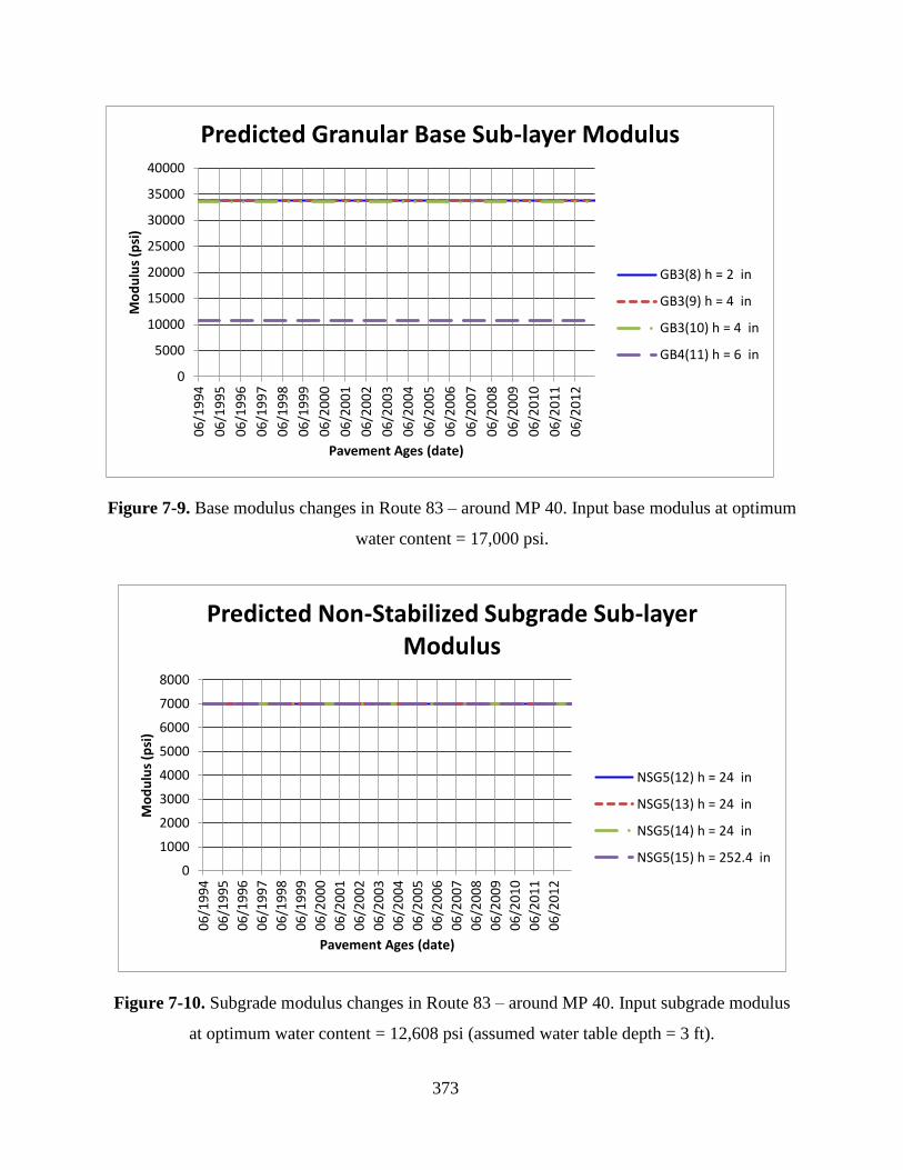
373

Figure 7-9. Base modulus changes in Route 83 – around MP 40. Input base modulus at optimum

water content = 17,000 psi.

Figure 7-10. Subgrade modulus changes in Route 83 – around MP 40. Input subgrade modulus

at optimum water content = 12,608 psi (assumed water table depth = 3 ft).

0

5000

10000

15000

20000

25000

30000

35000

40000

06

/19

94

06

/19

95

06

/19

96

06

/19

97

06

/19

98

06

/19

99

06

/20

00

06

/20

01

06

/20

02

06

/20

03

06

/20

04

06

/20

05

06

/20

06

06

/20

07

06

/20

08

06

/20

09

06

/20

10

06

/20

11

06

/20

12

Mo

du

lus

(psi

)

Pavement Ages (date)

Predicted Granular Base Sub-layer Modulus

GB3(8) h = 2 in

GB3(9) h = 4 in

GB3(10) h = 4 in

GB4(11) h = 6 in

0

1000

2000

3000

4000

5000

6000

7000

8000

06

/19

94

06

/19

95

06

/19

96

06

/19

97

06

/19

98

06

/19

99

06

/20

00

06

/20

01

06

/20

02

06

/20

03

06

/20

04

06

/20

05

06

/20

06

06

/20

07

06

/20

08

06

/20

09

06

/20

10

06

/20

11

06

/20

12

Mo

du

lus

(psi

)


Predicted Non-Stabilized Subgrade Sub-layer Modulus

NSG5(12) h = 24 in

NSG5(13) h = 24 in

NSG5(14) h = 24 in

NSG5(15) h = 252.4 in

374

Figure 7-11. Base modulus changes in Route H1 – around MP 19.5. Input base modulus at

optimum water content = 12,000 psi (assumed water table depth = 3 ft).

Figure 7-12. Subgrade modulus changes in Route H-1 – around MP 19.5. Input subgrade

modulus at optimum water content = 11,400 psi (assumed water table depth = 3 ft).

0

5000

10000

15000

20000

25000

06

/20

03

12

/20

03

06

/20

04

12

/20

04

06

/20

05

12

/20

05

06

/20

06

12

/20

06

06

/20

07

12

/20

07

06

/20

08

12

/20

08

06

/20

09

12

/20

09

06

/20

10

12

/20

10

06

/20

11

12

/20

11

06

/20

12

12

/20

12

Mo

du

lus

(psi

)



GB3(8) h = 4 in

GB4(9) h = 4 in

GB4(10) h = 4 in

GB4(11) h = 4 in

0

1000

2000

3000

4000

5000

6000

7000

06

/20

03

12

/20

03

06

/20

04

12

/20

04

06

/20

05

12

/20

05

06

/20

06

12

/20

06

06

/20

07

12

/20

07

06

/20

08

12

/20

08

06

/20

09

12

/20

09

06

/20

10

12

/20

10

06

/20

11

12

/20

11

06

/20

12

12

/20

12

Mo

du

lus

(psi

)



NSG5(12) h = 24.3 in

NSG5(13) h = 24.3 in

NSG5(14) h = 24.3 in

NSG5(15) h = 248.7 in

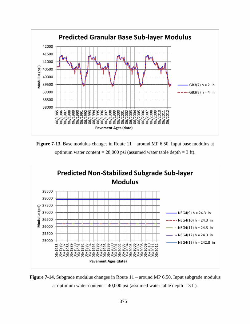
375

Figure 7-13. Base modulus changes in Route 11 – around MP 6.50. Input base modulus at

optimum water content = 28,000 psi (assumed water table depth = 3 ft).

Figure 7-14. Subgrade modulus changes in Route 11 – around MP 6.50. Input subgrade modulus

at optimum water content = 40,000 psi (assumed water table depth = 3 ft).

38000

38500

39000

39500

40000

40500

41000

41500

42000

06

/19

85

06

/19

86

06

/19

87

06

/19

88

06

/19

89

06

/19

90

06

/19

91

06

/19

92

06

/19

93

06

/19

94

06

/19

95

06

/19

96

06

/19

97

06

/19

98

06

/19

99

06

/20

00

06

/20

01

06

/20

02

06

/20

03

06

/20

04

06

/20

05

06

/20

06

06

/20

07

06

/20

08

06

/20

09

06

/20

10

06

/20

11

06

/20

12

Mo

du

lus

(psi

)



GB3(7) h = 2 in

GB3(8) h = 4 in

25000

25500

26000

26500

27000

27500

28000

28500

06

/19

85

06

/19

86

06

/19

87

06

/19

88

06

/19

89

06

/19

90

06

/19

91

06

/19

92

06

/19

93

06

/19

94

06

/19

95

06

/19

96

06

/19

97

06

/19

98

06

/19

99

06

/20

00

06

/20

01

06

/20

02

06

/20

03

06

/20

04

06

/20

05

06

/20

06

06

/20

07

06

/20

08

06

/20

09

06

/20

10

06

/20

11

06

/20

12

Mo

du

lus

(psi

)



NSG4(9) h = 24.3 in

NSG4(10) h = 24.3 in

NSG4(11) h = 24.3 in

NSG4(12) h = 24.3 in

NSG4(13) h = 242.8 in

376

The above analysis shows that there are still some elements of concern about the moduli

changes with climate. In all the examples, when the base modulus changes from one sublayer to

the next it does so quite dramatically as shown in Figure 7-9 and in Figure 7-11. There are

usually no transitions from a wet to a dry condition. There is currently no information to validate

this but such predictions appear a bit extreme.

7.4.2 Stress Dependency

As discussed in section 6.3, laboratory determinations of resilient modulus of unbound

materials always exhibit stress dependency. However, for the analysis with the MEPDG (or any

other software based on linear layer elastic analysis), a single modulus is required for each layer.

This presents a difficult dilemma for the designer. As discussed in the previous section, the

MEPDG requires the input of the resilient modulus at optimum water content and 100% relative

compaction. However, it must be realized that this value depends on the state of stresses selected.

This section analyzes the estimated variation of the resilient moduli within non-linear

layers. A large number of finite element simulations with non-linear constitutive models were

performed with variations in HMA layer thickness (6 and 12 inches), HMA modulus (100,000

psi, 500,000 psi, and 1,500,000 psi) and base thickness (6 and 12 inches). The above layer

thicknesses encompass common situations found in the calibration data set. The three HMA

moduli selected are intended to simulate high temperatures, intermediate temperatures, and low

temperatures representative of Hawaiian conditions. Most of the predicted HMA moduli using

the MEPDG with Hawaii climatic stations result in HMA modulus values within 100,000 psi to

1,500,000 psi. Nevertheless, modulus values as high as 2,500,000 psi are predicted for the lowest

temperatures. Most of the simulations were performed with a wheel load of 9,000 lb

(representing a standard axle load) applied over a circular area of 5.91 inches (as it could be

applied, for example, with a Falling Weight Deflectometer, FWD). In order to illustrate the effect

of the load level, a few simulations were also performed for a load of 14,000 lb. The simulations

were performed using parameters for different materials evaluated in section 6.3. Poisson ratios

were assumed to be 0.35, 0.35 and 0.40 for the HMA, base, and subbase, respectively. For this

analysis, the values assumed were deemed appropriate but a more thorough study of Poisson

ratio is probably warranted in the future. Only some illustrative examples are presented in what

follows.

377

Figure 7-15 shows the estimated Mr’s for a section loaded with a 9,000 lb load and with a

6” HMA layer, a 12” base with the characteristics of the Makakilo base material presented in

page 316 (k1 = 870, k2 = 0.40, and k3 = 0.82) and a 182” subgrade with k1 = 1,821, k2 = 0.42, and

k3 = -3.86 (these parameters were obtained with the model presented in section 6.3.1.2.3, Local

Models of Mr, for a soil with w = 29%, wopt = 27.4%, e = 0.93, eopt = 0.93, PSilt = 45%, S = 0.90,

Sopt = 0.85, and Gs = 2.90). A total depth of 200 inches was used to minimize the boundary

effects. These figures clearly show that according to the laboratory results, resilient modulus of

the base material varies widely. It is also quite evident that as the modulus of the HMA increases

the modulus of the base decreases. This is logical as with an increase of the HMA modulus the

load is spread out over a wider area and thus the stresses on the underlying base layers are lower,

which in turn results in lower base moduli. On the other hand, for the subgrade, which has a

relatively large and negative k3 and thus, it is sensitive to shear, the modulus is lower with the

softer HMA layer than with the stiffer layer. Clearly, there is no such thing as a single equivalent

modulus for each layer that would produce the same effects for all types of distresses that one

would want to predict. Thus, any value selected would be a compromise.

Figure 7-16 illustrates a situation with a thicker HMA layer (12 inches) and a stronger

subgrade with k1 = 2,765, k2 = 0.62, and k3 = -3.72 corresponding to w = 13.0%, wopt = 12.0%, e

= 0.46, eopt = 0.41, PSilt = 52.0%, S = 0.75, Sopt = 0.77, and Gs = 2.64. The base material is the

same as in the previous example. This example illustrates that the effect of a thicker layer is

similar to having a stiffer layer, i.e. spreading the load over a larger area reduces the stresses on

the base and result in lower base moduli. The example also shows (for a 9,000 lb load) that the

approximations of linear elastic analysis (i.e., constant modulus) are much more reasonable than

for thinner HMA layers.

Figure 7-17 shows the same structure used in the previous figure but subjected to a load

of 14,000 lb instead of 9,000 lb. Comparison of these results with those shown in Figure 7-16

illustrate the effect of the loading level on the resilient modulus.

Figure 7-18 shows the modulus distribution for the coral base with k1 = 1,760, k2 = 0.18,

and k3 = 0.932 and a subgrade with k1 = 1,821, k2 = 0.42, and k3 = -5.51. Once again, the lateral

and vertical variations of the modulus are substantial even with a 12 in HMA layer.

378

Figure 7-19 shows a simulation with the 3-Fine material with k1 = 1,230, k2 = 0.495, and

k3 = 0.0 over the subgrade with k1 = 1,821, k2 = 0.42, and k3 = -5.51 and under a 6 inch HMA

layer. Compared to the response of the base material in Figure 7-15 (in both cases the HMA

thickness is 6 inches), it is seen that the 3-Fine material provides a slightly softer support but the

differences do not appear to be substantial. Of course, with the 3-Fine material Mr is likely to

change little with changes in moisture but the conventional base material Mr would tend to

increase significantly dry of optimum and decrease wet of optimum.

Figure 7-20 shows a simulation with a Foamed Asphalt (FA) base material with k1 =

2,955, k2 = 0.39, and k3 = -0.14 and a subgrade with k1 = 1,821, k2 = 0.42, and k3 = -5.51 for a

load of 9,000 lb and HMA thickness of 12 inches. Clearly, under optimum conditions the FA

base material has the potential of increasing the resilient modulus. An interesting question is how

the modulus of this material would change with changes in post-compaction moisture content.

There is currently no local information to address this question.

As illustrated by the previous examples, the number of combinations are endless. Notice

that the figures presented show only some specific conditions (for example, a given subgrade

condition, one HMA thickness, and one load level.) Many other situations were analyzed but

they are not presented here. Note that in some cases, with thin HMA sections and high loads, the

bulk stress can become very small in the base or even negative, which causes some instabilities

in the predictions. Unfortunately, none of the models are well defined for those conditions and

thus either a lower limit has to be used (as has traditionally being done) or a study of base

material behavior at low stress levels need to be carried out.

In general, it can be seen that for optimum water content and maximum dry density, the

resilient modulus values are substantially lower than those generally suggested for design. For

example, the MEPDG manual of practice suggested values for materials classified as A-1-a, A-1-

b, A-2-4, A-2-5, A-2-6, A-2-7, and A-3 are 40,000 psi, 38,000 psi, 32,000 psi, 28,000 psi, 26,000

psi, 24,000 psi, and 29,000 psi respectively [22]. These values are probably intended to represent

average conditions over the service life. Note that in many of the examples above, even doubling

the maximum simulated value to account for drying of the base would result in values lower

(sometimes substantially lower) than those typically suggested. Of course, arbitrary picking the

maximum value on the base is also questionable.

379

(a) |E*| = 100,000 psi (b) |E*| = 500,000 psi (c) |E*| = 1,500,000 psi

Figure 7-15. Resilient modulus distributions for an aggregate base with Makakilo characteristics (see page 316) and a weak subgrade

(w > wopt) according to the model of section 6.3.1.2.3.1. Load = 9,000 lb.

380


Figure 7-16. Resilient modulus distributions for an aggregate base with Makakilo characteristics (see page 316) and a stronger

subgrade according to the model of section 6.3.1.2.3.1. Load = 9,000 lb.

381


Figure 7-17. Resilient modulus distributions for an aggregate base with Makakilo characteristics (see page 316) and a stronger

subgrade according to the model of section 6.3.1.2.3.1. Load = 14,000 lb.

382


Figure 7-18. Resilient modulus distributions for a Coral Base (page 300) and weak subgrade (w > wopt) according to the model of

section 6.3.1.2.3.1. Load = 9,000 lb.

383


Figure 7-19. Resilient modulus distributions for the 3-Fine aggregate (see Table 6-11 on page 314) and weak subgrade (w > wopt)

according to the model of section 6.3.1.2.3.1. Load = 9,000 lb.

384


Figure 7-20. Resilient modulus distributions for the Foamed Asphalt base with k1 = 2,955, k2 = 0.39, and k3 = -0.14 and a subgrade

with k1 = 1,821, k2 = 0.42, and k3 = -5.51. Load = 9,000 lb.

385

If the procedure described by Von Quintus and Killingsworth is used ( [81] and [82]), the

modulus under the center of the load and at a depth of ¼ of the base layer height should be

selected, which result in even lower values. In fact, it is not clear to the PI why a value selected

at that location would be the most representative one to use. As described in Huang [34],

different stress points are appropriate depending on what the designer is interested in predicting

(vertical compressive strains, tensile strains at the bottom of the HMA, tensile strains at the top

of the HMA, etc.) In any case, the observation about the low Mr values created some concern

about the validity of the local observations. Thus, laboratory results reported for other locations

were used to analyze the predicted Mr values. Figure 7-21 shows the results of simulations

performed using the resilient modulus model parameters for granular base materials used in New

Jersey reported by Bennert and Maher [60]. Specifically, the values of k1 = 992.4, k2 = 0.594, and

k3 = -0.0285 were used. Only the simulations with a |E*|HMA = 100,000 psi are presented since

these result in the highest predictions of Mr for the base. Figure 7-21 shows the results side by

side for a 6-inch HMA layer thickness and a 12-inch HMA layer thickness. As for the local

materials, the maximum predicted Mr values are relatively low (less than 20,000 psi for the 6-

inch HMA) and less than 12,000 psi for the 12-inch HMA). Of course, at ¼ depth of the base, the

values are even lower. Thus, for this material, if the user were to enter a value of 12,000 psi at

optimum water content and maximum dry density, the MEPDG would predict for dry of

optimum conditions a resilient modulus value of at most 24,000 psi, which is again lower than

the value typically suggested even though, based on the laboratory resilient modulus, the 12,000

psi input is probably an overestimate of the effective modulus. These simulations provide some

independent validation to the predictions with the local materials.

Finally, it is interesting to note the work of Sagario [83], who tested RCA (Recycled

Concrete Aggregate) and RAP (Reclaimed Asphalt Pavement) compacted in two cross-linked

polyethylene storage tanks 4-foot high and 3-foot diameter. She used a Portable Falling Weight

Deflectometer (PFWD) and a GeoGauge to measure the stiffness of the compacted material to

compare the measurements with these two devices. Interestingly, the PFWD stiffnesses

measured on the top layer were 16,550 psi and 15,000 psi for the RCA and RAP, respectively.

These results are of the same order of magnitude as those presented earlier for granular bases

with 6-inch HMA layers. It must be noted that the vertical stress at the top of the base predicted

386

for a 9,000-lb load on a 6-inch HMA layer with low to intermediate stiffness on top of the

granular base is similar to the vertical stress applied by the PFWD (on the order of 21 psi).

Furthermore, Sagario [83] also found that the modulus for RAP almost doubled with

time. This was possibly attributable to the fact that the moisture content of RAP decreased over

the duration of the experiment due to a downward percolation of the water in the RAP.

7.4.3 Mr values used for calibration

The previous sections have illustrated the challenges for selecting reasonable Mr values

for use in calibration of the MPEDG. Since the unbound materials response is non-linear but in

the MEPDG it is assumed to be linear for simplicity, it is clear that no single modulus value

would result in an equivalent strain for each load level and environmental conditions57.

Furthermore, the location of a stress point to compute an equivalent Mr also depends on the type

of distress of interest. For example, the most appropriate modulus to compute the strains for

permanent deformation modeling is not the same as the one for computing bottom up fatigue

cracking. Yet, a single value needs to be input into the MEPDG.

Von Quintus and Killingsworth [84] use the Mr values at one quarter of the layer depth

for bases and subbases and 18 inches into the subgrade58. However, as reported by the same

authors, the procedure was based on result from other studies. In their study, they found that in

75% of the sections the back-calculated values significantly exceeded those values measured in

the laboratory, such as there is no stress state for which the two moduli are equal59. As illustrated

in section 7.4.2, the lateral variation of the modulus can be quite substantial as well. This also

affects the deflections on sensors further from the load and the overall backcalculation results.

57 Recall that temperature changes result in changes of the HMA modulus. As a result of a change in the

HMA modulus, for a given load magnitude the stresses transmitted to the underlying layer by the HMA would also

change and thus, the modulus of the underlying unbound non-linear layer would also change.

58 Although not explicitly specified, it is apparent that the values are computed directly underneath the load.

59 Put another way, as they computed values of Mr corresponding to the state of stress for points at different

depths in a given layer, they found that for 75% of the sections none of those Mr values matched the back-calculated

value.

387

(a) hHMA = 6 inches (b) hHMA = 12 inches

Figure 7-21. Resilient modulus distributions of base material tested by Bennert and Maher [60] for the New Jersey (k1 = 992.4,

k2 = 0.594, and k3 = -0.0285 and a subgrade with k1 = 1,821, k2 = 0.42, and k3 = -5.51. Load = 9,000 lb. |E*|HMA = 100,000 psi.

388

For this study, the following simplified procedure was adopted to account for the effect

of the thickness of layers above the base and for the subgrade characteristics.

For bases/subbases, a value of 12,000 psi was used for an HMA thickness of 16 inches or

more, and 2,000 psi were added for each 1-inch reduction in HMA thickness. Thus, for a 10-inch

HMA layer, the assumed modulus of the base is 12,000 psi + 2,000 psi/inch × (16 – 10) inch =

24,000 psi. This should produce values that are a reasonable approximation to the values

corresponding to 100% compaction and optimum moisture content (in most situations, the values

will be within the ranges simulated in section 7.4.2.) When a subbase was present, a 3,000 psi

were added to the Mr of the subbase to account for the usually higher confinement of this layer.

Notice that subbases are more likely to be affected by moisture since they are closer to the water

table. Thus, the slightly higher input modulus does not necessarily result in a higher modulus

than that of the base when the simulations are performed with the MEPDG. Other characteristics

were obtain from the results of Rayapeddi Kumar [47].

For subgrades, the Arizona State University Soil Unit Map Application

(http://nchrp923b.lab.asu.edu/index.htm) developed under NCHRP Study 9-23b [68] was utilized

to estimate the resilient modulus and other characteristics. However, as observed in Section

6.3.1.2.3.3, Hawaiian soils are stiffer than the mainland counterparts with similar characteristics.

Based on the analysis of that section, and for simplicity it is recommended that the resilient

modulus estimates from the NCHRP 9-23B website be increased by 100% (i.e., to multiply them

by 2).

7.5 CALIBRATION EFFORT FOR NEW PAVEMENTS

With the information described in previous sections, an effort was made to provide a first

calibration of the MEPDG for new pavement segments. As discussed in Section 7.3, some of the

distress data available from HDOT, particularly for 2006, were questionable. Furthermore, the

historical information was not detailed enough for calibration.

Even with the limited scope of the calibration attempt, the effort was challenging as some

of the input information, such as resilient moduli of unbound materials, axle load spectra for

each section, or even percentage of heavy trucks on the calibration lane are only approximate.

http://nchrp923b.lab.asu.edu/index.htm

389

Traffic loading inputs used for calibration for each section were assigned following the

recommendations presented in section 3.4. Resilient moduli of unbound materials were assigned

according to the rules described in the previous section with the option of modifying input values

for temperature/moisture. HMA dynamic moduli for State Mix Type IV and Superpave mixes

were entered as if they were input level 1 (i.e., pseudo-level 1), which requires entering a set of

values corresponding to a set of frequency and temperature pairs. The values entered as pseudo-

level 1 for these type of mixes were derived from the local model presented in Section 6.2.4.2

using the volumetrics corresponding to a mix with 5.2% binder content and 7.5% air voids. This

was considered preferable than entering level 3 information. For asphalt concrete bases, inputs

were at level 3 using the gradation in the HDOT specifications. The closest climatic weather

station was assigned for each pavement section.

Figure 7-22 shows an example of HMA dynamic modulus, Figure 7-23 provides an

example of some of the traffic inputs, and Figure 7-24 shows binder inputs required when level 1

data is input for the HMA dynamic modulus.

Figure 7-22. Example of HMA Dynamic Modulus input.

390

Figure 7-23. Example of Traffic Loading input.

Figure 7-24. Example of Binder Dynamic Shear Modulus and Phase Angle input.

391

Several runs were needed to calibrate the prediction of rutting, cracking and roughness.

Thermal cracking was always predicted to be zero no matter what values of the calibration

parameters were used. Given the Hawaiian climate, this is quite logical. The results for the other

distresses are discussed in more detail in the following subsections.

The AASHTO Guide for the Local Calibration of the Mechanistic-Empirical Pavement

design Guide [31] provides a Step-by-Step procedure for local calibration. The 11 steps include:

1. Selecting a Hierarchical Input Level for Each Input Parameter

2. Developing Local Experimental Plan and Sampling Template

3. Estimating Sample Size for Specific Distress Prediction Models

4. Selecting Roadway Segments

5. Extracting and Evaluating Distress and Project Data

6. Conducting Field and Forensic Investigations

7. Assessing Local Bias: Validation of Global Calibration Values to Local Conditions, Policies, and

Materials

8. Eliminating Local Bias of Distress and IRI Prediction Models

9. Assessing the Standard Error of the Estimate

10. Reducing Standard Error of the Estimate

11. Interpreting the results, deciding on Adequacy of Calibration Parameters

Unfortunately, as illustrated by the complexities and data issues discussed in previous

chapters, most of the steps in the procedure could not be applied. For example, it is simply not

possible to develop an experimental plan with only 29 pavement segments (step 2). Also,

estimating an appropriate sample size and selecting the roadway segments are simply academic

exercises for the new pavement sections since the sample was so small that all observations

needed to be used. These are tasks that could be performed for rehabilitated sections but more

reliable distress records are needed in these cases, particularly for cracking. Furthermore,

documenting the condition of the pavement before rehabilitation complemented with FWD

testing is also needed. Forensic investigations are desirable but they were beyond the scope of

this project. Finally, the information was simply too limited to assess standard errors. Therefore,

most of the effort was directed towards attempting to eliminate the bias and reduce the errors.

392

7.5.1 Rutting or Permanent Deformation

Calibration of the rutting model consists of changing one, two, or three of the parameters

available in the MEPDG for this purpose until the errors and the bias in the predictions are

minimized. Recall that rutting prediction in the MEPDG is based on equation (5-7), which is

reproduced here for convenience:

HMAr

βkk

rzHMAHMApHMAp hεnTβkhεΔrβk

r33

221101 (7-2)

In this equation T is the temperature, n is the number of load repetitions producing a

certain strain r, and hHMA is the thickness of the HMA layer. kz provides an adjustment for the

effect of confinement with depth and k1, k2, and k3 are the laboratory developed model

parameters that were adjusted during the global calibration process. The parameters r1, r2, and

r3 are provided specifically for local calibration of the guide to field conditions. They provide a

simple way to modify the parameters k1, k2, and k3.

After several runs and together with the experiences with the development of the local

permanent deformation model presented in section 6.5.1, the following calibration parameters

were used: r1 = 0.11, r2 = 1, and r3 = 1.35. In addition, since it has been reported that the

MEPDG overestimates the rutting contributed by the unbound layers and it appears that in most

locations with significant rutting most of the rutting originates in the HMA, the calibration

parameter for unbound materials were reduced significantly, s1 = 0.01. This had the effect of

significantly limiting the contribution of the unbound layers to rutting. As shown in Figure 7-25,

simulations with these calibration parameters provide modestly reasonable predictions and a

significant improvement over the predictions obtained with the initial runs without calibration

shown in Figure 7-26. Note that a slight upward bias still remains as there are more points above

the equality line than below. It is important to note that a slightly better fit could have been

obtained with other calibration parameter combination. However, in addition to the overall fit,

the predictions for each individual section were also considered.

393

Figure 7-25. Observed vs. Predicted Permanent Deformation after calibration.

0

0.05

0.1

0.15

0.2

0.25

0 0.05 0.1 0.15 0.2 0.25

Pre

dic

ted

Per

man

ent

Def

orm

atio

n (

in)

Observed Permanent Deformation (in)

394

Figure 7-26. Observed vs. Predicted Permanent Deformation without calibration.

As shown in Figure 7-27, the predictions for individual sections are more or less parallel

to the 45° line although in general they have a slope of less than 45°. Further reduction of the

bias made these slopes worse than the ones shown here. Thus, elimination of the overall bias

without consideration of individual section predictions can be dangerous since the model may

not simulate well the individual section rutting performance. Considering the level of precision

with which the data is currently collected (i.e., with only 3 sensors per wheelpath), the rutting

predictions are modestly acceptable.

0

0.05

0.1

0.15

0.2

0.25

0 0.05 0.1 0.15 0.2 0.25

Pre

dic

ted

Per

man

ent

Def

orm

atio

n (

in)


395

Figure 7-27. Observed vs. Predicted Permanent Deformation after calibration with different

symbols for each individual pavement section.

7.5.2 Fatigue Cracking

Calibration for fatigue cracking became a large effort since analysis of the original data

led to the conclusion that there were inconsistencies with them. Thus, as explained in Section

7.3, a big part of the effort was directed towards obtaining the data used for calibration from the

HDOT’s photo logs. Even after this effort, the attempt to reduce the bias was a difficult

endeavor. It is important to note, however, that this is not a unique situation for Hawaii. Some of

the same issues that will discussed with the Hawaiian data can be pointed out for other studies

with more controlled data.

Specifically, consider the results shown on Figure 7-28 reproduced from Figure 3 in the

article by Timm et al. [85]. The figure was created with data from the National Center of Asphalt

Technology Test track. Despite this being a very well controlled full-scale experiment with

known layer thicknesses, materials, traffic and environment, there is a large degree of scatter

within the data with reasonably accurate predictions for only two sections. This was noted by the

authors of the article who further pointed out

0

0.05

0.1

0.15

0.2

0.25

0 0.05 0.1 0.15 0.2 0.25

Pre

dic

ted

Per

man

ent

Def

orm

atio

n (

in)


396

“The remaining sections were grossly over- or under-predicted, which would lead to inefficient designs.

Unfortunately, after attempting many combinations of calibration coefficients, a better fit between

measured and predicted cracking was not found. …”

Figure 7-28. Measured vs. Predicted Fatigue Cracking with the National Calibration obtained at

NCAT (Source: [85]).

It is also instructive to see results for top-down fatigue cracking from another MEPDG

calibration effort. Figure 7-29 shows the results reported in [86] during the NCHRP study 1-40D.

The similarity with the results in Figure 7-28 is that in both cases a high proportion of the data lie

on the axes. The data lying on the x-axis in Figure 7-29 correspond to zero predictions when top-

down cracking is actually observed and those on the y-axis correspond to predictions of cracking

when non cracking is observed. In many cases, the differences are substantial. A cursory view of

the figure may lead the casual observer to believe that the fit is actually quite good. However, a

careful view indicates that this is not the case. This is because the fit is based on 312

observations whereas the trend is governed mostly by about 25 to 30 points that lie close to the

45° line. Most other points lie on the axes or on the origin. Thus, despite the large amount of data

points, many of them do not provide very useful information for calibration.

397

Figure 7-29. Measured vs. Predicted Top-Down Cracking results obtained during the global

calibration of efforts of the NCHRP 1-40D study (Source: [86]).

The results described above are quite relevant to the Hawaii calibration effort as similar

issues were encountered. The full fatigue cracking expression used in the MEPDG to relate the

number of repetitions to failure to strain level was presented as equation (6-32) in Section 6.4.2.

The expression is repeated below for convenience.

3322

1|*|1

ffff k

HMA

k

tfHfHMAf ECCkN

(7-3)

As for the rutting model, this equation contains three parameters 1f, 2f, and 3f provided

to facilitate the local calibration. Recall that the number of repetitions to failure for each strain

(or equivalently, for each load and environmental conditions on the specific pavement structure)

is used with the expected number of repetitions over a time interval to estimate the increment in

damage caused by the given load on the interval and then the cumulative damage is used to

predict the amount of cracking using the following equation:

398

60

1

1

000,610010log'

22'11

DCCCCBottom

eFC (7-4)

Notice that with C1 = C2 = 1 and C2′ = - 2 C2′ this expression is identical to equation (5-3)

presented in Section 5.4.2.1. Recall that in this expression D is the cumulative damage and C2′ is

a function of thickness (see page 206). The parameters C1 and C2 are also provide to facilitate the

local calibration of the MEPDG.

The results of running the MEPDG for each section with the default global calibration

factors (i.e., 1f = 2f = 3f = C1 = C2 = 1) are presented in Figure 7-30.

Figure 7-30. Measured vs. Predicted Fatigue Cracking results with the default global calibration

factors.

Clearly, the predictions with the global calibration factors are biased downward. Actual

fatigue cracking values are much larger than predicted. Thus, modification of the parameters 1f,

Predicted = 0.0422 Observed + 0.1131R² = 0.3813

0

5

10

15

20

25

30

35

0 5 10 15 20 25 30 35

Pre

dic

ted

To

tal C

rack

ing

(%)

Observed Total Cracking (%)

399

2f, 3f, C1, and C2 was evaluated. The initial calibration efforts were performed by changing the

parameters by trial and error combined with engineering judgment. The process is extremely

slow and depending on the analyst intuition it may require an unnecessarily high number of runs.

However, as explained below, if only parameters 1f, C1 and C2 are considered for calibration

then the process can be considerably simplified. Attempting the calibration with parameters 2f

and 3f would be worthwhile if reliable local fatigue cracking information were available. As

presented in Section 6.4, the beam fatigue data developed locally had some limitations in the

compaction procedure and thus there appeared to be too much variation on the exponent of the

stiffness. Nevertheless, the results provide guidance about potential calibration factors. For

example, comparing the global exponent of the strain with those obtained with the local mixes

suggest using values of 2f of 1.56 for unmodified mixes and 1.45 for modified mixes. Given all

the uncertainties in the inputs, these values have not been tried yet but should be considered in

further calibration attempts.

So far, calibration has been attempted only with the use of parameters 1f, C1 and C2.

Using these three parameters, the procedure used to calibrate for fatigue cracking is relatively

simple since it requires a single run for each section with 1f = 1. This defines a basic level of

damage for each section. Notice that the effect of the parameter 1f is to simply scale the damage.

For example, if 1f is 0.5, Nf is halved and consequently the damaged is doubled. Thus, the

damage changes inversely proportional to the value of 1f. Notice that this observation is valid

for every value of the strain and mix modulus. Therefore, calibration can be achieved by simply

scaling the damage for each section by the same factor (which is equivalent to varying 1f) and

simultaneously changing the parameters C1 and C2 to obtain the best fit possible. This can be

easily achieved with a tool such as Solver in Microsoft Excel® with the objective of minimizing

the sum of the squared residuals.

Application of the above procedure resulted in 1f = 0.137, C1 = 1.639, and C2 = 2.277.

The corresponding observed vs. predicted chart is shown in Figure 7-31. Clearly, there is a

significant improvement over the fit shown in Figure 7-30. Nevertheless, similarly to other

studies, a significant number of observations can be observed along one of the axes (the observed

axis in this case). Furthermore, the slope of the observed vs. predicted line is 0.55, which is

significantly different from 1.

400

Figure 7-31. Measured vs. Predicted Fatigue Cracking results obtained with 1f = 1.188, C1 =

1.6394, and C2 = 2.277.

One of the premises of the local calibration is to eliminate the bias, as described by step 8

on page 390. This can also be done with a modification of the procedure described earlier. All it

takes is to write an equation in Excel to find the slope of the regression of the predicted values on

the observed values, and then create a restriction in Solver that limits the value of the slope to a

value close to 1 (say, Slope > 0.99 and Slope < 1.01; only the first restriction was needed with

the Hawaiian data.) Performing this analysis resulted in in 1f = 0.771, C1 = 0.686, and C2 =

2.506 and the Observed vs. Predicted Cracking shown in Figure 7-32. The line fitting the data is

now almost indistinguishable from the 45° line. Clearly, since this is a more constrained

optimization problem than the one without the constraint in the slope, the fit is reduced

substantially. Although the fitting line is now at almost 45°, there is a clearly seen larger scatter

of the data around this line.


0

5

10

15

20

25

30

35

0 5 10 15 20 25 30 35

Pre

dic

ted

To

tal C

rack

ing

(%)


401

In this case, eliminating the bias is perhaps questionable. Comparing the results in Figure

7-32 with those in Figure 7-31 shows that points on the x-axis or very close to it have moved by

imperceptible amounts. Thus, all that is gained is a theoretical unbiasedness at the expense of

significantly more scatter. The calibration has not really taken care of the real reason behind the

under prediction for the observations on the x-axis. This is yet unknown here and apparently in

other studies. Thus, until more data are obtained for a more robust calibration, it is recommended

to use the values 1f = 0.13697, C1 = 1.6394, and C2 = 2.277.

It is interesting to note that the observations below the equality line in Figure 7-32

correspond to thick sections and those above mostly to thinner sections. This may indicate that

two different mechanism are acting or that top down cracking is the main mechanism. Top down

cracking is suspected to be the mechanism in many of the sections in the sample for several

reasons: 1) cracking usually appears longitudinally (which per se may be top-down or bottom-

up) but it stays like that for a very long time. It rarely develops into a typical alligator cracking

pattern; 2) as shown later in Section 7.6.4 (page 420), there are certain combinations of moduli

that may result in minimum principal strain distributions with maximum tensile strains near the

top of the surface; and 3) some of the sections are simply very thick (about 13 inches of HMA

with traffic loading that is apparently not too high.)

Calibration attempts were also performed using the top-down fatigue equations. Similar

issues were confronted. Since at present there is uncertainty about the mechanism of cracking,

these results are not presented. However, it is recommended to perform forensic studies on

different type of pavements (soon after cracking is first detected) to determine how cracking

initiates so as to better guide its modeling. Confirmation of the prevalence of top-down fatigue

cracking would indicate the need of further research to more accurately model this distress

mechanism.

402

Figure 7-32. Measured vs. Predicted Fatigue Cracking results with the default global calibration

factors.

7.5.3 International Roughness Index (IRI)

The MEPDG predicts IRI based on the initial IRI after construction (IRI0), a site factor

(SF), area of fatigue cracking as a percent of the total lane area (FCTotal), transverse cracking

(TC), and rut depth (RD). The equation relating these variables is:

SFCTCCFCCRDCIRIIRI Total 43210 (7-5)

where

IRI0 = Initial IRI after construction, in/mi,

RD = average rut depth, in,

Predicted = 0.9942 Observed - 0.0429R² = 0.4962

0

5

10

15

20

25

30

35

0 5 10 15 20 25 30 35

Pre

dic

ted

To

tal C

rack

ing

(%)


403

FCTotal = Area of fatigue cracking (combined alligator, longitudinal, and reflection

cracking in the wheel path), percent of total lane area. All load related

cracks are combined on an area basis – lengths of cracks is multiplied by 1 ft

to convert length into an area basis [22].

TC = Length of transverse cracking (including the reflection of transverse cracks

in existing HMA pavements), ft/mi, and

SF = Site factor, computed with equation (7-6) below, and

C1 to C4 = model coefficients.

1000636.01Pr007947.0102003.0 FIecipPIAgeSF (7-6)

where

Age = Pavement age, yr.,

PI = Percent plasticity index of the soil.

FI = Average annual freezing, °F-days, and

Precip = Average annual precipitation or rainfall, in.

For most Hawaiian locations, FI is zero. The default coefficients of equation (7-5) in the

MEPDG are C1 = 40.0, C2 = 0.400, C3 = 0.0080, and C4 = 0.0150. Calibration of the IRI model

in the MEPDG consists of essentially changing these parameters to eliminate the bias and reduce

the error. In addition to the above parameters, the predictions are highly dependent on the initial

value of IRI, IRI0. Unfortunately, IRI0 was known for only a few sections in the calibration

sample.

Simulation runs with the default coefficients C1 = 40.0, C2 = 0.400, C3 = 0.0080, and C4

= 0.0150 performed after calibration of the cracking and rutting models presented earlier and

with a default IRI0 = 63 (default value in the MEPDG) resulted in the predicted vs. observed

values presented in Figure 7-33. Clearly, there is a substantial under-prediction of roughness.

Since the global calibration of the MEPDG was performed with national data, these results

indicate that most of the new pavements/reconstructions in the State are being built with

considerable more roughness than in the mainland US.

404

Figure 7-33. Predicted vs. Observed results with the default global calibration factors and

IRI0 = 63.

The large cluster of points on the lower right of Figure 7-33 also appears to indicate that

there is a group of pavements that have substantially more roughness than expected (roughly 75

in/mile more than other sections). The only common feature that was identified for these sections

is that in general, they are fill sections with relatively important embankments. Sections in this

group included the sections for H-2 0.21-0.39 (fill section), H-3 (fill section), R83 16.09-16.19

and 16.22-16.30 (fill on bridge approach), R50 0.00-0.13 (fill section), R50 18.93-19.10

(widening), R50 21.71-21.81 (fill section), R32 0.40-0.51 (fill section between retaining walls).

This may indicate that the specification, materials, and construction practices of this type of

embankments may need to be evaluated further. Hawaii is rated consistently among the States

with worst pavements in the nation with ratings that are based mostly on IRI. Thus, in addition to

potentially improving the ride conditions for the traveling public, determining the causes of the

substantially higher roughness on embankments may help improve the overall State rating.


20

40

60

80

100

120

140

160

180

200

220

20 40 60 80 100 120 140 160 180 200 220

Pre

dic

ted

IRI (

in/m

ile)

Observed IRI (in/mile)

405

As indicated earlier, for a few sections (actually, for eight sections), IRI0 could be

estimated from the information available on the construction year. Figure 7-34 shows the results

of the simulations with the same inputs used to generate Figure 7-33 but with the actual IRI0

value for each of the eight pavement sections. Clearly, using this additional information helps

with the predictions for the sections in question.

Figure 7-34. Predicted vs. Observed results with the default global calibration factors and actual

IRI0 for sections with known values and IRI0 = 63 for the rest of the sections.

The goal of the calibration is to obtain appropriate values of C1, C2, C3, and C460. It is also

desirable to obtain a reasonably representative value of IRI0 to use in the simulations. However,

IRI0 is not available for every section, which poses a challenge for calibration of C1, C2, and C4.

60 As indicated before, thermal cracking is not relevant for Hawaii, so using the default value is acceptable.


20

40

60

80

100

120

140

160

180

200

220

20 40 60 80 100 120 140 160 180 200 220

Pre

dic

ted

IRI (

in/m

ile)


406

This challenge was overcome by minimizing the sum of squared residuals by varying the

parameters C1, C2, and C4 and simultaneously varying the values of IRI0 for each section. Thus,

in addition to the three parameters C1, C2, and C4, an additional value was estimated for each

section. It is important to note that the only goal of this exercise was to obtain unbiased estimates

of C1, C2, and C4. The estimated values were C1 = 23.1, C2 = 0.323, and C4 = 0.01561. Figure

7-35 shows the results. This figure clearly shows that with good estimates of IRI0 the model has

the potential of providing better predictions.

Figure 7-35. Predicted vs. Observed results with the estimated C1, C2, and C4 and IRI0 values

estimated for each section.

61 The optimizations resulted in a value for C4 of zero. Since the data used for the site factor are not entirely

reliable, it was preferred to fix the value of C4 to be the same as the global calibration factor, i.e., C4 = 0.015.


20

40

60

80

100

120

140

160

180

200

220

20 40 60 80 100 120 140 160 180 200 220

Pre

dic

ted

IRI (

in/m

ile)


407

With the estimated values of C1, C2, and C4 in hand, attention was turned again to obtain

a reliable estimate of IRI0. An alternative would have been to use the average of the IRI0 values

for all sections estimated when obtaining C1, C2, and C4. However, this was not considered

appropriate because as indicated before, two groups with very different IRI0 values appear to be

present in the sample. Therefore, the two groups of pavements were assumed to have different

representative IRI0 values and these were estimated by minimizing the sum of squared residuals

with the values of C1 = 23.1, C2 = 0.323, and C4 = 0.015 and varying the IRI0 value for each

group. These resulted in IRI0 = 78.0 in/mile for “normal” sections and IRI0 = 150.5 in/mile for

fill sections. Figure 7-36 shows the predicted vs. observed results.

Figure 7-36. Predicted vs. Observed results with the estimated C1, C2, and C4 and IRI0 = 78.0

in/mile for “normal” sections and IRI0 = 150.5 in/mile for fill sections.


20

40

60

80

100

120

140

160

180

200

220

20 40 60 80 100 120 140 160 180 200 220

Pre

dic

ted

IRI (

in/m

ile)


408

Considering the uncertainty in the IRI0 and other input values, the predictions above are

quite reasonable. Of course, additional data are needed to validate these results.

It is important to note that IRI0 = 78.0 in/mile is 15 in/mile higher than the default

recommended value. This again, points out that for some reason the pavements in our State

appear to have larger built-in roughness. For sections in fill, the values of IRI0 = 150.5 in/mile is

almost doubled the value for other sections, which is something that needs to be investigated in

more detail.

7.6 TOP-DOWN FATIGUE CRACKING

As noted in section 7.5.2, it is suspected that top-down fatigue cracking may be the main

mechanism of cracking on state roads with thick HMA layers. This section presents an analysis

supporting this hypothesis.

The variation of the HMA modulus with depth has an important bearing on the strain

distribution within the HMA layers and in turn on the location with the largest fatigue damage.

The MEPDG currently assumes that that location of largest fatigue damage is at the bottom of

the HMA for bottom-up fatigue cracking or at the surface or 0.5 in below the surface for top-

down fatigue cracking. As was illustrated in Figure 6-9 on page 246, the MEPDG typically

predicts that the modulus of the HMA decreases with depth, which implies that the effects of

frequency and aging on the HMA modulus always supersede the effect of temperature. In all the

simulations performed for this research project with Hawaiian climatic stations, the MEPDG has

always predicted a decrease in modulus with depth. Since with Hawaii’s weather one should

expect to have a large proportion of time with high temperatures at the top accompanied by a

relatively large gradient with decreasing temperatures with depth, the consistent decrease of

modulus with depth predicted by the MEPDG is a bit puzzling. Therefore, the following

subsections analyze this issue in more detail.

7.6.1 Frequency of Loading Calculations

As discussed in section 6.2, the frequency of loading has an important effect on the

dynamic modulus, |E*|. Unfortunately, as mentioned on footnote 41 on page 246, there is still

some controversies about its calculation. The goal of this section is not to take sides on the

controversy but instead to analyze the reasonableness of the |E*| calculations with depth in the

409

MEPDG. Therefore, the following paragraphs present only the method used in the MEPDG to

compute the frequency of loading. If the frequency variation with depth were less severe, as

indicated by the results of other researchers [87], the findings on the following subsections

would be reinforced even more.

The MEPDG uses the following equation to relate the time of loading to the vehicle

speed (velocity) and the effective length of the load pulse.

s

eff

v

Lt

6.17 (7-7)

where

t = time of loading (sec),

Leff = effective length of the load pulse (inches), and

vs = velocity (mph).

According to the MEPDG documentation (Appendix CC in [1]), the effective length at a

given point in the above equation is the duration of the haversine stress pulse and is dependent

upon the layer properties and the loading configuration (axle spacing and the radius of contact).

Since HMA layers are at or close to the surface of the pavement, the loading configuration has

practically no effect on the frequency calculations and thus, only the case with single axles are

described here. After computing the time of loading with the equation (7-7), the corresponding

loading frequency (f) is estimated according to the following relationship:

t

f1

(7-8)

Therefore, the key to computing the time of loading or the frequency of loading is in the

determination of the effective load pulse length with depth.

410

7.6.1.1 Effective Length Calculations

The effective length is the length that defines the extent of the stress pulse at a specified

depth within the pavement system. The MEPDG represents this schematically as shown in

Figure 7-37.

Figure 7-37. Effective Length Concept within the Pavement System (Source: [1]).

In Figure 7-37, the segment AA represents the effective length of the load pulse at a

certain depth within the asphalt concrete (AC) (or HMA) layer (typically, the mid depth would

be considered). The segment BB represents the effective length at another depth in a granular

layer. To interpret these, one needs to imagine a moving load. As the load moves, points outside

the segment experience zero load, points within the effective length experience a load that

increases to a maximum under the center of the load. Clearly, the longer the effective length the

longer is the time of loading.

As indicated in the MEPDG [1], stiffer materials tend to distribute the stresses over a

much wider area compared to less stiff materials, which is why the slope of the lines delimiting

the effective lengths in Figure 7-37 are considered to vary with material stiffness. In order to

account for this, the MEPDG uses a simplified procedure based on an equivalent thickness

concept first establish by Odermark. The method is based on the assumption that the stresses and

strains below a layer depend on the stiffness of that layer only. If the thickness, modulus and

Poisson’s ratio of a layer are changed, but the stiffness remains unchanged, the stresses and

strains below the layer should also remain (relatively) unchanged [1].

411

The stiffness of a layer is proportional to:

)1( 2

3

Eh (7-9)

where

h = thickness

E = elastic modulus

= Poisson ratio

With the concept of equivalent thickness based on stiffness, a two-layer system with layer

1 having thickness h1, modulus E1, and Poisson ration 1 and layer 2 having modulus E2 and

Poisson ration 2 can be converted into a single layer system with modulus E2 and Poisson ratio

2 by converting the thickness of layer 1 into an equivalent thickness he and simultaneously

changing the properties of layer 1 such that the stiffness of layer 1 is unaltered (Figure 7-38). The

stresses and strains computed in layer 2 in both systems should be approximately the same. Note

that if another layer exists above layer 1 the same transformation can be applied to that layer as

well. Thus, the method works for any number of layers

Figure 7-38. Odemark’s transformation of a layered system (Source: [1]).

Mathematically, the transformation is given by:

32

1

2

2

2

112

2

2

3

2

1

1

3

1

)1(

)1(

)1()1(

E

Ehh

EhEhe

e (7-10)

h1, E1,

E2,

he, E2,

E2,

412

If the Poisson ratio is assumed to be the same for all layers, an assumption that is justified

in the MEPDG because Poisson ratio is seldom known with any degree of accuracy, the

transformation simplifies to:

3

2

11

E

Ehhe (7-11)

Figure 7-39. Equivalent Layer Thickness (Source: [1]).

For any pavement layer, the effective length of the stress pulse is computed at a specific

depth (typically at mid depth) for which the loading frequency is needed for the computation of

the modulus. This depth is the transformed depth and is termed as effective depth (Zeff). The

effective depth is computed by the following relationship:

3

1

1

3

SG

nn

n

i SG

iieff

E

Eh

E

EhZ

(7-12)

where Ei is the modulus of layer i, hi is the thickness of layer i, En is the modulus of the layer

containing the point at which the frequency is desired, and hn is the depth from the top of the

layer to the point for which the time or frequency of loading is being determined. If the effective

Transformed HMA

Layer

Subgrade layer

45°

ac

Transformed

Granular Layer

32

22

SG

eE

Ehh

31

11

SG

eE

Ehh

413

depth is needed at the mid-depth of the layer in the pavement structure, then hn is half the layer

thickness.

To compute the effective length, it is assumed for simplicity that the stress in the

transformed structure is distributed at angle of 45° as shown in Figure 7-40. Then, the effective

length or the length of the stress pulse at any depth is defined by the following equation:

)(2 effceff ZaL (7-13)

The effective length can then be used with equation (7-7) to estimate the time of loading.

This is then used with equation (7-8) to estimate the frequency of loading for the single axle

configuration. As indicated before, overlapping of stresses need to be considered for other axle

configurations but this is typically not relevant when computing moduli in HMA layers.

Figure 7-40. Effective Length Calculations using Transformed Thicknesses (Source: [1]).

7.6.2 Temperature Gradients

In order to estimate the variation of modulus with depth, it is also necessary to estimate

the temperature variation with depth. For this purpose, a simplified analysis was performed to

determine the heat flow within the pavement structure.

The one-dimensional diffusion law that governs the movement of heat within the

pavement layers is:

Transformed HMA

Layer

Subgrade layer

45°

ac

Transformed

Granular Layer Zeff Zeff 2 ac

Leff = 2(ac+Zeff)

Zeff

414

t

T

k

c

z

T

2

2

(7-14)

where

T = temperature,

t = time,

z = depth within the layer,

= density,

k = thermal conductivity,

c = mass-specific heat of the material.

As explained in [36], equation (7-14) can be solved using a numerical technique such as

the finite difference procedure. The finite difference equation used to advance the solution from

time t to time t+1 is [36]:

t

i

t

i

t

i

t

i Tz

t

c

kTT

z

t

c

kT

2112

1 21

(7-15)

with superscripts denoting time, subscripts denoting location, and z and t distance and time

steps respectively.

At the boundary between layers (with different k, , and c), the equation needs to be

modified to account for the different material properties above and below the boundary:

t

i

t

i

t

i

t

i Tc

k

z

t

c

k

z

tT

c

kT

c

k

z

tT

1

2

2

21

2

1

1

2

1 1

(7-16)

Examples of the use of these equations are presented in [36]. These can be easily

implemented in a spreadsheet if the temperature at the pavement surface is known and it is

assumed that there is no significant heat flow below at certain depth.

Using the values for the HMA layer and granular materials used in the simulations with

the MEPDG (i.e., thermal conductivity k = 0.67 BTU/hr/ft/°F, heat capacity c = 0.23 BTU/lb/°F,

415

and = 155 lb/ft3), heat profiles were computed for different scenarios for 1 inch intervals. The

scenarios were based on plausible situations in Hawaii. During the day, at about 2:00 PM in a

sunny day, it is quite possible measure temperatures of up 140°F (60°C) at the surface of the

pavement. Actually, measurements of that order were obtained by the PI with an infrared

thermometer on some occasions. Furthermore, these temperatures are consistent with the PG

binder grading system, which for Hawaii’s climate requires a high temperature grade of 64°C at

98% reliability. A temperature of 58°C is often appropriate for a 50% reliability, which means

that there is a 50% chance that the mean highest pavement temperature over the course of the

hottest week will exceed this value.

Scenarios, with maximum temperatures at the surface of 131°F (55°C), 122°F (50°C),

and 112°F (45°C) were also considered to evaluate the conditions with smaller gradients. At a

depth of 400 inches (~33 ft or 10 m), a constant temperature of 68°F (20°C) was assumed as a

reasonable estimate of temperature with depth (and this was also the initial temperature at all

depths). As a result of these simulations, the interpolated temperatures profiles shown in Table

7-4 were obtained with depth after 8 hours of constant temperature at the surface. The values

presented in the table were interpolated to correspond with the mid depth of each sublayer that

would be created by the MEPDG with its automatic sub layering process. Thus, these values are

appropriate for HMA layers up to 12 inches thick.

Three additional scenarios were simulated with 78.8°F (26°C) as the constant

temperature at a depth of 400 inches The value of 78.8°F (26°C) was also used as the

temperature at all depths at t =0. This value was based on measurements obtained under a bridge

by the co-PI. In these additional scenarios, instead of maintaining the temperature at the surface

constant, a more realistic situation was created in which the temperature increases slowly from

78°F (26°C) to 140°F (60°C) over a period of 5 hours (a quite reasonable assumption from 8:00

AM to 1:00 PM), stays at that temperature for 1 hour, and then it decreases to about 113°F

(45°C) over a period of 2 hours. The columns for these scenarios are under the title “Variable

Surface Temperature” in Table 7-4. The temperatures used were the ones computed after 4, 6,

and 8 hours.

The estimated variations of temperature with depth for the variable surface temperature

scenarios are shown in Figure 7-41 after 2, 4, 6, and 8 hours.

416

In the next subsection, the temperatures presented in Table 7-4 are used together with the

estimated frequencies with depth (obtained using the approach of the previous subsection) to

estimate dynamic modulus of HMA with depth.

Table 7-4. Temperatures with depth (°F) for different surface temperature scenarios.

Depth

(inches)

Temperature at the surface

113°F

(45°C)

122°F

(50°C)

131°F

(55°C)

140°F

(60°C)

Variable Surface Temperature

4 hr 6 hr 8 hr

0.25 111.6 120.4 129.1 137.8 124.2 136.99 112.1

0.75 108.9 117.1 125.3 133.5 116.9 130.96 113.2

1.5 104.9 112.3 119.7 127.1 107.8 122.35 113.0

2.5 99.7 106.1 112.4 118.8 98.4 111.93 110.4

3.5 94.8 100.2 105.6 110.9 91.7 103.16 106.2

6.0 84.3 87.6 90.8 94.1 82.7 88.65 94.4

10.0 73.8 75 76.2 77.3 79.2 80.56 83.3

Figure 7-41. Temperature profile with depth after 2, 4, 6, and 8 hours for the scenario

with variable pavement surface temperatures.

0

1

2

3

4

5

6

7

8

9

10

11

12

13

14

15

70 75 80 85 90 95 100 105 110 115 120 125 130 135 140

Dep

th

Temperature

2 hours

4 hours

6 hours

8 hours

417

7.6.3 Combined Effect of Frequency and Temperature on |E*|

The temperatures and frequencies with depth estimated using the procedures in the

previous two sections were used to compute the dynamic modulus using equations (6-6) and (6-

7) (see page 241) for a mix with parameters = 2.637, = 3.950, = -1.268, = 0.418, A = 2.15

×10-4, B = -0.105, and C = 6.30, which corresponds to the mix type IV utilized for most

simulations with the MEPDG.

Since the calculation of the effective load pulse length used to compute frequency of

loading depends on the modulus of the layer and the layers above it, an iterative procedure needs

to be used to determine the modulus. This was implemented in Excel® in the form shown in

Table 7-5. The simulations were performed for a wheel radius of 4 inches and a subgrade

modulus of 12,000 psi62.

With reference to Table 7-5, the calculations were performed as follows. The

temperatures for one of the scenarios estimated with the procedure described in section 7.6.2 are

listed in column (2) for each of the depths shown in column (1) (these depths correspond to the

mid depth of each sublayer). In column (3), an assumed value of |E*| is entered to start the

calculations. Initially, these values would be different from those listed in column (11), which

are described below. With an estimate of the modulus, the effective depth shown in column (4) is

computed using equation (7-12). Then, the effective length of the load pulse in column (5) is

computed with equation (7-13). Equation (7-7) is used to compute the time of loading shown in

column (6) and equation (7-8) is used to compute the frequency shown in column (7). Equation

(6-7) on page 242 is then used to calculate the logarithm of the shift factor in column (8). The

corresponding shift factor is shown in column (9). The shift factor is then multiplied by the

frequency to obtain the reduced frequency (column 10) and with these, the |E*| values are

calculated using equation (6-6) on page 241. Since, the assumed values of |E*| used to compute

the frequencies are not necessarily the same as the values obtained in column (11), in column 12

the differences between the assumed and predicted values are computed. Ideally, one would like

to make the differences equal to zero so that the frequency calculations correspond to the |E*|

62 A wheel radius of 4 inches was selected conservatively to obtain a severe effect of frequency at the

surface.

418

values calculated from the master curve. This is accomplished with solver by minimizing the

sum of the values in column (12) by varying the assumed modulus values. As shown in Table

7-5, this is easily accomplished with Excel®.

In order to account for aging, the values obtained with the above procedure were

multiplied by a factor that varied from 1.56 for the top sublayer to 1.10 for the last sublayer. The

multipliers are based on the typical increase of |E*| with time simulated by the MEPDG for the

Hawaiian conditions. In this way, an approximation to the simulation of aging in the MEPDG is

obtained without having to implement the Global Aging System used by the MEPDG.

Table 7-6 shows the modulus values obtained under the different temperature scenarios

described in the previous section and for a speed of 45 mph. The computation of these values

already account for temperature, frequency, and aging.

Clearly, the values under the four first scenarios are in distinct disagreement with all the

simulations that have been performed in this project with the MEPDG in that the modulus

increases with depth instead of decreasing as the MEPDG suggests. This is very puzzling, as the

same procedure supposedly used by the MEPDG has been followed closely. Note that even for

the variable surface temperatures scenarios, the modulus often increases with depth. Only in the

last scenario, it decreases at first with depth but then it increases at higher depths. The results of

this analysis actually coincide with a priori expectations for high temperature gradients in which

the temperature decreases with depth (which is why the analysis was performed in the first

place.)

A potential source for the discrepancy is that the MEPDG does not model every single

situation but instead it models only five quintiles as was described in Figure 5-17 on page 212.

The scenarios described would be completely missed by the MEPDG if they represented about

less than 10% of the potential situations. Yet, as described below, most of the top-down fatigue

cracking is likely to be generated during situations such those described by this type of scenarios.

The MEPDG modeling may be too coarse to capture these conditions. At least for top-down

fatigue, instead of subdividing the pavement temperatures in each analysis period into five equal

quintiles, a more detailed analysis of the highest temperatures may be more appropriate.

Arguably, this may also be convenient for rutting predictions.

419

Table 7-5. Illustration of the procedure used to estimate |E*| as a function of frequency and temperature.

Depth

(in)

(1)

Estimated

temperature

(°F)

(2)

Assumed

modulus

(psi)

(3)

Effective

Depth

(in)

(4)

Effective

Length

(in)

(5)

Time of

loading

(sec)

(6)

Frequency

(Hz)

(7)

Log

Shift

Factor

(8)

Shift

Factor

(9)

Red Freq

(Hz)

(10)

|E*|

(psi)

(11)

|E*|- |E*assumed|

(psi)

(12)

0.25 112.1 286,267 0.72 9.44 0.0119 83.9 -2.772 0.00169 0.142 286,267 0

0.75 113.2 249,270 2.13 12.25 0.0155 64.6 -2.834 0.00147 0.095 249,270 0

1.5 113.0 227,610 4.15 16.29 0.0206 48.6 -2.822 0.00150 0.073 227,610 0

2.5 110.4 232,227 6.82 21.65 0.0273 36.6 -2.674 0.00212 0.077 232,227 0

3.5 106.2 261,359 9.56 27.12 0.0342 29.2 -2.429 0.00372 0.109 261,359 0

6 94.4 390,809 17.35 42.69 0.0539 18.6 -1.699 0.01998 0.371 390,809 0

10 83.3 558,452 30.93 69.85 0.0882 11.3 -0.958 0.11012 1.249 558,452 0

14 79.7 594,948 45.47 98.93 0.1249 8.0 -0.706 0.19664 1.574 594,948 0

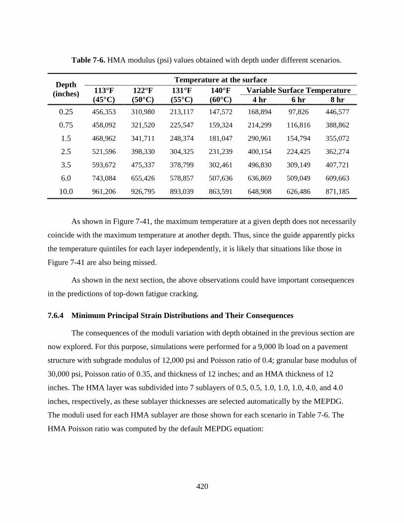
420

Table 7-6. HMA modulus (psi) values obtained with depth under different scenarios.

Depth

(inches)

Temperature at the surface

113°F

(45°C)

122°F

(50°C)

131°F

(55°C)

140°F

(60°C)

Variable Surface Temperature

4 hr 6 hr 8 hr

0.25 456,353 310,980 213,117 147,572 168,894 97,826 446,577

0.75 458,092 321,520 225,547 159,324 214,299 116,816 388,862

1.5 468,962 341,711 248,374 181,047 290,961 154,794 355,072

2.5 521,596 398,330 304,325 231,239 400,154 224,425 362,274

3.5 593,672 475,337 378,799 302,461 496,830 309,149 407,721

6.0 743,084 655,426 578,857 507,636 636,869 509,049 609,663

10.0 961,206 926,795 893,039 863,591 648,908 626,486 871,185

As shown in Figure 7-41, the maximum temperature at a given depth does not necessarily

coincide with the maximum temperature at another depth. Thus, since the guide apparently picks

the temperature quintiles for each layer independently, it is likely that situations like those in

Figure 7-41 are also being missed.

As shown in the next section, the above observations could have important consequences

in the predictions of top-down fatigue cracking.

7.6.4 Minimum Principal Strain Distributions and Their Consequences

The consequences of the moduli variation with depth obtained in the previous section are

now explored. For this purpose, simulations were performed for a 9,000 lb load on a pavement

structure with subgrade modulus of 12,000 psi and Poisson ratio of 0.4; granular base modulus of

30,000 psi, Poisson ratio of 0.35, and thickness of 12 inches; and an HMA thickness of 12

inches. The HMA layer was subdivided into 7 sublayers of 0.5, 0.5, 1.0, 1.0, 1.0, 4.0, and 4.0

inches, respectively, as these sublayer thicknesses are selected automatically by the MEPDG.

The moduli used for each HMA sublayer are those shown for each scenario in Table 7-6. The

HMA Poisson ratio was computed by the default MEPDG equation:

421

|*|1

35.015.0

Ebae (7-17)

with a = -1.63, b = 3.84 × 10-6, and with |E*| expressed in psi.

Figure 7-42 shows the minimum principal strain distributions corresponding to the first

four moduli scenarios shown on Table 7-6. Except for the 113°F (45°C) scenario, it is clear that

in all other situations the maximum tensile strain occurs near the surface of the pavement instead

of at the bottom as it would be predicted with modulus values that decrease with depth. Although

during a whole day the higher temperature situations may be less frequent, the magnitude of the

strains are also much higher and so may be the potential for fatigue cracking. Notice that the

previous sentence is purposely weak as the fatigue cracking potential is affected not only by the

strain but also by the stiffness of the mix (see equations (5-1) on page 201 or equation (7-3) on

page 397.) Thus, the location of the critical point cannot be determined solely by the strain.

Consequently, an analysis was made to obtain the number of repetitions to failure, Nf, for each

strain level as estimated from equation (6-32) on page 324 with C = 1 and CH = 0.1 (the exact

value of CH for a 12 inch HMA layer is 0.083). In order to deal with smaller numbers, the

logarithm of the number of repetitions to failure (log Nf) was calculated.

Clearly, the lower the number of repetitions to failure the higher is damage ratio. Thus,

the critical points are located were the lowest numbers are found. The results are shown in Figure

7-43. As observed in the figure, apparently, the effect of the change in modulus is not generally

high enough to affect the location of the critical point, except when the strains near the top and at

the bottom of the layer are of similar magnitude such as the case with 122°F (50°C).

It is important to stress that although the situations depicted in these figures may occur

over a relatively short intervals during the day (say, 1, 2, or 3 hours depending on actual

conditions), the damage occurring during these periods can be substantial. Notice that the

differences in the log Nf between the scenario with 140°F (60°C) maximum temperature and that

with 122°F (50°C) maximum temperature imply a six fold change in Nf for the 9,000 lb load. For

higher loads the differences would be even higher. This may be a significant factor affecting the

predictions of fatigue cracking.

422

Figure 7-44 shows the minimum principal strain distributions for the last three scenarios

in Table 7-6 (all three including the aging effect). For the 8-hours scenario, the simulation was

performed with and without aging. Figure 7-45 shows the coresponding log Nf distributions. The

observations are similar to the ones presented above. Again, the longer the pavement is heated

from the top the more likely the fatigue cracking starts at the top and as the pavement cools

down, fatigue from the bottom becomes more likely.

A comparison of parts c) and d) of Figure 7-45 shows that the location of the critical

point changes from the top inmediately after construction to the bottom after a few years. Of

course, damage accumulates continuously and at which point cracking will initiate depends on

many factors.

The above analysis illustrate some of the complexities involved in predicting fatigue

cracking. For example, based on the above, if a substantial portion of the loading occurs during

the periods with high temperature gradients (hotter on top), then the likelihood of top-down

cracking appearing before bottom-up fatigue cracking increases. On the other hand, if not much

loading occurs during the hotter periods, then top-down cracking is less likely. The above

analysis is very limited as it was performed for a single load magnitude and one layer thickness.

Clearly, these factors also play an important role. The main point of the analysis, however, is that

the critical conditions for top-down fatigue cracking currently may not be accounted for properly

in the MEPDG. Unfortunately, there is nothing that the user can do at this point to address this

issue. This analysis also sheds some light on why top-down fatigue cracking appears to be a

prevalent distress in Hawaii roads, which is an assumption that needs to be verified.

Confirmation of this assumption could also impact the analysis of reinforcements such as glass

grids and mix with fiber and polymers.

423

a) b)

c) d)

Figure 7-42. Minimum principal strain distributions for a speed of 45 mph and maximum surface temperature for 8 hours of

a) 140°F (60°C), b) 131°F (55°C), c) 122°F (50°C), and d) 113°F (45°C).

424

a) b)

c) d)

Figure 7-43. Number of repetitions to failure for a speed of 45 mph and maximum surface temperature for 8 hours of

a) 140°F (60°C), b) 131°F (55°C), c) 122°F (50°C), and d) 113°F (45°C).

425

a) b)

c) d)

Figure 7-44. Minimum principal strain distributions for a speed of 45 mph and varying surface temperature

a) After 4 hours, b) After 6 hours, c) After 8 hours, and d) After 8 hours – no aging.

426

a) b)

c) d)

Figure 7-45. Number of repetitions to failure for a speed of 45 mph and variable maximum surface temperature

a) After 4 hours, b) After 6 hours, c) After 8 hours, and d) After 8 hours – no aging.

427

7.7 SUMMARYAND A FEW OTHER OBSERVATIONS

In this chapter, the efforts towards calibration of the MEPDG have been described in

detail. Because of data limitations, the calibration attempt has been limited to new HMA

pavements. Significant challenges have been faced with the calibration for rutting, fatigue

cracking, and roughness. This first calibration attempt presents some very promising results as it

shows that predictions can be within reasonable ranges. Nevertheless, considerable work is still

needed for regular use of the MEPDG.

In particular, it is imperative to obtain distress and FWD information for calibration of

the rehabilitation procedures. Furthermore, usable information for a larger sample of sections is

needed to obtain standard error estimates. Although with the local calibration the predictions for

mean behavior of new pavement sections may be reasonable, the standard errors (and

consequently the reliability analysis) would still be based on the global calibration results.

Calibration needs to be redone considering that in the State, the most trafficked lane is

not necessarily the rightmost lane (or simply considering the adequate lane distribution factors

based on more specific lane distribution factors for the pavement sections in the calibration data

set.) In addition, based on the roughness information and video logs, it is believed that in some

situations the construction date may be off by one, two or three years, which may have adversely

influenced some of the predictions. In other occasions, there may have been temporary

construction traffic. For low volume roads, a big construction project may end up being

equivalent to a few years of load applications under normal circumstances, so documenting when

such situations occur is desirable to account for them during calibration.

One of the major features of the MEPDG is the predictions of the effects of

environmental factors on pavement performance. In this respect, however, to take full advantage

of the MEPDG it is desirable to develop information for new weather stations to account, for

example, for the differences in weather (rain, cloud cover, wind, etc.) between the different sides

of the islands. Furthermore, mapping water table depths could go a long way to improve the

predictions of resilient moduli of unbound materials.

As described in section 7.4, non-linearities creates substantial uncertainty in the selection

of appropriate resilient moduli for design. This may be complicated even further with the wetting

428

and drying that occurs with soils in practice. It would be desirable to perform a study of the

resilient moduli of unbound materials and soils by varying the post-compaction moisture content

(as opposed to compacting the materials at different moisture content). This could help guide in

the interpretation of backcalculation results, particularly if non-linearities are considered. Field

backcalculation studies with different load levels are also desirable to determine the effect of

non-linearities on the resilient modulus of bases. For subgrades, it would be important to start

documenting in a database their characteristics encountered in rehabilitation or reconstruction

projects. Ideally, resilient modulus determinations would be desirable.

Finally, it would be extremely important to conduct forensic studies on thick pavements

with recently formed cracks to determine where they originate and also monitor pavement

temperatures so as to validate or invalidate the belief that a significant proportion of the fatigue

cracking observed on the State on pavements with thick HMA layers originates near the top of

the HMA.

429

PAVEMENT MANAGEMENT SYSTEM

8.1 Introduction

One of the most important aspects of a PMS is its ability to determine effective

maintenance and rehabilitation strategies. Many agencies use assignment procedures or decision

trees to connect a type of pavement and condition of the pavement with a treatment at the

network level [88]. The selection of strategies range from selecting an M&R category for each

condition level and pavement type category to more elaborate trees or decision matrices (based

on either pavement condition, roughness, deflections, friction or a combination of these

pavement characteristics) sometimes combined with cost-effectiveness calculations or

optimization. Hass et al. [3] give examples of different treatment selection strategies whereas

Wolters et al. [89] provide a more contemporaneous description of software capabilities.

In general, to determine cost-effective strategies, some sort of “optimization”, as used by

some PMS programs, is needed to identify trade-offs caused by treatments with different costs

and performance lives as well as the timing of treatment application and the consideration of

budget constraints. For these programs, the policies consist of parameters that will be used in the

“optimization” to determine the most desirable strategy as opposed to fixed rules of what should

be done for each pavement section. The word “optimization” is presented in quotes, as in reality

most programs use some form of optimization combined with “heuristics”63 to obtain reasonable

strategies.

Pavement management systems (PMS) help in the selection of effective maintenance and

rehabilitation strategies. The terminology on maintenance and rehabilitation treatments varies

widely in the literature, therefore section 8.2 provides the description of commonly used terms.

63 Heuristics are simple sets of rules that in general provide a near optimal solution but are not guaranteed

to find it.

430

The implementation of a pavement management system (PMS) requires the selection of

appropriate software to store, manage, and process the large amount of information needed to

administer the pavement network. A large number of software packages are available with

different capabilities. Thus, section 8.3 provides a brief summary of those most commonly used

by DOTs and local agencies in North America. Most of the discussion in that section is based on

reviews by other researchers or on claims from the vendors’ websites. In contrast, section 8.4

concentrates on specific features of three of the programs for which licenses were obtained at

different points during this project. The goal of that section is to provide a more detailed

description of software capabilities (based on experiences and/or the software documentation)

that may aid in the final selection of a PMS program. Although not every single issue that may

be encountered during implementation is covered, some important aspects that need to be

considered are discussed.

It is important to stress that the use of a modern PMS software is only one of the

requirements for a successful PMS implementation. Among others, data quality, workforce

assignment and training, personnel buy-in, communication protocols, institutional barriers, and

trade-offs with other highway assets are also important. Section 8.5 (page 568) provides some

observations on some of these aspects.

8.2 Maintenance and Rehabilitation Categories

There is an abundance of terms used in the pavement literature referring to pavement

maintenance and rehabilitation (M&R). The following are relatively common terms. These are

not always mutually exclusive. Thus, some treatments may fall under more than one of the

categories described below.

Pavement preservation, pavement rehabilitation and pavement reconstruction are the

three general treatment categories used for Pavement Management.

8.2.1 General Definitions of Treatment Categories

Pavement Preservation, as defined by the Federal Highway Administration’s (FHWA)

Pavement Preservation Expert Task Group is: “A program employing a network level, long-term

strategy that enhances pavement performance by using an integrated, cost-effective set of

431

practices that extend pavement life, improve safety, and meet motorist expectations.” Since the

above definition is not very specific about what it involves, pavement preservation can also be

thought of as the sum of all activities undertaken to provide and maintain serviceable roadways,

including preventive maintenance (defined below), corrective maintenance as well as minor

rehabilitation projects. Thus, pavement preservation is a more general term than preventive

maintenance (http://www.fhwa.dot.gov/pavement/preservation/091205.cfm.)

Pavement maintenance activities are the key to pavement preservation. An effective

pavement preservation program integrates many maintenance strategies and treatments.

Pavement maintenance is described as doing inexpensive repairs on good roads to keep them

good [90]. According to the Asphalt Institute’s Asphalt Handbook [91], there are three categories

of pavement maintenance, namely, Preventive Maintenance, Corrective Maintenance, and

Emergency Maintenance.

Preventive Maintenance activities are those performed with the primary objective of

preserving the existing pavement and extending the life of the pavement by slowing its rate of

deterioration. It is a strategy of surface treatments and operations intended to retard progressive

failures. It is important to note that preventive maintenance activities are not intended to increase

structural capacity. On flexible pavements, it includes crack sealing, surface treatments, thin

overlays, drainage maintenance, etc. Surface treatments that are less than two inches in

thickness, which are not considered as adding structural capacity, fall under this category.

Corrective Maintenance is performed after a deficiency occurs in the pavement, such as

loss of friction, moderate to severe rutting, or extensive cracking. This may also be referred to as

“reactive” maintenance. An example is a chip seal used to repair a low friction condition or the

filling of ruts with slurry seal mix.

Emergency or Safety Maintenance is a stop-gap measure (also known locally as first-

aid) performed shortly after an emergency situation, such as a severe pothole on a high volume

roadway that needs repair immediately mostly for safety reasons and to maintain a road

operational. This could also include temporary treatments that hold the surface together until a

more permanent treatment can be performed.

432

Pavement Rehabilitation is work undertaken to extend the service life of an existing

pavement. This includes the restoration of the structural capacity, placing of a structural overlay

to accommodate projected traffic loading, and/or other work required to return an existing

roadway to a condition of structural and functional adequacy. Rehabilitation can be subdivided

into minor and major. According to the Asphalt Handbook [91], minor rehabilitation treatments

include non-structural enhancements such as thin functional overlays. Notice that a thin, non-

structural overlay can also be considered a preventive maintenance treatment, which explains

why there is usually confusion about the use of some of these terms. Another example may

involve placing of a deep patch on a medium size area exhibiting a locally high level of cracking.

Major pavement rehabilitation, such as a thick overlay, adds structural enhancements to a

pavement section [91].

Pavement Reconstruction consists of construction of the equivalent of a new pavement

structure which usually involves complete removal and replacement of the existing pavement

structure including new and/or recycled materials.

8.2.2 Treatment Trade-offs

A major determinant of the most appropriate maintenance treatment is the current

condition of the pavement. According to reference [92], preventive maintenance is most

appropriate for pavements in good condition, corrective maintenance is appropriate for

pavements in fair condition, whereas emergency maintenance and rehabilitation are appropriate

for pavements in poor condition (Figure 8-1). There are no clear boundaries between when a

treatment is preventive versus corrective, or corrective versus emergency.

Often, preventive maintenance methods are designed to repair damage caused by the

environment. The renewal of the pavement surface prevents water from penetrating into the

pavement structure by sealing the surface and controlling the effects of oxidation, raveling, and

surface cracking. Since environmental conditions remain fairly consistent over time, so should

the maximum time between preventive maintenance treatments. Thus, preventive maintenance is

generally planned and cyclical in nature.

433

Figure 8-1. Maintenance Categories (source: [92]).

Preventive maintenance activities can include conventional treatments such as crack

sealing, chip sealing, fog sealing, rut filling, and thin overlays. They can also include newer

technologies such as ultra-thin wearing courses, very thin overlays, and microsurfacing

applications. Aside from crack treatments, all of these treatments leave the pavement with a new

wearing surface. A fog seal provides a new wearing surface, although it will generally provide

lower friction than the original surface.

Figure 8-2 shows the relationship between pavement condition and time (or traffic).

Since a PMS must strive to complete the right repair on the right road at the right time, it needs

to use the pavement deterioration curves along with cost information to analyze the trade-offs

between strategies with recurrent preventive maintenance activities and those with longer spaced

rehabilitations. Furthermore, it must do this for all sections in a network simultaneously and

accounting for budget constraints. Since it is typically reported that strategies including

preventive maintenance are more cost-effective than those that do not, use of the PMS should

result in a more widespread use of preventive maintenance activities. For example, the

Minnesota Asphalt Pavement Maintenance Manual, [92] indicates that preventive maintenance is

six to ten times more cost-effective than a “do-nothing” maintenance strategy (i.e. one including

only Major M&R).

Pavement

condition

Time or traffic

Preventive

Corrective

Emergency

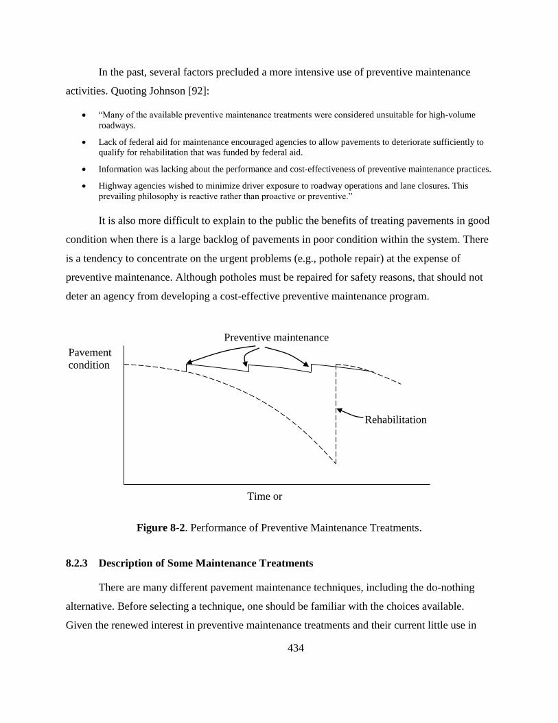
434

In the past, several factors precluded a more intensive use of preventive maintenance

activities. Quoting Johnson [92]:

“Many of the available preventive maintenance treatments were considered unsuitable for high-volume

roadways.

Lack of federal aid for maintenance encouraged agencies to allow pavements to deteriorate sufficiently to

qualify for rehabilitation that was funded by federal aid.

Information was lacking about the performance and cost-effectiveness of preventive maintenance practices.

Highway agencies wished to minimize driver exposure to roadway operations and lane closures. This

prevailing philosophy is reactive rather than proactive or preventive.”

It is also more difficult to explain to the public the benefits of treating pavements in good

condition when there is a large backlog of pavements in poor condition within the system. There

is a tendency to concentrate on the urgent problems (e.g., pothole repair) at the expense of

preventive maintenance. Although potholes must be repaired for safety reasons, that should not

deter an agency from developing a cost-effective preventive maintenance program.

Figure 8-2. Performance of Preventive Maintenance Treatments.

8.2.3 Description of Some Maintenance Treatments

There are many different pavement maintenance techniques, including the do-nothing

alternative. Before selecting a technique, one should be familiar with the choices available.

Given the renewed interest in preventive maintenance treatments and their current little use in

Pavement

condition

Time or

traffic

Preventive maintenance

Rehabilitation

435

Hawaii, the list below provides an brief description of several techniques falling in that

preventive category (the only exception is pothole patching, which is an emergency repair.).

Most of the following descriptions are adopted with minor modifications from Minnesota [92]

and Michigan [93] manuals.

Crack sealing. A localized treatment method used to prevent water and debris from

entering a crack, which might include routing to clean the entire crack and to create a reservoir to

hold the sealant. It is only effective for a few years and must be repeated. However, this

treatment is very effective at prolonging the pavement life. It typically includes the following

two crack repair methods:

Clean and seal: Used on all types of cracks, it involves using a hot air lance or compressed

air to blow out the debris in the crack, then filling with a sealant.

Route and seal: Used on transverse and longitudinal cracks. It involves using a pavement

saw or router to create a reservoir centered over existing cracks, and then

filling with a sealant.

Crack filling: Differs from crack sealing mainly in the preparation given to the crack

prior to treatment and the type of sealant used. Crack filling is most often reserved for more worn

pavements with wider, more random cracking.

Full-depth crack repair: A localized treatment method to repair cracks that are too

deteriorated to benefit from sealing or filling. Secondary cracking requires the reestablishment of

the underlying base materials.

Fog seal: An application of diluted emulsion (typically at a rate of 1:1) to enrich the

pavement surface and delay raveling and oxidation. This is considered a temporary treatment.

Chip seal/Seal coat: Used to waterproof the surface, seal small cracks, reduce oxidation

of the pavement surface, and improve friction.

Double chip seal: An application of two single seal coats/chip seals. The second coat is

placed immediately after the first. This treatment waterproofs the surface, seals small cracks,

reduces oxidation of the pavement surface, and improves friction.

436

Slurry seal: A mixture of fine aggregate, asphalt emulsion, water, and mineral filler,

used when the primary problem is excessive oxidation and hardening of the existing surface.

Slurry seals are used to retard surface raveling, seal minor cracks, and improve surface friction.

Microsurfacing: Microsurfacing is a mix of polymer-modified emulsion, well-graded

crushed mineral aggregate, mineral filler (normally Portland cement), water, and chemical

additives that control the break time. Microsurfacing differs from slurry seals in that it uses

polymer modified asphalt and in that the curing process for microsurfacing is a chemically

controlled process, versus the thermal process used by slurry seals and chip seals.

Microsurfacing also may be used to fill ruts [92].

Thin hot-mix asphalt (HMA) overlays: These include dense, open, and gap-graded

HMA mixes that improve ride quality, reduce oxidation of the pavement surface, provide surface

drainage and friction, and correct surface irregularities.

Pothole patching: Includes using cold- and hot-asphalt concrete mixture, spray injection

methods, as well as slurry and microsurfacing materials, to repair distress and improve ride

quality.

8.3 Commonly used PMS Software

Many public and private domain programs are available. A good summary of the

capabilities of most of these programs is provided by Wolters et al. [89]. The public domain

programs included in their review are:

1) MicroPAVER® (now named PAVERTM) (U.S. Army Corp of Engineers),

2) RoadSoft® (Michigan Tech Transportation Institute at Michigan Technological

University),

3) StreetSaver® (Metropolitan Transportation Commission of the San Francisco Bay

Area, California), and

4) The Utah LTAP Transportation Asset Management System (TAMS).

437

The private software programs reviewed by these authors are:

1. PAVEMENTview and PAVEMENTview Plus by Cartegraph,

2. PavePRO Manager by Infrastructure Management Services,

3. PubWorks by Tracker Software Corporation, and

4. RoadCare by Applied Research Associates, Inc.

Table 8-1 reproduces the comparison provided by Wolters et al. [89] of the various

features of these eight PMS software programs. Additional details of each program are provided

in [89]. Some of the information in Table 8-1 should be looked with caution as it may be

outdated. In particular, this is known to be the case for the cost information.

Probably because the report of Wolters at el. [89] was geared towards PMS

implementations for local agencies, widely used enterprise asset management systems, such as

those of Deighton [94] and Agile Assets [95], were not included in their review. These two

companies provide PMS modules with capabilities rivaling those of any of the systems

mentioned above and can also be integrated with other asset management modules (signs,

markings, culverts, etc.) offered by the same companies. Allegedly, they also allow optimal

allocation of resources across different asset classes64 and can be integrated with work order

systems. Furthermore, these companies also provide services to maintain the databases and

implement the systems, such as customization, configuration, user interface development,

training, etc.

64 These claims have not been evaluated and it is beyond the scope of this project.

438

Table 8-1. Comparison of Pavement Management Software Features (Source: [89]).

Criterion

Description

PAVEMENT MANAGEMENT SOFTWARE PROGRAMS

PUBLIC PRIVATE

MicroPAVER RoadSoft GIS Utah LTAP TAMS StreetSaver RoadCare PAVEMENTview

Plus PubWorks PavePro Manager

Vendor U.S. Army Corps of

Engineers

Michigan

Technological University – Center

for Technology &

Training

Utah Local Technical

Assistance Program

Metropolitan Transportation

Commission

Applied Research

Associates Cartograph

Tracker Software

Corporation

Infrastructure

management Services

Website www.apwa.net www.roadsoft.org www.utahltap.org www.mtcpms.org www.ara.com www.cartegraph.com www.pubworks.com www.ims-rst.com

Laptop Data

Collection Yes Yes Yes

Additional Program

Needed * Yes Yes *

Ability to Analyze

Other Assets No

Yes, signs, pavement

markings, traffic

counts, and traffic crashes

Yes

Yes, sidewalks,

lights, signs, curb and

gutter, & user defined.

* Yes, sewer, signal,

sign storm, bridge, &

lights

Yes, bridges, signs, culverts, guardrails,

parks, & buildings.

*

Default Pavement

Condition Rating

Measure

PCI PASER RSL PCI PCI, IRI OCI PASER *

Analyzes Different

Maintenance

Strategies

Yes Yes Yes Yes Yes Yes No Yes

GASB 34

Reporting No Yes No Yes * Yes Yes *

GIS Integration Yes Yes Additional Software

Needed

Additional Software

Needed

Additional Software

Needed

Additional Module-GIS director or own

software

Addition module

MapViewer needed

Additional Software

Needed

Customization

Capabilities Yes Only certain aspects Yes Yes * *

Additional modules available

Additional modules available

Costs (2011)

APWA members

$995; non-members $1095

Contact vendor for

more information

Utah-free/Out of state

$500

$1500+, contact

vendor for more information

Varies, contact

vendor

Varies, contact

vendor

Varies, contact

vendor

Varies, contact

vendor

User’s Manual Yes Yes Yes Yes * Yes Yes *

Technical

Assistance

Training courses or

four-part web-based training

Telephone or web-

based training

Free Telephone or

paid on-site arrangements

4-day training class twice per year and

customized on-site

training.

*

On-site or web based

training, technical support by phone

Formal training at 1 day per module, free

updates, software

helpdesk

*

http://www.apwa.net/

439

Consideration of different assets and training opportunities are also true for some of the

other programs in Table 8-1. For example, RoadSoft® also includes modules for other assets and

MTU (Michigan Technological University) provides services and training.

The programs listed above are by no means an exhaustive list of options for managing

pavement networks. Two important programs not included above are the Highway Development

and Management Model (HDM-4) and the Highway Economic Requirements System - State

Version (HERS-ST).

HDM-4 [96] is the successor of HDM-3 (the Highway Design and Maintenance Model)

developed by the World Bank. This is one of the most commonly used PMS programs in the

world because it is required for evaluation of projects financed by the World Bank. It is based on

rigorous economic principles where costs and benefits are compared using decision criteria such

as Net Present Value and Internal Rate of Return. It includes agency and user costs (vehicle

operating costs and delay costs.)

HDM-4 does not appear to have been used much in the US perhaps because their

pavement deterioration models, speed prediction models, and vehicle operating costs models

were developed from large scale research projects funded by the World Bank in developing

countries. An interesting feature of HDM-4 is that models individual distresses separately.

In the US, a tool that is available for all states is the Highway Economic Requirement

System – State Version (HERS-ST) [97]. Reference [97] describes it as:

“HERS-ST is an engineering/economic analysis (EEA) tool that uses engineering standards to identify

highway deficiencies, and then applies economic criteria to select the most cost-effective mix of

improvements for system-wide implementation. HERS-ST is designed to evaluate the implications of

alternative programs and policies on the conditions, performance, and user cost levels associated with

highway systems.”

HEST-ST does incorporate many of the elements of PMS systems and similarly to HDM-

4, it accounts for things such as travel time, safety, and vehicle operating and emissions costs

that are not part of some other PMS systems. It uses a rigorous incremental benefit cost analysis

to optimize highway investment. It also uses travel forecasts for each highway facility included

in the Highway Performance Monitoring System (HPMS) sample database to predict future

pavement and capacity deficiencies ( [97], [98]).

440

The HERS-ST program was studied at the beginning of this project but it was determined

that it was more appropriate for long term planning. Pavement deterioration predictions in

HERS-ST [99] are based on structural number (SN) for flexible pavements or the slab thickness

(D) for rigid pavements, on the present serviceability rating (PSR), and on the deterioration

models of the AASHTO 1993 Design Guide [12]. Since the program assumes a one-to-one

relationship between PSR and roughness (IRI), IRI could be used instead of PSR.

Although the program provides for a large number of highway improvements (e.g.,

addition of lanes and highway re-alignments), it considers only two pavement treatments:

resurfacing and reconstruction. It is not clear how other pavement preservation treatments could

be considered. Thus, it appears that the analysis is too coarse at this time for some desirable PMS

activities. Nevertheless, if the program were updated to incorporate the new HPMS data fields

[9] and improved to account for some of the factors mentioned above, it could be a viable and

low cost alternative.

With the varied capabilities of the different programs, it is clearly not possible to say that

one program is better than another in all respects. Preference for implementation of one program

over another depends on many factors, many of which are non-technical: implementing agency

goals; upper level management commitment to implementation; budget allocated for software

purchase, maintenance, and service; internal organizational structure; intended users of the

system (centralized, at the county level, or combination); database location, security and

availability within districts; current data availability and future commitments for data collection;

preferences for quantifying pavement condition; etc.

Early in the project, consideration of the expertise of HDOT’s Materials Testing and

Research Branch personnel assigned to work on the PMS and suggestions by one of the project

managers together with the understanding of the resources already available at the Planning

Branch led to the selection of three of the above systems for further study: StreetSaver®,

RoadSoft®, and PAVERTM. Two of these (StreetSaver® and PAVERTM ) are self-contained

PMS programs and the other (RoadSoft®) can deal with several assets, including pavements. All

three have a relatively low purchase cost and annual renewal cost. The following section

describes these programs in more detail.

441

Before turning attention to these programs, it is important to note that the recent

enactment of the MAP-21 legislation, the Moving Ahead for Progress in the 21st Century Act,

signed into law on July 6, 2012, has revived the interest on the PMS and other asset management

systems. This project started prior to the enactment of this legislation and its focus was on self-

contained PMS software that could be implemented at HDOT’s Materials and Research Testing

(MT&R) Branch. Nevertheless, prior to MAP-21, the principal investigator consulted with the

project manager at the time (around 2007-2008) about pursuing the study of the Deighton system

in detail. However, not much interest in pursuing this possibility was shown at that time. Clearly,

such systems cannot be evaluated without significant involvement from the agency. Therefore,

this possibility was not evaluated further. Nevertheless, MAP-21 may have made the

consideration of these enterprise systems more appealing since within 18 months of enactment, a

process will be published for States to use in developing a risk-based, performance-based asset

management plan for preserving and improving the condition of the National Highway System

(NHS). Thus, the need to consider different assets and the risk of losing funding because of not

meeting performance standards has made the investment on more comprehensive albeit more

expensive asset management system software more attractive. However, considering the current

personnel expertise, it is unlikely that if one of such system is selected it could be maintained at

the MT&R branch without support from other branches.

8.4 PMS Software Evaluated

For this project, several options were considered. As indicated earlier, at the beginning of

the project consideration was given to Asset Management Software such as dTIMS CT (Version

8) by Deighton [94]. At that time, it was implemented in seventeen State DOTs in the US and

twenty one Canadian municipalities. They had 250 users worldwide. Several of the features

claimed by the vendor include: data integration, centralized data management, client definable

framework integrating client business processes, interaction with maintenance management

systems, centralized data base, reporting via LAN or Web, cross asset optimization, advanced

reporting and charting capabilities, and integration with GIS. The current version of this software

is Version 9. However, in addition to the lack of interest on this software by the project manager

(at the time this was suggested), it was not clear what data were available to feed the program, it

represented a relatively high investment, and it would have required additional commitments

442

from different branches of HDOT. For all the above reasons the software in the end was not

evaluated.

The licenses for three different programs were acquired at different points throughout the

project: StreetSaver®, RoadSoft®, and PAVERTM. The following subsections provide more

details about these. The length of the descriptions are related to how much was accomplished

with each program for the reasons described in each case.

8.4.1 StreetSaver®

The first version of StreetSaver® was released in 1987 by the Metropolitan

Transportation Commission (MTC) – the transportation planning, financing and coordinating

agency for the nine-county San Francisco Bay Area, California [100]. In the more than two

decades that StreetSaver® has been in use, there have been 109 users in the San Francisco Bay

Area and more than 250 users nationwide and internationally [100].

In the past, StreetSaver® was a standalone program. However, the current version of the

program, Version 9, is offered online. That is, the user interface is accessed through a web

browser. Furthermore, the SQL Server database used by the program resides on MTC servers.

This has the advantage of releasing the users of server maintenance and security.

StreetSaver® utilizes a modified version of ASTM Standard D 6433 to identify seven (7)

distresses and three (3) severity levels to calculate the condition of pavements surfaced with

asphalt concrete and surface treatments. The distress types are: 1) alligator cracking, 2) block

cracking, 3) distortions, 4) longitudinal & transverse cracking, 5) patching & utility cuts,

6) rutting and depressions, and 7) weathering & raveling.

For Portland cement concrete (PCC) pavements, the distresses considered include:

1) corner break, 2) divided slab, 3) faulting, 4) linear cracking (longitudinal, transverse and

diagonal cracks), 5) patching and utility cuts, 6) scaling/map cracking/crazing, and 7) spalling.

Based on the above distresses, StreetSaver® computes the pavement condition index

(PCI) to measure the condition of a given section of pavement on a scale from 0 to 100, with 100

representing a pavement in excellent condition (see section 4.3.1.1.1, page 133) for a brief

description of the PCI calculation.

443

StreetSaver® provides real-time PCI (i.e., computed based on existing distresses) and

projected PCI based on projected deterioration and future treatment strategy on each road

segment, as well as overall road network.

The prediction of PCI over time is based on the last observed PCI combined with the

deterioration curve of the family to which a pavement section belongs. Pavement sections are

assigned to different pavement families based on their surface type (AC, AC/AC, ST, AC/PCC,

PCC, and Gravel) (Figure 8-3) and on their functional classification (Arterial, Collector,

Residential, and Other). The meaning of the symbols for surface types above (other than Gravel,

that has an obvious meaning) are: AC = Asphalt Concrete, AC/AC = Asphalt Concrete Overlay

over Asphalt Concrete, ST = Surface Treatment (e.g., chip seal, slurry seal, or microsurfacing),

AC/PCC = Asphalt Concrete over Portland Cement Concrete, and PCC = Portland Cement

Concrete.

Figure 8-3. Surface types in StreetSaver®.

StreetSaver® uses the computed PCIs and the pavement families’ deterioration curves to

predict the future condition of each pavement section. The equation used to model deterioration

(i.e., PCI vs. Age) is:

444

1

ln

100

Age

PCI

(8-1)

where , , and are model parameters.

The parameter controls the age at which the PCI is projected to reach zero, the

parameter controls how sharp the curve bends, and the parameter controls the location of the

curve inflexion point [7].

Budget needs and budget consequences are determined with the help of decision trees. As

shown in Figure 8-4, in StreetSaver® different condition categories (I, II, III, IV, and V) are

defined for each surface type (AC, AC/AC, AC/PCC. ST, and PCC) within a given highway

functional classification (Arterial, Collector, Residential/Local, and Other). For each of the

condition categories shown in Figure 8-4, the suggested treatment as well as the cost per unit

area (or per unit length for crack sealing) and the number of years between treatments must be

defined (this is done is a separate form not shown here.) Then, based on these decision trees, the

program can determine budget needs to maintain the network at the optimal level over an

analysis period (commonly 5 years, but the program can analyze up to 30 years). The use of the

word “optimal” here needs clarification as it depends on whether the decision trees are the most

appropriate for the types of pavements analyzed. Note that no “optimization” is really carried out

in the budget needs analysis but instead appropriate treatments are identified when each section

reaches threshold values in the corresponding decision tree. The premise is that with enough

funding, it is cheaper to maintain pavements in good condition. When budgets are constrained,

weather a treatment is applied to a given section when it reaches a trigger value depends on the

availability of funds and the prioritization described next.

It is important to note that the user has control over what constitute the different

condition categories (Figure 8-5).

The budget needs analysis can then be used to analyze several budget scenarios.

Typically, funding is insufficient to address the budget needs. Therefore, some form of

prioritization needs to be carried out to allocate a given budget. For this purpose, StreetSaver®

445

computes a Weighted Effectiveness Rating (WER) for each treatment assigned and ranks the

sections by WER, from highest to lowest.

The effectiveness rating is based on the ratio of the expected effectiveness65 for the

identified maintenance and rehabilitation treatment per year of influence to their equivalent

uniform annual cost per square yard adjusted by a weighting factor. The user is allowed to

specify different weighting factors based on functional classification to account for the fact that it

is generally less costly to repair residential/local streets, and that in general, they will have longer

lives than arterial streets. These weighting factors avoid that all the funding be allocated to

streets of lower categories by essentially weighting for roadway usage.

Figure 8-4. Decision tree definition in StreetSaver®.

65 Effectiveness is typically defined by the area under the deterioration curve.

446

Figure 8-5. Definition categories in StreetSaver®.

StreetSaver® provides the capability to analyze different “Budget Scenarios”. For a

budget scenario, sections are selected for rehabilitation treatments from the ranked list obtained

from the needs analysis until the funds available for rehabilitation projects (equal to the total

budget for the year minus the portion reserved for preventive maintenance) have been allocated.

The program then totals the amount of deferred maintenance (rehabilitation only), and estimates

stop gap costs. The amount of stop gap costs is subtracted from the preventive maintenance

budget and then sections are selected for preventive maintenance treatments from the previously

developed ranked list. Finally, the program totals the amount of deferred preventive

maintenance.66 These “Budget Scenarios” calculations can be used to determine the impact of

various funding strategies.

Other features of StreetSaver® include “Project Selection Analysis” that assists users in

translating network pavement repair recommendations into contract packages, XML (extended

markup language) importing and exporting of inspections or inventory data from 3rd party

software vendors, attachment of supplemental documents (JPG, PDF, Rich Text (.rtf), Word

66 It is important to note that the user can define what treatments constitute preventive maintence. The

above is just a general explanation of the logic used by the program. It is not intended to describe all the options

available.

447

(.doc), Excel (.xls), and MPEG) to provide background information to each individual road

segment, and up to 10 customized user-defined fields. The program also provides the capability

to generate more than 40 standard reports and graphs, customized reports utilizing a built-in

“Custom Report Wizard”. Reports can also be exported to various formats (e.g., .xls, .rtf, .txt,

PDF, and MDB). In addition, the program has a GASB 34 reporting module to facilitate the

reporting of pavement assets to comply with the requirements of the Government Accounting

Standard Board’s Statement 34 (GASB 34) .

StreetSaver® also provides a GIS Toolbox to allow users to link their street networks to a

GIS basemap so that they can display and plot results graphically.

A companion software to StreetSaver®, MobileRater™, is available to assist with the

collection of pavement distress data with handheld computers. MTC offers several user services

such as virtual on-site and hotline support and training workshops. In addition, it holds a User

Week event three times a year (typically in Oakland, California): in March, July and November.

The current cost of the annual license of StreetSaver® outside the San Francisco Bay

Area is $1,500 ($2,000 for consultants.) There are additional costs for a Software Support

Service Plan, a Technical Support Plan, GIS Mapping Integration, Data Migration, and the

MobileRaterTM license. The up-to-date costs can be found at http://www.mtcpms.org/products/.

Compared to the costs needed to adequately feed any PMS, the above costs are relatively minor.

As part of this research project, the license for this program was paid for a period of two

years (2007-2009). Unfortunately, at the time, there was little reliable data to define the

sectioning of the network (see the description of the efforts in this respect in the PAVERTM

description below) and the corresponding pavement conditions. Consequently, most the program

features were not evaluated with actual data.

8.4.2 RoadSoft®

8.4.2.1 General

RoadSoft® is a roadway asset management system for collecting, storing, and analyzing

data associated with transportation infrastructure [101]. The Michigan Tech Transportation

Institute at the Michigan Technological University (MTU) began its development in 1992 on

input and guidance from local road agencies in Michigan. According to [89], clients of

http://www.mtcpms.org/products/

448

RoadSoft® include the Michigan Department of Transportation, Federal Highway

Administration, over 200 cities and villages, and almost 100 county road agencies in Michigan

and throughout the U.S.

Roadsoft® is built on a combination of a database engine and GIS mapping tools. Figure

8-6 shows the main interface of the version of RoadSoft evaluated in this project (V7.2.0.7). As

shown in that figure, in addition to pavements (as indicated by the layer “Road”), RoadSoft®

considers other assets such as culverts, point pavement markings, signs, traffic counts,

driveways, sidewalks, and linear pavement markings. Furthermore, according to [101], other

assets or data now considered include bridges, crash data, and intersections.

Figure 8-7 shows a screenshot of part of the culvert module and Figure 8-8 shows a

screenshot of part of the sign module. Each module contains many more associated windows and

details not explained here.

Figure 8-6. RoadSoft® main interface.

449

Figure 8-7. RoadSoft® culver module.

Figure 8-8. RoadSoft® sign module.

450

8.4.2.2 Inventory and Condition

In RoadSoft®, several pieces of information can be stored. Assets are located in reference

to a base map. As illustrated later, in some of its screens, RoadSoft® uses information about

cross streets to more easily locate segments. This is a very nice feature of the program but, at

least for the version evaluated, it comes at the cost of depending on MTU for its creation and

modification. A discussion of this issue is presented later.

Figure 8-9 shows a portion of the base map created by MTU for Hawaii based in part on

shapefiles provided by HDOT to the Hawaii Statewide GIS Program in 2011 [102]. Those

familiar with Hawaii’s State Roads network can recognize that the base map includes much more

than just State roads. Once a road segment or set of roads segments are selected by the user,

clicking on the View Module button (see the second to last button on the toolbar above the map

in Figure 8-9) brings up the Road module screen shown in Figure 8-10, which is where the

inventory and condition information is entered.

Figure 8-9. Illustration of part of the RoadSoft® base map with a selection set corresponding to

the westbound direction of H-1.

451

Figure 8-10. RoadSoft® Road module with Inventory Segment tab selected.

At the top-left corner of Figure 8-10, there is a list box (displaying two items in this

example.) The items in the list box are the roads for which the user selected at least one segment

in the base map in Figure 8-9. For the particular example of Figure 8-10 only two roads were

selected. The list box is labeled with the text “PR”, which represents a unique number assigned

to each Physical Road. Below this list box, there is a chart with three vertical lines, each

representing the linear referencing for inventory segments, surface segments, and rating

segments, respectively. In this chart, the horizontal lines represent the location of cross-roads and

provide a visual cue for users to easily locate segments of interest. As shown in Figure 8-10, for

long roads, the information about the cross streets can become cluttered. Fortunately, the

program also provides zooming and panning capabilities to overcome this issue. As shown in

Figure 8-11, the user can zoom to a level where there is no more clutter on the cross street

information.

The three vertical lines correspond to the three tabs located to the right of the “PR” list

box, which are used for entering information about inventory, surface type, and rating segments.

452

The information for each segment on each tab is discussed shortly. The location of these

segments (or more appropriately, their endpoints) are created independently for each tab. Thus,

for example, the segmentation for inventory may be different from that for surface type and

rating segment. This is a very convenient feature, for example, to deal with pavement condition

information collected every 0.1 mi (as currently contracted by HDOT). Such information can be

entered in RoadSoft® regardless of how the inventory and surface type segments are defined.

As can be observed from Figure 8-10, the inventory information for each segment

consists of identification information (e.g., labels for the end points) and physical design

characteristics such as surface width, number of lanes, and year of last resurface. In addition, at

the bottom of the form, there are different tabs that permit the user to enter information in a

memo form as well as shoulder information (surface types and width), curb and gutter

information (type, curb reveal, configuration, year built, rating, and rating year), traffic counts,

and traffic volumes. The surface width together with the actual length of the segments (taken

from the actual end points) are fundamental to compute costs when analyzing funding strategies.

Figure 8-11 displays some of the information shown in the Surface Type tab. Again, the

user can enter a description for the endpoints of the segments (“From” and “To” descriptions)

and select the surface type (asphalt, brick, composite, concrete, graded earth, gravel-standard,

seal coat-standard, undefined, or unimproved earth). The form displays actual material types and

thicknesses for each layer (Surface, Base, Subbase, and Subgrade) as well as information about

geotextiles, traffic loading in term of ESALs, and structural number. Input of the aforementioned

information is actually performed in another form, Figure 8-12, that is accessed by selecting the

“Edit Design Characteristics” button shown on Figure 8-11. The types of materials in the

Pavement Design form can be easily configured based on agency practices. As shown in Figure

8-12, it is easy to configure the program to accept the labels of local mixes such as State Mixes

II, III, IV, and V.

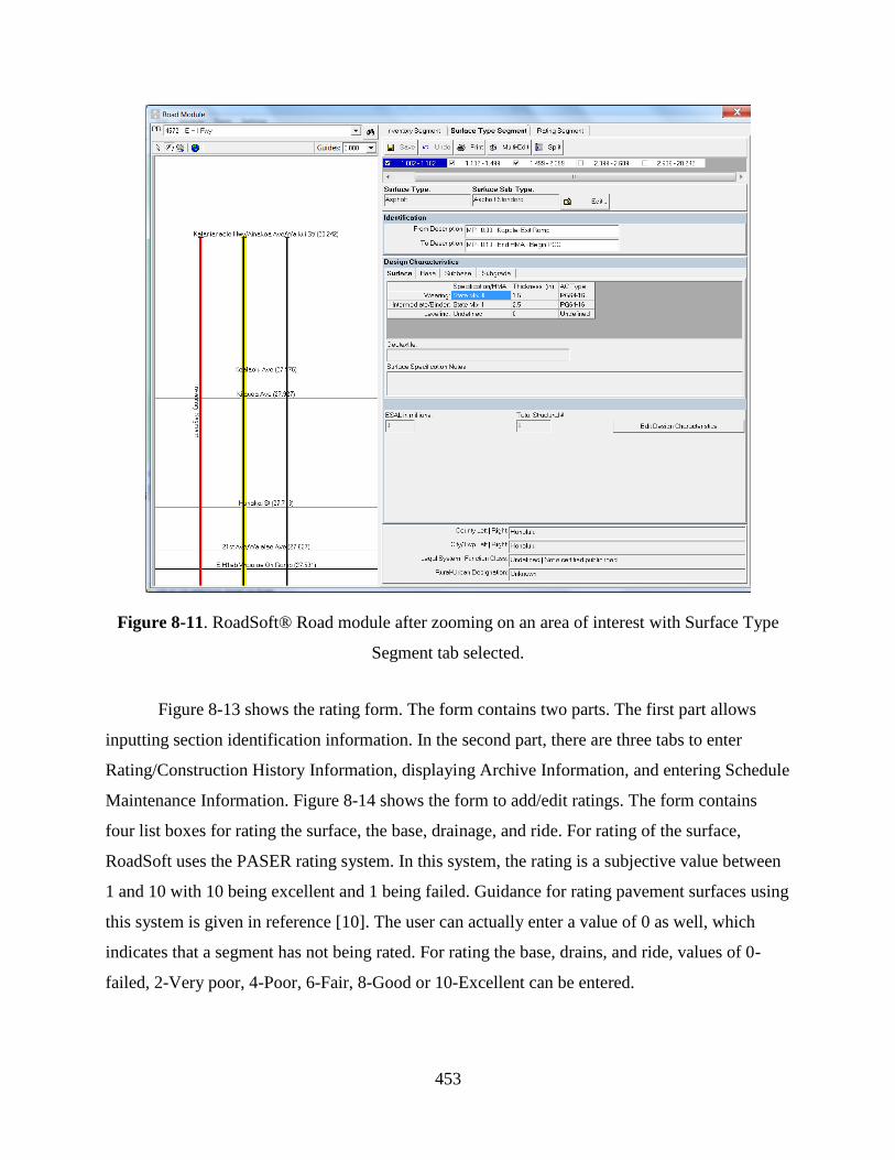
453

Figure 8-11. RoadSoft® Road module after zooming on an area of interest with Surface Type

Segment tab selected.

Figure 8-13 shows the rating form. The form contains two parts. The first part allows

inputting section identification information. In the second part, there are three tabs to enter

Rating/Construction History Information, displaying Archive Information, and entering Schedule

Maintenance Information. Figure 8-14 shows the form to add/edit ratings. The form contains

four list boxes for rating the surface, the base, drainage, and ride. For rating of the surface,

RoadSoft uses the PASER rating system. In this system, the rating is a subjective value between

1 and 10 with 10 being excellent and 1 being failed. Guidance for rating pavement surfaces using

this system is given in reference [10]. The user can actually enter a value of 0 as well, which

indicates that a segment has not being rated. For rating the base, drains, and ride, values of 0-

failed, 2-Very poor, 4-Poor, 6-Fair, 8-Good or 10-Excellent can be entered.

454

Figure 8-12. Pavement Design information form.

In the Rating Segment tab, the user may also record the activities performed to a given

segment as shown in Figure 8-15. As indicated earlier, RoadSoft® is very flexible, allowing

ratings at every 0.1-mi segment, as currently collected by the HDOT’s Planning Branch.

However, most often, activities would be performed over segments much longer than 0.1-mi

long. RoadSoft® helps in this respect by providing a Rating Segment Multi-Edit option. Thus,

the user does not need to enter the activity information on every 0.1-mi segment.

Within the rating segments tab, RoadSoft® provides the option of entering and editing

schedule maintenance activities. This is shown in Figure 8-16.

So far, all the discussion has been about entering information for inventory, surface type,

and rating segments but no explanation has been provided about how those segments are defined.

Initially, each route (a single PRNo in RoadSoft®) constitutes a single segment. The user can

then use the “Split” button (shown in Figure 8-10, Figure 8-11, and Figure 8-13) to split a

segment into two. Actually, selecting split provides three options: splitting of a segment,

adjusting an existing split, or merging segments. Only the splitting option is discussed here.

455

Figure 8-13. RoadSoft® Road module with Rating Segment tab selected.

Figure 8-14. Add/Edit Rating form.

Figure 8-15. Add/Edit Activity form.

456

Figure 8-16. Editing Scheduled Maintenance.

The Split Inventory Segment form (shown in Figure 8-17), provides a visually attractive

and intuitive way to create segments. The user can drag the splitting point either in the map or in

the straight line diagram next to it. In either case, the point is updated simultaneously in the other

graph and in the text box at the bottom. Alternatively, the user can also enter a value in the text

box to define more precisely the splitting point.

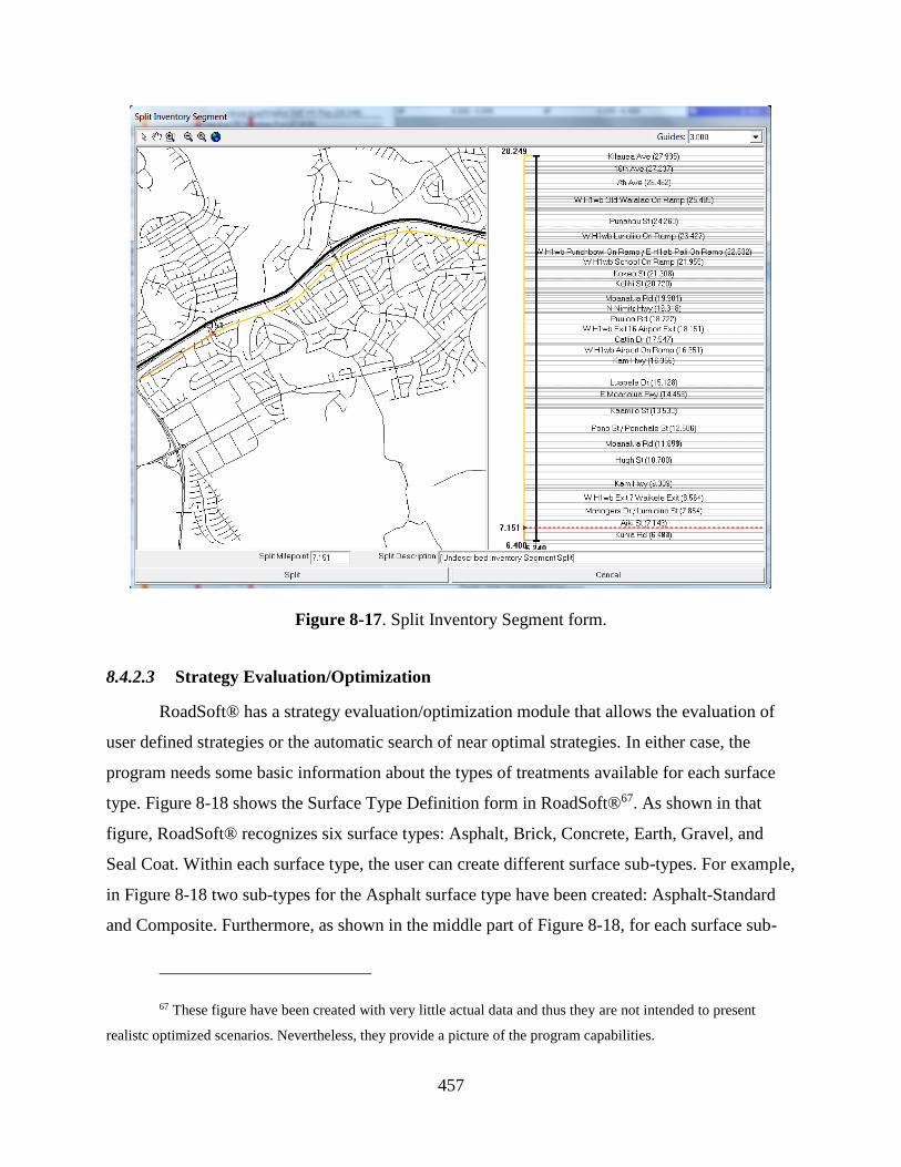
457

Figure 8-17. Split Inventory Segment form.

8.4.2.3 Strategy Evaluation/Optimization

RoadSoft® has a strategy evaluation/optimization module that allows the evaluation of

user defined strategies or the automatic search of near optimal strategies. In either case, the

program needs some basic information about the types of treatments available for each surface

type. Figure 8-18 shows the Surface Type Definition form in RoadSoft®67. As shown in that

figure, RoadSoft® recognizes six surface types: Asphalt, Brick, Concrete, Earth, Gravel, and

Seal Coat. Within each surface type, the user can create different surface sub-types. For example,

in Figure 8-18 two sub-types for the Asphalt surface type have been created: Asphalt-Standard

and Composite. Furthermore, as shown in the middle part of Figure 8-18, for each surface sub-

67 These figure have been created with very little actual data and thus they are not intended to present

realistc optimized scenarios. Nevertheless, they provide a picture of the program capabilities.

458

type, the user can define the type of treatments that can be performed as well as the information

needed for evaluating/optimizing strategies (trigger values and costs).

Figure 8-19 shows the screen where the user specifies which treatments to use for

optimizing a strategy as well as the inflation rate, the number of years to program, and the

budget. Running the optimization results in output such as that shown in Figure 8-2068, which

includes the cost by year, percent of good, fair, and poor by year, lane miles of activity

performed by year, and average remaining service life by year.

Clearly, for the selection and evaluation of strategies, the program needs to predict the

pavement condition over time. As with other PMS software, RoadSoft® uses the concept of

pavement families. As seen at the bottom of Figure 8-18, for each surface sub-type the user must

associate a “curve” (meaning a deterioration curve). Deterioration curves are defined as shown in

Figure 8-21, in which the number of years that pavements in the family stay in each condition

rating must be specified. The user can select among different types of models to fit to the data

(Gompertz forced through zero, Gompertz unforced through zero, Logistic Growth forced

through zero, Logistic Growth unforced through zero, and Sigmoid S curve).

In one of the approaches used by RoadSoft®, the family curve is adapted for each section

to the deterioration observed over time on the particular section. This is illustrated in Figure

8-22.

8.4.2.4 Reporting

Since RoadSoft® is built on GIS mapping tools, it is relatively easy to create map reports

identifying features of interest such as pavement conditions, surface types, remaining service

life, etc. In addition, the program also provides the capability of creating tabular road reports that

are configurable by the user. In order to create and/or edit reports, users need some basic

understanding of database queries (as is the case for most PMS software) (Figure 8-23).

68 Note again that the screenshot was created without almost no data in the program, which explains the

very small mileages shown in the figure and the single bar in the cost by year chart.

459

Figure 8-18. Surface types and treatment data in RoadSoft®.

8.4.2.5 Issues to Overcome for Implementation

In general, RoadSoft® presents a very attractive alternative. However, for

implementation, a few issues need to be considered and studied in more detail.

The main issue found during the evaluation of the program is a common PMS problem,

which is appropriately locating pavement sections. As indicated earlier, as currently

implemented, the base map and associated database for RoadSoft® is created by MTU based on

information provided by the user. For the evaluation in this study, the shapefiles provided by

HDOT to the Hawaii Statewide GIS Program in 2011 [102] were provided to MTU.

After the first delivery, it was noted that the base map in RoadSoft® did not agree in

some respects with the shapefiles given to MTU. Specifically, according to the base map in

RoadSoft®, H-1 was approximately 8 miles long, whereas in the shapefile and HDOT’s RIS H-1

is 27.16 mi long.

460

Figure 8-19. Strategy Evaluation/Optimization screen in RoadSoft®.

After discussions with the vendor, it was acknowledged that there had been a problem in

the data translation algorithm. Thus, a new database with a new base map was provided to UH.

Unfortunately, some issues were also discovered with the new delivery. Specifically, as

illustrated in Figure 8-11 (page 453), H-1 is shown as being 28.24 miles long, which is still more

than one mile longer than it actually is. A careful analysis of the new base map revealed that the

problem with the second database was not with the geometry but with the definition of when a

road starts or ends. For the H-1 example, a 1.082-mi long portion of State Route 93 had been

assigned as being part of H-1 (conversely, State Route 93 was shorter that it should have been by

the same amount.)

461

Figure 8-20. RoadSoft® strategy evaluation results.

The issue described above is a perfectly solvable problem but it needs coordination

between the vendor and HDOT (with the associated additional service costs that this would

entail) if the program is considered further for implementation.

Note that the distress would be located appropriately if the Laptop Data Collector created

by MTU together with a GPS unit is used. Also, one could easily enter an offset to define the

segment into their appropriate locations. For example, for the selected segment on Figure 8-16

(page 456), which goes from mile points 1.082 to 1.182, the “From” and “To” descriptions were

entered as MP+ 0.00 and MP+ 0.10, respectively, which is the results of using an implicit offset

of 1.082 miles. However, these “fixes” would most likely results in errors (it is easy to get

confused whether an offset has to be added or subtracted, forgetting that an offset needs to be

applied, etc.) and require unnecessary additional bookkeeping.

462

Figure 8-21. RoadSoft® family deterioration curve definition.

Figure 8-22. RoadSoft® deterioration curve for a given section.

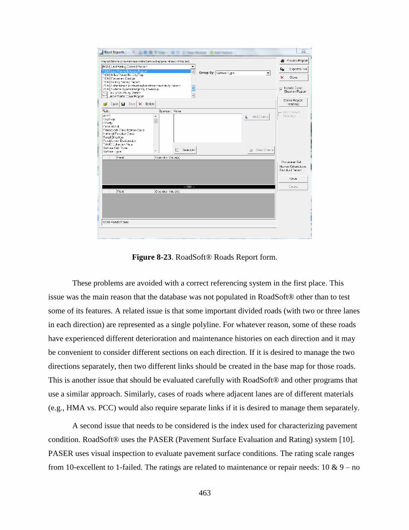
463

Figure 8-23. RoadSoft® Roads Report form.

These problems are avoided with a correct referencing system in the first place. This

issue was the main reason that the database was not populated in RoadSoft® other than to test

some of its features. A related issue is that some important divided roads (with two or three lanes

in each direction) are represented as a single polyline. For whatever reason, some of these roads

have experienced different deterioration and maintenance histories on each direction and it may

be convenient to consider different sections on each direction. If it is desired to manage the two

directions separately, then two different links should be created in the base map for those roads.

This is another issue that should be evaluated carefully with RoadSoft® and other programs that

use a similar approach. Similarly, cases of roads where adjacent lanes are of different materials

(e.g., HMA vs. PCC) would also require separate links if it is desired to manage them separately.

A second issue that needs to be considered is the index used for characterizing pavement

condition. RoadSoft® uses the PASER (Pavement Surface Evaluation and Rating) system [10].

PASER uses visual inspection to evaluate pavement surface conditions. The rating scale ranges

from 10-excellent to 1-failed. The ratings are related to maintenance or repair needs: 10 & 9 – no

464

maintenance required, 8 – little or no maintenance, 7 – routine maintenance, crack sealing and

minor patching, 6 & 5 – preservation treatments (sealcoating), 4 & 3 – structural improvements

and leveling (overlay or recycling), and 2 & 1 – reconstruction. In contrast, HDOT has been

collecting individual distresses and during the last few years computing the Pavement Condition

Index (PCI). Thus, use of RoadSoft® would require either a change of rating system or the

conversion of PCI into an index from 1 to 10.

Note that the ratings in RoadSoft® are discrete (that is, an integer from 1 to 10.) This is

consistent with how PASSER defines the ratings. However, the restriction to integer ratings from

1 to 10 is an important consideration if one wanted to use this program with a different rating

system such as PCI. In addition to dividing the index by 10, the values would have to be rounded

to integer values. More importantly, it must realized that the two indices may not be directly

comparable. For example, for PCI values below 60 or 55, typically no preservation treatments

would be recommended. On the other hand, a section with a PASER rating of 5 is still a

candidate for treatments such as seal coats. Therefore, if such procedure were use, most likely

different trigger values would need to be used. Finally, this may also have some consequences

for the contracts for pavement distress data collection. Nevertheless, since HDOT has partnered

twice with the county of Hawaii to collect data using using the PASER system, collecting data

with this system should not be a problem for the vendor.

8.4.3 PAVERTM (MicroPAVER®)

8.4.3.1 General

The research and development of PAVERTM has been in progress since the early 1970s

and continues active to this date. The latest version of PAVERTM used in this project is version

6.5.7. The logic within PAVERTM has not changed throughout the length of this project.

However, some significant improvements have been implemented. The improvements have

occurred mostly in terms of GIS capabilities and importing/exporting information. The upcoming

release of version 7.0 [103] promises also some significant improvements, among others, in

GIS/GPS capabilities, splitting of pavement sections, and the choice of single install, network

install, or web access installs.

465

As with other PMS systems, key components include pavement inventory, current and

historical conditions of the PMS sections, prediction of future conditions, logic for programming

maintenance and rehabilitation activities, and reporting capabilities. The following sections

describe these components in some detail.

8.4.3.2 Pavement Inventory

PAVERTM organizes the inventory information into Networks, Branches, and Sections.

For HDOT, for example, a network could be all roads in one of the islands. What constitute a

network depends on user preferences, as networks could be created for freeways, primary roads,

and other roads. Branches are typically the different routes (H-1, 72, 63, etc.) Sections that

represent relatively homogeneous areas of pavement are defined by the user. In addition to the

organization provided by the network, branch, and section structure, PAVERTM provides three

user defined fields used for sorting at the network, branch, and section levels. That is, three fields

are available for each level. These fields provide additional flexibility to organize the

information.

Structural, traffic loading, and pavement condition information (as discussed in chapters

2, 3, and 4, respectively) are useful for the splitting of roads (branches in PAVERTM) into

sections. This task is common to all the PMS programs discussed in this report in some detail.

However, unlike in RoadSoft® which provides a facility for splitting segments very easily, on

PAVERTM more thought is needed69. Although the definition of the pavement management

sections would typically need to be modified over time, a small number of changes would be

required on a given year. Thus, the sectioning described below is mostly a one-time effort that it

is needed regardless of the PMS program considered. Of course, every year some modifications

may be needed and for those, the use of a program that facilitates joining or splitting sections is

advantageous.

69 As indicated earlier, version 7.0 of PAVERTM is expected to facilitate the splitting of sections within the

program, which would be an extremely useful feature addition.

466

8.4.3.2.1 Sectioning of the Oahu Network

In order to perform a hands on evaluation of PAVERTM, creation of a network and

importing it into PAVERTM was needed70. For this purpose, a network was created for all State

roads on the island of Oahu. For the reasons discussed below, this was a major endeavor. To

understand this, it is important to note that only recently (with PAVERTM version 6.0), facilities

were added to import inventory information from ESRI shapefiles. Furthermore, on that version,

only polygons could be imported, which meant that polyline information available at HDOT

could not be used. Thus, a big part of the effort described below was related to the need to

digitize the polygons representing the road segments, and of course, finding out a reasonable

sectioning of each route.

After the release of PAVERTM version 6.5, ESRI Shapefiles with polylines can also be

imported. Thus, some of the work described below, performed with polygons for the island of

Oahu, could be simplified significantly for the other islands71. Nevertheless, digitizing of the

sections is only part of the effort, albeit a very time consuming one. Another big part of the effort

is studying all the information available to determine reasonably homogeneous segments, work

which is needed regardless of the type of geometry used to represent the roads. Furthermore,

although the use of polygons is a bit more cumbersome, it is somewhat easier to consider cases

where tapers are occurring (a very common occurrence on freeways off- and on- ramps),

complex intersections, turning lanes, adjacent lanes with PCC and HMA (e.g. Pali Hwy and Ala

Moana), bus pads, etc.

70 It is important to stress that sectioning is also needed with other programs. Although a program such as

RoadSoft® allows the splitting/joining of sections within the program, changes of pavement management section

definitions should not be overused as this makes the use and interpretation of pavement condition information more

difficult (particularly for sections used to develop pavement deterioration models) and depending on the agency’s

pavement condition data collection method, it may also cause some issues when assigning pavement conditions to

pavement sections.

71 Of course, it is desirable to be consistent and use the same type of geometry to represent road segments

for all Islands. Therefore, if polylines are used for the other islands, then they should also be used for Oahu, which

would demand some additional effort.

467

Several sources of information can be used to help the sectioning. In particular, for

HDOT personnel, use of the photo log in the RIS together with other information in the RIS and

the Straight Line Diagrams (SLD) can be extremely useful. The photo log allows a direct

visualization of the number of lanes, surface type, shoulder type, curb and gutters, etc., along

with the mile-point and GPS location information. Some of the same information is also given in

numeric form in the RIS GIS and the SLD. These sources complement each other and should all

be consulted when performing the sectioning to spot gross inconsistencies or outdated

information72. A field survey with a GPS and a laptop data collector program related to the PMS

software used may also be considered.

Unfortunately, for technical and security reasons, access to the RIS and the photo log for

the research team was intermittent during the duration of this project. In particular, at the time

the Oahu network was digitized, access was not available. Furthermore, even if it had been

available, use of the photo log would have been useful mostly for spot checking considering the

slow data transmission speeds when accessing it from UH. Consequently, a different approach

(described below in Section 8.4.3.2.1.2) was used in the creation of the network for Oahu. It is

important to note that the issue of data transmission speeds should be relatively easy to overcome

for HDOT, as the option of working near the source of data should be available.

8.4.3.2.1.1 PAVERTM Tool for Creating Inventory from Shape Data

The PAVERTM Engineering Management System contains a separate program (currently,

at no additional cost beyond the PAVERTM license) with several tools for manipulating inventory

data (Figure 8-24). The last radio button on the set of Inventory Tools shown in this figure allows

importing of a network inventory from a shapefile. As indicated earlier, until recently, only

shapefiles with polygon data could be imported but now the program also accepts shapefiles with

polylines. Selecting this option and selecting a shapefile (as shown in Figure 8-25) brings up the

form shown in Figure 8-26.

As can be seen in Figure 8-26, PAVERTM requires three set of fields for networks,

branches, and sections, respectively. The fields with an asterisk in Figure 8-26 are mandatory

72 For this type of information, the quality of the data that was checked during this project was high.

468

fields. Thus, to import this information into PAVERTM, in addition to the geometric information,

the shapefile must also contain a table with different fields representing different attributes of the

section. In the input form shown in Figure 8-26, the user must select the appropriate field from

the shapefile on each of the drop down boxes73. Non-mandatory fields can be left blank.

Figure 8-24. PAVERTM Inventory Tools.

8.4.3.2.1.2 Tools used in this study for sectioning

As indicated earlier, the research team did not have access to the photo log and the RIS

GIS at the time the Oahu network was created. Although some information from the RIS GIS

had been downloaded a few years earlier, the information was limited since it had not been

downloaded for creation of the whole network. Consequently, it was decided to use publicly

available information from sources such as Google Earth (Figure 8-27) to obtain the geometric

information and validate some other data such as number of lanes, surface type, etc. (use of

StreetView in GoogleEarth is extremely useful for this purpose and in some cases, to determine

whether a section was on fill, cut or a combination of both. Nevertheless, a field survey would be

more useful for this last purpose.) In addition, the Pavement Structure Processing Tool (PSPT)

described in section 2.4 (page 18) together with the available data from the pavement structure

data mining effort were used.

73 Clicking one of the downward arrows brings up a drop down list with the fields available in the shapefile

attribute table. This is not shown in Figure 8-26.

469

Figure 8-25. PAVERTM Inventory Import – Selecting a Shapefile.

Figure 8-26. PAVERTM Inventory Import – Connecting fields with shape file attributes.

470

Figure 8-27. Collection of geometric information for each section.

A challenge of this effort was that although the latitude and longitude information for a

point of interest can be easily obtained in Google Earth (or for that matter for all points defining

the geometry of a section), most of the available data are referenced to milepoints. Thus, in addition

to the geometry, it is important to obtain the begin and end milepoints for each section. Having

these data for each section is essential for the correct assignment of pavement condition

information, which as explained in chapter 4, is currently collected and reported every 0.1 mi.

Consequently, in order to obtain the milepoint of any point of interest, a small program was created

to translate the latitude and longitude data into Universal Transverse Mercator (UTM) coordinates

(UTM zones 4 or 5, depending on the Island). UTM coordinates are plane coordinates, from which

it is easy to compute horizontal distances between points. Thus, if the latitude and longitude of the

points in a representative line of the alignment of a route (for example, the left edge of the

pavement) are known and the exact location of the first point on the route (obtained from the

information provided in the SLD) is also known, then the milepoints of any other point of the

alignment can be easily obtained.74

74 The decision to compute distances based on plane coordinates is consistent with the stationing used in

highway design, where distances along an alignment are measured on the projections on a horizontal plane. This can

471

Figure 8-28 shows the simple interface of the program that translate latitude and longitude

into UTM coordinates (Northing and Easting in meters). As seen in the figure, the program has a

button for importing data. When the this button is clicked, the program displays a standard File

Open dialog box (not shown) so that the user can select a previously created comma delimited file

(csv). The input comma delimited file simply contains a list of latitude and longitude (separated

by a comma) of consecutive points in the alignment (with each point on a separate line). After the

information is successfully imported, a single click of the “Calculate Coordinates” button

populates the rest of the table as shown in Figure 8-29. The column labels in the form are self-

explanatory. The column labeled “Cumulative Distance (mi)” provides the correct milepoint if the

first point in the list corresponds to the beginning of the route.

Figure 8-28. Importing latitude/longitude data into the coordinate transformation program.

cause small differences with measurements obtained with distance measurement instruments which are affected by

the ups and downs of the road. Nevertheless, for most roads, the differences are relatively small. For example, for a

road with a sustained grade of 5% the difference is of only 0.124%. Thus, for a 30 miles long road, the difference

between the total lengths is of about 0.04 mi. Few roads have sustained grades like this on all its length, so in

general smaller differences are expected. Notice that this issue is also relevant because it appears that the Planning

Branch is using the elevation information together with the latitude and longitude to obtain distances. This is similar

to what one would obtain from a distance measuring instrument. However, since the accuracy with which elevations

can be obtained is about half of those for latitude and longitude, the computed distances are expected to have a small

upward bias. A consensus on this issue between different branches of HDOT is desirable.

472

Figure 8-29. Translation of latitude/longitude into UTM coordinates and computation of

cumulative distances.

Although the same information can be obtained with a properly linear referenced

shapefile, this type of table provided for a simple look-up approach to obtain the end points of

prospective pavement sections.

8.4.3.2.1.3 Creation of the shapefile with pavement section attributes

The first step in the creation of the shapefile to import the inventory into PAVERTM

consisted on digitizing the left edge of each direction of divided roadways or the centerline of

two-lane, two-way highways75. The information obtained with Google Earth for each section was

exported into KML files (these are text files following XML rules, which among other things

contain the latitude and longitude information.) Then, the latitude and longitude data were

extracted and modified into the appropriate format using Excel® and imported into the

coordinate transformation program. At this point, a simple look-up of the table in the program

allowed the determination of the milepoints of points with known latitude and longitude (as seen

75 This step is not really needed anymore for the other islands since HDOT has the KML files available

with the paths followed for each route and ramp during the photolog. Unfortunately, this information was obtained

after this task had been completed for Oahu. Furthermore, the same type of information could also be obtained from

existing Shapefiles although for this, information on the associated projection is needed.

473

in Google Earth) or the appropriate location in terms of latitude and longitude of points identified

by their milepoint (as given in the other data sources.)

Then, all the sources described earlier were used to identify changes in pavement

characteristics such number of lanes, pavement type, begin and end of bridges as seen in Google

Earth or as reported in RIS files, significant changes in AADT (typically coincident with on-

ramps, off-ramps, and intersections), and points with significant structural changes as indicated

by the mined structural information. An attempt was also made to discriminate large fills but

time constraints and imaging quality limited this effort.

Once the end points of a section were identified from the above information, the section

was digitized. Figure 8-27 (page 470) shows a few of the digitized sections with one of them

selected (the section corresponding to H201 between milepoints 4.12 and 4.38 in the westbound

direction or negative direction.) Notice that the known information for the section (number of

lanes, surface type, and pavement structure) was included whenever possible. Large segments

with no apparent changes were subdivided to maintain lengths typically smaller than 0.5 mi long

since it is more likely for shorter sections to be more or less homogeneous (However, since this

was not done from the beginning of the process, there are many segments that are larger than 0.5

miles.) In addition, smaller sections also provide greater flexibility for grouping sections into

projects.

The digitized sections were then exported into KML files and then put together in a

single file that was imported into ArcGIS. The sections’ geometry was then corrected in ArcGIS

so that the edges of adjacent sections matched perfectly. Finally, an attribute table, containing all

the fields required by PAVERTM and some of the non-required fields, was populated in ArcGIS.

The ArcGIS shapefile and part of the attribute table are shown in Figure 8-3076. A total of 1,942

sections were created for the Oahu network.

An essential step in the development of the attribute table is the creation of a field named

PID, which is unique for each section to be imported. The PID field must contain the

76 Actually, in Figure 8-30, the geometry created as described above is hidden by a pavement condition

layer generated by PAVERTM with identical geometry.

474

NetworkID, BranchID, and SectionID of the section as shown in the respective fields of the

attribute table separated by double colons (i.e., separated by “::”).

8.4.3.2.2 Naming Convention

In order to uniquely identify a pavement section, PAVERTM uses the three key fields:

NetworkID, BranchID, and SectionID. For network and branches (routes), PAVERTM has two

additional fields (NetworkName and BranchName) that allow the input of longer alphanumerics

(including spaces). These two fields are useful for providing more descriptive information of the

network and the branches. However, the keys for identifying networks, branches or sections are

the ID fields. The NetworkID, BranchID, and SectionID fields accept alphanumeric data with up

to 10 characters each (letters or numbers). Thus, given the limited number of characters that can

be used, some thought is needed to develop a naming convention that helps the identification of

sections without much effort.

Figure 8-30. Shapefile’s attribute table needed for PAVERTM inventory import.

For the Oahu network, the following naming convention was used. For NetworkID, the

obvious choice was the text “Oahu”. As the network for the other counties are created, the name

475

of each county can be used. For the county of Maui, one of the network sorting fields could be

used to identify roads from the different islands in the county.

For BranchID, different identifiers were used for two different type of branches: routes

and connector ramps. For ramps, the main associated route number followed by the letter R was

used. Thus, for example, all ramps associated with the H-1 freeway are identified with the

BranchID H1R and all ramps for route 63 are identified with the BranchID 63R. Clearly, the

convention for ramps differs from the traditional definition of a route in that the sections (the

different ramps or portions of them) are not necessarily continuous. Nevertheless, this

convention makes finding the ramps for a given route relatively easy. Clearly, in the case of a

ramp connecting two roads of equal category, it is not obvious what is meant by the main

associated road. However, since the names selected were based on names used in the past by

HDOT, it is believed that this convention will not be problematic.

Since roads and freeways are typically identified by the route number (with the prefix H

for the interstate freeways), the route number (with the appropriate prefix) was used as the ID to

identify these branches.77

Some exceptions to the above convention were made for a few roads (mostly in the area

of the Honolulu Airport). Many of the connectors in that area appear to share a single route

number (e.g., 21103) even though they were not always continuous. Thus, in those situations, the

roads were differentiated with arbitrarily letters A, B, etc. Furthermore, some of these were also

oriented in different directions. Thus, in those situations, a + or – was also used to differentiate

the segments.

The convention for the SectionID field was also different for routes and ramps. For

sections on routes, the name was formed by parsing together the begin and end milepoints of the

section to the nearest 0.01 mi but without the decimal points. In addition, if a section represents

77 Since for many divided multi-lane highways it may be desirable to manage the two directions separately,

consideration was given to include a directional feature in the name of the route. However, this would be

problematic for routes that that have segments with only two lanes in both directions and divided multi-lane

segments. These routes would have required more than one identifier. Thus, this idea was abandoned in favor of

including a directional feature in the name of the section when needed.

476

one direction of a divided roadway, either the sign + or – is added to the name to indicate that the

section is in the direction of increasing milepoints or decreasing milepoints, respectively. For

example, the ID of a section on the positive direction of a route between milepoints 0.82 and

1.31 is 00820131+. In addition, in a few occasions, two sections were needed side by side in the

same direction. For example, the right lane of a section of the Pali Hwy (route 61) is made of

PCC but the two other lanes correspond to an HMA overlay. This is easily accommodated by

adding the letter B to one of the sections to differentiate it from the adjacent section (this is the

only situation where all the 10 characters of the SectionID field are used.)78

Figure 8-31 shows a section of the Pali Hwy with an HMA overlay (identified in

PAVERTM with the symbol AAC for the surface type). Note the list selector overlaid to the

inventory form at the bottom of the figure. The list selector is one of the tools used to choose a

section to work on. As seen in this figure, the Section field in the list selector corresponds to the

Section ID in the inventory form. Figure 8-32 shows the information for the adjacent PCC lane.

As can be seen by comparing both figures, different information can be entered for the two

adjacent sections.

For ramps, the names assigned in the photo log survey were used whenever available.

These names are of the form NB7, EB10, WB13A, SB1B, etc., where the first two letters

indicate the general destination direction (Northbound, Eastbound, Westbound, or Southbound)

and the number(s) following the first two letters is (are) the closest milepoint of the main

associated road. It is not entirely clear the meaning of the letters that follow, though they appear

to distinguish different branches where a ramp divides into two or where two ramps merge. Even

though most ramps are relatively short, it was often necessary to divide ramps into different

sections to account for changes in the pavement type. Because of the nature of the ramps, they

often include overpasses between two sections in fill or changes in pavement type. Thus,

78 In restrospect, it is believed that a better convention would be to identify the sections by their lowest

milepoint only. This would free characters to accommodate the sections on route 11 on the Big Island, which is

longer than 100 miles. In addition, it makes possible to include the decimal point, which makes reading of the

milepoint clearer, and perhaps add one more decimal, which is useful for the definition of very short segments such

as short span bridges or some ramp sections.

477

similarly to other roads, it would have been desirable for the name to give some indication of

which part of the ramp is covered by the section. However, there is not yet an equivalent of the

straight line diagram for ramps indicating the exact start point and their length. Thus, for the time

being, a + sign was always added as a simple separator to the end of the name sometimes

followed by letters A, B, etc. distinguishing consecutive sections.

Figure 8-31. Inventory information for an HMA section of the Pali Hwy (Route 61).

478

Figure 8-32. Inventory information for a PCC section of the Pali Hwy (Route 61).

Figure 8-33 shows an example of a ramp section using the above convention. Note that

the “From” and “To” fields of ramp sections were populated with the approximate distances

from the start of the ramp. However, the start of the ramps as defined in the network created in

this study for Oahu may not be the same as those currently used to survey the distresses and

consequently the automated assignment of distresses to sections may not always be accurate. The

reason that the word “approximate” was used above is that many of the off-ramps in the network

include a taper, which in many situations is relatively long (see for example, the off-ramp

towards the Middle St. shown in Figure 8-27, page 470.) In those situations, the ramps were

considered to start at a place such that the multiplication of its length and its width resulted in an

area approximately equivalent to the actual pavement surface of the ramp section. In many other

situations, it was possible to detect a change in pavement surface perpendicular to the alignment

of the ramp after the taper. In those situations, the ramp section was started (or ended) at the

pavement change and the taper was considered to be part of the section of the main road

connected by the ramp.

479

Figure 8-33. Example of inventory information for a ramp section (Route H-201).

As can be seen, the issue of the accurate definition of the locations of the start and end of

ramps deserves further study (or consensus) so that the distress surveys are performed

consistently with the ramp section definitions. Given the relatively short length of ramps, starting

the distress measurements in the wrong location could result in erroneous assignments.

Advances in technology, such as the PAVERTM Image Inspector mentioned later, similar

programs associated with other PMS systems, or vendor algorithms can solve the problem

relatively easily if a clearly defined network is provided.

8.4.3.2.3 Inventory Import

Once a shapefile with the needed inventory information has been created, the import

process into PAVERTM can be started as described in section 8.4.3.2.1.1. As was shown in

Figure 8-26 (page 469), after selecting the input shapefile, the user needs to connect the inputs

required by PAVERTM with the corresponding attribute fields in the shapefile. This is actually

the first of a multi-step process. In the next step, the user can select user defined fields (Figure

8-34.)

480

Figure 8-34. Defining user defined fields to import.

In the following step, PAVERTM displays the number of valid and invalid records in the

shapefile and shows the information for the valid records in a table. Each record can be reviewed

and selected or deselected for import (Figure 8-35). Figure 8-35 also illustrates the PID field

described in the previous subsection.

Finally, in the last step, the program just lists the sections as they are added to the

PAVERTM database (Figure 8-36). After closing the Import Tool, re-starting PAVERTM and

opening the new database, the user can select sections for further manipulation. PAVERTM

provides various selection methods. Figure 8-37 illustrates three of them. The user can select

sections in the GIS view, the tree view on the left of the GIS view (which in this figure does not

really look like a tree because the network root and the branch leaves are out of sight), or with

the list selector described earlier and shown near the bottom of the figure. Being able to visualize

a selected section within PAVERTM is a very useful feature.

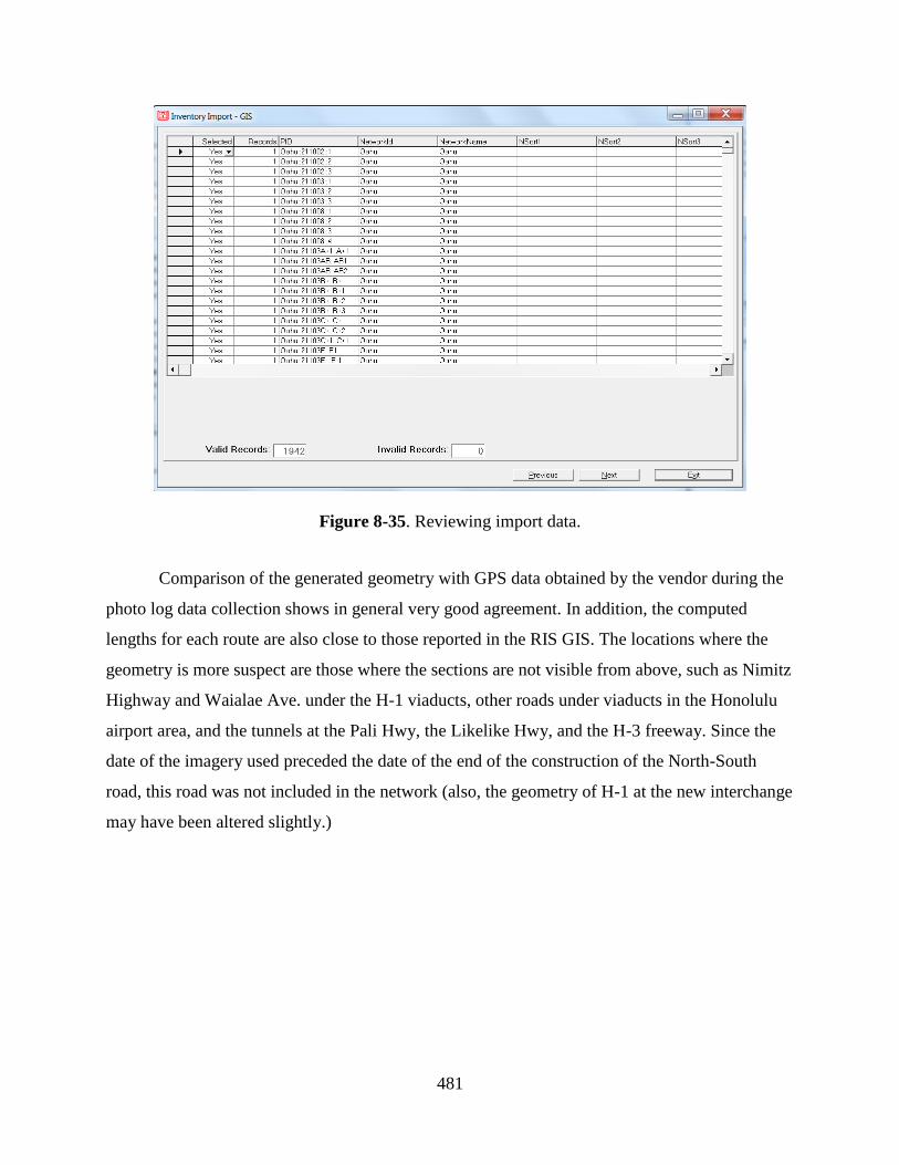
481

Figure 8-35. Reviewing import data.

Comparison of the generated geometry with GPS data obtained by the vendor during the

photo log data collection shows in general very good agreement. In addition, the computed

lengths for each route are also close to those reported in the RIS GIS. The locations where the

geometry is more suspect are those where the sections are not visible from above, such as Nimitz

Highway and Waialae Ave. under the H-1 viaducts, other roads under viaducts in the Honolulu

airport area, and the tunnels at the Pali Hwy, the Likelike Hwy, and the H-3 freeway. Since the

date of the imagery used preceded the date of the end of the construction of the North-South

road, this road was not included in the network (also, the geometry of H-1 at the new interchange

may have been altered slightly.)

482

Figure 8-36. Listing of sections as they are imported.

Figure 8-37. Selection of sections after importing them into PAVERTM.

Two very important pieces of information required when creating the inventory are the

surface type and the last construction date of each section. These are specified when a section is

created inside PAVERTM or when imported into PAVERTM. After this, the surface type and the

483

last construction date are only changed for sections receiving a Major Maintenance and

Rehabilitation (Major M&R) (as defined later in section 8.4.3.6.6, page 552) or some Global

Maintenance and Rehabilitation (Global M&R) (as defined later in section 8.4.3.6.5, page 537).

The rules for changing the surface type are given under the headings Consequent Surface on the

aforementioned subsections.

The following are some of the reporting capabilities of PAVERTM with respect to the

inventory information. Figure 8-38 shows the GIS visualization of surface types. The PAVERTM

standard surface types shown in this figure include AAC: asphalt concrete overlay over asphalt

concrete, AC: asphalt concrete, PCC: Portland cement concrete, and APC: asphalt concrete

overlay over PCC. Figure 8-38 also shows user defined surface types, including: ACbS: asphalt

concrete over a structure (bridge or viaduct), PCCbS: PCC over structure, and UTW: ultra-thin

whitetopping. These were created with the intent to define separate deterioration curves for these

types of pavements. However, a few problems have been encountered when these surface types

have been created (some systems tables appear to get corrupted) and therefore its usage is not

recommended at this point, particularly since assigning different deterioration curves to these

sections can still be accomplished within PAVERTM without the need to create new surface

types.

Figure 8-39 is one of the standard charts in PAVERTM showing the percent area with

each pavement type. Figure 8-40 shows the distribution of ages of the pavement sections in the

network. The user has the option to select a subset of the network (e.g., all AC, AAC, and APC

pavements, etc.)

It is interesting to note in Figure 8-39 the large percentage of the Oahu network with PCC

surfaces (PCC, PCCbS, and UTW). These three surface types represent about 21% of the

network area, which is higher than usual. This is in part a reflection of the large percentage of

PCC surfaces and viaducts on the interstate portion of the network.

484

Figure 8-38. GIS Visualization of Pavement Surface Types in PAVERTM.

Figure 8-39. Chart of the Percent of Each Surface Type in PAVERTM.

485

On Figure 8-40, it can be observed what appears to be an unusually large percentage

(48%) of pavement sections with ages (time since the last reconstruction) above 21 years. This

large percentage is explained in part by the large percentage of PCC pavements in the network.

Nevertheless, even though some sections are known to have lasted a long time, the percentage

remaining after accounting for the PCC pavements appear unusually high. This indicates that

there are still holes in the data. Particularly, it is believed that some important maintenance

activities, including overlays, are still missing.

Figure 8-40. Chart in PAVERTM of the Percent Area vs. Age at Time of Report.

8.4.3.3 Pavement Condition

As discussed in the previous section, importing the inventory data requires substantial

processing. Nevertheless, this is mostly a one-time effort for the whole network. After this large

effort, only a small number of annual record updates may be needed. On the other hand,

pavement condition information needs to be input for most of the network recurrently.

486

8.4.3.3.1 Sampling vs. Continuous Measurements and Survey Frequency

In order to determine the PCI for a pavement section, the section is typically divided into

sampling units. ASTM D6433 and the PAVERTM documentation recommend sampling unit sizes

of 2,500 ± 1,000 sq. ft. Shahin [7] indicates that at the network level the survey should be

performed on sample units representative (not random) of the overall condition of the section

since the main objective for budget estimating and network condition assessment is to obtain a

meaningful rating with the least cost.

Shahin [7] also points out that a network-level survey can be conducted by surveying

only a few sample units per section and provides some guidance on sampling rates. As reported

by Shahin [7], some agencies go as low as 10% sampling with more than 40 sampling units (i.e.,

for large sections). However, it is important to realize that these guidelines were developed

mostly for manual data collection efforts.

With respect to sampling rates when automated data collection means are used, some of

the relevant findings of NCHRP Synthesis 334 [104] include:

“Most agencies using automated means of data collection sample continuously, or very

nearly so, on the outer traffic lane.

In a few instances, a worst lane is selected for evaluation and in no case is an agency

evaluating all lanes.

The essentially universal practice is to evaluate the outermost traffic lane (no parking

spaces) in one direction for pavements having fewer than four lanes and in both

directions for roadways having four or more lanes.

Three agencies collect cracking data on a segment-by-segment basis (usually defined as

a pavement management segment of varying length), whereas five sample 10% to 30%

of the roadway, usually on a random sampling basis.”

Based on the above, it appears that the practice at HDOT of collecting distress

information continuously from images is in line with the practices at many other state DOTs.

However, although HDOT practice includes collecting data continuously for one lane, the lane

for which the data is collected (on multi-lane highways) is typically not the outermost lane.

Instead, it is the innermost lane (or “CTR” lane in the HDOT Planning Branch naming

convention.) Although the practice appears to be related to the need to collect other information

simultaneously with the distress survey, it also appears to be supported in part by the limited

analysis presented in Section 3.7, which showed the leftmost lane to be often the lane with higher

487

lane distribution factors for heavy vehicles. A more in-depth study is needed of the data from

automated vehicle classification stations on multilane highways located throughout the islands to

ascertain whether this strategy is appropriate.

As reported in [104], almost all agencies monitor pavement surface distress (cracking,

etc.) at 1-, 2-, or 3-year frequencies. That report also indicates that a few agencies do one-half of

the system each year, with others doing one-third each year and that a few states monitor

interstate pavements at 1-year intervals and other pavements at 2-year intervals. The most

common occurrence is capturing of pavement cracking at 2-year intervals.

Wolters et al. [89] provide more recent information on data collection frequency by local

agencies. According to these authors, most local agencies collect distress information every year

(45%), about 9% collect data every two years, 18% every three years, 8% every four years, and

8% every 5 years. Note that it is also common to collect data every year but on only one half or

one third of the network. In addition to reducing the costs by a factor of 2 or 3, this also has the

advantage of leveling the data collection funding needs.

Therefore, collecting distress data every two years (or alternatively every year on half of

the network) is consistent with the need to report HMPS data and a common practice elsewhere.

This is probably a good strategy for HDOT as well.

8.4.3.3.2 Importing Pavement Distress Data Into PAVERTM

Although PAVERTM provides a form (Figure 8-41) intended for rapid entry of distress

information (from which the PCI is computed), the process is slow, tedious, and prone to the

introduction of errors. Note that the information entered into the form of Figure 8-41 is at the

sample level (in that particular figure, the sample unit is 001). Thus, when dealing with

thousands of sections and several sampling units per section, the data input process is slow.

Therefore, an automated process for importing distress information or condition information is

also desirable. PAVERTM provides a few options for this and this subsection briefly describes the

option that was found to be the more useful in this study.

Importing distress information for each section essentially involves the creation of an

XML file containing the network, branch, section, sample number and size, and the list of

distresses for each sample (including type, severity, and extent.)

488

Figure 8-41. PAVERTM form for entering/editing distress information.

As illustrated in Figure 8-42, the data are used to create the attributes of different

elements of the file usually identified by two corresponding tags. For example, the information

for a sample unit is found between the tags <inspectedElement> and </inspectedElement>. The

inspected element is identified by its attributes PID (which identifies the section) and the

inspectedElementID (which identifies the sample). The third attribute required for each sample is

the size in square feet (which is used to compute distress densities.) For each sampling unit on

which distresses are observed, the distresses are listed between the tags <PCIDistresses> and

</PCIDistresses>. Each distress record is identified with a single tag that includes attributes

<levelDistress severity=”X” quantity=”YYY.YY” distressCode=”YY”>, where X is L, M, or H

depending on whether the distress is low, medium, or high severity, respectively, and the Y’s are

numbers defining the extent (quantity) of distress and the type of distress (for HMA pavements,

the distress codes coincide with those shown in Figure 8-41.) Although this type of file can be

created with a text editor (e.g., Notepad), this would not be practical for the whole HDOT

network for the same reasons cited for the PAVERTM form shown in Figure 8-41.

489

Figure 8-42. Example of XML file with pavement distress information for import into

PAVERTM.

A fundamental aspect of the file is the PID attribute of the inspected element (a sample

unit in this case), which uniquely identifies the existing section within PAVERTM to which the

sample belongs. The PID field and the sample number (identified by the inspectedElementID

attribute in Figure 8-42) uniquely identify the sampling unit. The PID is the same PID that was

described in the discussion of the pavement inventory (section 8.4.3.2.1.3, page 472). Recall that

the PID is formed as NetworkID::BranchID::SectionID (i.e., with the IDs for the network,

branch, and section, respectively, separated by “::”)

Creating this XML file automatically with the information available presented several

challenges. These challenges and the steps followed to overcome them are briefly described in

the following paragraphs. The description is not abundant in details since, as it will be explained

shortly, these issues should be easier to overcome in the near future.

490

As just noted, the PID field is formed with the information of the network as imported in

PAVERTM. Note that this information (NetworkID + BranchID + SectionID) uniquely identifies

a section but it does not directly provide information about the location of the section. In addition

to the SectionID, PAVERTM also has two fields labeled “From” and “To” that make the

identification of sections easier. These fields accept an alphanumeric and could contain

descriptive information such as the name of cross streets or the description of some important

feature identifying the begin or the end of the section. As described earlier, for Oahu network the

milepoints (with an accuracy of 0.01 mi for roads and 0.001 mi for ramps) of the start and the

end of the section were used instead for the “From” and “To” fields, respectively.

Then, to assign the distress data to the appropriate sections, a text file was created with

the PID and the From and To fields for each pavement section. In addition, the distress data were

exported from the vendor provided Microsoft Access® database files into ASCII (text) files.

As indicated in section 4.3.2 (page 142), a custom made program originally develop to

compute PCI outside PAVERTM was adapted to compute distress quantities as required by

PAVERTM. Recall that the distress data were collected according to the SHRP specifications

instead of the ASTM specification used by PAVERTM. Also, recall that the distress data were

delivered mostly in 0.1 mi long segments even though the actual data were collected for each

video image frame, every 0.002 mi (10.56 ft). Therefore, for simplicity, whenever possible each

0.1 lane-mile segment in the distress survey was considered a sampling unit even though this is

about twice the recommended sampling unit length. The computation of distress quantities was

based on the transformations for computing distress densities multiplied by estimated sample

unit sizes described in section 4.3.2.

An can be seen in many of the examples presented in the development of the Oahu

network, it is quite often the case that a pavement management section will not start or end at an

exact 0.1-mi multiple. Therefore, the custom program was made to read the information from

both text files (one file containing the structural information and the other the distress

information). Then, those 0.1-mi segments straddling the boundary of two consecutive pavement

management sections were subdivided into two different sampling units (one for each section)

and the correponding distress quantities were pro-rated according to the sampling unit sizes. For

491

those 0.1-mi survey segments completely contained on a pavement mananegement section, a

sample unit was simply created and assigned to the PMS section.

Although the above process may not sound too complicated (in terms of the computations

needed), there are several special cases that needed to be taken into account. One example is that

if a short bridge section is present, say for example 0.02 mi long, a 0.1-mi segment may cover

parts of three consecutive sections. Another more common and serious example is if one of the

end points of a survey reporting segment is erroneously reported, then the data may be

erroneously assigned to many adjacent pavement mangement sections. There were indeed cases

of some reporting segments being several miles long. To avoid the problems caused by these

segments, the lengths above a certain threshodls were ignored.

With the distress quantities converted and assigned to samplig units, then creating

programmatically an XML file (Figure 8-42, page 489) was relatively simple.

Once the XML has been created, importing it into PAVERTM is a relatively simple

process as explained next (of course, it is simple provided the file does not contain errors or

inconsistencies.) Selecting the “Wizards” button in the main PAVERTM toolbar displays the

Wizards form shown in Figure 8-43. Then, selecting the last option in the form and pressing the

“Continue” button brings up the form shown in Figure 8-44. In this form, the name of the file to

be imported and the directory where it is located must be selected. Pressing the next button on

this form shows the form for the next step (Figure 8-45) in which the option “Convert XML into

inspection files using PID” needs to be selected and the button “Convert” needs to be pressed. As

the program starts converting the distress information, it highlights the section to which a sample

is being imported. After this, a confirmation to import the data and the possibility to create a

report are presented (these are not shown here.)

492

Figure 8-43. PAVERTM Wizards form.

Figure 8-44. PAVERTM form to select the XML containing the distress information.

493

Figure 8-45. Sections containing the sample unit being imported are highlighted by PAVERTM.

8.4.3.3.3 Future Distress Surveys

Clearly, a more streamlined and sustainable process without so many manipulations

would be required for future surveys if PAVERTM is selected (actually, this would be true for

most PMS software.) A few options are available for this. First, notice that in Figure 8-45

another option to import the data includes the use of UTM coordinates. This is an alternative that

should be evaluated since the vendor does collect GPS coordinates together with the distresses.

In order to create sampling units with the PMS segments and avoid the splitting of sections, the

data at the frame level (every 0.02 mi) before aggregation should be used. A clear advantage of

this procedure would be that no connection of the inventory and distress data is needed outside

PAVERTM (of course, the UTM distress data needs to be consistent with the inventory network.)

A second option, would be the use of the distress data collected every frame (i.e., before

aggregating it) using the PID process described above. This process does not add much in terms

494

of data manipulation savings but it presents fewer problems for correctly assigning the distresses

to the PMS sections.

Finally, consideration may also be given to a recently developed tool, PAVER

ImageInspectorTM, which according to the site http://www.paver.colostate.edu/upcoming.php

(last accessed 12/28/2013) uses state-of-the-art pavement image data collection methods,

automatically assigning collected images to the appropriate pavement section using GIS and

Global Positioning System (GPS) technology. It also provides an interface for automatically

calculating quantities of identified distresses, and offers real-time PCITM calculation and data

transfer to PAVERTM. The PAVER ImageInspectorTM is to be licensed separately from

PAVERTM and the cost of the license is currently $650. This is listed as the last option since the

use of this software may not be compatible with the vendor’s workflow.

In any case, probably the best option for HDOT would be to include a requirement to

have the data delivered in a format that is easy to import into PAVERTM or any other PMS

software selected by HDOT or better yet, already in a databse of the PMS program selected. It is

important to note that although all this discussion was centered on PAVERTM, many of the issues

are not software specific.

8.4.3.4 Pavement Deterioration Modeling

A challenge commonly found in the implementation of a new PMS is the lack of

information on the existing pavement structures and the loading imposed on them. In this

respect, although the database still needs improvements, significant advances have been made.

Fortunately, a common approach used by some PMS programs to model the progression of

deterioration, including PAVERTM, StreetSaver®, and RoadSoft® is to use the concept of

“pavement families”, which requires a rough knowledge of the pavement structure. A pavement

family consists of a group of pavements that exhibit similar performance because they have

similar structures, construction histories, and traffic loading. The advantage of this approach is

that existing institutional knowledge can be used to create a rough clustering of existing

pavement sections into pavement families to get the PMS going and then that clustering can be

improved over time.

The assignment of pavement sections into families is only one part of the equation. The

other is the creation of reliable deterioration curves for each family. For this purpose, in

http://www.paver.colostate.edu/upcoming.php

495

PAVERTM, it is important to know the last construction date of each pavement section as well as

their pavement conditions over time (as measured by the Pavement Condition Index or PCI).

The Last Construction Date (LCD) corresponds to the date of the most recent major

M&R, as defined in PAVERTM. In general, this would be the date of any overlay larger than or

equal to 2 inches, mill & overlay larger than or equal to 2 inches, or the date of original

construction. Notice that the dates of thin overlays used for preventive maintenance (≤ 1.5

inches) or of other preventive maintenance activities such as slurry seals, chips seals, etc., should

not be used as LCD.

As indicated earlier on this report, the age of many sections are suspect. It appears that

some significant maintenance activities/rehabilitations are missing from the database. Similarly,

as discussed in previous sections, there appears to be situations where some distresses (e.g.,

cracking, raveling, etc.) are being under-reported, which would translate in overestimation of the

PCI. The two problems combined may have a significant effect on the deterioration curves.

Figure 8-46 shows the “Prediction Modeling” form used in PAVERTM to develop

deterioration curves for families of pavements. The form has six tabs that allow, respectively, the

collection of subsets of data from the database for pavement condition modeling, the review of

the model data, the application of boundary/outlier filters, the definition of pavement

deterioration curve options such as the critical PCI and the number of parameters in the

polynomial fit used for the deterioration model, the inspection of the resulting deterioration

model equation and statistics, and the assignment of family models to sections in the network.

The details for each of these tabs are not discussed here. They are described in the PAVERTM

user manual.

The data points shown in Figure 8-46 (both, the green crosses and the red triangles)

correspond to PCIs observed on AAC surfaces (HMA overlays of asphalt concrete pavements)

with low AADT/lane. This was an attempt to cluster pavements expected to deteriorate similarly.

As can be observed, the cloud of points does not exhibit a typical deterioration pattern. Clearly,

there is a large number of points that indicate little or no deterioration over time. The two

problems mentioned before may be at play here. First, if some distresses are not being captured

adequately in the survey, then some of the points should be lower.

496

Figure 8-46. PCI prediction modeling in PAVERTM. AAC surfaces with low traffic loading.

Also, on sections on which the last rehabilitation has not been identified correctly, the age

would be greatly exaggerated and therefore the corresponding points should be moved

substantially to the left. Unfortunately, as shown in Figure 8-47 for AAC surfaces with high

traffic loadings, other clustering attempts did not result in any better results.

It also interesting to analyze the time it would take for a section to reach a critical PCI of

60 (a typical threshold below which preventive maintenance is not recommended.) Sections

crossing this threshold are good candidates for major rehabilitation. A line fitting all the points in

Figure 8-46 (not shown in the figure) would indicate that after 20 years, on average, the

threshold would not even be reached. In fact, only a few points are below that threshold. This

does not appear realistic or consistent with the needs for pavement rehabilitation.

The original intent with the creation of the Pavement Structure Processing Tool (PSTS)

discussed in chapter 2 was the development of distributions of times between rehabilitations/

reconstructions. Unfortunately, the distribution generated with the PSTS for Oahu is suspected to

have too many missing projects. Thus, a distribution obtained for the Big Island with the PSTS is

instead presented in Figure 8-48. Before comparing the implications from this figure with those

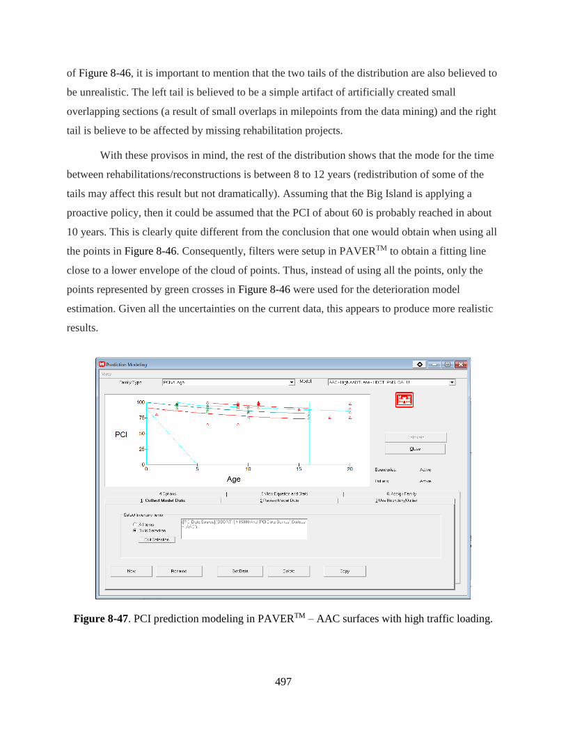
497

of Figure 8-46, it is important to mention that the two tails of the distribution are also believed to

be unrealistic. The left tail is believed to be a simple artifact of artificially created small

overlapping sections (a result of small overlaps in milepoints from the data mining) and the right

tail is believe to be affected by missing rehabilitation projects.

With these provisos in mind, the rest of the distribution shows that the mode for the time

between rehabilitations/reconstructions is between 8 to 12 years (redistribution of some of the

tails may affect this result but not dramatically). Assuming that the Big Island is applying a

proactive policy, then it could be assumed that the PCI of about 60 is probably reached in about

10 years. This is clearly quite different from the conclusion that one would obtain when using all

the points in Figure 8-46. Consequently, filters were setup in PAVERTM to obtain a fitting line

close to a lower envelope of the cloud of points. Thus, instead of using all the points, only the

points represented by green crosses in Figure 8-46 were used for the deterioration model

estimation. Given all the uncertainties on the current data, this appears to produce more realistic

results.

Figure 8-47. PCI prediction modeling in PAVERTM – AAC surfaces with high traffic loading.

498

The main conclusion from the above discussion is that the current data set does not lend

itself to derive reliable deterioration models. Since the family deterioration curves are at the core

of the PMS predictions of future conditions (and hence at the selection of efficient strategies),

initial use of the PMS will have to rely to some degree on curves borrowed from other agencies.

Until data are collected that can provide more reliable estimates, one of the models typically used

in the literature or a polynomial model as used by PAVERTM providing a PCI of 60 after, say, 12

years is probably a good option for programming purposes. A selected sample of sections for

different pavement categories and for which good information exists about the last construction

date should be selected and followed over time to derive more reliable models.

It would also be important at this point to identify those sections that were rehabilitated in

the last five years (ideally, it is desirable to identify the timing and type of work, including

pavement materials, thicknesses and locations). However, at the very least, the last construction

date should be added to the database. Several pavement sections with different ages should be

identified for each pavement family so that the trends in the first five years can be identified.

Five years is suggested as a compromise since it is most likely that the information will be

readily available for recent projects.

Figure 8-48. Historical times between rehabilitations/reconstructions on the Big Island.

8.9%

16.1%

23.7%

20.8%

10.9%

6.6%

4.3%

3.0%

0.9%1.3%

3.4%

0.0%

5.0%

10.0%

15.0%

20.0%

25.0%

0 to 4 4 to 8 8 to 12 12 to 16 16 to 20 20 to 24 24 to 28 28 to 32 32 to 36 36 to 40 > 40

Years between rehabilitations or reconstructions

Nu

mb

er

of

se

cti

on

s

499

In addition, any new rehabilitation or reconstruction work in between condition surveys

must also be recorded to maintain the database. In this way, the system will eventually have the

most relevant historic information for all pavement sections in the network.

8.4.3.5 PAVERTM M&R Categories

PAVERTM groups M&R activities into four categories:

Localized safety

Localized preventive

Global preventive

Major M&R

The definitions of these categories provided by Shahin [7] are:

“Localized safety: Localized safety M&R is defined as the localized distress repair

needed to keep the pavement operation in a safe condition.

Localized preventive: Localized preventive M&R is defined as distress maintenance

activities performed with the primary objective of slowing the rate of deterioration. These

activities include crack sealing and patching.

Global preventive M&R is defined as activities applied to entire pavement sections with

the primary objective of slowing the rate of deterioration. These activities are primarily for

asphalt surfaced pavements, e.g., surface treatments.

Major M&R: Major M&R is defined as activities applied to the entire pavement section

to correct or improve existing structural or functional requirements. Major M&R includes

reconstruction and structural overlays. The PCI value after major M&R is assumed to be 100.”

Note that in PAVERTM Major M&R includes reconstruction and rehabilitation, while

preventive maintenance is separated into two categories (local and global). A relationship

between these terms and those described in section 8.2 is presented in [105].

8.4.3.6 Selection of M&R Strategies with PAVERTM

This section discusses input parameters and policy factors for treatment selection. Since

most of the figures were developed working with part of the City and County of Honolulu

500

(C&CH) network, reference is often made to the C&CH. However, the discussion is also

applicable HDOT.

Before describing the input parameters, a brief introduction to the procedures used by

PAVERTM to select M&R strategies is provided. Shahin [7] and the PaverTM 6.5 User’s Manual

[106] provide more detailed descriptions of the program logic.

8.4.3.6.1 Network-Level M&R Planning in PAVERTM

PAVER™ contains a Work Plan tool that is used for planning, scheduling, budgeting,

and analysis of alternative pavement maintenance and rehabilitation (M&R) activities. This tool

utilizes basic inventory data combined with inspection information, maintenance policies,

maintenance costs, and predictions about future pavement condition [106].

The Work Plan tool provides three types of analysis to create M&R plans, identified as:

Consequence of Localized Distress Maintenance

Major M&R based on Minimum Condition

Critical PCI

The first two types of analysis do not generally result in efficient allocation of resources;

nevertheless, they are still quite useful. The Critical PCI approach is recommended for

developing near optimum multi-year M&R plans.

With “Consequence of Localized Distress Maintenance” localized repairs (either safety

or preventive) are assigned for one-year based on existing distress types and severities. This one-

year assignment without prioritization is the simplest type of M&R Plan analysis performed by

the program. Shahin [7] recommends that an agency develop at least two policies – one for

pavements in good condition and one for pavements in bad condition. The type of M&R

categories resulting from these two policies were described in section 8.4.3.5 as localized safety

(mostly pothole repairs) and localized preventive (mostly crack filling and sealing), respectively.

This type of analysis is useful for determining the critical PCI. As defined by Shahin et

al. [106], the critical PCI is the PCI value at which the rate of PCI loss increases with time, or the

cost of applying localized preventive maintenance increases significantly. The critical PCI is

typically a value between 55 and 70 that needs to be determined for the particular deterioration

501

conditions and costs of each network. The Critical PCI is obtained by estimating two different

critical values, one from the deterioration curve and another one using the “Consequence of

Localized Distress Maintenance” tool to apply a selected localized maintenance policy to a set of

pavement sections belonging to a pavement family and plotting the cost of localized maintenance

per unit area versus PCI. By inspecting the cost vs. PCI curve, a “critical PCI” at which the cost

increases rapidly with decreasing PCI may be observed and compared with a “critical PCI”

determined from a family deterioration curve. The critical PCI value determined from the

deterioration curve is that at which a sudden drop on the pavement condition is observed. Shahin

[7] recommends determining the critical PCI based on the two critical PCI values described

above supplemented with engineering judgment.

Unfortunately, as of the writing of this report, as discussed earlier reliable family

deterioration curves have not yet been obtained. However, the critical PCI based on costs can

still be analyzed. Figure 8-49 shows the cost of localized preventive maintenance versus PCI

generated with PAVERTM for 3,425 pavement sections that were surveyed by a City and County

of Honolulu (C&CH) contractor.79 With so many data points, it may be misleading to simply

look at this graph to try to estimate the critical PCI, as for a given PCI, a few points with costs

above normal produce the visual impression that the costs start increasing with PCI even for

relatively very high PCIs. What this graph cannot show is that for a given PCI, there are multiple

sections with zero or very low costs (i.e., a single point in the figure may represent several

sections.)

79 It was preferred to use C&CH distress information since it appears to more realistic capture pavements in

bad condition. Very tentative estimates of localized preventive maintenance costs were used to develop this figure.

Thus, the figure may not be representative of the actual costs for the C&CH. Similarly to the C&CH, the HDOT

needs to obtain cost estimates of the different treatments discussed in the rest of the report.

502

Figure 8-49. Localized preventive maintenance cost ($/sq.yd.) vs. PCI for individual

C&CH roads surveyed with Earthmine.

The picture is significantly clearer when the average localized preventive maintenance

cost per unit area vs. PCI is plotted as shown in Figure 8-50. Although there is some irregularity

in the trend between PCI values of 57 and 67, it is clear that the critical PCI based on costs is

apparently between these two values. One of the possible reasons for the irregularity is that at

present all the pavements have been lumped together irrespective of traffic level, structural

design, etc. Another possible explanation for the drop that starts at a PCI of 60 is that around this

PCI the deterioration of many cracks may be accelerated with spalling, raveling or even some

potholes that require safety treatments. Thus, around this level the amount of cracking may be

reduced simply because those cracks have been transformed into a different distress or into

patching areas. In any case, at present, this is the best information available to estimate the

Critical PCI.

Based on Figure 8-50, it appears that a good estimate of the critical PCI for the sections

analyzed is around 65. Of course, this value will need to be revised once families with similar

deterioration curves can be established. It is nevertheless comforting to see that the estimate is

within the typical range of 55 to 70 ( [7]).

PCI vs. Cost

$/SqFt

PCI

0

5

10

15

20

25

30

0 20 40 60 80 100

503

Figure 8-50. Example of average localized preventive maintenance cost ($/sq.ft.) vs. PCI for

C&CH roads80.

The “Major M&R based on Minimum Condition” analysis in PAVERTM is basically a

worst first approach without any budget optimization. As it is well known, this is not a cost-

effective approach. Under this option PAVERTM provides budget requirements needed to

maintain the pavement above a specified condition [7]. The minimum pavement condition can be

varied by the user by pavement use and rank. Furthermore, the minimum condition can also be

varied by year. By slowly increasing the minimum PCI, the likelihood of developing a plan with

a high, unaffordable budget in the first year can be reduced.

Under the “Major M&R based on Minimum Condition” analysis, as stated by Shahin [7]

“the cost of applying the major M&R is estimated for each section by projecting the year in

which the section will deteriorate to a specified minimum condition and multiplying the section

area by the unit M&R cost.” For any pavement section needing major M&R in the first year the

costs could simply be calculated from the cost of each treatment. However, since the program

estimates the condition of the pavement sections in future years, the cost of M&R in the future or

80 The average costs in the figure are for illustrative purposes only. The C&CH and HDOT need to develop

cost estimates more representative of local conditions.

0

2

4

6

8

10

12

14

0 5 10 15 20 25 30 35 40 45 50 55 60 65 70 75 80 85 90 95 100

Ave

rage

loca

lize

d p

reve

nti

ve m

ain

ten

ace

cost

($

/sq

.ft.

)

PCI

504

for sections in which the current condition is estimated can only be predicted from a table of

major M&R costs versus PCI developed by the user for the specific network.

As explained also in Shahin [7], the critical PCI approach was developed by studying

results from dynamic programming network optimization analysis and performing many life-

cycle cost analyses on many projects. Thus, since the procedure was designed to approximate the

results of the optimization it should provide near optimum alternatives. The critical PCI is based

on the concept that is more economical to maintain pavements above a certain PCI threshold (the

critical PCI defined earlier) than below it [107]. The next section is dedicated to this approach in

more detail.

8.4.3.6.2 Critical PCI method for Multi-Year M&R Section Assignment

In the critical PCI method (Figure 8-51), the M&R category assigned to a given section

depends on whether the section is above or below the critical PCI. If a section is above the

critical PCI, localized preventive and/or global preventive maintenance are applied if the section

is structurally adequate or Major M&R is applied if the section is structurally deficient (the

actual selection of the specific M&R treatment is explained later.) If a section is below the

critical PCI, localized safety or major M&R is applied (again, which treatment is selected is

explained later). The actual assignments are performed by trying to optimize the allocation of

resources to the different pavement sections and accounting for budget constraints. Thus, the

program will attempt to assign a preferred treatment to each pavement section, but depending on

the availability of funds on a given section, actions may be deferred. The following paragraphs

explain in more detail the assignment of M&R treatments.

8.4.3.6.2.1 M&R Assignment for Sections Above or Equal to The Critical PCI

For sections with a PCI above critical but structurally deficient, the recommended

treatment is major M&R. PAVERTM determines whether a section is structurally deficient by

comparing the densities (as defined for PCI calculations) of some distresses with the threshold

values provided in Table 8-2.

505

Figure 8-51. Assignment of M&R Category Using the Critical PCI Method (Source: [7])

Table 8-2. List of structural distresses used in Critical PCI method (source: [7]).

Pavement Type Distress Severities Density (%)

Asphalt

Pavement

Alligator cracking L+M+H > 0.5%

Patching M+H > 10%

Potholes L+M+H > 0.1%

Rutting M+H > 1.0%

Concrete

Pavement

Large Patching M+H > 10%

Corner break +

Divided Slab (Shattered

Slab) + Punchout

L+M+H

L+M+H

M+H

> 5%

The cost of major M&R is determined based on the PCI vs. unit cost relationship by

multiplying the section area by the unit cost. As explained by Shahin [7], the unit cost vs. PCI

relationship for Major M&R can be approximated by a straight line interpolation between the

Pavement

condition

Years

Localized safety or

Major M&R

Localized Preventive or

Global Preventive or

if structurally deficient Major M&R

Critical PCI

506

cost at the largest PCI below which reconstruction is needed (PCI ~ 30) to the cost at the lowest

PCI at which an overlay is adequate (PCI ~ 75), as illustrated in Figure 8-52.81

Figure 8-52. Guideline for Development of PCI vs. Unit Cost for Major M&R (source: [7]).

If the section is structurally deficient, the program checks on funds availability and major

M&R priorities (as discussed later in the document). If funds are available, major M&R is

applied and the PCI value of the section is set to 100. If funds are not available, localized

preventive and/or global preventive are applied as explained below for the current year and funds

availability for Major M&R is checked in the following years [7].

Pavement sections for which funds for major M&R are not available or that are

not structurally deficient receive localized preventive M&R. The cost of application is

determined in the first year either based on the results of the most recent distress inspection (if

performed within the last year) or through the PCI vs. unit cost relationship. For the second year

and beyond, only the PCI vs. cost approach can be used since the program needs to estimate the

81 An adaptation of this guideline for HDOT is described with the Major M&R policy later in this

document.

0 10 20 30 40 60 80 50 70 90

Reconstruction Cold Mill & Overlay Patch & Overlay

Likely cost curve

$/u

nit

are

a

Approximate cost

100

PCI

Overlay

507

PCI in future years. The details of the assignment of localized preventive maintenance

treatments is explain later in section 8.4.3.6.4.

Global preventive M&R is applied based on the specified interval between applications.

Figure 8-53 shows graphically the assignment of M&R treatments for sections above the critical

PCI.

Figure 8-53. M&R Assignment of Sections above or equal to the Critical PCI (Source: [7]).

8.4.3.6.2.2 M&R Assignment for Sections Below to The Critical PCI

Sections below the Critical PCI have typically deteriorated to a point where preventive

maintenance activities are not cost effective. Thus, these sections need to be rehabilitated if

sufficient funds are available or subjected to safety treatments if funds for major M&R are not

available. If Major M&R is applied, then the PCI is set to 100. Figure 4.6 illustrates the process.

PCI ≥ PCI Critical

Check for Load

Related Distresses

Apply Localized

Preventive

Maintenance

Apply Global

Preventive

Maintenance

Funds Available

Apply Major

M&R

Set PCI= 100

YES NO

NO

PCI

$/SY

508

Figure 8-54. M&R Assignment of Sections above or equal to the Critical PCI (Source: [7])

The check for availability of funds for each section is based on budget and the Major

M&R priorities explained later.

As for the case of sections with PCI above the Critical PCI, the cost of applying localized

safety M&R is determined in the first year either though using the PCI vs. cost relationship or

based on the results of the most recent distress inspection. For the second year and beyond, only

the PCI vs. cost method can be used.

8.4.3.6.2.3 M&R Budget Prioritization/Optimization

The Critical PCI method places emphasis on preventive maintenance (localized

preventive and global preventive) by trying to keep pavements above the Critical PCI, which

results in lower M&R spending. Ideally, a pavement section should receive Major M&R

immediately after reaching the Critical PCI, bringing its PCI back to 100. This would result in a

near optimal allocation of resources for that particular pavement section. However, since several

sections may reach the critical PCI at about the same time and budgets may be limited, it is often

PCI < PCI Critical

Apply Stop-Gap (Safety) Maintenance Funds Available

Apply Major

M&R

Set PCI= 100

NO

YES

$

509

necessary to prioritize which sections will receive Major M&R first and for which sections

Major M&R will have to be deferred and for how long. For a given prioritization scheme

between sections, the optimal allocation of resources is achieved with an optimization algorithm.

Notice that with unlimited funding, there is no need for prioritization between pavement

sections. In this case, M&R treatments are assigned following the procedures presented in

sections 8.4.3.6.2.1 or 8.4.3.6.2.2 depending on whether the PCI is above or below the Critical

PCI, respectively. This should produce a cost-effective treatment assignment. Note also that

since it is generally more economical to maintain pavements in good condition, in the long term,

the strategy should result mostly in the recurrent application of preventive maintenance

treatments without much needs for rehabilitation.

When the available M&R budget is lower than that required by needs alone, prioritization

and optimization are needed to obtain the maximum return on investment. The prioritization

scheme used in PAVERTM emphasizes budget optimization but it recognizes that certain projects

need to be performed to account for factors not considered in the optimization. As pointed out by

Shahin [7], some of these factors may include functional requirements (user costs), mission

objectives (e.g., increase in traffic loading), and in some cases, political/social realities (e.g., title

6 – environmental justice areas.) The program allows the consideration of projects that must be

included for the type of reasons just described. Once those projects are identified, PAVERTM

estimates their cost and then it subtract it from the budget to obtain the budget available for the

rest of the pavement sections. Finally, PAVERTM selects an approximate cost-effective M&R

strategy by allocating the available budget among the candidate pavement sections by following

the prioritization scheme described later in the text. Before explaining how the budget is

allocated to each pavement section it is convenient to discuss the types of analyses available.

1. Type of Analyses

PAVERTM provides various types of multi-year analyses using the Critical PCI approach.

These include determining the consequence of a budget plan or determining budget requirements

for:

eliminating the backlog of Major M&R in a specified period of time,

maintaining current area-weighted PCI over a specified period of time, or

510

reaching the desired area-weighted PCI in a specified period of time.

2. M&R Budget Prioritization/Optimization - Budget Determination

PAVERTM attempts to find the lowest budget that will achieve the specified objective.

The objectives for each of these budget requirement plans are considered to be achieved when

the following are within certain tolerances [7]:

Backlog Elimination: No unfunded Major M&R in the last year of the analysis.

Maintain condition: Compare the area-weighted PCI at the beginning of the analysis

period (before M&R) with the value at the end of the analysis period plus one year

where no work is performed in the last year.

Reach a specified condition value: Compare the specified PCI with the value at the

end of the analysis period plus one year where no work is performed in the last year.

For any of three objectives, the budget requirements are computed by PAVERTM with the

following built in iterative procedure [7]:

Step 1: Determine a plan with unlimited budget and set the maximum budget equal to

the highest annual budget during the analysis period (which is usually the first

year budget) and set the minimum budget equal to zero.

Step 2: If an unlimited budget cannot achieve the objective, then the desired PCI may be

unrealistically high. Thus, the analysis is stopped. If the goal can be achieved go

to step 3.

Step 3: Set the current budget equal to the average of the minimum and maximum

budgets. If the goal is achieved with the current budget set the maximum budget

equal to the current budget and if the goal is not achieved set the minimum

budget equal to the current budget.

Step 4: Repeat step 3 until the end condition tolerance is achieved.

Notice that up to this point the method used to select the specific treatment for each

section have not been discussed in detail. Now, attention is turned to this important issue.

511

3. M&R Budget Prioritization/Optimization – Treatment selection

From Figure 8-53 and Figure 8-54, it is clear that with unlimited funds, a section will

receive either Major M&R or preventive treatment (localized or global) but it will never receive

a localized safety treatment. This is reasonable since localized safety treatments are the least

cost-effective of all the treatments (as observed every year when potholes are filled with patching

mixes only to see many of the same potholes in the same or worst condition the following year.)

Proper repair of potholes (e.g., with a deep asphalt concrete patch of an area larger than the

pothole and adequately compacted) may ameliorate the problem but it is still not the most cost-

effective treatment. Furthermore, the pothole problems typically occur in a short period of time

and because of labor force limitations it is typically unfeasible to perform quality pothole repairs.

Clearly, the main reason for applying localized safety treatments is for budget constraints.

Unfortunately, this is a common situation that takes significant time to reverse if funding levels

in previous years have not been adequate.

As indicated by Shahin [7], the first factor in the prioritization is the M&R category,

which is given the following priorities:

1. Localized safety

2. Localized preventive

3. Global preventive82

a. Type 1

b. Type 2

c. Type 3

4. Major above critical PCI

5. Major below critical PCI

Unfortunately, this description is not clear about how the program proceeds in the

allocation of treatments. The following is a possible scenario that is also consistent with the logic

of Figure 8-53 and Figure 8-54. Although the actual PAVERTM implementation could vary

slightly, it is believed that this is the approximate logic used by the program.

82 The types of global preventive maintenance are described later in the sequel (see section 8.4.3.6.5.1).

512

First, for all pavement sections with PCI below critical, the cost of application of

localized safety (e.g., pothole repair) is calculated. Clearly if the sum of localized safety costs

were larger than the current budget then not even all the needs for safety treatments could be

satisfied. In that case, the sections are selected based on section use and rank priorities. Within

each M&R category, PAVERTM assigns a priority factor based on the combination of pavement

use (e.g., roadway, parking lot, etc.) and rank (e.g., primary, secondary, etc.). Table 8-3 shows

an example priority table.83

Table 8-3. Priority based on use/rank (source: [7]).

RANK ► High Medium Low

USE ▼

High 1 3 6

Medium 2 5 8

Low 4 7 9

Typically, budgets are big enough to cover at least the safety treatments.

In the next step, the rest of the budget is allocated to satisfy localized preventive

maintenance needs (e.g., crack sealing). Recall that localized preventive maintenance is applied

only to pavement sections with a PCI above the Critical PCI. Again, if the budget is not enough

for all sections requiring localized preventive maintenance, then the sections are selected for

localized preventive maintenance from the set of sections with PCI above critical based on

use/rank priorities (first all the sections with highest priorities are selected, that is with priority 1,

then all the sections with second highest priorities, etc.).

Then, the same process is repeated for global preventive maintenance treatments (e.g.,

fog seals, slurry seals, etc.)

83 The user defines what constitutes high/medium/low levels for use and rank in two separate tables. These

are described in Section 4.8.

513

The next priority is given to Major M&R for sections above the Critical PCI. As

explained by Shahin [7], the reason that major M&R above Critical PCI has higher priority than

Major M&R below Critical PCI is that this strategy minimizes costs. Remember that sections

above Critical PCI require major M&R when they show structural distresses. At this point, a 2”

overlay (or a 2” mill and overlay if grade needs to be maintained) can be a very effective

treatment. Once again, sections are analyzed in the order of their use/rank priorities and

treatments are assigned until all sections above Critical PCI with structural distress are treated or

until the budget is exhausted. Notice that each time a section above critical PCI is assigned a

Major M&R treatment, the previously assigned monies for localized and global preventive for

the given section must be released. As shown in Figure 8-53 (page, 507), a section receives a

Major M&R if funding is available or Localized Preventive and/or Global Preventive if funding

for Major M&R is not available. However, it does not receive both84.

Finally, sections below critical PCI are considered for Major M&R. Again, sections are

analyzed in the order of their use/rank priorities and each time a Major M&R treatment is

assigned the cost of the previously assigned localized safety or stop gap must be subtracted.

Again, the budget is allocated until all sections are assigned the desired treatment or until the

budget is exhausted.

Notice that within a given use/rank priority category there may be hundredths of sections.

Thus, within each category some priorities also need to be defined. In this case, PAVERTM

breaks ties based on the PCI of each section. In general, within a given user/rank category the

program gives higher priorities to sections with PCI closer to the critical PCI. Thus, for sections

above the critical PCI, lower PCIs result in higher priorities and for sections below the critical

PCI higher PCIs result in higher priorities. The exception to this rule is for localized safety (stop

gap) treatments where sections with lower PCIs receive higher priority. The reason is that stop

gap treatments are required for safety reasons whereas the other treatments are selected for their

cost-effectiveness.

84 Of course, the cost estimates for Major M&R treatments should include the costs of local repairs needed

prior to application of the M&R.

514

8.4.3.6.3 Stop Gap M&R Treatments, Policies, Consequences, and Costs

In order to carry out the Critical PCI analysis described in the previous section,

PAVERTM requires the definition of M&R policies as well as their effects and estimates of the

different treatment costs. All these parameters need to be defined and entered into different

program tables before the program can carry out the analysis.

Figure 8-55 shows one such program table available for Localized Stop Gap (or

Localized Safety) M&R (this particular table is also used by the program for Localized

Preventive M&R.) This table provides the Work Types that can be performed under localized

M&R strategies (either stopgap or preventive). The values with yellow background are defaults

provided by the program but the user can add other types of work to customize the program to

local practice (this is a common feature in PAVERTM). It is important to note from this figure

that for each M&R policy (localized safety, localized preventive, global preventive and major

M&R) there are different tabs with information requirements that need to be completed to

perform the analysis. The following subsections explain the M&R policies for each of the M&R

categories.

8.4.3.6.3.1 Localized Repairs M&R Policy

Localized repairs (including localized safety and localized preventive maintenance) are

assigned based on existing distress types and severities. Two different policies are typically

specified for localized safety/stopgap treatments (e.g., pothole repair) and for localized

preventive maintenance (e.g., crack sealing).

515

Figure 8-55. Example of M&R Input Table.

8.4.3.6.3.2 Stopgap (safety) M&R Policy

Table 8-4 provides a suggested Localized Safety M&R policy. The work types in the

table are described shortly. It must be emphasized that at this point only the part of the policy

related to asphalt concrete distresses has been considered in detail. Note that the part of the

policy related to Portland Cement Concrete (PCC) pavements has been reproduced from one of

the tables suggested in Shahin [7]. A detailed analysis with input from HDOT should be

performed with more information on costs and currently used local HMA and PCC repair

practices. The following sections provide more information on the most common work types for

flexible pavements in this table.

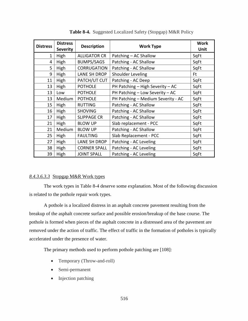
516

Table 8-4. Suggested Localized Safety (Stopgap) M&R Policy

Distress Distress Severity

Description Work Type Work Unit

1 High ALLIGATOR CR Patching – AC Shallow SqFt

4 High BUMPS/SAGS Patching - AC Shallow SqFt

5 High CORRUGATION Patching - AC Shallow SqFt

9 High LANE SH DROP Shoulder Leveling Ft

11 High PATCH/UT CUT Patching - AC Deep SqFt

13 High POTHOLE PH Patching – High Severity – AC SqFt

13 Low POTHOLE PH Patching – Low Severity – AC SqFt

13 Medium POTHOLE PH Patching – Medium Severity - AC SqFt

15 High RUTTING Patching - AC Shallow SqFt

16 High SHOVING Patching - AC Shallow SqFt

17 High SLIPPAGE CR Patching - AC Shallow SqFt

21 High BLOW UP Slab replacement - PCC SqFt

21 Medium BLOW UP Patching - AC Shallow SqFt

25 High FAULTING Slab Replacement - PCC SqFt

27 High LANE SH DROP Patching - AC Leveling SqFt

38 High CORNER SPALL Patching - AC Leveling SqFt

39 High JOINT SPALL Patching - AC Leveling SqFt

8.4.3.6.3.3 Stopgap M&R Work types

The work types in Table 8-4 deserve some explanation. Most of the following discussion

is related to the pothole repair work types.

A pothole is a localized distress in an asphalt concrete pavement resulting from the

breakup of the asphalt concrete surface and possible erosion/breakup of the base course. The

pothole is formed when pieces of the asphalt concrete in a distressed area of the pavement are

removed under the action of traffic. The effect of traffic in the formation of potholes is typically

accelerated under the presence of water.

The primary methods used to perform pothole patching are [108]:

Temporary (Throw-and-roll)

Semi-permanent

Injection patching

517

Injection patching is an alternative to the “throw-and-roll” method [108]. It requires

specialized equipment and it is considered by some as a rapid and effective method for

temporary patches. Although it is reported that injection patches typically have longer lives than

throw-and-roll patches [108], past experience with this method in Oahu has been negative (see

for example http://the.honoluluadvertiser.com/article/2003/Feb/26/ln/ln04a.html (last accessed

March 2013) and http://the.honoluluadvertiser.com/article/2004/Jan/06/ln/ln10a.html (last

accessed March 2013). Whatever the reasons for the past negative experience, the technique is

unlikely to be a viable alternative in the short term in Oahu, therefore injection patching is not

discussed further in this report.

In the throw-and-roll technique [109], the patching material is placed into the pothole

with or without cleaning and/or drying of the pothole. Then the material is compacted using the

maintenance truck tires (usually 4 to 8 passes). It is recommended for the finished patch to have

a ⅛ to ¼ in (3 to 6 mm) of crown to help avoid water ponding. The throw-and-roll method is

used when weather conditions are too poor for a semi-permanent patch or when the immediate

pothole repair demands are so high that performing semi-permanent patches is impractical. The

main advantage of this method is productivity in terms of potholes patched per day, although

patching appearance is not visually appealing.

Figure 8-56. Throw-and-roll pothole patch.

Wilson and Romine [110] indicate that Semi-Permanent patching (Figure 8-57) is

considered one of the best repairing potholes methods, short of full-depth removal and

replacement.

http://the.honoluluadvertiser.com/article/2003/Feb/26/ln/ln04a.html

http://the.honoluluadvertiser.com/article/2004/Jan/06/ln/ln10a.html

518

Figure 8-57. Example of a semi-permanent patch.

The semi-permanent procedure for repairing potholes includes the following steps

(adapted from [110]):

1. Remove all water (the pothole should be reasonably dry) and debris from the pothole.

2. Mark and square off an area at least 6” to 12” beyond the pothole area (using a

diamond saw, pneumatic hammer, or a milling machine). The area is cut such that

vertical sides exist in reasonably sound pavement.

3. Place the patching material.

4. Compact with a device smaller than the patch area. (Single-drum vibratory rollers and

vibratory plate compactors work best.)

5. Open the repaired section to traffic as soon as maintenance workers are cleared from

the area.

Before placing the mix, the vertical faces of the pothole may be tacked with a light

application of asphalt material to promote bonding between the pothole material and the existing

asphalt concrete. An excess of asphalt tack material should be avoided.

As with new pavement construction, achieving adequate density is extremely important.

In this respect, the Maintenance Technical Advisory Guide (MTAG) of the California Division

of Maintenance [108] recommends that the patch be compacted thoroughly. It is also

recommended that the finished patch have a 0.1 in to 0.2 in (3 to 6 mm) crown to account for

additional compaction by traffic and to help prevent standing water accumulate in the patching

area. Several MTAG recommendations [108] are given in Figures 5-7 to 5-11 of that report,

which are reproduced here in Figure 8-58.

519

Different recommendations are found in the literature about the compaction of the patch

material (though they are not always referring explicitly to the semi-permanent pothole patching

technique.) For example, for “Deep Patch Repair” of asphalt concrete pavements, Shahin [7]

indicates that Hot Mix Asphalt (HMA) should be placed in layers not to exceed 3 in. On the

other hand, for pothole patching Wolters [111] recommends placing HMA mix in one lift with

the loose mixture higher than the patch area. He recommends using only one lift to promote

mixture heat retention and obtain maximum in-place density (this is apparently achieved with

one lift because most potholes dimensions are small in area.)

.

Figure 8-58. Recommendations for Semi-permanent patches [108].

MTAG [108] also recommends to seal with crack sealant the edges of the patch area. For

areas with significant amount of rainfall, they recommend to fog seal the entire patch area. As

illustrated by the relatively wide gap between the patch and the rest of the pavement in Figure

8-59, the edges of the patch are a potential route for water to ingress into the pavement structure.

The references cited in the previous paragraphs provide several other valuable

recommendations that are worth consulting by maintenance personnel. Another reference

providing interesting information of pothole repairs is [112].

520

For larger patching areas, it is recommended to follow the guidelines for Full-Depth

Patching provided in “The Asphalt Handbook” [91]. Note that the Asphalt Institute also

recommends backfilling a patch with dense graded HMA but if HMA is not available, they

recommend using an appropriate cold mix, specialty mix, or proprietary mix. If the patch is

more than 6 in (150 mm) deep, the Asphalt Institute recommends placing the material in layers,

each compacted thoroughly with a vibratory plate for smaller patches and a roller in bigger

patches. Contrary to the California Division of Maintenance [108] recommendations, the Asphalt

Institute [91] indicates that the patch should not be overfilled in anticipation of traffic

compaction. This recommendation is consistent with achieving adequate compaction of the

patched area (similar to that achieved on new pavements.)

Figure 8-59. Untreated edges in a semi-permanent patch.

8.4.3.6.3.4 Proposed pothole repair policy

As discussed in the previous section, several options are available for pothole patching.

In this section, the rationale for the policy on pothole patching proposed in Table 8-4 (page 516)

is discussed. The proposed policy is intended to define some general direction on how to proceed

with pothole patching. However, more input and discussion is needed from stakeholders to

define some important details and obtain a practical policy.

For semi-permanent pothole patches, the vertical faces of the squared off area are

intended to provide lateral restraint against movement of the patch, which can be achieved for

pavements in relatively good condition (i.e., without not much deterioration other than the

pothole in question.) Thus, semi-permanent “pothole” patching is not recommended for a

“single” pothole in an otherwise severely deteriorated area since the lateral support will be

521

difficult to obtain. Furthermore, in a deteriorated area, the cutting operation may dislodge

additional pieces. However, semi-permanent patching may still be a good alternative for patching

the pothole together with the adjacent severely cracked areas.

In terms of effectiveness, the FHWA's Long Term Pavement Performance (LTPP) Study

found that the "throw-and-roll technique proved just as effective as the semi-permanent

procedure for those materials for which the two procedures were compared directly" [109].

Considering that the semi-permanent method is more labor and material intensive, the throw-

and-roll technique is generally more cost effective if quality materials are used.

As indicated by Wilson and Romine [110], MTAG [108] and the Asphalt Institute [91],

Hot Mix Asphalt (HMA) concrete is recognized as a preferred alternative for patching

operations. However, since pothole repairs often need to be performed quickly after rain events,

Cold-Mix Asphalt (CMA) is often used. Patches completed with CMA, however, are most often

believed to be for temporary fixes. Nevertheless, most of the consulted pothole repair patching

literature provide details of patching with CMA and not much is said about the logistics of

handling HMA for pothole repairs.

The observations in the previous paragraphs guided the pothole repair policy in Table

8-4, which is now described in more detail.

Specifically, for low severity potholes it is proposed to continue using the throw-and-roll

method with quality CMA. It is important to emphasize that adequate compaction should be

provided in all cases. Productivity is of no value if the treatment does not last a reasonable period

of time. In Table 8-4 , the throw-and-roll method for low severity potholes has been termed PH

Patching – Low severity - AC to account for the fact that the same technique applied to other

severity levels has a different average cost. Low severity potholes are probably the most

common type of potholes encountered. Therefore, use of the throw-and-roll method would result

in an effective operation.

522

For medium severity potholes (diameter of 18-30” and depth of ½” to 1”85 or diameter of

8-18” and depth >1” or diameter of 4-8” and depth > 2” according to ASTM D6433), it is also

proposed to use the throw-and-roll method with quality CMA. The potholes in this category can

still be compacted with the truck tire. Patching for medium severity potholes has been termed PH

Patching – Medium severity – AC in Table 8-4.

Depending on the mix tenderness, it may be more difficult to obtain a smooth surface in

larger potholes (Figure 8-60).

Figure 8-60. Questionable smoothness of throw-and-roll patches in larger potholes.

Consequently, for high severity potholes (diameter > 18” and any depth > 1”), semi-

permanent patches are proposed. First, as seen in Figure 8-60, even if an effective patch could be

performed with the throw-and-roll method, the patching area becomes unattractive and gives the

appearance of poor workmanship, which will affect public perception regardless of the patch

effectiveness. If the pavement around the potholes is in relatively good condition, the squared-

off area will provide good confinement to the patch as required for this method. If the area

around the pothole exhibits high severity fatigue cracking, then consideration of a larger patch

including the cracked area is warranted.

85 Some of these “potholes” are probably the result of de-lamination instead of being a real pothole. Thus, if

it is evaluated that the mix will not adhere to the existing surface, a different repair technique is required.

523

Overuse of the throw-and-roll technique can cause situations such as that depicted in

Figure 8-61, which should be avoided. Additional throw-and-roll patching in such situations is

ineffective, the ride for users becomes unacceptable, the patching is unsightly, and the public

perception extremely negative. These, together with the higher likelihood of high severity

potholes being in areas severely cracked that may be recommended for patching by the

preventive maintenance policy, are the main reasons why the throw-and-roll method is not

proposed for high severity potholes. The pothole repair for large severity potholes has been

termed PH Patching – High Severity – AC in Table 8-4.

Figure 8-61. Ineffective throw and roll patching.

For planning purposes, it is assumed that HMA will be used for semi-permanent repair of

high severity potholes. For the use of HMA to be effective, the potholes would have to form part

of a bigger area to be patched (e.g., because of alligator cracking around the pothole) or several

patching operations will need to be coordinated in the vicinity of the pothole.

It is recognized that the proposed policy may require additional efforts and costs

compared with the current practice. Nevertheless, increasing the quality of pothole patching

combined with other M&R treatments discussed later not only should result in lower M&R costs

in the long run but also a lower number of reimbursement claims, thus offsetting even more the

additional costs.

524

8.4.3.6.3.5 Stopgap M&R Costs

For illustrative purposes, this section provides estimates of patching costs for use in

M&R analyses scenarios with PAVERTM. As discussed in previous sections, two different types

of cost information are required by PAVERTM for Stopgap M&R treatments: “Cost by Work

Types” and “Stopgap Cost by Condition”. Unfortunately, at this point neither of these can be

estimated accurately.

Figure 8-62 shows an example of the Cost by Work Types table.

Figure 8-62. Cost by Work Type Table86

Wilson and Romine [110] provide detailed procedures for estimating pothole patching

costs. Unfortunately, these procedures require very detailed information that has not been

collected and analyzed. The information required for the calculations include among other things

86 The costs in this figure are provided for illustrative purposes only. They may not be representative of

local conditions, particularly those for PCC pavements, which are PAVERTM.

525

material purchase costs, number in patching crew, average daily wage per person, equipment

costs, daily productivity, and expected patch survival.

The costs in Figure 8-62 are very rough estimates based on extremely simplified

assumptions. HDOT needs to develop estimates that are representative of local conditions and

patching/sealing practices. The figure illustrates some of the information needed to run

PAVERTM (this is also applicable to other software.) In particular, development of the cost

estimates requires identifying all the costs involved (materials, labor, equipment, traffic control,

police, etc.)

The other costs required by PAVERTM for Stopgap M&R treatments are contained in the

“Stopgap Cost by Condition” table illustrated in Figure 8-63. This is important for making future

budget needs projections. Typically, the information in this type of table would be obtained by

running a “Consequence of Localized Distress Maintenance Plan” with a stopgap policy for

which PAVERTM will compute the cost/sq.ft. vs. PCI for the current distresses resulting in a plot

similar to that shown in Figure 8-50 (page 503) for preventive maintenance.

Since the values of the costs by work types are not reliable, so are the cost by condition

derived from them. Thus, in order to obtain a reasonable table of the cost by condition, the values

in the default “Stop Gap Cost by Condition” table in PAVERTM were multiplied by 3 to account

for the typically higher labor and material costs in Hawaii compared to the US mainland. Figure

8-63 shows the assumed “Stop Gap Cost by Condition” table. It is important to stress that this

table is very tentative. A table more representative of actual local costs needs to be developed by

HDOT.

8.4.3.6.3.6 Stop Gap Budget Consequence

In PAVERTM, for each treatment, a table needs to be specified with the consequences of

the treatment application. Figure 8-64 illustrates the consequences when Patching – AC

Shallow is applied to different distresses. As can be seen, application of this treatment converts

the existing distresses into Patching/Utility Cut Patching of low severity.

526

Figure 8-63. Stop Gap Cost by Condition Table.

Figure 8-64. Example of Consequence of Maintenance Policy.

The above is considered a logical conversion. No matter how well a patch is constructed,

it is never as good as the original pavement. Now, how is this information used by PAVERTM?

527

The program uses this information by first converting distress quantities into work quantities

using built-in conversion factors (this, for example, would account for the need to square-off a

larger area when patching a high severity pothole) and then each distress is adjusted based on the

applied repair method to compute the resulting PCI after the repairs are applied.

As shown in Figure 8-64, low severity potholes are converted to medium severity patches

when the work type is PH Patching – Low severity – AC. A similar table for PH Patching –

Medium Severity – AC converts medium severity potholes into medium severity patches. This

will result in lower improvements in the PCI and higher future repair costs. In light of the

conditions observed in Figure 8-61, this seems a bening assumption. On the other hand, it is

assumed that semi-permanent pothole patches (applied to high severity potholes) will result in

low severity patches (the corresponding table is not shown here.)

8.4.3.6.3.7 Putting everything together - Stopgap M&R Families

PAVERTM requires additional instructions to put together all of the pieces of information

described in the previous sections. This is done on the Stopgap M&R Families tab illustrated in

Figure 8-66. In the example of Figure 8-66, the table indicates that a M&R family named

Roadway Stopgap uses the distress maintenace policy named C&CH StopGap AC (the

information in Table 8-4 "constitutes this policy) with cost by work types given in a table titled

C&CH Localized (which contains for example the cost/sq.ft. of the different pothole repair

options as well as other treatament costs) and with costs by condition given in a CCH Safety AC

table (this would be a table similar to the HDOT AC Stopgap by Condition shown in Figure

8-63 (page 526)).

Finally, the user needs to define to which Stopgap M&R family each section belongs to.

This is done by assigning sections to M&R families as shown in Figure 8-67. As can be seen in

that Figure, the stop-gap M&R family selected (that to which sections will be assigned) is

Roadway Stopgap. When this window is first opened, it will typically show a list of sections on

the left pane that have not been assigned to the current family (or to any other family depending

on the radio button selection on top of the pane). The user can select a subset of those sections by

accessing the PAVER query wizard, which is invoked by selecting the show subset radio button

underneath the pane diplaying the sections. Once a set of sections has been selected (filtered)

they can be assigned with the button “>>”. Of course, sections can also be assigned/unassigned

528

one by one as well. In the example of Figure 8-67, all sections were assigned to the Roadway

Stopgap family. The user can open the “Assign Localized Stopgap M&R Families” dialog box

by selecting the Visual Menu button in the PAVERTM main toolbar, after which the dialog box

shown in Figure 8-68 will be displayed. Then, the user must select the M&R Familiy

Assignment radio button on the left side of the Visual Menu dialog box and the Assign

Localized Stopgap M&R Families on the right side and finally press the Continue button.

Assignment of sections to different rehabilitation families provides great flexibility to

accommodate different type of treatments for different road types and different counties.

Figure 8-65. Assumed consequence of filling potholes of low severity.

Figure 8-66. Stopgap (Safety) M&R Families.

529

Figure 8-67. Assignment of sections to Stop-gap M&R families.

Figure 8-68. Accessing the “Assign Localized Stopgap M&R Families” dialog box.

8.4.3.6.4 Localized Preventive M&R Treatments, Policies, Consequences, and Costs

This section describes the input parameters required to define the Preventive M&R

Policies. The structure of the input tables is the same as that explained for Stopgap M&R, thus,

only the most significant differences are explained.

The Work Types table is the same that is used for Stopgap M&R. This table was

presented in Figure 8-55.

530

8.4.3.6.4.1 Localized Preventive Work types

A main concern with localized preventive maintenance is avoiding the ingress of water

through the pavement surface into the pavement structure. Therefore, emphasis should be put

into treating cracks. The crack treatments available include:

Crack filling

Crack sealing

Full- and partial-depth crack repair

Crack filling and sealing operations (or crack treatments) can be effective if cracks are

moderate in density and show moderate to no deterioration at the edges [113]. Since crack

sealing is a preventive maintenance activity that adds no structural capacity, ideal sections for

this technique should exhibit minor pavement distresses and have sufficient structural capacity to

meet future needs [114]. This is typically the situation of pavements above the Critical PCI for

which the localized preventive maintenance policy is applied. Pavements with transverse and

non-load associated longitudinal cracks are good candidates for crack sealing.

When cracks are low to moderate in density and have typically progressed to a point of

high edge deterioration, crack repair strategies, such as partial-depth patching or spot patching

may be warranted. If both the crack density and the edge deterioration level are high, then

rehabilitation may be warranted. However, this last situation is unlikely for pavements above the

Critical PCI.

The following paragraphs describe the different alternative treatments and the situations

in which their use is recommended in more detail.

Crack sealing: Crack sealing is generally described as a localized maintenance

procedure that involves placement of specialized materials into working cracks used to prevent

water and incompressibles from entering a crack. Crack sealing involves blowing out the debris

in the crack or using a saw or router to create a reservoir which is filled with a sealant. Cracks

that are sealed are typically less than 3/4-inch (19 mm) wide. Working cracks are those that have

more than 0.1 in (0.25 mm) of annual vertical or horizontal movement. Normally, cracks that are

spaced uniformly along the pavement, have limited edge deterioration, and are less than 3/4-inch

wide should be sealed.

531

To effectively seal the cracks, the router or saw must touch both sides of the crack.

Cracks that are greater than 3/4-inch wide and are very numerous are not practical to seal, both

because the router or saw will not touch both sides of the crack and because of the number of

cracks present [92].

Crack Filling: Crack filling is the placement of materials into cracks to reduce the

amount of water infiltration into a pavement while also reinforcing the adjacent pavement. It is

used in sections that are unsuitable for crack sealing due to excessive crack width, secondary

cracking and/or crack edge deterioration/spalling and in non-working cracks.

Crack filling should be distinguished from crack sealing. It differs from crack sealing

mainly in the preparation given to the crack prior to treatment and the type of sealant used.

The identification of working cracks requires some annual monitoring of crack widths, an

activity that is currently not practical for HDOT. Smith and Romine [113] indicate that working

cracks are usually transverse in orientation but that some longitudinal and diagonal cracks may

meet the 0.1-in movement criterion. For proper sealing, materials placed on working cracks must

adhere to the crack sidewalls and flex as the crack opens and closes. This is the reason why

rubber-modified materials designed for low-stress elongation, especially at low temperatures, are

preferred for treating working cracks.

The SHRP Materials and Procedures for Sealing and Filling Cracks in Asphalt Surfaced

Pavements – Manual of Practice [113] provides basic definitions of the density of cracking and

level of edge deterioration (although density thresholds are not provided). As pointed out in the

Michigan DOT Manual “Sealing and Filling of Cracks for Bituminous Concrete Pavements –

Selection and Installation Procedures“ [93], the first step in the process to select crack

treatments is to characterize the density of cracking and the level of edge deterioration. The

Michigan DOT manual [93] also provides guidance on density thresholds. These are shown in

Table 8-5. The threshold between moderate and high densities is based on the approximate point

where transverse and longitudinal cracking would be classified as block cracking. The threshold

between low and moderate cracking is based on the observation that 2 to 3 transverse cracks in a

100 m (328 ft) section would justify a sealing operation.

532

Table 8-5. Thresholds to determine crack density levels

Linear Crack Length per 100 m (328 ft)

Pavement Section Density

< 10 m (32.8 ft) Low

10 m (32.8 ft) to 135 m (443 ft) Moderate

> 135 m (443 ft) High

Notice that the emphasis put in determining the density of cracking is related to its

potential origin. That is, if cracking is related to environmental/construction factors (e.g., block

cracking and longitudinal and transverse cracking), application of a crack treatment is

appropriate. HDOT collects the distress information in a format that indicates what caused it.

Thus, the policy for crack sealing/filling can be defined to a certain extent by the type of cracks.

The other criterion used in those manuals to define the crack treatment is the degree of

edge deterioration. Typically, cracks with edges deteriorated in more than 50% of their length

should be repaired instead of treated. Since edge deterioration is not a variable on the pavement

condition survey performed for pavement management, this criterion cannot be used for budget

plan determination. Nevertheless, this can still be used by maintenance crews or the engineer to

decide the type of crack treatment/repair to apply during maintenance operations.

As discussed before, the Michigan DOT [93] provides different alternatives for working

and non-working cracks. This differentiation between types of cracks is not considered practical

for the HDOT at this time. Therefore, the following guideline is recommended for determining

budget requirements: for Block, Edge, Joint Reflection, and Longitudinal and Transverse cracks

of low and moderate severity sealing or filling is recommended and crack repair is

recommended for the high severity level of these types of cracks.

It is recommended to seal cracks less than ¾ in and fill the cracks wider than ¾ in.

Weather sealing or filling will be needed cannot be determined in the budget plan analysis. This

would have to be an operational decision. Notice that based on the width of the cracks for which

the two treatments are recommended more sealant will typically be needed for filling cracks than

for sealing them. On the other hand, sealing cracks demands more preparation of the crack. In

533

the following recommendations, the cost estimate for crack sealing is also used for crack filling.

However, these should be revised if later it is determined that crack filling costs differs

substantially from those of crack sealing.

In general, sealing/filling treatments should be applied when pavement cracks first

develop, as this timely treatment will help prevent further pavement deterioration. Therefore,

consistent pavement management practice should result in a relatively minor need for filling

wide cracks. Crack filling is not as efficient as crack sealing; nevertheless it still reduces water

infiltration into the pavement structure and the intrusion of incompressibles into the crack. Thus,

its use may still be warranted when crack sealing is not effective as it happens for wide cracks

with moderate edge deterioration.

Full- and partial-depth crack repair: This is a localized treatment method to repair

cracks that are too deteriorated to benefit from sealing or filling. It involves cutting a trench

centered over an existing crack, placing hot-mix asphalt (HMA) into the reservoir in one or more

lifts, and compacting it to achieve appropriate density. This treatment is recommended for high

severity cracks. The need for this type of treatment should be rare for pavement with PCI above

critical (for which the localized preventive treatments discussed in this section are

recommended).

Other repairs: For distresses other than cracks or for small areas of fatigue cracking

either shallow or deep patching are recommended. Pavements with large areas of fatigue

cracking will either not have a PCI above the Critical PCI or if they do, they will typically be

recommended for Major M&R if funds are available.

8.4.3.6.4.2 Localized Preventive M&R Policy

Figure 8-69 provides a suggested Localized Preventive M&R policy. At this point, only

the policy for asphalt concrete pavements has been considered in detail.

534

Figure 8-69. Suggested Localized Preventive Distress Maintenance Policy.

The policy calls for sealing of any low or medium severity linear cracking distresses

(block, edge, joint reflection, or longitudinal and transverse cracking) and for repairing those

with high severity. For crack repair, a patch with a depth of 6 in and 1 ft width is assumed.

For the other distresses in the policy, either deep or shallow patching is recommended.

Specifically, Patching – AC Shallow (2 in mill and fill) is recommended for bumps/sags,

corrugation, shoving, and slippage cracking. Patching – AC Deep (6 in mill and fill) is

recommended for alligator cracking of medium and high severity, high severity patches, and

rutting (rutting is not shown in the figure). In addition, pothole patching is treated in the same

way as in the Stopgap policy (not many potholes are expected to be observed in sections with

PCI above critical.)

8.4.3.6.4.3 Localized Preventive Maintenance Costs

As for safety maintenance, for illustrative purposes, this section provides rough estimates

of patching costs for use in M&R analyses scenarios with PAVERTM. As discussed in previous

535

sections, two different types of cost information are required by PAVERTM for Localized

Preventive M&R treatments: “Cost by Work Types” and “Stopgap Cost by Condition”. The cost

by work types table is the same one that was presented for Stopgap treatments in Figure 8-62.

The other cost information required by PAVERTM for Localized Preventive M&R

treatments is contained in the “Preventive Cost by Condition” tab illustrated in Figure 8-70. The

information in the table named C&CH Localized Preventive AC was obtained by running a

“Consequence of Localized Distress Maintenance Plan” for which PAVERTM computes the

cost/sq.ft. vs. PCI for the current distresses. The raw results of the analysis were presented in

Figure 8-49 (page 502) and the averages cost vs. PCI was presented in Figure 8-50 (page 503).

The values in Figure 8-70 provide an approximation to the points in Figure 8-50.

Figure 8-70. Localized Preventive Cost by Condition Table.

8.4.3.6.4.4 Localized Preventive Budget Consequence

As in the case of stopgap treatments, for each localized preventive treatment, a table

needs to be specified with the consequences of the treatment application (the list of treatments

for localized repair, either stopgap or localized preventive is unique, so these tables need to be

specified only once.) Figure 8-71 illustrates the consequences when Crack Sealing – AC is

applied to different types of cracks. As can be seen, application of this treatment converts the

existing cracks to cracks of the same type but of lower severity. Recall that the only purpose of

536

specifying these consequences is to be able to compute an estimate of the pavement condition

immediately after the treatment application.

Figure 8-71. Another example of Consequence of Maintenance Policy

The program uses this information by first converting distress quantities into work

quantities using built-in conversion factors and then each distress is adjusted based on the

corresponding consequence table to compute the resulting PCI.

8.4.3.6.4.5 Putting everything together – Localized Preventive M&R Families

Again, PAVERTM requires additional instructions to put together all of the pieces of

information described in the previous sections for localized preventive M&R. This is done on the

Preventive M&R Families tab illustrated in Figure 8-72. As can be seen, the table indicates that

a M&R family named Roadway Prev. uses the distress maintenace policy named C&CH

Localized Preventive (the information in Figure 8-69, page 534, constitutes this policy) with

cost by work types given in a table titled C&CH Localized M&R Costs and with costs by

condition given in the C&CH Localized table shown in Figure 8-70.

537

Figure 8-72. Localized Preventive M&R Families.

Finally, the user needs to define to which Localized Preventive M&R family each section

belongs to. The procedure is entirely analagous as what was explained for the Stopgap M&R

policy. The assignment of sections to the Roadway Prev. family is shown in Figure 8-73.

Figure 8-73. Assignment of sections to Preventive M&R families.

8.4.3.6.5 Global Preventive M&R Treatments, Policies, Consequences, and Costs

This section describes the input parameters required to define the Global Preventive

M&R Policies. The structure of the input tables in this case is slightly different than the structure

538

in the previous two cases. The information required is spread in four tabs instead of the six

needed for the other M&R treatment families. Figure 8-74 shows the four different tabs:

1 – Work Types, 2 – Consequent Surface, 3 – Costs by Work Types Table, and 4 – Global M&R

Families. The Figure also displays the Work Types table.

Figure 8-74. Global Preventive M&R Tables and Families – Work Types table.

The Work Types table differs from that for localized repairs in that in addition to the

code, the name, and the work unit of the work type the application interval and resulting

increased in life of the treatments need to be specified. The Application Interval is the interval

at which a work type would be reapplied. The Resulting Increase in Life, or change in age, of

the pavement is defined as the time (in years) it would take for the condition of the pavement to

return to where it was prior to application of the global treatment. If a treatment changes the type

of surface then the Changes Surface field must be set to Yes, as can be seen for the overlays in

the figure. This is simply because an asphalt concrete pavement becomes an overlay over

asphalt concrete pavement after the treatment, which is considered a different surface type (the

deterioration curves are usually different.)

539

8.4.3.6.5.1 Global Preventive Work types

There are a large number of alternatives that fall under the category of surface treatments

or seals. These are generally less than one inch or one inch and a half thick. The objective of

these seals is to waterproof the pavement, restore skid resistance, and restore oxidized surfaces.

In some situations, some of these seals can be used to fill minor ruts. Surface treatments do not

add any structural strength [115].

The treatments briefly described in this section include fog seal, seal coat, double chip

seal, slurry seal, microsurfacing, and thin hot-mix asphalt overlays. Not all these treatments are

currently used on state roads. However, they are included because of their potential use in the

future. Sand sealing is not included because quantities are difficult to control, resulting in

bleeding or excess sand on the pavement surface [92]. Only some of the more important

characteristics of the treatments and a few other details are presented here. For more details on

construction and materials specifications, the reader is referred to Johnson [92] (from which most

of the descriptions below were extracted) or other DOT/industry manuals on the subject. The

HAPI (Hawaii Asphalt Pavement Industry) Asphalt Pavement Guide [116] provides an

illustrated introduction to some of the treatments available.

1. Fog Seal

A fog seal is a light application of diluted slow-setting asphalt emulsion without a cover

aggregate used to seal and enrich the surface of aged (oxidized) asphalt pavement, seal minor

cracks, prevent raveling, and provide shoulder delineation. Typically, an asphalt emulsion

diluted mix with 50 percent water (such as CSS-1, CSS-1H) or proprietary rejuvenators are used.

A sand cover may be used to improve the surface friction.

For Hawaiian conditions, fog seals are more suitable for low-volume roads (residential

streets) or parking lots, which can be closed to traffic for the time it takes for the slow-setting

asphalt emulsion to break and set and where the potential for reduced pavement friction is not a

concern. Under favorable conditions, two to three hours may be sufficient but normally it takes 4

to 6 hours for the slow-setting asphalt emulsion to break and set. Traffic should be kept off the

emulsion until it has cured significantly. Sand should be used to blot up areas of excess

application.

540

Fog seals are effective when light to moderate raveling and/or oxidation and weathering

develop. They should be used only where the existing pavement is sufficiently porous to absorb a

substantial amount of the emulsion and they should be avoided in areas with a significant

number of cracks larger than hairline. All necessary repairs or reconditioning work should be

completed before application of the treatment. Furthermore, the fog seal should only be applied

when the pavement is dry and clean. Fog seals may be able to temporarily postpone the need for

a chip seal or non-structural overlay.

The performance life of this type of treatment is fairly short, ranging from one to three

years.

2. Seal Coat/Chip Seal

A seal coat, also known as chip seal or bituminous surface treatment (BST), is a thin

protective wearing surface formed by an application of an asphalt (typically a rapid-setting

asphalt emulsion) followed immediately with an aggregate cover.

The primary reason to seal coat an asphalt pavement is to protect the pavement from the

deteriorating effects of sun and water. Exposure to sun, wind, and water, results in oxidation and

hardening of the asphalt. This causes the pavement to become brittle and more prone to cracking.

A seal coat provides a waterproof membrane that not only slows down the oxidation process but

also helps to prevent water from entering the base material (it seals low-severity cracks and fills

raveled surfaces.) A secondary benefit is an increase in the surface friction, which happens

because the aggregate adds additional texture to the pavement. In addition, seal coats reduced

glare in wet weather and increase the pavement night reflectivity. Pavements that are dry and

raveled but in otherwise good condition are good candidates for seal coating.

Traffic should not be allowed on the seal coated surface until after all rolling has been

completed and the emulsion has set so that there is no pick up on vehicle tires. Although seal

coats provide effective sealing and friction, the possibility of loose chips and broken windshields

along with excessive noise has prompted some states to restrict use of chip seals to low-volume

roads. Nevertheless, new technique (e.g., use of pre-coated aggregates) have reduced these

effects.

Expected life of a seal coat is approximately three to six years.

541

3. Double Chip Seal

This treatment involves the application of two single seal coats. The second coat is placed

immediately after and directly over the first. Sixty percent of the total asphalt binder required is

placed in the first pass, with larger aggregate. The remaining forty percent is placed in the second

pass, with aggregates half as large as those placed first.

It is strongly recommended that a polymer-modified emulsion be used on double chip

seals to increase early retention of aggregate.

Similarly to seal coats, the purposes of double chips seals are to waterproof the surface,

seal small- to medium-sized cracks, and improve surface friction. This treatment reinforces the

benefits of a single chip seal. As the top layer of aggregate wears off, the bottom layer remains.

It offers better aggregate retention overall, as the bottom layer is more deeply embedded. A

double chip seal results in a quieter, smoother surface than a single chip seal, and is a good

alternative for pavements in fair condition without structural distresses.

Similarly to the other surface treatments described in this document, this treatment is

appropriate for stable pavements on a sound base with a good cross section. Visible surface

distresses may include moderate raveling, surface wear, longitudinal cracks, and transverse

thermal cracks with some secondary cracking and some deterioration along crack faces. A minor

amount of patching in good condition is acceptable. The surface may show signs of slight to

moderate block cracking, moderate to severe oxidation, and/or slight to moderate flushing or

polishing.

Heavy commercial traffic and frequent stopping and turning movements reduce the life of

this application and cause local deterioration. Thus, they are also mostly applicable to low

volume roads.

4. Slurry Seal

A slurry seal is a mixture of well-graded fine aggregate, asphalt emulsion, water, and

mineral filler with a creamy fluid-like appearance during application. The mineral filler most

often used is Portland cement. Aggregate, water, filler, and emulsion are proportioned and mixed

together in a truck-mounted mixer and applied immediately to the pavement surface with a

spreader box.

542

They are used to seal the existing asphalt pavement surface, retard surface raveling, seal

small cracks, and improve surface friction. Slurry seals are similar to chip seals in that they use a

thermal break process, requiring heat from the sun and pavement. This process takes anywhere

from two to eight hours depending on the heat and humidity.

In addition to the required curing time, another challenge for their use in high-volume

roads is that friction initially may be reduced until traffic wears some of the asphalt from the

surface.

The slurry seal mixes are used as either a preparatory treatment (e.g., pavement leveling

and pothole patching) for other maintenance treatments or as a wearing courses. As wearing

courses, they are appropriate to maintain pavements when they first develop a moderate density

of surface cracking with low to moderate edge deterioration and secondary cracking, or to treat

light to moderate raveling and/or oxidation.

Slurry seals are effective where the primary problem is excessive oxidation and

hardening of the existing surface. As other surface treatments, slurry seals will not perform well

if the underlying pavement contains extensive cracks.

Aggregates for slurry mixes may consist of most hard crushed aggregates such as basalt.

They conform to one of three gradations: Type 1, Type 2, and Type 3. The maximum size for

slurry aggregates is 2.36 mm (#8 sieve) for Type 1, and 9.5 mm (3/8-inch sieve) for Types 2 and

3. Type 3 has a coarser gradation than Type 2. All slurry gradations have between 5 and 15

percent passing the 75-micron sieve (#200). The slurry is applied basically one aggregate layer

thick. A tack coat is not necessary unless the pavement to be sealed is extremely dry and raveled

or the slurry is being placed on a concrete surface.

The slurry seals in Hawaii typically contain a latex modified cationic quick set (LMCQS-

1h) or cationic quick set (CQS-1h) emulsion [116].

Expected life of a slurry seal is three to five years.

5. Microsurfacing

Microsurfacing is a mix of polymer-modified emulsion, well-graded crushed mineral

aggregate, mineral filler (normally Portland cement), water, and chemical additives that control

543

the break time. Except for the polymer additives, it uses the same basic ingredients as slurry seals

and consequently it is sometimes incorrectly referred to as a polymer-modified slurry seal. The

major difference however is that the curing process for microsurfacing is chemically controlled,

whereas slurry seals and chip seals use the thermal process. The aggregate, mineral filler,

emulsion, and water are mixed in a truck-mounted traveling plant, which is deposited into a

spreader box. No compaction is needed.

Many states have used this treatment for both surfacing and rut filling on roads with

moderate- to heavy-volume traffic. As a preventive maintenance or surface treatment for an

existing AC pavement, microsurfacing provides a skid-resistant surface and reduces the amount

of water that enters the pavement layers through the pavement surface. Microsurfacing restores

the transverse cross-section profile and may also be used to fill ruts.

As with slurry seals, microsurfacing is effective where the primary problem is excessive

oxidation and hardening of the existing surface. It will not perform well if the underlying

pavement contains high density of cracks or a moderate density of cracking with high edge

deterioration and secondary cracking. Prior to the application of microsurfacing, all necessary

repairs or reconditioning work must have been previously performed and the surface must be

clean and dry.

Microsurfacing cures and develops strength faster than conventional slurry seals and can

be opened to rolling traffic in about an hour. Service life is about seven or more years for high

traffic and considerably longer for low to moderate traffic. Comparative costs reported in the

literature indicate that the cost ranges from about the same order as slurry seals [117] to about

17% higher than slurry seals [92] but the differences are sometimes as high as 39% [90].

6. Thin Hot-Mix Overlays

Thin hot-mix asphalt (HMA) overlays are constructed with a thin layer of HMA typically

ranging from 3/4 to 1-1/2 inch. Three types of HMAs (dense-graded, open-graded friction

courses, and gap-graded) have been used in the United States to improve the functional (non-

structural) condition of the pavement. The mixes are often modified with polymers to meet high

performance expectations, though to date in Hawaii, the supply modified mixes has been limited.

544

Thin hot-mix asphalt overlays are used on all types of roadways for functional

improvements. Functional improvements are those improvements that enhance the smoothness,

friction, and/or profile of the roadway while adding little or no additional load-carrying capacity.

They are particularly suitable for high-volume roads in urban areas where longer life and

relatively low-noise surfaces are desired. Other benefits include enhanced appearance and

reduction of road-tire noise.

As with other preventive maintenance treatments, thin HMA overlays add little structure

to the existing pavement and therefore they should not be used on pavements showing structural

distress or deterioration, unless the distresses are corrected first. Visible surface distresses to be

corrected by thin HMA overlays may include moderate to extreme raveling and longitudinal and

transverse cracks with some secondary cracking. A moderate amount of patching in good

condition is acceptable. Milling prior to overlay is recommended when severe surface distresses

are present. Note, however, that the milled surface should be in generally good condition.

The requirement of having a pavement in relatively good condition cannot be

overemphasized. Application of thin hot-mix overlays to pavements in conditions such as the one

shown in Figure 8-75 would perform poorly. The cracks and localized pavement failures will

quickly reflect through the new surface.

Milling or a leveling course should precede thin HMA overlays where pavements need

cross-section improvements. Any minor cracks should be sealed several months in advance prior

to application to allow for curing of the sealing material. Excessive amounts of uncured crack

sealant should be avoided as they can create bumps and checking on the new asphalt mat due to

sealant expansion (see Figure 8-76). A tack coat must be applied when using thin HMA overlays

to promote bonding with the existing pavement.

545

Figure 8-75. Unsuitable conditions for thin hot-mix overlays.

Figure 8-76. Potential problems with sealed cracks

Due to their low mass, thin HMA overlays lose heat to the atmosphere very

quickly. Thus, achieving density is only possible if they are compacted very quickly while they

are still hot.

The principal problems with thin HMA overlays are similar to those of other thin overlay

techniques including: delamination, reflective cracking, poor friction, low durability, excessive

permeability, and maintenance problems.

The Hawaii Pavement Guide (HAPI 2013), citing NAPA 1995, lists several construction

concerns:

“Thin lifts require less HMA per foot of road length than thick lifts. This can result in high paver

speeds (in excess of 70 ft/min) making it difficult for rollers to keep up.

546

Thin lifts will cool quickly. This can result in little time available for compaction before the thin

overlay reaches cessation temperature (sometimes as little as 3 to 5 minutes).

Thin lift construction produces greater screed wear. If the lift depth is less than about twice the

maximum aggregate size, the HMA may tear under the paver screed. Very thin lifts (less than 1

inch) can be damaged by the screed dragging large particles.

Thin lifts are more sensitive to vibratory rolling. Incorrectly chosen amplitude, frequency or roller

speed can result in aggregate breakage and damage of the bond between the overlay and the

existing pavement.

Density control is difficult. Thin lifts provide fewer options for aggregate particles to rearrange

under compaction. Thus, mat densities will tend to be less uniform than those associated with a

thicker lift. This should be recognized if pay is in any way tied to mat density.”

The service life of thin HMA overlays is expected to average five to eight years

depending on existing pavement condition, overlay thickness, and type of binder. Some states

report as low as two to four years; others report as many as ten years.

The cost of thin HMA overlays depends largely on the layer thickness and miscellaneous

expenses such as traffic control and pavement markings.87

8.4.3.6.5.2 Consequent Surface

As explained at the beginning of section 8.4.3.6.5, each global preventive treatment may

change the surface of the pavement. For those treatments who do, the program needs to know

how the surface is transformed. Figure 8-77 shows how this is specified in the Consequent

Surface tab, which shows a table with a different row for each of the global preventive M&R

treatments (work types) for which the Changes Surface field in the Work Types table is Yes

(see Figure 8-75, page 545). The table also contains a column for each surface type in the

PAVERTM database. For those surface types that get changed by the application of a work type,

the user needs to specify the new surface type. Figure 8-77 shows that each of the asphalt

concrete overlays transform a conventional asphalt concrete pavement surface, identified with

87 Note that the costs for milling, traffic control, pavement markings, etc. do not change with the thickness,

thus a 15% increase in the cost of the material can translate into about a 10% increase in the overall cost. In other

words, in general, the cost/unit area of a 1.5” overlay will typically be less than 1.5 times the cost of a 1” overlay.

547

the symbol AC, into an overlay over asphalt surface, identified with the symbol AAC. Notice

that the program changes the cell background to yellow whenever a work type would produce a

change of the pavement surface.

As another example, the overlays in Figure 8-77 would change the surface type of a

Portland Cement Concrete (PCC) pavement into an asphalt overlay over PCC. Thus, under a

column labeled PCC, the user would need to select APC, which is the symbol for asphalt over

PCC to indicate the change of surface.

Figure 8-77. Specifying Consequent Surface types.

8.4.3.6.5.3 Global Preventive Costs by Work Types

In the Costs by Work Type Tables the user can create a customized table with the cost

for each treatment. This is illustrated in Figure 8-78 in which a table named C&CH Default

Global Preventive was created. Once again, the cost are provided for illustrative purposes and

may not be representative of local conditions.

548

Figure 8-78. Costs by Work Type.

8.4.3.6.5.4 Assignment of Global Preventive Surface Treatments

As mentioned in section 8.4.3.6.2.3 (page 508), PAVERTM considers the application of

different types of Global Preventive M&R treatments. The assignment of treatments is based on

existing distress types. PAVERTM allows the consideration of up three different types of surface

treatments. The methodology is illustrated with the help of Figure 8-79 for an example policy

assignment. As shown in the figure, a Type 3 treatment (e.g., a 1” thin overlay on secondary

roads) is assigned to pavements with skid-causing distresses such as polished aggregate. Type 2

(a 1.5” thin overlay on secondary roads) is assigned to pavements with climate-related distresses

such as weathering and raveling. Finally, Type 1 (fog seal) is assigned to pavements with little or

no distress. Notice that a chip seal could be as easily assigned as a Type 1 treatment. The

selection of which treatments to apply is a matter of agency policy.

Different policies can be applied to different sets of pavements. For example, Figure 8-80

shows that in addition to the Default Global Policy, four additional policies were created for four

different sets of pavements defined by whether the PCI is above or below 70 (termed high PCI

and low PCI, respectively in the family names) and by whether the road is a primary or

secondary road. The policy shown in Figure 8-79 corresponds to the last row of the table in

Figure 8-80 for the family named HNL Global Low PCI - Secondary. Notice that the two

policies for secondary roads specify a fog seal for Work Type for Minimal Distress (Type 1)

549

whereas the two policies for primary roads specify No Global M&R for Work Type for Minimal

Distress (Type 1). As mentioned in the section describing fog seals, these tend to reduce the

friction and thus may be a concern on primary roads. A probably better option for a type 1

treatment on secondary roads is a chip seal, which improves friction and seals the surface.

Figure 8-79. Assignment methodology for up to three different treatments.

This type of assignment provides a mechanism to differentiate policies in several ways.

For example, the two policies for secondary roads differ in the type of treatment assigned for

Work Type for Climate-related Distress (Type 2). For pavements with PCI above 70 (high PCI) a

slurry seal would be assigned whereas for pavements with PCI below 70 (low PCI), a 1.5”

overlay is assigned. The rationale for this type of assignment is that pavements with PCI between

Does the section have any of the

following distresses: L, M, H Polished aggregate?

L, M, H Bleeding?

Type 3 Example: Overlay – AC Thin 1.0” - Secondary

Does the section have any of the

following distresses: L, M, H Block cracking?

L, M, H Weathering/raveling?

L, M, H Longitudinal and

Transverse Cracking?

Type 2 Example: Overlay–AC Thin 1.5”- Secondary

Type 1 Example:

Fog seal

550

the critical PCI88 and 70, though still in satisfactory condition, are more likely to start suffering

from some structural deterioration. Thus, a 1.5” overlay would be more effective at delaying the

progression of those distresses than a slurry seal. On the other hand, a slurry seal is a perfect

candidate to restore the surface for pavements with a PCI above 70.

Figure 8-80. Global M&R Families.

Finally, the user needs to define to which Global Preventive M&R family each section

belongs to. This is done by assigning sections to M&R families as shown in Figure 8-81. As can

be seen in that figure, in this example, the Global Preventive M&R family selected (that to which

sections will be assigned) is HNL Global Low PCI - Secondary. When this window is first

opened, it will typically show a list of sections on the left pane that have not been assigned to the

current family (or to any other family depending on the radio button selection on top of the

pane). This is exactly the situation shown in the figure. The user can select a subset of those

sections by accessing the PAVER query wizard, which is invoked by selecting the show subset

radio button underneath the pane diplaying the sections.

88 Recall that Global Preventive M&R treatments may be assigned only to sections with PCI above the

critical PCI.

551

Figure 8-81. Assignment of Global Preventive M&R Families.

Figure 8-82 shows the query wizard with part of the query that will be created to select

the secondary pavements with PCI below 70. As shown in this figure, the user has clicked on the

Section leaf of the tree on the right side pane and then under the Select Rows tab has chosen the

field Secion Rank and set it equal to S for secondary roads (the options are only S and P in the

current C&CH database). Then, by clicking on the Latest Conditions leaf of the tree on the left

pane, the user can select first the PCI under field, then set the comparison to “<” and finaly the

value to compare to equal to 70 (these actions are not illustrated in the figure). This completes

the query that will select secondary pavements with PCI below 70. Pressing the Ok button

replaces the selected sections on the left pane of Figure 8-82. Then, the user can proceed to

assign them to the Global Preventive M&R familiy selected by pressing the “>>” button. A

similar process has to be performed to assign sections to the other families.

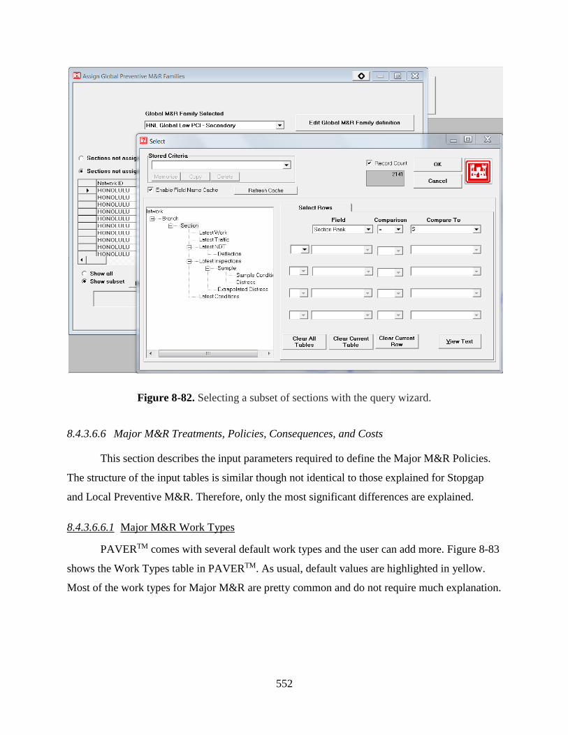
552

Figure 8-82. Selecting a subset of sections with the query wizard.

8.4.3.6.6 Major M&R Treatments, Policies, Consequences, and Costs

This section describes the input parameters required to define the Major M&R Policies.

The structure of the input tables is similar though not identical to those explained for Stopgap

and Local Preventive M&R. Therefore, only the most significant differences are explained.

8.4.3.6.6.1 Major M&R Work Types

PAVERTM comes with several default work types and the user can add more. Figure 8-83

shows the Work Types table in PAVERTM. As usual, default values are highlighted in yellow.

Most of the work types for Major M&R are pretty common and do not require much explanation.

553

Figure 8-83. Major M&R Work Types.

8.4.3.6.6.2 Major M&R Costs by Work Types

The Cost by Work Types table, shown in Figure 8-84 is self-explanatory89. For HDOT, it

is expected that the most common Major M&R will consists of mill and fill operations. Although

on occasion a single overlay may be adequate, the need to maintain grade makes the overlay

option less viable, particularly on primary roads. On secondary or local roads, an overlay may be

a more viable option. Thus, several mill and fill of different depth (2 in to 6 in) were created to

consider the most common situations as well as one 2” overlay.

89 Once again, the costs in this table are for illustrative purposes. Cost estimates representative of local

conditions need to be developed by the HDOT.

554

This table appears to be used mostly for documentation purposes as it is not really used in

the selection of M&R strategies.

8.4.3.6.6.3 Major M&R Costs by PCI

The recommendations in Figure 8-52 (page 506) were used to develop approximate

Major M&R Costs by PCI. Since the Major M&R costs are expected to be different for primary

and secondary roads two different tables were created (Figure 8-85).

Figure 8-84. Costs by Work Type table.

555

(a) (b)

Figure 8-85. Major M&R Costs by PCI for (a) Local (secondary) and (b) Primary roads.

For secondary roads, it was assumed that the minimum Major M&R would consists of a 2

in overlay and the maximum work would be a 6 in mill and fill.

For primary roads, the minimum Major M&R was assumed to be a 2” mill and fill and

the maximum full reconstruction. A $1,000,000 per lane-mile was used to obtain the value

corresponding to full reconstruction.

8.4.3.6.6.4 Consequent Surface from Major M&R

As was the case for Global Preventive M&R, each Major M&R may change the surface

of the pavement. For those Major M&R that change the surface, PAVERTM needs to know how

the surface is transformed. Figure 8-86 shows how this is specified in the Consequent Surface

tab, which shows a table with a different row for each of the Major M&R work types. The table

also contains a column for each surface type in the PAVERTM database. For those surface types

that get changed the user needs to specify the new surface type. The procedure is identical to that

described in section 8.4.3.6.5.2 for global preventive M&R.

556

Figure 8-86. Specifying Consequent Surface types for Major M&R.

8.4.3.6.6.5 Major M&R Minimum Condition Table

This table is not used in the Critical PCI analysis. It is described however for

completeness. As mentioned in section 8.4.3.6.1 (page 500), one of the M&R Plan options in

PAVERTM is Major M&R based on Minimum Condition. When performing this type of analysis,

PAVERTM assigns Major M&R whenever a section reaches the minimum condition. The

minimum condition in turn can be changed over time to slowly improve the network condition

and avoid large budgets in the initial years. As shown in Figure 8-87, the Minimum Condition

Table simply defines the minimum PCI for each year.

8.4.3.6.6.6 Major M&R Families

As with the other M&R categories, PAVERTM can group pavements sharing costs into

families. For Major M&R, these families are defined by the costs and the minimum condition

(remember that minimum condition is not used in the Critical PCI analysis). For Major M&R

there is no such thing as a maintenance policy. The program does not specify a specific M&R

action but instead determines a budget for Major M&R based on the Costs by PCI tables.

Whether Major M&R is required for a given section is determined with the logic presented in

Figure 8-53 (page 507) and Figure 8-54 (page 508) and the logic presented in section 8.4.3.6.2

(page 504.)

557

Figure 8-87. Minimum Condition Table used in Minimum PCI analysis.

In section 8.4.3.6.6.3, page 554, two different Costs by PCI tables were created. One for

Primary roads and the other for Secondary roads. PAVERTM then needs to know which of these

two tables will be used for a specific section. This is accomplished by creating two families, one

for primary roads and the other for secondary road. Obviously, the Costs by PCI table

corresponding to primary roads will be assigned to the family for primary roads and likewise for

secondary roads. This is illustrated in Figure 8-88, where the family for primary roads has been

given the same name as the Cost by PCI table, namely C&CH Primary. For secondary roads,

the family was named C&CH Locals with the Costs by PCI table named C&CH Local.

Once these families have been defined, the user needs to assign the pavement sections to

each family. The process is identical to those described in section 8.4.3.6.5.4, so it is not repeated

here.

558

Figure 8-88. Major M&R Families.

4.7 M&R Priority Table

In some situations, PAVERTM utilizes a priority table to prioritize assignment of funds to

sections within a given M&R category. The priority indexes based on section use and rank were

presented in Table 8-3. For convenience, the same information but as display in PAVERTM is

presented in Figure 8-89.

In order to assign a priority index to each section, PAVERTM needs to know whether the

rank of the section is Low, Medium or High priority. The user controls this by linking the section

rank (an input that is defined for each pavement section) to the priority with the help of the table

displayed in Figure 8-90. In the C&CH example, the roads have been categorized as either

Primary (P) or Secondary(S). As seen in the figure, primary roads have been assigned a high

section rank priority and secondary roads a medium rank priority.

559

Figure 8-89. Priorities based on section use and rank.

Figure 8-90. Section Rank Priority.

Similarly, PAVERTM needs to know whether the use of the section is Low, Medium or

High priority. The user controls this by linking the branch use (also an input that is defined for

each pavement section) to the priority with the help of the table displayed in Figure 8-91. In the

C&CH example all the roads have been categorized as roadway and given a high priority. Note

that except for Parking and Shoulder all the other default branch uses are not relevant for

highway pavements. Nevertheless, other branch uses can be easily created by HDOT in the form

560

shown in Figure 8-91, for example, to give different priority to service roads. Thus, the use of

these tables can be customized in the future if other prioritization schemes are required.

Figure 8-91. Branch Use Priority.

8.4.3.6.7 Summary

This section has presented the logic of how PAVERTM determines M&R plan

requirements and the parameters that the program needs for determining such a plan. Since the

program performs a (pseudo) optimization, it is not possible to present a simple recipe such as “if

the condition is X then do Y”. Instead, as described in previous sections, several tables need to

be specified with distress maintenance policies and costs for each the four M&R categories.

Although many of the tables appear to be of the type “if the condition is X do Y”, it has to be

remembered that none of these are absolute. The actions depend on conditions, availability of

funds and competing resource requirements between sections.

The policy is actually contained on the values provided in each of the tables and the logic

described in the previous sections.

561

8.4.3.7 Program uses

Different uses of the program can be made at different levels.

At a higher level, PAVERTM can produce tables such as the one shown in Figure 8-92,

which contains estimates of how much money should be allocated to each M&R category for a

given annual budget (the costs have been blown up for easier reading). The program can provide

these estimates for multiple years (in the example of the figure only two years were used.) Also,

depending on several plan parameters beyond the scope of this report, the user can ask the

program to obtain appropriate funding levels to achieve a given overall network condition or to

eliminate the backlog in a specified number of years. In any of these cases, the program will

produce estimates of the funding that should be allocated to each M&R category. The program

also produces estimates of the pavement conditions that will be obtained with those budget

allocations.

Figure 8-92. Total funding allocations.

At a lower level, one may be interested in what type of treatments should be applied to

each section in the network. PAVERTM also provides some useful outputs for these types of

activities.

As shown in Figure 8-93, among other things, the program produces funding allocation

tables for each section. Clearly, after studying the assumptions and issues in the previous

sections, it should be understood that these are approximate but neverthless useful for

programming funding M&R activities.

562

Figure 8-93. Sections’ funding allocations.

For Global Preventive M&R, the program is very specific since it indicates the type of

global preventive M&R treatment that must be applied to each section on every year in the

analysis period (only sections on which a treatment is planned in a given year are listed.) This is

illustrated in Figure 8-94.

For the other types of M&R categories, the program provides estimated

appropriate funding levels and predicts their consequences. Although defining the actual

treatments demand some additional work, the output in Figure 8-93 still provides useful

information. Furthermore, for the stopgap and local preventive maintenace categories some

flexibility is needed since it is very difficult to predict exactly how many potholes will need to be

repaired and how many cracks will need to be filled for a particular section. Also, it is difficult to

estimate whether cracks should be filled or sealed from the network distress survey alone. These

563

are more operational issues that can be dealt with with appropriate levels of funding, which is

what the program attempts to provide.

Finally, for Major M&R, a more thorough study is needed anyway at the

pavement section level (i.e., for a specific section, a formal pavement design needs to be

completed to address all the potential problems and obtain more reliable costs estimates.)

Figure 8-94. Global Preventive treatment allocation by section.

In addition to the tabular output, PAVERTM also provides several GIS outputs for a

particular plan. The following figures illustrate some of these outputs. For example, Figure 8-95

shows the locations, by year, on which Major M&R should be performed based on a 10-year

plan obtained using the Critical PCI analysis for part of the C&CH network. Figure 8-96 shows

the Major M&R needed in 2015 (corresponding to year 3 in Figure 8-95) for the same plan. In

Figure 8-96, the major M&R is shown separately for roads with PCI below and above critical.

Note that with a worst-first approach, the sections with some structural problems above the

critical PCI would probably not have been considered for this type of treatment.

564

Figure 8-95. GIS output example – Major M&R all years.

Figure 8-96. GIS output example – Major M&R by Year.

Figure 8-97, Figure 8-98, and Figure 8-99 show the predicted conditions for the same

plan at three points in time, 2013, 2017, and 2021, respectively. These types of plots are useful

for visualizing the evolution of the network condition over time. One can clearly see the

reduction of pavements falling in the lower PCI categories from 2013 to 2017. It can also be

565

observed an increment in pavements in fair condition from 2017 to 2021, which illustrates the

cyclical nature of the rehabilitation problem. In the long term, use of PMS software can help

stabilize the budget needs and achieve steadier budget requirements.

PAVERTM also allows grouping of recommended treatments into projects. The user has

significant flexibility on how to group pavement sections using queries (e.g., by M&R category,

geographically, or based on combinations of factors.) Figure 8-100 shows a hypothetical

grouping of some treatments into two projects. One of the projects is for a particular road, while

the other is for a set of roads dispersed over the network. Once a programmed project is

completed, the information can be set as work completed with the press of a button (in this case,

the conditions are updated as needed.)

The shapefiles created by PAVERTM can be easily imported into GIS software to enhance

legends, plotting, etc.

Figure 8-97. GIS output example – Predicted PCIs in 2013.

566



567

Figure 8-100. GIS output example – Grouping of sections into projects.

568

8.5 Other PMS implementation challenges

While the use of a modern PMS software is required for a successful PMS

implementation, other challenges must be overcome including data quality, workforce

assignment and training, personnel buy-in, communication protocols, institutional barriers, and

trade-offs with other highway assets. This project has concentrated for the most part on technical

issues. However, it is recognized that proper consideration of non-technical issues may be as

critical. This section identifies some issues as perceived by the research team.

One of the challenges is for HDOT personnel to really buy-in about the benefits of using

a PMS system. Although there is a real sense of urgency of its need, much of it appears to be

driven by legislation requirements. Federal requirements help to keep a PMS going but in the

long run real buy-in is needed. Thus, having a champion within HDOT that firmly believes in the

benefits of a PMS, that can communicate with other stakeholders and foster cooperation within

the agency can go a long way. Encouragement and support from upper management can be very

useful in this respect.

The success of the PMS relies on adequate staffing levels and resources. Two types of

profiles are desirable: a person with good knowledge of pavement engineering and pavement

management systems and another with good knowledge on systems, database principles, and

GIS. Finding a single person with both sets of skills is usually very difficult and given the

amount of information that needs to be managed, it can be overwhelming as well. Thus,

appropriate staffing and training should be provided so that the workload is adequate to avoid a

rapid turnaround. If hiring staff with appropriate skill sets becomes difficult, it is imperative to

invest in properly training existing personnel.

A substantial part of this report has been devoted to data analysis and a lot of good

information has been analyzed. However, as shown in previous sections, there are several data

issues that may be improved. What appears to be missing is the feedback from the districts since

apparently much of the information collected over time is collected mostly for federal reporting

purposes instead of (or in addition to) local analysis. Developing an internal feedback

mechanism can improve the efficiency and usefulness of the data.

569

FINDINGS AND RECOMMENDATIONS

This chapter summarizes the findings and provides several recommendations. However,

it is recognized that some recommendations are more urgent than others. Also, some are

implementable without much effort and others require substantial effort. Thus, recommendations

are accompanied with a letter in parenthesis to indicate whether the recommendation is critical

(C), intermediate (I), or desirable (D).

9.1 PMS Implementation

As discussed throughout this report, several technical aspects must be considered for

implementing a PMS at HDOT, along with institutional aspects that are as important as the

technical ones for its successful implementation. All these are discussed in this section.

9.1.1 PMS Software

Clearly, for the size of the network managed by HDOT, the PMS data should be

incorporated and processed in a modern commercial PMS program instead of Excel®

worksheets. This was also one of the recommendations of the 2009 Pavement Preservation

Technical Appraisal [8] and one of the main reasons for performing this research project.

Although substantial information is available online through HDOT’s RIS, PMS

recommendations are still based mostly on analyses carried out on spreadsheets.

As discussed in section 8.3, there is a large number of candidate PMS programs with

different capabilities. Most of them would meet HDOT needs from a purely technical point of

view. However, consideration of the network size and personnel at HDOT’s MT&R branch

(HWY-L) lead to the consideration of only three of these for a more detailed evaluation, namely,

StreetSaver®, RoadSoft®, and PAVERTM (section 8.4). Again, the technical capabilities of the

three programs are believed to be adequate to address HDOT needs. Because of different data

and timing issues, the program that was evaluated more thoroughly was PAVERTM. The

following subsections present a comparison of some of their features and other issues that need

to be addressed for a successful PMS implementation.

570

9.1.1.1 Comparison of some of the features of StreetSaver®, RoadSoft®, and PAVERTM

Characterization of Pavement Condition: The three programs use an aggregate index for

pavement condition. StreetSaver® and PAVERTM use PCI whereas RoadSoft® uses the PASER

system. Thus, implementation of RoadSoft® would require a different paradigm for

distress/condition data collection. Although the PASER system has been developed to simplify

the determination of pavement condition and the current HDOT distress data collection process

is subject to improvements, changing the system may present additional training needs for

HDOT personnel.

Modeling of Pavement Deterioration: The three programs also have in common that they

all use the concept of pavement families to model pavement deterioration but they differ on the

models used.

PAVERTM uses constrained or unconstrained polynomials fitted to PCI values that are

computed from distress data. The process is very transparent since the program provides

facilities to collect the relevant data from the condition information available for a given network

database, filter the data for outliers, select constraints, perform the fitting, and assign the models

to pavement sections. Default models are also available.

In RoadSoft®, the creation of models is also relatively simple since the user essentially

needs to define for each model (usually for different pavement types) a table containing the

consecutive ratings in decreasing order along with the number of years it takes to move from one

rating to the next (Figure 8-21, page 462). The most difficult task is really obtaining

representative values to fill in the table, something that needs to be done separately.

In StreetSaver® deterioration curves vary based upon surface type and functional

classification but apparently these curves are pre-specified, i.e., they cannot be updated based on

local data. This presupposes that the default curves are representative of local conditions.

Section Split/Combine Capabilities: RoadSoft® and StreetSaver® currently provide

facilities for splitting/combining segments, a feature that is extremely useful for updating the

changes that occur in the network. On the other hand, for PAVERTM, only recently it has been

announced that its next version will also have this feature [103].

571

Data Import Capabilities: Both PAVERTM and StreetSaver® provide tools to import

inventory and distress information (see section 8.4.3.2.3 on page 479 and section 8.4.3.3.2 on

page 487 for the descriptions for PAVERTM). Since the process of sectioning the Oahu network

presented in section 8.4.3.2.1 (page 466) was done after the license for StreetSaver® Online had

expired, the import operations were not evaluated with StreetSaver®. Apparently, no such tool is

available in RoadSoft®. Thus, the options for a vendor would be to use their laptop data

collector (which would transfer the information directly in RoadSoft®) or key in the data.

Although the amount of data may be less voluminous, this is still not considered an efficient

process.

Strategy Development: One aspect on which the three programs differ is in the

development of M&R strategies. For this purpose, StreetSaver® uses decision trees together with

a prioritization scheme based on a measure of effectiveness. RoadSoft® uses decision trees

together with an optimization algorithm (though the documentation is not specific as to exactly

what function is being optimized and the criteria used formulate the objective function.)

PAVERTM uses what is known as the Critical PCI analysis described section 8.4.3.6.2 (page

504). The critical PCI analysis also involves the use of decision trees together with a heuristic to

optimize the allocation of funds.

GIS Capabilities: All three program provide some GIS capabilities. RoadSoft® is

essentially a GIS based program with several modules for managing different roadway assets

(culverts, point pavement markings, linear pavement markings, signs, traffic counts, driveways,

sidewalks, bridges, crash data, and intersections) The capability of dealing with different assets is

an important advantage of RoadSoft® over the two other programs. Furthermore, since the

program is based on a GIS, creation of GIS reports is also relatively simple.

On the other hand, the information on StreetSaver® and PAVERTM is linked to

shapefiles. Although this approach may be somewhat less flexible for obtaining the desired GIS

reporting results, the GIS reports created are for most purposes adequate. Furthermore, they can

be easily enhanced with GIS software.

The disadvantage of using segments in the GIS “framework” to define the set of routes or

roadways (as done in RoadSoft®) over having inventory segments linked to GIS segments or

polygons (as done in PAVERTM) is that in the RoadSoft® approach any misclassification of a

572

route cannot be corrected unless the base map is re-created, a task that at present can only be

performed by the vendor (section 8.4.2.5, page 459.) Similar issues may be encountered when a

road alignment is changed substantially, a unidirectional framework segment represents a

divided road, or two different pavement types are used for adjacent lanes of a road section.

PAVER ImageInspectorTM: This is a relatively new tool developed to work with

downward images to collect pavement distress information and transfer it directly to PAVERTM.

It has the potential of simplifying many of the distress issues discussed in the report. However, to

benefit from it, downward imaging needs to be captured, which is not currently being collected

by HDOT.

Reports: The three programs provide a wide variety of reports. StreetSaver® probably

has the widest variety of standard reports. Wizzards to configure reports according to user needs

are also available on the three programs.

In summary, the three programs compared in this section, PAVERTM, StreetSaver®, and

RoadSoft® have the capabilities to satisfy HDOT needs. No single program appears to be

superior to the others in all respects. However, for reasons related to the lack of availability of

some data when evaluating StreetSaver® or issues with the network definition with RoadSoft®,

most of the advances were made with PAVERTM. Thus, the possibilities to assist HDOT locally

are also greater with PAVERTM.

(I) Based on program capabilities, cost, documentation,

possibilities of training, and present MT&R branch personnel expertise, it is

recommended to consider the evaluated PMS programs in the following order of

preference 1) PAVERTM, 2) StreetSaver®, and 3) RoadSoft®.

If PAVERTM is selected for implementation, the upcoming release (version 7.0) should be

given preference as, in addition to the improvements noted before, it will improve the approach

to account for benefits of preservation treatments (Global Preventive Treatments in PAVERTM).

The authors recently found that the version evaluated does not automatically update the

condition of pavements subjected to preservation treatmenents. Although this can be overcome,

it requires unnecessary additional effort by the user.

573

Note that if HDOT were willing to change its rating system to the PASER system and

were to work with the vendor to solve the route linear reference issues, then RoadSoft® could be

the top option considering that other assets can be managed with the same software.

The new MAP-21 requirements may have made consideration of more expensive

enterprise programs such as those of Deighton [94] and Agile Assets [95] more appealing. Note

that by more expensive it is meant only that the cost of purchasing and maintaining the software

is higher. Detailed evaluation of these systems is beyond the scope of the project (they require a

more direct involvement of HDOT in non-technical aspects) but HDOT may want to consider

them as viable alternatives.

9.1.1.2 Inventory and Distress Data

Reliable inventory and distress data are essential to take advantage of the capabilities of

any PMS software.

9.1.1.2.1 Inventory

There is substantial valuable inventory information in HDOT’s RIS (number of lanes,

lane widths, etc.) Furthermore, the data mining effort together with the PSPT tool described in

section 2.4 (page 18), have produced a significant amount of structural information. To date, no

subgrade and water table depth information has been included, which may significantly affect

pavement performance. As discussed in section 7.5.3 (page 402), whether a section is a fill or a

cut may be another factor influencing the pavement performance worthy of further investigation.

In addition, there are some known issues with the proper location of treatments within the

mined data that need to be corrected. Fortunately, this activity is currently underway at the

MT&R branch. However, the data mining effort is still missing important maintenance

information from open ended pavement repair/maintenance contracts. Those activities influence

significantly the condition of the pavement, and depending on the type of activity, they may also

affect the Last Construction Date (LCD) (or equivalently, the pavement age.) Proper

determination of the LCD and reporting of all maintenance activities would allow the

determination of pavement deterioration models based on local values rather than default

models.

574

As recently suggested by HDOT personnel, one possible source for these data is the

AS400 accounting system used by all the districts. The compatibility of the maintenance control

sections (MCS) with the PMS segments should be studied. For compatibility, at a minimum, the

MCS should provide an indication of the percent of the area of the PMS segments affected by the

treatment, the material used, the thickness, and the cost of the treatment. If possible, this could be

extended to localized treatments such as crack sealing (measured in linear feet) to quantify the

benefits of these types of treatment.

If the above is not possible, HDOT must develop a communication protocol (timing or

frequency, type of information to be included, generating and receiving party, etc.) between

HDOT sections and branches to ensure that maintenance treatments are included in the PMS

database. Although it is recognized that this may involve additional effort, the potential benefits

are substantial. Again, it is important to note that the amount of information required for the

PMS is relatively minor. For example, the following items are adequate for most practical

purposes: date, from milepoint, to milepoint, lane(s) affected, material, area affected

(alternatively, average width) and thickness. This task would require that different HDOT

branches and districts use the same referencing system. Note that with advances and cost

reductions in GPS technology, field crews could be equipped with GPS units to provide the

latitude and longitude of the “from” and “to” points instead of their milepoints. A program that

automatically translates latitudes and longitudes into route milepoints could then be created to

locate these points in the PMS (in software such as RoadSoft®, the location can be done directly

with the GPS data.)

Based on the above observations, the following recommendations are provided:

(I) Create PMS segments for the whole state network

(similarly to what was made for Oahu in this study). The segments should be

delimited by substantial changes in traffic loading (e.g., AADTT/lane), pavement

structure, subgrade support, fill/cut sections, number of lanes, and other factors

such as bridge ends. The Oahu network created in this study should be revised for

consistency with criteria used for the other islands and improvement of the areas

with poor imagery (under viaducts, tunnels, etc.).

575

(C) The PMS segments (or at least a manageable subset for

which good information is available) should be categorized into a relatively small

number of families with similar deterioration patterns. Some of the same factors

above should be used for this purpose (e.g., heavy and low traffic loading with

strong or weak support)

(C) A relatively small number of PMS segments on each

family (20-30) should be monitored over time to obtain reliable deterioration

models and to redefine the families if needed.

(C) A study should be conducted to evaluate the feasibility

of using the AS400 accounting system database to obtain maintenance

information from open ended contracts for the PMS. Alternatively, a protocol

should be developed to feed the maintenance information from open ended

maintenance contracts back into the PMS.

9.1.1.2.2 Distress

In the last few data collection cycles collected by HDOT, the distress surveys have been

improved in aspects such as the sampling interval and the specific consideration of PCC

distresses. Nevertheless, the widely varying PCI values shown in section 8.4.3.4 (page 494)

indicate that improvements are still needed. Some of that variation is explained in part by the

artificially long lives created by missing rehabilitation data explained in the previous section and

random variation. Also, some distresses (e.g., cracking, raveling, etc.) appear to be under-

reported, which would translate in overestimation of the PCI. These problems combined have a

significant effect on the deterioration curves.

Cracking characterization could be improved if cracking data are obtained automatically

from downward pictures and 3D laser scanning, which as far as the PI knows, is planned for the

576

next pavement deterioration data collection cycle. It is expected that the lengths and areas of

cracking (depending on the type being measured) will be more repeatable with an automated

process.

(I) It is recommended that HDOT evaluates the collection

of cracking using automated image analysis algorithms from downward images

and 3D laser scanning.

Raveling is a difficult distress to quantify from photographs and appears to be currently

under-reported. However, significant technological advances have been made in recent years that

may help measuring indicators of raveling at the network level. As discussed in section 8.4.3.4

(page 494) 3D Laser technology has been develop to quantify reveling [33].

(I) It is recommended that HDOT consider evaluating the

use of 3D Laser technology to quantify raveling.

As pointed out in section 8.4.3.4, the same technology can also provide measurements of

a Road Porosity Index, with relevance to safety (tire/road friction level, water runoff and

aquaplanning conditions) and noise.

Although the interval of 0.1 mi is appropriate for most practical purposes, the allocation

of sampling segments to PMS sections oftentimes requires prorating of the 0.1 distress data,

which results in additional uncertainty. Since the data are collected on shorter intervals anyway,

automatic aggregation should be relatively simple.

(C) Distress information should be aggregated on sampling

units entirely within PMS segments. Sampling units straddling the boundary

between two PMS sections should be avoided.

Currently, the distress data are subjected to minimal quality assurance procedures that

appear to be limited to consistency checks. However, these data should also be subjected to

quality assurance from the pavement engineering point of view.

577

(I) HDOT personnel should be trained in distress data

collection and on the use of the same software as the vendor so that quality

assurance can be performed.

9.1.1.3 Cost information

The strategies recommended by a PMS are heavily dependent on the relative costs of the

different treatments (and on user costs for those PMS programs that account for them). For

accurate budgeting, the actual costs are needed.

Given that most of the efforts in this project were directed towards determining the

pavement lives and conditions and that, as described in the previous sections, these exhibited

large uncertainties, a detailed analysis of cost information was deferred for a future study.

In a previous study [46], it was observed that the cost information of HMA layers showed

significant variability on some of the items affecting the overall treatment costs (markings,

reflectors, police control, traffic control, etc.) Since for preservation treatments the material costs

are typically lower, these items may have a larger influence on the overall treatment cost.

However, considering the yet scarce application of preservation treatments in Hawaii, there is

still a need to develop cost estimates of preservation treatments. In section 8.4.3.6 (page 499)

rough cost estimates for the City and County of Honolulu were used instead of the costs for

HDOT because some very crude cost estimates for preservation treatments were available from

the C&CH. It is important to point out that these were presented for illustration purposes only.

Since they are based on some very crude assumptions, they may not represent HDOT’s or

C&CH’s actual costs.

(C) HDOT should perform a parametric study of

treatment costs such that only periodic updating of the costs of the items effecting

the treatments are needed to maintain them.

9.1.2 Other issues

This project has concentrated for the most part on technical issues. However, it is

recognized that proper consideration of non-technical issues may be as critical.

578

(I) Staff dedicated to the PMS should be adequate for

the tasks required. If possible, two engineers should be assigned to the PMS unit

along with a proper level of technical assistance. It is recommended that those

engineers work on the same office to minimize communication problems.

Adequate training should be provided to the staff.

(I) The main activities of the PMS unit members should

be related to the PMS needs. While the unit members may need to contribute to

other activities such as pavement design, the main occupation should be on PMS

activities such as quality assurance of condition data; updating of inventory,

condition, and cost information; communication with stakeholders; development

of plans; creation of reports, and overseeing research on PMS issues.

(I) Coordination and communication between

stakeholders needs to be improved. As mentioned before, an area that appears to

need improvement is in the coordination of the location referencing system used

by different branches/districts.

9.2 Pavement ME Design

Because of its nature, implementation of the Pavement ME Design guide (MEPDG)

requires a significant amount of effort in terms of training and in terms of calibration for which

the appropriate data need to be gathered and assembled. In this study, considerable progress has

been made towards the calibration of the guide. As with the PMS efforts, the availability of data

has limited what could be accomplished and therefore the calibration so far has been constrained

to new HMA pavement sections. The following paragraphs summarize the major areas where

advances have been made and provide recommendations for those areas where substantial work

is still needed.

579

9.2.1 Traffic Loading

A large amount of data collected by the Planning Branch over the years for a limited

number of WIM stations was analyzed and substantial progress was made on several aspects of

this important input for ME design. Nevertheless, although the WIM data available in the state is

voluminous, the criteria recommendations in the Traffic Monitoring Guide [15] to test the quality

of selected truck weight groups cannot be applied because of the small number of WIM stations.

The axle load spectra (ALS) (or axle load weight distributions) for the different axle

configurations (single, tandem, tridem, and quads) were obtained for vehicle classes 4 to 13 for

individual stations. In addition, the data from seven stations with reliable information were used

to obtain interpolated ALSs. Significant effort was put to clean the data by eliminating the

information with potential calibration problems. The derived ALS (those that were identified as

reliable) are believed to be adequate for the design of most state roadways.

(I) For pavement designs performed with the Pavement

ME Design software, use of the ALS derived in this study is recommended (see

Table 3-21, page 98 for the recommended assignment of ALS to individual

roadways).

Clearly, most of the current WIM locations have been appropriately selected to capture

heavy traffic loading in the islands. However, it would also be desirable to obtain weight

information on locations that provide a greater geographic coverage. Currently, most stations

with reliable data are located either on freeways or on roadways with some particular

characteristics, such as access roads to ports (e.g., Station C202B on San Island Access Road),

on roads with industrial traffic (e.g., Station 10W on Kalaeloa Blvd.), or roads with heavy bus

traffic and weight loading (e.g., Station 438 on Ala Moana Blvd.) Unfortunately, no reliable

information is currently available for the stations that could provide ALS on roadways with

suspected lower traffic loadings such as Station 023 on the Likelike Hwy in Oahu or Station

C12E on the Honoapiilani Hwy in Maui. With any new WIM deployments, it would be desirable

to locate some stations that could provide axle loading information on the Windward and East

side of Oahu, the Hilo side of Hawaii, as well as on the other islands.

580

(D) With any new WIM station’s deployment, consider

locating some WIM stations at locations providing a larger geographic coverage

so that more economical designs at locations with lower traffic loadings can be

accomplished if appropriate.

Although the ALS can always be improved, it is also necessary to look at other factors

affecting the estimation of the number of load applications. The lane distribition factor (LDF)

has not received much attention in the recent past for pavement design in Hawaii probably

because its value is specified in the design procedure. However, use of unrealistic lane

distribution factors can have almost as much of an adverse effect (over or under design of a

pavement) as any other traffic loading input.

Currently, in some situations, the percentage of trucks in the design lane may be

overestimated. The 2002 HDOT Pavement Design Manual [13] assumes 100% for 2 lanes in one

direction, 80% for 3 lanes in one direction and 75% for 4 lanes in one direction. These values

(particularly those for 3 and 4 lanes) appear to be extremely conservative. Values of percentage

of trucks in the design lane based on the most recent WIM and AVC measurements (albeit

limited) indicate that in general these values are too high. It must be recognized that many older

design procedures used conservative values of many factors (including LDF) to provide a factor

of safety. However, even in this case the values appear too conservative. Furthermore, in the

MEPDG, the factor of safety is controlled by the reliability chosen for the design and thus

average values should be used as input values.

(I) Conduct a study of the data from automated vehicle

classification stations on multi-lane highways and streets throughout the islands

to improve the estimates of prevailing lane distribution factors for each vehicle

class for use in pavement design.

In the MEPDG, the lane distribution factor is defined by the primary truck class for the

roadway, where the primary truck class is defined as “the truck class with the majority of

applications using the roadway.” Since this statement is vague, use of a more specific definition

of predominant truck class is recommended.

581

(I) For Hawaii, it is recommended to estimate what

truck class has the most damaging power and use it as the predominant truck

class. A simple way proposed here to estimate which vehicle class has the most

damaging power is simply to multiply the percentage of vehicles in each class by

the corresponding ESALC appropriate for the section and selecting the class with

the largest product. In cases where the numbers for the two top classes are close

(say, withing 20% of each other), an average of the lane distribution factors for

those two classes could be used instead of simply selecting the one for the largest.

A particularly useful quality assurance procedure to discriminate between potential

calibration problems and actual seasonal changes in ALS was the observation of whether any

temporal shifts in the distributions within a given year for a given axle/vehicle class combination

or GVW were repeated for different vehicle classes and axle types on the same year. In

particular, the comparison between the shifts in the distributions of class 9 vehicles (semi-

trailers) and class 4 vehicles (buses) was extremely useful, with similar shifts indicating a

potential calibration problem.

(I) Use the comparison of the types of shifts in the ALS

of the axles of buses and semitrailers (and other vehicle classes as appropriate)

as a quality assurance procedure to identify data with WIM calibration issues.

Although the literature presents extremely valuable suggestions for verifying the quality

of WIM data, the application of some of the rules are sometimes subjective.

(I) All WIM data quality controls need to be applied

carefully as in Hawaii there appear to be many loading situations that do not

conform to what is considered “normal”. It is recommended that the procedures

used in this report (which were based on judgment of the analyst helped with

knowledge of local conditions and proper data visualization tools) are considered

for further use. Completely automated procedures may discard substantial valid

information and should be used with care.

582

At some WIM stations, it was observed that the ALS had long tails to the right, which

may indicate that there is a relatively high proportion of overloaded trucks crossing these

stations.

(I) Consider increasing weight limitation enforcement

and limiting special weight permits since these measures can pay off substantially

in terms of the reduction of maintenance costs.

For some WIM stations, averaging the directional distributions would have only a modest

effect on designs. For those stations, it is recommended to use the average of the directional

ALS. However, for other stations the differences are so significant that separate consideration of

the heavier loaded direction is warranted.

9.2.2 Material’s Characterization

9.2.2.1 Dynamic Modulus

The two models currently used in the MEPDG for levels 2 and 3 (NCHRP 1-37A and

NCHRP 1-40D) provide in general reasonable estimates of |E*| for those levels of analysis,

although for the mixes analyzed in this study, the results appear to be biased.

A local model for predicting dynamic modulus (equations (6-12) to (6-16), page 261)

estimated with data from State Mix IV is available to generate |E*| values for selected

temperatures and frequencies as pseudo-level 1 input into the MEPDG. Relatively accurate

results can be achieved with this model, which is based on local material characteristics. It also

provides a better alternative to the use of level 2 or 3 inputs, which are based solely on gradation

and binder characteristics.

(C) For State IV mixes, use the locally developed model

to generate pseudo-level 1 |E*| input values for designs with the Pavement ME.

Since no local model has yet been estimated for other type of mixes, level 3 inputs

(gradation and binder grade) need to be used for these.

583

The above model was validated in this study with additional HMA specimens compacted

and tested for dynamic modulus and permanent deformation. Since the aggregates were from a

different quarry (Kapa’a instead of Makakilo) and the binder also changed from the old Tesoro

PG 64-16 to the somewhat softer PG 64-22 supplied by Asphalt Hawaii (crude source: Saudi

Arabia), small adjustments to two of the model parameters were needed. However, the model

still replicates the mix behavior extremely well.

(C) For new designs with State Mix IV, use the

adjustments for the parameters and of the local |E*| model developed in

section 6.2.4.2.4.2 (page 275).

The |E*| model is applicable to mixes prepared with unmodified and modified (with SBS

or Elvaloy®) binders. It is also applicable to mixes prepared with Forta FI® HMA blend fibers.

Since the source of the binder has changed once again (it is currently imported from Venezuela),

it is likely that some additional small adjustments to some of the model parameters will be

needed. Nevertheless, no dramatic changes are expected.

(D) Perform further testing with the new source of

binder to obtain corrections to the |E*| model parameters for State IV mixes.

Perform testing with other commonly used mixes to obtain their master curve

model parameters.

More research is needed to develop models that determine |E*| as a function of

confinement level since without confinement, the |E*| values at high temperatures and low

frequencies of loading appear to be conspicuously low for some mixes. Another related issue is

that all the |E*| testing is performed in compression, where the aggregate and the binder

contribute to the modulus. However, in tension, the modulus is expected to be more dependent

on the binder.

584

(D) It is desirable that constitutive models for |E*| that

account for the state of stresses (level of confinement) and the different moduli in

compression and tension be developed.

9.2.2.2 Resilient Modulus of Unbound Materials

For fine grained materials, the available resilient modulus information indicates that, all

else equal, the resilient modulus of a Hawaiian fine grained soil is between 50% to 210% higher

than that of a soil from the continental US with similar parameters (gradation, plasticity, voids

ratio, etc.) In addition to the soil characteristics, the resilient modulus is significantly affected by

moisture conditions and the state of stresses (which are in turn affected by the load level and the

depth of layers above the subgrade). However, for input levels 2 and 3 (the only levels currently

active for resilient modulus input in the Pavement ME Design software) the non-linearities due

to the state of stresses are not considered. Furthermore, water table depth information in the State

(which may have a significant effect on the computed adjustment for moisture conditions) is not

currently available for calibration. Thus, important simplifications are needed to input resilient

modulus in the MEPDG. Consequently, any input value is a compromise that provides a

reasonable value of Mr at optimum conditions for different loading levels, HMA thickness and

stiffness, etc. Thus, the following is recommended to select a reasonable input value for subgrade

soils:

(I) At this time, for those projects on which no other

information can be obtained (either through sampling and FWD testing) it is

recommended as a practical alternative for subgrade soils to use the NCHRP 9-

23B website to obtain a first estimate of the resilient modulus and increase it by

100% (i.e., multiply by 2). The 100% increase with respect to continental US soils

was found to be a reasonably good compromise value (see Section 6.3.1.2, page

287).

Since base/subbase materials are typically subjected to higher state of stresses than

subgrade soils, their resilient moduli are much more affected by the state of stresses than those of

subgrades. However, for input level 3, the Pavement ME Design software (MEPDG) [2] still

585

requires the input of a single value of Mr. The user has the option of allowing the program to

modify the value according to the temperature and moisture predictions or to use the value

entered as an annual representative value. For input level 2, the software adds an option of

entering monthly representative values instead of a single value. Unfortunately, not much

information is currently available on monthly Mr changes. Clearly, there is no such thing as a

single equivalent modulus for each layer that would produce the same effects for all types of

distresses that one would want to predict. Thus, any value selected would be a compromise.

Based on the results of a large number of finite element simulations using resilient

modulus parameters obtained from tests of local base/subbase materials, the following simplified

procedure was used to determine a compromise input Mr value at optimum conditions for

base/subbase materials. This simplified procedure accounts to some extent for the effect of the

thickness of layers above the base and for the subgrade characteristics.

(I) For bases/subbases, use a value of 12,000 psi for an

HMA thickness of 16 inches or more, and add 2,000 psi for each 1-inch reduction

in HMA thickness. Thus, for example, for a 10-inch HMA layer, the assumed

modulus of the base at optimum is 12,000 psi + 2,000 psi/inch × (16 – 10) inch =

24,000 psi. This should produce values that are a reasonable approximation to

the values corresponding to 100% compaction and optimum moisture content (in

most situations, the values will be within the ranges observed in the finite element

simulations in section 7.4.2.) When a subbase is present, add 3,000 psi to the Mr

of the subbase to account for the usually higher confinement of this layer. Notice

that subbases are more likely to be affected by moisture since they are closer to

the water table. Thus, the slightly higher input modulus does not necessarily

result in a higher modulus than that of the base when the simulations are

performed with the MEPDG.

The above simplified procedure provides values that are in general within the ranges

simulated under the load with the finite element analysis at optimum. Note that for very thick

HMA layers (say 12 to 16 inches) the input values range from 20,000 psi to 12,000 psi. These

values are much lower than those recommended in the MEPDG Manual of Practice [22] (Table

586

6-13, page 319). However, they are more compatible with the larger scale results of Sagario [83],

who tested RCA and RAP compacted in cross-linked polyethylene storage tanks 4-foot high and

3-foot diameter with a Portable Falling Weight Deflectometer. They also agree better with a few

backcalculations results performed locally. Nevertheless, regardless of the input resilient

modulus values, the MEPDG very quickly converges to a modulus corresponding to an

“equilibrium”. The reason is that it uses the EICM (Enhanced Integrated Climatic Model) to

compute moisture and temperature changes throughout the design life. In most situations, the

MEPDG will double the Mr values when the moisture transitions to dry of optimum. Note that

even when doubled, the values for very thick layers are lower than those usually assumed. The

values for thinner HMA layers are more in line with traditional recommendations (which were

probably developed using data from older pavements that were in general thinner.) For example,

for a 6-inch layer, the recommended value is 32,000 psi. Using the MEPDG Manual of Practice

values and allowing the program to make corrections for moisture conditions results in values

that are generally too high. If the MEPDG Manual of Practice recommended values are used,

then the adjustment for environmental effects should be disabled.

(C) If the MEPDG Manual of Practice recommended Mr

values are used, then the option to adjust the modulus for environmental effects

should be disabled.

It must be noted that the procedure recommended here is only for HDOT unbound bases

and it is very approximate since the state of stresses on a given unbound material element can

vary widely depending on other factors such as the thickness of the HMA layer, stiffness of the

HMA layer, stiffness parameters of other layers in the pavement, and thicknesses of other layers

in the pavement. The suggested procedure gives some consideration to the thickness of HMA.

9.2.3 Calibration Effort For New Pavements

An effort was made to provide a first calibration of the MEPDG for new pavement

segments. Even with the limited scope of the calibration attempt, the effort was challenging as

some of the input information, such as resilient moduli of unbound materials, axle load spectra

for each section, or even percentage of heavy trucks on the calibration lane are only approximate.

587

The AASHTO Guide for the Local Calibration of the Mechanistic-Empirical Pavement

Design Guide [31] provides an 11-step procedure for local calibration, most of which could not

be applied locally with the existing data. Thus, most of the effort was directed towards

attempting to eliminate the bias and reduce the errors. The information was simply too limited to

assess standard errors as indicated in one of the steps.

9.2.3.1 Rutting or Permanent Deformation

After several runs and together with the experiences with the development of the local

permanent deformation model, the following calibration parameters were used: r1 = 0.11, r2 =

1, and r3 = 1.35. In addition, the calibration parameter for unbound materials was set at

s1 = 0.01, which had the effect of significantly limiting the contribution of the unbound layers to

rutting. Simulations with these calibration parameters provided reasonable predictions and a

significant improvement over the predictions obtained with the initial runs without calibration.

(C) For rutting use the calibration factors r1 = 0.11, r2

= 1, and r3 = 1.35 for HMA layers and s1 = 0.01 for unbound materials.

A slight upward bias (overprediction) still remains as there are more points above the

equality line than below. Although this bias could have been slightly reduced, this would have

been at the expense of worsening the trends for each individual section. Nevertheless, the fit is

considered acceptable given that the rut depth data is based on three sensors only and that the

contribution to rutting from unbound layers has been limited substantially.

9.2.3.2 Fatigue Cracking

The Hawaii predictions using the global calibration factors were found to be biased

downwards. Actual fatigue cracking values are much larger than predicted. Thus, modification of

the parameters 1f, 2f, 3f, C1, and C2 was evaluated.

Since changing the parameters by trial and error is extremely slow, a process was devised

to perform the calibration using only the parameters 1f, C1 and C2 with a single set of

simulations. If modifications in parameters 2f and 3f are also needed, a combination of the

proposed procedure with the trial and error process for these two parameters can be used. That is,

588

a single set of runs is needed for each combination of parameters 2f and 3f. Trial and error is

needed to find the combination of 2f and 3f that results in the best fit when the other three

parameters are obtained with optimization. Although the process in this case is a bit more

involved, it can still decrease the number of trial and errors substantially.

(I) The procedure developed in section 7.5.2 (page 395)

is recommended for reducing the calibration effort. It requires a single set of runs

with optimization to obtain the best fit if 1f, C1 and C2 are used or a set of runs

for each combination of 2f and 3f if all five parameters are used in the

calibration process. The optimization can be constrained to produce a slope of 1

to eliminate the bias.

Due to the data limitations, calibration has been attempted only with the use of

parameters 1f, C1 and C2. The calibration process resulted in 1f = 1.188, C1 = 0.571, and C2 =

2.277. These values provide a significant improvement over the national global calibration fit.

Nevertheless, similarly to other studies, a significant number of observations can be observed

along one of the axes (the observed axis in this case). Furthermore, the slope of the regression

line is 0.55, which indicates that the bias has not been eliminated completely.

Performing the calibration with a restriction on the slope of the fitted line resulted in

1f = 0.771, C1 = 0.686, and C2 = 2.506 and an observed vs. predicted line almost

indistinguishable from the 45° line. Eliminating the bias in this case was considered questionable

since all that was gained was a theoretical unbiasedness at the expense of significantly more

scatter. The calibration does not appear to really take care of the real reason behind the under

prediction for some observations. For many sections in the sample, top-down rather than bottom-

up fatigue cracking is suspected to be the mechanism for several reasons: 1) cracking usually

appears longitudinally (which per se may be top-down or bottom-up) but it stays like that for a

relatively long time. It rarely develops into a typical alligator cracking pattern; 2) there are

certain combinations of moduli that may result in minimum principal strain distributions with

maximum tensile strains near the top of the surface; and 3) some of the sections are simply very

thick (about 13 inches of HMA with traffic loading that is apparently not too high.) Whether the

589

cracking on most of the problematic data points is top-down or not is yet unknown here. Thus,

until more data are obtained for a more robust calibration, it is recommended to use the values 1f

= 1.188, C1 = 0.571, and C2 = 2.277.

(I) Until more data is obtained for a more robust

calibration, it is recommended to use the values 1f = 1.188, C1 = 0.571, and

C2 = 2.277.

Calibration attempts were also performed using the top-down fatigue equations. Similar

issues were confronted. Since at present there is uncertainty about the mechanism of cracking,

these results are not presented.

(I) It is recommended to perform forensic studies on

different type of pavements (soon after cracking is first detected) to determine

how cracking initiates so as to better guide its modeling.

9.2.3.3 International Roughness Index (IRI)

Simulation runs with the default coefficients performed after calibration of the cracking

and rutting models presented earlier and with a default IRI0 = 63 (default value in the MEPDG)

resulted in a substantial under-prediction of roughness. Since the global calibration of the

MEPDG was performed with national data, these results indicate that most of the new

pavements/reconstructions in the State are being built with considerable more roughness than in

the mainland US.

There is a group of pavements that have substantially more roughness than expected

(roughly 70 in/mile more than other sections). The only common feature that was identified for

these sections is that, in general, they are fill sections with relatively important embankments.

This may indicate that the specification, materials, and construction practices of this type of

embankments may need to be evaluated further.

590

(I) Further study is needed to determine the cause of the

substantially higher roughness on fills and embankments. Specification,

materials, and construction practice of high embankments may need to be

evaluated further.

The goal of the calibration is to obtain appropriate values of C1, C2, C3, and C4 (C3 is

irrelevant for Hawaii since no transverse cracking is predicted.) It is also desirable to obtain a

reasonably representative value of IRI0 to use in the simulations. However, IRI0 is not available

for every calibration section, which poses a challenge for calibration of C1, C2, and C4. This

challenge was overcome by minimizing the sum of squared residuals by varying the parameters

C1, C2, and C4 and simultaneously varying the values of IRI0 for each section. Thus, in addition

to the three parameters C1, C2, and C4, an additional value was estimated for each section. It is

important to note that the only goal of this exercise was to obtain unbiased estimates of C1, C2,

and C4. The estimated values were C1 = 0.323, C2 = 23.1, and C4 = 0.015 (global factor).

(I) Until more data is obtained for a more robust

calibration, it is recommended to use the values C1 = 0.323, C2 = 23.1, and

C4 = 0.015.

Then, IRI0 values were estimated for two groups of pavements by minimizing the sum of

squared residuals with the values of C1 = 0.323, C2 = 23.1, and C4 = 0.015 and varying the IRI0

value for each group. These resulted in IRI0 = 78.0 in/mile for “normal” sections and IRI0 =

150.5 in/mile for fill sections.

Note that IRI0 = 78.0 in/mile is 15 in/mile higher than the default recommended value.

This again, points out that for some reason the pavements in our State appear to have larger built-

in roughness. For sections in fill, the values of IRI0 = 150.5 in/mile is almost double the value for

other sections, which as indicated before is something that needs to be investigated in more

detail.

591

9.2.3.4 Top-Down Fatigue Cracking

It is suspected that top-down fatigue cracking may be the main mechanism of cracking on

state roads with thick HMA layers.

The variation of the HMA modulus with depth has an important bearing on the strain

distribution within the HMA layers and in turn on the location with the largest fatigue damage.

Computations of stresses and strains within the pavement structure for different simulated

temperature profiles and the frequency of loading as computed in the MEPDG (including the

effect of binder aging) indicate that there are situations in which the HMA modulus increases

with depth, which results in the greatest estimated damage occuring near the top of the HMA

layer next to the tire. However, for the Hawaii weather stations, the MEPDG never predicts that

the modulus increases with depth. The apparent contradiction may be explained by the fact the

the MEPDG simulates only five temperature profiles corresponding to the 10th, 30th, 50th, 70th,

and 90th percentiles. Since the conditions leading to the modulus increasing with depth

correspond to the hottest temperatures in the day, they are likely to be above the 90th percentile.

Thus, the MEPDG modeling may be too coarse to capture these conditions, which although they

occur on less than 10% of the time, may be where most of the damage occurs. The predicted

strains for the situations described are much larger than those at the bottom of the layer and so

are the corresponding damages despite of the lower moduli.

In order to verify the hypothesis that top-down fatigue cracking may be induced by these

strains at high temperatures, monitoring of actual pavement temperatures for a few sections is

desirable.

(D) It is desirable to instrument a few pavement sections

to monitor the pavement temperatures with depth.

If the above hypothesis about the effect of temperature is correct, then it would be

desirable for the MEPDG to model the environmental effects more finely at high temperatures

(for example including the 95th and 98th pavement temperature percentiles.

Another factor worth exploring is that the modulus of the HMA is different in tension and

compression. All the strains calculations are currently performed assuming a single modulus

592

value for each sublayer. However, for HMA elements within the pavement structure subjected to

tension in some direction, a different modulus should be used in that direction. Since elements

may be subjected to compression in one of the principal directions and tension in another,

different moduli may be needed in different directions for the constitutive modeling, leading to

some form of anisotropy. This has the potential of significantly altering the distribution of

stresses and strains within the pavement structure and it is worth exploring it further. The effect

of confinement, which is known to affect dynamic modulus at high temperatures and low

frequencies, should also be included in the constitutive modeling.

(D) Perform an additional study to quantify the

differences of the HMA modulus in tension and compression to develop a

constitutive model and study the potential effect on top-down fatigue cracking

using Finite Element Analysis.

Other theories for predicting top-down fatigue cracking exist [118] that should also be

considered.

9.2.3.5 General Observations

Because of data limitations, the calibration attempt has been limited to new HMA

pavements. Significant challenges have been faced with the calibration for rutting, fatigue

cracking, and roughness. This first calibration attempt presents some very promising results as it

shows that predictions can be within reasonable ranges. Nevertheless, considerable work is still

needed for regular use of the MEPDG.

In particular, it is imperative to obtain distress and FWD information for calibration of

the rehabilitation procedures for HMA pavements.

(C) Collect reliable distress and FWD information,

together with conditions before rehabilitation, to calibrate the MEPDG for

rehabilitation projects.

593

For PCC pavements, faulting data should be collected over time, along with other other

distresses so that calibration is possible. Several years are needed to determine faulting trends.

(C) Collect faulting data over time for PCC pavements

along with other distresses to make calibration possible.

Reliable information for a larger sample of sections is needed to obtain standard error

estimates. This may be challenging in the state for new HMA or PCC pavements. However, for

HMA rehabilitation projects, it should be possible to obtain samples of adequate size. Good

standard error estimates are needed for reliability analysis.

(C) Collect reliable distress information for a larger

number of rehabilitation projects (including the condition before rehabilitation)

to allow the determination of standard error estimates for reliability analysis.

In addition, based on the roughness information and video logs, it is believed that in some

situations the construction date may be off by up to three years, which may have adversely

influenced some of the predictions. For long projects, the construction date for different sections

within the project may need to be different.

(I) Improve the communication protocols to make sure

that the construction dates are accurate within each section (as opposed to a

whole project).

One of the major features of the MEPDG is the prediction of the effects of environmental

factors on pavement performance. In this respect, however, to take full advantage of the MEPDG

it is desirable to develop information for new weather stations to account, for example, for the

differences in weather (rain, cloud cover, wind, etc.) between the different sides of the islands.

Furthermore, mapping water table depths could go a long way to improve the predictions of

resilient moduli of unbound materials.

594

(I) Perform an additional study to develop additional

weather stations within the state to take advantage of the environmental modeling

capabilities within the MEPDG.

As described in section 7.4, non-linearities create substantial uncertainty in the selection

of appropriate resilient moduli for design. This may be complicated even further with the wetting

and drying that occurs with soils in practice. It would be desirable to perform a study of the

resilient moduli of unbound materials and soils by varying the post-compaction moisture content

(as opposed to compacting the materials at different moisture contents). This could help in

guiding in the interpretation of backcalculation results, particularly if non-linearities are

considered. Field backcalculation studies with different load levels are also desirable to

determine the effect of non-linearities on the resilient modulus of bases.

(D) Perform a study to evaluate the effect of post-

compaction moisture changes on the resilient moduli of unbound materials.

It would also be extremely important to conduct forensic studies on thick pavements with

recently formed cracks to determine where they originate and also monitor pavement

temperatures so as to validate or invalidate the belief that a significant proportion of the fatigue

cracking observed in the State on pavements with thick HMA layers originates near the top of

the HMA at relatively high temperatures.

(I) Conduct forensic studies on thick pavements with

recently formed cracks to determine where they originate and also monitor

pavement temperatures so as to validate or invalidate the belief that a significant

proportion of the fatigue cracking observed in the State on pavements with thick

HMA layers originates near the top of the HMA at high temperatures.

Finally, given all the uncertainties discussed in the previous sections, it is recommended

to maintain most threshold values suggested by default in the MEPDG. Once pavement

conditions are determined more accurately than currently done, these can be updated.

595

(I) Use the following suggested distress thresholds:

2,000 ft/mi for top-down fatigue cracking, 20% of the lane area for bottom-up

fatigue cracking, 0.5 in. for total permanent deformation, 0.4 in. for permanent

deformation on HMA layers and 163 inches/mi for roughness on freeways and

200 inches/mi for roughness on other roads (no threshold is provided for thermal

cracking as the MEPDG never predicts the presence of this distress for Hawaii’s

weather.)

9.3 Suggested Modifications to the Current HDOT Design Procedure

It is recognized that due to the need for additional calibration efforts and the learning

curve to implement the MEPDG the current HDOT pavement design procedure will continue to

be used for some time. However, based on the results and/or analysis of this research a few

changes are recommended.

9.3.1 Permeable Base

9.3.1.1 Permeable Base Material

The gradation of the 3-Fine material used for several mixes in the State was identified as

a potential alternative gradation for permeable bases since it meets the widely used Wisconsin

Open Graded Base Course gradation. The 3-Fine material provides a slightly softer support than

conventional bases but the differences do not appear to be substantial. Of course, with the 3-Fine

material Mr is likely to change little with changes in moisture (if the base is material is kept free

from intrusion of fines) but the conventional base material Mr would tend to increase

significantly dry of optimum and decrease wet of optimum. In addition, the permeability values

observed during laboratory tests of the 3-Fine material ranged between 36,000 and 140,000

ft/day, well above the minimum values recommended by the HDOT current design guide. This

indicates that the material tested is extremely permeable.

(I) Consider the 3-Fine base material produced at the

local quarries as an alternative unbound permeable base material.

596

9.3.1.2 Permeable Layer Need

The 2002 HDOT pavement design manual [13] essentially requires a permeable layer for

all pavements with the exception of locations with rainfall less than 5 inches or where the

basement soil is free draining (a permeability greater than or equal to 100 ft/day). Other

exceptions must be justified in the structural section submittal.

On the other hand, the MEPDG provides different recommendations about the need of

subdrainage for four different climatic zones of the country. Much of Hawaii falls within the

Wet-No freeze climatic conditions defined in the MEPDG (Annual precipitation > 508 mm (20

in) and annual freezing index ≤ 83 °C-days (150 °F-days)). For these conditions, the MEPDG

provides the recommendations in Table 6-22. These are less restrictive than the current HDOT

requirements and leave more room to the designer to determine when a permeable layer is

needed.

(I) With respect to the need for a permeable layer, it is

recommended to adopt the MEPDG guidelines in reference [1] (see Table 6-22,

page 349), which relax the requirements of the current pavement design guide but

still require a drainage layer for the conditions when it can be most cost-effective.

The MEPDG also indicates that additional factors must be considered in the

decision for installing permeable bases over subgrades with higher permeability.

The requirement of permeable over lava flow formations should be maintained.

9.3.1.3 Minimum Permeable Base Layer Thickness

The Hawaii Pavement Design guide currently requires a minimum of 6” of permeable

base over a geotextile permeable separator on a 6” granular material layer to protect the

permeable layer from infiltration of fines from the subgrade. In contrast, the design guides of

several states (e.g., CA, FL, and MO) do not use a variable thickness of the drainage layer but

rather a fixed value governed by local experience and constructability issues. Based on drainage

analyses, the MEPDG recommends 4 inches as an appropriate permeable base layer thickness

(maximum and minimum), allowing compaction without segregation while providing an

acceptable hydraulic conduit. This justification makes good engineering sense and it is practical.

597

(D) Selection of an appropriate minimum thickness

should depend on the material used for constructing the permeable layer.

Untreated permeable bases (UPB) with gradations in accordance with current

Section 306 of the Hawaii Standard Specifications for Roads and Bridge

Construction should be constructed with a thickness of 6 inches to accommodate

the large aggregate sizes. For other materials with maximum aggregate sizes of 1

inch or less, a thickness of 4 inches is recommended.

In order to address recommendation 46, it is recommended to change item f of page 25 of

the current HDOT design procedure [13] to the following:

“If a permeable base is required, it shall have a minimum thickness of 4 inches and a

maximum of 6 inches. A layer thickness of 6 inches is recommended only for materials meeting

the grading requirements of Table 703.04-2 of the Hawaii Standard Specifications for Road and

Bridge Construction to accommodate their large particles sizes. A thickness of 4 inches is

recommended for other permeable base gradations with maximum aggregate size of 1” or

smaller. Since the permeable base material is usually relatively unstable, the alternative with a 4”

thickness may be more desirable.”

(D) The previous practice of fixing the subbase to a

thickness of 6 inches and designing a drainage layer to absorb as much water as

it can infiltrate the pavement surface is discouraged since the additional

permeable material may lead to stability problems and not much benefit is

obtained in terms of time-to-drain.

In order to address this recommendation, it is recommended to change items g and h of

page 25 of the current HDOT design procedure [13] to:

“When aggregate subbase or aggregate base is used as a granular layer separating the

permeable base from the basement soil, the R-value of the aggregate subbase or aggregate base

shall be the same as the permeable base (i.e, 55). In such cases, the thickness of the base/subbase

in terms of GE is determined by subtracting the GE contribution of the permeable base (1.1 ×

598

tUPB/12 for UPB or 1.4 × tTPB/12 for treated permeable base) from the gravel equivalent required

to protect the subgrade (GE = 0.0032 TI (100 – Rsubgrade))”.

9.3.2 Structural Design

It is suggested to use the most up-to-date traffic loading information. Suggested ESALC

derived in this study were presented in Table 3-24 (page 104) of section 3.6.2. Except for those

road sections with more detailed WIM data for which more representative ESALC are available

(as presented in Table 3-20, page 95), it is suggested to use the values of Table 3-24 (page 104)

as a reasonable compromise. As discussed in section 3.6.2 (page 102), the use of the different

ESALC can result in different in thicknesses of about 10%.

(I) Use the ESALC presented in Table 3-24 (page 104)

of section 3.6.2, except for those road sections for which WIM data are available

in Table 3-20, page 95.

As indicated in Section 3.7 (page 104), the Design Lane Factors in the current HDOT

design procedure (commonly known as the Lane Distribution Factor or LDF) appear to be too

conservative for multilane highways. It is suggested instead to use the values in Table 3-26 (page

109) for design when field data collection is not possible or when AVC data are not available.

These LDF or Design Lane Factor values represent a compromise between the highly

conservative values in the current HDOT design procedure [13] and the values in the MEPDG.

(I) Use the Design Lane Factors or LDFs in Table 3-26

(page 109).

9.4 Implementation of Pavement ME Design

Substantial progress has been made towards the calibration of the MEPDG, particularly

for new pavement sections, but more work is still required on the overlay procedures and on

PCC pavement designs for its full implementation. Thus, the old design procedure is expected to

continue to be used for some time.

599

Implementation of the MEPDG will take considerable effort in terms of training and

additional calibration. Thus, it is desirable for HDOT personnel to start learning it to familiarize

themselves with the interface, procedures, and outputs. After training of the personnel in the use

of the Pavement ME software, it is recommended to continue using the HDOT design procedure

in tandem with the Pavement ME software for selected sections. These sections, for which there

would be available detailed input information during the design phase (subgrade information,

water table depth, base/subbase characteristics, etc.), should be carefully monitored (i.e.,

collecting distress information over time) to obtain the data necessary for re-calibration of the

MEPDG prior to its adoption as the primary design method. This, should produce several

desirable results. 1) HDOT personnel would get familiar with the Pavement ME software

without the risk of designing subpar structures due to the change in design procedure; 2) detailed

material, traffic, and performance data would be generated for a better calibration of the guide

(for new and rehabilitated sections); and 3) gaining confidence in the use of the MEPDG will

allow its use for the evaluation of new materials.

(C) In order to transition to the use of the Pavement ME

design procedure, it is recommended to use the HDOT and Pavement ME design

procedures in tandem for several years so that detailed data are generated for a

re-calibration and so that the personnel is thoroughly familiar with its use before

the transition is completed.

600

REFERENCES

[1] NCHRP 1-37A, "Guide for Mechanistic-Empirical Design of New and Rehabilitated

Pavement Structures," National Cooperative Highway Research Program, Champaign,

Illinois, 2004.

[2] AASHTO, "AASHTOWare Pavement ME Design," 29 June 2013. [Online]. Available:

http://www.darwinme.org/MEDesign/Index.html.

[3] R. Haas, W. R. Hudson and J. Zaniewski, Modern Pavement Management, Malabar,

Florida: Krieger, 1994.

[4] K. Zimmerman, "Pavement Management Systems Workshop," in International Road

Federation Asia-Pacific Regional Meeting, 1996.

[5] K. McPherson and C. Bennett, "Success Factors for Road Management Systems," The

World Bank, Washington, D.C., 2005.

[6] W. Patterson and T. Scullion, "Information Systems for Road Management: Draft

Guidelines for System Design and Data Issues," The World Bank, Washington, D. C., 1990.

[7] M. Shahin, Pavement Management for Airports, Roads, and Parking Lots, 2nd Edition,

Norwell, Massachusetts: Springer, 2005.

[8] Hawaii Department of Transportation, "Pavement Preservation Technical Appraisal,

Hawaii Executive Summary," 2009.

[9] FHWA, Highway Performance Monitoring System - Field Manual, March 2013 ed., U.S.

Department of Transportation, Federal Highway Administration, Office of Highway

Poliicy Information, 2013.

[10] D. Walker, Pavement Surface Evaluation and Rating - PASER Manual - Asphalt Roads,

Transportation Information Center, University of Wisconsin-Madison, 2002.

601

[11] A. R. Archilla and L. G. Diaz, "Development of an Inventory Processing Tool to Generate

Historical Pavement Structural Information," Proceedings of the 8th International

Conference on Managing Pavement Assets, November 2011.

[12] AASHTO, Guide for Design of Pavement Structures, Washington, D.C.: American

Association of State Highway and Transportation Officials, 1993.

[13] HDOT, Pavement Design Manual, Revision March 2002, Honolulu, Hawaii: Department

of Transportation, Highways Division, Materials Testing and Research Branch, 2002.

[14] R. Quinley, "WIM Data Analyst's Manual," Federal Highway Administration, Office of

Pavement Technology, U.S. Department of Transportation, 2010.

[15] USDOT, "Traffic Monitoring Guide," U.S. Department of Transportation, Federal

Highway Administration, Office of Highway Policy Information, Washington, D.C., 2001.

[16] NCHRP, "Traffic Data Collection, Analysis, and Forecasting for Mechanistic Pavement

Design," National Cooperative Highway Research Program, Washignton, D.C., 2005.

[17] HRS §291-35, "www.capitol.hawaii.gov," 12 July 2013. [Online]. Available:

www.capitol.hawaii.gov/hrscurrent/Vol05_Ch261-0319/HRS0291/HRS_0291-0035.htm.

[18] C&CH, "The Bus Fast Facts," City and County of Honolulu Department of Transit

Services/Oahu Transit Services, 2013. [Online]. Available: www.thebus.org/

AboutTheBus/TheBusFacts.pdf. [Accessed 12 July 2013].

[19] FTA, "Study & Report to Congress: Applicability of Maximum Axle Weight Limitations

to Over-the-Road and Public Transit Buses," 2003.

[20] Metro, 12 July 2013. [Online]. Available: www.ctha.org/Rosters/Go-Metro/Gillig/

C27D102N4.asp.

[21] PTI, "Partial STURAA Test, 12 Year 500,000 Mile Bus," 2002.

[22] AASHTO, Mechanistic-Empirical Pavement Design Guide - A Manual of Practice, Vols.

July 2008, Interim Edition, American Association of State Highways and Transportation

Officials, 2008.

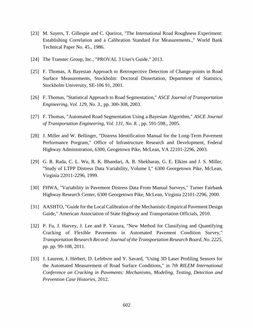
602

[23] M. Sayers, T. Gillespie and C. Queiroz, "The International Road Roughness Experiment:

Establishing Correlation and a Calibration Standard For Measurements.," World Bank

Technical Paper No. 45., 1986.

[24] The Transtec Group, Inc., "PROVAL 3 User's Guide," 2013.

[25] F. Thomas, A Bayesian Approach to Retrospective Detection of Change-points in Road

Surface Measurements, Stockholm: Doctoral Dissertation, Department of Statistics,

Stockholm University, SE-106 91, 2001.

[26] F. Thomas, "Statistical Approach to Road Segmentation," ASCE Journal of Transportation

Engineering, Vol. 129, No. 3., pp. 300-308, 2003.

[27] F. Thomas, "Automated Road Segmentation Using a Bayesian Algorithm," ASCE Journal

of Transportation Engineering, Vol. 131, No. 8. , pp. 591-598., 2005.

[28] J. Miller and W. Bellinger, "Distress Identification Manual for the Long-Term Pavement

Performance Porgram," Office of Infrastructure Research and Development, Federal

Highway Administration, 6300, Geogetown Pike, McLean, VA 22101-2296, 2003.

[29] G. R. Rada, C. L. Wu, R. K. Bhandari, A. R. Shekharan, G. E. Elkins and J. S. Miller,

"Study of LTPP Distress Data Variability, Volume I," 6300 Georgetown Pike, McLean,

Virginia 22011-2296, 1999.

[30] FHWA, "Variability in Pavement Distress Data From Manual Surveys," Turner Fairbank

Highway Research Center, 6300 Georgetown Pike, McLean, Virginia 22101-2296, 2000.

[31] AASHTO, "Guide for the Local Calibration of the Mechanistic-Empirical Pavement Design

Guide," American Association of State Highway and Transportation Officials, 2010.

[32] P. Fu, J. Harvey, J. Lee and P. Vacura, "New Method for Classifying and Quantifying

Cracking of Flexible Pavements in Automated Pavement Condition Survey,"

Transportation Research Record: Journal of the Transportation Research Board, No. 2225,

pp. pp. 99-108, 2011.

[33] J. Laurent, J. Hérbert, D. Lefebvre and Y. Savard, "Using 3D Laser Profiling Sensors for

the Automated Measurement of Road Surface Conditions," in 7th RILEM International

Conference on Cracking in Pavements: Mechanisms, Modeling, Testing, Detection and

Prevention Case Histories, 2012.

603

[34] Y. H. Huang, Pavement Analysis and Design, 2nd Edition, New Jersey: Prentice Hall, 2004.

[35] R. B. Mallick and T. El-Korchi, Pavement Engineering - Principles and Practice, Second

Edition, Boca Raton, Florida: CRC Press, Taylor & Francis Group, 2013.

[36] A. T. Papagiannakis and E. A. Masad, Pavement Design and Materials, Hoboken, New

Jersey: Johm Wiley & Sons, Inc., 2008.

[37] NCHRP, "NCHRP 09-29 - Simple Performance Tester for Superpave Mix Design," 2011.

[Online]. Available: http://apps.trb.org/cmsfeed/TRBNetProjectDisplay.asp?ProjectID=

963.

[38] R. Bonaquist, "NCHRP Report 614: Refining the Simple Performance Tester for Use in

Routine Practice," National Cooperative Highway Research Program, Transportation

Research Board, Washington, D.C., 2008a.

[39] R. Bonaquist, "NCHRP Report 629: Ruggedness Testing of the Dynamic Modulus and

Flow Number Tests with the Simple Performance Tester.," National Cooperative Highway

Research Program, Transportation Research Board, Washington, D.C., 2008b.

[40] W. Abd-Elaziz Zeiada, K. Kaloush, K. Biligiri, J. Reed and J. Stempihar, "Significance of

confined dynamic modulus laboratory testing for asphalt concrete: Conventional, gap-

graded, and open graded mixtures.," Transportation Research Record 2210: Journal of the

Transportation Research Board, pp. 9-19, 2011.

[41] AASHTO, Standard Method of Test for Determining the Dynamic Modulus and Flow

Number of Hot Mix Asphalt (HMA) Using the Asphalt Mixture Performance Tester

(AMPT)., American Association of State Highways and Transportation Officials, 2012.

[42] AASHTO, Standard Method of Test for Determining Dynamic Modulus of Hot Mix Asphalt

(HMA)., American Association of State Highways and Transportation Officials., 2011.

[43] Abatech, "Rheology Analysis Software Users Manual," Abatech Inc. Blooming Glen, PA

(2011), 2013. [Online]. Available: http://www.abatech.com/documents/

RHEA%20Manual%201%202011.pdf. [Accessed 28 May 2013].

[44] L. G. Diaz and A. R. Archilla, "An Easy Way to Use and Interpret the Results from the

Asphalt Mixture Performance Tester," International Journal of Pavement Research and

Technology, p. (forthcoming), 2013.

604

[45] A. R. Archilla, "Developing Master Curve Predictive Equation Models for Local

Conditions: A Case Study for Hawaii," Journal of the Association of Asphalt Paving

Technologists, vol. 79, pp. 325-362, 2010.

[46] A. Archilla, "Effect of Polymer Modified Asphalt Binders on the Performance of Asphalt

Concrete Mixes Used in Hawaii," Honolulu, 2008.

[47] J. K. Rayapeddi Kumar, "Material Characterization in Support of the Implementation of the

Mechanistic-Empirical Pavement Design Guide," Honolulu, 2012.

[48] J. Bari and M. Witczak, "Development of a New Revised Version of the Witczak E*

Predictive Development of a New Revised Version of the Witczak E* Predictive Model for

Hot Mix Asphalt Mixtures," Journal of the Association of Asphalt Paving Technologists,

vol. 75, pp. 381-424, 2006.

[49] J. Bari and M. Witczak, "New Predictive Models for Viscosity and Complex Shear Modulus

of Asphalt Binders For Use with Mechanistic-Empirical Pavement Design Guide,"

Transportation Research Record: Journal of the Transportation Research Board,

Transportation Research Board of the National Academies, vol. 2001, pp. 9-19., 2007.

[50] A. R. Archilla, L. de Lannoy Kobayashi and L. G. Diaz, "Using Permanent Deformation

Tests and the MEPDG to Quantify Permanent Deformation Improvements from Modified

Binders," Journal of the Association of Asphalt Paving Technologists, vol. 77, pp. 1005-

1036, 2008.

[51] Asphalt Institute, "Quantification of the Effects of Polymer-Modified Asphalt for Reducing

Pavement Distress," Asphalt Institute, 2005.

[52] A. R. Archilla and L. G. Diaz, "Effects of Asphalt Mixture Properties on Permanent

Deformation Response," Transportation Research Record: Journal of the Transportation

Research Board, No. 2210, pp. 1-8, 2011.

[53] M. Thompson, S. Baremberg, S. Brown, M. Wilson, M. Darter, G. Larson, M. Witczak and

M. El-Basyouny, "Independent Review of the Mechanistic-Empirical Pavement Design

Guide and Software," Research Results Digest 307, 2006.

[54] D. Li and E. T. Selig, "Resilient modulus for fine-grained subgrade soils.," Journal of

Geotechnical Engineering, Vol. 120, No. 6, pp. 939-957, 1994.

605

[55] P. S. Ooi, A. R. Archilla and K. G. Sandefur, "Resilient Modulus Models for Compacted

Cohesive Soils," Transportation Research Record: Journal of the Transportation Research

Board. No. 1874., pp. 115-124, 2004.

[56] FHWA, "Study of LTPP Laboratory Resilient Modulus Test Data and Response

Characteristics: Final Report.," 2002.

[57] K. George, "Prediction of Resilient Modulus from Soil Index Properties.," 2004.

[58] S. Hossain, "Characterization of Subgrade Resilient Modulus for Virginia Soils and Its

Correlation with the Results of Other Soil Tests.," Report No. VTRC 09-R4. Virginia

Transportation Research Council, VA, 2008.

[59] A. G. Heydinger, Q. L. Xie, B. W. Randolph and J. D. Gupta, "Analysis of Resilient

Modulus of Dense and Open-graded Aggregates.," Transportation Research Record:

Journal of the Transportation Research Board, National Research Council, National

Research Council, Washington, D.C., No. 1547, pp. 1-6., 1996.

[60] T. Bennert and A. Maher, "The Development of a Performance Specification for Granular

Base and Subbase Material," New Jersey Department of Transportation, Final Report,

Project FHWA-NJ-2005-003, 2005.

[61] Y. Song, "Testing and Analysis of Recycled Materials for Highway Projects," Ph.D.

Dissertation, University of Hawaii at Manoa, Honolulu, 2009.

[62] P. Ooi, A. Archilla and Y. S. M. Song, "Application of Recycled Materials in Highway

Projects," Final Report prepared for the Hawaii Department of Transportation, Highways

Division, Honolulu, 2010.

[63] D. Stolle, P. Guo and L. Y., "Unbound Resilient Modulus Testing of Granular Base,

Subbase Materials in Ontario," Ontation Ministry of Transportation, Provincial Highways

Management Division Report HIIFP-033, 2005.

[64] J. Mitchell and N. Sitar, "Engineering Properties of Tropical Residual Soils," Proc.,

Engineering and Construction in Tropical Residual Soils, ASCE, pp. 30-57, 1982.

[65] Sandefur, K.G, "Correlation of Resient Modulus, Mr, of Fine-Grained Soils with Common

Soil Parameters for Use in Design of Flexible Pavements," M.S. Thesis, University of

Hawaii at Manoa, Honolulu, 2003.

606

[66] S. Alavi, T. Merport, J. Wilson, J. Groeger and A. Lopez, "LTPP materials characterization

program: resilient modulus of unbound materials (LTPP Protocol P46) laboratory startup

and quality control procedure.," Report No. FHWA-RD-96-176, U.S. Department of

Transportation, Federal Highway Administration, McLean, Virginia, 1997.

[67] A. R. Archilla, P. S. Ooi and K. G. Sandefur, "Estimation of a Resilient Modulus Model for

Cohesive Soils Using Joint estimation and Mixed Effects," Journal of Geotechnical and

Geoenvironmental Engineering, Vol. 133, No. 8, pp. 984-994, 2007.

[68] C. Zapata and C. Cary, "Integrating The National Database of Subgrade Soil-water

Characteristic Curves and Soil Index Properties with the MEPDG," National Cooperative

Research Program, NCHRP Project No. 9-23B, Arizona, 2012.

[69] A. Yau and H. von Quintus, "Predicting Elastic Response Characteristics of Unbound

Materials and Soils.," Transportation Research Record 1874, Transportation Research

Board of the National Academies, pp. 47-56, 2004.

[70] F. Akeroyd and B. J. Hicks, "Foamed Bitumen Road Recycling.," Highways, vol. 56, no.

1933, pp. 42, 43, 45, 1988.

[71] D. Munar-Castaneda, Study of Fatigue Performance of a Mixture with Unmodified and

Polymer-Modified Asphalt, Honolulu: M.Sc. Thesis, University of Hawaii at Manoa, 2009.

[72] R. Lundstrom, H. Di Benedetto and U. Isacsson, "Influence of Asphalt Mixture Stiffness

on Fatigue Failure," Journal of Materials in Civil Engineering, ASCE, vol. 16, no. 6, 2004.

[73] L. Diaz and A. Archilla, "Effect of Laboratory Data Range Selection in Permanent

Deformation Characterization of Asphalt Mixtures," Transportation Research Record:

Journal of the Transportation Research Boad, N. 2057, Transportation Research Board of

the National Academies, pp. 126-133, 2008.

[74] A. Archilla, L. de Lannoy Kobayashi and L. Diaz, "Using permanent deformation tests and

the MEPDG to quantify permanent deformation improvements from modified binders.,"

Journal of the Association of Asphalt Paving Technologists, vol. 77, pp. 1005-1035, 2008.

[75] K. Hall and J. Crovetti, "Effects of Subsurface Drainage on Pavement Performance:

Analysis of the SPS-1 and SPS-2 Field Sections," National Cooperative Highway Research

Program, Washington, D.C., 2007.

607

[76] K. T. Hall and J. Crovetti, "Performance of Drained and Undrained Flexible Pavements in

the LTPP SPS-1 Experiment," in 86th Annual Meeting of the Transportation Research

Board, Compendium of Papers CD-ROM, Washington, D.C., January 21-25, 2007.

[77] B. Christopher, "Maintenance of Highway Edgedrains," National Cooperative Highway

Research Program, 2000.

[78] ERES Consultants, Inc., "Pavement Subsurface Drainage Design—Reference Manual,"

Federal Highway Administration, Washington D.C., 1999.

[79] HDOT, "Hawaii Standard Specifications and Special Provisions for Road and Bridge

Construction," Hawaii Department of Transportation, 2005.

[80] FHWA, "Drainable Pavement Systems – Participant Notebook, Demonstration Poject 87,"

U.S. Department of Transportation, Federal Highway Administration, 1992.

[81] H. L. Von Quintus and B. M. Killingsworth, Design Pamphlet for the Backcalculation of

Pavement Layer Moduli in Support of the Guide for the Design of Pavement Structures

(AASHTO 1993), McLean, VA: Federal Highway Adminstration, 1997, a..

[82] H. L. Von Quintus and B. M. Killingsworth, "Design Pamphlet for the Determination of

Design Subgrade Modulus in Support of the Guide for the Design of Pavement Structures

(AASHTO, 1993)," McLean, VA, 1997, b.

[83] M. Sagario, "Assessing the Compactability of Recycled Concrete Aggregate and Reclaimed

Asphalt Pavement," University of Hawaii at Manoa, Honolulu, 2009.

[84] H. Von Quintus and B. Killingsworth, "Analyses Related to Pavement Material

Characterization and Their Effects on Pavement Performance," Federal Highway

Adminstration, 6300 Georgetown Pike, McLean, VA, 1998.

[85] D. Timm, X. Guo, M. M. Robbins and C. Wagner, "M-E Calibration Studies at the NCAT

Test Track," Asphalt Pavement Magazzine, pp. 45-51, September/October 2012.

[86] M. Darter, J. Mallela, L. Titus-Glover, C. Rao, G. Larson, A. Gotlif, H. Von Quintus, L.

Khazanovich, M. Witczak, M. El-Basyouny, S. El-Badawy, A. Zborowski and C. Zapata,

"Changes to th Mechanistic-Empirical Design Guide Software Through Version 0.900, July

2006," Transportation Research Board of the National Academies, 2006.

608

[87] I. Al-Qadi, W. Xie and M. Elseifi, "Frequency Determination from Vehicular Loading Time

Pulse to Predict Appropriate Complex Modulus in MEPDG," Journal of the Association of

Asphalt Paving Technologists, vol. 77, pp. 739-772, 2008.

[88] AASHTO, "Pavement Management Guide," American Association of Transportation

Officials., Washington, D.C., 2001.

[89] A. Wolters, K. Zimmerman, K. Schattler and A. Rietgraf, "Implementing Pavement

Management Systems for Local Agencies - State-of-the Art/State-of-the-Practice," Illinois

Center for Transportation, Springfield, Illinois, 2012.

[90] G. Hicks, S. B. Seeds and D. Peshkin, "Selecting a Preventive Maintenance Treatment for

Flexible Pavements," Foundation for Pavement Preservation, 2000.

[91] Asphalt Institute, "The Asphalt Handbook," Asphalt Institute (2007), 2007.

[92] A. Johnson, "Best Practices Handbook on Asphalt Pavement Maintenance," Minnesota

Technology Trasfer (T2) Center/LTAP Program, Center for Transportation Studies,

University of Minnesota, Minneapolis, Minnesota., 2000.

[93] MDOT, "Sealing and Filing of Cracks for Bituminous Concrete Pavements – Selection and

Installation Procedures," Michigan Technological University in cooperation with the

Michigan Department of Transportation., 1999.

[94] Deighton, Deighton, [Online]. Available: http://www.deighton.com/dtims.html. [Accessed

10 10 2013].

[95] Agile Assets, "Pavement Analyst | Advanced Pavement Management Systems (PMS) and

Analysis Software," Agile Assets, [Online]. Available: http://www.agileassets.com/

products/pavement-analyst/. [Accessed 26 October 2013].

[96] University of Birmingham, Highways Management Research Group,, "HDM-4 Technical

Manual," Birmingham, UK, 1999.

[97] US Department of Transportation - Federal Highway Administration, "HERS-ST Highway

Economic Requirements System - State Version," 2013. [Online]. Available:

http://www.fhwa.dot.gov/infrastructure/asstmgmt/hersindex.cfm. [Accessed 12 2013].

609

[98] US Department of Transportation - Federal Highway Adminstration , "HERS-ST -

Highway Economic Requirement Systems - State Version - User's Guide," Washington,

D.C., 2009.

[99] US Department of Transportation - Federal Highway Adminstration, "HERS-ST: Highway

Economic Requirements System - State Version - Technical Report," Washington, D.C.,

2005.

[100] Metropolitan Transportation Commission., "StreetSaver Products, Regional Streets and

Roads Program, 2003-2013," 2013. [Online]. Available: www.mtcpms.org/products/

index.html. [Accessed 15 11 2013].

[101] MTU, "Roadsoft(R)," Michigan Technological University, [Online]. Available:

http://roadsoft.org. [Accessed 30 11 2013].

[102] State of Hawaii - Office of Planning, "Hawaii Statewide GIS Program," [Online].

Available: http://planning.hawaii.gov/gis/download-gis-data/. [Accessed 30 11 2013].

[103] Colorado State University, "PAVER," [Online]. Available:

http://www.paver.colostate.edu/upcoming.php. [Accessed 23 December 2013].

[104] K. McGhee, "Automated Pavement Distress Collection Techniques," National Cooperative

Highway Research Program, Washington, D.C., 2004.

[105] A. Archilla, "Report on Pavement Management Practices - Adaptation of MicroPAVERTM

(or PAVERTM) Input Parameters (and Guidelines) for the City and County of Honolulu,"

Honolulu, 2013.

[106] M. Shahin, W. Welborn, L. Hammond, S. Kim, R. Meisel, L. Cerda and S. Franzen, "User

Manual – PAVERTM 6.5," US Army Corps of Engineers, Engineer Research and

Development Center, Construction Engineering Research Laboratory, USACE., 2012.

[107] M. Shahin and J. Walthers, "Pavement Maintenace Management For Roads and Streets

Using the PAVER System," Construction Engineering Research Laboratory, U.S. Army

Corps of Engineers, 1990.

[108] CALTRANS, "Flexible Pavement Preservation Second Edition: Maintenance Technical

Advisory Guide (MTAG) Volume I, Chapter 5 – Patching and Edge Repair," 2007.

610

[109] FHWA, "Long-Term Monitoring of Pavement Maintenance Materials Test Sites," McLean,

VA, 1998.

[110] T. Wilson and A. Romine, "Materials and Procedures for Repair of Potholes in Asphalt-

Surfaced Pavements – Manual of Practice," 6300 Georgetown Pike, McLean, Virginia

22101-2296, 1999.

[111] R. Wolters, "Repair of Potholes with Hot Mix Asphalt (HMA)," Minnesota Asphalt

Pavement Association, 2003.

[112] T. Kuennen, "The Pothole Patching Playbook - Why potholes occur, how to patch them,

and how to prevent them in the first place.," Better Roads, February 2004.

[113] K. Smith and A. Romine, "Materials and Procedures for Sealing and Filling Cracks in

Asphalt-Surfaced Pavements – Manual of Practice," Strategic Highway Research Program,

National Research Council, Transportation Research Board of the National Academies,

Washignton, D.C., 1993.

[114] Y. Yildirim, A. Qatan and J. Prozzi, "Field Manual for Crack Sealing in Asphalt

Pavements," 2006.

[115] D. Orr, "Pavement Maintenance, Cornell Local Roads Program, Ithaca, New York," 2006.

[Online]. Available: www.clrp.cornell.edu/workshops/pdf/pavement_maintenace-web.pdf.

[116] HAPI, "HAPI Asphalt Pavement Guide," Hawaii Asphalt Pavement Industry, 2013.

[Online]. Available: http://www.stmuench.com/modules/11_maint-rehab/11_maintenance

.htm. [Accessed March 2013].

[117] Nebraska Department of Roads, "Pavement Maintenance Manual," 2002.

[118] R. Roque, J. Zou, Y. Kim, C. Baek, S. Thirunavukkarasu, B. Underwwod and M. Guddati,

"Top Down Cracking of Hot-Mix Asphalt Layers; Models for Initiation and Propagation,"

February 2010. [Online]. Available: http://onlinepubs.trb.org/onlinepubs/nchrp/

nchrp_w162.pdf. [Accessed 28 12 2013].

[119] B. Christopher and V. McGuffey, "Pavement Subsurface Drainage Systems," NCHRP

Synthesis 239, A Synthesis of Highway Practice, Transportation Research Board, National

Research Council, 1997.

611

[120] J. Mallela, L. Titus-Glover and M. Darter, "Considerations for Providing Subsurface

Drainage in Jointed Concrete Pavements," Transportation Research Record 1709,

Transportation Research Board of the National Academies, 174–180, 2000.

[121] B. Christopher, "Maintenance of Highway Edgedrains," NCHRP Synthesis of Highway

Practice 285, National Cooperative Highway Research Program, 2000.

[122] T. Kuennen, "Making edge drains work : base edge drains can enhance pavement life - but

only if you maintain them," Better Roads, Volume 73, Issue 1, 2003 .

[123] E. Harrigan, "NCHRP Research Results Digest Number 268 (Summary of key findings

from NCHRP Project 1-34 “Performance of Subsurface Pavement Drainage”)," National

Cooperative Research Program, 2002..

[124] B. Diefenderfer, K. Galal and D. Mokarem, "Effect of Subsurface Drainage on the

Structural Capacity of Flexible Pavement," Report VTRC 05-R35, Virginia Department of

Transportation., 2005.

[125] M. Darter, H. Von Quintus, Y. Jiang, E. Owusu-Antwi and B. Killingsworth, "Catalog of

Recommended Pavement Design Features," National Cooperative Highway Research

Program, NCHRP Project 1-32, Washington, D.C., 1997.

[126] Florida State Department of Transportation, "Standard Specifications for Road and Bridge

Construction," Florida State Department of Transportation, 2004.

[127] California Department of Transportation, "Standard Specifications for Construction of

Local Streets and Roads," California Department of Transportation, 2002.

[128] Louisiana Department of Transportation, "Louisiana Standard Specifications for Road and

Bridges," 2006.

[129] Federal Highway Administration, "Drainable Pavement Systems, Participant Notebook,

Demonstration Project 87," 1992.

[130] CALTRANS, "CALTRANS Highway Design Manual," California Department of

Transportation.

[131] J. P. Donahue, "Missouri Guide for Pavement Rehabilitation," Missouri Department of

Transportation, Report RDT 02-013, October 2002., 2002.

612

[132] MnDOT, Road Design Manual, Developed by the Office of Project Management and

Technical Support, Minnesota Department of Transportation, 2007.

[133] K. Hall and C. Correa, "Effects of Subsurface Drainage on Performance of Asphalt and

Concrete Pavements," Transportation Research Board of the National Academies,

Washignton, D.C., 2003.

[134] M. Bejarano and J. Harvey, "Accelerated Pavement Testing of Drained and Undrained

Pavements under Wet Base Conditions," Transportation Research Record 1816,

Transportation Research Board of the National Academies, 137–147, 2002.

[135] H. Melhem and R. Swart, "Evaluation of the Performance of Permeable and Semi-

Permeable Unbound Granular Bases Under Portland Cement Concrete Pavement (PCCP)

Slabs and Alternate Load Transfer Devices for Joint Repair," Kansas Department of

Transportation, 2003.

[136] M. Elseifi, I. Al-Qadi, A. Loulizi and J. Wilkes, "Performance of Geocomposite Membrane

as Pavement Moisture Barrier," Transportation Research Record 1772, Transportation

Research Board of the National Academies, pp. 168-173, 2001.

[137] T. Winkelman, "Open Graded Drainage Layer Performance in Illinois," 2004.

[138] S. Jahangirnejad, N. Buch and A. Kravchenko, "Evaluation of Coefficient of Thermal

Expansion Test Protocol and Its Impact on Jointed Concrete Pavement Performance.," vol.

Vol. 106, no. 1, pp. pp 64-71., 2009.

[139] A. Neville, Properties of Concrete, New York: John Wiley and Sons, Inc., 1996.

[140] J. Mallela, A. Abbas, T. Harman, C. Rao, R. Liu and M. Darter, "Measurement and

Significance of the Coefficient of Thermal Expansion of Concrete in Rigid Pavement

Design," Transportation Research Board: Journal of the Transportation Research Board,

vol. 1919, pp. 38-46., 2005.

[141] J. H. Yeon, S. Choi and M. C. Won, "Effect of Relative Humidity on Coefficient of Thermal

Expansion of Hardened Cement Paste and Concrete," Transportation Research Record:

Journal of the Transportation Research Board, vol. 2113, pp. 83-91, 2009.

[142] N. Tran, K. Hall and M. James, "Coefficient of Thermal Expansion of Concrete Materials,

Characterization to Support Implementation of the Mechanistic–Empirical Pavement

613

Design Guide," Transportation Research Record: Journal of the Transportation Research

Board, No. 2087, pp. 51-56, 2008.

[143] K. Shushkewich and I. Robertson, "Instrumentation of the North Halawa Valley Viaduct,

Oahu, Hawaii," Progress Report prepared for the Hawaii Department of Transportation and

the Federal Highway Administration, Honolulu, 1998.

[144] FORTA-Ferro. [Online]. Available: http://www.forta-ferro.com/products/macrofibers/

forta-ferro/. [Accessed 9 August 2011].

[145] S. A. Havel, "Coefficient of Thermal Expansion of Concrete Mixes in Hawaii:

Determination and Implications for Concrete Pavement Design," M.Sc. Thesis, University

of Hawaii at Manoa, 2011.

[146] J. Tanesi, G. Crawford, M. Nicolaescu, R. Meininger and J. Gudimettla, "New AASHTO

T336-09 Coefficient of Thermal Expansion Test Method How Will It Affect You?,"

Transportation Research Record: Journal of the Transportation Research Board, No. 2164,

pp. 52-57, 2010.

[147] G. Crawford, J. Gudimettla and J. and Tanesi, "Interlaboratory Study on Measuring

Coefficient of Thermal Expansion of Concrete," Transportation Research Record: Journal

of the Transportation Research Board, No. 2164, pp. 58-65, 2010.

[148] S. H. Kosmatka, B. Kerhoff, N. MacLeod and R. J. McGrath, "Design and Control of

Concrete Mixtures," EB101, 7th Canadian ed. Cement Association of Canada, Ottawa,

Ontario, 2002.

[149] W. Navidi, Statistics for Engineers and Scientists, McGraw Hill Higher Education, New

York, 2006., New York: McGraw Hill Higher Education, 2006.

[150] S. Jahangirnejad, "Evaluation of Portland Cement Concrete Coefficient of Thermal

Expansion Test Protocol and the Impact of CTE on Performance of Jointed Concrete

Pavements," Ph.D. Dissertation, Michigan State University, 2009.

[151] F. Wittmann and J. Lucas, "Experimental Study of Thermal Expansion of Hardened Cement

Paste," Materials and Structures, vol. 7, no. 40, 1974.

[152] Rudeloff and Sieglerschmidt, Deutscher Ausschuss f. Eisenbeton, vol. 23, 1913.

614

[153] S. Jahangirnejad, N. Buch and A. Kravchenko, "Evaluation of Coefficient of Thermal

Expansion Test Protocol and Its Impact on Jointed Concrete Pavement Performance," ACI

Materials Journal, vol. 106, no. 1, pp. 64-71, 2009.

[154] D. T. Hartgen, M. G. Fields, E. San José and A. Moore, "20th Annual Highway Report on

the Performance of State Highway Systems," 2013.

[155] "Developing Master Curve Predictive Equation Models for Local Conditions: A Case Study

for Hawaii," Journal of the Association of Asphalt Paving Technologists, 2010.

[156] D. Muir Wood, Soil Behaviour and Critical State Soil Mechanics, Cambridge: Cambridge

University Press, 1990.

[157] P. Ooi, K. Sandefur and A. R. Archilla, "Correlation of Resilient Modulus of Fine-Grained

Soils with Common Soil Parameters for Use in Design of Flexible Pavements," Final Report

prepared for the Hawaii Department of Transportation, Honolulu, 2006.

[158] LADOT, Road Design Manual, Louisiana Department of Transportation, 2009.

[159] ASTM, "Standard Test Method for Permeability of Granular Soils (Constant Head),"

American Society for Testing and Materials, 221-225.

[160] "Guide for Design of Pavement Structures," AASHTO, Washington, D.C., 1993.

[161] [Online]. Available: http://www.pewcenteronthestates.org/. [Accessed 04 2011].

[162] [Online]. Available: http://www.infrastructurereportcard.org/state-page/hawaii. [Accessed

13 February 2011].

[163] Guide for Mechanistic-Empirical Design of New and Rehabilitated Pavement Structures.

NCHRP Project 1-37A. Final report, Part 2., Champaign: ERES Consultants Divisions,

Applied Research Associates, Inc., 2004.

[164] FHWA, Integrated Materials and Construction Practices for Concrete Pavements: A State-

of-the-Practice Manual, HIF-07-004, Federal Highway Administration, U.S. Department of

Transportation, 2006.

[165] L. N. Mohammad, Z. Wu, S. Obulareddy, S. Cooper and C. Abadie, "Permanent

Deformation Analysis of Hot-Mix Asphalt Mixtures Using Simple Performance Tests and

615

2002 Mechanistic–Empirical Pavement Design Software," Transportation Research

Record: Journal of the Transportation Research Board, No. 1970, p. 133–142, 2006.

[166] FHWA, Highway Economic Requirements System – State Version User’s Guide.,

Washington, D.C.: US Department of Transportaiton, Federal Highway Administration,

2007.

[167] J. K. E. Tanesi, A. A. M. and R. Meininger, "Effect of Coefficient of Thermal Expansion

Test Variability on Concrete Pavement Performance as Predicted by Mechanistic-

Emperical Pavement Design Guide.," In Transportation Research Record: Journal of the

Transportation Research Board, vol. 2020, pp. 40-44, 2007.

[168] M. Won, "Improvements of Testing Procedures for Concrete Coefficient of Thermal

Expansion.," In Transportation Research Record: Journal of the Transportation Research

Board,, vol. 1919, pp. 23-28, 2005.

[169] K. Hall and S. Beam, "Estimating the Sensitivity of Design Input Variables for Rigid

Pavement Analysis with a Mechanistic-Empirical Design Guide.," In Transportation

Research Record: Journal of the Transportation Research Board, vol. 1919, pp. 65-73,

2005.

616

APPENDIX A – LITERATURE REVIEW ON PERMEABLE BASES

A.1 Introduction

In order to update the current HDOT Pavement Design Manual, a comprehensive review

of the literature was conducted regarding the practices related to the use of permeable bases in

pavement design across the United States. The objective of the review was to identify and

document current practices across the country, particularly those that may differ from current

HDOT procedures. Experiences from other states regarding the use subsurface drainage features,

particularly those involving the use of drainage layers in pavement structural sections, are

emphasized in this section.

A.2 Pavement Subsurface Drainage Systems

It is widely recognized that excess moisture within the pavement system is greatly

responsible for accelerated deterioration rates and subsequent diminished pavement life. Excess

moisture can enter the pavement structure from surface infiltration through cracks and joints in

the pavement surface, from groundwater from a high water table, interrupted aquifers and/or

localized springs, and from capillary suction in the soil from the water table.

The strategies used to avoid moisture related problems in pavement systems range from

use of relatively moisture-insensitive materials (e.g., some treated materials), to the construction

of complete subsurface drainage systems including permeable layers within the pavement

structure to evacuate infiltration water. In a study involving a survey of state highway agencies

(SHA), Christopher and McGuffey [119] concluded that a preponderance of evidence supports

the philosophy that “good sealing and good drainage, along with a commitment to long term

maintenance will lead to optimum performance of a pavement system.” Nevertheless, the same

study indicated uncertainty in the cost-effectiveness of edge drains and permeable bases, and that

SHA consider it as a topic that needs to be a priority for further investigations.

Mallela et al. [120] list five specific issues that must be addressed in a successful drainage

design, including first the evaluation of the need for subdrainage, followed by the determination

of the drainage components needed in each situation, the hydraulic and structural design of the

subdrainage system within the overall pavement design process, the specifications of the materials

617

used in the drainage system to ensure long-term performance, and finally, the documentation of

construction and maintenance considerations.

Site and design factors are commonly taken into account when deciding if subsurface

drainage is required, and the criteria and level of complexity in the decision process varies among

agencies. Mallela et al. [120] present an approach recommended in NHI Course 13126, which

consists in assessing the need for a drainage system based in an objective ranking of both site and

design conditions. A summary table for the determination of the need for subsurface drainage in

jointed plain concrete pavements (JPCP) is included in [120].

The basic components of a pavement drainage system include a permeable base layer, a

separator or filter layer to avoid intrusion of fines from the subgrade or subbase materials to the

permeable base (usually a specifically graded aggregate layer and/or a geotextile filter fabric),

and a collector system (edge drain structures and outlet pipes) to transport the intercepted water

within the pavement structure to an outside drainage ditch or water sewer system. The essential

components of an edge drain structure include [121]:

A trench filled with filter-graded aggregate, open graded aggregate wrapped with a

geotextile filter, or a prefabricated geocomposite drain; and

A longitudinal conduit consisting of a perforated pipe or other hollow plastic core.

The incorporation of a drainage system into the pavement structure design introduces a

wide variety of complexities related to construction practices that need to be addressed in order

to ensure that the pavement structure works as originally intended in the design. NCHRP

Synthesis 239 “Pavement Subsurface Drainage Systems” [119] recommends having from the

start of the construction activities the presence and active participation from someone with

knowledge about drain installation principles and practices.

A.3 Potential Problems with Subsurface Drainage

As indicated before, a properly designed, constructed, and maintained drainage system

usually improves the performance of pavement structures. However, over time the drainage

system may be affected by problems, particularly without proper maintenance.

618

The first indicator that problems with the drainage system are present is that there is no

longer flow of water from the permeable base to the ditch. In contrast, an indication of a

functioning system is the presence of deeper grass around a lateral outlet.

The majority of the problems within the drainage system are created during the

construction stage, due to crushed pipes by construction equipment, and undulating drain lines

that will accumulate water in depressed areas [119]. Other problems encountered with subsurface

drainage systems include clogging of edge drains and outlet pipes from fine particles

accumulation, rodent nests, lack of transverse drains in the lowest vertical alignment points, and

backup of water from drain ditches ( [119], [122]).

Video inspection of the drainage system right after construction is an excellent way to

evaluate if the system is in proper operating conditions, and can also be used for work

acceptance purposes [119].

When the presence of distress in the pavement surface is what suggests there are

problems with the drainage system, the situation is almost always irreversible, although

successful correction of the problem will slow the deterioration rate of the pavement structure.

This situation stresses the idea that a well-established inspection and maintenance plan for the

subsurface drainage system should be implemented [119].

A.4 Drainage System Maintenance Activities

A structured inspection and maintenance plan for the subsurface drainage of a pavement

system is generally recommended in order to ensure that the system performs as designed. Some

authors also suggest that if no maintenance is expected to be done, the presence of an inoperative

drainage system could be more detrimental to the pavement structure than not having a system at

all ( [119], [120], [122], [122], [123], and [124]). The general consensus is that continuous

inspection and maintenance of outlets and edge drain pipes contributes to maintain the roads in

good condition.

The Christopher and McGuffey [119] study encountered different levels of maintenance

activities across the United States. According to the responses received from SHA, there was not

a clear maintenance policy established within the individual agencies, and the activities relied

heavily on the responsible individuals in each maintenance jurisdiction. Most states reported

619

inspection of outlet condition in a yearly basis, and most maintenance strategies were selected

with little central control. Detailed findings about the maintenance of subsurface drainage

systems can be found in Chapter 5 of NCHRP Synthesis 239 “Pavement Subsurface Drainage

Systems” [119].

Christopher and McGuffey [119] indicate different instances of pavement systems in

Europe incorporating drainage with no maintenance that performed sometimes as if there were

no drains at all after 14 years. The same report cites findings from France where operating edge

drains at time of construction became inoperative after 11 years without maintenance, and

showed moisture related distresses (pumping) after only 7 years under these circumstances.

It is generally accepted that if distress from subsurface drainage blockage is visible, the

damage is irreversible. According to the above authors, good sealing and good drainage, along

with a commitment to long-term maintenance lead to optimum pavement performance. This

stresses the need for the implementation of regular inspection and preventive maintenance

programs for the subsurface drainage systems.

The 1998 “Catalog Of Recommended Flexible Pavement Design Features” prepared by

Darter et al. [125], describe four levels of solutions for pavement drainage problems, ranging

from basic joint and crack sealing combined with proper geometrics (including side ditches on

both sides of the pavement section), to more complex (and expensive) sub drainage systems

including permeable bases and edge drains, to rapidly remove excess moisture that enters the

pavement section before it can cause damage. They also mention the use of moisture insensitive

and non-erodible materials as an effective measure to minimize moisture-induced distresses in

the pavement structure.

A.5 Drainage Layer

A permeable base (or drainage layer) is a treated or untreated layer of open graded

aggregate, designed with the primary function of collecting surface infiltration water in the

pavement and direct it towards the edge drains within an acceptable time frame, while providing

adequate support to the pavement.

There is not a unique set of requirements or specifications for the materials and

construction procedures for permeable bases, as they vary from agency to agency (specification

620

details for CA, LA and FL can be found in [126], [127], and [128]). In general, the aggregate

should come from crushed stone, with very little, if any, fine material. This is necessary to

improve the interlock between the aggregate particles, critical to ensure proper stability in the

drainage layer.

Permeable bases can be treated with asphalt cement (ATPB) or Portland cement (CTPB).

Asphalt cement contents between 2 – 4 percent by weight of mix are common practice, although

the specific amount varies from state to state. The general requirement is that 95% of the

aggregate particles be fully coated with asphalt cement, as a minimum. The use of a standard

permeable base thickness is common practice, usually between 75 mm to 100 mm for ATPB

(CA and FL, respectively), and 105mm for CTPB (CA). These standard thicknesses have been

established in most cases from local experience and constructability issues. No specific

recommendations have been found for untreated permeable base thickness. However, the

MEPDG documentation [1] states that “The recommended minimum and maximum thickness of

permeable base layers is 4 inches. This recommendation ensures an adequate hydraulic channel

for the free flow of water and places an upper limit on the thickness of this relatively unstable

layer. Permeable bases could be asphalt treated, cement-treated, or untreated, depending on

structural requirements”.

In terms of gradation, reference [129] indicates that several states use the AASHTO No.

57 gradation for their stabilized permeable bases. This gradation and the current HDOT (and

CALTRANS) specifications are shown Table A-1.

As can be observed in Table A-2, Hawaii uses by far the coarser gradation (the filler

changes the gradation only in the upper part of the permeable layer). This may be explain some

of the construction difficulties of permeable layers in Hawaii and it may additionally lead to

higher costs. It is worth mentioning that aggregates such as 3-Fine commonly used in Hawaii

typically fall within the gradation limits for the Wisconsin OGBC No. 1.

A.6 Drainage Layer Use

Literature regarding the use of permeable base in pavement construction covers published

pavement design manuals from different State Departments of Transportation such as California,

Florida, and Minnesota, published papers regarding controlled experimentation with permeable

621

base materials under accelerated loading conditions, and reports from evaluations of in-service

pavements across the United States.

For untreated permeable bases, reference [129] shows the gradations used by several

states. These, along with the current HDOT gradation are shown in Table A-2.

Table A-1. Gradations of AASHTO No. 57 and HDOT and CALTRANS stabilized permeable

bases.

A.7 CALTRANS Highway Design Manual

The CALTRANS Highway Design Manual is discussed first because the Hawaii

pavement design guide draws heavily from earlier versions of this manual, particularly for

flexible pavement design.

A.7.1 Philosophy and Standards

The state of California requires that the standards used for any project meet or exceed the

minimum standards provided in their guide. Three categories for standards are used in the

CALTRANS Highway Design Manual (from Chapter 80 “Application of Design Standards”,

page 80-2 [130]):

Sieve Size

Percent Passing By Weight

AASHTO No. 57

Gradation

HDOT and CALTRANS

Specifications

1.5” 100 100

1” 95 – 100 100

0.75” 90 – 100

0.5” 25 – 60 35 – 65

0.375” 20 – 45

No. 4 0 – 10 0 – 10

No. 8 0 – 5 0 – 5

No. 200 0 – 2

622

“(2) Mandatory Standards. Mandatory design standards are those considered most essential to

achievement of overall design objectives. Many pertain to requirements of law or regulations such as those

embodied in the FHWA's 13 controlling criteria (see below). Mandatory standards use the word “shall" and

are printed in Boldface type (see Table 82.1A).

(3) Advisory Standards. Advisory design standards are important also, but allow greater flexibility in

application to accommodate design constraints or be compatible with local conditions on resurfacing or

rehabilitation projects. Advisory standards use the word "should" and are indicated by Underlining (see

Table 82.1B).

(4) Permissive Standards. All standards other than mandatory or advisory, whether indicated by the use of

"should" or "may", are permissive with no requirement for application intended.”

Table A-2. Untreated base gradations.

Sieve

Size Iowa Minnesota

New

Jersey Pennsylvania

Wisconsin

OGBC No.

1

Hawaii

Coarse Filler

2’ 100 100

1.5” 100 75 – 100

1” 100 100 95 – 100 100 15 – 55

0.75” 65 – 100 52 – 100 90 – 100 0 – 15

.5” 60 – 80 - 100

0.375” 35 – 70 33 – 65 20 – 55 0 - 5 85 – 100

No. 4 20- 45 40 – 55 8 – 40 0 – 10 10 – 30

No 8 10 -35 5 – 25 0 – 5 0 – 10

N 10 8 – 25

No. 16 0 – 8 0 – 12 0 – 5

No. 40 2 – 10

No. 50 0 – 15 0 – 5

No. 200 0 – 6 0 - 3 0 - 5

The Mandatory and Advisory standards are listed in Table 82.1A and 82.1B, respectively,

in reference [130], Chapter 80 “Application of Design Standards”.

Proposals for the implementation of new ideas and techniques in California’s highway

system, particularly in the design, construction, maintenance, and materials engineering of the

structural section, are encouraged. The proposed research must be first submitted to the Division

of Research and Innovation, while approval and implementation of experimental construction

features must be done by the Pavement Standards Team (who can also receive suggestions about

623

changes in design standards and research studies). They recommend the involvement of

maintenance personnel in discussions related to any experimental construction features

The above discussion is introduced here because it may help in writing the standards for

Hawaii, since it appears it is not always clear whether a given standard is a requirement or not. In

addition, it helps in the interpretation of the summary of CALTRANS practices below.

A.7.2 Drainage Layer in Caltrans Highway Design Manual (CALTRANS Highway Design

Manual)

There is no mandatory standard regarding the utilization of permeable base in the

CALTRANS Highway Design Manual. However, its utilization is recommended in most cases,

except when environmental or subgrade conditions do not justify it90.

When Treated Permeable Base (TPB) is included in the design, standard thicknesses of

75 and 105mm for Asphalt Treated Permeable Base (ATPB) and Cement Treated Permeable

Base (CTPB), respectively, are suggested. This differs from the current HDOT Pavement Design

Manual, where the thickness of the drainage layer is based on surface water infiltration rate. In

the case of California, the recommended thicknesses are based primarily on constructability, with

an added allowance to compensate for construction tolerances. They indicate that the fixed TPB

thicknesses will generally be more than enough to evacuate the surface infiltration water (Section

606.3 (1) [130]).

While the placement of at least 6” of an aggregate separation layer covered by a

permeable geotextile between the subgrade and the TPB is currently required by HDOT (due to

the amount of fines commonly encountered in subgrade soils in the state, Chapter 2, pg. 17 [13]),

no mandatory standard regarding the utilization of an aggregate separation layer below the

permeable base was found in the CALTRANS manual. However, they indicate that a filter fabric

or other suitable membrane should be placed on top of the layer supporting the TPB when there

90 From CALTRANS Highway Design Manual, Section 606.2, pg. 31.

“The structural section should include a layer of Treated Permeable Base (TPB) under the pavement except

in areas where the mean annual rainfall is very low (less than 125 mm) or where the basement soil is free draining (a

permeability greater than 3.53 x 10-4m/s)”.

624

is concern that the infiltrating surface water may saturate and soften the underlying subbase or

subgrade, generating migration of fines and contamination of the TPB.

For structural design purposes, no R-value is assigned to TPB materials (Section

606.3(2), pg. 600-33 [130]). Use of TPB layers thicker than the 75 or 105mm recommended

(ATPB or CTPB, respectively) are only recommended under unique combination of conditions

(footnote Table 604.3 in [130]). CALTRANS does not prohibit the use of other types of drainage

layers, but suggests that checks for suitability regarding permeability and structural capacity

should be performed.

Asphalt treated permeable base material is plant produced, and production requirements

can be found in Section 29-1.04A from “Standard Specifications for Construction of Local

Streets and Roads” [127]. Aggregate requirements for ATPB are included in Section 29-1.02A of

the same document. It is important to note that the gradation requirements for ATPB are identical

for both HDOT and CALTRANS (gradation requirements in Section 703.04 in HDOT

specifications refer to Untreated Permeable Bases (UPB) alone). Even though use of drainage

layers other than ATPB and CTPB is not forbidden in the CALTRANS manual, no specifications

were found regarding aggregate gradation for untreated permeable bases (UPB) layers.

A.8 Drainage Layer Use in Other Design Guides

This section first discusses the information regarding drainage layer included in the

mechanistic-empirical design guide documentation and then discusses the information found on

the same subject on several State DOT’s design guides and specifications.

A.8.1 MEPDG Drainage Layer Treatment

The use of subsurface drainage (and therefore of permeable base) is not mandatory in all

cases, but rather depends on the conditions of the particular project. Table 3.1.1 in [1] gives an

indication on when subsurface drainage might be required, as a function of general climatic

conditions and traffic level. According to that table, for Hawaiian climatic conditions and with

less than 2.5 million 20-year design lane heavy trucks, subsurface drainage is not required for

subgrades with coefficients of permeability of 3 m/day (10 ft/day) and above. This is in contrast

to the requirement by HDOT of 30 m/day (100 ft/day) (irrespective of traffic level and only for

“pavement layers” (asphalt concrete?) placed directly on the pavement soil), which is an order of

625

magnitude higher than the recommended values in the new guide. This may point out situations

in which the usage of a permeable layer may not be warranted.

For intermediate traffic loadings (between 2.5 and 12 million 20-year design lane heavy

trucks), the MEPDG requires the use of a permeable layer for subgrades with permeability of

less than 3 m/day (10 ft/day) and indicates that additional factors must be considered in the

decision for installing permeable bases over subgrades with higher permeability.

For higher traffic loadings (greater than 12 million 20-year design lane heavy trucks), the

MEPDG requires a drainage layer for subgrade permeability lower than 30 m/day (100 ft/day),

and also indicates the consideration of additional factors for higher permeability.

In summary, the MEPDG provides conditions under which a drainage layer is not

required and intermediate conditions under which it may be required depending on other factors.

Unfortunately, the additional factors, which include past pavement performance and experience

in similar conditions, cost differential and anticipated increase in service life, and anticipated

durability and/or erodability of paving materials, may not be easy to quantify.

Also, as is the case with some other state’s current design guides (CA, FL, and MO), the

thickness of the drainage layer is not variable, but rather a fixed value governed by local

experience and constructability issues ( [126], [127], [131]).

As reported in Part 3, Chapter 1, Section 3.1.5.3 in [1], the layer thickness has the least

effect on the “time-to-drain” parameter in a permeable base, while permeability has the greatest

effect, as the time to drain decreases exponentially with an increase in permeability. Based on

this, the MEPDG recommends 4 inches as an appropriate permeable base layer thickness

(maximum and minimum), allowing compaction without segregation while providing an

acceptable hydraulic conduit.

To ensure appropriate stability in an untreated permeable base, a minimum Coefficient of

Uniformity (Cu) of 3.5 is required. If this cannot be achieved, the base should be asphalt or

cement treated. The aggregate used for untreated permeable bases should have 98% crushed

faces, and have no more than 45% loss in the Los Angeles Abrasion Test (AASHTO T96), while

soundness should not exceed 12 to 18% loss (AASHTO T104). Minimum permeability of

1000ft/day is required, and fines should be non-plastic (AASHTO T90). (The MEPSG excerpted

626

these requirements from the “Guide Specification for Material Selection and Construction of

Unstabilized Permeable Base Layers available from FHWA).

For ATPB, the asphalt cement content must be 3 0.5 percent by weight of dry

aggregate, and gradation should ensure mix permeability of at least 1000 ft-day. Restrictions for

aggregates in CTPB are the same as those for untreated permeable bases.

Use of a separation layer is recommended to avoid penetration of subgrade fines into the

permeable base, to serve as a moisture barrier to horizontally remove any excess water from the

pavement to the edges, and to support construction traffic. This layer can be an untreated dense

aggregate base, or a geotextile layer.

The requirements for an Untreated Dense Aggregate Separation Layer, as listed in the MEPDG

[1] are:

Fractured Faces on material retained on No. 4 sieve (98% crushed stone is preferred)

L.A Abrasion Test below 50% (AASHTO T96)

Loss from soundness test (AASHTO T104) should not exceed 12 to 18%

Maximum Permeability of 15 ft/day

Maximum % passing N200 of 12%

Material passing N40 sieve must be no plastic (AASHTO T90)

If the edge drain pipes can resist the loads imposed during construction, it can be

expected that they resist the whole design life of the pavement without crushing. The MEPDG

suggests using existing state specifications for edge drain construction, and indicates that the

permeability of the backfill used in edge drain trenches must be greater than or equal to the

permeability of the permeable base. Appendix SS of the MEPDG [1] covers hydraulic design,

material selection, and construction issues of edge drains with and without permeable bases.

A.8.2 Florida DOT

The Florida DOT Design Guide of Rigid Pavements describes the use of 100 mm of

Asphalt Treated Permeable Base (ATPB) or Cement Treated Permeable Base (CTPB) as their

typical drainage layer section [126]. This drainage layer is sitting on top of a 30 mm Structural

Course that acts as a separation and waterproofing blanket, which is placed on top 300mm

stabilization layer, which acts as a construction-working platform. The infiltration water is then

627

directed to the nearest outfall located on the shoulder slope, or to a storm sewer system in urban

areas.

The state of Florida allows gradations with 1 and ¾” maximum nominal size to be used in

ATPB layers. Other properties specified include:

Los Angeles abrasion test Max 45% (50% for Granites)

Soundness Max 12%

Flat and Elongated particles Max 10%

For Natural Stones:

o Fractured Faces Min 85% (Retained in N4 sieve)

o Dry Unit Weight Min 95lb/ft3 (AASHTO T19)

Detailed specifications for aggregates to be used in ATPB, including specific aggregate

gradations, can be found in “Standard Specifications for Road and Bridge Construction”, Section

901 [126].

Differences between FLDOT and CALTRANS compaction of ATPB include:

Installation (spread) temperature (above 5C for CALTRANS, 10C for FL)

Compaction Temperature Start/Finish: 65C/38C for CALTRANS; 88C/38C for

Florida DOT (Both using steel 2 axle tandem roller between 8 – 12 tons).

Use of water to cool ATPB material allowed in FL, forbidden in CA.

The gradation requirements for both CTPB and ATPB are the same (both specify use of

gradations 57 or 67 from “Standard Specifications for Road and Bridge Construction”, Section

901 [126]).

A.8.3 Missouri DOT

The preferred base type in Missouri for concrete pavements is a 2-feet, day lighted rock

base, which provides a stiff platform and that is currently believed to be a very drainable layer

(performance to date is reported as excellent). Missouri also uses an alternate 4” TPB over 4” of

Type 5 subbase with edge drains, as indicated in the document “Missouri Guide for Pavement

Rehabilitation” [131]. The daylighted recommendation is in contrast from the recommendation

in [129], which states “daylighting the permeable base layer is not recommended since the

628

daylighted layers are subject to clogging from roadway debris and vegetation”. However, the

latter reference is 10 years older than the Missouri DOT reference.

A.8.4 Minnesota DOT

MnDOT does not require the use of permeable base as mandatory, but includes it in one of their

pavement design standards. Consideration about the use of drainage layer in pavement structures

is given in “Permeable Aggregate Base Drainage Systems Design Guidelines”, 1994. The use of

an impervious layer is illustrated in Figure 8-3.06A [132].

A.8.5 Louisiana DOTD (Louisiana Department of Transportation and Development)

To help prevent water from entering the pavement structure from beneath, the design

high water elevation should be 2 ft below the base course, and roadside ditches should be set a

minimum of 2 ft below the lowest part of the base course [from Section 5.1.3 in Louisiana’s

Road Design Manual [128].

It is apparent from Section 307 in their Standard Specifications Manual that only treated

permeable bases are prescribed in their pavement designs. Thickness of the permeable base

appears to be a variable in the pavement design process, in contrast with current practice in

California and Florida, where the thickness of the permeable base is fixed, and based on

constructability. Pavement structural section design in the state of Louisiana follows the

AAHSTO design method, as specified in the Pavement Structural Design Directive EDSM

II.2.1.12.

A.8.6 Reported Performance Information

A considerable amount of research has been published regarding the use of permeable

bases within pavement structures. The general consensus is that properly constructed permeable

bases within a well-designed subsurface drainage system contribute to extend the service life of

pavements.

Use of permeable base does not appear to be necessary for Doweled JPCP, as reported in

NCHRP Project 1-34 “Performance of Pavement Subsurface Drainage”. However, the

performance of undoweled JPCP is greatly improved with permeable base layers and edge

drains. The incorporation of a permeable layer beneath the dense asphalt concrete was reported

629

as being the most cost-effective design. It was indicated that in any case, proper maintenance of

drainage structures (permeable layers, edge drains, etc.) must be warranted, as abandoned

drainage structures can lead to a more rapid failure of the pavement. This information was

obtained from NCHRP Research Results Digest Number 268 [123].

A lot of confusion reported from “as designed” and “as constructed” records was reported

in NCHRP Report 499, “Effects of Subsurface Drainage on Performance of Asphalt and

Concrete Pavements” [133]. No statistically significant difference between the uses of drained or

undrained structures was obtained from this study. The general feeling is that a permeable base

(asphalt treated) improves pavement performance (measured with IRI, cracking, and rutting).

In a study of accelerated pavement testing of drained and undrained pavements under

saturated base conditions, Bejarano and Harvey [134] report that the failure modes for drained

and undrained pavement sections are different (bottom up fatigue for undrained while rutting for

drained sections), but that similar pavement life was observed for both types of structures. They

recommend the elimination of Asphalt Treated Permeable Base (ATPB) use by increasing the

asphalt concrete (AC) thickness to reduce the risk of load induced cracking, and to ensure low

permeability of the AC layer through proper compaction. They suggest that special steps and

care needs to be taken in order to avoid stripping of the asphalt binder in the ATPB material.

In another study, after evaluating the performance of permeable and semi-permeable

unbound granular bases under PCC slabs, it was concluded that PCC sections over permeable

bases perform better than under semi-permeable bases [135].

Use of an impervious separator layer was investigated in Virginia by Elseifi et al [136]. They

report the use of a specially designed geocomposite membrane as a moisture barrier, consisting of

a low modulus polyvinyl chloride (PVC) backed on both sides with polyester nonwoven geotextile,

installed under 75mm of ATPB. The researchers report prior success in the use of this membrane

as an impermeable material for dams, canals, reservoirs, and hydraulic tunnels. The results from

the investigation suggested that for pavement systems with low water table conditions, an

impervious membrane used in combination with a permeable base layer is capable of removing

surface infiltration water, and can provide a dry service condition for the underneath layers even

in the event of heavy rain.

630

The performance of different types of drainage layers constructed during the late 80’s and

early 90’s was evaluated by the Illinois Department of Transportation, and reported by

Winkelman [137]. The report covered the construction, performance, and rehabilitation of six

projects, and studied the effects of using both asphalt and cement treated permeable bases, as

well as the effects of placing an aggregate separation layer between the drainage layer and the

lime-modified subgrade, as opposed to placing the drainage layer directly on top of it. Pavement

performance was measured by means of visual distress surveys, FWD testing, IRI values, and

Condition Rating Survey (CRS) values. The use of drainage layers was evaluated in three types

of rigid pavements (JPCP, JRCP, and CRCP)91, and in one full depth Hot Mix Asphalt (HMA)

pavement.

Mid panel cracks in 99% of the JRCP slabs triggered the abandonment of this type of

design, and set to 15 feet the maximum joint spacing allowed for jointed concrete pavements in

the state. Based on the poor performance of two CRCP projects, a moratorium on the

construction of drainage layers under state maintained highways was issued in January 1996.

One of the reasons identified for the poor performance of these projects was the intrusion of fine

materials into the permeable base, in part due to high moisture levels within the subgrade, and

the presence of silty soils that were non-reactive to the lime modification process.

91 JPCP, JRCP, and CRCP stand for Jointed Plain Concrete Pavement, Jointed Reinforced Concrete

Pavement, and Continuously Reinforced Concrete Pavement, respectively.

631

APPENDIX B COEFFICIENT OF THERMAL EXPANSION OF PORTLAND CEMENT

CONCRETE MIXES IN HAWAII

B.1 ABSTRACT

The coefficient of thermal expansion (CTE) of Portland Cement Concrete (PCC) is a

significant factor affecting the performance of concrete pavements. It is also required as a direct

input in the Mechanistic-Empirical Pavement Design Guide (MEPDG). The primary objective

of this study was to determine CTE values of PCC mixes used in Hawaiian pavements. A

secondary objective was to study the effect that curing time has on the CTE. To achieve these

objectives, forty five concrete specimens were prepared onsite at three Hawaiian concrete

companies using local basaltic aggregates. For each site, 15 replicate test specimens (five sets of

three) were cured in a 100% humidity room for 3, 7, 14, 28, and 56 days before determining their

CTEs following AASHTO T-336. It was found that CTE values vary significantly with curing

time. It was also observed that the CTEs at 28 days computed in this study, ranging from 6.1 to

6.6 × 10−6/℉, differ significantly from the value recommended in the MEPDG Manual of

Practice for concrete specimens with basaltic rock as a constituent (5.2×10-6/˚F), which can lead

to designs whose performance is overestimated. Based on the study results, it is recommended

to use the CTE obtained after 28 days of curing for design. Possible implications of the results

obtained in this study are illustrated with a particular Jointed Plain Concrete Pavement (JPCP)

design with the MEPDG.

B.2 INTRODUCTION

The coefficient of thermal expansion (CTE) of Portland Cement Concrete (PCC), defined

as the unrestrained change in unit length per degree of temperature change, has significant

influence on the design of joints and temperature-related pavement deformations

(expansion/contraction and curling) in jointed concrete pavements (JCPs) [138].

It has been reported that the measured CTE is affected by several factors. For example,

Huang [34] states: “The thermal coefficient of expansion for PCC, c, depends on many factors

such as the water-cement ratio, concrete age, richness of mix, relative humidity, and the type of

aggregate in the mix. However, the type of coarse aggregate has the most influence.” According

632

to Jahangirnejad et al. [138], the CTE of PCC is influenced significantly by: 1) the volume and

geology of coarse aggregate present in the mixture, 2) moisture conditioning of the sample at the

time of testing, and 3) the number of heating-and-cooling cycles applied to the test specimen.

These authors also found the CTE to be affected by curing time.

As for the moisture condition, Neville [139] indicates that the maximum value for the

CTE of a concrete specimen is found at a relative moisture content of 60% to 70% (70-80%

saturated according to [138]). This condition is not practical for a large scale project due to the

difficulty of accurately obtaining the same degree of saturation for hundreds of samples.

Furthermore, concrete in the field typically has a relative humidity of 80% or more, except for

the top portion of the slab which is dryer due to the environment [140]; therefore, using a low

relative humidity may not be representative. Yeon et al. [141] reported that little difference

(~3%) was observed between maximum concrete CTE at 70% - 80% relative humidity (RH) and

CTE of concrete at 100% RH.

Tran et al. [142] reported that “the CTEs of PCC mixtures and cement paste specimens at

the fully saturated condition determined at 7 and 28 days were not significantly different.

However, these CTE values would be significantly different if the samples were not fully

saturated”. As a result, AASHTO T 336 requires that the concrete sample be completely

saturated in limewater until approximately 100% relative moisture content is met (approximately

48+ hours).

Despite its importance, the CTE was not directly used as a design input in the AASHTO

Guide for the Design of Pavement Structures [12]; instead, it was only employed to determine

the magnitude of joint movement and sealant reservoir dimensions. However, the Mechanistic-

Empirical Pavement Design Guide (MEPDG) [1], developed under NCHRP Project 1-37A,

recognized it as an important factor by using it as a direct input design variable to analyze critical

slab distresses and joint/crack openings. This means that in order to achieve more reliable PCC

pavement designs with the MEPDG, state highway agencies need to determine the CTE for their

local paving mixtures rather than taking advantage of default or recommended values.

Otherwise, input of non-representative values of CTE into the MEPDG may result in larger

prediction errors of distresses in PCC pavements.

There is not much information on the value of CTE of Hawaiian concrete mixes.

Shushkewich and Robertson [143] reported values measured in accordance with CRD C39 for

633

seven sections of the North Halawa Valley Viaduct, a section of the H-3 freeway in Oahu. They

found values varying between 3.78 and 6.06 microstrain/ºF with an average of 4.58

microstrain/ºF at an age of 3 days, between 4.1 and 5.34 microstrain/ºF with an average of 4.64

microstrain/ºF at an age of 28 days, and between 4.06 and 6.53 microstrain/ºF with an average of

5.33 microstrain/ºF at an age of 90 days. In addition to having being obtained with a different

standard, these values display high variability for each age.

The main goal of this study is to quantify the value of the CTE of PCC mixes prepared

with aggregates from quarries found throughout the state of Hawaii. A secondary objective is to

study the effect that curing time has on the CTE. To achieve these objectives, forty five concrete

specimens were prepared onsite at three Hawaiian concrete companies using local basaltic

aggregates. For each site, 15 replicate test specimens (five sets of three) were cured in a 100%

humidity room for 3, 7, 14, 28, and 56 days before determining their CTEs following AASHTO

T-336.

B.3 EXPERIMENTAL WORK

B.3.1 Mixes

The CTEs of three mixes used in recent jobs by three separate Hawaiian concrete

companies were studied. Two of the companies are located in the island of Oahu (Island Ready

Mix and Hawaiian Cement) and one in the Island of Hawaii (West Hawaii Concrete). Mix

characteristics provided by each company are shown in Table B-1. The aggregates from the three

quarries consist of basaltic rock that has been crushed into a gradation with a nominal maximum

aggregate size of 3/4 inch used as the coarse aggregate (3 Coarse and 3 Fine aggregates are

aggregates with maximum nominal sizes of ¾”). The water/cement (w/c) ratio did vary from one

mix to another, but the type (Type I/II) and source of the cement used in all three mixes was the

same. According to Tran et al. [142], the type or mixture of cement (i.e. cement mixed with fly

ash) does not significantly affect the CTE. Due to time constraints; the individual effects of the

type or mixture of cement, the w/c ratio and other variables present in the mixes (i.e. sand, fine

aggregates, and admixtures) have on the CTE were not investigated. However, it is important to

point out that the amount of cement per cubic yard of three mixes is higher than normal, and

particularly for the mixes from the two companies from Oahu (Island Ready Mix and Hawaiian

Cement) is substantially higher than normal, which in turn may have had some effect on CTE.

634

FORTA-FERRO® Fibers were used in the Hawaiian Cement mix. These fibers are

typically used to reduce plastic and hardened concrete shrinkage, improve impact strength, and

increase fatigue resistance and concrete toughness [144]. This is noted because Hawaiian

Cement is the only company that used these fibers, which could affect the measurements of the

CTE on these mixes.

Other admixtures were used throughout the mix designs of each of the companies. The

admixtures were used for increased strength, durability, and workability. These design aspects,

along with the FORTA-FERRO® fibers, were beyond the scope of this research and therefore

their individual effects were not studied.

635

Table B-1. Mix Characteristics

Mix

Materials

Source and

Type

SSD

(Weight)

(lbs)

Specific

Gravity

Absolute

Volume (ft3) Admixture(s) & Dosage

Water-

Cement

Ratio

Island

Ready Mix

Hawaiian

Cement

(Type I/II)

799 3.15 4.06

Master Builder’s Pozz 322N

(Water-Reducer) @ 1-5 oz./cwt,

Pozz 100XR (Set-Retarding) @ 0-

5 oz./cwt, Micro Air (Air-

Entraining) @ 0.1-1.0 oz./cwt

0.34

Maui Sand 212 2.65 1.28

Kapaa

Crushed

Fine

845 2.65 5.11

Kapaa 3Fine 763 2.70 4.53

Kapaa 3

Coarse 1146 2.70 6.80

Water 275 1.00 4.41

Total 4040 - 26.19

Hawaiian

Cement

Hawaiian

Cement

(Type I/II)

893 3.15 4.54

Glenium 3030 (Water-Reducer)

@ 54 oz./cy, DELVO (Hydration

Control) @ 22 oz./cy, VMA

(Viscosity-Modifier) 362 @ 17.9

oz./cy, FORTA-FERRO FIBERs

(Strength Reinforcement) @ 3.5

lbs/cy

0.35

Halawa #3

Fine Washed 1360 2.65 8.22

Halawa 3/8”

Chips 338 2.65 2.04

ORCA Sand 851 2.69 5.07

Halawa No.

4 210 2.65 1.27

Water 275 1.00 4.41

Total 3927 25.55

West

Hawaiian

Concrete

Hawaiian

Cement

(Type I/II)

682 3.15 3.47

Micro Air (Air-Entraining) @

1.36%, Pozz 220N (Water-

Reducer) @ 25.23 oz.

0.46

Kona Fine

Aggregate 1383 2.90 7.64

Waimea 3

Coarse 1650 2.65 9.98

Water 317 1.00 5.07

Total 4032 26.16

636

B.3.2 Sample Preparation

Following AASHTO T23, concrete cylinders were cast and prepared on-site, and brought

to the University of Hawaii at Manoa laboratory. Once in the laboratory, the specimens were

cured for a predetermined amount of days (3, 7, 14, 28, and 56 days) in a 100 percent humidity

room.

After the predetermined curing time was reached, the specimens were properly sawed

and prepared for the CTE measurements. Once a specimen was sized, it was then placed in

limewater for a minimum of 48 hours and until a change in weight of less than 0.5 percent over a

24 hour period was achieved.

Other quality control tests were performed on the fresh concrete. The details of these tests

can be found in [145].

B.4 CTE Measurement

The CTE of the concrete cylinders cast on-site and cured were measured following

AASHTO T 336-09. Much of the literature refers to the test protocol AASHTO TP 60-00, on

which AASHTO T 336-09 is based. However, a major difference between the two test protocols

is that an erroneous value of the CTE of the 304 stainless steel calibration specimen was

recommended in AASHTO TP 60.

Figure B- shows the concrete thermal expansion measuring setup prepared for this study.

The setup has four major parts: linear variable differential transformer (LVDT) and

thermocouples, data acquisition controller, custom water bath with overflow return system, and

factory built water bath with heating/cooling capabilities. A stainless steel frame and calibration

specimen are seen inside the custom water bath.

637

To calibrate the amount of expansion or contraction of the measuring frame, a 410

stainless steel (SS) specimen was used. AASHTO T 336-09 indicates that a calibration specimen

“should be composed of a material that is essentially linearly-elastic, non-corroding, non-

oxidizing, nonporous, and non-magnetic, and it should have a known thermal coefficient as close

as possible to that of concrete [e.g., a range of 9 to 18 x 10-6/°C within the temperature range of

10 to 50°C (304 stainless steel is a suitable material)]”. For this study, a 410 SS specimen was

available to determine the amount of expansion and contraction of the measuring frame. A study

completed by Tanesi et al. [146], reported values for a 410 SS calibration specimen obtained by

two independent laboratories to be between 10.2 x 10-6/°C and 10.4 x 10-6/°C. The CTEs

reported in this study are based on a CTE of 10.4 x 10-6/°C (5.8 x 10-6/°F) for the calibration

specimen. Notice that the CTE of 410 SS falls within the acceptable range for AASHTO T 366-

09. Tanesi et al. [146] also noted that although 410 stainless steel has a weak magnetic field that

could affect the LVDT during testing, their preliminary evaluations did not show any effect on

the CTE units at the FHWA Turner-Fairbank Highway Research Center or the FHWA Mobile

Concrete Laboratory.

The specimen was completely submerged in the water bath. An LVDT with a minimum

resolution of 0.00025 mm (0.00001 in) was mounted on the stainless frame to capture the axial

length change of the specimen due to the set temperature changes. Once the specimen was

centered on the frame, it was subjected to two temperature cycles: from 10 ± 1 °C (50 ± 2 °F) it

was heated up to 50 ± 1 °C (122 ± 2 °F), then back down to 10 ± 1 °C (50 ± 2 °F), then up to 50

LVDT

Data

Acquisition

Controller

Custom Water Bath

with Overflow

Return System

Factory Built Water

Bath with

Heating/Cooling

Capabilities

Thermocouples

Figure B-1. Custom Water Bath Employed by UH Manoa.

638

± 1 °C (122 ± 2 °F), and then finally back to 10 ± 1 °C (50 ± 2 °F). In the AASHTO T 336

standard, there is no protocol regarding the rate at which the temperature change must occur.

Crawford et al. [147] studied if the rate of temperature change could significantly affect the CTE.

Their results showed that the influence of the rate of temperature change on the CTE is not

statistically significant. This is in an important consideration for this study since as described

before the need to circulate water from the factory built water bath to the plastic water bath made

the heating and cooling cycles longer than with a single bath.

The software LabVIEW SignalExpress Version 3.0 was used to process the signals from

the LVDT and the thermocouples. This program, which monitors the test startup and run

parameters, acquires and displays the temperature change recorded from the thermocouples and

the length changes measured by the LVDT. The information retrieved from the LVDT and

thermocouples were recorded at 30 second intervals so as to obtain enough points to verify that

the specimen and frame were in thermal equilibrium at 10°C and 50°C. According to AASHTO

T 336, thermal equilibrium is achieved when the LVDT values show consistent readings to the

nearest 0.00025mm (0.00001 in) every 10 minutes over a one-half hour period. Figure 2 is a

typical screenshot of LabVIEW SignalExpress Version 3.0 displaying a graph with readings

from the LVDT and thermocouples. Following AASHTO T 336-09, four thermocouples were

placed at various depths to ensure that temperature equilibrium was consistent throughout the

water bath. This was important because of the use of a custom water bath, which was potentially

susceptible to temperature differentials within the bath due to the larger than usual surface

exposure. As can be observed in Figure B-, where the lines for each thermocouple practically

overlap, the temperature stayed consistent throughout the depth of the bath.

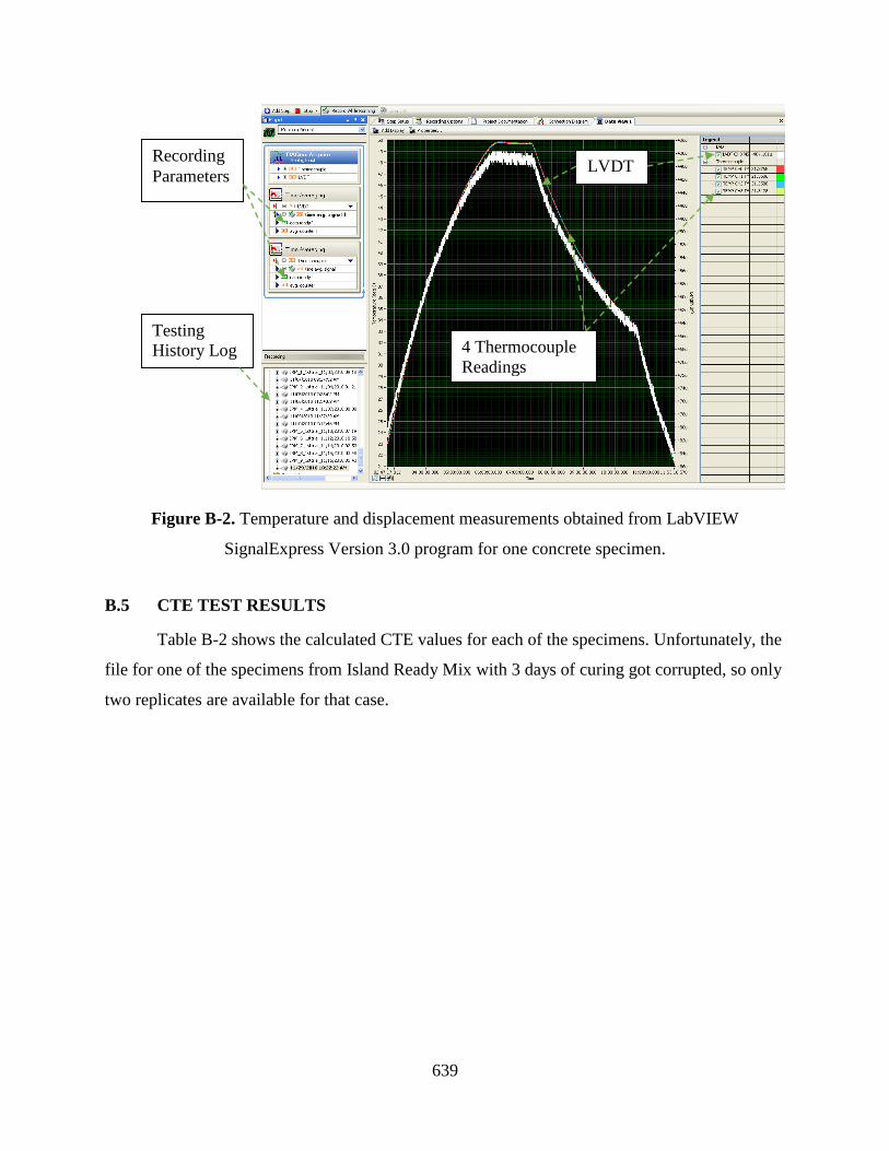
639

Figure B-2. Temperature and displacement measurements obtained from LabVIEW

SignalExpress Version 3.0 program for one concrete specimen.

B.5 CTE TEST RESULTS

Table B-2 shows the calculated CTE values for each of the specimens. Unfortunately, the

file for one of the specimens from Island Ready Mix with 3 days of curing got corrupted, so only

two replicates are available for that case.

4 Thermocouple

Readings

Testing

History Log

Recording

Parameters LVDT

640

Table B-2. Coefficients of thermal expansion of the testing specimens.

Mix Curing Time

CTE (10-6/˚F)

Replicate Average

1 2 3

Island Ready Mix

3 Days 7.1 6.9 - 7.0

7 Days 6.7 6.9 6.4 6.7

14 Days 6.1 6.1 6.2 6.1

28 Days 6.2 6.2 6.1 6.2

56 Days 6.1 6.1 5.9 6.0

Hawaiian Cement

3 Days 6.1 6.4 6.4 6.3

7 Days 6.3 6.6 6.4 6.4

14 Days 6.1 5.9 6.0 6.0

28 Days 6.1 6.2 6.0 6.1

56 Days 6.2 6.3 6.0 6.2

West Hawaii Concrete

3 Days 6.9 6.9 6.9 6.9

7 Days 7.2 6.9 6.8 7.0

14 Days 6.9 6.8 6.8 6.8

28 Days 6.8 6.5 6.6 6.7

56 Days 6.6 6.4 6.5 6.5

Figure B- illustrates for each PCC mix at different curing times the averages of the CTE

test results. The average values of CTE after 28 days of curing for the three Hawaiian companies

range from 6.1 to 6.6 × 10-6/°F (11.0 to 11.9 × 10-6/°C), which are substantially higher than the

5.2 × 10-6/°F (9.4 × 10-6/°C) value recommended in the MEPDG Manual of Practice [22] for

mixes prepared with basaltic aggregates. Common values found in the literature for PCC mixes

with basaltic aggregates range from 3.3 × 10-6/°F to 5.7 × 10-6/°F ( [139], [147], [148]), though it

must be recognized that these values were obtained before the problem with the calibration

specimen discussed in [146] was discovered. Hawaiian basalts are Tholeiitic basalts, which are

relatively rich in silica and differ in composition from alkali olivine basalt, which occurs along

continental rifts. This may partly explain the differences in the CTEs measured in this study with

the values reported in the literature for mixes with basaltic aggregates.

641

Figure B-3. Variation of the CTE with respect to curing time of concrete specimens for

Hawaiian companies.

The three PCC mixes show different trends with curing times. In two of them (Hawaiian

Cement and West Hawaii Concrete), the CTE first increases with 7 days curing time relative to 3

days curing time whereas for the Island Ready Mix the CTE decreases. On the other hand, the

CTE values at 56 days are lower than the values at 28 days for the Island Ready Mix and West

Hawaii Concrete mixes but the opposite happens for the Hawaiian Cement mix. There is no clear

explanation for these discrepancies between mixes. Nevertheless, using Fisher’s Least

Significant Difference Method [149] to make pair wise comparisons from the results of a one

factor ANOVA analysis (where the factor is curing time), it can be concluded that in all cases the

values at 3 and 7 days are statistically significantly higher at a 5% significance level than those at

5.8E-06

6.0E-06

6.2E-06

6.4E-06

6.6E-06

6.8E-06

7.0E-06

7.2E-06

0 10 20 30 40 50 60

CT

E (

10

-6/°

F)

Curing Time (Days)

Island

Ready

Mix

Hawaiian

Cement

West

Hawaii

Concrete

642

28 and 56 days and that the results at 28 and 56 days are not statistically significantly different

from each other, also at a 5% significance level.

Notice that the CTEs at the longer curing times for the two mixes produced in Oahu are

close two each other whereas the CTE for the mix produced in the Island of Hawaii is

significantly higher. Although this may indicate a difference in aggregate thermal expansion

characteristics between the islands it may also be related to other mix characteristics (e.g., the

water cement ratio is higher for the West Hawaii Concrete mix than for the other two mixes.)

The changes in CTE with curing time, expressed as a percentage, vary depending on the

values selected for comparison (3 or 7 days and 28 or 56 days) but are roughly between 5 and

10%, which are quite substantial (and as indicated earlier, statistically significant).

It must be pointed out that the trends with curing time found in this study are surprising

since other researchers have found results that conflict with these. As reported in [150] Wittmann

and Lukas [151] found an increase in the CTE of saturated concrete specimens around room

temperature up to 56 days of age and Rudeloff and Sieglerschmidt [152] also reported increases

in CTE of wet-cured specimens up to 90 days. Jahangirnejad [150] states that the effect of age on

CTE is associated with proceeding hydration and change in the composition of the cement paste

which in turn affects the CTE of concrete. However, except for the experimental observations, he

does not provide an explanation for why the CTE should increase with curing time. In his study,

he found statistically significant increases with curing time up to 365 days. However, in ( [153],

[150]), except for an air entraining agent (and fly ash for one of the eight mixes) no other

additives were used. With so many variables that may be playing a factor, it is not clear why the

results in the present study display a different trend. It may well be that with curing times longer

than 56 days the CTE may increase or that other mix characteristics affect the CTE differently

(e.g., the higher cement contents per cubic yard in this study). Either way, this is a subject that

deserves further study.

Notice that there is no recommendation in the MEPDG regarding the most appropriate

curing time to determine the CTE of concrete specimens for pavement design. The statistical

results described in the previous paragraph support computing the CTE for pavement design at a

curing time of 28 for days from a theoretical and practical point of view. The values at longer

curing times appear not to be significantly different and demand longer waiting. On the other

643

hand, the values at shorter curing times produced statistically significantly higher CTEs that are

probably not representative of the concrete behavior throughout most of the life the pavement.

B.6 EFFECT OF CTE ON PAVEMENT PERFORMANCE

The MEPDG [1] addresses many aspects that were missing or that were inadequately

addressed in other pavement design procedures. The consideration of the CTE in the design

procedure is perhaps one of the most important aspects addressed by the MEPDG. Its

consideration gives the engineer a more site specific design possibility.

This section illustrates the effect of CTE on pavement performance by using the

MEPDG. The effects of changes in CTE are shown for a Jointed Plain Concrete Pavement

(JPCP) section with the characteristics shown in Table B-3. The purpose of the analysis is not to

show absolute values of the different distresses as these may be different for different structural

designs (slab thickness, use of dowels, joint spacing, etc.) and traffic and climate conditions but

instead to illustrate the performance differences resulting from the different values of CTE for

the different mixes and curing times. The analysis also intends to illustrate the difference

between using a level 3 analysis (with a default CTE value for PCC mixes with basaltic

aggregates suggested in the MEPDG manual of practice [22]) and using a level 2 analysis with

the CTE value corresponding to each of the local mixes analyzed in this study.

A hierarchical method is employed in the MEPDG which includes three levels for

specifying the CTE. Level-1 CTE input requires a CTE value of a mixture tested in the

laboratory in compliance with AASHTO T 336 standard. In contrast, Level-3 CTE input

requires the designer to estimate the most appropriate design input value of the material property

based on experience with little or no testing. Published and default values are also used in this

input level. Level-2 CTE inputs are estimated through correlations with other material properties

that are measured in the laboratory or field. As a case in point, if the CTE values obtained here

were utilized in further studies, they would have to be considered as Level-2 inputs.

644

Table B-3. Characteristics of the evaluation pavement section.

Parameter Input

General

Type of design Jointed Plain Concrete Pavement (JPCP)

Design Life 35 years

Traffic

Initial two-way annual AADTT 4500

Lanes in design direction 3

Operational speed 55 mph

Climate

Location Honolulu International Airport

Depth to water table 10 ft

Structure

Joint spacing 15 ft

Dowels Without and with dowels

Layers (from top to bottom)

Portland Cement Concrete (PCC)

Layer thickness 9 in.

Coefficient of Thermal Expansion 5.2 x 10-6 (default) and values in Table 2

Joint spacing 15 ft

Cement Stabilized


Elastic/resilient modulus 2,000,000 psi

Crushed gravel


Modulus 25,000 psi

Subgrade (CL)

Layer thickness ∞

Modulus 16,000 psi

The structural design was obtained from an actual section of the H-1 freeway, near

Kapolei in Oahu. The pavement section was built in 1966 and rehabilitated in 1986 (although the

type of work done is not known, the original thickness in 1966 was 9” but the record for 1986

indicates a thickness of only 8.5”). Between 2010 and 2011, the section was retrofitted with

dowel bars and diamond grinded. Axle load spectra, vehicle class distribution, and number of

axles per vehicle were obtained from data for the Kalaeloa Weigh in Motion (WIM) station close

to the section. For other traffic inputs and other variables not mentioned here, default values

645

were used. Except for the CTE, water cement ratio, and the amount of cement per cubic yard, all

variables were held constant throughout the analysis.

For JPCP, the MEPDG provides estimates of the progression of the pavement distresses

(faulting and fatigue cracking) as well as of the International Roughness Index (IRI). The

controlling distress can vary from one design to the next depending on certain factors, including

traffic characteristics, weather patterns, and the pavement section characteristics. For the

particular design analyzed here, faulting was the limiting distress.

The effects of the estimated CTE for each mix at different curing times are the focus of

the following paragraphs. Figure B-4 shows the estimated time to reach 0.12 in (0.3 mm) faulting

at a 50% reliability for the design without dowel bars (i.e., it shows how long it would take to

reach the threshold on average.) It can be observed that the variation in CTE caused by curing

time translates directly into a high variation of the times to reach the threshold. Notice that the

variation caused by curing time is similar in magnitude to the variation caused by the use of

different mixes for a giving curing time. Therefore, the wide range of values presented in this

graph supports the need to establish a standard curing time when determining an appropriate

CTE for design.

Although the MEPDG is not yet calibrated for Hawaii and the criteria used for

rehabilitating this pavement section are unknown, the estimated time to reach the threshold (~20

years at the longer curing times) does not appear unreasonable considering that the pavement

received some rehabilitation after 20 years and needed to be retrofitted with dowel bars after

another 24 years.

The figure also illustrates the substantial differences with the predictions obtained using

the value of 5.2 × 10-6/°F suggested in the MEPDG Manual of Practice [22] for mixes prepared

with basaltic aggregates. Not surprisingly, a substantially better performance is predicted with

this lower CTE value.

646

Figure B-4. Effect of CTE on the predicted time to reach 0.12 in faulting at 50% reliability for a

pavement design without dowels (IRM = Island Ready Mix, HC = Hawaiian Cement, and WHC

= West Hawaii Concrete)

Figure B-5 shows the faulting values predicted after 35 years on the pavement section

with dowel bars also with 50% reliability. For this particular pavement section, faulting is the

governing distress with and without dowel bars. Again, the differences in the predicted values

produced by different curing times are about the same order of magnitude as the differences

produced by the different mixes. Furthermore, one can notice that the difference produced by the

use of a not representative default value can be higher than the differences between mixes or

curing times.

3 days 7 days 14 days 28 days 56 daysCTE = 5.2

microstrain/°F

IRM 16.1 18.8 25.1 24.0 26.3 36.0

HC 22.2 21.2 25.5 24.3 23.3 34.8

WHC 16.9 16.1 17.8 18.8 20.8 35.8

0.0

5.0

10.0

15.0

20.0

25.0

30.0

35.0

40.0

45.0

50.0Ye

ars

to r

eac

h 0

.12

in f

au

ltin

g

647

Figure B-5. Effect of CTE on the predicted faulting at 50% reliability for a pavement design

with dowels (IRM = Island Ready Mix, HC = Hawaiian Cement, and WHC = West Hawaii

Concrete).

Although cracking does not govern the design in this case, it is instructive to analyze the

effect of CTE on this distress as well since by changing some design parameters one could make

this the critical distress. Figure B-6 illustrates the results for 90% reliability for the case with

dowels. Using a 15% slabs cracked criterion, one can see that in this case a 35 years design could

be considered acceptable or not depending on the mix used and on the curing time used to obtain

the CTE.


microstrain/°F

IRM 0.145 0.134 0.113 0.117 0.109 0.082

HC 0.122 0.125 0.111 0.115 0.118 0.085

WHC 0.141 0.145 0.138 0.134 0.127 0.083

0.000

0.020

0.040

0.060

0.080

0.100

0.120

0.140

0.160

0.180

0.200Fa

ult

ing

aft

er

35

ye

ars

648

Figure B-6. Effect of CTE on the predicted percent of slabs cracked at 90% reliability for a

pavement design with dowels (IRM = Island Ready Mix, HC = Hawaiian Cement, and WHC =

West Hawaii Concrete).

Similar observations can be made about the roughness output which is not presented here.

The wide range of values presented in the previous figures provides another argument

towards the need to establish a standard for curing time when determining an appropriate CTE

for a design.

As expected, in all cases, CTE affects the service life of the pavement, i.e. the higher the

CTE, the shorter the expected service life.

B.7 CONCLUSIONS

The main conclusions of this study are:


microstrain/°F

IRM 32.8 21.4 9.6 10.8 8.6 5.0

HC 12.3 14.1 8.7 9.7 10.9 5.0

WHC 28.8 33.1 25.0 21.7 16.1 5.0

0.0

5.0

10.0

15.0

20.0

25.0

30.0

35.0P

erc

en

t sla

bs

cra

cke

d a

fte

r 3

5 y

ear

s

649

There is a large discrepancy between the CTE values found for Hawaiian mixes with

basaltic aggregates (6.1 to 6.6 × 10-6/°F for 28 days curing) with the CTE value

suggested in the MEPDG manual of practice [22] for a mix prepared with basaltic

aggregates (5.2 × 10-6/°F). Use of the MEPDG suggested value would lead to significant

differences in the predicted performance of the pavement.

The MEPDG does not provide guidance about the curing time to use for the

determination of the CTE. In this study, the CTE varied significantly until about the 28th

day curing time and then it tended to stabilize. Thus, the value of the CTE at the 28th day

curing time could be a reasonable choice for design purposes.

B.8 RECOMMENDATIONS

Although this study provides some useful information for the design of pavements in Hawaii, it

also brings up additional questions. Further study could potentially focus on:

Including more quarries to increase the reliability of the study, since due to time and

economic constraints, only three of the potential quarries were studied.

Perform a larger study to evaluate the effects of other mix characteristics.

Study the effect of curing time more in depth so that it can be determined with more

confidence whether the CTE increases with curing time, decreases with curing time, or

whether the trend is affected by some other mix design variable.

Perform a petrography analysis to study if the composition of the Hawaiian basalts can

explain the larger CTE for the Hawaiian mixes when compared to mixes prepared with

basaltic aggregates from the continental US.

empirical pavement design guide - ROSA P

Documents

Transcript of empirical pavement design guide - ROSA P