engineering characterization of waste derived geopolymer

ENGINEERING CHARACTERIZATION OF WASTE DERIVED GEOPOLYMER

CEMENT CONCRETE FOR STRUCTURAL APPLICATIONS

by

Brett Tempest

A dissertation submitted to the faculty of

The University of North Carolina at Charlotte

in partial fulfillment of the requirements

for the degree of Doctor of Philosophy in

Infrastructure and Environmental Systems

Charlotte

2010

Approved by:

_______________________

Dr. Janos Gergely

_______________________

Dr. Rajaram Janardhanam

_______________________

Dr. Helene Hilger

_______________________

Dr. Vincent Ogunro

_______________________

Dr. Jeff Ramsdell

_______________________

Dr. David Weggel

ii

ii

© 2010

Brett Tempest

ALL RIGHTS RESERVED

iii

iii

ABSTRACT

BRETT TEMPEST. Engineering characterization of waste derived geopolymer cement

concrete for structural applications. (Under direction of DR. JANOS GERGELY)

Geopolymer cements provide an alternative to the Portland cement used to

manufacture structural concrete. The material commonly used to produce geopolymers is

fly ash, which is found in the waste stream of power generation facilities. Therefore,

replacing Portland cement with geopolymer cement improves the sustainability of

concrete by reducing emissions and diverting waste from landfils. In this study,

geopolymer cements were used to create concrete having compressive strength in the

range of 5,000 to 12,000 psi (34-83 MPa). The mechanical properties of these concretes

were evaluated to determine the compressive, tensile and elastic behaviors. Durability

tests were also performed to assess creep and shrinkage characteristics. Prestressed and

mild steel reinforced beams were made with the geopolymer cement concrete (GCC) and

were tested to failure. The results of these flexural tests were used to confirm the

applicability of traditional concrete design criteria and techniques. The GCC was found

to perform in a similar manner to Portland cement concrete and the efficacy of existing

design formulations was verified with small changes to some design values. Finally, the

processes and materials used to prepare the concretes were used to make a preliminary

lifecycle assessment to verify the sustainability gains of GCC. Reduced energy use and

emissions generation were confirmed.

iv

iv

AKNOWLEDGMENTS

I have been fortunate throughout my graduate studies for having strong support

from my advisor, my classmates, my committee and my family. Thank you to Dr. Janos

Gergely for your guidance, encouragement and mentorship over the many years I have

been your student. Thank you to Tina, Ailee, Mom and Dad for tolerating the mania that

these studies sometimes brought. Thank you to Jeff Berryman, Alex Gotta, Cassanni

Laville, Olanrewaju Sanusi, Angela Sims and Mitch Taylor for your dedication to the

project and the long hours you contributed. Special thanks to Mike Moss for all the times

you’ve rolled your sleeves up and gotten the work done in spite of the budget, the hours

or the challenges of the task. Finally, thank you to the members of my dissertation

committee, Drs. Helene Hilger, Rajaram Janardhanam Vincent Ogunro, Jeff Ramsdell

and David Weggel, for your generous contributions of time, advice and direction.

v

v

TABLE OF CONTENTS

LIST OF FIGURES viii

LIST OF TABLES xvi

CHAPTER 1: INTRODUCTION 1

1.1 Background ............................................................................................... 1

1.2 Geopolymers ............................................................................................. 2

1.3 A civil engineering perspective on geopolymer research ......................... 4

1.4 Background on geopolymers ..................................................................... 5

1.5 Source materials ........................................................................................ 7

1.6 Activating solutions................................................................................. 11

1.7 Performance in structural elements ......................................................... 13

1.8 Scope of research .................................................................................... 20

CHAPTER 2: DEVELOPMENT AND OPTIMIZATION OF 22

GEOPOLYMER CEMENT CONCRETE MIX DESIGNS

2.1 Development of activating solution and aggregate proportions .............. 23

2.2 Further mix development ........................................................................ 30

2.3 Conclusions ............................................................................................. 39

2.4 Preparation of concrete materials for ..................................................... 42

constitutive property characterization .........................................................

2.5 Mixing process ........................................................................................ 44

vi

vi

2.6 Experimental procedures ......................................................................... 48

2.7 Material characteristics tests results ........................................................ 50

2.8 Mechanical properties ............................................................................. 56

2.9 Creep ....................................................................................................... 58

2.10 Shrinkage ................................................................................................. 66

2.11 Discussion of results and conclusions ..................................................... 74

CHAPTER 3: RECYCLED AGGREGATES IN GEOPOLYMER 76

CEMENT CONCRETE

3.1 Background on recycled concrete aggregate use .................................... 76

3.2 Collecting recycled concrete aggregates for gcc use .............................. 83

3.3 Incorporation of recycled aggregate in GCC .......................................... 87

3.4 Discussion of results................................................................................ 90

CHAPTER 4: BEAM TESTS 92

4.1 Concrete for demonstration beams .......................................................... 92

4.2 Mild steel reinforced beams .................................................................... 95

4.3 Prestressed concrete beams ................................................................... 108

CHAPTER 5: FLEXURAL BEAM-COLUMN TESTS 120

5.1 Analysis of stress and strain under compressive loading ...................... 120

5.2 Flexural beam-column test procedure ................................................... 127

5.3 Test results and data reduction .............................................................. 134

vii

vii

5.4 Conclusions ........................................................................................... 157

CHAPTER 6: VERIFICATION OF BEAM PERFORMANCE 159

AND DESIGN COMPUTATIONS

6.1 Moment-curvature models .................................................................... 159

6.2 Flexural performance assessed by moment-curvature models .............. 169

6.3 Prestressed concrete beams ................................................................... 174

6.4 Conclusions ........................................................................................... 180

CHAPTER 7: LIFE CYCLE ANALYSIS OF GEOPOLYMER 181

CEMENT CONCRETE

7.1 Life cycle assessment for geopolymer cement concrete production ..... 181

7.2 Environmental impact ........................................................................... 189

7.3 Reducing the life cycle impact of geopolymer concrete ....................... 190

CHAPTER 8: CONCLUSIONS AND RECOMMENDATIONS FOR 192

FURTHER STUDIES

REFERENCES 196

APPENDIX A: STEEL STRESS-STRAIN CURVES 203

APPENDIX B: MOMENT-CURVATURE MODEL DESCRIPTION 206

a. Preparation of the moment-curvature model ......................................... 206

b. Computation of beam deflection from ................................................. 211

moment-curvature relationships. .................................................................

viii

viii

LIST OF FIGURES

FIGURE 2-1: Optimum NaOH Addition For MA Ashes. 28

FIGURE 2-2: Optimum NaOH Addition For BL Ashes. 28

FIGURE 2-3: Activator Design and 7-Day Strength for MA Ashes. 29

FIGURE 2-4: w/c ratio and 28-day compressive strength. 31

FIGURE 2-5: w/c ratio and strength development for two activator concentrations. 32

FIGURE 2-6: Activator Design and 28-Day Strength for CL Ashes. 40

FIGURE 2-7: Activator design and 28-day strength for BC ashes. 40

FIGURE 2-8: Increase in compressive strength between day 41

7 and day 28 for CL ashes.

FIGURE 2-9: Increase in compressive strength between day 41

7 and day 28 for BC ashes.

FIGURE 2-10: Fly ash storage silo. 43

FIGURE 2-11: Preparing activating solution. 45

FIGURE 2-12: Measuring aggregates. 46

FIGURE 2-13: Adding activating solution. 46

FIGURE 2-14: Consolidating geopolymer concrete in 3X6‖ cylinders. 47

FIGURE 2-15: Oven for curing geopolymer concrete specimens. 47

FIGURE 2-16: Splitting tensile test set-up. 49

FIGURE 2-17: Static modulus of elasticity test set-up. 50

FIGURE 2-18: Compressive strength development with aging and curing time. 53

ix

ix

FIGURE 2-19: Compressive strength after 24 and 48 hours of curing for Mix #1. 54



FIGURE 2-22: Relationship between splitting tensile and 57

compressive strength of GCC cylinders

FIGURE 2-23: Compressive strength and Young’s Modulus for Mix #1 and Mix #2. 58

FIGURE 2-24: Consolidating creep specimens. 62

FIGURE 2-25: Gage stud layout for creep specimens. 62

FIGURE 2-26: Creep specimen loading apparatus. 63

FIGURE 2-27: Relationship of creep strain with time for GCC specimens. 64

FIGURE 2-28: Relationship of creep strain with time for PCC specimens. 65

FIGURE 2-29: GCC and PCC creep compared to the 66

range of ultimate creep values for Portland cement concrete.

FIGURE 2-30: PCC-1 shrinkage strain versus time. 71

FIGURE 2-31: GCC-2 shrinkage strain versus time. 71

FIGURE 2-32: GCC-R shrinkage strain versus time. 72

FIGURE 2-33: Comparison of shrinkage in PCC-1, GCC-2 and GCC-R specimens. 72

FIGURE 2-34: Prediction of shrinkage using =0.8 and =0.9. 74

FIGURE 3-1: Batch 1 compressive strength at 7 and 28 days. 89

FIGURE 3-2: Batch 2 compressive strength at 7 and 28 days. 90

FIGURE 4-1: Adding materials to mixing truck. 94

x

x

FIGURE 4-2: Beam and heater inside curing oven. 95

FIGURE 4-3: Placement and size of reinforcing steel in GCC-1-B1. 97

FIGURE 4-4: Placement and size of reinforcing steel in GCC-2-B2, 98

PCC-1-B3, and GCC-R-B4.

FIGURE 4-5: Beam loading and support geometry. 99

FIGURE 4-6: Mild steel reinforced beam loaded in the test frame. 100

FIGURE 4-7: Support conditions for mild steel reinforced beams. 100

FIGURE 4-8: Strain gage mounted to reinforcing steel. 101

FIGURE 4-9: Load-deflection relationship for reinforced concrete beams. 102

FIGURE 4-10: GCC-1-B1 load vs. mid-span deflection. 103

FIGURE 4-11: GCC-2-B2 load vs. mid-span deflection. 104

FIGURE 4-12: PCC-1-B3 load vs. mid-span deflection. 104

FIGURE 4-13: GCC-R-B4 load vs. mid-span deflection. 105

FIGURE 4-14: Combined plots of load vs. mid-span deflection. 105

FIGURE 4-15: GCC-1-B1 at maximum load. 106

FIGURE 4-16: Crushing failure in GCC-2-B2. 106

FIGURE 4-17: Crushing failure in PCC-1-B3. 107

FIGURE 4-18: Crushing failure near load application in GCC-R-B4. 107

FIGURE 4-19: Reinforcing cage and prestressing tendons in formwork. 109

FIGURE 4-20: Extra reinforcing near the end of the prestressed beams. 110

xi

xi

FIGURE 4-21: Reinforcing steel placement and beam 111

cross section for prestressed beams.

FIGURE 4-22: Jacking configuration used to tension prestressing tendons. 113

FIGURE 4-23: Prestressing tendons passing through the abutment. 113

FIGURE 4-24: Prestressed beam test set-up. 114

FIGURE 4-25: Prestressed beam loaded in the test frame. 114

FIGURE 4-26: GCC-2-P1 beam load vs. midspan deflection. 116

FIGURE 4-27: PCC-1-P2 beam load vs. midspan deflection. 116

FIGURE 4-28: GCC-R-P3 beam load vs. midspan deflection. 117

FIGURE 4-29: Load deflection curves for prestressed beams plotted together. 117

FIGURE 4-30: GCC-2-P1 beam failure by concrete crushing. 118

FIGURE 4-31: PCC-1-P2 beam failure by concrete crushing. 118

FIGURE 4-32: GCC-R-P3 beam failure by concrete crushing. 119

FIGURE 5-1: stress-strain relationship of concrete in compression. 120

FIGURE 5-2: Stresses and strains in concrete beams. 121

FIGURE 5-3: Relationship of k1, k2 and k3 to the resultant compressive force. 122

FIGURE 5-4: Hognestad flexural beam-column test set-up. 124

FIGURE 5-5: Free body diagram of the beam-column specimen cut at midheight. 124

FIGURE 5-6: Quantities fc, εc and c. 125

FIGURE 5-7: Beam-column specimen dimensions. 128

xii

xii

FIGURE 5-8: Casting beam-column specimens. 129

FIGURE 5-9: Moment arm section and end-plate details. 129

FIGURE 5-10: Reinforcing at the ends of the beam-columns. 130

FIGURE 5-11: Strain gage locations on beam-column specimens. 131

FIGURE 5-12: 4’ abutment, primary axial load application piston and end roller. 132

FIGURE 5-13: Application of P2 with a 30 ton jack and prestressing strand. 133

FIGURE 5-14: Full test set-up for flexural beam columns. 133

FIGURE 5-15: Midspan deflection vs. P2 for GCC-3-BC1. 136

FIGURE 5-16: Neutral face strain vs. P2 for GCC-3-BC1. 136









FIGURE 5-25: Failure of GCC-3-BC1. 141


xiii

xiii




FIGURE 5-30: computed from and from and average values. 144

FIGURE 5-31: GCC-3-BC1 stress-strain relationship from flexural tests. 144





FIGURE 5-36: Relative slopes of stress strain curves. 147

FIGURE 5-37: Relationship between k1,k2, k3 and α1 and β1. 149

FIGURE 5-38: related to cylinder compressive strength for beam-columns. 151

FIGURE 5-39: related to cylinder compressive strength for beam-columns. 151

FIGURE 5-40: Formula to determine parameter a based on compressive strength. 154

FIGURE 5-41: Formula to determine parameter ―b‖ based on compressive strength 154

FIGURE 5-42. Experimental results and Equation 5-15 for 9.0 ksi concrete. 155

FIGURE 5-43: Experimental results and Equation 5-15 for 7.9 ksi concrete. 155

FIGURE 5-44. Experimental results and Equation 5-15 for 7.3 ksi concrete. 156


xiv

xiv


FIGURE 6-1a,b,c. Moment-curvature analysis. 162

FIGURE 6-2: Distribution of forces in the moment curvature model. 162

FIGURE 6-3: Moment curvature plot. 163

FIGURE 6-4: Moment-curvature relationship plotted along beam length. 163

FIGURE 6-5: Modeled and actual deflection for GCC-1-B1. 172

FIGURE 6-6: Modeled and. actual deflection for GCC-2-B2. 172

FIGURE 6-7: Modeled and actual deflection for PCC-1-B3. 173

FIGURE 6-8: Modeled and actual deflection for GCC-R-B4. 173

FIGURE 7-1: Manufacture processes for geopolymer cement concrete. 183

FIGURE 7-2: Manufacture processes for Portland cement concrete. 183

FIGURE A-1: Grade 60 steel fs vs.ε. 203

FIGURE A-2: Grade 40 steel fs vs.ε. 204

FIGURE A-3: Grade 270 prestressing steel fs vs.ε. 205

FIGURE B-1: Division of beam into horizontal strips. 206

FIGURE B-2: Cross-sectional dimensions and position of steel reinforcing. 207

FIGURE B-3: From left a) concrete strips and steel areas; b) strain distribution, 209

c) stress in each strip and in steel bars.

FIGURE B-4: Moment curvature relationship through failure. 210

FIGURE B-5: (from top) a) loading geometry, b) moment diagram, 212

c) distribution of curvature.

xv

xv

FIGURE B-6: Division of beam and curvature diagram into vertical segments. 212

xvi

xvi

LIST OF TABLES

TABLE 2-1: Fly ash composition. 24

TABLE 2-2: Activator design for preliminary batches. 24

TABLE 2-3: Gradation of fine and coarse aggregates. 25

TABLE 2-4: Compressive strength of concretes made with BC and MA ashes. 27

TABLE 2-5: XRF analysis of BC and CL ashes. 30

TABLE 2-6: Mixing proportions for w/c ratio specimens, lb (kg). 32

TABLE 2-7: Mix Designs, lb (kg). 34

TABLE 2-8: Ratios of NaOH to silica fume for optimal strength development. 34

TABLE 2-9: Compression test results for geopolymer made from BC and CL ashes. 35

TABLE 2-10: XRF analysis of CL ashes. 43

TABLE 2-11: Mixing proportions lb/yd3 (kg/m

3). 48

TABLE 2-12: Number of cylinders made for each aging and curing regimen. 48

TABLE 2-13: Results of compression and tension tests. 52

TABLE 2-14: Mix proportions for creep specimens lb/yd3 (kg/m

3). 61

TABLE 2-15: Compressive strength and initial elastic modulus of creep specimens 64

TABLE 2-16: Mixing proportions for shrinkage specimens lb/yd3 (kg/m

3). 69

TABLE 2-17: Shrinkage test results. 70

TABLE 3-1: Various guidelines for use of RCA. 82

xvii

xvii

TABLE 3-2: Strength reduction factors for specimen aspect ratios less than 2.0. 85

TABLE 3-3: Compressive strength of cores removed from the slab. 86

TABLE 3-4: Gradation of recycled aggregates produced from 86

Idlewild Elementary School demolition rubble.

TABLE 3-5: Mixing proportions for GCC containing 88

recycled aggregate, lb/yd3 (kg/m

3).

TABLE 3-6: Compressive strength results for GCC mixes containing 88

recycled aggregate, psi (MPa).

TABLE 4-1: Mix designs for concrete used to prepare 93

beam specimens, lb/yd3 (kg/m

3).

TABLE 4-2: Concrete cylinder compressive strength at time of testing. 95

TABLE 4-3: Reinforcing steel schedule for GCC-1-B1, inches (mm). 97

TABLE 4-4: Reinforcing steel schedule for GCC-2-B2, PCC-1-B3 and GCC-R-B4. 98

TABLE 4-5: Description of reinforced concrete beam load history. 102

TABLE 4-6: Prestressed beam concrete details. 108

TABLE 4-7: Reinforcing steel schedule for GCC-2-B2, PCC-1-B3 111

and GCC-R-B4, in (cm).

TABLE 4-8: Critical points in prestressed beam load histories. 119

TABLE 5-1: Cylinder compressive strength for beam-column concrete. 134

TABLE 5-2: Slope of stress-strain curves versus estimated modulus 148

of elasticity, psi (GPa).

TABLE 5-3: Calculated values of k1k3, k2 and k3 for beam columns. 148

TABLE 5-4: Parameters a and b for GCC stress-strain relationship 153

xviii

xviii

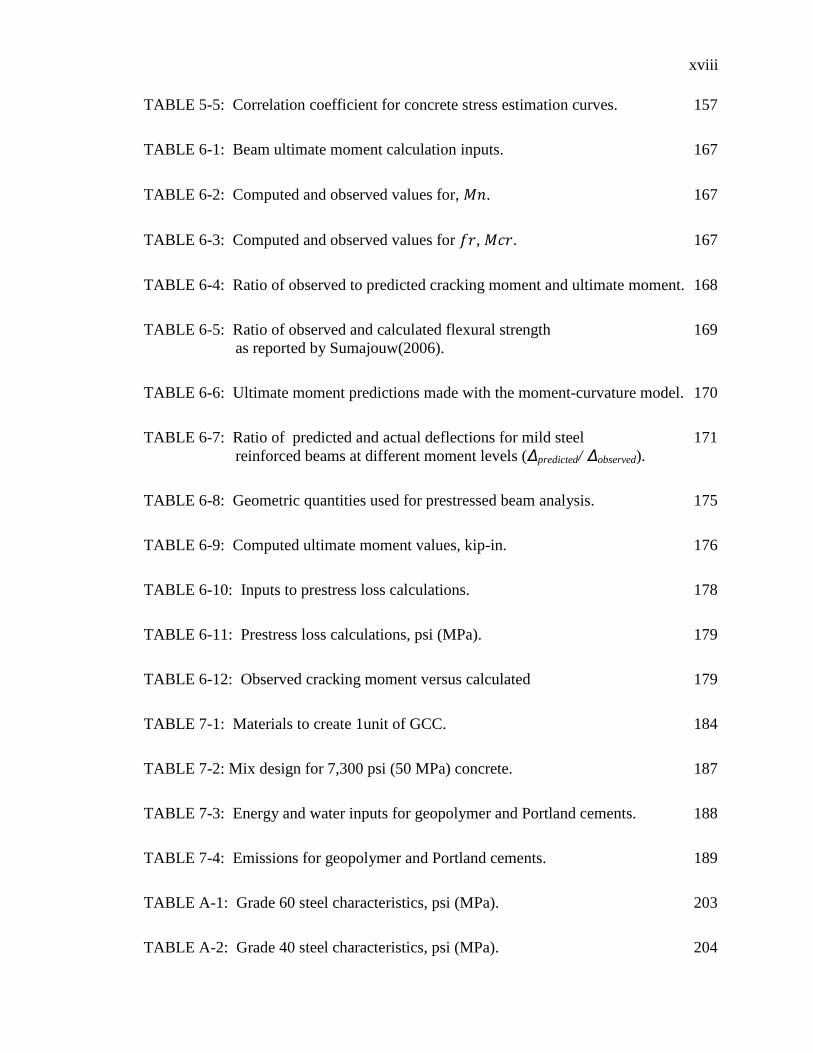
TABLE 5-5: Correlation coefficient for concrete stress estimation curves. 157

TABLE 6-1: Beam ultimate moment calculation inputs. 167

TABLE 6-2: Computed and observed values for, . 167

TABLE 6-3: Computed and observed values for , . 167

TABLE 6-4: Ratio of observed to predicted cracking moment and ultimate moment. 168

TABLE 6-5: Ratio of observed and calculated flexural strength 169

as reported by Sumajouw(2006).

TABLE 6-6: Ultimate moment predictions made with the moment-curvature model. 170

TABLE 6-7: Ratio of predicted and actual deflections for mild steel 171

reinforced beams at different moment levels (Δpredicted/ Δobserved).

TABLE 6-8: Geometric quantities used for prestressed beam analysis. 175

TABLE 6-9: Computed ultimate moment values, kip-in. 176

TABLE 6-10: Inputs to prestress loss calculations. 178

TABLE 6-11: Prestress loss calculations, psi (MPa). 179

TABLE 6-12: Observed cracking moment versus calculated 179

TABLE 7-1: Materials to create 1unit of GCC. 184

TABLE 7-2: Mix design for 7,300 psi (50 MPa) concrete. 187

TABLE 7-3: Energy and water inputs for geopolymer and Portland cements. 188

TABLE 7-4: Emissions for geopolymer and Portland cements. 189

TABLE A-1: Grade 60 steel characteristics, psi (MPa). 203

TABLE A-2: Grade 40 steel characteristics, psi (MPa). 204

xix

xix

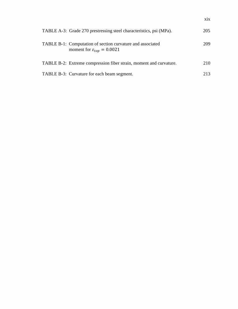
TABLE A-3: Grade 270 prestressing steel characteristics, psi (MPa). 205

TABLE B-1: Computation of section curvature and associated 209

moment for

TABLE B-2: Extreme compression fiber strain, moment and curvature. 210

TABLE B-3: Curvature for each beam segment. 213

CHAPTER 1: INTRODUCTION

1.1 Background

Concrete is one of the most ubiquitous construction materials in the world due to

its durability, flexibility and economy. The latter two of these features arise from the

ability of concrete producers to incorporate a variety of source materials, while still

guaranteeing suitable structural performance. For instance, the aggregates used in

concrete vary widely from granitic to calciferous materials depending on the geology

local to the production site. The cementitious constituents also tend to be locally

produced from materials that are available in proximity to the cement mill. Because of

this tradition of local production and flexibility in the nature of source materials, concrete

could become one of the most sustainable construction materials available. However,

even with modern production techniques it is extremely energy and emissions intensive

to manufacture.

The production of Portland cement for concrete is becoming an unattractive

industrial process as concern mounts over energy use and greenhouse gas production. In

order to manufacture Portland cement, limestone is heated in a kiln until CaCO3 is

reduced to CaO. This results in the release of one molecule of CO2 for every molecule of

CaO produced as well as an assortment of greenhouse gasses originating from the

combustion of fuels used to heat the kiln. In total, 0.8 tons of CO2 are released for every

ton of cement produced (Gartner, 2004). The manufacture of cement accounts for at least

2

2

7% of worldwide greenhouse gas generation on an annual basis (Chindaprasirt et al.,

2007).

Two existing strategies to reduce the energy and greenhouse gas intensiveness of

concrete use are to seek alternate energy sources for heat generation during cement

manufacture and to reduce the quantity of Portland cement required to mix concrete of

various strengths. For instance, waste solvents and tires have been used in place of oil

and natural gas in the kilns as energy sources. Research and practice have also shown

that up to 35% of the cement can be replaced by the pozzolan, fly ash (ACI, 2003).

While the inclusion of fly ash represents some progress towards ―green‖ concrete,

the energy intensiveness of Portland cement remains a major impediment to true

sustainability. However, despite the problems with Portland cement, concrete has an

institutionalized role in economical construction and does provide many positive

environmental features such as durability, recycleability and thermal mass. A new

material, geopolymer cement, appears to be an alternative to Portland cement that can

continue to provide concrete, but with a reduction in carbon dioxide.

As acceptance of global climate change grows, the motives for reducing

greenhouse gas emissions are becoming imperatives for businesses. Limits to greenhouse

gas production in the form of economic penalties are already appearing on the regulatory

horizons for industrial emitters. Geopolymers could provide a solution to the challenges

of manufacturing Portland cement (Duxson et al., 2007b).

1.2 Geopolymers

The term ―geopolymer‖ was instituted by Davidovits (1991)following research

into inorganic-polymer technologies for industrial applications. Geopolymers are formed

3

3

when alumino-silicates dissolve in a strong base, reorganize and precipitate in a hardened

state (Davidovits, 1991; Duxson et al., 2007a). They can have properties very similar to

Portland cement when formed under suitable conditions (Sofi et al., 2007b).

Geopolymers have been manufactured from industrial wastes, such as blast furnace slag,

for more than 60 years and are also often referred to as alkali-activated cements or

inorganic polymer cements (Duxson et al., 2007a). Many researchers have produced

geopolymer paste with kaolinite and metakaolinite as a source material of aluminates and

silicates (Alonso and Palomo, 2001; Xu and Van Deventer, 2002). Construction silt and

industrial waste products have also been successfully used (Lampris et al., 2009). Slavik

et al. (2008) produced geopolymer material that attained structural strength with coal

bottom ash and demonstrated its durability with freeze-thaw tests as well as wet-dry tests.

However, the bulk of research into the use of industrial waste in geopolymer cements has

centered on pulverized fuel ash or fly ash due to its wide and plentiful availability

(Andini et al., 2008; Buchwald and Schulz, 2005; Duxson et al., 2007a; Duxson et al.,

2007b; Jo et al., 2007; Palomo et al., 1999; Roy, 1999; Sun, 2005; van Deventer et al.,

2007).

Of the more than 70 million tons of fly ash produced in the United States in 2006,

much less than half was used; the remainder entered the waste stream. The southeast

alone produced more than 30 million tons (American Coal Ash Association, 2007).

Landfilling fly ash has been shown to have negative environmental consequences,

including leaching toxic compounds and heavy metals into groundwater. The use of fly

ash as an alumino-silicate source material for geopolymer gives rise to many

environmental benefits. Not only does it eliminate the pollution problems associated

4

4

with Portland cement production, it relieves the burden of safely disposing of fly ash

(Roy, 1999).

1.3 A civil engineering perspective on geopolymer research

As the material science research community has continued to study geopolymers, it

has established that these materials can match or surpass Portland cement concrete in

areas of strength and durability (van Deventer et al., 2007). Much of the research

described in the literature is related to understanding the chemistry of inorganic polymer

formation, reaction mechanisms and the relationship between base material composition,

activating solution, curing conditions and characteristics of the hardened product

(Fernandez-Jimenez and Palomo, 2003; van Jaarsveld et al., 2002). More recently, study

of the engineering properties of geopolymer in terms of modulus of elasticity, Poisson’s

ratio and flexural strength has begun (Sofi et al., 2007b). Research has also been

conducted on reinforced concrete columns created from geopolymer concrete that

verified the relevance of existing design protocols to geopolymer structural elements

(Sumajouw et al., 2007). Although there is a small body of research on the engineering

properties of geopolymer cement, the quantity of data in this area is not sufficient to

encourage its use in heavy construction. It is this area that must be researched from a

civil engineering perspective.

5

5

1.4 Background on geopolymers

1.4.1 Geopolymerization process

Most of the research into the reaction mechanisms present during the formation of

geopolymers has been based on metakaolin as the alumino-silicate source material. This

is due to the greater homogeneity of metakaolin over fly ash. However, it is expected

that the general geopolymerization mechanism is similar for the two materials, with the

addition of subprocesses related to contaminants in the case of fly ash. The reaction of

alumino-silicate materials in alkaline environments gives rise to the geopolymeric

cements under consideration in this dissertation. The basic conceptual model of the

geopolymerization process is a series of three phases, which are (Glukhovsky, 1959):

1) Dissolution- the aluminosilicate material is dissolved in an alkaline solution

2) Reorientation- the liberated silicate and aluminate monomers form short

aluminosilicate oligomers

3) Solidification- the three dimensional geopolymer matrix becomes rigid

1.4.1.1 Dissolution

Aluminate and silicate ions are provided in solution via the dissolution process.

Various source materials have characteristically different levels of reactivity in alkaline

solutions. Panagiotopoulou (2007) dissolved pozzolana, fly ash, slag, kaolinite,

metakaolinite and zeolite in solutions of varying alkalinity for varying amounts of time.

It was found that the reactivity of the materials in decreasing order was,

metakaolin>zeolite>slag>fly ash>pozzolana>kaolin. The degree of reactivity is likely

related to multiple source material characteristics, including fineness, capability of cation

6

6

exchange and Al coordination (Panagiotopoulou et al., 2007). Panagiotopoulou et al. also

found significant increases in the dissolution rates of Si by increasing the molarity of the

alkaline solution from 2 to 5M. Using NaOH as the alkalinity source was found to be

more effective at dissolving greater amounts of Si and Al than KOH (Panagiotopoulou et

al., 2007).

The dissolution of fly ash in alkaline solutions has also been investigated by

Mikuni et al. (2007). By dissolving fly ashes from pulverized coal combustion plants as

well as pressurized fluidized bed combustion plants, high dissolution rates were found for

aluminates at alkalinities between 5 and 10N at 25⁰ C. Silicates were found to dissolve at

increasing rates with increasing alkalinity.

The dissolution of aluminate and silicate into solution is described by the

following three reactions:

Al2O3 + 3H2O + 2OH- → 2[Al(OH)4]

- (1-1)

SiO2 + H2O + OH- → [SiO(OH)3]

- (1-2)

SiO2 + 2OH-→ [SiO2(OH)2]

2- (1-3)

1.4.1.2 Reorientation

During the reorientation phase, the free aluminate and silicate monomers begin to

form oligomers. First, the [Al(OH)4]- and [SiO(OH)3]

- groups form an attraction between

the Al and OH. As the two OH groups condense, an H2O molecule is released. A similar

reaction can occur between [Al(OH)4]- and [SiO2(OH)2]

2-. This arrangement results in

smaller oligomers than the condensation of [Al(OH)4]- and [SiO(OH)3]

- (Weng and

Sagoe-Crentsil, 2007). Because the proportion of [SiO(OH)3]-/ [SiO2(OH)2]

2- is

7

7

dependent on the alkalinity of the activating solution, the formation of the whole

geopolymer network is affected by the initial dissolution conditions.

1.4.1.3 Hardening

During the reorientation phase, a continuous gel network of three dimensional

alumino-silicate structures is formed. As polymerization and hardening begin to occur,

the possibility for transport of monomer species is precluded. Depending on the nature of

the precursor groups, these structures may form the polysialate type (Si-O-Al-O-),

polysialate-siloxo type (Si-O-Al-O-Si-O), or the polysialatedisiloxo type (Si-O-Al-O-Si-

O-Si-O), as termed by Davidovits (1991).

Geopolymers have been cured at a variety of temperatures ranging from room-

temperature to nearly 212 ⁰F (100⁰C) depending on the source materials and strength

development requirements. Alonso and Palomo studied the effect of heat addition to the

geopolymer gel. Increased temperatures were found to accelerate the reaction and

promote hardening (Alonso and Palomo, 2001). Swanepoel and Strydom (2002) found

that an unsuitably slow reaction rate occurred under 140⁰F (60⁰C) in fly ashes sourced

from the SASOL steam station. Others have developed geopolymers with compressive

strengths suitable for structural application through room temperature curing (Sun, 2005).

1.5 Source materials

The precursors to geopolymer formation are sources of silicate and aluminate that

form the backbone of the inorganic polymer. During the history of geopolymer

development, most research has revolved around a two-part mixture system in which an

alumino-silicate powder is combined with an alkaline liquid activator in order to initiate

8

8

the dissolution reaction. In this case, the alumino-silicate powder may consist of coal fly

ashes or metakaolin. Some research has investigated biomass ashes from rice husk

combustion as a partial replacement for the fly ash (Songpiriyakij et al., 2009). A second

branch of geopolymer research is centered on the development of ―one-part‖ systems or

―just add water‖ mixes, in which the powder contains sufficient soluable alkaline

components to initiate dissolution of silica with the addition of water (Duxson and Provis,

2008). Research presented in this document utilized a two-part system.

Although geopolymer materials can be reliably produced in the laboratory from

pure reagents, the challenge comes in producing a consistent material from fly ash and

other industrial byproducts that have variable compositions. The fly-ash can be

characterized in terms of its physical features and chemical composition. Each of these

features has an impact on the material properties of the hardened polymer.

1.5.1 Fly ash

Geopolymer made during the course of this research utilized fly ash as the source

of aluminosilicates. Difficulty arises in manufacturing geopolymer from fly ash because

it is a waste product from a highly variable stream. Even different samples from the

same source have been known to produce final geopolymer concrete products with

dissimilar rheology and strength development. Due to the magnitude of its production,

fly ash is widely regarded as the most viable source material for bulk production of

geopolymer cement concrete, much work presented in the literature has focused on

empirically determining the characteristics of the material that produce acceptable results.

Ash characteristics that impact their usability in geopolymer applications are

physical qualities, oxide composition and crystallography. Each of these characteristics

9

9

impacts either the rheology and reaction rate of the fresh material or the mechanical and

microstructural characteristics of the hardened material (Diaz et al., 2009). Van Jaarsveld

et al. found the particle size, calcium content, alkali metal content, amorphous content

and origin of the fly ash to be important properties that contribute to the quality of the

final geopolymer product (van Jaarsveld et al., 2003). Fernández-Jiménez (2003)

described an activatable fly ash as having LOI less than 5%, Fe2O3 less than 10%, low

CaO, reactive silica between 40 and 50% and 80 to 90% of particles smaller than

1.80X10-3

‖ (45μm). The following is a summary of fly ash characteristics that determine

its suitability as a source material for geopolymer.

1) Typical diameters for fly ash range between 3.9X10-5

and 7.9X10-3

in (1 μm - 1

mm (Mehta, 1989). However, the average size is highly dependent on the

combustion process in the furnace where it is produced. The gradation of the fly

ash is also important. Work done by Fernández-Jiménez and Palomo determined

that removal of particle fractions larger than 1.80X10-3

in (45 μm) is related to

substantial improvements in the 1-day compressive strength of samples and was

able to develop 1-day strengths of over 10,000 psi (69 MPa) by removing these

larger particles (Fernandez-Jimenez and Palomo, 2003). Because the fly ash is

formed as molten coal ash molecules condense in the exhaust flue of the furnace

where they are produced, the shape tends to be spherical.

2) The specific surface is often determined via the Blaine method or the BET

method (named for its developers, Stephan Brunauer, Paul Emmett and Edward

Teller). During the polymerization reactions, the gel matrix may begin to harden

before the dissolution of the fly ash is complete. Therefore, surface reactions

10

10

most likely play a significant role in the set-up of the geopolymer matrix (van

Jaarsveld et al., 2003). Since small particle size corresponds to greater surface

area in aggregate, this might explain the increase in specimen strength related to

eliminating larger size fractions. Using the BET method of nitrogen absorption,

the specific surface areas of fly ashes are typically found in the range of 1,464

ft2/lb to 2,440 ft

2/lb (300 to 500 m

2/kg) (Malhotra et al., 1989).

3) Although most geopolymers are typically based on low calcium fly ashes, the

reactivity of high calcium material has also been investigated. The most

immediately apparent effect of the addition of calcium is to increase the rate of set

for the geopolymer. It is known that as the solution pH begins to decrease from

14 to lower values, the polycondensation reactions begin to occur (Lee and van

Deventer, 2002). Calcium in the fly ash tends to precipitate as Ca(OH)2 upon

addition of the alkaline activation solution. As OH- ions are removed from the

activating solution, the pH falls and the solidification begins. van Deventer found

that the Ca precipitates provide nucleation sites but also generate competition for

crystal growth nutrients (van Deventer et al., 2007). Fe present in the source

materials has a similar effect, precipitating as a hydroxide or oxy-hydroxide.

4) The bituminous coal that is most often burned in US steam plants typically

produces an ash with SiO2 in the range of 45-60% and Al2O3 in the range of 4-

20% (Mehta, 1989). While this chemical composition besides the loss on ignition

and the calcium content is not a determinant of pozzolanic activity, it is important

in the development of geopolymers. The most effective ratio of silica to

aluminum has been determined by Davidovits to be between 3.3 and 6.5 (1991).

11

11

This was confirmed by Sun in experiments that tested the strength of geopolymer

specimens made with mortars that varied the ratio of silica to aluminum (Sun,

2005).

5) Although the x-ray fluorescence (XRF) method of chemical composition used in

this research to determine the quantities of SiO2 and Al2O3 are accurate and

accepted, the portion of these oxides that participate in the geopolymer reaction is

referred to as the ―reactive‖ component. The proportion of reactive silica is

reported as a ratio with total silica. The amorphous fraction of fly ash has been

estimated between 60 and 80% of the total quantity. Of this amorphous fraction,

60-80% of the material is silicates and 10-20% is aluminates (Henry et al., 2004).

1.6 Activating solutions

The initiation of the geopolymerization phases described in the previous sections is

caused by the addition of an activating solution to the source material. The solution

contains the alkalinity that causes the dissolution of the source material solids and

sometimes also contains a supplementary source of soluble silicates. Activating solutions

must be carefully designed because their composition has several impacts on the

development of the mechanical properties in the hardened geopolymer.

1.6.1 Alkali species

The two predominant alkaline salts used in geopolymer formation are NaOH and

KOH. Each of these results in slightly different dissolution rates and hardened

geopolymer characteristics. Greater dissolution rates for both Si and Al have been found

12

12

in solutions of NaOH. The impact of the more effective dissolution ability of NaOH

solutions is that equilibrium of dissolved species and undissolved species is reached at

lower levels of alkalinity (Panagiotopoulou et al., 2007). Comparison of the hardened

properties of geopolymers formed with activating solutions containing either potassium

or sodium have shown impacts to compressive strength and durability. Van Jaarsveld

and van Deventer (1999) demonstrated that potassium activating solutions produced

slightly higher compressive strength geopolymers. However, the potassium based

activators also produced materials with higher specific surface area and lower resistance

to acid attack.

1.6.2 Alkalinity level

The dissolution rates of aluminate and silicate species in the activating solution are

affected by a combination of thermal conditions and the molarity of the alkaline solution.

With both sodium and potassium based activating solutions, dissolution rates are known

to increase with increasing alkalinity (Mikuni et al., 2007) (Sagoe-Crentsil and Weng,

2007). However, despite the dissolution capacity of higher alkalinity solutions, excessive

presence of concentrations of sodium hydroxide have been found to reduce the

compressive strength of hardened geopolymer. This is due to the reduced degree of

polymerization that is caused by excessive NaOH concentrations. The balance of silicate

species at high alkalinity levels tends to favor smaller monomers over the larger

oligomers and therefore, less polycondensation (Panias et al., 2007).

13

13

1.6.3 Supplementary silica

The initial assembly of the alumino-silicate matrix is heavily controlled by the

availability of aluminum. The supply of aluminum in the solution is known to dictate the

setting time, durability and strength development (Duxson and Provis, 2008). However,

the dissolution of the aluminum is dictated largely by the specific phases that exist in the

source material. Because its bonds with oxygen in the source material are weaker, it

tends to be provided more readily during dissolution. The activating solution can be a

source of soluble silica for the reaction in order to either supplement the amorphous silica

in the source material or to provide sufficient silica to the gel formation prior to it being

made available through dissolution. Addition of soluble silica has been shown to

increase the degree of polymerization in the hardened geopolymer and therefore improve

the compressive strength (Criado et al., 2007).

1.7 Performance in structural elements

As the bulk of geopolymer research has been conducted on small specimens by

material scientists and chemists, there are fewer reported studies on structural

applications. Most data has been published on either neat geopolymer pastes or on

geopolymer mortar. However, a small number of studies have been published on

geopolymer concrete and geopolymer concrete in structural applications. The extension

of geopolymer formation research to structural applications research involves

investigating the binder as it is mixed with aggregates to form concretes. Once these

materials are developed, the dimensions of research into structural uses include strength,

durability, and performance in reinforced structural elements.

14

14

1.7.1 Interaction with other materials

In order to be used as structural concrete, geopolymer paste must interact with

aggregates and reinforcing steel. The mechanical aspects of the cement-aggregate

composite are of critical importance. Equally important is the bond with reinforcing

steel.

1.7.1.1 Bond with aggregate

The interfacial transition zone (IZT) is the boundary between binder gel and

aggregate in PCC as well as in GCC. A complex set of hydration processes affect the

morphology of the IZT in PCC such that there is less gel present and the zone has greater

porosity than gel at points away from the aggregate. In geopolymeric systems, the

absence of hydration reactions and the much different hardening and curing process result

in an IZT that is not as strongly affected. Lee et al. (2004) used a series of specimens

with geopolymer paste bonded to polished slices of stone to measure the strength of the

bond between the cement and aggregate. Samples were also examined under an electron

microscope to determine the effect of the geopolymer materials on the mineralogy of the

aggregate. It was found that systems activated with low soluble silicate activators formed

low compressive strength bulk material and poor bonds with the stone (Lee and van

Deventer, 2004). Materials with higher soluble silicate had denser binder phases and

better bonds with the aggregates. The area near the aggregate surface had the same

morphology as the bulk binder, indicating that there is not a heavily impacted ITZ as with

PCC (Lee and van Deventer, 2004).

15

15

1.7.1.2 Bond with steel

The primary tensile reinforcement in concrete is present in the form of

longitudinal bars or tendons. Stresses are transferred from the concrete to the tensile

material through a bond at the surface. Prior to substantial loading, the bond consists of

adhesion, friction and bearing. However, the first two of these mechanisms are typically

broken after relatively low load application rates. Therefore, bearing is the only

mechanism considered in the design process and reinforcing bars are deformed in order

to improve the surface for stress transfer (MacGregor and Wight, 2005). ACI has given

an equation to determine the development length for various sized bars in various

strength concrete (ACI Committee 318. and American Concrete Institute., 2008).

(1-4)

where:

: development length

: yield stress of bar

: lightweight concrete reduction factor

: bar location factor

: coating factor

: bar diameter factor to favor smaller bars

: factor representing concrete cover around bar

: concrete confinement across splitting planes

: diameter of the reinforcing bar

: concrete compressive strength

It can be seen from the terms in the equation that many of the factors affecting the

development length of the reinforcing material are related to concrete properties that are

similar for GCC and PCC. For instance, the term,

, describes the propensity of

beams to generate longitudinal cracks due to radial tensile forces transferred from the

16

16

steel to the concrete. Since the relationship between tensile and compressive strength for

GCC and PCC are relatively similar, it is expected that they will have similar responses

to these radial forces. The remaining geometric and tensile material surface and strength

properties are also similar for GCC and PCC.

Sofi et al. (2007a) conducted tests to verify the bond performance of steel

reinforcing materials with geopolymer concrete. The research group created geopolymer

concretes from fly ashes from three steam generation units. The concretes were tested

with the direct pull-out method given in American Society for Testing and Materials

(ASTM) C 234-91 as well as the beam-end specimen method given in ASTM A 944-99

(ASTM, 1991; ASTM, 1999). It was found that the provisions given in ACI 318-02 and

AS3600 for predicting development length are applicable to GCC.

1.7.2 Durability

1.7.2.1 Asr

In PCC, alkali-silica reaction is a threat to the durability of concretes containing

expansive aggregates. Reactive aggregates are ones in which certain forms of silica

engage in forming a swelling alkali-silicate-hydrate. This resulting gel attracts water and

increases in size to cause cracks in the concrete (Mindess et al., 2003). Because of the

high pH found in geopolymer pore solution, alkali-silica reaction ASR has been a

concern for aggregates used in GCC. The performance of aggregates in GCC was

investigated by Garcìa-Lodeiro, et al. (2007). ASR in several aggregates was measured

by means of ASTM C1260-94 (ASTM, 1994). Concretes were produced with

geopolymer cement as well as Portland cement and a range of reactive and sTABLE

17

17

aggregates. While all concretes exhibited some degree of expansion due to alkali-

aggregate reactions, the alkali-activated fly ash systems exhibited less expansion than

OPC systems with similar aggregates. The cause of the lesser expansion is speculated to

be the low availability of calcium in class F fly ashes (Garcia-Lodeiro et al., 2007).

1.7.2.2 Creep

Creep behavior of GCC has been investigated by Wallah (2004). Concretes with

compressive strength in the range of 5,800-10,000 psi (40 to 70 MPa) were prepared

using two levels of alkalinity in the activating solution and two curing procedures. Half

of the specimens were subjected to steam curing at 140○F (60

○C) for 24 hours and the

remaining specimens were cured at the same temperature, but under dry conditions. All

specimens were loaded at a load intensity of 40% of the cylinder compressive strength.

Specific creep levels ranged from 15 to 29 microstrain. Lower specific creep was found

for concrete having higher compressive strength. Wallah (2004) determined that the

measured creep in geopolymer specimens was uniformly less than creep strains predicted

using the Gillbert model specified in the Austrailian code AS3600 (Standards Association

of Australia., 2001).

1.7.2.3 Chemical resistance

Portland cement concretes are frequently degraded when exposed to aggressive

chemical environments. This exposure may occur because they are intentionally exposed

to elevated concentrations of chemicals due to the specifics of their intended service or

unintentionally due to deleterious chemicals present in the environment. Sulfates and

acids are two substances that can cause significant durability issues for concrete. When

18

18

exposed to sulfates, tri-calcium aluminate can form monosulfoaluminate. The reaction

products occupy 55% more volume than the precursors, which causes stresses in the

concrete. Further expansion can be caused by the reaction products absorbing water.

Bakharev (2005) studied the sulfate resistance of geopolymer concrete by immersing

specimens in solutions of sodium sulfate and magnesium sulfate. The changes caused by

exposure to these sulfate solutions were of a different type than would be expected of

Portland cement specimens. In the sodium sulfate solution, the alkali cations from the

geopolymer matrix diffused out into the solution and caused significant microcracking.

The magnesium sulfate solution caused magnesium and calcium to migrate into the

matrix and improve the compressive strength (Bakharev, 2005a). As has been shown by

other authors, the finer pore structure of geopolymers activated by sodium hydroxide

results in materials that have lower susceptibility to attack in aggressive environments.

Acids can also cause problems in Portland cement mortars and concretes. As the

calcium phases of the Portland cement hydration products are exposed to acid, calcium

salts are formed which immediately weaken the material. Bakharev (2005) exposed

geopolymer materials to acetic and sulfuric acid solutions to study their durability. The

degree of degradation was linked to several factors of the geopolymer microstructure and

chemistry. Polymer structures having lower Si/Al ratios were more heavily affected.

Microstructural characteristics such as pore size and degree of polymerization were also

correlated with greater resistance. Thus, geopolymers activated with potassium solutions

had coarser pore structures and were more subject to degradation in the sulfuric acid.

The most stable materials were geopolymers activated by sodium hydroxide and heat

cured (Bakharev, 2005b).

19

19

1.7.3 Use in structural elements

Geopolymer cements have been used to create structural concretes by Hardjito

and Rangan. In the course of their preliminary research, mixing procedures similar to

those developed for Portland cement concrete (PCC) were used. The researchers found

that PCC superplasticizers could be used effectively to manipulate the workability of the

GCC. Concretes were produced with compressive strength in the range of 6,400-13,000

psi (44-90 MPa). The authors also measured Poisson’s ratio and Young’s modulus and

found them to be similar to expected values for OPC concretes with comparable

compressive strength (Hardjito and Rangan, 2005).

Sumanjouw et al. used fly ash geopolymer to build slender reinforced columns

(Sumajouw et al., 2007; Sumajouw and Rangan, 2006). The concrete was cured at

elevated temperatures and achieved compressive strengths of 5,800 and 8,700 psi (40 - 60

MPa). The columns were tested by loading to failure with eccentricities of 0.6‖, 1.4‖ and

2‖ (15, 35 and 50 mm). The failure modes were as expected, and the failure loads were

predictable using formulas available in ACI 318-02 and AS3600 (ACI Committee 318.

and American Concrete Institute., 2002; Standards Association of Australia., 2001).

Prestressed railway sleepers have been manufactured from geopolymer cement

concrete. The geopolymer provides advantages in terms of fast strength development,

allowing rapid turn-around and the ability to transfer prestress at an early concrete age.

Palomo et al. (2007) has reported that the further benefits of geopolymer in this

application include better durability under the harsh chemical and physical service

environment of railway sleepers. The concrete also exhibits less drying shrinkage, and

therefore lower prestress losses (Palomo et al., 2007).

20

20

Reinforced GCC columns have also been evaluated by Sarker (2009). The

experimental results of testing GCC columns to failure were compared with analytical

results. The columns were modeled with a moment-curvature relationship which relied

on material properties determined by standard tests. A modified version of the Popovics

stress-strain relationship was used to estimate the concrete compressive behavior

(Popovics, 1973). The authors were able to predict the failure loads for the columns with

a test/prediction ratio of 1.03, and the midspan deflections with test/prediction ratio of

1.14. This was seen as confirmation that conventional PCC design methodology may be

applied to GCC applications (Sarker, 2009).

The engineering properties of GCC have been investigated by a limited number of

research teams. In addition to the short supply of data regarding these characteristics, the

composition of GCC materials is not consistent between the research groups. Therefore,

the available data has a considerable spread, which is a result of the mortar fraction,

aggregate type, activator composition and curing schedule that each author used.

1.8 Scope of research

The research presented in this dissertation is oriented towards developing a

structural-grade concrete that is as energy and emissions efficient as possible. Further,

the suitability of the concrete is demonstrated to the material producing community by

the creation of typical and familiar structural elements. In order to develop an energy

efficient concrete, mix designs were studied that incorporate varying quantities of virgin

and recycled materials. After a structural strength (6,000-8,000 psi (41.4-55.1 MPa)) mix

design was developed, its performance was tested through a variety of established

material tests and structural component tests.

21

21

Fly ashes from multiple sources, collected at different times, were examined to

determine the optimum mixing methods to account for their chemical and physical

differences. Since a rigorous physical and chemical analysis of fly ash characteristics is

beyond the scope of this research, a single source of fly ash was selected for use

throughout the remainder of the project. The single source of fly ash was used to prepare

concrete specimens and components. Small specimens were used to establish the

material characteristics f’c, Ec and fct via customary ASTM methods. Specimens were

also created to test the durability characteristics, creep and shrinkage, which are critical in

prestressed applications. Larger beam-column specimens were prepared in order to

evaluate compressive stress response of the GCC. Finally, four mid-sized beams (10 ft

(3m) in length) were created to verify geopolymer performance in reinforced concrete

applications. Finally, three larger scale girders (18 ft (5.5m) in length) were produced

from geopolymer to demonstrate geopolymer performance in prestressed concrete.

Following this work, the results provide an initial engineering characterization of

geopolymer concrete structural components. The final analysis includes comparisons

between the energy and material requirements to produce Portland cement concrete and

those for producing geopolymer concrete.

CHAPTER 2: DEVELOPMENT AND OPTIMIZATION OF GEOPOLYMER

CEMENT CONCRETE MIX DESIGNS

The source materials for geopolymer cement concrete (GCC), as with Portland

cement concrete (PCC) are local in their origin. The primary cementitious component,

fly ash, is a byproduct of coal combustion which is captured by emissions control devices

at power generation stations. As such, its composition is highly dependent on a range of

variables including the mine where the coal was collected and the operational particulars

of the furnace that burned it. In order to begin GCC research at UNC Charlotte, an initial

exercise in collecting and characterizing the source materials was undertaken. This

chapter describes the following research activities:

1) Developing activating solution and aggregate proportions for GCC

2) Optimizing the aging and curing routine

3) Scaling up to larger batches

4) Determining the modulus of elasticity of the concrete

5) Determining the splitting tensile strength of the concrete

The research presented in this dissertation required the development and

implementation of several types of material preparation and experimental techniques.

Some of the techniques are based on existing and accepted material testing methods put

forth by the American Society for Testing and Materials (ASTM). Whenever possible,

existing test methods were used so that the geopolymer concrete may be more readily

accepted by the materials production and construction communities. In other cases, no

23

23

suitable existing method was available and attempts were made to develop appropriate

and reliable procedures for the purposes of this project.

2.1 Development of activating solution and aggregate proportions

2.1.1 Determining requisite ash quality

In the summer of 2008, a series of experiments was conducted on a range of fly

ashes available in proximity to Charlotte, North Carolina. The goal in completing these

tests was to arrive at a baseline set of mix designs and to determine the qualities of local

ashes that indicated their acceptability for geopolymer manufacture. In the first phase,

ashes came from two primary local sources, designated MA and BL.

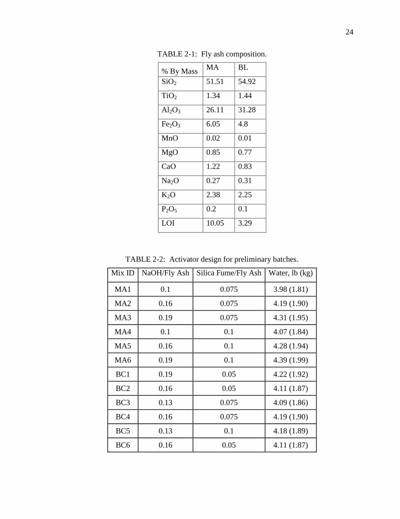
Oxide analysis via XRD was carried out by an external lab and yielded the

compositional data in TABLE 2-1. As can be seen from the results, the ashes contained

Si/Al ratios of roughly 2:1. The MA ashes had very high carbon content as evidenced by

a measured loss on ignition (LOI) of 10%. The BL ashes had much lower LOI, with only

3.3% carbon.

A mix proportioning methodology was designed, which is organized in a similar

manner to that developed by Sun (2005). Various combinations of NaOH and Silica

Fume were used to create the activating solution. The specific proportions for the

activating solution used in this study are presented in TABLE 2-2. The quantities of

NaOH and silica fume are presented as ratios to the weight quantity of fly ash used,

which was 8.50 lb (3.90 kg) in all cases. The water content was adjusted so that despite

the increasing quantity of activating solids (NaOH and silica fume) the ratio between

cementitous materials (activating solids and fly ash) and water was always 0.40.

24

24

TABLE 2-1: Fly ash composition.

% By Mass MA BL

SiO2 51.51 54.92

TiO2 1.34 1.44

Al2O3 26.11 31.28

Fe2O3 6.05 4.8

MnO 0.02 0.01

MgO 0.85 0.77

CaO 1.22 0.83

Na2O 0.27 0.31

K2O 2.38 2.25

P2O5 0.2 0.1

LOI 10.05 3.29

TABLE 2-2: Activator design for preliminary batches.

Mix ID NaOH/Fly Ash Silica Fume/Fly Ash Water, lb (kg)

MA1 0.1 0.075 3.98 (1.81)

MA2 0.16 0.075 4.19 (1.90)

MA3 0.19 0.075 4.31 (1.95)

MA4 0.1 0.1 4.07 (1.84)

MA5 0.16 0.1 4.28 (1.94)

MA6 0.19 0.1 4.39 (1.99)

BC1 0.19 0.05 4.22 (1.92)

BC2 0.16 0.05 4.11 (1.87)

BC3 0.13 0.075 4.09 (1.86)

BC4 0.16 0.075 4.19 (1.90)

BC5 0.13 0.1 4.18 (1.89)

BC6 0.16 0.05 4.11 (1.87)

25

25

The aggregates used in this phase of the work were sourced from local quarries.

The coarse aggregate was a 3/8‖, granite stone and the fine aggregate was silica concrete

sand. The gradation for these aggregates is given in TABLE 2-3. The quantity of

aggregate used was proportioned so that it accounted for roughly 80% of the total mass of

the concrete. This ratio is typical of OPC concretes.

TABLE 2-3: Gradation of fine and coarse aggregates.

% finer

Sieve

Opening

in (mm)

Coarse Fine

5/8 100.0 100

1/2 99.5 100

3/8 85.3 99.77

no. 4 28.8 99.54

no. 8 5.5 97.94

no. 16 1.3 90.37

no. 40 0.7 37.16

no. 50 0.7 19.95

no. 100 0.5 1.61

Pan 0.0 0.00

2.1.2 Results of preliminary tests

The results of the preliminary tests are partly anecdotal and partly quantitative.

Although none of the mixes developed strength in the desired range of 4,500-6,000 psi

(27.5-41.3 MPa) for structural use, there were clear trends in the relationship between the

26

26

activator solution make-up and strength development. This information was useful in the

development of subsequent procedures.

2.1.2.1 Activating solution proportions

The two ashes used in the preliminary tests had very different physical and

chemical characteristics and produced concretes with various compressive strengths. In

general, the MA ashes produced lower strength concrete than the BL ashes. This might

be attributable to the very high LOI of the MA ashes. Despite the difference in strength

produced, both ashes showed improved strength development associated with similar

activating solution compositions. In this series of experiments, two variables were

systematically manipulated- the ratio of NaOH to fly ash and the ratio of Silica Fume to

fly ash. The mix proportions shown in TABLE 2-2 were used. 11.2 lb (5.1 kg) of coarse

aggregate and 11.2 lb (5.1 kg) of fine aggregate were used in each batch.

Generally, nine 3‖x6‖ (76mmx152mm) cylindrical specimens were made from

each batch. These were tested in compression after seven and twenty-eight days. The

results of the compression tests are shown in TABLE 2-4. The experiments revealed

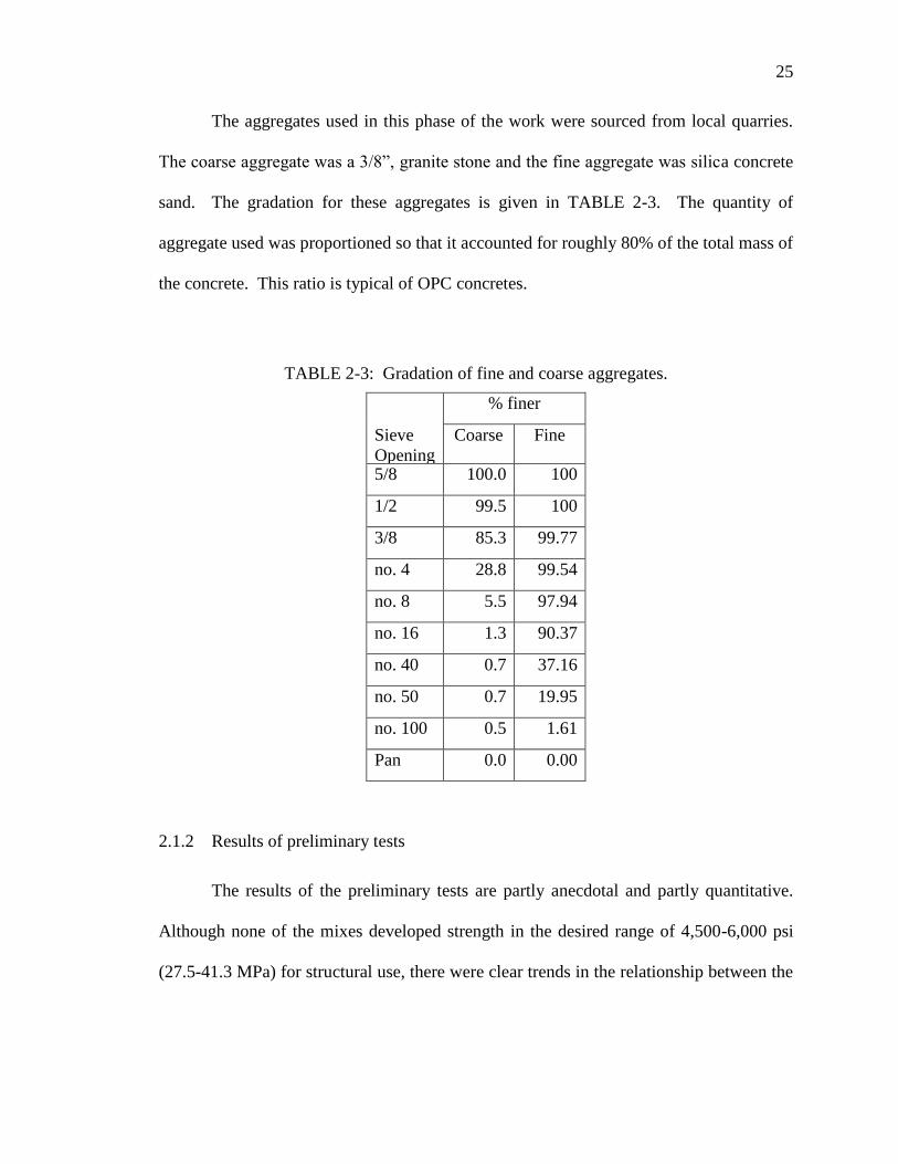
some important trends in the activator design and the development of compressive

strength. As is shown in FIGURE 2-1 and FIGURE 2-2, compressive strength increased

up to the NaOH/Fly Ash ratio of 0.15 and then decreased for higher alkalinity solutions.

Strength also increased with the addition of silica fume to the activating solution.

However, the limited number of data points does not indicate an optimal amount of silica

fume for strength development. As is shown in FIGURE 2-3, there is no peak in the

strength vs. silica fume addition for the ratios tested.

27

27

The compressive strength results given in TABLE 2-4 show uniformly higher

values for the BL ashes over the MA ashes. Since the oxide composition of the two ashes

was very similar and the preparation and proportioning of the concrete was also alike, the

main difference seems to be the LOI. In the case of the MA ashes, the high LOI seemed

to inhibit the development of compressive strength in the cylinders. The appearance of

the cylinders also seemed to be affected by the high carbon content. Whereas the

cylinders prepared with BL ashes had a grayish color very similar to PCC, the MA

cylinders were very dark.

TABLE 2-4: Compressive strength of concretes made with BC and MA ashes.

Mix ID , psi (MPa)

MA1 476 (3.3)

MA2 2,031 (14.03)

MA3 1,854 (12.8)

MA4 986 (6.8)

MA5 2,680 (18.5)

MA6 2,158 (14.9)

BC1 1,265 (8.7)

BC2 2,883 (19.9)

BC3 1,285 (8.9)

BC4 2,006 (13.8)

BC5 2,521 (17.4)

BC6 3,207 (22.1)

28

28

FIGURE 2-1: Optimum NaOH Addition For MA Ashes.

FIGURE 2-2: Optimum NaOH Addition For BL Ashes.

0

5

10

15

20

0

500

1000

1500

2000

2500

3000

3500

0.000 0.050 0.100 0.150 0.200 0.250

Com

pre

ssiv

e S

tren

gth

[M

pa]

Com

pre

ssiv

e S

tren

gth

[psi

]

NaOH/Fly Ash

0.075

0.1

Silica Fume/

Fly ASh

0

5

10

15

20

0

500

1000

1500

2000

2500

3000

3500

0.000 0.050 0.100 0.150 0.200 0.250

Com

pre

ssiv

e S

tren

th [

MP

a]

Com

pre

ssiv

e S

tren

gth

[psi

]

NaOH/Fly Ash

0.05

0.075

0.1

Silica Fume/

Fly ASh

29

29

FIGURE 2-3: Activator Design and 7-Day Strength for MA Ashes.

Although the results did not provide sufficient data for strong conclusions about

geopolymer mix design, they did set the stage for further testing. The following

guidelines were established from the first tests:

1) Future activator designs should incorporate more silica fume

2) Only class F fly ashes should be used

3) The total quantity of cementitious solids (NaOH, silica fume, fly ash) should be

held constant rather than simply the fly ash quantity. This will result in constant

batch masses and fewer variables between batches.

4) The w/c ratio has a significant role in strength determination and should be held

as low as possible. Experiments should be performed to determine a target w/c

ratio for workability and strength development.

0

5

10

15

20

0

500

1,000

1,500

2,000

2,500

3,000

0.000 0.050 0.100

Com

pre

ssiv

e S

tren

gth

[M

Pa]

Com

pre

ssiv

e S

tren

gth

[psi

]

Silica Fume/Fly Ash

9.60%

16%

19%

NaOH/

Fly ASh

30

30

2.2 Further mix development

In the second round of tests, the lessons learned from round one were applied.

Here, the w/c ratio was to be studied and controlled more closely and the mix designs

used in the experiments were adjusted to include more silica fume. Higher grade fly ash

was also used in these experiments.

2.2.1 New fly ash

For the second round of tests, fly ashes of more verifiable quality were collected.

These were from sources specifically designated for concrete use and were marketed by

the supplier as Class F. Once these ashes were collected, they were designated BC and

CL. An XRF analysis was completed and provided the results shown in TABLE 2-5.

The ash was collected and stored in sealed 55 gallon steel drums.

TABLE 2-5: XRF analysis of BC and CL ashes.

% by Mass BC CL

SiO2 58.08 56.20

TiO2 1.56 1.46

Al2O3 28.63 28.00

Fe2O3 4.12 5.22

MnO 0.02 0.02

MgO 0.94 1.00

CaO 0.74 1.52

Na2O 0.22 0.21

K2O 2.44 2.74

P2O5 0.10 0.18

Totals 96.85 96.55

LOI 3.03 3.32

31

31

2.2.2 W/c ratio

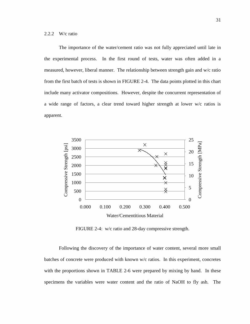
The importance of the water/cement ratio was not fully appreciated until late in

the experimental process. In the first round of tests, water was often added in a

measured, however, liberal manner. The relationship between strength gain and w/c ratio

from the first batch of tests is shown in FIGURE 2-4. The data points plotted in this chart

include many activator compositions. However, despite the concurrent representation of

a wide range of factors, a clear trend toward higher strength at lower w/c ratios is

apparent.

FIGURE 2-4: w/c ratio and 28-day compressive strength.

Following the discovery of the importance of water content, several more small

batches of concrete were produced with known w/c ratios. In this experiment, concretes

with the proportions shown in TABLE 2-6 were prepared by mixing by hand. In these

specimens the variables were water content and the ratio of NaOH to fly ash. The

0

5

10

15

20

25

0

500

1000

1500

2000

2500

3000

3500

0.000 0.100 0.200 0.300 0.400 0.500

Com

pre

ssiv

e S

tren

gth

[M

Pa]

Com

pre

ssiv

e S

tren

gth

[psi

]

Water/Cementitious Material

32

32

strength development results can be seen in FIGURE 2-5. For both activating solution

concentrations, there was an improvement in strength achieved by reducing the w/c ratio.

For the 0.13 NaOH/Fly ash activating solutions, the strength development with reduced

water content was more pronounced.

TABLE 2-6: Mixing proportions for w/c ratio specimens, lb (kg).

NaOH/Fly

Ash

Silica Fume NaOH Fly Ash Fine

Aggregate

Coarse

Aggregate

0.10 0.2 (0.091) 0.3 (0.1361) 3.1 (1.41) 3.7 (1.68) 3.7 (1.68)

0.13 0.2 (0.091) 0.4 (0.181) 3.1 (1.41) 3.7 (1.68) 3.7 (1.68)

FIGURE 2-5: w/c ratio and strength development for two activator concentrations.

Although quantitative tests for workability were not used during the water content

experiments (due to the reactivity of the aluminum test equipment), qualitative

0

5

10

15

20

25

30

0

1,000

2,000

3,000

4,000

5,000

0.200 0.250 0.300 0.350 0.400

Com

pre

ssiv

e S

tren

gth

[M

Pa]

Com

pre

ssiv

e S

tren

gth

[psi

]

Water/Cementitious Solids

NaOH/Fly

Ash=0.10

NaOH/Fly

Ash=0.13

33

33

assessments were made. The workability of mixes with w/c ratios below ~0.27 was very

poor. These concretes were difficult to mix and to mold into suitable specimens.

Therefore, the w/c ratio selected for subsequent tests was 0.28. This low w/c ratio

required the use of high range water reducer.

Based on lessons learned in the previous series of tests, the experiment parameters

for the activator mix design were set as is shown in TABLE 2-7. Each batch included

11.2 (5.1 kg) and 11.5 lb (5.2 kg) of fine and coarse aggregate, respectively. Following

the conclusions from the water content tests described above, the w/c ratio was fixed at

0.28, where weight of cementitous solids includes the sum of the fly ash, silica fume and

sodium hydroxide. In each batch, the total weight of cementitious solids is constant,

although the relative proportions of fly ash, silica fume and sodium hydroxide change in

each activator design. 10 ml of ADVA 190 superplasticizer was used in each batch.

Nine cylinders were made from each batch. Three were tested at seven days and

three were tested at 28 days using the procedures for compression tests given in ASTM

C39 (ASTM, 2005). The remaining three were retained as alternates in case there were

problems with any of the tests. The results of the compression tests are given in TABLE

2-9. In the TABLE, ―No Data‖ implies that there was a problem mixing the batch and no

cylinders were created. This typically occurred with the higher alkalinity mixes that were

either not workable enough to create cylinders, or set-up in the mixer.

There are general similar trends for concretes made from the two types of fly ash.

As shown in TABLE 2-5, the chemical composition of BC and CL ashes is very similar,

although they were produced at different steam stations. The results were analyzed to

34

34

determine trends in strength development and to select the best activator design for future

work.

TABLE 2-7: Mix Designs, lb (kg).

Activator

#

NaOH/

Fly

Ash

Silica Fume/

Fly Ash

Fly Ash Water Silica

Fume

NaOH

10 0.1 0.08 11.1 (5.05) 3.7 (1.68) 0.89 (0.4) 1.11 (0.5)

11 0.1 0.11 10.8 (4.91) 3.7 (1.68) 1.19 (0.54) 1.08 (0.49)

12 0.1 0.14 10.6 (4.82) 3.7 (1.68) 1.48 (0.67) 1.06 (0.48)

13 0.13 0.08 10.8 (4.91) 3.7 (1.68) 0.87 (0.4) 1.41 (0.64)

14 0.13 0.11 10.6 (4.82) 3.7 (1.68) 1.16 (0.53) 1.38 (0.63)

15 0.13 0.14 10.3 (4.68) 3.7 (1.68) 1.45 (0.66) 1.34 (0.61)

16 0.16 0.08 10.6 (4.82) 3.7 (1.68) 0.85 (0.39) 1.69 (0.77)

17 0.16 0.11 10.3 (4.68) 3.7 (1.68) 1.14 (0.52) 1.65 (0.75)

18 0.16 0.14 10.1 (4.59) 3.7 (1.68) 1.41 (0.64) 1.62 (0.74)

19 0.19 0.08 10.3 (4.68) 3.7 (1.68) 0.83 (0.38) 1.96 (0.89)

20 0.19 0.11 10.1 (4.59) 3.7 (1.68) 1.11 (0.5) 1.92 (0.87)

21 0.19 0.14 9.9 (4.5) 3.7 (1.68) 1.38 (0.63) 1.87 (0.85)

22 0.16 0.16 9.9 (4.5) 3.7 (1.68) 1.6 (0.73) 1.6 (0.73)

23 0.16 0.18 9.8 (4.45) 3.7 (1.68) 1.8 (0.82) 1.6 (0.73)

TABLE 2-8: Ratios of NaOH to silica fume for optimal strength development.

NaOH/Fly ash BC CL

0.10 1.3 1.3

0.13 1.6 1.2

0.16 1.1 2.0

Average 1.41

35

35

TABLE 2-9: Compression test results for geopolymer made from BC and CL ashes.

Mix ID NaOH/

Fly Ash

Silica

Fume/Fly

Ash

7-Day Strength

psi (MPa)

28-Day Strength

psi (MPa)

Standard

Deviation

BC-10 0.1 0.08 3,405 (23.5) 4,131 (28.5) 88.5

BC-11 0.1 0.11 2,482 (17.1) 3,157 (21.8) 30.3

BC-12 0.1 0.14 671 (4.6) 1,042 (7.2) 4.7

BC-13 0.13 0.08 4,933 (34) 5,558 (38.3) 77.3

BC-14 0.13 0.11 4,780 (33) 5,241 (36.1) 262.9

BC-15 0.13 0.14 2,402 (16.6) 2,908 (20.1) 155.0

BC-16 0.16 0.08 2,530 (17.4) 3,136 (21.6) 157.4

BC-17 0.16 0.11 5,096 (35.1) 5,454 (37.6) 196.2

BC-18 0.16 0.14 7,068 (48.7) 7,064 (48.7) 89.0

BC-19 0.19 0.08 4,554 (31.4) 4,644 (32) 657.4

BC-19b 0.19 0.08 3,846 (26.5) No Data

BC-20 0.19 0.11 6,777 (46.7) No Data

BC-21 0.19 0.14 6,621 (45.7) No Data

BC-22 0.16 0.16 5,368 (37) 6,264 (43.2) 98.1

BC-23 0.16 0.18 4,818 (33.2) 5,308 (36.6) 138.3

CL-10 0.1 0.08 6,620 (45.6) 7,625 (52.6) 193.1

CL-11 0.1 0.11 4,613 (31.8) 5,683 (39.2) 200.9

CL-12 0.1 0.14 2,117 (14.6) 2,728 (18.8) 37.2

CL-13 0.13 0.08 8,593 (59.2) 9,122 (62.9) 367.9

CL-14 0.13 0.11 9,833 (67.8) 1,0665 (73.5) 353.0

CL-15 0.13 0.14 8029 (55.4) 8962 (61.8) 440.0

CL-16 0.16 0.08 9459 (65.2) 10337 (71.3) 327.9

CL-17 0.16 0.11 8592 (59.2) 8956 (61.7) 209.1

CL-18 0.16 0.14 9835 (67.8) 10281 (70.9) 158.5

CL-19 0.19 0.08 No Data No Data

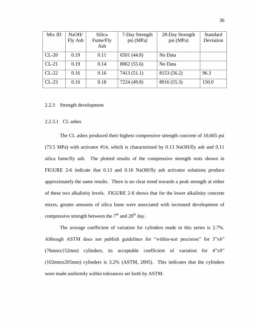
36

36

Mix ID NaOH/

Fly Ash

Silica

Fume/Fly

Ash

7-Day Strength

psi (MPa)

28-Day Strength

psi (MPa)

Standard

Deviation

CL-20 0.19 0.11 6501 (44.8) No Data

CL-21 0.19 0.14 8062 (55.6) No Data

CL-22 0.16 0.16 7413 (51.1) 8153 (56.2) 96.3

CL-23 0.16 0.18 7224 (49.8) 8016 (55.3) 150.0

2.2.3 Strength development

2.2.3.1 CL ashes

The CL ashes produced their highest compressive strength concrete of 10,665 psi

(73.5 MPa) with activator #14, which is characterized by 0.13 NaOH/fly ash and 0.11

silica fume/fly ash. The plotted results of the compressive strength tests shown in

FIGURE 2-6 indicate that 0.13 and 0.16 NaOH/fly ash activator solutions produce

approximately the same results. There is no clear trend towards a peak strength at either

of these two alkalinity levels. FIGURE 2-8 shows that for the lower alkalinity concrete

mixes, greater amounts of silica fume were associated with increased development of

compressive strength between the 7th

and 28th

day.

The average coefficient of variation for cylinders made in this series is 2.7%.

Although ASTM does not publish guidelines for ―within-test precision‖ for 3‖x6‖

(76mmx152mm) cylinders, its acceptable coefficient of variation for 4‖x8‖

(102mmx205mm) cylinders is 3.2% (ASTM, 2005). This indicates that the cylinders

were made uniformly within tolerances set forth by ASTM.

37

37

2.2.3.2 BC ashes

The BC ashes produced the highest compressive strength concrete with activator

#18, characterized by 0.16 NaOH/fly ash and 0.14 silica fume/fly ash. This resulted in a

strength of 7,064 psi (48.7MPa). As is seen in

FIGURE 2-7, strength results for this mix up to and past the optimum form a clear

peak. Data for the other activator designs are less clear in their trends because the lower

part of the curve is missing.

The average coefficient of variation for compressive strength of cylinders made

from BC ashes was 3.6%. This includes BC-19, which had a strong outlier. If this batch

is removed from the data, the average coefficient of variation is 2.7%.

2.2.3.3 General trends

Since the overall objective of these experiments was to discover the optimum

activator design to achieve structural strength concrete, it is necessary to study general

trends in strength development between the two fly ash types used.

Strength Development Over Time

As is evident from FIGURE 2-8 and FIGURE 2-9, there is the greatest 7-28 day

strength gain in concretes made with the lower alkalinity activator solutions. For BC

ashes, this increase ranged from <2% for activator #19, which is characterized by 0.19

NaOH/fly ash and 0.08 silica fume/fly ash. The greatest 7-28 day strength gain in BC

ashes was >35% and occurred in the batch made with activator #12 , which is

characterized by 0.10 NaOH/fly ash and 0.14 silica fume/fly ash. The same trend held

true for CL ashes, where the average strength gain for the 0.10 NaOH/fly ash activators

38

38

was 18%, 8% for the 0.13 activators and 6% for the 0.16 NaOH/fly ash activators. This

indicates that, while lower alkalinity activating solutions produce lower final compressive

strengths, there is a greater degree of strength gain over the course of the first month than

with higher alkalinity activating solutions.

Another disadvantage of the higher alkalinity activating solutions was found to be

reduced workability. Several times, activators with the 0.19 NaOH/Fly ash ratios caused

concrete to set-up in the mixer before cylinders could be made. When the concrete was

workable enough to produce cylinders, these were always of lower visual quality than

cylinders made with lower alkalinity activating solutions. These had variations in color

as well as more small voids near the surface. Overall, the results of using the high

alkalinity solutions were less predictable.

For the same activator solutions, CL ashes tended to produce stronger concretes

than the BC ashes. Because their chemical compositions as determined by XRF are very

similar, there is no data available on which to speculate about the cause of this trend. In

the literature, researchers have determined that amorphous content and particle size are

important factors in fly ash performance as a source material for geopolymer (Sun, 2005;

van Jaarsveld et al., 2003). Tests for these two features were not been completed, but

might illuminate the difference in strength development.

For both sets of ashes, the results indicate that as the alkalinity of the solution

increases, additional silica fume is also required to generate the maximum improvement

in compressive strength. Although the strength results plotted in FIGURE 2-6 and

FIGURE 2-7 do not indicate a clear trend, when viewed in tabular form as in

TABLE 2-8, they are more appreciable.

39

39

This indicates that the optimal strength is developed with the activating solution

containing a mass ratio of NaOH to silica fume of 1.41. If the process for producing the

sodium silicate solution used in these experiments follows the reaction shown in Equation

(2-1), the weight ratio should be 1.3.

2NaOH + SiO2 + H2O → Na2O + SiO2 + 2H2O (2-1)

2.3 Conclusions

1) Activators other than those with NaOH/silica fume ratios near 1.4 need not be

tested.

2) The 0.19 NaOH/fly ash activators should not be tested further as they do not

produce workable mixes.

3) The w/c ratio of 0.28 can produce workable concretes if superplasticizer is added

to the mix.

4) Ashes from the CL source should be used for further work as they seem to

produce stronger concrete.

40

40

FIGURE 2-6: Activator Design and 28-Day Strength for CL Ashes.

FIGURE 2-7: Activator design and 28-day strength for BC ashes.

0

10

20

30

40

50

60

70

80

0

1000

2000

3000

4000

5000

6000

7000

8000

0.000 0.050 0.100 0.150 0.200

Com

pre

ssiv

e S

tren

gth

[M

Pa]

Com

pre

ssiv

e S

tren

gth

[psi

]

Silica Fume/Fly Ash

10%

13%

16%

19%

0

10

20

30

40

50

60

70

80

0

2000

4000

6000

8000

10000

12000

0.00 0.05 0.10 0.15 0.20

Com

pre

ssiv

e S

tren

gth

[M

Pa]

Com

pre

ssiv

e S

tren

gth

[psi

]

Silica Fume/Fly Ash

10%

13%

16%

19%

41

41

FIGURE 2-8: Increase in compressive strength between day 7 and day 28 for CL ashes.

FIGURE 2-9: Increase in compressive strength between day 7 and day 28 for BC ashes.

0

0.05

0.1

0.15

0.2

0.25

0.1 0.13 0.16

% i

ncr

ease

in f

' c

NaOH/Fly Ash

0.08

0.11

0.14

0.16

0.18

Silica Fume/

Fly ASh

-0.2

-0.15

-0.1

-0.05

0

0.05

0.1

0.15

0.2

0.25

0.1 0.13 0.16% i

ncr

ease

in f

' c

NaOH/Fly Ash

0.08

0.11

0.14

0.16

0.18

Silica Fume/

Fly ASh

42

42

2.4 Preparation of concrete materials for constitutive property characterization

Following the development of the guidelines presented in the previous section,

several batches of GCC material were prepared in order to generate data on the

constitutive properties of the concrete.

2.4.1 Fly ash

Fly ashes used in these experiments were sourced from a southeastern steam

station. They were collected in a silo used for distribution of concrete-grade, Class-F

ashes to tanker trucks, as shown in FIGURE 2-10. This allowed them to be transported

and stored in a dry condition to preserve their reactivity. Depending on the quantity

sampled for research, the ashes were stored in a variety of containers including 3 cubic

yard hoppers (2.3 cubic meter), 55 gallon steel drums (208 l) and 2 ton (1.8 tonne),

polyethylene lined tote sacks. The ash oxide characteristics are described in TABLE

2-10 as determined by XRF analysis. As many ashes were used in the course of this

research, these ashes are identified by the initials ―CL.‖

2.4.2 Aggregates

The aggregates used in this phase of the work were sourced from local quarries.

The coarse aggregate was a 3/8‖, granite stone and the fine aggregate was silica concrete

sand. The gradations for these aggregates are given in TABLE 2-3.

43

43

FIGURE 2-10: Fly ash storage silo.

TABLE 2-10: XRF analysis of CL ashes.

% by Mass CL

SiO2 56.20

TiO2 1.46

Al2O3 28.00

Fe2O3 5.22

MnO 0.02

MgO 1.00

CaO 1.52

Na2O 0.21

K2O 2.74

P2O5 0.18

Totals 96.55

LOI 3.32

44

44

2.5 Mixing process

1) Preparing the Activating Solution

The sodium silicate activating solution is prepared by mixing the required amount

of sodium hydroxide in the specified amount of water, as is demonstrated in FIGURE

2-11. Next, the silica fume is added slowly. The reaction between the silica fume

and the sodium hydroxide is fairly violent and requires that additions be made slowly.

After all the silica fume is included, the solution is mixed for two minutes at low

speed with a paddle stirrer mounted in a hand drill. The sodium silicate solution is

placed in a polyethylene pitcher, partially sealed and placed in a 167⁰ F (75⁰ C) oven

overnight (~20 hours). A small amount of water 0.4-0.6 lb (200-500g) is usually

withheld from the activating solution so that it can be used to disperse any admixtures

through the dry ingredients immediately prior to mixing. Adding this small amount

of mixing water also helped reduce the dust and fly ash leaving the mixer.

2) Preparing the Aggregate

The coarse aggregate is brought to a saturated-surface-dry condition by soaking it

overnight in tap water and then drying the surface of the stones with terrycloth

towels. The fine aggregate is oven-dried at 167 ⁰ F (75⁰ C) overnight. Immediately

before mixing, the aggregates and fly ash are measured out in the proportions

specified for the mix under consideration, as is demonstrated in FIGURE 2-12.

3) Mixing the concrete

The dry ingredients are added to the mixer with the mixing water and admixtures,

and the mixer is started. After a two minute mixing session the activating solution is

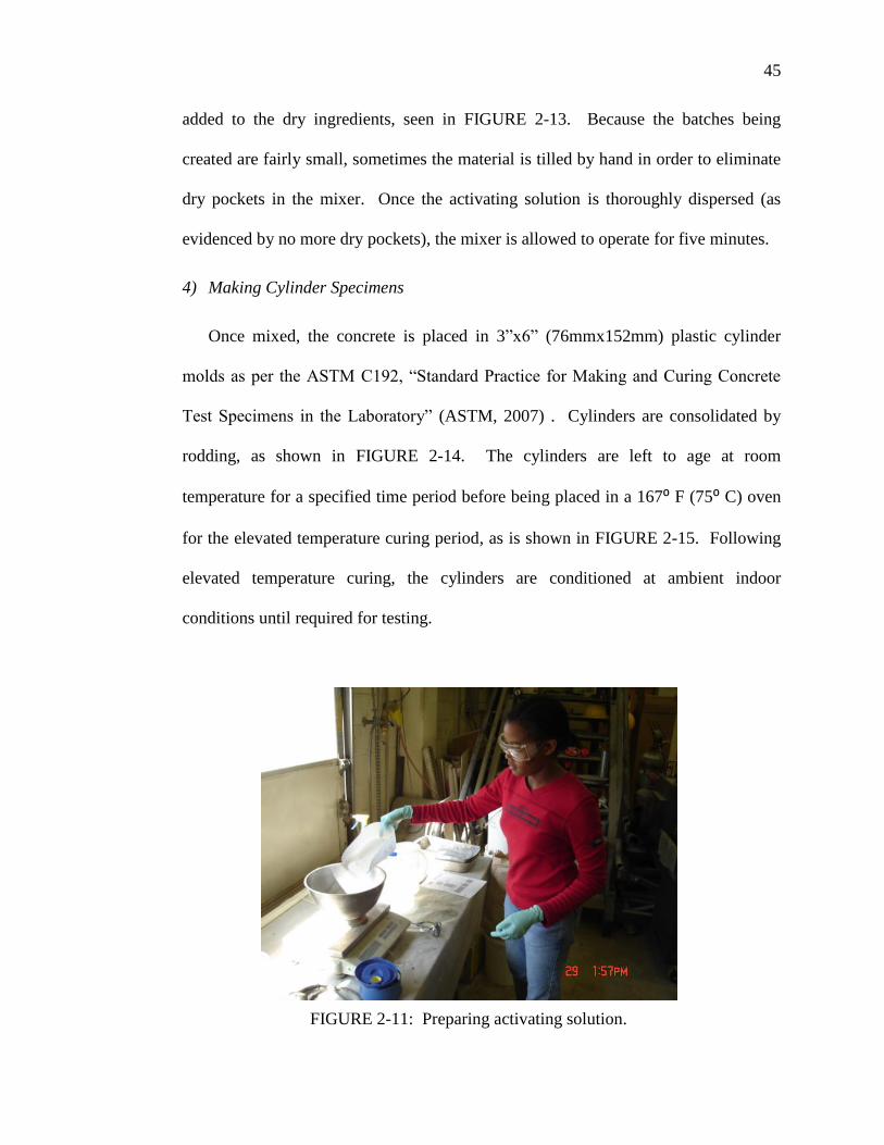
45

45

added to the dry ingredients, seen in FIGURE 2-13. Because the batches being

created are fairly small, sometimes the material is tilled by hand in order to eliminate

dry pockets in the mixer. Once the activating solution is thoroughly dispersed (as

evidenced by no more dry pockets), the mixer is allowed to operate for five minutes.

4) Making Cylinder Specimens

Once mixed, the concrete is placed in 3‖x6‖ (76mmx152mm) plastic cylinder

molds as per the ASTM C192, ―Standard Practice for Making and Curing Concrete

Test Specimens in the Laboratory‖ (ASTM, 2007) . Cylinders are consolidated by

rodding, as shown in FIGURE 2-14. The cylinders are left to age at room

temperature for a specified time period before being placed in a 167⁰ F (75⁰ C) oven

for the elevated temperature curing period, as is shown in FIGURE 2-15. Following

elevated temperature curing, the cylinders are conditioned at ambient indoor

conditions until required for testing.

FIGURE 2-11: Preparing activating solution.

46

46

FIGURE 2-12: Measuring aggregates.

FIGURE 2-13: Adding activating solution.

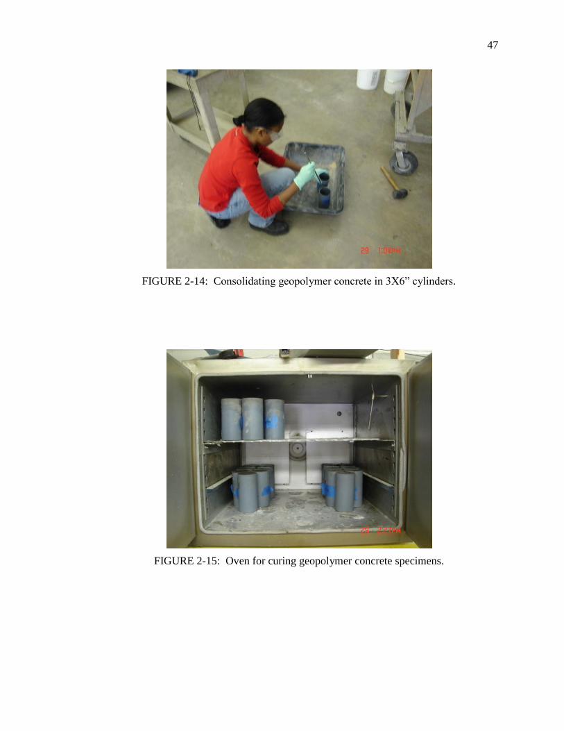
47

47

FIGURE 2-14: Consolidating geopolymer concrete in 3X6‖ cylinders.

FIGURE 2-15: Oven for curing geopolymer concrete specimens.

48

48

2.6 Experimental procedures

Three 1.5 ft3 (0.04 m

3) batches of geopolymer concrete were made in the lab. The

aggregates used were the same as described in TABLE 2-3. The proportions for the three

batches are presented in TABLE 2-11. For mix #1 and #2, 60 3‖x6‖ (76mmx152mm)

cylinders were made. 18 cylinders were made for mix # 3. Mixing was performed in a

3ft3 (0.08 m

3) rotary mixer according to the procedure described in the previous section.

Procedures for creating the cylinders followed ASTM C192 (ASTM, 2007). For

consistency, the step of vibrating all the cylinders for 1 minute after rodding was added.

TABLE 2-11: Mixing proportions lb/yd3 (kg/m

3).

Mix # 1 2 3

Fly Ash 834 (495) 798 (474) 766 (455)

Water 274 (163) 274 (163) 274 (163)

NaOH 83 (49.5) 103 (61.6) 122 (72.7)

Silica Fume 62 (37.1) 77 (46.2) 91 (54.5)

Fine Aggregate 1336 (793) 1336 (793) 1336 (793)

Coarse Aggregate 1336 (793) 1336 (793) 1336 (793)

TABLE 2-12: Number of cylinders made for each aging and curing regimen.

Aging Curing

24 hours 48 hours

0 hours 10 10

24 hours 10 10

48 hours 10 10

49

49

The cylinders were aged and cured according to the schedule presented in TABLE

2-12. The aging process occurred under ambient conditions in the structures lab at UNC

Charlotte. After the cylinders were made, the 0-hour aging batch was placed directly in

the 167⁰F (75⁰C) curing oven. The other cylinders were left out in the lab and added to

the oven after either 24 or 48 hours of aging. Cylinders were demolded immediately after

they were removed from the oven and were stacked on a pallet under ambient conditions

in the lab until testing on the 28th

day.

From each batch and curing group, three cylinders were tested in compression in

accordance with ASTM C39, three were tested in splitting according to ASTM C496 and

three were tested for the static modulus of elasticity according to ASTM C469 (ASTM,

2002a; ASTM, 2004b; ASTM, 2007). The procedures were carried out on a universal

testing machine at UNC Charlotte as depicted in FIGURE 2-16 and FIGURE 2-17.

FIGURE 2-16: Splitting tensile test set-up.

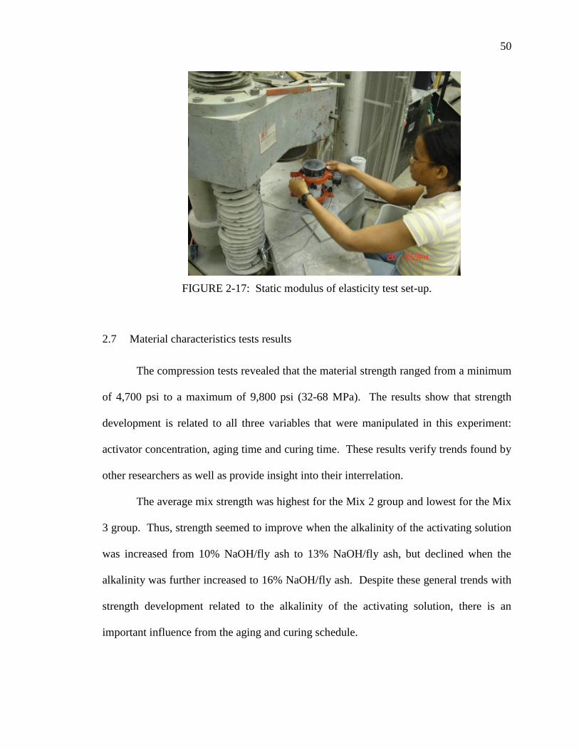
50

50

FIGURE 2-17: Static modulus of elasticity test set-up.

2.7 Material characteristics tests results

The compression tests revealed that the material strength ranged from a minimum

of 4,700 psi to a maximum of 9,800 psi (32-68 MPa). The results show that strength

development is related to all three variables that were manipulated in this experiment:

activator concentration, aging time and curing time. These results verify trends found by

other researchers as well as provide insight into their interrelation.

The average mix strength was highest for the Mix 2 group and lowest for the Mix

3 group. Thus, strength seemed to improve when the alkalinity of the activating solution

was increased from 10% NaOH/fly ash to 13% NaOH/fly ash, but declined when the

alkalinity was further increased to 16% NaOH/fly ash. Despite these general trends with

strength development related to the alkalinity of the activating solution, there is an

important influence from the aging and curing schedule.

51

51

The results presented in TABLE 2-13 show two main trends in strength

development for the aging and curing routines used in this course of experiments.

Increasing aging time from 0 to 2 days improved the 28-day compressive strength in all

cases. Increased curing time at 167⁰ F (75⁰ C) also improved the 28 day strength in all

cases. These results are illustrated in FIGURE 2-18. For the Mix 1 specimens, high

temperature curing for an additional day improved the compressive strength an average

of 12%. For these same specimens, the impact of additional aging was an average of 6%

increase in compressive strength. For the Mix 2 specimens, the effect of additional high

temperature curing time was an average compressive strength increase of 13%. The

impact of additional aging time on these specimens was an increase of strength by 8% on

average. Mix 3 showed the greatest improvement in strength with both increased aging

time and 24 hours of curing. However, the maximum strength was achieved for Mix 2.

FIGURE 2-18 also shows that there might be room for further improvement in

compressive strength by aging the specimens for more than two days prior to heat curing.

Whereas the improvement in strength for Mix 1 has leveled off by day two, Mixes 2 and

3 appear to still be increasing at day two. Further experimental work would be required

to examine this trend.

52

52

TABLE 2-13: Results of compression and tension tests.

Mix # Aging

Time

(days)

Curing

Time

(hours)

psi,

(MPa) psi,

(MPa)

1 0 24 5,302 (37) 474 (3.3)

1 0 48 6,010 (41) 558 (3.9)

1 1 24 5,915 (41) 420 (2.9)

1 1 48 6,465 (45) 544 (3.8)

1 2 24 5,939 (41) 485 (3.3)

1 2 48 6,978 (48) 550 (3.8)

2 0 24 7,356 (51) 708 (4.9)

2 0 48 7,983 (55) 764 (5.3)

2 1 24 7,732 (53) 555 (3.8)

2 1 48 9,308 (64) 696 (4.8)

2 2 24 8,287 (57) 879 (6.1)

2 2 48 9,787 (67) 851 (5.9)

3 0 24 4,708 (32)

3 0 48 6,336 (44)

3 1 24 6,171 (43)

3 1 48 6,780 (47)

3 2 24 7,926 (55)

3 2 48 8,094 (56)

The benefit of aging for longer periods versus curing for longer periods is

demonstrated in FIGURE 2-19 through FIGURE 2-21. Mixes 1 and 2 both showed

compressive strength gains of approximately 25% through the combination of increased

aging and curing periods. By comparing the batches that were aged for 0 days and cured

for 24 hours with those aged for 2 days and then cured for 24 and 48 hours, it is possible

to determine the effect of each process on the final strength development. These

differences are illustrated in FIGURE 2-19 by the regions labeled ―A‖ and ―B.‖ Region

―A‖ is the difference in compressive strength of cylinders that were aged for 0 days and

cured for 24 hours and the strength of cylinders that were aged for 2 days and cured for

24 hours. Thus, it describes the effect of two days of aging time. Region ―B‖ quantifies

53

53

the difference in compressive strength of cylinders aged for two days and cured for 24 or

48 hours. For Mixes #1 and #2, 38% of the gains between the batch not aged and cured

for only 24 hours and the batch aged for two days and cured for two days were related to

aging while 62% were related to heat curing. The higher alkalinity Mix #3 showed much

different behavior with 95% of the strength gains being attributable to aging and only 5%

attributable to heat curing.

FIGURE 2-18: Compressive strength development with aging and curing time.

0

10

20

30

40

50

60

0

1000

2000

3000

4000

5000

6000

7000

8000

9000

10000

0 1 2

Com

pre

ssiv

e S

tren

gth

[M

Pa]

Com

pre

ssiv

e S

tren

gth

[psi

]

Aging Time [days]

Mix #1-24

Mix #2-24

Mix #3-24

Mix #1-48

Mix #2-48

Mix #3-48

54

54

It would appear that heat is playing a role in two different reaction mechanisms.

For instance, in the lower alkalinity concretes, the heat might help strength development

by improving the dissolution processes by increasing the solubility of silica. In higher

alkalinity systems the heat is probably not required to improve dissolution due to the

greater quantity of available OH- ions. This may be explained by the very small

difference in strength between Mix #3 specimens aged for 2 days and cured for 24 hours

versus those cured for 48 hours.

FIGURE 2-19: Compressive strength after 24 and 48 hours of curing for Mix #1.

0

10

20

30

40

50

60

0

1000

2000

3000

4000

5000

6000

7000

8000

9000

10000

0 24 48

Com

pre

ssiv

e S

tren

gth

[M

pa]

Com

pre

ssiv

e S

tren

gth

[psi

]

Aging Time [hours]

48 hours

24 hours

Curing Time

A

B

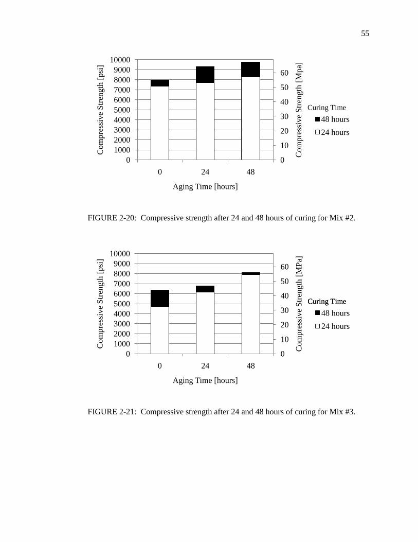
55

55



0

10

20

30

40

50

60

0

1000

2000

3000

4000

5000

6000

7000

8000

9000

10000

0 24 48

Co

mp

ress

ive

Str

ength

[M

pa]

Co

mp

ress

ive

Str

ength

[p

si]

Aging Time [hours]

48 hours

24 hours

Curing Time

0

10

20

30

40

50

60

0

1000

2000

3000

4000

5000

6000

7000

8000

9000

10000

0 24 48

Com

pre

ssiv

e S

tren

gth

[M

Pa]

Com

pre

ssiv

e S

tren

gth

[psi

]

Aging Time [hours]

48 hours

24 hours

Curing TimeCuring Time

56

56

2.8 Mechanical properties

2.8.1 Tensile strength

As with Portland cement concrete, the split cylinder tensile strength of the

geopolymer cement concrete specimens was found to be proportional to the compressive

strength. TABLE 2-13 shows that the tensile strength ranged from 7.1% to 10.6% of the

compressive strength. Large numbers of combined results from Portland cement split

cylinder tests have revealed an average tensile strength, , of (MacGregor and Wight,

2005)

[psi] (2-2)

[MPa] (2-3)

(2-4)

where:

: concrete cylinder splitting stress

: concrete cylinder compressive strength

FIGURE 2-22 shows a strong relationship between the tensile and compressive

strength of GCC cylinders. A non-linear multiple regression analysis was used to

establish the value of the parameter ―X‖ in Equation (2-4) The value, X=0.616, creates the

regression line shown in FIGURE 2-22 and matches the data with R=0.796 for

compressive strength in MPa. For English customary units, the parameter is 7.4. These

Equations are

[psi] (2-5)

[MPa] (2-6)

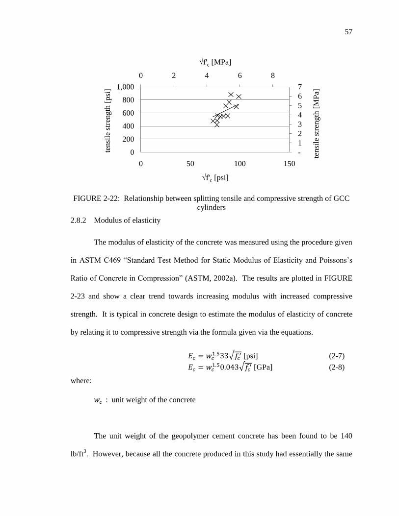
57

57

FIGURE 2-22: Relationship between splitting tensile and compressive strength of GCC

cylinders

2.8.2 Modulus of elasticity

The modulus of elasticity of the concrete was measured using the procedure given

in ASTM C469 ―Standard Test Method for Static Modulus of Elasticity and Poissons’s

Ratio of Concrete in Compression‖ (ASTM, 2002a). The results are plotted in FIGURE

2-23 and show a clear trend towards increasing modulus with increased compressive

strength. It is typical in concrete design to estimate the modulus of elasticity of concrete

by relating it to compressive strength via the formula given via the equations.

[psi] (2-7)

[GPa] (2-8)

where:

: unit weight of the concrete

The unit weight of the geopolymer cement concrete has been found to be 140

lb/ft3. However, because all the concrete produced in this study had essentially the same

0 2 4 6 8

-

1

2

3

4

5

6

7

0

200

400

600

800

1,000

0 50 100 150

√f'c [MPa]

tensi

le s

tren

gth

[M

Pa]

tensi

le s

tren

gth

[psi

]

√f'c [psi]

58

58

unit weight, there is no basis to use the unit weight as a predictor of GCC modulus of

elasticity. More data would be required to make such correlations. The relationship

between cylinder compressive strength and modulus of elasticity found for the materials

produced in this study is given by

[psi] (2-9)

[GPa] (2-10)

FIGURE 2-23: Compressive strength and Young’s Modulus for Mix #1 and Mix #2.

2.9 Creep

The time-dependent deformation of concrete under sustained loads is referred to as

creep. In Portland cement concrete, the paste fraction undergoes dimensional changes

while the aggregates tend to restrain creep-related deformation. After concrete cures and

enters service, a series of processes that result in volumetric changes occur, including free

shrinkage strain , basic creep , drying creep , and elastic strains . The total

0 2 4 6 8

0

5

10

15

20

25

30

0500

1,0001,5002,0002,5003,0003,5004,0004,5005,000

0 50 100 150

√f'c [MPa]

Modulu

s of

Ela

stic

ity [

Gpa]

Modulu

s of

Ela

stic

ity [

ksi

]

√f'c [psi]

59

59

strain measured in a concrete element is a combination of these constituent strains, as

given by

(2-11)

The summation of these strains is the total measurable strain.

The ratio of creep strain, , to elastic strain, , is known as the creep coefficient, C, as

given by

(2-12)

The creep coefficient changes over time as the strains attributable to creep

processes become similar in magnitude to and greater than elastic strains. For design

purposes, ACI Committee 209 provides the equation

(2-13)

where:

t: time (days)

D: constant usually taken as 10 (days)

. Ultimate creep

as a means of estimating the creep coefficient at a given time interval, t days, as a

function of the ultimate creep, . Ultimate creep for Portland cement concrete is known

to range from 1.30 to 4.15, with an average value of 2.35 (Branson, 1976).

The measurement of creep in controlled laboratory settings is undertaken by

preparing concrete cylinders, allowing them to cure for a specified period of time and

then subjecting them to a stress that does not exceed the proportional limit for the

material. The range typically used is less than 40% of the cylinder’s compressive

strength. In order to compare the results of tests completed using differing stress

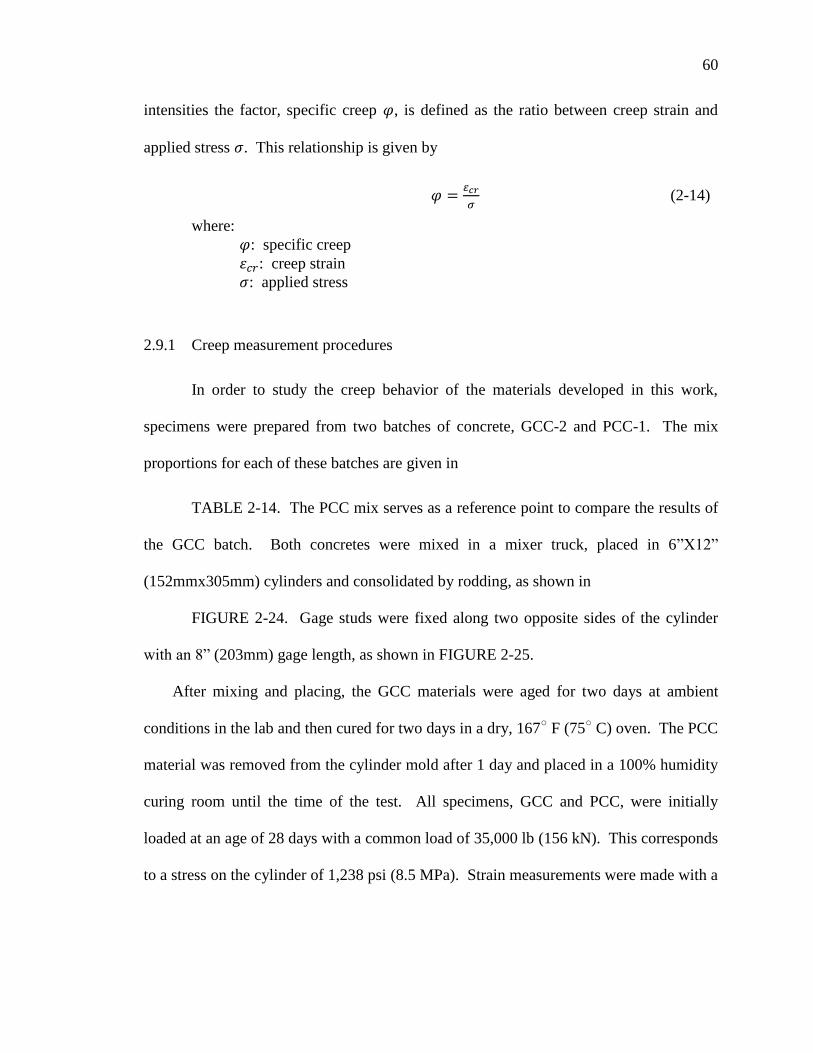
60

60

intensities the factor, specific creep , is defined as the ratio between creep strain and

applied stress . This relationship is given by

(2-14)

where:

: specific creep

: creep strain

: applied stress

2.9.1 Creep measurement procedures

In order to study the creep behavior of the materials developed in this work,

specimens were prepared from two batches of concrete, GCC-2 and PCC-1. The mix

proportions for each of these batches are given in

TABLE 2-14. The PCC mix serves as a reference point to compare the results of

the GCC batch. Both concretes were mixed in a mixer truck, placed in 6‖X12‖

(152mmx305mm) cylinders and consolidated by rodding, as shown in

FIGURE 2-24. Gage studs were fixed along two opposite sides of the cylinder

with an 8‖ (203mm) gage length, as shown in FIGURE 2-25.

After mixing and placing, the GCC materials were aged for two days at ambient

conditions in the lab and then cured for two days in a dry, 167○ F (75

○ C) oven. The PCC

material was removed from the cylinder mold after 1 day and placed in a 100% humidity

curing room until the time of the test. All specimens, GCC and PCC, were initially

loaded at an age of 28 days with a common load of 35,000 lb (156 kN). This corresponds

to a stress on the cylinder of 1,238 psi (8.5 MPa). Strain measurements were made with a

61

61

demountable mechanical strain gage at the intervals specified in ASTM C512 (ASTM,

2002b).

The cylinders were capped with a sulfur compound and loaded in pairs into the

frame shown in FIGURE 2-26. The load was transmitted from the end plates to the

cylinders through small cylinder slices of similar strength concrete, also visible in

FIGURE 2-26. The loads were maintained on the specimens via heavy springs to prevent

small dimensional changes in the concrete from creating large reductions in stress. The

magnitude of the load was monitored with a load cell connected to a digital read-out. If

the load was found to differ from 35,000 lb (156 kN) by more than 2%, it was adjusted

with a hydraulic pump.

TABLE 2-14: Mix proportions for creep specimens lb/yd3 (kg/m

3).

Material Mix Designation

GCC-1 PCC-1

Portland Cement 0 386 (229)

Fly Ash 835 (495) 89 (53)

Water 275 (163) 173 (103)

NaOH 84 (50) 0

Silica Fume 63 (37) 0

Fine Aggregate 1,336 (793) 709 (421)

Coarse Aggregate 1,336 (793) 1,127 (669)

62

62

FIGURE 2-24: Consolidating creep specimens.

Gage Studs

6" (152mm)

12" (305mm)8" (203mm)

FIGURE 2-25: Gage stud layout for creep specimens.

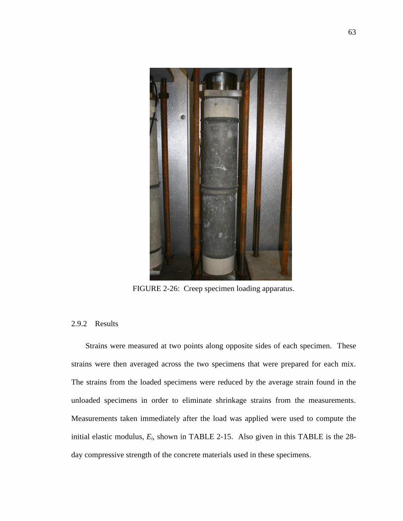
63

63

FIGURE 2-26: Creep specimen loading apparatus.

2.9.2 Results

Strains were measured at two points along opposite sides of each specimen. These

strains were then averaged across the two specimens that were prepared for each mix.

The strains from the loaded specimens were reduced by the average strain found in the

unloaded specimens in order to eliminate shrinkage strains from the measurements.

Measurements taken immediately after the load was applied were used to compute the

initial elastic modulus, Ei, shown in TABLE 2-15. Also given in this TABLE is the 28-

day compressive strength of the concrete materials used in these specimens.

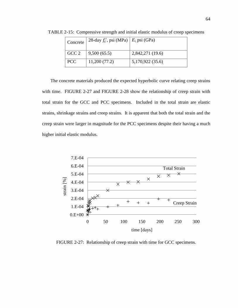
64

64

TABLE 2-15: Compressive strength and initial elastic modulus of creep specimens

Concrete 28-day

, psi (MPa) Ei, psi (GPa)

GCC 2 9,500 (65.5) 2,842,271 (19.6)

PCC 11,200 (77.2) 5,170,922 (35.6)

The concrete materials produced the expected hyperbolic curve relating creep strains

with time. FIGURE 2-27 and FIGURE 2-28 show the relationship of creep strain with

total strain for the GCC and PCC specimens. Included in the total strain are elastic

strains, shrinkage strains and creep strains. It is apparent that both the total strain and the

creep strain were larger in magnitude for the PCC specimens despite their having a much

higher initial elastic modulus.

FIGURE 2-27: Relationship of creep strain with time for GCC specimens.

0.E+00

1.E-04

2.E-04

3.E-04

4.E-04

5.E-04

6.E-04

7.E-04

0 50 100 150 200 250 300

stra

in [

%]

time [days]

Total Strain

Creep Strain

65

65

FIGURE 2-28: Relationship of creep strain with time for PCC specimens.

The ratio of elastic strains and creep strains is described by the creep coefficient.

It approaches a limiting value of ultimate creep, Cu, which represents the maximum strain

that would be found after a long period of time under loading. In FIGURE 2-29,

Equation (2-13) is used to plot the creep coefficient using the upper and lower bound

ultimate creep values for typical Portland cement concrete.

The PCC control specimens displayed typical behavior. The ultimate creep

appears that it will lie within the range of expected values for Portland cement concretes.

After 100 days of loading, the creep coefficient equaled 1.25, as compared to 0.09 as the

lower end of creep behavior

FIGURE 2-29 shows that Cu for the GCC appears to be less than 1.0. Although

data are only presented for 200 days of loading, creep does not seem to be increasing

significantly for successive measurements beyond the 100th

day. The range defined by

Cu=1.30 and Cu=4.15 on the charts denote the typical range of ultimate strain for Portland

cement concrete. The GCC is well outside the lower end of this range. This indicates

0.E+00

1.E-04

2.E-04

3.E-04

4.E-04

5.E-04

6.E-04

7.E-04

0 50 100 150 200 250

stra

in [

%]

time [days]

Total Strain

Creep Strain

66

66

that the creep behavior of GCC is significantly improved over the expected behavior of

PCC.

FIGURE 2-29: GCC and PCC creep compared to the range of ultimate creep values for

Portland cement concrete.

2.10 Shrinkage

Removal of water from the concrete matrix causes shrinkage strains as the overall

volume of the monolith is reduced. When the water is removed from fresh concrete, the

resulting shrinkage is known as plastic shrinkage. The effects of plastic shrinkage are

manifested in crack patterns that negatively impact the appearance and durability of

concrete surfaces. In hardened concrete, shrinkage processes are a result of the continued

removal of water from the pore system of the concrete either by self-desiccation in

autogenous shrinkage, by chemical reaction in carbonation shrinkage or by evaporation

(Mindess et al., 2003).

Predicting the magnitude of shrinkage is important to the design of concrete

structures. If the designer can properly locate contraction joints and control restraint

0

0.5

1

1.5

2

2.5

3

3.5

0 50 100 150 200 250 300

Cre

ep C

oef

fici

ent,

C

time [days]

PCC

Cu=4.15

Cu=1.30

GCC

67

67

against shrinkage, cracks can be eliminated or limited to acceptable locations. Passive or

prestressing reinforcement is also a design requirement to restrain shrinkage in concrete

structures, with minimum steel ratios given by ACI 318 (American Concrete Institute,

2008).

Shrinkage of concrete is a process that involves many variables for structures in

service. These include the duration of wet curing, air content, aggregate characteristics

and temperature, and relative humidity around the structure. ACI committee 209

provides guidelines for estimating shrinkage of concrete after periods of time. Prediction

of the magnitude of the shrinkage is made with

(2-15)

where:

: shrinkage strain at time, t =800x10-6

in/in (mm/mm) for PCC

: power of t ~1.0

: constant taken as 20-130 days

: ultimate shrinkage, 800x10-6

in/in [mm/mm]

Although shrinkage can cause serious durability and aesthetic problems in all types

of concrete structures, it presents a special concern in prestressed concrete sections. As

shrinkage strains increase in the concrete, the elongation of the prestressing steel tendons

is reduced, causing a net reduction in the effective prestress. The magnitude of this

reduction is related to the modulus of the steel as given by

(2-16)

where:

: change in stress in the prestressing steel due to concrete shrinkage, psi or

MPa

: shrinkage strain

68

68

: modulus of elasticity for prestressing steel, psi or MPa

2.10.1 Measurement of shrinkage

In order to determine shrinkage experimentally, concrete is cured and aged under

controlled environmental conditions that are set at temperature and humidity levels of

interest. Generally, the environmental conditions used to establish baseline shrinkage

magnitudes are 73○F (22.7

○C) and 50% relative humidity. General procedures for

conducting shrinkage measurements are given by ASTM 157 (ASTM, 2008b).

3‖x3‖x11.25‖ (76mmx76mmx286mm) concrete prisms are formed and outfitted with

gage studs in each end. The length of the prism is measured after the concrete initially

sets, again after the primary curing is completed and then at intervals through 64 weeks.

Three batches of concrete were prepared using the mixing proportions given in

TABLE 2-16. Data were collected for the shrinkage behavior of three concrete mix

types. PCC is a Portland cement concrete mix, GCC-2 represents a geopolymer cement

concrete with virgin aggregates and GCC-R represents a geopolymer cement concrete

with 45% of the virgin aggregates replaced by recycled aggregates. Four prisms were

prepared from each concrete mix. In order to not confound the results with processes that

are not related to drying shrinkage, the PCC specimens were handled in accords with

ASTM 157 (ASTM, 2008b). The specimens were removed from the molds after 24

hours, placed in lime-saturated water for 1 hour and then an initial measurement was

made. The specimens were stored in the lime water for a period of 28 days, after which

readings were made at 4, 7, 14, 28 and 56 days.

69

69

GCC-2 and GCC-R were handled slightly differently from the ASTM procedures

since these guidelines do not have provision for geopolymer cement concretes. The

specimens were consolidated in the forms by rodding, covered with plastic and allowed

to age for two days. Following the aging period, they were cured at 167○F (75

○C) for 48

hours. During preparation of GCC-R, there were problems with the heating apparatus

and the temperature in the curing chamber did not reach the target temperature during the

initial 24 hours of the curing period. Therefore, it was permitted to cure for additional

time to allow at least 48 hours at the target temperature, 167○F (75

○C).

Following removal from the forms after curing at elevated temperature, the GCC

specimens were measured immediately with a length comparator and then stored for the

duration of the test in an environmental chamber set at 73○F (22.7

○C) and 50% relative

humidity. Length measurements were made at 4, 7, 14, 28, and 56 days.

TABLE 2-16: Mixing proportions for shrinkage specimens lb/yd3 (kg/m

3).

Component Mix Designation

PCC-1 GCC-2 GCC-R

Portland Cement 386 (229) 0 0

Fly Ash 89 (53) 835 (495) 815 (483)

Water 173 (103) 275 (163) 268 (159)

NaOH 0 84 (49.5) 81 (48)

Silica Fume 0 63 (37.1) 61 (36)

Fine Aggregate 709 (421) 1,336 (793) 1304 (773)

Coarse Aggregate 1127 (669) 1,336 (793) 718 (426)

Recycled Coarse

Aggregate 587 (348)

70

70

2.10.2 Shrinkage test results

Data was available for 224 days of post-curing shrinkage for PCC and GCC-2.

However, data only extend 56 days for the GCC-R batch. TABLE 2-17 provides the

average strain for each group of four prisms. FIGURE 2-30 through 2-32 illustrate the

increase in shrinkage strain with time. The largest shrinkage strains were found in the

PCC mix. Shrinkage increased rapidly between day 0 and day 28. The strains appear to

be approaching 700 X 10-6

%, which is within the typical range for Portland cement

concrete. Moist-cured Portland cement concrete has an average ultimate strain of 800 X

10-6

%.

The GCC-2 concrete indicates a more gradual approach to an upper value of

220X10-6

% at 112 days. Some data from cylinders created for creep testing was

supplemented in FIGURE 2-31 since the data from the shrinkage tests 4, day 14 and day

28 were strong outliers. The cylinders were stored in the same environmental chamber

and were instrumented for precision measurements over a gage length of 8‖ (203 mm).

The same shrinkage trends are seen in the cylinders as in the shrinkage prisms and the

proximity of the data points along the curve in FIGURE 2-31 verify the behavior in place

of the missing measurements.

TABLE 2-17: Shrinkage test results.

Batch Microstrain at Day

0 4 7 14 28 56 112 224

PCC-1 -40 180 230 430 480 510 630 760

GCC-2 0 - 60 - - 120 240 220

GCC-R 0 260 130 - 260 270 - -

71

71

FIGURE 2-30: PCC-1 shrinkage strain versus time.

FIGURE 2-31: GCC-2 shrinkage strain versus time.

0.00E+00

1.00E-04

2.00E-04

3.00E-04

4.00E-04

5.00E-04

6.00E-04

7.00E-04

8.00E-04

0 50 100 150 200 250

Shri

nkag

e S

trai

n [

%]

time [days]

0.00E+00

1.00E-04

2.00E-04

3.00E-04

4.00E-04

5.00E-04

6.00E-04

7.00E-04

8.00E-04

0 50 100 150 200 250

Shri

nkag

e S

trai

n [

%]

time [days]

Shrinkage Prisms

Unloaded Creep

Cylinders

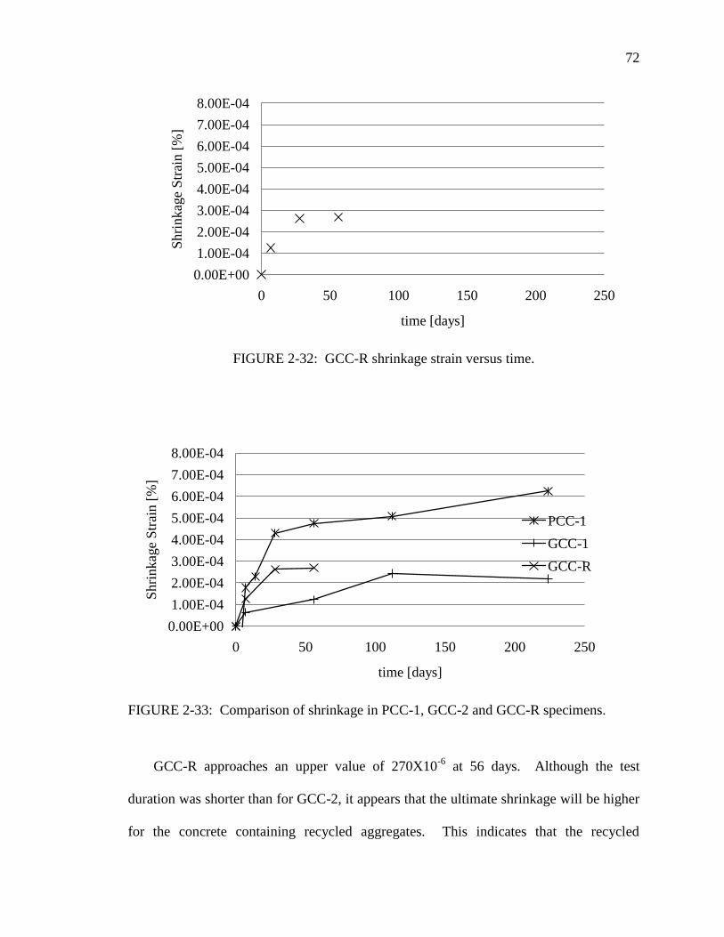
72

72

FIGURE 2-32: GCC-R shrinkage strain versus time.

FIGURE 2-33: Comparison of shrinkage in PCC-1, GCC-2 and GCC-R specimens.

GCC-R approaches an upper value of 270X10-6

at 56 days. Although the test

duration was shorter than for GCC-2, it appears that the ultimate shrinkage will be higher

for the concrete containing recycled aggregates. This indicates that the recycled

0.00E+00

1.00E-04

2.00E-04

3.00E-04

4.00E-04

5.00E-04

6.00E-04

7.00E-04

8.00E-04

0 50 100 150 200 250

Shri

nkag

e S

trai

n [

%]

time [days]

0.00E+00

1.00E-04

2.00E-04

3.00E-04

4.00E-04

5.00E-04

6.00E-04

7.00E-04

8.00E-04

0 50 100 150 200 250

Shri

nkag

e S

trai

n [

%]

time [days]

PCC-1

GCC-1

GCC-R

73

73

aggregates have made some impact on the shrinkage characteristics of the concrete.

Without mineralogical or microstructural data to evaluate, the exact cause of the

additional shrinkage is not apparent. However, it may be related to the proportion of

concrete mortar in the matrix which could have undergone swelling and shrinkage as a

result of remixing in the geopolymer. Also, the presence of calcium from the old cement

particles in the recycled aggregate could have also lead to the formation of C-S-H phases

that coexist with the geopolymer. The C-S-H could make the concrete more prone to

autogenous shrinkage.

2.10.3 Analysis of gcc-2 results

In order to use Equation (2-15) to estimate shrinkage in concrete, the terms and

must be determined. As Equation (2-15) is simply a hyperbolic equation, reducing

below values of 1.0 will tend to steepen the ascending branch of the curve. Values of

affect how quickly the curve approaches the asymptotic value, . Using a multi-

parameter curve fitting tool in MathCAD, values for and were found to describe the

behavior of the GCC-2 materials. In the model was taken to be 300 X 10-6

. With

values of =0.8 and =0.9, the curve fits the data with R=0.952. A plot showing this

curve is given in FIGURE 2-34.

74

74

FIGURE 2-34: Prediction of shrinkage using =0.8 and =0.9.

2.11 Discussion of results and conclusions

Both geopolymer cement concretes tested for shrinkage resulted in lower strains at

each time increment than Portland cement concrete. Strains in the PCC batch were more

than 200% of the strains found in both geopolymer materials. Although the duration of

the tests are not long enough to provide a conclusive magnitude for the ultimate

shrinkage strain the data do appear to approach an asymptote. For PCC the

shrinkage strains appear to approach 700 X 10-6

in/in (mm/mm), which is typical for

moist cured Portland cement materials. For the GCC-2 batch, the limit appears that it

will be in the range of 300 X 10-6

in/in (mm/mm). Data for GCC-R do not extend far

enough to extrapolate their upper limit. Equation (2-15) is effective at modeling

shrinkage in geopolymer cement concrete with virgin aggregates. For the materials

tested, =0.8 and =0.9.

0.00E+00

1.00E-04

2.00E-04

3.00E-04

4.00E-04

5.00E-04

6.00E-04

7.00E-04

8.00E-04

0 50 100 150 200 250

Shri

nkag

e S

trai

n [

%]

time [days]

75

75

It is important to note that the test procedure is only set-up to measure shrinkage in

the GCC that occurred after high temperature curing. However, it will be important to

understand and predict any volume changes that occur in the GCC as it undergoes the

aging process and the high temperature curing process. These changes could be

attributable to both the action of water evaporation from pore spaces in the GCC as well

as to the formation of polymeric bonds during the hardening phase. A technique to

measure these strains would need to account for the thermal expansion that occurs during

elevated temperature curing.

CHAPTER 3: RECYCLED AGGREGATES IN GEOPOLYMER CEMENT

CONCRETE

The sustainability benefits of geopolymer cement concretes (GCC) are related to its

use of the waste material, fly ash. By incorporating the fly ash into the concrete, the dual

environmental challenges of landfilling the ash and reducing the amount of Portland

cement-related greenhouse gas emissions are addressed. One means of improving the

sustainability farther is by the incorporation of recycled material for aggregate. Once mix

designs were developed using virgin, granite aggregates as described in 0, portions of the

aggregate were replaced by crushed demolition rubble. This chapter describes the

process of collecting and evaluating the rubble as well as developing mix designs that

incorporate it in the GCC.

3.1 Background on recycled concrete aggregate use

Demolition rubble comprises 8% of the construction and demolition waste

produced in Mecklenburg County, North Carolina. In 2005, this equaled more than

31,000 tons (Mecklenburg County Land Use and Environmental Services Agency, 2006).

When it is diverted from the landfill, its current uses are largely restricted to low-grade,

non-structural applications such as road sub-base and erosion control. While researchers

have used RCA to manufacture structural strength concretes, there have been problems

associated with the high water absorption capacity and interrupted interfacial transition

zone of reclaimed aggregates (Topçu and Sengel, 2004; Tu et al., 2006). These

challenges might not have the same impacts in geopolymer concretes due to the absence

77

77

of hydration processes and the ability of geopolymer to bond with Portland cement

mortar.

RCA is used in concrete in order to reduce the natural resource demands of

concrete production as well as to create an outlet for a large waste stream. The

aggregates are produced by crushing pieces of concrete that are generated from

demolition projects. This sort of demolition work is often aligned with large-scale

material disposal undertakings. Examples include clean-up in the aftermath of

earthquakes and other natural disasters as well as wrecking large facilities like the

Stapleton Airport in Denver, Colorado. Elias-Ozkan (2001) suggests that municipalities

can control the quantities of concrete rubble destined for landfills or unsuitable dumping

grounds by more tightly controlling the issuance of demolition permits. The

opportunities for reclaiming material for aggregate in this manner could include

production of aggregates on-site in the case of demolition-rebuild projects (Elias-Ozkan,

2001). Doing so would reduce the energy required for transporting construction

materials to the site and would control the source content.

The crushed pieces may be regraded in order to produce material suitable for use

in concrete. However, there are other quality issues related to using a material of such

variable consistency. Oikonomou (2005) surveyed the current state of RCA knowledge

and determined that industrial and municipal requirements for greater use include a

control system for collection and sorting of demolition waste, greater public support,

more technical studies and development of specifications. While there are preliminary

documents published by RILEM and BRE, Oikonomou categorizes the information

required for the safe and sustainable use of RCA as:

78

78

1) Historical data on the make-up of antiquated concretes

2) Physical characteristics- presence of contaminants, water absorption, specific

gravity

3) Mechanical characteristics- abrasion, degradation

4) Environmental characteristics- leaching potential

Although the original, virgin aggregates might be visible, between 25 and 60% of

volume occupied by a single RCA particle is the mortar paste that remains adhered (Tu et

al., 2006). The presence of this paste affects the performance and characteristics of the

aggregate in several ways. The absorption capacity of recycled aggregates tends to be

higher and can require larger amounts of water to achieve adequate workability (Topçu

and Sengel, 2004). Hydration might also be delayed as a result of the absorption

capacity. The workability of the mix is also affected by the greater angularity of RCA.

Tam et al. (2007) conducted research whereby the cement mortar was removed

from the aggregate particles by treating them with acidic solutions. The acid attacks the

CaO in the mortar and was found to be effective at reducing some of the negative

physical characteristics of the RCA surrounding absorption capacity and affected surface

at the interfacial zone. The process was determined to be cost effective when the benefits

of waste diversion from the landfill were included (Tam et al., 2007).

The impact of RCA use on compressive strength has been well researched. In

general, researchers have found that compressive strength decreases as the ratio of

recycled aggregate to virgin aggregate increases. Tupcu and Sengel (2004) created

concrete specimens with target strengths of 2300 psi and 2900 psi (15.9 MPa -20.0 MPa)

and then replaced virgin aggregates with RCA at the rate of 30, 50, 70 and 100%. The

79

79

specimens were subjected to compressive testing, freeze-thaw cycling and flexural

testing. It was found that the compressive strength decreased at a rate relative to the

addition of RCA. However, the freeze-thaw cycling had little effect on the flexural or

compressive strength of the specimens (Topçu and Sengel, 2004).

Tu et al explored the use of RCA in high performance concrete (HPC). The

research group tested concretes in strength ranges suitable for structural applications

(3,000-6,000 psi) (20.7-41.4 MPa) that had been created with either recycled coarse or

recycled coarse and fine aggregates. It was determined that, while a strength reduction of

20-30% could be expected due to aggregate replacement, the durability of the concrete

matrix and its ability to protect steel from chloride intrusion was suitable for reinforced,

structural applications (Tu et al., 2006).

The challenges to maintaining stringent mechanical performance standards while

using RCA in concrete mixes have been overcome by adapting either the batching

process or reducing the proportion of recycled material. Tam et al. (2005) have adapted

the mixing process into two stages- the first to coat the aggregate in a rich cement slurry,

and the second to complete the addition of mixing water. The author found that this

technique filled microcracks along the interfacial transition zone and also allowed fresh

paste to reach the surface of the mineral aggregate. The problem of high water

absorption capacity in RCA has been addressed by simple techniques such as presoaking

aggregates prior to batching (American Concrete Pavement Association, 2009).

State departments of transportation as well as national level agencies, such as the

National Cooperative Highway Research Program (NCHRP), National Ready Mix

Concrete Association (NRMCA), the American Concrete Pavement Association (ACPA)

80

80

and the Federal Highway Administration (FHWA) have produced guidance on the

implementation of projects that permit or encourage recycled concrete aggregates in new

PCC applications.

Control of concrete quality when RCA is used is achieved via several strategies

that are given in state department of transportation materials specifications or in the

guidance published by the previously listed agencies. These strategies include the

following major themes:

1) Limitation to the quantity of RCA in the concrete

2) Preparation and handling guidelines

3) Limits to the source of acceptable materials

4) Restrictions on the type of elements permitted to contain RCA

5) Characterization requirements

TABLE 3-1 provides a sampling of the specifications and guidelines given by

various groups. Perhaps the most conservative risk reduction technique for specifying

RCA concrete products is to limit the type or allowable proportion of recycled material in

the mix design. For instance, Texas Department of Transportation (TXDOT) permits a

maximum of 20% recycled fine aggregate in certain non-structural concrete elements

(Texas Department of Transportation, 2004). A strategy introduced in Europe

encourages the segregation of incoming material by source or quality so as to maintain

stockpiles of rubble having known origins and quality. The Michigan Department of

Transportation (MDOT) specification only permits RCA that was collected from MDOT

demolition projects. In this way, the source material is known to have met Michigan

quality standards when it was originally created (Michigan Department of Transportation,

81

81

2003). The NRMCA has proposed similar recommendations for returned concrete

aggregates- suggesting that they be divided by the grade of concrete in the truck (Obla et

al., 2007).

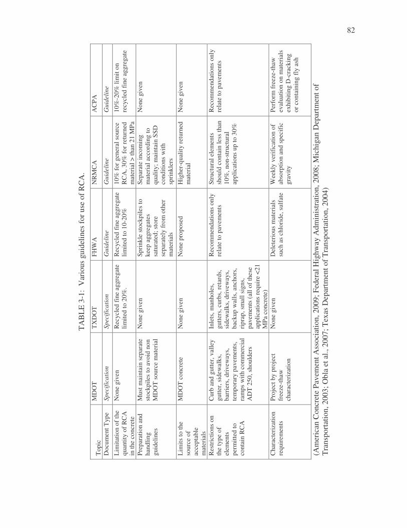
82

TA

BLE

3-1

: V

ario

us g

uide

lines

for u

se o

f RC

A.

Top

ic

MD

OT

T

XD

OT

FH

WA

N

RM

CA

A

CPA

Doc

umen

t Typ

e Sp

ecifi

catio

n Sp

ecifi

catio

n G

uide

line

Gui

delin

e G

uide

line

Lim

itatio

n of

the

quan

tity

of R

CA

in

the

conc

rete

Non

e gi

ven

Rec

ycle

d fi

ne a

ggre

gate

lim

ited

to 2

0%.

R

ecyc

led

fine

agg

rega

te

limite

d to

10-

20%

10

% fo

r gen

eral

sou

rce

RC

A, 3

0% fo

r ret

urne

d m

ater

ial >

than

21

MPa

10%

-20%

lim

it on

re

cycl

ed fi

ne a

ggre

gate

Prep

arat

ion

and

hand

ling

guid

elin

es

Mus

t mai

ntai

n se

para

te

stoc

kpile

s to

avo

id n

on

MD

OT

sou

rce

mat

eria

l

Non

e gi

ven

Spri

nkle

sto

ckpi

les

to

keep

agg

rega

tes

satu

rate

d; s

tore

se

para

tely

from

oth

er

mat

eria

ls

Sepa

rate

inco

min

g m

ater

ial a

ccor

ding

to

qual

ity; m

aint

ain

SSD

co

nditi

ons

with

sp

rink

lers

Non

e gi

ven

Lim

its to

the

sour

ce o

f ac

cept

able

m

ater

ials

MD

OT

con

cret

e

Non

e gi

ven

Non

e pr

opos

ed

Hig

her-

qual

ity re

turn

ed

mat

eria

l N

one

give

n

Res

tric

tions

on

the

type

of

elem

ents

pe

rmitt

ed to

co

ntai

n R

CA

Cur

b an

d gu

tter,

valle

y gu

tter,

side

wal

ks,

barr

iers

, dri

vew

ays,

te

mpo

rary

pav

emen

ts,

ram

ps w

ith c

omm

erci

al

AD

T 2

50, s

houl

ders

Inle

ts, m

anho

les,

gu

tters

, cur

bs, r

etar

ds,

side

wal

ks, d

rive

way

s,

back

up w

alls

, anc

hors

, ri

prap

, sm

all s

igns

, pa

vem

ents

(all

of th

ese

appl

icat

ions

requ

ire

<21

MPa

con

cret

e)

Rec

omm

enda

tions

onl

y re

late

to p

avem

ents

St

ruct

ural

ele

men

ts

shou

ld c

onta

in le

ss th

an

10%

, non

-str

uctu

ral

appl

icat

ions

up

to 3

0%

Rec

omm

enda

tions

onl

y re

late

to p

avem

ents

Cha

ract

eriz

atio

n re

quir

emen

ts

Proj

ect b

y pr

ojec

t fr

eeze

-tha

w

char

acte

riza

tion

Non

e gi

ven

Del

eter

ious

mat

eria

ls

such

as

chlo

ride

, sul

fate

W

eekl

y ve

rifi

catio

n of

ab

sorp

tion

and

spec

ific

gr

avity

Perf

orm

free

ze-t

haw

ev

alua

tion

on m

ater

ials

ex

hibi

ting

D-c

rack

ing

or c

onta

inin

g fl

y as

h

(Am

eric

an C

oncr

ete

Pave

men

t Ass

ocia

tion,

200

9; F

eder

al H

ighw

ay A

dmin

istr

atio

n, 2

008;

Mic

higa

n D

epar

tmen

t of

Tra

nspo

rtat

ion,

200

3; O

bla

et a

l., 2

007;

Tex

as D

epar

tmen

t of T

rans

port

atio

n, 2

004)

83

83

Other waste stream constituents have also been researched as virgin aggregate

replacements. Kou et al. studied the possibility of replacing fine aggregates with small

particles of discarded PVC pipe. By mixing the material into a concrete at river-sand

replacement rates of 5, 15, 30 and 45%, it was found that the PVC granules reduced the

compressive strength, modulus of rupture, elastic modulus and workability. However,

quantity of charge passed by the concrete was reduced, indicating that PVC could

improve the durability of concrete. It was also found that drying shrinkage was reduced

by adding PVC pieces. The author suggests PVC for use in non-structural applications at

a sand replacement rate of 15% (Kou et al., 2009).

3.2 Collecting recycled concrete aggregates for gcc use

UNC Charlotte researchers observed the demolition of an elementary school facility

in order to study the physical processes included in the tear-down as well as the decision

making process for the disposal or the recycling methods applied to the demolished

materials. The construction of the school was typical for a wide range of commercial and

institutional buildings at the time. Therefore, the information presented here regarding

the demolition process should be relevant to many of the buildings in the local inventory.

Walls were reinforced and unreinforced masonry, the roof was a combination of

prestressed concrete double-tees and steel framing, and the floor system was a concrete

slab-on-grade. The demolition process was found to be very orderly and included many

techniques that simplified the separation of materials such that contamination of the

rubble destined for the crusher was minimized. General steps followed in the demolition

(in sequential order) were:

1) Removal of hazardous materials such as asbestos

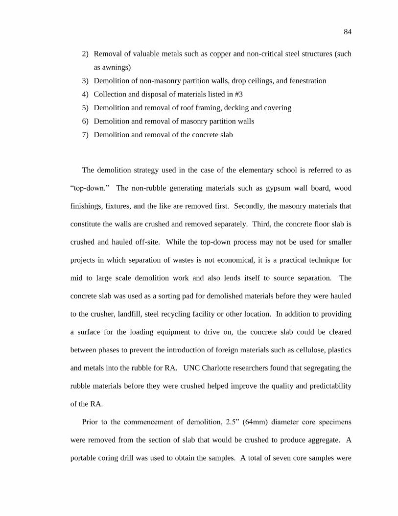
84

84

2) Removal of valuable metals such as copper and non-critical steel structures (such

as awnings)

3) Demolition of non-masonry partition walls, drop ceilings, and fenestration

4) Collection and disposal of materials listed in #3

5) Demolition and removal of roof framing, decking and covering

6) Demolition and removal of masonry partition walls

7) Demolition and removal of the concrete slab

The demolition strategy used in the case of the elementary school is referred to as

―top-down.‖ The non-rubble generating materials such as gypsum wall board, wood

finishings, fixtures, and the like are removed first. Secondly, the masonry materials that

constitute the walls are crushed and removed separately. Third, the concrete floor slab is

crushed and hauled off-site. While the top-down process may not be used for smaller

projects in which separation of wastes is not economical, it is a practical technique for

mid to large scale demolition work and also lends itself to source separation. The

concrete slab was used as a sorting pad for demolished materials before they were hauled

to the crusher, landfill, steel recycling facility or other location. In addition to providing

a surface for the loading equipment to drive on, the concrete slab could be cleared

between phases to prevent the introduction of foreign materials such as cellulose, plastics

and metals into the rubble for RA. UNC Charlotte researchers found that segregating the

rubble materials before they were crushed helped improve the quality and predictability

of the RA.

Prior to the commencement of demolition, 2.5‖ (64mm) diameter core specimens

were removed from the section of slab that would be crushed to produce aggregate. A

portable coring drill was used to obtain the samples. A total of seven core samples were

85

85

removed from three locations in the slab. Of these, due to the relatively shallow

thickness of the slab-on-grade, five core samples were found to be suitable for

compression testing. The ends of the cylinders were trimmed with a wet diamond saw

and the specimens were tested to failure in a universal testing machine. Due to the

location of the reinforcing mesh and the slab thickness, the length to diameter ratios of

the trimmed cylinders were typically less than two. The compressive strength was

discounted by interpolating between the values given in TABLE 3-2, which are provided

in ASTM C42 (ASTM, 2004a). The results of these compression tests are given in

TABLE 3-3. The average adjusted compressive strength was found to be 6,800 psi (47

MPa). This indicates that the aggregates should be suitable for concrete products in the

range of 5,000-7,000 psi (34-48 MPa).

In addition to collecting compressive strength information from core specimens,

Schmidt Hammer readings were taken from the slab in proximity to the location of the

core specimens. The procedure is outlined in ASTM C805 (ASTM, 2008a). No clear

correlation was found between the rebound hardness measured in situ and the

compressive strength of the core specimens determined in the lab.

TABLE 3-2: Strength reduction factors for specimen aspect ratios less than 2.0.

Length to

Diameter

Ratio

Strength

Reduction

Factor

1.75 0.98

1.50 0.96

1.25 0.93

1.00 0.87

86

86

TABLE 3-3: Compressive strength of cores removed from the slab.

Specimen L/D Reduction Factor

, psi (MPa) Adjusted [MPa]

1 1.1 0.90 7,411 (51.1) 6,672 (46.0)

2 1.3 0.94 6,396 (44.1) 6,034 (41.6)

3 1.2 0.92 8,528 (58.8) 7,817 (53.9)

4 1.2 0.93 7,934 (54.7) 7,368 (50.8)

5 2.0 1.00 6,469 (44.6) 6,454 (44.5)

Concrete slab-on-grade materials from the demolition case study were separated

on-site, transported, and then crushed at the demolition contractor’s aggregate production

facility. Once crushed, these aggregates were taken to UNC Charlotte for study. The

crushed aggregate was characterized in terms of gradation, bulk density and absorption

capacity. The sieve analysis is presented in TABLE 3-4.

TABLE 3-4: Gradation of recycled aggregates produced from Idlewild Elementary

School demolition rubble.

Sieve Opening, in (mm) % Finer

0.75‖ (19) 100

0.50‖ (13) 100

0.375‖ (9.5) 85.0

0.187‖ (4.75) 14.0

0.0935‖ (2.36) 3.0

Pan 0.0

The bulk density of the recycled concrete aggregates was found to be 80.0 lb/ft3

(1,281 kg/m3), which is lower than typical granite aggregates used in the region. The

87

87

absorption rate of the recycled aggregate was found to be 7.6%, which is considerably

higher than locally available granite aggregate.

3.3 Incorporation of recycled aggregate in GCC

The materials collected from the demolition project described in the previous section

were incorporated at various rates into the GCC-1 mix devised in 0 and using the same

procedures presented there. Concrete cylinders were prepared from the recycled

aggregate mixes and were tested after 7 and 28 days. The compressive strength

developed after 28 days as well as the ease of mixing was used to select a mix design to

employ in the creation of mild steel reinforced and prestressed concrete beam specimens.

3.3.1 Production process

Since it is known that recycled aggregates have very high absorption rates, all

aggregates were prepared by soaking them overnight in water. Prior to weighing the

aggregates, they were towel dried on their surface to bring them to saturated surface dry

(SSD) conditions. The weight quantity of the recycled aggregates was adjusted because

of the lower bulk density relative to virgin aggregates. This was done to maintain a

consistent volume between batches. The mixing proportions are shown in TABLE 3-5.

3.3.2 Compressive strength of recycled aggregate mixes

Two sets of cylinders were made using the mix designs given in TABLE 3-5.

Thus, two batches representing each virgin aggregate replacement ratio was mixed two

times. The cylinders were aged for two days and then cured at 167○F (75

○C) for two

days. The cylinders were tested in compression using ASTM C39 procedures at cylinder

ages of 7 days and 28 days (ASTM, 2005). The results of the compression test are

88

88

provided in TABLE 3-6. The strength ranged from 4,997 psi (34.5 MPa) to 7,290 psi

(50.3 MPa) at 7 days. 28 day cylinder strengths ranged from 5,310 psi (36.6 MPa) to

8,359 psi (57.6 MPa). All mix designs showed an increase in compressive strength

between the 7th

and 28th

day.

TABLE 3-5: Mixing proportions for GCC containing recycled aggregate, lb/yd3 (kg/m

3).

Virgin Aggregate Replacement Ratio

Component 100% 80% 50% 40% 30% 20% 10%

Fly Ash 815

(484)

815

(484)

815

(484)

815

(484)

815

(484)

815

(484)

815

(484)

Water 268

(160)

268

(160)

268

(160)

268

(160)

268

(160)

268

(160)

268

(160)

NaOH 82 (48) 82 (48) 82 (48) 82 (48) 82 (48) 82 (48) 82 (48)

Silica Fume 61 (36) 61 (36) 61 (36) 61 (36) 61 (36) 61 (36) 61 (36)

Fine Aggregate 1304

(774)

1304

(774)

1304

(774)

1304

(774)

1304

(774)

1304

(774)

1304

(774)

Coarse

Aggregate

0 (0) 261

(155)

652

(387)

783

(464)

913

(542)

1044

(619)

1174

(697)

Recycled

Coarse

Aggregate

1305

(774)

1044

(619)

652

(387)

522

(310)

391

(232)

261

(155)

131

(77)

TABLE 3-6: Compressive strength results for GCC mixes containing recycled aggregate,

psi (MPa).

Virgin Aggregate Replacement Ratio

100% 80% 50% 40% 30% 20% 10%

Batch 1, 7-

Day

5,490

(37.9)

4,997

(34.5)

6,388

(44)

6,964

(48)

5,218

(36)

4,607

(31.8)

6,771

(46.7)

Batch 1,

28-Day

6,336

(43.7)

6,220

(42.9)

7,505

(51.7)

8,127

(56)

5,310

(36.6)

6,111

(42.1)

7,570

(52.2)

Batch 2, 7-

Day

6,715

(46.3)

6,157

(42.5)

7,290

(50.3)

6,694

(46.2)

6,657

(45.9)

6,517

(44.9)

7,163

(49.4)

Barch 2,

28-Day

7,209

(49.7)

6,677

(46)

8,359

(57.6)

7,310

(50.4)

7,318

(50.5)

7,324

(50.5)

7,938

(54.7)

89

89

As is apparent in FIGURES 3-1 and 3-2 compressive strength declined as the

proportion of virgin aggregates replaced increased from 10 to 30%. However, in both

batches, there was a spike in compressive strength with the addition of 40-50% recycled

aggregates. Following the peak, compressive strength tended to decline with each

increase in recycled aggregate content until the virgin aggregates were fully replaced.

FIGURE 3-1: Batch 1 compressive strength at 7 and 28 days.

0

10

20

30

40

50

60

0

1000

2000

3000

4000

5000

6000

7000

8000

9000

10000

0% 20% 40% 60% 80% 100%

Com

pre

ssiv

e S

tren

gth

[M

pa]

Com

pre

ssiv

e S

tren

gth

[psi

]

Virgin Aggregate Replacement Rate

7-day Batch 1

28-day Batch 1

90

90

FIGURE 3-2: Batch 2 compressive strength at 7 and 28 days.

3.4 Discussion of results

The results from the two sets of GCC mixed with recycled aggregates indicate that it

is possible to develop compressive strength suitable for structural applications while

using significant proportions of recycled aggregates. All replacement ratios from 10%

through 100% provided concrete with greater than 6,000 psi (41.4 MPa) at 28 days. For

strength development purposes, the optimal quantity of recycled aggregate to replace, as

determined by this study, is between 40 and 50% by weight.

The spike in compressive strength when 40-50% of the virgin aggregate is replaced

by recycled aggregate could result from numerous factors. Many of these would not be

differentiable without chemical or microanalysis of the mortar structure to determine

what type of binding materials have formed. However, one probable reaction that is

occurring is related to the calcium brought to the mix by the old cement in the recycled

aggregate. The presence of calcium is known to accelerate the hardening of geopolymer

0

10

20

30

40

50

60

0

1000

2000

3000

4000

5000

6000

7000

8000

9000

10000

0% 20% 40% 60% 80% 100%

Co

mp

ress

ive

Str

ength

[M

pa]

Com

pre

ssiv

e S

tren

gth

[psi

]

Virgin Aggregate Replacement Rate

7-day Batch 2

28-day Batch 2

91

91

matrices. Although not quantified, stiffening of the fresh material was experienced by

the research team during sample preparation. The extent of the reduced workability was

directly related to the proportion of recycled aggregate contained in the mix. Researchers

have detected the formation of C-S-H gels in geopolymer matrices formed in the

presence of calcium. In some cases, the calcium was found to improve the mechanical

strength characteristics of the hardened product. This was characterized by finer pore

structures, lower setting temperatures and improved compressive strength (Guo et al.,

2009; Temuujin et al., 2009).

In systems with moderate alkalinity (<7.5 M), C-S-H gel was detected as forming in

conjunction with the geopolymer gels (Yip et al., 2005). The improvements in

compressive strength were thought to have resulted from the C-S-H gel bridging

geopolymer gel phases with unreacted particles. The formation is much reduced in

systems having alkalinity greater than 7.5M (Yip et al., 2005).

The results of this study indicate that adding recycled aggregate can improve the

mechanical properties of the GCC. This may be for the reasons presented by other

research teams with regards to calcium modifying the microstructure of the geopolymer

matrix. To proceed with the practical study of GCC in this research, a mix incorporating

45% recycled aggregate was selected for further analysis. The mix is referred to as GCC-

R throughout this dissertation.

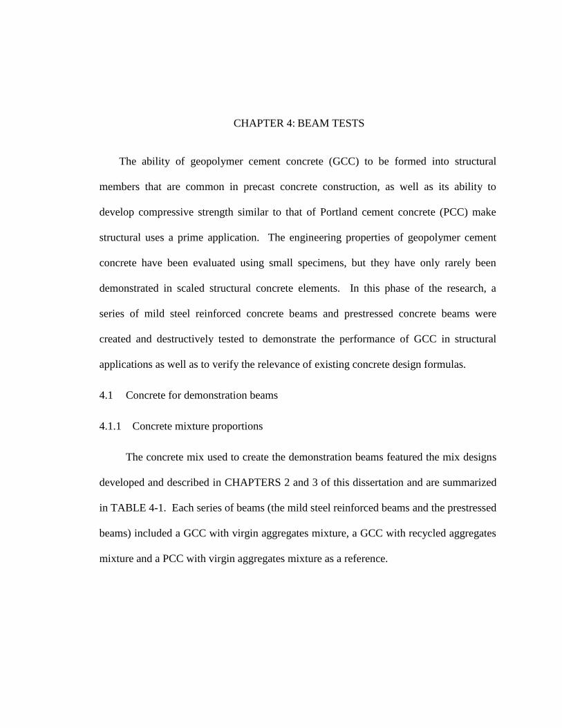
CHAPTER 4: BEAM TESTS

The ability of geopolymer cement concrete (GCC) to be formed into structural

members that are common in precast concrete construction, as well as its ability to

develop compressive strength similar to that of Portland cement concrete (PCC) make

structural uses a prime application. The engineering properties of geopolymer cement

concrete have been evaluated using small specimens, but they have only rarely been

demonstrated in scaled structural concrete elements. In this phase of the research, a

series of mild steel reinforced concrete beams and prestressed concrete beams were

created and destructively tested to demonstrate the performance of GCC in structural

applications as well as to verify the relevance of existing concrete design formulas.

4.1 Concrete for demonstration beams

4.1.1 Concrete mixture proportions

The concrete mix used to create the demonstration beams featured the mix designs

developed and described in CHAPTERS 2 and 3 of this dissertation and are summarized

in TABLE 4-1. Each series of beams (the mild steel reinforced beams and the prestressed

beams) included a GCC with virgin aggregates mixture, a GCC with recycled aggregates

mixture and a PCC with virgin aggregates mixture as a reference.

93

93

TABLE 4-1: Mix designs for concrete used to prepare beam specimens, lb/yd3 (kg/m

3).

Mix Designation

Component GCC-1 GCC-2 PCC-1 GCC-R

Portland Cement 0 0 386 (229) 0

Fly Ash 834 (495) 835 (495) 89 (53) 815 (483)

Water 274 (163) 275 (163) 173 (103) 268 (159)

NaOH 83 (49.5) 84 (49.5) 0 81 (48)

Silica Fume 62 (37.1) 63 (37.1) 0 61 (36)

Fine Aggregate 1,336 (793) 1,336 (793) 709 (421) 1,304 (773)

Coarse Aggregate 1,336 (793) 1,336 (793) 1,127 (669) 718 (426)

Recycled Coarse Aggregate 587 (348)

4.1.2 Mixing the concretes

The dry ingredients were weighed out into 55 gallon (200 liter) drums several days

ahead of time and left in the ambient conditions of the workshop to equilibrate. The

activator was similarly proportioned and mixed in a 55 gallon (200 liter) drum that was

fitted with a special valve for dosing it into the mixer truck in a controlled fashion. The

activator drum was placed into an oven and held at 167○F (75

○C) overnight.

The GCC was mixed in a ready-mix truck designed for delivering small batches of

PCC. As much as was practicable, the same mixing procedure designed for the smaller

batches of GCC made during previous phases of the research was used here. The dry

ingredients were added to the drum of the truck with 1/3 of the water, as shown in

FIGURE 4-1. After the dry ingredients were well combined, the activator was added and

the mixer ran for 250 revolutions. The mixing period lasted approximately ten minutes

beyond the addition of the activating solution.

94

94

FIGURE 4-1: Adding materials to mixing truck.

After the mixing period, the truck was able to enter the lab facility where the

formwork and reinforcing had been prepared. GCC was added to the molds and a

vibrator was used to ensure proper consolidation. Due to the flowable nature of the GCC,

the truck was able to pause at just a few positions along the beam in order to deliver

concrete to the whole length. As the beams were filled, an assortment of 3‖x6‖

(76mmx152mm) cylinder specimens was also prepared. A curing oven was assembled

over the specimens and they were left to age for two days before heaters inside the oven

were started. The heaters maintained a 167○F (75

○ C) curing condition for two more

days. The oven is shown in FIGURE 4-2. The beams were identified as per the

descriptions in TABLE 4-2.

The PCC used to prepare the reference beams was sourced from a local ready-mix

plant and delivered in the same mixer truck that mixed the GCC batches. The mix design

is given as PCC-1 in TABLE 4-1.

95

95

FIGURE 4-2: Beam and heater inside curing oven.

4.2 Mild steel reinforced beams

Four mild steel reinforced concrete beams were prepared. Each beam reflected a

variation either in the concrete materials or the reinforcing. TABLE 4-2 describes the

characteristics of each beam. The cross-section GCC-1-B1 is shown in FIGURE 4-3 with

reinforcing details in TABLE 4-3. Elevations, cross sections, and reinforcement details

of GCC-2-B2, PCC-1-B3 and GCC-R-B4 are shown in FIGURE 4-4 and TABLE 4-4.

TABLE 4-2: Concrete cylinder compressive strength at time of testing.

Beam ID Concrete

Mix

Characteristic Compressive

Strength, psi

(MPa)

GCC-1-B1 GCC-1 First batch of geopolymer

cement concrete with virgin

aggregates

11,000 (75.8)

GCC-2-B2 GCC-2 Second batch of geopolymer


aggregates

11,900 (82.0)

PCC-1-B3 PCC-1 Portland cement concrete 12,500 (86.2)

GCC-R-B4 GCC-R Geopolymer cement concrete

with 45% recycled aggregates

9,200 (63.4)

96

96

The beams were designed to achieve a ductile, flexural failure, with the

longitudinal reinforcing steel reaching yield in tension well before the compression

concrete began compressive crushing. For preliminary design, a speculative strength of

6,500 psi (45 MPa) was assumed, although much higher strengths were ultimately

obtained. This affected the applicability of the initial design calculations, however, all

beams achieved ductile failures.

97

97

TABLE 4-3: Reinforcing steel schedule for GCC-1-B1, inches (mm).

Dimension

Bar

Type

Grade Diameter 1 2 3 4 5 6

A 40 0.625 (15.9) 140 (3,560)

B 60 0.375 (9.5) 4.5 (114) 5.0 (127) 9 ( 2 2 9 ) 5 ( 1 2 7 ) 9 ( 2 2 9 ) 4.5 (114)

8" (203mm)

12" (305mm)

1.5" 38mm

9" (230mm)

12' (3.66m)

12" (305mm)

A

B

Section

Section

Stirrups spaced 5‖ (127mm) on center

FIGURE 4-3: Placement and size of reinforcing steel in GCC-1-B1.

A

4

3

5

6

1 2

B

2

98

98

TABLE 4-4: Reinforcing steel schedule for GCC-2-B2, PCC-1-B3 and GCC-R-B4.

Dimension

Bar

Type


A 60 0.5 (12.7) 140 (3,560)

B 60 0.375 (9.5) 4.5 (114) 5.0 (127) 9 ( 2 2 9 ) 5 ( 1 2 7 ) 9 ( 2 2 9 ) 4.5 (114)

8" (203mm)

12" (305mm)

1.5" 38mm

9" (230mm)

12' (3.66m)

12" (305mm)

A

B

Section

Section


FIGURE 4-4: Placement and size of reinforcing steel in GCC-2-B2, PCC-1-B3,

and GCC-R-B4.

A

4

3

5

6

1 2

B

2

99

99

4.2.1 Test set-up for the mild steel reinforced beams

Beams were supported and loaded as shown in FIGURE 4-5. Equal loads were

applied at the 1/3 span points. Displacements were measured at the beam centerline as

well as directly under the loading points. The load was applied through a deep steel

spreader beam and was generated with a hydraulic cylinder mounted to the load-frame.

The application rate was metered with a manually controlled hydraulic pump and metered

such that it increased at 100 lb per second (445 N per second). FIGURE 4-6 shows an

example of the beam loaded in the test frame. Also visible in the picture are the spreader

beam, as well as the loading jack. At the beams end supports, plates were provided

between the support rollers and the bottom of the beams to prevent crushing. These are

shown in FIGURE 4-7.

P/2 P/2

120" (305 cm)

40" (102 cm) 40" 40"

FIGURE 4-5: Beam loading and support geometry.

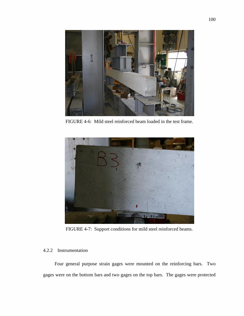
100

100

FIGURE 4-6: Mild steel reinforced beam loaded in the test frame.

FIGURE 4-7: Support conditions for mild steel reinforced beams.

4.2.2 Instrumentation

Four general purpose strain gages were mounted on the reinforcing bars. Two

gages were on the bottom bars and two gages on the top bars. The gages were protected

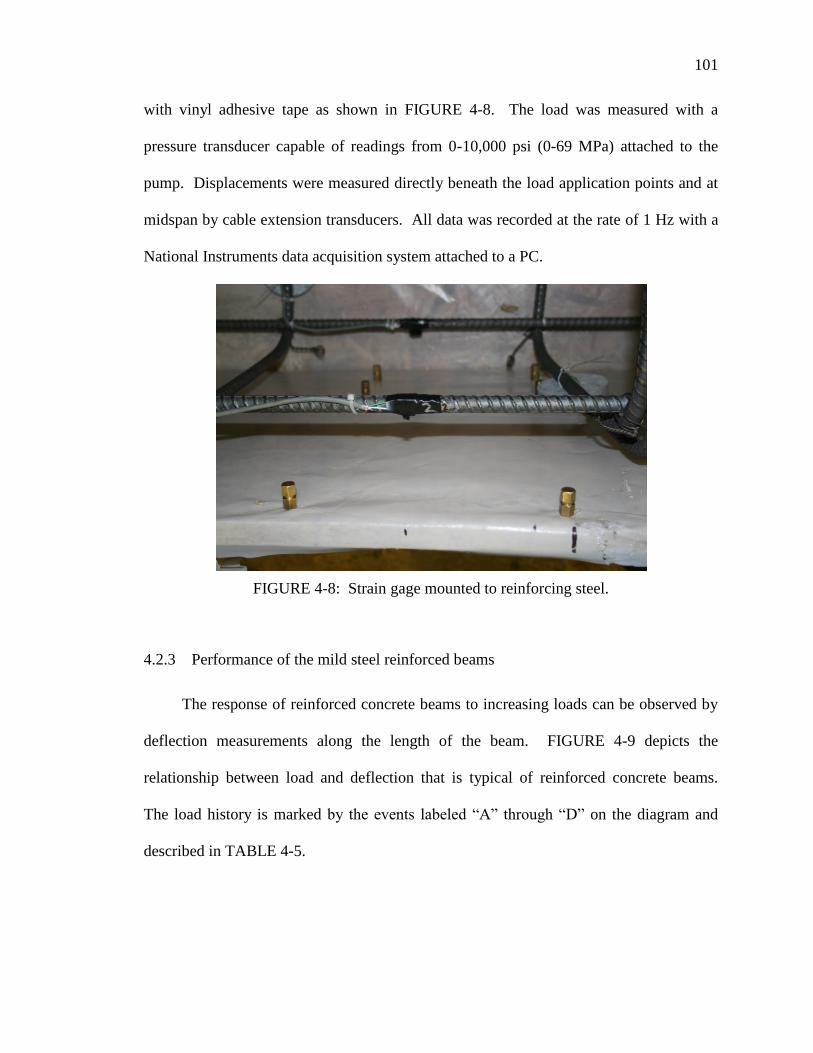
101

101

with vinyl adhesive tape as shown in FIGURE 4-8. The load was measured with a

pressure transducer capable of readings from 0-10,000 psi (0-69 MPa) attached to the

pump. Displacements were measured directly beneath the load application points and at

midspan by cable extension transducers. All data was recorded at the rate of 1 Hz with a

National Instruments data acquisition system attached to a PC.

FIGURE 4-8: Strain gage mounted to reinforcing steel.

4.2.3 Performance of the mild steel reinforced beams

The response of reinforced concrete beams to increasing loads can be observed by

deflection measurements along the length of the beam. FIGURE 4-9 depicts the

relationship between load and deflection that is typical of reinforced concrete beams.

The load history is marked by the events labeled ―A‖ through ―D‖ on the diagram and

described in TABLE 4-5.

102

102

TABLE 4-5: Description of reinforced concrete beam load history.

Event Description

A First crack

B Initiation of tensile steel yielding

C Initiation of concrete crushing in

compression

D Rupture of concrete in compression

A

B

C

DLo

ad

Midspan Deflection

FIGURE 4-9: Load-deflection relationship for reinforced concrete beams.

As the beams were designed to achieve a ductile failure, they all exhibited similar

behavior. Each failure was characterized by a long period of steel yielding, during which

cracks grew and the deflection increased prominently. Completion of the test was

marked by the rupture of concrete in the compression zone.

The moment-midspan deflection charts are given in FIGURE 4-10 through

FIGURE 4-13. In the case of GCC-1-B1, the test was inadvertently discontinued prior to

ultimate failure, so a full load-deflection profile is not available. However, all other

beams exhibited the type of behavior anticipated (see FIGURE 4-9).

103

103

FIGURE 4-14 provides a comparison of the four beams’ load-deflection behavior.

There is a large variation in the magnitude to the load which caused initial concrete

cracking and also the magnitude of the ultimate moment. However, the deflection

behavior which is related to the elastic and inelastic properties of the steel reinforcing is

uniform for all beams. This is reflected in the slope of the load-deflection curve between

points A and B, and B and C (as identified in FIGURE 4-9).

FIGURE 4-10: GCC-1-B1 load vs. mid-span deflection.

0 50 100

0

50

100

150

200

0

5000

10000

15000

20000

25000

30000

35000

40000

45000

50000

0 1 2 3 4 5

Deflection [mm]

Load

[kN

]

Load

[lb

]

Deflection [in]

104

104

FIGURE 4-11: GCC-2-B2 load vs. mid-span deflection.

FIGURE 4-12: PCC-1-B3 load vs. mid-span deflection.

0 50 100

0

50

100

150

200

0

5000

10000

15000

20000

25000

30000

35000

40000

45000

50000

0 1 2 3 4 5

Deflection [mm]

Lo

ad [

kN

]

Lo

ad [

lb]

Deflection [in]

0 50 100

0

50

100

150

200

0

5000

10000

15000

20000

25000

30000

35000

40000

45000

50000

0 1 2 3 4 5

Deflection [mm]

Load

[kN

]

Load

[lb

]

Deflection [in]

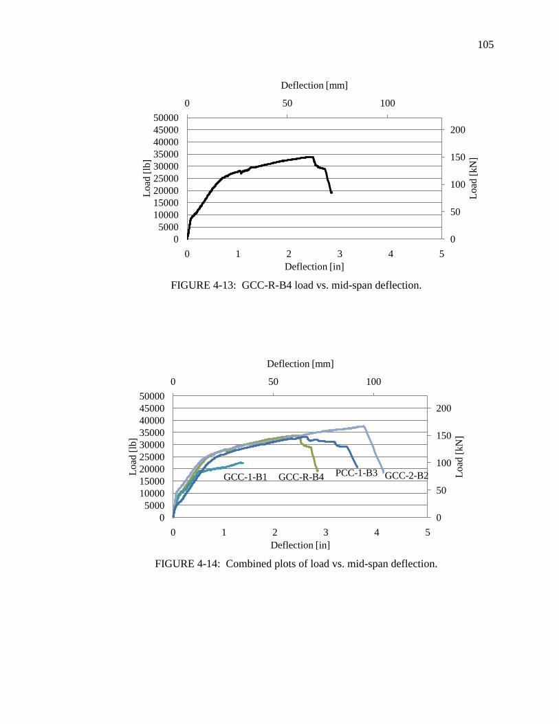
105

105

FIGURE 4-13: GCC-R-B4 load vs. mid-span deflection.

FIGURE 4-14: Combined plots of load vs. mid-span deflection.

0 50 100

0

50

100

150

200

0

5000

10000

15000

20000

25000

30000

35000

40000

45000

50000

0 1 2 3 4 5

Deflection [mm]

Lo

ad [

kN

]

Lo

ad [

lb]

Deflection [in]

0 50 100

0

50

100

150

200

0

5000

10000

15000

20000

25000

30000

35000

40000

45000

50000

0 1 2 3 4 5

Deflection [mm]

Lo

ad [

kN

]

Load

[lb

]

Deflection [in]

GCC-1-B1 GCC-2-B2PCC-1-B3GCC-R-B4

106

106

FIGURE 4-15: GCC-1-B1 at maximum load.

FIGURE 4-16: Crushing failure in GCC-2-B2.

107

107

FIGURE 4-17: Crushing failure in PCC-1-B3.

FIGURE 4-18: Crushing failure near load application in GCC-R-B4.

108

108

4.3 Prestressed concrete beams

Three prestressed concrete beams were prepared. As with the mild steel reinforced

beams, each beam featured a different concrete mix, as described in TABLE 4-6.

TABLE 4-6: Prestressed beam concrete details.

Beam ID Concrete Mix Characteristic , psi (MPa)

GCC-2-P2 GCC-2 Second batch of geopolymer


aggregates

11,900 (82.0)

PCC-1-P3 PCC-1 Portland cement concrete 12,500 (86.2)

GCC-R-P4 GCC-R Geopolymer cement concrete with

45% recycled aggregates

9,200 (63.4)

4.3.1 Beam design and construction

FIGURE 4-21 shows the cross section and reinforcing details of the prestressed

concrete beams. In addition to the stirrups shown in the figure, extra 8‖ (200 mm) steel

hoops were placed around the prestressing strands within 300 mm of the end of the beam

to prevent rupture of the concrete during prestress transfer, as shown in FIGURE 4-20.

All steel was grade 60. Stirrups were #3 (71 mm2) bars and longitudinal steel was #4

(129 mm2) bars. Prestressing tendons were 0.5‖ (13mm) diameter, seven wire, grade

270, low relaxation strand. Stress-strain profiles for all the reinforcing steel products are

available in Appendix A.

As with the mild reinforced concrete beams, the formwork was lined with

polyethylene sheeting to preserve the wood, as shown in FIGURE 4-19. Cover blocks

were used on the sides and bottom of the reinforcing cage in order to maintain the desired

geometry and cover. Since the forms were 18‖ (457mm) tall, cross-ties braced the top of

109

109

the formwork from bowing under the pressure of the fresh concrete. These ties are also

visible in FIGURE 4-19.

FIGURE 4-19: Reinforcing cage and prestressing tendons in formwork.

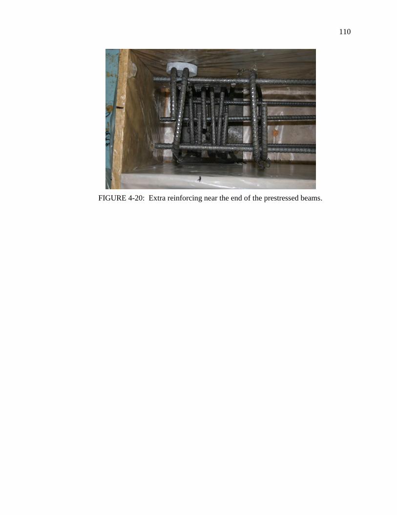
110

110

FIGURE 4-20: Extra reinforcing near the end of the prestressed beams.

111

111

TABLE 4-7: Reinforcing steel schedule for GCC-2-B2, PCC-1-B3 and GCC-R-B4, in

(cm).

Dimension

Bar

Type


A 60 0.5 (1.27) 212 (538)

B 60 0.375 (.95) 4.5 (114) 8.0 (20) 16 (41) 8 (20) 16 (41) 4.5 (11)

C 270 0.5 (1.27) 216 (549)

18' (5.49m)

18" (457mm)

X

X

X

X

18" (457 mm)

2" (51 mm)

8" (203 mm)

10" (254 mm)

A

B

C

C

A


FIGURE 4-21: Reinforcing steel placement and beam cross section for prestressed

beams.

B

4

3

5

6

1 2

A

2

112

112

4.3.2 Prestressing the beams

The three beams were prestressed in-house. This was accomplished by

constructing the formwork and reinforcing cage between two abutments in a strong-wall

load frame. The strands were secured to the abutments with reusable prestressing strand

chucks and were tensioned with a hollow-core hydraulic jack. The configuration of the

jack and chucks is shown in FIGURE 4-22. The chucks and abutments are shown in

FIGURE 4-23. During the prestressing operation, tension on the strand was measured

with a pressure transducer attached to the hydraulic hose as well as by a load cell

mounted between the strand chuck and the jack. The tension was maintained by the

abutment throughout the casting and curing phase of beam construction. Once cylinder

tests ensured that the concrete had developed sufficient strength to transfer prestress from

the abutments to the beam, the strands were cut with an acetylene torch.

After prestressing beams GCC-2-P2 and PCC-1-P3, it was noted that some

prestress was being lost as the load was transferred from the jack to the chuck. This loss

occurred as the jaws of the chuck slid into the bore of the chuck. For GCC-R-P4 a set of

rudimentary load cells were fabricated by attaching strain gages to thick steel tubes that

were mounted between the chuck and the abutment. With these load cells, it was

possible to continue monitoring tension in the strand after the jack was removed. It was

noted that approximately 30% of the prestress was lost due to chuck seating. This was

accounted for in subsequent computations requiring values for effective prestress.

113

113

FIGURE 4-22: Jacking configuration used to tension prestressing tendons.

FIGURE 4-23: Prestressing tendons passing through the abutment.

114

114

4.3.3 Prestressed concrete beam test set-up

Using the test set-up shown in FIGURE 4-24, the beams were loaded until they

failed. Load was applied through the spreader beam that is visible in FIGURE 4-25 and

was generated by a hydraulic jack attached to a manually controlled hydraulic pump.

The load application was monotonic and proceeded at a rate of 3,000 lb/sec (13 kN/sec)

during the linear portions of the load-deflection history.

P/2 P/2

18' (5.49 m)

64" (163 cm) 64" 64"

FIGURE 4-24: Prestressed beam test set-up.

FIGURE 4-25: Prestressed beam loaded in the test frame.

115

115

4.3.4 Prestressed beam instrumentation and test monitoring

Strain gages were placed on the upper and lower mild steel reinforcing bars at

midspan. Although the gages were protected with a vinyl adhesive tape, many of them

failed to function during the test. External instrumentation included three cable extension

displacement transducers set at midspan, and points directly under the load application

plates, as shown in FIGURE 4-24.

The load was measured with a pressure transducer capable of readings from 0-

10,000 psi (0-69 MPa) attached to the pump. Displacements were measured beneath the

load application points and at midspan by cable extension transducers. All data was

recorded at the rate of 1 Hz with a National Instruments data acquisition system attached

to a PC. Additionally, the development of crack patterns along the beam was monitored

until the beam approached 80% of its predicted failure load, after which the research

assistants moved away from the beam for safety.

4.3.5 Prestressed beam test results

FIGURE 4-26 through FIGURE 4-28 present the load-deflection history of the

prestressed beams. As is apparent in FIGURE 4-30 through FIGURE 4-32, all beam

failures occurred by crushing of the concrete on the compression face of the beam. It

should be noted that the crushing originated near one of the loading points for all three

prestressed beams. Broad steel plates were used beneath the spreader beam, however

localized bearing stresses may have been involved in the failure mechanism for the

compression concrete. The failure loads were very similar for all three beams, as is

reported in TABLE 4-8. Here the forces have been expressed as midspan flexural

116

116

moments as determined by beam geometry and the magnitude of the measured point

loads.

FIGURE 4-26: GCC-2-P1 beam load vs. midspan deflection.

FIGURE 4-27: PCC-1-P2 beam load vs. midspan deflection.

0 50 100

0

100

200

300

400

500

0

20000

40000

60000

80000

100000

120000

0 1 2 3 4 5

Deflection [mm]

Lo

ad [

kN

]

Load

[lb

]

Deflection [in]

0 50 100

0

100

200

300

400

500

0

20000

40000

60000

80000

100000

120000

0 1 2 3 4 5

Deflection [mm]

Lo

ad [

kN

]

Lo

ad [

lb]

Deflection [in]

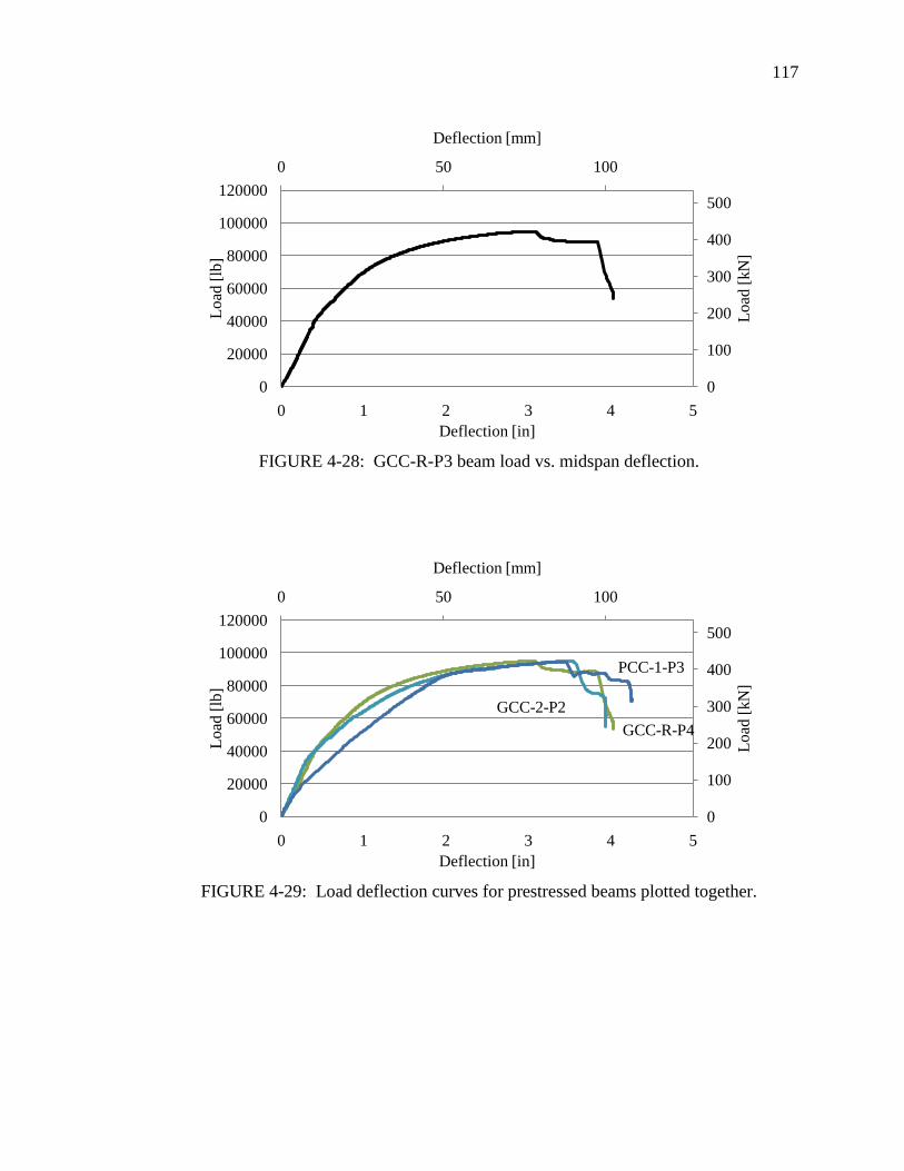
117

117

FIGURE 4-28: GCC-R-P3 beam load vs. midspan deflection.

FIGURE 4-29: Load deflection curves for prestressed beams plotted together.

0 50 100

0

100

200

300

400

500

0

20000

40000

60000

80000

100000

120000

0 1 2 3 4 5

Deflection [mm]

Lo

ad [

kN

]

Lo

ad [

lb]

Deflection [in]

0 50 100

0

100

200

300

400

500

0

20000

40000

60000

80000

100000

120000

0 1 2 3 4 5

Deflection [mm]

Load

[kN

]

Load

[lb

]

Deflection [in]

GCC-2-P2

PCC-1-P3

GCC-R-P4

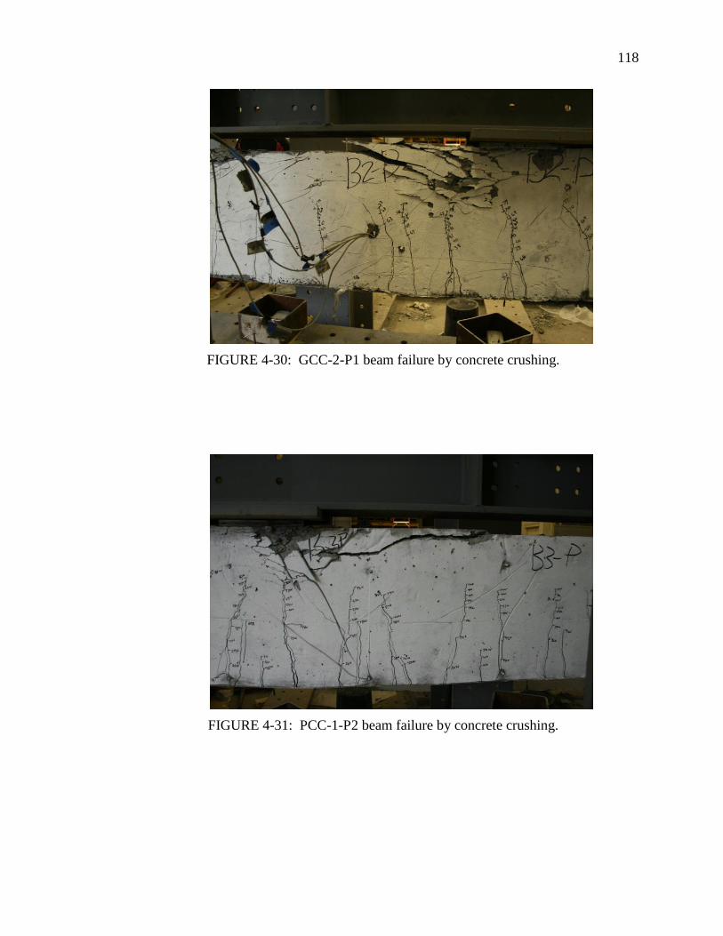
118

118

FIGURE 4-30: GCC-2-P1 beam failure by concrete crushing.

FIGURE 4-31: PCC-1-P2 beam failure by concrete crushing.

119

119

FIGURE 4-32: GCC-R-P3 beam failure by concrete crushing.

TABLE 4-8: Critical points in prestressed beam load histories.

Beam ID Mcr kip-in (kN-m) Mn kip-in (kN-m)

GCC-2-P1 989 (118) 3,125 (353)

PCC-1-P2 Not observed 3,112 (352)

GCC-R-P3 1,261 (142) 3,124 (353)

CHAPTER 5: FLEXURAL BEAM-COLUMN TESTS

5.1 Analysis of stress and strain under compressive loading

As stresses in concrete increase beyond approximately 30-40% of the compressive

strength, microcracks begin to form. Once this cracking is initiated, the load response of

the concrete shifts from one that is essentially linear and elastic to one that is non-linear

and inelastic. Thus, the stress-strain relationship resembles that shown in FIGURE 5-1,

where the peak stress, , occurs well beyond the linear and elastic portion of the stress-

strain curve. Beyond stress reduces with increasing strain, until a limiting strain, , is

reached. The magnitude of is taken as 0.003 % for purposes of design (American

Concrete Institute, 2008).

fc

f’c

εu

ε

FIGURE 5-1: stress-strain relationship of concrete in compression.

In concrete beams, ultimate failure is typically marked by crushing of concrete at

the compression face once strain in this region has reached εu. Although it is assumed

121

121

that the strain distribution at points throughout the beam cross-section remains linear, the

non-proportional relationship between stress and strain results in stress distributions that

resemble parabolas. The hatched area in FIGURE 5-2a represents the compression zone

of a beam in positive flexure. The strain distribution for this segment of the cross-section

is linear as in FIGURE 5-2b; however, these strains are related to stresses as per the curve

shown in FIGURE 5-1 and so create the stress distribution shown in FIGURE 5-2c.

εc

c

fc

β1c

α1f’c

β1c/2

a) b) c) d)

T

dh

b

C

FIGURE 5-2: Stresses and strains in concrete beams.

For design purposes, the Whitney Stress Block, shown in FIGURE 5-2d is used as

an approximation of the area enclosed by the parabolic area shown in FIGURE 5-1c

(Whitney, 1937). The block is defined by the factors shown in FIGURE 5-3, where:

k1: ratio of average compressive stress to maximum compressive stress

k2: ratio of distance from top of beam to the force C, and the depth to the neutral

axis, c

k3 : ratio of cylinder concrete strength to beam concrete strength

122

122

k3f’c

k2c

C=k1k3f’cbc

c

FIGURE 5-3: Relationship of k1, k2 and k3 to the resultant compressive force.

There are many challenges in determining the stress-strain relationship shown in

FIGURE 5-1 experimentally. Although concentric compression tests can be used to

determine stress-strain relationship through the initiation of crushing, the post-peak

behavior is typically obscured by the rapid release of strain energy stored in the testing

device. In unreinforced beams, the tensile limit of the concrete is reached well in

advance of the ultimate compressive stresses developing. Even in reinforced beams, the

impact of tensile stresses and cracks developing below the neutral axis is sufficient to

make analysis very difficult. For purposes of estimating k1 k2 and k3 as well as measuring

the stress-strain relationship, a combined axial-flexure test was developed by Hognestad

(1955).

In this procedure, a short beam-column is loaded axially while an eccentric load is

applied through two ―arms‖ attached to the ends of the specimen. The eccentric load

produces a moment that maintains a neutral face on one side of the beam-column while

the opposite side approaches the compressive strain limit. In this way, the area between

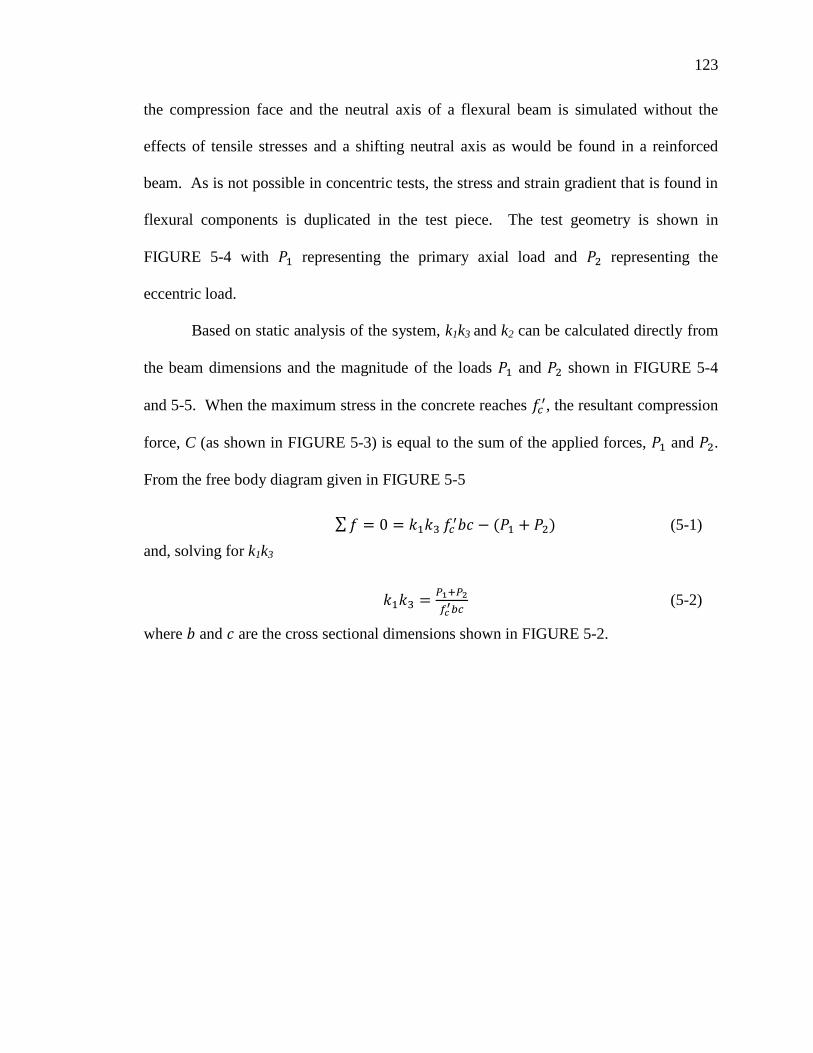
123

123

the compression face and the neutral axis of a flexural beam is simulated without the

effects of tensile stresses and a shifting neutral axis as would be found in a reinforced

beam. As is not possible in concentric tests, the stress and strain gradient that is found in

flexural components is duplicated in the test piece. The test geometry is shown in

FIGURE 5-4 with representing the primary axial load and representing the

eccentric load.

Based on static analysis of the system, k1k3 and k2 can be calculated directly from

the beam dimensions and the magnitude of the loads and shown in FIGURE 5-4

and 5-5. When the maximum stress in the concrete reaches , the resultant compression

force, C (as shown in FIGURE 5-3) is equal to the sum of the applied forces, and .

From the free body diagram given in FIGURE 5-5

(5-1)

and, solving for k1k3

(5-2)

where and are the cross sectional dimensions shown in FIGURE 5-2.

124

124

Moment Arm

a1

a2

P1 P2

P2P1

Moment Arm

Neu

tral

Fac

e

Co

mp

ress

ion

Fac

e

FIGURE 5-4: Hognestad flexural beam-column test set-up.

a1

a2

C=k1k3f’cbc=P1+P2

k2c (1-k2)c

P1 P2

Neu

tral

Fac

e

Co

mp

ress

ive

Fac

e

FIGURE 5-5: Free body diagram of the beam-column specimen cut at midheight.

125

125

Summing moments about the neutral face of the beam generated by the forces

shown in FIGURE 5-5, leads to

(5-3)

(5-4)

The relationship between stress and strain must be determined by a process of

numerical integration. It is necessary to assume that fc is a function of εc, such that

fc=F(εc) and that εc is a linear distribution across c as shown in FIGURE 5-6. However,

since the function is not known, some substitution of known or measurable

quantities must be made to determine fc from data collected during experiments.

fc

cF(εx)

x

εc

εx

FIGURE 5-6: Quantities fc, εc and c.

C, the resultant compressive force, may be defined by using

(5-5)

126

126

and the moment, M, by using

(5-6)

The average stress on the cross-section is,

(5-7)

and from Equation (5-6), a term for average moment is,

(5-8)

Differentiating the third and last terms of Equation (5-5) with respect to results in

Equation (5-9). Substituting the relationship in Equation (5-10), which is obtained by

manipulating the third and fifth terms of Equation (5-5), into Equation (5-9) leads to

Equation (5-11), in which

is approximately equal to

, two quantities that are

measured during testing. The unknown function has been removed from the

analysis, permitting the measured quantities P1, P2 and to be used to directly calculate

.

(5-9)

(5-10)

Using the same strategy

127

127

(5-11)

5.2 Flexural beam-column test procedure

5.2.1 Specimen preparation

In order to carry out the flexural test to collect the quantities described above, a

series of five beam-columns were constructed. The specimens had the cross sectional

and elevation details shown in FIGURE 5-7. The formwork was constructed of ¾‖

(19mm) thick oriented strand board and was heavily braced in order to maintain its

geometry under the pressure of the fresh concrete. The forms were also lined with

polyethylene sheeting in order to prohibit the absorption of water or the alkaline activator

by the wood. The beam-columns were cast in an upright orientation as shown in

FIGURE 5-8.

Sleeves fabricated from 3/8‖ (9.5mm) thick 8‖X8‖ (203mmx203mm) square

tubing were cast onto each end of the specimen. The holes were precisely located to

accommodate the bolting pattern from the moment arm end-plates (FIGURE 5-9).

Passages for the bolts were blocked out with lengths of PVC pipe that were

removed after the concrete hardened. Hoops bent in grade 60, #3 (metric #10) rebar

provided reinforcing inside of the sleeve. #4 (metric #13) bars extended 9‖ (229mm )

beyond the end of the sleeve in order to transfer forces from the loaded ends of the beam-

column into the unreinforced central portion of the specimen. The end reinforcing is

shown in FIGURE 5-10.

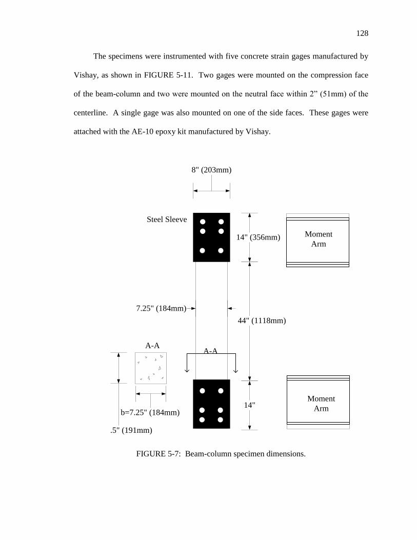
128

128

The specimens were instrumented with five concrete strain gages manufactured by

Vishay, as shown in FIGURE 5-11. Two gages were mounted on the compression face

of the beam-column and two were mounted on the neutral face within 2‖ (51mm) of the

centerline. A single gage was also mounted on one of the side faces. These gages were

attached with the AE-10 epoxy kit manufactured by Vishay.

8" (203mm)

14" (356mm)

44" (1118mm)

14"

7.25" (184mm)

b=7.25" (184mm)

c=7.5" (191mm)

Moment

Arm

Moment

Arm

Steel Sleeve

A-AA-A

FIGURE 5-7: Beam-column specimen dimensions.

129

129

FIGURE 5-8: Casting beam-column specimens.

1"X12" Plate

(25mmX305mm)

3/8"X11" Plate

(9.5mmX279mm)

C12X30

1"Bolt (25mm)

Side View End View

Moment Arm

FIGURE 5-9: Moment arm section and end-plate details.

130

130

FIGURE 5-10: Reinforcing at the ends of the beam-columns.

131

131

22" (559mm)

Compression and

Tension Faces Side Face

FIGURE 5-11: Strain gage locations on beam-column specimens.

5.2.2 Loading apparatus

Cross sectional details for the steel moment arms are given in FIGURE 5-9. The

arms were fixed to the specimens with six, 1‖ (25.4mm) diameter bolts. The arms were

secured to the load frame with loose chains that did not impede their movement during

the test but kept them under control after specimen failure. The beam-columns were

loaded in an apparatus that was built into the load frame at UNC Charlotte. Two 4’

(1.2m) sections of steel were bolted to the bottom rung of the load frame to form

abutments, as shown in FIGURE 5-12. Also in FIGURE 5-12 is the 420 ton (4,000 kN)

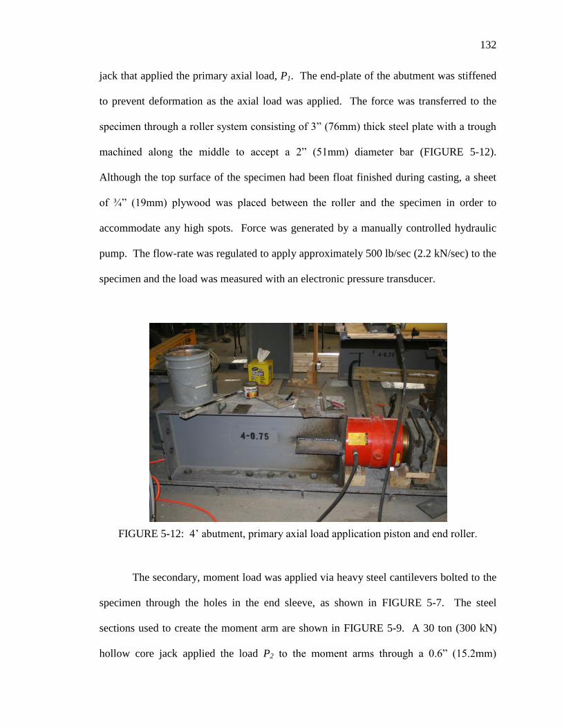
132

132

jack that applied the primary axial load, P1. The end-plate of the abutment was stiffened

to prevent deformation as the axial load was applied. The force was transferred to the

specimen through a roller system consisting of 3‖ (76mm) thick steel plate with a trough

machined along the middle to accept a 2‖ (51mm) diameter bar (FIGURE 5-12).

Although the top surface of the specimen had been float finished during casting, a sheet

of ¾‖ (19mm) plywood was placed between the roller and the specimen in order to

accommodate any high spots. Force was generated by a manually controlled hydraulic

pump. The flow-rate was regulated to apply approximately 500 lb/sec (2.2 kN/sec) to the

specimen and the load was measured with an electronic pressure transducer.

FIGURE 5-12: 4’ abutment, primary axial load application piston and end roller.

The secondary, moment load was applied via heavy steel cantilevers bolted to the

specimen through the holes in the end sleeve, as shown in FIGURE 5-7. The steel

sections used to create the moment arm are shown in FIGURE 5-9. A 30 ton (300 kN)

hollow core jack applied the load P2 to the moment arms through a 0.6‖ (15.2mm)

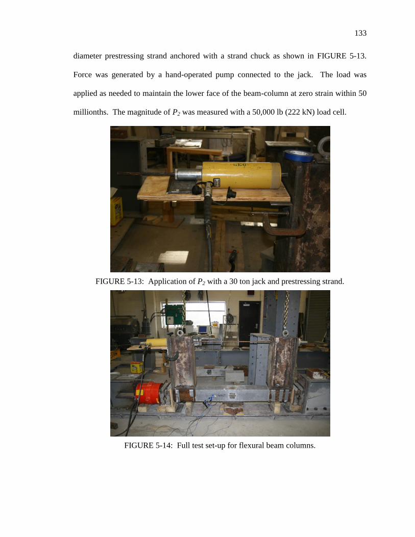
133

133

diameter prestressing strand anchored with a strand chuck as shown in FIGURE 5-13.

Force was generated by a hand-operated pump connected to the jack. The load was

applied as needed to maintain the lower face of the beam-column at zero strain within 50

millionths. The magnitude of P2 was measured with a 50,000 lb (222 kN) load cell.

FIGURE 5-13: Application of P2 with a 30 ton jack and prestressing strand.

FIGURE 5-14: Full test set-up for flexural beam columns.

134

134

5.3 Test results and data reduction

A set of 3‖x6‖ (76mmx152mm) cylinders was cast with each of the five beam-

column specimens. These cylinders were tested to determine the cylinder compressive

strength on the same day as the beam-column tests. The compressive strength results are

given in TABLE 5-1. Although all mixes followed the same proportioning, there is great

variation in the compressive strength. During the mixing process, small amounts of

water were added to the concrete to improve workability. This addition was not closely

monitored but seems to have sufficiently affected the w/c ratio to cause reductions in

concrete strength.

TABLE 5-1: Cylinder compressive strength for beam-column concrete.

Beam-Column , psi (MPa)

GCC-3-BC1 7,900 (54)

GCC-4-BC2 9,000 (62)

GCC-5-BC3 6,700 (46)

GCC-6-BC4 7,300 (50)

GCC-7-BC5 4,000 (28)

During the testing process, measurements were recorded by a data acquisition system

set to make a reading twice per second. The system recorded the loads P1 and P2, strain

from each of the five strain gages and displacement at the inside and outside of the beam

at midspan. As each test required approximately 15 minutes to complete, the quantity of

data recorded was too great for the numerical integration technique that was to be

employed to analyze the results. Small errors in each collected data point, which are

caused by the accuracy limits of the instruments as well as electromagnetic interference,

135

135

translated into considerable scatter in the analysis output. Therefore, prior to performing

the integration, each data set was reduced in size by 95% by selecting one point out of

each 20 that was defined by the average value of the 10 points ahead and 10 points

behind. This provided a moving average while reducing the number of data points from

approximately 1,800 per test to fewer than 100, based on the actual duration of each test.

The displacement data recorded during the test was used to compute additional

stresses caused by secondary moments. These additional stresses were calculated with

(5-12)

where is eccentricity (in) (mm)

5.3.1 Neutral face strain and midspan eccentricity

FIGURE 5-15 through 5-24 display the strain recorded on the neutral face of the

beam during the loading as well as the midspan deflection due to the applied forces. In

all cases, the eccentricity was less than 0.1‖ (2.54mm). Strains were controlled within

about 20 millionths at points prior to the failure approach.

136

136

FIGURE 5-15: Midspan deflection vs. P2 for GCC-3-BC1.

FIGURE 5-16: Neutral face strain vs. P2 for GCC-3-BC1.

0 20 40 60

-0.4

0.6

1.6

2.6

3.6

4.6

5.6

6.6

7.6

0

0.05

0.1

0.15

0.2

0.25

0.3

0 5000 10000 15000

P2 [kN]

Mid

span

ecc

entr

icit

y [

mm

]

Mid

span

ecc

entr

icit

y [

in]

P2 [lb]

0 20 40 60

-1.00E-04

-5.00E-05

-1.00E-18

5.00E-05

1.00E-04

0 5000 10000 15000

P2 [kN]

Neu

tral

fac

e st

rain

[%

]

P2 [lb]

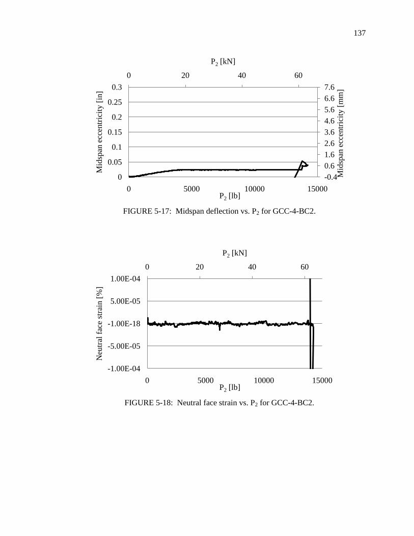
137

137



0 20 40 60

-0.4

0.6

1.6

2.6

3.6

4.6

5.6

6.6

7.6

0

0.05

0.1

0.15

0.2

0.25

0.3

0 5000 10000 15000

P2 [kN]

Mid

span

ecc

entr

icit

y [

mm

]

Mid

span

ecc

entr

icit

y [

in]

P2 [lb]

0 20 40 60

-1.00E-04

-5.00E-05

-1.00E-18

5.00E-05

1.00E-04

0 5000 10000 15000

P2 [kN]

Neu

tral

fac

e st

rain

[%

]

P2 [lb]

138

138



0 20 40 60

-0.4

0.6

1.6

2.6

3.6

4.6

5.6

6.6

7.6

0

0.05

0.1

0.15

0.2

0.25

0.3

0 5000 10000 15000

P2 [kN]

Mid

span

ecc

entr

icit

y [

mm

]

Mid

span

ecc

entr

icit

y [

in]

P2 [lb]

0 20 40 60

-1.00E-04

-5.00E-05

-1.00E-18

5.00E-05

1.00E-04

0 5000 10000 15000

P2 [kN]

Neu

tral

fac

e st

rain

[%

]

P2 [lb]

139

139



0 20 40 60

-0.4

0.6

1.6

2.6

3.6

4.6

5.6

6.6

7.6

0

0.05

0.1

0.15

0.2

0.25

0.3

0 5000 10000 15000

P2 [kN]

Mid

span

ecc

entr

icit

y [

mm

]

Mid

span

ecc

entr

icit

y [

in]

P2 [lb]

0 20 40 60

-1.00E-04

-5.00E-05

-1.00E-18

5.00E-05

1.00E-04

0 5000 10000 15000

P2 [kN]

Neu

tral

fac

e st

rain

[%

]

P2 [lb]

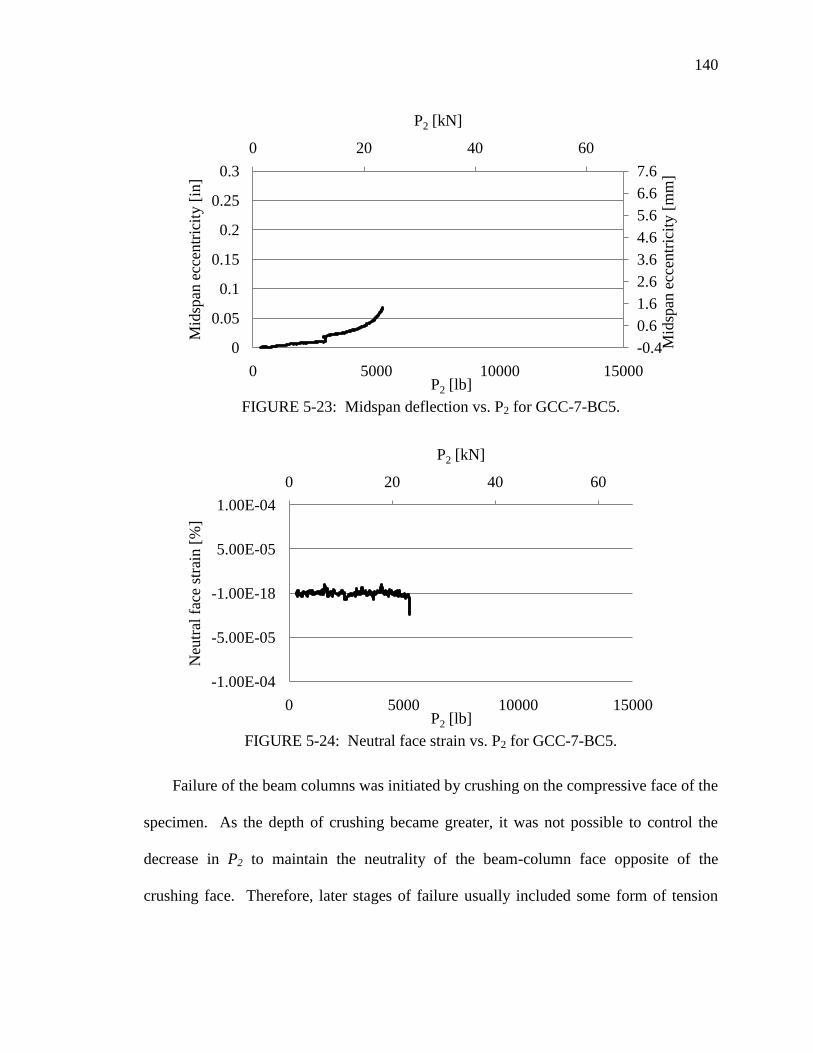
140

140



Failure of the beam columns was initiated by crushing on the compressive face of the

specimen. As the depth of crushing became greater, it was not possible to control the

decrease in P2 to maintain the neutrality of the beam-column face opposite of the

crushing face. Therefore, later stages of failure usually included some form of tension

0 20 40 60

-0.4

0.6

1.6

2.6

3.6

4.6

5.6

6.6

7.6

0

0.05

0.1

0.15

0.2

0.25

0.3

0 5000 10000 15000

P2 [kN]

Mid

span

ecc

entr

icit

y [

mm

]

Mid

span

ecc

entr

icit

y [

in]

P2 [lb]

0 20 40 60

-1.00E-04

-5.00E-05

-1.00E-18

5.00E-05

1.00E-04

0 5000 10000 15000

P2 [kN]

Neu

tral

fac

e st

rain

[%

]

P2 [lb]

141

141

cracking. FIGURE 5-25 through 5-29 illustrate the failure modes of each of the five

beam-column specimens.

FIGURE 5-25: Failure of GCC-3-BC1.


142

142



143

143


The stress in the concrete, , was computed numerically using both from

Equation (5-12) and from Equation (5-7). These two calculation methods resulted in

slightly different values for , as seen in FIGURE 5-30. Therefore, an average value was

used as the final result as plotted in FIGURE 5-31 through FIGURE 5-35, the results of

all five beam-columns.

144

144

FIGURE 5-30: computed from and from and average values.

FIGURE 5-31: GCC-3-BC1 stress-strain relationship from flexural tests.

0

0.2

0.4

0.6

0.8

1

1.2

0

1,000

2,000

3,000

4,000

5,000

6,000

7,000

8,000

9,000

10,000

0.00E+00 1.00E-03 2.00E-03 3.00E-03

fc[M

Pa]

fc[p

si]

ε [%]

fc from m0

fc from f0

average

0

10

20

30

40

50

60

0

1,000

2,000

3,000

4,000

5,000

6,000

7,000

8,000

9,000

10,000

0.00E+00 1.00E-03 2.00E-03 3.00E-03

fc[M

Pa]

fc[p

si]

ε [%]

145

145



0

10

20

30

40

50

60

0

1,000

2,000

3,000

4,000

5,000

6,000

7,000

8,000

9,000

10,000

0.00E+00 1.00E-03 2.00E-03 3.00E-03

fc[M

Pa]

fc[p

si]

ε [%]

0

10

20

30

40

50

60

0

1,000

2,000

3,000

4,000

5,000

6,000

7,000

8,000

9,000

10,000

0.00E+00 1.00E-03 2.00E-03 3.00E-03

fc[M

Pa]

fc[p

si]

ε [%]

146

146



0

10

20

30

40

50

60

0

1,000

2,000

3,000

4,000

5,000

6,000

7,000

8,000

9,000

10,000

0.00E+00 1.00E-03 2.00E-03 3.00E-03

fc[M

Pa]

fc[p

si]

ε [%]

0

10

20

30

40

50

60

0

1,000

2,000

3,000

4,000

5,000

6,000

7,000

8,000

9,000

10,000

0.00E+00 1.00E-03 2.00E-03 3.00E-03

fc[M

Pa]

fc [

psi

]

ε [%]

147

147

5.3.2 Discussion of beam column results

The five beam-columns provided a spectrum of stress-strain response that appears

to be related to concrete compressive strength. As is apparent in FIGURE 5-36, the slope

of the stress strain curve increases as the concrete compressive strength increases.

TABLE 5-2 also shows this relationship and provides a comparison with the slope of

each curve between zero strain and 0.001% strain and the estimated modulus of elasticity

for each concrete compressive strength using Equations (2-9) and (2-10). These formulas

verify the linear portion of the results curves by accurately predicting the slope within

5%.

FIGURE 5-36: Relative slopes of stress strain curves.

0

10

20

30

40

50

60

70

0

1,000

2,000

3,000

4,000

5,000

6,000

7,000

8,000

9,000

10,000

0.00E+00 1.00E-03 2.00E-03 3.00E-03

fc[M

Pa]

fc[p

si]

ε [%]

4.0 ksi

7.3 ksi

6.7 ksi

9.0 ksi

7.9 ksi

148

148

TABLE 5-2: Slope of stress-strain curves versus estimated modulus of elasticity, psi

(GPa).

Specimen , psi

(MPa)

Estimated E psi

(Gpa)

Slope of Stress-

Strain curve

%

Difference

GCC-3-BC1 7,900 (54) 3.66x106 (25.26) 3.82 x10

6 (26.33) 4%

GCC-4-BC2 9,000 (62) 3.91 x106 (26.96) 4.13 x10

6 (28.48) 5%

GCC-5-BC3 6,700 (46) 3.37 x106 (23.27) 3.54 x10

6 (24.44) 5%

GCC-6-BC-4 7,300 (50) 3.52 x106 (24.28) 3.76 x10

6 (25.94) 6%

GCC-7-BC-5 4,000 (28) 2.61 x106 (17.98) 2.48 x10

6 (17.13) -5%

5.3.3 Analysis of beam-column test data

Equations (5-2) and (5-4) allow the computation of k1k3 and k2, respectively. The

data presented in the FIGURES above was used to compute these values and is presented

in TABLE 5-3. k3 was found as the ratio of to the maximum concrete stress fc

determined during the test.

TABLE 5-3: Calculated values of k1k3, k2 and k3 for beam columns.

Beam-Column , psi (MPa) k1k3 k2 k3 α1 β1

GCC-3-BC1 7,900 (45) 0.513 0.228 1.03 1.13 0.46

GCC-4-BC2 9,000 (62) 0.519 0.231 0.98 1.12 0.46

GCC-5-BC3 6,700 (46) 0.644 0.240 1.21 1.34 0.48

GCC-6-BC4 7,300 (50) 0.593 0.275 1.10 1.08 0.55

GCC-7-BC5 4,000 (28) 0.539 0.266 0.97 1.01 0.53

In order to use these values for practical design purposes, the quantities α1 and β1 are

used to define a rectangular area that has the same volume as the parabolic shape

depicted in FIGURE 5-37. Based on the relationships in FIGURE 5-37, α1 and β1 were

computed using Equations (5-13) and (5-14) and are presented in TABLE 5-3.

149

149

(5-13)

(5-14)

k3f’c

k2c

C=k1k3f’cbc

c c

a

α1f’c

β1c/2

C=α1β1f’cbc

FIGURE 5-37: Relationship between k1,k2, k3 and α1 and β1.

The relationship of and to the cylinder compressive strength of the concrete

in the beam-columns is shown in FIGURE 5-38 and FIGURE 5-39. For there is a

trend towards increasing with increasing cylinder strength. This implies that the

maximum stress attained by concrete in the column was greater than the maximum stress

attained by concrete in cylinder tests. As the concrete became stronger, the ratio of

cylinder strength to element strength increases. In PCC structural elements, this

phenomenon is often related to the altered proportion of mortar and aggregate found in

concrete before and after vibratory consolidation. The consolidation process causes

lighter, fluid constituents of the fresh concrete to rise towards the upper surface of the

element, while aggregate and less mobile constituents remain on the bottom. Such

segregation could have occurred in the beam-column elements tested here. Unlike PCC,

these beam-columns were cured under elevated temperatures. Fans inside the curing

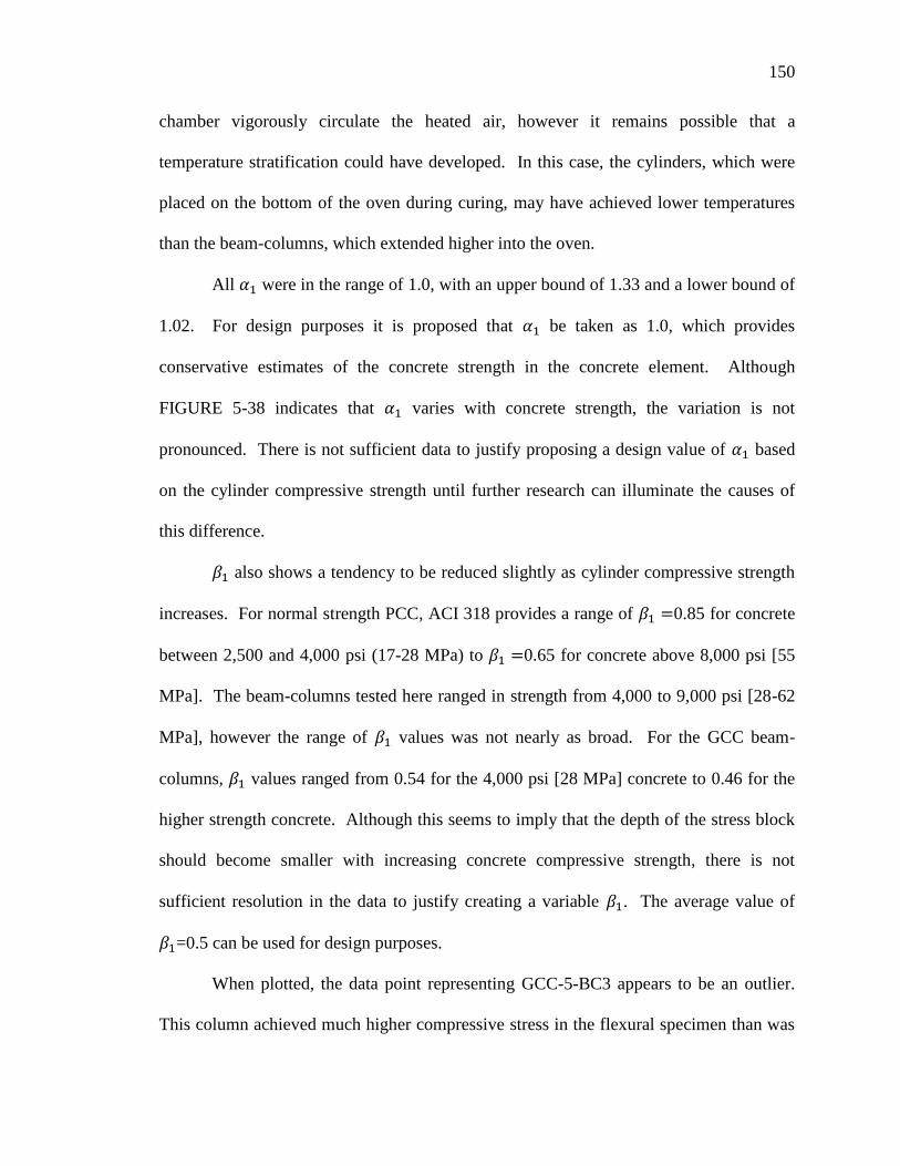
150

150

chamber vigorously circulate the heated air, however it remains possible that a

temperature stratification could have developed. In this case, the cylinders, which were

placed on the bottom of the oven during curing, may have achieved lower temperatures

than the beam-columns, which extended higher into the oven.

All were in the range of 1.0, with an upper bound of 1.33 and a lower bound of

1.02. For design purposes it is proposed that be taken as 1.0, which provides

conservative estimates of the concrete strength in the concrete element. Although

FIGURE 5-38 indicates that varies with concrete strength, the variation is not

pronounced. There is not sufficient data to justify proposing a design value of based

on the cylinder compressive strength until further research can illuminate the causes of

this difference.

also shows a tendency to be reduced slightly as cylinder compressive strength

increases. For normal strength PCC, ACI 318 provides a range of 0.85 for concrete

between 2,500 and 4,000 psi (17-28 MPa) to 0.65 for concrete above 8,000 psi [55

MPa]. The beam-columns tested here ranged in strength from 4,000 to 9,000 psi [28-62

MPa], however the range of values was not nearly as broad. For the GCC beam-

columns, values ranged from 0.54 for the 4,000 psi [28 MPa] concrete to 0.46 for the

higher strength concrete. Although this seems to imply that the depth of the stress block

should become smaller with increasing concrete compressive strength, there is not

sufficient resolution in the data to justify creating a variable . The average value of

=0.5 can be used for design purposes.

When plotted, the data point representing GCC-5-BC3 appears to be an outlier.

This column achieved much higher compressive stress in the flexural specimen than was

151

151

expected considering the cylinder tests. These results show and that are higher

than the rest of the specimens.

FIGURE 5-38: related to cylinder compressive strength for beam-columns.

FIGURE 5-39: related to cylinder compressive strength for beam-columns.

The values for α1 and β1 indicate that an equivalent rectangular stress block for

GCC materials is significantly smaller than similar blocks representing Portland cement

concrete behavior. The factor k1 describes the ratio of the area defined by the parabolic

0 10 20 30 40 50 60 70

0.000.200.400.600.801.001.201.401.60

0 2,000 4,000 6,000 8,000 10,000

f'c [MPa]α

1

f'c [psi]

0 10 20 30 40 50 60 70

0.00

0.10

0.20

0.30

0.40

0.50

0.60

0 2,000 4,000 6,000 8,000 10,000

f'c [MPa]

β1

f'c [psi]

152

152

stress distribution shown in FIGURE 5-37 to the area of a rectangle fitted around its

border. For a triangular distribution, the appropriate factor would be 0.5, meaning that

the triangle occupies half the area of the rectangle. Similarly, for parabolic distributions

the appropriate factor is 0.67. The k1 for the GCC materials was 0.54, indicating that the

distribution was very nearly triangular.

The factor k2 describes the depth of the resultant force, C (defined in FIGURE

5-37), from the extreme compressive fiber. The average computed value for k2 found

here was 0.25, which indicates a more strongly linear portion to the lower-strain portions

followed by a plateau near the upper strain regions of the stress-strain relationship. This

is apparent from the plots shown in FIGURE 5-31 through FIGURE 5-35.

These conclusions presuppose that the entire range of stress-strain behavior for

the GCC beam-columns was captures during the test. PCC materials would be expected

to exhibit a descending branch of the stress-strain relationship. The GCC beam columns

did not produce this descending branch, but there is not sufficient data to conclude

whether the test was not capable of measuring it, or whether GCC materials do not

undergo strain softening.

5.3.4 Generalized stress-strain relationship for gcc

The stress strain profiles given in FIGURE 5-31 through FIGURE 5-35 are only

directly applicable to concrete having similar composition and compressive strength as

the concretes that were tested in these experiments. However, there is a trend of

increasing slope with increasing compressive strength. Therefore, it may be possible to

relate the shape of the stress-strain profile with a generalized, continuous function whose

slope is defined by the compressive strength of the material.

153

153

The basic contour of the stress-strain profiles that of a very shallow parabola. The

model function given in Equation (5-15) was used as an input to a curve-fitting routine in

MathCAD to determine the parameters a and b for each of the profiles in FIGURE 5-31

through FIGURE 5-35. The basic form of the equation is a power function. The slope of

the function can be increased or reduced with the parameter a, and the degree of

curvature is fixed by adjusting parameter b. The curve fitting routine returned the values

in TABLE 5-4. These values were further parameterized with the relationships shown in

FIGURE 5-40 and FIGURE 5-41.

(5-15)

TABLE 5-4: Parameters a and b for GCC stress-strain relationship

ksi

a b

8.7 2.45 0.26

7.9 2.74 0.26

7.3 3.83 0.38

6.7 4.89 0.36

4.0 4.10 1.07

154

154

FIGURE 5-40: Formula to determine parameter a based on compressive strength.

FIGURE 5-41: Formula to determine parameter ―b‖ based on compressive strength

The proposed relationship between stress and strain of GCC is given as Equation (5-

15) with the parameters a and b defined in Equations (5-16) and (5-17). Its ability to

approximate the performance of the concretes tested in this study is presented graphically

a = 2.6f'c2.8

R² = 0.9887

0.00E+00

2.00E+02

4.00E+02

6.00E+02

8.00E+02

1.00E+03

1.20E+03

0 2 4 6 8 10

Par

amet

er "

a"

Compressive Strength [ksi]

b = 0.28x0.5

R² = 0.9829

0

0.1

0.2

0.3

0.4

0.5

0.6

0.7

0.8

0.9

0 2 4 6 8 10

Par

amet

er "

b"

Compressive Strength [ksi]

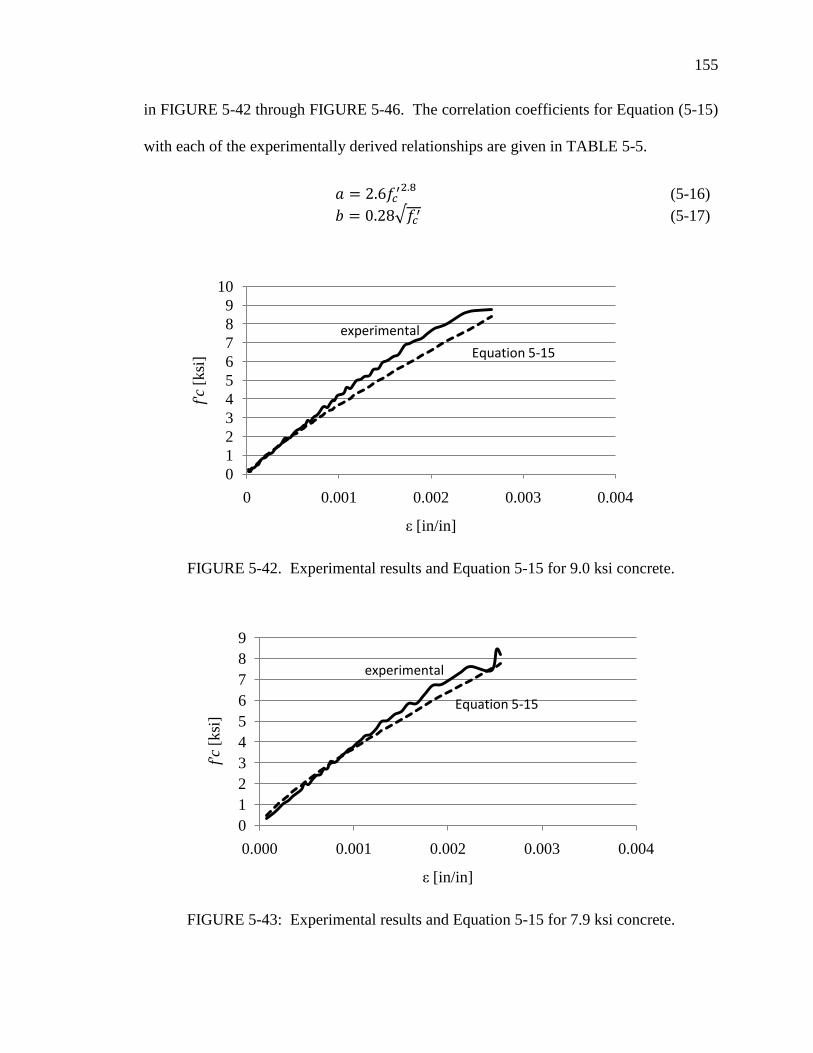
155

155

in FIGURE 5-42 through FIGURE 5-46. The correlation coefficients for Equation (5-15)

with each of the experimentally derived relationships are given in TABLE 5-5.

(5-16)

(5-17)

FIGURE 5-42. Experimental results and Equation 5-15 for 9.0 ksi concrete.

FIGURE 5-43: Experimental results and Equation 5-15 for 7.9 ksi concrete.

0

1

2

3

4

5

6

7

8

9

10

0 0.001 0.002 0.003 0.004

f'c

[ksi

]

ε [in/in]

Equation 5-15

experimental

0

1

2

3

4

5

6

7

8

9

0.000 0.001 0.002 0.003 0.004

f'c

[ksi

]

ε [in/in]

Equation 5-15

experimental

156

156

FIGURE 5-44. Experimental results and Equation 5-15 for 7.3 ksi concrete.


0

1

2

3

4

5

6

7

8

9

0.000 0.001 0.002 0.003 0.004

f'c

[ksi

]

ε [in/in]

estimate

experimental

0

1

2

3

4

5

6

7

8

9

0.000 0.001 0.002 0.003 0.004

f'c

[ksi

]

ε [in/in]

Equation 5-15

experimental

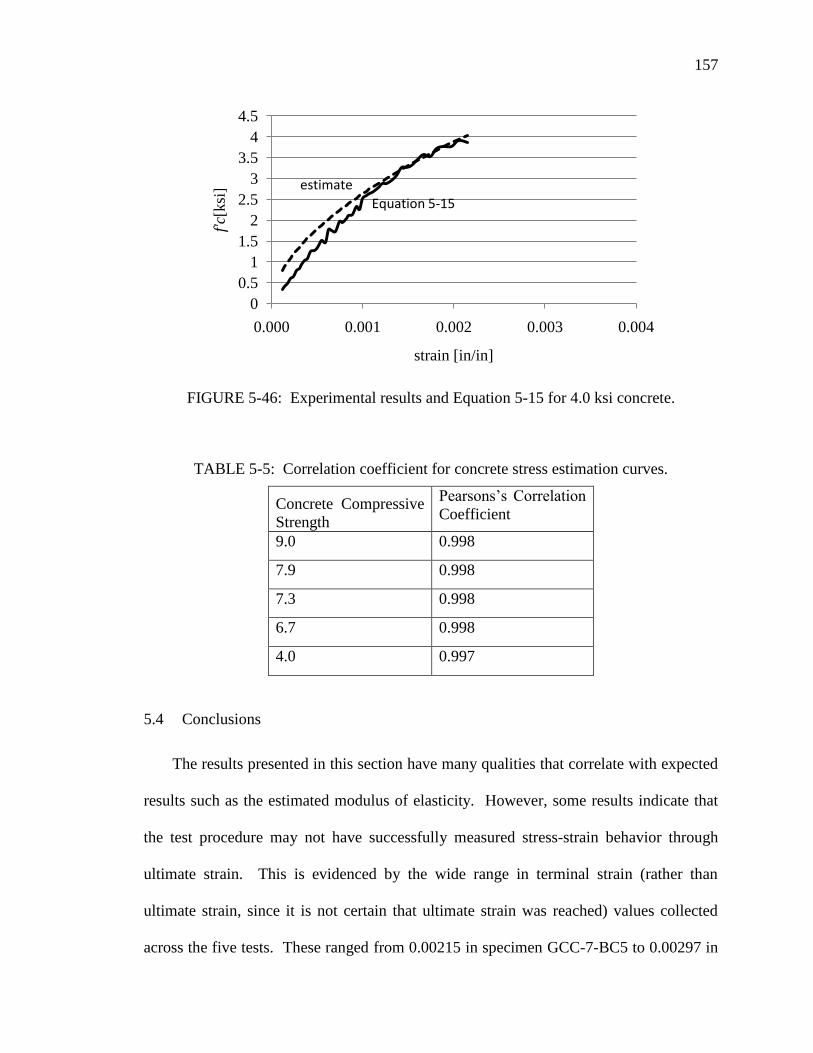
157

157


TABLE 5-5: Correlation coefficient for concrete stress estimation curves.

Concrete Compressive

Strength

Pearsons’s Correlation

Coefficient

9.0 0.998

7.9 0.998

7.3 0.998

6.7 0.998

4.0 0.997

5.4 Conclusions

The results presented in this section have many qualities that correlate with expected

results such as the estimated modulus of elasticity. However, some results indicate that

the test procedure may not have successfully measured stress-strain behavior through

ultimate strain. This is evidenced by the wide range in terminal strain (rather than

ultimate strain, since it is not certain that ultimate strain was reached) values collected

across the five tests. These ranged from 0.00215 in specimen GCC-7-BC5 to 0.00297 in

0

0.5

1

1.5

2

2.5

3

3.5

4

4.5

0.000 0.001 0.002 0.003 0.004

f'c[

ksi

]

strain [in/in]

estimate

Equation 5-15

158

158

specimen GCC-6-BC4. The terminal strain recorded in the tests was not linked to

concrete compressive strength.

Difficulty measuring the ultimate strain could have arisen from several issues related

to the specimen construction or the test protocol. The specimens did not fail in the

instrumented zone of the beam. This means that when crushing was initiated, the strains

local to the instrumented area actually would have reduced due to the declining loads on

the specimen and the peak strain would not likely be recorded. Since data is not available

in the literature regarding post peak or ultimate strain behavior of GCC materials, more

specialized tests are required to ascertain whether the full range of elastic and post elastic

response was measured by these tests.

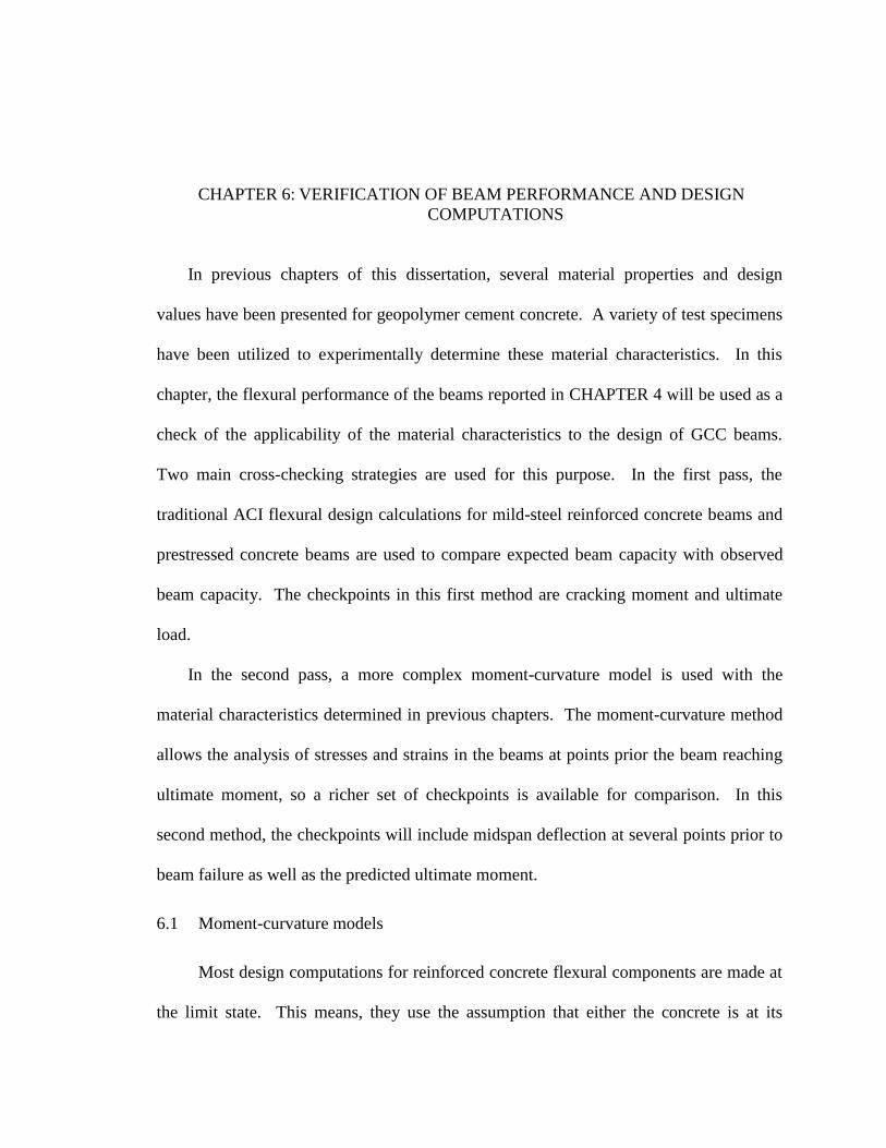
CHAPTER 6: VERIFICATION OF BEAM PERFORMANCE AND DESIGN

COMPUTATIONS

In previous chapters of this dissertation, several material properties and design

values have been presented for geopolymer cement concrete. A variety of test specimens

have been utilized to experimentally determine these material characteristics. In this

chapter, the flexural performance of the beams reported in CHAPTER 4 will be used as a

check of the applicability of the material characteristics to the design of GCC beams.

Two main cross-checking strategies are used for this purpose. In the first pass, the

traditional ACI flexural design calculations for mild-steel reinforced concrete beams and

prestressed concrete beams are used to compare expected beam capacity with observed

beam capacity. The checkpoints in this first method are cracking moment and ultimate

load.

In the second pass, a more complex moment-curvature model is used with the

material characteristics determined in previous chapters. The moment-curvature method

allows the analysis of stresses and strains in the beams at points prior the beam reaching

ultimate moment, so a richer set of checkpoints is available for comparison. In this

second method, the checkpoints will include midspan deflection at several points prior to

beam failure as well as the predicted ultimate moment.

6.1 Moment-curvature models

Most design computations for reinforced concrete flexural components are made at

the limit state. This means, they use the assumption that either the concrete is at its

160

160

compression failure strain or the steel is at its tension yield strain. This strategy

eliminates the more complicated process of predicting the nonlinear response of the

materials at points prior to failure. In order to model the full range of beam behavior up

to failure, a more complex computation strategy is required. Moment-curvature analysis

is one such method for modeling reinforced concrete beam behavior throughout a loading

range.

The model assumes that as a moment is applied to a segment of a beam, as in

FIGURE 6-1a, strains develop which lead to the deformation of the cross section

(FIGURE 6-1b). The strain distribution across the section is linear, as shown in FIGURE

6-1c, even after the concrete is cracked. The linear distribution of strain is

experimentally verifiable. The assumed strain can then be related to stresses in the

constituent materials via their known elastic and inelastic properties. To create such a

model numerically, the cross-section of the concrete beam is divided into many

horizontal strips as shown in FIGURE 6-2. Each strip is assumed to have uniform strain

over its depth, which is taken as the average of the range of strains found in the

continuous cross-section. The constitutive properties of the material in the strip are used

to compute stress from the strain, and the area of the strip can be used to determine the

force generated at the centroid of each strip, also shown in FIGURE 6-2.

In order to determine the magnitude of the strains in the cross-section, a value is

assumed for strain in the extreme compression fiber. Once maximum strain is

established, the curvature, φ (FIGURE 6-1b,c), is computed based on maintaining force

equilibrium. The moment acting on the section may be computed by summing the

moments generated by the force acting in each strip about any convenient point, such as

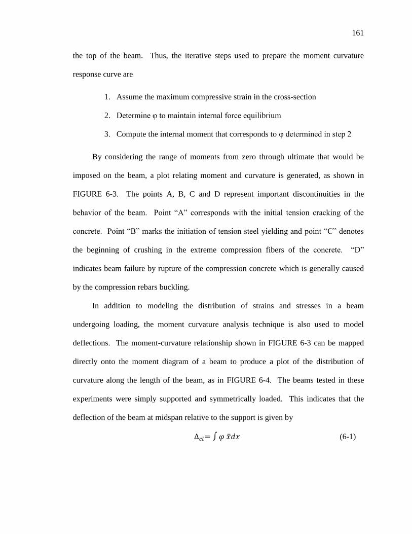
161

161

the top of the beam. Thus, the iterative steps used to prepare the moment curvature

response curve are

1. Assume the maximum compressive strain in the cross-section

2. Determine φ to maintain internal force equilibrium

3. Compute the internal moment that corresponds to φ determined in step 2

By considering the range of moments from zero through ultimate that would be

imposed on the beam, a plot relating moment and curvature is generated, as shown in

FIGURE 6-3. The points A, B, C and D represent important discontinuities in the

behavior of the beam. Point ―A‖ corresponds with the initial tension cracking of the

concrete. Point ―B‖ marks the initiation of tension steel yielding and point ―C‖ denotes

the beginning of crushing in the extreme compression fibers of the concrete. ―D‖

indicates beam failure by rupture of the compression concrete which is generally caused

by the compression rebars buckling.

In addition to modeling the distribution of strains and stresses in a beam

undergoing loading, the moment curvature analysis technique is also used to model

deflections. The moment-curvature relationship shown in FIGURE 6-3 can be mapped

directly onto the moment diagram of a beam to produce a plot of the distribution of

curvature along the length of the beam, as in FIGURE 6-4. The beams tested in these

experiments were simply supported and symmetrically loaded. This indicates that the

deflection of the beam at midspan relative to the support is given by

(6-1)

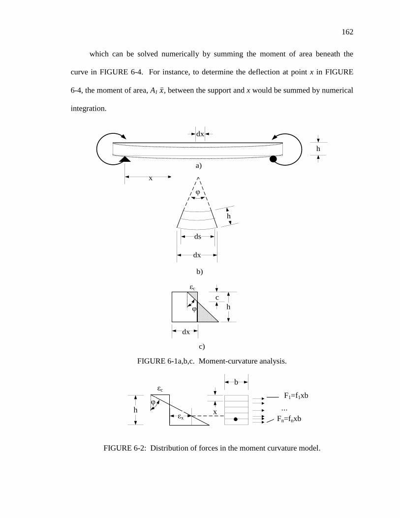
162

162

which can be solved numerically by summing the moment of area beneath the

curve in FIGURE 6-4. For instance, to determine the deflection at point x in FIGURE

6-4, the moment of area, A1 , between the support and x would be summed by numerical

integration.

dx

a)

b)

εc

φ

c)

h

φ

dx

ds

h

h

dx

c

x

FIGURE 6-1a,b,c. Moment-curvature analysis.

εc

φh

Fn=fnxb

...x

b

F1=f1xb

εx

FIGURE 6-2: Distribution of forces in the moment curvature model.

163

163

A

B

C

D

Mo

men

t

Curvature

FIGURE 6-3: Moment curvature plot.

Mom

ent

Curv

ature

, φ

x

A1

x

FIGURE 6-4: Moment-curvature relationship plotted along beam length.

Moment curvature models were used in this study to verify the applicability of the

concrete stress-strain characteristics measured via the flexural beam-column tests with

the component tests of reinforced concrete beams. In the model prepared for this study,

the beams were divided into 0.25‖ (6.4mm) horizontal strips.

164

164

6.1.1 Traditional analysis methods

Two points in the load history, ―A‖- initial cracking of the concrete section, and

―C‖- initiation of concrete crushing at the compression face of the beam, are important to

the design process and are calculated using formulas provided by ACI 318 (American

Concrete Institute, 2008). For the purposes of determining the cracking moment, ACI

gives

(6-2)

where:

(for rectangular beams) (6-3)

[psi] (6-4)

or [MPa] (6-5)

For ultimate moment capacity, ACI gives

(6-6)

where:

: area of steel

: steel yield stress

: depth of steel in the beam relative to the extreme compression fiber

: depth of the compressive stress block

Inputs to the ultimate moment calculations are presented in TABLE 6-1. The

computed ultimate moment values for the four beams reported here are given in TABLE

6-2. It can be seen that for all the mild steel reinforced beams the design values are very

conservative in comparison to the recorded performance. In order to make the

165

165

calculations in TABLE 6-2, the actual steel yield stress values determined by tensile tests

were used rather than the assumption that grade 60 steel would yield at 60 ksi . Plots of

these values are provided in APPENDIX A. Also, stresses in the compression steel were

considered. Since the beams were highly underreinforced, the neutral axis was above the

top bars and they acted as tensile reinforcement near beam failure.

6.1.1.1 Example calculation method for ultimate moment

Step 1: Determine the depth of the compressive stress block, a

Balancing compressive and tensile forces in the concrete cross section gives

(6-7)

which can be used to solve for a by simplifying and using the quadratic formula. In the

case of GCC-1-B1, geometric and material strength quantities In this example, traditional

ACI 318 values were used and . For GCC-1-B1, geometric and

material strength quantities are:

=10.5

=3

=10.5‖ (267mm)

=0.31 in2 (398mm

2)

=0.31 in

2 (398mm

2)

=54,000 psi (558 MPa)

=11,000 psi (372 MPa)

Solving Equation (6-7), =1.06‖ (26.9mm) and = 0.00252%. Since this indicates that

the top steel has yielded, the depth of the stress block must be recalculated using

(6-8)

166

166

Solving for , the depth of the stress block is found to be 1.09‖ (27.7mm) and =

0.00233%.

Step 2: Determine the moment, Mn

Considering that the top steel acts in tension rather than compression, the ultimate

moment is computed with

(6-9)

Therefore, using the section and material qualities for the beam,

The same computation strategy was used for all the mild steel reinforced beams.

Input values and calculation points are listed in TABLE 6-1. Results are reported in

TABLE 6-2. The cracking moment was computed by estimating the modulus of rupture

using ACI methods. Results are presented in TABLE 6-3.

167

167

TABLE 6-1: Beam ultimate moment calculation inputs.

and and

Beam psi (MPa) a, in (mm)

a, in (mm)

GCC-1-B1 11,000 (75.8) 1.10 (27.9) 0.00233 1.29 0.00049

GCC-2-B2 11,900 (82.0) 1.00 (25.4) 0.00286 0.82 0.00251

PCC-1-B3 12,500 (86.2) 1.00 (25.4) 0.00298 - -

GCC-R-B4 9,200 (63.4) 1.16 (29.5) 0.00205 0.94 0.00178

TABLE 6-2: Computed and observed values for, .

Beam

and and

kip-in,

(kn-m)

kip-in,

(kn-m)

GCC-1-B1 600 (68) 423 (47.8) 1.42 416 (47.0) 1.44

GCC-2-B2 760 (85.9) 567 (64.1) 1.34 566 (63.9) 1.34

PCC-1-B3 670 (75.7) 568 (64.2) 1.18 - -

GCC-R-B4 682 (77.0) 540 (61.0) 1.26 540 (61.0) 1.25

TABLE 6-3: Computed and observed values for , .

Beam psi, (MPa) in

4, (cm

4)

k-in, (kN-m)

k-in, (kN-m)

GCC-1-B1 787 (5.4) 1,152

(47,950)

151 (17.1) 160 (18.1)

GCC-2-B2 818 (5.6) ― 157 (17.7) 187 (21.1)

PCC-1-B3 838 (5.8) ― 161 (18.2) 80 (9.0)

GCC-R-B4 719 (5.0) ― 138 (15.6) 144 (16.3)

ACI design formulas conservatively predicted the performance of the GCC beams in

all cases. TABLE 6-4 provides the ratios of predicted to observed flexural performance

for the four mild-steel reinforced beams. The ultimate moment predictions for the GCC

beams were conservative by an average factor of 1.29. This is similar to the same ratio

168

168

for the PCC beam of 1.18. For cracking moments, the predictions were very accurate in

the case of the GCC beams. Only for the PCC beam were the design formulations

unconservative. The first crack appeared in the PCC beam at half the expected load.

This could have been caused by damage to the beam during transportation. Since the

value is so different from expected, it should be treated as an outlier.

TABLE 6-4: Ratio of observed to predicted cracking moment and ultimate moment.

Beam

GCC-1-B1 1.06 1.42

GCC-2-B2 1.19 1.34

PCC-1-B3 0.50 1.18

GCC-R-B4 1.04 1.26

Similar flexural tests conducted by Sumajouw et al. (2005) resulted in very

comparable results. Beams having the same reinforcement ratio, ρ=0.64 defined by

(6-10)

displayed the ratios of predicted to observed flexural capacity given in TABLE 6-5. As

with the results collected in this study, Sumajouw found that over-estimates are made for

beams with very low reinforcement ratios. As the ρ increases, the design formulations

result in smaller overestimates.

169

169

TABLE 6-5: Ratio of observed and calculated flexural strength as reported by

Sumajouw(2006).

psi (MPa) ρ

5,531 (37) 0.64 1.24

6,876 (46) 0.64 1.28

11,361 (76) 0.64 1.42

6.2 Flexural performance assessed by moment-curvature models

The moment-curvature model was used to predict the failure load as well as the

deflection of the reinforced concrete beams. Inputs to the models were the concrete

compressive strength for each beam, the stress-strain curve given by Equation (5-16) and

the beam geometry presented in FIGURE 4-3. The model, executed in the spreadsheet

application Excel, used the techniques described in Section 6.1.1 to make midspan

deflection estimates as well as maximum moment computations. These were compared

with the results given in CHAPTER 4.

6.2.1 Ultimate moment

The ultimate moment is defined as the maximum resisting moment achieved by

the reinforced concrete beams during the flexural tests. The experimental results of these

tests were presented in CHAPTER 4, and are summarized in TABLE 6-6. It can be seen

that the moment curvature model provided slightly conservative results for the strength of

the beams.

170

170

TABLE 6-6: Ultimate moment predictions made with the moment-curvature model.

Beam kip-in (kn-m)

kip-in (kn-m)

GCC-1-B1 494 (55.8) 600 (68) 1.21

GCC-2-B2 615 (69.5) 760 (85.9) 1.24

PCC-1-B3 657 (74.2) 670 (75.7) 1.02

GCC-R-B4 589 (66.5) 682 (77.0) 1.16

6.2.2 Correlation of moment-curvature model results with beam performance

The moment-curvature model was used to predict midspan deflection of the

reinforced concrete beams. The predicted and actual deflection is plotted in FIGURE 6-5

through FIGURE 6-8. Based on the changes in slope along the load history displayed in

these charts, the model does accurately predict cracking and the onset of reinforcement

yielding. However, it loses accuracy in the upper regions of the beam’s moment

capacity. TABLE 6-6 gives the accuracy of the models in terms of the ratio of actual to

predicted deflection.

FIGURES 6-5 through 6-8 also provide model results using a stress-strain

relationship sometimes applied to PCC. Due to uncertainty in the results of the flexural

beam-column tests, the stress-strain relationship proposed by Popovics and refined for

high strength concrete by Mertol was used to model the GCC stress-strain response

(Mertol, 2006; Popovics, 1973). This equation is give as

(6-11)

where

171

171

(6-12)

(6-13)

(6-14)

Since reliable values for were not determined during the flexural beam

column tests, this value was taken as 0.0035 for all tests, rather than the variable value

proposed by Mertol (2006).

TABLE 6-7: Ratio of predicted and actual deflections for mild steel reinforced beams at

different moment levels (Δpredicted/ Δobserved).

Maximum Moment, kip-in (kN-M)

Beam 100 (11.3) 200 (22.6) 300 (33.9) 400 (45.2) 500 (56.5)

GCC-1-B1 (GCC) 0.88 1.11 1.11 1.91 1.14

GCC-1-B1 (Popovics) 0.76 0.79 1.03 1.56 1.08

GCC-2-B2 (GCC) 1.15 3.12 1.62 1.37 1.74

GCC-2-B2 (Popovics) 1.04 2.58 1.52 1.25 1.55

PCC-1-B3 (Popovics) 0.41 0.44 0.82 0.84 1.13

GCC-R-B4 (GCC) 0.51 0.75 1.02 1.00 1.45

GCC-R-B4 (Popovics) 0.62 1.04 1.09 1.09 1.51

172

172

FIGURE 6-5: Modeled and actual deflection for GCC-1-B1.

FIGURE 6-6: Modeled and. actual deflection for GCC-2-B2.

0 50 100

0

10

20

30

40

50

60

70

80

90

0

100

200

300

400

500

600

700

800

0 1 2 3 4

Midspan Deflection (mm)

Mom

ent

(kN

-m)

Mom

ent

(kip

-in)

Midspan Deflection (in)

Popovics

GCC

Experimental

0 50 100

0

10

20

30

40

50

60

70

80

90

0

100

200

300

400

500

600

700

800

0 1 2 3 4


Mom

ent

(kN

-m)

Mom

ent

(kip

-in)


Popovics

GCC

Experimental

173

173

FIGURE 6-7: Modeled and actual deflection for PCC-1-B3.

FIGURE 6-8: Modeled and actual deflection for GCC-R-B4.

0 50 100

0

10

20

30

40

50

60

70

80

90

0

100

200

300

400

500

600

700

800

0 1 2 3 4


Mo

men

t (k

N-m

)

Mom

ent

(kip

-in)


Popovics

Experimental

0 50 100

0

10

20

30

40

50

60

70

80

90

0

100

200

300

400

500

600

700

800

0 1 2 3 4


Mom

ent

(kN

-m)

Mom

ent

(kip

-in)


Popovics

GCC

Experimental

174

174

6.2.3 Discussion of moment-curvature modeling results

Because the concrete beams used in this study were very under-reinforced, the

depths of the compression zones in the beam were small. This resulted in the ultimate

moment calculations having a high sensitivity to quantities that are not well defined for

the GCC, such as ultimate strain and post-peak stress-strain relationships. The results of

the deflection-correlation study had less sensitivity to the ultimate and post-peak stress

characteristics of the GCC and therefore, provided more reliable results for moment loads

less than the ultimate moment. The results in TABLE 6-7 as well as in FIGURE 6-5

through 6-8 show that the moment-curvature models typically predicted larger deflections

than were observed during the tests. At service load levels (300 kip-in) the ratio of

predicted to observed deflections ranged from 1.02 to 1.62. Although the difference

between using Popovic’s stress-strain relationship and the one presented in CHAPTER 5

is fairly small, Popovic’s relationship produced more accurate models. This is most

likely due to its inclusion of post-peak strains.

6.3 Prestressed concrete beams

For the prestressed concrete beams, two points in the load-deflection history were

used to verify the applicability of design formulations and material properties to GCC

beam components. These were cracking moment Mcr and nominal ultimate moment Mn.

The ultimate moment was predicted using both existing ACI design values for and

as well as the special GCC values presented in CHAPTER 5. Shrinkage and creep

parameters for GCC were used to estimate the effective prestress at the time of the test.

The magnitude of the measured cracking moment was further used to estimate the

175

175

accuracy of the calculation. For purposes of making the design calculations presented in

this chapter, the geometric quantities given in TABLE 6-8 were used.

TABLE 6-8: Geometric quantities used for prestressed beam analysis.

Quantity Notation Value Units

Beam width bw 10 In

Beam length L 18 Ft

Beam height h 18 In

Depth to the centroid

of the prestressing

steel

dp 14 In

Depth to the mild

steel reinforcing

ds 16.25 in

Moment of inertia I 4860 in4

Cross sectional area ac 180 in2

Distance from beam

centroid to beam top

ytop 9 in

Distance from beam

centroid to beam

bottom

ybot 9 in

Section modulus for

beam bottom

Sbot 540 in3

Section modulus for

beam top

Stop 540 in3

Radius of gyration r2 27 in

2

Length l 216 in

Prestressing steel

eccentricity

e 5 in

6.3.1 Ultimate moment

The prestressed beams contained both prestressing steel at two depths in the beam as

well as mild steel reinforcing at the top and the bottom as shown in FIGURE 4-21. All

four of these steel groups were considered as contributing to the ultimate moment

capacity of the beam. The depth to the neutral axis was computed by balancing the

176

176

forces from each of these reinforcing groups as well as the compressive zone of the

concrete. Analysis accounted for increasing strain in the prestressing steel and related the

magnitude of the stress to stress-strain test results provided by the manufacturer.

TABLE 6-9 gives the results of the ultimate moment computation using the ACI 318

design guidelines for and where

=0.85

=0.65

Also in TABLE 6-9 are the results of the same computation using the updated design

quantities developed in CHAPTER 5:. These were given as

=1.0

=0.5

TABLE 6-9: Computed ultimate moment values, kip-in.

Beam

ACI

318

and

Updated

and

GCC-2-P1 3,125 3,255 0.96 3,126 1.00

PCC-1-P2 3,112 3,350 0.93 - -

GCC-R-P3 3,124 2,805 1.11 2,988 1.05

The ratio of experimental to calculated results shows a very good ability to predict

the ultimate moment for GCC prestressed flexural beams. Using the and values

proposed in CHAPTER 5, calculations are slightly more accurate than when using values

proposed for general Portland cement concrete design. It is important to note that using

the ACI values provides a risk of over-estimating the flexural strength, as seen in the case

of GCC-1. However, the ACI values also over estimated the strength of the PCC beam.

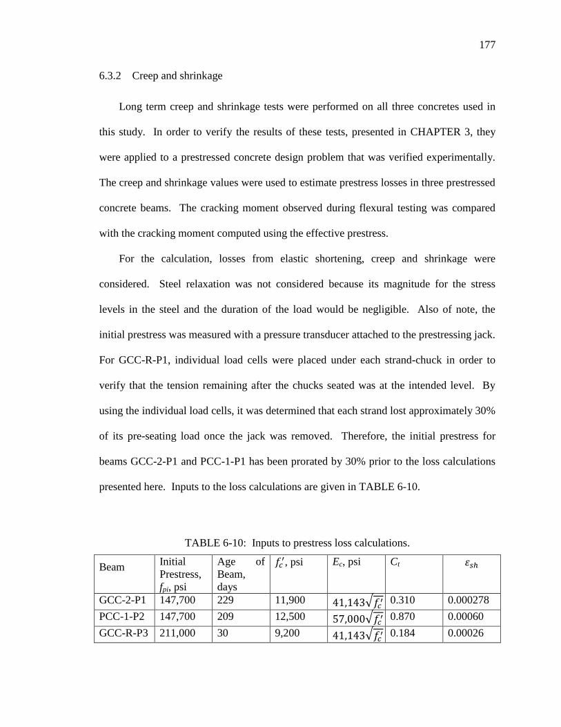
177

177

6.3.2 Creep and shrinkage

Long term creep and shrinkage tests were performed on all three concretes used in

this study. In order to verify the results of these tests, presented in CHAPTER 3, they

were applied to a prestressed concrete design problem that was verified experimentally.

The creep and shrinkage values were used to estimate prestress losses in three prestressed

concrete beams. The cracking moment observed during flexural testing was compared

with the cracking moment computed using the effective prestress.

For the calculation, losses from elastic shortening, creep and shrinkage were

considered. Steel relaxation was not considered because its magnitude for the stress

levels in the steel and the duration of the load would be negligible. Also of note, the

initial prestress was measured with a pressure transducer attached to the prestressing jack.

For GCC-R-P1, individual load cells were placed under each strand-chuck in order to

verify that the tension remaining after the chucks seated was at the intended level. By

using the individual load cells, it was determined that each strand lost approximately 30%

of its pre-seating load once the jack was removed. Therefore, the initial prestress for

beams GCC-2-P1 and PCC-1-P1 has been prorated by 30% prior to the loss calculations

presented here. Inputs to the loss calculations are given in TABLE 6-10.

TABLE 6-10: Inputs to prestress loss calculations.

Beam Initial

Prestress,

fpi, psi

Age of

Beam,

days

, psi Ec, psi Ct

GCC-2-P1 147,700 229 11,900 0.310 0.000278

PCC-1-P2 147,700 209 12,500 0.870 0.00060

GCC-R-P3 211,000 30 9,200 0.184 0.00026

178

178

Losses were calculated with the following equations

(6-15)

where is the stress at the centroid of the steel and all other quantities are given in

the preceding TABLEs.

(6-16)

where:

: change in prestress due to elastic shortening

(6-17)

where:

: change in prestress due to creep

(6-18)

where:

: change in prestress due to shrinkage

TABLE 6-11 gives a summary of the calculations related to prestress losses.

Computations make use of the equations presented above. Mcr, given by

(6-19)

and are presented in the last column of TABLE 6-11 using the values for effective

prestress presented in the same TABLE. It is compared with the observed cracking

moment in TABLE 6-12. This test involves the interaction of the multiple variables:

concrete strength, creep coefficient and shrinkage coefficient. However the results

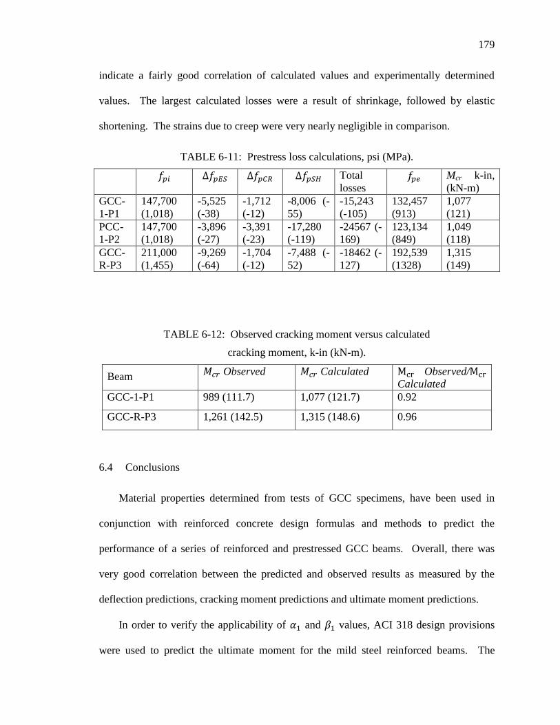
179

179

indicate a fairly good correlation of calculated values and experimentally determined

values. The largest calculated losses were a result of shrinkage, followed by elastic

shortening. The strains due to creep were very nearly negligible in comparison.

TABLE 6-11: Prestress loss calculations, psi (MPa).

Total

losses Mcr k-in,

(kN-m)

GCC-

1-P1

147,700

(1,018)

-5,525

(-38)

-1,712

(-12)

-8,006 (-

55)

-15,243

(-105)

132,457

(913)

1,077

(121)

PCC-

1-P2

147,700

(1,018)

-3,896

(-27)

-3,391

(-23)

-17,280

(-119)

-24567 (-

169)

123,134

(849)

1,049

(118)

GCC-

R-P3

211,000

(1,455)

-9,269

(-64)

-1,704

(-12)

-7,488 (-

52)

-18462 (-

127)

192,539

(1328)

1,315

(149)

TABLE 6-12: Observed cracking moment versus calculated

cracking moment, k-in (kN-m).

Beam Observed Calculated Observed/

Calculated

GCC-1-P1 989 (111.7) 1,077 (121.7) 0.92

GCC-R-P3 1,261 (142.5) 1,315 (148.6) 0.96

6.4 Conclusions

Material properties determined from tests of GCC specimens, have been used in

conjunction with reinforced concrete design formulas and methods to predict the

performance of a series of reinforced and prestressed GCC beams. Overall, there was

very good correlation between the predicted and observed results as measured by the

deflection predictions, cracking moment predictions and ultimate moment predictions.

In order to verify the applicability of and values, ACI 318 design provisions

were used to predict the ultimate moment for the mild steel reinforced beams. The

180

180

average ratio of predicted to observed performance was 1.34. This indicates that the

design provisions are slightly conservative. However, since the beams were

underreinforced, the design calculations are not very sensitive to changes in the value .

The traditional ACI design formulations were also used to analyze the ultimate

capacity of the prestressed beams. Since the depth of the compressive stress block a for

the prestressed beams is deeper, this exercise provided a better assessment of the and

values proposed in 0. The average ratio of predicted to observed moment capacity

was 1.025. This indicates that the existing design formulations for reinforced concrete

may be applied to GCC beams when values of and modified for geopolymer

applications are used.

181

181

CHAPTER 7: LIFE CYCLE ANALYSIS OF GEOPOLYMER CEMENT CONCRETE

Geopolymer cement concrete (GCC) can be used to make many of the structural

members that are commonly formed from Portland cement concrete (PCC). The Portland

cement binder in PCC requires large inputs of energy and natural resources during its

manufacture whereas the binder in GCC is sourced from the waste stream and less energy

is required to develop its cementitious properties. The GCC and PCC materials are very

similar in many aspects aside from the make-up of their binders. A life cycle assessment

can be used to compare the lifecycle impacts of each material in order to verify the

improved environmental performance of GCC.

7.1 Life cycle assessment for geopolymer cement concrete production

The results of GCC development presented in CHAPTER 3 were used to generate

the inputs to a lifecycle model for the production of geopolymer cements. These inputs

include the materials and energy that were used to manufacture the mix designs that were

presented. The diagrams in FIGURE 7-1 and FIGURE 7-2 depict the inputs to the

manufacture of each material. The quantities of the inputs and outputs shown in the

FIGUREs are given in the description of each process later in this dissertation.

In order to compare the results of a life cycle analysis for different materials, it is

necessary to define a functional unit. This is an especially critical step when comparing

radically different systems, such as timber columns versus steel columns. But, since

182

182

concrete bound with geopolymer cement can be used in an overwhelmingly similar

capacity as precast Portland cement concrete, the functional unit used for this analysis is

simply 1.3 yd3 (1 m

3) of 7,300 psi (50 MPa) concrete. The two materials can be cast into

identical shapes that can be expected to offer similar structural performance. Therefore,

the LCA comparison that is presented here is solely related to the development of the

concrete strength and does not include the energy required for other concreting tasks.

The main differences in the two processes relate to the preparation of the cement. In the

case of Portland cement, manufacturing energy is applied prior to mixing the concrete.

For geopolymer cement, the energy used to develop strength is applied to prepare the

activating solution and to heat the concrete after it is mixed and placed. However, the

mixing processes, formwork preparation, reinforcing requirements, concrete placement

and consolidation practices are very similar. Therefore, the boundaries of the comparison

for the two materials are simplified by considering the following stages for each:

Geopolymer Cement Concrete Portland Cement Concrete

Preparation of cementitious

material

Manufacture of Portland cement

High temperature curing

The mixing process and delivery of structural components from the precasting plant

to the jobsite is considered to be similar for both materials.

183

183

FIGURE 7-1: Manufacture processes for geopolymer cement concrete.

FIGURE 7-2: Manufacture processes for Portland cement concrete.

Aggregate

Manufacture

Quarry

Materials

Emissions

Water Energy

Portland Cement

Emissions

Water Energy

Limestone

Mix Concrete

Quarry

Materials

Emissions

Energy

Water

Aggregate Manufacture

Quarry

Emissions

Energy

Cementitious Material

Preparation

Emissions

Water Energy NaOH Fume

Silica Fly Ash

Mix Concrete

Quarry Materials

Emissions

Energy

High Temperature Curing

Emissions

Energy

Materials Water

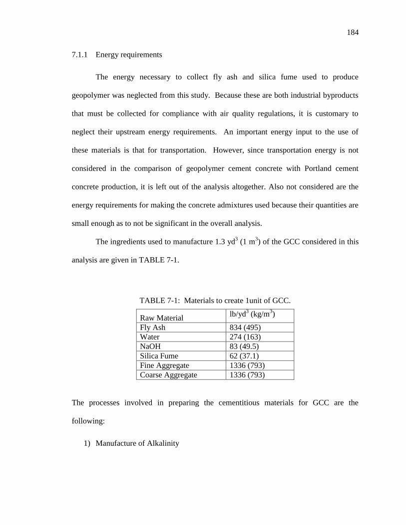
184

184

7.1.1 Energy requirements

The energy necessary to collect fly ash and silica fume used to produce

geopolymer was neglected from this study. Because these are both industrial byproducts

that must be collected for compliance with air quality regulations, it is customary to

neglect their upstream energy requirements. An important energy input to the use of

these materials is that for transportation. However, since transportation energy is not

considered in the comparison of geopolymer cement concrete with Portland cement

concrete production, it is left out of the analysis altogether. Also not considered are the

energy requirements for making the concrete admixtures used because their quantities are

small enough as to not be significant in the overall analysis.

The ingredients used to manufacture 1.3 yd3 (1 m

3) of the GCC considered in this

analysis are given in TABLE 7-1.

TABLE 7-1: Materials to create 1unit of GCC.

Raw Material lb/yd

3 (kg/m

3)

Fly Ash 834 (495)

Water 274 (163)

NaOH 83 (49.5)

Silica Fume 62 (37.1)

Fine Aggregate 1336 (793)

Coarse Aggregate 1336 (793)

The processes involved in preparing the cementitious materials for GCC are the

following:

1) Manufacture of Alkalinity

185

185

NaOH is most commonly produced by electrolysis of brine solution. The reaction

produces chlorine gas at the anode and a weak alkali at the cathode. The alkaline

solution is typically concentrated to 50% strength for shipment. The SPLINE

LCA dataset quantifies the energy required to produce sodium hydroxide as 8,917

BTU/lb (20.74 MJ/kg) (Center for Environmental Assessment of Product and

Material Systems, 2008).

2) Production of the activator solution

The method of producing alkaline activator solution for the concretes made in this

set of experiments was to mix water, silica fume and the sodium hydroxide

together and then to heat the solution overnight. To estimate the energy required

for this process only the energy required to maintain an elevated temperature of

167⁰ F (75⁰ C) in a well insulated tank was included. The energy required to heat

the solution to 167⁰ F (75⁰ C) was not included because the dissolution of the

sodium hydroxide in the water produces temperatures that far exceed 167⁰ F

(75⁰C). The reaction with the silica fume is also quite violent and elevates the

temperature further. It was estimated that a well insulated tank will lose heat

energy at the rate of 0.194 MJ m-2

h-1

when the contents are maintained at 167⁰ F

(75⁰ C) and the ambient conditions outside the tank are 70⁰ F (21⁰ C). In the lab,

small quantities of activator are produced in an oven. However, in an industrial

setting it would be produced in a much different manner. In this work, the

quantity of activator solution required to produce 1.3 yd2 (1 m

3) of concrete is

about 26 gallons (100 L). A cylindrical 26 gallon (100 L) tank with a height

186

186

twice its diameter would have a surface area of 13.5 ft2 (1.25 m

2). Thus, the

energy required to maintain the sodium silicate solution at 167⁰ F (75⁰ C) for 24

hours would be 5,497 BTU (5.8 MJ).

The second process within the boundaries of this LCA is the high temperature curing

of the GCC.

3) High Temperature Curing

In the absence of measured quantities, the specific heat of geopolymer concrete

was assumed to be similar to that of Portland cement concrete, 0.88 J G-1

K-1

.

Other researchers have determined the specific heat of geopolymer-sand mortars

to range between 0.7 and 1.0 J G-1

K-1

(Geopolymer Institute, 2009). As the bulk

of constituents in both materials is aggregate (~80%), this assumption is felt to be

reasonably valid. However, properly measuring the specific heat of geopolymer

concrete would refine the accuracy of this energy analysis. The heat required to

raise the geopolymer concrete from 70 ⁰ F to 167⁰ F (21⁰ C to 75⁰ C) is calculated

as 97,436 BTU (102.8 MJ). The concrete must then be held at an elevated

temperature for 24-48 hours. As with the activating solution production, heat

losses from a well insulated oven wall were estimated at 1,979 BTU ft-2

hr-1

(0.194 MJ m-2

h-1

). An oven slightly larger in volume than the concrete would

show losses of 2,464 BTU hr-1

(2.6 MJ h-1

). Longer curing durations will require

greater inputs of energy to maintain elevated temperatures for longer periods of

time. In total, the energy required to develop the cementitious component of 1.3

yd2 (1 m

3) of this concrete is estimated at 1,178,137 BTU (1.243 GJ).

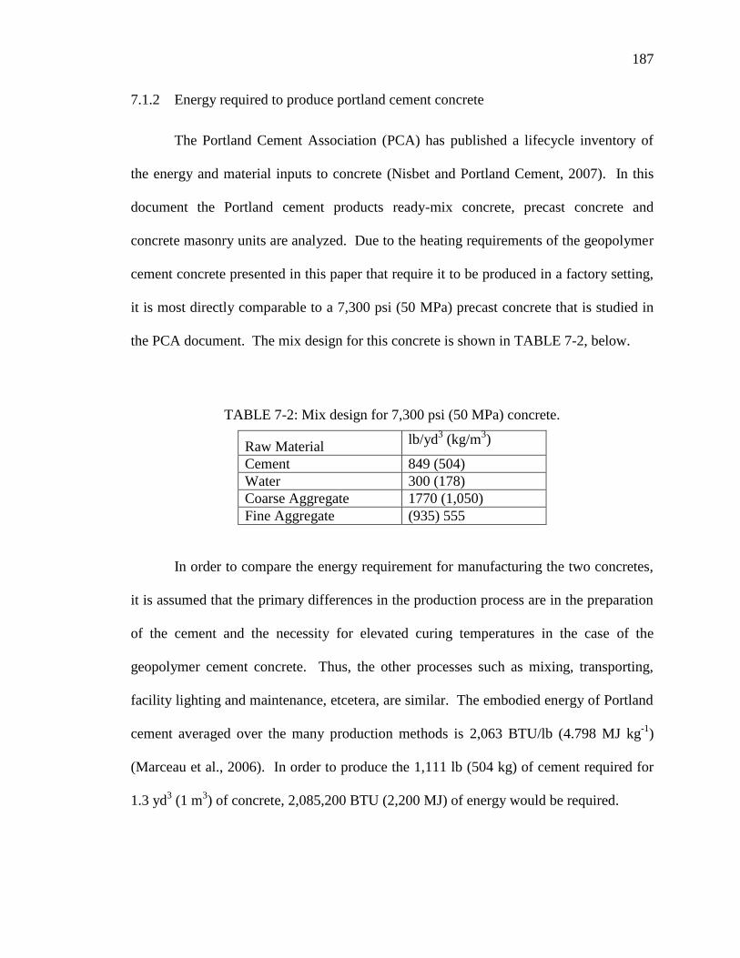
187

187

7.1.2 Energy required to produce portland cement concrete

The Portland Cement Association (PCA) has published a lifecycle inventory of

the energy and material inputs to concrete (Nisbet and Portland Cement, 2007). In this

document the Portland cement products ready-mix concrete, precast concrete and

concrete masonry units are analyzed. Due to the heating requirements of the geopolymer

cement concrete presented in this paper that require it to be produced in a factory setting,

it is most directly comparable to a 7,300 psi (50 MPa) precast concrete that is studied in

the PCA document. The mix design for this concrete is shown in TABLE 7-2, below.

TABLE 7-2: Mix design for 7,300 psi (50 MPa) concrete.

Raw Material lb/yd

3 (kg/m

3)

Cement 849 (504)

Water 300 (178)

Coarse Aggregate 1770 (1,050)

Fine Aggregate (935) 555

In order to compare the energy requirement for manufacturing the two concretes,

it is assumed that the primary differences in the production process are in the preparation

of the cement and the necessity for elevated curing temperatures in the case of the

geopolymer cement concrete. Thus, the other processes such as mixing, transporting,

facility lighting and maintenance, etcetera, are similar. The embodied energy of Portland

cement averaged over the many production methods is 2,063 BTU/lb (4.798 MJ kg-1

)

(Marceau et al., 2006). In order to produce the 1,111 lb (504 kg) of cement required for

1.3 yd3 (1 m

3) of concrete, 2,085,200 BTU (2,200 MJ) of energy would be required.

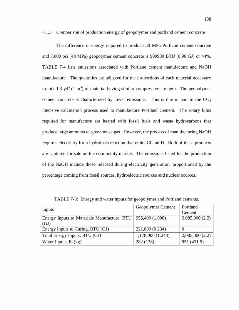
188

188

7.1.3 Comparison of production energy of geopolymer and portland cement concrete

The difference in energy required to produce 50 MPa Portland cement concrete

and 7,000 psi (48 MPa) geopolymer cement concrete is 909900 BTU (0.96 GJ) or 44%.

TABLE 7-4 lists emissions associated with Portland cement manufacture and NaOH

manufacture. The quantities are adjusted for the proportions of each material necessary

to mix 1.3 yd3 (1 m

3) of material having similar compressive strength. The geopolymer

cement concrete is characterized by lower emissions. This is due in part to the CO2

intensive calcination process used to manufacture Portland Cement. The rotary kilns

required for manufacture are heated with fossil fuels and waste hydrocarbons that

produce large amounts of greenhouse gas. However, the process of manufacturing NaOH

requires electricity for a hydrolosis reaction that emits Cl and H. Both of these products

are captured for sale on the commodity market. The emissions listed for the production

of the NaOH include those released during electricity generation, proportioned by the

percentage coming from fossil sources, hydroelectric sources and nuclear sources.

TABLE 7-3: Energy and water inputs for geopolymer and Portland cements.

Inputs Geopolymer Cement Portland

Cement

Energy Inputs to Materials Manufacture, BTU

(GJ)

955,400 (1.008) 2,085,000 (2.2)

Energy Inputs to Curing, BTU (GJ) 221,800 (0.234) 0

Total Energy Inputs, BTU (GJ) 1,178,000 (1.243) 2,085,000 (2.2)

Water Inputs, lb (kg) 282 (128) 951 (431.5)

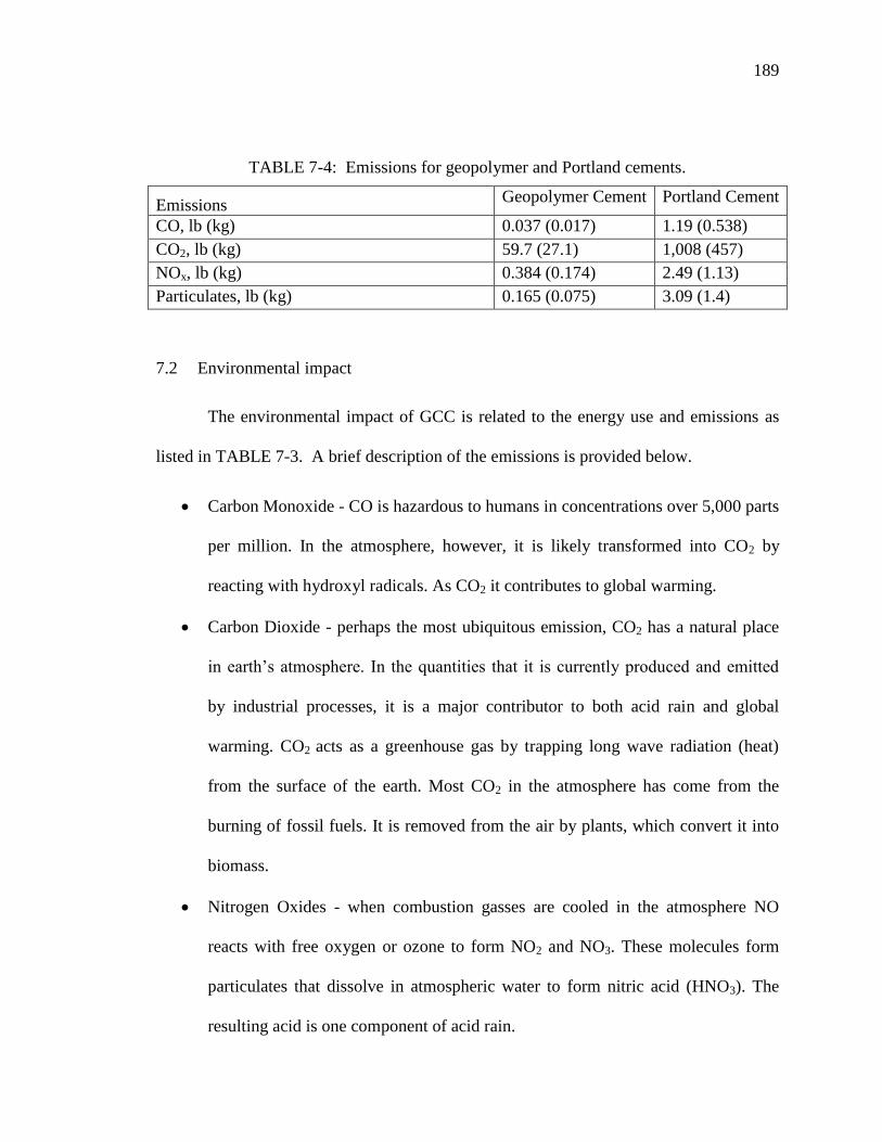
189

189

TABLE 7-4: Emissions for geopolymer and Portland cements.

Emissions Geopolymer Cement Portland Cement

CO, lb (kg) 0.037 (0.017) 1.19 (0.538)

CO2, lb (kg) 59.7 (27.1) 1,008 (457)

NOx, lb (kg) 0.384 (0.174) 2.49 (1.13)

Particulates, lb (kg) 0.165 (0.075) 3.09 (1.4)

7.2 Environmental impact

The environmental impact of GCC is related to the energy use and emissions as

listed in TABLE 7-3. A brief description of the emissions is provided below.

Carbon Monoxide - CO is hazardous to humans in concentrations over 5,000 parts

per million. In the atmosphere, however, it is likely transformed into CO2 by

reacting with hydroxyl radicals. As CO2 it contributes to global warming.

Carbon Dioxide - perhaps the most ubiquitous emission, CO2 has a natural place

in earth’s atmosphere. In the quantities that it is currently produced and emitted

by industrial processes, it is a major contributor to both acid rain and global

warming. CO2 acts as a greenhouse gas by trapping long wave radiation (heat)

from the surface of the earth. Most CO2 in the atmosphere has come from the

burning of fossil fuels. It is removed from the air by plants, which convert it into

biomass.

Nitrogen Oxides - when combustion gasses are cooled in the atmosphere NO

reacts with free oxygen or ozone to form NO2 and NO3. These molecules form

particulates that dissolve in atmospheric water to form nitric acid (HNO3). The

resulting acid is one component of acid rain.

190

190

Particulates come from smoke and dust. They can cause respiratory difficulty and

contribute to smog.

The environmental aspects of the GCC lifecycle are not known as accurately as

those for PCC. This is because there are very few examples of the material being

exposed in the environment for long periods. Laboratory leaching tests have indicated

that arsenic leaching might be an issue for fly-ash based geopolymers (Olanrewaju et al.,

2009). This would particularly be a problem at the end of a GCC structural element’s

service life. If GCC components were crushed and landfilled in the same fashion typical

for PCC components, the loose arsenic would present a hazard to soils and groundwater.

Also, maintenance of GCC components would be hazardous if personnel attempted to

refinish the surface by grinding.

7.3 Reducing the life cycle impact of geopolymer concrete

The main lifecycle impacts to the production, use and disposal/recycling of

geopolymer cement concrete are related to emissions generation, energy consumption

and leaching. The following are strategies that could be instituted to improve the

environmental performance of geopolymer cement concrete.

1) Locate Waste Sources of Alkalinity – if alkalinity sources could be located in the

waste stream, geopolymer cement production could become a recycling strategy

for their disposal. Currently wastes that are too alkaline to enter the municipal

wastewater system are neutralized with acid to reduce their pH. Mixing them in

with geopolymer would be a safe means of recycling them as well as reducing the

191

191

demand for virgin materials in the GCC. Manufacturing the alkalinity source

accounts for 80% of the energy input to developing the cementitious properties of

the fly ashes. A waste source of alkalinity could greatly reduce the energy inputs.

2) Use Waste or Solar Heat for Curing – the LCA provided in this report shows that

20% of the energy inputs to developing GCC strength are due to elevating

temperature curing. However, the temperature range required (<212⁰ F (100 ⁰C)

is attainable by collecting solar heat or locating the production facility near a

source of waste heat. Since most sources of fly ash are also sources of waste heat,

an optimal way to capitalize on industrial synergies is to situate the precasting

plant near such a source. This will also eliminate the additional energy (not

considered in this dissertation) required to transport fly ash or other

aluminosilicates from their production point to the precasting facility.

CHAPTER 8: CONCLUSIONS AND RECOMMENDATIONS FOR FURTHER

STUDIES

Geopolymer cement concretes offer an alternative to Portland cement concrete that

can provide many of the same structural functions but in a more sustainable fashion by

reducing the energy inputs and emissions outputs of the manufacturing process. A series

of studies were performed to assess the mechanical performance of geopolymer material

test specimens and structural components. These tests have verified the applicability of

some design methods for flexural Portland cement concrete components to GCC.

Small specimen studies of GCC materials have correlated splitting tensile strength

and compressive elastic modulus with concrete compressive strength. These studies have

indicated that the splitting tensile strength of GCC is approximately 15% higher than for

similar strength PCC. However, the elastic modulus is slightly lower than for PCC. This

implies that while cracking moments for reinforced and prestressed concrete beams

would be higher for GCC materials, expected deflections would likely also be higher.

Five flexural beam-columns were prepared in order to study the compressive stress-

strain behavior of GCC material under the influence of a strain gradient similar to the

gradient that would be developed in a beam undergoing flexure. These tests indicated

that GCC concretes are characterized by a long, linear stress-strain relationship followed

by a period of diminishing slope. This behavior is similar to the stress-strain response of

PCC prior to the onset of strain softening. The experiments reported in this dissertation

did not capture a descending branch of the stress-strain relationship. However, they were

193

193

also not sufficiently conclusive to rule out the existence of post-peak stress response. As

applied to beam analysis, the results were used to prepare modified values of and to

be used with traditional ACI 318 analysis and design methodologies. The magnitude of

these two factors reflected the reduced slope of the stress-strain relationship as compared

to similar strength PCC.

A series of reinforced and prestressed concrete beams were fabricated with GCC

materials along with similar control beams made from PCC. The beams were tested to

failure under controlled loading. The performance of these GCC beams versus PCC

beams was qualitatively very similar with steel yielding prior to rupture of concrete in the

compressive zone of the beam. The design factors, and , were applied to analyses

of the GCC beams and found to provide accurate predictions for the beam behavior

determined experimentally.

Finally, a life cycle assessment was completed to verify the sustainable aspects of the

concrete. Using inputs to the concretes prepared for this study, the energy requirements

and emissions generation related to manufacturing the GCC were quantified. The results

were compared to a similar life cycle assessment for Portland cement concrete. It was

determined that manufacturing GCC produces fewer emissions and requires less energy

than manufacturing a similar quantity of similar strength PCC for precasting use.

These results indicate that GCC is a feasible material for structural concrete

applications. This study has focused on concretes made from only a few batches of

source materials and has evaluated the performance of concretes under limited

conditions. In order to improve the quality of some of the results, as well as to increase

confidence in some of the conclusions, the following are suggested for further study:

194

194

The gradation of aggregates should be optimized more rigorously for the

concretes under evaluation. It may be possible to improve the workability

and some mechanical characteristics of the concrete by studying the

interaction of mortar and aggregate in both the plastic material as well as

cured material.

The tests presented here did not give a conclusive correlation between

compressive strength and ultimate strain due to the limited post-peak data

recorded in the flexural beam-column tests. The columns tended to fail away

from the instrumented zone and may have suffered unintended slenderness

effects. For future study, a smaller cross-section should be coupled with

shorter overall specimen length to reduce the slenderness effects as well as

the required compressive loads. The termination of reinforcement should

also be designed to eliminate abrupt stiffness discontinuities and stress

concentrations.

The lifecycle assessment for geopolymer use should extend beyond the

manufacture phase. Further work is required on the risks associated with

GCC materials exposure to the environment, where they can leach potentially

hazardous heavy metals. It is possible that the mix proportions can be further

optimized to eliminate this phenomenon.

Although there was not sufficient data recorded in this study to provide a

correlation, it appears that the age of the concrete may have a significant

impact on the stress-strain relationship or the ultimate strain. Higher ultimate

strains may be found in GCC materials at later ages. This was evidenced by

195

195

the very large deflections recorded in the test of the 229 day-old beam GCC-

2-B2 prior to reaching its ultimate moment. Mineralogical changes over time

might cause such a change in the macro-performance of the material and

should be investigated.

196

196

REFERENCES

ACI. (2003). "ACI manual of concrete practice - 2003." American Concrete Institute,

Detroit, Mich.

ACI Committee 318., and American Concrete Institute. (2002). Building code

requirements for structural concrete : (ACI 318-02) and commentary (ACI 318R-

02), American Concrete Institute, Farmington Hills, Mich.

ACI Committee 318., and American Concrete Institute. (2008). Building code

requirements for structural concrete : (ACI 318-08) and commentary (ACI 318R-

08), American Concrete Institute, Farmington Hills, Mich.

Alonso, S., and Palomo, A. (2001). "Alkaline activation of metakaolin and calcium

hydroxide mixtures: influence of temperature, activator concentration and solids

ratio." Materials Letters, 47(1-2), 55-62.

American Coal Ash Association. (2007). "2006 Coal Combustion Products Production

and Use Survey." American Coal Ash Association, Aurora.

American Concrete Institute. (2008). Building code requirements for structural concrete :

(ACI 318-08) and commentary (ACI 318R-08), American Concrete Institute,

Farmington Hills, Mich.

American Concrete Pavement Association. (2009). "Recycling Concrete Pavements."

Andini, S., Cioffi, R., Colangelo, F., Grieco, T., Montagnaro, F., and Santoro, L. (2008).

"Coal fly ash as raw material for the manufacture of geopolymer-based products."

Waste Management, 28(2), 416-423.

ASTM. (1991). "C234-91 Standard Test Method for Comparing Concretes on the Basis

of the Bond Developed with Reinforcing Steel ", ASTM International, West

Conshohocken, PA.

ASTM. (1994). "C1260 Standard Test Method for Potential Alkali Reactivity of

Aggregates (Mortar-Bar Method)." ASTM International, West Conshohocken,

PA.

ASTM. (1999). "A944-99 Standard Test Method for Comparing Bond Strength of Steel

Reinforcing Bars to Concrete Using Beam-End Specimens." ASTM International,

West Conshohocken, PA.

ASTM. (2002a). "C469-02e1 Standard Test Method for Static Modulus of Elasticity and

Poissons Ratio of Concrete in Compression ", ASTM International, West

Conshohocken, PA.

197

197

ASTM. (2002b). "C512-02 Standard Test Method for Creep of Concrete in

Compression." ASTM International, West Conshohocken, PA.

ASTM. (2004a). "C42-04 Standard Test Method for Obtaining and Testing Drilled Cores

and Sawed Beams of Concrete ", ASTM International, West Conshohocken, PA.

ASTM. (2004b). "C496/C496M-04e1 Standard Test Method for Splitting Tensile

Strength of Cylindrical Concrete Specimens ", ASTM International, West

Conshohocken, PA.

ASTM. (2005). "C39/C39M-05e1 Standard Test Method for Compressive Strength of

Cylindrical Concrete Specimens ", ASTM International, West Conshohocken,

PA.

ASTM. (2007). "C192 Standard Practice for Making and Curing Concrete Test

Specimens in the Laboratory." ASTM International, West Conshohocken, PA.

ASTM. (2008a). "C805-08 Standard Test Method for Rebound Number of Hardened

Concrete." ASTM International, West Conshohocken, PA.

ASTM. (2008b). "C 157 Standard Test Method for Length Change of Hardened

Hydraulic-Cement Mortar and Concrete." ASTM International, West

Conshohocken, PA.

Bakharev, T. (2005a). "Durability of geopolymer materials in sodium and magnesium

sulfate solutions." Cement and Concrete Research, 35(6), 1233-1246.

Bakharev, T. (2005b). "Resistance of geopolymer materials to acid attack." Cement and

Concrete Research, 35(4), 658-670.

Branson, D. E. (1976). Deformation of concrete structures, McGraw-Hill, New York.

Buchwald, A., and Schulz, M. (2005). "Alkali-activated binders by use of industrial by-

products." Cement and Concrete Research, 35(5), 968-973.

Center for Environmental Assessment of Product and Material Systems. (2008).

"Sustainable Product Information Network for the Environment." Chalmers.

Chindaprasirt, P., Chareerat, T., and Sirivivatnanon, V. (2007). "Workability and strength

of coarse high calcium fly ash geopolymer." Cement and Concrete Composites,

29(3), 224-229.

Criado, M., Fernandez-Jimenez, A., de la Torre, A. G., Aranda, M. A. G., and Palomo, A.

(2007). "An XRD study of the effect of the SiO2/Na2O ratio on the alkali

activation of fly ash." Cement and Concrete Research, 37(5), 671-679.

Davidovits, J. (1991). "Geopolymers." Journal of Thermal Analysis and Calorimetry,

37(8), 1633-1656.

198

198

Diaz, E. I., Allouche, E. N., and Eklund, S. (2009). "Factors affecting the suitability of fly

ash as source material for geopolymers." Fuel, 89(5), 992-996.

Duxson, P., Fernández-Jiménez, A., Provis, J., Lukey, G., Palomo, A., and van Deventer,

J. (2007a). "Geopolymer technology: the current state of the art." Journal of

Materials Science, 42(9), 2917-2933.

Duxson, P., and Provis, J. (2008). "Designing Precursors for Geopolymer Cements."

Journal of the American Ceramic Society, 91(12), 3864-3869.

Duxson, P., Provis, J. L., Lukey, G. C., and van Deventer, J. S. J. (2007b). "The role of

inorganic polymer technology in the development of `green concrete'." Cement

and Concrete Research, 37(12), 1590-1597.

Elias-Ozkan, S. T. (2001). "Recycling rubble into aggregates: a model for local

governments." Habitat International, 25(4), 493-502.

Federal Highway Administration. (2008). "User Guidelines for Byproducts and

Secondary Use Materials in Pavement Construction."

Fernandez-Jimenez, A., and Palomo, A. (2003). "Characterisation of fly ashes. Potential

reactivity as alkaline cements*." Fuel, 82(18), 2259-2265.

Garcia-Lodeiro, I., Palomo, A., and Fernandez-Jimenez, A. (2007). "Alkali-aggregate

reaction in activated fly ash systems." Cement and Concrete Research, 37(2),

175-183.

Gartner, E. (2004). "Industrially interesting approaches to "low-CO2" cements." Cement

and Concrete Research, 34(9), 1489-1498.

Geopolymer Institute. (2009). "Technical Data Sheet." Institut Géopolymère, Saint-

Quentin, France, quick facts on geopolymer mortars.

Glukhovsky, V. D. (1959). Soil silicates, Gosstroyizdat, Kiev.

Guo, X., Shi, H., Chen, L., and Dick, W. A. (2009). "Alkali-activated complex binders

from class C fly ash and Ca-containing admixtures." Journal of Hazardous

Materials, In Press, Corrected Proof.

Hardjito, D., and Rangan, B. (2005). "Development and properties of low-calcium fly

ash-based geopolymer concrete." Curtin University of Technology, Perth,

Australia.

Henry, J., Towler, M. R., Stanton, K. T., Querol, X., and Moreno, N. (2004).

"Characterisation of the glass fraction of a selection of European coal fly ashes."

540-546.

199

199

Hognestad, E., Hanson, N. W., and McHenry, D. (1955). "Concrete Stress Distribution in

Ultimate Strength Design." Journal of the American Concrete Institute., 52(12),

455-480.

Jo, B. w., Park, S. k., and Park, J. b. (2007). "Properties of concrete made with alkali-

activated fly ash lightweight aggregate (AFLA)." Cement and Concrete

Composites, 29(2), 128-135.

Kou, S. C., Lee, G., Poon, C. S., and Lai, W. L. (2009). "Properties of lightweight

aggregate concrete prepared with PVC granules derived from scraped PVC

pipes." Waste Management, In Press, Corrected Proof.

Lampris, C., Lupo, R., and Cheeseman, C. R. (2009). "Geopolymerisation of silt

generated from construction and demolition waste washing plants." Waste

Management, In Press, Corrected Proof.

Lee, W. K. W., and van Deventer, J. S. J. (2002). "The effect of ionic contaminants on

the early-age properties of alkali-activated fly ash-based cements." Cement and


Lee, W. K. W., and van Deventer, J. S. J. (2004). "The interface between natural siliceous

aggregates and geopolymers." Cement and Concrete Research, 34(2), 195-206.

MacGregor, J. G., and Wight, J. K. (2005). Reinforced concrete : mechanics and design,

Prentice Hall, Upper Saddle River, N.J.

Malhotra, V. M., American Concrete Institute., Canada Centre for Mineral and Energy

Technology., and Norges tekniske høgskole. (1989). Fly ash, silica fume, slag,

and natural pozzolans in concrete : proceedings, third international conference,

Trondheim, Norway, 1989, American Concrete Institute, Detroit.

Marceau, M., Nisbet, M. A., Van Geem, M. G., and Portland Cement, A. (2006). "Life

cycle inventory of portland cement manufacture." Portland Cement Association,

Skokie, Ill.

Mecklenburg County Land Use and Environmental Services Agency. (2006).

"Mecklenburg County Solid Waste Management Plan, 2006-2016." Mecklenburg

County.

Mehta, P. K. (1989). "Pozzolanic and Cementitious by-Products in Concrete--Another

Look." Fly ash, silica fume, slag, and natural pozzolans in concrete, American

Concrete Institute, Trondheim, Norway, 1-44.

Mertol, H. (2006). "Behavior of high-strength concrete members subjected to combined

flexure and axial compression loadings," North Carolina State University,

Raleigh, NC.

200

200

Michigan Department of Transportation. (2003). "MDOT Standard Specifications for

Construction." 692-703.

Mikuni, A., Komatsu, R., and Ikeda, K. (2007). "Dissolution properties of some fly ash

fillers applying to geopolymeric materials in alkali solution." Journal of Materials

Science, 42(9), 2953-2957.

Mindess, S., Young, J. F., and Darwin, D. (2003). Concrete, Prentice Hall, Upper Saddle

River, NJ.

Nisbet, M. A., and Portland Cement, A. (2007). "Life cycle inventory of Portland cement

concrete." Portland Cement Association, Skokie, Ill.

Obla, K., Kim, H., and Lobo, C. (2007). "Crushed Returned Concrete as Aggregates for

New Concrete." National Ready Mix Concrete Association.

Olanrewaju, S., Tempest, B., Ogunro, V., Gergely, J., and Daniels, J. (2009). "Effect of

Hydroxyl Ion on Immobilization of Oxyanions Forming Trace Elements from Fly

Ash-based Geopolymer Concrete." 2009 World of Coal Ash, Lexington, KY.

Palomo, A., Fernandez-Jimenez, A., Lopez-Hombrados, C., and Lleda, J. (2007).

"Railway Sleepers made from alkali activated fly ash concrete." Revista Inenieria

de construccion, 22(2), 5.

Palomo, A., Grutzeck, M. W., and Blanco, M. T. (1999). "Alkali-activated fly ashes: A

cement for the future." Cement and Concrete Research, 29(8), 1323-1329.

Panagiotopoulou, C., Kontori, E., Perraki, T., and Kakali, G. (2007). "Dissolution of

aluminosilicate minerals and by-products in alkaline media." Journal of Materials

Science, 42(9), 2967-2973.

Panias, D., Giannopoulou, I. P., and Perraki, T. (2007). "Effect of synthesis parameters

on the mechanical properties of fly ash-based geopolymers." Colloids and

Surfaces A: Physicochemical and Engineering Aspects, 301(1-3), 246-254.

Popovics, S. (1973). "A Numerical Approach to the Complete Stress-Strain Curve of

Concrete." Cement and Concrete Research, 2, 583-599.

Roy, D. M. (1999). "Alkali-activated cements Opportunities and challenges." Cement and


Sagoe-Crentsil, K., and Weng, L. (2007). "Dissolution processes, hydrolysis and

condensation reactions during geopolymer synthesis: Part II. High Si/Al ratio

systems." Journal of Materials Science, 42(9), 3007-3014.

Sarker, P. (2009). "Analysis of geopolymer concrete columns." Materials and Structures,

42(6), 715-724.

201

201

Slavik, R., Bednarik, V., Vondruska, M., and Nemec, A. (2008). "Preparation of

geopolymer from fluidized bed combustion bottom ash." Journal of Materials

Processing Technology, 200(1-3), 265-270.

Sofi, M., van Deventer, J., Mendis, P., and Lukey, G. (2007a). "Bond performance of

reinforcing bars in inorganic polymer concrete (IPC)." Journal of Materials

Science, 42(9), 3107-3116.

Sofi, M., van Deventer, J. S. J., Mendis, P. A., and Lukey, G. C. (2007b). "Engineering

properties of inorganic polymer concretes (IPCs)." Cement and Concrete

Research, 37(2), 251-257.

Songpiriyakij, S., Kubprasit, T., Jaturapitakkul, C., and Chindaprasirt, P. (2009).

"Compressive strength and degree of reaction of biomass- and fly ash-based

geopolymer." Construction and Building Materials, 24(3), 236-240.

Standards Association of Australia. (2001). AS3600 Concrete Structures Code, Standards

Association of Australia, Sydney.

Sumajouw, D., Hardjito, D., Wallah, S., and Rangan, B. (2007). "Fly ash-based

geopolymer concrete: study of slender reinforced columns." Journal of Materials

Science, 42(9), 3124-3130.

Sumajouw, D., and Rangan, B. (2006). "Low-Calcium fly ash-based geopolymer

concrete: reinforced beams and columns." Curtin University of Technology,

Perth, Australia.

Sun, P. (2005). "Fly ash based inorganic polymeric building material." 216 p.

Swanepoel, J. C., and Strydom, C. A. (2002). "Utilisation of fly ash in a geopolymeric

material." Applied Geochemistry, 17(8), 1143-1148.

Tam, V. W. Y., Gao, X. F., and Tam, C. M. (2005). "Microstructural analysis of recycled

aggregate concrete produced from two-stage mixing approach." Cement and


Tam, V. W. Y., Tam, C. M., and Le, K. N. (2007). "Removal of cement mortar remains

from recycled aggregate using pre-soaking approaches." Resources, Conservation

and Recycling, 50(1), 82-101.

Temuujin, J., van Riessen, A., and Williams, R. (2009). "Influence of calcium

compounds on the mechanical properties of fly ash geopolymer pastes." Journal

of Hazardous Materials, In Press, Corrected Proof.

Texas Department of Transportation. (2004). "Texas Department of Transportation

Materials Requirements."

202

202

Topçu, I. B., and Sengel, S. (2004). "Properties of concretes produced with waste

concrete aggregate." Cement and Concrete Research, 34(8), 1307-1312.

Tu, T.-Y., Chen, Y.-Y., and Hwang, C.-L. (2006). "Properties of HPC with recycled

aggregates." Cement and Concrete Research, 36(5), 943-950.

van Deventer, J. S. J., Provis, J. L., Duxson, P., and Lukey, G. C. (2007). "Reaction

mechanisms in the geopolymeric conversion of inorganic waste to useful

products." Journal of Hazardous Materials, 139(3), 506-513.

van Jaarsveld, J. G. S., and van Deventer, J. S. J. (1999). "Effect of the Alkali Metal

Activator on the Properties of Fly Ash-Based Geopolymers." Industrial &

Engineering Chemistry Research, 38(10), 3932-3941.

van Jaarsveld, J. G. S., van Deventer, J. S. J., and Lukey, G. C. (2002). "The effect of

composition and temperature on the properties of fly ash- and kaolinite-based

geopolymers." Chemical Engineering Journal, 89(1-3), 63-73.

van Jaarsveld, J. G. S., van Deventer, J. S. J., and Lukey, G. C. (2003). "The

characterisation of source materials in fly ash-based geopolymers." Materials

Letters, 57(7), 1272-1280.

Wallah, S., Hardjito, D., Sumajouw, D., and Rangan, B. (2004). "Creep behaviour of fly

ash-based geopolymer concrete." 7th CANMET/ACI international conference on

recent advances in concrete technology, CANMET/ACI Las Vegas, NV.

Weng, L., and Sagoe-Crentsil, K. (2007). "Dissolution processes, hydrolysis and

condensation reactions during geopolymer synthesis: Part I—Low Si/Al ratio

systems." Journal of Materials Science, 42(9), 2997-3006.

Whitney, C. S. (1937). "Design of Reinforced Concrete Members Under Flexure or

Combined Flexure and Direct Compression." Concrete international : design &

construction, 33(3), 483-498.

Xu, H., and Van Deventer, J. S. J. (2002). "Microstructural characterisation of

geopolymers synthesised from kaolinite/stilbite mixtures using XRD, MAS-

NMR, SEM/EDX, TEM/EDX, and HREM." Cement and Concrete Research,

32(11), 1705-1716.

Yip, C. K., Lukey, G. C., and van Deventer, J. S. J. (2005). "The coexistence of

geopolymeric gel and calcium silicate hydrate at the early stage of alkaline

activation." Cement and Concrete Research, 35(9), 1688-1697.

203

203

APPENDIX A: STEEL STRESS-STRAIN CURVES

FIGURE A-1: Grade 60 steel fs vs.ε.

TABLE A-1: Grade 60 steel characteristics, psi (MPa).

fy 80,000 (552)

E 28.6X106 (19.7X10

4)

0

500

1000

1500

2000

0

20,000

40,000

60,000

80,000

100,000

120,000

0 0.05 0.1 0.15 0.2

fs[M

Pa]

fs[p

si]

ε [%]

204

204

FIGURE A-2: Grade 40 steel fs vs.ε.

TABLE A-2: Grade 40 steel characteristics, psi (MPa).

fy 54,000 (379)

E 28.8X106 (19.9X10

4)

0

500

1000

1500

2000

0

10,000

20,000

30,000

40,000

50,000

60,000

70,000

80,000

90,000

0 0.01 0.02 0.03 0.04

fs[M

Pa]

fs[p

si]

ε [%]

205

205

FIGURE A-3: Grade 270 prestressing steel fs vs.ε.

TABLE A-3: Grade 270 prestressing steel characteristics, psi (MPa).

fy 257,000 (1,172)

E 28.3X106 (19.5X10

4)

0

500

1000

1500

2000

0

50,000

100,000

150,000

200,000

250,000

300,000

0 0.005 0.01 0.015 0.02

fs[M

Pa]

fs[p

si]

ε [%]

206

206

APPENDIX B: MOMENT-CURVATURE MODEL DESCRIPTION

The moment-curvature model used to analyze the moment-deflection behavior of

the beams includes two components. The first component is an iterative routine that

relates moment to curvature for the beam cross-section broken into 50 horizontal strips in

the manner depicted in FIGURE B-1. 48 elements are horizontal strips and two elements

represent the compression and tension reinforcing steel. The second component of the

model relates curvature to deflection. The following sections of this APPENDIX present

the computation technique used for each of these model components.

Strip 1

Strip 2

Strip 3

Depth of strip

b

Strip n

FIGURE B-1: Division of beam into horizontal strips.

a. Preparation of the moment-curvature model

The reinforced concrete beams described in this dissertation featured the cross-

sectional details shown in FIGURE B-2. In order to model them the cross section was

divided into 48 horizontal strips having a depth of 0.25‖. Steel in the beam is placed in

two layers, which are assigned adjacent to the strip at the same depth in the beam. As is

207

207

shown in the first three columns of TABLE B-1, each layer is described by its cross-

sectional area and material properties.

8"

12"

1.5"

9"

FIGURE B-2: Cross-sectional dimensions and position of steel reinforcing.

An initial value of φ and (as defined in FIGURE B-3) is selected and used to

determine the strain at the mid-depth of each segment by

(B-1)

In the example presented in the TABLE B-1, the strain in the extreme compressive fiber

was assumed to be 0.0021. Based on the strain in each strip, the stress in the concrete

regions is calculated using the formula,

(B-2)

where

(B-3)

(B-4)

(B-5)

208

208

Because the compression steel never yielded, the formula

ksi (B-6)

is used for steel with compressive strains. For steel in tension the actual stress-strain

curve, as measured by direct tension testing, was used to determine stress. The steel

stress-strain curves are given in APPENDIX A.

After the concrete cracks in tension it cannot contribute to the development of

tension stresses in the cross-section and is no longer considered in the model. Most of

the cracked strips are not listed in TABLE B-1 in order to improve readability. The

concrete in the beam is assumed to have a limiting compressive strain of 0.0035%.

Therefore, a range of maximum compressive strains from 0-0.0035 were modeled to

establish the complete range of moment-curvature response.

Once stress is computed, the cross-sectional area of each strip may be used to

determine the horizontal force contribution from the strip. The stress associated with

each horizontal concrete strip as well as the steel reinforcing is plotted in FIGURE B-3.

Also apparent in FIGURE B-3 is the absence of stress in concrete strips beneath the

neutral axis since the model has determined that they have cracked.

Using static equilibrium, the angle φ is adjusted so that the sum of the horizontal

forces equals 0. Once equilibrium is achieved by balancing φ, the internal moment is

computed by taking the moment of the forces from each strip about the compression face

of the beam. This process is repeated for each of the values shown in TABLE B-2 and

the results are used to generate the moment-curvature plot given in FIGURE B-4.

209

209

-20 0 20 40 60 80 100εtop

φ

Strip 1

Strip 50

Steel

Stress, ksi

FIGURE B-3: From left a) concrete strips and steel areas; b) strain distribution, c) stress

in each strip and in steel bars.

TABLE B-1: Computation of section curvature and associated moment for

.

a b c d e f

Strip Material Area,

in2

Depth

of

strip,

in

(x10

-5 %)

Stress in

Strip, ksi

Force from

strip, kip

Moment,

kip-in

Results of

column c

applied in

Equations

1 Concrete 2.0 0.25 -19.45 -9.38 -18.75 -2.34

2 Concrete 2.0 0.5 -16.35 -7.89 -15.78 -5.92

3 Concrete 2.0 0.75 -13.25 -6.39 -12.79 -7.99

4 Concrete 2.0 1 -10.15 -4.90 -9.80 -8.57

5 Concrete 2.0 1.25 -7.05 -3.40 -6.81 -7.66

6 Concrete 2.0 1.5 -3.96 -1.91 -3.82 -5.25

7 Concrete 2.0 1.75 -0.86 -0.41 -0.83 -1.34

8 Concrete 2.0 2 2.24 0 0 0

12 Steel 0.4 3 14.64 41.96 16.79 50.36

13 Concrete 2.0 3 14.64 0 0 0

42 Concrete 2.0 10.25 104.51 0 0 0

43 Steel 0.6 10.5 107.61 86.29 51.77 543.63

44 Concrete 2.0 10.5 107.61 0 0 0

50 Concrete 2.0 12 126.21 0 0 0

210

210

TABLE B-2: Extreme compression fiber strain, moment and curvature.

Moment φ

0 0 0

-0.0001 104 1.5E-05

-0.0006 280 0.00022

-0.0009 415 0.00035

-0.0012 476 0.00053

-0.0015 506 0.00075

-0.0018 530 0.00099

-0.0021 555 0.00124

-0.0024 578 0.00149

-0.0027 602 0.00173

-0.003 628 0.00203

-0.0033 642 0.00233

-0.0036 653 0.0026

-0.0039 657 0.0028

-0.0042 655 0.00293

-0.0045 650 0.003

-0.005 637 0.00305

-0.006 608 0.00314

-0.009 539 0.00365

FIGURE B-4: Moment curvature relationship through failure.

0

100

200

300

400

500

600

700

0 0.0005 0.001 0.0015 0.002 0.0025 0.003 0.0035

Mom

ent

[k-i

n]

curvature [rad]

Point computed in example

211

211

b. Computation of beam deflection from moment-curvature relationships.

The beams tested in this study were supported and loaded with the geometry

shown in FIGURE B-5a. The beam moment diagram is given in FIGURE B-5b. Using

the moment-curvature relationship computed in the previous section, the distribution of

curvatures may be assigned to the beam as shown in FIGURE B-5c by relating the

magnitude of the moment to the moment curvature relationship. Since this was achieved

numerically in the model, the beam was divided into 1‖ vertical strips oriented

perpendicular to the longitudinal axis as shown in FIGURE B-6. The average curvature

of each strip is found by relating the moment at that segment with the moment-curvature

diagram.

For the simple support conditions used in the experiment, deflection at the

midspan is equal to the moment of area about the support of the curvature diagram

between the support and midspan. In order to determine the deflection at the midspan,

the sum of the moment of area about the west support for each vertical strip in the

curvature diagram was computed. For the moment-curvature relationship described in

section a), the distribution of curvature for each strip is given in TABLE B-3. The sum

of the rightmost column of TABLE B-3 is equal to the deflection of the midspan of the

beam. The load P corresponding to a midspan moment of 555 kip-in is

555 kip-in/60 in=9.25 kip (B-7)

212

212

P P

l/3 l/3l/3

Moment, kip-in

Curvature, radians

FIGURE B-5: : (from top) a) loading geometry, b) moment diagram, c) distribution of

curvature.

Beam

Segment 1

Beam

Segment 60

x

l/2

φ

FIGURE B-6: Division of beam and curvature diagram into vertical segments.

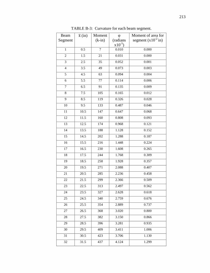
213

213

TABLE B-3: Curvature for each beam segment.

Beam

Segment (in) Moment

(k-in)

φ

(radians

x10-5

)

Moment of area for

segment (x10-2

in)

1 0.5 7 0.010 0.000

2 1.5 21 0.031 0.000

3 2.5 35 0.052 0.001

4 3.5 49 0.073 0.003

5 4.5 63 0.094 0.004

6 5.5 77 0.114 0.006

7 6.5 91 0.135 0.009

8 7.5 105 0.165 0.012

9 8.5 119 0.326 0.028

10 9.5 133 0.487 0.046

11 10.5 147 0.647 0.068

12 11.5 160 0.808 0.093

13 12.5 174 0.968 0.121

14 13.5 188 1.128 0.152

15 14.5 202 1.288 0.187

16 15.5 216 1.448 0.224

17 16.5 230 1.608 0.265

18 17.5 244 1.768 0.309

19 18.5 258 1.928 0.357

20 19.5 271 2.088 0.407

21 20.5 285 2.236 0.458

22 21.5 299 2.366 0.509

23 22.5 313 2.497 0.562

24 23.5 327 2.628 0.618

25 24.5 340 2.759 0.676

26 25.5 354 2.889 0.737

27 26.5 368 3.020 0.800

28 27.5 382 3.150 0.866

29 28.5 396 3.281 0.935

30 29.5 409 3.411 1.006

31 30.5 423 3.706 1.130

32 31.5 437 4.124 1.299

214

214

Beam

Segment (in) Moment

(k-in)

φ

(radians

x10-5

)

Moment of area for

segment (x10-2

in)

33 32.5 451 4.541 1.476

34 33.5 464 4.958 1.661

35 34.5 478 5.461 1.884

36 35.5 492 6.459 2.293

37 36.5 505 7.455 2.721

38 37.5 519 8.792 3.297

39 38.5 533 10.147 3.907

40 39.5 547 11.544 4.560

41 40.5 553 12.249 4.961

42 41.5 554 12.265 5.090

43 42.5 554 12.280 5.219

44 43.5 554 12.293 5.348

45 44.5 554 12.307 5.476

46 45.5 554 12.319 5.605

47 46.5 554 12.330 5.734

48 47.5 554 12.341 5.862

49 48.5 554 12.351 5.990

50 49.5 555 12.360 6.118

51 50.5 555 12.368 6.246

52 51.5 555 12.375 6.373

53 52.5 555 12.382 6.500

54 53.5 555 12.387 6.627

55 54.5 555 12.392 6.754

56 55.5 555 12.396 6.880

57 56.5 555 12.400 7.006

58 57.5 555 12.402 7.131

59 58.5 555 12.404 7.256

60 59.5 555 12.405 7.381

engineering characterization of waste derived geopolymer

Documents

Transcript of engineering characterization of waste derived geopolymer