Measuring and testing dependence by correlation of distances

arX

iv:0

803.

4101

v1 [

mat

h.ST

] 2

8 M

ar 2

008

The Annals of Statistics

2007, Vol. 35, No. 6, 2769–2794DOI: 10.1214/009053607000000505c© Institute of Mathematical Statistics, 2007

MEASURING AND TESTING DEPENDENCE BY CORRELATIONOF DISTANCES

By Gabor J. Szekely,1 Maria L. Rizzo and Nail K. Bakirov

Bowling Green State University, Bowling Green State University andUSC Russian Academy of Sciences

Distance correlation is a new measure of dependence between ran-dom vectors. Distance covariance and distance correlation are anal-ogous to product-moment covariance and correlation, but unlike theclassical definition of correlation, distance correlation is zero only ifthe random vectors are independent. The empirical distance depen-dence measures are based on certain Euclidean distances betweensample elements rather than sample moments, yet have a compactrepresentation analogous to the classical covariance and correlation.Asymptotic properties and applications in testing independence arediscussed. Implementation of the test and Monte Carlo results arealso presented.

1. Introduction. Distance correlation provides a new approach to theproblem of testing the joint independence of random vectors. For all dis-tributions with finite first moments, distance correlation R generalizes theidea of correlation in two fundamental ways:

(i) R(X,Y ) is defined for X and Y in arbitrary dimensions;(ii) R(X,Y ) = 0 characterizes independence of X and Y .

Distance correlation has properties of a true dependence measure, analogousto product-moment correlation ρ. Distance correlation satisfies 0 ≤R ≤ 1,and R= 0 only if X and Y are independent. In the bivariate normal case,R is a function of ρ, and R(X,Y )≤ |ρ(X,Y )| with equality when ρ = ±1.

Throughout this paper X in Rp and Y in R

q are random vectors, wherep and q are positive integers. The characteristic functions of X and Y aredenoted fX and fY , respectively, and the joint characteristic function of X

Received November 2006; revised March 2007.1Supported by the National Science Foundation while working at the Foundation.AMS 2000 subject classifications. Primary 62G10; secondary 62H20.Key words and phrases. Distance correlation, distance covariance, multivariate inde-

pendence.

This is an electronic reprint of the original article published by theInstitute of Mathematical Statistics in The Annals of Statistics,2007, Vol. 35, No. 6, 2769–2794. This reprint differs from the original inpagination and typographic detail.

1

http://arXiv.org/abs/0803.4101v1

http://www.imstat.org/aos/

http://dx.doi.org/10.1214/009053607000000505

http://www.imstat.org

http://www.ams.org/msc/

http://www.imstat.org

http://www.imstat.org/aos/

http://dx.doi.org/10.1214/009053607000000505

2 G. J. SZEKELY, M. L. RIZZO AND N. K. BAKIROV

and Y is denoted fX,Y . Distance covariance V can be applied to measure thedistance ‖fX,Y (t, s)− fX(t)fY (s)‖ between the joint characteristic functionand the product of the marginal characteristic functions (the norm ‖ · ‖ isdefined in Section 2), and to test the hypothesis of independence

H0 :fX,Y = fXfY vs. H1 :fX,Y 6= fXfY .

The importance of the independence assumption for inference arises, for ex-ample, in clinical studies with the case-only design, which uses only diseasedsubjects assumed to be independent in the study population. In this design,inferences on multiplicative gene interactions (see [1]) can be highly distortedwhen there is a departure from independence. Classical methods such as theWilks Lambda [14] or Puri–Sen [8] likelihood ratio tests are not applicable ifthe dimension exceeds the sample size, or when distributional assumptionsdo not hold (see, e.g., [7] regarding the prevalence of nonnormality in biol-ogy and ecology). A further limitation of multivariate extensions of methodsbased on ranks is that they are ineffective for testing nonmonotone types ofdependence.

We propose an omnibus test of independence that is easily implementedin arbitrary dimension. In our Monte Carlo results the distance covariancetest exhibits superior power against nonmonotone types of dependence whilemaintaining good power performance in the multivariate normal case rela-tive to the parametric likelihood ratio test. Distance correlation can also beapplied as an index of dependence; for example, in meta-analysis [12] dis-tance correlation would be a more generally applicable index than product-moment correlation, without requiring normality for valid inferences.

Theoretical properties of distance covariance and correlation are coveredin Section 2, extensions in Section 3, and results for the bivariate normalcase in Section 4. Empirical results are presented in Section 5, followed bya summary in Section 6.

2. Theoretical properties of distance dependence measures.Notation. The scalar product of vectors t and s is denoted by 〈t, s〉. For

complex-valued functions f(·), the complex conjugate of f is denoted byf and |f |2 = f f. The Euclidean norm of x in R

p is |x|p. A sample fromthe distribution of X in R

p is denoted by the n × p matrix X, and thesample vectors (rows) are labeled X1, . . . ,Xn. A primed variable X ′ is anindependent copy of X ; that is, X and X ′ are independent and identicallydistributed.

Definition 1. For complex functions γ defined on Rp × R

q the ‖ · ‖w-norm in the weighted L2 space of functions on R

p+q is defined by

‖γ(t, s)‖2w =

∫

Rp+q|γ(t, s)|2w(t, s)dt ds,(2.1)

DISTANCE CORRELATION 3

where w(t, s) is an arbitrary positive weight function for which the integralabove exists.

2.1. Choice of weight function. Using the ‖ · ‖w-norm (2.1) with a suit-able choice of weight function w(t, s), we define a measure of dependence

V2(X,Y ;w) = ‖fX,Y (t, s)− fX(t)fY (s)‖2w

(2.2)

=

∫

Rp+q|fX,Y (t, s)− fX(t)fY (s)|2w(t, s)dt ds,

such that V2(X,Y ;w) = 0 if and only if X and Y are independent. In thispaper V will be analogous to the absolute value of the classical product-moment covariance. If we divide V(X,Y ;w) by

√V(X;w)V(Y ;w), where

V2(X;w) =

∫

R2p|fX,X(t, s)− fX(t)fX(s)|2w(t, s)dt ds,

we have a type of unsigned correlation Rw.Not every weight function leads to an “interesting” Rw, however. The

coefficient Rw should be scale invariant, that is, invariant with respect totransformations (X,Y ) 7→ (ǫX, ǫY ), for ǫ > 0. We also require that Rw ispositive for dependent variables. It is easy to check that if the weight functionw(t, s) is integrable, and both X and Y have finite variance, then the Taylorexpansions of the underlying characteristic functions show that

limǫ→0

V2(ǫX, ǫY ;w)√V2(ǫX;w)V2(ǫY ;w)

= ρ2(X,Y ).

Thus for integrable w, if ρ = 0, then Rw can be arbitrarily close to zero evenif X and Y are dependent. However, by applying a nonintegrable weightfunction, we obtain an Rw that is scale invariant and cannot be zero fordependent X and Y . We do not claim that our choice for w is the onlyreasonable one, but it will become clear in the following sections that ourchoice (2.4) results in very simple and applicable empirical formulas. (A morecomplicated weight function is applied in [2], which leads to a more com-putationally difficult statistic and does not have the interesting correlationform.)

The crucial observation is the following lemma.

Lemma 1. If 0 < α < 2, then for all x in Rd

∫

Rd

1− cos〈t, x〉|t|d+α

d

dt = C(d,α)|x|α,

where

C(d,α) =2πd/2Γ(1−α/2)

α2αΓ((d + α)/2)


and Γ(·) is the complete gamma function. The integrals at 0 and ∞ aremeant in the principal value sense: limε→0

∫Rd\{εB+ε−1Bc}, where B is the

unit ball (centered at 0) in Rd and Bc is the complement of B.

See [11] for the proof of Lemma 1. In the simplest case, α = 1, the constant

in Lemma 1 is

cd = C(d,1) =π(1+d)/2

Γ((1 + d)/2).(2.3)

In view of Lemma 1, it is natural to choose the weight function

w(t, s) = (cp cq |t|1+pp |s|1+q

q )−1,(2.4)

corresponding to α = 1. We apply the weight function (2.4) and the cor-

responding weighted L2 norm ‖ · ‖, omitting the index w, and write thedependence measure (2.2) as V2(X,Y ). In integrals we also use the symbol

dω, which is defined by

dω = (cp cq |t|1+pp |s|1+q

q )−1 dt ds.

For finiteness of ‖fX,Y (t, s)−fX(t)fY (s)‖2 it is sufficient that E|X|p <∞and E|Y |q <∞. By the Cauchy–Bunyakovsky inequality

|fX,Y (t, s)− fX(t)fY (s)|2 = [E(ei〈t,X〉 − fX(t))(ei〈s,Y 〉 − fY (s))]2

≤ E[ei〈t,X〉 − fX(t)]2E[ei〈s,Y 〉 − fY (s)]2

= (1− |fX(t)|2)(1− |fY (s)|2).

If E(|X|p + |Y |q) <∞, then by Lemma 1 and by Fubini’s theorem it followsthat

∫

Rp+q|fX,Y (t, s)− fX(t)fY (s)|2 dω

≤∫

Rp

1− |fX(t)|2

cp|t|1+pp

dt

∫

Rq

1− |fY (s)|2

cq|s|1+qq

ds

(2.5)

= E

[∫

Rp

1− cos〈t,X −X ′〉cp|t|1+p

p

dt

]·E

[∫

Rq

1− cos〈s,Y − Y ′〉cq|s|1+q

q

ds

]

= E|X −X ′|pE|Y − Y ′|q < ∞.

Thus we have the following definitions.


2.2. Distance covariance and distance correlation.

Definition 2 (Distance covariance). The distance covariance (dCov)between random vectors X and Y with finite first moments is the nonneg-ative number V(X,Y ) defined by

V2(X,Y ) = ‖fX,Y (t, s)− fX(t)fY (s)‖2

(2.6)

=1

cpcq

∫

Rp+q

|fX,Y (t, s)− fX(t)fY (s)|2|t|1+p

p |s|1+qq

dt ds.

Similarly, distance variance (dVar) is defined as the square root of

V2(X) = V2(X,X) = ‖fX,X(t, s)− fX(t)fX(s)‖2.

Remark 1. If E(|X|p + |Y |q) = ∞ but E(|X|αp + |Y |αq ) < ∞ for some

0 < α < 1, then one can apply V(α) and R(α) (see Section 3.1); otherwiseone can apply a suitable transformation of (X,Y ) into bounded random

variables (X, Y ) such that X and Y are independent if and only if X andY are independent.

Definition 3 (Distance correlation). The distance correlation (dCor)between random vectors X and Y with finite first moments is the nonneg-ative number R(X,Y ) defined by

R2(X,Y ) =

V2(X,Y )√V2(X)V2(Y )

, V2(X)V2(Y ) > 0,

0, V2(X)V2(Y ) = 0.

(2.7)

Clearly the definition of R in (2.7) suggests an analogy with the product-moment correlation coefficient ρ. Analogous properties are established inTheorem 3. The relation between V , R and ρ in the bivariate normal casewill be established in Theorem 7.

The distance dependence statistics are defined as follows. For an observedrandom sample (X,Y) = {(Xk, Yk) :k = 1, . . . , n} from the joint distributionof random vectors X in R

p and Y in Rq, define

akl = |Xk −Xl|p, ak·=

1

n

n∑

l=1

akl, a·l,=

1

n

n∑

k=1

akl,

a··

=1

n2

n∑

k,l=1

akl, Akl = akl − ak·− a

·l + a··,


k, l = 1, . . . , n. Similarly, define bkl = |Yk − Yl|q and Bkl = bkl − bk·− b

·l + b··,

for k, l = 1, . . . , n.

Definition 4. The empirical distance covariance Vn(X,Y) is the non-negative number defined by

V2n(X,Y) =

1

n2

n∑

k,l=1

AklBkl.(2.8)

Similarly, Vn(X) is the nonnegative number defined by

V2n(X) = V2

n(X,X) =1

n2

n∑

k,l=1

A2kl.(2.9)

Although it may not be immediately obvious that V2n(X,Y)≥ 0, this fact

as well as the motivation for the definition of Vn will be clear from Theorem1 below.

Definition 5. The empirical distance correlation Rn(X,Y) is the squareroot of

R2n(X,Y) =

V2n(X,Y)√

V2n(X)V2

n(Y), V2

n(X)V2n(Y) > 0,

0, V2n(X)V2

n(Y) = 0.

(2.10)

Remark 2. The statistic Vn(X) = 0 if and only if every sample observa-tion is identical. Indeed, if Vn(X) = 0, then Akl = 0 for k, l = 1, . . . , n. Thus0 = Akk =−ak·

− a·k + a

··implies that ak·

= a·k = a

··/2, and

0 = Akl = akl − ak·− a

·l + a··

= akl = |Xk −Xl|p,so X1 = · · ·= Xn.

It is clear that Rn is easy to compute, and in the following sections it willbe shown that Rn is a good empirical measure of dependence.

2.3. Properties of distance covariance. It would have been natural, butless elementary, to define Vn(X,Y) as ‖fn

X,Y (t, s)− fnX(t)fn

Y (s)‖, where

fnX,Y (t, s) =

1

n

n∑

k=1

exp{i〈t,Xk〉+ i〈s,Yk〉}

is the empirical characteristic function of the sample, {(X1, Y1), . . . , (Xn, Yn)},and

fnX(t) =

1

n

n∑

k=1

exp{i〈t,Xk〉}, fnY (s) =

1

n

n∑

k=1

exp{i〈s,Yk〉}


are the marginal empirical characteristic functions of the X sample and Ysample, respectively. Our first theorem shows that the two definitions areequivalent.

Theorem 1. If (X,Y) is a sample from the joint distribution of (X,Y ),then

V2n(X,Y) = ‖fn

X,Y (t, s)− fnX(t)fn

Y (s)‖2.

Proof. Lemma 1 implies that there exist constants cp and cq such thatfor all X in R

p, Y in Rq,

∫

Rp

1− exp{i〈t,X〉}|t|1+p

p

dt = cp|X|p,(2.11)

∫

Rq

1− exp{i〈s,Y 〉}|s|1+q

q

ds = cq|Y |q,(2.12)

∫

Rp

∫

Rq

1− exp{i〈t,X〉 + i〈s,Y 〉}|t|1+p

p |s|1+qq

dt ds = cpcq|X|p|Y |q,(2.13)

where the integrals are understood in the principal value sense. For sim-plicity, consider the case p = q = 1. The distance between the empiricalcharacteristic functions in the weighted norm w(t, s) = π−2t−2s−2 involves|fn

X,Y (t, s)|2, |fnX(t)fn

Y (s)|2 and fnX,Y (t, s)fn

X(t)fnY (s). For the first we have

fnX,Y (t, s)fn

X,Y (t, s) =1

n2

n∑

k,l=1

cos(Xk −Xl)t cos(Yk − Yl)s + V1,

where V1 represents terms that vanish when the integral ‖fnX,Y (t, s)−fn

X(t)fnY (s)‖2

is evaluated. The second expression is

fnX(t)fn

Y (s)fnX(t)fn

Y (s)

=1

n2

n∑

k,l=1

cos(Xk −Xl)t1

n2

n∑

k,l=1

cos(Yk − Yl)s + V2

and the third is

fnX,Y (t, s)fn

X(t)fnY (s)

=1

n3

n∑

k,l,m=1

cos(Xk −Xl)t cos(Yk − Ym)s + V3,

where V2 and V3 represent terms that vanish when the integral is evaluated.To evaluate the integral ‖fn

X,Y (t, s) − fnX(t)fn

Y (s)‖2, apply Lemma 1, andstatements (2.11), (2.12) and (2.13) using

cosu cosv = 1− (1− cosu)− (1− cos v) + (1− cosu)(1− cosv).


After cancellation in the numerator of the integrand it remains to evaluateintegrals of the type

∫

R2(1− cos(Xk −Xl)t)(1− cos(Yk − Yl)s)

dt

t2ds

s2

=

∫

R

(1− cos(Xk −Xl)t)dt

t2

×∫

R

(1− cos(Yk − Yl)s)ds

s2

= c21|Xk −Xl| |Yk − Yl|.

For random vectors X in Rp and Y in R

q, the same steps are appliedusing w(t, s) = {cp cq|t|1+p

p |s|1+qq }−1. Thus

‖fnX,Y (t, s)− fn

X(t)fnY (s)‖2 = S1 + S2 − 2S3,(2.14)

where

S1 =1

n2

n∑

k,l=1

|Xk −Xl|p|Yk − Yl|q,(2.15)

S2 =1

n2

n∑

k,l=1

|Xk −Xl|p1

n2

n∑

k,l=1

|Yk − Yl|q,(2.16)

S3 =1

n3

n∑

k=1

n∑

l,m=1

|Xk −Xl|p|Yk − Ym|q.(2.17)

To complete the proof we need to verify the algebraic identity

V2n(X,Y) = S1 + S2 − 2S3.(2.18)

For the proof of (2.18) see the Appendix. Then (2.14) and (2.18) imply thatV2

n(X,Y) = ‖fnX,Y (t, s)− fn

X(t)fnY (s)‖2. �

Theorem 2. If E|X|p <∞ and E|Y |q < ∞, then almost surely

limn→∞

Vn(X,Y ) = V(X,Y ).(2.19)

Proof. Define

ξn(t, s) =1

n

n∑

k=1

ei〈t,Xk〉+i〈s,Yk〉 − 1

n

n∑

k=1

ei〈t,Xk〉 1n

n∑

k=1

ei〈s,Yk〉,

so that V2n = ‖ξn(t, s)‖2. Then after elementary transformations

ξn(t, s) =1

n

n∑

k=1

ukvk −1

n

n∑

k=1

uk1

n

n∑

k=1

vk,


where uk = exp(i〈t,Xk〉)− fX(t) and vk = exp(i〈s,Yk〉)− fY (s).For each δ > 0 define the region

D(δ) = {(t, s) : δ ≤ |t|p ≤ 1/δ, δ ≤ |s|q ≤ 1/δ}(2.20)

and random variables

V2n,δ =

∫

D(δ)|ξn(t, s)|2 dω.

For any fixed δ > 0, the weight function w(t, s) is bounded on D(δ). HenceV2

n,δ is a combination of V -statistics of bounded random variables. For eachδ > 0 by the strong law of large numbers (SLLN) for V -statistics, it followsthat almost surely

limn→∞V2

n,δ = V2·,δ =

∫

D(δ)|fX,Y (t, s)− fX(t)fY (s)|2 dω.

Clearly V2·,δ converges to V2 as δ tends to zero. Now it remains to prove that

almost surely

lim supδ→0

lim supn→∞

|V2n,δ −V2

n|= 0.(2.21)

For each δ > 0

|V2n,δ −V2

n| ≤∫

|t|p<δ|ξn(t, s)|2 dω +

∫

|t|p>1/δ|ξn(t, s)|2 dω

(2.22)

+

∫

|s|q<δ|ξn(t, s)|2 dω +

∫

|s|q>1/δ|ξn(t, s)|2 dω.

For z = (z1, z2, . . . , zp) in Rp define the function

G(y) =

∫

|z|<y

1− cos z1

|z|1+pdz.

Clearly G(y) is bounded by cp and limy→0 G(y) = 0. Applying the inequality|x + y|2 ≤ 2|x|2 + 2|y|2 and the Cauchy–Bunyakovsky inequality for sums,one can obtain that

|ξn(t, s)|2 ≤ 2

∣∣∣∣∣1

n

n∑

k=1

ukvk

∣∣∣∣∣

2

+ 2

∣∣∣∣∣1

n

n∑

k=1

uk1

n

n∑

k=1

vk

∣∣∣∣∣

2

(2.23)

≤ 4

n

n∑

k=1

|uk|21

n

n∑

k=1

|vk|2.

Hence the first summand in (2.22) satisfies

∫

|t|p<δ|ξn(t, s)|2 dω ≤ 4

n

n∑

k=1

∫

|t|p<δ

|uk|2 dt

cp|t|1+pp

1

n

n∑

k=1

∫

Rq

|vk|2 ds

cq|s|1+qq

.(2.24)


Here |vk|2 = 1 + |fY (s)|2 − ei〈s,Yk〉fY (s)− e−i〈s,Yk〉fY (s), thus∫

Rq

|vk|2 ds

cq|s|1+qq

= (2EY |Yk − Y | −E|Y − Y ′|) ≤ 2(|Yk|+ E|Y |),

where the expectation EY is taken with respect to Y , and Y ′ D= Y is inde-

pendent of Yk. Further, after a suitable change of variables∫

|t|p<δ

|uk|2 dt

cp|t|1+pp

= 2EX |Xk −X|G(|Xk −X|δ) −E|X −X ′|G(|X −X ′|δ)

≤ 2EX |Xk −X|G(|Xk −X|δ),

where the expectation EX is taken with respect to X , and X ′ D= X is inde-

pendent of Xk. Therefore, from (2.24)∫

|t|p<δ|ξn(t, s)|2 dω

≤ 42

n

n∑

k=1

(|Yk|+ E|Y |) 2

n

n∑

k=1

EX |Xk −X|G(|Xk −X|δ).

By the SLLN

limsupn→∞

∫

|t|p<δ|ξn(t, s)|2 dω ≤ 4 · 2 · 2E|Y | · 2E|X1 −X2|G(|X1 −X2|δ)

almost surely. Therefore by the Lebesgue bounded convergence theorem forintegrals and expectations

lim supδ→0

lim supn→∞

∫

|t|p<δ|ξn(t, s)|2 dω = 0

almost surely.Consider now the second summand in (2.22). Inequalities (2.23) imply

that |uk|2 ≤ 4 and 1n

∑nk=1 |uk|2 ≤ 4, hence

∫

|t|p>1/δ

|uk|2 dt

cp|t|1+pp

≤ 16

∫

|t|p>1/δ

dt

cp|t|1+pp

∫

Rq

1

n

n∑

k=1

|vk|2ds

cq|s|1+qq

≤ 16δ2

n

n∑

k=1

(|Yk|+ E|Y |).

Thus, almost surely

lim supδ→0

lim supn→∞

∫

|t|p>1/δ|ξn(t, s)|2 dω = 0.

One can apply a similar argument to the remaining summands in (2.22) toobtain (2.21). �


Corollary 1. If E(|X|p + |Y |q) < ∞, then almost surely,

limn→∞

R2n(X,Y) = R2(X,Y ).

The definition of dCor suggests that our distance dependence measuresare analogous in at least some respects to the corresponding product-momentcorrelation. By analogy, certain properties of classical correlation and vari-ance definitions should also hold for dCor and dVar. These properties areestablished in Theorems 3 and 4.

Theorem 3 (Properties of dCor).

(i) If E(|X|p + |Y |q) <∞, then 0≤R≤ 1, and R(X,Y ) = 0 if and onlyif X and Y are independent.

(ii) 0 ≤Rn ≤ 1.(iii) If Rn(X,Y) = 1, then there exist a vector a, a nonzero real number

b and an orthogonal matrix C such that Y = a + bXC.

Proof. In (i), R(X,Y ) exists whenever X and Y have finite first mo-ments, and X and Y are independent if and only if the numerator

V2(X,Y ) = ‖fX,Y (t, s)− fX(t)fY (s)‖2

of R2(X,Y ) is zero. Let U = ei〈t,X〉 − fX(t) and V = ei〈s,Y 〉 − fY (s). Then

|fX,Y (t, s)− fX(t)fY (s)|2 = |E[UV ]|2 ≤ (E[|U | |V |])2 ≤ E[|U |2|V |2]= (1− |fX(t)|2)(1− |fY (s)|2).

Thus∫

Rp+q|fX,Y (t, s)− fX(t)fY (s)|2 dω

≤∫

Rp+q|(1− |fX(t)|2)(1− |fY (s)|2)|2 dω;

hence 0≤R(X,Y ) ≤ 1, and (ii) follows by a similar argument.(iii) If Rn(X,Y) = 1, then the arguments below show that X and Y are

similar almost surely, thus the dimensions of the linear subspaces spannedby X and Y respectively are almost surely equal. (Here similar means thatY and εX are isometric for some ε 6= 0.) For simplicity we can suppose thatX and Y are in the same Euclidean space and both span R

p. From theCauchy–Bunyakovski inequality it is easy to see that Rn(X,Y) = 1 if andonly if Ak l = εBk l for some factor ε. Suppose that |ε| = 1. Then

|Xk −Xl|p = |Yk − Yl|q + dk + dl


for all k, l, for some constants dk, dl. Then with k = l we obtain dk = 0 forall k. Now, one can apply a geometric argument. The two samples are iso-metric, so Y can be obtained from X through operations of shift, rotationand reflection, and hence Y = a+ bXC for some vector a, b = ε and orthog-onal matrix C. If |ε| 6= 1 and ε 6= 0, apply the geometric argument to εXand Y and it follows that Y = a + bXC where b = ε. �

Theorem 4 (Properties of dVar). The following properties hold for ran-dom vectors with finite first moments:

(i) dVar(X) = 0 implies that X = E[X], almost surely.(ii) dVar(a+bCX) = |b|dVar(X) for all constant vectors a in R

p, scalarsb and p× p orthonormal matrices C.

(iii) dVar(X + Y ) ≤ dVar(X)+ dVar(Y ) for independent random vectorsX in R

p and Y in Rp.

Proof. (i) If dVar(X) = 0, then

(dVar(X))2 =

∫

Rp

∫

Rp

|fX,X(t, s)− fX(t)fX(s)|2c2p|t|p+1

p |s|p+1p

dt ds = 0,

or equivalently, fX,X(t, s) = fX(t + s) = fX(t)fX(s) for all t, s. That is,

fX(t) = ei〈c,t〉 for some constant vector c, and hence X is a constant vector,almost surely.

Statement (ii) is obvious.(iii) Let ∆ = fX+Y,X+Y (t, s)−fX(t+s)fY (t+s), ∆1 = fX(t, s)−fX(t)fX(s)

and ∆2 = fY (t, s)− fY (t)fY (s). If X and Y are independent, then

∆ = fX+Y,X+Y (t, s)− fX+Y (t)fX+Y (s)

= fX(t + s)fY (t + s)− fX(t)fX(s)fY (t)fY (s)

= [fX(t + s)− fX(t)fX(s)]fY (t + s)

+ fX(t)fX(s)[fY (t + s)− fY (t)fY (s)]

= ∆1fY (t + s) + fX(t)fX(s)∆2,

and therefore |∆|2 ≤ |∆1|2 + |∆2|2 + 2|∆1| |∆2|. Equality holds if and only if∆1∆2 = 0, that is, if and only if X or Y is a constant almost surely. �

2.4. Asymptotic properties of nV2n. Our proposed test of independence

is based on the statistic nV2n/S2. If E(|X|p + |Y |q) < ∞, we prove that under

independence nV2n/S2 converges in distribution to a quadratic form

QD=

∞∑

j=1

λjZ2j ,(2.25)


where Zj are independent standard normal random variables, {λj} are non-negative constants that depend on the distribution of (X,Y ) and E[Q] = 1.A test of independence that rejects independence for large nV2

n/S2 is statis-tically consistent against all alternatives with finite first moments.

Let ζ(·) denote a complex-valued zero-mean Gaussian random processwith covariance function

R(u,u0) = (fX(t− t0)− fX(t)fX(t0))(fY (s− s0)− fY (s)fY (s0)),

where u = (t, s), u0 = (t0, s0) ∈ Rp ×R

q.

Theorem 5 (Weak convergence). If X and Y are independent andE(|X|p + |Y |q) <∞, then

nV2n

D−→n→∞

‖ζ(t, s)‖2.

Proof. Define the empirical process

ζn(u) = ζn(t, s) =√

nξn(t, s) =√

n(fnX,Y (t, s)− fn

X(t)fnY (s)).

Under the independence hypothesis, E[ζn(u)] = 0 and E[ζn(u)ζn(u0)] =n−1

n ×R(u,u0). In particular, E|ζn(u)|2 = n−1

n (1− |fX(t)|2)(1− |fY (s)|2)≤ 1.For each δ > 0 we construct a sequence of random variables {Qn(δ)} with

the following properties:

(i) Qn(δ) converges in distribution to a random variable Q(δ).(ii) E|Qn(δ)− ζn| ≤ δ.(iii) E|Q(δ)− ζ| ≤ δ.

Then the weak convergence of ‖ζn‖2 to ‖ζ‖2 follows from the convergenceof the corresponding characteristic functions.

The sequence Qn(δ) is defined as follows. Given ǫ > 0, choose a partition{Dk}N

k=1 of D(δ) (2.20) into N = N(ǫ) measurable sets with diameter atmost ǫ. Define

Qn(δ) =N∑

k=1

∫

Dk

|ζn|2 dω.

For a fixed M > 0 let

β(ǫ) = supu,u0

E||ζn(u)|2 − |ζn(u0)|2|,

where the supremum is taken over all u = (t, s) and u0 = (t0, s0) such thatmax{|t|, |t0|, |s|, |s0|} < M , and |t− t0|2 + |s−s0|2 < ǫ2. Then limǫ→0 β(ǫ) = 0for every fixed M > 0, and for fixed δ > 0

E

∣∣∣∣∫

D(δ)|ζn(u)|2 dω −Qn(δ)

∣∣∣∣ ≤ β(ǫ)

∫

D|ζn(u)|2 dω−→

ǫ→0= 0.


On the other hand,∣∣∣∣∫

D|ζn(u)|2 dω −

∫

Rp+q|ζn(u)|2 dω

∣∣∣∣

≤∫

|t|<δ|ζn(u)|2 dω +

∫

|t|>1/δ|ζn(u)|2 dω

+

∫

|s|<δ|ζn(u)|2 dω +

∫

|s|>1/δ|ζn(u)|2 dω.

By similar steps as in the proof of Theorem 2, one can derive that

E

[∫

|t|<δ|ζn(u)|2 dω +

∫

|t|>1/δ|ζn(u)|2 dω

]

≤ n− 1

n(E|X1 −X2|G(|X1 −X2|δ) + wpδ)E|Y1 − Y2|δ−→

δ→00,

where wp is a constant depending only on p, and similarly

E

[∫

|s|<δ|ζn(u)|2 dω +

∫

|s|>1/δ|ζn(u)|2 dω

]−→δ→0

0.

Similar inequalities also hold for the random process ζ(t, s) with

Q(δ) =N∑

k=1

∫

Dk

|ζ(u)|2 dω.

The weak convergence of Qn(δ) to Q(δ) as n →∞ follows from the multi-

variate central limit theorem, and therefore nV2n = ‖ζn‖2 D−→

n→∞‖ζ‖2. �

Corollary 2. If E(|X|p + |Y |q) < ∞, then:

(i) If X and Y are independent, nV2n/S2

D−→n→∞

Q where Q is a non-

negative quadratic form of centered Gaussian random variables (2.25) andE[Q] = 1.

(ii) If X and Y are dependent, then nV2n/S2

P−→n→∞

∞.

Proof. (i) The independence of X and Y implies that ζn and thus ζ is azero-mean process. According to Kuo [5], Chapter 1, Section 2, the squarednorm ‖ζ‖2 of the zero-mean Gaussian process ζ has the representation

‖ζ‖2 D=

∞∑

j=1

λjZ2j ,(2.26)

where Zj are independent standard normal random variables, and the non-negative constants {λj} depend on the distribution of (X,Y ). Hence, under


independence, nV2n converges in distribution to a quadratic form (2.26). It

follows from (2.5) that

E‖ζ‖2 =

∫

Rp+qR(u,u)dω

=

∫

Rp+q(1− |fX(t)|2)(1− |fY (s)|2)dω

= E(|X −X ′|p|Y − Y ′|q).

By the SLLN for V -statistics, S2a.s.−→

n→∞E(|X−X ′|p|Y −Y ′|q). Therefore nV2n/

S2D−→

n→∞Q, where E[Q] = 1 and Q is the quadratic form (2.25).

(ii) Suppose that X and Y are dependent and E(|X|p + |Y |q) < ∞.

Then V(X,Y ) > 0, Theorem 2 implies that V2n(X,Y)

a.s.−→n→∞

V2(X,Y ) > 0, and

therefore nV2n(X,Y)

P−→n→∞

∞. By the SLLN, S2 converges to a constant and

therefore nV2n/S2

P−→n→∞

∞. �

Theorem 6. Suppose T (X,Y,α,n) is the test that rejects independenceif

nV2n(X,Y)

S2> (Φ−1(1−α/2))2,

where Φ(·) denotes the standard normal cumulative distribution function,and let α(X,Y,n) denote the achieved significance level of T (X,Y,α,n). IfE(|X|p + |Y |q) <∞, then for all 0 < α≤ 0.215

(i) limn→∞ α(X,Y,n) ≤ α,(ii) supX,Y {limn→∞ α(X,Y,n) :V(X,Y ) = 0}= α.

Proof. (i) The following inequality is proved as a special case of atheorem of Szekely and Bakirov [9], page 189. If Q is a quadratic form ofcentered Gaussian random variables and E[Q] = 1, then

P{Q≥ (Φ−1(1−α/2))2} ≤ α

for all 0 < α≤ 0.215.(ii) For Bernoulli random variables X and Y we have that Rn(X,Y) =

|ρ(X,Y)|. By the central limit theorem, under independence√

nρ(X,Y) isasymptotically normal. Thus, in case X and Y are independent Bernoullivariables, the quadratic form Q contains only one term, Q = Z2

1 , and theupper bound α is achieved. �


Thus, a test rejecting independence of X and Y when√

nV2n/S2 ≥ Φ−1(1−

α/2) has an asymptotic significance level at most α. The asymptotic test cri-terion could be quite conservative for many distributions. Alternatively onecan estimate the critical value for the test by conditioning on the observedsample, which is discussed in Section 5.

Remark 3. If E|X|2p <∞ and E|Y |2q < ∞, then E[|X|p|Y |q] < ∞, so byLemma 1 and by Fubini’s theorem we can evaluate

V2(X,Y ) = E[|X1 −X2|p|Y1 − Y2|q] + E|X1 −X2|p E|Y1 − Y2|q− 2E[|X1 −X2|p|Y1 − Y3|q].

If second moments exist, Theorem 2 and weak convergence can be estab-lished by V -statistic limit theorems [13]. Under the null hypothesis of inde-pendence, V2

n is a degenerate kernel V -statistic. The first-order degeneracyfollows from inequalities proved in [10]. Thus nV2

n converges in distributionto a quadratic form (2.26).

3. Extensions.

3.1. The class of α-distance dependence measures. We introduce a one-parameter family of distance dependence measures indexed by a positiveexponent α. In our definition of dCor we have applied exponent α = 1.

Suppose that E(|X|αp + |Y |αq ) <∞. Let V(α) denote the α-distance covari-ance, which is the nonnegative number defined by

V2(α)(X,Y ) = ‖fX,Y (t, s)− fX(t)fY (s)‖2α

=1

C(p,α)C(q,α)

∫

Rp+q

|fX,Y (t, s)− fX(t)fY (s)|2|t|α+p

p |s|α+qq

dt ds.

Similarly, R(α) denotes α-distance correlation, which is the square root of

R2(α) =V2(α)(X,Y )√

V2(α)(X)V2(α)(Y ), 0 < V2(α)(X), V2(α)(Y ) <∞,

and R(α) = 0 if V2(α)(X)V2(α)(Y ) = 0.The α-distance dependence statistics are defined by replacing the expo-

nent 1 with exponent α in the distance dependence statistics (2.8), (2.9) and(2.10). That is, replace akl = |Xk − Xl|p with akl = |Xk − Xl|αp and replacebkl = |Yk − Yl|q with bkl = |Yk − Yl|αq , k, l = 1, . . . , n.

Theorem 2 can be generalized for ‖ · ‖α-norms, so that almost sure con-

vergence of V(α)n → V(α) follows if the α-moments are finite. Similarly one

can prove the weak convergence and statistical consistency for α exponents,0 < α < 2, provided that α moments are finite.


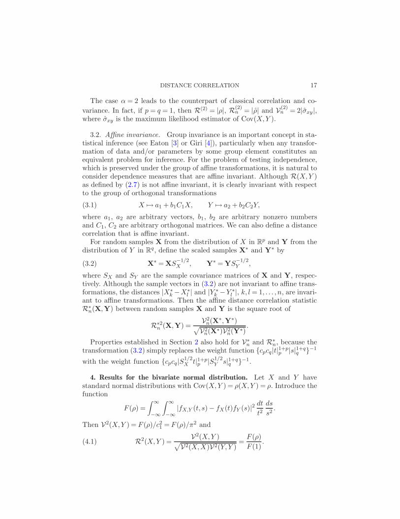
The case α = 2 leads to the counterpart of classical correlation and co-

variance. In fact, if p = q = 1, then R(2) = |ρ|, R(2)n = |ρ| and V(2)

n = 2|σxy|,where σxy is the maximum likelihood estimator of Cov(X,Y ).

3.2. Affine invariance. Group invariance is an important concept in sta-tistical inference (see Eaton [3] or Giri [4]), particularly when any transfor-mation of data and/or parameters by some group element constitutes anequivalent problem for inference. For the problem of testing independence,which is preserved under the group of affine transformations, it is natural toconsider dependence measures that are affine invariant. Although R(X,Y )as defined by (2.7) is not affine invariant, it is clearly invariant with respectto the group of orthogonal transformations

X 7→ a1 + b1C1X, Y 7→ a2 + b2C2Y,(3.1)

where a1, a2 are arbitrary vectors, b1, b2 are arbitrary nonzero numbersand C1, C2 are arbitrary orthogonal matrices. We can also define a distancecorrelation that is affine invariant.

For random samples X from the distribution of X in Rp and Y from the

distribution of Y in Rq, define the scaled samples X

∗ and Y∗ by

X∗ = XS

−1/2X , Y

∗ = YS−1/2Y ,(3.2)

where SX and SY are the sample covariance matrices of X and Y, respec-tively. Although the sample vectors in (3.2) are not invariant to affine trans-formations, the distances |X∗

k −X∗l | and |Y ∗

k −Y ∗l |, k, l = 1, . . . , n, are invari-

ant to affine transformations. Then the affine distance correlation statisticR∗

n(X,Y) between random samples X and Y is the square root of

R∗2n (X,Y) =

V2n(X∗,Y∗)√

V2n(X∗)V2

n(Y∗).

Properties established in Section 2 also hold for V∗n and R∗

n, because thetransformation (3.2) simply replaces the weight function {cpcq|t|1+p

p |s|1+qq }−1

with the weight function {cpcq|S1/2X t|1+p

p |S1/2Y s|1+q

q }−1.

4. Results for the bivariate normal distribution. Let X and Y havestandard normal distributions with Cov(X,Y ) = ρ(X,Y ) = ρ. Introduce thefunction

F (ρ) =

∫ ∞

−∞

∫ ∞

−∞|fX,Y (t, s)− fX(t)fY (s)|2 dt

t2ds

s2.

Then V2(X,Y ) = F (ρ)/c21 = F (ρ)/π2 and

R2(X,Y ) =V2(X,Y )√

V2(X,X)V2(Y,Y )=

F (ρ)

F (1).(4.1)


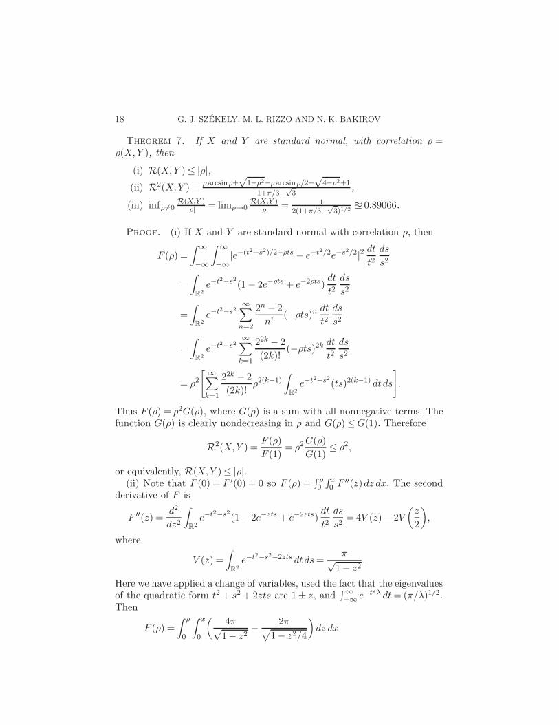
Theorem 7. If X and Y are standard normal, with correlation ρ =ρ(X,Y ), then

(i) R(X,Y )≤ |ρ|,(ii) R2(X,Y ) =

ρarcsinρ+√

1−ρ2−ρarcsinρ/2−√

4−ρ2+1

1+π/3−√

3,

(iii) infρ6=0R(X,Y )

|ρ| = limρ→0R(X,Y )

|ρ| = 12(1+π/3−

√3)1/2 ≅ 0.89066.

Proof. (i) If X and Y are standard normal with correlation ρ, then

F (ρ) =

∫ ∞

−∞

∫ ∞

−∞|e−(t2+s2)/2−ρts − e−t2/2e−s2/2|2 dt

t2ds

s2

=

∫

R2e−t2−s2

(1− 2e−ρts + e−2ρts)dt

t2ds

s2

=

∫

R2e−t2−s2

∞∑

n=2

2n − 2

n!(−ρts)n

dt

t2ds

s2

=

∫

R2e−t2−s2

∞∑

k=1

22k − 2

(2k)!(−ρts)2k dt

t2ds

s2

= ρ2

[ ∞∑

k=1

22k − 2

(2k)!ρ2(k−1)

∫

R2e−t2−s2

(ts)2(k−1) dt ds

].

Thus F (ρ) = ρ2G(ρ), where G(ρ) is a sum with all nonnegative terms. Thefunction G(ρ) is clearly nondecreasing in ρ and G(ρ) ≤ G(1). Therefore

R2(X,Y ) =F (ρ)

F (1)= ρ2 G(ρ)

G(1)≤ ρ2,

or equivalently, R(X,Y )≤ |ρ|.(ii) Note that F (0) = F ′(0) = 0 so F (ρ) =

∫ ρ0

∫ x0 F ′′(z)dz dx. The second

derivative of F is

F ′′(z) =d2

dz2

∫

R2e−t2−s2

(1− 2e−zts + e−2zts)dt

t2ds

s2= 4V (z)− 2V

(z

2

),

where

V (z) =

∫

R2e−t2−s2−2zts dt ds =

π√1− z2

.

Here we have applied a change of variables, used the fact that the eigenvaluesof the quadratic form t2 + s2 + 2zts are 1± z, and

∫ ∞−∞ e−t2λ dt = (π/λ)1/2.

Then

F (ρ) =

∫ ρ

0

∫ x

0

(4π√

1− z2− 2π√

1− z2/4

)dz dx


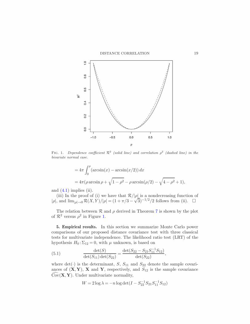
Fig. 1. Dependence coefficient R2 (solid line) and correlation ρ2 (dashed line) in thebivariate normal case.

= 4π

∫ ρ

0(arcsin(x)− arcsin(x/2)) dx

= 4π(ρarcsinρ +√

1− ρ2 − ρarcsin(ρ/2)−√

4− ρ2 + 1),

and (4.1) implies (ii).(iii) In the proof of (i) we have that R/|ρ| is a nondecreasing function of

|ρ|, and lim|ρ|→0R(X,Y )/|ρ| = (1 + π/3−√

3)−1/2/2 follows from (ii). �

The relation between R and ρ derived in Theorem 7 is shown by the plotof R2 versus ρ2 in Figure 1.

5. Empirical results. In this section we summarize Monte Carlo powercomparisons of our proposed distance covariance test with three classicaltests for multivariate independence. The likelihood ratio test (LRT) of thehypothesis H0 :Σ12 = 0, with µ unknown, is based on

det(S)

det(S11)det(S22)=

det(S22 − S21S−111 S12)

det(S22),(5.1)

where det(·) is the determinant, S, S11 and S22 denote the sample covari-ances of (X,Y), X and Y, respectively, and S12 is the sample covariance

Cov(X,Y). Under multivariate normality,

W = 2 logλ =−n logdet(I − S−122 S21S

−111 S12)


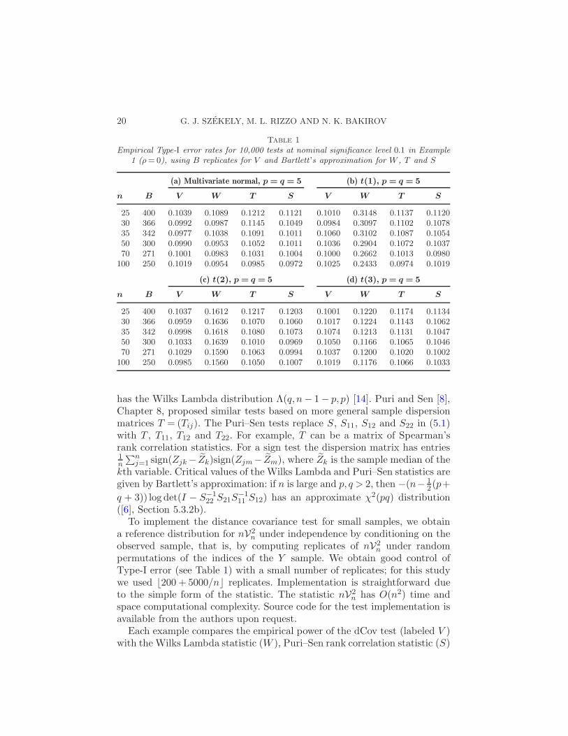
Table 1Empirical Type-I error rates for 10,000 tests at nominal significance level 0.1 in Example

1 (ρ = 0), using B replicates for V and Bartlett ’s approximation for W , T and S

(a) Multivariate normal, p = q = 5 (b) t(1), p = q = 5

n B V W T S V W T S

25 400 0.1039 0.1089 0.1212 0.1121 0.1010 0.3148 0.1137 0.112030 366 0.0992 0.0987 0.1145 0.1049 0.0984 0.3097 0.1102 0.107835 342 0.0977 0.1038 0.1091 0.1011 0.1060 0.3102 0.1087 0.105450 300 0.0990 0.0953 0.1052 0.1011 0.1036 0.2904 0.1072 0.103770 271 0.1001 0.0983 0.1031 0.1004 0.1000 0.2662 0.1013 0.0980

100 250 0.1019 0.0954 0.0985 0.0972 0.1025 0.2433 0.0974 0.1019

(c) t(2), p = q = 5 (d) t(3), p = q = 5

n B V W T S V W T S

25 400 0.1037 0.1612 0.1217 0.1203 0.1001 0.1220 0.1174 0.113430 366 0.0959 0.1636 0.1070 0.1060 0.1017 0.1224 0.1143 0.106235 342 0.0998 0.1618 0.1080 0.1073 0.1074 0.1213 0.1131 0.104750 300 0.1033 0.1639 0.1010 0.0969 0.1050 0.1166 0.1065 0.104670 271 0.1029 0.1590 0.1063 0.0994 0.1037 0.1200 0.1020 0.1002

100 250 0.0985 0.1560 0.1050 0.1007 0.1019 0.1176 0.1066 0.1033

has the Wilks Lambda distribution Λ(q,n− 1− p, p) [14]. Puri and Sen [8],Chapter 8, proposed similar tests based on more general sample dispersionmatrices T = (Tij). The Puri–Sen tests replace S, S11, S12 and S22 in (5.1)with T , T11, T12 and T22. For example, T can be a matrix of Spearman’srank correlation statistics. For a sign test the dispersion matrix has entries1n

∑nj=1 sign(Zjk − Zk)sign(Zjm− Zm), where Zk is the sample median of the

kth variable. Critical values of the Wilks Lambda and Puri–Sen statistics aregiven by Bartlett’s approximation: if n is large and p, q > 2, then −(n− 1

2 (p+

q + 3)) log det(I − S−122 S21S

−111 S12) has an approximate χ2(pq) distribution

([6], Section 5.3.2b).To implement the distance covariance test for small samples, we obtain

a reference distribution for nV2n under independence by conditioning on the

observed sample, that is, by computing replicates of nV2n under random

permutations of the indices of the Y sample. We obtain good control ofType-I error (see Table 1) with a small number of replicates; for this studywe used ⌊200 + 5000/n⌋ replicates. Implementation is straightforward dueto the simple form of the statistic. The statistic nV2

n has O(n2) time andspace computational complexity. Source code for the test implementation isavailable from the authors upon request.

Each example compares the empirical power of the dCov test (labeled V )with the Wilks Lambda statistic (W ), Puri–Sen rank correlation statistic (S)


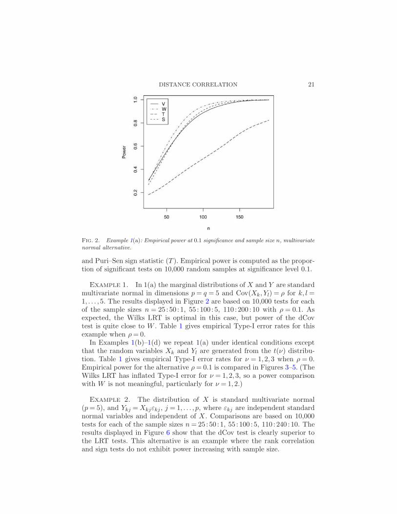
Fig. 2. Example 1(a): Empirical power at 0.1 significance and sample size n, multivariatenormal alternative.

and Puri–Sen sign statistic (T ). Empirical power is computed as the propor-tion of significant tests on 10,000 random samples at significance level 0.1.

Example 1. In 1(a) the marginal distributions of X and Y are standardmultivariate normal in dimensions p = q = 5 and Cov(Xk, Yl) = ρ for k, l =1, . . . ,5. The results displayed in Figure 2 are based on 10,000 tests for eachof the sample sizes n = 25 : 50 : 1, 55 : 100 : 5, 110 : 200 : 10 with ρ = 0.1. Asexpected, the Wilks LRT is optimal in this case, but power of the dCovtest is quite close to W . Table 1 gives empirical Type-I error rates for thisexample when ρ = 0.

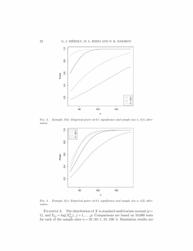
In Examples 1(b)–1(d) we repeat 1(a) under identical conditions exceptthat the random variables Xk and Yl are generated from the t(ν) distribu-tion. Table 1 gives empirical Type-I error rates for ν = 1,2,3 when ρ = 0.Empirical power for the alternative ρ = 0.1 is compared in Figures 3–5. (TheWilks LRT has inflated Type-I error for ν = 1,2,3, so a power comparisonwith W is not meaningful, particularly for ν = 1,2.)

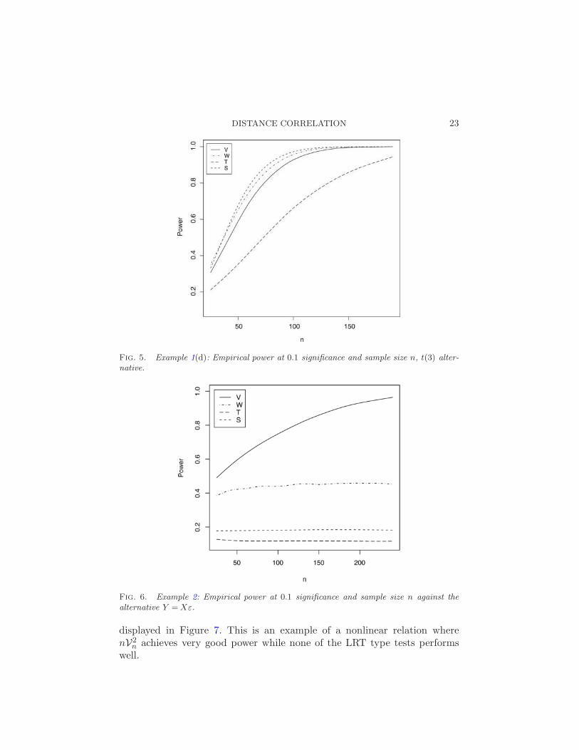
Example 2. The distribution of X is standard multivariate normal(p = 5), and Ykj = Xkjεkj , j = 1, . . . , p, where εkj are independent standardnormal variables and independent of X . Comparisons are based on 10,000tests for each of the sample sizes n = 25 : 50 : 1, 55 : 100 : 5, 110 : 240 : 10. Theresults displayed in Figure 6 show that the dCov test is clearly superior tothe LRT tests. This alternative is an example where the rank correlationand sign tests do not exhibit power increasing with sample size.


Fig. 3. Example 1(b): Empirical power at 0.1 significance and sample size n, t(1) alter-native.

Fig. 4. Example 1(c): Empirical power at 0.1 significance and sample size n, t(2) alter-native.

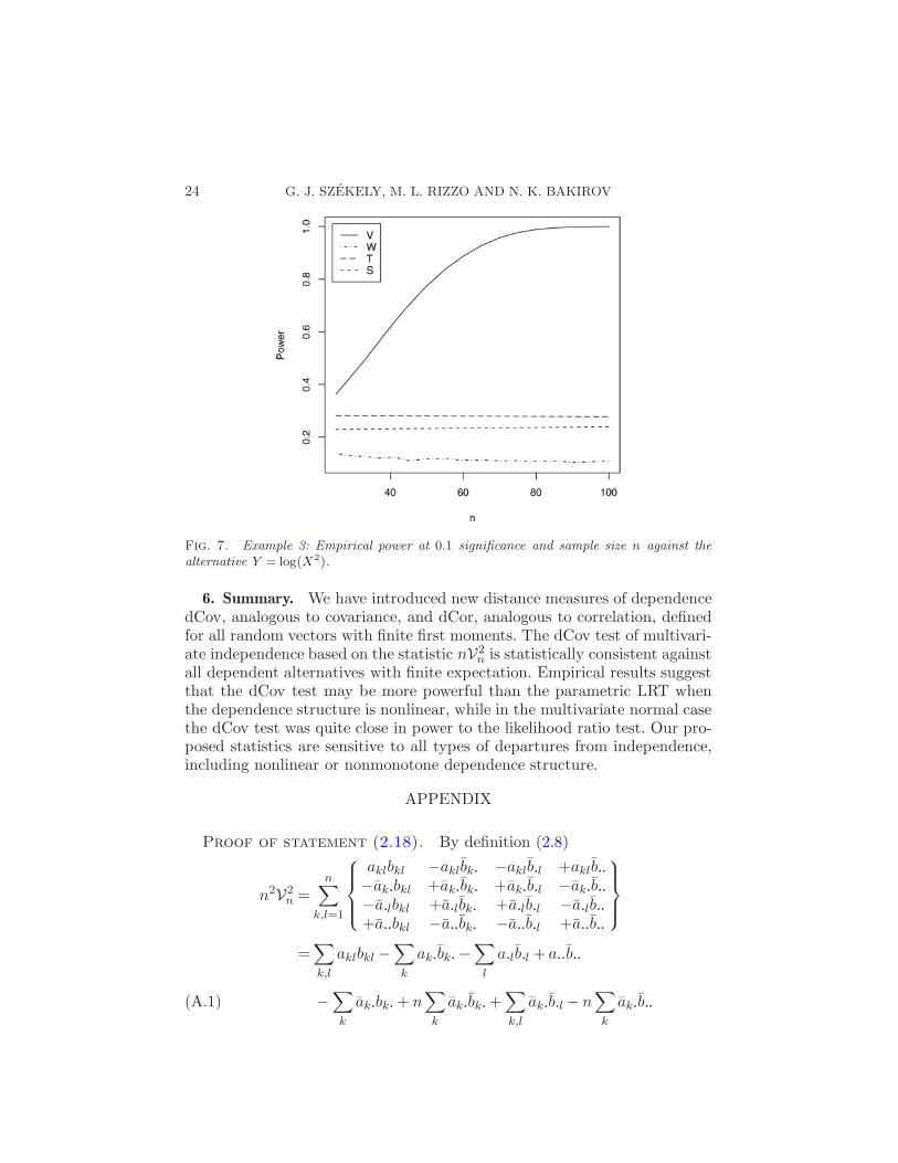
Example 3. The distribution of X is standard multivariate normal (p =5), and Ykj = log(X2

kj), j = 1, . . . , p. Comparisons are based on 10,000 testsfor each of the sample sizes n = 25 : 50 : 1, 55 : 100 : 5. Simulation results are


Fig. 5. Example 1(d): Empirical power at 0.1 significance and sample size n, t(3) alter-native.

Fig. 6. Example 2: Empirical power at 0.1 significance and sample size n against thealternative Y = Xε.

displayed in Figure 7. This is an example of a nonlinear relation wherenV2

n achieves very good power while none of the LRT type tests performswell.


Fig. 7. Example 3: Empirical power at 0.1 significance and sample size n against thealternative Y = log(X2).

6. Summary. We have introduced new distance measures of dependencedCov, analogous to covariance, and dCor, analogous to correlation, definedfor all random vectors with finite first moments. The dCov test of multivari-ate independence based on the statistic nV2

n is statistically consistent againstall dependent alternatives with finite expectation. Empirical results suggestthat the dCov test may be more powerful than the parametric LRT whenthe dependence structure is nonlinear, while in the multivariate normal casethe dCov test was quite close in power to the likelihood ratio test. Our pro-posed statistics are sensitive to all types of departures from independence,including nonlinear or nonmonotone dependence structure.

APPENDIX

Proof of statement (2.18). By definition (2.8)

n2V2n =

n∑

k,l=1

aklbkl −aklbk·−aklb·l +aklb··

−ak·bkl +ak·

bk·+ak·

b·l −ak·

b··

−a·lbkl +a

·lbk·+a

·lb·l −a·lb··

+a··bkl −a

··bk·

−a··b·l +a

··b··

=∑

k,l

aklbkl −∑

k

ak·bk·

−∑

l

a·lb·l + a

··b··

−∑

k

ak·bk·

+ n∑

k

ak·bk·

+∑

k,l

ak·b·l − n

∑

k

ak·b··

(A.1)


−∑

l

a·lb·l +

∑

k,l

a·lbk·

+ n∑

l

a·lb·l − n

∑

l

a·lb··

+ a··b··− n

∑

k

a··bk·

− n∑

l

a··b·l + n2a

··b··,

where ak·= nak·

, a·l = na

·l, bk·= nbk·

and b·l = nb

·l. Applying the identities

S1 =1

n2

n∑

k,l=1

aklbkl,(A.2)

S2 =1

n2

n∑

k,l=1

akl1

n2

n∑

k,l=1

bkl = a··b··,(A.3)

n2S2 = n2a··b··

=a

··

n

n∑

l=1

b·l

n=

n∑

k,l=1

ak·b·l,(A.4)

S3 =1

n3

n∑

k=1

n∑

l,m=1

aklbkm =1

n3

n∑

k=1

ak·bk·

=1

n

n∑

k=1

ak·bk·

(A.5)

to (A.1), we obtain

n2V2n = n2S1 − n2S3 − n2S3 + n2S2

− n2S3 + n2S3 + n2S2 − n2S2

− n2S3 + n2S2 + n2S3 − n2S2

+ n2S2 − n2S2 − n2S2 + n2S2 = n2(S1 + S2 − 2S3). �

Acknowledgments. The authors are grateful to the Associate Editor andreferee for many suggestions that greatly improved the paper.

REFERENCES

[1] Albert, P. S., Ratnasinghe, D., Tangrea, J. and Wacholder, S. (2001). Lim-itations of the case-only design for identifying gene-environment interactions.Amer. J. Epidemiol. 154 687–693.

[2] Bakirov, N. K., Rizzo, M. L. and Szekely, G. J. (2006). A multivariate nonpara-metric test of independence. J. Multivariate Anal. 97 1742–1756. MR2298886

[3] Eaton, M. L. (1989). Group Invariance Applications in Statistics. IMS, Hayward,CA. MR1089423

[4] Giri, N. C. (1996). Group Invariance in Statistical Inference. World Scientific, RiverEdge, NJ. MR1626154

[5] Kuo, H. H. (1975). Gaussian Measures in Banach Spaces. Lecture Notes in Math.463. Springer, Berlin. MR0461643

[6] Mardia, K. V., Kent, J. T. and Bibby, J. M. (1979). Multivariate Analysis. Aca-demic Press, London. MR0560319

http://www.ams.org/mathscinet-getitem?mr=2298886






[7] Potvin, C. and Roff, D. A. (1993). Distribution-free and robust statistical meth-ods: Viable alternatives to parametric statistics? Ecology 74 1617–1628.

[8] Puri, M. L. and Sen, P. K. (1971). Nonparametric Methods in Multivariate Analysis.Wiley, New York. MR0298844

[9] Szekely, G. J. and Bakirov, N. K. (2003). Extremal probabilities for Gaussianquadratic forms. Probab. Theory Related Fields 126 184–202. MR1990053

[10] Szekely, G. J. and Rizzo, M. L. (2005). A new test for multivariate normality. J.Multivariate Anal. 93 58–80. MR2119764

[11] Szekely, G. J. and Rizzo, M. L. (2005). Hierarchical clustering via joint between-within distances: Extending Ward’s minimum variance method. J. Classification22 151–183. MR2231170

[12] Tracz, S. M., Elmore, P. B. and Pohlmann, J. T. (1992). Correlational meta-analysis: Independent and nonindependent cases. Educational and PsychologicalMeasurement 52 879–888.

[13] von Mises, R. (1947). On the asymptotic distribution of differentiable statisticalfunctionals. Ann. Math. Statist. 18 309–348. MR0022330

[14] Wilks, S. S. (1935). On the independence of k sets of normally distributed statisticalvariables. Econometrica 3 309–326.

G. J. SzekelyDepartment of Mathematics and StatisticsBowling Green State UniversityBowling Green, Ohio 43403USAandRenyi Institute of MathematicsHungarian Academy of SciencesHungaryE-mail: [email protected]

M. L. RizzoDepartment of Mathematics and StatisticsBowling Green State UniversityBowling Green, Ohio 43403USAE-mail: [email protected]

N. K. BakirovInstitute of MathematicsUSC Russian Academy of Sciences112 Chernyshevskii St.

450000 UfaRussia






mailto:[email protected]

mailto:[email protected]

Measuring and testing dependence by correlation of distances

Documents

Transcript of Measuring and testing dependence by correlation of distances