Linear correlationLet X and Y be two random variables. The linear correlation coefficient (or Pearson's correlation coefficient) between X and Y denoted by r  is defined as follows: σx σy

r=Cov [X,Y ]σxσy

where Cov[X,Y] is the covariance between X and Y and σx  and  σy are the standard deviations of X and Y. Of course, the linear correlation coefficient is well-defined only as long as  Cov[X,Y], σx and σy exist and are well-defined. Moreover, while the ratio is well-defined only if  σx and σy  are strictly greater than zero, it is often assumed that  r = 0 when one of the two standard deviations is zero. This is equivalent to assuming that 0/0=0, because Cov[X,Y] =0 when one of thetwo standard deviations is zero.

Correlation coefficients measure the strength of association between two variables. The most common correlation coefficient, called the Pearson product-moment correlation coefficient, measures the strength of the linear association between variables.

Properties of the Correlation Coefficient

1. The correlation coefficient does not change the measurementscale.

That is, if the height is expressed in meters or feet, the correlation coefficient does not change.

2. The sign of the correlation coefficient is the same as the covariance .

3. The linear correlation coefficient is a real number between−1 and 1.

−1 ≤ r ≤ 1

4. If the linear correlation coefficient takes values closer to −1, the correlation is strong and negative, and will becomestronger the closer rapproaches −1.

Prepared by: Agra, Kenneth M.

5. If the linear correlation coefficient takes values close to 1 the correlation is strong and positive, and will become stronger the closer r approaches 1

6. If the linear correlation coefficient takes values close to 0, the correlation is weak.

7. If r = 1 or r = −1, there is perfect correlation and the line on the scatter plot is increasing or decreasing respectively.

8. If r = 0, there is no linear correlation.

Prepared by: Agra, Kenneth M.

Scatterplots and Correlation Coefficients

The scatterplots below show how different patterns of data produce different degrees of correlation.

Maximum positivecorrelation(r = 1.0)

Strong positivecorrelation(r = 0.80)

Zero correlation(r = 0)

Maximum negativecorrelation(r = -1.0)

Moderate negativecorrelation(r = -0.43)

Strong correlation& outlier(r = 0.71)

Several points are evident from the scatterplots.

When the slope of the line in the plot is negative, the correlation is negative; and vice versa.

The strongest correlations (r = 1.0 and r = -1.0 ) occur when data points fall exactly on a straight line.

The correlation becomes weaker as the data points become more scattered.

If the data points fall in a random pattern, the correlation is equal to zero.

Correlation is affected by outliers. Compare the first scatterplot with the last scatterplot. The single outlier in the last plot greatly reduces the correlation (from 1.00 to 0.71).

Prepared by: Agra, Kenneth M.

How to Calculate a Correlation Coefficient

If you look in different statistics textbooks, you are likely to find different-looking (but equivalent) formulas for computing a correlation coefficient. In this section, we present several formulas that you may encounter.

The most common formula for computing a product-moment correlation coefficient (r) is given below.

Product-moment correlation coefficient. The correlation r between two variables is:

r = Σ (xy) / sqrt [ ( Σ x2 ) * ( Σ y2 ) ]

where Σ is the summation symbol, x = xi - x, xi is the x value for observation i, x is the mean x value, y = yi - y, yi is the y value for observation i, and y is the mean y value.

The formula below uses population means and population standard deviations to compute a population correlation coefficient (ρ) from population data.

Prepared by: Agra, Kenneth M.

Population correlation coefficient. The correlation ρ between two variablesis:

ρ = [ 1 / N ] * Σ { [ (Xi - μX) / σx ] * [ (Yi - μY) / σy ] }

where N is the number of observations in the population, Σ is the summationsymbol, Xi is the X value for observation i, μX is the population mean for variable X, Yi is the Y value for observation i, μY is the population mean

The formula below uses sample means and sample standard deviations to compute a correlation coefficient (r) from sample data.

Sample correlation coefficient. The correlation r between two variables is:

r = [ 1 / (n - 1) ] * Σ { [ (xi - x) / sx ] * [ (yi - y) / sy ] }

where n is the number of observations in the sample, Σ is the summation symbol, xi is the x value for observation i, x is the sample mean of x, yi is the y value for observation i, y is the sample mean of y, sx is the sample standard deviation of x, and sy is the sample standard deviation of

The interpretation of the sample correlation coefficient depends on how the sample data are collected. With a simple random sample, the sample correlation coefficient is an unbiased estimate of the populationcorrelation coefficient.

Each of the latter two formulas can be derived from the first formula.Use the first or second formula when you have data from the entire population. Use the third formula when you only have sample data, but want to estimate the correlation in the population. When in doubt, usethe first formula.

Problem 1

The scores of 12 students in their mathematics and physics classes are:

Mathematics 2 3 4 4 5 6 6 7 7 8 10 10

Prepared by: Agra, Kenneth M.

Physics 1 3 2 4 4 4 6 4 6 7 9 10

Find the correlation coefficient distribution and interpret it.

xi yi xi ·yi xi2 yi2

2 1 2 4 1

3 3 9 9 9

4 2 8 16 4

4 4 16 16 16

5 4 20 25 16

6 4 24 36 16

6 6 36 36 36

7 4 28 49 16

7 6 42 49 36

8 7 56 64 49

10 9 90 100 81

10 10 100 100 100

72 60 431 504 380

1. Find the arithmetic means.

2. Calculate the covariance.

Prepared by: Agra, Kenneth M.

3. Calculate the standard deviations.

4. Apply the formula for the linear correlation coefficient.

The correlation is positive.

As the correlation coefficient is very close to 1, the correlation is very strong.

The values of the two variables X and Y are distributed according to the following table:

Y/X 0 2 41 2 1 32 1 4 23 2 5 0

Calculate the correlation coefficient.

Turn the double entry table into a single table.

xi

yi

fi

xi · fi

xi2 · fi

yi · fi

yi2 · fi

xi · yi · fi

Prepared by: Agra, Kenneth M.

0 1 2 0 0 2 2 0

0 2 1 0 0 2 4 0

0 3 2 0 0 6 18 0

2 1 1 2 4 1 1 2

2 2 4 8 16 8 16 16

2 3 5 10 20 15 45 30

4 1 3 12 48 3 3 12

4 2 2 8 32 4 8 16

    20 40 120 41 97 76

The correlation is negative.

As the correlation coefficient is very close to 0, the correlation is very weak.

Problem 2

 Five children aged 2, 3, 5, 7 and 8 years old weigh 14, 20, 32, 42 and 44 kilograms respectively.

1. Find the equation of the regression line of age on weight.

Prepared by: Agra, Kenneth M.

2. Based on this data, what is the approximate weight of a six year old child?

xi yi xi ·yi xi2 yi2

2 14 4 196 28

3 20 9 400 60

5 32 25 1,024 160

7 42 49 1,764 294

8 44 64 1,936 352

25 152 151 5,320 894

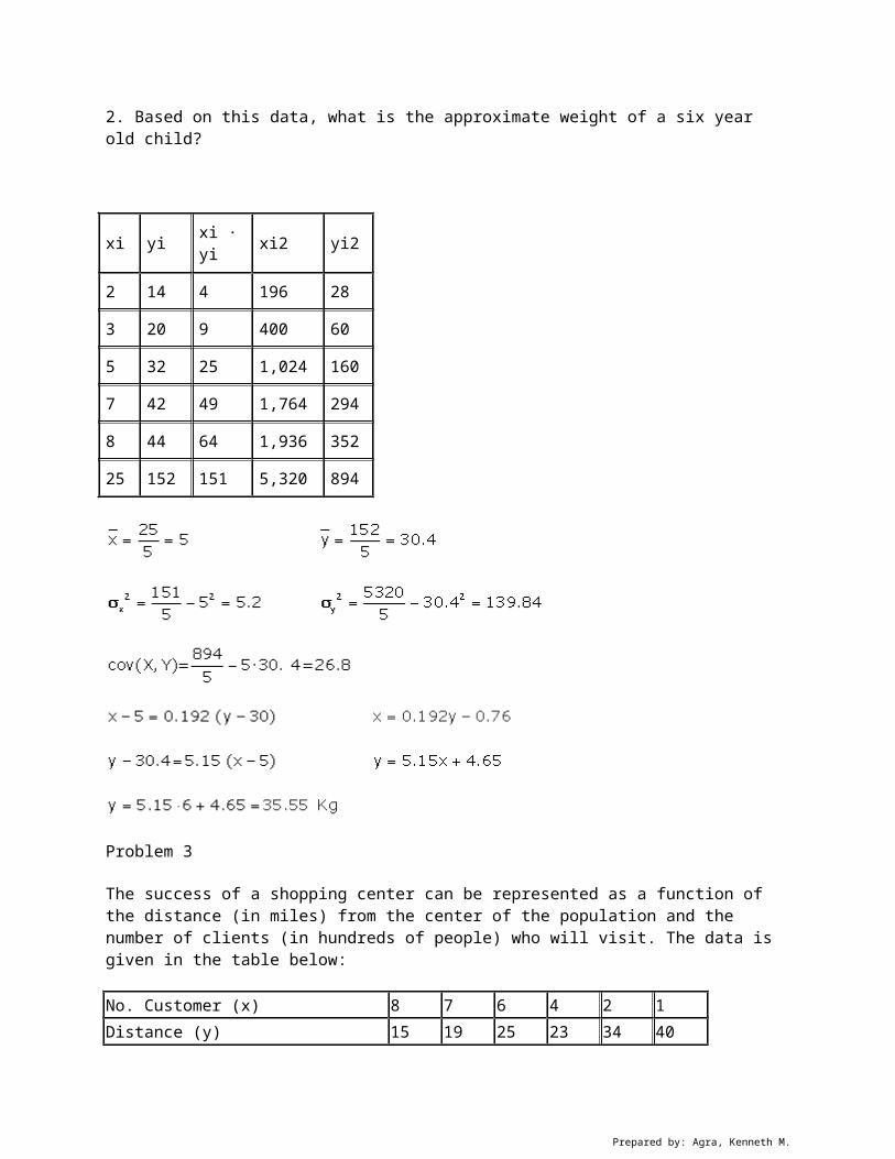
Problem 3

The success of a shopping center can be represented as a function of the distance (in miles) from the center of the population and the number of clients (in hundreds of people) who will visit. The data is given in the table below:

No. Customer (x) 8 7 6 4 2 1Distance (y) 15 19 25 23 34 40

Prepared by: Agra, Kenneth M.

1 .Calculate the linear correlation coefficient.

2. If the mall is located 2 miles from the center of the population, how many customers should the shopping center expect?

3 .To receive 500 customers, at what distance from the center of the population should the shopping centre be located?

xi yi xi ·yi xi2 yi2

8 15 120 64 225

7 19 133 49 361

6 25 150 36 625

4 23 92 16 529

2 34 68 4 1,156

1 40 40 1 1,600

28 156 603 170 4,496

There is a very strong negative correlation.

Prepared by: Agra, Kenneth M.

Problem 4

The grades of five students in mathematics and chemistry are:

Mathematics 6 4 8 5 3. 5Chemistry 6. 5 4. 5 7 5 4

Determine the regression lines and calculate the expected grade in chemistry for a student who has a 7.5 in mathematics.

xi yi xi ·yi xi2 yi2

6 6. 5 36 42.25 39

4 4. 5 16 20.25 18

8 7 64 49 56

5 5 25 25 25

3.5 4 12.25 16 14

26.5 27 153.25 152.5 152

Prepared by: Agra, Kenneth M.

Problem 5

A data set has a correlation coefficient of r = −0.9, with the means of marginal distributions of x = 1 and y = 2. It is known that one of the following four equations corresponds to the regression of y on x:

Select the correct line.

y = −x + 2 3x − y = 1 2x + y = y = x + 1

Since the linear correlation coefficient is negative, the slope of theline will also be negative, thus ruling out the 2nd and 4th options.

A point on the line is (x, y), that is to say, (1, 2).

2 ≠ −1 + 2

2 · 1 + 2 = 4

The correct line is: 2x + y = 4.

Problem 6

The heights (in centimeters) and weight (in kilograms) of 10 basketball players of a team are:

Height (X) 186 189 190 192 193 193 198 201 203 205

Prepared by: Agra, Kenneth M.

Weight (Y) 85 85 86 90 87 91 93 103 100 101

Calculate:

1 .The regression line of y on x.2. The coefficient of correlation.3 .The estimated weight of a player who measures 208 cm.

xi yi xi2 yi2 xi ·yi

186 85 34,596 7,225 15,810

189 85 35,721 7,225 16,065

190 86 36,100 7,396 16,340

192 90 36,864 8,100 17,280

193 87 37,249 7,569 16,791

193 91 37,249 8,281 17,563

198 93 39,204 8,649 18,414

201 103 40,401 10,609 20,703

203 100 41,209 10,000 20,300

205 101 42,025 10,201 20,705

1,950 921 380,618 85,255 179,971

Prepared by: Agra, Kenneth M.

There is a strong positive correlation.

Prepared by: Agra, Kenneth M.

Problem 7

From the following data of hours worked in a factory (x) and output units (y), determine the regression line of y on x, the linear correlation coefficient and determine the type of correlation.

Hours (x) 80 79 83 84 78 60 82 85 79 84 80 62Production (y) 300 302 315 330 300 250 300 340 315 330 310 240

xi yi xi ·yi xi2 yi2

80 300 6,400 90,000 24,000

79 302 6,241 91,204 23,858

83 315 6,889 99,225 26,145

84 330 7,056 108,900 27,720

78 300 6,084 90,000 23,400

60 250 3,600 62,500 15,000

82 300 6,724 90,000 24,600

85 340 7,225 115,600 28,900

79 315 6,241 99,225 24,885

84 330 7,056 108,900 27,720

80 310 6,400 96,100 24,800

62 240 3,844 57,600 14,880

936 3,632 73,760 1,109,254 285,908

Prepared by: Agra, Kenneth M.

There is a strong positive correlation.

Problem 8

A group of 50 individuals has been surveyed on the number of hours devoted each day to sleeping and watching TV. The responses are summarized in the following table:

No. of sleeping hours (x) 6 7 8 9 10No. of hours of television (y) 4 3 3 2 1Absolute frequencies (fi) 3 16 20 10 11. Calculate the correlation coefficient.2. Determine the equation of the regression line of y on x.3. If a person sleeps eight hours, how many hours of TV are they expected to watch?

xi yi fi xi ·

fixi2 ·fi

yi ·fi

yi2 ·fi

xi · yi · fi

6 4 3 18 108 12 48 72

7 3 16 112 784 48 144 336

8 3 20 160 1,280 60 180 480

9 2 10 90 810 20 40 180

10 1 1 10 100 1 1 10

    50 390 3,082 141 413 1,078

Prepared by: Agra, Kenneth M.

There is a strong negative correlation.

Problem 9

The following table summarizes the results of an aptitude test given to six clerks to determine the correlation between test scores (x) andsales in the first month (y) in hundreds of dollars.

X 25 42 33 54 29 36Y 42 72 50 90 45 481.Find the correlation coefficient and interpret the results.2.Calculate the regression line of y on x and predict the sales of a vendor who obtains 47 on the test.

xi yi xi ·yi xi2 yi2

25 42 625 1,764 1,050

42 72 1,764 5,184 3,024

33 50 1,089 2,500 1,650

54 90 2,916 8,100 4,860

29 45 841 2,025 1,305

36 48 1,296 2,304 1,728

209 347 8,531 21,877 13,617

Prepared by: Agra, Kenneth M.

Prepared by: Agra, Kenneth M.