ltblackgray0.1@let@token Benchmarking Asset Managers

Benchmarking Asset Managers

Anil Kashyap∗

Chicago Booth andBank of England

Natalia KovrijnykhArizona State

University

Jian LiUniversity of

Chicago

Anna PavlovaLondon Business

School

June 2018

Preliminary and Incomplete

∗The views here are those of the authors only and not necessarily of the Bank of England

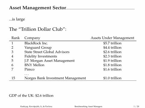
Asset Management Sector

...is large

The “Trillion Dollar Club”:

Rank Company Assets Under Management1 BlackRock Inc. $5.7 trillion2 Vanguard Group $4.4 trillion3 State Street Global Advisors $2.6 trillion4 Fidelity Investments $2.3 trillion5 J.P. Morgan Asset Management $1.9 trillion6 BNY Mellon $1.8 trillion7 Pimco $1.6 trillion

. . .15 Norges Bank Investment Management $1.0 trillion

GDP of the UK: $2.6 trillion

Kashyap, Kovrijnykh, Li, & Pavlova Benchmarking Asset Managers 1 / 20

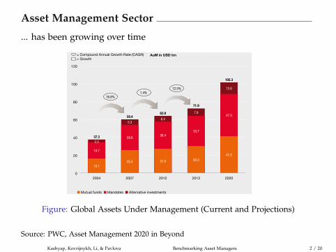
Asset Management Sector

... has been growing over time

5 PwC Asset Management 2020 and beyond

While the asset management industry will grow rapidly in the coming years (see Figure 1), growth for individual asset management firms will not be automatic. The risks will change, as the tax and regulatory environments continue to develop. Tax, in particular, will be a key operational and business activity, requiring specialist resources, a new approach, and integration into front and middle office activities – including data reporting, product development, distribution and brand strategy. Tax and reputation will be inseparable concepts. Taxes will now be viewed as an operational risk, joining the ranks of other key risks which senior management takes a keen interest in, and one that needs a strategically planned risk management programme integrated into all aspects of their business operations. How a firm deals with tax risk will be viewed as a competitive advantage or disadvantage.

In 2020, investors’ expectations will include a robust and efficient tax infrastructure. And zero tolerance of tax uncertainty or tax adjustments. In addition, as many countries struggle with deficit reduction and the need to invest, the whole of the financial services industry, including asset management, will be expected to play its part in policing the global financial system and ensuring that tax authorities have the correct tax information on taxpayers.

Total transparency of investor residency and identity will be the norm. Asset managers will have to demonstrate the highest standards of anti-money laundering (AML) and know-your-customer (KYC) responsibilities, plus reporting to tax authorities and to taxpayers on the returns flowing from their funds. Politicians, regulators, the media and the public will all expect nothing less.

However, tax should not be considered solely as a risk to manage – it is also an opportunity. Managing tax risks and leakages well at all levels (investments, funds and investors) can distinguish asset managers from their peers. While managers have traditionally been tasked with generating performance ‘alpha’ for their investors, ‘service alpha’ in 2020 will be a key differentiator. The concept of service alpha implies an entirely new challenge for asset managers: how to communicate with investors about tax matters. Service alpha will require the asset manager to first explain it and then help investors recognise its benefits.

To help asset managers plan for the future, in the last section of this paper PwC has set out a vision of what the tax landscape should look like in 2020 to adequately address the new tax environment.

The issues addressed by the CEO of our fictional firm, Investar Asset Management1 (on page 6 and throughout our paper) give an indication of the challenges the industry faces in putting the management of tax risk at the heart of all strategic business change.

Tax should not be considered solely as a risk to manage – it is also an opportunity.

1 Noneoftheinformationorfactsaboutthefictionalinvestmentfirm,InvestarAssetManagement,aresourcedfromPwCclientsorPwCclientengagements.Theexampleshavebeendevelopedsolelytoillustratekeypointsinthispaper.

Figure 1: Global Assets under management (AuM) to reach above USD100trn by 2020

nMutualfundsn Mandates nAlternativeinvestmentsSource:PwCanalysisNote:WehaverevisedourestimatesforAlternativeinvestmentsin2020upwardstoUSD13.6trngivenstrongmarketperformancein2013andH12014.

120

100

80

60

40

20

02004 2007 2012 2013 2020

=CompoundAnnualGrowthRate(CAGR) =Growth

AuM in USD trn

18.7

2.5

16.125.4 27.0 30.3

41.2

28.830.4

33.7

47.5

5.36.4

7.9

13.6

16.8%1.4%

12.5%

37.3

59.463.9

71.9

102.3

Figure: Global Assets Under Management (Current and Projections)

Source: PWC, Asset Management 2020 in Beyond


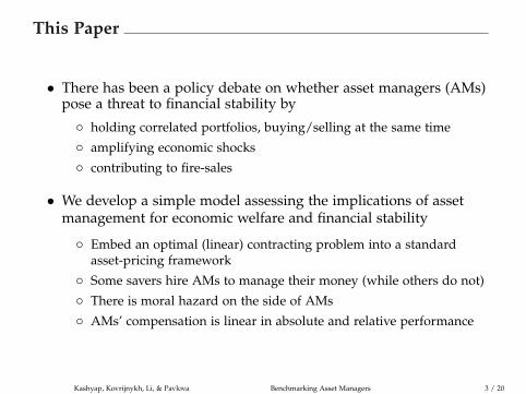
This Paper

• There has been a policy debate on whether asset managers (AMs)pose a threat to financial stability by

◦ holding correlated portfolios, buying/selling at the same time

◦ amplifying economic shocks

◦ contributing to fire-sales

• We develop a simple model assessing the implications of assetmanagement for economic welfare and financial stability

◦ Embed an optimal (linear) contracting problem into a standardasset-pricing framework

◦ Some savers hire AMs to manage their money (while others do not)

◦ There is moral hazard on the side of AMs

◦ AMs’ compensation is linear in absolute and relative performance


This Paper (Cont’d)

• Questions:

◦ What is the optimal contract from the viewpoint of fund investors?

◦ What are the effects of contracts on asset prices?

◦ Individual contracts impose a pecuniary externality on marketparticipants by affecting asset prices because

- markets are incomplete: there is an aggregate, uninsurable shock

- contracts cannot be made contingent on the shock

◦ Suppose a social planner is subject to the same restrictions, butinternalizes the effect of the contract on asset prices

- How does the socially-optimal contract differ from the privately-optimalone?

• Main Insight: Incentive contracts amplify the effects of aggregateshocks (fire-sales) on prices


Environment

Investment Opportunities

• Two periods, t = 0, 1

• This talk: one risky stock (paper: multiple assets)

• Claim to cash flow D ∼ N(D, σ2) in the final date

• Net supply of stock is x

• Stock price is denoted by S

• One risk-free bond with a zero interest rate

◦ In infinite net supply, i.e., just a storage technology


Investors

• Three types of agents:

◦ Normal investors—invest on their own (fraction λN)

◦ Shareholders—delegate investment to AMs (fraction λS)

◦ AMs (fraction λAM)

- λN + λS + λAM = 1

- For this talk, assume λS = λAM — one shareholder per one AM

• All agents have CARA utility: −E exp(−αW1)

◦ where W1 is final wealth

• All agents have equal endowments of the bond and stock

◦ Initial wealth is W0 = B + xS, whereB is the endowment of bond, x is the endowment of stock


Normal Investors

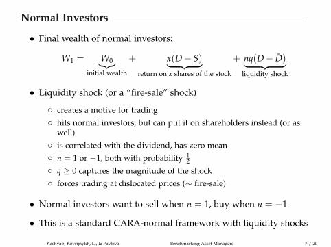
• Final wealth of normal investors:

W1 = W0︸︷︷︸initial wealth

+ x(D− S)︸︷︷︸return on x shares of the stock

+ nq(D− D)︸︷︷︸liquidity shock

• Liquidity shock (or a “fire-sale” shock)

◦ creates a motive for trading

◦ hits normal investors, but can put it on shareholders instead (or aswell)

◦ is correlated with the dividend, has zero mean

◦ n = 1 or −1, both with probability 12

◦ q ≥ 0 captures the magnitude of the shock

◦ forces trading at dislocated prices (∼ fire-sale)

• Normal investors want to sell when n = 1, buy when n = −1

• This is a standard CARA-normal framework with liquidity shocks


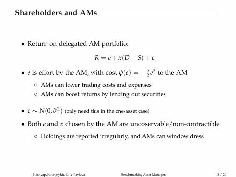
Shareholders and AMs

• Return on delegated AM portfolio:

R = e + x(D− S) + ε

• e is effort by the AM, with cost ψ(e) = − γ2 e2 to the AM

◦ AMs can lower trading costs and expenses

◦ AMs can boost returns by lending out securities

• ε ∼ N(0, σ2) (only need this in the one-asset case)

• Both e and x chosen by the AM are unobservable/non-contractible

◦ Holdings are reported irregularly, and AMs can window dress


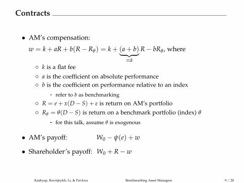
Contracts

• AM’s compensation:

w = k + aR + b(R− Rθ) = k + (a + b)︸︷︷︸≡a

R− bRθ , where

◦ k is a flat fee

◦ a is the coefficient on absolute performance◦ b is the coefficient on performance relative to an index

- refer to b as benchmarking

◦ R = e + x(D− S) + ε is return on AM’s portfolio◦ Rθ = θ(D− S) is return on a benchmark portfolio (index) θ

- for this talk, assume θ is exogenous

• AM’s payoff: W0 − ψ(e) + w

• Shareholder’s payoff: W0 + R−w


Timing

• Shareholders choose contracts (a, b, k)

• The realization of the liquidity shock becomes known

• AMs choose effort, and AMs and normal investors trade

• Returns are observed, contract payments are made, consumptiontakes place


Privately-Optimal Contracts

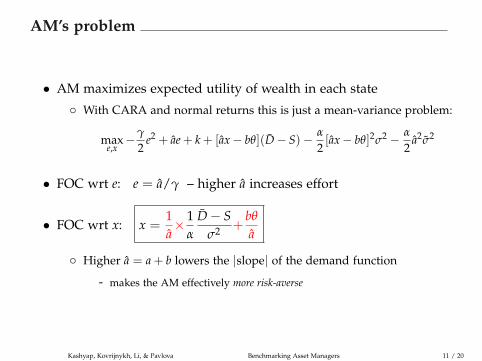
AM’s problem

• AM maximizes expected utility of wealth in each state

◦ With CARA and normal returns this is just a mean-variance problem:

maxe,x−γ

2e2 + ae + k + [ax− bθ](D− S)− α

2[ax− bθ]2σ2 − α

2a2σ2

• FOC wrt e: e = a/γ – higher a increases effort

• FOC wrt x: x =1a× 1

α

D− Sσ2 +

bθ

a

◦ Higher a = a + b lowers the |slope| of the demand function

- makes the AM effectively more risk-averse


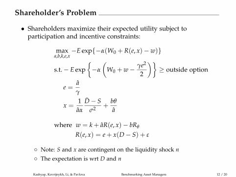
Shareholder’s Problem

• Shareholders maximize their expected utility subject toparticipation and incentive constraints:

maxa,b,k,e,x

−E exp{−α(W0 + R(e, x)−w)}

s.t.− E exp{−α

(W0 + w− γe2

2

)}≥ outside option

e =aγ

x =1aα

D− Sσ2 +

bθ

a

where w = k + aR(e, x)− bRθ

R(e, x) = e + x(D− S) + ε

◦ Note: S and x are contingent on the liquidity shock n◦ The expectation is wrt D and n


Privately-Optimal Contracts

• If effort was observable, the shareholder would choose a = 12 and b = 0.

This achieves perfect risk sharing between the shareholder and AM

◦ The first-best effort is eFB = 1γ

• If effort is unobservable, a = 12 underprovides effort (e = 1

2γ ). Incentiveprovision calls for a larger a

• Suppose we restrict b = 0. Setting a larger a increases risk faced by AM,and makes him reduce the risky-asset holdings xAM

• To raise xAM, it is optimal to set b > 0.

• This makes effort provision less costly, and allows the shareholder toincrease a further to bring effort closer to eFB

◦ So b mitigates the undesirable effect of a (on the AM’s asset holdings)

• In the privately-optimal contract, shareholders and AMs share riskoptimally (50/50) in expectation, but not state by state

◦ The fact that contracts can’t be contingent on shock is crucial here


Aggregate Demand and Equilibrium Price

• Recall that a higher a makes the AM’s demand function flatter⇒aggregate demand function is also flatter:

λAM × xAM︸︷︷︸= 1

aD−Sασ2 + bθ

a

+λN × xN︸︷︷︸= D−S

ασ2 −nq

=

[λAM

a+ λN

]1

ασ2 (D− S) + λAMbθ

a− λNnq =︸︷︷︸

market clearing

x,

• Main Result: Incentive contracts (higher a) make prices vary morewith the liquidity shock relative to the frictionless economy

◦ i.e., relative to the economy with observable effort,or to the economy where everyone invests on their own

S = D−Λασ2(

x− λAMbθ

a+ λNnq

), where Λ = 1

λAM/a+λN


Asset Management Amplifies Illiquidity Discount

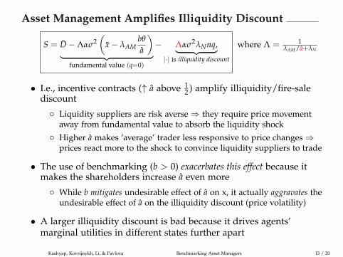
S = D−Λασ2(

x− λAMbθ

a

)︸︷︷︸

fundamental value (q=0)

− Λασ2λNnq,︸︷︷︸|·| is illiquidity discount

where Λ = 1λAM/a+λN

• I.e., incentive contracts (↑ a above 12 ) amplify illiquidity/fire-sale

discount

◦ Liquidity suppliers are risk averse⇒ they require price movementaway from fundamental value to absorb the liquidity shock

◦ Higher a makes ‘average’ trader less responsive to price changes⇒prices react more to the shock to convince liquidity suppliers to trade

• The use of benchmarking (b > 0) exacerbates this effect because itmakes the shareholders increase a even more

◦ While b mitigates undesirable effect of a on x, it actually aggravates theundesirable effect of a on the illiquidity discount (price volatility)

• A larger illiquidity discount is bad because it drives agents’marginal utilities in different states further apart


Socially-Optimal Contracts

Social Planner’s Choice of a

• Consider the problem of a social planner

◦ who is subject to the same restrictions as shareholders

◦ but recognizes that contracts affect asset prices

◦ and maximizes weighted-average of all agents’ expected utilities

• Planner’s choice of a:

◦ On the one hand, the planner is able to achieve better risk sharingbetween the shareholder and AM state-by-state

- Lower cost of effort provision pushes the planner to ↑ a

◦ On the other hand, the planner internalizes the fact that contractsamplify the illiquidity/fire-sale discount

- This pushes the planner to ↓ a

◦ We show that the second effect dominates for some parameter values

- In particular, when q, α, and/or σ2 are large enough


Social Planner’s Choice of b

• Recall that keeping a = a + b fixed, b simply increases the assetprice by a constant:

S = D−Λασ2(

x− λAMbθ

a+ λNnq

)

• Thus an increase in b benefits sellers and hurts buyers

◦ We choose Pareto weights that eliminate the redistribution motive:

ωj =λj

E MUj=

λj

Eα exp(−αWj1)

, j = S, AM, N


Social Planner’s Choice of b (Cont’d)

• Changing b can help bring MUs in different states closer together

◦ E.g., normal investors are worse off in state n = 1 than in n = −1

- When n = −1, Corr(shock, returns) < 0, so there’s a “natural” hedge

◦ Also, they sell in state n = 1 and buy in state n = −1

- So they benefit from ↑ price when n = 1 and are hurt by it when n = −1

◦ To bring their MUs closer together, need to ↑ price

◦ In the one-asset case, other agents’ MUs are the same across states

- So planner only cares about normal investors’ MUs, and wants to ↑ b

◦ But in the multi-asset case all agents’ MUs differ across states, andthere is a tradeoff

- We show that for some parameter values the planner wants to ↓ b


Extensions

• With multiple correlated assets, asset management amplifiesspillover from a fire-sale of one asset to movement in prices ofother assets

• In a two-period version of the model, there is an additionalchannel through which b amplifies the illiquidity discount

◦ and the illiquidity discount is larger for stocks that have largerweights in the index

• Endogenizing the benchmark portfolio θ


Conclusions

• Develop a simple asset-pricing model with asset management

• Shareholders use linear contracts to incentivize AMs to exert effortand choose investment portfolios

• Shareholders, who do not account for the effects of their contractson prices, impose a pecuniary externality on other agents

◦ This is due to contract inflexibility and uninsurable aggregate shocks

• Contracts amplify the effects of aggregate shocks on asset prices

• While there are opposing forces, we show that for some parametervalues the planner wants to reduce both a and b


Other Results

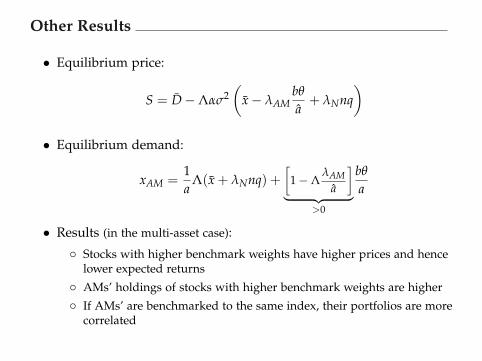
• Equilibrium price:

S = D−Λασ2(

x− λAMbθ

a+ λNnq

)

• Equilibrium demand:

xAM =1a

Λ(x + λNnq) +[

1−ΛλAM

a

]︸︷︷︸

>0

bθ

a

• Results (in the multi-asset case):

◦ Stocks with higher benchmark weights have higher prices and hencelower expected returns

◦ AMs’ holdings of stocks with higher benchmark weights are higher

◦ If AMs’ are benchmarked to the same index, their portfolios are morecorrelated

ltblackgray0.1@let@token Benchmarking Asset Managers

Documents

Transcript of ltblackgray0.1@let@token Benchmarking Asset Managers