Computers & Graphics 28 (2004) 345–359

ARTICLE IN PRESS

E-mail addr

0097-8493/$ - se

doi:10.1016/j.ca

Hierarchical graph maps

James Abello

DIMACS Center, Rutgers University, CoRE Building/4th Floor, 96 Frelinghuysen Road, Piscataway, NJ 08854, USA

Abstract

Graphs and maps are powerful abstractions. Their combination, Hierarchical Graph Maps, provide effective tools to

process a graph that is too large to fit on the screen. They provide hierarchical visual indices (i.e. maps) that guide

navigation and visualization. Hierarchical graph maps deal in a unified manner with both the screen and I/O

bottlenecks. This line of thinking adheres to the Visual Information Seeking Mantra: Overview first, zoom and filter,

then details on demand (Information Visualization: dynamic queries, star field displays and lifelines, in

www.cr.umd.edu, 1997). We highlight the main tasks behind the computation of Graph Maps and provide several

examples. The techniques have been used experimentally in the navigation of graphs defined on vertex sets ranging from

100 to 250 million vertices.

r 2004 Elsevier Ltd. All rights reserved.

Keywords: Visualization; Massive data sets; Graphs; Hierarchy trees

1. Introduction

Geographic Information Systems, telecommunica-

tions traffic [1], World-Wide Web [2] and Internet data

[3] are prime examples of the type of graphs whose

navigation can be guided by the techniques described in

this work.

1.1. What is the problem and a hint to its solution

Consider a call detail graph, where vertices are

telephone numbers and edges represent phone calls,

weighted by the number of phone calls. In the year 2000,

during a period of 20 days, the AT&T domestic call

graph had approximately 260 million vertices and 1.5

billion edges. Notice that at any time t we only have for

each vertex the set of phone calls made by that vertex up

to that time. Sheer size makes it apparent that the screen

and RAM bottlenecks are the two of the main issues

that we need to face in order to achieve reasonable

processing and navigation of this type of data.

ess: abello@dimacs.rutgers.edu (J. Abello).

e front matter r 2004 Elsevier Ltd. All rights reserve

g.2004.03.012

Fortunately, phone calls represent communication

between vertices (i.e. phone numbers) each of which has

a geographical location. In other words, the vertices of

the call graph are in one-to-one correspondence with the

leaves of a tree T that encodes the geography of the

space where communication is taking place, i.e. country,

states, counties (provinces), towns, blocks, buildings,

etc. In summary, the vertices of the graph live on a map.

This allows us to compute macro-views of the input

graph at different levels of detail. Navigation from one

level of the hierarchy to the next is provided by

refinement or partial aggregation of some sets in the

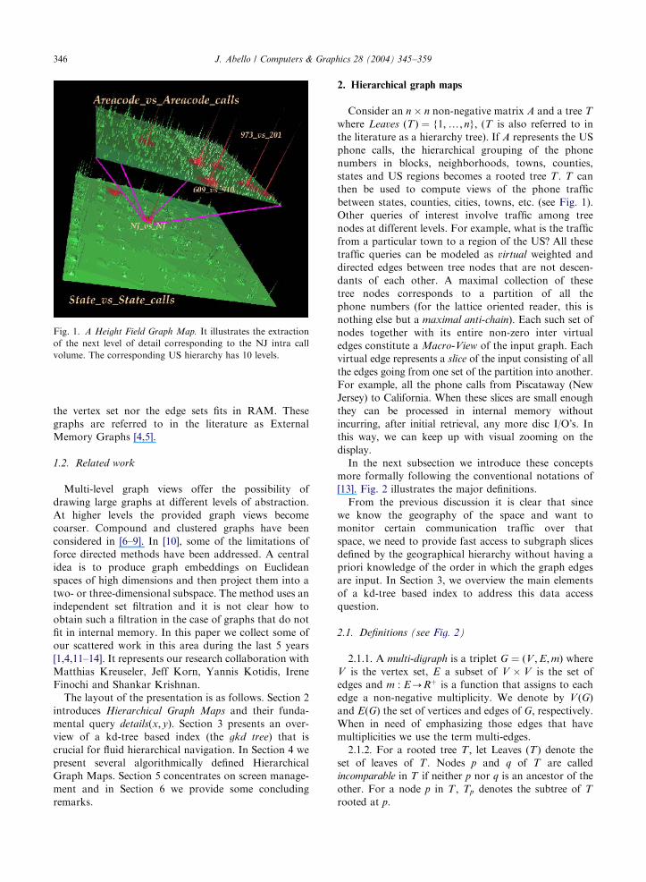
corresponding levels. For example, in Fig. 1, a height

field is used to represent the aggregate US states traffic

matrix. When a particular entry (like NJ–NJ) is selected

the height field representing the traffic between the NJ

area codes is brought into the screen. The height field in

this case plays the role of an interactive map that guides

the navigation. Other representations are possible and

we will introduce some of them later on. The point is

that devising useful hierarchical graph maps for very

large graphs is a tantalizing visualization research area

and we invite the reader to join us in this quest. We

consider a graph large if only its vertex set fits in RAM

but not its edge set. We call a graph very large if neither

d.

ARTICLE IN PRESS

Fig. 1. A Height Field Graph Map. It illustrates the extraction

of the next level of detail corresponding to the NJ intra call

volume. The corresponding US hierarchy has 10 levels.

J. Abello / Computers & Graphics 28 (2004) 345–359346

the vertex set nor the edge sets fits in RAM. These

graphs are referred to in the literature as External

Memory Graphs [4,5].

1.2. Related work

Multi-level graph views offer the possibility of

drawing large graphs at different levels of abstraction.

At higher levels the provided graph views become

coarser. Compound and clustered graphs have been

considered in [6–9]. In [10], some of the limitations of

force directed methods have been addressed. A central

idea is to produce graph embeddings on Euclidean

spaces of high dimensions and then project them into a

two- or three-dimensional subspace. The method uses an

independent set filtration and it is not clear how to

obtain such a filtration in the case of graphs that do not

fit in internal memory. In this paper we collect some of

our scattered work in this area during the last 5 years

[1,4,11–14]. It represents our research collaboration with

Matthias Kreuseler, Jeff Korn, Yannis Kotidis, Irene

Finochi and Shankar Krishnan.

The layout of the presentation is as follows. Section 2

introduces Hierarchical Graph Maps and their funda-

mental query details(x; y). Section 3 presents an over-

view of a kd-tree based index (the gkd tree) that is

crucial for fluid hierarchical navigation. In Section 4 we

present several algorithmically defined Hierarchical

Graph Maps. Section 5 concentrates on screen manage-

ment and in Section 6 we provide some concluding

remarks.

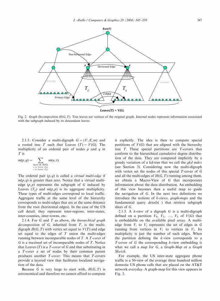
2. Hierarchical graph maps

Consider an n � n non-negative matrix A and a tree T

where Leaves ðTÞ ¼ f1;y; ng; (T is also referred to in

the literature as a hierarchy tree). If A represents the US

phone calls, the hierarchical grouping of the phone

numbers in blocks, neighborhoods, towns, counties,

states and US regions becomes a rooted tree T : T can

then be used to compute views of the phone traffic

between states, counties, cities, towns, etc. (see Fig. 1).

Other queries of interest involve traffic among tree

nodes at different levels. For example, what is the traffic

from a particular town to a region of the US? All these

traffic queries can be modeled as virtual weighted and

directed edges between tree nodes that are not descen-

dants of each other. A maximal collection of these

tree nodes corresponds to a partition of all the

phone numbers (for the lattice oriented reader, this is

nothing else but a maximal anti-chain). Each such set of

nodes together with its entire non-zero inter virtual

edges constitute a Macro-View of the input graph. Each

virtual edge represents a slice of the input consisting of all

the edges going from one set of the partition into another.

For example, all the phone calls from Piscataway (New

Jersey) to California. When these slices are small enough

they can be processed in internal memory without

incurring, after initial retrieval, any more disc I/O’s. In

this way, we can keep up with visual zooming on the

display.

In the next subsection we introduce these concepts

more formally following the conventional notations of

[13]. Fig. 2 illustrates the major definitions.

From the previous discussion it is clear that since

we know the geography of the space and want to

monitor certain communication traffic over that

space, we need to provide fast access to subgraph slices

defined by the geographical hierarchy without having a

priori knowledge of the order in which the graph edges

are input. In Section 3, we overview the main elements

of a kd-tree based index to address this data access

question.

2.1. Definitions (see Fig. 2)

2.1.1. A multi-digraph is a triplet G ¼ ðV ;E;mÞ whereV is the vertex set, E a subset of V � V is the set of

edges and m : E-Rþ is a function that assigns to each

edge a non-negative multiplicity. We denote by V ðGÞand EðGÞ the set of vertices and edges of G; respectively.When in need of emphasizing those edges that have

multiplicities we use the term multi-edges.

2.1.2. For a rooted tree T ; let Leaves ðTÞ denote the

set of leaves of T : Nodes p and q of T are called

incomparable in T if neither p nor q is an ancestor of the

other. For a node p in T ; Tp denotes the subtree of T

rooted at p:

ARTICLE IN PRESS

Tp Tq

……...

p qHorizontal Edge

Root(T)

Leaves(T) = V(G)

Non-horizontal Edge

∈ E(G)Primary Edge

……... ……...

Fig. 2. Graph Decomposition HðG;TÞ. Tree leaves are vertices of the original graph. Internal nodes represent information associated

with the subgraph induced by its descendant leaves.

J. Abello / Computers & Graphics 28 (2004) 345–359 347

2.1.3. Consider a multi-digraph G ¼ ðV ;E;mÞ and

a rooted tree T such that Leaves ðTÞ ¼ V ðGÞ: The

multiplicity of an ordered pair of nodes p and q in

T is

mðp; qÞ ¼X

ðu;vÞ in EðGÞu in Leaves ðTp Þv in Leaves ðTq Þ

mðu; vÞ:

The ordered pair ðp; qÞ is called a virtual multi-edge if

mðp; qÞ is greater than zero. Notice that a virtual multi-

edge ðp; pÞ represents the subgraph of G induced by

Leaves ðTpÞ and mðp; pÞ is its aggregate multiplicity.

These types of multi-edges correspond to local traffic.

Aggregate traffic at the same level of the hierarchy

corresponds to multi-edges that are at the same distance

from the root (horizontal edges). In the case of the US

call detail, they represent inter-regions, inter-states,

inter-counties, inter-towns, etc.

2.1.4. For G and T as above, the hierarchical graph

decomposition of G; inherited from T ; is the multi-

digraph HðG;TÞ with vertex set equal to V ðTÞ and edge

set equal to the edges of T union the multi-edges

running between incomparable nodes of T : A T-cover of

G is a maximal set of incomparable nodes of T : Noticethat Leaves (T) is a T-cover of G and that substituting in

a T-cover a set of nodes by their common parent

produces another T-cover. This means that T-covers

provide a layered view that facilitates localized naviga-

tion of the data.

Because G is very large to start with, HðG;TÞ is

astronomical and therefore we cannot afford to compute

it explicitly. The idea is then to compute special

partitions of V ðGÞ that are aligned with the hierarchy

tree T : These special partitions are T-covers that

conform to the hierarchical cumulative degree distribu-

tion of the data. They are computed implicitly by a

greedy variation of a kd-tree that we call the gkd index

(see Section 3). Considering now the multi-digraph

with vertex set the nodes of this special T-cover of G

and all the multi-edges of HðG;TÞ running among them,we obtain a Macro-View of G that incorporates

information about the data distribution. An embedding

of this view becomes then a useful map to guide

the navigation of G: In the next two definitions we

introduce the notions of k-views, graph-maps and the

fundamental query details( ) that retrieve subgraph

slices of G:2.1.5. A k-view of a digraph G is a multi-digraph

defined on a partition V0; V1; y, Vk of V ðGÞ that

is embeddable on the available pixel array. A multi-

edge from Vi to Vj represents the set of edges in G

running from vertices in Vi to vertices in Vj : Its

multiplicity is just the number of such edges. When

the partition defining the k-view corresponds to a

T-cover of G the corresponding k-view embedding is

what we call a map for G; a Graph-Map or a Graph

Sketch.

For example, the US inter-state aggregate phone

traffic is a 50-view of the average three hundred million

domestic US phone calls that are placed on the AT&T

network everyday. A graph-map for this view appears in

Fig. 3.

ARTICLE IN PRESS

Fig. 3. A Graph Map representing the phone traffic among the 50 US states. The T-cover in this case corresponds to the partition of the

US telephone numbers determined by the US states. Each state contains a glyph that consists of 50 line segments in a particular circular

order of the states. The length and color of the segments encode the traffic volume. Longer and darker segments correspond to higher

traffic volume. A particular segment direction identifies a unique state uniformly. For example, the 50 south-east most segments (one

per state) collectively represent the phone traffic from all the states into Florida. Zooming into one particular state subdivides it into

counties and on each county the corresponding glyph appears. The ‘‘sum’’ of all of these lower level glyphs is equal to the higher level

glyph.

J. Abello / Computers & Graphics 28 (2004) 345–359348

2.1.6. For a multi-edge ðp; qÞ; expansionðp; qÞ is

the subgraph of HðG;TÞ whose nodes are childrenðpÞU childrenðqÞ and all the multi-edges running from

childrenðpÞ to childrenðqÞ: Fig. 1 depicts expansion(NJ,

NJ).

2.1.7. The subgraph slice detailsðp; qÞ is the subgraphof G with vertices Leaves(Tp) U Leaves(Tq) and all the

edges of G running from Leaves(Tp) into Leaves(Tq) .

For example, details(NJ,CA) consists of all the phone

calls originating in New Jersey and terminating in

California.

A good mental picture is that each virtual multi-edge

ðp; qÞ has its own hierarchy of edge slices where each

level represents an aggregation of previous levels and

where the bottom most level is the subgraph of G

consisting of the directed edges running from Leaves(Tp)

to Leaves(Tq).

3. The gkd-tree index

We assume in this section that the input is a multi-

digraph G and that we have a rooted tree T such that

Leaves(T)=V ðGÞ: By numbering the nodes of T in

depth-first search order we notice that, for a given node

p, the set Leaves(Tp) lies in the integer interval

span(p)=[min(p), max(p)] where min(p) and max(p)

denote the minimum and maximum depth-first search

numbered nodes in Leaves(Tp), respectively.

3.1. Why do we use yet another index

Considering a jV ðTÞj � jV ðTÞj integral matrix with a

point ðu; vÞ for each edge ðu; vÞ in EðGÞ we have that

detailsðx; yÞ correspond precisely to the points within therectangle span(x)� span(y). One could think then in

ARTICLE IN PRESSJ. Abello / Computers & Graphics 28 (2004) 345–359 349

applying directly classical range query results; however

this ignores completely the structure imposed on the

search space by T : The gkd-tree remedies this by

exploiting the fact that only OðjV ðGÞjÞ one-dimensionalsub ranges can participate in any two-dimensional query

and uses the distribution of the incoming input graph to

split index pages in a manner that is fully aligned with

the tree providing at the same time good page occupancy

factor. This is achieved by recursively indexing the edges

of G based on the grid specified by the tree T and

partitioning subspaces that are full using horizontal and

vertical splitters similar to a kd tree. The main difference

is that the selection of the splitters is done by balancing

the utilization of the data pages and by using the

structure of the tree T : In summary, the gkd split

algorithm can be viewed as follows: first, a split direction

is decided (assume to be x). Then a set of vertical bands

is superimposed over the grid and the number of points

on each band is registered. It then splits at a band

boundary so that points are equally balanced. Com-

pared to a kd tree, this split is faster to compute (we

refer the reader to [14] for details).

3.2. Dealing with an unbalanced index

Since the gkd tree is an unbalanced index, much

like the kd-tree itself, the number of root to leaf

nodes accessed is not the same for all data pages. In

order to have the performance guarantees provided by

balanced indexes we rely on the fact that for our

application the index is appended only with bulk

insertions. This means that, during data loading, besides

constructing the gkd tree as described in Section 3.1 we

can also build a redundant R�-tree [14] that indexes theleaf pages of the gkd tree. In this way, fast construction

and balanced lookups are possible if the redundant R�

tree can be built without scanning the gkd leaves

themselves. The details of how this is achieved can be

found in [14].

With multi-gigabyte RAMs being a reality and

using this index-based approach, one can process

in principle any secondary storage multi-digraph

defined on several hundred millions of vertices provided

that an explicit hierarchy tree T on the vertex set of G is

known a priori. This assumes enough RAM space to

store the tree T : In the following sections we deal with

the case when the hierarchy tree T is not known in

advance.

4. Algorithmically defined graph maps

In this section we discuss how it is possible to use

hierarchical graph maps when the hierarchy tree is

algorithmically defined. Namely, given an algorithm

that computes a k-view for a graph G; it can be used

recursively to generate a tree T ; such that Leaves(T)

represent a refinement of the original partition defining

the k-view. As before T determines a hierarchical

partition of EðGÞ and therefore a detailed view of a

k-view multi-edge can be obtained by zooming into it. In

other words, if an initial planar embedding of the k-view

is possible, one can zoom in locally into any of the multi-

edges. This locality provided by a planar clustering

allows the user to explore the multi-digraph edge

hierarchy in a fluid manner. All of this is possible only

if the detailed view of a macro-edge can be computed

efficiently.

4.1. A sample of algorithmically defined graph maps

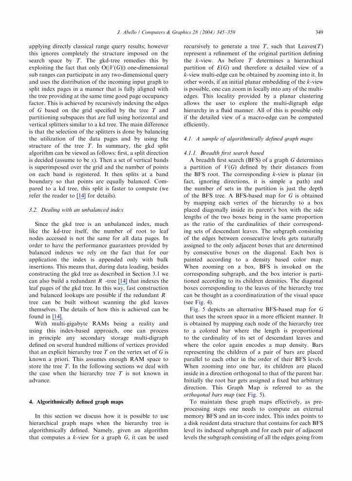
4.1.1. Breadth first search based

A breadth first search (BFS) of a graph G determines

a partition of V ðGÞ defined by their distances from

the BFS root. The corresponding k-view is planar (in

fact, ignoring directions, it is simple a path) and

the number of sets in the partition is just the depth

of the BFS tree. A BFS-based map for G is obtained

by mapping each vertex of the hierarchy to a box

placed diagonally inside its parent’s box with the side

lengths of the two boxes being in the same proportion

as the ratio of the cardinalities of their correspond-

ing sets of descendant leaves. The subgraph consisting

of the edges between consecutive levels gets naturally

assigned to the only adjacent boxes that are determined

by consecutive boxes on the diagonal. Each box is

painted according to a density based color map.

When zooming on a box, BFS is invoked on the

corresponding subgraph, and the box interior is parti-

tioned according to its children densities. The diagonal

boxes corresponding to the leaves of the hierarchy tree

can be thought as a coordinatization of the visual space

(see Fig. 4).

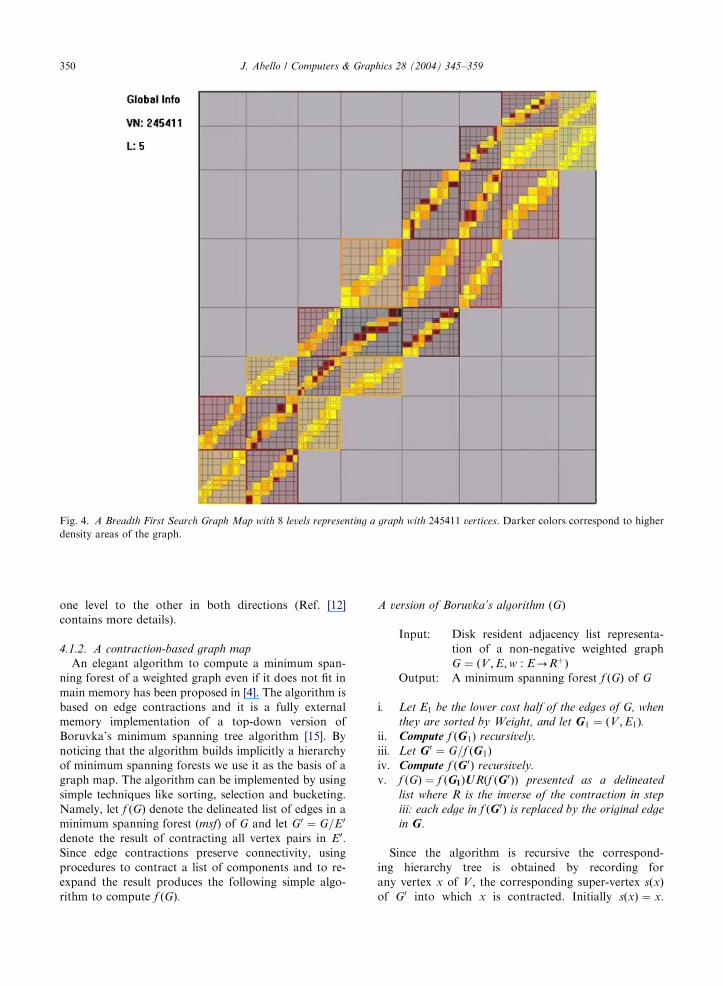
Fig. 5 depicts an alternative BFS-based map for G

that uses the screen space in a more efficient manner. It

is obtained by mapping each node of the hierarchy tree

to a colored bar where the length is proportional

to the cardinality of its set of descendant leaves and

where the color again encodes a map density. Bars

representing the children of a pair of bars are placed

parallel to each other in the order of their BFS levels.

When zooming into one bar, its children are placed

inside in a direction orthogonal to that of the parent bar.

Initially the root bar gets assigned a fixed but arbitrary

direction. This Graph Map is referred to as the

orthogonal bars map (see Fig. 5).

To maintain these graph maps effectively, as pre-

processing steps one needs to compute an external

memory BFS and an in-core index. This index points to

a disk resident data structure that contains for each BFS

level its induced subgraph and for each pair of adjacent

levels the subgraph consisting of all the edges going from

ARTICLE IN PRESS

Fig. 4. A Breadth First Search Graph Map with 8 levels representing a graph with 245411 vertices. Darker colors correspond to higher

density areas of the graph.

J. Abello / Computers & Graphics 28 (2004) 345–359350

one level to the other in both directions (Ref. [12]

contains more details).

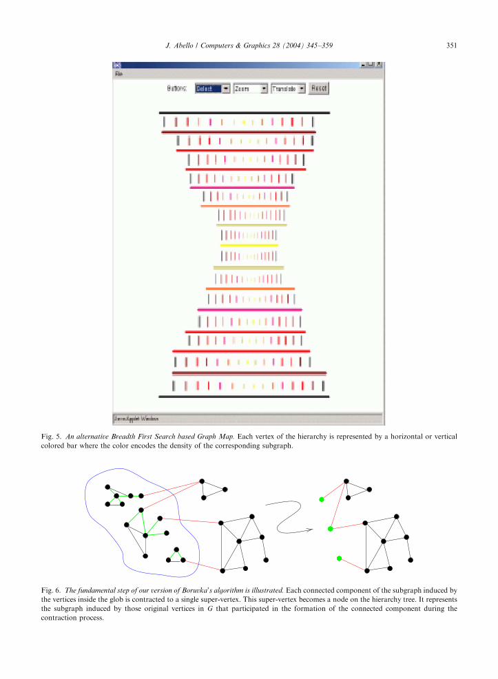
4.1.2. A contraction-based graph map

An elegant algorithm to compute a minimum span-

ning forest of a weighted graph even if it does not fit in

main memory has been proposed in [4]. The algorithm is

based on edge contractions and it is a fully external

memory implementation of a top-down version of

Boruvka’s minimum spanning tree algorithm [15]. By

noticing that the algorithm builds implicitly a hierarchy

of minimum spanning forests we use it as the basis of a

graph map. The algorithm can be implemented by using

simple techniques like sorting, selection and bucketing.

Namely, let f ðGÞ denote the delineated list of edges in a

minimum spanning forest (msf) of G and let G0 ¼ G=E0

denote the result of contracting all vertex pairs in E0:Since edge contractions preserve connectivity, using

procedures to contract a list of components and to re-

expand the result produces the following simple algo-

rithm to compute f ðGÞ:

A version of Boruvka’s algorithm ðGÞ

Input:

Disk resident adjacency list representa-

tion of a non-negative weighted graph

G ¼ ðV ;E;w : E-RþÞ

Output: A minimum spanning forest f ðGÞ of G

i.

Let E1 be the lower cost half of the edges of G, when

they are sorted by Weight, and let G1 ¼ ðV ;E1Þ.

ii. Compute f ðG1Þ recursively.

iii.

Let G 0 ¼ G=f ðG1Þ iv. Compute f ðG 0Þ recursively.

v.

f ðGÞ ¼ f ðG1ÞURðf ðG 0ÞÞ presented as a delineated

list where R is the inverse of the contraction in step

iii: each edge in f ðG 0Þ is replaced by the original edge

in G :

Since the algorithm is recursive the correspond-

ing hierarchy tree is obtained by recording for

any vertex x of V ; the corresponding super-vertex sðxÞof G0 into which x is contracted. Initially sðxÞ ¼ x:

ARTICLE IN PRESS

Fig. 5. An alternative Breadth First Search based Graph Map. Each vertex of the hierarchy is represented by a horizontal or vertical

colored bar where the color encodes the density of the corresponding subgraph.

Fig. 6. The fundamental step of our version of Boruvka’s algorithm is illustrated. Each connected component of the subgraph induced by

the vertices inside the glob is contracted to a single super-vertex. This super-vertex becomes a node on the hierarchy tree. It represents

the subgraph induced by those original vertices in G that participated in the formation of the connected component during the

contraction process.

J. Abello / Computers & Graphics 28 (2004) 345–359 351

ARTICLE IN PRESS

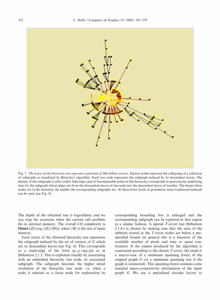
Fig. 7. The leaves of this hierarchy tree represent a partition of 260 million vertices. Interior nodes represent the collapsing of a collection

of subgraphs as mandated by Boruvka’s algorithm. Each tree node represents the subgraph induced by its descendant leaves. The

density of this subgraph is color coded. Selecting a pair of incomparable nodes in this hierarchy corresponds to querying the underlying

data for the subgraph whose edges run from the descendant leaves of one node into the descendant leaves of another. The deeper these

nodes are in the hierarchy the smaller the corresponding subgraphs are. At these lower levels of granularity more traditional methods

can be used (see Fig. 8).

J. Abello / Computers & Graphics 28 (2004) 345–359352

The depth of the obtained tree is logarithmic and we

can stop the recursion when the current sub problem

fits in internal memory. The overall I/O complexity is

O(sort ðjEjÞ log2 ðjEj=jM jÞ), where jM j is the size of mainmemory.

Each vertex of the obtained hierarchy tree represents

the subgraph induced by the set of vertices of G which

are its descendant leaves (see Fig. 6). This corresponds

to a multi-edge of the form ðp; p; mðp; pÞÞ as in

Definition 2.1.3. This is exploited visually by associating

with an embedded hierarchy tree node, its associated

subgraph. The subgraph becomes the higher detail

resolution of the hierarchy tree node, i.e. when a

node is selected as a focus node for exploration its

corresponding bounding box is enlarged and the

corresponding subgraph can be explored in that region

in a similar fashion. A special T-cover (see Definition

2.1.4.) is chosen by making sure that the sizes of the

subtrees rooted at the T-cover nodes are below a pre-

specified bound (in general this is a function of the

available number of pixels and time or space con-

straints). If the output produced by the algorithm is

contracted according to the chosen T-cover, the result is

a macro-view of a minimum spanning forest of the

original graph G (or a minimum spanning tree if the

graph is connected). This spanning forest contains some

essential macro-connectivity information of the input

graph G: We use a specialized circular layout to

ARTICLE IN PRESS

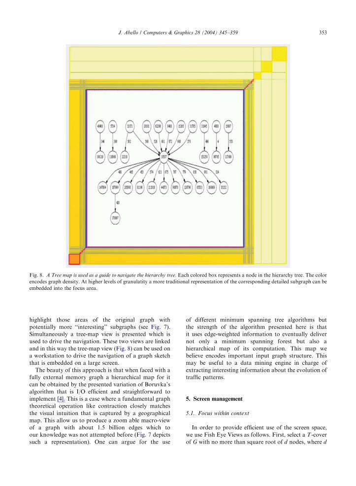
Fig. 8. A Tree map is used as a guide to navigate the hierarchy tree. Each colored box represents a node in the hierarchy tree. The color

encodes graph density. At higher levels of granulatity a more traditional representation of the corresponding detailed subgraph can be

embedded into the focus area.

J. Abello / Computers & Graphics 28 (2004) 345–359 353

highlight those areas of the original graph with

potentially more ‘‘interesting’’ subgraphs (see Fig. 7).

Simultaneously a tree-map view is presented which is

used to drive the navigation. These two views are linked

and in this way the tree-map view (Fig. 8) can be used on

a workstation to drive the navigation of a graph sketch

that is embedded on a large screen.

The beauty of this approach is that when faced with a

fully external memory graph a hierarchical map for it

can be obtained by the presented variation of Boruvka’s

algorithm that is I/O efficient and straightforward to

implement [4]. This is a case where a fundamental graph

theoretical operation like contraction closely matches

the visual intuition that is captured by a geographical

map. This allow us to produce a zoom able macro-view

of a graph with about 1.5 billion edges which to

our knowledge was not attempted before (Fig. 7 depicts

such a representation). One can argue for the use

of different minimum spanning tree algorithms but

the strength of the algorithm presented here is that

it uses edge-weighted information to eventually deliver

not only a minimum spanning forest but also a

hierarchical map of its computation. This map we

believe encodes important input graph structure. This

may be useful to a data mining engine in charge of

extracting interesting information about the evolution of

traffic patterns.

5. Screen management

5.1. Focus within context

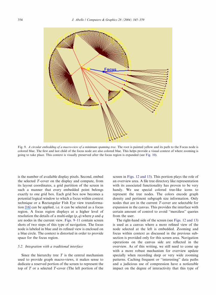
In order to provide efficient use of the screen space,

we use Fish Eye Views as follows. First, select a T-cover

of G with no more than square root of d nodes, where d

ARTICLE IN PRESS

Fig. 9. A circular embedding of a macro-view of a minimum spanning tree. The root is painted yellow and its path to the Focus node is

colored blue. The first and last child of the focus node are also colored blue. This helps provide a visual context of where zooming is

going to take place. This context is visually preserved after the focus region is expanded (see Fig. 10).

J. Abello / Computers & Graphics 28 (2004) 345–359354

is the number of available display pixels. Second, embed

the selected T-cover on the display and compute, from

its layout coordinates, a grid partition of the screen in

such a manner that every embedded point belongs

exactly to one grid box. Each grid box now becomes a

potential logical window to which a focus within context

technique or a Rectangular Fish Eye view transforma-

tion [16] can be applied, i.e. it can be selected as a focus

region. A focus region displays at a higher level of

resolution the details of a multi-edge ðp; qÞ where p and q

are nodes in the current view. Figs. 9–11 contain screen

shots of two steps of this type of navigation. The focus

node is labeled in blue and its refined view is enclosed on

a blue circle. The context is distorted in order to provide

space for the focus region.

5.2. Integration with a traditional interface

Since the hierarchy tree T is the central mechanism

used to provide graph macro-views, it makes sense to

dedicate a reserved portion of the screen to represent the

top of T or a selected T-cover (The left portion of the

screen in Figs. 12 and 13). This portion plays the role of

an overview area. A file tree directory like representation

with its associated functionality has proven to be very

handy. We use special colored tree-like icons to

represent the tree nodes. The colors encode graph

density and pertinent subgraph size information. Only

nodes that are in the current T-cover are selectable for

expansion in the canvas. This provides the interface with

certain amount of control to avoid ‘‘merciless’’ queries

from the user.

The right-hand side of the screen (see Figs. 12 and 13)

is used as a canvas where a more refined view of the

node selected at the left is embedded. Zooming and

focus within context as discussed in the previous sub-

section is provided only for this screen area. Navigation

operations on the canvas side are reflected in the

overview. As of this writing, we still need to come up

with a more robust mechanism for overview update

specially when recording deep or very wide zooming

patterns. Caching frequent or ‘‘interesting’’ data paths

and a judicious use of compression have a noticeable

impact on the degree of interactivity that this type of

ARTICLE IN PRESS

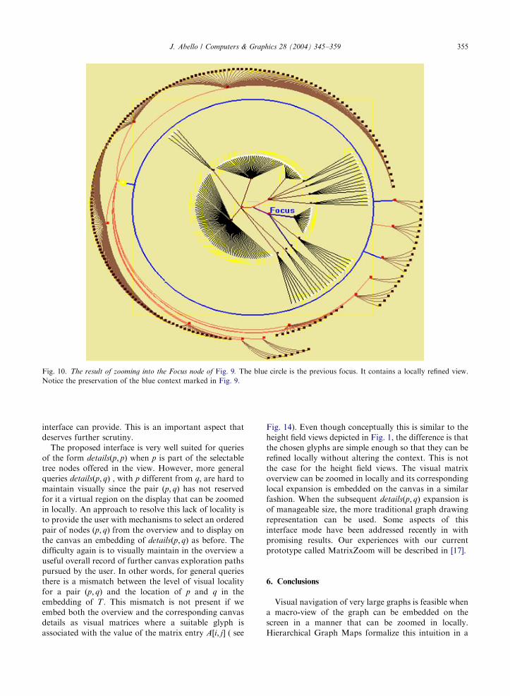
Fig. 10. The result of zooming into the Focus node of Fig. 9. The blue circle is the previous focus. It contains a locally refined view.

Notice the preservation of the blue context marked in Fig. 9.

J. Abello / Computers & Graphics 28 (2004) 345–359 355

interface can provide. This is an important aspect that

deserves further scrutiny.

The proposed interface is very well suited for queries

of the form detailsðp; pÞ when p is part of the selectable

tree nodes offered in the view. However, more general

queries detailsðp; qÞ , with p different from q; are hard to

maintain visually since the pair ðp; qÞ has not reservedfor it a virtual region on the display that can be zoomed

in locally. An approach to resolve this lack of locality is

to provide the user with mechanisms to select an ordered

pair of nodes ðp; qÞ from the overview and to display on

the canvas an embedding of detailsðp; qÞ as before. Thedifficulty again is to visually maintain in the overview a

useful overall record of further canvas exploration paths

pursued by the user. In other words, for general queries

there is a mismatch between the level of visual locality

for a pair ðp; qÞ and the location of p and q in the

embedding of T : This mismatch is not present if we

embed both the overview and the corresponding canvas

details as visual matrices where a suitable glyph is

associated with the value of the matrix entry A½i; j� ( see

Fig. 14). Even though conceptually this is similar to the

height field views depicted in Fig. 1, the difference is that

the chosen glyphs are simple enough so that they can be

refined locally without altering the context. This is not

the case for the height field views. The visual matrix

overview can be zoomed in locally and its corresponding

local expansion is embedded on the canvas in a similar

fashion. When the subsequent detailsðp; qÞ expansion is

of manageable size, the more traditional graph drawing

representation can be used. Some aspects of this

interface mode have been addressed recently in with

promising results. Our experiences with our current

prototype called MatrixZoom will be described in [17].

6. Conclusions

Visual navigation of very large graphs is feasible when

a macro-view of the graph can be embedded on the

screen in a manner that can be zoomed in locally.

Hierarchical Graph Maps formalize this intuition in a

ARTICLE IN PRESS

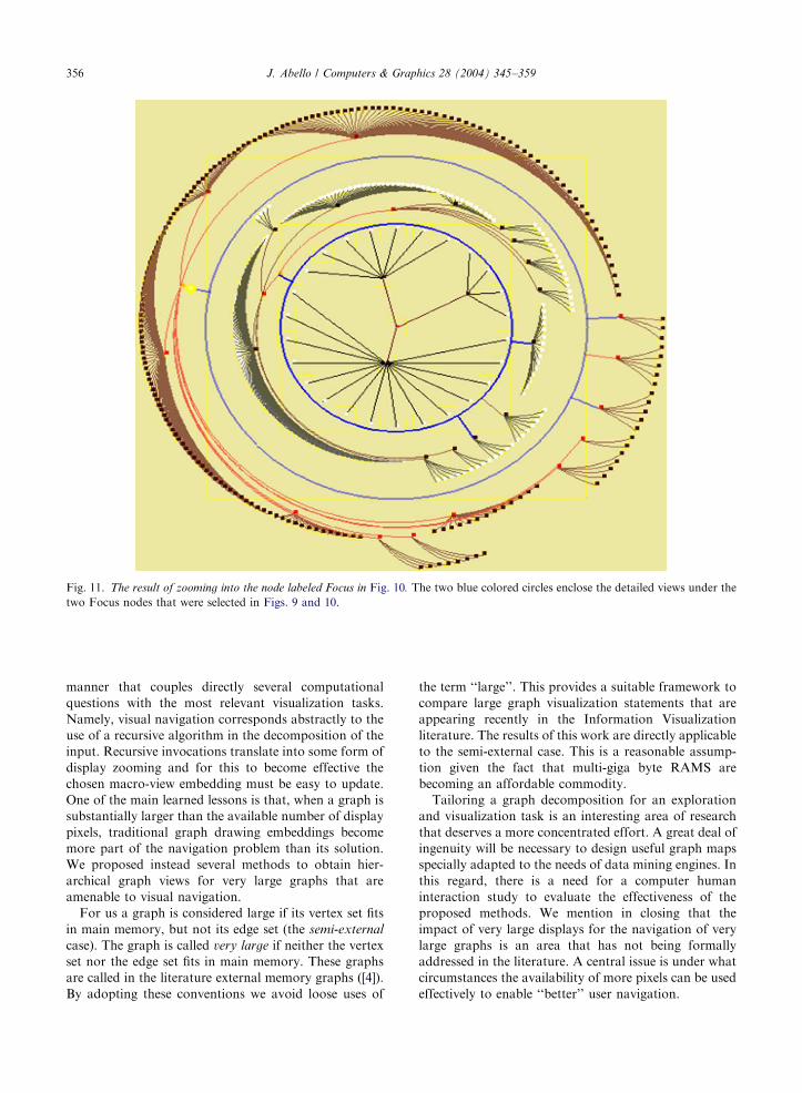
Fig. 11. The result of zooming into the node labeled Focus in Fig. 10. The two blue colored circles enclose the detailed views under the

two Focus nodes that were selected in Figs. 9 and 10.

J. Abello / Computers & Graphics 28 (2004) 345–359356

manner that couples directly several computational

questions with the most relevant visualization tasks.

Namely, visual navigation corresponds abstractly to the

use of a recursive algorithm in the decomposition of the

input. Recursive invocations translate into some form of

display zooming and for this to become effective the

chosen macro-view embedding must be easy to update.

One of the main learned lessons is that, when a graph is

substantially larger than the available number of display

pixels, traditional graph drawing embeddings become

more part of the navigation problem than its solution.

We proposed instead several methods to obtain hier-

archical graph views for very large graphs that are

amenable to visual navigation.

For us a graph is considered large if its vertex set fits

in main memory, but not its edge set (the semi-external

case). The graph is called very large if neither the vertex

set nor the edge set fits in main memory. These graphs

are called in the literature external memory graphs ([4]).

By adopting these conventions we avoid loose uses of

the term ‘‘large’’. This provides a suitable framework to

compare large graph visualization statements that are

appearing recently in the Information Visualization

literature. The results of this work are directly applicable

to the semi-external case. This is a reasonable assump-

tion given the fact that multi-giga byte RAMS are

becoming an affordable commodity.

Tailoring a graph decomposition for an exploration

and visualization task is an interesting area of research

that deserves a more concentrated effort. A great deal of

ingenuity will be necessary to design useful graph maps

specially adapted to the needs of data mining engines. In

this regard, there is a need for a computer human

interaction study to evaluate the effectiveness of the

proposed methods. We mention in closing that the

impact of very large displays for the navigation of very

large graphs is an area that has not being formally

addressed in the literature. A central issue is under what

circumstances the availability of more pixels can be used

effectively to enable ‘‘better’’ user navigation.

ARTICLE IN PRESS

Fig. 12. A view of our current interface. The left hand side depicts the top of the hierarchy tree. The numbers next to the tree icons are

just node identifiers. The last column records the number of descendant leaves in the hierarchy tree under the corresponding tree node.

When a node is selected (indicated by a blue rectangle) its corresponding next level view is brought into the canvas at the right hand

side and its associated graph parameter values are presented in a textual manner. The user can explore the canvas embedding by using

some of the Focus within Context techniques described in this section. For example, Fig. 13 displays the resulting view after the user

has selected the focus node in the canvas area.

Fig. 13. The graph view presented at the right hand side is the refined version of the corresponding view presented in Fig. 12. In both cases

the corresponding hierarchy tree node at the left is enclosed in a blue rectangle. The darker blue bar indicates that zooming is taking

place within the corresponding subtree.

J. Abello / Computers & Graphics 28 (2004) 345–359 357

ARTICLE IN PRESS

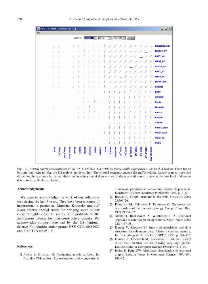
Fig. 14. A visual matrix representation of the US–CANADA–CARIBEAN phone traffic aggregated at the level of regions. From top to

bottom (and right to left), the US regions are listed first. The colored segments encode the traffic volume. Larger segments are also

darker and have a more horizontal direction. Selecting any of these entries produces a similar matrix view at the next level of detail as

determined by the hierarchy tree.

J. Abello / Computers & Graphics 28 (2004) 345–359358

Acknowledgements

We want to acknowledge the work of our collabora-

tors during the last 5 years. They have been a source of

inspiration. In particular, Matthias Kreuseler and Jeff

Korn deserve special credit for bringing some of our

crazy thoughts closer to reality. Our gratitude to the

anonymous referees for their constructive remarks. We

acknowledge support provided by the US National

Science Foundation under grants NSF CCR 00-87022

and NSF EIA 02-05116.

References

[1] Abello J, Krishnan S. Navigating graph surfaces. In:

Pardalos PM, editor. Approximation and complexity in

numerical optimization: continuous and discrete problems.

Dordrecht: Kluwer Academic Publishers; 1999. p. 1–12.

[2] Broder A. Graph structure in the web. Networks 2000;

33:309–20.

[3] Faloutsos M, Faloutsos P, Faloutsos C. On power-law

relationships of the Internet topology. Comp. Comm. Rev.

1999;29:251–62.

[4] Abello J, Buchsbaum A, Westbrook J. A functional

approach to external graph algorithms. Algorithmica 2002;

32(3):437–58.

[5] Kumar V, Schwabe EJ, Improved algorithms and data

structures for solving graph problems in external memory.

In: Proceedings of the 8th IEEE SPDP, 1996. p. 169–176.

[6] Duncan C, Goodrich M, Kobourov S. Balanced aspect

ratio trees and their use for drawing very large graphs.

Lecture Notes in Computer Science 1998;1547:111–24.

[7] Eades P, Feng QW. Multilevel visualization of clustered

graphs. Lecture Notes in Computer Science 1997;1190:

101–12.

ARTICLE IN PRESSJ. Abello / Computers & Graphics 28 (2004) 345–359 359

[8] Eades P, Feng QW, Lin X, Straight-line drawing

algorithms for hierarchical and clustered graphs. Proceed-

ings of the Fourth Symposium on Graph Drawing, 1996.

p. 113–28.

[9] Sugiyama K, Misue K. Visualization of structural infor-

mation: automatic drawing of compound digraphs. In

IEEE Transactions on Systems, Man and Cybernetics

1991;21(4):876–92.

[10] Gajer P, Goodrich M, Kobourov S. A multidimensional

approach to force directed layouts of large graphs. In

proceedings of the graph drawing, lecture notes in

computer science. Berlin: Springer; 2000.

[11] Abello J, Finocchi I, Korn J, Graph Sketches. In: IEEE

InfoVis Proceedings. San Diego, CA, October 2001. p. 67–71.

[12] Abello J, Korn J, Kreuseler M, Navigating giga-graphs.

In: ACM Proceedings of Advanced Visualization Inter-

faces (AVI), Trento, Italy, 2002. p. 290–9.

[13] Abello J, Korn J. MGV: A system for visualizing massive

multidigraphs. IEEE Transactions on Visualization and

Computer Graphics 2002;8(1):21–38.

[14] Abello J, Kotidis Y, Hierarchical graph indexing. In: ACM

12th International Conference on Information and Knowl-

edge Management, ICKM, New Orleans, November 3–9,

2003.

[15] Boruvka O. O jistem problemu minimalnim. Acta Socie-

tatis Science Natur. Moravicae, 1926;3:37–58.

[16] Rauschenbach U, Jeschke S, Schumann H, General

rectangular fish eye views for 2D graphics. In: Proceedings

of the Intelligent Interactive Assistance and Mobile

Computing, IMC, 2000.

[17] J. Abello, F.V. Ham. Matrix-zoom: an experimental graph

map system, DIMACS technical report, in preparation.

James Abello is the co-editor of External Memory Algorithms,

Vol. 50 of the AMS-DIMACS series (with J. Vitter, 1999)

and The Kluwer Handbook of Massive Data Sets (with

P. Pardalos and M. Resende, 2002). James research focus has

been on Algorithms and Data Structures, Massive Data Sets,

Algorithm Animation and Visualization, Combinatorial and

Computational Geometry, Discrete Mathematics, and some

applications in Petroleum Engineering and Biology. He has

held several academic positions and has been a senior member

of technical staff at AT&T Shannon Laboratories and Bell

Labs. He is currently a research associate at DIMACS, Rutgers

University. Information about some of James’s current

visualization research projects can be obtained by accessing

www.mgvis.com.