Technische Universität ChemnitzUlrich ElsnerGraph PartitioningA survey

SFB 393

MASSIV

SIM

UL

AT

ION P

AR

AL

LE

LSMSonderforschungsbereich 393Numerische Simulationauf massiv parallelen RechnernPreprint SFB393/97-27, Dec. 1997

ContentsContents iNotation iii1 The problem 11.1 Introduction . . . . . . . . . . . . . . . . . . . . . . . . . . . . . . . . . 11.2 Graph Partitioning . . . . . . . . . . . . . . . . . . . . . . . . . . . . . 21.3 Examples . . . . . . . . . . . . . . . . . . . . . . . . . . . . . . . . . . 41.3.1 Partial Di�erential Equations . . . . . . . . . . . . . . . . . . . 41.3.2 Sparse Matrix-Vector Multiplication . . . . . . . . . . . . . . . . 61.3.3 Other Applications . . . . . . . . . . . . . . . . . . . . . . . . . 81.4 Time vs. Quality . . . . . . . . . . . . . . . . . . . . . . . . . . . . . . 92 Miscellaneous Algorithms 112.1 Introduction . . . . . . . . . . . . . . . . . . . . . . . . . . . . . . . . . 112.2 Recursive Bisection . . . . . . . . . . . . . . . . . . . . . . . . . . . . . 112.3 Partitioning with geometric information . . . . . . . . . . . . . . . . . 142.3.1 Coordinate Bisection . . . . . . . . . . . . . . . . . . . . . . . . 152.3.2 Inertial Bisection . . . . . . . . . . . . . . . . . . . . . . . . . . 162.3.3 Geometric Partitioning . . . . . . . . . . . . . . . . . . . . . . . 173 Partitioning without geometric information 233.1 Introduction . . . . . . . . . . . . . . . . . . . . . . . . . . . . . . . . . 233.2 Graph Growing and Greedy Algorithms . . . . . . . . . . . . . . . . . . 233.2.1 Kernigan�Lin Algorithm . . . . . . . . . . . . . . . . . . . . . . 253.3 Spectral Bisection . . . . . . . . . . . . . . . . . . . . . . . . . . . . . . 283.3.1 Spectral Bisection for weighted graphs . . . . . . . . . . . . . . 333.3.2 Spectral Quadri� and Octasection . . . . . . . . . . . . . . . . . 343.3.3 Multilevel Spectral Bisection . . . . . . . . . . . . . . . . . . . . 373.3.4 Algebraic Multilevel . . . . . . . . . . . . . . . . . . . . . . . . 403.4 Multilevel Partitioning . . . . . . . . . . . . . . . . . . . . . . . . . . . 423.4.1 Coarsening the graph . . . . . . . . . . . . . . . . . . . . . . . . 43i

Contents3.4.2 Partitioning the smallest graph . . . . . . . . . . . . . . . . . . 453.4.3 Projecting up and re�ning the partition . . . . . . . . . . . . . . 463.5 Other methods . . . . . . . . . . . . . . . . . . . . . . . . . . . . . . . 46Bibliography 47

ii

NotationBelow we list (most of) the symbols used in the text together with a brief explanationof their meaning.(V; E) A (undirected) graph with vertices V and edges E.E = fei;j j there is an edge between vi and vjg, the setof edges.V = fvi j i = 1; : : : ; ng, the set of vertices.WE = fwe(ei;j) 2 N j ei;j 2 Eg, weights of the edges in E.WV = fwv(vi) 2 N j vi 2 Vg, weights of the vertices in V.deg(vi) = ��fvj 2 V jei;j 2 Eg�� the degree of vertex vi.(The number of adjacent vertices)L(G) The Laplacian matrix of the graph G = (V; E).lij = 8>><>>:�1 if i 6= j and ei;j 2 E0 if i 6= j and ei;j 62 Ed(vi) if i = jA(G) The adjacency matrix of the graph G = (V; E).aij = (�1 if i 6= j and ei;j 2 E0 otherwise; the empty set.j : j for X a set, jX j is the number of elements in X .iii

Notationk : kp for x 2 C n a vector, jxj is the p-norm of x,kxkp = (Pni=1 jxijp)1=p.k : k = k : k2, the Euklidian norm.e = (1; 1; : : : 1)T .O(f(n)) = f g(n) j there exists a C > 0 with jg(n)j � C �f(n) for all n � n0g,the Landau symbol.A _[B = A [ B with A \ B = ;, disjoint union. The dot just emphasizesthat the two sets are disjoint.In; I The identity matrix of size n. If the size is obvious from thecontext, I is used.�(A) spectrum of A.diag(w) a diagonal matrix with the components of the vector w on thediagonal.

iv

1 The problem1.1 IntroductionWhile the performance of classical (von Neumann) computers has grown tremen-dously, there is always demand for more than the current technology can deliver. Atany given moment, it is only possible to put so many transistors on a chip and whilethat number increases every year, certain physical barriers loom on the horizon (sim-ply put, an electron has to �t through each data path, the information has to travel acertain distance in each cycle) that cannot be be surpassed by the technology knowntoday.But while it is certainly important to pursue new methods and technologies thatcan push these barriers a bit further or even break them, what can be done to getbigger performance now?Mankind has for eons used teamwork to achieve things that a single human beingis incapable of (from hunting as a group to building the pyramids). The same ideacan be used with computers: parallel computing. Invented or rather revived about15 years ago, parallel computers achieve performances that are impossible or much toexpensive to achieve with single processor machines. Therefore parallel computers ofone architecture or another have become increasingly popular with the scienti�c andtechnical community.But just as working together as a team does not always work e�ciently (10 peoplecannot dig a post-hole 10 times as fast as one) and creates new problems that do notoccur when one is working alone (how to coordinate the 10000 peasants working on thepyramid), obstacles unknown to single processor programmers occur when workingon a parallel machine.First, not all parts of a problem can be parallelized but some have to be executedserially. This limits the total possible speedup (Ahmdal's law [1]) for a given problemof constant size. Quite often though the sequential part of the work tends to beindependent from the size of the input and so for a bigger problem (adequate forsharing the work among more processors) a higher speedup is possible. Problems ofthis kind are called scalable [43].Second, the amount of work done has to be distributed evenly amongst the pro-1

1 The problemcessors. This is even more necessary if during the course of the computation somedata has to be exchanged or some process synchronized. In this case, some of theprocessors have to wait for others to �nish. This load-balancing might be easy forsome problems but quite complicated for others. The amount of work per processormight vary during the course of the computation, for example when some criticalpoint needs to be examined closer. So perfect balance in one step does not have tomean balance in the next.This could easily be avoided by moving some of the work to another, underutilizedprocessor. But this always means communication between di�erent processors. Andcommunication is, alas, time-consuming.This brings us to the third obstacle. In almost all �real-life� problems, the proces-sors regularly need information from each other to continue their work. This has twoe�ects. As mentioned above, these exchanges entail synchronization points, makingit necessary for some of the processors to wait for others. And of course communica-tion itself takes some time. Depending on the architecture, exchanging even one bitof information between two processors might be many times slower than accessing abit in the processor itself. There might be a high startup time such that exchanginghundreds of bytes takes almost the same amount of time as exchanging one byte. Itmight or might not be possible that exchanges between two disjoint pairs of processorstakes place at the same time.While all this is highly machine-dependent, it is evident that it is desirable topartition the problem (or the data) in such a way that not only the work is distributedevenly but also that at the same time communication is minimized. As we will see, forcertain problems this will lead to the problem of partitioning a graph. In its simplestform this means that we divide the vertices of a graph into equal sized parts such thatthe number of edges connecting these parts is minimal.1.2 Graph PartitioningFirst, some notations (cf. [34,61]):A graph (V; E) consists of a number of vertices V = fvi j i = 1; : : : ; ng, someof which are connected by edges in E = fei;j = (i; j) j there is an edge betweenvi and vjg. Other names for vertices include nodes, grid points or mesh points.In order to avoid excessive subscripts, we will sometimes equate i with vi and (i; j)with ei;j if there is no danger of confusion .Given a subset �V � V of vertices, the induced subgraph ( �V; �E) contains all thoseedges �E � E that join two vertices in �V.Both vertices and edges can have weights associated with them.2

1.2 Graph PartitioningWE = fwe(ei;j) 2 N j ei;j 2 Eg are the weights of the edges and WV = fwv(vi) 2N j vi 2 Vg are the weights of the vertices.The weights are non-negative integers. This often allows for a more e�cient analy-sis or implementation of algorithms. For example, sorting a list of integers of restrictedsize can be done using the bucket-sort algorithm with its O(n) performance. But thisrestriction is not as big as it seems. For example, positive rational weights can easilybe mapped to N+ by scaling them with the smallest common multiple of the denom-inators. If no weights are given, all weights should be considered to be 1.The simplest form of graph partitioning, unweighted graph bisection is this: given agraph consisting of vertices and edges, divide the vertices in two sets of equal size suchthat the number of edges between these two parts is minimized. Or, more formally:Let G = (V; E) be a graph with jVj (the number of of elements in V) even.Find a partition (V1;V2) of V (i.e., V1 [ V2 = V and V1 \ V2 = ;. This disjointunion ist sometimes expressed by V1 _[V2 = V) withjV1j = jV2jsuch that jfei;j 2 E j vi 2 V1 and vj 2 V2gj (1.1)is minimized among all possible partitions of V with equal size.A more general formulation involves weighted edges, weighted vertices and p dis-joint subsets . Then the sum of weights of vertices in each of the subsets should beequal while the sum of the edges between these subsets is minimized. Again, moreformally:Let G = (V; E) be a graph with weights WV and WE (with Pvi2V wv(vi) divisibleby p).Find a p�partition (V1;V2; : : : ;Vp) of V, i.e.,p[i=1Vi = V and Vi \ Vj = ; for all i 6= jwith Xv(i)2Vjwv(vi) equal for all j 2 f1; 2; : : : ; pgsuch that Xei;j2E withvi2Vp; vj2Vq and p6=qwe(ei;j) (1.2)is minimized among all possible partitions of V. 3

1 The problem(1.1) and (1.2) are also referred to as cut-size, implying the picture that one takesthe whole graph, �cuts� these edges and is left with the subgraphs induced by thesubsets of the vertices. Other names used include edgecut or cost of the partition.As described above, we are looking for a small subset of edges that, when takenaway, separates the graph in two disjoint subsets. This is called �nding an edgeseparator.Instead of edges, one can also look for a subset of vertices, the so-called vertexseparator that separates the graph:Given a graph G = (V; E), �nd three disjoint subsets V1;V2 and VS with� V1 _[V2 _[VS = V� jVSj small� jV1j � jV2j� no edge joins V1 and V2Depending on the application, either the edge separator or the vertex separatoris needed. Fortunately, it is easy to convert these two kinds of separators into eachother.For example, assume we have an edge separator but need a vertex separator.Consider the graph �G consisting only of the separating edges and their endpoints.Any vertex cover of �G (that is, any set of vertices that include at least one endpointof every edge in G) is a vertex separator for the graph. Since �G is bipartite, we cancompute the smallest vertex cover e�ciently by bipartite matching.1.3 ExamplesIn the following examples we assume that we have a parallel computer with distributedmemory, that is, each processor has its own memory. If it needs to access data in someother processors memory, communication is necessary. Many of the parallel computersof today are of this kind.1.3.1 Partial Di�erential EquationsA lot of the methods for solving partial di�erential equations (PDEs) are grid-oriented,i.e. the data is de�ned on a discrete grid of points, �nite elements or �nite volumesand the calculation consists of applying certain operations on the data associated withall the points, elements or volumes of the grid [61]. These calculations usually alsoinvolve some of the data of the neighboring elements.4

1.3 Examples���� ���� ���� ���� ���� �������� ���� ���� ���� ���� ������������ �������� bad partitiongood partition Figure 1.1: Two partitionsc c cc cc c c cc ccc������AAA���QQQQQ �����HHHHHHDDDDDDDHHHHHH����������� �����ccccccc���������HHHHHHHHH���������AAAAAA @@@����� ������@@@@@������BBBBB��� XXXXXX������AAA @@@c @@@�����1 23 45 678 9 1011 12 1314 v3 v5 v8 v9 v11 v13v14v10v12v7v6v1 v4v2Figure 1.2: A �nite element mesh and the corresponding dependency graphDistributing the problem to parallel processors is done by partitioning the grid intosubgrids and solving the associated subproblems on the di�erent processors. Since theelements on the �borders� of the subgrids need to access data on the other processors,communication is necessary. Using the reasonable assumption that the amount ofcommunication between two neighbors is constant, one has to minimize the �borderlength�, i.e. the number of neighbors in di�erent partitions. (cf. Figure 1.1)To formulate the problem as a graph partitioning problem, we look at the so-calleddependency graph of the grid (cf. Figure 1.2).Every grid-point (or �nite element) has a corresponding vertex on this graph. Theweight of the vertex is proportional to the amount of computational work done onthis grid point. (Quite often the weights of all vertices are equal).For each pair of neighboring (or otherwise dependent) grid points the correspond-ing vertices are connected by an edge. The weight of this edge is proportional tothe amount of communication between these two grid points. (Again, quite often theweights of all edges are equal). 5

1 The problemFor �nite element meshes (A mesh is a graph embedded into (usually) two� orthree�dimensional space so that the coordinates of the vertices are known.), the un-weighted dependency graph is equal to the dual graph of the mesh.Now the optimal grid partitioning can simply be found by solving the graph par-titioning problem on the dependency graph and distributing the gridpoint or �niteelement to the j-th processor if its corresponding vertex is in the j-th partition of thegraph.1.3.2 Sparse Matrix-Vector MultiplicationA sparse matrix is a matrix containing so many zero entries that savings in spaceor computational work can be achieved by taking them into consideration in thealgorithm.A fundamental operation in many matrix related algorithms is the multiplicationof the matrix A with a vector x. For example, in iterative methods for the solutionof linear system (like cg [25], QMR [22] or GMRES [57]), the amount of work spendon this operation can dominate the total amount of work done.Now we want to distribute the matrix on a parallel computer with p processors.One of the ways that a sparse matrix can be distributed is row-wise, i.e. each row ofthe matrix is distributed to one processor. If the i-th row of A is kept on a processorthen so is the i-th element xi of the vector x.How should the rows be distributed amongst the processors for the workload tobe balanced and the necessary communication minimized?Consider the workload: to calculate the i-th element of the vector y = Ax, weneed to calculate yi = nXj=1 aijxj:But, since A is sparse, it su�ces to calculateyi = Xj: aij 6=0 aijxj: (1.3)So, the amount of work to calculate yi is proportional to the amount of non-zeroelements in the i-th row of A.But, as we see in (1.3), we not only need the values of the i-th row of A but alsoof some of the xj, namely those where aij 6= 0. Now, if those values are stored onthe same processor, we are in luck. Otherwise, we have to communicate with theprocessor where those values are stored.6

1.3 Examples0BBBBBBBBBBBBBBBBBBBBBBBBB@� �� � � �� � � �� � �� � �� � � � �� � � �� � � � �� � � � �� � � �� � � � �� � �� � � � �� � � �� � � �� � �

1CCCCCCCCCCCCCCCCCCCCCCCCCA0BBBBBBBBBBBBBBBBBBBBBBBBB@

� � �� � � �� � � �� � � � �� � � �� � �� � � � �� � � �� � � �� � � � �� � �� � � �� � � � �� � � �� � � �� � �1CCCCCCCCCCCCCCCCCCCCCCCCCAFigure 1.3: Distribution of matrix rows to processorsTo minimize communication, we will have to try to store those values (and conse-quently the associated rows) on the same processor. Thus we want to minimize theoccurrence of the following: the i-th row of A is stored on a processor, aij 6= 0 butthe j-th row of A is stored on another processor.Figure 1.3 shows a bad (on the left side ) and a good (on the right) distribution ofmatrix rows to processors. In each matrix, the �rst four rows are distributed to oneprocessor, the second four to the next and so on. Elements that cause communicationare shown by a �. Note that there are many more � in the left matrix. But note thatthe right matrix is just the left matrix with permuted rows and columns and a di�erentrow-processor assignment. Permuting rows and columns and the matching processordistribution does not change the amount of work and communication necessary. (Itis just easier to see rows 1�4 as belonging together than e.g. rows 1, 2, 5 and 12.) So,the lesser number of � in the right matrix demonstrates how much communicationcan be saved by the proper distribution.Again, the problem can be reformulated as a graph partitioning problem. In orderto simplify the example, we will look at a structurally symmetricmatrix (i.e. if aij 6= 0then so is aji 6= 0).The graph of a matrix A 2 Rn�n is de�ned as follows: It consists of n verticesv1; : : : ; vn. There is an edge between vi and vj (with i 6= j) if aij 6= 0.The degree of a vertex is the number of direct neighbors it has. For our purpose,we de�ne the weight wv(vi) of a vertex vi as the degree of this vertex plus 1. Thenthe weight of vi is equal to the number of non-zero elements of the i-th row of thematrix and therefore proportional to the amount of work to calculate yi.The edges all have unit weight. Each edge ei;j symbolizes a data dependencybetween row i and row j and corresponding vector element xj and thus a possiblecommunication. 7

1 The problemrfrfbfv

vrfrfv

bfffv

bfbfff

rfrfvv

rfrfvv

bfbfff

bfbfff

1210131 1149

215863

161475

11931

121042

151375

161486

Figure 1.4: Partitioned graphs of matrices in �gure 1.3.Partitioning the weighted graph in p parts with the minimal amount of edges cutallows us to �nd a good distribution of the sparse matrix on the parallel processors.If vi is in the j-th subpartition, we store the i-th row of the matrix on processor j.Since the weight of the vertices is proportional to the work and the partitions areof equal weight, perfect load-balance is achieved. And since each cut edge stands fornecessary communication between two processors a minimized cut-size means thatcommunication is minimized.In Figure 1.4 we show the partitioned graphs of to the matrices in Figure 1.3. Thenumbers at the vertices correspond to the line/column number in the matrix. Eachcut edge corresponds to a � in Figure 1.3. It is now easy to see that both matricesare essentially the same, just with permuted rows/columns leading to a di�erent row-processor assignment.1.3.3 Other ApplicationsWhile both detailed examples above stem from the area of parallelizing mathematicalalgorithms graph partitioning is applicable to many other, quite di�erent problemsand areas as well. One of the �rst algorithm, the Kernigan�Lin algorithm was de-veloped to assign the components of electronic circuits to circuit boards such thatthe number of connections between boards is minimized [42]. This algorithm is, withsome modi�cations, still much in use and will be discussed in more detail in section3.2.1.Other applications include VLSI (Very Large Scale Integration) design, CAD(Computer AidedDesign), decomposition or envelope reduction of sparse matrices, hy-pertext browsing, geographic information services and physical mapping of DNA (De-8

1.4 Time vs. QualityoxyriboNucleic Acid, basic constituent of the gene), see, e.g., [38,53] [53] [27,50,52,56][2][6] [41] [33] and references therein.1.4 Time vs. QualityIn the sections above we have always talked about �minimizing the cut-size� under cer-tain conditions. But for all but some well-structured or small graphs real minimizationis infeasible because it will take to much time. Finding the optimal solution for thegraph partitioning problem is for all non-trivial cases known to be NP-complete [23].Very simply put, this means that there is no known algorithm that is much fasterthan trying all possible combinations and there is little hope that one will be found.A little more exact (but still ignoring some fundamentals of the NP theory) itmeans that graph bisection falls in a huge class of problems all of which can betransformed into each other and for which there are no known algorithms that cansolve the problem in polynomial time in the size of the input.Given a graph (V; E) without special properties and k = jVj + jEj it is suspectedthat there exists no algorithm for solving the graph bisection problem which runs inO(kn) time for any given n 2 N.So, instead of �nding the optimal solution, we resort to heuristics. That is, we tryto use algorithms which may not deliver the optimal solution every time but whichwill give a good solution at least most of the time.As we will see, there often is a tradeo� between the execution time and the qualityof the solution. Some algorithms run quite fast but �nd only a solution of mediumquality while others take a long time but deliver excellent solutions and even otherscan be tuned between both extremes.The choice of time vs. quality depends on the intended application. For VLSI-design or network layout it might be acceptable to wait for a very long time becausean even slightly better solution can save real money.On the other hand, in the context of sparse matrix-vector multiplication, we areonly interested in the total time. Therefore the execution time for the graph parti-tioning has to be less than the time saved by the faster matrix-vector multiplication.If we only use a certain matrix once, a fast algorithm delivering only �medium qual-ity� partitions might overall be faster than a slower algorithm with better qualitypartitions. But if we use the same matrix (or di�erent matrices with the same graph)often, the slower algorithm might well be preferable.In fact, there are be even more factors to consider. Up to now we wanted thedi�erent partitions to be of the same weight. As we will see in section 2.2, it might beof advantage to accept partitions of slightly di�erent size in order to achieve a better9

1 The problemcut-size.All this should demonstrate that there is no single best algorithm for all situationsand that the di�erent algorithms described in the following chapters all have theirapplications.

10

2 Miscellaneous Algorithms2.1 IntroductionThere are many di�erent approaches to graph bisection. Some of them depend on thegeometrical properties of the mesh and are thus only applicable for some problemswhile others only need the graph itself and no additional information. Some take alocal view of the graph and only try to improve a given partition while others treatthe problem globally. Some are strictly deterministic, always giving the same resultwhile others use quite a lot of random decisions. Some apply graph-theoretic methodswhile others just treat the problem as a special instance of some other problem (likenonlinear optimization).In this chapter we will survey some of these algorithms.The selection of the algorithms in this chapter is somewhat arbitrary but we triedto include both the more commonly used and the ones that are of a certain historicalinterest. For some other summaries of algorithms, see [32,53,61].In the interest of simplicity, the algorithms will be presented for unweighted graphswherever generalization to weighted graphs is easy. We also tend to ignore techni-calities (like dealing with unconnected graphs) which have to be considered in realimplementations of these algorithms.2.2 Recursive BisectionAs we will see, most of the algorithms are (at least originally) designed for bisectiononly. But the general formulation of the graph partitioning problem involves �ndinga p�partition.It turns out that in many �real-life� applications p is a power of 2, i.e. p = 2k. Forexample, most parallel computers have 2k processors. So a natural idea is to workrecursively. First partition the graph in two partitions, then partition each of thesetwo in two subpartitions and so on (see Figure 2.1).But even if we could �nd a perfect bisection, will this give a partition with (nearly)the same cut-size as a proper p�way partition? As H. Simon and S. Teng have shownin [59], the answer is: No, but : : : . In this section, we will recapitulate their re-11

2 Miscellaneous Algorithmsbbbbbbbb bbbbbbbb bbbbbbbb bbbbbbbb bbbbbbbb bbbbbbbb bbbbbbbb bbbbbbbb bbbbbbbb bbbbbbbb bbbbbbbb bbbbbbbb bbbbbbbb bbbbbbbb bbbbbbbb bbbbbbbb bbbbbbbb bbbbbbbb bbbbbbbb bbbbbbbb bbbbbbbb bbbbbbbb bbbbbbbb bbbbbbbb=) =)Figure 2.1: Recursive Bisection.������� @@@@@@@ �������@@@@@@@������� @@@@@@@�������@@@@@@@

B1 A1 B2A2 B3A3B4 A4Figure 2.2: Example of a graph with good 4�way partition but bad recursive bisection.sults: Recursive bisection can deliver nearly arbitrarily bad cut-sizes compared top�partitions. But that might not be as bad as it sounds. For some important classesof graphs recursive bisection works quite well. And if one does not insist on partitionsof exactly equal size, it is possible to use recursive bisection to �nd partitions that arenearly as good as the ones found by p�way partitioning.First the bad news: We will demonstrate it by an example: We give a graph with nvertices that has a constant cut-size of 12 using a 4�way partition but where recursivebisection produces a cut-size of size O(n2).Consider the graph sketched in Figure 2.2. Its eight subgraphs Ai; Bi; (i =1; 2; 3; 4) are cliques (i.e., totally connected graphs) with Ai having (1=8+"i)n verticesand Bi having (1=8� "i)n vertices (with i = 1; 2; 3; 4), where the "i have the followingproperties:1. �1=8 + � � "i � 1=8 � �; with � > 0 �xed and "i 6= 0,12

2.2 Recursive Bisectiona) 8 parts, cut-size 128 b) 8 parts, cut-size 116Figure 2.3: Real-life Counterexample for recursive bisection2. "1 + "2 + "3 + "4 = 0,3. "i + "j 6= 0 for all i; j 2 f1; 2; 3; 4g,4. (1=8 � "i)n 2 N for i 2 f1; 2; 3; 4g .(One possible combination would be "1 = 1=9, "2 = 1=11, "3 = 1=13 and"4 = �("1 + "2 + "3) and n = 8 � 9 � 11 � 13.)The optimal 4�way partition decomposes the graph into Ai [ Bi, (i = 1; 2; 3; 4).The total cut-size is obviously 12.In contrast, the recursive bisection �rst decomposes the graph into S4i=1Ai andS4i=1Bi. But then, in the next recursion level at least one of the Ai and one of theBi will have to be cut. This is because condition 3 ensures that it is not possibleto combine any Ai; Aj (Bi; Bj) to the proper size. Since the Ai and Bj are cliques,cutting even one vertex out of them will increase the cut-size by at least (1=8 � "i)n(the number of vertices in Ai resp. Bi). So the cost of the partition is O(n2) (at least2(�n)2 + 4).This example can be easily adjusted for general p�partitions. And Figure 2.3shows that this problem does not only occur in contrived examples. Partitioning a32� 32 grid into 8 parts using (perfect) recursive bisection (Figure 2.3a) will lead toan cut-size of 128 while the optimal 8-partition (Figure 2.3b) has an cut-size of only116. (Note that in Figure 2.3a, the cuts into 2 and 4 parts are optimal.)Now for the good news. For some of the more common graphs, it is proved in [59]that recursive bisection is not much worse than real p-partitioning. (In this section,13

2 Miscellaneous Algorithmswe assume that p�partition and bisection deliver the optimal solution and are notsome heuristics.)A planar graph is a graph that can be drawn on a piece of paper so that no edgescross each other. Discretizations of 2�dimensional structures are often planar.In the �nite element method, the domain of the problem is subdivided into a meshof polyhedral elements. A common choice for an element is a d-dimensional simplex(i.e. a triangle in two dimensions). In classical �nite element methods, it is usually arequirement for numerical accuracy that the triangulation is uniformly regular, thatis that the simplices are �well shaped� [12]. A common shape criteria used in mesh-generation is an upper bound on the aspect ratio of the simplices. This term hasmany de�nitions which are roughly equivalent [46]. For the following theorem, theaspect ratio of a simplex T is the radius of the smallest sphere containing T dividedby the radius of the largest sphere that can be inscribed in T .For planar graphs, it is shown in [59, Theorem 4.3] that the solution found byrecursive bisection will have a cut-size that is, in the worst case, only O(pn=p) timesbigger than that of the p�partition (with n = jVj). With a factor of O((n=p)1�1=d),the same statement holds for well shaped meshes in d dimensions.Now what happens if we do not insist on partitions of exactly the same size butallow for some imbalance?A (1+"; p)-way partition (" > 0) is a p�partition where we allow the subpartitionsVi to be a little bigger than jVj=p, e.g. jVij � (1 + ")jVj=p.Then Theorem 5.5 in [59] states among other things that if the cut-size of theoptimal p�partition is C then one can �nd a (1 + "; p)�partition with an cut-size ofsize O(C log p) using recursive partitioning. This is a more theoretical result, sincethe execution time may be exponential in n. But the theorem also shows that there isan algorithm using recursive partitioning that runs in polynomial time and that will�nd a (1 + "; p)�partition with an cut-size of size of O(C log p log n)This shows that by allowing a little imbalance in the partition size, one can con-tinue to use recursive bisection without paying to much of a penalty in the cut-sizecompared to real p-partitioning.2.3 Partitioning with geometric informationSometimes there is additional information available that may help to solve the prob-lem. For example, in many cases (like in the solution of PDEs, cf. section 1.3.1) thegraph is derived from some structure in two- or three-dimensional space, so geometriccoordinates can be attached to the vertices and therefore the �geometric layout� ofthe graph is known. In this case, the graph is also called a mesh.14

2.3 Partitioning with geometric informationeeee

eeee

eeee

eeee

a. eeee

eeee

eeee

eeee

b. eeee eeee eeee eeee"""" """" ""TT TT TTTT """" """""" TT TT TT TTc.Figure 2.4: Problems with Coordinate Bisection.The algorithms described in this section implicitly assume that vertices that areclose together physically are close together in the mesh (i.e. connected by a shortpath). In fact, they make no use of the information about the edges at all. This limitstheir applicability to problems where such geometric information is both available andmeaningful. It also implies that these algorithms cannot easily be extended to graphswith weighted edges.But for these problems, geometrical partitioning techniques are cheap methodsthat nevertheless produce acceptable partitions.All of these methods work by �nding some structure that divides the underlyingspace into two parts in such a way that each part contains half of the points (or, forweighted vertices, half of the weight). If some of the points lie on the structure, sometie-breaking mechanism will have to be used. Often this structure is a hyperplane (i.e.a plane in two dimensions, a line in two dimensions) but it can also be some otherstructure like a sphere.2.3.1 Coordinate BisectionCoordinate Bisection is the simplest coordinate-based method. It simply consists of�nding the hyperplane orthogonal to a chosen coordinate axis (e.g. the y-axis) thatdivides the points in two equal parts. This is done by only looking at the y-coordinatesand �nding a value �y such that half of the points have a y-value of less than �y andhalf of the points have a y-value bigger than �y. The separating structure in this caseis the hyperplane orthogonal to the y-axis containing the point (0; �y) (resp. (0; �y; 0)).Recursive application of this technique can be done in two ways.Always choosing the same axis will lead to thin strips and is usually undesir-able, since it leads to long boundaries and thus (probably) to a high cut-size (seeFigure 2.4.a). 15

2 Miscellaneous Algorithmst d d dd d dr d���������������:�����������������������������diPi = (xi; yi)(�x; �y) u LFigure 2.5: Inertial Bisection in 2D.A better way is to alternately bisect the x-, y- (and z-) coordinates. This leads toa better aspect-ratio and (hopefully) to a lower cut-size (see Figure 2.4.b).One of the problems of coordinate bisection is that it is coordinate-dependent.Hence in another coordinate system, the same structure may be partitioned quitedi�erently (see Figure 2.4.c). The so-called Inertial Bisection described in the nextsection tries to remedy this problem by choosing its own coordinate system.2.3.2 Inertial BisectionThe basic idea of Inertial Bisection (e.g., [32,53] and references therein) is the follow-ing: instead of choosing a hyperplane orthogonal to some �xed coordinate axis onechooses an axis that runs through �the middle� of the points.Mathematically, we choose the line L in such a way that the sum of the squaresof the distance of the mesh points to the line is minimized.The physical interpretation is that the line is the axis of minimal rotational inertia.If the domain in nearly convex, this axis will align itself with the overall shape of themesh and the mesh will have a small spatial extend in the directions orthogonal tothe axis. This hopefully minimizes the footprint of the domain in the hyperplane andtherefore the cut-size.We state the algorithm in two dimensions. The generalization to three dimensionsand to weighted vertices is easy.Let Pi = (xi; yi); i = 1; : : : ; n be the position of the points.Let the line L be given by a point �P = (�x; �y) and a direction u = (v;w) withkuk2 = pv2 + w2 = 1 such that L = f �P + �u j� 2 Rg (see also Figure 2.5).16

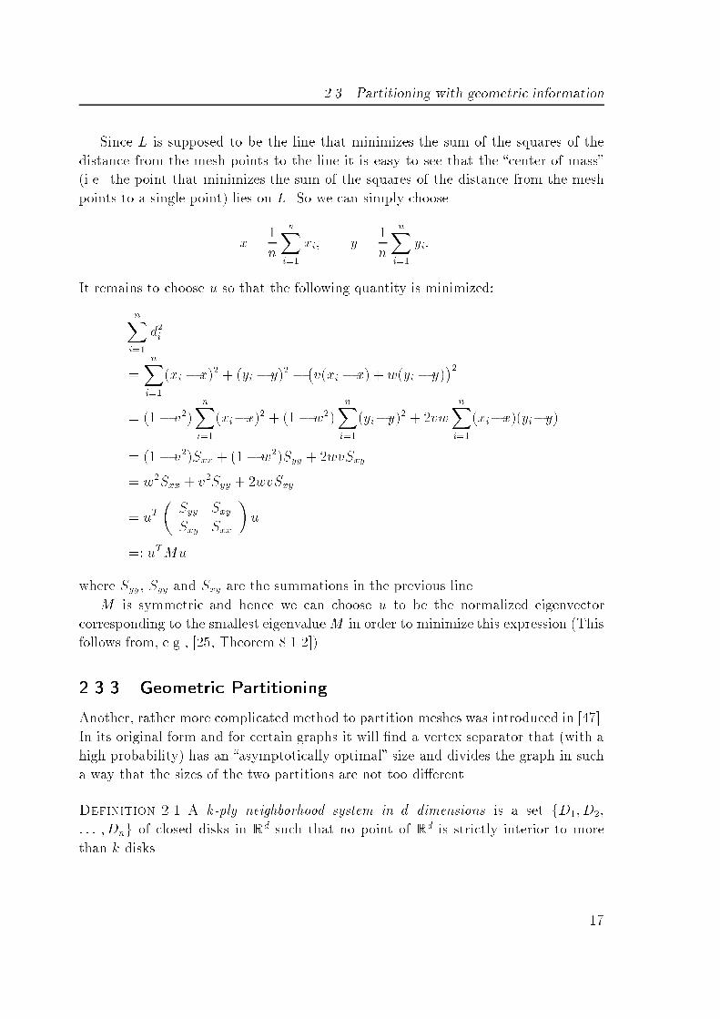
2.3 Partitioning with geometric informationSince L is supposed to be the line that minimizes the sum of the squares of thedistance from the mesh points to the line it is easy to see that the �center of mass�(i.e. the point that minimizes the sum of the squares of the distance from the meshpoints to a single point) lies on L. So we can simply choose�x = 1n nXi=1 xi; �y = 1n nXi=1 yi:It remains to choose u so that the following quantity is minimized:nXi=1 d2i= nXi=1 (xi � �x)2 + (yi � �y)2 � �v(xi � �x) + w(yi � �y)�2= (1� v2) nXi=1 (xi��x)2 + (1� w2) nXi=1 (yi��y)2 + 2vw nXi=1 (xi��x)(yi��y)= (1� v2)Sxx + (1� w2)Syy + 2wvSxy= w2Sxx + v2Syy + 2wvSxy= uT � Syy SxySxy Sxx �u=: uTMuwhere Syy, Syy and Sxy are the summations in the previous line.M is symmetric and hence we can choose u to be the normalized eigenvectorcorresponding to the smallest eigenvalueM in order to minimize this expression (Thisfollows from, e.g., [25, Theorem 8.1.2]).2.3.3 Geometric PartitioningAnother, rather more complicated method to partition meshes was introduced in [47].In its original form and for certain graphs it will �nd a vertex separator that (with ahigh probability) has an �asymptotically optimal� size and divides the graph in sucha way that the sizes of the two partitions are not too di�erent.Definition 2.1 A k-ply neighborhood system in d dimensions is a set fD1;D2;: : : ;Dng of closed disks in Rd such that no point of Rd is strictly interior to morethan k disks. 17

2 Miscellaneous Algorithmstttt tttt tttt tttt����������������������������������������������������������������a. b. ������������ppppppppppppppp p p p p p p p p p p�����

��Figure 2.6: a. A regular mesh as a (1; 1) overlap graph.b. Bisecting a 3 dim. cube.Definition 2.2 An (�; k) overlap graph is a graph de�ned in terms of a k-ply neigh-borhood system fD1;D2; : : : ;Dng and a constant � � 1.There is a vertex for each disk Di. The vertices i and j are connected by an edge ifexpanding the radius of the smaller of Di and Dj by a factor � causes the disks tooverlap, i.e. E = �ei;j ��Di \ �Dj 6= 0 and �Di \Dj 6= 0Overlap graphs are good models of computational meshes because every wellshaped mesh in two or three dimensions and every planar graph are contained insome (�; k)-overlap graph (for suitable � and k).For example, a regular n-by-n mesh is a (1; 1)-overlap graph (see Figure 2.6.a).We have the following theorem:Theorem 2.1 ([47])Let G = (V; E) be an (�; k)-overlap graph in d dimensions with n nodes. Then thereis a vertex separator VS so that V = V1 _[VS _[V2 with the following properties:1. V1 and V2 each have at most n(d+ 1)=(d + 2) vertices, and2. VS has at most O(�k1=dn(d�1=d)) vertices.It is easy to see that for regular meshes in simple geometric shapes (like balls,squares or cubes, cf. Figure 2.6.b ), the separator size given in the theorem is �asymp-totically optimal�.18

2.3 Partitioning with geometric informationa) The mesh. −0.4 −0.2 0 0.2 0.4 0.6

−0.6

−0.4

−0.2

0

0.2

0.4

0.6

0.8

1

b) The scaled points.Figure 2.7: Geometric Bisection IThe proof for this theorem is rather long and involved but it leads to a randomizedalgorithm running in linear time that will �nd, with high probability, a separator ofthe size given in the theorem.The separator is de�ned by a d-dimensional sphere. The algorithm randomlychooses the separating circle from a distribution that is constructed so that the sepa-rator will satisfy the conclusions of the theorem with high probability.To describe the algorithm, we will introduce some terminology:A stereographic projection is a mapping of points in Rd to the unit-sphere centeredat the origin in Rd+1. First, a point p 2 Rd is embedded in Rd+1 by setting the d + 1coordinate to 0. It is then projected on the surface of the sphere along a line passingthrough p and the �north pole� (0; : : : ; 0; 1).The centerpoint of a given set of points in Rd has the property that every hyper-plane through the centerpoint divides the set into two subsets whose sizes di�er by atmost a ratio of 1:d. Note that the centerpoint does not have to be one of the originalpoints.With these de�nitions, the algorithm is as follows (see also Fig. 2.7 � 2.9):Algorithm 2.1 (Geometric Bisection)Project up: Stereographically project the vertices from Rd to the unit-spherein Rd+1. 19

2 Miscellaneous Algorithms−1

−0.50

0.51

−1

−0.5

0

0.5

1−1

−0.8

−0.6

−0.4

−0.2

0

0.2

a) Projected meshpoints withcenterpoint. −1−0.5

00.5

1

−1

−0.5

0

0.5

1−1

−0.5

0

0.5

1

b) Comformally mapped pointswith great circle.Figure 2.8: Geometric Bisection IIFind centerpoint z of the projected points.Conformal Map: Conformally map the points on the sphere such that thecenterpoint now lies at the origin. This is done in the following way: First,rotate the sphere around the origin so that the centerpoint has the coordinates(0; : : : 0; r) for some r. Second, dilate the points so that the (new) centerpointlies in the origin. This can be done by projecting the rotated points back on theRd�plane (using the inverse of the stereographic projection), scaling the pointsin Rd by a factor of p(1� r)=(1+ r), and then stereographically projecting thepoints back on the sphere.Find a great circle by intersecting the Rd+1�sphere with a random d�dimensional hyperplane through the origin.Unmap the great circle to a circle C in Rd by inverting the dilation, the rotationand the stereographic projection.Find separator: A vertex separator is found by choosing all those verticeswhose corresponding disk (cf. Def. 2.2), magni�ed by a factor of � intersectsC.While implementing this algorithm, the following simpli�cations (suggested in [24])can be made.Instead of �nding a vertex separator, it is easier to �nd an edge-separator bychoosing all those edges cut by the circle C. This has the advantage that one doesnot have to know the neighborhood system for the graph.20

2.3 Partitioning with geometric information−0.4 −0.2 0 0.2 0.4 0.6

−0.6

−0.4

−0.2

0

0.2

0.4

0.6

0.8

1

a) Separating circle projected backon the plane. b) The edge separator induced bythe separating circle.Figure 2.9: Geometric Bisection IIIThe theorem only guarantees a ratio of 1 : d+ 1 between the two partitions whilefor bisection we want the two partitions to be of the same size (possibly up to adi�erence of one vertex). To achieve this, the hyperplane is moved along its normalvector until it divides the points evenly. Thus the separator is a circle, but not a greatcircle, on the unit-sphere in Rd+1; its projection to the Rd plane is still a circle (orpossibly a line).The centerpoint can be found by linear programming and although this is donein polynomial time it is still a slow process. So, instead of using the real centerpoint,one can use a heuristic to �nd an approximate centerpoint. This can be done in lineartime using a randomized algorithm.To speed up the computation even more, only a randomly chosen subset of pointsis used to compute the centerpoint.A random great circle has a good possibility to induce a good partition. Butaccording to [24] experiments showed that it is worthwhile to generate di�erent cir-cles and choose the one that delivers the best result. One can further improve thealgorithm by modifying this selection such that the normal vector of the randomlygenerated great circles are biased in the direction of the moment of inertia of thepoints (see also Section 2.3.2: Inertial Bisection). 21

2 Miscellaneous Algorithms

22

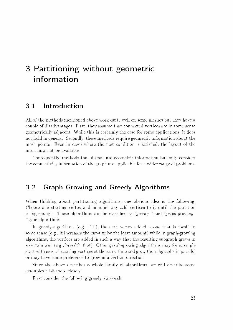
3 Partitioning without geometricinformation3.1 IntroductionAll of the methods mentioned above work quite well on some meshes but they have acouple of disadvantages. First, they assume that connected vertices are in some sensegeometrically adjacent. While this is certainly the case for some applications, it doesnot hold in general. Secondly, these methods require geometric information about themesh points. Even in cases where the �rst condition is satis�ed, the layout of themesh may not be available.Consequently, methods that do not use geometric information but only considerthe connectivity information of the graph are applicable for a wider range of problems.3.2 Graph Growing and Greedy AlgorithmsWhen thinking about partitioning algorithms, one obvious idea is the following:Choose one starting vertex and in some way add vertices to it until the partitionis big enough. These algorithms can be classi�ed as �greedy�� and �graph-growing�� type algorithms.In greedy-algorithms (e.g., [11]), the next vertex added is one that is �best� insome sense (e.g., it increases the cut-size by the least amount) while in graph-growingalgorithms, the vertices are added in such a way that the resulting subgraph grows ina certain way (e.g., breadth��rst). Other graph-growing algorithms may for examplestart with several starting vertices at the same time and grow the subgraphs in parallelor may have some preference to grow in a certain direction.Since the above describes a whole family of algorithms, we will describe someexamples a bit more closely.First consider the following greedy approach: 23

3 Partitioning without geometric informationAlgorithm 3.1 (Greedy Partitioning)Unmark all vertices.Choose a pseudo-peripheral vertex (one of a pair of vertices that are approxi-mately at the greatest distance from each other in the graph, cf. [58]) as startingvertex, mark it and add it to the �rst partition.For the desired number of partitions do� repeat� Among all the unmarked vertices adjacent to the current partition,choose the one with the least number of unmarked neighbors.� Mark it and add it to the current partition.until the current partition is big enough.� If there are unmarked vertices left, choose one adjacent to the currentpartition with the least number of unmarked neighbors as starting vertexfor the next partition.Note that by choosing new vertices only adjacent to the current partition, thisalgorithm tries to keep the subpartitions connected and thus also does some kind ofgraph growing.Another well-known algorithm that is often called �greedy� is the Farhat�algo-rithm ([17]). A closer look reveals that it is a graph growing algorithm which onlychooses the starting vertices of each partition in a greedy way.Adapted to work on a graph (the original works on nodes and elements of a FEMmesh) it can be described as follows:Algorithm 3.2 (Farhat's Algorithm)Unmark all vertices.For the desired number of partitions do� Among all the vertices chosen for the last partition, choose the one with thesmallest nonzero number of unmarked neighbors, mark all these neighborsand add them to the current partition. (For the �rst vertex, one couldagain choose a pseudo-peripheral vertex, mark it and add it to the currentpartition.)� repeatFor each vertex v in the current partition do� For each unmarked neighbor vn of v do� Add vn to the current partition.� mark vn.until the current partition is big enough.24

3.2 Graph Growing and Greedy AlgorithmsThese algorithms, in particular the graph growing ones, are very fast.They alsohave the additional advantage of being able to divide the graph into the desirednumber of partitions directly, thereby avoiding recursive bisection. Therefore theirrunning time is essentially independent of the desired number of subpartitions.The ability to divide the graph into any number of partitions is also attractive ifthe desired number is not a power of 2.On the downside, the quality of the partitions (measured in cut-size) is not alwaysgreat and when partitioning complicated graphs into several subpartitions the lastsubpartitions tend to be disconnected (see e.g., [61]). They also tend to be sensitiveto the choice of the starting vertex (but since they are quite fast, one can run thealgorithms with di�erent starting vertices and simply choose the best result).3.2.1 Kernigan�Lin AlgorithmThe Kernigan�Lin algorithm [42], often abbreviated as K/L, is one of the earliestgraph partitioning algorithms and was originally developed to optimize the place-ment of electronic circuits onto printed circuit cards so as to minimize the number ofconnections between cards.The K/L algorithm does not create partitions but rather improves them iteratively(there is no need for the partitions to be of equal size). The original idea was to take arandom partition and apply Kernigan�Lin to it. This would be repeated several timesand the best result chosen. While for small graphs this delivers reasonable results, itis quite ine�cient for larger problem sizes.Nowadays, the algorithm is used to improve partitions found by other algorithms.As we will see, K/L has a somewhat �local� view of the problem, trying to improvepartitions by exchanging neighboring nodes. So it nicely complements algorithmswhich have a more �global� view of the problem but tend to ignore local characteristics.Examples for these kinds of algorithms would be inertial partitioning and spectralpartitioning (see sections 2.3.2 and 3.3 resp.).Important practical advances were made by C. Fiduccia and R. Mattheyses in [18]who implemented the algorithm in such a way that one iteration runs inO(jEj) insteadof O(jVj2 log jVj). We will �rst describe the original algorithm and later discuss theseand other improvements.Let us introduce some notation: It is actually easier to describe the algorithm fora graph with weighted edges; so let (V; E;WE) be a graph with given subpartitionsVA _[VB = V.The di��value of a vertex v is the amount the cut-size will decrease if it is moved25

3 Partitioning without geometric informationto the other partition, i.e., for v 2 VA :di�(v) = di�(v;VA;VB) := Xb2VB we(ev;b)� Xa2VAwe(ev;a)Note that if a vertex is moved from one subpartition to the other, only its di��valueand the di��values of its neighbors change.The gain�value of a pair a 2 VA; b 2 VB of vertices is the amount the cut-sizechanges if we swap a into subpartition VB and b into VA. One can easily see thatgain(a; b) = gain(a; b;VA;VB) := di�(a) + di�(b)� 2we(ea;b):With this, we will now describe one pass of the algorithm:Algorithm 3.3 (Kernigan�Lin)Given two subpartitions VA;VBCompute the di��value of all vertices.Unmark all vertices.Let k0 = cut-size.For i = 1 to min(jVAj; jVBj) do� Among all unmarked vertices, �nd the pair (ai; bi) with the biggest gain(which might be negative).� mark ai and bi.� For each neighbor v of ai or bi doUpdate di�(v) as if ai and bi had been swapped, i.e.,di�(v) := di�(v) +(2we(ev;ai)� 2we(ev;bi) for v 2 VA2we(ev;bi)� 2we(ev;ai) for v 2 VB� ki = ki�1 + gain(ai; bi), i.e., ki would be the cut-size if a1; a2; : : : ; ai andb1; b2; : : : ; bi had been swapped.Find the smallest j such that kj =miniki.Swap the �rst j pairs, i.e.,VA:= VA�fa1; a2; : : : ; ajg[fb1; b2; : : : ; bjgVB:= VB�fb1; b2; : : : ; bjg[fa1; a2; : : : ; bjgContinue these iterations until no further cut-size improvement is achieved.26

3.2 Graph Growing and Greedy AlgorithmsSo, in each phase, K/L swaps pairs of vertices chosen to maximize the gain. Itcontinues doing so until all vertices of the smaller subpartition are swapped. Theimportant part is that the algorithm does not stop as soon as there are no moreimprovements to be made. Instead it continues, even accepting negative gains in thehope that later gains will be large and that the overall cut-size will later be reduced.This ability to climb out of local minima is a crucial feature. (See also Figure 3.1,taken from [15]).d dd d ddd dm md ddd��@@@@�� @@�� @@��Original Graph, k0 = 2 d dd d td t ddd dd@@�� m���������� ��@@��@@ mFirst swap, k1 = 4d dd t d t dtt dd d@@�� @@ mmHHHH ��@@����Second swap, k2 = 3 d dd t tt t tt dd d@@�� �� ��@@ @@����@@Result, k4 = 0d unmarked t marked nselectedFigure 3.1: The Kernigan�Lin algorithm at workAs mentioned above, the algorithm implemented in [18] takes O(jEj) time for oneiteration. The reduction is partly achieved by choosing single nodes to be swappedinstead of pairs. Furthermore, the di��values of the vertices are bucket-sorted andthe moves associated with each gain value are stored in a doubly linked list. Choosinga move with the highest di��value involves �nding a nonempty list with the highestdi��value, while updating the di��value of a vertex is done by deleting it from onedoubly linked list and inserting it into another (this can be done in constant time).There are many variations of the Kernigan�Lin algorithm ([31,39,44,54,67]) oftentrading execution time against quality or generalizing the algorithm to more than twosubpartitions. Some examples are: 27

3 Partitioning without geometric information� Instead of exchanging all vertices, limit the exchange to some �xed number orallow only a �xed number of exchanges with negative gain. This is based on theobservation that often the largest gain is achieved early on.� Use only a �xed number of inner iterations (often only one).� Only evaluate di��values of vertices near the boundary since it is unlikely thatmoving inner nodes will be helpful.3.3 Spectral BisectionThe spectral bisection algorithm described in this section is quite di�erent from allthe other algorithms described so far. It does not use geometric information yet itdoes not operate on the graph itself but on some mathematical representation ofit. While the other algorithms use (almost) no �oating point calculations at all, themain computational e�ort of the spectral bisection algorithm are standard vectoroperations on �oating point numbers. The decision about each vertex is based on thewhole graph, so it takes a more global view of the problem.The method itself is quite easy to explain but why the heuristic works is not atall obvious.Definition 3.1 Let G = (V; E) be a graph with n = jVj vertices numbered in someway and with deg(vi) the degree of vertex i (i.e., the number of adjacent vertices).The Laplacian matrix L(G) (or only L if the context is obvious) is an n�n symmetricmatrix with one row and column for each vertex. Its entries are de�ned as follows:lij = 8>><>>:�1 if i 6= j and ei;j 2 E0 if i 6= j and ei;j 62 Edeg(vi) if i = jThe same matrix with a zero diagonal is often called the adjacency matrix A(G)of G.Since a permutation of the vertex numbering will lead to a di�erent matrix it issloppy to speak of the Laplacian of a graph. But since matrices induced by di�erentvertex numberings can be derived from each other by permuting rows and columnsthey share most properties, so we will continue to speak of the Laplacian unless acloser distinction is necessary.The Laplacian has some nice properties (cf. e.g., [19,45]):28

3.3 Spectral BisectionTheorem 3.11. L(G) is real and symmetric, its eigenvalues �1 � �1 � � � � � �n are thereforereal and its eigenvectors are real and orthogonal.2. All eigenvalues �j are nonnegative and hence L(G) is positive semide�nite.3. With e := (1; 1; : : : ; 1)T , L(G)e = 0�e, so �1 = 0 with e an associated eigenvector.4. The multiplicity of the zero eigenvalue is equal to the number of connectedcomponents of G. In particular:�2 6= 0 , G is connected. (3.1)Proof. 1. and 3. are trivial and 2. follows from the Gershgorin Circle Theorem([25, Theorem 7.2.1]) together with the simple fact (from the de�nition of L) thatnXi=1i6=j jlijj = ljj > 0 for all j 2 f1; : : : ; ngand so all Gershgorin circles have nonnegative real parts. Since all eigenvalues arereal, they are all nonnegative. This also shows that �n � 2maxi(deg(vi)) � 2(n� 1).For part 4, we �rst show that �2 6= 0 if G is connected. Note that G is connectedif and only if L(G) is irreducible and if L is irreducible then so is the nonnegativematrix ~L = 2nI �L. Also, �i is an eigenvalue of L if and only if ~�n�i = 2n� �i is aneigenvalue of ~L. In particular, the largest eigenvalue ~�n of ~L and all other eigenvaluesof ~L are positive.The Perron�Frobenius theorem ([5, Theorem 2.1.4]) applied to ~L implies that if ~Lis connected, ~�n is a simple eigenvalue and hence so is �1. Therefore �2 > �1 = 0.Now assume that G not connected but that it consists of k connected componentsG1; : : : ;Gk. By �rst numbering the vertices of G1, then of G2 and so on, L(G) has block-diagonal form with L(G1); : : : ; L(Gk) as diagonal blocks. So �(L(G)) = Ski=1 �(L(Gi))and since each of the �(L(Gi)) contains one 0, the �rst k eigenvalues of L(G) are 0.We have thus shown that G is connected if and only if �2 6= 0.But what if �1 = �2 = � � � = �k = 0? Then G cannot be connected and con-sequently consists of at least two unconnected components G1 and G2. As above wesee that �(L(G)) = �(L(G1)) [ �(L(G2)) and if k > 2, at least one of the submatri-ces has more than one zero-eigenvalue and is therefore disconnected. Repeating thisargument, we see that G has k connected components.Equation (3.1) also motivates the following:Definition 3.2 �2(L(G)) is called the algebraic connectivity. 29

3 Partitioning without geometric informationThe corresponding eigenvector is often called Fiedler vector. It was named tohonor Miroslav Fiedler's pioneering work on these objects [19,20]. One of his discov-eries, which serves as a �rst (very) small motivation for the following algorithm, isthe followingTheorem 3.2 ([20])Let G = (V; E) (with V = fv1; v2; : : : ; vng) be a connected graph and let u be itsFiedler vector. For any given real number r � 0, de�ne V1 := fvi 2 V j ui � �rg.Then the subgraph induced by V1 is connected.Similarly, for a real number r � 0, the subgraph induced by V2 := fvi 2 V j ui � �rgis also connected.Note that the theorem is independent of the length and sign of the Fiedler vector.This theorem does not imply anything about a good bisection but it does implythat the Fiedler vector does somehow divide the vertices in a �sensible� way. Afterall, it guarantees at least one connected partition. This is much more than what wowould achieve by choosing just a random subset.This leads us to the idea of using the Fiedler vector to bisect the graph. We will�rst describe the algorithm and then later try to explain why it works.Algorithm 3.4 (Spectral Bisection)Given a connected graph G, number the vertices in some way and form theLaplacian matrix L(G).Calculate the second-smallest eigenvalue �2 and its eigenvector u.Calculate the median mu of all the components of u.Choose V1 := fvi 2 V j ui < mug, V2 := fvi 2 V j ui > mug, and, if some ele-ments of u equal mu, distribute the corresponding vertices so that the partitionis balanced.But why does this algorithm work? There are some very di�erent approaches thattry to answer this question. In addition to the graph-theoretic approach (cf. Theorem3.2), one can look at graph bisection as a discrete optimization problem (in [3,29]) oras a quadratic assignment problem (in [53]), look at several physical models (like avibrating string or a net of connected weights) (in [30, 51]) or examine the output ofa certain neural net trained to bisect a graph (in [21]).Among all of these, the following approach via the discrete optimization formula-tion is (in the authors opinion) the most convincing derivation of the spectral bisectionalgorithm.30

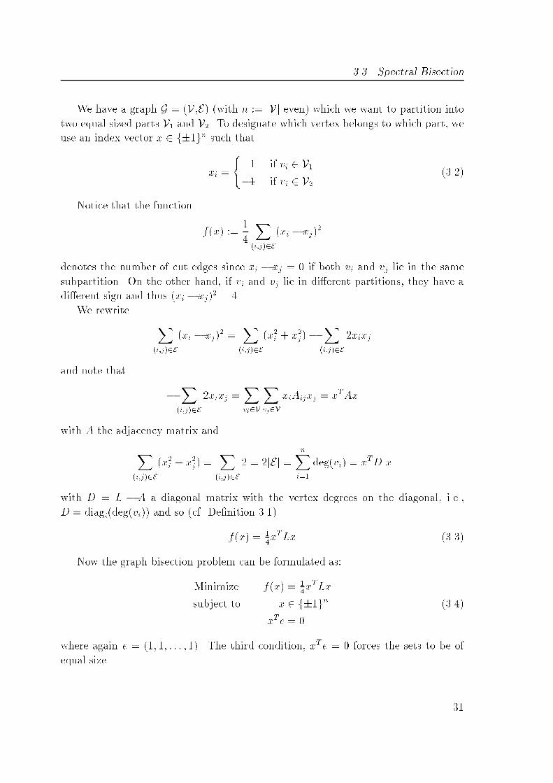
3.3 Spectral BisectionWe have a graph G = (V;E) (with n := jVj even) which we want to partition intotwo equal sized parts V1 and V2. To designate which vertex belongs to which part, weuse an index vector x 2 f�1gn such thatxi = ( 1 if vi 2 V1�1 if vi 2 V2 (3.2)Notice that the function f(x) := 14 X(i;j)2E(xi � xj)2denotes the number of cut edges since xi � xj = 0 if both vi and vj lie in the samesubpartition. On the other hand, if vi and vj lie in di�erent partitions, they have adi�erent sign and thus (xi � xj)2 = 4.We rewrite X(i;j)2E(xi � xj)2 = X(i;j)2E(x2i + x2j)� X(i;j)2E 2xixjand note that � X(i;j)2E 2xixj = Xvi2VXvj2V xiAijxj = xTAxwith A the adjacency matrix andX(i;j)2E(x2i + x2j ) = X(i;j)2E 2 = 2jEj = nXi=1 deg(vi) = xTD xwith D = L � A a diagonal matrix with the vertex degrees on the diagonal, i.e.,D = diagi(deg(vi)) and so (cf. De�nition 3.1)f(x) = 14xTLx (3.3)Now the graph bisection problem can be formulated as:Minimize f(x) = 14xTLxsubject to x 2 f�1gn (3.4)xTe = 0where again e = (1; 1; : : : ; 1). The third condition, xT e = 0 forces the sets to be ofequal size. 31

3 Partitioning without geometric informationGraph partitioning is NP-complete and (3.4) is just another formulation, so wecannot really solve this problem either. But we can relax the constraints a bit: insteadof choosing discrete values for the xi we look for a real vector z which has the same(Euclidean) length as x and ful�lls the other conditions:Minimize f(z) = 14zTLzsubject to zTz = n (3.5)zT e = 0As we will see, this problem is easy to solve. Since the feasible set of the continuousproblem (3.4) is a subset of the feasible set of the discrete problem (3.5), every solutionof (3.5) will give us a lower bound for (3.4) and we hope that the continuous solutionwill give us a good approximation to the solution of (3.4).From Theorem 3.1 we know that the eigenvectors u1; u2; : : : ; un of L are orthonor-mal (and therefore span Rn) and that u1 = pne. We can thus decompose everyz 2 Rn into a linear combination z =Pni=1 �iui of these vectors.In order to to meet the restrictions, we have to place some conditions on the �i.We want zTe = 0 and sincezT e = � nXi=1 �iui�Tu1 = nXi=1 (�iui)Tu1 = �1 uT1 u1 = �1we need to have �1 = 0. For zT z = n, we needzTz = � nXi=1 �iui�T� nXi=1 �iui�= nXi=1 nXj=1 �i�juTi uj = nXi=1 �2i = nFurthermore, we have4f(z) = zTLz = � nXi=1 �iui�TL � nXi=1 �iui�= � nXi=1 �iui�T� nXi=1 �i�iui� = nXi=1 nXj=1 �i�j�juTi uj= nXi=1 �2i�i= nXi=2 �2i�i � �2 nXi=1 �2i = �2n (3.6)32

3.3 Spectral Bisectionwhere (3.6) holds since �1 = 0 and the inequality follows from 0 < �2 � �i fori = 3; : : : ; n . Since we can achieve 4f(z) = �2n by choosing z = pnu2, we �ndthat the correctly scaled Fiedler vector pnu2 (which satis�es both constraints) is asolution of the continuous optimization problem (3.5). In fact, if �3 > �2 the solutionis unique up to a factor of �1(cf. also [35, p. 178]). In addition, n4�2 is a lower boundfor the cut-size of a bisection of V.Having found the solution of the continuous problem (3.5), we need to map itback to a discrete partition and hope that the result is a good approximation to thesolution of the discrete problem (3.4).There seem to be two �natural� ways to do this. The �rst method ([10]) placesmore importance on the sign of the result and just map xi = sign(zi), dealing withzero elements of x in some way (e.g., assigning them all to one partition). Its drawbackis that the partitions need not be balanced. Consequently, some additional work isnecessary.The second (and more often used) method (e.g., [29, 51, 61]) places its emphasison the balance and assigns the largest n=2 elements of z to one partition and the restto the other partition. This can easily be done by computing the median �z of the zi,setting xi = (�1 if zi < �z1 if zi > �zand distributing the elements zi = �z in such a way that the balance is preserved.T. Chan, P. Ciarlet and W. Szeto showed in [9] that the vector x formed that wayis closest in any �-norm to z amongst all balanced �1-vectors, i.e.,x = arg minp2f�1gn; pT e=0 kp� zk�Note that in both cases, it is not necessary to compute the eigenvector to a highdegree of accuracy. If we use an iterative method (like the Lanczos algorithm [25,Ch. 9] or the Rayleigh quotient iteration (RQI) ([25, Sec. 8.2.3])), we can stop iteratingonce the result is su�ciently accurate to either decide on the sign of the elements orto recognize the n=2 largest elements. This can be much cheaper than computing theexact eigenvector.3.3.1 Spectral Bisection for weighted graphsIt is easy to generalize the spectral bisection algorithm to handle weighted graphs.33

3 Partitioning without geometric informationGiven a graph G = (V; E) with weighted edges WE , one can de�ne the weightedLaplacian L = (lij)ij withlij = 8<: �we(ei;j) if i 6= j and ei;j 2 E0 if i 6= j and ei;j 62 EPnk=1 we(ei;k) if i = jWith this de�nition and x as above (see equation (3.2)), 14xTLx still denotes theweight of the cut edges and so we can proceed as above.If the graph has weighted vertices WV , the subsets have equal weights if wTx = 0with w = (wv(vi))ni=1 the vector of the vertex weights. Using V = diag(w) (a diagonalmatrix with the components of w on the diagonal), we reformulate this condition asxTV e = 0. We therefore have to solve the problemMinimize f(x) = 14xTLxsubject to x 2 f�1gn (3.7)xTV e = 0Again we relax the constraints a bit: instead of choosing discrete values for the xiwe now look for a real vector z which has the same (weighted) length as x, i.e.,zTV z = eTV e(=Pni=1 wv(vi)) (note that the feasible solutions of the discrete problem(3.7) satisfy this condition) and ful�lls the other conditions:Minimize f(z) = 14zTLzsubject to zTV z = eTV e (3.8)zTV e = 0A solution for the relaxed equation (3.8) is the eigenvector corresponding to thesecond smallest eigenvalue of the generalized eigenproblem Lx = �V z. But since Vis diagonal with positive elements on the diagonal, the problem can be reduced toan ordinary eigenproblem by substituting y = V 1=2z. This leads to Ay = �y withA = V �1=2LV �1=2. The new matrix A is also positive semide�nite with the samestructure as L.3.3.2 Spectral Quadri� and OctasectionAs seen in section 2.2, it can be advantageous to divide a graph into more than twoparts at once, so it would be interesting to �nd a spectral algorithm doing this. Rendland Wolkowitz describe one such technique in [55]. While their algorithm allows thedecomposition of a graph in p parts, it requires the calculation of p eigenvectors and34

3.3 Spectral Bisectionis thus expensive. But as we will see, the spectral bisection idea described above canbe also adapted to divide a graph into more than two parts at once. Hendrickson andLeland [30,34] developed a way to partition a graph into four (or eight) partitions ofequal size at once using two (or three) eigenvectors, i.e., spectral quadrisection (resp.octasection). R. Van Driessche [61] later generalized the quadrisection algorithm todivide the graph into partitions of unequal size.Contrary to spectral bisection, these algorithms do e ee eee00 0110 11w = 1w = 2w = 1Figure 3.2: Hypercube hopmetric in 2Dnot minimize the cut-size but a closely related size,the hypercube hop or Manhattan metric. In this, theweight of each cut edge is multiplied by the number wof bits that di�er in the binary representation of thesubset numbers (see Figure 3.2). This models the per-formance of parallel communication on hypercube and2- or 3-dimensional mesh topologies (cf. [28]). In thesetopologies, w can be interpreted as the number of wiresa message must take while being transfered between therespective processors.We will describe only the derivation of the quadri-section. For the similar but slightly more complicatedoctasection, see [30] or [34].To distinguish between the four subpartitions V0; : : : ;V3, we will use two indexvectors x; y 2 f�1gn withxi = �1 and yi = �1 () vi 2 V0xi = �1 and yi = +1 () vi 2 V1xi = +1 and yi = �1 () vi 2 V2xi = +1 and yi = +1 () vi 2 V3Using considerations similar to the ones that that lead to (3.3), we �nd thatf(x; y) = 14(xTLx+ yTLy)gives us the hop weight of the partition induced by x and y. Assuming that n is amultiple of 4, the constraints that all Vi are to be of the same size can be expressed35

3 Partitioning without geometric informationas Xi(1 � xi)(1 � yi) = (e� x)T (e� y) = nXi(1� xi)(1 + yi) = (e� x)T (e+ y) = nXi(1 + xi)(1 � yi) = (e+ x)T (e� y) = nXi(1 + xi)(1 + yi) = (e+ x)T (e+ y) = nwhich (after expanding and solving a small linear system) simpli�es toeTx = 0 eTy = 0 xTy = 0:Therefore we want to solve the following discrete minimization problemMinimize f(x; y) = 14(xTLx+ yTLy)subject to eTx = eTy = xTy = 0 (3.9)x; y 2 f�1gn (3.9.a)Again, since this problem is too di�cult to solve, we relax the discreteness condi-tion (3.9.a) and only demand that the solutions z;w 2 Rn have the same Euclideanlength (pn) as x; y. We then getMinimize f(z;w) = 14(zTLz + wTLw)subject to eTz = eTw = zTw = 0 (3.10)zT z = wTw = n (3.10.a)Using an argument similar to the one in the bisection case (p. 32 �.), we see thatthe scaled eigenvectors z = pnu2 and w = pnu3 belonging to the second- and third-smallest eigenvalues �2 and �3 are a solution of the continuous problem (3.10) andn4 (�2 + �3) is a lower bound on the number of hops induced by any quadrisection ofG. But any orthonormal pair �z; �w from the subspace spanned by �2 and �3 (i.e., �z =pnu2 cos �+pnu3 sin � and �w = �pnu2 sin �+pnu3 cos �) are also solutions of (3.10).The question now remains which of the solutions to choose. One idea is to choose �in such a way that the resulting values closest to the discrete values �1 that we wereoriginally looking for, i.e., choose a �0 that minimizes g(�) =Pi(1� �z2i )2 + (1� �w2i )2for � 2 [0; 2�).g(�) reduces to a quartic expression in sin(�) and cos(�). After constructing g(�)(at a cost of O(n)), the cost of evaluating (and thus minimizing) g(�) is independent36

3.3 Spectral Bisectionof n and usually insigni�cant compared to calculating the eigenvectors. In [30] it isrecommended to use a local minimizer with some random starting points.But of course originally we were looking for an approximative solution to thediscrete problem (3.9). So the last hurdle is the assignment of the continuous points(zi; wi) to discrete points (�1;�1). Since we need to adhere to the restrictions givenin (3.9), i.e., the partitions need to have the same size, we cannot simply use themedian method we used for the bisection case. If we de�ne a distance function fromcontinuous points (zi; wi) to discrete points (�1;�1), distributing the points evenlywhile minimizing the sum of the distance is known as the minimum cost assignmentproblem. According to [29] there exist e�cient algorithms to solve the problem.3.3.3 Multilevel Spectral BisectionFor the above algorithms, we have to compute the Fiedler-vector or the eigenvectorassociated with the third-smallest eigenvalue (and, for octasection, the forth-smallest)of a sparse, symmetric matrix. First choice for such an algorithm is some variation ofthe Lanczos-algorithm ([25, Ch. 9]). But it turns out that compared to other graphpartitioning algorithms, spectral bisection using the Lanczos-algorithm is extremelyslow.But how to speed up the calculation of the eigenvector(s) and thus the spectralbisection algorithm? Luckily, we do not need to calculate the eigenvectors of just anysparse matrix but only those of the Laplacian of a graph. In [3], S. Barnard and H.Simon found a clever way to pro�t from the connections between the eigenvectors andthe graph. We will present their idea in this section.The basic idea is quite simple. Given a graph G(0), we try to contract it to anew graph G(1) that is in some sense similar to G(0) but with fewer vertices. Sincethe new graph (and consequently its Laplacian) is smaller, it is cheaper to calculatethe Fiedler-vector u(1)2 of the new graph. We then use u(1)2 as a starting point tocalculate the Fiedler-vector u(0)2 of the original graph. This process has also beentermed coarsening the graph and the smaller graph is also called coarser.Of course, we can use this idea recursively, constructing ever smaller graphsG(2);G(3); : : : to calculate u(1)2 , u(2)2 and so on. These di�erent sized graphs lead tothe name of this algorithm: Multilevel Spectral Bisection or MSB.So the �rst, rough draft of the eigenvector calculation for MSB looks like this(again, we present it only for an unweighted graph; generalization to the case withweighted edges is quite straightforward): 37

3 Partitioning without geometric informationAlgorithm 3.5 (Multilevel Fiedler-vector calculation )Function Fiedler(G)If G is small enough thenCalculate f = u2 using the Lanczos algorithmelse Construct the smaller graph G 0 and (implicitly) the corresponding LaplacianL0.f0 = Fiedler(G 0)Use f 0 to �nd an initial guess f (0) for f.calculate f from the initial guess f (0) .endifReturn fOf course, we have left out three rather important details: How to construct thesmaller graph, how to �nd an initial guess f (0) for f and how to e�ciently calculatef using f (0).Constructing the smaller graphFirst, we need the following de�nitions:Definition 3.3 Given a graph G = (V; E), a subset V 0 � V is called an independentset with respect to V if no two elements of V 0 are connected by an edge.Definition 3.4 V 0 is called a maximal independent set with respect to V if addingany vertex from V n V 0 to V 0 would no longer make it an independent set.(Note that there is another de�nition of a maximal independent set that requiresthe independant set to be of maximal size, i.e., V 0 is a maximal independent set withrespect to V if there does not exist an independant subset V 00 of V with jV 0j < jV 00j.The two de�nitions are not equivalent.)It is easy to see that an independent set V 0 � V is maximal if and only if everynode from V n V 0 is adjacent to a node in V.A maximal independent set can easily and e�ciently be found by using a greedyalgorithm and while they are by no means unique, di�erent maximal independent setstypically have a similar size.So, to coarsen a graph G = (V; E) to a new, smaller graph G 0 = (V 0; E 0), we do thefollowing:38

3.3 Spectral Bisection- Choose a maximal independent subset V 0 of V and use it as the vertex set ofthe new graph. (any subset of V would do, but a maximally independent set isguaranteed to be evenly distributed over G.)- Grow domains in G around the vertices in V 0 and add an edge e0ij to E 0 wheneverthe domains around v0i and v0j intersectGrowing a domain around a vertex is done by repeatedly adding all neighborsof vertices already in the domain. If the starting set is maximal independent, twocycles of domain growth are enough to cover the whole graph and therefore determineE 0. In that case, two vertices in V 0 are connected exactly if there exists a path with4 vertices or less connecting the corresponding vertices in V. It is also easy to seethat the resulting graph is connected if and only if the original one was connected aswell [4] (Note that contrary to what is stated in [4], two growth cycles are enoughsince (using the notation in [4]) G[k] �shortcuts� all paths of length 2k instead of theclaimed k + 1).Finding an initial guessHaving calculated the Fiedler vector f 0 of the smaller graph, we now face the problemof how to use it to approximate the Fiedler vector f of the bigger graph. Here we useour knowledge about the relationship between G and G 0. First we assign the valuesfi to the appropriate elements of f . In mathematical terms: Let m(i) be a mappingbetween the vertices of the condensed graph and the vertices of G such that i is theindex of the vertex in V 0 that corresponds to the m(i)th vertex in V. Then letfm(i) = f 0i for i = 1; : : : ; jV 0jFinally, for the components j of f corresponding to vertices in V n V 0, we assignthe average of the values corresponding to those vertices in V 0 adjacent to vj. Themathematical formulation of this is:fj = Xi:vi2G0ei;j2E fi. Xi: vi2G0ei;j2E 1 for all j with vj 2 V n V 0Since V 0 is maximal independent, every element in V nV 0 has at least one neighbor inV 0. With the above we have thus assigned a value to each component of f (0).One should note that this operation is similar to the prolongation operation inclassical multigrid methods for linear systems [7]. 39

3 Partitioning without geometric informationCalculating the Fiedler-vector using the estimate f(0)The last detail to solve is: how to calculate the Fiedler-vector f using the estimate f (0).While the Lanczos-algorithm is the usual favorite for extreme eigenpairs of symmetricsparse matrices, it does not e�ectively take advantage of an initial guess. In [3], theRayleigh quotient iteration (RQI) ([25, Sec. 8.2.3]) was choosen to re�ne the initialguess f (0). Since we already have a good approximation and our accuracy demandsare rather low, RQI will usually take only very few iterations to converge.Algorithm 3.6 (Rayleigh quotient iteration)Given an initial guess (f (0); �(0)) for an eigenpair (f; �), set v = f (0)=kf (0)k andrepeat� := vTLvSolve (L � �I)x = vv := x=kxkuntil � is �close enough� to �A closer look at the RQI algorithm reveals that we have to solve a linear equationwith L��I in each step. Since this matrix is sparse, symmetric but probably inde�niteand ill-conditioned, the method of choice is the SYMMLQ iteration [48]. Accordingto [3] the total number of matrix-vector operations in all RQI steps combined isgenerally less than 10.In experiments (described in [3]), the MSBwith RQI and SYMMLQ has turned outto be very e�cient. Compared with the normal spectral bisection using the Lanczosalgorithm, it usually is at least an order of magnitude faster.3.3.4 Algebraic MultilevelIn the MSB algorithm described above, the smaller graph was constructed solely outof the larger graph and only then the corresponding Laplacian matrix was (implicitly)build and its Fiedler-vector computed.But the problem can also be approached in another way, more in tune with theclassical multilevel algorithms for linear systems [7]. That is: given a Laplacian matrixL 2 Rx�n, we construct a restriction operator R 2 Rn�n0 and a prolongation operatorP 2 Rn0�n and study the relation between (prolongated) solution of the smaller,restricted problem and the original problem. In [61], R. Van Driessche did just that.We will report some of his results in this section.Also choosing a maximal independent subset of V, the matrix equivalent of theinterpolation method above (in section 3.3.3) was used as prolongation operator P .40

3.3 Spectral BisectionFurther two restriction operators were choosen, RP = P T and RI a simple injectionoperator (rIij = �m(i);j) for i = 1; : : : ; n0 and j = 1; : : : ; n.It turns out that usingRI leads to another eigenproblemwith a matrix L0 = RILP .L can be interpreted as the Laplacian matrix of a new, smaller graph with weightededges. This new graph can be shown to be connected, so we can repeat the procedurerecursively.RP does not have these nice properties. Using it leads to a generalized eigenprob-lem. L0 = RPLP is again the Laplacian of a weighted graph but that graph cannotbe guaranteed to be connected and the weights of the edges might not be positive.A repeated application may therefore not be possible. Finally, the solution of thegeneralized eigenproblem is computationally more expensive.In [61], the prolongations vIi and vPi of the second, third and fourth eigenvectorof the contracted graph were compared with the corresponding eigenvectors uj; (j =2; 3; 4) of the original graph. This was done by examining the absolute values of theinner products of the (normalized) vectors. Notable results were:� The prolongations vIi ; vPi were quite rich in ui (i = 2; 3; 4), that is the absolutevalue of the inner product was quite big (well above 0.95 for j = 2; 3 and above0.8 for j = 4).� The contributions of the other eigenvectors (i.e., for i 6= j) were much smaller(most of the time les than 0.1).This means that the prolonged eigenvectors are good approximations of the eigen-vector of the original graph and are thus good starting vectors for the Rayleigh quo-tient iteration.Further �ndings included:� The method using RP delivered better eigenvector approximations. But thisdoes not o�set the more expensive solution of the generalized eigenproblem andso the other method (using RI) may often be faster in delivering the �nal result.� The quality of the eigenvector approximation is not only determined by theeigenvalue approximation but also by the gap between its eigenvalue and neigh-boring eigenvalues.Other implementations of MSB use even other methods of constructing the smallermeshes (Chaco ([33]) for example uses one of the algorithms described in section 3.4)but report similar �nal results so it seems that the choice of the coarsening methodis not critical. 41

3 Partitioning without geometric informationPSfrag replacements coarsen graphpartition graphproject and refine graph

Figure 3.3: Multilevel graph partitioning3.4 Multilevel PartitioningThe multilevel spectral bisection algorithm described in section 3.3.3 has turned outto be very e�cient. Since the multilevel approach obviously has a lot of merit, can itbe applied in some other way as well?In MSB, we transfer approximate information about the second eigenvector of theoriginal graph between levels, improve this information on each level and �nally, usethis eigenvector to partition the graph. A more direct way would be to simply transferinformation about the partitions itself between levels and improve the partitions oneach level. And this is, in a rough outline, the description of one of the most successfulalgorithms, the multilevel graph partitioning.Algorithm 3.7 (Multilevel graph bisection)Function ML-Partition(G)If G is small enough thenFind partition (V1;V2) of G in some way.else Construct a smaller approximation G 0(V 01;V 02) = ML-Partition(G 0)(~V1; ~V2) = Project-partition-up (V 01;V 02)(V1;V2) = Re�ne-partition (~V1; ~V2)endif42

3.4 Multilevel Partitioningt#" !ttAAAAAAAAA���������AAAAAAAAA1 33 2t1 2 2 t tt����@@@@@@@@@ 1 41 35a) original graph w. weights b) contracted graphFigure 3.4: Coarsening a graphReturn (V1;V2)In algorithm 3.7, we bisect the graph but the same idea can be used to partitionthe graph into p parts at once. Actually there is a whole family of slightly di�erentmultilevel graph partitioning algorithms which di�er in the three generic parts �con-struct smaller approximation�, �project partition up� and �re�e projected partition�and in the way the smallest graph is partitioned. We will describe some of the so-lutions implemented in software packages like Chaco ([33]), METIS ([40]) or WGPP([26]).All of the following coarsening algorithms lead to graphs with edge and vertexweights so we might as well start with a weighted graph (V; E).3.4.1 Coarsening the graphIn all of the following methods, the coarser graph is constructed in similar ways. First,we �nd a maximal matching. A matching is a subsetM� E of edges no two of whichshare an endpoint. A matching is maximal if no other edges from E can be added.Given the matching M, the new graph is constructed in the following way: foreach edge ei;j 2 M, we contract its endpoints vi and vj into a new vertex vn. Itsweight equals the sum wv(vi) + wv(vj) of the weights of vi and vj. Its neighbors arethe combined neighbors of vi and vj with accumulated edge-weights, i.e., we(en;k) =we(ei;k) + we(ei;k) (where the weight on nonexistent edges is assumed to be 0). Theedge ei;j disappears. (See also Figure 3.4). 43

3 Partitioning without geometric informationThe main di�erence between the di�erent implementations is the constructionof the maximal matching. The simplest method (suggested by B. Hendrickson andR. Leland in [31]) is randomized matching (RM) which randomly selects �tting edgesuntil the matching is maximal:Algorithm 3.8 (Randomized Matching (RM))Unmark all vertices and set M = ;.While there are unmarked vertices leftRandomly select unmarked vertex viMark viIf vi has unmarked neighborsRandomly choose unmarked neighbor vj of vi (?)Mark vjAdd edge ei;j to MIf we look at the way the coarser graph is constructed, we notice that the edges inthe matching �disappear� from the lower levels. The total edge-weight of the coarsergraph equals the edge-weight of the original graph minus the weight of the edges inthe matching. In [39] it is suggested that by decreasing the total edge-weight of thecoarser graph one might lower its cutsize and also the cutsize of the original graph.Experiments con�rmed this assumption and also showed that this choice acceleratedthe re�nement process.To achieve this, G. Karypis and V. Kumar use a slight modi�cation of the RMalgorithm called heavy edge matching (HEM). Instead of choosing a random neighbor(in line (?) of Algorithm 3.8), they simply select the unmarked neighbor which isconnected to vi by the heaviest edge.The problem with this approach is that it might miss some heavy edges. If inFigure 3.5 vertex vi is selected �rst, the edge with weight 3 will be selected. Conse-quently the heavier edge with weight 7 will not be selected. To avoid this, A. Guptasuggests in [27] to sort the edges by weight and then to choose the heaviest permissibleedge �rst (ties are broken randomly). He calls this method is heaviest edge matching.Is usually done only in the later stages of the coarsening process when the graphsare considerably smaller and thus the sorting is cheap. Furthermore, heaviest edgematching is particularly e�cient when the graph has edges with very di�erent weights.This weight inequilibrium will often appear after some coarsening steps.44

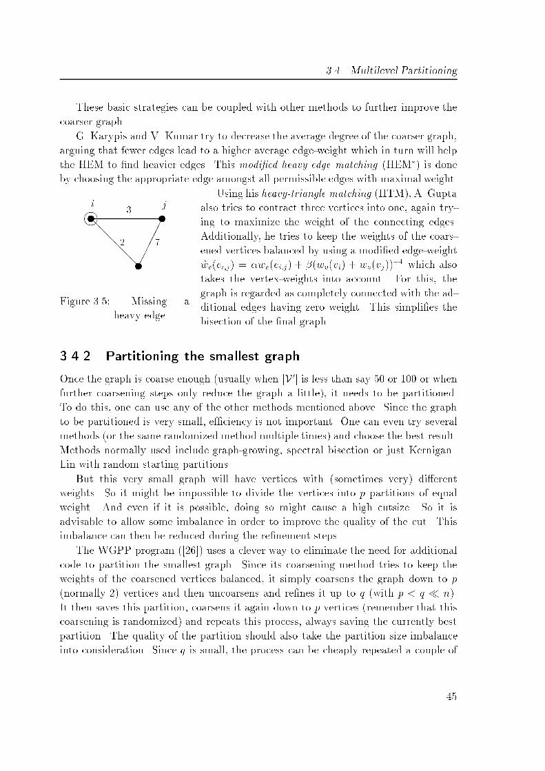
3.4 Multilevel PartitioningThese basic strategies can be coupled with other methods to further improve thecoarser graph.G. Karypis and V. Kumar try to decrease the average degree of the coarser graph,arguing that fewer edges lead to a higher average edge-weight which in turn will helpthe HEM to �nd heavier edges. This modi�ed heavy edge matching (HEM�) is doneby choosing the appropriate edge amongst all permissible edges with maximal weight.Using his heavy-triangle matching (HTM), A. Guptavvvm ������@@@@@@i j32 7Figure 3.5: Missing aheavy edge also tries to contract three vertices into one, again try-ing to maximize the weight of the connecting edges.Additionally, he tries to keep the weights of the coars-ened vertices balanced by using a modi�ed edge-weight~we(ei;j) = �we(ei;j) + �(wv(vi) + wv(vj))�1 which alsotakes the vertex-weights into account. For this, thegraph is regarded as completely connected with the ad-ditional edges having zero weight. This simpli�es thebisection of the �nal graph.3.4.2 Partitioning the smallest graphOnce the graph is coarse enough (usually when jV 0j is less than say 50 or 100 or whenfurther coarsening steps only reduce the graph a little), it needs to be partitioned.To do this, one can use any of the other methods mentioned above. Since the graphto be partitioned is very small, e�ciency is not important. One can even try severalmethods (or the same randomized method multiple times) and choose the best result.Methods normally used include graph-growing, spectral bisection or just Kernigan�Lin with random starting partitions.But this very small graph will have vertices with (sometimes very) di�erentweights. So it might be impossible to divide the vertices into p partitions of equalweight. And even if it is possible, doing so might cause a high cutsize. So it isadvisable to allow some imbalance in order to improve the quality of the cut. Thisimbalance can then be reduced during the re�nement steps.The WGPP program ([26]) uses a clever way to eliminate the need for additionalcode to partition the smallest graph. Since its coarsening method tries to keep theweights of the coarsened vertices balanced, it simply coarsens the graph down to p(normally 2) vertices and then uncoarsens and re�nes it up to q (with p < q � n).It then saves this partition, coarsens it again down to p vertices (remember that thiscoarsening is randomized) and repeats this process, always saving the currently bestpartition. The quality of the partition should also take the partition size imbalanceinto consideration. Since q is small, the process can be cheaply repeated a couple of45

3 Partitioning without geometric informationtimes and the best result is chosen.3.4.3 Projecting up and re�ning the partitionGiven the partition of the coarser graph, we now need to �nd a good partition of the�ner graph. First, we �project up� the partition of the coarser graph to the �ner one.Each vertex of the �ner graph can be traced to exactly one vertex in the coarser graph:either it (together with one (or more) other vertices) is contracted into a new coarser-level vertex or it is simply copied to the coarser level. So having partitioned thecoarser graph, we can simply assign the vertices on the �ner graph to the appropriatepartitions.But on the �ner graph we now have more �degrees of freedom� to �nd a betterpartition (with a lower cutsize), so we need to re�ne the graph, improving both thecutsize and the balance (since the partitions might be of di�erent weight).The re�nement is usually done by using one of the variants of the Kernigan�Linalgorithm described in section 3.2.1. The Fiduccia�Mattheyses variant [18] in par-ticular can easily be modi�ed to improve the balance at the same time by addingsome term describing the imbalance into the cost-function used to �nd the next ver-tex to move. Other changes include using only one inner pass and considering only�boundary-vertices�.3.5 Other methodsIn the sections above, we have described the more common methods for graph par-titioning. But there are many other methods as well, both geometrically orientedand graph based, which we will only cite here ([8, 14, 16, 55, 63, 65�67]). Some of themethods are specialized for �nite element meshes for PDEs ([13,60,62]). Others havetried to apply general optimization techniques like simulated annealing or genetic al-gorithms to the partitioning problem ([36, 37, 61, 68]). And �nally, in addition to thesoftware libraries mentioned above, there are other programs available as well, forexample Jostle ([64]), Party ([54]) and Scotch ([49]).46

Bibliography[1] G. Ahmdahl. The validity of the single processor approach to achieving large scalecomputing capabilities. In AFIPS Proc. of the SJCC, volume 30, pages 483�485, 1967.[2] S. T. Barnard, A. Pothen, and H. Simon. A spectral algorithm for envelope reductionof sparse matrices. Numerical Linear Algebra with Applications, 2(4):317�334, 1995.[3] S. T. Barnard and H. D. Simon. A fast multilevel implementation of recursive spectralbisection for partitioning unstructured problems. Concurrency: Practice and Experi-ence, 6:101�107, Feb. 1994.[4] S. T. Barnard. PMRSB: Parallel multilevel recursive spectral bisection. In Proceedingsof the 1995 ACM/IEEE Supercomputing Conference. ACM / IEEE, 1995. publishedonline and as CD.[5] A. Berman and R. J. Plemmons. Nonnegative Matrices in the Mathematical Sciences.Academic Press, 1979.[6] M. W. Berry, B. Hendrickson, and P. Raghavan. Sparse matrix reordering schemes forbrowsing hypertext. In J. Renegar, M. Shub, and S. Smale, editors, The Mathematicsof Numerical Analysis, volume 32 of Lectures in Applied Mathematics, pages 99�123.AMS, 1996.[7] W. L. Briggs. A Multigrid Tutorial. SIAM, 1987.[8] T. F. Chan, J. R. Gilbert, and S.-H. Teng. Geometric spectral partitioning. TechnicalReport CSL-94-15, Parc Xerox, Jan. 1995.[9] T. F. Chan, J. P. Ciarlet, and W. K. Szeto. On the optimality of the median cutspectral bisection graph partitioning method. SIAM Journal on Scienti�c Computing,18(3):943�948, May 1997.[10] T. F. Chan and W. K. Szeto. A sign cut version of the recursive spectral bisection graphpartitioning algorithm. In J. G. Lewis, editor, Proceedings of the 5th SIAM Conferenceon Applied Linear Algebra (Snowbird UT). SIAM, 1994.[11] G. Chartrand and O. R. Oellermann. Applied and algorithmic graph theory. Interna-tional series in pure and applied mathematics. McGraw-Hill, New York, 1993. 47

Bibliography[12] P. G. Ciarlet and J. L. Lions. Handbook of numerical analysis; Part 2: Finite elementmethods. North-Holland, Amsterdam, 1992.[13] H. L. deCougny, D. D. Devine, J. E. Flaherty, R. M. Loy, C. Özturan, and M. S. Shep-hard. Load balancing for the parallel adaptive solution of partial di�erential equations.Applied Numerical Mathematics, 16:157�182, 1994.[14] R. Dieckmann, B. Monien, and R. Preis. Using helpful sets to improve graph bisections.Technical Report tr-rf-94-008, Fak. f. Informatik, Universität-GH Paderborn, June 1994.[15] R. Dieckmann, B. Monien, and R. Preis. Load balancing strategies for distributed mem-ory machines. Technical Report tr-rsfb-97-050, SFB 376, Universität-GH Paderborn,Sept. 1997.[16] J. Falkner, F. Rendl, and H. Wolkowitz. A computational study of graph partition-ing. Mathematical Programming, 66(2):211�239, 1994. Also University of WaterlooTech.Report CORR-92-25, 1993.[17] C. Farhat. A simple and e�cient automatic FEM domain decomposer. Computers andStructures, 28(5):579�602, 1988.[18] C. M. Fiduccia and R. M. Mattheyses. A linear time heuristic for improving networkpartitions. Technical Report 82CRD130, General Electric Co, Corporate Research andDevelopment Center, Schenectady,NY, May 1982.[19] M. Fiedler. Algebraic connectivity of graphs. Czecheslovak Mathematical Journal,23(98):298�305, 1973.[20] M. Fiedler. A property of eigenvectors of nonnegative symmetric matrices and itsapplication to graph theory. Czecheslovak Mathematical Journal, 25(100):619�633, 1975.[21] G. C. Fox, R. D. Williams, and P. C. Messing. Parallel Computing Works. MorgamKaufmann Publishers, 1994.[22] R. Freund and N. Nachtigal. Qmr: A quasi-minimal residual method for non-hermitianlinear systems. Numerical Mathematics, 60:315�339, 1991.[23] M. R. Garey and D. S. Johnson. Computers and Intractability: A Guide to the Theoryof NP�Completeness. Freeman, 1979.[24] J. R. Gilbert, G. L. Miller, and S.-H. Teng. Geometric mesh partitioning: Implemen-tation and experiments. Technical Report CSL-94-13, Xerox PARC, 1994. to appear:SIAM J Sci. Comp.[25] G. H. Golub and C. F. v. Loan. Matrix Computations. Johns Hopkins University Press,Baltimore and London, third edition, 1996.48

[26] A. Gupta. WGPP: Watson Graph Partitioning (and sparse matrix ordering) Package.IBM Research Division, T.J. Watson Research Center, P.O.Box 218, Yorktown Heights,New York 10598, 1996.[27] A. Gupta. Graph partitioning based sparse matrix orderings for interior point algo-rithms. IBM Journal of Research and Development, 41(1/2):171�184, 1997.[28] S. Hammond. Mapping unstructured grid computations to massively parallel computers.PhD thesis, Rensselaer Polytechnic Institute, Dept. of Computer Science, Renssselaer,NY, 1992.[29] B. Hendrickson and R. Leland. Multidimensional spectral load balancing. In Proc. 6thSIAM Conf. Par. Proc. Sci. Comput., 1993.[30] B. Hendrickson and R. Leland. Multidimensional spectral load balancing. TechnicalReport SAND93-0074, Sandia National Laboratories, 1993. also in Proc. 6th SIAMConf. Par. Proc. Sci. Comput.[31] B. Hendrickson and R. Leland. A multilevel algorithm for partitioning graphs. Tech-nical Report SAND93-1301, Sandia National Laboratories, 1993. appeared in Proc.Supercomputing 95.[32] B. Hendrickson and R. Leland. An empirical study of static load balancing algorithms.In Proceedings of the Scalable High Performance Computer Conference, pages 682�685.IEEE, 1994.[33] B. Hendrickson and R. Leland. The Chaco User's Guide Version 2. Sandia NationalLaboratories, Albuquerque NM, 1995.[34] B. Hendrickson and R. Leland. An improved spectral graph partitioning algorithm formapping parallel computations. SIAM Journal on Scienti�c Computing, 16(2):452�469,1995.[35] R. A. Horn and C. R. Johnson. Matrix Analysis. Cambridge University Press, 1985.[36] M. Jerrum and G. Sorkin. Simulated annealing for graph bisection. Technical ReportECS-LFCS-93-260, Dept. of Computer Science, University of Edinburgh, 1993.[37] D. S. Johnson, C. R. Aragon, L. A. McGeoch, and C. Schevon. Optimization by sim-ulated annealing: an experimental evaluation; part 1, graph partitioning. OperationsResearch, 37(6):865�892, Nov. 1989.[38] G. Karypis, R. Aggarwal, V. Kumar, and S. Shekhar. Multilevel hypergraph partition-ing: Applications in vlsi domain. Technical report, University of Minnesota, Departmentof Computer Science, 1997. short version in 34th Design Automation Conference. 49

Bibliography[39] G. Karypis and V. Kumar. A fast and high quality multilevel scheme for partitioningirregular graphs. Technical Report TR 95-035, University of Minnesota, Department ofComputer Science, July 1995. to appear SIAM J. Sci. Comp.[40] G. Karypis and V. Kumar. MeTis: Unstrctured Graph Partitioning and Sparse MatrixOrdering System, Version 2.0, Aug. 1995.[41] G. Karypis and V. Kumar. Parallel multilevel k-way partitioning scheme for irregulargraphs. Technical Report TR 95-036, University of Minnesota, Department of ComputerScience, 1996.[42] B. Kernigan and S. Lin. An e�cient heuristic procedure for partitioning graphs. TheBell System Technical Journal, 29(2):291�307, 1970.[43] V. Kumar, A. Grama, A. Gupta, and G. Karypis. Introduction to Parallel Computing.Benjamin/Cummings, Redwood City, CA, 1994.[44] L.-T. Liu, M.-T. Kuo, S.-C. Huang, and C.-K. Cheng. A gradient method on the initialpartition of Fiduccia�Mattheyses algorithm. In IEEE/ACM Int. Conf. on Computer-Aided Design, pages 229�234. IEEE/ACM, Nov. 1995.[45] R. Merris. Laplacians matrices of graphs: A survey. Linear Algebra and its Applications,197, 198:143�176, 1994.[46] G. L. Miller, S.-H. Teng, W. Thurston, and S. A. Vavasis. Automatic mesh partitioning.In A. George, J. R. Gilbert, and J. W. Liu, editors, Graph Theory and Sparse MatrixComputation, volume 56 of IMA Volumes in Mathematics and its Applications, pages57�84. Springer, 1993.[47] G. L. Miller, S.-H. Teng, W. Thurston, and S. A. Vavasis. Geometric separators for�nite element meshes. Technical report, University of Minnesota, 1994. to appear SIAMJ. Sci. Comp, Vol.19, Nr.2, march 1998.[48] C. C. Paige and M. A. Saunders. Solution of sparse inde�nite systems of linear equations.SIAM Journal on Numerical Analysis, 12:617�629, 1975.[49] F. Pellegrini. SCOTCH 3.1 Users Guide. Université Bordeaux I, Aug. 1996.[50] A. Pothen, E. Rothberg, H. Simon, and L. Wang. Parallel sparse Cholesky factoriza-tion with spectral nested bisection ordering. Technical Report RNR-94-011, NumericalAerospace Simulation Facility, NASA Ames Research Center, May 1994.[51] A. Pothen, H. Simon, and K.-P. Liou. Partitioning sparse matrices with eigenvectors ofgraphs. SIAM Journal on Matrix Analysis and Applications, 11(3):430�452, July 1990.50

[52] A. Pothen, H. Simon, and L. Wang. Spectral nested disection. Technical Report RNR-92-003, NASA Ames Research Center, 1992. Short version in Supercomputing '92, pp.42�51, Nov. 1992.[53] A. Pothen. Graph partitioning algorithms with applications to scienti�c computing.In D. E. Keyes, A. H. Sameh, and V. Venkatakrishnan, editors, Parallel NumericalAlgorithms. Kluwer Academic Press, 1995.[54] R. Preis and R. Dieckmann. The PARTY Partitioning � Library User Guide � Version1.1. SFB 376, Univ. Paderborn.[55] F. Rendl and H. Wolkowicz. A projection technique for partitioning the nodes of agraph. Annals of Operations Research, 58:155�179, 1995.[56] E. Rothberg and B. Hendrickson. Sparse matrix ordering methods for interior pointlinear programming. Technical Report SAND96-0475J, Sandia National Laboratories,Jan. 1996.[57] Y. Saad and M. Schultz. GMRES: A generalized minimal residual algorithm for solvingnonsymmetric linear systems. SIAM Journal on Scienti�c and Statistical Computing,7:856�869, 1986.[58] Y. Saad. Iterative methods for sparse linear system. PWS Publishing Company, Boston,MA, 1996.[59] H. Simon and S.-H. Teng. How good is recursive bisection. SIAM Journal on Scienti�cComputing, 18(5):1436�1445, Sept. 1997.[60] D. Vanderstraeten and R. Keunings. Optimized partitioning of unstructured �niteelement meshes. International Journal for Numerical Methods in Engineering, 38:433�450, 1995.[61] R. Van Driessche. Algorithms for static and dynamic Load Balancing on Parallel Com-puters. PhD thesis, KU Leuven, Nov. 1995.[62] C. Walshaw and M. Berzins. Dynamic load balancing for PDE solvers on adaptiveunstructured meshes. Research Report Series 92.32, University of Leeds School of Com-puter Studies, Dec. 1992.[63] C. Walshaw, M.Cross, M. G. Everett, S.Johnson, and K. McManus. Partitioning &mapping of unstructured meshes to parallel machine topologies. In A. Ferreira andJ. Rolim, editors, Irregular 95: Parallel Algorithms for Irregularly Structured Problems,volume 980 of LNCS, pages 121�126. Springer, 1995. 51

Bibliography[64] C. Walshaw, M.Cross, M. G. Everett, and S.Johnson. JOSTLE: Partitioning of unstruc-tured meshes for massively parallel machines. In N. S. et al, editor, Parallel Computa-tional Fluid Dynamics: New Algorithms and Applications, pages 273�280, Amsterdam,1994. Elsevier.[65] C. Walshaw, M.Cross, and M. G. Everett. Dynamic mesh partitioning: a uni�ed opti-misation and load-balancing algorithm. Technical Report 95/IM/03, School of Mathe-matics, Statistics & Computer Science, University of Greenwich, 1995.[66] C. Walshaw, M.Cross, and M. G. Everett. A localised algorithm for optimising unstruc-tured mesh partitions. International Journal of Supercomputer Applications, 9(4):280�295, 1995.[67] C. Walshaw, M.Cross, and M. G. Everett. A parallelisable algorithm for optimising un-stuctured mesh partitions. Technical Report 95/IM/06, School of Mathematics, Statis-tics & Computer Science, University of Greenwich, Jan. 1995.[68] R. D. Williams. Performance of dynamic load balancing algorithms for unstructuredmesh calculations. Concurrency, 3:457�481, 1991.

52