Graph Databases - UOP eClass

Ian Robinson, Jim Webber, and Emil Eifrem

Graph Databases

Graph Databasesby Ian Robinson, Jim Webber, and Emil Eifrem

Published by O’Reilly Media, Inc., 1005 Gravenstein Highway North, Sebastopol, CA 95472.

Proofreader: FIX ME!Cover Designer: FIX ME!

Interior Designer: FIX ME!Illustrator: FIX ME!

Revision History for the :

2013-02-25: Early release revision 1

See http://oreilly.com/catalog/errata.csp?isbn=9781449356262 for release details.

ISBN: 978-1-449-35626-2

http://oreilly.com/catalog/errata.csp?isbn=9781449356262

Table of Contents

Part I. GDB Book

1. Introduction. . . . . . . . . . . . . . . . . . . . . . . . . . . . . . . . . . . . . . . . . . . . . . . . . . . . . . . . . . . . . . . . 3What is a Graph? 5Making the Connection to NOSQL 7

2. The NOSQL Phenomenon. . . . . . . . . . . . . . . . . . . . . . . . . . . . . . . . . . . . . . . . . . . . . . . . . . . . . 9The Rise of NOSQL 9ACID Versus BASE 11The NOSQL Quadrants 12Document Stores 13Key-Value Stores 16Column Stores 19Query Versus Processing in Aggregate Stores 23Moving Onwards and Upwards 24

3. Graphs and Connected Data. . . . . . . . . . . . . . . . . . . . . . . . . . . . . . . . . . . . . . . . . . . . . . . . . . 25The Aggregate Model: Lacking Relationships 25The Relational Model: Also Lacking Relationships 29Connected Data and Graph Databases 32Schema-Free Development and Pain-Free Migrations 38Connecting the Dots 39

4. Working with Graph Data. . . . . . . . . . . . . . . . . . . . . . . . . . . . . . . . . . . . . . . . . . . . . . . . . . . . 41Models and Goals 41Relational Modeling in a Systems Management Domain 42Modeling for relational data 44The Property Graph Model 48The Cypher Query Language 51

iii

Cypher Philosophy 52Creating Graphs 53Beginning a Query 55Declaring information patterns to find 56Constraining Matches 57Processing Results 58Query Chaining 58

Graph Modeling in a Systems Management Domain 59Testing the model 62

Common Modeling Pitfalls 63Email Provenance Problem Domain 63A Sensible First Iteration? 64Second Time’s the Charm 66Evolving the Domain 69

Avoiding Anti-Patterns 74Summary 74

5. Graph Databases. . . . . . . . . . . . . . . . . . . . . . . . . . . . . . . . . . . . . . . . . . . . . . . . . . . . . . . . . . . 75Graph databases: a definition 75

Hypergraphs 75Triples 77

Graph-Native Stores 79Architecture 81Neo4j Programmatic APIs 88

Kernel API 89Core (or “Beans”) API 90Neo4j Traversal API 91

Non-Functional Characteristics 92Transactions 92Recoverability 93Availability 94Scale 96

Graph Compute Platforms 99Summary 104

6. Working with a Graph Database. . . . . . . . . . . . . . . . . . . . . . . . . . . . . . . . . . . . . . . . . . . . . 105Data Modeling 105

Describe the Model in Terms of Your Application’s Needs 105Nodes for Things, Relationships for Structure 107Model Facts as Nodes 107Represent Complex Value Types as Nodes 109Time 110

iv | Table of Contents

Iterative and Incremental Development 112Application Architecture 113

Embedded Versus Server 113Clustering 118Load Balancing 119

Testing 122Test-Driven Data Model Development 122Performance Testing 129

Capacity Planning 132Optimization Criteria 133Performance 133Redundancy 136Load 136

7. Graph Data in the Real World. . . . . . . . . . . . . . . . . . . . . . . . . . . . . . . . . . . . . . . . . . . . . . . 139Reasons for Choosing a Graph Database 139Common Use Cases 140

Social Networks 140Recommendation Engines 141Geospatial 142Master Data Management 142Network Management 143Access Control and Authorization 144

Detailed Use Cases 144Social Networking and Recommendations 145Access Control 156Logistics 164

8. Predictive Analysis with Graph Theory. . . . . . . . . . . . . . . . . . . . . . . . . . . . . . . . . . . . . . . . 179Depth- and Breadth-First Search 179Path-Finding with Dijkstra’s Algorithm 181The A* Algorithm 192Graph Theory and Predictive Modeling 193

Triadic Closures 194Structural Balance 196

Local Bridges 203Summary 205

Table of Contents | v

PART I

GDB Book

CHAPTER 1

Introduction

Graph databases address one of the great macroscopic business trends of today: lever‐aging complex and dynamic relationships to generate insight and competitive advan‐tage. Whether we want to understand relationships between customers, elements in atelephone or datacenter network, entertainment producers and consumers, or genesand proteins, the ability to understand and analyze vast graphs of highly-connected datawill be a key factor in the determining which companies outperform their competitorsover the coming decade.

For data of any significant size or value, graph databases are the best way to representand query connected data. While large corporates realized this some time ago, creatingtheir own proprietary graph processing technologies, we’re now in an era where thattechnology has rapidly become democratized. Today, general-purpose graph databasesare a reality, allowing mainstream users to experience the benefits of connected datawithout having to invest in building their own graph infrastructure.

What’s remarkable about this renaissance of graph data and graph thinking is that graphtheory itself is not new. Graph theory was pioneered by Euler in the 18th century, andhas been actively researched and improved by mathematicians, sociologists, anthro‐pologists, and others since then. However, it is only in the last few years that graph theoryand graph thinking have been applied to information management. Graph databaseshave been proven to solve some of the more relevant data management challenges oftoday, including important problems in the areas of social networking, master datamanagement, geospatial, recommendations engines, and more. This increased focus ongraph is driven by the massive commercial successes of companies such as Facebook,Google, and Twitter, all of whom have centered their business models around their ownproprietary graph technologies, together with the introduction of general purpose graphdatabases into the technology landscape (a very recent phenomenon in informatics).

Graphs and graph databases are tremendously relevant to anyone seeking to model thereal world. The real world—unlike the forms-based model behind the relational data‐

3

base—is rich and interrelated: uniform and rule-bound in parts, exceptional and irreg‐ular in others. Unlike relational databases, which require a level of erudition and spe‐cialized training to understand, graph databases store information in ways that muchmore closely resemble the ways humans think about data.

One of the unique things about graph databases that makes them especially adapted tomodelling the real world is that they elevate relationships to be first-class citizens of thedata model. We take for granted the fact that the items stored in a database—whetherthey are rows, documents, objects, or nodes—each merit their own rich set of descrip‐tors. A Person, for example, is often attributed with rich metadata such as name, gender,and date of birth. What may not be so clear, however, is that metadata also exists in therelationships between people. Unlike a relational database, where a relationship is ef‐fectively just a runtime constraint, part of what makes graph databases special is thatthey put relationships on the same level as the data items themselves. A “friend” rela‐tionship can therefore include a “friends since” datestamp, together with propertiesdescribing the degree and quality of friendship, and so on. As information processingcontinues to evolve, the next frontier arguably lies in the ability to capture, analyze, andunderstand these rich relationships.

We believe, and many of the major analysts agree, that in a few years the “Not Only SQL”conversation that appears so pertinent today will cease to be about the “Not”, and willinstead focus on what is: a heterogeneous data landscape where post-relational tech‐nologies sit alongside relational. There is no question that graph databases, which arecurrently recognized as one of the four major types of NOSQL database, will be one ofthe technology categories from which future data architects will choose the best tool forthe job at hand.

The purpose of this book is to introduce graphs and graph databases to technologyworkers, including developers, database professionals, and technology decision makers.Reading this book, you will come away with a practical understanding of graph data‐bases. We show how data is “shaped” by the graph model, and how it is queried, reasonedabout, understood and acted upon using a graph database. We discuss the kinds ofproblems that are well aligned with graph databases, with examples drawn from prac‐tical, real-world use cases. And we describe the surrounding ecosystem of complemen‐tary technologies, highlighting what differentiates graph databases from other databasetechnologies, both relational and NOSQL.

While much of the book talks about graph data models, it is not a book about graphtheory. The annals of graph theory include numerous fascinating and complex academicpapers, yet very little graph theory is needed in order to take advantage of the practicalbenefits afforded by graph databases—provided we understand what a graph is, we’repractically there. Before we discuss just how productive graph data and graph databasescan be, let’s refresh our memories about graphs in general.

4 | Chapter 1: Introduction

What is a Graph?Formally a graph is just a collection of vertexes and edges (as we learned in school)--or,in less intimidating language, a set of nodes and the relationships that connect them.We can use graphs to model all kinds of scenarios, from the construction of a spacerocket, to a system of roads, and from the supply-chain or provenance of foodstuff, tomedical history for populations, and beyond. Graphs are general-purpose and expres‐sive, allowing us to model entities as nodes and their semantic contexts using relation‐ships.

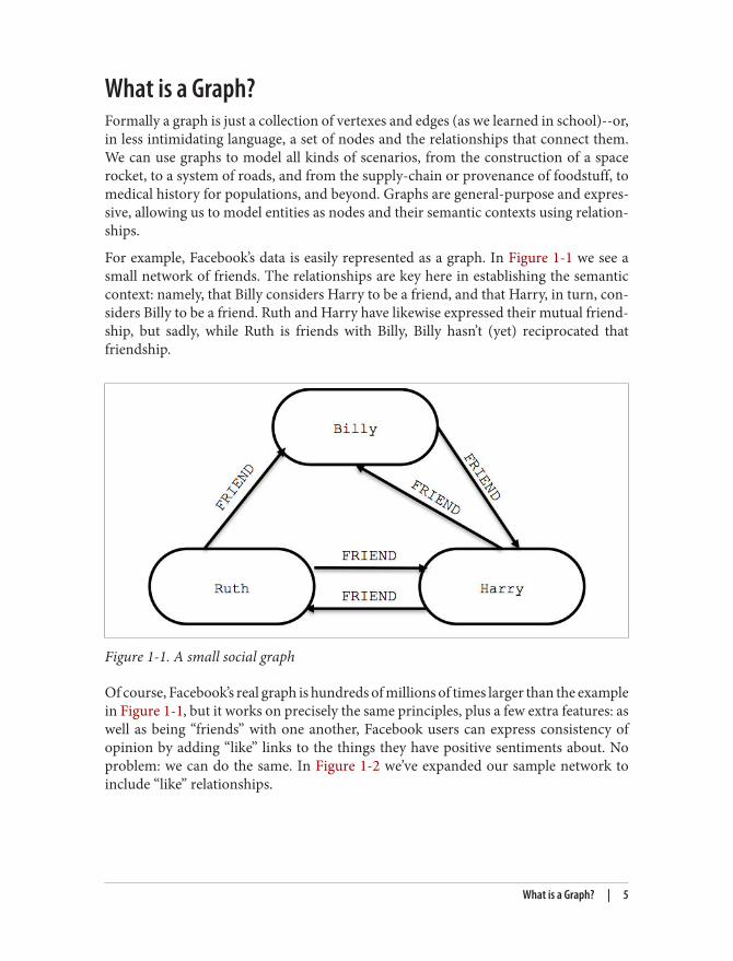
For example, Facebook’s data is easily represented as a graph. In Figure 1-1 we see asmall network of friends. The relationships are key here in establishing the semanticcontext: namely, that Billy considers Harry to be a friend, and that Harry, in turn, con‐siders Billy to be a friend. Ruth and Harry have likewise expressed their mutual friend‐ship, but sadly, while Ruth is friends with Billy, Billy hasn’t (yet) reciprocated thatfriendship.

Figure 1-1. A small social graph

Of course, Facebook’s real graph is hundreds of millions of times larger than the examplein Figure 1-1, but it works on precisely the same principles, plus a few extra features: aswell as being “friends” with one another, Facebook users can express consistency ofopinion by adding “like” links to the things they have positive sentiments about. Noproblem: we can do the same. In Figure 1-2 we’ve expanded our sample network toinclude “like” relationships.

What is a Graph? | 5

Figure 1-2. Liking posts on Facebook

Though simple, the graph in Figure 1-2 shows the expressive power of the model. It’seasy to see that Ruth has made a list of status updates (starting from status message 101all the way back to status message 99); that the most recent of these updates is linkedvia a relationship marked CURRENT; and that earlier updates are joined into a kind of listby relationships marked PREVIOUS, thus creating a timeline of posts. We can also seethat Harry ̀ LIKE`s Ruth’s status message 100, but hasn’t expressed the same sentimentsabout any of the others.

6 | Chapter 1: Introduction

1. There are other graph models with different constraints. For example property graphs don’t natively suithyperedges without some additional effort, but that’s really the only drawback.

In discussing Figure 1-2 we’ve also informally introduced the most popular variant ofgraph model, the Property Graph. A Property Graph has the following characteristics:

• It contains nodes and relationships• Nodes contain properties (key-value pairs)• Relationships are named, directed and always have a start and end node• Relationships can also contain properties

Most people find the Property Graph model intuitive and easy to understand. Whilesimple, it can be used to describe the overwhelming majority of graph use cases in waysthat yield useful insight into our data.1 The Property Graph model is supported by mostof the popular graph databases on the market today—including the market leader, Neo4j—and in consequence, it’s the model we’ll use throughout the remainder of this book.

Making the Connection to NOSQLNow we’ve refreshed our memory on graphs, it’s time for us to to move on to data anddatabases. Not only must graph databases support graph modelling, they must alsosupport querying and analysing graph data. Fortunately, we have hundreds of years ofgraph theory to help with analytics, and decades of research into graph algorithms tohelp with queries. Today this knowledge has been packaged into a set of database tech‐nologies that together bring the power of the graph to the developer community.

It’s an exciting time to be working with data, and the current trends around NOSQLand Big Data are fascinating (and fast-moving). To put the expressive power of graphdatabases into context, we need first to understand what is offered by the non-graphdatabases.

Making the Connection to NOSQL | 7

CHAPTER 2

The NOSQL Phenomenon

Recent years have seen a meteoric rise in popularity of a family of data storage tech‐nologies known as NOSQL (a cheeky acronym for Not Only SQL, or more confronta‐tionally, No to SQL). But NOSQL as a term defines what those data stores are not—they’re not SQL-centric relational databases—rather than what they are, an interestingand useful set of storage technologies whose operational, functional, and architecturalcharacteristics are many and varied.

In this chapter we’re going to discuss some of the recent forces that have given rise tothese NOSQL databases: the exponential growth in data volumes, the rise of connect‐edness, and the increase in degrees of semi-structure. We define data complexity interms of these three forces: data size, connectedness and semi-structure. By examininghow the different NOSQL technologies address these forces, we’ll be better placed tounderstand the role of graph databases in the rapidly changing world of data technol‐ogies.

The Rise of NOSQLHistorically, most enterprise-level Web apps could be run atop a relational database.The NOSQL movement has arisen in response to the needs of an emerging class ofapplications that must easily store and process data which is bigger in volume, changesmore rapidly, and is more structurally varied than can be dealt with by traditionalRDBMS deployments. For these applications, data has begun to move out of the SQLsweet-spot.

It’s no surprise that as storage has increased dramatically, volume has become the prin‐cipal driver behind much of the penetration of NOSQL stores into organizations. Vol‐ume may be defined simply as:

• Volume: the size of the stored data

9

As is well known, large datasets become unwieldy when stored in relational databases;in particular, query execution times increase as the size of tables and the number of joinsgrow (so called join pain). This isn’t the fault of the databases themselves; rather, it is anaspect of the underlying data model, which builds a set of all possible answers to a querybefore filtering to arrive at the correct solution.

In an effort to avoid joins and join pain, and thereby cope better with extremely largedata sets, the NOSQL world has adopted several alternatives to the relational model.Though more adept at dealing very large data sets, these alternative models tend to beless expressive than the relational one (with the exception of the graph model, which ismore expressive).

But volume isn’t the only problem modern Web-facing systems have to deal with. Be‐sides being big, today’s data often changes very rapidly. This is the velocity metric:

• Velocity: the rate at which data changes over time

Velocity is rarely a static metric: internal and external changes to a system and thecontext in which it is employed can have considerable impact on velocity. Coupled withhigh volume, variable velocity requires data stores to not only handle sustained levelsof high write-loads, but also deal with peaks.

There is another aspect to velocity, which is the rate at which the structure of the datachanges. In other words, as well as the value of specific properties changing, the overallstructure of the elements hosting those properties can change as well. This commonlyoccurs for two reasons. The first is fast-moving business dynamics: as the businesschanges, so do its data needs. The second is that data acquisition is often an experimentalaffair: some properties are captured “just in case”, others are introduced at a later pointbased on changed needs; the ones that prove valuable to the business stay around, othersfall by the wayside. Both these forms of velocity are problematic in the relational world,where high write loads translate into a high processing cost, and high schema volatilityhas a high operational cost.

While commentators have later added other useful requirements to the original questfor scale, the final key aspect is the realization that data is far more varied than we’vebeen comfortably been able to cope with in the relational world — for existential proofthink of all those nulls in our tables and the null checks in our code — that has drivenout the final widely agreed upon facet, variety which we can define as:

• Variety: the degree to which data is regularly or irregularly structured, dense orsparse, and importantly connected or disconnected.

The notion of variety manifests itself in different ways. For some data stores it’s simplythat denormalized documents are easier for developers than shoe-horning data into a

10 | Chapter 2: The NOSQL Phenomenon

1. For the graph stores that we consider elsewhere, it’s that the relational model is semantically weak in com‐parison.

2. The .NET-based RavenDB has bucked the trend amongst aggregate stores in supporting ACID transactions.As we’ll see in subsequent chapters, ACID properties are still upheld by competent graph databases.

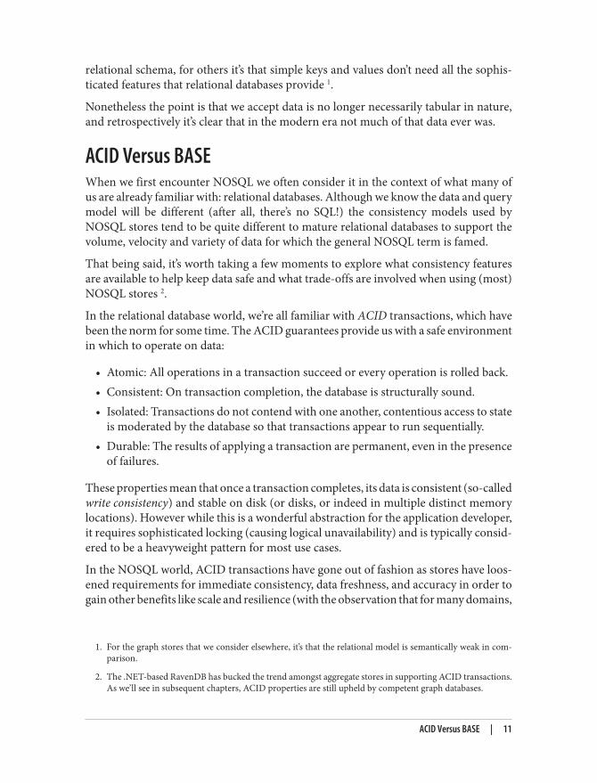
relational schema, for others it’s that simple keys and values don’t need all the sophis‐ticated features that relational databases provide 1.

Nonetheless the point is that we accept data is no longer necessarily tabular in nature,and retrospectively it’s clear that in the modern era not much of that data ever was.

ACID Versus BASEWhen we first encounter NOSQL we often consider it in the context of what many ofus are already familiar with: relational databases. Although we know the data and querymodel will be different (after all, there’s no SQL!) the consistency models used byNOSQL stores tend to be quite different to mature relational databases to support thevolume, velocity and variety of data for which the general NOSQL term is famed.

That being said, it’s worth taking a few moments to explore what consistency featuresare available to help keep data safe and what trade-offs are involved when using (most)NOSQL stores 2.

In the relational database world, we’re all familiar with ACID transactions, which havebeen the norm for some time. The ACID guarantees provide us with a safe environmentin which to operate on data:

• Atomic: All operations in a transaction succeed or every operation is rolled back.• Consistent: On transaction completion, the database is structurally sound.• Isolated: Transactions do not contend with one another, contentious access to state

is moderated by the database so that transactions appear to run sequentially.• Durable: The results of applying a transaction are permanent, even in the presence

of failures.

These properties mean that once a transaction completes, its data is consistent (so-calledwrite consistency) and stable on disk (or disks, or indeed in multiple distinct memorylocations). However while this is a wonderful abstraction for the application developer,it requires sophisticated locking (causing logical unavailability) and is typically consid‐ered to be a heavyweight pattern for most use cases.

In the NOSQL world, ACID transactions have gone out of fashion as stores have loos‐ened requirements for immediate consistency, data freshness, and accuracy in order togain other benefits like scale and resilience (with the observation that for many domains,

ACID Versus BASE | 11

3. Though often non-functional requirements strongly influence our choice of database too.

ACID transactions are far more pessimistic than the domain actually requires). Insteadof using ACID, the term BASE has arisen as a popular way of describing the propertiesof a more optimistic storage strategy.

• Basic Availability: The store appears to work most of the time.• Soft-state: Stores don’t have to be write-consistent, nor do different replicas have to

be mutually consistent all the time.• Eventual consistency: Stores exhibit consistency at some later point (e.g. lazily at

read time).

The BASE properties are far looser than the ACID guarantee, and there is no directmapping between them. A BASE store values availability (since that is a core buildingblock for scale) and does not offer write-consistency (though read your own writes tendsto mask this). BASE stores provide a less strict assurance that data will be consistent inthe future, perhaps at read time (e.g. Riak), or that data will always be consistent butonly for certain processed past snapshots (e.g. Datamic).

Given such loose support for consistency, we as developers need to be far more rigorousin our approach to developing against these stores and cannot any longer rely on thetransaction manager to sort out all our data access woes. Instead we must be intimatelyfamiliar with the BASE behavior of our chosen stores and work within those constraints.

The NOSQL QuadrantsHaving discussed the BASE model that underpins consistency in NOSQL stores, we’reready to start thinking about the numerous user-level data models. To disambiguatethese models, we’ve devised a simple taxonomy in Figure 2-1. That taxonomy shows ofthe four fundamental types of data store in the contemporary NOSQL space. Withinthat taxonomy, each store type addresses a different kind of functional use case 3.


Figure 2-1. The NOSQL store quadrants

In the following sections we’ll deal with each of these (with the exception of graphswhich will receive a much fuller analysis in subsequent chapters), highlighting the char‐acteristics of the data model, operational aspects, and drivers for adoption.

Document StoresThe document databases are perhaps offer the most immediately familiar paradigm fordevelopers. At its most fundamental level the model is simply that we store and retrievedocuments, just like an electronic filing cabinet. Documents tend to comprise the usualproperty key-value pairs, but where those values themselves can be lists, maps, or similarallowing for natural hierarchies in the document just as we’re used to with formats likeJSON and XML.

At the simplest level, documents can be stored and retrieved by ID. Providing an ap‐plication remembers the IDs it’s interested in (e.g. usernames) then a document storecan act much like a key-value store (of which we’ll see more later). But in the generalcase document stores rely on indexes to facilitate access to documents based on any oftheir attributes. For example, in an e-commerce scenario a it would be useful to haveindexes that represent distinct product types so that they can be offered up to potential

Document Stores | 13

4. This isn’t the case for graph databases because the graph itself provides a natural adjacency index

sellers as we see in Figure 2-2. In general indexes are used to reify sets of related docu‐ments out of the store for some application use.

Figure 2-2. Indexing reifies sets of entities in a document store

Much like indexes in relational databases, indexes in a document store allow us to tradewrite performance (since we have to maintain indexes) for greater read performance(because we examine fewer records to find pertinent data). For write-heavy records, it’sworth bearing in mind that indexes might actually degrade performance overall.

Where data hasn’t been indexed, queries are typically much slower since a full searchof the data set has to happen 4. This is obviously an expensive task and is to be avoidedwherever possible — and as we shall see rather than process these queries internally, it’snormal for document database users to externalize this kind of processing in parallelcompute frameworks.

Since the data model of a document store is one of disconnected entities, documentstores tend to have interesting and useful operational characteristics. For example, sincedocuments are mutually independent, document stores should have the ability to scale


5. Key-value and column stores tend not to require this planning, and subsume allocation of data to replicas asa normal part of their internal implementation

6. assuming the administrator has opted for safe levels of persistence when setting up the database

7. Though optimistic concurrency control mechanisms are useful, we also rather like transactions, and thereare numerous example of high-throughput performance transaction processing systems in the literature.

horizontally very well since there is no contended state between records at write time,and no need to transact across replicas.

ShardingMost document databases (e.g. MongoDB, RavenDB) make scaling-out an explicit as‐pect of development and operations by requiring that the user plan for sharding of dataacross logical instances to support horizontal scale 5. It’s often also puzzlingly cited as apositive reason for embracing such stores, most likely because it induces a (misplaced)excitement that scale is something to be embraced and lauded rather than somethingto be skilfully and diligently mastered.

At the write level, document databases overwhelmingly provide (limited) transaction‐ality at the individual record level. That is a document database will ensure that writesto a single document are atomically persisted 6, but do not help across document updates.That is, there is no locking support for operating across sets of documents atomically,and such abstractions are left to application code to implement in a domain-specificmanner.

However since stored documents are not connected (save through indexes) there arenumerous optimistic concurrency control mechanisms that can be used to help recon‐cile concurrent contending writes for a single document without having to resort tostrict locks. In fact some document stores (like CouchDB) have made this a key pointof their value proposition: that documents can be held in a multi-master database whichautomatically replicates concurrently accessed, contended state across instanceswithout undue interference from the user, making such stores very operationally con‐venient.

In other stores too the database management system may be able to distinguish andreconcile writes to different parts of a document, or even use logical timestamps toreconcile several contended writes into a single logically consistent outcome. This kindof feature is an example of a reasonable, optimistic trade off: it reduces the need fortransactions (which we know tend to be latent and decrease availability 7) by usingalternative mechanisms which optimistically provide greater availability, lower latencyand higher throughput.

Document Stores | 15

8. http://www.allthingsdistributed.com/files/amazon-dynamo-sosp2007.pdf

9. The formula for number of replicas required is given by R = 2F +1 where F is the number of failures we shouldtolerate.

Key-Value StoresKey-value stores are cousins of the document store family but their lineage comes fromthe Amazon’s Dynamo database 8. They act like (large, distributed) hashmap data struc‐tures where (usually) opaque values are stored and retrieved by key.

As shown in Figure 2-3 the key space of the hashmap is spread across numerous bucketson the network. For fault-tolerance reasons each bucket is replicated onto several ma‐chines and such that every bucket is replicated the desired number of times 9 and so thatno machine (where possible) is an exact replica of any other so that we can load-balanceduring recovery of a machine and its buckets (and avoid hotspots causing inadvertentself denial-of-service).

Clients by comparison have an easy task. They store a data element by hashing a domain-specific identifier (key). The hash function is crafted such that it provides a uniformdistribution across the available buckets, so that no single machine becomes a hotspot.Given the hashed key, the client can use that address to store the value in a correspondingbucket. A similar process occurs for retrieval of stored values.


10. http://en.wikipedia.org/wiki/Consistent_hashing

Figure 2-3. Key-Value stores act like distributed hashmap data structures

Consistent hashingIn any computer system failures will occur. In dependable systems those failures aremasked via redundant replacements being switched in for faulty components. In a key-value store — as with any distributed database — individual machines will likely be‐come unavailable during normal operation as networks go down, or internal hardwarefails.

Such events are to be considered normal for any long running system, but the side effectsof recovering from such failures should not itself cause problems. For example if amachine supporting a particular hash-range fails, it should not prevent new values inthat range being stored or cause unavailability while internal reorganization occurs.

This is where the technique of consistent hashing 10 is often applied. With this techniquewrites to a failed hash-range are (cheaply) remapped to the next available machinewithout disturbing the entire stored data set (in fact typically only the fraction of thekeys within the failed range need to be remapped, rather than the whole set). When the

Key-Value Stores | 17

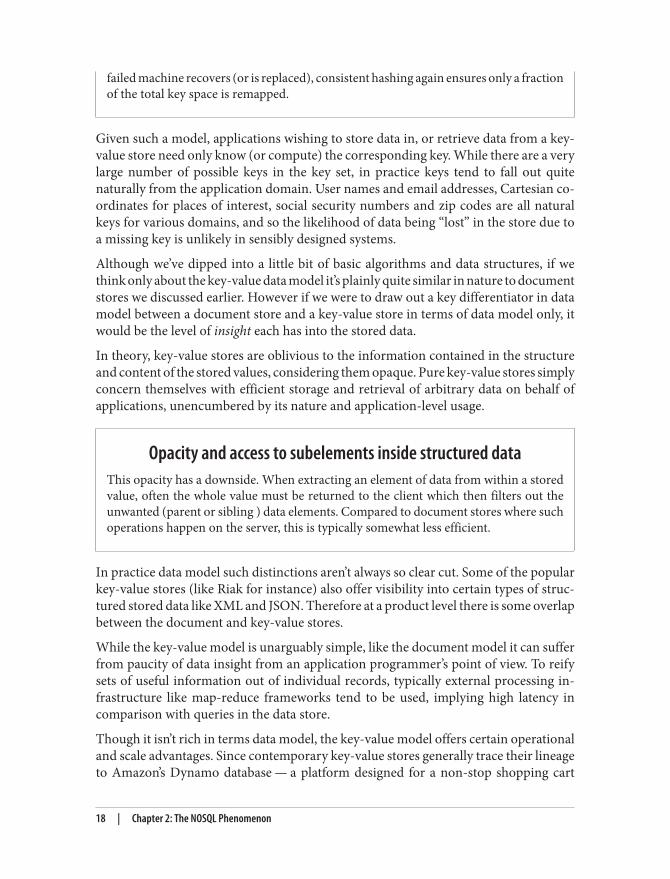
http://en.wikipedia.org/wiki/Consistent_hashing

failed machine recovers (or is replaced), consistent hashing again ensures only a fractionof the total key space is remapped.

Given such a model, applications wishing to store data in, or retrieve data from a key-value store need only know (or compute) the corresponding key. While there are a verylarge number of possible keys in the key set, in practice keys tend to fall out quitenaturally from the application domain. User names and email addresses, Cartesian co‐ordinates for places of interest, social security numbers and zip codes are all naturalkeys for various domains, and so the likelihood of data being “lost” in the store due toa missing key is unlikely in sensibly designed systems.

Although we’ve dipped into a little bit of basic algorithms and data structures, if wethink only about the key-value data model it’s plainly quite similar in nature to documentstores we discussed earlier. However if we were to draw out a key differentiator in datamodel between a document store and a key-value store in terms of data model only, itwould be the level of insight each has into the stored data.

In theory, key-value stores are oblivious to the information contained in the structureand content of the stored values, considering them opaque. Pure key-value stores simplyconcern themselves with efficient storage and retrieval of arbitrary data on behalf ofapplications, unencumbered by its nature and application-level usage.

Opacity and access to subelements inside structured dataThis opacity has a downside. When extracting an element of data from within a storedvalue, often the whole value must be returned to the client which then filters out theunwanted (parent or sibling ) data elements. Compared to document stores where suchoperations happen on the server, this is typically somewhat less efficient.

In practice data model such distinctions aren’t always so clear cut. Some of the popularkey-value stores (like Riak for instance) also offer visibility into certain types of struc‐tured stored data like XML and JSON. Therefore at a product level there is some overlapbetween the document and key-value stores.

While the key-value model is unarguably simple, like the document model it can sufferfrom paucity of data insight from an application programmer’s point of view. To reifysets of useful information out of individual records, typically external processing in‐frastructure like map-reduce frameworks tend to be used, implying high latency incomparison with queries in the data store.

Though it isn’t rich in terms data model, the key-value model offers certain operationaland scale advantages. Since contemporary key-value stores generally trace their lineageto Amazon’s Dynamo database — a platform designed for a non-stop shopping cart


11. http://research.google.com/archive/bigtable.html

service — they are optimized for high availability and scale, or as the Amazon team putsit, they should work even “if disks are failing, network routes are flapping, or data centersare being destroyed by tornados. 9“. This impressive model might sway a decision to usesuch a store even if the data model isn’t a perfect fit simply because operationally thesestores tend to be very robust.

Column StoresThe heritage of the column family stores comes from Google’s BigTable paper 11 wherethe authors described a novel kind of data store whose data model is based on a sparselypopulated table where each row can contain arbitrary columns. At first this seems anunusual data model, but a positive side-effect of this model means that column storesprovide natural data indexing based on the keys stored. Let’s dig a little deeper.

In our discussion we’ll use terminology from Apache Cassandra.Cassandra isn’t necessarily a faithful interpretation of BigTable, butit is widely deployed and its terminology is widely understood.

In Figure 2-4 we see the four common building blocks used in column stores. Thesimplest unit of storage is the column itself, consisting of a name-value pair. Any numberof columns can be combined into a super column which gives a name to a sorted set ofcolumns. Columns are stored in rows, and when a row contains columns only it isknown as a column family. Similarly when a row contains super columns it is known asa super column family.

Column Stores | 19

http://research.google.com/archive/bigtable.html

Figure 2-4. The four building blocks of column storage

It might seem odd to focus on rows to such an extent in a data model which is ostensiblycolumnar, but at in individual level rows really are important, providing the nestedhashmap structure into which we decompose our data. In Figure 2-5 we’ve shown anexample of how we might map a recording artist and their albums into a super columnfamily structure — it really is logically nothing more than maps of maps which is asimple metaphor even if this column nomenclature seems unfamiliar.


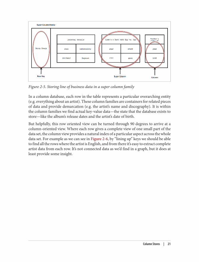
Figure 2-5. Storing line of business data in a super column family

In a column database, each row in the table represents a particular overarching entity(e.g. everything about an artist). These column families are containers for related piecesof data and provide demarcation (e.g. the artist’s name and discography). It is withinthe column families we find actual key-value data—the state that the database exists tostore—like the album’s release dates and the artist’s date of birth.

But helpfully, this row oriented view can be turned through 90 degrees to arrive at acolumn-oriented view. Where each row gives a complete view of one small part of thedata set, the column view provides a natural index of a particular aspect across the wholedata set. For example as we can see in Figure 2-6, by “lining up” keys we should be ableto find all the rows where the artist is English, and from there it’s easy to extract completeartist data from each row. It’s not connected data as we’d find in a graph, but it does atleast provide some insight.

Column Stores | 21

Figure 2-6. Keys form a natural index through rows in a column store

But it’s not just the more expressive data model (compared to document and key-valuestores at least) which are exciting about column store, but their operational character‐istics too. For example, although Apache Cassandra is famed for being based on anAmazon Dynamo-like infrastructure for distribution, scale, and failover, under the


12. http://martinfowler.com/bliki/NosqlDistilled.html

13. http://domaindrivendesign.org/

14. http://research.google.com/archive/mapreduce.html

covers there are several storage engines (including the default) which have shown to bevery competent at dealing with high write loads — the kind of peak write load problemwhen popular TV shows encourage interaction for example.

All in all, the column stores present themselves as reasonably expressive and opera‐tionally very competent. And yet at the end of the day, they’re still simply aggregatestores just like document and key-value databases and as such querying is still going tobe substantially augmented by processing to reify useful information at scale.

Query Versus Processing in Aggregate StoresIn focussing on the data models for (non-graph) NOSQL stores, we’ve highlighted eachmodel and some of the similarities and differences between them. But on balance, thedifferences have been far fewer than the similarities. In fact these stores are sufficientlysimilar to be abstracted into one larger super-class of store which Fowler and Sadalage12 have chosen to call aggregate stores, stemming from the observation that each of thesestores persists standalone complex records which reflect the notion of an Aggregate inDomain-Driven design 13.

The details the underlying storage strategy differs a great deal between each aggregatestore, yet they all have a great deal in common when it comes to their query model.While aggregate stores might provide features like indexing, simple document linking,or query languages for simple ad-hoc queries, it’s commonplace to identify and extract(a subset of) data from the store before piping it through some processing externalinfrastructure. Typically that infrastructure is a map-reduce framework and it is usedin order to reify deep insight into data which cannot be inferred by considering eachaggregate individually.

Map-reduce, like BigTable, is another technique published by Google 14 and rapidlyimplemented in the open source community with Apache Hadoop and its ecosystembeing the frontrunner map-reduce framework for the rest of us.

Map-reduce is a relatively simple parallel programming model where data is split andoperated upon in parallel before being gathered back together and aggregated for pro‐vide focussed information. For example, if we wanted to count how many Americalartists are in a database of recording artists we would extract al of the artist records anddiscard all those representing non-American artists in the map phase, before countingthe remaining records in the reduce phase to obtain our answer.

Query Versus Processing in Aggregate Stores | 23

http://martinfowler.com/bliki/NosqlDistilled.html

http://domaindrivendesign.org/

http://research.google.com/archive/mapreduce.html

Of course doing this kind of operation on a large database — even where we have manymachines to execute map and reduce code, and fast network infrastructure to move dataaround — is an enormous endeavour. Instead the usual approach is to try to use thefeatures of the data store to provide a more focussed data set (e.g. using indexes or otherad-hoc queries) asnd then map-reduce that smaller data set to arrive at our answer.

Sometimes processing data in this way can prove to be beneficial, after all map-reduceis highly parallelizable and frameworks like Hadoop are a commodity. However thoughenormous processing throughput can be achieved this comes at the expense of bothlatency (extracting and re-assimilating the data) and risk since data is ripped out of itssafe home in the database and crunched through some external machinery that has nosense of the underlying consistency model the database enforces.

Moving Onwards and UpwardsWe’ve seen the three popular aggregate store types—key-value, document, and columnstore—in this chapter and understood their strengths and weaknesses. We’ve discussedhow the aggregate data model often results in data stores that have excellent operationalcharacteristics, but we’ve also seen how the query and processing models supported bythose stores highlight the paucity of the underlying standalone aggregate data modelpresented to users, and the (latent) machinery that needs to be deployed to redress thatshortcoming.

Aggregate stores are not natively suited to most domains where data is interconnected(the canonical case, if you give it a moment’s consideration). You can use them that way,but then it’s your job as the developer to fill in where the underlying data model leavesoff. While the data might be big, it’s not necessarily smart.

However it’s now time for us to move on from the world of simple aggregates and intoa world where data is habitually interconnected as we delve into the domain of graphdatabases.


CHAPTER 3

Graphs and Connected Data

In this chapter we’ve going to immerse ourselves in the world of graphs and connecteddata and make the case for graph databases as the sanest means for graph storage andquerying. We’re going to define connected data and show the benefits of working withgraphs to solve complex data and business problems, and demonstrate how graphs area natural model for a wide variety of domains. But before we dive into that, let’s revisitwhy contemporary NOSQL stores and relational databases can struggle when used formanaging graphs and connected data.

The Aggregate Model: Lacking RelationshipsAs we saw in the previous chapter, aggregate databases — key-value, document, andcolumn stores — are popular members of the NOSQL family for storing sets of dis‐connected documents/values/columns. However by convention, it’s possible to fake re‐lationships (or at least pointers) in these stores by embedding the identifier of one ag‐gregate inside well-known field in another. As we can see in as we see in Figure 3-1, ashumans it’s deceptively easy for us to infer relationships between our aggregates byvisually inspecting them.

25

1. Remember in most aggregate stores, it’s inside the aggregates themselves are where structure is given to data,often as nested maps.

Figure 3-1. Reifying relationships in an aggregate store

In Figure 3-1 we can (somewhat reasonably) infer that some property values are reallyreferences to foreign aggregates elsewhere in the database. But that inference doesn’tcome for free, since support for relationships does not exist at all in this data model.Instead it’s left to developers do the hard work to infer and reify useful knowledge outof these flat, disconnected data structures 1. It’s also left to developers to remember toupdate or delete those foreign aggregate references in tandem with the rest of the data,otherwise the store will quickly contain overwhelming numbers of dangling references,both harmful to data quality and query performance.

Links and walkingThe Riak key-value store allows each of its stored values to be augmented with linkmetadata. Each link is one-way, pointing from one stored value to another. Riak allowsany number of these links to be walked (in Riak terminology), making the model help‐fully somewhat connected. However as a native key-value store (rather than graph da‐

26 | Chapter 3: Graphs and Connected Data

2. http://en.wikipedia.org/wiki/Graph_database

3. Social graph is the poster child for graphs in general, but as we’ll see there are other interesting and valuableuse cases we can address

tabase) at query time link walking is powered by map-reduce and is relatively latent,suited for simple graph-structured programming rather than general graph algorithms.

But there’s another weak point in this scheme, because in the absence of more identifiersto “point” back (the foreign aggregate “links” are not reflexive of course) we also losethe ability to be able to run other interesting queries on the database. For example withthe current structure it is expensive to ask of the database who has bought a particularproduct in order to perhaps recommend it based on customer profile. In those cases wecan export the data set and process it via external compute infrastructure (likely Ha‐dooop) in order to brute-force compute the result. Another option is to retrospectivelyinsert the backwards pointing foreign aggregate references before then querying for theresult. Either way the results will be latent.

Sometimes it might be tempting to think that there is equivalence between aggregatestores and graph databases. This is a forlorn hope since aggregate stores do not maintainconsistency of connected data nor provide index-free adjacency 2, and therefore are slowwhen used for graph problems. This results in an inherently latent compute mode wheredata is crunched outside the database rather than queried within it.

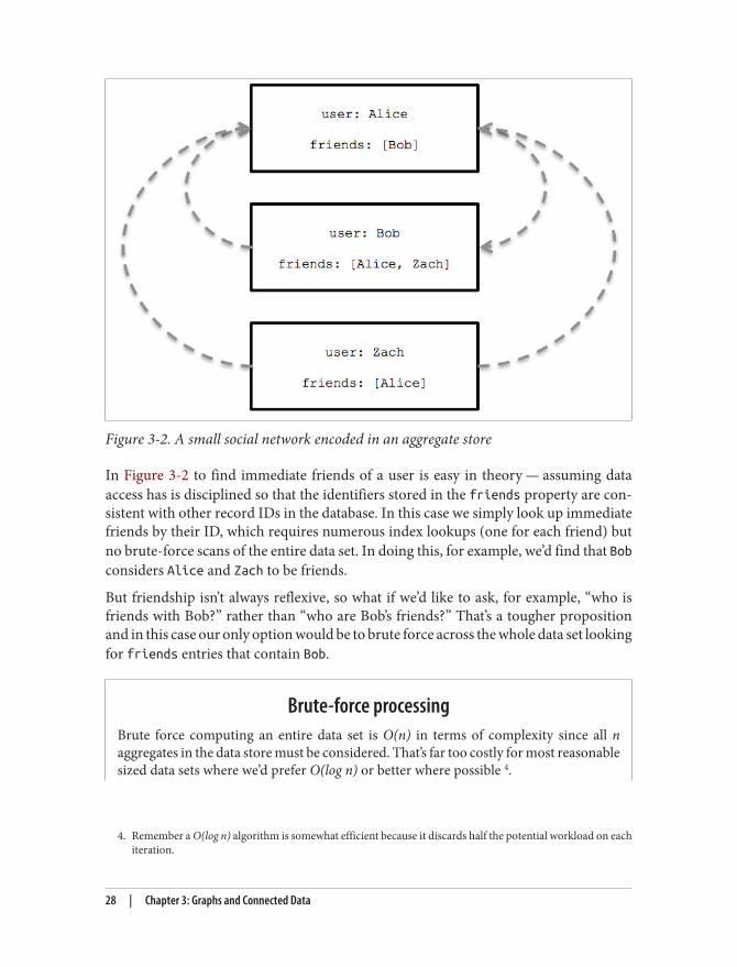
It’s easy to see how these aggregate model limitations impact us even in a simple socialdomain 3. In Figure 3-2 we see a (small) social network — a trivial example of a graphtacitly encoded inside documents.

The Aggregate Model: Lacking Relationships | 27

http://en.wikipedia.org/wiki/Graph_database

4. Remember a O(log n) algorithm is somewhat efficient because it discards half the potential workload on eachiteration.

Figure 3-2. A small social network encoded in an aggregate store

In Figure 3-2 to find immediate friends of a user is easy in theory — assuming dataaccess has is disciplined so that the identifiers stored in the friends property are con‐sistent with other record IDs in the database. In this case we simply look up immediatefriends by their ID, which requires numerous index lookups (one for each friend) butno brute-force scans of the entire data set. In doing this, for example, we’d find that Bobconsiders Alice and Zach to be friends.

But friendship isn’t always reflexive, so what if we’d like to ask, for example, “who isfriends with Bob?” rather than “who are Bob’s friends?” That’s a tougher propositionand in this case our only option would be to brute force across the whole data set lookingfor friends entries that contain Bob.

Brute-force processingBrute force computing an entire data set is O(n) in terms of complexity since all naggregates in the data store must be considered. That’s far too costly for most reasonablesized data sets where we’d prefer O(log n) or better where possible 4.


Conversely a graph database provides constant order lookup in this case, we’d simplyfind the node in the graph that represents Bob, and then follow any incoming friendrelationships to other nodes which represent people who consider Bob to be their friend.This is far cheaper than brute-forcing (unless everybody is friends with Bob) since farfewer members of the network are considered — only those that are connected to Bob.

To prevent the need for constant processing of the entire data set, we’d have to furtherdenormalize the storage model by adding backward links. In this case we’d have to adda second property, perhaps called friended_by to list the perceived incoming friendshiprelations. This doesn’t come for free. For instance we have to pay the initial and ongoingcost of increased write latency, and increased disk space utilization for storing that ad‐ditional metadata. Traversing those links is expensive because each hop requires anindex lookup, as aggregates have no notion of locality, unlike graphs which naturallyprovide index-free adjacency through real — not reified — relationships. That is, byimplementing a graph structure atop a non-native store, we may get some of the benefitsin terms of partial connectedness but at substantial cost.

That substantial cost is amplified when you consider traversing deeper than just onehop. Friends are easy enough, but imagine trying to compute — in real time — friendsof friends, or friends of friends of friends. That’s impractical with this kind of databasesince traversing a fake relationship is not cheap enough. This doesn’t only limit yourchances of expanding your social network, but in other use cases will reduce profitablerecommendations, will miss faulty equipment in your data center, will let fraudulentpurchasing activity slip through the net. Most systems try to maintain the appearanceof such graph-like processing, but inevitably it’s done in batches and doesn’t providethat high-value real-time interaction that users demand.

The Relational Model: Also Lacking RelationshipsThings aren’t all that rosy in the relational database world either. For several decades,developers have tried to accommodate increasingly connected, semi-structured datasetsinside relational databases. But whereas relational databases were initially designed tocodify paper forms and tabular structures—something they do exceedingly well—theystruggle when attempting to model the ad hoc, exceptional relationships that crop upin the real world. It’s an ironic twist that relational databases are in fact so poor at dealingwith relationships. While relationships do at least exist in the vernacular of relationaldatabases, they exist only as a means of joining tables and are completely free of se‐mantics (like direction, name). Worse still, as outlier data multiplies, and the amountof semi-structured information increases, the relational model becomes burdened withlarge join tables, sparsely populated rows and lots of null-checking logic. The rise inconnectedness translates in the relational world into increased joins, which impede

The Relational Model: Also Lacking Relationships | 29

performance and make it more difficult to evolve an existing database in response tochanging business needs.

Figure 3-3. Semantic relationships are hidden in a relational database

Even in a simple relational schema like that shown in Figure 3-3, many of these problemsare immediately apparent.

• Manifest accidental complexity and additional development and maintenanceoverheads because of join tables and maintaining foreign key constraints just tomake the database work.

• Sparse tables require special checking in code while schema gives false confidenceabout perceived data structure.

• Several expensive joins needed just to discover what a customer bought.• No cheap way of asking reciprocal queries. For example it’s acceptable from a time

perspective to ask ''what products did a customer buy?`` but not at all reasonableto ask ''which customers bought this product?``, which is the basis of recommen‐dation systems and numerous other valuable applications.


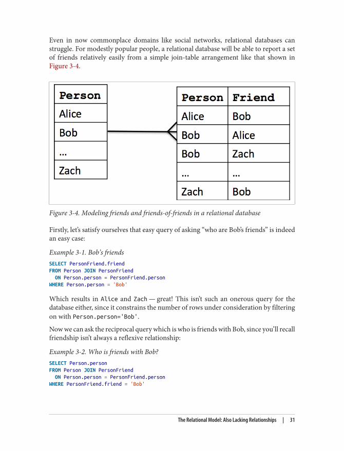
Even in now commonplace domains like social networks, relational databases canstruggle. For modestly popular people, a relational database will be able to report a setof friends relatively easily from a simple join-table arrangement like that shown inFigure 3-4.

Figure 3-4. Modeling friends and friends-of-friends in a relational database

Firstly, let’s satisfy ourselves that easy query of asking “who are Bob’s friends” is indeedan easy case:

Example 3-1. Bob’s friendsSELECT PersonFriend.friendFROM Person JOIN PersonFriend ON Person.person = PersonFriend.personWHERE Person.person = 'Bob'

Which results in Alice and Zach — great! This isn’t such an onerous query for thedatabase either, since it constrains the number of rows under consideration by filteringon with Person.person='Bob'.

Now we can ask the reciprocal query which is who is friends with Bob, since you’ll recallfriendship isn’t always a reflexive relationship:

Example 3-2. Who is friends with Bob?SELECT Person.personFROM Person JOIN PersonFriend ON Person.person = PersonFriend.personWHERE PersonFriend.friend = 'Bob'

The Relational Model: Also Lacking Relationships | 31

5. Some relational databases provide syntactic sugar for this, for instance Oracle supports CONNECT BY whichsimplifies the query, but not the underlying computational complexity.

This query results only in the row for Alice being returned, implying that Zach doesn’tconsider Bob to be a friend, sadly. The reciprocal query is still easy to implement, butfor the database to work out who is friends with Bob it requires more effort since all ofthe rows in the PersonFriend table must be considered.

Things degenerate further when we ask “who are my friends of friends”. Firstly thingsget a little tougher simply because of query complexity, since hierarchies are not a par‐ticularly natural or pleasant thing to express in SQL, relying on recursive joins 5.

Example 3-3. Alice’s friends-of-friendsSELECT pf1.person as PERSON, pf3.person as FRIEND_OF_FRIENDFROM PersonFriend pf1 INNER JOIN Person ON pf1.person = Person.personINNER JOIN PersonFriend pf2 ON pf1.friend = pf2.personINNER JOIN PersonFriend pf3 ON pf2.friend = pf3.personWHERE pf1.person = 'Alice' AND pf3.person <> 'Alice'

This query is computationally complex, not to mention it only deals with Alice’s friendsof friends and goes no further out into Alice’s social network. While “who are my friends-of-friends-of-friends” is feasible, beyond that to 4, 5, or 6 degrees of friends is not suitedto relational computation due to computational and space complexity of recursivelyjoining tables, either through clever SQL or by having application code explicitly enu‐merate the joins.

In a relational database, we work against the grain. We have often brittle schemas whichrigidly describe the structure of the data only to have those schemas’ intended behavioroverridden by code that ostensibly obeys the laws but bends all the rules. Consequentlya web of sparsely populated tables propagates through the database and a plethora ofcode to handle each of the exceptional cases is spread through the application. Thisincreases coupling and all but destroys any semblance of cohesion.

And for most of us, relational technology simply doesn’t evolve or scale easily enough.It’s time to move on.

Connected Data and Graph DatabasesIn the previous example with aggregate and relational stores we were dealing withimplicitly connected data. That is, as users we could infer semantic dependencies be‐tween entities but the data model — and as a consequence the databases themselves —could not recognize or assist us in taking advantage of those connections. As a result


6. We can expand the network in this example because the graph data model is more expressive and performantthan the other models we’ve considered

the workload of reifying a network out of the flat, disconnected data fell to us and wehad to deal with the consequences of slow queries, latent writes across denormalizedstores, etc.

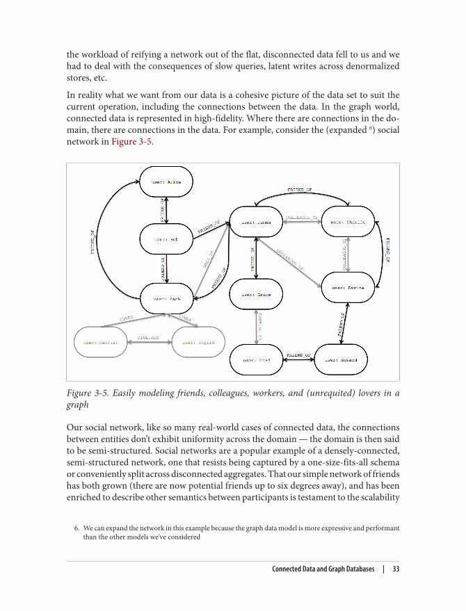
In reality what we want from our data is a cohesive picture of the data set to suit thecurrent operation, including the connections between the data. In the graph world,connected data is represented in high-fidelity. Where there are connections in the do‐main, there are connections in the data. For example, consider the (expanded 6) socialnetwork in Figure 3-5.

Figure 3-5. Easily modeling friends, colleagues, workers, and (unrequited) lovers in agraph

Our social network, like so many real-world cases of connected data, the connectionsbetween entities don’t exhibit uniformity across the domain — the domain is then saidto be semi-structured. Social networks are a popular example of a densely-connected,semi-structured network, one that resists being captured by a one-size-fits-all schemaor conveniently split across disconnected aggregates. That our simple network of friendshas both grown (there are now potential friends up to six degrees away), and has beenenriched to describe other semantics between participants is testament to the scalability

Connected Data and Graph Databases | 33

7. You can infer that Ingrid and Zach both LOVES one-another and that Harriet unrequitedly LOVES Zach, thatIngrid and Harriet are probably within their rights to DISLIKE each other.

8. http://www.manning.com/partner/

of graph modeling. New nodes and new relationships have been added without com‐promising the existing social network nor prompting any migrations to occur — theoriginal data and its intent remain intact.

But now we have a much richer picture of the network. We can see who LOVES someone(and whether that love is returned), who works with whom via COLLEAGUE_OF, who tosuck up to through BOSS_OF, who’s off the market because they’re MARRIED_TO someoneelse even introduce an antisocial element into our otherwise social network with DISLIKES 7. With this dataset like this at our disposal, we can now look at the performanceadvantages of graph databases for connected data.

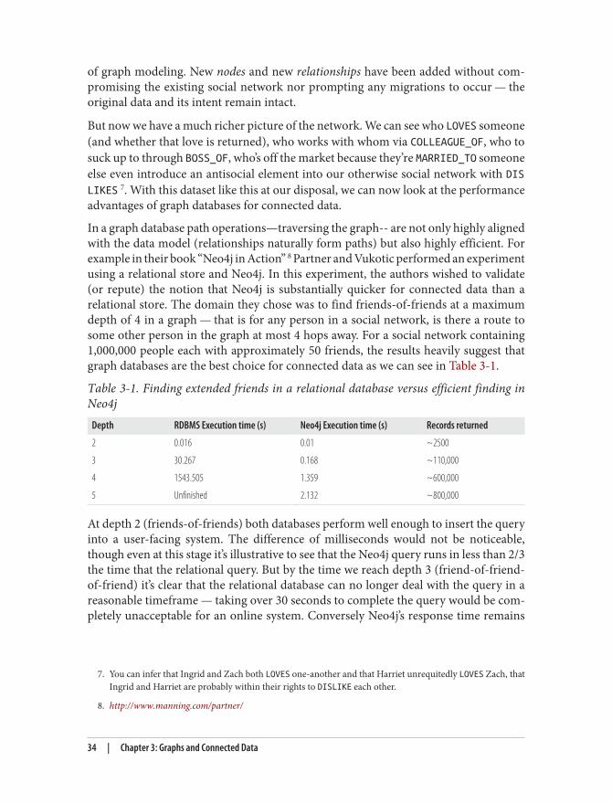
In a graph database path operations—traversing the graph-- are not only highly alignedwith the data model (relationships naturally form paths) but also highly efficient. Forexample in their book “Neo4j in Action” 8 Partner and Vukotic performed an experimentusing a relational store and Neo4j. In this experiment, the authors wished to validate(or repute) the notion that Neo4j is substantially quicker for connected data than arelational store. The domain they chose was to find friends-of-friends at a maximumdepth of 4 in a graph — that is for any person in a social network, is there a route tosome other person in the graph at most 4 hops away. For a social network containing1,000,000 people each with approximately 50 friends, the results heavily suggest thatgraph databases are the best choice for connected data as we can see in Table 3-1.

Table 3-1. Finding extended friends in a relational database versus efficient finding inNeo4j

Depth RDBMS Execution time (s) Neo4j Execution time (s) Records returned

2 0.016 0.01 ~2500

3 30.267 0.168 ~110,000

4 1543.505 1.359 ~600,000

5 Unfinished 2.132 ~800,000

At depth 2 (friends-of-friends) both databases perform well enough to insert the queryinto a user-facing system. The difference of milliseconds would not be noticeable,though even at this stage it’s illustrative to see that the Neo4j query runs in less than 2/3the time that the relational query. But by the time we reach depth 3 (friend-of-friend-of-friend) it’s clear that the relational database can no longer deal with the query in areasonable timeframe — taking over 30 seconds to complete the query would be com‐pletely unacceptable for an online system. Conversely Neo4j’s response time remains


http://www.manning.com/partner/

relatively flat, just a fraction of a second to perform the query and definitely quicklyenough for an online system.

At depth 4 the relational database exhibits terrible latency for an online system, to theextent where it’s practically useless. Neo4j timing’s are a marginally less good too, but isstill at the periphery of being acceptable for a responsive online system. Finally at depth5 the relational database simply takes too long to complete the query while Neo4j re‐mains relatively modest at around 2 seconds, and yet this timing can be highly trimmedshould we (sensibly) choose to return only a handful of the many thousands of possibledistant friends .

Aggregate and relational stores both perform poorly for connected dataBoth aggregate stores and relational databases perform poorly we moveaway from modestly sized set operations — operations that both kindsof databases should be good at. When we try to mine path informationout of the graph like the classic finding of friends and friends-of-friendsthat we’re all used to from social media platforms and applicationsthings demonstrably slow down. We don’t mean to unduly beat up oneither aggregate stores or relational databases, they have a fine tech‐nology pedigree for the things they’re good at but for managing con‐nected data they fall short as we’ve discussed. Anything more than ashallow traversal of immediate friends or possibly friend-of-friend willbe slow because of the number of index lookups involved. Graphs onthe other hand offer index-free adjacency so that traversing connecteddata is extremely rapid.

Friends and social networks are all well and good, but at this point you might reasonablywonder whether finding such remote friends is a valid use-case. After all, it’s rare thatwe’d be so desperate for company that we’d traverse so far out of the core of our socialnetwork. The point is that we can substitute social networks for any other domain andexperience similar performance, modeling and maintenance benefits. Whether thosedomains are music or data center management, bio-informatics or football statistics,network sensors or time-series of trades, graphs are a powerful source of insight. So let’savail ourselves of the power of graphs for connected data with a contemporary example:social recommendation of products not only based on a user’s purchase history but onthe histories of their friends, neighbours and other people like them, bringing together


several independent facets of the user’s lifestyle to make more accurate and more prof‐itable recommendations.

Productive analysisOne of the most appealing aspects of the graph data model is its intuitiveness. Peoplewithout any background in data modeling — which is to say, relational modeling —easily grasp the graph approach. The typical “whiteboard” or “back of the napkin” rep‐resentation of a data problem is a graph. More often than not such representations canbe directly translated into a graph data model. One of the most important contributionsof graphs to informatics is how they make data modeling and data interrelationshipsavailable to the layperson.

Let’s start off by modeling the classic purchase history of a user as connected data. In agraph, this can be as simple as linking between the user and their orders, and insertinglinks between orders to provide a purchase history as we see in Figure 3-6.

Figure 3-6. Modeling a user’s order history in a graph


9. There’s no need for a reciprocal NEXT relationship unless we’d we want to. Traversing the PREVIOUS relation‐ship from head to tail provides the same affordance.

10. http://en.wikipedia.org/wiki/R-tree

11. The various terms associated with the geography and nationhood in the British Isles is intricate, but this willhelp the unitiated: http://www.visualnews.com/2011/02/03/the-difference-between-great-britain-england-the-united-kingdom-and-a-whole-lot-more/

The kind of graph shown in Figure 3-6 provides a great deal of insight into customerbehavior. We can see all the orders that the user PLACED and we can easily reason aboutwhat each order CONTAINS. So far so good, but we can take the opportunity to enrichthis graph to support well-known access patterns. For example, users often want to seetheir order history, so we’ve added a linked list structure into the graph such that theuser’s most recent order is found by following the outgoing MOST_RECENT relationship,and we can iterate through the lsat going further back in time by following the PREVIOUS relationships 9.

Having even this simple data allows us to start to make recommendations. If we noticethat users who buy strawberry ice cream, also buy espresso beans then we can start torecommend those beans to users who normally only buy the ice cream. But this is arather one-dimensional recommendation even if we traverse lots of orders to ensurethere’s a strong correlation between strawberry ice cream and espresso beans. We cando much better, and the way we do that is to intersect the purchasing graph with graphsfrom other domains. Since graphs are naturally multi-dimensional structures, it’s quitestraightforward to ask a much more sophisticated question of the data to gain access toa fine-tuned market segment. For example to ask “all of the flavors of ice cream thatpeople living near a user like who also enjoy espresso but dislike Brussels sprouts.”

From our point of view, enjoying and disliking items could be easily considered iso‐morphic to having ordered those items repeatedly or infrequently (perhaps once only).How would we define “living near?” Well it turns out that, perhaps unsurprisingly,geospatial coordinates are easily graphed. The most likely implementation of this is tocreate an R-Tree 10 to represent bounded boxes around geographies. Using such a struc‐ture it’s natural to describe overlapping hierarchies of locations. For example, we canexpress that London is in the UK, but we can also express that the postal code SW111BD is in Battersea which is a district in London (which is in south-eastern England,which in turn is in Great Britain 11). And since UK postal codes are fine-grained, we canuse that boundary to target people with somewhat similar tastes.


http://en.wikipedia.org/wiki/R-tree

http://www.visualnews.com/2011/02/03/the-difference-between-great-britain-england-the-united-kingdom-and-a-whole-lot-more/

http://www.visualnews.com/2011/02/03/the-difference-between-great-britain-england-the-united-kingdom-and-a-whole-lot-more/

12. http://docs.neo4j.org/chunked/milestone/cypher-query-lang.html

Such pattern matching queries are extremely difficult to write in SQL,and laborious to write against aggregate stores, and tend to performvery poorly. Graph databases on the other hand are optimized forprecisely these types of traversal and pattern matching queries whichbe written very easily using a query language (such as Cypher 12inNeo4j), and can be expected to perform very well (milliseconds re‐sponse time).

This graph isn’t only useful for recommendations on the buyer’s side, it’s also usefuloperationally for the seller. For example, given certain buying patterns (products, costof typical order, etc) we can establish whether a particular transaction might constitutefraud. Patterns outside of the norm for a given user can easily be detected in a graphand be flagged for further attention (using well-known similarity measures from thegraph data-mining literature), thus reducing the risk for the seller.

From the data practitioner’s point of view, it’s clear that the graph database’s sweet spotlies in handling data sets that are so sophisticated that they are unwieldy when treatedin any other form than as a graph. We therefore define the term connected data todescribe data that is best handled as a graph.

Schema-Free Development and Pain-Free MigrationsNotwithstanding the fact that just about anything can be modeled as a graph, we live ina pragmatic world, and novel, powerful data modeling techniques do not in themselvesprovide sufficient justification for replacing standard, well-known platforms. Theremust also be an immediate and very significant practical benefit. In the case of graphdatabases as we’ve seen, this motivation exists in the form of a set of use cases and datapatterns whose performance improves by one or more orders of magnitude when im‐plemented in a graph, and whose latency is much lower compared to batch processingaggregates. However when we factor in the increase in performance with the benefitsof agility, schemaless flexibility, and ease of development, the case for graph databasescan readily be made.

Developers today want to connect data as the domain dictates, thereby allowing struc‐ture and schema to emerge rather than having to pre-define it upfront. Moreover, theywant to be able to evolve their model in step with the rest of their application, using atechnology aligned with the incremental and iterative software delivery practices thathave come to the fore in recent years. The graph database data model provides theflexibility necessary to help IT move at the speed of business, while today’s graph database


http://docs.neo4j.org/chunked/milestone/cypher-query-lang.html

technologies provide the APIs and query languages necessary for widespread adoptionby mainstream programmers.

This has generally positive implications for developer productivity and project risk. Forinstance, we don’t need to model exhaustively ahead of time — a practice which is allbut foolhardy in the face of changing business requirements since the graph model isnaturally additive. As new facts come to light we design the graph structures for themand pour in the new data in with the existing. Such an additive mindset tends to meanthat we don’t migrate graphs often either, we migrate much less often, in fact only whenwe’re performing breaking changes on existing structures.

There are implications, of course, for development and maintenance of applicationssince graph users cannot rely on the (rotten) crutch of a relational schema to try to fixsome level of governance into the database—often much to the confusion of traditionaldata and application architects. Instead that governance is typically applied in the ap‐plications themselves through tests which assert the business rules (and by implicationthe way data is stored and queried) are valid over time. This isn’t something to get excitedabout, that tests drive out the behavior of a system is uncontroversial in the 21st centuryand that tests providing ongoing governance (particularly around regressions) is alsorecognized as beneficial by the developer community at large.

Connecting the DotsIn this chapter we’ve highlighted the fact that data is most useful when it’s connected.We’ve seen how other kinds of data stores leave connectedness as an exercise in dataprocessing to the developer, and contrasted that with graph databases where connect‐edness is first-class citizen. Finally we’ve show how the expressive and flexible natureof graphs makes them ideal for high-fidelity domain analysis, frictionless developmentand graceful system maintenance

Connecting the Dots | 39

CHAPTER 4

Working with Graph Data

In previous chapters we’ve described the substantial benefits of the graph database whencompared both with document, columnar and key-value NOSQL stores and with tra‐ditional relational databases. But having chosen to adopt a graph database, the questionarises: how do we model the world in graph terms?

In this chapter we’ll look at graph modeling. We’ll focus in particular on the expres‐siveness of the graph model and the ease with which it can be queried. Because graphsare extremely flexible, lending themselves to many different domain representations,there’s often no absolute right or wrong way to model with graphs, just some layoutsthat work better than others for a given problem. We’ll highlight these good practiceswhile also covering some classic pitfalls of graph modeling for the unwary.

Models and GoalsBefore we dig deeper into modeling with graphs, a word on models in general. Modelingis an abstracting activity motivated by a particular need or goal. We model in order tobring specific facets of an unruly domain into a space where they can be structured andmanipulated. There are no natural representations of the world the way it “really is,” justmany purposeful selections, abstractions and simplifications, some of which are moreuseful than others for a satisfying a particular goal.

Graph representations are no different in this respect. What perhaps differentiates themfrom many other data modeling techniques, however, is the close affinity between thelogical and physical graph models. Relational data management techniques require usto deviate from our natural language representation of the domain: first by cajoling ourrepresentation into a logical model; and then by forcing it into a physical model. Thesetransformations introduce semantic dissonance between our conceptualisation of theworld and the database’s instantiation of that model. With graph databases this gapshrinks considerably.

41

Graph modeling naturally fits with the way we tend to abstract the salient details froma domain using circles and boxes, and then describe the connections between thesethings by joining them with lines. Today’s graph databases, more than any other databasetechnologies, are “whiteboard friendly.” The typical whiteboard view of a problem is agraph. What we sketch in our creative and analytical modes maps closely to data modelwe implement inside the database. In terms of expressivity, graph databases reduce theimpedance mismatch between analysis and implementation that has plagued relationaldatabase implementations for many years. What is particularly interesting about suchgraph models is the fact that they not only communicate how we think things are related,they also clearly communicate the kinds of questions we want to ask of our domain. Aswe’ll see throughout this chapter, graph models and graph queries are really just twosides of the same coin.

Relational Modeling in a Systems Management DomainThis book is primarily concerned with graphs, graph databases, graph modeling andgraph queries. To introduce graph modeling, however, it’s useful to compare how wework with graphs versus how we work in relational world, since RDBMS systems andtheir associated data modeling techniques are familiar to most developers and dataprofessionals.

To help compare graph and relational modeling techniques, we’ll examine a simple data-center management domain. In this domain, data centers support many applicationson behalf of many customers using a whole plethora of infrastructure, from virtualmachines to physical load balancers. A micro-level view of this domain is shown inFigure 4-1.

42 | Chapter 4: Working with Graph Data

Figure 4-1. Simplified snapshot of application deployment within a data center

In Figure 4-1 we see a somewhat simplified view of several applications and the datacenter infrastructure necessary to support them. The applications, represented by nodesApp 1, App 2 and App 3, depend on a cluster of databases labelled Database Server1, 2, 3. While users logically depend on the availability of an application and its data,there is additional physical infrastructure between the users and the application; thisinfrastructure includes virtual machines (Virtual Machine 10, 11, 20, 30, 31), realservers (Server 1, 2, 3), racks for the servers (Rack 1, 2 ), and load balancers (LoadBalancer 1, 2), which front the apps. In between each of the components there are ofcourse many networking elements: cables, switches, patch panels, NICs, power supplies,air conditioning and so on—all of which can fail at inconvenient times. To complete thepicture we have a straw-man single user of application 3, represented by User 3.

As the operators of such a system, we have two primary concerns:

• Ongoing provision of functionality to meet (or exceed) a service-level agreement,including the ability to perform forward-looking analyses to determine single

Relational Modeling in a Systems Management Domain | 43

1. Such approaches aren’t always necessary: adept relational users often move directly to table design and nor‐malization without first describing an intermediate E-R diagram.

points of failure, and retrospective analyses to rapidly determine the cause of anycustomer complaints regarding the availability of service;

• Billing for resources consumed, including the cost of hardware, virtualisation, net‐work provision and even the costs of software development and operations (sincethese are a simply logical extension of the system we see here).

If we are building a data center management solution, we’ll want to ensure that theunderlying data model allows us to store and query data in a way that efficiently ad‐dresses these primary concerns. We’ll also want to be able to update the underlyingmodel as the application portfolio changes, as the physical layout of the data centreevolves or as virtual machine instances migrate. Given these needs and constraints, let’ssee how the relational and graph models compare.

Modeling for relational dataThe initial stage of modeling in the relational world is similar to the first stage of manyother data modeling techniques: that is, we seek to understand and agree on the entitiesin the domain, how they interrelate and the rules that govern their state transitions.Most of this tends to be done informally, often through whiteboard sketches and dis‐cussions between subject matter experts and system and data architects, until the par‐ticipants reach some kind of agreement—expressed perhaps in the form of a diagramsuch as the one in Figure 4-1.

The next stage captures that agreement in a more rigorous form such as an entity-relationship diagram. This transformation of the model using a more strict notationprovides us with a second chance to refine a common domain vocabulary that can beshared with relational database specialists 1. In our example, we’ve captured the domainin the E-R diagram Figure 4-2.

Ironically E-R diagrams immediately demonstrate the shortcomingsof the relational model for capturing a rich domain. Although E-Rdiagrams allow relationships to be named (something which rela‐tional stores disallow, and which graph databases fully embrace) theyonly allow single, undirected named relationships between entities. Inthis respect, the relational model is a poor fit for real-world domainswhere relationships between entities are both numerous and seman‐tically rich and diverse.


Figure 4-2. An Entity-Relationship diagram for the data center domain

Once we have arrived at a suitable logical model, we map it into tables and relations,which are then normalized to ensure high fidelity and zero data redundancy. In manycases this step can be as simple as transcribing the E-R diagram into a tabular form andthen loading those tables via SQL commands into the database. But even the simplestcase serves to highlight the idiosyncrasies of the relational model. For example, inFigure 4-3 we see that a great deal of accidental complexity creeps into the model in theform of foreign key constraints (everything annotated [FK]), which support one-to-many relationships, and join tables (e.g. AppDatabase), which support many-to-manyrelationships—and all this before we’ve added a single row of real user data. Theseconstraints are model-level metadata that exist simply so that we can reify relationsbetween tables at query time. Yet the presence of this structural data is keenly felt, forit clutters and obscures the domain data with data that serves the database, not the user.

Modeling for relational data | 45

Figure 4-3. Tables and relationships for the data center domain

We have now arrived at a high fidelity, normalized model that is relatively faithful tothe domain. This model, though imbued with substantial accidental complexity, con‐tains no duplicate data. But our design work is not yet complete. One of the challengesof the relational paradigm is that normalized models generally aren’t fast enough forreal-world needs. For many production systems, a normalized schema, which in theoryis fit for answering any kind of ad hoc question we may wish to pose the domain, mustin practice be further adapted and specialised for specific access patterns. In other words,to make relational stores perform well enough for regular application needs, we haveto abandon any vestiges of true domain affinity and accept that we have to change theuser’s data model to suit the database engine not the user. This technique is given thename denormalization.

Denormalization involves duplicating data (substantially in some cases) in order to gainquery performance. Take as an example users and their contact details. A typical useroften has several email addresses, which, in a fully normalised model, we would storein a separate ‘EMAIL` table. To reduce joins and the performance penalty imposed byjoining between two tables, however, it is quite common to inline this data in the USERtable, adding one or more columns to store users’ most important email addresses.

While denormalization may be a safe thing to do (assuming developers understand thedenormalized model and how it maps to their typically domain-centric code, and haverobust transactional support from the database), it is usually not a trivial task. For thebest results, we usually turn to a true RDBMS expert to munge our normalized modelinto a denormalized one that is aligned with the characteristics of the underlyingRDBMS and physical storage tier. In doing this, we accept that there may be substantialdata redundancy.

We might be tempted to think that all this design-normalize-denormalize effort is ac‐ceptable because it is a one-off task. This school of thought suggests that the cost of the


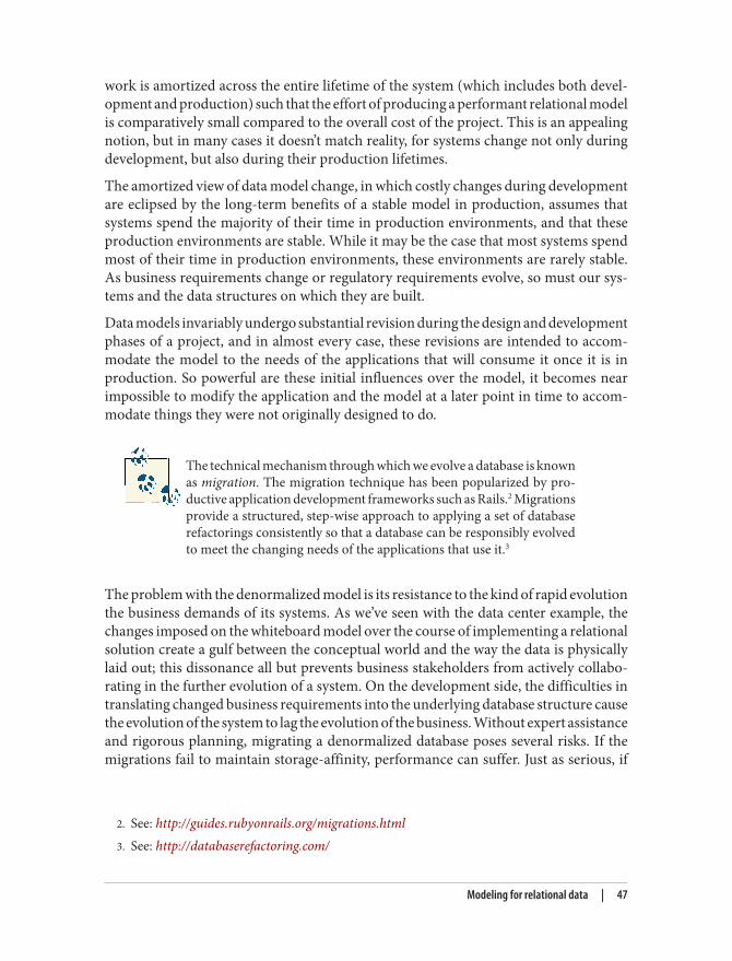
2. See: http://guides.rubyonrails.org/migrations.html3. See: http://databaserefactoring.com/

work is amortized across the entire lifetime of the system (which includes both devel‐opment and production) such that the effort of producing a performant relational modelis comparatively small compared to the overall cost of the project. This is an appealingnotion, but in many cases it doesn’t match reality, for systems change not only duringdevelopment, but also during their production lifetimes.

The amortized view of data model change, in which costly changes during developmentare eclipsed by the long-term benefits of a stable model in production, assumes thatsystems spend the majority of their time in production environments, and that theseproduction environments are stable. While it may be the case that most systems spendmost of their time in production environments, these environments are rarely stable.As business requirements change or regulatory requirements evolve, so must our sys‐tems and the data structures on which they are built.

Data models invariably undergo substantial revision during the design and developmentphases of a project, and in almost every case, these revisions are intended to accom‐modate the model to the needs of the applications that will consume it once it is inproduction. So powerful are these initial influences over the model, it becomes nearimpossible to modify the application and the model at a later point in time to accom‐modate things they were not originally designed to do.

The technical mechanism through which we evolve a database is knownas migration. The migration technique has been popularized by pro‐ductive application development frameworks such as Rails.2 Migrationsprovide a structured, step-wise approach to applying a set of databaserefactorings consistently so that a database can be responsibly evolvedto meet the changing needs of the applications that use it.3

The problem with the denormalized model is its resistance to the kind of rapid evolutionthe business demands of its systems. As we’ve seen with the data center example, thechanges imposed on the whiteboard model over the course of implementing a relationalsolution create a gulf between the conceptual world and the way the data is physicallylaid out; this dissonance all but prevents business stakeholders from actively collabo‐rating in the further evolution of a system. On the development side, the difficulties intranslating changed business requirements into the underlying database structure causethe evolution of the system to lag the evolution of the business. Without expert assistanceand rigorous planning, migrating a denormalized database poses several risks. If themigrations fail to maintain storage-affinity, performance can suffer. Just as serious, if

Modeling for relational data | 47

http://guides.rubyonrails.org/migrations.html

http://databaserefactoring.com/

deliberately duplicated data is left orphaned after a migration, we risk compromisingthe integrity of the data as a whole.

Relational databases—with their rigid schemas and complex modeling characteristics—are not an especially good tool for supporting rapid change. To face up to these chal‐lenges we need a model that is closely aligned with the domain without sacrificingperformance, that supports evolution while providing enough structural affordances toguide the designer, and that maintains the integrity of the data as it undergoes rapidchange and growth. To that end, it’s time for us to get to grips with property graphs andgraph modeling.

The Property Graph ModelThe rise of graph databases like Neo4j helps bridge the divide between businesses andtheir data. In terms of domain affinity, Euler’s graph theory (from the first half of theeighteenth century) is an early example of structured business analysis, whereby a real-world problem (the Seven Bridges of Königsberg) is purposely abstracted to a datamodel that can generate useful insight. What graph databases provide is a platform forstoring and querying that data to generate insight on-demand.

While there are numerous kinds of graphs, Neo4j, like several other notable graph da‐tabases, has settled on the property graph as its graph model. The property graph bal‐ances simplicity and expressiveness. (The next most-popular alternative, the triple store,popularized by RDF, is theoretically elegant but generally considered less practicable,in large part because in a triple store everything is decomposed into individual nodesand relationships.) Property graphs sacrifice some graph purity for pragmatism bygrouping properties into nodes, thereby making them easier to work with. The mainabstractions in a property graph are nodes, relationships and properties.

• Nodes are placeholders for properties. Think of nodes as documents that storeproperties in the form of arbitrary key-value pairs. The keys are strings and thevalues can be arbitrary data types.

• Relationships connect nodes. Relationships in Neo4j are always connected anddirected (that is, they always have a start node and an end node). In addition, everyrelationship has a label. A relationship’s label and its direction add semantic clarityto the connections between nodes. Like nodes, relationships can also house prop‐erties. The ability to add properties to relationships is particularly useful for pro‐viding additional metadata for graph algorithms, and for constraining queries atrun time.

These simple primitives are all we need to create some sophisticated and semanticallyrich models. For example, in Figure 4-4 we have high-quality information about Shake‐speare and some of his plays, together with details of one of the companies that has


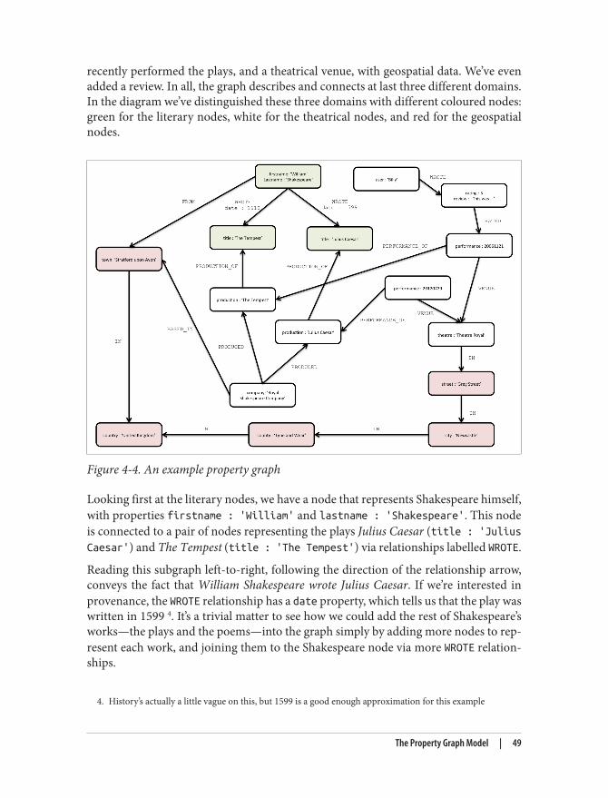
4. History’s actually a little vague on this, but 1599 is a good enough approximation for this example

recently performed the plays, and a theatrical venue, with geospatial data. We’ve evenadded a review. In all, the graph describes and connects at last three different domains.In the diagram we’ve distinguished these three domains with different coloured nodes:green for the literary nodes, white for the theatrical nodes, and red for the geospatialnodes.

Figure 4-4. An example property graph

Looking first at the literary nodes, we have a node that represents Shakespeare himself,with properties firstname : 'William' and lastname : 'Shakespeare'. This nodeis connected to a pair of nodes representing the plays Julius Caesar (title : 'JuliusCaesar') and The Tempest (title : 'The Tempest') via relationships labelled WROTE.

Reading this subgraph left-to-right, following the direction of the relationship arrow,conveys the fact that William Shakespeare wrote Julius Caesar. If we’re interested inprovenance, the WROTE relationship has a date property, which tells us that the play waswritten in 1599 4. It’s a trivial matter to see how we could add the rest of Shakespeare’sworks—the plays and the poems—into the graph simply by adding more nodes to rep‐resent each work, and joining them to the Shakespeare node via more WROTE relation‐ships.

The Property Graph Model | 49

5. Part of the RSC’s summer season which they traditionally spend touring

By traversing the WROTE relationship—even by tracing that arrow withour finger—we’re effectively doing the kind of work that a graph data‐base performs, albeit at human latency rather than at microsecond-level. As we’ll see later, this simple traversal primitive is the buildingblock for arbitrarily sophisticated graph queries.

Turning next to the theatrical nodes, you can see that we’ve added some informationabout the Royal Shakespeare Company (often known simply as the RSC) in the form ofa node with the key company and value Royal Shakespeare Company. The theatricaldomain is, unsurprisingly, connected to the literary domain: in our graph, this is re‐flected by the fact that the RSC has PRODUCED versions of Julius Caesar and The Tem‐pest. The graph also captures details of specific performances: the RSC’s production ofJulius Caesar, for example, was performed on the 29 July 2012. 5 If we’re interested inthe performance venue, we simply follow the outgoing VENUE relationship from theperformance node to find that the play was performed at the Theatre Royal.

The graph also allows us to capture reviews of specific performances. In our samplegraph we’ve included just one review, for the 29 July performance, written by the userBilly. We can see this in the top right of Figure 4-4 with the interplay of the performance,rating and user nodes. In this case we have a node representing Billy (user :

'Billy') whose outgoing WROTE relationship connects to a node representing his review.The review node contains a numeric rating property and a free-text review property.The review is linked to a specific performance through an outgoing RATED relationship.To scale this up to many users, many reviews and many performances we simply addmore nodes and more identically-named relationships to the graph.

The third domain, that of geospatial data, comprises a simple hierarchical tree of places.This geospatial domain is connected to the other two domains at several points in thegraph. The town of Stratford upon Avon (with property town : 'Stratford uponAvon') is connected to the literary domain as a result of its being Shakespeare’s birthplace(Shakespeare is FROM Stratford). It is connected to the theatrical domain insofar as it ishome for the RSC (the RSC is BASED_IN Stratford). To learn more about Stratford uponAvon’s geography, we can follow its outgoing IN relationship to discover it is in theUnited Kingdom.

The property graph makes it possible to capture more complex geospatial data. Lookingat the Theatre Royal, for example, we see that it is located in Grey Street, which is INthe city of Newcastle, which is IN the county of Tyne and Wear, which ultimately is INthe United Kingdom—just like Stratford upon Avon.


6. This section is not intended to be a reference document for Cypher, merely a friendly introduction to enableus to explore more interesting graph query scenarios. For reference documentation see: http://docs.neo4j.org/chunked/milestone/cypher-query-lang.html

7. http://www.w3.org/TR/rdf-sparql-query/

As you can see from this relatively simple example, property graphs make it easy to unitedifferent domains—each with its own particular entities, properties and relationships—in a way that not only makes each domain accessible, but also generates insight fromthe connections between domains.

Unlike document, column, or key-value stores, graph databases don’trequire us to infer connections between documents using contrivedproperties such as foreign keys, or out-of-band processing like map-reduce. Instead, relationships are a first-class citizen in the data model.By assembling the simple abstractions of nodes and relationships intoconnected structures, graph databases allow us to build arbitrarily so‐phisticated models with high domain affinity. Modeling is simpler andat the same time more expressive than what we experience with bothtraditional relational database and the other NOSQL stores.

Diagrams are good for communicating the fundamentals of the property graph model,but when it comes to using a database, we need to create, manipulate and query data.Having familiarised ourselves with the property graph model, it’s now time to look atquery languages.

The Cypher Query LanguageModeling expressivity is only one of the reasons graph databases appeal to the needs oftoday’s IT professionals. The graph model really shines when the interpretation of thedomain requires an understanding of how, or in what way, or to what degree entitiesare related or connected to one another. That is, graph databases address the increasingneed to not only store but also to query connected data. In Neo4j the humane andexpressive query language Cypher is the primary means of accessing the database. Bothin this chapter and throughout this book we’ll use Cypher extensively to illustrate graphqueries and graph constructions and so at this point it’s worthwhile taking a brief detourto learn the basics 6 of the language.

Other query languagesOther graph databases have other means of querying data. Most, including Neo4j, sup‐port the RDF query language SPARQL 7 and the imperative, path-based query language

The Cypher Query Language | 51



http://www.w3.org/TR/rdf-sparql-query/

8. https://github.com/tinkerpop/gremlin/wiki/

Gremlin. 8 Our interest, however, is in the expressive power of the declarative model,and so in this book we’ll focus almost exclusively on Cypher.

Cypher PhilosophyCypher is a humane query language for developers and database operations professio‐nals alike. By humane we mean a language that is aligned with how we intuitively de‐scribe graphs—which, as we’ve already seen, is often through a diagram. The interestingthing about graph diagrams is that they tend to contain specific instances of nodes andrelationships, rather than classes or archetypes. Even very large graphs are illustratedusing smaller subgraphs made from real nodes and relationships. In other words, wedescribe graphs using specification by example.

Cypher enables a user (or an application acting on behalf of a user) to ask the databaseto find data that matches a pattern. Colloquially, we say that we ask the database to “findthings like this"--and the way we specify the things we want the database to find is todraw a picture of them, in ASCII art. We have to employ a few tricks to get around thefact that a query language has only one dimension (text proceeding from left to right),whereas a graph diagram can be laid out in two dimensions, but on the whole, Cypherpatterns follow very naturally from the way we draw graphs on the whiteboard.

Like most query languages, Cypher is composed of clauses. A reasonably simple queryis made up of START, MATCH and RETURN clauses (we’ll describe the other clauses you canuse in a Cypher query later in this chapter):

• START: Specifies one or more starting points in the graph. These starting points areobtained via index lookups or, more rarely, accessed directly based on element IDs.

• MATCH: This is the specification by example part. Using ASCII characters to representnodes and relationships (round brackets for nodes, dashes, and greater-than andless-than signs for relationships), we draw the data we’re interested in.

• RETURN: Specifies which nodes, relationships and properties in the matched datashould be returned to the client.

Here’s an example of a Cypher query that uses these three clauses to find the plays writtenby Shakespeare:

START bard=node:authors('firstname:"William" AND lastname:"Shakespeare"')MATCH (bard)-[:WROTE]->(plays)RETURN plays


https://github.com/tinkerpop/gremlin/wiki/

At the heart of this query is the simple pattern (bard)-[:WROTE]->(plays). This patterndescribes two nodes, one of which we’ve bound to an identifier bard, the other to anidentifier plays. These nodes are connected by way of a WROTE relationship, which ex‐tends from bard to plays. The dashes and greater-than sign that surround the rela‐tionship name (-->) indicate relationship direction. The rounded brackets help furtherdiscriminate the node identifiers.

Now this pattern could, in theory, occur many times throughout our graph data. Tolocalise the query, we need to anchor some part it to one or more places in the graph.What we’ve done with the START clause is lookup a real node in the graph—the noderepresenting Shakespeare. We bind this Shakespeare node to the bard identifier, whichthen carries over to the MATCH clause. This has the effect of anchoring our pattern to aspecific point in the graph. Cypher can then rotate the pattern around this anchor pointto discover actual nodes to bind to the plays identifier. While bard will always be anch‐ored to the one real Shakespeare node in our graph, plays will (in our sample data) bebound to a list of nodes representing the plays Julius Caesar and The Tempest. Thesenodes are returned to the client in the RETURN clause.

The other clauses we can use in a Cypher query include:

• WHERE: Provides criteria for filtering portions of a pattern.• CREATE and CREATE UNIQUE: Creates nodes and relationships.• DELETE: Removes nodes, relationships and properties.• SET: Set property values.• FOREACH: Performs an updating action for each element in a list.• WITH: Divides a query into multiple, distinct parts.

If these clauses look familiar—especially if you’re a SQL developer—that’s great! Cypherisn’t intended to cause headaches when it’s written or read; it’s intended to be familiarenough to help you rapidly along the learning curve. At the same time, it’s differentenough to emphasize that we’re dealing with graphs not sets. With that in mind, let’slook in more detail at the kind of Cypher queries we can write for the graph in Figure 4-4.

Creating GraphsTo create the Figure 4-4 graph, we use a number of CREATE statements to build the overallstructure. These statements are executed by the Cypher runtime within a single trans‐action such that once the statements have executed, we can be confident the graph is


9. Normally it’s applications that issue database commands: humans don’t normally have to see so many CREATE statements!

present in the database (or not at all, should the transaction fail). As we might expect,Cypher has a humane and visual way of building graphs: 9

CREATE shakespeare = { firstname : 'William', lastname : 'Shakespeare' }, juliusCaesar = { title : 'Julias Caesar' }, (shakespeare)-[:WROTE { date : 1599 }]->(juliusCaesar), theTempest = { title : 'The Tempest' }, (shakespeare)-[:WROTE { date : 1610}]->(theTempest), rsc = { company : 'Royal Shakespeare Company' }, production1 = { production : 'Julius Caesar' }, (rsc)-[:PRODUCED]->(production1), (production1)-[:PRODUCTION_OF]->(juliusCaesar), performance1 = { performance : 20120729 }, (performance1)-[:PERFORMANCE_OF]->(production1), production2 = { production : 'The Tempest' }, (rsc)-[:PRODUCED]->(production2), (production2)-[:PRODUCTION_OF]->(theTempest), performance2 = { performance : 20061121 }, (performance2)-[:PERFORMANCE_OF]->(production2), performance3 = { performance : 20120730 }, (performance3)-[:PERFORMANCE_OF]->(production1), billy = { user : 'Billy' }, rating = { rating: 5, review : 'This was awesome!' }, (billy)-[:WROTE]->(rating), (rating)-[:RATED]->(performance1), theatreRoyal = { theatre : 'Theatre Royal' }, (performance1)-[:VENUE]->(theatreRoyal), (performance2)-[:VENUE]->(theatreRoyal), greyStreet = { street : 'Grey Street' }, (theatreRoyal)-[:IN]->(greyStreet), newcastle = { city : 'Newcastle' }, (greyStreet)-[:IN]->(newcastle), tyneAndWear = { county: 'Tyne and Wear' }, (newcastle)-[:IN]->(tyneAndWear), uk = { country: 'United Kingdom' }, (tyneAndWear)-[:IN]->(uk), stratford = { town : 'Stratford upon Avon' }, (stratford)-[:IN]->(uk), (rsc)-[:BASED_IN]->(stratford)

In the Cypher code above, we’re doing two different things: creating nodes and theirproperties, and relating nodes (with relationship properties where necessary). For ex‐ample CREATE shakespeare = { firstname : 'William', lastname : 'Shakespeare' } creates a node representing William Shakespeare. The newly created nodeis assigned to the identifier shakespeare, which remains available for the duration of


10. The identifiers we introduce are only available within the current scope. Should we wish to give long-livednames to nodes (or relationships) then we simply add them to an index.

the current scope 10. This shakespeare identifier is used later in the code to attachrelationships to the underlying node. For example, the clause CREATE (shakespeare)-[:WROTE { date : 1599 }]->(juliusCaesar)" creates a WROTE relationship fromShakespeare to the play Julius Caesar. With enough of these, we can build some veryinteresting and expressive graphs.

Unlike the relational model, these commands don’t introduce any ac‐cidental complexity into the graph. The information meta-model—that is, the structuring of nodes through relationships—is kept sepa‐rate from the business data, which lives exclusively as properties. Weno longer have to worry about foreign key and cardinality constraintspolluting our real data, since both are explicit in the graph model asthe nodes and the semantically rich relationships that interconnectthem.

We can modify the graph at a later point in time in two different ways. We can, of course,continue using the CREATE clause to simply add to the graph. But we can also use CREATEUNIQUE, which has the semantics of ensuring a particular sub-graph structure—some ofwhich may already exist, some of which may be missing—is in place once the commandhas executed. In practice, we tend to use CREATE when we’re adding to the graph anddon’t mind duplication, and CREATE UNIQUE when duplication is not permitted by thedomain.

Beginning a QueryNow that we have a graph, we can start to query it. In Cypher we always begin ourqueries from one or more well-known starting points in the graph—what are calledbound nodes. (We can also start a query by binding to one or more relationships, butthis happens far less frequently than binding to nodes.). This is the purpose of the STARTclause: to give us some starting points, usually drawn from underlying indexes, fromwhich we can explore the remainder of the graph.

For instance, if we wanted to discover more about the performances at the TheatreRoyal, we would use that as our starting point. However, if we were more interested inthe works of reviewers or the county of Tyne and Wear, we’d use those nodes to startinstead. Since we want to know about all things Shakespeare that have taken place inthe Theatre Royal in Newcastle, we’ll start our query with these three nodes.

START theater=node:venues(theatre = 'Theatre Royal'), newcastle=node:cities(city = 'Newcastle'), bard=node:authors('firstname:"William" AND lastname:"Shakespeare"')


11. This is in fact Lucene query syntax. Lucene is Neo4j’s default index provider.

This START clause identifies all nodes that have a property key venue and property valueTheatre Royal in a node index called venues. The results of this index lookup are boundto the identifier theater. (What if there are many Theatre Royal nodes in this index?We’ll deal with that shortly.) In a second index lookup, we find the node representingthe city of Newcastle; we bind this node to the identifier newcastle.

To find the Shakespeare node itself, we use a more sophisticated query syntax: we declarethat we want to retrieve the node that has properties firstname:William and lastname:Shakespeare 11. We bind the result of this lookup to bard.

From now on in our query, wherever we use the identifiers theater, newcastle andbard in a pattern, that pattern will be anchored to the real nodes associated with theseidentifiers. In effect, the START clause localises the query, giving us starting points fromwhich to match patterns in the surrounding nodes and relationships.

Declaring information patterns to findThe MATCH clause in Cypher is where the magic happens. Much as the CREATE clausetries to convey intent using ASCII art to describe the desired state of the graph, so theMATCH clause uses the same syntax to describe patterns to discover in the database. We’vealready looked at a very simple MATCH clause; now we’ll look at a more complex patternthat finds all the Shakespeare performances at Newcastle’s Theatre Royal:

MATCH (newcastle)<-[:IN*1..4]-(theater)<-[:VENUE]-()-[p:PERFORMANCE_OF]->()-[:PRODUCTION_OF]->(play)<-[w:WROTE]-(bard)

This MATCH pattern uses several syntactic elements we’ve not yet come across. As wellas including bound nodes based on index lookups (discussed above), it uses patternnodes, arbitrary depth paths, and anonymous nodes. Let’s take a look at these in turn:

• The identifiers newcastle, theater and bard carry over from the START clause,where they were bound to nodes in the graph using index lookups, as describedabove.

• If there are several Theatre Royals in our database (the cities of Plymouth, Bath,Winchester and Norwich all have a Theatre Royal, for example), then theater willbe bound to all these nodes. To restrict our pattern to the Theatre Royal in New‐castle, we use the syntax <-[:IN*1..4]-, which means the theater node can be nomore than four outgoing IN relationships away from the node representing the cityof Newcastle. By providing a variable depth path, we allow for relatively fine-grainedaddress hierarchies (comprising, for example street, district or borough, and city).

• The syntax (venue)<-[:VENUE]-() uses the anonymous node, hence the emptyparentheses. Knowing the data as we do, we expect the anonymous node to match


performances, but because we’re not interested in using the details of individualperformances elsewhere in the query or in the results, we don’t name the node orbind it to an identifier.

• We use the anonymous node again to link the performance to the production (()-[:PERFORMANCE_OF]->()). If we were interested in returning details of perform‐ances and productions, we would replace these occurrences of the anonymous nodewith identifiers: (performance)-[:PERFORMANCE_OF]->(production).

• The remainder of the MATCH is a straightforward (play)<-[w:WROTE]-(bard) node-to-relationship-to-node pattern match. This pattern ensures we only return playswritten by Shakespeare. Since (play) is joined to the anonymous production node,and by way of that to the performance node, we can safely infer that it has beenperformed in Newcastle’s Theatre Royal. In naming the play node we bring it intoscope so that we can use it later in the query.

• Finally, while most relationships are not bound to identifiers (for example, -[:VENUE]- doesn’t have an identifier), two relationships -[w:WROTE]- and -[p:PERFORMANCE_OF]- do include identifiers (w and p respectively). This allows usto refer to those relationships later in the query (in the WHERE and RETURN clauses).

At this point our query looks like this:

START theater=node:venues(theatre = 'Theatre Royal'), newcastle=node:cities(city = 'Newcastle'), bard=node:authors('firstname:"William" AND lastname:"Shakespeare"')MATCH (newcastle)<-[:IN*1..4]-(theater)<-[:VENUE]-()-[p:PERFORMANCE_OF]->()-[:PRODUCTION_OF]->(play)<-[w:WROTE]-(bard)RETURN play

Running this query yields all the Shakespeare plays that have been performed at theTheatre Royal in Newcastle. That’s great if we’re interested in the entire history ofShakespeare at the Theatre Royal, but if we’re only interested in specific plays, produc‐tions or performances, we need somehow to constrain the set of results.

Constraining MatchesWe constrain graph matches using the WHERE clause to stipulate one or more of thefollowing:

• That certain additional nodes and relationships must be present (or absent) in thematched subgraphs.

• That specific properties on matched nodes and relationships must be present (orabsent)--irrespective of their values.

• That certain properties on matched nodes and relationships must have specificvalues.


Compared to the MATCH clause, which describes structural relationships and assignsidentifiers to parts of the pattern, WHERE is more of a tuning exercise to refine the currentpattern match. For example, if we want to restrict the range of plays that we’re interestedin to Shakespeare’s final period, we can supplement our MATCH with the following WHEREclause:

WHERE w.date > 1608

Adding this clause means that for each successful match, the Cypher execution enginewill check that the WROTE relationship between the Shakespeare node and the matchedplay has a date property with a value greater than 1608—the generally accepted begin‐ning of Shakespeare’s late period. Matches with a WROTE relationship whose date valueis greater than 1608 will pass the test; these plays will then be included in the results.Matches that fail the test will not be included in the results. By adding this clause weensure that only plays from Shakespeare’s late period are returned.

Processing ResultsCypher’s RETURN clause allows us to perform some processing on the matched graphdata before returning it to the user (or the application) that executed the query.

The simplest thing we can do is to return the plays that matched our criteria:

RETURN play

We can enrich this result in several ways: by aggregating, ordering, filtering and limitingthe returned data. For example, if we’re only interested in how many plays match ourcriteria, we apply the count aggregator:

RETURN count(play)

If we want to rank the plays by the number of performances, we count a different value,and use ORDER BY:

RETURN play, count(p) AS performance_count ORDER BY performance_count DESC LIMIT 10

This RETURN clause counts the number of PERFORMANCE_OF relationships using the iden‐tifier p (which is bound to the PERFORMANCE_OF relationships in the MATCH clause) andaliases the result as performance_count. It then orders the results based on performance_count, with the most frequently performed listed first, and limits the final resultsto the top 10.

Query ChainingBefore we leave our brief tour of Cypher, there is one more feature that it is useful toknow about—the WITH clause. Sometimes it’s just not practical (or possible) do every‐thing you want in a single MATCH clause. The WITH clause allows us to chain togetherseveral matches, with the results of the previous MATCH being piped into the next.


As queries become more complex, WITH instils a sense of discipline, in large part becauseit insists on separating read-only clauses from write-centric SET operations.

The Neo4j Core API and Traverser FrameworkBesides Cypher, which we use for graph pattern matching, Neo4j has several lower-levelAPIs, which developers can use to perform graph traversals. A traversal is effectively aset of instructions for following a path, from one or more starting points to some in‐formational goal elsewhere in the graph. Traversals are the building blocks of other graphquery approaches. In Neo4j, traversals can be programmed either imperatively againstthe low-level Core API, or declaratively against the Traverser Framework.

The Core API allows developers to fine-tune their queries so that they exhibit highaffinity with the underlying graph. A well-written Core API query is often faster thanany other approach. The downside is that such queries can be verbose, requiring con‐siderable developer effort. Moreover, their high affinity with the underlying graph makesthem tightly coupled to its structure: when the graph structure changes, they can oftenbreak. Cypher can be more tolerant of structural changes—things such as variable lengthpaths help mitigate variation and change.

The Traverser Framework is both more loosely coupled than the Core API (since itallows the developer to declare informational goals), and less verbose, and as a result aquery written using the Traverser Framework typically requires less developer effortthan the equivalent written using the Core API. Because it is a general-purpose frame‐work, however, the Traverser Framework tends to perform marginally less well than awell-written Core API query.

If we find ourselves in the unusual situation of coding at with the Core API or TraverserFramework (and thus eschewing Cypher and its affordances), it’s because we are work‐ing on an edge case where we need to finely craft an algorithm that cannot be expressedeffectively using Cypher’s pattern matching. Choosing between the Core API and theTraverser Framework is a matter of deciding whether the higher abstraction/lower cou‐pling of the Traverser Framework is sufficient, or whether the close-to-the-metal/highercoupling of the Core API is in fact necessary for implementing an algorithm correctlyand in accordance with our performance requirements.

Graph Modeling in a Systems Management DomainNow that we understand the property graph model and the basics of the Cypher querylanguage, we’re ready to revisit the systems management domain from Figure 4-1. Inthis section we’ll walk through the analysis and modeling steps necessary to build agraph representation of the domain.

Graph Modeling in a Systems Management Domain | 59

In the early stages of analysis the work required of us is similar to the relational approach:using lo-fi methods such as whiteboard sketches, we describe and agree upon the do‐main. After that, however, the methodologies start to diverge. Instead of transformingthe domain model into tables, we enrich it, with the aim of producing a high-fidelityrepresentation of the domain suited to what we are trying to achieve in that domain.That is, for each entity in our domain we ensure that we’ve captured both the propertiesand the connections to neighbouring entities necessary to support our application goals.

Helpfully, domain modeling is completely isomorphic to graph modeling. By ensuringthe correctness of the domain model we’re implicitly improving the graph model, sincein a graph database what you sketch on the whiteboard is typically what you store inthe database. Remember, the domain model is not a transparent, context-free windowonto reality: rather, it is a purposeful abstraction of those aspects of our domain relevantto our application goals. By enriching the domain model, we effectively produce a graphmodel attuned to our application’s data needs.

In graph terms what we’re doing is ensuring each node has the appropriate propertiesso that it can fulfil its specific domain responsibilities. But we’re also ensuring that everynode is in the correct semantic context; we do this by creating named and directed (andoften attributed) relationships between the nodes to capture the structural aspects ofthe domain. For our data center scenarion, the resulting graph model looks likeFigure 4-5.


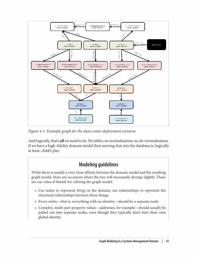
Figure 4-5. Example graph for the data center deployment scenario

And logically, that’s all we need to do. No tables, no normalization, no de-normalization.If we have a high-fidelity domain model then moving that into the database is, logicallyat least, child’s play.

Modeling guidelinesWhile there is usually a very close affinity between the domain model and the resultinggraph model, there are occasions where the two will necessarily diverge slightly. Theseare our rules of thumb for refining the graph model:

• Use nodes to represent things in the domain; use relationships to represent thestructural relationships between those things.

• Every entity—that is, everything with an identity—should be a separate node.• Complex, multi-part property values—addresses, for example—should usually be

pulled out into separate nodes, even though they typically don’t have their ownglobal identity.

Graph Modeling in a Systems Management Domain | 61

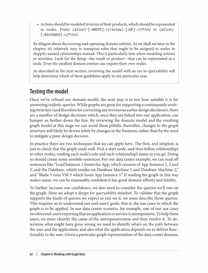
• Actions should be modeled in terms of their products, which should be representedas nodes. Prefer (alice)-[:WROTE]->(review)-[:OF]->(film) to (alice)-[:REVIEWED]->(film).

Be diligent about discovering and capturing domain entities. As we shall see later in thechapter, it’s relatively easy to transpose roles that ought to be assigned to nodes tosloppily-named relationships instead. This is particularly true when modeling actionsor activities. Look for the thing—the result or product—that can be represented as anode. Even the smallest domain entities can require their own nodes.

As described in the next section, reviewing the model with an eye to queryability willhelp determine which of these guidelines apply in any particular case.

Testing the modelOnce we’ve refined our domain model, the next step is to test how suitable it is foranswering realistic queries. While graphs are great for supporting a continuously evolv‐ing structure (and therefore for correcting any erroneous earlier design decisions), thereare a number of design decisions which, once they are baked into our application, canhamper us further down the line. By reviewing the domain model and the resultinggraph model at this stage we can avoid these pitfalls; thereafter, changes to the graphstructure will likely be driven solely by changes in the business, rather than by the needto mitigate a poor design decision.

In practice there are two techniques that we can apply here. The first, and simplest, isjust to check that the graph reads well. Pick a start node, and then follow relationshipsto other nodes, reading each node’s role and each relationship’s name as you go. Doingso should create some sensible sentences. For our data center example, we can read offsentences like “Load balancer 1 fronts the App, which consists of App Instance 1, 2 and3, and the Database, which resides on Database Machine 1 and Database Machine 2,”and “Blade 3 runs VM 3 which hosts App Instance 3.” If reading the graph in this waymakes sense, we can be reasonably confident it has good domain affinity and fidelity.

To further increase our confidence, we also need to consider the queries we’ll run onthe graph. Here we adopt a design for queryability mindset. To validate that the graphsupports the kinds of queries we expect to run on it, we must describe those queries.This requires us to understand our end-users’ goals; that is, the use cases to which thegraph is to be applied. In our data center scenario, for example, one of our use casesinvolves end-users reporting that an application or service is unresponsive. To help theseusers, we must identify the cause of the unresponsiveness and then resolve it. To de‐termine what might have gone wrong we need to identify what’s on the path betweenthe user and the application, and also what the application depends on to deliver func‐tionality to the user. Given a particular graph representation of the data center domain,


12. With a large physical network, we might use Complex Event Processing to process streams of low-levelnetwork events, updating the graph only when the CEP solution raises a significant domain event. See: http://en.wikipedia.org/wiki/Complex_event_processing

if we can craft a Cypher query that addresses this use case, we can be even more certainthat the graph meets the needs of our domain.

Continuing with our example use case, let’s assume that we can update the graph fromour regular network monitoring tools, thereby providing us with a near real-time viewof the state of the network 12. When a user reports a problem, we can limit the physicalfault-finding to problematic network elements between the user and the application andthe application and its dependencies. In our graph we can find the faulty equipmentwith the following query:

START user=node:users(id = 'User 3')MATCH (user)-[*1..5]-(asset) WHERE asset.status! = 'down'RETURN distinct asset

That is, starting from the user who reported the problem, we MATCH against all assets inthe graph along an undirected path of length 1 to 5. We store asset nodes with a status property whose value is 'down' in our results. The exclamation mark in asset.status! ensures that assets that lack a status property are not included in the results.RETURN distinct asset ensures that unique assets are returned in the results, no matterhow many times they are matched.

Given that such a query is readily supported by our graph, we gain confidence that thedesign is fit for purpose.

Common Modeling PitfallsWhile graph modeling is a very expressive way of mastering the complexity in a problemdomain, expressivity in and of itself is no guarantee that a particular graph is fit forpurpose. In fact there have been occasions where even those of us who work with graphsall the time make mistakes. In this section we’ll take a look at a model that went wrong.In so doing, we’ll learn how to identify problems early in the modeling effort, and howto fix them.

Email Provenance Problem DomainIn this case we were working on a problem involving the analysis of email communi‐cations. Communication pattern analysis is a classic graph problem. Normally, we’dinterrogate the graph to discover subject matter experts, key influencers, and the com‐munication chains through which information is propagated. On this occasion, how‐ever, instead of looking for positive role models (in the form of experts) we were search‐

Common Modeling Pitfalls | 63

http://en.wikipedia.org/wiki/Complex_event_processing


ing for rogues: that is, suspicious patterns of email communication that fall foul ofcorporate governance—or even break the law.

A Sensible First Iteration?In analyzing the domain we learnt about all the clever patterns that potential wrong-doers adopt to cover their tracks: using BCC, using aliases—even conducting conver‐sations with those aliases to mimic legitimate interactions between real business stake‐holders. Based on this analysis we produced a representative graph model that seemedto capture all the relevant entities and their activities.

To illustrate this early model, we’ll use Cypher’s CREATE clause to generate some nodesrepresenting users and aliases. We also generate a relationship that shows that Alice isone of Bob’s known aliases. (We’ll assume that the underlying Neo4j instance is indexingthese nodes so that we can later look them up and use them as starting points in ourqueries.) Here’s the Cypher query to create our first graph:

CREATE alice = {username : 'alice'}CREATE bob = {username : 'bob'}CREATE charlie = {username : 'charlie'}CREATE davina = {username : 'davina'}CREATE edward = {username : 'edward'}

CREATE (alice)-[:ALIAS_OF]->(bob)

The resulting graph model makes it easy to observe that Alice is an alias of Bob, as wesee in Figure 4-6.

Figure 4-6. Users and aliases

Now we join the users together through the emails they’ve exchanged:

CREATE (bob)-[:EMAILED]->(charlie)CREATE (bob)-[:CC]->(davina)CREATE (bob)-[:BCC]->(edward)

At first sight this looks like a reasonably faithful representation of the domain. Eachclause lends itself to being read comfortably left to right, thereby passing one of our


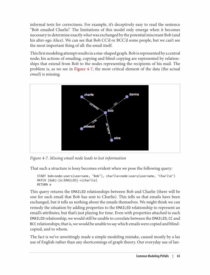
informal tests for correctness. For example, it’s deceptively easy to read the sentence“Bob emailed Charlie”. The limitations of this model only emerge when it becomesnecessary to determine exactly what was exchanged by the potential miscreant Bob (andhis alter-ego Alice). We can see that Bob CC’d or BCC’d some people, but we can’t seethe most important thing of all: the email itself.

This first modeling attempt results in a star-shaped graph. Bob is represented by a centralnode; his actions of emailing, copying and blind-copying are represented by relation‐ships that extend from Bob to the nodes representing the recipients of his mail. Theproblem is, as we see in Figure 4-7, the most critical element of the data (the actualemail) is missing.

Figure 4-7. Missing email node leads to lost information

That such a structure is lossy becomes evident when we pose the following query:

START bob=node:users(username, "Bob"), charlie=node:users(username, "Charlie")MATCH (bob)-[e:EMAILED]->(charlie)RETURN e

This query returns the EMAILED relationships between Bob and Charlie (there will beone for each email that Bob has sent to Charlie). This tells us that emails have beenexchanged, but it tells us nothing about the emails themselves. We might think we canremedy the situation by adding properties to the EMAILED relationship to represent anemail’s attributes, but that’s just playing for time. Even with properties attached to eachEMAILED relationship, we would still be unable to correlate between the EMAILED, CC andBCC relationships; that is, we would be unable to say which emails were copied and blind-copied, and to whom.

The fact is we’ve unwittingly made a simple modeling mistake, caused mostly by a laxuse of English rather than any shortcomings of graph theory. Our everyday use of lan‐


guage has lead us to focus on the verb “emailed” rather than the email itself, and as aresult we’ve produced a model lacking domain insight.

In English, it’s easy and convenient to shorten the phrase “Bob sent an email to Charlie”to “Bob emailed Charlie”. In most cases that loss of a noun (the actual email) doesn’tmatter since the intent is still clear. But when it comes to our forensics scenario, theseelided statements are problematic. The intent remains the same, but the details of thenumber, contents and recipients of the emails that Bob sent have been lost throughhaving been folded into a relationship EMAILED, rather than being modeled explicitly asnodes in their own right.

Second Time’s the CharmTo fix our lossy model, we need to insert email nodes to represent the real emails ex‐changed within the business, and expand our set of relationship names to encompassthe full set of addressing fields that email supports. Now instead of creating lossy struc‐tures like this:

CREATE (bob)-[:EMAILED]->(charlie)

-we’ll instead create more detailed structures, like this:

CREATE email = {id : '1234', content : "Hi Charlie, ... Kind regards, Bob"}

CREATE (bob)-[:SENT]->(email)CREATE (email)-[:TO]->(charlie)CREATE (email)-[:CC]->(davina)CREATE (email)-[:CC]->(alice)CREATE (email)-[:BCC]->(edward)

This results in the kind of graph structure we see in Figure 4-8:


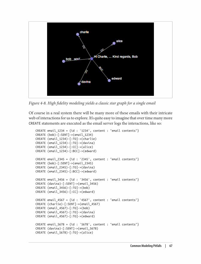
Figure 4-8. High fidelity modeling yields a classic star graph for a single email

Of course in a real system there will be many more of these emails with their intricateweb of interactions for us to explore. It’s quite easy to imagine that over time many moreCREATE statements are executed as the email server logs the interactions, like so:

CREATE email_1234 = {id : '1234', content : "email contents"}CREATE (bob)-[:SENT]->(email_1234)CREATE (email_1234)-[:TO]->(charlie)CREATE (email_1234)-[:TO]->(davina)CREATE (email_1234)-[:CC]->(alice)CREATE (email_1234)-[:BCC]->(edward)

CREATE email_2345 = {id : '2345', content : "email contents"}CREATE (bob)-[:SENT]->(email_2345)CREATE (email_2345)-[:TO]->(davina)CREATE (email_2345)-[:BCC]->(edward)

CREATE email_3456 = {id : '3456', content : "email contents"}CREATE (davina)-[:SENT]->(email_3456)CREATE (email_3456)-[:TO]->(bob)CREATE (email_3456)-[:CC]->(edward)

CREATE email_4567 = {id : '4567', content : "email contents"}CREATE (charlie)-[:SENT]->(email_4567)CREATE (email_4567)-[:TO]->(bob)CREATE (email_4567)-[:TO]->(davina)CREATE (email_4567)-[:TO]->(edward)

CREATE email_5678 = {id : '5678', content : "email contents"}CREATE (davina)-[:SENT]->(email_5678)CREATE (email_5678)-[:TO]->(alice)


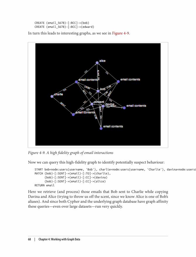
CREATE (email_5678)-[:BCC]->(bob)CREATE (email_5678)-[:BCC]->(edward)

In turn this leads to interesting graphs, as we see in Figure 4-9.

Figure 4-9. A high fidelity graph of email interactions

Now we can query this high-fidelity graph to identify potentially suspect behaviour:

START bob=node:users(username, 'Bob'), charlie=node:users(username, 'Charlie'), davina=node:users(username, 'Davina')MATCH (bob)-[:SENT]->(email)-[:TO]->(charlie), (bob)-[:SENT]->(email)-[:CC]->(davina) (bob)-[:SENT]->(email)-[:CC]->(alice)RETURN email

Here we retrieve (and process) those emails that Bob sent to Charlie while copyingDavina and Alice (trying to throw us off the scent, since we know Alice is one of Bob’saliases). And since both Cypher and the underlying graph database have graph affinitythese queries—even over large datasets—run very quickly.


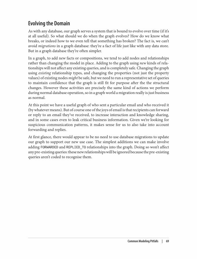
Evolving the DomainAs with any database, our graph serves a system that is bound to evolve over time (if it’sat all useful). So what should we do when the graph evolves? How do we know whatbreaks, or indeed how to we even tell that something has broken? The fact is, we can’tavoid migrations in a graph database: they’re a fact of life just like with any data store.But in a graph database they’re often simpler.

In a graph, to add new facts or compositions, we tend to add nodes and relationshipsrather than changing the model in place. Adding to the graph using new kinds of rela‐tionships will not affect any existing queries, and is completely safe. Changing the graphusing existing relationship types, and changing the properties (not just the propertyvalues) of existing nodes might be safe, but we need to run a representative set of queriesto maintain confidence that the graph is still fit for purpose after the the structuralchanges. However these activities are precisely the same kind of actions we performduring normal database operation, so in a graph world a migration really is just businessas normal.

At this point we have a useful graph of who sent a particular email and who received it(by whatever means). But of course one of the joys of email is that recipients can forwardor reply to an email they’ve received, to increase interaction and knowledge sharing,and in some cases even to leak critical business information. Given we’re looking forsuspicious communication patterns, it makes sense for us to also take into accountforwarding and replies.

At first glance, there would appear to be no need to use database migrations to updateour graph to support our new use case. The simplest additions we can make involveadding FORWARDED and REPLIED_TO relationships into the graph. Doing so won’t affectany pre-existing queries: these new relationships will be ignored because the pre-existingqueries aren’t coded to recognise them.


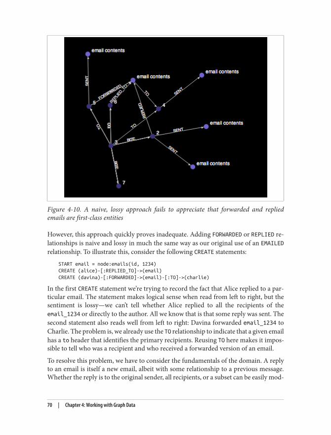
Figure 4-10. A naive, lossy approach fails to appreciate that forwarded and repliedemails are first-class entities

However, this approach quickly proves inadequate. Adding FORWARDED or REPLIED re‐lationships is naive and lossy in much the same way as our original use of an EMAILEDrelationship. To illustrate this, consider the following CREATE statements:

START email = node:emails(id, 1234)CREATE (alice)-[:REPLIED_TO]->(email)CREATE (davina)-[:FORWARDED]->(email)-[:TO]->(charlie)

In the first CREATE statement we’re trying to record the fact that Alice replied to a par‐ticular email. The statement makes logical sense when read from left to right, but thesentiment is lossy—we can’t tell whether Alice replied to all the recipients of theemail_1234 or directly to the author. All we know that is that some reply was sent. Thesecond statement also reads well from left to right: Davina forwarded email_1234 toCharlie. The problem is, we already use the TO relationship to indicate that a given emailhas a to header that identifies the primary recipients. Reusing TO here makes it impos‐sible to tell who was a recipient and who received a forwarded version of an email.

To resolve this problem, we have to consider the fundamentals of the domain. A replyto an email is itself a new email, albeit with some relationship to a previous message.Whether the reply is to the original sender, all recipients, or a subset can be easily mod‐


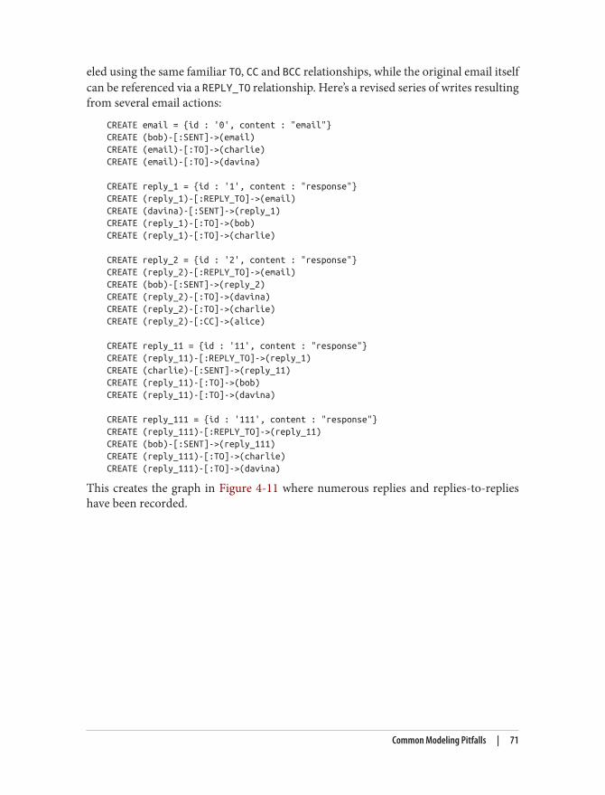
eled using the same familiar TO, CC and BCC relationships, while the original email itselfcan be referenced via a REPLY_TO relationship. Here’s a revised series of writes resultingfrom several email actions:

CREATE email = {id : '0', content : "email"}CREATE (bob)-[:SENT]->(email)CREATE (email)-[:TO]->(charlie)CREATE (email)-[:TO]->(davina)

CREATE reply_1 = {id : '1', content : "response"}CREATE (reply_1)-[:REPLY_TO]->(email)CREATE (davina)-[:SENT]->(reply_1)CREATE (reply_1)-[:TO]->(bob)CREATE (reply_1)-[:TO]->(charlie)

CREATE reply_2 = {id : '2', content : "response"}CREATE (reply_2)-[:REPLY_TO]->(email)CREATE (bob)-[:SENT]->(reply_2)CREATE (reply_2)-[:TO]->(davina)CREATE (reply_2)-[:TO]->(charlie)CREATE (reply_2)-[:CC]->(alice)

CREATE reply_11 = {id : '11', content : "response"}CREATE (reply_11)-[:REPLY_TO]->(reply_1)CREATE (charlie)-[:SENT]->(reply_11)CREATE (reply_11)-[:TO]->(bob)CREATE (reply_11)-[:TO]->(davina)

CREATE reply_111 = {id : '111', content : "response"}CREATE (reply_111)-[:REPLY_TO]->(reply_11)CREATE (bob)-[:SENT]->(reply_111)CREATE (reply_111)-[:TO]->(charlie)CREATE (reply_111)-[:TO]->(davina)

This creates the graph in Figure 4-11 where numerous replies and replies-to-replieshave been recorded.


Figure 4-11. Explicitly modeling replies in high-fidelity

Now it is easy to see who replied to Bob’s original email. First locate the email of interest,then match against incoming REPLY_TO relationships (since there may be multiple re‐plies) and from there match against incoming SENT relationships to find the sender(s).In Cypher this is simple to express. In fact, Cypher makes it easy to look for replies toreplies to replies, and so on to an arbitrary depth (though we limit it to depth 4 here):

START email = node:emails(id, '6789')MATCH (email)<-[:REPLY_TO*1..4]-()<-[:SENT]-(replier)RETURN replier

It’s a similar pattern for a forwarded email: a forwarded email is simply a new email thathappens to contain some of the text of the original email (possibly with additions bythe forwarder). In that case we should model the new email explicitly, just as in the replycase. But from an application point of view we should also be able to reference theoriginal email from the forwarded mail so that we always have high fidelity provenancedata. And the same applies if the forwarded mail is itself forwarded, and so on. Forexample, if Alice (Bob’s alter-ego) emails Bob to try to establish separate concrete iden‐tities, and then Bob (wishing to perform some subterfuge) forwards that email ontoCharlie who forwards it onto Davina, we actually have three emails to consider. As‐suming the users (and their aliases) are already in the database, in Cypher we’d writethat audit information into the database as follows:


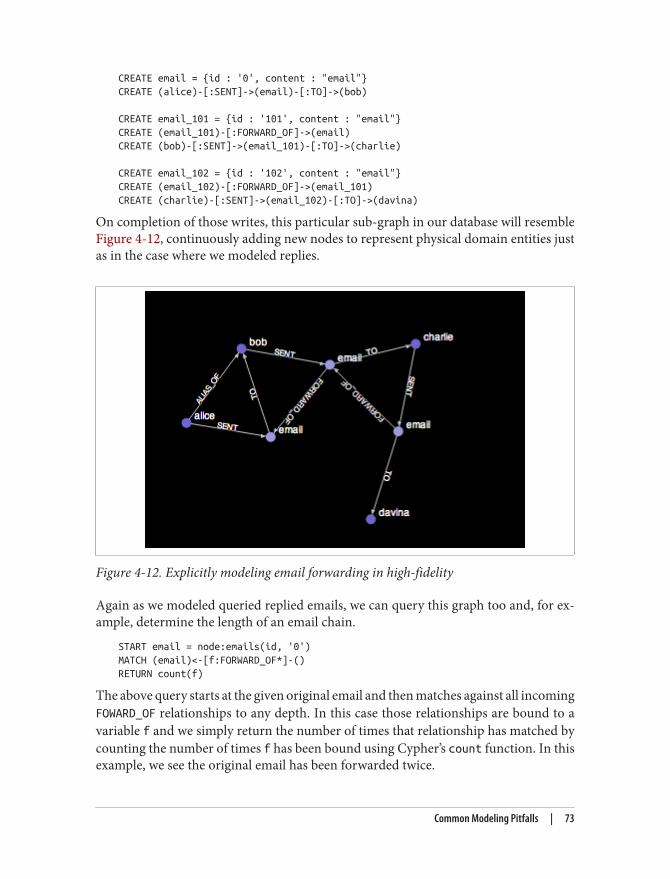
CREATE email = {id : '0', content : "email"}CREATE (alice)-[:SENT]->(email)-[:TO]->(bob)

CREATE email_101 = {id : '101', content : "email"}CREATE (email_101)-[:FORWARD_OF]->(email)CREATE (bob)-[:SENT]->(email_101)-[:TO]->(charlie)

CREATE email_102 = {id : '102', content : "email"}CREATE (email_102)-[:FORWARD_OF]->(email_101)CREATE (charlie)-[:SENT]->(email_102)-[:TO]->(davina)

On completion of those writes, this particular sub-graph in our database will resembleFigure 4-12, continuously adding new nodes to represent physical domain entities justas in the case where we modeled replies.

Figure 4-12. Explicitly modeling email forwarding in high-fidelity

Again as we modeled queried replied emails, we can query this graph too and, for ex‐ample, determine the length of an email chain.

START email = node:emails(id, '0')MATCH (email)<-[f:FORWARD_OF*]-()RETURN count(f)

The above query starts at the given original email and then matches against all incomingFOWARD_OF relationships to any depth. In this case those relationships are bound to avariable f and we simply return the number of times that relationship has matched bycounting the number of times f has been bound using Cypher’s count function. In thisexample, we see the original email has been forwarded twice.


Avoiding Anti-PatternsIn the general case, don’t encode entities (nouns) into relationships. Use relationshipsto convey semantics about how entities are related, and the quality of those relationships,not to directly encode verbs. And remember that domain entities aren’t always clear inthe way humans communicate, so think carefully about the nouns that you’re actuallydealing with.

It’s also important to realize that graphs are a naturally additive structure. Pouring infacts in terms of domain entities and how they interrelate is natural, even if it might atfirst feel like you’re flooding the database with a great deal of painstaking data. In generalit’s a both bad practice and futile to try to conflate data elements at write time to preservequery-time efficiency, so model naturally and in high-fidelity and trust in the graphdatabase to do the right thing.

Good graph databases like Neo4j maintain fast query times even whenstoring vast amounts of data. Learning to trust your graph database isimportant when learning to structure (and not denormalize) yourgraphs.

SummaryModeling with graphs is one of the most expressive and powerful tools at our disposalas software professionals, providing high affinity between domain and data and re‐moving the need for complex normalization and deormalization and the correspond‐ingly complex data management code. However, modeling with graphs is a new tech‐nique for most of us, and so we should take care to ensure that the graphs we’re creatingread well (for queries) and don’t conflate entities and actions (losing useful domainknowledge). While there are no absolute rights or wrongs to graph modeling, by fol‐lowing the guidance in this chapter, we can have confidence that our graph data willserve our systems’ needs over many iterations and keep pace with code evolution.


CHAPTER 5

Graph Databases

In this chapter we discuss the characteristics of graph database management systems(“graph databases” for short, or Graph DBMSs), showing how graph databases differfrom other means of storing and querying complex, semi-structured, densely-connected data. Throughout this chapter we’re going to ground the discussion in thearchitecture and open source code of Neo4j - the most popular graph database.

Graph databases: a definitionA graph database is a storage engine which supports a graph data model backed bynative graph persistence, with access and query methods for the graph primitives tomake querying the stored data pleasant and performant. However there are numerousgraph data models and while the rest of this book focuses on the most common andpragmatic model — the property graph, or simply graph database — there are otherkinds of stores which lay claim to the name “graph database” including triple stores andhypergraph stores.

HypergraphsHypergraphs are a generalized graph model where a relationship (called a hyper-edge)can connect any number of nodes. More specifically while the property graph modelpermits a relationship have a single start and end node, the hypergraph model allowsany number of nodes at a relationship’s start and end. For some problems hypergraphscould be a useful model. For example in Figure 5-1 we see that Alice and Bob are theowners of three vehicles which is expressed through a single hyper-edge (rather thanpotentially six relationships in a property graph).

75

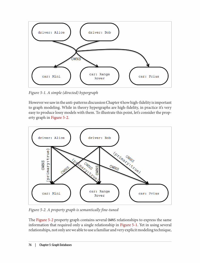
Figure 5-1. A simple (directed) hypergraph

However we saw in the anti-patterns discussion Chapter 4 how high-fidelity is importantto graph modeling. While in theory hypergraphs are high-fidelity, in practice it’s veryeasy to produce lossy models with them. To illustrate this point, let’s consider the prop‐erty graph in Figure 5-2.

Figure 5-2. A property graph is semantically fine-tuned

The Figure 5-2 property graph contains several OWNS relationships to express the sameinformation that required only a single relationship in Figure 5-1. Yet in using severalrelationships, not only are we able to use a familiar and very explicit modeling technique,

76 | Chapter 5: Graph Databases

1. http://www.w3.org/standards/semanticweb/

2. http://www.w3.org/TR/rdf-sparql-query/

3. http://www.w3.org/RDF/

but we’re also able to fine-tune that model. For example we’ve taken the opportunity todistinguish the “primary driver” for each vehicle for insurance purposes by adorningthe appropriate relationships, something which can’t be done with a single hyper-edge.

It’s a fair to say that hypergraphs are a more general model than propertygraphs since hyper-edges are multidimensional. However it is possibleto represent the information of any hypergraph as a property graph(albeit using more relationships and intermediary nodes) because thetwo models are isomorphic. Whether a hypergraph or a property graphis best for you is going to depend on your modeling mindset and thekinds of applications you’re building. Anecdotally, for most purposesproperty graphs seem to have the best balance of pragmatism and mod‐eling efficiency, hence their overwhelming popularity in the graph da‐tabase space. However for situations where meta-intent is desired (e.g.I like the fact that you liked that car) then hypergraphs require fewerprimitives than property graphs.

TriplesThe triple-store family of databases comes from the Semantic Web 1 movement, whereresearchers are interested in large-scale knowledge inference by adding semantic mark‐up on links between Web resources. To-date there’s relatively little of the Web which isusefully marked-up so running queries across the semantic layer is uncommon. Insteadmost effort in the semantic Web appears to be invested in harvesting useful data andrelationship information from the Web (or other more mundane data sources like ap‐plications) and depositing it in triple stores for querying.

Triple stores are a specialized kind of database into which harvested triples are deposited.Triple typically provide SPARQL 2 capabilities to reason about stored RDF 3 data. Inturn, the stored triples of the form subject-predicate-object provide a set of facts suchthat we can easily capture knowledge via numerous pithy statements like “Ginger danceswith Fred” and “Fred likes ice cream.” Individually a single triple is semantically ratherpoor, but en-masse they provide a rich data set from which to harvest knowledge andinfer connections.

While RDF — the lingua franca of triple stores and the Semantic Web — can be serial‐ized several ways, using the RDF/XML format we can begin to see how triples cometogether to form linked data in RDF encoding of a simple three-node graph.

Graph databases: a definition | 77

http://www.w3.org/standards/semanticweb/

http://www.w3.org/TR/rdf-sparql-query/

http://www.w3.org/RDF/

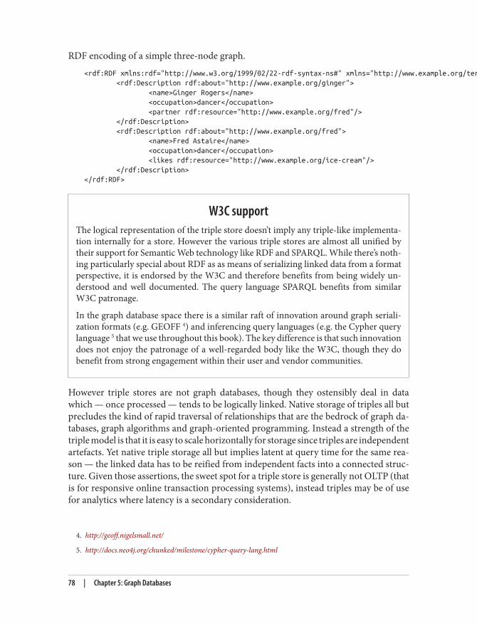
4. http://geoff.nigelsmall.net/

5. http://docs.neo4j.org/chunked/milestone/cypher-query-lang.html

RDF encoding of a simple three-node graph.

<rdf:RDF xmlns:rdf="http://www.w3.org/1999/02/22-rdf-syntax-ns#" xmlns="http://www.example.org/terms/"> <rdf:Description rdf:about="http://www.example.org/ginger"> <name>Ginger Rogers</name> <occupation>dancer</occupation> <partner rdf:resource="http://www.example.org/fred"/> </rdf:Description> <rdf:Description rdf:about="http://www.example.org/fred"> <name>Fred Astaire</name> <occupation>dancer</occupation> <likes rdf:resource="http://www.example.org/ice-cream"/> </rdf:Description></rdf:RDF>

W3C supportThe logical representation of the triple store doesn’t imply any triple-like implementa‐tion internally for a store. However the various triple stores are almost all unified bytheir support for Semantic Web technology like RDF and SPARQL. While there’s noth‐ing particularly special about RDF as as means of serializing linked data from a formatperspective, it is endorsed by the W3C and therefore benefits from being widely un‐derstood and well documented. The query language SPARQL benefits from similarW3C patronage.

In the graph database space there is a similar raft of innovation around graph seriali‐zation formats (e.g. GEOFF 4) and inferencing query languages (e.g. the Cypher querylanguage 5 that we use throughout this book). The key difference is that such innovationdoes not enjoy the patronage of a well-regarded body like the W3C, though they dobenefit from strong engagement within their user and vendor communities.

However triple stores are not graph databases, though they ostensibly deal in datawhich — once processed — tends to be logically linked. Native storage of triples all butprecludes the kind of rapid traversal of relationships that are the bedrock of graph da‐tabases, graph algorithms and graph-oriented programming. Instead a strength of thetriple model is that it is easy to scale horizontally for storage since triples are independentartefacts. Yet native triple storage all but implies latent at query time for the same rea‐son — the linked data has to be reified from independent facts into a connected struc‐ture. Given those assertions, the sweet spot for a triple store is generally not OLTP (thatis for responsive online transaction processing systems), instead triples may be of usefor analytics where latency is a secondary consideration.


http://geoff.nigelsmall.net/


6. https://github.com/tinkerpop/blueprints/wiki/Sail-Implementation7. The main citation for the term is at http://en.wikipedia.org/wiki/Graph_database, but it is believed to have

originated from Marko Rodriguez, a well-known graph advocate.

Though it’s clear that graph databases emphasize traversal performanceand the ability to execute graph algorithms, it is possible to use a graphdatabase as a backing store behind a RDF/SPARQL endpoint. For ex‐ample the Blueprints SAIL 6API provides an RDF interface to severalgraph databases, including Neo4j. In practice this implies a level offunctional isomorphism between graph databases and triple stores.However each store type is suited to different kinds of workload, withgraph databases being optimized for graph workloads and especiallyrapid traversals.

Graph-Native StoresWe’ve discussed the property graph model several times throughout this book, and bynow we’re familiar with the notion of nodes containing properties connected by named,directed relationships which themselves can contain properties. However there a nu‐merous ways to encode and store a property graph, some of which take advantage oftheir natural index-free adjacency model which is which is crucial for fast, efficient graphtraversals.

The term index-free adjacency 7 has been advanced as a means of reasoning about non-graph native databases from more general-purpose graph databases. In a non-nativestore (global) indexes are used to link together nodes, where as in a native graph storeeach node acts as a kind of micro-index of other nearby nodes (at low computationalcost). In a native property graph, there is no requirement to maintain large overarchingindexes to describe connectivity (at greater computational cost).

Using indexes to discover adjacent nodes is a more expensive operation case than usingthe relationships incident on a node. Depending on the implementation, index lookupsare typically O(log n) in algorithmic complexity versus O(1) for looking up relationships.To traverse a network, the cost of an indexed approach at O(m log n) dwarfs the cost ofO(m) for an index-free adjacency approach for a traversal of m steps.

Graph-Native Stores | 79

https://github.com/tinkerpop/blueprints/wiki/Sail-Implementation

http://en.wikipedia.org/wiki/Graph_database

Figure 5-3. Non-native graph stores use indexing to traverse between nodes

For example in Figure 5-3 to find Alice’s friends costs an index lookup at cost O(log n)which may be an acceptable cost for occasional lookups. But to find who is friends withAlice, the costs are far more onerous. For example, it’s O(log n) cost to find out whoAlice’s friends are, but O(m log n) to find out who is friends with Alice as we have tointerrogate the index for each node that could potentially be a friend with Alice.

Index-free adjacency leads to lower-cost “joins”When using indexes to fake connections between records, there is no actual relationshipstored in the database. This is problematic when we try to traverse in the “opposite”direction compared to how the index was constructed. Since we have to brute forcesearch through the index — an O(n) operation — joins like this are simply too costly tobe of any practical use.

While the cost of index lookups might not be considered too onerous for very smallnetworks like Figure 5-3 or the kind of example often seen in demos, in the general caseit is too costly to be practical since it directly limits the scope and richness of the resultset for a responsive application. It is for that reason that performant graph databaseslike Neo4j tend towards index-free adjacency to ensure high performance traversals asan essential design goal.


Recall that in a general-purpose graph database relationships can be traversed in eitherdirection (tail to head, or head to tail) extremely cheaply. The graph in Figure 5-4 helpsillustrate this point in contrast to the far more expensive index-bound approach.

Figure 5-4. Neo4j uses relationships, not indexes for fast traversals

As we can see in Figure 5-4, to discover who Alice’s friends are in a graph, we simplyfollow her outgoing FRIEND relationships at O(1) cost each. For who is friends with Alice,we simply follow all her incoming FRIEND relationships to their source at O(1) cost eachonce again. This observation should lead to very efficient graph traversals in theory, butsuch high-performance traversals only become reality when they are supported by anarchitecture designed for that purpose as we shall now discuss.

ArchitectureGiven that index-free adjacency is the key to high performance traversals and thus highperformance queries and writes, one key aspect of the design of a graph database is theway in which graphs are stored. An efficient, native graph storage format supports ex‐tremely rapid traversals for arbitrary graph algorithms — an important reason for usinggraphs — and is a key differentiator between a native graph database and other non-native graph databases (e.g. triple stores).

For illustrative purposes we’ll use the Neo4j database as a canonical example of how agraph database is architected. We choose Neo4j for a variety of reasons — it’s very pop‐ular, it’s graph-native, and it’s open source so our discussion here can be readily tiedback to corresponding code.

Firstly let’s contextualize our discussion by looking at Neo4j’s high level architecture,presented in Figure 5-5. We’ll work bottom-up from the files on disk through to theprogrammatic APIs and up to the Cypher query language. Along the way we’ll discussthe performance and dependability characteristics and the design decisions that enableNeo4j to be a performant, reliable graph database.

Architecture | 81

Figure 5-5. Neo4j architecture

Neo4j stores graph data spread across a number of store files. Each store file containsthe data for a specific part of the graph (e.g. nodes, relationships, properties). The di‐vision of storage responsibilities — particularly the separation of graph structure fromproperty data — exists for performant graph traversals even if though it means the user’sview of their graph and the actual records on disk are structurally dissimilar. Let’s startour exploration of physical storage by looking at the structure of nodes and relationshipson disk as shown in Figure 5-6.

Figure 5-6. Neo4j Node and Relationship Store File Record Structure

The node store file is where, unsurprisingly, node records are stored. Every node createdin the user-level graph ends up in this node store, and is stored in the physical file


neostore.nodestore.db. Like most of the Neo4j store files, the node store is a fixed-size record store where each record is 9 bytes in length. Fixed record sizes enable fastlookups for nodes within the store file — if we have a node with id 100 then we knowits record begins 900 bytes into the file and so the database can directly compute therecord location at cost O(1) without performing a search at cost O(log n).

Inside a node record, the first byte is the in-use flag which tells the database whetherthe record is currently used or can be reclaimed to store new records (withNeo4j’s .id files being used to keep track of unused records). The next four bytes arethe of the first relationship connected to the node. The last four nodes bytes are the idof the first property for the node. The node record is pretty lightweight, it’s really just acouple of pointers to lists of relationships and properties.

Correspondingly, relationships are stored in the relationship store file ‘neostore.rela‐tionshipstore.db`. Like the node store file, the relationship store contains fixed-size (inthis case 33 bytes) records and each record contains the id of the nodes at the start andend of each relationship, a pointed to the relationship type (stored in the relationshiptype store) and pointers for the relationship chains for the start and end node (as adoubly linked list) since a relationships logically belongs to both nodes and thereforeshould appear in the list of both nodes’ relationships.

Both the node and relationship stores are only concerned with thestructure of the graph, not the property data it holds. Furthermore, bothnode and relationship stores use fixed-sized records such that any in‐dividual record’s location within the store file can be rapidly computedgiven its id. These are critical design decisions that underlines Neo4j’scommitment to high performance traversals.

In Figure 5-7 we see how the various store files interact on disk. The node recordscontain only a pointer to their first property and their first relationship (in what is oftentermed the _relationship chain). From here, we can follow the (doubly) linked-list ofrelationships until we find the one we’re interested in, the LIKES relationship from Node1 to Node 2 in this case. Once we’ve found the relationship record of interest, we cansimply read its properties if there are any via the same singly-linked list structure asnode properties, or we can examine the node records that it relates via its start node andend node IDs. These IDs, multiplied by the node record size, of course give the imme‐diate offset of both nodes in the node store file.

Architecture | 83

Figure 5-7. How a graph is physically stored in Neo4j

Doubly linked lists in the relationship storeDon’t worry if the relationship store structure seems a little complex at first; it’s definitelynot as simple as the node store or property store.

It’s helpful to think of a relationship record as “belonging” to two nodes—the start nodeand the end node of the relationship. Clearly, however, we don’t want to store two re‐lationship records, because that would be wasteful. And yet it’s equally clear that therelationship record should somehow belong to both the start node and the end node.

That’s why there are pointers (aka record ids) for two doubly-linked lists: one is the listof relationships visible from the start node; the other is the list of relationships visiblefrom the end node. That each list is doubly-linked simply allows us to rapidly iteratethrough that list in either direction, and insert and delete relationships efficiently.

Choosing to follow a different relationship involves iterating through a linked list ofrelationships until we find a good candidate (e.g. matching the correct type, or havingsome matching property value). Once we have a suitable relationship we’re back inbusiness simply multiplying id by record size, and thereafter chasing pointers.


8. in fact these computations are much cheaper than searching global indexes as we’d do if faking a graph in anon-graph native database

9. Neo4j allows any primitive JVM type, plus strings and arrays of all the previous.

10. Recall that properties are held as a singly linked-list on disk compared to the doubly linked-list for relation‐ships.

With fixed sized records and pointer-like record ids, traversals are implemented simplyby`‘pointer chasing’' around a data structure which can be performed at very high speed.To traverse a particular relationship from one node to another the database performsseveral cheap id computations 8:

1. From a given node record, locate the first record in the relationship chain by com‐puting its offset into the relationship store by multiplying its id by the fixed rela‐tionship record size (remember that’s 33 bytes at time of writing). This gets us intoright record in the relationship store.

2. From the relationship record look at the second node field for the id of the secondnode. Multiply that id by the node record size (9 bytes at time of writing) to locatethe correct node record in the store.

Should we wish to constrain the traversal to relationships with particular types, thenwe’d add a lookup in the relationship type store. Again this is a simple multiplication ofid by record size (5 bytes at time of writing) to find the offset for the appropriate rela‐tionship type record in the relationship store.

In addition to the node and relationship stores which contain the graph structure, wehave the property store files that store the user’s key-value pairs. Recall that Neo4j, as aproperty graph database, allows properties — name-value pairs — to be stored in bothnodes and relationships and so the property store is referenced from both node andrelationship records.

Records in the property store are physically stored in the neostore.propertystore.db file, and in that file each (fixed-size) entry contains fields representing theproperty type 9, a pointer into the property index store file (neostore.propertystore.db.index), a pointer to a DynamicStore record (being either in the Dynami‐cStringStore in neostore.propertystore.db.strings or the DynamicArrayStore inneostore.propertystore.db.arrays depending on the property type) and finally theid of the next property in the chain 10.

Inlining and optimizing property store utilizationNeo4j supports store optimizations where some properties can be inlined into the prop‐erty store file directly (neostore.propertystore.db). This can happen where property

Architecture | 85

11. See: http://docs.neo4j.org/chunked/stable/configuration-caches.html for tuning options

data can be encoded to fit within the size normally allocated for a pointer to a record(minus a little overhead for descriptive metadata). In practice this means that data likephone numbers and zip codes can be inlined in the property store file directly ratherthan being pushed out to the dynamic stores. This results in reduced I/O operationsand improved throughput since only a single file access is required.

In addition to inlining certain compatible property values, Neo4j also maintains spacediscipline on property names. For example in a social graph, there will likely be manynodes with properties like first_name and last_name. It would be wasteful if eachproperty name was written out to disk verbatim, and so instead property names areindirectly referenced from the property store through the property index file. The prop‐erty index allows all properties with the same name to share a single record, and thusfor repetitive graphs — a very common use case — a great space, and subsequently I/O,saving is achieved.

Having an efficient storage layout is only half of the picture. Even though the store filesare optimized for rapid traversals, we live in a world where disk storage vastly outsizesmain memory capacity. However disks have seek times in single digit milliseconds forspinning disks which — although fast by human standards — are ponderously slow incomputing terms. Though Solid State Disks (SSDs) are far better (since there’s no sig‐nificant seek penalty waiting for platters to rotate) the path between CPU and disk isstill more latent than the path to L2 cache or main memory where we’d ideally like tooperate on our graph.

However we can use in-memory caching to mask the lower performance characteristicsof mechanical/electronic mass storage devices and probabilistically provide low latencyaccess to the graph. In Neo4j there is a two-tiered caching architecture which providesthis functionality.

The lowest tier in the Neo4j cache stack is the filesystem cache. This cache is page-affined,dividing the store into discrete regions with the cache holding a fixed number of thoseregions per store file. The actual amount of memory to be used to cache each store file’spages can be fine-tuned, though Neo4j will use sensible default values based on thecapacity of the underlying hardware in the absence of input from the user 11.

Pages are evicted based on a least frequently used policy, with the default implementationdelegating responsibility for to underlying operating system’s memory mapped file sys‐tem such that the operating system itself determines which segments of virtual memorywill be in real memory and which will be flushed out to disk. The filesystem cache isparticularly beneficial where related parts of the graph are written together so that theyoccupy the same page. This is a common pattern for writes since we tend to persistwhole subgraphs to disk rather than random nodes and relationships.


http://docs.neo4j.org/chunked/stable/configuration-caches.html

If the filesystem cache reflects the write characteristics of typical usage, then the highlevel or object cache is all about optimizing for arbitrary read patterns. The high-levelcache stores nodes, relationships, and properties for rapid, in-memory graph traversal.Unlike the store files where the node records are light compared to the relationshiprecords, in the high level cache nodes are richer and much closer to what we expect asprogrammers since they hold properties and references to their relationships. Con‐versely the relationship objects refer only to their properties. Relationships for eachnode are grouped by RelationshipType and direction for fast lookup of specific rela‐tionships based on those characteristics. As with the underlying stores, all lookups areby id meaning they are very performant as we can see in Figure 5-8.

Architecture | 87

Figure 5-8. Nodes and relationships in the object cache

Neo4j Programmatic APIsWhile the filesystem and caching infrastructure is fascinating, it is all for nothingwithout the APIs to drive it. Though we’ve focussed on the high-level query languageCypher for much of this book, Neo4j also offers programmatic APIs, which Cypher uses,


12. See: http://docs.neo4j.org/chunked/stable/transactions-events.html

but which are also available to developers. Logically it’s easy to think of these APIs in astack where at the top of the stack we prize expressiveness and declarative programming,while at the bottom of the stack we prize precision and imperative style, as depicted inFigure 5-9.

Figure 5-9. Logical view of the user-facing APIs in Neo4j

We’ll step through these from the bottom up in the following sections.

Kernel APIThough it’s not too often the focus of development, the lowest level API that regularNeo4j users access are transaction event handlers 12 in the kernel. These allow user codeto listen to transactions as they flow through the kernel and react (or not) based on thedata content and lifecycle stage of each transaction by user code.

Kernel transaction event handlersA typical use-case for transaction event handlers is to prevent physical deletion of re‐cords. A handler can be set up to intercept deletion of a node and instead simply mark

Neo4j Programmatic APIs | 89

http://docs.neo4j.org/chunked/stable/transactions-events.html

13. See: https://github.com/jimwebber/neo4j-tutorial. Doctor Who is the world’s longest-running science-fictionshow and a firm favorite of the Neo4j team.

that node as deleted logically (or in a more sophisticated manner move the node ''backin time`` by creating timestamped archive relationships).

Core (or “Beans”) APINeo4j’s core API is a popular imperative Java API which exposes the graph primitivesof node, relationship, and properties to the user. As a rule, it’s a lazily evaluated API forreads which means a relationships are only traversed as quickly as the API caller canconsume the data being returned. For writes, the Core API provides transaction man‐agement capabilities to ensure atomic, consistent, isolated, and durable persistence.

In the following code, we see a snippet of code borrowed from the Neo4j tutorial inwhich we try to find human companions from the Doctor Who universe.13

// Index lookup for the node representing the doctor is omitted for brevity

Iterable<Relationship> relationships = doctor.getRelationships( Direction.INCOMING, COMPANION_OF );

for ( Relationship rel : relationships ){ Node companionNode = rel.getStartNode(); if ( companionNode.hasRelationship( Direction.OUTGOING, IS_A ) ) { Relationship singleRelationship = companionNode .getSingleRelationship( IS_A, Direction.OUTGOING ); Node endNode = singleRelationship.getEndNode(); if ( endNode.equals( human ) ) { // Found one! } }}

The specific domain in the code in this snippet isn’t too important, but it’s safe to saythe code is very imperative (and somewhat verbose compared the the equivalent Cypherquery). We simply loop round the Doctor’s companions and check to see if any of thecompanion nodes have an IS_A relationship to the node representing the human species.If so we do something with it.

As an imperative API, the Core API can be fine-tuned to the underlying graph structure.However compared to the higher-level APIs (and particularly Cypher) more code isneeded to achieve an equivalent goal. Nonetheless the affinity between the Core API


https://github.com/jimwebber/neo4j-tutorial

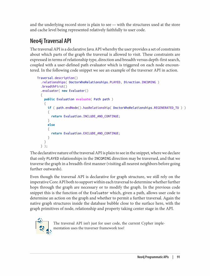
and the underlying record store is plain to see — with the structures used at the storeand cache level being represented relatively faithfully to user code.

Neo4j Traversal APIThe traversal API is a declarative Java API whereby the user provides a set of constraintsabout which parts of the graph the traversal is allowed to visit. These constraints areexpressed in terms of relationship type, direction and breadth versus depth-first search,coupled with a user-defined path evaluator which is triggered on each node encoun‐tered. In the following code snippet we see an example of the traverser API in action.

Traversal.description() .relationships( DoctorWhoRelationships.PLAYED, Direction.INCOMING ) .breadthFirst() .evaluator( new Evaluator() { public Evaluation evaluate( Path path ) { if ( path.endNode().hasRelationship( DoctorWhoRelationships.REGENERATED_TO ) ) { return Evaluation.INCLUDE_AND_CONTINUE; } else { return Evaluation.EXCLUDE_AND_CONTINUE; } } } );

The declarative nature of the traversal API is plain to see in the snippet, where we declarethat only PLAYED relationships in the INCOMING direction may be traversed, and that wetraverse the graph in a breadth-first manner (visiting all nearest neighbors before goingfurther outwards).

Even though the traversal API is declarative for graph structure, we still rely on theimperative Core API both to support within each traversal to determine whether furtherhops through the graph are necessary or to modify the graph. In the previous codesnippet this is the function of the Evaluator which, given a path, allows user code todetermine an action on the graph and whether to permit a further traversal. Again thenative graph structures inside the database bubble close to the surface here, with thegraph primitives of node, relationship and property taking center stage in the API.

The traversal API isn’t just for user code, the current Cypher imple‐mentation uses the traverser framework too!

Neo4j Programmatic APIs | 91

14. The formal definition of dependability is the “trustworthiness of a computing system which allows relianceto be justifiably placed on the service it delivers” as per http://www.dependability.org/

15. Because there’s an unvalidated assumption that transactional systems scale less well. There is some truth tothis, insofar as (distributed) two-phase commit can to exhibit unavailability problems in pathological cases,but for the most part transactions don’t limit scalability.

We’ve now seen the graph-centric APIs, and how they are sympathetic to the structuresused in the lower levels of the Neo4j stack to support rapid graph traversals. Accordingly,we can now move begin to discuss why we can depend on Neo4j to store our data reliably,and not just idiomatically and rapidly.

Non-Functional CharacteristicsAt this point we’ve understood a great deal about how Neo4j is designed and what itmeans to construct a native graph database. But to be considered dependable any datastorage technology must provide some level of guarantee as to the durability and ac‐cessibility of the stored data.14

Relational databases are traditionlly evaluated on the number of transactions per secondthey can process. It is assumed that these transactions uphold the ACID properties (evenin the presence of failures) such that data is consistent and recoverable. For non-stopprocessing and managing large volumes, a database is expected to scale so that manyinstances are available to process queries and updates, with the loss of an individualinstance not unduly affecting the running of the cluster as a whole.

At a high level at least, much the same applies to graph databases: they need to guaranteeconsistency, and to recover gracefully from crashes and prevent data corruption; further,they need to scale out to provide high availability, and scale up for performance. In thefollowing sections we’ll explore what each of these means to a graph database and showwhy Neo4j’s architecture means it can be considered dependable from a systems engi‐neering point of view.

TransactionsTransactions have been a bedrock of dependable computing systems for decades, andthough many NOSQL stores aren’t transactional 15 they remain a fundamental abstrac‐tion for dependability in contemporary graph databases (including Neo4j).

Transactions in Neo4j are semantically identical to traditional database transactions.Writes occur within a transaction context, taking write locks (for consistency) on anynecessary nodes and relationships, and on successful completion of the transaction only(for atomicity) the changes made to the graph and/or index is flushed to disk (for du‐rability) and the write locks released. Should the transaction fail for some reason then


http://www.dependability.org/

16. Even Neo4j cannot be provably bug-free.

the writes will be discarded and the write locks released maintaining the graph in itsprevious consistent state.

Should two or more transactions attempt to mutate the same data concurrently, Neo4jwill detect that potential deadlock and serialize the transactions. Furthermore writeswithin a single transactional context will not be visible to other transactions (for isola‐tion).

Transactions in Neo4jIn Neo4j the transaction implementation is conceptually straightforward. Each trans‐action is represented as an in-memory object whose state represents writes to the da‐tabase. This object is supported by a lock manager that applies write locks to nodes andrelationships as they are created, updated, and deleted. On transaction rollback, thetransaction object is simply discarded and the write locks released, whereas on successfulcompletion the transaction is committed to disk.

Committing data to disk in Neo4j uses a Write Ahead Log approach whereby changesare appended as actionable entries in the active transaction log. On transaction com‐mit (assuming a positive response to the prepare phase) a commit entry will be writtento the log, causing it to be flushed to disk, thereby making the changes durable. Oncethe disk flush has occurred the changes are applied to the graph itself. After all thechanges have been applied to the graph, any write locks associated with the transactionare released.

One of the advantages of transactional behavior from a database system is that once thetransaction has committed, the system is in a state where changes are guaranteed to bein the database even if a fault causes a (non-pathological) failure. This, as we shall nowsee, confers substantial advantages for recoverability and hence ongoing provision ofservice.

RecoverabilityDatabases are no different from any other software in that they are susceptible to bugsin their implementation 16, in the hardware they run on and in the power and coolinginfrastructure that hardware needs. Though diligent engineers try to minimize the pos‐sibility of failure in all of these, at some point it’s inevitable the database will crash(though the mean time between failures should be very long indeed).

In a well designed system, a database server crash is an annoyance but does not impingeavailability (though it may affect throughput). However when that failed server resumes

Non-Functional Characteristics | 93

17. This is a simplification, in reality the master and some slaves have a completely up to date copy of the graph,while other slaves will be catching up typically being milliseconds behind.

operation it must not source corrupt data to its users irrespective of how inconvenientor problematic the nature or timing of the crash.

In case of an unclean shutdown (perhaps caused by a fault or even an overzealous op‐erator), Neo4j checks in the most recently active transaction log and replays any trans‐actions it finds against the store. It’s possible that some of those transactions may havealready been applied to the store, but since replaying is an idempotent action, the netresult is the same: that the store is consistent with all successfully committed transac‐tions prior to the failure when recovery completes.

Of course, recovering locally is fine if all we have is a single database instance, butgenerally we run databases in clusters (which we’ll discuss next) to assure high availa‐bility to applications. Fortunately clustering confers an additional benefit to the recov‐ering database that, not only will it be consistent with respect to the time of failure whenit recovers, but it can quickly catch up to be consistent with other instances in the cluster.That is, once local recovery has completed, then a replica can ask other members of thecluster (typically the master) for any newer transactions that it has missed which it thenapplies to its own data set via transaction replay.

Recoverability deals with the capability of the database to set things right after a faulthas arisen. Even so, a good database still needs to be highly available to meet the in‐creasingly sophisticated needs of data-heavy applications.

AvailabilitySince Neo4j is both transactional and recoverable, it bodes well for availability since theability to recognize and (if necessary) repair an instance after crashing means that dataquickly becomes available again without human intervention. And of course, more liveinstances increases the overall availability of the database to process queries.

However it’s uncommon that we want individual disconnected database instances in atypical production scenario. In those cases databases (of all kinds) tend to be clusteredfor high availability. In Neo4j’s case a master-slave cluster arrangement is used so thata complete replica of the graph is stored on each machine 17.

For writes, the classic write-master with read-slaves is a popular topology whereby alldatabase writes are directed at the master, while read operations are directed at slaves.This provides asymptotic scalability for writes (up to the capacity of a single spindle)but allows for near linear scalability for reads (accounting for the modest overhead inmanaging the cluster).


Although write-master with read-slaves is a classic deployment topology, Neo4j alsosupports writing through slaves. In this scenario, the slave first ensures that it is con‐sistent with the master (it is said to “catch up”) and then the write is synchronouslytransacted across both instances. This is useful where we want immediate durability intwo database instances but at the cost of higher write latency owing to the forced catchupphase, and offers additional deployment flexibility. However it does not imply that writesare distributed around the system, since all writes must still pass through the master atsome point.

Other replication options in Neo4jIn Neo4j version 1.9 onwards it’s also possible to specify an arbitrary number of replicasto be written before a transaction is considered complete in a best-effort manner. Thisan be combined with writing through slaves to provide “at least two” level of durability.

Another aspect of availability is contention for access to resources. A query that con‐tends for exclusive access (e.g. for writes) to a particular part of the graph may sufferfrom high enough latency to appear unavailable. We’ve seen similar contention withcoarse-grained table-level locking in RDBMSs where writes are latent even when there’slogically no contention.

Fortunately in a graph, access patterns tend to be more evenly spread, especially whereidiomatic graph-local queries are executed. A graph local operation is one that starts atone or more given places in the graph and traverses the surrounding subgraphs fromthere. The starting points for such queries tend to be things that are especially significantin the domain, such as users or products, and so the overall query load tends to bedistributed with low contention. In turn the perception is one of greater responsivenessand higher availability.

The benefits of idiomatic queriesJackie Stewart, the Formula 1 racing driver, is reputed to have said that to drive a carwell you don’t need to be an engineer but you do need mechanical sympathy with yourcar. That is, the best performance comes as a result of the driver and car working togetherharmoniously.

In much the same way, Neo4j queries are mechanically sympathetic to the database whenthey are framed as idiomatic, graph local queries that begin their traversal from one ormore start points. The underlying infrastructure, including caching and store access, isoptimized to support this kind of workload.

Being idiomatic has beneficial side effects. For example, because caching is aligned withidiomatic searches, queries that are themselves idiomatic tend to exploit caches better


and run faster than non-idiomatic queries. In turn, faster running queries free up thedatabase to run more of them, which means higher throughput and the sense of betteravailability from the client’s point of view because there’s less waiting around.

Unidiomatic queries (e.g. those which pick random nodes/relationships rather thantraversing) exhibit the opposite characteristics: they disrespect the underlying cachinglayers and therefore run more slowly as more disk I/O is needed. Since the queries runslowly, the database can process fewer of them per second, which means the availabilityof the database to do useful work diminishes from the client’s point of view.

Therefore in Neo4j, we should always strive for idiomatic operations so that we aremechanically sympathetic to the database and so maximise its performance.

Our final observation on availability is that scaling for cluster-wide replication has apositive impact not just in terms of fault-tolerance, but also in terms of responsiveness.Since there are many machines available for a given workload, query latency is low andavailability is maintained. But as we’ll now discuss, scale itself is more nuanced thansimply the number of servers we deploy.

ScaleThe topic of scale has become more important now that we’re in an era where we areaware of enormous and ever-increasing data volumes that surround us. In fact, a sub‐stantial motivation for the NOSQL movement has been to address the problems of dataat scale which have proven difficult to solve with relational databases. In some sense,graph databases are no different since they also need to scale to meet the workloaddemands of modern applications. But scale isn’t a simple value like transactions persecond, it’s an aggregate value that we measure across multiple axes.

For graph databases, we will decompose our broad discussion on scale into three keythemes: * Graph size * Response time * Read and write throughput

Starting with Graph size, Neo4j can store tens of billions of nodes, relationships, andproperties in a single (non-distributed) graph. Specifically the upper bound for thecurrent (at time of writing) release of Neo4j (1.9) is as follows: * Number of nodes: 34billion * Number of relationships: 34 billion * Number of properties: 68 billion

These (relatively generous) upper bounds result from a technical drive to balance effi‐ciency versus scale. One reason Neo4j is so fast for graph traversals is that it makesextensive use of fixed record sizes behind the scenes as we have discussed. Each recordincludes a number of pointers: the larger the pointers, the larger the fixed record sizes,


18. This means Neo4j can grow to accommodate a very large number of records, but it tries to stay in the sweetspot for most users, maintaining a careful balance of disk footprint versus storage headroom.

19. This simple fact of life is one of the key reasons that performance tuning is nearly always the very top issueon a relational DBA’s mind.

20. As we discussed in Chapter 4, it’s still sensible to tune the structure of the graph to suit the queries, even ifwe’re dealing with lower data volumes

and the more capacious the graph can be. However as these pointers increase in size,memory and disk requirements increase 18.

At time of writing, the Neo4j team has publicly expressed its inten‐tion to support 100B+ nodes/relationships/properties in a forth‐coming release. At some point the fixed limit will be so large as to belogically infinite, but retain the benefits of fixed-sized records andpointers for high-speed traversals.

In terms of latency, graph databases don’t suffer the same problems as traditionalRDBMS where the more data you have in in tables — and in indexes — the longer joinoperations take 19. Instead with Neo4j, most queries follow a pattern where an index isused simply to find a starting node (or nodes), and the remainder of the traversal usesa combination of pointer chasing and pattern matching to search the datastore. Wherethis is very different from a relational database is that performance does not depend onthe total size of the data set, but only on the data being queried. This leads to performancetimes that are nearly constant (i.e. are related to the size of the result set), even as thesize of the data set grows 20.

Capacity and latency leave only one remaining axis along which we measure databaseperformance: IO throughput (for mature databases, this is measured in transactions persecond). It’s a simple trap to fall into to immediately think that we need to scale databaseshorizontally, especially since we can also scale graph databases vertically to great effect.Vertical scale is in fact an important distinguishing feature of graphs. Because when itcomes to vertical scaling, not all databases are created equal. In fact graphs tend to scalevery well vertically because they need fewer writes to store the same high-fidelity databecause of the incredible expressiveness of the data model - graphs scale vertically bydoing less work for the same outcome.

For example, imagine a publishing platform where we’d like to read the latest piece froman author. In a RDBMS we typically select the author’s works by joining the authorstable to a table of publications on matching author id, and then ordering them by pub‐lication date and limiting to the newest handful. Depending on the characteristics ofthe ordering operation that might be a O(log(n)) operation which isn’t so very bad.


However as we can easily see in Figure 5-10, the equivalent graph operation is O(1) —meaning constant performance irrespective of dataset size. With a graph we simplyfollow the outbound relationship called WROTE from the author to the work at the headof a list (or tree) of published articles. Should we wish to find older publications, wesimply follow the PREV relationships and iterate through a linked list (or alternativelyrecurse through a tree). Writes follow suit because we always insert new publications atthe head of the list (or root of a tree), which is another constant time operation. Thiscompares favourably to the alternatives, particularly since it naturally maintains con‐stant time performance for reads.

Figure 5-10. Constant time operations for a publishing system

Of course it may be the case that eventually a single machine won’t have sufficient IOthroughput to serve all the queries directed to it. In that case it’s straightforward withNeo4j to build a cluster that allows both high availability and the opportunity to spreadread load across many machines. For typical workloads with more reads than writesthis solution architecture can be ideal.

But finally, should we exceed the capacity of a cluster then graphs can be still spreadacross database instances if the application builds in sharding logic. Sharding involvesthe use of a synthetic identifier to join records across database instances at the applica‐tion level. How well this will perform depends very much on the shape of the graph.Some graphs lend themselves very well to this. Mozilla for instance use the Neo4j graphdatabase as part of their next-generation cloud browser: Pancake. Rather than havinga single large graph, they store a large number of small independent graphs, each tiedto an end user. This makes it very easy to scale with no performance penalty.

Of course not all graphs have such convenient boundaries. If your graph is large enoughthat it needs to be broken up and no natural boundaries exist, then the approach youwould use is much the same as one would use with a NOSQL store like MongoDB: wecreate synthetic keys, and relate records via the application layer using those keys plussome application-level resolution algorithm. The main difference from the MongoDBapproach is that Neo4j will provide you with a performance boost anytime you are doingtraversals within a database instance, while hose parts of the traversal that run between


21. A graph global operation is one in which elements from the graph are accessed at random to calculate someproperty of the graph (e.g. PageRank), by contrast a graph-local operation is where we find a specific startingpoint and traverse paths from there.

22. See: http://dl.acm.org/citation.cfm?id=1807184

instances will run at roughly the same speed as a MongoDB join. Overall performanceshould be markedly faster however.

The holy grail of graph scalabilityThe eventual aim of most graph databases is to be able to partition a graph across manymachines without application-level intervention so that access to the graph can be scaledhorizontally. In the general case this is known to be an NP Hard problem, and thus isimpractical to solve. This manifests itself in graph databases as unpredictable querytimes as traversals unexpectedly jump between machines over a (relatively slow) net‐work. However there is innovation happening in this space with triple stores able toscale horizontally very well (at the expense of latency), some non-native graph storespiggy-backing on other distributed databases like Cassandra or HBase, or Neo4j’s ownhorizontally scalable solution. This is certainly an exciting time to be in the data space.

Graph Compute PlatformsOne key characteristic of a native graph database is its OLTP capabilities, with clientsable to modify and query data in end-user in near real time. While this behavior fits amajority of user-facing applications, sometimes we’re prepared to sacrifice latency topermit more sophisticated processing. In the broader NOSQL world, this is most clearlyepitomized by the affinity between aggregate data stores and map-reduce, whereby datais pumped through external processing infrastructure (e.g. Apache Hadoop) to distiluseful information out of disconnected records.

In the graph space there is a related technology category, the Graph Compute Engine,which is used to conduct specialized analytics involving graph-global operations incontrast to the graph-local operations for which graph databases are optimized 21. Aprominent example of this technology in the literature is Google’s Pregel 22 which has

Graph Compute Platforms | 99

http://dl.acm.org/citation.cfm?id=1807184

23. See: http://incubator.apache.org/giraph/

24. See: http://incubator.apache.org/giraph/

an open-source copycat implementation in Apache Giraphe 23 which can both helpfullybe thought of as a kind of “Hadoop for graphs.”

Graph theoryFor analytics, it’s truly hard to beat graphs. The properties of graph data are well un‐derstood and the fundamental toolkit that is graph theory has broad applicability acrossdomains. From its Eulerian origins in the 18th century, our understanding of networkshas continued to provide amazing insight and predictive analysis into data. Graph anal‐ysis will be a tremendously important aspect of data science in the coming years.

While some may choose to analyze networks the hard way by reifying graphs out ofdisconnected aggregates and pumping that data through a plain map-reduce imple‐mentation, the combination of a native graph database and native graph processing isfar more powerful.

Pregel and equivalent open source implementations like Apache Giraph 24 are examplesof just such a graph processing platform (as distinct from, but complimentary to graphdatabases). Pregel is an evolution of the map-reduce pattern to take advantage of theimplicit locality provided by a graph structure. It’s no surprise then, that at a high levelthe architecture resembles the familiar picture of any map-reduce architecture as wesee in Figure 5-11.

Figure 5-11. Pregel high-level architecture


http://incubator.apache.org/giraph/

http://incubator.apache.org/giraph/

The input to a Pregel computation is a directed graph. The source of the graph can comefrom any source (e.g. flat files), but it is reasonable to use a graph database as the sourcesince it allows subgraphs to be easily extracted for graph-global processing. The graphis then partitioned so that it can be distributed across machines. While default strategiesare available for this, it’s typically better for developers to provide a domain-awarestrategy to preserve subgraph locality. Once partitions are distributed to machines anynon-local accesses are punished by network latency. In turn this implies that each par‐tition tends to contain many nodes to exploit coarse-grained computation.

Pregel has a very node-centric approach to processing. The graph algorithm to be com‐puted is implemented from the point of view of a single node and the transformationsthat happen to its messages, data and local topology. A node consists solely of its algo‐rithm and an incoming and outgoing communication port. Scaling that algorithm toall of the nodes in the graph is how the overall behavior the system is expressed, whilethe scheduling of execution and communication for each node is the responsibility ofthe platform.

Each node uses its incoming and outgoing message queues to transmit the (partial)results of processing between nodes. Communication paths are (usually) constrainedby the structure of the graph such that nodes can only address messages to other nodesto which they have an outgoing relationship. However messages can also be sent to anynode whose identifier is known (thus avoiding intermediate nodes having to act as latentrelays). The logical architecture for partitions and local graph topology is shown inFigure 5-12.


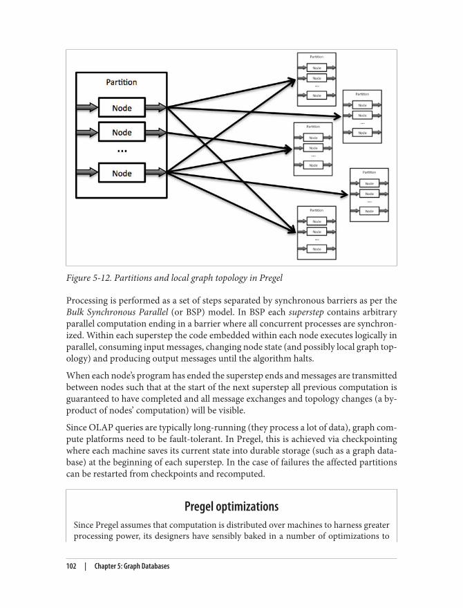
Figure 5-12. Partitions and local graph topology in Pregel

Processing is performed as a set of steps separated by synchronous barriers as per theBulk Synchronous Parallel (or BSP) model. In BSP each superstep contains arbitraryparallel computation ending in a barrier where all concurrent processes are synchron‐ized. Within each superstep the code embedded within each node executes logically inparallel, consuming input messages, changing node state (and possibly local graph top‐ology) and producing output messages until the algorithm halts.

When each node’s program has ended the superstep ends and messages are transmittedbetween nodes such that at the start of the next superstep all previous computation isguaranteed to have completed and all message exchanges and topology changes (a by-product of nodes’ computation) will be visible.

Since OLAP queries are typically long-running (they process a lot of data), graph com‐pute platforms need to be fault-tolerant. In Pregel, this is achieved via checkpointingwhere each machine saves its current state into durable storage (such as a graph data‐base) at the beginning of each superstep. In the case of failures the affected partitionscan be restarted from checkpoints and recomputed.

Pregel optimizationsSince Pregel assumes that computation is distributed over machines to harness greaterprocessing power, its designers have sensibly baked in a number of optimizations to


help reduce the overheads of running a distributed computation, particularly for avoid‐ing expensive network transfers.

Pregel’s Combiners allow for multiple messages between nodes on one machine to anode on another to be combined into a single value before transmission. A motivatingexample is to send a single value for a weighted path over the network rather thannumerous individual weights. However combining makes no guarantees about howvalues are combined, and so it’s unlikely they can be uncombined. Hence it’s safe to useonly functions which are both commutative and associative in a combiner.

Aggregators allow (computed) values to be shared across all nodes the graph. Any nodecan provide a value to an aggregator in a superstep, which is combined with values fromany other nodes. On the next superstep, the aggregate value is made available to everynode in the graph. The typical use-case for aggregators is for global coordination, forexample to terminate computation upon reaching some graph-wide condition. Anothermotivating case is to maintain graph statistics like the number of relationships or nodesin the graph.

In Pregel, processing completes when all nodes in the graph vote to halt — that eachnode believes it has no more work to do and when no messages are incident on a node.When processing ends a final result (from an entire graph to as little as a single value)is produced.

Compute or query?Given that graph compute platforms are powerful machines for processing connecteddata, the question naturally arises why we wouldn’t use them habitually in our infor‐mation systems? The key to answering this question is understanding our appetite forlatency.

Graph compute platforms can compute over large graphs but they do so in a latentmanner by the very nature of the work they undertake. Even if we choose to processsmall graphs in this way however, we still have to deal with the latency of extracting andloading data into the platform which may still take several seconds.

Ultimately today’s graph processing platforms are far more suited to OLAP analysis thanin-the-clickstream OLTP applications. And in OLTP applications most of the time wedon’t want to compute enormous volumes of data anyway since most requests are highlycontextualized by user, product, etc and are therefore generally graph local.

For a point in case, consider a typical e-commerce solution. A local graph query fromthe user will be able to efficiently recommend friends’ and friend-of-friends’ purchasestaking into account both the user’s recently viewed and purchased items. This is theright choice for an interactive Web store.


However to analyse all products, to rank them against one-another is a reasonable can‐didate for a graph compute solution. The synergy between the two is when the rankingalgorithm enriches the graph such that the recommendations query provides even moreaccurate recommendations to the user.

Though a distinct technology category in their own right, it’s clear that graph databasesare a sensible underlay — they have the right APIs and data model affordances to sup‐port seamless integration — for graph compute platforms (like Pregel). The virtuouscycle of enriching the (authoritative) graph with the results from graph-global process‐ing is a compelling strategy. Combining the ability to perform graph-local queries forOLTP scenarios on authoritative data in the graph database with the ability to performarbitrary (graph) computation in an OLAP scenario that enriches the authoritative dataprovides covers all reasonable expectations of data platform.

SummaryIn this chapter we’ve discussed the common types of graph and shown how propertygraphs are an excellent choice for pragmatic data modelling. We’ve also explored thearchitecture of a popular graph database (Neo4j) and discussed the non-functionalcharacteristics of graph database implementations and what it means for them to bedependable. Finally we discussed the different between a graph database (OLTP, forgraph local queries) and a graph processing engine (OLAP, for graph global processing)and explained how graph databases and graph processing are natural bedfellows.

Yet the discussion to this point has asked the reader to take on faith and implied rea‐soning that the technology is a sound choice (and not just an exciting one). In the nextchapter we’ll set that straight by presenting real-world deployment planning use cases— harvested from production systems — to bring home the utility of graphs and graphdatabases for a range of sophisticated scenarios.


CHAPTER 6

Working with a Graph Database

In this chapter we discuss some of the practical issues of working with a graph database.In previous chapters we’ve looked graph data, and the architecture and capabilities ofgraph databases; in this chapter, we’ll apply that knowledge in the context of developinga graph database application. We’ll look at some of the data modeling questions thatmay arise, and at some of the application architecture choices available to you.

In our experience, graph database applications are highly amenable to being developedusing the evolutionary, incremental and iterative software development practices thathave risen to prominence in the last decade. A key feature of these practices is theprevalence of testing throughout the software development lifecycle. Here we’ll showhow to develop your data model and your application in a test-driven fashion.

At the end of the chapter, we’ll look at some of the issues you’ll need to consider whenplanning for production.

Data ModelingWe covered modeling and working with graph data in detail in Chapter 4. Here wesummarize some of the more important modeling guidelines, and discuss how imple‐menting a graph data model fits with iterative and incremental software developmenttechniques.

Describe the Model in Terms of Your Application’s NeedsThe questions you need to ask of the data help identify entities and relationships. Agileuser stories provide a concise means for expressing an outside-in, user-centred view of

105

1. For agile user stories, see Mike Cohn, User Stories Applied (Addison-Wesley, 2004)

an application’s needs, and the questions that arise in the course of satisfying this need.1 Here’s an example of a user story for a book reviews Web application:

• AS A reader who likes a book• I WANT to know which books other readers who like the same book have liked• SO THAT I can find other books to read

This story expresses a user need, which motivates our data model. From a data modelingpoint of view, the AS A clause establishes a context comprising two entities—a readerand a book—and the LIKES relationship that connects them. The I WANT clause thenposes a question: which books have other readers who like the book I’m reading liked?This question exposes more LIKES relationships, and more entities: other readers andother books.

The entities and relationships that we’ve surfaced in analyzing the user story quicklytranslate into a simple data model, as shown in Figure 6-1:

Figure 6-1. Data model for the book reviews user story

Because this data model directly encodes the question presented by the user story, itlends itself to being queried in a way that similarly reflects the structure of the questionwe want to ask of the data:

START reader=node:users(name={readerName}) book=node:books(isbn={bookISBN})MATCH reader-[:LIKES]->book<-[:LIKES]-other_readers-[:LIKES]->booksRETURN books.title

106 | Chapter 6: Working with a Graph Database

Nodes for Things, Relationships for StructureWhile not applicable in every situation, these general guidelines will help you to choosewhen to use nodes, and when relationships:

• Use nodes to represent entities—that is, the things that are of interest to you in yourdomain.

• Use relationships to express the connections between entities and establish semanticcontext for each entity, thereby structuring the domain.

• Use node properties to represent entity attributes, plus any necessary entity meta‐data, such as timestamps, version numbers, etc.

• Use relationship properties to express the strength, weight or quality of a relation‐ship, plus any necessary relationship metadata, such as timestamps, version num‐bers, etc.

If you’re tempted to use a relationship to model an entity—an email, or a review, forexample—make certain that this entity cannot be related to more than two other entities.Remember, a relationship must have a start node and an end node—nothing more,nothing less. If you find later that you need to connect something you’ve modeled as arelationship to more than two other entities, you’ll have to refactor the entity inside therelationship out into a separate node. This is a breaking change to the data model, andwill likely require

Model Facts as NodesWhen two or more domain entities interact for a period of time, a fact emerges. Rep‐resent these facts as separate nodes, with connections to each of the entities engaged inthat fact. Modeling an action in terms of its product—that is, in terms of the thing thatresults from the action—produces a similar structure: an intermediate node that rep‐resents the outcome of an interaction between two or more entities. You can use time‐stamp properties on this intermediate node to represent start and end times.

The following examples show how we might model facts and actions using intermediatenodes.

EmploymentFigure 6-2 shows how the fact of Ian being employed by Neo Technology in the role ofengineer can be represented in the graph.

Data Modeling | 107

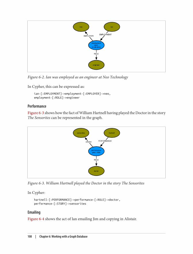
Figure 6-2. Ian was employed as an engineer at Neo Technology

In Cypher, this can be expressed as:

ian-[:EMPLOYMENT]->employment-[:EMPLOYER]->neo,employment-[:ROLE]->engineer

PerformanceFigure 6-3 shows how the fact of William Hartnell having played the Doctor in the storyThe Sensorites can be represented in the graph.

Figure 6-3. William Hartnell played the Doctor in the story The Sensorites

In Cypher:

hartnell-[:PERFORMANCE]->performance-[:ROLE]->doctor,performance-[:STORY]->sensorites

EmailingFigure 6-4 shows the act of Ian emailing Jim and copying in Alistair.


Figure 6-4. Ian emailed Jim, and copied in Alistair

In Cypher, this can be expressed as:

ian-[:SENT]->email-[:TO]->jim,email-[:CC]->alistair

ReviewingFigure 6-5 shows how the act of Alistair reviewing a film can be represented in the graph.

Figure 6-5. Alistair wrote a review of a film, which was published in a magazine

In Cypher:

alistair-[:WROTE]->review-[:OF]->film,review-[:PUBLISHED_IN]->magazine

Represent Complex Value Types as NodesValue types are things that do not have an identity, and whose equivalence is based solelyon their values. Examples include money, address, and SKU. Complex value types are

Data Modeling | 109

value types with more than one field or property. Address, for example, is a complexvalue type. Such multi-property value types are best represented as separate nodes:

START ord=node:orders(orderid={orderId})MATCH ord-[:DELIVERY_ADDRESS]->addressRETURN address.first_line, address.zipcode

TimeTime can be modelled in several different ways in the graph. Here we describe twotechniques: timeline trees and linked lists.

Timeline treesIf you need to find all the events that have occurred over a specific period, you can builda timeline tree, as shown in Figure 6-6:

Figure 6-6. A timeline tree showing the broadcast dates for four episodes of a TV pro‐gramme

You need only insert nodes into the timeline tree as and when they are needed. Assumingthe root timeline node has been indexed, or is in some other way discoverable, thefollowing Cypher statement will insert all necessary nodes—year, month, day, plus thenode to be attached to the timeline:


START timeline=node:timeline(name={timelineName})CREATE UNIQUE timeline-[:YEAR]->(year{value:{year}, name:{yearName}}) -[:MONTH]->(month{value:{month}, name:{monthName}}) -[:DAY]->(day{value:{day}, name:{dayName}}) <-[:BROADCAST_ON]-(n {newNode})

Querying the calendar for all events between a start date (inclusive) and an end date(exclusive) can be done with the following Cypher:

START timeline=node:timeline(name={timelineName})MATCH timeline-[:YEAR]->year-[:MONTH]->month-[:DAY]->day<-[:BROADCAST_ON]-nWHERE ((year.value > {startYear} AND year.value < {endYear}) OR ({startYear} = {endYear} AND {startMonth} = {endMonth} AND year.value = {startYear} AND month.value = {startMonth} AND day.value >= {startDay} AND day.value < {endDay}) OR ({startYear} = {endYear} AND {startMonth} < {endMonth} AND year.value = {startYear} AND ((month.value = {startMonth} AND day.value >= {startDay}) OR (month.value > {startMonth} AND month.value < {endMonth}) OR (month.value = {endMonth} AND day.value < {endDay}))) OR ({startYear} < {endYear} AND year.value = {startYear} AND ((month.value > {startMonth}) OR (month.value = {startMonth} AND day.value >= {startDay}))) OR ({startYear} < {endYear} AND year.value = {endYear} AND ((month.value < {endMonth}) OR (month.value = {endMonth} AND day.value < {endDay}))))RETURN n

The WHERE clause here, though somewhat verbose, simply filters each match based onthe start and end dates supplied to the query.

Linked listsMany events have temporal relationships to the events that precede and follow them.You can use NEXT and PREVIOUS relationships (or similar) to create linked lists thatcapture this natural ordering, as shown in Figure 6-7. Linked lists allow for very rapidtraversal of time-ordered events.

Figure 6-7. A doubly linked list representing a time-ordered series of events

Data Modeling | 111

2. See, for example, https://github.com/dmontag/neo4j-versioning, which hooks into Neo4j’s transaction lifecycleto created versioned copies of nodes and relationships.

VersioningA versioned graph allows you to recover the state of the graph at a particular point intime. Neo4j doesn’t support versioning as a first-class concept: it is possible, however,to create a versioning scheme inside the graph model whereby nodes and relationshipsare timestamped and archived whenever they are modified.2 The downside of suchversioning schemes is they leak into any queries written against the graph, adding alayer of complexity to even the simplest query.

Iterative and Incremental DevelopmentDevelop the data model feature by feature, user story by user story. This will ensure youidentify the relationships your application will use to query the graph. A data modelthat is developed in line with the iterative and incremental delivery of application fea‐tures will look quite different from one drawn up using data model-first approach, butit will be the correct model, motivated throughout by specific needs, and the questionsthat arise in conjunction with those needs.

Graph databases provide for the smooth evolution of your data model. Migrations anddenormalization are rarely an issue. New facts and new compositions become new nodesand relationships, while optimizing for performance-critical access patterns typicallyinvolves introducing a direct relationship between two nodes that would otherwise beconnected only by way of intermediaries. Unlike the relational model, this is not aneither/or issue: either the high-fidelity structure, or the high performance compromise.With the graph we retain the original high-fidelity graph structure while at the sametime enriching it with new elements that cater to new needs.

You’ll quickly see how different relationships can sit side-by-side with one another,catering to different needs without distorting the model in favour of any one particularneed. Addresses help illustrate the point here. Imagine, for example, that we are devel‐oping a retail application. While developing a fulfilment story, we add the ability todispatch a parcel to a customer’s delivery address, which we find using the followingquery:

START user=node:users(id={userId})MATCH user-[:DELIVERY_ADDRESS]->addressRETURN address

Later on, when adding some billing functionality, we introduce a BILLING_ADDRESSrelationship. Later still, we add the ability for customers to manage all their addresses.This last feature requires us to find all addresses—whether delivery, or billing, or someother address. To facilitate this, we introduce a general ADDRESS relationship:


https://github.com/dmontag/neo4j-versioning

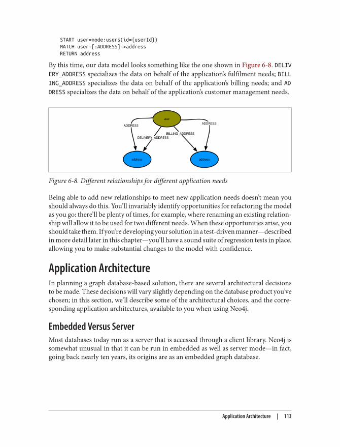
START user=node:users(id={userId})MATCH user-[:ADDRESS]->addressRETURN address

By this time, our data model looks something like the one shown in Figure 6-8. DELIVERY_ADDRESS specializes the data on behalf of the application’s fulfilment needs; BILLING_ADDRESS specializes the data on behalf of the application’s billing needs; and ADDRESS specializes the data on behalf of the application’s customer management needs.

Figure 6-8. Different relationships for different application needs

Being able to add new relationships to meet new application needs doesn’t mean youshould always do this. You’ll invariably identify opportunities for refactoring the modelas you go: there’ll be plenty of times, for example, where renaming an existing relation‐ship will allow it to be used for two different needs. When these opportunities arise, youshould take them. If you’re developing your solution in a test-driven manner—describedin more detail later in this chapter—you’ll have a sound suite of regression tests in place,allowing you to make substantial changes to the model with confidence.

Application ArchitectureIn planning a graph database-based solution, there are several architectural decisionsto be made. These decisions will vary slightly depending on the database product you’vechosen; in this section, we’ll describe some of the architectural choices, and the corre‐sponding application architectures, available to you when using Neo4j.

Embedded Versus ServerMost databases today run as a server that is accessed through a client library. Neo4j issomewhat unusual in that it can be run in embedded as well as server mode—in fact,going back nearly ten years, its origins are as an embedded graph database.

Application Architecture | 113

3. See http://docs.neo4j.org/chunked/stable/transactions-events.html

An embedded database is not the same as an in-memory database. Anembedded instance of Neo4j still makes all data durable on disk. Later,in the “Testing” section, we’ll discuss ImpermanentGraphDatabase,which is an in-memory version of Neo4j designed for testing purposes.

Embedded Neo4jIn embedded mode, Neo4j runs in the same process as your application. EmbeddedNeo4j is ideal for hardware devices, desktop applications, and for incorporating in yourown application servers. Some of the advantages of embedded mode include:

• Low latency. Because your application speaks directly to the database, there’s nonetwork overhead.

• Choice of APIs. You have access to the full range of APIs for creating and queryingdata: the core API, traversal framework, and the Cypher query language.

• Explicit transactions. Using the core API, you can control the transactional lifecycle,executing an arbitrarily complex sequence of commands against the database inthe context of a single transaction. The Java APIs also expose the transaction life‐cycle, allowing you to plug in custom transaction event handlers that execute ad‐ditional logic with each transaction.3

• Named indexes. Embedded mode gives you full control over the creation and man‐agement of named indexes. This functionality is also available through the RESTinterface; it is not, however, available in Cypher.

When running in embedded mode, however, you should bear in mind the following:

• JVM only. Neo4j is a JVM-based database. Many of its APIs are, therefore, onlyaccessible from a JVM-based language.

• GC behaviours. When running in embedded mode, Neo4j is subject to the garbagecollection behaviours of the host application. Long GC pauses can effect on querytimes. Further, when running an embedded instance as part of an HA cluster, longGC pauses can cause the cluster protocol to trigger a master reelection.

• Database lifecycle. The application is responsible for controlling the database life‐cycle, which includes starting it, and closing it safely.

Embedded Neo4j can be clustered for high availability and horizontal read scaling justas the server version. In fact, you can run a mixed cluster of embedded and serverinstances (clustering is performed at the database level, rather than the server level).This is common in enterprise integration scenarios, where regular updates from other


http://docs.neo4j.org/chunked/stable/transactions-events.html

4. A list of Neo4j remote client libraries, as developed by the community, is maintained at http://docs.neo4j.org/chunked/stable/tutorials-rest.html

systems are executed against an embedded instance, and then replicated out to serverinstances.

Server modeRunning Neo4j in server mode is the most common means of deploying the databasetoday. At the heart of each server is an embedded instance of Neo4j. Some of the benefitsof server mode include:

• REST API. The server exposes a rich REST API that allows clients to send JSON-formatted requests over HTTP. Responses comprise JSON-formatted documentsenriched with hypermedia links that advertise additional features of the dataset.

• Platform independence. Because access is by way of JSON-formatted documentssent over HTPP, a Neo4j server can be accessed by a client running on practicallyany platform. All that’s needed is an HTTP client library.4

• Scaling independence. With Neo4j running in server mode, you can scale yourdatabase cluster independently of your application server cluster.

• Isolation from application GC behaviours. In server mode, Neo4j is protected fromany untoward GC behaviours triggered by the rest of the application. Of course,Neo4j still produces some garbage, but its impact on the garbage collector has beencarefully monitored and tuned during development to mitigate any significant sideeffects. Note, however, that because server extensions allow you to run arbitraryJava code inside the server (see “Server extensions” later in this section), the use ofserver extensions may impact the server’s GC behaviour.

When using Neo4j in server mode, bear in mind the following:

• Network overhead. There is some communication overhead to each HTTP request,though it’s fairly minimal. After the first client request, the TCP connection remainsopen until closed by the client.

• Per request transactions. Each client request is executed in the context of a separatetransaction, though there is some support in the REST API for batch operations.For more complex, multistep operations requiring a single transactional context,consider using a server extension (see “Server extensions” later in this section).

Access to Neo4j server is typically by way of its REST API, as discussed above. The RESTAPI comprises JSON-formatted documents over HTTP. Using the REST API you cansubmit Cypher queries, configure named indexes, and execute several of the built-ingraph algorithms. You can also submit JSON-formatted traversal descriptions, and per‐


http://docs.neo4j.org/chunked/stable/tutorials-rest.html

http://docs.neo4j.org/chunked/stable/tutorials-rest.html

5. See http://docs.neo4j.org/chunked/stable/rest-api.html

6. See http://jax-rs-spec.java.net/

form batch operations. 5 For the majority of use cases the REST API is sufficient; how‐ever, if you need to do something you cannot currently accomplish using the REST API,you may wish to consider developing a server extension.

Server extensionsServer extensions allow you to run Java code inside the server. Using server extensions,you can extend the REST API, or replace it entirely.

Extensions take the form of JAX-RS annotated classes. JAX-RS is a Java API for buildingRESTful resources.6 Using JAX-RS annotations, you decorate each extension class toindicate to the server which HTTP requests it handles. Additional annotations controlrequest and response formats, HTTP headers, and the formatting of URI templates.

Here’s an implementation of a simple server extension that allows a client to request thedistance between two members of a social network:

@Path("/distance")public class SocialNetworkExtension{ private final ExecutionEngine executionEngine;

public SocialNetworkExtension( @Context GraphDatabaseService db ) { this.executionEngine = new ExecutionEngine( db ); }

@GET @Produces("text/plain") @Path("/{name1}/{name2}") public String getDistance ( @PathParam("name1") String name1, @PathParam("name2") String name2 ) { String query = "START first=node:user(name={name1}),\n" + " second=node:user(name={name2})\n" + "MATCH p=shortestPath(first-[*..4]-second)\n" + "RETURN length(p) AS depth";

Map<String, Object> params = new HashMap<String, Object>(); params.put( "name1", name1 ); params.put( "name2", name2 );

ExecutionResult result = executionEngine.execute( query, params );

return String.valueOf( result.columnAs( "depth" ).next() );


http://docs.neo4j.org/chunked/stable/rest-api.html

http://jax-rs-spec.java.net/

}}

Of particular interest here are the various annotations:

• @Path("/distance") specifies that this extension will respond to requests directedto relative URIs beginning /distance.

• The @Path("/{name1}/{name2}") annotation on getDistance() further qualifiesthe URI template associated with this extension. The fragment here is concatenatedwith /distance to produce /distance/{name1}/{name2}, where {name1} and {name2}are placeholders for any characters occurring between the forward slashes. Lateron, in the section “Testing server extensions”, we’ll register this extension underthe /socnet relative URI. At that point, these several different parts of the path ensurethat HTTP requests directed to a relative URI beginning /socnet/distance/{name1}/{name2} (for example, http://<server>/socnet/distance/Ben/Mike) will be dispatch‐ed to an instance of this extension.

• @GET specifies that getDistance() should be invoked only if the request is an HTTPGET. @Produces indicates that the response entity body will be formatted as text/plain.

• The two @PathParam annotations prefacing the parameters to getDistance() serveto map the contents of the {name1} and {name2} path placeholders to the method’sname1 and name2 parameters. Given the URI http://<server>/socnet/distance/Ben/Mike, getDistance() will be invoked with Ben for name1 and Mike for name2.

• The @Context annotation in the constructor causes this extension to be handed areference to the embedded graph database inside the server. The server infrastruc‐ture takes care of creating an extension and injecting it with a graph database in‐stance, but the very presence of the GraphDatabaseService parameter here makesthis extension exceedingly testable. As we’ll see later, in “Testing server extensions”,we can unit test extensions without having to run them inside a server.

Server extensions can be powerful elements in your application architecture. Their chiefbenefits include:

• Complex transactions. Extensions allow you to execute an arbitrarily complex se‐quence of operations in the context of a single transaction.

• Choice of APIs. Each extension is injected with a reference to the embedded graphdatabase at the heart of the server. This gives you access to the full range of APIs—core API, traversal framework, graph algorithm package, and Cypher—for devel‐oping your extension’s behaviour.

• Encapsulation. Because each extension is hidden behind a RESTful interface, youcan improve and modify its implementation over time.


7. See http://docs.neo4j.org/chunked/milestone/ha-configuration.html

• Response formats. You control the response: both the representation format andthe HTTP headers. This allows you to create response messages whose contentsemploy terminology from your domain, rather than the graph-based terminologyof the standard REST API (users, products and orders for example, rather thannodes, relationships and properties). Further, in controlling the HTTP headers at‐tached to the response, you can leverage the HTTP protocol for things such ascaching and conditional requests.

If you’re considering using server extensions, bear in mind the following points:

• JVM only. As with developing against embedded Neo4j, you’ll have to use a JVM-based language.

• GC behaviours. You can do arbitrarily complex (and dangerous) things inside aserver extension. Monitor garbage collection behaviours to ensure you don’t in‐troduce any untoward side effects.

ClusteringAs discussed in “Availability” in Chapter 5, Neo4j clusters for high availability and hor‐izontal read scaling using master-slave replication. In this section we discuss some ofthe strategies you should consider when using clustered Neo4j.

ReplicationWhile all writes to a cluster are coordinated through the master, Neo4j does allow writingthrough slaves, but even then, the slave syncs with the master before returning to theclient. Because of the additional network traffic and coordination protocol, writingthrough slaves can be an order of magnitude slower than writing direct to the master.The only reasons for writing through slaves are to increase the durability guarantees ofeach write (the write is made durable on two instances, rather than one) and to ensureyou can read your own writes when employing cache sharding (see “Cache sharding”and “Read your won writes” later in this chapter). Since newer versions of Neo4j allowyou to specify that writes to the master must be replicated out to one or more slaves,thereby increasing the durability guarantees of writes to the master, the case for writingthrough slaves is now less compelling. Today it is recommended that all writes be di‐rected to the master, and then replicated to slaves using the ha.tx_push_factor andha.tx_push_strategy configuration settings.7


http://docs.neo4j.org/chunked/milestone/ha-configuration.html

Buffer writes using queuesIn high write load scenarios, use queues to buffer writes and regulate load. With thisstrategy, writes to the cluster are buffered in a queue; a worker then polls the queue andexecutes batches of writes against the database. Not only does this regulate write traffic,it reduces contention, and allows you to pause write operations without refusing clientrequests during maintenance periods.

Global clustersFor applications catering to a global audience, it is possible to install a multi-regioncluster in multiple datacenters and on cloud platforms such as Amazon Web Services(AWS). A multi-region cluster allows you to service reads from the portion of the clustergeographically closest to the client. In these situations, however, the latency introducedby the physical separation of the regions can sometimes disrupt the coordination pro‐tocol; it is, therefore, often desirable to restrict master reelection to a single region. Toachieve this, create slave-only databases for the instances you don’t want to participatein master reelection; you do this by including the ha.slave_coordinator_update_mode=none configuration parameter in an instance’s configuration.

Load BalancingIf you’re using a clustered graph database, consider load balancing traffic across thecluster to help maximize throughput and reduce latency. Neo4j doesn’t include a nativeload balancer, relying instead on the load balancing capabilities of the network infra‐structure.

Separate read traffic from write trafficGiven the recommendation to direct the majority of write traffic to the master, youshould consider clearly separating read requests from write requests. Configure yourload balancer to direct write traffic to the master, while balancing the read traffic acrossthe entire cluster.

In a Web-based application, the HTTP method is often sufficient to distinguish a requestwith a significant side-effect—a write—from one that has no significant side-effect onthe server: POST, PUT and DELETE can modify server-side resources, whereas GETis side-effect free.

If you’re using server extensions, make sure to distinguish read and write operationsusing @GET and @POST annotations. If your application depends solely on server exten‐sions, this will suffice to separate the two. If you’re using the REST API to submit Cypherqueries to the database, however, the situation is not so straightforward. The REST APIuses POST as a general “process this” semantic for requests whose contents can includeCypher statements that modify the database. To separate read and write requests in thisscenario, introduce a pair of load balancers: a write load balancer that always directs


requests to the master, and a read load balancer that balances requests across the entirecluster. In your application logic, where you know whether the operation is a read or awrite, you will then have to decide which of the two addresses you should use for anyparticular request, as illustrated in Figure 6-9.

When running in server mode, Neo4j exposes a URI that indicates whether that instanceis currently the master, and if it isn’t, which is. Load balancers can poll this URI atintervals to determine where to route traffic.

Figure 6-9. Using read/write load balancers to direct requests to a cluster

Cache shardingQueries run fastest when the portions of the graph needed to satisfy them reside in mainmemory (that is, in the filesystem cache and the object cache). A single graph databaseinstance today can hold many billions of nodes, relationships and properties; somegraphs, therefore, will be just too big to fit into main memory. Partitioning or sharding


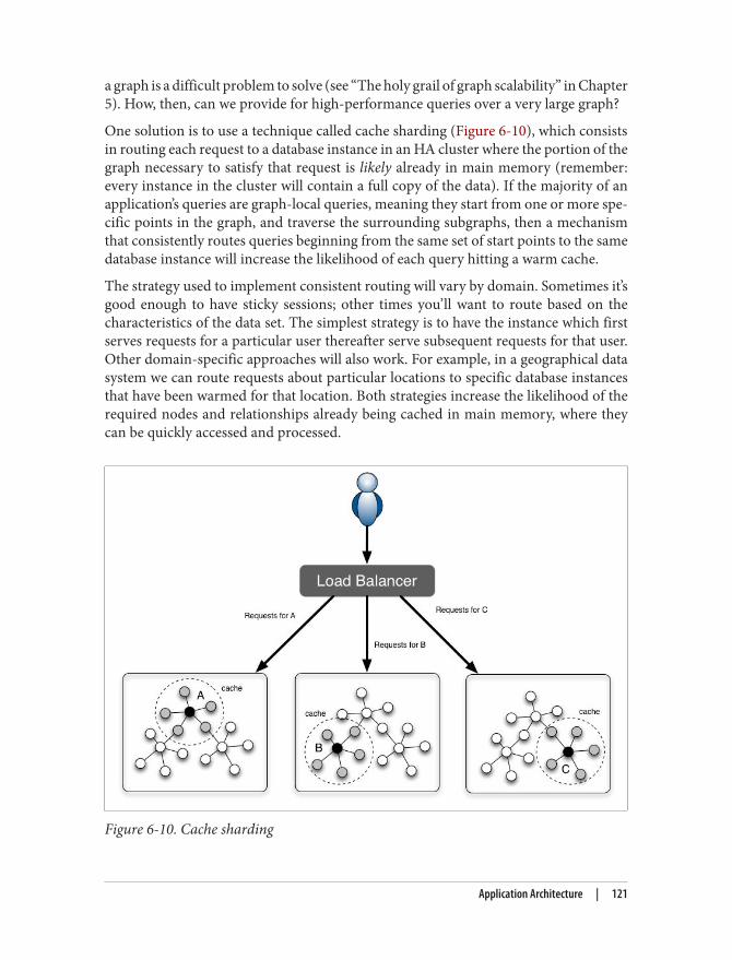
a graph is a difficult problem to solve (see “The holy grail of graph scalability” in Chapter5). How, then, can we provide for high-performance queries over a very large graph?

One solution is to use a technique called cache sharding (Figure 6-10), which consistsin routing each request to a database instance in an HA cluster where the portion of thegraph necessary to satisfy that request is likely already in main memory (remember:every instance in the cluster will contain a full copy of the data). If the majority of anapplication’s queries are graph-local queries, meaning they start from one or more spe‐cific points in the graph, and traverse the surrounding subgraphs, then a mechanismthat consistently routes queries beginning from the same set of start points to the samedatabase instance will increase the likelihood of each query hitting a warm cache.

The strategy used to implement consistent routing will vary by domain. Sometimes it’sgood enough to have sticky sessions; other times you’ll want to route based on thecharacteristics of the data set. The simplest strategy is to have the instance which firstserves requests for a particular user thereafter serve subsequent requests for that user.Other domain-specific approaches will also work. For example, in a geographical datasystem we can route requests about particular locations to specific database instancesthat have been warmed for that location. Both strategies increase the likelihood of therequired nodes and relationships already being cached in main memory, where theycan be quickly accessed and processed.

Figure 6-10. Cache sharding


Read your own writesOccasionally you may need to read your own writes—typically when the applicationapplies an end-user change, and needs on the next request to reflect the effect of thischange back to the user. While writes to the master are immediately consistent, thecluster as a whole is eventually consistent. How can we ensure that a write directed tothe master is reflected in the next load-balanced read request? One solution is to usethe same consistent routing technique used in cache sharding to direct the write to theslave that will be used to service the subsequent read. This assumes that the write andthe read can be consistently routed based on some domain criteria in each request.

This is one of the few occasions where it makes sense to write through a slave. Butremember: writing through a slave can be an order of magnitude slower than writingdirect to the master. Use this technique sparingly. If a high proportion of your writesrequire you to read your own write, this technique will significantly impact throughputand latency.

TestingTesting is a fundamental part of the application development process—not only as ameans of verifying that a query or application feature behaves correctly, but also as away of designing and documenting your application and its data model. Throughoutthis section we emphasize that testing is an everyday activity; by developing your graphdatabase solution in a test-driven manner, you provide for the rapid evolution of yoursystem, and its continued responsiveness to new business needs.

Test-Driven Data Model DevelopmentIn discussing data modeling, we’ve stressed that your graph model should reflect thekinds of queries you want to run against it. By developing your data model in a test-driven fashion you document your understanding of your domain, and validate thatyour queries behave correctly.

With test-driven data modeling, you write unit tests based on small, representativeexample graphs drawn from your domain. These example graphs contain just enoughdata to communicate a particular feature of the domain; in many cases, they might onlycomprise ten or so nodes, plus the relationships that connect them. Use these examplesto describe what is normal for the domain, and also what is exceptional. As you discoveranomalies and corner cases in your real data, write a test that reproduces what you’vediscovered.

The example graphs you create for each test comprise the setup or context for that test.Within this context you exercise a query, and assert that the query behaves as expected.Because you control the context, you, as the author of the test, know what results toexpect.


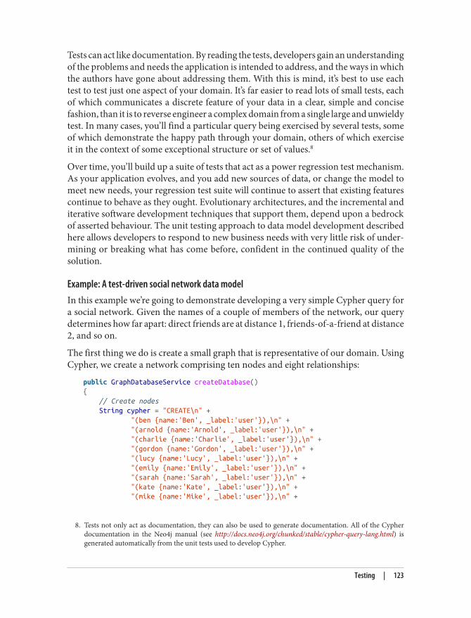
8. Tests not only act as documentation, they can also be used to generate documentation. All of the Cypherdocumentation in the Neo4j manual (see http://docs.neo4j.org/chunked/stable/cypher-query-lang.html) isgenerated automatically from the unit tests used to develop Cypher.

Tests can act like documentation. By reading the tests, developers gain an understandingof the problems and needs the application is intended to address, and the ways in whichthe authors have gone about addressing them. With this is mind, it’s best to use eachtest to test just one aspect of your domain. It’s far easier to read lots of small tests, eachof which communicates a discrete feature of your data in a clear, simple and concisefashion, than it is to reverse engineer a complex domain from a single large and unwieldytest. In many cases, you’ll find a particular query being exercised by several tests, someof which demonstrate the happy path through your domain, others of which exerciseit in the context of some exceptional structure or set of values.8

Over time, you’ll build up a suite of tests that act as a power regression test mechanism.As your application evolves, and you add new sources of data, or change the model tomeet new needs, your regression test suite will continue to assert that existing featurescontinue to behave as they ought. Evolutionary architectures, and the incremental anditerative software development techniques that support them, depend upon a bedrockof asserted behaviour. The unit testing approach to data model development describedhere allows developers to respond to new business needs with very little risk of under‐mining or breaking what has come before, confident in the continued quality of thesolution.

Example: A test-driven social network data modelIn this example we’re going to demonstrate developing a very simple Cypher query fora social network. Given the names of a couple of members of the network, our querydetermines how far apart: direct friends are at distance 1, friends-of-a-friend at distance2, and so on.

The first thing we do is create a small graph that is representative of our domain. UsingCypher, we create a network comprising ten nodes and eight relationships:

public GraphDatabaseService createDatabase(){ // Create nodes String cypher = "CREATE\n" + "(ben {name:'Ben', _label:'user'}),\n" + "(arnold {name:'Arnold', _label:'user'}),\n" + "(charlie {name:'Charlie', _label:'user'}),\n" + "(gordon {name:'Gordon', _label:'user'}),\n" + "(lucy {name:'Lucy', _label:'user'}),\n" + "(emily {name:'Emily', _label:'user'}),\n" + "(sarah {name:'Sarah', _label:'user'}),\n" + "(kate {name:'Kate', _label:'user'}),\n" + "(mike {name:'Mike', _label:'user'}),\n" +

Testing | 123

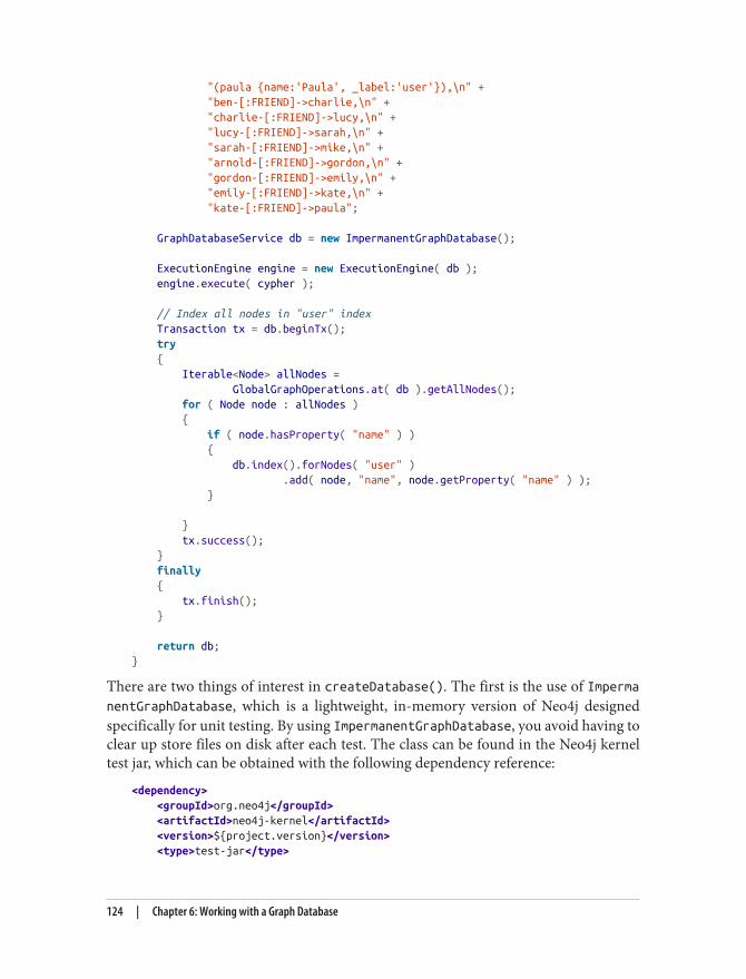
http://docs.neo4j.org/chunked/stable/cypher-query-lang.html

"(paula {name:'Paula', _label:'user'}),\n" + "ben-[:FRIEND]->charlie,\n" + "charlie-[:FRIEND]->lucy,\n" + "lucy-[:FRIEND]->sarah,\n" + "sarah-[:FRIEND]->mike,\n" + "arnold-[:FRIEND]->gordon,\n" + "gordon-[:FRIEND]->emily,\n" + "emily-[:FRIEND]->kate,\n" + "kate-[:FRIEND]->paula";

GraphDatabaseService db = new ImpermanentGraphDatabase();

ExecutionEngine engine = new ExecutionEngine( db ); engine.execute( cypher );

// Index all nodes in "user" index Transaction tx = db.beginTx(); try { Iterable<Node> allNodes = GlobalGraphOperations.at( db ).getAllNodes(); for ( Node node : allNodes ) { if ( node.hasProperty( "name" ) ) { db.index().forNodes( "user" ) .add( node, "name", node.getProperty( "name" ) ); }

} tx.success(); } finally { tx.finish(); }

return db;}

There are two things of interest in createDatabase(). The first is the use of ImpermanentGraphDatabase, which is a lightweight, in-memory version of Neo4j designedspecifically for unit testing. By using ImpermanentGraphDatabase, you avoid having toclear up store files on disk after each test. The class can be found in the Neo4j kerneltest jar, which can be obtained with the following dependency reference:

<dependency> <groupId>org.neo4j</groupId> <artifactId>neo4j-kernel</artifactId> <version>${project.version}</version> <type>test-jar</type>


<scope>test</scope></dependency>

ImpermanentGraphDatabase should only be used in unit tests. It is nota production-ready, in-memory version of Neo4j.

The second thing of interest in createDatabase() is the code for adding nodes to anamed index. Cypher doesn’t add the newly created nodes to an index, so for now, wehave to do this manually by iterating all the nodes in the sample graph, adding any witha name property to the users named index.

Having created a sample graph, we can now write our first test. Here’s the test fixturefor testing our social network data model and its queries:

public class SocialNetworkTest{ private static GraphDatabaseService db; private static SocialNetworkQueries queries;

@BeforeClass public static void init() { db = createDatabase(); queries = new SocialNetworkQueries( db ); }

@AfterClass public static void shutdown() { db.shutdown(); }

@Test public void shouldReturnShortestPathBetweenTwoFriends() throws Exception { // when ExecutionResult results = queries.distance( "Ben", "Mike" );

// then assertTrue( results.iterator().hasNext() ); assertEquals( 4, results.iterator().next().get( "distance" ) ); }

// more tests}

This test fixture includes an initialization method, annotated with @BeforeClass, whichexecutes before any tests start. Here we call createDatabase() to create an instance of

Testing | 125

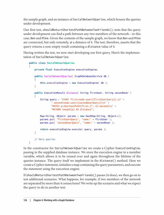
the sample graph, and an instance of SocialNetworkQueries, which houses the queriesunder development.

Our first test, shouldReturnShortestPathBetweenTwoFriends(), tests that the queryunder development can find a path between any two members of the network—in thiscase, Ben and Mike. Given the contents of the sample graph, we know that Ben and Mikeare connected, but only remotely, at a distance of 4. The test, therefore, asserts that thequery returns a non-empty result containing a distance value of 4.

Having written the test, we now start developing our first query. Here’s the implemen‐tation of SocialNetworkQueries:

public class SocialNetworkQueries{ private final ExecutionEngine executionEngine;

public SocialNetworkQueries( GraphDatabaseService db ) { this.executionEngine = new ExecutionEngine( db ); }

public ExecutionResult distance( String firstUser, String secondUser ) { String query = "START first=node:user({firstUserQuery}),\n" + " second=node:user({secondUserQuery})\n" + "MATCH p=shortestPath(first-[*..4]-second)\n" + "RETURN length(p) AS distance";

Map<String, Object> params = new HashMap<String, Object>(); params.put( "firstUserQuery", "name:" + firstUser ); params.put( "secondUserQuery", "name:" + secondUser );

return executionEngine.execute( query, params ); }

// More queries}

In the constructor for SocialNetworkQueries we create a Cypher ExecutionEngine,passing in the supplied database instance. We store the execution engine in a membervariable, which allows it to be reused over and again throughout the lifetime of thequeries instance. The query itself we implement in the distance() method. Here wecreate a Cypher statement, initialize a map containing the query parameters, and executethe statement using the execution engine.

If shouldReturnShortestPathBetweenTwoFriends() passes (it does), we then go on totest additional scenarios. What happens, for example, if two members of the networkare separated by more than 4 connections? We write up the scenario and what we expectthe query to do in another test:


@Testpublic void shouldReturnNoResultsWhenNoPathUnderAtDistance4OrLess() throws Exception{ // when ExecutionResult results = queries.distance( "Ben", "Arnold" );

// then assertFalse( results.iterator().hasNext() );}

In this instance, this second test passes without us having to modify the underlyingCypher query. In many cases, however, a new test will force you to modify a query’simplementation. When that happens, modify the query to make the new test pass, andthen run all the tests in the fixture. A failing test anywhere in the fixture indicates you’vebroken some existing functionality. Continue to modfy the query until all tests are greenonce again.

Testing server extensionsServer extensions can be developed in a test-driven manner just as easily as embeddedNeo4j. Using the simple server extension described earlier, here’s how we test it:

@Testpublic void extensionShouldReturnDistance() throws Exception{ // given SocialNetworkExtension extension = new SocialNetworkExtension( db );

// when String distance = extension.getDistance( "Ben", "Mike" );

// then assertEquals( "4", distance );}

Because the extension’s constructor accepts a GraphDatabaseService instance, we caninject a test instance (an ImpermanentGraphDatabase instance), and then call its meth‐ods as per any other object.

If, however, we wanted to test the extension running inside a server, we have a littlemore setup to do:

public class SocialNetworkExtensionTest{ private static CommunityNeoServer server;

@BeforeClass public static void init() throws IOException { server = ServerBuilder.server() .withThirdPartyJaxRsPackage(

Testing | 127

9. See http://jersey.java.net/

"org.neo4j.graphdatabases.queries.server", "/socnet" ) .build(); server.start(); populateDatabase( server.getDatabase().getGraph() ); }

@AfterClass public static void teardown() { server.stop(); }

@Test public void serverShouldReturnDistance() throws Exception { ClientConfig config = new DefaultClientConfig(); Client client = Client.create( config );

WebResource resource = client .resource( "http://localhost:7474/socnet/distance/Ben/Mike" ); ClientResponse response = resource .accept( MediaType.TEXT_PLAIN ) .get( ClientResponse.class );

assertEquals( 200, response.getStatus() ); assertEquals( "text/plain", response.getHeaders().get( "Content-Type" ).get( 0 ) ); assertEquals( "4", response.getEntity( String.class ) ); }

// Populate graph

}

Here we’re using an instance of CommunityNeoServer to host the extension. We createthe server and populate its database in the test fixture’s init() method using a ServerBuilder, which is a helper class from Neo4j’s server test jar. This builder allows us toregister the extension package, and associate it with a relative URI space (in this case,everything below /socnet). Once init() has completed, we have a server instance upand running and listening on port 7474.

In the test itself, serverShouldReturnDistance(), we access this server using an HTTPclient from the Jersey client library.9 The client issues an HTTP GET request for theresource at http://localhost:7474/socnet/distance/Ben/Mike. (At the server end, this re‐quest is dispatched to an instance of SocialNetworkExtension.) When the client re‐


http://jersey.java.net/

http://localhost:7474/socnet/distance/Ben/Mike

ceives a response, the test asserts that the HTTP status code, content-type, and contentof the response body are correct.

Performance TestingThe test-driven approach that we’ve described so far communicates context and domainunderstanding, and tests for correctness. It does not, however, test for performance.What works fast against a small, twenty node sample graph may not work so well whenconfronted with a much larger graph. Therefore, to accompany your unit tests, youshould consider writing a suite of query performance tests. On top of that, you shouldalso invest in some thorough application performance testing early in your application’sdevelopment lifecycle.

Query performance testsQuery performance tests are not the same as full-blown application performance tests.All we’re interested in at this stage is whether a particular query performs well whenrun against a graph that is proportionate to the kind of graph you expect to encounterin production. Ideally, these tests are developed side-by-side with your unit tests. There’snothing worse than investing a lot of time in perfecting a query, only to discover it isnot fit for production-sized data.

When creating query performance tests, bear in mind the following guidelines:

• Create a suite of performance tests that exercise the queries developed through yourunit testing. Record the performance figures so that you can see the relative effectsof tweaking a query, modifying the heap size, or upgrading from one version ofNeo4j to another.

• Run these tests often, so that you quickly become aware of any deterioration inperformance. You might consider incorporating these tests into a continuous de‐livery build pipeline, failing the build if the test results exceed a certain value.

• You can run these tests in-process on a single thread. There’s no need to simulatemultiple clients at this stage: if the performance is poor for a single client, it’s unlikelyto improve for multiple clients. Even though they are not strictly speaking unit tests,you can drive them using the same unit testing framework you use to develop yourunit tests.

• Run each query many times, picking starting nodes at random each time, so thatyou can see the effect of starting from a cold cache, which is then gradually warmedas multiple queries execute.

Testing | 129

10. A thorough discussion of agile performance testing can be found in Alistair Jones and Patrick Kua, “ExtremePerformance Testing”, The ThoughtWorks Anthology, Volume 2 (Pragmatic Bookshelf, 2012)

11. See http://grinder.sourceforge.net/, http://jmeter.apache.org/ and http://gatling-tool.org/. Max De Marzi de‐scribes using Gatling to test Neo4j here: http://maxdemarzi.com/2013/02/14/neo4j-and-gatling-sitting-in-a-tree-performance-t-e-s-t-ing/

Application performance testsApplication performance tests, as distinct from query performance tests, test the per‐formance of the entire application under representative production usage scenarios.

As with query performance tests, we recommend that this kind of performance testingis done as part of everyday development, side-by-side with the development of appli‐cation features, rather than as a distinct project phase.10 To facilitate application per‐formance testing early in the project lifecycle, it is often necessary to develop a “walkingskeleton”, an end-to-end slice through the entire system, which can be accessed andexercised by performance test clients. By developing a walking skeleton, you not onlyprovide for performance testing, you also establish the architectural context for thegraph database part of your solution. This allows you to verify your application archi‐tecture, and identify layers and abstractions that allow for discrete testing of individualcomponents.

Performance tests serve two purposes: they demonstrate how the system will performwhen used in production, and they drive out the operational affordances that make iteasier to diagnose performance issues, incorrect behaviour, and bugs. What you learnin creating and maintaining a performance test environment will prove invaluable whenit comes to deploying and operating the system for real.

As with your unit tests and query performance tests, application performance testsprove most valuable when employed in an automated delivery pipeline, where succes‐sive builds of the application are automatically deployed to a testing environment, thetests executed, and the results automatically analyzed. Log files and test results shouldbe stored for later retrieval, analysis and comparison. Regressions and failures shouldfail the build, prompting developers to address the issues in a timely manner. One ofthe big advantages of conducting performance testing over the course of an application’sdevelopment lifecycle, rather than at the end, is that failures and regressions can veryoften be tied back to a recent piece of development; this allows you to diagnose, pinpointand remedy issues rapidly and succinctly.

For generating load, you’ll need a load-generating agent. For Web applications, thereare several open source stress and load testing tools available, including Grinder, JMeterand Gatling.11 When testing load balanced Web applications, you should ensure yourtest clients are distributed across different IP addresses so that requests are balancedacross the cluster.


http://grinder.sourceforge.net/

http://jmeter.apache.org/

http://gatling-tool.org/

http://maxdemarzi.com/2013/02/14/neo4j-and-gatling-sitting-in-a-tree-performance-t-e-s-t-ing/

http://maxdemarzi.com/2013/02/14/neo4j-and-gatling-sitting-in-a-tree-performance-t-e-s-t-ing/

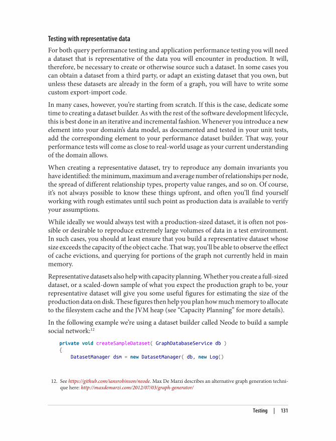
12. See https://github.com/iansrobinson/neode. Max De Marzi describes an alternative graph generation techni‐que here: http://maxdemarzi.com/2012/07/03/graph-generator/

Testing with representative dataFor both query performance testing and application performance testing you will needa dataset that is representative of the data you will encounter in production. It will,therefore, be necessary to create or otherwise source such a dataset. In some cases youcan obtain a dataset from a third party, or adapt an existing dataset that you own, butunless these datasets are already in the form of a graph, you will have to write somecustom export-import code.

In many cases, however, you’re starting from scratch. If this is the case, dedicate sometime to creating a dataset builder. As with the rest of the software development lifecycle,this is best done in an iterative and incremental fashion. Whenever you introduce a newelement into your domain’s data model, as documented and tested in your unit tests,add the corresponding element to your performance dataset builder. That way, yourperformance tests will come as close to real-world usage as your current understandingof the domain allows.

When creating a representative dataset, try to reproduce any domain invariants youhave identified: the minimum, maximum and average number of relationships per node,the spread of different relationship types, property value ranges, and so on. Of course,it’s not always possible to know these things upfront, and often you’ll find yourselfworking with rough estimates until such point as production data is available to verifyyour assumptions.

While ideally we would always test with a production-sized dataset, it is often not pos‐sible or desirable to reproduce extremely large volumes of data in a test environment.In such cases, you should at least ensure that you build a representative dataset whosesize exceeds the capacity of the object cache. That way, you’ll be able to observe the effectof cache evictions, and querying for portions of the graph not currently held in mainmemory.

Representative datasets also help with capacity planning. Whether you create a full-sizeddataset, or a scaled-down sample of what you expect the production graph to be, yourrepresentative dataset will give you some useful figures for estimating the size of theproduction data on disk. These figures then help you plan how much memory to allocateto the filesystem cache and the JVM heap (see “Capacity Planning” for more details).

In the following example we’re using a dataset builder called Neode to build a samplesocial network:12

private void createSampleDataset( GraphDatabaseService db ){ DatasetManager dsm = new DatasetManager( db, new Log()

Testing | 131

https://github.com/iansrobinson/neode

http://maxdemarzi.com/2012/07/03/graph-generator/

{ @Override public void write( String value ) { System.out.println(value); } } );

// User node specification NodeSpecification userSpec = dsm.nodeSpecification( "user", indexableProperty( "name" ) );

// FRIEND relationship specification RelationshipSpecification friend = dsm.relationshipSpecification( "FRIEND" );

Dataset dataset = dsm.newDataset( "Social network example" );

// Create user nodes NodeCollection users = userSpec.create( 1000000 ) .update( dataset );

// Relate users to each other users.createRelationshipsTo( getExisting( users ) .numberOfTargetNodes( minMax( 50, 100 ) ) .relationship( friend ) .relationshipConstraints( BOTH_DIRECTIONS ) ) .updateNoReturn( dataset );

dataset.end();}

Neode uses node and relationship specifications to describe which nodes and relation‐ships are to be found in the graph, together with their properties and permitted propertyvalues. Neode then provides a fluent interface for creating and relating nodes.

Capacity PlanningAt some point in your application’s development lifecycle you’ll want to start planningfor production deployment. In many cases, an organization’s project management gat‐ing processes mean a project cannot get underway without some understanding of theproduction needs of the application. Capacity planning is essential both for budgetingpurposes and for ensuring there is sufficient lead time for procuring hardware andreserving production resources.


In this section we describe some of the techniques you can use for hardware sizing andcapacity planning. Your ability to estimate your production needs depends on a numberof factors: the more data you have regarding representative graph sizes, query perfor‐mance, and the number of expected users and their behaviors, the better your ability toestimate your hardware needs. You can gain much of this information by applying thetechniques described in the “Testing” section early in your application developmentlifecycle. In addition, you should understand the cost/performance tradeoffs availableto you in the context of your business needs.

Optimization CriteriaAs you plan your production environment you will be faced with a number of optimi‐zation choices. Which you favour will depend upon your business needs:

• Cost. You can optimize for cost by installing the minimum hardware necessary toget the job done.

• Performance. You can optimize for performance by procuring the fastest solution(subject to budgetary constraints).

• Redundancy. You can optimize for redundancy and availability by ensuring thedatabase cluster is big enough to survive a certain number of machine failures (i.e.,to survive two machines failing, you will need a cluster comprising five instances).

• Load. With a replicated graph database solution, you can optimize for load by scal‐ing horizontally (for read load), and vertically (for write load).

PerformanceRedundancy and load can be costed in terms of the number of machines necessary toensure availability (five machines to provide continued availability in the face of twomachines failing, for example) and scalability (one machine per some number of con‐current requests, as per the calculations in the “Load” section later in this Chapter). Butwhat about performance? How can we cost performance?

Calculating the cost of graph database performanceIn order to understand the cost implications of optimizing for performance, we needto understand the performance characteristics of the database stack. As we describe in“Architecture” in Chapter 5, a graph database uses disk for durable storage, and mainmemory for caching portions of the graph. In Neo4j, the caching parts of main memoryare further divided between the filesystem cache (which is typically managed by theoperating system) and the object cache. The filesystem cache is a portion of off-heapRAM into which files on disk are read and cached before being served to the application.

Capacity Planning | 133

The object cache is an on-heap cache that stores object instances of nodes, relationshipsand properties.

Spinning disk is by far the slowest part of the database stack. Queries that have to reachall the way down to spinning disk will be orders of magnitude slower than queries whichtouch only the object cache. Disk access can be improved by using SSDs in place ofspinning disks, providing an approximate 20 times increase in performance, or enter‐prise flash hardware, which can reduce latencies yet further.

Spinning disks and SDDs are cheap, but not very fast. Far more significant performancebenefits accrue when the database has to deal only with the caching layers. The filesystemcache offers up to 500 times the performance of spinning disk, while the object cachecan be up to 5000 times faster.

For comparative purposes, graph database performance can be expressed as a functionof the percentage of data available at each level of the object cache-filesystem cache-diskhierarchy:

(% graph in object cache x 5000) * (% graph in filesystem cache * 500) * 20 (if using SSDs)

An application in which 100 percent of the graph is available in the object cache (as wellas in the filesystem cache, and on disk) will be more performant than one in which 100percent is available on disk, but only 80 percent in the filesystem cache and 20 percentin the object cache.

Performance optimization optionsThere are, then, three areas in which we can optimize for performance:

• Increase the object cache (from 2 GB, all the way up to 200 GB or more in exceptionalcircumstances)

• Increase the percentage of the store mapped into the filesystem cache• Invest in faster disks: SSDs or enterprise flash hardware

The first two options here require adding more RAM. In costing the allocation of RAM,however, there are a couple of things to bear in mind. First, while the size of the storefiles in the filesystem cache map one-to-one with the size on disk, graph objects in theobject cache can be up to 10 times bigger than their on-disk representations. AllocatingRAM to the object cache is, therefore, far more expensive per graph element than allo‐cating it to the filesystem cache. The second point to bear in mind relates to the locationof the object cache. If your graph database uses an on-heap cache, as does Neo4j, thenincreasing the size of the cache requires allocating more heap. Most modern JVMs do


13. Neo4j Enterprise Edition includes a cache implementation that mitigates the problems encountered withlarge heaps, and is being successfully used with heaps in the order of 200 GB.

not cope well with heaps much larger than 8 GB. Once you start growing the heap beyondthis size, garbage collection can impact the performance of your application.13

As Figure 6-11 shows, the sweet spot for any cost versus performance tradeoff liesaround the point where you can map your store files in their entirety into RAM, whileallowing for a healthy, but modestly-sized object cache. Heaps of between 4 and 8 GBare not uncommon, though in many cases, a smaller heap can actually improve per‐formance (by mitigating expensive GC behaviors).

Calculating how much RAM to allocate to the heap and the filesystem cache dependson your knowing the projected size of your graph. Building a representative datasetearly in your application’s development lifecycle will furnish you with some of the datayou need to make your calculations. If you cannot fit the entire graph into main memory(that is, at a minimum, into the filesystem cache), you should consider cache sharding(see the section on “Cache sharding” earlier in this chapter).

The Neo4j documentation includes details of the size of recordsand objects that you can use in your calculations. See http://docs.neo4j.org/chunked/stable/configuration-caches.html.

Figure 6-11. Cost versus performance tradeoffs

In optimizing a graph database solution for performance, bear in mind the followingguidelines:




• Utilize the filesystem cache as much as possible; if possible map your store files intheir entirety into this cache

• Tune the JVM heap and keep an eye on GC behaviors• Consider using fast disks—SSDs or enterprise flash hardware—to bring up the

bottom line when disk access becomes inevitable

RedundancyPlanning for redundancy requires you to determine how many instances in a clusteryou can afford to lose while keeping the application up and running. For non-businesscritical applications, this figure might be as low as one (or even zero); once a first instancehas failed, another failure will render the application unavailable. Business-critical ap‐plications will likely require redundancy of at least two; that is, even after two machineshave failed, the application continues serving requests.

For a graph database whose cluster management protocol requires a majority of coor‐dinators to be available to work properly, redundancy of one can be achieved with threeor four instances, redundancy of two with five instances. Four is no better than threein this respect, since if two instances from a four-instance cluster become unavailable,the remaining coordinators will no longer be able to achieve majority.

Neo4j permits coordinators to be located on separate machines fromthe database instances in the cluster. This allows you to scale the coor‐dinators independently of the databases. With three database instancesand five coordinators located on different machines, you could lose twodatabases and two coordinators, and still achieve majority, albeit witha lone database.

LoadOptimizing for load is perhaps the trickiest part of capacity planning. As a rule of thumb:

number of concurrent requests = (1000 / average request time (in milliseconds)) * numberof cores per machine * number of machines

Actually determining what some of these figures are, or are projected to be, can some‐times be very difficult:

• Average request time. This covers the period from when a server receives a request,to when it sends a response. Performance tests can help determine average requesttime, assuming the tests are are running on representative hardware against a rep‐resentative dataset (you’ll have to hedge accordingly if not). In many cases, the


“representative dataset” itself is based on a rough estimate; you should modify yourfigures whenever this estimate changes.

• Number of concurrent requests. You should distinguish here between average loadand peak load. Determining the number of concurrent requests a new applicationmust support is a difficult thing to do. If you’re replacing or upgrading an existingapplication you may have access to some recent production statistics you can useto refine your estimates. Some organizations are able to extrapolate from existingapplication data the likely requirements for a new application. Other than that, it’sdown to your stakeholders to estimate the projected load on the system, but bewareinflated expectations.


CHAPTER 7

Graph Data in the Real World

In this chapter we look at some of the common real-world use cases for graph databasesand identify the reasons why organisations choose to use a graph database rather thana relational or other NOSQL store. The bulk of the chapter comprises three in-depthuse cases, with details of the relevant data models and queries. Each of these exampleshas been drawn from a real-world production system; the names, however, have beenchanged, and the technical details simplified where necessary to hide any accidentalcomplexity, and thereby highlight key design points.

Reasons for Choosing a Graph DatabaseThroughout this book, we’ve sung the praises of the graph data model, its power andflexibility, and its innate expressiveness. When it comes to applying a graph database toa real-world problem, with real-world technical and business constraints, organisationschoose graph databases for the following reasons:

1. “Minutes to milliseconds” performance. Query performance and responsivenessare top of many organisations’ concerns with regard to their data platforms. Onlinetransactional systems, large Web applications in particular, must respond to end-users in milliseconds if they are to be successful. In the relational world, as anapplication’s dataset size grows, join pains begin to manifest themselves, and per‐formance deteriorates. Using index-free adjacency, a graph database turns complexjoins into fast graph traversals, thereby maintaining millisecond performance ir‐respective of the overall size of the dataset.

2. Drastically-accelerated development cycles. The graph data model reduces the im‐pedance mismatch that has plagued software development for decades, therebyreducing the development overhead of translating back and forth between an objectmodel and a tabular relational model. More importantly, the graph model reducesthe impedance mismatch between the technical and business domains: subject

139

matter experts, architects and developers can talk about and picture the core do‐main using a shared model that is then incorporated into the application itself.

3. Extreme business responsiveness. Successful applications rarely stay still; changesin business conditions, user behaviours and technical and operational infrastruc‐tures drive new requirements. In the past, this has required organisations to un‐dertake careful and lengthy data migrations that involve modifying schemas, trans‐forming data, and maintaining redundant data to serve old and new features. Theschema-free nature of a graph database coupled with the ability to simultaneouslyrelate data elements in lots of different ways allows a graph database solution toevolve as the business evolves, reducing risk and time-to-market.

4. Enterprise ready. Data is important: when employed in a business-critical applica‐tion, a data technology must be robust, scalable, and more often than not, trans‐actional. A graph database like Neo4j provides all the enterprise -ilities --ACIDtransactionality, high-availability, horizontal read scalability, and storage of billionsof entities—on top of the performance and flexibility characteristics discussedabove.

Common Use CasesIn this section we describe some of the most common graph database use cases, iden‐tifying how the graph model and the specific characteristics of the graph database canbe applied to generate competitive insight and significant business value.

Social NetworksSocial networking allows organisations to gain competitive and operational advantageby leveraging social computing to identify the impact of social context on individualpreferences and behaviour. As Facebook’s use of the term social graph implies, the graphdata model and by extension graph databases are a natural fit for this overtlyrelationship-centerd domain. Social networks help us identify the direct and indirectrelationships between people, groups and the things with which they interact, allowingusers to rate, review and discover each other and the things they care about. By under‐standing who interacts with whom, how people are connected, and what representativeswithin a group are likely to do or choose based on the aggregate behaviour of the group,we generate tremendous insight into the unseen forces that influence individual be‐haviours. We discuss predictive modeling and its role in social network analysis in moredetail in the section “Graph Theory and Predictive Modeling”, in Chapter 8.

Social relations may be either explicit or implicit. Explicit relations occur wherever socialsubjects volunteer a direct link—by liking someone on Facebook, for example, or in‐dicating someone is a current or former colleague, as happens on LinkedIn. Implicitrelations emerge out of other relationships that indirectly connect two or more subjects

140 | Chapter 7: Graph Data in the Real World

by way of an intermediary. We can relate subjects based on their opinions, likes, pur‐chases, even the products of their day-to-day work. Such indirect relationships lendthemselves to being applied in multiple suggestive and inferential ways: we can say thatA is likely to know, or like, or otherwise connect to B based on some common inter‐mediaries. In so doing, we move from social network analysis into the realm of recom‐mendation engines.

Recommendation EnginesRecommendation engines are a prime example of generating end-user value throughthe application of an inferential or suggestive capability. Whereas line of business ap‐plications typically apply deductive and precise algorithms—calculating payroll, apply‐ing tax, and so on—to generate end-user value, recommendation engines are inductiveand suggestive, identifying people, products or services an individual or group is like‐ly to have some interest in.

Recommendation engines establish relationships between people and things: otherpeople, products, services, media content—whatever is relevant to the domain in whichthe engine is employed. Relationships are established based on users’ behaviours,whether purchasing, producing, consuming, rating or reviewing the resources in ques‐tion. The engine can then identify resources of interest to a particular individual orgroup, or individuals and groups likely to have some interest in a particular resource.With the first approach, identifying resources of interest to a specific user, the behaviourof the user in question—their purchasing behaviour, expressed preferences, and atti‐tudes as expressed in ratings and reviews—are correlated with those of other users inorder to identify similar users and thereafter the things with they are connected. Thesecond approach, identifying users and groups for a particular resource, focusses on thecharacteristics of the resource in question; then engine then identifies similar resources,and the users associated with those resources.

As with social networks, recommendation engines depend on understanding the con‐nections between things, as well as the quality and strength of those connections—allof which are best expressed as a property graph. Queries are primarily graph local, inthat they start with one or more identifiable subjects, whether people or resources, andthereafter discover surrounding portions of the graph.

Taken together, social networks and recommendation engines provide key differenti‐ating capabilities in the areas of retail, recruitment, sentiment analysis, search andknowledge management. Graphs are a good fit for the densely connected data structuresgermane to each of these areas; storing and querying this data using a graph databaseallows an application to surface end-user realtime results that reflect recent changes tothe data, rather than pre-calculated, stale results.

Common Use Cases | 141

1. See http://en.wikipedia.org/wiki/R-tree

2. Neo4j Spatial is an open source library of utilities that implement spatial indexes and expose Neo4j data togeotools. See https://github.com/neo4j/spatial

GeospatialGeospatial is the original graph use case: Euler solved the Seven Bridges of Königsbergproblem by positing a mathematical theorem which later came to form the basis of graphtheory. Geospatial applications of graph databases range from calculating routes be‐tween locations in an abstract network such as a road or rail network, airspace network,or logistical network (as illustrated by the logistics example later in this chapter) tospatial operations such as find all points of interest in a bounded area, find the centerof a region, and calculate the intersection between two or more regions.

Geospatial operations depend upon specific data structures, ranging from simpleweighted and directed relationships, through to spatial indexes, such as R-Trees, whichrepresent multi-dimensional properties using tree data structures.1 As indexes, thesedata structures naturally take the form of a graph, typically hierarchical in form, and assuch they are a good fit for a graph database. Because of the schema-free nature of graphdatabases, geospatial data can reside in the database beside other kinds of data—socialnetwork data, for example—allowing for complex multidimensional querying acrossseveral domains.2

Geospatial applications of graph databases are particularly relevant in the areas of tel‐ecommunications, logistics, travel, timetabling and route planning.

Master Data ManagementMaster data is data that is critical to the operation of a business, but which itself is non-transactional. Master data includes data concerning users, customers, products, sup‐pliers, departments, geographies, sites, cost centers and business units. In large organ‐isations, this data is often held in many different places, with lots of overlap and redun‐dancy, in many different formats, and with varying degrees of quality and means ofaccess. Master Data Management (MDM) is the practice of identifying, cleaning, stor‐ing, and, most importantly, governing this data. Its key concerns include managingchange over time as organisational structures change, businesses merge, and businessrules change; incorporating new sources of data; supplementing exiting data with ex‐ternally sourced data; addressing the needs of reporting, compliance and business in‐telligence consumers; and versioning data as its values and schemas change.

Graph databases don’t provide a full MDM solution; they are however, ideally appliedto the modeling, storing and querying of hierarchies, master data metadata, and masterdata models. Such models include type definitions, constraints, relationships betweenentities and the mappings between the model and the underlying source systems. A


http://en.wikipedia.org/wiki/R-tree

https://github.com/neo4j/spatial

3. See http://en.wikipedia.org/wiki/Complex_event_processing

graph database’s structured yet schema-free data model provides for ad hoc, variableand exceptional structures—schema anomalies that commonly arise when there aremultiple redundant data sources—while at the same time allowing for the rapid evolu‐tion of the master data model in line with changing business needs.

Network ManagementIn Chapter 4 we looked at a simple data center domain model, showing how the physicaland virtual assets inside a data center can be easily modeled with a graph. Communi‐cations networks are graph structures; graph databases are, therefore, a great fit formodeling, storing and querying this kind of domain data.

A graph representation of a network allows us to catalogue assets, visualize how theyare deployed, and identify the dependencies between them. The graph’s connectedstructure, together with a query language like Cypher, enable us to conduct sophisticatedimpact analyses, answering questions such as:

• Which parts of the network—which applications, services, virtual machines, phys‐ical machines, data centers, routers, switches and fibre—do important customersdepend on? (top-down analysis)

• Conversely, which applications and services, and ultimately, customers, in the net‐work will be affected if a particular network element—a router or switch, for ex‐ample—fails? (bottom-up analysis)

• Is there redundancy throughout the network for the most important customers?

Graph database solutions complement existing network management and analysistools. As with master data management, they can be used to bring together data fromdisparate inventory systems, providing a single view of the network and its consumers,from the smallest network element all the way to application and services and the cus‐tomer who use them. A graph database representation of the network can also be usedto enrich operational intelligence based on event correlations: whenever an event cor‐relation engine (a Complex Event Processor, for example) infers a complex event froma stream of low-level network events, it can assess the impact of that event using thegraph model, and thereafter trigger any necessary compensating or mitigating actions.3

Today, graph databases are being successfully employed in the areas of telecommuni‐cations, network management and analysis, cloud platform management, data centerand IT asset management, and network impact analysis, where they are reducing impactanalysis and problem resolution times from days and hours down to minutes and sec‐

Common Use Cases | 143


onds. Performance, flexibility in the face of changing network schemas, and fit for thedomain are all important factors here.

Access Control and AuthorizationAccess control and authorization solutions store information about parties (e.g. ad‐ministrators, organizational units, end-users) and resources (e.g. files, shares, networkdevices, products, services, agreements), together with the rules governing access tothose resources; they then apply these rules to determine who can access or manipulatea resource. Access control has traditionally been implemented either using directoryservices or by building a custom solution inside an application’s back-end. Hierarchicaldirectory structures, however, cannot cope with the non-hierarchical organizationaland resource dependency structures that characterize multi-party distributed supplychains. Hand-rolled solutions, particularly those developed on a relational database,suffer join pain as the dataset size grows, becoming slow and unresponsive, and ulti‐mately delivering a poor end-user experience.

A graph database such as Neo4j can store complex, densely-connected access controlstructures spanning billions of parties and resources. Its structured, schema-free datamodel supports both hierarchical and non-hierarchical structures, while its extensibleproperty model allows for capturing rich metadata regarding every element in the sys‐tem. With a query engine that can traverse millions of relationships per second, accesslookups over large, complex structures execute in milliseconds.

As with network management and analysis, a graph database access control solutionallows for both top-down and bottom-up queries:

• Which resources—company structures, products, services, agreements and end-users—can a particular administrator manage? (Top-down)

• Which resource can an end-user access?• Given a particular resource, who can modify its access settings? (Bottom-up)

Graph database access control and authorization solutions are particularly applicablein the areas of content management, federated authorization services, social networkingpreferences, and software as a service offerings, where they realizing minutes to milli‐seconds increases in performance over their hand-rolled, relational predecessors.

Detailed Use CasesIn this section we describe three use cases in detail: social networking and recommen‐dations, access control, and logistics. Each use case is drawn from one or more pro‐duction applications of Neo4j; however, company names, context, data models and


queries have been tweaked to eliminate accidental complexity and so highlight impor‐tant design and implementation choices.

Social Networking and RecommendationsSocNet is a social networking and recommendations application that allows users todiscover their own professional network, and identify other users with particular skillsets. Users work for companies, work on projects, and have one or more interests orskills. Based on this information, SocNet can describe a user’s professional network byidentifying other subscribers who share their interests. Searches can be restricted to theuser’s current company, or extended to encompass the entire subscriber base. SocNetcan also identify individuals with specific skills who are directly or indirectly connectedto the current user; such searches are useful when looking for a subject matter expertfor a current engagement.

SocNet illustrates how a powerful inferential capability can be developed using a graphdatabase. While many line-of-business applications are deductive and precise—calcu‐lating tax or salary, or balancing debits and credits, for example—a new seam of end-user value opens up when we apply inductive algorithms to our data. This is what SocNetdoes. Based on people’s interests and skills, and their work history, the application cansuggest likely candidates for including in one’s professional network. These results arenot precise in the way a payroll calculation must be precise, but they are extremely usefulnonetheless.

The important point with SocNet is that the connections between people are inferred.Contrast this with LinkedIn, for example, where users explicitly declare that they knowor have worked with someone. This is not to say that LinkedIn is solely a precise socialnetworking capability, for it too applies inductive algorithms to generate further insight.But with SocNet even the primary tie, A-[:KNOWS]->B, is inferred, rather than volun‐teered.

Today, SocNet depends on users having supplied information regarding their interests,skills and work history before it can infer their professional social relations. But withthe core inferential capabilities in place, the platform is set to generate even greaterinsight for less end-user effort. Skills and interests, for example, can be inferred fromthe processes and products surrounding people’s day-to-day work activities. Writingcode, writing documents, exchanging emails: activities such as these require interactingwith systems that allow us to capture hints as to a person’s skills. Other sources of datathat help contextualize a user include group memberships and meetup lists. While theuse case presented here does not cover these higher-order inferential features, theirimplementation requires mostly application integration and partnership agreementsrather than any significant change to the graph or the algorithms used.

Detailed Use Cases | 145

SocNet data modelTo help describe the SocNet data model, we’ve created a small sample graph, as shownin Figure 7-1, which we’ll use throughout this section to illustrate the Cypher queriesbehind the main SocNet use cases.

Figure 7-1. Sample of the SocNet social network

The sample graph shown here has just two companies, each with several employees. Anemployee is connected to their employer by a WORKS_FOR relationship. Each employeeis INTERESTED_IN one or more topics, and has WORKED_ON one or more projects. Occa‐sionally, employees from different companies work on the same project.

This structure addresses two important use cases:

• Given a user, inferring social relations—that is, identifying their professional socialnetwork—based on shared interests and skills.

• Given a user, recommend someone that they have worked with, or who has workedwith people they have worked with, who has a particular skill.

The first use case helps build communities around shared interests; the second helpsidentify people to fill specific project roles.


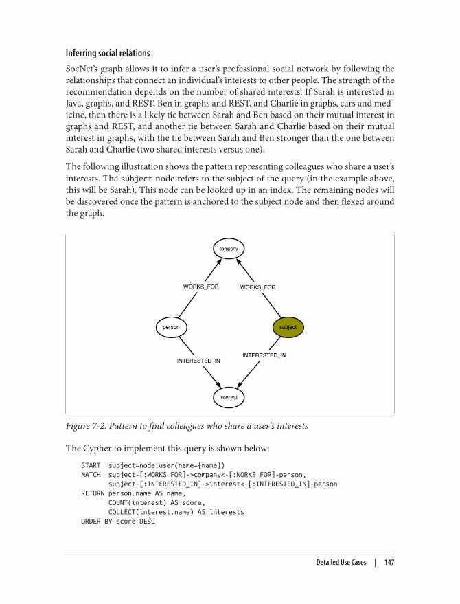
Inferring social relationsSocNet’s graph allows it to infer a user’s professional social network by following therelationships that connect an individual’s interests to other people. The strength of therecommendation depends on the number of shared interests. If Sarah is interested inJava, graphs, and REST, Ben in graphs and REST, and Charlie in graphs, cars and med‐icine, then there is a likely tie between Sarah and Ben based on their mutual interest ingraphs and REST, and another tie between Sarah and Charlie based on their mutualinterest in graphs, with the tie between Sarah and Ben stronger than the one betweenSarah and Charlie (two shared interests versus one).

The following illustration shows the pattern representing colleagues who share a user’sinterests. The subject node refers to the subject of the query (in the example above,this will be Sarah). This node can be looked up in an index. The remaining nodes willbe discovered once the pattern is anchored to the subject node and then flexed aroundthe graph.

Figure 7-2. Pattern to find colleagues who share a user’s interests

The Cypher to implement this query is shown below:

START subject=node:user(name={name})MATCH subject-[:WORKS_FOR]->company<-[:WORKS_FOR]-person, subject-[:INTERESTED_IN]->interest<-[:INTERESTED_IN]-personRETURN person.name AS name, COUNT(interest) AS score, COLLECT(interest.name) AS interestsORDER BY score DESC


The query works as follows:

• The START clause looks up the subject of the query in the user index, and assignsthe result to the subject identifier.

• The MATCH clause then matches this person with people who work for the samecompany, and who share one or more of their interests. If the subject of the queryis Sarah, who works for Acme, then in the case of Ben, this MATCH clause will matchtwice: ('Acme')<-[:WORKS_FOR]-('Ben')-[:INTERESTED_IN]->('graphs') and('Acme')<-[:WORKS_FOR]-('Ben')-[:INTERESTED_IN]->('REST'). In the case ofCharlie, it will match once: ('Acme')<-[:WORKS_FOR]-('Charlie')-

[:INTERESTED_IN]->('graphs').• The RETURN clause creates a projection of the matched data: for each matched col‐

league, we extract their name, count the number of interests they have in commonwith the subject of the query (aliasing this result as score), and, using COLLECT,create a comma-separated list of these mutual interests. Where a person has mul‐tiple matches, as does Ben in our example, COUNT and COLLECT serve to aggregatetheir matches into a single row in the returned results (in fact, both COUNT andCOLLECT can perform this aggregating function alone).

• Finally, we order the results based on each colleague’s score, highest first.

Running this query against our sample graph, with Sarah as the subject, yields the fol‐lowing results:

+---------------------------------------+| name | score | interests |+---------------------------------------+| "Ben" | 2 | ["Graphs","REST"] || "Charlie" | 1 | ["Graphs"] |+---------------------------------------+2 rows0 ms

Here’s the portion of the graph that was matched to generate these results:


Figure 7-3. Colleagues who share Sarah’s interests

You’ll notice that this query only finds people who work for the same company as Sarah.If we want to extend the search to find people who work for other companies, we needto modify the query slightly:

START subject=node:user(name={name})MATCH subject-[:INTERESTED_IN]->interest<-[:INTERESTED_IN]-person, person-[:WORKS_FOR]->companyRETURN person.name AS name, company.name AS company, COUNT(interest) AS score, COLLECT(interest.name) AS interestsORDER BY score DESC

The changes are as follows:

• In the MATCH clause, we no longer require matched persons to work for the samecompany as the subject of the query. (We do, however, still capture the companyfor whom each matched person works, because we want to return this informationin the results.)

• In the RETURN clause we now include the company details for each matched person.

Running this query against our sample data returns the following results:

+---------------------------------------------------------------+| name | company | score | interests |


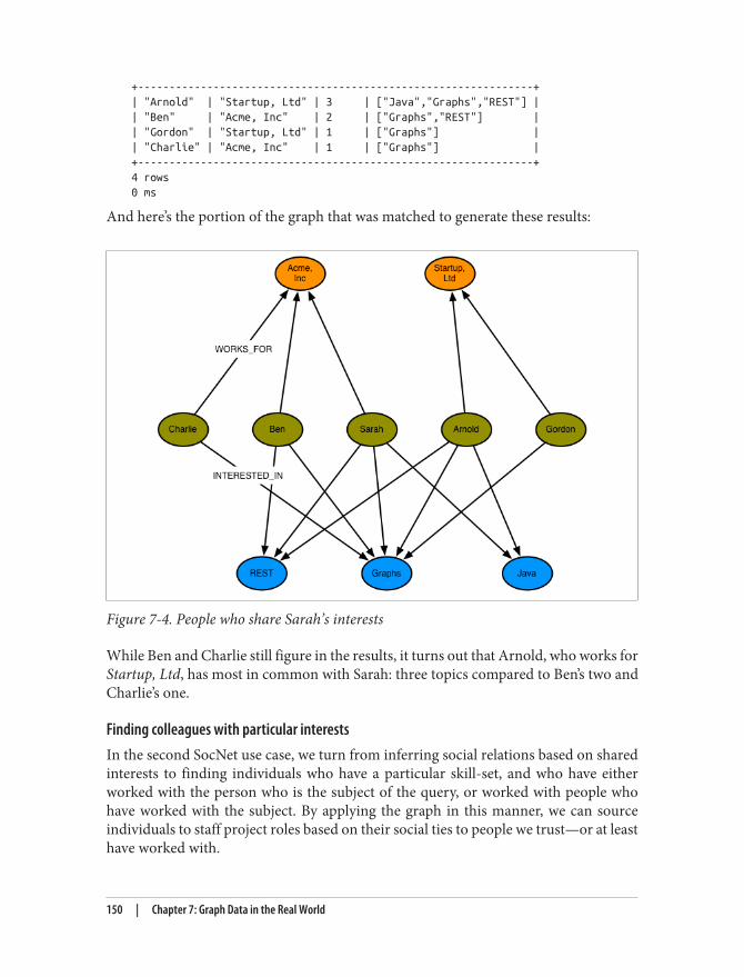
+---------------------------------------------------------------+| "Arnold" | "Startup, Ltd" | 3 | ["Java","Graphs","REST"] || "Ben" | "Acme, Inc" | 2 | ["Graphs","REST"] || "Gordon" | "Startup, Ltd" | 1 | ["Graphs"] || "Charlie" | "Acme, Inc" | 1 | ["Graphs"] |+---------------------------------------------------------------+4 rows0 ms

And here’s the portion of the graph that was matched to generate these results:

Figure 7-4. People who share Sarah’s interests

While Ben and Charlie still figure in the results, it turns out that Arnold, who works forStartup, Ltd, has most in common with Sarah: three topics compared to Ben’s two andCharlie’s one.

Finding colleagues with particular interestsIn the second SocNet use case, we turn from inferring social relations based on sharedinterests to finding individuals who have a particular skill-set, and who have eitherworked with the person who is the subject of the query, or worked with people whohave worked with the subject. By applying the graph in this manner, we can sourceindividuals to staff project roles based on their social ties to people we trust—or at leasthave worked with.


The social ties in question arise from individuals having worked on the same project.Contrast this with the previous use case, where the social ties were inferred based onshared interests. If people have worked on the same project, we infer a social tie. Theprojects, then, form intermediate nodes that bind two or more people together: they areinstances of collaboration that have brought people into contact with one another. Any‐one we discover in this fashion is a candidate for including in our results—as long asthey possess the interests or skills we are looking for.

Here’s a Cypher query that finds colleagues, and colleagues-of-colleagues, who have oneor more particular interests:

START subject=node:user(name={name})MATCH p=subject-[:WORKED_ON]->()-[:WORKED_ON*0..2]-() <-[:WORKED_ON]-person-[:INTERESTED_IN]->interestWHERE person<>subject AND interest.name IN {interests}WITH person, interest, MIN(LENGTH(p)) as pathLengthRETURN person.name AS name, COUNT(interest) AS score, COLLECT(interest.name) AS interests, ((pathLength - 1)/2) AS distanceORDER BY score DESCLIMIT {resultLimit}

This is quite a complex query. Let’s break it down little, and look at each part in moredetail:

• The START clause looks up the subject of the query in the user index, and assignsthe result to the subject identifier.

• The MATCH clause finds people who are connected to the subject by way of havingworked on the same project, or having worked on the same project as people whohave worked with the subject. For each person we match, we capture their interests.This match is then further refined by the WHERE clause, which exclude nodes thatmatch the subject of the query, and ensures we only match people who are interestedin the things we care about. For each successful match, we assign the entire path ofthe match—that is, the path that extends from the subject of the query all the waythrough the matched person to their interest—to the identifier p. We’ll look at thisMATCH clause in more detail shortly.

• The WITH clause pipes the results to the RETURN clause, filtering out redundant pathsas it does so. Redundant paths are present in the results at this point because col‐leagues and colleagues-of-colleagues are often reachable through different paths,some longer than others. We want to filter these longer paths out. That’s exactlywhat the WITH clause does. The WITH clause emits triples comprising a person, aninterest, and the length of the path from the subject of the query through the personto their interest. Given that any particular person/interest combination may appearmore than once in the results, but with different path lengths, we want to aggregate


these multiple lines by collapsing them to a triple containing only the shortest path,which we do using MIN(LENGTH(p)) as pathLength.

• The RETURN clause creates a projection of the data, performing more aggregationas it does so. The data piped by the WITH clause to the RETURN clause contains oneentry per person per interest: if a person matches two of the supplied interests, therewill be two separate data entries. We aggregate these entries using COUNT and COLLECT: COUNT to create an overall score for a person, COLLECT to create a comma-separated list of matched interests for that person. As part of the results, we alsocalculate how far the matched person is from the subject of the query: we take thepathLength for that person, subtract 1 (for the INTERESTED_IN relationship at theend of the path), and then divide by 2 (because the person is separated from thesubject by pairs of WORKED_ON relationships). Finally, we order the results based onscore, highest score first, and limit them according to a resultLimit parametersupplied by the query’s client.

The MATCH clause in the preceding query uses a variable length path,[:WORKED_ON*0..2], as part of a larger pattern to match people who have worked di‐rectly with the subject of the query, as well as people who have worked on the sameproject as people who have worked with the subject. Because each person is separatedfrom the subject of the query by one or two pairs of WORKED_ON relationships, SocNetcould have written this portion of the query as MATCH p=subject-[:WORKED_ON*2..4]-person-[:INTERESTED_IN]->interest, with a variable length path of between two andfour WORKED_ON relationships. However, long variable length paths can be relativelyinefficient. When writing such queries, it is advisable to restrict variable length pathsto as narrow a scope as possible. To increase the performance of the query, SocNet usea fixed length outgoing WORKED_ON relationship that extends from the subject to theirfirst project, and another fixed length WORKED_ON relationship that connects the matchedperson to a project, with a smaller variable length path in between.

Running this query against our sample graph, and again taking Sarah as the subject ofthe query, if we look for colleagues and colleagues-of-colleagues who have interests inJava, travel or medicine, we get the following results:

+--------------------------------------------------+| name | score | interests | distance |+--------------------------------------------------+| "Arnold" | 2 | ["Travel","Java"] | 2 || "Charlie" | 1 | ["Medicine"] | 1 |+--------------------------------------------------+2 rows0 ms


Note that the results are ordered by score, not distance. Arnold has two out of thethree interests, and therefore scores higher than Charlie, who only has one, even thoughhe is at two removes from Sarah, whereas Charlie has worked directly with Sarah.

This is the portion of the graph that was traversed and matched to generate these results:

Figure 7-5. Finding people with particular interests

Let’s take a moment to understand how this query executes in more detail. Figure 7-6shows three stages in the execution of the query. The first stage shows each of the pathsas they are matched by the MATCH and WHERE clauses. As you can see, there is one re‐dundant path: Charlie is matched directly, through Next Gen Platform, and indirectly,by way of Quantum Leap and Emily. The second stage represents the filtering that takesplace in the WITH clause. Here we emit triples comprising the matched person, thematched interest, and the length of the shortest path from the subject through thematched person to their interest. The third stage represents the RETURN clause, whereinwe aggregate the results on behalf of each matched person, and calculate their score anddistance from the subject.


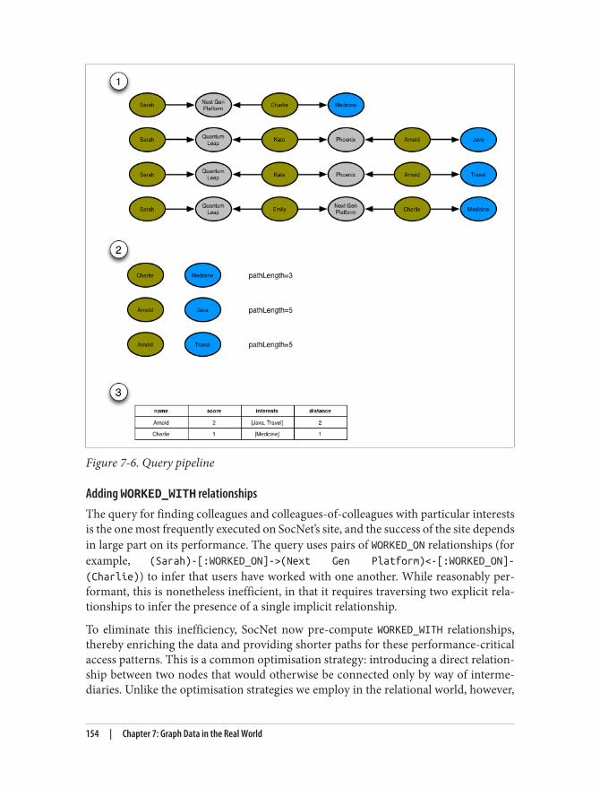
Figure 7-6. Query pipeline

Adding WORKED_WITH relationshipsThe query for finding colleagues and colleagues-of-colleagues with particular interestsis the one most frequently executed on SocNet’s site, and the success of the site dependsin large part on its performance. The query uses pairs of WORKED_ON relationships (forexample, (Sarah)-[:WORKED_ON]->(Next Gen Platform)<-[:WORKED_ON]-

(Charlie)) to infer that users have worked with one another. While reasonably per‐formant, this is nonetheless inefficient, in that it requires traversing two explicit rela‐tionships to infer the presence of a single implicit relationship.

To eliminate this inefficiency, SocNet now pre-compute WORKED_WITH relationships,thereby enriching the data and providing shorter paths for these performance-criticalaccess patterns. This is a common optimisation strategy: introducing a direct relation‐ship between two nodes that would otherwise be connected only by way of interme‐diaries. Unlike the optimisation strategies we employ in the relational world, however,


which typically involve denormalising and thereby compromising a high-fidelity model,this is not an either/or issue: either the high-fidelity structure, or the high performancecompromise. With the graph we retain the original high-fidelity graph structure whileat the same time enriching it with new elements catering to different access patterns.

In terms of the SocNet domain, WORKED_WITH is a bi-directional relationship. In thegraph, however, it is implemented using a uni-directional relationship. While a rela‐tionship’s direction can often add useful semantics to its definition, in this instance thedirection is meaningless. This isn’t a significant issue, so long as any queries that operatewith WORKED_WITH relationships ignore the relationship direction.

Calculating a user’s WORKED_WITH relationships and adding them to the graph isn’t dif‐ficult, nor is it particularly expensive in terms of resource consumption. It can, however,add milliseconds to any end-user interactions that update a user’s profile with newproject information, so SocNet have decided to perform this operation asynchronouslyto end-user activities. Whenever a user changes their project history, SocNet add a jobthat recalculates that user’s WORKED_WITH relationships to a queue. A single writer threadpolls this queue and executes the jobs using the following Cypher statement:

START subject = node:user(name={name})MATCH subject-[:WORKED_ON]->()<-[:WORKED_ON]-personWHERE NOT(subject-[:WORKED_WITH]-person)WITH DISTINCT subject, personCREATE UNIQUE subject-[:WORKED_WITH]-personRETURN subject.name AS startName, person.name AS endName

This is what our sample graph looks like once it has been enriched with WORKED_WITHrelationships:


Figure 7-7. SocNet graph enriched with WORKED_WITH relationships

Using the enriched graph, SocNet now finds colleagues and colleagues-of-colleagueswith particular interests using a slightly simpler version of the query we looked at above:

START subject=node:user(name={name})MATCH p=subject-[:WORKED_WITH*0..1]-()-[:WORKED_WITH]-person-[:INTERESTED_IN]->interestWHERE person<>subject AND interest.name IN {interests}WITH person, interest, MIN(LENGTH(p)) as pathLengthRETURN person.name AS name, COUNT(interest) AS score, COLLECT(interest.name) AS interests, (pathLength - 1) AS distanceORDER BY score DESCLIMIT {resultLimit}

Access ControlSaasNet is an international telecommunications services company, with millions of do‐mestic and business users subscribed to its products and services. For several years, ithas offered its largest business customers the ability to self-service their accounts. Usinga browser-based application, administrators within each of these customer organisa‐tions can add and remove services on behalf of their employees. To ensure that usersand administrators see and change only those parts of the organisation and the productsand services they are entitled to manage, the application employs a complex accesscontrol system, which assigns privileges to many millions of users across tens of millionsof product and service instances.


SaasNet has decided to replace the existing access control system with a graph databasesolution. There are two drivers here: performance and business responsiveness.

Performance issues have dogged SaasNet’s service-service application for several years.The original system is based on a relational database, which uses recursive joins to modelcomplex organisational structures and product hierarchies, and stored procedures toimplement the access control business logic. Because of the join-intensive nature of thedata model, many of the most important queries are unacceptably slow: for an admin‐istrator in a large company, generating a view of the things that administrator can man‐age takes many minutes. This creates a very poor user experience, and hampers therevenue-generating capabilities of the self-service offering.

The performance issues that affect the original application suggest it is no longer fit fortoday’s needs, never mind tomorrow’s. SaasNet has ambitious plans to move into newregions and markets, effectively increasing its customer base by an order of magnitude.The existing solution clearly cannot accommodate the needs of this new strategy. Agraph database solution, in contrast, offers the performance, scalability and adaptive‐ness necessary for dealing with a rapidly changing market.

SaasNet data modelFigure 7-8 shows a sample of the SaasNet data model. The model comprises two hier‐archies. In the first hierarchy, administrators within each customer organization areassigned to groups; these groups are then accorded various permissions against thatorganization’s organizational structure:

• ALLOWED_INHERIT connects an administrator group to an organizational unit,thereby allowing administrators within that group to manage the organizationalunit. This permission is inherited by children of the parent organizational unit. Wesee na example of inhereited permissions in the SaasNet example data model in therelationships between Group 1 and Acme, and the child of Acme, Spinoff. Group1 is connected to Acme using an ALLOWED_INHERIT relationship. Ben, as a memberof Group 1, can manage employees both of Acme and Spinoff thanks to this ALLOWED_INHERIT relationship.

• ALLOWED_DO_NOT_INHERIT connects an administrator group to an organizationalunit in a way that allows administrators within that group to manage the organi‐zational unit, but not any of its children. Sarah, as a member of Group 2, can ad‐minister Acme, but not its child Spinoff, because Group 2 is connected to Acme byan ALLOWED_DO_NOT_INHERIT relationship, not an ALLOWED_INHERIT relationship.

• DENIED forbids administrators from accessing an organizational unit. This permis‐sion is inherited by children of the parent organizational unit. In the SaasNet dia‐gram, this is best illustrated by Liz and her permissions with respect to Big Co,Acquired Ltd, Subsidiary and One-Map Shop. As a result of her membership of


Group 4 and its ALLOWED_INHERIT permission on Big Co, Liz can manage BigCo. But despite this being an inheritable relationship, Liz cannot manage AcquiredLtd or Subsidiary; the reason being, Group 5, of which Liz is a member, is DENIED access to Acquired Ltd and its children (which includes Subsidiary). Lizcan, however, manage One-Map Shop, thanks to an ALLOWED_DO_NOT_INHERIT per‐mission granted to Group 6, the last group to which Liz belongs.

DENIED takes precedence over ALLOWED_INHERIT, but is subordinate to AL

LOWED_DO_NOT_INHERIT. Therefore, if an administrator is connected to a company byway of ALLOWED_DO_NOT_INHERIT and DENIED, ALLOWED_DO_NOT_INHERIT prevails.

Figure 7-8. Access control graph

Fine-grained relationships, or relationships with properties?You’ll notice that the SaasNet access control data model uses fine-grained relationships(ALLOWED_INHERIT, ALLOWED_DO_NOT_INHERIT and DENIED) rather than a single rela‐tionship type qualified by properties—something like PERMISSION with allowed andinherited boolean properties. Why is this? And when would you choose between thesetwo options?


SaasNet performance tested both approaches and determined that the fine-grained,property-free approach was nearly twice as fast as the one using properties. This shouldcome as no surprise. Relationships are the royal road into the graph; differentiating byrelationship type is the best way of eliminating large swathes of the graph from a tra‐versal. Using one or more property values to decide whether or not to follow a rela‐tionship incurs extra IO—because the properties reside in a separate store file from therelationships—the first time those properties are accessed (after that, they’re cached).

Consider using fine-grained relationships whenever you have a closed set of relationshiptypes. Here, SaasNet has a closed set of permissions, ideal for representing as fine-grained relationships. In contrast, weightings—as required by a shortest weighted pathalgorithm—rarely comprise a closed set, and these are usually best represented as prop‐erties on relationships.

Sometimes, however, you have a closed set of relationships where in some traversals youwant to follow specific kinds of relationship within that set, but in others you want tofollow all of them, irrespective of type. Addresses are a good example. Following theclosed-set principle, we might choose to create HOME_ADDRESS, WORK_ADDRESS and DELIVERY_ADDRESS relationships. This allows us to follow specific kinds of address rela‐tionship (DELIVERY_ADDRESS, for example) while ignoring all the rest. But what do wedo if we want to find all addresses for a user? There are a couple of options here. First,we can encode knowledge of all the different relationship types in the relevant MATCHclauses: e.g. MATCH user-[:HOME_ADDRESS|WORK_ADDRESS|DELIVERY_ADDRESS]-

>address. This, however, quickly becomes unwieldy when there are lots of differentkinds of relationship. Alternatively, we can add a more generic ADDRESS relationship toour model, in addition to the fine-grained relationships. Every node representing anaddress is then connected to a user using two relationships: a fined-grained relationship(e.g. DELIVERY_ADDRESS) and the more generic ADDRESS relationship.

As we discuss in “Describe the Model in Terms of Your Application’s Needs” in Chapter6, the key here is to let the questions you want to ask of your data guide the kinds ofrelationship you introduce into the model.

Finding all accessible resources for an administratorThe SaasNet application uses many different Cypher queries; we’ll look at just a few ofthem here.

First up is the ability to find all resources accessible by a particular administrator.Whenever an onsite administrator logs in to the system, they are presented with abrowser-based list of all the employees and employee accounts they can administer. Thislist is generated based on the results returned by the following query:

START admin=node:administrator(name={administratorName})MATCH paths=admin-[:MEMBER_OF]->()-[:ALLOWED_INHERIT]->()<-[:CHILD_OF*0..3]-company <-[:WORKS_FOR]-employee-[:HAS_ACCOUNT]->account


WHERE NOT (admin-[:MEMBER_OF]->()-[:DENIED]->()<-[:CHILD_OF*0..3]-company)RETURN employee.name AS employee, account.name AS accountUNIONSTART admin=node:administrator(name={administratorName})MATCH paths=admin-[:MEMBER_OF]->()-[:ALLOWED_DO_NOT_INHERIT]->() <-[:WORKS_FOR]-employee-[:HAS_ACCOUNT]->accountRETURN employee.name AS employee, account.name AS account

This query sets the template for all the other queries we’ll be looking at in this section,in that it comprises two separate queries joined by a UNION operator. The query beforethe UNION operator handles ALLOWED_INHERIT relationships qualified by any DENIEDrelationships; the query following the UNION operator handles any ALLOWED_DO_NOT_INHERIT permissions. This pattern, ALLOWED_INHERIT minus DENIED, followed by ALLOWED_DO_NOT_INHERIT, is repeated in all of the access control example queries thatfollow.

The first query here, the one before the UNION operator, can be broken down as follows:

• The START clause finds the logged-in administrator in the administrator index,and binds the result to the admin identifier.

• The MATCH clause matches all the groups to which this administrator belongs, andfrom these groups, all the parent companies connected by way of an ALLOWED_INHERIT relationship. The MATCH then uses a variable length path ([:CHILD_OF0..3])to discover children of these parent companies, and thereafter the employees andaccounts associated with all matched companies (whether parent company orchild). At this point, the query has matched all companies, employees and accountsaccessible by way of ALLOWED_INHERIT relationships.

• The WHERE clause eliminates matches where the company bound in the MATCH clause,or any of its parents, is connected by way of DENIED relationship to the adminis‐trator’s groups. This WHERE clause is invoked for each match; if there is a DENIEDrelationship anywhere between the admin node and the company node bound bythe match, that match is eliminated.

• The RETURN clause creates a projection of the matched data in the form of a list ofemployee names and accounts.

The second query here, following the UNION operator, is a little simpler:

• The MATCH clause simply matches companies (plus employees and accounts) whichare directly connected to an administrator’s groups by way of an AL

LOWED_DO_NOT_INHERIT relationship.


The UNION operator joins the results of these two queries together, eliminating any du‐plicates. Note that the RETURN clause in each query must contain the same projection ofthe results; in other words, the column names in the results must match.

Cypher supports both UNION and UNION ALL operators. UNION eliminatesduplicate results from the final result set, whereas UNION ALL includesany duplicates.

Figure 7-9 shows how this query matches all accessible resources for Sarah in the sampleSaasNet graph. Note how, because of the DENIED relationship from Group 2 to Skunkworkz, Sarah cannot administer Kate and Account 7.

Figure 7-9. Finding all accessible resources for a user

Determining whether an administrator has access to a resourceThe query we’ve just looked at returned a list of employees and accounts that an ad‐ministrator can manage. In a Web application, each of these resources (employee, ac‐count) is accessible through its own URI. Given a friendly URI (e.g. http://saasnet/


http://saasnet/accounts/5436

accounts/5436), what’s to stop someone from hacking a URI and gaining illegal accessto an account?

What’s needed is a query that will determine whether an administrator has access toaspecific resource. This is that query:

START admin=node:administrator(name={adminName}), company=node:company(resourceName={resourceName})MATCH p=admin-[:MEMBER_OF]->()-[:ALLOWED_INHERIT]->()<-[:CHILD_OF*0..3]-companyWHERE NOT (admin-[:MEMBER_OF]->()-[:DENIED]->()<-[:CHILD_OF*0..3]-company)RETURN COUNT(p) AS accessCountUNIONSTART admin=node:administrator(name={adminName}), company=node:company(resourceName={resourceName})MATCH p=admin-[:MEMBER_OF]->()-[:ALLOWED_DO_NOT_INHERIT]->companyRETURN COUNT(p) AS accessCount

This query works by determining whether an administrator has access to the companyto which an employee or an account belongs. How do we identify to which companyan employee or account belongs? Through clever use of indexes.

In the SaasNet data model, companies are indexed both by their name, and by the namesof their employees and employee accounts. Given a company name, employee name,or account name, we can, therefore, lookup the relevant company node in the companyindex.

Given that bit of insight, we can see that this resource authorization check query issimilar to the query for finding all companies, employees and accounts, but for severalsmall differences:

• company is bound in the START clause, not the MATCH clause. Using the indexingstrategy described above, we lookup the node representing the relevant companybased on the name of the resource to be authorized—whether employee or account.

• We don’t match any further than company. Since company has already been boundbased on an employee or account name, there’s no need to drill further into thegraph to match that employee or account.

• The RETURN clauses for the queries before and after the UNION operator return acount of the number of matches. For an administrator to have access to a resource,one or other of these accessCount values must be greater than 0.

The WHERE clause in the query before the UNION operator once again eliminates matcheswhere the company in question is connected to one of the administrator’s groups by wayof a DENIED relationship.

Because the UNION operator eliminates duplicate results, the overall result set for thisquery can contain either one or two values. The client-side logic for determiningwhether an administrator has access to a resource looks like this in Java:


http://saasnet/accounts/5436

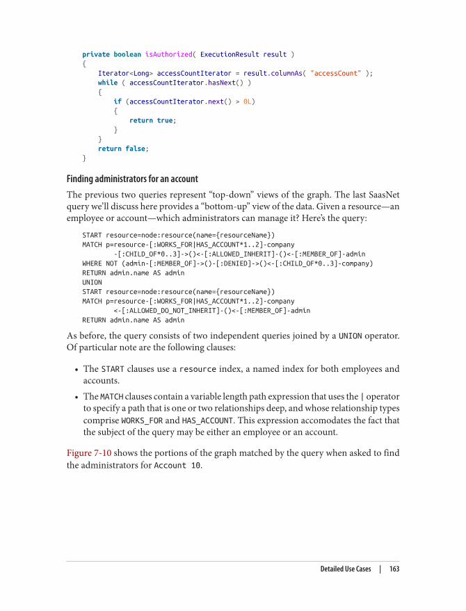
private boolean isAuthorized( ExecutionResult result ){ Iterator<Long> accessCountIterator = result.columnAs( "accessCount" ); while ( accessCountIterator.hasNext() ) { if (accessCountIterator.next() > 0L) { return true; } } return false;}

Finding administrators for an accountThe previous two queries represent “top-down” views of the graph. The last SaasNetquery we’ll discuss here provides a “bottom-up” view of the data. Given a resource—anemployee or account—which administrators can manage it? Here’s the query:

START resource=node:resource(name={resourceName})MATCH p=resource-[:WORKS_FOR|HAS_ACCOUNT*1..2]-company -[:CHILD_OF*0..3]->()<-[:ALLOWED_INHERIT]-()<-[:MEMBER_OF]-adminWHERE NOT (admin-[:MEMBER_OF]->()-[:DENIED]->()<-[:CHILD_OF*0..3]-company)RETURN admin.name AS adminUNIONSTART resource=node:resource(name={resourceName})MATCH p=resource-[:WORKS_FOR|HAS_ACCOUNT*1..2]-company <-[:ALLOWED_DO_NOT_INHERIT]-()<-[:MEMBER_OF]-adminRETURN admin.name AS admin

As before, the query consists of two independent queries joined by a UNION operator.Of particular note are the following clauses:

• The START clauses use a resource index, a named index for both employees andaccounts.

• The MATCH clauses contain a variable length path expression that uses the | operatorto specify a path that is one or two relationships deep, and whose relationship typescomprise WORKS_FOR and HAS_ACCOUNT. This expression accomodates the fact thatthe subject of the query may be either an employee or an account.

Figure 7-10 shows the portions of the graph matched by the query when asked to findthe administrators for Account 10.


Figure 7-10. Finding an administrator for a specific account

LogisticsLogisticsNet is a large courier company whose domestic operation delivers millions ofparcels to over 30 million addresses each day. In recent years, as a result of the rise ininternet shopping, the number of parcels has increased significantly. Amazon and eBaydeliveries now account for over half the parcels routed and delivered by LogisticsNeteach day.

With parcel volumes continuing to grow, and facing strong competition from othercourier services, LogisticsNet has begun a large change programme to upgrade all as‐pects of its parcel network, including buildings, equipment, systems and processes.

One of the most important and time-critical components in the parcel network is theroute calculation engine. Between one and three thousand parcels enter the networkeach second. As parcels enter the network they are mechanically sorted according totheir destination. To maintain a steady flow during this process the engine must calculatea parcel’s route before it reaches a point where the sorting equipment has to make achoice, which happens only seconds after the parcel has entered the network—hencethe strict time requirements on the engine.


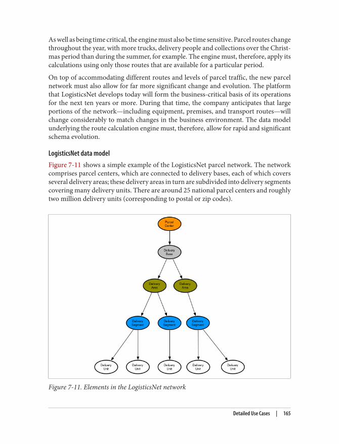
As well as being time critical, the engine must also be time sensitive. Parcel routes changethroughout the year, with more trucks, delivery people and collections over the Christ‐mas period than during the summer, for example. The engine must, therefore, apply itscalculations using only those routes that are available for a particular period.

On top of accommodating different routes and levels of parcel traffic, the new parcelnetwork must also allow for far more significant change and evolution. The platformthat LogisticsNet develops today will form the business-critical basis of its operationsfor the next ten years or more. During that time, the company anticipates that largeportions of the network—including equipment, premises, and transport routes—willchange considerably to match changes in the business environment. The data modelunderlying the route calculation engine must, therefore, allow for rapid and significantschema evolution.

LogisticsNet data modelFigure 7-11 shows a simple example of the LogisticsNet parcel network. The networkcomprises parcel centers, which are connected to delivery bases, each of which coversseveral delivery areas; these delivery areas in turn are subdivided into delivery segmentscovering many delivery units. There are around 25 national parcel centers and roughlytwo million delivery units (corresponding to postal or zip codes).

Figure 7-11. Elements in the LogisticsNet network


Over time, the delivery routes change. Figure 7-12, Figure 7-13 and Figure 7-14 showthree distinct delivery periods. For any given period there is at most one route betweena delivery base and any particular delivery area or segment. In contrast, there may bemultiple routes between delivery bases and parcel centers. For any given point in time,therefore, the lower portions of the graph—the individual subgraphs that depend fromeach delivery base—comprise simple tree structures, whereas the upper portions of thegraph—made up of delivery bases and parcel centers—are more complexly structured.

Figure 7-12. Structure of the delivery network for Period 1




You’ll notice that delivery units are not included in the production data. This is becauseeach delivery unit is always associated with the same delivery segments, irrespective ofthe period. Because of this invariant, it is possible to index each delivery segment by itsmany delivery units. To calculate the route to a particular delivery unit, the system needonly actually calculate the route to its associated delivery segment, which can be recov‐ered from the index using the delivery unit as a key. This optimisation helps both reduce


the size of the production graph, and reduce the number of traversals needed to calculatea route.

The production database contains the details of many different delivery periods, asshown in Figure 7-15. This multi-period graph demonstrates some of the overall com‐plexity present in the data.

Figure 7-15. Sample of the LogisticsNet network

In the production data, nodes are connected by multiple relationships, each of which istimestamped with a start_date and end_date property, whose long value representsthe number of milliseconds since 1970-01-01T00:00:00Z. Relationships are of twotypes: CONNECTED_TO, which connect parcel centers and delivery bases, and DELIVERY_ROUTE, which connect delivery bases to delivery areas, and delivery areas to deliverysegments. These two different types of relationship effectively partition the graph intoits upper and lower parts, which, as we’ll see shortly provides for efficient traversals.Figure 7-16 shows three of the timestamped CONNECTED_TO relationships connecting aparcel center to a delivery base:


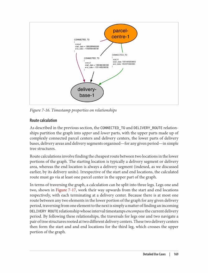
Figure 7-16. Timestamp properties on relationships

Route calculation

As described in the previous section, the CONNECTED_TO and DELIVERY_ROUTE relation‐ships partition the graph into upper and lower parts, with the upper parts made up ofcomplexly connected parcel centers and delivery centers, the lower parts of deliverybases, delivery areas and delivery segments organised—for any given period—in simpletree structures.

Route calculations involve finding the cheapest route between two locations in the lowerportions of the graph. The starting location is typically a delivery segment or deliveryarea, whereas the end location is always a delivery segment (indexed, as we discussedearlier, by its delivery units). Irrespective of the start and end locations, the calculatedroute must go via at least one parcel center in the upper part of the graph.

In terms of traversing the graph, a calculation can be split into three legs. Legs one andtwo, shown in Figure 7-17, work their way upwards from the start and end locationsrespectively, with each terminating at a delivery center. Because there is at most oneroute between any two elements in the lower portion of the graph for any given deliveryperiod, traversing from one element to the next is simply a matter of finding an incomingDELIVERY ROUTE relationship whose interval timestamps encompass the current deliveryperiod. By following these relationships, the traversals for legs one and two navigate apair of tree structures rooted at two different delivery centers. These two delivery centersthen form the start and and end locations for the third leg, which crosses the upperportion of the graph.


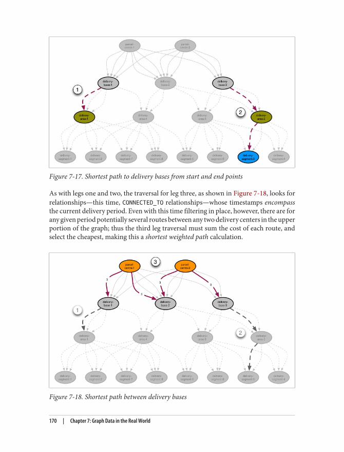
Figure 7-17. Shortest path to delivery bases from start and end points

As with legs one and two, the traversal for leg three, as shown in Figure 7-18, looks forrelationships—this time, CONNECTED_TO relationships—whose timestamps encompassthe current delivery period. Even with this time filtering in place, however, there are forany given period potentially several routes between any two delivery centers in the upperportion of the graph; thus the third leg traversal must sum the cost of each route, andselect the cheapest, making this a shortest weighted path calculation.

Figure 7-18. Shortest path between delivery bases


To complete the calculation, we need then simply add the paths for legs one, three andtwo, which gives the full path from the start to the end location.

Finding the shortest delivery route using CypherThe Cypher query to implement the parcel route calculation engine is as follows:

START s=node:location(name={startLocation}), e=node:location(name={endLocation})MATCH p1 = s<-[:DELIVERY_ROUTE*1..2]-db1WHERE ALL(r in relationships(p1) WHERE r.start_date <= {intervalStart} AND r.end_date >= {intervalEnd})WITH e, p1, db1MATCH p2 = db2-[:DELIVERY_ROUTE*1..2]->eWHERE ALL(r in relationships(p2) WHERE r.start_date <= {intervalStart} AND r.end_date >= {intervalEnd})WITH db1, db2, p1, p2MATCH p3 = db1<-[:CONNECTED_TO]-()-[:CONNECTED_TO*1..3]-db2WHERE ALL(r in relationships(p3) WHERE r.start_date <= {intervalStart} AND r.end_date >= {intervalEnd})WITH p1, p2, p3, REDUCE(weight=0, r in relationships(p3) : weight+r.cost) AS score ORDER BY score ASC LIMIT 1RETURN (nodes(p1) + tail(nodes(p3)) + tail(nodes(p2))) AS n

At first glance this query appears quite complex. It is, however, made up of four simplerqueries joined together with WITH clauses. We’ll look at each of these subqueries in turn.

Here’s the first subquery:

START s=node:location(name={startLocation}), e=node:location(name={endLocation})MATCH p1 = s<-[:DELIVERY_ROUTE*1..2]-db1WHERE ALL(r in relationships(p1) WHERE r.start_date <= {intervalStart} AND r.end_date >= {intervalEnd})

This query calculates the first leg of the overall route. It can be broken down as follows:

• The START clause finds the start and end locations in an index, binding them to thes and e identifiers respectively. (Remember, the endLocation lookup term describesa delivery unit, but the node returned from the location index represents a deliverysegment.)

• The MATCH clause finds the route from the start location, s, to a delivery base usinga directed, variable length DELIVERY_ROUTE path. This path is then bound to theidentifier p1. Because delivery bases are always the root nodes of DELIVERY_ROUTE


trees, and therefore have no incoming DELIVERY_ROUTE relationships, we can beconfident that the db1 node at the end of this variable length path represents adelivery base and not some other parcel network element.

• The WHERE clause applies additional constraints to the path p1, ensuring that weonly match DELIVERY_ROUTE relationships whose start_date and end_date prop‐erties encompass the supplied delivery period.

The second subquery calculates the second leg of the route, which comprises the pathfrom the end location to another delivery center elsewhere in the network. This queryis very similar to the first:

WITH e, p1, db1MATCH p2 = db2-[:DELIVERY_ROUTE*1..2]->eWHERE ALL(r in relationships(p2) WHERE r.start_date <= {intervalStart} AND r.end_date >= {intervalEnd})

The WITH clause here chains the first subquery to the second, piping the end locationand the first leg’s path and delivery base to the second subquery. The second subqueryuses only the end location, e, in its MATCH clause; the rest is provided so that it can bepiped to subsequent queries.

The third subquery identifies all candidate paths for the third leg of the route, as follows:

WITH db1, db2, p1, p2MATCH p3 = db1<-[:CONNECTED_TO]-()-[:CONNECTED_TO*1..3]-db2WHERE ALL(r in relationships(p3) WHERE r.start_date <= {intervalStart} AND r.end_date >= {intervalEnd})

This subquery is broken down as follows:

• The WITH clause chains this subquery to the previous one, piping the delivery basesand paths identified in legs one and two to the current query.

• The MATCH clause identifies all paths between the first and second leg delivery bases,to a maximum depth of four, and binds them to the p3 identifier.

• The WHERE clause constrains the p3 paths to those whose start_date and end_dateproperties encompass the supplied delivery period.

The fourth and final subquery selects the shortest path for leg three, and then calculatesthe overall route:

WITH p1, p2, p3, REDUCE(weight=0, r in relationships(p3) : weight+r.cost) AS score ORDER BY score ASC LIMIT 1RETURN (nodes(p1) + tail(nodes(p3)) + tail(nodes(p2))) AS n


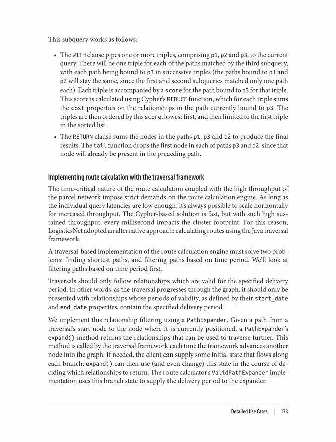
This subquery works as follows:

• The WITH clause pipes one or more triples, comprising p1, p2 and p3, to the currentquery. There will be one triple for each of the paths matched by the third subquery,with each path being bound to p3 in successive triples (the paths bound to p1 andp2 will stay the same, since the first and second subqueries matched only one patheach). Each triple is accompanied by a score for the path bound to p3 for that triple.This score is calculated using Cypher’s REDUCE function, which for each triple sumsthe cost properties on the relationships in the path currently bound to p3. Thetriples are then ordered by this score, lowest first, and then limited to the first triplein the sorted list.

• The RETURN clause sums the nodes in the paths p1, p3 and p2 to produce the finalresults. The tail function drops the first node in each of paths p3 and p2, since thatnode will already be present in the preceding path.

Implementing route calculation with the traversal frameworkThe time-critical nature of the route calculation coupled with the high throughput ofthe parcel network impose strict demands on the route calculation engine. As long asthe individual query latencies are low enough, it’s always possible to scale horizontallyfor increased throughput. The Cypher-based solution is fast, but with such high sus‐tained throughput, every millisecond impacts the cluster footprint. For this reason,LogisticsNet adopted an alternative approach: calculating routes using the Java traversalframework.

A traversal-based implementation of the route calculation engine must solve two prob‐lems: finding shortest paths, and filtering paths based on time period. We’ll look atfiltering paths based on time period first.

Traversals should only follow relationships which are valid for the specified deliveryperiod. In other words, as the traversal progresses through the graph, it should only bepresented with relationships whose periods of validity, as defined by their start_dateand end_date properties, contain the specified delivery period.

We implement this relationship filtering using a PathExpander. Given a path from atraversal’s start node to the node where it is currently positioned, a PathExpander’sexpand() method returns the relationships that can be used to traverse further. Thismethod is called by the traversal framework each time the framework advances anothernode into the graph. If needed, the client can supply some initial state that flows alongeach branch; expand() can then use (and even change) this state in the course of de‐ciding which relationships to return. The route calculator’s ValidPathExpander imple‐mentation uses this branch state to supply the delivery period to the expander.


Here’s the code for the ValidPathExpander:

private static class ValidPathExpander implements PathExpander<Interval>{ private final RelationshipType relationshipType; private final Direction direction;

private ValidPathExpander( RelationshipType relationshipType, Direction direction ) { this.relationshipType = relationshipType; this.direction = direction; }

@Override public Iterable<Relationship> expand( Path path, BranchState<Interval> deliveryInterval ) { List<Relationship> results = new ArrayList<Relationship>(); for ( Relationship r : path.endNode().getRelationships( relationshipType, direction ) ) { Interval relationshipInterval = new Interval( (Long) r.getProperty( "start_date" ), (Long) r.getProperty( "end_date" ) ); if ( relationshipInterval.contains( deliveryInterval.getState() ) ) { results.add( r ); } }

return results; }

@Override public PathExpander<Interval> reverse() { return null; }}

The ValidPathExpander’s constructor takes two arguments: a relationshipType anda direction. This allows the expander to be re-used for different types of relationship:in the case of the LogisticsNet graph, the expander will be used to filter both CONNECTED_TO and DELIVERY_ROUTE relationships.

The expander’s expand() method takes the path to the current node, and the deliveryInterval as supplied by the client. Each time it is called, expand() iterates the relevantrelationships on the current node (the current node is given by path.endNode()). Foreach relationship, the method then compares the relationship’s interval with the deliveryinterval. If the relationship interval contains the delivery interval, the relationship isadded to the results.


Having looked at the ValidPathExpander, we can now turn to the ParcelRouteCalculator itself. This class encapsulates all the logic necessary to calculate a route betweenthe point where a parcel enters the network and the final delivery destination. It employsa similar strategy to the Cypher query we’ve already looked at: it works its way up thegraph from both the start node and the end node in two separate traversals, until it findsa delivery base for each leg. It then performs a shortest weighted path search that joinsthese two delivery bases.

Here’s the beginning of the ParcelRouteCalculator class:

public class ParcelRouteCalculator{ private static final PathExpander<Interval> DELIVERY_ROUTE_EXPANDER = new ValidPathExpander( withName( "DELIVERY_ROUTE" ), Direction.INCOMING );

private static final PathExpander<Interval> CONNECTED_TO_EXPANDER = new ValidPathExpander( withName( "CONNECTED_TO" ), Direction.BOTH );

private static final TraversalDescription TRAVERSAL = Traversal.description() .depthFirst() .evaluator( new Evaluator() { private final RelationshipType DELIVERY_ROUTE = withName( "DELIVERY_ROUTE");

@Override public Evaluation evaluate( Path path ) { if ( !path.endNode() .hasRelationship( DELIVERY_ROUTE, Direction.INCOMING ) ) { return Evaluation.INCLUDE_AND_PRUNE; }

return Evaluation.INCLUDE_AND_CONTINUE; } } );

private static final CostEvaluator<Double> COST_EVALUATOR = CommonEvaluators.doubleCostEvaluator( "cost" );

private final Index<Node> locationIndex;

public ParcelRouteCalculator( GraphDatabaseService db ) { this.locationIndex = db.index().forNodes( "location" ); }

...

}


Here we define two expanders—one for DELIVERY_ROUTE relationships, another forCONNECTED_TO relationships—and the traversal that will find the two legs of our route.This traversal terminates whenever it encounters a node with no incoming DELIVERY_ROUTE relationships. Since each delivery base is at the root of a delivery route tree,we can infer that a node without any incoming DELIVERY_ROUTE relationships representsa delivery base in our graph.

The constructor for ParcelRouteCalculator accepts the current database instance.From this it obtains the location index, which it stores in a member variable.

Each route calculation engine maintains a single instance of this route calculator. Thisinstance is capable of servicing multiple requests. For each route to be calculated, theclient calls the calculator’s calculateRoute() method, passing in the names of the startand end points, and the interval for which the route is to be calculated:

public Iterable<Node> calculateRoute( String start, String end, Interval interval ){ TraversalDescription deliveryBaseFinder = createDeliveryBaseFinder( interval );

Collection<Node> upLeg = findRouteToDeliveryBase( start, deliveryBaseFinder ); Collection<Node> downLeg = findRouteToDeliveryBase( end, deliveryBaseFinder ); Collection<Node> topRoute = findRouteBetweenDeliveryBases( IteratorUtil.last( upLeg ), IteratorUtil.last( downLeg ), interval );

return combineRoutes( upLeg, downLeg, topRoute );}

calculateRoute() first obtains a deliveryBaseFinder for the specified interval, whichit then uses to the find the routes for the two legs. Next, it finds the route between thedelivery bases at the top of each leg, these being the last nodes in each leg’s node col‐lection. Finally, it combines these route to generate the final results.

The createDeliveryBaseFinder() helper method creates a traversal description con‐figured with the supplied interval:

private TraversalDescription createDeliveryBaseFinder( Interval interval ){ return TRAVERSAL.expand( DELIVERY_ROUTE_EXPANDER, new InitialBranchState.State<Interval>( interval, interval ) );}

This traversal description is built by expanding the ParcelRouteCalculator’s staticTRAVERSAL description using the DELIVERY_ROUTE_EXPANDER. The branch state for theexpander is initialised at this point with the interval supplied by the client.


Properly configured with an interval, the traversal description is then supplied to findRouteToDeliveryBase(), which looks up a starting node in the location index, andthen executes the traversal:

private Collection<Node> findRouteToDeliveryBase( String startPosition, TraversalDescription deliveryBaseFinder ){ Node startNode = locationIndex.get( "name", startPosition ).getSingle(); return IteratorUtil.asCollection( deliveryBaseFinder.traverse( startNode ) .nodes() );}

That’s the two legs taken care of. The last part of the calculation requires us to find theshortest path between the delivery bases at the top of each of the legs. calculateRoute() takes the last node from each leg’s node collection, and supplies these two nodestogether with the client-supplied interval to findRouteBetweenDeliveryBases().Here’s the implementation of findRouteBetweenDeliveryBases():

private Collection<Node> findRouteBetweenDeliveryBases( Node deliveryBase1, Node deliveryBase2, Interval interval ){ PathFinder<WeightedPath> routeBetweenDeliveryBasesFinder = GraphAlgoFactory.dijkstra( CONNECTED_TO_EXPANDER, new InitialBranchState.State<Interval>( interval, interval ), COST_EVALUATOR );

return IteratorUtil.asCollection( routeBetweenDeliveryBasesFinder .findSinglePath( deliveryBase1, deliveryBase2 ) .nodes() );}

Rather than use a traversal description to find the shortest route between two nodes,this method uses a shortest weighted path algorithm from Neo4j’s graph algorithm li‐brary—in this instance, we’re using the Dijkstra algorithm (see “Path-Finding withDijkstra’s Algorithm” in Chapter 8 for more details of the Dijkstra algorithm). Thisalgorithm is configured with ParcelRouteCalculator’s static CONNECTED_TO_EXPANDER, which in turn is initialised with the client-supplied branch state interval. The algo‐rithm is also configured with a cost evaluator (another static member), which simplyidentifies the property on a relationship representing that relationship’s weight or cost.A call to findSinglePath on the Dijkstra path finder returns the shortest path betweenthe two delivery bases.

That’s the hard work done. All that remains to do is to join these routes to form the finalresults. This is relatively straightforward, the only wrinkle being that the down leg’s nodecollection must be reversed before being added to the results (the leg was calculatedfrom final destination upwards, whereas it should appear in the results delivery basedownwards):


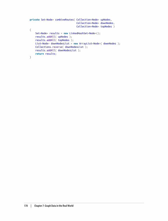
private Set<Node> combineRoutes( Collection<Node> upNodes, Collection<Node> downNodes, Collection<Node> topNodes ){ Set<Node> results = new LinkedHashSet<Node>(); results.addAll( upNodes ); results.addAll( topNodes ); List<Node> downNodesList = new ArrayList<Node>( downNodes ); Collections.reverse( downNodesList ); results.addAll( downNodesList ); return results;}


CHAPTER 8

Predictive Analysis with Graph Theory

In this chapter we’re going consider analytical techniques and algorithms for processinggraph data. Both graph theory and graph algorithms are mature and well-understoodfields of computing science and we’ll demonstrate how both can can be used to minesophisticated information from graph databases. While the reader with a backgroundin computing science will no doubt recognize (and reminisce about) these algorithmsand techniques, the discussion in this chapter is handled as humanely as possible —with virtually no mathematics — to encourage the curious reader to dive right in.

Depth- and Breadth-First SearchBefore we can dive into higher-order analytical techniques we need to re-acquaint our‐selves with the fundamental breadth-first search algorithm, which is used as the basisfor iterating over an entire graph. Most of the queries we’ve seen throughout this bookhave been depth-first rather than breadth-first in nature. That is, they traverse outwardsfrom a starting node to some end node before repeating a similar search down a differentpath from the same start node. Depth-first is a good strategy when we’re trying to followa path to discover discrete information goals.

Informed depth-first searchThe classic depth-first algorithm search is said to be uninformed in that it simply searchesa path until it finds the end of the graph before backtracking to the start node and tryinga different path. However graph databases are semantically rich, so terminating a searchalong a particular branch (for example having found a node with no compatible out‐going relationships, or having traversed “far enough”) can happen early resulting intypically lower execution times for such informed cases — exactly the kind of situationfor which we optimized our Cypher matches and traversals in previous chapters.

179

Though we’ve used depth-first search as our underlying strategy for general graph tra‐versals, many interesting “higher order” algorithms traverse the (entire) graph in abreadth-first manner. That is they explore the graph layer by layer exploring the nearestneighbor nodes of a starting node before the next nearest and so on until the searchterminates.

Breadth-first search by contrast explores the graph one layer at a time, by first visitingeach node at depth 1 from the start node, then depth 2, then depth 3 and so on potentiallyuntil the entire graph has been visited. This progression is easily visualized starting atthe node labelled O (for origin) and progressing outwards a layer at a time as perFigure 8-1.

180 | Chapter 8: Predictive Analysis with Graph Theory

Figure 8-1. The progression of a breadth-first search

Where the search terminates depends on the algorithm being executed (since mostuseful algorithms aren’t pure breadth-first search but are informed to some extent), butbreadth-first search is often used in path-finding algorithms and when the entire graphneeds to be systematically searched (for the likes of graph global algorithms we discussedin Chapter 5).

Path-Finding with Dijkstra’s AlgorithmBreadth-first search underpins numerous classical graph algorithms, including Dijk‐stra’s algorithm. Dijkstra (as it is often abbreviated) is used to find the shortest path

Path-Finding with Dijkstra’s Algorithm | 181

1. That is, the algorithm runs in time proportional to the number of relationships in the graph plus the size ofthe number of nodes multiplied by the log of the size of the node set

2. The algorithm runs in time proportional to the square of the size of the number of relationships in the graph

between two nodes in a graph. Dijkstra’s algorithm is mature (having first been publishedin 1956) and widely studied and optimized by computer scientists and behaves as fol‐lows:

1. Pick the start and end nodes, and add the start node to the set of solved nodes (nodeswith known shortest path from the start node) with value 0, since the start node isby definition 0 path length away from itself.

2. From the starting node, traverse (breadth-first) to the nearest neighbors and recordthe path length against each neigbor node.

3. Take the shortest path found to one of the neighbors (picking arbitrarily in the caseof ties) and mark that node as solved since we now know the shortest path fromthe start node to this neighbor.

4. From the set of solved nodes, visit the nearest neighbors (notice the breath-firstprogression) and record the path lengths from the start node against those neig‐bors — but don’t both visiting any neighboring solved nodes since we know theshortest paths to them already.

5. Repeat steps 3 and 4 until the destination node has been marked solved.

Efficiency of Dijkstra’s algorithmDijkstra’s algorithm is quite efficient since it computes only the lengths of a (relativelysmall) subset of the possible paths through the graph. When we’ve solved a node, theshortest path from the start node is then known meaning all subsequent paths can safelybuild on that knowledge.

In fact we know Dijkstra’s algorithm has performance of O(|R| + |N| log |N|) 1 fastestknown worst-case implementation though the original was O(|R|^2) 2.

Since Dijkstra is often used to find real-world shortest paths (e.g. for navigation), it’sfun to see how it plays out in a real country, certainly more so than the rather dryalgorithmic description. In Figure 8-2 we see a logical map of the (rather large) countryof Australia, and our challenge is to discover the shortest driving route between Sydneyon the East coast (marked SYD) and Perth — a continent away — on the West coast ofthe country marked PER. The other major towns and cities are marked with their re‐spective airport codes and we’ll discover many of them along the way.


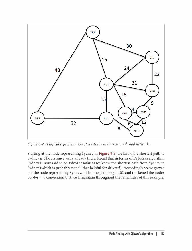
Figure 8-2. A logical representation of Australia and its arterial road network.

Starting at the node representing Sydney in Figure 8-3, we know the shortest path toSydney is 0 hours since we’re already there. Recall that in terms of Dijkstra’s algorithmSydney is now said to be solved insofar as we know the shortest path from Sydney toSydney (which is probably not all that helpful for drivers!). Accordingly we’ve greyedout the node representing Sydney, added the path length (0), and thickened the node’sborder — a convention that we’ll maintain throughout the remainder of this example.


Figure 8-3. The shortest path from Sydney to Sydney is unsurprisingly 0 hours.

Moving one level out from Sydney, our candidate cities are Brisbane to the North by 9hours, Canberra (surprisingly Australia’s capital city) 4 hours to the West and Melbourne12 hours to the South.

The shortest path we can find is Sydney to Canberra at 4 hours, and so we considerCanberra to be solved as we see in Figure 8-4.


Figure 8-4. Canberra is the closest city to Sydney

The next nodes out are Melbourne at 10 hours from Sydney via Canberra or 12 hoursfrom Sydney directly as we’ve already seen. We also have Alice Springs at 15 hours fromCanberra (19 hours from Sydney) or Brisbane at 9 hours direct from Sydney.

Accordingly we explore the shortest path which is 9 hours from Sydney to Brisbane andconsider Brisbane solved at 9 hours in Figure 8-5.


Figure 8-5. Brisbane is the next closest city

The next neighboring nodes from our solved ones are Melbourne (at 10 hours via Can‐berra or 12 hours direct from Sydney along a different road), Cairns at 31 hours fromSydney via Brisbane, Alice Springs at 40 hours via Brisbane or 19 hours via Canberra— some eye-reddening drive times before we’ve even left the East coast!

Accordingly we choose the shortest path which is Melbourne at 10 hours from Sydneyvia Canberra which is shorter than the existing 12 hours direct link, and now considerMelbourne solved as shown in Figure 8-6.


Figure 8-6. Reaching Melbourne, the third-closest city to the start node at representingSydney

In Figure 8-7 the next layer of neighboring nodes from our solved ones are Adelaide at18 hours from Sydney (via Canberra and Melbourne), Cairns at 31 hours from Sydney(via Brisbane), and Alice Springs at 19 or 40 hours from Sydney via Canberra or Brisbanerespectively. Accordingly we choose Adelaide and consider it solved at a cost of 18 hours.

We don’t consider the path Melbourne → Sydney since its destinationis a solved node (in fact in this case the start node, Sydney).


Figure 8-7. Solving Adelaide

The next layer of neighboring nodes from our solved ones are Perth — our final desti‐nation — at 50 hours from Sydney (via Adelaide), Alice Springs at 19 hours from Sydney(via Canberra) or 33 hours via Adelaide, and Cairns at 31 hours from Sydney (via Bris‐bane).

We choose Alice Springs in the case since it has the current shortest path, even thoughwith a god’s eye view we know that actually it’ll be shorter in the end to go from Adelaideto Perth — just ask any passing bushman. Our cost is 19 hours as shown in Figure 8-8.


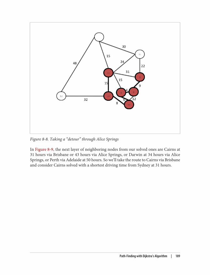
Figure 8-8. Taking a “detour” through Alice Springs

In Figure 8-9, the next layer of neighboring nodes from our solved ones are Cairns at31 hours via Brisbane or 43 hours via Alice Springs, or Darwin at 34 hours via AliceSprings, or Perth via Adelaide at 50 hours. So we’ll take the route to Cairns via Brisbaneand consider Cairns solved with a shortest driving time from Sydney at 31 hours.


Figure 8-9. Back to Cairns on the East coast

The next layer of neighboring nodes from our solved ones are Darwin at 34 hours fromAlice Springs, 61 hours via Cairns, or Perth via Adelaide at 50 hours. Accordingly, wechoose the path to Darwin from Alice Springs at a cost of 34 hours and consider Darwinsolved as we can see in Figure 8-10.


Figure 8-10. To Darwin in Australia’s “top-end”

Finally the only neighboring node left is Perth itself as we can see in Figure 8-11. It isaccessible via Adelaide at a cost of 50 hours or via Darwin at a cost of 82 hours. Ac‐cordingly we choose the route via Adelaide and consider Perth from Sydney solved ata shortest path of 50 hours.


Figure 8-11. Finally reaching Perth, a mere 50 driving hours from Sydney

Dijkstra’s algorithm is a good approach but since it’s exploration is undirected, there aresome pathological graph topologies that can cause worst-case performance problems(where we explore more of the graph that is intuitively necessary, up to the entire graph).Since each possible node is considered one at a time in relative isolation, the algorithmnecessarily follows paths that intuitively will never contribute to the final shortest path.

Despite successfully computing the shortest path between Sydney and Perth usingDijkstra’s algorithm, anyone with any intuition about map reading would likely not havechosen, for instance, to explore the route northwards from Adelaide since it feels longer.If we had some heuristic mechanism to guide the algorithm like in a best-first search(e.g. prefer to head west over east, prefer south over north) we could have perhapsavoided the side-trips to Brisbane, Cairns, Alice Springs, and Darwin in this example.However best-first searches are greedy and try to move towards the destination nodeeven if there is an obstacle (e.g. dirt track), but we can do better.

The A* AlgorithmThe A* (pronounced “A-star”) algorithm is an improvement on the classic Dijkstraalgorithm based on the observation that some searches are informed and that by being


informed we can make better choices about paths to take through the graph (for examplethat we don’t reach Perth from Sydney traversing the height of an entire continent toDarwin first). A* is both like Dijkstra in that it can potentially search a large swathes ofa graph, but it’s also like a greedy best-first search insofar as it uses a heuristic to guideit. A* thus combines aspects of Dijkstra’s algorithm (which prefers nodes close to thecurrent starting point) and best-first search (which prefers nodes closer to the destina‐tion) to provide a provably optimal solution for finding shortest paths in a graph.

In A* we split the path cost into two parts, one g(n) that is the cost of the path from thestarting point to some node n and h(n) which represents the estimated cost of the pathfrom the node n to the destination node, computed by heuristic (an intelligent guess).The A* algorithm balances g(n) and h(n) as it iterates the graph ensuring that at eachiteration it chooses the node with the lowest overall cost f(n) = g(n) + h(n).

But breadth-first algorithms aren’t only good for path finding. In fact using breadth-first search as our method for iterating over all elements of a graph, we can now considera number of interesting higher-order algorithms from graph theory that yield significant(predictive) insight into the behavior of connected data.

Graph Theory and Predictive ModelingGraph theory is a mature and well-understood field of study concerning the nature ofnetworks (or from our point of view, connected data). The analytic techniques that havebeen developed by graph theoreticians can be brought to bear on a range of interestingproblems, and since the low-level traversal mechanisms (like breadth-first search) arealready known to us, we can start to consider higher order analyses.

What’s particularly appealing about applying graph theory techniques to data analysisis their broad applicability. They’re especially valuable where we’re presented with adomain into which we have little insight, or little comprehension of what insight we’reeven able to extract. In such cases there are a range of techniques from graph theoryand social sciences which we can straightforwardly apply to gain insight.

In the next few sections we’ll introduce some of the key concepts in social graph theory.And we’ll introduce those concepts in a humane and (mostly) non-mathematical way

Graph Theory and Predictive Modeling | 193

3. In particular his pivotal work on the strength of weak ties in social communities, see: http://sociology.stanford.edu/people/mgranovetter/documents/granstrengthweakties.pdf

4. See: http://www.cs.cornell.edu/home/kleinber/networks-book/

in a typical social domain based on the works of sociologist Mark Granovetter 3 andEasley/Kleinberg 4.

Property graphs and graph theoryMuch of the work on graph theory assumes a slightly different model to the propertygraphs we’ve been using throughout this book. Typical problem spaces ignore directionand labeling of graphs, instead assuming a single label derived from the domain (e.g.friend or colleague) and ignoring direction.

We’re going to take a hybrid approach here. Supporting relationship names is helpfulfor naming various kinds of relationships from graph theory with more domain-specificmeaning. However where it suits, we’ll ignore (or not) relationship direction.

Importantly, the same principles are upheld by the graph structure whether we’re usinga property graph or a semantically poorer graph model.

Triadic ClosuresA triadic closure is a property of (social) graphs whereby if two nodes are connected viaa path involving a third node, there is an increased likelihood that the two nodes willbecome directly connected in future. This is a familiar enough situation for us in a socialsetting whereby if we happen to be friends with two people, ultimately there’s an in‐creased chance that those people will become direct friends too, since by being our friendin the first place, it’s an indication of social similarity and suitability.

From his analysis, Granovetter noted that a subgraph upholds the strong triadic closureproperty if it has a node A with strong relationships to two other nodes B and C, andthose two other nodes B and C then have at least a weak and potentially a strong rela‐tionship between them. This is an incredibly strong assertion and will not be typicallyupheld by all subgraphs in a graph. Nonetheless it is sufficiently commonplace (partic‐ularly in social networks) to be trusted as a predictive aid.

Strong and weak relationshipsWe purposely won’t explicitly define weak and strong relationships, since they’redomain-specific characteristics. But for example a strong social relationship might be


http://sociology.stanford.edu/people/mgranovetter/documents/granstrengthweakties.pdf

http://sociology.stanford.edu/people/mgranovetter/documents/granstrengthweakties.pdf

http://www.cs.cornell.edu/home/kleinber/networks-book/

friends who’ve exchanged phone calls in the last week, whereas a weak social relationshipmight be friends who’ve merely observed one-another’s Facebook status.

Let’s see how the strong triadic closure property works as a predictive aid in a workplacegraph. Let’s start with a simple organizational hierarchy where Alice managed Bob andCharlie, but where there are not (yet) any connections between her subordinates as inFigure 8-12.

Figure 8-12. Alice manages Bob and Charlie

This is a rather strange situation in the workplace, since it’s unlikely that Bob and Charliewill be disconnected strangers. Whether they’re high level executives and will thereforebe peers under Alice’s executive management or whether they’re assembly line workersand therefore will be close colleagues again under Alice who acts as foreman, eveninformally we expect Bob and Charlie to be somehow connected.


Figure 8-13. Bob and Charlie work together under Alice

However since Bob and Charlie both work with Alice, there’s a strong possibility they’regoing to end up working together as we see in Figure 8-13. This is consistent with thestrong triadic closure property, which suggests that either Bob is a peer of Charlie (we’llcall this a weak relationship) or Bob works with Charlie (which we’ll term a strongrelationship). Adding the third WORKS_WITH or PEER_OF relationship between Bob andCharlie closes the triangle and hence the term triadic closure.

The empirical evidence from many domains including sociology, public health, psy‐chology, anthropology and even technology (e.g. Facebook, Twitter, LinkedIn) suggeststhat the tendency towards triadic closure is real and substantial, consistent with anec‐dotal evidence and sentiment. But simple geometry isn’t all that’s at work here, thesentiment of the relationships involved in a graph also have a significant bearing on theformation of stable triadic closures.

Structural BalanceIf we recall Figure 8-12 it’s intuitive to see how Bob and Charlie can become co-workers(or peers) under Alice’s management. For example purposes, we’re going to make anassumption that the MANAGES relationship is somewhat negative (after all people don’t


like getting bossed around) whereas the PEER_OF and WORKS_WITH relationship are pos‐itive (since people like their peers and the folks they work with).

We know from our previous discussion on the strong triadic closure principle that inFigure 8-12 where Alice MANAGES Bob and Charlie, a triadic closure should be formed.That is in the absence of any other constraints, we would expect at least a PEER_OF, aWORKS_WITH or even a MANAGES relationship between Bob and Charlie.

A similar tendency towards creating a triadic closure exists if Alice MANAGES Bob whoin turn WORKS_WITH Charlie as we can see in Figure 8-14. Anecdotally this rings true: ifBob and Charlie work together it makes sense for them to share a manager, especiallyif the organization seemingly allows Charlie to function without managerial supervi‐sion.

Figure 8-14. Alice manages Bob who works with Charlie

However, applying the strong triadic closure principle blindly can lead to some ratherodd and uncomfortable-looking organization hierarchies. For instance, If Alice MANAGES Bob and Charlie but Bob also MANAGES Charlie, we have a recipe for discontent.Nobody would wish it upon Charlie that he’s managed both by his boss and his boss’boss as in Figure 8-15!


Figure 8-15. Alice manages Bob and Charlie, while Bob also manages Charlie

Similarly it’s uncomfortable for Bob if he is managed by Alice while working with Charliewho is also Alice’s workmate. This cuts awkwardly across organization layers as we seein Figure 8-16. It also means Bob could never safely let off steam about Alice’s man‐agement style!


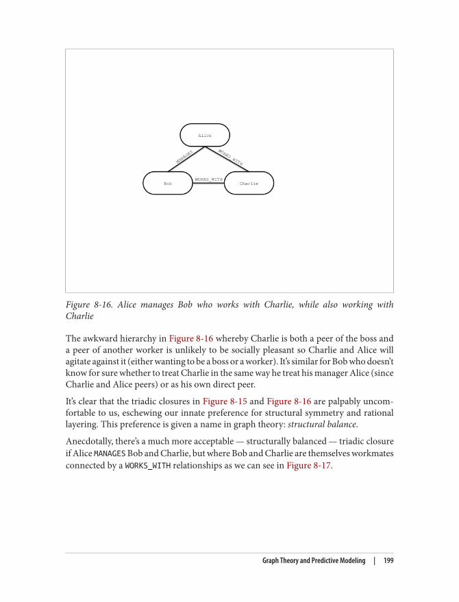
Figure 8-16. Alice manages Bob who works with Charlie, while also working withCharlie

The awkward hierarchy in Figure 8-16 whereby Charlie is both a peer of the boss anda peer of another worker is unlikely to be socially pleasant so Charlie and Alice willagitate against it (either wanting to be a boss or a worker). It’s similar for Bob who doesn’tknow for sure whether to treat Charlie in the same way he treat his manager Alice (sinceCharlie and Alice peers) or as his own direct peer.

It’s clear that the triadic closures in Figure 8-15 and Figure 8-16 are palpably uncom‐fortable to us, eschewing our innate preference for structural symmetry and rationallayering. This preference is given a name in graph theory: structural balance.

Anecdotally, there’s a much more acceptable — structurally balanced — triadic closureif Alice MANAGES Bob and Charlie, but where Bob and Charlie are themselves workmatesconnected by a WORKS_WITH relationships as we can see in Figure 8-17.


Figure 8-17. Workmates Bob and Charlie are managed by Alice

The same structural balance manifests itself in an equally acceptable triadic closurewhere Alice, Bob, and Charlie are all workmates. In this arrangement the workers arein it together which can be a socially amicable arrangement that engenders camaraderieas in Figure 8-18.


Figure 8-18. Alice, Bob and Charlie are all workmates

In Figure 8-17 and Figure 8-18 the triadic closures are idiomatic and constructed witheither three WORKS_WITH relationships or two MANAGES and a single WORKS_WITH rela‐tionship. They are all balanced triadic closures. To understand what it means to havebalanced and unbalanced triadic closures, we’ll add more semantic richness to the modelby declaring that the WORKS_WITH relational is socially positive (since co-workers spenda lot of time interacting) while MANAGES is negative relationship since managers spendoverall less of their time interacting with individuals in their charge.

Given this new dimension of positive and negative sentiment, we can now ask the ques‐tion “What is so special about these balanced structures?” It’s clear that strong triadicclosure is still at work, but that’s not the only driver. In this case the notion of structuralbalance also has an effect. A structurally balanced triadic closure consists of relation‐ships of all strong sentiments (our WORKS_WITH or PEER_OF relationships) or two rela‐tionships have negative sentiments (MANAGES in our case) with a single positive rela‐tionship.

We see this often in the real world. If we have two good friends, then social pressuretends towards those good friends themselves becoming good friends. It’s unusual thatthose two friends themselves are enemies because that puts a strain on our friendships.


5. With due respect to our colleagues in HR, the map is not the territory.

One friend cannot express their dislike of the other to us, since the other person is ourfriend too! Given those pressures, it’s reasonably likely that ultimately the group willresolve its differences and good friends will emerge.

This would change our unbalanced triadic closure (two relationships with positive sen‐timents and one negative) to a balanced closure since all relationships would be of apositive sentiment much like our collaborative scheme where Alice, Bob, and Charlieall work together in Figure 8-18.

However another plausible (though arguably less pleasant) outcome would be wherewe take sides in the dispute between our “friends” creating two relationships with neg‐ative sentiments — effectively ganging up on an individual. Now we can engage in gossipabout our mutual dislike of a former friend and the closure again becomes balanced.Equally we see this reflected in the organizational scenario where Alice, by managingBob and Charlie, becomes in effect their workplace enemy as in Figure 8-17.

Mining organizational data in the real worldWe don’t have to derive these graphs from analyzing organizational charts, since that’sa static and often inconsistent view of how an organization really works 5. A practicaland timely way of generating the graph would instead be to run these kinds of analysesover the history of email exchanges between individuals within a company.

We’d easily be able to identify a graph at large scale and from that we’d be able to makepredictive analyses about the evolution of organizational structure by looking for op‐portunities to create balanced closures. Such structures might be a boon – that we ob‐serve employees are already self-organizing for a successful outcome – or they might beindicative of some malpractice – that some employees moving into shadowy corners tocommit corporate fraud! Either way the predictive power of graphs enable us to engagethose issues proactively.

Balanced closures add another dimension to the predictive power of graphs. Simply bylooking for opportunities to create balanced closures across a graph, even at very largescale, we can modify the graph structure for accurate predictive analyses. But we cango further, and in the next section we’ll bring in the notion of local bridges which giveus valuable insight into the communications flow of our organization and from thatknowledge comes the ability to adapt it to meet future challenges.


Local BridgesAn organization of only three people as we’ve been using is anomalous, and the graphswe’ve studied in this section are best thought of as small sub-graphs as part of a largerorganizational hierarchy. When we start to consider managing a larger organization weexpect a much more complex graph structure, but we can also apply other heuristics tothe structure to help make sense of the business. In fact once we have introduced otherparts of the organization into the graph, we can reason about global properties of thegraph based on the locally-acting strong triadic closure principle.

Figure 8-19. Alice has skewed line management responsibility

In Figure 8-19 we’re presented with a counter-intuitive scenario where two groups inthe organization are managed by Alice and Davina respectively. However, we have theslightly awkward structure that Alice not only runs a team with Bob and Charlie butalso manages Davina. While this isn’t beyond the realms of possibility (Alice may indeedhave such responsibilities) it feels intuitively awkward from an organization designperspective.

From a graph theory perspective it’s also unlikely. Since Alice participates in two strongrelationships, she MANAGES Charlie (and Bob) and MANAGES Davina, naturally we’d like

Local Bridges | 203

to create a triadic closure by adding at least a PEER_OF relationship between Davina andCharlie (and Bob). But Alice is also involved in a local bridge to Davina – together they’rea sole communication path between groups in the organization. Having the relationshipAlice MANAGES Davina means we’d in fact have to create the closure. These two properties– local bridge and strong triadic closure – are in opposition.

Yet if Alice and Davina are peers (a weak relationship), then the strong triadic closureprinciple isn’t activated since there’s only one strong relationship — the MANAGES rela‐tionship to Bob (or Charlie) — and the local bridge property is valid as we can see inFigure 8-20.

Figure 8-20. Alice and Davina are connected by a local bridge

What’s interesting about this local bridge is that it describes a communication channelbetween groups in our organization and those channels are extremely important to thevitality of our enterprise. In particular to ensure the health of our company we’d make


sure that local bridge relationships are healthy and active, or equally we might keep aneye on local bridges to ensure no impropriety (embezzlement, fraud, etc) occurs.

Finding your next jobThis notion of weak social links is particularly pertinent in algorithms like (social) jobsearch. The remarkable thing about job searches is that it’s rarely a close friend thatprovides the best recommendation, but a looser acquaintance.

Why should this be? Our close friends share a similar world view (they’re in the samegraph component) and have similar access to the available jobs data and hold similaropinions about those jobs. A friend across a local bridge is clearly in a different socialnetwork (a different component) and have correspondingly different access to jobs anda different viewpoint about them. So if you’re going to find a job, look across a localbridge since that’s where people who have different knowledge to you and your friendshang out.

This same property of local bridges being weak links (PEER_OF in our example organi‐zation) is a property that is prevalent throughout social graphs. This means we can startto make predictive analyses of how our organization will evolve based on empirically-derived local bridge and strong triadic closure notions. So given an arbitrary organi‐zational graph we can see how the business structure is likely to evolve and plan forthose eventualities.

SummaryGraphs are a remarkable structure and are well studied and often fruitfully applied tomodeling and analysis. We now have native graph databases which project the powerfulgraph model into our applications, bringing with them numerous powerful algorithmicand graph theory techniques which we can use to build better, smarter informationsystems.

As we’ve seen throughout this book, graph algorithms and analytical techniques fromgraph theory are not demanding: we need only understand how to apply them to achieveour goals since the fundamental techniques are mature and well-studied. We leave thisbook with a simple call to arms: to ask the reader to embrace graph data and to applythe modeling, processing, and analytical patterns we’ve shown in this book to createtruly pioneering and impactful information systems.

Summary | 205

Graph Databases - UOP eClass

Documents

Transcript of Graph Databases - UOP eClass