Graph-based transfer learning

Graph-based Transfer Learning

Jingrui HeSchool of Computer ScienceCarnegie Mellon [email protected]

Yan LiuPredictive Modeling Group

IBM [email protected]

Richard LawrencePredictive Modeling Group

IBM [email protected]

ABSTRACTTransfer learning is the task of leveraging the informationfrom labeled examples in some domains to predict the labelsfor examples in another domain. It finds abundant practi-cal applications, such as sentiment prediction, image clas-sification and network intrusion detection. In this paper,we propose a graph-based transfer learning framework. Itpropagates the label information from the source domain tothe target domain via the example-feature-example tripar-tite graph, and puts more emphasis on the labeled exam-ples from the target domain via the example-example bi-partite graph. Our framework is semi-supervised and non-parametric in nature and thus more flexible. We also developan iterative algorithm so that our framework is scalable tolarge-scale applications. It enjoys the theoretical propertyof convergence. Compared with existing transfer learningmethods, the proposed framework propagates the label in-formation to both the features irrelevant to the source do-main and the unlabeled examples in the target domain viathe common features in a principled way. Experimental re-sults on 3 real data sets demonstrate the effectiveness of ouralgorithm.

Categories and Subject DescriptorsH.2.8 [Database Management]: Database Applications –Data Mining

General TermsAlgorithm, experimentation

KeywordsTransfer learning, graph-based

1. INTRODUCTIONTransfer learning refers to the process of leveraging the

information from a source domain to train a better classifierfor a target domain. Typically there are plenty of labeled

Permission to make digital or hard copies of all or part of this work forpersonal or classroom use is granted without fee provided that copies arenot made or distributed for profit or commercial advantage and that copiesbear this notice and the full citation on the first page. To copy otherwise, torepublish, to post on servers or to redistribute to lists, requires prior specificpermission and/or a fee.CIKM’09, November 2–6, 2009, Hong Kong, China.Copyright 2009 ACM 978-1-60558-512-3/09/11 ...$10.00.

examples in the source domain, whereas very few or no la-beled examples in the target domain. Transfer learning isof key importance in many real applications. For example,in sentiment analysis, we may have many labeled movie re-views (labels obtained according to the movie ratings), butwe are interested in analyzing the polarity of reviews aboutan electronic product [4]; in face recognition, we have manytraining images under certain lightening and occlusion con-ditions based on which a model is trained, but practicallythe model will be used under totally different conditions [14].

Generally speaking, transfer learning can follow one of thefollowing three scenarios:

1. The source domain and the target domain have thesame feature space and the same feature distribution,and only the labeling functions are different, such asmulti-label text classification [24];

2. The source domain and the target domain have thesame feature space, but the feature distribution andthe labeling functions are different, such as sentimentclassification for different purposes [4];

3. The source domain and the target domain have dif-ferent feature space, feature distribution and labelingfunctions, such as verb argument classification [10].

In this paper, we focus on the second scenario, which some-times is formalized as the problem that the training set andthe test set have different feature distribution [7].

The main contribution of this paper is to develop a graph-based transfer learning framework based on separate con-structions of a tripartite graph (labeled examples - features- unlabeled examples) and a bipartite graph (labeled exam-ples - unlabeled examples). By propagating the label in-formation from labeled examples (mostly from the sourcedomain) to unlabeled examples (from the target domain)via the features on the tripartite graph, and by imposingdomain related constraints on the bipartite graph, we areable to learn a classification function that takes values on allthe unlabeled examples in the target domain. Finally, theseexamples are labeled according to the sign of the functionvalues. The proposed framework is semi-supervised since itmakes use of unlabeled examples to help propagate the labelinformation. Furthermore, in the second transfer learningscenario (which we are interested in), the labeling functionsin different domains may be closely related to the featuredistribution; thus unlabeled examples are helpful in con-structing the classifiers. However, our framework is differ-ent from traditional semi-supervised learning due to the factthat labeled examples from different domains are treated dif-

ferently in order to construct an accurate classifier in the tar-get domain, whereas in traditional semi-supervised learning,all the labeled examples are treated in the same way. Theframework is also non-parametric in nature, which makes itmore flexible compared with parametric models.

The proposed transfer learning framework is fundamen-tally different from existing graph-based methods. For ex-ample, the authors of [9] proposed a locally weighted ensem-ble framework to combine multiple models for transfer learn-ing, where the weights of different models are approximatedusing a graph-based approach; the authors of [12] proposed asemi-supervised multi-task learning framework, where t-steptransition probabilities in a Markov random walk are incor-porated into the neighborhood-conditional likelihood func-tion to find the optimal parameters. Generally speaking,none of these methods try to propagate the label informa-tion to the features irrelevant to the source domain and theunlabeled examples in the target domain via the commonfeatures. Some non-graph-based methods try to address thisproblem in an ad-hoc way, such as [4], whereas our paperprovides a principled way to do the propagation.

The rest of the paper is organized as follows. Firstly, Sec-tion 2 introduces the tripartite graph and a simple iterativealgorithm for transfer learning based on this graph. Thenin Section 3, we present the graph-based transfer learningframework and associate it with the iterative algorithm fromSection 2. Experimental results are shown in Section 4, fol-lowed by some discussion. Section 5 introduces related work.Finally, we conclude the paper in Section 6.

2. TRANSFER LEARNING WITH TRIPAR-TITE GRAPH

In this section, we first introduce the tripartite graph thatpropagates the label information from the source domainto the target domain via the features. Using this graph,we can obtain a classification function that takes values onall the unlabeled examples from the target domain. Thenwe present an iterative algorithm to find the classificationfunction efficiently.

2.1 NotationLet XS denote the set of examples from the source do-

main, i.e. XS = {xS1 , . . . , xS

m} ⊂ Rd, where m is the numberof examples from the source domain, and d is the dimen-sionality of the feature space. Let YS denote the labelsof these examples, i.e. YS = {yS

1 , . . . , ySm} ⊂ {−1, 1}m,

where ySi is the class label of xS

i , 1 ≤ i ≤ m. Similarly, forthe target domain, let X T denote the set of examples, i.e.X T = {xT

1 , . . . , xTn} ⊂ Rd, where n is the number of exam-

ples from the target domain. Among these examples, onlythe first εn examples are labeled, i.e. YT = {yT

1 , . . . , yTεn} ⊂

{−1, 1}εn, where yTi is the class label of xT

i , 1 ≤ i ≤ εn.Here 0 ≤ ε ¿ 1, i.e. only a small fraction of the examples inthe target domain are labeled, and ε = 0 corresponds to nolabeled examples in the target domain. Our goal is to find aclassification function for all the unlabeled examples in X T

with a small error rate.

2.2 Tripartite GraphLet G(3) = {V (3), E(3)} denote the undirected tripartite

graph, where V (3) is the set of nodes in the graph, and E(3)

is the set of weighted edges. V (3) consists of three types

of nodes: the labeled nodes, i.e. the nodes that correspondto the labeled examples (most of them are from the sourcedomain); the feature nodes, i.e. the nodes that correspondto the features; and the unlabeled nodes, i.e. the nodesthat correspond to the unlabeled examples from the targetdomain. Both the labeled nodes and the unlabeled nodesare connected to the feature nodes, but the labeled nodesare not connected to the unlabeled nodes, and the nodesof the same type are not connected either. Furthermore,there is an edge between a labeled (unlabeled) node and afeature node if and only if the corresponding example hasthat feature, i.e. xS

i,j 6= 0 (xTi,j 6= 0), where xS

i,j (xTi,j) is

the jth feature component of xSi (xT

i ), and the edge weightis set to xS

i,j (xTi,j). Here we assume that the edge weights

are non-negative. This is true in many applications, suchas document analysis where each feature corresponds to aunique word and the edge weight is binary or equal to thetfidf value. In a general setting, this may not be the case.However, we could perform a linear transformation to thefeatures and make them non-negative.

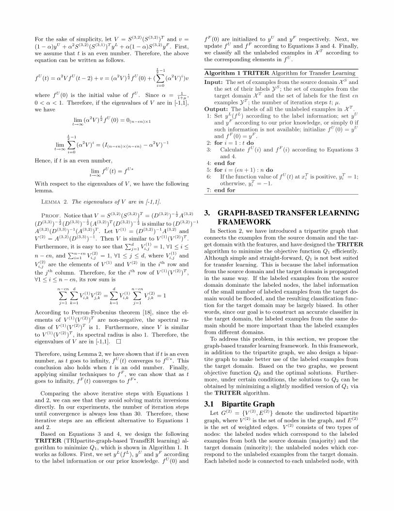
Fig. 1a shows an example of the tripartite graph. Thediamond-shaped nodes correspond to the feature nodes, thelighter circle nodes correspond to the examples from thesource domain, and the darker circle nodes correspond tothe examples from the target domain. Notice that the la-beled nodes are on the left hand side, the feature nodesare in the middle, and the unlabeled nodes are on the righthand side. The intuition of the graph can be explained asfollows. Consider sentiment classification in different do-mains as an example. Each of the diamond-shaped nodesin Fig. 1a corresponds to a unique word; the lighter circlenodes correspond to labeled movie reviews; and the darkercircle nodes correspond to product reviews that we are in-terested in. The labeled reviews on the left hand side ofFig. 1a propagate their label information to the unlabeledproduct reviews via the feature nodes. Notice that each ofthe two domains may have some unique words that neveroccur in the other domain. For example, the word ‘actor’often occurs in a movie review, but may never occur in aproduct review; similarly, the word ‘polyethylene’ may oc-cur in a product review, but is never seen in a movie review.Based on this graph structure, the label information can bepropagated to the domain-specific words, i.e. the words ir-relevant to the movie reviews, which will help classify theunlabeled product reviews.

Given the tripartite graph, we define affinity matrix A(3),which is (m + n + d)× (m + n + d). The first m + εn rows(columns) correspond to the labeled nodes, the next n− εnrows (columns) correspond to the unlabeled nodes, and theremaining d rows (columns) correspond to the feature nodes.

Therefore, A(3) has the following block structure

A(3) =

0(m+εn)×(m+εn) 0(m+εn)×(n−εn) A(3,1)

0(n−εn)×(m+εn) 0(n−εn)×(n−εn) A(3,2)

(A(3,1))T (A(3,2))T 0d×d

where 0a×b is an a × b 0 matrix, A(3,1) and A(3,2) are bothsub-matrices of A(3), and (·)T is the transpose of a matrix.

Let A(3,1)i,j (A

(3,2)i,j ) denote the element in the ith row and the

jth column of A(3,1) (A(3,2)). Based on the discussion above,

A(3,1)i,j = xS

i,j and A(3,2)i,j = xT

i,j . Note that the elements of

A(3) are non-negative. Furthermore, define diagonal matrixD(3), which is (m + n + d) × (m + n + d). Its diagonal

element D(3)i =

∑m+n+dj=1 A

(3)i,j , i = 1, . . . , m + n + d, where

A(3)i,j denote the element in the ith row and the jth column of

A(3). Similar as A(3), D(3) has the following block structure

D(3) =

D(3,1) 0(m+εn)×(n−εn) 0(m+εn)×d

0(n−εn)×(m+εn) D(3,2) 0(n−εn)×d

0d×(m+εn) 0d×(n−εn) D(3,3)

where D(3,1), D(3,2) and D(3,3) are diagonal matrices whosediagonal elements are equal to the row sums of A(3,1), A(3,2)

and (A(3,1))T + (A(3,2))T respectively. Finally, define the

normalized affinity matrix S(3) = (D(3))−1/2A(3)(D(3))−1/2,which also has the following block structure

S(3) =

0(m+εn)×(m+εn) 0(m+εn)×(n−εn) S(3,1)

0(n−εn)×(m+εn) 0(n−εn)×(n−εn) S(3,2)

(S(3,1))T (S(3,2))T 0d×d

where S(3,1) = (D(3,1))−12 A(3,1)(D(3,3))−

12 , and S(3,2) =

(D(3,2))−12 A(3,2)(D(3,3))−

12 . Similar as A(3), the elements

of S(3) are also non-negative.

2.3 Objective Function Q1

Given the tripartite graph and the corresponding affin-ity matrix, we can define three functions fL, fF and fU ,which take values on the labeled nodes, the feature nodes,and the unlabeled nodes respectively. Note that the functionvalue of fU will be used to classify the unlabeled examplesin the target domain, and the function value of fF can beused to infer the polarity of the features. Similarly, definethree vectors yL, yF and yU , whose lengths are equal tothe number of labeled nodes m + εn, the number of fea-ture nodes d, and the number of unlabeled nodes n − εnrespectively. The elements of yL are set to be the classlabel of the corresponding labeled example, whereas the ele-ments of yF and yU could reflect our prior knowledge aboutthe polarity of the features and the unlabeled examples, orsimply 0 if such information is not available. For the sakeof notation simplicity, let f = [(fL)T , (fU )T , (fF )T ]T andy = [(yL)T , (yU )T , (yF )T ]T .

To find the classification function with a low error rate, wepropose to minimize the following objective function, whichis motivated by [25].

Q1(f) =1

2

m+n+d∑i,j=1

A(3)ij (

fi√D

(3)i

− fj√D

(3)j

)2 + µ

m+n+d∑i=1

(fi − yi)2

= fT (I(m+n+d)×(m+n+d) − S(3))f + µ‖f − y‖2

where µ is a small positive parameter, Ia×b is an a× b iden-tity matrix, and fi and yi are the ith element of f and yrespectively.

This objective function can be interpreted as follows. Thefirst term of Q1, fT (I(m+n+d)×(m+n+d) − S(3))f , measuresthe label smoothness of f . In other words, neighboring nodeson the graph should have similar f values. The second term,µ‖f−y‖2, measures the consistency of f with the label infor-mation and the prior knowledge encoded in y. By minimiz-ing Q1, we hope to obtain a smooth classification functionfU with a small error rate.

In our implementation, we fix fL = yL. In this way, wecan make better use of the label information in yL. Thismodification distinguishes our method from the manifold

ranking algorithm proposed in [25], where each element off needs to be optimized. Minimizing Q1 with the aboveconstraint, we have the following lemma.

Lemma 1. If fL = yL, Q1 is minimized at

fU∗ = (I(n−εn)×(n−εn) − α2S(3,2)(S(3,2))T )−1 (1)

((1− α)yU + α(1− α)S(3,2)yF + α2S(3,2)(S(3,1))T yL)

fF∗ = (Id×d − α2(S(3,2))T S(3,2))−1((1− α)yF (2)

+α(S(3,1))T yL + α(1− α)(S(3,2))T yU )

where α = 11+µ

.

Proof. Replacing fL with yL, Q1 becomes

Q1 = (yL)T yL + (fU )T fU + (fF )T fF − 2(yL)T S(3,1)fF

− 2(fU )T S(3,2)fF + µ‖fU − yU‖2 + µ‖fF − yF ‖2

Therefore,

∂Q1

∂fU= 2fU − 2S(3,2)fF + 2µ(fU − yU )

∂Q1

∂fF= 2fF − 2(S(3,1))T yL − 2(S(3,2))T fU + 2µ(fF − yF )

Setting ∂Q1∂fU and ∂Q1

∂fF to 0, we get Equations 1 and 2.

Notice that in Lemma 1, in order to get fU∗ and fF∗,we need to solve matrix inversions. This is computationallyexpensive especially when the number of unlabeled examplesin XT or the number of features is very large. To addressthis problem, we propose the following iteration steps toobtain the optimal solutions.

fU (t + 1) = αS(3,2)fF (t) + (1− α)yU (3)

fF (t+1) = α(S(3,1))T yL +α(S(3,2))T fU (t)+(1−α)yF (4)

where fU (t) and fF (t) denote fU and fF at the tth itera-tion. The two equations can be interpreted as follows. Basedon Equation 3, if an example has many positive (negative)features or it is believed to be positive (negative) a priori,its function value would be large (small), indicating that itis a positive (negative) example. Based on Equation 4, ifa feature is contained in many positive (negative) labeledexamples, or it is shared by many unlabeled examples withlarge (small) function values, or it is believed to be positive(negative) a priori, its function value would be large (small).In this way, the label information is gradually propagatedto the unlabeled examples in the target domain and thefeatures irrelevant to the source domain via the commonfeatures on the tripartite graph.

The following theorem guarantees the convergence of theiteration steps.

Theorem 1. When t goes to infinity, fU (t) converges tofU∗ and fF (t) converges to fF∗.

Proof. According to Equations 3 and 4

fU (t) = αS(3,2)fF (t− 1) + (1− α)yU = (1− α)yU

+ αS(3,2)(α(S(3,1))T yL + α(S(3,2))T fU (t− 2)

+ (1− α)yF )

= α2S(3,2)(S(3,2))T fU (t− 2) + (1− α)yU

+ α2S(3,2)(S(3,1))T yL + α(1− α)S(3,2)yF

For the sake of simplicity, let V = S(3,2)(S(3,2))T and v =

(1 − α)yU + α2S(3,2)(S(3,1))T yL + α(1 − α)S(3,2)yF . First,we assume that t is an even number. Therefore, the aboveequation can be written as follows.

fU (t) = α2V fU (t− 2) + v = (α2V )t2 fU (0) + (

t2−1∑i=0

(α2V )i)v

where fU (0) is the initial value of fU . Since α = 11+µ

,

0 < α < 1. Therefore, if the eigenvalues of V are in [-1,1],we have

limt→∞

(α2V )t2 fU (0) = 0(n−εn)×1

limt→∞

t2−1∑i=0

(α2V )i = (I(n−εn)×(n−εn) − α2V )−1

Hence, if t is an even number,

limt→∞

fU (t) = fU∗

With respect to the eigenvalues of V , we have the followinglemma.

Lemma 2. The eigenvalues of V are in [-1,1].

Proof. Notice that V = S(3,2)(S(3,2))T = (D(3,2))−12 A(3,2)

(D(3,3))−12 (D(3,3))−

12 (A(3,2))T (D(3,2))−

12 is similar to (D(3,2))−1

A(3,2)(D(3,3))−1(A(3,2))T . Let V (1) = (D(3,2))−1A(3,2) and

V (2) = A(3,2)(D(3,3))−1. Then V is similar to V (1)(V (2))T .

Furthermore, it is easy to see that∑d

j=1 V(1)

i,j = 1, ∀1 ≤ i ≤n − εn, and

∑n−εni=1 V

(2)i,j = 1, ∀1 ≤ j ≤ d, where V

(1)i,j and

V(2)

i,j are the elements of V (1) and V (2) in the ith row and

the jth column. Therefore, for the ith row of V (1)(V (2))T ,∀1 ≤ i ≤ n− εn, its row sum is

n−εn∑j=1

d∑

k=1

V(1)

i,k V(2)

j,k =

d∑

k=1

V(1)

i,k

n−εn∑j=1

V(2)

j,k = 1

According to Perron-Frobenius theorem [18], since the el-

ements of V (1)(V (2))T are non-negative, the spectral ra-

dius of V (1)(V (2))T is 1. Furthermore, since V is similar

to V (1)(V (2))T , its spectral radius is also 1. Therefore, theeigenvalues of V are in [-1,1].

Therefore, using Lemma 2, we have shown that if t is an evennumber, as t goes to infinity, fU (t) converges to fU∗. Thisconclusion also holds when t is an odd number. Finally,applying similar techniques to fF , we can show that as tgoes to infinity, fF (t) converges to fF∗.

Comparing the above iterative steps with Equations 1and 2, we can see that they avoid solving matrix inversionsdirectly. In our experiments, the number of iteration stepsuntil convergence is always less than 30. Therefore, theseiterative steps are an efficient alternative to Equations 1and 2.

Based on Equations 3 and 4, we design the followingTRITER (TRIpartite-graph-based TransfER learning) al-gorithm to minimize Q1, which is shown in Algorithm 1. Itworks as follows. First, we set yL(fL), yU and yF accordingto the label information or our prior knowledge. fU (0) and

fF (0) are initialized to yU and yF respectively. Next, weupdate fU and fF according to Equations 3 and 4. Finally,we classify all the unlabeled examples in X T according tothe corresponding elements in fU .

Algorithm 1 TRITER Algorithm for Transfer Learning

Input: The set of examples from the source domain XS andthe set of their labels YS ; the set of examples from thetarget domain X T and the set of labels for the first εnexamples YT ; the number of iteration steps t; µ.

Output: The labels of all the unlabeled examples in X T .1: Set yL(fL) according to the label information; set yU

and yF according to our prior knowledge, or simply 0 ifsuch information is not available; initialize fU (0) = yU

and fF (0) = yF .2: for i = 1 : t do3: Calculate fU (i) and fF (i) according to Equations 3

and 4.4: end for5: for i = (εn + 1) : n do6: If the function value of fU (t) at xT

i is positive, yTi = 1;

otherwise, yTi = −1.

7: end for

3. GRAPH-BASED TRANSFER LEARNINGFRAMEWORK

In Section 2, we have introduced a tripartite graph thatconnects the examples from the source domain and the tar-get domain with the features, and have designed the TRITERalgorithm to minimize the objective function Q1 efficiently.Although simple and straight-forward, Q1 is not best suitedfor transfer learning. This is because the label informationfrom the source domain and the target domain is propagatedin the same way. If the labeled examples from the sourcedomain dominate the labeled nodes, the label informationof the small number of labeled examples from the target do-main would be flooded, and the resulting classification func-tion for the target domain may be largely biased. In otherwords, since our goal is to construct an accurate classifier inthe target domain, the labeled examples from the same do-main should be more important than the labeled examplesfrom different domains.

To address this problem, in this section, we propose thegraph-based transfer learning framework. In this framework,in addition to the tripartite graph, we also design a bipar-tite graph to make better use of the labeled examples fromthe target domain. Based on the two graphs, we presentobjective function Q2 and the optimal solutions. Further-more, under certain conditions, the solutions to Q2 can beobtained by minimizing a slightly modified version of Q1 viathe TRITER algorithm.

3.1 Bipartite GraphLet G(2) = {V (2), E(2)} denote the undirected bipartite

graph, where V (2) is the set of nodes in the graph, and E(2)

is the set of weighted edges. V (2) consists of two types ofnodes: the labeled nodes which correspond to the labeledexamples from both the source domain (majority) and thetarget domain (minority); the unlabeled nodes which cor-respond to the unlabeled examples from the target domain.Each labeled node is connected to each unlabeled node, with

the edge weight indicating the domain related similarity be-tween the two examples, whereas the same type of nodes arenot connected.

Fig. 1b shows an example of the bipartite graph which hasthe same labeled and unlabeled nodes as in Fig. 1a. Sim-ilarly, the lighter circle nodes correspond to the examplesfrom the source domain, and the darker circle nodes corre-spond to the examples from the target domain. The labelednodes on the left hand side are connected to each unlabelednode on the right hand side. Again take sentiment classi-fication in different domains as an example. The labelednodes correspond to all the labeled reviews, most of whichare movie reviews, and the unlabeled nodes correspond toall the unlabeled product reviews. The edge weights are setto reflect the domain related similarity between two reviews.Therefore, if two reviews are both product reviews, one la-beled and one unlabeled, their edge weight would be large;whereas if two reviews are from different domains, the moviereview labeled and the product review unlabeled, their edgeweight would be small. In this way, we hope to make betteruse of the labeled product reviews to construct the classifi-cation function for the unlabeled product reviews.

(a) Tripartite graph (b) Bipartitegraph

Figure 1: An example of the graphs.

Let A(2) denote the affinity matrix for the bipartite graph,which is (m+n)× (m+n). The first m+ εn rows (columns)correspond to the labeled nodes, and the remaining n − εnrows (columns) correspond to the unlabeled nodes. Accord-

ing to the structure of the bipartite graph, A(2) has thefollowing form.

A(2) =

[0(m+εn)×(m+εn) A(2,1)

(A(2,1))T 0(n−εn)×(n−εn)

]

where A(2,1) is the sub-matrix of A(2). Note that the ele-ments of A(2) are set to be non-negative. Let D(2) denote the(m+n)× (m+n) diagonal matrix, the ith diagonal element

of which is defined D(2)i =

∑m+nj=1 A

(2)i,j , i = 1, . . . , m + n,

where A(2)i,j is the element of A(2) in the ith row and the

jth column. Similar as A(2), D(2) has the following blockstructure.

D(2) =

[D(2,1) 0(m+εn)×(n−εn)

0(n−εn)×(m+εn) D(2,2)

]

where D(2,1) and D(2,2) are diagonal matrices whose diago-

nal elements are equal to the row sums and the column sumsof A(2,1) respectively. Finally, let S(2) denote the normalizedaffinity matrix S(2) = (D(2))−1/2A(2)(D(2))−1/2, which alsohas the following block structure.

S(2) =

[0(m+εn)×(m+εn) S(2,1)

(S(2,1))T 0(n−εn)×(n−εn)

]

where S(2,1) = (D(2,1))−12 A(2,1)(D(2,2))−

12 .

3.2 Objective Function Q2

In Subsection 2.2, we introduced a tripartite graph whichpropagates the label information from the labeled nodes tothe unlabeled nodes via the feature nodes; and in Subsec-tion 3.1, we introduced a bipartite graph which puts highweights on the edges connecting examples from the samedomain and low weights on the edges connecting examplesfrom different domains. In this section, we combine the twographs to design objective function Q2. By minimizing Q2,we can obtain a smooth classification function for the unla-beled examples in the target domain which relies more onthe labeled examples from the target domain than on thosefrom the source domain.

For the sake of simplicity, define g = [(fL)T , (fU )T ]T . It iseasy to see that g = Bf , where B = [I(m+n)×(m+n), 0(m+n)×d].Thus the objective function Q2 can be written as follows.

Q2(f) =1

2γ

m+n+d∑i,j=1

A(3)i,j (

fi√D

(3)i

− fj√D

(3)j

)2

+1

2τ

m+n∑i,j=1

A(2)i,j (

gi√D

(2)i

− gj√D

(2)j

)2 + µ

m+n+d∑i=1

(fi − yi)2

= γfT (I(m+n+d)×(m+n+d) − S(3))f

+ τfT BT (I(m+n)×(m+n) − S(2))Bf + µ‖f − y‖2

where γ and τ are two positive parameters. Similar as inQ1, the first term of Q2, γfT (I(m+n+d)×(m+n+d) − S(3))f ,measures the label smoothness of f on the tripartite graph;the second term, τfT BT (I(m+n)×(m+n)−S(2))Bf , measuresthe label smoothness of f on the bipartite graph; and thethird term, µ‖f − y‖2, measures the consistency of f withthe label information and the prior knowledge. It shouldbe pointed out that the first two terms in Q2 can be com-bined mathematically; however, the two graphs can not becombined due to the normalization process.

Based on Q2, we can claim that our method is differ-ent from semi-supervised learning, which treats the labeledexamples from different domains in the same way. In ourmethod, by imposing the label smoothness constraint onthe bipartite graph, we can see that the labeled examplesfrom the target domain have more impact on the unlabeledexamples from the same domain than the labeled examplesfrom the source domain. In the next section, we will com-pare our method with a semi-supervised learning methodexperimentally.

Similar as before, we fix fL = yL, and minimize Q2 withrespect to fU and fF . The solutions can be obtained by thefollowing lemma.

Lemma 3. If fL = yL, Q2 is minimized at

fU∗ = ((γ + τ + µ)I(n−εn)×(n−εn) − γ2

γ + µS(3,2)(S(3,2))T )−1

(5)

(µyU +γ2

γ + µS(3,2)(S(3,1))T yL +

γµ

γ + µS(3,2)yF

+ τ(S(2,1))T yL)

fF∗ =γ

γ + µ((S(3,1))T yL + (S(3,2))T fU∗) +

µ

γ + µyF (6)

Proof. Replacing fL with yL, Q2 becomes

Q2 = γ((yL)T yL + (fU )T fU + (fF )T fF

− 2(yL)T S(3,1)fF − 2(fU )T S(3,2)fF )

+ τ((yL)T yL + (fU )T fU − 2(yL)T S(2,1)fU )

+ µ‖fU − yU‖2 + µ‖fF − yF ‖2

Therefore,

∂Q2

∂fU= 2γ(fU − S(3,2)fF ) + 2τ(fU − (S(2,1))T yL)

+ 2µ(fU − yU )

∂Q2

∂fF= 2γ(fF − (S(3,1))T yL − (S(3,2))T fU )

+ 2µ(fF − yF )

Setting ∂Q2∂fU and ∂Q2

∂fF to 0, we get Equations 5 and 6.

In Equation 5, if we ignore the matrix inversion term inthe front, we can see that fU∗ gets the label informationfrom the labeled nodes through the following two terms:

γ2

γ+µS(3,2)(S(3,1))T yL and τ(S(2,1))T yL, which come from

the tripartite graph and the bipartite graph respectively.Recall that yL is defined on the labeled nodes from boththe source domain and the target domain. In particular, ifa labeled node is from the target domain, its correspondingrow in S2,1 would have large values, and it will make a bigcontribution to fU∗ via τ(S(2,1))T yL. This is in contrast tolabeled nodes from the source domain, whose correspondingrows in S2,1 have small values, and their contribution to fU∗

would be small as well.Similar to objective function Q1, we can also design an

iterative algorithm to find the solutions of Q2. However, inthe following, we focus on the relationship between Q1 andQ2, and will introduce an iterative algorithm based on theTRITER algorithm to solve Q2.

Comparing Equations 1 with 5, we can see that they arevery similar to each other. The following theorem builds aconnection between objective functions Q1 and Q2.

Theorem 2. If fL = yL, then fU∗ can be obtained by

minimizing Q1 with the following parametrization

α′ =γ√

(µ + γ)(µ + γ + τ)

y′L = yL

y′U =µyU + τ(S(2,1))T yL

µ + γ + τ − γ√

µ+γ+τµ+γ

y′F =µ√

(µ + γ)(µ + γ + τ)− γyF

Proof. Replacing α, yL, yU and yF with α′, y′L, y′U andy′F respectively in Equations 1, we get Equations 5.

The most significant difference between the parameter set-tings in Theorem 2 and the original settings is in the defini-tion of y′U . That is, y′U consists of two parts, one from itsown prior information, which is in proportion to µyU , andthe other from the label information of the labeled exam-ples, which is in proportion to τ(S(2,1))T yL. Note that thesecond part is obtained via the bipartite graph, and it en-codes the domain information. In other words, incorporatingthe bipartite graph into the transfer learning framework isequivalent to working with the tripartite graph alone, witha domain specific prior for the unlabeled examples in thetarget domain and slightly modified versions of α and yF .

Finally, to minimize Q2, we can simply apply the TRITERalgorithm with the parameter settings specified in Theo-rem 2, which usually converges within 30 iteration steps.

4. EXPERIMENTAL RESULTSIn this section, we present some experimental results, and

compare the proposed graph-based transfer learning frame-work with state-of-the-art techniques.

4.1 Experiment SettingsTo demonstrate the performance of the proposed graph-

based transfer learning framework, we perform experimentsin the following 3 areas.

1. Sentiment classification (SC). In this area, we use themovie and product review data set. The movie re-views come from [15]. Positive labels are assigned toratings above 3.5 stars and negative to 2 and fewerstars. The product reviews are collected from Amazonfor software worth more than 50 dollars. In our exper-iments, we use the movie reviews as the source domainand the product reviews as the target domain. Afterstemming and stop word removal, the feature space is34305-dimensional.

2. Document classification (DC). In this area, we use the20 newsgroups data set [16]. The documents withinthis data set has a two-level categorical structure. Basedon this structure, we generate 3 transfer learning tasks.Each task involves distinguishing two higher-level cat-egories. The source domain and the target domaincontains examples from different lower-level categories.For example, one transfer learning task is to distin-guish between rec and talk. The source domain con-tains examples from rec.sport.baseball and talk.politics.misc; whereas the target domain contains examplesfrom rec.sport.hockey and talk.religion.misc. The way

that the transfer learning tasks are generated is similarto [9] and [6]. After stemming and stop word removal,the feature space is 53975-dimensional.

3. Intrusion detection (ID). In this area, we use the KDDCup 99 data set [1]. It consists of both normal con-nections and attacks of different types, including DOS(denial-of-service), R2L (unauthorized access from aremote machine), U2R (unauthorized access to localsuperuser privileges), and probing (surveillance andother probing). For this data set, we also generate 3transfer learning tasks. In each task, both the sourcedomain and the target domain contain some normalexamples as the positive class, but the negative classin the two domains corresponds to different types ofattacks. Similar as in [9], only the 34 continuous fea-tures are used.

The details of the transfer learning tasks are summarizedin Table 1. Notice that in SC and DC, we tried both binaryfeatures and tfidf features. It turns out that binary featureslead to better performance. Therefore, we only report theexperimental results with the binary features here. Notethat the features in ID are not binary.

In our proposed transfer learning framework, the bipartitegraph is constructed as follows. A(2,1) is a linear combina-tion of two matrices. The first matrix is based on domaininformation, i.e. its element is set to 1 iff the correspondinglabeled and unlabeled examples are both from the targetdomain, and it is set to 0 otherwise. The second matrixis A(3,1)(A(3,2))T , i.e. if a labeled example shares a lot offeatures with an unlabeled example, the corresponding ele-ment in this matrix is large. Note that this is only one way ofconstructing the bipartite graph with domain information.Exploring the optimal bipartite graph for transfer learningis beyond the scope of this paper.

We compare our method with the following methods.

1. Learning from the target domain only, which is de-noted target only. With this method, we ignore thesource domain, and construct the classification func-tion solely based on the labeled examples from thetarget domain. In other words, none of the nodes inthe tripartite graph and bipartite graph correspond toexamples from the source domain.

2. Learning from the source domain only, which is de-noted source only. With this method, we ignore thelabel information from the target domain, and con-struct the classification function solely based on thelabeled examples from the source domain. In otherwords, all of the nodes on the left hand side of thetripartite graph and the bipartite graph correspond toexamples from the source domain, and the nodes thatcorrespond to the target domain examples are all onthe right hand side of the two graphs.

3. Learning from both the source domain and the targetdomain, which is denoted source+target. With thismethod, we combine the function fU output by targetonly and source only linearly, and predict the classlabels of the unlabeled examples accordingly.

4. Semi-supervised learning, denoted semi-supervised.It is based on the manifold ranking algorithm [25].With this method, all the labeled examples are consid-ered from the target domain, and we propagate their

label information to the unlabeled examples in thesame way.

5. The transfer learning toolkit developed by UC Berke-ley (http://multitask.cs.berkeley.edu/). The methodthat we use is based on [2], which is denoted BTL.Note that for document classification and sentimentclassification, the feature space is too large to be pro-cessed by BTL. Therefore, as a preprocessing step,we perform singular value decomposition (SVD) toproject the data onto the 100-dimensional space spannedby the first 100 singular vectors.

6. The boosting-based transfer learning method [7], whichis denoted TBoost.

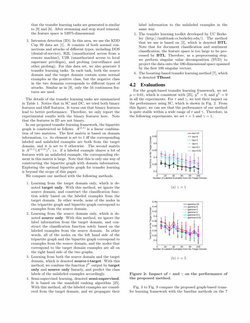
4.2 EvaluationsFor the graph-based transfer learning framework, we set

µ = 0.01, which is consistent with [25], yF = 0, and yU = 0in all the experiments. For τ and γ, we test their impact onthe performance using SC, which is shown in Fig. 2. Fromthis figure, we can see that the performance of our methodis quite stable within a wide range of τ and γ. Therefore, inthe following experiments, we set τ = 5 and γ = 1.

0 20 40 60 80 100

0.3

0.35

0.4

0.45

0.5

0.55

Number of Labeled Examples from the Target Domain

Tes

t Err

or o

n th

e T

arge

t Dom

ain

tau=10

tau=5

tau=2

tau=1

tau=0.1

tau=0.01

(a) γ = 1

0 20 40 60 80 100

0.3

0.32

0.34

0.36

0.38

0.4

0.42

0.44

0.46


Tes

t Err

or o

n th

e T

arge

t Dom

ain

gamma=10gamma=5gamma=2gamma=1gamma=0.1gamma=0.01

(b) τ = 5

Figure 2: Impact of τ and γ on the performance ofthe proposed method.

Fig. 3 to Fig. 9 compare the proposed graph-based trans-fer learning framework with the baseline methods on the 7

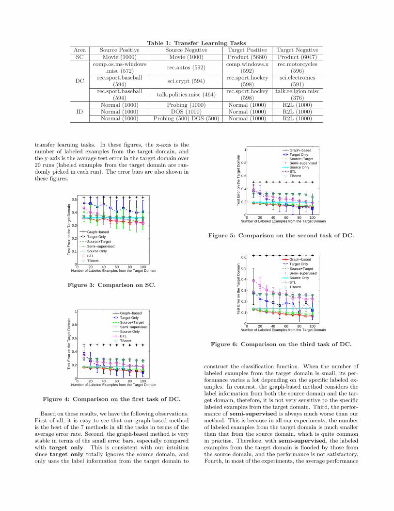
Table 1: Transfer Learning TasksArea Source Positive Source Negative Target Positive Target NegativeSC Movie (1000) Movie (1000) Product (5680) Product (6047)

DC

comp.os.ms-windowsrec.autos (592)

comp.windows.x rec.motorcycles.misc (572) (592) (596)

rec.sport.baseballsci.crypt (594)

rec.sport.hockey sci.electronics(594) (598) (591)

rec.sport.baseballtalk.politics.misc (464)

rec.sport.hockey talk.religion.misc(594) (598) (376)

IDNormal (1000) Probing (1000) Normal (1000) R2L (1000)Normal (1000) DOS (1000) Normal (1000) R2L (1000)Normal (1000) Probing (500) DOS (500) Normal (1000) R2L (1000)

transfer learning tasks. In these figures, the x-axis is thenumber of labeled examples from the target domain, andthe y-axis is the average test error in the target domain over20 runs (labeled examples from the target domain are ran-domly picked in each run). The error bars are also shown inthese figures.

0 20 40 60 80 1000

0.1

0.2

0.3

0.4

0.5


Tes

t Err

or o

n th

e T

arge

t Dom

ain

Graph−basedTarget OnlySource+TargetSemi−supervisedSource OnlyBTLTBoost

Figure 3: Comparison on SC.

0 20 40 60 80 1000

0.2

0.4

0.6

0.8

1


Tes

t Err

or o

n th

e T

arge

t Dom

ain


Figure 4: Comparison on the first task of DC.

Based on these results, we have the following observations.First of all, it is easy to see that our graph-based methodis the best of the 7 methods in all the tasks in terms of theaverage error rate. Second, the graph-based method is verystable in terms of the small error bars, especially comparedwith target only. This is consistent with our intuitionsince target only totally ignores the source domain, andonly uses the label information from the target domain to

0 20 40 60 80 1000

0.2

0.4

0.6

0.8

1


Tes

t Err

or o

n th

e T

arge

t Dom

ain


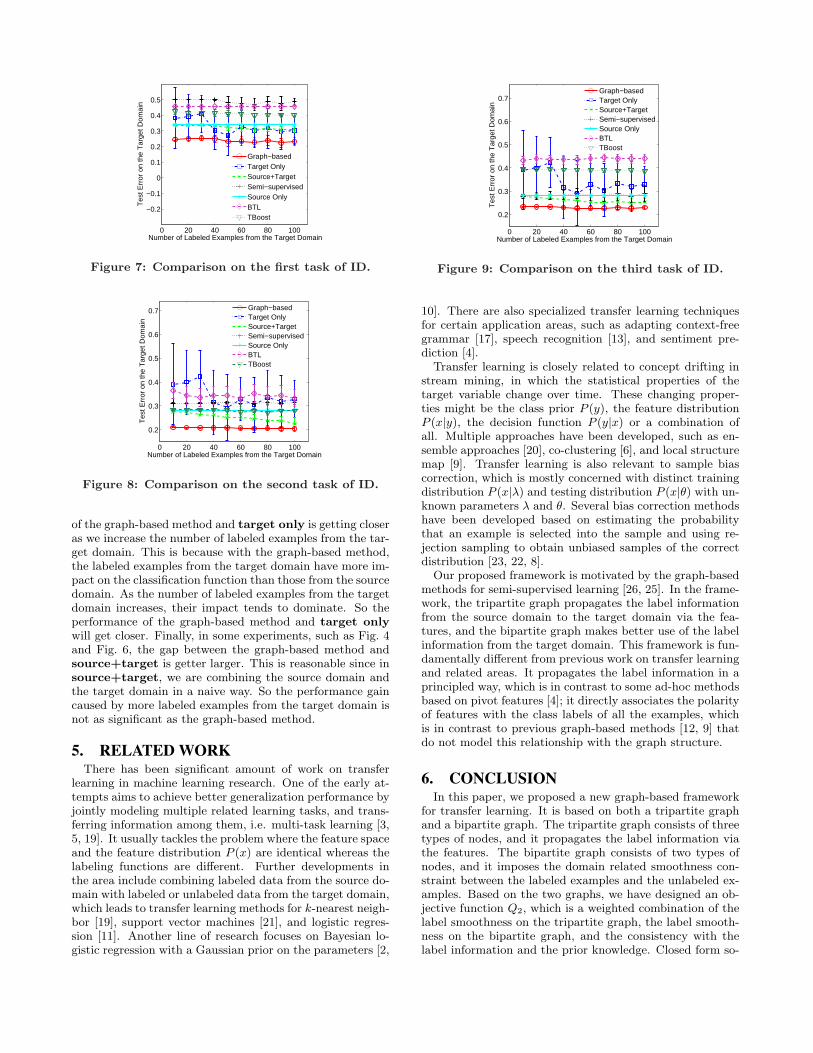
Figure 5: Comparison on the second task of DC.

0 20 40 60 80 1000

0.1

0.2

0.3

0.4

0.5

0.6


Tes

t Err

or o

n th

e T

arge

t Dom

ain


Figure 6: Comparison on the third task of DC.

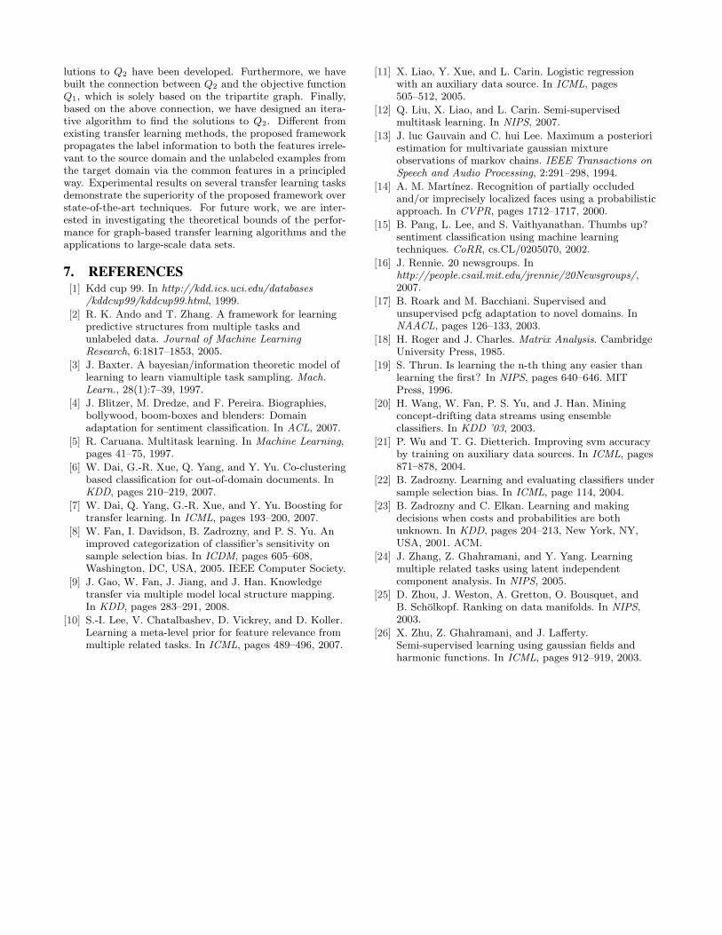
construct the classification function. When the number oflabeled examples from the target domain is small, its per-formance varies a lot depending on the specific labeled ex-amples. In contrast, the graph-based method considers thelabel information from both the source domain and the tar-get domain, therefore, it is not very sensitive to the specificlabeled examples from the target domain. Third, the perfor-mance of semi-supervised is always much worse than ourmethod. This is because in all our experiments, the numberof labeled examples from the target domain is much smallerthan that from the source domain, which is quite commonin practise. Therefore, with semi-supervised, the labeledexamples from the target domain is flooded by those fromthe source domain, and the performance is not satisfactory.Fourth, in most of the experiments, the average performance

0 20 40 60 80 100

−0.2

−0.1

0

0.1

0.2

0.3

0.4

0.5


Tes

t Err

or o

n th

e T

arge

t Dom

ain


Figure 7: Comparison on the first task of ID.

0 20 40 60 80 100

0.2

0.3

0.4

0.5

0.6

0.7


Tes

t Err

or o

n th

e T

arge

t Dom

ain


Figure 8: Comparison on the second task of ID.

of the graph-based method and target only is getting closeras we increase the number of labeled examples from the tar-get domain. This is because with the graph-based method,the labeled examples from the target domain have more im-pact on the classification function than those from the sourcedomain. As the number of labeled examples from the targetdomain increases, their impact tends to dominate. So theperformance of the graph-based method and target onlywill get closer. Finally, in some experiments, such as Fig. 4and Fig. 6, the gap between the graph-based method andsource+target is getter larger. This is reasonable since insource+target, we are combining the source domain andthe target domain in a naive way. So the performance gaincaused by more labeled examples from the target domain isnot as significant as the graph-based method.

5. RELATED WORKThere has been significant amount of work on transfer

learning in machine learning research. One of the early at-tempts aims to achieve better generalization performance byjointly modeling multiple related learning tasks, and trans-ferring information among them, i.e. multi-task learning [3,5, 19]. It usually tackles the problem where the feature spaceand the feature distribution P (x) are identical whereas thelabeling functions are different. Further developments inthe area include combining labeled data from the source do-main with labeled or unlabeled data from the target domain,which leads to transfer learning methods for k-nearest neigh-bor [19], support vector machines [21], and logistic regres-sion [11]. Another line of research focuses on Bayesian lo-gistic regression with a Gaussian prior on the parameters [2,

0 20 40 60 80 100

0.2

0.3

0.4

0.5

0.6

0.7


Tes

t Err

or o

n th

e T

arge

t Dom

ain


Figure 9: Comparison on the third task of ID.

10]. There are also specialized transfer learning techniquesfor certain application areas, such as adapting context-freegrammar [17], speech recognition [13], and sentiment pre-diction [4].

Transfer learning is closely related to concept drifting instream mining, in which the statistical properties of thetarget variable change over time. These changing proper-ties might be the class prior P (y), the feature distributionP (x|y), the decision function P (y|x) or a combination ofall. Multiple approaches have been developed, such as en-semble approaches [20], co-clustering [6], and local structuremap [9]. Transfer learning is also relevant to sample biascorrection, which is mostly concerned with distinct trainingdistribution P (x|λ) and testing distribution P (x|θ) with un-known parameters λ and θ. Several bias correction methodshave been developed based on estimating the probabilitythat an example is selected into the sample and using re-jection sampling to obtain unbiased samples of the correctdistribution [23, 22, 8].

Our proposed framework is motivated by the graph-basedmethods for semi-supervised learning [26, 25]. In the frame-work, the tripartite graph propagates the label informationfrom the source domain to the target domain via the fea-tures, and the bipartite graph makes better use of the labelinformation from the target domain. This framework is fun-damentally different from previous work on transfer learningand related areas. It propagates the label information in aprincipled way, which is in contrast to some ad-hoc methodsbased on pivot features [4]; it directly associates the polarityof features with the class labels of all the examples, whichis in contrast to previous graph-based methods [12, 9] thatdo not model this relationship with the graph structure.

6. CONCLUSIONIn this paper, we proposed a new graph-based framework

for transfer learning. It is based on both a tripartite graphand a bipartite graph. The tripartite graph consists of threetypes of nodes, and it propagates the label information viathe features. The bipartite graph consists of two types ofnodes, and it imposes the domain related smoothness con-straint between the labeled examples and the unlabeled ex-amples. Based on the two graphs, we have designed an ob-jective function Q2, which is a weighted combination of thelabel smoothness on the tripartite graph, the label smooth-ness on the bipartite graph, and the consistency with thelabel information and the prior knowledge. Closed form so-

lutions to Q2 have been developed. Furthermore, we havebuilt the connection between Q2 and the objective functionQ1, which is solely based on the tripartite graph. Finally,based on the above connection, we have designed an itera-tive algorithm to find the solutions to Q2. Different fromexisting transfer learning methods, the proposed frameworkpropagates the label information to both the features irrele-vant to the source domain and the unlabeled examples fromthe target domain via the common features in a principledway. Experimental results on several transfer learning tasksdemonstrate the superiority of the proposed framework overstate-of-the-art techniques. For future work, we are inter-ested in investigating the theoretical bounds of the perfor-mance for graph-based transfer learning algorithms and theapplications to large-scale data sets.

7. REFERENCES[1] Kdd cup 99. In http://kdd.ics.uci.edu/databases

/kddcup99/kddcup99.html, 1999.

[2] R. K. Ando and T. Zhang. A framework for learningpredictive structures from multiple tasks andunlabeled data. Journal of Machine LearningResearch, 6:1817–1853, 2005.

[3] J. Baxter. A bayesian/information theoretic model oflearning to learn viamultiple task sampling. Mach.Learn., 28(1):7–39, 1997.

[4] J. Blitzer, M. Dredze, and F. Pereira. Biographies,bollywood, boom-boxes and blenders: Domainadaptation for sentiment classification. In ACL, 2007.

[5] R. Caruana. Multitask learning. In Machine Learning,pages 41–75, 1997.

[6] W. Dai, G.-R. Xue, Q. Yang, and Y. Yu. Co-clusteringbased classification for out-of-domain documents. InKDD, pages 210–219, 2007.

[7] W. Dai, Q. Yang, G.-R. Xue, and Y. Yu. Boosting fortransfer learning. In ICML, pages 193–200, 2007.

[8] W. Fan, I. Davidson, B. Zadrozny, and P. S. Yu. Animproved categorization of classifier’s sensitivity onsample selection bias. In ICDM, pages 605–608,Washington, DC, USA, 2005. IEEE Computer Society.

[9] J. Gao, W. Fan, J. Jiang, and J. Han. Knowledgetransfer via multiple model local structure mapping.In KDD, pages 283–291, 2008.

[10] S.-I. Lee, V. Chatalbashev, D. Vickrey, and D. Koller.Learning a meta-level prior for feature relevance frommultiple related tasks. In ICML, pages 489–496, 2007.

[11] X. Liao, Y. Xue, and L. Carin. Logistic regressionwith an auxiliary data source. In ICML, pages505–512, 2005.

[12] Q. Liu, X. Liao, and L. Carin. Semi-supervisedmultitask learning. In NIPS, 2007.

[13] J. luc Gauvain and C. hui Lee. Maximum a posterioriestimation for multivariate gaussian mixtureobservations of markov chains. IEEE Transactions onSpeech and Audio Processing, 2:291–298, 1994.

[14] A. M. Martınez. Recognition of partially occludedand/or imprecisely localized faces using a probabilisticapproach. In CVPR, pages 1712–1717, 2000.

[15] B. Pang, L. Lee, and S. Vaithyanathan. Thumbs up?sentiment classification using machine learningtechniques. CoRR, cs.CL/0205070, 2002.

[16] J. Rennie. 20 newsgroups. Inhttp://people.csail.mit.edu/jrennie/20Newsgroups/,2007.

[17] B. Roark and M. Bacchiani. Supervised andunsupervised pcfg adaptation to novel domains. InNAACL, pages 126–133, 2003.

[18] H. Roger and J. Charles. Matrix Analysis. CambridgeUniversity Press, 1985.

[19] S. Thrun. Is learning the n-th thing any easier thanlearning the first? In NIPS, pages 640–646. MITPress, 1996.

[20] H. Wang, W. Fan, P. S. Yu, and J. Han. Miningconcept-drifting data streams using ensembleclassifiers. In KDD ’03, 2003.

[21] P. Wu and T. G. Dietterich. Improving svm accuracyby training on auxiliary data sources. In ICML, pages871–878, 2004.

[22] B. Zadrozny. Learning and evaluating classifiers undersample selection bias. In ICML, page 114, 2004.

[23] B. Zadrozny and C. Elkan. Learning and makingdecisions when costs and probabilities are bothunknown. In KDD, pages 204–213, New York, NY,USA, 2001. ACM.

[24] J. Zhang, Z. Ghahramani, and Y. Yang. Learningmultiple related tasks using latent independentcomponent analysis. In NIPS, 2005.

[25] D. Zhou, J. Weston, A. Gretton, O. Bousquet, andB. Scholkopf. Ranking on data manifolds. In NIPS,2003.

[26] X. Zhu, Z. Ghahramani, and J. Lafferty.Semi-supervised learning using gaussian fields andharmonic functions. In ICML, pages 912–919, 2003.

Graph-based transfer learning

Documents

Transcript of Graph-based transfer learning