HAL Id: tel-03206378https://tel.archives-ouvertes.fr/tel-03206378

Submitted on 23 Apr 2021

HAL is a multi-disciplinary open accessarchive for the deposit and dissemination of sci-entific research documents, whether they are pub-lished or not. The documents may come fromteaching and research institutions in France orabroad, or from public or private research centers.

L’archive ouverte pluridisciplinaire HAL, estdestinée au dépôt et à la diffusion de documentsscientifiques de niveau recherche, publiés ou non,émanant des établissements d’enseignement et derecherche français ou étrangers, des laboratoirespublics ou privés.

Neural Transfer Learning for Domain Adaptation inNatural Language Processing

Sara Meftah

To cite this version:Sara Meftah. Neural Transfer Learning for Domain Adaptation in Natural Language Processing.Artificial Intelligence [cs.AI]. Université Paris-Saclay, 2021. English. �NNT : 2021UPASG021�. �tel-03206378�

Neural Transfer Learning for Domain

Adaptation in Natural Language Processing Apprentissage par Transfert Neuronal pour

l'Adaptation aux Domaines en Traitement

Automatique de la Langue

Thèse de doctorat de l'université Paris-Saclay

École doctorale n°580, Sciences et Technologies de l’Information et de

la Communication (STIC)

Spécialité de doctorat : Informatique

Unité de recherche : Université Paris-Saclay, CEA, LIST, 91191, Gif-sur-Yvette, France

Référent : Faculté des sciences d'Orsay

Thèse présentée et soutenue à Paris-Saclay,

le 10/03/2021, par

Sara MEFTAH

Composition du Jury

Anne VILNAT

Professeure, Université Paris-Saclay Présidente

Eric GAUSSIER

Professeur, Université Grenoble Alpes Rapporteur & Examinateur

Philippe LANGLAIS

Professeur, Université de Montréal Rapporteur & Examinateur

Alexandre ALLAUZEN

Professeur, Université de Paris-Dauphine Examinateur

Zied BOURAOUI

Maître de conférences, Université d’Artois Examinateur

Direction de la thèse

Nasredine SEMMAR

Ingénieur chercheur - HDR, Commissariat à l'énergie

atomique et aux énergies alternatives (CEA)

Directeur de thèse

Fatiha SADAT

Professeure, Université du Québec à Montréal Co-Encadrante

Th

èse

de d

octo

rat

NN

T : 2

021U

PA

SG

021

Acknowledgements

First of all I would like to thank the members of my thesis committee, Eric Gaussier and Philippe

Langlais, for accepting to evaluate my work, for devoting their time in reviewing this manuscript

and for their constructive remarks and questions, in the reports but also during the defence, that

will certainly improve the quality of the final version of this manuscript. In addition, my thanks

go to Anne Vilnat, Alexandre Allauzen and Zied Bouraoui for accepting to examine my work

and for their enriching questions and comments during the defence. I would like to thank again

Alexandre Allauzen and Zied Bouraoui for their valuable advice during the mid-term defence.

The work presented in this thesis would not have been possible without the support of many

researchers who have accompanied me throughout this adventure. I have learned a lot from

working with all of them. I direct my sincere gratitude to my supervisors, Nasredine Semmar

and Fatiha Sadat, for their availability, their advice, their involvement and particularly for their

human values. I am particularly grateful to Nasredine Semmar for giving me the chance to work

on a subject that still fascinates me, for his daily-basis availability and help and for giving me a

lot of freedom to explore all my ideas. I am also grateful to Fatiha Sadat who offered her time,

experience and attention despite the distance. I have also had the chance to collaborate with

Hassane Essafi and Youssef Tamaazousti during this thesis. I am sincerely grateful to them for

generously devoting their valuable time, their ideas and their enthusiasm to help me fulfilling

perfectly the work of this thesis.

My thanks also go to Othmane Zennaki for his advice during the first months of this thesis

and to Guilhem Piat for proofreading a part of this manuscript. In addition, I would like to thank

the LASTI laboratory for the welcoming and for financing my research. My thanks also go to

my former colleagues for their presence during my 3 years in the LASTI laboratory. Particularly

PhD students: Eden, Jessica, Maâli, Jérôme and Guilhem.

Last but not least, I would like to express my warmest gratitude to the pillars of this adventure,

without whom this thesis would not be accomplished. Thanks to my sister and brothers for your

continual love, support and encouragements. My thanks can never express my gratitude to my

mother and my father; thank you for your precious love, support and patience but also for the

values and the knowledge that you have transmitted to me and for encouraging me to always

give the best of myself. This thesis is dedicated to you.

i

Résumé en Français

Les méthodes d’apprentissage automatique qui reposent sur les Réseaux de Neurones (RNs) ont démontré

des performances de prédiction qui s’approchent de plus en plus de la performance humaine dans

plusieurs applications du Traitement Automatique des Langues (TAL) qui bénéficient de la capacité des

différentes architectures des RNs à généraliser en exploitant les régularités apprises à partir d’exemples

d’apprentissage. Toutefois, ces modèles sont limités par leur dépendance aux données annotées. En effet,

pour être performants, ces modèles ont besoin de corpus annotés de taille importante. Par conséquent,

uniquement les langues bien dotées peuvent bénéficier directement de l’avancée apportée par les RNs,

comme par exemple les formes formelles des langues.

Dans le cadre de cette thèse, nous proposons des méthodes d’apprentissage par transfert neuronal pour

la construction des outils de TAL pour les langues et domaines peu dotés en exploitant leurs similarités

avec des langues et des domaines bien dotés. Précisément, nous expérimentons nos approches pour le

transfert à partir du domaine source des textes formels vers le domaine cible des textes informels (langue

utilisée dans les réseaux sociaux). Tout au long de cette thèse nous présentons différentes contributions.

Tout d’abord, nous proposons deux approches pour le transfert des connaissances encodées dans les

représentations neuronales d’un modèle source, pré-entraîné sur les données annotées du domaine source,

vers un modèle cible, adapté par la suite sur quelques exemples annotés du domaine cible. La première

méthode transfère des représentations contextuelles pré-entraînées sur le domaine source. Tandis que

la deuxième méthode utilise des poids pré-entraînés pour initialiser les paramètres du modèle cible.

Ensuite, nous effectuons une série d’analyses pour repérer les limites des méthodes proposées. Nous

constatons que, même si l’approche d’apprentissage par transfert proposée améliore les résultats sur le

domaine cible, un transfert négatif « dissimulé » peut atténuer le gain final apporté par l’apprentissage par

transfert. De plus, une analyse interprétative du modèle pré-entraîné montre que les neurones pré-entraînés

peuvent être biaisés par ce qu’ils ont appris du domaine source, et donc peuvent avoir des difficultés à

apprendre des « patterns » spécifiques au domaine cible. Suite à cette analyse, nous proposons un nouveau

schéma d’adaptation qui augmente le modèle cible avec des neurones normalisés, pondérés et initialisés

aléatoirement permettant une meilleure adaptation au domaine cible tout en conservant les connaissances

apprises du domaine source. Enfin, nous proposons une approche d’apprentissage par transfert qui permet

de tirer profit des similarités entre différentes tâches, en plus des connaissances pré-apprises du domaine

source.

Mots clés: Apprentissage par transfert, Adaptation aux domaines, réseaux de neurones, Langues et

domaines peu dotés, Étiquetage de séquences

ii

Abstract

Recent approaches based on end-to-end deep neural networks have revolutionised Natural Language

Processing (NLP), achieving remarkable results in several tasks and languages. Nevertheless, these

approaches are limited with their gluttony in terms of annotated data, since they rely on a supervised

training paradigm, i.e. training from scratch on large amounts of annotated data. Therefore, there is a

wide gap between NLP technologies capabilities for high-resource languages compared to the long tail of

low-resourced languages. Moreover, NLP researchers have focused much of their effort on training NLP

models on the news domain, due to the availability of training data. However, many research works have

highlighted that models trained on news fail to work efficiently on out-of-domain data, due to their lack of

robustness against domain shifts.

This thesis presents a study of transfer learning approaches through which we propose different

methods to take benefit from the pre-learned knowledge from high-resourced domains to enhance the

performance of neural NLP models in low-resourced settings. Precisely, we apply our approaches to

transfer from the news domain to the social media domain. Indeed, despite the importance of its valuable

content for a variety of applications (e.g. public security, health monitoring, or trends highlight), this

domain is still lacking in terms of annotated data. We present different contributions. First, we propose two

methods to transfer the knowledge encoded in the neural representations of a source model – pretrained on

large labelled datasets from the source domain – to the target model, further adapted by a fine-tuning on

few annotated examples from the target domain. The first transfers supervisedly-pretrained contextualised

representations, while the second method transfers pretrained weights used to initialise the target model’s

parameters. Second, we perform a series of analysis to spot the limits of the above-mentioned proposed

methods. We find that even though transfer learning enhances the performance on social media domain, a

hidden negative transfer might mitigate the final gain brought by transfer learning. Besides, an interpretive

analysis of the pretrained model shows that pretrained neurons may be biased by what they have learnt

from the source domain, thus struggle with learning uncommon target-specific patterns. Third, stemming

from our analysis, we propose a new adaptation scheme which augments the target model with normalised,

weighted and randomly initialised neurons that beget a better adaptation while maintaining the valuable

source knowledge. Finally, we propose a model that, in addition to the pre-learned knowledge from the

high-resource source-domain, takes advantage of various supervised NLP tasks.

Keywords: Transfer Learning, Domain Adaptation, Neural Networks, Low-resource languages and

domains, Sequence labelling

iii

Glossary

AI: Artificial Intelligence

CK: Chunking

DP: Dependency Parsing

HRLs: High-Resource Languages

LRLs: Low-Resource Languages

LM: Language Model

MST: Morpho-Syntactic Tagging

MSDs: Morpho-Syntactic Descriptions

NLP: Natural Language Processing

NMT: Neural Machine Translation

NER: Named Entity Recognition

OOV: Out-Of-Vocabulary

PTB: Penn TreeBank

POS: Part-Of-Speech tagging

SOTA: State-Of-The-Art

SM: Social Media

UGC: User-Generated-Content

WSJ: Wall Street Journal

WEs: Word-level Embeddings

CEs: Character-level Embeddings

NNs: Neural Networks

DNNs: Deep Neural Networks

RNNs: Recurrent Neural Networks

LSTM: Long Short-Term Memory

biLSTM: bidirectional Long Short-Term Memory

CNNs: Convolutional Neural Networks

FCL: Fully Connected Layer

MLP: Milti-Layer Perceptron

SGD: Stochastic Gradient Descent

SCE: Softmax Cross-Entropy

iv

TL: Transfer Learning

MTL: Multi-Task Learning

STL: Sequential Transfer Learning

DA: Domain Adaptation

biLM: bidirectional Language Model

ELMo: Embeddings from Language Models

BERT: Bidirectional Encoder Representations from Transformers

SFT: Standard Fine-Tuning

CEs: Character-level Embeddings

WEs: Word-level Embeddings

UD: Universal Dependencies

WRE: Word Representation Extractor

FE: Feature Extractor

MuTSPAd: Multi-Task Supervised Pre-training and Adaptation

v

Contents

Acknowledgements i

Résumé en Français ii

Abstract iii

Glossary iv

1 Introduction 11.1 Context . . . . . . . . . . . . . . . . . . . . . . . . . . . . . . . . . . . . . . 1

1.2 Problems . . . . . . . . . . . . . . . . . . . . . . . . . . . . . . . . . . . . . . 2

1.2.1 NLP for Low-Resource Languages . . . . . . . . . . . . . . . . . . . . 2

1.2.2 User Generated Content in Social Media: a Low-Resource Domain . . . 5

1.3 Motivation . . . . . . . . . . . . . . . . . . . . . . . . . . . . . . . . . . . . . 6

1.4 Main Contributions . . . . . . . . . . . . . . . . . . . . . . . . . . . . . . . . 7

1.5 Thesis Outline . . . . . . . . . . . . . . . . . . . . . . . . . . . . . . . . . . . 8

2 State-of-the-art: Transfer Learning 102.1 Introduction . . . . . . . . . . . . . . . . . . . . . . . . . . . . . . . . . . . . 10

2.2 Formalisation . . . . . . . . . . . . . . . . . . . . . . . . . . . . . . . . . . . 12

2.3 Taxonomy . . . . . . . . . . . . . . . . . . . . . . . . . . . . . . . . . . . . . 13

2.4 What to Transfer? . . . . . . . . . . . . . . . . . . . . . . . . . . . . . . . . . 14

2.4.1 Transfer of Linguistic Annotations . . . . . . . . . . . . . . . . . . . . 14

2.4.2 Transfer of Instances . . . . . . . . . . . . . . . . . . . . . . . . . . . 16

2.4.3 Transfer of Learned Representations . . . . . . . . . . . . . . . . . . . 19

2.5 How to Transfer Neural Representations? . . . . . . . . . . . . . . . . . . . . 20

2.5.1 Domain-Adversarial Neural Networks . . . . . . . . . . . . . . . . . . 20

2.5.2 Multi-Task Learning . . . . . . . . . . . . . . . . . . . . . . . . . . . 22

2.5.3 Sequential Transfer Learning . . . . . . . . . . . . . . . . . . . . . . . 25

2.6 Why Transfer? . . . . . . . . . . . . . . . . . . . . . . . . . . . . . . . . . . . 27

2.6.1 Universal Representations . . . . . . . . . . . . . . . . . . . . . . . . 27

2.6.2 Domain Adaptation . . . . . . . . . . . . . . . . . . . . . . . . . . . . 32

2.7 Discussion . . . . . . . . . . . . . . . . . . . . . . . . . . . . . . . . . . . . . 33

vi

3 State-of-the-art: Interpretability Methods for Neural NLP 353.1 Introduction . . . . . . . . . . . . . . . . . . . . . . . . . . . . . . . . . . . . 35

3.2 Descriptive Methods: What? . . . . . . . . . . . . . . . . . . . . . . . . . . . 37

3.2.1 Representation-level Visualisation . . . . . . . . . . . . . . . . . . . . 37

3.2.2 Individual Units Stimulus . . . . . . . . . . . . . . . . . . . . . . . . . 38

3.2.3 Probing Classifiers . . . . . . . . . . . . . . . . . . . . . . . . . . . . 39

3.2.4 Neural Representations Correlation Analysis . . . . . . . . . . . . . . 39

3.2.5 Features Erasure (Ablations) . . . . . . . . . . . . . . . . . . . . . . . 40

3.3 Explicative Methods: Why? . . . . . . . . . . . . . . . . . . . . . . . . . . . . 41

3.3.1 Selective Rationalisation . . . . . . . . . . . . . . . . . . . . . . . . . 41

3.3.2 Attention Explanations . . . . . . . . . . . . . . . . . . . . . . . . . . 43

3.3.3 Gradients-based Methods . . . . . . . . . . . . . . . . . . . . . . . . . 44

3.3.4 Surrogate Models . . . . . . . . . . . . . . . . . . . . . . . . . . . . . 44

3.3.5 Counterfactual explanations . . . . . . . . . . . . . . . . . . . . . . . 45

3.3.6 Influence Functions . . . . . . . . . . . . . . . . . . . . . . . . . . . . 45

3.4 Mechanistic Methods: How? . . . . . . . . . . . . . . . . . . . . . . . . . . . 46

3.5 Discussion . . . . . . . . . . . . . . . . . . . . . . . . . . . . . . . . . . . . . 46

4 Background: NLP Tasks and Datasets 484.1 Introduction . . . . . . . . . . . . . . . . . . . . . . . . . . . . . . . . . . . . 48

4.2 POS tagging . . . . . . . . . . . . . . . . . . . . . . . . . . . . . . . . . . . . 49

4.3 Morpho-Syntactic Tagging . . . . . . . . . . . . . . . . . . . . . . . . . . . . 50

4.4 Chunking . . . . . . . . . . . . . . . . . . . . . . . . . . . . . . . . . . . . . 50

4.5 Named Entity Recognition . . . . . . . . . . . . . . . . . . . . . . . . . . . . 51

4.6 Dependency Parsing . . . . . . . . . . . . . . . . . . . . . . . . . . . . . . . . 51

4.7 Evaluation Metrics . . . . . . . . . . . . . . . . . . . . . . . . . . . . . . . . 54

5 Sequential Transfer Learning from News to Social Media 575.1 Introduction . . . . . . . . . . . . . . . . . . . . . . . . . . . . . . . . . . . . 57

5.2 Standard Supervised Training for Sequence Tagging . . . . . . . . . . . . . . . 58

5.2.1 Neural Sequence Labelling Model . . . . . . . . . . . . . . . . . . . . 58

5.2.2 Experimental Results . . . . . . . . . . . . . . . . . . . . . . . . . . . 62

5.3 Proposed Methods . . . . . . . . . . . . . . . . . . . . . . . . . . . . . . . . . 66

5.3.1 General Transfer Learning Problem Formulation . . . . . . . . . . . . 66

5.3.2 Our Approaches . . . . . . . . . . . . . . . . . . . . . . . . . . . . . . 67

5.4 Experimental Results . . . . . . . . . . . . . . . . . . . . . . . . . . . . . . . 69

5.4.1 Transferring Supervisedly-Pretrained Representations . . . . . . . . . . 70

5.4.2 Transferring Pretrained Models . . . . . . . . . . . . . . . . . . . . . . 71

5.4.3 Comparing the Proposed Transfer Methods . . . . . . . . . . . . . . . 76

vii

5.4.4 The Impact of ELMo Contextual Representations . . . . . . . . . . . . 77

5.5 In-Depth Analysis . . . . . . . . . . . . . . . . . . . . . . . . . . . . . . . . . 79

5.5.1 Extremely Low-Resource Settings . . . . . . . . . . . . . . . . . . . . 80

5.5.2 The impact of model size . . . . . . . . . . . . . . . . . . . . . . . . . 81

5.5.3 The Impact of Transfer Learning on Convergence . . . . . . . . . . . . 81

5.5.4 The impact of the pretraining state . . . . . . . . . . . . . . . . . . . . 82

5.5.5 What Does Transfer Learning Improve? . . . . . . . . . . . . . . . . . 83

5.6 Conclusion . . . . . . . . . . . . . . . . . . . . . . . . . . . . . . . . . . . . 85

6 Neural Domain Adaptation by Joint Learning of Pretrained and Random Units 876.1 Introduction . . . . . . . . . . . . . . . . . . . . . . . . . . . . . . . . . . . . 87

6.2 Analysis of the Standard Fine-tuning Scheme of Transfer Learning . . . . . . . 89

6.2.1 Experimental Setup . . . . . . . . . . . . . . . . . . . . . . . . . . . . 90

6.2.2 Analysis of the Hidden Negative Transfer . . . . . . . . . . . . . . . . 90

6.2.3 Interpreting the Bias in Pretrained Models . . . . . . . . . . . . . . . . 95

6.2.4 Conclusion . . . . . . . . . . . . . . . . . . . . . . . . . . . . . . . . 102

6.3 The Proposed Method: PretRand . . . . . . . . . . . . . . . . . . . . . . . . . 103

6.3.1 Method Description . . . . . . . . . . . . . . . . . . . . . . . . . . . . 103

6.3.2 Experimental Results . . . . . . . . . . . . . . . . . . . . . . . . . . . 106

6.3.3 Analysis . . . . . . . . . . . . . . . . . . . . . . . . . . . . . . . . . . 114

6.4 Conclusion . . . . . . . . . . . . . . . . . . . . . . . . . . . . . . . . . . . . 120

7 Multi-task Pretraining and Adaptation 1217.1 Introduction . . . . . . . . . . . . . . . . . . . . . . . . . . . . . . . . . . . . 121

7.2 Proposed Approach . . . . . . . . . . . . . . . . . . . . . . . . . . . . . . . . 122

7.2.1 Basic Models . . . . . . . . . . . . . . . . . . . . . . . . . . . . . . . 123

7.2.2 Multi-Task Learning . . . . . . . . . . . . . . . . . . . . . . . . . . . 125

7.2.3 MuTSPad: Multi-Task Supervised Pretraining and Adaptation . . . . . 127

7.2.4 Heterogeneous Multi-Task Learning . . . . . . . . . . . . . . . . . . . 129

7.3 Experiments . . . . . . . . . . . . . . . . . . . . . . . . . . . . . . . . . . . . 130

7.3.1 Datasets . . . . . . . . . . . . . . . . . . . . . . . . . . . . . . . . . . 130

7.3.2 Comparison methods . . . . . . . . . . . . . . . . . . . . . . . . . . . 130

7.3.3 Implementation details . . . . . . . . . . . . . . . . . . . . . . . . . . 132

7.4 Results . . . . . . . . . . . . . . . . . . . . . . . . . . . . . . . . . . . . . . . 133

7.4.1 Comparison to SOTA and Baselines . . . . . . . . . . . . . . . . . . . 133

7.4.2 Impact of Datasets Unification . . . . . . . . . . . . . . . . . . . . . . 134

7.4.3 Low-Level Tasks Importance Analysis . . . . . . . . . . . . . . . . . . 135

7.5 Conclusion . . . . . . . . . . . . . . . . . . . . . . . . . . . . . . . . . . . . 136

8 Conclusions and Perspectives 138

viii

8.1 Conclusions . . . . . . . . . . . . . . . . . . . . . . . . . . . . . . . . . . . . 138

8.2 Perspectives . . . . . . . . . . . . . . . . . . . . . . . . . . . . . . . . . . . . 140

8.2.1 Short-term Perspectives . . . . . . . . . . . . . . . . . . . . . . . . . . 141

8.2.2 Long-term Perspectives . . . . . . . . . . . . . . . . . . . . . . . . . . 143

Appendix A List of Publications 145

Appendix B Tagsets 147B.1 TPoS Tagset . . . . . . . . . . . . . . . . . . . . . . . . . . . . . . . . . . . . 147

B.2 ArK Tagset . . . . . . . . . . . . . . . . . . . . . . . . . . . . . . . . . . . . 148

B.3 TweeBank POS Tagset . . . . . . . . . . . . . . . . . . . . . . . . . . . . . . 149

B.4 TChunk Chunking Tagset . . . . . . . . . . . . . . . . . . . . . . . . . . . . . 150

B.5 Universal Dependencies . . . . . . . . . . . . . . . . . . . . . . . . . . . . . . 151

Appendix C Résumé En Français 152

Bibliographie 193

ix

1 | Introduction

1.1 Context

Human language is fascinating; it expresses thoughts for various aims, e.g. information, questions,

orders, etc. According to Ethnologue,1 the online encyclopedia of language, there are 7,139

distinct languages spoken in the world. The list includes formal languages, such as English,

Chinese, Arabic, etc. but also their varieties, such as Arabic dialects (e.g. Algerian and Egyptian)

or Chinese dialects (e.g. Mandarin and Gan).

Natural Language Processing (NLP) is a field of Artificial Intelligence (AI) that allows human-

computer communication. Precisely, NLP aims to produce tools to understand (Natural Language

Understanding) and generate (Natural Language Generation) human language. Various NLP

applications have been developed to facilitate humans life. For instance, machine translation

(e.g. Google Translate [385], DeepL, etc), Dialogue Systems (e.g. Siri, Alexa, etc.), text

summarization [322, 236, 206], fraud detection [126, 94] and information extraction from

electronic health records [286, 106].

Historically, the interest in building NLP tools to imitate humans brain has passed through

several milestones and dates back to the 50s. First, Alan Turing’s Thinking Machine [361], an

“imitation game that investigates whether machines can think”. It consists in a real-time artificial

conversational agent (chatbot) that attempts to imitate human writing sufficiently well that the

human judge (interlocutor) is unable to distinguish reliably between the chatbot and the human,

based solely on the conversational content. Later, Noam Chomsky’s seminal work, Syntactic

Structures [61], have revolutionised linguistics by constructing a formalised general theory to

produce a deep-level linguistic structure of sentences in a format that is usable by computers.

Up to the 80s, most NLP systems were rule-based (a symbolic approach), i.e. founded

on sets of rules that are hand-written by experts. For instance, the Brill part-of-speech tagger

[43]; ELIZA, the rule-based artificial psychotherapist [376] and SHRDLU, the English natural

language understanding program [382]. Such methods work extremely well but rely heavily on

hand-crafted features and domain-specific resources (morphological, orthographic and lexical

features as well as external resources such as gazetteers or dictionaries). However, designing

such domain-specific knowledge that captures all the possible scenarios is time-consuming and a

1 https://www.ethnologue.com (04-2021)

1

2 1.2. PROBLEMS

tedious labour, making NLP models limited to the domain they had been designed for and thus

difficult to adapt to new tasks and domains.

Further, in the late 80s, the introduction of machine learning algorithms was the snowball

which triggered an avalanche of statistical methods for NLP [250]. For instance, n-gram language

modelling for speech recognition [22], part-of-speech tagging using hidden Markov models [74]

and word sense disambiguation using Bayesian classifiers [393]. These methods have allowed

bypassing the flexibility problem of rule-based systems by learning rules automatically from

data. However, even if they do not require rules to follow, they still need some human effort for

feature-engineering. Thus they constrain the flexibility of NLP models for new domains and

languages.

Thereafter, throughout the past ten years, and in conjunction with the steady increase of the

computational and storage power, recent approaches based on end-to-end Deep Neural Networks

(DNNs) have revolutionised NLP. Their success is mainly attributed to their ability to extract

a multi-layered hierarchy of features, directly from data and without any need of hand-crafted

features. Specifically, DNNs models found their niche in NLP in 2001 with the first neural

language model, based on a feed-forward neural network [31]. Several studies [165] have

shown that NNs architectures, from fully-connected networks to more complex architectures

like Recurrent Neural Networks (RNNs) [319] and its variants (Long Short-Term Memory

networks - LSTMs [150] and Gated Recurrent Units - GRUs [62]), and Convolutional Neural

Networks (CNNs) [71, 173], represent a practical approach to extract morphological information

(root, prefix, suffix, etc.) from words and encode it into neural representations, especially for

morphologically rich languages [59, 210].

Nevertheless, DNNs models are in most cases based on a supervised learning paradigm,

i.e. trained from scratch on large amounts of labelled examples to learn a function that maps

these examples (inputs) to labels (outputs). Consequently, the great success of neural networks

models for NLP ensued also from the community efforts on creating annotated datasets. For

instance, CoNLL 2003 [355] for English named entity recognition, SNLI for Natural Language

Inference [42] and EuroParl [174] for Machine Translation, etc. Therefore, models with high

performance often require huge volumes of manually annotated data to produce high results and

prevent over-fitting [135]. However, manual annotation is time-consuming. As a consequence,

throughout the past years, research in NLP has focused on well-resourced languages, specifically

standard forms of languages, like English, French, German, etc.

1.2 Problems

1.2.1 NLP for Low-Resource Languages

Low-Resource Languages (LRLs) are languages lacking sufficient linguistic resources for build-

ing statistical NLP models compared to High-Resource Languages (HRLs). Many definitions

Introduction 3

were attributed to LRLs. According to Low Resource Languages for Emergent Incidents

(LORELEI),2 LRLs are “languages for which no automated human language technology ca-

pability exists”.3 According to Cieri et al. [63], LRLs may be classified into two categories:

Endangered Languages are moribund because of “the risk of losing their native speakers through

death and shift to other languages”, like indigenous languages. In comparison, critical languages

are standard languages spoken in their homelands but suffer from a lack of language resources.

However, these definitions are loose. According to Duong [98], there is a disparity within the

same language depending on the NLP task. Specifically, he considers that a language may be

low-resourced for a given task if there are no available language resources to automatically

perform the said task with good performance; “A language is considered low-resourced for a

given task if there is no algorithm using currently available data to do the task with adequate

performance automatically”. For instance, Spanish has been considered as high-resourced for

part-of-speech tagging task but low-resourced for sentiment analysis [404].4

Most world’s languages and varieties are low-resourced in terms of annotated datasets that

are essential for building statistical NLP models. According to ELRA (European Language

Resources Association), less than 2% have some Language Technologies (LT) with various

levels of quality.5 Furthermore, most of popular NLP technologies support only a small number

of languages, e.g. actually Google Translate supports 109 out of 6,909 languages with an

outstanding gap between LRLs and HRLs in terms of the quality of translations [399]. Notably,

an interesting recent report [380] studied the issue of LRLs long-tail in NLP applications. First,

the report outlines that, mainly, long-tail languages are from low-income countries, e.g. only

3% of languages supported by Dialogflow6 are spoken by those living on countries with less

than $1.90 income per day, as a function of the availability of training data. This substantial

gap between LRLs and HRLs in terms of language technologies deepens and exacerbates the

discrimination and inequality between populations.

Recently, Joshi et al. [164] defined a taxonomy for languages based on data availability. As

illustrated in Figure 1.1, languages that are widely spoken are suffering from a lack of available

unlabelled and labelled data. For instance, Africa, with a population of 1.2 billion, has a high

linguistic diversity between 1.5k and 2k languages [399], most of which have not attracted

enough the attention of NLP technologies providers. This is due to two main reasons: the low

commercial benefits from low-income countries and the difficulty of the informal nature of the

language used by low-income populations, with code-switching and languages varieties.

2 A DARPA program that aims to advance the state of computational linguistics and human Language Technology(LT) for low-resource languages.

3 https://www.darpa.mil/program/low-resource-languages-for-emergent-incidents4 It should be noted that there are different types of linguistic resources. Monolingual data, like crawled monolingual

data from the web and Wikipedia; Comparable and bilingual corpora; Bilingual dictionaries; Annotated data,lexicons (expert description of the morphology and phonology of languages).

5 http://www.elra.info/en/elra-events/lt4all/6 https://dialogflow.com/

4 1.2. PROBLEMS

Figure 1.1 – Language resources distribution (The size of a circle represents the number of

languages and speakers in each category) - Source: [164].

After years of neglect, there is a raising awareness (by researchers, companies, international

organisations and governments) about the opportunities of developing NLP technologies for

LRLs. This emergent interest is mainly for social-good reasons, e.g. emergency response

to natural disasters like Haiti earthquake [244, 279], identifying outbreaks of diseases like

COVID-19 [205], population mental health monitoring [46], etc. This interest has also been

through new workshops dedicated for LRLs, like SLTU-CCURL; Joint Workshop of SLTU

(Spoken Language Technologies for Under-resourced languages) and CCURL (Collaboration

and Computing for Under-Resourced Languages) [28]. Moreover, international programs like

the UNESCO international conference Language Technologies for All (LT4All),7 aiming to

encourage linguistic diversity and multilingualism worldwide.

It should be noted that the increasing attention dedicated to LRLs is in parallel with the

AI community interest on the ethical side of AI applications and its possible consequences on

society. For instance, the Montreal Declaration of Responsible AI 8 promotes ethical and social

principles for the development of AI, e.g. equity (reducing inequalities and discrimination based

on social, sexual, ethnic, cultural, or religious differences ) and inclusion (AI must be inclusive

and reflect the diversity of the individuals and groups of the society). Also, Cedric Villani’s

report,9 which defines the AI strategy for the French government, highlights the importance of

inclusion and ethics principles. Furthermore, the international cooperation PMIA (Partenariat

Mondial sur l’Intelligence Artificielle) has been recently launched with a particular interest for

responsible AI.

7 https://en.unesco.org/LT4All8 https://www.montrealdeclaration-responsibleai.com/9 https://www.vie-publique.fr/sites/default/files/rapport/pdf/184000159.pdf

Introduction 5

1.2.2 User Generated Content in Social Media: a Low-Resource Domain

Low-resource NLP does not concern only languages, but also domains. There is a wide gap

between NLP technologies capabilities for the news domain, i.e. formal language, compared

to the long tail of specific domains. Indeed, NLP researchers have focused much of their effort

on learning NLP models for the news domain, due to the availability of training data [24].

However, it has been highlighted in many research works that models trained on news fail to

work efficiently on out-of-domain data, due to their lack of robustness against domain shifts.

For instance, the accuracy of the Stanford part-of-speech tagger [358] trained on the Wall Street

Journal part of Penn Treebank [215] falls from 97% on formal English news to 85% accuracy on

English Tweets [122]. Likewise, Scheible et al. [317] observed a severe accuracy drop of the

TreeTagger [318] part-of-speech tagger from 97% on German news to 69.6% on early modern

German. Similarly, Derczynski et al. [84] found that named entity recognition model falls from

89% F1 on the news domain to 41% on the Tweets domain.

Particularly, throughout the few past years, Social Media (SM) platforms have revolutionised

inter-individuals, inter-groups, and inter-communities communication [168] and thus have

succeeded to attract billions of users in record time, since they were offered an active role

on the internet, where they can easily interconnect and generate content in various forms of

content: words, pictures, audio, and videos [242]. This rapid growth gave rise to an enormous

and plentiful flow of User-Generated-Content (UGC). This content has been proven to be a

valuable and reliable source of information for various NLP applications [121], e.g. fact-checking

[36], stance detection [237], trends highlight [140], language identification [312], hate speech

detection [213, 241, 129, 170], public security [12], preventing human trafficking [52, 356, 45],

or health monitoring such as mental health [72, 46]. Besides, it has been shown recently that

UGC in social media is an impulse for the emergence of linguistic structures [293].

More importantly, many new scopes dedicated to NLP of LRLs have been created thanks to

UGC. Indeed, SM platforms are snowballing among developing countries populations, where

they can express and exchange in their native languages (LRLs in most cases) [111]. These

forthcoming opportunities have promoted the organisation of multiple regular NLP workshops

dedicated to SM content analysis, such as LASM (Workshop on Language Analysis in Social

Media) [107], SocialNLP (Workshop on Natural Language Processing for Social Media) [177]

and W-NUT (Workshop on Noisy User-generated Text) [388].

As aforementioned, traditional NLP models trained on news are not efficient enough for SM

texts (out-of-domain) compared to their performance on news (in-domain) [271]. This is due

to the informal and conversational nature of SM texts [108] with more similarities in common

with spoken language than classical formally written one [101], e.g. the lack of conventional

orthography, the noise, linguistic, spelling and grammatical errors, the idiosyncratic style,

the use of improper sentence structure and mixed languages, lack of context, inconsistent (or

absent) punctuation and capitalisation (which may complicate finding sentence boundaries [307]),

6 1.3. MOTIVATION

acronyms: “laugh out loud”→“lol”, “as soon as possible”→“asap”, “as far as I know”→“afaik”,

“rolled on the floor laughing”→“rofl”, etc., letters repetition (“heyyyyyy”, “NOOO”), slangs (e.g.

“gobsmacked”, “knackered”), contractions (e.g. “I am not”→“ain’t”, “I am going to”→“imma”,

“want to”→“wanna”, etc.), use of emoticons or emojis, colloquial expressions. In addition,

code-switching (i.e. many languages and dialects are used in the same sentence [18, 116]) poses

an additional hurdle [312, 13, 321].

1.3 Motivation

Notwithstanding that neural NLP models have succeeded to achieve remarkable results in several

well-resourced tasks, languages, and domains such as the news domain, they are limited by their

gluttony in terms of annotated data. In addition, given the vast diversity of languages, dialects,

domains and tasks in the world, having manually-annotated datasets for each setting is laboured.

Furthermore, these models are often effective only within the domain wherein they were trained,

causing difficulties when attempting to generalise to new domains such as the social media

domain.

It has been shown in many works in the literature [297, 397, 146] that, in second language

acquisition [118] by humans when learning a second language (L2), the first language (L1)

knowledge plays an important role to boost the learning process, by assimilating and subsuming

new L2 knowledge into already existing cognitive structures for L1 [352]. Similarly, in artificial

neural networks, languages, tasks, varieties, and domains may share some common knowledge

about language (e.g. linguistic representations, structural and semantic similarities, etc.). There-

fore, relevant knowledge previously learned in a source NLP problem can be exploited to help to

solve a new target NLP problem. Hence, the main research question of the present thesis is “How

can we best improve the performance of NLP neural models for low-resource domains with small

annotated datasets, by exploiting large annotated source datasets from related high-resource

source domains?”.

To respond to our research question, Transfer Learning (TL) [357] is a promising method

that has been shown to be efficient for NLP and outperforms the standard supervised learning

paradigm, because it takes benefit from the pre-learned knowledge. In addition, it permits to

make use of as much supervision as available. The work of this thesis is based on the intuition

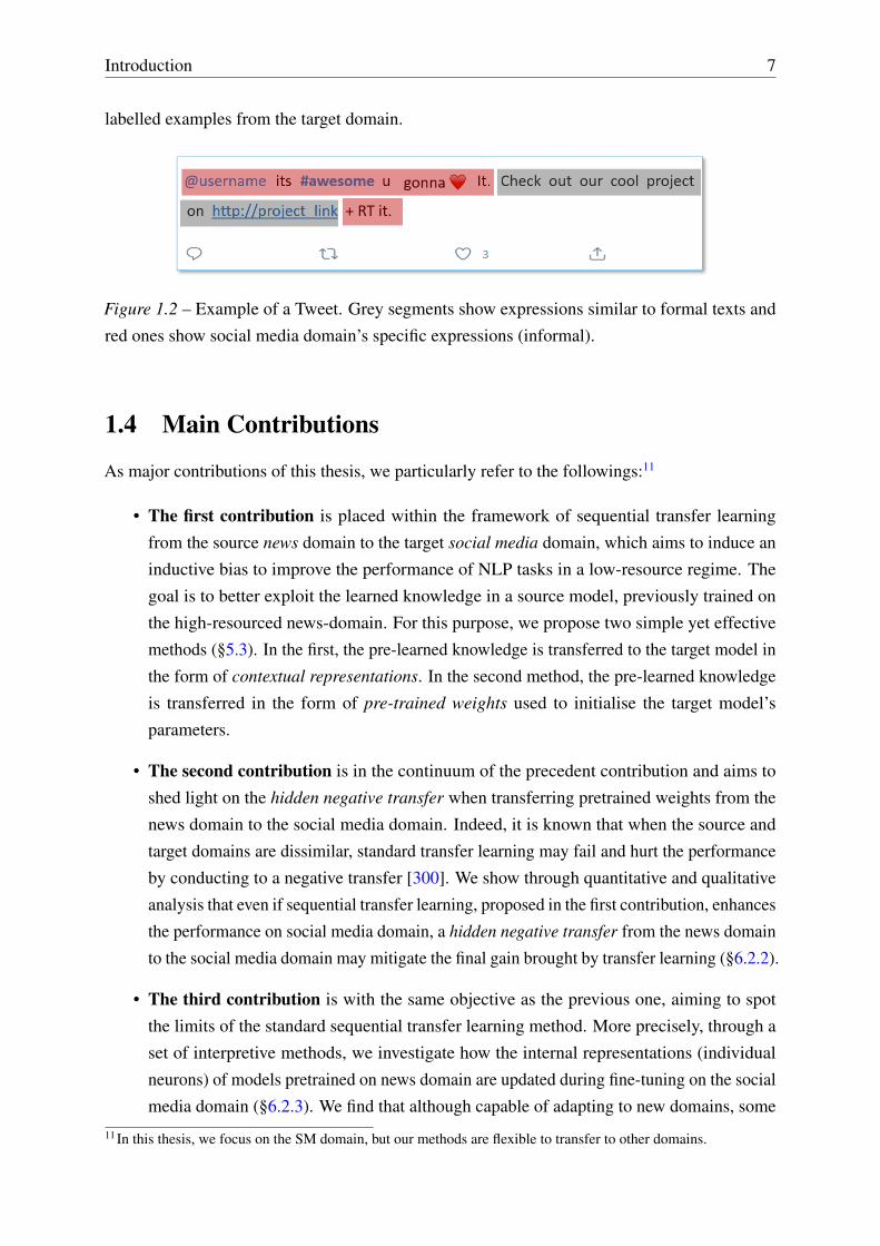
that SM domain is an informal variety of the news domain.10 As illustrated in Figure 1.2, in

the same Tweet (UGC in Twitter), one can find a part which is formal and the other which is

informal. For this, we develop and study the efficiency of different TL techniques to overcome

the sparse annotated-data problem in the SM domain by leveraging the huge annotated data

from the news domain. Specifically, in this work, we consider the supervised domain adaptation

setting, having a large amount of labelled data from a source domain and – additionally – few

10Here we use the term “domain” to denote a language variety.

Introduction 7

labelled examples from the target domain.

Figure 1.2 – Example of a Tweet. Grey segments show expressions similar to formal texts and

red ones show social media domain’s specific expressions (informal).

1.4 Main Contributions

As major contributions of this thesis, we particularly refer to the followings:11

• The first contribution is placed within the framework of sequential transfer learning

from the source news domain to the target social media domain, which aims to induce an

inductive bias to improve the performance of NLP tasks in a low-resource regime. The

goal is to better exploit the learned knowledge in a source model, previously trained on

the high-resourced news-domain. For this purpose, we propose two simple yet effective

methods (§5.3). In the first, the pre-learned knowledge is transferred to the target model in

the form of contextual representations. In the second method, the pre-learned knowledge

is transferred in the form of pre-trained weights used to initialise the target model’s

parameters.

• The second contribution is in the continuum of the precedent contribution and aims to

shed light on the hidden negative transfer when transferring pretrained weights from the

news domain to the social media domain. Indeed, it is known that when the source and

target domains are dissimilar, standard transfer learning may fail and hurt the performance

by conducting to a negative transfer [300]. We show through quantitative and qualitative

analysis that even if sequential transfer learning, proposed in the first contribution, enhances

the performance on social media domain, a hidden negative transfer from the news domain

to the social media domain may mitigate the final gain brought by transfer learning (§6.2.2).

• The third contribution is with the same objective as the previous one, aiming to spot

the limits of the standard sequential transfer learning method. More precisely, through a

set of interpretive methods, we investigate how the internal representations (individual

neurons) of models pretrained on news domain are updated during fine-tuning on the social

media domain (§6.2.3). We find that although capable of adapting to new domains, some11 In this thesis, we focus on the SM domain, but our methods are flexible to transfer to other domains.

8 1.5. THESIS OUTLINE

pretrained neurons are biased by what they have learnt in the source dataset, thus struggle

with learning unusual target-specific patterns, which may explain the observed hidden

negative transfer.

• The fourth contribution: Stemming from our analysis, we propose an extension of the

standard adaptation scheme (fine-tuning) of sequential transfer learning. To do so, we

propose to augment the pretrained model with randomly initialised layers. Specifically, we

propose a method that takes benefit from both worlds, supervised learning from scratch and

transfer learning, without their drawbacks. Our approach is composed of three modules:

(1) Augmenting the source-model (set of pre-trained neurons) with a random branch

composed of randomly initialised neurons, and jointly learn them; (2) Normalising the

outputs of both branches to balance their different behaviours. (3) Applying attention

learnable weights on both branches predictors to let the network learn which of random or

pre-trained one is better for every class (§6.3).

• The fifth contribution is an extension of our precedent contributions where we performed

mono-source mono-target transfer learning, i.e. both pre-training and fine-tuning are

performed on a single task. Here, we propose a multi-source multi-target transfer learning

approach to overcome the rare annotated data problem in social media. Our approach

consists in learning a multi-task transferable model which leverages diverse linguistic

properties from multiple supervised NLP tasks from the news source domain, further

fine-tuned on multiple tasks from the social media target domain (§7.2).

1.5 Thesis Outline

This manuscript is organised as follow. Chapter 2 and chapter 3 discuss the state-of-the-art with

regard to our two research directions: Transfer learning and neural NLP models interpretability,

respectively. For each, we propose a categorisation of the current works of the literature.

Chapter 4 provides an overview of the NLP tasks and datasets involved in this thesis as well as

evaluation metrics. Then, the following chapters describe the different contributions that we have

made during the course of this thesis. Chapter 5 describes our start-up contributions to overcome

the problem of the lack of annotated data in low-resource domains and languages. Precisely,

two sequential transfer learning approaches are discussed: “transfer of supervisedly-pretrained

contextual representations” and “transfer of pretrained models”. Chapter 6 describes three of

our contributions. First, it sheds light on the hidden negative transfer arising when transferring

from the news domain to the social media domain. Second, an interpretive analysis of individual

pre-trained neurons behaviours is performed in different settings, finding that pretrained neurons

are biased by what they have learnt in the source-dataset. Third, we propose a new adaptation

scheme, PretRand, to overcome these issues. Chapter 7 presents a new approach, MuTSPad, a

multi-source multi-target transfer learning approach to overcome the rare annotated data problem

Introduction 9

in the social media by learning a multi-task transferable model, which leverages various linguistic

properties from multiple supervised NLP tasks. Chapter 8 finally summarises our findings and

contributions and provides some perspective research directions.

2 | State-of-the-art: Transfer Learning

2.1 Introduction

In this thesis we focus on the Social Media (SM) domain. Ideally, we have at our disposal enough

annotated SM texts to train NLP models dedicated for the SM domain. However, this last is

actually still lacking in terms of annotated data. In the following, we present three common

approaches that were adopted in the literature to deal with this issue:

• Normalisation is a prominent approach to deal with the informal nature of the User-

Generated-Content (UGC) in SM [143, 144, 145, 363]. It consists in mapping SM (infor-

mal) texts into formal texts by reducing the noise (orthographic and syntactical anomalies).

For instance, ideally, “imma” is normalised into “I’m going to”, “Lol” into “lough out

loud”, “u’r” into “you are”, “gimme” into “give me”, “OMG” into “oh my god”, repeti-

tions like “happpyy”, “noooo” and “hahahaha” into “happy”, “no” and “haha”. There are

many approaches in the literature to perform normalisation. We can cite rule-based ap-

proaches [9, 212, 41, 100, 23] and noisy-channel methods [73]. Also, machine translation

based approaches view the task of normalisation as a translation problem from the SM

language to the formal language; e.g. using phrase-based statistical MT [20] or using a

character-level machine translation model trained on a parallel corpus [261]. However,

multiple works showed that the efficacy of normalisation for SM texts is limited [84, 247].

Indeed, in addition to be a difficult and an intensive task, normalisation is not flexible

over time since SM language is constantly changing [102]. Also, normalisation may

conceal the meaning of the original text [364], e.g. non-standard character repetitions

and capitalisation may have a semantic meaning, “happpyyyy” could mean “very happy”,

which may hide important signals for tasks like sentiment analysis.

• Automatic Annotation consists of tagging unlabelled SM data using off-the-shelf models

(trained on news domain). The automatically annotated examples are subsequently used

to train a new model for the SM domain. Generally, a voting strategy is used to select

the “best” automatically annotated examples, i.e. a sentence is added to the training set if

all models assign the same predictions to it. Horsmann & Zesch [152] experimented this

voting approach on the predictions of ClearNLP [60] and OpenNLP Part-Of-Speech (POS)

10

State-of-the-art: Transfer Learning 11

taggers. Similarly, Derczynski et al. [86] performed a vote constrained bootstrapping [128]

on unlabelled Tweets to increase the amounts of training examples for Tweets POS tagging.

Besides, crowd-sourcing [113] has also been used to obtain large manually annotated SM

datasets, at low cost but with lower quality since examples are not annotated by experts but

by online users. However, Horbach et al. [151] showed that extending the training set with

automatically annotated datasets leads to small improvement of POS tagging performance

on German SM texts. In contrast, a much bigger improvement of performance can be

obtained by using small amounts of manually annotated from the SM domain.

• Mixed Training is used when small annotated data-sets from the SM domain are available.

It consists in training the model on a mix of large annotated data from out-of-domain well-

resourced domains with small amounts of annotated examples from the SM domain [151].

However, since out-of-domain examples are more frequent in the training phase, the effect

of out-of-domain data will dominate that of SM data. In order to overcome this issue,

weighting and oversampling methods are commonly used to balance the two domains and

thus make the SM examples more competitive to the out-of-domain ones. For instance,

Daumé III [80], Horsmann & Zesch [152] and Neunerdt et al. [246] experimented mixed-

training with oversampling for SM POS tagging by adding annotated examples from the

SM domain multiple times and using different strategies.

In this thesis, we propose to develop and study the effectiveness of different Transfer Learning

techniques to overcome the sparse annotated-data problem in the social media domain by

leveraging annotated datasets from the high-resource source news-domain.

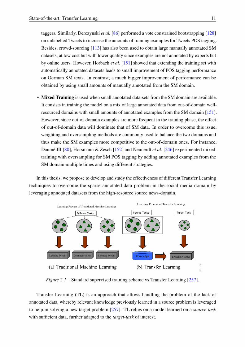
Figure 2.1 – Standard supervised training scheme vs Transfer Learning [257].

Transfer Learning (TL) is an approach that allows handling the problem of the lack of

annotated data, whereby relevant knowledge previously learned in a source problem is leveraged

to help in solving a new target problem [257]. TL relies on a model learned on a source-task

with sufficient data, further adapted to the target-task of interest.

12 2.2. FORMALISATION

TL is similar to the natural process of learning, which is a sequential long-life developmental

process [50]. In simple words, when humans tackle new problems, they make use of what they

have learned before from past related problems. Consider the example of two people who want

to learn Spanish. One person is native in the French language, and the other person is native

Indian. Considering the high similarities between French and English languages, the person

already speaking French will be able to learn Spanish more rapidly.

Here, we overview works and approaches related to transfer learning for NLP with a focus

on neural transfer learning. Note that transfer learning is a broad topic; our survey is necessarily

incomplete. We try nevertheless to cover major lines related to the contributions of this thesis.

The remainder of the following sub-sections is organised as follows. We start by presenting the

formalisation of the transfer learning problem (§2.2). Then, we propose a taxonomy of transfer

learning approaches and techniques (§2.3) based on three criteria: What to transfer? (§2.4); How

to Transfer? (§2.5); and Why transfer? (§2.6). Finally, we wrap up by summarising the proposed

categorisation of TL approaches and discussing the position of our work (§2.7).

2.2 Formalisation

Let us consider a domain D = {X , P (X)} consisting of two components:1 the feature space Xand the marginal probability distribution P (X), where X = {x1, x2, ..., xn} ∈ X . For instance,

for a sentiment analysis task, X is the space of all document representations and X is the random

variable associated with the sample of documents used for training.

Let us consider a task T = {Y , P (Y ), f}, where Y is the label space, P (Y ) is the prior distri-

bution, and f is the predictive function that transforms inputs to outputs: f : X → Y . If we re-

sume the sentiment analysis task, Y is the set of all labels, e.g. it can beY = {positive, negative}.In a supervised training paradigm, f is learned from n training examples: {(xi, yi) ∈

X × Y : i ∈ (1 , ..., n)}. Therefore, the predictive function f corresponds to the joint

conditional probability P (Y |X).

In a transfer learning scenario, we have a source domain DS = {XS, PS(XS)}, a source

task TS = {YS, Ps(YS), fS}, a target domain DT = {Xt, PT (XT )}, and a target task

TT = {YT , PT (XT ), fT}, whereXS = {xS1 , xS2 , ..., xSnS} ∈ XS ,XT = {xT1 , xT2 , ..., xTnt} ∈ XTand ns >> nt. The aim behind using transfer learning is to improve the learning of the predic-

tive target function fT by leveraging the knowledge gained from DS and TS . Generally, in a

transfer learning scheme, labelled training examples from the source domain DS = {(xSi , ySi ) ∈XS × YS : i ∈ (1 , ..., nS )} are abundant. Concerning target domain, either a small number of

labelled target examples DT,l = {(xT,li , yT,li ) ∈ XT × YT : i ∈ (1 , ..., nT ,l)}, where nS >> nT ,

or a large number of unlabelled target examples DT,u = {(xT,ui ) ∈ XT : i ∈ (1 , ..., nT ,u)} are

assumed to be available.

1 In this section, we follow the definitions and notations of Pan et al. [257], Weiss et al. [375] and Ruder [303].

State-of-the-art: Transfer Learning 13

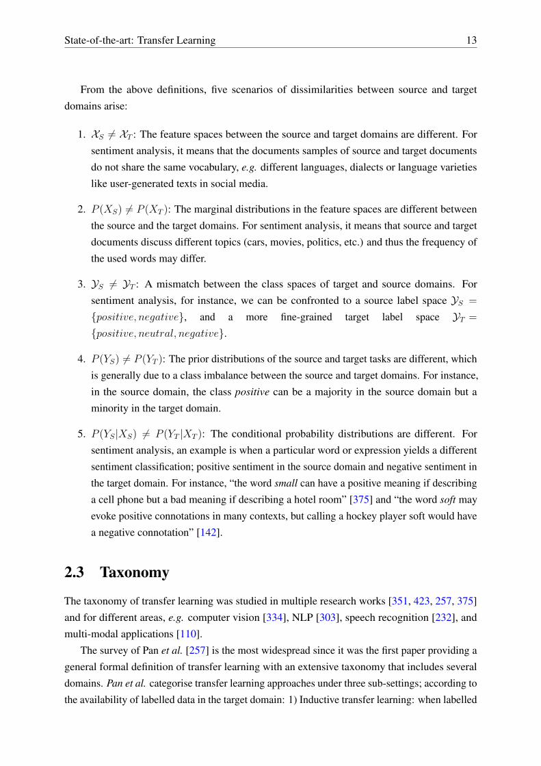
From the above definitions, five scenarios of dissimilarities between source and target

domains arise:

1. XS 6= XT : The feature spaces between the source and target domains are different. For

sentiment analysis, it means that the documents samples of source and target documents

do not share the same vocabulary, e.g. different languages, dialects or language varieties

like user-generated texts in social media.

2. P (XS) 6= P (XT ): The marginal distributions in the feature spaces are different between

the source and the target domains. For sentiment analysis, it means that source and target

documents discuss different topics (cars, movies, politics, etc.) and thus the frequency of

the used words may differ.

3. YS 6= YT : A mismatch between the class spaces of target and source domains. For

sentiment analysis, for instance, we can be confronted to a source label space YS =

{positive, negative}, and a more fine-grained target label space YT =

{positive, neutral, negative}.

4. P (YS) 6= P (YT ): The prior distributions of the source and target tasks are different, which

is generally due to a class imbalance between the source and target domains. For instance,

in the source domain, the class positive can be a majority in the source domain but a

minority in the target domain.

5. P (YS|XS) 6= P (YT |XT ): The conditional probability distributions are different. For

sentiment analysis, an example is when a particular word or expression yields a different

sentiment classification; positive sentiment in the source domain and negative sentiment in

the target domain. For instance, “the word small can have a positive meaning if describing

a cell phone but a bad meaning if describing a hotel room” [375] and “the word soft may

evoke positive connotations in many contexts, but calling a hockey player soft would have

a negative connotation” [142].

2.3 Taxonomy

The taxonomy of transfer learning was studied in multiple research works [351, 423, 257, 375]

and for different areas, e.g. computer vision [334], NLP [303], speech recognition [232], and

multi-modal applications [110].

The survey of Pan et al. [257] is the most widespread since it was the first paper providing a

general formal definition of transfer learning with an extensive taxonomy that includes several

domains. Pan et al. categorise transfer learning approaches under three sub-settings; according to

the availability of labelled data in the target domain: 1) Inductive transfer learning: when labelled

14 2.4. WHAT TO TRANSFER?

data are available in the target domain and TS 6= TT . 2) Transductive transfer learning: when

labelled data are only available in the source domain and TS = TT . 3) Unsupervised Transfer

Learning: when labelled data are not available in both source and target domain. Weiss et al.

[375] devise transfer learning settings into two categories. 1) Heterogeneous transfer learning is

the case where XS 6= XT , i.e. the feature spaces between the source and target domains are

different. Alternately, 2) homogeneous transfer learning is the case where XS = XT . Ruder

[303] provides an overview of the literature of transfer learning in general with a focus on NLP

applications. The taxonomy proposed by Ruder is an adapted version of the one proposed by Pan

et al.. Recently, Ramponi & Plank [289] classified transfer learning into data-centric methods

and model-centric methods.

Based on the former categorisations, we propose a three-dimensional categorisation of

transfer learning in NLP; each answers a specific question:

1. What to transfer? asks which type of knowledge is transferred from the source domain

to the target domain.

2. How to transfer? discusses the algorithms and methods used to transfer each type of

knowledge. Note that each type of transferred knowledge has its own methods and

algorithms.

3. Why transfer? discusses the different research objectives behind transfer learning from

source to target domains.

2.4 What to Transfer?

Here we classify transfer learning approaches according to the type of the transferred knowledge.

We distinguish three categories:

1. Transfer of linguistic annotations (§2.4.1): Unlabelled data from the target domain are

automatically annotated with transferred annotations from the source data. Then, the new

annotated target examples are used to train a new target model.

2. Transfer of instances (§2.4.2): A training on selected annotated source examples.

3. Transfer of learned representations (§2.4.3): Transferring representations consists in the

reuse and/or modification of the underlying representations learnt from a source domain to

boost the performance on a target domain.

2.4.1 Transfer of Linguistic Annotations

Cross-lingual projection of linguistic annotations [394] allows an automatic generation of

linguistic annotations for low-resource languages. Precisely, the direct naive projection method

State-of-the-art: Transfer Learning 15

consists in projecting annotations from a high-resource language to a low-resource language

through bilingual alignments from parallel corpora. Then, the automatically annotated target

data are used to train the target model.2

Parallel corpora are made of pairs of translated documents. In simple words, a parallel corpus

between two or more languages is composed of an original text in a particular language and its

translation to the remaining languages [342]. For instance, European Parliament transactions

(EuroParl) [174] contain parallel corpora between 11 European languages.

Bilingual alignments are constructed from parallel corpora and consist of links that correspond

to a translation relation between portions of text from a pair of documents. The most common

levels of alignment are word-level alignments [368, 329, 309, 308, 310, 311], multi-word-level

alignments [330, 37, 214, 39, 38, 40, 327, 323, 331] and sentence-level alignments [58, 324,

326, 325, 256]. Many automatic word alignment tools are available, e.g. GIZA++ [253].

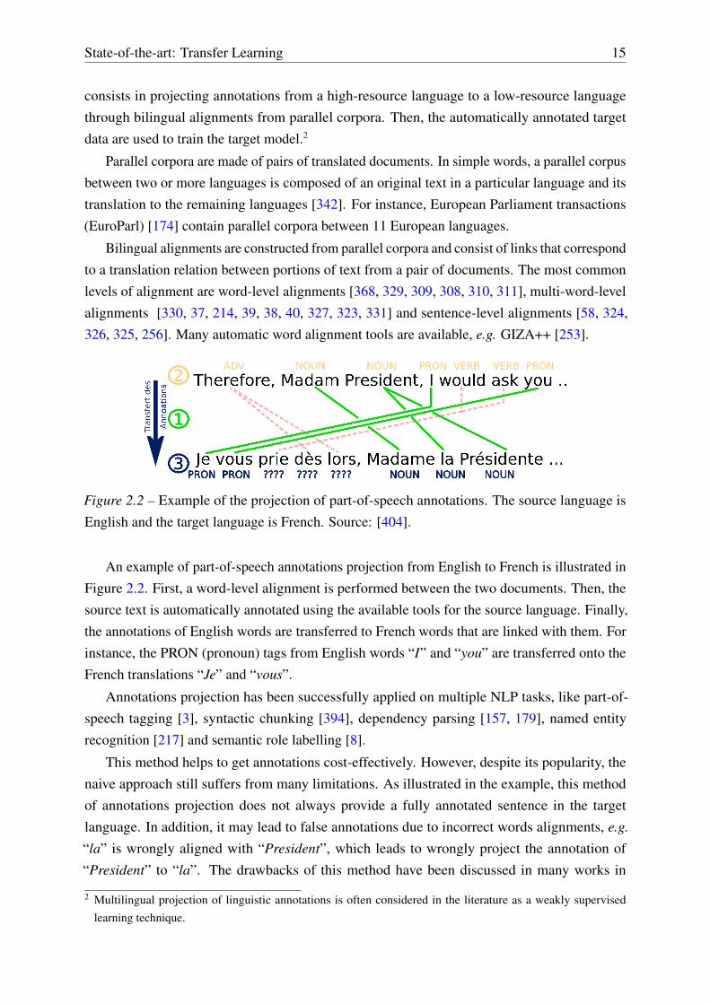
Figure 2.2 – Example of the projection of part-of-speech annotations. The source language is

English and the target language is French. Source: [404].

An example of part-of-speech annotations projection from English to French is illustrated in

Figure 2.2. First, a word-level alignment is performed between the two documents. Then, the

source text is automatically annotated using the available tools for the source language. Finally,

the annotations of English words are transferred to French words that are linked with them. For

instance, the PRON (pronoun) tags from English words “I” and “you” are transferred onto the

French translations “Je” and “vous”.

Annotations projection has been successfully applied on multiple NLP tasks, like part-of-

speech tagging [3], syntactic chunking [394], dependency parsing [157, 179], named entity

recognition [217] and semantic role labelling [8].

This method helps to get annotations cost-effectively. However, despite its popularity, the

naive approach still suffers from many limitations. As illustrated in the example, this method

of annotations projection does not always provide a fully annotated sentence in the target

language. In addition, it may lead to false annotations due to incorrect words alignments, e.g.

“la” is wrongly aligned with “President”, which leads to wrongly project the annotation of

“President” to “la”. The drawbacks of this method have been discussed in many works in

2 Multilingual projection of linguistic annotations is often considered in the literature as a weakly supervisedlearning technique.

16 2.4. WHAT TO TRANSFER?

the literature [256, 365, 8, 406, 405, 408, 407, 409], especially when the source and target

languages are syntactically and morphologically different, and for multi-words expressions [328,

327, 323, 288, 331]. Indeed, the underlying assumption in annotations projection is a 1-to-

1 correspondence of word sequences between language pairs [19], which is unrealistic even

for languages from the same family. Since then, many improvements have been proposed to

overcome these limitations. We can cite the work of Täckström et al. [346] who improved

POS tags projections by adding external information sources such as dictionaries. In the same

vein, Wisniewski et al. [383] exploited crowd-sourced constraints, and Wang & Manning [371]

proposed to integrate softer constraints using expectation regularisation techniques. On another

aspect, Zennaki et al. [409] proposed to extract a common (multilingual) and agnostic words

representation from parallel or multi-parallel corpus between a resource-rich language and one

or many target (potentially under-resourced) language(s).

When parallel text is available, “annotations projection is a reasonable first choice” [273].

Still, the main limitation of this method is its dependence to parallel corpora which are not

available for all low-resource languages. In addition, it is limited to the cross-lingual setting

of transfer learning [392] and thus not applicable to transfer between domains. It is not either

applicable to transfer between tasks with different tag-sets, since this method assumes that

YS = YT or at least a 1-1 mapping between YS and YT is possible.

A related method to transfer annotations from a resource-rich language to a low-resource

language is data translation which consists in translating labelled source data into the target

language. This method has been proven to be successful in many applications. However, it suffers

from translation noise, in addition to labelling mismatch and instance mismatch issues [97].

2.4.2 Transfer of Instances

Transferring instances consists in a training on a selection of annotated source examples. Two

approaches are commonly used, Instance Weighting and Instance Selection.

Instance weighting consists in weighting source annotated instances with instance-dependent

weights, which are then used to weight the loss function [161]. The weight assigned to an

individual instance from the source domain is supposed to reflect the degree of similarity of the

said instance to the target distribution.

Following the notations of Jiang [162], let DT = {(xTi , yTi )}NTi=1 be a set of training instances

randomly sampled from the true underlying target joint distribution PT (X, Y ) from the target

domain DT . Typically, in machine learning, we aim to minimise the following objective function

of some loss functionL(x, y, f) in order to obtain the best predictive function from the hypothesis

space f ?T ∈ H with regard to PT (X, Y ):

State-of-the-art: Transfer Learning 17

f ?T = argminf ∈ H

∑(x,y) ∈ (X ,Y)

PT (x, y) L(x, y, f) . (2.1)

However, in reality PT (X, Y ) is unknown, we thus aim to minimise the expected error in

order to obtain the best predictive function from the hypothesis space fT ∈ H with regard to

the empirical target distribution PT (X, Y ):

fT = argminf ∈ H

∑(x,y) ∈ (X ,Y)

PT (x, y) L(x, y, f) = argminf ∈ H

i=NT∑i=1

L(xTi , yTi , f) . (2.2)

When transferring instances, the objective is to find the optimal target model with only

annotated examples from the source domain DS = {(xSi , ySi )}NSi=1, randomly sampled from the

source distribution PS(X, Y ). The above equation can be rewrote as such:

f ?T = argminf ∈ H

∑(x,y) ∈ (X ,Y)

PT (x, y)

PS(x, y)PS(x, y) L(x, y, f)

≈ argminf ∈ H

∑(x,y) ∈ (X ,Y)

PT (x, y)

PS(x, y)PS(x, y) L(x, y, f)

= argminf ∈ H

i=NS∑i=1

PT (xSi , ySi )

PS(xSi , ySi )L(xSi , y

Si , f) . (2.3)

Consequently, a solution is to calculate the weight PT (xSi ,ySi )

PS(xSi ,y

Si )

for each source example (xSi , ySi ).

However, in practice, exact computation of PT (x,y)PS(x,y)

is infeasible, mainly because labelled examples

from the target domain are not available.

Expanding the last equation using the product rule brings us to the following:

f ?T ≈ argminf ∈ H

i=NS∑i=1

PT (xSi )

PS(xSi )

PT (ySi |xSi )

PS(ySi |xSi )L(xSi , y

Si , f) . (2.4)

From the above equation, we end up with two possible differences between the source and

target domains:

1. Instance mismatch (PT (X) 6= PS(X) and PT (Y |X) = PS(Y |X)): The conditional

distribution is the same in both domains, but the marginal distributions in the feature spaces

are different. Here, unlabelled target domain instances can be used to bias the estimate of

PS(X) toward a better approximation of PT (X).

2. Labelling mismatch (PT (Y |X) 6= PS(Y |X)): the difference between the two domains is

due to the conditional distribution. State-Of-The-Art (SOTA) approaches in this category,

generally, assume the availability of a limited amount of labelled data from the target

domain.

18 2.4. WHAT TO TRANSFER?

There are multiple works on instances-weighting. We can cite the work of Jiang & Zhai

[163] who proposed an implementation based on several adaptation heuristics, first by removing

misleading source training instances (i.e. where PT (Y |X) highly differs from PS(Y |X)), then

assigning higher weights to labelled target instances than labelled source instances, and finally

augmenting training instances with automatically labelled target instances. Another approach

consists in training a domain classifier to discriminate between source and target instances. Then,

source labelled examples are weighted with the probability (the classifier output) that a sentence

comes from the target domain [341, 274].

Instance Selection consists in ignoring source examples that are potentially harmful to the target

domain, i.e. which are likely to produce a negative transfer. It differs from instance weighting

method in two points. First, instance weighting is a soft data selection, while here selection

is hard, i.e. source examples are either attributed a weight equals to 1 or 0. Second, instance

selection is performed as a pre-processing step, while in instance weighting, weights are used at

the loss computation during training.

Domain similarity metrics are often used to perform instance selection, e.g. proxy A [33],

Jensen Shannon divergence for sentiment analysis task [295] and parsing [276]. Søgaard [339]

proposed to select sentences from the source domain that have the lowest word-level perplexity

in a language model trained on unlabelled target data. van der Wees et al. [366] investigated

a dynamic data selection for Neural Machine Translation (NMT) and proposed to vary the

selected data between training epochs. Ruder & Plank [304] used a Bayesian optimisation

method to select instances for parsing task. Recently, Aharoni & Goldberg [4] investigated

instance selection for NMT using cosine similarity in embedding space, using the representations

generated by a pretrained Transformer-based model (DistilBERT) [313]. Another approach

to perform instance selection is transfer self-training. We can cite the work of cross-lingual

opinion classification by Xu et al. [387], who proposed to start the training of the classifier on

the available training data from the target language. Then, the classifier is iteratively trained by

appending new selected translated examples from the source language. However, the computation

cost of this method is high since the model needs to be trained repeatedly [191].

Both approaches for transferring instances require the same tag-set for both the source

domain and the target domain, or at least a mapping between the two tag-sets is possible. For

instance, Søgaard [339] performed a mapping of part-of-speech tags into a common tag-set before

performing domain adaptation using instances-weighting. In addition, transferring instances is

only efficient when transferring between similar domains; when a broad set of target words are

out of source-vocabulary, transferring instances is not very useful and importance weighting

cannot help [272].

State-of-the-art: Transfer Learning 19

2.4.3 Transfer of Learned Representations

Transferring representations consists in the reuse and modification of the underlying represen-

tations learned from a source domain to boost the performance on a target domain. Weiss

et al. [375] categorised these approaches into two categories. First, asymmetric approaches

aim to transform the source model representations to be as similar as possible to the marginal

distribution of the target domain. Second, symmetric approaches aim to reduce the dissimilarities

between the marginal distributions between the source domain and the target domain by finding

a common representation.

Notably, research on transfer learning of neural representations has received an increasing

attention over the last three years. Indeed, when annotated datasets are available, neural networks

achieve excellent results in an end-to-end manner, with a unified architecture and without task-

specific feature engineering. Moreover, the hierarchical nature of neural networks makes that the

learned knowledge (in the form of learned weights) in their latent representations transit from

general information at the lower-layers to task-specific at the higher layers [243, 396]. Hence, the

lower-layers tend to encode knowledge that is, generally, transferable across tasks and domains.

Four main methods are used in the literature to transfer neural representations. First, Au-toencoders [369] are neural networks that are unsupervisedly trained on raw data to learn to

reconstruct the input. In domain adaptation, autoencoders are used to learn latent representations

that are invariant to domain shift. We can cite the pioneering work of Glorot et al. [125] who

proposed denoising autoencoders for domain adaptation for sentiment analysis task. First, a de-

noising autoencoder is trained on raw data from different source and target domains to reconstruct

the input text, in an unsupervised fashion. Then, a Support Vector Machine (SVM) sentiment

classifier, built on top of the latent representations generated by the denoising autoencoder, is

trained on annotated examples from the source domain. Second, Domain-Adversarial training,

initiated by Ganin et al. [115], aims to generate domain-invariant latent representations, from

which an algorithm cannot learn to distinguish the domain of origin of the input features. Third,

Multi-Task Learning (MTL) [50] consists of a joint training of related tasks and thus leverages

training signals generated by each one. Fourth, Sequential Transfer Learning, where training

is performed in two stages, sequentially: pretraining on the source task, followed by adaptation

on the downstream target tasks.

As discussed in the introduction, we aim in this thesis to transfer the learned knowledge in

neural NLP models from the high-resourced news domain to the low-resourced social media

domain. Hence, we discuss these methods in more details in the following section (§2.5).

20 2.5. HOW TO TRANSFER NEURAL REPRESENTATIONS?

2.5 How to Transfer Neural Representations?

2.5.1 Domain-Adversarial Neural Networks

Domain-Adversarial training has been initiated by Ganin et al. [115], following the theoretical

motivation of domain adaptation [30], which aims to generate domain-invariant latent represen-

tations from which an algorithm cannot learn to distinguish the domain of origin of the input

features. Adversarial training requires two kinds of training data: (i) annotated source examples

and (ii) unlabelled examples from the target domain. In addition, in some cases, some labelled

instances from the target domain can be used to boost the performance.

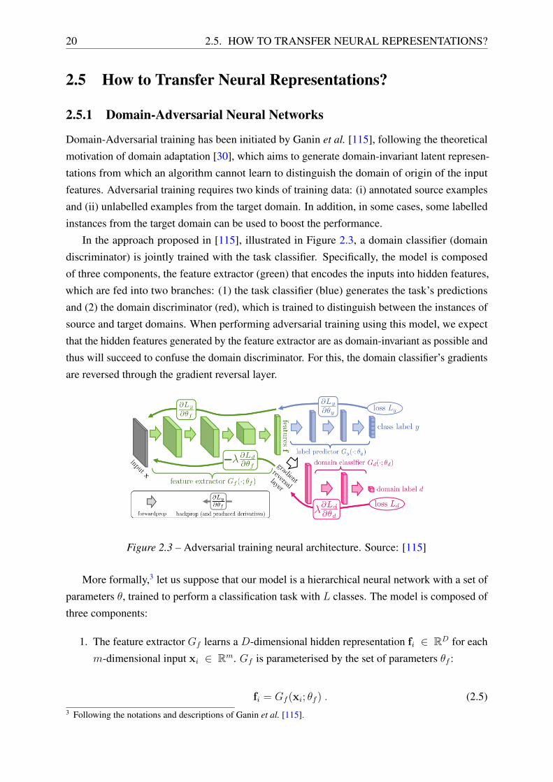
In the approach proposed in [115], illustrated in Figure 2.3, a domain classifier (domain

discriminator) is jointly trained with the task classifier. Specifically, the model is composed

of three components, the feature extractor (green) that encodes the inputs into hidden features,

which are fed into two branches: (1) the task classifier (blue) generates the task’s predictions

and (2) the domain discriminator (red), which is trained to distinguish between the instances of

source and target domains. When performing adversarial training using this model, we expect

that the hidden features generated by the feature extractor are as domain-invariant as possible and

thus will succeed to confuse the domain discriminator. For this, the domain classifier’s gradients

are reversed through the gradient reversal layer.

Figure 2.3 – Adversarial training neural architecture. Source: [115]

More formally,3 let us suppose that our model is a hierarchical neural network with a set of

parameters θ, trained to perform a classification task with L classes. The model is composed of

three components:

1. The feature extractor Gf learns a D-dimensional hidden representation fi ∈ RD for each

m-dimensional input xi ∈ Rm. Gf is parameterised by the set of parameters θf :

fi = Gf (xi; θf ) . (2.5)3 Following the notations and descriptions of Ganin et al. [115].

State-of-the-art: Transfer Learning 21

2. The task classifier Gy is fed with the output of Gf and predicts the label yi for each input

xi. Gy is parameterised by the set of parameters θy:

yi = Gy(Gf (xi; θf ); θy) . (2.6)

3. The domain discriminator Gd learns a classifier Gd : RD → [0, 1], which predicts the

domain of each input xi. Gd is parameterised by the set of parameters θd:

di = Gd(Gf (xi; θf ); θd) . (2.7)

Given a source labelled example (xi, yi), the task classifier cross entropy loss is defined such

as:

Liy(θf , θy) = Ly(Gy(Gf (xi; θf ); θy), yi) = yi × log(yi) . (2.8)

Thus during training the task classifier on ns annotated source examples, the task classifier

loss is defined as follows:

Ly(θf , θy) = − 1

ns

ns∑i=1

Liy(θf , θy) . (2.9)

Given an example (xi, di) from source or target domain where di is the ground truth domain

label for the instance xi, the domain discriminator loss is defined such as:

Lid(θf , θd) = Ld(Gd(Gf (xi; θf ); θd), yi) = di log(di) + (1− di) log(1− di) . (2.10)

Thus, during training the domain discriminator on ns source examples and nt unlabelled target

examples, the domain discriminator loss is defined as follows:

Ld(θf , θd) = −(1

ns

ns∑i=1

Lid(θf , θd) +1

nt

ns+nt∑i=ns+1

Lid(θf , θd) ) . (2.11)

Training the adversarial neural network consists in optimising the error E(θf , θy, θd), by

finding a saddle point (θf , θy, θd):

(θf , θy) = argminθf ,θy

E(θf , θy, θd) , (2.12)

θd = argmaxθd

E(θf , θy, θd) , (2.13)

with λ ∈ R is the domain discriminator loss weight. Hence, the domain discriminator is

optimised through maximising the loss over θf and minimising the loss over θd. This “minmax”

optimisation allows the feature extractor to learn features that help to improve the performance

22 2.5. HOW TO TRANSFER NEURAL REPRESENTATIONS?

of the classification task, but are indistinguishable whether they are from the source or the target

domain.

The saddle point is obtained by updating the model’s gradients as follows:

θf ← θf − µ (∂ Ly∂ θf

− λ∂ Ld∂ θf

) , (2.14)

θd ← θd − µ λ∂ Ld∂ θd

, (2.15)

θy ← θy − µ∂ Ly∂ θy

, (2.16)

with µ being the learning rate.

The gradient reversal layer (GRL) in Figure 2.3 allows performing this optimisation problem

in a simple way. The GRL is added between the feature extractorGf and the domain discriminator

Gd. It does not impact the forward propagation. But during backward propagation, it negates the

gradients.

Another approach to perform adversarial training consists in minimising the divergence

between the source distribution PS and the target distribution PT . For instance, Arjovsky et al.

[15] used the Jensen-Shannon divergence and Shah et al. [333] used the Wasserstein distance to

compute the divergence loss.

2.5.2 Multi-Task Learning

Multi-Task Learning (MTL) [50] consists in a joint learning of related tasks and thus leverages

training signals generated by each one. MTL is based on the intuition that, if tasks are related,

features trained for one task can be useful for the other tasks. For instance, detecting proper

nouns in the POS tagging task would hopefully help to better identify named entities in Named

Entity Recognition (NER) task. As discussed in [50] and [302], when tasks are related, the

efficiency of MTL is significant for many evidences. First, MTL allows augmenting training

data, implicitly, which begets a better regularisation and thus avoids over-fitting. Second, MTL

allows an “eavesdropping” process, which means that when two tasks “A” and “B” are jointly

trained, in some cases, a set of features that are important for task “A” can be easier to learn by

task “B”. Third, MTL introduces an inductive bias that begets a better generalisation for new

tasks and domains.

Performing MTL requires conceptual and architectural choices with regards to the parameters

sharing scheme, the tasks scheduling procedure and the loss calculation. The three depend on

the nature of the problem and the relatedness between tasks.

• Parameters sharing schemes: One can separate MTL approaches according to the param-

eters sharing scheme. MTL is typically done with either hard or soft parameters sharing of

the hidden layers, as illustrated in Figure 2.4.

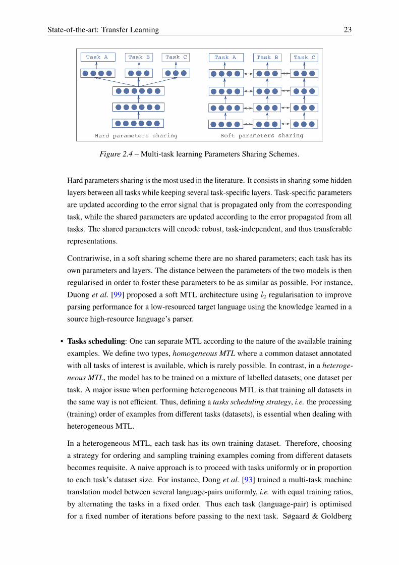
State-of-the-art: Transfer Learning 23

Figure 2.4 – Multi-task learning Parameters Sharing Schemes.

Hard parameters sharing is the most used in the literature. It consists in sharing some hidden

layers between all tasks while keeping several task-specific layers. Task-specific parameters

are updated according to the error signal that is propagated only from the corresponding

task, while the shared parameters are updated according to the error propagated from all

tasks. The shared parameters will encode robust, task-independent, and thus transferable

representations.

Contrariwise, in a soft sharing scheme there are no shared parameters; each task has its

own parameters and layers. The distance between the parameters of the two models is then

regularised in order to foster these parameters to be as similar as possible. For instance,

Duong et al. [99] proposed a soft MTL architecture using l2 regularisation to improve

parsing performance for a low-resourced target language using the knowledge learned in a

source high-resource language’s parser.

• Tasks scheduling: One can separate MTL according to the nature of the available training

examples. We define two types, homogeneous MTL where a common dataset annotated

with all tasks of interest is available, which is rarely possible. In contrast, in a heteroge-

neous MTL, the model has to be trained on a mixture of labelled datasets; one dataset per

task. A major issue when performing heterogeneous MTL is that training all datasets in

the same way is not efficient. Thus, defining a tasks scheduling strategy, i.e. the processing

(training) order of examples from different tasks (datasets), is essential when dealing with

heterogeneous MTL.

In a heterogeneous MTL, each task has its own training dataset. Therefore, choosing

a strategy for ordering and sampling training examples coming from different datasets

becomes requisite. A naive approach is to proceed with tasks uniformly or in proportion

to each task’s dataset size. For instance, Dong et al. [93] trained a multi-task machine

translation model between several language-pairs uniformly, i.e. with equal training ratios,

by alternating the tasks in a fixed order. Thus each task (language-pair) is optimised

for a fixed number of iterations before passing to the next task. Søgaard & Goldberg

24 2.5. HOW TO TRANSFER NEURAL REPRESENTATIONS?

[340] trained a hierarchical multi-task model using a uniform training over tasks, where

the selection of the next task to train is done in random. Similarly, Subramanian et al.

[345] trained a multi-task model to learn universal sentence representations using uniform

training ratios for each task. Likewise, Zaremoodi et al. [403] performed a uniform multi-

task training, where at each iteration of the training process, the task to train is selected

randomly.

However, the naive uniform approach is not always efficient, typically when some datasets

are over-sampled compared to the other datasets. In this case, the model will likely focus

on the richest tasks. Luong et al. [209] proposed to train tasks periodically while using

different training ratios per task based on their respective training-sets size. Similarly, Sanh

et al. [314] compared uniform sampling to proportional sampling of training examples

from different tasks and found that proportional sampling is outperforming in terms of

performance and speed of convergence.

Nevertheless, the above approaches are maladaptive, i.e. are not adapted during training,

which can be an issue when easy tasks are trained with more challenging tasks; in the

course of training, the more straightforward tasks are likely to be over-trained. Adaptive

scheduling was used by Kiperwasser & Ballesteros [171], who studied multiple adaptive

schedules that increasingly favour the principal task over training iterations. The objective

of the work of Kiperwasser & Ballesteros [171] is to improve NMT with the help of

POS and Dependency Parsing (DP) tasks by scheduling tasks during training, starting

with multi-tasking of the principal task with auxiliary lower-level tasks (POS and DP)

and as the training graduates, the model trains only to the main task. Further, Jean et al.

[160] proposed an adaptive scheduling method that varies during training according to

the validation performance of each task. Precisely, when the performance of the model is

low on one task compared to the baseline (mono-task training performance), the sampling-

weight assigned to this task is increased.

It is noteworthy that all the above-mentioned scheduling methods are explicit, i.e. they

consist in only controlling the sampling of each task during training. In contrast, there

are some works on implicit methods, which act on learning rates, model gradients or loss

calculation [160].

• Loss Calculation: In MTL, we aim to optimise the model with respect to multiple

objectives. Thus, we generally minimise a weighted sum of the loss over all tasks:

L =1

T

T∑i=1

αi Li , (2.17)

where T is the number of the jointly trained tasks, Li is the loss of the task i, and αi is the

weight attributed to the task i. A naive setting consists in using equal weights for all tasks

State-of-the-art: Transfer Learning 25

α1 = α2 = ... = αT . However, when tasks training sets have different sizes or some

tasks are easier to learn than the other tasks, weights may differ from one task to another

or adapted during training.

In the literature, MTL is used in two situations. The first is interested in building a joint

model which produces predictions for multiple tasks. Thus, the model is optimised to improve

the performance of all tasks. As shown by Caruana [50], many real-world problems are, in

reality, multi-task problems by nature. For instance, in autonomous driving, the model needs to

be able to perform multiple tasks simultaneously, e.g. recognition of pedestrians, traffic lights,

cars, etc. In the second scenario, a main task of interest is trained with a set of auxiliary tasks.

The advantage of using MTL over independent task learning has been shown in some NLP tasks

and applications [195]. For instance, POS tagging task has been shown to be beneficial for other

tasks in [67, 339, 412, 221, 171, 208, 340]. The same for NER in [314], CK [67, 148] and DP

[171, 416].

2.5.3 Sequential Transfer Learning

In contrast to MTL, which is a parallel training process where tasks often benefit each other

mutually, in Sequential Transfer Learning (STL) training is performed serially and thus only

target tasks benefit from source ones. The term STL was firstly used by Caruana [50], but

the idea was explored much earlier [277, 353]. In STL, training is performed in two stages

sequentially: pretraining on the source tasks, followed by adaptation on downstream target tasks.

In the following, we discuss the methods used to perform each stage.

PretrainingIn the pretraining stage, a crucial key to the success of transfer is the ruling about the pretrained

task and domain. For universal representations, the pretrained task is expected to encode useful

features for a vast number of target tasks and domains. In contrast, for domain adaptation, the

pretrained task is expected to be most suitable for the target task in mind.4 We classify pretrain-

ing methods into four main categories: unsupervised, supervised, multi-task and adversarial

pretraining:

• Unsupervised pretraining uses raw unlabelled data for pretraining. Particularly, it has

been successfully used in a wide range of seminal works to learn universal representations.

Language modelling task has been particularly used thanks to its ability to capture general-

purpose features of language.5 For instance, TagLM [263] is a pretrained model based on

4 The difference between universal representations and domain adaptation will be discussed in the following section2.6.

5 Note that language modelling is also considered as a self-supervised task since, in fact, labels are automaticallygenerated from raw data.

26 2.5. HOW TO TRANSFER NEURAL REPRESENTATIONS?

a bidirectional language model (biLM), also used to generate ELMo (Embeddings from

Language Models) representations [265]. In addition, with the recent emergence of the

“Transformers” architectures [367], many works propose pretrained models based on these

architectures [87, 391, 283]. Unsupervised Pretraining has also been used to improve

sequence to sequence learning. We can cite the work of Ramachandran et al. [287] who

proposed to improve the performance of an encoder-decoder NMT model by initialising

both encoder and decoder parameters with pretrained weights from two language models.

• Supervised pretraining has been particularly used for cross-lingual transfer (e.g. machine

translation [424]); cross-task transfer from POS tagging to words segmentation task [390];

and cross-domain transfer for biomedical question answering by Wiese et al. [378] and

NER to biomedical texts by Giorgi & Bader [123]. Cross-domain transfer has also been

used to transfer from news to SM for POS tagging [227, 222, 216] and sentiment analysis

[414]. Supervised pretraining has been also used effectively for universal representations

learning, e.g. neural machine translation [218], language inference [69] and discourse

relations [248].

• Multi-task pretraining has been successfully applied to learn general universal sentence

representations by a simultaneous pretraining on a set of supervised and unsupervised

tasks [345, 51]. Subramanian et al. [345], for instance, proposed to learn universal

sentences representations by a joint pretraining on skip-thoughts, machine translation,

constituency parsing and natural language inference. In [223], we proposed multi-task

pretraining for supervised domain adaptation from news domain to the social media

domain.

• Adversarial pretraining is particularly used for domain adaptation when some annotated

examples from the target domain are available. Adversarial training – as previously

described – is used as a pretraining step followed by an adaptation step on the target

dataset. Adversarial pretraining demonstrated its effectiveness in several NLP tasks, e.g.

cross-lingual sentiment analysis [55]. Also, it has been used to learn cross-lingual words

embeddings [182].

AdaptationDuring the adaptation stage one or more layers from the pretrained model are transferred to the

downstream task, and one or more randomly initialised layers are added on top of pretrained

ones. Three main adaptation schemes are used in sequential transfer learning: Feature Extraction,

Fine-Tuning and the recent Residual Adapters.

In a Feature Extraction scheme, the pretrained layers’ weights are frozen (not updated) during

adaptation, while in Fine-Tuning scheme weights are fine-tuned. Accordingly, the former is

computationally inexpensive while the last allows better adaptation to target domains peculiarities.

In general, fine-tuning pretrained models begets better results, except in cases wherein the target

State-of-the-art: Transfer Learning 27

domain’s annotations are sparse or noisy [90, 243]. Moreover, Peters et al. [264] found that, for

contextualised representations, both adaptation schemes are competitive, but the appropriate

adaptation scheme to pick depends on the similarity between the source and target problems.

Recently, Residual Adapters were proposed by Houlsby et al. [154] to adapt pretrained models

based on Transformers architecture, which aim to keep Fine-Tuning scheme’s advantages while

reducing the number of parameters to update during the adaptation stage. This is achieved

by adding adapters (intermediate layers with a small number of parameters) on top of each

pretrained layer. Thus, pretrained layers are frozen, and only adapters are updated during training.

Therefore, Residual Adapters performance is near to Fine-tuning while being computationally

cheaper [267, 266, 268].

2.6 Why Transfer?

There are some terminology inconsistencies throughout the literature of transfer learning. Mainly,

transfer learning and domain adaptation are sometimes used to refer to the same process [420,

191, 257, 176]. Many other papers use the two expressions to mean different things. For instance,

Wilson & Cook [381] and Ruder [303] consider that domain adaptation is a particular case of

transfer learning, where source and target tasks are the same (TS = TT ), while the source and

target domains differ (DS 6= DT ).

In this thesis, we consider that the purpose behind using transfer learning approaches for

NLP can be divided into two main research areas, universal representations and domain adapta-

tion. Universal representations aim to learn representations, e.g. words embeddings, sentence

embeddings and pretrained models, that are transferable and beneficial to a wide range of

downstream NLP tasks and domains. Domain adaptation seeks to learn representations that

are beneficial for a particular target domain rather than being useful in general. In comparison,

domain adaptation aims to harness the knowledge represented in features learned on a source

domain (high-resourced in most cases) to improve the performance on a specific target domain

(low-resourced in most cases). The source and the target domains may differ on the task, the

language or the domain. In the following, we present some notable works from each category:

universal representations (§2.6.1) and domain adaptation (§2.6.2).

2.6.1 Universal Representations

Transfer learning in the form of universal representations is not a recent phenomenon in NLP;

their usage as extra word features for supervised tasks was common long before the outburst

of neural models. According to Turian et al. [360], three categories of algorithms have been

used to induce unsupervised word representations that are expected to encode general language

knowledge and beneficial to a wide range of NLP tasks.

1. Clustering-based representations: are one-hot representations induced from a clustering

28 2.6. WHY TRANSFER?

over words. Hence, the dimension of the induced representations equals to the number

of clusters. Particularly, Brown Clustering [44], which builds unsupervised hierarchical

word clusters, was commonly used in NLP. For instance, it was successfully used for POS

tagging of English Tweets [255], English news NER [290] and cross-lingual NER [217].

2. Distributional representations: are mainly based on word-word co-occurrence matrices

factorisation. However, due to their size and scarcity, using these matrices directly as

words representations is impractical. Thus, dimensionality reduction methods are often

used to obtain dense representations. For instance, canonical correlation analysis was used

by Dhillon et al. [89] and latent semantic analysis by Levy et al. [188] to generate words

representations.

3. Distributed representations: are low-dimensional and dense representations, typically

learned using language models. The probabilistic language model proposed by Bengio

et al. [31] and improved in [67] & [68] was the genesis of what we call words embedding

in NLP, while Word2Vec [233, 234] was its outbreak and a starting point for a surge of

works on learning distributional words embeddings, e.g. FastText [35] enriches Word2Vec

with subword information. One of the strengths of word embeddings is that they encode

the semantics of words taking into account their contexts of use while keeping a low

dimensionality.

Traditional Words Representations:6

Let us consider a text sentence S with a set of N tokens, S = (t1, t2, ..., tN). Traditional word

embeddings approaches assign a dense vector wi for each token ti, on a function of ti solely;

without taking into account its context. When training a neural model on a raw corpus, an embed-

ding matrix W ∈ RV × d is learned for the corpus vocabulary, where d is the embedding size

and V is the vocabulary size. In the following, we provide a brief description of the pioneering

frameworks that learn traditional words representations: Word2Vec, FastText and GloVe.

Word2Vec [233] is based on a shallow fully connected neural network, composed of an input

layer, one hidden layer and an output layer. Two architectures were proposed: the first is

Continuous Bag Of Words (CBOW) and the second is Continuous Skip-Gram. CBOW predicts

the actual word from its surrounding context words. In the Skip-Gram model, on the other hand,

the reverse operation is performed; the surrounding context words are predicted from the current

word.

The objective of the CBOW model is to predict the probability of the target word given its

context (a window of C surrounding words). As illustrated in the left scheme of Figure 2.5, the

model takes the one-hot encoding of the C context words as inputs, and it outputs the probability

6 Here we discuss only word-level representations, since in this thesis we focus on sequence labelling tasks.However, there are many successful universal representations at the sentence-level.

State-of-the-art: Transfer Learning 29

of each word in the vocabulary being the actual word. Generally, the learned weights matrix

W2 ∈ Rd × V between the hidden layer and the output layer is the embedding matrix, where d

is the hidden layer size (d=embedding dimension), and V is the vocabulary size. Each line j of

W2T corresponds to the global embedding of the word type j in the vocabulary.

Figure 2.5 – Illustrative schemes of CBOW and Skip-gram neural architectures.

In the Skip-Gram model, the reverse operation is performed. The aim is to predict the C

surrounding words given the target word. As illustrated in the right scheme of Figure 2.5, the

model takes the one-hot encoding of the target word as input, and it outputs the probability of

each word in the vocabulary being a surrounding word. Generally, the learned weights matrix

W3 ∈ RV × d between the input layer and the hidden layer is the embedding matrix, where d is

the hidden layer size (=embedding dimension), and V is the vocabulary size. Each line j of W3

corresponds to the global embedding of the word type j in the vocabulary.

FastText [35] is an extension of Word2Vec algorithm, which represents each word as a bag of

n-grams characters, in addition to the word itself. Hence, FastText generates embedding for the

words that do not appear in the training raw corpus, which allows for a better management of

rare words.

GloVe (Global Vectors for Word Representation) is an algorithm developed by Stanford university

[262] to learn distributed dense representations of words by referring to their contexts in large

corpora of texts. While Word2Vec is a predictive model, GloVe is based on co-occurrences

matrix from large corpora. First, a co-occurrence matrix C is created, where an element cij from

30 2.6. WHY TRANSFER?

the matrix represents the number of times the word type i appeared in the context of the word

type j. However, the vectors generated in this co-occurrences matrix are sparse and with high

dimensions (vocabulary size). GloVe algorithm allows a factorisation of this co-occurrences

matrix. Precisely, two randomly initialised vectors, xi , xi ∈ Rd, are assigned for each word wiin the corpora, where d is the embedding dimension. The first as its column instance and the

second for its row instance. Then, the difference between the dot product of the embedding of

the target word xi with the embedding of its context word xj and the logarithm of their number

of co-occurrences cij is minimised:

LGloV e =V∑

i,j=1

f(cij) (xTi xj + bi + bj − log(cij))2 , (2.18)

where xi and bi represent, respectively, the embedding and the bias for the word i. xi and birepresent, respectively, the embedding and the bias for the context word j. f(.) is a weighting

function that assigns low weights to rare words and higher wights for more frequent words to

avoid learning only on very frequent words.

Contextual Embeddings

Recently, universal representations re-emerged with contextualised representations, handling

a major drawback of traditional words embedding. Indeed, these last learn a single context-

independent representation for each word thus ignoring words polysemy. Therefore, contextu-

alised words representations aim to learn context-dependent word embeddings, i.e. considering

the entire sequence as input to produce each word’s embedding. Multiple training objectives

were used to generate contextualised representations. For instance, CoVe [218] use a neural

machine translation encoder. TagLM [263] use an unsupervised bidirectional language model

(biLM), also used to generate ELMo (Embeddings from Language Models) representations

[265]. In contrast to CoVe and TagLM, ELMo representations are a function of all of the internal

layers of the biLM.

Formally, methods that learn contextual embeddings associate each token ti from a sequence

of tokens S = (t1, t2, ..., tN) with an embedding vector that is a function of the whole sentence.

Hence, if a word type appears in different contexts, the attributed contextual vector will be

different. In the following, we provide a short description of the ELMo model.

ELMo (Embeddings from Language Models) [265] is a bidirectional language model based

on two LSTM-based language models. The first language model (LM) is a forward L-layer

LSTM that encodes the left context of words, and the second LM is a backward L-layer LSTM

that encodes the right context of words. The forward LM calculates the probability of a sequence

of tokens S = (t1, t2, ..., tN) such as:

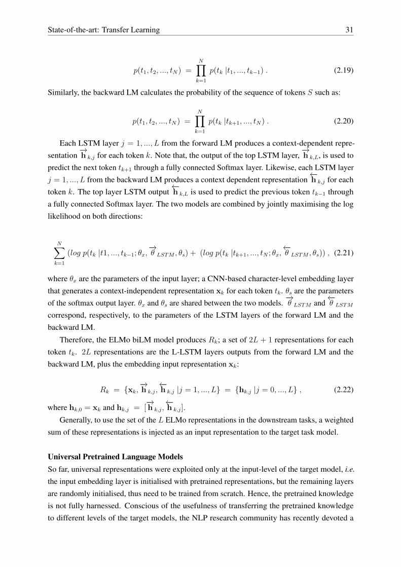
State-of-the-art: Transfer Learning 31

p(t1, t2, ..., tN) =N∏k=1

p(tk |t1, ..., tk−1) . (2.19)

Similarly, the backward LM calculates the probability of the sequence of tokens S such as:

p(t1, t2, ..., tN) =N∏k=1

p(tk |tk+1, ..., tN) . (2.20)

Each LSTM layer j = 1, ..., L from the forward LM produces a context-dependent repre-

sentation−→h k,j for each token k. Note that, the output of the top LSTM layer,

−→h k,L, is used to

predict the next token tk+1 through a fully connected Softmax layer. Likewise, each LSTM layer

j = 1, ..., L from the backward LM produces a context dependent representation←−h k,j for each

token k. The top layer LSTM output←−h k,L is used to predict the previous token tk−1 through

a fully connected Softmax layer. The two models are combined by jointly maximising the log

likelihood on both directions:

N∑k=1

(log p(tk |t1, ..., tk−1; θx,−→θ LSTM , θs) + (log p(tk |tk+1, ..., tN ; θx,

←−θ LSTM , θs)) , (2.21)

where θx are the parameters of the input layer; a CNN-based character-level embedding layer

that generates a context-independent representation xk for each token tk. θs are the parameters

of the softmax output layer. θx and θs are shared between the two models.−→θ LSTM and

←−θ LSTM

correspond, respectively, to the parameters of the LSTM layers of the forward LM and the

backward LM.

Therefore, the ELMo biLM model produces Rk; a set of 2L + 1 representations for each

token tk. 2L representations are the L-LSTM layers outputs from the forward LM and the

backward LM, plus the embedding input representation xk:

Rk = {xk,−→h k,j,

←−h k,j |j = 1, ..., L} = {hk,j |j = 0, ..., L} , (2.22)

where hk,0 = xk and hk,j = [−→h k,j,

←−h k,j].

Generally, to use the set of the L ELMo representations in the downstream tasks, a weighted

sum of these representations is injected as an input representation to the target task model.

Universal Pretrained Language ModelsSo far, universal representations were exploited only at the input-level of the target model, i.e.

the input embedding layer is initialised with pretrained representations, but the remaining layers

are randomly initialised, thus need to be trained from scratch. Hence, the pretrained knowledge

is not fully harnessed. Conscious of the usefulness of transferring the pretrained knowledge

to different levels of the target models, the NLP research community has recently devoted a

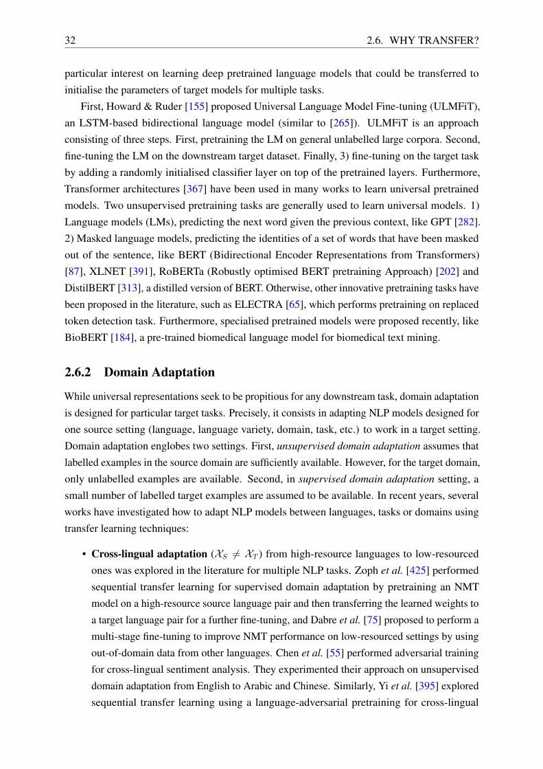
32 2.6. WHY TRANSFER?

particular interest on learning deep pretrained language models that could be transferred to

initialise the parameters of target models for multiple tasks.

First, Howard & Ruder [155] proposed Universal Language Model Fine-tuning (ULMFiT),

an LSTM-based bidirectional language model (similar to [265]). ULMFiT is an approach

consisting of three steps. First, pretraining the LM on general unlabelled large corpora. Second,

fine-tuning the LM on the downstream target dataset. Finally, 3) fine-tuning on the target task

by adding a randomly initialised classifier layer on top of the pretrained layers. Furthermore,

Transformer architectures [367] have been used in many works to learn universal pretrained

models. Two unsupervised pretraining tasks are generally used to learn universal models. 1)

Language models (LMs), predicting the next word given the previous context, like GPT [282].

2) Masked language models, predicting the identities of a set of words that have been masked

out of the sentence, like BERT (Bidirectional Encoder Representations from Transformers)

[87], XLNET [391], RoBERTa (Robustly optimised BERT pretraining Approach) [202] and

DistilBERT [313], a distilled version of BERT. Otherwise, other innovative pretraining tasks have

been proposed in the literature, such as ELECTRA [65], which performs pretraining on replaced

token detection task. Furthermore, specialised pretrained models were proposed recently, like

BioBERT [184], a pre-trained biomedical language model for biomedical text mining.

2.6.2 Domain Adaptation

While universal representations seek to be propitious for any downstream task, domain adaptation

is designed for particular target tasks. Precisely, it consists in adapting NLP models designed for

one source setting (language, language variety, domain, task, etc.) to work in a target setting.

Domain adaptation englobes two settings. First, unsupervised domain adaptation assumes that

labelled examples in the source domain are sufficiently available. However, for the target domain,

only unlabelled examples are available. Second, in supervised domain adaptation setting, a

small number of labelled target examples are assumed to be available. In recent years, several

works have investigated how to adapt NLP models between languages, tasks or domains using

transfer learning techniques:

• Cross-lingual adaptation (XS 6= XT ) from high-resource languages to low-resourced

ones was explored in the literature for multiple NLP tasks. Zoph et al. [425] performed

sequential transfer learning for supervised domain adaptation by pretraining an NMT

model on a high-resource source language pair and then transferring the learned weights to

a target language pair for a further fine-tuning, and Dabre et al. [75] proposed to perform a

multi-stage fine-tuning to improve NMT performance on low-resourced settings by using

out-of-domain data from other languages. Chen et al. [55] performed adversarial training

for cross-lingual sentiment analysis. They experimented their approach on unsupervised

domain adaptation from English to Arabic and Chinese. Similarly, Yi et al. [395] explored

sequential transfer learning using a language-adversarial pretraining for cross-lingual

State-of-the-art: Transfer Learning 33

speech recognition. Transfer Learning was also used to transfer between Arabic dialects.

We can cite the work of Zalmout & Habash [401], who explored multitask learning and

adversarial training for supervised domain adaptation from the resource-rich Modern

Standard Arabic to the Egyptian Arabic.

• Cross-task adaptation (YS 6= YT ) was explored in [243] to investigate different settings

of sequential transfer learning from sentiment analysis task to question classification

task. Yang et al. [390] proposed to transfer a model pretrained on POS tagging to word

segmentation using sequential transfer learning. Niehues & Cho [249] exploited multi-task

learning to transfer the encoded knowledge from POS and NER tasks to neural machine

translation task, by first training the model on all tasks and then continued training only

on the target task. Kiperwasser & Ballesteros [171] proposed to improve neural machine

translation with the help of POS and DP tasks by starting with multi-tasking of the principal

task with auxiliary lower-level tasks (POS and DP). As the training progresses, the model

trains progressively more on the main task dataset compared to auxiliary tasks datasets.

• Cross-domain adaptation (P (XS) 6= P (XT ) or P (YS|XS) 6= P (YT |XT )): Sequential

transfer learning with supervised pretraining was used by Lee et al. [185] and Giorgi &

Bader [123] for supervised domain adaptation between different biomedical datasets for

NER task. It was also applied for supervised adaptation from news to social media by

März et al. [216] for POS tagging, by Zhao et al. [414] for Sentiment Analysis and by

Lin & Lu [193] for NER task. Adversarial training was used in many research works for

cross-domain adaptation. We can cite: [333] for unsupervised domain adaptation between

different forums (Stack Exchange, Sprint FAQ and Quora) for duplicate question detection

task; [138] for supervised domain adaptation from news domain to social media domain

for POS task; [245] for unsupervised domain adaptation between English literature texts

and English news for event trigger identification task. Multi-task learning on multiple

tasks from the source domain has also been used by Peng & Dredze [260] for unsupervised

domain adaptation.

2.7 Discussion

SummaryIn this chapter, we have discussed transfer learning approaches and methods used in NLP. To

recapitulate, first, we discern the aim behind using transfer learning (“Why transfer?”) into two

lines of research: universal representations and domain adaptation. The former aims to produce

universal words embeddings, sentence embeddings and pretrained models, which are transferable

and beneficial to a wide range of downstream tasks and domains. In comparison, the latter seeks

to learn representations that are beneficial for a particular target domain rather than being useful

in general. Second, we categorise transfer learning approaches according to the type of the

34 2.7. DISCUSSION

transferred knowledge (“What to transfer?”) into three categories: (1) transfer of annotations,

(2) transfer of instances, and (3) transfer of models. The first and the second categories are –

by design – only convenient for domain adaptation, whereas the third is applicable whether for

universal representations and domain adaptation. Third, for each category, we have provided

some existing methods to perform the transfer (“How to transfer?”).

Table 2.1 summarises the categorisation presented in this sub-chapter, by showing the

cases where different transfer approaches are used for each research area. First, the two main

columns for “Why transfer?” categorisation: domain adaptation (divided into unsupervised

DA and supervised DA) and universal representations. Second, the three main rows for “What

to transfer?” categorisation: transfer of annotations, instances and models. Note that, by

design, universal representations could only be produced using sequential transfer learning.

Unsupervised domain adaptation could not be performed using sequential transfer learning since

this last assumes a fine-tuning step on the target annotated dataset. Likewise, unsupervised

domain adaptation could not be performed using multi-task learning.

What to Transfer?Why Transfer? Domain Adaptation

Universal RepresentationsUnsupervised DA Supervised DA

Transfer of annotations

Transfer of instances

Transfer of learned representations Adversarial TrainingMulti-task learningSequential Transfer Learning

Table 2.1 – Different transfer learning approaches used for different research objectives.

Positioning of our workOur work falls under supervised domain adaptation research area. Specifically, cross-domain

adaptation from the news domain to social media domain.7 For this purpose, we propose

throughout this thesis a set of approaches based on sequential transfer learning and multi-task

learning. Note that, universal representations research area is orthogonal to our work, and thus

could be incorporated with our approaches to boost the performance further. In chapters 5

and 6, we investigate the impact of ELMo contextualised words representations when used,

simultaneously, with our cross-domain adaptation scheme.

7 Note that social media texts may be considered as a language variety of the formal language, since new words andexpressions are not used in the formal language.

3 | State-of-the-art: Interpretability Meth-ods for Neural NLP

3.1 Introduction

Approaches based on end-to-end Deep Neural Networks (DNNs) have been successfully applied

to a variety of Natural Language Processing (NLP) tasks and applications. However, DNNs

receive much criticism for their lack of interpretability. This is due to the opacity of their internal

representations, thence referred to as black-box models. Nevertheless, understanding AI models,

including NLP models, is particularly essential for critical and life-threatening applications such

as medicine, aviation, security, autonomous cars, etc. where the reliability, transparency, privacy,

accountability and confidentiality must be guaranteed before use. This is one of the reasons for

the low use of DNNs based models in areas where interpretability is requisite. In the last few

years, there is a rising awareness of the critical need for AI models interpretability. Consequently,

research in NLP neural models interpretability is flourishing. Besides, the “right to explanation”

article [130] in the General Data Protection Regulation (GDPR) of the European Union has

undoubtedly spurred widespread and sped-up research in the field.

In this thesis we exploit interpretive techniques to better understand the functioning of our

proposed transfer learning methods. Thus, we present in this chapter the most related works in

the field of NLP neural models interpretability.

There is little consensus about the definition or desideratum for explanations or interpreta-

tions and about what are the differences between “interpretability” and “explainability” with

non-overlapping definitions. In most cases, “interpretability” and “explainability” are used

interchangeably. However, distinctions between the two terms are discussed in many research

works. Montavon et al. [238] define an interpretation as “the mapping of an abstract concept

(e.g. a predicted class) into a domain that the human can make sense of”. For instance, extracting

the linguistic knowledge encoded in words embeddings is considered as an understandable

interpretation. In comparison, they define an explanation as “the collection of features from

the interpretable domain that have contributed to produce the decision for a given example”. In

simple words, explanations are interpretable justifications for the model’s predictions. Lipton

[198] considers that interpretability methods fall into two distinct categories: transparency (i.e.

35

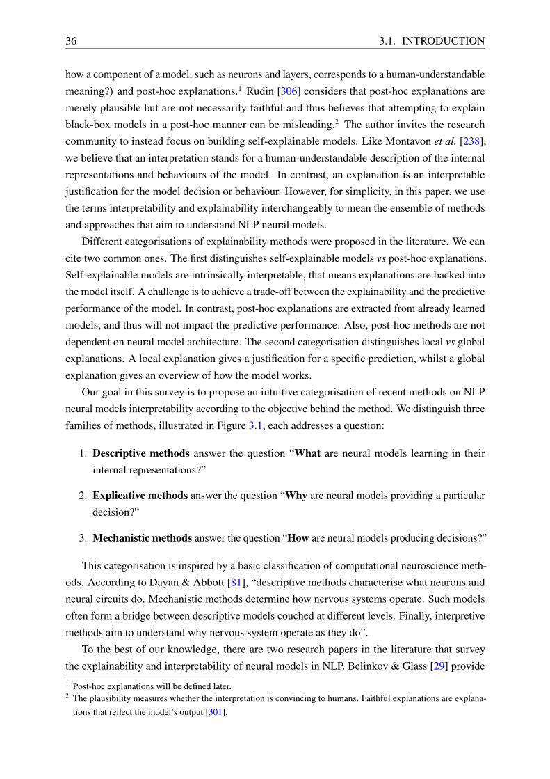
36 3.1. INTRODUCTION

how a component of a model, such as neurons and layers, corresponds to a human-understandable

meaning?) and post-hoc explanations.1 Rudin [306] considers that post-hoc explanations are

merely plausible but are not necessarily faithful and thus believes that attempting to explain

black-box models in a post-hoc manner can be misleading.2 The author invites the research

community to instead focus on building self-explainable models. Like Montavon et al. [238],

we believe that an interpretation stands for a human-understandable description of the internal

representations and behaviours of the model. In contrast, an explanation is an interpretable

justification for the model decision or behaviour. However, for simplicity, in this paper, we use

the terms interpretability and explainability interchangeably to mean the ensemble of methods

and approaches that aim to understand NLP neural models.

Different categorisations of explainability methods were proposed in the literature. We can

cite two common ones. The first distinguishes self-explainable models vs post-hoc explanations.

Self-explainable models are intrinsically interpretable, that means explanations are backed into

the model itself. A challenge is to achieve a trade-off between the explainability and the predictive

performance of the model. In contrast, post-hoc explanations are extracted from already learned

models, and thus will not impact the predictive performance. Also, post-hoc methods are not

dependent on neural model architecture. The second categorisation distinguishes local vs global

explanations. A local explanation gives a justification for a specific prediction, whilst a global

explanation gives an overview of how the model works.

Our goal in this survey is to propose an intuitive categorisation of recent methods on NLP

neural models interpretability according to the objective behind the method. We distinguish three

families of methods, illustrated in Figure 3.1, each addresses a question:

1. Descriptive methods answer the question “What are neural models learning in their

internal representations?”

2. Explicative methods answer the question “Why are neural models providing a particular

decision?”

3. Mechanistic methods answer the question “How are neural models producing decisions?”

This categorisation is inspired by a basic classification of computational neuroscience meth-

ods. According to Dayan & Abbott [81], “descriptive methods characterise what neurons and

neural circuits do. Mechanistic methods determine how nervous systems operate. Such models

often form a bridge between descriptive models couched at different levels. Finally, interpretive

methods aim to understand why nervous system operate as they do”.

To the best of our knowledge, there are two research papers in the literature that survey

the explainability and interpretability of neural models in NLP. Belinkov & Glass [29] provide1 Post-hoc explanations will be defined later.2 The plausibility measures whether the interpretation is convincing to humans. Faithful explanations are explana-

tions that reflect the model’s output [301].

State-of-the-art: Interpretability Methods for Neural NLP 37

Figure 3.1 – Classification of analysis and interpretability methods for neural NLP models.

an extensive review of some analysis and visualisation methods for NLP models and discuss

the challenges that should be addressed in the field. More recently, Danilevsky et al. [79]

present state-of-the-art works according to two of the aforementioned classifications: ad-hoc

explanations vs post-hoc explanations and local explanations vs global explanations. In addition,

they present some of the techniques that are actually used to generate and visualise explanations

in the NLP field. However, the study of Danilevsky et al. [79] includes only explainability

methods that aim to justify the model’s predictions, which correspond to explicative methods in

our proposed categorisation.

In the following sections, we present some techniques from each category from our proposed

categorisation. This survey is not exhaustive, we only focus on some promising techniques and

point to some representative papers for each technique. Considering that in this thesis we exploit

descriptive methods to analyse our proposed transfer learning approaches, the section related to

descriptive methods is the most expanded.

3.2 Descriptive Methods: What?

Descriptive methods aim to investigate the knowledge encoded in the internal representations of

neural models. We present 5 widely used approaches: representation-level visualisation (§3.2.1),

individual units stimulus (§3.2.2), probing classifiers (§3.2.3), similarity analysis (§3.2.4), and

features erasure (§3.2.5). It is noteworthy that although descriptive methods allow an analysis of

the information captured by the model, they do not give insights into whether this information is

actually used by the model to produce the final decision.

3.2.1 Representation-level Visualisation

Representation-level visualisation methods aim to project high-dimensional vectors, such as

word or sentence embeddings or model’s internal representations, into two-dimensional or three-

dimensional spaces to facilitate their visualisation in a scatterplot, while preserving as much as

possible of the significant structure of the high-dimensional data. Thus, similar data points are

likely to appear close together in the scatterplot. t-Distributed Stochastic Neighbor Embedding

(t-SNE) [211] is the most popular tool to visualise embeddings. In the same vein, Escolano et al.

38 3.2. DESCRIPTIVE METHODS: WHAT?

[105] proposed a tool that visualises the internal representations both at the sentence and token

levels. Kahng et al. [167] proposed ActiVis, an interactive visualisation and exploration tool

of large-scale deep learning models. Similarly, Strobelt et al. [344] proposed LSTMVis, a tool

that visualises the dynamics of the hidden states of RNNs in the course of treating the sentence

sequentially.

3.2.2 Individual Units Stimulus

Inspired by works on receptive fields of biological neurons [156], which investigate what stimulus-

features do single neurons represent, several works have been devoted to interpret and visualise

artificial neural networks individual hidden units stimulus-features. Initially, in computer vision

[66, 124, 418] and more recently in NLP, wherein units3 activations are visualised in heatmaps.

Karpathy et al. [169] visualised character-level LSTM cells learned in language modelling. They

found, for instance, multiple interpretable units that track long-distance dependencies, such as

line lengths and quotes. Bau et al. [27] visualised neurons specialised on tense, gender, number,

etc. in NMT models. Radford et al. [281] visualised the activations of a neuron that seems to

perform sentiment analysis in an RNNs-based LM. Figure 3.2 shows character-by-character

activations of the sentiment neuron. Clearly, words like “best” and “good” trigger big jumps in

the neuron’s activation.

Figure 3.2 – Character-by-character activations of the sentiment neuron discovered in RNNs-

based language model [281]. Bright red displays high negative activation values and the bright

green displays high positive activation values.

Kádár et al. [166] proposed top-k-contexts approach to identify sentences, and thus linguistic

patterns, sparking the highest activation values of each unit in RNNs. Kahng et al. [167] proposed

ActiVis, an interactive visualisation and exploration tool of large-scale deep learning models

including neuron-level activations. The main limitation of this method is that it measures the

degree of alignment between individual neurons activations and a linguistic knowledge. However,

as we know, neurons work in synergy, so individual units stimulus will not identify a group of

neurons that might be jointly specialised on one linguistic phenomenon [343].

3 We use neuron and unit interchangeably.

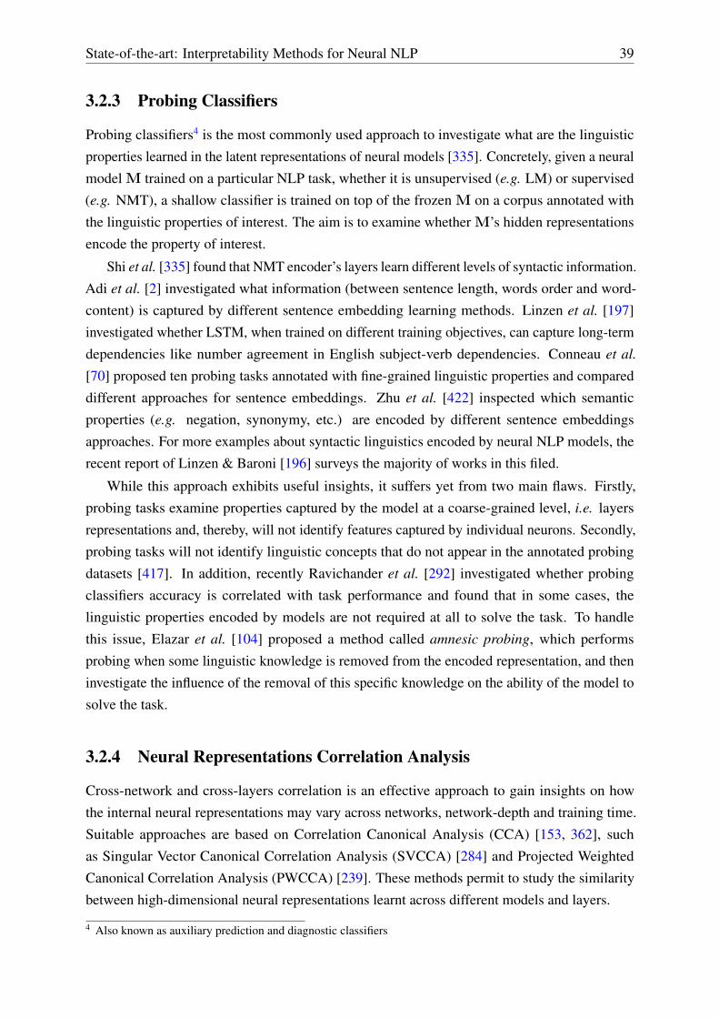
State-of-the-art: Interpretability Methods for Neural NLP 39

3.2.3 Probing Classifiers

Probing classifiers4 is the most commonly used approach to investigate what are the linguistic

properties learned in the latent representations of neural models [335]. Concretely, given a neural

model M trained on a particular NLP task, whether it is unsupervised (e.g. LM) or supervised

(e.g. NMT), a shallow classifier is trained on top of the frozen M on a corpus annotated with

the linguistic properties of interest. The aim is to examine whether M’s hidden representations

encode the property of interest.

Shi et al. [335] found that NMT encoder’s layers learn different levels of syntactic information.

Adi et al. [2] investigated what information (between sentence length, words order and word-

content) is captured by different sentence embedding learning methods. Linzen et al. [197]

investigated whether LSTM, when trained on different training objectives, can capture long-term

dependencies like number agreement in English subject-verb dependencies. Conneau et al.

[70] proposed ten probing tasks annotated with fine-grained linguistic properties and compared

different approaches for sentence embeddings. Zhu et al. [422] inspected which semantic

properties (e.g. negation, synonymy, etc.) are encoded by different sentence embeddings

approaches. For more examples about syntactic linguistics encoded by neural NLP models, the

recent report of Linzen & Baroni [196] surveys the majority of works in this filed.

While this approach exhibits useful insights, it suffers yet from two main flaws. Firstly,

probing tasks examine properties captured by the model at a coarse-grained level, i.e. layers

representations and, thereby, will not identify features captured by individual neurons. Secondly,

probing tasks will not identify linguistic concepts that do not appear in the annotated probing

datasets [417]. In addition, recently Ravichander et al. [292] investigated whether probing

classifiers accuracy is correlated with task performance and found that in some cases, the

linguistic properties encoded by models are not required at all to solve the task. To handle

this issue, Elazar et al. [104] proposed a method called amnesic probing, which performs

probing when some linguistic knowledge is removed from the encoded representation, and then

investigate the influence of the removal of this specific knowledge on the ability of the model to

solve the task.

3.2.4 Neural Representations Correlation Analysis

Cross-network and cross-layers correlation is an effective approach to gain insights on how

the internal neural representations may vary across networks, network-depth and training time.

Suitable approaches are based on Correlation Canonical Analysis (CCA) [153, 362], such

as Singular Vector Canonical Correlation Analysis (SVCCA) [284] and Projected Weighted

Canonical Correlation Analysis (PWCCA) [239]. These methods permit to study the similarity

between high-dimensional neural representations learnt across different models and layers.

4 Also known as auxiliary prediction and diagnostic classifiers

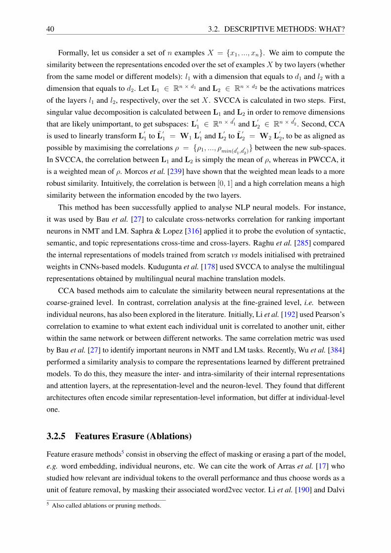
40 3.2. DESCRIPTIVE METHODS: WHAT?

Formally, let us consider a set of n examples X = {x1, ..., xn}. We aim to compute the

similarity between the representations encoded over the set of examplesX by two layers (whether

from the same model or different models): l1 with a dimension that equals to d1 and l2 with a

dimension that equals to d2. Let L1 ∈ Rn × d1 and L2 ∈ Rn × d2 be the activations matrices

of the layers l1 and l2, respectively, over the set X . SVCCA is calculated in two steps. First,

singular value decomposition is calculated between L1 and L2 in order to remove dimensions

that are likely unimportant, to get subspaces: L′1 ∈ Rn × d′1 and L

′2 ∈ Rn × d

′2 . Second, CCA

is used to linearly transform L′1 to L

′1 = W1 L

′1 and L

′2 to L

′2 = W2 L

′2, to be as aligned as

possible by maximising the correlations ρ = {ρ1, ..., ρmin(d′1,d′2)} between the new sub-spaces.

In SVCCA, the correlation between L1 and L2 is simply the mean of ρ, whereas in PWCCA, it

is a weighted mean of ρ. Morcos et al. [239] have shown that the weighted mean leads to a more

robust similarity. Intuitively, the correlation is between [0, 1] and a high correlation means a high

similarity between the information encoded by the two layers.

This method has been successfully applied to analyse NLP neural models. For instance,

it was used by Bau et al. [27] to calculate cross-networks correlation for ranking important

neurons in NMT and LM. Saphra & Lopez [316] applied it to probe the evolution of syntactic,

semantic, and topic representations cross-time and cross-layers. Raghu et al. [285] compared

the internal representations of models trained from scratch vs models initialised with pretrained

weights in CNNs-based models. Kudugunta et al. [178] used SVCCA to analyse the multilingual

representations obtained by multilingual neural machine translation models.

CCA based methods aim to calculate the similarity between neural representations at the

coarse-grained level. In contrast, correlation analysis at the fine-grained level, i.e. between

individual neurons, has also been explored in the literature. Initially, Li et al. [192] used Pearson’s

correlation to examine to what extent each individual unit is correlated to another unit, either

within the same network or between different networks. The same correlation metric was used

by Bau et al. [27] to identify important neurons in NMT and LM tasks. Recently, Wu et al. [384]

performed a similarity analysis to compare the representations learned by different pretrained

models. To do this, they measure the inter- and intra-similarity of their internal representations

and attention layers, at the representation-level and the neuron-level. They found that different

architectures often encode similar representation-level information, but differ at individual-level

one.

3.2.5 Features Erasure (Ablations)

Feature erasure methods5 consist in observing the effect of masking or erasing a part of the model,

e.g. word embedding, individual neurons, etc. We can cite the work of Arras et al. [17] who

studied how relevant are individual tokens to the overall performance and thus choose words as a

unit of feature removal, by masking their associated word2vec vector. Li et al. [190] and Dalvi

5 Also called ablations or pruning methods.

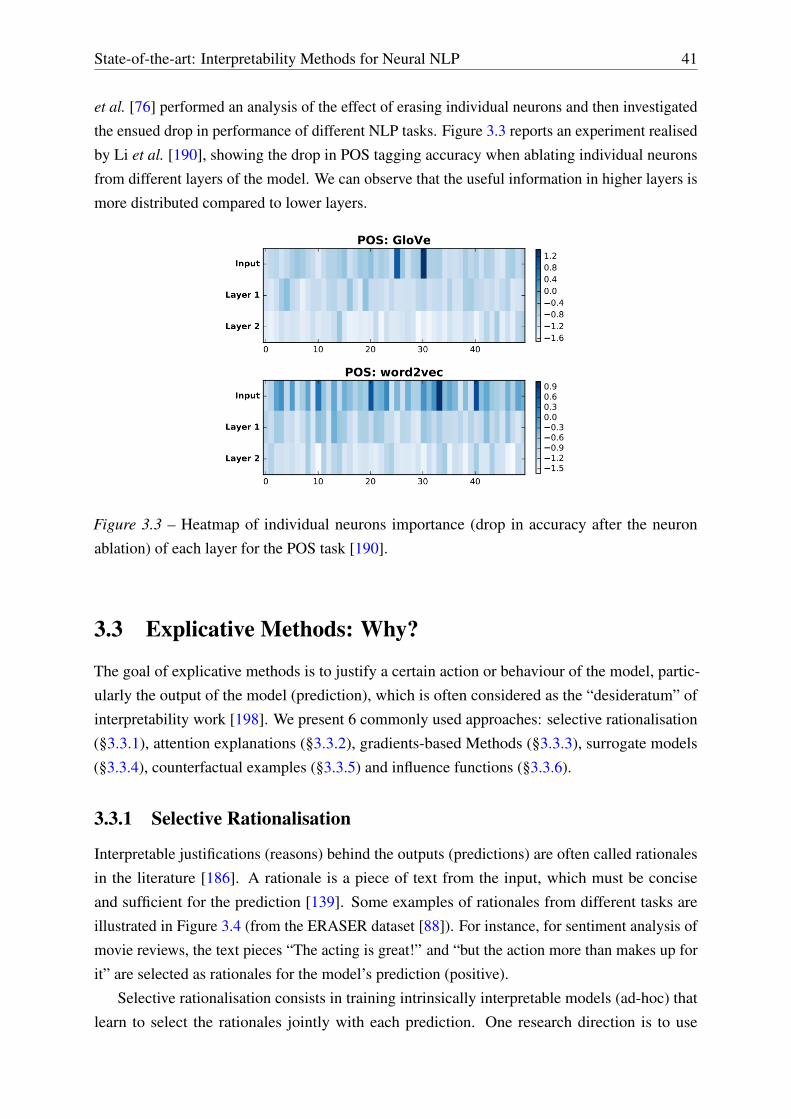
State-of-the-art: Interpretability Methods for Neural NLP 41

et al. [76] performed an analysis of the effect of erasing individual neurons and then investigated

the ensued drop in performance of different NLP tasks. Figure 3.3 reports an experiment realised

by Li et al. [190], showing the drop in POS tagging accuracy when ablating individual neurons

from different layers of the model. We can observe that the useful information in higher layers is

more distributed compared to lower layers.

Figure 3.3 – Heatmap of individual neurons importance (drop in accuracy after the neuron

ablation) of each layer for the POS task [190].

3.3 Explicative Methods: Why?

The goal of explicative methods is to justify a certain action or behaviour of the model, partic-

ularly the output of the model (prediction), which is often considered as the “desideratum” of

interpretability work [198]. We present 6 commonly used approaches: selective rationalisation

(§3.3.1), attention explanations (§3.3.2), gradients-based Methods (§3.3.3), surrogate models

(§3.3.4), counterfactual examples (§3.3.5) and influence functions (§3.3.6).

3.3.1 Selective Rationalisation

Interpretable justifications (reasons) behind the outputs (predictions) are often called rationales

in the literature [186]. A rationale is a piece of text from the input, which must be concise

and sufficient for the prediction [139]. Some examples of rationales from different tasks are

illustrated in Figure 3.4 (from the ERASER dataset [88]). For instance, for sentiment analysis of

movie reviews, the text pieces “The acting is great!” and “but the action more than makes up for

it” are selected as rationales for the model’s prediction (positive).

Selective rationalisation consists in training intrinsically interpretable models (ad-hoc) that

learn to select the rationales jointly with each prediction. One research direction is to use

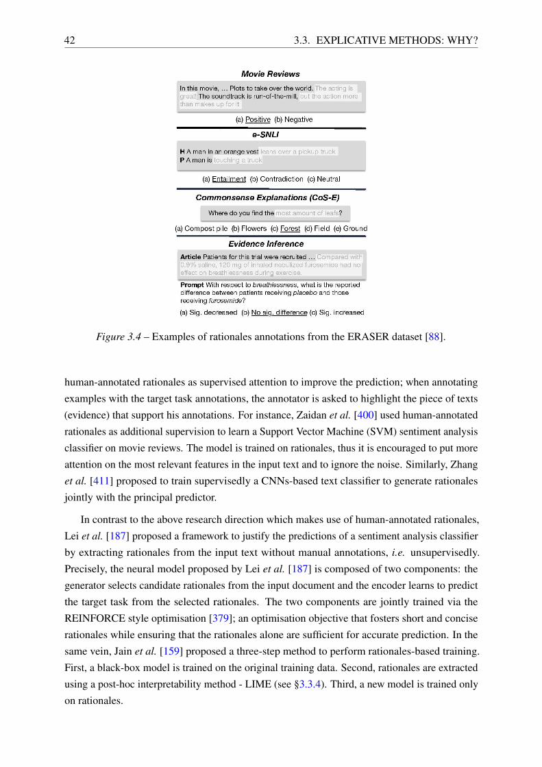
42 3.3. EXPLICATIVE METHODS: WHY?

Figure 3.4 – Examples of rationales annotations from the ERASER dataset [88].

human-annotated rationales as supervised attention to improve the prediction; when annotating

examples with the target task annotations, the annotator is asked to highlight the piece of texts

(evidence) that support his annotations. For instance, Zaidan et al. [400] used human-annotated

rationales as additional supervision to learn a Support Vector Machine (SVM) sentiment analysis

classifier on movie reviews. The model is trained on rationales, thus it is encouraged to put more

attention on the most relevant features in the input text and to ignore the noise. Similarly, Zhang

et al. [411] proposed to train supervisedly a CNNs-based text classifier to generate rationales

jointly with the principal predictor.

In contrast to the above research direction which makes use of human-annotated rationales,

Lei et al. [187] proposed a framework to justify the predictions of a sentiment analysis classifier

by extracting rationales from the input text without manual annotations, i.e. unsupervisedly.

Precisely, the neural model proposed by Lei et al. [187] is composed of two components: the

generator selects candidate rationales from the input document and the encoder learns to predict

the target task from the selected rationales. The two components are jointly trained via the

REINFORCE style optimisation [379]; an optimisation objective that fosters short and concise

rationales while ensuring that the rationales alone are sufficient for accurate prediction. In the

same vein, Jain et al. [159] proposed a three-step method to perform rationales-based training.

First, a black-box model is trained on the original training data. Second, rationales are extracted

using a post-hoc interpretability method - LIME (see §3.3.4). Third, a new model is trained only

on rationales.

State-of-the-art: Interpretability Methods for Neural NLP 43

3.3.2 Attention Explanations

The attention mechanism [21] is widely adopted in neural NLP models since it allows to boost

the predictive performance. Interestingly, the attention mechanism is interpretable by design

since it assigns an attention weight to each token from the input. Thus, one can consider highly

weighted tokens as explanations [190]. Figure 3.5 shows attention weights in an encoder-decoder

NMT model when translating from a French sentence to an English sentence. For instance, we

can see that the model puts a high value of attention on the source words “signé” and “été” to

produce the target word “signed”.

Figure 3.5 – Learned attention weights in a NMT model French - English [21]. Brighter colour

implies a higher attention weight.

However, it has been shown that attention weights do not provide, in fact, faithful explanations

for predictions. Jain & Wallace [158] investigated whether attention weights provide faithful

explanations across different NLP tasks by comparing attention weights to feature importance

measures (gradient-based and feature erasure approaches). They found that they do not, i.e.

highly weighted tokens are not the most influential on the model’s output, likely due to complex

encoders which may entangle inputs. Similarly, Serrano & Smith [332] found that attention

weights fail to explain the model’s decisions.

Later, Wiegreffe & Pinter [377] challenged the assumptions of the former work finding that, in

certain conditions, attention can be considered as a plausible explanation. Indeed, they highlight

that claiming that attention is an explanation or not depends on one’s definition of explanation.

For instance, under the definitions of Lipton [198], attention scores should be considered as a

way to improve the transparency of the model. In comparison, under the definition of Rudin

[306] who defines explainability as providing a plausible but not necessarily faithful justifications

for the model’s decision, attentions scores should be considered as explanations.

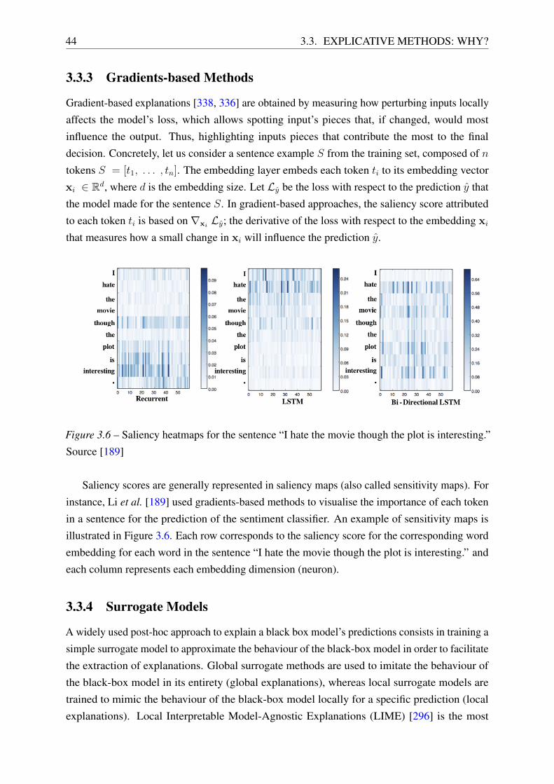
44 3.3. EXPLICATIVE METHODS: WHY?

3.3.3 Gradients-based Methods

Gradient-based explanations [338, 336] are obtained by measuring how perturbing inputs locally

affects the model’s loss, which allows spotting input’s pieces that, if changed, would most

influence the output. Thus, highlighting inputs pieces that contribute the most to the final

decision. Concretely, let us consider a sentence example S from the training set, composed of n

tokens S = [t1, . . . , tn]. The embedding layer embeds each token ti to its embedding vector

xi ∈ Rd, where d is the embedding size. Let Ly be the loss with respect to the prediction y that

the model made for the sentence S. In gradient-based approaches, the saliency score attributed

to each token ti is based on∇xiLy; the derivative of the loss with respect to the embedding xi

that measures how a small change in xi will influence the prediction y.

Figure 3.6 – Saliency heatmaps for the sentence “I hate the movie though the plot is interesting.”

Source [189]

Saliency scores are generally represented in saliency maps (also called sensitivity maps). For

instance, Li et al. [189] used gradients-based methods to visualise the importance of each token

in a sentence for the prediction of the sentiment classifier. An example of sensitivity maps is

illustrated in Figure 3.6. Each row corresponds to the saliency score for the corresponding word

embedding for each word in the sentence “I hate the movie though the plot is interesting.” and

each column represents each embedding dimension (neuron).

3.3.4 Surrogate Models

A widely used post-hoc approach to explain a black box model’s predictions consists in training a

simple surrogate model to approximate the behaviour of the black-box model in order to facilitate

the extraction of explanations. Global surrogate methods are used to imitate the behaviour of

the black-box model in its entirety (global explanations), whereas local surrogate models are

trained to mimic the behaviour of the black-box model locally for a specific prediction (local

explanations). Local Interpretable Model-Agnostic Explanations (LIME) [296] is the most

State-of-the-art: Interpretability Methods for Neural NLP 45

popular tool in this category. It consists in approximating the original black-box classifier (i.e.

approximate the local decision boundaries for a specific instance) with a shallow interpretable

classifier (surrogate model); usually a simple linear model whose weights explain the relevance

of an input feature to a prediction. The surrogate model is trained on perturbations of the original

instance and aims to explain the prediction provided by the black-box classifier for the instance of

interest. For NLP, perturbations could be done by masking words or characters from the original

text. In the same vein as LIME, Alvarez-Melis & Jaakkola [11] proposed a causal framework to

approximate the local behaviour of black-box models for sequence-to-sequence NLP tasks.

3.3.5 Counterfactual explanations

Counterfactual explanations are inspired by causal inference works, which investigate the impact

of a treatment (medical treatment, advertisement campaign, etc.) on a population. Causal-based

explainability approaches aim to assess the importance of a feature for a given prediction by

measuring the effect of a causal intervention which modify the feature of interest from the input

representation. We can cite the work of Goyal et al. [132] who introduced the causal concept

effect in a computer vision application and proposed to change the pixels of an image to those of

another image classified differently by the classifier, in order to compute the effect of those pixels.

Alvarez-Melis & Jaakkola [11] proposed a causal framework for sequence-to-sequence NLP tasks

to discover word-level input-output associations by perturbing the input texts. Recently, Feder

et al. [109] proposed CausalLM, a model for explaining NNs predictions formulated as a causal

inference problem. In CausalLM, an adversarial pre-training of pretrained language models, such

as BERT, is performed to learn a counterfactual representation for a given concept of interest,

which is then used to estimate the real causal effect of the concept on the model’s performance.

Elazar et al. [104] proposed to enhance probing methods to investigate what information is

being used for prediction. As discussed above, probing methods help to get insights about what

information is encoded in the inner representations of the model. However, they do not allow

knowing whether this information is actually used by the model to get decisions. Precisely,

Elazar et al. [104] proposed a method called amnesic probing, which performs probing when

some linguistic knowledge is removed from the encoded representation, and then investigate the

influence of the removal of this specific knowledge on the ability of the model to solve the task.

For this, they use the algorithm Iterative Nullspace Projection (INLP) [291] (as an alternative to

adversarial training) which allows to neutralise the possibility of predicting a certain concept

from a representation with a linear function.

3.3.6 Influence Functions

In contrast to the above-mentioned explicative methods that construct the importance scores

over each token from the input sentence on the final prediction of this sentence, “influence

functions” [175] is a post-hoc explainability method which approximates the change on the

46 3.4. MECHANISTIC METHODS: HOW?

model’s parameters when the instance is up-weighted in the empirical risk by an infinitesimal

amount. Thus, it allows measuring the influence of each training instance on the model’s

prediction for a test example. In NLP, we can cite the work of Han et al. [147] who investigated

whether influence functions can be reliably used to interpret decisions of deep transformer-based

models such as BERT [87] and compared their results to leave-one-out training as well as the

consistency with gradient-based saliency scores. In addition, they found that influence functions

help to reveal artifacts in training data. However, as showed by Basu et al. [26], first-order

influence functions are principally accurate only in the case of machine learning algorithms with

a convex loss functions like SVM. Hence, in the case of DNNs with non-convex loss functions,

influence functions are brittle and their efficiency depends on the the network architecture and

regularisation parameters.

3.4 Mechanistic Methods: How?

Descriptive methods aim to shed light on the model’s black-box internal representations and

explicative methods aim to extract input pieces that explain (justify) the model’s prediction.

However, both categories are not necessarily interested in elucidating the inner workings of the

model. In comparison, we discern mechanistic methods which seek to go further by providing

a functional understanding of the model, i.e. how a neural model goes about accomplishing a

particular function. For instance, mechanistic methods can help to check if the explanations

provided by the explicative methods genuinely reflect the real mechanism that generated the pre-

dictions. Also, how the linguistic knowledge encoded by the model is processed and propagated

between the model’s layers. Given its intricacy, works in this category are scarce. Notwithstand-

ing, we have identified two lines of works that provide someway a functional understanding

of the model. One line of research focuses on the theoretical understanding of how recurrent

networks process information [374, 259, 57, 207] and how information is accumulated towards

a prediction [141]. Another line of research proposes self-explainable models offering the ability

to retrace a complete reasoning path of the model’s decision [1, 421].

3.5 Discussion

In this chapter, we have presented the main research directions of neural NLP models inter-

pretability and explainability. We proposed a new taxonomy that segregates the SOTA works on

three categories. First, descriptive methods aim to investigate the knowledge learned by neural

models in their internal representations. Second, explicative methods aim to justify the predic-

tions of the model. Finally, mechanistic methods seek to provide a functional understanding of

the model.

In addition to the necessity of justifying predictions and decisions for critical applications, a

State-of-the-art: Interpretability Methods for Neural NLP 47

better understanding can allow to spot the weaknesses of NLP models and improve them. For

instance, influence functions were used by Han et al. [147] to reveal artifacts (i.e. Human-made

statistical correlations in the text, making the task easier [370]) in training data that might be

exploited by models. Further, using counterfactual examples can help to identify models that are

vulnerable to adversarial attacks and thus posing security risks [175]. Otherwise, interpreting

black box models can help to identify and neutralise these models from social biases [34], like

gender bias [25, 415, 119, 112, 92].

Within the framework of transfer learning, a large body of analysis and interpretability works

attempts to investigate the linguistic knowledge encoded in pretrained universal representations.

Particularly, probing classifiers are broadly used [199, 64, 47]. Moreover, some recent works

attempt to investigate the impact of fine-tuning on these representations. We can cite the work of

Talmor et al. [347] who investigated whether the performance on a downstream task is attributed

to the knowledge encoded in pretrained representations or to the knowledge encoded during fine-

tuning. Pruksachatkun et al. [278] studied the accuracy of probing classifiers after fine-tuning

on different target tasks. Merchant et al. [231] investigated how fine-tuning leads to changes in

the representations of the BERT pre-trained model, showing that fine-tuning is a “conservative

process”. Mosbach et al. [240] investigated the effect of fine-tuning in three Transformer models

(BERT, RoBERTa and ALBERT) through sentence-level probing classifiers. They found that

fine-tuning can lead to substantial changes in probing accuracy. However, these changes vary

greatly depending on the encoder model as well as fine-tuning and probing tasks combination.

In a different line of research, Dalvi et al. [77] proposed to detect general and task-specific

redundancy at both the layer-level and neuron-level. The analysis is conducted on BERT and

XLNet pretrained models. The results on eight sequence labelling and sequence classification

tasks show that a large portion of the neurons in these models are redundant. Then, they proposed

a set of pruning methods to reduce the pretrained model’s parameters while preserving most of

the model’s performance on downstream tasks.

In this thesis, we employ descriptive methods for two objectives. First, in chapter 6, we

propose to use individual units stimulus and neural representations correlation analysis to

highlight the bias effect in the standard fine-tuning scheme of transfer learning in NLP. Second,

in chapter 7, we make use of individual neurons ablation to highlight the impact of individual

neurons from low-level tasks on high-level tasks in a hierarchical multi-task model. To the best

of our knowledge, we are the first to harness those interpretive methods to analyse individual

units behaviour in Transfer Learning for domain adaptation.

4 | Background: NLP Tasks and Datasets

4.1 Introduction

In this chapter, we provide some background knowledge about the NLP tasks that will be tackled

in this thesis. Given the sequential nature of the spoken and written text, labelling sequences

of words is needed in many NLP applications. We focus in this thesis on sequence labelling

tasks. Formally, given an input sentence of n successive tokens S = [w1, . . . , wn], the goal of a

sequence labelling model is to predict the label ci ∈ C of every wi, with C being the tag-set.

We start by describing each task and the datasets experimented in this work. Namely, Part-

Of-Speech tagging (POS) (§4.2), Morpho-Syntactic Tagging (MST) (§4.3), Chunking (CK)

(§4.4), Named Entity Recognition (NER) (§4.5) and Dependency Parsing (DP) (§4.6). Then, we

present the metrics we will use to evaluate and compare our models (§4.7). Table 4.1 summarises

the statistics of the datasets used in this thesis. Given that user-generated-content in social

media may contain personal data and thus privacy-sensitive information, we use simple rules to

anonymise usernames and URLs in datasets that are not already anonymised by the publisher.

Task Data-set # Classes # Tokens splits (train - val - test)

POS Tagging

WSJ 36 912,344 - 131,768 - 129,654TPoS 40 10,500 - 2,300 - 2,900ArK 25 26,500 - / - 7,700TweeBank 17 24,753 - 11,742 - 19,112

CK: ChunkingCONLL2000 22 211,727 - n/a - 47,377

TChunk 18 10,652 - 2,242 - 2,291

NER: Named Entity RecognitionCONLL-03 4 203,621 - 51,362 - 46,435

WNUT-17 6 62,729 - 15,734 - 23,394

DP: Dependency ParsingUD-English-EWT 51 204,585 - 25,148 - 25,096TweeBank 51 24,753 - 11,742 - 19,112

MST: Morpho-syntactic Tagging

Slovene-news 1304 439k - 58k - 88kSlovene-sm 1102 37,756 - 7,056 - 19,296Croatian-news 772 379k - 50k - 75kCroatian-sm 654 45,609 - 8,886 - 21,412

Table 4.1 – Statistics of the used datasets. Grey rows: news-domain datasets. White rows: social

media domain datasets.

48

Background 49

POS

ArK

TPoS

Tweebank

CK Tchunk

NER Wnut

MST Slovene

Table 4.2 – Illustrative examples of annotated sentences from each social media dataset.

4.2 POS tagging

Part-Of-Speech (POS) tagging assigns an adequate and unique grammatical category (POS tag)

to each word in a text. It indicates how the word is used in a sentence, e.g. noun, verb, adjective,

adverb, pronoun, preposition, conjunction, etc. The main difficulty of the POS tagging task is

related to the ambiguity, as many words can have multiple parts of speech [32]. Note that tag-sets

may differ from one data-set to another. The most common tag-sets are:

1. The Treebank’s tag-sets, where POS tags vary between languages due to cross-lingual

differences. For example the English Penn TreeBank (PTB) [215] comprises 36 tags1 and

the French TreeBank (FTB) comprises 34 tags2.

2. The Universal Dependencies (UD) 2.0 [251] POS tag-set3 contains a tag-set of 17 POS

tags that are common between all languages.

DatasetsIn this thesis, we perform experiments on transfer learning from the news source domain to the

social media target domain. Hence, we use a set of datasets from each domain. For the source

dataset, we use the Wall Street Journal (WSJ) part of the Penn TreeBank, a large English dataset

(formal texts) from the news domain, annotated with the PTB tag-set. Regarding the target

datasets, we use three English social media datasets:

1 https://www.ling.upenn.edu/courses/Fall_2003/ling001/penn_treebank_pos.

html2 http://ftb.linguist.univ-paris-diderot.fr/treebank.php3 https://universaldependencies.org/u/pos/

50 4.3. MORPHO-SYNTACTIC TAGGING

• TPoS [298]: 787 hand-annotated English Tweets, which uses the same tag-set as PTB’s

plus four Twitter unique tags: “URL” for web addresses, “HT” for hashtags, “USR” for

username mentions and “RT” for Retweet signifier (40 tags in total). For our experiments

on TPoS, we use the same data splits used by Derczynski et al. [86]; 70:15:15 into training,

validation and test sets. The tag-set list of TPoS dataset is provided in Table B.1.

• ARK [255]: published in two parts, Oct27 and Daily547, using a novel and coarse grained

tag-set comprising 25 tags4. For example, its “V” tag corresponds to any verb, conflating

PTB’s “VB”, “VBD”, “VBG”, “VBN”, “VBP”, “VBZ”, and “MD” tags or ARK’s tag “L”

corresponding to nominal + verbal (e.g. ur (you are)) and verbal + nominal (e.g. let’s (let

us)). Since data splits portions are not mentioned in original paper, we split the Oct27

dataset into training-set and validation-set (90:10) and use Daily547 as a test-set. The

tag-set list of ArK dataset is provided in Table B.2.

• TweeBank [203]: is a collection of Tweets annotated with the UD 2.0 POS tag-set, which

includes 17 tags. A primary difference of the annotation scheme of TweeBank compared

the two previous datasets concerns the abbreviations, where the tag of the syntactic head

of the expression is attributed to the abbreviation. The tag-set list of TweeBank dataset is

provided in Table B.3.

4.3 Morpho-Syntactic Tagging

When POS tags are enriched with Morpho-Syntactic Descriptions (MSDs), such as gender, case,

tense, etc.5, the task is called Morphosyntactic Tagging (MST). For instance, in the example

of the morphologically-tagged Slovene sentence in Table 4.2: To ni nobena novost (“This is

not a novelty” in English), the word “novost” is annotated as Ncfcn, that stands for POS=Noun,

Type=common, Gender=feminine, Number=singular and Case=nominative.

DatasetsWe performed experiments on three South-Slavic languages: Slovene, Serbian and Croatian. We

used Vardial18 datasets provided in the Morphosyntactic Tagging of Tweets (MTT) shared-task

[402] containing two types of datasets for each language: Twitter (informal texts) and news

(formal texts).

4.4 Chunking

Chunking (CK), also called shallow parsing, is “an intermediate step from POS tagging towards

dependency parsing”6, which aims to extract high-order syntactic spans (chunks) from texts.

4 http://www.cs.cmu.edu/~ark/TweetNLP/annot_guidelines.pdf5 http://nl.ijs.si/ME/V5/msd/html/msd-sl.html6 https://www.clips.uantwerpen.be/conll2000/chunking/

Background 51

For instance in the provided example in Table 1.2, “they” is a noun phrase and “do n’t wanna

talk” is a verbal phrase. CK datasets generally use the BIO (Begin, Inside, Outside) annotation

scheme that categorises tokens as either being outside the syntactic span (O), the beginning

of the syntactic span (B_X) or inside the syntactic span (I_X). Here X refers to one of the 11

syntactic chunk types like NP: Nominal Phrase, VP: Verbal Phrase, PP: Prepositional Phrase,

ADJP: Adjectival Phrase, ADVP: Adverbial Phrase, etc.

DatasetsFor the source dataset, we used the CONLL2000 shared task’s English data-set [354] that uses

sections 15-18 from the WSJ corpus for training and section 20 for testing. Regarding the target

dataset, we used TChunk Tweets data-set [298] (the same corpus as TPoS). Both datasets use

the BIO format annotation scheme. For instance, in the provided example in Table 4.2: “!!!!!” is

outside the syntactic span, “do” is the beginning of a verbal-phrase span, while “do n’t wanna

talk” are inside the verbal-phrase span. The Chunking tag-set used in both datasets is provided

in Table B.4.

4.5 Named Entity Recognition

Compared to the above tasks that act mostly in the syntactic level, NER extracts semantic

information from textual documents and could be considered as a semantic task. It consists on

classifying named entities that are present in a text into pre-defined categories like names of

persons, organisations or locations [32].

DatasetsRegarding the source domain, we make use of the English news dataset CONLL-03 from the

CONLL 2003 shared task [355], tagged with four different entity types (Persons, Locations,

Organisations and MISC). For the target domain, we conducted our experiments on the Emerging

Entity Detection shared task of WNUT-17 [85], which includes six entity types, three of which

are common with CONLL-03’s types: Persons, Organisations and Locations, while three are

emergent: Products, Groups (e.g. the warriors) and Creative Works (e.g. Mcchoke (Machoke)).

The training-set of WNUT-17 is made-up of 1,000 annotated Tweets, validation-set from Youtube

comments and test-set from a mix of different sources of noisy texts: Twitter, Reddit and

StackExchange. Similarly to CK datasets, both NER datasets use the BIO format annotation

scheme that categorises tokens as either being outside the entity type (O), the beginning of the

entity type (B_X) or inside the entity type (I_X), here X refers to one of the entity types.

4.6 Dependency Parsing

Given an input sentence S = [w1, . . . , wn] of n successive tokens, the goal of DP is two folds

[32]:

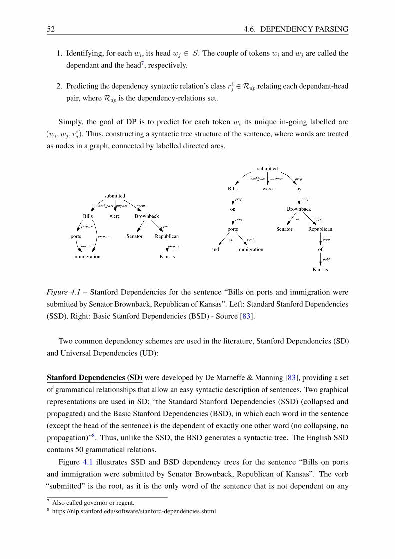
52 4.6. DEPENDENCY PARSING

1. Identifying, for each wi, its head wj ∈ S. The couple of tokens wi and wj are called the

dependant and the head7, respectively.

2. Predicting the dependency syntactic relation’s class rij ∈Rdp relating each dependant-head

pair, whereRdp is the dependency-relations set.

Simply, the goal of DP is to predict for each token wi its unique in-going labelled arc

(wi, wj, rij). Thus, constructing a syntactic tree structure of the sentence, where words are treated

as nodes in a graph, connected by labelled directed arcs.

Figure 4.1 – Stanford Dependencies for the sentence “Bills on ports and immigration were

submitted by Senator Brownback, Republican of Kansas”. Left: Standard Stanford Dependencies

(SSD). Right: Basic Stanford Dependencies (BSD) - Source [83].

Two common dependency schemes are used in the literature, Stanford Dependencies (SD)

and Universal Dependencies (UD):

Stanford Dependencies (SD) were developed by De Marneffe & Manning [83], providing a set

of grammatical relationships that allow an easy syntactic description of sentences. Two graphical

representations are used in SD; “the Standard Stanford Dependencies (SSD) (collapsed and

propagated) and the Basic Stanford Dependencies (BSD), in which each word in the sentence

(except the head of the sentence) is the dependent of exactly one other word (no collapsing, no

propagation)”8. Thus, unlike the SSD, the BSD generates a syntactic tree. The English SSD

contains 50 grammatical relations.

Figure 4.1 illustrates SSD and BSD dependency trees for the sentence “Bills on ports

and immigration were submitted by Senator Brownback, Republican of Kansas”. The verb

“submitted” is the root, as it is the only word of the sentence that is not dependent on any

7 Also called governor or regent.8 https://nlp.stanford.edu/software/stanford-dependencies.shtml

Background 53

head-word. We can observe that SSD and BSD are sightly different. The following SSD relations

are connecting words of the sentence:

• nsubjpass(submitted, Bills) (passive nominal subject): “Bills” is the passive nominal

subject of the verb “submitted” in the passive clause.

• auxpass(submitted, were) (passive auxiliary): “were” is the non-main verb of the passive

clause.

• agent(submitted, Brownback): “Brownback” is the complement of the passive verb

“submitted”, introduced by the preposition “by”. This relation only appears in the collapsed

dependencies (SSD); it does not appear in basic dependencies (BSD). Where two relations

replace it: prep(submitted, by) for prepositional modifier and pobj(by, Brownback) for

object of a preposition.

• nn(Brownback, Senator) (noun compound modifier): In the nominal phrase (NP), “Sen-

ator Brownback”, “Senator” is a noun modifier of the head noun “Brownback”.

• appos(Brownback, Republican) (appositional modifier): “Republican of Kanas” is an

NP that serves to define the preceding NP, “Senator Brownback”. Thus, “Republican” is

an appositional modifier of “Brownback”.

• prep_of(Republican, Kansas) (prepositional modifier): “Kansas” is a prepositional mod-

ifier of “Republican”, introduced by the preposition “of”. This relation only appears in the

collapsed dependencies; it does not appear in basic dependencies. It is replaced by two

relations: prep(Republican, of) and pobj(of, Kansas).

• prep_on(Bills, ports) and prep_on(Bills, immigration): Both “immigration” and “ports”

are prepositional modifier of “Bills”, introduced by the preposition “on”.

• conj_and(ports, immigration) (conjunction): “ports” and “immigration” are connected

by the coordinating conjunction “and”.

Universal Dependencies (UD) appeared initially in [82] intending to extend the SD to other

languages to be generally applicable cross-linguistically. Further, the UD have been developed

for 60+ languages with a cross-linguistically consistent annotation [251]. Specifically, English

TreeBank contains 51 relations, including the 37 multi-lingual relations, which are provided in

Table B.5.

DatasetsFor the source domain, we use UD_English-EWT, the English corpus of gold standard Universal

Dependencies, built over the English Web Treebank9. The corpus comprises 254,830 words9 https://catalog.ldc.upenn.edu/LDC2012T13

54 4.7. EVALUATION METRICS

Figure 4.2 – An illustrative example from the TweeBank dataset showing non-syntactic tokens -

Source: [203].

Figure 4.3 – An Illustrative example of informal but syntactic tokens - Source: [203].

(16,622 sentences). For the target domain, we use the recently published TweeBank dataset

[203], annotated following the UD 2.0 guidelines. Considering the characteristics that distin-

guish Tweets from formal texts, the following special rules were adopted for the annotation of

TweeBank dataset with syntactic dependencies:

• Multiple roots are allowed. Indeed, a single Tweet might be composed of more than one

sentence. As illustrated in the provided example in Figure 4.2, the Tweet contains two

sentences separated with “:”.

• In Tweets, many tokens do not carry a syntactic function in the sentence, i.e. non-syntactic

tokens (sentiment emoticons, urls, hashtags, etc.). As illustrated in Figure 4.2, heart,

RT and @coldplay are non-syntactic tokens and thus are respectively POS annotated as

“SYM”, “X” and “X”. Regarding dependency relations, they are connected to their heads

with the “discourse” syntactic relation. “The discourse relation is used for interjections

and other discourse particles and elements (which are not clearly linked to the structure of

the sentence)”10. However, these tokens may be used in Tweets with a syntactic function.

For instance, in the syntactic tree of the Tweet in Figure 4.3, the hashtag #awesome is a

content word, used as an adjective. Likewise, RT abbreviates the verb retweet.

4.7 Evaluation Metrics

Throughout this thesis, we evaluate our models using metrics that are commonly used by the

community. Specifically, for sequence labelling tasks the accuracy (acc.) is commonly used,

10https://universaldependencies.org/u/dep/discourse.html

Background 55

calculated by dividing the number of correct predictions by the number of all predictions, based

on the number of true positives (TP), true negatives (TN), false positives (FP), and false negatives

(FN), which is defined as follows:

Acc =TP + TN

TP + TN + FP + FN. (4.1)

For NER and CK, the F1 score is typically used, which is the harmonic mean of precision (P)

and recall (R):

R =TP

TP + TN, (4.2)

P =TP

TP + FP, (4.3)

F1 = 2× P ×RP +R

. (4.4)

The F1 metric provides a good estimate of the overall quality of a model. Indeed, as aforemen-

tioned, CK and NER datasets are annotated using the BIO scheme. Thus, F1 is used to calculate

entity-level performances, i.e. exact match of the whole entity is needed, e.g. “Micchoke but the

warriors blew a 3-1 lead” in the example provided in Table 4.2, both words of the entity group

“the warriors” should be predicted correctly.

For DP task, two evaluation measures are commonly used, unlabelled attachment score

(UAS) [103] and labelled attachment score (LAS) [252]. UAS does not consider the relation (arc

label), while LAS requires a correct label for each arc. Specifically, “LAS is the percentage of

words that are assigned both the correct syntactic head and the correct dependency label. We use

CoNLL 2017 Shared Task evaluation script, where only universal dependency labels are taken

into account, which means that language-specific subtypes such as acl:relcl (relative clause), a

subtype of the universal relation acl (adnominal clause), will be truncated to acl both in the gold

standard and in the parser output in the evaluation.”11

A common approach to compare the performance between different approaches across

different datasets and tasks is to take the average of each approach across all tasks and datasets.

Precisely given a set of L datasets, the average score Avgi of a particular approach i is calculated

using:

Avgi =1

L

L∑j=1

sij , (4.5)

with sij being the score of the approach i on dataset j. However, as it has been discussed in many

research papers [345, 294, 348], when tasks are not evaluated using the same metrics or results

across datasets are not of the same order of magnitude, the simple average does not allow a

11https://universaldependencies.org/conll18/evaluation.html

56 4.7. EVALUATION METRICS

“coherent aggregation”. For this, we use the average Normalized Relative Gain (aNRG) proposed

by Tamaazousti et al. [350], where a score aNRGi for each approach i is calculated compared

to a reference approach (baseline) as follows:

aNRGi =1

L

L∑j=1

(sij − srefj )

(smaxj − srefj ), (4.6)

with sij being the score of the approachi on datasetj , srefj being the score of the reference approach

on dataset j and smaxj is the score of the best score achieved across all approaches on dataset j.

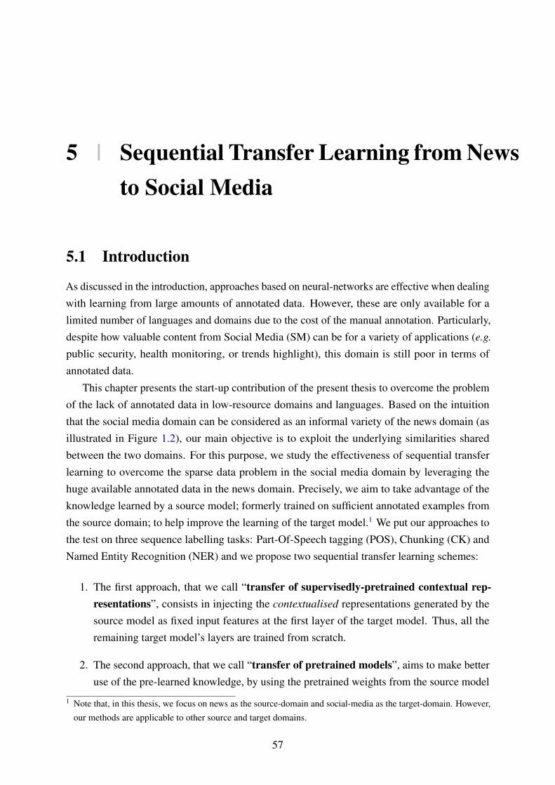
5 | Sequential Transfer Learning from Newsto Social Media

5.1 Introduction

As discussed in the introduction, approaches based on neural-networks are effective when dealing

with learning from large amounts of annotated data. However, these are only available for a

limited number of languages and domains due to the cost of the manual annotation. Particularly,

despite how valuable content from Social Media (SM) can be for a variety of applications (e.g.

public security, health monitoring, or trends highlight), this domain is still poor in terms of

annotated data.

This chapter presents the start-up contribution of the present thesis to overcome the problem

of the lack of annotated data in low-resource domains and languages. Based on the intuition

that the social media domain can be considered as an informal variety of the news domain (as

illustrated in Figure 1.2), our main objective is to exploit the underlying similarities shared

between the two domains. For this purpose, we study the effectiveness of sequential transfer

learning to overcome the sparse data problem in the social media domain by leveraging the

huge available annotated data in the news domain. Precisely, we aim to take advantage of the

knowledge learned by a source model; formerly trained on sufficient annotated examples from

the source domain; to help improve the learning of the target model.1 We put our approaches to

the test on three sequence labelling tasks: Part-Of-Speech tagging (POS), Chunking (CK) and

Named Entity Recognition (NER) and we propose two sequential transfer learning schemes:

1. The first approach, that we call “transfer of supervisedly-pretrained contextual rep-resentations”, consists in injecting the contextualised representations generated by the

source model as fixed input features at the first layer of the target model. Thus, all the

remaining target model’s layers are trained from scratch.

2. The second approach, that we call “transfer of pretrained models”, aims to make better

use of the pre-learned knowledge, by using the pretrained weights from the source model

1 Note that, in this thesis, we focus on news as the source-domain and social-media as the target-domain. However,our methods are applicable to other source and target domains.

57

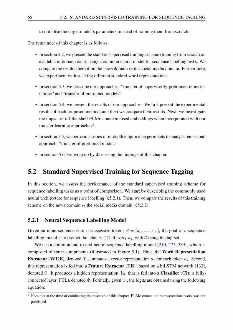
58 5.2. STANDARD SUPERVISED TRAINING FOR SEQUENCE TAGGING

to initialise the target model’s parameters, instead of training them from scratch.

The remainder of this chapter is as follows:

• In section 5.2, we present the standard supervised training scheme (training from scratch on

available in-domain data), using a common neural model for sequence labelling tasks. We

compare the results thereof on the news domain vs the social media domain. Furthermore,

we experiment with stacking different standard word representations.

• In section 5.3, we describe our approaches: “transfer of supervisedly-pretrained represen-

tations” and “transfer of pretrained models”.

• In section 5.4, we present the results of our approaches. We first present the experimental

results of each proposed method, and then we compare their results. Next, we investigate

the impact of off-the-shelf ELMo contextualised embeddings when incorporated with our

transfer learning approaches2.

• In section 5.5, we perform a series of in-depth empirical experiments to analyse our second

approach: “transfer of pretrained models”.

• In section 5.6, we wrap up by discussing the findings of this chapter.

5.2 Standard Supervised Training for Sequence Tagging

In this section, we assess the performance of the standard supervised training scheme for

sequence labelling tasks as a point of comparison. We start by describing the commonly used

neural architecture for sequence labelling (§5.2.1). Then, we compare the results of this training

scheme on the news domain vs the social media domain (§5.2.2).

5.2.1 Neural Sequence Labelling Model

Given an input sentence S of n successive tokens S = [w1, . . . , wn], the goal of a sequence

labelling model is to predict the label ct ∈ C of every wt, with C being the tag-set.

We use a common end-to-end neural sequence labelling model [210, 275, 389], which is

composed of three components (illustrated in Figure 5.1). First, the Word RepresentationExtractor (WRE), denoted Υ, computes a vector representation xt for each token wt. Second,

this representation is fed into a Feature Extractor (FE): based on a biLSTM network [133],

denoted Φ. It produces a hidden representation, ht, that is fed into a Classifier (Cl): a fully-

connected layer (FCL), denoted Ψ. Formally, givenwt, the logits are obtained using the following

equation:2 Note that at the time of conducting the research of this chapter, ELMo contextual representations work was not

published.

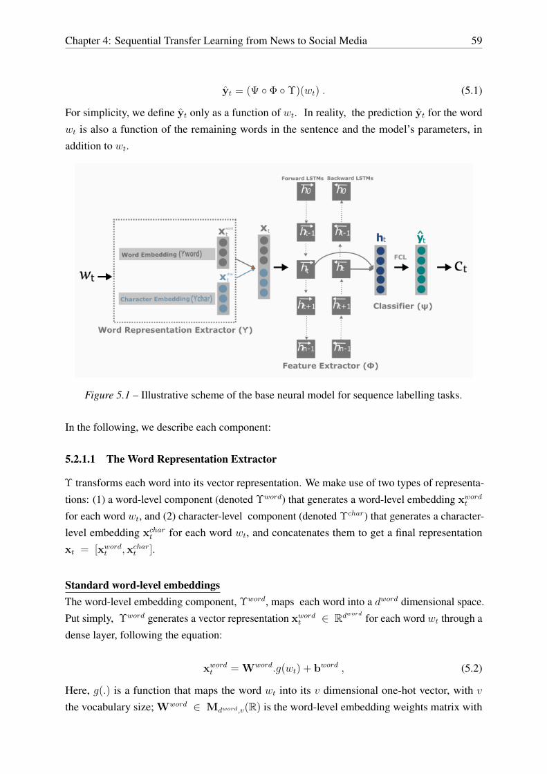
Chapter 4: Sequential Transfer Learning from News to Social Media 59

yt = (Ψ ◦ Φ ◦Υ)(wt) . (5.1)

For simplicity, we define yt only as a function of wt. In reality, the prediction yt for the word

wt is also a function of the remaining words in the sentence and the model’s parameters, in

addition to wt.

Figure 5.1 – Illustrative scheme of the base neural model for sequence labelling tasks.

In the following, we describe each component:

5.2.1.1 The Word Representation Extractor

Υ transforms each word into its vector representation. We make use of two types of representa-

tions: (1) a word-level component (denoted Υword) that generates a word-level embedding xwordt

for each word wt, and (2) character-level component (denoted Υchar) that generates a character-

level embedding xchart for each word wt, and concatenates them to get a final representation

xt = [xwordt ,xchart ].

Standard word-level embeddingsThe word-level embedding component, Υword, maps each word into a dword dimensional space.

Put simply, Υword generates a vector representation xwordt ∈ Rdword for each word wt through a

dense layer, following the equation:

xwordt = Wword.g(wt) + bword , (5.2)

Here, g(.) is a function that maps the word wt into its v dimensional one-hot vector, with v

the vocabulary size; Wword ∈ Mdword,v(R) is the word-level embedding weights matrix with

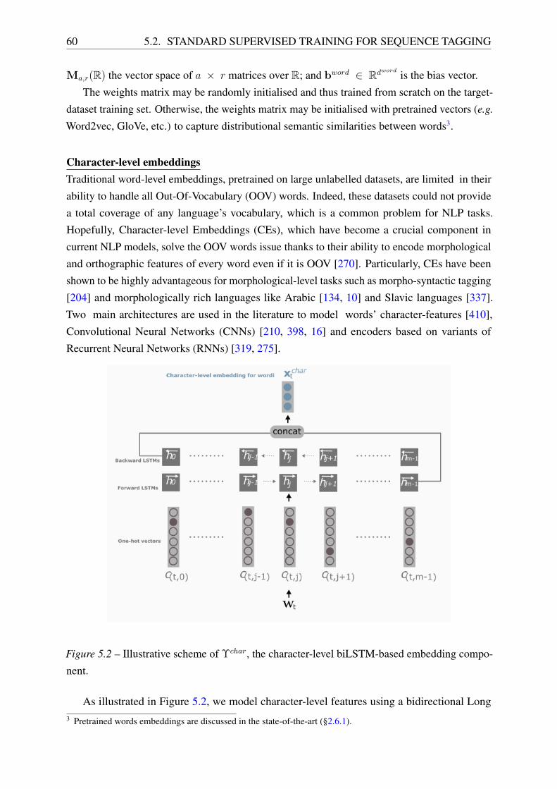
60 5.2. STANDARD SUPERVISED TRAINING FOR SEQUENCE TAGGING

Ma,r(R) the vector space of a × r matrices over R; and bword ∈ Rdword is the bias vector.

The weights matrix may be randomly initialised and thus trained from scratch on the target-

dataset training set. Otherwise, the weights matrix may be initialised with pretrained vectors (e.g.

Word2vec, GloVe, etc.) to capture distributional semantic similarities between words3.

Character-level embeddingsTraditional word-level embeddings, pretrained on large unlabelled datasets, are limited in their

ability to handle all Out-Of-Vocabulary (OOV) words. Indeed, these datasets could not provide

a total coverage of any language’s vocabulary, which is a common problem for NLP tasks.

Hopefully, Character-level Embeddings (CEs), which have become a crucial component in

current NLP models, solve the OOV words issue thanks to their ability to encode morphological

and orthographic features of every word even if it is OOV [270]. Particularly, CEs have been

shown to be highly advantageous for morphological-level tasks such as morpho-syntactic tagging

[204] and morphologically rich languages like Arabic [134, 10] and Slavic languages [337].

Two main architectures are used in the literature to model words’ character-features [410],

Convolutional Neural Networks (CNNs) [210, 398, 16] and encoders based on variants of

Recurrent Neural Networks (RNNs) [319, 275].

Figure 5.2 – Illustrative scheme of Υchar, the character-level biLSTM-based embedding compo-

nent.

As illustrated in Figure 5.2, we model character-level features using a bidirectional Long3 Pretrained words embeddings are discussed in the state-of-the-art (§2.6.1).

Chapter 4: Sequential Transfer Learning from News to Social Media 61

Short-Term Memory (biLSTM) encoder, trained from scratch, to induce a fully context-sensitive

character-level embedding. Concretely, a word wt is divided into a succession of Lt characters

[c(t,1), . . . , c(t,Lt)], each c(t,j) ∈ Rvchar defined as the one-hot vector of the corresponding

character. Here, Lt is the length of the word wt and vchar is the characters’ vocabulary size. First,

an embedding, x(t,j) ∈ Rdchar , is computed for each character c(t,j) through an embedding

dense layer, following the equation:

x(t,j) = Wchar.c(t,j) + bchar , (5.3)

where Wchar ∈ Mdchar,vchar(R) is the character-level embedding weight matrix and bchar ∈ Rdchar

is the bias vector.

Next, a forward LSTM model reads the character vectors (x(t,j)) from left to right and a

backward LSTM model reads characters from right to left. The combination between the last

hidden state of the forward LSTM and the last hidden state of the backward LSTM represents

xchart ∈ Rdchar : the character-level embedding for the word wt, where dchar is the character

embedding’s dimension.

5.2.1.2 Feature Extractor

To learn a context sensitive representation for each token, the word representation extractor’s

outputs, [x1, . . . ,xn], are fed into the feature extractor. It consists of a single biLSTM layer

which iteratively passes through the sentence in both directions. Formally, a forward LSTM

layer at a time-step t takes xt and the previous hidden state−→h t−1 as input, and outputs the

current forward hidden state−→h t, whilst a backward LSTM layer at time-step t takes xt and

the following hidden state←−h t+1 as input, and outputs the current backward hidden state

←−h t. In

order to take into account the context on both sides of that word, hidden representations−→ht and

←−h t from forward and backward biLSTM units, respectively, are concatenated at every time-step,

resulting ht vector: ht = [−→ht;←−ht].

To obtain−→ht , the following transformations are applied in the forward LSTMs:

it = σ(Wi.[−−→ht−1,xt]) (5.4a)

ft = σ(Wf .[−−→ht−1,xt]) (5.4b)

ot = σ(Wo.[−−→ht−1,xt]) (5.4c)

ct = tanh(Wc.[−−→ht−1,xt]) (5.4d)

ct = ft � ct−1 + it � ct (5.4e)−→ht = ot � tanh(ct) (5.4f)

Where σ is an element-wise sigmoid logistic function defined as σ(a) = [ 11+exp(−ai)

]i=|a|i=1

for a vector a. � denotes element-wise multiplication of two vectors. it, ft and ot represent

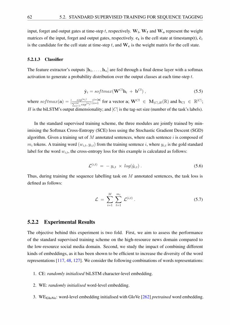
62 5.2. STANDARD SUPERVISED TRAINING FOR SEQUENCE TAGGING

input, forget and output gates at time-step t, respectively. Wi, Wf and Wo represent the weight

matrices of the input, forget and output gates, respectively. ct is the cell state at timestamp(t), ctis the candidate for the cell state at time-step t, and Wc is the weight matrix for the cell state.

5.2.1.3 Classifier

The feature extractor’s outputs [h1, . . . ,hn] are fed through a final dense layer with a softmax

activation to generate a probability distribution over the output classes at each time-step t.

yt = softmax(WClht + bCl) , (5.5)

where softmax(a) = [ exp(ai)∑|a|j=1 exp

(aj)]i=|a|i=1 for a vector a; WCl ∈ M|C|,H(R) and bCl ∈ R|C|;

H is the biLSTM’s output dimensionality; and |C| is the tag-set size (number of the task’s labels).

In the standard supervised training scheme, the three modules are jointly trained by min-

imising the Softmax Cross-Entropy (SCE) loss using the Stochastic Gradient Descent (SGD)

algorithm. Given a training set of M annotated sentences, where each sentence i is composed of

mi tokens. A training word (wi,t, yi,t) from the training sentence i, where yi,t is the gold standard

label for the word wi,t, the cross-entropy loss for this example is calculated as follows:

L(i,t) = − yi,t × log(yi,t) . (5.6)

Thus, during training the sequence labelling task on M annotated sentences, the task loss is

defined as follows:

L =M∑i=1

mi∑t=1

L(i,t) . (5.7)

5.2.2 Experimental Results

The objective behind this experiment is two fold. First, we aim to assess the performance

of the standard supervised training scheme on the high-resource news domain compared to

the low-resource social media domain. Second, we study the impact of combining different

kinds of embeddings, as it has been shown to be efficient to increase the diversity of the word

representations [117, 48, 127]. We consider the following combinations of words representations:

1. CE: randomly initialised biLSTM character-level embedding.

2. WE: randomly initialised word-level embedding.

3. WEGloVe: word-level embedding initialised with GloVe [262] pretrained word embedding.

Chapter 4: Sequential Transfer Learning from News to Social Media 63

4. WEFastText: word-level embedding initialised with FastText [35] pretrained representa-

tions.

5. WEFastText+WEGloVe: word-level embedding initialised with the concatenation of Fast-

Text and GloVe pretrained representations.

6. WE+CE: concatenation of a word-level and a biLSTM character-level embeddings, both

randomly initialised.

7. CE+WEGloVe: concatenation of GloVe pretrained embeddings with and randomly ini-

tialised character embedding.

8. CE+WEFastText: concatenation of word-level embedding initialised with FastText pre-

trained representations with the randomly initialised biLSTM character-level embedding.

9. CE+WEFastText+WEGloVe: concatenation of FastText and GloVe pretrained word-level

embeddings with the randomly initialised biLSTM character-level embedding.

5.2.2.1 Datasets

Throughout this chapter, we conduct experiments on three sequence labelling tasks (POS, CK

and NER). For the source-datasets, we use the news domain with the following datasets: the WSJ

part of Penn-Tree-Bank (PTB) [215] for POS; CONLL-03 for NER [355]; and CONLL2000

[354] for CK. In the same vein, for the target-datasets, we use the social media with the following

datasets: TPoS, ArK and TweeBank [203] for POS; WNUT-17 [85] for NER; and TChunk [298]

for CK. Statistics of all the datasets are summarised in Table 5.1. More details about the tasks

and datasets are provided in chapter 4.

Task #Classes Sources Eval. Metrics Splits (train - val - test)POS: POS Tagging 36 WSJ Top-1 Acc. 912,344 - 131,768 - 129,654

CK: Chunking 22 CONLL-2000 Top-1 Acc. 211,727 - n/a - 47,377

NER: Named Entity Recognition 4 CONLL-2003 Top-1 Exact-match F1. 203,621 - 51,362 - 46,435

POS: POS Tagging40 TPoS Top-1 Acc. 10,500 - 2,300 - 2,90025 ArK Top-1 Acc. 26,500 - / - 7,70017 TweeBank Top-1 Acc. 24,753 - 11,742 - 19,112

CK: Chunking 18 TChunk Top-1 Acc.. 10,652 - 2,242 - 2,291

NER: Named Entity Recognition 6 WNUT-17 Top-1 Exact-match F1. 62,729 - 15,734 - 23,394

Table 5.1 – Statistics of the used datasets. Top: datasets of the source domain. Bottom: datasets

of the target domain.

5.2.2.2 Implementation details

In the standard word-level embeddings, tokens are converted to lower-case while the character-

level component still retains access to the capitalisation information. We set the randomly

64 5.2. STANDARD SUPERVISED TRAINING FOR SEQUENCE TAGGING

initialised character embedding dimension (dchar) at 50, the dimension of hidden states of the

character-level biLSTM (dchar) at 100 and used 300-dimensional word-level embeddings (dword).

Word-level embeddings were pre-loaded from publicly available GloVe vectors pre-trained on

42 billion words collected through web crawling and containing 1.9M different words [262]

and from the publicly available FastText [35] vectors pre-trained on common crawl4. These

embeddings are also updated during training. For the FE component, we use a single layer

biLSTM (token-level feature extractor) and set the number of units (H) to 200. In all of our

experiments, both pretraining and fine-tuning were performed using the same training settings,

i.e. SGD with momentum and early stopping, mini-batches of 16 sentences, and a fixed learning

rate of 1.5 × 10−2. Throughout this thesis, all our models are implemented with the PyTorch

library [258].

5.2.2.3 Results

Results are reported in Tables 5.2. The top table provides the results (accuracy %) on POS

datasets and the bottom one provides the results on CK datasets (accuracy %) and NER datasets

(F1 %). As discussed in section 4.7, we use the average (Avg.) as well as the aNRG metric (see

equation 4.6) to compare the scores of the different methods. For the aNRG, the methods are

compared to the reference CE+WE.

In light of the results displayed in Table 5.2, we make the following observations. First, All

of our models perform significantly better on the news domain compared to the social media

domain. This is mainly due to the lack of in-domain training data for the social media domain.

Second, we can observe that CE+WEFastText+WEGloVe setting outperforms all other settings in

most tasks and datasets, which indicates that the inductive biases encoded by different types of

pretrained embeddings are complementary.

Third, character-level embeddings (CE) outperform randomly initialised word-level embed-

dings (WE) across all social media datasets, while both representations perform comparably

on news-domain data-sets. Because OOV words are rare in news-domain datasets, randomly

initialised word-level embeddings (WE) are sufficient to encode the majority of words. On the

other hand, since OOV words are frequent in social media datasets, character-level information

is essential to encode new tokens, we can observe that CE performs comparably with CE+WE,

whereas WE degrades severely the performance compared to CE+WE (-32.1 aNRG for PoS

tagging task and -21.1 aNRG for NER and CK tasks).

Fourth, The use of both pretrained word-level embeddings, WEfastext and WEGloVe, is

highly advantageous across all datasets of both domains, enhancing the performance compared

to WE (from scratch). For news domain datasets, WEGloVe exhibits better results. For the

social media domain, WEGloVe performs better on the POS task, while WEFastText is better

4 https://github.com/facebookresearch/fastText/blob/master/docs/

crawl-vectors.md

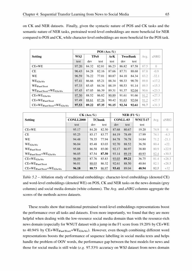
Chapter 4: Sequential Transfer Learning from News to Social Media 65

on CK and NER datasets. Finally, given the syntactic nature of POS and CK tasks and the

semantic nature of NER tasks, pretrained word-level embeddings are more beneficial for NER

compared to POS and CK, while character-level embeddings are more beneficial for the POS task.

SettingPOS (Acc.%)

Avg. aNRGWSJ TPoS ArK TweeBanktest dev test test dev test

CE+WE 97.20 84.32 82.81 86.23 86.82 87.58 87.5 0

CE 96.43 84.28 82.16 87.66 87.71 88.68 87.8 -0.9WE 96.59 76.22 77.01 80.87 84.10 84.34 83.2 -32.1WEGloVe 97.41 86.66 85.21 88.34 90.33 90.70 89.8 +17.2WEFastText 97.33 85.45 84.34 88.19 90.53 91.14 89.5 +15.3WEFastText+WEGloVe 97.45 87.05 86.39 89.31 91.37 92.04 90.6 +23.3

CE+WEGloVe 97.50 88.52 86.82 90.89 91.61 91.66 91.2 +27.3CE+WEFastText 97.49 88.61 87.26 90.42 91.63 92.04 91.2 +27.7CE+WEFastText+WEGloVe 97.53 89.22 87.35 91.15 92.34 92.61 91.7 +31.3

SettingCK (Acc.%) NER (F1 %)

Avg. aNRGCONLL2000 TChunk CONLL-03 WNUT-17test dev test dev test test

CE+WE 95.17 84.20 82.50 87.68 80.67 19.20 74.9 0

CE 95.25 85.17 83.77 84.19 78.49 17.99 74.1 -4.3WE 94.48 78.35 77.94 84.78 76.78 14.84 71.2 -21.1WEGloVe 96.04 85.48 83.03 92.70 88.52 36.58 80.4 +22.WEFastText 95.88 86.58 85.00 92.17 86.97 38.80 80.9 +22.9WEFastText+WEGloVe 96.05 87.54 87.50 93.14 89.19 40.93 82.4 +30.5

CE+WEGloVe 96.09 87.76 85.83 93.03 89.21 36.75 81.4 +28.3CE+WEFastText 96.01 88.03 86.32 92.61 88.50 40.84 82.1 +28.5CE+WEFastText+WEGloVe 96.18 88.73 86.97 93.41 89.04 40.94 82.5 +32

Table 5.2 – Ablation study of traditional embeddings: character-level embeddings (denoted CE)

and word-level embeddings (denoted WE) on POS, CK and NER tasks on the news domain (grey

columns) and social media domain (white columns). The Avg. and aNRG columns aggregate the

scores of the methods across datasets.

These results show that traditional pretrained word-level embeddings representations boost

the performance over all tasks and datasets. Even more importantly, we found that they are more

helpful when dealing with the low-resource social media domain than with the resource-rich

news domain (especially for WNUT dataset with a jump in the F1 score from 19.20% by CE+WE

to 40.94% by CE+WEFastText+WEGloVe). However, even though combining different word

representations boosts the performance of sequence labelling in social media texts and helps

handle the problem of OOV words, the performance gap between the best models for news and

those for social media is still wide (e.g. 97.53% accuracy on WSJ dataset from news domain

66 5.3. PROPOSED METHODS

compared to 87.35%, 91.15% and 92.61% on TPoS, ArK and TweeBank, respectively).

In the following sections, we propose two methods of transfer learning to reduce this gap.

Despite the best results having been yielded by CE+WEGloVe+WEFastText, we use the sequence

labelling architecture with the CE+WEGloVe setting for word representation going forward, as a

trade-off between performance and computation time since using both pretrained embeddings

doubles the number of parameters to train.

5.3 Proposed Methods

As mentioned above, the neural sequence labelling model with standard word representations

achieves high performance on high-resource languages and domains, such as the news domain.

However, when it is trained on few annotated examples like the social media domain, the model

performs poorly. Therefore, here we propose to improve sequence labelling performance on the

social media domain by leveraging the knowledge learned from the news domain. We start by

formulating transfer learning problem in section 5.3.1. Then, in section 5.3.2, we present our

proposed approaches.

5.3.1 General Transfer Learning Problem Formulation

Here is a reminder for the transfer learning problem formulation given in chapter 2 (§2.2). Let us

consider5 a domain D = {X , P (X)} consisting of two components: the feature space X and

the marginal probability distribution P (X), where X = {x1, x2, ..., xn} ∈ X . Let us consider

a task T = {Y , P (Y ), f}, where Y is the label space, P (Y ) is the prior distribution, and f is

the predictive function that transforms inputs to outputs: f : X → Y . In a supervised training

paradigm, f is learned from n training examples: {(xi, yi) ∈ X ×Y : i ∈ (1 , ..., n)}. Therefore,

the predictive function f corresponds to the joint conditional probability P (Y |X).

In a transfer learning scenario, we have a source domain DS = {XS, PS(XS)}, a source

task TS = {YS, Ps(YS), fS}, a target domain DT = {Xt, PT (XT )}, and a target task

TT = {YT , PT (XT ), fT}, whereXS = {xS1 , xS2 , ..., xSnS} ∈ XS ,XT = {xT1 , xT2 , ..., xTnt} ∈ XTand ns >> nt. The aim behind using transfer learning is to improve the learning of the predictive

function of the target domain fT by leveraging the knowledge gained from DS and TS .

Generally, in a transfer learning scheme, labelled training examples from the source domain

DS = {(xSi , ySi ) ∈ XS × YS : i ∈ (1 , ..., nS )} are abundant. As for the target domain, either a

small number of labelled target examples DT,l = {(xT,li , yT,li ) ∈ XT × YT : i ∈ (1 , ..., nT ,l)},where nS >> nT , or a large number of unlabelled target examples DT,u = {(xT,ui ) ∈ XT :

i ∈ (1 , ..., nT ,u)} are assumed to be available. From the above definitions, five scenarios of

dissimilarities between source and target domains arise:

5 In this section, we follow the definitions and notations of Pan et al. [257], Weiss et al. [375] and Ruder [303].

Chapter 4: Sequential Transfer Learning from News to Social Media 67

1. XS 6= XT : The feature spaces between the source and target domains are different.

2. P (XS) 6= P (XT ): The marginal distributions in the feature spaces are different between

the source and the target domains.

3. YS 6= YT : A mismatch between the class spaces of target and source domains.

4. P (YS) 6= P (YT ): The prior distributions of the source and target tasks are different, which

is generally due to a class imbalance between the source and target domains.

5. P (YS|XS) 6= P (YT |XT ): the conditional probability distributions between the domains

are different.

5.3.2 Our Approaches

When transferring from the news-domain to the social media domain, we first observe a difference

in the marginal distributions P (XS) 6= P (XT ). Second, a difference in the feature space

Xs 6= Xt since, in social media, we can find new words and expressions that are not used in

news. In addition, the label spaces are different Ys 6= Yt, since as seen in the chapter 4, there

are many tasks where news datasets and social media datasets do not share the same tag-set.

Let us consider a target modelMt, which consists of the sequence labelling model (Fig-

ure 5.1) with the set of parameters θt. Mt is composed of three components: Υt generates a

word representation xti for each token wi, Φt transforms the word representation into a hidden

representation hti, and Ψt generates the class-probabilities yti. In the standard supervised training

scheme, in order to learn the target predictive function Ft, θt would be randomly initialised, and

the model would be trained from scratch on target-data from the target task Tt, i.e. labelled data

{(xi, yi) ∈ Xt × Yt : i ∈ (1 , ..., n t)}.However, when labelled examples are rare, the trained model is brittle and more vulnerable

to over-fitting. Thus, we propose to leverage the pre-learned knowledge by a source model

Ms, which consists of a sequence labelling model (Figure 5.1). Likewise,Ms is composed

of three pretrained components: Υs generates a word representation xsi for each token wi, Φs

that transforms the word representation into a hidden representation hsi and Ψs that generates

the class-probabilities ysi . Ms is trained from scratch on a source task Ts with labelled data

{(xi, yi) ∈ Xs × Ys : i ∈ (1 , ..., ns)} from the source domain Ds.Our aim is to leverage the knowledge acquired by the source modelMs’s parameters θs,

learned using the source predictive function Fs, to help improve the learning of the target

predictive function Ft. We attempt this by proposing two methods: Transferring Supervisedly-

Pretrained Contextual Representations and Transferring Pretrained Models. We describe each

one in the following sub-sections.

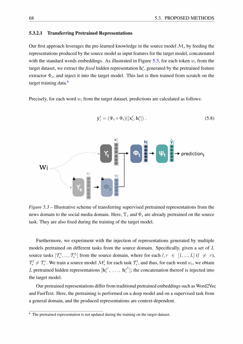
68 5.3. PROPOSED METHODS

5.3.2.1 Transferring Pretrained Representations

Our first approach leverages the pre-learned knowledge in the source modelMs by feeding the

representations produced by the source model as input features for the target model, concatenated

with the standard words embeddings. As illustrated in Figure 5.3, for each token wi from the

target dataset, we extract the fixed hidden representation hsi , generated by the pretrained feature

extractor Φs, and inject it into the target model. This last is then trained from scratch on the

target training data.6

Precisely, for each word wi from the target dataset, predictions are calculated as follows:

yti = (Ψt ◦ Φt)([xti,h

si ]) . (5.8)

Figure 5.3 – Illustrative scheme of transferring supervised pretrained representations from the

news domain to the social media domain. Here, Υs and Φs are already pretrained on the source

task. They are also fixed during the training of the target model.

Furthermore, we experiment with the injection of representations generated by multiple

models pretrained on different tasks from the source domain. Specifically, given a set of L

source tasks [T 1s , ..., T Ls ] from the source domain, where for each l, r ∈ [1, ..., L] (l 6= r),

T ls 6= T rs . We train a source modelMls for each task T ls , and thus, for each word wi, we obtain

L pretrained hidden representations [hs1

i , . . . , hsL

i ]; the concatenation thereof is injected into

the target model.

Our pretrained representations differ from traditional pretrained embeddings such as Word2Vec

and FastText. Here, the pretraining is performed on a deep model and on a supervised task from

a general domain, and the produced representations are context-dependent.

6 The pretrained representation is not updated during the training on the target-dataset.

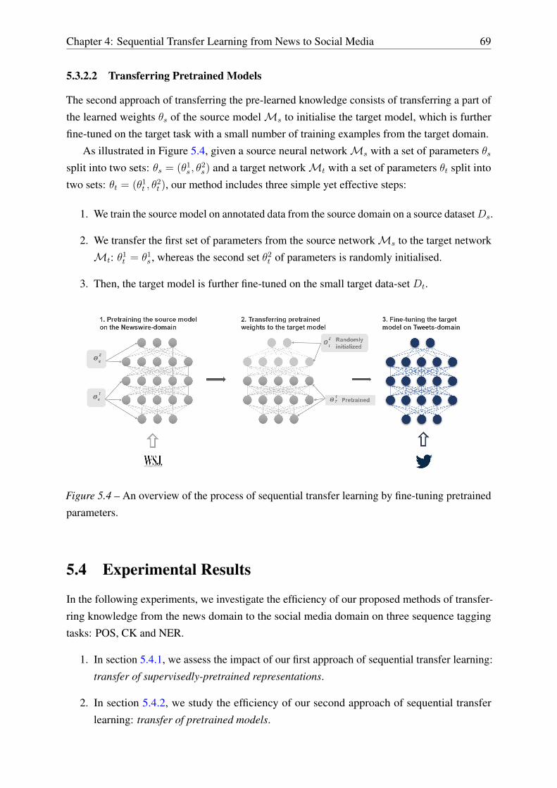
Chapter 4: Sequential Transfer Learning from News to Social Media 69

5.3.2.2 Transferring Pretrained Models

The second approach of transferring the pre-learned knowledge consists of transferring a part of

the learned weights θs of the source modelMs to initialise the target model, which is further

fine-tuned on the target task with a small number of training examples from the target domain.

As illustrated in Figure 5.4, given a source neural networkMs with a set of parameters θssplit into two sets: θs = (θ1s , θ

2s) and a target networkMt with a set of parameters θt split into

two sets: θt = (θ1t , θ2t ), our method includes three simple yet effective steps:

1. We train the source model on annotated data from the source domain on a source datasetDs.

2. We transfer the first set of parameters from the source networkMs to the target network

Mt: θ1t = θ1s , whereas the second set θ2t of parameters is randomly initialised.

3. Then, the target model is further fine-tuned on the small target data-set Dt.

Figure 5.4 – An overview of the process of sequential transfer learning by fine-tuning pretrained

parameters.

5.4 Experimental Results

In the following experiments, we investigate the efficiency of our proposed methods of transfer-

ring knowledge from the news domain to the social media domain on three sequence tagging

tasks: POS, CK and NER.

1. In section 5.4.1, we assess the impact of our first approach of sequential transfer learning:

transfer of supervisedly-pretrained representations.

2. In section 5.4.2, we study the efficiency of our second approach of sequential transfer

learning: transfer of pretrained models.

70 5.4. EXPERIMENTAL RESULTS

3. In section 5.4.3, we compare the results of the two aforementioned methods.

4. In section 5.4.4, we investigate the performance of the recent ELMo contextualised

representations when combined with our proposed approaches.

5.4.1 Transferring Supervisedly-Pretrained Representations

In this section, we investigate the impact of transferring supervisedly-pretrained representations

from the news-domain to the social media domain. Specifically, we make use of the following

pretrained representations:

• hs−pos: Representations generated by the source model, pretrained on the POS tagging

source dataset (WSJ).

• hs−ck: Representations generated by the source model, pretrained on the CK source dataset

(CONLL2000).

• hs−ner: Representations generated by the source model, pretrained on the NER source

dataset (CONLL-03).

The results are reported in Table 5.3. In the top half of the table, we combine the pretrained

representations with randomly initialised character-level embeddings (CE). In the bottom half, we

experiment with combining the transferred representations with both character-level embeddings

and word-level embeddings, the latter of which are initialised with GloVe (CE+WEGloVe). We

compare the results between the different settings using the aNRG metric (see equation 4.6). In

the top half of the table, the aNRG metric is calculated in comparison to the reference CE and in

the bottom half, the aNRG metric is calculated in comparison to the reference CE+WEGloVe.

From the results in Table 5.3, we draw the following observations. It is apparent that

our pretrained representations yield a greater improvement when combined with CE than

with CE+WEGloVe. For instance, when adding CK representations (hs−ck), we observe a

+23.4 point increase in terms of aNRG with CE+hs−ck compared to the +8.5 increase with

CE+WEGloVe + hs−ck. An expected observation since the traditional pretrained word-

embeddings already accommodate valuable pretrained knowledge helpful to handle the problem

of the lack of annotated examples in the social media domain. Notwithstanding, even when

combined with WEGloVe, our pretrained representations still yield a major performance in-

crease, pointing to the fact that supervised pretraining helps encode new task-specific knowledge

that is useful for many NLP tasks. NER representations are a notable exception, as we can

observe a severe drop in the performance gain, from +16.1 aNRG for CE+hs−ner to +1.1 for

CE+WEGloVe + hs−ner. This observation may be explained by the fact that NER is a semantic

task, thus the knowledge encoded by NER on the news-domain is similar to that encoded by

GloVe pretrained embeddings.

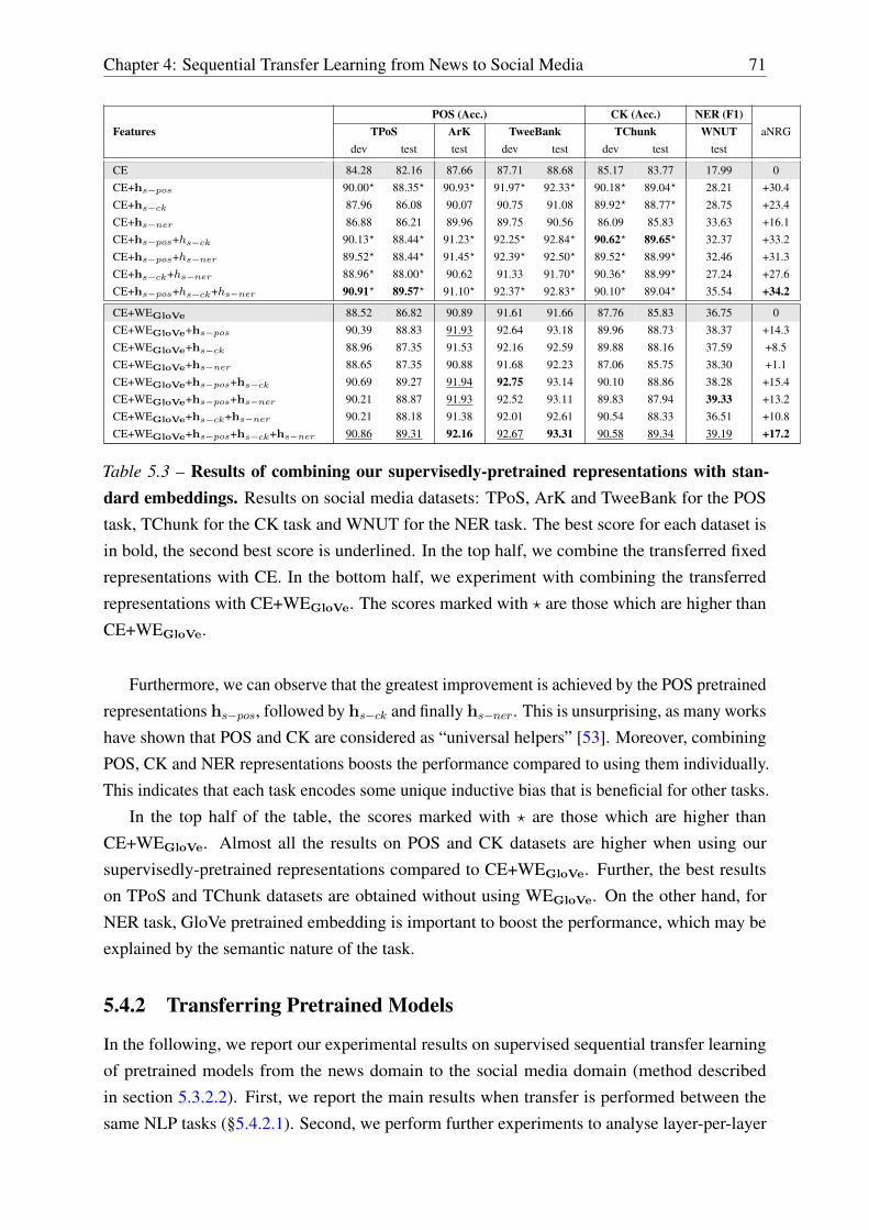
Chapter 4: Sequential Transfer Learning from News to Social Media 71

FeaturesPOS (Acc.) CK (Acc.) NER (F1)

aNRGTPoS ArK TweeBank TChunk WNUTdev test test dev test dev test test

CE 84.28 82.16 87.66 87.71 88.68 85.17 83.77 17.99 0CE+hs−pos 90.00? 88.35? 90.93? 91.97? 92.33? 90.18? 89.04? 28.21 +30.4CE+hs−ck 87.96 86.08 90.07 90.75 91.08 89.92? 88.77? 28.75 +23.4CE+hs−ner 86.88 86.21 89.96 89.75 90.56 86.09 85.83 33.63 +16.1CE+hs−pos+hs−ck 90.13? 88.44? 91.23? 92.25? 92.84? 90.62? 89.65? 32.37 +33.2CE+hs−pos+hs−ner 89.52? 88.44? 91.45? 92.39? 92.50? 89.52? 88.99? 32.46 +31.3CE+hs−ck+hs−ner 88.96? 88.00? 90.62 91.33 91.70? 90.36? 88.99? 27.24 +27.6CE+hs−pos+hs−ck+hs−ner 90.91? 89.57? 91.10? 92.37? 92.83? 90.10? 89.04? 35.54 +34.2

CE+WEGloVe 88.52 86.82 90.89 91.61 91.66 87.76 85.83 36.75 0CE+WEGloVe+hs−pos 90.39 88.83 91.93 92.64 93.18 89.96 88.73 38.37 +14.3CE+WEGloVe+hs−ck 88.96 87.35 91.53 92.16 92.59 89.88 88.16 37.59 +8.5CE+WEGloVe+hs−ner 88.65 87.35 90.88 91.68 92.23 87.06 85.75 38.30 +1.1CE+WEGloVe+hs−pos+hs−ck 90.69 89.27 91.94 92.75 93.14 90.10 88.86 38.28 +15.4CE+WEGloVe+hs−pos+hs−ner 90.21 88.87 91.93 92.52 93.11 89.83 87.94 39.33 +13.2CE+WEGloVe+hs−ck+hs−ner 90.21 88.18 91.38 92.01 92.61 90.54 88.33 36.51 +10.8CE+WEGloVe+hs−pos+hs−ck+hs−ner 90.86 89.31 92.16 92.67 93.31 90.58 89.34 39.19 +17.2

Table 5.3 – Results of combining our supervisedly-pretrained representations with stan-dard embeddings. Results on social media datasets: TPoS, ArK and TweeBank for the POS

task, TChunk for the CK task and WNUT for the NER task. The best score for each dataset is

in bold, the second best score is underlined. In the top half, we combine the transferred fixed

representations with CE. In the bottom half, we experiment with combining the transferred

representations with CE+WEGloVe. The scores marked with ? are those which are higher than

CE+WEGloVe.

Furthermore, we can observe that the greatest improvement is achieved by the POS pretrained

representations hs−pos, followed by hs−ck and finally hs−ner. This is unsurprising, as many works

have shown that POS and CK are considered as “universal helpers” [53]. Moreover, combining

POS, CK and NER representations boosts the performance compared to using them individually.

This indicates that each task encodes some unique inductive bias that is beneficial for other tasks.

In the top half of the table, the scores marked with ? are those which are higher than

CE+WEGloVe. Almost all the results on POS and CK datasets are higher when using our

supervisedly-pretrained representations compared to CE+WEGloVe. Further, the best results

on TPoS and TChunk datasets are obtained without using WEGloVe. On the other hand, for

NER task, GloVe pretrained embedding is important to boost the performance, which may be

explained by the semantic nature of the task.

5.4.2 Transferring Pretrained Models

In the following, we report our experimental results on supervised sequential transfer learning

of pretrained models from the news domain to the social media domain (method described

in section 5.3.2.2). First, we report the main results when transfer is performed between the

same NLP tasks (§5.4.2.1). Second, we perform further experiments to analyse layer-per-layer

72 5.4. EXPERIMENTAL RESULTS

transferability (§5.4.2.2). Third, we investigate the transferability between different NLP tasks

(§5.4.2.3).

5.4.2.1 Overall Performance

Here, we discuss the results of the main experiment of our approach, transferring pretrained

models, where the pretraining and fine-tuning tasks are the same. For TPoS, ArK and TweeBank

datasets, the pretrained weights are learned on the WSJ dataset; for TChunk, the pretrained

weights are learned on CONLL2000 dataset; and for WNUT dataset, the pretrained weights are

learned on CONLL-03 dataset.

As shown in chapter 4, source and target datasets may have different tag-sets, even within

the same NLP task. Hence, transferring the parameters of the classifier (Ψ) may not be feasible

in all cases. Therefore, in this experiment, WRE’s layers (Υ) and FE’s layers (Φ) are pre-trained

on the source-dataset and Ψ is randomly initialised. Then, the three modules are further jointly

trained on the target-dataset by minimising a SCE (Softmax Cross-Entropy) loss using the SGD

algorithm.

Results are reported in Table 5.4. We report the results of our reference training from scratch

on target data (using CE+WEGloVe scheme), followed by the results of the transfer learning

approach, which greatly outperforms the reference. Specifically, transfer learning exhibits an

improvement of ∼+3% acc. for TPoS, ∼+1.2% acc. for ArK, ∼+1.6% acc. for TweeBank,

∼+3.4% acc. for TChunk and ∼+4.5% F1 for WNUT.

POS (Acc.) CK (Acc.) NER (F1)

MethodDataset TPoS ARK Tweebank TChunk WNUT

dev test test dev test dev test test

From scratch 88.52 86.82 90.89 91.61 91.66 87.76 85.83 36.75

Transfer Learning 90.95 89.79 92.09 93.04 93.29 90.71 89.21 41.25

Table 5.4 – Main results of our proposed approach, transferring pretrained models, on social

media datasets (Acc (%) for POS and CK and F1 (%) for NER). The best score for each dataset

is highlighted in bold.

5.4.2.2 Layer-per-Layer Transferability

In this experiment, we investigate the transferability of each layer of our model. We start by

transferring from the bottom-most layers (Υ) up to the top-most layers (Φ). In addition, we

conduct experiments on two settings: 1) : pretrained layers are frozen; and 2) : pretrained

layers are fine-tuned. As illustrated in Figure 5.5, we define 4 transfer schemes:7

7 Transfer Learning in Table 5.4 corresponds to scheme D.

Chapter 4: Sequential Transfer Learning from News to Social Media 73

Figure 5.5 – Overview of the experimental schemes of transferring pretrained parameters.

Scheme A & B: Only WRE’s layers are initialised with pretrained weights from the news

domain whereas FE’s layers and the classifier are randomly initialised. Scheme C & D: In

addition to WRE’s layers, FE’s layers are initialised with pretrained weights from the news

domain whereas the classifier is randomly initialised. The pretrained layers are frozen in schemes

A and C and tuned in schemes B and D during fine-tuning on the social media domain.

• Scheme A: Only WRE (Υ) layers; i.e. word-level embedding and biLSTM character

embedding; are initialised with pretrained weights from the source model whereas the FE

(Φ) and the classifier (Ψ) are randomly initialised. The pretrained layers are frozen ( )

during fine-tuning on social media domain dataset.

• Scheme B: The same as Scheme A, except that the pretrained layers are tuned ( ) during

fine-tuning on social media domain dataset.

• Scheme C: In addition to WRE layers, FE layers are initialised with pretrained weights

from the source model, whereas the classifier is randomly initialised. The pretrained layers

are frozen ( ) during fine-tuning on social media domain.

• Scheme D: The same as Scheme C, except that the pretrained layers are tuned ( ) during

fine-tuning on social media domain.

74 5.4. EXPERIMENTAL RESULTS

SchemePOS (Acc.) CK(Acc.) NER (F1)

aNRG.TPoS ArK TweeBank TChunk WNUTdev test test dev test dev test test

O 88.52 86.82 90.89 91.61 91.66 87.76 85.83 36.75 0.0

A 88.87� 87.48� 90.85 92.05� 92.48� 87.85� 86.10� 39.27� +3.7

B 90.17� 88.66� 91.55� 92.31� 92.65� 89.22� 87.19� 40.97� +10.5

C 86.10 86.91� 85.39 87.48 87.92 82.35 81.75 27.83 -32.7

D 90.95� 89.79� 92.09� 93.04� 93.29� 90.71� 89.21� 41.25� +18.6

Table 5.5 – Layer-per-layer transferability analysis results on social media datasets TPoS,

ARK, TweeBank, TChunk and WNUT. Scheme O consists of training target models from scratch

(random initialisation) on social media training-sets. Transfer schemes A,B, C and D are

illustrated in Figure 5.5. Scores marked with � are higher than the reference training from scratch

(scheme O). Best scores by dataset are highlighted in bold, second best scores are underlined.

The last column gives the aNRG score of each method compared to the reference (scheme O).

Results are shown in Table 5.5. First, as expected, the best performance across all tasks and

datasets is yielded by the transfer scheme D. This is unsurprising since transfer is performed

between the same tasks and thus transferring both low-most and top-most layers is beneficial.

Second, we can observe that the transferability of each layer depends on whether the pretrained

parameters are frozen or tuned:

• When pretrained layers are frozen ( ) (schemes A and C), only the bottom-most layers are

transferable, with little improvement (+3.7 aNRG) compared to the reference training

from scratch (scheme O). Whereas, when also transferring the top-most layers (scheme

C), the performance degrades dramatically (-32.7 aNRG) compared to the reference. This

can be explained by the fact that the top-most layers are grossly domain specific, and thus

need to be updated during fine-tuning to learn new patterns that are specific to the social

media domain.

• When pretrained layers are tuned ( ) (schemes B and D): both pretrained bottom-most

and top-most layers are beneficial across all tasks and datasets. Specifically, transferring

embeddings layers that are updated during fine-tuning (Scheme B) yields a slight im-

provement (+10.5 aNRG) compared to the reference. Moreover, transferring the feature

extractor layers as well further enhances performance (+18.6 aNRG).

5.4.2.3 Inter-Tasks Transferability

Through the precedent experiments, we have analysed transfer learning from the news domain

to the social media domain in a scenario where the pretraining (source) task is the same as the

fine-tuning (target) one. Here, we carry out further experiments to analyse the transferability

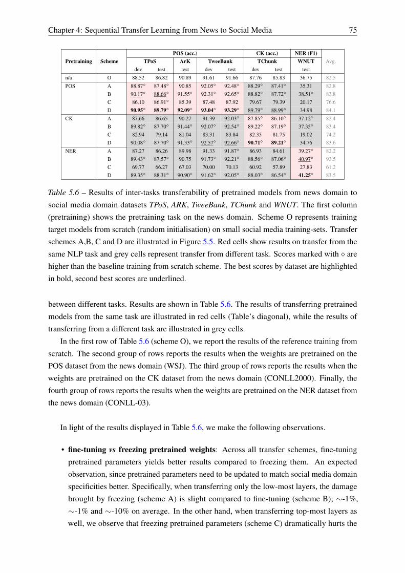
Chapter 4: Sequential Transfer Learning from News to Social Media 75

Pretraining SchemePOS (acc.) CK (acc.) NER (F1)

Avg.TPoS ArK TweeBank TChunk WNUTdev test test dev test dev test test

n/a O 88.52 86.82 90.89 91.61 91.66 87.76 85.83 36.75 82.5

POS A 88.87� 87.48� 90.85 92.05� 92.48� 88.29� 87.41� 35.31 82.8B 90.17� 88.66� 91.55� 92.31� 92.65� 88.82� 87.72� 38.51� 83.8C 86.10 86.91� 85.39 87.48 87.92 79.67 79.39 20.17 76.6D 90.95� 89.79� 92.09� 93.04� 93.29� 89.79� 88.99� 34.98 84.1

CK A 87.66 86.65 90.27 91.39 92.03� 87.85� 86.10� 37.12� 82.4B 89.82� 87.70� 91.44� 92.07� 92.54� 89.22� 87.19� 37.35� 83.4C 82.94 79.14 81.04 83.31 83.84 82.35 81.75 19.02 74.2D 90.08� 87.70� 91.33� 92.57� 92.66� 90.71� 89.21� 34.76 83.6

NER A 87.27 86.26 89.98 91.33 91.87� 86.93 84.61 39.27� 82.2B 89.43� 87.57� 90.75 91.73� 92.21� 88.56� 87.06� 40.97� 93.5C 69.77 66.27 67.03 70.00 70.13 60.92 57.89 27.83 61.2D 89.35� 88.31� 90.90� 91.62� 92.05� 88.03� 86.54� 41.25� 83.5

Table 5.6 – Results of inter-tasks transferability of pretrained models from news domain to

social media domain datasets TPoS, ARK, TweeBank, TChunk and WNUT. The first column

(pretraining) shows the pretraining task on the news domain. Scheme O represents training

target models from scratch (random initialisation) on small social media training-sets. Transfer

schemes A,B, C and D are illustrated in Figure 5.5. Red cells show results on transfer from the

same NLP task and grey cells represent transfer from different task. Scores marked with � are

higher than the baseline training from scratch scheme. The best scores by dataset are highlighted

in bold, second best scores are underlined.

between different tasks. Results are shown in Table 5.6. The results of transferring pretrained

models from the same task are illustrated in red cells (Table’s diagonal), while the results of

transferring from a different task are illustrated in grey cells.

In the first row of Table 5.6 (scheme O), we report the results of the reference training from

scratch. The second group of rows reports the results when the weights are pretrained on the

POS dataset from the news domain (WSJ). The third group of rows reports the results when the

weights are pretrained on the CK dataset from the news domain (CONLL2000). Finally, the

fourth group of rows reports the results when the weights are pretrained on the NER dataset from

the news domain (CONLL-03).

In light of the results displayed in Table 5.6, we make the following observations.

• fine-tuning vs freezing pretrained weights: Across all transfer schemes, fine-tuning

pretrained parameters yields better results compared to freezing them. An expected

observation, since pretrained parameters need to be updated to match social media domain

specificities better. Specifically, when transferring only the low-most layers, the damage

brought by freezing (scheme A) is slight compared to fine-tuning (scheme B); ∼-1%,

∼-1% and ∼-10% on average. In the other hand, when transferring top-most layers as

well, we observe that freezing pretrained parameters (scheme C) dramatically hurts the

76 5.4. EXPERIMENTAL RESULTS

performance compared to fine-tuning (scheme D); ∼-7.5%, ∼-9.4% and ∼-22.3% on

average. A plausible explanation is that, generally, the lowest layers of NNs tend to

represent domain-independent features and thus encode information that could be useful

for all tasks and domains, whereas top-most ones are more domain-specific, and thus,

should be updated. These observations are not surprising and confirm the observations of

many works in the literature [243, 396].

• Pretraining task: We can observe that the best average score is obtained when using

parameters pretrained on POS tagging task. Specifically, the first best score is obtained

using the scheme D and the second by scheme B. Which confirms the fact that the

information encoded by POS task is universal and important for higher-level NLP tasks

and applications [53]. Notably, for POS→POS (Which includes POS→TPoS, POS→ArK

and POS→TweeBank) and POS→TChunk, we can observe that both low-most and top-

most layers play an important role. Transferring low-most layers (scheme B) yields an

average improvement of ∼+1.13% for POS→POS and ∼+1.27% for POS→TChunk.

In addition, transferring top-most layers as well (scheme D) yields an improvement of

∼+1.8% for POS→POS and ∼+2.6% for POS→TChunk. However, only low-most layers

are transferable from POS to NER. As illustrated in the results, for POS→WNUT transfer

scenario, scheme B yields an improvement in F1 of ∼+1.75%, while scheme D degrades

the F1 score by ∼-1.8% compared to training from scratch. A plausible explanation is that

the transferability decreases as the dissimilarity between source and target tasks increases,

and since NER task is less similar to POS, only low-level features learned in embedding

layers are beneficial for NER.

5.4.3 Comparing the Proposed Transfer Methods

In this section, we compare the performance of our two proposed methods, i.e. transferring repre-

sentations vs transferring models. Specifically, for each pretraining task; POS, CK and NER; we

investigate whether it is better to transfer the pre-learned knowledge as pretrained representations

(fixed features) or as pretrained models (pretrained weights). When transferring representations,

we report the results from the bottom half of Table 5.3; where representations are injected

individually. Namely, CE+WEGloVe+hs−pos, CE+WEGloVe+hs−ck and CE+WEGloVe+hs−ner.

When transferring models, we pick the best transfer scheme for each dataset from Table 5.6, e.g.

when transferring from POS to WNUT dataset, the best F1 score is obtained using the transfer

architecture B. While, when transferring parameters from NER to WNUT dataset, the best F1

score is obtained using the transfer scheme D.

Results are reported in Table 5.7. Clearly, transferring models begets better results across

all pretraining tasks and target datasets. Particularly, the best performance per target-dataset is

obtained when using transferred parameters from the same NLP task. For instance, for WNUT,

the NER social media dataset, the best F1 score is obtained by transferring models from NER

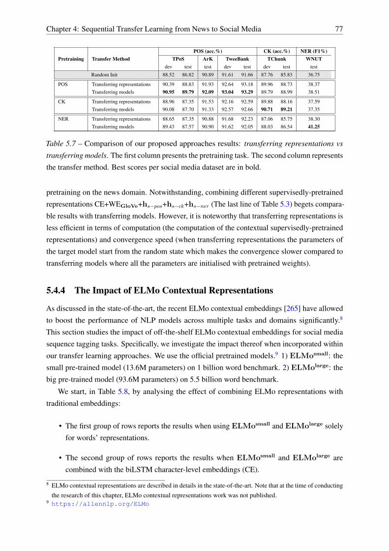
Chapter 4: Sequential Transfer Learning from News to Social Media 77

Pretraining Transfer MethodPOS (acc.%) CK (acc.%) NER (F1%)

TPoS ArK TweeBank TChunk WNUTdev test test dev test dev test test

Random Init 88.52 86.82 90.89 91.61 91.66 87.76 85.83 36.75

POS Transferring representations 90.39 88.83 91.93 92.64 93.18 89.96 88.73 38.37Transferring models 90.95 89.79 92.09 93.04 93.29 89.79 88.99 38.51

CK Transferring representations 88.96 87.35 91.53 92.16 92.59 89.88 88.16 37.59Transferring models 90.08 87.70 91.33 92.57 92.66 90.71 89.21 37.35

NER Transferring representations 88.65 87.35 90.88 91.68 92.23 87.06 85.75 38.30Transferring models 89.43 87.57 90.90 91.62 92.05 88.03 86.54 41.25

Table 5.7 – Comparison of our proposed approaches results: transferring representations vs

transferring models. The first column presents the pretraining task. The second column represents

the transfer method. Best scores per social media dataset are in bold.

pretraining on the news domain. Notwithstanding, combining different supervisedly-pretrained

representations CE+WEGloVe+hs−pos+hs−ck+hs−ner (The last line of Table 5.3) begets compara-

ble results with transferring models. However, it is noteworthy that transferring representations is

less efficient in terms of computation (the computation of the contextual supervisedly-pretrained

representations) and convergence speed (when transferring representations the parameters of

the target model start from the random state which makes the convergence slower compared to

transferring models where all the parameters are initialised with pretrained weights).

5.4.4 The Impact of ELMo Contextual Representations

As discussed in the state-of-the-art, the recent ELMo contextual embeddings [265] have allowed

to boost the performance of NLP models across multiple tasks and domains significantly.8

This section studies the impact of off-the-shelf ELMo contextual embeddings for social media

sequence tagging tasks. Specifically, we investigate the impact thereof when incorporated within

our transfer learning approaches. We use the official pretrained models.9 1) ELMosmall: the

small pre-trained model (13.6M parameters) on 1 billion word benchmark. 2) ELMolarge: the

big pre-trained model (93.6M parameters) on 5.5 billion word benchmark.

We start, in Table 5.8, by analysing the effect of combining ELMo representations with

traditional embeddings:

• The first group of rows reports the results when using ELMosmall and ELMolarge solely

for words’ representations.

• The second group of rows reports the results when ELMosmall and ELMolarge are

combined with the biLSTM character-level embeddings (CE).

8 ELMo contextual representations are described in details in the state-of-the-art. Note that at the time of conductingthe research of this chapter, ELMo contextual representations work was not published.

9 https://allennlp.org/ELMo

78 5.4. EXPERIMENTAL RESULTS

• The third group of rows reports the results when ELMosmall and ELMolarge are com-

bined with the randomly initialised word-level embeddings (WE).

• The fourth group of rows reports the results when ELMosmall and ELMolarge are

combined with the GloVe pretrained word-level embeddings (WEGloVe).

• The fifth group of rows reports the results when ELMosmall and ELMolarge are combined

with the concatenation of the biLSTM character-level embeddings and the GloVe pretrained

word-level embeddings (CE+WEGloVe).

SettingPOS (Acc.%) CK (Acc.%) NER (F1 %)

avg. aNRG.TPoS ArK TweeBank TChunk WNUTdev test test dev test dev test test

ELMosmall 90.21 88.35 90.62 92.19 92.93 90.36 89.61 34.35 83.6 –ELMolarge 91.99 90.10 92.27 93.41 94.01 91.68 90.57 39.44 85.4 –

CE 84.28 82.16 87.66 87.71 88.68 85.17 83.77 17.99 77.2 0.0CE+ELMosmall 90.91 89.01 91.48 92.69 93.34 91.55 89.25 33.99 84.00 +36.2CE+ELMolarge 91.38 89.05 92.27 93.38 93.92 92.47 90.44 43.03 85.7 +41.8

WE 76.22 77.01 80.87 84.10 84.34 78.35 77.94 14.84 71.7 0.0WE+ELMosmall 90.26 88.48 90.89 92.35 92.98 90.14 88.73 38.03 84.00 +49.9WE+ELMolarge 91.51 90.31 91.99 93.38 94.14 91.99 90.26 40.27 85.5 +56.2

WEGloVe 86.66 85.21 88.34 90.33 90.70 85.48 83.03 36.58 80.8 0.0WEGloVe+ELMosmall 90.73 89.31 91.57 93.09 93.55 90.98 88.64 40.16 85.1 +27.7WEGloVe+ELMolarge 91.99 90.66 92.95 93.49 94.40 91.59 90.26 42.88 86.0 +35.4

CE+WEGloVe 88.52 86.82 90.89 91.61 91.66 87.76 85.83 36.75 82.5 0.0CE+WEGloVe+ELMosmall 91.29 90.01 92.09 93.07 93.73 90.85 89.47 41.57 85.3 +20.3CE+WEGloVe+ELMolarge 92.20 90.18 92.88 93.52 94.29 91.51 90.66 44.95 86.3 +26.4

Table 5.8 – The effect of combining ELMo representations with traditional embeddings into the

standard supervised training scheme. The best score per dataset is highlighted in bold. In each

set of lines, the aNRG metric is calculated compared to the reference without ELMo embeddings

(Grey rows).

Note that in each group of rows, the aNRG (see equation 4.6) metric is calculated compared

to the reference without ELMo embeddings (Grey rows). From the results, we make the

following observations. First, ELMo representations yield powerful results across all tasks

and datasets. Second, in most cases concatenating more variants of embeddings leads to

better results. Third, since ELMo (especially ELMolarge) is already based on character-level

information, adding character-level biLSTM embeddings have a marginal effect the performance.

For instance, WEGloVe+ELMolarge setting provides 94.40% of accuracy on TweeBank dataset,

while CE+WEGloVe+ELMolarge provides 94.29% of accuracy. Finally, the gain brought by

ELMo decreases when combined with more representations. For instance, the gain in terms of

aNRG of adding ELMosmall decreases from +36.2 when combined with CE solely, to +20.3

when combined with CE+WEGloVe.

Furthermore, in Table 5.9, we analyse the effect of incorporating ELMo representations

with our supervisedly-pretrained representations. We can observe that concatenating ELMo

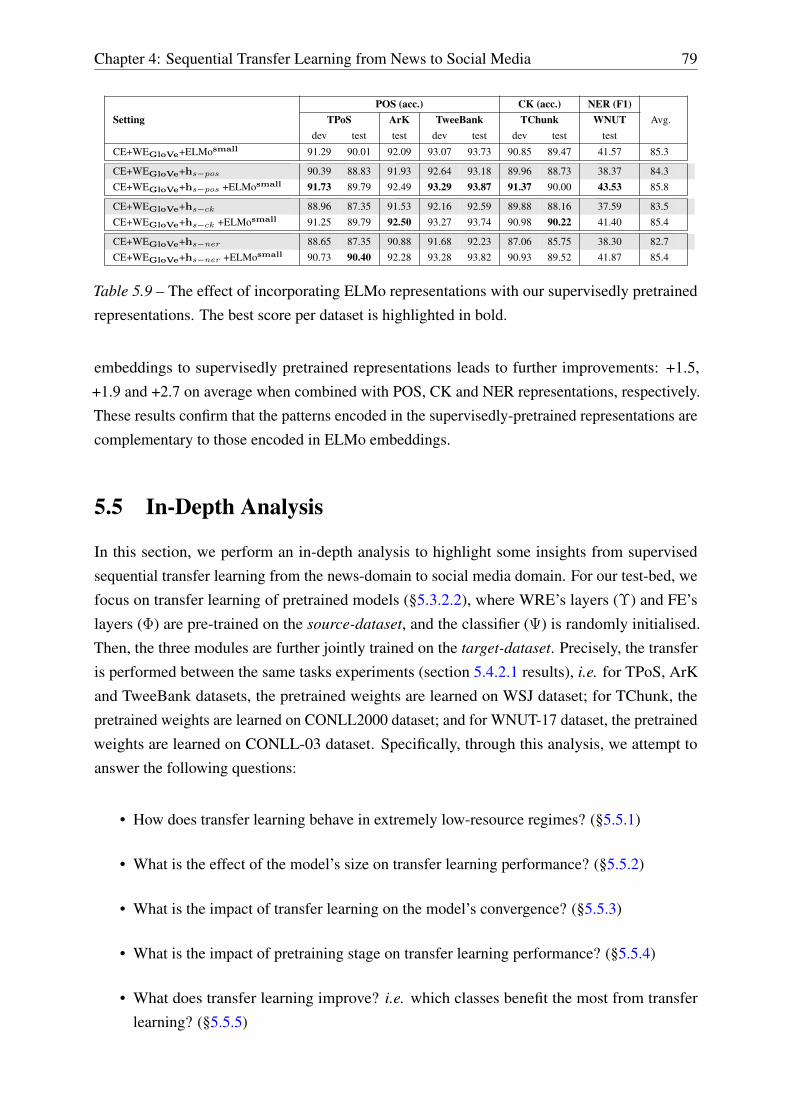
Chapter 4: Sequential Transfer Learning from News to Social Media 79

SettingPOS (acc.) CK (acc.) NER (F1)

Avg.TPoS ArK TweeBank TChunk WNUTdev test test dev test dev test test

CE+WEGloVe+ELMosmall 91.29 90.01 92.09 93.07 93.73 90.85 89.47 41.57 85.3

CE+WEGloVe+hs−pos 90.39 88.83 91.93 92.64 93.18 89.96 88.73 38.37 84.3CE+WEGloVe+hs−pos +ELMosmall 91.73 89.79 92.49 93.29 93.87 91.37 90.00 43.53 85.8

CE+WEGloVe+hs−ck 88.96 87.35 91.53 92.16 92.59 89.88 88.16 37.59 83.5CE+WEGloVe+hs−ck +ELMosmall 91.25 89.79 92.50 93.27 93.74 90.98 90.22 41.40 85.4

CE+WEGloVe+hs−ner 88.65 87.35 90.88 91.68 92.23 87.06 85.75 38.30 82.7CE+WEGloVe+hs−ner +ELMosmall 90.73 90.40 92.28 93.28 93.82 90.93 89.52 41.87 85.4

Table 5.9 – The effect of incorporating ELMo representations with our supervisedly pretrained

representations. The best score per dataset is highlighted in bold.

embeddings to supervisedly pretrained representations leads to further improvements: +1.5,

+1.9 and +2.7 on average when combined with POS, CK and NER representations, respectively.

These results confirm that the patterns encoded in the supervisedly-pretrained representations are

complementary to those encoded in ELMo embeddings.

5.5 In-Depth Analysis

In this section, we perform an in-depth analysis to highlight some insights from supervised

sequential transfer learning from the news-domain to social media domain. For our test-bed, we

focus on transfer learning of pretrained models (§5.3.2.2), where WRE’s layers (Υ) and FE’s

layers (Φ) are pre-trained on the source-dataset, and the classifier (Ψ) is randomly initialised.

Then, the three modules are further jointly trained on the target-dataset. Precisely, the transfer

is performed between the same tasks experiments (section 5.4.2.1 results), i.e. for TPoS, ArK

and TweeBank datasets, the pretrained weights are learned on WSJ dataset; for TChunk, the

pretrained weights are learned on CONLL2000 dataset; and for WNUT-17 dataset, the pretrained

weights are learned on CONLL-03 dataset. Specifically, through this analysis, we attempt to

answer the following questions:

• How does transfer learning behave in extremely low-resource regimes? (§5.5.1)

• What is the effect of the model’s size on transfer learning performance? (§5.5.2)

• What is the impact of transfer learning on the model’s convergence? (§5.5.3)

• What is the impact of pretraining stage on transfer learning performance? (§5.5.4)

• What does transfer learning improve? i.e. which classes benefit the most from transfer

learning? (§5.5.5)

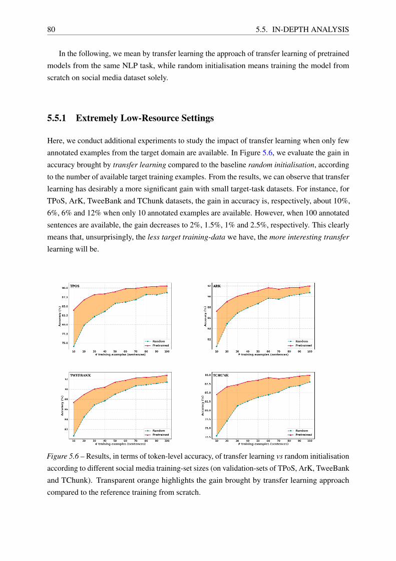
80 5.5. IN-DEPTH ANALYSIS

In the following, we mean by transfer learning the approach of transfer learning of pretrained

models from the same NLP task, while random initialisation means training the model from

scratch on social media dataset solely.

5.5.1 Extremely Low-Resource Settings

Here, we conduct additional experiments to study the impact of transfer learning when only few

annotated examples from the target domain are available. In Figure 5.6, we evaluate the gain in

accuracy brought by transfer learning compared to the baseline random initialisation, according

to the number of available target training examples. From the results, we can observe that transfer

learning has desirably a more significant gain with small target-task datasets. For instance, for

TPoS, ArK, TweeBank and TChunk datasets, the gain in accuracy is, respectively, about 10%,

6%, 6% and 12% when only 10 annotated examples are available. However, when 100 annotated

sentences are available, the gain decreases to 2%, 1.5%, 1% and 2.5%, respectively. This clearly

means that, unsurprisingly, the less target training-data we have, the more interesting transfer

learning will be.

Figure 5.6 – Results, in terms of token-level accuracy, of transfer learning vs random initialisation

according to different social media training-set sizes (on validation-sets of TPoS, ArK, TweeBank

and TChunk). Transparent orange highlights the gain brought by transfer learning approach

compared to the reference training from scratch.

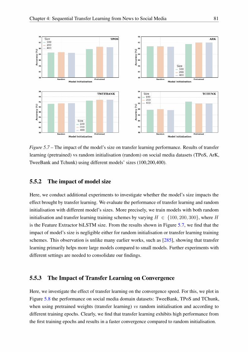
Chapter 4: Sequential Transfer Learning from News to Social Media 81

Figure 5.7 – The impact of the model’s size on transfer learning performance. Results of transfer

learning (pretrained) vs random initialisation (random) on social media datasets (TPoS, ArK,

TweeBank and Tchunk) using different models’ sizes (100,200,400).

5.5.2 The impact of model size

Here, we conduct additional experiments to investigate whether the model’s size impacts the

effect brought by transfer learning. We evaluate the performance of transfer learning and random

initialisation with different model’s sizes. More precisely, we train models with both random

initialisation and transfer learning training schemes by varying H ∈ {100, 200, 300}, where H

is the Feature Extractor biLSTM size. From the results shown in Figure 5.7, we find that the

impact of model’s size is negligible either for random initialisation or transfer learning training

schemes. This observation is unlike many earlier works, such as [285], showing that transfer

learning primarily helps more large models compared to small models. Further experiments with

different settings are needed to consolidate our findings.

5.5.3 The Impact of Transfer Learning on Convergence

Here, we investigate the effect of transfer learning on the convergence speed. For this, we plot in

Figure 5.8 the performance on social media domain datasets: TweeBank, TPoS and TChunk,

when using pretrained weights (transfer learning) vs random initialisation and according to

different training epochs. Clearly, we find that transfer learning exhibits high performance from

the first training epochs and results in a faster convergence compared to random initialisation.

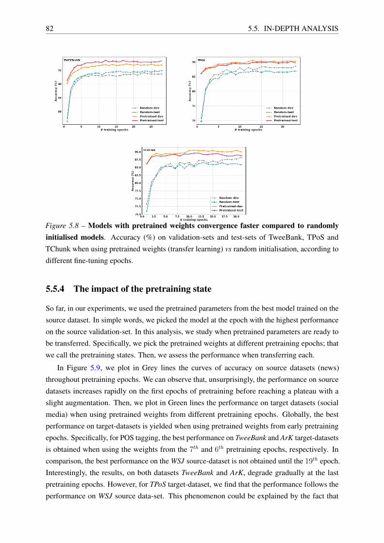
82 5.5. IN-DEPTH ANALYSIS

Figure 5.8 – Models with pretrained weights convergence faster compared to randomlyinitialised models. Accuracy (%) on validation-sets and test-sets of TweeBank, TPoS and

TChunk when using pretrained weights (transfer learning) vs random initialisation, according to

different fine-tuning epochs.

5.5.4 The impact of the pretraining state

So far, in our experiments, we used the pretrained parameters from the best model trained on the

source dataset. In simple words, we picked the model at the epoch with the highest performance

on the source validation-set. In this analysis, we study when pretrained parameters are ready to

be transferred. Specifically, we pick the pretrained weights at different pretraining epochs; that

we call the pretraining states. Then, we assess the performance when transferring each.

In Figure 5.9, we plot in Grey lines the curves of accuracy on source datasets (news)

throughout pretraining epochs. We can observe that, unsurprisingly, the performance on source

datasets increases rapidly on the first epochs of pretraining before reaching a plateau with a

slight augmentation. Then, we plot in Green lines the performance on target datasets (social

media) when using pretrained weights from different pretraining epochs. Globally, the best

performance on target-datasets is yielded when using pretrained weights from early pretraining

epochs. Specifically, for POS tagging, the best performance on TweeBank and ArK target-datasets

is obtained when using the weights from the 7th and 6th pretraining epochs, respectively. In

comparison, the best performance on the WSJ source-dataset is not obtained until the 19th epoch.

Interestingly, the results, on both datasets TweeBank and ArK, degrade gradually at the last

pretraining epochs. However, for TPoS target-dataset, we find that the performance follows the

performance on WSJ source data-set. This phenomenon could be explained by the fact that

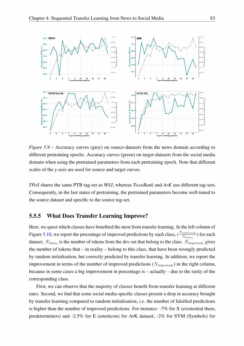
Chapter 4: Sequential Transfer Learning from News to Social Media 83

Figure 5.9 – Accuracy curves (grey) on source-datasets from the news domain according to

different pretraining epochs. Accuracy curves (green) on target-datasets from the social media

domain when using the pretrained parameters from each pretraining epoch. Note that different

scales of the y-axis are used for source and target curves.

TPoS shares the same PTB tag-set as WSJ, whereas TweeBank and ArK use different tag-sets.

Consequently, in the last states of pretraining, the pretrained parameters become well-tuned to

the source dataset and specific to the source tag-set.

5.5.5 What Does Transfer Learning Improve?

Here, we quest which classes have benefited the most from transfer learning. In the left column of

Figure 5.10, we report the percentage of improved predictions by each classi (Nimprovedi

Nclassi) for each

dataset. Nclassi is the number of tokens from the dev-set that belong to the class. Nimprovedi gives

the number of tokens that – in reality – belong to this class, that have been wrongly predicted

by random initialisation, but correctly predicted by transfer learning. In addition, we report the

improvement in terms of the number of improved predictions (Nimprovedi) in the right column,

because in some cases a big improvement in percentage is – actually – due to the rarity of the

corresponding class.

First, we can observe that the majority of classes benefit from transfer learning at different

rates. Second, we find that some social media-specific classes present a drop in accuracy brought

by transfer learning compared to random initialisation, i.e. the number of falsified predictions

is higher than the number of improved predictions. For instance: -7% for X (existential there,

predeterminers) and -2.5% for E (emoticon) for ArK dataset; -2% for SYM (Symbols) for

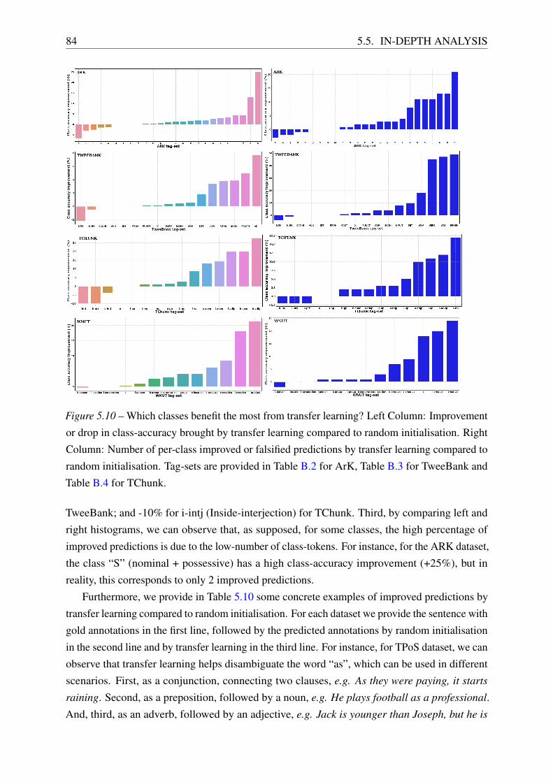
84 5.5. IN-DEPTH ANALYSIS

Figure 5.10 – Which classes benefit the most from transfer learning? Left Column: Improvement

or drop in class-accuracy brought by transfer learning compared to random initialisation. Right

Column: Number of per-class improved or falsified predictions by transfer learning compared to

random initialisation. Tag-sets are provided in Table B.2 for ArK, Table B.3 for TweeBank and

Table B.4 for TChunk.

TweeBank; and -10% for i-intj (Inside-interjection) for TChunk. Third, by comparing left and

right histograms, we can observe that, as supposed, for some classes, the high percentage of

improved predictions is due to the low-number of class-tokens. For instance, for the ARK dataset,

the class “S” (nominal + possessive) has a high class-accuracy improvement (+25%), but in

reality, this corresponds to only 2 improved predictions.

Furthermore, we provide in Table 5.10 some concrete examples of improved predictions by

transfer learning compared to random initialisation. For each dataset we provide the sentence with

gold annotations in the first line, followed by the predicted annotations by random initialisation

in the second line and by transfer learning in the third line. For instance, for TPoS dataset, we can

observe that transfer learning helps disambiguate the word “as”, which can be used in different

scenarios. First, as a conjunction, connecting two clauses, e.g. As they were paying, it starts

raining. Second, as a preposition, followed by a noun, e.g. He plays football as a professional.

And, third, as an adverb, followed by an adjective, e.g. Jack is younger than Joseph, but he is

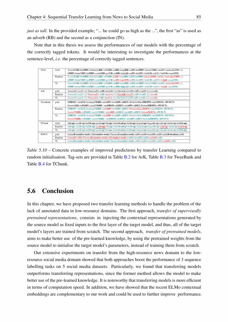
Chapter 4: Sequential Transfer Learning from News to Social Media 85

just as tall. In the provided example; “... he could go as high as the ...”, the first “as” is used as

an adverb (RB) and the second as a conjunction (IN).

Note that in this thesis we assess the performances of our models with the percentage of

the correctly tagged tokens. It would be interesting to investigate the performances at the

sentence-level, i.e. the percentage of correctly tagged sentences.

TPoS Gold @user(USR) He(PRP) definitely(RB) will(MD) as(RB) long(RB) as(IN) he(PRP) checks(VBZ) out(RP) medically(NN) .(.)I(PRP) think(VBP) he(PRP) could(MD) go(VB) as(RB) high(JJ) as(IN) the(DT) 2nd(CD) or(CC) 3rd(CD) round(NN)

Random @user(USR) He(PRP) definitely(RB) will(MD) as(IN) long(RB) as(IN) he(PRP) checks(NNS) out(IN) medically(VBN) .(.)I(PRP) think(VBP) he(PRP) could(MD) go(VB) as(IN) high(NN) as(IN) the(DT) 2nd(CD) or(CC) 3rd(JJ) round(NN)

TL @user(USR) He(PRP) definitely(RB) will(MD) as(RB) long(RB) as(IN) he(PRP) checks(VBZ) out(RP) medically(NN) .(.)I(PRP) think(VBP) he(PRP) could(MD) go(VB) as(RB) high(JJ) as(IN) the(DT) 2nd(CD) or(CC) 3rd(JJ) round(NN)

ArK gold @user(@) yay(!) !(,) Thanyou(G) so(R) much(R) !(,) Much(A) love(N) to(P) you(O) !(,) xxxx(E)Random @user(@) yay(!) !(,) Thanyou(L) so(R) much(A) !(,) Much(R) love(V) to(P) you(O) !(,) xxxx(#)TL @user(@) yay(!) !(,) Thanyou(!) so(R) much(A) !(,) Much(A) love(N) to(P) you(O) !(,) xxxx(G)

TweeBank gold I(PRON) ’m(AUX) heading(VERB) out(ADV) for(ADP) a(DET) #PokeGoBike(PROPN) ride(NOUN) .(PUNCT)Easier(ADJ) to(PART) catch(VERB) ’em(PRON) all(DET) on(ADP) a(DET) Koben(PROPN) .(PUNCT)

Random I(PRON) ’m(AUX) heading(VERB) out(ADP) for(ADP) a(DET) #PokeGoBike(NOUN) ride(NOUN) .(PUNCT)Easier(VERB) to(PART) catch(VERB) ’em(ADP) all(DET) on(ADP) a(DET) Koben(NOUN) .(PUNCT)

TL I(PRON) ’m(AUX) heading(VERB) out(ADP) for(ADP) a(DET) #PokeGoBike(PROPN) ride(NOUN) .(PUNCT)Easier(VERB) to(PART) catch(VERB) ’em(PRON) all(DET) on(ADP) a(DET) Koben(PROPN) .(PUNCT)

TChunk Gold it(b-np) was(b-vp) half(b-np) past(i-np) 8(i-np) when(b-advp) the(b-np) drugs(i-np) began(b-vp) to(i-vp) take(i-vp) hold(b-np)Random it(b-np) was(b-vp) half(b-np) past(b-np) 8(i-np) when(b-advp) the(b-np) drugs(i-np) began(b-vp) to(b-vp) take(i-vp) hold(i-vp)TL it(b-np) was(b-vp) half(b-np) past(i-np) 8(i-np) when(b-advp) the(b-np) drugs(i-np) began(b-vp) to(i-vp) take(i-vp) hold(b-np)

WNUT gold Game(B-creative-work) of(I-creative-work) Thrones(I-creative-work) is(O) not(O) based(O) on(O) earth(B-location) js(O)Random Game(O) of(O) Thrones(B-creative-work) is(I-creative-work) not(O) based(O) on(O) earth(O) js(O)TL Game(B-creative-work) of(I-creative-work) Thrones(I-creative-work) is(O) not(O) based(O) on(O) earth(O) js(O)

Table 5.10 – Concrete examples of improved predictions by transfer Learning compared to

random initialisation. Tag-sets are provided in Table B.2 for ArK, Table B.3 for TweeBank and

Table B.4 for TChunk.

5.6 Conclusion

In this chapter, we have proposed two transfer learning methods to handle the problem of the

lack of annotated data in low-resource domains. The first approach, transfer of supervisedly

pretrained representations, consists in injecting the contextual representations generated by

the source model as fixed inputs to the first layer of the target model, and thus, all of the target

model’s layers are trained from scratch. The second approach, transfer of pretrained models,

aims to make better use of the pre-learned knowledge, by using the pretrained weights from the

source model to initialise the target model’s parameters, instead of training them from scratch.

Our extensive experiments on transfer from the high-resource news domain to the low-

resource social media domain showed that both approaches boost the performance of 3 sequence

labelling tasks on 5 social media datasets. Particularly, we found that transferring models

outperforms transferring representations, since the former method allows the model to make

better use of the pre-learned knowledge. It is noteworthy that transferring models is more efficient

in terms of computation speed. In addition, we have showed that the recent ELMo contextual

embeddings are complementary to our work and could be used to further improve performance.

86 5.6. CONCLUSION

Our in-depth analysis on our method of transferring pretrained models, showed that: 1) The

method is more advantageous in extremely low-resource scenarios. 2) The method helps to

improve the performance over all datasets classes. 3) The method leads to a faster convergence

compared to training from scratch. 4) The model’s size does not have an observable effect on the

transfer performance. Finally, 5) the pretraining performance on the source task is not a predictor

of performance on the target task.

6 | Neural Domain Adaptation by JointLearning of Pretrained and RandomUnits

6.1 Introduction

In the previous chapter, we have performed sequential transfer learning from the news-domain to

the social media domain. Precisely, we used the Standard Fine-Tuning (SFT) adaptation scheme

of transfer learning, by a supervised pretraining on the news-domain followed by an adaptation

on the social media domain. Our results showed that using SFT boosts the performance positively

on three NLP tasks from the social media domain, especially in extremely low-resource settings.

In this chapter, we attempt to improve the SFT adaptation scheme through three steps. First,

through quantitative and qualitative analysis, we shed light on the hidden negative transfer

occurring when transferring from news to social media despite the high relatedness between both

domains. Second, we inspect the pretrained internal neural representations, at the representation-

level and a more fine-grained neuron-level, showing that pretrained neurons are biased by what

they have learnt from the source dataset. Thus, they struggle with learning certain patterns

that are specific to the target domain. Third, to address this issue, we propose a new method

to improve the SFT adaptation scheme by augmenting the pretrained model with normalised,

weighted and randomly initialised neurons that foster a better adaptation while maintaining the

valuable source knowledge.

This chapter is devised into two sub-chapters:

• The first sub-chapter (§6.2) proposes a series of analysis to spot the drawbacks of the

SFT adaptation scheme of transfer learning. We start in section 6.2.2 by taking a step

towards identifying and analysing the hidden negative transfer when transferring from the

news domain to the social media domain. Negative transfer [300, 373] occurs when the

knowledge learnt in the source domain hampers the learning of new knowledge from the

target domain. Particularly, when the source and target domains are dissimilar, transfer

learning may fail and hurt the performance, leading to a worse performance compared to

87

88 6.1. INTRODUCTION

the standard supervised training from scratch. In this chapter, we decorticate the results of

the SFT scheme obtained in the precedent chapter. Precisely, we perceive the gain brought

by SFT, compared to random initialisation, as a combination of a positive transfer and

a hidden negative transfer. We define positive transfer as the percentage of predictions

that were wrongly predicted by random initialisation1, but using transfer learning changed

to the correct ones. The negative transfer represents the percentage of predictions that

were tagged correctly by random initialisation, but using transfer learning gives incorrect

predictions. Hence, the final gain brought by transfer learning would be the difference

between positive and negative transfer. We show through a series of empirical analysis

that, the hidden negative transfer mitigates the final gain brought by transfer learning.

Next, in section 6.2.3, we perform an interpretive analysis of individual pre-trained neurons

behaviours in different settings. We find that pretrained neurons are biased by what they

have learnt in the source-dataset. For instance, we observe a unit2 firing on proper

nouns (e.g.“George” and “Washington”) before fine-tuning, and on words with capitalised

first-letter whether the word is a proper noun or not (e.g. “Man” and “Father”) during

fine-tuning. Indeed, in news domain, only proper nouns start with an upper-case letter;

thus the pre-trained units fail to discard this pattern which is not always respected in

User-Generated-Content (UGC) in social media.3 As a consequence of this phenomenon,

specific patterns to the target-dataset (e.g. “wanna” or “gonna” in the UGC in social media)

are difficult to learn by pre-trained units. This phenomenon is non-desirable, since such

specific units are essential, especially for target-specific classes [419, 181].

• The second sub-chapter (§6.3) proposes a new method to overcome the above-mentioned

drawbacks of the SFT scheme of transfer learning. Precisely, we propose a hybrid method

that takes benefit from both worlds, random initialisation and transfer learning, without

their drawbacks. It consists in augmenting the source-network (set of pre-trained units)

with randomly initialised units (that are by design non-biased) and jointly learn them. We

call our method PretRand (Pretrained and Random units). PretRand consists of three

main ideas: 1) Augmenting the source-network (set of pre-trained units) with a random

branch composed of randomly initialised units, and jointly learn them. 2) Normalising the

outputs of both branches to balance their different behaviours and thus forcing the network

to consider both. 3) Applying learnable attention weights on both branches predictors to

let the network learn which of random or pre-trained one is better for every class. Our

experiments on 4 NLP tasks: Part-of-Speech tagging (POS), Chunking (CK), Named

Entity Recognition (NER) and Morphosyntactic Tagging (MST); show that PretRand

1 We recall that random initialisation means training from scratch on target data.2 We use “unit” and “neuron” interchangeably.3 The same observation was pointed out in computer-vision [417] when fine-tuning on scenes a model pre-trained

on objects, it is the neuron firing on the “white-dog” object that becomes highly sensitive to the “white-waterfall”scene.

chapter 5: Neural Domain Adaptation by Joint Learning of Pretrained and Random Units 89

enhances considerably the performance compared to the standard fine-tuning adaptation

scheme.

6.2 Analysis of the Standard Fine-tuning Scheme of TransferLearning

We perform our analysis on three sequence labelling tasks: POS, CK and NER. Given an input

sentence S = [w1, . . . , wn] of n successive tokens and a tag-set C, the aim of sequence labelling

is to predict the tag ci ∈ C of every wi. For the basic neural architecture, we use a commonly

used model (described in details in section 5.2.1), which includes three main components: the

Word Representation Extractor (WRE), denoted Υ; the Features Extractor (FE), denoted Φ

and the Classifier (Cl), denoted Ψ.

Υ computes for each token wi a word-level embedding (xwordi =Υword(wi)) and a character-

level biLSTM encoder-based embedding (xchari =Υchar(wi)), and concatenates them to get a

final representation xi=(xwordi ,xchari ). Then, Υ’s outputs [x1, . . . ,xn] are fed into the Φ that

outputs a context sensitive representation for each token, consisting of a single biLSTM layer

which iteratively passes through the sentence in both directions. Finally, Ψ consists of a

softmax fully-connected layer that produces the classes-probabilities for each wi as follows:

yi = (Ψ ◦ Φ ◦ Υ)(wi).

In this sub-chapter, we analyse the precedent chapter’s results of the fine-tuning adaptation

scheme of transfer learning, referred to as Standard Fine-tuning (SFT) henceforth. Recall that

SFT (§5.3.2.2) consists on three steps:

1. Pretraining the source-model on the source-task;

2. Initialising target model’s word representation component (Υ) and feature extractor compo-

nent (Φ) weights with source model’s ones, while the classifier (Ψ) is randomly initialised;

3. And finally, in the adaptation stage, the three modules are jointly trained on the target-

dataset by minimising the SCE loss using the SGD algorithm.

Our results, in the precedent chapter (Table 5.4), show that applying this method improves the

results compared to training from scratch (random initialisation), across all tasks and social

media data-sets. Here, we carry out a series of analysis to spot some of the limits of this method,

namely, the hidden negative transfer (§6.2.2) and the bias in pretrained neurons (§6.2.3).

906.2. ANALYSIS OF THE STANDARD FINE-TUNING SCHEME OF TRANSFER

LEARNING

6.2.1 Experimental Setup

DatasetsThroughout this sub-chapter, we conduct experiments on three sequence labelling tasks (POS, CK

and NER). For the source-datasets, we use the news domain with the following datasets: the WSJ

part of Penn-Tree-Bank (PTB) [215] for POS; CONLL2003 for NER [355]; and CONLL2000

[354] for CK. In the same vein, for the target-datasets, we use the social media with the following

datasets: TPoS, ArK and TweeBank [203] for POS; WNUT-17 [85] for NER; and TChunk [298]

for CK. Statistics of all the datasets are summarised in Table 6.1. More details about the tasks

and datasets are provided in chapter 4.

Task #Classes Sources Eval. Metrics #Tokens-splits (train - val - test)POS: POS Tagging 36 WSJ Top-1 Acc. 912,344 - 131,768 - 129,654

CK: Chunking 22 CONLL-2000 Top-1 Acc. 211,727 - n/a - 47,377

NER: Named Entity Recognition 4 CONLL-2003 Top-1 Exact-match F1. 203,621 - 51,362 - 46,435

POS: POS Tagging40 TPoS Top-1 Acc. 10,500 - 2,300 - 2,90025 ArK Top-1 Acc. 26,500 - / - 7,70017 TweeBank Top-1 Acc. 24,753 - 11,742 - 19,112

CK: Chunking 18 TChunk Top-1 Top-1 Acc.. 10,652 - 2,242 - 2,291

NER: Named Entity Recognition 6 WNUT-17 Top-1 Exact-match F1. 62,729 - 15,734 - 23,394

Table 6.1 – Statistics of the used datasets. Top: datasets of the source domain. Bottom: datasets

of the target domain.

Training detailsIn the standard word-level embeddings, tokens are lower-cased while the character-level compo-

nent still retains access to the capitalisation information. We set the randomly initialised character

embedding dimension (dchar) at 50, the dimension of hidden states of the character-level biLSTM

(dchar) at 100 and used 300-dimensional word-level embeddings (dword). Word-level embedding

were pre-loaded from publicly available GloVe pre-trained vectors on 42 billions words from a

web crawling and containing 1.9M words [262]. Note that, these embeddings are also updated

during training. For the FE component, we use a single layer biLSTM (token-level feature

extractor) and set the number of units (H) to 200. In all experiments, both pretraining and

fine-tuning were performed using the same training settings, SGD with momentum with early

stopping and mini-batches of 16 sentences, with a fixed learning rate of 1.5× 10−2.

6.2.2 Analysis of the Hidden Negative Transfer

It has been shown in many works in the literature [300, 120, 303, 137, 49, 56, 373, 254] that,

when the source and target domains are less related (e.g. languages from different families),

sequential transfer learning may lead to a negative effect on the performance, instead of improving

it. This phenomenon is referred to as negative transfer. Precisely, negative transfer is considered

when transfer learning is harmful to the target task/dataset, i.e. the performance when using

chapter 5: Neural Domain Adaptation by Joint Learning of Pretrained and Random Units 91

transfer learning algorithm is lower than that with a solely supervised training on in-target data

[357]. In NLP, negative transfer phenomenon has only seldom been studied. We can cite the

recent work of Kocmi [172] who evaluated the negative transfer in transfer learning in Neural

Machine Translation (NMT) when the transfer is performed between different language-pairs.

They found that: 1) The distributions mismatch between source and target language-pairs does

not beget a negative transfer. 2) The transfer may have a negative impact when the source

language-pair is less-resourced compared to the target one, in terms of annotated examples.

Our experiments have shown that transfer learning techniques from news domain to social

media domain boosts tagging performance. Hence, following the above definition, transfer

learning from news to social media does not beget a negative transfer. Contrariwise, in this work,

we instead consider the hidden negative transfer, i.e. the percentage of predictions that were

correctly tagged by random initialisation, but using transfer learning gives wrong predictions.

Precisely, we perform empirical analysis to investigate the hidden negative transfer in SFT.

We propose the following experiments: 1) we show that the final gain brought by SFT can be

separated into two categories: positive transfer and negative transfer. We define positive transfer

as the percentage of tokens that were wrongly predicted by random initialisation, but the SFT

changed to the correct ones, while negative transfer represents the percentage of words that

were tagged correctly by random initialisation, but using SFT gives wrong predictions (§6.2.2.1).

2) We study the impact of the pretraining state on negative and positive transfer (§6.2.2.2).

Finally, 3) we provide some qualitative examples of negative transfer (§6.2.2.3).

6.2.2.1 Quantifying Positive Transfer & Negative Transfer

Let us consider the gain Gi brought by the SFT scheme of transfer learning compared to random

initialisation for the dataset i. Gi is defined as the difference between positive transfer PT i and

negative transfer NT i:

Gi = PT i −NT i, (6.1)

where positive transfer PT i represents the percentage of tokens that were wrongly predicted by

random initialisation, but the SFT changed to the correct ones. Negative transfer NT i represents

the percentage of words that were tagged correctly by random initialisation, but using SFT gives

wrong predictions. PT i and NT i are defined as follows:

PT i =N correctedi

Ni

, (6.2)

NT i =N falsifiedi

Ni

, (6.3)

where Ni is the total number of tokens in the validation-set, N correctedi is the number of tokens

from the validation-set that were wrongly tagged by the model trained from scratch but are

926.2. ANALYSIS OF THE STANDARD FINE-TUNING SCHEME OF TRANSFER

LEARNING

correctly predicted by transfer learning scheme, and N falsifiedi is the number of tokens from the

validation-set that were correctly tagged by the the model trained from scratch but are wrongly

predicted by the transfer learning scheme.

Figure 6.1 – The percentage of negative transfer and positive transfer brought by SFT adaptation

scheme compared to supervised training from scratch scheme.

Figure 6.1 shows the results on English social media datasets, first tagged with the classic

supervised training scheme and then using SFT. Blue bars show the percentage of positive

transfer and red bars give the percentage of negative transfer. We observe that even though

the SFT approach is effective since the resulting positive transfer is higher than the negative

transfer in all cases, this last mitigates the final gain brought by SFT. For instance, for TChunk

dataset, SFT corrected ∼4.7% of predictions but falsified ∼1.7%, which reduces the final gain to

∼3%. Here we calculate positive and negative transfer at the token-level. Thus, the gain shown

in Figure 6.1 for WNUT dataset does not correspond to the one in Table 5.4, since the F1 metric

is calculated only on named-entities.

6.2.2.2 The impact of pretraining state on Negative Transfer

The experiment of this section is in the same vein as the experiment of section 5.5.4, where we

investigated the question “when are pretrained parameters ready to transfer?”. Likewise, here we

pick the pretrained weights at different pretraining epochs; that we call the pretraining states.

Then, we assess the performance when transferring each. Nevertheless, here we are instead

interested by the impact of the pretraining state on negative and positive transfer. Specifically,

in Figure 6.2, we plot for each target dataset, the curves of positive transfer (green curves) and

negative transfer (red curves) brought by initialising the target model with pretrained weights

from different pretraining states compared to the random initialisation. Clearly, both negative

and positive transfer increase with pretraining epochs, since more source domain knowledge is

acquired in the course of pretraining. More importantly, for TweeBank and ArK datasets, the

negative transfer increases rapidly in the last pretraining epochs. However, for TPoS dataset,

the negative transfer stays almost stable throughout pretraining epochs. This observation is tied

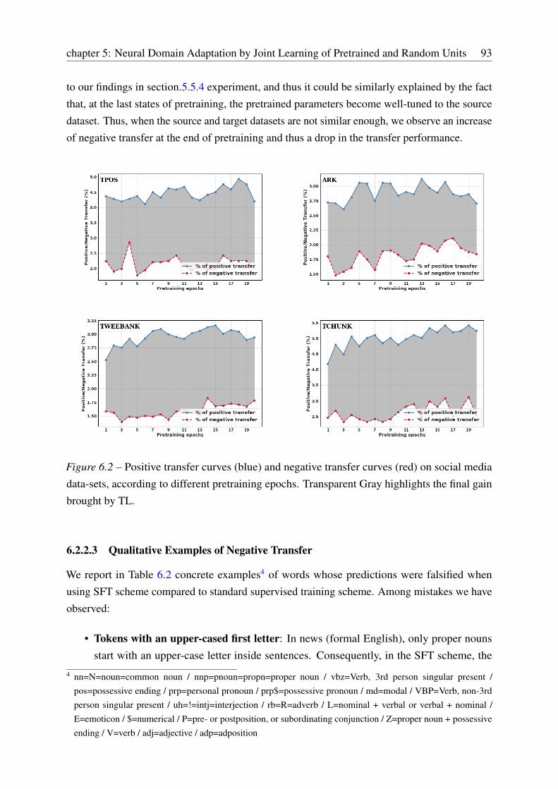
chapter 5: Neural Domain Adaptation by Joint Learning of Pretrained and Random Units 93

to our findings in section.5.5.4 experiment, and thus it could be similarly explained by the fact

that, at the last states of pretraining, the pretrained parameters become well-tuned to the source

dataset. Thus, when the source and target datasets are not similar enough, we observe an increase

of negative transfer at the end of pretraining and thus a drop in the transfer performance.

Figure 6.2 – Positive transfer curves (blue) and negative transfer curves (red) on social media

data-sets, according to different pretraining epochs. Transparent Gray highlights the final gain

brought by TL.

6.2.2.3 Qualitative Examples of Negative Transfer

We report in Table 6.2 concrete examples4 of words whose predictions were falsified when

using SFT scheme compared to standard supervised training scheme. Among mistakes we have

observed:

• Tokens with an upper-cased first letter: In news (formal English), only proper nouns

start with an upper-case letter inside sentences. Consequently, in the SFT scheme, the

4 nn=N=noun=common noun / nnp=pnoun=propn=proper noun / vbz=Verb, 3rd person singular present /pos=possessive ending / prp=personal pronoun / prp$=possessive pronoun / md=modal / VBP=Verb, non-3rdperson singular present / uh=!=intj=interjection / rb=R=adverb / L=nominal + verbal or verbal + nominal /E=emoticon / $=numerical / P=pre- or postposition, or subordinating conjunction / Z=proper noun + possessiveending / V=verb / adj=adjective / adp=adposition

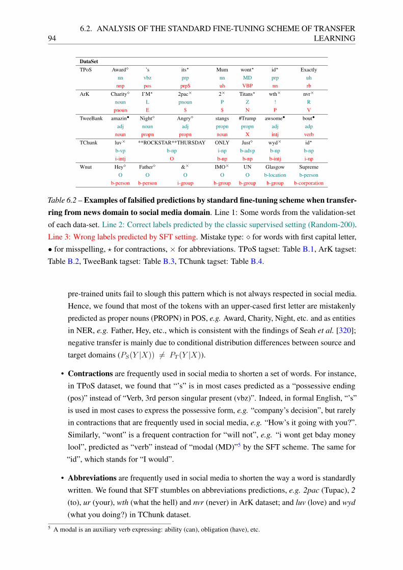
946.2. ANALYSIS OF THE STANDARD FINE-TUNING SCHEME OF TRANSFER

LEARNING

DataSetTPoS Award� ’s its? Mum wont? id? Exactly

nn vbz prp nn MD prp uhnnp pos prp$ uh VBP nn rb

ArK Charity� I’M? 2pac× 2× Titans? wth× nvr×

noun L pnoun P Z ! Rpnoun E $ $ N P V

TweeBank amazin• Night� Angry� stangs #Trump awsome• bout•

adj noun adj propn propn adj adpnoun propn propn noun X intj verb

TChunk luv× **ROCKSTAR**THURSDAY ONLY Just� wyd× id?

b-vp b-np i-np b-advp b-np b-npi-intj O b-np b-np b-intj i-np

Wnut Hey� Father� &× IMO× UN Glasgow SupremeO O O O O b-location b-person

b-person b-person i-group b-group b-group b-group b-corporation

Table 6.2 – Examples of falsified predictions by standard fine-tuning scheme when transfer-ring from news domain to social media domain. Line 1: Some words from the validation-set

of each data-set. Line 2: Correct labels predicted by the classic supervised setting (Random-200).

Line 3: Wrong labels predicted by SFT setting. Mistake type: � for words with first capital letter,

• for misspelling, ? for contractions, × for abbreviations. TPoS tagset: Table B.1, ArK tagset:

Table B.2, TweeBank tagset: Table B.3, TChunk tagset: Table B.4.

pre-trained units fail to slough this pattern which is not always respected in social media.

Hence, we found that most of the tokens with an upper-cased first letter are mistakenly

predicted as proper nouns (PROPN) in POS, e.g. Award, Charity, Night, etc. and as entities

in NER, e.g. Father, Hey, etc., which is consistent with the findings of Seah et al. [320];

negative transfer is mainly due to conditional distribution differences between source and

target domains (PS(Y |X)) 6= PT (Y |X)).

• Contractions are frequently used in social media to shorten a set of words. For instance,

in TPoS dataset, we found that “’s” is in most cases predicted as a “possessive ending

(pos)” instead of “Verb, 3rd person singular present (vbz)”. Indeed, in formal English, “’s”

is used in most cases to express the possessive form, e.g. “company’s decision”, but rarely

in contractions that are frequently used in social media, e.g. “How’s it going with you?”.

Similarly, “wont” is a frequent contraction for “will not”, e.g. “i wont get bday money

lool”, predicted as “verb” instead of “modal (MD)”5 by the SFT scheme. The same for

“id”, which stands for “I would”.

• Abbreviations are frequently used in social media to shorten the way a word is standardly

written. We found that SFT stumbles on abbreviations predictions, e.g. 2pac (Tupac), 2

(to), ur (your), wth (what the hell) and nvr (never) in ArK dataset; and luv (love) and wyd

(what you doing?) in TChunk dataset.5 A modal is an auxiliary verb expressing: ability (can), obligation (have), etc.

chapter 5: Neural Domain Adaptation by Joint Learning of Pretrained and Random Units 95

• Misspellings: Likewise, we found that the SFT scheme often gives wrong predictions for

misspelt words, e.g. awsome, bout, amazin.

6.2.3 Interpreting the Bias in Pretrained Models

Much effort has been devoted to understand and interpret the information encoded in pre-trained

models, especially pretrained contextual embeddings (ELMo, BERT, etc.). However, how this

information is evolving during fine-tuning in the target task is relatively poorly understood. Here,

we aim to gain some insights into how the inner pretrained representations are updated during

fine-tuning on social media datasets when using the SFT scheme of transfer learning. For this,

we propose to analyse the feature extractor’s (Φ) activations. Specifically, we attempt to visualise

biased neurons, i.e. pre-trained neurons that do not change that much from their initial state.

Formally, let us consider a validation-set of N words, the feature extractor Φ generates a

matrix h ∈ MN,H(R) of activations over all validation-set’s words, where Mf ,g(R) is the space

of f × g matrices over R, and H is the size of the hidden representation (number of neurons).

Each element hi,j from the matrix represents the activation of the neuron j on the word wi.

Given two models, the first before fine-tuning and the second after fine-tuning, we obtain two

matrices hbefore ∈ MN,H(R) and hafter ∈ MN,H(R), which give, respectively, the activations

of Φ over all validation-set’s words before and after fine-tuning. Here we aim to visualise and

quantify the change of the representations generated by the model from the initial state, hbefore

(before fine-tuning), to the final state, hafter (after fine-tuning). For this purpose, we perform

two experiments: 1) quantifying the change of pretrained individual neurons (§6.2.3.1), and 2)

visualising the evolution of pretrained neurons stimulus during fine-tuning (§6.2.3.2).

6.2.3.1 Quantifying the change of individual pretrained neurons

ApproachHere, we propose to quantify the change of the knowledge encoded in pretrained neurons after

fine-tuning. For this purpose, we propose to calculate the similarity (correlation) between neurons

activations before and after fine-tuning, when using the SFT adaptation scheme. Precisely, we

calculate the correlation coefficient between each neuron’s activation on the target-domain

validation-set before starting fine-tuning and at the end of fine-tuning.

Following the above formulation, and as illustrated in Figure 6.3, from hbefore and hafter

matrices, we extract two vectors hbefore.j ∈ RN and hafter.j ∈ RN , representing respectively

the activations of a unit j over all validation-set’s words before and after fine-tuning, where

N is the number of words in the validation-set. Next, we generate an asymmetric correlation

matrix C ∈MH,H(R), where each element cjt in the matrix represents the Pearson’s correlation

between the unit j activation vector after fine-tuning (hafter.j ) and the unit t activation vector

before fine-tuning (hbefore.t ), computed as follows:

966.2. ANALYSIS OF THE STANDARD FINE-TUNING SCHEME OF TRANSFER

LEARNING

Figure 6.3 – Illustrative scheme of the computation of the charge of unit j, i.e. the Pearson

correlation between unit j activations vector after fine-tuning to its activations vector before

fine-tuning.

cjt =E[(hafter.j − µafterj )(hbefore.t − µbeforet )]

σafterj σbeforet

. (6.4)

Here µbeforej and σbeforej represent, respectively, the mean and the standard deviation of unit j

activations over the validation set. Clearly, we are interested by the matrix diagonal, where cjjrepresents the charge of each unit j from Φ, i.e. the correlation between each unit’s activations

after fine-tuning to its activations before fine-tuning.

ResultsTo visualise the bias phenomenon occurring in the SFT scheme, we quantify the charge of

individual neurons. Precisely, we plot the asymmetric correlation matrix (C) between the Φ

layer’s units before and after fine-tuning for each social media dataset (ArK for POS, TChunk

for CK and WNUT-17 for NER). From the resulting correlation matrices illustrated in Figure 6.4,

we can observe the diagonal representing the charge of each unit, with most of the units having a

high charge (light colour), alluding the fact that, every unit after fine-tuning is highly correlated

with itself before fine-tuning. Hypothesising that high correlation in the diagonal entails high

bias, the results of this experiment confirm our initial motivation that pre-trained units are

highly biased to what they have learnt in the source-dataset, making them limited to learn some

patterns specific to the target-dataset. Our remarks were confirmed recently in the recent work of

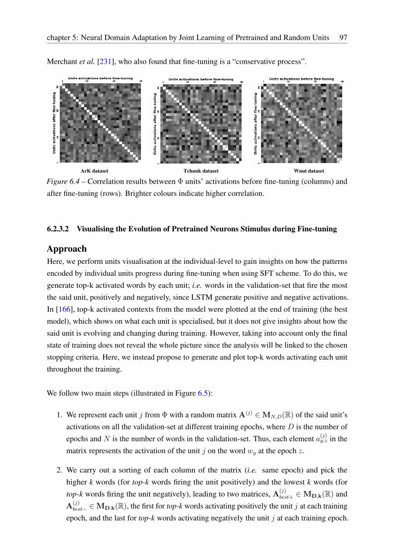
chapter 5: Neural Domain Adaptation by Joint Learning of Pretrained and Random Units 97

Merchant et al. [231], who also found that fine-tuning is a “conservative process”.

ArK dataset Tchunk dataset Wnut dataset

Figure 6.4 – Correlation results between Φ units’ activations before fine-tuning (columns) and

after fine-tuning (rows). Brighter colours indicate higher correlation.

6.2.3.2 Visualising the Evolution of Pretrained Neurons Stimulus during Fine-tuning

ApproachHere, we perform units visualisation at the individual-level to gain insights on how the patterns

encoded by individual units progress during fine-tuning when using SFT scheme. To do this, we

generate top-k activated words by each unit; i.e. words in the validation-set that fire the most

the said unit, positively and negatively, since LSTM generate positive and negative activations.

In [166], top-k activated contexts from the model were plotted at the end of training (the best

model), which shows on what each unit is specialised, but it does not give insights about how the

said unit is evolving and changing during training. However, taking into account only the final

state of training does not reveal the whole picture since the analysis will be linked to the chosen

stopping criteria. Here, we instead propose to generate and plot top-k words activating each unit

throughout the training.

We follow two main steps (illustrated in Figure 6.5):

1. We represent each unit j from Φ with a random matrix A(j) ∈MN,D(R) of the said unit’s

activations on all the validation-set at different training epochs, where D is the number of

epochs and N is the number of words in the validation-set. Thus, each element a(j)y,z in the

matrix represents the activation of the unit j on the word wy at the epoch z.

2. We carry out a sorting of each column of the matrix (i.e. same epoch) and pick the

higher k words (for top-k words firing the unit positively) and the lowest k words (for

top-k words firing the unit negatively), leading to two matrices, A(j)best+ ∈MD,k(R) and

A(j)best− ∈MD,k(R), the first for top-k words activating positively the unit j at each training

epoch, and the last for top-k words activating negatively the unit j at each training epoch.

986.2. ANALYSIS OF THE STANDARD FINE-TUNING SCHEME OF TRANSFER

LEARNING

Figure 6.5 – Illustrative scheme of the calculus of top-k-words activating unit j, positively

(A(j)best+) and negatively (A(j)

best−) during fine-tuning epochs. hepochz states for Φ’s outputs at

epoch number z.

ResultsHere, we give concrete visualisations of the evolution of pretrained neurons stimulus during fine-

tuning when transferring from the news domain to the social media domain. Specifically, we plot

the matrices of top-10 words activating each neuron j, positively (A(j)best+) or negatively (A(j)

best−).

The results are plotted in Figure 6.6 for ArK (POS) dataset, Figure 6.7 for TweeBank dataset

(POS) and Figure 6.8 for WNUT dataset (NER). Rows represent the top-10 words from the

target dataset activating each unit, and columns represent fine-tuning epochs; before fine-tuning

in column 0 (at this stage the model is only trained on the source-dataset), and during fine-tuning

(columns 5 to 20). Additionally, to get an idea about each unit’s stimulus on source dataset, we

also show, in the first column (Final-WSJ for POS and Final-CONLL-03 for NER), top-10 words

from the source dataset activating the same unit before fine-tuning. In the following, we describe

the information encoded by each provided neuron.6

6 Here we only select some interesting neurons. However we also found many neurons that are not interpretable.

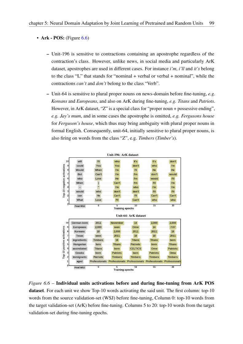
chapter 5: Neural Domain Adaptation by Joint Learning of Pretrained and Random Units 99

• Ark - POS: (Figure 6.6)

– Unit-196 is sensitive to contractions containing an apostrophe regardless of the

contraction’s class. However, unlike news, in social media and particularly ArK

dataset, apostrophes are used in different cases. For instance i’m, i’ll and it’s belong

to the class “L” that stands for “nominal + verbal or verbal + nominal”, while the

contractions can’t and don’t belong to the class “Verb”.

– Unit-64 is sensitive to plural proper nouns on news-domain before fine-tuning, e.g.

Koreans and Europeans, and also on ArK during fine-tuning, e.g. Titans and Patriots.

However, in ArK dataset, “Z” is a special class for “proper noun + possessive ending”,

e.g. Jay’s mum, and in some cases the apostrophe is omitted, e.g. Fergusons house

for Ferguson’s house, which thus may bring ambiguity with plural proper nouns in

formal English. Consequently, unit-64, initially sensitive to plural proper nouns, is

also firing on words from the class “Z”, e.g. Timbers (Timber’s).

Unit-196: ArK dataset

Unit-64: ArK dataset

Figure 6.6 – Individual units activations before and during fine-tuning from ArK POSdataset. For each unit we show Top-10 words activating the said unit. The first column: top-10

words from the source validation-set (WSJ) before fine-tuning, Column 0: top-10 words from

the target validation-set (ArK) before fine-tuning. Columns 5 to 20: top-10 words from the target

validation-set during fine-tuning epochs.

1006.2. ANALYSIS OF THE STANDARD FINE-TUNING SCHEME OF TRANSFER

LEARNING

• Tweebank - POS: (Figure 6.7)

– Unit-37 is sensitive before and during fine-tuning on plural nouns, such as gazers

and feminists. However, it is also firing on the word slangs because of the s ending,

which is in fact a proper noun. This might explain the wrong prediction for the word

slangs (noun instead of proper noun) given by the SFT scheme (Table 6.2).

– Unit-169 is highly sensitive to proper nouns (e.g. George and Washington) before

fine-tuning, and to words with capitalised first-letter whether the word is a proper

noun or not (e.g. Man and Father) during fine-tuning on the TweeBank dataset.

Which may explain the frequent wrong predictions of tokens with upper-cased first

letter as proper nouns by the SFT scheme.

Unit-37: Tweebank dataset

Unit-169: Tweebank dataset

Figure 6.7 – Individual units activations before and during fine-tuning on Tweebank POSdataset. For each unit we show Top-10 words activating the said unit. The first column: top-10

words from the source validation-set (WSJ) before fine-tuning, Column 0: top-10 words from

the target validation-set (Tweebank) before fine-tuning. Columns 5 to 20: top-10 words from the

target validation-set during fine-tuning epochs.

chapter 5: Neural Domain Adaptation by Joint Learning of Pretrained and Random Units 101

• WNUT - NER: (Figure 6.8)

– Unit-101 is firing before and after fine-tuning on words that are part of an “Or-

ganisation” entity, e.g County (Ross County), Park (Queens Park Rangers), etc.

Accordingly, it is sensitive to the word Supreme. As illustrated in Table 6.2, this word

was mistakenly predicted as a part of an “Organisation” by SFT. Indeed, Supreme

Court is frequently used in CONLL-03 (the source dataset) as an Organisation.

However in rare cases such as Supreme Court judge, which is a “Person”, Supreme

should be tagged as a part of a “Person” entity.

– Unit-184 is firing before and after fine-tuning on words that are part of an “Organi-

sation” entity, e.g Bank, inc and “&”. Indeed, this last is frequently used in formal

English in organisation names such as: Jones & co. However, in social media, it is

mostly used as a contraction for the connector “and”. Consequently, as illustrated

in Table 6.2. “&” is mistakenly predicted as a part of an “Organisation” by the SFT

scheme.

Unit-101: WNUT dataset

Unit-184: WNUT dataset

Figure 6.8 – Individual units activations before and during fine-tuning on WNUT NERdataset. For each unit we show Top-10 words activating the said unit. The first column: top-10

words from the source validation-set (CONLL-03) before fine-tuning, Column 0: top-10 words

from the target validation-set (WNUT-17) before fine-tuning. Columns 5 to 20: top-10 words

from the target validation-set during fine-tuning epochs.

1026.2. ANALYSIS OF THE STANDARD FINE-TUNING SCHEME OF TRANSFER

LEARNING

6.2.4 Conclusion

In this sub-chapter, we have analysed the results of the standard fine-tuning adaptation scheme

of transfer learning. Firstly, we were interested in the hidden negative transfer that arises when

transferring from the news domain to the social media domain. Indeed, negative transfer has

only seldom been tackled in sequential transfer learning works in NLP. In addition, earlier

research papers evoke negative transfer only when the source domain has a negative impact on

the target model. We showed that despite the positive gain brought by transfer learning from the

high-resource news domain to the low-resource social media domain, we found that the hidden

negative transfer mitigates the final gain brought by transfer learning. Second, we carried out

an interpretive analysis of the evolution, during fine-tuning, of pretrained representations. We

found that while fine-tuning necessarily makes some changes during fine-tuning on social media

datasets, pretrained neurons are biased by what they have learnt in the source domain. In simple

words, pretrained neurons tend to conserve much information from the source domain. Some

of this information is undoubtedly beneficial for the social media domain (positive transfer),

but some of it is indeed harmful (negative transfer). We hypothesise that this phenomenon of

biased neurons restrains the pretrained model from learning some new features specific to the

target domain (social media). To overcome this drawback of the standard fine-tuning adaptation

scheme, we propose in the next sub-chapter a new scheme of adaptation.

We believe that more extensive experiments would be interesting to better understand the

phenomenon of the hidden negative transfer and to confirm our observations. First, one can

investigate the impact of the model’s hyper-parameters (size, activation functions, learning

rate, etc.) as well as regulation methods (dropout, batch normalisation, weights decay, etc.).

Second, we suppose that the hidden negative transfer would be more prominent when the target

dataset is too small since the pre-learned source knowledge will be more preserved. Hence, it

would be interesting to assess the impact of target-training size. Third, a promising experiment

would be to study the impact of the similarity between the source and the target distributions.

For instance, one can use instance selection methods (§2.4.2) to select source examples for

pretraining. Concerning the quantification of the change of pretrained individual neurons, it

would be interesting to observe the percentage of biased neurons according to different thresholds

of correlation. It would also be interesting to perform a representation-level similarity analysis

to gain more insights, as it has been shown by Wu et al. [384] that representation-level similarity

measures the distributional similarity while individual-level measures local similarity.

chapter 5: Neural Domain Adaptation by Joint Learning of Pretrained and Random Units 103

6.3 The Proposed Method: PretRand

From our analysis, we have found that the SFT scheme suffers from a main limitation. Indeed,

despite the fine-tuning on the target domain, pre-trained neurons still biased by what they have

learnt from the source domain, and thus some of these neurons struggle with learning uncommon

target-specific patterns. We propose a new adaptation scheme that we call PretRand, joint

learning of Pretrained and Random units. We start by presenting our proposed approach in

section 6.3.1. Then, we report the results thereof in section 6.3.2. Finally, we carry out an

empirical analysis of PretRand approach in section 6.3.3.

6.3.1 Method Description

We propose to take benefit from both worlds, the pre-learned knowledge in the pretrained

neurons and the target-specific features easily learnt by random neurons. Roughly, we propose to

augment the target-network with normalised, weighted and randomly initialised units that beget

a better adaptation while maintaining the valuable source knowledge. Specifically, our proposed

approach, PretRand, consists of three main ideas (illustrated in Figure 6.9):

1. Augmenting the pre-trained branch with a random one to facilitate the learning of new

target-specific patterns (§6.3.1.1);

2. Normalising both branches to balance their behaviours during fine-tuning (§6.3.1.2);

3. Applying learnable weights on both branches to let the network learn which of random or

pre-trained one is better for every class. (§6.3.1.3).

6.3.1.1 Adding the Random Branch

We expect that augmenting the pretrained model with new randomly initialised neurons allows a

better adaptation during fine-tuning. Thus, in the adaptation stage, we augment the pre-trained

model with a random branch consisting of additional random units (as illustrated in scheme “a” of

Figure 6.9). Several works have shown that deep (top) layers are more task-specific than shallow

(low) ones [265, 243]. Thus, deep layers learn generic features easily transferable between tasks.

In addition, word embeddings (shallow layers) contain the majority of parameters. Based on

these factors, we choose to expand only the top layers as a trade-off between performance and

number of parameters (model complexity). In terms of the expanded layers, we add an extra

biLSTM layer of k units in the FE: Φr (r for random); and a new FC layer of C units: Ψr.

With this choice, we increase the complexity of the model only 1.02× compared to the base one

(SFT).

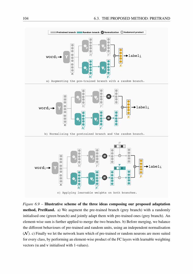
104 6.3. THE PROPOSED METHOD: PRETRAND

Figure 6.9 – Illustrative scheme of the three ideas composing our proposed adaptationmethod, PretRand. a) We augment the pre-trained branch (grey branch) with a randomly

initialised one (green branch) and jointly adapt them with pre-trained ones (grey branch). An

element-wise sum is further applied to merge the two branches. b) Before merging, we balance

the different behaviours of pre-trained and random units, using an independent normalisation

(N ). c) Finally we let the network learn which of pre-trained or random neurons are more suited

for every class, by performing an element-wise product of the FC layers with learnable weighting

vectors (u and v initialised with 1-values).

chapter 5: Neural Domain Adaptation by Joint Learning of Pretrained and Random Units 105

Concretely, for every wi, two predictions vectors are computed; ypi from the pre-trained

branch and yri from the random one. Specifically, the pre-trained branch predicts class-

probabilities following:

ypi = (Ψp ◦ Φp)(xi) , (6.5)

with xi = Υ(wi). Likewise, the additional random branch predicts class-probabilities following:

yri = (Ψr ◦ Φr)(xi). (6.6)

To get the final predictions, we simply apply an element-wise sum between the outputs of the

pre-trained branch and the random branch:

yi = ypi ⊕ yri . (6.7)

As in the classical scheme, the SCE (Softmax Cross-Entropy) loss is minimised but here, both

branches are trained jointly.

6.3.1.2 Independent Normalisation

Our first implementation of adding the random branch was less effective than expected. The

main explanation is that the pre-trained units were dominating the random units, which means

that the weights as well as the gradients and outputs of pre-trained units absorb those of the

random units. As illustrated in the left plot of Figure 6.10, the absorption phenomenon stays true

even at the end of the training process; we observe that random units weights are closer to zero.

This absorption propriety handicaps the random units in firing on the words of the target dataset

(The same problem was stated in some computer-vision works [200, 372, 349]).

To alleviate this absorption phenomenon and push the random units to be more competitive,

we normalise the outputs of both branches (ypi and yri ) using the `2-norm, as illustrated in the

scheme “b” of Figure 6.9. The normalisation of a vector “x” is computed using the following

formula:

N2(x) =x

||x||2. (6.8)

Thanks to this normalisation, the absorption phenomenon was solved, and the random branch

starts to be more effective (see the right distribution of Figure 6.10).

Furthermore, we have observed that despite the normalisation, the performance of the pre-

trained classifiers is still much better than the randomly initialised ones. Thus, to make them

more competitive, we propose to start with optimising only the randomly initialised units while

freezing the pre-trained ones, then, launch the joint training. We call this technique random++.

106 6.3. THE PROPOSED METHOD: PRETRAND

Figure 6.10 – The distributions of the learnt weight-values for the randomly initialised (green) and

pre-trained (grey) fully-connected layers after their joint training. Left: without normalisation,

right: with normalisation.

6.3.1.3 Attention Learnable Weighting Vectors

Heretofore, pre-trained and random branches participate equally for every class’ predictions,

i.e. we do not weight the dimensions of ypi and yri before merging them with an element-wise

summation. Nevertheless, random classifiers may be more efficient in specific classes compared

to pre-trained ones and vice-versa. In other terms, we do not know which of the two branches

(random or pre-trained) is better for making a suitable decision for each class. For instance, if

the random branch is more efficient for predicting a particular class cj , it would be better to give

more attention to its outputs concerning the class cj compared to the pretrained branch.

Therefore, instead of simply performing an element-wise sum between the random and

pre-trained predictions, we first weight ypi with a learnable weighting vector u ∈ RC and yri

with a learnable weighting vector v ∈ RC , where C is the tagset size (number of classes).

Such as, the element uj from the vector u represents the random branch’s attention weight for

the class cj , and the element vj from the vector v represents the pretrained branch’s attention

weight for the class cj . Then, we compute a Hadamard product with their associated normalised

predictions (see the scheme “c” of Figure 6.9). Both vectors u and v are initialised with 1-values

and are fine-tuned by back-propagation. Formally, the final predictions are computed as follows:

yi = u � Np(ypi ) ⊕ v � Np(y

ri ). (6.9)

6.3.2 Experimental Results

First, we present the experimental setup in section 6.3.2.1. Second, in section 6.3.2.2, we compare

PretRand’s to the baseline methods. Third, in section 6.3.2.3, we measure the importance of each

component of PretRand for the overall performance. Fourth, in section 6.3.2.4, we investigate the

impact of incorporating ELMo contextual representations, in the baseline methods vs PretRand.

Finally, in section 6.3.2.5, we compare PretRand to best SOTA (State-Of-The-Art) approaches.

chapter 5: Neural Domain Adaptation by Joint Learning of Pretrained and Random Units 107

6.3.2.1 Experimental Setup

DatasetsIn this sub-chapter, we assess PretRand’s performance on POS, CK, NER and MST tasks on the

Social Media domain. For POS task, we use the WSJ part of Penn-Tree-Bank (PTB) [215] news

dataset for the source news domain and TPoS, ArK and TweeBank [203] for the target social

media domain. For CK task, we use the CONLL2000 [354] dataset for the news source domain

and TChunk [298] for the target domain. For NER task, we use the CONLL2003 [355] for the

source news domain and WNUT-17 [85] dataset for the social media target domain. For MST,

we use the MTT shared-task [402] benchmark containing two types of datasets: social media and

news, for three south-Slavic languages: Slovene (sl), Croatian (hr) and Serbian (sr). Statistics

of all the datasets are summarised in Table 6.3. More details about the tasks and datasets are

provided in chapter 4.

Task #Classes Sources Eval. Metrics # Tokens-splits (train - val - test)POS: POS Tagging 36 WSJ Top-1 Acc. 912,344 - 131,768 - 129,654

CK: Chunking 22 CONLL-2000 Top-1 Acc. 211,727 - n/a - 47,377

NER: Named Entity Recognition 4 CONLL-2003 Top-1 Exact-match F1. 203,621 - 51,362 - 46,435

MST: Morpho-syntactic Tagging1304 Slovene-news Top-1 Acc. 439k - 58k - 88k

772 Croatian-news Top-1 Acc. 379k - 50k - 75k557 Serbian-news Top-1 Acc. 59k - 11k, 16k

POS: POS Tagging40 TPoS Top-1 Acc. 10,500 - 2,300 - 2,90025 ArK Top-1 Acc. 26,500 - / - 7,70017 TweeBank Top-1 Acc. 24,753 - 11,742 - 19,112

CK: Chunking 18 TChunk Top-1 Top-1 Acc.. 10,652 - 2,242 - 2,291

NER: Named Entity Recognition 6 WNUT-17 Top-1 Exact-match F1. 62,729 - 15,734 - 23,394

MST: Morpho-syntactic Tagging1102 Slovene-sm Top-1 Acc. 37,756 - 7,056 - 19,296

654 Croatian-sm Top-1 Acc. 45,609 - 8,886 - 21,412589 Serbian-sm Top-1 Acc. 45,708- 9,581- 23,327

Table 6.3 – Statistics of the used datasets. Top: datasets of the source domain. Bottom: datasets

of the target domain.

Training detailsWe use the following Hyper-Parameters (HP): WRE’s HP: In the standard word-level embed-

dings, tokens are lower-cased while the character-level component still retains access to the

capitalisation information. We set the randomly initialised character embedding dimension at 50,

the dimension of hidden states of the character-level biLSTM at 100 and used 300-dimensional

word-level embeddings. The latter were pre-loaded from publicly available GloVe pre-trained

vectors on 42 billions words from a web crawling and containing 1.9M words [262] for English

experiments, and pre-loaded from publicly available FastText [35] pre-trained vectors on com-

mon crawl7 for South-Slavic languages. Note that, these embeddings are also updated during

7 https://github.com/facebookresearch/fastText/blob/master/docs/

crawl-vectors.md

108 6.3. THE PROPOSED METHOD: PRETRAND

training. For contextual words embeddings, we used ELMo embeddings. For English, we used

the small official pre-trained model on 1 billion word benchmark (13.6M parameters)8. Regard-

ing South-Slavic languages, pre-trained models are not available but for Croatian9 [54]. Note that,

in all experiments contextual embeddings are frozen during training. FE’s HP: we used a single

layer biLSTM (token-level feature extractor) and set the number of units to 200. PretRand’srandom branch HP: we experimented our approach with k = 200 added random-units. GlobalHP: In all experiments, training (pretraining and fine-tuning) was performed using the SGD with

momentum with early stopping, mini-batches of 16 sentences and learning rate of 1.5× 10−2.

6.3.2.2 Comparison with Baseline Methods

In this section, we assess the performance of PretRand through a comparison to six baseline-

methods, illustrated in Figure 6.11. First, since PretRand is an amelioration of the standard

fine-tuning (SFT) adaptation scheme, we mainly compare it to the SFT baseline. Besides, we

assess whether the gain brought by PretRand is due to the increase in the number of parameters;

thus we also compare with the standard supervised training scheme with a wider model. Finally,

the final predictions of PretRand are the combination of the predictions of the two branches,

randomly initialised and pretrained, which can make one think about ensemble methods [91].

Thus we also compare with ensemble methods. The following items describe the different

baseline-methods used for comparison:

• (a) From-scratch200: The base model described in section 5.1, trained from scratch using

the standard supervised training scheme on social media dataset (without transfer learning).

Here the number 200 refers to the dimensionality of the biLSTM network in the FE (Φ).

• (b) From-scratch400: The same as “From-scratch200” baseline but with 400 instead of 200

biLSTM units in the FE. Indeed, by experimenting with this baseline, we aim to highlight

that the impact of PretRand is not due to the increase in the number of parameters.

• (c) Standard Fine-tuning (SFT): Pre-training the base model on the source-dataset,

followed by an adaptation on the target-dataset with the standard fine-tuning scheme

(chapter 5 - scheme D in section 5.4.2.2).

• (d) Standard Feature Extraction (SFE): The same as SFT, but the pretrained parameters

are frozen during fine-tuning on the social media datasets (chapter 5 - scheme C in

section 5.4.2.2).

• (e) Ensemble (2 rand): Averaging the predictions of two base models that are randomly

initialised and learnt independently on the same target dataset, but with a different random

initialisation.8 https://allennlp.org/elmo9 https://github.com/HIT-SCIR/ELMoForManyLangs

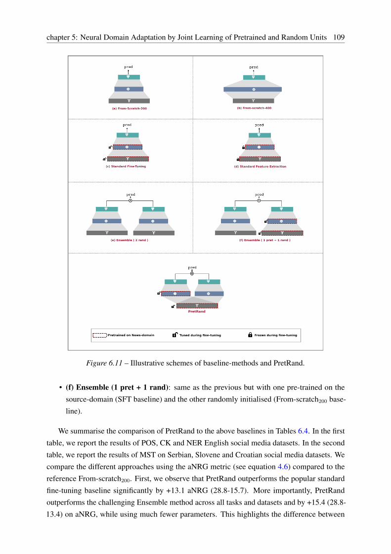
chapter 5: Neural Domain Adaptation by Joint Learning of Pretrained and Random Units 109

Figure 6.11 – Illustrative schemes of baseline-methods and PretRand.

• (f) Ensemble (1 pret + 1 rand): same as the previous but with one pre-trained on the

source-domain (SFT baseline) and the other randomly initialised (From-scratch200 base-

line).

We summarise the comparison of PretRand to the above baselines in Tables 6.4. In the first

table, we report the results of POS, CK and NER English social media datasets. In the second

table, we report the results of MST on Serbian, Slovene and Croatian social media datasets. We

compare the different approaches using the aNRG metric (see equation 4.6) compared to the

reference From-scratch200. First, we observe that PretRand outperforms the popular standard

fine-tuning baseline significantly by +13.1 aNRG (28.8-15.7). More importantly, PretRand

outperforms the challenging Ensemble method across all tasks and datasets and by +15.4 (28.8-

13.4) on aNRG, while using much fewer parameters. This highlights the difference between

110 6.3. THE PROPOSED METHOD: PRETRAND

Method #paramsPOS (acc.) CK (acc.) NER (F1)

aNRGTPoS ArK TweeBank TChunk WNUT

From-scratch200 1× 86.82 91.10 91.66 85.96 36.75 0

From-scratch400 1.03× 86.61 91.31 91.81 87.11 38.64 +2.7

Feature Extraction 1× 86.08 85.25 87.93 81.49 27.83 -32.4

Fine-Tuning 1× 89.57 92.09 93.23 88.86 41.25 +15.7

Ensemble (2 rand) 2× 88.98 91.45 92.26 86.72 39.54 +7.5

Ensemble (1p+1r) 2× 88.74 91.67 93.06 88.78 42.66 +13.4

PretRand 1.02× 91.27 93.81 95.11 89.95 43.12 +28.8

Method #paramsMST (acc.)

aNRGSerbian Slovene Croatian

From-scratch200 1× 86.18 84.42 85.67 0

From-scratch400 1.03× 86.05 84.37 85.77 -0.2

Feature Extraction 1× 73.56 70.22 79.11 -76.1

Fine-Tuning 1× 87.59 88.76 88.79 +19.9

Ensemble (2 rand) 2× 87.01 84.67 86.05 +3.4

Ensemble (1p+1r) 2× 87.96 88.54 88.87 +20.6

PretRand 1.02× 88.21 90.01 90.23 +27.5

Table 6.4 – Comparison of PretRand to baselines methods. Comparison of our method to

baselines in terms of token-level accuracy for POS, CK and MST and entity-level F1 for NER

(in %) on social media test-sets. In the second column (#params), we highlight the number

of parameters of each method compared to the reference From-scratch200 baseline. In the last

column, we report the aNRG score of each method compared to the reference From-scratch200.

Best score per dataset is in bold, and the second best score is underlined.

our method and the ensemble methods. Indeed, in addition to normalisation and weighting

vectors, PretRand is conceptually different since the random and pretrained branches share the

WRE component. Also, the results of From-scratch400 compared to From-scratch200 baseline

confirm that the gain brought by PretRand is not due to the supplement parameters. In the

following (§6.3.2.3), we show that the gain brought by PretRand is mainly due to the shared

word representation in combination with the normalisation and the learnable weighting vectors

during training. Moreover, a key asset of PretRand is that it uses only 0.02% more parameters

compared to the fine-tuning baseline.

6.3.2.3 Diagnostic Analysis of the Importance of PretRand’s Components

While in the precedent experiment we reported the best performance of PretRand, here we carry

out an ablation study to diagnose the importance of each component in our proposed approach.

chapter 5: Neural Domain Adaptation by Joint Learning of Pretrained and Random Units 111

Specifically, we successively ablate the main components of PretRand, namely, the learnable

weighting vectors (learnVect), the longer training of the random branch (random++) and the

normalisation (`2-norm). From the results in Table 6.5, we can first observe that ablating each of

them successively degrades the results across all datasets, which highlights the importance of

each component. Second, the results are only marginally better than than the SFT when ablating

the three components from PretRand (the last line in Table 6.5). Third, ablating the normalisation

layer significantly hurts the performance across all data-sets, confirming the importance of this

step, making the two branches more competitive.

MethodPOS CK NER MST

TPoS ArK TweeBank TChnuk WNUT Serbian Slovene CroatianPretRand 91.27 93.81 95.11 89.95 43.12 88.21 90.01 90.23-learnVect 91.11 93.41 94.71 89.64 42.76 88.01 89.83 90.12-learnVect -random++ 90.84 93.56 94.26 89.05 42.70 87.85 89.39 89.51-learnVect -random++ -l2 norm 90.54 92.19 93.28 88.66 41.84 87.66 88.64 88.49

Table 6.5 – Diagnostic analysis of the importance of each component in PretRand. Accuracy for

POS, CK and MST and F1 for NER (in %) when progressively ablating PretRand components.

6.3.2.4 Incorporating Contextualised Word Representations

So far in our experiments, we have used only the standard pre-loaded words embeddings and

character-level embeddings in the WRE component. Here, we perform a further experiment that

examines the effect of incorporating the ELMo contextualised word representations in different

tasks and training schemes (From-scratch, SFT and PretRand). Specifically, we carry out an

ablation study of WRE’s representations, namely, the standard pre-loaded words embeddings

(word), character-level embeddings (char) and ELMo contextualised embeddings (ELMo). The

ablation leads to 7 settings; in each, one or more representations are ablated. Results are provided

in Table 6.6, “ ” means that the corresponding representation is used and “ ” means that it is

ablated. For instance, in setting A only character-level representation is used.

Three important observations can be highlighted. First, in training from scratch scheme,

as expected, contextualised ELMo embeddings have a considerable effect on all datasets and

tasks. For instance, setting D (using ELMo solely) outperforms setting C (standard concatenation

between character-level and word-level embeddings), considerably on Chunking and NER

and slightly on POS tagging (except ArK). Furthermore, combining ELMo embeddings to the

standard concatenation between character-level and word-level embeddings (setting G) gives

the best results across all tasks and social media datasets. Second, when applying our transfer

learning approaches, whether SFT or PretRand, the gain brought by ELMo embeddings (setting

G) compared to standard concatenation between character-level and word-level embeddings

(setting C) is slight on POS tagging (in average, SFT: +0.76% , PretRand: +0.22%) and Croatian

MS tagging (SFT: +0.21% , PretRand: +0.10%), whilst is considerable on CK (SFT: +1.89% ,

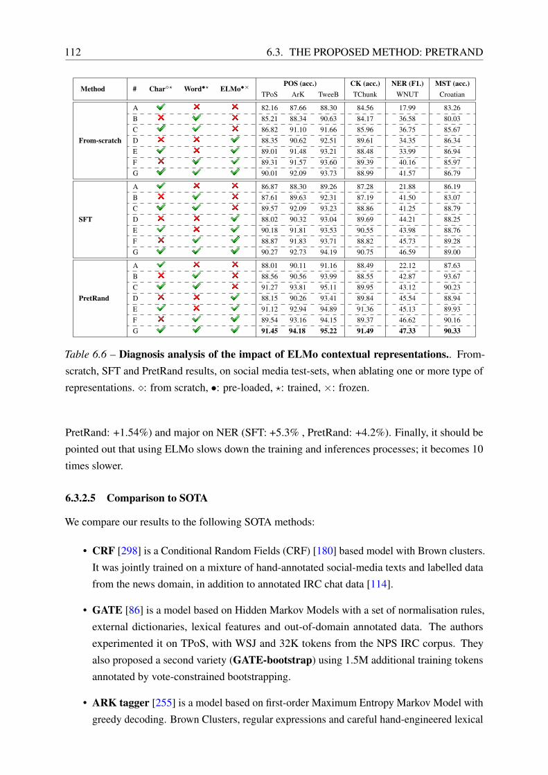
112 6.3. THE PROPOSED METHOD: PRETRAND

Method # Char�? Word•? ELMo•×POS (acc.) CK (acc.) NER (F1.) MST (acc.)

TPoS ArK TweeB TChunk WNUT Croatian

From-scratch

A 82.16 87.66 88.30 84.56 17.99 83.26B 85.21 88.34 90.63 84.17 36.58 80.03C 86.82 91.10 91.66 85.96 36.75 85.67D 88.35 90.62 92.51 89.61 34.35 86.34E 89.01 91.48 93.21 88.48 33.99 86.94F 89.31 91.57 93.60 89.39 40.16 85.97G 90.01 92.09 93.73 88.99 41.57 86.79

SFT

A 86.87 88.30 89.26 87.28 21.88 86.19B 87.61 89.63 92.31 87.19 41.50 83.07C 89.57 92.09 93.23 88.86 41.25 88.79D 88.02 90.32 93.04 89.69 44.21 88.25E 90.18 91.81 93.53 90.55 43.98 88.76F 88.87 91.83 93.71 88.82 45.73 89.28G 90.27 92.73 94.19 90.75 46.59 89.00

PretRand

A 88.01 90.11 91.16 88.49 22.12 87.63B 88.56 90.56 93.99 88.55 42.87 93.67C 91.27 93.81 95.11 89.95 43.12 90.23D 88.15 90.26 93.41 89.84 45.54 88.94E 91.12 92.94 94.89 91.36 45.13 89.93F 89.54 93.16 94.15 89.37 46.62 90.16G 91.45 94.18 95.22 91.49 47.33 90.33

Table 6.6 – Diagnosis analysis of the impact of ELMo contextual representations.. From-

scratch, SFT and PretRand results, on social media test-sets, when ablating one or more type of

representations. �: from scratch, •: pre-loaded, ?: trained, ×: frozen.

PretRand: +1.54%) and major on NER (SFT: +5.3% , PretRand: +4.2%). Finally, it should be

pointed out that using ELMo slows down the training and inferences processes; it becomes 10

times slower.

6.3.2.5 Comparison to SOTA

We compare our results to the following SOTA methods:

• CRF [298] is a Conditional Random Fields (CRF) [180] based model with Brown clusters.

It was jointly trained on a mixture of hand-annotated social-media texts and labelled data

from the news domain, in addition to annotated IRC chat data [114].

• GATE [86] is a model based on Hidden Markov Models with a set of normalisation rules,

external dictionaries, lexical features and out-of-domain annotated data. The authors

experimented it on TPoS, with WSJ and 32K tokens from the NPS IRC corpus. They

also proposed a second variety (GATE-bootstrap) using 1.5M additional training tokens

annotated by vote-constrained bootstrapping.

• ARK tagger [255] is a model based on first-order Maximum Entropy Markov Model with

greedy decoding. Brown Clusters, regular expressions and careful hand-engineered lexical

chapter 5: Neural Domain Adaptation by Joint Learning of Pretrained and Random Units 113

features were also used.

• TPANN [138] is a biLSTM-CRF model that uses adversarial pre-training (the method

described in §2.5.1) to leverage huge amounts of unlabelled social media texts, in addition

to labelled datasets from the news domain. Next, the pretrained model is further fine-

tuned on social media annotated examples. Also, regular expressions were used to tag

Twitter-specific classes (hashtags, usernames, urls and @-mentions).

• Flairs [6] is a biLSTM-CRF sequence labelling architecture fed with the Pooled Contextual

Embeddings [7] (pre-trained on character-level language models).

• UH&CU [337] is a biLSTM-based sequence labelling model for MST, jointly trained on

formal and informal texts. It is similar to our base model, but used 2-stacked biLSTM

layers. In addition, the particularity of UH&CU is that the final predictions are generated

as character sequences using an LSTM decoder, i.e. a character for each morpho-syntactic

feature instead of an atomic label.

• Multi-dataset-multi-task (MDMT) [235] consists in a multi-task training of 4 NLP tasks:

POS, CK, super sense tagging and NER, on 20 Tweets datasets 7 POS, 10 NER, 1 CK,

and 2 super sense–tagged datasets. The model is based on a biLSTM-CRF architecture

and words representations are based on the pre-trained ELMo embeddings.

• Data Annealing (DA) [136] is a fine-tuning approach similar to our SFT baseline, but

the passage from pretraining to fine-tuning is performed gradually, i.e. the training starts

with only formal text data (news) at first; then, the proportion of the informal text data

(social media) is gradually increased during the training process. They experiment with

two architectural varieties, a biLSTM-based architecture (DA-LSTM) and a Transformer-

based architecture (DA-BERT). In the last variety, the model is initialised with BERTbasepretrained model (110 million parameters). A CRF classifier is used as a classifier on the

top of both varieties, biLSTM and BERT.

• BertTweet [247] is a large-scale model pretrained on an 80GB corpus of 850M English

Tweets. The model is trained using BERTbase [87] architecture and following the pre-

training procedure of RoBERTa [202]. In order to perform POS tagging and NER, a

randomly initialised linear prediction layer is appended on top of the last Transformer

layer of BERTweet, and then the model is fine-tuned on target tasks examples. In addition,

lexical dictionaries were used to normalise social media texts.

In Table 6.7, we compare our best results (PretRand with the incorporation of ELMo) to

SOTA across tasks and datasets. We can observe that PretRand outperforms best SOTA results on

POS tagging datasets (except TPoS), Chunking (+4%) and Slovene (+1.5%) and Croatian (1.6%)

MS tagging. However, it performs worse than UH&UC for Serbian MS tagging. This could be

114 6.3. THE PROPOSED METHOD: PRETRAND

MethodPOS (acc.) CK (acc.) NER (F1.) MST (acc.)

TPoS ArK TweeBank TChunk WNUT Sr Sl Hr

CRF [298]? 88.3 n/a n/a 87.5 n/a n/a n/a n/aGATE [86]? 88.69 n/a n/a n/a n/a n/a n/a n/aGATE-bootstrap [86]? 90.54 n/a n/a n/a n/a n/a n/a n/aARK tagger [255]? 90.40 93.2 94.6 n/a n/a n/a n/a n/aTPANN [138]? × 90.92 92.8 n/a n/a n/a n/a n/a n/aFlairs [6]� n/a n/a n/a n/a 49.59 n/a n/a n/aMDMT [235]� × 91.70 91.61 92.44 n/a 49.86 n/a n/a n/aDA-LSTM [136]× 89.16 n/a n/a n/a n/a n/a n/a n/aDA-BERT [136]• × 91.55 n/a n/a n/a n/a n/a n/a n/aBertTweet [247]• ? 90.1 94.1 95.2 n/a 54.1 n/a n/a n/aUH&UC [337] n/a n/a n/a n/a n/a 90.00 88.4 88.7

PretRand (our best)� 91.45 94.18 95.22 91.49 47.33 88.21 90.01 90.33

Table 6.7 – Comparison of PretRand to the best published state-of-the-art methods in terms of

token-level accuracy for POS, CK and MST and F1 for NER (in %) on social media datasets. �:use of contextualised representations. •: use of BERT pretrained model. ?: use of normalisation

dictionaries, regular expressions or external knowledge. ×: use of a CRF classifier on top of the

neural model.

explained by the fact that the Serbian source dataset (news) is small compared to Slovene and

Croatian, reducing the gain brought by pretraining and thus that brought by PretRand. Likewise,

Akbik et al. [6] outperforms our approach on NER task, in addition to using a CRF on top of

the biLSTM layer, they used Contextual string embeddings that have been shown to perform

better on NER than ELMo [6]. Also, MDMT outperforms PretRand slightly on TPoS dataset.

We can observe that BERT-based approaches (DA-BERT and BertTweet) achieve strong results,

especially on NER, where BertTweet begets the best SOTA score. Finally, we believe that adding

a CRF classification layer on top of our models will boost our results (like TPANN, MDMT,

DA-LSTM and DA-BERT), as it is able to model strong dependencies between adjacent words.

Note that, MDMT, DA-LSTM, DA-BERT and BertTweet are recent works, published after our

work.

6.3.3 Analysis

In this section, we perform an empirical analysis of PretRand. First, we investigate the scenarios

in which PretRand is most advantageous (§6.3.3.1). Second, we compare the hidden negative

transfer brought by SFT vs PretRand (§6.3.3.2). Third, we visualise new target-specific features

learnt by individual neurons in the random branch of PretRand (§6.3.3.3).

6.3.3.1 When and where PretRand is most Beneficial?

Here, we attempt to examine in which scenarios PretRand is most beneficial. We firstly explore in

Figure 6.12, which class from TweeBank dataset benefits more from PretRand compared to SFT.

chapter 5: Neural Domain Adaptation by Joint Learning of Pretrained and Random Units 115

After that, we evaluate in Figure 6.13 the gain on accuracy brought by PretRand compared to SFT,

according to different target-datasets’ sizes. We observe that PretRand has desirably a bigger

gain with bigger target-task datasets, which clearly means that the more target training-data, the

more interesting our method will be. This observation may be because the random branch needs

sufficient amounts of target training samples to become more competitive with the pretrained

one.

Figure 6.12 – Sorted class-accuracy improvement (%) on TweeBank of PretRand compared to

fine-tuning.

Figure 6.13 – Performances (on dev-set of TweeBank) according different training-set sizes

for the target-dataset. Transparent green highlights the difference between our PretRand and

standard fine-tuning.

6.3.3.2 Negative Transfer: PretRand vs SFT

Here, we resume the negative transfer experiment performed in section 6.2.2.1. Precisely, we

compare the results of PretRand to those of SFT. We show in Figure 6.14 the results on English

social media datasets, first tagged with the classic training scheme (From-scratch-200) and then

using SFT in the left plot (or using PretRand in the right plot). Blue bars show the percentage

of positive transfer, i.e. predictions that were wrong, but the SFT (or PretRand) changed to the

correct ones, and red bars give the percentage of negative transfer, i.e. predictions that were

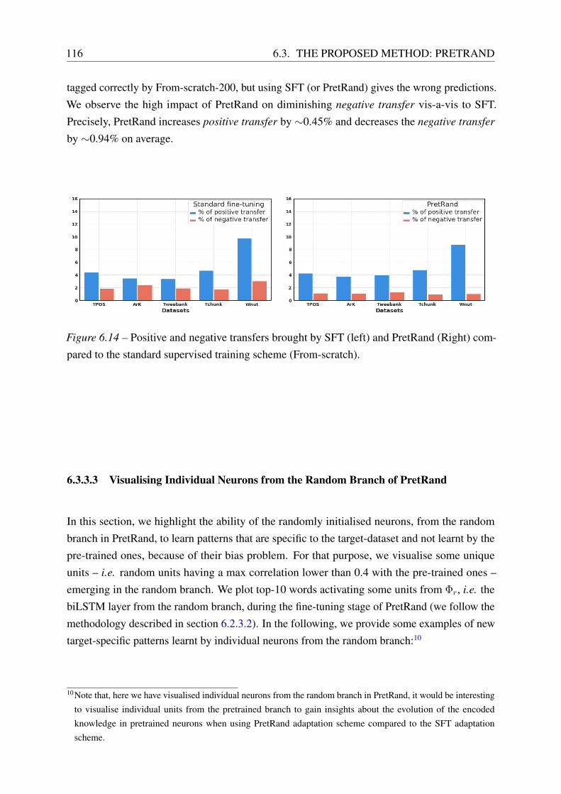
116 6.3. THE PROPOSED METHOD: PRETRAND

tagged correctly by From-scratch-200, but using SFT (or PretRand) gives the wrong predictions.

We observe the high impact of PretRand on diminishing negative transfer vis-a-vis to SFT.

Precisely, PretRand increases positive transfer by ∼0.45% and decreases the negative transfer

by ∼0.94% on average.

Figure 6.14 – Positive and negative transfers brought by SFT (left) and PretRand (Right) com-

pared to the standard supervised training scheme (From-scratch).

6.3.3.3 Visualising Individual Neurons from the Random Branch of PretRand

In this section, we highlight the ability of the randomly initialised neurons, from the random

branch in PretRand, to learn patterns that are specific to the target-dataset and not learnt by the

pre-trained ones, because of their bias problem. For that purpose, we visualise some unique

units – i.e. random units having a max correlation lower than 0.4 with the pre-trained ones –

emerging in the random branch. We plot top-10 words activating some units from Φr, i.e. the

biLSTM layer from the random branch, during the fine-tuning stage of PretRand (we follow the

methodology described in section 6.2.3.2). In the following, we provide some examples of new

target-specific patterns learnt by individual neurons from the random branch:10

10Note that, here we have visualised individual neurons from the random branch in PretRand, it would be interestingto visualise individual units from the pretrained branch to gain insights about the evolution of the encodedknowledge in pretrained neurons when using PretRand adaptation scheme compared to the SFT adaptationscheme.

chapter 5: Neural Domain Adaptation by Joint Learning of Pretrained and Random Units 117

• ARK dataset - POS: (Figure 6.15)

– Unit-69 is sensitive to the ARK’s special tag “L” that stands for “nominal + verbal”

(e.g. i’m, it’s, that’s).

– Unit-84 is specific to frequent misspellings in Tweets. For instance, omitting the last

“g” in words ending with “ing”, e.g. doin, goin, tryin.

ARK dataset - Unit-69: Specific to ARK’s special tag (L)

ArK dataset - Unit-84: Specific to frequent misspellings in Tweets

Figure 6.15 – Individual units activations (from the random branch) before and duringfine-tuning PretRand on ArK social media dataset. For each unit we show in column 0:

top-10 words from ArK dev-set before fine-tuning (random init). Columns 1 to 10: top-10 words

from the target dev-set during fine-tuning epochs.

• TweeBank dataset - POS: (Figure 6.16)

We show top-10 words activating two units, unit-160 and unit-04. Both are sensitive to

words like gonna (going to) or wanna (want to), frequently used contractions in Tweets.

Indeed, in TweeBank, these words are tokenized into two tokens: gon and na, with the

later annotated as a “particle” and the former as a “verb”. We observe that unit-160 is

highly discriminative to the “verb” part and unit-04 to the “particle” part.

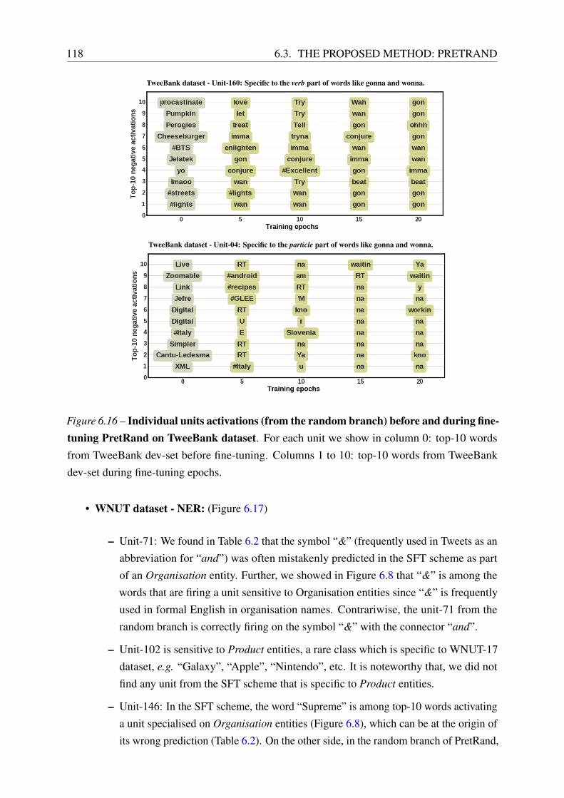
118 6.3. THE PROPOSED METHOD: PRETRAND

TweeBank dataset - Unit-160: Specific to the verb part of words like gonna and wonna.

TweeBank dataset - Unit-04: Specific to the particle part of words like gonna and wonna.

Figure 6.16 – Individual units activations (from the random branch) before and during fine-tuning PretRand on TweeBank dataset. For each unit we show in column 0: top-10 words

from TweeBank dev-set before fine-tuning. Columns 1 to 10: top-10 words from TweeBank

dev-set during fine-tuning epochs.

• WNUT dataset - NER: (Figure 6.17)

– Unit-71: We found in Table 6.2 that the symbol “&” (frequently used in Tweets as an

abbreviation for “and”) was often mistakenly predicted in the SFT scheme as part

of an Organisation entity. Further, we showed in Figure 6.8 that “&” is among the

words that are firing a unit sensitive to Organisation entities since “&” is frequently

used in formal English in organisation names. Contrariwise, the unit-71 from the

random branch is correctly firing on the symbol “&” with the connector “and”.

– Unit-102 is sensitive to Product entities, a rare class which is specific to WNUT-17

dataset, e.g. “Galaxy”, “Apple”, “Nintendo”, etc. It is noteworthy that, we did not

find any unit from the SFT scheme that is specific to Product entities.

– Unit-146: In the SFT scheme, the word “Supreme” is among top-10 words activating

a unit specialised on Organisation entities (Figure 6.8), which can be at the origin of

its wrong prediction (Table 6.2). On the other side, in the random branch of PretRand,

chapter 5: Neural Domain Adaptation by Joint Learning of Pretrained and Random Units 119

the word “Supreme” is among top-10 words activating unit-146, which is specialised

in PERSON entities.

WNUT dataset: Unit-71 is firing on “&” , “and” and “with”

WNUT dataset: Unit-102 is sensitive to PRODUCTS (Specific class to WNUT dataset)

WNUT dataset: Unit-146 is sensitive to PERSONS, including “Supreme”.

Figure 6.17 – Individual units activations (from the random branch) before and duringfine-tuning PretRand on WNUT NER dataset. For each unit we show in column 0: top-10

words from WNUT dev-set before fine-tuning. Columns 1 to 10: top-10 words from WNUT

dev-set during fine-tuning epochs.

120 6.4. CONCLUSION

6.4 Conclusion

Stemming from our analysis, we have introduced a novel approach, that we called PretRand, to

overcome the observed problems using 3 main ideas: adding random units and jointly learn them

with pre-trained ones; normalising the activations of both to balance their different behaviours;

applying learnable weights on both predictors to let the network learn which of random or

pre-trained one is better for every class. The underlying idea is to take advantage of both,

target-specific features from the former and general knowledge from the latter. We carried

out experiments on domain adaptation for 4 tasks: part-of-speech tagging, morpho-syntactic

tagging, chunking and named entity recognition. Our approach exhibits performances that are

significantly above standard fine-tuning scheme and is highly competitive when compared to the

state-of-the-art.

We believe that many prosperous directions should be addressed in future research. First,

PretRand’s good results on sequence labelling tasks suggest to consider other kinds of NLP tasks,

e.g. sequence-to-sequence and text classification tasks. Further, as negative transfer, and thus

bias, is highly arising when transferring between less-related source-target domains [373], we

suppose that PretRand’s impact would be more interesting for cross-lingual transfer. Second, in

this work, we experimented PretRand adaptation scheme on models pre-trained in a supervised

manner, an important step forward is to examine its scalability with other pretraining methods,

e.g adversarial or unsupervised pretraining. Third, the increasing omnipresence of Transformers

architectures in a wide range of NLP tasks, due to their improved performances, motivates

us to experiment with Transformer-based architecture instead of LSTM-based one. Last, a

propitious continuity of our work to tackle the bias problem, would be to identify automatically

biased neurons in the pre-trained model and proceed to a pruning of the most biased ones before

fine-tuning.

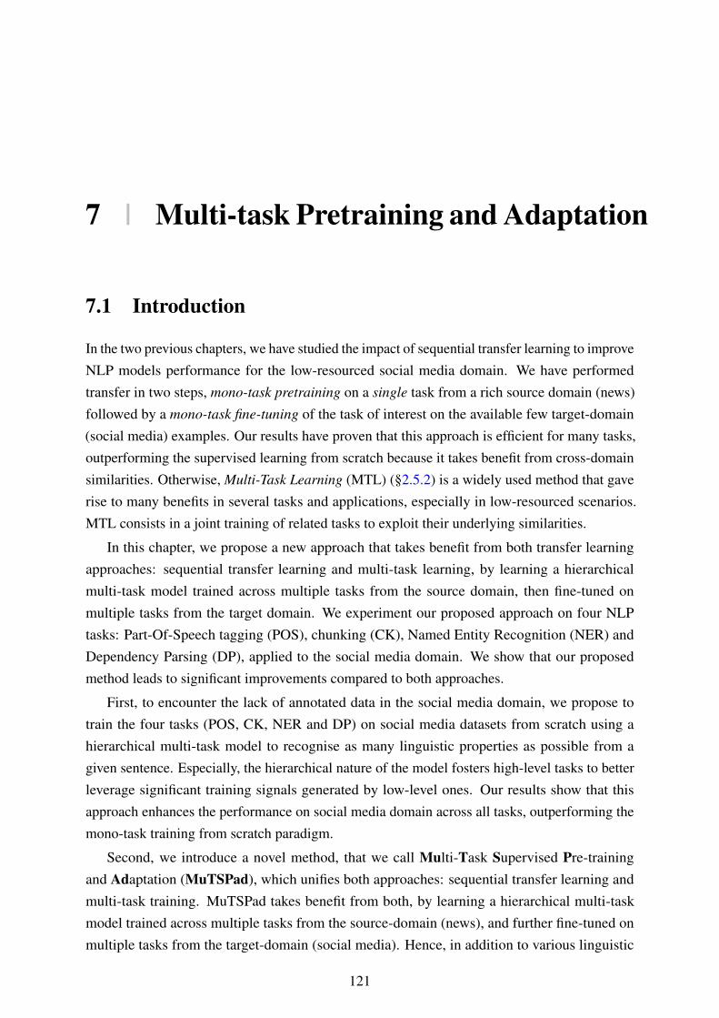
7 | Multi-task Pretraining and Adaptation

7.1 Introduction

In the two previous chapters, we have studied the impact of sequential transfer learning to improve

NLP models performance for the low-resourced social media domain. We have performed

transfer in two steps, mono-task pretraining on a single task from a rich source domain (news)

followed by a mono-task fine-tuning of the task of interest on the available few target-domain

(social media) examples. Our results have proven that this approach is efficient for many tasks,

outperforming the supervised learning from scratch because it takes benefit from cross-domain

similarities. Otherwise, Multi-Task Learning (MTL) (§2.5.2) is a widely used method that gave

rise to many benefits in several tasks and applications, especially in low-resourced scenarios.

MTL consists in a joint training of related tasks to exploit their underlying similarities.

In this chapter, we propose a new approach that takes benefit from both transfer learning

approaches: sequential transfer learning and multi-task learning, by learning a hierarchical

multi-task model trained across multiple tasks from the source domain, then fine-tuned on

multiple tasks from the target domain. We experiment our proposed approach on four NLP

tasks: Part-Of-Speech tagging (POS), chunking (CK), Named Entity Recognition (NER) and

Dependency Parsing (DP), applied to the social media domain. We show that our proposed

method leads to significant improvements compared to both approaches.

First, to encounter the lack of annotated data in the social media domain, we propose to

train the four tasks (POS, CK, NER and DP) on social media datasets from scratch using a

hierarchical multi-task model to recognise as many linguistic properties as possible from a

given sentence. Especially, the hierarchical nature of the model fosters high-level tasks to better

leverage significant training signals generated by low-level ones. Our results show that this

approach enhances the performance on social media domain across all tasks, outperforming the

mono-task training from scratch paradigm.

Second, we introduce a novel method, that we call Multi-Task Supervised Pre-training

and Adaptation (MuTSPad), which unifies both approaches: sequential transfer learning and

multi-task training. MuTSPad takes benefit from both, by learning a hierarchical multi-task

model trained across multiple tasks from the source-domain (news), and further fine-tuned on

multiple tasks from the target-domain (social media). Hence, in addition to various linguistic

121

122 7.2. PROPOSED APPROACH

properties learned from various supervised NLP tasks, MuTSPad takes advantage of the pre-

learned knowledge from the high-resource source-domain. MuTSPad exhibits significantly better

performance than both TL approaches.

Third, as in our case, we have two datasets, the first for news domain and the second for social

media domain, both are heterogeneous, i.e. having one task-annotation per sentence.1 Though,

many early works had highlighted the intricacy of multi-task training from heterogeneous

datasets [345] since a scheduling procedure is needed. Therefore, we propose to build multi-task

datasets for the news and social media domains, by automatically augmenting the data to unify

the aforementioned task-independent datasets.

The remainder of this chapter is as follows. First, we describe our approaches in section 7.2.

Second, we present the experimental settings in section 7.3. Third, we provide our results and

analysis in section 7.4. Finally, we conclude our findings in section 7.5.

7.2 Proposed Approach

We propose a new approach that combines two transfer learning approaches:

1. Mono-task pretraining (standard fine-tuning): pretraining the neural model on a rich

source-task before updating its weights using the standard fine-tuning scheme on the task

of interest (target task);

2. Multi-task learning: training the task of interest jointly with other auxiliary tasks with

labelled data that might force the network to learn useful features.

Both approaches are known to work very well since a while and have yielded impressive

results in recent years. Here, to make sure that we learn useful features that are relevant for the

tasks of our interest, we propose an approach that combines pretraining and multi-task learning,

and thus takes benefits from the rich source-domain, and especially all its available annotated data

and tasks. We call our method: Multi-Task Supervised Pre-training and Adaptation (MuTSPad).

MuTSPad roughly consists in pretraining on a large annotated multi-task source datasets and

then fine-tuning it on the multi-task target datasets.

We present in this section our proposed approach. We start by describing briefly the basic

neural models to perform POS, NER, CK and DP tasks (§7.2.1). Then, we present the hierarchical

multi-task architecture that allows training the four tasks jointly (§7.2.2). Next, we present

our approach to train MuTSPad (§7.2.3). Finally, we discuss how we perform MTL with

heterogeneous datasets (§7.2.4).

1 To the best of our knowledge, there are no available common datasets containing annotations for all the above-mentioned tasks, neither for the news domain or the social media domain.

Chapter 6: Multi-task Pretraining and Adaptation 123

7.2.1 Basic Models

As mentioned above, POS, CK, NER and DP are the four tasks considered in this work. We

start by describing briefly the base neural model used to train each task individually; sequence

labelling architecture (POS, CK, NER) (§7.2.1.1) and DP architecture (§7.2.1.2).

7.2.1.1 Sequence Labelling Architecture

Recalling that, given an input sentence S of n successive tokens S = [w1, . . . , wn] and a tag-set

C, sequence labelling aims to predict the tag ci ∈ C of every wi. For the base neural architecture,

we use the commonly used model (described in details in section 5.2.1), that includes three main

components:

1. Word Representation Extractor (WRE), denoted Υ.

2. Features Extractor (FE), denoted Φ.

3. Classifier (Cl), denoted Ψ.

WRE computes a word-level embedding (xwordi =Υword(wi)) and a character-level biLSTMs

encoder-based embedding (xchari =Υchar(wi)), and concatenates them to get a final representation

xi=(xwordi ,xchari ) for each token wi. WRE’s outputs [x1, . . . ,xn] are fed into the FE, a single

biLSTMs layer, that outputs a context sensitive representation for each wi. Finally, Cl consists

of a softmax fully-connected layer that produces the classes-probabilities for each wi as follows:

yi = (Ψ ◦ Φ ◦Υ)(wi).

7.2.1.2 Dependency Parsing Architecture

Given an input sentence S = [w1, . . . , wn] of n successive tokens, the goal of DP is two folds:

1. Identifying, for each wi, its head wj ∈ S. The couple of tokens wi and wj are called the

dependant and the head, respectively.

2. Predicting the dependency syntactic relation’s class rij ∈Rdp relating each dependant-head

pair, whereRdp is the dependency-relations set.

In simple words, the goal is to predict the out-going labelled arc (wi, wj, rij) for each token wi.

Thus, constructing a syntactic tree structure of the sentence, where words are treated as nodes in

a graph, connected by labelled directed arcs.

We use the neural arc-factored graph-based dependency parser [280] which is based on the

“Deep biAffine parser” [95]. As in sequence labelling models, the DP architecture is composed of

three components (illustrated in Figure 7.1): a word representation component (WRE), denoted

Υdp, followed by a feature extractor, denoted Φdp, and a classifier, denoted Ψdp. Except that Φdp

124 7.2. PROPOSED APPROACH

is a 3-stacked biLSTM network,2 and Ψdp consists of four classifiers, producing four distinct

vectors for representing the word: (i) as a dependant seeking its head; (ii), as a head seeking all

its dependants; (iii), as a dependant deciding on its relation; and (iv), as a head deciding on the

labels of its dependants. These representations are then passed to the biAffine softmax classifiers.

Figure 7.1 – Illustrative scheme of the neural arc-factored graph-based dependency parser.

Precisely, the biAffine classifier component (Ψdp) calculates the arc probability between each

pair of words as well as a syntactic label for each arc. The FE outputs [h1, . . . ,hn] are fed into

the biaffine classifier. Then, for each word wi, the four MLP (Multi-Layer Perceptron) layers

produce 4 vectors as follows:

varc−headi = MLP arc−head(hi) , (7.1)

varc−depi = MLP arc−dep(hi) , (7.2)

vlabel−headi = MLP label−head(hi) , (7.3)

vlabel−depi = MLP label−dep(hi) , (7.4)

where varc−headi , varc−depi ∈ Rn and vlabel−headi , vlabel−depi ∈ R|Rdp|. The first vector is a head

seeking all its dependants; the second is a dependant seeking its head; the third is a head deciding

on the labels of its dependants, and the fourth is a dependant deciding on its relation. Then, a

score sarci,j of arc between each words-pair (wi, wj) is calculated using a biaffine transformation:

sarci,j = (varc−headi )T W varc−depj + (varc−headi )T barc , (7.5)

where W ∈ Rn × n and b ∈ Rn.

Similarly, a score sli,j for each l ∈ Rdp being the label of the arc relating the head wi to its

dependant wj is calculated as follows:

2 Here we use the same hyper-parameters as the original paper.

Chapter 6: Multi-task Pretraining and Adaptation 125

sli,j = (vlabel−headi )T Ul vlabel−headj + (vlabel−headi ⊕ vlabel−depj )T bl + bl , (7.6)

where the parameters Ul ∈ R|Rdp| × |Rdp|, bl ∈ R2 × |Rdp| and the scalar bl are distinct for each

label l ∈ Rdp.

7.2.2 Multi-Task Learning

We describe, in section 7.2.2.1, the proposed hierarchical multi-task model for the joint learning

of POS, CK, NER and DP. Then, in section 7.2.2.2, we discuss the training process.

7.2.2.1 Hierarchical Multi-Task Architecture

As we aim to learn a multi-task model where POS, CK, NER and DP tasks are learned jointly,

we choose a hard-sharing architecture scheme which contains a common branch as well as four

exits, one per task. Also, as the tasks are hierarchically related to each other, we adopted a

hierarchical architecture. The hierarchical structure in multi-task learning has been successfully

used in the literature. First, Søgaard and Goldberg [340] showed that, considering the linguistic

hierarchies of NLP tasks, the standard multi-task architecture where all tasks are at the same

outermost level is “sub-optimal”. Further, Hashimoto et al. [148] proposed a joint model for a set

of syntactic and semantic tasks: POS, CK, DP, semantic relatedness and textual entailment, and

Sanh et al. [314] proposed a joint hierarchical model for semantic tasks: co-reference resolution,

relation extraction, entity mention Detection and NER.

We organise the four tasks from low-level to high-level ones, with each task being fed with a

shared word embedding as well as the outputs of all the lower tasks. To construct that hierarchy of

tasks, we followed some linguistic hints from the literature. Indeed, many works have shown that

POS improves CK [392, 305]; NER benefits from POS [303] and CK [67]; and DP profits from

POS and CK [148]. In simple terms, POS and CK are considered as “universal helpers” [53].

Thus, based on these linguistic hierarchy observations, we feed POS features to CK; then POS

and CK features to both NER and DP.

An illustration of our multi-task hierarchical model is given in Figure 7.2. We can separate

the multi-task model into 5 parts, a shared part and one branch per task:

• Shared parameters (Gray): The word representation extractor Υ is shared across all

tasks. It generates a word representation xi for each word wi: xi = Υ(wi), which is fed to

all tasks branches.

• POS branch (Black): The feature extractor component of the POS tagging branch (Φpos)

is fed with the output of the shared Υ and after processing, it outputs BiLSTMs features

hposi . This is then fed into the POS classifier Ψpos to calculate a probability distribution for

the POS tag-set as follows:

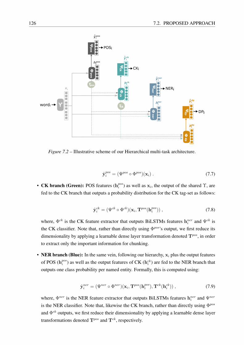
126 7.2. PROPOSED APPROACH

Figure 7.2 – Illustrative scheme of our Hierarchical multi-task architecture.

yposi = (Ψpos ◦ Φpos)(xi) . (7.7)

• CK branch (Green): POS features (hposi ) as well as xi, the output of the shared Υ, are

fed to the CK branch that outputs a probability distribution for the CK tag-set as follows:

ycki = (Ψck ◦ Φck)(xi,Tpos(hposi )) , (7.8)

where, Φck is the CK feature extractor that outputs BiLSTMs features hneri and Ψck is

the CK classifier. Note that, rather than directly using Φpos’s output, we first reduce its

dimensionality by applying a learnable dense layer transformation denoted Tpos, in order

to extract only the important information for chunking.

• NER branch (Blue): In the same vein, following our hierarchy, xi plus the output features

of POS (hposi ) as well as the output features of CK (hcki ) are fed to the NER branch that

outputs one class probability per named entity. Formally, this is computed using:

yneri = (Ψner ◦ Φner)(xi,Tpos(hposi ),Tck(hcki )) , (7.9)

where, Φner is the NER feature extractor that outputs BiLSTMs features hneri and Ψner

is the NER classifier. Note that, likewise the CK branch, rather than directly using Φpos

and Φck outputs, we first reduce their dimensionality by applying a learnable dense layer

transformations denoted Tpos and Tck, respectively.

Chapter 6: Multi-task Pretraining and Adaptation 127

• DP branch (Orange): similarly to the NER branch, the shared embedding, plus the output

features of POS as well as the output features of CK are fed to FEdp, followed by Cdp

which outputs:

ydpi = (Ψdp ◦ Φdp)(xi,Tpos(hposi ),Tck(hcki )) , (7.10)

where, Φdp is the DP feature extractor that outputs BiLSTMs features hdpi and Ψdp is

the DP classifier. Note that, likewise the other branches, rather than directly using Φpos

and Φck outputs, we first reduce their dimensionality by applying a learnable dense layer

transformations denoted Tpos and Tck, respectively.

7.2.2.2 Multi-Task Loss Calculation

In terms of loss functions, as in classical multi-task learning, we minimise the weighted sum of

each task loss:

LMT =

∑Mj=1 αtaskj × Ltaskj

N, (7.11)

where αtaskj represents the weight attributed to the taskj , and M is the number of tasks, and

Ltaskj is the loss of the task j.

As we used a hierarchical model for reasons mentioned in Section 7.2.2.1, we propose to

focus, at the early-stage training, on low-level tasks and progressively increase the focus on

higher-level ones3. Specifically, we tune the loss calculation minimisation by adapting the

loss weights during the training, starting with heavier weights for low-level tasks compared to

high-level ones. These weights are linearly increased for the first epochs, then kept constant

afterwards.

7.2.3 MuTSPad: Multi-Task Supervised Pretraining and Adaptation

Multi-task pretraining has been especially explored for learning universal representations. We

can cite the work of Cer et al. [51] who proposed joint learning of sentence embedding on a set of

unsupervised (SkipThought) and supervised (natural language inference) tasks. Ahmed et al. [5]

showed that joint learning of a biLSTM-based model on multiple tasks provides universal

sentence representations that generalise better using two classification tasks: natural language

inference and duplicate question detection. Similarly, Subramanian et al. [345] proposed to

build a general-purpose sentence encoder by a joint learning of machine translation, parse tree

generation and unsupervised skip-thought tasks. Likewise, multi-task fine-tuning has been

recently explored as part of universal models fine-tuning. Liu et al. [201] proposed to fine-tune

3 Along the same line of thought of Kiperwasser & Ballesteros [171] who modified tasks sampling during training.

128 7.2. PROPOSED APPROACH

the pre-trained universal model, BERT, in a multi-task fashion on multiple tasks: single-sentence

classification, pairwise text classification, text similarity, and relevance ranking.

Furthermore, in terms of using multi-task features for domain adaptation, Søgaard and Gold-

berg [340] showed the benefit of multi-task learning for domain adaptation from news-domain to

Weblogs-domain for CK task, when disposing of CK’s supervision only for the source-domain,

and lower-level POS supervision for the target-domain. Finally, in terms of unifying multi-task

learning and fine-tuning, Kiperwasser and Ballesteros [171] proposed to improve machine trans-

lation with the help of POS and DP tasks by scheduling tasks during training; starting with

multi-tasking of the principal task with auxiliary lower-level tasks (POS and DP), and as the

training graduates, the model trains only to the main task. However, to the best of our knowledge,

performing pretraining and fine-tuning on multi-task models for supervised domain adaptation

has not been explored in the literature.

In this work, we study multi-task pretraining and fine-tuning for supervised domain adap-

tations. We propose Multi-Task Supervised Pre-training and Adaptation (MuTSPad) which

consists in pretraining on a large annotated multi-task source dataset and then fine-tuning it on the

multi-task target dataset. As supervised and unsupervised pretraining, MuTSPad alleviates the

lack of annotated data in a target domain by taking benefit from rich source-domains. However,

compared to them, it does the pretraining on multiple tasks, and not only one. This brings even

more real supervision to the network and thus gives more chance to end up with more features.

Also important, as source-domains are usually richer than target-domains, we might always find

source-datasets that are labelled exactly with all the tasks we want to solve in the target-domain.

This enforces the network to learn only features that might be relevant for our tasks of interest,

and thus avoid filling up the network with irrelevant features.

Let us assume a set of M tasks T = [T1 , . . . , TM ], a set of datasets from the source domain

Ds = [Ds1 , . . . , D

sM ], and a set of datasets from the target domain Dt = [Dt

1 , . . . , DtM ],

where each task Ti is associated with a source dataset Dsi and a target dataset Dt

i .4 MuTSPad

consists of three steps:

1. A source hierarchical multitask model Ms is first trained on the set of heterogeneous

source-datasets Ds.

2. The learned parameters θs of the source modelMs are separated into two sets θs = (θ1s , θ2s).

The first set of parameters are then used to initialise the first set of parameters of the target

multi-task model (Mt), θ1t = θ1s , while the second set of target model parameters θ2t is

randomly initialised.

3. All the parameters ofMt are then adapted on the set of heterogeneous target-datasets Dt.

4 Here we use the same source and target tasks. However, the method can be extended to handle different sourceand target tasks.

Chapter 6: Multi-task Pretraining and Adaptation 129

Note that, even if the target-tasks and source-tasks might be the same, their label-sets might

differ. Thus as in classical fine-tuning, the parameters of each task-classifier (Ψpos, Ψck, Ψner

and Ψdp) are randomly initialised, while the shared Υ as well as the features extractors (Φpos,

Φck, Φner and Φdp) are initialised with the pretrained weights.

7.2.4 Heterogeneous Multi-Task Learning

When working on multi-task learning, we mostly face the heterogeneous scenario, where only

one task-labels might be assigned to a dataset. In that case, the classical multi-task learning

approach is not directly applicable; thus, we need to choose a “scheduling process” [403].

However, since training with different datasets for each task remains challenging [345], we

propose to perform a “Datasets Unification” to simplify the learning scenario.

7.2.4.1 Tasks Scheduling Procedure

To deal with this heterogeneous aspect, we first use a simple frozen uniform scheduling, which

we call “one task per batch”, where at each iteration of the training process, the task to train is

selected randomly (Similar to Zaremoodi et al. [403]). Specifically, the base steps of “one task

per mini-batch” scheduling process are as follow: 1) picking a mini-batch of samples from only

one particular task and 2) updating only the parameters corresponding to the selected task, as well

as the the task-agnostic parameters. Thus, at every step, only one task is trained. We successively

pick all the tasks following a constant ordering strategy “from lower-level to higher-level tasks”

[148]: POS then CK then NER then DP. Thus, every four steps, the model sees all the tasks once

and learns their corresponding parameters once.

7.2.4.2 Datasets Unification

To overcome the intricacy of the “tasks scheduling process”, we propose to construct a unified

dataset by combining several sources of independent textual annotations using a self-training

method. Since we are interested in benefiting from pretraining and fine-tuning, we apply the

unification process on both source and target datasets. These datasets contain samples of a broad

range of heterogeneous annotations in a variety of contexts (initially sentences are labelled only

with one task rather than all), making the multi-task training challenging. Thus, to circumvent this

problem, we propose to unify the target (social media domain) set of datasets Dt to form a unified

target dataset that we call SocialAll, denoted Dallt . We do the same with source datasets (news

domain) to form a unified multi-task dataset that we name NewsAll, denoted Dalls . Concretely,

we enrich the gold annotations of each task with an automatic annotation by applying on its

training-set our baseline Mono-Task Learning model of the other three tasks. In the end, we

obtain two unified datasets, one for the target domain and one for the source domain. Thus, in

both datasets each sentence is labelled with all tasks (one label is the initial manual annotation,

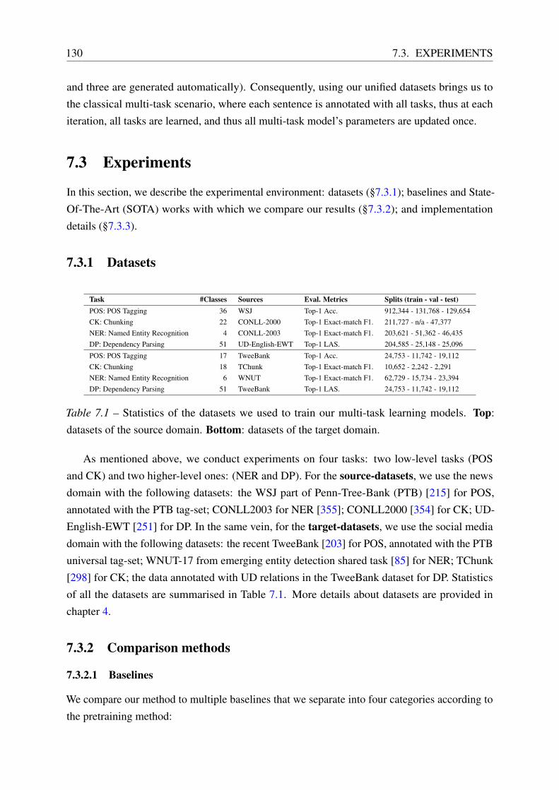
130 7.3. EXPERIMENTS

and three are generated automatically). Consequently, using our unified datasets brings us to

the classical multi-task scenario, where each sentence is annotated with all tasks, thus at each

iteration, all tasks are learned, and thus all multi-task model’s parameters are updated once.

7.3 Experiments

In this section, we describe the experimental environment: datasets (§7.3.1); baselines and State-

Of-The-Art (SOTA) works with which we compare our results (§7.3.2); and implementation

details (§7.3.3).

7.3.1 Datasets

Task #Classes Sources Eval. Metrics Splits (train - val - test)POS: POS Tagging 36 WSJ Top-1 Acc. 912,344 - 131,768 - 129,654CK: Chunking 22 CONLL-2000 Top-1 Exact-match F1. 211,727 - n/a - 47,377NER: Named Entity Recognition 4 CONLL-2003 Top-1 Exact-match F1. 203,621 - 51,362 - 46,435DP: Dependency Parsing 51 UD-English-EWT Top-1 LAS. 204,585 - 25,148 - 25,096

POS: POS Tagging 17 TweeBank Top-1 Acc. 24,753 - 11,742 - 19,112CK: Chunking 18 TChunk Top-1 Exact-match F1. 10,652 - 2,242 - 2,291NER: Named Entity Recognition 6 WNUT Top-1 Exact-match F1. 62,729 - 15,734 - 23,394DP: Dependency Parsing 51 TweeBank Top-1 LAS. 24,753 - 11,742 - 19,112

Table 7.1 – Statistics of the datasets we used to train our multi-task learning models. Top:

datasets of the source domain. Bottom: datasets of the target domain.

As mentioned above, we conduct experiments on four tasks: two low-level tasks (POS

and CK) and two higher-level ones: (NER and DP). For the source-datasets, we use the news

domain with the following datasets: the WSJ part of Penn-Tree-Bank (PTB) [215] for POS,

annotated with the PTB tag-set; CONLL2003 for NER [355]; CONLL2000 [354] for CK; UD-

English-EWT [251] for DP. In the same vein, for the target-datasets, we use the social media

domain with the following datasets: the recent TweeBank [203] for POS, annotated with the PTB

universal tag-set; WNUT-17 from emerging entity detection shared task [85] for NER; TChunk

[298] for CK; the data annotated with UD relations in the TweeBank dataset for DP. Statistics

of all the datasets are summarised in Table 7.1. More details about datasets are provided in

chapter 4.

7.3.2 Comparison methods

7.3.2.1 Baselines

We compare our method to multiple baselines that we separate into four categories according to

the pretraining method:

Chapter 6: Multi-task Pretraining and Adaptation 131

Without Pretraining: Training from scratch on the social media datasets (target-domain).

• Mono-Task Learning: an independent training of our mono-tasks models (one model per

task) on every target-task separately.5

• Multi-Task Learning: Joint training of our multi-task model described in section 7.2.2.1

on all the tasks from the target-domain; trained from scratch on social media datasets (one

model for all the tasks).

Unsupervised pretraining: We replace the WRE component in Mono-Task Learning by the un-

supervisedly pre-trained model, ELMo6 (Embeddings from Language Models) [265], consisting

of a CNNs-based character-level representation followed by a 2-layer LSTM. Thus, ELMo with

the randomly initialised FE and Cl are further trained on the target-domain tasks. Specifically,

we run experiments with two ELMo models: 1) ELMosmall: the small pre-trained model (13.6M

parameters) on 1 billion word benchmark. 2) ELMolarge: the big pre-trained model (93.6M

parameters) on 5.5 billion word benchmark.

Supervised pretraining7 on the source-domain of the network on each task independently then

fine-tuning on the same task in the target domain. Here, we call this method: Mono-Taskpretraining. A variant of it is marked with * and consists of just pretraining, i.e. without

fine-tuning. Note that this variant is possible only when the target dataset has the same tagset as

the source dataset.

Adversarial pretraining is particularly used for domain adaptation that aims to reduce the shift

between the source and target domains at the pretraining stage. Precisely, in parallel to task’s

objective trained on supervised annotations from the source domain, an adversarial objective

with respect to a domain discriminator is trained on unsupervised target data8 to minimise the

distance between source and target representations. Followed by a fine-tuning on the same task

in the social media domain.

7.3.2.2 State-Of-The-Art (SOTA)

We compare our approach to the best SOTA performances for each task:

• BiAffine [95] (DP): We report the LAS score for DP reported by Liu et al. [203]. Note

that, in addition to word-level and character-level embeddings, which we use in our model

to represent words, they make use predicted POS labels and lemmas as input.5 From-scratch200 in chapter 66 https://allennlp.org/elmo7 Equivalent to standard fine-tuning scheme in the previous chapters.8 We use the Tweets raw data provided by Gui et al. [138] https://github.com/guitaowufeng/TPANN/tree/master/data.

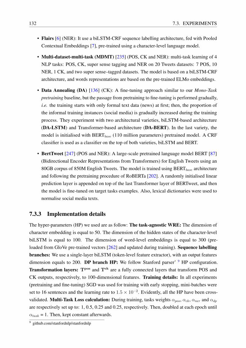
132 7.3. EXPERIMENTS

• Flairs [6] (NER): It use a biLSTM-CRF sequence labelling architecture, fed with Pooled

Contextual Embeddings [7], pre-trained using a character-level language model.

• Multi-dataset-multi-task (MDMT) [235] (POS, CK and NER): multi-task learning of 4

NLP tasks: POS, CK, super sense tagging and NER on 20 Tweets datasets: 7 POS, 10

NER, 1 CK, and two super sense–tagged datasets. The model is based on a biLSTM-CRF

architecture, and words representations are based on the pre-trained ELMo embeddings.

• Data Annealing (DA) [136] (CK): A fine-tuning approach similar to our Mono-Task

pretraining baseline, but the passage from pretraining to fine-tuning is performed gradually,

i.e. the training starts with only formal text data (news) at first; then, the proportion of

the informal training instances (social media) is gradually increased during the training

process. They experiment with two architectural varieties, biLSTM-based architecture

(DA-LSTM) and Transformer-based architecture (DA-BERT). In the last variety, the

model is initialised with BERTbase (110 million parameters) pretrained model. A CRF

classifier is used as a classifier on the top of both varieties, biLSTM and BERT.

• BertTweet [247] (POS and NER): A large-scale pretrained language model BERT [87]

(Bidirectional Encoder Representations from Transformers) for English Tweets using an

80GB corpus of 850M English Tweets. The model is trained using BERTbase architecture

and following the pretraining procedure of RoBERTa [202]. A randomly initialised linear

prediction layer is appended on top of the last Transformer layer of BERTweet, and then

the model is fine-tuned on target tasks examples. Also, lexical dictionaries were used to

normalise social media texts.

7.3.3 Implementation details

The hyper-parameters (HP) we used are as follow: The task-agnostic WRE: The dimension of

character embedding is equal to 50. The dimension of the hidden states of the character-level

biLSTM is equal to 100. The dimension of word-level embeddings is equal to 300 (pre-

loaded from GloVe pre-trained vectors [262] and updated during training). Sequence labellingbranches: We use a single-layer biLSTM (token-level feature extractor), with an output features

dimension equals to 200. DP branch HP: We follow Stanford parser’ 9 HP configuration.

Transformation layers: Tpos and Tck are a fully connected layers that transform POS and

CK outputs, respectively, to 100-dimensional features. Training details: In all experiments

(pretraining and fine-tuning) SGD was used for training with early stopping, mini-batches were

set to 16 sentences and the learning rate to 1.5× 10−2. Evidently, all the HP have been cross-

validated. Multi-Task Loss calculation: During training, tasks weights αpos, αck, αner and αdpare respectively set up to: 1, 0.5, 0.25 and 0.25, respectively. Then, doubled at each epoch until

αtask = 1. Then, kept constant afterwards.9 github.com/stanfordnlp/stanfordnlp

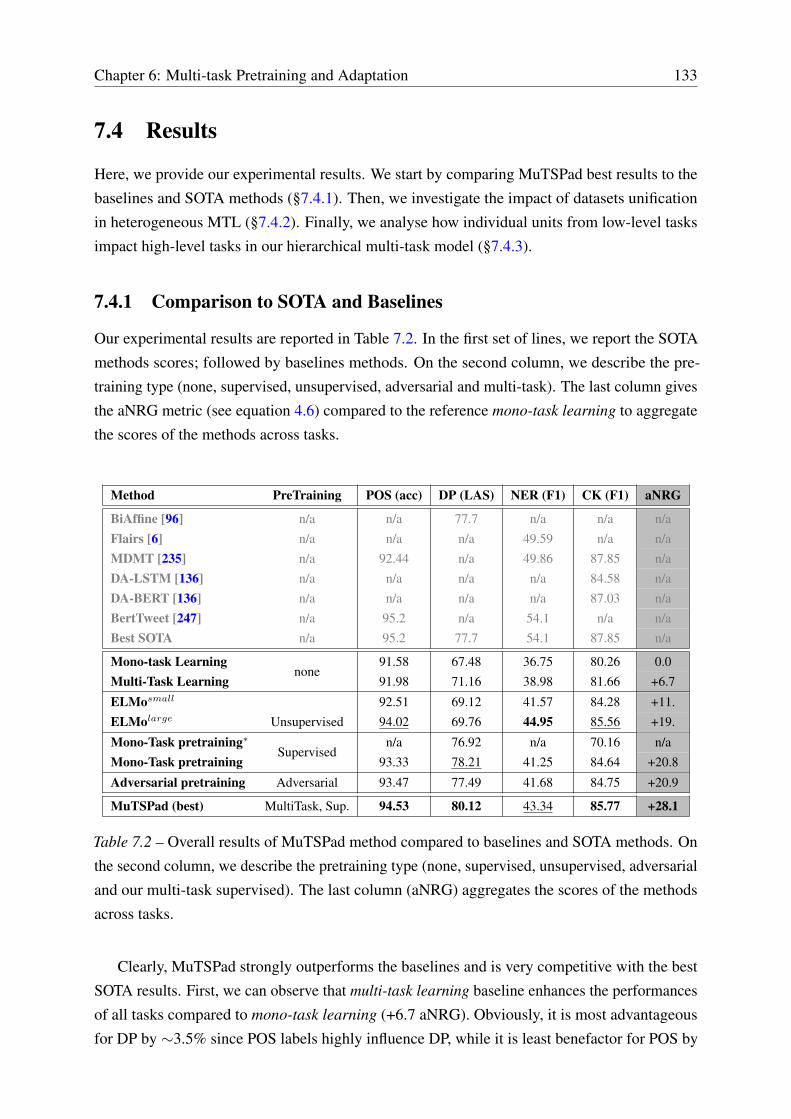
Chapter 6: Multi-task Pretraining and Adaptation 133

7.4 Results

Here, we provide our experimental results. We start by comparing MuTSPad best results to the

baselines and SOTA methods (§7.4.1). Then, we investigate the impact of datasets unification

in heterogeneous MTL (§7.4.2). Finally, we analyse how individual units from low-level tasks

impact high-level tasks in our hierarchical multi-task model (§7.4.3).

7.4.1 Comparison to SOTA and Baselines

Our experimental results are reported in Table 7.2. In the first set of lines, we report the SOTA

methods scores; followed by baselines methods. On the second column, we describe the pre-

training type (none, supervised, unsupervised, adversarial and multi-task). The last column gives

the aNRG metric (see equation 4.6) compared to the reference mono-task learning to aggregate

the scores of the methods across tasks.

Method PreTraining POS (acc) DP (LAS) NER (F1) CK (F1) aNRG

BiAffine [96] n/a n/a 77.7 n/a n/a n/aFlairs [6] n/a n/a n/a 49.59 n/a n/aMDMT [235] n/a 92.44 n/a 49.86 87.85 n/aDA-LSTM [136] n/a n/a n/a n/a 84.58 n/aDA-BERT [136] n/a n/a n/a n/a 87.03 n/aBertTweet [247] n/a 95.2 n/a 54.1 n/a n/aBest SOTA n/a 95.2 77.7 54.1 87.85 n/a

Mono-task Learningnone

91.58 67.48 36.75 80.26 0.0Multi-Task Learning 91.98 71.16 38.98 81.66 +6.7

ELMosmall

Unsupervised92.51 69.12 41.57 84.28 +11.

ELMolarge 94.02 69.76 44.95 85.56 +19.

Mono-Task pretraining∗Supervised

n/a 76.92 n/a 70.16 n/aMono-Task pretraining 93.33 78.21 41.25 84.64 +20.8

Adversarial pretraining Adversarial 93.47 77.49 41.68 84.75 +20.9

MuTSPad (best) MultiTask, Sup. 94.53 80.12 43.34 85.77 +28.1

Table 7.2 – Overall results of MuTSPad method compared to baselines and SOTA methods. On

the second column, we describe the pretraining type (none, supervised, unsupervised, adversarial

and our multi-task supervised). The last column (aNRG) aggregates the scores of the methods

across tasks.

Clearly, MuTSPad strongly outperforms the baselines and is very competitive with the best

SOTA results. First, we can observe that multi-task learning baseline enhances the performances

of all tasks compared to mono-task learning (+6.7 aNRG). Obviously, it is most advantageous

for DP by ∼3.5% since POS labels highly influence DP, while it is least benefactor for POS by

134 7.4. RESULTS

∼0.5% since POS branch is in the lower level and thus benefits only from the learned knowledge

in the shared parameters (WRE).

Second, incorporating pre-trained ELMo representations performs better compared to mono-

task learning. Particularly for NER task with ∼+8% by ELMolarge. We also found that it

improves the other tasks but not with the same order of improvement as for NER, which we

mainly attribute to the fact that contextual representations that are pre-trained on language

modelling capture more semantic features. Notably, we find that DP gains the least from ELMo

compared to the other syntactic tasks.

Third, compared to baselines, MuTSPad outperforms both TL methods, multi-task learning

and mono-task pretraining, on all data-sets, by∼+21.4 and∼+7.3 aNRG, respectively. Compared

to unsupervised pretraining, we can observe that MuTSPad outperforms ELMo on POS, CK and

DP, where ElMolarge brought higher performances for NER. Note that ELMo is complementary

to our approach; hence, we expect a higher performance when incorporating ElMolarge to

MuTSPad.

Finally, compared to SOTA, MuTSPad LAS score on DP is about ∼2.5% higher than the

best SOTA score. Also for POS we achieve better accuracy score than the best SOTA. For CK

and NER experiments, we achieve lower scores than SOTA. It is noteworthy that, first, contrary

to our approach, all these methods are mono-task models (except MDMT), i.e., unable to solve

other tasks. Second, NER and CK best SOTA used pretrained contextualised representations that

boost the performance, namely, Flairs embeddings by Akbik et al. [6], ELMo by Mishra [235]

and BERT by Gu & Yu [136] and Nguyen et al. [247].

7.4.2 Impact of Datasets Unification

Method POS DP NER CK

w/o unif. 94.08 79.17 43.34 84.87

w/ source unif. 94.36 79.67 43.21 85.77w/ source+target unif. 94.53 80.12 40.65 85.71

Table 7.3 – Impact of Datasets Unification on MuTSPad.

We report in Table 7.3 MuTSPad’s results: 1) w/o unif.: Training on independent datasets,

using the “one batch per task” scheduling rule, on both stages: pretraining and fine-tuning. 2) w/source unif. : In the pretraining stage, training is performed on the unified dataset. While in

fine-tuning, training is performed on independent datasets. 3) w/ source+target unif. : In both

pretraining and fine-tuning stages, training is performed on the unified datasets.

Clearly, pretraining on unified source datasets (w/source unif) slightly improved performances

on all tasks. Nevertheless, fine-tuning on unified target datasets (w/source+target unif) is

beneficial only for POS and DP tasks, while it strongly hurts NER’s F1 score. We mainly

Chapter 6: Multi-task Pretraining and Adaptation 135

attribute this to the low F1 score of the "Mono-task learning" baseline on the NER WNUT-17

dataset, leading to noisy NER automatic predictions.

7.4.3 Low-Level Tasks Importance Analysis

In this section, we investigate how low-level tasks impact high-level tasks in our hierarchical

multi-task model (See Figure 7.2). Specifically, we focus on the impact of hpos, the representation

encoded by the POS task, for CK, NER and DP tasks. For this purpose, we quantify the

importance of hpos individual units for POS, CK, NER and DP performances. Assuming that

ablating the most important units for a task should bring a higher drop in performance compared

to the least important units, we perform an individual ablation10 of hpos units (neurons), as in

[419] and [76].

Given the already trained target multi-task modelMt, we set the relating weights of each

uniti from hpos to zero, (i.e. Tpos layer’s weights for CK, NER and DP; and Clpos layer’s

weights for POS). Hence, the ablated unit will not contribute to the final prediction for any

input word. Then, with one unit ablated at a time, we launch the inference on each task’s

dev-set, then compute the resulting score-drop for each class (label), leading to a matrix per task

Atask ∈ Md,m (R), where d is hpos’s dimension and m is the number of task’ classes. This

matrix can be summarised in a max-class-score-drop vector vtask ∈ Rd, where each element

vtaski from the vector represents the max-class-score-drop when ablating the uniti from hpos.

Figure 7.3 – Maximum drop in performance on POS, CK, DP and NER tasks when ablating

individual POS units. from the POS Feature Extractor output (hpos). Dark/light blue: high/low

drop. One can see that it is the POS task that is most impacted by the POS units.

Applying this method, for POS, CK, NER and DP, leads to 4 max-class-score-drop vectors,

one for each task, vpos, vck, vner and vdp. In the heatmap in Figure 7.4, we plot one vector

per line: vpos, vck, vner then vdp. This figure illustrates the importance of POS units for each

task, where darker blue means a higher drop (thus higher importance) and lighter blue means

10Also called pruning or features erasure. (section 3.2.5)

136 7.5. CONCLUSION

lower drop (thus lower importance). We observe high values of vpos for POS compared to the

remaining tasks since hpos’s units are more important for POS tagging than all other tasks. Also,

hpos’s units are directly used for prediction for POS while transformed through several layers for

the other tasks. Furthermore, we can also observe that hpos’s units are more important for CK

and DP compared to NER since this last is semantic while the POS, CK and DEP are syntactic.

Task Class Unit Top-10 activations

CKB-INTJ POS-Unit-112 :); awwwwwwww; uggghh; Omg; lol; hahahaha; WELL; Nope; LOL; NoB-ADJP POS-Unit-99 rapidely; Deeply; fine; more; hardly; particulary; slower; guilty; loose; entirely

DPauxiliary POS-Unit-47 do; can; was; ca; can; ’s; would; have; ame; Wodiscourse POS-Unit-112 Hhhahahh; no; lmao; sorry; omg; hey; lol; yea; haha; please

NERB-location POS-Unit-35 North; Ireland; Italy; Kelly; Qatar; in; southafrica; new; over; WellingtonB-person POS-Unit-115 Trilarion; Jo; Watson; Hanzo; Abrikosov; Lily; jellombooty; theguest; Professor

Table 7.4 – Top-10 words activating positively (red) or negatively (blue) (Since LSTMs generate

positive and negative activations) some units from hpos that are the most important for different

classes from CK, DP and NER.

Moreover, we attempt to peek inside specific units from hpos, which the ablation thereof

begets a high drop in CK, DP and NER classes-scores. Specifically, we report in Table 7.4 the

top-10 words activating some of these units. Expectedly, we found that some of POS’ units are

firing, and thus specialised, on patterns that are beneficial for higher-level tasks. For instance,

Unit-99, specialised on adjectives ending with the suffix “ly”, is highly important for the CK

class “B-ADJP” (beginning of adjectival phrase). Also, Unit-115 is firing on person names,

a valuable pattern for “B-person” class of NER. Interestingly, we found some units that are

beneficial for multiple tasks, e.g. Unit-112, which is specific for interjections, is also important

for both “discourse” class for DP and “B-INTJ” (beginning of an interjection phrase) for CK.

7.5 Conclusion

In this chapter, we have proposed MuTSPad, a new approach based on transfer learning for

supervised domain adaptation with three main contributions: 1) Consolidating two transfer

learning approaches, sequential transfer learning and multi-task learning, by pretraining on a

resource-rich domain and fine-tuning on a low-resourced domain in a multi-task fashion; 2)

Unifying independent datasets to overcome the intricacy of multi-task training from heteroge-

neous datasets; and 3) Conducting a set of individual units ablation, refining our understanding

on how individual neurons from lower-level tasks impact high-level tasks. We showed through

empirical results on domain adaptation from news to social media that the proposed method

MuTSPad allows a simultaneous benefit from similarities between domains and tasks, yielding

better transfer learning performances on four NLP tasks.

This study leaves several important open directions for future work. First, we believe that

it would be beneficial to explore the combination of supervised and unsupervised multi-task

Chapter 6: Multi-task Pretraining and Adaptation 137

pretraining. Second, concerning conceptual choices for the multi-task model architecture, it

would be interesting to incorporate the attention mechanism [21] in our hierarchical multi-task

architecture. Indeed, actually, low-level tasks outputs are transformed through a simple fully

connected layers (T pos and T ck) to reduce their dimensionality before their injection to the

higher tasks. Thus, to help high-level tasks focus only on the most relevant units from the lower

tasks, one can incorporate attention weights in the transformation layers. Third, actually, we

perform the adaptation step using the standard fine-tuning scheme, a promising direction would

be to use our adaptation method PretRand (Chapter 6) at the adaptation stage of MuTSPad by

augmenting the source multi-task modelMs with randomly initialised layers before adaptation.

Finally, it would be interesting to explore the benefit of MuTSPad’s learned representations for

higher-level NLP applications such as machine translation and sentiment analysis.

8 | Conclusions and Perspectives

8.1 Conclusions

Throughout this thesis, we have explored different neural transfer learning approaches and

scenarios to improve the performance of neural NLP tools in low-resource settings. In particular,

starting from the hypothesis that social media domain (informal texts) is an informal variety of

the news domain (formal texts), we have demonstrated the advantage of neural transfer learning

for supervised domain adaptation from the high-resource news domain to the low-resource social

media domain. We have focused on the case where sufficient annotated datasets are available

from the source domain while only small annotated datasets from the target domain are available.

We summarise our main contributions and findings as follow:

• Neural sequential transfer learning across domains: After an in-depth study of transfer

learning techniques and approaches, we started by a sequential transfer learning method

that allows taking advantage of the knowledge learnt by a source model, formerly trained

on available annotated datasets from the source domain, to help improve the learning of the

target model. Specifically, we have proposed two sequential transfer learning schemes. The

first, transfer of supervisedly-pretrained contextual representations that consists in feeding

the representations generated by the source model as features to the target model, and thus,

all target model’s layers are trained from scratch. The second, transfer of pretrained models,

allows taking more advantages of the pre-learned knowledge, using the pretrained weights

from the source model to initialise the target model’s parameters, instead of training them

from scratch. Our experiments on sequence labelling tasks showed that both proposed

methods yield significant improvements compared to the standard supervised training

scheme, but transferring pretrained models approach begets better results across target

tasks and datasets. Besides, transferring models is more efficient in terms of computation

and convergence speeds. To have more insights about the impact of sequential transfer

learning of models, we performed an in-depth analysis that showed the following findings:

First, our method is more advantageous in extremely low-resource scenarios. Second, our

method leads to a faster convergence compared to training from scratch. Third, the model’s

138

Conclusions and perspectives 139

size does not have an observable effect on the transfer performance. Fourth, the pretraining

performance on the source task is not a reliable predictor for the performance on the target

task. Finally, off-the-shelf ELMo universal representations are complementary to our

proposed approaches and thus can be used for further improvements.

• Negative transfer in sequential transfer learning: The encouraging results that we

obtained with transferring pertained models using the standard fine-tuning (SFT) scheme

pushed us to dig deeper and look for potential improvements. Specifically, we analysed

the negative transfer when transferring from the news domain to the social media domain.

Roughly, negative transfer occurs when the knowledge learnt in the source domain hampers

the learning of new knowledge from the target domain. Particularly, when the source and

target domains are dissimilar, transfer learning may fail and hurt the performance, leading

to a worse performance compared to the standard supervised training from scratch. In

this thesis, we have proposed to analyse deeply the results of the SFT scheme; i.e. we

perceive the gain brought by SFT, compared to random initialisation, as a combination of a

hidden positive transfer and a hidden negative transfer. We define positive transfer as the

percentage of predictions that were wrongly predicted by random initialisation, but using

transfer learning changed to the correct ones. Negative transfer represents the percentage

of predictions which were tagged correctly by random initialisation, but using transfer

learning provides incorrect predictions. Hence, the final gain brought by transfer learning

would be the difference between positive and negative transfers. We have shown through

a series of empirical analysis that, the hidden negative transfer mitigates the final gain

brought by transfer learning. We believe that analysing the hidden negative transfer is

an essential step towards spotting the limits and the potential improvement tracks of the

actual transfer learning tasks.

• Analysis and interpretation methods: First, we have proposed a new categorisation of

interpretability methods in NLP. (1) Descriptive methods aim to investigate the knowledge

learnt by neural models in their internal representations. (2) Explicative methods aim to

justify the predictions of the model. (3) Mechanistic methods seek to provide a functional

understanding of the model. Second, to go even further in our analysis of the SFT scheme,

we have investigated how the internal representations of the pretrained models are updated

during fine-tuning on the social media domain. We have addressed this question with

two distinct interpretive approaches: correlation analysis and individual units stimulus.

Following our proposed taxonomy, these methods belong to the descriptive methods

category. We found that pretrained neurons are biased by what they have learnt in the

source-dataset, i.e. pretrained neurons tend to conserve much information from the source

domain. Some of this information is undoubtedly beneficial for the social media domain

(positive transfer), but some of it is indeed harmful (negative transfer). We suppose that,

as a consequence of this phenomenon, specific patterns to the target-dataset are difficult to

140 8.2. PERSPECTIVES

learn by pre-trained units. This phenomenon is non-desirable, since such specific units are

important for performance, especially for target-specific classes.

• PretRand - a novel adaptation method for neural sequential transfer learning: We

have proposed a hybrid method that takes benefit from both approaches, random initiali-

sation (standard supervised training scheme from scratch) and transfer learning, without

their drawbacks. It consists in augmenting the source-network with randomly initialised

units and jointly learn them. PretRand consists of three main ideas. First, augmenting the

source-network (set of pre-trained units) with a random branch composed of randomly

initialised units, and jointly learn them. Second, normalising the outputs of both branches

to balance their different behaviours and thus forcing the network to consider both. Indeed,

we found that when naively augmenting the pretrained branch with the random branch, the

former strongly fires discriminatively on many words, while the latter does not fire on any

word at the initial stage of fine-tuning. Therefore, the random units do not significantly

contribute to the computation of gradients and are thus slowly updated. Third, applying

attention learnable weights on both branches predictors to let the network learn which

of random or pre-trained one is better for every class. Our experiments on sequence

labelling tasks showed that PretRand significantly enhances the performance compared to

the standard fine-tuning adaptation scheme. It is noteworthy that PretRand does not slow

down the model compared to SFT, since as shown in Table 6.4, PretRand uses only 0.02%

more parameters compared to the standard fine-tuning baseline.

• MuTSPad - consolidating sequential transfer learning and multi-task learning: In

the above contributions, we have studied the impact of mono-source mono-target sequen-

tial transfer learning to improve NLP models performance for low-resource domains

(social media texts), where the transfer is performed in two steps: mono-task pretraining

on a single task from a rich source domain followed by a mono-task fine-tuning of the task

of interest on the available few target-domain examples. Nevertheless, as shown in many

research works, but also our results in chapter 5, transferring knowledge, simultaneously,

from multiple tasks can boost the performance. Therefore, we have proposed in chap-

ter 7 a new approach that we called Multi-Task Supervised Pre-training and Adaptation

(MuTSPad). It performs a multi-source multi-target sequential transfer learning and thus

takes advantage of both approaches, sequential transfer learning and multi-task learning,

by learning a hierarchical model trained across multiple tasks from the source domain,

then fine-tuned on multiple tasks from the target domain.

8.2 Perspectives

Several paths of research arise from the work carried out during this thesis. We briefly discuss

a few of them below. We start, in section 8.2.1, by research tracks that were partially or were

Conclusions and perspectives 141

not addressed during this thesis, but we believe that their investigation will boost our proposed

approaches. Then, in section 8.2.2, we present some broader promising research directions that

are related to our research.

8.2.1 Short-term Perspectives

• Fine-tuning strategies in the standard fine-tuning scheme: In chapter 5 experiments,

we have performed the fine-tuning stage in a naive manner. i.e. pretraining and fine-tuning

stages are performed using the same settings. One can explore different strategies recently

proposed in the literature to improve the fine-tuning process on the target task. A standard

method is to attribute lower learning rates for the low-most pretrained layers. Indeed,

as discussed in [396, 243, 265], model’s layers learn different types of knowledge, i.e.

top layers are more task-specific than low ones. Thus, low layers learn generic features

easily transferable between tasks, while top layers learn features that are specific to the

learnt task and domain. For instance, Howard & Ruder [155] proposed more sophisticated

approaches. Namely, discriminative fine-tuning and Slanted triangular learning rates. The

former comes down to the approach affecting different learning rates per layer. The latter

consists in tuning the learning rate in two steps: first, it linearly increases the learning rate

and then linearly decays. This method allows converging rapidly to a suitable region of

parameters before slowly tuning the parameters to the best parameters.

• Explaining the hidden negative transfer: In chapter 6, we have performed a set of

analysis to assess the hidden negative transfer occurring when transferring from the news

domain to the social media domain using the standard fine-tuning scheme. We believe

that it is worth going further in this analysis. A fruitful direction would be to explain this

hidden negative transfer using explicative methods (§3.3). Notably, one can use influence

functions (§3.3.6) to identify source training examples responsible for the negative transfer.

Further, to identify text pieces of the evaluated sentence that justify a prediction with a

negative transfer, one can use surrogate methods (§3.3.4) or gradients based methods

(§3.3.3).

• Pruning biased neurons in the standard fine-tuning scheme: In chapter 6, we have

shown through our analysis that pretrained neurons are biased by what they have learnt in

the source task. Certainly, some of these neurons keep valuable knowledge from the source

domain that are beneficial to the target domain (positively biased neurons). However, a part

of these neurons may contain knowledge that is harmful to the target domain (negatively

biased neurons). To handle this problem, we have proposed in section 6.3 to augment

the pretrained neurons with random neurons to learn new features that are specific to the

target domain. Another promising method to avoid the harmful effect of negatively biased

neurons would be to automatically identify negatively biased neurons in the pre-trained

142 8.2. PERSPECTIVES

model using features erasure methods (§3.2.5). And then, proceed to a pruning of the

most biased ones before fine-tuning. Note that pruning pretrained transformer-based

models, like BERT, has been recently investigated in the literature [219, 131, 315, 78] to

achieve an accuracy-speed tradeoff. Furthermore, Knowledge Distillation is a promising

method that aims to transfer the knowledge from a large teacher model to a smaller student

model through a distillation process [149]. For instance, a distilled version of BERT was

proposed by Sanh et al. [313] to reduce the size of the original BERT while keeping its

valuable knowledge. An intriguing direction would be to distil the teacher model pretrained

on the source domain on a smaller target model containing only the information encoded

by positively biased neurons.

• More sophisticated multi-task learning for multi-source multi-target transfer learn-ing: The positive results of our proposed approach, MuTSPad, leaves several important

open directions for future work. Notably, we did not explore all the potential of multi-task

learning. First, we should explore soft multi-task architectures. Second, we can investigate

the combination of supervised and unsupervised multi-tasking. Third, we can incorpo-

rate an attention mechanism in our hierarchical multi-task architecture. Indeed, actually,

low-level tasks outputs are transformed through a simple fully connected layers to reduce

their dimensionality before their injection to the higher tasks. Thus, to help high-level

tasks to focus only on the most important units from the lower tasks, one can incorporate

attention weights in the transformation layers. Finally, a promising direction would be to

use our adaptation method PretRand (chapter 6) at the adaptation stage of MuTSPad by

augmenting the source multi-task model with randomly initialised layers before adaptation.

• Transformer-based architectures: The increasing omnipresence of Transformers archi-

tectures in a wide range of NLP tasks, due to their improved performances, motivates

us to experiment our approaches on Transformer-based architecture instead of LSTM-

based one. Furthermore, it would be interesting to combine pretrained Transformer-based

models, like BERT or RoBERTa, with our approaches. For this, we propose to use our

pretraining approaches as an Intermediate Pretraining Task, also called Supplementary

Training on Intermediate Labelled-data Tasks (STILT) [269, 278]. In simple words, the

approach will be performed in 3 steps; the Transformer-based model is firstly pretrained

on self-supervised tasks (e.g. language modelling). Then, the model is further trained on

news source datasets using the approaches discussed in this thesis. Finally, the model is

fine-tuned on social media small datasets.

• Application of our approaches on less similar source-target languages: In this thesis,

we have experimented our approaches on transfer from the news domain to the social

media domain. It would be interesting to investigate the flexibility of our approaches in

more challenging settings. e.g. transfer between the formal Arabic language (Modern

Conclusions and perspectives 143

Standard Arabic) and informal Arabic languages (22 dialects distributed over five regional

categories) that we can find on social media.

8.2.2 Long-term Perspectives

Stemming from the research work carried out during this thesis, we believe in the importance of

the following research directions.

• Opportunities and challenges of social media data analysis: Social media has offered

access to vast amounts of textual data. Otherwise, social media is also a rich source

of multi-modal data, which will allow unfolding many opportunities and applications.

Recently, there is a rising interest in the NLP community on multi-modal data. For

instance, multi-modal pretraining has been studied by Lin et al. [194] who proposed

interBERT, a multi-modal model for images and text. Zhang et al. [413] used multi-modal

representations for Neural Machine Translation (NMT). Kiela et al. [170] performed hate

speech detection in multi-modal data in social media. However, this data abundance

in social media may impose many challenges. First, it threatens users’ privacy. Indeed,

User-Generated-Content (UGC) in social media may contain personal data and thus privacy-

sensitive information. Hence, training neural models directly on these data makes them

vulnerable to malicious actors. Therefore, thinking about privacy-preserving methodsfor NLP is becoming crucial. Second, UGC in social media may be socially biased. Thus,

training neural networks directly on this type of data may generate unfair and harmful

models. Actually, detecting bias in NLP models and de-biasing these models is a firing

research topic [34].

• Transfer Learning for emerging topics: In this thesis, we have shown the efficiency of

transfer learning from the news domain to social media. We believe that Transfer learning

is a promising approach that can be perfectly applied to a variety of emerging topics where

low-data settings are frequent and solutions are urgently requested, e.g. climate change

[299] and COVID-19 [14, 220].

• Incorporating expert knowledge into deep neural models: As we have shown in this

thesis, specific languages used in social media platforms generally share a number of

syntactic structures and vocabulary with formal languages. Another avenue for research

consists in analysing close languages and modelling their divergences and similarities in

the form of linguistic rules and resources and then incorporating this expert knowledge

into deep neural models in order to improve the training step and to obtain more accurate

predictions. The WALS (World Atlas of Language Structures) database 1 can be exploited

to extract structural and lexical properties of close languages. The idea of incorporating

1 https://wals.info/

144 8.2. PERSPECTIVES

external knowledge to improve the performance of deep learning models for image analysis

is not new [257, 386], but there are only a few works on how linguistic resource can be

introduced in these models and how these resources can help them to improve their

performance [359, 183].

A | List of Publications

• Sara Meftah, Nasredine Semmar, Youssef Tamaazousti, Hassane Essafi and Fatiha Sadat.

"On the Hidden Negative Transfer in Sequential Transfer Learning from News to Tweets."

In Adapt-NLP@EACL2021, The Second Workshop on Domain Adaptation for NLP

@ The 16th Conference of the European Chapter of the Association for Computational

Linguistics. [226]

• Sara Meftah, Nasredine Semmar, Othman Zennaki, and Fatiha Sadat. "Supervised Transfer

Learning for Sequence Tagging of User-Generated-Content in Social Media." In Lecture

Notes in Artificial Intelligence 2020 (Human Language Technology. Challenges for

Computer Science and Linguistics). [229]

• Sara Meftah, Nasredine Semmar, Mohamed-Ayoub Tahiri, Youssef Tamaazousti, Has-

sane Essafi, and Fatiha Sadat. "Multi-Task Supervised Pretraining for Neural Domain

Adaptation." In Proceedings of the Eighth International Workshop on Natural Language

Processing for Social Media, pp. 61-71. 2020.[223]

• Sara Meftah, Nasredine Semmar, Youssef Tamaazousti, Hassane Essafi and Fatiha Sadat.

"Apprentissage mixte de neurones pré-entraînés et aléatoires dans un modèle neuronal

pour l’adaptation au domaine." In Actes de la conférence Reconnaissance des Formes,

Image, Apprentissage et Perception (RFIAP), 2020. [225]

• Sara Meftah, Youssef Tamaazousti, Nasredine Semmar, Hassane Essafi, and Fatiha Sadat.

"Joint Learning of Pre-Trained and Random Units for Domain Adaptation in Part-of-

Speech Tagging." In Proceedings of the 2019 Conference of the North American Chapter

of the Association for Computational Linguistics: Human Language Technologies, Volume

1 (Long and Short Papers), pp. 4107-4112. 2019.[230]

• Sara Meftah, Nasredine Semmar, Youssef Tamaazousti, Hassane Essafi, and Fatiha Sadat.

"Exploration de l’apprentissage par transfert pour l’analyse de textes des réseaux soci-

aux (Exploring neural transfer learning for social media text analysis)." In Actes de la

Conférence sur le Traitement Automatique des Langues Naturelles (TALN) PFIA 2019.

Volume II: Articles courts, pp. 293-302. 2019. [224]

145

146

• Sara Meftah, Nasredine Semmar, Fatiha Sadat, and Stephan Raaijmakers. "Using neural

transfer learning for morpho-syntactic tagging of South-Slavic languages tweets." In

Proceedings of the Fifth Workshop on NLP for Similar Languages, Varieties and Dialects

(VarDial 2018), pp. 235-243. 2018. [222]

• Sara Meftah, Nasredine Semmar and Fatiha Sadat. "A neural network model for part-

of-speech tagging of social media texts." In Proceedings of the Eleventh International

Conference on Language Resources and Evaluation (LREC 2018). 2018. [221]

• Sara Meftah, Nasredine Semmar, Othman Zennaki, and Fatiha Sadat. "Using transfer

learning in part-of-speech tagging of English Tweets." In The Language and Technology

Conference, pp. 236-240. 2017. [228]

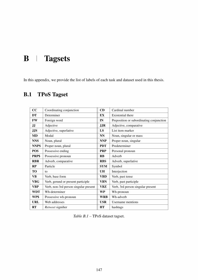
B | Tagsets

In this appendix, we provide the list of labels of each task and dataset used in this thesis.

B.1 TPoS Tagset

CC Coordinating conjunction CD Cardinal number

DT Determiner EX Existential there

FW Foreign word IN Preposition or subordinating conjunction

JJ Adjective JJR Adjective, comparative

JJS Adjective, superlative LS List item marker

MD Modal NN Noun, singular or mass

NNS Noun, plural NNP Proper noun, singular

NNPS Proper noun, plural PDT Predeterminer

POS Possessive ending PRP Personal pronoun

PRP$ Possessive pronoun RB Adverb

RBR Adverb, comparative RBS Adverb, superlative

RP Particle SYM Symbol

TO to UH Interjection

VB Verb, base form VBD Verb, past tense

VBG Verb, gerund or present participle VBN Verb, past participle

VBP Verb, non-3rd person singular present VBZ Verb, 3rd person singular present

WDT Wh-determiner WP Wh-pronoun

WP$ Possessive wh-pronoun WRB Wh-adverb

URL Web addresses USR Username mentions

RT Retweet signifier HT hashtags

Table B.1 – TPoS dataset tagset.

147

148 B.2. ARK TAGSET

B.2 ArK Tagset

N common noun

O pronoun (personal/WH; not possessive)

ˆ proper noun

S nominal + possessive

V verb incl. copula, auxiliaries

A adjective

! interjection

D determiner

P pre- or postposition, or subordinating conjunction

& coordinating conjunction

T verb particle

X existential there, predeterminers

# hashtag (indicates topic/category for tweet)

∼ discourse marker, indications of continuation of a message across multiple tweets

U URL or email address

E emoticon

$ numeral

, punctuation

G other abbreviations, foreign words, possessive endings, symbols, garbage

L nominal + verbal (e.g. i’m), verbal + nominal (let’s, lemme)

M proper noun + verbal

Y X + verbal

Table B.2 – ArK dataset tagset.

Tagsets 149

B.3 TweeBank POS Tagset

ADJ: adjective Words that typically modify nouns and specify their properties or attributes.

ADP: adposition Prepositions and postpositions (e.g. in, to, during, etc.).

AUX: auxiliary A function word that accompanies the lexical verb of a verb phrase.

CCONJ: coordinating conjunction Words that link words or larger constituents.

DET: determiner Express the reference of a noun or a noun phrase.

INTJ: interjection A word that is used most often as an exclamation or an emotion.

NOUN: noun Words denoting a person, place, thing, animal or idea.

NUM: numeral Express quantity, sequence, frequency, fraction, etc.

PART: particle Function words that must be associated with another word or phrase.

PRON: pronoun Words that substitute for nouns or noun phrases.

PROPN: proper noun A noun that is the name of a specific individual, place, or object.

PUNCT: punctuation Used to delimit linguistic units in printed text.

SCONJ: subordinating conjunction link constructions by making one of them a constituent of the other.

SYM: symbol e.g. +, ×, ÷, =, <, >, :)

VERB: verb Words that typically signal events and actions.

X: other Words that for some reason cannot be assigned a real POS category.

Table B.3 – TweeBank dataset POS tagset.1

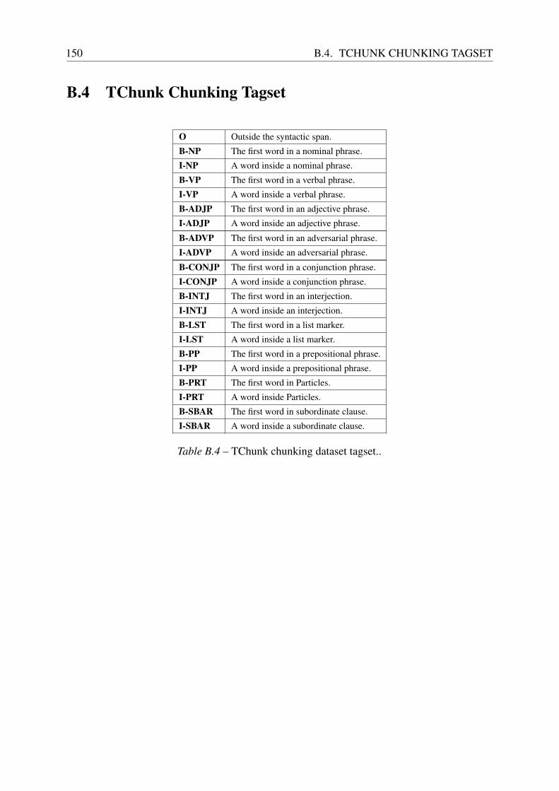
150 B.4. TCHUNK CHUNKING TAGSET

B.4 TChunk Chunking Tagset

O Outside the syntactic span.

B-NP The first word in a nominal phrase.

I-NP A word inside a nominal phrase.

B-VP The first word in a verbal phrase.

I-VP A word inside a verbal phrase.

B-ADJP The first word in an adjective phrase.

I-ADJP A word inside an adjective phrase.

B-ADVP The first word in an adversarial phrase.

I-ADVP A word inside an adversarial phrase.

B-CONJP The first word in a conjunction phrase.

I-CONJP A word inside a conjunction phrase.

B-INTJ The first word in an interjection.

I-INTJ A word inside an interjection.

B-LST The first word in a list marker.

I-LST A word inside a list marker.

B-PP The first word in a prepositional phrase.

I-PP A word inside a prepositional phrase.

B-PRT The first word in Particles.

I-PRT A word inside Particles.

B-SBAR The first word in subordinate clause.

I-SBAR A word inside a subordinate clause.

Table B.4 – TChunk chunking dataset tagset..

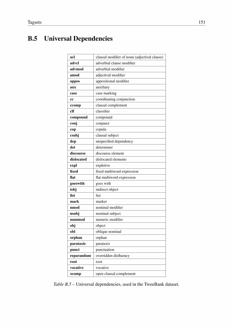
Tagsets 151

B.5 Universal Dependencies

acl clausal modifier of noun (adjectival clause)

advcl adverbial clause modifier

advmod adverbial modifier

amod adjectival modifier

appos appositional modifier

aux auxiliary

case case marking

cc coordinating conjunction

ccomp clausal complement

clf classifier

compound compound

conj conjunct

cop copula

csubj clausal subject

dep unspecified dependency

det determiner

discourse discourse element

dislocated dislocated elements

expl expletive

fixed fixed multiword expression

flat flat multiword expression

goeswith goes with

iobj indirect object

list list

mark marker

nmod nominal modifier

nsubj nominal subject

nummod numeric modifier

obj object

obl oblique nominal

orphan orphan

parataxis parataxis

punct punctuation

reparandum overridden disfluency

root root

vocative vocative

xcomp open clausal complement

Table B.5 – Universal dependencies, used in the TweeBank dataset.

C | Résumé En Français

Les méthodes d’apprentissage automatique qui reposent sur les Réseaux de Neurones (RNs)

obtiennent des performances qui s’approchent de plus en plus de la performance humaine dans

plusieurs applications du Traitement Automatique de la Langue (TAL) qui bénéficient de la

capacité des différentes architectures des RNs à généraliser à partir des régularités apprises à

partir des exemples d’apprentissage. En particulier, la structure ordonnée et les dépendances

temporelles des données textuelles nécessitent un traitement spécifique. En effet, le contexte

joue un rôle important pour identifier le sens d’un mot ou comprendre une phrase dans un

document. Pour ce type de tâches, les RNs récurrents (RNNs pour Reccurent Neural Networks)

et ses variantes; dont les deux principales: le modèle Long Short-Term Memory (LSTM) et sa

version simplifiée Gated Recurrent Units (GRUs) sont les plus adaptés grâce à leur capacité

à conserver en mémoire les informations pertinentes en analysant les mots (ou les caractères)

dans un ordre précis. En outre, les RNs à convolutions (CNNs pour Convolutional Neural

Networks) ont aussi montré leur efficacité pour l’encodage des caractères. Plusieurs études [165]

ont montré que les CNNs représentaient l’architecture idéale pour l’extraction et l’encodage

des informations morphologiques (racine, préfixe, suffixe, etc.), en particulier pour les langues

avec une morphologie riche [59, 210] comme l’Arabe, les langues Slovaques, le Hindi, etc.

Toutefois, ces modèles sont limités par leur dépendance aux données annotées. En effet, pour

être performants, ces modèles ont besoin de corpus annotés de taille importante. Par conséquent,

uniquement les langues bien dotées peuvent bénéficier directement de l’avancée apportée par les

RNs, comme par exemple les formes formelles des langues.

Dans le cadre de cette thèse, nous avons proposé des méthodes d’apprentissage par transfert

neuronal pour la construction des outils de TAL pour les langues et domaines peu dotés en

exploitant leurs similarités avec des langues et des domaines bien dotés. Précisément, nous avons

expérimenté nos approches pour le transfert à partir du domaine source des textes formels vers

le domaine cible des textes informels (langue utilisée dans les réseaux sociaux). Nous avons

commencé par introduire une nouvelle classification des méthodes d’apprentissage par transfert

pour le TAL selon trois dimensions (Chapitre 2). La première dimension classifie les méthodes

selon le type des connaissances transférées de la tâche source vers la tâche cible. La deuxième

dimension classifie ces méthodes selon l’objectif derrière l’utilisation de l’apprentissage par

transfert. La troisième dimension distingue les méthodes permettant de transférer les différents

152

APPENDIX C. RÉSUMÉ EN FRANÇAIS 153

types de connaissances.

Tout au long de cette thèse nous avons présenté différentes contributions. Tout d’abord,

nous avons proposé deux approches pour le transfert des connaissances encodées dans les

représentations neuronales d’un modèle source, pré-entraîné sur les données annotées du domaine

source, vers un modèle cible, adapté par la suite sur quelques exemples annotés du domaine cible.

La première méthode transfère des représentations contextuelles pré-entraînées sur le domaine

source (§5.3.2.1). Tandis que la deuxième méthode utilise des poids pré-entraînés pour initialiser

les paramètres du modèle cible qui sera adapté par la suite sur les exemples d’apprentissage du

domaine cible en utilisant le schéma du fine-tuning standard (§5.3.2.2).

Ensuite, nous avons effectué une série d’analyses pour repérer les limites des méthodes

proposées. Nous avons constaté que, même si l’approche d’apprentissage par transfert proposée

en utilisant le schéma du fine-tuning standard améliore les résultats sur le domaine cible, un

transfert négatif « dissimulé » peut atténuer le gain final apporté par l’apprentissage par transfert.

Parmi les erreurs causées par le transfert négatif que nous avons constaté les mots avec une

première lettre en majuscule qui sont souvent prédis, par erreur, par le modèle avec apprentissage

par transfert comme des noms propres (§6.2.2).

De plus, nous avons proposé une analyse interprétative (§6.2.3) du modèle pré-entraîné qui

montre que les neurones pré-entraînés peuvent être biaisés par ce qu’ils ont appris du domaine

source, et donc peuvent avoir des difficultés à apprendre des patterns spécifiques au domaine

cible. A titre d’exemple, nous avons repéré un neurone qui est très sensible aux noms propres

(par exemple, George et Washington) avant le fine-tuning, et aux mots dont la première lettre est

en majuscule, que le mot soit un nom propre ou pas (par exemple, Man et Father) pendant le

fine-tuning sur l’ensemble de données des réseaux sociaux. En effet, nous avons constaté que

la plupart des mots dont la première lettre est en majuscule sont prédits par erreur comme des

noms propres dans le schéma de fine-tuning standard. En fait, en anglais standard, à l’intérieur

des phrases, seuls les noms propres commencent par une lettre majuscule, ce qui fait que le

fine-tuning du modèle pré-appris ne parvient pas à éliminer ce pattern qui n’est pas toujours

respecté dans les réseaux sociaux.

Suite à cette analyse, nous avons proposé un nouveau schéma d’adaptation hybride (§6.3)

qui augmente le modèle cible avec des neurones normalisés, pondérés et initialisés aléatoirement

permettant une meilleure adaptation au domaine cible tout en conservant les connaissances

apprises du domaine source. Notre méthode consiste à augmenter le réseau de neurones source

(ensemble de neurones pré-entraînés) avec des neurones initialisés de façon aléatoire et à les

apprendre conjointement. Nous appelons notre méthode PretRand (Pretrained and Rand units).

La principale difficulté est de forcer le réseau à prendre en compte les neurones aléatoires, car

elles ont des comportements différents de ceux des neurones pré-entraînés. En effet, si ces

derniers sont activés fortement de manière discriminatoire sur de nombreux mots, les premiers ne

s’activent sur aucun mot au stade initial du fine-tuning. Par conséquent, les neurones aléatoires

ne contribuent pas de manière significative au calcul des gradients et sont donc lentement mises

154

à jour. Pour surmonter ce problème, nous avons proposé de normaliser indépendamment les

couches pré-entraînées et aléatoires. Cette normalisation équilibre leur échelle d’activations

et force ainsi le réseau à les prendre en compte toutes les deux. Enfin, nous ne savons pas

lesquels des prédicteurs, pré-entraînés ou aléatoires sont les meilleurs pour chaque classe. Nous

proposons, donc, d’apprendre des vecteurs de pondération sur chaque branche.

Enfin, nous avons proposé une approche d’apprentissage par transfert qui permet de tirer

profit des similarités entre différentes tâches, en plus des connaissances pré-apprises du domaine

source. Nous appelons notre méthode Multi-Task Supervised Pre-training and Adaptation

(MuTSPad). Elle consiste à apprendre un modèle multi-tâches hiérarchique sur le domaine

source qui sera adapté par la suite sur multiple tâches du domaine cible (chapitre 7).

List of Figures

1.1 Language resources distribution - Source: [164]. . . . . . . . . . . . . . . . . . 4

1.2 Example of a Tweet. Grey segments show expressions similar to formal texts

and red ones show social media domain’s specific expressions (informal). . . . 7

2.1 Standard supervised training scheme vs Transfer Learning [257]. . . . . . . . . 11

2.2 Example of the projection of part-of-speech annotations. The source language is

English and the target language is French. Source: [404]. . . . . . . . . . . . . 15

2.3 Adversarial training neural architecture. Source: [115] . . . . . . . . . . . . . 20

2.4 Multi-task learning Parameters Sharing Schemes. . . . . . . . . . . . . . . . . 23

2.5 Illustrative schemes of CBOW and Skip-gram neural architectures. . . . . . . . 29

3.1 Classification of analysis and interpretability methods for neural NLP models. . 37

3.2 Character-by-character activations of the sentiment neuron discovered in RNNs-

based language model [281]. . . . . . . . . . . . . . . . . . . . . . . . . . . . 38

3.3 Heatmap of individual neurons importance using feature erasure methods [190]. 41

3.4 Examples of rationales annotations from the ERASER dataset [88]. . . . . . . . 42

3.5 Learned attention weights in a NMT model French - English. . . . . . . . . . . 43

3.6 Gradients-based Saliency heatmaps. . . . . . . . . . . . . . . . . . . . . . . . 44

4.1 Example of Stanford Dependencies - Source [83]. . . . . . . . . . . . . . . . . 52

4.2 An illustrative example from the TweeBank dataset showing non-syntactic tokens

- Source: [203]. . . . . . . . . . . . . . . . . . . . . . . . . . . . . . . . . . . 54

4.3 An Illustrative example of informal but syntactic tokens - Source: [203]. . . . . 54

5.1 Illustrative scheme of the base neural model for sequence labelling tasks. . . . . 59

5.2 Illustrative scheme of Υchar, the character-level biLSTM-based embedding com-

ponent. . . . . . . . . . . . . . . . . . . . . . . . . . . . . . . . . . . . . . . . 60

5.3 Illustrative scheme of transferring contextual supervisedly pretrained representa-

tions from news-domain to social media domain . . . . . . . . . . . . . . . . . 68

5.4 An overview of the process of sequential transfer learning by fine-tuning pre-

trained parameters. . . . . . . . . . . . . . . . . . . . . . . . . . . . . . . . . 69

5.5 Overview of the experimental schemes of layer-per-Layer transferability experi-

ment. . . . . . . . . . . . . . . . . . . . . . . . . . . . . . . . . . . . . . . . . 73

155

156 LIST OF FIGURES

5.6 Results of transfer learning vs random initialisation according to different social

media training-set sizes. . . . . . . . . . . . . . . . . . . . . . . . . . . . . . . 80

5.7 The impact of the model’s size on transfer learning performance . . . . . . . . 81

5.8 The impact of transfer learning on training convergence. . . . . . . . . . . . . 82

5.9 The impact of pretraining state on transfer learning performance. . . . . . . . . 83

5.10 Which classes benefit the most from transfer learning? . . . . . . . . . . . . . 84

6.1 The percentage of negative transfer and positive transfer brought by SFT adapta-

tion scheme compared to supervised training from scratch. . . . . . . . . . . . 92

6.2 Positive transfer curves and negative transfer curves on social media data-sets,

according to different pretraining epochs. . . . . . . . . . . . . . . . . . . . . 93

6.3 The Pearson correlation between unit j activations vector after fine-tuning to its

activations vector before fine-tuning. . . . . . . . . . . . . . . . . . . . . . . . 96

6.4 Correlation results between Φ units’ activations before fine-tuning and after

fine-tuning. . . . . . . . . . . . . . . . . . . . . . . . . . . . . . . . . . . . . 97

6.5 Illustrative scheme of the calculus of top-k-words activating a unit j during

fine-tuning . . . . . . . . . . . . . . . . . . . . . . . . . . . . . . . . . . . . . 98

6.6 Individual units activations before and during fine-tuning from ArK POS dataset. 99

6.7 Individual units activations before and during fine-tuning on Tweebank POS

dataset. . . . . . . . . . . . . . . . . . . . . . . . . . . . . . . . . . . . . . . . 100

6.8 Individual units activations before and during fine-tuning on WNUT-17 NER

dataset. . . . . . . . . . . . . . . . . . . . . . . . . . . . . . . . . . . . . . . . 101

6.9 Illustrative scheme of the three ideas of our proposed adaptation method, PretRand.104

6.10 The distributions of the learnt weight-values for the randomly initialised and

pre-trained branches after their joint training. . . . . . . . . . . . . . . . . . . 106

6.11 Illustrative schemes of baseline-methods and PretRand. . . . . . . . . . . . . . 109

6.12 Sorted class-accuracy improvement (%) on TweeBank of PretRand compared to

fine-tuning. . . . . . . . . . . . . . . . . . . . . . . . . . . . . . . . . . . . . 115

6.13 Performances (on dev-set of TweeBank) according different training-set sizes

for the target-dataset. . . . . . . . . . . . . . . . . . . . . . . . . . . . . . . . 115

6.14 Positive transfer and negative transfer brought by SFT (left) and PretRand (Right)

compared to standard supervised training scheme . . . . . . . . . . . . . . . . 116

6.15 Individual units activations (from the random branch) before and during fine-

tuning PretRand on ArK social media dataset. . . . . . . . . . . . . . . . . . . 117

6.16 Individual units activations (from the random branch) before and during fine-

tuning PretRand on TweeBank dataset. . . . . . . . . . . . . . . . . . . . . . . 118

6.17 Individual units activations (from the random branch) before and during fine-

tuning PretRand on WNUT NER dataset . . . . . . . . . . . . . . . . . . . . . 119

7.1 Illustrative scheme of the neural arc-factored graph-based dependency parser. . 124

LIST OF FIGURES 157

7.2 Illustrative scheme of the Hierarchical multi-task architecture of MuTSPad. . . 126

7.3 Maximum drop in performance on POS, CK, DP and NER tasks when ablating

individual POS units. . . . . . . . . . . . . . . . . . . . . . . . . . . . . . . . 135

List of Tables

2.1 Different transfer learning approaches used for different research objectives. . . 34

4.1 Statistics of the used datasets. . . . . . . . . . . . . . . . . . . . . . . . . . . . 48

4.2 Illustrative examples of annotated sentences from each social media dataset. . . 49

5.1 Statistics of the used datasets. . . . . . . . . . . . . . . . . . . . . . . . . . . . 63

5.2 Ablation study of traditional embeddings: character-level embeddings and word-

level embeddings. . . . . . . . . . . . . . . . . . . . . . . . . . . . . . . . . . 65

5.3 Results of combining our supervisedly-pretrained representations with standard

embeddings. . . . . . . . . . . . . . . . . . . . . . . . . . . . . . . . . . . . . 71

5.4 Main results of our proposed approach, transferring pretrained models. . . . . 72

5.5 Layer-per-layer transferability analysis results. . . . . . . . . . . . . . . . . . . 74

5.6 Results of inter-tasks transferability of pretrained models. . . . . . . . . . . . . 75

5.7 Comparison of our proposed approaches results: transferring representations vs

transferring models . . . . . . . . . . . . . . . . . . . . . . . . . . . . . . . . 77

5.8 Results of combining ELMo contextual representations with traditional embed-

dings. . . . . . . . . . . . . . . . . . . . . . . . . . . . . . . . . . . . . . . . 78

5.9 Results of combining ELMo contextual representations with our supervisedly-

pretrained representations. . . . . . . . . . . . . . . . . . . . . . . . . . . . . 79

5.10 Concrete examples of improved predictions by transfer Learning compared to

random initialisation . . . . . . . . . . . . . . . . . . . . . . . . . . . . . . . 85

6.1 Statistics of the used datasets. . . . . . . . . . . . . . . . . . . . . . . . . . . . 90

6.2 Examples of falsified predictions by the standard fine-tuning scheme of transfer

learning. . . . . . . . . . . . . . . . . . . . . . . . . . . . . . . . . . . . . . . 94

6.3 Statistics of the used datasets. . . . . . . . . . . . . . . . . . . . . . . . . . . . 107

6.4 Comparison of PretRand to baselines methods. . . . . . . . . . . . . . . . . . . 110

6.5 Diagnostic analysis of the importance of each component in PretRand. . . . . . 111

6.6 Diagnosis analysis of the impact of ELMo contextual representations in training

schemes: From-scratch, SFT and PretRand. . . . . . . . . . . . . . . . . . . . 112

6.7 Comparison of PretRand to best the published SOTA methods. . . . . . . . . . 114

7.1 Statistics of the datasets we used to train our multi-task learning models. . . . . 130

158

LIST OF TABLES 159

7.2 Overall results of MuTSPad method compared to baselines and SOTA methods. 133

7.3 Impact of Datasets Unification on MuTSPad. . . . . . . . . . . . . . . . . . . 134

7.4 Top-10 words activating positively (red) or negatively (blue) some units from

POS branch units. . . . . . . . . . . . . . . . . . . . . . . . . . . . . . . . . . 136

B.1 TPoS dataset tagset. . . . . . . . . . . . . . . . . . . . . . . . . . . . . . . . . 147

B.2 ArK dataset tagset. . . . . . . . . . . . . . . . . . . . . . . . . . . . . . . . . 148

B.3 TweeBank dataset POS tagset. . . . . . . . . . . . . . . . . . . . . . . . . . . 149

B.4 TChunk chunking dataset tagset. . . . . . . . . . . . . . . . . . . . . . . . . . 150

B.5 Universal dependencies. . . . . . . . . . . . . . . . . . . . . . . . . . . . . . . 151

Bibliography

[1] Abdalghani Abujabal, Rishiraj Saha Roy, Mohamed Yahya et Gerhard Weikum (2017). Quint:

Interpretable question answering over knowledge bases. Proceedings of the 2017 Conference on

Empirical Methods in Natural Language Processing: System Demonstrations, p. 61–66. [46]

[2] Yossi Adi, Einat Kermany, Yonatan Belinkov, Ofer Lavi et Yoav Goldberg (2016). Fine-grained

analysis of sentence embeddings using auxiliary prediction tasks. Proceedings of ICLR Conference

Track. [39]

[3] Željko Agic, Anders Johannsen, Barbara Plank, Héctor Martínez Alonso, Natalie Schluter et Anders

Søgaard (2016). Multilingual projection for parsing truly low-resource languages. Transactions of

the Association for Computational Linguistics, 4:301–312. [15]

[4] Roee Aharoni et Yoav Goldberg (2020). Unsupervised domain clusters in pretrained language models.

ACL. [18]

[5] Wasi Uddin Ahmad, Xueying Bai, Zhechao Huang, Chao Jiang, Nanyun Peng et Kai-Wei Chang

(2018). Multi-task Learning for Universal Sentence Representations: What Syntactic and Semantic

Information is Captured? arXiv preprint arXiv:1804.07911. [127]

[6] Alan Akbik, Tanja Bergmann et Roland Vollgraf (2019). Pooled contextualized embeddings for

named entity recognition. Proceedings of the 2019 Conference of the North American Chapter of the

Association for Computational Linguistics: Human Language Technologies, Volume 1 (Long and

Short Papers), p. 724–728. [113, 114, 132, 133, and 134]

[7] Alan Akbik, Duncan Blythe et Roland Vollgraf (2018). Contextual string embeddings for sequence

labeling. Proceedings of the 27th International Conference on Computational Linguistics, p. 1638–

1649. [113,132]

[8] Alan Akbik, Laura Chiticariu, Marina Danilevsky, Yunyao Li, Shivakumar Vaithyanathan et Huaiyu

Zhu (2015). Generating high quality proposition banks for multilingual semantic role labeling.

Proceedings of the 53rd Annual Meeting of the Association for Computational Linguistics and the

7th International Joint Conference on Natural Language Processing (Volume 1: Long Papers), p.

397–407. [15,16]

[9] Md Shad Akhtar, Utpal Kumar Sikdar et Asif Ekbal (2015). IITP: Hybrid approach for text

normalization in Twitter. Proceedings of the Workshop on Noisy User-generated Text, p. 106–110.

[10]

160

BIBLIOGRAPHY 161

[10] Mohamed Ali (2018). Character level convolutional neural network for Arabic dialect identification.

Proceedings of the Fifth Workshop on NLP for Similar Languages, Varieties and Dialects (VarDial

2018), p. 122–127. [60]

[11] David Alvarez-Melis et Tommi Jaakkola (2017). A causal framework for explaining the predictions

of black-box sequence-to-sequence models. Proceedings of the 2017 Conference on Empirical

Methods in Natural Language Processing, p. 412–421. [45]

[12] Flora Amato, Giovanni Cozzolino, Antonino Mazzeo et Sara Romano (2016). Detecting anomalies

in Twitter stream for public security issues. 2016 IEEE 2nd International Forum on Research and

Technologies for Society and Industry Leveraging a better tomorrow (RTSI), p. 1–4. IEEE. [5]

[13] Djegdjiga Amazouz, Martine Adda-Decker et Lori Lamel (2017). Addressing code-switching in

French/Algerian Arabic speech. Interspeech 2017, p. 62–66. [6]

[14] Ioannis D Apostolopoulos et Tzani A Mpesiana (2020). Covid-19: automatic detection from x-ray

images utilizing transfer learning with convolutional neural networks. Physical and Engineering

Sciences in Medicine, p. 1. [143]

[15] Martin Arjovsky, Soumith Chintala et Léon Bottou (2017). Wasserstein generative adversarial

networks. Proceedings of the 34th International Conference on Machine Learning-Volume 70, p.

214–223. [22]

[16] Monika Arora et Vineet Kansal (2019). Character level embedding with deep convolutional neural

network for text normalization of unstructured data for Twitter sentiment analysis. Social Network

Analysis and Mining, 9(1):12. [60]

[17] Leila Arras, Franziska Horn, Grégoire Montavon, Klaus-Robert Müller et Wojciech Samek (2017). "

What is relevant in a text document?": An interpretable machine learning approach. PloS one, 12(8).

[40]

[18] Peter Auer (2013). Code-switching in conversation: Language, interaction and identity. Routledge.

[6]

[19] Lauriane Aufrant (2018). Training parsers for low-resourced languages: improving cross-lingual

transfer with monolingual knowledge. PhD thesis, Paris Saclay. [16]

[20] AiTi Aw, Min Zhang, Juan Xiao et Jian Su (2006). A phrase-based statistical model for SMS text

normalization. Proceedings of the COLING/ACL 2006 Main Conference Poster Sessions, p. 33–40.

[10]

[21] Dzmitry Bahdanau, Kyunghyun Cho et Yoshua Bengio (2015). Neural machine translation by

jointly learning to align and translate Proceedings of the 3rd International Conference on Learning

Representations. San Diego, USA. [43,137]

[22] Lalit R Bahl, Frederick Jelinek et Robert L Mercer (1983). A maximum likelihood approach to

continuous speech recognition. IEEE transactions on pattern analysis and machine intelligence, p.

162 BIBLIOGRAPHY

179–190. [2]

[23] Tyler Baldwin et Yunyao Li (2015). An in-depth analysis of the effect of text normalization in social

media. Proceedings of the 2015 Conference of the North American Chapter of the Association for

Computational Linguistics: Human Language Technologies, p. 420–429. [10]

[24] David Bamman (2017). Natural Language Processing for the Long Tail. Digital Humanities. [5]

[25] Christine Basta, Marta R Costa-jussà et Noe Casas (2019). Evaluating the Underlying Gender Bias

in Contextualized Word Embeddings. Proceedings of the First Workshop on Gender Bias in Natural

Language Processing, p. 33–39. [47]

[26] Samyadeep Basu, Philip Pope et Soheil Feizi (2020). Influence functions in deep learning are fragile.

arXiv preprint arXiv:2006.14651. [46]

[27] Anthony Bau, Yonatan Belinkov, Hassan Sajjad, Nadir Durrani, Fahim Dalvi et James Glass (2019).

Identifying and controlling important neurons in neural machine translation. ICLR. [38,40]

[28] Dorothee Beermann, Laurent Besacier, Sakriani Sakti et Claudia Soria (2020). Proceedings of

the 1st Joint Workshop on Spoken Language Technologies for Under-resourced languages (SLTU)

and Collaboration and Computing for Under-Resourced Languages (CCURL). Proceedings of the

1st Joint Workshop on Spoken Language Technologies for Under-resourced languages (SLTU) and

Collaboration and Computing for Under-Resourced Languages (CCURL). [4]

[29] Yonatan Belinkov et James Glass (2019). Analysis methods in neural language processing: A survey.

Transactions of the Association for Computational Linguistics, 7:49–72. [36]

[30] Shai Ben-David, John Blitzer, Koby Crammer et Fernando Pereira (2007). Analysis of represen-

tations for domain adaptation. Advances in neural information processing systems, p. 137–144.

[20]

[31] Yoshua Bengio, Réjean Ducharme, Pascal Vincent et Christian Jauvin (2003). A neural probabilistic

language model. Journal of machine learning research, 3(Feb):1137–1155. [2,28]

[32] Romaric Besançon, Gaël De Chalendar, Olivier Ferret, Faiïza Gara, Olivier Mesnard, Meriama

Laïb et Nasredine Semmar (2010). LIMA: A Multilingual Framework for Linguistic Analysis and

Linguistic Resources Development and Evaluation. Proceedings of the LREC 2010. [49,51]

[33] John Blitzer, Mark Dredze et Fernando Pereira (2007). Biographies, bollywood, boom-boxes and

blenders: Domain adaptation for sentiment classification. Proceedings of the 45th annual meeting of

the association of computational linguistics, p. 440–447. [18]

[34] Su Lin Blodgett, Solon Barocas, Hal Daumé III et Hanna Wallach (2020). Language (Technology)

is Power: A Critical Survey of" Bias" in NLP. arXiv preprint arXiv:2005.14050. [47,143]

[35] Piotr Bojanowski, Edouard Grave, Armand Joulin et Tomas Mikolov (2017). Enriching word vectors

with subword information. Transactions of the Association for Computational Linguistics, 5:135–146.

[28, 29, 63, 64, and 107]

BIBLIOGRAPHY 163

[36] Alessandro Bondielli et Francesco Marcelloni (2019). A survey on fake news and rumour detection

techniques. Information Sciences, 497:38–55. [5]

[37] Dhouha Bouamor, Nasredine Semmar et Pierre Zweigenbaum (2011). Improved Statistical Machine

Translation Using MultiWord Expressions. Proceedings of the International Workshop on Using

Linguistic Information for Hybrid Machine Translation (LIHMT 2011). [15]

[38] Dhouha Bouamor, Nasredine Semmar et Pierre Zweigenbaum (2012). Automatic Construction of a

MultiWord Expressions Bilingual Lexicon: A Statistical Machine Translation Evaluation Perspective.

Proceedings of the 3rd Workshop on Cognitive Aspects of the Lexicon (CogALex-III) co-located with

the 24th International Conference on Computational Linguistics (COLING 2012). [15]

[39] Dhouha Bouamor, Nasredine Semmar et Pierre Zweigenbaum (2012). Identifying bilingual Multi-

Word Expressions for Statistical Machine Translation. Proceedings of the Eighth International

Conference on Language Resources and Evaluation (LREC 2012), p. 674–679. [15]

[40] Dhouha Bouamor, Nasredine Semmar et Pierre Zweigenbaum (2012). A study in using English-

Arabic MultiWord Expressions for Statistical Machine Translation. Proceedings of the 4th Interna-

tional Conference on Arabic Language Processing (CITALA 2012). [15]

[41] Rahma Boujelbane, Inès Zribi, Syrine Kharroubi et Mariem Ellouze (2016). An automatic process

for Tunisian Arabic orthography normalization. 10th International Conference on Natural Language

Processing, HRTAL. [10]

[42] Samuel Bowman, Gabor Angeli, Christopher Potts et Christopher D Manning (2015). A large

annotated corpus for learning natural language inference. Proceedings of the 2015 Conference on

Empirical Methods in Natural Language Processing, p. 632–642. [2]

[43] Eric Brill (1992). A simple rule-based part of speech tagger. PENNSYLVANIA UNIV PHILADEL-

PHIA DEPT OF COMPUTER AND INFORMATION SCIENCE. [1]

[44] Peter F Brown, Peter V Desouza, Robert L Mercer, Vincent J Della Pietra et Jenifer C Lai (1992).

Class-based n-gram models of natural language. Computational linguistics, 18(4):467–479. [28]

[45] Danilo Burbano et Myriam Hernandez-Alvarez (2017). Identifying human trafficking patterns online.

2017 IEEE Second Ecuador Technical Chapters Meeting (ETCM), p. 1–6. IEEE. [5]

[46] Rafael A Calvo, David N Milne, M Sazzad Hussain et Helen Christensen (2017). Natural language

processing in mental health applications using non-clinical texts. Natural Language Engineering,

23(5):649–685. [4,5]

[47] Jize Cao, Zhe Gan, Yu Cheng, Licheng Yu, Yen-Chun Chen et Jingjing Liu (2020). Behind the Scene:

Revealing the Secrets of Pre-trained Vision-and-Language Models. arXiv preprint arXiv:2005.07310.

[47]

[48] Kris Cao et Marek Rei (2016). A Joint Model for Word Embedding and Word Morphology.

Proceedings of the 1st Workshop on Representation Learning for NLP, p. 18–26. [62]

164 BIBLIOGRAPHY

[49] Zhangjie Cao, Mingsheng Long, Jianmin Wang et Michael I Jordan (2018). Partial transfer learning

with selective adversarial networks. Proceedings of the IEEE Conference on Computer Vision and

Pattern Recognition, p. 2724–2732. [90]

[50] R Caruana (1997). Multitask learning [PhD dissertation]. School of Computer Science. [12, 19, 22,

and 25]

[51] Daniel Cer, Yinfei Yang, Sheng-yi Kong, Nan Hua, Nicole Limtiaco, Rhomni St John, Noah Constant,

Mario Guajardo-Cespedes, Steve Yuan, Chris Tar et al. (2018). Universal Sentence Encoder for

English. Proceedings of the 2018 Conference on Empirical Methods in Natural Language Processing:

System Demonstrations, p. 169–174. [26,127]

[52] Nate Chambers (2019). Character-Based Models for Adversarial Phone Number Extraction: Pre-

venting Human Sex Trafficking. Workshop on Noisy User-Generated Text at EMNLP. [5]

[53] Soravit Changpinyo, Hexiang Hu et Fei Sha (2018). Multi-Task Learning for Sequence Tagging: An

Empirical Study. Proceedings of the 27th International Conference on Computational Linguistics, p.

2965–2977. [71, 76, and 125]

[54] Wanxiang Che, Yijia Liu, Yuxuan Wang, Bo Zheng et Ting Liu (2018). Towards Better UD Parsing:

Deep Contextualized Word Embeddings, Ensemble, and Treebank Concatenation. Proceedings of

the CoNLL 2018 Shared Task: Multilingual Parsing from Raw Text to Universal Dependencies, p.

55–64. [108]

[55] Xilun Chen, Yu Sun, Ben Athiwaratkun, Claire Cardie et Kilian Weinberger (2018). Adversarial

deep averaging networks for cross-lingual sentiment classification. Transactions of the Association

for Computational Linguistics, 6:557–570. [26,32]

[56] Xinyang Chen, Sinan Wang, Bo Fu, Mingsheng Long et Jianmin Wang (2019). Catastrophic

forgetting meets negative transfer: Batch spectral shrinkage for safe transfer learning. Advances in

Neural Information Processing Systems, p. 1908–1918. [90]

[57] Yining Chen, Sorcha Gilroy, Andreas Maletti, Jonathan May et Kevin Knight (2018). Recurrent

Neural Networks as Weighted Language Recognizers. Proceedings of the 2018 Conference of

the North American Chapter of the Association for Computational Linguistics: Human Language

Technologies, Volume 1 (Long Papers), p. 2261–2271. [46]

[58] Yun-Chuang Chiao, Olivier Kraif, Dominique Laurent, Thi Minh Huyen Nguyen, Nasredine Semmar,

François Stuck, Jean Véronis et Wajdi Zaghouani (2006). Evaluation of multilingual text alignment

systems: the ARCADE II project. Proceedings of the 5th International Conference on Language

Resources and Evaluation (LREC 2006). [15]

[59] Jason PC Chiu et Eric Nichols (2015). Named entity recognition with bidirectional LSTM-CNNs.

arXiv preprint arXiv:1511.08308. [2,152]

[60] Jinho D Choi et Martha Palmer (2012). Fast and robust part-of-speech tagging using dynamic model

selection. Proceedings of the 50th Annual Meeting of the Association for Computational Linguistics

BIBLIOGRAPHY 165

(Volume 2: Short Papers), p. 363–367. [10]

[61] Noem Chomsky (1957). Syntactic structures. Mouton. [1]

[62] Junyoung Chung, Caglar Gulcehre, KyungHyun Cho et Yoshua Bengio (2014). Empirical evaluation

of gated recurrent neural networks on sequence modeling. arXiv preprint arXiv:1412.3555. [2]

[63] Christopher Cieri, Mike Maxwell, Stephanie Strassel et Jennifer Tracey (2016). Selection criteria for

low resource language programs. Proceedings of the Tenth International Conference on Language

Resources and Evaluation (LREC’16), p. 4543–4549. [3]

[64] Kevin Clark, Urvashi Khandelwal, Omer Levy et Christopher D Manning (2019). What Does BERT

Look At? An Analysis of BERT’s Attention. arXiv preprint arXiv:1906.04341. [47]

[65] Kevin Clark, Minh-Thang Luong, Quoc V Le et Christopher D Manning (2020). Electra: Pre-training

text encoders as discriminators rather than generators. arXiv preprint arXiv:2003.10555. [32]

[66] Adam Coates et Andrew Y Ng (2011). Selecting receptive fields in deep networks. Advances in

neural information processing systems, p. 2528–2536. [38]

[67] Ronan Collobert et Jason Weston (2008). A unified architecture for natural language processing:

Deep neural networks with multitask learning. Proceedings of the 25th international conference on

Machine learning, p. 160–167. ACM. [25, 28, and 125]

[68] Ronan Collobert, Jason Weston, Léon Bottou, Michael Karlen, Koray Kavukcuoglu et Pavel Kuksa

(2011). Natural language processing (almost) from scratch. Journal of machine learning research,

12(Aug):2493–2537. [28]

[69] Alexis Conneau, Douwe Kiela, Holger Schwenk, Loïc Barrault et Antoine Bordes (2017). Supervised

Learning of Universal Sentence Representations from Natural Language Inference Data. Proceedings

of the 2017 Conference on Empirical Methods in Natural Language Processing, p. 670–680. [26]

[70] Alexis Conneau, Germán Kruszewski, Guillaume Lample, Loïc Barrault et Marco Baroni (2018).

What you can cram into a single $ &!#* vector: Probing sentence embeddings for linguistic properties.

Proceedings of the 56th Annual Meeting of the Association for Computational Linguistics (Volume 1:

Long Papers), p. 2126–2136. [39]

[71] Alexis Conneau, Holger Schwenk, Loïc Barrault et Yann Lecun (2017). Very Deep Convolutional

Networks for Text Classification. Proceedings of the 15th Conference of the European Chapter of

the Association for Computational Linguistics: Volume 1, Long Papers, p. 1107–1116. [2]

[72] Benjamin L Cook, Ana M Progovac, Pei Chen, Brian Mullin, Sherry Hou et Enrique Baca-Garcia

(2016). Novel use of natural language processing (NLP) to predict suicidal ideation and psychiatric

symptoms in a text-based mental health intervention in Madrid. Computational and mathematical

methods in medicine, 2016. [5]

[73] Paul Cook et Suzanne Stevenson (2009). An unsupervised model for text message normalization.

Proceedings of the workshop on computational approaches to linguistic creativity, p. 71–78. [10]

166 BIBLIOGRAPHY

[74] Douglass Cutting, Julian Kupiec, Jan Pedersen et Penelope Sibun (1992). A practical part-of-speech

tagger. Third Conference on Applied Natural Language Processing, p. 133–140. [2]

[75] Raj Dabre, Atsushi Fujita et Chenhui Chu (2019). Exploiting multilingualism through multistage

fine-tuning for low-resource neural machine translation. Proceedings of the 2019 Conference on

Empirical Methods in Natural Language Processing and the 9th International Joint Conference on

Natural Language Processing (EMNLP-IJCNLP), p. 1410–1416. [32]

[76] Fahim Dalvi, Nadir Durrani, Hassan Sajjad, Yonatan Belinkov, Anthony Bau et James Glass (2019).

What is one grain of sand in the desert? analyzing individual neurons in deep nlp models. Proceedings

of the AAAI Conference on Artificial Intelligence, p. 6309–6317. [41,135]

[77] Fahim Dalvi, Hassan Sajjad, Nadir Durrani et Yonatan Belinkov (2020). Analyzing redundancy

in pretrained transformer models. Proceedings of the 2020 Conference on Empirical Methods in

Natural Language Processing (EMNLP), p. 4908–4926. [47]

[78] Fahim Dalvi, Hassan Sajjad, Nadir Durrani et Yonatan Belinkov (2020). Exploiting Redundancy in

Pre-trained Language Models for Efficient Transfer Learning. EMNLP2020. [142]

[79] Marina Danilevsky, Kun Qian, Ranit Aharonov, Yannis Katsis, Ban Kawas et Prithviraj Sen (2020).

A Survey of the State of Explainable AI for Natural Language Processing. Proceedings of the 1st

Conference of the Asia-Pacific Chapter of the Association for Computational Linguistics and the

10th International Joint Conference on Natural Language Processing, p. 447–459. [37]

[80] Hal Daumé III (2007). Frustratingly Easy Domain Adaptation. ACL 2007, p. 256. [11]

[81] Peter Dayan et Laurence F Abbott (2001). Theoretical neuroscience: computational and mathemati-

cal modeling of neural systems. Computational Neuroscience Series. [36]

[82] Marie-Catherine de Marneffe, Timothy Dozat, Natalia Silveira, Katri Haverinen, Filip Ginter,

Joakim Nivre et Christopher D Manning (2014). Universal Stanford dependencies: A cross-linguistic

typology. Proceedings of the Ninth International Conference on Language Resources and Evaluation

(LREC’14), p. 4585–4592. [53]

[83] Marie-Catherine De Marneffe et Christopher D Manning (2008). Stanford typed dependencies

manual. Technical report, Stanford University. [52,155]

[84] Leon Derczynski, Diana Maynard, Niraj Aswani et Kalina Bontcheva (2013). Microblog-genre

noise and impact on semantic annotation accuracy. Proceedings of the 24th ACM Conference on

Hypertext and Social Media, p. 21–30. [5,10]

[85] Leon Derczynski, Eric Nichols, Marieke van Erp et Nut Limsopatham (2017). Results of the

WNUT2017 shared task on novel and emerging entity recognition. Proceedings of the 3rd Workshop

on Noisy User-generated Text, p. 140–147. [51, 63, 90, 107, and 130]

[86] Leon Derczynski, Alan Ritter, Sam Clark et Kalina Bontcheva (2013). Twitter part-of-speech tagging

for all: Overcoming sparse and noisy data. Proceedings of the International Conference Recent

BIBLIOGRAPHY 167

Advances in Natural Language Processing RANLP 2013, p. 198–206. [11, 50, 112, and 114]

[87] Jacob Devlin, Ming-Wei Chang, Kenton Lee et Kristina Toutanova (2019). BERT: Pre-training of

Deep Bidirectional Transformers for Language Understanding. Proceedings of the 2019 Conference

of the North American Chapter of the Association for Computational Linguistics: Human Language

Technologies, Volume 1 (Long and Short Papers), p. 4171–4186. [26, 32, 46, 113, and 132]

[88] Jay DeYoung, Sarthak Jain, Nazneen Fatema Rajani, Eric Lehman, Caiming Xiong, Richard

Socher et Byron C Wallace (2020). ERASER: A Benchmark to Evaluate Rationalized NLP Models.

Transactions of the Association for Computational Linguistics. [41, 42, and 155]

[89] Paramveer Dhillon, Dean P Foster et Lyle H Ungar (2011). Multi-view learning of word embeddings

via cca. Advances in neural information processing systems, p. 199–207. [28]

[90] Bhuwan Dhingra, Hanxiao Liu, Ruslan Salakhutdinov et William W Cohen (2017). A comparative

study of word embeddings for reading comprehension. arXiv preprint arXiv:1703.00993. [27]

[91] Thomas G Dietterich (2000). Ensemble methods in machine learning. International workshop on

multiple classifier systems, p. 1–15. Springer. [108]

[92] Emily Dinan, Angela Fan, Ledell Wu, Jason Weston, Douwe Kiela et Adina Williams (2020).

Multi-Dimensional Gender Bias Classification. arXiv preprint arXiv:2005.00614. [47]

[93] Daxiang Dong, Hua Wu, Wei He, Dianhai Yu et Haifeng Wang (2015). Multi-task learning

for multiple language translation. Proceedings of the 53rd Annual Meeting of the Association

for Computational Linguistics and the 7th International Joint Conference on Natural Language

Processing (Volume 1: Long Papers), p. 1723–1732. [23]

[94] Wei Dong, Shaoyi Liao et Zhongju Zhang (2018). Leveraging financial social media data for

corporate fraud detection. Journal of Management Information Systems, 35(2):461–487. [1]

[95] Timothy Dozat et Christopher D Manning (2016). Deep biaffine attention for neural dependency

parsing. arXiv preprint arXiv:1611.01734. [123,131]

[96] Timothy Dozat, Peng Qi et Christopher D Manning (2017). Stanford’s graph-based neural depen-

dency parser at the conll 2017 shared task. Proceedings of the CoNLL 2017 Shared Task: Multilingual

Parsing from Raw Text to Universal Dependencies, p. 20–30. [133]

[97] Kevin Duh, Akinori Fujino et Masaaki Nagata (2011). Is machine translation ripe for cross-

lingual sentiment classification? Proceedings of the 49th Annual Meeting of the Association for

Computational Linguistics: Human Language Technologies, p. 429–433. [16]

[98] Long Duong (2017). Natural language processing for resource-poor languages. PhD thesis,

University of Melbourne. [3]

[99] Long Duong, Trevor Cohn, Steven Bird et Paul Cook (2015). Low resource dependency parsing:

Cross-lingual parameter sharing in a neural network parser. Proceedings of the 53rd Annual Meeting

of the Association for Computational Linguistics and the 7th International Joint Conference on

168 BIBLIOGRAPHY

Natural Language Processing (Volume 2: Short Papers), p. 845–850. [23]

[100] Rehab M Duwairi, Raed Marji, Narmeen Sha’ban et Sally Rushaidat (2014). Sentiment analysis

in arabic tweets. 2014 5th International Conference on Information and Communication Systems

(ICICS), p. 1–6. IEEE. [10]

[101] Jacob Eisenstein (2013). What to do about bad language on the internet. Proceedings of the 2013

conference of the North American Chapter of the association for computational linguistics: Human

language technologies, p. 359–369. [5]

[102] Jacob Eisenstein (2019). Measuring and Modeling Language Change. Proceedings of the 2019 Con-

ference of the North American Chapter of the Association for Computational Linguistics: Tutorials,

p. 9–14. [10]

[103] Jason M Eisner (1996). Three new probabilistic models for dependency parsing: An exploration.

Proceedings of the 16th conference on Computational linguistics-Volume 1, p. 340–345. Association

for Computational Linguistics. [55]

[104] Yanai Elazar, Shauli Ravfogel, Alon Jacovi et Yoav Goldberg (2020). When Bert Forgets

How To POS: Amnesic Probing of Linguistic Properties and MLM Predictions. arXiv preprint

arXiv:2006.00995. [39,45]

[105] Carlos Escolano, Marta R Costa-jussà, Elora Lacroux et Pere-Pau Vázquez (2019). Multilingual,

Multi-scale and Multi-layer Visualization of Intermediate Representations. Proceedings of the

2019 Conference on Empirical Methods in Natural Language Processing and the 9th International

Joint Conference on Natural Language Processing (EMNLP-IJCNLP): System Demonstrations, p.

151–156. [38]

[106] Andre Esteva, Alexandre Robicquet, Bharath Ramsundar, Volodymyr Kuleshov, Mark DePristo,

Katherine Chou, Claire Cui, Greg Corrado, Sebastian Thrun et Jeff Dean (2019). A guide to deep

learning in healthcare. Nature medicine, 25(1):24–29. [1]

[107] Atefeh Farzindar, Diana Inkpen, Michael Gamon et Meena Nagarajan, Eds. (2014). Proceedings of

the 5th Workshop on Language Analysis for Social Media (LASM), Gothenburg, Sweden. Association

for Computational Linguistics. [5]

[108] A Farzindar et M Roche (2013). Les défis de l’analyse des réseaux sociaux pour le traitement

automatique des langues. Revue TAL-Traitement Automatique des Langues. [5]

[109] Amir Feder, Nadav Oved, Uri Shalit et Roi Reichart (2020). CausaLM: Causal Model Explanation

Through Counterfactual Language Models. arXiv preprint arXiv:2005.13407. [45]

[110] Kexin Feng et Theodora Chaspari (2020). A Review of Generalizable Transfer Learning in

Automatic Emotion Recognition. Frontiers in Computer Science, 2:9. [13]

[111] Joseba Fernandez de Landa, Rodrigo Agerri et Iñaki Alegria (2019). Large Scale Linguistic Pro-

cessing of Tweets to Understand Social Interactions among Speakers of Less Resourced Languages:

BIBLIOGRAPHY 169

The Basque Case. Information, 10(6):212. [5]

[112] Anjalie Field et Yulia Tsvetkov (2020). Unsupervised Discovery of Implicit Gender Bias. arXiv

preprint arXiv:2004.08361. [47]

[113] Tim Finin, William Murnane, Anand Karandikar, Nicholas Keller, Justin Martineau et Mark Dredze

(2010). Annotating named entities in Twitter data with crowdsourcing. Proceedings of the NAACL

HLT 2010 Workshop on Creating Speech and Language Data with Amazon’s Mechanical Turk, p.

80–88. [11]

[114] Eric N Forsythand et Craig H Martell (2007). Lexical and discourse analysis of online chat dialog.

Semantic Computing, 2007. ICSC 2007. International Conference on, p. 19–26. IEEE. [112]

[115] Yaroslav Ganin, Evgeniya Ustinova, Hana Ajakan, Pascal Germain, Hugo Larochelle, François

Laviolette, Mario Marchand et Victor Lempitsky (2016). Domain-adversarial training of neural

networks. The Journal of Machine Learning Research, 17(1):2096–2030. [19, 20, and 155]

[116] Penelope Gardner-Chloros et al. (2009). Code-switching. Cambridge university press. [6]

[117] Justin Garten, Kenji Sagae, Volkan Ustun et Morteza Dehghani (2015). Combining Distributed

Vector Representations for Words. NAACL HLT 2015, p. 95–101. [62]

[118] Susan M Gass (2013). Second language acquisition: An introductory course. Routledge. [6]

[119] Andrew Gaut, Tony Sun, Shirlyn Tang, Yuxin Huang, Jing Qian, Mai ElSherief, Jieyu Zhao, Diba

Mirza, Elizabeth Belding, Kai-Wei Chang et al. (2020). Towards Understanding Gender Bias in

Relation Extraction. ACL2020. [47]

[120] Liang Ge, Jing Gao, Hung Ngo, Kang Li et Aidong Zhang (2014). On handling negative transfer

and imbalanced distributions in multiple source transfer learning. Statistical Analysis and Data

Mining: The ASA Data Science Journal, 7(4):254–271. [90]

[121] Norjihan Abdul Ghani, Suraya Hamid, Ibrahim Abaker Targio Hashem et Ejaz Ahmed (2019).

Social media big data analytics: A survey. Computers in Human Behavior, 101:417–428. [5]

[122] Kevin Gimpel, Nathan Schneider, Brendan O’Connor, Dipanjan Das, Daniel Mills, Jacob Eisenstein,

Michael Heilman, Dani Yogatama, Jeffrey Flanigan et Noah A Smith (2011). Part-of-speech tagging

for Twitter: annotation, features, and experiments. Proceedings of the 49th Annual Meeting of the

Association for Computational Linguistics: Human Language Technologies: short papers-Volume 2,

p. 42–47. Association for Computational Linguistics. [5]

[123] John M Giorgi et Gary D Bader (2018). Transfer learning for biomedical named entity recognition

with neural networks. Bioinformatics, 34(23):4087–4094. [26,33]

[124] Ross Girshick, Jeff Donahue, Trevor Darrell et Jitendra Malik (2014). Rich feature hierarchies

for accurate object detection and semantic segmentation. Proceedings of the IEEE conference on

computer vision and pattern recognition, p. 580–587. [38]

[125] Xavier Glorot, Antoine Bordes et Yoshua Bengio (2011). Domain adaptation for large-scale

170 BIBLIOGRAPHY

sentiment classification: A deep learning approach. ICML. [19]

[126] Sunita Goel (2009). Qualitative Information in Annual Reports & the Detection of Corporate

Fraud: A Natural Language Processing Perspective. ERIC. [1]

[127] Josu Goikoetxea, Eneko Agirre et Aitor Soroa (2016). Single or multiple? combining word

representations independently learned from text and wordnet. Thirtieth AAAI Conference on Artificial

Intelligence. [62]

[128] Sally Goldman et Yan Zhou (2000). Enhancing supervised learning with unlabeled data. ICML, p.

327–334. Citeseer. [11]

[129] Raul Gomez, Jaume Gibert, Lluis Gomez et Dimosthenis Karatzas (2020). Exploring Hate Speech

Detection in Multimodal Publications. The IEEE Winter Conference on Applications of Computer

Vision, p. 1470–1478. [5]

[130] Bryce Goodman et Seth Flaxman (2017). European Union regulations on algorithmic decision-

making and a “right to explanation”. AI magazine, 38(3):50–57. [35]

[131] Mitchell A Gordon, Kevin Duh et Nicholas Andrews (2020). Compressing BERT: Studying the

Effects of Weight Pruning on Transfer Learning. arXiv, p. arXiv–2002. [142]

[132] Yash Goyal, Amir Feder, Uri Shalit et Been Kim (2019). Explaining classifiers with causal concept

effect (cace). arXiv preprint arXiv:1907.07165. [45]

[133] Alex Graves, Navdeep Jaitly et Abdel-rahman Mohamed (2013). Hybrid speech recognition with

deep bidirectional LSTM. 2013 IEEE workshop on automatic speech recognition and understanding,

p. 273–278. IEEE. [58]

[134] Mourad Gridach (2016). Character-aware neural networks for Arabic named entity recognition

for social media. Proceedings of the 6th workshop on South and Southeast Asian natural language

processing (WSSANLP2016), p. 23–32. [60]

[135] Jiatao Gu, Hany Hassan, Jacob Devlin et Victor OK Li (2018). Universal Neural Machine

Translation for Extremely Low Resource Languages. Proceedings of the 2018 Conference of the

North American Chapter of the Association for Computational Linguistics: Human Language

Technologies, Volume 1 (Long Papers), p. 344–354. [2]

[136] Jing Gu et Zhou Yu (2020). Data Annealing for Informal Language Understanding Tasks. Proceed-

ings of the 2020 Conference on Empirical Methods in Natural Language Processing: Findings, p.

3153–3159. [113, 114, 132, 133, and 134]

[137] Lin Gui, Ruifeng Xu, Qin Lu, Jiachen Du et Yu Zhou (2018). Negative transfer detection in

transductive transfer learning. International Journal of Machine Learning and Cybernetics, 9(2):185–

197. [90]

[138] Tao Gui, Qi Zhang, Haoran Huang, Minlong Peng et Xuan-Jing Huang (2017). Part-of-speech

tagging for twitter with adversarial neural networks. Proceedings of the 2017 Conference on

BIBLIOGRAPHY 171

Empirical Methods in Natural Language Processing, p. 2411–2420. [33, 113, 114, and 131]

[139] Riccardo Guidotti, Anna Monreale, Salvatore Ruggieri, Franco Turini, Fosca Giannotti et Dino

Pedreschi (2018). A survey of methods for explaining black box models. ACM computing surveys

(CSUR), 51(5):1–42. [41]

[140] Weiwei Guo, Hao Li, Heng Ji et Mona Diab (2013). Linking tweets to news: A framework to

enrich short text data in social media. Proceedings of the 51st Annual Meeting of the Association for

Computational Linguistics (Volume 1: Long Papers), p. 239–249. [5]

[141] Pankaj Gupta et Hinrich Schütze (2018). LISA: Explaining Recurrent Neural Network Judgments

via Layer-wIse Semantic Accumulation and Example to Pattern Transformation. Proceedings of the

2018 EMNLP Workshop BlackboxNLP: Analyzing and Interpreting Neural Networks for NLP, p.

154–164. [46]

[142] William L Hamilton, Kevin Clark, Jure Leskovec et Dan Jurafsky (2016). Inducing domain-specific

sentiment lexicons from unlabeled corpora. Proceedings of the Conference on Empirical Methods in

Natural Language Processing. Conference on Empirical Methods in Natural Language Processing,

p. 595. NIH Public Access. [13]

[143] Bo Han et Timothy Baldwin (2011). Lexical normalisation of short text messages: Makn sens a#

twitter. Proceedings of the 49th Annual Meeting of the Association for Computational Linguistics:

Human Language Technologies-Volume 1, p. 368–378. Association for Computational Linguistics.

[10]

[144] Bo Han, Paul Cook et Timothy Baldwin (2012). Automatically constructing a normalisation

dictionary for microblogs. Proceedings of the 2012 joint conference on empirical methods in natural

language processing and computational natural language learning, p. 421–432. Association for

Computational Linguistics. [10]

[145] Bo Han, Paul Cook et Timothy Baldwin (2013). Lexical normalization for social media text. ACM

Transactions on Intelligent Systems and Technology (TIST), 4(1):1–27. [10]

[146] Weifeng Han (2020). Cross-Linguistic Transfer and Second Language Learnability. Universal

Grammar and the Initial State of Second Language Learning, p. 17–25. Springer. [6]

[147] Xiaochuang Han, Byron C Wallace et Yulia Tsvetkov (2020). Explaining Black Box Predictions

and Unveiling Data Artifacts through Influence Functions. Proceedings of the 58th Annual Meeting

of the Association for Computational Linguistics, p. 5553–5563. [46,47]

[148] Kazuma Hashimoto, Yoshimasa Tsuruoka, Richard Socher et al. (2017). A Joint Many-Task

Model: Growing a Neural Network for Multiple NLP Tasks. Proceedings of the 2017 Conference on

Empirical Methods in Natural Language Processing, p. 1923–1933. [25, 125, and 129]

[149] Geoffrey Hinton, Oriol Vinyals et Jeff Dean (2015). Distilling the knowledge in a neural network.

arXiv preprint arXiv:1503.02531. [142]

172 BIBLIOGRAPHY

[150] Sepp Hochreiter et Jürgen Schmidhuber (1997). Long short-term memory. Neural computation,

9(8):1735–1780. [2]

[151] Andrea Horbach, Diana Steffen, Stefan Thater et Manfred Pinkal (2014). Improving the perfor-

mance of standard part-of-speech taggers for computer-mediated communication. Proceedings of

KONVENS 2014, p. 171–177. [11]

[152] Tobias Horsmann et Torsten Zesch (2015). Effectiveness of domain adaptation approaches for

social media POS tagging. CLiC it, p. 166. [10,11]

[153] Harold Hotelling (1992). Relations between two sets of variates. Breakthroughs in statistics, p.

162–190. Springer. [39]

[154] Neil Houlsby, Andrei Giurgiu, Stanislaw Jastrzebski, Bruna Morrone, Quentin De Laroussilhe,

Andrea Gesmundo, Mona Attariyan et Sylvain Gelly (2019). Parameter-Efficient Transfer Learning

for NLP. International Conference on Machine Learning, p. 2790–2799. [27]

[155] Jeremy Howard et Sebastian Ruder (2018). Universal Language Model Fine-tuning for Text

Classification. Proceedings of the 56th Annual Meeting of the Association for Computational

Linguistics (Volume 1: Long Papers), p. 328–339. [32,141]

[156] David H Hubel et Torsten N Wiesel (1965). Receptive fields and functional architecture in two

nonstriate visual areas (18 and 19) of the cat. Journal of neurophysiology, 28(2):229–289. [38]

[157] Rebecca Hwa, Philip Resnik, Amy Weinberg, Clara Cabezas et Okan Kolak (2005). Bootstrapping

parsers via syntactic projection across parallel texts. Natural language engineering, 11(3):311–326.

[15]

[158] Sarthak Jain et Byron C Wallace (2019). Attention is not Explanation. Proceedings of the 2019

Conference of the North American Chapter of the Association for Computational Linguistics: Human

Language Technologies, Volume 1 (Long and Short Papers), p. 3543–3556. [43]

[159] Sarthak Jain, Sarah Wiegreffe, Yuval Pinter et Byron C Wallace (2020). Learning to Faithfully

Rationalize by Construction. Proceedings of the Association for Computational Linguistics (ACL).

[42]

[160] Sébastien Jean, Orhan Firat et Melvin Johnson (2019). Adaptive Scheduling for Multi-Task

Learning. arXiv preprint arXiv:1909.06434. [24]

[161] Jing Jiang (2008). Domain adaptation in natural language processing. PhD thesis, University of

Illinois. [16]

[162] Jing Jiang (2008). A literature survey on domain adaptation of statistical classifiers. [16]

[163] Jing Jiang et ChengXiang Zhai (2007). Instance weighting for domain adaptation in NLP. Pro-

ceedings of the 45th annual meeting of the association of computational linguistics, p. 264–271.

[18]

[164] Pratik Joshi, Sebastin Santy, Amar Budhiraja, Kalika Bali et Monojit Choudhury (2020). The state

BIBLIOGRAPHY 173

and fate of linguistic diversity and inclusion in the NLP world. arXiv preprint arXiv:2004.09095. [3,

4, and 155]

[165] Rafal Jozefowicz, Oriol Vinyals, Mike Schuster, Noam Shazeer et Yonghui Wu (2016). Exploring

the limits of language modeling. arXiv preprint arXiv:1602.02410. [2,152]

[166] Akos Kádár, Grzegorz Chrupała et Afra Alishahi (2017). Representation of linguistic form and

function in recurrent neural networks. Computational Linguistics, 43(4):761–780. [38,97]

[167] Minsuk Kahng, Pierre Y Andrews, Aditya Kalro et Duen Horng Polo Chau (2017). A cti v is:

Visual exploration of industry-scale deep neural network models. IEEE transactions on visualization

and computer graphics, 24(1):88–97. [38]

[168] Andreas M Kaplan et Michael Haenlein (2010). Users of the world, unite! The challenges and

opportunities of Social Media. Business horizons, 53(1):59–68. [5]

[169] Andrej Karpathy, Justin Johnson et Li Fei-Fei (2016). Visualizing and Understanding Recurrent

Networks. Proceedings of ICLR Conference Track. [38]

[170] Douwe Kiela, Hamed Firooz, Aravind Mohan, Vedanuj Goswami, Amanpreet Singh, Pratik

Ringshia et Davide Testuggine (2020). The Hateful Memes Challenge: Detecting Hate Speech in

Multimodal Memes. arXiv preprint arXiv:2005.04790. [5,143]

[171] Eliyahu Kiperwasser et Miguel Ballesteros (2018). Scheduled multi-task learning: From syntax to

translation. Transactions of the Association of Computational Linguistics, 6:225–240. [24, 25, 33,

127, and 128]

[172] Tom Kocmi (2020). Exploring Benefits of Transfer Learning in Neural Machine Translation. PhD

thesis, Univerzita Karlova, Matematicko-fyzikální fakulta. [91]

[173] Dorian Kodelja Bonan (2020). Prise en compte du contexte inter-phrastique pour l’extraction

d’événements supervisée. PhD thesis, Université Paris-Saclay. [2]

[174] Philipp Koehn (2005). Europarl: A parallel corpus for statistical machine translation. MT summit,

p. 79–86. Citeseer. [2,15]

[175] Pang Wei Koh et Percy Liang (2017). Understanding Black-box Predictions via Influence Functions.

International Conference on Machine Learning, p. 1885–1894. [45,47]

[176] Wouter M Kouw et Marco Loog (2018). An introduction to domain adaptation and transfer learning.

arXiv preprint arXiv:1812.11806. [27]

[177] Lun-Wei Ku et Cheng-Te Li, Eds. (2017). Proceedings of the Fifth International Workshop on

Natural Language Processing for Social Media, Valencia, Spain. Association for Computational

Linguistics. [5]

[178] Sneha Kudugunta, Ankur Bapna, Isaac Caswell et Orhan Firat (2019). Investigating Multilingual

NMT Representations at Scale. Proceedings of the 2019 Conference on Empirical Methods in

Natural Language Processing and the 9th International Joint Conference on Natural Language

174 BIBLIOGRAPHY

Processing (EMNLP-IJCNLP), p. 1565–1575. [40]

[179] Ophélie Lacroix, Lauriane Aufrant, Guillaume Wisniewski et François Yvon (2016). Apprentissage

d’analyseur en dépendances cross-lingue par projection partielle de dépendances. Actes de la 23e

conférence sur le Traitement Automatique des Langues Naturelles, p. 1–14. [15]

[180] John D Lafferty, Andrew McCallum et Fernando CN Pereira (2001). Conditional Random Fields:

Probabilistic Models for Segmenting and Labeling Sequence Data. Proceedings of the Eighteenth

International Conference on Machine Learning, p. 282–289. [112]

[181] Yair Lakretz, Germán Kruszewski, Théo Desbordes, Dieuwke Hupkes, Stanislas Dehaene et Marco

Baroni (2019). The emergence of number and syntax units in LSTM language models. Proceedings of

the 2019 Conference of the North American Chapter of the Association for Computational Linguistics:

Human Language Technologies, Volume 1 (Long and Short Papers), p. 11–20. [88]

[182] Guillaume Lample, Alexis Conneau, Marc’Aurelio Ranzato, Ludovic Denoyer et Hervé Jégou

(2018). Word translation without parallel data. ICLR2018. [26]

[183] Yunshi Lan et Jing Jiang (2018). Embedding WordNet Knowledge for Textual Entailment. Pro-

ceedings of the 27th International Conference on Computational Linguistics, p. 270–281. [144]

[184] Jinhyuk Lee, Wonjin Yoon, Sungdong Kim, Donghyeon Kim, Sunkyu Kim, Chan Ho So et Jaewoo

Kang (2020). BioBERT: a pre-trained biomedical language representation model for biomedical text

mining. Bioinformatics, 36(4):1234–1240. [32]

[185] Ji Young Lee, Franck Dernoncourt et Peter Szolovits (2017). Transfer Learning for Named-Entity

Recognition with Neural Networks. arXiv preprint arXiv:1705.06273. [33]

[186] Tao Lei (2017). Interpretable Neural Models for Natural Language Processing. PhD thesis,

Massachusetts Institute of Technology. [41]

[187] Tao Lei, Regina Barzilay et Tommi Jaakkola (2016). Rationalizing Neural Predictions. Proceedings

of the 2016 Conference on Empirical Methods in Natural Language Processing, p. 107–117. [42]

[188] Omer Levy, Anders Søgaard et Yoav Goldberg (2017). A Strong Baseline for Learning Cross-

Lingual Word Embeddings from Sentence Alignments. Proceedings of the 15th Conference of the

European Chapter of the Association for Computational Linguistics: Volume 1, Long Papers, p.

765–774. [28]

[189] Jiwei Li, Xinlei Chen, Eduard H Hovy et Dan Jurafsky (2016). Visualizing and Understanding

Neural Models in NLP. HLT-NAACL. [44]

[190] Jiwei Li, Will Monroe et Dan Jurafsky (2016). Understanding neural networks through representa-

tion erasure. arXiv preprint arXiv:1612.08220. [40, 41, 43, and 155]

[191] Qi Li (2012). Literature survey: domain adaptation algorithms for natural language processing.

Department of Computer Science The Graduate Center, The City University of New York, p. 8–10.

[18,27]

BIBLIOGRAPHY 175

[192] Yixuan Li, Jason Yosinski, Jeff Clune, Hod Lipson et John Hopcroft (2015). Convergent Learning:

Do different neural networks learn the same representations? Feature Extraction: Modern Questions

and Challenges, p. 196–212. [40]

[193] Bill Yuchen Lin et Wei Lu (2018). Neural Adaptation Layers for Cross-domain Named Entity

Recognition. Proceedings of the 2018 Conference on Empirical Methods in Natural Language

Processing, p. 2012–2022. [33]

[194] Junyang Lin, An Yang, Yichang Zhang, Jie Liu, Jingren Zhou et Hongxia Yang (2020). InterBERT:

Vision-and-Language Interaction for Multi-modal Pretraining. arXiv preprint arXiv:2003.13198.

[143]

[195] Ying Lin, Shengqi Yang, Veselin Stoyanov et Heng Ji (2018). A Multi-lingual Multi-task Architec-

ture for Low-resource Sequence Labeling. Proceedings of the 56th Annual Meeting of the Association

for Computational Linguistics (Volume 1: Long Papers), p. 799–809, Melbourne, Australia. [25]

[196] Tal Linzen et Marco Baroni (2020). Syntactic structure from deep learning. Annual Review of

Linguistics, 7. [39]

[197] Tal Linzen, Emmanuel Dupoux et Yoav Goldberg (2016). Assessing the ability of LSTMs to

learn syntax-sensitive dependencies. Transactions of the Association for Computational Linguistics,

4:521–535. [39]

[198] Zachary C Lipton (2018). The mythos of model interpretability. Queue, 16(3):31–57. [35, 41,

and 43]

[199] Nelson F Liu, Matt Gardner, Yonatan Belinkov, Matthew E Peters et Noah A Smith (2019).

Linguistic Knowledge and Transferability of Contextual Representations. Proceedings of the 2019

Conference of the North American Chapter of the Association for Computational Linguistics: Human

Language Technologies, Volume 1 (Long and Short Papers), p. 1073–1094. [47]

[200] Wei Liu, Andrew Rabinovich et Alexander C Berg (2015). Parsenet: Looking wider to see better.

arXiv preprint arXiv:1506.04579. [105]

[201] Xiaodong Liu, Pengcheng He, Weizhu Chen et Jianfeng Gao (2019). Multi-task deep neural

networks for natural language understanding. arXiv preprint arXiv:1901.11504. [127]

[202] Yinhan Liu, Myle Ott, Naman Goyal, Jingfei Du, Mandar Joshi, Danqi Chen, Omer Levy, Mike

Lewis, Luke Zettlemoyer et Veselin Stoyanov (2019). Roberta: A robustly optimized bert pretraining

approach. arXiv preprint arXiv:1907.11692. [32, 113, and 132]

[203] Yijia Liu, Yi Zhu, Wanxiang Che, Bing Qin, Nathan Schneider et Noah A Smith (2018). Parsing

Tweets into Universal Dependencies. Proceedings of the 2018 Conference of the North American

Chapter of the Association for Computational Linguistics: Human Language Technologies, Volume 1

(Long Papers), p. 965–975. [50, 54, 63, 90, 107, 130, 131, and 155]

[204] Nikola Ljubešic (2018). Comparing CRF and LSTM performance on the task of morphosyntactic

176 BIBLIOGRAPHY

tagging of non-standard varieties of South Slavic languages. Proceedings of the Fifth Workshop on

NLP for Similar Languages, Varieties and Dialects (VarDial 2018), p. 156–163. [60]

[205] Christian E Lopez, Malolan Vasu et Caleb Gallemore (2020). Understanding the perception of

COVID-19 policies by mining a multilanguage Twitter dataset. arXiv preprint arXiv:2003.10359. [4]

[206] Jessica Lopez (2019). Automatic summarization of medical conversations, a review. TALN-

RECITAL 2019-PFIA 2019, p. 487–498. ATALA. [1]

[207] Kaiji Lu, Piotr Mardziel, Klas Leino, Matt Fedrikson et Anupam Datta (2020). Influence Paths

for Characterizing Subject-Verb Number Agreement in LSTM Language Models. arXiv preprint

arXiv:2005.01190. [46]

[208] Peng Lu, Ting Bai et Philippe Langlais (2019). SC-LSTM: Learning Task-Specific Representations

in Multi-Task Learning for Sequence Labeling. Proceedings of the 2019 Conference of the North

American Chapter of the Association for Computational Linguistics: Human Language Technologies,

Volume 1 (Long and Short Papers), p. 2396–2406. [25]

[209] Minh-Thang Luong, Quoc V Le, Ilya Sutskever, Oriol Vinyals et Lukasz Kaiser (2015). Multi-task

sequence to sequence learning. arXiv preprint arXiv:1511.06114. [24]

[210] Xuezhe Ma et Eduard Hovy (2016). End-to-end Sequence Labeling via Bi-directional LSTM-CNNs-

CRF. Proceedings of the 54th Annual Meeting of the Association for Computational Linguistics

(Volume 1: Long Papers), p. 1064–1074. [2, 58, 60, and 152]

[211] Laurens van der Maaten et Geoffrey Hinton (2008). Visualizing data using t-SNE. Journal of

machine learning research, 9(Nov):2579–2605. [37]

[212] Fatma Mallek, Billal Belainine et Fatiha Sadat (2017). Arabic social media analysis and translation.

Procedia Computer Science, 117:298–303. [10]

[213] Shervin Malmasi et Marcos Zampieri (2017). Detecting Hate Speech in Social Media. Proceedings

of the International Conference Recent Advances in Natural Language Processing, RANLP 2017, p.

467–472. [5]

[214] Morgane Marchand et Nasredine Semmar (2011). A Hybrid Multi-Word Terms Alignment Ap-

proach Using Word Co-occurrence with a Bilingual Lexicon. Proceedings of 5th Language &

Technology Conference: Human Language Technologies as a Challenge for Computer Science and

Linguistics (LTC’11). [15]

[215] Mitchell Marcus, Beatrice Santorini et Mary Ann Marcinkiewicz (1993). Building a large annotated

corpus of English: The Penn Treebank. University of Pennsylvania Department of Computer and

Information Science. [5, 49, 63, 90, 107, and 130]

[216] Luisa März, Dietrich Trautmann et Benjamin Roth (2019). Domain adaptation for part-of-speech

tagging of noisy user-generated text. Proceedings of the 2019 Conference of the North American

Chapter of the Association for Computational Linguistics: Human Language Technologies, Volume 1

BIBLIOGRAPHY 177

(Long and Short Papers), p. 3415–3420. [26,33]

[217] Stephen Mayhew, Chen-Tse Tsai et Dan Roth (2017). Cheap translation for cross-lingual named

entity recognition. Proceedings of the 2017 conference on empirical methods in natural language

processing, p. 2536–2545. [15,28]

[218] Bryan McCann, James Bradbury, Caiming Xiong et Richard Socher (2017). Learned in translation:

Contextualized word vectors. Advances in Neural Information Processing Systems, p. 6294–6305.

[26,30]

[219] J Scott McCarley (2019). Pruning a bert-based question answering model. arXiv preprint

arXiv:1910.06360. [142]

[220] Clara H McCreery, Namit Katariya, Anitha Kannan, Manish Chablani et Xavier Amatriain (2020).

Effective Transfer Learning for Identifying Similar Questions: Matching User Questions to COVID-

19 FAQs. Proceedings of the 26th ACM SIGKDD International Conference on Knowledge Discovery

& Data Mining, p. 3458–3465. [143]

[221] Sara Meftah, Nasredine Semmar et Fatiha Sadat (2018). A neural network model for part-of-speech

tagging of social media texts. Proceedings of the Eleventh International Conference on Language

Resources and Evaluation (LREC 2018). [25,146]

[222] Sara Meftah, Nasredine Semmar, Fatiha Sadat et Stephan Raaijmakers (2018). Using neural

transfer learning for morpho-syntactic tagging of South-Slavic languages tweets. Proceedings of the

Fifth Workshop on NLP for Similar Languages, Varieties and Dialects (VarDial 2018), p. 235–243.

[26,146]

[223] Sara Meftah, Nasredine Semmar, Mohamed-Ayoub Tahiri, Youssef Tamaazousti, Hassane Essafi et

Fatiha Sadat (2020). Multi-Task Supervised Pretraining for Neural Domain Adaptation. Proceedings

of the Eighth International Workshop on Natural Language Processing for Social Media, p. 61–71.

[26,145]

[224] Sara Meftah, Nasredine Semmar, Youssef Tamaazousti, Hassane Essafi et Fatiha Sadat (2019).

Exploration de l’apprentissage par transfert pour l’analyse de textes des réseaux sociaux (Exploring

neural transfer learning for social media text analysis). Actes de la Conférence sur le Traitement

Automatique des Langues Naturelles (TALN) PFIA 2019. Volume II: Articles courts, p. 293–302.

[145]

[225] Sara Meftah, Nasredine Semmar, Youssef Tamaazousti, Hassane Essafi et Fatiha Sadat (2020). Ap-

prentissage mixte de neurones pré-entraînés et aléatoires dans un modèle neuronal pour l’adaptation

au domaine. Conference: Congrès Reconnaissance des Formes, Image, Apprentissage et Perception

(RFIAP 2020). [145]

[226] Sara Meftah, Nasredine Semmar, Youssef Tamaazousti, Hassane Essafi et Fatiha Sadat (2021). On

the Hidden Negative Transfer in Sequential Transfer Learning for Domain Adaptation from News to

Tweets. Proceedings of the Second Workshop on Domain Adaptation for NLP, p. 140–145. [145]

178 BIBLIOGRAPHY

[227] Sara Meftah, Nasredine Semmar, Othman Zennaki et Fatiha Sadat (2017). Using Transfer Learning

in Part-Of-Speech Tagging of English Tweets. LTC 2017. [26]

[228] Sara Meftah, Nasredine Semmar, Othman Zennaki et Fatiha Sadat (2017). Using Transfer Learning

in Part-Of-Speech Tagging of English Tweets. [146]

[229] Sara Meftah, Nasredine Semmar, Othmane Zennaki et Fatiha Sadat (2020). Supervised Transfer

Learning for Sequence Tagging of User-Generated-Content in Social Media. Zygmunt Vetulani,

Patrick Paroubek et Marek Kubis, Eds., Human Language Technology. Challenges for Computer

Science and Linguistics, p. 43–57, Cham. [145]

[230] Sara Meftah, Youssef Tamaazousti, Nasredine Semmar, Hassane Essafi et Fatiha Sadat (2019).

Joint Learning of Pre-Trained and Random Units for Domain Adaptation in Part-of-Speech Tag-

ging. Proceedings of the 2019 Conference of the North American Chapter of the Association for

Computational Linguistics: Human Language Technologies, Volume 1 (Long and Short Papers), p.

4107–4112. [145]

[231] Amil Merchant, Elahe Rahimtoroghi, Ellie Pavlick et Ian Tenney (2020). What Happens To BERT

Embeddings During Fine-tuning? arXiv preprint arXiv:2004.14448. [47,97]

[232] Josh Meyer (2019). Multi-Task and Transfer Learning in Low-Resource Speech Recognition. PhD

thesis, The University of Arizona. [13]

[233] Tomas Mikolov, Kai Chen, Greg Corrado et Jeffrey Dean (2013). Efficient estimation of word repre-

sentations in vector space. Proceedings of the International Conference on Learning Representations

(ICLR 2013). [28]

[234] Tomas Mikolov, Ilya Sutskever, Kai Chen, Greg S Corrado et Jeff Dean (2013). Distributed

representations of words and phrases and their compositionality. Advances in neural information

processing systems, p. 3111–3119. [28]

[235] Shubhanshu Mishra (2019). Multi-dataset-multi-task Neural Sequence Tagging for Information

Extraction from Tweets. Proceedings of the 30th ACM Conference on Hypertext and Social Media, p.

283–284. ACM. [113, 114, 132, 133, and 134]

[236] Maali Mnasri (2018). Résumé automatique multi-document dynamique. PhD thesis, Paris Saclay.

[1]

[237] Saif Mohammad, Svetlana Kiritchenko, Parinaz Sobhani, Xiaodan Zhu et Colin Cherry (2016).

Semeval-2016 task 6: Detecting stance in tweets. Proceedings of the 10th International Workshop on

Semantic Evaluation (SemEval-2016), p. 31–41. [5]

[238] Grégoire Montavon, Wojciech Samek et Klaus-Robert Müller (2018). Methods for interpreting and

understanding deep neural networks. Digital Signal Processing, 73:1–15. [35,36]

[239] Ari Morcos, Maithra Raghu et Samy Bengio (2018). Insights on representational similarity in

neural networks with canonical correlation. Advances in Neural Information Processing Systems, p.

BIBLIOGRAPHY 179

5727–5736. [39,40]

[240] Marius Mosbach, Anna Khokhlova, Michael A Hedderich et Dietrich Klakow (2020). On the

Interplay Between Fine-tuning and Sentence-Level Probing for Linguistic Knowledge in Pre-Trained

Transformers. Proceedings of the 2020 Conference on Empirical Methods in Natural Language

Processing: Findings, p. 2502–2516. [47]

[241] Zewdie Mossie (2020). Social Media Dark Side Content Detection using Transfer Learning

Emphasis on Hate and Conflict. Companion Proceedings of the Web Conference 2020, p. 259–263.

[5]

[242] Sai Moturu (2009). Quantifying the trustworthiness of user-generated social media content.

Arizona State University. [5]

[243] Lili Mou, Zhao Meng, Rui Yan, Ge Li, Yan Xu, Lu Zhang et Zhi Jin (2016). How Transferable are

Neural Networks in NLP Applications? Proceedings of the 2016 Conference on Empirical Methods

in Natural Language Processing, p. 479–489. [19, 27, 33, 76, 103, and 141]

[244] Robert Munro (2010). Crowdsourced translation for emergency response in Haiti: the global

collaboration of local knowledge. AMTA Workshop on Collaborative Crowdsourcing for Translation,

p. 1–4. [4]

[245] Aakanksha Naik et Carolyn Rosé (2020). Towards Open Domain Event Trigger Identification

using Adversarial Domain Adaptation. ACL2020. [33]

[246] Melanie Neunerdt, Michael Reyer et Rudolf Mathar (2014). Efficient training data enrichment and

unknown token handling for POS tagging of non-standardized texts. Proceedings of the 12th edition

of the KONVENS conference. [11]

[247] Dat Quoc Nguyen, Thanh Vu et Anh Tuan Nguyen (2020). BERTweet: A pre-trained language

model for English Tweets. arXiv preprint arXiv:2005.10200. [10, 113, 114, 132, 133, and 134]

[248] Allen Nie, Erin D Bennett et Noah D Goodman (2017). Dissent: Sentence representation learning

from explicit discourse relations. arXiv preprint arXiv:1710.04334. [26]

[249] Jan Niehues et Eunah Cho (2017). Exploiting Linguistic Resources for Neural Machine Translation

Using Multi-task Learning. Proceedings of the Second Conference on Machine Translation, p. 80–89.

[33]

[250] Joakim Nivre (2001). On statistical methods in natural language processing. Proceedings of the

13th Nordic Conference of Computational Linguistics (NODALIDA 2001). [2]

[251] Joakim Nivre, Marie-Catherine De Marneffe, Filip Ginter, Yoav Goldberg, Jan Hajic, Christopher D

Manning, Ryan McDonald, Slav Petrov, Sampo Pyysalo, Natalia Silveira et al. (2016). Universal

dependencies v1: A multilingual treebank collection. Proceedings of the Tenth International

Conference on Language Resources and Evaluation (LREC 2016), p. 1659–1666. [49, 53, and 130]

[252] Joakim Nivre, Johan Hall et Jens Nilsson (2004). Memory-based dependency parsing. Proceedings

180 BIBLIOGRAPHY

of the Eighth Conference on Computational Natural Language Learning (CoNLL-2004) at HLT-

NAACL 2004, p. 49–56. [55]

[253] Franz Josef Och et Hermann Ney (2000). Improved statistical alignment models. Proceedings of

the 38th annual meeting of the association for computational linguistics, p. 440–447. [15]

[254] James O’Neill (2019). Learning To Avoid Negative Transfer in Few Shot Transfer Learning.

openreview.net. [90]

[255] Olutobi Owoputi, Brendan O’Connor, Chris Dyer, Kevin Gimpel, Nathan Schneider et Noah A

Smith (2013). Improved part-of-speech tagging for online conversational text with word clusters. Pro-

ceedings of the 2013 conference of the North American chapter of the association for computational

linguistics: human language technologies, p. 380–390. [28, 50, 112, and 114]

[256] Sebastian Padó (2007). Cross-lingual annotation projection models for role-semantic information.

Saarland University. [15,16]

[257] Sinno Jialin Pan, Qiang Yang et al. (2010). A survey on transfer learning. IEEE Transactions on

knowledge and data engineering, 22(10):1345–1359. [11, 12, 13, 27, 66, 144, and 155]

[258] Adam Paszke, Sam Gross, Soumith Chintala, Gregory Chanan, Edward Yang, Zachary DeVito,

Zeming Lin, Alban Desmaison, Luca Antiga et Adam Lerer (2017). Automatic differentiation in

PyTorch. [64]

[259] Hao Peng, Roy Schwartz, Sam Thomson et Noah A Smith (2018). Rational Recurrences. Proceed-

ings of the 2018 Conference on Empirical Methods in Natural Language Processing, p. 1203–1214.

[46]

[260] Nanyun Peng et Mark Dredze (2017). Multi-task Domain Adaptation for Sequence Tagging.

Proceedings of the 2nd Workshop on Representation Learning for NLP, p. 91–100. [33]

[261] Deana Pennell et Yang Liu (2011). A character-level machine translation approach for normalization

of sms abbreviations. Proceedings of 5th International Joint Conference on Natural Language

Processing, p. 974–982. [10]

[262] Jeffrey Pennington, Richard Socher et Christopher Manning (2014). Glove: Global vectors for

word representation. Proceedings of the 2014 conference on empirical methods in natural language

processing (EMNLP), p. 1532–1543. [29, 62, 64, 90, 107, and 132]

[263] Matthew Peters, Waleed Ammar, Chandra Bhagavatula et Russell Power (2017). Semi-supervised

sequence tagging with bidirectional language models. Proceedings of the 55th Annual Meeting of the

Association for Computational Linguistics (Volume 1: Long Papers), p. 1756–1765. [25,30]

[264] Matthew Peters, Sebastian Ruder et Noah A Smith (2019). To tune or not to tune? adapting

pretrained representations to diverse tasks. arXiv preprint arXiv:1903.05987. [27]

[265] Matthew E Peters, Mark Neumann, Mohit Iyyer, Matt Gardner, Christopher Clark, Kenton Lee et

Luke Zettlemoyer (2018). Deep contextualized word representations. Proceedings of NAACL-HLT,

BIBLIOGRAPHY 181

p. 2227–2237. [26, 30, 32, 77, 103, 131, and 141]

[266] Jonas Pfeiffer, Aishwarya Kamath, Andreas Rücklé, Kyunghyun Cho et Iryna Gurevych

(2020). AdapterFusion: Non-destructive task composition for transfer learning. arXiv preprint

arXiv:2005.00247. [27]

[267] Jonas Pfeiffer, Andreas Rücklé, Clifton Poth, Aishwarya Kamath, Ivan Vulic, Sebastian Ruder,

Kyunghyun Cho et Iryna Gurevych (2020). AdapterHub: A Framework for Adapting Transformers.

arXiv preprint arXiv:2007.07779. [27]

[268] Jonas Pfeiffer, Ivan Vulic, Iryna Gurevych et Sebastian Ruder (2020). MAD-X: An Adapter-based

Framework for Multi-task Cross-lingual Transfer. arXiv preprint arXiv:2005.00052. [27]

[269] Jason Phang, Thibault Févry et Samuel R Bowman (2018). Sentence encoders on stilts: Supple-

mentary training on intermediate labeled-data tasks. arXiv preprint arXiv:1811.01088. [142]

[270] Yuval Pinter, Robert Guthrie et Jacob Eisenstein (2017). Mimicking Word Embeddings using

Subword RNNs. Proceedings of the 2017 Conference on Empirical Methods in Natural Language

Processing, p. 102–112. [60]

[271] Alexandre Pinto, Hugo Gonçalo Oliveira et Ana Oliveira Alves (2016). Comparing the performance

of different NLP toolkits in formal and social media text. 5th Symposium on Languages, Applications

and Technologies (SLATE’16). Schloss Dagstuhl-Leibniz-Zentrum fuer Informatik. [5]

[272] Barbara Plank, Anders Johannsen et Anders Søgaard (2014). Importance weighting and unsuper-

vised domain adaptation of POS taggers: a negative result. Proceedings of the 2014 Conference on

Empirical Methods in Natural Language Processing (EMNLP), p. 968–973. [18]

[273] Barbara Plank, Sigrid Klerke et Zeljko Agic (2018). The best of both worlds: Lexical resources to

improve low-resource part-of-speech tagging. arXiv preprint arXiv:1811.08757. [16]

[274] Barbara Plank et Alessandro Moschitti (2013). Embedding semantic similarity in tree kernels for

domain adaptation of relation extraction. Proceedings of the 51st Annual Meeting of the Association

for Computational Linguistics (Volume 1: Long Papers), p. 1498–1507. [18]

[275] Barbara Plank, Anders Søgaard et Yoav Goldberg (2016). Multilingual Part-of-Speech Tagging

with Bidirectional Long Short-Term Memory Models and Auxiliary Loss. Proceedings of the 54th

Annual Meeting of the Association for Computational Linguistics (Volume 2: Short Papers), p.

412–418, Berlin, Germany. [58,60]

[276] Barbara Plank et Gertjan Van Noord (2011). Effective measures of domain similarity for parsing.

Proceedings of the 49th Annual Meeting of the Association for Computational Linguistics: Human

Language Technologies, p. 1566–1576. [18]

[277] Lorien Y Pratt, Jack Mostow, Candace A Kamm et Ace A Kamm (1991). Direct Transfer of

Learned Information Among Neural Networks. Aaai, p. 584–589. [25]

[278] Yada Pruksachatkun, Jason Phang, Haokun Liu, Phu Mon Htut, Xiaoyi Zhang, Richard Yuanzhe

182 BIBLIOGRAPHY

Pang, Clara Vania, Katharina Kann et Samuel R Bowman (2020). Intermediate-Task Transfer

Learning with Pretrained Models for Natural Language Understanding: When and Why Does It

Work? arXiv preprint arXiv:2005.00628. [47,142]

[279] Junaid Qadir, Anwaar Ali, Raihan ur Rasool, Andrej Zwitter, Arjuna Sathiaseelan et Jon Crowcroft

(2016). Crisis analytics: big data-driven crisis response. Journal of International Humanitarian

Action, 1(1):12. [4]

[280] Peng Qi, Timothy Dozat, Yuhao Zhang et Christopher D. Manning (2018). Universal Dependency

Parsing from Scratch. Proceedings of the CoNLL 2018 Shared Task: Multilingual Parsing from Raw

Text to Universal Dependencies, p. 160–170, Brussels, Belgium. [123]

[281] Alec Radford, Rafal Jozefowicz et Ilya Sutskever (2017). Learning to generate reviews and

discovering sentiment. arXiv preprint arXiv:1704.01444. [38,155]

[282] Alec Radford, Karthik Narasimhan, Tim Salimans et Ilya Sutskever (2020). Improving language

understanding by generative pre-training. [32]

[283] Colin Raffel, Noam Shazeer, Adam Roberts, Katherine Lee, Sharan Narang, Michael Matena,

Yanqi Zhou, Wei Li et Peter J. Liu (2019). Exploring the Limits of Transfer Learning with a Unified

Text-to-Text Transformer. arXiv e-prints. [26]

[284] Maithra Raghu, Justin Gilmer, Jason Yosinski et Jascha Sohl-Dickstein (2017). Svcca: Singular

vector canonical correlation analysis for deep learning dynamics and interpretability. Advances in

Neural Information Processing Systems, p. 6076–6085. [39]

[285] Maithra Raghu, Chiyuan Zhang, Jon Kleinberg et Samy Bengio (2019). Transfusion: Understanding

transfer learning with applications to medical imaging. NeurIPS. [40,81]

[286] Alvin Rajkomar, Eyal Oren, Kai Chen, Andrew M Dai, Nissan Hajaj, Michaela Hardt, Peter J

Liu, Xiaobing Liu, Jake Marcus, Mimi Sun et al. (2018). Scalable and accurate deep learning with

electronic health records. NPJ Digital Medicine, 1(1):18. [1]

[287] Prajit Ramachandran, Peter J Liu et Quoc Le (2017). Unsupervised Pretraining for Sequence to

Sequence Learning. Proceedings of the 2017 Conference on Empirical Methods in Natural Language

Processing, p. 383–391. [26]

[288] Carlos Ramisch et Aline Villavicencio (2018). Computational treatment of multiword expressions.

[16]

[289] Alan Ramponi et Barbara Plank (2020). Neural Unsupervised Domain Adaptation in NLP—A

Survey. arXiv preprint arXiv:2006.00632. [14]

[290] Lev Ratinov et Dan Roth (2009). Design challenges and misconceptions in named entity recognition.

Proceedings of the Thirteenth Conference on Computational Natural Language Learning (CoNLL-

2009), p. 147–155. [28]

[291] Shauli Ravfogel, Yanai Elazar, Hila Gonen, Michael Twiton et Yoav Goldberg (2020). Null It Out:

BIBLIOGRAPHY 183

Guarding Protected Attributes by Iterative Nullspace Projection. Proceedings of the 58th Annual

Meeting of the Association for Computational Linguistics, p. 7237–7256. [45]

[292] Abhilasha Ravichander, Yonatan Belinkov et Eduard Hovy (2020). Probing the Probing Paradigm:

Does Probing Accuracy Entail Task Relevance? arXiv preprint arXiv:2005.00719. [39]

[293] Limor Raviv, Antje Meyer et Shiri Lev-Ari (2020). The role of social network structure in the

emergence of linguistic structure. Cognitive Science, 44(8):e12876. [5]

[294] Sylvestre-Alvise Rebuffi, Hakan Bilen et Andrea Vedaldi (2017). Learning multiple visual domains

with residual adapters. Advances in Neural Information Processing Systems, p. 506–516. [55]

[295] Robert Remus (2012). Domain adaptation using domain similarity-and domain complexity-based

instance selection for cross-domain sentiment analysis. 2012 IEEE 12th international conference on

data mining workshops, p. 717–723. IEEE. [18]

[296] Marco Tulio Ribeiro, Sameer Singh et Carlos Guestrin (2016). Why should i trust you?: Explaining

the predictions of any classifier. Proceedings of the 22nd ACM SIGKDD international conference on

knowledge discovery and data mining, p. 1135–1144. ACM. [44]

[297] Håkan Ringbom (1987). The role of the first language in foreign language learning, volume 34.

Multilingual Matters Clevedon. [6]

[298] Alan Ritter, Sam Clark, Oren Etzioni et al. (2011). Named entity recognition in tweets: an

experimental study. Proceedings of the conference on empirical methods in natural language

processing, p. 1524–1534. Association for Computational Linguistics. [50, 51, 63, 90, 107, 112, 114,

and 130]

[299] David Rolnick, Priya L Donti, Lynn H Kaack, Kelly Kochanski, Alexandre Lacoste, Kris Sankaran,

Andrew Slavin Ross, Nikola Milojevic-Dupont, Natasha Jaques11, Anna Waldman-Brown11 et al.

(2020). Tackling Climate Change with Machine Learning. Transportation, 2(2.2):2–4. [143]

[300] Michael T Rosenstein, Zvika Marx, Leslie Pack Kaelbling et Thomas G Dietterich (2005). To

transfer or not to transfer. In NIPS’05 Workshop, Inductive Transfer: 10 Years Later. Citeseer. [7, 87,

and 90]

[301] Andrew Slavin Ross, Michael C Hughes et Finale Doshi-Velez (2017). Right for the right reasons:

Training differentiable models by constraining their explanations. arXiv preprint arXiv:1703.03717.

[36]

[302] Sebastian Ruder (2017). An overview of multi-task learning in deep neural networks. arXiv

preprint arXiv:1706.05098. [22]

[303] Sebastian Ruder (2019). Neural Transfer Learning for Natural Language Processing. PhD thesis,

NATIONAL UNIVERSITY OF IRELAND, GALWAY. [12, 13, 14, 27, 66, 90, and 125]

[304] Sebastian Ruder et Barbara Plank (2017). Learning to select data for transfer learning with bayesian

optimization. arXiv preprint arXiv:1707.05246. [18]

184 BIBLIOGRAPHY

[305] Sebastian Ruder12, Joachim Bingel, Isabelle Augenstein et Anders Søgaard (2019). Latent multi-

task architecture learning. AAAI2019. [125]

[306] Cynthia Rudin (2019). Stop explaining black box machine learning models for high stakes decisions

and use interpretable models instead. Nature Machine Intelligence, 1(5):206–215. [36,43]

[307] Dwijen Rudrapal, Anupam Jamatia, Kunal Chakma, Amitava Das et Björn Gambäck (2015). Sen-

tence Boundary Detection for Social Media Text. Proceedings of the 12th International Conference

on Natural Language Processing, p. 254–260. [5]

[308] Houda Saadane, Ouafa Benterki, Nasredine Semmar et Christian Fluhr (2012). Using Arabic

Transliteration to Improve Word Alignment from French-Arabic Parallel Corpora. Proceedings of the

Fourth Workshop on Computational Approaches to Arabic Script-based Languages co-located with

the Tenth Biennial Conference of the Association for Machine Translation in the Americas (AMTA

2012). [15]

[309] Houda Saadane et Nasredine Semmar (2012). Utilisation de la translittération arabe pour

l’amélioration de l’alignement de mots à partir de corpus parallèles français-arabe. Proceedings of

JEP-TALN-RECITAL 2012. [15]

[310] Houda Saadane et Nasredine Semmar (2013). Using Transliteration of Proper Names from Arabic

to Latin Script to Improve English-Arabic Word Alignment. Proceedings of the 6th International

Joint Conference on Natural Language Processing (IJCNLP 2013). [15]

[311] Houda Saadane et Nasredine Semmar (2014). Etude de l’impact de la translittération de noms

propres sur la qualité de l’alignement de mots à partir de corpus parallèles français-arabe. Proceedings

of the 21ème Conférence sur le Traitement Automatique des Langues Naturelles (TALN 2014). [15]

[312] Fatiha Sadat, Farzindar Kazemi et Atefeh Farzindar (2014). Automatic identification of arabic

language varieties and dialects in social media. Proceedings of the Second Workshop on Natural

Language Processing for Social Media (SocialNLP), p. 22–27. [5,6]

[313] Victor Sanh, Lysandre Debut, Julien Chaumond et Thomas Wolf (2020). DistilBERT, a distilled

version of BERT: smaller, faster, cheaper and lighter. Workshop on Energy Efficient Machine Learning

and Cognitive Computing. [18, 32, and 142]

[314] Victor Sanh, Thomas Wolf et Sebastian Ruder (2019). A hierarchical multi-task approach for

learning embeddings from semantic tasks. Proceedings of the AAAI Conference on Artificial

Intelligence, p. 6949–6956. [24, 25, and 125]

[315] Victor Sanh, Thomas Wolf et Alexander M Rush (2020). Movement Pruning: Adaptive Sparsity by

Fine-Tuning. arXiv preprint arXiv:2005.07683. [142]

[316] Naomi Saphra et Adam Lopez (2019). Understanding Learning Dynamics Of Language Models

with SVCCA. Proceedings of the 2019 Conference of the North American Chapter of the Association

for Computational Linguistics: Human Language Technologies, Volume 1 (Long and Short Papers),

p. 3257–3267. [40]

BIBLIOGRAPHY 185

[317] Silke Scheible, Richard J Whitt, Martin Durrell et Paul Bennett (2011). Evaluating an’off-the-

shelf’POS-tagger on early modern German text. Proceedings of the 5th ACL-HLT workshop on

language technology for cultural heritage, social sciences, and humanities, p. 19–23. Association for

Computational Linguistics. [5]

[318] H Schmid, M Baroni, E Zanchetta et A Stein (2007). The enriched treetagger system. proceedings

of the EVALITA 2007 workshop. [5]

[319] Mike Schuster et Kuldip K Paliwal (1997). Bidirectional recurrent neural networks. IEEE

transactions on Signal Processing, 45(11):2673–2681. [2,60]

[320] Chun-Wei Seah, Yew-Soon Ong et Ivor W Tsang (2012). Combating negative transfer from

predictive distribution differences. IEEE transactions on cybernetics, 43(4):1153–1165. [94]

[321] Djamé Seddah, Farah Essaidi, Amal Fethi, Matthieu Futeral, Benjamin Muller, Pedro Javier Ortiz

Suárez, Benoît Sagot et Abhishek Srivastava (2020). Building a user-generated content north-african

arabizi treebank: Tackling hell. Proceedings of the 58th Annual Meeting of the Association for

Computational Linguistics, p. 1139–1150. [6]

[322] Abigail See, Peter J Liu et Christopher D Manning (2017). Get To The Point: Summarization

with Pointer-Generator Networks. Proceedings of the 55th Annual Meeting of the Association for

Computational Linguistics (Volume 1: Long Papers), p. 1073–1083. [1]

[323] Nasredine Semmar (2018). A hybrid approach for automatic extraction of bilingual multiword

expressions from parallel corpora. Proceedings of the Eleventh International Conference on Language

Resources and Evaluation (LREC-2018). [15,16]

[324] Nasredine Semmar et Christian Fluhr (2006). Using Cross-language Information Retrieval for

Sentence Alignment. Proceedings of International Conference at the British Computer Society. [15]

[325] Nasredine Semmar et Christian Fluhr (2007). Arabic to French Sentence Alignment: Exploration

of A Cross-language Information Retrieval Approach. Proceedings of ACL 2007 Workshop on

Computational Approaches to Semitic Languages co-located with ACL 2007 (SEMITIC@ACL 2007).

[15]

[326] Nasredine Semmar et Christian Fluhr (2007). Utilisation d’une approche basée sur la recherche

cross-lingue d’information pour l’alignement de phrases à partir de textes bilingues Arabe-Français.

Proceedings of TALN 2007. [15]

[327] Nasredine Semmar et Meriama Laib (2017). Building Multiword Expressions Bilingual Lexicons

for Domain Adaptation of an Example-Based Machine Translation System. Proceedings of the

Recent Advances in Natural Language Processing (RANLP 2017). [15,16]

[328] Nasredine Semmar et Meriama Laib (2017). Integrating Specialized Bilingual Lexicons of Multi-

word Expressions for Domain Adaptation in Statistical Machine Translation. International Confer-

ence of the Pacific Association for Computational Linguistics, p. 101–114. Springer. [16]

186 BIBLIOGRAPHY

[329] Nasredine Semmar et Laib Meriama (2010). Using a Hybrid Word Alignment Approach for

Automatic Construction and Updating of Arabic to French Lexicons. Proceedings of the Workshop

on Language Resources and Human Language Technologies for Semitic Languages co-located with

the seventh international conference on Language Resources and Evaluation (LREC 2010), p. 114.

[15]

[330] Nasredine Semmar, Christophe Servan, Gaël De Chalendar, Benoît Le Ny et Jean-Jacques Bouza-

glou (2010). A hybrid word alignment approach to improve translation lexicons with compound

words and idiomatic expressions. Proceedings of the 32nd Conference of Translating and the

Computer, London, UK. [15]

[331] Nasredine Semmar, Christophe Servan, Meriama Laib, Dhouha Bouamor et Morgane Marchand

(2019). Extracting and aligning multiword expressions from parallel corpora. Representation and

parsing of multiword expressions, p. 239. [15,16]

[332] Sofia Serrano et Noah A Smith (2019). Is Attention Interpretable? Proceedings of the 57th Annual

Meeting of the Association for Computational Linguistics, p. 2931–2951. [43]

[333] Darsh Shah, Tao Lei, Alessandro Moschitti, Salvatore Romeo et Preslav Nakov (2018). Adversarial

Domain Adaptation for Duplicate Question Detection. Proceedings of the 2018 Conference on

Empirical Methods in Natural Language Processing, p. 1056–1063. [22,33]

[334] Ling Shao, Fan Zhu et Xuelong Li (2014). Transfer learning for visual categorization: A survey.

IEEE transactions on neural networks and learning systems, 26(5):1019–1034. [13]

[335] Xing Shi, Inkit Padhi et Kevin Knight (2016). Does string-based neural MT learn source syntax?

Proceedings of the 2016 Conference on Empirical Methods in Natural Language Processing, p.

1526–1534. [39]

[336] Avanti Shrikumar, Peyton Greenside et Anshul Kundaje (2017). Learning Important Features

Through Propagating Activation Differences. International Conference on Machine Learning, p.

3145–3153. [44]

[337] Miikka Silfverberg et Senka Drobac (2018). Sub-label dependencies for neural morphological

tagging–the joint submission of University of Colorado and University of Helsinki for VarDial 2018.

Proceedings of the Fifth Workshop on NLP for Similar Languages, Varieties and Dialects (VarDial

2018), p. 37–45. [60, 113, and 114]

[338] Daniel Smilkov, Nikhil Thorat, Been Kim, Fernanda Viégas et Martin Wattenberg (2017). Smooth-

grad: removing noise by adding noise. arXiv preprint arXiv:1706.03825. [44]

[339] Anders Søgaard (2011). Data point selection for cross-language adaptation of dependency parsers.

Proceedings of the 49th Annual Meeting of the Association for Computational Linguistics: Human

Language Technologies, p. 682–686. [18,25]

[340] Anders Søgaard et Yoav Goldberg (2016). Deep multi-task learning with low level tasks supervised

at lower layers. Proceedings of the 54th Annual Meeting of the Association for Computational

BIBLIOGRAPHY 187

Linguistics (Volume 2: Short Papers), p. 231–235. [24, 25, 125, and 128]

[341] Anders Søgaard et Martin Haulrich (2011). Sentence-level instance-weighting for graph-based and

transition-based dependency parsing. Proceedings of the 12th International Conference on Parsing

Technologies, p. 43–47. [18]

[342] Harold Somers (2001). Bilingual parallel corpora and language engineering. Anglo Indian

Workshop “Language Engineering for South Asian Languages” LESAL. [15]

[343] Lothar Spillmann, Birgitta Dresp-Langley et Chia-huei Tseng (2015). Beyond the classical receptive

field: the effect of contextual stimuli. Journal of Vision, 15(9):7–7. [38]

[344] Hendrik Strobelt, Sebastian Gehrmann, Hanspeter Pfister et Alexander M Rush (2017). Lstmvis: A

tool for visual analysis of hidden state dynamics in recurrent neural networks. IEEE transactions on

visualization and computer graphics, 24(1):667–676. [38]

[345] Sandeep Subramanian, Adam Trischler, Yoshua Bengio et Christopher J Pal (2018). Learning

general purpose distributed sentence representations via large scale multi-task learning. arXiv

preprint arXiv:1804.00079. [24, 26, 55, 122, 127, and 129]

[346] Oscar Täckström, Dipanjan Das, Slav Petrov, Ryan McDonald et Joakim Nivre (2013). Token

and type constraints for cross-lingual part-of-speech tagging. Transactions of the Association for

Computational Linguistics, 1:1–12. [16]

[347] Alon Talmor, Yanai Elazar, Yoav Goldberg et Jonathan Berant (2019). oLMpics–On what Language

Model Pre-training Captures. arXiv preprint arXiv:1912.13283. [47]

[348] Youssef Tamaazousti (2018). On The Universality of Visual and Multimodal Representations. PhD

thesis. [55]

[349] Youssef Tamaazousti, Hervé Le Borgne et Céline Hudelot (2017). Mucale-net: Multi categorical-

level networks to generate more discriminating features. IEEE Computer Vision and Pattern Recog-

nition. [105]

[350] Youssef Tamaazousti, Hervé Le Borgne, Céline Hudelot, Mohamed Tamaazousti et al. (2019).

Learning more universal representations for transfer-learning. IEEE transactions on pattern analysis

and machine intelligence, 42(9):2212–2224. [56]

[351] Chuanqi Tan, Fuchun Sun, Tao Kong, Wenchang Zhang, Chao Yang et Chunfang Liu (2018). A

survey on deep transfer learning. International conference on artificial neural networks, p. 270–279.

Springer. [13]

[352] Barry P Taylor (1975). THE USE OF OVERGENERALIZATION AND TRANSFER LEARNING

STRATEGIES BY ELEMENTARY AND INTERMEDIATE STUDENTS OF ESL 1. Language

learning, 25(1):73–107. [6]

[353] Sebastian Thrun et Tom M Mitchell (1994). Learning one more thing. CARNEGIE-MELLON

UNIV PITTSBURGH PA DEPT OF COMPUTER SCIENCE. [25]

188 BIBLIOGRAPHY

[354] Erik F Tjong Kim Sang et Sabine Buchholz (2000). Introduction to the CoNLL-2000 shared task:

chunking. Proceedings of the 2nd workshop on Learning language in logic and the 4th conference

on Computational natural language learning-Volume 7, p. 127–132. [51, 63, 90, 107, and 130]

[355] Erik F Tjong Kim Sang et Fien De Meulder (2003). Introduction to the CoNLL-2003 shared task:

language-independent named entity recognition. Proceedings of the seventh conference on Natural

language learning at HLT-NAACL 2003-Volume 4, p. 142–147. [2, 51, 63, 90, 107, and 130]

[356] Edmund Tong, Amir Zadeh, Cara Jones et Louis-Philippe Morency (2017). Combating human

trafficking with multimodal deep models. Proceedings of the 55th Annual Meeting of the Association

for Computational Linguistics (Volume 1: Long Papers), p. 1547–1556. [5]

[357] Lisa Torrey et Jude Shavlik (2010). Transfer learning. Handbook of research on machine learning

applications and trends: algorithms, methods, and techniques, p. 242–264. IGI global. [6,91]

[358] Kristina Toutanova, Dan Klein, Christopher D Manning et Yoram Singer (2003). Feature-rich

part-of-speech tagging with a cyclic dependency network. Proceedings of the 2003 Conference of

the North American Chapter of the Association for Computational Linguistics on Human Language

Technology-Volume 1, p. 173–180. Association for Computational Linguistics. [5]

[359] Yulia Tsvetkov (2016). Linguistic Knowledge in Data-Driven Natural Language Processing. PhD

thesis, PhD thesis, Carnegie Mellon University. [144]

[360] Joseph Turian, Lev Ratinov et Yoshua Bengio (2010). Word representations: a simple and general

method for semi-supervised learning. Proceedings of the 48th annual meeting of the association for

computational linguistics, p. 384–394. Association for Computational Linguistics. [27]

[361] INTELLIGENCE BY AM TURING (1950). Computing machinery and intelligence-AM Turing.

Mind, 59(236):433. [1]

[362] Viivi Uurtio, João M Monteiro, Jaz Kandola, John Shawe-Taylor, Delmiro Fernandez-Reyes et

Juho Rousu (2018). A tutorial on canonical correlation methods. ACM Computing Surveys (CSUR),

50(6):95. [39]

[363] Rob van der Goot, Barbara Plank et Malvina Nissim (2017). To normalize, or not to normalize:

The impact of normalization on Part-of-Speech tagging. Proceedings of the 3rd Workshop on Noisy

User-generated Text, p. 31–39. [10]

[364] Rob Matthijs van der Goot (2019). Normalization and Parsing Algorithms for Uncertain Input.

PhD thesis, University of Groningen. [10]

[365] Lonneke van der Plas, Marianna Apidianaki et Chenhua Chen (2014). Global Methods for Cross-

lingual Semantic Role and Predicate Labelling. Proceedings of COLING 2014, the 25th International

Conference on Computational Linguistics: Technical Papers, p. 1279–1290. [16]

[366] Marlies van der Wees, Arianna Bisazza et Christof Monz (2017). Dynamic Data Selection for

Neural Machine Translation. Proceedings of the 2017 Conference on Empirical Methods in Natural

BIBLIOGRAPHY 189

Language Processing, p. 1400–1410. [18]

[367] Ashish Vaswani, Noam Shazeer, Niki Parmar, Jakob Uszkoreit, Llion Jones, Aidan N Gomez,

Łukasz Kaiser et Illia Polosukhin (2017). Attention is all you need. Advances in neural information

processing systems, p. 5998–6008. [26,32]

[368] Jean Veronis, Olivier Hamon, Christelle Ayache, Rachid Belmouhoub, Olivier Kraif, Dominique

Laurent, Thi Minh Huyen Nguyen, Nasredine Semmar, François Stuck et Wajdi Zaghouani (2008).

La campagne d’évaluation Arcade II. L’évaluation des technologies de traitement de la langue, p.

47–69. [15]

[369] Pascal Vincent, Hugo Larochelle, Yoshua Bengio et Pierre-Antoine Manzagol (2008). Extracting

and composing robust features with denoising autoencoders. Proceedings of the 25th international

conference on Machine learning, p. 1096–1103. [19]

[370] Alex Wang, Amanpreet Singh, Julian Michael, Felix Hill, Omer Levy et Samuel R Bowman (2018).

Glue: A multi-task benchmark and analysis platform for natural language understanding. arXiv

preprint arXiv:1804.07461. [47]

[371] Mengqiu Wang et Christopher D Manning (2014). Cross-lingual projected expectation regulariza-

tion for weakly supervised learning. Transactions of the Association for Computational Linguistics,

2:55–66. [16]

[372] Yu-Xiong Wang, Deva Ramanan et Martial Hebert (2017). Growing a brain: Fine-tuning by

increasing model capacity. CVPR, p. 2471–2480. [105]

[373] Zirui Wang, Zihang Dai, Barnabás Póczos et Jaime Carbonell (2019). Characterizing and avoiding

negative transfer. Proceedings of the IEEE Conference on Computer Vision and Pattern Recognition,

p. 11293–11302. [87, 90, and 120]

[374] Gail Weiss, Yoav Goldberg et Eran Yahav (2018). On the Practical Computational Power of

Finite Precision RNNs for Language Recognition. Proceedings of the 56th Annual Meeting of the

Association for Computational Linguistics (Volume 2: Short Papers), p. 740–745. [46]

[375] Karl Weiss, Taghi M Khoshgoftaar et DingDing Wang (2016). A survey of transfer learning.

Journal of Big data, 3(1):9. [12, 13, 14, 19, and 66]

[376] Joseph Weizenbaum (1966). ELIZA—a computer program for the study of natural language

communication between man and machine. Communications of the ACM, 9(1):36–45. [1]

[377] Sarah Wiegreffe et Yuval Pinter (2019). Attention is not not Explanation. Proceedings of the 2019

Conference on Empirical Methods in Natural Language Processing and the 9th International Joint

Conference on Natural Language Processing (EMNLP-IJCNLP), p. 11–20. [43]

[378] Georg Wiese, Dirk Weissenborn et Mariana Neves (2017). Neural Domain Adaptation for Biomed-

ical Question Answering. Proceedings of the 21st Conference on Computational Natural Language

Learning (CoNLL 2017), p. 281–289. [26]

190 BIBLIOGRAPHY

[379] Ronald J Williams (1992). Simple statistical gradient-following algorithms for connectionist

reinforcement learning. Machine learning, 8(3-4):229–256. [42]

[380] Adam Wills, Georgia Barrie et Jake Kendall (2019). Conversational interfaces and the long tail of

languages in developing countries, volume 92. The opportunities and challenges in the application

of Natural Language Processing in low income countries. [3]

[381] Garrett Wilson et Diane J Cook (2020). A survey of unsupervised deep domain adaptation. ACM

Transactions on Intelligent Systems and Technology (TIST), 11(5):1–46. [27]

[382] Terry Winograd (1971). Procedures as a representation for data in a computer program for

understanding natural language. MASSACHUSETTS INST OF TECH CAMBRIDGE PROJECT

MAC. [1]

[383] Guillaume Wisniewski, Nicolas Pécheux, Souhir Gahbiche-Braham et François Yvon (2014). Cross-

lingual part-of-speech tagging through ambiguous learning. Proceedings of the 2014 Conference on

Empirical Methods in Natural Language Processing (EMNLP), p. 1779–1785. [16]

[384] John Wu, Yonatan Belinkov, Hassan Sajjad, Nadir Durrani, Fahim Dalvi et James Glass (2020).

Similarity Analysis of Contextual Word Representation Models. Proceedings of the 58th Annual

Meeting of the Association for Computational Linguistics, p. 4638–4655. [40,102]

[385] Yonghui Wu, Mike Schuster, Zhifeng Chen, Quoc V Le, Mohammad Norouzi, Wolfgang Macherey,

Maxim Krikun, Yuan Cao, Qin Gao, Klaus Macherey et al. (2016). Google’s neural machine

translation system: Bridging the gap between human and machine translation. arXiv preprint

arXiv:1609.08144. [1]

[386] Xiaozheng Xie, Jianwei Niu, Xuefeng Liu, Zhengsu Chen et Shaojie Tang (2020). A Survey on

Domain Knowledge Powered Deep Learning for Medical Image Analysis. arXiv, p. arXiv–2004.

[144]

[387] Ruifeng Xu, Jun Xu et Xiaolong Wang (2011). Instance level transfer learning for cross lingual

opinion analysis. Proceedings of the 2nd Workshop on Computational Approaches to Subjectivity

and Sentiment Analysis (WASSA 2.011), p. 182–188. [18]

[388] Wei Xu, Alan Ritter, Tim Baldwin et Afshin Rahimi, Eds. (2018). Proceedings of the 2018 EMNLP

Workshop W-NUT: The 4th Workshop on Noisy User-generated Text, Brussels, Belgium. Association

for Computational Linguistics. [5]

[389] Jie Yang, Shuailong Liang et Yue Zhang (2018). Design Challenges and Misconceptions in Neural

Sequence Labeling. Proceedings of the 27th International Conference on Computational Linguistics

(COLING). [58]

[390] Jie Yang, Yue Zhang et Fei Dong (2017). Neural Word Segmentation with Rich Pretraining.

Proceedings of the 55th Annual Meeting of the Association for Computational Linguistics (Volume 1:

Long Papers), p. 839–849. [26,33]

BIBLIOGRAPHY 191

[391] Zhilin Yang, Zihang Dai, Yiming Yang, Jaime Carbonell, Ruslan Salakhutdinov et Quoc V Le

(2019). XLNet: Generalized Autoregressive Pretraining for Language Understanding. arXiv preprint

arXiv:1906.08237. [26,32]

[392] Zhilin Yang, Ruslan Salakhutdinov et William W Cohen (2017). Transfer learning for sequence

tagging with hierarchical recurrent networks. arXiv preprint arXiv:1703.06345. [16,125]

[393] David Yarowsky (1992). Word-sense disambiguation using statistical models of Roget’s categories

trained on large corpora. Proceedings of the 14th conference on Computational linguistics-Volume 2,

p. 454–460. Association for Computational Linguistics. [2]

[394] David Yarowsky, Grace Ngai et Richard Wicentowski (2001). Inducing multilingual text analysis

tools via robust projection across aligned corpora. JOHNS HOPKINS UNIV BALTIMORE MD

DEPT OF COMPUTER SCIENCE. [14,15]

[395] Jiangyan Yi, Jianhua Tao, Zhengqi Wen et Ye Bai (2018). Language-adversarial transfer learning

for low-resource speech recognition. IEEE/ACM Transactions on Audio, Speech, and Language

Processing, 27(3):621–630. [32]

[396] Jason Yosinski, Jeff Clune, Yoshua Bengio et Hod Lipson (2014). How transferable are features in

deep neural networks? Advances in neural information processing systems, p. 3320–3328. [19, 76,

and 141]

[397] Liming Yu et Terence Odlin (2016). New perspectives on transfer in second language learning,

volume 92. Multilingual Matters. [6]

[398] Xiang Yu, Agnieszka Falenska et Ngoc Thang Vu (2017). A General-Purpose Tagger with

Convolutional Neural Networks. EMNLP 2017, p. 124. [60]

[399] Yulia Tsvetkov (2017). Opportunities and Challenges in Working with Low-Resource Languages.

[3]

[400] Omar Zaidan, Jason Eisner et Christine Piatko (2007). Using “annotator rationales” to improve

machine learning for text categorization. Human language technologies 2007: The conference of the

North American chapter of the association for computational linguistics; proceedings of the main

conference, p. 260–267. [42]

[401] Nasser Zalmout et Nizar Habash (2019). Adversarial Multitask Learning for Joint Multi-Feature and

Multi-Dialect Morphological Modeling. Proceedings of the 57th Annual Meeting of the Association

for Computational Linguistics, p. 1775–1786. [33]

[402] Marcos Zampieri, Shervin Malmasi, Preslav Nakov, Ahmed Ali, Suwon Shon, James Glass, Yves

Scherrer, Tanja Samardžic, Nikola Ljubešic, Jörg Tiedemann et al. (2018). Language identification

and morphosyntactic tagging: The second VarDial evaluation campaign. Proceedings of the Fifth

Workshop on NLP for Similar Languages, Varieties and Dialects (VarDial 2018), p. 1–17. [50,107]

[403] Poorya Zaremoodi, Wray Buntine et Gholamreza Haffari (2018). Adaptive knowledge sharing

192 BIBLIOGRAPHY

in multi-task learning: Improving low-resource neural machine translation. Proceedings of the

56th Annual Meeting of the Association for Computational Linguistics (Volume 2: Short Papers), p.

656–661. [24,129]

[404] Othman Zennaki (2019). Construction automatique d’outils et de ressources linguistiques à partir

de corpus parallèles. PhD thesis, Université Grenoble Alpes. [3, 15, and 155]

[405] Othman Zennaki, Nasredine Semmar et Laurent Besacier (2015). Unsupervised and Lightly

Supervised Part-of-Speech Tagging Using Recurrent Neural Networks. Proceedings of the 29th

Pacific Asia Conference on Language, Information and Computation, p. 133–142. [16]

[406] Othman Zennaki, Nasredine Semmar et Laurent Besacier (2015). Utilisation des réseaux de

neurones récurrents pour la projection interlingue d’étiquettes morpho-syntaxiques à partir d’un

corpus parallèle. Proceedings of TALN 2015. [16]

[407] Othman Zennaki, Nasredine Semmar et Laurent Besacier (2016). Inducing Multilingual Text

Analysis Tools Using Bidirectional Recurrent Neural Networks. Proceedings of COLING 2016, the

26th International Conference on Computational Linguistics: Technical Papers, p. 450–460. [16]

[408] Othman Zennaki, Nasredine Semmar et Laurent Besacier (2016). Projection Interlingue d’Étiquettes

pour l’Annotation Sémantique Non Supervisée. Proceedings of TALN 2016. [16]

[409] Othman Zennaki, Nasredine Semmar et Laurent Besacier (2019). A neural approach for inducing

multilingual resources and natural language processing tools for low-resource languages. Natural

Language Engineering, 25(1):43–67. [16]

[410] Zenan Zhai, Dat Quoc Nguyen et Karin Verspoor (2018). Comparing CNN and LSTM character-

level embeddings in BiLSTM-CRF models for chemical and disease named entity recognition. arXiv

preprint arXiv:1808.08450. [60]

[411] Ye Zhang, Iain Marshall et Byron C Wallace (2016). Rationale-Augmented Convolutional Neural

Networks for Text Classification. Proceedings of the 2016 Conference on Empirical Methods in

Natural Language Processing, p. 795–804. [42]

[412] Yuan Zhang et David Weiss (2016). Stack-propagation: Improved Representation Learning for

Syntax. Proceedings of the 54th Annual Meeting of the Association for Computational Linguistics

(Volume 1: Long Papers), p. 1557–1566. [25]

[413] Zhuosheng Zhang, Kehai Chen, Rui Wang, Masao Utiyama, Eiichiro Sumita, Zuchao Li et Hai Zhao

(2020). Neural machine translation with universal visual representation. International Conference on

Learning Representations. [143]

[414] Chuanjun Zhao, Suge Wang et Deyu Li (2017). Deep transfer learning for social media cross-

domain sentiment classification. Chinese National Conference on Social Media Processing, p.

232–243. Springer. [26,33]

[415] Jieyu Zhao, Tianlu Wang, Mark Yatskar, Ryan Cotterell, Vicente Ordonez et Kai-Wei Chang (2019).

BIBLIOGRAPHY 193

Gender Bias in Contextualized Word Embeddings. Proceedings of the 2019 Conference of the North

American Chapter of the Association for Computational Linguistics: Human Language Technologies,

Volume 1 (Long and Short Papers), p. 629–634. [47]

[416] Kai Zhao et Liang Huang (2017). Joint Syntacto-Discourse Parsing and the Syntacto-Discourse

Treebank. Proceedings of the 2017 Conference on Empirical Methods in Natural Language Process-

ing, p. 2117–2123. [25]

[417] Bolei Zhou, David Bau, Aude Oliva et Antonio Torralba (2018). Interpreting deep visual represen-

tations via network dissection. IEEE Transactions on Pattern Analysis and Machine Intelligence.

[39,88]

[418] Bolei Zhou, Aditya Khosla, Agata Lapedriza, Aude Oliva et Antonio Torralba (2015). Object

detectors emerge in deep scene cnns. ICLR2015. [38]

[419] Bolei Zhou, Yiyou Sun, David Bau et Antonio Torralba (2018). Revisiting the Importance of

Individual Units in CNNs via Ablation. arXiv preprint arXiv:1806.02891. [88,135]

[420] Joey Tianyi Zhou, Sinno Jialin Pan, Ivor W Tsang et Yan Yan (2014). Hybrid heterogeneous transfer

learning through deep learning. Proceedings of the national conference on artificial intelligence. [27]

[421] Mantong Zhou, Minlie Huang et Xiaoyan Zhu (2018). An Interpretable Reasoning Network

for Multi-Relation Question Answering. Proceedings of the 27th International Conference on

Computational Linguistics, p. 2010–2022. [46]

[422] Xunjie Zhu, Tingfeng Li et Gerard De Melo (2018). Exploring semantic properties of sentence em-

beddings. Proceedings of the 56th Annual Meeting of the Association for Computational Linguistics

(Volume 2: Short Papers), p. 632–637. [39]

[423] Fuzhen Zhuang, Zhiyuan Qi, Keyu Duan, Dongbo Xi, Yongchun Zhu, Hengshu Zhu, Hui Xiong et

Qing He (2020). A comprehensive survey on transfer learning. Proceedings of the IEEE. [13]

[424] Barret Zoph et Kevin Knight (2016). Multi-Source Neural Translation. Proceedings of NAACL-HLT,

p. 30–34. [26]

[425] Barret Zoph, Deniz Yuret, Jonathan May et Kevin Knight (2016). Transfer Learning for Low-

Resource Neural Machine Translation. Proceedings of the 2016 Conference on Empirical Methods

in Natural Language Processing, p. 1568–1575. [32]

Maison du doctorat de l’Université Paris-Saclay

2ème étage aile ouest, Ecole normale supérieure Paris-Saclay

4 avenue des Sciences,

91190 Gif sur Yvette, France

Titre : Apprentissage par Transfert Neuronal pour l'Adaptation aux Domaines en Traitement Automatique de

la Langue

Mots clés : Apprentissage par transfert, Adaptation aux domaines, réseaux de neurones, Langues et domaines

peu dotées, Étiquetage de séquences

Résumé : Les méthodes d’apprentissage

automatique qui reposent sur les Réseaux de

Neurones (RNs) ont démontré des performances de

prédiction qui s'approchent de plus en plus de la

performance humaine dans plusieurs applications du

Traitement Automatique des Langues (TAL) qui

bénéficient de la capacité des différentes

architectures des RNs à généraliser en exploitant les

régularités apprises à partir d'exemples

d'apprentissage. Toutefois, ces modèles sont limités

par leur dépendance aux données annotées. En effet,

pour être performants, ces modèles ont besoin de

corpus annotés de taille importante. Par conséquent,

uniquement les langues bien dotées peuvent

bénéficier directement de l'avancée apportée par les

RNs, comme par exemple les formes formelles des

langues. Dans le cadre de cette thèse, nous

proposons des méthodes d'apprentissage par

transfert neuronal pour la construction des outils de

TAL pour les langues et domaines peu dotés en

exploitant leurs similarités avec des langues et des

domaines bien dotés. Précisément, nous

expérimentons nos approches pour le transfert à

partir du domaine source des textes formels vers le

domaine cible des textes informels (langue utilisée

dans les réseaux sociaux). Tout au long de cette thèse

nous présentons différentes contributions. Tout

d'abord, nous proposons deux approches pour le

transfert des connaissances encodées dans les

représentations neuronales d'un modèle source, pré-

entraîné sur les données annotées du domaine

source, vers un modèle cible, adapté par la suite sur

quelques exemples annotés du domaine cible.

La première méthode transfère des représentations

contextuelles pré-entraînées sur le domaine

source. Tandis que la deuxième méthode utilise des

poids pré-entraînés pour initialiser les paramètres

du modèle cible. Ensuite, nous effectuons une série

d'analyses pour repérer les limites des méthodes

proposées. Nous constatons que, même si

l'approche d'apprentissage par transfert proposée

améliore les résultats sur le domaine cible, un

transfert négatif « dissimulé » peut atténuer le gain

final apporté par l'apprentissage par transfert. De

plus, une analyse interprétative du modèle pré-

entraîné montre que les neurones pré-entraînés

peuvent être biaisés par ce qu'ils ont appris du

domaine source, et donc peuvent avoir des

difficultés à apprendre des « patterns » spécifiques

au domaine cible. Suite à cette analyse, nous

proposons un nouveau schéma d'adaptation qui

augmente le modèle cible avec des neurones

normalisés, pondérés et initialisés aléatoirement

permettant une meilleure adaptation au domaine

cible tout en conservant les connaissances apprises

du domaine source. Enfin, nous proposons une

approche d’apprentissage par transfert qui permet

de tirer profit des similarités entre différentes

tâches, en plus des connaissances pré-apprises du

domaine source.

Maison du doctorat de l’Université Paris-Saclay

2ème étage aile ouest, Ecole normale supérieure Paris-Saclay

4 avenue des Sciences,

91190 Gif sur Yvette, France

Title: Neural Transfer Learning for Domain Adaptation in Natural Language Processing

Keywords: Transfer Learning, Domain Adaptation, Neural Networks, Low-resource languages and domains,

Sequence labelling

Abstract: Recent approaches based on end-to-end

deep neural networks have revolutionised Natural

Language Processing (NLP), achieving remarkable

results in several tasks and languages. Nevertheless,

these approaches are limited with their gluttony in

terms of annotated data, since they rely on a

supervised training paradigm, i.e. training from

scratch on large amounts of annotated data.

Therefore, there is a wide gap between NLP

technologies capabilities for high-resource

languages compared to the long tail of low-

resourced languages. Moreover, NLP researchers

have focused much of their effort on training NLP

models on the news domain, due to the availability

of training data. However, many research works have

highlighted that models trained on news fail to work

efficiently on out-of-domain data, due to their lack of

robustness against domain shifts. This thesis presents

a study of transfer learning approaches through

which we propose different methods to take benefit

from the pre-learned knowledge from high-

resourced domains to enhance the performance of

neural NLP models in low-resourced settings.

Precisely, we apply our approaches to transfer from

the news domain to the social media domain. Indeed,

despite the importance of its valuable content for a

variety of applications (e.g. public security, health

monitoring, or trends highlight), this domain is still

lacking in terms of annotated data. We present

different contributions.

First, we propose two methods to transfer the

knowledge encoded in the neural representations

of a source model -- pretrained on large labelled

datasets from the source domain -- to the target

model, further adapted by a fine-tuning on few

annotated examples from the target domain. The

first transfers supervisedly-pretrained

contextualised representations, while the second

method transfers pretrained weights used to

initialise the target model's parameters. Second,

we perform a series of analysis to spot the limits of

the above-mentioned proposed methods. We find

that even though transfer learning enhances the

performance on social media domain, a hidden

negative transfer might mitigate the final gain

brought by transfer learning. Besides, an

interpretive analysis of the pretrained model shows

that pretrained neurons may be biased by what

they have learnt from the source domain, thus

struggle with learning uncommon target-specific

patterns. Third, stemming from our analysis, we

propose a new adaptation scheme which augments

the target model with normalised, weighted and

randomly initialised neurons that beget a better

adaptation while maintaining the valuable source

knowledge. Finally, we propose a model that, in

addition to the pre-learned knowledge from the

high-resource source-domain, takes advantage of

various supervised NLP tasks.