C '~SWI RU Vol . 25. So . 8. pp . 1051-1062, 1995 00X-6989 85 5300-000

Pnnred m Great Bri tain . .AII nphrs reserved Copyright c 1985 Perp; lmon Press Lrd

ADAPTATION TO APPARENT MOTION

STUART ANSTIS and DEBORAH GIASCHI Department of Psychology, York University, 4700 Keele St., Downsview.

Ontario M3J IP3, Canada

and

ALEXANDER I. C~GAN Smith-Kettlewell Institute of Visual Science, 2232 Webster St., San Francisco, CA 94115, U.S.A.

(Receiced 2 August 1984; in revised form 5 February 1985)

Abstract-A spot alternating between two positions can produce apparent motion (AM). Following prolonged inspection. the AM degenerates into flicker. This adaptation effect was found to depend on spacing and timing; the probability of seeing motion during a 30-set inspection period declined linearly with log spatial separation (over a range from 0.1 to I deg), and with log alternation rate (over a range from 2 to 4.5 Hz). Cross-adaptation, in which subjects were adapted to one alternation rate and tested at another, showed that low alternation rates gave stronger motion signals than high rates did. Adaptation to real motion (RM) strongly suppressed AM, which suggests that AM must be stimulating the same neural pathways as RM. Flickering spots (i.e. in-phase flicker) produced less adaptation than did a spot alternating between two positions (i.e. counterphase flicker), so the adapting mechanism must be responding to relative temporal phase. Embedding the adapting spots in configurations of other spots, which altered the pattern of perceived adapting motion without altering the local retinal stimulation. minimized the adaptation, so the adapting mechanism must be responding to the path of seen motion. Adaptation can be used to measure the strength of AM and shows that AM is strongest for small separations, low alternation rates and high luminance contrast.

Movement Apparent motion Phi Flicker Adaptation Aftereffects

INTRODUCTION

It is well known that if two spots are flashed in alternation at suitably chosen intervals of space and time, apparent motion (AM) can be seen. With “optimal” or beta-motion (Wertheimer, 1912), one spot is seen moving across the gap between the two spots. In some way which is not really understood the visual system “knits together” the intermittent dis- crete stimuli into a perception of smooth, continuous motion. This topic has been reviewed by Kolers (1972) and by Anstis (1978, 1980).

However, the perception of apparent motion will eventually break down if the stimulus is viewed for a period of time (DeSilva, 1928; Kolers, 1964). The perception of motion is replaced by the impression of two spots flickering, each in its own place. The perception of one spot jumping to and fro across the gap then returns, only to lapse again (Tyler, 1973). Although the jumping spot alternates in appearance between motion and flicker, flicker predominates as time goes on. For this reason we regard this deterio- ration of the perception of AM as a phenomenon of visual adaptation. The perceived change between motion and flicker was a robust effect, and our subjects had no difficulty in reporting which they saw at any given time. Tyler (1973) found that apparent motion was stable (did not give way to other per- cepts, including flicker) at around 2 Hz, but the duration of the perception of movement decreased

rapidly with increasing alternation frequency. Caelli and Finlay (1979) and Finlay and Caelli (1979) found that, when an interstimulus interval was present, apparent motion had spatial and temporal band-pass characteristics, being seen best at alternation rates of 2-3 Hz. Other percepts including sequential and simultaneous flicker were reported at lower and higher frequencies.

In our experiments we show that the decay of AM with adaptation can be used as a measure of AM strength. In the first five experiments we examined the rate at which apparent motion decayed into apparent flicker as a function of the frequency of alternation, the presence or absence of an interstimulus interval (ISI), the spatial separation between the spots, and the luminance contrast between the spots and the background. A subsequent series of cross-adaptation experiments, in which subjects adapted to one stimu- lus condition and were tested on another condition, were used to assess the strength of the motion signals given by different AM stimuli. Some AM stimuli were effective adaptors, causing subsequently viewed AM stimuli to degenerate readily into flicker, and we found that when the stimuli that were effective adapt- ors were used as test fields they resisted adaptation and tended to be seen as moving, not as flickering. We called these “strong” AM stimuli. Other stimuli were ineffective adaptors, but when used as test fields were labile and thus readily adaptable. We called these “weak” AM stimuli.

IO51

\lETHODS

The stimulus in nearlq all our experiments was a white spot which alternated between two fixed posi- tions on a dark background. A small fixation spot was placed midway between the two positions, level \vith the bottom edge of the spot. The stimuli for Experiments I . 2, 3, 4, 6, 7, 10. and 11 were generated by an Apple II microcomputer (Cavanagh and .Anstis. 1950) and displayed on the screen of a video monitor with a white phosphor. The Apple II pro- vides a noninterlaced video signal and a frame rate of 60 Hz. This imposes a blank interval of approxi- mately I7 msec between successive presentations of the stimulus. The 2t-cm screen was viewed binocu- larly in the dark from a distance of II4 cm, and its picture area subtended 7.25 deg wide by 5.25 deg high at the eye. Experiments 5 and S required variations in stimulus contrast which were beyond the powers of an Appie 11. so the stimuli were generated by a Grinneli graphics computer and dispiayed on a 37 cm Hitachi video monitor with a picture area 14.25deg wide by 10.25deg high at a viewing distance of i 14 cm. The timing of the stimulus presentations in these experiments was also constrained by the TV frame rate. Experiment 9 required a spot which first oscillated sinusoidally in real motion and then jumped back and forth in AM. These displays were produced by sine wave and square wave oscillators whose outputs were fed to the horizontal deflection plates of a Textronix oscilloscope. The viewing dis- tance for this experiment was 57cm, and the screen of the oscilloscope subtended 13.5 deg wide by lO.5deg high at the eye.

Subjects were asked to fixate steadily throughout each trial, which lasted 30, 60 or 120 set in different experiments. and to press keys on the computer keyboard to indicate when the display appeared to be moving and when it appeared to be flickering. Sub- jects held down a “I” key while they perceived a single spot in motion, and held down a “2” key while they perceived two spots flickering in place. At the

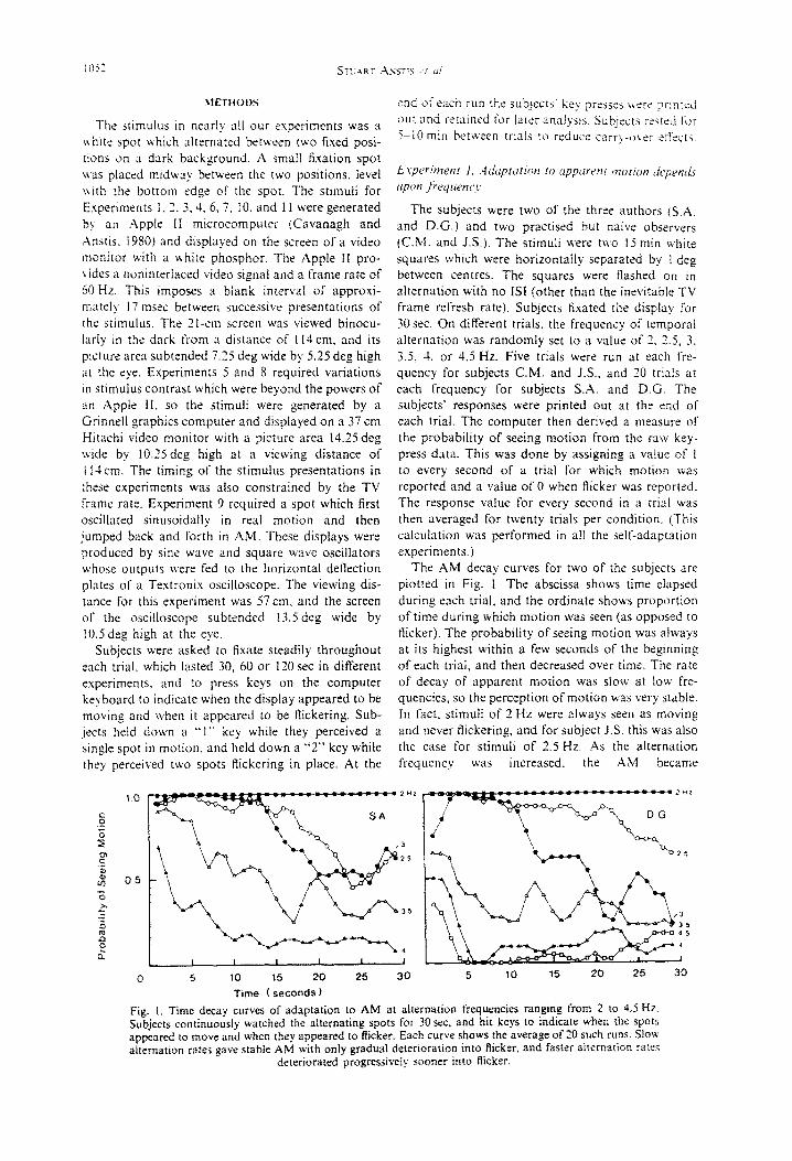
The subjects were two of the three authors (S.A. and D.G.) and two practised but naive observers (C.&f. and J.S.). The stimuli were two 15 min white squares which were horizontally separated by 1 deg between centres. The squares were flashed on in alternation with no IS1 (other than the inevitable TV frame refresh rate). Subjects fixated the display for 30sec. On different trials, the frequency of temporal alternation was randomly set to a value of 2. 7.5, 3. 3.5, -I, or 4.5 Hz. Five trials were run at each fre- quency for subjects C.M. and J.S., and 20 trials at each frequency for subjects S.A. and D.G. The subjects’ responses were printed out at the end of each trial. The computer then derived a measure of the probability of seeing motion from the TBW key- press data. This was done by assigning a value of 1 to every second of a trial for which motion was reported and a value of 0 when flicker was reported. The response value for every second in a trial was then averaged for twenty trials per condition. (This calculation was performed in all the self-adaptation experiments.)

The AM decay curves for two of the subjects are plotted in Fig. I. The abscissa shows time elapsed during each trial, and the ordinate shows proportion of time during which motion was seen (as opposed to flicker). The probability of seeing motion was always at its highest within a few seconds of the beginning of each trial, and then decreased over time. The rate of decay of apparent motion WBS slow at tow ke-

quencies, so the perception of motion was very stable. In fact, stimuli of 2 Hz were always seen as moving and never flickering, and for subject J.S. this was also the case for stimuli of 2.5 Hz. .4s the alternation frequency was increased, the AM became

1.0

0.5

2 HZ

3

25

35

2 HZ

Time ( seconds) fig. i. Time decay curves of adaptation to AM at alternation frequencies ranging from 2 to 4.5 Hz. Subjects continuously watched the alternating spots for 30 sec. and hit keys to indicate when the spots appeared to move and when they appeared to flicker. Each curve shows the average of 20 such runs. Slow alternation rates gave stable AM with only gradual deterioration into flicker, and faster alternation rates

deteriorated progressively sooner into Ricker.

Adaptation to apparent motton I053

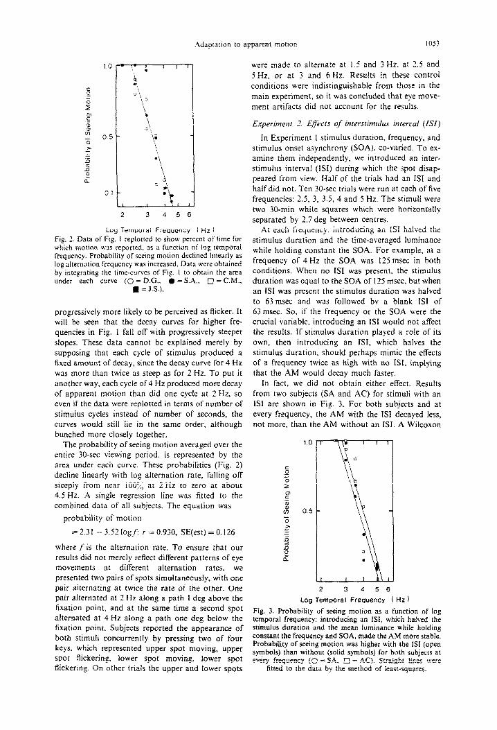
2 3 4 56

Log Temporal Frequency ( Hz ) Fig. 3. Data of Fig. I replotted to show percent of time for which motion was repoited. as a function of log temporal freouencv. Probabilitv of seeing motion declined linearly as logalternation frequency was increased. Data were obtained by integrating the time-curves of Fig. I to obtain the area under each curve {O = D.G., 0 = S.A.. D = C.M.,

m = J.S.).

progressively more likely to be perceived as flicker. It will be seen that the decay curves for higher fre- quencies in Fig. 1 fall off with progressively steeper slopes. These data cannot be explained merely by supposing that each cycle of stimulus produced a fixed amount of decay, since the decay curve for 4 Hz was more than twice as steep as for 2 Hr. To put it another way, each cycle of 4 Hz produced more decay of apparent motion than did one cycle at 2 Hz, so even if the data were replotted in terms of number of stimulus cycles instead of number of seconds, the curves would still lie in the same order, although bunched more closely together.

The probability of seeing motion averaged over the entire 30-see viewing period, is represented by the area under each curve. These probabilities (Fig. 2) decline linearly with log alternation rate, falling off steeply from near lOOl:,i at 2 Hz to zero at about 4.5 Hz. .4 single regression line was fitted to the combined data of all subjects. The equation was

probability of motion

=2.31 - 3.52iogf: r =0.930, SE(est)=O.l26

where f‘is the alternation rate. To ensure that our results did not merely reflect different patterns of eye movements at different alternation rates, we presented two pairs of spots simultaneously, with one pair alternating at twice the rate of the other. One pair alternated at 2 Hz along a path 1 deg above the fixation point, and at the same time a second spot alternated at 4 Hz along a path one deg below the fixation point. Subjects reported the appearance of both stimuli concurrently by pressing two of four keys. which represented upper spot moving, upper spot flickering, lower spot moving, lower spot flickering. On other trials the upper and lower spots

were made to alternate at I.5 and 3 Hz. at 2.5 and 5 Hz, or at 3 and 6 Hz. Results in these control conditions were indistinguishable from those in the main experiment, so it was concluded that eye move- ment artifacts did not account for the results.

In Experiment 1 stimulus duration, frequency, and stimulus onset asynchrony (SOA). co-varied. To ex- amine them independently, we introduced an inter- stimulus interval (ISI) during which the spot disap- peared from view. Half of the trials had an ISI and half did not. Ten 30-set trials were run at each of live frequencies: 2.5, 3, 3.5, 4 and 5 Hz. The stimuli were two 30-min white squares which were horizontally separated by 2.7 deg between centres.

At each frequency, introducing an ISI halved the stimulus duration and the time-averaged luminance while holding constant the SOA. For example, at a frequency of 4 Hz the SOA was I23 msec in both conditions. When no ISI was present, the stimulus duration was equal to the SOA of I25 msec, but when an IS1 was present the stimulus duration was halved to 63 msec and was followed by a blank ISI of 63 msec. So, if the frequency or the SOA were the crucial variable. introducing an ISI would not affect the results. If stimulus duration played a role of its own, then introducing an ISI, which halves the stimulus duration, should perhaps mimic the effects of a frequency twice as high with no ISI, implying that the AM would decay much faster.

in fact, we did not obtain either effect. Results from two subjects (SA and AC) for stimuli with an ISI are shown in Fig. 3. For both subjects and at every frequency, the AM with the ISI decayed less, not more, than the AM without an ISI. A Wilcoxon

2 3 4 56 Log Temporal Frequency ( Hz )

Fig. 3. Probability of seeing motion as a function of log temporal frequency: introducing an 1.X which halved the stimulus duration and the mean luminance while holding constant the frequency and SOA, made the AM more stable. Probability of seeing motion was higher with the ISI (open symbols) than without (solid symbols) for both subjects at every frequency (0 =SA, 17 = AC). Straight lines were

fitted to the data by the method of least-squares.

matched-pairs signed-ranks test of the data for each subject. showed this difference to be significant at the 0.05 ievel (SA T = 0. .V = 5; AC T = I, .L’ = j). Thus. introducing an iSI. while keeping frequency and SOA constant, stabilized the perception of motion, render- ing it less vulnerable to adaptation. This conclusion was confirmed as well in Experiment 7 by cross- Ltdaptation with and without an ISI.

Adaptation to AM was measured by a nulling technique. ProIonged viewing of AM at a given alternation rate leads to a reduced probability of seeing motion. However, as Experiment 1 showed, reducing the alternation rate can increase the proba- bility of seeing motion. Therefore. in this experiment subjects were given a potentiometer which controlled the alternation rate, and were instructed that as soon as the motion degenerated into flicker they should reduce the alternation rate until they saw motion again. This process was continued so that the gradu- ally increasing level of adaptation was nulled by a eradually falling alternation rate.

The spots were 25 min white squares, separated by I deg between centers. The initial alternation rate for each 60-see run was arbitrarily set at 8 Hz. Results for the two subjects are plotted in Fig. 4(a) {mean of 5 runs per subject), on linear co-ordinates. This figure shows that the alternation rate had to be reduced, first rapidly then more slowly. in order to hold the stimulus at the perceptual borderline between motion :tnd flicker. The state of adaptation at any instant resulted from exposure to a constantly changing adapting stimulus. The region above each curve portrays the stimulus conditions which give flicker, while in the region below, motion would be seen. The results are re-plotted on double logarithmic co-

ordinates in Flp. -l(b). The data he along srraipht Iin<, on the i~g-to$ plot. whrch shows that the! obeb power laws. The best fitting power functions ‘tre:

r = O.oYJ. SE(est) = 0.0046 (S.4)

nulling frequencv = 6.43 x I ,? -0.X?@ ; = 0.996. SEfest) = 0.0077 (DG).

where f is the elapsed time in seconds (2 <: f <: 60). Since the amount of adaptation was increasing

over time. the subject had to reduce the nulting frequency to keep the motion visible. Thus. the adapting stimulus became continually stronger (see experiment 6) as the frequency of alternation was decreased.

The state of adaptation at any instant is equal to the integral of the adapting strength of all previous nulling frequencies. This integral drives the nulling frequency along a power law curve.

Experimenr 4. Efect o/’ sparid sqmrnrion

We measured the effect of spatial separation be- tween two thin vertical lines each 15 min high x I.5 min wide, and separated horizontally by 0.1, 0.75, 0.5. 0.73 or I.0 deg. Two subjects watched the stimulus alternating at 4Hz for a 30-set in- spection period, and recorded when they saw flicker or motion. The mean probabilities of seeing motion, averaged over twenty 30-set trials per subject, are shown in Fig. 5. Note that the spatial separation on the “r-axis is a log scale: this gave a much better fit to a straight line than did linear separation. the probability of seeing motion at a spatial separation of 1 .O deg and an alternation rate of 4 Hz is quite LOW, as in Experiment 1. but this probability is higher at smaller separations even with this high alternation rate. This result suggests that decreasing the spatial

0 10 20 40 60 I J 40 60 Log Elapsed Time i seconds)

Elapsed 11me (seconds)

Fig. 4. (a) Frequency needed to just maintain the impression of motion as a function of elapsed time. Each c&e shows the mean of five 60 set runs. As adaptation continued, the: frequency had to be reduced. first rapidly then more slowly in order to null the adapting effect and hold the stimulus at the perceptual borderline between motion and flicker (0 = S.A.. 0 = D.G.). (b) S;fme data repIotted on double logarithmic co-ordinates. Best fitting straight lines are power functions with slopes of -O.ZJZ (S.A.) and

-0.22 (D.G.).

Adaptation to apparent motion 1055

I- i

, -

IL cl

.

\ 3 L

1 .1 0.25 0.5 0.75 1 .0

Log Spatial Separation (degrees ) Fig. 5. Mean probability of seeing motion as a function of log spatial separation. Each point is the average of twenty 30-set runs. with a fixed alternation rate of 4 Hz. As the spatial separation increased from 0. I to 1.0 deg visual angle, the probability of seeing motion decreased. A single line has been fitted to the data of both subjects (0 = S.A..

r

0 = D.G.).

separation while holding alternation rate constant, and decreasing frequency while holding spatial sepa- ration constant, have similar stabilising effects on the perception of motion.

Since the two subjects gave such similar results, a single line was fitted to their combined data. This best fitting function was

probability of motion = 0.03 - 0.941 log S: r = 0.986, SE(est) = 0.065

where S is the spatial separation in degrees of visual angle.

The slope of this log spatial function was -0.941 while the slope of the log temporal function in Experiment 1 was - 3.52, which suggests that adapta- tion to AM may be more sensitive to time than to space.

Experiment 5. Eflect of stimulus contrast

Subjects viewed for 30sec a 25-min square spot that alternated between two positions 1 deg apart at an alternation rate of 3.75 Hz. They reported by means of computer keys when they saw motion and when they saw flicker. The background was a mid- gray and the spot was lighter than the surround. The contrast of the spot was set to either 0.15 (low contrast) or 0.6 (high contrast). The probabilities of seeing AM (mean of twenty 30-see trials) with a low contrast spot were 0.25 and 0.30 for D.G. and S.A. respectively, and with a high contrast spot were 0.50 and 0.49. Thus, AM was seen more with high con- trast than with low contrast spots.

Experiment 6. Adapting to one frequency and testing at another

In all the experiments described so far the adapting stimulus was the same as the test stimulus, but in the

experiments that follow we adapted to one stimulus and tested on another. This cross-adaptation para- digm allowed us to separate out experimentally the roles of the adapting and the test stimulus.

In Experiment 1 the test frequency was always the same as the adapting frequency, and there are two possible reasons why higher alternation frequencies of AM showed more rapid adaptation than lower frequencies: (1) higher frequencies gave a stronger motion signal. and so produced stronger adaptation. or (2) higher frequencies gave a weaker motion signal, and so were more labile and more susceptible to being adapted. In this experiment, we adapted our subjects to one frequency and tested them at another. We were able to show that lower frequencies give stronger motion signals than higher frequencies.

We used a 3 x 3 design in which three adapting frequencies 3, 3.5 and 4 Hz were each paired with three test frequencies also 3, 3.5 and 4 Hz. A con- tinuously cycling “topping-up” adaptation procedure was used. Subjects adapted for approximately 5.7 set to one of the adapting frequencies, and a click sounded as the display then switched for approxi- mately 1.1 set to the test frequency. Another click signalled the end of the test interval, and subjects reported whether the test stimulus appeared to move or flicker by pressing the “1” or “2” key on the computer keyboard. The cycle then repeated, with another 5.7sec of exposure to the same adapting frequency followed by another 1.1 set test period. Seventeen cycles were presented in a total period of two minutes. Four 2-min runs were made for each of the nine conditions. Both adapting and test stimuli consisted of two 15-min white squares separated horizontally by 2 deg.

Figure 6 shows the proportion of test presentations on which motion was reported, plotted as a three- dimensional surface with adapting frequency running from left to right, test frequency running from far to near, and percent probability of seeing motion plot- ted as height. Clearly, the surface for each subject slopes steeply downwards from rear to front. This shows that high test frequencies are much more readily adaptable than low frequencies. The surface also slopes up to the right, but much less steeply. This shows that high adapting frequencies are less effective adaptors than are low frequencies. Since the slope from rear to front is about 21 times steeper than the slope from left to right, we can say that the results are determined more strongly by adaptive susceptibility than by adapting strength.

In Experiment 1, subjects observed the same stim- ulus continuously and reported the frequency of seeing AM. The same stimulus therefore served as both adapting and test field. When the adapting and test frequencies are the same, adapting strength and adaptive susceptibility work in opposite directions; a stimulus that is a strong adaptor is also less sus- ceptible to adaptation. However, as the frequency is raised the lability or adaptability of the test stimulus

1056 STUART .A.\;sm zt ul

Fig. 6. Cross-adaptation between frequencies. In Experiment 6, an adapt-test sequence cycled con- tinuously. One datum point was collected at each test period (about every 7secf: subjects adapted for 5.6sec to one frequency and tested for 1.1 set at the same or another frequency. Five I!-min runs were made in each condition. Data are plotted as a 3-D surface, where .X = adapting frequency (left to right), z = test frequency (far to near). and .v = percentage of time for which motion was seen (vertical axis). Surfaces slope down steeply from rear to front, showing that high test frequencies are much more adaptable than low ones. Surface also slopes gently up from left to right. showing that high adapting frequencies are slightly less effective adaptors than are low ones. But adaptation is determined much more

by adaptability of test frequency than by the adapting power of the inspection frequency.

increases much more rapidly than the adapting power of the adapting stimulus decreases, so there is a net increase in the amount of adaptation. This is shown by the dashed lines along the positive diagonals in Fig. 6, which show a downward slope-an in- creasing lability of apparent motion-with rising frequency.

The data show no sign of temporal frequency “tuning”. Frequency tuning has been demonstrated in the spatial domain for luminance gratings, in that following exposure to a grating of fixed frequency, test gratings of the same or neighbouring spatial frequencies become more difficult to see. However, test gratings of very different spatial frequencies are unaffected (Blakemore and Campbell, 1969). There is some evidence for a temporal analog, in the form of narrow-band visual tuning to the temporal frequency of flicker (Smith, 1970; Pantle, 1971, 1972; Nilsson et RI., 1975), but the effect is rather weak. If the visual system were tuned to the spatio-temporal frequency of apparent motion, then adapting to apparent mo- tion of 3.5 Hz should especially degrade test apparent motion of the same frequency, and should have less effect on the neighbouring frequencies of 3 and 4 Hz. Similarly adaptation to 3 Hz (or 4 Hz) should have a greater effect on 3 (or 4) Hz. Any such tuning would have shown up in our data as a V-shaped valley impressed into our 3-D surface and running along the positive diagonal (dashed line in Fig. 6). There was no sign of any such tuning valley in our results. The range of temporal frequencies used in past studies

which found some evidence for temporal frequency tuning was much wider than the range we used (l-50 Hz vs our 3-4 Hz), so we are not attempting to criticise previous studies. However, we found no evidence for temporal tuning over the small range of frequencies for which we obtained reports of AM. We hypothesise that strong motion signals adapt the visual system more readily and are more resistant to adaptation. On this hypothesis, our results imply that low alternation rates gave stronger motion signals than higher rates did.

Experiments 7, Band 9. Adapt to one stimulus, test on another

The cross-adaptation used in Experiment 6 can be generalized to allow the relative motion strength of various AM stimuli to be compared. We used it to show that:

{I) AM with an ISI gives a stronger signal than AM of the same temporal frequency without an ISI.

(2) High contrast spots give a stronger motion signal than low contrast spots.

(3) Real sinusoidal motion (RM) gives a stronger motion signal than square-wave apparent motion.

The next three experiments all used a 2 x 2 matrix design in which both the test and the adapting stimuli were set to one of two values along some continuum (IS1 vs no ISI; high vs low contrast; real vs apparent motion). In each experiment two subjects made five 120-set runs in each of the four (2 adapting x 2 test)

+\daptatlon to apparent motion

D,G. S.A.

N I% H ISI

Adapt Adapt

Fig. 7. Cross-adaptation with or without an ISI. Conventions are the same as for Fig. 6 (perspective viewpoint is changed for easier viewing). The gradual downward slope from left to right and the steeper slope from rear to front. show that the IS1 adapting stimulus was a slightly stronger adaptor than the no-IS1 adapting stimulus, and the ISI test stimulus gave a stronger motion signal than the no-IS1 test

stimulus. since it resisted adaptation much better.

1057

conditions. A cyclic, topping-up adaptation pro- cedure was used in which the adapting stimulus was viewed for 5 set, then replaced for 1 set by the test stimulus. A click at the beginning of the test period served as an auditory cue reminding the subject to report whether the stimulus appeared to be moving or Pickering. The adapting stimulus was then presented for a further 5 see, followed by the test stimulus for I sec. and so on. The two spots were Ifi-min squares separated by 1 deg between centers, alternating at a rate of 2.5, 3 or 3.75 Hz in the different experiments described below.

The mean probability of motion in each condition is depicted in the three-dimensional plots of Figs 7, 8 and 9. In each of these plots the adapting stimuli lie along the .r-axis from left to right, the test stimuli lie along the z-axis going into the page in depth, and the probability of seeing apparent motion lies along the vertical y-axis.

Cross-adaptation with or without an i.V

in this experiment the alternation rate was always 3 Wz. In the no-I% conditions the duration of each spot presentation was therefore one-sixth of a second (170msec). In the iSI conditions this stimulus du- ration was halved to S5 msec and followed by a dark ISI also of 85 msec. Thus the alternation rate was held constant at 3 Hz whether there was an ISI or not.

Results are shown in Fig. 7. The data show a gradual slope downward from left to right, showing that the IS1 adapting stimulus was a slightly stronger adaptor (producing more adaptation) than the no-IS1 adapting stimulus. The data also show a steeper slope downward from rear to front, showing that the IS1 test stimulus gave a much stronger motion signal than the no-IS1 test stimulus, since it resisted adapta- tion much better. An analysis of variance showed that the difference in test stimulus accounted for 85 and 94”/, of the variance for D.G. and S.A. re- spectively, while the adapting stimulus accounted for only IO and 8% of the variance.

To summarise. adding an ISI to a spot which alternated at 3 Hz strengthened the motion signal, even when the alternation rate was held constant: and the adaptation to AM was more sensitive to the test stimulus than to the adapting stimulus.

Cross-adaptation with high or few stj~ulus contrast

The alternation rate was held constant at 3.75 Hz, with no ISI. The contrast of the spots was either high (0.6) or low (0.15). The subjects were D.G. (the second author) and J.S., a practised observer who was unfamiliar with the purpose of the experiment.

Results are shown in Fig. 8. The overall pattern of results is comparable to that in the previous experi- ment. Adaptation was most pronounced with high contrast adapting stimuli and low contrast test stim- uli, so we conclude that high contrast spots gave a stronger motion signal than low contrast spots. As before, the adaptation to AM appeared to be more sensitive to the test than to the adapting stimulus. The difference in test stimulus accounted for 68 and 49% of the variance for D.G. and 3.S. respectively, while the adapting stimulus accounted for 19 and 45% of the variance.

Similarly, Keck et al. (1976) found that the motion aftereffect was strongest, as measured by its duration and apparent speed, with high contrast adapting gratings and low contrast test gratings. They ex- plained the dependence of the motion aftereffect on the contrast of the stimuli, in terms of the imbalance between the discharges of ceils tuned to motion in opposite directions. Presumably, the adapting stimu- lus desensitises cells whose preferred direction of movement coincides with that of the adapting stimu- lus, but leaves cells with the opposite preferred direc- tion unaffected. High contrast adapting stimuli pro- duce more excitation (desensitisation) and thus a larger imbalance than low contrast stimuli. When the test stimulus is of high contrast, the imbalance be- tween adapted and unadapted cells is reduced and the motion aftereffect is smaller.

The effect of contrast on adaptation to AM in our

STUART ANSTIS ef al.

n,qn 10* il,pn

Adapt Adapt Fig. 8. Cross-adaptation with high or low stimutus contrast. This 3-D plot of adapting contrast level 5s test contrast ievel shows that high contrast (0.6) spots gave a stronger motion signal than low contrast

(0.15) spots.

experiments may also be related to the amount of excitation produced in neural motion detectors.

Cross-adaptation with real or apparent motion

Kolers (19444) proposed that adaptation to AM is one of the strongest pieces of evidence that RM and AM are mediated by different neural mechanisms. He argued that whereas one can readily adapt to AM, staring at sinusoidal RM never produces adaptation-the motion continues to be seen as motion. Clatworthy and Frisby (1973) suggested, on the other hand, that AM may stimulate the neural pathways which also respond to RM, but may do so rather weakly and inadequately, such that prolonged inspection leads to a breakdown. Sekuler (1975) has indicated a need for data on cross-adaptation be- tween real and apparent motion to resolve this issue. Our experiment showed strong cross-adaptation be- tween RM and AM, and we therefore agree with Clatworthy and Frisby that AM must be stimulating the same neural pathways as RM.

We measured cross-adaptation between real and apparent motion. The apparent motion was a 1 mm (3min arc) spot on an oscilloscope, driven by a square wave generator so that it jumped to and fro at a rate of 2.5 Hz over a path length of 1 deg. The

real motion was the same spot driven by a sinusoidal generator so that it oscillated back and forth at 2.5 Hz along the same path length of I deg.

The results, which are shown in Fig. 9, are com- parable to those in the two previous experiments. Figure 9 shows that a test stimulus in real motion (rear plane) gave such a strong motion signal that it was virtually always reported as moving, whether the subject had previously adapted to real or to apparent motion. However, an AM test stimulus (front plane) was considerably adapted by prior exposure to AM, and was adapted even more by prior exposure to real motion. This also shows that real motion gave a stronger motion signal (was a more effective adaptor) than apparent motion. Note that the slope from front to back in Fig. 9 is appreciably steeper than the slope down from left to right, although the presence of an interaction between adapt and test conditions pre- vents determination of the variances involved. How- ever, this interaction is interesting in itself. The mean probability of reporting motion of a test stimulus was higher when the test stimulus was RM than when it was AM, but this probability was lower when the adapting stimulus was RM than when it was AM. This suggests that a motion signal’s adaptability cannot be separated from its effectiveness as an adaptor. The interaction reached significance because

S.A. 1.0

Test

aDo*IN)1 <all .DDC**n, rt.4

Adapt Adapt Fig. 9. Cross-adaptation between real (sine-wave) and apparent (square-wave) motion. A test stimulus in real motion gave such a strong motion signal that it was always reported as moving (rear plane). An AM test stimulus was considerably adapted by prior exposure to AM, and was adapted even more by prior exposure to RM. This strong cross-adaptation from RM to AM suggests that AM must be stimulating

the same neural pathways as RM.

Adaptation to apparent motion 1059

a test stimulus in mat motion always appeared to be moving regardless of the adapt condition. The overall trend suggests that the adaptation was more sensitive to the test stimulus than to the adapting stimulus for .4M but not for RM.

More importantly. this experiment revealed very strong cross-adaptation between real and apparent motion. Following exposure to AM, the probability of seeing AM was 0.56 and 0.47 for D.G. and S.A. respectively, but following exposure to RM, this probabi!ity was reduced to only 0.12 and 0.19. This cross-adaptation provides strong evidence that real and apparent motion are mediated by overlapping neural pathways. Thus, our study of the phenomenon described by Kolers goes against his theoretical inter- pretation, but is consistent with Clatworthy and Frisby’s (1973) position. Gregory and Harris (1984) reached the same conclusion through a different method. They found that ciockwise real motion and anticlockwise apparent motion coufd cancel at a critical balance of intensities, which suggests that a single neural channel mediates both real and appar- ent motion.

Experiment IO. Flickering or stationary spots produce less a~aptatjon than apparent motion does

Adaptation to apparent motion has several poss- ible causes. The least interesting possibility is that exposure to the bright adapting spots merely light- adapts the stimulated patches of retina. if so, then the adaptation would have little or nothing to do with motion per se, and could be achieved just as readily with stationary adapting spots as with apparently moving ones. A more interesting possibility is that the adaptation is related to the tempera! rate of stimu- lation. Experiments l-9 showed that the adaptation of AM depends on the spatio-temporal properties of the stimulus. If frequency is the crucial factor, spots flickering in phase ought to be more effective adapt- ors than stationary ones. If the adaptation involves mechanisms of motion perception per se, then spots alternating in counterphase, which produce apparent motion, ought to be more effective than spots flickering in phase, which produces only Bicker with- out apparent motion.

We tested these predictions by exposing our four subjects to the following adapting stimuli:

(1) Stationary spots. (2) Spots flickering in phase: the spots turned on

and off together SimuItaneously at 3.5 Hz. (3) Spots alternating in counterphase: the spots

turned on alternately at 3.5 Hz, giving apparent motion.

The same cyclic “topping-up” adapting procedure was used as before. The display cycled between 4 set (14 cycles) of 3.5 Hz adapting stimulus, alternating with 0.6 set (2 cycles) of 3.5 Hz AM test stimulus. On an auditory cue after each test stimulus the subject signalled whether the test had appeared to move or

to flicker, as before. The alternation between adapt- ing and test periods continued over a total run time of 12Osec. In al! three conditions the adapting and test stimuli consisted of two 15 min white squares horizontally separated by 1 deg. The mean luminance was kept constant by presenting the stationary spots at half the lu~nance of the flickering spots.

Results are shown in Fig. IO, which shows the probabiiity of seeing motion over the whole run for each condition, averaged over 4 subjects by 5 runs per condition. Apparent motion gave the greatest adap- tation: flicker produced much less adaptation, and stationary spots even less. Since neither stationary nor Bickering spots were effective adaptors, we con- clude that the adaptation to apparent motion is not a local process, concerned only with each spot indi- vidually. Any mechanism which looked only at one spot could not distinguish flicker from motion. and could not adapt differently to them. The mechanism must be responding to both spots and be sensitive to the temporal phase between them.

Green (1981) Observed a significant threshold el- evation for detection of a moving grating after adap- tation to a flickering field. He proposed the existence of a transient system in which flicker and motion are processed by common neural mechanisms, and a separate sustained system which also processes mo- tion information. Green found more flicker adapta- tion than we did, but this may be because he used higher temporal frequencies than we did. He obtained significant adaptation to 9 Hz flicker, but found only a small amount of adaptation at the freqeuncy of 3.5 Hz that we used. Green did not state a temporal frequency limit for the transient motion system, but it is possible that our AM stimulus was in the range of the sustained system which is not sensitive to

Stotionory Flickerinq AM

Adapting Condition

Fig. 10. Mean probability of seeing motion following adap- tation to stationary, flickering or apparently moving spots. Each bar shows the mean response of four subjects x five IZO-sec runs. Short vertical lines show standard errors. Flickering and stationary spots produced much less adapta- tion than AM did. The process of adaptation cannot be confined to the retinal locus of each spot considered on its own, since neither stationary nor flickering spots were

particularly effective adaptors.

(a) (bl

Two swts Four Soots

Adapting Condition CC)

Fig. I I. Altering the perceived pattern of motion without altering the retinal stimulation greatly reduced adaptation to AM, so adaptation depends upon the perceived path of the adapting AM. (a) Adapting and testing on the same two alternating spots reduced the probability of seeing test motion to 57”; (left bar in c). (b) Adding two extra adapting spots made the apparent path of AM follow the two arrowed vertical paths. This produced very little adaptation: motion was seen in the test field for W”,, of the time (right bar in c). (c) Results of adapting to two vs four spots (mean of four subjects x five IX-set runs).

Short vertical lines are standard errors.

Experiment IO showed that the visual channels which adapt to AM are sensitive to spatiotemporal phase and are adapted more readily by motion than by Hicker. It follows that the visual channels must be looking at both spots, not just at one spot. Experi- ment I I shows that they can also be affected by other spots which happen to be in the visuai field.

The test field was still two spots, but the adapting fields consisted of either two or four spots. The same cycling “topping-up” procedure was used, with the display alternating between a four-spot (or two-spot) adapting field and a two-spot test field. Both fields were in apparent motion at a repetition frequency of 3.5 Hz. Four set of the adapting field were followed by 0.6 set of the test field, and this adapt-test-adapt sequence ran continuously for one minute. An audi- tory cue accompanying each test presentation re- minded the subject to press a computer key to indicate whether the stimulus looked like motion or like flicker.

Two different adapting fields, illustrated in Fig. 11, were used on different trials, as follows:

Condition 1. The adapting and test field each consisted of the same two IS mitt spots in apparent motion, alternating at 3.5 Hz and separated horizon- tally by I deg [Fig. I l(a)].

Condition 2. The test field was the same as before. The adapting field included the two original spots, but two extra spots were added, one being 1 deg below the left hand spot and the other being 1 deg above the right hand spot [Fig. II(b)]. These spots were switched on and off in step with the original two spots so that a pair of spots appeared to jump vertically up and down. Notice that the adapting

apparent motion did not traverse the horizontal path between the two original spots. but now lay along two vertical paths at right angles to it.

The adapting stimulus at the retinal site of the test spots was identical in both conditions-namely, con- tinuous alternation between the two spots at 3.5 Hz throughout the experiment. So, if the adapting mech- anism were responding only to what happened at these two retinal sites, even including the spatio- temporal relations between them, then both condi- tions should give the same results. In fact, they gave very different results.

Fig. 11 shows the mean probability of seeing motion during each two-minute run. Each datum point is based on 6.5 judgments (five runs of I3 judgments in each IZO-set run) by each of four subjects. Condition I (adapt and test on two spots, in horizontal AM) gave marked adaptation, with mo- tion being seen for 57Y0 of the time (mean of 4 subjects). However, the presence of two extra spots in condition 2 (which were positioned well away from the test spots} greatly diminished the adaptation, with motion now being seen for 87’:; of the time. Thus, the vertical adapting jumps had little effect on the visi- bility of the horizontal test motion.

We conclude from Experiments 10 and I i that the adaptable visual channels must be responding not only to the two original spots, but also to other neighbouring spots. Moreover, they must also be taking account of the spatio-temporal phase relations between the test spots and these extraneous spots. Beck and Stevens (1972) also attributed AM percep- tion to specific neural mechanisms selectively re- sponsive to sequentiat changes in stimulus position. After observation of two sequentially presented fights that produced the perception of unidirectional AM.

the presentation of lights in the opposite directiort gave the impression ot‘ mote rapid mobement. This directional aftereffect w a s also observed when the lights uere perceived as successive stationary lights.

~everley and Regan (1979. 138Oi also reported an & c t of stimulus c0nfiguratio,n on motion adapta- tion. They found that a strong changing-sire aftereffect w a s produced by P rectangle whose vertical sides oscillated in Countetphase (size oscillation), but only a small aftereffect was produced when the sides u~dlatsd iri phase (positional osciilaliun). Thus em- bedding an oscillating line in a configuration OF other lines aitered the pattern of perceived morion wthout attcrinp the local retinal stimulation, so the adapting mechanism must be comparing the phase re- lationships of the opposite sides of the square.

What visual channels ate adapting when perceived apparent motion decays into flicker? Experiment 10 showed that adaptatiurl to retinal illuminancr and 10 temporal r;ltr of alternation (flicker) were only par- tially responsible for adaptation to AM. The major factor in adaptation was the spatio-temporal phase relarions btrween the two spots. This relation is. as ti;eti! the source OF the percept of apparent motion. The disruptive effects or the added extraneous spots m Experiment 11 showed that the adapting channels are also akcted by the visual context. The adapta- tion depended not only upon the s&o-temporal phase relations. but also upon the path of seen motion. When the extraneous spots were added the visual system broke the horizontal links or correspon- dences which established apparent motion between the two original adapling spots, and substituted vertical motion links from each original spar to the nearest extraneous spot. We Conch& that the adap- tation process OCCurs at a location in the visual system at OF upstream of the point where the “Corre- spondence prob~em”~U~~~~~ 1979) is solved, that is, after points have been linked up into patterns of notion.

Our experiments demonstrate that adaptation to .tM provides a usefuul technique for assessing the strength of motion signals. AM was strongest for low temporal frequencies, alternations including an ISI. small spatial separations. and high contrast. The self-adaptation experiments /Experiments I-5) showed that the deterioration of motion into flicker was greatest under these conditions, and the cross- adaptation experiments [Experiments 6-9) showed that a strong motion signal was provided by these stimuli. They were the most effective as adaptors, and the most resistant to adaptation when used as test s:imuli.

It is not easy to measure the strength of AM. Kolers (t972) found th;tt when a circIe was follnvxd by a displaced square or triangle, one shape changed

smoothly into the other and _eaod AM was seen between them. Within very broad limirs. any stimulus could k paired tith any other one. Kolers attempted unsuccessfully to rank the stimulus pairs in order of -‘guodness” of AM. He tried two critena: timing range and smoothness of motion. tt is known that the perception of AM depends upon the timing of the stimulus presentations. so it might be that the stron- ger a pair’s tendency to fwse. the more tolerant it would be to deviations from optimal timing. How- ever. K&-s found that timing tolerance did not differ significantly from one srimulus pair IO another. Nor did subjective judgments of smoothness of motion,

Ulhnan (1979) investigated the “correspondence problem”, in which the visual system must decide which items in the initial image correspond IO which items in a succeeding image. The important questions are, first. what constitutes an item. that is. what are the primitives or elementary tokens which are se? into correspondence. and second, on what basis are items set in correspondence? He concluded that the tokens were fairly low-tevel features such as edges of blobs. and &at correspondences were established in twb stages F&t, the correspondence between isolated token pairs was governed by a certain “builr-in” similarity metric, termed afinity. Second. when rival candidates had about the same afinity the correspon- dence was decided by means of local competitive interactions. Their correspondence strength, which we have called the strength of the AM signal, can be assessed by a competing split-motion technique in which a vertical line is replaced by a line to its left and another line to its right. AM will typically be seen zoward the nearer or the more similar line. A change in length of one line by a factor of 3/2 produces the same charige in similarity as z change in orientation of 45 deg.

Burt and Sperling jt98l) also measured the strength of ANI by putting different AM paths into competition. A horizontal row of dots was flashed successively in a sequence of positions on a screen, each position being below the previous one and displaced sideways. The dots appeared to jump diag- ona.lly downwards, with the perceived direction (left or right) being determined by trade-offs in space and time between potentially corresponding dors. Our technique of assessing the strength of AM by mea- suring its adaptability offers an independent measure of the strength of AM. We found, as did Ullman (1979), that AM strength incfeased with decreasing spatial separation (Experiment J), but we found that adding an IS! tended to increase AM strength (Ex- periment 7}, whereas Ullman found (p_ 40) that an ISI tended to make all correspondence strengths more equal. reducing the effects of differing spatiat separations.

The strong cross-adaptation that we found from real to apparent motion (Experiment 9) suggests that AM must be stimulating the: same neural pathways as RM. This is contrary to Kolers’ argument [ 1964) that

diffsrent mechanisms are involved because only AM adapts.

Our data suggest that the adapting m~hanisms respond to spatio-temporal phase relations, not merely to the temporal rate of stimulation. Counter- phase flicker, which produces AM, was an effective adaptor, but in-phase flickering spots produced little adaptation (Experiment 10). These mechanisms are also affected by context, and adapt only along paths where the adapting motion is visible (Experiment II). The visible AM xas changed by adding extra spots which were perceptually organised into vertical mo- tion correspondence instead of horizontal. Hence, the adapting mechanisms are probably located centrally to the neural site at which motion correspondences (Uliman. 1979) are established between successive spots.

Finally, the phenomena described here are not unique to visual motion but may reflect more general perceptual responses to changing stimuli. Anstis and Saida (1985) asked subjects to listen to a tonal stimulus which alternated between two audio fre- quencies. At low alternation rates subjects reported hearing a single stream of sound which jumped up and down in pitch, analogous to visual AM of a spot which jumped up and down in position. At higher alternation rates the stimulus appeared to segregate into two auditory streams, namely a high-pitched interrupted tone and a concurrent low-pitched inter- rupted tone. This is analogous to two visual spots flickering in place. The effects of adapting to these alternating tones were quite similar to those reported here for visual stimuli. At high alternation rates, or with large tonal intervals between the two audio frequencies, the single stream deteriorated into two interrupted monotones more rapidly than at low alternation rates or small tonal intervals. This is analogous to the more rapid deterioration of visual AM into flicker which we found at high alternation rates and at large spatial separations. Even the quan- titative relationships were similar. Just as the prob- ability of seeing motion fell off linearly as the log alternation rate (Experiment I) or the log spatial separation (Experiment 4) was increased, so Anstis and Saida found that the probability of hearing a temporally coherent sequence of tones fell off linearly as the log alternation rate or the log tonal interval was increased. Just as the nulling alternation rate decreased in Experiment 3 along a power law, so the corresponding settings in an auditory nulling experi- ment decreased along a power law. Possibly the auditory algorithms used to solve the cocktail party problem, assigning a stream of incoming sounds to different speakers, are similar to the visual algorithms used to solve the correspondence problem, inter- preting a stream of incoming images as a set of stationary or moving objects.

.~~~X-notvirdRrmenis-S.A. and D.G. uere supponed b) Grant No. A 0260 from the Natural Science and En- gineering Council of Canada INSERC). and .+..C. v.3~ supported by Grdnt i\;o. EY 015% from the Eiational Ere Institute. Part of this work was carried out while S.r\ was Visiting Professor at the Smith-Kettlewell Instltuti- of Visual Science. San Francisco. We thank Dr A. Jampolskk and the Smith-Kettleaell Eye Research Foundation for support and facilities.

REFERENCES

Anstis S. MCI. (1978) Apparent movement. In Handbook of Sensory Ph.vsioiog_v (edited by Held R.. Leibowitz H. W. and Teuber H.-L.), Vol. VHI, pp. 65%673. Springer, Berlin.

Anstis S. M. (1980) The perception of apparent movement. Phil. Trans. R. .Soc. Land. B 290, 153-168. Reprinted in The Psychology of Vision (edited by Longuet-Higgins H. C. and Sutherland N. S.). The Royal Society. London.

Anstis S. M. and Saida S. (1985) Adaptation to auditory stream segregation of frequency-modulated tones. J. P.YR Psychol. Hum. Percept. Perform.

Beck f. and Stevens A. (197 If An aftereffect to discrete stimuli producing apparent movement and succession. Percept. Psychophys. 12, 4824%.

Beverley K. and Regan D. (1979) Separable aftereffects of changing-size and motion-in-depth: Different neural mechanisms? Vision Res. 19, 727-732.

Beverley K. and Regan D. (1980) Temporal selectivity of changing-size channels. J. opt. Sot. Am. 70, 1375-1377.

Burt P. and Sperling G. (1981) Time, distance, and feature trade-O% in visual apparent motion. Psychoi. Rn. 88. 171-195.

Caelli T. and Finlay D. (1979) Frequency. phase, and colour coding in apparent motion. fekeption 8, 59-68.

Cavanaah P. and Anstis S. M. (1980) Visual osvchoohysics . . . . on the APPLE II: Getting started. Behal. Rex. .Meth. Insrrwn. 12, 614-626.

Clatworthy J. L. and Frisby J. P. (t973) Real and apparent visual movement: Evidence for a unitary mechanism. Perception 2, 161-164.

De Sif;a H. R. (1928) Kinematographic movement of oarallel lines. J. pen. Psrchoi. 1, 550-577.

FiAlay D. and Caeli T. (1579) Frequency. phase and colour coding in apparent motion: 2. Perception 8, 595-602.

Green M. (1981) Psychophysical relationships among msch- anisms sensitive to oattern, motion and flicker. Msiun Rex. 21, 971-983.

Gregory R. L. and Harris J. P. (1983) Real and apparent movement nulled. IVurure 307, 729-730.

Keck M. J.. Palella T. and Pantie A. (1976) Motion aftereffect as a function of the contrast of sinusoidal gratings. Vision Res. 16, 187-191.

Kolers P. A. (1964) The illusion of movement. Scienr. Lm. 211, 98-106.

Kolers P. A. (1972) Aspecu ofMotion Perception. Pergamon Press, New York.

Nilsson T. H., Richmond C. F. and Nelson T. IM. (1973) Flicker adaptation shows evidence of many visual chan- nels selectively sensitive to temporal frequeney. Vision Rex. 15, 621-624.

Tyler C. W. (1973) Temporal characteristics in apparent movement: Omega movement vs. phi movement. Q. f. exp. Psychol. 25, 182-192.

Ullman S. (I 979) The Inrerpretation of Visuof Mofion. XI IT Press, Cambridge, MA.

Wertheimer M. (1912) Experimentelle Studien uber das Sehen van Beweeune. Z. Psrchol. 61, 161-265.