sensors

Article

Deep and Wide Transfer Learning with Kernel Matching forPooling Data from Electroencephalography andPsychological Questionnaires

Diego Fabian Collazos-Huertas * , Luisa Fernanda Velasquez-Martinez, Hernan Dario Perez-Nastar,Andres Marino Alvarez-Meza and German Castellanos-Dominguez

�����������������

Citation: Collazos-Huertas, D.F.;

Velasquez-Martinez, L.F.;

Perez-Nastar, H.D.; Alvarez-Meza,

A.M.; Castellanos-Dominguez, G.

Deep and Wide Transfer Learning

with Kernel-Matching for Pooling

Data from Electroencephalography

and Psychological Questionnaires.

Sensors 2021, 21, 5105. https://

doi.org/10.3390/s21155105

Academic Editors: Natsue Yoshimura,

Ludovico Minati, Masaki Nakanishi

and Fernando E. Rosas

Received: 13 May 2021

Accepted: 9 July 2021

Published: 28 July 2021

Publisher’s Note: MDPI stays neutral

with regard to jurisdictional claims in

published maps and institutional affil-

iations.

Copyright: © 2021 by the authors.

Licensee MDPI, Basel, Switzerland.

This article is an open access article

distributed under the terms and

conditions of the Creative Commons

Attribution (CC BY) license (https://

creativecommons.org/licenses/by/

4.0/).

Signal Processing and Recognition Group, Universidad Nacional de Colombia, Manizales 170001, Colombia;lfvelasquezm@unal.edu.co (L.F.V.-M.); hdperezn@unal.edu.co (H.D.P.-N.);amalvarezme@unal.edu.co (A.M.A.-M.); cgcastellanosd@unal.edu.co (G.C.-D.)* Correspondence: dfcollazosh@unal.edu.co

Abstract: Motor imagery (MI) promotes motor learning and encourages brain–computer interfacesystems that entail electroencephalogram (EEG) decoding. However, a long period of training isrequired to master brain rhythms’ self-regulation, resulting in users with MI inefficiency. We introducea parameter-based approach of cross-subject transfer-learning to improve the performances of poor-performing individuals in MI-based BCI systems, pooling data from labeled EEG measurementsand psychological questionnaires via kernel-embedding. To this end, a Deep and Wide neuralnetwork for MI classification is implemented to pre-train the network from the source domain.Then, the parameter layers are transferred to initialize the target network within a fine-tuningprocedure to recompute the Multilayer Perceptron-based accuracy. To perform data-fusion combiningcategorical features with the real-valued features, we implement stepwise kernel-matching viaGaussian-embedding. Finally, the paired source–target sets are selected for evaluation purposesaccording to the inefficiency-based clustering by subjects to consider their influence on BCI motorskills, exploring two choosing strategies of the best-performing subjects (source space): single-subjectand multiple-subjects. Validation results achieved for discriminant MI tasks demonstrate that theintroduced Deep and Wide neural network presents competitive performance of accuracy even afterthe inclusion of questionnaire data.

Keywords: kernel-embedding; transfer learning; Deep and Wide network; motor imagery

1. Introduction

Motor imagery (MI) is related to the process of mentally generating a quasi-perceptualexperience in the absence of any appropriate external stimuli [1]. MI practice promoteschildren’s motor learning and has been suggested to provide benefits in enhancing themusicality of untrained children [2,3], in evaluating the screen-time and cognitive develop-ment [4], and improving attentional focus and rehabilitation [5–7], among others. MI-basedbrain–computer interface (BCI) systems often entail electroencephalogram (EEG)-decodingbecause of their ease of use, safety, high portability, relatively low cost, and, most impor-tantly, high temporal resolution [8]. EEG is a non-invasive and portable neuroimagingtechnique that records brain electrical signals over the scalp, reflecting the synchronizedoscillatory activity originating from the pyramidal cells of the sensorimotor cortex. How-ever, evoked responses in frequency bands, besides the eliciting stimuli, depend uponevery individual. In addition, in MI-based cognitive tasks, the evoked event-relatedde/synchronization of the sensorimotor area is perturbed by other background brain pro-cesses or even artifacts, seriously reducing the signal-to-noise ratio [9]. Hence, to generatesteady evoked control patterns, long training must master brain rhythms’ self-regulation.As a result, the percentage of users with MI inefficiency (or BCI-illiteracy) is high enough

Sensors 2021, 21, 5105. https://doi.org/10.3390/s21155105 https://www.mdpi.com/journal/sensors

Sensors 2021, 21, 5105 2 of 17

to limit this technology to lab environments even that MI research has been going for manyyears [10].

In practice, the MI ability can be assessed to determine to what extent a user en-gages in a mental representation of movements, mainly through self-report questionnairesdeveloped explicitly for this purpose [11]. Yet, there is very little evidence stating a confi-dent correlation between the classification accuracy and the questionnaire scores. Severalreasons may account in this regard [12,13]: weak and ambiguous self-interpretation inunderstanding the questionnaire instructions, laboratory paradigms restricted to a narrowclass of motor activity, timeline limitations guaranteeing consistent mental states, anddifficulty in learning features from subjects with BCI-illiteracy, among others. Hence,although psychological assessment and questionnaires are probably the most accepted andvalidated methods in medical contexts [14], their inclusion in the automated prediction ofthe BCI skills remains very rare due to their disputed reliability and reproducibility [15].For enhancing the predictive utility, the joint analysis of different imaging modalities isachieved, which may explain the discovered relationships between anatomical, functional,and electrophysiological properties of the brain [16,17]. Nonetheless, besides those issuesthat may arise by the questionary implementation, research endeavors of multimodalanalysis pose a challenging problem in terms of combining categorical data with imagingmeasurements, facing the following restrictions [18,19]: Different spatial and temporalsampling rates, noninstantaneous and nonlinear coupling, low signal-to-noise ratios, alack of interpretable results, and the optimal combination of individual modalities is stillundetermined, as well as effective dimensionality reduction to enhance the discriminabilityof extracted multi-view features [20].

Another approach to improve BCI skills is to perform several training sessions inwhich participants learn how to modulate their sensorimotor rhythms appropriately, re-lying on the spatial specificity of MI-induced brain plasticity [21]. However, collectingextensive data is time-consuming and mentally exhausting during a prolonged recordingsession, deteriorating the measurement quality. To overcome this lack of subject-specificdata, transfer learning-based approaches are increasingly integrated into MI systems usingpre-existing information from other subjects (source domain) to facilitate the calibration fora new subject (target domain) through a set of shared features among individuals underthe assumption of a unique data acquisition paradigm [22–24]. Therefore, to have theadvantages of transfer learning in EEG signal analysis, strategies for individual differencematching and data requirement reduction are needed to fine-tune the model for the targetsubject [25]. For example, in [26], the authors use pre-trained models (e.g., VGG16 andAlex-net) as the starting point for approach-fitting. This strategy limits the amount oftraining data required to support the MI classification task. In this case, they compute thecontinuous wavelet transform from EEG signals to represent the time-series data into equiv-alent image representation that can be trained in deep networks. Similarly, Zhang et al.in [27] proposed five schemes for adaptation of a deep convolutional neural network-basedEEG-BCI system for decoding MI. Specifically, each procedure fine-tunes a pre-trainedmodel to enhance the evaluation performed on a target subject. Recently, approachesbased on weighted instances [28] and domain adaptation [29] have been studied. In thefirst case, instance-based transfer learning is used to select the source domain data that ismost similar to the target domain to assist the training of the target domain classificationmodel. In the second case, researchers extend deep transfer learning techniques to theEEG multi-subject training case. In particular, they explore the possibility of applyingmaximum-mean discrepancy to align better distributions of features from individual fea-ture extractors in an MI-based BCI system. Nonetheless, to extract sets of shared featuresamong subjects with a similar distribution, there is a need to adequately handle two mainlimitations of subject-dependent and subject-independent training strategies: small-scaledatasets and a significant difference in signals across subjects [30]. In fact, several issuesremain as challenges to obtaining adequate consistency of the feature space and probabilitydistribution of training and test data, avoiding negative transfer effects [31,32]: feature

Sensors 2021, 21, 5105 3 of 17

extraction from available multimodal data effective enough to discriminate between MItasks, and the choosing of transferable objects and transferability measures along with theassignation of their weights [33].

Here, we introduce a parameter-based approach of cross-subject transfer learningfor improving poor-performing individuals in MI-based BCI systems, and pooling datafrom labeled EEG measurements and psychological questionnaires via kernel-embedding.For sharing the discovered model parameters, as presented in [34], an end-to-end Deep andWide neural network for MI classification is implemented that is, firstly, fed by data from thewhole trial set to pre-train the network from the source domain. Then, the layer parameterlayers are transferred to initialize the target network within a fine-tuning procedure torecompute the Multilayer Perceptron-based accuracy. To perform data fusion combiningcategoricals with the real-valued features, we implement the stepwise kernel-matching viaGaussian embedding, resulting in similarity matrices that hold a relationship with the BCIinefficiency clusters. For evaluation purposes, the paired source–target sets are selectedaccording to the inefficiency-based clustering by subjects to consider their influence onBCI motor skills, exploring two choosing strategies of the best-performing subjects (sourcespace): Single-subject and multiple-subjects, as delivered in [35]. The validation resultsfor discriminating MI tasks show that the proposed Deep and Wide neural network givespromising accuracy performance, even after including questionnaire data. Therefore, thisdeep learning framework with cross-subject transfer learning is a promising way to addresssmall-scale data limitations from the best-performing subjects.

The remainder of this paper is as follows: Section 2 presents the materials and methods,Section 3 describes the experiments and the corresponding results, putting effort into theirinterpretation. Lastly, Section 4 highlights the conclusions and recommendations.

2. Materials and Methods2.1. 2D Feature Representation of EEG Data

From the EEG database collected by an C-channel montage, we build a single matrixfor the n-th trial {Xn∈RC × T , λn∈{0, 1}Λ}N

n=1, that contains T time points at the samplingrate Fs. Along with the EEG data, we also create the one-hot output vector λn in Λ∈N labels.For evaluation in discriminating MI tasks, the proposed transfer learning model is assessedon a trial basis. That is, we extract the feature sets per trial {Xr

n∈RC}Rr=1, incorporating

a pair of EEG-based feature representation approaches (R = 2): Continuous WaveletTransform (CWT) and Common Spatial Patterns (CSP), as recommended for Deep andWide learning frameworks in [36].

Further, the extracted multi-channel features (using CSP and CWT methods) are con-verted into a two-dimensional topographic interpolation RC → RW × H to preserve theirspatial interpretation, mapping into a two-dimensional circular view for every extractedtrial feature set. As a result, we obtain the labeled 2D data {Yz

n∈RW × H , λn : n∈N}, whereYz

n is a single-trial bi-domain t-f feature array, termed topogram, extracted from every z-thset. Of note, the triplet z = {r, ∆t, ∆ f (with z∈Z) indexes a topogram estimated for eachincluded domain principle r∈R at the time-segment ∆t∈T, and within the frequency-band∆ f∈F.

Besides, we estimate the local spatial patterns of relationships from the input topo-graphic set through the square-shaped layer kernel arrangement {Kz

i,l∈RP × P}Il ,Z (asin straightforward convolutional networks), where P holds the kernel size. Therefore,the number of kernels varies at each layer i∈Il , so that the stepwise 2D-convolutionaloperation is performed over the input topogram, Yz, as follows:

YzL = (ϕz

L ◦ · · · ◦ ϕz1)(Y

z), (1)

where ϕzl (Y

zl–1) = γl(Kz

i,l ⊗ Yzl–1 + Bz

i,l) is the convolutional layer, followed by a non-linear

activation function γl : RWzl × Hz

l → RWzl × Hz

l , Yzl ∈RWz

l ×Hzl is the resulting 2D feature

map of the l-th layer (adjusting Yz0 = Yz), and the arrangement Bz

i,l∈RWzl ×Hz

l denotes

Sensors 2021, 21, 5105 4 of 17

the bias matrix. Notations ◦ and ⊗ stand, respectively, for the function composition andconvolution operator.

2.2. Multi-Layer Perceptron Classifier Using 2D Feature Representation

In this stage, we employ the deep learning-based classifier function ϕ : RW × H 7→ Λdeveloped through a Multilayer Perceptron (MLP) Neural Network that predicts the labelprobability vector v∈{0, 1}Λ, as below [37]:

v = ϕ(u0, Θ; φzD ◦ · · · ◦ φz

1), (2a)

s.t.: Θ∗0 = arg minKz

i,l ,Ad ,Bzi,l ,αd{L(vn, λn|Θ); ∀n∈N} (2b)

where φd(ud−1) = ηd(Adud−1+αd) is the fully-connected layer ruled by the non-linearactivation function: ηd : RP′d → RP′d , P′d∈N is the number of hidden units at the d-thlayer, d = {0, . . . , D} (d = 0 is the initial concatenation before the classification layer),Ad∈RP′d × P′d−1 is the weighting matrix containing the connection weights between the pre-ceding neurons and the hidden units P′ of layer d, αd∈RP′d is the bias vector, and the ud∈RP′d

hidden layer vector holds the extracted spatial information encoded by the resulting 2Dfeature maps in the Q domain.

For computation at each layer, the hidden layer vector is iteratively updated by therule (composition function-based approach of deep learning methods) ud = φd(ud−1),for which the initial state vector is flattened by concatenating all matrix rows across zand Il domains as u0 = [vec(Yz

L) : ∀z∈Z]. The input vector u0 sizes G = W ′H′Z ∑l∈L Il ,holding W ′ < W, H < H′. Besides, the optimizing estimation framework of label adjust-ment estimates the training parameter set Θ0 = {Kz

i,l , Ad, bzi,l , αd}, fixing the loss function

L : RΛ × RΛ → R to calculate the gradients employed to update the weights and biasof the proposed Deep and Wide neural network through a certain number of trainingepochs. Remarkably, we refer to our method as Deep and Wide because of the inclusionof a set of different topograms (along time and frequency domains) from the extractedmulti-channel features using CSP and CWT algorithms. A mini-batch-based gradientimplements the solution, as commonly used in deep learning methods, equipped withautomatic differentiation and back-propagation [38].

2.3. Transfer Learning with Added Questionnaire Data

In EEG analysis based on Deep Learning, for enhancing the classifier performance,transfer learning is a common approach to adjust a pre-trained neural network modelequipped with the label probability vector v, aiming to provide a close domain distancemeasurement δ(·, ·)R+, lower than a given value ε∈R+, between the paired domains toapproximate the source Y(s) to the target Y(t) [24], as follows:

δ(Y(s)(Y , S),Y(t)(Y , S)|v) ≤ ε (3)

s.t.: Θ∗ = {Kq∗i,l , Bq∗

i,l } (4)

Here, we propose to conduct the transfer learning procedure to learn a target predic-tion function that is enhanced by the addition of the categorical assessments of a psycholog-ical questionnaire data matrix, S, along with the stepwise multi-space kernel-embedding,including EEG-based features, to perform the whole network parameter optimizationin Equation (2b). Besides, for interpretation purposes, selecting the paired source–targetsets is accomplished according to the inefficiency-based clustering of subjects.

Therefore, to combine the categorical data, S, with the real-valued feature map setextracted from EEG as exposed in Sections 2.1 and 2.2, Y , we compute the tensor productspace between the corresponding kernel-matching representations, κU and κS, as suggestedin [39]:

κ = κU ◦ κS, κ∈RJ×J (5)

Sensors 2021, 21, 5105 5 of 17

where J = ∑Mm=1 Nm (Nm holds the trials for the m-th subject), κS∈RJ × J is the kernel

matrix directly extracted from the questionnaire data S∈RJ × NQ (NQ is the questionnairevector length), κU∈RJ×J is the kernel topographic matrix estimated from the projected ver-sion U = UΥΥΥ∗, with U∈RJ×G′ (holding that G′ < G), U∈RJ×G U∈RJ×G is the initial datamatrix build by concatenating across the trial and subject sets all flattened vectors u∗0 , whichare computed by adjusting the optimized parameters Θ∗ = {Kq∗

i,l , Bq∗i,l }, and ΥΥΥ∗∈RG×G′

is the projection matrix introduced to maximize the similarity between both estimatedkernel-embeddings derived from the labeled EEG measurements of MI responses, namely,one from the one-hot label vectors, κV∈RJ×J , and another from the topographic features,κU∈RJ×J .

In particular, we match both estimated kernel-embeddings through the centered kernelalignment (CKA), as detailed in [40]:

ΥΥΥ∗ = arg maxΥΥΥ

CKA(κU , κV ) (6)

where the kernel κV is obtained from the matrix of predicted label probabilities V∈RJ×Λ

build by concatenating across the trial and subject sets all label probability vectors vmn.

3. Experimental Set-Up

Training of the proposed Deep and Wide neural network model for transfer learning toimprove classification of MI responses, including EEG and questionnaire data, encompassesthe following stages (see Figure 1): (i) Preprocessing and spatial filtering of EEG signals,followed by 2D features extracted from the input topogram set using the convolutionalnetwork (see Section 2.1). (ii) MLP classification applying the extracted 2D feature maps(see Section 2.2), (iii) Cross-subject transfer learning, including stepwise multi-space kernel-embedding of the real-valued and categorical variables (see Section 2.3). The pairedsource–target sets are selected according to the inefficiency-based clustering by subjects toconsider their influence on BCI motor skills.

Nonetheless, the classifier performance can decrease since the extracted representationsets may still involve irrelevant and/or similar features. Therefore, for reducing thedata complexity, we accomplish dimensionality reduction by evaluating a widely-usedunsupervised feature extractor of Kernel PCA (KPCA) that provides a representation ofdata points’ global structure [41].

Dee

p&

Wid

e net

work Feature map

representation

MLP-based

classifier

Input

topograms

Multi-space kernel embedding

Questionnaire

dataFeature map

representation

MLP-based

classifier

Target

topograms

Transfer learning approach

Kernel

Matching

by CKA

Tensor

Product

Paired

Source-Target

Selection

Figure 1. Guideline of the proposed transfer learning approach, including Stepwise Kernel Matchingto combine data from Electroencephalography and Psychological Questionnaires.

3.1. Database Description and Preprocessing

GigaScience (publicly available at http://gigadb.org/dataset/100295 (accessed on 9July 2021)): This acquisition holds EEG data recorded by a BCI experimental paradigm of MImovement collected from 52 subjects (though only 50 is available). Data were acquired bya 10–10 C-electrode system C = 64 with 512 Hz sampling rates, collecting 100 individual

Sensors 2021, 21, 5105 6 of 17

trials (each one lasting 7 s) in either task (left or right hand). The MI paradigm begins witha fixation cross presented on a black screen within 2 s. Next, a cue instruction appearedrandomly on the screen for 3 s to ask each subject to imagine moving the fingers, startingto from the forefinger and proceeding to the little finger, touching each to their thumb.A blank screen was then shown at the beginning of a break period, lasting randomlybetween 4.1 and 4.8 s. For each MI class, these procedures were repeated 20 times within asingle testing run.

GigaScience also collected subjective answers to physiological and psychological ques-tionnaires (categorical data), intending to investigate the evidence on performance vari-ations to work out strategies of subject-to-subject transfer in response to intersubjectvariability. To this end, all subjects were invited to fill out a questionnaire during threedifferent phases of the MI paradigm timeline: before beginning the experiment (eachsubject answered NQ = 15 questions); after every run within the experiment (NQ =10 questions were answered); and at the experiment’s termination (NQ = 4 answeredquestions, {Qi : i = 1, 2, 3, 4}).

As preprocessing, we filtered each raw channel xcn∈RT within [8–30] Hz using a

five-order Butterworth band-pass filter. Further, we carry out a bi-domain short-timefeature extraction (i.e., CWT and CSP—see Section 2.1), as performed in [42]. In the formerextraction, the wavelet coefficients are assumed to provide a compact representationpinpointing the EEG data energy distribution, yielding a time-frequency map in whichthe amplitudes of individual frequencies (rather than frequency bands) are represented.In the latter extraction, the goal of CSP is to employ a linear relationship to transfer a multi-channel EEG dataset into a subspace with a lower dimension (i.e., latent source space),aiming to enhance the class separability by maximizing the labeled covariance in the latentspace. In both extraction cases, we fix the sliding short-time window length parameterτ∈R+ according to the accuracy achieved by the baseline Filter Bank CSP algorithm that isperformed using the whole range of considered frequency bands. The sliding window isadjusted to τ = 2 s with a step size of 1 s as an appropriate choice to extract Nτ = 5 EEGsegments, as performed in [43]. Since electrical brain activities provoked by MI tasks arecommonly related to µ and β rhythms [44], the spectral range is split into the followingbandwidths of interest: ∆ f∈{µ∈[8–12], β∈[12–30]} Hz. The CWT feature set is computedby the Complex Morlet function frequently applied in the spectral EEG analysis, fixing ascaling value to 32. Additionally, we set the number of CSP components as 3Λ (Λ∈N holdsthe number of MI tasks), utilizing a regularized sample covariance estimation.

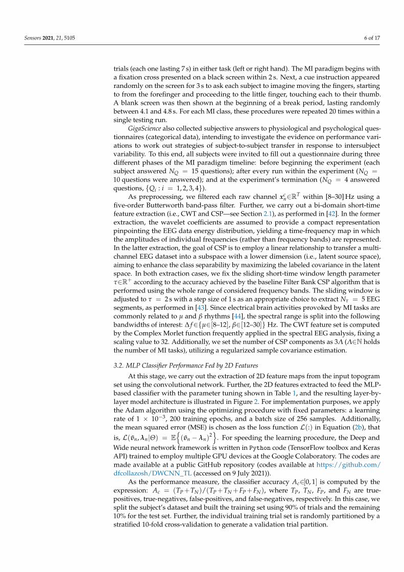
3.2. MLP Classifier Performance Fed by 2D Features

At this stage, we carry out the extraction of 2D feature maps from the input topogramset using the convolutional network. Further, the 2D features extracted to feed the MLP-based classifier with the parameter tuning shown in Table 1, and the resulting layer-by-layer model architecture is illustrated in Figure 2. For implementation purposes, we applythe Adam algorithm using the optimizing procedure with fixed parameters: a learningrate of 1 × 10−3, 200 training epochs, and a batch size of 256 samples. Additionally,the mean squared error (MSE) is chosen as the loss function L(:) in Equation (2b), thatis, L(vn, λn|Θ) = E

{(vn − λn)

2}

. For speeding the learning procedure, the Deep andWide neural network framework is written in Python code (TensorFlow toolbox and KerasAPI) trained to employ multiple GPU devices at the Google Colaboratory. The codes aremade available at a public GitHub repository (codes available at https://github.com/dfcollazosh/DWCNN_TL (accessed on 9 July 2021)).

As the performance measure, the classifier accuracy Ac∈[0, 1] is computed by theexpression: Ac = (TP+TN)/(TP+TN +FP+FN), where TP, TN , FP, and FN are true-positives, true-negatives, false-positives, and false-negatives, respectively. In this case, wesplit the subject’s dataset and built the training set using 90% of trials and the remaining10% for the test set. Further, the individual training trial set is randomly partitioned by astratified 10-fold cross-validation to generate a validation trial partition.

Sensors 2021, 21, 5105 7 of 17

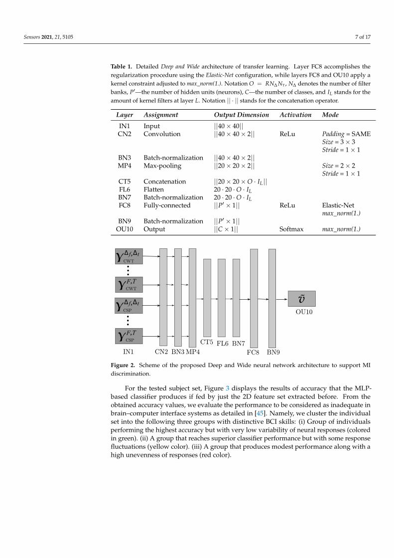
Table 1. Detailed Deep and Wide architecture of transfer learning. Layer FC8 accomplishes theregularization procedure using the Elastic-Net configuration, while layers FC8 and OU10 apply akernel constraint adjusted to max_norm(1.). Notation O = RN∆ Nτ , N∆ denotes the number of filterbanks, P′—the number of hidden units (neurons), C—the number of classes, and IL stands for theamount of kernel filters at layer L. Notation || · || stands for the concatenation operator.

Layer Assignment Output Dimension Activation Mode

IN1 Input ||40× 40||CN2 Convolution ||40× 40× 2|| ReLu Padding = SAME

Size = 3× 3Stride = 1× 1

BN3 Batch-normalization ||40× 40× 2||MP4 Max-pooling ||20× 20× 2|| Size = 2× 2

Stride = 1× 1CT5 Concatenation ||20× 20×O · IL||FL6 Flatten 20 · 20 ·O · ILBN7 Batch-normalization 20 · 20 ·O · ILFC8 Fully-connected ||P′ × 1|| ReLu Elastic-Net

max_norm(1.)BN9 Batch-normalization ||P′ × 1||

OU10 Output ||C× 1|| Softmax max_norm(1.)Version July 3, 2021 submitted to Sensors 7 of 16

IN1 CN2 BN3MP4

CT5 FL6 BN7

FC8 BN9

OU10

Δ f ΔtCWT

CWT

F T

...

,

,Δ f ΔtCWT

CWT

F T,

,

Δ f ΔtCWT

CWT

F T

...

,

,Δ f ΔtCSP

CSP

F T,

,

Figure 2. Scheme of the proposed Deep&Wide neural network architecture to support MI discrimination.

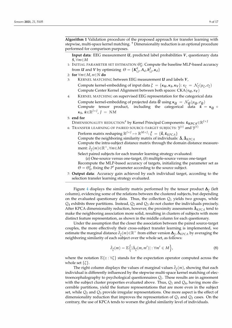
For the tested subject set, Fig. 3 displays the results of accuracy that the MLP-based classifier252

produces if fed by just the 2D feature set extracted before. From the obtained accuracy values,253

we evaluate the performance to be considered as inadequate in brain-computer interface systems254

as detailed in [46]. Namely, we cluster the individual set into the following three groups with255

distinctive BCI skills: i) Group of individuals performing the highest accuracy but with very low256

variability of neural responses (colored in green). ii) A group that reaches superior classifier257

performance but with some response fluctuations (yellow color). iii) A group that produces258

modest performance along with a high unevenness of responses (red color).259

Ac

0.9

0.8

0.7

0.6

0.5

14 3 4144 214349285036

35

1226 5 823

3027 15 9 6461710 41925 148 51313952

47133738454222241618203332

40 2 11 7

Subject ID

Figure 3. Partitions of individuals clustered by the MLP-based accuracy. Each subject performance ispainted by his estimated BCI inefficiency partition: Group I (green), Group II (yellow), and Group III (red).

3.3. Performed stepwise multi-space kernel matching260

Algorithm 1 presents the procedures to complete the validation of the suggested transfer261

learning with multi-space kernel embedding. We implement the Gaussian kernel to represent262

the available data because of its universal approximating ability and mathematical tractability.263

The length scale hyperparameter σ∈R+, ruling the variance of the described data, is adjusted to264

their median estimate. The following steps (3: and 4:) accomplish the pairwise kernel matching,265

firstly between the sets of EEG measurement U and label probability V . To this end, the CKA266

matching estimator is fed by the concatenated EEG features together with the predicted label267

probabilities to perform alignment across the whole subject set, empirically fixing the parameter268

G′ to 50 according to the subjects’ number in this experiment. In the second matching, we encode269

all the available categorical information about the psychological and physiological evaluation270

with the relevant feature set, resulting from CKA, by their projection onto a common matrix271

space representation, using the kernel/tensor product. Note that the projected data U by CKA272

is also embedded. We also perform dimensionality reduction of the feature sets generated after273

Figure 2. Scheme of the proposed Deep and Wide neural network architecture to support MIdiscrimination.

For the tested subject set, Figure 3 displays the results of accuracy that the MLP-based classifier produces if fed by just the 2D feature set extracted before. From theobtained accuracy values, we evaluate the performance to be considered as inadequate inbrain–computer interface systems as detailed in [45]. Namely, we cluster the individualset into the following three groups with distinctive BCI skills: (i) Group of individualsperforming the highest accuracy but with very low variability of neural responses (coloredin green). (ii) A group that reaches superior classifier performance but with some responsefluctuations (yellow color). (iii) A group that produces modest performance along with ahigh unevenness of responses (red color).

Sensors 2021, 21, 5105 8 of 17

Ac

0.9

0.8

0.7

0.6

0.5

14 3 4144 214349285036

35

1226 5 823

3027 15 9 6461710 41925 148 51313952

47133738454222241618203332

40 2 11 7

Subject ID

Figure 3. Partitions of individuals clustered by the MLP-based accuracy. Each subject performance is painted by thisestimated BCI inefficiency partition: Group I (green), Group II (yellow), and Group III (red).

3.3. Performed Stepwise Multi-Space Kernel Matching

Algorithm 1 presents the procedures to complete the validation of the suggestedtransfer learning with multi-space kernel-embedding. We implement the Gaussian kernelto represent the available data because of its universal approximating ability and math-ematical tractability. The length scale hyperparameter σ∈R+, ruling the variance of thedescribed data, is adjusted to their median estimate. The following steps (3: and 4:) accom-plish the pairwise kernel matching, firstly between the sets of EEG measurement U andlabel probability V . To this end, the CKA matching estimator is fed by the concatenatedEEG features together with the predicted label probabilities to perform alignment acrossthe whole subject set, empirically fixing the parameter G′ to 50 according to the subjects’number in this experiment. In the second matching, we encode all the available categoricalinformation about the psychological and physiological evaluation with the relevant featureset, resulting from CKA, by their projection onto a common matrix space representation,using the kernel/tensor product. Note that the projected data U by CKA are also em-bedded. We also perform dimensionality reduction of the feature sets generated afterstepwise-matching using Kernel Principal Component Analysis (KPCA) for evaluating therepresentational ability.

Further, we estimate the subject similarity matrix from the extracted feature sets,aiming to assess the domain distance between the source-target pairs, which are to beselected from different clusters of BCI inefficiency. Since the clustering of individuals relieson the ordered accuracy vector, we introduce the following neighboring similarity matrix∆ξ with pairwise metric elements computed from the matrices ξ = { ˆκ, κKPCA}, as follows:

∆ξ(m, m′) = cov(seq(∆ξ(m, ∀m′)), seq(∆ξ(m′, ∀m))), ∆ξ(m, m′) ∈ ∆∆∆ξ ∈ RM×M (7)

∆ξ(m, m′) = ∑∀j∈J|ξ(m, j)− ξ(m′, j)|2, ∆ξ(m, m′) ∈ ∆∆∆ξ ∈ RM×M

where notations cov(·, ·) and seq(∆(m, ∀m′))∈RM stand for, respectively, the covarianceoperator and the sequence composed of all ∀m′∈M elements of row m ranked in decreasingorder of the achieved MLP-based accuracy. The rationale for applying the covariance overthe ranked row vectors of ∆∆∆ξ is to preserve the similarity information between neighbor-ing subjects.

Sensors 2021, 21, 5105 9 of 17

Algorithm 1 Validation procedure of the proposed approach for transfer learning withstepwise, multi-space kernel matching. † Dimensionality reduction is an optional procedureperformed for comparison purposes.

Input data: EEG measurement U, predicted label probabilities V , questionary dataS, ∀m∈M

1: INITIAL PARAMETER SET ESTIMATION Θ∗0 : Compute the baseline MLP-based accuracyfrom U and V by optimizing Θ = {Kq

i,l , Ad, bqi,l , αd}

2: for ∀m∈M, n∈N do3: KERNEL MATCHING between EEG measurement U and labels V ,

Compute kernel-embedding of input data ξ = {κU , κS, κV}: κξ = Nξ(µξ , σξ)

Compute Center Kernel Alignment between both spaces: CKA(κU , κV )

4: KERNEL MATCHING on supervised EEG representation for the categorical dataCompute kernel-embedding of projected data U using κU = NU(µU , σU)Compute tensor product, including the categorical data κ = κU ◦κS, κ∈RJ×J , J = NM

5: end forDIMENSIONALITY REDUCTION† by Kernel Principal Components: κKPCA∈RJ×J

6: TRANSFER LEARNING OF PAIRED SOURCE-TARGET SUBJECTS: Y(s) and Y(t)

Perform matrix reshaping RJ×J 7→ RM×J : ξ = { ˆκ, κKPCA}Compute the neighboring similarity matrix of individuals: ∆, ∆KPCACompute the intra-subject distance matrix through the domain distance measure-ment: δξ(m)∈R+, ∀m∈MSelect paired subjects for each transfer learning strategy evaluated:

(a) One-source versus one-target, (b) multiple-source versus one-targetRecompute the MLP-based accuracy of targets, initializing the parameter set asΘ = Θ∗0 , fixing the P′ parameter according to the source subject.

7: Output data: Accuracy gain achieved by each individual target, according to theselection transfer learning strategy evaluated.

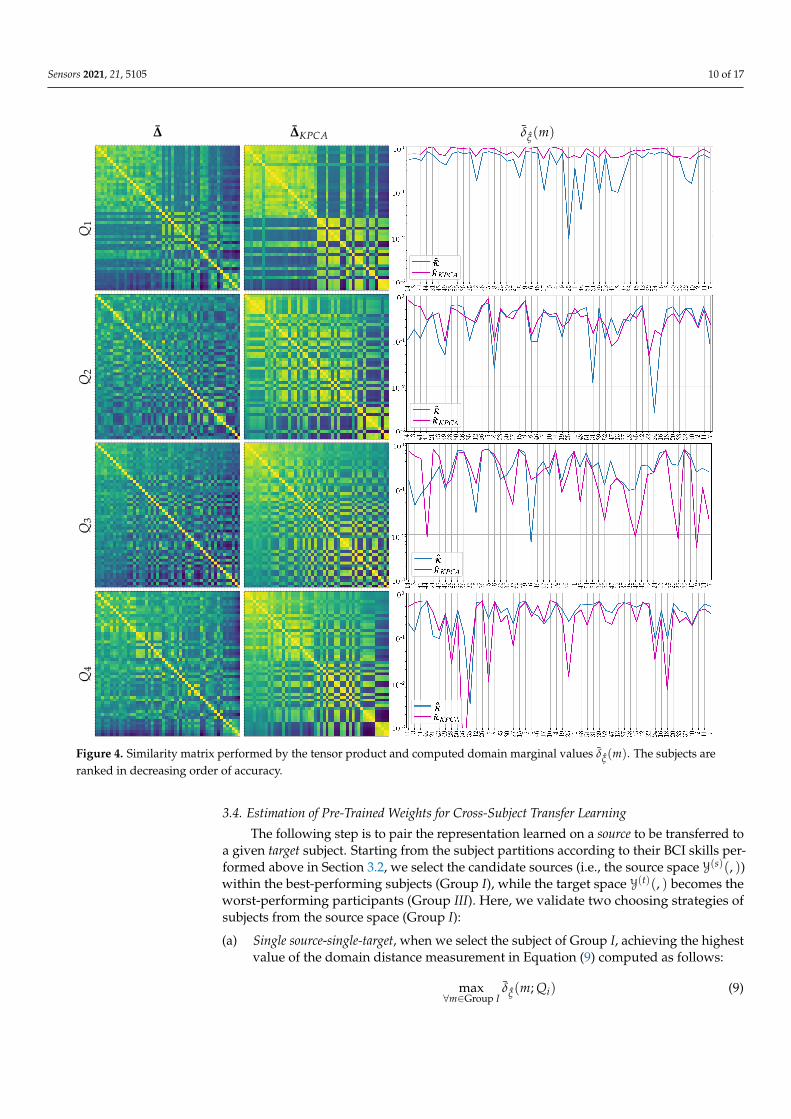
Figure 4 displays the similarity matrix performed by the tensor product ∆∆∆ξ (leftcolumn), evidencing some of the relations between the clustered subjects, but dependingon the evaluated questionary data. Thus, the collection Q1 yields two groups, whileQ4 exhibits three partitions. Instead, Q2 and Q3 do not cluster the individuals precisely.After KPCA dimensionality reduction, however, the proximity assessments ∆KPCA tend tomake the neighboring association more solid, resulting in clusters of subjects with moredistinct feature representation, as shown in the middle column for each questionary.

Under the assumption that the closer the association between the paired source-targetcouples, the more effectively their cross-subject transfer learning is implemented, weestimate the marginal distance δξ(m)∈R+ from either version ∆∆∆ξ , ∆KPCA by averaging theneighboring similarity of each subject over the whole set, as follows:

δξ(m) = E{|∆ξ(m, m′)| : ∀m′ ∈ M

}, (8)

where the notation E{z : ∀ζ} stands for the expectation operator computed across thewhole set {ζ}.

The right column displays the values of marginal values δξ(m), showing that eachindividual is differently influenced by the stepwise multi-space kernel matching of elec-troencephalography to psychological questionnaires Qi. These results are in agreementwith the subject cluster properties evaluated above. Thus, Q1 and Q4, having more dis-cernible partitions, yield the feature representations that are more even in the subjectset, while Q2 and Q3 provide irregular representations. One more aspect is the effect ofdimensionality reduction that improves the representation of Q1 and Q2 cases. On thecontrary, the use of KPCA tends to worsen the global similarity level of individuals.

Sensors 2021, 21, 5105 10 of 17

∆ ∆KPCA δξ(m)

Q1

Q2

Q3

Q4

Figure 4. Similarity matrix performed by the tensor product and computed domain marginal values δξ(m). The subjects areranked in decreasing order of accuracy.

3.4. Estimation of Pre-Trained Weights for Cross-Subject Transfer Learning

The following step is to pair the representation learned on a source to be transferred toa given target subject. Starting from the subject partitions according to their BCI skills per-formed above in Section 3.2, we select the candidate sources (i.e., the source space Y(s)(, ))within the best-performing subjects (Group I), while the target space Y(t)(, ) becomes theworst-performing participants (Group III). Here, we validate two choosing strategies ofsubjects from the source space (Group I):

(a) Single source-single-target, when we select the subject of Group I, achieving the highestvalue of the domain distance measurement in Equation (9) computed as follows:

max∀m∈Group I

δξ(m; Qi) (9)

Sensors 2021, 21, 5105 11 of 17

Once the source-target pairs are selected, the pre-trained weights are computed fromeach designed source subject to initialize the Deep and Wide neural network, ratherthan introducing a zero-valued starting iterate, and thus enabling a better convergenceof the training algorithm. Note that the fulfilling condition in Equation (9) dependson Qi, meaning distinct selected sources for each questionnaire data.

(b) Multiple sources-single-target when the selected subjects of Group I achieve the fourhighest domain distance values. In this case, the Deep and Wide initialization proce-dure applies the pre-trained weights estimated from the concatenation of the sourcetopograms.

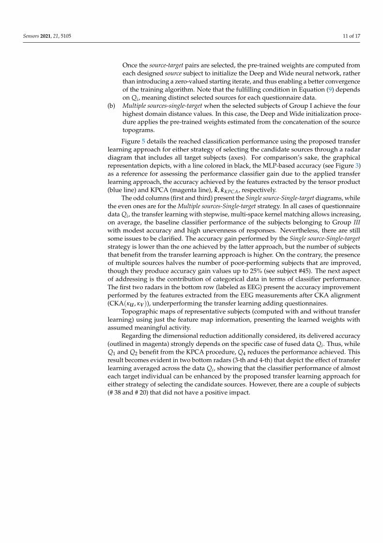
Figure 5 details the reached classification performance using the proposed transferlearning approach for either strategy of selecting the candidate sources through a radardiagram that includes all target subjects (axes). For comparison’s sake, the graphicalrepresentation depicts, with a line colored in black, the MLP-based accuracy (see Figure 3)as a reference for assessing the performance classifier gain due to the applied transferlearning approach, the accuracy achieved by the features extracted by the tensor product(blue line) and KPCA (magenta line), ˆκ, κKPCA, respectively.

The odd columns (first and third) present the Single source-Single-target diagrams, whilethe even ones are for the Multiple sources-Single-target strategy. In all cases of questionnairedata Qi, the transfer learning with stepwise, multi-space kernel matching allows increasing,on average, the baseline classifier performance of the subjects belonging to Group IIIwith modest accuracy and high unevenness of responses. Nevertheless, there are stillsome issues to be clarified. The accuracy gain performed by the Single source-Single-targetstrategy is lower than the one achieved by the latter approach, but the number of subjectsthat benefit from the transfer learning approach is higher. On the contrary, the presenceof multiple sources halves the number of poor-performing subjects that are improved,though they produce accuracy gain values up to 25% (see subject #45). The next aspectof addressing is the contribution of categorical data in terms of classifier performance.The first two radars in the bottom row (labeled as EEG) present the accuracy improvementperformed by the features extracted from the EEG measurements after CKA alignment(CKA(κU , κV )), underperforming the transfer learning adding questionnaires.

Topographic maps of representative subjects (computed with and without transferlearning) using just the feature map information, presenting the learned weights withassumed meaningful activity.

Regarding the dimensional reduction additionally considered, its delivered accuracy(outlined in magenta) strongly depends on the specific case of fused data Qi. Thus, whileQ1 and Q2 benefit from the KPCA procedure, Q4 reduces the performance achieved. Thisresult becomes evident in two bottom radars (3-th and 4-th) that depict the effect of transferlearning averaged across the data Qi, showing that the classifier performance of almosteach target individual can be enhanced by the proposed transfer learning approach foreither strategy of selecting the candidate sources. However, there are a couple of subjects(# 38 and # 20) that did not have a positive impact.

Sensors 2021, 21, 5105 12 of 17

(a) (b) (c) (d)

Q1

Q2

Q3

Q4

EEG

Indi

vidu

alga

in

Figure 5. Achieved accuracy by validated strategies of selecting source subjects from Group I. (a,c) Single source-single-target,(b,d) Multiple sources-single-target. Individual gain reports the average accuracy per subject of questionnaire data Qi andEEG.

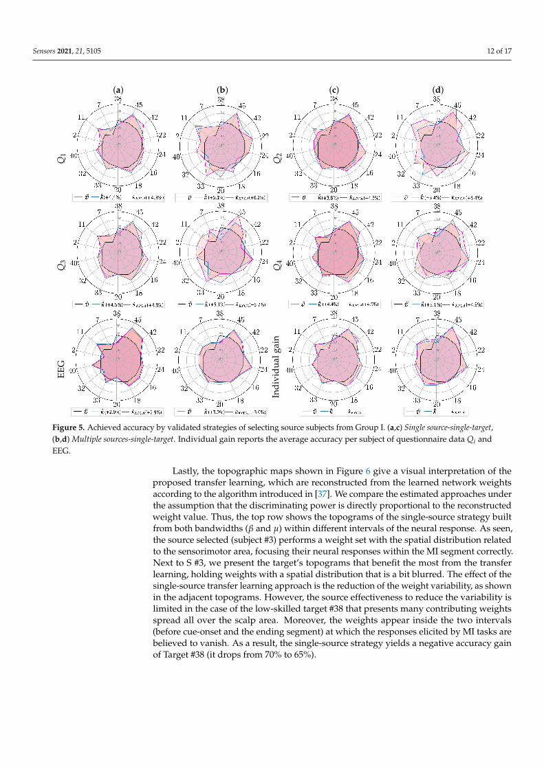
Lastly, the topographic maps shown in Figure 6 give a visual interpretation of theproposed transfer learning, which are reconstructed from the learned network weightsaccording to the algorithm introduced in [37]. We compare the estimated approaches underthe assumption that the discriminating power is directly proportional to the reconstructedweight value. Thus, the top row shows the topograms of the single-source strategy builtfrom both bandwidths (β and µ) within different intervals of the neural response. As seen,the source selected (subject #3) performs a weight set with the spatial distribution relatedto the sensorimotor area, focusing their neural responses within the MI segment correctly.Next to S #3, we present the target’s topograms that benefit the most from the transferlearning, holding weights with a spatial distribution that is a bit blurred. The effect of thesingle-source transfer learning approach is the reduction of the weight variability, as shownin the adjacent topograms. However, the source effectiveness to reduce the variability islimited in the case of the low-skilled target #38 that presents many contributing weightsspread all over the scalp area. Moreover, the weights appear inside the two intervals(before cue-onset and the ending segment) at which the responses elicited by MI tasks arebelieved to vanish. As a result, the single-source strategy yields a negative accuracy gainof Target #38 (it drops from 70% to 65%).

Sensors 2021, 21, 5105 13 of 17

S #3 T #45 S#3-T#45 T #38 S#3-T#38

Sing

le-s

ourc

eCSP

CSP

CWT

CWT

S #3,14,41,28 T #11 S#3,14,41,28-T#11 T #22 S#3,14,41,28-T#22M

ulti

-sou

rce(

4)CSP

CSP

CWT

CWT

S Group I T #40 S Group I-T#40 T #18 S Group I-T#18

Mul

ti-s

ourc

e(al

l)CSP

CSP

CWTCWT

-1.5-0.5s

-0.5-1.5s

0.5-2.5s

1.5-3.5s

2.5-4.5s

-1.5-0.5s

-0.5-1.5s

0.5-2.5s

1.5-3.5s

2.5-4.5s

-1.5-0.5s

-0.5-1.5s

0.5-2.5s

1.5-3.5s

2.5-4.5s

-1.5-0.5s

-0.5-1.5s

0.5-2.5s

1.5-3.5s

2.5-4.5s

-1.5-0.5s

-0.5-1.5s

0.5-2.5s

1.5-3.5s

2.5-4.5s

Figure 6. Topographic maps of representative subjects with and without transfer learning using justfeature map information, presenting the learned weights with meaningful activity reconstructedwithin both bandwidths (β and µ) across the whole signal length, Nτ .

Similar behavior is also observed in the second row, displaying the topograms of themulti-source strategy performed by the most benefitting (T#11) and the worst-achievingtarget (T#22), respectively. However, the inclusion of multiple sources leads to weights witha sparse distribution, as observed in the topograms of the selected subjects (S#3,14,41,28).This effect may explain the small number of targets improved by the multi-source strategy.In order to clarify this point, the bottom row displays the corresponding spatial distributionperformed by the multi-source strategy when including the whole subject set of Group I,resulting in weights that are very weak and scattered. Moreover, compared with the firsttwo rows, the all-subjects source approach of the bottom row makes the related transferlearning deliver the worst performance averaged across the target subject set.

4. Discussion and Concluding Remarks

Here, we introduce a cross-subject transfer learning approach for improving theclassification accuracy of elicited neural responses, pooling data from labeled EEG measure-ments and psychological questionnaires through a stepwise multi-space kernel-embedding.For validation purposes, the transfer learning is implemented in a Deep and Wide frame-work, for which the source-target sets are paired according to the BCI inefficiency, showingthat the classifier performance of almost each target individual can be enhanced usingsingle or multiple sources.

From the evaluation results, the following aspects are to be highlighted:Evaluated NN framework: The Deep and Wide learning framework is supplied by

the 2D feature maps extracted to support the MLP-based classifier. As a result, Table 2compares the bi-class accuracy of the GigaScience database achieved by several recentlypublished approaches, which are outperformed by the learning algorithm with the pro-posed transfer learning method. Of note, the MSNN algorithm presented in [46] achievesa competitive classification accuracy on average, 82.6 (ours) vs. 81.0 (MSNN), but witha higher standard deviation in comparison with our proposal, 12.0 vs. 8.4. Besides, ourmethod can include categorical data from questionnaires within the MI paradigm, whichfavors the interpretability concerning the studied subject from spatial, time, and frequencypatterns from EEG data coupled with categorical physiological and psychological data.

Sensors 2021, 21, 5105 14 of 17

Table 2. Comparison of bi-class accuracy achieved by state-of-the-art approaches in GigaScience.The best value is marked in bold. Notation * denotes Deep and Wide framework results withtransfer learning (TL). CSP + FLDA: Common spatial patterns and Fisher linear discriminant analysis,LSTM + Optical: Long-short term memory network and optical predictor, SFCSP: Sparse filter-bankCSP, DCJNN: Deep CSP neural network with joint distribution adaptation, MINE+EEGnet: Mutualinformation neural estimation, MSNN: Multi-scale Neural Network.

Approach Ac Interpretability

CSP + FLDA [47] 67.60 –LSTM + Optical [48] 68.2 ± 9.0 –SFBCSP [49] 72.60 –DCJNN [50] 76.50 XMINE + EEGnet [51] 76.6 ± 12.48 XMSNN [46] 81.0 ± 12.00 X

Proposal 79.5 ± 10.80 XProposal + TL * 82.6 ± 8.40 X

Feature representation challenges and computational requirements: The bi-domain extrac-tion is presented (CWT and CSP) to deal with the substantial intra-subject variability inpatterns across trials. However, for improving their combination with categorical data,more compact feature representations can be explored, for instance, using connectivitymetrics like in [52]. Besides, neural network architectures capturing the temporal dy-namics local structures of the EEG time-series associated with the elicited MI responsescould be helpful to upgrade our approach [53]. Moreover, it is well-known that deeplearning approaches require considerable computational time when training the model.For clarity, a computational time experiment is carried out. Specifically, for the parame-ter setting of the FC8 layer, with regularization values l1 and l2 tuned by a grid searcharound [0.0005, 0.001, 0.005], and a number of neurons fixed through a grid search withinP′ = [100, 200, 300], the fitting time with and without our transfer learning approach issummarized in Table 3. As seen, the multi-source scheme requires more computation timeper fold. Still, real-time BCI requirements can be satisfied once the model is trained, and anew instance must be predicted. In short, for a new subject, the following stages mustbe carried out: (i) Store the EEG and questionnaire information of the new and trainingsubjects. (ii) Apply our transfer learning approach as exposed in Figure 1 to couple EEGand questionary psychological data for the new subject. (iii) Once the model is trained,new instances of the studied subject can be predicted as straightforward deep learningmethods (in this stage, only the EEG data is required).

Table 3. Computational time experiments. The achieved training time (average) per fold and epochis presented.

Approach Time per Fold Time per Training Epoch

Proposal (Single-source) ∼984 s <1 sProposal (Multi-source (4)) ∼1663 s <1 sProposal (Multi-source (all)) ∼3176 s ∼1 s

Proposal + TL ∼341 s <1 s

Multi-space kernel matching: To overcome the difficulties in utilizing data-fusion combin-ing categorical with the real-valued features, we implement the stepwise kernel matchingvia Gaussian embedding. As a consequence, the obtained similarity matrices evidence therelationship with the BCI inefficiency clusters of subjects. Even though the association ishighly influenced by each evaluated questionnaire data, this result becomes essential inlight of previous reports stating that no statistically significant differences can be detected

Sensors 2021, 21, 5105 15 of 17

between questionary scores and EEG-based performance [54]. One more aspect is the effectof dimensionality reduction through kernel PCA that improves the representation, but to acertain extent (only in Q1 and Q2 cases). For tackling the differences in subjective criteriafor predicting MI performance, however, two main issues need to be addressed: The use ofmore appropriate kernel-embedding for categorical scores [55] and dimensionality reduc-tion approaches, providing representation of data points with a wide range of structureslike t-Distributed Stochastic Neighbor Embedding [56].

Cross-subject transfer learning: We conduct the transfer learning to infer a target predic-tion function from the kernel spaces embedded before, selecting the paired source-targetsets according to the Inefficiency-based clustering by subjects. Overall, the transfer learningwith feature representations, combined with questionary data, allows for an increase of thebaseline classifier accuracy of the worst-performing subjects. Nevertheless, source selectionthrough a different method impacts the classifier performance; while the Multiple-source-Single-target strategy tends to produce accuracy improvements that are bigger than theSingle-source-Single-target, and the number of the benefited targets declines. This result maypoint to future exploration of more effective transfer learning of BCI inefficiency devotedto bringing together, as much as possible, the source domain to each target space. Thistask also implies improving the similarity metric in Equation (7) proposed for comparingordered-by-accuracy vectors of different BCI inefficiency clusters.

As future work, the authors plan to validate the cross-subject transfer learningapproach in applications with the joint incorporation of two or more databases (cross-database), growing the tested number of individuals significantly. For instance, we planto consider the dataset collected by the Department of Brain and Cognitive Engineering,Korea University in [57], since this set holds questionnaire data information about the phys-iological and psychological condition of subjects. As a result, we will obtain classificationperformances based on transfer learning at intra-subject and inter-dataset levels.

Author Contributions: Conceptualization, D.F.C.-H., A.M.A.-M. and G.C.-D.; methodology, D.F.C.-H.and H.D.P.-N.; validation, D.F.C.-H., H.D.P.-N. and L.F.V.-M.; data curation, D.F.C.-H., H.D.P.-N. andL.F.V.-M.; writing—original draft preparation, D.F.C.-H. and A.M.A.-M.; writing—review and editing,D.F.C.-H. and G.C.-D. All authors have read and agreed to the published version of the manuscript.

Funding: This research manuscript is developed supported by “Convocatoria Doctorados NacionalesCOLCIENCIAS 727 de 2015” and “Convocatoria Doctorados Nacionales COLCIENCIAS 785 de 2017”(Minciencias). Additionally, A.M. Álvarez-Meza thanks to the project: Prototipo de interfaz cerebro-computador multimodal para la detección de patrones relevantes relacionados con trastornos de impulsividad-Hermes 50835, funded by Universidad Nacional de Colombia.

Informed Consent Statement: No aplicable since this study uses duly anonymized public databases.

Data Availability Statement: The databases used in this study are public and can be found at thefollowing links: GigaScience: http://gigadb.org/dataset/100295, accessed on 10 March 2021.

Conflicts of Interest: The authors declare no conflict of interest.

References1. Ladda, A.; Lebon, F.; Lotze, M. Using motor imagery practice for improving motor performance—A review. Brain Cogn. 2021,

150, 105705. [CrossRef] [PubMed]2. James, C.; Zuber, S.; Dupuis Lozeron, E.; Abdili, L.; Gervaise, D.; Kliegel, M. How Musicality, Cognition and Sensorimotor Skills

Relate in Musically Untrained Children. Swiss J. Psychol. 2020, 79, 101–112. [CrossRef]3. Basso, J.; Satyal, M.; Rugh, R. Dance on the Brain: Enhancing Intra- and Inter-Brain Synchrony. Front. Hum. Neurosci. 2021,

14, 586. [CrossRef]4. Suggate, S.; Martzog, P. Screen-time influences children’s mental imagery performance. Dev. Sci. 2020, 23, e12978. [CrossRef]

[PubMed]5. Bahmani, M.; Babak, M.; Land, W.; Howard, J.; Diekfuss, J.; Abdollahipour, R. Children’s motor imagery modality dominance

modulates the role of attentional focus in motor skill learning. Hum. Movem. Sci. 2020, 75, 102742. [CrossRef]6. Souto, D.; Cruz, T.; Fontes, P.; Batista, R.; Haase, V. Motor Imagery Development in Children: Changes in Speed and Accuracy

With Increasing Age. Front. Pediatr. 2020, 8, 100. [CrossRef]

Sensors 2021, 21, 5105 16 of 17

7. Simpson, T.; Ellison, P.; Carnegie, E.; Marchant, D. A systematic review of motivational and attentional variables on children’sfundamental movement skill development: The OPTIMAL theory. Int. Rev. Sport Exer. Psychol. 2020, 1–47. [CrossRef]

8. Singh, A.; Hussain, A.; Lal, S.; Guesgen, H. A Comprehensive Review on Critical Issues and Possible Solutions of Motor ImageryBased Electroencephalography brain–computer Interface. Sensors 2021, 21, 2173. [CrossRef] [PubMed]

9. Al-Saegh, A.; Dawwd, S.; Abdul-Jabbar, J. Deep learning for motor imagery EEG-based classification: A review. Biomed. SignalProcess. Control 2021, 63, 102172. [CrossRef]

10. Thompson, M. Critiquing the Concept of BCI Illiteracy. Sci. Eng. Ethics 2019, 25, 1217–1233. [CrossRef] [PubMed]11. McAvinue, L.; Robertson, I. Measuring motor imagery ability: A review. Eur. J. Cogn. Psychol. 2008, 20, 232–251. [CrossRef]12. Yoon, J.; Lee, M. Effective Correlates of Motor Imagery Performance based on Default Mode Network in Resting-State. In

Proceedings of the 2020 8th International Winter Conference on brain–computer Interface (BCI), Gangwon, Korea, 26–28 February2020; pp. 1–5.

13. Rimbert, S.; Gayraud, N.; Bougrain, L.; Clerc, M.; Fleck, S. Can a Subjective Questionnaire Be Used as brain–computer InterfacePerformance Predictor? Front. Hum. Neurosci. 2019, 12, 529. [CrossRef] [PubMed]

14. Vasilyev, A.; Liburkina, S.; Yakovlev, L.; Perepelkina, O.; Kaplan, A. Assessing motor imagery in brain–computer interfacetraining: Psychological and neurophysiological correlates. Neuropsychologia 2017, 97, 56–65. [CrossRef]

15. Seo, S.; Lee, M.; Williamson, J.; Lee, S. Changes in Fatigue and EEG Amplitude during a Longtime Use of brain–computerInterface. In Proceedings of the 2019 7th International Winter Conference on brain–computer Interface (BCI), Gangwon, Korea,18–20 February 2019; pp. 1–3.

16. Lioi, G.; Cury, C.; Perronnet, L.; Mano, M.; Bannier, E.; Lécuyer, A.; Barillot, C. Simultaneous MRI-EEG during a motor imageryneurofeedback task: An open access brain imaging dataset for multi-modal data integration. bioRxiv 2019, 2019, 862375.

17. Collet, C.; Hajj, M.E.; Chaker, R.; Bui-xuan, B.; Lehot, J.; Hoyek, N. Effect of motor imagery and actual practice on learningprofessional medical skills. BMC Med. Educ. 2021, 21, 59. [CrossRef]

18. Dähne, S.; Bießmann, F.; Samek, W.; Haufe, S.; Goltz, D.; Gundlach, C.; Villringer, A.; Fazli, S.; Müller, K. Multivariate MachineLearning Methods for Fusing Multimodal Functional Neuroimaging Data. Proc. IEEE 2015, 103, 1507–1530. [CrossRef]

19. Dai, C.; Wang, Z.; Wei, L.; Chen, G.; Chen, B.; Zuo, F.; Li, Y. Combining early post-resuscitation EEG and HRV features improvesthe prognostic performance in cardiac arrest model of rats. Am. J. Emerg. Med. 2018, 36, 2242–2248. [CrossRef] [PubMed]

20. Xu, J.; Zheng, H.; Wang, J.; Li, D.; Fang, X. Recognition of EEG Signal Motor Imagery Intention Based on Deep Multi-ViewFeature Learning. Sensors 2020, 20, 3496. [CrossRef]

21. Zhuang, M.; Wu, Q.; Wan, F.; Hu, Y. State-of-the-art non-invasive brain–computer interface for neural rehabilitation: A review. J.Neurorestoratol. 2020, 8, 4. [CrossRef]

22. Wu, D.; Jiang, X.; Peng, R.; Kong, W.; Huang, J.; Zeng, Z. Transfer Learning for Motor Imagery Based brain–computer Interfaces:A Complete Pipeline. arXiv 2021, arXiv:eess.SP/2007.03746.

23. Zheng, M.; Yang, B.; Xie, Y. EEG classification across sessions and across subjects through transfer learning in motor imagery-basedbrain-machine interface system. Med. Biol. Eng. Comput. 2020, 58, 1515–1528. [CrossRef]

24. Wan, Z.; Yang, R.; Huang, M.; Zeng, N.; Liu, X. A review on transfer learning in EEG signal analysis. Neurocomputing 2021,421, 1–14. [CrossRef]

25. Zhang, R.; Zong, Q.; Dou, L.; Zhao, X.; Tang, Y.; Li, Z. Hybrid deep neural network using transfer learning for EEG motorimagery decoding. Biomed. Sig. Process. Control 2021, 63, 102144. [CrossRef]

26. Kant, P.; Laskar, S.; Hazarika, J.; Mahamune, R. CWT Based Transfer Learning for Motor Imagery Classification for Braincomputer Interfaces. J. Neurosci. Methods 2020, 345, 108886. [CrossRef] [PubMed]

27. Zhang, K.; Robinson, N.; Lee, S.; Guan, C. Adaptive transfer learning for EEG motor imagery classification with deep Convolu-tional Neural Network. Neural Netw. 2021, 136, 1–10. [CrossRef] [PubMed]

28. Wei, X.; Ortega, P.; Faisal, A. Inter-subject Deep Transfer Learning for Motor Imagery EEG Decoding. arXiv 2021,arXiv:cs.LG/2103.0535 .

29. Zheng, M.; Yang, B.; Gao, S.; Meng, X. Spatio-time-frequency joint sparse optimization with transfer learning in motor imagery-based brain-computer interface system. Biomed. Signal Process. Control 2021, 68, 102702. [CrossRef]

30. Zhang, K.; Xu, G.; Chen, L.; Tian, P.; Han, C.; Zhang, S.; Duan, N. Instance transfer subject-dependent strategy for motor imagerysignal classification using deep convolutional neural networks. Comput. Math. Methods Med. 2020, 2020. [CrossRef] [PubMed]

31. Luo, W.; Zhang, J.; Feng, P.; Yu, D.; Wu, Z. A concise peephole model based transfer learning method for small sample temporalfeature-based data-driven quality analysis. Knowl. Based Syst. 2020, 195, 105665. [CrossRef]

32. Zhang, K.; Xu, G.; Zheng, X.; Li, H.; Zhang, S.; Yu, Y.; Liang, R. Application of Transfer Learning in EEG Decoding Based onbrain–computer Interfaces: A Review. Sensors 2020, 20, 6321. [CrossRef]

33. Tan, C.; Sun, F.; Kong, T.; Zhang, W.; Yang, C.; Liu, C. A Survey on Deep Transfer Learning. In Artificial Neural Networksand Machine Learning—ICANN 2018; Kurková, V., Manolopoulos, Y., Hammer, B., Iliadis, L., Maglogiannis, I., Eds.; SpringerInternational Publishing: Cham, Switzerland, 2018; pp. 270–279.

34. Zhao, D.; Tang, F.; Si, B.; Feng, X. Learning joint space–time–frequency features for EEG decoding on small labeled data. NeuralNetw. 2019, 114, 67–77. [CrossRef] [PubMed]

Sensors 2021, 21, 5105 17 of 17

35. Parvan, M.; Ghiasi, A.R.; Rezaii, T.; Farzamnia, A. Transfer Learning based Motor Imagery Classification using ConvolutionalNeural Networks. In Proceedings of the 2019 27th Iranian Conference on Electrical Engineering (ICEE), Yazd, Iran, 30 April–2May 2019; pp. 1825–1828.

36. Collazos-Huertas, D.; Álvarez-Meza, A.; Acosta-Medina, C.; Castaño-Duque, G.; Castellanos-Dominguez, G. CNN-basedframework using spatial dropping for enhanced interpretation of neural activity in motor imagery classification. Brain Inf. 2020,7, 8. [CrossRef] [PubMed]

37. Collazos-Huertas, D.; Álvarez-Meza, A.; Castellanos-Dominguez, G. Spatial interpretability of time-frequency relevanceoptimized in motor imagery discrimination using Deep and Wide networks. Biomed. Sig. Process. Control 2021, 68, 102626.[CrossRef]

38. Mammone, N.; Ieracitano, C.; Morabito, F. A deep CNN approach to decode motor preparation of upper limbs fromtime–frequency maps of EEG signals at source level. Neural Netw. 2020, 124, 357–372. [CrossRef]

39. Song, L.; Fukumizu, K.; Gretton, A. kernel-embeddings of Conditional Distributions: A Unified Kernel Framework forNonparametric Inference in Graphical Models. IEEE Signal Process. Mag. 2013, 30, 98–111. [CrossRef]

40. Alvarez-Meza, A.M.; Orozco-Gutierrez, A.; Castellanos-Dominguez, G. Kernel-Based Relevance Analysis with EnhancedInterpretability for Detection of Brain Activity Patterns. Front. Neurosci. 2017, 11, 550. [CrossRef]

41. You, Y.; Chen, W.; Zhang, T. Motor imagery EEG classification based on flexible analytic wavelet transform. Biomed. SignalProcess. Control 2020, 62, 102069. [CrossRef]

42. Collazos-Huertas, D.; Caicedo-Acosta, J.; Castaño-Duque, G.A.; Acosta-Medina, C.D. Enhanced Multiple Instance RepresentationUsing Time-Frequency Atoms in Motor Imagery Classification. Front. Neurosci. 2020, 14, 155. [CrossRef]

43. Velasquez, L.; Caicedo, J.; Castellanos-Dominguez, G. Entropy-Based Estimation of Event-Related De/Synchronization in MotorImagery Using Vector-Quantized Patterns. Entropy 2020, 22, 703. [CrossRef] [PubMed]

44. McFarland, D.; Miner, L.; Vaughan, T.; Wolpaw, J. Mu and Beta Rhythm Topographies During Motor Imagery and ActualMovements. Brain Topogr. 2004, 12, 177–186. [CrossRef]

45. Sannelli, C.; Vidaurre, C.; Muller, K.; Blankertz, B. A large scale screening study with a SMR-based BCI: Categorization of BCIusers and differences in their SMR activity. PLoS ONE 2019, 14, e0207351. [CrossRef]

46. Ko, W.; Jeon, E.; Jeong, S.; Suk, H. Multi-Scale Neural Network for EEG Representation Learning in BCI. 2020. Available online:http://xxx.lanl.gov/abs/2003.02657 (accessed on 9 July 2021).

47. Cho, H.; Ahn, M.; Ahn, S.; Kwon, M.; Jun, S. EEG datasets for motor imagery brain–computer interface. GigaScience 2017, 6,gix034. [CrossRef] [PubMed]

48. Kumar, S.; Sharma, A.; Tsunoda, T. Brain wave classification using long short-term memory network based OPTICAL predictor.Sci. Rep. 2019, 9, 9153. [CrossRef] [PubMed]

49. Zhang, Y.; Zhou, G.; Jin, J.; Wang, X.; Cichocki, A. Optimizing spatial patterns with sparse filter bands for motor-imagery basedbrain–computer interface. J. Neurosci. Methods 2015, 255, 85–91. [CrossRef] [PubMed]

50. Zhao, X.; Zhao, J.; Liu, C.; Cai, W. Deep Neural Network with Joint Distribution Matching for Cross-Subject Motor Imagerybrain–computer Interfaces. BioMed Res. Int. 2020, 2020. [CrossRef]

51. Jeon, E.; Ko, W.; Yoon, J.; Suk, H. Mutual Information-Driven Subject-Invariant and Class-Relevant Deep Representation Learningin BCI. 2020. Available online: http://xxx.lanl.gov/abs/1910.07747 (accessed on 9 July 2021).

52. Mirzaei, S.; Ghasemi, P. EEG motor imagery classification using dynamic connectivity patterns and convolutional autoencoder.Biomed. Signal Process. Control 2021, 68, 102584. [CrossRef]

53. Freer, D.; Yang, G. Data augmentation for self-paced motor imagery classification with C-LSTM. J. Neural Eng. 2020, 17, 016041.[CrossRef]

54. Lee, M.; Yoon, J.; Lee, S. Predicting Motor Imagery Performance From Resting-State EEG Using Dynamic Causal Modeling. Front.Human Neurosci. 2020, 14, 321. [CrossRef]

55. Cardona, L.; Vargas-Cardona, H.; Navarro, P.; Cardenas Peña, D.; Orozco Gutiérrez, A. Classification of Categorical Data Basedon the Chi-Square Dissimilarity and t-SNE. Computation 2020, 8, 104. [CrossRef]

56. Anowar, F.; Sadaoui, S.; Selim, B. Conceptual and empirical comparison of dimensionality reduction algorithms (PCA, KPCA,LDA, MDS, SVD, LLE, ISOMAP, LE, ICA, t-SNE). Comput. Sci. Rev. 2021, 40, 100378. [CrossRef]

57. Lee, M.; Kwon, O.; Kim, Y.; Kim, H.; Lee, Y.; Williamson, J.; Fazli, S.; Lee, S. EEG dataset and OpenBMI toolbox for three BCIparadigms: An investigation into BCI illiteracy. GigaScience 2019, 8, giz002. [CrossRef] [PubMed]