Kernel Spectral Clustering with Memory Effect

Rocco Langone, Carlos Alzate and Johan A. K. Suykens

Department of Electrical Engineering ESAT-SCD-SISTA, Katholieke Universiteit Leuven, Kasteelpark Arenberg 10,B-3001 Leuven, Belgium

Email: rocco.langone, carlos.alzate, johan.suykens@esat.kuleuven.be.

Abstract

Evolving graphs describe many natural phenomena changing over time, such as social relation-ships, trade markets, methabolic networks etc. In this framework, performing community detec-tion and analyzing the cluster evolution represents a critical task. Here we propose a new modelfor this purpose, where the smoothness of the clustering results over time can be considered asa valid prior knowledge. It is based on a constrained optimization formulation typical of LeastSquares Support Vector Machines (LS-SVM), where the objective function is designed to ex-plicitly incorporate temporal smoothness. The latter allows the model to cluster the current datawell and to be consistent with the recent history. We also propose new model selection criteria inorder to carefully choose the hyper-parameters of our model, which is a crucial issue to achievegood performances. We successfully test the model on four toy problems and on a real worldnetwork. We also compare our model with Evolutionary Spectral Clustering, which is a state-of-the-art algorithm for community detection of evolving networks, illustrating that the kernelspectral clustering with memory effect can achieve better or equal performances.

Keywords: kernel spectral clustering, community detection, evolving networks, temporalsmoothness, memory.

1. Introduction

In many practical applications we face the problem of community detection in dynamic sce-narios, which recently gained much attention in the sciencecommunity [26, 25, 6, 4, 29]. Weaim to cluster objects whose characteristics change over time and we wish to obtain a meaningfulclustering result at each time step. This situation arises for instance in segmentation of movingobjects in a dynamic environment, community detection of evolving networks such as in the blogdata, telephone traffic data, time-series microarray data etc. A desirable feature of a clusteringmodel which has to capture the evolution of communities overtime is the temporal smoothnessbetween clusters in successive timesteps. In this way the model is able to track the long-termtrend and at the same time it smoothens out short-term variation due to noise, similarly to whathappens with moving averages in time-series analysis. Thisissue was first addressed in [8] and[7].

In this paper our starting point is the kernel spectral clustering (KSC) model, which representsa spectral clustering formulation as a weighted kernel PCA problem with primal and dual rep-resentations [1]. The dual problem is an eigenvalue problem, related to spectral clustering. Asin classical spectral clustering, if we are given data points we build-up a weighted graph wherePreprint submitted to Physica A January 4, 2013

each node represents a point and the weights are related to the similarity between the points,according to a particular similarity measure. In what follows for the sake of simplicity we willrefer to nodes and networks (or graphs) either if we are givendata points or we start our analysisdirectly from a graph.

The KSC has two main advantages:

• a systematic model selection scheme for the tuning of the parameters

• the extension of the clustering model to out-of-sample nodes.

The clustering model can be trained on a subset of the whole network (by solving an affordableeigenvalue problem) and then be applied to the rest of the network in a learning framework.The out-of-sample extension allows then to predict the memberships of a new node thanks tothe model learned during the training phase. This is a uniquefeature in the community detectionfield, since most of the algorithms work only at the training level and the out-of-sample extension(if any) is done in a heuristic way. Also in [11], the out-of-sample extension performed by thekernelk-means model is based on the same assignment rule used for training, but there is not anunderlying predictive model like in the KSC case.

The KSC model is static, in the sense that there is no temporalinformation in it. Then, in orderto cluster an evolving network, we can apply the model to eachsnapshot separately. This proce-dure, as we discussed, is not advisable if we want to track thelong-term drift of the communitiesby ignoring meanwhile the short-term fluctuations.

In this framework, we propose an extension of the KSC model that we call kernel spectralclustering with memory effect (MKSC). In this new formulation we incorporate the desired tem-poral smoothness at the primal level, as a kind of prior knowledge incorporation. This leads to adual problem which is no longer an eigenvalue problem but a set of linear systems.

The rest of this paper is organized as follows: Section 2 summarizes the KSC model. Section3 introduces our new contribution, that is the MKSC model. InSection 4 we propose new clusterquality measures, we describe the model selection issue forKSC and MKSC and we brieflyreview the evolutionary spectral clustering algorithm. Some simulation results on both real-lifeand artificial datasets are presented in Section 5: we compare the MKSC model with KSC andthe evolutionary spectral clustering. In Section 6 we discuss the drawbacks of Modularity and wedescribe another well known quality function, namely the Conductance. Moreover we interpretthe results shown in Section 5 also in terms of Conductance. Section 7 contains a discussion onthe computational complexity of our method. Finally, in Section 8 we draw some conclusionsand we suggest some future work.

2. Kernel spectral clustering model

Given a graph (weighted or unweighted), several propertiesof it can be explained throughspectral graph theory, which is the study of the eigenspectrum of graph Laplacian matrices[9, 33, 28]. Spectral clustering methods make use of the eigenvectors of the Laplacian tofind useful partitions of the data, and they have been reported to be successful in cases whereclassical clustering schemes such ask-means and hierarchical clustering fail.

2

Given training dataD = xiNi=1, xi ∈ R

d and the number of clustersk, the primal problem ofspectral clustering via weighted kernel PCA is formulated as follows [1]:

minw(l),e(l),bl

12

k−1∑

l=1

w(l)Tw(l) −

12N

k−1∑

l=1

γle(l)T

D−1e(l) (1)

such thate(l)= Φw(l)

+ bl1N (2)

wheree(l)= [e(l)

1 , . . . , e(l)N ]T are the projections,l = 1, . . . , k − 1 indicates the score variables

needed to encode thek clusters to find,D−1 ∈ RN×N is the inverse of the degree matrixD, Φ is

theN×dh feature matrixΦ = [ϕ(x1)T ; . . . ;ϕ(xN)T ] andγl ∈ R+ are regularization constants. The

clustering model is expressed by:

e(l)i = w(l)T

ϕ(xi) + bl, i = 1, . . . ,N (3)

whereϕ : Rd → R

dh is the mapping to a high-dimensional feature space,bl are bias terms,l = 1, . . . , k − 1. The projectionse(l)

i represent the latent variables of a set ofk − 1 binaryclustering indicators given by sign(e(l)

i ). The binary indicators are combined to form a codebookCB = cp

kp=1, where each codeword is a binary string of lengthk − 1 representing a cluster. The

dual problem related to this primal formulation is:

D−1MDΩα(l)= λlα

(l) (4)

whereΩ is the kernel matrix withi j-th entryΩi j = K(xi, x j) = ϕ(xi)Tϕ(x j), D is the graph degreematrix which is diagonal with positive elementsDii =

∑jΩi j, MD is a centering matrix defined

asMD = IN−1

1TN D−11N

1N1TN D−1, theα(l) are dual variables. The kernel functionK : R

d×Rd → R

+

plays the role of the similarity function of the graph: it hasto be positive definite, to take positivevalues and to be localized (such that the similarity betweenpoints belonging to different clusterstends to 0). Finally, the eigenvalue problem (4) is related to spectral clustering with random walkLaplacianLRW. In this case, the clustering problem can be interpreted as finding a partition ofthe graph in such a way that the random walker remains most of the time in the same clusterwith few jumps to other clusters, minimizing the probability of transitions between clusters. Thestochastic transition matrixP of a random walker on a graph can be obtained by normalizingthe similarity matrixS associated to the graph such that its rows sum to 1. Thei j-th entry ofP represents the probability of moving from nodei to node j in one step of the process. Thistransition matrix can be defined asP = D−1S . The corresponding eigenvalue problem becomesPr = ξr. The latter is equivalent to problem (4) (exept for the presence of the centering matrixMD), where the kernel matrix acts as the similarity matrixS .

The out-of-sample extension to new nodes is done by an Error-Correcting Output Codes(ECOC) decoding procedure. The decoding scheme consists ofcomparing the cluster indica-tors obtained in the validation/test stage with the codebook and selecting the nearest codewordin terms of Hamming distance. The cluster indicators can be obtained by binarizing the scorevariables for out-of-sample nodes as follows:

sign(e(l)test) = sign(Ωtestα

(l)+ bl1Ntest) (5)

with l = 1, . . . , k−1.Ωtest is theNtest×N kernel matrix evaluated using the test nodes with entriesΩtest,ri= K(xtest

r , xi), r = 1, . . . ,Ntest, i = 1, . . . ,N. This natural extension to out-of-sample pointscorresponds to the main advantage of the KSC framework. In this way, the clustering model canbe trained, validated and tested in an unsupervised learning scheme.

3

3. Kernel spectral clustering with memory effect

3.1. Introduction

The KSC model summarized in the previous section has been designed to cluster static graphs.In this section we present an extension of such a model that can produce cluster results moreconsistent over time when applied to changing networks. A dynamic networkG is a sequenceof networksGt(Vt, Et), i.e. G = (G1, ...,Gt, ...), wheret indicates the time index. The symbolVt indicates the set of nodes in the graphGt and Et the related set of edges. In what followswe assume that|Vt| is constant, that is all the graphs in the sequence have the same number ofnodes (the symbol|Vt| indicates as usual the cardinality of a set). The new model implementsa trade-off between the current clustering and the previouspartitioning and is referred as kernelspectral clustering with memory effect or MKSC. Finally, for simplicity we assume that the totalnumber of communities does not change over time and we introduce a memory of one snapshot.

3.2. Mathematical formulation

The primal problem of the MKSC model can be stated as follows:

minw(l),e(l),bl

12

k−1∑

l=1

w(l)Tw(l) −

γ

2N

k−1∑

l=1

e(l)TD−1

Meme(l) − ν

k−1∑

l=1

w(l)Tw(l)

old (6)

such thate(l)= Φw(l)

+ bl1N (7)

The symbols have the same meaning as for the KSC, but here we have only one regularizationconstantγ instead of multipleγl. Moreoverw(l)

old represents thelth binary model developed for theprevious snapshot of the evolving network (as mentioned we consider a memory of one snapshotin the past),ν is an additional regularization constant andD−1

Mem is a weighting matrix whosemeaning will be clear soon. Since we consider only one snapshot in the past, we say that ourmodel has a memory of one snapshot. The termw(l)T

w(l)old describes the correlation between the

actual and the previous model, which we want to maximize. In this way we are able to introducetemporal smoothness in our formulation, such that the current partition does not deviate toodrammatically from the recent history. The clustering model is expressed, as before, by:

e(l)i = w(l)T

ϕ(xi) + bl, i = 1, . . . ,N (8)

The Lagrangian of the problem (6), (7) is:

L(w(l), e(l), bl;α(l)) =12

k−1∑

l=1

w(l)Tw(l) −

γ

2N

k−1∑

l=1

e(l)TD−1

Meme(l) − ν

k−1∑

l=1

w(l)Tw(l)

old + α(l)T

(e(l) − Φw(l) − bl1N)

The KKT optimality conditions are:

∂L∂w(l) = 0→ w(l)

= ΦTα(l)

+ νw(l)old,

∂L∂e(l) = 0→ α(l)

= γD−1Meme(l),

∂L∂bl= 0→ 1T

Nα(l)= 0,

∂L∂α(l) = 0→ e = Φw(l)

+ bl1N .

From w(l)old = Φ

Toldα

(l)old, the bias term becomes− 1

1TN D−1

Mem1N1T

N D−1Mem(Ωα(l)

+ νΩnew-oldα(l)old).

4

Eliminating the primal variablese(l), w(l), bl leads to the following set of linear systems in thedual problem:

(D−1MemMDMemΩ −

Iγ

)α(l)= −νD−1

MemMDMemΩnew-oldα(l)old, l = 1, . . . , k − 1 (9)

whereΩnew-old captures the similarity between the nodes of the current graph and the nodes ofthe previous snapshot and has thei j − th entryΩnew-old,i j = K(xnew

i , xoldj ) = ϕ(xnew

i )Tϕ(xoldj ).

D−1Mem ∈ R

N×N is the inverse of the degree matrixDMem = D + Dnew-old, which is the sum of theactual degree matrixD and the degree matrix with entriesDnew-old,ii =

∑jΩnew-old,i j. MDMem is the

centering matrix equal toMDMem = IN −1

1TN D−1

Mem1N1N1T

N D−1Mem. Finally, the cluster indicators for

the training points become:

sign(e(l)) = sign(Ωα(l)+ νΩnew-oldα

(l)old + b1N). (10)

The out-of-sample extension is done in a similar way, but considering the test kernel matricesinstead of the training kernel matrices:

e(l)= Ω

testα(l)+ νΩtest

new-oldα(l)old + bl1N . (11)

Finally, the MKSC algorithm can be summarized as follows:

———————————————————————————————————Algorithm MKSC Kernel Spectral Clustering with Memory Effect algorithm———————————————————————————————————Input: Training setsD = xi

Ni=1 and Dold = xold

i Ni=1, test setsDtest

= xtestm

Ntestm=1 and

Dtestold = x

test,oldm

Ntest

m=1, α(l)old (the α(l) calculated for the previous snapshot), kernel function

K : Rd × R

d → R+ positive definite and localized (K(xi, x j) → 0 if xi andx j belong to different

clusters), kernel parameters (if any), number of clustersk, regularization constantsγ andν.Output: ClustersA1, . . . ,Ap, cluster codesetCB = cp

kp=1, cp ∈ −1, 1k−1.

1. Initialization by solving eq. (4).

2. Compute the solution vectorsα(l), l = 1, . . . , k − 1, related to the linear systems(D−1

MemMDMemΩ −Iγ)α(l)= −νD−1

MemMDMemΩnew-oldα(l)old (eq. (9)).

3. Binarize the solution vectors: sign(α(l)i ), i = 1, . . . ,N, l = 1, . . . , k − 1, and let sign(αi) ∈

−1, 1k−1 be the encoding vector for the training data pointxi, i = 1, . . . ,N.

4. Count the occurrences of the different encodings and find thek encodings with most occur-rences. Let the codeset be formed by thesek encodings:CB = cp

kp=1, cp ∈ −1, 1k−1.

5. ∀i, assignxi to Ap∗ wherep∗ = argminpdH(sign(αi), cp) anddH(., .) is the Hamming dis-tance.

6. Binarize the test data projections sign(e(l)m ), m = 1, . . . ,Ntest, l = 1, . . . , k − 1 and let

sign(em) ∈ −1, 1k−1 be the encoding vector ofxtestm , m = 1, . . . ,Ntest.

7. ∀m, assignxtestm to Ap∗ , wherep∗ = argminpdH(sign(em), cp).

———————————————————————————————————-5

4. Cluster quality

Since clustering is an unsupervised learning procedure, the partitioning produced by an al-gorithm requires an evaluation regarding its validity [17]. There are two main cluster qualitymeasures:

• internal evaluation: these methods usually assign the bestscore to the partitions with highsimilarity within a cluster and low similarity between clusters

• external criteria: they measure the similarity between twopartitions. They are useful tocompare the results of two different algorithms or to assessthe similarity between the par-tition produced by a clustering method and a golden standardfor the evaluation.

4.1. Static measuresIn this paper, we will consider as internal measure for the evaluation of our experimental

results (see section 5) the Modularity criterion and the BLFcriterion and as external measure theadjusted Rand index (ARI).

4.1.1. ModularityModularity is the most widely accepted quality function of agraph introduced in [27]. It is

very well considered due to the fact that closely agrees withintuition on a wide range of realworld networks. It is based on the idea that a random graph is not expected to have a clusterstructure, so the possible existence of clusters can be revealed by the comparison between theactual density of inter-community edges and the density onewould expect to have in the graphif the vertices were attached randomly, regardless of community structure. Positive high values1

indicate the possible presence of a strong community structure. Moreover it has been shownthat finding the modularity of a network is analogous to finding the ground-state energy of aspin system [16]. Modularity can be written asmod = XT MX, whereM = S − 1

2m ddT is themodularity matrix or Q-Laplacian,S indicates the similarity matrix,d = [d1, . . . , dN]T indicatesthe vector of the degrees of each node andX represents the cluster indicator matrix.

4.1.2. ARIThe Adjusted Rand Index [19] is used as a performance measurewhen comparing two cluster-

ing results. The ARI equals 1 when the cluster memberships agree completely. Its most commonuse is as measure of agreement between clustering results ofa model and a known groupingwhich acts like a ground-truth.

4.2. New smoothed measures

Here we introduce new measures in order to assess the qualityof a partition related to anevolving network, taking inspiration from [8] (see also Section 4.4). The new measures are theweighted sum of the snapshot quality and the temporal quality. The former only measures thequality of the current clustering with respect to the current data, while the latter measures thetemporal smoothness in terms of the ability of the actual model to cluster the historic data. Apartition related to a particular snapshot will then receive an higher score the more consistentwith the past it is (for a particular value ofη).

1In the literature values above 0.2 are considered already good to indicate a meaningful community structure of anetwork.

6

4.2.1. Smoothed modularityWe define the smoothed modularitymodMem of the partition related to the actual snapshotGt

as:modMem(Xα,Gt) = ηmod(Xα,Gt) + (1− η)mod(Xα,Gt−1). (12)

It is equivalent to writing:

modMem(α,Gt) = ηXTαMtXα + (1− η)XT

αMt−1Xα. (13)

whereXα indicates the cluster indicator matrix calculated by usingthe current solution vectorsα(l). With η we indicate a user-defined parameter which takes values in the range [0, 1] andreflects the emphasis given to the snapshot quality and the temporal smoothness, respectively.

4.2.2. Smoothed ARIThe smoothed adjusted Rand indexARIMem is:

ARIMem(Xα,Gt) = ηARI(Xα,Gt) + (1− η)ARI(Xα,Gt−1). (14)

The symbols have the same meaning as in the previous Section.

4.3. NMI

Given two partitionsU andV, the NMI (Normalized Mutual Information) [30] measuresthe information thatU andV share and it takes values in the range [0, 1]. It tells us howmuch knowing one of these clusterings reduces our uncertainty about the other. The higherthe NMI, the more useful the information inV helps us to predict the cluster memberships inUand viceversa. NMI has been proven to be reliable and is currently used in testing communitydetection algorithms. We will use the NMI to compare two consecutive partitions over timefound by the KSC, MKSC and ESC algorithms, in Section 5: the higher the NMI, the smootherand the more consistent over time can be considered the clustering results.

4.4. Evolutionary spectral clustering

The evolutionary spectral clustering (ESC) was proposed in[8] and aims to optimize the costfunction:

Ctot = αESCCtemp+ (1− αESC)Csnap.

Csnap describes the classical spectral clustering objective (i.e. ratio cut, normalized cut etc.)related to each snapshot of an evolving graph.Ctempcan be defined in two ways, in the PreservingCluster Quality (PCQ) framework or in the Preserving Cluster Membership (PCM) framework.From now on, we will always refer to the former. In PCQ,Ctemp measures the cost of applyingthe partitioning found at timet to the snapshot at timet − 1, penalizing then clustering resultsthat disagree with the recent past.

4.5. Model selection

A proper way of choosing the tuning parameters in a kernel model is critical for determiningthe success of the model in dealing with a given problem. For KSC some model selection criteriahave been proposed, based on the modularity statistic (discussed in [23]), Balanced Line Fit(BLF) [1], or the Fisher criterion (see [2]). In the experiments described later we use the BLFand the modularity criteria to select the parameters of the KSC model. For what concern the

7

MKSC model, in the same way as we did in the previous subsection, we can define a smoothedversion of the BLF criterionBLFMem to judge the cluster quality over time:

BLFMem(Xα,Gt) = ηBLF(Xα,Gt) + (1− η)BLF(Xα,Gt−1). (15)

So, to summarize, for the MKSC model we use a model selection scheme based on the smoothedmodularity and BLF criteria, which can be described as follows:———————————————————————————————————Algorithm MS Model selection algorithm for MKSC———————————————————————————————————Input: training sets and validation sets (actual and previous snapshots), kernel functionK : R

d × Rd → R

+ positive definite and localized.Output: selected number of clustersk, kernel parameters (if any),γ, ν.

For every snapshot:

1. Define a grid of values for the parameters to select2. Train the related kernel machines using the training subgraph3. Compute the cluster indicator matrix corresponding to the nodes of the validation graph4. For every partition calculate the related score (by usingmodMem or BLFMem)5. Choose the model with the highest score.

———————————————————————————————————-This scheme is quite general but often we do not need to tune all the parameters, due for exampleto some prior knowledge we can take advantage of. Moreover itcan also be that the same valueof some parameters is optimal for all the snapshots, so we do not need to tune for every timestep.Finally some parameters selected for KSC can also be used in the MKSC model.

5. Experimental Results

In this section we show the results of MKSC model on four toy problems and one real dataset.We compare the performance of MKSC with respect to KSC applied separately on each snap-shot of the evolving network under investigation, in terms of the new smoothed quality measuresintroduced in section 4.2 and the NMI between two consecutive partitions as described in 4.3.As expected, in general the outcome suggests that the simpleapproach based on applying a staticclustering model (in our case KSC) at each timestep is less able than a model with temporalsmoothness (in our case the MKSC model) to produce a consistent and meaningful partitioningover time. Moreover, we compare MKSC with the ESC algorithm,which is considered amongthe state-of-the-art methods for community detection on evolving networks. We obtain compa-rable or better clustering performances, as we show further.

5.1. Data setsFour synthetic datasets and one real world network have beenstudied:

• two moving Gaussians: the setup for this experiment is shown in Fig.1. We generate1000 samples from a mixture of two 2-D Gaussians, with 500 samples drawn from eachcomponent of the mixture. From timesteps 1 to 10 we move the means of the two Gaussianclouds towards each other until they overlap almost completely. This phenomenon can bealso described by considering the points of the 2 Gaussians as nodes of a weighted network(as briefly discussed in section 1) where the weights of the edges change over time.

8

• three moving Gaussians: three merging Gaussian clouds, shown in Fig. 2.

• switching network: we build up 9 snapshots of a network of 1000 nodes formed by 2 com-munities. At each timestep some nodes switch their membership between the two clusters.We used the software related to [15] to generate this benchmark.

• expanding/contracting network: a network with 5 communities experiences over-time 24expansion events and 16 contractions of its communities.

• cellphone network: this dataset records the cellphone activity for students and staff fromtwo different labs in MIT [12]. It is constructed on users whose cellphones periodically scanfor nearby phones over Bluetooth at five minute intervals. The similarity between two usersis related to the number of intervals where they were in physical proximity. Each graphsnapshot is a weighted network corresponding to 1 week activity. In particular we consider42 nodes, representing students always present during the fall term of the academic year2004-2005, for a total of 12 snapshots.

5.2. The choice of the kernel functions

The choice of the appropriate kernel function used to depictthe similarity between the nodesis a critical issue. Here we use the radial basis function (RBF) kernel for the two and threeGaussians datasets and the cellphone network, and the community kernel [20] for the unweightedartificial evolving networks. Indeed, for the weighted networks we change representation byconsidering each row of the adjacency matrix as a datapoint in an Euclidean space and we applythe RBF kernel as similarity function in the usual way. Even if the dimension of each datapointcan appear large, it is not the case since most of the real graphs are very sparse. The RBF kernelis characterized by the bandwidth parameterσ while the community kernel does not have anyparameter to tune. In this case the similarityKi j between two nodesi and j is defined as thenumber of edges connecting the common neighbors of these twonodes:Ki j =

∑k,l∈Ni j

Akl. HereNi j is the set of the common neighbors of nodesi and j, A indicates the adjacency matrix of thegraph,K is the kernel function. As a consequence, even if two nodes are not directly connectedto each other, if they share many common neighbors their similarity ki j will be set to a largevalue.

5.3. Model selection

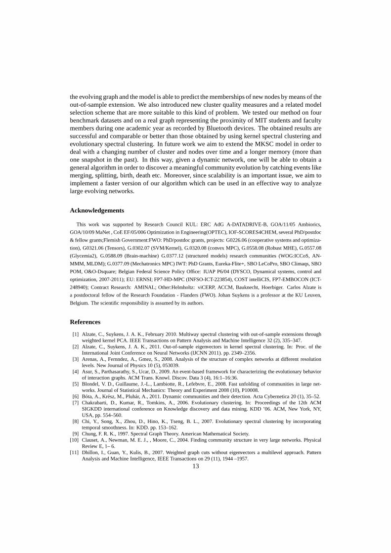
For the KSC we use the BLF criterion [1] to tunek andσ in the two and three moving Gaussianproblem. The results are shown in Fig. 3 and 4 and refer to the first snapshot (for the othersnapshots the plots are similar). For the switching network, in Fig. 5, we illustrate how themodularity-based model selection correctly identifies thepossible presence of two communities(in this casek is the only parameter to tune since the community kernel is parameter-free asexplained in Section 5.2). Also in the case of the expanding/contracting artificial network ourmodel selection technique detects the correct number of clusters, which is 5 in this case (seeFig. 6). Regarding the cellphone network, we have a partial ground truth, namely the affiliationsof each participant. In particular, as observed in [12] and in [31], 2 dominant clusters could beidentified from the Bluetooth proximity data, corresponding to new students at the Sloan businessschool and coworkers who work in the same building. Then for this experiment we will performclustering with number of clustersk = 2, while the optimalσ over time is estimated by using themodularity-based model selection algorithm on each snapshot (see Fig. 7).

9

For what concerns the MKSC model, for all the datasets we use the same values ofσ andkfound for KSC and we need to tuneν andγ. For simplicity we fix the value ofν to 1 and we tuneonly γ. The optimalγ over time for the two and three moving Gaussian experiments are shownrespectively in Fig. 3 and 4. In Fig. 5 the optimal value ofγ over time for the the switchingnetwork suggested by our model selection scheme is shown. Fig. 6 depicts the optimalγ for theexpanding/contracting synthetic network. For the cellphone networkk = 2 andγ = 1 are optimalhyper-parameters for each of the 12 weeks, while the values of σ2 over time are reported in Fig.7.

5.4. Final results

Here we present the simulation results. For what concerns the models with temporal smooth-ness (MKSC or ESC) the first partition is found by applying thecorresponding static model (KSCor spectral clustering) to the first snapshot since we do not have any information from the past.Then we move along the next snapshots one by one since we consider a memory of one snap-shot, as explained in section 3.2. In Fig. 8, 9, 10, 11 and 12 wepresent the performance of KSC,MKSC and ESC in analyzing the five evolving networks under study, in terms of the smoothedcluster quality measures introduced in section 4.2. In all the experiments we useη = αES C = 0.5.Moreover, for what concerns the two and three Gaussian experiments, we also show the out-of-sample clustering results evaluated on grid points surrounding the Gaussian clouds. By lookingat the figures, we can draw the following observations:

• two Gaussians experiment: the models with temporal smoothness (ESC and MKSC) canbetter distinguish between the two Gaussians while they arevery overlapping with respectto the static model KSC, and obtain comparable results.

• three Gaussians dataset: the same consideration valid for the two moving Gaussians can bedrawn (here the ESC algorithm obtains the best results). In this case, however, we can noticealso from the out-of-sample plot that MKSC, thanks to the memory effect introduced in theformulation of the primal problem, remembers the old clustering boundaries compared toKSC (see in particular the results related to the 9th snapshot).

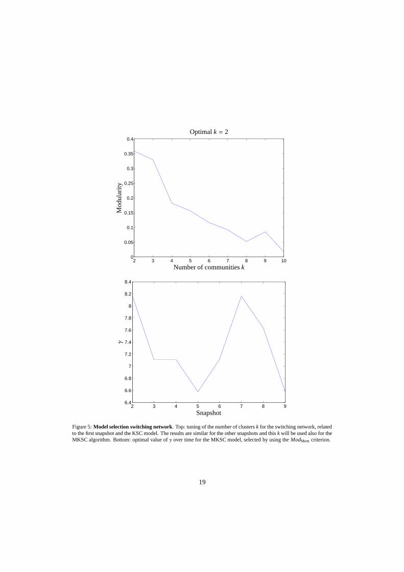
• switching network: MKSC performs slightly better than KSC and much better than ESC.The bad results obtained by ESC are quite unexpected and needfurther investigation. Prob-ably they can be explained by considering that the communitystructure is quite differentfrom snapshot to snapshot and while MKSC is flexible in adapting to this situation, ESC isnot.

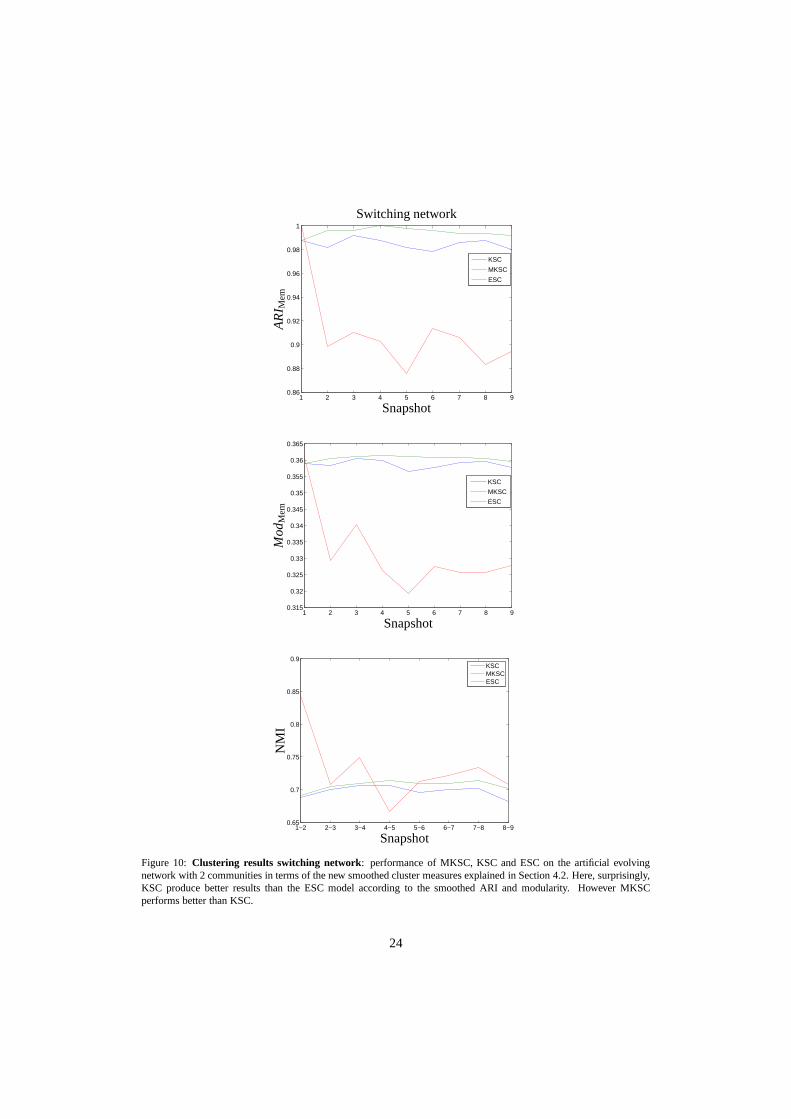
• expanding/contracting graph: as expected the models with temporal smoothness (MKSCand ESC) obtain better results than the static KSC model. MKSC produces the best perfor-mances.

• cellphone network: MKSC performs better than ESC in some periods and worse in otherones. Both obtain better performances than KSC.

Finally it has to be mentioned that ESC provides unstable results, since sometimes the perfor-mances can decrease in quality (see for example the NMI plot in Fig. 9). This is possibly dueto the use ofk-means to produce the final clustering. Indeed it is well known that thek meansalgorithm depends on a random initialization which can leadsometimes to suboptimal results.On the other hand, our model (MKSC) does not suffer from this drawback.

10

6. Flexibility of our framework

6.1. Limitations of Modularity

For the analysis of the networks considered in this paper we used Modularity in order to selectthe optimal parameters of our model. As it has been pointed out in [14] and [13], Modularitysuffers from some drawbacks:

• resolution limit: it contains an intrinsic scale that depends on the total number of links inthe network. Modules that are smaller than this scale may notbe resolved.

• exhibits degeneracies: it typically admits an exponentialnumber of distinct high-scoringsolutions and often lacks a clear global maximum.

• it does not capture overlaps among communities in real networks.

All these limitations, however, do not represent an issue inour framework for several reasons:

• the MKSC model described in equation (6) is quite general (Modularity is not explicitlyoptimized as in other algorithms like for example [5], [10])

• Modularity (and its smoothed version) has been used only at the model selection level.However, our framework is quite flexible and allows to plug-in during the validation phaseany other quality measure

• many of the abovementioned drawbacks of Modularity have been solved by properly mod-ifying its definition, as for example in [3] where a multi-resolution Modularity has beenintroduced. In this case, however, as pointed out in [22], multi-resolution Modularity hasa double simultaneous bias: it leads to a splitting of large clusters and a merging of smallclusters, and both problems cannot be usually handled at thesame time for any value of theresolution parameter.

6.2. Conductance

In order to better understand these issues we present a further analysis based on another qualityfunction called Conductance. For every community, the Conductance is defined as the ratiobetween the number of edges leaving the cluster and the number of edges inside the cluster [21],[24]. In particular, ConductanceC(S ) of a set of nodesS ⊂ V is C(S ) = cS /min(Vol(S ),Vol(V \S )), wherecS denotes the size of the edge boundary,cS = (u, v) : u ∈ S , v < S , andVol(S ) =∑

u∈S d(u), with d(u) representing the degree of nodeu. In other words the conductance describesthe concept of a good network community as a set of nodes that has a better internal than externalconnectivity; thus the lower the Conductance the better thecommunity structure. Moreover,in the same way as for Modularity in section 4.2, we can define the smoothed ConductanceCondMem of the partition related to the actual snapshotGt as:

CondMem(Xα,Gt) = ηCond(Xα,Gt) + (1− η)Cond(Xα,Gt−1). (16)

In Table 1 we show the mean smoothed Conductance over-time for the 3 networks under in-vestigation related to the partitions found by MKSC, ESC, KSC and Louvain method (LOUV)[5]. The Louvain method is based on a greedy optimization of Modularity and has a runtimethat increases linearly with the number of nodes. From the table we can draw the followingconsiderations:

11

• the methods with temporal smoothness (MKSC and ESC) achievean equal or better scorethan the static methods (KSC and LOUV)

• the Louvain method gives the worst results in terms of Conductance. This is not surprisingsince it is biased toward partitions maximizing the Modularity, which may not be good interms of Conductance. On the other hand, as already pointed out, MKSC does not sufferof this drawback since Modularity is used only at the validation level. Moreover for modelselection every quality function could in principle be used. It is a user-dependent choice.

7. Computational complexity

In this section a brief discussion about the computational complexity of the MKSC methodis given. In fact nowadays many large data-sets are available and the algorithms for communitydetection are required to scale well. In order to test the runtime of our method we generated someswitching network (see section 5.1) of increasing size, namely from 103 to 105 nodes. In Fig.13 we show the results. We can see that the MKSC model runs faster than ESC. Moreover thelatter cannot be applied to networks with more than 10.000 nodes because of memory problems.However, the complexity of MKSC appears to be exponential and then needs to be improved.By performing the profiling of our code, we can notice that about 99% of the time is spentto calculate the train (8%) and test (91%) kernel matrices. We believe that an optimized C++implementation of the code (the actual one is done in Matlab)could allow our method to achievea much faster runtime. In fact also the Louvain method runtime, in its Matlab implementation,is higher than MKSC. On the other hand it is well known that theC++ implementation of theLouvain method allows the latter to scale linearly with the number of nodes of the entire graphand then to be considered among the fastest state-of-the-art algorithms. Moreover the calculationof the kernel matrices is easily parallelizable.

Finally, for very large networks (≥ 106 nodes) it can happen that the solution of the linearsystem (9) requires a considerable amount of time. In this case a possible way to overcomethis issue is to use the Woodbury matrix identity, also knownas matrix inversion lemma [18].Suppose that we have to perform community detection of a network formed by 106 nodes. Wecan select for example a training set consisting ofNtr = 50000 nodes. In order to find the solutionvectorα we have to solve the dual problem (9). This implies to find the inverse of aNtr × Ntr

matrix. Now, instead of calculating this inverse, we could select for instance 1000 nodes fromthe training set, solve the small linear system of dimension1000× 1000, and then calculateiteratively theNtr × 1 solution vectorα by using the Woodbury formula.

8. Conclusions and perspectives

In this paper we faced the problem of community detection on evolving networks in the casethat we can include prior knowledge of temporal smoothness.This is an emerging researchtopic and represents a challenge for actual clustering algorithms. In fact, a desirable propertyis that the latter should be able to catch the long-term drifts characterizing the evolution of thecommunities and neglect short-term variations due to noise. As mentioned, this can be thoughtas a kind of temporal smoothness, in the same sense as in time-series analysis. We proposed anew model, the kernel spectral clustering with memory effect or MKSC, casted in the LS-SVM[32] framework. We explicitly designed our clustering model in order to incorporate temporalsmoothness. The clustering is performed by solving a set of linear systems for every snapshot of

12

the evolving graph and the model is able to predict the memberships of new nodes by means of theout-of-sample extension. We also introduced new cluster quality measures and a related modelselection scheme that are more suitable to this kind of problem. We tested our method on fourbenchmark datasets and on a real graph representing the proximity of MIT students and facultymembers during one academic year as recorded by Bluetooth devices. The obtained results aresuccessful and comparable or better than those obtained by using kernel spectral clustering andevolutionary spectral clustering. In future work we aim to extend the MKSC model in order todeal with a changing number of cluster and nodes over time anda longer memory (more thanone snapshot in the past). In this way, given a dynamic network, one will be able to obtain ageneral algorithm in order to discover a meaningful community evolution by catching events likemerging, splitting, birth, death etc. Moreover, since scalability is an important issue, we aim toimplement a faster version of our algorithm which can be usedin an effective way to analyzelarge evolving networks.

Acknowledgements

This work was supported by Research Council KUL: ERC AdG A-DATADRIVE-B, GOA/11/05 Ambiorics,

GOA/10/09 MaNet , CoE EF/05/006 Optimization in Engineering(OPTEC), IOF-SCORES4CHEM, several PhD/postdoc

& fellow grants;Flemish Government:FWO: PhD/postdoc grants, projects: G0226.06 (cooperative systems and optimiza-

tion), G0321.06 (Tensors), G.0302.07 (SVM/Kernel), G.0320.08 (convex MPC), G.0558.08 (Robust MHE), G.0557.08

(Glycemia2), G.0588.09 (Brain-machine) G.0377.12 (structured models) research communities (WOG:ICCoS, AN-

MMM, MLDM); G.0377.09 (Mechatronics MPC) IWT: PhD Grants, Eureka-Flite+, SBO LeCoPro, SBO Climaqs, SBO

POM, O&O-Dsquare; Belgian Federal Science Policy Office: IUAP P6/04 (DYSCO, Dynamical systems, control and

optimization, 2007-2011); EU: ERNSI; FP7-HD-MPC (INFSO-ICT-223854), COST intelliCIS, FP7-EMBOCON (ICT-

248940); Contract Research: AMINAL; Other:Helmholtz: viCERP, ACCM, Bauknecht, Hoerbiger. Carlos Alzate is

a postdoctoral fellow of the Research Foundation - Flanders(FWO). Johan Suykens is a professor at the KU Leuven,

Belgium. The scientific responsibility is assumed by its authors.

References

[1] Alzate, C., Suykens, J. A. K., February 2010. Multiway spectral clustering with out-of-sample extensions throughweighted kernel PCA. IEEE Transactions on Pattern Analysisand Machine Intelligence 32 (2), 335–347.

[2] Alzate, C., Suykens, J. A. K., 2011. Out-of-sample eigenvectors in kernel spectral clustering. In: Proc. of theInternational Joint Conference on Neural Networks (IJCNN 2011). pp. 2349–2356.

[3] Arenas, A., Fernndez, A., Gmez, S., 2008. Analysis of thestructure of complex networks at different resolutionlevels. New Journal of Physics 10 (5), 053039.

[4] Asur, S., Parthasarathy, S., Ucar, D., 2009. An event-based framework for characterizing the evolutionary behaviorof interaction graphs. ACM Trans. Knowl. Discov. Data 3 (4),16:1–16:36.

[5] Blondel, V. D., Guillaume, J.-L., Lambiotte, R., Lefebvre, E., 2008. Fast unfolding of communities in large net-works. Journal of Statistical Mechanics: Theory and Experiment 2008 (10), P10008.

[6] Bota, A., Kresz, M., Pluhar, A., 2011. Dynamic communities and their detection. Acta Cybernetica 20 (1), 35–52.[7] Chakrabarti, D., Kumar, R., Tomkins, A., 2006. Evolutionary clustering. In: Proceedings of the 12th ACM

SIGKDD international conference on Knowledge discovery and data mining. KDD ’06. ACM, New York, NY,USA, pp. 554–560.

[8] Chi, Y., Song, X., Zhou, D., Hino, K., Tseng, B. L., 2007. Evolutionary spectral clustering by incorporatingtemporal smoothness. In: KDD. pp. 153–162.

[9] Chung, F. R. K., 1997. Spectral Graph Theory. American Mathematical Society.[10] Clauset, A., Newman, M. E. J., , Moore, C., 2004. Findingcommunity structure in very large networks. Physical

Review E, 1– 6.[11] Dhillon, I., Guan, Y., Kulis, B., 2007. Weighted graph cuts without eigenvectors a multilevel approach. Pattern

Analysis and Machine Intelligence, IEEE Transactions on 29(11), 1944 –1957.

13

[12] Eagle, N., Pentland, A. S., Lazer, D., 2009. Inferring social network structure using mobile phone data. PNAS106 (1), 15274–15278.

[13] Fortunato, S., Barthlemy, M., 2007. Resolution limit in community detection. Proceedings of the National Academyof Sciences 104 (1), 36–41.

[14] Good, B., Montjoye, Y. D., Clauset, A., 2010. Performance of modularity maximization in practical contexts.Physical Review E 81 (4), 046106.

[15] Greene, D., Doyle, D., Cunningham, P., 2010. Tracking the evolution of communities in dynamic social networks.In: Proceedings of the 2010 International Conference on Advances in Social Networks Analysis and Mining.ASONAM ’10. IEEE Computer Society, Washington, DC, USA, pp.176–183.

[16] Guimera, R., Sales-Pardo, M., Amaral, L., 2004. Modularity from fluctuations in random graphs and complexnetworks. Physical Review E 70 (2), 025101.

[17] Halkidi, M., Batistakis, Y., Vazirgiannis, M., 2001. On clustering validation techniques. Journal of IntelligentInformation Systems 17, 107–145.

[18] Higham, N. J., 1996. Accuracy and Stability of Numerical Algorithms. Society for Industrial and Applied Mathe-matics, Philadelphia, PA, USA.

[19] Hubert, L., Arabie, P., 1985. Comparing partitions. Journal of Classification 1 (2), 193–218.[20] Kang, Y., Choi, S., 2009. Kernel PCA for community detection. In: Business Intelligence Conference.[21] Kannan, R., Vempala, S., Vetta, A., 2000. On clusterings: Good, bad and spectral.[22] Lancichinetti, A., Fortunato, S., Dec 2011. Limits of modularity maximization in community detection. Phys. Rev.

E 84, 066122.[23] Langone, R., Alzate, C., Suykens, J. A. K., 2011. Modularity-based model selection for kernel spectral clustering.

In: Proc. of the International Joint Conference on Neural Networks (IJCNN 2011). pp. 1849–1856.[24] Leskovec, J., Lang, K. J., Mahoney, M., 2010. Empiricalcomparison of algorithms for network community detec-

tion. In: Proceedings of the 19th international conferenceon World wide web. WWW ’10. ACM, New York, NY,USA, pp. 631–640.

[25] Lin, Y.-R., Chi, Y., Zhu, S., Sundaram, H., Tseng, B. L.,2009. Analyzing communities and their evolutions indynamic social networks. ACM Trans. Knowl. Discov. Data 3 (2).

[26] Mucha, P. J., Richardson, T., Macon, K., Porter, M. A., Onnela, J.-P., 2010. Community structure in time-dependent,multiscale, and multiplex networks. Science 328 (5980), 876–878.

[27] Newman, M. E. J., 2006. Modularity and community structure in networks. Proc. Natl. Acad. Sci. USA 103 (23),8577–8582.

[28] Ng, A. Y., Jordan, M. I., Weiss, Y., 2002. On spectral clustering: Analysis and an algorithm. In: Dietterich, T. G.,Becker, S., Ghahramani, Z. (Eds.), Advances in Neural Information Processing Systems 14. MIT Press, Cambridge,MA, pp. 849–856.

[29] Palla, G., lszl Barabsi, A., Vicsek, T., Hungary, B., 2007. Quantifying social group evolution. Nature 446, 2007.[30] Strehl, A., Ghosh, J., 2002. Cluster ensembles - a knowledge reuse framework for combining multiple partitions.

Journal of Machine Learning Research 3, 583–617.[31] Sun, J., Faloutsos, C., Papadimitriou, S., Yu, P. S., 2007. Graphscope: parameter-free mining of large time-evolving

graphs. In: Proceedings of the 13th ACM SIGKDD international conference on Knowledge discovery and datamining. KDD ’07. ACM, New York, NY, USA, pp. 687–696.

[32] Suykens, J. A. K., Van Gestel, T., De Brabanter, J., De Moor, B., Vandewalle, J., 2002. Least Squares SupportVector Machines. World Scientific, Singapore.

[33] von Luxburg, U., 2007. A tutorial on spectral clustering. Statistics and Computing 17 (4), 395–416.

14

Switching network Smoothed ConductanceMKSC 0.0020

ESC 0.0022KSC 0.0022

LOUV 0.0024Expanding network Smoothed Conductance

MKSC 0.0050ESC 0.0051KSC 0.0051

LOUV 0.0184Cellphone network Smoothed Conductance

MKSC 0.0019ESC 0.0042KSC 0.0056

LOUV 0.0153

Table 1: Average smoothed Conductance over time for theswitching network (top), theexpanding/contracting net-work (middle) and thecellphone network.

15

−20 0 20−15

−10

−5

0

5

10

15

20

G3

−20 0 20−15

−10

−5

0

5

10

15

G6

−20 0 20−15

−10

−5

0

5

10

15

G9

Figure 1:Two moving Gaussians dataset. Only the snapshots 3, 6 and 9 are shown.

−20 0 20−15

−10

−5

0

5

10

15

G3

−20 0 20−15

−10

−5

0

5

10

15

G6

−10 0 10−10

−8

−6

−4

−2

0

2

4

6

8

10

G9

Figure 2:Three moving Gaussians dataset. Snapshots 3, 6 and 9 are depicted.

16

5 10 15 20 25 30 35 40 45 502

3

4

5

0.2

0.3

0.4

0.5

0.6

0.7

0.8

0.9

1

σ2

Nu

mb

ero

fclu

ster

skBLF, Optimal values:k = 2,σ2

= 8.5

2 3 4 5 6 7 8 9 100

0.5

1

1.5

2

2.5

3

3.5

4

Snapshot

γ

Figure 3:Model selection two moving Gaussians. Top: tuning of the number of clusterk and the RBF kernel parameterσ2 related to the first snapshot of the two moving Gaussians experiment, for KSC. The optimalσ2 does not change overtime (the model selection procedure gives similar results also for the other snapshots). Moreover, this value will alsobeused for the MKSC model. Bottom: optimal value ofγ over time for MKSC, tuned using theBLFMem method.

17

5 10 15 20 25 30 35 40 45 502

3

4

5

0.4

0.45

0.5

0.55

0.6

0.65

0.7

0.75

0.8

0.85

0.9

σ2

Nu

mb

ero

fclu

ster

sk

BLF, Optimal values:k = 3,σ2= 3

2 3 4 5 6 7 8 9 100.1

0.2

0.3

0.4

0.5

0.6

0.7

0.8

0.9

1

Snapshot

γ

Figure 4: Model selection three moving Gaussians. Top: tuning of the RBF kernel parameterσ2 and the numberof clustersk related to the first snapshot of the three moving Gaussians experiment, for KSC. Bottom: tuning ofγ forMKSC. The same comments made for Fig. 3 are still valid here.

18

2 3 4 5 6 7 8 9 100

0.05

0.1

0.15

0.2

0.25

0.3

0.35

0.4

Number of communitiesk

Mo

du

lari

ty

Optimalk = 2

2 3 4 5 6 7 8 96.4

6.6

6.8

7

7.2

7.4

7.6

7.8

8

8.2

8.4

Snapshot

γ

Figure 5:Model selection switching network. Top: tuning of the number of clustersk for the switching network, relatedto the first snapshot and the KSC model. The results are similar for the other snapshots and thisk will be used also for theMKSC algorithm. Bottom: optimal value ofγ over time for the MKSC model, selected by using theModMem criterion.

19

2 3 4 5 6 7 8 9 100.1

0.15

0.2

0.25

0.3

0.35

0.4

0.45

0.5

Number of communitiesk

Mo

du

lari

ty

Optimalk = 5

2 3 4 5 6 7 8 95.5

6

6.5

7

7.5

8

8.5

9

9.5

10

10.5

Snapshot

γ

Figure 6: Model selection expanding/contracting network. Top: tuning of the number of clustersk for the expand-ing/contracting network, related to the first snapshot and the KSC algorithm. Bottom: tuning ofγ for MKSC. Thecomments made for Fig. 5 hold also in this case.

20

2 4 6 8 10 120

100

200

300

400

500

600

700

800

900

Week

σ2

Figure 7:Model selection cellphone network. Optimalσ2 over time for the cellphone network, related to MKSC. Thenumber of clusters isk = 2, γ = 1 is an optimal value for all the snapshots.

21

SmoothedARI

1 2 3 4 5 6 7 8 9 10

0.4

0.5

0.6

0.7

0.8

0.9

1

KSCMKSCESC

time

AR

I Me

m

Two moving Gaussian

NMI between2 consecutivepartitions

1−2 2−3 3−4 4−5 5−6 6−7 7−8 8−9 9−100.1

0.2

0.3

0.4

0.5

0.6

0.7

0.8

0.9

1

KSCMKSCESC

time

NM

I

MKSC

KSC

Ground truth

−20 0 20−15

−10

−5

0

5

10

15

20

G3

−20 0 20−15

−10

−5

0

5

10

15

G6

−10 0 10−8

−6

−4

−2

0

2

4

6

8

10

G10

Figure 8:Clustering results two moving Gaussians: performance of MKSC, KSC and ESC in the two moving Gaus-sians experiment (first row) and out-of-sample plot for MKSCand KSC (only the results related to snapshots 3, 6 and10 are shown). The true partitioning is depicted in the fifth row. The smoothed ARI plot and the NMI trend tell us that,as expected, the models with temporal smoothness are more able than KSC to produce clustering results which are moresimilar to the ground truth and also more consistent and smooth over time (in the sense explained in Sections 4.2 and4.3). However, in the out-of-sample plot we cannot visuallyappreciate the better performance of MKSC with respect toKSC.

22

SmoothedARI

1 2 3 4 5 6 7 8 9 100.1

0.2

0.3

0.4

0.5

0.6

0.7

0.8

0.9

1

KSC

MKSC

ESC

time

AR

I Me

m

Three moving Gaussian

NMI between2 consecutivepartitions

1−2 2−3 3−4 4−5 5−6 6−7 7−8 8−9 9−100

0.1

0.2

0.3

0.4

0.5

0.6

0.7

0.8

0.9

1

KSCMKSCESC

time

NM

I

MKSC

KSC

Ground truth

−20 0 20−15

−10

−5

0

5

10

15

G3

−20 0 20−15

−10

−5

0

5

10

15

G6

−10 0 10−10

−8

−6

−4

−2

0

2

4

6

8

10

G9

Figure 9: Clustering results three moving Gaussians: Performance of MKSC, KSC and ESC in the three movingGaussians experiment in terms of smoothed ARI and NMI between two consecutive partitions, and out-of-sample plotfor MKSC and KSC (only the results related to snapshots 3, 6 and 9 are shown). The true partitioning is depicted in thelast row. The same observations made for Fig 8 are still validhere. In this case, however, in the out-of-sample plots wecan better recognize that MKSC, thanks to the memory effect introduced in the formulation of the primal problem, ismore able than KSC to remember the old clustering boundariesand produces then smoother results over time (considerin particular the 9th snapshot). Finally, from the NMI plot we can notice that sometimes the ESC algorithm producesunstable results, as mentioned in Section 5.4.

23

1 2 3 4 5 6 7 8 90.86

0.88

0.9

0.92

0.94

0.96

0.98

1

KSC

MKSC

ESC

Snapshot

AR

I Me

m

Switching network

1 2 3 4 5 6 7 8 90.315

0.32

0.325

0.33

0.335

0.34

0.345

0.35

0.355

0.36

0.365

KSC

MKSC

ESC

Snapshot

Mod

Me

m

1−2 2−3 3−4 4−5 5−6 6−7 7−8 8−90.65

0.7

0.75

0.8

0.85

0.9

KSCMKSCESC

Snapshot

NM

I

Figure 10: Clustering results switching network: performance of MKSC, KSC and ESC on the artificial evolvingnetwork with 2 communities in terms of the new smoothed cluster measures explained in Section 4.2. Here, surprisingly,KSC produce better results than the ESC model according to the smoothed ARI and modularity. However MKSCperforms better than KSC.

24

1 2 3 4 5 6 7 8 9

0.4

0.5

0.6

0.7

0.8

0.9

1

KSCMKSCESC

Snapshot

AR

I Me

m

Expanding/contracting network

1 2 3 4 5 6 7 8 90.25

0.3

0.35

0.4

0.45

0.5

0.55

0.6

KSCMKSCESC

Snapshot

Mod

Me

m

1−2 2−3 3−4 4−5 5−6 6−7 7−8 8−90.35

0.4

0.45

0.5

0.55

0.6

0.65

0.7

0.75

0.8

KSCMKSCESC

Snapshot

NM

I

Figure 11:Clustering results expanding/contracting network: performance of MKSC, KSC and ESC on the artificialevolving network with 5 communities. The models with temporal smoothness produce partitions of higher quality thanKSC (according to the smoothed measures introduced in Section 4.2 and the NMI discussed in Section 4.3), encouragingmore consistent clustering over time. If we consider the NMIplot, ESC is the best method while MKSC outperforms allthe others in terms of the smoothed measures.

25

2 4 6 8 10 120.2

0.25

0.3

0.35

0.4

0.45

0.5

KSCMKSCESC

Week

Mod

Me

mCellphone network

1−2 2−3 3−4 4−5 5−6 6−7 7−8 8−9 9−10 10−11 11−120.8

0.82

0.84

0.86

0.88

0.9

0.92

0.94

0.96

0.98

1

KSCMKSCESC

Week

NM

I

Figure 12:Clustering results cellphone network: performance of MKSC, KSC and ESC on the cellphone network interms of the smoothed modularity and the NMI between consecutive clustering results. Also in this case the models withtemporal smoothness MKSC and ESC, in the most of the time period, perform better than the static KSC.

26

0 2 4 6 8 10

x 104

0

2

4

6

8

10

12x 10

4

MKSC

ESC

Number of nodes

Ru

ntim

e(s

)

Figure 13: Evolution of the speed with the size of the benchmark network for ESC (until 104 because of memoryproblems) and MKSC. For MKSC the training set size is the 10% of the size of the whole network.

27