Towards Clustering with XCS Kreangsak Tamee

Department of Computer Engineering King Mongkut’s Institute of Technology

Bangkok, Thailand 10520

kreangsakt@yahoo.com

Larry Bull School of Computer Science

University of the West of England Bristol BS16 1QY, U.K.

+44 (0)117 3283161 larry.bull@uwe.ac.uk

Ouen Pinngern Department of Computer Engineering King Mongkut’s Institute of Technology

Bangkok, Thailand 10520

kpoeun@kmitl.ac.th

ABSTRACT This paper presents a novel approach to clustering using an accuracy-based Learning Classifier System. Our approach achieves this by exploiting the generalization mechanisms inherent to such systems. The purpose of the work is to develop an approach to learning rules which accurately describe clusters without prior assumptions as to their number within a given dataset. Favourable comparisons to the commonly used k-means algorithm are demonstrated on a number of synthetic datasets.

Categories and Subject Descriptors I.2.8 [Artificial Intelligence]: Problem Solving, Control Methods and Search – backtracking, control theory, dynamic programming, graph and tree search strategies, heuristic methods, plan execution formation and execution, scheduling.

General Terms Algorithms, Performance, Experimentation.

Keywords Data mining, k-means, Learning Classifier Systems.

1. INTRODUCTION This paper presents results from a rule-based approach to clustering through the development of a Learning Classifier System (LCS)[9] based on Wilson’s XCS [16]. A number of studies have indicated good performance for XCS in classification tasks (e.g., see [2] for examples). We are interested in the utility of such systems to perform unsupervised learning tasks.

Clustering is an important unsupervised classification technique where a set of data are grouped into clusters in such a way that data in the same cluster are similar in some sense and data in different clusters are dissimilar in the same sense. For this it is necessary to first define a measure of similarity which will establish a rule for assigning data to the domain of a particular cluster centre. One such measure of similarity may be the

Euclidean distance D between two data x and y defined by D=||x-y||. Typically in data clustering there is no one perfect clustering solution of a dataset, but algorithms that seek to minimize the cluster spread, i.e., the family of centre-based clustering algorithms, are the most widely used (e.g., [21]). They each have their own mathematical objective function which defines how well a given clustering solution fits a given dataset. In this paper our system is compared to the most well-known of such approaches, the k-means algorithm. We use as a measure of the quality of each clustering solution the total of the k-means objective function:

2( , ) || ||min{1... }1

no X C x ci jj ki

= −∑∈=

(1)

Define a d-dimensional set of n data points X = {x1 ,…., xn } as the data to be clustered and k centers C = {c1 ,…., ck } as the clustering solution. However most clustering algorithms require the user to provide the number of clusters (k), and the user in general has no idea about the number of clusters (e.g., see [14]). Hence this typically results in the need to make several clustering trials with different values for k where k = 2 to kmax = square-root of n (data points) and select the best clustering among the partitioning with different number of clusters. The commonly applied Davies-Bouldin [5] validity index is used as a guideline to the underlying number of clusters here.

The paper is structured as follows: first we describe the alterations to XCS and then present initial results. A form of rule compaction for clustering with LCS, as opposed to classification, is then presented. A form of local search is then introduced before a number of increasingly difficult synthetic datasets are used to test the algorithm.

2. XCSc In this paper we present a version of the accuracy-based XCS, here termed XCSc. XCSc is a Learning Classifier System without internal memory, where the rulebase consists of a number (N) of rules. Associated with each rule is a scalar which indicates the average error (ε) in the rule’s matching process and the fitness (F) estimates the accuracy of the average error and an estimate of the average size of the niches (match sets - see below) in which that rule participates (σ).

On receipt of an input data, the rulebase is scanned, and any rule whose condition matches the message at each position is tagged as a member of the current match set [M]. The rule representation

Permission to make digital or hard copies of all or part of this work for personal or classroom use is granted without fee provided that copies are not made or distributed for profit or commercial advantage and that copies bear this notice and the full citation on the first page. To copy otherwise, or republish, to post on servers or to redistribute to lists, requires prior specific permission and/or a fee. GECCO’07, July 7–11, 2007, London, England, United Kingdom. Copyright 2007 ACM 978-1-59593-697-4/07/0007…$5.00.

1854

here is the Centre-Spread encoding (see [13] for discussions). A condition consists of interval predicates of the form {{c1 ,s1}, ….. {cd ,sd}}, where c is the interval’s range centre from [0.0,1.0] and s is the “spread” from that centre from the range (0.0,s0] and d is a number of dimensions. Each interval predicates’ upper and lower bounds are calculated as follows: [ci - si, ci + si]. If an interval predicate goes outside the problem space bounds, it is truncated. A rule matches an input x with attributes xi if and only if i i i i ic - s x < c + s≤ for all xi.

Reinforcement in XCSc consists of updating the matching error ε which is derived from the Euclidean distance with respect to the input x and c in the condition of each member of the current [M] using the Widrow-Hoff delta rule with learning rate β:

εj εj + β( 2/1

1

2 )))(((∑=

−d

lljl cx - εj ) (2)

Next, the niche size estimate is updated:

σj σj + β( |[M]| - σj) (3)

The rest of the fitness update follows that of standard XCS with parameters α, ν and ε0 (see [3] for details).

XCSc employs two discovery mechanisms, a niche genetic algorithm (GA)[8] and a covering operator. The general niche GA technique was introduced by Booker [1], who based the trigger on a number of factors including the payoff prediction "consistency" of the rules in a given [M], to improve the performance of LCS. XCS uses a time-based mechanism under which each rule maintains a time-stamp of the last system cycle upon which it was consider by the GA. The GA is applied within the current niche when the average number of system cycles since the last GA in the set is over a threshold θGA. If this condition is met, the GA time-stamp of each rule in the niche is set to the current system time, two parents are chosen according to their fitness using standard roulette-wheel selection, and their offspring are potentially crossed and mutated, before being inserted into the rulebase. This mechanism is used here within match sets, as in the original XCS algorithm [16], which was subsequently changed to work in action sets to aid generalization per action [3].

Offspring are produced via mutation (probability μ) where, after [17], we mutate an allele by adding an amount + or - rand(m0), where m0 is a fixed real, rand picks a real number uniform randomly from (0.0,m0], and the sign is chosen uniform randomly. Crossover (probability χ, two-point) can occur between any two alleles, i.e., within an interval predicate as well as between predicates, inheriting the parents’ parameter values or their average if crossover is invoked. Replacement of existing members of the rulebase uses roulette wheel selection based on estimated niche size (if its fitness F is significantly lower than the average fitness of rules in [P], its deletion probability is further increased as in XCS). If no rules match on a given time step, then a covering operator is used which creates a rule with its condition centre on the input value and the spread with a range of rand(s0),

which then replaces an existing member of the rulebase in the usual way (see [3]).

Recently, Butz et al. [4] have proposed a number of interacting "pressures" within XCS. Their "set pressure" considers the more frequent reproduction opportunities of more general rules. Opposing the set pressure is the pressure due to fitness since it represses the reproduction of inaccurate overgeneral rules. Thus to produce an effective, i.e., general but appropriately accurate, solution an accuracy-based LCS using a niche GA with global replacement should have these two pressures balanced through the setting of the associated parameters. In this paper we show how the same mechanisms can be used within XCSc to identify clusters within a given dataset; the set pressure encourages the evolution of rules which cover many data points and the fitness pressure acts as a limit upon the separation of such data points, i.e., the error.

Previously, evolutionary algorithms have been used for clustering in two principle ways. The first uses them to search for appropriate centers of clusters with established clustering algorithms such as the k-means algorithm, e.g., the GA-clustering algorithm [10]. However this approach typically requires the user to provide the number of clusters. Tseng and Yang [15] proposed the CLUSTERING algorithm which has two stages. In the first stage a nearest-neighbor algorithm is used to reduce the size of data set and in the second the GA-clustering algorithm approach is used. Sarafis [12] has recently proposed a further stage which uses a density-based merging operator to combine adjacent rules to identify the underlying clusters in the data. We suggest that modern accuracy-based LCS are well-suited to the clustering problem due to their generalization capabilities.

3. INITIAL PERFORMANCE In this section we apply XCSc as described above on two datasets for the first experiment to test the performance of the system. The first dataset is well-separated as shown in Fig 1(a). We use a randomly generated synthetic dataset. This dataset has k = 25 true clusters arranged in a 5x5 grid in d = 2 dimension. Each cluster is generated from 400 data points using a Gaussian distribution with a standard deviation of 0.02, for a total of n = 10,000 datum. The second dataset is not well-separated as shown in Fig 1(b). We generated it in the same way as the first dataset except the clusters are not centred on that of their given cell in the grid.

The parameters used were: N=800, β=0.2, 0ε = 0.03, v=5, α=0.1,

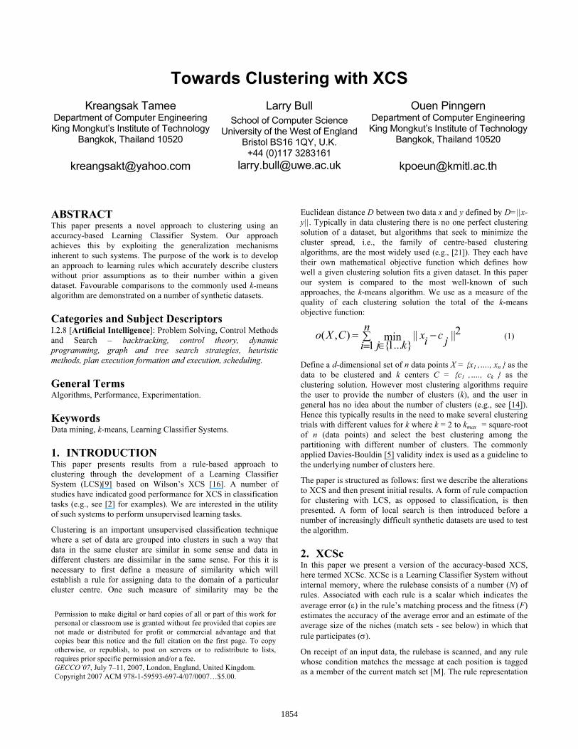
χ=0.8, μ =0.04, θGA =12, s0 =0.03, m0 =0.006. All results presented are the average of ten runs. Learning trials consisted of 200,000 presentations of a randomly sampled data point. Figure 2 shows typical example solutions produced by XCSc on both data sets. That is, the region of the 2D input space covered by each rule in the final rule-base is plotted along with the data. As can be seen, in the well-separated and less-separated case the system roughly identifies all 25 clusters.

As expected, solutions contain many overlapping rules around each cluster. The next section presents a rule compaction algorithm which enables identification of the underlying clusters.

1855

(a)

(b)

Figure 1. The well-separated (a) and less-separated (b) data sets used.

(a)

(b)

Figure 2. Typical solutions for the well-separated (a) and less-separated (b) data sets.

4. RULE COMPACTION Wilson [18] introduced a rule compaction algorithm for XCS to aid knowledge discovery during classification problems (see also [6][7][20]). We have developed a compaction algorithm for clustering:

Step 1 Delete the useless rules: The useless rules are identified and then deleted from the ruleset in the population based on their coverage. Low coverage means that a rule matches a small fraction (20%) of the average number of datum.

Step 2: Sort based on numerosity: The population is sorted according to the numerosity of the rules and then the rules that have the lowest numerosity - less than 2 – are deleted. Then [P]M (M < N) is formed by selecting the minimum sequential set of rules that covers all the data.

Step 3: Sort based on error: The population [P]M is sorted according to the average error of the rules. Then [P]P (P < M) is formed by selecting the minimum sequential set of rules that covers all the data.

Step 4: Remove redundant rules: This step is an iterative process. On each cycle of inputting a data point it selects the rule in [P]P in the largest number of match sets. This rule is removed into the final ruleset [P]F and the data that it covers deleted from the dataset. The process continues until the dataset is empty.

Figure 3 shows the final set [P]F for both the full solutions shown in Figure 2. XCSc’s identification of the clusters is now clear. Under the (simplistic) assumption of non-overlapping regions as described by rules in [P]F it is easy to identify the clusters after compaction. In the case where no rules subsequently match data we could of course identify a cluster by using the distance between it and the centre of each rule.

We have examined the average quality of the clustering solutions produced during the ten runs by measuring the total objective function described in equation (1) and checking the number of clusters defined. The average of quality on the well-separated dataset is 6.65 +/- 0.12 and the number of clusters is 25.0 +/- 0. The average quality on the not well-separated dataset is 6.71 +/- 0.14 and the number of clusters is 25.0 +/- 0. That is, it correctly identifies the number of clusters every time. For comparison, the k-means algorithm was applied to the datasets. The k-means algorithm (assigned with the known k=25 clusters) averaged over 10 runs gives a quality of 32.42 +/- 9.49 and 21.07 +/- 5.25 on the well-separated and less-separated datasets respectively. The low quality of solutions in the well-separated case is due to the choice of the initial centres; k-means is well-known for becoming less reliable as the number of underlying clusters increases. For estimating the number of clusters we ran, for 10 times each, different k (2 to 30) with different random initializations. To select the best clustering with different numbers of clusters, the Davies-Bouldin validity index is shown in Figure 4. The result on well-separated dataset has a lower negative peak at 23 clusters and the less-separated dataset has a lower negative peak at 14 clusters. That is, it is not correct on both datasets, for the same reason as noted above regarding quality. Thus XCSc performs better than k-means whilst also identifying the number of clusters during learning.

1856

0 5 10 15 20 25 300.3

0.4

0.5

0.6

0.7

0.8

0.9

1

1.1

1.2

1.3Davies-Bouldin's index

(a)

(b)

Figure 3. Effects of compaction on the typical solutions in Figure 2 for the well-separated (a) and less-separated (b) data.

(a)

(b)

Figure 4: K-means algorithm performance using the Davies-Bouldin index for well-separated (a) and less-separated (b)

data. Varying k shown on x-axis and index on y-axis.

5. LOCAL SEARCH Previously, Wyatt and Bull [19] have introduced the use of local search within XCS for continuous-valued problem spaces. Within the classification domain, they used the Widrow-Hoff delta rule to adjust rule condition interval boundaries towards those of the fittest rule within each niche on each matching cycle, reporting significant improvements in performance. Here good rules serve as a basin of attraction under gradient descent search thereby complimenting the GA search. The same concept has also been applied to a neural rule representation scheme in XCS [11]. We have examined the performance of local search for clustering using Wyatt and Bull’s scheme: once a focal rule (the highest fitness rule) has been identified from the current match set all rules in [M] use the Widrow-Hoff update procedure to adjust each of the two interval descriptor pairs towards those of the focal rule, e.g., ,,],[ jicFcc ijjlijij ∀−+−< β where cij

represents gene j of rule i in the match set, Fj represent gene j of the focal rule, and βl is a learning set to 0.1. The spread parameters are adjusted in the same way and the mechanism is applied on every match cycle before the GA trigger is tested. Initial results using Wyatt and Bull’s scheme gave a reduction in performance, typically more specific rules, i.e., too many clusters, were identified (not shown).

We here introduce a scheme which uses the current data as the target for the local learning to adjust only the centres of the rules:

)( ijjlijij cxcc −+−< β (4)

Where cij represents the centre of gene j of rule i in the current match set, xj represents the value in dimension j of the current input data, and βl is the learning rate, here set to 0.1. This is applied on every match cycle before the GA trigger is tested, as before. In the well-separated case, the quality of solutions was 6.50 +/- 0.09. In the less-separated case, the quality of solutions was 6.48 +/- 0.07. The same number of clusters was identified as before, i.e., 25 and 25 respectively. Thus results indicate that our data-driven local search improves the quality of the clustering over the non-local search approach and is used hereafter.

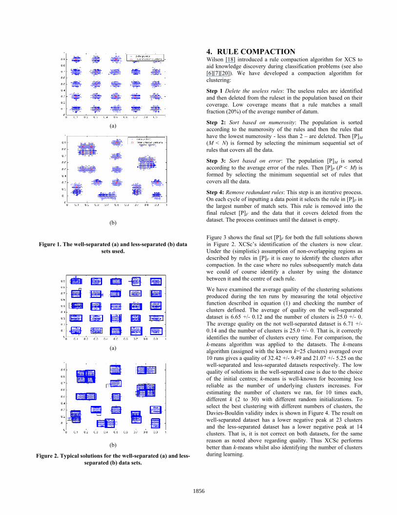
6. ADAPTIVE THRESHOLD PARAMETER The 0ε parameter controls the error threshold of rules and we have investigated the sensitivity of XCSc to its value by varying it. Experiments show that, if 0ε is set high, e.g., 0.1, in the less-separated case the contiguous clusters are covered by the same rules (Figure 5). We therefore developed an adaptive threshold parameter scheme which uses the average error of the current [M]:

)/( ][0 ∑= Mj Nετε (5)

Where jε is the average error of each rule in the current match

set and N[M] is the number of rules in the current match set. This is applied before the fitness function calculations. Experimentally we find τ=1.2 is most effective for the problems used here.

Figure 6 shows how in the well-separated case, the average quality and number of clusters from 10 runs is as before, being

0 5 1 0 1 5 2 0 2 5 3 00 . 3

0 . 4

0 . 5

0 . 6

0 . 7

0 . 8

0 . 9

1

1 . 1

1 . 2

1 . 3D a vie s -B o u ld in 's in d e x

1857

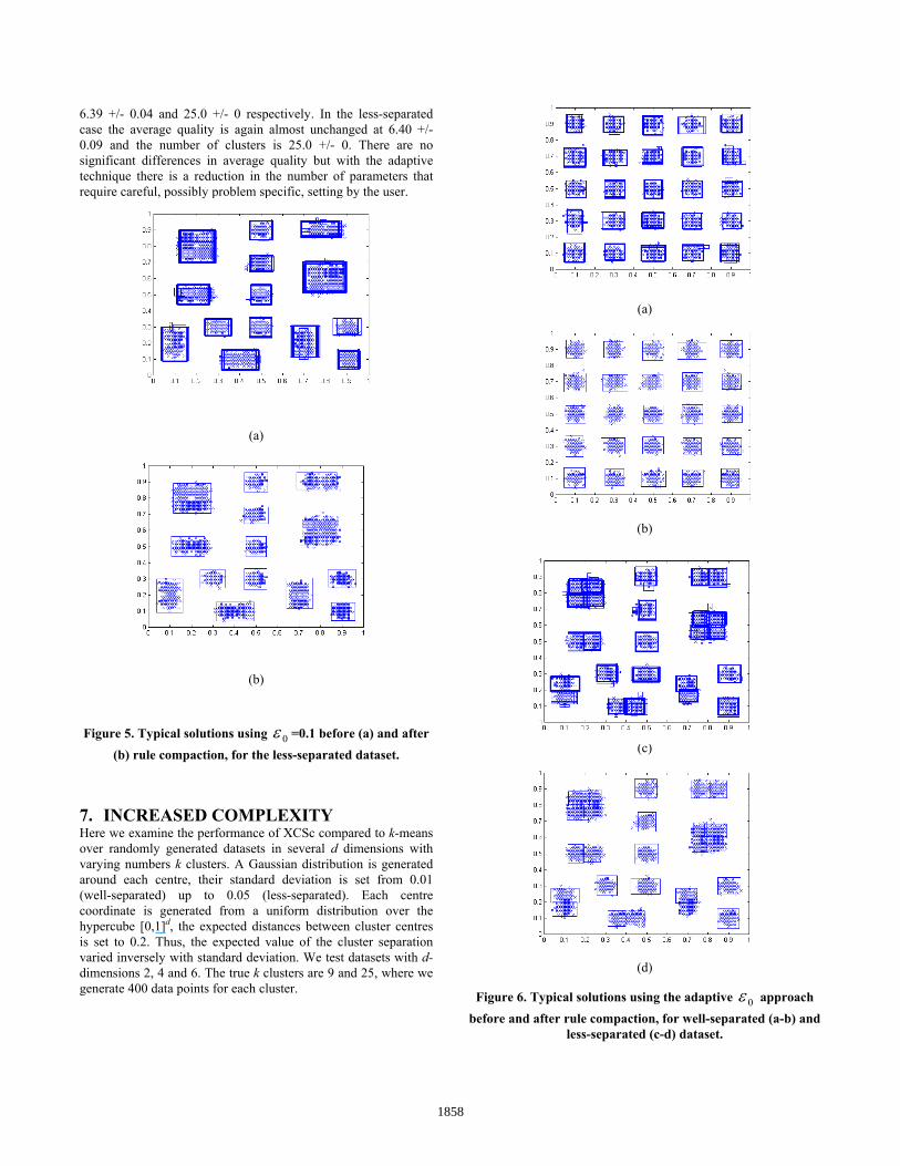
6.39 +/- 0.04 and 25.0 +/- 0 respectively. In the less-separated case the average quality is again almost unchanged at 6.40 +/- 0.09 and the number of clusters is 25.0 +/- 0. There are no significant differences in average quality but with the adaptive technique there is a reduction in the number of parameters that require careful, possibly problem specific, setting by the user.

(a)

(b)

Figure 5. Typical solutions using 0ε =0.1 before (a) and after (b) rule compaction, for the less-separated dataset.

7. INCREASED COMPLEXITY Here we examine the performance of XCSc compared to k-means over randomly generated datasets in several d dimensions with varying numbers k clusters. A Gaussian distribution is generated around each centre, their standard deviation is set from 0.01 (well-separated) up to 0.05 (less-separated). Each centre coordinate is generated from a uniform distribution over the hypercube [0,1]d, the expected distances between cluster centres is set to 0.2. Thus, the expected value of the cluster separation varied inversely with standard deviation. We test datasets with d-dimensions 2, 4 and 6. The true k clusters are 9 and 25, where we generate 400 data points for each cluster.

(a)

(a)

(b)

(c)

(d)

Figure 6. Typical solutions using the adaptive 0ε approach before and after rule compaction, for well-separated (a-b) and

less-separated (c-d) dataset.

1858

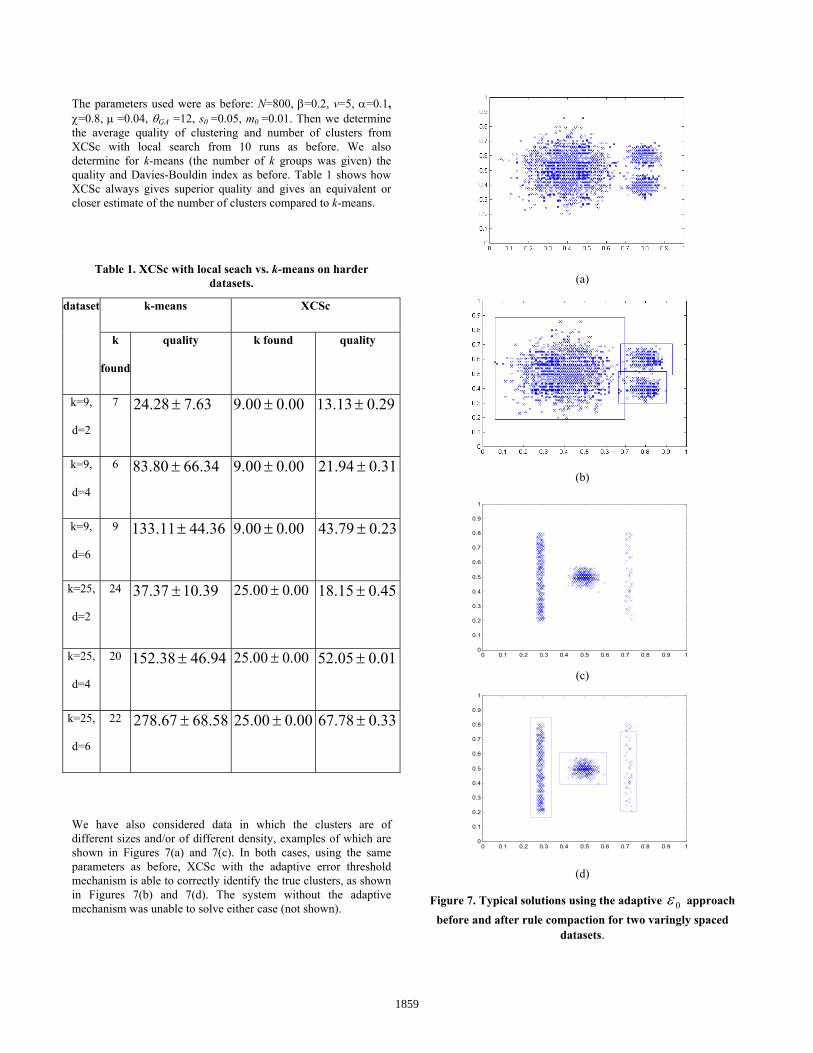
The parameters used were as before: N=800, β=0.2, v=5, α=0.1, χ=0.8, μ =0.04, θGA =12, s0 =0.05, m0 =0.01. Then we determine the average quality of clustering and number of clusters from XCSc with local search from 10 runs as before. We also determine for k-means (the number of k groups was given) the quality and Davies-Bouldin index as before. Table 1 shows how XCSc always gives superior quality and gives an equivalent or closer estimate of the number of clusters compared to k-means.

Table 1. XCSc with local seach vs. k-means on harder datasets.

k-means XCSc dataset

k

found

quality k found quality

k=9,

d=2

7 63.728.24 ± 00.000.9 ± 29.013.13 ±

k=9,

d=4

6 34.6680.83 ± 00.000.9 ± 31.094.21 ±

k=9,

d=6

9 36.4411.133 ± 00.000.9 ± 23.079.43 ±

k=25,

d=2

24

39.1037.37 ± 00.000.25 ± 45.015.18 ±

k=25,

d=4

20 94.4638.152 ± 00.000.25 ± 01.005.52 ±

k=25,

d=6

22 58.6867.278 ± 00.000.25 ± 33.078.67 ±

We have also considered data in which the clusters are of different sizes and/or of different density, examples of which are shown in Figures 7(a) and 7(c). In both cases, using the same parameters as before, XCSc with the adaptive error threshold mechanism is able to correctly identify the true clusters, as shown in Figures 7(b) and 7(d). The system without the adaptive mechanism was unable to solve either case (not shown).

(a)

(b)

(c)

(d)

Figure 7. Typical solutions using the adaptive 0ε approach before and after rule compaction for two varingly spaced

datasets.

0 0.1 0.2 0.3 0.4 0.5 0.6 0.7 0.8 0.9 10

0.1

0.2

0.3

0.4

0.5

0.6

0.7

0.8

0.9

1

0 0.1 0.2 0.3 0.4 0.5 0.6 0.7 0.8 0.9 10

0.1

0.2

0.3

0.4

0.5

0.6

0.7

0.8

0.9

1

1859

8. CONCLUSIONS Our experiments clearly show how a new clustering technique based on the XCS accuracy-based learning classifier system, here termed XCSc, is effective at finding clusters of high quality whilst automatically finding the number of clusters. That is, XCSc can reliably evolve an optimal population of rules through the use of reinforcement learning to update rule parameters and a genetic algorithm to evolve generalizations over the space of possible clusters in dataset. The compaction algorithm presented reduces the number of rules in the total population to identify the rules that provide the clustering. The local search mechanism helps guide the centres of the rules’ intervals in the solution space to approach the true centres of clusters; results show that local search improves the quality of the clustering over a non-local search approach. The original system showed a sensitivity to the setting of the error threshold but an effective adaptive scheme has been introduced which compensates for this behaviour. We are currently applying the approach to a number of large real-world datasets and comparing the performance of XCSc to other clustering algorithms which also determine an appropriate number of clusters during learning.

9. ACKNOWLEDGMENTS This work was partially supported by the Commission On Higher Education of Thailand.

10. REFERENCES [1] Booker, L.B. (1989) Triggered Rule Discovery in Classifier

Systems. In J.D. Schaffer (ed) Proceeding of the Third International Conference on Genetic Algorithms. Morgan Kaufmann, pp265-274.

[2] Bull, L. (2004)(ed.) Applications of Learning Classifier Systems. Springer.

[3] Butz, M. and Wilson, S. (2001) An algorithmic description of XCS. In Lanzi, P. L., Stolzmann, W., and S. W. Wilson (eds.), Advances in Learning Classifier Systems. Third International Workshop (IWLCS-2000). Springer, pp253-272.

[4] Butz, M., Kovacs, T., Lanzi, P-L and Wilson, S.W. (2004) Toward a Theory of Generalization and Learning in XCS. IEEE Transactions on Evolutionary Computation 8(1): 28-46.

[5] Davies, D. L. and Bouldin, D. W. (1979) A Cluster Separation Measure. IEEE Trans. On Pattern Analysis and Machine Intelligence, vol. PAMI-1 (2): 224-227.

[6] Dixon, P., Corne, D., and Oates, M. (2003) A Ruleset Reduction Algorithm for the XCS Learning Classifier System. In Lanzi, Stolzmann & Wilson (eds.), Proceedings of the 5th International Workshop on Learning Classifier Systems. Springer, pp.20-29.

[7] Fu, C. and Davis, L. (2002). A Modified Classifier System Compaction Algorithm. In Banzhaff et al. (eds.) Proceedings of GECCO 2002. Morgan Kaufmann, pp 920-925.

[8] Holland, J.H. (1975) Adaptation in Natural and Artificial Systems. Univ. of Michigan Press.

[9] Holland, J.H. (1976) Adaptation. In Rosen & Snell (eds) Progress in Theoretical Biology, 4. Plenum

[10] Maulik, U. and Bandyopadhyay, S. (2000) Genetic algorithm-based clustering technique. Pattern Recognition 33: 1455-1465.

[11] O'Hara, T. and Bull, L. (2005) A Memetic Accuracy-based Neural Learning Classifier System. In Proceedings of the IEEE Congress on Evolutionary Computation. IEEE Press, pp2040-2045.

[12] Sarafis, I.A., Trinder, P.W., and Zalzala, A.M.S. (2003) Mining comprehensible clustering rules with an evolutionary algorithm. In E. Cant´u- Paz et al. (eds.) Proc Genetic and Evolutionary Computation Conference. Springer, pp2301–2312.

[13] Stone, C. and Bull, L. (2003) For real! XCS with continuous-valued inputs. Evolutionary Computation 11(3):299–336.

[14] Tibshirani, R., Walther, G., and Hastie, T. (2001) Estimating the Number of Clusters in a Dataset Via the Gap Statistic. Journal of the Royal Statistical Society, B, 63: 411-423.

[15] Tseng, L. Y. and Yang, S. B. (2001) A genetic approach to the automatic clustering problem. Pattern Recognition 34: 415-424.

[16] Wilson, S.W. (1995) Classifier Fitness Based on Accuracy. Evolutionary Computation 3(2):149-76.

[17] Wilson, S. W. (2000) Get real! XCS with continuous-valued inputs. In P. L. Lanzi, W. Stolzmann and S. W. Wilson (eds.) Learning Classifier Systems. From Foundations to Applications. Springer, pp209–219.

[18] Wilson, S. (2002). Compact Rulesets from XCSI. In Lanzi, Stolzmann & Wilson (eds.), Proceedings of the 4th International Workshop on Learning Classifier Systems. Springer, pp197-210.

[19] Wyatt, D. and Bull, L. (2004) A Memetic Learning Classifier System for Describing Continuous-Valued Problem Spaces. In N. Krasnagor, W. Hart & J. Smith (eds) Recent Advances in Memetic Algorithms. Springer, pp355-396.

[20] Wyatt, D., Bull, L. and Parmee, I. (2004) Building Compact Rulesets for Describing Continuous-Valued Problem Spaces Using a Learning Classifier System. In I. Parmee (ed) Adaptive Computing in Design and Manufacture VI. Springer, pp235-248.

[21] Xu, R and Winch, D. (2005) Survey of Clustering Algorithms. IEEE Transactions on neural networks 16 (3): 645-678.

1860