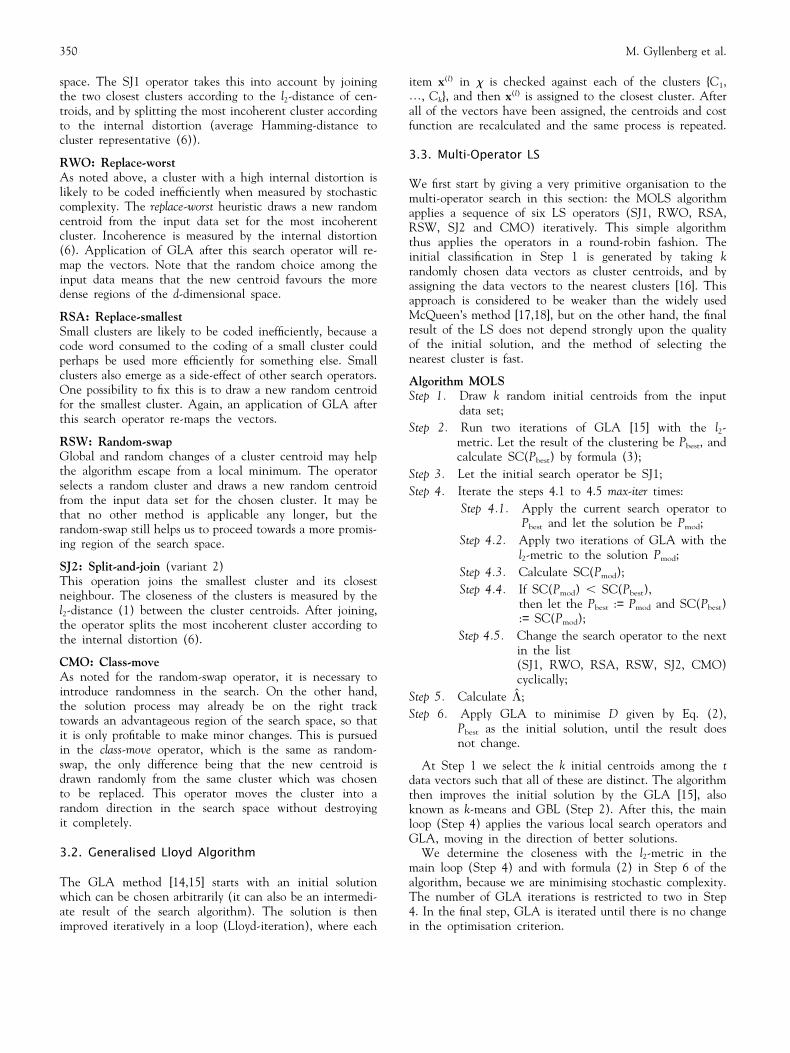
Pattern Analysis & Applications (2000)3:348–357 2000 Springer-Verlag London Limited

Clustering by Adaptive Local Search withMultiple Search Operators

M. Gyllenberg1,2, T. Koski1,3, T. Lund1 and O. Nevalainen1,2

1Department of Mathematical Sciences, University of Turku, Finland; 2Turku Center for Compute Science(TUCS), University of Turku, Finland; 3Department of Mathematics, Royal Institute of Technology, Stockholm,Sweden

Abstract: Local Search (LS) has proven to be an efficient optimisation technique in clustering applications and in the minimisation ofstochastic complexity of a data set. In the present paper, we propose two ways of organising LS in these contexts, the Multi-operatorLocal Search (MOLS) and the Adaptive Multi-Operator Local Search (AMOLS), and compare their performance to single operator(random swap) LS method and repeated GLA (Generalised Lloyd Algorithm). Both of the proposed methods use several different LSoperators to solve the problem. MOLS applies the operators cyclically in the same order, whereas AMOLS adapts itself to favour theoperators which manage to improve the result more frequently. We use a large database of binary vectors representing strains of bacteriabelonging to the family Enterobacteriaceae and a binary image as our test materials. The new techniques turn out to be very promising inthese tests.

Keywords: Adaptation; Clustering; GLA; Local Search; Stochastic complexity

1. INTRODUCTION

Local Search (LS) has proven to be an efficient optimisationtechnique in clustering applications [1]. In the present paper,we propose two ways of organising LS, the Multi-OperatorLocal Search (MOLS) and the Adaptive Multi-OperatorLocal Search (AMOLS). Both techniques use several differ-ent LS operators to solve the problem.

In recent years, there has been great activity in theresearch of efficient solution methods for hard combinatorialoptimisation problems (see Reeves [2] for a survey ofmethods). The exact solution of relatively small probleminstances can sometimes be found by modern optimisationpackages like CPLEX, or by tailored branch-and-boundmethods due to the remarkable progress of these systems.There are still numerous problems (like clustering), wherethe exact solution is ruled out, at least for instances ofpractical relevance, and one has to resort to approximativesearch methods. These can be roughly categorised as con-struction heuristics, descent methods (including local search

Received: 8 November 1999Received in revised form: 15 February 2000Accepted: 11 September 2000

heuristics), genetic algorithms, tabu search and simulatedannealing. The above classification is not strict, and hybridmethods are becoming more and more popular. In fact, thegenetic algorithms belong to a larger set of evolutionarycomputation methods (containing genetic algorithms, gen-etic programming and evolutionary strategies) [3].

Local Search (LS), simulated annealing [4] and Tabu Search(TS) [5] type algorithms modify the current candidate sol-ution by a search (modification or move) operator whichlooks for a better solution in a neighbourhood of the currentsolution. These algorithms are usually written to use onlyone modification operator [1,6].

Here, we investigate alternative methods of cycling a poolof various different LS operators (MOLS), and adaptivelydrawing random methods from the pool of available oper-ators (AMOLS). Different LS operators have their advan-tages and drawbacks; a globally best optimiser does not exist.Here we refer to the ‘no-free-lunch’ theorem [7]. Usually, adeterministic approach leads to losses in robustness of thealgorithm, i.e. the efficiency depends strongly upon theproblem instance and the initial solution. On the otherhand, most of the search steps in LS do not produce anyenhancement in the value of the cost function. The use ofmultiple search operators of LS can be fruitful because (1)

349Clustering by Adaptive Local Search

despite the determinism, several directions in the searchspace are examined, and (2) some operators still can exploitrandomness, even if we have reached a local minimum point.

The idea of multiple search operators has previously beensuccessfully applied in the design of Adaptive Genetic Algor-ithms (AGA). In this context, various different crossovertechniques and different mutation probabilities are used inan adaptive way [8,9]. This gives us a robust techniquewhich adapts itself to use those search operators which arebest suited for the problem instance at hand.

In the present paper, we apply the above idea in adifferent way. While the adaptation in AGA is made for apopulation of solutions, in our LS-implementation we con-sider only one solution. This solution will be greedilyimproved by several different LS-operators. The benefit ofthis approach is the simplicity of the implementation. Onthe other hand, we loose the potential power of parallelsearch of GA.

The rest of the paper is organised as follows. Backgroundtheory is presented in Section 2. In Section 3 we presentthe different LS operators and MOLS algorithm in detail.Then we extend MOLS to its adaptive version (AMOLS).We discuss the data and the test procedures in Section 4,and in Section 5 we present the results. The paper endswith a short discussion.

2. PROBLEM FORMULATION

Let x(l) be a d-dimensional binary vector, i.e. a vector withcomponents x1, x2, %, xd, where xi = 0 or 1 for i = 1, %,d. Suppose that we have a set of t binary vectors x = {x(1),x(2), %, x(t)} to be clustered (or placed, partitioned) into kdisjoint clusters C1, C2, %, Ck. We define the centroid ofthe cluster Cj as uj = (u1,j, %, udj), where 0ij = tij/tj. Here tj

stands for the number of vectors in the cluster Cj, and tij

the number of vectors in cluster j with the ith componentbeing one. For each vector x(l), the distortion from thecentre of its cluster is defined by the squared l2-distance(Minkowsky 2-metric)

ix(l) − uji22 = Od

i=1

(x(l)i − u(l)

ij )2 (1)

It is common to assign a vector to the cluster for whichEq. (1) is minimised. Another method of clustering is basedon the minimisation of stochastic complexity [10,11]. In thiscase, if we define a set of cluster weights L = (l1, %, lk),where lj = tj/t and we assign x(l) to the cluster for whichthe codelength

D(x(l), uj) =

− Od

i=1

((1 − x(l)i ) log2 (1 − uij) (2)

+ x(l)i log2 uij) − log2 lj

assumes its least value.Following Gyllenberg et al [10], we define the stochastic

complexity

SC = log2 S t!t1! % tk!

D+ log2 St + k − 1

t D (3)

+ Ok

j=1

Od

i=1

log2 S (tj + 1)!tij!(tj − tij)!D

The first two terms on the right-hand side of Eq. (3) canbe interpreted as the length of the prefix, i.e. the complexityof the clustering structure (cluster representatives). The lastterm of Eq. (3) is the complexity of describing the vectorswith respect to the clustering (3). The minimisation ofstochastic complexity as a function of k is an answer to thequestion of finding the optimal number of clusters, and isrelated to the principle of the minimum description/messagelength (MDL/MML) [10,12].

We consider two different ways of constructing a clus-tering, viz. minimisation of Eq. (1) over all sample vectorsfor {C1, %, Ck}, and minimisation of Eq. (3). The firstalternative produces ball-like clusters, whereas the secondmethod minimises the total complexity of the clustering.

For some operators used by the clustering algorithms, weneed a simple measure for the distortion or incoherence ofa single cluster. We chose to define the distortion of thecluster Cj as the average Hamming-distance to therounded centroid

aj = (a1j, %, adj), aij = uij + 1/2 (4)

The Hamming-distance of the vector x(l) to the roundedcentroid of Cj is defined by

r(x(l), Cj) = Od

i=1

ux(l)i − aiju (5)

and thus the distortion of a cluster Cj is the average distanceover the vectors x(l) assigned to the cluster, i.e. the distortionof Cj is given by

Rj =1tjO

xPCj

r(x, Cj) (6)

3. ALGORITHMS

3.1. Search Operators

Let us suppose that we are given a set x of t d-dimensional,binary data vectors x = {x(1), %, x(t)} and an initial clusteringas defined by the k cluster centroids (u1j, %, udj). We nextrecall six local search operators which can be used forimproving the clustering. These operators are known fromthe context of vector quantisation [13], but we have modi-fied them to suit the minimisation of stochastic complexity.

SJ1: Split-and-join (variant 1)Often it turns out to be profitable to code two very closeclusters as a single one, and to use the centroid thusobtained to code a cluster at some other part of the vector

350 M. Gyllenberg et al.

space. The SJ1 operator takes this into account by joiningthe two closest clusters according to the l2-distance of cen-troids, and by splitting the most incoherent cluster accordingto the internal distortion (average Hamming-distance tocluster representative (6)).

RWO: Replace-worstAs noted above, a cluster with a high internal distortion islikely to be coded inefficiently when measured by stochasticcomplexity. The replace-worst heuristic draws a new randomcentroid from the input data set for the most incoherentcluster. Incoherence is measured by the internal distortion(6). Application of GLA after this search operator will re-map the vectors. Note that the random choice among theinput data means that the new centroid favours the moredense regions of the d-dimensional space.

RSA: Replace-smallestSmall clusters are likely to be coded inefficiently, because acode word consumed to the coding of a small cluster couldperhaps be used more efficiently for something else. Smallclusters also emerge as a side-effect of other search operators.One possibility to fix this is to draw a new random centroidfor the smallest cluster. Again, an application of GLA afterthis search operator re-maps the vectors.

RSW: Random-swapGlobal and random changes of a cluster centroid may helpthe algorithm escape from a local minimum. The operatorselects a random cluster and draws a new random centroidfrom the input data set for the chosen cluster. It may bethat no other method is applicable any longer, but therandom-swap still helps us to proceed towards a more promis-ing region of the search space.

SJ2: Split-and-join (variant 2)This operation joins the smallest cluster and its closestneighbour. The closeness of the clusters is measured by thel2-distance (1) between the cluster centroids. After joining,the operator splits the most incoherent cluster according tothe internal distortion (6).

CMO: Class-moveAs noted for the random-swap operator, it is necessary tointroduce randomness in the search. On the other hand,the solution process may already be on the right tracktowards an advantageous region of the search space, so thatit is only profitable to make minor changes. This is pursuedin the class-move operator, which is the same as random-swap, the only difference being that the new centroid isdrawn randomly from the same cluster which was chosento be replaced. This operator moves the cluster into arandom direction in the search space without destroyingit completely.

3.2. Generalised Lloyd Algorithm

The GLA method [14,15] starts with an initial solutionwhich can be chosen arbitrarily (it can also be an intermedi-ate result of the search algorithm). The solution is thenimproved iteratively in a loop (Lloyd-iteration), where each

item x(l) in x is checked against each of the clusters {C1,%, Ck}, and then x(l) is assigned to the closest cluster. Afterall of the vectors have been assigned, the centroids and costfunction are recalculated and the same process is repeated.

3.3. Multi-Operator LS

We first start by giving a very primitive organisation to themulti-operator search in this section: the MOLS algorithmapplies a sequence of six LS operators (SJ1, RWO, RSA,RSW, SJ2 and CMO) iteratively. This simple algorithmthus applies the operators in a round-robin fashion. Theinitial classification in Step 1 is generated by taking krandomly chosen data vectors as cluster centroids, and byassigning the data vectors to the nearest clusters [16]. Thisapproach is considered to be weaker than the widely usedMcQueen’s method [17,18], but on the other hand, the finalresult of the LS does not depend strongly upon the qualityof the initial solution, and the method of selecting thenearest cluster is fast.

Algorithm MOLSStep 1. Draw k random initial centroids from the input

data set;Step 2. Run two iterations of GLA [15] with the l2-

metric. Let the result of the clustering be Pbest, andcalculate SC(Pbest) by formula (3);

Step 3. Let the initial search operator be SJ1;Step 4. Iterate the steps 4.1 to 4.5 max-iter times:

Step 4.1. Apply the current search operator toPbest and let the solution be Pmod;

Step 4.2. Apply two iterations of GLA with thel2-metric to the solution Pmod;

Step 4.3. Calculate SC(Pmod);Step 4.4. If SC(Pmod) , SC(Pbest),

then let the Pbest := Pmod and SC(Pbest):= SC(Pmod);

Step 4.5. Change the search operator to the nextin the list(SJ1, RWO, RSA, RSW, SJ2, CMO)cyclically;

Step 5. Calculate L;Step 6. Apply GLA to minimise D given by Eq. (2),

Pbest as the initial solution, until the result doesnot change.

At Step 1 we select the k initial centroids among the tdata vectors such that all of these are distinct. The algorithmthen improves the initial solution by the GLA [15], alsoknown as k-means and GBL (Step 2). After this, the mainloop (Step 4) applies the various local search operators andGLA, moving in the direction of better solutions.

We determine the closeness with the l2-metric in themain loop (Step 4) and with formula (2) in Step 6 of thealgorithm, because we are minimising stochastic complexity.The number of GLA iterations is restricted to two in Step4. In the final step, GLA is iterated until there is no changein the optimisation criterion.

351Clustering by Adaptive Local Search

3.4. Adaptive Local Search

Cyclical application of the LS operators in MOLS is, in thelong run, very similar to a random choice of LS operatorswith uniform distribution. This observation helps us toenhance the multi-operator search. Depending upon thedata, the initial values of the centroids and the state of thesearch, different search operators work better than others.On the other hand, when a certain operator is used insuccession, its power may become exhausted. One way toovercome this shortcoming is to make the algorithm adaptive.This means that when one operator turns out to be successful(the application of the operator leads to a better value ofthe function representing the optimisation criterion, herestochastic complexity), the algorithm should use it morefrequently. When doing this, we should still keep the optionof switching to another search operator at a later stage ofthe solution process. Next, we propose a way ofaccomplishing this kind of strategy.

Let the initial distribution of the probabilities of usingthe different LS operators be

p(0)(y) =16, y = 1, %, 6

Here y is an operator from the set {SJ1, RWO, RSA, RSW,SJ2, CMO}. This means that each operator is initiallyequally probable to be used. We define the indicator func-tion

f(s)(y) =

51, if operation y was successful (decreased Eq. (3)) at the

iteration s

0, otherwise

Let n(s)y be the number of successes for operator y from the

beginning up to iteration s. Initially, n(0)y = 0 for all y. In

every iteration, the success counts are updated by

n(s+1)y = n(s)

y + f(s+1)(y)

and we denote the sum of successes by n(s) = S6y=1 n(s)

y . Thenwe update the probabilities for using different operators by

p(s+1)(y) = Hp(s)(y) if f(s+1)(y) = 0 for all y

n(s)y + f(s+1)(y)+a

n(s) + 1 + 6aotherwise

Because f(t+1)(y) = 1 is only true for one y (= y*),

O6

y=1

p(s+1)(y) =n

(s)y p

+ 1 + a + n(s) − n(s)y p

+ 5a

n(s) + 1 + 6a= 1 (7)

In this model, the parameter a controls the weight ofthe underlying uniform distribution. If a is small, adaptationhappens faster. On the other hand, a should not be toosmall, because this implies that no p(s)(y) ever becomes zero.There is one drawback in this simple model; it has a longmemory. Next we enhance this model to use a shortermemory, so that in a situation where a previously successful

operator becomes inefficient, the model can adapt to thesituation. We define a weight w(s)

y for each operator;initially, take

w(0)y = 0, for all y

and denote the sum of the weights by w(s) = S6y=1 w(s)

y .The update values of the probabilities for using different

operators is now given by

p(s+1)(y) = Hp(s)(y) if f(s+1)(y) = 0 for all y

w(s)y + f(s+1)(y) + a

w(s) + 1 + 6aotherwise

(8)

We update the weights w(s)y after each iteration by

w(s+1)y = w(s)

y + f(s+1)(y) − b(t) (9)if w(s)

y + f(s+1)(y) − b(s) $ 0

In this model, we have a new control parameter b(s),which controls the length of the memory. If b(s) = 0 forall s, then w(s)

y = n(s)y for all s and y, and the new model is

identical to the previous one. The larger the value of b(s),the quicker the model forgets its past history. Usually, atthe beginning of the clustering process, the operators havelarger success rates than at the end. Thus, the model worksbetter if b(s) is larger for small s, and vice versa. Bysubstituting n(s)

y* with w(s)y* Eq. (7) also holds for the new

model.The new improved algorithm looks as follows:

Algorithm AMOLSStep 1. Draw initially k random cluster centroids from the

input data set;

Step 2. Let s = 0 and p(s)(y) =16

for all y;

Step 3. Perform two iterations of GLA with the l2-metric.Let the result of the clustering be Pbest and calcu-late SC(Pbest) by formula (3);

Step 4. Draw a random initial search operator amongst(SJ1, RWO, RSA, RSW, SJ2, CMO);

Step 5. Iterate the steps 5.1 to 5.7 until s = max-iter:Step 5.1. Apply search operator to Pbest and let

the solution be Pmod;

Step 5.2. Apply two iterations of GLA with l2-metrics to the solution Pmod;

Step 5.3. Calculate SC(Pmod);Step 5.4. If SC(Pmod) , SC(Pbest),

then let the Pbest := Pmod and SC(Pbest):= SC(Pmod);

Step 5.5. Increase s by one.Update probabilities p(s)(y) as definedby formula (8);

Step 5.6. Update weights w(s)y as defined by for-

mula (9);Step 5.7. Draw a random operator amongst

(SJ1, RWO, RSA, RSW, SJ2, CMO)weighted by distribution p(s)(y);

352 M. Gyllenberg et al.

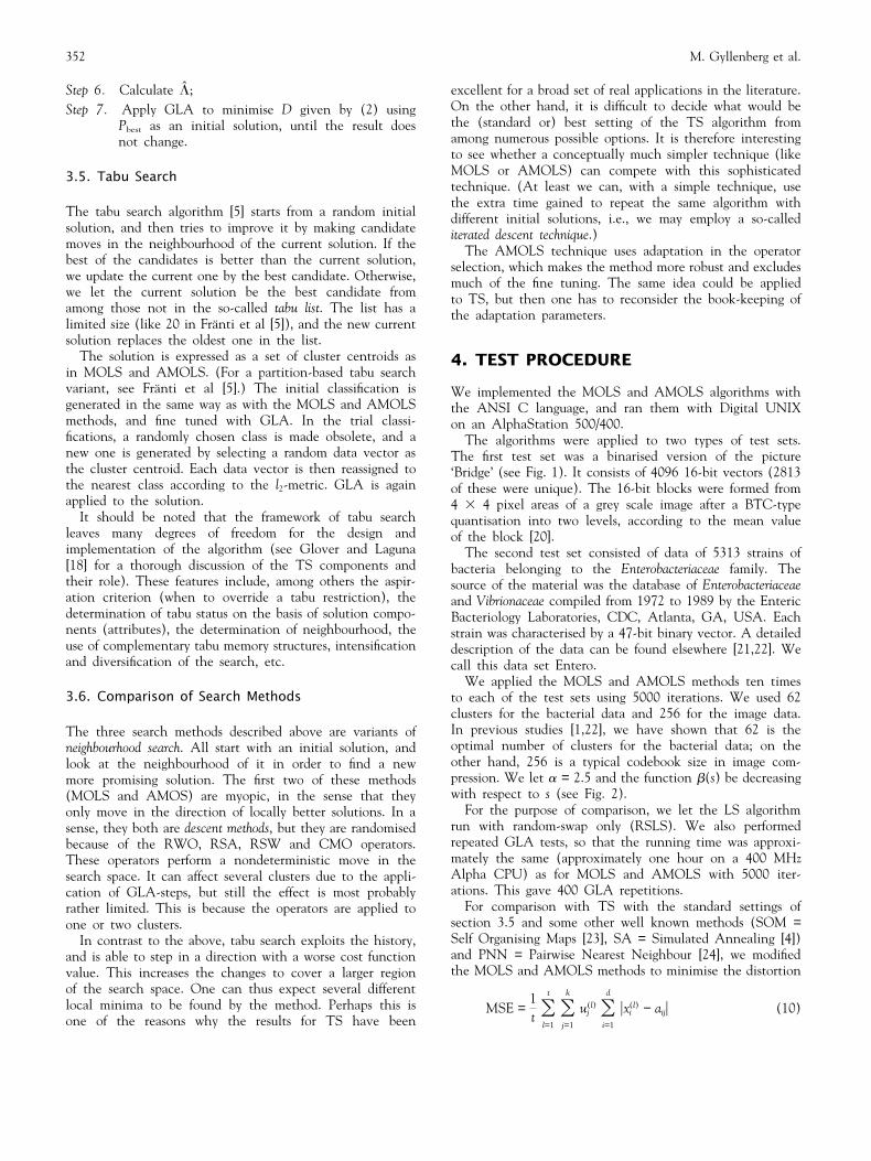
Step 6. Calculate L;Step 7. Apply GLA to minimise D given by (2) using

Pbest as an initial solution, until the result doesnot change.

3.5. Tabu Search

The tabu search algorithm [5] starts from a random initialsolution, and then tries to improve it by making candidatemoves in the neighbourhood of the current solution. If thebest of the candidates is better than the current solution,we update the current one by the best candidate. Otherwise,we let the current solution be the best candidate fromamong those not in the so-called tabu list. The list has alimited size (like 20 in Franti et al [5]), and the new currentsolution replaces the oldest one in the list.

The solution is expressed as a set of cluster centroids asin MOLS and AMOLS. (For a partition-based tabu searchvariant, see Franti et al [5].) The initial classification isgenerated in the same way as with the MOLS and AMOLSmethods, and fine tuned with GLA. In the trial classi-fications, a randomly chosen class is made obsolete, and anew one is generated by selecting a random data vector asthe cluster centroid. Each data vector is then reassigned tothe nearest class according to the l2-metric. GLA is againapplied to the solution.

It should be noted that the framework of tabu searchleaves many degrees of freedom for the design andimplementation of the algorithm (see Glover and Laguna[18] for a thorough discussion of the TS components andtheir role). These features include, among others the aspir-ation criterion (when to override a tabu restriction), thedetermination of tabu status on the basis of solution compo-nents (attributes), the determination of neighbourhood, theuse of complementary tabu memory structures, intensificationand diversification of the search, etc.

3.6. Comparison of Search Methods

The three search methods described above are variants ofneighbourhood search. All start with an initial solution, andlook at the neighbourhood of it in order to find a newmore promising solution. The first two of these methods(MOLS and AMOS) are myopic, in the sense that theyonly move in the direction of locally better solutions. In asense, they both are descent methods, but they are randomisedbecause of the RWO, RSA, RSW and CMO operators.These operators perform a nondeterministic move in thesearch space. It can affect several clusters due to the appli-cation of GLA-steps, but still the effect is most probablyrather limited. This is because the operators are applied toone or two clusters.

In contrast to the above, tabu search exploits the history,and is able to step in a direction with a worse cost functionvalue. This increases the changes to cover a larger regionof the search space. One can thus expect several differentlocal minima to be found by the method. Perhaps this isone of the reasons why the results for TS have been

excellent for a broad set of real applications in the literature.On the other hand, it is difficult to decide what would bethe (standard or) best setting of the TS algorithm fromamong numerous possible options. It is therefore interestingto see whether a conceptually much simpler technique (likeMOLS or AMOLS) can compete with this sophisticatedtechnique. (At least we can, with a simple technique, usethe extra time gained to repeat the same algorithm withdifferent initial solutions, i.e., we may employ a so-callediterated descent technique.)

The AMOLS technique uses adaptation in the operatorselection, which makes the method more robust and excludesmuch of the fine tuning. The same idea could be appliedto TS, but then one has to reconsider the book-keeping ofthe adaptation parameters.

4. TEST PROCEDURE

We implemented the MOLS and AMOLS algorithms withthe ANSI C language, and ran them with Digital UNIXon an AlphaStation 500/400.

The algorithms were applied to two types of test sets.The first test set was a binarised version of the picture‘Bridge’ (see Fig. 1). It consists of 4096 16-bit vectors (2813of these were unique). The 16-bit blocks were formed from4 3 4 pixel areas of a grey scale image after a BTC-typequantisation into two levels, according to the mean valueof the block [20].

The second test set consisted of data of 5313 strains ofbacteria belonging to the Enterobacteriaceae family. Thesource of the material was the database of Enterobacteriaceaeand Vibrionaceae compiled from 1972 to 1989 by the EntericBacteriology Laboratories, CDC, Atlanta, GA, USA. Eachstrain was characterised by a 47-bit binary vector. A detaileddescription of the data can be found elsewhere [21,22]. Wecall this data set Entero.

We applied the MOLS and AMOLS methods ten timesto each of the test sets using 5000 iterations. We used 62clusters for the bacterial data and 256 for the image data.In previous studies [1,22], we have shown that 62 is theoptimal number of clusters for the bacterial data; on theother hand, 256 is a typical codebook size in image com-pression. We let a = 2.5 and the function b(s) be decreasingwith respect to s (see Fig. 2).

For the purpose of comparison, we let the LS algorithmrun with random-swap only (RSLS). We also performedrepeated GLA tests, so that the running time was approxi-mately the same (approximately one hour on a 400 MHzAlpha CPU) as for MOLS and AMOLS with 5000 iter-ations. This gave 400 GLA repetitions.

For comparison with TS with the standard settings ofsection 3.5 and some other well known methods (SOM =Self Organising Maps [23], SA = Simulated Annealing [4])and PNN = Pairwise Nearest Neighbour [24], we modifiedthe MOLS and AMOLS methods to minimise the distortion

MSE =1t O

t

l=1

Ok

j=1

u(l)j Od

i=1

ux(l)i − aiju (10)

353Clustering by Adaptive Local Search

Fig. 1. Greyscale and binary versions of the ‘Bridge’ test image.

where u(l)j = 1 when x(l) belongs to the jth cluster, and zero

otherwise. Here the cluster centroids a1, %, ad are therounded Eq. (4). In this test, we used 10,000 iterations ofMOLS and AMOLS, which roughly corresponds to theparameter settings of the TS. This comparison was onlyperformed for the data set Bridge due to the availability ofthe results for TS, GLA, SA, SOM and PNN (see Frantiet al [5]).

Finally we studied the effect of different choices of b(s).To do this, we sampled 1000 vectors from the Bridge dataset, and applied the AMOLS algorithm to this sample. Weused various different b(s) functions for k = 64 clusters. We

Fig. 2. The function b(s) used in test runs for Bridge and Entero.

let b(s) be a constant (0.0, 0.2 and 1.0) and a decreasingfunction of s (see Fig. 2). The value 0.0 means that AMOLSnever forgets what it has learnt (i.e. it uses the first adaptivemodel presented in Section 3.4). On the other hand, thevalue 1.0 means that AMOLS forgets everything after oneiteration step.

5. RESULTS

It is evident that, during the solution process, the power ofsome search operators is exhausted, and the MOLS shouldskip these and use other operators instead. The question iswhether AMOLS can do any better. Figure 3 demonstratesthe operation of the two algorithms for a typical run withBridge. An ‘x’ is marked each time the algorithm finds anew, better value of SC. The figure shows that the adaptivepattern is already more clearly present at the beginning ofthe AMOLS process, whereas due to the cyclic applicationof the search operators, MOLS improves the solution quiteevenly by all six operators. At the end of the process,patterns of improving methods look similar for AMOLS andMOLS, but AMOLS has the ability to alternate betweendifferent operators.

If we count the percentage of successful applications ofthe different operators, we can see that with MOLS, theprofiles are similar with both data sets, whereas withAMOLS they are different. Figure 4 shows the relativefrequencies of successful applications of different operatorswhen counted over all of the repetitions. The figure showsthat AMOLS can exploit the random-swap operator moreeffectively on the image data (the proportion of random-swap is 29% versus 8% of all successful applications). Onthe bacterial data, AMOLS exploits more replace-worst oper-ator (46% versus 37% of successful applications). Both casesshow the power of adaptation; different operators are moreeffective on different types of data sets.

Figure 5 shows the development of SC as a function ofiteration index s for the best runs. We observe that the SCvalues of AMOLS are lower throughout the search with the

354 M. Gyllenberg et al.

Fig. 3. Typical operator usage patterns of AMOLS (left) and MOLS for Bridge data set.

image data. This also holds for the bacterial data, approxi-mately from iteration 1000 onwards. We also notice thatsuccessful iterations of AMOLS happen more in successionthan with MOLS. Note that there is not much correlationbetween the SC values at the beginning and end of thetwo LS algorithms. This indicates that they concentrate onmore promising areas of the search space.

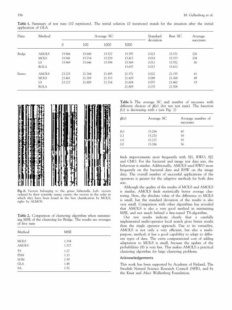
Table 1 compares the average SC values of ten repetitionscounted at a given iteration. The standard deviation is forthe SC-values of the ten repetitions after 5000 iterations,

and the ‘best SC’ gives the minimum of these SC-values.The last column shows the average number of successfulapplications of the operators. On the bacterial data, AMOLShad more successful applications of operators than MOLS(61% versus 49% on average). Also, the average SC(21.371) was statistically smaller than with MOLS (21.429)when tested with the t-test (p = 0.0036 , 0.05). The sameholds for the image data. Here we have 226 successfulapplications for AMOLS against 204 of MOLS. The averageSC for AMOLS (15.397) is statistically smaller (p = 0.027)

355Clustering by Adaptive Local Search

Fig. 4. Comparison of percentages of successful operator applications.There are four sets of six bars. The first set is for the MOLS Bridge,the second for the MOLS Entero, and the two next set for AMOLS.Six bars from the left are percentages per operation SJ1, RWO,RSA, RSW, SJ2 and CMO.

Fig. 5. Development of SC as a function of the iteration index(data plots of the best runs).

than for MOLS (15.417). The standard deviation of the SCvalues for the image data was almost the same for all ofthe algorithms, whereas with the bacterial data, AMOLSgave rise to the smallest standard deviation of the results.

The best SC produced by AMOLS for the bacterial datawas 21.336, whereas MOLS produced 21.368. For the imagedata these values were 15.371 and 15.374, respectively. Acloser investigation of the best results reveals that AMOLSproduced a smaller number of small clusters than MOLS onthe bacterial data: AMOLS produces no singleton clusters,while MOLS found four such clusters. On the other hand,the figures were just the opposite (45 and 35) for theimage data.

When using only random-swap in our framework, theresults were worse than those obtained by AMOLS andMOLS (SC was, on average, 21.604 with a = 0.057 forEntero and 15.569 with a = 0.011 for Bridge). If we lookat the first 100 iterations, random-swap LS seems to workfine, but it does not succeed in any further iterations.However, RSLS gives better results than repeated GLA.Note that there was a considerably smaller number of suc-cessful iterations with RSLS than with AMOLS and MOLS.This suggests that other operators in AMOLS and MOLSdo not exhaust the power of the random-swap operator.

Figure 6 illustrates the clustering results of the data setEntero by showing all 145 vectors (as rows of small whiteand black squares) belonging to genus Salmonella. Vectorsappear in the figure in the order of their scientific name(left), and by the order in which they appear in the resultingclusterings of the MOLS (middle) and AMOLS (right)methods. The figure shows that clusters are not as clearlyvisible in the microbiological clustering as in the MOLSand AMOLS clusterings.

Table 2 compares a number of clustering techniques forthe Bridge test set. The results for PNN, SOM, SA and TSare from Franti et al [5]. The version of TS is highlyoptimised; this can be seen in its high quality MSE-value(1.27 in comparison to 1.32 of AMOLS). On the otherhand, AMOLS performs well in comparison to the othermethods, which have also been optimised.

Table 3 is a summary of test runs with different b(s)settings (for ten repetitions) with a test data sample fromBridge. The decreasing b(s)-function of Fig. 2 gives theoverall best results. The intuition is that, at the beginningof the search process, the operators are more successful andthe learning process should use shorter memory there. Witha value of 0.0, the method does not abandon an operatorwhich has once been successful, and with a value of 1.0,AMOLS behaves more like MOLS. A compromise betweenthese two extremes (like 0.2) works satisfactorily.

6. DISCUSSION

We have studied two versions of a multi-operator LS algor-ithm; non-adaptive and adaptive. Our study shows that theMulti-Operator Local Search (MOLS and AMOLS) is cap-able of finding very low cost clusterings. The AMOLS adaptsquickly to favour SJ1, RWO, RSW and SJ2, whereas MOLS

356 M. Gyllenberg et al.

Table 1. Summary of test runs (10 reptitions). The initial solution (0 iterations) stands for the situation after the initialapplication of GLA

Data Method Average SC Standard Best SC Averagedeviation successes

0 100 1000 5000

Bridge AMOLS 15.966 15.688 15.527 15.397 0.023 15.371 226MOLS 15.941 15.714 15.529 15.417 0.018 15.373 204LS 15.969 15.646 15.598 15.569 0.011 15.552 80RGLA 15.657 0.017 15.612

Entero AMOLS 23.225 21.764 21.495 21.371 0.022 21.335 61MOLS 23.461 21.769 21.513 21.429 0.049 21.368 49LS 23.227 21.809 21.714 21.604 0.057 21.462 19RGLA 21.809 0.135 21.508

Fig. 6. Vectors belonging to the genus Salmonella. Left: vectorsordered by their scientific name; centre: the vectors in the order inwhich they have been found in the best classification by MOLS;right: by ALMOS.

Table 2. Comparison of clustering algorithm when minimis-ing MSE of the clustering for Bridge. The results are averagesof five runs

Method MSE

MOLS 1.334AMOLS 1.327

TS 1.27PNN 1.33SOM 1.39GLA 1.48SA 1.52

Table 3. The average SC and number of successes withdifferent choices of b(s) (for ten test runs). The functionf(s) is decreasing with s (see Fig. 2)

b(s) Average SC Average number ofsuccesses

f(s) 15.264 600.2 15.270 581.0 15.277 550.0 15.286 56

finds improvements most frequently with SJ1, RWO, SJ2and CMO. For the bacterial and image test data sets, thebehaviour is similar. Additionally, AMOLS used RWO morefrequently on the bacterial data and RSW on the imagedata. The overall number of successful applications of theoperators is greater for the adaptive methods for both datasets.

Although the quality of the results of MOLS and AMOLSis similar, AMOLS finds statistically better average clus-tering. Here, the absolute value of the difference to MOLSis small, but the standard deviation of the results is alsovery small. Comparison with other algorithms has revealedthat AMOLS is also a very good method in minimisingMSE, and not much behind a fine-tuned TS-algorithm.

Our test results indicate clearly that a carefullyimplemented multi-operator local search gives better resultsthan the single operator approach. Due to its versatility,AMOLS is not only a very efficient, but also a multi-purpose, method; it has a good capability to adapt to differ-ent types of data. The extra computational cost of addingadaptation to MOLS is small, because the update of theprobabilities (8) is very fast. This makes AMOLS a practicalclustering algorithm for large clustering problems.

Acknowledgements

This work has been supported by Academy of Finland, TheSwedish Natural Science Research Council (NFR), and bythe Knut and Alice Wallenberg Foundation.

357Clustering by Adaptive Local Search

References

1. Franti P, Gyllenberg HG, Gyllenberg M, Kivijarvi J, Koski T,Lund T, Nevalainen O. Minimizing stochastic complexity usinglocal search and GLA with applications to classification ofbacteria. Biosystems 2000; 57:37–48

2. Reeves RC, ed. Modern Heuristic Techniques for CombinatorialProblems. McGraw-Hill, 1995; 70–150

3. Hoffmeister F, Back T. Genetic self-learning. In: Varela FJ,Bourgine P, eds, Toward a Practice of Autonomous Systems:Proc First European Conf Artificial Life (ECAL ’92), Paris,December 11–13 1991; 227–235

4. Vaisey J, Gersho A. Simulated annealing and codebook design.Proc. ICASSP 1988; 1176–1179

5. Franti P, Kivijarvi J, Nevalainen O. Tabu search algorithm forcodebook generation in vector quantization. Pattern Recognition1998; 31(8):1139–1148

6. Franti P, Kivijarvi J. Random swapping technique for improvingclustering in an unsupervised classification. Proc 11th Scandi-navian Conf on Image Analysis (SCIA ’99), Kangerlussuaq,Greenland, 1999; 407–413

7. Wolpert DH, Macready WG. No free lunch theorems foroptimziation. IEEE Trans on Evolutionary Computation 1997;1(1):67–82

8. Hinterding R, Michalewicz Z, Eiben AE. Adaptation in evol-utionary computation: A survey. IEEE Int Conf on EvolutionaryComputation, Indianapolis, April 13–16, 1997; 65–69

9. Magyar G, Johnsson M, Nevalainen O. An adaptive hybridgenetic algorithm for the 3-matching problem. IEEE Trans-actions on Evolutionary Computation 2000; 4

10. Gyllenberg M, Koski T, Verlaan M. Classification of binaryvectors by stochastic complexity. Multivariate Analysis 1997;63:47–72

11. Rissanen J. Stochastic Complexity in Statistical Inquiry. WorldScientific, 1989

12. Bischof H, Leonardis A, Sleb A. MDL principle for robustvector quantization. Pattern Analysis and Applications 1999;2:59–72

13. Kaukoranta T, Franti P, Nevalainen O. Reallocation of GLACodevectors for Evading Local Minimum. Turku Center forComputer Science, TUCS Technical Report No 25, 1996

14. Cherkassky V, Mulier F. Learning from Data: Concepts, Theoryand Methods. Wiley, 1998

15. Linde Y, Buzo A, Gray RM. An algorithm for vector quantizierdesign. IEEE Trans on Commun 1980; 28:84–95

16. Forgy E. Cluster analysis of multivariate data: Efficiency vs.interpretability of classifications. Biometrics 1965; 21:768

17. McQueen JB. Some methods of classification and analysis ofmultivariate observations. Proc 5th Berkeley Symposium inMathematics, Statistics and Probability 1967; 1:281–296

18. Pena JM, Lozano JA, Larranaga P. An empirical comparison offour initialization methods for the k-means algorithm. PatternRecognition Letters 1999; 20:1027–1040

19. Glover F, Laguna M. Tabu search. In Reeves RC, ed, ModernHeuristic Techniques for Combinatorial Problems. McGraw-Hill,1995; 70–150

20. Franti P, Kaukoranta T. Binary vector quantizer design usingsoft centroids. Signal Processing: Image Commun 1999; 14:677–681

21. Farmer III, JJ, Davis BR, Hickman-Brenner FW, McWhorter A,Huntley-Carter GP, Asbury MA, Riddle C, Wahten-Grady HG,Elias C, Fanning GR, Steigerwalt AG, O’Hara M, Morris GK,Smith PB, Brenner DJ. Biochemical identification of new speciesand biogroups of Enterobacteriaceae isolated from clinical speci-mens. J Clinical Microbiology 1985; 21:46–76

22. Gyllenberg HG, Gyllenberg M, Koslei T, Lund T, Schindler J,Verlaan M. Classification of Enterobacteriaceae by minimizationof stochastic complexity. Microbiology 1997; 143:721–732

23. Nasrabadi NM. Vector quantization of images based upon theKohonen self-organization feature maps. Neural Networks 1988;1:518–518

24. Equitz WH. A new vector quantization clustering algorithm.IEEE Trans Acoustics Speech Signal Process 1989; 1:1568–1575

Mats Gyllenberg received his Doctor of Technology degree from the HelsinkiUniversity of Technology. He has been Professor of Applied Mathematics at theLulea University of Technology (1989–1992) and at the University of Turkusince 1992. He was a visiting scientist at the Center for Mathematics andInformatics in Amsterdam (1984–1985), and a visiting professor at VanderbiltUniversity, Nashville Tennessee (1985–1986), the National Center for EcologicalAnalysis and Synthesis, Santa Barbara, California (1996), the University ofUtrecht (1997) and at the Chalmers University of Technology, Gothenburg(1998). He is presently a Member of the Research Council for Natural Sciencesand Technology Academy of Finland, and the Vice President of the EuropeanSociety for Mathematical and Theoretical Biology. His research interests includemathematical population dynamics, theoretical ecology and mathematical tax-onomy.

Timo Koski is Professor of Mathematical Statistics at the Royal Institute ofTechnology, and acting as a part time Professor of Applied Mathematics at theUniversity of Turku. He has previously worked as an associate professor withLulea University of Technology, Luleå, Sweden, and took his PhD at the AboAkademi University in 1986. His scientific interests are in probability theoryand bioinformatics.

Tatu Lund received a MSc degree in computer science from the University ofTurku, Finland in 1997. Since 1995 he has been working at the Department ofMathematical Sciences, Institute of Applied Mathematics at University of Turku,Finland as an assistant. He has also been a PhD student of ComBi (GraduateSchool in Computational Biology, Bioinformatics, and Biometry) since 1998.His research interests include classification algorithms, Bayesian learning andneural computing.

Olli Nevalainen received his MSc and PhD degrees in 1969 and 1976, respect-ively. From 1972 to 1979, he was lecturer in the Department of ComputerScience, University of Turku, Finland, where from 1979 to 1999 he was anAssociate Professor, and since 1999 a Professor. He lectures in the area of datastructures, algorithm design and analysis, compiler construction and operatingsystems. His research interests are algorithm design, including image compression,vector quantisation, scheduling algorithms and production planning.

Correspondence and offprint requests to: T. Lund, Department of MathematicalSciences, University of Turku, FIN-20014, Turku, Finland.