Comput Econ (2007) 29:199–212DOI 10.1007/s10614-006-9078-7

Clustering by kernel density

Christian Mauceri · Diem Ho

Received: 15 November 2006 / Accepted: 12 December 2006 /Published online: 1 March 2007© Springer Science+Business Media B.V. 2007

Abstract Kernel methods have been used for various supervised learningtasks. In this paper, we present a new clustering method based on kernel density.The method does not make any assumption on the number of clusters or ontheir shapes. The method is simple, robust, and behaves equally or better thanother methods on problems known as difficult.

Keywords Clustering · Kernel

1 Introduction

The objective of clustering is to group data points based on their character-istic attributes. Clustering can use parametric model, as in mixture param-eter estimation whose k-means algorithm of MacQueen (1967) is a specialcase. They can also use non-parametric model as in the scale space clusteringmethod of Roberts (1996). The multiplicity of methods has often been quotedby many authors and very good surveys have been written on the subject (seeJain, Murty, & Flynn, 1999 for instance). A kernel on a set X is an appli-cation X × X → R, (x, y) → k(x, y), such that k is symmetric, definite and

C. Mauceri (B) · D. HoIBM Europe, 2 avenue Gambetta, Tour Descartes - La Défense 5,92066 Courbevoie, Francee-mail: mauceri@fr.ibm.com

D. Hoe-mail: diem_ho@fr.ibm.com

C. MauceriÉcole Nationale Supérieure des Télécommunications – Bretagne, Technopôle Brest-Iroise, CS83818, 29238 Brest, France

200 Comput Econ (2007) 29:199–212

positive.1 Kernel methods, whose Support Vector Machine (see Burges, 1998 fora good tutorial) is certainly the best known example, have been initially used forsupervised learning algorithms. The principle governing these methods is to mapobjects into richer high-dimensional spaces called feature spaces where a dotproduct is used for classification, regression or clustering purpose. The advan-tage of such a principle is that the dot product in the feature space is representedby a kernel in the original space avoiding explicit and intractable mapping inthe feature space.

Three very popular clustering methods using kernels are kernel k-means,spectral clustering and support vector clustering. The first method applies thek-means algorithm in the feature space in order to extract clusters which wouldnot be separable in the original space. Spectral clustering algorithms computethe primary dominant eigenvectors of a distance matrix (see Ng, Jordan, &Weiss, 2002), project the data points onto the space spanned by the selectedeigenvectors and then cluster them using a simple algorithm like k-means. Sup-port vector clustering algorithms look for the smallest sphere in the featurespace containing the data image with a tolerance threshold and looks at theconnected component in the original space (see Ben-Hur, Horn, Siegelmann,& Vapnik, 2001). Kernel k-means are attractive because of their simplicity,rapidity, and low-memory requirements but they are sensitive to initial con-ditions and require a pre-set number of clusters. One great advantage of thespectral approach is its representation of the clusters in matrix form allowing avisual analysis of the clustering in term of density and inter-cluster connectivity.It needs however, eigenvector computation which can be costly and somewhatdifficult to interpret. Support vector clustering is very appealing because of itselegance and its strong connection with the support vector supervised learning.It suffers, however, from a lack of natural visual representation.

In this paper, we propose a non-parametric clustering algorithm based on akernel density approach. We identify the initial clusters using a simple algorithmto find a diagonal block structure of the kernel matrix2 depending on a givenkernel density for these blocks. The outcome is refined by using a connectivitythreshold to obtain the final clustering. We use a connected component algo-rithm at the dense cluster level and improve the clustering sharpness by tuningthe kernel density of the diagonal block structure. This is simpler and in con-trast with other methods which use the connected components at the elementlevel and use the Gaussian kernel radius to refine the clustering outcome. Ourmethod allows us to use it with any type of kernels.

We present the proposed method in Sect. 2, we then discuss its benefits inSect. 3 and conclude by a summary and some future directions of research inSect. 4.

1 ∀(x, y) ∈ X × X we have k(x, y) = k(y, x) and ∀(xi)1≤i≤n ∈ Xn and ∀(ci)1≤i≤n ∈ Rn we have∑n

i=1∑n

j=1 cicjk(xi, xj) ≥ 0 (see Haussler, 1999). We call X the original space.2 Given a set of elements S = {xi ∈ X | 1 ≤ i ≤ n} and a kernel X × X → R, (x, y) → k(x, y), thekernel matrix K is a n × n matrix whose entries are Ki,j = k(xi, xj).

Comput Econ (2007) 29:199–212 201

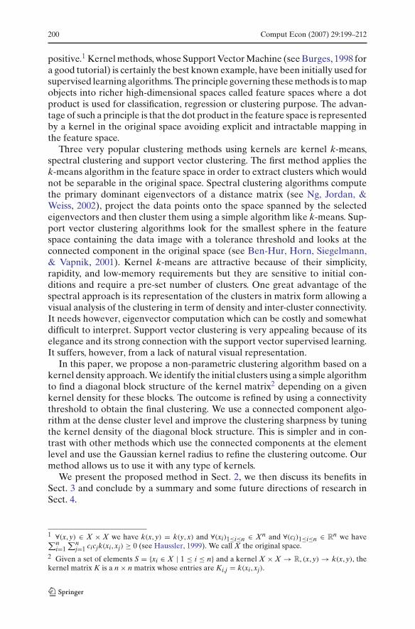
Fig. 1 The inner cluster iscomposed of 50 pointsgenerated from a Gaussiandistribution. The twoconcentric rings contain,respectively, 150 and 300points, generated from auniform angular distributionand radial Gaussiandistribution. The horizontaland the vertical axis give thecoordinates of the points incentimeters

2 Kernel density

Our method based on kernel density is closely related to spectral clusteringin term of cluster representation but is rooted in similarity aggregation (seeMarcotorchino, 1981 and Michaud, 1985). The difference is that, instead ofusing the intra-cluster Kernel sum, we maximize the intra-cluster kernel den-sity as the objective function. This helps us to avoid size dominance effect thatleads to disparity in cluster size and thus difficult to analyze. Our approachis based on kernel matrix transformation into dense block diagonal3 matrixand connected component identification to detect non-convex and overlappingclusters. The advantages of our method are:

• Capability of correctly identifying clusters in well known difficult configu-ration (non-convex and overlapping clusters) with no prior knowledge ofcluster’s number or shape.

• Independence of kernel type.• Rapidity of processing in particular in case of sparse data.• Consistent treatment of heterogeneous data types (quantitative and quali-

tative mix).• Intuitive interpretation of the results.

2.1 The procedure

To illustrate our method we use the synthetic data in Fig. 1, as similarly generatedby Ben-Hur et al. (2001). Suppose the dots in the inner cluster are numberedfrom 1 to 50, those of the first ring from 51 to 200 and those of the second andouter ring from 201 to 500. When the kernel k : (x, y) → e−‖x−y‖2

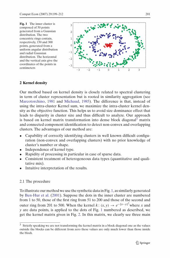
where x andy are data points, is applied to the dots of Fig. 1 numbered as described, weget the kernel matrix given in Fig. 2. In this matrix, we clearly see three main

3 Strictly speaking we are not transforming the kernel matrix in a block diagonal one as the valuesoutside the blocks can be different from zero these values are only much lower than those insidethe block.

202 Comput Econ (2007) 29:199–212

Fig. 2 Kernel matrix of theprevious figure. The dots ofthe previous figure arenumbered from 1 to 50 forthose belonging to the innercluster, from 51 to 200 forthose of the first ring and from201 to 500 those of the secondand outer ring. Values of thekernel are represented bygray levels (1 is representedby black dot and 0 by a whiteone). It is striking to see thenatural clusters as squares onthe diagonal. The square(1,1)–(50,50) seems almostblack as the dots in the innercluster are very close to oneanother

squared blocks on the diagonal. The first very dark block corresponds to theinner cluster, the second less dark block corresponds to the first ring, and thethird and lighter block corresponds to the last and outer ring. The proximitybetween two clusters is represented by symmetric gray rectangles delimitedby the diagonal squares associated with the considered clusters. For instancethe gray rectangles4 (1,50), (51,200) and (50,1), (200,51) in Fig. 2 represent theproximity between the inner circle and the first ring.

The above example suggests that the clusters appear as dense square blockson the diagonal of the kernel matrix when they are arranged in a suitable way.However, the density of the kernel inside these blocks depends on the dataconfiguration and may differ from one cluster to another. For instance, on Fig. 2the inner cluster appears much denser than the outer ring whereas the averagedistance of neighboring points inside any cluster is of the same order.

Our method is based on a two step approach:

• Gather the points in high-density kernel clusters (Fig. 3), using the algorithmdescribed below in 2.2.

• Build the density matrix of these dense clusters (Fig. 4) to assess their intercluster density and find the connected components for a given thresholddeduced from its analysis. The density matrix is a p × p matrix where p isthe number of initial clusters. The density matrix shows, on its diagonal, thedensity of the previously calculated dense clusters and, off the diagonal, theinter cluster density between two different clusters. So if di,j is the generalterm of the density matrix and k is the Kernel we have:

4 Rectangles and squares in the matrices are described by two of their diagonally opposed vertices,these vertices are represented by pairs of integer corresponding to line and column number of thematrix.

Comput Econ (2007) 29:199–212 203

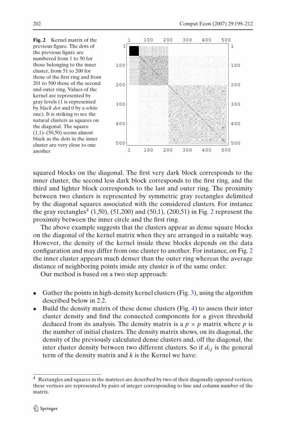
Fig. 3 The original points ofFig. 1 are gathered in clustersof 0.5 kernel density.Different colors stand fordifferent clusters

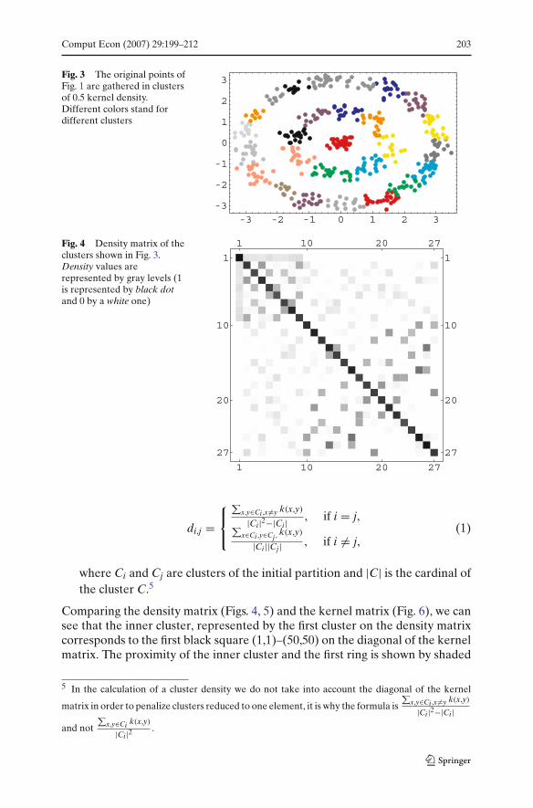
Fig. 4 Density matrix of theclusters shown in Fig. 3.Density values arerepresented by gray levels (1is represented by black dotand 0 by a white one)

di,j =⎧⎨

⎩

∑x,y∈Ci ,x�=y k(x,y)

|Ci|2−|Ci| , if i = j,∑

x∈Ci ,y∈Cj ,k(x,y)

|Ci||Cj| , if i �= j,(1)

where Ci and Cj are clusters of the initial partition and |C| is the cardinal ofthe cluster C.5

Comparing the density matrix (Figs. 4, 5) and the kernel matrix (Fig. 6), we cansee that the inner cluster, represented by the first cluster on the density matrixcorresponds to the first black square (1,1)–(50,50) on the diagonal of the kernelmatrix. The proximity of the inner cluster and the first ring is shown by shaded

5 In the calculation of a cluster density we do not take into account the diagonal of the kernel

matrix in order to penalize clusters reduced to one element, it is why the formula is∑

x,y∈Ci ,x�=y k(x,y)

|Ci|2−|Ci|and not

∑x,y∈Ci k(x,y)

|Ci|2 .

204 Comput Econ (2007) 29:199–212

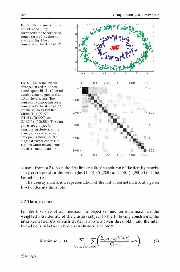
Fig. 5 The original clustersare retrieved. Theycorrespond to the connectedcomponents of the densitymatrix in Fig. 4 for aconnectivity threshold of 0.2

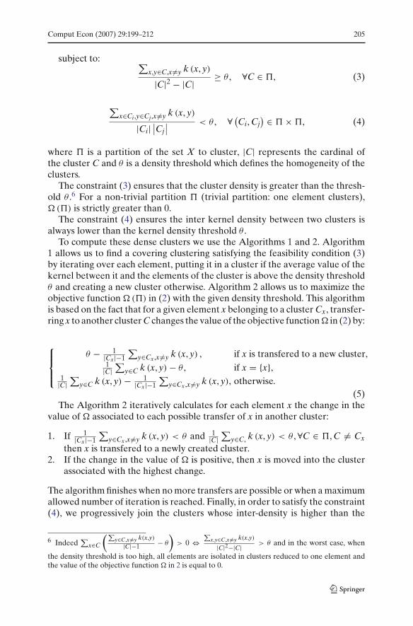
Fig. 6 The kernel matrixarranged in order to showdense square blocks of kerneldensity equal or greater than0.5 on the diagonal. Theconnected components for aconnectivity threshold of 0.2,are the squares identifiedwithin (1,1)–(50,50),(51,51)–(200,200) and(201,201)–(500,500). The datapoints are grouped byneighboring clusters, as theresult, we can observe moredark points along side thediagonal axis; in contrast toFig. 2 in which the data pointsare distributed randomly

squares from to 2 to 9 on the first line and the first column of the density matrix.They correspond to the rectangles (1,50)–(51,200) and (50,1)–(200,51) of thekernel matrix.

The density matrix is a representation of the initial kernel matrix at a givenlevel of density threshold.

2.2 The algorithm

For the first step of our method, the objective function is to maximize theweighted intra density of the clusters subject to the following constraints: theintra kernel density of each cluster is above a given threshold θ and the interkernel density between two given clusters is below θ .

Maximize �(�) =∑

C∈�,|C|>1

∑

x∈C

(∑y∈C,x �=y k (x, y)

|C| − 1− θ

)

(2)

Comput Econ (2007) 29:199–212 205

subject to: ∑x,y∈C,x �=y k (x, y)

|C|2 − |C| ≥ θ , ∀C ∈ �, (3)

∑x∈Ci,y∈Cj,x �=y k (x, y)

|Ci|∣∣Cj

∣∣

< θ , ∀ (Ci, Cj

) ∈ � × �, (4)

where � is a partition of the set X to cluster, |C| represents the cardinal ofthe cluster C and θ is a density threshold which defines the homogeneity of theclusters.

The constraint (3) ensures that the cluster density is greater than the thresh-old θ .6 For a non-trivial partition � (trivial partition: one element clusters),�(�) is strictly greater than 0.

The constraint (4) ensures the inter kernel density between two clusters isalways lower than the kernel density threshold θ .

To compute these dense clusters we use the Algorithms 1 and 2. Algorithm1 allows us to find a covering clustering satisfying the feasibility condition (3)by iterating over each element, putting it in a cluster if the average value of thekernel between it and the elements of the cluster is above the density thresholdθ and creating a new cluster otherwise. Algorithm 2 allows us to maximize theobjective function �(�) in (2) with the given density threshold. This algorithmis based on the fact that for a given element x belonging to a cluster Cx, transfer-ring x to another cluster C changes the value of the objective function � in (2) by:

⎧⎪⎨

⎪⎩

θ − 1|Cx|−1

∑y∈Cx,x �=y k (x, y) , if x is transfered to a new cluster,

1|C|

∑y∈C k (x, y) − θ , if x = {x},

1|C|

∑y∈C k (x, y) − 1

|Cx|−1

∑y∈Cx,x �=y k (x, y), otherwise.

(5)The Algorithm 2 iteratively calculates for each element x the change in the

value of � associated to each possible transfer of x in another cluster:

1. If 1|Cx|−1

∑y∈Cx,x �=y k (x, y) < θ and 1

|C|∑

y∈C, k (x, y) < θ , ∀C ∈ �, C �= Cx

then x is transfered to a newly created cluster.2. If the change in the value of � is positive, then x is moved into the cluster

associated with the highest change.

The algorithm finishes when no more transfers are possible or when a maximumallowed number of iteration is reached. Finally, in order to satisfy the constraint(4), we progressively join the clusters whose inter-density is higher than the

6 Indeed∑

x∈C

(∑y∈C,x�=y k(x,y)

|C|−1 − θ

)

> 0 ⇔∑

x,y∈C,x�=y k(x,y)

|C|2−|C| > θ and in the worst case, when

the density threshold is too high, all elements are isolated in clusters reduced to one element andthe value of the objective function � in 2 is equal to 0.

206 Comput Econ (2007) 29:199–212

density threshold θ , starting with the highest inter-density and updating thedensity matrix after each junction.

At the end of this step, we obtain a partition of X in which each cluster isdenser than θ and the inter-cluster density between two clusters is below θ .

It should be noted the θ threshold is an adjustable parameter and must bechosen as a tradeoff between the complexity of the algorithm and its precision;a too low value of θ leading to a too coarse clustering and a too high-valueleading to too many dense clusters. In general, we use 0.5 as the starting valueof θ .

The above described algorithm might not give the correct solution. For thesecond step, we need a second criterion on the proximity relation among theclusters to arrive at the final clustering. We identify the connected compo-nents of the partition for the relation: Ci and Cj are connected if their inter-density is greater than a given threshold we call the connectivity threshold. Thisthreshold is determined by the analysis of the density matrix. Similar thresholdshave also been used by Fischer and Poland (2004) for their conductivity matrix,or by Ben-Hur et al. (2001) in their Gaussian Kernel spread. As in these twoapproaches the determination of our threshold is rather empirical but, in ourcase, guided by the density matrix. The initial clustering reduces the complexityof the analysis: inter clustering kernel density is high when clusters are closeor adjacent which facilitates the choice. We can also use an assignment-likealgorithm to progressively link the clusters to reduce the partition size to thedesired final number of connected clusters.

The density matrix in (Fig. 4), for instance, shows cluster 1 is linked to clusters2–9 because of the light gray squares (1,2)–(1,9). However, the darker squareslike (3,4) or (2,5) show stronger relations between clusters 3, 4, 2, and 5. It isthe corresponding value of these darker regions we used as the connectivitythreshold to separate correctly the rings. This clustering has been done withoutany prior knowledge of the original space or the feature space.

2.3 Complexity

The complexity of the algorithm is O(ln2) kernel operations where l is the

number of iterations necessary to improve the initial covering clustering andn the number of objects to cluster, plus O

(n2) kernel operations to compute

the density matrix. This is comparable to the SMO7 approach (Platt, 1998) inwhich O

(n2) kernel operations is needed to compute the radius function plus

O(dn2) kernel operations to compute the connected components, where d is

a constant depending on the desired precision of the connected componentcomputation. The spectral methods described in Fischer and Poland (2004) isgreedier because of the spectral decomposition of the kernel matrix, and theconductivity matrix computation of O

(n3) operations.

7 Sequential minimum optimization.

Comput Econ (2007) 29:199–212 207

When, the feature space dimension is finite, it is represented by Rm, and:

∃φ:X−→ Rm,x−→ (φi(x))1≤i≤m such as :

k(x, y) =m∑

i=1

φi(x)φi(y) =< φ(x).φ(y) >

Algorithm 1 � = φFor each x in X {

bestGain = 0For each C in �{

gain = 1|C|

∑y∈C,x �=y k (x, y)

If(bestGain < gain) {bestGain = gainbestClass = C

}}If(bestGain > θ) {

C= bestClass� = (� − {C}) ∪ {C ∪ {x}}/* x is put in C*/

}else {C = φ /* A new empty cluster C is created */� = � ∪ {C ∪ {x}} /* x is put in C */

}}.

Algorithm 2 � = �initdo {

For each x in X {Let be Cx the cluster of XxDensity = 1

|Cx|−1∑

y∈Cx,x �=y k (x, y)

bestGain = 0For each C in �{

gain = 1|C|

∑y∈C,x �=y k (x, y)−xDensity

If(bestGain < gain) {bestGain = gainbestClass = C

}}If(bestGain > 0) {

C= bestClass� = (� − {Cx, C}) ∪ {Cx − {x} , C ∪ {x}}

} else if (xDensity < θ)C = φ /* A new empty cluster C is created */� = � ∪ {C ∪ {x}} /* x is put in C */

}}

} while (� has changed and the number of iterations is not too high).

208 Comput Econ (2007) 29:199–212

we have:∀A, B ⊂ X,

∑

x∈A

∑

y∈B

k(x, y) =<∑

x∈A

φ(x).∑

y∈B

φ(y) >

in such a case the complexity of the algorithm can be O (lnpm), where p is thenumber of clusters. The kernel can be directly computed in the feature space. Ifpm � n then lnpm will be much less than ln2. In addition, when the vectors inthe feature space are very sparse the complexity is O (lnpu) � O

(ln2) where u

is the average non-null components of a vector in the feature space and u � mp .

When dealing with texts this characteristic is important because the algorithmcan be extremely fast allowing for large document quantity processing.

3 Discussion

In this section, we present some of the benefits of the proposed approach, itsability to deal with difficult problems and its consistency.

3.1 Non-convex clusters

The above example, also described in Ben-Hur et al. (2001), is a difficult prob-lem because the natural clusters are non-convex. The kernel value for twoopposed points of a ring is very low and, worse, can be much lower than thekernel value of two points belonging to different rings. In order to separatethe three rings (Ben-Hur et al., 2001) use also two parameters: the kernelspread and a slack variable in order to eliminate the outliers. Then, a connectedcomponents algorithm is used to retrieve clusters in the original space. In thissense our method is comparable; we use a θ kernel density of 0.5 for the ini-tial covering clusters and a connectivity threshold of 0.2. However, by workingwith the density matrix of the initial covering clusters we reduce the complexityof the analysis because the density matrix is much smaller than the kernelmatrix. The data analysis, no matter what the original space or how big thefeature space are, is simpler. In the algorithm described above, the number ofclusters is not required to be specified. However, it is also possible to set, apriori, a number of clusters8 making the density matrix analysis tractable whendealing with very large datasets.

3.2 Strongly overlapping clusters

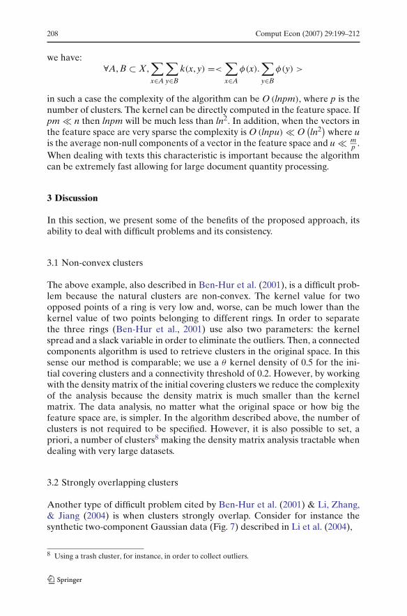
Another type of difficult problem cited by Ben-Hur et al. (2001) & Li, Zhang,& Jiang (2004) is when clusters strongly overlap. Consider for instance thesynthetic two-component Gaussian data (Fig. 7) described in Li et al. (2004),

8 Using a trash cluster, for instance, in order to collect outliers.

Comput Econ (2007) 29:199–212 209

Fig. 7 The left bottomcomponent consists of 800points and the upper one of400. The mean and covariancematrix of the two componentsare

(0, 0

)and

(1, 1

),

(1 0.3

0.3 1

)

and(

1 −0.3−0.3 1

)

,

respectively

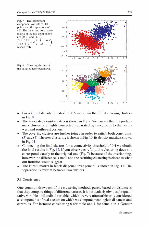
Fig. 8 Covering clusters ofthe data set described in Fig. 7

• For a kernel density threshold of 0.5 we obtain the initial covering clustersin Fig. 8.

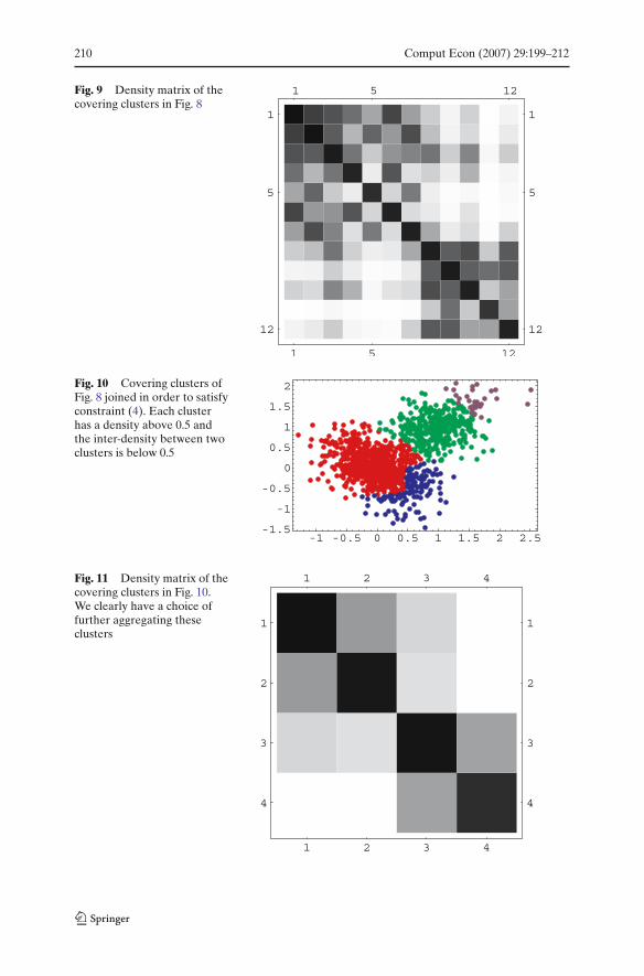
• The associated density matrix is shown in Fig. 9. We can see that the prelim-inary clusters are highly connected, separated by two groups to the north-west and south-east corners.

• The covering clusters are further joined in order to satisfy both constraints(3) and (4). The new clustering is shown in Fig. 10, its density matrix is shownin Fig. 11.

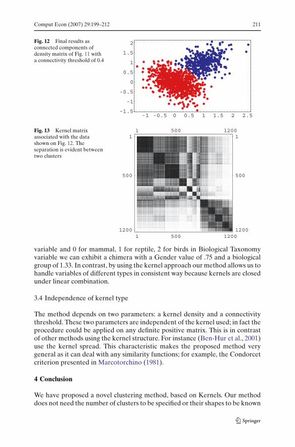
• Connecting the final clusters for a connectivity threshold of 0.4 we obtainthe final results in Fig. 12. If you observe carefully, this clustering does notcorrespond exactly to the original one (Fig. 7) because of the overlapping,however the difference is small and the resulting clustering is closer to whatour intuition would suggest.

• The kernel matrix in block diagonal arrangement is shown in Fig. 13. Theseparation is evident between two clusters.

3.3 Consistency

One common drawback of the clustering methods purely based on distance isthat they compare things of different natures. It is particularly obvious for quali-tative variables and ordinal variables which are very often arbitrarily consideredas components of real vectors on which we compute meaningless distances andcentroids. For instance considering 0 for male and 1 for female in a Gender

210 Comput Econ (2007) 29:199–212

Fig. 9 Density matrix of thecovering clusters in Fig. 8

Fig. 10 Covering clusters ofFig. 8 joined in order to satisfyconstraint (4). Each clusterhas a density above 0.5 andthe inter-density between twoclusters is below 0.5

Fig. 11 Density matrix of thecovering clusters in Fig. 10.We clearly have a choice offurther aggregating theseclusters

Comput Econ (2007) 29:199–212 211

Fig. 12 Final results asconnected components ofdensity matrix of Fig. 11 witha connectivity threshold of 0.4

Fig. 13 Kernel matrixassociated with the datashown on Fig. 12. Theseparation is evident betweentwo clusters

variable and 0 for mammal, 1 for reptile, 2 for birds in Biological Taxonomyvariable we can exhibit a chimera with a Gender value of .75 and a biologicalgroup of 1.33. In contrast, by using the kernel approach our method allows us tohandle variables of different types in consistent way because kernels are closedunder linear combination.

3.4 Independence of kernel type

The method depends on two parameters: a kernel density and a connectivitythreshold. These two parameters are independent of the kernel used; in fact theprocedure could be applied on any definite positive matrix. This is in contrastof other methods using the kernel structure. For instance (Ben-Hur et al., 2001)use the kernel spread. This characteristic makes the proposed method verygeneral as it can deal with any similarity functions; for example, the Condorcetcriterion presented in Marcotorchino (1981).

4 Conclusion

We have proposed a novel clustering method, based on Kernels. Our methoddoes not need the number of clusters to be specified or their shapes to be known

212 Comput Econ (2007) 29:199–212

a priori as many other algorithms do. It has two parameters: a Kernel densitythreshold, which defines a set of initial covering clusters and a connectivitythreshold, derived from the cluster density matrix, which allows us to groupthem into connected components. The cluster density matrix representationprovided by our algorithm allows us to simplify and to fine tune these twoparameters by looking at its characteristic shape. Our method depends on theshape of the kernel matrix for general cluster analysis but is independent ofthe feature space, the original space or the type of kernel used. Experimentalresults as illustrated above indicate that our algorithm performs equivalentlyor better than other algorithms like k-means, Minimum Entropy Clustering orSupport Vector Clustering. We have used this method to cluster millions ofbank customer records. We have also used different variable definition schemesto take into account the difference between ordinal and qualitative variables.The result is favorably compared to other Data Mining clustering tools, in termsof rapidity and population coherence within segments. We plan to use in thefuture this algorithm on sentences and texts clustering based on convolutionkernels as described by Haussler (1999). We also plan to automatically generatedensity thresholds by a statistical analysis of the kernel matrix.

Acknowledgements The authors are grateful to one referee for his critical reading of the man-uscript and many thoughtful and valuable comments that help us to improve considerably ourpaper.

References

Ben-Hur, A., Horn, D., Siegelmann, H., & Vapnik, V. (2001). Support vector clustering. Journal ofMachine Learning Research, 2, 125–137.

Burges, C. J. (1998). A tutorial on support vector machines for pattern recognition. Data Miningand Knowledge Discovery, 2, 121–167.

Fischer, I., & Poland, J. (2004). New methods for spectral clustering. Technical report No. IDSIA-12-04.

Haussler, D. (1999). Convolution kernels on discrete structures. Technical report, Department ofComputer Science, University of California at Santa Cruz.

Jain, A., Murty, M., & Flynn, P. (1999). Data clustering: A review. A.C.M. Computing Surveys, 31,264–323.

Li, H., Zhang, K., & Jiang, T. (2004). Minimum entropy clustering and applications to gene expres-sion analysis. In Proceedings of the 2004 IEEE Computational Bioinformatics Conference.

MacQueen, J. (1967). Some methods for classification and analysis of multivariate observations.In Proceedings of Fifth Berkeley Symposium on Mathematical Statistics and Probability, 1965,University of California, 281–297.

Marcotorchino, F. (1981). Agrgation des similarits. PhD dissertation.Michaud, P. (1985). Agrgation la majorit: Analyse de rsultats d’un vote. IBM Scientific Center of

Paris, Technical report F052.Ng, A. Y., Jordan, M., & Weiss, Y. (2002). On spectral clustering: Analysis and an algorithm.

Advances in Neural Information Processing Systems, 14.Platt, J. C. (1998). A fast algorithm for training support vector machines. Technical Report MSR-

TR-98-14.Roberts, S. J. (1996). Parametric and non-parametric unsupervised cluster analysis. Pattern

Recognition, 30(2), 261–272.