UNIFYING KERNEL METHODS AND NEURAL NETWORKS AND MODULARIZING DEEPLEARNING

By

SHIYU DUAN

A DISSERTATION PRESENTED TO THE GRADUATE SCHOOLOF THE UNIVERSITY OF FLORIDA IN PARTIAL FULFILLMENT

OF THE REQUIREMENTS FOR THE DEGREE OFDOCTOR OF PHILOSOPHY

UNIVERSITY OF FLORIDA

2020

c⃝ 2020 Shiyu Duan

To my family

ACKNOWLEDGMENTS

When I started my first term of graduate school as a master’s student in electrical and

computer engineering at University of Florida (UF), I knew little about machine learning and

had an undergraduate GPA of 2.99/4. My advisor, Dr. Jose Prıncipe, discovered me from his

classroom, miraculously saw the potential in me, and took me into his lab despite the many

stupid questions I pestered him with during and after classes. He gave me patience, trust, and

the freedom to grow — things that not a lot of Ph.D. students are lucky enough to get from

their advisors. He always asked the right questions that pointed me in the right direction. And

more importantly, he also asked the tough questions that pushed me forward. I did not even

believe in myself in the beginning, but my advisor made this possible. My gratitude toward him

is beyond words.

I am grateful to all that I’ve met along the way. But there are a few that I am particularly

thankful to. Dr. Shujian Yu has been a collaborator and a role model. His contributions made

this dissertation possible, and he greatly affected how I approach research through setting a

positive example himself. Dr. Eder Santana provided much guidance when I started in the

lab. And his passion for building wonderful things sparked my own. Spencer Chang proofread

this dissertation, to which I am very thankful. Dr. Luis Gonzalo Sanchez Giraldo, Dr. Robert

Jenssen, and Dr. Pingping Zhu’s times in the lab did not overlap with mine. But I was lucky

enough to know them in person and I’ve constantly looked up to them as role models. They’ve

also deeply inspired me through the excellence of their works. Outside of my lab, I have had

the pleasure to work with some extraordinary researchers during internships, including Dr.

Huaijin Chen, Dr. Jun Jiang, Dr. Jinwei Gu, Dr. Hao Pan, and Xiaohua Yang. The projects

we worked on are not directly related to this dissertation, but their research methodologies,

philosophies, and passions all have had a tremendous impact on me.

There are a few faculty members from UF that have directly helped with or indirectly

inspired my work. Dr. Yunmei Chen and Dr. Murali Rao have provided continuous guidance

and support for my research. Their brilliance and humility have helped me become a better

4

researcher as well as a better person. I’ve also met some of the best teachers in my life here at

UF, who introduced me, in their own ingenious ways, to the magnificence of mathematics and

statistics, the two fields that I have found the most inspirations from and am deeply fascinated

by. They are Dr. Scott McCullough, Dr. Kshitij Khare, Dr. Paul Robinson, Dr. Malay Ghosh,

Dr. Brett Presnell, Dr. William Hager, and Dr. James Hobert. Last but definitely not the

least, I would like to thank my committee members, Dr. Alina Zare, Dr. Kshitij Khare, Dr.

Sean Meyn, and Dr. Yunmei Chen, for the many helpful discussions and key insights that made

this work possible.

I think pursuing a Ph.D. is a privilege and a somewhat selfish thing to do, especially for

those of us who chose to do it in somewhere far away from home and from the ones we love.

Despite being at a age where most of our peers have to take responsibility of various other

concrete things in life, we isolate ourselves in a vacuum environment, laser-focused on our

research and thoroughly enjoying the good times as well as the bad times with little regard

of what happens outside of our little bubble. A lot of us glorify this action as advancing the

knowledge of the entire human race, something that is for the greater good and something

that will eventually benefit us and our family in a tangible way. While I definitely hope that

this is true, I cannot help but feel apologetic toward my loved ones for taking four years of my

companionship away from them and for avoiding for so long responsibilities that should have

been mine. I thank you all for your understanding and always being immensely supportive of

anything that I chose to do. This dissertation is your work as much as it is mine.

5

TABLE OF CONTENTS

page

ACKNOWLEDGMENTS . . . . . . . . . . . . . . . . . . . . . . . . . . . . . . . . . . . 4

LIST OF TABLES . . . . . . . . . . . . . . . . . . . . . . . . . . . . . . . . . . . . . . 9

LIST OF FIGURES . . . . . . . . . . . . . . . . . . . . . . . . . . . . . . . . . . . . . 10

ABSTRACT . . . . . . . . . . . . . . . . . . . . . . . . . . . . . . . . . . . . . . . . . 11

CHAPTER

1 INTRODUCTION . . . . . . . . . . . . . . . . . . . . . . . . . . . . . . . . . . . 13

1.1 Kernel Networks: Connectionist Models Based On Kernel Machines . . . . . . 131.2 Neural Networks Are Kernel Networks . . . . . . . . . . . . . . . . . . . . . . 141.3 Modularizing Deep Architecture Training With Provable Optimality . . . . . . 161.4 Contributions . . . . . . . . . . . . . . . . . . . . . . . . . . . . . . . . . . . 191.5 Dissertation Structure . . . . . . . . . . . . . . . . . . . . . . . . . . . . . . 19

2 RELATED WORK . . . . . . . . . . . . . . . . . . . . . . . . . . . . . . . . . . . 21

2.1 Kernel Method-Based Connectionist Models . . . . . . . . . . . . . . . . . . 212.2 Connections Between Deep Learning and Kernel Method . . . . . . . . . . . . 23

2.2.1 Exact Equivalences . . . . . . . . . . . . . . . . . . . . . . . . . . . . 232.2.2 Equivalences in Infinite Widths and/or in Expectation . . . . . . . . . . 24

2.3 Modular Learning of Deep Architectures . . . . . . . . . . . . . . . . . . . . 25

3 MATHEMATICAL PRELIMINARIES . . . . . . . . . . . . . . . . . . . . . . . . . 28

3.1 Notations . . . . . . . . . . . . . . . . . . . . . . . . . . . . . . . . . . . . . 283.2 Kernel Method in Machine Learning . . . . . . . . . . . . . . . . . . . . . . . 28

3.2.1 A Primer on Kernel Method . . . . . . . . . . . . . . . . . . . . . . . 293.2.2 The “Kernel Trick” . . . . . . . . . . . . . . . . . . . . . . . . . . . . 30

3.2.2.1 Kernel machines: linear models on nonlinear features . . . . . 313.2.2.2 Kernel functions as similarity measures . . . . . . . . . . . . 33

4 KERNEL NETWORKS: DEEP ARCHITECTURES POWERED BY KERNEL MACHINES 34

4.1 A Recipe for Building Kernel Networks . . . . . . . . . . . . . . . . . . . . . 344.2 Why Kernel Networks? . . . . . . . . . . . . . . . . . . . . . . . . . . . . . . 364.3 Robustness in Choice of Kernel . . . . . . . . . . . . . . . . . . . . . . . . . 364.4 An Example: Kernel MLP . . . . . . . . . . . . . . . . . . . . . . . . . . . . 374.5 Experiments: Comparing KNs with Classical Kernel Machines . . . . . . . . . 40

5 NEURAL NETWORKS ARE KERNEL NETWORKS . . . . . . . . . . . . . . . . . 43

5.1 Notations . . . . . . . . . . . . . . . . . . . . . . . . . . . . . . . . . . . . . 43

6

5.2 Revealing the Disguised Kernel Machines in Neural Networks . . . . . . . . . . 435.2.1 Fully-Connected Neural Networks . . . . . . . . . . . . . . . . . . . . 445.2.2 Convolutional Neural Networks . . . . . . . . . . . . . . . . . . . . . . 475.2.3 Recurrent Neural Networks . . . . . . . . . . . . . . . . . . . . . . . . 485.2.4 Modules: Combinations of Sets of Layers . . . . . . . . . . . . . . . . 495.2.5 Add-Ons . . . . . . . . . . . . . . . . . . . . . . . . . . . . . . . . . 50

5.2.5.1 Batch normalization . . . . . . . . . . . . . . . . . . . . . . 505.2.5.2 Pooling and padding layers . . . . . . . . . . . . . . . . . . 505.2.5.3 Residual connection . . . . . . . . . . . . . . . . . . . . . . 51

5.3 Strength in Numbers: Universality Through Tractable Kernels . . . . . . . . . 525.4 Neural Operator Design Is a Way to Encode Prior Knowledge Into Kernel Machine 52

6 A PROVABLY OPTIMAL MODULAR LEARNING FRAMEWORK . . . . . . . . . 54

6.1 The Modular Learning Methodology . . . . . . . . . . . . . . . . . . . . . . . 566.1.1 The Setting, Goal, and Idea . . . . . . . . . . . . . . . . . . . . . . . 566.1.2 The Main Theoretical Result . . . . . . . . . . . . . . . . . . . . . . . 576.1.3 Applicability of the Main Result . . . . . . . . . . . . . . . . . . . . . 59

6.1.3.1 Network architecture . . . . . . . . . . . . . . . . . . . . . . 596.1.3.2 Objective function . . . . . . . . . . . . . . . . . . . . . . . 60

6.1.4 From Theory to Algorithm . . . . . . . . . . . . . . . . . . . . . . . . 616.1.4.1 Geometric interpretation of learning dynamics . . . . . . . . 646.1.4.2 Accelerating the approximated kernel network layers . . . . . 64

6.2 A Method for Module Reusability and Task Transferability Estimation . . . . . 65

7 MODULAR LEARNING: EXPERIMENTS . . . . . . . . . . . . . . . . . . . . . . . 70

7.1 Sanity Checks . . . . . . . . . . . . . . . . . . . . . . . . . . . . . . . . . . 717.1.1 Sanity Check: Modular Training Results in Identical Learning Dynamics

As End-to-End . . . . . . . . . . . . . . . . . . . . . . . . . . . . . . 717.1.2 Sanity Check: Proxy Objectives Align Well With Accuracy . . . . . . . 72

7.2 Modular Learning: Simple Network Backbones With Classical Kernels . . . . . 747.2.1 Fully Layer-Wise kMLPs . . . . . . . . . . . . . . . . . . . . . . . . . 747.2.2 The LeNet-5 . . . . . . . . . . . . . . . . . . . . . . . . . . . . . . . 80

7.3 Modular Learning: State-of-the-Art Network Backbones With NN-InspiredKernels . . . . . . . . . . . . . . . . . . . . . . . . . . . . . . . . . . . . . . 827.3.1 Accuracy on MNIST and CIFAR-10 . . . . . . . . . . . . . . . . . . . 827.3.2 Label Efficiency of Modular Deep Learning . . . . . . . . . . . . . . . 837.3.3 Transferability Estimation With Proxy Objective . . . . . . . . . . . . . 877.3.4 Architecture Selection With Proxy Objective . . . . . . . . . . . . . . 88

8 CONCLUSIONS . . . . . . . . . . . . . . . . . . . . . . . . . . . . . . . . . . . . 93

APPENDIX

A PROOF OF PROPOSITION 4.2 & 4.3 . . . . . . . . . . . . . . . . . . . . . . . . 95

7

B PROOF OF THEOREM 6.1 . . . . . . . . . . . . . . . . . . . . . . . . . . . . . . 100

C ADDITIONAL TRANSFERABILITY ESTIMATION PLOTS . . . . . . . . . . . . . 109

REFERENCES . . . . . . . . . . . . . . . . . . . . . . . . . . . . . . . . . . . . . . . . 112

BIOGRAPHICAL SKETCH . . . . . . . . . . . . . . . . . . . . . . . . . . . . . . . . . 120

8

LIST OF TABLES

Table page

4-1 Kernel networks vs. classical kernel machines as well as kernel machines boostedwith multiple kernel learning techniques. (part 1) . . . . . . . . . . . . . . . . . . . 42

4-2 Kernel networks vs. classical kernel machines as well as kernel machines boostedwith multiple kernel learning techniques. (part 2) . . . . . . . . . . . . . . . . . . . 42

6-1 Comparisons between transferability estimations methods. . . . . . . . . . . . . . . 69

7-1 Testing modular training and acceleration method on kMLPs with classical kernels(Gaussian) for MNIST. (part 1) . . . . . . . . . . . . . . . . . . . . . . . . . . . . 77

7-2 Testing modular training and acceleration method on kMLPs with classical kernels(Gaussian) for MNIST. (part 2) . . . . . . . . . . . . . . . . . . . . . . . . . . . . 77

7-3 Comparing layer-wise kMLPs with classical kernels (Gaussian) against other deeparchitectures. (part 1) . . . . . . . . . . . . . . . . . . . . . . . . . . . . . . . . . 78

7-4 Comparing layer-wise kMLPs with classical kernels (Gaussian) against other deeparchitectures. (part 2) . . . . . . . . . . . . . . . . . . . . . . . . . . . . . . . . . 79

7-5 Testing modular learning on a simple LeNet-5 with classical kernels (Gaussian). . . . 81

7-6 Modular learning on LeNet-5 with NN-inspired kernels for MNIST. . . . . . . . . . 83

7-7 Modular learning on ResNets with NN-inspired kernels for CIFAR-10. . . . . . . . . 84

9

LIST OF FIGURES

Figure page

5-1 Revealing the hidden kernel machines in fully-connected neural networks. . . . . . . 44

5-2 Revealing the hidden kernel machines in convolutional neural networks. . . . . . . . 46

6-1 Illustrating the proposed modular training framework. . . . . . . . . . . . . . . . . 63

7-1 Learning dynamics of modular and end-to-end training agree with each other. . . . . 73

7-2 Overall accuracy is positively correlated with proxy value, validating the optimalityof our modular learning method. . . . . . . . . . . . . . . . . . . . . . . . . . . . 74

7-3 Data examples. . . . . . . . . . . . . . . . . . . . . . . . . . . . . . . . . . . . . 76

7-4 Geometrically interpreting the modular learning dynamics in a two-hidden-layer kMLP. 79

7-5 The representations learned by our modular learning method is more disentangled. . 81

7-6 Label efficiency of our modular learning method. . . . . . . . . . . . . . . . . . . . 85

7-7 Trasferability estimation results. . . . . . . . . . . . . . . . . . . . . . . . . . . . . 88

7-8 Architecture selection results: Setting 1 . . . . . . . . . . . . . . . . . . . . . . . . 91

7-9 Architecture selection results: Setting 2 . . . . . . . . . . . . . . . . . . . . . . . . 92

C-1 Additional transferability estimation results. . . . . . . . . . . . . . . . . . . . . . . 110

C-2 Additional transferability estimation results. . . . . . . . . . . . . . . . . . . . . . . 111

10

Abstract of Dissertation Presented to the Graduate Schoolof the University of Florida in Partial Fulfillment of theRequirements for the Degree of Doctor of Philosophy

UNIFYING KERNEL METHODS AND NEURAL NETWORKS AND MODULARIZING DEEPLEARNING

By

Shiyu Duan

December 2020

Chair: Jose C. PrıncipeMajor: Electrical and Computer Engineering

We study three important problems at the intersection of kernel methods and deep

learning.

Compared to deep neural networks (NNs), classical kernel machines lack a connectionist

nature and therefore cannot learn hierarchical, distributed representations. This has been

considered the key reason behind the suboptimal performance of kernel machines in

cutting-edge machine learning applications. The first problem we study is therefore how to

combine classical kernel machines with connectionism, creating new model families that are at

the same time as performant as NNs and as analyzable as kernel machines.

Understanding the connections between kernel methods in machine learning and deep

NNs in order to discover novel theoretical insights as well as powerful algorithms has been a

long-sought goal. Existing works in this regard established connections that rely on nontrivial

assumptions such as infinite network widths. Thus, the second problem we study is how to

create links between kernel methods and deep NNs that are direct and work for practical

network architectures without the need for unrealistic assumptions. This sheds new light on the

study of kernel methods as well as deep learning.

For a long time now, deep learning has been tied to end-to-end optimization. As a result,

practitioners cannot resort to divide-and-conquer strategies when developing deep learning

pipelines. This significantly complicates the process and rules out the adaptation of many

established best practices for fast up-scaling in engineering, e.g., regression test, module reuse,

11

and so on. Therefore, the third problem we study is how to reliably train deep architectures

in a completely modular fashion by borrowing theoretical tools from kernel methods. This will

enable modular deep learning workflows, which, as we have argued, has significant practical

implications for deep learning engineering.

12

CHAPTER 1INTRODUCTION

This work begins by extending kernel machines to connectionist models. These new

deep architectures, dubbed “kernel networks” (KNs), are analogs to neural networks (NNs)

powered by the more mathematically tractable kernel machines instead of artificial neurons.

We then proceed to show that by taking an alternative view on NN architectures, there exists

a single abstraction that captures both NNs and KNs. Specifically, we show that NNs can be

interpreted as KNs. Finally, based on these constructions, we end by presenting a theoretical

framework that modularizes the training of deep architectures. This framework is provably

optimal in many common situations, yet much more agile than the existing end-to-end solution

for training.

1.1 Kernel Networks: Connectionist Models Based On Kernel Machines

Connectionist models in machine learning are those that attempt to carry out computations

in a way that vaguely resembles a model of the human brain (Buckner & Garson, 2019).

These artificial neural networks (ANNs) are essentially sets of artificial neurons connected

in somewhat arbitrary ways. The most popular artificial neuron model can be described as a

function: fn(x) = ϕn

(w⊤

n x+ bn), with x in some Euclidean space and wn, bn some trainable

“weights”, and ϕn : R → R a nonlinear mapping (Rosenblatt, 1957). These base functions can

then be composed or concatenated, forming the modern ANNs.

Kernel machines, i.e., functions of the form fk(x) = ⟨wk,ϕk(x)⟩H + bk, with H being

an inner product space over the real line, x in some Euclidean space Rd, ϕk : Rd → H a

nonlinear mapping, wk, bk the trainable weights, have long been considered one of the most

representative “non-connectionist” models. They are among the most popular instantiations of

the broader family of methods in machine learning dubbed “kernel methods”, that is, methods

that use a positive definite kernel function k and/or an identity called the “kernel trick”: For

certain kernel functions k : X × X → R and ϕ : X → H, H an inner product space, one

may establish k(u,v) = ⟨ϕ(u),ϕ(v)⟩H ,∀u,v (Shalev-Shwartz & Ben-David, 2014). Other

13

members of the kernel methods family include, for example, Gaussian processes (Williams &

Rasmussen, 2006).

Despite its solid theoretical foundation and wild popularity in the early 2000s thanks

to the then highly performant support vector machines (SVMs) (Vapnik, 2000b), kernel

machines have been largely eclipsed by deep NNs (DNNs) in today’s machine learning

landscape especially in domains where large-scale training data is available. Many attribute the

underwhelming performance of kernel machines compared to DNNs to the fact that the former

cannot learn hierarchical, distributed representations as connectionist models would (Hinton,

2007).

We present a recipe that extends the kernel machines to form connectionist models.

The idea is that one can build connectionist models out of kernel machines in the same

way that one builds them out of artificial neurons since they can be abstracted as functions

with identical domains and co-domains. We call these connectionist models built from

kernel machines kernel networks (KNs). In fact, it is easy to see that for any NN, there is an

equivalent KN sharing exactly the same architecture in the sense that, albeit the base units are

different, the patterns of connections among these units are identical.

For the field of kernel methods in machine learning, this work expands the existing family

of models. On the other hand, for the field of deep learning (DL), our kernel machine-based

networks are as performant but more analyzable than the existing neural networks, thanks to

the mathematical tractability of the kernel machine.

1.2 Neural Networks Are Kernel Networks

The effort in understanding the connections between kernel methods and DL has began

since at least the mid 1990s (Neal, 1995). Recently, this topic has gained renewed interest

due to several key observations (Lee et al., 2017; Jacot et al., 2018; Shankar et al., 2020; Cho

& Saul, 2009; Arora et al., 2019b,a; Li et al., 2019). Namely, it has been established that

feedforward DNNs can be equated to kernel methods in certain situations. The established

connections, however, require highly nontrivial assumptions: The equivalence between a

14

particular kernel method, such as Gaussian process or kernel machine, and a family of NNs

only exists in the limit of the NN layer widths tending to infinity and having been trained with

a simple gradient descent scheme for infinitely long and/or in expectation of random NNs.

In the first case, these networks cannot possibly be implemented and actually underperform

their finitely-wide counterparts trained with a finite amount of time. In the latter case, the

networks are not even fully trainable (sometimes referred to as weakly-trained (Arora et al.,

2019a)). Moreover, these works sometimes propose kernels inspired by NNs and instantiate

kernel methods with these kernels. However, these algorithms, like their counterparts using

traditional kernels, typically have prohibitively high computational complexity (super-quadratic

in sample size, to be exact (Arora et al., 2019b)).

Contrasting existing works, we establish a strong connection between fully-trainable,

finitely-wide NNs to the KNs mentioned in Sec. 1.1. Specifically, we show that NNs are KNs,

without any limiting assumption.

The idea is that, as opposed to the common perception, where the elementwise

nonlinearity is considered to be the last component of an NN layer or module (combination of

layers), we view it as the first component of the immediate downstream node(s)1 . This way,

each node can be identified as a kernel machine, as defined in Sec. 1.1, with the kernel defined

by the NN nonlinearity.

Our construction is advantageous compared to the existing ones mainly in the following

regards. First, we establish exact equivalence on a model level that is agnostic to training,

whereas many existing works assume simple but infinitely-long training on the NNs (which is

not necessarily ideal for performance). Second, we consider fully-trainable and finitely-wide

NNs, which are much more practical than the weakly-trainable, infinitely-wide counterparts

considered by existing works. Further, the proposed construction works for NNs of all

1 We use the word “node” to refer to a base unit in a network with its parametric formunspecified. It can be a neuron or a kernel machine.

15

types with minimal adjustment, contrasting existing works where only feedforward NNs are

considered and significant modifications have to be made when extending from fully-connected

models to convolutional ones. Finally, our NN-equivalent KNs run in linear time instead of

super-quadratic, as existing NN-inspired kernel methods do.

1.3 Modularizing Deep Architecture Training With Provable Optimality

While the resurgence of DL (Krizhevsky et al., 2012) has enabled countless powerful yet

conceptually simple predictive models in various machine learning applications, its end-to-end

nature is forcing practitioners to abandon one of the most useful concepts in engineering:

modularization. When building a NN, large or small, the user is constrained to designing

and optimizing the entire model as a whole instead of taking a modular approach as in

other disciplines of engineering, namely dividing it into components, configuring each of the

components, and wiring them together to form the model.

The current end-to-end approach to DL has tremendously increased the complexity

of building a state-of-the-art model. Indeed, when implementing and training a DNN, it is

extremely difficult to debug unsatisfying performance without tearing down the entire model

and retraining from scratch. Tracing the source of the problem to one or several particular

layers and fixing it directly from there is virtually impossible. This also means that when

designing a new model, the user has to navigate in the hyperparameter space consisting of all

hyperparameters of all trainable components. For any reasonably-sized model, this translates

to hundreds of hyperparameters to be tuned simultaneously, making it practically impossible to

find the optimal combination. In fact, a typical DL work nowadays would start off from one of

the few iconic model designs and simply follow most of the original hyperparameter selections

even though there likely exists a better backbone and set of hyperparameters for the particular

task being tackled in this said work. Moreover, part or parts of a trained model cannot be

easily reused across tasks, which means that days of hyperparameter tuning and training would

be wasted if one wants to deploy the same model on a different dataset. Transfer learning

mitigates the issue, but gives no rigorous performance guarantee. Overall, the design and

16

training process of a state-of-the-art DL model has become so elusive that some are calling it

the modern-day alchemy (Synced, 2018).

Why are we not modularizing DL? Specifically, how can we train a feedforward multi-layer

network in a modular, sequential fashion? In other words, we would like to proceed from the

input layer to the output, greedily train a stack of layers as a module, freeze it afterwards, then

repeat with downstream layers without fine-tuning the trained modules. The difficulty with this

approach in supervised learning is that there is no explicit supervision for the latent modules.

Indeed, such supervision is only present in the output layer and can only be propagated to the

hidden modules via gradient information that “flows through” all modules, forcing one to train

the entire model as a whole.

In this work, we propose a novel modular training approach. Using a two-module network

F2 F1 as an example, where F1 is an input module and F2 an output module, suppose we are

given a loss function L and a set of training data S. We first identify the set of optimal input

modules F⋆1 to be the input modules of all minimizers of L. Further, we distinguish between

the set of trainable parameters of F2, denoted θ22 , and the non-trainable ones, denoted ω2

3 .

The key idea is that if we could find a proxy hidden objective L1 that is a function of only F1,

ω2, and S with the property

argminF1

L1(F1,ω2, S) ⊂ F⋆1, (1-1)

then we would be able to use this loss as the explicit supervision for F1 and decouple the

training of the two modules: We may first train F1 to minimize L1 and freeze it afterwards at,

say, F′1, then train F2 F′

1 to minimize L. Due to the construction of L1, the resulting solution

we get from wiring together the two trained modules would be as good as if we had trained

them simultaneously to minimize L.

2 An example would be the layer weights.

3 An example would be the type of nonlinearity used.

17

The main result of this part of the dissertation is that if F2 admits a kernel machine-like

representation, then in classification and for the commonly-used loss functions, such a proxy L1

can be found and is simple to use.

An overview can be given using a two-player game as an analogy. Player 1, i.e., F1,

transforms S to a new representation S ′, whereas player 2, i.e., F2, seeks to achieve optimal

performance in the given task using S ′. The objective of player 1 is to find a transformation

that maximizes player 2’s performance. The conventional view is that player 1 needs full

information on player 2, that is, both ω2 and θ2, to be able to produce the optimal solution

in this set-up. This work demonstrates that under mild conditions on player 2, player 1

can achieve the optimal solution by having access to (1) partial information on player 2

(specifically, only ω2), and (2) pairwise summary of examples in S ′. In other words, pairwise

information on S ′, typically overlooked in the existing end-to-end scheme of deep learning, is

sufficient to compensate any missing information on θ2.

To showcase one of the main benefits of modularization — module reuse with confidence

— we demonstrate that one can easily and reliably quantify the reusability of a pre-trained

module on a new target task with our proxy objective function, providing a fast yet effective

solution to an important practical issue in transfer learning. Moreover, this method can be

extended to measure task transferability, a central problem in transfer learning, continual/lifelong

learning, and multi-task learning (Tran et al., 2019). Unlike many existing methods,

our approach requires no training. Moreover, it is task-agnostic, flexible, and completely

data-driven. Nevertheless, in our experiments, it accurately described the task space structure

on binary classification tasks derived from CIFAR-10 using only a small amount of labeled data.

As another example demonstrating the practical benefits of modular workflows, we show that

accurate network architecture search can be performed in polynomial time (linear in depth)

using components from our modular learning framework, contrasting how a naive approach

would take exponential time.

18

Our modular learning framework utilizes labels in a way that drastically differs from

and is more efficient than how labels are typically used in the existing end-to-end paradigm.

Specifically, training of the latent modules requires only pairwise label information on pairs of

examples in the form of whether or not they belong to the same class. The full label of each

individual example is not needed. Neither does the algorithm need to know the relationship

among all examples simultaneously. In contrast, backpropagation requires full label information

on all examples. We then empirically show that the output module, which indeed requires

full supervision for training, is highly label-efficient, achieving state-of-the-art accuracy on

benchmarking datasets such as CIFAR-10 with as few as a single randomly-selected labeled

example from each class. Overall, our modular training requires a different, weaker form

of supervision than the existing end-to-end method yet still produces models that are as

performant. This indicates that the existing form of supervision used in backpropagation (full

labels on individual data examples), which drives nearly all fully supervised and semi-supervised

learning paradigms, is not efficient enough. This observation potentially enables less expensive

label acquisition pipelines and more efficient un/semi-supervised learning algorithms.

1.4 Contributions

This dissertation makes the following contributions:

1. We detail a recipe for building connectionist models with kernel machines, and call these

models “kernel networks”.

2. We show that neural networks can in fact be viewed as kernel networks, thus providing a

unified perspective on kernel method and deep learning.

3. We propose a theoretical framework for modularizing the training of deep architectures

with provable optimality, which can serve as the foundation for future deep learning

workflows with enhanced analyzability, reusability, and interpretability.

1.5 Dissertation Structure

The rest of this dissertation is organized as follows. In Chapter 2, we review related

work in the literature. Chapter 3 contains the mathematical preliminaries necessary for our

19

constructions. We then proceed to present our recipe for building KNs in detail in Chapter 4.

Next, we show that NNs are in fact special cases of KNs in Chapter 5. Finally, the modular

learning framework is described in Chapter 6. Experiments for modular learning are presented

in Chapter 7. Chapter 8 concludes the main text, where we shall provide conclusions.

20

CHAPTER 2RELATED WORK

2.1 Kernel Method-Based Connectionist Models

Arguably, the four most widely-adopted members of the kernel method family in machine

learning are SVM (Vapnik, 2000b) in classification, Gaussian process (Williams & Rasmussen,

2006) in regression, kernel adaptive filter (KAF) (Liu et al., 2011) in temporal filtering, and

RBF network (Broomhead & Lowe, 1988) as a general-purpose function approximator1 .

SVM and KAF can both be viewed as groups of carefully-designed training algorithms

combined with underlying models that are kernel machines as defined in this work (Vapnik,

2000b; Liu et al., 2011). The kernel trick was used here to enable linear inference in

potentially nonlinear feature spaces, boosting the capacity of the algorithms without losing

the mathematical tractability. The classical training algorithm of SVM seeks to find the

separating hyperplane in a feature space (induced by the kernel used) with the largest margin,

which has been shown to produce the hyperplane with the minimum capacity, guaranteeing

best generalization among all separating hyperplanes (Vapnik, 2000b). The hyperplane solution

can be obtained via constrained optimization methods. For KAF, one of the most popular

members in the family, the kernel least-mean-square (KLMS) algorithm (Liu et al., 2008),

inherits its training algorithm from the famed least-mean-squares filter, which can be viewed as

an online version of the Wiener optimal solution. KLMS works in an online set-up and updates

the filter weights with a closed-form update that can be shown to converge to the optimal

solution (in the mean-squared-error sense) given stationary signal.

RBF network can be understood as special cases of kernel machines using radial basis

functions as kernels expanded using the kernel trick. They can be used as general-purpose

function approximators, just as any kernel machine. And they have been shown to possess the

1 We are aware that these methods can be configured for other purposes, e.g., that Gaussianprocess can be extended to classification. Here, however, we focus on their most popularusages in the literature.

21

universal approximation capability when the number of centers used is unbounded (Park &

Sandberg, 1991). The kernel trick is used to enable linear inference on nonlinear features, as in

the case of SVM and KAF.

Gaussian process is used for regression and achieves predictions on unknown test points

by sampling from a posterior normal distribution modeled using training data (Williams &

Rasmussen, 2006). The kernel is used as a similarity measure to construct the covariance

matrix of the distribution.

Note that none of these methods are connectionist models per se.

Kernel machines have been extended to connectionist models. Perhaps one of the earliest

attempts in this direction is (Zhuang et al., 2011), where individual kernel machines are

concatenated and composed to form architectures similar to a two-layer multi-layer perceptron

(MLP). This work focused on multiple kernel learning (MKL). As a further generalization,

(Zhang et al., 2017) proposed special cases of KNs that are equivalent to MLPs and CNNs.

These works share the same idea as ours, where connectionist models with kernel machines

as the base building blocks are proposed. Among works of this kind, ours enjoys the greatest

generality in the sense that we present a generic recipe that works for any network architecture.

Apart from efforts in extending kernel machines to connectionist models, there are other

attempts combining connectionism with other members of the kernel method family. (Suykens,

2017) created restricted Boltzmann machines (RBM)-like representations for kernel machines.

The resulting restricted kernel machines (RKMs) are then composed to build deep RKMs. For

Gaussian process, (Wilson et al., 2016) proposed to learn the covariance kernel matrix with

NN in an attempt to make the kernel “adaptive”. This idea also underlies the now standard

approach of learning features with NN for an SVM to classify, which was discussed in details

by, e.g., (Huang & LeCun, 2006; Tang, 2013). This approach can be viewed as building

neural-classical kernel hybrid networks. (Mairal et al., 2014) proposed to learn hierarchical

representations by learning to approximate kernel feature maps on training data in an attempt

to capture features that are invariant to irrelevant variations in images.

22

2.2 Connections Between Deep Learning and Kernel Method

The links between deep learning and kernel method has been long known. Some works

establish connections via exactly matching one architecture to the other, to which, evidently, all

works in Sec. 2.1 belong since they attempt to propose kernel method-based models that are

deep architectures themselves. Others establish links between deep learning and kernel method

from a probabilistic perspective by, for example, studying large-sample behavior in the limit of

infinite layer widths and/or in expectation over random network parameters.

Arguably the most practical results produced by existing works on connecting NNs with

KMs are the simpler training schemes to obtain useful NNs (Neal, 1995; Lee et al., 2017; Arora

et al., 2019a). The paradigm is usually that certain kernels are identified to be equivalent to

NNs in the infinite widths limit and/or in expectation. Then these kernels are plugged into

models that typically do not require iterative training, such as kernel regression (Arora et al.,

2019a) or Gaussian process (Lee et al., 2017). The performance of the resulting KMs reflect

that of unrealistic NNs (usually in the sense that they are only partially trainable or infinitely

wide) and is empirically much inferior at least on vision benchmarking datasets when compared

to the NNs commonly used in practice.

2.2.1 Exact Equivalences

The exact equivalence between kernel machines and certain shallow NNs have been

established. (Vapnik, 2000a) defined kernels that mimic single-hidden-layer MLPs. The

resulting KMs bear the same mathematical formulations as the corresponding NNs with

the constraint that the input layer weights of these NNs are fixed. (Suykens & Vandewalle,

1999) modified these kernels to allow the kernel machines to be interpreted as fully-trainable

single-hidden-layer MLPs. Their construction can be viewed as a special case of ours. They

did not, however, point out the connections between MLPs and kernel machines. Instead, their

work focused on an alternative approach to train shallow MLPs in classification. Specifically,

the input and output layers were trained alternately, with the former learning to minimize the

23

VC dimension (Vapnik & Chervonenkis, 1971) of the latter while the latter learning to classify.

An optimality guarantee of the training was hinted.

2.2.2 Equivalences in Infinite Widths and/or in Expectation

That single-hidden-layer MLPs are Gaussian processes in the infinite width limit and in

expectation of random input layer has been known at least since (Neal, 1995). (Lee et al.,

2017) generalized the classic result to deeper MLPs. (Cho & Saul, 2009) defined a family

of “arc-cosine” kernels to imitate the computations performed by infinitely-wide networks

in expectation. (Shankar et al., 2020) proposed kernels that are equivalent to expectations

of finite-widths random networks. Note that the above works equate Gaussian process to

NNs that are not fully-trainable. Indeed, equivalence was only established in expectation of

random network weights, limiting the capability of the resulting models in practice. (Hermans

& Schrauwen, 2012) used the kernel method to expand the echo state networks to essentially

infinite-sized recurrent neural networks. The resulting network can then be viewed as a

recursive kernel that can be used in SVMs.

Recent works succeeded in establishing stronger connections, ones that link fully-trainable

NNs with Gaussian process. (Jacot et al., 2018) studied the learning dynamics and generalization

of NNs in the infinite widths limit and proved that gradient descent (and also some more

general formulations of training) is equivalent to the so-called “kernel gradient descent” with

respect to a fixed neural tangent kernel (NTK). The special case of least-squares regression

was described in full details, in which the evolution of the network function during training was

explicitly characterized and related to properties of the NTK. (Arora et al., 2019a) presented

exact computations of some kernels, using which the kernel regression models can be shown

to be the limit (in widths and training time) of fully-trainable, infinitely-wide fully-connected

networks trained with gradient descent. The authors then presented kernels corresponding to

CNNs without proving convergence of the network functions to the kernel-based presentations.

Despite the full trainability and elegant theoretical construction, the resulting models are often

outperformed by the corresponding NNs on competitive benchmarking datasets and suffer from

24

high computational complexity. This underwhelming performance from kernel method inspired

by infinitely-wide networks is further confirmed by some recent work (Lee et al., 2020), limiting

the practical value of these models compared to, e.g., standard, finitely-wide CNNs.

2.3 Modular Learning of Deep Architectures

Many existing works in machine learning can be analyzed from the perspective of

modularization. An old example is the mixture of experts (Jacobs et al., 1991; Jordan &

Jacobs, 1994), which uses a gating function to enforce each expert in a committee of networks

to solve a distinct group of training cases. For every input data point, multiple expert networks

compete to take on a given supervised learning task. Instead of winner-take-all, all expert

networks may work together but the winner expert plays a more important role than the

others (Chen, 2015). Another recent example is the generative adversarial networks (GANs)

(Goodfellow et al., 2014). Typical GANs have two adversarial networks that are essentially

decoupled in functionality and can be viewed as two modules. One of the two networks,

dubbed a generator, attempts to synthesize contents that are “realistic” according to some

criterion specified by user through the choice in “real” examples and the objective function.

The other network, a discriminator, tries to distinguish the synthesized content from the

given, real ones. The two networks, however, are typically trained jointly despite their distinct

roles. (Watanabe et al., 2018) proposed an a posteriori method that analyzes a trained

network as modules in order to extract useful information. The network was trained end-to-end

beforehand. These works do not focus on fully modularizing the training of deep architectures,

contrasting ours.

Among works on improving or substituting backpropagation (Rumelhart et al., 1986)

in learning a deep architecture, most aim at improving the classical method, working as

add-ons. The most notable ones are perhaps the unsupervised greedy pre-training methods

in, e.g, (Hinton et al., 2006) and (Bengio et al., 2007). (Erdogmus et al., 2005) proposed an

initialization scheme for backpropagation that can be interpreted as propagating the output

target to the latent layers. (Lee et al., 2015a) used auxiliary classifiers to aid the training of

25

latent layers. These classifiers operate on latent activations and induce loss values that are

minimized during training alongside the main objective. (Raghu et al., 2017) tried to quantify

the quality of hidden representations toward learning more interpretable deep architectures, but

the proposed quality measure was not directly used in optimization. All these methods still rely

on end-to-end backpropagation for learning the underlying network.

As for works that attempt to fully modularize training, on the other hand, (Fahlman &

Lebiere, 1990) pioneered the idea of fully greedy learning of NNs. In their work, each new node

is added to maximize the correlation between its output and the residual error. This can also

be viewed from an ensemble method perspective, similar to, e.g., how new learners are added

into an ensemble in boosting algorithms (Freund et al., 1999). (Xu & Principe, 1999) proposed

to train MLPs layer-by-layer by maximizing mutual information. The idea was to consider a

MLP as a communication channel and the objective was to transmit as much information as

possible about the desired target at each layer. Then each layer, a stage in this communication

channel, was trained so that the mutual information between its output and the desired signal

was maximized. They did not provide an optimality guarantee for this approach, however.

Another way to remove the need for global backpropagation, thus enabling fully-modularized

training, is to locally approximate supervision rather than basing it on flowing gradient through

all layers. (Bengio, 2014; Lee et al., 2015b) locally approximates a “target” for each layer with

the target of layer i being the target at the output sent through the approximate inverse of

all layers in between layer i and the output. This inverse is approximated with autoencoders.

There is no guarantee, however, that any layer is always or even sometimes invertible during

training. And approximating inverse can easily introduce large error. (Jaderberg et al.,

2017) approximates gradient locally at each layer or each node. The gradient information

is again approximated by individual networks. This removes the need for each layer to

“wait” for other layers to pass over the necessary information during training, opening up

possibilities for highly-parallel, much accelerated NN training. (Carreira-Perpinan & Wang,

2014) reformulates the NN optimization problem by explicitly writing out the latent activation

26

vectors as optimization variables and solves it with alternatively optimizing the latent auxiliary

optimization variables and the network layers. No gradient computation across layers is

necessary. (Balduzzi et al., 2015) factorizes the error signal in backpropagation to form local

approximations, removing the need to pass gradient across layers and modularizing training.

Some authors pursue the goal of modularizing deep architectures with different

approaches. In (Zhou & Feng, 2017), the connectionist model analog of decision trees are

proposed, the training of which does not need end-to-end backpropagation. (Lowe et al., 2019)

proposed to learn the hidden layers with unsupervised contrastive learning, decoupling their

training from that of the output layer. In terms of performance, however, the authors only

demonstrated results on fully or partly self-supervised tasks instead of fully supervised ones.

27

CHAPTER 3MATHEMATICAL PRELIMINARIES

3.1 Notations

Throughout, we use bold capital letters for matrices and tensors, bold lower-case letters

for vectors, and unbold lower-case letters for scalars. (v)i denotes the ith component of vector

v. And W(j) denotes the jth column of matrix W unless noted otherwise. For a 3D tensor

X, X[:, :, c] denotes the cth matrix indexing along the third dimension from the left (or the cth

channel). We use ⟨·, ·⟩H to denote the inner product in an inner product space H. And the

subscript shall be omitted if doing so causes no confusion. For functions, we use bold letters

to denote vector/matrix/tensor-valued functions, and unbold lower-case letters are reserved

specifically for scalar-valued ones. Function compositions shall be denoted with the usual . In

a network, we call a composition of an arbitrary number of layers as a module for convenience.

We call models that are linear in their trainable weights (not necessarily their inputs) linear

models.

3.2 Kernel Method in Machine Learning

In this work, we consider a kernel to be a bivariate, symmetric, continuous function over

the real numbers defined on some Euclidean space:

k : Rd × Rd → R. (3-1)

It is worth noting that more general definitions exist. For example, a kernel might be defined

on any nonempty set in general and might map into the complex numbers instead of only the

reals. We only consider this restricted definition as it suffices for our purposes.

A kernel is said to be positive semidefinite if for any finite sequence u1, ...,un and any real

sequence c1, ..., cn, we haven∑

i=1

n∑j=1

cicjk(ui,uj) ≥ 0. (3-2)

A Hilbert space is a complete inner product space. We consider only Hilbert spaces over

the reals, i.e., those whose inner products are defined over the real numbers.

28

3.2.1 A Primer on Kernel Method

There is a two-way connection between certain Hilbert spaces and positive semidefinite

kernels (Scholkopf & Smola, 2001).

Let H be a Hilbert space of real functions on an Euclidean space X. Let ϕ : X → H be

an injective mapping. Then if the evaluation functional over H is continuous everywhere in H,

we can define a unique kernel for H with

k(u,v) = ⟨ϕ(u),ϕ(v)⟩H , ∀u,v. (3-3)

These Hilbert spaces are called reproducing kernel Hilbert spaces (RKHSs).

We now detail this construction and show that k is indeed a valid kernel. Specifically, the

evaluation functional Lu is defined as

Lu : H → R : f 7→ f(u),∀f ∈ H. (3-4)

If H is such that this functional is continuous in H for all u ∈ X, then Riesz representation

theorem states that for all u ∈ X, there is a unique uH ∈ H such that

Lu(f) = ⟨f,uH⟩H ,∀f ∈ H. (3-5)

We can then define an injective mapping ϕ : X → H : u 7→ uH . Now, it is easy to see that

uH(v) = ⟨ϕ(u),ϕ(v)⟩H , ∀u,v ∈ X. (3-6)

Defining our kernel via

k(u,v) := uH(v), (3-7)

it is easy to see that it is positive semidefinite and symmetric. Indeed, continuity and symmetry

follows immediately from definition. To see that this kernel is positive semidefinite,

n∑i=1

n∑j=1

cicjk(ui,uj) =

⟨n∑

i=1

ciϕ(ui),n∑

j=1

cjϕ(uj)

⟩H

=

∥∥∥∥∥n∑

i=1

ciϕ(ui)

∥∥∥∥∥2

H

≥ 0, (3-8)

where the norm is the one induced by the inner product.

29

The connection between certain Hilbert spaces and positive semidefinite kernels can be

established in the other direction as well. Per Moore-Aronszajn Theorem, for every symmetric,

continuous, positive semidefinite bivariate function k that maps into R, one can find a unique

RKHS H such that

k(u,v) = ⟨ϕ(u),ϕ(v)⟩H ,∀u,v, (3-9)

where the mapping ϕ is defined through k as ϕ(u) := k(u, ·) (Aronszajn, 1950).

3.2.2 The “Kernel Trick”

While the kernel theory is profound and has found use in mathematics, statistics, etc., its

single most useful property for the machine learning community is perhaps that certain kernels

k represent inner products between features under certain (potentially nonlinear) feature maps.

Indeed, the machine learning community typically considers an input Euclidean space X and a

feature space H with a feature map ϕ : X → H, and since for certain k,ϕ, H, we have

k(u,v) = ⟨ϕ(u),ϕ(v)⟩H ,∀u,v ∈ X, (3-10)

any inner product in the feature space can be conveniently computed by evaluating k without

explicitly knowing what ϕ is. This identity is sometimes referred to as the “kernel trick”

(Shalev-Shwartz & Ben-David, 2014).

Thanks to the kernel trick, one can represent many useful geometric quantities with kernel

values. For example, one can evaluate distance between feature vectors with only kernel values

as follows.

∥ϕ(u)− ϕ(v)∥2H = k(u,u) + k(v,v)− k(u,v). (3-11)

Examples of such k that are popular with the machine learning community include:

1. linear kernel: k(u,v) = uTv;

2. Gaussian kernel: k(u,v) = e−∥u−v∥2/σ2, where σ is a hyperparameter;

3. polynomial kernel: k(u,v) = (u⊤v + c)d, where c ∈ R, d ∈ N are hyperparameters.

The ϕ of a Gaussian kernel can be shown to be an infinite series in ℓ2 (Scholkopf & Smola,

2001).

30

Two popular usages of kernel method based on this identity are discussed below.

3.2.2.1 Kernel machines: linear models on nonlinear features

A classic usage of the kernel trick is to boost the capacity of linear algorithms without

compromising their mathematical tractability. One example is the kernel machine. Kernel

machines can be considered as linear models in feature spaces, the mappings into which

are potentially nonlinear (Shalev-Shwartz & Ben-David, 2014). Consider a feature map

ϕ : Rd → H, where H is an RKHS, a kernel machine is a linear model in this feature space H:

f(x) = ⟨w,ϕ(x)⟩H + b,w ∈ H, b ∈ R, (3-12)

where w, b are its trainable weights and bias, respectively. It is easy to see that the function

is still linear in the trainable weights, yet it is capable of representing mappings that are

potentially nonlinear in its input.

One can use the kernel trick to implement highly nontrivial feature maps, thus realizing

highly complicated functions in the input space. For feature maps that are not implementable,

e.g., when ϕ(x) is an infinite series as in the case of the Gaussian kernel, one can approximate

the kernel machine with a set of “centers” x1, . . . ,xn as follows:

f(x) ≈ ⟨w,ϕ(x)⟩H + b,w ∈ spanϕ(x1), . . . ,ϕ(xn), b ∈ R, (3-13)

Assuming a kernel k can be used for the kernel trick, the right hand side is equal to

n∑i

αik(xi,x) + b, αi, b ∈ R. (3-14)

Now, the learnable parameters of this model become the αi’s and b. This implicit implementation

without evaluating ϕ directly is typically how RBF networks are presented.

Note that for kernels whose feature maps are implementable, e.g., the polynomial kernel,

the approximation is not necessary and one may implement the kernel machines in exact forms,

i.e., by implementing ϕ directly. On the other hand, when estimation is indeed necessary, one

may take the training set to be the set of centers.

31

This approximation changes the computational complexity of evaluating the kernel

machine on a single example from O(h), where h is the dimension of the feature space H

and can be infinite for certain kernels, to O(nd), where d is the dimension of the input space.

In practice, the runtime for a sample is quadratic in sample size since n is typically on the

same order as the sample size. In particular, since one usually uses the entire training set as

the centers, the complexity of running the kernel machine over the training set is quadratic,

contrasting the linear complexity of other popular models such as NNs. This severely limits the

practicality of kernel machines on today’s machine learning datasets, which usually have sample

sizes on the order of tens of thousands, rendering super-quadratic complexity not acceptable.

There exists acceleration methods that reduce the complexity via further approximation in this

case (e.g., (Rahimi & Recht, 2008)), yet the compromise in performance can be nonnegligible

in practice especially when the input space dimension is large.

There are essentially two key results guaranteeing the expressiveness of kernel machines

even under their approximated representations in Eq. 3-14. Many kernels, including the

Gaussian, induce kernel machines that are universal function approximators, meaning essentially

that they can approximate arbitrary function with arbitrary precision under mild assumptions

(Micchelli et al., 2006). These results typically require that one has the freedom to sample

potentially an arbitrarily large set of centers. Another important result, dubbed the representer

theorem (Scholkopf et al., 2001), states that for minimizing an objective function

ℓ (xi,yi, f(xi)ni=1) + g(∥f∥H) (3-15)

over all f that admits a representation

∞∑i=1

αik(zi,x) + b, αi, b ∈ R, (3-16)

the optimal solution takes the form

n∑i

αik(xi,x) + b, αi, b ∈ R, (3-17)

32

where g can be any strictly increasing real function and the norm ∥ · ∥H is the canonical one

induced by the inner product in H. In effect, this theorem states that it suffices to use the

training set as centers. And without further assumptions, reducing the number of centers

breaks the optimality guarantee and usually worsens performance in practice.

SVM (Vapnik, 2000b) and many kernel adaptive filters such as KLMS (Liu et al., 2008)

are essentially kernel machines optimized with a specialized algorithm and/or for a specific

objective function.

Some other classical machine learning algorithms that use the kernel trick to turn linear

algorithms into nonlinear ones include kernel principal component analysis (Scholkopf et al.,

1998). But we do not delve into the details of these methods since they are less related to our

work.

3.2.2.2 Kernel functions as similarity measures

Since positive semidefinite kernels can be associated with inner product values, they can

be used to quantify similarity between examples. Further, since they induce Gram matrices

that are themselves positive semidefinite, these kernels enable concise ways to compute the

covariance matrices of Gaussian processes (Williams & Rasmussen, 2006), which is how the

kernel method is mainly used in the Gaussian process literature. Choosing different kernels can

be a way to inject prior knowledge about a given task into the learning process, reflecting that

a specific notion of similarity is preferred for the given task.

33

CHAPTER 4KERNEL NETWORKS: DEEP ARCHITECTURES POWERED BY KERNEL MACHINES

In this chapter, we present the details of our proposed kernel networks — an extension of

the classical kernel machines to connectionist models. We first describe a simple, generic

recipe for building KNs. The idea is that for any given NN architecture, one can swap

artificial neurons with kernel machines since they have the same “I/O”. Then one may

follow this procedure and end up with either a full KN, where all neurons became kernel

machines, or a neural-kernel hybrid network, where only some of the neurons were substituted

by kernel machines. We then discuss characteristics of KNs that make them interesting

compared to NNs. A concrete example is presented afterwards, where we describe in detail the

KN-equivalent of MLP. Its model complexity is also described.

4.1 A Recipe for Building Kernel Networks

Given a set of artificial neurons fi : Xi → Rsi=1, with each Xi being an Euclidean space

and each neuron defined as a set of mappings admitting such a representation:

fi : x → ϕi(wTi x+ bi),wi ∈ Xi, bi ∈ R, (4-1)

ϕi some real-valued function. The procedure of building a network from these base neurons

can be abstracted as a functional: F : fisi=1 7→ f , where f itself is a set of mappings

defined on some Euclidean space mapping into another Euclidean space. The set is over all the

wi, bi, i = 1, ..., s. Note that F is defined on a set of sets of real-valued functions.

This functional F performs only two bivariate operations between pairs of elements in

its input (pairs of sets of real functions): exhaustively composing () or concatenating ([·, ·])

pairs of functions (“exhaustively” in the sense that these operations are performed on each

and every pair of functions from the two operand sets), where the concatenation between two

functions (hi, hj) is defined to return a vector-valued function with its first coordinate being hi

and the second hj, both operating on the same input.

34

As an example, given three neurons f1, f2, f3 : R2 → R with weights (w1, b1), (w2, b2), (w3, b3),

respectively, one can build a two-layer MLP with the first layer having two neurons and the

second layer one neuron with a network-building functional F defined as:

F(f1, f2, f3) = f3 [f1, f2]. (4-2)

The resulting NN is defined on R2 and maps into R with trainable weights w1,w2,w3, b1, b2, b3.

Note that in general, an element in input may appear more than once in order to make possible

recurrent connection(s).

We now present a recipe for building KNs. First of all, it is easy to see that any given NN

fNN is fully characterized by a set of base neurons fi : Xi → Rsi=1 and a network-building

functional F as

fNN := F(fisi=1). (4-3)

Define a set of kernel machines gi : Xi → Rsi=1 with each being a set of mappings admitting

the form:

gi : x 7→ ⟨ϕi(x),w⟩Hi+ bi,wi ∈ Hi, bi ∈ R,

ki(u,v) = ⟨ϕi(u),ϕi(v)⟩Hi, ∀u,v,

(4-4)

where Hi is an RKHS feature space with kernel ki and ϕi a feature map. Now, for this

NN fNN , one can build a KN with the exact same connectivity by adopting the same

network-building functional on the gi’s:

gKN := F(gisi=1). (4-5)

Evidently, one may also apply the same F on

hi|hi = fi,∀i ∈ I, hj = gj,∀j ∈ J, I, J form a partition of 1, ..., s (4-6)

and obtain a neural-kernel hybrid model.

35

4.2 Why Kernel Networks?

Despite their strong performance in the most challenging machine learning problems, NNs

are notoriously difficult to analyze both due to the fact that each neuron itself is a nonlinear

model and that the connectivities can be largely arbitrary.

Kernel machines, in comparison, are much more mathematically tractable since they are

simply linear models, for which profound theory has been developed. Further, their linearity

and the fact that they operate in feature spaces equipped with useful constructions such

as an inner product together allows users to comfortably conceptualize learning in terms of

geometrical concepts, making it much more intuitive to understand or interpret the model.

However, largely due to the lack of flexibility in architecture, which in turn is caused by their

non-connectionist nature, kernel machines have been unable to learn powerful representations

as NNs do (Bengio et al., 2013). The result of that is the underwhelming performance in

cutting-edge machine learning applications.

KN, as a new family of connectionist models, is a step towards models that combine

the best of both worlds. Indeed, KN shares the same strong expressive power as NN since a

kernel machine is a universal function approximator under mild conditions (Park & Sandberg,

1991; Micchelli et al., 2006). KN is also flexible thanks to its connectionist nature, and similar

to NN, domain knowledge can be injected into the model via architecture design. On the

other hand, in KN, each node is a linear model, of which we have deep understanding. While,

admittedly, the mathematical tractability of KN is still not ideal given the arbitrariness in

connectivity among nodes, we now can at least conceptualize and interpret learning more

comfortably locally at each node. We hope this can serve as a step toward more interpretable

yet performant deep learning systems.

4.3 Robustness in Choice of Kernel

A criticism toward kernel methods in general is that their performance typically strongly

relies on the choice of kernel and the related hyperparameters. This issue is somewhat

automatically mitigated in KN, as has been noted in, for example, (Huang & LeCun, 2006).

36

The reason behind KN’s robustness to choice of kernel or kernel hyperparameters is that

it automatically performs kernel learning alongisde learning to perform the given task. To

see this, note that even though the network is built from generic kernels, each kernel on a

non-input layer admits the form k (Fi(·),Fj(·)), where Fi,Fj are upstream modules in the

network. The fact that these modules are learnable makes this kernel adaptive, mitigating to

some extent any limitation caused by using a fixed, generic kernel k. With training, Fi,Fj

tunes this adaptive kernel according to the task at hand. And it is always a valid kernel if the

generic kernel k is. Other works, such as (Wilson et al., 2016), essentially also build on this

idea to learn adaptive kernels with nonparametric module(s) and mitigate the limitation from

using fixed, generic kernels.

4.4 An Example: Kernel MLP

To provide a concrete example for KN, we now define the KN equivalent of an l-layer

MLP.

Recall that MLP with l layers is defined as the set of functions:

FMLP,l :=Fl · · · F1

∣∣∣Fi : Rdi−1 → Rdi : u 7→ (fi,1(u), ..., fi,di(u))⊤ ,

fi,j(u) = ϕi,j(w⊤i,ju+ bi,j),wi,j ∈ Rdi−1 , bi,j ∈ R

,

(4-7)

where ϕi,j is usually user-specified and the same for the same i across all j.

Now, the KN equivalent of such a model, which we shall refer to as kernel MLP (kMLP),

is defined as the set of functions:

FkMLP,l :=Fl · · · F1

∣∣∣Fi : Rdi−1 → Rdi : u 7→ (fi,1(u), ..., fi,di(u))⊤ ,

fi,j(u) = ⟨wi,j,ϕi,j(u)⟩Hi,j+ bi,j,wi,j ∈ Hi,j, bi,j ∈ R

,

(4-8)

where ϕi,j is a feature map into a RKHS feature space Hi,j with kernel ki,j. Evidently, we also

have

ki,j(u,v) = ⟨ϕi,j(u),ϕi,j(v)⟩Hi,j,∀u,v. (4-9)

37

For kernels with intractable feature maps, this kMLP can be approximated using the

kernel trick. Specifically, suppose we choose xtmt=1,xt ∈ R0,∀t = 1, ...,m to be our set of

centers. Denote Fi · · · F1(xt) as x(i)t for i ≥ 1 and also define x

(0)t = xt for consistency, we

have

FkMLP,l :=Fl · · · F1

∣∣∣Fi : Rdi−1 → Rdi : u 7→ (fi,1(u), ..., fi,di(u))⊤ ,

fi,j(u) =m∑p=1

αi,j,pki,j

(x(i−1)t ,u

)+ bi,j, αi,j,p, bi,j ∈ R

,

(4-10)

Clearly, the main difference among these models is the definition of the base unit fi,j.

Model Complexity Model complexity, on a high level, quantifies how “expressive” a model

can be. It is an integral part of bounds on the generalization performance of a specific model

architecture (Shalev-Shwartz & Ben-David, 2014). And for this reason, estimating model

complexity is a central topic in statistical learning theory and provides much insights into

both theoretical understanding of machine learning models as well as practical issues such as

architecture design.

In this section, we give a bound on the model complexity of FkMLP,l in terms of the

well-known complexity measure, Gaussian complexity (Bartlett & Mendelson, 2002). In

particular, this bound quantifies the relationship between the depth and width of the model

and its expressive power. We first review the definition of Gaussian complexity.

Definition 1 (Gaussian complexity(Bartlett & Mendelson, 2002)). Let X1, ..., Xn be i.i.d.

random elements defined on metric space X. Let F be a set of functions mapping from X into

R. Define

Gn(F) = E

[supF∈F

1

n

n∑i=1

ZiF (Xi)∣∣∣X1, ..., Xn

], (4-11)

where Z1, ..., Zn are standard normal random variables. The Gaussian complexity of F is

defined as

Gn(F) = EGn(F). (4-12)

38

Intuitively, Gaussian complexity quantifies “expressiveness” of a model through how

well its output sequence can correlate with a normally distributed noise sequence (Bartlett &

Mendelson, 2002). And it has been widely considered as one of the most popular complexity

measures, along with Rademacher complexity (Bartlett & Mendelson, 2002) and VC

dimension (Vapnik, 2000b; Mohri et al., 2018). It is well-known that Gaussian complexity

and Rademacher complexity are closely related, and generalization bounds stated in terms of

one can often be easily reformulated in terms of the other with similar tightness guarantees

(Bartlett & Mendelson, 2002).

For the following Propositions and the Lemma based on which they are proved (in

Appendix A), we impose the following assumptions:

1. ∀i, ki,1 = ki,2 = · · · = ki,di = ki;

2. ∀u ∈ Rdi−1 , ki(u, ·) is Li,u-Lipschitz with respect to the Euclidean metric on Rdi−1 . And

supu∈Rdi−1 Li,u = Li < ∞.

These two Propositions are proved in Appendix A

Proposition 4.1 (Gaussian complexity of kMLP, 1-norm). Let FkMLP,l be defined as in

Section 4.4 with dl = 1. Define Ω1 to be the set formed by all possible f1,j. Denote αi,j =

(αi,j,1, ..., αi,j,m)⊤. Assuming ∥αi,j∥1 ≤ Ai, ∀j for some Ai for all i = 2, ..., l, we have

Gn(FkMLP,l) ≤ 2d1

l∏i=2

AiLidiGn(Ω1). (4-13)

Proposition 4.2 (Gaussian complexity of kMLP, 2-norm). Let FkMLP,l be defined as in

Section 4.4 with dl = 1. Define Ω1 to be the set formed by all possible f1,j. Denote αi,j =

(αi,j,1, ..., αi,j,m)⊤. Assuming ∥αi,j∥2 ≤ Ai, ∀j for some Ai for all i = 2, ..., l, we have

Gn(FkMLP,l) ≤ 2d1ml−12

l∏i=2

AiLidiGn(Ω1). (4-14)

From these Propositions, we see that the model complexity of a kMLP grows in the

network depth and width in a similar way as that of MLP (Sun et al., 2015). In particular,

39

kMLP’s expressive power increases linearly in the width of any given layer and exponentially in

the depth of the network.

Further, we have the following result completing these earlier ones.

Proposition 4.3 (Gaussian complexity of a single kernel machine(Bartlett & Mendelson,

2002)). Assuming for all f1,j, we have

m∑p=1

m∑q=1

α1,j,pα1,j,qk(xp,xq) ≤ A21 (4-15)

for some A1 ≥ 0. Let Ω1 be the set of all such f1,j’s. Then

Gn(Ω1) ≤2A1

m

√√√√ m∑p=1

k(xp,xp). (4-16)

This Proposition describes how the choice of centers affects the overall model complexity

and can be directly plugged in the earlier ones to complete the bounds therein.

4.5 Experiments: Comparing KNs with Classical Kernel Machines

In this section, we compare KNs against classical kernel machines on some popular

benchmarking datasets to showcase how combining connectionism with kernel method

improves performance of the latter. Comparisons with NNs are deferred to Chapter 7.

We now compare a single-hidden-layer kMLP using simple, generic kernels with the

classical SVM and SVMs enhanced by multiple kernel learning (MKL) algorithms that used

significantly more kernels to demonstrate the competence of kMLP and in particular, its

ability to perform well without excessive kernel parameterization thanks to connectionism.

The standard SVM and seven other SVMs enhanced by popular MKL methods were

compared (Zhuang et al., 2011), including the classical convex MKL (Lanckriet et al.,

2004) with kernels learned using the extended level method proposed in (Xu et al., 2009)

(MKLLEVEL); MKL with Lp norm regularization over kernel weights (Kloft et al., 2011)

(LpMKL), for which the cutting plane algorithm with second order Taylor approximation of Lp

was adopted; Generalized MKL in (Varma & Babu, 2009) (GMKL), for which the target kernel

class was the Hadamard product of single Gaussian kernel defined on each dimension; Infinite

40

Kernel Learning in (Gehler & Nowozin, 2008) (IKL) with MKLLEVEL as the embedded optimizer

for kernel weights; 2-layer Multilayer Kernel Machine in (Cho & Saul, 2009) (MKM); 2-Layer

MKL (2LMKL) and Infinite 2-Layer MKL in (Zhuang et al., 2011) (2LMKLINF).

Eleven binary classification datasets that have been widely used in MKL literature were

split evenly for training and test and were all normalized to zero mean and unit variance prior

to training. Twenty runs with identical settings but random weight initializations were repeated

for each model. For each repetition, a new training-test split was selected randomly.

For kMLP, all results were achieved using a greedily-trained (this training algorithm is

described in Chapter 6), one-hidden-layer model with the number of kernel machines ranging

from 3 to 10 on the first layer for different data sets. The second layer was a single kernel

machine. All kernel machines within one layer used the same Gaussian kernel, and the two

kernels on the two layers differed only in kernel width σ. All hyperparameters were chosen via

5-fold cross-validation.

As for the other models compared, for each data set, SVM used a Gaussian kernel. For

the MKL algorithms, the base kernels contained Gaussian kernels with 10 different widths

on all features and on each single feature and polynomial kernels of degree 1 to 3 on all

features and on each single feature. For 2LMKLINF, one Gaussian kernel was added to the base

kernels at each iteration. Each base kernel matrix was normalized to unit trace. For LpMKL,

p was selected from 2, 3, 4. For MKM, the degree parameter was chosen from 0, 1, 2. All

hyperparameters were selected via 5-fold cross-validation. These baseline results are obtained

from (Zhuang et al., 2011)

From Table 4-1, kMLP compares favorably with other models, which validates our

claim that kMLP can be more expressive than traditional single kernel machines and that it

learns its own kernels nonparametrically hence can work well even without excessive kernel

parameterization, all thanks to its connectionist nature. Performance difference among models

can be small for some data sets, which is expected since these datasets are all rather small

in size and not too challenging. Nevertheless, it is worth noting that only two Gaussian

41

Table 4-1. Kernel networks vs. classical kernel machines: Average test error (%) and standarddeviation (%) from 20 runs. Results with overlapping 95% confidence intervals (notshown) are considered equally good. Best results are marked in bold. The averageranks (calculated using average test error) are provided in the bottom row. Whencomputing confidence intervals, due to the limited sizes of the data sets, we pooledthe twenty random samples.

Size/Dim. SVM MKLLEVEL LpMKL GMKL IKL MKMBreast 683/10 3.2± 1.0 3.5± 0.8 3.8± 0.7 3.0± 1.0 3.5± 0.7 2.9± 1.0Diabetes 768/8 23.3± 1.8 24.2± 2.5 27.4± 2.5 33.6± 2.5 24.0± 3.0 24.2± 2.5Australian 690/14 15.4± 1.4 15.0± 1.5 15.5± 1.6 20.0± 2.3 14.6± 1.2 14.7± 0.9Iono 351/33 7.2± 2.0 8.3± 1.9 7.4± 1.4 7.3± 1.8 6.3± 1.0 8.3± 2.7Ringnorm 400/20 1.5± 0.7 1.9± 0.8 3.3± 1.0 2.5± 1.0 1.5± 0.7 2.3± 1.0Heart 270/13 17.9± 3.0 17.0± 2.9 23.3± 3.8 23.0± 3.6 16.7± 2.1 17.6± 2.5Thyroid 140/5 6.1± 2.9 7.1± 2.9 6.9± 2.2 5.4± 2.1 5.2± 2.0 7.4± 3.0Liver 345/6 29.5± 4.1 37.7± 4.5 30.6± 2.9 36.4± 2.6 40.0± 2.9 29.9± 3.6German 1000/24 24.8± 1.9 28.6± 2.8 25.7± 1.4 29.6± 1.6 30.0± 1.5 24.3± 2.3Waveform 400/21 11.0± 1.8 11.8± 1.6 11.1± 2.0 11.8± 1.8 10.3± 2.3 10.0± 1.6Banana 400/2 10.3± 1.5 9.8± 2.0 12.5± 2.6 16.6± 2.7 9.8± 1.8 19.5± 5.3Rank - 4.2 6.3 7.0 6.9 4.3 5.4

Table 4-2. Table 4-1, continued.2LMKL 2LMKLINF kMLP-13.0± 1.0 3.1± 0.7 2.4± 0.723.4± 1.6 23.4± 1.9 23.2± 1.914.5± 1.6 14.3± 1.6 13.8± 1.77.7± 1.5 5.6± 0.9 5.0± 1.42.1± 0.8 1.5± 0.8 1.5± 0.616.9± 2.5 16.4± 2.1 15.5± 2.76.6± 3.1 5.2± 2.2 3.8± 2.134.0± 3.4 37.3± 3.1 28.9± 2.925.2± 1.8 25.8± 2.0 24.0± 1.811.3± 1.9 9.6± 1.6 10.3± 1.913.2± 2.1 9.8± 1.6 11.5± 1.95.0 2.8 1.6

kernels were used for kMLP, whereas all other models except for SVM used significantly

more kernels. When comparing with the classic SVM, kMLP is better in almost all datasets

although sometimes not by a statistically significant margin. One thing to note is that the

SVM was trained with a more sophisticated and perhaps better optimization algorithm whereas

kMLP with simple gradient descent. The constrained optimization approach used by SVM

can be adopted to train the output layer of kMLP, which can potentially further improve its

performance.

42

CHAPTER 5NEURAL NETWORKS ARE KERNEL NETWORKS

We describe an alternative view on NNs that allows them to be formally equated to

instantiations of KNs. This establishes a strong connection between finitely-wide, fully-trainable

NNs and kernel method. To begin with, we introduce a set of notations exclusively used in

this chapter to simplify discussions. We then formally introduce our construction, starting from

fully-connected networks and then extending to convolutional ones and more. Only minimal

adjustments are needed when extending from the fully-connected models to more complicated

ones.

5.1 Notations

In this chapter, we shall propose an alternative view on NN layers, making possible

an interpretation of these modules as KN layers. Therefore, it simplifies the presentation

if we represent layers or modules under our view with symbols different from those under

the conventional view. For this purpose, we use letter Gi (or gi,j) with a numeric subscript

i ∈ N \ 0 to refer to the ith network layer or module (or node) under the conventional

view and letter Fi (fi,j) layer or module (node) (of the same model) under our view. Whether

the involved component is a layer or potentially a module will be clear from context if such

distinction needs to be made.

5.2 Revealing the Disguised Kernel Machines in Neural Networks

To show that NNs can be alternatively interpreted as KNs, we proceed by showing that

the base neurons can be interpreted as kernel machines. The idea can be described as follows.

An artificial neuron and a kernel machine differ in the relative order of their inner product

operation and nonlinearity. Based on this observation, instead of considering the nonlinearity

to be the ending nonlinearity of a given node gi,j, which would make the unit a neuron, we

consider it to be a part of the beginning nonlinearity of some immediate downstream node

gi+1,p. After potentially repeating this process to remove the ending nonlinearity of gi+1,p and

43

⟨wi,1, ⋅ ⟩ ϕi( ⋅ )

Conventional View: ( layer or module), Gi ith Gi+1

Our View: ( layer or module), , is a kernel machine layer w/ kernel defined by

Fi ith Fi+1 Fi+2Fi+1 ϕi

⟨wi,2, ⋅ ⟩ ϕi( ⋅ )

ϕi+1( ⋅ )

ϕi+1( ⋅ )

……

⟨wi+1,1, ⋅ ⟩

⟨wi+1,2, ⋅ ⟩

Figure 5-1. Viewing the layers from a new perspective, we identify the kernel machines“hidden” in neural networks and subsequently show that neural networks are in factkernel networks (c.f. Chapter 4) in disguise. Specifically, by absorbing the endingnonlinearity of a node into some immediate downstream node, the base unitsbecome linear models in feature spaces. These linear models can be shown to bekernel machines. If there is a trailing nonlinearity after the output layer, we canabsorb it into the loss function instead of considering it as a part of the network,making our proposed view universally applicable to all neural networks. Best viewedin color.

denoting this new node fi+1,p, we can show that fi+1,p admits the representation of a kernel

machine. This is illustrated in Fig. 5-1

5.2.1 Fully-Connected Neural Networks

In this section, we describe our method for fully-connected NNs in full details. To simplify

the presentation, we use a one-hidden-layer MLP as an example. Nevertheless, the idea scales

easily to deeper models.

Note that we assume the output layer has a single neuron. When the output layer has

multiple neurons, one can apply the same analysis to each of these output neurons individually.

Finally, we assume the output layer to be linear without loss of generality since if there is a

trailing nonlinearity at the output, it can be viewed as a part of the loss function instead of a

part of the network.

44

Considering an input vector x ∈ Rd0 , a one-hidden-layer MLP h = g2 G1 is given as

G1(x) = ϕ(W⊤1 x) ∈ Rd1 ; (5-1)

f(x) = g2(G1(x)) = w⊤2 G1(x), (5-2)

where ϕ is an elementwise nonlinearity such as ReLU (Nair & Hinton, 2010) with ϕ(v) :=

(ϕ ((v)1) , . . . , ϕ ((v)d1))⊤ for any v ∈ Rd1 and some ϕ : R → R, G1 the input layer, g2 the

output layer, h(x) the final model output, and W1 and w2 the learnable weights of the NN

model.

We can re-group the base units into layers differently. Indeed, without changing the

overall input-output mapping h, we can redefine the layers as follows.

h(x) = ⟨w2,ϕ(W⊤1 x)⟩Rd1 = ⟨w2,ϕ(F1(x))⟩Rd1 = f2(F1(x)), (5-3)

where F1(x) =(⟨W(1)

1 ,x⟩Rd0 , . . . , ⟨W(d1)1 ,x⟩Rd0

)⊤and ⟨·, ·⟩Rk is the canonical inner product

of Rk for k = d0, d1, i.e., the dot product. In other words, we treat F1 as the new input layer

and absorb the nonlinearity ϕ into the old output layer g2, forming the new output layer f2.

Now, it is easy to see that f2 and all nodes on F1, denoted f1,j, are kernel machines.

Indeed, each f1,j can be written as f1,j(·) = ⟨W(j)1 ,ψ(·)⟩Rd0 with ψ being the identity

mapping on Rd0 , which is a kernel machine on Rd0 with the identity kernel, i.e., k1(·, ·) :=

⟨·, ·⟩Rd0 . On the other hand, f2 can be written as f2(·) = ⟨w2,ϕ(·)⟩Rd1 , which is a kernel

machine on Rd1 with kernel k2(·, ·) := ⟨ϕ(·),ϕ(·)⟩Rd1 .

Note that the kernel k2 (together with F1) can also be considered as a kernel on Rd0 :

k′2 (F1(·),F1(·)) := ⟨ϕ (F1(·)) ,ϕ (F1(·))⟩Rd1 .

All kernels involved in this construction are positive semidefinite (see the Lemma below).

In particular, the fact that k2 is positive semidefinite enables using convex optimization

techniques for training the output layer under many loss function formulations (Scholkopf &

Smola, 2001), assuming the input layer has been trained (a greedy training scheme will be later

discussed).

45

𝝓!

𝝓"

𝝓#

𝒘,𝝓! (𝒙) + 𝑏

𝒘,𝝓"(𝒙) + 𝑏

𝒘,𝝓#(𝒙) +

𝑏𝒙

Figure 5-2. A convolutional layer (illustrated is a single-filter instantiation), similar to thefully-connected case before, can be considered as a special case of kernel networklayers. Each color corresponds to a kernel machine. Elements in black are sharedacross kernel machines. The main difference of a convolutional layer compared to afully-connected one, from a kernel network standpoint, is that all kernel machineson a given channel of the former share weights but use distinct kernels. Incomparison, all kernel machines on a fully-connected neural network layer sharekernels but not weights. Best viewed in color.

Lemma 1. For any ϕ : X → Rp for some p ∈ N \ 0, k(·, ·) := ⟨ϕ(·),ϕ(·)⟩Rp is a positive

semidefinite kernel on X.

Proof. It suffices to show that for any ci ∈ R,xi ∈ X, i = 1, ..., n, we have

n∑i

n∑j

cicjk(xi,xj) ≥ 0. (5-4)

To see that this is indeed true, we have

n∑i

n∑j

cicjk(xi,xj) = c⊤Kc = c⊤P⊤Pc = ∥Pc∥2 ≥ 0, (5-5)

where c = (c1, . . . , cn)⊤, K is the matrix whose ijth entry is k(xi,xj), and P is the matrix

whose ith column is ϕ(xi).

46

5.2.2 Convolutional Neural Networks

We show that convolutional layers, similar to the fully-connected ones, can also be

interpreted as instantiations of kernel network layers. Despite that we use 2D convolution

layers as an example in this discussion, the same idea can be easily extended to more complex

models.

Assuming we are given a network consisting solely of 2D convolution layers (without

padding) with the output layer being linear, then similar to the fully-connected case, we first

absorb the ending elementwise nonlinearity ϕi of each layer into the immediate downstream

one. Now, suppose the activation tensor of layer i is X(i) ∈ RHi×Wi×Ci , each node on layer

i+1 is a kernel machine with some nodes sharing weights with each other. There are Ci+1 sets

of weight-sharing nodes, with each set having exactly Hi+1 ×Wi+1 elements.

We index each set of weight-sharing kernel machines with the double index p ∈ P, q ∈ Q.

Then each kernel machine within a weight-sharing set have feature map ψi+1,p,q(X) :=

ri+1,p,q ϕi(X), where rp,q : RHi×Wi×Ci → Rh×w×Ci : Z 7→ [si+1,p,q(Z[:, :, 1]), ..., si+1,p,q(Z[:

, :, Ci])]. si+1,p,q denotes an operator that returns a vectorized receptive field with size h,w

centered at a specific location (depending on p, q and parameters of convolution including, e.g.,

stride) upon receiving a matrix (the exact formulation of this operator depends on convolution

parameters such as dilation). And [·, ..., ·] denotes vector concatenation.

Layer i + 1 is formed by concatenating these individual kernel machines (in three

dimensions, forming a tensor). Specifically, all kernel machines sharing weights (and only these

kernel machines) are grouped into a matrix (a channel) with order determined by the double

index p, q. The channels are further concatenated to form the entire layer i+ 1.

This is illustrated in Fig. 5-2.

From a kernel network standpoint, convolutional layers differ from fully-connected ones

mainly in the following two aspects. First, in the convolutional case, some kernel machines

within a layer share weights, whereas fully-connected layers do not impose such constraint.

47

Second, each set of weight-sharing kernel machines on a given convolutional layer use distinct

kernels. In comparison, all nodes on a fully-connected layer share the same kernel.

These observations allow for a new perspective in interpreting convolutional networks.

Indeed, the fact that each convolutional layer is essentially kernel machines using distinct

kernels but sharing weights suggests that it can be viewed as an instantiation of the

multiple kernel learning framework that has been studied in the kernel method literature

for decades (Gonen & Alpaydın, 2011). However here the composition is different because it is

an embedding of functions.

In MKL, the goal is to learn a composite kernel from a pool of base kernels in the

hope that this new kernel is better-suited for the task at hand. Given a pool of base kernels

k1, . . . , km, a popular choice of a composite kernel model is k =∑m

i=1 ηiki, where the ηi’s

are free parameters. Convolutional networks can be viewed as a new deep MKL scheme, where

the importance of each kernel in any given layer is learned implicitly through the training of the

network.

5.2.3 Recurrent Neural Networks

Recurrent NNs (RNNs) can also be formulated as kernel networks. Due to the degree of

arbitrariness involved in RNNs, we demonstrate the process on a specific architecture despite

that the same idea works for other models too. Similar as before, we assume without loss of

generality that the output layer is linear.

Given a input sequence xt ∈ Rd0t=1 Consider the following RNN instantiation

(sometimes referred to as the Jordan network (Jordan, 1997)):

ht = ϕ(W⊤

h [xt,ht−1] + bh

)yt = w⊤

y ht + by,

(5-6)

where [·, ·] denotes vector concatenation, Wh,Wy,bh, by are the learnable weights, and ϕ is a

given elementwise nonlinearity. Let Wh,t denote the weight matrix of the hidden layer at time

48

t and define similarly for other weights and biases, we can rewrite this formulation into

G1,t(xt) = ϕ(W⊤

h,t [xt,G1,t−1(xt−1)] + bh,t

)ut(xt) = g2,t (G1,t(xt)) = w⊤

y,tG1,t(xt) + by,t,

(5-7)

To see that this can be re-written into a KN, first, we re-group layers such that each new

node consists of a nonlinearity followed by an inner product with weights and a summation

with a bias. Then the output node becomes a kernel machine f2,t(·) = ⟨wy,t,ϕ(·)⟩Rd1 +

by,t, where d1 is the width of the hidden layer. The kernel is defined through k2(·, ·) =

⟨ϕ(·),ϕ(·)⟩Rd1 . Each node on the hidden layer F1,t, denoted f1,j,t, is a kernel machine

f1,j,t(·) =⟨W

(j)h,t,ψt(xt)

⟩Rd0+d1

+ bh,t, where ψt is defined as ψt(·) = [·,ϕ(F1,t−1,xt−1)] and

F1,t−1,xt−1 is the output of F1,t−1 on xt−1, which can be further expanded backwards in time.

The kernel of this kernel machine is defined through k1,t(·, ·) = ⟨ψt(·),ψt(·)⟩Rd0+d1 .

The recurrency of this network manifests itself through the definition of ψt, which is

recurrent in itself. Also, it is easy to see that the feature map ψt (and hence the kernel k1,t)

has memory and is in charge of the storage of the internal state of the model through time.

5.2.4 Modules: Combinations of Sets of Layers

A module, in our context, is a set of layers connected in some fashion, forming an overall

mapping denoted as F : Rd0 → Rdt . An example of a module can be m layers composed to

form a feedforward module: F := Gm · · · G1.

Given any module F, let the output layer be Fm and the other layers be F′. So F =

Fm F′. As we have shown, as long as the network consists of layers that fall into the

three categories above (fully-connected, convolutional, and recurrent), we can always assume

that Fm admits the representation where each node fm,j is a kernel machine fm,j(·) =

⟨ϕm,j(·),wm,j⟩Rdm−1 + bm,j. Then the entire module F can be written into a single KN layer,

with each node being a kernel machine defined as

hm,j(·) = ⟨ψm,j(·),wm,j⟩Rdm−1 + bm,j;

ψm,j(·) = ϕm,j F′(·).(5-8)

49

Clearly, this kernel machine has a trainable feature map ψm,j.

5.2.5 Add-Ons

There are many popular operators in NNs that are typically used alongside one of the

three main layer types instead of independently. And they can also be reformulated as KN

layers.

5.2.5.1 Batch normalization

Suppose we are given a layer F1 : Rd0 → Rd1 that is of one of the types we have

covered earlier (fully-connected, convolutional, or recurrent), ahead of which a batch

normalization operator (Ioffe & Szegedy, 2015) is applied to its input. Consider that

F1 have already been formulated into a KN layer, i.e., each node is a kernel machine

with f1,j(·) = ⟨w1,j,ϕ1,j(·)⟩Rd0 + b1,j. Denote the batch normalization operator as

ϕBN : Rd0 → Rd0 , the entire layer (batch normalization together with F1) can be written as a

new KN layer with each node being a kernel machine defined as

fBN,1,j(·) = ⟨w1,j,ϕBN,1,j(·)⟩Rd0 + b1,j;

ϕBN,1,j := ϕ1,j ϕBN ;

ϕBN(·) =· − µσ

∗ γ + β,

(5-9)

where µ,σ is the sample mean and sample standard deviation vector, respectively, and γ,β

are some learnable parameters of ϕBN . In other words, ϕBN both has an internal state and is

trainable. Therefore, the kernel machine fBN,1,j both has memory and a learnable feature map.

5.2.5.2 Pooling and padding layers

Pooling layers are typically used to reduce feature map dimension and/or filter out

irrelevant information. A pooling layer is similar to a convolutional layer. Let the input

tensor be X ∈ RHi×Wi×Ci , A pooling layer can be considered as a set of kernel machines

concatenated in three dimensions. We index the kernel machines with the triple index p ∈

P, q ∈ Q, t ∈ 1, ..., Ci, where the exact elements in P,Q depend on, e.g., the stride of the

pooling operation. Then each kernel machine within a weight-sharing set have feature map

50

ψi+1,p,q,t : RHi×Wi×Ci → R : Z 7→ pool si+1,p,q,t(Z[:, :, t]). sp,q,t denotes an operator that

returns a vectorized receptive field with size h,w centered at a specific location (depending

on p, q) upon receiving a matrix. And pool is an operator that performs the pooling operation

(e.g., vector mean for the average pool, max for the max pool). The weight of this kernel

machine is fixed to 1.

Padding layers perform padding operations around input tensor to provide user with more

control on the output shape. By itself, a padding layer can be represented as a kernel feature

map ϕ : RH×H×C → RH′×W ′×C , that returns a new tensor that is the input tensor with extra

padded values. The specific padded values depend on the type of padding operator involved.

This kernel feature map can be composed with potentially some other feature map(s) and

absorbed into a downstream layer kernel machine.

5.2.5.3 Residual connection

Let F be a module1 . One may assume without loss of generality that this module is

defined on a vector. As we have seen, this module can be re-written into a KN layer with each

node formulated as a kernel machine fj(·) = ⟨ϕj(·),wj⟩Rp + bj. A residual block with this

module as the backbone can be written as (He et al., 2016):

Fres(·) = F(·) + ·. (5-10)

This residual block can be formulated into a KN layer with each node being a kernel machine

defined as

fres,j(·) = ⟨ϕres,j(·), [wj, 1]⟩Rp+1 + bj

ϕres,j(·) = [ϕj(·), (·)j],(5-11)

where [·, ·] denotes vector concatenation.

1 Residual connection is typically used within a module of multiple layers instead of a singlelayer, which is why we assume a module instead of a layer here.

51

5.3 Strength in Numbers: Universality Through Tractable Kernels

Note that all kernels involved in our earlier constructions equating NNs to KNs have

feature maps mapping from Rp to Rq for some finite p, q, where p, q are determined by the

layer architecture of the NNs. This suggests that, these models, when viewed as KNs, use only

kernels with tractable feature maps. In other words, the kernel machines involved do not need

to be approximated with the kernel trick: One can directly implement the explicit linear model

representation f(x) = ⟨w,ϕ(x)⟩ + b instead. Then the computational complexity of running

the network on a dataset is linear in the size of the dataset, contrasting the super-quadratic

growth of typical kernel methods.

The implication of this observation is profound. First, note that to build a universal kernel

machine, one has to use a kernel that has intractable feature map such as the Gaussian since

simpler kernels do not possess an universal property (Micchelli et al., 2006). This directly

causes the kernel machine to have super-quadractic runtime due to the necessary use of

the kernel trick approximation. On the other hand, our NN-equivalent KNs are universal

approximators since the NNs are. However, these KNs use simple, generic kernels with

tractable feature maps throughout their architectures. Together, these observations show

that connectionism removes the need for a complicated kernel in order for the resulting kernel

method to be universal, serving as another strong argument in favor of combining kernel

method with connectionism, as we have done in proposing KNs. To put this in some more

intuitive but less rigorous terms, going “deep” allows kernel method to be expressive without

using an intractable kernel.

5.4 Neural Operator Design Is a Way to Encode Prior Knowledge Into KernelMachine

There exists a large body of work on designing kernels for kernel methods with prior

knowledge on the learning task encoded into the design (Scholkopf & Smola, 2001). A good

example would be the string kernels (Scholkopf & Smola, 2001), which are kernel functions

defined on finite symbol sequences (strings) in order to handle data of that nature and have

52

been proven highly useful in learning tasks where sequence data are processed, such as text

classification.

On the other hand, the growth rate of the amount of work on designing specialized

modules and components for NNs has been exponential over the past decade. Similar to kernel

design, these works seek to inject some prior belief on the task at hand into the model in the

hope that learning can be accelerated or simplified. A representative work in this regard can be

the ResNets (He et al., 2016), where the authors introduced residual connection, i.e., summing

module input directly to its output, to reflect the notion that deep models should be at least as

good as their shallow counterparts since the extra layers can simply learn to approximate the

identity mapping and recover the shallow networks. This has been shown to tremendously ease

the training of deep architectures, by mitigating the vanishing gradient problem.

As we have shown in this chapter, these specialized neural operators can be reformulated

into kernel machines with specialized kernels and/or constraints on weights. These kernels and

constraints evidently reflect the same prior belief represented by the original neural operator.

In other words, neural operator design can also be considered from a kernel design perspective.

This provides a unified view on the two important yet hitherto separated research topics.

53

CHAPTER 6A PROVABLY OPTIMAL MODULAR LEARNING FRAMEWORK

In this chapter, we study the modular learning of deep architectures, a problem that is of

interest to theorists and practitioners alike.

In any scalable engineering workflow, modularization is among the core components.

Indeed, to build pretty much anything at scale, the rule of thumb is to “divide and conquer”,

i.e., divide the overall pipeline into components with clearly-defined functionalities, and then

design, implement, and fine-tune each component individually before gradually connecting

them back together to form the pipeline. Such a philosophy is advantageous in many aspects.

First, via breaking the overall task into subtasks, the scale of each task space is significantly

reduced, making it much more tractable to engineer a solution. Moreover, such a practice

enables clearly-defined unit tests that further enable precisely pinpointing sources of error. A

modular system is also more understandable and conveys more information to people beyond

the designer herself. Last but not the least, each functional module can potentially be reused

for new tasks, drastically reducing the time and effort for pivoting a pipeline for a different

task.

Contrasting the rest of the engineering world, deep learning models are typically not

modularized. In fact, they can not be reliably modularized due to the fact that their

training has to be end-to-end. Therefore, deep learning engineers often have to give up on

leveraging the powerful concept of modularization. And deep learning workflows have been

notoriously vague, labor-consuming, and even painful sometimes. As an example illustrating

the ramification from the absence of modularization, one of the major bottlenecks in scaling

up a deep learning pipeline is the lack of reliable testing procedures like those used in regular

software engineering. Indeed, there exist mature continuous integration test procedures based

on unit tests for regular software to ensure, e.g., the backward compatibility of any software

update. But a group of deep learning engineers working on the same model backbone can

almost never guarantee that a newly-added network head does not worsen performance of

54

other heads on existing tasks. And, when performance is in fact worsened, there is no reliable

procedure to debug.

To enable modular deep learning workflows, we develop a modular learning framework

for classification that trains each module in the network individually without the need for

end-to-end fine-tuning. The key contribution is that we prove this training procedure, albeit

modular, still finds the overall best solution as an end-to-end approach would. The optimality

of this framework holds for a large family of objective functions for NNs and KNs alike, using

our earlier observation that NNs can be interpreted as KNs.

Specifically, focusing on the two-module case, we prove that the training of input and

output modules can be decoupled without compromise in performance by leveraging pairwise

kernel evaluations on training examples from distinct classes, where the kernel is defined by the

output module’s nonlinearity. It suffices to have the input module optimize a proxy objective

function that does not involve the trainable parameters of the output one, removing the need

for error backpropagation between modules. The idea can be easily generalized to enable

modular training with more than two modules by analyzing one pair of modules at a time.

This is, to the best of our knowledge, the first purely modular yet provably optimal

training scheme for NNs, opening up the possibility of modularized deep learning with improved

user-friendliness, interpretability, maintainability, and reusability.

Besides enabling modularized pipelines, our proposed training method utilizes labels

more efficiently than the existing end-to-end backpropagation. To be specific, the training

of the latent modules only requires relative labels on pairs of data, that is, whether each

pair of examples are from the same class or not. The exact class of each data example

is not needed. This is evidently a weaker form of supervision than the full labels used in

backpropagation. The training of the output module in our framework indeed requires full

labels just as backpropagation. However, we empirically show that, given that the latent

modules have been well-trained, the output module is extremely label-efficient, needing as few

as a single full label per class to achieve the same accuracy as end-to-end backpropagation.

55

Overall, our modular training requires a different but more efficient form of supervision than

the existing end-to-end backpropagation and can potentially enable less costly procedures for

acquiring labeled data and more powerful un/semi-supervised learning algorithms.

In the following, we first present our proposed learning method in details. Then, we

quantitative demonstrate the superior label efficiency of our proposed training method,

validating our claim. To showcase one of the major benefits of modular workflows — module

reuse with confidence — we propose a simple method using components from our modular

learning framework (specifically, our proxy objective function) that enables efficient yet reliable

module reusability estimation, i.e., quantifying the competence of a pre-trained module on

a new target task. Specifically, this method allows the user to effectively determine among

numerous network bodies pre-trained on different datasets which one is the most suitable for

the task at hand at practically no computational cost. Moreover, this method can be extended

to measure task transferability, a central problem in transfer learning, continual/lifelong

learning, and multi-task learning (Tran et al., 2019). Unlike many existing methods, our

approach requires no training, is task agnostic, flexible, and completely data-driven.

6.1 The Modular Learning Methodology

In this section, we present our method for modular training with two modules. A

generalization to cases with more modules can be achieved by analyzing pairs of modules

at a time with our results here. The set-up and goal are first described, followed by a sketch of

our idea. Then the main theoretical results are provided, proving the optimality of our proposed

method.

6.1.1 The Setting, Goal, and Idea

Suppose we have a deep feedforward model consisting of two modules F = F2 F1 and an

objective function L(F, S), where S is a training set S = (xi, yi)ni=1. Note that both F2 and

F1 can be compositions of an arbitrary number of layers.

The goal of our proposed modular learning framework can be described as follows.

56

1. The training algorithm works by first learning F1 without touching F2, freeze it

afterwards at, say, F′1, then learning F2 (without fine-tuning F1). Suppose the output

module converged at F′2.

2. F′2 F′

1 ∈ argminF L(F, S).

To achieve this goal, in particular, part 2, an important observation is that for a given S,

define

F⋆1 := F1 : ∃F2 s.t. F2 F1 ∈ argmin

FL(F, S). (6-1)

Then the goal during training F1 can be to find an F′1 that is in F⋆

1. With that done, one

can simply train F2 to minimize L(F2 F′1, S) and the resulting minimizer F′

2 will satisfy

F′2 F′

1 ∈ argminF L(F, S). And if we can characterize F⋆1 independently of the trainable

parameters of F2, the training of F1 will not involve training F2.

Therefore, the key missing component in this framework is a F2-free characterization

of F⋆1. More concretely, denoting the trainable parameters of F2 as θ2 and the nontrainable

ones, e.g., layer width, as ω2, and assuming that we train F1 by maximizing a proxy objective

function L1. We need to find a proxy objective function L1 that is only a function of F1,ω2, S

and such that

argmaxF1

L1(F1,ω2, S) ∈ F⋆1. (6-2)

We now show that this is possible for a large family of L under mild architectural assumptions

on F2.

6.1.2 The Main Theoretical Result

Some assumptions are imposed before we discuss the main result. To simplify the

presentation, we discuss only binary classification in this section. The result easily extends to

classification with more classes. With this binary classification assumption, we may further

assume that F2 is scalar-valued. In other words, we may write f2 instead. Further, we assume

that f2 admits the form f2(·) = ⟨w,ϕ(·)⟩ + b with kernel k(·, ·) = ⟨ϕ(·),ϕ(·)⟩. This

assumption is actually satisfied by a large family of architectures, per our previous discussion

that many NN components can be rewritten into this form. And we may assume without loss

57

of generality that there is no further nonlinearity at the output of f2 since if there is any, we

could absorb it into the formulation of the objective function instead.

The following Theorem states that a F⋆1 can be characterized solely using pairwise

evaluations of k on pairs training data from distinct classes. This Theorem is proved in

Appendix B.

Theorem 6.1. Let S = (xi, yi)ni=1,xi ∈ Rd0 , yi ∈ +,−,∀i, be given and consider

F1 : Rd0 → Rd1 , f2 : Rd1 → R : z 7→ ⟨w,ϕ(z)⟩ + b, where w, b are free parameters and ϕ is a

given mapping into a real inner product space with ∥ϕ(u)∥ = α for all u ∈ Rd1 and some fixed

α > 0.1 Let I+ be the set of i’s in 1, . . . , n such that yi = +. And let I− be the set of j’s

in 1, . . . , n such that yj = −. Suppose the objective function L admits the following form:

L(f2 F1, S)

=1

n

∑i∈I+

ℓ+ (f2 F1(xi)) +1

n

∑j∈I−

ℓ− (f2 F1(xj)) + λg(∥w∥), (6-3)

where λ ≥ 0, g, ℓ+, ℓ− are all real-valued with g, ℓ−nondecreasing and ℓ+ nonincreasing.

For an F⋆1, let f

⋆2 be in argminf2 L(f2 F

⋆1, S). If ∀i ∈ I+, j ∈ I−, F

⋆1 satisfies

∥ϕ(F⋆1(xi))− ϕ(F⋆

1(xj))∥ ≥ ∥ϕ(s)− ϕ(t)∥,∀s, t ∈ Rd1 , (6-4)

then

f ⋆2 F⋆

1 ∈ argminf2F1

L(f2 F1, S). (6-5)

Remark: Defining kernel

k (F1(u),F1(v)) = ⟨ϕ (F1(u)) ,ϕ (F1(v))⟩ , (6-6)

1 Throughout, we consider the natural norm induced by the inner product, i.e., ∥t∥2 :=⟨t, t⟩, ∀t.

58

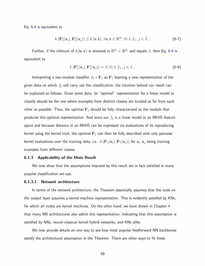
Eq. 6-4 is equivalent to

k (F⋆1(xi),F

⋆1(xj)) ≤ k (s, t) , ∀s, t ∈ Rd1 ,∀i ∈ I+, j ∈ I−. (6-7)

Further, if the infimum of k(u,v) is attained in Rd1 × Rd1 and equals β, then Eq. 6-4 is

equivalent to

k (F⋆1(xi),F

⋆1(xj)) = β, ∀i ∈ I+, j ∈ I−. (6-8)

Interpreting a two-module classifier f2 F1 as F1 learning a new representation of the

given data on which f2 will carry out the classification, the intuition behind our result can

be explained as follows. Given some data, its “optimal” representation for a linear model to

classify should be the one where examples from distinct classes are located as far from each

other as possible. Thus, the optimal F1 should be fully characterized as the module that

produces this optimal representation. And since our f2 is a linear model in an RKHS feature

space and because distance in an RKHS can be expressed via evaluations of its reproducing

kernel using the kernel trick, the optimal F1 can then be fully described with only pairwise

kernel evaluations over the training data, i.e., k (F1(xi),F1(xj)) for xi,xj being training

examples from different classes.

6.1.3 Applicability of the Main Result

We now show that the assumptions imposed by this result are in fact satisfied in many

popular classification set-ups.

6.1.3.1 Network architecture

In terms of the network architecture, the Theorem essentially assumes that the node on

the output layer assumes a kernel machine representation. This is evidently satisfied by KNs,

for which all nodes are kernel machines. On the other hand, we have shown in Chapter 4

that many NN architectures also admit this representation, indicating that this assumption is

satisfied by NNs, neural-classical kernel hybrid networks, and KNs alike.

We now provide details on one way to see how most popular feedforward NN backbones

satisfy the architectural assumption in the Theorem. There are other ways to fit these

59

backbones into a model formulation that works with the Theorem, but they may not

immediately yield an implementable modular training algorithm. For example, as we have

discussed in Chapter 4, some NN layers can be abstracted as kernel machines but with

trainable ϕ. These abstractions may satisfy the assumptions of the Theorem, but won’t work

with the modular training algorithm proposed in the next section, which requires ϕ to be a

fixed function.

Most feedforward NN structures, including the ResNet (He et al., 2016) and the VGG

(Simonyan & Zisserman, 2014), admit the following representation:

f = G2 G1, (6-9)

where G2 is the output linear layer: g2,j(·) = ⟨w2,j, ·⟩ + b2,j, and G1 can be a composition of

arbitrary layers ending with an elementwise nonlinearity ϕ. When the model uses a nonlinearity

on top of the output layer, one may absorb this nonlinearity into the objective function such

that the model would still assume the aforementioned representation. That this model satisfies

the condition on network architecture in the Theorem becomes evident after re-grouping the

modules. Specifically, write G1 = ϕ F1 for some F1, and, considering the binary classification

case with the model having a single output node, we can rewrite the model as

f = f2 F1,

f2(·) = ⟨w2,ϕ(·)⟩+ b2.

(6-10)

This formulation of the same model satisfies the requirement of the Theorem.

Note that the assumption that ∥ϕ(u)∥ is fixed for all u may require that one normalizes

the activation vector/matrix/tensor in practice.

6.1.3.2 Objective function

Theorem 6.1 works for objective functions of a specific form defined in Eq. 6-3. This

formulation is general enough to include many popular objective functions including softmax

+ cross-entropy, any monotonic nonlinearity + mean squared error, and hinge loss. Indeed,

60

the empirical risks of these objective functions can be decomposed into two terms with one

nondecreasing and the other nonincreasing such that the condition required by Theorem 6.1 is

satisfied. The details are provided below.

• softmax + cross-entropy (two-class version):

ℓ(f, S) =1

n

n∑i=1

−1i∈I+ ln (σ (f(xi)))− 1i∈I− ln (1− σ (f(xi))) (6-11)

=1

n

∑i∈I+

ln(e−f(xi) + 1

)+

1

n

∑j∈I−

ln(ef(xj) + 1

), (6-12)

where σ is the softmax nonlinearity.

• tanh + mean squared error (this decomposition works for any monotonic nonlinearitywith the value of yi adjusted for the range of the nonlinearity):

ℓ(f, S) =1

n

n∑i=1

(yi − δ (f(xi)))2 (6-13)

=1

n

∑i∈I+

(1− δ (f(xi)))2 +

1

n

∑j∈I−

(1 + δ (f(xj)))2 (6-14)

where δ is the hyperbolic tangent nonlinearity.

• hinge loss:

ℓ(f, S) =1

n

n∑i=1

max(0, 1− yif(xi)) (6-15)

=1

n

∑i∈I+

max(0, 1− f(xi)) +1

n

∑j∈I−

max(0, 1 + f(xj)). (6-16)

6.1.4 From Theory to Algorithm

The theoretical result can be used as the foundation of an actionable training algorithm.

As we have discussed early on in this Chapter, the missing piece linking our Theorem and

a concrete algorithm is a proxy objective function for training the hidden module. We now

present in details such an algorithm for classification with potentially more than two classes.

Assume without loss of generality that the model architecture is F = F2 F1, with each

node on the output layer as f2,j(·) = ⟨w2,j,ϕ(·)⟩ + b2,j. If ϕ does not satisfy ∥ϕ(u)∥ = α

61

for all u and some α > 0, normalize it by, e.g., dividing (elementwise) by its norm, such

that this condition is satisfied. Let an objective function L be given and suppose it (or its

two-class analog) satisfies the requirement of Theorem 6.1. Define kernel k(F1(·),F1(·)) =

⟨ϕ(F1(·)),ϕ(F1(·))⟩. Determine β := min k based on ϕ. Some examples include: β = 0 for

ReLU and sigmoid; β = −1 for tanh.

Given a batch of training data (xi, yi)ni=1 and let N (for negative) denote all pairs of

indices i, j such that yi = yj and P (for positive) denote all pairs of indices i = j with yi = yj.

Train F1 to maximize one of the following proxy objective functions.

• Alignment (negative only) (AL-NEO):

L1(F1) =β∑

(i,j)∈N k (F1(xi),F1(xj))

|β||N |1/2√∑

(i,j)∈N (k (F1(xi),F1(xj)))2; (6-17)

• Contrastive (negative only) (CTS-NEO):

L1(F1) = − 1

|N |∑

(i,j)∈N

exp (k (F1(xi),F1(xj))) ; (6-18)

• Negative Mean Squared Error (negative only) (NMSE-NEO):

L1(F1) = − 1

|N |∑

(i,j)∈N

(k (F1(xi),F1(xj))− β)2 . (6-19)

All of the above proxy objectives can be shown to learn an F1 that satisfies the optimality

condition required by Theorem 6.1.

Note that in cases where some of these proxies are undefined (for example, when β = 0),

we may train F1 to maximize the following alternative proxy objectives instead assuming

α := sup k is known, where we define k⋆ij to be α if (i, j) ∈ P or if i = j and β if otherwise.

Compared to the previous proxies, these are applicable to all k’s and impose a stronger

constraint on learning. Specifically, in addition to controlling the inter-class pairs, these proxies

force intra-class pairs to share representations.

62

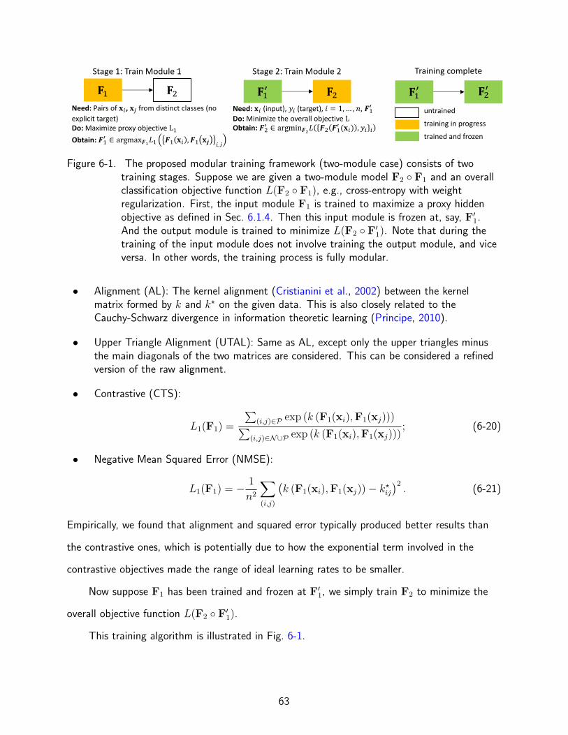
𝐅! 𝐅" 𝐅!# 𝐅"Need: Pairs of 𝐱!, 𝐱" from distinct classes (no explicit target)Do: Maximize proxy objective L#Obtain: 𝑭#$ ∈ argmax𝑭!𝐿# 𝑭# 𝐱! , 𝑭# 𝐱𝒋 !,"

training in progress

untrained

Stage 1: Train Module 1 Stage 2: Train Module 2 Training complete

trained and frozen

Need: 𝐱! (input), 𝑦! (target), 𝑖 = 1, … , 𝑛, 𝑭#$Do: Minimize the overall objective LObtain: 𝑭($ ∈ argmin𝑭"𝐿 𝑭( 𝑭#$ (𝐱!) , 𝑦! !

𝐅!# 𝐅"#

Figure 6-1. The proposed modular training framework (two-module case) consists of twotraining stages. Suppose we are given a two-module model F2 F1 and an overallclassification objective function L(F2 F1), e.g., cross-entropy with weightregularization. First, the input module F1 is trained to maximize a proxy hiddenobjective as defined in Sec. 6.1.4. Then this input module is frozen at, say, F′

1.And the output module is trained to minimize L(F2 F′

1). Note that during thetraining of the input module does not involve training the output module, and viceversa. In other words, the training process is fully modular.

• Alignment (AL): The kernel alignment (Cristianini et al., 2002) between the kernelmatrix formed by k and k⋆ on the given data. This is also closely related to theCauchy-Schwarz divergence in information theoretic learning (Principe, 2010).

• Upper Triangle Alignment (UTAL): Same as AL, except only the upper triangles minusthe main diagonals of the two matrices are considered. This can be considered a refinedversion of the raw alignment.

• Contrastive (CTS):

L1(F1) =

∑(i,j)∈P exp (k (F1(xi),F1(xj)))∑

(i,j)∈N∪P exp (k (F1(xi),F1(xj))); (6-20)

• Negative Mean Squared Error (NMSE):

L1(F1) = − 1

n2

∑(i,j)

(k (F1(xi),F1(xj))− k⋆

ij

)2. (6-21)

Empirically, we found that alignment and squared error typically produced better results than

the contrastive ones, which is potentially due to how the exponential term involved in the

contrastive objectives made the range of ideal learning rates to be smaller.

Now suppose F1 has been trained and frozen at F′1, we simply train F2 to minimize the

overall objective function L(F2 F′1).

This training algorithm is illustrated in Fig. 6-1.

63

6.1.4.1 Geometric interpretation of learning dynamics

The sufficient conditions described by Theorem 6.1 can be interpreted geometrically:

Under an F1 satisfying these conditions, images of examples from distinct classes are as distant

as possible in the RKHS induced by k. Intuitively, such a representation is the “easiest” for the

classification task. And our Theorem essentially justified this intuition in a rigorous fashion.

Therefore, the learning dynamics of this training algorithm on the latent module can

be given a straightforward geometric interpretation: It trains the latent module to push

apart examples from different classes in a feature space. When using the second set of

proxy objectives, the algorithm also squeezes together those examples within the same class.

Eventually, the output module works as a classifier on the final hidden representation in the

feature space.

6.1.4.2 Accelerating the approximated kernel network layers

When using the kernel trick to approximate some kernel machines in the network,

there is a natural method to accelerate the approximated kernel machines on non-input

layers and reduce the otherwise super-quadratic runtime: When using the second set of

proxy objectives, the hidden targets are sparse in the sense that for an ideal F1, we have

ϕ(F1(xp)) = ϕ(F1(xq)) for those xp,xq with yp = yq and ϕ(F1(xp)) = ϕ(F1(xq))

otherwise. Since for approximated kernel machines, we usually approximate w2,j using∑mp=1 α2,j,pϕ(F1(xp)) with some examples from the training set as the centers, retaining only

one example from each class would result in exactly the same hypothesis class for the model

f2,j because ∑m

p=1 α2,j,pϕ(F1(xp)) : α2,j,p = α+ϕ(F1(x+)) + α−ϕ(F1(x−)) : α−, α+ for

arbitrary x+,x− in the training set.

Thus, after training a given hidden module, depending on how well its objective function

has been maximized, one may discard some of the centers for kernel machines of the next

module to speed up the training of that module without sacrificing performance. This

trick also has a regularization effect on the kernel machines since the number of trainable

64

parameters of an approximated kernel machine grows linearly in the number of its centers and

fewer centers would therefore result in fewer parameters.

6.2 A Method for Module Reusability and Task Transferability Estimation

Among the many benefits of modular workflows, one that is of particular interest to

practitioners is improved module reusability. For example, in software engineering, standalone

components can be reused across the system, saving developers from re-implementations,

thanks to how the functionality of each component can be clearly defined without overlap or

significant dependence between modules. This degree of reliable module reusability, although

common in most practices of engineering, is sorely missed in deep learning workflows.

In this section, we demonstrate how our proposed modular training enables modular

workflows and subsequently a simple yet highly reliable module reusability estimation approach.

Formally, we consider the following problem: Assume that one is given a set of network bodies

pre-trained on some source tasks, i.e., tasks that we have already solved. Then consider a

target task, i.e., a task to be solved. If one were to pick a pre-trained network body, freeze it,

and then train a new network head on top of it to solve the target task, which pre-trained body

should one pick in order to maximize performance on the target task? We name this problem

module reusability estimation.

This practical problem is essentially equivalent to the theoretical problem of describing

task space structure among tasks. Specifically, given a set of tasks, we would like to

quantitative describe the relationships among them. And one popular notion of a task pair

relationship is that of task transferability, that is, how helpful the features useful for one source

task is to a target task. This theoretical issue that is central to many important research

domains including transfer learning, continual/lifelong learning, meta learning, and multi-task

learning (Zamir et al., 2018; Achille et al., 2019; Tran et al., 2019; Nguyen et al., 2020).

We propose a solution to module reusability estimation based on components from our

modular learning framework. Let a target task be characterized by the objective function

L(F2 F1, S), where L is an objective function satisfying the requirements in Theorem 6.1 and

65

S is some training data. And suppose we are given a set of pre-trained F1’s. This formulation

is standard in the task transferability literature (Tran et al., 2019). Our modular learning

framework suggests that we can measure the goodness of these pre-trained F1’s for this target

task by measuring L1(F1, S), where L1 can be any proxy objective defined in Sec. 6.1.4. This

is based on the fact that the F1 that maximizes the proxy objective L1(F1, S) constitutes

the input module of a minimizer for L(F2 F1, S), per Theorem 6.1. Therefore, one can

simply rank the pre-trained F1’s in terms of how well they maximize L1(F1, S) and select the

maximizer among the given.

How does this serve as a solution to the theoretical problem of describing task space

structure? Since a well-trained network body must encode key information for the source

task, this procedure can quantify how helpful knowledge on one source task is to a target

task via the lens of optimal model performance by fully training a network head to solve the

target task, thus fully describing the task space structure among the given tasks in terms of

transferability.

The main advantage of our proposed solution is that this procedure requires no training.

Indeed, one only needs to run the given modules on potentially a subset of S. And empirically,

we found that a small subset of target task training data is usually enough to give quality

estimate. Moreover, this method is task-agnostic in the sense that the method works regardless

of the tasks (datasets) at hand, without the need for modification.

In terms of the optimality of our transferability measure, if we define the true transferability

of a particular F1 to be minF2 E(x,y)L(F2 F1, (x, y)) (Tran et al., 2019), then minF2 L(F2

F1, S) is a bound on the true transferability minus a complexity measure on the model class

from which we choose our model (Bartlett & Mendelson, 2002).

Comparisons of our method against some notable related work are provided in Sec. 6.2

and summarized in Table 6-1, from which it is clear that our method is among the fastest and

most flexible.

Related Work: Model Reusability and Task Transferability

66

For practitioners in particular, a central issue in the current deep learning is that highly

performant models trained with significant resources might be immediately rendered useless

on a fresh dataset. Therefore, it is highly relevant to design reliable metrics with which one

can estimate the reusability of a model or certain modules within a model, thus shortening the

development cycle of deep learning pipelines.

From a theoretical standpoint, the issue of model reusability is essentially an issue of

quantitatively describing the task landscape among a few tasks of interest in terms of their

pairwise relationships, i.e., estimating to what extent representations or features learned from

one task might aid the learning of another. Also known as task transferability estimation,

this topic is central to many important, active research domains including transfer learning,

multi-task learning, meta learning, continual/lifelong learning, etc (Zamir et al., 2018; Achille

et al., 2019; Tran et al., 2019; Nguyen et al., 2020).

The task where the representations are learned is usually referred to as the source task.

From a model reusability perspective, this is the task where the model of interest was trained

on. On the other hand, the task for which we are interested in solving with the learned

representations is called the target task. Again, for model reusability, this is the task to which

we’d like to apply our pre-trained model.

Task transferability measures based on information-theoretical concepts have been

proposed. Early task-relatedness measures include the F -relatedness (Ben-David & Schuller,

2003) and the A-distance (Ben-David et al., 2007). And more recently, H-divergence (Ganin

et al., 2016) and Wasserstein distance (Li et al., 2018) are gaining increasing attention.

Specifically, (Liu et al., 2017) applied H-divergence in natural language processing for

text classification, and (Janati et al., 2018) used Wasserstein distance to estimate the

similarity of linear parameters instead of the data generation distributions. Along this

line of research, some more recent methods include H-score (Bao et al., 2019) and the

Bregman-correntropy conditional divergence (Yu et al., 2020), the latter of which used the

67

correntropy functional (Liu et al., 2007) and the Bregman matrix divergence (Kulis et al.,

2009) to quantify divergence between mappings.

Another direction in which some task transferability works follow is to extract relevant

knowledge about tasks from trained models. Compared to the earlier information-theoretic

measure-based methods, these model-based ones, as the name suggests, rely on the availability

of performant trained models. Below are some notable works following this line of research.

They are more related to our approach.

Assuming that identical data was used between two tasks, (Tran et al., 2019) estimated

task transferability via the negative conditional entropy between label sequences. No actual

trained model was used in the estimation, but the existence of an optimal trained source

model was assumed. Moreover, the source and the target task were both assumed to be

characterized, besides the data, by the cross-entropy loss. This assumption on identical training

data between tasks was removed by (Nguyen et al., 2020). (Nguyen et al., 2020) also assumes

that the cross-entropy loss is the loss used by both the source and the target task.

Compared to the earlier two methods, Taskonomy (Zamir et al., 2018) and Task2Vec (Achille

et al., 2019) more heavily rely on the performance of trained models to measure task

relatedness. And they both require actually training models on target tasks. Specifically,

in Taskonomy, transferability between a given task pair is quantified through the relative

transfer performance to a third target task using either as the source. Task2Vec, on the other

hand, exhaustively tunes a “probe” network on all target tasks and extracts task-characterizing

information from the learnable parameters of this network.

All of the existing model-based methods, including our own, make limiting assumption(s)

on the set-up. The main assumption of our method, required by our modular training

optimality guarantee, is that the output module (classifier) that will be tuned on top of

the transferred component admits a particular form as described earlier. Specifically, this

module is assumed to be a linear model in a (potentially nonlinear) feature space. This is

68

satisfied, of course, by a single-layer NN/KN, which is the commonly-assumed classifier head in

model reusability or task transferability estimation set-ups.

We summarize the properties of these related methods in Table 6-1.

Table 6-1. Comparisons with similar methods for task transferability estimation. For thetraining-free methods, we also provide the test runtime in terms of n, the size ofthe target task dataset that is being used for the estimation. Note that the extratrainings constitute the main overhead of the methods that require actual training,making comparisons on their test runtime against the training-free methodsmeaningless. Details are provided in Sec. 6.2.

Method Training Test Runtime Main AssumptionTASK2VEC (Achilleet al., 2019)

3 a reference model

Taskonomy (Zamiret al., 2018)

3 a third reference task

NCE (Tran et al.,2019)

7 O(n3) tasks share input

LEEP (Nguyen et al.,2020)

7 O(n2) cross-entropy loss

Ours 7 O(n2) form of classifier

69

CHAPTER 7MODULAR LEARNING: EXPERIMENTS

In this chapter, we present experimental results validating the efficacy of our proposed

architectures and, more importantly, the modular learning method. To begin with, we perform

two sanity checks showing that modular training results in identical learning dynamics as

end-to-end and also that our proposed proxy objectives align well with overall classification

accuracy. This confirms that our approach is as effective as end-to-end in terms of learning to

minimize the overall objective despite its modular nature.

We then evaluate our learning algorithm on simple network backbones. Two main sets

of comparisons are performed. First, we compare KNs using only classical kernels (Gaussian)

with NNs (can be viewed as KNs using NN-inspired kernels) to showcase how connectionism

enabled classical kernel method to achieve strong performance. Second, we compare MLPs

with end-to-end training and other greedily-pretrained architectures with our modular learning

algorithm applied to KNs with classical kernels. This is mainly to verify the effectiveness of our

modular algorithm. These experiments are performed on relatively less challenging datasets as

they mainly serve the purpose of providing some initial insights into the KN architecture as well

as the training algorithm.

In the next section, we evaluate our modular learning method on more complex NN

backbones and more challenging datasets. These are our main results. First, we present test

results on MNIST (LeCun et al., 1998) and CIFAR-10 (Krizhevsky et al., 2009). On both

MNIST and CIFAR-10, our modular approach compares favorably against end-to-end training

in terms of accuracy. We then discuss the label efficiency of our method. Recall that the

training of the latent module involves only pairs of examples from distinct classes with no

need for knowing the actual classes. This is a weaker form of supervision than knowing exactly

which class each example belongs to as required by backpropagation. Indeed, without caching

information over samples, sampling strict subsets (mini-batches) from the training set and

knowing only this pairwise relationship on pairs of examples in each subset is insufficient

70

for recovering the full labels of the training set. And we empirically show that the output

module, which requires full supervision in training, is highly label-efficient, achieving 94.88%

accuracy on CIFAR-10 with 10 randomly selected labeled examples (one from each class) using

a ResNet-18 (He et al., 2016) backbone (94.93% when using all 50000 labels). The fact that

our modular approach runs almost only on pairwise labels (weak supervision) yet still produces

performant models shows that our approach can leverage supervision more efficiently than

traditional end-to-end backpropagation using full labels on individual examples. Then, we

show that our proposed task transferability estimation method accurately describes the task

space structure on 15 binary classification tasks derived from CIFAR-10 using only a small

amount of labeled data, demonstrating a practical advantage of modular workflows. Finally,

we demonstrate that modular workflows enable fast network architecture search as another

example on their practical benefits. Using a proxy objective function from our modular learning

framework, the search for optimal network depth and widths can be done with high accuracy

in polynomial time (linear in network depth), contrasting how a naive approach would take

exponential runtime.

7.1 Sanity Checks

We first perform two sanity checks to verify that our learning method can indeed

effectively learn a deep architecture without between-module backpropagation.

7.1.1 Sanity Check: Modular Training Results in Identical Learning Dynamics AsEnd-to-End

In this section, we attempt to answer the important question: Do end-to-end and the

proposed modular training, when restricted to the architecturally identical hidden modules,

drive the underlying modules to functions that are identical in terms of minimizing the overall

loss function? Clearly, a positive answer would verify empirically the optimality of the modular

approach.

We now test this hypothesis with toy data. The set-up is as follows. We generate 1000

32-dimensional random input and assign them random labels from 10 classes. The underlying

71

network consists two modules. The input module is a (32 → 512) fully-connected (fc) layer

followed by ReLU nonlinearity and another (512 → 2) fc layer. The output module is a

(2 → 10) fc layer. The two modules are linked by a tanh nonlinearity (output normalized to

unit vector). The overall loss is the cross-entropy loss. And for modular training, the proxy

objective is CTS-NEO. We visualize the activations from the tanh nonlinearity as an indicator

of the behavior of the hidden layers under training.

From Fig. 7-1, we see that the underlying input modules are indeed driven to the same

functions (when restricted to the training data and in terms of minimizing the overall loss) by

both modular and end-to-end in the limit of training time going to infinity. This confirms the

optimality of our proposed method (albeit in a simplified set-up) and allows us to modularize

learning with confidence.

7.1.2 Sanity Check: Proxy Objectives Align Well With Accuracy

We now extend the verification of optimality from the simplified set-up in the previous

section to a more practical setting. Recall that we have characterized our proxy objective

as function of the input module whose maximizers constitute parts of the overall objective

minimizers and we have proposed to train the input module to maximize the proxy objective.

Ideally, however, a proxy objective for input module should satisfy: The overall accuracy

is a function of solely the proxy value and the output module and as a function of the proxy

value, the overall accuracy is strictly increasing. This type of results is reminiscent of the

“ideal bounds” for representation learning sought for in, e.g., (Arora et al., 2019c). We now

demonstrate empirically that the proxies we proposed enjoy this property.

The set-up is as follows. We train a LeNet-5 as two modules on MNIST with (conv1 →

tanh → max pool → conv2 → tanh → max pool → fc1 → tanh → fc2) as the input

module, and (tanh → fc3) as the output one. The input module is trained with a number

of different epochs so as to achieve different proxy values. And for each epoch, we freeze the

input module and train output module to minimize the overall cross-entropy until it converges.

Mathematically, suppose we froze input module at F′1 and we denote the proxy as L1 and

72

1 0 1x1

1.5

1.0

0.5

0.0

0.5

1.0

1.5x2

mdlr repr., epoch 200

1 0 1x1

1.5

1.0

0.5

0.0

0.5

1.0

1.5

x2

mdlr repr., epoch 5100

1 0 1x1

1.5

1.0

0.5

0.0

0.5

1.0

1.5

x2

mdlr repr., epoch 12600

1 0 1x1

1.5

1.0

0.5

0.0

0.5

1.0

1.5

x2

e2e repr., epoch 100

1 0 1x1

1.5

1.0

0.5

0.0

0.5

1.0

1.5x2

e2e repr., epoch 6100

1 0 1x1

1.5

1.0

0.5

0.0

0.5

1.0

1.5

x2

e2e repr., epoch 11300

Figure 7-1. Using toy data, we visualize the learning dynamics of our modular trainingapproach and that of backpropagation by visualizing the output representationsfrom the input module. We observe that the two methods result in input modulesthat are identical functions when restricted to the random training data, confirmingthat one may greedily optimize the input module using a proxy objective andobtain the same outcome as an end-to-end approach. e2e for end-to-end training.mdlr for modular training. Classes are color-coded.

overall accuracy as A, we are visualizing maxF2 A(F2 F′1) vs. L1(F

′1), where F2 is the output

module.

Fig. 7-2 shows that the overall accuracy, as a function of the proxy value, is indeed

approximately increasing. Further, this positive correlation becomes near perfect in high-accuracy

regime, which agrees with our theoretical results. To summarize, we have extended our

theoretical guarantees and empirically verified that maximizing the proposed proxy objectives

effectively learns input modules that are optimal in terms of maximizing the overall accuracy,

rendering end-to-end training unnecessary.

73

0.0 0.2 0.4 0.6 0.8 1.0proxy objective (normalized)

80.0

82.5

85.0

87.5

90.0

92.5

95.0

97.5

100.0

acc.

(%)

MNIST Accuracy vs. Proxy Objective

proxy name:nmse_neo

utal_neocts_neo

Figure 7-2. The overall accuracy, as a function of the proxy objective, is increasing. Thepositive correlation becomes near perfect in high-performance regime, validatingour theoretical results. Overall, this justifies the optimality of training the inputmodule to maximize the proxy objective. Note that the values of the illustratedproxies were normalized to [0, 1] in order for them to be properly visualized in thesame plot.

7.2 Modular Learning: Simple Network Backbones With Classical Kernels

These experiments were conducted with simple network backbones using classical kernels

(Gaussian) to provide initial insights into our KN architecture and the modular learning

approach. In particular, we show that connectionism helps classical kernel machines achieve

performance comparable to NNs, and that our modular learning, without bells and whistles,

compares favorably with end-to-end and end-to-end enhanced with various techniques.

7.2.1 Fully Layer-Wise kMLPs

We first demonstrate the competence of KNs and the effectiveness of the modular

learning method using simple networks (kMLPs) with classical kernels (Gaussian). The kMLPs

were trained fully layer-wise, using an extension of our two-module algorithm proposed earlier.

Here, the extension of this two-module method to networks with more than two modules was

74

obtained by analyzing pairs of modules at a time. Adam (Kingma & Ba, 2014) was used as

the underlying optimization algorithm. We then compare kMLPs trained with end-to-end

backpropagation against the same kMLPs trained with our modular algorithm to show the

effectiveness of the latter. We also compare kMLPs learned layer-wise with other popular deep

architectures including MLPs, deep belief networks (DBNs) (Hinton & Salakhutdinov, 2006)

and stacked autoencoders (SAEs) (Vincent et al., 2010), with the last two trained using a

combination of unsupervised greedy pre-training and standard backpropagation (Hinton et al.,

2006; Bengio et al., 2007). We also visualize the learning dynamics of modular kMLPs and

show that it is intuitive and simple to interpret.

In terms of the datasets used, rectangles, rectangles-image and convex are binary

classification datasets, mnist (50k test) and mnist (50k test) rotated are variants of MNIST.

mnist (50k test) contains 10000 training images, 2000 validation images, and 50000 test

images taken from the standard MNIST. mnist (50k test) rotated is the same as the fourth

except that the digits have been randomly rotated. fashion-mnist is the Fashion-MNIST

dataset (Xiao et al., 2017). These datasets all contain 28× 28 grayscale images. In rectangles,

rectangles-image, the model needs to learn if the height of the rectangle is longer than the

width, and in convex, if the white region is convex. Examples from these datasets are shown in

Fig 7-9. For detailed descriptions of these datasets, see (Larochelle et al., 2007).

The experimental set-up for the modular kMLPs is as follows. kMLP-1 corresponds to a

one-hidden-layer kMLP with the first layer consisting of 15 to 150 kernel machines using the

same Gaussian kernel and the second layer being a single or ten (depending on the number of

classes) kernel machines using another Gaussian kernel. In training, no preprocessing method

was used for all models. To ensure that the comparisons with other models are fair, we

used the regularized (two-norm regularization on weights) cross-entropy loss as the objective

function for the output layer of all models. The hidden proxy objective used for modular

kMLPs was AL, NMSE, and NMSE with the squared error substituted by absolute error. On

convex, a two-hidden-layer kMLP achieved a test error rate of 19.36%, 18.53% and 21.70%

75

using AL, NMSE, and NMSE with absolute error as the hidden objectives, respectively. As

a baseline, our best two-hidden-layer MLP achieved an error rate of 23.28% on this dataset.

For all results that follow, we present the better result among the three. Hyperparameters

were selected using the validation set. The validation set was then used in final training only

for early-stopping based on validation error. For the standard MNIST and Fashion-MNIST,

the last 5000 training examples were held out as validation set. kMLP-1FAST is the same

kMLP for which we accelerated by randomly choosing a subset of the training set as centers

for the second layer after the first had been trained. The kMLP-2 and kMLP-2FAST are

the two-hidden-layer kMLPs, the second hidden layers of which contained 15 to 150 kernel

machines. Settings of all the kMLPs trained with backpropagation can be found in (Zhang

et al., 2017). Note that because it is extremely time/memory-consuming to train kMLP-2 with

backpropagation without any acceleration method, to make training possible, we could only

randomly use 10000 examples from the entire training set of 55000 examples as centers for the

kMLP-2 (e2e) from Table 7-1.

Figure 7-3. From left to right: example from rectangles, rectangles-image, convex, mnist (50ktest) and mnist (50k test) rotated.

We now test the layer-wise learning algorithm against end-to-end backpropagation using

the standard MNIST dataset (LeCun et al., 1998). Results from several MLPs were added

as benchmarks. These models were trained with Adam or RMSProp (Tieleman & Hinton,

2012) and extra training techniques such as dropout (Srivastava et al., 2014) and batch

normalization (BN) (Ioffe & Szegedy, 2015) were applied to boost performance. kMLPs

accelerated using the proposed method (kMLPFAST) were also tested, for which we randomly

discarded some centers of each non-input layer before its training. Two popular acceleration

methods for kernel machines were compared, including using a parametric representation

76

(kMLPPARAM), i.e., for each node in a kMLP, f(·) =∑m

p=1 αpk(·,wp), αp,wp learnable and m

a hyperparameter, and using random Fourier features (kMLPRFF) (Rahimi & Recht, 2008).

Table 7-1. Testing the proposed layer-wise algorithm and acceleration method on MNIST withkMLP backbone. The numbers following the model names indicate the number ofhidden layers used. mdlr stands for modular training, whereas e2e stands forend-to-end. All other models were trained with end-to-end backpropagation. ForkMLPFAST, we also include in parentheses the ratio between the number of trainingexamples randomly chosen as centers for the kernel machines on the layer and thesize of the training set. Apart from kMLP-2 (e2e), the backpropagation kMLPresults are from (Zhang et al., 2017). The entries correspond to test errors (%) and95% confidence intervals (%). Results with overlapping confidence intervals areconsidered equally good. Best results are marked in bold.MLP-1

(RMSProp+BN)MLP-1

(RMSProp+dropout)MLP-2

(RMSProp+BN)MLP-2

(RMSProp+dropout)

2.05 ± 0.28 1.77 ± 0.26 1.58 ± 0.24 1.67 ± 0.25

kMLP-1PARAM

(e2e)kMLP-1FAST

(mdlr)kMLP-2(e2e)

kMLP-2(mdlr)

1.88 ± 0.27 1.75 ± 0.26 (0.54) 3.66 ± 0.37 1.56 ± 0.24

Table 7-2. Table 7-1, continued.

kMLP-1(e2e)

kMLP-1(mdlr)

kMLP-1RFF

(e2e)

3.44 ± 0.36 1.77 ± 0.26 2.01 ± 0.28

kMLP-2RFF

(e2e)kMLP-2PARAM

(e2e)kMLP-2FAST

(mdlr)

1.92 ± 0.27 2.45 ± 0.30 1.47 ± 0.24 (1/0.19)

Results in Table 7-1 validate the effectiveness of the KN architecture and our modular

training algorithm. For both the single-hidden-layer and the two-hidden-layer kMLPs, the

layer-wise algorithm consistently outperformed backpropagation. The modular method is also

much faster than end-to-end. In fact, it is practically impossible to use backpropagation to

train kMLP with more than two hidden layers without any acceleration method due to the

computational complexity involved. Moreover, it is worth noting that the proposed acceleration

trick is clearly very effective despite its simplicity and even produced models outperforming the

original ones, which may be due to its regularization effect. This shows that kMLP together

77

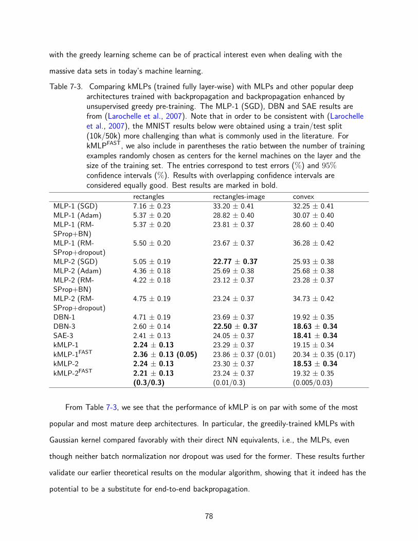
with the greedy learning scheme can be of practical interest even when dealing with the

massive data sets in today’s machine learning.

Table 7-3. Comparing kMLPs (trained fully layer-wise) with MLPs and other popular deeparchitectures trained with backpropagation and backpropagation enhanced byunsupervised greedy pre-training. The MLP-1 (SGD), DBN and SAE results arefrom (Larochelle et al., 2007). Note that in order to be consistent with (Larochelleet al., 2007), the MNIST results below were obtained using a train/test split(10k/50k) more challenging than what is commonly used in the literature. ForkMLPFAST, we also include in parentheses the ratio between the number of trainingexamples randomly chosen as centers for the kernel machines on the layer and thesize of the training set. The entries correspond to test errors (%) and 95%confidence intervals (%). Results with overlapping confidence intervals areconsidered equally good. Best results are marked in bold.

rectangles rectangles-image convex

MLP-1 (SGD) 7.16 ± 0.23 33.20 ± 0.41 32.25 ± 0.41MLP-1 (Adam) 5.37 ± 0.20 28.82 ± 0.40 30.07 ± 0.40MLP-1 (RM-SProp+BN)

5.37 ± 0.20 23.81 ± 0.37 28.60 ± 0.40

MLP-1 (RM-SProp+dropout)

5.50 ± 0.20 23.67 ± 0.37 36.28 ± 0.42

MLP-2 (SGD) 5.05 ± 0.19 22.77 ± 0.37 25.93 ± 0.38MLP-2 (Adam) 4.36 ± 0.18 25.69 ± 0.38 25.68 ± 0.38MLP-2 (RM-SProp+BN)

4.22 ± 0.18 23.12 ± 0.37 23.28 ± 0.37

MLP-2 (RM-SProp+dropout)

4.75 ± 0.19 23.24 ± 0.37 34.73 ± 0.42

DBN-1 4.71 ± 0.19 23.69 ± 0.37 19.92 ± 0.35DBN-3 2.60 ± 0.14 22.50 ± 0.37 18.63 ± 0.34SAE-3 2.41 ± 0.13 24.05 ± 0.37 18.41 ± 0.34kMLP-1 2.24 ± 0.13 23.29 ± 0.37 19.15 ± 0.34

kMLP-1FAST 2.36 ± 0.13 (0.05) 23.86 ± 0.37 (0.01) 20.34 ± 0.35 (0.17)kMLP-2 2.24 ± 0.13 23.30 ± 0.37 18.53 ± 0.34kMLP-2FAST 2.21 ± 0.13

(0.3/0.3)23.24 ± 0.37(0.01/0.3)

19.32 ± 0.35(0.005/0.03)

From Table 7-3, we see that the performance of kMLP is on par with some of the most

popular and most mature deep architectures. In particular, the greedily-trained kMLPs with

Gaussian kernel compared favorably with their direct NN equivalents, i.e., the MLPs, even

though neither batch normalization nor dropout was used for the former. These results further

validate our earlier theoretical results on the modular algorithm, showing that it indeed has the

potential to be a substitute for end-to-end backpropagation.

78

Table 7-4. Table 7-3, continued.

MNIST (50k test) MNIST (50k test) rotated Fashion-MNIST

4.69 ± 0.19 18.11 ± 0.34 15.47 ± 0.714.71 ± 0.19 18.64 ± 0.34 12.98 ± 0.664.57 ± 0.18 18.75 ± 0.34 14.55 ± 0.694.31 ± 0.18 14.96 ± 0.31 12.86 ± 0.665.17 ± 0.19 18.08 ± 0.34 12.94 ± 0.664.42 ± 0.18 17.22 ± 0.33 11.48 ± 0.623.57 ± 0.16 13.73 ± 0.30 11.51 ± 0.633.95 ± 0.17 13.57 ± 0.30 11.05 ± 0.613.94 ± 0.17 14.69 ± 0.31 N/A3.11 ± 0.15 10.30 ± 0.27 N/A3.46 ± 0.16 10.30 ± 0.27 N/A3.10 ± 0.15 11.09 ± 0.28 11.72 ± 0.632.95 ± 0.15 (0.1) 12.61 ± 0.29 (0.1) 11.45 ± 0.62 (0.28)3.16 ± 0.15 10.53 ± 0.27 11.23 ± 0.623.18 ± 0.15 (0.3/0.3) 10.94 ± 0.27 (0.1/0.7) 10.85 ± 0.61 (1/0.28)

(a) Examples from testset.

(b) Kernel matrix of thefirst hidden layer(epoch 25).

(c) Kernel matrix of thesecond hidden layer(epoch 0).

(d) Kernel matrix of thesecond hidden layer(epoch 15).

Figure 7-4. Visualizing the learning dynamics in a two-hidden-layer kMLP. Each entry in thekernel matrices corresponds to the inner product between the learnedrepresentations of two examples in the RKHS. The labels are given on the twoaxes. The examples used to produce this figure are provided in Fig. 7-4a in theorder of the labels plotted. The darker the entry, the more distant the learnedrepresentations are in the RKHS.

In Fig. 7-9, we visualize the learning dynamics within a two-hidden-layer kMLP learned

layer-wise. Since by construction of the Gaussian kernel, the image vectors are all of unit

norm in the RKHS, we can visualize the distance between two vectors by visualizing the value

of their inner product. In Fig. 7-4d, we can see that while the image vectors are distributed

randomly prior to training (see Fig. 7-4c), there is a clear pattern in their distribution after

training that reflects the dynamics of training: The layer-wise algorithm squeezes examples

79

from the same class closer together while pushes examples from different class farther apart

during training the latent layers. And it is easy to see that such a representation would

be simple to classify for the output layer. Fig. 7-4b and 7-4d suggest that this greedy,

layer-wise algorithm still learns “deep” representations: The higher-level representations

are more distinctive for different digits than the lower-level ones. Moreover, since learning

becomes increasingly simple for the upper layers as the representations become more and more

well-behaved, these layers are usually easy to set up and converge very fast during training.

7.2.2 The LeNet-5

We created and trained with our modular method a neural-classical kernel hybrid version

of the classic LeNet-5 (LeCun et al., 1998) and compare it with the original trained end-to-end.

The hidden representations learned from the two models are visualized. We show that the

hidden representations learned by the modular model are much more discriminative than those

from the original.

Specifically, we substitute the output layer of the classic LeNet-5 (LeCun et al., 1998)

architecture with kernel machines using Gaussian kernels, call this the kLeNet-5, and train it

using our modular algorithm with all the layers but the output layer as one module and the

output layer as a the other one. Since this experiment serves the purpose of providing more

insights into our learning algorithm instead of demonstrating state-of-the-art performance

(this is deferred to the next section), we use the original LeNet-5 without increasing the size

of any layer or the number of layers. ReLU (Glorot et al., 2011) and max pooling were used

as activations and pooling layers, respectively. Adam was used as the underlying optimizer for

both end-to-end and modular. The networks were trained and tested on the unpreprocessed

MNIST, Fashion-MNIST and CIFAR-10.

In Table 7-5, the results suggest that the hybrid model, trained with our modular method,

is on par with the NN counterpart trained end-to-end. We emphasize that the modular

framework does not help the network learn superior solutions compared to the traditional

end-to-end method. In that regard, it offers the same optimality guarantee as that provided

80

Table 7-5. Substituting the output layer of LeNet-5 with classical kernel machines usingGaussian kernels (kLeNet-5). This neural-classical kernel hybrid network was trainedin a modular fashion as two modules. The entries correspond to test errors (%) and95% confidence intervals (%). Results with overlapping confidence intervals areconsidered equally good. Best results are marked in bold.

MNIST Fashion-MNIST CIFAR-10LeNet-5 0.76 ± 0.17 9.34 ± 0.57 36.42 ± 0.94kLeNet-5 0.75 ± 0.17 8.67 ± 0.55 35.87 ± 0.94

Figure 7-5. Visualizing the data representation of the MNIST test set in the last hidden layerof kLeNet-5 (left) and LeNet-5 (right). Each color corresponds to a digit.Representations learned by kLeNet-5 are more discriminative for different digits.

by end-to-end backpropagation. The value of the modular learning framework is that it can

enables modular workflows, as we have argued earlier.

Fig. 7-5 provides more insights into the difference of kLeNet-5 and LeNet-5, in which

we plotted the activations of the last hidden layer of the two models after PCA dimension

reduction using the MNIST test set. In particular, we see that the representations in the

last hidden layer of kLetNet-5 are much more discriminative for different digits than those

in the corresponding layer of LeNet-5. Note that since the two models differed only in their

output layers, this observation suggests that the modular training algorithm together with

classical kernels such as Gaussian turns deep architectures into more efficient representation

learners, which may prove useful for computer vision tasks that build on convolutional features

(Gatys et al., 2015; Gardner et al., 2015). Further, it is conceivable that a greedily-trained,

81

neural-classical kernel hybrid models are more robust against perturbations on the pixels of the

test images than the original NN trained end-to-end. This feature may help the model defend

against adversarial examples, leading to more secure deep learning systems.

7.3 Modular Learning: State-of-the-Art Network Backbones With NN-InspiredKernels

These experiments were performed to demonstrate the efficacy of our modular learning on

state-of-the-art network backbones. The backbones we used in this section are all NNs, and

we did not modify their architectures by introducing classical kernels as we did in the previous

section.

7.3.1 Accuracy on MNIST and CIFAR-10

We now present the main results on MNIST and CIFAR-10 demonstrating the effectiveness

of our modular learning method. To facilitate fair comparisons, end-to-end and modular

training operate on the same backbone network. For all results, we used stochastic gradient

descent as the optimizer with batch size 128. For each module in the modular method as well

as the end-to-end baseline, we trained with annealing learning rates (0.1, 0.01, 0.001, each for

200 epochs). The momentum was set to 0.9 throughout. For data preprocessing, we used

simple mean subtraction followed by division by standard deviation. On CIFAR-10, we used the

standard data augmentation pipeline from (He et al., 2016), i.e., random flipping and clipping

with the exact parameters specified therein. In modular training, the models were trained as

two modules, with the output layer alone as the output module and everything else as the

input module as specified in Sec. 6.1.4. We normalized the activation vector right before the

output layer of each model to a unit vector such that the equal-norm condition required by

Theorem 6.1 is satisfied. We did not observe a significant performance difference after this

normalization.

From Table 7-6 and 7-7, we see that on three different backbone networks and both

MNIST and CIFAR-10, our modular learning compares favorably against end-to-end. Since

under two-module modular training, the ResNets can be viewed as kernel machines with

82

adaptive kernels (c.f. Sec. 5.2.4), we also compared performance with other NN-inspired kernel

methods in the literature. In Table 7-7, the ResNet kernel machines clearly outperformed other

kernel methods by a considerable margin.

Table 7-6. Accuracy on MNIST. e2e for end-to-end. mdlr for modular as two modules. Obj.Fn. specifies the overall objective function (and the proxy objective for the inputmodule, if applicable) used. XE stands for cross-entropy. Definitions of the proxyobjectives can be found in Sec. 6.1.4. Using LeNet-5 as the network backbone onMNIST, our modular approach compares favorably against end-to-end training.

Model Training Obj. Fn. Acc. (%)LeNet-5 (ReLU) e2e XE 99.33LeNet-5 (tanh) e2e XE 99.32LeNet-5 (ReLU) mdlr AL/XE 99.35LeNet-5 (ReLU) mdlr UTAL/XE 99.42LeNet-5 (ReLU) mdlr MSE/XE 99.36LeNet-5 (tanh) mdlr AL(-NEO)/XE 99.11 (99.19)LeNet-5 (tanh) mdlr UTAL(-NEO)/XE 99.21 (99.11)LeNet-5 (tanh) mdlr MSE(-NEO)/XE 99.27 (99.23)LeNet-5 (tanh) mdlr CTS(-NEO)/XE 99.16 (99.16)

7.3.2 Label Efficiency of Modular Deep Learning

In our proposed modular learning framework, the training of the latent modules requires

only implicit labels (weak supervision): Only pairs of training examples from distinct classes

are needed. And their specific class identities are not. On the other hand, training the output

module requires full labels. But we hypothesize that the number of full labels needed should be

much smaller than that needed for training the entire model with end-to-end backpropagation,

thus rendering the overall training pipeline more label efficient that an end-to-end pipeline.

Our reasoning is explained as follows. Intuitively, the input module in a deep architecture

can be understood as learning a new representation of the given data with which the output

module’s classification task is simplified. A simple way to quantify the difficulty of a learning

task is through its sample complexity, which, when put in simple terms, refers to the number of

labeled examples needed for a given model and a training algorithm to achieve a certain level

of test accuracy (Shalev-Shwartz & Ben-David, 2014).

83

Table 7-7. Accuracy on CIFAR-10. Modular training yielded favorable results compared toend-to-end. To the best of our knowledge, there is no other purely modular trainingmethod that matches backpropagation with a competitive network backbone onCIFAR-10 (Jaderberg et al., 2017; Lee et al., 2015b; Carreira-Perpinan & Wang,2014; Lowe et al., 2019; Duan et al., 2019). The ResNets trained with our modularapproach can be viewed as kernel machines and outperformed other existingNN-inspired kernel methods. ∗ means the method used more sophisticated datapreprocessing than the ResNets. Note that all of the baseline kernel methods havequadratic runtime and it is nontrivial to incorporate data augmentation into theirpipelines.

Model Data Aug. Training Obj. Fn. Acc. (%)ResNet-18 flip & clip e2e XE 94.91ResNet-152 flip & clip e2e XE 95.87ResNet-18 flip & clip mdlr AL/XE 94.93ResNet-152 flip & clip mdlr AL/XE 95.73CKN (Mairalet al., 2014)

none 82.18

CNTK (Li et al.,2019)

flip 81.40

CNTK∗ (Liet al., 2019)

flip 88.36

CNN-GP (Liet al., 2019)

flip 82.20

CNN-GP∗ (Liet al., 2019)

flip 88.92

NKWT∗ (Shankaret al., 2020)

flip 89.80

In a modular training setting, one can decouple the training of input and output modules

and then it would make sense to discuss the sample complexity of the two modules individually.

The output modules should require fewer labeled data examples to train since its task has been

simplified when the input one has been well-trained. We now observe that this is indeed the

case.

We trained ResNet-18 on CIFAR-10 with end-to-end and our modular approach. The

input module was trained with the full training set in the modular method, but again, this only

requires implicit pairwise labels. We now compare the need for fully-labeled data between the

two training methods.

84

0 1000 2000 3000fully-labeled sample size

20

40

60

80

100

acc.

(%)

CIFAR-10 Label Efficiency:Modular vs. End-to-End

0 20 40 6020

40

60

80

100

CIFAR-10 Label Efficiency:Modular vs. End-to-End

(Zoomed-In)

training:mdlr

mdlr (balanced)e2e

Figure 7-6. With the output module trained with only 30 randomly chosen fully-labeledexamples, the modular model still achieved 94.88% accuracy on CIFAR-10 (thesame model achieved 94.93% when using all 50000 labeled examples). When thetraining data has balanced classes (mdlr (balanced)), modular training onlyrequired 10 randomly chosen examples to achieve 94.88% accuracy — a singleexample per class. In contrast, the end-to-end model achieved 94.91%/21.22%when trained with 50000/50 labeled examples, respectively. Note that the inputmodule is trained with weak supervision in modular training: the module only seeswhether each pair of examples are from the same class or not. Overall, thisindicates that our learning approach utilizes supervisions more efficiently thantraditional end-to-end backpropagation with full labels on individual examples.

With the full training set of 50000 labeled examples, the modular and end-to-end model

achieved 94.93% and 94.91% test accuracy, respectively. From Fig. 7-6, we see that while the

end-to-end model struggled in the label-scarce regime, achieving barely over 20% accuracy

with 50 fully-labeled examples, the modular model consistently achieved strong performance,

achieving 94.88% accuracy with 30 randomly chosen fully-labeled examples for training. In

fact, if we ensure that there is at least one example from each class in the training data,

the modular approach needed as few as 10 randomly chosen examples to achieve 94.88%

accuracy, that is, a single randomly chosen example per class. The fact that the modular

model underperformed at 10 and 20 labels is likely caused by that there were some classes

85

missing in the training data that we randomly selected. Specifically, 4 classes were missing in

the 10-example training data, and 2 in the 20-example data.

These observations suggest that our modular training method for classification can almost

completely rely on implicit pairwise labels and still produce highly performant models, which

suggests new paradigms for obtaining labeled data that can potentially be less costly than the

existing ones. This also indicates that the current form of strong supervision, i.e., full labels on

individual data examples, relied on by existing end-to-end training, is not efficient enough. In

particular, we have shown that by leveraging pairwise information in the RKHS, implicit labels

in the form of whether pairs of examples are from the same class are just as informative. This

may have further implications for un/semi-supervised learning.

Connections With Un/Semi-Supervised Learning. Whenever the training batch size

is less than the size of the entire training set, we are using strictly less supervision than using

full labels. This is because if one does not cache information over batches, it is impossible to

recover the labels for the entire training set if one is only given pairwise relationships on each

batch. The fact that our learning method still produces equally performant models suggests

that we are using supervision more efficiently.

Existing semi-supervised methods also aim at utilizing supervision more efficiently. They

still rely on end-to-end training and use full labels, but achieve enhanced efficiency mostly

through data augmentation. While our results are not directly comparable to those from

existing methods (these methods do not work in the same setting as ours: They use fewer

full labels while we use mostly implicit labels), as a reference point, the state-of-the-art

semi-supervised algorithm achieves 88.61% accuracy on CIFAR-10 with 40 labels with a

stronger backbone network (Wide ResNet-28-2) and a significantly more complicated training

pipeline (Sohn et al., 2020).

Therefore, we think the insights gained from our modular learning suggest that (1) the

current form of supervision, i.e., full labels on individual data examples, although pervasively

used by supervised and semi-supervised learning paradigms, is far from efficient and (2) by

86

leveraging novel forms of labels and training methods, simpler yet stronger un/semi-supervised

learning paradigms exist.

7.3.3 Transferability Estimation With Proxy Objective

To empirically verify the effectiveness of our transferability estimation method, we created

a set of tasks by selecting 6 classes from CIFAR-10 and grouping each pair into a single binary

classification task. The classes selected are: cat, automobile, dog, horse, truck, deer. Each new

task is named by concatenating the first two letters from the classes involved, e.g., cado refers

to the task of classifying dogs from cats.

We trained one ResNet-18 using the proposed modular method for each source task,

using AL as the proxy objective. For each model, the output linear layer plus the nonlinearity

preceding it is the output module, and everything else belongs to the input module. All

networks achieved on average 98.7% test accuracy on the task they were trained on1 ,

suggesting that each frozen input module possesses information essential to the source task.

Therefore, the question of quantifying input module reusability is essentially the same as

describing the transferability between each pair of tasks.

The true transferability between a source and a target task in the task space can be

quantified by the test performance of the optimal output module trained for the target task

on top of a frozen input module from a source task (Tran et al., 2019). Our estimation of

transferability is based purely on proxy objective: A frozen input module achieving higher proxy

objective value on a target task means that the source and target are more transferable. This

estimation is performed using a randomly selected subset of the target task training data.

In Fig. 7-7, we visualize the target space structure with trdo being the source and the

target, respectively. Each task is assigned a distinct color and an angle in polar coordinate. A

task that is more transferable to trdo is plotted closer to the origin. We see from the figures

that our method accurately described the target space structure despite its simplicity, using

1 Highest accuracy was 99.95%, achieved on audo. Lowest was 93.05%, on cado.

87

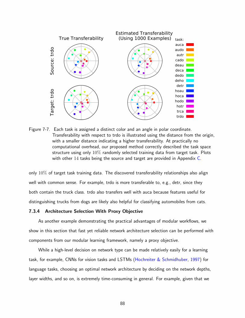
True Transferability

Sour

ce: t

rdo

Estimated Transferability (Using 1000 Examples)

Targ

et: t

rdo

task:aucaaudoautr

cadodeaudecadedodehodetr

hoauhocahodohotrtrcatrdo

Figure 7-7. Each task is assigned a distinct color and an angle in polar coordinate.Transferability with respect to trdo is illustrated using the distance from the origin,with a smaller distance indicating a higher transferability. At practically nocomputational overhead, our proposed method correctly described the task spacestructure using only 10% randomly selected training data from target task. Plotswith other 14 tasks being the source and target are provided in Appendix C.

only 10% of target task training data. The discovered transferability relationships also align

well with common sense. For example, trdo is more transferable to, e.g., detr, since they

both contain the truck class. trdo also transfers well with auca because features useful for

distinguishing trucks from dogs are likely also helpful for classifying automobiles from cats.

7.3.4 Architecture Selection With Proxy Objective

As another example demonstrating the practical advantages of modular workflows, we

show in this section that fast yet reliable network architecture selection can be performed with

components from our modular learning framework, namely a proxy objective.

While a high-level decision on network type can be made relatively easily for a learning

task, for example, CNNs for vision tasks and LSTMs (Hochreiter & Schmidhuber, 1997) for

language tasks, choosing an optimal network architecture by deciding on the network depths,

layer widths, and so on, is extremely time-consuming in general. For example, given that we

88

would like to use a MLP for a certain task, how many hidden layers should that MLP have and

how many nodes should there be on each hidden layer? One reliable solution is to exhaustively

train and test all possible architectures in a reasonable range of depths and widths. But even

if one assumes that the optimal learning hyperparameters such as step size can be efficiently

determined for each training session, this would still be a daunting task. For example, assume

that a single training session takes O(t) time2 , then if we were to search all architectures with

depth less than or equal to d and with the number of widths to be searched for each layer

less than or equal to w, the total time complexity would be O((wt)d) – an unacceptably large

number for any reasonable d.

In contrast, our modular learning enables a much more efficient search procedure with

polynomial time (linear in depth, to be exact). Indeed, if we were to greedily search over the

candidate widths at each depth by choosing the width that maximized the hidden proxy, then

the entire process is O(wtd) since we fix all upstream layers during the search at any particular

depth. The question, however, is whether this greedy search procedure is equally accurate

compared to the exhaustive one with exponential complexity above?

We now validate that our fast greedy search scheme is reliable with experiments. The

set-up is as follows. We trained MLPs on MNIST. Two architecture search spaces were

considered.

1. In the first search space, the network hidden layer number was fixed at 2 and for each

hidden layer, we searched over 13 different widths3 . This is to give a fine-grained

illustration on how well our strategy works for determining optimal layer widths. And we

keep the network shallow so that we can perform this fine-grained widths search using

the exhaustive baseline strategy in a reasonable time.

2 This can be refined by considering, e.g., that bigger networks typically take longer to train.

3 They are 2, 4, 8, 16, 32, 64, 128, 256, 512, 1024, 2048, 4096.

89

2. In the second search space, we varied the number of hidden layers in 1, 2, 3, 4, 5, and

each hidden layer width was allowed to vary in 4, 16, 64. This setting is to show how our

strategy can accurately determine a network architecture (depth and widths). Although,

the search in each layer width is not as fine-grained as in the first setting due to the

prohibitively high computational complexity of exhaustive search when the network is

deep.

In each setting, we exhaustively trained all possible network architectures with end-to-end

backpropagation to obtain the ground truth competence (test accuracy) of that architecture.

Then in the first setting, the true competence of each layer width is the maximum competence

among all architectures with the corresponding layer having this specific width. In the second

setting, the true competence of each network depth is the maximum competence among

all architectures with this specific depth. Each of such a competence estimation requires

exponential runtime (in network depth).

For our greedy fast search strategy, each hidden layer was searched greedily among

candidate widths. All upstream layers were held fixed at the optimal widths obtained via earlier

search sessions. These upstream layers were still trained together with the layer being searched

to give the module enough model capacity. In both settings, the estimated competence of a

layer width or network depth is how well a specific architecture maximized a proxy objective.

We used UTAL as the proxy objective throughout the experiments. After a search in a

particular layer was complete, we fixed this layer at the optimal width and continued to the

next layer. This process started from the input layer and proceeded to the output. Each

competence estimate using our method can be obtained in linear time (in network depth).

From Fig. 7-7 and 7-9, we can see that in both search settings, the predicted competence

using our greedy search scheme aligns well with the actual competence (test accuracy). The

advantage of the greedy scheme is its speed. Indeed, obtaining each predicted competence

took only linear time in network depth. But obtaining each true competence took exponential

time in depth. Even in setting 1, where the network was shallow, this means 12× longer due

90

101 102 103 104

hidden layer 1 width

0.0

0.2

0.4

0.6

0.8

1.0

101 102 103 104

hidden layer 2 width

relative accuracyrelative competence

MNIST Network Body: Predicted Competence vs. Actual Acc.

Figure 7-8. Network architecture search setting 1: Fine-grained search for optimal layerwidths. For each layer width, “accuracy” (ground truth competence) was obtainedas the optimal test accuracy among all models with the corresponding layer havingthis particular width. On the other hand, the estimated “competence” wasobtained with our greedy strategy, where we first searched the first hidden layerand chose the most competent width as the one that maximized the proxy, andthen kept it fixed to search the second hidden layer in the same manner. The“accuracy” and “competence” values were normalized to [0, 1] (the higher thebetter) so that they could be plotted on the same scale, and hence the name“relative”. Our greedy strategy can find near-optimal widths using 12× less timethan the exhaustive search used to find ground truth.

to that there were 12 candidate widths. To conclude, modular workflow enables fast and

reliable architecture selection schemes, which potentially has practical implications for research

fields such as neural architecture search and other deep learning applications in both the

academia and the industry. The same idea of course extends to searching for optimal network

nonlinearities and so on.

91

1 2 3 4 5# hidden layers

0.0

0.2

0.4

0.6

0.8

1.0

relative competencerelative accuracy

MNIST Network Body: Predicted Competence vs. Actual Acc.

Figure 7-9. Network architecture search setting 2: Search for optimal network depth. At eachnetwork depth, the “accuracy” (ground truth competence) was obtained as theoptimal test accuracy among all architectures with this particular depth. Threewidths were searched for each layer. For each depth, the search time is exponentialin network depth. The estimated “competence” values were obtained through agreedy procedure, where we searched and fixed the width of each layer sequentiallywith each layer fixed at the width that maximized the proxy. The competence of aspecific depth was how well the optimal architecture with this depth maximized theproxy, which can be determined in linear time in network depth. Our greedystrategy concluded that the optimal depth is 4 for this task, which agrees with theground truth. However, the greedy process took merely a couple of hours, whereasobtaining the ground truth via the exhaustive search took days on a Tesla V100GPU.

92

CHAPTER 8CONCLUSIONS

This work is one that is situated at the intersection of deep learning and kernel method,

using theoretical tools from kernel method to enrich our understanding on deep learning

approaches. We set out to address three open questions, all of which are of both theoretical

and practical importance.

We first combine connectionism, the “secret sauce” behind the success of deep learning

architectures, and classical kernel method, and propose a family of deep models that are based

on kernel machines. These so-called kernel networks are as expressive as neural networks,

but at the same time are more mathematically tractable thanks to the linear nature of kernel

machines. We compared kernel networks against both classical kernel machines and equivalent

neural networks and demonstrated strong performance.

We then reveal that kernel networks, as a model abstraction, subsumes neural networks.

This conclusion was established by taking a new perspective on the neural network layers.

In particular, we absorbed the ending nonlinearity of each node into a part of a beginning

nonlinearity of the immediate downstream nodes, enabling a novel kernel machine interpretation

on these neural network nodes. This newly established connection between deep learning and

kernel method is among the simplest and strongest in the literature, requiring no infinite

network width or random weights as many existing works do.

Finally, we addressed the important yet understudied problem of modular training of deep

architectures. In this regard, we put forward a framework that allows a deep architecture to be

trained in a purely module-by-module fashion. We proved its optimality for classification with

a wide range of objective functions under mild assumptions on the network architecture.

Our modular approach learns an overall solution that is as strong as that learned by

end-to-end backpropagation. On the other hand, our method makes it possible for users

to reliably modularize their workflows, enhancing the analyzability, module reusability, and user

friendliness of deep learning. We demonstrate strong performance from our modular learning

93

on state-of-the-art network backbones. We also showed that our training approach almost

solely relies on implicit, pairwise labels, making it more efficient than traditional end-to-end

training in terms of sample complexity. As a demonstration on how modular workflow can

significantly simplify deep learning applications, we proposed a simple module reusability

and task transferability estimation method based on components from our modular learning

framework and showed strong experimental results.

Overall, we believe that this work merely scratched the surface of the many topics that

it touched on. Some of these topics, such as modular learning, have significant practical

implications and are yet heavily understudied. We hope that our work can serve as a proof

of concept on the value of these research topics, and then draw more attention from the

community to them. And we also wish that our initial attempts at solving these problems can

inspire more and better solutions in the future.

94

APPENDIX APROOF OF PROPOSITION 4.2 & 4.3

Lemma 2. Suppose f1 ∈ F1, ..., fd ∈ Fd are elements from sets of real-valued functions de-

fined on Rp for some p ≥ 1, F ⊂ F1×· · ·×Fd is a subset of their direct sum. For f ∈ F, define

ω f : Rp × · · · × Rp × Rq → R : (x1, ...,xγ,y) 7→ ω(f1(x1), ..., fd(x1), f1(x2), ..., fd(xγ),y),

where x1, ...,xγ ∈ Rp,y ∈ Rq and ω : Rγ·d × Rq → R is bounded and L-Lipschitz for each

y ∈ Rq with respect to the Euclidean metric on Rγ·d. Let ω F = ω f : f ∈ F.

Define

Gn,j(Fi) = E

[supf∈Fi

1

n

n∑t=1

Ztf (Xt,j)

], i = 1, ..., d, j = 1, ..., γ, (A-1)

where Xt,j, t = 1, ..., n are i.i.d. random vectors defined on Rp. We have

Gn(ω F) ≤ 2Ld∑

i=1

γ∑j=1

Gn,j(Fi). (A-2)

In particular, if for all j, the Xt,j on which the Gaussian complexities of the Fi are

evaluated are sets of i.i.d. random vectors with the same distribution, we have G1n(Fi) = · · · =

Gγn(Fi) =: Gn(Fi) for all i and Eq. A-2 becomes

Gn(ω F) ≤ 2γLd∑

i=1

Gn(Fi). (A-3)

This Lemma is a generalization of a result on the Gaussian complexity of Lipschitz

functions on Rp from (Bartlett & Mendelson, 2002).

Proof. We prove the case where γ = 2. An extension to the general case is simple.

Let F be indexed by A. Without loss of generality, assume |A| < ∞. Define

Tα =n∑

t=1

ω (fα,1 (Xt) , ..., fα,d (X′t) ,Yt)Zt,

Vα = L

n∑t=1

d∑i=1

(fα,i (Xt)Zt,i + fα,i (X′t)Zn+t,i) ,

(A-4)

95

where α ∈ A, Xtnt=1, X′t

nt=1 are i.i.d. random samples on Rp × Rp, Ytnt=1 an i.i.d.

random sample on Rq, and Z1, ..., Zn, Z1,1, ..., Z2n,d are i.i.d. standard normal random

variables. The Xt’s, X′t’s, and the Yt’s are mutually independent.

Let arbitrary α, β ∈ A be give, and define ∥Tα−Tβ∥22 := EZ1,...,Zn(Tα−Tβ)2, ∥Vα−Vβ∥22 :=

EZ1,...,Zn(Vα − Vβ)2. We have

∥Tα − Tβ∥22 =n∑

t=1

(ω (fα,1 (Xt) , ..., fα,d (X′t) ,Yt)− ω (fβ,1 (Xt) , ..., fβ,d (X

′t) ,Yt))

2

≤ L2

n∑t=1

d∑i=1

((fα,i (Xt)− fβ,i (Xt))

2 + (fα,i (X′t)− fβ,i (X

′t))

2)

= ∥Vα − Vβ∥22.

(A-5)

By Slepian’s Lemma (Pisier, 1999),

nGn(ω F) = EZ1,...,Zn supα∈A

Tα

≤ 2EZ1,1,...,Z2n,dsupα∈A

Vα

≤ 2nLd∑

i=1

(Gn(Fi) + G ′

n(Fi)),

(A-6)

where Gn is computed on X1, ...,Xn and G ′n is computed on X′

1, ...,X′n.

Taking the expectation over X1, ...,Xn,X′1, ...,X

′n,Y1, ...,Yn proves the result.

Lemma 3. Given kernel k : Rd1 × Rd1 → R, let

F1 =(f1, ..., fd1) : u 7→ (f1(u), ..., fd1(u))

⊤ ,u ∈ Rd0∣∣∣f1, ..., fd1 ∈ Ω

, (A-7)

where Ω is a given set of real-valued functions on Rd0 . Also define

F =

h : u 7→

m∑ν=1

ανk (F(xν),F(u))∣∣∣∥α∥1 ≤ A, b ∈ R,F ∈ F1

, (A-8)

where α := (α1, ..., αm)⊤ and x1, ...,xm is a given set of examples. We have

Gn(F) ≤ 2ALd1Gn(Ω). (A-9)

96

Proof. First, note that the bias b does not change Gn(F).

Gn(F) = E supα,F

1

n

n∑t=1

m∑ν=1

ανk (F(xν),F(ut))Zt

≤ E∑

α,F,yν∈Rd1

1

n

n∑t=1

m∑ν=1

ανk (yν ,F(ut))Zt.

(A-10)

Suppose the supremum over the yν ’s is attained at Y1, ...,Ym, which are random vectors

since they are functions of the Zt’s.

Write

gν F(u) = k(F(u),Yν),

ω F(u,Y) =m∑

ν=1

ανgν F(u) =m∑

ν=1

ανk(F(u),Yν),(A-11)

where Y is the concatenation of all Yν ’s.

Then we have

Gn(F) ≤ E supα,F

1

n

n∑t=1

m∑ν=1

ανk (Yν ,F(ut))Zt

= E supα,F

1

n

n∑t=1

ω F(ut,Y)Zt

= Gn(ω F1).

(A-12)

We now prove a Lipschitz property for ω. For any ξ1, ξ2 ∈ Rd1 , we have

|ω(ξ1,Y)− ω(ξ2,Y)| =

∣∣∣∣∣m∑

ν=1

αν (gν(ξ1)− gν(ξ2))

∣∣∣∣∣≤

m∑ν=1

|αν | |gν(ξ1)− gν(ξ2)|

≤ Amaxν

|gν(ξ1)− gν(ξ2)|

= Amaxν

|k(ξ1,Yν)− k(ξ2,Yν)|

≤ Amaxν

LYν∥ξ1 − ξ2∥2

≤ AL∥ξ1 − ξ2∥2.

(A-13)

97

Therefore, ω F(u), as a function of F(u), is Lipschitz with respect to the Euclidean

metric on Rd1 with Lipschitz constant at most AL. It is easy to check that ω is bounded.

Now, the result follows from Lemma 2 with γ = 1.

Proof of Proposition 4.1. The result follows from recursively applying Lemma 3 to all layer

pairs.

Lemma 4. Given kernel k : Rd1 × Rd1 → R, let

F1 =(f1, ..., fd1) : u 7→ (f1(u), ..., fd1(u))

⊤ ,u ∈ Rd0∣∣∣f1, ..., fd1 ∈ Ω

, (A-14)

where Ω is a given set of real-valued functions on Rd0 . Also define

F =

h : u 7→

m∑ν=1

ανk (F(xν),F(u))∣∣∣∥α∥2 ≤ A, b ∈ R,F ∈ F1

, (A-15)

where α := (α1, ..., αm)⊤ and x1, ...,xm is a given set of examples. We have

Gn(F) ≤ 2m12ALd1Gn(Ω). (A-16)

Proof. The proof is the same as that of Lemma 3 except for Eq. A-13 (and subsequently the

bound on the Lipschitz constant of ω), which becomes

|ω(ξ1,Y)− ω(ξ2,Y)| =

∣∣∣∣∣m∑

ν=1

αν (gν(ξ1)− gν(ξ2))

∣∣∣∣∣≤ ∥α∥2

√√√√ m∑ν=1

(gν(ξ1)− gν(ξ2))2

≤ m12Amax

ν|gν(ξ1)− gν(ξ2)|

= m12Amax

ν|k(ξ1,Yν)− k(ξ2,Yν)|

≤ m12Amax

νLYν∥ξ1 − ξ2∥2

≤ m12AL∥ξ1 − ξ2∥2.

(A-17)

98

Proof of Proposition 4.2. The result follows from recursively applying Lemma 4 to all layer

pairs.

99

APPENDIX BPROOF OF THEOREM 6.1

Lemma 5. Given an inner product space H, a unit vector e ∈ H, and four other vectors

v+,v−,v⋆+, and v⋆

− with ∥v+∥H = ∥v−∥H = ∥v⋆+∥H = ∥v⋆

−∥H > 0, where the norm is the

canonical norm induced by the inner product, i.e., ∥u∥2H := ⟨u,u⟩H ,∀u ∈ H. Assume

∥v+ − v−∥H ≤ ∥v⋆+ − v⋆

−∥H . (B-1)

Then there exists a unit vector e⋆ ∈ H such that

⟨e,v+⟩H ≤ ⟨e⋆,v⋆+⟩H ; (B-2)

⟨e,v−⟩H ≥ ⟨e⋆,v⋆−⟩H . (B-3)

Proof. Throughout, we omit the subscript H on inner products and norms for brevity, which

shall cause no ambiguity since no other inner product or norm will be involved in this proof.

If v⋆+ = v⋆

−, then ∥v⋆+ − v⋆

−∥ = 0, which would imply

∥v+ − v−∥ = 0 ⇐⇒ v+ = v−. (B-4)

Then we may choose e⋆ such that ⟨e⋆,v⋆+⟩ = ⟨e,v+⟩ and the result holds trivially.

On the other hand, if v⋆+ = −v⋆

+, e⋆ = v⋆

+/∥v⋆+∥ would be a valid choice of e⋆. Indeed,

by Cauchy-Schwarz,

⟨e⋆,v⋆+⟩ = ∥v⋆

+∥ ≥ ⟨e,v+⟩; (B-5)

⟨e⋆,v⋆−⟩ = −∥v⋆

−∥ ≤ ⟨e,v−⟩. (B-6)

Therefore, we may assume that v⋆+ = ±v⋆

−.

For two vectors a,b, we define the “angle” between them, denoted θ ∈ [0, π], via

cos θ := ⟨a,b⟩/(∥a∥∥b∥). This angle is well-defined since cos is injective on [0, π].

Since

⟨a,b⟩ = −1

2∥a− b∥2 + 1

2∥a∥2 + 1

2∥b∥2,∀a,b, (B-7)

100

∥v+∥ = ∥v−∥ = ∥v⋆+∥ = ∥v⋆

−∥ > 0 and ∥v+ − v−∥ ≤ ∥v⋆+ − v⋆

−∥ together implies

⟨v+,v−⟩/(∥v+∥∥v−∥) ≥ ⟨v⋆+,v

⋆−⟩/(∥v⋆

+∥∥v⋆−∥), which then implies θ ≤ θ⋆ since cos is strictly

decreasing on [0, π], where θ is the angle between v+,v− and θ⋆ is the angle between v⋆+,v

⋆−.

Let γ+ be the angle between e,v+ and γ− that between e,v−. Note that γ−−γ+ ∈ [0, π].

Define

p := ⟨e,v+⟩ = ∥v+∥ cos γ+; (B-8)

n := ⟨e,v−⟩ = ∥v−∥ cos γ−. (B-9)

Now, suppose that we have shown

γ− − γ+ ≤ θ; (B-10)

∃e⋆ s.t. γ⋆− − γ⋆

+ = θ⋆ and γ⋆− = γ−, (B-11)

where γ⋆+ is the angle between e⋆,v⋆

+ and γ⋆− that between e⋆,v⋆

−. Define:

p⋆ := ⟨e⋆,v⋆+⟩ = ∥v⋆

+∥ cos γ⋆+; (B-12)

n⋆ := ⟨e⋆,v⋆−⟩ = ∥v⋆

−∥ cos γ⋆−. (B-13)

Then using ∥v−∥ = ∥v⋆−∥ > 0 and the earlier result that θ ≤ θ⋆, we would have

n = n⋆; (B-14)

γ+ ≥ γ⋆+, (B-15)

which, together with the fact that cos is strictly decreasing on [0, π] and the assumption that

∥v+∥ = ∥v⋆+∥ > 0, implies

n = n⋆; (B-16)

p ≤ p⋆, (B-17)

proving the result.

101

To prove Eq. B-10, it suffices to show cos(γ− − γ+) ≥ cos θ since cos is decreasing on

[0, π], to which both γ− − γ+ and θ belong. To this end, we have

cos(γ− − γ+) = cos γ− cos γ+ + sin γ− sin γ+ (B-18)

=pn

∥v+∥∥v−∥+

√(∥v+∥2 − p2)(∥v−∥2 − n2)

∥v+∥2∥v−∥2. (B-19)

Since ∥v+∥2 − p2 = ∥v+∥2 + p2 − 2p2 = ∥v+∥2 + p2 − 2p⟨e,v+⟩ = ∥v+ − pe∥2 and similarly

∥v−∥2 − n2 = ∥v− − ne∥2,

cos(γ− − γ+) =pn+ ∥v+ − pe∥∥v− − ne∥

∥v+∥∥v−∥(B-20)

≥ pn+ ⟨v+ − pe,v− − ne⟩∥v+∥∥v−∥

(B-21)

=⟨v+,v−⟩∥v+∥∥v−∥

(B-22)

= cos θ, (B-23)

where the inequality is due to Cauchy-Schwarz.

To prove B-11, it suffices to show that there exists e⋆ such that

A one of v⋆+ − p⋆e⋆,v⋆

− − n⋆e⋆ is a scalar multiple of the other;

B cos γ⋆− = cos γ−.

Indeed, A implies ∥v⋆+ − p⋆e⋆∥∥v⋆

− − n⋆e⋆∥ = ⟨v⋆+ − p⋆e⋆,v⋆

− − n⋆e⋆⟩, which, together

with similar arguments as we used to prove Eq. B-10, implies γ⋆− − γ⋆

+ = θ⋆. Also note that B

is equivalent to n = n⋆.

We prove existence constructively. Specifically, we set e⋆ = av⋆+ + bv⋆

−, a, b ∈ R and find

a, b such that e⋆ satisfies A and B simultaneously.

Let s = ⟨v⋆+,v

⋆−⟩, r = ∥v⋆

+∥2 = ∥v⋆−∥2. Note that we immediately have:

r > 0; |s| ≤ r. (B-24)

The assumption v⋆+ = ±v⋆

− implies |s| < r.

102

Since e⋆ is a unit vector, we have the following constraint on a, b:

a2r + b2r + 2abs = 1. (B-25)

And some simple algebra yields

p⋆ = ar + bs; (B-26)

n⋆ = as+ br. (B-27)

To identify those a, b such that A holds, we first rewrite v⋆+ − p⋆e⋆ and v⋆

− − n⋆e⋆ as

follows.

v⋆+ − p⋆e⋆ = v⋆

+ − (ar + bs)(av⋆+ + bv⋆

−) (B-28)

= (1− a2r − abs)v⋆+ + (−abr − b2s)v⋆

−. (B-29)

Similarly,

v⋆− − n⋆e⋆ = (−a2s− abr)v⋆

+ + (1− abs− b2r)v⋆−. (B-30)

Define

w1,+ := 1− a2r − abs; (B-31)

w1,− := −abr − b2s; (B-32)

w2,+ := −a2s− abr; (B-33)

w2,− := 1− abs− b2r. (B-34)

Then we have

v⋆+ − p⋆e⋆ = w1,+v

⋆+ + w1,−v

⋆−; (B-35)

v⋆− − n⋆e⋆ = w2,+v

⋆+ + w2,−v

⋆−. (B-36)

Assuming none of w1,+, w1,−, w2,+, w2,− is 0, A is equivalent to

w1,+w2,− = w1,−w2,+. (B-37)

103

To check that this is always true, we have

w1,+w2,− (B-38)

= a3brs+ ab3rs+ a2b2s2 + a2b2r2 − 2abs− r(a2 + b2) + 1 (B-39)

= a3brs+ ab3rs+ a2b2s2 + a2b2r2 (B-40)

because of Eq. B-25. And

w1,−w2,+ = a3brs+ ab3rs+ a2b2s2 + a2b2r2. (B-41)

Therefore, A is always true.

If at least one of w1,+, w1,−, w2,+, w2,− is 0, we have the following mutually exclusive

cases:

i one of the four coefficients is 0 while the other three are not; 7

ii w1,+ = w1,− = 0, the others are not 0; 3

iii w2,+ = w2,− = 0, the others are not 0; 3

iv w1,+ = w2,− = 0, the others are not 0; 7

v w1,− = w2,+ = 0, the others are not 0; 7

vi w1,+ = w2,+ = 0, the others are not 0; 3

vii w1,− = w2,− = 0, the others are not 0; 3

viii three of the four coefficients are 0 while one is not; 3

ix w1,+ = w1,− = w2,+ = w2,− = 0, 3

where the cases marked with 7 are the ones where A cannot be true (so our choice of a, b

cannot fall into these cases) and the ones marked with 3 are the ones where A is true. Note

that A cannot be true in cases iv and v because if A was true, it would imply that v⋆+ and

v⋆− are linearly dependent. However, since ∥v⋆

+∥ = ∥v⋆−∥, we would have either v⋆

+ = v⋆− or

v⋆+ = −v⋆

−, both of which have been excluded from the discussion in the beginning of this

proof.

Therefore, A is satisfied by any a, b that satisfy Eq. B-25 but none of case i, iv, and v.

104

We now turn to the search for a, b such that B holds. B is equivalent to

as+ br = n ⇐⇒ b =1

r(n− as). (B-42)

Therefore, finding a, b such that A and B hold simultaneously amounts to finding a, b such

that

b =1

r(n− as); (B-43)

a2r + b2r + 2abs = 1; (B-44)

none of case i, iv, v is true. (B-45)

Now, substituting b = (n− as)/r into Eq. B-44 and solving for a, we have

a2 =r − n2

r2 − s2, (B-46)

and we choose

a =

√r − n2

r2 − s2. (B-47)

This root is real since n = ⟨e,v−⟩ and therefore n2 = r cos2 γ− ≤ r.

To verify that

a =

√r − n2

r2 − s2, b =

1

r(n− as). (B-48)

satisfies B-45, first note that since this solution of a, b comes from solving n = n⋆ and

Eq. B-44, we have

w1,+ = 1− a(bs+ ar) = b(br + as) = bn; (B-49)

w1,− ∝ b(bs+ ar); (B-50)

w2,+ ∝ a(as+ br) = an; (B-51)

w2,− = 1− b(as+ br) = 1− bn. (B-52)

105

We now analyze each one of case i, iv, and v individually and show that our choice of a, b

does not fall into any of them, proving that this particular a, b satisfies Eq. B-43, B-44, and

condition B-45.

case i:

If w1,+ = 0, then either b = 0 or n = 0, resulting in w1,− ∝ b(bs + ar) = 0 or

w2,+ ∝ an = 0, i.e., there must be at least 2 coefficients being 0.

If w1,− = 0, then either b = 0, in which case w1,+ = 0, or bs + ar = 0. In the latter case,

we would then use Eq. B-44 and have

abs+ a2r = 0 =⇒ b2r + abs = 1 =⇒ b(br + as) = bn = 1

=⇒ w2,− = 1− bn = 0. (B-53)

Again, we would have at least 2 nonzero coefficients.

If w2,+ = 0, then either n = 0, which would result in w1,+ = bn = 0, or a = 0. Assuming

a = 0, Eq. B-48 would imply n = ±√r and b = n/r. Either way, we would have b = 1/n and

therefore w2,− = 1− bn = 0.

Finally, if w2,− = 0, then first assuming n = 0, we would have b = 1/n. Then Eq. B-48

would give 1/n = (n − as)/r. Solving for a, we have a = (n2 − r)/(ns). r ≥ n2 would imply

that a ≤ 0. On the other hand, Eq. B-48 also implied a ≥ 0. Hence, a must be 0, in which

case w2,+ ∝ an = 0. If n = 0, we would have w2,+ = 0 as well.

case iv:

It is easy to see that this case is impossible since w1,+ + w2,− = 1.

case v:

If w1,− = w2,+ = 0, then we have already shown in the proof of case i that either w1,+ or

w2,− must be 0, that is, at least 3 coefficients would be 0.

In summary, we have found an e⋆ such that A and B hold simultaneously, proving B-11.

106

Proof of Theorem 6.1. The result amounts to proving

L(f ⋆2 F⋆

1, S) ≤ L(f2 F1, S), ∀f2,F1. (B-54)

Define S+ to be the set of all xi such that i ∈ I+ and S− the set of all xj such that

j ∈ I−. Let κ = 1n

∑ni=1 1i∈I+, we have

L(f2 F⋆1, S)

≤ κℓ+(f2 F⋆

1(x⋆+))+ (1− κ)ℓ−

(f2 F⋆

1(x⋆−))

+ λg(∥w∥) (B-55)

= κℓ+

(⟨w

∥w∥,ϕ⋆

+

⟩∥w∥+ b

)(B-56)

+ (1− κ)ℓ−

(⟨w

∥w∥,ϕ⋆

−

⟩∥w∥+ b

)+ λg(∥w∥)

for some x⋆+,x

⋆− from S+, S−, respectively, where ϕ

⋆+ := ϕ

(F⋆

1(x⋆+))and ϕ⋆

− := ϕ(F⋆

1(x⋆−)).

For any f ′2 F′

1, let f′2 be parameterized by w′, b′. We have

L(f ′2 F′

1, S)

≥ κℓ+(f ′2 F′

1(x′+))+ (1− κ)ℓ−

(f ′2 F′

1(x′−))

+ λg(∥w′∥) (B-57)

= κℓ+

(⟨w′

∥w′∥,ϕ′

+

⟩∥w′∥+ b′

)(B-58)

+ (1− κ)ℓ−

(⟨w′

∥w′∥,ϕ′

−

⟩∥w′∥+ b′

)+ λg(∥w′∥)

for x′+,x

′− with x′

+ maximizing f ′2 F′

1(xi) over xi ∈ S+ and x′− minimizing f ′

2 F′1(xj) over

xj ∈ S−, where ϕ′+ := ϕ

(F′

1(x′+))and ϕ′

− := ϕ(F′

1(x′−)).

Using the assumption on F⋆1,

∥ϕ⋆+ − ϕ⋆

−∥ ≥ ∥ϕ′+ − ϕ′

−∥. (B-59)

107

Then using Lemma 5, there exists a unit vector e⋆ such that

⟨e⋆,ϕ⋆

+

⟩≥

⟨w′

∥w′∥,ϕ′

+

⟩; (B-60)

⟨e⋆,ϕ⋆

−⟩≤

⟨w′

∥w′∥,ϕ′

−

⟩. (B-61)

(B-62)

Let A := w : ∥w∥ = ∥w′∥, then evidently, e⋆∥w′∥ ∈ A, and we have,

L(f ′2 F′

1, S)

≥ κℓ+(⟨e⋆,ϕ⋆

+

⟩∥w′∥+ b′

)(B-63)

+ (1− κ)ℓ−(⟨e⋆,ϕ⋆

−⟩∥w′∥+ b′

)+ λg (∥w′∥)

= κℓ+

(⟨e⋆∥w′∥

∥e⋆∥w′∥∥,ϕ⋆

+

⟩∥e⋆∥w′∥∥+ b′

)(B-64)

+ (1− κ)ℓ−

(⟨e⋆∥w′∥∥e⋆∥w′∥∥

,ϕ⋆−

⟩∥e⋆∥w′∥∥+ b′

)+ λg (∥e⋆∥w′∥∥) (B-65)

≥ minw∈A

κℓ+

(⟨w

∥w∥,ϕ⋆

+

⟩∥w∥+ b′

)(B-66)

+ (1− κ)ℓ−

(⟨w

∥w∥,ϕ⋆

−

⟩∥w∥+ b′

)+ λg (∥w∥)

≥ minw∈A,b

κℓ+

(⟨w

∥w∥,ϕ⋆

+

⟩∥w∥+ b

)(B-67)

+ (1− κ)ℓ−

(⟨w

∥w∥,ϕ⋆

−

⟩∥w∥+ b

)+ λg (∥w∥)

≥ minw∈A,b

L(f2 F⋆1, S) (B-68)

≥ minw,b

L(f2 F⋆1, S) (B-69)

= L(f ⋆2 F⋆

1, S). (B-70)

This proves the result.

108

APPENDIX CADDITIONAL TRANSFERABILITY ESTIMATION PLOTS

109

True Transferability

Sour

ce: a

uca

Estimated Transferability (Using 1000 Examples)

Targ

et: a

uca

task:aucaaudoautr

cadodeaudecadedodehodetr

hoauhocahodohotrtrcatrdo

True Transferability

Sour

ce: a

udo

Estimated Transferability (Using 1000 Examples)

Targ

et: a

udo

task:aucaaudoautr

cadodeaudecadedodehodetr

hoauhocahodohotrtrcatrdo

True Transferability

Sour

ce: a

utr

Estimated Transferability (Using 1000 Examples)

Targ

et: a

utr

task:aucaaudoautr

cadodeaudecadedodehodetr

hoauhocahodohotrtrcatrdo

True Transferability

Sour

ce: c

ado

Estimated Transferability (Using 1000 Examples)

Targ

et: c

ado

task:aucaaudoautr

cadodeaudecadedodehodetr

hoauhocahodohotrtrcatrdo

True Transferability

Sour

ce: d

eau

Estimated Transferability (Using 1000 Examples)

Targ

et: d

eau

task:aucaaudoautr

cadodeaudecadedodehodetr

hoauhocahodohotrtrcatrdo

True Transferability

Sour

ce: d

eca

Estimated Transferability (Using 1000 Examples)

Targ

et: d

eca

task:aucaaudoautr

cadodeaudecadedodehodetr

hoauhocahodohotrtrcatrdo

True Transferability

Sour

ce: d

edo

Estimated Transferability (Using 1000 Examples)

Targ

et: d

edo

task:aucaaudoautr

cadodeaudecadedodehodetr

hoauhocahodohotrtrcatrdo

True Transferability

Sour

ce: d

eho

Estimated Transferability (Using 1000 Examples)

Targ

et: d

eho

task:aucaaudoautr

cadodeaudecadedodehodetr

hoauhocahodohotrtrcatrdo

Figure C-1. Additional figures with other tasks as the source/target task, supplementingFig. 7-7.

110

True Transferability

Sour

ce: d

etr

Estimated Transferability (Using 1000 Examples)

Targ

et: d

etr

task:aucaaudoautr

cadodeaudecadedodehodetr

hoauhocahodohotrtrcatrdo

True Transferability

Sour

ce: h

oau

Estimated Transferability (Using 1000 Examples)

Targ

et: h

oau

task:aucaaudoautr

cadodeaudecadedodehodetr

hoauhocahodohotrtrcatrdo

True Transferability

Sour

ce: h

oca

Estimated Transferability (Using 1000 Examples)

Targ

et: h

oca

task:aucaaudoautr

cadodeaudecadedodehodetr

hoauhocahodohotrtrcatrdo

True TransferabilitySo

urce

: hod

o

Estimated Transferability (Using 1000 Examples)

Targ

et: h

odo

task:aucaaudoautr

cadodeaudecadedodehodetr

hoauhocahodohotrtrcatrdo

True Transferability

Sour

ce: h

otr

Estimated Transferability (Using 1000 Examples)

Targ

et: h

otr

task:aucaaudoautr

cadodeaudecadedodehodetr

hoauhocahodohotrtrcatrdo

True Transferability

Sour

ce: t

rca

Estimated Transferability (Using 1000 Examples)

Targ

et: t

rca

task:aucaaudoautr

cadodeaudecadedodehodetr

hoauhocahodohotrtrcatrdo

Figure C-2. Additional figures with other tasks as the source/target task, supplementingFig. 7-7.

111

REFERENCES

Achille, A., Lam, M., Tewari, R., Ravichandran, A., Maji, S., Fowlkes, C. C., Soatto, S., &Perona, P. (2019). Task2vec: Task embedding for meta-learning. In Proceedings of the IEEEInternational Conference on Computer Vision, (pp. 6430–6439).

Aronszajn, N. (1950). Theory of reproducing kernels. Transactions of the American mathemat-ical society , 68(3), 337–404.

Arora, S., Du, S. S., Hu, W., Li, Z., Salakhutdinov, R. R., & Wang, R. (2019a). On exactcomputation with an infinitely wide neural net. In Advances in Neural Information ProcessingSystems, (pp. 8139–8148).

Arora, S., Du, S. S., Li, Z., Salakhutdinov, R., Wang, R., & Yu, D. (2019b). Harnessing thepower of infinitely wide deep nets on small-data tasks. arXiv preprint arXiv:1910.01663 .

Arora, S., Khandeparkar, H., Khodak, M., Plevrakis, O., & Saunshi, N. (2019c). A theoreticalanalysis of contrastive unsupervised representation learning. arXiv preprint arXiv:1902.09229 .

Balduzzi, D., Vanchinathan, H., & Buhmann, J. (2015). Kickback cuts backprop’s red-tape:biologically plausible credit assignment in neural networks. In Twenty-Ninth AAAI Confer-ence on Artificial Intelligence.

Bao, Y., Li, Y., Huang, S.-L., Zhang, L., Zheng, L., Zamir, A., & Guibas, L. (2019). Aninformation-theoretic approach to transferability in task transfer learning. In 2019 IEEEInternational Conference on Image Processing (ICIP), (pp. 2309–2313). IEEE.

Bartlett, P. L., & Mendelson, S. (2002). Rademacher and gaussian complexities: Risk boundsand structural results. Journal of Machine Learning Research, 3(Nov), 463–482.

Ben-David, S., Blitzer, J., Crammer, K., & Pereira, F. (2007). Analysis of representations fordomain adaptation. In Advances in neural information processing systems, (pp. 137–144).

Ben-David, S., & Schuller, R. (2003). Exploiting task relatedness for multiple task learning. InLearning Theory and Kernel Machines, (pp. 567–580). Springer.

Bengio, Y. (2014). How auto-encoders could provide credit assignment in deep networks viatarget propagation. arXiv preprint arXiv:1407.7906 .

Bengio, Y., Courville, A., & Vincent, P. (2013). Representation learning: A review and newperspectives. IEEE transactions on pattern analysis and machine intelligence, 35(8),1798–1828.

Bengio, Y., Lamblin, P., Popovici, D., & Larochelle, H. (2007). Greedy layer-wise training ofdeep networks. In Advances in neural information processing systems, (pp. 153–160).

Broomhead, D. S., & Lowe, D. (1988). Radial basis functions, multi-variable functionalinterpolation and adaptive networks. Tech. rep., Royal Signals and Radar EstablishmentMalvern (United Kingdom).

112

Buckner, C., & Garson, J. (2019). Connectionism. In E. N. Zalta (Ed.) The StanfordEncyclopedia of Philosophy . Metaphysics Research Lab, Stanford University, fall 2019 ed.

URL https://plato.stanford.edu/archives/fall2019/entries/connectionism/

Carreira-Perpinan, M., & Wang, W. (2014). Distributed optimization of deeply nested systems.In Artificial Intelligence and Statistics, (pp. 10–19).

Chen, K. (2015). Deep and modular neural networks. In Springer Handbook of ComputationalIntelligence, (pp. 473–494). Springer.

Cho, Y., & Saul, L. K. (2009). Kernel methods for deep learning. In Advances in neuralinformation processing systems, (pp. 342–350).

Cristianini, N., Shawe-Taylor, J., Elisseeff, A., & Kandola, J. S. (2002). On kernel-targetalignment. In Advances in neural information processing systems, (pp. 367–373).

Duan, S., Yu, S., Chen, Y., & Principe, J. C. (2019). On kernel method–based connectionistmodels and supervised deep learning without backpropagation. Neural computation, (pp.1–39).

Erdogmus, D., Fontenla-Romero, O., Principe, J. C., Alonso-Betanzos, A., & Castillo, E.(2005). Linear-least-squares initialization of multilayer perceptrons through backpropagationof the desired response. IEEE Transactions on Neural Networks, 16(2), 325–337.

Fahlman, S. E., & Lebiere, C. (1990). The cascade-correlation learning architecture. InAdvances in neural information processing systems, (pp. 524–532).

Freund, Y., Schapire, R., & Abe, N. (1999). A short introduction to boosting. Journal-Japanese Society For Artificial Intelligence, 14(771-780), 1612.

Ganin, Y., Ustinova, E., Ajakan, H., Germain, P., Larochelle, H., Laviolette, F., Marchand, M.,& Lempitsky, V. (2016). Domain-adversarial training of neural networks. The Journal ofMachine Learning Research, 17(1), 2096–2030.

Gardner, J. R., Upchurch, P., Kusner, M. J., Li, Y., Weinberger, K. Q., Bala, K., & Hopcroft,J. E. (2015). Deep manifold traversal: Changing labels with convolutional features. arXivpreprint arXiv:1511.06421 .

Gatys, L. A., Ecker, A. S., & Bethge, M. (2015). A neural algorithm of artistic style. arXivpreprint arXiv:1508.06576 .

Gehler, P. V., & Nowozin, S. (2008). Infinite kernel learning.

Glorot, X., Bordes, A., & Bengio, Y. (2011). Deep sparse rectifier neural networks. InProceedings of the fourteenth international conference on artificial intelligence and statistics,(pp. 315–323).

Gonen, M., & Alpaydın, E. (2011). Multiple kernel learning algorithms. Journal of machinelearning research, 12(Jul), 2211–2268.

113

Goodfellow, I., Pouget-Abadie, J., Mirza, M., Xu, B., Warde-Farley, D., Ozair, S., Courville,A., & Bengio, Y. (2014). Generative adversarial nets. In Advances in neural informationprocessing systems, (pp. 2672–2680).

He, K., Zhang, X., Ren, S., & Sun, J. (2016). Deep residual learning for image recognition.In Proceedings of the IEEE conference on computer vision and pattern recognition, (pp.770–778).

Hermans, M., & Schrauwen, B. (2012). Recurrent kernel machines: Computing with infiniteecho state networks. Neural Computation, 24(1), 104–133.

Hinton, G. E. (2007). Learning multiple layers of representation. Trends in cognitive sciences,11(10), 428–434.

Hinton, G. E., Osindero, S., & Teh, Y.-W. (2006). A fast learning algorithm for deep beliefnets. Neural computation, 18(7), 1527–1554.

Hinton, G. E., & Salakhutdinov, R. R. (2006). Reducing the dimensionality of data with neuralnetworks. science, 313(5786), 504–507.

Hochreiter, S., & Schmidhuber, J. (1997). Long short-term memory. Neural computation,9(8), 1735–1780.

Huang, F. J., & LeCun, Y. (2006). Large-scale learning with svm and convolutional for genericobject categorization. In 2006 IEEE Computer Society Conference on Computer Vision andPattern Recognition (CVPR’06), vol. 1, (pp. 284–291). IEEE.

Ioffe, S., & Szegedy, C. (2015). Batch normalization: Accelerating deep network training byreducing internal covariate shift. arXiv preprint arXiv:1502.03167 .

Jacobs, R. A., Jordan, M. I., Nowlan, S. J., & Hinton, G. E. (1991). Adaptive mixtures of localexperts. Neural computation, 3(1), 79–87.

Jacot, A., Gabriel, F., & Hongler, C. (2018). Neural tangent kernel: Convergence andgeneralization in neural networks. In Advances in neural information processing systems, (pp.8571–8580).

Jaderberg, M., Czarnecki, W. M., Osindero, S., Vinyals, O., Graves, A., Silver, D., &Kavukcuoglu, K. (2017). Decoupled neural interfaces using synthetic gradients. In Pro-ceedings of the 34th International Conference on Machine Learning-Volume 70 , (pp.1627–1635). JMLR. org.

Janati, H., Cuturi, M., & Gramfort, A. (2018). Wasserstein regularization for sparse multi-taskregression. arXiv preprint arXiv:1805.07833 .

Jordan, M. I. (1997). Serial order: A parallel distributed processing approach. In Advances inpsychology , vol. 121, (pp. 471–495). Elsevier.

114

Jordan, M. I., & Jacobs, R. A. (1994). Hierarchical mixtures of experts and the em algorithm.Neural computation, 6(2), 181–214.

Kingma, D. P., & Ba, J. (2014). Adam: A method for stochastic optimization. arXiv preprintarXiv:1412.6980 .

Kloft, M., Brefeld, U., Sonnenburg, S., & Zien, A. (2011). Lp-norm multiple kernel learning.The Journal of Machine Learning Research, 12 , 953–997.

Krizhevsky, A., Hinton, G., et al. (2009). Learning multiple layers of features from tiny images.

Krizhevsky, A., Sutskever, I., & Hinton, G. E. (2012). Imagenet classification with deepconvolutional neural networks. In P. L. Bartlett, F. C. N. Pereira, C. J. C. Burges, L. Bottou,& K. Q. Weinberger (Eds.) Advances in Neural Information Processing Systems 25: 26thAnnual Conference on Neural Information Processing Systems 2012. Proceedings of ameeting held December 3-6, 2012, Lake Tahoe, Nevada, United States, (pp. 1106–1114).

URL http://papers.nips.cc/paper/4824-imagenet-classification-with-deep-convolutional-neural-networks

Kulis, B., Sustik, M. A., & Dhillon, I. S. (2009). Low-rank kernel learning with bregman matrixdivergences. Journal of Machine Learning Research, 10(Feb), 341–376.

Lanckriet, G. R., Cristianini, N., Bartlett, P., Ghaoui, L. E., & Jordan, M. I. (2004). Learningthe kernel matrix with semidefinite programming. Journal of Machine learning research,5(Jan), 27–72.

Larochelle, H., Erhan, D., Courville, A., Bergstra, J., & Bengio, Y. (2007). An empiricalevaluation of deep architectures on problems with many factors of variation. In Proceedingsof the 24th international conference on Machine learning , (pp. 473–480).

LeCun, Y., Bottou, L., Bengio, Y., & Haffner, P. (1998). Gradient-based learning applied todocument recognition. Proceedings of the IEEE , 86(11), 2278–2324.

Lee, C.-Y., Xie, S., Gallagher, P., Zhang, Z., & Tu, Z. (2015a). Deeply-supervised nets. InArtificial intelligence and statistics, (pp. 562–570).

Lee, D.-H., Zhang, S., Fischer, A., & Bengio, Y. (2015b). Difference target propagation. InJoint european conference on machine learning and knowledge discovery in databases, (pp.498–515). Springer.

Lee, J., Bahri, Y., Novak, R., Schoenholz, S. S., Pennington, J., & Sohl-Dickstein, J. (2017).Deep neural networks as gaussian processes. arXiv preprint arXiv:1711.00165 .

Lee, J., Schoenholz, S. S., Pennington, J., Adlam, B., Xiao, L., Novak, R., & Sohl-Dickstein,J. (2020). Finite versus infinite neural networks: an empirical study. arXiv preprintarXiv:2007.15801 .

115

Li, Y., Carlson, D. E., et al. (2018). Extracting relationships by multi-domain matching. InAdvances in Neural Information Processing Systems, (pp. 6798–6809).

Li, Z., Wang, R., Yu, D., Du, S. S., Hu, W., Salakhutdinov, R., & Arora, S. (2019). Enhancedconvolutional neural tangent kernels. arXiv preprint arXiv:1911.00809 .

Liu, P., Qiu, X., & Huang, X. (2017). Adversarial multi-task learning for text classification.arXiv preprint arXiv:1704.05742 .

Liu, W., Pokharel, P. P., & Prıncipe, J. C. (2007). Correntropy: Properties and applications innon-gaussian signal processing. IEEE Transactions on Signal Processing , 55(11), 5286–5298.

Liu, W., Pokharel, P. P., & Principe, J. C. (2008). The kernel least-mean-square algorithm.IEEE Transactions on Signal Processing , 56(2), 543–554.

Liu, W., Principe, J. C., & Haykin, S. (2011). Kernel adaptive filtering: a comprehensiveintroduction, vol. 57. John Wiley & Sons.

Lowe, S., O’Connor, P., & Veeling, B. (2019). Putting an end to end-to-end: Gradient-isolatedlearning of representations. In Advances in Neural Information Processing Systems, (pp.3033–3045).

Mairal, J., Koniusz, P., Harchaoui, Z., & Schmid, C. (2014). Convolutional kernel networks. InAdvances in neural information processing systems, (pp. 2627–2635).

Micchelli, C. A., Xu, Y., & Zhang, H. (2006). Universal kernels. Journal of Machine LearningResearch, 7(Dec), 2651–2667.

Mohri, M., Rostamizadeh, A., & Talwalkar, A. (2018). Foundations of machine learning . MITpress.

Nair, V., & Hinton, G. E. (2010). Rectified linear units improve restricted boltzmann machines.In Proceedings of the 27th international conference on machine learning (ICML-10), (pp.807–814).

Neal, R. M. (1995). BAYESIAN LEARNING FOR NEURAL NETWORKS . Ph.D. thesis,University of Toronto.

Nguyen, C. V., Hassner, T., Archambeau, C., & Seeger, M. (2020). Leep: A new measure toevaluate transferability of learned representations. arXiv preprint arXiv:2002.12462 .

Park, J., & Sandberg, I. W. (1991). Universal approximation using radial-basis-functionnetworks. Neural computation, 3(2), 246–257.

Pisier, G. (1999). The volume of convex bodies and Banach space geometry , vol. 94.Cambridge University Press.

Principe, J. C. (2010). Information theoretic learning: Renyi’s entropy and kernel perspectives.Springer Science & Business Media.

116

Raghu, M., Gilmer, J., Yosinski, J., & Sohl-Dickstein, J. (2017). Svcca: Singular vectorcanonical correlation analysis for deep learning dynamics and interpretability. In Advances inNeural Information Processing Systems, (pp. 6076–6085).

Rahimi, A., & Recht, B. (2008). Random features for large-scale kernel machines. In Advancesin neural information processing systems, (pp. 1177–1184).

Rosenblatt, F. (1957). The perceptron, a perceiving and recognizing automaton Project Para.Cornell Aeronautical Laboratory.

Rumelhart, D. E., Hinton, G. E., & Williams, R. J. (1986). Learning representations byback-propagating errors. nature, 323(6088), 533–536.

Scholkopf, B., Herbrich, R., & Smola, A. J. (2001). A generalized representer theorem. InInternational conference on computational learning theory , (pp. 416–426). Springer.

Scholkopf, B., Smola, A., & Muller, K.-R. (1998). Nonlinear component analysis as a kerneleigenvalue problem. Neural computation, 10(5), 1299–1319.

Scholkopf, B., & Smola, A. J. (2001). Learning with kernels: support vector machines,regularization, optimization, and beyond . MIT press.

Shalev-Shwartz, S., & Ben-David, S. (2014). Understanding machine learning: From theory toalgorithms. Cambridge university press.

Shankar, V., Fang, A., Guo, W., Fridovich-Keil, S., Schmidt, L., Ragan-Kelley, J., & Recht, B.(2020). Neural kernels without tangents. arXiv preprint arXiv:2003.02237 .

Simonyan, K., & Zisserman, A. (2014). Very deep convolutional networks for large-scale imagerecognition. arXiv preprint arXiv:1409.1556 .

Sohn, K., Berthelot, D., Li, C.-L., Zhang, Z., Carlini, N., Cubuk, E. D., Kurakin, A., Zhang,H., & Raffel, C. (2020). Fixmatch: Simplifying semi-supervised learning with consistency andconfidence. arXiv preprint arXiv:2001.07685 .

Srivastava, N., Hinton, G., Krizhevsky, A., Sutskever, I., & Salakhutdinov, R. (2014). Dropout:a simple way to prevent neural networks from overfitting. The journal of machine learningresearch, 15(1), 1929–1958.

Sun, S., Chen, W., Wang, L., Liu, X., & Liu, T.-Y. (2015). On the depth of deep neuralnetworks: A theoretical view. arXiv preprint arXiv:1506.05232 .

Suykens, J. A. (2017). Deep restricted kernel machines using conjugate feature duality. Neuralcomputation, 29(8), 2123–2163.

Suykens, J. A., & Vandewalle, J. (1999). Training multilayer perceptron classifiers based on amodified support vector method. IEEE transactions on Neural Networks, 10(4), 907–911.

Synced (2018). LeCun vs Rahimi: Has Machine Learning Become Alchemy?

117

URL https://medium.com/@Synced/lecun-vs-rahimi-has-machine-learning-become-alchemy-21cb1557920d

Tang, Y. (2013). Deep learning using linear support vector machines. arXiv preprintarXiv:1306.0239 .

Tieleman, T., & Hinton, G. (2012). Lecture 6.5-rmsprop, coursera: Neural networks formachine learning. University of Toronto, Technical Report.

Tran, A. T., Nguyen, C. V., & Hassner, T. (2019). Transferability and hardness of supervisedclassification tasks. In Proceedings of the IEEE International Conference on ComputerVision, (pp. 1395–1405).

Vapnik, V. (2000a). The nature of statistical learning theory.

Vapnik, V., & Chervonenkis, A. Y. (1971). On the uniform convergence of relative frequenciesof events to their probabilities. Theory of Probability & Its Applications, 16(2), 264–280.

Vapnik, V. N. (2000b). The Nature of Statistical Learning Theory, Second Edition. Statisticsfor Engineering and Information Science. Springer.

Varma, M., & Babu, B. R. (2009). More generality in efficient multiple kernel learning.In Proceedings of the 26th Annual International Conference on Machine Learning , (pp.1065–1072).

Vincent, P., Larochelle, H., Lajoie, I., Bengio, Y., Manzagol, P.-A., & Bottou, L. (2010).Stacked denoising autoencoders: Learning useful representations in a deep network with alocal denoising criterion. Journal of machine learning research, 11(12).

Watanabe, C., Hiramatsu, K., & Kashino, K. (2018). Modular representation of layered neuralnetworks. Neural Networks, 97 , 62–73.

Williams, C. K., & Rasmussen, C. E. (2006). Gaussian processes for machine learning , vol. 2.MIT press Cambridge, MA.

Wilson, A. G., Hu, Z., Salakhutdinov, R., & Xing, E. P. (2016). Deep kernel learning. InArtificial intelligence and statistics, (pp. 370–378).

Xiao, H., Rasul, K., & Vollgraf, R. (2017). Fashion-mnist: a novel image dataset forbenchmarking machine learning algorithms. arXiv preprint arXiv:1708.07747 .

Xu, D., & Principe, J. C. (1999). Training mlps layer-by-layer with the information potential.In IJCNN’99. International Joint Conference on Neural Networks. Proceedings (Cat. No.99CH36339), vol. 3, (pp. 1716–1720). IEEE.

Xu, Z., Jin, R., King, I., & Lyu, M. (2009). An extended level method for efficient multiplekernel learning. In Advances in neural information processing systems, (pp. 1825–1832).

Yu, S., Shaker, A., Alesiani, F., & Principe, J. C. (2020). Measuring the discrepancy betweenconditional distributions: Methods, properties and applications.

118

Zamir, A. R., Sax, A., Shen, W., Guibas, L. J., Malik, J., & Savarese, S. (2018). Taskonomy:Disentangling task transfer learning. In Proceedings of the IEEE Conference on ComputerVision and Pattern Recognition, (pp. 3712–3722).

Zhang, S., Li, J., Xie, P., Zhang, Y., Shao, M., Zhou, H., & Yan, M. (2017). Stacked kernelnetwork. arXiv preprint arXiv:1711.09219 .

Zhou, Z.-H., & Feng, J. (2017). Deep forest. arXiv preprint arXiv:1702.08835 .

Zhuang, J., Tsang, I. W., & Hoi, S. C. (2011). Two-layer multiple kernel learning. InProceedings of the Fourteenth International Conference on Artificial Intelligence andStatistics, (pp. 909–917).

119

BIOGRAPHICAL SKETCH

Shiyu Duan received his B.S. in electronic engineering from Fudan University in 2016.

From 2016 to 2020, he worked at the Computational NeuroEngineering Laboratory in

University of Florida as a research assistant under the supervision of Dr. Jose C. Prıncipe.

He received his Ph.D. in electrical and computer engineering from University of Florida in 2020.

His research interests include machine learning theory and computer vision.

120