arX

iv:0

708.

0234

v1 [

mat

h.D

G]

1 A

ug 2

007

New Mexico Tech (July 2007)

to be published in the special volume ofSIGMA, Proceedings of the2007 Mid-west Geometry Conferencein Honor ofThomas P. Branson, Iowa City, IA, May18-20, 2007

Heat Kernel Asymptotics on Homogeneous Bundles

Ivan G. Avramidi

Department of MathematicsNew Mexico Institute of Mining and Technology

Socorro, NM 87801, USA

Dedicated to theMemory of Thomas P. Branson

Abstract

We consider Laplacians acting on sections of homogeneous vector bun-dles over symmetric spaces. By using an integral representation of the heatsemi-group we find a formal solution for the heat kernel diagonal that givesa generating function for the whole sequence of heat invariants. We arguethat the obtained formal solution correctly reproduces theexact heat kerneldiagonal after a suitable regularization and analytical continuation.

Keywords: Heat Kernel; Symmetric Spaces; Homogeneous Bundles2000 Mathematics Subject Classification: 58J35; 53C35

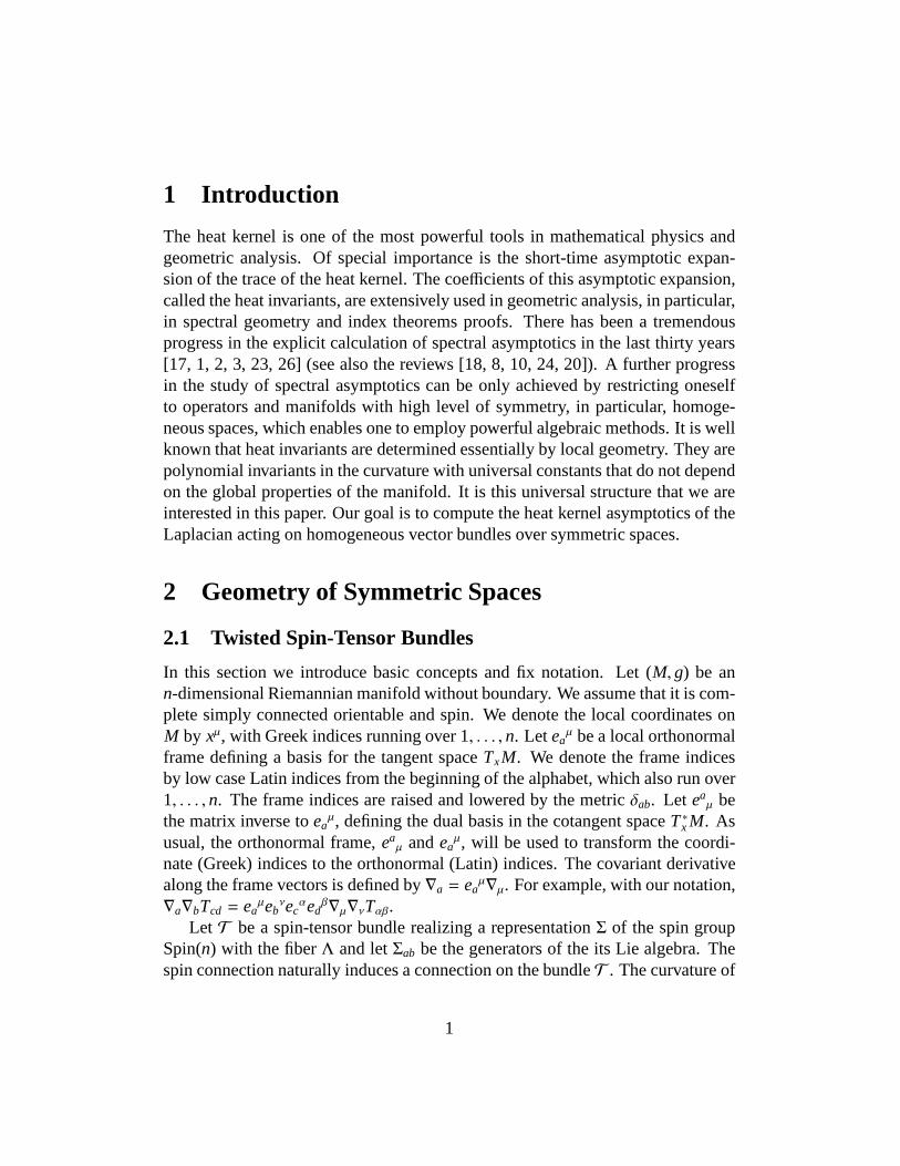
1 Introduction

The heat kernel is one of the most powerful tools in mathematical physics andgeometric analysis. Of special importance is the short-time asymptotic expan-sion of the trace of the heat kernel. The coefficients of this asymptotic expansion,called the heat invariants, are extensively used in geometric analysis, in particular,in spectral geometry and index theorems proofs. There has been a tremendousprogress in the explicit calculation of spectral asymptotics in the last thirty years[17, 1, 2, 3, 23, 26] (see also the reviews [18, 8, 10, 24, 20]).A further progressin the study of spectral asymptotics can be only achieved by restricting oneselfto operators and manifolds with high level of symmetry, in particular, homoge-neous spaces, which enables one to employ powerful algebraic methods. It is wellknown that heat invariants are determined essentially by local geometry. They arepolynomial invariants in the curvature with universal constants that do not dependon the global properties of the manifold. It is this universal structure that we areinterested in this paper. Our goal is to compute the heat kernel asymptotics of theLaplacian acting on homogeneous vector bundles over symmetric spaces.

2 Geometry of Symmetric Spaces

2.1 Twisted Spin-Tensor Bundles

In this section we introduce basic concepts and fix notation.Let (M, g) be ann-dimensional Riemannian manifold without boundary. We assume that it is com-plete simply connected orientable and spin. We denote the local coordinates onM by xµ, with Greek indices running over 1, . . . , n. Let ea

µ be a local orthonormalframe defining a basis for the tangent spaceTxM. We denote the frame indicesby low case Latin indices from the beginning of the alphabet,which also run over1, . . . , n. The frame indices are raised and lowered by the metricδab. Let ea

µ bethe matrix inverse toea

µ, defining the dual basis in the cotangent spaceT∗x M. Asusual, the orthonormal frame,ea

µ andeaµ, will be used to transform the coordi-

nate (Greek) indices to the orthonormal (Latin) indices. The covariant derivativealong the frame vectors is defined by∇a = ea

µ∇µ. For example, with our notation,∇a∇bTcd = ea

µebνec

αedβ∇µ∇νTαβ.

Let T be a spin-tensor bundle realizing a representationΣ of the spin groupSpin(n) with the fiberΛ and letΣab be the generators of the its Lie algebra. Thespin connection naturally induces a connection on the bundleT . The curvature of

1

this connection is12RabΣab, whereRab is the curvature 2-form of the spin connec-tion.

In the present paper we will further assume thatM is alocally symmetric spacewith a Riemannian metric with the parallel curvature, that is,∇µRαβγδ = 0, whichmeans, in particular, that the Riemann curvature tensor satisfies the integrabilityconstraints

Rf geaR

ebcd− Rf g

ebReacd+ Rf g

ecRedab− Rf g

edRecab = 0 . (2.1)

Let GYM be a compact Lie group (called a gauge group). It naturally definesthe principal fiber bundle over the manifoldM with the structure groupGYM. Weconsider a representation of the structure groupGYM and the associated vectorbundle through this representation with the same structuregroupGYM whose typ-ical fiber is ak-dimensional vector spaceW. Then for any spin-tensor bundleTwe define the twisted spin-tensor bundleV via the twisted product of the bundlesW andT . The fiber of the bundleV is V = Λ ⊗W so that the sections of thebundleV are represented locally byk-tuples of spin-tensors.

A connection on the bundleW (called Yang-Mills or gauge connection) takingvalues in the Lie algebraGYM of the gauge groupGYM naturally defines the totalconnection on the bundleV with the curvatureΩ = 1

2RabΣab⊗ IW+ IΛ ⊗F , whereF is the curvature of the Yang-Mills connection.

In the following we will considerhomogeneous vector bundleswith parallelbundle curvature, that is,∇µFαβ = 0 , which means that the curvature satisfies theintegrability constraints

[Fcd,Fab] − RfacdF f b − Rf

bcdFa f = 0 . (2.2)

2.2 Normal Coordinates

Let x′ be a fixed point inM andU be a sufficiently small coordinate patch con-taining the pointx′. Then every pointx inU can be connected with the pointx′ bya unique geodesic. We extend the local orthonormal frameea

µ(x′) at the pointx′

to a local orthonormal frameeaµ(x) at the pointx by parallel transport. Of course,

the frameeaµ depends on the fixed pointx′ as a parameter. Here and everywhere

below the coordinate indices of the tangent space at the point x′ are denoted byprimed Greek letters. They are raised and lowered by the metric tensorgµ′ν′(x′) atthe pointx′. The derivatives with respect tox′ will be denoted by primed Greekindices as well.

2

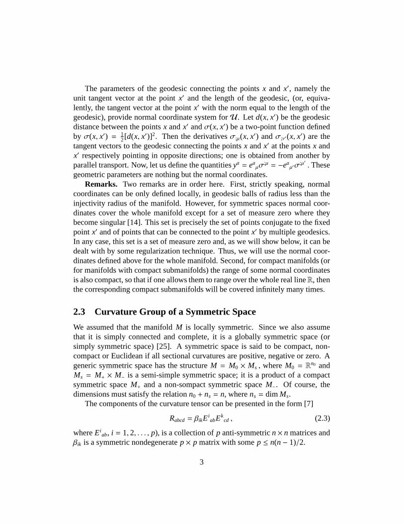
The parameters of the geodesic connecting the pointsx and x′, namely theunit tangent vector at the pointx′ and the length of the geodesic, (or, equiva-lently, the tangent vector at the pointx′ with the norm equal to the length of thegeodesic), provide normal coordinate system forU. Let d(x, x′) be the geodesicdistance between the pointsx andx′ andσ(x, x′) be a two-point function definedby σ(x, x′) = 1

2[d(x, x′)]2. Then the derivativesσ;µ(x, x′) andσ;ν′(x, x′) are thetangent vectors to the geodesic connecting the pointsx andx′ at the pointsx andx′ respectively pointing in opposite directions; one is obtained from another byparallel transport. Now, let us define the quantitiesya = ea

µσ;µ = −ea

µ′σ;µ′ . These

geometric parameters are nothing but the normal coordinates.Remarks. Two remarks are in order here. First, strictly speaking, normal

coordinates can be only defined locally, in geodesic balls ofradius less than theinjectivity radius of the manifold. However, for symmetricspaces normal coor-dinates cover the whole manifold except for a set of measure zero where theybecome singular [14]. This set is precisely the set of pointsconjugate to the fixedpoint x′ and of points that can be connected to the pointx′ by multiple geodesics.In any case, this set is a set of measure zero and, as we will show below, it can bedealt with by some regularization technique. Thus, we will use the normal coor-dinates defined above for the whole manifold. Second, for compact manifolds (orfor manifolds with compact submanifolds) the range of some normal coordinatesis also compact, so that if one allows them to range over the whole real lineR, thenthe corresponding compact submanifolds will be covered infinitely many times.

2.3 Curvature Group of a Symmetric Space

We assumed that the manifoldM is locally symmetric. Since we also assumethat it is simply connected and complete, it is a globally symmetric space (orsimply symmetric space) [25]. A symmetric space is said to becompact, non-compact or Euclidean if all sectional curvatures are positive, negative or zero. Ageneric symmetric space has the structureM = M0 × Ms , whereM0 = R

n0 andMs = M+ × M− is a semi-simple symmetric space; it is a product of a compactsymmetric spaceM+ and a non-sompact symmetric spaceM−. Of course, thedimensions must satisfy the relationn0 + ns = n, wherens = dim Ms.

The components of the curvature tensor can be presented in the form [7]

Rabcd = βikEiabE

kcd , (2.3)

whereEiab, i = 1, 2, . . . , p), is a collection ofp anti-symmetricn× n matrices and

βik is a symmetric nondegeneratep× p matrix with somep ≤ n(n− 1)/2.

3

In the following the Latin indices from the middle of the alphabet will be usedto denote such matrices; they run over 1, . . . , p and should not be confused withthe Latin indices from the beginning of the alphabet which denote tensors inM.They will be raised and lowered with the matrixβik and its inverse (βik).

Next, we define the tracelessn× n matricesDi = (Daib), where

Daib = −βikEk

cbδca . (2.4)

The matricesDi are known to be the generators of the holonomy algebra,H ,i.e. the Lie algebra of the restricted holonomy group,H,

[Di ,Dk] = F jikD j , (2.5)

whereF jik are the structure constants of the holonomy group. The structure con-

stants of the holonomy group define thep× p matricesFi, by (Fi) jk = F j

ik, whichgenerate the adjoint representation of the holonomy algebra,

[Fi , Fk] = F jikF j . (2.6)

For symmetric spaces the introduced quantities satisfy additional algebraicconstraints. The most important consequence of the eq. (2.1) is the equation [7]

EiacD

ckb − Ei

bcDcka = F i

k jEjab . (2.7)

Now, by using the eqs. (2.5) and (2.7) one can prove that the matrix βik satisfiesthe equation

βikFkjl + βlkFk

ji = 0 . (2.8)

Let hab be the projection to the subspaceTxMs of the tangent space of dimen-

sionns, that is, the tensorhab is nothing but the metric tensor on the semi-simplesubspaceTxMs. Since the curvature exists only in the semi-simple submanifoldMs, the components of the curvature tensorRabcd, as well as the tensorsEi

ab, arenon-zero only in the semi-simple subspaceTxMs. Let qa

b = δab − ha

b be theprojection tensor to the flat subspaceRn0. Then

Rabcdqa

e = Rabqa

e = Eiabq

ae = Da

ibqbe = Da

ibqae = 0 . (2.9)

Now, we introduce a new type of indices, the capital Latin indices,A, B,C, . . . ,which split according toA = (a, i) and run from 1 toN = p + n. We define newquantitiesCA

BC by

Ciab = Ei

ab, Caib = −Ca

bi = Daib, Ci

kl = F ikl , (2.10)

4

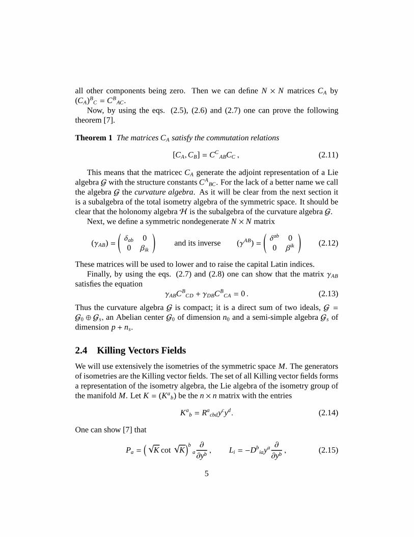
all other components being zero. Then we can defineN × N matricesCA by(CA)B

C = CBAC.

Now, by using the eqs. (2.5), (2.6) and (2.7) one can prove thefollowingtheorem [7].

Theorem 1 The matrices CA satisfy the commutation relations

[CA,CB] = CCABCC , (2.11)

This means that the matricecCA generate the adjoint representation of a LiealgebraG with the structure constantsCA

BC. For the lack of a better name we callthe algebraG the curvature algebra. As it will be clear from the next section itis a subalgebra of the total isometry algebra of the symmetric space. It should beclear that the holonomy algebraH is the subalgebra of the curvature algebraG.

Next, we define a symmetric nondegenerateN × N matrix

(γAB) =

(

δab 00 βik

)

and its inverse (γAB) =

(

δab 00 βik

)

(2.12)

These matrices will be used to lower and to raise the capital Latin indices.Finally, by using the eqs. (2.7) and (2.8) one can show that the matrixγAB

satisfies the equationγABC

BCD + γDBCB

CA = 0 . (2.13)

Thus the curvature algebraG is compact; it is a direct sum of two ideals,G =G0 ⊕ Gs, an Abelian centerG0 of dimensionn0 and a semi-simple algebraGs ofdimensionp+ ns.

2.4 Killing Vectors Fields

We will use extensively the isometries of the symmetric space M. The generatorsof isometries are the Killing vector fields. The set of all Killing vector fields formsa representation of the isometry algebra, the Lie algebra ofthe isometry group ofthe manifoldM. Let K = (Ka

b) be then× n matrix with the entries

Kab = Ra

cbdycyd. (2.14)

One can show [7] that

Pa =(√

K cot√

K)b

a∂

∂yb, Li = −Db

iaya ∂

∂yb, (2.15)

5

are Killing vector fields. In the following we will only need these Killing vectors.We introduce the following notation (ξA) = (Pa, Li).

Next, by using the explicit form of the Killing vector fields one can prove thefollowing theorem [7].

Theorem 2 The Killing vector fieldsξA satisfy the commutation relations

[ξA, ξB] = CCABξC . (2.16)

Notice that theydo notgenerate the complete isometry algebra of the sym-metric spaceM but rather they form a representation of the curvature algebraGintroduced in the previous section, which is a subalgebra ofthe total isometryalgebra. It is clear that the Killing vector fieldsLi form a representation of theholonomy algebraH , which is the isotropy algebra of the semi-simple subman-ifold Ms, and a subalgebra of the total isotropy algebra of the symmetric spaceM.

We list some properties of the Killing vector fields that willbe used below (fordetails, see [12])

γABξAµξB

ν = gµν , (2.17)

γABξAαξB

µ;νλ = Rα

λνµ , (2.18)

γABξAµξB

ν;β = 0 , (2.19)

ξcA;aξB

b;c − ξc

B;aξAb

;c = CCABξC

b;a − Rb

acdξAcξB

d , (2.20)

γABξAµ

;αξBν;β = Rµ

ανβ . (2.21)

2.5 Homogeneous Vector Bundles

Equation (2.2) imposes strong constraints on the curvatureof the homogeneousbundleW. We define

Bab = Fcdqcaq

db , Eab = Fcdh

cbh

db , (2.22)

so thatBabhac = 0 , andEabqa

c = 0 . Then, from eq. (2.2) we obtain

[Bab,Bcd] = [Bab,Ecd] = 0 , (2.23)

and[Ecd,Eab] − Rf

acdE f b − RfbcdEa f = 0 . (2.24)

6

This means thatBab takes values in an Abelian ideal of the gauge algebraGYM

andEab takes values in the holonomy algebra. More precisely, eq. (2.24) is onlypossible if the holonomy algebraH is an ideal of the gauge algebraGYM. Thus,the gauge groupGYM must have a subgroupZ × H, whereZ is an Abelian groupandH is the holonomy group.

The matricesDaib provide a natural embedding of the holonomy algebraH in

the orthogonal algebraSO(n) in the following sense. LetXab be the generatorsof the orthogonal algebraSO(n) is some representation. LetTi be the matricesdefined by

Ti = −12

DaibXb

a . (2.25)

Then one can show that they satisfy the commutation relations

[Ti ,Tk] = F jikT j . (2.26)

ThusTi are the generators of the gauge algebraGYM realizing a representationTof the holonomy algebraH . SinceBab takes values in the Abelian ideal of thealgebra of the gauge group we also have

[Bab,T j] = 0 . (2.27)

Then by using eq. (2.7) one can show that1

Eab =12

RcdabXcd = −Ei

abTi . (2.28)

and

Fab = −EiabTi + Bab =

12

RcdabXcd + Bab . (2.29)

Now, we consider the representationΣ of the orthogonal algebra defining thespin-tensor bundleT and define the matrices

Gab = Σab⊗ IX + IΣ ⊗ Xab . (2.30)

Obviously, these matrices are the generators of the orthogonal algebra in the prod-uct representationΣ ⊗ X. Next, the matrices

Qi = −12

DaibΣ

ba (2.31)

1We correct here a sign misprint in eq. (3.24) in [7].

7

form a representationQ of the holonomy algebraH , and the matrices

Ri = Qi ⊗ IT + IΣ ⊗ Ti = −12

DaibGb

a (2.32)

are the generators of the holonomy algebra in the product representationR =Q⊗ T. Then the total curvature of a twisted spin-tensor bundleV is

Ωab = −EiabRi + Bab =

12

RcdabGcd + Bab . (2.33)

2.6 Twisted Lie Derivatives

Let ϕ be a section of a twisted homogeneous spin-tensor bundleT . Let ξA be thebasis of Killing vector fields. Then the covariant (or generalized, or twisted) Liederivative ofϕ alongξA is defined by

LAϕ = LξAϕ =(

∇ξA + SA

)

ϕ , (2.34)

where∇ξA = ξAµ∇µ, andSA =

12ξA

a;bGb

a . Note thatSaqab = 0 .

Proposition 1 There hold

[∇ξA,∇ξB]ϕ =(

CCAB∇ξC − RAB+ BAB

)

ϕ , (2.35)

∇ξASB = RAB , (2.36)

[SA,SB] = CCABSC − RAB , (2.37)

where

RAB = ξAaξB

bEiabRi = −

12

RcdabξA

aξBbGcd , (2.38)

BAB = ξAaξB

bBab . (2.39)

Proof. By using the properties of the Killing vectors described in the previoussection and the eq. (2.33) we obtain first (2.35). Next, we obtain (2.36), and,further, by using the eq. (2.20) we get (2.37).

We define the operatorL2 = γABLALB . (2.40)

8

Theorem 3 The operatorsLA andL2 satisfy the commutation relations

[LA,LB] = CCABLC + BAB, (2.41)

[LA,L2] = 2γBCBABLC . (2.42)

Proof. This follows from

[LA,LB] = [∇ξA,∇ξB] + [∇ξA,SB] − [∇ξB,SA] + [SA,SB] (2.43)

and eqs. (2.35), (2.36), and (2.37). The eq. (2.42) follows directly from (2.41).The operatorsLA form an algebra that is a direct sum of a nilpotent ideal and

a semisimple algebra. For the lack of a better name we call this algebragaugedcurvature algebraand denote it byGgauge.

Now, by using the eqs. (2.19), (2.36) and (2.18) one can provethat

γABξAµSB = 0 , γAB∇ξASB = 0 , γABSASB = R2 . (2.44)

We define the Casimir operator

R2 = βi jRiR j =14

RabcdGabGcd . (2.45)

Theorem 4 The Laplacian∆ acting on sections of a twisted spin-tensor bundleV over a symmetric space has the form

∆ = L2 − R2 . (2.46)

Therefore,[LA,∆] = 2γBCBABLC . (2.47)

Proof. We have

γABLALB = γAB∇ξA∇ξB + γ

ABSA∇ξB + γAB∇ξASB + γ

ABSASB . (2.48)

Now, by using eqs. (2.17) and (2.19) we get

γAB∇ξA∇ξB = ∆ . (2.49)

Next, by using the eqs. (2.36) and (2.44) we obtain (2.46). The eq. (2.47) followsfrom the commutation relations (2.41).

9

2.7 Isometries and Pullbacks

Letωi be the canonical coordinates on the holonomy group and (kA) = (pa, ωi) bethe canonical coordinates on the gauged curvature group. Let ξ = 〈k, ξ〉 = kAξA =

paPa + ωiLi be a Killing vector field and letψt : M → M be the one-parameter

diffeomorphism (the isometry) generated by the vector fieldξ. Let x = ψt(x), sothat dx

dt = ξ(x) and x|t=0 = x . The solution of this equation ˆx = x(t, p, ω, x, x′) .depends on the parameterst, p, ω, x and x′. We will be interested mainly in thecase when the pointsx and x′ are close to each other. In fact, at the end of ourcalculations we will take the limitx = x′.

Now, we choose the normal coordinatesya of the point defined above andthe normal coordinates ˆya of the pointx with the origin atx′, so that the normalcoordinatesy′ of the pointx′ are equal to zero. Recall that the normal coordinatesare equal to the components of the tangent vector at the pointx′ to the geodesicconnecting the pointsx′ and the current point, that is,ya = −ea

µ′(x′)σ;µ′(x, x′)andya = −ea

µ′(x′)σ;µ′(x, x′). Then by taking into account the explicit form of theKilling vectors given by eq. (2.15) we have

dya

dt=

( √

K(y) cot√

K(y))a

bpb − ωiDa

ibyb , (2.50)

with the initial conditionya|t=0 = ya . The solution of this equation defines a func-tion y = y(t, p, ω, y).

We define the matrixD(ω) = ωiDi . (2.51)

Proposition 2 The Taylor expansion of the functiony = y(t, p, ω, y) in p and yreads

ya =(

exp[−tD(ω)])a

byb +

(

1− exp[−tD(ω)]D(ω)

)a

bpb +O(y2, p2, py) . (2.52)

There holds

det

(

∂ya

∂pb

)∣

∣

∣

∣

∣

∣

p=y=0,t=1

= detT M

(

sinh[D(ω)/2]D(ω)/2

)

. (2.53)

Proof. First, for p = 0 from eq. (2.50) we obtain ˆy(t, 0, ω, 0) = 0 . Next, bydifferentiating the eq. (2.50) with respect toyb and settingp = y = 0 we obtain

∂ya

∂yb

∣

∣

∣

∣

∣

∣

p=y=0

=(

exp[−tD(ω)])a

b . (2.54)

10

Further, by differentiating the eq. (2.50) with respect topb and settingp = 0,

we obtain a differential equation for the matrix∂ya

∂pb

∣

∣

∣

∣

p=y=0whose solution is

(

∂ya

∂pb

)

∣

∣

∣

∣

p=y=0=

1− exp[−tD(ω)]D(ω)

. (2.55)

By using the obtained results we get the desired formula (2.52). Finally, by takinginto account that the matrixD(ω) is traceless, by using eq. (2.55) we obtain (2.53).

The functiony = y(t, p, ω, y) implicitly defines the functionp = p(t, ω, y, y) .The function p = p(ω, y) is now defined by the equation ˆy(1, p, ω, y) = 0 , orp(ω, y) = p(1, ω, 0, y) .

Proposition 3 The Taylor expansion of the functionp(ω, y) in y has the form

pa = −(

D(ω)exp[−D(ω)]

1− exp[−D(ω)]

)a

byb +O(y2) . (2.56)

Therefore,

det

(

−∂pa

∂yb

)∣

∣

∣

∣

∣

∣

y=0

= detT M

(

sinh[D(ω)/2]D(ω)/2

)−1

. (2.57)

Proof. Next, by taking into account the eq. ˆy|p=y=0 = 0 we have ¯p∣

∣

∣

∣

y=0= 0 . Further,

by differentiating the equation ˆy(1, p, ω, y) = 0 with respect toyc and settingy = 0we get

∂ya

∂yb

∣

∣

∣

∣

p=y=0,t=1+∂ya

∂pc

∣

∣

∣

∣

p=y=0,t=1

∂pc

∂yb

∣

∣

∣

∣

y=0= 0 , (2.58)

and, therefore,∂pa

∂yb

∣

∣

∣

∣

y=0= −

(

D(ω)exp[−D(ω)]

1− exp[−D(ω)]

)a

b . (2.59)

This leads to both (2.56) and (2.57).

Now, we define

Λµν =∂xµ

∂xν, so that (Λ−1)µα = gµν(x)Λβνgβα(x) . (2.60)

11

Let eaµ andea

µ be a local orthonormal frame that is obtained by parallel transportalong geodesics from a pointx′ andψ∗t be the pullback of the isometryψt de-fined above. Then the frames of 1-formsea andψ∗t e

a are related by an orthogonaltransformation (ψ∗t e

a)(x) = Oabeb(x) , where the matrixOa

b is defined by

Oab = ea

α(x)Λαµebµ(x) . (2.61)

Since the matrixO is orthogonal, it can be parametrized byO = expθ , whereθab

is an antisymmetric matrix.

Proposition 4 For p = y = 0 the matrix O has the form

O∣

∣

∣

∣

p=y=0= exp [−tD(ω)] . (2.62)

Proof. We use normal coordinates ˆya andya. Then the matrixO takes the form

Oab = ea

α

∂xα

∂yc

∂yc

∂yd

∂yd

∂xµebµ . (2.63)

Now, by using the explicit form of the Jacobian in normal coordinates and the factthat y|p=y=0 = 0 we obtain

∂ya

∂xµeb

µ

∣

∣

∣

∣

∣

∣

p=y=0

= eaα

∂xα

∂yb

∣

∣

∣

∣

∣

∣

p=y=0

= δab . (2.64)

Therefore,

Oab

∣

∣

∣

∣

p=y=0=∂ya

∂yb

∣

∣

∣

∣

∣

∣

p=y=0

, (2.65)

and, finally (2.54) gives the desired result (2.62).

Let ϕ be a section of the twisted spin-tensor bundleV. Let Vx be the fiberat the pointx and Vx be the fiber at the point ˆx = ψt(x). The pullback of thediffeomorphismψt defines the map, that we call just the pullback,ψ∗t : C∞(V) →C∞(V) on smooth sections of the twisted spin-tensor bundleV.

Proposition 5 Letϕ be a section of a twisted spin-tensor bundleV. Then

(ψ∗t ϕ)(x) = exp

(

−12θabG

ab

)

ϕ(x) . (2.66)

12

In particular, for p= y = 0 (or x = x′)

(ψ∗t ϕ)(x)∣

∣

∣

∣

p=y=0= exp [tR(ω)] ϕ(x′) , (2.67)

whereR(ω) = ωiRi .

Proof. First, from the eq. (2.62) we see thatθab

∣

∣

∣

∣

p=y=0= −tωiDa

ib . Then, from the

definition (2.32) of the matricesRi we get (2.67).

3 Heat Semigroup

3.1 Geometry of the Curvature Group

Let Ggaugebe the gauged curvature group andH be its holonomy subgroup. Boththese groups have compact algebras. However, while the holonomy group is al-ways compact, the curvature group is, in general, a product of a nilpotent group,G0, and a semi-simple group,Gs, Ggauge= G0 ×Gs . The semi-simple groupGs isa productGs = G+ ×G− of a compactG+ and a non-compactG− subgroups.

Let ξA be the basis Killing vectors,kA be the canonical coordinates on thecurvature groupG andξ(k) = kAξA. The canonical coordinates are exactly thenormal coordinates on the group defined above. LetCA be the generators of thecurvature group in adjoint representation andC(k) = kACA. In the following∂M

means the partial derivative∂/∂kM with respect to the canonical coordinates. Wedefine the matrixYA

M by the equation

exp[−ξ(k)]∂M exp[ξ(k)] = YAMξA , (3.1)

which is well defined since the right hand side lies in the Lie algebra of the curva-ture group. The matrixY = (YA

M) can be computed explicitly, namely,

Y =1− exp[−C(k)]

C(k). (3.2)

Let X = (XAM) = Y−1 be the inverse matrix ofY. Then we define the 1-formsYA

and the vector fieldsXA on the groupG by

YA = YAMdkM , XA = XA

M∂M . (3.3)

13

Proposition 6 There holds

XA exp[ξ(k)] = exp[ξ(k)]ξA . (3.4)

Proof. This follows immediately from the eq. (3.1).

Next, by differentiating the eq. (3.1) with respect tokL and alternating theindicesL andM we obtain

∂LYAM − ∂MYA

L = −CABCYB

LYCM , (3.5)

which, of course, can also be written as

dYA = −12

CABCYB ∧ YC . (3.6)

Proposition 7 The vector fields XA satisfy the commutation relations

[XA,XB] = CCABXC . (3.7)

Proof. This follows from the eq. (3.5).The vector fieldsXA are nothing but the right-invariant vector fields. They

form a representation of the curvature algebra.We will also need the following fundamental property of Lie groups.

Proposition 8 Let G be a Lie group with the structure constants CABC, CA =

(CBAC) and C(k) = CAkA. Let γ = (γAB) be a symmetric non-degenerate matrix

satisfying the equation(CA)T = −γCAγ

−1 . (3.8)

Let X= (XAM) be a matrix defined by

X =C(k)

1− exp[−C(k)]. (3.9)

Then

(detX)−1/2γABXAM∂MXB

N∂N(detX)1/2 = − 124γABCC

ADCDBC . (3.10)

14

Proof. It is easy to check that this equation holds atk = 0. Now, it can be provedby showing that it is a group invariant. For a detailed proof for semisimple groupssee [19, 14, 16].

It is worth stressing that this equation holds not only on semisimple Lie groupsbut on any group with a compact Lie algebra, that is, when the structure constantsCA

BC and the matrixγAB, used to define the metricGMN and the operatorX2,satisfy the eq. (2.13). Such algebras can have an Abelian center.

Now, by using the right-invariant vector fields we define a metric on the cur-vature groupG

GMN = γABYAMYB

N , GMN = γABXAMXB

N . (3.11)

This metric is bi-invariant. This means that the vector fields XA are the Killingvector fields of the metricGMN. One can easily show that this metric defines thefollowing natural affine connection∇G on the group

∇GXC

XA = −12

CABCXB , ∇G

XCYA =

12

CBACYB , (3.12)

with the scalar curvature

RG = −14γABCC

ADCDBC . (3.13)

Since the matrixC(k) is traceless we have det exp[C(k)/2] = 1, and, therefore,the volume element on the group is

|G|1/2 = (detGMN)1/2 = |γ|1/2 detG

(

sinh[C(k)/2]C(k)/2

)

, (3.14)

where|γ| = detγAB.It is not difficult to see that

kMYAM = kMXM

A = kA . (3.15)

By differentiating this equation with respect tokB and contracting the indicesAandB we obtain

kM∂AXMA = N − XA

A . (3.16)

Now, by contracting the eq. (3.12) withGBC we obtain the zero-divergencecondition for the right-invariant vector fields

|G|−1/2∂M

(

|G|1/2XAM)

= 0 . (3.17)

15

Next, we define the Casimir operator

X2 = C2(G,X) = γABXAXB . (3.18)

By using the eq. (3.17) one can easily show thatX2 is an invariant differentialoperator that is nothing but the scalar Laplacian on the group

X2 = |G|−1/2∂M |G|1/2GMN∂N = GMN∇GM∇G

N . (3.19)

Then, by using the eqs. (2.13) and (2.11) one can show that theoperatorX2

commutes with the operatorsXA,

[XA,X2] = 0 . (3.20)

Since we will actually be working with the gauged curvature group, we intro-duce now the operators (covariant right-invariant vector fields)JA by

JA = XA −12BABkB , (3.21)

and the operatorJ2 = γABJAJB . (3.22)

Proposition 9 The operators JA and J2 satisfy the commutation relations

[JA, JB] = CCABJC + BAB , (3.23)

and[JA, J

2] = 2BABJB . (3.24)

Proof. By using the eq. (2.22) we obtain

XBABAM = γBNγ

ACXCNBAM = BBM , (3.25)

and, hence,γABXB

MBAM = 0 , (3.26)

and, further, by using (3.7) we obtain (3.23). By using the eqs. (3.25) we get(3.24).

Thus, the operatorsJA form a representation of the gauged curvature alge-bra. Now, letLA be the operators of Lie derivatives satisfying the commutationrelations (2.41) andL(k) = kALA.

16

Proposition 10 There holds

JA exp[L(k)] = exp[L(k)]LA . (3.27)

and, therefore,J2 exp[L(k)] = exp[L(k)]L2 . (3.28)

Proof. We have

exp[−L(k)]∂M exp[L(k)] = exp[−AdL(k)]∂M . (3.29)

By using the commutation relations (2.41) and eq. (2.22) we obtain

exp[−L(k)]∂M exp[L(k)] = YAMLA +

12BMNkN . (3.30)

The statement of the proposition follows from the definitionof the operatorsJA,J2 andL2.

3.2 Heat Kernel on the Curvature Group

LetB be the matrix with the componentsB = (γABBBC) so that

B = (BAB) =

(

Bab 00 0

)

(3.31)

Let kA be the canonical coordinates on the curvature groupG and A(t; k) be afunction defined by

A(t; k) = detG

(

sinh [C(k)/2+ tB]C(k)/2+ tB

)−1/2

. (3.32)

By using the eqs. (3.25) one can rewrite this in the form

A(t; k) = detG

(

sinh [C(k)/2]C(k)/2

)−1/2

detG

(

sinh [tB]tB

)−1/2

. (3.33)

Notice also that

detG

(

sinh [tB]tB

)−1/2

= detT M

(

sinh [tB]tB

)−1/2

, (3.34)

17

whereB is now regarded as just the matrixB = (Bab).

LetΘ(t; k) be another function on the groupG defined by

Θ(t; k) =12

⟨

k, γΘk⟩

, (3.35)

whereΘ is the matrixΘ = tB coth(tB) (3.36)

and〈u, γv〉 = γABuAvB is the inner product on the algebraG.

Theorem 5 LetΦ(t; k) be a function on the group G defined by

Φ(t; k) = (4πt)−N/2A(t; k) exp

(

−Θ(t; k)2t

+16

RGt

)

, (3.37)

ThenΦ(t; k) satisfies the equation

∂tΦ = J2Φ , (3.38)

and the initial conditionΦ(0;k) = |γ|−1/2δ(k) . (3.39)

Proof. We compute first

∂tΦ =

[

16

RG −12t

tr GΘ +1

4t2

⟨

k, γΘ2k⟩

− 14

⟨

k, γB2k⟩

]

Φ . (3.40)

Next, we have

J2 = X2 − γABBACkCXB +14γABBACBBDkCkD . (3.41)

By using the eqs. (3.25) and (3.31) and the anti-symmetry of the matrixBAB weshow that

BACkCXBΦ = 0 . (3.42)

Thus,

J2Φ =

[

A−1(X2A) − 12t

(X2Θ) +1

4t2γAB(XAΘ)(XBΘ)

−1tA−1γAB(XBA)(XAΘ) − 1

4

⟨

k, γB2k⟩

]

Φ . (3.43)

18

Further, by using 3.25) we get

γAB(XAΘ)(XBΘ) =⟨

k, γΘ2k⟩

, X2Θ = tr GX + tr GΘ − N . (3.44)

Now, by using the eq. (3.17) and eqs. (3.31) and (3.16) we showthat

A−1γAB(XAΘ)XBA =12(

N − tr GX)

, (3.45)

and by using eq. (3.10) we obtain

A−1X2A =16

RG . (3.46)

Finally, substituting the eqs. (3.44)-(3.46) into eq. (3.43) and comparing itwith eq. (3.40) we prove the eq. (3.38). The initial condition (3.39) follows easilyfrom the well known property of the Gaussian. This completesthe proof of thetheorem.

3.3 Regularization and Analytical Continuation

In the following we will complexify the gauged curvature group in the followingsense. We extend the canonical coordinates (kA) = (pa, ωi) to the whole com-plex Euclidean spaceCN. Then all group-theoretic functions introduced abovebecome analytic functions ofkA possibly with some poles on the real sectionRN

for compact groups. In fact, we replace the actual real sliceRN of CN with anN-dimensional subspaceRN

reg in CN obtained by rotating the real sectionRN coun-terclockwise inCN by π/4. That is, we replace each coordinatekA by eiπ/4kA. Inthe complex domain the group becomes non-compact. We call this procedure thedecompactification. If the group is compact, or has a compact subgroup, then thisplane will cover the original group infinitely many times.

Since the metric (γAB) = diag (δab, βi j ) is not necessarily positive definite, (ac-tually, only the metric of the holonomy groupβi j is non-definite) we analyticallycontinue the functionΦ(t; k) in the complex plane oft with a cut along the negativeimaginary axis so that−π/2 < arg t < 3π/2. Thus, the functionΦ(t; k) defines ananalytic function oft andkA. For the purpose of the following exposition we shallconsidert to bereal negative, t < 0. This is needed in order to make all integralsconvergent and well defined and to be able to do the analyticalcontinuation.

As we will show below, the singularities occur only in the holonomy group.This means that there is no need to complexify the coordinates pa. Thus, in the

19

following we assume the coordinatespa to be real and the coordinatesωi to becomplex, more precisely, to take values in thep-dimensional subspaceRp

reg of Cp

obtained by rotatingRp counterclockwise byπ/4 in Cp That is, we haveRNreg =

Rn × Rp

reg.This procedure (that we call a regularization) with the nonstandard contour of

integration is necessary for the convergence of the integrals below since we aretreating both the compact and the non-compact symmetric spaces simultaneously.Recall, that, in general, the nondegenerate diagonal matrix βi j is not positive defi-nite. The spaceRp

reg is chosen in such a way to make the Gaussian exponent purelyimaginary. Then the indefiniteness of the matrixβ does not cause any problems.Moreover, the integrand does not have any singularities on these contours. Theconvergence of the integral is guaranteed by the exponential growth of the sinefor imaginary argument. These integrals can be computed then in the followingway. The coordinatesω j corresponding to the compact directions are rotated fur-ther by anotherπ/4 to imaginary axis and the coordinatesω j corresponding to thenon-compact directions are rotated back to the real axis. Then, for t < 0 all theintegrals below are well defined and convergent and define an analytic function oft in a complex plane with a cut along the negative imaginary axis.

3.4 Heat Semigroup

Theorem 6 The heat semigroupexp(tL2) can be represented in form of the inte-gral

exp(tL2) =∫

RNreg

dk |G|1/2(k)Φ(t; k) exp[L(k)] . (3.47)

Proof. Let

Ψ(t) =∫

RNreg

dk |G|1/2Φ(t; k) exp[L(k)] . (3.48)

By using the previous theorem we obtain

∂tΨ(t) =∫

RNreg

dk |G|1/2 exp[L(k)]J2Φ(t; k) . (3.49)

Now, by integrating by parts we get

∂tΨ(t) =∫

RNreg

dk |G|1/2Φ(t; k)J2 exp[L(k)] , (3.50)

20

and, by using eq. (3.28) we obtain

∂tΨ(t) = Ψ(t)L2 . (3.51)

Finally from the initial condition (3.39) for the functionΦ(t; k) we getΨ(0) = 1 ,and, therefore,Ψ(t) = exp(tL2).

Theorem 7 Let∆ be the Laplacian acting on sections of a homogeneous twistedspin-tensor vector bundle over a symmetric space. Then the heat semigroupexp(t∆) can be represented in form of an integral

exp(t∆) = (4πt)−N/2 detT M

(

sinh(tB)tB

)−1/2

exp

(

−tR2 +16

RGt

)

×∫

RNreg

dk |γ|1/2 detG

(

sinh[C(k)/2]C(k)/2

)1/2

× exp

− 14t〈k, γtB coth(tB)k〉

exp[L(k)] . (3.52)

Proof. By using the eq. (2.46) we obtain

exp(t∆) = exp(

−tR2)

exp(

tL2)

. (3.53)

The statement of the theorem follows now from the eqs. (3.47), (3.37), (3.33)-(3.36) and (3.14).

4 Heat Kernel

4.1 Heat Kernel Diagonal and Heat Trace

The heat kernel diagonal on a homogeneous bundle over a symmetric space isparallel. In a parallel local frame it is just a constant matrix. The fiber trace ofthe heat kernel diagonal is just a constant. That is why, it can be computed at anypoint in M. We fix a pointx′ in M and choose the normal coordinatesya with theorigin at x′ such that the Killing vectors are given by the explicit formulas above(2.15). We compute the heat kernel diagonal at the pointx′.

21

The heat kernel diagonal can be obtained by acting by the heatsemigroupexp(t∆) on the delta-function, [5, 7]

Udiag(t) = exp(t∆)δ(x, x′)∣

∣

∣

∣

x=x′

= exp(

−tR2)

∫

RNreg

dk |G|1/2Φ(t; k) exp[L(k)]δ(x, x′)∣

∣

∣

∣

x=x′. (4.1)

To be able to use this integral representation we need to compute the action of theisometries exp[L(k)] on the delta-function.

It is not very difficult to check that the Lie derivatives are nothing but thegenerators of the pullback, that is,

Lξϕ = kALAϕ =ddt

(ψ∗t ϕ)∣

∣

∣

∣

t=0. (4.2)

By using this fundamental fact we can prove the following proposition.

Proposition 11 Letϕ be a section of the twisted spin-tensor bundleV,LA be thetwisted Lie derivatives, kA = (pa, ωi) be the canonical coordinates on the groupandL(k) = kALA. Letξ = kAξA be the Killing vector andψt be the correspondingone-parameter diffeomorphism. Then

exp [L(k)] ϕ(x) = exp

(

−12θabG

ab

)

ϕ(x)

∣

∣

∣

∣

∣

∣

t=1

, (4.3)

wherex = ψt(x) and the matrixθ is defined above by O= expθ where O is definedby (2.61). In particular, for p= 0 and x= x′

exp[L(k)]ϕ(x)∣

∣

∣

∣

p=0,x=x′= exp [R(ω)] ϕ(x) . (4.4)

Proof. This statement follows from eqs. (2.66) and (2.67).

Proposition 12 Let ωi be the canonical coordinates on the holonomy group Hand (kA) = (pa, ωi) be the natural splitting of the canonical coordinates on thecurvature group G. Then

exp[L(k)]δ(x, x′)∣

∣

∣

∣

x=x′= detT M

(

sinh[D(ω)/2]D(ω)/2

)−1

exp[R(ω)]δ(p) . (4.5)

22

Proof. Let x(t, p, ω, x, x′) = ψt(x). By making use of the eq. (4.3) we obtain

exp[L(k)]δ(x, x′)∣

∣

∣

∣

x=x′= exp

(

−12θabG

ab

)

δ(x(1, p, ω, x, x′), x′)∣

∣

∣

∣

x=x′ ,t=1.(4.6)

Now we change the variables fromxµ to the normal coordinatesya to get

δ(x(1, p, ω, x, x′), x′)∣

∣

∣

∣

x=x′= |g|−1/2 det

(

∂ya

∂xµ

)

δ(y(1, p, ω, y))∣

∣

∣

∣

y=0. (4.7)

This delta-function picks the values ofp that make ˆy = 0, which is exactly thefunctionsp = p(ω, y) defined above by ˆy(1, p, ω, y) = 0. By switching further tothe variablesp we obtain

δ(x(1, p, ω, x, x′), x′)∣

∣

∣

∣

x=x′= |g|−1/2 det

(

∂ya

∂xµ

)

det

(

∂yb

∂pc

)−1

δ(p− p(ω, y))∣

∣

∣

∣

y=0,t=1.

(4.8)Now, by recalling that ¯p|y=0 = 0 and by using the Jacobian∂ya/∂xν of the trans-formation to the normal coordinates in symmetric spaces and(2.53) we evaluatethe Jacobians forp = y = 0 andt = 1 to get the eq. (4.5).

Remarks. Some remarks are in order here. We implicitly assumed thatthere are no closed geodesics and that the equation of closedorbits of isometriesya(1, p, ω, 0) = 0 has a unique solution ¯p = p(ω, 0) = 0. On compact symmetricspaces this is not true: there are infinitely many closed geodesics and infinitelymany closed orbits of isometries. However, these global solutions, which reflectthe global topological structure of the manifold, will not affect our local analysis.In particular, they do not affect the asymptotics of the heat kernel. That is why,we have neglected them here. This is reflected in the fact thatthe Jacobian in(4.5) can become singular when the coordinates of the holonomy groupωi varyfrom −∞ to∞. Note that the exact results for compact symmetric spaces can beobtained by an analytic continuation from the dual noncompact case when suchclosed geodesics are absent [14]. That is why we proposed above to complexifyour holonomy group. If the coordinatesωi are complex taking values in the sub-spaceRp

reg defined above, then the equation ˆya(1, p, ω, 0) = 0 should have a uniquesolution and the Jacobian is an analytic function. It is worth stressing once againthat the canonical coordinates cover the whole group exceptfor a set of measurezero. Also a compact subgroup is covered infinitely many times.

Now by using the above lemmas and the theorem we can compute the heatkernel diagonal. We define the matrix

F(ω) = ωiFi , (4.9)

23

and

RH = −14βikF j

imFmk j , (4.10)

which is nothing but the scalar curvature of the isotropy group H.

Theorem 8 The heat kernel diagonal of the Laplacian on twisted spin-vector bun-dles over a symmetric space has the form

Udiag(t) = (4πt)−n/2 detT M

(

sinh(tB)tB

)−1/2

exp

(

18

R+16

RH − R2

)

t

×∫

Rnreg

dω(4πt)p/2

|β|1/2 exp

− 14t〈ω, βω〉

cosh [R(ω)]

× detH

(

sinh [F(ω)/2]F(ω)/2

)1/2

detT M

(

sinh [D(ω)/2]D(ω)/2

)−1/2

, (4.11)

where|β| = detβi j and〈ω, βω〉 = βi jωiω j.

Proof. First, we havedk = dp dω and|γ| = |β| . By using the equations (4.1) and(4.5) and integrating overp we obtain the heat kernel diagonal

Udiag(t) =∫

Rpreg

dω |G|1/2(0, ω)Φ(t; 0, ω) detT M

(

sinh[D(ω)/2]D(ω)/2

)−1

× exp[R(ω) − tR2] . (4.12)

Further, by using the definition of the matricesCA we compute the determinants

detG

(

sinh[C(ω)/2]C(ω)/2

)

= detT M

(

sinh[D(ω)/2]D(ω)/2

)

detH

(

sinh[F(ω)/2]F(ω)/2

)

. (4.13)

Now, by using (3.31) we compute (3.35)Θ(t; 0, ω) = 12 〈ω, βω〉 , and, finally, by

using eq. (3.37), (3.33), (3.13) and (4.10) we get the result(4.11).

By using this theorem we can also compute the heat trace for compact sym-metric spaces

Tr L2 exp(t∆) =∫

M

dvol tr VUdiag(t) = vol (M)tr VUdiag(t)

where trV is the fiber trace.

24

4.2 Heat Kernel Asymptotics

It is well known that there is the following asymptotic expansion ast → 0 of theheat kernel diagonal [18]

Udiag(t) ∼ (4πt)−n/2∞∑

k=0

tkak . (4.14)

The coefficientsak are called the local heat kernel coefficients. On compact sym-metric spaces there is a similar asymptotic expansion of theheat trace

Tr L2 exp(t∆) ∼ (4πt)−n/2∞∑

k=0

tkAk (4.15)

with the global heat invariantsAk defined by

Ak =

∫

Mdvol tr Vak = vol (M)tr Vak . (4.16)

We introduce a Gaussian average over the holonomy algebra by

〈 f (ω)〉 =∫

Rpreg

dω(4π)p/2

|β|1/2 exp

(

−14〈ω, βω〉

)

f (ω) (4.17)

Then we can write

Udiag(t) = (4πt)−n/2 detT M

(

sinh(tB)tB

)−1/2

exp

(

18

R+16

RH − R2

)

t

(4.18)

×⟨

cosh[√

tR(ω)]

detH

sinh[√

t F(ω)/2]

√t F(ω)/2

1/2

detT M

sinh[√

t D(ω)/2]

√t D(ω)/2

−1/2⟩

This equation can be used now to generate all heat kernel coefficientsak for anylocally symmetric space simply by expanding it in a power series in t. By usingthe standard Gaussian averages

⟨

ωi1 · · ·ωi2k+1

⟩

= 0 , (4.19)⟨

ωi1 · · ·ωi2k⟩

=(2k)!

k!β(i1i2 · · ·βi2k−1i2k) , (4.20)

one can obtain now all heat kernel coefficients in terms of traces of various con-tractions of the matricesDa

ib andF jik with the matrixβik. All these quantities are

curvature invariants and can be expressed directly in termsof the Riemann tensor.

25

5 Conclusion

We have continued the study of the heat kernel on homogeneousspaces initiatedin [4, 5, 6, 7]. In those papers we have developed a systematictechnique forcalculation of the heat kernel in two cases: a) a Laplacian ona vector bundlewith a parallel curvature over a flat space [4, 6], and b) a scalar Laplacian onmanifolds with parallel curvature [5, 7]. What was missing in that study wasthe case of a non-scalar Laplacian on vector bundles with parallel curvature overcurved manifolds with parallel curvature.

In the present paper we considered the Laplacian on a homogeneous bundleand generalized the technique developed in [7] to compute the corresponding heatsemigroup and the heat kernel. It is worth pointing out that our formal resultapplies to general symmetric spaces by making use of the regularization and theanalytical continuation procedure described above. Of course, the heat kernelcoefficients are just polynomials in the curvature and do not depend on this kindof analytical continuation (for more details, see [7]).

As we mentioned above, due to existence of multiple closed geodesics theobtained form of the heat kernel for compact symmetric spaces requires an ad-ditional regularization, which consists simply in an analytical continuation of theresult from the complexified noncompact case. In any case, itgives a generatingfunction for all heat invariants and reproduces correctly the whole asymptotic ex-pansion of the heat kernel diagonal. However, since there are no closed geodesicson non-compact symmetric spaces, it seems that the analytical continuation of theobtained result for the heat kernel diagonal should give theexact resultfor thenon-compact case, and, even more generally, for the generalcase too.

Acknowledgements

I would like to thank the organizers of the special 2007 Midwest Geometry Con-ference in the honor of Thomas P. Branson, in particular, Palle Jorgensen, for theinvitation and for the financial support. I would like to dedicate this contributionto the memory of Thomas P. Branson (1953-2006) whose sudden death shockedall his friends, collaborators and relatives. Tom was a goodfriend and a greatmathematician who had a major impact on many areas of modern mathematics.

26

References[1] I. G. Avramidi, Background field calculations in quantum field theory (vacuum polariza-

tion), Teor. Mat. Fiz.,79 (1989), 219–231.

[2] I. G. Avramidi, The covariant technique for calculation of the heat kernel asymptotic ex-pansion, Phys. Lett. B,238 (1990), 92–97.

[3] I. G. Avramidi, A covariant technique for the calculation of the one-loop effective action,Nucl. Phys. B355 (1991) 712–754; Erratum: Nucl. Phys. B509 (1998) 557-558.

[4] I. G. Avramidi,A new algebraic approach for calculating the heat kernel in gauge theories,Phys. Lett. B,305 (1993), 27–34.

[5] I. G. Avramidi, The heat kernel on symmetric spaces via integrating over thegroup ofisometries, Phys. Lett. B336 (1994) 171–177.

[6] I. G. Avramidi, Covariant algebraic method for calculation of the low-energy heat kernel,J. Math. Phys.36 (1995) 5055–5070; Erratum: J. Math. Phys.39 (1998) 1720.

[7] I. G. Avramidi,A new algebraic approach for calculating the heat kernel in quantum grav-ity, J. Math. Phys.37 (1996) 374–394.

[8] I. G. Avramidi, Covariant techniques for computation of the heat kernel, Rev. Math. Phys.,11 (1999), 947–980.

[9] I. G. Avramidi,Heat Kernel and Quantum Gravity, Lecture Notes in Physics, Series Mono-graphs, LNP:m64, Springer-Verlag, Berlin, 2000.

[10] I. G. Avramidi,Heat kernel approach in quantum field theory, Nucl. Phys. Proc. Suppl.,104(2002), 3–32.

[11] I. G. Avramidi,Heat kernel asymptotics on symmetric spaces, Int. J. Geom. Topol., (2007)(to be published); arXiv:math.DG/0605762

[12] I. G. Avramidi, Heat kernel on homogeneous bundles over symmetric spaces,arXiv:math.AP/0701489, 55 pp., submitted to Advances in Math. (2007),

[13] A. O. Barut and R. Raszka,Theory of Group Representations and Applications, PWN,Warszawa, 1977.

[14] R. Camporesi,Harmonic analysis and propagators on homogeneous spaces, Phys. Rep.196, (1990), 1–134.

[15] J. S. Dowker,When is the “sum over classical paths” exact?, J. Phys. A,3 (1970), 451–461.

[16] J. S. Dowker,Quantum mechanics on group space and Huygen’s principle, Ann. Phys.(USA), 62 (1971), 361–382.

[17] P. B. Gilkey,The spectral geometry of Riemannian manifold, J. Diff. Geom.,10 (1975),601–618.

[18] P. B. Gilkey,Invariance Theory, the Heat Equation and the Atiyah-SingerIndex Theorem,CRC Press, Boca Raton, 1995.

27

[19] S. Helgason,Groups and Geometric Analysis: Integral Geometry, Invariant Differential Op-erators, and Spherical Functions, Mathematical Surveys and Monographs, vol. 83, AMS,Providence, 2002, p. 270

[20] K. Kirsten,Spectral Functions in Mathematics and Physics, CRC Press, Boca Raton, 2001.

[21] H. Ruse, A. G. Walker and T. J. Willmore,Harmonic Spaces, Edizioni Cremonese, Roma,1961.

[22] M. Takeuchi,Lie Groups II, in: Translations of Mathematical Monographs, vol. 85, AMS,Providence, 1991, p.167.

[23] A. E. M. Van de Ven,Index free heat kernel coefficients, Class. Quant. Grav.15 (1998),2311–2344.

[24] D. V. Vassilevich,Heat kernel expansion: user’s manual, Phys. Rep.,388 (2003), 279–360.

[25] J. A. Wolf, Spaces of Constant Curvature, University of California, Berkeley, 1972.

[26] S. Yajima, Y. Higasida, K. Kawano, S.-I. Kubota, Y. Kamoand S. Tokuo,Higher coefficientsin asymptotic expansion of the heat kernel, Phys. Rep. Kumamoto Univ.,12 (2004), No 1,39–62.

28