submitted to GLOBECOM'96System Theoretic Approach to Teletra�c Problems:A Unifying Framework1Nail Akar and Khosrow SohrabyComputer Science TelecommunicationsUniversity of Missouri - Kansas City5100 Rockhill RoadKansas City, MO 64110, USAPhone: 1-816-235-2361Fax: 1-816-235-5159fakar; sohrabyg@cstp:umkc:eduAbstractThere is a remarkable similarity between the solutions for Quasi-Birth-and-Death(QBD) chains and the well-known Algebraic Riccati Equations (ARE) of control the-ory. The interconnection arises due to similar matrix quadratic equations encounteredin each problem and the fact that solutions for either equation can be reduced to �nd-ing the stable subspace of a certain matrix. Motivated by this interconnection, a newtheory that is suitable for e�cient and reliable computation for a rich class of teletra�cproblems based on Markov chains of M/G/1 and G/M/1 type has been reported in [2]and [3]. In this paper, we �rst present the linkage between QBD chains and Riccatiequations and then provide a unifying framework based on state-space representationsfor a set of continuous-time teletra�c problems some of which cannot be analyzed viathe classical approach of using Markov chains of M/G/1 and G/M/1 type. Once thedynamical state equations are obtained, the problem naturally reduces to the followingopen-loop control problem: Bring the dynamical system with some unstable modes toan initial state so that all the states remain bounded. From a system theory pointof view, this problem is equivalent to posing that the initial state of the represen-tation should lie in the stable subspace of the state matrix. An e�cient solution tothis problem is proposed through the matrix sign function iterations with quadraticconvergence rates. The main idea of this approach is that the stable subspace of amatrix can e�ciently be computed via the matrix sign function without the need forcomputing the individual eigenvalues and eigenvectors. Furthermore, the algorithmsare multiplication-rich and are based on block matrix operations which make themsuitable for implementation for vector and parallel machines.1Technical Subject Category: Modelling and Simulation Techniques

N. Akar and K. Sohraby, System Theoretic Approach to Teletra�c Problems 21 IntroductionThe solution methodology of a large class of teletra�c problems are based on Markov chainsof M/G/1 and G/M/1 type, the study of which requires numerically e�cient and reliablealgorithms to solve the nonlinear matrix equations arising in such chains. A new theory thatis suitable for e�cient and numerically reliable computation has recently been provided forthe numerical solution of such chains in two companion papers [2] and [3]. The theory is basedon computing the stable subspace of a certain matrix that is easily constructed through theproblem parameters. The motivation in using the invariant subspace approach for teletra�cproblems is based on the linkage between numerical solutions of QBD chains and algebraicRiccati equations, which we will present in the current paper. Invariant subspace methodsbased on the matrix sign function have particularly proven to be attractive for the numericalsolution of large-scale ARE's [29] since they are suitable for implementation in vector andparallel machines. An extensive numerical experimentation with the serial version of thematrix sign function based algorithms for M/G/1 type Markov chains is presented in [3] andsigni�cant improvements in computational e�ort are reported compared with the existingalgorithms.Although, M/G/1 and G/M/1 type Markov chains cover a rich variety of teletra�c prob-lems encountered in practice, there are teletra�c models which in the context of M/G/1 andG/M/1 type Markov chains,� cannot be analyzed (e.g., uid ow models),� are not suitable to study due to large state space dimensionalities, for example GI/G/1queues for which large number of \phases" are required to model either/both interar-rival times and service time.We propose a general framework based on state-space representations for the numericalsolution of a large class of continuous-time teletra�c problems which cover the particularexamples we have given above. The system theoretic approach we provide in this paperconsiders the desired performance measure of interest (e.g., un�nished work in the queueingsystem) as the output of a linear dynamical system represented in state form. Althoughthe output can easily be written in terms of a compact matrix exponential form, the initialcondition for the state space representation is unknown but should be determined so thatthe unstable modes of the dynamical system should not be excited. We �rst propose amatrix sign function based algorithm for the numerical solution of these teletra�c models.The algorithms are fast and are suitable for parallel implementation which brings a new

N. Akar and K. Sohraby, System Theoretic Approach to Teletra�c Problems 3dimension to teletra�c theory where numerical solution of large-scale problems is a majorconcern and long execution times for such problems have been a bottleneck.2 Linkage Between QBD Chainsand Riccati EquationsTo motivate and study the invariant subspace approach, let us now focus our attention tothe particular Quasi-Birth-and-Death (QBD) chains. Although the approach is very generaland is already shown in [2] to apply to Markov chains of M/G/1 and G/M/1 type, in the caseof QBD chains, there is an interesting interconnection between solutions of QBD chains andthe well-known Algebraic Riccati Equations (ARE) of optimal control and �ltering theory[4, 5]. The interconnection is through the similarities in numerical solutions of the matrixequations encountered in either case rather than similarities in the physical interpretation ofthe underlying problems. What we attempt to present now is how this interconnection takesplace and how the results pertaining to the mature �eld of control theory in the context ofsolving ARE's can be applied to the solution of QBD chains.A QBD is a Markov chain with state space f(i; j); i � 0; 0 � j � m�1g, which in discretetime has a transition probability matrix of the following form [27]:P = 2666666664 C1 A0 0 0 � � �A2 A1 A0 0 � � �0 A2 A1 A0 � � �0 0 A2 A1 � � �... ... ... ... . . . 3777777775 ; (1)where A0, A1, A2, and C1 are non-negative m-by-m matrices.We assume that A = A0 + A1 + A2 is irreducible and the QBD is recurrent [27] so that� < 1, where � = (� A0 e)(� A2 e)�1, � is the stationary probability vector of the matrix Aand e is a column vector of ones.The analysis of QBD's is facilitated through the matrix-geometric method proposed byEvans [14] and Wallace [38], and extensively developed by Neuts [33]. The key to the matrix-geometric methods to solve QBD chains is a pair of matrices, G� and R�, which are the theminimal non-negative solutions of the following nonlinear equations [33]:G = A2 + A1 G+ A0 G2; (2)R = A0 +RA1 +R2 A2: (3)

N. Akar and K. Sohraby, System Theoretic Approach to Teletra�c Problems 4The two matrices are shown to be related as follows [17],[26]:G� = (I � A1 �R� A2)�1 A2; (4)R� = A0 (I � A1 � A0 G�)�1: (5)We have shown in [2] that the matrix G0 de�ned by G0 = (G� � I)(G� + I)�1 for G�satisfying (2) is the unique stable (having all eigenvalues in the closed left-half-plane) solutionto the matrix quadratic equation H0 + H1 G+G2 = 0; (6)In the above equation, the matrices H0 and H1 are de�ned as:H0 = (I + A2 � A1 +A0)�1(A0 + A1 + A2 � I);H1 = 2 (I +A2 �A1 +A0)�1(A2 �A0):The two quadratic matrix equations (2) and (6) are equivalent in the sense that given G0 wecan �nd G� by G� = (I +G0)(I �G0)�1 and vice versa. However, the equation (6) plays akey role in our analysis since it is closely related to the ARE [29] arising from the so-calledcontinuous-time linear quadratic optimal control problem [25, 5]. We now outline below thecontrol problem and the associated algebraic Riccati equation based on [29]:Determine the control input u(t) that minimizes the quadratic costZ 10 [ xT (t)Q x(t) + uT (t)R u(t) ] dtsubject to the dynamical system equations in state formd x(t)dt = A x(t) + B u(t):Here, A;Q are m�m, B is m�n, and R is n�n matrices. With a few natural assumptionson controllability, observability and positive de�niteness of the weighting matrices Q and R,the solution to this problem is well known to be in feedback form [5]u�(t) = �R�1BTX� x(t);where X� is the unique symmetric nonnegative de�nite solution of the Riccati equation [29]ATX +XA�XBR�1BTX +Q = 0; (7)which is a matrix quadratic equation in X. The matrix equation (7), though being quitedi�erent than the quadratic equation for G0 for QBD chains (6), has a similar solutionprocedure outlined below [29].

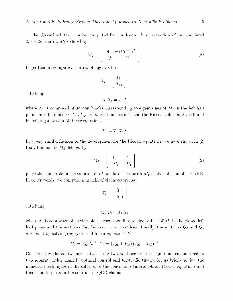
N. Akar and K. Sohraby, System Theoretic Approach to Teletra�c Problems 5The Riccati solution can be computed from a Jordan form reduction of an associated2m� 2m matrix M1 de�ned byM1 = 24 A �BR�1BT�Q �AT 35 : (8)In particular, compute a matrix of eigenvectorsT1 = 24 T11T12 35 ;satisfying M1 T1 = T1 �1where �1 is composed of Jordan blocks corresponding to eigenvalues of M1 in the left halfplane and the matrices T11; T12 are m�m matrices. Then, the Riccati solution X� is foundby solving a system of linear equationsX� = T12T�111 :In a very similar fashion to the development for the Riccati equations, we have shown in [2]that, the matrix M2 de�ned by M2 = 24 0 I�H0 �H1 35 (9)plays the same role in the solution of (2) as does the matrix M1 in the solution of the ARE.In other words, we compute a matrix of eigenvectors, sayT2 = 24 T21T22 35satisfying M2 T2 = T2 �2;where �2 is composed of Jordan blocks corresponding to eigenvalues of M2 in the closed lefthalf plane and the matrices T21; T22 are m �m matrices. Finally, the matrices G0 and G�are found by solving the system of linear equations [2]G0 = T22 T�121 ; G� = (T21 + T22) (T21 � T22)�1:Constructing the equivalence between the two nonlinear matrix equations encountered intwo separate �elds, namely optimal control and teletra�c theory, let us brie y review thenumerical techniques in the solution of the continuous-time algebraic Riccati equations andtheir counterparts in the solution of QBD chains.

N. Akar and K. Sohraby, System Theoretic Approach to Teletra�c Problems 61. Iterative techniques. Consider the ARE given in (7), replace the constant matrix Xwith the time-varying matrix X(t) and replace the right hand side of the equation(the zero matrix) with dX(t)dt . The new equation is called the Riccati matrix di�erentialequation [36]. One way to solve the ARE is to solve this di�erential equation andthen letting X = limt!1X(t). Throughout this approach, the Riccati solutionX� cannumerically be obtained via solving a matrix di�erence equation [22, 9] usingX(t +�t) � X(t) + dX(t)dt �t;and Xk+1 = Xk +�t hATXk +XkA�XkBR�1BTXk +Qi ; (10)where Xk = X(k�t) and �t is an a-priori speci�ed time-increment. We also notethat, when the optimal control problem is posed in discrete-time, we encounter adiscrete-time ARE for which the solution can be obtained through a matrix di�erenceequation of the form (10) (see [9] and the references therein). The counterpart of thisapproach is the Neuts' iterative algorithms [33] and it has been shown in [9] to havethe same monotonicity properties as the algorithms proposed by Neuts [34]. Due tolow convergence rates, this technique is not preferred in the optimal control �eld [29].2. Eigenvalue methods. The connection given above between the ARE of order m anda linear eigenvalue problem of order 2m is classical and dates back to Von Escherich[13] in 1898 according to Reid [36]. Methods based on �nding the eigenvalues andeigenvectors of the matrix M1 to compute the Riccati solution was introduced to thecontrol theory literature in 1963 [32]. The classical paper of Golub and Wilkinson [16]reports the severe numerical di�culties associated with the determination of Jordanforms when the matrix M1 has multiple or near-multiple eigenvalues. The counterpartof this approach in teletra�c theory is the spectral decomposition approach whichrequires root �nding or eigenanalysis [12]. Neuts reports similar numerical problems[33] with the spectral decomposition approach used for the solution of Markov chainsof M/G/1 and G/M/1 type.3. Invariant Subspace Approach. In this approach, instead of �nding the generalizedeigenvectors of M1 associated with its closed left-half-plane eigenvalues, any baseswhich span these eigenvectors, called the \left invariant subspace" or \stable subspace"of M1 is computed via e�cient techniques to avoid the di�culties mentioned above indetermining the Jordan form of matrices. The key observation is that �nd any matrixU1 U1 = 24 U11U12 35

N. Akar and K. Sohraby, System Theoretic Approach to Teletra�c Problems 7which spans the same invariant subspace that T1 spans and write X� = U12U�111 . Sincethe major tool is the computation of an invariant subspace, all these methods arereferred to invariant subspacemethods. These methods include Schur methods [28, 29],iterative re�nement techniques [21], and the matrix sign function algorithms [8, 10, 20,24]. It is the invariant subspace approach that has proved to be the most suitableapproach for solving the ARE among the three basic approaches mentioned above [29]due to its numerical e�ciency and reliability features.As shown above, the solution of algebraic Riccati equations and QBD chains is remarkablysimilar. Both problems are reduced to �nding a certain solution for a matrix quadraticequation. Both solutions for the matrix equations are reduced to �nding a bases for the leftinvariant subspace of certain 2m-by-2m matrices (i.e., matricesM1 and M2 de�ned as in (8)and (9), respectively). Moreover, the left invariant subspace of a matrix can be computedby numerically e�cient and reliable algorithms as indicated in [29] in the context of solvingRiccati equations. Although we have so far focused on the relation between the solutions forARE's and QBD chains, the use of computing invariant subspaces for teletra�c problems isnot restricted to only QBD chains. The extension to M/G/1 and G/M/1 chains has recentlybeen carried out in [2] and computational aspects of the approach are studied in [3]. Inthe next section, we will examine a set of teletra�c problems under a common frameworkwhere the computation of the stable subspace (left invariant subspace) plays a key role. Thecommon feature of these models is that, the paradigm of M/G/1 and G/M/1 type Markovchains either does not apply (e.g., uid ow models) or is not suitable (e.g., GI/G/1 queue)for these models. We also give a new framework for MAP/G/1 queues based on [1] whereMAP stands for Markovian Arrival Process [30].3 State Space Representations for Teletra�c ModelsIn this section, we will primarily be interested in setting up a common mathematical frame-work for a set of continuous-time queueingmodels ranging fromGI/G/1 queues andMAP/G/1queues to Markov modulated uid ow models. We will view the overall problem as one ofdetermining the output of a state-space representation of a linear, �nite-dimensional dynam-ical system [11] whose initial conditions are to satisfy certain constraints. In particular, thewaiting times in the system take over the role of the output whereas the unknown emptyqueue probabilities will act as the initial condition (or the input) of the linear dynamicalsystem. Irrespective of the underlying queueing model, the following procedure is commonto all problems:

N. Akar and K. Sohraby, System Theoretic Approach to Teletra�c Problems 81. Obtain the expression for the Laplace-Stieltjes Transform (LST) of the un�nishedwork Cumulative Distribution Function (CDF) (denoted by w(x)) for the associatedqueueing model in terms of an unknown boundary vector (denoted as y0). We assumethat the transform expression has rational functions as its entries.2. Write a state-space realization of the input-output relationship obtained in the previousstep in the form: ddx z(x) = A z(x); z(0) = B y0 ; w(x) = C z(x): (11)The above di�erential equations are in standard state space form [11],[19], z(x) denotesthe state vector of the dynamical system, A;B;C are constant matrices of suitable sizesand y0 is the unknown boundary vector which is to be determined. This step falls inthe context of \realization theory" in linear systems [11].3. Numerically solve for the initial conditions of the state-space representation (i.e., solv-ing for y0) obtained above, which satisfy a set of linear equations. However, theseequations are not immediate to write and determining these equations form the coreof the numerical solution procedure which will be given in section 4.4. Having obtained the state space realization as in (11) in step 2 and y0 in step 3, thesolution to the linear di�erential equations (11) takes the simple matrix exponentialform w(x) = C eAx B y0; (12)which is the unique solution of the di�erential equations (11).In the next section, we will focus on steps 1 and 2 for a set of continuous-time queueingmodels. We �rst begin with GI/G/1 queues.3.1 Example: GI/G/1 QueueThe system under consideration is one in which interarrival times between arrivals are inde-pendent and are given by an arbitrary distribution A(x), service times independently drawnfrom an arbitrary distribution B(x), and we assume there is a single server serving the cus-tomers on a �rst-come-�rst-serve basis [23]. We de�ne the transform for the ProbabilityDensity Function (PDF) of the interarrival time and for the PDF of the service time as A(s)

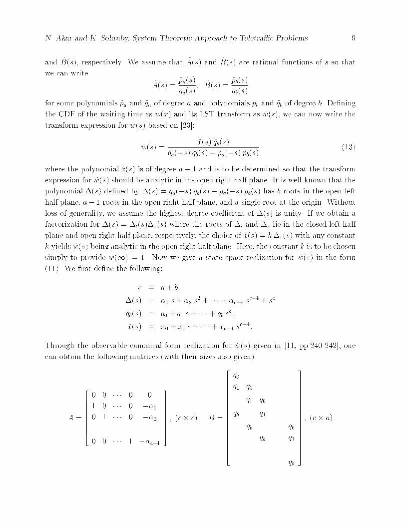
N. Akar and K. Sohraby, System Theoretic Approach to Teletra�c Problems 9and B(s), respectively. We assume that A(s) and B(s) are rational functions of s so thatwe can write A(s) = pa(s)qa(s) ; B(s) = pb(s)qb(s)for some polynomials pa and qa of degree a and polynomials pb and qb of degree b. De�ningthe CDF of the waiting time as w(x) and its LST transform as w(s), we can now write thetransform expression for w(s) based on [23]:w(s) = x(s) qb(s)qa(�s) qb(s)� pa(�s) pb(s) (13)where the polynomial x(s) is of degree a� 1 and is to be determined so that the transformexpression for w(s) should be analytic in the open right half plane. It is well-known that thepolynomial �(s) de�ned by �(s) = qa(�s) qb(s) � pa(�s) pb(s) has b roots in the open lefthalf plane, a� 1 roots in the open right half plane, and a single root at the origin. Withoutloss of generality, we assume the highest degree coe�cient of �(s) is unity. If we obtain afactorization for �(s) = �l(s)�r(s) where the roots of �l and �r lie in the closed left halfplane and open right half plane, respectively, the choice of x(s) = k�r(s) with any constantk yields w(s) being analytic in the open right half plane. Here, the constant k is to be chosensimply to provide w(1) = 1. Now we give a state space realization for w(s) in the form(11). We �rst de�ne the following:c = a+ b;�(s) = �1 s+ �2 s2 + � � � + �c�1 sc�1 + scqb(s) = q0 + q1 s+ � � � + qb sb;x(s) = x0 + x1 s+ � � � + xa�1 sa�1:Through the observable canonical form realization for w(s) given in [11, pp.240-242], onecan obtain the following matrices (with their sizes also given)A = 2666666664 0 0 � � � 0 01 0 � � � 0 ��10 1 � � � 0 ��2... ... ... ...0 0 � � � 1 ��c�1 3777777775 ; (c� c) B = 26666666666666666664

q0q1 q0... q1 q0qb ... q1 . . .qb ... . . . q0qb q1. . . ...qb37777777777777777775 ; (c� a)

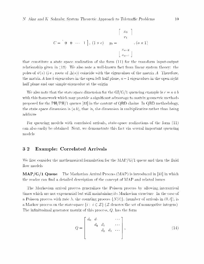
N. Akar and K. Sohraby, System Theoretic Approach to Teletra�c Problems 10C = h 0 0 � � � 1 i ; (1� c) y0 = 2666666664 x0x1...xa�2xa�1 3777777775 : (a� 1)that constitute a state space realization of the form (11) for the transform input-outputrelationship given in (13). We also note a well-known fact from linear system theory: thepoles of w(s) (i.e., roots of �(s)) coincide with the eigenvalues of the matrix A. Therefore,the matrix A has b eigenvalues in the open left half plane, a�1 eigenvalues in the open righthalf plane and one simple eigenvalue at the origin.We also note that the state space dimension for the GI/G/1 queueing example is c = a+bwith this framework which may provide a signi�cant advantage to matrix geometric methodsproposed for the PH/PH/1 queues [33] in the context of QBD chains. In QBD methodology,the state space dimension is (a b), that is, the dimension is multiplicative rather than beingadditive.For queueing models with correlated arrivals, state-space realizations of the form (11)can also easily be obtained. Next, we demonstrate this fact via several important queueingmodels.3.2 Example: Correlated ArrivalsWe �rst consider the mathematical formulation for the MAP/G/1 queue and then the uid ow models.MAP/G/1 Queue. The Markovian Arrival Process (MAP) is introduced in [31] in whichthe reader can �nd a detailed description of the concept of MAP and related issues.The Markovian arrival process generalizes the Poisson process by allowing interarrivaltimes which are not exponential but still maintaining its Markovian structure. In the case ofa Poisson process with rate �, the counting process fN(t)g, (number of arrivals in (0; t]), isa Markov process on the state-space fi : i 2 Zg (Z denotes the set of nonnegative integers).The in�nitesimal generator matrix of this process, Q, has the formQ = 2666664 d0 d1 � � �d0 d1 � � �d0 d1 � � �. . . 3777775 ; (14)

N. Akar and K. Sohraby, System Theoretic Approach to Teletra�c Problems 11where d0 = ��, d1 = �. In the case of a MAP, there is the additional phase process fJ(t)gassuming values in f1; 2; : : : ;mg. The two-dimensional Markov process fN(t); J(t)g is thenmodeled as a Markov process on the state-space f(i; j) : i 2 Z; 1 � j � mg whosein�nitesimal generator matrix Q can be represented in block form asQ = 2666664 D0 D1 � � �D0 D1 � � �D0 D1 � � �. . . 3777775 : (15)Here, D0; D1 are m�m matrices, D0 has negative diagonal elements and non-negative o�-diagonal elements, D1 is non-negative, and D 4= D0 + D1 is an irreducible in�nitesimalgenerator. Let � be the stationary probability vector of the phase process with generator Dso that � satis�es �D = 0; �e = 1; (16)where e is a column vector of ones. The mean arrival rate denoted by �� is given by�� = �D1e: (17)The MAP includes MMPP, PH-renewal processes and superpositions of these processes asspecial cases. The MMPP (see, e.g., [18]) with an in�nitesimal generator R and rate matrix� = diagf�1; �2; : : : ; �mg is a MAP with D0 = R�� and D1 = �. The PH-renewal process[31] with representation (�; T ), is a MAP with D0 = T and D1 = �Te�. This rich classincludes superpositions of the Erlangian (Ek) and Hyperexponential (Hk) distributions. Werefer to [31] for a general treatment of the subcases of the MAP.Let us now consider a single server queue o�ered with a MAP characterized by the matricesD0 and D1. Let the service time have an arbitrary distribution function B, with Laplace-Stieltjes Transform (LST), B. Hereafter, we assume that the parameters of the incomingMAP are normalized so that the mean service time is unity. We also assume a stable queue,i.e., �� < 1. We now restate the results for the virtual waiting time distribution in theMAP/G/1 queue given in [35],[30]. For this purpose, we �rst de�neW (x) = h W1(x) W2(x) � � � Wm(x) i ;where Wj(x) is the stationary probability that at an arbitrary time the arrival process isin phase j and the un�nished work at that time is at most x. The virtual waiting timecumulative distribution function (cdf) is denoted by w(x) = W (x)e. We de�ne W (s) andw(s) to be the LST of W (x) and w(x), respectively. Ramaswami [35] has shown thatW (s) = x0 [sI +D0 +D1B(s)]�1; (18)

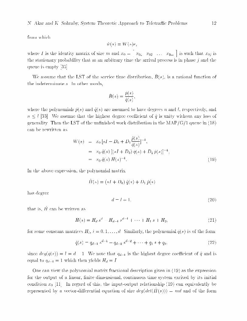
N. Akar and K. Sohraby, System Theoretic Approach to Teletra�c Problems 12from which w(s) = W (s)e;where I is the identity matrix of size m and x0 = h x01 x02 : : : x0m i is such that x0j isthe stationary probability that at an arbitrary time the arrival process is in phase j and thequeue is empty [35].We assume that the LST of the service time distribution, B(s), is a rational function ofthe indeterminate s. In other words, B(s) = p(s)q(s) ;where the polynomials p(s) and q(s) are assumed to have degrees n and l, respectively, andn � l [33]. We assume that the highest degree coe�cient of q is unity without any loss ofgenerality. Then the LST of the un�nished work distribution in the MAP/G/1 queue in (18)can be rewritten as W (s) = x0 [sI +D0 +D1 p(s)q(s) ]�1;= x0 q(s) [(sI +D0) q(s) +D1 p(s)]�1;= x0 q(s) H(s)�1: (19)In the above expression, the polynomial matrixH(s) = (sI +D0) q(s) +D1 p(s)has degree d = l + 1; (20)that is, H can be written asH(s) = Hd sd +Hd�1 sd�1 + � � � +H1 s+H0; (21)for some constant matrices Hi, i = 0; 1; : : : ; d. Similarly, the polynomial q(s) is of the formq(s) = qd�1 sd�1 + qd�2 sd�2 + � � � + q1 s+ q0; (22)since deg(q(s)) = l = d � 1. We note that qd�1 is the highest degree coe�cient of q and isequal to qd�1 = 1 which then yields Hd = I.One can view the polynomial matrix fractional description given in (19) as the expressionfor the output of a linear, �nite-dimensional, continuous-time system excited by its initialcondition x0 [11]. In regard of this, the input-output relationship (19) can equivalently berepresented by a vector-di�erential equation of size deg(det(H(s))) = md and of the form

N. Akar and K. Sohraby, System Theoretic Approach to Teletra�c Problems 13(11) via an md-dimensional state vector z(�) and A;B;C being constant matrices of sizemd �md, md�m, and 1 �md, respectively, [11],[19]. The choice of the suitable matricesthat yield C(sI � A)�1B = (q(s)H(s)�1e)Twhere e is a column vector of ones is called a state-space realization of (19) [11]. The followingchoice of matrices A, B, and C is shown in [1] to be a state-space realization of (19) of theform (11): A = 2666666664 0 0 � � � 0 �H0I 0 � � � 0 �H10 I � � � 0 �H2... ... ... ...0 0 � � � I �Hd�1 3777777775T ; C = h eT 0 � � � 0 iand y0 = xT0 ; B = h B1 B2 � � � Bd iT ;where B1 = I;and for i = 2; 3; : : : ; d, Bi = qd�iI � i�1Xj=1Bj Hd�i+j:Fluid Flow Models. Consider a bu�er with arrival rate �(S(t))where S(t) is the state ofa �nite irreducible Markov process at time t. Let the service rate be denoted by c. Let X(t)be the bu�er content at time t. Within the uid ow framework, the behavior of X(t) isdescribed byddtX(t) = �(S(t)) � c; if X(t) > 0 or �(S(t)) � c; zero otherwise:Without any loss of generality, s 2 S is assumed to be integer-valued, that is, S(t) 2f1; 2; : : : ;mg. Let W (s; x) = limt!1PrfS(t) = s; X(t) � xg:We de�ne � to be the in�nitesimal generator matrix of the underlying Markov chain. Wealso de�ne the drift matrix D asD = diag f�(1)� c; �(2)� c; : : : ; �(m)� cgA state-space realization for w(x) = PsW (s; x), the stationary un�nished work CDF, of theform (11) can immediately be written for this uid ow model with the following choices ofmatrices A, B, and C [6]: A = D�1�T ; C = e;

N. Akar and K. Sohraby, System Theoretic Approach to Teletra�c Problems 14and B is a m-by-r matrix where r is the number of underload states, i.e., fs j �(s) < cg.Assuming that the states are enumerated such that the �rst r states are underload states,the matrix B takes the form B = 24 Ir0m�r;r 35 :So far, we have considered several queueingmodels and formed a state-space representationof the form (11) for the desired functions of interest. Pictorially, we have a dynamical system(see Figure 1) characterized by the matrices A;B;C with its output being the stationaryun�nished work CDF, w(x) and which is driven by y0.Dynamical

System

A, B, C

y0 w(x)

Figure 1: Dynamical system view to queueing problems.However, we have not yet proposed a method for determining the unknown boundaryvector y0, which amounts to the core of the numerical solutions for these queueing problems.The next section addresses to a novel method to calculate y0 exactly, which together withthe state-space representation (11) and its solution (12) provides the stationary un�nishedwork distribution in a compact way through a matrix exponential representation.4 Numerical SolutionsIn the queueing problems we have presented in the previous section, the common frameworkis a state-space realization for the un�nished work which is of the form (11). Given thematrix exponential form of the virtual waiting time distribution (12), what remains is todetermine the boundary probability vector y0. The key to the determination of y0 is thatfor a stable queueing system, the solution w(x) is bounded for all x � 0. Therefore, we �ndthe boundary vector y0 such that w(x) is bounded for all x � 0 with the constraint that theinitial state should lie in the range space of B, i.e., z(0) = B y0.We will use this general state equations given in (11) to propose a numerical method tocalculate y0. Let us assume that the state vector has n components so that the matrix A is an

N. Akar and K. Sohraby, System Theoretic Approach to Teletra�c Problems 15n-by-n matrix. Let us also assume the unknown boundary vector y0 has r components withr < n. With this notation, it can be shown for the queueing problems of the previous sectionthat the matrix A has n� r eigenvalues in the open left half plane, r� 1 eigenvalues on theopen right half plane and a simple eigenvalue at the origin. We de�ne the n� (n� r) matrixSA whose columns are composed of the right eigenvectors of the matrix A associated withits n� r eigenvalues lying in the open left half plane. In other words, let ui; 1 � i � n� rbe such that ui �i = A ui; Re �i < 0:The matrix SA is then de�ned asSA = h u1 u2 � � � un�r i :The columns of SA form a basis for the stable subspace of A [39] where the term \stable" isinherited from the stability of di�erential systems.The unknown boundary probability vector y0 should be chosen so that no unstable modeof the matrix A should be excited. Otherwise, the solution for W (x) in (12) blows upas x ! 1. The problem is an open-loop control problem: Bring the dynamical systemto an initial state so that without any further excitation all the states stay bounded. Inmathematical terms, this is equivalent to saying z(0) � z(1) should lie in the range spaceof SA, i.e., z(0)� z(1) = SA y1;for some (n� r)� 1 column vector y1, or equivalently,B y0 � SA y1 = z(1): (23)Let u0 be the right eigenvector of A associated with its eigenvalue at the origin. Thenz(1) = k u0 where the normalization constant k should be chosen so that the un�nishedwork expression corresponds to a CDF.Then one can solve the linear square system below:h B �SA i 24 y0y1 35 = z(1) (24)for y0 and y1. The core of the computation in the above procedure consists of �nding theleft half plane eigenvalues and the associated right eigenvectors of the matrix A.We note that, in the above formulation one can replace SA by any matrix �SA whose rangespace is equal to the former. This will evidently have no impact on the solution y0. Thenthe problem reduces to �nding any bases for the stable subspace of the matrix A. We have

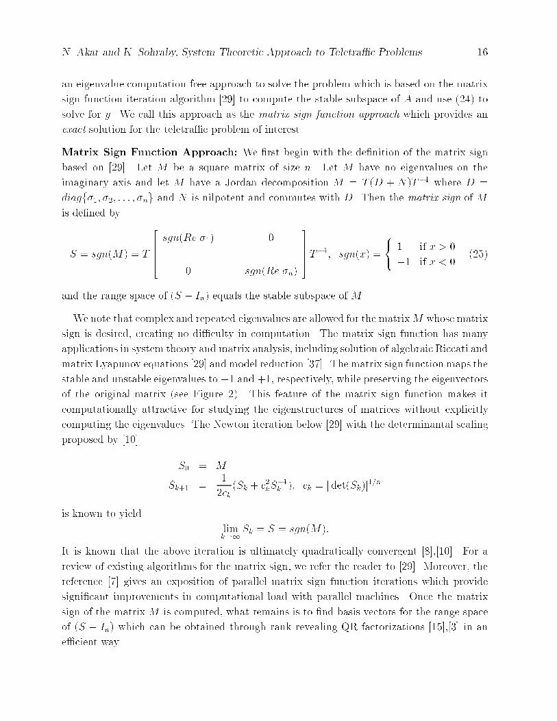
N. Akar and K. Sohraby, System Theoretic Approach to Teletra�c Problems 16an eigenvalue computation-free approach to solve the problem which is based on the matrixsign function iteration algorithm [29] to compute the stable subspace of A and use (24) tosolve for y. We call this approach as the matrix sign function approach which provides anexact solution for the teletra�c problem of interest.Matrix Sign Function Approach: We �rst begin with the de�nition of the matrix signbased on [29]. Let M be a square matrix of size n. Let M have no eigenvalues on theimaginary axis and let M have a Jordan decomposition M = T (D + N)T�1 where D =diagf�1; �2; : : : ; �ng and N is nilpotent and commutes with D. Then the matrix sign of Mis de�ned byS = sgn(M) = T 26664 sgn(Re �1) 0. . .0 sgn(Re �n) 37775T�1; sgn(x) = 8<: 1 if x > 0�1 if x < 0 (25)and the range space of (S � In) equals the stable subspace of M .We note that complex and repeated eigenvalues are allowed for the matrixM whose matrixsign is desired, creating no di�culty in computation. The matrix sign function has manyapplications in system theory and matrix analysis, including solution of algebraic Riccati andmatrix Lyapunov equations [29] and model reduction [37]. The matrix sign function maps thestable and unstable eigenvalues to �1 and +1, respectively, while preserving the eigenvectorsof the original matrix (see Figure 2). This feature of the matrix sign function makes itcomputationally attractive for studying the eigenstructures of matrices without explicitlycomputing the eigenvalues. The Newton iteration below [29] with the determinantal scalingproposed by [10] S0 = MSk+1 = 12ck (Sk + c2kS�1k ); ck = j det(Sk)j1=nis known to yield limk!1 Sk = S = sgn(M):It is known that the above iteration is ultimately quadratically convergent [8],[10]. For areview of existing algorithms for the matrix sign, we refer the reader to [29]. Moreover, thereference [7] gives an exposition of parallel matrix sign function iterations which providesigni�cant improvements in computational load with parallel machines. Once the matrixsign of the matrix M is computed, what remains is to �nd basis vectors for the range spaceof (S � In) which can be obtained through rank revealing QR factorizations [15],[3] in ane�cient way.

N. Akar and K. Sohraby, System Theoretic Approach to Teletra�c Problems 17I I

I I

−1 +1

−1 +1

+1

−1

Re z

Re z

x

sgn(x)

Im z

Im z

X X

X

X

X

O O

OO

X O

a) spectrum of matrix M, X: left half plane eig. , O:right half plane eig.

b) spectrum of matrix S = sgn(M)

c) transformation used to map the eigenvalues to −1 and +1while still preserving the eigenstructure

O

Figure 2: How matrix sign function works.The matrix sign function is a computationally e�cient method of computing the stablesubspace of a matrix if the matrix does not have any eigenvalues on the imaginary axis.For the teletra�c problems of our interest, the state matrix A turns out to have a simpleeigenvalue at the origin, due to which the matrix sign function iteration cannot be applieddirectly to the matrix A. There is a practical solution to this problem, the eigenvalueat the origin can easily be moved to the right half plane (e.g., � = 1) without changingthe eigenstructure of the matrix. Recall that the vector u0 is the right eigenvector of Acorresponding to this simple eigenvalue at the origin. Also let �u0 be the left eigenvector ofA associated with this particular eigenvalue. Then the matrix sign function iterations can

N. Akar and K. Sohraby, System Theoretic Approach to Teletra�c Problems 18be applied to the matrix Am which is de�ned asAm = A+ u0 �u0�u0 u0 : (26)We note that the stable subspaces of the two matrices A and Am are the same, but thematrix Am is free of imaginary axis eigenvalues so that we can apply the matrix sign functionalgorithm to Am. Let us now summarize the overall procedure, starting with the state-spacerepresentation (11).1. De�ne the matrix Am as in (26).2. Perform the following iterationS0 = Am; Sk+1 = 12ck (Sk + c2kS�1k ); ck = j det(Sk) j1=n; (27)until a certain stopping criterion is satis�ed.3. Compute the matrix �SA whose columns form a basis for the range space of SJ � I,where J the number of iterations in the previous step.4. Solve for y0 out of the linear equation (24) where the matrix SA is replaced with �SA.5 Numerical ExamplesIn this section, we will consider numerical examples for which we present some results andthe number of iterations required in the matrix sign function iterations when the stoppingcriterion proposed in [3] is used: jj Sj+1 � Sj jj1 > � jj Sj jj1: (28)Here, Sj is de�ned as in (27) and the 1-norm of a matrix ise de�ned as [15]jj A jj1 = max1�j�n mXi=1 j aij j:We will use � = 10�7 in the following examples. The algorithms are implemented in MAT-LAB version 4.1 running on a DEC 3100 workstation. We �rst present our results for Ek/El/1queues in terms of the number of iterations with respect to changing utilization of the sys-tem, which we denote by �, in Table 1. We take the mean service time as unity and denoteby I the number of iterations required in the algorithm to satisfy the stopping criterion (28).We note that we have used diagonal scaling on the matrix Am by which we start the matrix

N. Akar and K. Sohraby, System Theoretic Approach to Teletra�c Problems 19sign function iterations to improve the conditioning of the procedure. Examining Table 1,we conclude that the algorithm is fast and is numerically robust with respect to parameterchanges of the underlying queueing system. The computational e�ort at each iteration re-duces to a matrix inversion of size k + l, where k and l are the dimensions associated withthe interarrival time and service times. Compared with the QBD formulation with size (kl)[33], our algorithmic approach provides a signi�cant improvement to existing methods.E10/E10/1 E2/E50/1 E40/E20/1� I E[W ] E[W 2] I E[W ] E[W 2] I E[W ] E[W 2]0.2 7 7.35 e-5 2.88 e-5 10 2.55 e-2 1.52 e-2 10 4.55 e-11 9.87 e-120.4 7 5.93 e-3 2.65 e-3 10 1.08 e-1 8.39 e-2 9 2.74 e-5 5.71 e-60.6 7 5.01 e-2 2.87 e-2 10 3.06 e-1 3.61 e-1 9 3.94 e-3 1.02 e-30.8 7 2.64 e-1 2.74 e-1 10 9.41 e-1 2.31 9 6.07 e-2 2.54 e-20.9 7 7.48 e-1 1.51 11 2.23 1.13 e+1 9 2.29 e-1 1.78 e-10.95 8 1.74 6.98 12 4.83 4.95 e+1 9 5.94 e-1 9.02 e-10.99 10 9.74 1.95 e+3 13 2.56 e+1 1.33 e+3 11 3.59 2.69 e+10.999 12 9.97 e+1 1.99 e+4 16 2.59 e+2 1.35 e+5 14 3.73 e+1 2.80 e+3Table 1: Number of iterations and the �rst two moments of the waiting time in an Ek/El/1queue using the matrix sign function algorithm.We then consider the statistical multiplexing of a superposition of homogeneous 2-stateon-o� uid sources with the mean on and o� periods randomly assigned. The problem cane�ciently be solved by the classical algorithm [6]. However, our aim is to show the powerand the rapid convergence of these algorithms for uid ow models. Table 2 summarizes ourresults we obtained via the matrix sign function approach. Here, N denotes the number ofusers and � denotes the utilization in the system. We present the errorerror = jj y0 ([6])� y0 (matrix sign) jj2 (29)at each iteration of the algorithm. The error rapidly approaches the machine precisionirrespective of the load and the number of users. The computational gains in using thisapproach for uid ow models will especially be signi�cant when the underlying Markovchain is not structured (i.e., not obtained through a superposition of homogenous sourcesbut arbitrary) for which explicit results are not available as in [6].

N. Akar and K. Sohraby, System Theoretic Approach to Teletra�c Problems 20errornumber of � = 0:6 � = 0:9iterations N=16 N=64 N=16 N=641 3.3e-03 1.1e-07 1.1e-01 1.8e+012 5.9e-04 2.5e-08 2.4e-01 3.2e-013 9.5e-05 7.5e-09 5.5e-03 1.6e-014 5.6e-06 1.6e-09 5.8e-05 1.4e-025 2.5e-08 2.5e-10 5.7e-06 1.5e-046 5.1e-13 1.0e-11 6.2e-08 1.4e-067 < 1e-14 2.2e-14 8.6e-12 9.6e-118 < 1e-14 < 1e-14 < 1e-14 < 1e-14Table 2: Error in y0 with respect to the number of iterations in the matrix sign functionapproach.6 ConclusionsWe summarize the �ndings of this work and new directions.1. The procedure is a general one and the numerical techniques proposed here can beapplied to a rich variety of teletra�c problems. The algorithms we propose here areunifying in the sense that apparently di�erent problems can all be tackled in the sameway through the computation of the stable subspace of a certain matrix.2. The algorithms we propose are fast and rapidly converge within a few number of it-erations. Moreover, variants of the matrix sign function algorithms given in [29] aremultiplication-rich and based on block matrix operations and therefore they are suit-able for parallelization. In a recent paper [7], the authors study a set of parallel matrixsign iterations using Parallel Virtual Machine (PVM) software. The developments inthe parallel implementation of such iterations will have a large impact on teletra�ctheory since it will enlarge the set of teletra�c models that can be solved by algorithmicmethods.3. Examining Figure 2, the essential idea is to extract the stable modes from the spectrumwithout a-priori information on the eigenstructure of the system. The transformationused for this purpose is the signum function which has a discontinuity at zero and thistransformation can be applied to a matrix through a series of rational transformations

N. Akar and K. Sohraby, System Theoretic Approach to Teletra�c Problems 21of the form (27). An alternative is the use of linear �lters whose gain responses aredesired to be have sharp characteristics around a desired cut-o� frequency.References[1] N. Akar and E. Ar�kan. A numerically e�cient algorithm for the MAP/D/1/K queuevia rational approximations. to appear in Queueing Systems, 1996.[2] N. Akar and K. Sohraby. An invariant subspace approach in M/G/1 and G/M/1 typeMarkov chains. submitted to Commun. Stat.-Stochastic Models, 1995.[3] N. Akar and K. Sohraby. On computational aspects of the invariant subspace approachto teletra�c problems and comparisons. submitted to Commun. Stat.-Stochastic Models,1995.[4] B. D. O. Anderson and J. B. Moore. Optimal Filtering. Prentice-Hall, Englewood Cli�sNJ USA, 1979.[5] B. D. O. Anderson and J. B. Moore. Optimal Control: Linear Quadratic Methods.Prentice-Hall, Englewood Cli�s NJ USA, 1990.[6] D. Anick, D. Mitra, and M. M. Sondhi. Stochastic theory of a data handling systemwith multiple sources. Bell Syst. Tech. Jour., 61:1871{1894, 1982.[7] B. Bakkalo�glu, C. K. Ko�c, and M. _Inceo�glu. Parallel matrix sign iterations using PVM.IEEE Trans. Auto. Contr., 1995. submitted for publication.[8] L. Balzer. Accelerated convergence of the matrix sign function. Int. Jour. Contr.,32:1057{1078, 1980.[9] R. R. Bitmead and M. Gevers. Riccati di�erence and di�erential equations: convergence,monotonicity and stability. In S. Bittanti, A. J. Laub, and J. C. Willems, editors, TheRiccati Equation, chapter 10, pages 263{291. Springer-Verlag, Berlin, 1991.[10] R. Byers. Solving the algebraic Riccati equation with the matrix sign function. Lin.Alg. Appl., 85:267{279, 1987.[11] C. T. Chen. Linear System Theory and Design. Holt, Rinehart and Winston, Inc., NewYork, 1984.

N. Akar and K. Sohraby, System Theoretic Approach to Teletra�c Problems 22[12] J. N. Daigle and D. M. Lucantoni. Queueing systems having phase-dependent arrivaland service rates. In Numerical Solution of Markov chains, pages 223{238, New York,1991. Marcel Dekker Inc.[13] G. Von Escherich. Die zweite variation der einfachen integrale. Wiener Sitzungsberichte,pages 1191{1250, 1898.[14] R. V. Evans. Geometric distribution in some two-dimensional queueing systems. Oper-ations Research, 15:830{846, 1967.[15] G. H. Golub and C. F. Van Loan. Matrix Computations. The Johns Hopkins UniversityPress, Baltimore, 1989.[16] G. H. Golub and J. H. Wilkinson. Ill-conditioned eigensystems and the computation ofthe Jordan canonical form. SIAM Review, 18:578{619, 1976.[17] B. Hajek. Birth-and-death processes on the integers with phases and general boundaries.J. Appl. Prob., 19:488{499, 1982.[18] H. He�es and D. M. Lucantoni. A Markov modulated characterization of packetizedvoice and data tra�c and related statistical multiplexer performance. IEEE JSAC,4(6):856{868, 1986.[19] T. Kailath. Linear Systems. Prentice-Hall Inc., Englewood Cli�s NJ, 1980.[20] C. Kenney and A. J. Laub. Rational iterative methods for the matrix sign function.SIAM Matrix. Anal. Appl., 12(2):273{291, 1991.[21] C. Kenney, A. J. Laub, and M. Wette. Error bounds for Newton re�nement of solutionsto algebraic Riccati equations. Math. Control, Signal, Sys., 3:211{224, 1990.[22] C. Kenney and R. B. Leipnik. Numerical integration of the di�erential matrix Riccatiequation. IEEE Trans. Auto. Contr., 30:962{970, 1985.[23] L. Kleinrock. Queueing Systems Volume 1: Theory. Wiley-Interscience Publication,1975.[24] C. K. Ko�c and B. Bakkalo�glu. Computation of the matrix sign function using continuedfraction expansion. IEEE Trans. Auto. Contr., 39(8):1644{1647, 1994.[25] H. Kwakernaak and R. Sivan. Linear Optimal Control Systems. Wiley Interscience,New York, USA, 1972.[26] G. Latouche. A note on two matrices occuring in the solution of quasi-birth-and-deathprocesses. Commun. Statist. - Stochastic Models, 3(2):251{257, 1987.

N. Akar and K. Sohraby, System Theoretic Approach to Teletra�c Problems 23[27] G. Latouche and V. Ramaswami. A logarithmic reduction algorithm for quasi-birth-death processes. J. Appl. Prob., 30:650{674, 1993.[28] A. J. Laub. A Schur method for solving algebraic Riccati equations. IEEE Trans. Auto.Contr., 25:913{921, 1979.[29] A. J. Laub. Invariant subspace methods for the numerical solution of Riccati equations.In S. Bittanti, A. J. Laub, and J. C. Willems, editors, The Riccati Equation, chapter 7,pages 163{196. Springer-Verlag, Berlin, 1991.[30] D. M. Lucantoni. New results for the single server queue with a batch Markovian arrivalprocess. Stoch. Mod., 7:1{46, 1991.[31] D. M. Lucantoni, K. S. Meier-Hellstern, and M. F. Neuts. A single-server queue withserver vacations and a class of non-renewal arrival processes. Adv. Appl. Prob., 22:676{705, 1990.[32] A. G. J. MacFarlane. An eigenvector solution of the optimal linear regulator problem.Jour. Electron. Contr., 14:643{654, 1963.[33] M. F. Neuts.Matrix-geometric Solutions in Stochastic Models. Johns Hopkins UniversityPress, Baltimore, MD, 1981.[34] M. F. Neuts. Structured Stochastic Matrices of M=G=1 Type and Their Applications.Marcel Dekker, Inc., New York, 1989.[35] V. Ramaswami. The N=G=1 queue and its detailed analysis. Adv. Appl. Prob., 12:222{261, 1980.[36] W. T. Reid. Riccati Di�erential Equations. Academic Press, New York, 1972.[37] L. S. Shieh, H. M. Dib, and R. E. Yates. Seperation of matrix eigenvalues and structuraldecomposition of large-scale systems. Proc. IEEE, 133(2):90{96, 1986.[38] V. Wallace. The solution of quasi birth and death processes arising from multiple accesscomputer systems. PhD thesis, Systems Engineering Laboratory, University of Michigan,1969.[39] W. M. Wonham. Linear Multivariable Control: A Geometric Approach. Springer, NewYork, 1974.