Unifying Pairwise Interactions in Complex Dynamics - arXiv

Unifying Pairwise Interactions in Complex Dynamics

Oliver M. Cliff1,2, Joseph T. Lizier2,3, Naotsugu Tsuchiya4, and Ben D. Fulcher1,2

1School of Physics, The University of Sydney, Camperdown NSW 2006, Australia.2Centre for Complex Systems, The University of Sydney, Camperdown NSW 2006, Australia.

3Faculty of Engineering, The University of Sydney, Camperdown NSW 2006, Australia.4School of Psychological Sciences, Monash University, Melbourne, VIC 3800, Australia.

Abstract

Scientists have developed hundreds of techniques to measure the interactions between pairs

of processes in complex systems. But these computational methods—from correlation coefficients

to causal inference—rely on distinct quantitative theories that remain largely disconnected. Here

we introduce a library of 249 statistics for pairwise interactions and assess their behavior on

1053 multivariate time series from a wide range of real-world and model-generated systems. Our

analysis highlights new commonalities between different mathematical formulations, providing a

unified picture of a rich, interdisciplinary literature. We then show that leveraging many methods

from across science can uncover those most suitable for addressing a given problem, yielding high

accuracy and interpretable understanding. Our framework is provided in extendable open software,

enabling comprehensive data-driven analysis by integrating decades of methodological advances.

A fundamental question in science is how complex dynamics can be characterized by measuring the

interactions within a distributed system. To address this question, many approaches have been developed

to measure different types of pairwise interactions from dynamical data. For example, in neuroimaging,

functional connections between pairs of brain regions are quantified through statistical correlations, which

mark changes in human behaviors [3] and differ in neurological diseases [5]. In Earth systems science,

pairwise causal models have been used to infer mechanistic drivers of natural processes, from the influence

of sea-surface temperature on sardine and anchovy populations [37] to the atmospheric drivers of air

circulation [30]. And in economics, analysts have studied the cointegration of paired non-stationary time

series, such as stock-market indices and their associated future contracts, to infer a significant coupling

for building econometric models [11].

As illustrated in Fig. 1A, the common goal of these studies is to extract meaningful pairwise rela-

tionships from multivariate time series (MTS): sets of observations taken regularly over time [28]. In the

age of big data, the scientific problems that are studied in diverse disciplinary contexts—from genomics

to astronomy [35]—require novel ways to extract information from MTS data. However, from the myr-

iad ways to quantify a statistical dependency between two time series, it remains common practice to

manually select a single method with minimal comparison to alternatives. For instance, Pearson corre-

lation remains the most commonly used tool for measuring pairwise relationships in neuroimaging [17]

and Earth systems science [30], despite rather restrictive (and often unsatisfied) assumptions that the

data are serially independent and normally distributed [8]. Fortunately, many sophisticated and powerful

algorithms have been developed to overcome the limitations of simple correlation coefficients, including

where dependencies are lagged in time (e.g., cross-correlation [28]), may be misaligned (e.g., dynamic

time warping [31]), or where the knowledge of one variable improves the predictability of another (e.g.,

Granger causality [14]).

In this work, we represent algorithms for measuring interactions between pairs of time series as real-

valued summary statistics: statistics for pairwise interactions (SPIs). Figure 1B illustrates the diverse

1

arX

iv:2

201.

1194

1v1

[ph

ysic

s.da

ta-a

n] 2

8 Ja

n 20

22

Time

?

Miscellaneous (24 SPIs)Linear model fitsCointegrationEnvelope correlation...

Basic (23 SPIs)CovarianceKendall's tauCross-correlation...

Causal indices (10 SPIs)

Additive noise modelsConvergent cross-mapping...

Distance similarity (35 SPIs)Distance correlationHeller-Heller-Gorfine testDynamic time warping...

Information theory (37 SPIs)

Mutual informationTransfer entropyIntegrated information...

Spectral (120 SPIs)Coherence magnitudeDirected coherenceSpectral Granger causality...

Library of statistics for pairwise interactions (249 SPIs)

Library of multivariate time series (1053 datasets)

Synthetic models (505 time series)

Wave equations

Coupled oscillators

Coupled mapsBrownian motion

Ornstein-Uhlenbeck

Simulated climate

Simulated fMRI

Uncorrelated noise

Vector autoregressive

Real-world data (548 time series)

fMRI data

Daily stock prices

Epidemic incidence

River runoff

Earthquake seismograms

Articulogram

Human activity

EEG data

Heartbeat sonogram

A

B

C

Multivariate time series

Interacting pairs of time series

Pro

cess

Time

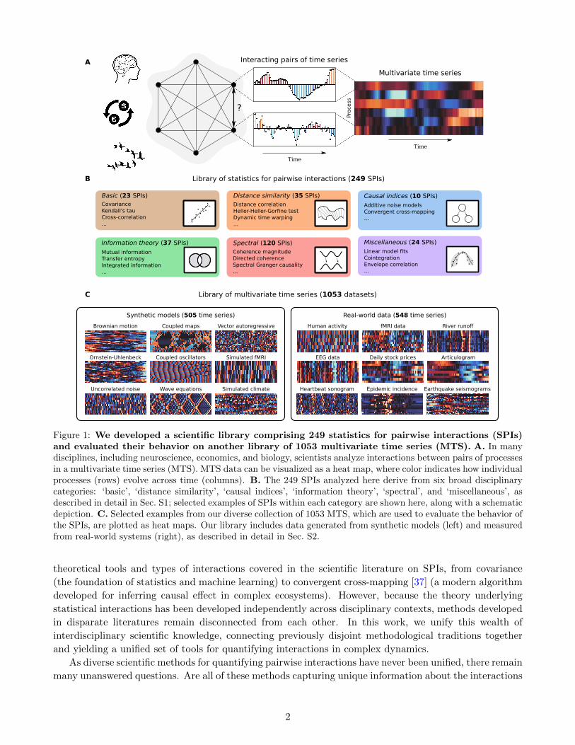
Figure 1: We developed a scientific library comprising 249 statistics for pairwise interactions (SPIs)and evaluated their behavior on another library of 1053 multivariate time series (MTS). A. In manydisciplines, including neuroscience, economics, and biology, scientists analyze interactions between pairs of processesin a multivariate time series (MTS). MTS data can be visualized as a heat map, where color indicates how individualprocesses (rows) evolve across time (columns). B. The 249 SPIs analyzed here derive from six broad disciplinarycategories: ‘basic’, ‘distance similarity’, ‘causal indices’, ‘information theory’, ‘spectral’, and ‘miscellaneous’, asdescribed in detail in Sec. S1; selected examples of SPIs within each category are shown here, along with a schematicdepiction. C. Selected examples from our diverse collection of 1053 MTS, which are used to evaluate the behavior ofthe SPIs, are plotted as heat maps. Our library includes data generated from synthetic models (left) and measuredfrom real-world systems (right), as described in detail in Sec. S2.

theoretical tools and types of interactions covered in the scientific literature on SPIs, from covariance

(the foundation of statistics and machine learning) to convergent cross-mapping [37] (a modern algorithm

developed for inferring causal effect in complex ecosystems). However, because the theory underlying

statistical interactions has been developed independently across disciplinary contexts, methods developed

in disparate literatures remain disconnected from each other. In this work, we unify this wealth of

interdisciplinary scientific knowledge, connecting previously disjoint methodological traditions together

and yielding a unified set of tools for quantifying interactions in complex dynamics.

As diverse scientific methods for quantifying pairwise interactions have never been unified, there remain

many unanswered questions. Are all of these methods capturing unique information about the interactions

2

occurring within a system? Is there synergy between complementary approaches that, when combined,

tells us more about the underlying system than any single method can? Or, do certain redundancies

exist, hinting at some theoretical underpinning that could stimulate new theory and understanding of

the techniques used across disciplines? Following previous highly comparative studies of univariate time

series [12] and graphs [26], this work addresses these questions by simultaneously evaluating hundreds of

different SPIs directly from data. Our empirical approach involves first developing the most comprehensive

library of methods used to measure pairwise interactions (SPIs) ever assembled (Fig. 1B), and then

applying them to another large and multidisciplinary library of MTS, illustrated in Fig. 1C, which we

have curated to represent a wide variety complex dynamics studied across scientific disciplines.

Comprehensive scientific libraries of methods (SPIs) and data (MTS). We constructed a

comprehensive, annotated library of 249 SPIs that we organized into six broad categories based on their

underlying theory: ‘basic’ (e.g., covariance, Kendall’s τ [19], and cross-correlation); ‘distance similarity’

(e.g., distance correlations [34], kernel-based independence tests [15, 16], and dynamic time warping [31]);

‘causal indices’ (e.g., additive noise models and convergent cross-mapping [37]); ‘information theory’ (e.g.,

Granger causality [14], transfer entropy [32], and integrated information [25]); ‘spectral’ (derived from

Fourier or wavelet transformations, e.g., coherence magnitude, phase-locking value [20], and spectral

Granger causality [10]); and ‘miscellaneous’ (e.g., cointegration [11] and model fits). A full list of SPIs,

along with descriptions and references is in Supplementary Sec. S1. Accompanying this paper is an

extendable python-based toolkit, pyspi [6], that includes implementations of all SPIs and allows users to

leverage a unified interdisciplinary literature by extracting hundreds of interactions from any MTS.

To understand the behavior of these SPIs on data, we constructed a library of 1053 diverse MTS with

the aim of capturing the main classes of systems and dynamics that are studied across scientific disciplines,

including synchronization, spatiotemporal chaos, wave propagation, criticality, and phase transitions. Our

library contains 505 synthetic MTS generated from mathematical models, including: uncorrelated and

correlated noise (e.g., Cauchy and normally distributed noise, and Brownian motion); coupled maps

(e.g., vector autoregression [28] and coupled map lattices [18]); coupled ordinary differential equations

(e.g., Kuramoto oscillators [36], Hodgkin–Huxley and Wilson–Cowan networks); and partial differential

equations (namely, wave equations, in which processes are embedded in physical space). It also contains

548 diverse real-world MTS from public databases across: geophysics (e.g., earthquake seismograms

and atmospheric processes); medicine (e.g., heartbeat sonograms, functional magnetic resonance imaging

(fMRI) data, and electroencephalograms (EEGs)); physiology (e.g., accelerometer and gyroscope readings

for sports and basic motions); and finance (e.g., exchange rates and stock prices), among others. Each MTS

comprises between 5–40 processes and between 100–2000 observations, characteristics that are designed

to match many real-world datasets, and which comprise 195 112 pairwise interactions that we will use

to evaluate the SPIs. Descriptions of all MTS are in Sec. S2, and the full database accompanies this

article [9], enabling scientists to test their methods on a diverse sample of complex dynamics.

Organizing pairwise interactions by their empirical behavior

Having assembled our libraries of methods (as 249 SPIs) and data (as 1053 MTS), we aimed to analyze

how similarly the SPIs behave on data. To achieve this, we developed an empirical similarity index,

R (0 ≤ R ≤ 1), that captures the relationship between any two SPIs by comparing their output when

applied to all 195 112 pairwise interactions that are present in the 1053 MTS. As detailed further in

Sec. S3, our index is derived from the average Spearman correlation between the SPIs when applied to

all pairs of processes in all datasets, where the minimum value, R = 0, indicates completely unrelated

methods, and the maximum, R = 1, indicates methods that are simple monotonic transformations of one

another. Using a distance measure derived from the similarity index, D = 1−R, we organized all 249 SPIs

3

M1: mean phase lag/slopeindices & group delay

M2: causal models

M3: directed information& causal entropy measures

M4: transfer entropy

M7: max phase lag indices

M5: parametric Granger causality& integrated information

M6: parametric Granger causality& directed spectral measures

M8: phase slope indices (wavelet)

M13: cointegration

M14: a mix of contemporaneous linear-dependence statistics, information-

theoretic measures, convergent cross-mapping, maximum barycenters,

distance- and kernel-based statisticsM12: undirected spectral measures

M10: dynamic time warping,phase coherence and locking values

M11: Power envelope correlation

M9: mean of barycenters

D

Spectral Grangercausality

(optimized order)

Phi* &Stochastic interaction

Grangercausality

CCM(optimized/high order)

C E

Spectral Grangercausality

(first order)DTW/LCSS

(Sakoe Chiba)

Phasecoherence

M1 M4 M8 M13M10M7M5 M14M60.0

0.2

0.4

0.6

0.8

M3 M12

Distance- and kernel- based statistics

Phase coherence

Phaselockingvalue

Maximumcross-correlation

Soft DTWand DTW

LCSS

CCM (first order)

PhiG

R > 0.50

R > 0.25

R > 0.75

Gaussian processfit (RBF)

A

B

Dis

tance

(D

)

i

ii

i

Figure 2: Statistics for measuring pairwise interactions (SPIs) between time series can be organizedinto 14 modules based on their behavior on over 1000 multivariate time series (MTS), providing anintuitive, data-driven organization of an interdisciplinary scientific literature. A. A brief summary ofthe main types of methods in each of the modules (see Fig. S3 for a full list). B. The dendrogram used to inferthe modules, produced by hierarchical clustering using a distance, D = 1 − R, based on the empirical similarityindex, R [Eq. (S1)]. SPIs are colored according to: (i) their module label (upper row), and (ii) their literaturecategorization from Fig. 1B (lower row). A high-resolution version of this dendrogram, including each of the SPIs(leaf nodes) that form the modules, is in Fig. S3. Three selected modules that mix of SPIs developed in differentdisciplinary contexts are shown as network plots in: M5 (C), M10 (D), and a subset of M14 (E). In these plots,we represent SPIs as nodes, display three different edge weight thresholds (corresponding to R > 0.25, R > 0.5,and R > 0.75), and shade connected components that have a high similarity, R > 0.75. Abbreviations used inC–E: DTW (dynamic time warping), LCSS (longest continuous subsequence), CCM (convergent cross-mapping),and RBF (radial basis function).

using hierarchical clustering, yielding the dendrogram shown in Fig. 2B. This provides an illuminating

representation of the literature that allows us to probe and interpret relationships between scientific

methods at multiple levels. We focus here on a 14-module resolution (with modules labeled M1–M14),

which allows us to demonstrate important methodological connections between groups of SPIs with similar

behavior on diverse MTS. As summarized in Fig. 2A, these fourteen modules grouped common conceptual

and theoretical approaches to measuring interactions between pairs of time series, demonstrating the

ability of our empirical approach to meaningfully organize this interdisciplinary literature.

4

In addition to grouping similar types of methods into modules, we found that different high-level con-

ceptual formulations of dynamical interactions were recapitulated in the relationships between modules.

For example, Modules M3–M6 contain distinct types of SPIs—including Granger causality [14], directed

information [22], and integrated information [38, 25]—which all capture statistical dependencies between

two time series by considering the context of their past. This idea that observable interactions are pred-

icated (or, from a statistical standpoint, conditioned) on the history of a process, was first proposed by

the Wiener–Granger theories of “causality” and “feedback” [39], specifically by measuring how one time

series might improve the self-predictability of another. Our results group SPIs based on this underlying

theoretical formulation, due to their characteristic behavior on data. Other types of SPIs (that do not

predicate on the self-predictability of a process), also display distinctive behavior, including measures of

contemporaneous relationships (as in the correlation coefficients of M14), dependencies that account for

temporal lags (as in the coherence measures of M12), or temporal dilation and shifts (as in dynamic time

warping and related methods in M10).

Most of the fourteen modules contain methods that are derived from similar underlying theory, indi-

cated by the color of the category labels in Fig. 2B(ii). Of the ten such ‘homogeneous’ modules, which

contain SPIs from the same literature category, six of them (M4, M7, M8, M9, M11, M13) comprise statis-

tics for measuring specifically one type of pairwise interaction, only differing either in their algorithms

(e.g., M13 contains both the Engle–Granger [11] and the Johansen [27] tests for measuring cointegra-

tion), summary statistics (e.g., M8 contains both mean and maximum of the wavelet-based phase lag

index [23]), or parameter settings (e.g., M4 contains five estimation techniques for transfer entropy [32]).

The remaining four homogeneous modules (M1, M2, M3, M12) comprise methods that have very similar

theoretical underpinnings, e.g., M12 contains many methods for measuring undirected interactions via

Fourier transformations, such as the magnitude and the imaginary part of the coherence [4]. Of partic-

ular interest are the four “heterogeneous” modules (M3, M5, M10, M14), which mix SPIs from different

literature categories, revealing interesting connections between different theoretical bases for quantify-

ing pairwise dependence. While M3 contains a mix of SPIs based on information theory (six labeled

‘information-theoretic measures’ and one labeled as a ‘causal index’, information-geometric conditional

independence), the remaining three modules establish connections in the behavior of seemingly disparate

SPIs on MTS data. Three networks that are derived from these modules are plotted in Figs 2C–E and

are investigated in detail below.

Module M5, shown in Fig. 2C, contains an intriguing mix of two distinct types of methods: (i) five

linear estimators for integrated information: ΦG [24], Φ∗ [25], and stochastic interaction [1]; and (ii) 16

estimators for Granger causality, in both the time and frequency domains [13]. While Granger causality

and integrated information theory were developed in very different contexts—Granger’s investigations

into “causality” between economic time series in 1969 [14] versus Tononi’s recent integrated information

theory (Φ) of consciousness [38, 25, 24]—our analysis reveals that all SPIs in this module nevertheless

behave similarly on real data (with an average empirical similarity, 〈R〉 = 0.52, in the 95th percentile

of all R values, see Fig. S1C). Despite their distinct disciplinary contexts, recent results have indeed

shown that Granger causality can be formulated as an information-theoretic measure [2], and can thus

be grouped under the same information-geometric framework as integrated information theory [24, 7].

However, it was not known whether or not these information-theoretic SPIs should behave similarly in

practice, and as such, their relationship is not widely recognized. Module M5 thus demonstrates an

important confirmation of our empirical approach in being able to recapitulate emerging theoretical work

and unify scientific tools for understand interacting processes.

Module M10, shown in Fig. 2D, reveals striking connections between three conceptually distinct types

of methods: (i) dynamic time warping (DTW), which was developed in the data-mining community to

quantify the similarity between two (potentially shifted and dilated) audio signals [31]; (ii) cross-spectral

5

phase-based measures—the maximum phase coherence [4] and the mean and maximum phase-locking

value (PLV) [20]—which were developed to examine frequency-specific synchronization in neuroimaging

data [4]; and (iii) the maximum cross correlation [28], a classic statistical technique for correlating two

time series at different lags. All of these SPIs capture time-lagged interactions between two processes,

but in slightly different ways: the maximum cross-correlation finds the highest fixed-lag match, while

DTW extends this idea by optimizing the distortion of the time axis to best match potentially misaligned

time series, and the cross-spectral measures account for time lags in terms of phase differences. Module

M10 thus reveals new connections between diverse approaches to capturing associations between pairs

of potentially unaligned time series, indicating a common conceptual basis for methods developed and

applied across disciplines—whether they are measuring synchronization between neuro-electric recordings

or recognizing speech from audio signals.

Finally we discuss module M14 which groups 66 SPIs from all literature categories (Fig. 1) except

for ‘spectral’. In part, this module recapitulates certain theoretical relationships that have already been

established, such as the equivalence between linear-Gaussian mutual information and absolute covari-

ance [21] (with the maximum similarity of R = 1). To highlight some new relationships, we focus on a

demonstrative submodule, shown in Fig. 2E, which comprises 17 SPIs from the ‘causal indices’, ‘distance

similarity’, and ‘miscellaneous’ categories. We first note the tight cluster of SPIs, labeled ‘i’ in Fig. 2E,

which were developed independently in two different domains: distance correlation-based methods [34]

from the statistics community; and kernel-based methods from the machine-learning community. This

cluster first highlights a recent finding that distance correlation and the Hilbert–Schmidt Independence

Criteria (HSIC, a kernel-based method) [15] are equivalent when computed using certain distance ker-

nels [33]; our results suggest that similar theoretical connections can be established between the other

SPIs of the cluster (including the Heller–Heller–Gorfine test [16] and multi-scale graph correlation [34]).

Second, we find that the distance- and kernel-based statistics exhibit a striking similarity with common

implementations of the convergent cross-mapping (CCM) algorithm, which was originally developed for

inferring causality in complex ecosystems [37]. CCM measures the causal effect of one time series on an-

other by the ability of the second to reconstruct the first with a nearest-neighbor approach. The fact that

these methods behave so similarly on MTS data indicates that the well-studied techniques of phase-space

reconstruction (used in the CCM algorithm) have a correspondence to the nonlinear kernel-estimation

techniques from the statistics and machine-learning community. These observed connections have im-

portant ramifications, e.g., our results suggest candidate statistical proxies for the often computationally

expensive CCM, which could yield major computational efficiencies, and enable new applications on large

datasets.

Leveraging diverse methods in addressing a scientific problem

Our results above illustrate the rich diversity of scientific methods for quantifying pairwise interactions.

This diversity suggests that, when quantifying pairwise interactions for a given application, there is

potential to: (i) select the most informative SPI for the application from across the scientific literature in

an unbiased, data-driven way; and (ii) leverage a synergistic combination of multiple complementary SPIs

to provide a more informative representation underlying relationships in MTS than any single SPI. We

aimed to test these ideas using a case study of classifying four types of activity from a human participant—

walking, resting, running, or playing badminton—using smart-watch recordings of a 3-axis accelerometer

and a 3-axis gyroscope [29], illustrated in Fig. 3A. To understand the behavior of different SPIs on this

task, we represented each MTS as a set of features corresponding to all pairwise interactions between its

constituent elements, and compared the performance of 216 SPIs (those that returned non-constant scalar

values) using a linear SVM classifier (averaged over multiple train–test splits, see Sec. S4 for details).

As shown in Fig. 3B, we found a wide range of performance accuracies across the 216 individual SPIs,

6

Running Badminton

Running

badminton

vs.

0.0

0.5

-0.5

-1.0

Kend

all'

s ta

u

BA

30 40 50 60 70 80 900.00

0.02

0.04

0.06

0.08

0.10

0.12

Average accuracy (%)

Pro

port

ion

Significant SPIs

All SPIs

C

x

z

y

Resting

BadmintonCla

ss

Running

Walking

x

z

y

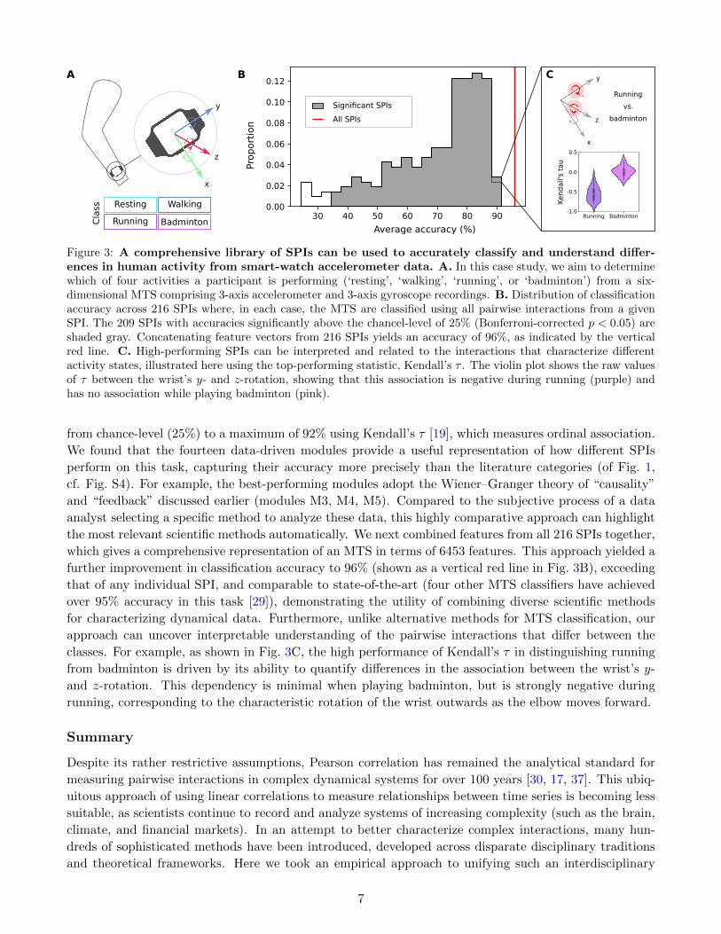
Figure 3: A comprehensive library of SPIs can be used to accurately classify and understand differ-ences in human activity from smart-watch accelerometer data. A. In this case study, we aim to determinewhich of four activities a participant is performing (‘resting’, ‘walking’, ‘running’, or ‘badminton’) from a six-dimensional MTS comprising 3-axis accelerometer and 3-axis gyroscope recordings. B. Distribution of classificationaccuracy across 216 SPIs where, in each case, the MTS are classified using all pairwise interactions from a givenSPI. The 209 SPIs with accuracies significantly above the chancel-level of 25% (Bonferroni-corrected p < 0.05) areshaded gray. Concatenating feature vectors from 216 SPIs yields an accuracy of 96%, as indicated by the verticalred line. C. High-performing SPIs can be interpreted and related to the interactions that characterize differentactivity states, illustrated here using the top-performing statistic, Kendall’s τ . The violin plot shows the raw valuesof τ between the wrist’s y- and z-rotation, showing that this association is negative during running (purple) andhas no association while playing badminton (pink).

from chance-level (25%) to a maximum of 92% using Kendall’s τ [19], which measures ordinal association.

We found that the fourteen data-driven modules provide a useful representation of how different SPIs

perform on this task, capturing their accuracy more precisely than the literature categories (of Fig. 1,

cf. Fig. S4). For example, the best-performing modules adopt the Wiener–Granger theory of “causality”

and “feedback” discussed earlier (modules M3, M4, M5). Compared to the subjective process of a data

analyst selecting a specific method to analyze these data, this highly comparative approach can highlight

the most relevant scientific methods automatically. We next combined features from all 216 SPIs together,

which gives a comprehensive representation of an MTS in terms of 6453 features. This approach yielded a

further improvement in classification accuracy to 96% (shown as a vertical red line in Fig. 3B), exceeding

that of any individual SPI, and comparable to state-of-the-art (four other MTS classifiers have achieved

over 95% accuracy in this task [29]), demonstrating the utility of combining diverse scientific methods

for characterizing dynamical data. Furthermore, unlike alternative methods for MTS classification, our

approach can uncover interpretable understanding of the pairwise interactions that differ between the

classes. For example, as shown in Fig. 3C, the high performance of Kendall’s τ in distinguishing running

from badminton is driven by its ability to quantify differences in the association between the wrist’s y-

and z-rotation. This dependency is minimal when playing badminton, but is strongly negative during

running, corresponding to the characteristic rotation of the wrist outwards as the elbow moves forward.

Summary

Despite its rather restrictive assumptions, Pearson correlation has remained the analytical standard for

measuring pairwise interactions in complex dynamical systems for over 100 years [30, 17, 37]. This ubiq-

uitous approach of using linear correlations to measure relationships between time series is becoming less

suitable, as scientists continue to record and analyze systems of increasing complexity (such as the brain,

climate, and financial markets). In an attempt to better characterize complex interactions, many hun-

dreds of sophisticated methods have been introduced, developed across disparate disciplinary traditions

and theoretical frameworks. Here we took an empirical approach to unifying such an interdisciplinary

7

methodological literature, by constructing a library of 249 SPIs and studying their behavior on 1053 di-

verse MTS. Our findings demonstrate the power of an empirical approach in: (i) grouping methods that

rely on similar underlying theory, highlighting previously reported and new theoretical connections be-

tween diverse methods; (ii) capturing common, higher-level conceptual framings of dynamical interactions

(such as whether methods predicate a statistical dependence on self-predictability); and (iii) providing

high performance and interpretability for MTS classification by comparing and combining diverse scientific

methods.

Understanding relationships between theoretical traditions is crucial for connecting ideas across the

sciences, towards a unified understanding of the most useful methods scientists have developed to date.

Our results reveal a rich variety of scientific approaches to quantifying interactions, with methods orga-

nizing around common underlying theoretical formulations of dependencies (such as how methods treat

contemporaneous associations and condition on the past of time series, following the Wiener–Granger

philosophy on ‘causality’ and ‘feedback’ [14]). Importantly, our empirical approach is able to recapitulate

known theoretical findings, and highlight new connections between scientific methods. In addition to

encouraging interdisciplinary perspectives on common problems and highlighting fruitful directions for

collaboration in developing new theory, establishing connections between how our methods behave on data

has practical benefits, including the ability to select suitable computationally simple and clear-to-interpret

proxies for complex methods.

Our highly comparative approach to selecting methods for MTS classification follows recent approaches

to comparing across interdisciplinary literatures on statistics of univariate time series [12] and complex

networks [26]. This breadth of methodological comparison stands in stark contrast to a more conventional

approach in which the analyst manually selects a single type of method to quantify interactions, leaving

open the possibility that alternative methods may provide clearer interpretation, better performance, or

computational efficiencies. Furthermore, unlike many machine-learning approaches to MTS classification,

which are challenging to understand [29], the ability to select the most suitable method from a diverse sci-

entific library connects scientists to deeper interpretable theory that can shape understanding of the most

important pairwise interactions in a dataset and the types of scientific methods that best capture them

(Fig. 3C). Our case study demonstrates that this approach can automatically tailor scientific methods to

a given task and yield high performance, with applicability to a much wider class of problems involving

MTS.

The flexible and extendable software that accompanies this work, pyspi [6], allows scientists to adopt

our highly comparative approach in their own applications, including comparing across diverse SPIs to ex-

tract the most appropriate scientific techniques for a given task. Our open-access data library of MTS [9],

is another valuable resource for researchers to characterize the behavior of their computational methods

on a comprehensive range of real-world and simulated dynamical systems. This work demonstrates the

ability of an empirical approach to unifying diverse complex dynamical systems and their methods of

analysis, providing new insights and tools with the potential to transform scientific discovery.

Acknowledgments

OMC, NT and BDF were supported by NHMRC Ideas Grant 1183280. High performance computing

facilities provided by The School of Physics, The University of Sydney contributed to our results.

References

[1] Nihat Ay. “Information geometry on complexity and stochastic interaction”. In: Entropy 17.4 (2015),

pp. 2432–2458.

8

[2] Lionel Barnett, Adam B Barrett, and Anil K Seth. “Granger causality and transfer entropy are

equivalent for Gaussian variables”. In: Phys. Rev. Lett. 103.23 (2009), p. 238701.

[3] Danielle S Bassett and Olaf Sporns. “Network neuroscience”. In: Nat. Neurosci. 20.3 (2017), pp. 353–

364.

[4] Andre M. Bastos and Jan-Mathijs Schoffelen. “A Tutorial Review of Functional Connectivity Anal-

ysis Methods and Their Interpretational Pitfalls”. In: Front. Syst. Neurosci. 9.175 (2016).

[5] Randy L Buckner et al. “Molecular, structural, and functional characterization of Alzheimer’s dis-

ease: Evidence for a relationship between default activity, amyloid, and memory”. In: J. Neurosci.

25.34 (2005), pp. 7709–7717.

[6] Oliver M Cliff. olivercliff/pyspi: First pre-release. Version v0.1.0. Dec. 2021. doi: 10.5281/zenodo.

5787486.

[7] Oliver M Cliff, Mikhail Prokopenko, and Robert Fitch. “Minimising the Kullback–Leibler divergence

for model selection in distributed nonlinear systems”. In: Entropy 20.2 (2018), p. 51.

[8] Oliver M Cliff et al. “Assessing the significance of directed and multivariate measures of linear

dependence between time series”. In: Phys. Rev. Res. 3.1 (2021), p. 013145.

[9] Oliver Michael Cliff. Library of multivariate time series. Version 0.9. Dec. 2021. doi: 10.5281/

zenodo.5787492.

[10] Mukeshwar Dhamala, Govindan Rangarajan, and Mingzhou Ding. “Estimating Granger causality

from Fourier and wavelet transforms of time series data”. In: Phys. Rev. Lett. 100.1 (2008), p. 018701.

[11] Robert F Engle and Clive WJ Granger. “Co-integration and error correction: Representation, esti-

mation, and testing”. In: Econometrica 55.2 (1987), pp. 251–276.

[12] Ben D. Fulcher, Max A. Little, and Nick S. Jones. “Highly comparative time-series analysis: The

empirical structure of time series and their methods”. In: J. R. Soc. 10.83 (2013), p. 20130048.

[13] John Geweke. “Measurement of linear dependence and feedback between multiple time series”. In:

J. Am. Stat. Assoc. 77.378 (1982), pp. 304–313.

[14] Clive WJ Granger. “Investigating causal relations by econometric models and cross-spectral meth-

ods”. In: Econometrica 37.3 (1969), pp. 424–438.

[15] Arthur Gretton et al. “A Kernel Statistical Test of Independence”. In: Advances in Neural Infor-

mation Processing Systems. Ed. by J. Platt et al. Vol. 20. Curran Associates, Inc., 2008.

[16] Ruth Heller, Yair Heller, and Malka Gorfine. “A consistent multivariate test of association based

on ranks of distances”. In: Biometrika 100.2 (2013), pp. 503–510.

[17] Martijn P. van den Heuvel and Hilleke E. Hulshoff Pol. “Exploring the brain network: A review

on resting-state fMRI functional connectivity”. en. In: Eur. Neuropsychopharmacol. 20.8 (2010),

pp. 519–534.

[18] Kunihiko Kaneko and Ichiro Tsuda. Complex systems: Chaos and Beyond. Springer Science &

Business Media, 2011.

[19] Maurice G Kendall. “A new measure of rank correlation”. In: Biometrika 30.1/2 (1938), pp. 81–93.

[20] Jean-Philippe Lachaux et al. “Measuring phase synchrony in brain signals”. In: Hum. Brain Mapp.

8.4 (1999), pp. 194–208.

[21] David JC MacKay. Information Theory, Inference and Learning Algorithms. Cambridge University

Press, 2003.

9

[22] James Massey. “Causality, feedback and directed information”. In: Proc. Int. Symp. Inf. Theory

Applic.(ISITA-90). 1990, pp. 303–305.

[23] Guido Nolte et al. “Robustly estimating the flow direction of information in complex physical

systems”. In: Phys. Rev. Lett. 100.23 (2008), p. 234101.

[24] Masafumi Oizumi, Naotsugu Tsuchiya, and Shun-ichi Amari. “Unified framework for informa-

tion integration based on information geometry”. In: Proc. Natl. Acad. Sci. U.S.A. 113.51 (2016),

pp. 14817–14822.

[25] Masafumi Oizumi et al. “Measuring integrated information from the decoding perspective”. In:

PLoS Comput. Biol. 12.1 (2016), e1004654.

[26] Robert L. Peach et al. “HCGA: Highly comparative graph analysis for network phenotyping”. In:

Patterns 2.4 (2021), p. 100227.

[27] M Hashem Pesaran and Yongcheol Shin. “An autoregressive distributed lag modelling approach to

cointegration analysis”. In: Econometrics and Economic Theory in the 20th Century: The Ragnar

Frisch Centennial Symposium. Ed. by Strom S. Cambridge University Press: Cambridge, 1999.

[28] Gregory C Reinsel. Elements of Multivariate Time Series Analysis. Springer Science & Business

Media, 2003.

[29] Alejandro Pasos Ruiz et al. “The great multivariate time series classification bake off: A review and

experimental evaluation of recent algorithmic advances”. In: Data Min. Knowl. Discov. 35.2 (2021),

pp. 401–449.

[30] Jakob Runge et al. “Inferring causation from time series in Earth system sciences”. In: Nat. Com-

mun. 10.1 (2019), p. 2553.

[31] Hiroaki Sakoe and Seibi Chiba. “Dynamic programming algorithm optimization for spoken word

recognition”. In: IEEE Trans. Signal Process. 26.1 (1978), pp. 43–49.

[32] Thomas Schreiber. “Measuring information transfer”. In: Phys. Rev. Lett. 85.2 (2000), p. 461.

[33] Dino Sejdinovic et al. “Equivalence of distance-based and RKHS-based statistics in hypothesis

testing”. In: The Annals of Statistics (2013), pp. 2263–2291.

[34] Cencheng Shen, Carey E Priebe, and Joshua T Vogelstein. “From distance correlation to multiscale

graph correlation”. In: J. Am. Stat. Assoc. 115.529 (2020), pp. 280–291.

[35] Zachary D Stephens et al. “Big data: astronomical or genomical?” In: PLoS Biol. 13.7 (2015),

e1002195.

[36] Steven H Strogatz. “From Kuramoto to Crawford: Exploring the onset of synchronization in popu-

lations of coupled oscillators”. In: Physica D 143.1-4 (2000), pp. 1–20.

[37] G. Sugihara et al. “Detecting causality in complex ecosystems”. In: Science 338.6106 (2012), pp. 496–

500.

[38] Giulio Tononi. “An information integration theory of consciousness”. In: BMC Neurosci. 5.1 (2004),

pp. 1–22.

[39] Norbert Wiener. “The theory of prediction”. In: Modern mathematics for engineers. Ed. by E.F.

Beckenback. McGraw-Hill, 1956.

10

Supplementary Text for ‘Unifying Pairwise Interactions in Complex

Dynamics’

Oliver M. Cliff1,2, Joseph T. Lizier2,3, Naotsugu Tsuchiya4, and Ben D. Fulcher1,2

1School of Physics, The University of Sydney, Camperdown NSW 2006, Australia.2Centre for Complex Systems, The University of Sydney, Camperdown NSW 2006, Australia.

3Faculty of Engineering, The University of Sydney, Camperdown NSW 2006, Australia.4School of Psychological Sciences, Monash University, Melbourne, VIC 3800, Australia.

This supplementary document includes: additional detail on the statistics for pairwise interactions

(SPIs), in Sec. S1, and the data included in our multivariate time series (MTS) library, in Sec. S2.

In Sec. S3, we include additional information on the empirical similarity index, and Sec. S4 provides

additional detail on the classification case study.

S1 Library of statistics for pairwise interactions (SPIs)

This section introduces our library of 249 SPIs that we have collected for evaluating pairwise interactions

in multivariate time series (MTS). Each method is a real-valued measurement, s(x, y) ∈ R, of some

type of dependency between two time series, x and y, and as such are referred to as statistics for pairwise

interactions (SPIs). We only include methods that can be computed on continuous-valued M -variate time

series (see Sec. S2), which can be used to compute an M -by-M square matrix of pairwise interactions

(referred to as an MPI, see Sec. S3). Prior to evaluating each statistic, we standardize (z-score) the

MTS (along the time axis). We include methods that both operate directly on pairs of time series (i.e.,

bivariate time series, like Kendall’s τ [41]), and methods that operate directly on the full MTS (like

precision matrices)—both are used to generate an MPI from an MTS.

Most SPIs in our library are based on existing implementations, but in some cases, especially where

the output of a method was not a single real number, we implemented new real-valued statistics. More-

over, many of the algorithms include a number of free parameters that we set either using optimization

procedures (often available within implementations) or fix to a small number of sensible predefined set-

tings. The combination of both the different parameter configurations and the different summary statistics

taken from each method gives each SPI in the library a unique identifier (as a string) that will be used

throughout this supplement. Consider the SPI identifier ‘xcorr_mean_sig-True’ (cf. Sec. S1.1.5); here,

xcorr refers to the method of cross-correlation between x and y, which itself does not provide a single

statistic but rather a correlogram (i.e., a series of correlation coefficients for each time delay between the

two signals). However, the two additional modifiers that are separated by underscores in the identifier,

mean and sig-True, gives a scalar value. The first modifier, mean, indicates that we are taking the average

across lags of the cross-correlation function. The second modifier, sig-True, indicates that we will only

take the mean over statistically significant lags. Therefore, the combination of the method (xcorr) with

the modifiers (mean and sig-True) gives a scalar value from the bivariate time series (x, y). By using

different parameters and modifiers of 45 distinct methodologies, we obtain 249 the SPIs used throughout

this work.

In order to simplify our presentation of the methods (and their modifiers) that are used to generate

these SPIs, we have organized each method into one of the following broad literature categories: ‘basic’,

1

arX

iv:2

201.

1194

1v1

[ph

ysic

s.da

ta-a

n] 2

8 Ja

n 20

22

‘distance similarity’, ‘causal’, ‘information theory’, ‘spectral’, and ‘miscellaneous’. Each of these categories

is included as a subsection below. Note that this grouping is for convenience and is not unambiguous—as

we find throughout this work, many existing statistics fit multiple descriptions and could thus be organized

validly into multiple categories. Finally, for each SPI, we include a small number of keywords to indicate

whether the interactions they measure are: undirected or directed; linear or nonlinear; signed or unsigned;

bivariate or multivariate; and contemporaneous, time-dependent, frequency-dependent, or time-frequency

dependent. These keywords help users to understand key assumptions of each of the SPIs.

S1.1 Basic statistics (23 SPIs)

In this section, we detail the 23 SPIs that we have categorized as ‘basic statistics’.

S1.1.1 Covariance (cov)

Keywords: undirected, linear, signed, multivariate, contemporaneous.

The covariance matrix is estimated for a wide variety of statistical procedures. Due to the z-scoring of

the time series, the correlation and covariance matrices are equivalent and thus the covariance statistic is

within [−1, 1]. We use v0.24.1 of scikit-learn [64] to compute the covariance matrix via a number of estima-

tors: the standard maximum likelihood estimate (MLE) (denoted by the modifier EmpiricalCovariance);

the elliptic envelope (EllipticEnvelope) [70] and the minimum covariance determinant (MinCovDet)

methods for outlier removal; the Lasso technique, which uses an `1-regularization to sparsify the covari-

ance matrix GraphicalLasso (as well a method with the regularization method chosen through cross

validation with five splits GraphicalLassoCV); a basic shrinkage covariance estimator with a fixed shrink-

age coefficient of 0.1 (ShrunkCovariance) [64]; the Ledoit-Wolf method for optimizing the shrinkage

coefficient (LedoitWolf) [50]; and the oracle approximating shrinkage, an improved method for optimiz-

ing the shrinkage coefficient if the data are Gaussian (OAS) [16]. By using all estimators, we obtain 8

SPIs:

1. cov_EmpiricalCovariance

2. cov_EllipticEnvelope

3. cov_GraphicalLasso

4. cov_ShrunkCovariance

5. cov_GraphicalLassoCV

6. cov_LedoitWolf

7. cov_MinCovDet

8. cov_OAS

S1.1.2 Precision (prec)

Keywords: undirected, linear, signed, multivariate, contemporaneous.

The precision matrix is the matrix inverse of the covariance matrix, and can be used to quantify

the association between each pair of time series while controlling for concomitant effects of all other

time series. For normalized time-series data, the precision matrix is equivalent to the partial correlation

between each pairwise time series, conditioned on all other time series, and is within [−1, 1]. The precision

matrix is computed via the same module as the covariance matrix (in scikit-learn [64]), and has the same

estimators. By using all estimators, we obtain 8 SPIs:

9. prec_EmpiricalCovariance

10. prec_EllipticEnvelope

11. prec_GraphicalLasso

12. prec_GraphicalLassoCV

13. prec_LedoitWolf

14. prec_MinCovDet

15. prec_OAS

16. prec_ShrunkCovariance

2

S1.1.3 Spearman’s rank-correlation coefficient (spearmanr)

Keywords: undirected, nonlinear, signed, bivariate, contemporaneous.

Spearman’s ρ is a nonparametric measure of rank correlation between variables. The use of ordinal

(ranked) variables allows the statistic to capture non-linear (but monotonic) relationships between random

variables. The method is implemented via function spearmanr in v1.6.3 of SciPy [94], and has a value in

[−1, 1].

17. spearmanr

S1.1.4 Kendall’s rank-correlation coefficient (kendalltau)

Keywords: undirected, nonlinear, signed, bivariate, contemporaneous.

Kendall’s τ [41] assesses the association of ordinal variables, similar to Spearman’s ρ, but has certain

differences, such as becoming more mathematically tractable in the event of ties [28]. The method is

implemented via function kendalltau in v1.6.3 of SciPy [94], and has a value in [−1, 1].

18. kendalltau

S1.1.5 Cross correlation (xcorr)

Keywords: undirected, linear, signed/unsigned, bivariate, time-dependent.

The cross-correlation function is defined as the Pearson correlation between two time series for all

lags [15], giving values in [−1, 1] for each lag. To estimate the cross-correlation function, we use v1.6.3 of

SciPy [94], which outputs a correlogram, i.e., the correlation from the MLE of the cross-covariance at a

given lag, normalised by the autocovariance. The cross-correlation is computed with fewer observations

at larger lags and so it is common to truncate the function at a given level [1, 18], which we do by only

using the first T/4 lags, where T is the number of observations. Moreover, a correlation below 1.96/√T

is considered statistically insignificant [15], thus we optionally cut-off the lags at this level (the modifier

sig-True means we only use the statistically significant values, and sig-False means we use all values).

We take the two summary statistics of the correlogram: the maximum over the considered lags (denoted

by modifier max), and the average over the considered lags (mean). We optionally square the correlogram

(denoted by -sq) prior to taking the mean summary statistic; however, we do not square prior to taking

the maximum, being a monotonic transformation of absolute value of the unsquared maximum. By using

each approach outlined above, we obtain six SPIs:

19. xcorr_max_sig-True

20. xcorr_mean_sig-True

21. xcorr-sq_mean_sig-True

22. xcorr_mean_sig-False

23. xcorr-sq_mean_sig-False

S1.2 Distance similarity (35 SPIs)

In this section, we detail SPIs that we have categorized as ‘distance-based similarity’ measures in that they

aim to establish statistical similarity or independence based on the pairwise distance between bivariate

observations. All of the methods presented in this section are implemented using one of the following

toolboxes:

• For distance correlation (and related) statistics, as well as reproducing kernel Hilbert space (RKHS)-

based statistics, we use v0.1.3 of the Hypothesis Testing in Python (hyppo) package [61].

• For dynamic time warping (and related) statistics, we use v0.5.1.0 of the tslearn package [86].

3

S1.2.1 Distance correlation (dcorr)

Keywords: undirected, nonlinear, unsigned, bivariate, contemporaneous.

Distance correlation is used to infer the independence between two random variables via pairwise

distance metrics and hypothesis tests [84]. The sample distance correlation is computed by summing

over the entry-wise product of Euclidean distance matrices. This statistic is biased, however an unbiased

estimator can be obtained by first double-centering the distance matrices [79]. Although any pairwise

distance metric can be used, here we only use Euclidean distance because distance correlation computed

with this metric has been shown to be universally consistent (asymptotically converging to the true value).

We compute both the biased and unbiased statistics from the hyppo package, yielding two SPIs:

24. dcorr 25. dcorr_biased

S1.2.2 Cross distance correlation (dcorrx)

Keywords: undirected, nonlinear, unsigned, bivariate, time-dependent.

The cross-distance correlation [61] quantifies the independence between two univariate time series

based on distance correlation [84] (see above, Sec. S1.2.1). This measure is the average of lagged distance

correlations between the past of time series x to the future of time series y, up to a given lag. We include

both a low-order (lag-1, maxlag-1) and a high-order (lag-10, maxlag-10) assumption of the number of

relevant lags, yielding two SPIs:

26. dcorrx_maxlag-1 27. dcorrx_maxlag-10

S1.2.3 Multiscale graph correlation (mgc)


Multiscale graph correlation (MGC) [79] is a generalization of distance correlation [84] (see Sec. S1.2.1)

that is designed to overcome its limitations in inferring nonlinear relationships such as circles and parabo-

las. Specifically, the algorithm truncates the Euclidean distance matrices (the procedure at the core of

distance correlation) at an optimal threshold. MGC also includes a smoothing function that is intended

to remove any bias introduced by disconnected components in the graph introduced by truncating the

distance matrix. Only this unbiased estimator is included here (as in hyppo):

28. mgc

S1.2.4 Cross multiscale graph correlation (mgcx)


The cross-multiscale graph correlation [61] is defined similarly to dcorrx (Sec. S1.2.2) but uses lagged

MGCs instead of lagged distance correlations (see Sec. S1.2.3). By taking lag-1 (maxlag-1) and lag-10

(maxlag-10), we get two SPIs:

29. mgcx_maxlag-1 30. mgcx_maxlag-10

S1.2.5 Hilbert-Schmidt Independence Criterion (hsic)


The Hibert-Schmidt Independence Criterion (HSIC) [31] is an RKHS-based statistic that quantifies a

statistical dependence between random variables via a sample kernel matrix. As with distance correlation,

HSIC yields a biased statistic, where the unbiased (and consistent) estimator can be derived by double

4

centering the kernel distance matrix [31]. Both biased and unbiased estimators are computed using hyppo,

yielding two SPIs:

31. hsic 32. hsic_biased

S1.2.6 Heller-Heller-Gorfine Independence Criterion (hhg)


The Heller-Heller-Gorfine (HHG) method [34] yields an RKHS-based statistic that uses the ranks of

random variables to obtain sample kernel matrices, rather than their distances (cf. HSIC in Sec. S1.2.5).

This SPI is computed via the hyppo package:

33. hhg

S1.2.7 Dynamic time warping (dtw)


Dynamic time warping (DTW) [73] extends the ideas of measuring the pairwise Euclidean distance

between time series by allowing for potentially dilated time series of variable size. Specifically, DTW

finds the minimum distance between two time series through alignment (shifting and dilating of the

sequences). This algorithm (and many outlined below) also include the Sakoe-Chiba band [73] and the

Itakura parallelogram [37] global constraints on the alignments to prevent pathological warpings. We

compute this statistic using the tslearn package for the three global constraints (i.e., no constraints (no

modifier), the band (modifier sakoe_chiba), and the parallelogram (itakura)), yielding three SPIs:

34. dtw

35. dtw_constraints-itakura

36. dtw_constraints-sakoe_chiba

S1.2.8 Longest common subsequence (lcss)


The longest common subsequence [95] generalizes ideas from DTW by measuring the similarity between

continuous subsections of time series, rather than the entire time series themselves, subject to distance

thresholds and alignment constraints. We use the default threshold from the tslearn package (ε = 1), and

include the three global constraints discussed above:

37. lcss

38. lcss_constraints-itakura

39. lcss_constraints-sakoe_chiba

S1.2.9 Soft dynamic time warping (softdtw)


Soft dynamic time warping [19] uses a smoothed formulation of DTW to optimize the minimal-cost

alignment as a differentiable loss function. This method is computed via the tslearn package (with the

default hyperparameter, γ = 1), and includes the same global constraints as DTW:

40. softdtw

41. softdtw_constraints-itakura

42. softdtw_constraints-sakoe_chiba

5

S1.2.10 Barycenter (bary)


A barycenter (or Frechet mean) [66, 76] is a (univariate) time series that minimizes the sum of squared

distances between MTS. The tslearn package provides functions to obtain barycenters by minimizing the

sum-of-squares of the following distance metrics: (unwarped) Euclidean distance (euclidean); alignment

via expectation maximization (dtw); alignment via a differential loss function (softdtw); and alignment

via a subgradient descent algorithm (sgddtw). For each pair of (bivariate) time series in an M -variate

MTS, we compute both the raw and squared (sq) barycenters, summarizing them by taking their mean

(modifier mean) and maximum (max), yielding 16 SPIs:

43. bary_euclidean_mean

44. bary_euclidean_max

45. bary_dtw_mean

46. bary_dtw_max

47. bary_softdtw_mean

48. bary_softdtw_max

49. bary_sgddtw_mean

50. bary_sgddtw_max

51. bary-sq_euclidean_mean

52. bary-sq_euclidean_max

53. bary-sq_dtw_mean

54. bary-sq_dtw_max

55. bary-sq_softdtw_mean

56. bary-sq_softdtw_max

57. bary-sq_sgddtw_mean

58. bary-sq_sgddtw_max

S1.3 Causal inference (10 SPIs)

In this section, we detail the 10 SPIs that we have categorized as ‘causal inference’. These statistics aim

to establish directed independence from bivariate observations, typically by making assumptions about

the underlying model. We use the following two packages:

• For convergent cross-mapping, we use the Empirical Dynamic Modeling (pyEDM) package [63].

• For all other SPIs, we use v0.5.23 of the Causal Discovery Toolbox (cdt) [38].

S1.3.1 Additive noise model (anm)

Keywords: directed, nonlinear, unsigned, bivariate, contemporaneous.

Additive noise models [36] are used for hypothesis testing directed nonlinear dependence (or causality)

of x → y by making the assumption that the effect variable, y, is a function of a cause variable, x, plus

a noise term (that is independent of the cause). In this framework we use the statistic from cdt as our

SPI, which is computed by first predicting y from x via a Gaussian process (with a radial basis function

kernel), and then computing the normalized HSIC test statistic from the residuals (see Sec. S1.2.5 above)

yielding the SPI:

59. anm

S1.3.2 Information-geometric causal inference (igci)


Information-geometric causal inference [20] is a method for inferring causal influence from x → y for

deterministic systems with invertible functions. The statistic is computed using cdt as the difference in

differential entropies where the probability density is computed via nearest-neighbor estimators.

60. igci

6

S1.3.3 Conditional distribution similarity fit (cds)


The conditional distribution similarity fit [25] is the standard deviation of the conditional probability

distribution of y given x, where the distributions are estimated by discretizing the values.

61. cds

S1.3.4 Regression error-based causal inference (reci)


The regression error-based causal inference method [13] is an estimate of the causal effect of x→ y by

quantifying the error in a regression of y on x with a monomial (power product) model. In the bivariate

case, this statistic is the MSE of the linear regression of the cubic (plus constant) of x with y, giving one

SPI:

62. reci

S1.3.5 Convergent cross-mapping (ccm)

Keywords: directed, nonlinear, unsigned, bivariate, time-dependent.

The idea behind convergent cross-mapping (CCM) [83] is that there is a causal influence from time

series x → y if the Takens time-delay embedding [85] of y can be used to predict the observations of

x. The algorithm quantifies the prediction error (in terms of Pearson’s ρ) of time series x from the

delay embedding of time series y for increasing library sizes (i.e., time series length being used in the

predictions). If, as the library size increases, the correlation converges and is higher in one direction than

the other, there is an inferred causal link. The results of CCM are typically represented as two curves [83];

one for each causal direction (x → y and y → x) with the library size on the horizontal axis and the

prediction quality (correlation) on the vertical axis.

We use the pyEDM package [63] to compute CCM, which requires an embedding dimension to be set

for the delay embedding of each time series. We use both fixed embedding dimensions (with dimension

1 and 10, indicated by modifiers E-1 and E-10, respectively) and an inferred embedding dimension from

univariate phase-space reconstruction methods (modifier E-None). Following the Supplementary Materials

of the original CCM paper [83] and the documentation in the pyEDM package, we infer the embedding

dimension to be the maximum of the two univariate delay embeddings that best predicted each time series.

Given a fixed or inferred embedding dimension, we have an upper and lower bound on the minimum and

maximum library size that can be used for computing CCM. In this work we use 21 uniformly sampled

library sizes between this minimum and maximum to generate the CCM curves. Once the curve (prediction

quality as a function of library size) is obtained, we take summary statistics of the mean (modifier mean)

and the maximum (max) across the curves. We do not explicitly measure convergence of the algorithm

as a function of library size, consistent with common practice in the literature (e.g., [62]), but note that

this differs from the original theory; no automatic algorithm or heuristic was originally proposed for

quantifying convergence [83]. The combination of statistics and embedding dimension parameters yields

nine SPIs:

63. ccm_E-1_mean

64. ccm_E-1_max

65. ccm_E-10_mean

66. ccm_E-10_max

67. ccm_E-None_mean

68. ccm_E-None_max

7

S1.4 Information theory (37 SPIs)

The pairwise measures that we employ from information theory are either intended to operate on seri-

ally independent observations (e.g., joint entropy and mutual information) or bivariate time series (e.g.,

transfer entropy and stochastic interaction). We primarily use v1.5 of the Java Information Dynamics

Toolkit [51] in this section, which allows us to compute differential entropy, mutual information, and

transfer entropy, in order to construct many information-theoretic measures. A density estimation is re-

quired to compute information-theoretic measures [53], and in this work we use four different estimators

(see references in [51]):

• The Gaussian-distribution model (denoted by modifier gaussian) assumes a linear-Gaussian mul-

tivariate, where the measure is derived from the cross-covariance matrix;

• Kernel estimation (kernel) uses a box kernel method with a specific kernel width (default width of

0.5 standard deviations (denoted by the modifier W-0.5));

• The Kozachenko-Leonenko technique (kozachenko) is a nearest-neighbour approach that is suitable

when measures can only be constructed using entropy or joint entropy (not mutual information); or

• The Kraskov-Stogbauer-Grassberger (KSG) technique (ksg) combines nearest-neighbor estimators

for mutual information based measures (default of four nearest neighbors, indicated by modifier

NN-4). The KSG estimator is effectively a combination of multiple Kozachenko estimators that

includes techniques to remove a bias that is introduced by taking the difference between two differ-

ential entropy estimates.

An alternative approach to using the continuous estimators above would be to discretise each observation

(e.g., through binning) and use a discrete estimator; however, discrete estimators are known to be heavily

dependent on the discretization size [14].

Density estimates for mutual information (and related measures) are biased by the autocorrelation

present in individuals signals [18, 75]. A common solution to reduce bias in nonlinear estimators (like the

KSG technique) is to use dynamic correlation exclusion (also known as a Theiler window) [88, 75], which

excludes any data points within a given time window from the density estimate and avoids oversampling.

The window size should be large enough to render observations included in the density estimate uncorre-

lated (sometimes called the “autocorrelation time” [88]); here, we set the window as the product of the

autocorrelation functions of both time series (a heuristic for the autocorrelation time based on Bartlett’s

formula [18, 11]). The DCE modifier indicates that the Theiler window is used for the KSG estimator.

S1.4.1 Joint entropy (je)


The joint entropy [53] quantifies the uncertainty over the paired observations:

69. je_gaussian

70. je_kozachenko

71. je_kernel_W-0.5

S1.4.2 Conditional entropy (ce)


Conditional entropy [53] quantifies the uncertainty over the observations in y the context of simulta-

neously observing x:

8

72. ce_gaussian

73. ce_kozachenko

74. ce_kernel_W-0.5

S1.4.3 Mutual information (mi)


Mutual information [53] is an undirected measure of the (potentially nonlinear) dependence between

paired observations of x and y.

75. mi_gaussian

76. mi_kraskov_NN-4

77. mi_kraskov_NN-4_DCE

78. mi_kernel_W-0.25

S1.4.4 Time-lagged mutual information (tlmi)


Time-lagged mutual information [75] is an undirected measure of the dependence between time series

x and a time-lagged instance of the series y. We include statistics for only lag-one mutual information,

giving four statistics:

79. tlmi_gaussian

80. tlmi_kraskov_NN-4

81. tlmi_kraskov_NN-4_DCE

82. tlmi_kernel_W-0.25

S1.4.5 Transfer entropy (te)


Transfer entropy [75] is a measure of information transfer from a source time series x to a target time

series y, based on the Takens time-delay embedding. Delay embeddings capture the relevant history of a

time series that can be used as a predictor of its future and are constructed from an embedding length

and a time delay. The embedding lengths are denoted by modifier’s l and k for the source, x, and target,

y, respectively; the time delay is denoted lt and kt for time series x and y. The embedding parameters

can be obtained in a number of ways, so long as their product is (significantly) less than the number of

observations. We compute transfer entropy for both fixed and optimized embedding parameters. The fixed

parameters are minimal values, i.e., typically with a fixed target embedding length of 1 (denoted by k-1)

or 2 (denoted by k-2). The optimized parameters are inferred by choosing the embedding parameters (up

to a maximum embedding length of 10, denoted by k-max-10, and maximum time delay of 2, tau-max-2)

that maximize a univariate information-theoretic measure known as active information storage (see the

MAX_CORR_AIS method of [51] for details). Note that there is no inclusion of the gaussian estimator for

transfer entropy, since this is equivalent to Granger causality (see below) [10]. We also include a symbolic

estimator for transfer entropy (denoted by the modifier symbolic), with details in [82].

83. te_kraskov_NN-4_k-max-10_tau-max-4

84. te_kraskov_NN-4_DCE_k-max-10_tau-max-4

85. te_kraskov_NN-4_DCE_k-2_kt-1_l-1_lt-1

86. te_kraskov_NN-4_DCE_k-1_kt-1_l-1_lt-1

87. te_kraskov_NN-4_k-1_kt-1_l-1_lt-1

88. te_kernel_W-0.25_k-1

89. te_symbolic_k-1_kt-1_l-1_lt-1

90. te_symbolic_k-10_kt-1_l-1_lt-1

S1.4.6 Granger causality (gc)

Keywords: directed, linear, unsigned, bivariate, time-dependent.

Granger causality [30] is obtained by assessing directed dependence of x→ y as the predictive power

of a bivariate autoregressive model (comprising x and y) over the univariate autoregressive model (with

9

y only). The statistic included in our framework is the log-ratio of residual variance for the two models,

which is a variant of Granger causality popularized by Geweke [27] later found to be equivalent to transfer

entropy with a Gaussian estimator [10]. We compute the time delay and embedding dimension in the

same way as transfer entropy (see Sec. S1.4.5), allowing for both fixed and optimized embedding lengths

(k and l) and a time delays (kt and lt), where the optimization procedure is identical to transfer entropy.

This gives two SPIs:

91. gc_gaussian_k-max-10_tau-max-2 92. gc_gaussian_k-1_kt-1_l-1_lt-1

S1.4.7 Causally conditioned entropy (cce)


Causally conditioned entropy [2, 101] is intended to measure the uncertainty left in time series y in

the context of the entire (causal) past of both time series x and time series y. The measure is computed

as a sum of conditional entropies (of y given both the past of x and the past of y) with increasing history

lengths. The standard assumption is that we consider the entire past of both time series (i.e., there are

T − 1 conditional entropies in the sum, from 1 to T − 1); however, for computational reasons, we restrict

the history length to 10. This implies that the joint process is, at maximum, a 10th-order Markov chain.

93. cce_gaussian

94. cce_kozachenko

95. cce_kernel_W-0.5

S1.4.8 Directed information (di)


Directed information [54] is a measure of information flow from a source time series x to a target time

series y that is related to transfer entropy, but has no time lag between source and target [52, App. C]..

The directed information can be computed as a difference between the conditional entropy of y given

its own past, and causal entropy [2, 101]. Thus, for the same reasons as causal entropy, we restrict its

computation up to a history length of 10.

96. di_gaussian

97. di_kozachenko

98. di_kernel_W-0.5

S1.4.9 Stochastic interaction (si)


Stochastic interaction [4, 5] is a measure of integrated information between two processes in the

context of their own past. It is quantified by the difference between the joint entropy of the bivariate

process and the individual entropies of each univariate process. Both entropies are measured in context

of (conditioned on) the history of the processes; we restrict this history to be only one-step, assuming a

first-order Markov process.

99. si_gaussian

100. si_kozachenko

101. si_kernel_W-0.5

S1.4.10 Integrated information (phi)


Integrated information was proposed to capture some aspects of consciousness as part of Integrated In-

formation Theory (IIT) [90, 45]. We implement two proxy measures for IIT 2.0 [9] from the PhiToolbox [43]:

10

• Φ∗ is a proxy of integrated information [60]. It is an undirected measure that uses the concept of

mismatched decoding in information theory [55] and can be considered as the amount of loss of

information due to the disconnection between two variables.

• ΦG is a measure of integrated information derived from information geometry [59]. It is an undirected

measure that quantifies the divergence between the actual probability distribution of a system

and an approximated probability distribution where influences among elements are statistically

disconnected. Here we implement the Gaussian-distribution model [60].

Both measures are optionally normalized (divided) by entropy (denoted by the modifier norm), yielding

four SPIs:

102. phi_star_t-1_norm-0

103. phi_star_t-1_norm-1

104. phi_Geo_t-1_norm-0

105. phi_Geo_t-1_norm-1

S1.5 Spectral (120 SPIs)

Spectral SPIs are computed in the frequency or time-frequency domain, using either Fourier or wavelet

transformations to derive spectral matrices. Unless otherwise stated, the frequency-domain (i.e., Fourier-

based) measures are computed using v0.2.5.dev0 of the Spectral Connectivity Toolbox [21]. Each measure

is based on the cross- and power-spectral densities at a given frequency and sampling rate, which is

estimated via the multitaper technique. All directed measures (excluding parametric spectral Granger

causality) are nonparametrically estimated through spectral matrix factorization [22, 23]. Moreover,

the phase slope index is both computed in the frequency domain (via Fourier transformation) and the

time-frequency domain (via Morlet transformation). For more detail on the calculation, limitations, or

interpretation of each of the following measures, see the review by Bastos and Schoffelen [12].

Most methods in this literature category return a discrete set of values across a given frequency range.

Specifically, there is one value per frequency bin, f , for a given sampling frequency, fs. In order to

compare processes with very different timescales in this work (e.g., economic time series sampled daily,

or neural activity sampled at millisecond scale), we consider the time step, ∆t (s), between successive

measurements of a time series to be rescaled by a timescale, ts appropriate for the process of interest,

yielding a dimensionless time step, ∆t = ∆t/ts. Accordingly, we assume a sampling frequency fs = 1

throughout (denoted by modifier fs-1). We use 125 uniformly sampled bins across the entire frequency

range, f ∈ [f0, fs/2], where fs/2 is the Nyquist frequency and f0 = 4/T is chosen as the minimal frequency

for computational reasons. In order to obtain SPIs, we take the mean (denoted by modifier mean) and the

maximum (max) values of each measure over three ranges of the spectrum with corresponding modifiers,

outlined below.

• fmin-0_fmax-0-25: the lower frequencies, f ∈ [0, fs/4];

• fmin-0-25_fmax-0-5: the higher frequencies, f ∈ [fs/4, fs/2]; and

• fmin-0_fmax-0-5: the full-frequency range, f ∈ [0, fs/2].

S1.5.1 Coherence magnitude (cohmag)

Keywords: undirected, linear, unsigned, bivariate, frequency-dependent.

The coherence (also known as coherence magnitude and ordinary coherence [74] or coherence coeffi-

cient [12]) is an undirected frequency-dependent measure of linear association between time series x and y.

Mathematically, it is the frequency domain equivalent of the squared time-domain cross correlation [12].

11

We compute mean (denoted by mean) and maximum (max) summary statistics of the coherence for the

three frequency ranges described above, giving 6 SPIs:

106. cohmag_multitaper_mean_fs-1_fmin-0_fmax-0-5

107. cohmag_multitaper_mean_fs-1_fmin-0_fmax-0-25

108. cohmag_multitaper_mean_fs-1_fmin-0-25_fmax-0-5

109. cohmag_multitaper_max_fs-1_fmin-0_fmax-0-5

110. cohmag_multitaper_max_fs-1_fmin-0_fmax-0-25

111. cohmag_multitaper_max_fs-1_fmin-0-25_fmax-0-5

S1.5.2 Coherence phase (phase)


By omitting the magnitude operator of the coherence (Sec. S1.5.1), we obtain the complex-valued

coherency, where the phase-difference angle (which we refer to as the coherence phase) has been used to

infer a time-delayed dependence between two signals [12]. We compute the coherence phase for the two

summary statistics and three frequency ranges described above, yielding six SPIs:

112. phase_multitaper_mean_fs-1_fmin-0_fmax-0-5

113. phase_multitaper_mean_fs-1_fmin-0_fmax-0-25

114. phase_multitaper_mean_fs-1_fmin-0-25_fmax-0-5

115. phase_multitaper_max_fs-1_fmin-0_fmax-0-5

116. phase_multitaper_max_fs-1_fmin-0_fmax-0-25

117. phase_multitaper_max_fs-1_fmin-0-25_fmax-0-5

S1.5.3 Group delay (gd)

Keywords: directed, linear, unsigned, bivariate, frequency-dependent.

The group delay [29] infers a directed, average time-delay between two signals by measuring the slope

of the phase differences (coherence phase, Sec. S1.5.2) as a function of the frequency (obtained through

linear regression). The slope is only computed for statistically significant coherence values and the time

delay is obtained by a simple rescaling of the slope by 2π. We output the (rescaled) time-delay statistic

for three frequency splits:

118. gd_multitaper_delay_fs-1_fmin-0_fmax-0-5

119. gd_multitaper_delay_fs-1_fmin-0_fmax-0-25

120. gd_multitaper_delay_fs-1_fmin-0-25_fmax-0-5

S1.5.4 Phase slope index (psi)

Keywords: directed, linear/nonlinear, unsigned, bivariate, frequency-dependent and time-frequency depen-

dent.

The phase slope index (PSI) [57] is a directed measure of information flow computed using the complex-

valued coherency (see Sec. S1.5.2). Specifically, the phase slope index evaluates the consistency of the

changes in phase differences across a pre-specified frequency range, weighted by the coherence. Due to its

availability in v0.23.0 of the MEG and EEG Analysis python package (MNE) [49], this is the only spectral

measure that is computed in the time-frequency domain (denoted by modifier wavelet) in addition to

the frequency domain (denoted by multitaper). The time-frequency decomposition is given by a Morlet

wavelet, with spectral densities indexed by a time-frequency tuple, given a sampling rate and number of

cycles. To obtain a statistic in the time-frequency domain, we take the average (denoted by the mean

12

modifier) or the maximum (max) PSI across all time points. We use the same pre-specified frequency

ranges as outlined at the beginning of this section (i.e., low, high or full), giving three frequency-domain

measures and six time-frequency domain measures due to the two summary statistics, i.e., nine SPIs in

total:

121. psi_multitaper_fs-1_fmin-0_fmax-0-5

122. psi_multitaper_fs-1_fmin-0_fmax-0-25

123. psi_multitaper_fs-1_fmin-0-25_fmax-0-5

124. psi_wavelet_mean_fs-1_fmin-0_fmax-0-5_mean

125. psi_wavelet_mean_fs-1_fmin-0_fmax-0-25_mean

126. psi_wavelet_mean_fs-1_fmin-0-25_fmax-0-5_mean

127. psi_wavelet_max_fs-1_fmin-0_fmax-0-5_max

128. psi_wavelet_max_fs-1_fmin-0_fmax-0-25_max

129. psi_wavelet_max_fs-1_fmin-0-25_fmax-0-5_max

S1.5.5 Imaginary coherence (icoh)


The imaginary part of the complex-valued coherency (referred to as imaginary coherence [12]) is argued

as a means to obtain the coherence exclusively caused by a time delay (i.e., by removing instantaneous

interactions that are present in the real axis) [56]. We compute the imaginary coherence for the three

typical frequency ranges and two summary statistics, giving six SPIs:

130. icoh_multitaper_mean_fs-1_fmin-0_fmax-0-5

131. icoh_multitaper_mean_fs-1_fmin-0_fmax-0-25

132. icoh_multitaper_mean_fs-1_fmin-0-25_fmax-0-5

133. icoh_multitaper_max_fs-1_fmin-0_fmax-0-5

134. icoh_multitaper_max_fs-1_fmin-0_fmax-0-25

135. icoh_multitaper_max_fs-1_fmin-0-25_fmax-0-5

S1.5.6 Phase locking value (plv)


The phase locking value (PLV) [48] is computed using the same formula as coherence, however applied

to the amplitude-normalized Fourier transformed signals (i.e., normalized by individual tapers), which is

argued to make it a more robust measure of phase synchronization than the coherence measures presented

earlier [12]. We compute the PLV for the three typical frequency ranges and two summary statistics, giving

six SPIs:

136. plv_multitaper_mean_fs-1_fmin-0_fmax-0-5

137. plv_multitaper_mean_fs-1_fmin-0_fmax-0-25

138. plv_multitaper_mean_fs-1_fmin-0-25_fmax-0-5

139. plv_multitaper_max_fs-1_fmin-0_fmax-0-5

140. plv_multitaper_max_fs-1_fmin-0_fmax-0-25

141. plv_multitaper_max_fs-1_fmin-0-25_fmax-0-5

S1.5.7 Pairwise phase consistency


13

The pairwise phase consistency (PPC) [93] measures phase synchronization by quantifying the distri-

bution of the (per taper) phase differences, which means that, unlike PLV, it is not biased by the sample

size [12]. We compute the PPC for the three typical frequency ranges and two summary statistics, giving

six SPIs:

142. ppc_multitaper_mean_fs-1_fmin-0_fmax-0-5

143. ppc_multitaper_mean_fs-1_fmin-0_fmax-0-25

144. ppc_multitaper_mean_fs-1_fmin-0-25_fmax-0-5

145. ppc_multitaper_max_fs-1_fmin-0_fmax-0-5

146. ppc_multitaper_max_fs-1_fmin-0_fmax-0-25

147. ppc_multitaper_max_fs-1_fmin-0-25_fmax-0-5

S1.5.8 Phase lag index (pli)


The phase lag index (PLI) [81] measures phase synchronization by averaging the sign of the (per taper)

phase difference [12]. In addition to computing the phase lag index (pli) for the frequency domain, we

include weighted variations that make the measure more robust against electrophysical artifacts (namely,

field spread), noise, and sample-size bias by weighting components based on the imaginary coherence [92]:

the weighted phase lag index (wpli), the debiased squared phase lag index (dspli), and the debiased

squared weighted phase lag index (dswpli). In total, this gives 24 SPIs:

148. pli_multitaper_mean_fs-1_fmin-0_fmax-0-5

149. pli_multitaper_mean_fs-1_fmin-0_fmax-0-25

150. pli_multitaper_mean_fs-1_fmin-0-25_fmax-0-5

151. pli_multitaper_max_fs-1_fmin-0_fmax-0-5

152. pli_multitaper_max_fs-1_fmin-0_fmax-0-25

153. pli_multitaper_max_fs-1_fmin-0-25_fmax-0-5

154. wpli_multitaper_mean_fs-1_fmin-0_fmax-0-5

155. wpli_multitaper_mean_fs-1_fmin-0_fmax-0-25

156. wpli_multitaper_mean_fs-1_fmin-0-25_fmax-0-5

157. wpli_multitaper_max_fs-1_fmin-0_fmax-0-5

158. wpli_multitaper_max_fs-1_fmin-0_fmax-0-25

159. wpli_multitaper_max_fs-1_fmin-0-25_fmax-0-5

160. dspli_multitaper_mean_fs-1_fmin-0_fmax-0-5

161. dspli_multitaper_mean_fs-1_fmin-0_fmax-0-25

162. dspli_multitaper_mean_fs-1_fmin-0-25_fmax-0-5

163. dspli_multitaper_max_fs-1_fmin-0_fmax-0-5

164. dspli_multitaper_max_fs-1_fmin-0_fmax-0-25

165. dspli_multitaper_max_fs-1_fmin-0-25_fmax-0-5

166. dswpli_multitaper_mean_fs-1_fmin-0_fmax-0-5

167. dswpli_multitaper_mean_fs-1_fmin-0_fmax-0-25

168. dswpli_multitaper_mean_fs-1_fmin-0-25_fmax-0-5

169. dswpli_multitaper_max_fs-1_fmin-0_fmax-0-5

170. dswpli_multitaper_max_fs-1_fmin-0_fmax-0-25

171. dswpli_multitaper_max_fs-1_fmin-0-25_fmax-0-5

S1.5.9 Directed transfer function (dtf)


14

The cross-spectral density matrix can be decomposed into a noise covariance matrix and a spectral

transfer matrix, from which we obtain the directed transfer function (DTF) [39], which quantifies the

inflow from x→ y (according to the transfer matrix) normalized by the total inflow from all other signals

into y (the row-wise sum of the spectral transfer matrix). In additional to the DTF, we include direct-DTF

(ddtf) [46], which extends DTF by conditioning out the influence of other signals (using the partialized

cross-spectrum), giving 12 SPIs:

172. dtf_multitaper_mean_fs-1_fmin-0_fmax-0-5

173. dtf_multitaper_mean_fs-1_fmin-0_fmax-0-25

174. dtf_multitaper_mean_fs-1_fmin-0-25_fmax-0-5

175. dtf_multitaper_max_fs-1_fmin-0_fmax-0-5

176. dtf_multitaper_max_fs-1_fmin-0_fmax-0-25

177. dtf_multitaper_max_fs-1_fmin-0-25_fmax-0-5

178. ddtf_multitaper_mean_fs-1_fmin-0_fmax-0-5

179. ddtf_multitaper_mean_fs-1_fmin-0_fmax-0-25

180. ddtf_multitaper_mean_fs-1_fmin-0-25_fmax-0-5

181. ddtf_multitaper_max_fs-1_fmin-0_fmax-0-5

182. ddtf_multitaper_max_fs-1_fmin-0_fmax-0-25

183. ddtf_multitaper_max_fs-1_fmin-0-25_fmax-0-5

S1.5.10 Directed coherence (dcoh)


The directed coherence [6] is obtained from the inflow of x→ y using the spectral transfer matrix (as

per DTF, Sec. S1.5.9), normalized by their noise covariance. We obtain six SPIs:

184. dcoh_multitaper_mean_fs-1_fmin-0_fmax-0-5

185. dcoh_multitaper_mean_fs-1_fmin-0_fmax-0-25

186. dcoh_multitaper_mean_fs-1_fmin-0-25_fmax-0-5

187. dcoh_multitaper_max_fs-1_fmin-0_fmax-0-5

188. dcoh_multitaper_max_fs-1_fmin-0_fmax-0-25

189. dcoh_multitaper_max_fs-1_fmin-0-25_fmax-0-5

S1.5.11 Partial directed coherence (pdcoh)


The partial directed coherence [7] from x→ y is the inflow (as per DTF, Sec. S1.5.9) normalized by the

total outflow from all other signals into y (the column-wise sum of the spectral transfer matrix). In addition

to the partial directed coherence, we include the generalized partial directed coherence (gpdoh) [8], which

scales the relative strength of inflow from x→ y by their noise covariance, yielding 12 SPIs:

190. pdcoh_multitaper_mean_fs-1_fmin-0_fmax-0-5

191. pdcoh_multitaper_mean_fs-1_fmin-0_fmax-0-25

192. pdcoh_multitaper_mean_fs-1_fmin-0-25_fmax-0-5

193. pdcoh_multitaper_max_fs-1_fmin-0_fmax-0-5

194. pdcoh_multitaper_max_fs-1_fmin-0_fmax-0-25

195. pdcoh_multitaper_max_fs-1_fmin-0-25_fmax-0-5

196. gpdcoh_multitaper_mean_fs-1_fmin-0_fmax-0-5

197. gpdcoh_multitaper_mean_fs-1_fmin-0_fmax-0-25

198. gpdcoh_multitaper_mean_fs-1_fmin-0-25_fmax-0-5

15

199. gpdcoh_multitaper_max_fs-1_fmin-0_fmax-0-5

200. gpdcoh_multitaper_max_fs-1_fmin-0_fmax-0-25

201. gpdcoh_multitaper_max_fs-1_fmin-0-25_fmax-0-5

S1.5.12 Spectral Granger causality (sgc)


Spectral Granger causality [30] is the frequency domain equivalent to Granger causality, computed

via the spectral transfer matrix and noise covariance that are estimated using either a parametric (VAR

model) approach [27] or nonparametric (spectral factorization) approach [22, 23]. We implement the

nonparametric form from the Spectral Connectivity Toolbox [21] and the parametric implementation from

v0.9 of NiTime [69]. The VAR model is estimated via least squares using the same order for both

processes, where the order is either inferred (denoted by modifier order-None) or fixed. We infer a VAR

model order from the Bayesian information criterion (with a maximum lag of 50, implemented in the

NiTime toolkit), as well as choosing fixed orders of one (denoted by order-1) and 20 (order-20). The

combination of parametric and nonparametric approaches, with each autoregressive order and summary

statistic, gives 24 SPIs:

202. sgc_nonparametric_mean_fs-1_fmin-0_fmax-0-5

203. sgc_nonparametric_mean_fs-1_fmin-0_fmax-0-25

204. sgc_nonparametric_mean_fs-1_fmin-0-25_fmax-0-5

205. sgc_nonparametric_max_fs-1_fmin-0_fmax-0-5

206. sgc_nonparametric_max_fs-1_fmin-0_fmax-0-25

207. sgc_nonparametric_max_fs-1_fmin-0-25_fmax-0-5

208. sgc_parametric_mean_fs-1_fmin-0_fmax-0-5_order-None

209. sgc_parametric_mean_fs-1_fmin-0_fmax-0-25_order-None

210. sgc_parametric_mean_fs-1_fmin-0-25_fmax-0-5_order-None

211. sgc_parametric_mean_fs-1_fmin-0_fmax-0-5_order-1


213. sgc_parametric_mean_fs-1_fmin-0-25_fmax-0-5_order-1



216. sgc_parametric_mean_fs-1_fmin-0-25_fmax-0-5_order-20

217. sgc_parametric_max_fs-1_fmin-0_fmax-0-5_order-None

218. sgc_parametric_max_fs-1_fmin-0_fmax-0-25_order-None

219. sgc_parametric_max_fs-1_fmin-0-25_fmax-0-5_order-None

220. sgc_parametric_max_fs-1_fmin-0_fmax-0-5_order-1


222. sgc_parametric_max_fs-1_fmin-0-25_fmax-0-5_order-1



225. sgc_parametric_max_fs-1_fmin-0-25_fmax-0-5_order-20

S1.6 Miscellaneous (24 SPIs)

A small number of methods do not fit squarely into any category listed above, and so we place them

in a ‘miscellaneous’ category. Here, we discuss the use of linear and nonlinear model fits, for which we

use v0.24.1 of scikit-learn [64], cointegration, for which we use v0.12.0 of statsmodels [77], and envelope

correlation, for which we use MNE [49].

16

S1.6.1 Linear model fit (lmfit)

Keywords: directed, linear, unsigned, bivariate, contemporaneous.

Linear regression is commonly used for establishing independence through model fits (e.g., see additive

noise models in Sec. S1.3.1). As such, we use a number of linear models and record the mean squared

error (MSE) of a regression of y on x. The following models (with the default parameters) from scikit-

learn [64] are included: stochastic gradient descent regression with a squared loss (ordinary least squares

fit) function (denoted by modifier SGDRegressor); Ridge regression, which uses `2-norm regularization

(Ride); Lasso regression [26, 3], which uses `1-norm regularization (Lasso); the Elastic-Net model [26,

3], which uses both `1 and `2-norm regularization (ElasticNet); and the Bayesian Ridge regressor uses

a gamma distribution prior (with λ1 = λ2 = 10−6) for the `2-norm regularizor in Ridge regression

(BayesianRidge). This yields five SPIs:

226. lmfit_SGDRegressor

227. lmfit_Ridge

228. lmfit_Lasso

229. lmfit_ElasticNet

230. lmfit_BayesianRidge

S1.6.2 Gaussian process model fit (gpfit)


Similar to the linear model fits, we also use Gaussian process [98] model fits as a nonparametric

measure of influence of x on y. Here, we use a combination of kernels (with parameters chosen from

default settings) from the scikit-learn package [64] and compute the MSE of their fit. The fits are

computed for the dot-product kernel with inhomogenity parameter σ0 = 1 (DotProduct) and the radial

basis function (RBF) kernel with length scale l = 1 (RBF). Each of these kernels are separately combined

with the constant kernel (with a constant of 1.0) and the white kernel (with a noise level of 1), giving two

SPIs:

231. gpfit_DotProduct 232. gpfit_RBF

S1.6.3 Cointegration (coint)

Keywords: undirected, linear, unsigned, bivariate, time-dependent.

If two time series are individually integrated but some linear combination of them has a lower order of

integration, then the series are said to be ‘cointegrated’ [68]. We implement statistics for quantifying the

cointegration of bivariate time series from two tests included in v0.12.0 of statsmodels [77]: the Augmented

Engle-Granger (AEG, modifier aeg) [24] two-step test and the Johansen test (johansen) [65].

• For the AEG test, we use a lag that is inferred via either AIC (modifier aic) or BIC (bic), with a

maximum lag of 10 and obtain a t-statistic (tstat) of the unit-root test on the residuals. The time

series is first detrended by assuming either a constant (c) or a constant and linear trend (ct).

• For the Johansen test, we output both the maximum eigenvalue (modifier max_eig_stat) and the

trace (trace_stat) of the vector error correction model. Similar to the AEG test, we also assume

a constant (order-0) or constant and linear trend (order-1) and fixed autoregressive lags of 1

(ardiff-1) and 10 (ardiff-10).

The combination of all tests and parameters gives 11 SPIs:

233. coint_johansen_max_eig_stat_order-0_ardiff-10

234. coint_johansen_trace_stat_order-0_ardiff-10

17







241. coint_aeg_tstat_trend-c_autolag-aic_maxlag-10

242. coint_aeg_tstat_trend-ct_autolag-aic_maxlag-10

243. coint_aeg_tstat_trend-ct_autolag-bic_maxlag-10

S1.6.4 Power envelope correlation (pec)

Keywords: undirected, linear, unsigned, bivariate, time-dependent.

The envelope correlation [35, 42] is the correlation between the two amplitude envelopes of x and y.

Power envelope correlation is computed using MNE, where we use six combinations parameters, including

whether the method was orthogonalized (modifier orth), the envelopes were squared and logs were taken

prior to correlation (log), or the absolute of the correlation coefficient was used (abs):

244. pec

245. pec_orth

246. pec_log

247. pec_orth_log

248. pec_orth_abs

249. pec_orth_log_abs

S2 Library of multivariate time series

This section summarizes the MTS assembled in our database. The database (or ‘library’ of MTS) includes

synthetic time series, which we have generated, and real-world time series, which we have obtained from

various publicly available resources.

MTS are described by M -vector processes, Z = (Z1, . . . , ZM ), where each Zi is a univariate stochastic

process [68]. Here we assume a constant sampling period, ∆t, such that each univariate time series in the

tuple, Z, can be represented by a discrete-time stochastic process, i.e., Zi = (Zi1, Zi2, . . .). The time series

obtained from recording T real-valued observations of these processes is referred to as a sample path (or

realization) and is represented by lower-case variables, i.e., z = (z1, . . . , zM ), where each zi = (zi1, . . . , ziT )

and zit ∈ R. Following conventional statistical notation, we use Z to denote a stochastic process, with z

it’s realization and z0 = (zi0, . . . , ziM ) any initial conditions. The length of a realization, z = (z1, . . . ,zT ),

is denoted T and the number of variables in a multivariate observation, z1 = (z11, z21, . . . , zM1)′, is denoted

M .

Time-series lengths, T , were chosen to be large enough to obtain reasonable statistics but small enough

to allow the entire library to be processed within a feasible time limit: all datasets have a length of greater

than T = 100 samples and less than T = 2000 samples. The number of processes, M , was chosen to

give enough data for correlating the SPIs (and, again, small enough to ensure we could process the

library). That is, for a given MTS, each SPI outputs M(M − 1) pairwise interactions that can be used

to correlate this SPI with every other SPI (see details in Sec. S3), and we need enough data to compute

such a correlation. The smallest multivariate system we consider has M = 5 processes (giving 20 pairwise

interactions/samples for directed SPIs, and 10 for undirected SPIs) and the largest is M = 40 (giving

1560 pairwise interactions/samples for directed SPIs, and 780 for undirected SPIs).

Finally, certain high-dimensional dynamics that are recorded from real-world systems or generated

from synthetic models can exhibit a low intrinsic dimensionality, meaning that the dynamics can be

reproduced with a smaller number of variables than originally present in the signal. For instance, fully

18

synchronized oscillators appear as a set of processes that are all copies of one another, and so there is no

more information in the entire system than the dynamics of one oscillator. Datasets with low intrinsic

dimensionality do not allow us to meaningfully capture similarities between different SPIs because the

number of effective samples in computing their similarity (as outlined above) is significantly lower than

the original number of pairwise interactions (due to spatiotemporal correlation) [18, 11]. In analyzing

the datasets, we therefore discard any MTS that requires less than three principal components to explain

95% of the variance, ensuring that the effective sample size is large enough to estimate the correlation,

and that we only include systems that exhibit complex and non-trivial dynamics.

S2.1 Noise models

We generated 96 datasets from uncorrelated noise (independently sampled from a distribution) and cor-

related noise (e.g., Brownian motion) models. These models simulate dynamics for each process indepen-

dently, and thus involve no interactions between processes.

S2.1.1 Uncorrelated noise

We generate a number of datasets using different distributions from the NumPy package. We perform

this generation procedure for each of the following standard distributions:

• Standard Normal distribution (mean µ = 0 and standard deviation σ = 1)

• Standard Cauchy distribution (location µ = 0 and scale γ = 1).

• Standard Exponential distribution (rate parameter γ = 1).

• Standard Gamma distribution (shape k = 1 and scale θ = 1).

• Standard t-distribution (degrees of freedom µ = 2).

Each dataset is generated by sampling T = [100, 500, 1000, 2000] observations from M = [5, 10, 20] inde-

pendent distributions, giving 12 instances each (60 total).

S2.1.2 Correlated noise

We use the Brain Dynamics Toolbox [33] to include stochastic differential equations for the following

correlated noise models:

• Ornstein-Uhlenbeck process: generated using M independent simulations of the differential equation:

dzit = θ(µ−zit) dt+σ dWit. Parameters chosen were µ = 0.5, σ = 0.1, dt = T/10, and with randomly

generated initial conditions (with zi0 ∈ [0, 1]) for each simulation.

• Arithmetic Brownian motion: generated using M independent simulations of the differential equa-

tion: dzit = µdt + σ dWt. Parameters chosen were µ = 1, σ = 1, dt = T/100, and z0 = 1M the

vector of ones for each simulation.

• Geometric Brownian motion: generated using M independent simulations of the differential equa-

tion: dzit = µZit dt+σzit dWit. Parameters chosen were µ = 0.5, σ = 0.5, dt = T/100, and z0 = 1M

for each simulation.

Each dataset is generated by sampling T = [100, 500, 1000] observations from M = [9, 16, 25] independent

processes, giving 12 instances each (36 total).

19

S2.2 State-space models

We generated 144 datasets from state space models, also known as vector autoregressive moving average

(VARMA) models [68]. These dynamics are governed, in general, by an autoregressive component (up to

order p) and a moving average component (up to order q):

zt = at +

p∑

i=1

Φizt−i +

q∑

i=1

Θiat−i, (1)

where the innovations at ∼ N (0,Σ) are normally distributed. We randomly generate autoregressive

matrices, Φi and Θi, for simulating these dynamics. Since it can be difficult to automate the generation

of high-order VARMA models, we restrict our attention to first-order VAR/VMA. For each type of system

(VAR or VMA), we have eight configurations, given by varying each parameter below:

• Coupling density : either independent or randomly sampled coupling with a density of 10%.

• Autocorrelation: either low autocorrelation (coefficients of the matrices, Φ and Θ, have magnitude in

[0, 0.5]) or high autocorrelation (coefficients have magnitude in [0.5, 1]). The sign of the coefficients

is randomly chosen to be positive or negative.

• Symmetry : either symmetric or asymmetric coefficient matrices.

Each set of these configurations are generated with T = [100, 500, 1000, 2000] observations and M =

[5, 10, 20] processes. Altogether, this gives 72 simulations from VAR models and 72 simulations from

VMA models.

S2.3 Distributed dynamical systems

In general, we consider three types of dynamical systems (with continuous states): coupled maps (discrete

space and time), system of ordinary differential equations (discrete space, continuous time), and partial

differential equations (continuous space and time).

S2.3.1 Coupled map lattice

We generated 108 datasets from coupled map lattices, which are a popular model for studying spatiotem-

poral chaos. Here, we use the model presented in [40], where each time series is generated from the

following equation

zit = (1− ε)f(zit) +ε

2(f(zi+1,t) + f(zi−1,t)) , (2)

applied to the map, f(z) = 1−αz2. We generate a number of well-studied parameter choices with periodic

boundary conditions (see [40] for details), where the initial state is sampled from a uniform distribution,

zi0 ∈ [−0.5, 1]. The qualitative classes of those parameters are listed below:

• Frozen Chaos: generated with α = 1.45, ε = 0.2 (with a transient period of 10,000 time points

excluded).

• Pattern Selection: generated with α = 1.71, ε = 0.4 (with a transient period of 10,000 time points

excluded).

• Chaotic Brownian Motion of a Defect : generated with α = 1.85, ε = 0.1 (with a transient period of

10,000 time points excluded).

20

• Defect Turbulence: generated with α = 1.895, ε = 0.1 (with a transient period of 10,000 time points

excluded).

• Spatiotemporal Intermittency (Type I): generated with α = 1.7522, ε = 0.00115, observed every 12

time steps (with no transient period).

• Spatiotemporal Intermittency (Type II): generated with α = 1.75, ε = 0.3 (with no transient period).

• Spatiotemporal Chaos: generated with α = 2.0, ε = 0.3 (with a transient period of 1,000 time points

excluded).

• Traveling wave: generated with α = 1.67, ε = 0.5, observed every 2,000 time points (with a transient

period of 10,000 time points excluded).

• Chaotic traveling wave: generated with α = 1.69, ε = 0.5, observed every 5,000 time points (with a

transient period of 10,000 time points excluded).

Each configuration was simulated with M = [5, 10, 20] and T = [100, 500, 1000, 2000], and low-dimensional

datasets were removed.

S2.3.2 Systems of ordinary differential equations (ODEs)

Coupled oscillators are a type of coupled (nonlinear) ordinary differential equation (ODE) and popular dis-

tributed dynamical systems model exhibiting spaiotemporal phenomena, like synchrony and chaos. Unless

stated otherwise, the ODEs were simulated with M = [5, 10, 20] processes and T = [100, 500, 1000, 2000]

observations. Note that some of these datasets were considered low-dimensional (according to our ap-

proximation of their intrinsic dimension) and so were not included in the final analysis.

• The Kuramoto model [47] is generated using the pyclustering library [58], which simulates the

following equation:

dθidt

= ωi +K

M

M∑

j=1

aij sin(θj − θi), (3)

where θi is the phase of oscillator i at time t, ωi is its natural frequency, K is the coupling constant,

and aij is a boolean indicating whether oscillator i is connected to oscillator j. In our library, we

convert the phase, θi, into a magnitude, i.e., zi = sin θi, to avoid discontinuities. We use three

different coupling schemes for aij : ‘all-to-all’, where every oscillator is connected to every other

oscillator; ‘bidirectional list’, where each oscillator is connected with two neighbors in a list format;

and ‘grid four’, where each oscillator is connected to four of its neighbors in a grid format. For

each coupling scheme, we use six different coupling strengths: K = [−20,−4,−1, 1, 4, 20], which

affect the synchronization of the network (see [47] for details). The combination of configurations,

network size (M), and observation length (T ), yielded 216 datasets, of which 130 were sufficiently

high-dimensional to include in our analysis.

• The Kuramoto-Sakaguchi model [47] model extends the Kuramoto model to include phase shifts:

dθidt

= ωi +K

M

M∑

j=1

aij sin(θj − θi −Aij), (4)

where Aij is the phase frustration. Similar to the Kuramoto model, we use the filter zi = sin θi,

and three different coupling schemes: an all-to-all network; a circular network; and a random

21

network. The phase frustration is set to the network adjacency (i.e., Aij = aij). These models

were simulated with M = [9, 16, 25] processes and T = [100, 500, 1000] observations via the Brain

Dynamics Toolkit [33, 33].

• The Stuart-Landau and Kuramoto model [47] combine the Stuart-Landau equations—representing

a nonlinear oscillator near the Hopf bifurcation—with the Kuramoto model for synchronization. We

use the pyclustering [58] implementation, which simulates the equation:

dθidt

= (iωi + ρ2i − |θi|2)θi +K

M

N∑

j=1

aij(θj − θi), (5)

where ρi is the radius, and iωi is the imaginary unit, i, multiplied by the natural frequency of that

oscillator, ωi. We use the following (six) configurations:

– Two-way split radius (half the oscillators have ρi = 1 and the other half have ρi = 2), fixed

natural frequency ωi = 1, with coupling strength K = 1, and an all-to-all network structure.

– Random radius ρi ∈ [0, 1], K = 1, fixed natural frequency ωi = 1, and an all-to-all network

structure.

– Fixed radius ρi = 1 for all oscillators, K = 1, random natural frequency ωi ∈ [0, 1], all-to-all

network structure.

– Fixed radius ρi = 1, K = 1, fixed ωi = 1, with a bidirectional list structure.

– Fixed radius ρi = 1, K = 1, two-way split natural frequency (half with ωi = 1, half with

ωi = 2), and an all-to-all network structure.

– Random radius ρi ∈ [0, 1], random natural frequency ωi ∈ [0, 1], K = 0.1, and an all-to-all

network structure.

• The Hodgkin-Huxley oscillatory network [17] is a collection of interacting artificial neurons where

the central element is based on the Hodgkin-Huxley model and the peripheral neurons take in

some stimulus. We include four configurations that have been simulated using the pyclustering [58]

toolbox, where we change only a small number of parameters that affect the synchronization of the

peripheral neurons and central elements. We use the following (four) configurations:

– Two-way split stimulus with splits 25 and 47. We use the default parameters (see [58]), except

with w1, w2, and w3 set to zero (intended to keep the oscillators unsynchonized).

– Two-way split stimulus with splits 25 and 27. We use the default parameters, except with w1

set to 0.1, and w2/w3 set to zero (intended to partially synchronize the oscillators).

– Two-way split stimulus with splits 25 and 47. We use the default parameters, except with w1

set to 0.1, w2 set to 5.0, and w3 set to zero (intended to synchronize the oscillators).

– Three-way split stimulus with splits 25, 47, and 67. We use the default parameters, except

with deltah set to 400.

• A Morris-Lecar model is an approximation to the original Hodgin-Huxley model for neuronal dynam-

ics. We simulate a network of these neurons, with M = [9, 16, 25] processes and T = [100, 500, 1000]

observations, via the Brain Dynamics Toolkit [33, 33] (with default toolkit settings).

• The local-excitatory, global-inhibitory oscillatory network (LEGION) [97, 96] is a class of synchro-

nization models where each oscillator corresponds to a standard relaxation oscillator with two time

scales. We use the pyclustering implementation [58], where the relaxation oscillator is based on

22

the van der Pol model. LEGION takes as input a number of parameters relating to biophysical

processes, a stimulus for the neural network, and a network structure. We use the following six

configurations:

– Stimulus of 1 for all oscillators, bidirectional list network structure, and otherwise default

parameters.

– Three-way uniform-split stimulus (one-third with stimulus 0, next third with stimulus 1, re-

mainder with stimulus 0), bidirectional list network structure, and otherwise default parame-

ters.

– Three-way uniform-split stimulus, bidirectional list network structure, parameter Wt set to 4,

parameter fi set to 10, and otherwise default parameters.

– Three-way random-split stimulus (same as uniform-split stimulus but the split locations are

chosen randomly), bidirectional list network structure, parameter Wt set to 4, parameter fi set

to 10, and otherwise default parameters.

– Three-way random-split stimulus, bidirectional list network structure, parameter Wt set to 4,

parameter fi set to 0.8, and otherwise default parameters.

– Three-way random-split stimulus, bidirectional list network structure, parameter teta_x set

to -1.1, and otherwise default parameters.

• The hysteresis neural network [99], implemented in the pyclustering toolkit, comprises a network of

neurons defined according to the following equations:

dzidt

= −zi +M∑

j=1

aijuj , (6)

uj = h(zj) =

{+1 for zj > −1,

−1 for zj < +1., (7)

where aij is the coupling between oscillators i and j, ui are outputs, and h(zj) is a bipolar piecewise

linear hysteresis. We generate dynamics using five configurations, each of which have an all-to-all

network configuration and a fixed self-coupling aii = −4, while varying the neighbor coupling (aijwhere j 6= i), the initial states z0, and the initial outputs u0:

– aij = 1, a two-way split for the initial states (half of z0 set to 1, remainder set to 0), and

all-positive outputs, ui0 = 1 for all i.

– aij = −1, a two-way split for the initial states (half of z0 set to 1, remainder set to 0), and

all-positive outputs, ui0 = 1 for all i.

– aij = −1, random initial states, z0 ∈ [0, 1], all-negative outputs, ui0 = −1 for all i.

– aij = 1, linearly increasing initial states, zi0 = 1/(M − i), all-positive outputs, ui0 = 1 for all i.

– aij = −1, linearly increasing initial states, zi0 = 1/(M − i), all-negative outputs, ui0 = −1 for

all i.

• A system of M coupled van der Pol oscillators is described by the equation:

dzidt

= ui (8)

duidt

= µ(1− z2i )ui − zi − νM∑

j=1

aij zi, (9)

23

where µ and ν are scalar parameters, and aij is the coupling strength between oscillator i and j (zero

if there is no relationship). We use the Brain Dynamics Toolkit [33, 32] to simulate the dynamics of

the network of oscillators, with: (i) a ring network structure, and (ii) uniformly random aij ∈ [0, 1].

• The Wilson-Cowan model describes the mean firing rates of reciprocally coupled excitatory and

inhibitory neurons We include simulations from a network of such oscillators from the Brain Dy-

namics Toolkit [33, 32], which solves the differential equations for excitatory, u, and inhibitory, v,

neurons according to the following equation:

duidt

= −ui + F

wuuui − wuvvi + Ju +

M∑

j=1

aijui

(10)

dvidt

= −vi + F (wieui − wiivi + Ji) , (11)

where aij is the coupling strength, wuv is the weight of the connection to u from v, Ju and Jvare injection currents, and F (v) = 1/(1 + exp(−v)) is a sigmoid function (note we removed any

variables from Eqs. (10) and (11) that were not used). For each of the simulations, we sample the

mean firing rate of the excitatory neurons only: zi = ui. Moreover, we obtain the connectivity

structure (aij) from the CoCoMac database (see [33]), and use the following parameters (obtained

from code examples in [33]): wuu = 10, wvv = −1, wuv = 10, wvu = 10, Jv = −2.5, and Ju = −8.5.

S2.3.3 Partial differential equations

Finally, partial differential equations represent spatiotemporally continuous systems that can be sampled

discretely in space and time. To obtain dynamics of this form, we simulated wave equations using the

Brain Dynamics Toolkit [33, 32]. The toolkit simulates these systems for both:

• One spatial dimension using the equations,

∂2z

∂t2= c2

∂2z

∂u2, (12)

where c is a scalar value representing the wave propogation speed and u is the spatial dimension;

and

• Two spatial dimensions using the equations,

∂2z

∂t2= c2

(∂2z

∂u2+∂2z

∂v2

), (13)

where u and v are the two spatial dimensions.

For each system, we use c = 10 (the default setting) and sample uniformly across space to obtain the

MTS, z. Moreover, we use the default initial conditions, z0, which are proportional to a (one- or two-

dimensional) Gaussian function with standard deviation based on the number of processes, σ = M/20.

The system is then solved using M = [9, 16, 25] processes and T = [100, 500, 1000] observations with

periodic boundary conditions.

S2.4 Real-world data

We obtained various real-world datasets from publicly available sources that cover geophysical, medical,

physiological, financial, and other datatypes. Many of these datasets were downloaded from the UEA

24

multivariate time-series classification database [71] (see this article for their references), where every task

has a number of different classes, and often many instances of each class. We attempt to minimize

biasing towards certain tasks by using only ten instances of each class when including MTS from the

UEA database.

S2.4.1 Medicine

• The UEA ArticularyWordRecognition datasets are electromagnetic articulographs of subjects

speaking 25 words. Nine sensors were used in data collection with a sampling rate of 200 Hz, giving

T = 144 observations across M = 9 sensors. We include 10 instances from each of the 25 classes of

this dataset, giving a total of 250 MTS for this datatype.

• The UEA FaceDetection datasets are 306-channel MEG recordings of subjects being shown either

a face or a scrambled image. The data are recorded over 1.5 s and then down-sampled to 250 Hz and

high-pass filtered at 1 Hz, giving T = 62 observations per 306 channels. We subsample the channels

by randomly choosing a subsequence of channels, with M ∈ [10, 30]. We include 10 instances from

each of the two classes of this dataset, giving a total of 20 MTS for this datatype.

• The UEA FingerMovements datasets are 28-channel EEG recordings of subjects using a keyboard,

intended for the classification task of predicting whether the subject was about to use their left or

right hand. The data were downsampled to 100 Hz, giving T = 50 observations for each of the

M = 28 channels. We include 10 instances from each of the two classes of this dataset, giving a

total of 20 MTS for this datatype.

• The UEA HandMovementDirection datasets are 10-channel MEG recordings of subjects whilst

moving a joystick towards one of four predetermined targets on a monitor. The trials have T = 500

observations of brain activity resampled at 400 Hz across each of the M = 10 channels. We include

10 instances from each of the four classes of this dataset, giving a total of 40 MTS for this datatype.

• The UEA Heartbeat datasets are spectrograms of various locations (mainly the aortic, pulmonic,

tricuspid, and mitral areas) of normal and abnormal heartbeats. The spectrogram is recorded over 5

s with a window size of 0.061 s and an overlap of 70%, where each process of the MTS is a frequency

band from the spectrogram. Originally containing 61 processes representing different frequency

bands, we subsampled the dataset to have between 15–25 processes. We include 10 instances from

each of the two classes of this dataset, giving a total of 20 MTS for this datatype..

• The UEA MotorImagery datasets are recordings from an 8 × 8 ECoG platinum electrode grid,

recorded at 1000 Hz while subjects were imagining moving either the left small finger or the tongue.

We subsample the 64 electrodes by randomly choosing a subsequence of electrodes, withM ∈ [10, 30].

We include 10 instances from each of the two classes of this dataset, giving a total of 20 MTS for

this datatype.

• The SelfRegulationSCP1 dataset records the 6-channel EEG signals of a subject, with the intention

to classify if they are moving a cursor up and down a computer screen. The signals were recorded

at a sampling rate of 256 Hz for 3.5 s, resulting in T = 896 observations per each of the M = 6

channels. We include 10 instances from each of the two classes of this dataset, giving a total of 20

MTS for this datatype.

• The UEA SelfRegulationSCP2 dataset records the 7-channel EEG signals of an artificially respi-

rated ALS patient, with the intention to classify if they are moving a cursor up and down a computer

25

screen The signals were recorded at a sampling rate of 256 Hz for 4.5 s, resulting in T = 1152 ob-

servations per each of the M = 7 channels. We include 10 instances from each of the two classes of

this dataset, giving a total of 20 MTS for this datatype.

• We obtained resting-state fMRI data of 100 subjects from the Human Connectome Project [91].

The fMRI data consists of blood-oxygenated level-dependent (BOLD) signals from 333 parcels in

the brain, which were minimally preprocessed and contain 1200 observations (see details in [80]).

From this data, we randomly chose 10 subjects from which we used a subsequence of M = 10 parcels

as our MTS.

• We obtainedN -Back fMRI data of 100 subjects from the Human Connectome Project [91], which was

minimally preprocessed and parcellated to give one 333-dimensional MTS with T = 580 observations

per subject (see details in [80]). From this data, we randomly chose 10 subjects from which we used

a subsequence of M = 10 parcels as our MTS.

• We obtained resting-state fMRI data from the UCLA Consortium for Neuropsychiatric Phenomics

on both healthy individuals (130 subjects), and individuals with neuropsychiatric disorders, includ-

ing schizophrenia (50 subjects), bipolar disorder (49 subjects), and attention deficit/hyperactivity

disorder (ADHD, 43 subjects) [67]. Each of the recordings had T = 152 observations and, from

each of the four subject types (healthy, schizophrenia, biopolar disorder, and ADHD), we randomly

selected 10 instances, and sampled M = 15 (sequential) brain regions from each instance.

• fMRI data was obtained for 100 anesthetized wild-type mice measured at rest [100]. The data were

parcellated using the Allen Common Coordinate Framework (CCF v3), and, similar to the human

fMRI data, we randomly chose ten subjects, from which we subsampled MTS with M = 10 parcels

and T = 2000 observations.

S2.4.2 Physiology

• The UEA BasicMotions dataset contains 3D accelerometer and 3D gyroscope recordings (at 10 Hz

for 10 s) of students performing four activities We include 10 instances from each of the four classes

of this dataset, giving a total of 40 MTS for this datatype.

• The UEA Cricket dataset [44] are 3D accelerometer readings (at 184 Hz) of hand signals of cricket

umpires performing twelve signals We include 10 instances from each of the twelve classes of this

dataset, giving a total of 120 MTS for this datatype.

• The UEA NATOPS data contains 3D Euclidean coordinate data from sensors recorded at eight lo-

cations on the hands, elbows, wrists and thumbs, while the subject was performing six different

gestures We include 10 instances from each of the six classes of this dataset, giving a total of 60

MTS for this datatype.

• The UEA RacketSports data contains 3D accelerometer and 3D gyroscope recordings (at 10 Hz for

3 s) of students playing a forehand/backhand in squash, or a clear/smash in badminton We include

10 instances from each of the four classes of this dataset, giving a total of 40 MTS for this datatype.

S2.4.3 Finance

We obtained financial data on the daily open prices for various stocks and foreign exchange rates using

the Pandas datareader [87]. For each datatype, we downloaded time series for a random number of days,

with T ∈ [500, 1500], between January 1 2010 to January 1 2020.

26

• We downloaded five MTS of daily open prices from Yahoo Finance, each of which comprised M ∈[7, 15] randomly sampled ticker symbols that made up the Dow-Jones Industrial Average index on

August 31, 2020.

• We downloaded five MTS of daily open prices from Yahoo Finance, each of which comprised M ∈[7, 15] randomly sampled ticker symbols that made up the SNP500 on August 31, 2020.

• We downloaded five MTS of daily open prices from the St. Louis FED (FRED), each of which com-

prised seven of the major foreign exchange rates: JPY/USD, USD/EUR, USD/CNY, USD/GBP,

CAD/AUD, USD/AUD, CHF/USD, BRL/USD, and DKK/USD.

S2.4.4 Geophysics

• A number of hybrid (real-world and model-generated) MTS were downloaded from the CauseMe

challenge [72]. For these datasets, daily components were simulated using a random CMIP5 model,

with random climate variables, that represent different climate subprocesses (thus, we refer to this

dataset as a hybrid of real-world and simulated data). Each of the datasets listed below are named

after the experiment names found on the website, with each originally comprising M = 40 processes

and T = 250 observations. Here, we include 10 instances of each datatype, subsampling the processes

to M ∈ [10, 20]:

– CLIM is a climate-type dataset (featuring autocorrelation and time delays) that is aggregated

to a monthly time resolution with dependencies up to a couple of months.

– CLIMnoise dataset is similar to CLIM but additionally contaminated with observational noise.

– CLIMnonstat dataset is similar to CLIM but additionally features nonstationarity.

– WEATH is a weather-type dataset (featuring autocorrelation, nonlinearity, and time delays) that

has a 5-day time resolution with dependencies of up to a couple of months.

– WEATHnoise is similar to WEATH but additionally contaminated with observational noise.

– WEATHsub is similar to WEATH but is time-subsampled, i.e., only every third time step is observed.

• Ten seismograms of recent earthquakes were downloaded from the IRIS Wilber 3 System [78]. We

downloaded seismic data from several (up to 25) stations that were closest to a given earthquake

epicenter, with data recorded from the time of the earthquake until five minutes later. We randomly

subsampled these datasets so that each of the ten MTS represented aligned seismic data from 15–25

stations, with between 1000–1500 observations in each dataset.

S2.4.5 Others

• The UEA LSST dataset is from the Photometric LSST Astronomical Time Series Classification

Challenge to classify astronomical time-series data The dataset contains simulations of the light

curves of 14 astronomical objects across six different filters (passbands). We include 10 instances

from each of the thirteen classes of this dataset, giving a total of 130 MTS for this datatype.

• The UEA EigenWorms dataset is intended to classify C. Elegans as either wild types or (one of

four) mutant types based on time series recordings of their movements (which is translated via a

projection onto a base shape known as eigenworms). We truncate the dataset to have T = 3000

observations. We include 10 instances from each of the five classes of this dataset, giving a total of

50 MTS for this datatype.

27

• The UEA PEMS-SF data describes the occupancy rate (between 0 and 1) of different car lanes of San

Francisco bay area freeways from Jan 1, 2008 to Mar 30, 2009. Each time series represents a single

day sampled every 10 minutes (giving 144 observations) and the goal was to classify the correct day

of the week. We subsample the channels by randomly choosing a subsequence of lanes (processes)

with a random length M ∈ [10, 30]. We include 10 instances from each of the seven classes of this

dataset, giving a total of 70 MTS for this datatype.

• We obtained county-level COVID-19 cases in the USA, including records from the 3,006 counties

over T = 700 days of the pandemic [89]. From this database, we generated 10 instances of both

the incidence (number of daily cases) and the cumulative incidence (cumulative sum of daily cases),

where, in each instance, we randomly chose M ∈ [7, 15] counties.

S3 The empirical similarity index

In the main text, we evaluated the relationship between each pair of SPIs (from Sec. S1) across all

MTS (from Sec. S2) using the empirical similarity index, R. This index measures whether two SPIs are

monotonically associated across a large number of datasets that may have a different number of processes

(and thus have a different number of pairwise interactions). To describe the index in more detail, we

introduce matrices of pairwise interactions (MPIs), which are square matrices constructed by evaluating

all pairs of interactions within an MTS. For an M -variate time series, z = (z1, . . . , zM ), an MPI is

an M -by-M square matrix of scalar values, S = (sij) ∈ RM×M , where the (i, j) entry of the matrix,

sij = s(zi, zj), denotes an SPI evaluated on the ith and the jth time series, zi and zj . Some example

MPIs are shown in Fig. S1A for SPIs based on transfer entropy (SPI 84), coherence magnitude (SPI 106),

Kendall’s τ (SPI 18), and convergent cross-mapping (SPI 67) applied to three different MTS.

Different SPIs can yield quite different structures in their corresponding MPIs, and the level of similar-

ity can vary across different datasets. For instance, in Fig. S1A, Kendall’s τ and convergent cross-mapping

exhibit markedly different behavior for the currency pair but qualitatively similar behavior on the cou-

pled map lattice and human fMRI data. In general, undirected statistics (for which sij = sji, such as

Kendall’s τ) yield symmetric MPIs, whereas directed statistics (which have sij 6= sji, such as transfer

entropy) yield asymmetric MPIs. Moreover, certain statistics may be signed (e.g., correlation coefficients

are within [−1, 1]) and others unsigned (e.g., distance correlation is within [0, 1]). To compare all methods

appropriately, we converted signed SPIs to their absolute value such that all statistics increase with an

increasing inferred dependency between zi and zj (e.g., we analyze the magnitude of the covariance rather

than its sign). Our main aim in this work was to assess the similarity of behavior of any two SPIs across

a diverse range of multivariate time-series data.

Our method for addressing this aim is outlined in Fig. S1B, where we compute the empirical similarity

index in a two-step process: (i) we compute the similarity between two SPIs for a single dataset as the

absolute value of Spearman’s rank correlation coefficient between all off-diagonal entries in their MPIs,

(ii) we take the average of this score across all (1053) MTS in our library. The approach can be expressed

mathematically by considering two SPIs, k and l; when computed on dataset d, these two SPIs yield

two distinct MPIs: Skd and Sld. We then take the absolute value of the (Spearman) correlation between

each of their (off-diagonal) entries, |rd|, and then average across all datasets, d, to obtain the empirical

similarity index:

R = 〈|rd|〉d . (14)

For a given dataset, using the Spearman correlation coefficient between off-diagonal entries allows

us to assesses the monotonic relationship between the statistics (avoiding issues of scaling), and taking

the absolute value allows us to focus on the strength of relationships (rather than their directionality).

28

A

B

Multivariate time series

Coupled map lattice

Sites

fMRI data

Brainregion

Time

Daily ForEx open price

Currencypair

Kendall's tauConvergent

cross-mapping

Kendall's tau (rank)

CC

M (

rank)

r = 0.57

Transferentropy

Coherencemagnitude

Transfer entropy (rank)

r = -0.34

|r|

R = 0.17R = 0.49

|r|

Cohere

nce

(rank)

0 1 0 0.8

MPIs

0.0 0.2 0.4 0.6 0.8 1.00.0

0.2

0.4

0.6

0.8

1.0

Empirical similarity index, R

Quanti

le

CCDF for empirical similarity index

Process

Pro

cess

Pro

ab

bili

ty

0

0.15

0

0.14

Pro

ab

bili

ty

Figure S1: We use a score, denoted R, to measure the similarity between two statistics basedon the Spearman’s correlation coefficient between their pairwise matrices. A. From our MTSlibrary, here we show three selected examples: (i) exchange rates; (ii) coupled maps; and (iii) a functionalMagnetic Resonance Imaging (fMRI) dataset. For each dataset, we also show how pairwise dependenciesbetween all elements of the system can be captured as a matrix of pairwise interactions (MPI). The MPIsare normalized and shaded in grayscale, with white being the lowest value, and black being the highest.We show four selected examples from our library of SPIs: (i) Kendall’s τ ; (ii) convergent cross-mapping,(iii) transfer entropy, and (iv) coherence magnitude. B. On a given dataset, we quantified the similaritybetween each pair of SPIs as the absolute Spearman’s correlation coefficient of (non-diagonal) elements ofthe resulting pairwise matrices, and averaged this quantity across all MTS to achieve an overall similarityscore, which was used to produce a data-driven, empirical organization of the behavior of all 249 SPIs.C. The CDF for the empirical score index across all pairs of SPIs, with annotations for the averagescore for: (i) transfer entropy and coherence magnitude (R = 0.17); and (ii) Kendall’s τ and convergentcross-mapping (R = 0.49).

Moreover, the 1053 MTS have an average of approximately 11.89 processes, yielding 195 112 pairwise

interactions in total with which to compute the empirical similarity index per SPI pair. Note, however,

29

that undirected statistics have repeated entries in the upper and lower diagonals of the MPIs, and so

the number of effective samples (in computing the correlation coefficient) is halved, which may induce a

higher variance for undirected SPIs across all datasets when compared to directed SPIs [18].

The calculation of rd is depicted as ranked scatter plots in Fig. S1B for the similarity on human fMRI

data between: (i) Kendall’s τ [41] and convergent cross-mapping (CCM) [83], rd = 0.57; and (ii) transfer

entropy [75] and coherence, rd = −0.34. For both of these pairs of SPIs, the distribution of |rd| across

all 1053 MTS is also shown in Fig. S1B: the empirical similarity index between two SPIs, R, is then the

average of this distribution, as in Eq. (14). While it was important to have a single summary of this

similarity for a pair of SPIs, as the mean, it is important to note that some pairs of SPIs have quite a

wide distribution of scores, |rd|, across datasets, d, indicating that they can give highly correlated outputs

on some MTS, but not on others. An example of a wide distribution is shown in Fig. S1B, where the

distribution of Kendall’s τ and CCM is approximately uniformly distributed between complete correlation

and no correlation.

When using this approach to compare each pair of SPIs across the MTS library, we found a wide range

of similarity indices, from R ≈ 0 to R ≈ 1, illustrated by the cumulative distribution function in Fig. S1C.

Each index was then used to construct the dendrogram (illustrated in Fig. S2) that gave us our findings

in the main text. While we were able to use our index to capture important empirical relationships using

hierarchical clustering, it is difficult to interpret the raw index value, R, in terms of a statistical model

(for, e.g., hypothesis testing). This is because of two reasons: (i) many MPIs contain values that are not

completely independent of one another (due to higher-order dependencies), and (ii) the set of all MPIs

are themselves not completely independent (having occasionally overlapping dynamics). As discussed in

Sec. S2, the fact that the data used in computing the index are not independent, may result in fewer

effective samples than expected, which could bias the estimate of an absolute Spearman correlation and

make many SPI pairs appear to have a higher correlation than they actually do. Nevertheless, the effective

sample size of the dataset does not affect empirical clustering.

30

psi_multitaper_mean_fs-1_fmin-0_fmax-0-5psi_multitaper_mean_fs-1_fmin-0_fmax-0-25

psi_multitaper_mean_fs-1_fmin-0-25_fmax-0-5gd_multitaper_delay_fs-1_fmin-0-25_fmax-0-5

gd_multitaper_delay_fs-1_fmin-0_fmax-0-25gd_multitaper_delay_fs-1_fmin-0_fmax-0-5

phase_multitaper_mean_fs-1_fmin-0-25_fmax-0-5wpli_multitaper_mean_fs-1_fmin-0-25_fmax-0-5

pli_multitaper_mean_fs-1_fmin-0-25_fmax-0-5phase_multitaper_mean_fs-1_fmin-0_fmax-0-25

wpli_multitaper_mean_fs-1_fmin-0_fmax-0-25pli_multitaper_mean_fs-1_fmin-0_fmax-0-25

phase_multitaper_mean_fs-1_fmin-0_fmax-0-5pli_multitaper_mean_fs-1_fmin-0_fmax-0-5

wpli_multitaper_mean_fs-1_fmin-0_fmax-0-5anmcdsigci

di_kernel_W-0.5cce_kernel_W-0.5cce_kozachenko

di_kozachenkodi_gaussian

cce_gaussiante_kraskov_NN-4_k-1_kt-1_l-1_lt-1

te_kraskov_NN-4_k-max-10_tau-max-4te_kraskov_NN-4_DCE_k-1_kt-1_l-1_lt-1te_kraskov_NN-4_DCE_k-2_kt-1_l-1_lt-1

te_kraskov_NN-4_DCE_k-max-10_tau-max-4te_symbolic_k-1_kt-1_l-1_lt-1

te_symbolic_k-10_kt-1_l-1_lt-1gc_gaussian_k-max-10_tau-max-2

gc_gaussian_k-1_kt-1_l-1_lt-1phi_Geo_t-1_norm-0phi_Geo_t-1_norm-1

si_gaussian_k-1phi_star_t-1_norm-0phi_star_t-1_norm-1

sgc_parametric_mean_fs-1_fmin-0-25_fmax-0-5_order-Nonesgc_parametric_max_fs-1_fmin-0-25_fmax-0-5_order-None

sgc_parametric_mean_fs-1_fmin-0_fmax-0-5_order-Nonesgc_parametric_mean_fs-1_fmin-0_fmax-0-25_order-None

sgc_parametric_max_fs-1_fmin-0_fmax-0-25_order-Nonesgc_parametric_max_fs-1_fmin-0_fmax-0-5_order-Nonesgc_parametric_mean_fs-1_fmin-0-25_fmax-0-5_order-1

sgc_parametric_max_fs-1_fmin-0-25_fmax-0-5_order-1sgc_parametric_max_fs-1_fmin-0_fmax-0-5_order-1

sgc_parametric_max_fs-1_fmin-0_fmax-0-25_order-1sgc_parametric_mean_fs-1_fmin-0_fmax-0-25_order-1

sgc_parametric_mean_fs-1_fmin-0_fmax-0-5_order-1sgc_parametric_max_fs-1_fmin-0-25_fmax-0-5_order-20

sgc_parametric_mean_fs-1_fmin-0-25_fmax-0-5_order-20sgc_parametric_mean_fs-1_fmin-0_fmax-0-5_order-20

sgc_parametric_mean_fs-1_fmin-0_fmax-0-25_order-20sgc_parametric_max_fs-1_fmin-0_fmax-0-25_order-20

sgc_parametric_max_fs-1_fmin-0_fmax-0-5_order-20gpdcoh_multitaper_max_fs-1_fmin-0-25_fmax-0-5sgc_nonparametric_max_fs-1_fmin-0-25_fmax-0-5

sgc_nonparametric_mean_fs-1_fmin-0-25_fmax-0-5gpdcoh_multitaper_mean_fs-1_fmin-0-25_fmax-0-5

dtf_multitaper_max_fs-1_fmin-0-25_fmax-0-5pdcoh_multitaper_max_fs-1_fmin-0-25_fmax-0-5

dcoh_multitaper_max_fs-1_fmin-0-25_fmax-0-5ddtf_multitaper_max_fs-1_fmin-0-25_fmax-0-5

ddtf_multitaper_mean_fs-1_fmin-0-25_fmax-0-5dcoh_multitaper_mean_fs-1_fmin-0-25_fmax-0-5

dtf_multitaper_mean_fs-1_fmin-0-25_fmax-0-5pdcoh_multitaper_mean_fs-1_fmin-0-25_fmax-0-5sgc_nonparametric_mean_fs-1_fmin-0_fmax-0-25gpdcoh_multitaper_mean_fs-1_fmin-0_fmax-0-25

gpdcoh_multitaper_mean_fs-1_fmin-0_fmax-0-5sgc_nonparametric_mean_fs-1_fmin-0_fmax-0-5sgc_nonparametric_max_fs-1_fmin-0_fmax-0-25

sgc_nonparametric_max_fs-1_fmin-0_fmax-0-5gpdcoh_multitaper_max_fs-1_fmin-0_fmax-0-5

pdcoh_multitaper_max_fs-1_fmin-0_fmax-0-5dtf_multitaper_max_fs-1_fmin-0_fmax-0-5

gpdcoh_multitaper_max_fs-1_fmin-0_fmax-0-25dtf_multitaper_max_fs-1_fmin-0_fmax-0-25

pdcoh_multitaper_max_fs-1_fmin-0_fmax-0-25d h ltit f 1 f i 0 f 0 25

0.0 0.2 0.4 0.6 0.8

Distance (D)

Figure S2: A high-resolution dendrogram illustrates the empirical organization of SPIs at afine-grained scale. The color scheme illustrates clusters of SPIs below a cut-off of 0.76, and leaf nodesare labeled according to the SPI identifiers given in Sec S1.

31

_ p _ _ _ _gpdcoh_multitaper_max_fs-1_fmin-0_fmax-0-25

dtf_multitaper_max_fs-1_fmin-0_fmax-0-25pdcoh_multitaper_max_fs-1_fmin-0_fmax-0-25

dcoh_multitaper_max_fs-1_fmin-0_fmax-0-25ddtf_multitaper_max_fs-1_fmin-0_fmax-0-25

ddtf_multitaper_max_fs-1_fmin-0_fmax-0-5dcoh_multitaper_max_fs-1_fmin-0_fmax-0-5dtf_multitaper_mean_fs-1_fmin-0_fmax-0-5

pdcoh_multitaper_mean_fs-1_fmin-0_fmax-0-5dcoh_multitaper_mean_fs-1_fmin-0_fmax-0-5ddtf_multitaper_mean_fs-1_fmin-0_fmax-0-5

dcoh_multitaper_mean_fs-1_fmin-0_fmax-0-25ddtf_multitaper_mean_fs-1_fmin-0_fmax-0-25

pdcoh_multitaper_mean_fs-1_fmin-0_fmax-0-25dtf_multitaper_mean_fs-1_fmin-0_fmax-0-25

wpli_multitaper_max_fs-1_fmin-0-25_fmax-0-5pli_multitaper_max_fs-1_fmin-0-25_fmax-0-5

dspli_multitaper_max_fs-1_fmin-0-25_fmax-0-5dswpli_multitaper_max_fs-1_fmin-0-25_fmax-0-5

dswpli_multitaper_max_fs-1_fmin-0_fmax-0-25dspli_multitaper_max_fs-1_fmin-0_fmax-0-25

dspli_multitaper_max_fs-1_fmin-0_fmax-0-5dswpli_multitaper_max_fs-1_fmin-0_fmax-0-5

wpli_multitaper_max_fs-1_fmin-0_fmax-0-5pli_multitaper_max_fs-1_fmin-0_fmax-0-5

pli_multitaper_max_fs-1_fmin-0_fmax-0-25wpli_multitaper_max_fs-1_fmin-0_fmax-0-25

psi_wavelet_max_fs-1_fmin-0_fmax-0-25_maxpsi_wavelet_mean_fs-1_fmin-0_fmax-0-25_mean

psi_wavelet_mean_fs-1_fmin-0_fmax-0-5_meanpsi_wavelet_mean_fs-1_fmin-0-25_fmax-0-5_mean

psi_wavelet_max_fs-1_fmin-0-25_fmax-0-5_maxpsi_wavelet_max_fs-1_fmin-0_fmax-0-5_max

bary_softdtw_meanbary_sgddtw_mean

bary_dtw_meanphase_multitaper_max_fs-1_fmin-0-25_fmax-0-5

plv_multitaper_mean_fs-1_fmin-0_fmax-0-25plv_multitaper_mean_fs-1_fmin-0_fmax-0-5

plv_multitaper_mean_fs-1_fmin-0-25_fmax-0-5plv_multitaper_max_fs-1_fmin-0-25_fmax-0-5

phase_multitaper_max_fs-1_fmin-0_fmax-0-25phase_multitaper_max_fs-1_fmin-0_fmax-0-5

lcss_constraint-itakuraxcorr_max_sig-True

lcssdtw_constraint-sakoe-chibalcss_constraint-sakoe-chiba

dtwdtw_constraint-itakura

softdtw_constraint-sakoe-chibasoftdtw_constraint-itakura

softdtwpec_orth_log_abs

pec_orth_abspec_orth_log

pec_orthpec

pec_logicoh_multitaper_max_fs-1_fmin-0-25_fmax-0-5

icoh_multitaper_mean_fs-1_fmin-0-25_fmax-0-5dspli_multitaper_mean_fs-1_fmin-0-25_fmax-0-5

dswpli_multitaper_mean_fs-1_fmin-0-25_fmax-0-5icoh_multitaper_max_fs-1_fmin-0_fmax-0-5

icoh_multitaper_max_fs-1_fmin-0_fmax-0-25icoh_multitaper_mean_fs-1_fmin-0_fmax-0-5

icoh_multitaper_mean_fs-1_fmin-0_fmax-0-25dswpli_multitaper_mean_fs-1_fmin-0_fmax-0-25

dspli_multitaper_mean_fs-1_fmin-0_fmax-0-25dspli_multitaper_mean_fs-1_fmin-0_fmax-0-5

dswpli_multitaper_mean_fs-1_fmin-0_fmax-0-5ppc_multitaper_max_fs-1_fmin-0-25_fmax-0-5

cohmag_multitaper_max_fs-1_fmin-0-25_fmax-0-5cohmag_multitaper_mean_fs-1_fmin-0-25_fmax-0-5

ppc_multitaper_mean_fs-1_fmin-0-25_fmax-0-5plv_multitaper_max_fs-1_fmin-0_fmax-0-25

plv_multitaper_max_fs-1_fmin-0_fmax-0-5ppc_multitaper_max_fs-1_fmin-0_fmax-0-5

ppc_multitaper_max_fs-1_fmin-0_fmax-0-25cohmag_multitaper_max_fs-1_fmin-0_fmax-0-5

cohmag_multitaper_max_fs-1_fmin-0_fmax-0-25ltit f 1 f i 0 f 0 25

0.0 0.2 0.4 0.6 0.8

Distance (D)

32

ppc_multitaper_max_fs 1_fmin 0_fmax 0 5ppc_multitaper_max_fs-1_fmin-0_fmax-0-25

cohmag_multitaper_max_fs-1_fmin-0_fmax-0-5cohmag_multitaper_max_fs-1_fmin-0_fmax-0-25

ppc_multitaper_mean_fs-1_fmin-0_fmax-0-25cohmag_multitaper_mean_fs-1_fmin-0_fmax-0-25

cohmag_multitaper_mean_fs-1_fmin-0_fmax-0-5ppc_multitaper_mean_fs-1_fmin-0_fmax-0-5

coint_johansen_max_eig_stat_order-0_ardiff-10coint_johansen_trace_stat_order-0_ardiff-10coint_johansen_trace_stat_order-1_ardiff-10

coint_johansen_max_eig_stat_order-1_ardiff-10coint_aeg_tstat_trend-ct_autolag-bic_maxlag-10coint_aeg_tstat_trend-ct_autolag-aic_maxlag-10coint_aeg_tstat_trend-c_autolag-aic_maxlag-10

coint_johansen_max_eig_stat_order-1_ardiff-1coint_johansen_max_eig_stat_order-0_ardiff-1

coint_johansen_trace_stat_order-0_ardiff-1coint_johansen_trace_stat_order-1_ardiff-1

bary_euclidean_maxbary_sgddtw_max

bary_dtw_maxbary_softdtw_maxsi_kozachenko_k-1

xcorr_mean_sig-Truexcorr_mean_sig-False

lmfit_ElasticNetreci

si_kernel_W-0.5_k-1te_kernel_W-0.25_k-1prec_EllipticEnvelope

prec_MinCovDetcov_MinCovDet

cov_EllipticEnvelopeprec_EmpiricalCovariance

prec_LedoitWolfprec_OAS

prec_ShrunkCovarianceprec_GraphicalLasso

prec_GraphicalLassoCVkendalltauspearmanr

cov_GraphicalLassoCVcov_GraphicalLassolmfit_SGDRegressorlmfit_BayesianRidge

gpfit_DotProductlmfit_Ridge

ce_gaussianmi_gaussian

cov_ShrunkCovariancecov_LedoitWolf

cov_OAScov_EmpiricalCovariance

je_gaussiance_kozachenkoje_kozachenko

je_kernel_W-0.5ce_kernel_W-0.5

tlmi_kraskov_NN-4tlmi_kraskov_NN-4_DCE

mi_kraskov_NN-4_DCEmi_kraskov_NN-4mi_kernel_W-0.25

tlmi_kernel_W-0.25tlmi_gaussian

ccm_E-None_meanccm_E-10_mean

ccm_E-10_maxccm_E-None_max

gpfit_RBFccm_E-1_max

ccm_E-1_meanmgcx_maxlag-10

dcorrx_maxlag-10dcorrx_maxlag-1mgcx_maxlag-1

mgchhg

dcorr_biaseddcorrhsic

hsic_biased

0.0 0.2 0.4 0.6 0.8

Distance (D)

33

B

1 2 3 4 5 6 7 8 109 11 12 13 14

Avera

ge a

ccura

cy

Module

0.3

0.4

0.5

0.6

0.7

0.8

0.9

A

0.3

0.4

0.5

0.6

0.7

0.8

0.9

Avera

ge a

ccura

cy

Figure S3: Distributions of the performance accuracy shows that certain empirical modulesof SPIs perform well compared to others at a given scientific task. A. The distribution ofSPI accuracy when it is categorized by the disciplinary context in which the SPIs were introduced (seeFig. S1) shows a significant variance across categories, with the “basic” category slightly outperformingothers. The significance threshold is indicated by a black line, which is the 95th percentile of the nulldistribution (after Bonferroni-correcting for the 249 hypotheses). B. Representing the SPI accuracyinstead by modules (see Fig. 2 in the main text) shows that there are a small number of related clusterswhere all members significantly outperform chance level (namely, M3–M5), which all relate to measuringthe communication and integration of information in a multidimensional process.

S4 Classification case study

The MTS classification dataset used in our case study was obtained from a recent multivariate time-series

classification challenge [71], and involves participants performing one of four actions (resting, walking,

running, or playing badminton) for a 10 s period while the sensors were recorded at 10 Hz, yielding

1000 observations per sample. The samples were originally split into 10 training and 10 test subsets;

following [71], we resample the split 30 times to obtain multiple trials of the same problem. In the

challenge, the baseline classifier (a DTW algorithm) achieved an accuracy of 95.25% and the best algorithm

(HIVE-COTE) achieved 100% accuracy.

Our approach involves computing the 6× 6 MPIs of each sample for each of the statistics discussed in

Sec. S1 and use these matrices for feature-based classification with a linear support vector machine (SVM)

classifier. As a preprocessing step, we removed 33 (of the original 249) SPIs that had invalid entries in

any of the MPIs, i.e., those that had numerical issues or gave approximately constant results for every

MTS. The linear SVM was implemented using the default settings from Python’s scikit-learn [64],

which allowed us to emphasize selecting a well-suited feature set, rather than focus on parameter tuning

or other modeling issues. In a given trial, we compute the accuracy for an SPI by, first, flattening their

corresponding MPI into a feature vector and, then, inputting this vector into the SVM classifier; as such,

each element of the MPI is interpreted as a feature of the MTS. For undirected statistics, the number of

features for a given MTS is half that of directed statistics (as the MPIs are symmetric).

The distribution of the average accuracy (across 30 train/test split resamples) of the 216 SPIs are shown

in Fig. S3A. We investigated how performance was distributed across different types of scientific methods:

categorized according to the six literature categories (discussed in Sec. S1), shown in Fig. S3B, or the

fourteen data-driven modules of SPIs introduced in the main text (shown in Fig. S3). Classification per-

formance varied dramatically, even for SPIs with a common disciplinary label, e.g., information-theoretic

34

measures vary from 55.4% (for time-lagged mutual information with a nearest-neighbor estimator, SPI 80)

to 90.5% (for transfer entropy with a nearest-neighbor estimator, SPI 84). By contrast, methods within

an empirical module are usually far more similar in their performance, e.g., SPIs from modules M3 (di-

rected information and causal entropy measures), M4 (transfer entropy), and M5 (parametric Granger

causality and integrated information) perform consistently well on this task. Each of these modules are

associated with the Wiener-Granger theories of ‘causality’ and ‘feedback’ that are discussed in the main

text, indicating that the ideas for modeling dependencies predicated on self-predictability may be critical

to understanding the physiological recordings of common human behaviors. The modular representation

of SPIs that exhibit similar behavior on real data thus provides a clear understanding of the types of

scientific methods that are most appropriate for a given application.

References

[1] Soroosh Afyouni, Stephen M Smith, and Thomas E Nichols. “Effective degrees of freedom of the

Pearson’s correlation coefficient under autocorrelation”. In: NeuroImage 199 (2019), pp. 609–625.

[2] Pierre-Olivier Amblard and Olivier J. J. Michel. “On directed information theory and Granger

causality graphs”. en. In: Journal of Computational Neuroscience 30.1 (2011), pp. 7–16. issn:

0929-5313, 1573-6873. doi: 10/bxxm8f.

[3] Martin Andersen et al. “Interior-point methods for large-scale cone programming”. In: Optimiza-

tion for machine learning 5583 (2011).

[4] Nihat Ay. “Information geometry on complexity and stochastic interaction”. In: Entropy 17.4

(2015), pp. 2432–2458.

[5] Nihat Ay and Thomas Wennekers. “Temporal infomax leads to almost deterministic dynamical

systems”. In: Neurocomputing 52 (2003), pp. 461–466.

[6] L. Baccala et al. “Studying the interaction between brain structures via directed coherence and

Granger causality”. In: Applied Signal Processing 5.40 (1998).

[7] Luiz A Baccala and Koichi Sameshima. “Partial directed coherence: a new concept in neural

structure determination”. In: Biological cybernetics 84.6 (2001), pp. 463–474.

[8] Luiz A Baccala, Koichi Sameshima, and Daniel Y Takahashi. “Generalized partial directed coher-

ence”. In: 2007 15th International conference on digital signal processing. IEEE. 2007, pp. 163–

166.

[9] David Balduzzi and Giulio Tononi. “Integrated information in discrete dynamical systems: moti-

vation and theoretical framework”. In: PLoS Comput Biol 4.6 (2008), e1000091.

[10] Lionel Barnett, Adam B Barrett, and Anil K Seth. “Granger causality and transfer entropy are

equivalent for Gaussian variables”. In: Phys. Rev. Lett. 103.23 (2009), p. 238701.

[11] M S Bartlett. “On the theoretical specification and sampling properties of autocorrelated time-

series”. In: Supplement to the Journal of the Royal Statistical Society 8.1 (1946), pp. 27–41. doi:

10/cksm66.

[12] Andre M. Bastos and Jan-Mathijs Schoffelen. “A Tutorial Review of Functional Connectivity

Analysis Methods and Their Interpretational Pitfalls”. In: Front. Syst. Neurosci. 9.175 (2016).

[13] Patrick Blobaum et al. “Cause-effect inference by comparing regression errors”. In: International

Conference on Artificial Intelligence and Statistics. PMLR. 2018, pp. 900–909.

[14] Terry Bossomaier et al. “Transfer entropy”. In: An introduction to transfer entropy. Springer, 2016,

pp. 65–95.

35

[15] Peter J Brockwell and Richard A Davis. Time series: theory and methods. Springer Science &


[16] Yilun Chen et al. “Shrinkage algorithms for MMSE covariance estimation”. In: IEEE Transactions

on Signal Processing 58.10 (2010), pp. 5016–5029.

[17] David Chik, Roman Borisyuk, and Yakov Kazanovich. “Selective attention model with spiking

elements”. In: Neural Networks 22.7 (2009), pp. 890–900.

[18] Oliver M Cliff et al. “Assessing the significance of directed and multivariate measures of linear

dependence between time series”. In: Phys. Rev. Res. 3.1 (2021), p. 013145.

[19] Marco Cuturi and Mathieu Blondel. “Soft-dtw: a differentiable loss function for time-series”. In:

International Conference on Machine Learning. PMLR. 2017, pp. 894–903.

[20] Povilas Daniusis et al. “Inferring deterministic causal relations”. In: arXiv preprint arXiv:1203.3475

(2012).

[21] Eric Denovellis, Max Myroshnychenko, and Danylo Ulianych. Eden-Kramer-Lab/spectral connectivity:

v0.2.5.dev0. Version 0.2.5.dev0. Oct. 2020. doi: 10.5281/zenodo.4088934. url: https://doi.

org/10.5281/zenodo.4088934.

[22] Mukeshwar Dhamala, Govindan Rangarajan, and Mingzhou Ding. “Analyzing information flow in

brain networks with nonparametric Granger causality”. In: NeuroImage 41.2 (June 2008), pp. 354–

362.

[23] Mukeshwar Dhamala, Govindan Rangarajan, and Mingzhou Ding. “Estimating Granger causal-

ity from Fourier and wavelet transforms of time series data”. In: Phys. Rev. Lett. 100.1 (2008),

p. 018701.

[24] Robert F Engle and Clive WJ Granger. “Co-integration and error correction: Representation,

estimation, and testing”. In: Econometrica 55.2 (1987), pp. 251–276.

[25] Jose AR Fonollosa. “Conditional distribution variability measures for causality detection”. In:

Cause Effect Pairs in Machine Learning. Springer, 2019, pp. 339–347.

[26] Jerome Friedman, Trevor Hastie, and Rob Tibshirani. “Regularization paths for generalized linear

models via coordinate descent”. In: Journal of statistical software 33.1 (2010), p. 1.

[27] John Geweke. “Measurement of linear dependence and feedback between multiple time series”. In:

J. Am. Stat. Assoc. 77.378 (1982), pp. 304–313.

[28] Andrew R Gilpin. “Table for conversion of Kendall’s Tau to Spearman’s Rho within the context of

measures of magnitude of effect for meta-analysis”. In: Educational and psychological measurement

53.1 (1993), pp. 87–92.

[29] Jean Gotman. “Measurement of small time differences between EEG channels: method and ap-

plication to epileptic seizure propagation”. In: Electroencephalography and clinical neurophysiology

56.5 (1983), pp. 501–514.

[30] Clive WJ Granger. “Investigating causal relations by econometric models and cross-spectral meth-

ods”. In: Econometrica 37.3 (1969), pp. 424–438.

[31] Arthur Gretton et al. “A Kernel Statistical Test of Independence”. In: Advances in Neural Infor-

mation Processing Systems. Ed. by J. Platt et al. Vol. 20. Curran Associates, Inc., 2008.

[32] Stewart Heitmann, Matthew J Aburn, and Michael Breakspear. “The brain dynamics toolbox for

Matlab”. In: Neurocomputing 315 (2018), pp. 82–88.

[33] Stewart Heitmann and Michael Breakspear. “Handbook for the brain dynamics toolbox”. In: Bris-

bane, QLD: QIMR Berghofer Medical Research Institute (2017).

36

[34] Ruth Heller, Yair Heller, and Malka Gorfine. “A consistent multivariate test of association based

on ranks of distances”. In: Biometrika 100.2 (2013), pp. 503–510.

[35] Joerg F Hipp et al. “Large-scale cortical correlation structure of spontaneous oscillatory activity”.

In: Nat. Neurosci. 15.6 (2012), pp. 884–890.

[36] Patrik Hoyer et al. “Nonlinear causal discovery with additive noise models”. In: Advances in Neural

Information Processing Systems 21 (2008), pp. 689–696.

[37] Fumitada Itakura. “Minimum prediction residual principle applied to speech recognition”. In: IEEE

Transactions on acoustics, speech, and signal processing 23.1 (1975), pp. 67–72.

[38] Diviyan Kalainathan and Olivier Goudet. “Causal discovery toolbox: Uncover causal relationships

in python”. In: arXiv preprint arXiv:1903.02278 (2019).

[39] Marcin Jan Kaminski and Katarzyna J Blinowska. “A new method of the description of the infor-

mation flow in the brain structures”. In: Biological Cybernetics 65.3 (1991), pp. 203–210.

[40] Kunihiko Kaneko and Ichiro Tsuda. Complex systems: Chaos and Beyond. Springer Science &


[41] Maurice G Kendall. “A new measure of rank correlation”. In: Biometrika 30.1/2 (1938), pp. 81–93.

[42] Sheraz Khan et al. “Maturation trajectories of cortical resting-state networks depend on the me-

diating frequency band”. In: NeuroImage 174 (2018), pp. 57–68.

[43] Jun Kitazono and Masafumi Oizumi. Practical Φ Toolbox for Integrated Information Analysis.

https://github.com/oizumi-lab/PhiToolbox/. 2020.

[44] Ming Hsiao Ko et al. “Online context recognition in multisensor systems using dynamic time warp-

ing”. In: 2005 International Conference on Intelligent Sensors, Sensor Networks and Information

Processing. IEEE. 2005, pp. 283–288.

[45] Christof Koch et al. “Neural correlates of consciousness: progress and problems”. In: Nature Re-

views Neuroscience 17.5 (2016), pp. 307–321.

[46] Anna Korzeniewska et al. “Determination of information flow direction among brain structures

by a modified directed transfer function (dDTF) method”. In: Journal of neuroscience methods

125.1-2 (2003), pp. 195–207.

[47] Yoshiki Kuramoto. Chemical oscillations, waves, and turbulence. Courier Corporation, 2003.

[48] Jean-Philippe Lachaux et al. “Measuring phase synchrony in brain signals”. In: Hum. Brain Mapp.

8.4 (1999), pp. 194–208.

[49] Eric Larson et al. mne-tools/mne-python: v0.23.0. Version v0.23.0. Apr. 2021. doi: 10.5281/

zenodo.4723951. url: https://doi.org/10.5281/zenodo.4723951.

[50] Olivier Ledoit and Michael Wolf. “A well-conditioned estimator for large-dimensional covariance

matrices”. In: Journal of multivariate analysis 88.2 (2004), pp. 365–411.

[51] Joseph T Lizier. “JIDT: An information-theoretic toolkit for studying the dynamics of complex

systems”. In: Frontiers in Robotics and AI 1 (2014), p. 11.

[52] Joseph T. Lizier. The Local Information Dynamics of Distributed Computation in Complex Sys-

tems. Berlin / Heidelberg: Springer, 2013. doi: 10.1007/978-3-642-32952-4.

[53] David JC MacKay. Information Theory, Inference and Learning Algorithms. Cambridge University

Press, 2003.

[54] James Massey. “Causality, feedback and directed information”. In: Proc. Int. Symp. Inf. Theory

Applic.(ISITA-90). 1990, pp. 303–305.

37

[55] Neri Merhav et al. “On information rates for mismatched decoders”. In: IEEE Transactions on

Information Theory 40.6 (1994), pp. 1953–1967.

[56] Guido Nolte et al. “Identifying true brain interaction from EEG data using the imaginary part of

coherency”. In: Clinical Neurophysiology 115.10 (2004), pp. 2292–2307.

[57] Guido Nolte et al. “Robustly estimating the flow direction of information in complex physical

systems”. In: Phys. Rev. Lett. 100.23 (2008), p. 234101.

[58] Andrei Novikov. “PyClustering: Data Mining Library”. In: Journal of Open Source Software 4.36

(2019), p. 1230. doi: 10.21105/joss.01230. url: https://doi.org/10.21105/joss.01230.

[59] Masafumi Oizumi, Naotsugu Tsuchiya, and Shun-ichi Amari. “Unified framework for information

integration based on information geometry”. In: Proc. Natl. Acad. Sci. U.S.A. 113.51 (2016),

pp. 14817–14822.

[60] Masafumi Oizumi et al. “Measuring integrated information from the decoding perspective”. In:

PLoS Comput. Biol. 12.1 (2016), e1004654.

[61] Sambit Panda et al. “hyppo: A Multivariate Hypothesis Testing Python Package”. In: arXiv

preprint arXiv:1907.02088 (2019).

[62] Gerald M Pao et al. “Experimentally testable whole brain manifolds that recapitulate behavior”.

In: arXiv preprint arXiv:2106.10627 (2021).

[63] Joseph Park and Cameron Smith. pyEDM. https://github.com/SugiharaLab/pyEDM. 2021.

[64] Fabian Pedregosa et al. “Scikit-learn: Machine learning in Python”. In: The Journal of Machine

Learning Research 12 (2011), pp. 2825–2830.

[65] M Hashem Pesaran and Yongcheol Shin. “An autoregressive distributed lag modelling approach to

cointegration analysis”. In: Econometrics and Economic Theory in the 20th Century: The Ragnar

Frisch Centennial Symposium. Ed. by Strom S. Cambridge University Press: Cambridge, 1999.

[66] Francois Petitjean, Alain Ketterlin, and Pierre Gancarski. “A global averaging method for dynamic

time warping, with applications to clustering”. In: Pattern Recognition 44.3 (2011), pp. 678–693.

[67] R.A. Poldrack et al. “A phenome-wide examination of neural and cognitive function”. en. In:

Scientific Data 3.1 (Dec. 2016), p. 160110. issn: 2052-4463. doi: 10/ghrr4g. url: http://www.

nature.com/articles/sdata2016110 (visited on 01/24/2022).

[68] Gregory C Reinsel. Elements of Multivariate Time Series Analysis. Springer Science & Business

Media, 2003.

[69] Ariel Rokem, M Trumpis, and F Perez. “Nitime: time-series analysis for neuroimaging data”. In:

Proceedings of the 8th Python in Science Conference. 2009, pp. 68–75.

[70] Peter J Rousseeuw and Katrien Van Driessen. “A fast algorithm for the minimum covariance

determinant estimator”. In: Technometrics 41.3 (1999), pp. 212–223.

[71] Alejandro Pasos Ruiz et al. “The great multivariate time series classification bake off: A review

and experimental evaluation of recent algorithmic advances”. In: Data Min. Knowl. Discov. 35.2

(2021), pp. 401–449.

[72] Jakob Runge et al. “The causality for climate competition”. In: NeurIPS 2019 Competition and

Demonstration Track. PMLR. 2020, pp. 110–120.

[73] Hiroaki Sakoe and Seibi Chiba. “Dynamic programming algorithm optimization for spoken word

recognition”. In: IEEE Trans. Signal Process. 26.1 (1978), pp. 43–49.

38

[74] Alois Schlogl and Gernot Supp. “Analyzing event-related EEG data with multivariate autoregres-

sive parameters”. In: Progress in Brain Research 159 (2006). Publisher: Elsevier, pp. 135–147. doi:

10/b6qtkp.

[75] Thomas Schreiber. “Measuring information transfer”. In: Phys. Rev. Lett. 85.2 (2000), p. 461.

[76] David Schultz and Brijnesh Jain. “Nonsmooth analysis and subgradient methods for averaging in

dynamic time warping spaces”. In: Pattern Recognition 74 (2018), pp. 340–358.

[77] Skipper Seabold and Josef Perktold. “statsmodels: Econometric and statistical modeling with

python”. In: 9th Python in Science Conference. 2010.

[78] Incorporated Research Institutions for Seismology. IRIS Wilber 3 system. https://ds.iris.edu/

wilber3/. 2021.

[79] Cencheng Shen, Carey E Priebe, and Joshua T Vogelstein. “From distance correlation to multiscale

graph correlation”. In: J. Am. Stat. Assoc. 115.529 (2020), pp. 280–291.

[80] James M Shine et al. “Human cognition involves the dynamic integration of neural activity and

neuromodulatory systems”. In: Nature neuroscience 22.2 (2019), pp. 289–296.

[81] Cornelis J Stam, Guido Nolte, and Andreas Daffertshofer. “Phase lag index: assessment of func-

tional connectivity from multi channel EEG and MEG with diminished bias from common sources”.

In: Human brain mapping 28.11 (2007), pp. 1178–1193.

[82] Matthaus Staniek and Klaus Lehnertz. “Symbolic transfer entropy”. In: Phys. Rev. Lett. 100.15

(2008), p. 158101.

[83] G. Sugihara et al. “Detecting causality in complex ecosystems”. In: Science 338.6106 (2012),

pp. 496–500.

[84] Gabor J Szekely, Maria L Rizzo, Nail K Bakirov, et al. “Measuring and testing dependence by

correlation of distances”. In: The Annals of Statistics 35.6 (2007), pp. 2769–2794.

[85] Floris Takens. “Detecting strange attractors in turbulence”. In: Dynamical Systems and Turbu-

lence. Ed. by David Rand and Lai-Sang Young. Vol. 898. Lecture Notes in Mathematics. Berlin /

Heidelberg: Springer, 1981, pp. 366–381.

[86] Romain Tavenard et al. “Tslearn, A Machine Learning Toolkit for Time Series Data”. In: Journal

of Machine Learning Research 21.118 (2020), pp. 1–6. url: http://jmlr.org/papers/v21/20-

091.html.

[87] The pandas development team. pandas-dev/pandas: Pandas. Version 1.1.5. Feb. 2020. doi: 10.

5281/zenodo.3509134. url: https://doi.org/10.5281/zenodo.3509134.

[88] James Theiler. “Spurious dimension from correlation algorithms applied to limited time-series

data”. In: Physical review A 34.3 (1986), p. 2427.

[89] The New York Times. Coronavirus (Covid-19) Data in the United States. https://github.com/

nytimes/covid-19-data. 2021.

[90] Giulio Tononi. “An information integration theory of consciousness”. In: BMC Neurosci. 5.1 (2004),

pp. 1–22.

[91] David C Van Essen et al. “The Human Connectome Project: a data acquisition perspective”. In:

NeuroImage 62.4 (2012), pp. 2222–2231.

[92] Martin Vinck et al. “An improved index of phase-synchronization for electrophysiological data

in the presence of volume-conduction, noise and sample-size bias”. In: NeuroImage 55.4 (2011),

pp. 1548–1565.

39

[93] Martin Vinck et al. “The pairwise phase consistency: A bias-free measure of rhythmic neuronal

synchronization”. en. In: NeuroImage 51.1 (May 2010), pp. 112–122. issn: 10538119. doi: 10.

1016/j.NeuroImage.2010.01.073. url: https://linkinghub.elsevier.com/retrieve/pii/

S1053811910000959 (visited on 06/03/2021).

[94] Pauli Virtanen et al. “SciPy 1.0: Fundamental Algorithms for Scientific Computing in Python”.

In: Nature Methods 17 (2020), pp. 261–272. doi: 10.1038/s41592-019-0686-2.

[95] Michail Vlachos, George Kollios, and Dimitrios Gunopulos. “Discovering similar multidimensional

trajectories”. In: Proceedings 18th international conference on data engineering. IEEE. 2002, pp. 673–

684.

[96] DeLiang Wang and David Terman. “Image segmentation based on oscillatory correlation”. In:

Neural Computation 9.4 (1997), pp. 805–836.

[97] DeLiang Wang and David Terman. “Locally excitatory globally inhibitory oscillator networks”. In:

IEEE transactions on neural networks 6.1 (1995), pp. 283–286.

[98] Christopher KI Williams and Carl Edward Rasmussen. “Gaussian processes for regression”. In:

(1996).

[99] Mona E Zaghloul, Jack L Meador, and Robert W Newcomb. Silicon implementation of pulse coded

neural networks. Vol. 266. Springer Science & Business Media, 2012.

[100] Valerio Zerbi et al. “Brain mapping across 16 autism mouse models reveals a spectrum of functional

connectivity subtypes”. In: Molecular psychiatry (2021), pp. 1–11.

[101] Brian D Ziebart, J Andrew Bagnell, and Anind K Dey. “The principle of maximum causal entropy

for estimating interacting processes”. In: IEEE Transactions on Information Theory 59.4 (2013),

pp. 1966–1980.

40

Unifying Pairwise Interactions in Complex Dynamics - arXiv

Documents

Transcript of Unifying Pairwise Interactions in Complex Dynamics - arXiv