INTERNATIONAL JOURNAL FOR NUMERICAL METHODS IN ENGINEERINGInt. J. Numer. Meth. Engng 2010; 82:671–698Published online 3 December 2009 in Wiley InterScience (www.interscience.wiley.com). DOI: 10.1002/nme.2763

Polygonal finite elements for topology optimization: A unifyingparadigm

Cameron Talischi1, Glaucio H. Paulino1,∗,†, Anderson Pereira2

and Ivan F. M. Menezes2

1Civil and Environmental Engineering, University of Illinois at Urbana-Champaign, IL, U.S.A.2Tecgraf, Pontifical Catholic University of Rio de Janeiro (PUC-Rio), Brazil

SUMMARY

In topology optimization literature, the parameterization of design is commonly carried out on uniformgrids consisting of Lagrangian-type finite elements (e.g. linear quads). These formulations, however, sufferfrom numerical anomalies such as checkerboard patterns and one-node connections, which has promptedextensive research on these topics. A problem less often noted is that the constrained geometry of thesediscretizations can cause bias in the orientation of members, leading to mesh-dependent sub-optimaldesigns. Thus, to address the geometric features of the spatial discretization, we examine the use ofunstructured meshes in reducing the influence of mesh geometry on topology optimization solutions.More specifically, we consider polygonal meshes constructed from Voronoi tessellations, which in additionto possessing higher degree of geometric isotropy, allow for greater flexibility in discretizing complexdomains without suffering from numerical instabilities. Copyright q 2009 John Wiley & Sons, Ltd.

Received 7 April 2009; Revised 26 August 2009; Accepted 31 August 2009

KEY WORDS: topology optimization; polygonal elements; Voronoi tessellations; unstructured meshing

1. INTRODUCTION AND MOTIVATION

The goal of topology optimization is to find the most efficient distribution of a fixed volumeof material in a specified design domain, without violating user-defined design constraints. Thecomputational solution procedure for solving such problems begins with a spatial discretization ofthe design domain, based on which the set of design variables are defined (e.g. element volumefractions) and candidate designs are analyzed. If additional constraints are not imposed on the

∗Correspondence to: Glaucio H. Paulino, Civil and Environmental Engineering, University of Illinois at Urbana-Champaign, IL, U.S.A.

†E-mail: paulino@uiuc.edu

Contract/grant sponsor: Office of Science and National Nuclear Security Administration; contract/grant number:DE-FG02-97ER25308Contract/grant sponsor: Tecgraf (Group of Technology in Computer Graphics), PUC-Rio, Rio de Janeiro, Brazil

Copyright q 2009 John Wiley & Sons, Ltd.

672 C. TALISCHI ET AL.

problem, the topology optimization solutions may not be convergent under mesh refinement becausethe oscillation of the design field is limited only by the grid scale. For example, the minimumcompliance problem does not have a physical length scale, and is ill-posed in the continuum setting(for a review, see Reference [1]). Therefore, one would obtain designs with finer features as the meshis refined. The issue of mesh dependency can be treated by imposing restrictions on the continuumproblem. For example, it has been shown that placing an upper bound on the total variation of thedesign field, corresponding to the perimeter of the design, guarantees the existence of an optimalsolution [2, 3]. However, Petersson [4] points out that the standard finite element formulation forthe perimeter-controlled method on structured square meshes suffers from a ‘rotational mesh-dependence’, which causes the members to align with the element edges. Therefore, one cannotexpect convergence of numerical results to the optimal solution. Here lies another form of meshdependency that stems from the geometric features of the spatial discretization. Thus, there is needfor better computational framework and techniques.

To simplify the discussion and avoid the ill-posed nature of the continuum problem, considerthe discrete topology optimization problem defined on a fixed mesh. Assuming that the designvariables take discrete values (what is often desired), then an optimal solution exists. Since thegeometry of the mesh dictates the possible layout of material and orientation of members, oneexpects the solution obtained on a less-biased mesh to be better. Moreover, if the geometricattributes of the mesh are too restricting, certain characteristic patterns of the optimal solution (e.g.orthogonality of members in classic Michell problems) may be excluded from the final design.Similarly, artificial features specific to the choice of discretization may be introduced. A commonlyencountered artifact is the one-node hinge that spuriously improves the performance of compliantmechanisms [5]. Therefore, it is important to examine the influence of geometric properties ofthe spatial discretization on topology optimization solutions. We remark that such investigationshave been conducted in computational fracture mechanics, in particular, for crack propagationsimulations, where quantities of interest such as crack path and crack length are sensitive tothe mesh geometry. Park et al. [6] employed topological operators such as edge-swap and nodalperturbation to avoid undesirable crack patterns in 4K structured meshes. Papoulia et al. [7] useda 2D pinwheel mesh with the isoperimetric property to ensure convergence of crack path, whileBolander and Saito [8] proposed fracture simulations on spring networks with random geometrythat maximize directional isotropy for crack propagation.

Another limitation of uniform grids is the difficulty in discretizing complex design domains andaccurately representing loading and support boundary conditions. In finite element applications,complex domains are usually discretized using triangular or tetrahedral elements. However, suchmeshes exhibit one-node connections and are susceptible to checkerboard patterns in topologyoptimization applications. Indeed, one can use regularization schemes such as filtering to suppressthe numerical instabilities, but these measures often involve heuristic parameters that can augmentthe optimization problem. Moreover, as Rozvany et al. [9] argue, these schemes can lead tosignificant weight increases. Therefore, there remains interest in obtaining checkerboard-free resultswithout placing additional constraints. Polygonal elements can be very useful in this respect sincethey naturally exclude checkerboard layouts [10, 11], and provide flexibility in discretizing complexdomains (see Section 2).

In this work, Voronoi diagrams are used as a natural and effective means for generating irregularpolygonal meshes. These diagrams have been studied extensively in mathematics, computer science,and natural sciences, and the interested reader is referred to [12] for a survey on the topic. We adoptan extension of the scheme proposed in [8, 13] for meshing arbitrary two or three-dimensional

Copyright q 2009 John Wiley & Sons, Ltd. Int. J. Numer. Meth. Engng 2010; 82:671–698DOI: 10.1002/nme

POLYGONAL FINITE ELEMENTS FOR TOPOLOGY OPTIMIZATION 673

domains using Voronoi tessellations. An attractive feature of the method is that randomness andsubsequently higher levels of geometric isotropy are obtained as a byproduct of arbitrary seedplacement. Furthermore, the use of Lloyd’s algorithm [14] can remove excessive element distortion,and allows for construction of meshes that are uniform in size.

The remainder of this paper is organized as follows. In Section 2, we discuss the approachfor generating Voronoi meshes. We review the finite element formulation for convex polygons inSection 3, and present the topology optimization solution scheme in Section 4. Next, we addresssome implementation issues in Section 5, and show several numerical results in Section 6. Finally,we conclude with some remarks in Section 7.

2. MESHING USING VORONOI TESSELLATIONS

In this work, we extend the method proposed in [8, 13] for generating polygonal meshes usingVoronoi diagrams. The main idea is to choose a set of generating points or seeds such that thecorresponding Voronoi tessellation incorporates the boundary of the domain. By requiring theVoronoi diagram to be centroidal, one can obtain high-quality meshes.

2.1. Concepts and definitions

Consider the set of seeds P={pi }ni=1 in domain �⊆Rd . The Voronoi tessellation of P , denotedby V(P), is the partitioning of the domain � into n regions defined by

Vi = ⋂∀ j, j �=i

{x∈�|�(x,pi )��(x,p j )}, i=1, . . . ,n (1)

where �(·, ·) is the Euclidean distance [15]. That is, the Voronoi cell Vi is composed of points thatare closer to pi than any other point in P . Note that each Vi is non-empty since pi ∈Vi . If � isunbounded (e.g. �=R2), some cells are unbounded because the number of Voronoi cells is equalto the number of seeds. Note also that the bounded Voronoi cells are necessarily convex polygonsas they are formed by finite intersection of half-planes. This is important because the finite elementformulation presented in the next section is restricted to convex polygonal discretizations. A numberof efficient algorithms are available that construct Voronoi tessellations directly, or based on itsdual, the Delaunay triangulation of the same point set [15], rendering this fundamental geometricconstruct an attractive tool for mesh generation.

A Voronoi tessellation is centroidal if each generating point coincides with the centroid of thecorresponding Voronoi cell, i.e.

pi =pi ∀i=1, . . . ,n where pi :=∫Vix�(x)dx∫

Vi�(x)dx

(2)

and �(x) is a given density function over domain � [16]. When �(x)≡1, pi is the geometric centerof Vi . Another description of Centroidal Voronoi tessellations (CVTs) is based on the following‘energy’ functional, which is a measure of the deviation of each cell from the corresponding seed:

E(P)=n∑

i=1

∫Vi

|x−pi |2�(x)dx (3)

Copyright q 2009 John Wiley & Sons, Ltd. Int. J. Numer. Meth. Engng 2010; 82:671–698DOI: 10.1002/nme

674 C. TALISCHI ET AL.

The minimizer of this functional is necessarily a CVT [16]. The converse, however, is not true.Square and regular hexagonal tessellations are both CVTs on �=R2, while only the hexagonaltessellation minimizes the energy [16, 17].

One of the most popular algorithms for constructing CVTs is an iterative scheme called Lloyd’salgorithm [14]. Since each iteration is guaranteed to reduce the energy, Lloyd’s algorithm is locallyconvergent [18]. The deterministic version of Lloyd’s algorithm is as follows:

1. Construct the Voronoi diagram V(P) associated with P={pi }ni=1.2. Compute the centroid of each Voronoi cell pi .3. Replace the original point set P with the set of centroids P={pi }ni=1 and go to step 1 unless

convergence is reached.

The convergence criterion can be based on the reduction in energy or the movement of seeds inthe last iteration. For example, consider the Voronoi diagram defined over a square domain shownin Figure 1. Clearly, the centroids of the Voronoi cells do not coincide with the generating pointset (Figure 1(a)). Figure 1(b) shows the Voronoi diagram generated by the centroids of the originalcells, i.e. after one iteration of Lloyd’s algorithm. After 10 iterations, the Voronoi diagram is nearlycentroidal (see Figure 1(c) and (d)).

2.2. Meshing algorithm

A polygonal mesh can be generated from a given set of points in the domain � by includingadditional points such that the resulting Voronoi tessellation incorporates an approximation to theboundary ��. The procedure proposed in [8, 13] is summarized as follows:

1. The interior of � is populated with a desired number of generating seeds. We denote thispoint set by Pint.

2. To establish an approximation to the boundary of the domain, the interior points are reflectedabout the edges of the domain. This set of auxiliary points is denoted by Paux.

3. The Voronoi diagram of point set P= Pint∪Paux is constructed.4. A polygonal discretization of the domain is given by the cells associated with the points in

Pint.

Note that if a seed and its reflection have adjacent Voronoi cells, the common edge between themlines up with the boundary. This procedure is illustrated in Figure 2 for discretizing a four-sidedregion with 10 points. It is clear that some auxiliary points do not affect the final Voronoi meshand therefore are unnecessary. By reflecting each point only about the ‘closest’ boundary, it ispossible to avoid including such unnecessary auxiliary points.

The main steps of this meshing procedure, namely seed placement and reflection, can beimplemented for general domains based on an implicit description of the geometry. One suchapproach is to construct a signed distance function, d(x), that gives the distance to the closestboundary of the domain. In [19], the construction of distance functions for some simple geometries,as well as operations for combining geometries (e.g. union, intersection, and subtraction) arediscussed. One can determine whether a randomly generated seed is inside the domain usingthe sign of the distance function, which by convention is taken to be negative in the interior ofthe domain. Moreover, the direction to the nearest boundary (i.e. outward normal at the closest

Copyright q 2009 John Wiley & Sons, Ltd. Int. J. Numer. Meth. Engng 2010; 82:671–698DOI: 10.1002/nme

POLYGONAL FINITE ELEMENTS FOR TOPOLOGY OPTIMIZATION 675

0 2 4 6 8 10

0.16

0.18

0.2

0.22

0.24

0.26

0.28

0.3

0.32

Number of Lloyd’s algorithm iterations

Ene

rgy

(a) (b)

(c) (d)

Figure 1. Illustration of Lloyd’s algorithm: (a) initial distribution of seeds (circles), the correspondingVoronoi diagram (E=0.3017), and the centroid of the Voronoi cells (crosses); (b) the Voronoi diagramafter one iteration. The distribution of points is substantially more regular (E=0.1796); (c) the Voronoidiagram after 10 iterations. The generating seeds (circles) and centroids (crosses) are nearly coincident

(E=0.1402); and (d) convergence of Lloyd’s algorithm in terms of energy.

(a) (b) (c)

Figure 2. Meshing procedure: (a) interior of the domain is populated with desired number of seeds(circles); (b) the Voronoi diagram of the seeds and the corresponding auxiliary points (squares) areobtained (unnecessary auxiliary points are not shown); and (c) the Voronoi discretization is given

by the cells associated with the seeds.

Copyright q 2009 John Wiley & Sons, Ltd. Int. J. Numer. Meth. Engng 2010; 82:671–698DOI: 10.1002/nme

676 C. TALISCHI ET AL.

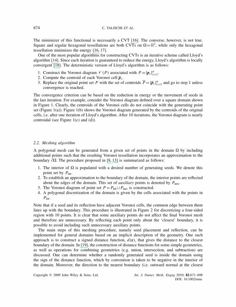
boundary point) is given by the gradient of the distance function at that point (Figure 3). Thismeans that the reflection of point x∈� can be generically computed as:

x=x−2d(x)∇d(x)|∇d(x)| (4)

Figure 4 illustrates example (7) of Reference [19], where the distance function is determined fromthe level set description of the domain boundary. Note that in order to accurately represent thecorners (where there is a jump in the outward normal), it is necessary to reflect the nearby seedsabout both boundary segments incident on that corner.

2.3. Mesh quality

In References [8, 13], it is recommended that the domain interior be populated in a quasi-randommanner by enforcing a minimum allowable distance between the interior points. This minimumseparation eliminates the bunching up of the random points, and can also be used to generategraded meshes. Even with such a measure, the method may produce distorted elements not suitablefor use in finite element analysis. An attractive alternative is to incorporate Lloyd’s algorithm sothat the resulting Voronoi mesh is centroidal. The modified procedure is as follows:

1. Perform one iteration of Lloyd’s algorithm on the point set Pint to obtain the new set ofinterior points P int.

2. Generate the auxiliary point set Paux corresponding to P int.3. Replace P with P= P int∪Paux and go to step 1 until desired level of regularity is reached.

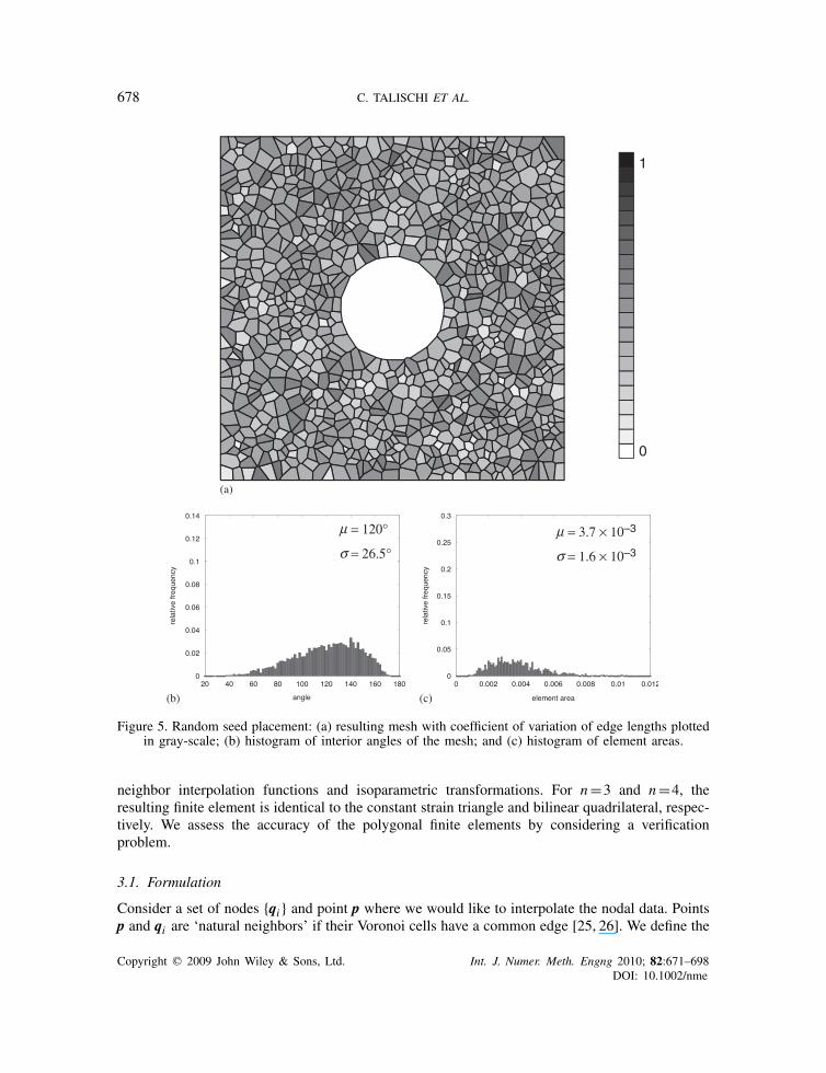
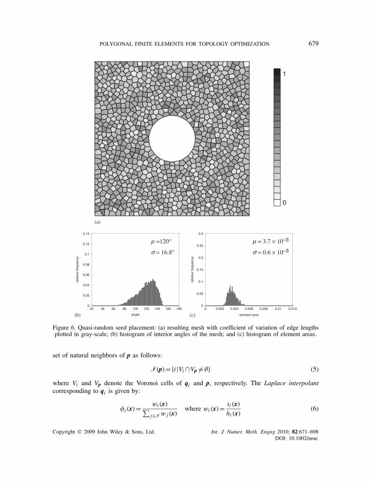
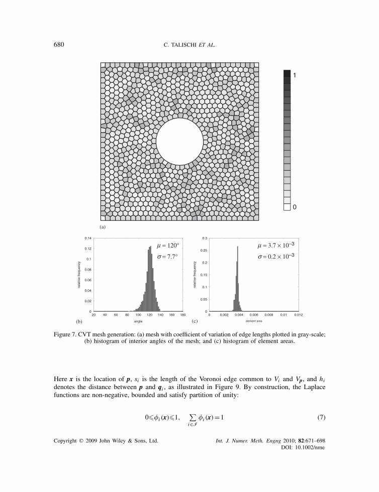
We compare the above-mentioned approaches by considering the discretization of a square domainwith a circular hole using random and quasi-random seed placement, and the proposed procedure.Meshes shown in Figures 5–7 have n=1000 elements. In the case of quasi-random discretization,we use a minimum allowable distance of

√0.68ab/n, as prescribed by Bolander and Saito [8]

for a rectangular domain with dimensions a and b. The CVT mesh was constructed with 100iterations of Lloyd’s algorithm. As a measure of mesh quality, the coefficient of variation of edgelengths for each element is plotted in gray-scale. The coefficient of variation for a regular polygonis zero (indicated as white in the figures) since all the edges have the same length. We observe thatthe CVT mesh is superior to the other two meshes in terms of element quality. The histogramsof interior angles (at the triple joints) and element areas are also shown in these figures. Theseplots indicate that Lloyd’s iterations drive the Voronoi mesh toward a regular hexagonal packing.Moreover, we note that the CVT mesh is significantly more uniform in size over the domain.

Before concluding this section, we remark that since the seeds are placed randomly, the elementand node numbering of the resulting mesh will be random. This, in turn, may cause the stiffnessmatrix to exhibit an undesirable sparsity pattern and suffer from a large bandwidth. A remedy to thisproblem consists of using the heuristic reverse Cuthill–McKee (RCM) algorithm, which is designedto reduce the bandwidth and profile (skyline) of sparse symmetric matrices by systematicallyreordering the node numbers [20]. For example, a typical mesh with 500 elements and 1002 nodeshas the sparsity pattern shown in Figure 8. After applying RCM, the bandwidth is reduced from966 (almost full) to 75. This leads to substantial savings in computational time needed for solvingthe linear systems with direct solvers. Other reordering algorithms (e.g. [21, 22]) and other solvers,including direct sparse solvers (see, for example, [23]) and iterative solvers tailored for topologyoptimization problems [24], can also be explored in this work.

Copyright q 2009 John Wiley & Sons, Ltd. Int. J. Numer. Meth. Engng 2010; 82:671–698DOI: 10.1002/nme

POLYGONAL FINITE ELEMENTS FOR TOPOLOGY OPTIMIZATION 677

Figure 3. Reflecting points about domain boundary using the distance function d(x).

(a)

(b)

(c)

Figure 4. Implicit description of meshing domain: (a) example domain boundaries (taken from [19]);(b) generated distance function; and (c) CVT mesh constructed using the distance function.

3. FINITE ELEMENT SCHEME

In this section, we briefly review the finite element scheme for convex n-gons outlined in [25].This approach constructs a conforming approximation space on polygonal meshes using natural

Copyright q 2009 John Wiley & Sons, Ltd. Int. J. Numer. Meth. Engng 2010; 82:671–698DOI: 10.1002/nme

678 C. TALISCHI ET AL.

(a)

(b) (c)

= 120°

= 26.5°= 3.7 × 10–3

= 1.6 × 10–3

1

0

Figure 5. Random seed placement: (a) resulting mesh with coefficient of variation of edge lengths plottedin gray-scale; (b) histogram of interior angles of the mesh; and (c) histogram of element areas.

neighbor interpolation functions and isoparametric transformations. For n=3 and n=4, theresulting finite element is identical to the constant strain triangle and bilinear quadrilateral, respec-tively. We assess the accuracy of the polygonal finite elements by considering a verificationproblem.

3.1. Formulation

Consider a set of nodes {qi } and point p where we would like to interpolate the nodal data. Pointsp and qi are ‘natural neighbors’ if their Voronoi cells have a common edge [25, 26]. We define the

Copyright q 2009 John Wiley & Sons, Ltd. Int. J. Numer. Meth. Engng 2010; 82:671–698DOI: 10.1002/nme

POLYGONAL FINITE ELEMENTS FOR TOPOLOGY OPTIMIZATION 679

(a)

(b) (c)

= 3.7 × 10–3

= 0.6 × 10–3

=120°

= 16.8°

1

0

Figure 6. Quasi-random seed placement: (a) resulting mesh with coefficient of variation of edge lengthsplotted in gray-scale; (b) histogram of interior angles of the mesh; and (c) histogram of element areas.

set of natural neighbors of p as follows:

I(p)={i |Vi ∩Vp �=∅} (5)

where Vi and Vp denote the Voronoi cells of qi and p, respectively. The Laplace interpolantcorresponding to qi is given by:

�i (x)=wi (x)∑j∈Iw j (x)

where wi (x)= si (x)hi (x)

(6)

Copyright q 2009 John Wiley & Sons, Ltd. Int. J. Numer. Meth. Engng 2010; 82:671–698DOI: 10.1002/nme

680 C. TALISCHI ET AL.

(a)

(b) (c)

1

0

= 3.7 × 10–3

= 0.2 × 10–3

= 120°

= 7.7°

Figure 7. CVT mesh generation: (a) mesh with coefficient of variation of edge lengths plotted in gray-scale;(b) histogram of interior angles of the mesh; and (c) histogram of element areas.

Here x is the location of p, si is the length of the Voronoi edge common to Vi and Vp, and hidenotes the distance between p and qi , as illustrated in Figure 9. By construction, the Laplacefunctions are non-negative, bounded and satisfy partition of unity:

0��i (x)�1,∑i∈I

�i (x)=1 (7)

Copyright q 2009 John Wiley & Sons, Ltd. Int. J. Numer. Meth. Engng 2010; 82:671–698DOI: 10.1002/nme

POLYGONAL FINITE ELEMENTS FOR TOPOLOGY OPTIMIZATION 681

0 200 400 600 800 1000

0

100

200

300

400

500

600

700

800

900

1000

Before resequencing

0 200 400 600 800 1000

0

100

200

300

400

500

600

700

800

900

1000

After resequencing

Figure 8. Sparsity pattern for the stiffness of polygonal mesh with 500 elements and 1002 nodes beforeRCM resequencing (left) and after resequencing (right). The bandwidth is reduced from 966 to 75.

Figure 9. For a convex polygon, every interior point is a natural neighbor to all the vertices. The geometricquantities si and hi used to define the Laplace shape functions are shown here.

Furthermore, it can be shown that these functions are linearly precise:

∑i∈I

xi�i (x)=x (8)

In this expression, xi represents the location of node qi . This property along with constant precision(partition of unity) ensures the convergence of the Galerkin method for second-order partial

Copyright q 2009 John Wiley & Sons, Ltd. Int. J. Numer. Meth. Engng 2010; 82:671–698DOI: 10.1002/nme

682 C. TALISCHI ET AL.

Figure 10. Typical Laplace shape function for a regular hexagon.

differential equations [27]. Moreover, Laplace functions are linear on the boundary of the convexhull of {qi |i ∈I} [28], and satisfy the Kronecker-delta property:

�i (x j )=�ij (9)

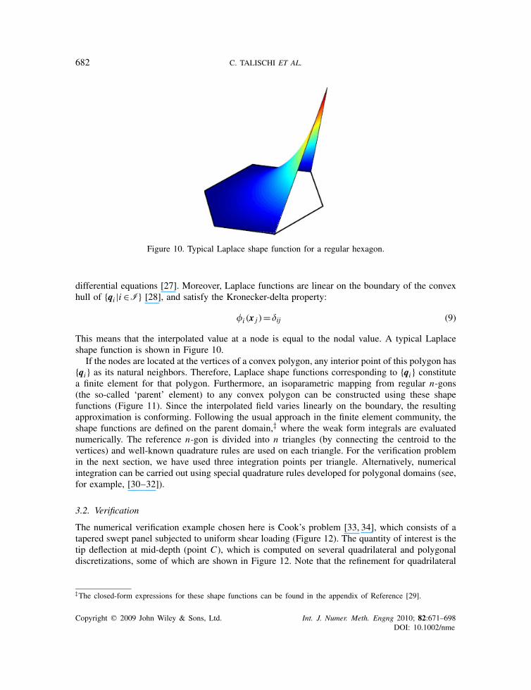
This means that the interpolated value at a node is equal to the nodal value. A typical Laplaceshape function is shown in Figure 10.

If the nodes are located at the vertices of a convex polygon, any interior point of this polygon has{qi } as its natural neighbors. Therefore, Laplace shape functions corresponding to {qi } constitutea finite element for that polygon. Furthermore, an isoparametric mapping from regular n-gons(the so-called ‘parent’ element) to any convex polygon can be constructed using these shapefunctions (Figure 11). Since the interpolated field varies linearly on the boundary, the resultingapproximation is conforming. Following the usual approach in the finite element community, theshape functions are defined on the parent domain,‡ where the weak form integrals are evaluatednumerically. The reference n-gon is divided into n triangles (by connecting the centroid to thevertices) and well-known quadrature rules are used on each triangle. For the verification problemin the next section, we have used three integration points per triangle. Alternatively, numericalintegration can be carried out using special quadrature rules developed for polygonal domains (see,for example, [30–32]).

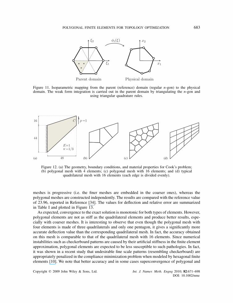
3.2. Verification

The numerical verification example chosen here is Cook’s problem [33, 34], which consists of atapered swept panel subjected to uniform shear loading (Figure 12). The quantity of interest is thetip deflection at mid-depth (point C), which is computed on several quadrilateral and polygonaldiscretizations, some of which are shown in Figure 12. Note that the refinement for quadrilateral

‡The closed-form expressions for these shape functions can be found in the appendix of Reference [29].

Copyright q 2009 John Wiley & Sons, Ltd. Int. J. Numer. Meth. Engng 2010; 82:671–698DOI: 10.1002/nme

POLYGONAL FINITE ELEMENTS FOR TOPOLOGY OPTIMIZATION 683

Figure 11. Isoparametric mapping from the parent (reference) domain (regular n-gon) to the physicaldomain. The weak form integration is carried out in the parent domain by triangulating the n-gon and

using triangular quadrature rules.

(a) (b) (c) (d)

Figure 12. (a) The geometry, boundary conditions, and material properties for Cook’s problem;(b) polygonal mesh with 4 elements; (c) polygonal mesh with 16 elements; and (d) typical

quadrilateral mesh with 16 elements (each edge is divided evenly).

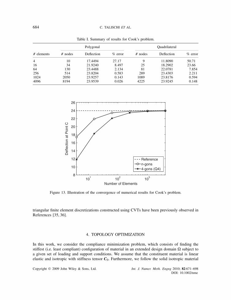
meshes is progressive (i.e. the finer meshes are embedded in the coarser ones), whereas thepolygonal meshes are constructed independently. The results are compared with the reference valueof 23.96, reported in Reference [34]. The values for deflection and relative error are summarizedin Table I and plotted in Figure 13.

As expected, convergence to the exact solution is monotonic for both types of elements. However,polygonal elements are not as stiff as the quadrilateral elements and produce better results, espe-cially with coarser meshes. It is interesting to observe that even though the polygonal mesh withfour elements is made of three quadrilaterals and only one pentagon, it gives a significantly moreaccurate deflection value than the corresponding quadrilateral mesh. In fact, the accuracy obtainedon this mesh is comparable to that of the quadrilateral mesh with 16 elements. Since numericalinstabilities such as checkerboard patterns are caused by their artificial stiffness in the finite elementapproximation, polygonal elements are expected to be less susceptible to such pathologies. In fact,it was shown in a recent study that undesirable fine scale patterns (resembling checkerboard) areappropriately penalized in the compliance minimization problem when modeled by hexagonal finiteelements [10]. We note that better accuracy and in some cases superconvergence of polygonal and

Copyright q 2009 John Wiley & Sons, Ltd. Int. J. Numer. Meth. Engng 2010; 82:671–698DOI: 10.1002/nme

684 C. TALISCHI ET AL.

Table I. Summary of results for Cook’s problem.

Polygonal Quadrilateral

# elements # nodes Deflection % error # nodes Deflection % error

4 10 17.4494 27.17 9 11.8090 50.7116 34 21.9240 8.497 25 18.2902 23.6664 130 23.4488 2.134 81 22.0781 7.854256 514 23.8204 0.583 289 23.4303 2.2111024 2050 23.9257 0.143 1089 23.8176 0.5944096 8194 23.9539 0.026 4225 23.9245 0.148

101

102

103

8

10

12

14

16

18

20

22

24

26

Number of Elements

Def

lect

ion

at P

oint

C

Referencen-gons4-gons (Q4)

Figure 13. Illustration of the convergence of numerical results for Cook’s problem.

triangular finite element discretizations constructed using CVTs have been previously observed inReferences [35, 36].

4. TOPOLOGY OPTIMIZATION

In this work, we consider the compliance minimization problem, which consists of finding thestiffest (i.e. least compliant) configuration of material in an extended design domain � subject toa given set of loading and support conditions. We assume that the constituent material is linearelastic and isotropic with stiffness tensor C0. Furthermore, we follow the solid isotropic material

Copyright q 2009 John Wiley & Sons, Ltd. Int. J. Numer. Meth. Engng 2010; 82:671–698DOI: 10.1002/nme

POLYGONAL FINITE ELEMENTS FOR TOPOLOGY OPTIMIZATION 685

with penalization (SIMP) method, in which the design field is characterized by a density function�(x), and the stiffness tensor follows the power-law relation [37]:

C(x)=[�(x)]pC0, 0<�(x)�1 (10)

To penalize the intermediate densities, the penalty exponent p is taken greater than 1. The minimumcompliance problem is given by

inf�

�(u) subject to∫

��(x)dx�V (11)

where V is a given upper bound for the total volume of structure and u is the displacement fieldcorresponding to the equilibrium configuration:

a(u,v)=�(v) ∀v∈U (12)

Here U={u∈H1(�)|u=0 on ��u} is the space of admissible displacement fields and

a(u,v) =∫

�C(x)e(u) :e(v)dx

�(v) =∫

�f ·vdx+

∫��t

v·tds(13)

are the energy bilinear form and linear form, respectively. In the above expression, f is the bodyforce, t is the traction applied to ��t=��\��u and e is the linearized strain given by:

e(u)= 12 (∇u+∇uT) (14)

To solve this problem numerically, we discretize the displacement field using polygonal finiteelements as described in Sections 2 and 3. The discretization of the density is implicitly carriedout on the same mesh by assuming a constant element density inside each displacement finiteelement �e:

�h(x)=n∑

e=1�e(x)�e where �e(x)=

⎧⎨⎩1, x∈�e

0, x /∈�e

(15)

With this discretization, {�e}ne=1 is the set of design variables. Alternatively, a continuous vari-ation of density can be obtained by sampling the density at the nodal locations and interpo-lating it with the shape functions [38, 39]. As mentioned before, the optimization problem (11)does not have a physical length scale. However, the mesh size induces a length scale on �h ,which effectively translates the ill-posedness of (11) into the mesh dependency of the discretesystem.

We can avoid this issue by imposing an explicit length scale on the problem independent of themesh size. One possibility is to use the projection method [40, 41] which introduces a minimum

Copyright q 2009 John Wiley & Sons, Ltd. Int. J. Numer. Meth. Engng 2010; 82:671–698DOI: 10.1002/nme

686 C. TALISCHI ET AL.

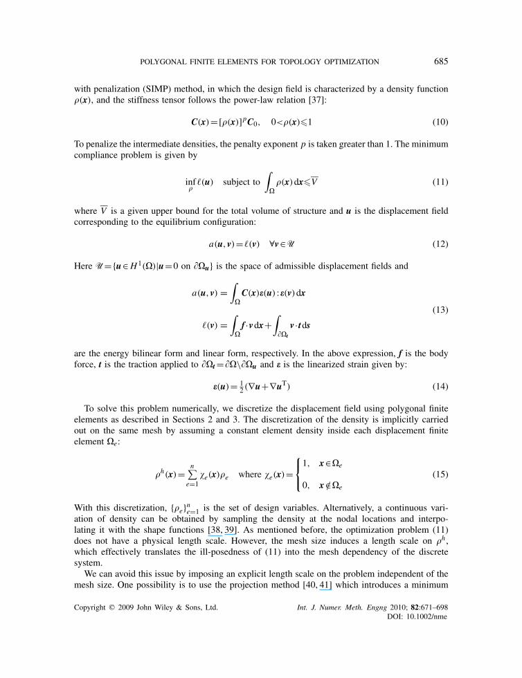
member size, rmin, into the discrete problem by assigning the weighted average of the nearby nodaldensities to each element. Thus, the projected element density becomes:

�e=∑m

i=1wie�

i∑mi=1wi

e(16)

Here {�i }mi=1 is the set of nodal densities (taken as the design variable for the optimization problem)and wi

e is the (linear) weight function defined as:

wie=max

(rmin−r iermin

,0

)(17)

As shown in Figure 14, r ie is the distance from the centroid of element e to node i . We remark thatthis projection is effectively a convolution of the density function with the weight functions. In thecontinuum setting, this amounts to regularizing the density field, which inherits the smoothnessproperties of the weight functions. According to the analysis by Bourdin [42], this convolu-tion removes the ill-posedness of the continuum problem and mesh dependency of the discreteproblem.

5. IMPLEMENTATION ISSUES

In this work, the polygonal finite element meshes are represented by a compact topological datastructure called TopS [43–45]. TopS is designed to provide direct and efficient access to localtopological information about the mesh, and it does so by relying on static element topologytemplates. A template consists of a table with all the topological relationships within an elementand is defined for each element type. Among the information stored in the template are the numberof nodes, vertex-, edge- and facet-uses of the element; the number and local indices of the nodesincident to a given edge- or facet-use; and the number and local indices of the edge- and facet-usesincident to a given vertex-use.

For the most element types (e.g. T 3, T 6, Q4, Q8, Tetra4, Tetra10), topological information iscommon to all the elements of the same type and thus can be efficiently represented by a statictemplate. However, polygonal elements contain a variable number of nodes, vertices, and edges.In order to represent these elements in TopS, we have extended the topological framework withsupport for dynamic templates. In this manner, if topological information is requested from apolygonal element, a virtual method of the element, rather than a static template, is invoked in orderto provide the required data. Moreover, nodal and adjacency data of each polygonal element areallocated dynamically. Although this approach introduces additional costs for polygonal elements,it has a very simple implementation and allows one to represent arbitrary elements in a seamlessway using the existing template-based topological framework of TopS.

The optimization problem described in the previous section is solved using the globally conver-gent method of moving asymptotes (GCMMA) [46, 47]. The algorithm requires the sensitivitiesof the objective and constraint functions, which are straightforward to compute for the minimumcompliance problem (this can be found in several references, for example, see [48]). To avoidconverging to local minima, we perform a continuation on the penalty parameter p by graduallyincreasing its value from p=1 to p=5. For each value of p, we terminate the iterations when themaximum change in the design variables is less than a given tolerance. Unless otherwise stated,

Copyright q 2009 John Wiley & Sons, Ltd. Int. J. Numer. Meth. Engng 2010; 82:671–698DOI: 10.1002/nme

POLYGONAL FINITE ELEMENTS FOR TOPOLOGY OPTIMIZATION 687

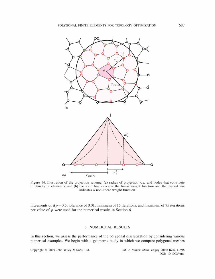
(a)

(b)

Figure 14. Illustration of the projection scheme: (a) radius of projection rmin and nodes that contributeto density of element e and (b) the solid line indicates the linear weight function and the dashed line

indicates a non-linear weight function.

increments of �p=0.5, tolerance of 0.01, minimum of 15 iterations, and maximum of 75 iterationsper value of p were used for the numerical results in Section 6.

6. NUMERICAL RESULTS

In this section, we assess the performance of the polygonal discretization by considering variousnumerical examples. We begin with a geometric study in which we compare polygonal meshes

Copyright q 2009 John Wiley & Sons, Ltd. Int. J. Numer. Meth. Engng 2010; 82:671–698DOI: 10.1002/nme

688 C. TALISCHI ET AL.

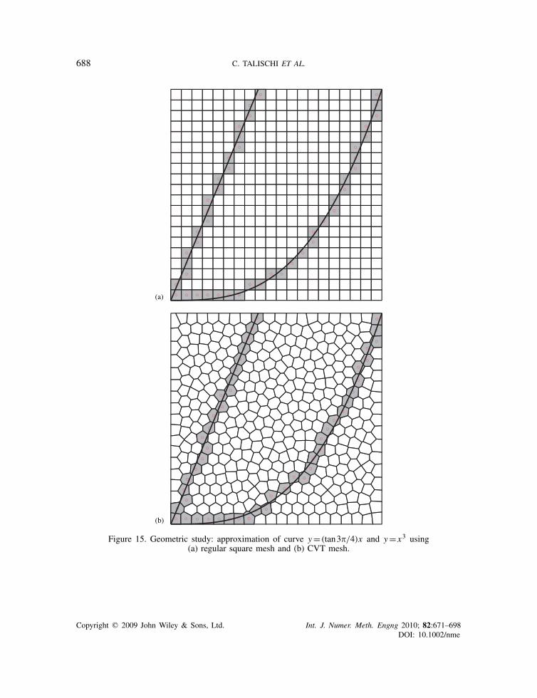
(a)

(b)

Figure 15. Geometric study: approximation of curve y=(tan3�/4)x and y= x3 using(a) regular square mesh and (b) CVT mesh.

Copyright q 2009 John Wiley & Sons, Ltd. Int. J. Numer. Meth. Engng 2010; 82:671–698DOI: 10.1002/nme

POLYGONAL FINITE ELEMENTS FOR TOPOLOGY OPTIMIZATION 689

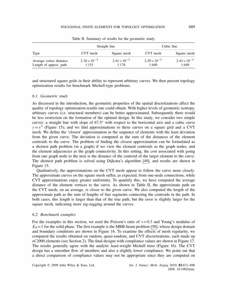
Table II. Summary of results for the geometric study.

Straight line Cubic line

Type CVT mesh Square mesh CVT mesh Square mesh

Average vertex distance 2.18×10−3 2.41×10−3 2.29×10−3 2.43×10−3

Length of approx. path 1.151 1.178 1.649 1.649

and structured square grids in their ability to represent arbitrary curves. We then present topologyoptimization results for benchmark Michell-type problems.

6.1. Geometric study

As discussed in the introduction, the geometric properties of the spatial discretizations affect thequality of topology optimization results one could obtain. With higher levels of geometric isotropy,arbitrary curves (i.e. structural members) can be better approximated. Subsequently there wouldbe less restriction on the formation of the optimal design. In this study, we consider two simplecurves: a straight line with slope of 67.5◦ with respect to the horizontal axis and a cubic curvey= x3 (Figure 15); and we find approximations to these curves on a square grid and a CVTmesh. We define the ‘closest’ approximation as the sequence of elements with the least deviationfrom the given curve. The deviation is computed as the sum of the distances of the elementcentroids to the curve. The problem of finding the closest approximation can be formulated asa shortest path problem (in a graph) if we view the element centroids as the graph nodes, andthe element adjacencies as the graph connectivity. In this setting, the cost associated with goingfrom one graph node to the next is the distance of the centroid of the target element to the curve.The shortest path problem is solved using Dijkstra’s algorithm [49], and results are shown inFigure 15.

Qualitatively, the approximations on the CVT mesh appear to follow the curve more closely.The approximate curves on the square mesh suffer, as expected, from one-node connections, whileCVT approximations enjoy greater uniformity. To quantify this, we have computed the averagedistance of the element vertices to the curve. As shown in Table II, the approximate path onthe CVT mesh, on an average, is closer to the given curve. We also computed the length of theapproximate path as the sum of lengths of line segments connecting the centroids in the path. Inboth cases, this length is larger than that of the true path, but the error is slightly larger for thesquare mesh, indicating more zig-zagging around the curves.

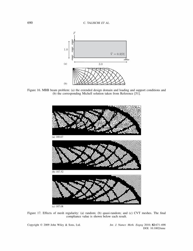
6.2. Benchmark examples

For the examples in this section, we used the Poisson’s ratio of �=0.3 and Young’s modulus ofE0=1 for the solid phase. The first example is the MBB-beam problem [50], whose design domainand boundary conditions are shown in Figure 16. To examine the effects of mesh regularity, wecompared the results obtained on random, quasi-random, and CVT discretizations, each made upof 2000 elements (see Section 2). The final designs with compliance values are shown in Figure 17.The results generally agree with the analytic least-weight Michell truss (Figure 16). The CVTdesign has a smoother flow of members and also a slightly lower compliance. We point out thata direct comparison of compliance values may not be appropriate since they are computed on

Copyright q 2009 John Wiley & Sons, Ltd. Int. J. Numer. Meth. Engng 2010; 82:671–698DOI: 10.1002/nme

690 C. TALISCHI ET AL.

(a)

(b)

Figure 16. MBB beam problem: (a) the extended design domain and loading and support conditions and(b) the corresponding Michell solution taken from Reference [51].

Figure 17. Effects of mesh regularity: (a) random; (b) quasi-random; and (c) CVT meshes. The finalcompliance value is shown below each result.

Copyright q 2009 John Wiley & Sons, Ltd. Int. J. Numer. Meth. Engng 2010; 82:671–698DOI: 10.1002/nme

POLYGONAL FINITE ELEMENTS FOR TOPOLOGY OPTIMIZATION 691

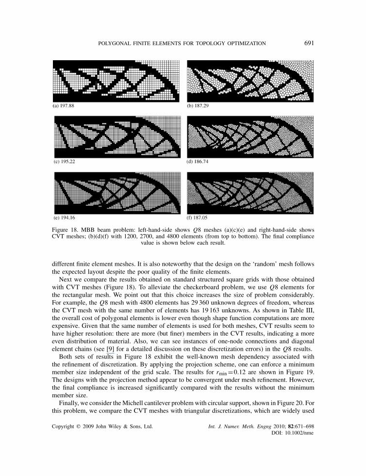
Figure 18. MBB beam problem: left-hand-side shows Q8 meshes (a)(c)(e) and right-hand-side showsCVT meshes; (b)(d)(f) with 1200, 2700, and 4800 elements (from top to bottom). The final compliance

value is shown below each result.

different finite element meshes. It is also noteworthy that the design on the ‘random’ mesh followsthe expected layout despite the poor quality of the finite elements.

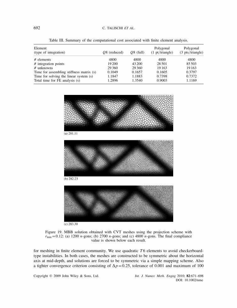
Next we compare the results obtained on standard structured square grids with those obtainedwith CVT meshes (Figure 18). To alleviate the checkerboard problem, we use Q8 elements forthe rectangular mesh. We point out that this choice increases the size of problem considerably.For example, the Q8 mesh with 4800 elements has 29 360 unknown degrees of freedom, whereasthe CVT mesh with the same number of elements has 19 163 unknowns. As shown in Table III,the overall cost of polygonal elements is lower even though shape function computations are moreexpensive. Given that the same number of elements is used for both meshes, CVT results seem tohave higher resolution: there are more (but finer) members in the CVT results, indicating a moreeven distribution of material. Also, we can see instances of one-node connections and diagonalelement chains (see [9] for a detailed discussion on these discretization errors) in the Q8 results.

Both sets of results in Figure 18 exhibit the well-known mesh dependency associated withthe refinement of discretization. By applying the projection scheme, one can enforce a minimummember size independent of the grid scale. The results for rmin=0.12 are shown in Figure 19.The designs with the projection method appear to be convergent under mesh refinement. However,the final compliance is increased significantly compared with the results without the minimummember size.

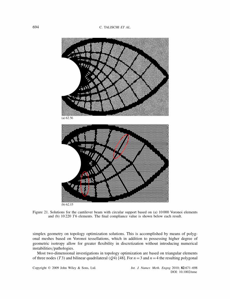
Finally, we consider theMichell cantilever problemwith circular support, shown in Figure 20. Forthis problem, we compare the CVT meshes with triangular discretizations, which are widely used

Copyright q 2009 John Wiley & Sons, Ltd. Int. J. Numer. Meth. Engng 2010; 82:671–698DOI: 10.1002/nme

692 C. TALISCHI ET AL.

Table III. Summary of the computational cost associated with finite element analysis.

Element Polygonal Polygonal(type of integration) Q8 (reduced) Q8 (full) (1 pt/triangle) (3 pts/triangle)

# elements 4800 4800 4800 4800# integration points 19 200 43 200 28 501 85 503# unknowns 29 360 29 360 19 163 19 163Time for assembling stiffness matrix (s) 0.1049 0.1657 0.1605 0.3797Time for solving the linear system (s) 1.1847 1.1883 0.7398 0.7372Total time for FE analysis (s) 1.2896 1.3540 0.9003 1.1169

Figure 19. MBB solution obtained with CVT meshes using the projection scheme withrmin=0.12: (a) 1200 n-gons; (b) 2700 n-gons; and (c) 4800 n-gons. The final compliance

value is shown below each result.

for meshing in finite element community. We use quadratic T 6 elements to avoid checkerboard-type instabilities. In both cases, the meshes are constructed to be symmetric about the horizontalaxis at mid-depth, and solutions are forced to be symmetric via a simple mapping scheme. Alsoa tighter convergence criterion consisting of �p=0.25, tolerance of 0.001 and maximum of 100

Copyright q 2009 John Wiley & Sons, Ltd. Int. J. Numer. Meth. Engng 2010; 82:671–698DOI: 10.1002/nme

POLYGONAL FINITE ELEMENTS FOR TOPOLOGY OPTIMIZATION 693

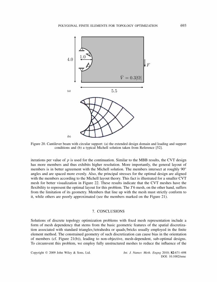
(a)

(b)

Figure 20. Cantilever beam with circular support: (a) the extended design domain and loading and supportconditions and (b) a typical Michell solution taken from Reference [52].

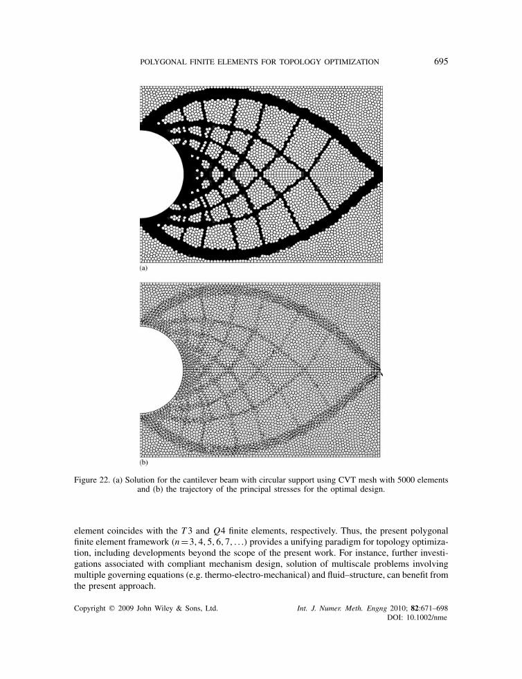
iterations per value of p is used for the continuation. Similar to the MBB results, the CVT designhas more members and thus exhibits higher resolution. More importantly, the general layout ofmembers is in better agreement with the Michell solution. The members intersect at roughly 90◦angles and are spaced more evenly. Also, the principal stresses for the optimal design are alignedwith the members according to the Michell layout theory. This fact is illustrated for a smaller CVTmesh for better visualization in Figure 22. These results indicate that the CVT meshes have theflexibility to represent the optimal layout for this problem. The T 6 mesh, on the other hand, suffersfrom the limitation of its geometry. Members that line up with the mesh must strictly conform toit, while others are poorly approximated (see the members marked on the Figure 21).

7. CONCLUSIONS

Solutions of discrete topology optimization problems with fixed mesh representation include aform of mesh dependency that stems from the basic geometric features of the spatial discretiza-tion associated with standard triangles/tetrahedra or quads/bricks usually employed in the finiteelement method. The constrained geometry of such discretization can cause bias in the orientationof members (cf. Figure 21(b)), leading to non-objective, mesh-dependent, sub-optimal designs.To circumvent this problem, we employ fully unstructured meshes to reduce the influence of the

Copyright q 2009 John Wiley & Sons, Ltd. Int. J. Numer. Meth. Engng 2010; 82:671–698DOI: 10.1002/nme

694 C. TALISCHI ET AL.

Figure 21. Solutions for the cantilever beam with circular support based on (a) 10 000 Voronoi elementsand (b) 10 220 T 6 elements. The final compliance value is shown below each result.

simplex geometry on topology optimization solutions. This is accomplished by means of polyg-onal meshes based on Voronoi tessellations, which in addition to possessing higher degree ofgeometric isotropy allow for greater flexibility in discretization without introducing numericalinstabilities/pathologies.

Most two-dimensional investigations in topology optimization are based on triangular elementsof three nodes (T 3) and bilinear quadrilateral (Q4) [48]. For n=3 and n=4 the resulting polygonal

Copyright q 2009 John Wiley & Sons, Ltd. Int. J. Numer. Meth. Engng 2010; 82:671–698DOI: 10.1002/nme

POLYGONAL FINITE ELEMENTS FOR TOPOLOGY OPTIMIZATION 695

Figure 22. (a) Solution for the cantilever beam with circular support using CVT mesh with 5000 elementsand (b) the trajectory of the principal stresses for the optimal design.

element coincides with the T 3 and Q4 finite elements, respectively. Thus, the present polygonalfinite element framework (n=3,4,5,6,7, . . .) provides a unifying paradigm for topology optimiza-tion, including developments beyond the scope of the present work. For instance, further investi-gations associated with compliant mechanism design, solution of multiscale problems involvingmultiple governing equations (e.g. thermo-electro-mechanical) and fluid–structure, can benefit fromthe present approach.

Copyright q 2009 John Wiley & Sons, Ltd. Int. J. Numer. Meth. Engng 2010; 82:671–698DOI: 10.1002/nme

696 C. TALISCHI ET AL.

NOMENCLATURE

pi generating seed for the Voronoi diagramVi Voronoi cell corresponding to seed piV(P) Voronoi diagram generated from the set of seeds P�(·, ·) Euclidean distance in Rd

�(x) density function defining the centroid of Voronoi cellspi centroid of cell ViE(P) energy functional for diagram V(P)

Pint set of interior seeds for the mesh generation procedurePaux set of auxiliary points for the mesh generation procedured(x) distance function at point xI(p) index set for the natural neighbors of point p�i (x) Laplace shape functionwi (x) weight function used to define the Laplace interpolantssi (x) length of Voronoi edge common to Vi and Vphi (x) distance between p and node qiC0 stiffness tensor for the base materialC(x) stiffness tensor following the SIMP law�(x) material density characterizing the topologyV upper bound for the volume of design� extended design domainU space of admissible displacement fieldsa(·, ·) energy bilinear form�(·) load linear forme(·) linearized strain operatorf body force defined over �t traction applied to ��tu admissible displacement field satisfying equilibrium�h(x) discretization of density field�e(x) characteristic function associated with finite element �e{�e}ne=1 set of element densities{�i }mi=1 set of nodal densitieswie weight function associated with element e and node i

r ie distance from centroid of element e to node irmin prescribed radius of projection

ACKNOWLEDGEMENTS

The first two authors acknowledge the support by the Department of Energy Computational ScienceGraduate Fellowship Program of the Office of Science and National Nuclear Security Administration inthe Department of Energy under contract DE-FG02-97ER25308. The last two authors acknowlege thefinancial support by Tecgraf (Group of Technology in Computer Graphics), PUC-Rio, Rio de Janeiro,Brazil. The authors are grateful to Prof. Krister Svanberg for providing his GCMMA code, which wasused to generate the examples in this paper. Also, the authors thank Prof. John Bolander for providinghis Voronoi meshing code; and Rodrigo Espinha and Prof. Waldemar Celes for their help with theimplementation of polygonal finite elements in the TopS code.

Copyright q 2009 John Wiley & Sons, Ltd. Int. J. Numer. Meth. Engng 2010; 82:671–698DOI: 10.1002/nme

POLYGONAL FINITE ELEMENTS FOR TOPOLOGY OPTIMIZATION 697

REFERENCES

1. Sigmund O, Petersson J. Numerical instabilities in topology optimization: a survey on procedures dealing withcheckerboards, mesh-dependencies and local minima. Structural Optimization 1998; 16(1):68–75.

2. Ambrosio L, Buttazzo G. An optimal design problem with perimeter penalization. Calculus of Variations andPartial Differential Equations 1993; 1(1):55–69.

3. Haber RB, Jog CS, Bendsoe MP. A new approach to variable-topology shape design using a constraint onperimeter. Structural Optimization 1996; 11(1):1–12.

4. Petersson J. Some convergence results in perimeter-controlled topology optimization. Computer Methods inApplied Mechanics and Engineering 1999; 171(1–2):123–140.

5. Pedersen CBW, Buhl T, Sigmund O. Topology synthesis of large-displacement compliant mechanisms.International Journal for Numerical Methods in Engineering 2001; 50(12):2683–2705.

6. Park K, Paulino GH, Celes W, Espinha R. Adaptive dynamic cohesive fracture simulation using edge-swap andnodal pertubation operators. International Journal for Numerical Methods in Engineering, submitted.

7. Papoulia KD, Vavasis SA, Ganguly P. Spatial convergence of crack nucleation using a cohesive finite-elementmodel on a pinwheel-based mesh. International Journal for Numerical Methods in Engineering 2006; 67(1):1–16.

8. Bolander JE, Saito S. Fracture analyses using spring networks with random geometry. Engineering FractureMechanics 1998; 61:569–591.

9. Rozvany GIN, Querin OM, Gaspar Z, Pomezanski V. Weight-increasing effect of topology simplification. Structuraland Multidisciplinary Optimization 2003; 25(5–6):459–465.

10. Talischi C, Paulino GH, Le CH. Honeycomb Wachspress finite elements for structural topology optimization.Structural and Multidisciplinary Optimization 2009; 37(6):569–583.

11. Saxena A. A material-mask overlay strategy for continuum topology optimization of compliant mechanisms usinghoneycomb discretization. Journal of Mechanical Design 2008; 130(8):082304.

12. Aurenhammer F. Voronoi diagrams—a survey of a fundamental geometric data structure. Computing Surveys1991; 23(3):345–405.

13. Yip M, Mohle J, Bolander JE. Automated modeling of three-dimensional structural components using irregularlattices. Computer Aided Civil and Infrastructure Engineering 2005; 20(6):393–407.

14. Lloyd S. Least squares quantization in PCM. IEEE Transactions on Information Theory 1982; 28(2):129–137.15. Preparata FP, Shamos MI. Computational Geometry—An Introduction. Springer: New York, 1985.16. Du Q, Faber V, Gunzburger M. Centroidal Voronoi tessellations: applications and algorithms. SIAM Review 1999;

41(4):637–676.17. Newman D. The hexagon theorem. IEEE Transactions on Information Theory 1982; 28:137–139.18. Du Q, Emelianenko M, Ju L. Convergence of the Lloyd algorithm for computing centroidal Voronoi tessellations.

SIAM Journal on Numerical Analysis 2006; 44:102–119.19. Persson PO, Strang G. A simple mesh generator in MATLAB. SIAM Review 2004; 46:329–345.20. Cuthill E, McKee J. Reducing the bandwidth of sparse symmetric matrices. Proceedings of the 24th National

Conference. ACM Press: New York, NY, U.S.A., 1969; 157–172.21. Paulino GH, Menezes IFM, Gattass M, Mukherjee S. Node and element resequencing using the Laplacian of

a finite element graph. Part I: general concepts and algorithm. International Journal for Numerical Methods inEngineering 1994; 37(9):1511–1530.

22. Paulino GH, Menezes IFM, Gattass M, Mukherjee S. Node and element resequencing using the Laplacian of afinite element graph. Part II: implementation and numerical results. International Journal for Numerical Methodsin Engineering 1994; 37(9):1531–1555.

23. Dongarra JJ, Duff IS, Sorensen DC, van der Vorst HA. Numerical Linear Algebra for High-PerformanceComputers. SIAM: Philadelphia, PA, U.S.A., 1998.

24. Wang S, de Sturler E, Paulino GH. Large-scale topology optimization using preconditioned Krylov subspacemethods with recycling. International Journal for Numerical Methods in Engineering 2007; 69(12):2441–2468.

25. Sukumar N, Tabarraei A. Conforming polygonal finite elements. International Journal for Numerical Methodsin Engineering 2004; 61(12):2045–2066.

26. Sibson R. A vector identity for the Dirichlet tessellation.Mathematical Proceedings of the Cambridge PhilosophicalSociety 1980; 87:151–155.

27. Hughes TJR. The Finite Element Method: Linear Static and Dynamic Finite Element Analysis. Dover: New York,2000.

28. Sukumar N, Moran B, Semenov AY, Belikov VV. Natural neighbour Galerkin methods. International Journalfor Numerical Methods in Engineering 2001; 50(1):1–27.

Copyright q 2009 John Wiley & Sons, Ltd. Int. J. Numer. Meth. Engng 2010; 82:671–698DOI: 10.1002/nme

698 C. TALISCHI ET AL.

29. Tabarraei A, Sukumar N. Application of polygonal finite elements in linear elasticity. International Journal ofComputational Methods 2006; 3(4):503–520.

30. Lyness JN, Monegato G. Quadrature rules for regions having regular hexagonal symmetry. SIAM Journal onNumerical Analysis 1977; 14(2):283–295.

31. Natarajan S, Bordas S, Mahapatra DR. Numerical integration over arbitrary polygonal domains based onSchwarz–Christoffel conformal mapping. International Journal for Numerical Methods in Engineering 2009;80(1):103–134.

32. Mousavi SE, Xiao H, Sukumar N. Generalized Gaussian quadrature rules on arbitrary polygons. InternationalJournal for Numerical Methods in Engineering 2009; DOI: 10.1002/nme.2759.

33. Cook RD, Malkus DS, Plesha ME. Concepts and Applications of Finite Element Analysis (4th edn). Wiley:New York, 2002.

34. Yuqui L, Yin X. Generalized conforming triangular membrane element with vertex rigid rotational freedoms.Finite Elements in Analysis and Design 1994; 17:259–271.

35. Tabarraei A, Sukumar N. Adaptive computations using material forces and residual-based error estimators onquadtree meshes. Computer Methods in Applied Mechanics and Engineering 2007; 196(25–28):2657–2680.

36. Huang Y, Qin H, Desheng W. Centroidal Voronoi tessellation based finite element superconvergence. InternationalJournal for Numerical Methods in Engineering 2008; 76:1819–1839.

37. Bendsoe MP. Optimal design as material distribution. Structural Optimization 1989; 1:193–202.38. Rahmatalla SF, Swan CC. A Q4/Q4 continuum structural topology optimization implementation. Structural and

Multidisciplinary Optimization 2004; 27(1–2):130–135.39. Matsui K, Terada K. Continuous approximation of material distribution for topology optimization. International

Journal for Numerical Methods in Engineering 2004; 59(14):1925–1944.40. Guest JK, Prevost JH, Belytschko T. Achieving minimum length scale in topology optimization using nodal

design variables and projection functions. International Journal for Numerical Methods in Engineering 2004;61(2):238–254.

41. Almeida SRM, Paulino GH, Silva ECN. A simple and effective inverse projection scheme for void distributionin topology optimization. Structural and Multidisciplinary Optimization 2009; 39(4):359–371.

42. Bourdin B. Filters in topology optimization. International Journal for Numerical Methods in Engineering 2001;50(9):2143–2158.

43. Celes W, Paulino GH, Espinha R. A compact adjacency-based topological data structure for finite element meshrepresentation. International Journal for Numerical Methods in Engineering 2005; 64(11):1529–1556.

44. Celes W, Paulino GH, Espinha R. Efficient handling of implicit entities in reduced mesh representations. Journalof Computing and Information Science in Engineering 2005; 5(4):348–359.

45. Paulino GH, Celes W, Espinha R, Zhang Z. A general topology-based framework for adaptive insertion ofcohesive elements in finite element meshes. Engineering with Computers 2008; 24(1):59–78.

46. Svanberg K. The method of moving asymptotes—a new method for structural optimization. International Journalfor Numerical Methods in Engineering 1987; 24(2):359–373.

47. Svanberg K. A class of globally convergent optimization methods based on conservative convex separableapproximations. SIAM Journal on Optimization 2002; 12(2):555–573.

48. Bendsoe MP, Sigmund O. Topology Optimization—Theory, Methods and Applications. Springer: New York, 2003.49. Dijkstra EW. A note on two problems in connexion with graphs. Numerische Mathematik 1959; 1:269–271.50. Olhoff N, Bendsoe MP, Rasmussen J. On CAD-integrated structural topology and design optimization. Computer

Methods in Applied Mechanics and Engineering 1991; 89(1–3):259–279.51. Rozvany GIN. A critical review of established methods of structural topology optimization. Structural and

Multidisciplinary Optimization 2009; 37(3):217–237.52. Suzuki K, Kikuchi N. A homogenization method for shape and topology optimization. Computer Methods in

Applied Mechanics and Engineering 1991; 93(3):291–318.

Copyright q 2009 John Wiley & Sons, Ltd. Int. J. Numer. Meth. Engng 2010; 82:671–698DOI: 10.1002/nme