IEEE TRANSACTIONS ON PATTERN ANALYSIS AND MACHINE INTELLIGENCE, VOL. 13, NO. 3, MARCH 1991

An Effic iently Computable Metric for Comparing Polygonal Shapes

Esther M. Arkin, L. Paul Chew, Daniel P. Huttenlocher, Klara Kedem, and Joseph S. B.

Abstract- Model-based recognition is concerned with comparing a shape A, which is stored as a model for some particular object, with a shape B, which is found to exist in an image. If A and B ate close to being the same shape, then a vision system should report a match and return a measure of how good that match is. To be useful this measure should satisfy a number of properties, including: 1) it should be a metric, 2) it should be invariant under translation, rotation, and change-of-scale, 3) it should be reasonably easy to compute, and 4) it should match our intuition (i.e., answers should be similar to those that a person might give). We develop a method for comparing polygons that has these properties. The method is based on the L2 distance between the turning functions of the two polygons. It works for both convex and nonconvex polygons and runs in time O(mn log mn) where m is the number of vertices in one polygon and n is the number of vertices in the other. We also present some examples to show that the method produces answers that are intuitively reasonable.

Zndex Terms-Computational geometry, distance metric, model-based matching, shape comparison, similarity transformation, turning angle (theta-s) representation.

I. INTRODUCTION

A PROBLEM of both theoretical and practical importance in computer vision is that of comparing two shapes. To what

extent is shape A similar to shape B? Model-based recognition is concerned with comparing a shape A, which is stored as a model for some particular object, with a shape B, which is found to exist in an image. If A and B are close to being of the same shape, then a vision system should report a match and return a measure of how good that match is. Hence, we are interested in defining and computing a cost function d(A, B) associated with two shapes A and B that measures their dissimilarity.

The long-term goal of this research is to develop methods of comparing arbitrary shapes in two or three dimensions. Here, we restrict our attention to polygonal shapes in the plane, with an extension to the case in which a boundary may contain circular arcs in addition to straight line segments. Our technique is designed to work with objects for which the entire boundaries are known.

Before suggesting a measure to be used for comparing poly- gons, we examine several properties that such a measure d(., .)

Manuscript received July 17, 1989; revised October 4, 1990. Recommended for acceptance by G.T. Toussaint. This work was supported in part by the National Science Foundation under Grants DMC 8451984, ECSE 8857642, and DMS 8903304. L.P. Chew and K. Kedem were supported by DARPA under ONR Contract N0014-86-K-0591, NSF Grant DMC-86-17355, and ONR Contract N00014-86-K-0281. J. S. B. Mitchell was supported in part by the National Science Foundation under Grants IRI-8710858 and ECSE 8857642, and by a grant from Hughes Research Laboratories,

E. M. Arkin and J. S. B. Mitchell are with the School of Operations Research and Industrial Engineering, Cornell University, Ithaca, NY 14853.

L. P. Chew and D. P. Huttenlocher are with the Department of Computer Science, Cornell University, Ithaca, NY 14853.

K. Kedem was with the Department of Computer Science, Cornell Univer- sity, Ithaca, NY 14853. She is now with the Department of Computer Science, Tel Aviv University, Tel Aviv, Israel,

IEEE Log Number 9041536.

209

Mitchell

should have (for related arguments see [7]). l It should be a metric.

d(A, B) 2 0 for all A and B. d(A, B) = 0 if and only if A = B. We expect a shape to

resemble itself. d(A, B) = d(B, A) f or all A and B (Symmetry). The order

of comparison should not matter. d(A, B) + d(B, C) 2 d(A, C) for all A, B, and C (Triangle

Inequality). The triangle inequality is necessary since without it we can have a case in which d(A, B) and d(B, C) are both very small, but d(A, C) is very large. This is undesirable for pattern matching and visual recognition applications. If A is very similar to B and B is very similar to C, then A and C should not be too dissimilar.

l It should be invariant under translation, rotation, and change- of-scale. In other words, we want to measure shape alone.

l It should be reasonably easy to compute. This must hold for the measure to be of practical use.

l Most important of all, it should match our intuitive notions of shape resemblance. In other words, answers should be similar to those that a human might give. In particular, the measure should be insensitive to small perturbations (or small errors) in the data. For example, moving a vertex by a small amount or breaking a single edge into two edges should not have a large effect.

A. Representation of Polygons A standard method of representing a simple polygon A is

to describe its boundary by giving a (circular) list of vertices, expressing each vertex as a coordinate pair. An alternative representation of the boundary of a simple polygon A is to give the turning function Oa (3). The function OA (s) measures the angle of the counterclockwise tangent as a function of the arc- length s, measured from some reference point 0 on A’s boundary. Thus Oa (0) is the angle v that the tangent at the reference point 0 makes with some reference orientation associated with the polygon (such as the x-axis). OA(s) keeps track of the turning that takes place, increasing with left-hand turns and decreasing with right-hand turns (see Fig. 1). Formally, if K(S) is the curvature function for a curve, then K(S) = O ’(s) [13]. The curvature function K(S) is frequently used as a shape signature 1% [61, [ill, [141.

Other authors have used a slightly different definition of the turning function in which O,(O) is defined to be 0. Our definition, in which OA(0) is the angle of the tangent line at the reference point, leads to a simple correspondence between a shift of O,(s) in the 6’ direction and a rotation of A. This correspondence is less clear for the alternate definition.

Without loss of generality, we assume that each polygon is resealed so that the total perimeter length is 1; hence, Oa is a

0162-8828/91/030~0209$01.00 0 1991 IEEE

210 IEEE TRANSACTIONS ON PATTERN ANALYSIS AND MACHINE INTELLIGENCE, VOL. 13, NO. 3, MARCH 1991 ” 0

a-

Fig. 1. Defining the turn function O(S).

function from [0, l] to ?l?. For a convex polygon A, @A(S) is a monotone function, starting at some value v and increasing to u + 27r. For a nonconvex polygon, OA(s) may become arbitrarily large, since it accumulates the total amount of turn, which can grow as a polygon “spirals” inward. Although O,(s) may become very large over the interval s E [0, 11, in order for the function to represent a simple closed curve, we must have Q,(l) = Q,(O) + 2 x ( assuming that the origin 0 is placed at a differentiable point along the curve).

The domain of O,(s) can be extended to the entire real line in a natural way by allowing angles to continue to accumulate as we continue around the perimeter of the polygon A. Thus, for a simple closed polygon, the value of OA(S + 1) is @A(S) + 2~ for all s. Note that the function OA(s) is well-defined even for arbitrary (not necessarily simple or closed or polygonal) paths A in the plane. When the path is polygonal, the turning function is piecewise-constant, with jump points corresponding to the vertices of A.

Representation of planar curves (and, in particular, polygons) in terms of some function of arc length has been used by a number of other researchers in computational geometry (e.g., [8], [ll]) and computer vision (cf. [2]) We use this representation to compute a distance function for comparing two simple polygons (A and B) by looking at natural notions of distances between the turning functions eA(s) and Or,(s).

The function OA(s) has several properties which make it especially suitable for our purposes. It is piecewise-constant for polygons (and polygonal paths), making computations particu- larly easy and fast. By definition, the function Q,(s) is invariant under translation and scaling of the polygon A. Rotation of A corresponds to a simple shift of @A(S) in the f3 direction. Note also that changing the location of the origin 0 by an amount t E [0, l] along the perimeter of polygon A corresponds to a horizontal shift of the function OA(s) and is simple to compute [the new turning function is given by OA(s + t)].

n A A

B Fig. 2. Nonuniform noise is problematic for the proposed distance function.

We formally define the distance function between two poly- gons A and B as the L, distance between their two turning functions @A(S) and @B(S), minimized with respect to vertical and horizontal shifts of the turning functions (in other words, we minimize with respect to rotation and choice of reference points). For p = 2 we show that this distance function can be computed efficiently in O(n2 log n) time for polygons with n vertices.

One possible drawback of our distance function is that it may be unstable under certain kinds of noise, in particular, nonuniform noise. For example suppose we have a triangle with one very wiggly side, such as the one shown in Fig. 2. Comparing it to a triangle we will get a very bad (in fact arbitrarily bad) match, because the proportion of the perimeter corresponding to the sides labeled A and B can approach zero. Fortunately, in many computer vision applications it is reasonable to assume that the noise is roughly uniformly distributed over the sides of the polygon, in which case the similarity measure we define performs nicely. See Section IV for examples.

Schwartz and Sharir [ll] have defined a notion of distance similar to ours. However, they compute an approximation based on discretizing the turning functions of the two shapes into many equally spaced points; thus, the quality of the approximation depends on the number of points chosen. Our approach, on the other hand, is to examine the combinatorial complexity of computing the exact metric function between two polygon boundaries, using only the original vertices. Thus, our method runs in time O(nZ log n) where n is the total number of polygon vertices, while their method computes an approximate distance in time O(k log Ic), where k >> n is the total number of inter- polation points used. Furthermore, [ 1 l] suggest “convexifying” nonconvex polygons in order to compare them, as their method does not apply to nonconvex polygons. Our algorithm applies to both convex and nonconvex polygons (and even to nonsimple polygons).

The remainder of this paper is organized as follows. In Section II we give a formal definition of the distance between two polygons based on their turning functions. We prove that this function is a metric and show some of its properties. These results are used in Section III to develop an O(n3) algorithm for computing the distance between two polygons, where n is the total number of vertice.s; we then refine this algorithm to obtain an O(n2 log n) running time. Section IV contains examples of the distance function computed for several polygons using an implementation of our method. Section V is a summary and discussion of extensions and further research.

II. A POLYGON DISTANCE FUNCTION

Consider two polygons A and B and their associated turning functions @a(s) and OR(s). The degree to which A and B are

ARKIN et al.: METRIC FOR COMPARING POLYGONAL SHAPES 211

similar can be measured by taking the distance between the functions OA (s) and OB(s) according to our favorite metric on function spaces (e.g., L, metrics). Define the L, distance between A and B as

b(A>B) = ,,@A -@Blip = (1’ /O/I(S) -Cl,(s),‘&)‘, 0

where 11 . &, denotes the L, norm [9]. 6, has some undesirable properties: it is sensitive to both

rotation of polygon A (or B) and choice of reference point on the boundary of A (or B). Since rotation and choice of reference point are arbitrary, it makes more sense to consider the distance to be the minimum over all such choices. If we shift the reference point 0 along A’s boundary by an amount t, then the new turning function is given by OA(s + t). If we rotate A by angle B then the new function is given by OA(s) + 8. Thus, we want to find the minimum over all such shifts t and rotations B (i.e., over all horizontal and vertical shifts of OA (s)). In other words, we wan to solve for

,Q.A(s + t) - OR(s) + OIPds >

where

D;.B(t, 0) = 1 J

l ,QA(s + t) - OR(s) + Blpds. 0

Lemma 1: d, (A, B) is a metric for all p > 0. Proof: Clearly d,( ., .) is everywhere positive, is symmetric,

and has the identity property, because I/ t 1 Ip is a metric and has these properties. We now show that d,(., .) also obeys the triangle inequality, d,(A, B) + d,(B, C) > d,(A, C), by a straightforward application of the Minkowski inequality for L, metrics.

Let tab and 6ob be the minimizers of d,(A, B) (i.e., d,(A, B) = [Di.B(tob, ti”b)] I”). Similarly let tbc and Obc be the minimizers of d,(B. C). We define t’ = tab + tbc and 8’ = Bnb + Obc. Now, d,(A: B) + d,(B: C) =

= [.I

’ ’ ,Qs,(s + tab) - OR(s) + BablPds 0 1

+ [s

l I@B(S + tbc) - @C(S) + 6&lPds ’ 0 1

= [.i

’ ’

IQAcS + tub + t/r) - @B(s + tbc) + @,blPds 0 1

+ [I

' ,@B(S + tbc) - o,(s) + &,,Pds ' 0 1

which by the Minkowski inequality (cf. 191) is

> - [I

’ ,Q.A(s + tab + tbc) - @B(s + tbr) + Bab 0

+ OB(S + tbc) - @c(S) + &lPds 1 = [J1~qs+ty~c(s)+qpds 1 ’

= &.‘(1’, 00.

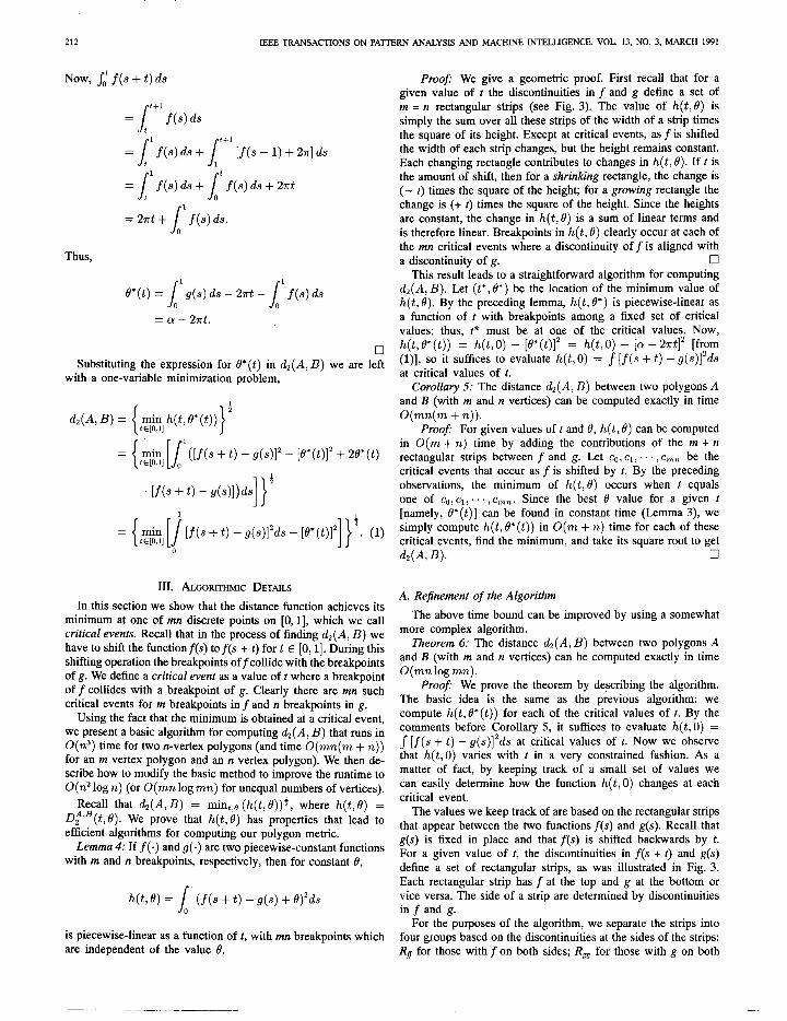
O,(S)

Fig. 3. The rectangular strips formed by the functions @a(s) and @B(S).

Clearly DAsC(t’, 0’) > d,(A, C) because the latter is minimized over all vilues of t aid 0 including t’ and 8’. 0

Lemma 2: For any fixed value of t, and for any p 2 1, D,A,B(t, 0) is a convex function of 19.

Proof: For fixed s and fixed t, the function F(0) = ,@.4(s + t) - @B(s) + 6,’ is clearly a convex function by the convexity of G(y) = IyIp (for p 2 l), and integrating a convex function maintains convexity (i.e., if a positive valued function 7(x, y) is convex in y for fixed x, then s y(z, y) dx is also a convex function of y). 0

In particular, using the L2 metric, Dt’B(t, 0) is a quadratic function of 0 for any fixed value of t. This holds for any closed shapes, but it is especially easy to see for polygons.

We assume from now on that A and B are polygons. Then, for a fixed t, the integral so* I@.4(s + t) - O*(s) + 8j2ds can be computed by adding up the value of the integral within each strip defined by a consecutive pair of discontinuities in O.4 (s) and OR(s) (see Fig. 3). The integral within a strip is trivially computed as the width of the strip times the square of the difference IQA(s + t) - @g(s) 1 (which is constant within each strip). Note that if m and II are the numbers of the vertices in A and B, respectively, then there are m + n strips and that as 8 changes, the value of the integral for each strip is a quadratic function of 0.

In order to compute d,(A, B), we must minimize Dt,B(t, 6’) over all t and 0. We begin by finding the optimal 0 for any fixed value of t. To simplify notation in the following discussion, we use f(s) = O,4(s), g(s) = @B(s), and h(t, 8) = Df’“(t, 0).

Lemma 3: Let h(t. 0) = 1; (f(s + t) - g(s) + fI)‘ds. Then, in order to minimize h(t, 0), the best value of 6’ is given by

O*(t) = J

o1 (g(s) - f(s + t)) ds

= a - 27Tt.

where o = Jig(s)& - sd f(s)ds. Proof:

WC 0) _ do J

’ (20 + 2f(s + t) - 2g(s)) ds 0

= 26’ + 2 J

o1 (f(s + t) - g(s)) ds.

Lemma 2 assures us that the minimum occurs when we set this quantity equal to zero and solve for 8. Thus,

O*(t) = J

’ (g(s) - f(s + t)) ds. 0

212 IEEE TRANSACTIONS ON PATTERN ANALYSIS AND MACHINE INTELLIGENCE, VOL. 13, NO. 3, MARCH 1991

Now, so1 f(s + t) ds

J t+1

= t f(s)ds

= 2rt + J o’f(s)ds.

Thus,

J 1

e*(t) = g(s) ds - 2rt - 0 J o’fWs

= cl! - 2&.

0 Substituting the expression for 8*(t) in dz(A, B) we are left

with a one-variable minimization problem,

&(A, B) = { ’

’ t’Etonl h(t, O* (t))

= 1 [s gj&, o’(lf(s + Q - g(s)]’ - [e*(t)]’ + 20*(t)

I> 1

. MS + t) - g(4) ds 1 =

{ [I $j, [f(s + t) - d4l”ds - P*(t>l’ I> 1 . (9

0

III. ALGORITHMIC DETAILS

In this section we show that the distance function achieves its minimum at one of mn discrete points on [0, 11, which we call critical events. Recall that in the process of finding d2(A, B) we have to shift the function f(s) to f(s + t) for t E [0, 11. During this shifting operation the breakpoints off collide with the breakpoints of g. We define a critical event as a value of t where a breakpoint off collides with a breakpoint of g. Clearly there are mn such critical events for m breakpoints in f and n breakpoints in g.

Using the fact that the minimum is obtained at a critical event, we present a basic algorithm for computing d2(A, B) that runs in O(n3) time for two n-vertex polygons (and time O(mn(m + n)) for an m vertex polygon and an n vertex polygon). We then de- scribe how to modify the basic method to improve the mntime to O(n2 log n) (or O(mn log mn) for unequal numbers of vertices).

Recall that d,(A,B) = min,,e (h(t,e))j, where h(t,0) = DfaB(t, 0). We prove that h(t, 0) has properties that lead to efficient algorithms for computing our polygon metric.

Lemma 4: If f( .) and g( .) are two piecewise-constant functions with m and n breakpoints, respectively, then for constant 8,

h(4 0) = J o1 (f(s + t) - g(s) + O)2ds

is piecewise-linear as a function of t, with mn breakpoints which are independent of the value 8.

Proof: We give a geometric proof. First recall that for a given value of t the discontinuities in f and g define a set of m = n rectangular strips (see Fig. 3). The value of h(t, 0) is simply the sum over all these strips of the width of a strip times the square of its height. Except at critical events, as f is shifted the width of each strip changes, but the height remains constant. Each changing rectangle contributes to changes in h(t, 0). If t is the amount of shift, then for a shrinking rectangle, the change is (- r) times the square of the height; for a growing rectangle the change is (+ t) times the square of the height. Since the heights are constant, the change in h(t, 8) is a sum of linear terms and is therefore linear. Breakpoints in h(t, 0) clearly occur at each of the mn critical events where a discontinuity off is aligned with a discontinuity of g. 0

This result leads to a straightforward algorithm for computing d,(A, B). Let (t*,19*) be the location of the minimum value of h(t, 0). By the preceding lemma, h(t, 19*) is piecewise-linear as a function of t with breakpoints among a fixed set of critical values; thus, t* must be at one of the critical values. Now, h(t,O*(t)) = h(t, 0) - [O*(t)]’ = h(t,O) - [a - 27rt]* [from (l)], so it suffices to evaluate h(t, 0) = s [f(s + t) - g(s)}‘ds at critical values of t.

Corollary 5: The distance d,(A, B) between two polygons A and B (with m and n vertices) can be computed exactly in time O(mn(m + n)).

Proof: For given values oft and 0, h(t, 0) can be computed in O(m + n) time by adding the contributions of the m + n rectangular strips between f and g. Let Q,, cl, . . + , c,, be the critical events that occur as f is shifted by t. By the preceding observations, the minimum of h(t, 0) occurs when t equals one of Q,c~,...,c,,. Since the best 19 value for a given t [namely, O*(t)] can be found in constant time (Lemma 3), we simply compute h(t, O*(t)) in O(m + n) time for each of these critical events, find the minimum, and take its square root to get &(A, B). q

A. Refinement of the Algorithm

The above time bound can be improved by using a somewhat more complex algorithm.

Theorem 6: The distance d2(A, B) between two polygons A and B (with m and n vertices) can be computed exactly in time O(mn log mn).

Proof: We prove the theorem by describing the algorithm. The basic idea is the same as the previous algorithm: we compute h(t,O*(t)) for each of the critical values of t. By the comments before Corollary 5, it suffices to evaluate h(t, 0) = J [f(s + t) - d412d s a critical values of t. Now we observe t that h&O) varies with t in a very constrained fashion. As a matter of fact, by keeping track of a small set of values we can easily determine how the function h(t,O) changes at each critical event.

The values we keep track of are based on the rectangular strips that appear between the two functions f(s) and g(s). Recall that g(s) is fixed in place and that f(s) is shifted backwards by t. For a given value of t, the discontinuities in f(.s + t) and g(s) define a set of rectangular strips, as was illustrated in Fig. 3. Each rectangular strip has f at the top and g at the bottom or vice versa. The side of a strip are determined by discontinuities in f and g.

For the purposes of the algorithm, we separate the strips into four groups based on the discontinuities at the sides of the strips: Rf for those with f on both sides; R, for those with g on both

-

ARKIN et&: METRIC FOR COMPARING POLYGONAL SHAPES 213

sides; Rfg for those with f on the left and g on the right; and R, for those with g on the left and f on the right. The sets Rfg and Rti are particularly important, as these are the strips whose widths change as t changes (as f is shifted). Thus, these strips affect the slope of h(t,O).

We keep track of two quantities: Hfg and Hti Hfg is the sum of the squares of all the heights of all the strips in Rfg, and Hgf is the sum of the squares of the heights of all the strips in Rti

The algorithm is based on the observation that for values of t between two critical events the slope of h(t, 0) is Hfg - Hti This follows from the fact that, as f is shifted backwards by t, R,, is the set of all strips that increase in width by t, and Rd is the set of all strips that decrease in width by t. The widths of the RR and R, strips remain unchanged.

Consider what happens at one of the critical events, where the change is no longer simply linear. We claim that quantities Hfg and Hti can be easily updated at these points. To see this note that, at a critical event, a gf-type strip disappears (its width goes to zero) and a new fg-type strip appears (see Fig. 3). At the same time, the right boundary of the adjacent strip to the left is converted from g to f, and the left boundary of the adjacent strip to the right is converted from f to g. To update Hfg and Hgf- we need to know just the values off and g around the critical event.

This gives us the following algorithm. 1) Initialize:

l Given the piecewise-constant functions f and g, deter- mine the critical events: the shifts off by t such that a discontinuity in f coincides with a discontinuity in g. Sort these critical events by how far f must be shifted for each event to occur. Let c,,, cl, . . . , c, be the ordered list of shifts for the critical events c0 = 0.

l Calculate h(0, 0). This involves summing the contribu- tions of each of m + n strips and takes linear time.

l Determine initial values for Hfg and Hti

2) For i = 1 to e

l Determine the value of

h(c,,O) = (H,, - Hgr)(cz - ~1) + h(ct--1,0).

l Update Hrg and Hti

The algorithm takes advantage of the fact that h(t,O) is piecewise-linear as a function of t; thus, the entire function can be determined once we know an initial value and the slope for each piece. It is easy to see that the time for initialization is dominated by the time it takes to sort the critical events: O(elog e), where e is the number of critical events, or O(mnlogmn) where m and n are the sizes of the two polygons. The updates required for the remainder of the algorithm take a total of O(e), or O(mn) time.

0 In practice, it might be useful to recalculate h(t, 0) periodically

from scratch to avoid errors that could accumulate. If this is done every O(c) steps then the time bound for the entire algorithm remains O(eloge).

IV. EXAMPLES

In this section we illustrate some of the qualitative aspects of the distance function dz(A, B) by comparing some simple polygons using the algorithm described in the previous section. In addition to providing a distance d,(A, B), between two polygonal

Fig. 4. Comparing two simple polygons.

shapes, the method gives the relative orientation 0* and the corresponding reference points of the two polygons for which this distance is attained.

The first example compares two simple polygons that are very similar in shape, but which are at different orientations (see Fig. 4). The value of &(A, B) is 0.144 which is attained at a rotation of 180 degrees and with the upper left vertex of the first polygon matched with the lower right vertex of the second one. (Distances less than about 0.5 seem to correspond to polygons that a person would rate as resembling each other; pairs of polygons that are very different can have arbitrarily high distances.)

To illustrate how the distance function can be used to compare a model with several different instances, we consider the eight shapes illustrated in Fig. S(a) and 5(b). In Fig. 5(a) the shapes are ordered by their distance from the square; in 5(b) the same shapes are ordered by their distance from the triangle. The order of the shapes corresponds remarkably well to our intuitive idea of shape-resemblance. The match to the cutoff triangles suggests that the metric is useful for matching partially occluded objects, as long as the overall shape of the object does not change too radically.

Our metric also provides a qualitatively good estimate of a match when one polygon is an instance of another, but with some perturbation of its boundary. A simple example is given by the cutoff triangle in Fig. 5. Another example is given in Fig. 6, where we compare a model rectangle against another rectangle with a notch removed. The distance is 0.327 with a relative orientation of 179 degrees.

An extreme case of matching distorted polygons is shown in Fig. 7, where a triangle is compared with a somewhat triangular shape. In this case the distance is 0.834, and the orientation difference is 16 degrees. Note however, that, as mentioned in the introduction (see Fig. 2), such perturbations must occur relatively uniformly along the perimeter of the polygon for the match to be reasonable. (A smoothing technique is likely to alleviate the problem of nonuniform perturbations.)

V. SUMMARY AND DISCUSSION

We have suggested using the L2 metric on the turning functions of polygons as a way to implement the intuitive notion of shape-resemblance. This method for comparing shapes has the following advantages:

l It is a metric on polygonal shapes. l It compares shape alone; it is invariant under translation,

rotation, and change-of-scale. l It is reasonably easy to compute, taking time O(mn log mn)

to compare an m vertex polygon against an n vertex polygon. l Finally, it corresponds well to intuitive notions of shape

resemblance.

214 IEEE TRANSACTIONS ON PAlTERN ANALYSIS AND MACHINE INTELLIGENCE, VOL. 13, NO. 3, MARCH 1991

Fig. 5. Comparing several polygons.

Fig. 6. A rectangle with a notch removed.

Fig. 7. Matching a triangle to a highly noisy shape.

In addition, this metric works for nonconvex as well as convex polygons, and even works for polygonal shapes that are not simple.

A number of other authors have considered the problem of determining the extent to which one shape resembles another (e.g., [l], [3], [5], [8], [lo], [ll]). In contrast to our distance

function, these methods either are not metrics, do not compare shapes independent of position, orientation and scale, or are not efficient to compute. The most similar method to ours is that of Schwartz and Sharir [ll], [12]. Huttenlocher and Kedem [4] have recently developed a metric for comparing polygonal shapes independently of an affine transformation, thus extending our results to a more general class of shape transformations. Their method computes a distance based on the Hausdorff metric, and also runs in time O(mnlogmn).

Like the method of [ll], [12], our method is actually based on a convolution. Recall that the major portion of our algorithm is devoted to minimizing h(t, 0) = s, (f(s + t) - g(s) + 8)2ds. When this formula is multiplied out, all the terms depend on f alone or g alone, except for the convolution term J; f(s + t)g(s) ds. If f an g are piecewise-constant with m and d n discontinuities, respectively, then each term can be calculated in either O(m) or O(n) time except for the convolution term, which seems to require O(mn log mn) time. Of course, the fast Fourier transform (FFT) can be used to compute a convolution in 0( Ic log k) time, but this requires k evenly spaced sample points for each off and g. For our problem, the discontinuities are not necessarily evenly spaced, so the FFT cannot be used unless we are willing to approximate our functions f and g. A good approximation may require more than mn points. (Schwartz and Sharir [ll] avoid these discontinuities by rotating the turning functions. This makes it possible to use the FFT, although it restricts their method to convex polygons.) In any case, the development of a fast method for convolutions using unevenly spaced sample points would lead to improvements in the time bound for our technique.

We used the L2 metric, but similar techniques can be used to develop polygon-resemblance metrics that are based on different function-space metrics. Unfortunately, not all such metrics have L2’s advantages of being reasonably easy to compute and match- ing our intuitive idea of shape resemblance. For instance, it is also possible to compute the L1 metric on two O(s) functions using an algorithm similar to that in Section III. In the case of the L1 metric, however, the value of 0* is not given directly for each value of t as it is for the L2 metric. Thus for each of the mn critical events, the optimal value of 8 must be computed explicitly. Using a data structure similar to that in Section III, the overall computation can be done in time O(n3 log n), as opposed to O(n2 logn) for the L2 metric.

The L1 metric has an additional drawback: the optimal match will occur when one side of polygon A is at the same orientation as some side of polygon B. This is because @ ‘“(t, 0) is a piecewise linear in both t and 0, so the minimum occurs at a critical event in 19 as well as at a critical event in t. In contrast, the L2 metric finds the optimal orientation (in a least squares sense) without requiring any two edges to be identically oriented. Examine Fig. 8 to see why requiring identical orientations can be undesirable; for the L1 metric the best match occurs at an orientation difference of 76 degrees, bringing two edges into alignment. This would rotate the two figures so that they approximately form a star, a bad match. In contrast, for the Lz metric the best match is at an orientation difference of 7 degrees, which agrees quite well with our intuitive sense of the best match.

It may be possible to apply our methods to problems involving partially occluded objects, that is objects for which the entire model is known, but for which only a portion of the boundary appears in the image. Our technique as presented here has not been designed to work with such objects, although, as shown by some of our examples, it seems to give intuitively correct answers

-

ARKIN ef al.: METRIC FOR COMPARING POLYGONAL SHAPES 215

Fig. 8. A match for which the Lt metric does poorly but the Lz does well.

when objects are not severely occluded. The combination of occluded objects and our desire to make our metric independent of change-of-scale causes some difficulty. We were able to control change-of-scale problems by normalizing our polygons to make all perimeters have length one. If portions of a boundary are unknown then it is unclear how this normalization should be done. If the scale of the image is known, then partially occluded objects should not present any severe difficulties.

Our results can be generalized to include cases in which the shapes A and B have some or all of their boundary represented as circular arcs. If A includes some circular arcs on its boundary, then the turning function o(s) is piecewise-linear instead of piecewise-constant. As before, to compare shapes A and B we need to minimize

h(t, 0) = .I

* l%(s + t) - @B(S) + 012ds. 0

[4] D.P. Huttenlocher and K. Kedem, “Computing the minimum Hausdorff distance for point sets under translation,” in Proc. ACM Symp. Computational Geometry, 1990, pp. 340-349.

151 J. Hone and X. Tan. “The similaritv between shapes under affine transformation,” in Proc. Second Int. Conj Comp2er Vision. Washington, DC: IEEE Comput. Sot. Press, 1988, pp. 489-493.

[6] J. Hong and H.J. Wolfson, “An improved model-based match- ing method using footprints,” in Proc. Ninth Int. Co@ Pattern Recognition, Rome, Italy, Nov. 14-18, 1988.

[7] D. Mumford, “The problem of robust shape descriptors,” in Proc. First Int. Co@ Computer Vision. Washington, DC: IEEE Comput. Sot. Press, 1987, pp. 602-606.

[B] J. O’Rourke and R. Washington, “Curve similarity via signatures,” in Computational Geometry, G. Toussaint, Ed. Amsterdam, The Netherlands: North-Holland, 1985, pp. 295-318.

[9] H. L. Royden, Real Analysis. New York: Macmillan, 1968. [lo] L.G. Shapiro and R. M. Haralick, “Organization of relational

models for scene analvsis,” IEEE Trans. Pattern Anal. Machine Intell., vol. PAMI-4, no. 6 pp. 595-602, 1982.

1111 J. T. Schwartz and M. Sharjr. “Some remarks on robot vision,” New L 1

York Univ., Courant Inst. Math. Sci., Tech. Rep. 119, Robotics Rep. 25, Apr. 1984.

[12] -, “Identification of objects in two and three dimensions by matching noisy characteristic curves,” Int. J. Robotics Res., vol. 6, no. 2, pp. 29-44, 1987.

-131 J. J. Stoker, Differential Geometry. New York: Wiley, 1969. ‘141 H. Wolfson. “On curve matching,” in Proc. IEEE Workshop Com-

. 1

puter Vision, Miami Beach, FL,Nov. 30-Dec. 2, 1987.

The derivation of O*(t) does not change at all, because h(t, 0) is still a quadratic function of 8. But if the shapes include circular arcs, then h can be piecewise-cubic as a function of t for fixed 0 (instead of simply piecewise-linear). Thus, the minimum value of h(t, 0) does not necessarily occur at a critical event, and more information is needed in order to determine the behavior of h between critical events.

However, since h(t,e*(t)) 1s recewise-cubic as a function p’ of t, we can determine the behavior of h between critical events if we have enough data points for h. If we collect two additional (t, h(t, 0*(t))) p airs between each adjacent pair of critical events then we can determine the coefficients of h(t, 8*(t)) (= alt” + a2t2 + a3t + Q) between critical events) and compute the minimum analytically. Thus, the basic approach of calculating h(t, 0) in O(m + n) time for each of O(mn) values is still valid and there is an algorithm that runs in time O(mn(m + n)). The 0( mn log mn) time algorithm can also be generalized to work with circular arcs, and the resulting algorithm has the same asymptotic time bound. The number of updates needed and the resulting accumulation of roundoff error may be problematic in practice.

ACKNOWLEDGMENT

We would like to thank K. Zikan for suggesting the L2 norm over the L1 norm.

REFERENCES

[l] D. Avis and H. ElGindy, “A combinatorial approach to polygon similarity,” IEEE Trans. Inform. Theory, vol. 29, 1983

[2] D.H. Ballard and C. M. Brown, Computer Vision. Englewood Cliffs, NJ: Prentice-Hall, 1982.

(31 P. Cox, H. Maitre, M. Minoux, and C. Ribeiro, “Optimal matching of convex polygons,” Pattern Recognition Lett., vol. 9, pp. 327-334, 1989.

Esther M. Arkin received the B.S. degree in mathematics from Tel Aviv University in 1981, and the MS. and Ph.D. degrees in operations research from Stanford University in 1983 and 1986 respectively.

Since graduation in 1986, she has been a Visiting Assistant Professor in the School of Operations Research and Industrial Engineering at Cornell University, where she conducts re- search in graph theory, computational geometry, scheduling, and optimization.

L. Paul Chew received the B.Sc. and M.S. degrees in mathematics and the Ph.D. degree in computer science from Purdue University in 1973, 1975, and 1981, respectively.

He was a faculty member at Dartmouth Col- lege until 1988 when he began his current po- sition as a Senior Research Associate in the Department of Computer Science at Cornell University. His research interests include com- putational geometry, design and analysis of al- gorithms, and mesh generation.

Daniel P. Huttenlocher received the B.S. de- gree from the University of Michigan in I 980 and the MS. and Ph.D. degrees from the Mass- achusetts Institute of Technolonv in 1984 and

“I

1988, respectively. He is currently an Assistant Professor in the

Department of Computer Science at Cornell University, and a member of the Research Staff at the Xerox Palo Alto Research Center. His research interests are in the areas of computer vision, computational geometry, speech recog- nition, and artificial intelligence.

216 IEEE TRANSACTIONS ON PA’ITERN ANALYSIS AND MACHINE INTELLIGENCE, VOL. 13, NO. 3, MARCH 1991

Klara Kedem received the B.A. degree in mathematics and philosophy in 1971, the M.Sc. degree in computer science in 1982 under the supervision of professor A. Pnueli, and the Ph.D. degree in 1989 under the supervision of professor M. Sharir, at Tel Aviv University.

In 196991983 she worked as a Software Engineer in developing scientific software. In 1989 she held a Visiting Scientist position at Cornell University. Currently she is in a research position at Tel Aviv University doing research in computational geometry and its applications in robotics and computer vision.

research interests are algorithms, computer

Dr. Mitchell is a chinery, the Operatic Computer Society.

Joseph S.B. Mitchell received the B.S. degree in applied mathematics and physics and the M.S. degree in mathematics from Carnegie-Mellon University, Pittsburgh, PA, both in 1981, and the Ph.D. degree in operations research from Stanford University in i986.

During his time at Stanford, he worked at the HughYes Artificial Intelligence Research Cen- ter. Since graduation, he has been an Assistant Professor of Ooerations Research and Industrial Engineering at’Cornel1 University. His primary

in the fields of computational geometry, design of vision, and optimization. member of the Association for Computing Ma-

ens Research Society of America, and the IEEE