A computable approach to measure and integration theory

Abbas EdalatDepartment of Computing

Imperial College London, UKae@doc.ic.ac.uk

Abstract

We introduce a computable framework for Lebesgue’s measure and integration theory in the spirit of domaintheory. For an effectively given second countable locally compact Hausdorff space and an effectively given finiteBorel measure on the space, we define a recursive measurable set, which extends the corresponding notion dueto Sanin for the Lebesgue measure on the real line. We also introduce the stronger notion of a computable mea-surable set, where a measurable set is approximated from inside and outside by sequences of closed and opensubsets respectively. The set of recursive measurable subsets and that of computable measurable subsets are bothclosed under complementation, finite unions and finite intersections. The more refined property of computablemeasurable sets give rise to the idea of partial measurable subsets, which naturally form a domain for measur-able subsets. We then introduce interval-valued measurable functions and develop the notion of recursive andcomputable measurable functions using interval-valued simple functions. This leads us to the interval versions ofthe main results in classical measure theory. The Lebesgue integral is shown to be a continuous operator on thedomain of interval-valued measurable functions and the interval-valued Lebesgue integral provides a computableframework for integration: The Lebesgue integral of a bounded recursive or computable measurable function withrespect to an effectively given finite Borel measure on an effectively given compact second countable Hausdorffspace can be computed up to any required accuracy.

Key Words: Domain theory, data type, recursive and computable measurable set, partial measurable set, interval-valued measurable function, interval-valued Lebesgue integral.

Double Dedication: This paper is dedicated to the historical memory of Jamshid Kashani (d. 1429), theIranian mathematician who was the first to use the recursive fixed point method in analysis with whichhe computed sin 1◦ correct to 9 sexagesimal places; he is also well-known for computing π to 16 decimalplaces [3, pages 7 and 151]. This work is also dedicated to my colleague and friend Giuseppe Longoon the occasion of his sixtieth birthday to commend him for his wide range of interdisciplinary researchinterests and for his internationalist outlook on human culture.

1. Introduction

In the past decades, there has been a wide range of applications of measure and integration theory in differentbranches of computer science including in probabilistic semantics [24, 18], stochastic hybrid systems [2] andlabelled Markov processes [11, 7]. Nevertheless, a systematic general framework for computability in measureand integration theory still remains in its infancy.

1

Computability of continuous functions and their integrals has been addressed by different schools in computableanalysis (for example [22, p 37] and [27, p 182]). In early 1990’s, the author developed a domain-theoreticframework for measure and integration theory which gave rise to a generalized Riemann integral [9, 8, 10, 12, 19, 1,20]. It has provided a computable framework for measure theory and a generalised Riemann theory of integration.However, this theory only deals with almost everywhere continuous functions and not with measurable functionsin general. Computability of measures on the unit interval has also been developed in type two theory [26] and, inaddition, by using the Prokhorov distance in the metric space of measures [15].

Computability of measurable subsets has a different story. In 1950’s, based on the Russian approach to com-putability in analysis, N. A. Sanin [25] initiated research into computability of measurable sets in Euclidean spaceswith respect to the Lebesgue measure. According to his definition, a bounded measurable set is recursive if thereexists a recursive sequence of “simple” open sets, namely finite unions of bounded rational open intervals, suchthat the Lebesgue measure of the symmetric difference of the set and the elements of the sequence tends to zeroeffectively. This differs completely from Bishop’s approach to constructive analysis [4].

The notion of a recursive measurable set is equivalent to that of a recursively approximable set, defined byKer-I Ko in terms of a function-oracle [16]. The measure of the symmetric difference of two sets provides apseudo-metric on the space of measurable subsets. Sanin’s notion is also at the basis of the approach adopted byresearchers in type two theory of computability [29, 28], where an abstract computable measure space is definedas one which is generated by a countable ring of subsets and which is endowed with the pseudo-metric of themeasure of symmetric difference.

We aim to develop here a new approach to computability of measurable sets and functions based on classicallogic and recursion theory that is motivated by interval analysis and domain theory, where data types for mathe-matical objects are produced by providing lower and upper bounds for them. A directly relevant example is thecomputable framework for geometric objects in [13] in which a subset of a topological space is approximated frominside and outside by open subsets.

In this paper, we first develop an effective structure on any second countable, locally compact Hausdorff spaceand then derive the notion of an effectively given locally finite measure on such a space. We then extend recursivemeasurable sets to effectively given Borel measures on effectively given second countable compact Hausdorffspaces and show that they are closed under finite union, finite intersection and complementation. A recursivemeasurable set corresponds to a “rapidly converging” Cauchy sequence of basic open subsets with respect to thepseudo-metric of the measure of symmetric difference. Such a Cauchy sequence therefore provides a data type formeasurable sets.

We then use a combined measure-theoretic and topological approach to define a computable measurable sub-set, which is given by the intersection of a recursive sequence of open sets containing the set and the union of arecursive sequence of closed sets contained in the set. Our notion of a computable measurable set, which gives ap-proximations to a measurable set both from within and from outside, is stronger than Sanin’s recursive measurablesets. The contrast between the two notions can be seen in constructing elementary sets equivalent to a recursiveand a computable measurable set. We will in fact construct a recursive Gδ set equivalent (up to a null set) to agiven recursive measurable set on a compact space. For a computable measurable set, we can however constructan equivalent Fσ set contained in it and an equivalent Gδ set containing it.

A computable measurable set in our framework is characterized for each positive integer n by a recursivelygiven closed set contained in the set and a recursively given open set containing the set, whose measure differby less that 1/2n. This provides us with a more refined data type for measurable sets, namely measurable-setintervals or partial measurable sets, leading to a domain for measurable sets. In this domain, measurable sets areconstructed as the least upper bound of increasing chains of basic partial measurable sets, each given by a pair ofclosed and open sets with the closed set contained in the open set. This is similar to the way the domain of realintervals, regarded as partial real numbers, forms a data-type for real numbers represented as the least upper boundof increasing chains of rational intervals.

2

Next we deal with measurable functions. We show generally that an interval-valued function on a measure spaceis measurable (with respect to the Borel σ-algebra induced by the Scott topology on the domain of intervals of theextended real line) if and only if the corresponding lower and upper extended real-valued functions are measurable.This observation allows us to develop measure theory for interval-valued maps on any measure space, giving riseto an ω-bi-complete function space of measurable maps, which provides a domain for these maps.

Simple interval-valued measurable maps, which only take a finite number of interval values, are of particularinterest: any bounded real-valued measurable function can be obtained as the supremum of an increasing chain ofinterval-valued simple measurable maps, which at each stage of computation gives lower and upper bounds for thereal-valued function. Moreover, the chain can be chosen so that the simple function at level n has, up to a constantfactor independent of n, a total of 2n distinct rational compact interval values each of width 2−n. This enablesus to define a µ-recursive and a µ-computable measurable map and present a data type for such maps in terms ofµ-recursive and µ-computable interval-valued simple maps respectively.

The notion of µ-computability enables us to develop a domain-theoretic data-type for measurable maps. Apartial measurable set induces an interval-valued characteristic function, which is reduced to a simple interval-valued function in the domain of measurable maps. Moreover, in the domain of measurable maps, a µ-computablemeasurable map can be constructed as the least upper bound of an effective increasing chain of simple interval-valued functions composed of characteristic maps of basic partial measurable sets. Therefore, we obtain a domain-theoretic data-type for µ-computable measurable maps based on the domain of partial measurable sets.

As our main results, we derive the interval versions of the basic results in Lebesgue’s theory of integrationfor bounded measurable functions with respect to finite Borel measures. In particular, the interval version of themonotone convergence theorem implies that the Lebesgue integral, as a functional on the space of interval-valuedmeasurable functions, is ω-continuous. This framework finally furnishes us with an effective method to computethe Lebesgue integral of a bounded computable measurable function with respect to an effectively given finiteBorel measure on a second countable compact Hausdorff space.

It is assumed that the reader is familiar with the basic concepts of recursion theory as in [6], the elements ofreal number computability, in particular the notions of a computable real number and computable sequences ofreal numbers together with their main properties, as in [22, Chapter 0], and finally a basic knowledge of measureand integration theory as in [23, 17]. For convenience, we denote both by X \ A and by Ac the complement of asubset A ⊆ X .

2. Measurable sets

In this section, we give two characterisations of measurable subsets with respect to a Borel measure on secondcountable locally compact Hausdorff spaces, which are used in the next section to define the notions of recursivemeasurable subsets and computable measurable subsets respectively. We first recall a number of definitions;see [23].

A Hausdorff topological space is said to be σ-compact if there exists an increasing sequence of compact sets(Xi)i≥0 with X =

⋃i≥0Xi. A measure µ on a topological space is said to be regular if for any µ-measurable set

A we have:µ(A) = inf{µ(O) : A ⊆ O, O open} = sup{µ(C) : C ⊆ A, C compact}.

A Borel measure µ on a Hausdorff space X is said to be locally finite if for any compact subset K ⊆ X wehave µ(K) < ∞. We start by providing a simple characterization of measurable sets on locally compact secondcountable Hausdorff spaces. Assume for the rest of this section that X is such a space.

Theorem 2.1 Let X be a locally compact second countable Hausdorff space and µ a locally finite Borel measureon X . Then a subset A ⊆ X is µ-measurable iff for each ε > 0 there exists an open set O and a closed set C suchthat C ⊆ A ⊆ O with µ(O \ C) < ε.

3

Proof The “only if” part follows from Theorem 2.14 (Riesz’s Representation Theorem) and Theorems 2.17 and2.18 in [23] as follows. Since X is second countable, every open set in X is σ-compact, and it follows fromTheorem 2.18 [23] that µ is regular. By Theorems 2.14 and 2.17 in [23], for the µ-measurable subset A and anyε > 0, there exist an open set O and a closed set C such that C ⊆ A ⊆ O with µ(O \ C) < ε as required. Forthe “if part”, we put ε = 1/2n for any integer n ≥ 0. Then there are open and closed sets On and Cn such thatCn ⊆ A ⊆ On with µ(On \ Cn) < 1/2n. Let F =

⋃n≥1Cn and G =

⋂n≥1On. Then F and G are Fσ and Gδ

subsets respectively and we have F ⊆ A ⊆ G with µ(G \ F ) = 0. Hence, A is µ-measurable.�

We will use the following consequence of the above theorem to develop our computability theory for measurablesubsets.

Corollary 2.2 Let X be a locally compact second countable Hausdorff space, with X =⋃i≥0Xi where each Xi

is compact, and µ a locally finite Borel measure on X . Then A ⊆ X is µ-measurable iff for each i ≥ 0 and ε > 0,there are open sets Ui ⊆ X and Vi ⊆ X such that

Xi \ Ui ⊆ A ∩Xi ⊆ Vi ∩Xi

andµ(Xi ∩ Ui ∩ Vi)) < ε.

Proof Suppose A is µ-measurable and ε > 0. Then by Theorem 2.1, there exist a closed set C and an open set Osuch that C ⊆ A ⊆ O and µ(O \C) < ε. Put Ui = X \C and Vi = O for all i ≥ 0. Conversely, if for each i ≥ 0and ε > 0 two open sets Ui and Vi with the above properties exist, then by Theorem 2.1, Xi ∩A is µ-measurable,and thus A =

⋃i≥0(Xi ∩A) is also µ-measurable.�

Next, we give an alternative characterisation of measurable sets. Note that the limit superior of a sequence(An)n≥0 of subsets of a set is defined as

lim supn→∞

An =⋂n≥0

⋃m≥n

Am.

Let ν be a measure on a measure space with σ-algebra F and let A∆B denote the symmetric difference betweensubsetsA andB. The following distance, which gives a pseudo-metric on F , is well-known in measure theory [5].

Definition 2.3 The dν-distance between A1, A2 ∈ F is defined as dν(A1, A2) = ν(A1∆A2).

The pseudo metric dν is complete and there is a constructive witness for this completion property. We say that aCauchy sequence (sn)n≥0 in a pseudo metric space is rapidly converging if, for all n ≥ 0, we have: d(si, sj) <1/2n for all i, j ≥ n; compare with the similar notion of a rapidly converging sequence of rational numbers in [27,page 88].

Lemma 2.4 If (An)n≥0 is a rapidly converging Cauchy sequence in (F , dν), then it has lim supn→∞An as alimit.

Proof See [5, 1.12.6 Theorem(ii),page 54]. �

Since any Cauchy sequence has a rapidly converging subsequence, it follows that every Cauchy sequence (An)n≥0

in (F , dν) has a limit of the form lim supn→∞Ain for some subsequence Ain . This limit is therefore a limit ofthe original sequence as well.

4

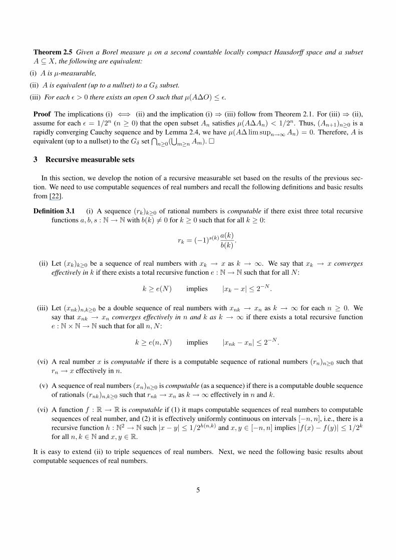
Theorem 2.5 Given a Borel measure µ on a second countable locally compact Hausdorff space and a subsetA ⊆ X , the following are equivalent:

(i) A is µ-measurable,

(ii) A is equivalent (up to a nullset) to a Gδ subset.

(iii) For each ε > 0 there exists an open O such that µ(A∆O) ≤ ε.

Proof The implications (i) ⇐⇒ (ii) and the implication (i) ⇒ (iii) follow from Theorem 2.1. For (iii) ⇒ (ii),assume for each ε = 1/2n (n ≥ 0) that the open subset An satisfies µ(A∆An) < 1/2n. Thus, (An+1)n≥0 is arapidly converging Cauchy sequence and by Lemma 2.4, we have µ(A∆ lim supn→∞An) = 0. Therefore, A isequivalent (up to a nullset) to the Gδ set

⋂n≥0(

⋃m≥nAm). �

3 Recursive measurable sets

In this section, we develop the notion of a recursive measurable set based on the results of the previous sec-tion. We need to use computable sequences of real numbers and recall the following definitions and basic resultsfrom [22].

Definition 3.1 (i) A sequence (rk)k≥0 of rational numbers is computable if there exist three total recursivefunctions a, b, s : N → N with b(k) 6= 0 for k ≥ 0 such that for all k ≥ 0:

rk = (−1)s(k)a(k)b(k)

.

(ii) Let (xk)k≥0 be a sequence of real numbers with xk → x as k → ∞. We say that xk → x convergeseffectively in k if there exists a total recursive function e : N → N such that for all N :

k ≥ e(N) implies |xk − x| ≤ 2−N .

(iii) Let (xnk)n,k≥0 be a double sequence of real numbers with xnk → xn as k → ∞ for each n ≥ 0. Wesay that xnk → xn converges effectively in n and k as k → ∞ if there exists a total recursive functione : N× N → N such that for all n,N :

k ≥ e(n,N) implies |xnk − xn| ≤ 2−N .

(vi) A real number x is computable if there is a computable sequence of rational numbers (rn)n≥0 such thatrn → x effectively in n.

(v) A sequence of real numbers (xn)n≥0 is computable (as a sequence) if there is a computable double sequenceof rationals (rnk)n,k≥0 such that rnk → xn as k →∞ effectively in n and k.

(vi) A function f : R → R is computable if (1) it maps computable sequences of real numbers to computablesequences of real number, and (2) it is effectively uniformly continuous on intervals [−n, n], i.e., there is arecursive function h : N2 → N such |x− y| ≤ 1/2h(n,k) and x, y ∈ [−n, n] implies |f(x)− f(y)| ≤ 1/2k

for all n, k ∈ N and x, y ∈ R.

It is easy to extend (ii) to triple sequences of real numbers. Next, we need the following basic results aboutcomputable sequences of real numbers.

5

Proposition 3.2 (i) If (aijn)i,j,n≥0 is a computable triple sequence of real numbers converging effectively ini, j and n as j → ∞ with limj→∞ aijn = bin then (bin)i,n≥0 is a computable double sequence of realnumbers.

(ii) If (aij)i,j≥0 is a computable double sequence of real numbers which converges monotonically as j → ∞to a computable sequence of real numbers (bi)i≥0, i.e., aij ≤ ai(j+1) for all i, j ≥ 0 and bi = limj→∞ aijthen the convergence of (aij)i,j≥0 is effective in both i and j as j →∞.

Proof (i) This is a straightforward extension of the result in [22, page 20] for computable double sequences ofreal numbers to computable triple sequence of real numbers.

(ii) See [22, page 20].�

We first develop the notions of recursive and computable measurable sets for a finite Borel measure on a compactsecond countable Hausdorff spaceX which will highlight the basic ideas and results. In a later section, these ideasand results are extended to the technically more involved case of locally finite Borel measures on locally compactspaces. We start by presenting a notion of effective structure for a second countable compact Hausdorff space Xby equipping its ω-continuous lattice of open subsets with an effective structure as a domain.

Definition 3.3 We say that a second countable compact Hausdorff space X is effectively given with respect to aneffective enumeration (Oi)i≥0 of a countable basis of open sets closed under finite union and intersection if thefollowing holds:

(i) O0 = ∅ and O1 = X .

(ii) There are total recursive functions φ and ψ such that Oi ∪Oj = Oφ(i,j) and Oi ∩Oj = Oψ(i,j).

(iii) The predicates Oi ⊆ Oj and Oi ⊆ Oj are decidable for i, j ≥ 0. �

Since Oi = ∅ iff Oi ⊆ O0, it follows that the equality relation Oi = ∅ is decidable and we can assume, byredefining the enumeration (Oi)i≥0, that Oi = ∅ iff i = 0. We note here that it would be possible to drop therequirement for the decidability of Oi ⊆ Oj in (iii) at the expense of some more work. For simplicity though, wechoose to keep this condition in our framework.

Proposition 3.4 For each i ≥ 0, the predicate X \ Oi ⊆⋃

1≤m≤nOim is decidable for any finite set of integersim ≥ 0 with 1 ≤ m ≤ n, i.e., from any effective covering of the compact subset X \Oi by basic open subsets, onecan effectively obtain a finite subcovering.

Proof Recall that X = O1. Thus, the relationX \Oi ⊆⋃

1≤m≤nOim , in other words X ⊆ Oi∪ (⋃

1≤m≤nOim),is equivalent, by using the total recursive function φ on the right hand side n− 1 times, to O1 ⊆ Oj . The latter isdecidable by condition (i) in Definition 3.3. �

Now assume that µ is a finite Borel measure on the effectively given compact second countable space X withits effective enumeration (Oi)i≥0 of basic open sets.

Definition 3.5 We say that the finite measure µ is effectively given on X if (µ(Oi))i≥0 is a computable sequenceof real numbers. �

We now use an effective version of the statement in Theorem 2.5 to define a recursive measurable set.

Definition 3.6 Suppose µ is effectively given on X . We say a measurable subset A ⊆ X is a µ-recursive measur-able set if there exists a total recursive function λ : N → N such that µ(A∆Oλ(n)) < 1/2n for all n ≥ 0. �

6

By Theorem 2.5, we know that a µ-recursive measurable set is indeed measurable (assuming that A∆Oλ(n) ismeasurable for all n ≥ 0). Note that in the above definition, the Cauchy sequence (Oλ(n+1))n≥0 is rapidlyconverging with A as a limit. We can therefore always assume that µ-recursive measurable sets are defined byrapidly converging effective Cauchy sequences of basic open sets. It thus follows, from Lemma 2.4, that thereis a one to one correspondence between µ-recursive measurable sets and rapidly converging effective Cauchysequences of basic open sets, i.e. sequences of the form (Oλ(n))n≥0 for a total recursive function λ satisfying, forall n ≥ 0, the relation µ(Oλ(i)∆Oλ(j)) < 1/2n for all i, j ≥ n.

Corollary 3.7 A µ-recursive measurable set is up to a null set a Gδ set whose µ-measure is a computable realnumber.

Proof Suppose A ⊆ X is a µ-recursive measurable set with a total recursive function λ : N → N such thatµ(A∆Oλ(n)) < 1/2n for all n ≥ 0. By Theorem 2.5, we know that A is equivalent to a Gδ set. On the other hand,since µ is an effectively given measure, (µ(On))n≥0 is a computable sequence of real numbers and, therefore,so is µ(Oλ(n))n≥0 as λ is a total recursive function. The latter sequence converges effectively to µ(A), which istherefore a computable number. (Note that the limit of a computable sequence of real numbers which convergeseffectively is a computable real number [22, page 20]). �

We also have the following closure properties of µ-recursive measurable subsets.

Theorem 3.8 The complement, finite union and finite intersection of µ-recursive measurable sets are µ-recursivemeasurable sets.

Proof Suppose A and B are µ-recursive measurable subsets with total recursive functions λ and η satisfying:

µ(A∆Oλ(n)) < 1/2n, µ(B∆Oη(n)) < 1/2n.

Note that Oλ(n) ∪ Oη(n) = Oφ(λ(n),η(n)) and for any subsets C,C ′, D,D′ we have: (C ∪ D)∆(C ′ ∪ D′) ⊆(C∆C ′) ∪ (D∆D′) . Thus,

µ((A ∪B)∆Oφ(λ(n),η(n))) = µ((A ∪B)∆(Oλ(n) ∪Oη(n))) <12n

+12n

=1

2n−1,

and hence the finite union of µ-recursive measurable sets is µ-recursive.Next we show that the complement of A is µ-recursive. Consider the compact set Ocλ(n+1). Since the basis

(Oi)i≥0 is closed under finite unions and by Proposition 3.4, there is a total recursive function θ such that the subsetrelation Ocλ(n+1) ⊆ Oθ(i) for i ≥ 0 enumerates the union of all finite open covers of Ocλ(n+1) by basis elements,i.e., θ(i) is, in the usual ordering of natural numbers, the ith natural number j withX = O1 ⊆ Oφ(j,λ(n+1)), whichis a decidable predicate by Definition 3.3. We have

⋂i≥0Oθ(i) = Ocλ(n+1), since for any point x ∈ O one can

find, by the Hausdorff property, a finite covering of Ocλ(n+1) by basic open sets that do not contain x. It followsthat there exists i ≥ 0 such that µ(Oθ(i) \ Ocλ(n+1)) = µ(Oθ(i) ∩ Oλ(n+1)) < 1/2n+1, or in other words, thereexists i ≥ 0 with:

µ(Oψ(θ(i),λ(n+1))) < 1/2n+1.

The above relation is semi-decidable as µ(Oi) is a computable real number for any i ≥ 0. We compute, in parallel,increasingly accurate approximations to the computable numbers µ(Oψ(θ(i),λ(n+1))) for a finite but increasingnumber of i ≥ 0. Let i(n) be the first integer in this parallel computation scheme so that the correspondingapproximation yields a result strictly less than 1/2n+1, i.e. for which the above inequality holds. Then,

µ(Ac∆Oθ(i(n))) ≤ µ(Ac∆Ocλ(n+1)) + µ(Ocλ(n+1)∆Oθ(i(n))) = µ(A∆Oλ(n+1)) + µ(Ocλ(n+1)∆Oθ(i(n))) <

7

12n+1

+ µ(Oψ(θ(i(n)),λ(n+1))) <1

2n+1+

12n+1

=12n.

This shows that Ac is µ-recursive. Since finite intersections of sets can be written as the complement of the unionof their complements, the result follows. �

For the Lebesgue measure µ on the real line, a countable union of µ-recursive open sets may not be a µ-recursiveopen set. In the next section, we give a simple counter example of this property for µ-computable open sets whichwill also be a counter example for the case of µ-recursive open sets.

4 Computable measurable sets

In this section we introduce the notion of a computable measurable set for Borel measures on compact secondcountable Hausdorff spaces. Assume that µ is an effectively given finite Borel measure on the effectively givencompact second countable space X with its effective enumeration (Oi)i≥0 of basic open sets. Recall from The-orem 2.1 that a subset A ⊆ X is measurable iff for all ε > there exist a closed set C and an open set O withC ⊆ A ⊆ O and µ(O \ C) < ε. Our task is to make this property effective with respect to the basic open subsets(Oi)i≥0 and the corresponding closed subsets (Oci )i≥0. From Proposition 3.4, it follows that there exists a totalrecursive function

α : N → N2 (1)

such that ~Oα(j) := (Oα1(j), Oα2(j)) gives an enumeration of covers of X by pairs of basic open sets, i.e., Oα1(j) ∪Oα2(j) = X , or equivalently, (Oα1(j))c ⊆ Oα2(j). This motivates the following formulation.

Definition 4.1 We say A ⊆ X is a µ-computable measurable set if there exists a total recursive function β :N2 → N such that the following holds:

(i) The two sequences (Oα1(β(j,n)))j,n≥0 and (Oα2(β(j,n)))j,n≥0 of open sets are increasing in j ≥ 0 for fixedn ≥ 0 and decreasing in n for fixed j.

(ii) For all n ≥ 0, we have: (⋃j≥0Oα1(β(j,n)))c ⊆ A ⊆ (

⋃j≥0Oα2(β(j,n))).

(iii) The two computable double sequences of real numbers (µ(Oα1(β(j,n))))j,n≥0 and (µ(Oα2(β(j,n))))j,n≥0 con-verge effectively in j and n as j →∞.

(iv) For all n ≥ 0, we have: µ((⋃j≥0Oα1(β(j,n))) ∩ (

⋃j≥0Oα2(β(j,n)))) < 1/2n.

Item (i) ensures that we only need to work with monotonic sequences of open subsets to characterize the µ-computability of a measurable subset A. Items (ii) and (iv) provide us, for each integer n ≥ 0, with a closed andan open subset, contained in and containingA respectively and effectively given in terms of the basic open subsets,such that the measure of their difference is 1/2n. Item (iii) ensures that the µ-measure of A is computable.

We know by Theorem 2.1 that the conditions in Definition 4.1 above imply that A is µ-measurable. Moreover,we have:

Proposition 4.2 If A is a µ-computable measurable set then µ(A) is a computable real number.

Proof Since the convergence in (iii) above is effective in j and n as j → ∞, it follows from Proposition 3.2 thatµ(X \

⋃j≥0Oα1(β(j,n))) and µ(

⋃j≥0Oα2(β(j,n))) are computable sequences of real numbers, with the first one

increasing and the second one decreasing in n. From (ii) and (iv), it follows that the common limit of these twosequences, i.e., µ(A), is a computable real number.�

8

Proposition 4.3 Let O =⋃j≥0Oγ(j) where γ : N → N is a total recursive function. Then O is a µ-computable

open set iff µ(O) is a computable real number.

Proof If O is µ-computable then by Proposition 4.2, µ(O) is a computable real number. Now, for the converse,assume µ(O) is a computable real number. It suffices to show that there is an effective decreasing sequence of basicopen sets whose complements are contained within O with the sequence of the µ-measure of these complementstending to µ(O). Using the total recursive function φ (Definition 3.3(ii)), we can assume without loss of generalitythat γ gives rise to an increasing sequence of basic open sets. From γ we can effectively obtain, by [14, Proposition3], a total recursive function δ : N → N such that O =

⋃j≥0Oδ(j) and Oδj ⊆ Oδ(j+1) for all j ≥ 0. Since

(µ(Oδ(j)))j≥0 increases monotonically to the computable real number µ(O), the convergence is effective in j.Since X is an effectively given compact space with respect to the basis (Oi)i≥0 and since Oδj ⊆ Oδ(j+1) for allj ≥ 0, we can effectively find a finite open covering X \ Oδ(j+1) ⊆

⋃1≤m≤nOim with Oim ∩ Oδ(j) = ∅ for

1 ≤ m ≤ n. Using the total recursive function φ for binary union (Definition 3.3), we obtain a total recursivefunction σ such that X \ Oδ(j+1) ⊆ Oσ(j) :=

⋃1≤m≤nOim . Moreover, by putting θ(0) := σ(0) and Oθ(j+1) :=

Oσ(j)∩Oθ(j) = Oψ(σ(j),θ(j)), we obtain a total recursive function θ which induces an effective decreasing sequenceof basic open sets that shares the above properties of the sequence induced by σ. This completes the proof.�

The above characterization of a µ-computable open set coincides with that in [13].

Corollary 4.4 Let O =⋃j≥0Oγ(j) where γ : N → N is a total recursive function. Then O is a µ-recursive open

set iff µ(O) is a computable real number.

Proof The “if” part follows from Proposition 4.3, since a µ-computable measurable set is µ-recursive. The “onlyif” part follows from Corollary 3.7.�

In view of Definition 4.1, consider any total recursive function β : N2 → N which satisfies the following threeconditions:

(E1) the two sequences (Oα1(β(j,n)))j,n≥0 and (Oα2(β(j,n)))j,n≥0 of open sets are increasing in j for fixed n anddecreasing in n for fixed j,

(E2) the two computable double sequences of real numbers (µ(Oα1(β(j,n))))j,n≥0 and (µ(Oα2(β(i,j,n))))j,n≥0

converge effectively in j and n as j →∞,

(E3) for all n ≥ 0, we have the relation:µ((

⋃j≥0Oα1(β(j,n)))) ∩ ((

⋃j≥0Oα2(β(j,n)))) < 1/2n.

Such a recursive function β characterizes an equivalence class of µ-computable measurable sets which differ by anull set. Two canonical representatives of this class are given by the Gδ set

⋂n≥0

⋃j≥0Oα2(β(j,n)) and the Fσ set

(⋂n≥0

⋃j≥0Oα1(β(j,n)))c.

Moreover, the one parameter family of pairs of closed and open sets in Definition 4.1(ii), for n ≥ 0, representa data-type for any member A of this equivalence class where (

⋃j≥0Oα1(β(j,n)))c ⊆ A ⊆ (

⋃j≥0Oα2(β(j,n))) and

the measure of the open subset and the closed subset in each pair differ by at most 1/2n, as can be seen followsfrom Definition 4.1(iv).

Proposition 4.5 (i) The complement of a computable measurable set is another computable measurable set.

(ii) A finite union or intersection of computable measurable subsets is a computable measurable subset.

9

Proof (i) Interchange 1 and 2 in the indices of α and β in Definition 4.1(ii) This follows easily using the total recursive functions φ and ψ for binary union and binary intersection of

basic open sets. intersection. �

We provide a simple example to show that µ-computable (or µ-recursive) measurable subsets are not closed undercountable union or intersection.

Example 4.6 Consider the Lebesgue measure µ on the real line and let (rk)k≥0 be an effective increasing sequenceof positive rational numbers converging to a left-computable but non-computable real number r ∈ R. (Such asequence can be constructed from a recursively enumerable but non-recursive subset of natural numbers.) Thenby Proposition 4.3, the open interval (0, r) =

⋃k≥0(0, rk) is not µ-computable though for each k ≥ 0 the open

interval (0, rk) is µ-computable. �

5 Domain of measurable subsets

We now introduce a domain for µ-measurable sets and show our notion of a µ-computable measurable setactually provides a domain-theoretic data type. Consider in general a measure space (X,S) with the underlyingset X and a σ-algebra S of subsets of X , which are regarded as measurable subsets. The domain (M(X,S),v)of measurable subsets of X is defined as follows. An element of M(X,S) is given by a pair of subsets A,B ∈ Swith A ⊆ B. The partial order is defined as [A1, B1] v [A2, B2] if A1 ⊆ A2 and B1 ⊇ B2. Thus, (M(X,S),v)is ω-bi-complete with⊔

i≥0[Ai, Bi] = [⋃i≥0Ai,

⋂i≥0Bi], ui≥0[Ai, Bi] = [

⋂i≥0Ai,

⋃i≥0Bi],

and the pair [∅, X] as the least element. We think of [A,B] as a partial, or partially defined, measurable set that canbe refined to any measurable set C with A ⊆ C ⊆ B, in much the same way that a real interval [a, b] is regardedas a partial real number that can be refined to any real number c with a ≤ c ≤ b.

Any measure on (X,S) extends to the domain of partial measurable subsets as an interval-valued map. Let[0,∞] be the one-point compactification of (0,∞) and I[0,∞] be the set of non-empty compact intervals of [0,∞]ordered by reverse inclusion. A measure µ on (X,S) induces a map M(µ) : (M(X,S)) → I[0,∞], defined byM(µ) : [A,B] 7→ [µ(A), µ(B)]. It is easy to check that this map is ω-bi-continuous, i.e., it is monotone andpreserves the supremums and infimums of increasing and decreasing ω-chains.

Assume now that µ is a finite measure on the measure space (X,S). We say that a subset D ⊆ M(X,S) is aµ-basis for the domain (M(X),v) if for any C ∈ A there exists an increasing chain [An, Bn]n≥0 in D with itslub [A,B] := [

⋃n≥0An,

⋂n≥0Bn] satisfying A ⊆ C ⊆ B and µ(B \ A) = 0. An effective sequence (Sn)n≥0,

such that Sn ∈ S for all n ≥ 0, S0 = ∅ and S1 = X , is said to be an ω-generator sequence for the µ-basis D of(X,S) if the following two conditions hold:

(G-1) For every element (A,B) ∈ D in the µ-basis, there are increasing sequences (Sf(n))n≥0 and (Sg(n))n≥0 fortotal functions f, g : N → N such that Ac =

⋃n≥0 Sf(n) and B =

⋃n≥0 Sg(n).

(G-2) The sequence (µ(Sn))n≥0 is a computable sequence of real numbers.

We say that the µ-basis element [A,B] is effectively given (with respect to the ω-generator sequence) if the totalfunctions f and g in (i) above are recursive. We finally say that an element C ∈ S is µ-domain computable withrespect to the ω-generator sequence (Sn)n≥0 of the µ-basisD if it is contained in the lub of an increasing recursivechain of effectively given µ-basis elements with the width of the nth element of the chain bounded by 1/2n, i.e.,if there exist total recursive functions f : N2 → N and g : N2 → N such that:

(C-1) For all n ≥ 0 we have: (⋃j≥0 Sf(j,n))c ⊆ C ⊆

⋃j≥0 Sg(j,n)

10

(C-2) The chain ([(⋃j≥0 Sf(j,n))c,

⋃j≥0 Sg(j,n)])n≥0 is increasing in n ≥ 0 and the sequences (µ(

⋃j≥0 Sf(j,n)))n≥0

and µ(⋃j≥0 Sg(j,n))n≥0 are computable sequences of real numbers.

(C-3) For all n ≥ 0, we have: µ(⋃j≥0 Sg(j,n))− µ(

⋃j≥0 Sf(j,n))c < 1/2n.

Now we consider a finite measure µ on a second countable compact Hausdorff space X . By Theorem 2.1,the collection D of pairs (C,O), with C closed and O open, forms a µ-basis for the domain (M(X,S),v)where S is the set of µ measurable subsets of X . Next assume further that X is effectively given with respectto an enumeration (Oi)i≥0 of a countable basis and µ is effectively given with respect to this enumeration as inDefinition 3.5. Then, (Oi)i≥0 is an ω-generator sequence forD as (G-1) and (G-2) are satisfied. Finally we obtain:

Proposition 5.1 A µ-computable measurable subset A ⊆ X with respect to the enumeration (Oi)i≥0 of basicopen subsets is a µ-domain computable subset with respect to (Oi)i≥0 as an ω-generator sequence of the basis ofpairs of closed and open sets.

Proof Let α and β be as in Definition 3.6 for the µ-computable measurable subset A ⊆ X . Putting f = α1 ◦ βand g = α2 ◦ β we see that the conditions (C-1)-(C-3) are met since by Proposition 3.2 µ(

⋃j≥0Oα1(β(j,n))) and

µ(⋃j≥0Oα2(β(j,n))) are computable sequences of real numbers. �

In Section 7, we will see how partial measurable sets naturally give rise to interval-valued measurable functions,which in turn provide a domain-theoretic data-type for measurable functions.

6 Locally compact spaces

We will show how to extend the results of the previous two sections to locally finite measures on locally compactspaces. We will treat the case of µ-computable measurable sets in detail and briefly indicate how the results forµ-recursive measurable sets can be generalized in this setting. Let X be a second countable locally compactHausdorff space. Let (Oj)j≥0 be an effective enumeration of a basis of relatively compact open sets, which isclosed under non-empty finite intersection and finite union. We note that X is σ-compact, i.e., there exists anincreasing sequence of compact sets (Xi)i≥0 with X =

⋃i≥0Xi, e.g., we can take Xi =

⋃n≤iOn. For each

i ≥ 0, the collection (Oj ∩Xi)j≥0 is a countable basis of the relative topology for Xi.

Definition 6.1 We say that X is effectively given with respect to (Xi)i≥0 and (Oj)j≥0 if the following holds:

(i) O0 = ∅.

(ii) The predicates Oi ⊆ Oj and Oi ⊆ Oj are decidable for i, j ≥ 0.

(iii) There are total recursive functions φ and ψ such that Oi ∪Oj = Oφ(i,j) and Oi ∩Oj = Oψ(i,j).

(iv) For each i, j, k ≥ 0, the predicate Xi \Oj ⊆ Ok ∩Xi is decidable. �

As in the compact case, we can and will assume that Oi = ∅ iff i = 0. Notice however that in contrast to thecompact setting (Definition 3.3), in the locally compact case we have an additional axiom (iv), which for a compactspace X follows from the other axioms by stipulating that X = O1 as shown in Proposition 3.4.

From our assumptions, it follows that there exists a total recursive function α : N2 → N2 such that ~Oα(i,j) :=(Oα1(i,j), Oα2(i,j)) gives an enumeration of covers of Xi by pairs of basic open sets, i.e., Xi ⊆ Oα1(i,j) ∪Oα2(i,j).

11

Example 6.2 As an important example, consider the real line R equipped with its Euclidean topology; it is asecond countable locally compact Hausdorff space. We put Xi = [−i, i] for i ∈ N. Consider any effectiveenumeration (Uj)j≥0 of the canonical basis B of R consisting of the set of finite unions of rational open intervalsand assume U0 = ∅. Then B is closed under finite intersections as well and it is easily seen by checking the clausesof Definition 6.1 that R is effectively given with respect to (Xi)i≥0 and (Uj)j≥0. Moreover, there exists an effectivescheme to express each Ui as the finite union of disjoint open rational intervals, i.e., there exists a total recursivefunction ρ : N → N∗ where N∗ is the set of finite sequences over N∗ such that if ρ(i) = (ρ(i)0, ρ(i)1, · · · , ρ(i)ni),for some ni ∈ N, then Ui = Uρ(i)0 ∪ Uρ(i)1 ∪ · · · ∪ Uρ(i)ni

, where Uρ(i)mare disjoint intervals for 0 ≤ m ≤ ni.

Let (Ci)i≥0 be an effective enumeration of the set of compact rational intervals of R. Since the interior C◦i is, foreach i ≥ 0, a rational open (possibly empty) interval, we can effectively obtain j ≥ 0 such that C◦i = Uj . Thus,there exists a total recursive function τ : N → N such that C◦i = Uτ(i) for all i ≥ 0. Finally, there is a partialrecursive function κ : N → N such that C◦κ(i) = Ui whenever Ui is an open interval.

We now give two other equivalent characterizations of computable functions of type R → R as defined in Defini-tion 3.1.

Lemma 6.3 A continuous function f : R → R is computable iff the relation f [Ci] ⊂ C◦j is r.e. in i, j.

Proof This follows from [14, Theorem 26 and Theorem 29]. �

Theorem 6.4 A continuous function f : R → R is computable iff the relation Ui ⊆ f−1(Uj) is r.e. in i, j.

Proof Suppose the relation Ui ⊆ f−1(Uj) is r.e. in i, j. We have: f [Ci] ⊆ C◦j iff Ci ⊆ f−1(C◦j ) iff Uτ(i) ⊆f−1(Uτ(j)). Since τ is a total recursive function the latter relation is by assumption r.e. in i, j and thus so is therelation f [Ci] ⊆ C◦j .

Suppose on the other hand that Ci ⊆ f−1(C◦j ) is r.e. in i, j. Since

Ui ⊆ f−1(Uj) ⇐⇒ Uρ(i)0 ∪ Uρ(i)1 ∪ · · · ∪ Uρ(i)ni⊆ f−1(Uρ(j)0 ∪ Uρ(j)1 ∪ · · · ∪ Uρ(j)nj

),

it is sufficient to show that the relation Ui0 ∪ Ui1 ∪ · · · ∪ Uim ⊆ f−1(Uj0∪Uj1∪· · ·∪Ujn), where all open subsetsare assumed to be open intervals, is r.e. in ((i0, i1, · · · , im), (j0, j1, · · · , jn)) ∈ N∗ × N∗. (Recall that N∗ is inbijective correspondence with N under the mapping {k1, k2, · · · , kn} 7→ pk11 p

k22 · · · pkn

n where k1 < k2 < · · · < knand pi is the ith prime number.) We can assume that open sets are open intervals by invoking the recursive functionκ introduced above, with Ui = C◦κ(i), which is defined for i ∈ N iff Ui is an open interval. Fix (m,n) ∈ N2. Wehave Ui0 ∪ Ui1 ∪ · · · ∪ Uim ⊆ f−1(Uj0 ∪Uj1 ∪ · · · ∪Ujn) iff ∀k(0 ≤ k ≤ m)∃l(0 ≤ l ≤ n). f [Uik ] ⊆ Ujl (sincef [Uik ] is a compact interval for each k) iff ∀k(0 ≤ k ≤ m)∃l(0 ≤ l ≤ n). f [Cκ(ik)] ⊆ C◦κ(jl). From this, we candeduce that the set

Emn := {((i0, i1, · · · , im), (j0, j1, · · · , jn)) : ∀k(0 ≤ k ≤ m)∃l(0 ≤ l ≤ n). f [Cκ(ik)] ⊆ C◦κ(jl)}

is r.e. In fact, for any pair k, l ∈ N, with 0 ≤ k ≤ m and 0 ≤ l ≤ n, the set

Eklmn = {((i0, i1, · · · , im), (j0, j1, · · · , jn)) : f [Cκ(ik)] ⊆ C◦κ(jl)}

is r.e. as follows. Since Emn =⋂

0≤k≤m⋃

0≤l≤nEklmn and since any finite union and any finite intersection of

r.e. sets are r.e., it follows that Emn is r.e. Finally, put

E := {((i0, i1, · · · , im), (j0, j1, · · · , jn)) : m,n ∈ N & ∀k(0 ≤ k ≤ m)∃l(0 ≤ l ≤ n). f [Cκ(ik)] ⊆ C◦κ(jl)}.

Then, E =⋃

(m,n)∈N2 Emn and is thus r.e. since any countable union of r.e. sets is r.e. [21, 5.9], and the proof iscomplete. �

12

Using Theorem 6.4, we can generalize the notion of a computable function to real-valued continuous functions ona locally compact second countable Hausdorff space.

Definition 6.5 A continuous function f : X → R on the effectively given locally compact second countableHausdorff spaceX with the enumeration (Oi)i≥0 of its basis elements is computable if the relation Oi ⊆ f−1(Uj)is r.e. in i, j.

Assume now that µ is a locally finite Borel measure on the effectively given locally compact second countablespace X with its effective enumeration (Oi)i≥0 of basis. We say that µ is effectively given on X if (µ(Oj ∩Xi))i,j≥0 is a computable double sequence of real numbers.

Definition 6.6 We sayA ⊆ X is a µ-recursive measurable set if there exists a total recursive function λ : N2 → Nsuch that the double computable sequence of real numbers (µ(Oλ(n,i)))n,i≥0 converges effectively in n and i asn→∞ with µ((A ∩Xi)∆(Oλ(n,i) ∩Xi)) < 1/2n for all n ≥ 0. �

One can extend the proof of Theorem 3.8 to show that the family of µ-recursive measurable sets are closed arefinite unions, intersections and complementation. We will not present the details here and instead move on to defineµ-computable measurable sets on locally compact spaces for which we will provide the proofs of the extendedresults.

Definition 6.7 We say A ⊆ X is a µ-computable measurable set if there exists a total recursive function β :N3 → N such that

(i) The two triple sequences (Oα1(i,β(i,j,n)))i,j,n≥0 and (Oα2(i,β(i,j,n)))i,j,n≥0 of open sets are both increasingin i for fixed j and n, increasing in j for fixed i and n and decreasing in n for fixed i and j.

(ii) For all i, n ≥ 0, we have: (Xi \⋃j≥0Oα1(i,β(i,j,n))) ⊆ Xi ∩A ⊆ (Xi ∩

⋃j≥0Oα2(i,β(i,j,n))).

(iii) The two computable triple sequences of real numbers

(µ(Xi ∩Oα1(i,β(i,j,n))))i,j,n≥0, (µ(Xi ∩Oα2(i,β(i,j,n))))i,j,n≥0,

converge effectively in i, j and n as j →∞.

(iv) For all i, n ≥ 0, we have:µ(Xi ∩ (

⋃j≥0Oα1(i,β(i,j,n))) ∩ (

⋃j≥0Oα2(i,β(i,j,n)))) < 1/2n. �

We know by Theorem 2.1 that the conditions in Definition 6.7 above imply that A is µ-measurable. Moreover,we have:

Proposition 6.8 If A is a computable µ-measurable set then (µ(A ∩ Xi))i≥0 is a computable sequence of realnumbers.

Proof Since the convergence in Definition 6.7(iii) above is effective in i, j and n as j → ∞, it follows fromProposition 3.2 that µ(Xi\

⋃j≥0Oα1(i,β(i,j,n))) and µ(Xi∩

⋃j≥0Oα2(i,β(i,j,n))) are computable double sequences

of real numbers, with the first one increasing and the second one decreasing in n for fixed i. From (iv) it followsthat these two double sequences of real numbers converge effectively in n and i to µ(A ∩Xi) as n → ∞. Thus,by Proposition 3.2, (µ(A ∩Xi))i≥0 is a computable sequence of real numbers. �

Proposition 4.3 can be extended to obtain:

13

Proposition 6.9 Let O be a recursive union of basic open sets. Then O is a µ-computable open set iff (µ(Xi ∩O))i≥0 is a computable sequence of real numbers.

Proof If O is µ-computable then by Proposition 6.8, (µ(Xi ∩ O))i≥0 is a computable sequence of real numbers.Now, for the converse, let O =

⋃j≥0Oγ(j) where the sequence of open sets is increasing and γ : N → N is a

total recursive function and assume (µ(Xi ∩O))i≥0 is a computable sequence of real numbers. Since⋃j≥0Oγ(j)

can be used as the first sequence of open sets in Definition 6.7, it suffices to construct the second sequence.As in the proof of Proposition 4.3, from γ we can effectively obtain, by [14, Proposition 3], a total recursivefunction δ : N → N such that O =

⋃j≥0Oδ(j) and Oδ(j) ⊆ Oδ(j+1) for all j ≥ 0. Consider the computable

double sequence of real numbers (µ(Xi ∩ Oδ(j))i,j≥0. It monotonically converges to the computable sequenceof real numbers (µ(Xi ∩ O))i≥0. Thus, by Proposition 3.2, the convergence is effective in i and j. Since X iseffectively locally compact with respect to the basis (Oj)j≥0 and the sequence of compact subsets (Xi)i≥0 andsinceOδj ⊆ Oδ(j+1) for all j ≥ 0, we can effectively find a finite open coveringXi\Oδ(j+1) ⊆

⋃1≤m≤nOtm with

Otm ∩Oδ(j) = ∅ for 1 ≤ m ≤ n. Using the total recursive function φ for binary union (Definition 6.1), we obtaina total recursive function σ such that Xi \Oδ(j+1) ⊆ Oσ(j) :=

⋃1≤m≤nOtm . Moreover, by putting θ(0) := σ(0)

and Oθ(j+1) := Oσ(j) ∩ Oθ(j) = Oψ(σ(j),θ(j)), for j ≥ 0, we obtain a total recursive function θ which induces aneffective decreasing sequence of basic open sets which shares the above properties of the sequence induced by σ.Since the construction is effective in i, this completes the proof. �

The proof of Proposition 4.5 easily extends to locally finite measures on locally compact spaces:

Proposition 6.10 (i) The complement of a computable measurable set is another computable measurable set.

(ii) A finite union or intersection of computable measurable subsets is a computable measurable subset. �

7 Measurable functions

Let (X,S) be a measure space with the underlying set X and a σ-algebra S of subsets of X . We work withsuch a general space first to develop the notion of interval-valued measurable functions, which we will motivateshortly. Later, in order to develop a computability theory for measurable functions, we assume that X is a locallycompact second countable Hausdorff space, equipped with its σ-algebra of measurable subsets induced by a Borelmeasure µ on X , i.e. S will be the set of all µ-measurable subsets of X .

Given any topological space Y , we say that a function f : X → Y is measurable if f−1(B) ∈ S for any Borelsubset B ⊆ Y . Let R be the extended real line, i.e., the two point compactification [−∞,∞] of R, where the basicopen sets are of the form (a, b), [−∞, b) and (a,∞], with a, b ∈ R. Let IR, respectively IR, be the domain of thenon-empty compact intervals of the real line, respectively of the extended real line, ordered by reverse inclusionand equipped with its σ-algebra of Borel subsets induced from the Scott topology.

In classical measure theory, measurable maps are built up from characteristic maps of measurable sets. It is thusnatural to seek to define computable measurable maps by using characteristic maps of µ-recursive or µ-computablemeasurable subsets. We have seen in section 5 that the domain of partial measurable subsets provides a data type topresent µ-computable measurable subsets. The notion of characteristic maps can be extended to partial measurablesubsets as follow. Define:

χ : M(X,S) → (X → IR)[A,B] 7→ χ[A,B]

with

χ[A,B] : x 7→

1 if x ∈ A0 if x /∈ B

[0, 1] if x ∈ B \A(2)

14

It is easily checked that χ is ω-continuous, i.e., it is monotone and preserves the lubs of increasing ω-chains.Consider the set (X →m IR) of measurable functions f : X → IR partially ordered pointwise, i.e., f v g if

f(x) v g(x) for all x ∈ X . Each such function is determined by the extended real-valued lower and upper partsf− and f+ of f defined such that for each x ∈ X we have f(x) = [f−(x), f+(x)].

Proposition 7.1 We have f ∈ (X →m IR) iff f−, f+ are measurable as extended real valued functions.

Proof We note first that the Scott topology on IR has a countable basis consisting of subsets of the form �I ={y : y ⊆ I} where I is any rational open interval, i.e., I = (a, b) or I = (a,∞] or I = [−∞, b) for rationalnumbers a, b ∈ R. Since the Borel σ-algebra on any topological space is generated by the open sets, f will bemeasurable iff f−1(�I) ∈ S for all rational open intervals I . The result now follows from observing the followingrelations:

f−1(�(a,∞]) = (f−)−1(a,∞]f−1(�([−∞, b)) = (f+)−1[−∞, b)

f−1(�(a, b)) = (f−)−1(a,∞] ∩ (f+)−1[−∞, b)

In fact, if f− and f+ are both measurable, then f will be measurable since by the above relations f−1(�I)is measurable for any rational interval I . On the other hand if f is measurable then by the first two relations,(f−)−1(a,∞] and (f+)−1[−∞, b) are measurable for all rational numbers a and b and it will follow that f− andf+ are both measurable.�

It follows immediately that the function space (X →m IR) is closed under finite sums; moreover we have:

Proposition 7.2 If α ∈ IR and f ∈ (X →m IR) then αf ∈ (X →m IR).

Proof We have:αf = [α−, α+][f−, f+]

= [min(α−f−, α−f+, α+f−, α+f+),max(α−f−, α−f+, α+f−, α+f+)] ∈ (X →m IR),

since the min and max of measurable maps are measurable. �

Corollary 7.3 If αi ∈ IR and fi ∈ (X →m IR) for 1 ≤ i ≤ n then∑n

i=1 αifi ∈ (X →m IR).

Since the supremum, respectively infimum, of an increasing, respectively decreasing, sequence of real-valuedmeasurable functions is measurable, the poset (X →m IR) is ω-bi-complete, i.e. the supremum (respectively infi-mum) of any increasing (respectively decreasing) sequence of interval valued measurable functions is an interval-valued measurable function. Similarly, since the supremum (respectively infimum) of any (finite or) countable setof measurable functions is measurable, it follows that (X →m IR) is ω-inf complete and bounded ω-sup complete.In fact, suppose (fi)i≥0 is a countable sequence of elements in (X →m IR). Then ui≥0fi = λx. ui≥0fi(x),whereui≥0fi(x) is the closure in R of the convex hull of

⋃i≥0 fi(x), which is compact since R is compact. On the

other hand, if (fi)i≥0 is a bounded sequence, then⊔i≥0 fi = λx.

⊔i≥0 fi(x) since

⊔i≥0 fi(x) is the intersection

of non-empty compact intervals is therefore a non-empty and compact interval.Given a sequence of intervals xi ∈ IR, i ≥ 0 and x ∈ IR, we write limi→∞ xi = x if x− = limi→∞ x−i and

x+ = limi→∞ x+i both exist in R with respect to its compact topology.

Furthermore, we introduce a limit operation on sequences in IR which we denote by lim∗:

lim∗ : (IR)ω → IR(xi)i≥0 7→ [lim infi→∞ x−i , lim supi→∞ x+

i ]

Note that lim∗i→∞ xi for xi ∈ IR is precisely the set of all limits of convergent sequences (ai)i≥0 with ai ∈ xi.

Note also that lim∗ is monotone but not continuous.

15

This induces a limit operation on sequences in (X →m IR) as follows:

lim∗ : (X →m IR)ω → (X →m IR)(fi)i≥0 7→ [lim infi→∞ f−i , lim supi→∞ f+

i ]

If f− = limi→∞ f−i and f+ = limi→∞ f+i both exist then we write limi→∞ fi = f = [f−, f+]. Clearly in this

case limi→∞ fi = lim∗i→∞ fi.

From the definition of a characteristic map in Equation 2, we immediately obtain:

Proposition 7.4 For any partial measurable subset [A,B] the characteristic map χ[A,B] : X → IR is measurable.

In analogy with simple functions in classical measure theory on the one hand and step functions in domaintheory on the other hand, we define the following:

Definition 7.5 Let [Ai, Bi] ⊆ X be partial measurable subsets of X for 1 ≤ i ≤ n and let αi ∈ IR be realintervals for 1 ≤ i ≤ n. Then

s =n∑i=1

αiχ[Ai,Bi] : X → IR

is called an interval-valued simple function. �

Since χ[A,B] = χA + [0, 1]χB\A, the characteristic function of a partial measurable function can be expressedin terms of characteristic function of measurable functions with interval coefficients. Therefore, without loss ofgenerality, we assume from now on that an interval-valued simple function has the form s =

∑ni=1 αiχAi : X →

IR. From this, we see that s = [s−, s+] where s± : X → R with s± =∑n

i=1 α±χAi are both measurable

functions. It follows that s is an interval-valued measurable function. Note also that we exclude extended realintervals from the definition of a simple function and that, as in the classical case, s takes only a finite number ofvalues and does not depend on the particular representation in terms of measurable sets Ai’s and intervals αi’s.There is indeed a canonical representation of s for which the αi’s are precisely the distinct non-zero values of sand Ai is precisely the set where s takes value αi. We define the order o(s) of s to be the number of distinctnon-zero values of s. Using the canonical representation of s we also define the width w(s) of s as the maximumlength of the intervals αi, i.e., w(s) = max{α+

i − α−i : 1 ≤ i ≤ n}. Finally, for the canonical representation, wedefine the maximum absolute value of s by m(s) = max{|α−i |, |α

+i | : 1 ≤ i ≤ n}. We say that s is a rational

interval-valued simple function if αi is a compact rational interval for 1 ≤ i ≤ n.We say f : X → IR is bounded by a compact interval K ∈ IR, if for all x ∈ X we have: K v f(x); we

denote this by K v f . We only deal with bounded measurable functions in this paper.Let the real-valued measurable function f : X → R be bounded so that |f | ≤ M for some M ≥ 0. Let m be

the least non-negative integer such that M < 2m. For a positive integer n and any integer k with −2m+n+1 + 2 ≤k ≤ 2m+n+1 let

Ank = f−1

(k − 22n+1

,k

2n+1

), (3)

which is measurable since f is measurable and the dyadic interval(k−22n+1 ,

k2n+1

)is an open set. For a measurable

f , let

sn =2(n+m+1)∑

k=−2(m+n+1)+2

[k − 22n

,k

2n

]χAnk

, (4)

then,, we have f =⊔n≥0 sn with w(sn) ≤ 1/2n with o(sn) ≤ 2n+m+2. We have therefore shown:

16

Proposition 7.6 Given a measure space X , every bounded real-valued measurable function f : X → R is thesupremum of an increasing sequence of rational interval-valued simple functions sn with o(sn) ≤ c 2n, where c isa positive constant independent of n, and w(sn) ≤ 1/2n.

The above proposition can easily be extended to bounded interval-valued measurable functions of type X → IR.

7.1 Recursive and computable measurable functions

An effective version of Proposition 7.6 provides us with the notion of a µ-recursive and a µ-computable real-valued measurable function and our data type for such functions. Let X be an effectively given compact secondcountable Hausdorff space as in Section 2. We fix an effectively given Borel measure µ on X .

Definition 7.7 (i) A rational interval-valued simple function

s =k∑i=1

αiχAi : X → IR

is µ-computable (µ-recursive) if for 1 ≤ i ≤ k, the subset Ai ⊆ X is a µ-computable (µ-recursive)measurable set for 1 ≤ i ≤ k.

(ii) A sequence (sn)n≥0 of µ-computable (µ-recursive)) interval-valued simple functions is effectively given ifthere is an effective procedure to obtain sn

(iii) We say that f : X → R is a µ-computable (µ-recursive) bounded measurable function if there is aneffective increasing sequence of µ-computable (µ-recursive) interval-valued simple functions sn : X → IRwith f =

⊔n≥0 sn such that

– there is an effectively given non-negative integer M ≥ 0 with m(sn) ≤M for all n ≥ 0,– w(sn) ≤ 1/2n for all n ≥ 0, and,– o(sn) ≤ c 2n for some effectively given positive constant c independent of n ≥ 0. �

Two remarks regarding the notion of a µ-computable (µ-recursive) simple function are in order.

(i) Firstly, note that Definition 7.7(i) of a µ-computable (µ-recursive) simple function is independent of thechoice of the representative of s as the complement and the finite union of µ-computable (µ-recursive)measurable sets are both µ-computable measurable sets.

(ii) We note that for a classical simple function s =∑k

i=1 aiχAi : X → R with ai ∈ R the two definitions inparts (i) and (ii) of Definition 7.7 are consistent. Indeed, if Ai’s are µ-computable (µ-recursive) measurablesets and ai’s are rational numbers, so that s is a µ-computable (µ-recursive) simple function accordingto Definition 7.7(i), then putting sn = s for all n ≥ 0 we see that s is µ-computable (µ-recursive) as ameasurable function in the sense of Definition 7.7(ii). On the other hand, suppose the simple function s withcanonical representation s =

∑ki=1 aiχAi : X → R is a µ-computable (µ-recursive) measurable function

in the sense of Definition 7.7(ii). Let V = {0} ∪ {ai : 1 ≤ i ≤ k} and put r = min{|v − w| : v, w ∈V with v 6= w}. By assumption, there is an increasing sequence of µ-computable (µ-recursive) simplefunctions sn with s =

⊔n sn and w(sn) ≤ 1/2n. Fix i with 1 ≤ i ≤ k, and let n be such that 1/2n < r/2.

Assume sn =∑mn

t=1 βntχBnt . Then, for ≤ i ≤ k, we have

Ai =⋃

ai∈βnt

Bnt

and it follows that Ai is the finite union of µ-computable (µ-recursive) measurable subsets and is thus aµ-computable (µ-recursive) measurable subset by Theorem 3.8 and Proposition 4.5.

17

Proposition 7.8 The set of bounded real-valued µ-computable (µ-recursive) measurable functions is closed undermultiplication by a computable real number and under taking sums, absolute value, maximum and minimum.

Proof Suppose f =⊔n≥0 sn and f ′ =

⊔n≥0 s

′n, where sn and s′n are µ-computable (µ-recursive) simple func-

tions satisfying the conditions in Definition 7.7(ii) and in particular: w(sn) ≤ 2n, o(sn) ≤ c2n and w(s′n) ≤ 2n,o(s′n) ≤ c′2n. Assume a ∈ R be a computable real number; we will show that af is a µ-computable (µ-recursive)measurable function. It is clear that af is effectively bounded. Let the positive integer p be such that |a| < 2p− 1.From the computability of a, Definition 3.1, it follows that there is a sequence (γn)n≥0 of compact rational in-tervals with w(γn) ≤ 1/2n that has a as their intersections. Note that if s = Σk

i=1αiχAi : X → IR is thecanonical representation of any interval-valued simple function (i.e.,with disjoint Ai’s, equivalently distinct αi’s)and if γ is any compact interval, then γs = Σk

i=1γαiχAi , where γα = {xy : x ∈ γ, y ∈ α}. We also have:w(αs) ≤ max(|γ−|, |γ+|)w(s) and o(αs) ≤ o(s). Consider now tn := γnsn. Clearly tn is µ-computable (µ-recursive). We have af =

⊔n≥0 tn, with w(tn) ≤ 2p−n and o(tn) ≤ o(sn) ≤ c2n. Since p is independent of n,

it follows easily that af is µ-computable (µ-recursive). Next, we consider the other operations. In all these cases,we construct a new effective sequence of µ-computable (µ-recursive) interval-valued simple functions. For thesum operation, we have: f + f ′ =

⊔n≥0 sn+ s′n. Note that for real intervals α, β ∈ IR and for subsets A,B ⊆ X

we have:αχA + βχB = (α+ β)χA∩B + αχA\B + βχB\A. (5)

Since µ-computable (µ-recursive) measurable subsets are closed under finite union, finite intersection and com-plementation, it follows that for each n ≥ 0, the interval-valued simple function sn + s′n is µ-computable (µ-recursive). From Equation 5, it also follows that w(sn + s′n) ≤ 1/2n−1 and, since o(sn) ≤ c2n and o(s′n) ≤ c′2n,then o(sn + s′n) ≤ 3k2n where k = max(c, c′). We conclude that f + f ′ is a µ-computable (µ-recursive) mea-surable function. Next, we show that |f | is µ-computable (µ-recursive). We use the pointwise extension of theabsolute value function to real intervals. Then, for any interval-valued simple function s =

∑ki=1 aiχAi : X → R

we have the interval-valued simple function: |s| =∑k

i=1 |αi|χAi with w(|s|) ≤ w(s) and o(|s|) ≤ o(s).It follows that |f | =

⊔n≥0 |sn| is a µ-computable (µ-recursive) measurable function. Finally, we note that

min(f, f ′) = (f + f ′ − |f − f ′|)/2 and max(f, f ′) = (f + f ′ + |f − f ′|)/2, from which we conclude thatmin(f, f ′) and max(f, f ′) are µ-computable (µ-recursive) measurable functions. �

Consider the increasing sequence of bounded µ-computable measurable functions (fk)k≥0 with fk = χ(0,rk),where (rk)k≥0 is the sequence of rational numbers in Example 4.6. Since supk≥0 fk = χ(0,r), we see that thesupremum of a countable set of bounded µ-computable (µ-recursive) measurable functions is not necessarily µ-computable (µ-recursive).

Given a µ-computable simple function s =∑k

i=1 αiχAi as in Definition 7.7, it follows by the µ-computabilityof the measurable subsets Ai (for 1 ≤ i ≤ k) that there are total recursive functions βi : N2 → N such that for1 ≤ i ≤ k we have (up to a null set):

Ai =⊔n≥0

[Cin, Oin],

where Cin = (⋃j≥0Oα1(βi(j,n)))c and Oin =

⋃j≥0Oα2(βi(j,n)). Thus, we have s =

⊔n≥0 sn with

sn =k∑i=1

αiχ[Cin,Oin].

We have thus shown:

Proposition 7.9 A µ-computable simple function is the lub of an increasing recursive chain of simple functionsmade up of effectively given µ-basis elements.

18

Finally, we present a condition for a computable continuous function as introduced in Definition 6.5 to be a µ-computable map. We say a real-valued continuous function f : X → R is effectively bounded if a nonnegativenumber M is effectively given such that |f(x)| ≤M for all x ∈ X .

Theorem 7.10 An effectively bounded, computable continuous real-valued function on an effectively given com-pact second countable Hausdorff space is µ-computable with respect to an effectively given finite Borel measureµ on the space if the µ-measure of the inverse image of each open dyadic rational interval is a computable realnumber.

Proof Let f : X → R be an effectively bounded, computable continuous real-valued function on an effectivelygiven compact second countable Hausdorff space X with enumeration (Oi)i≥0 and let µ be an effectively givenfinite Borel measure onX . LetM be the effectively given bound for f and letm,n, k andAnk be as in Equation 3.We have the simple functions sn in Equation 4 with f =

⊔n≥0 sn. Consider the open interval

(k−22n+1 ,

k2n+1

), with

−2m+n+1 + 2 ≤ k ≤ 2m+n+1, there is j ≥ 0 such that Uj =(k−22n+1 ,

k2n+1

)and thus Ank = f−1(Uj). Since, by

computability of f , the relation Oi ⊆ f−1(Uj) is, for fixed j, r.e. in i, it follows that there exists a total recursivefunction γ : N → N such that Ank =

⋃j≥0Oγ(j). By assumption, µ(Ank) is a computable real number. Thus,

by Proposition 4.3, Ank is a µ-computable measurable subset and it follows that sn is an effective sequence ofµ-computable interval-valued simple functions with lub f , which completes the proof. �

8 Interval Lebesgue Integral

We are now in a position to define the notion of interval Lebesgue integral as a map∫

: (X →m IR) → Rwith respect to a measure µ on the measure space (X,S). Later in this section, in order to develop a computabilitytheory, we work with a finite Borel measure µ on a locally compact second countable Hausdorff space X .

For a simple function s ∈ (X →m IR) with a representative s =∑n

i=1 αiχAi : X → IR, which vanishesoutside a set of finite measure, we define the µ-integral of s as:∫

Xs dµ =

n∑i=1

αiµ(Ai).

It follows that∫X s dµ = [

∫X s

− dµ,∫X s

+ dµ]. Thus, as in the classical case, the integral of a simple function isindependent of its representative. If E ⊆ X is measurable, then s ·χE =

∑ni=1 αiχAi∩E is also a simple function

and, as in the classical case, we define: ∫Es dµ =

∫Xs · χE dµ.

We also immediately deduce the following.

Proposition 8.1 If sand t are simple interval-valued functions then, for compact intervals a, b ∈ IR:

(i)∫

(as+ bt) dµ = a∫s dµ+ b

∫t dµ.

(ii) If s v t holds a.e., then∫s dµ v

∫t dµ. �

Now we deal with bounded measurable functions. We first consider a bounded measurable function f ∈(X →m IR) and define:

Definition 8.2 The Lebesgue integral of any bounded interval-valued measurable function f on a measurablesubset E with respect to a bounded measure µ on X is defined as:∫

Ef dµ =

⊔{∫Es dµ : simple s v f}.

19

We immediately obtain the following formula for computing the interval-valued Lebesgue integral:

Proposition 8.3∫E f dµ = [

∫E f

− dµ,∫E f

+ dµ].

We usually write∫f dµ for

∫X f dµ. The following results easily follow as in the classical case.

Proposition 8.4 If f and g are bounded measurable interval-valued functions and a and b are real numbers, then:

(i)∫

(af + bg) dµ = a∫f dµ+ b

∫g dµ.

(ii) If f v g holds a.e., then∫f dµ v

∫g dµ.

(iii) If A and B are disjoint measurable subsets then∫A∪B

f dµ =∫Af dµ+

∫Bf dµ.�

Note that, in Proposition 8.4(i) above, the linearity of the integral operator on interval valued functions only holdsfor real coefficients whereas for simple functions this linearity extends to compact real intervals as in Proposi-tion 8.1(i).

We can now obtain in a straightforward way, using Proposition 8.3, the interval version of some of the classicalresults in measure theory. Recall the definitions of lim and lim∗ in (X →m IR).

Proposition 8.5 Bounded Convergence Theorem Let fn ∈ (X →m IR), for n ≥ 0, be a sequence of uniformlybounded measurable functions with respect to a bounded Borel measure µ, such that limn→∞ fn = f exists. Then∫

limn→∞ fn dµ = limn→∞∫fn dµ. �

From this, we obtain what is essentially the ω-continuity of the Lebesgue integral operator:

Corollary 8.6 Monotone Convergence Theorem Let fn ∈ (X →m IR), for n ≥ 0, be an increasing sequenceof measurable functions with respect to a bounded Borel measure µ, with f0 bounded. Then

⊔n≥0

∫fn dµ =∫

(⊔n≥0 fn) dµ. �

Finally, from the Bounded Convergence Theorem above we obtain the interval version of Fatou’s lemma.

Lemma 8.7 Fatou’s Lemma Let fn ∈ (X →m IR), for n ≥ 0, be a sequence of uniformly bounded measurablefunctions with respect to a bounded Borel measure µ. Then

∫lim∗ fn dµ v lim∗ ∫

fn dµ. �

8.1 Computability of Lebesgue integral

We now assume X is an effectively given second countable compact Hausdorff space and µ is an effectivelygiven finite Borel measure µ on it as described in Section 2. Recall that we have an effective enumeration (Oj)j≥0

of a countable basis of X with X = O1 such that (µ(Oj))j≥0 is a computable sequence of real numbers. Thefollowing theorem, which is our main result, brings together and uses all the results in the previous sections, onµ-computable measurable sets and functions and on the interval-valued Lebesgue integral.

Theorem 8.8 Suppose f is a bounded µ-computable real-valued measurable function on X . Then the Lebesgueintegral of f with respect to µ is computable, i.e., given any positive integer k we can effectively compute theLebesgue integral of f up to 1/2k accuracy.

20

Proof LetM be an effectively given bound for f and (sn)n≥0 be the increasing sequence of µ-computable simplefunctions in (X →m IR) which witnesses the computability of f according to Definition 7.7 with effectivelygiven constant c > 0. By the interval version of the Monotone Convergence Theorem (Corollary 8.6), we knowthat

∫f dµ =

⊔n≥0

∫sn dµ, which means that the required integral lies in each compact interval of the shrinking

sequence of compact intervals given by the integrals of the simple functions. Our task is to effectively find n suchthat

∫sn dµ provides the required estimate. In fact, using the canonical representation:

sn =o(sn)∑i=1

αiχAi (6)

we obtain∫sn dµ =

∑o(sn)i=1 αiµ(Ai). Since each Ai is a µ-computable measurable subset, we can effectively

obtain for each nonnegative integer p an open set Oip and a closed set Cip such that Cip ⊆ Ai ⊆ Oip with µ(Oip)and µ(Cip) computable real numbers satisfying µ(Oip)− µ(Cip) < 1/2p.

We note that there are three types of intervals αi in the simple map sn of Equation 6: (i) 0 ≤ α−i , (ii) α+i ≤ 0

and (iii) α−i < 0 < α+i . This gives us three pairwise disjoint subsets:

I+n = {0 ≤ i ≤ o(sn) : 0 ≤ α−i }, I−n = {0 ≤ i ≤ o(sn) : α+

i ≤ 0}, I0n = {0 ≤ i ≤ o(sn) : α−i < 0 < α+

i }

with 0 ≤ i ≤ o(sn) iff i ∈ I+n ∪ I−n ∪ I0

n.We have∑

i∈I+n

α−i µ(Cip)+∑i∈I−n

α−i µ(Oip)+∑i∈I0n

α−i µ(Oip) ≤∫fn dµ ≤

∑i∈I+n

α+i µ(Oip)+

∑i∈I−n

α+i µ(Cip)+

∑i∈I0n

α+i µ(Oip).

Estimating the difference between the three types of terms in the two sums on the left and right hand side abovewe have:∑

i∈I+n α+i µ(Oip)− α−i µ(Cip) =

∑i∈I+n α

+i µ(Oip)− α+

i µ(Cip) + α+i µ(Cip)− α−i µ(Cip)

=∑o(sn)

i=1 α+i (µ(Oip)− µ(Cip)) + (α+

i − α−i )µ(Cip)

≤∑

i∈I+nm(sn)

2p + w(sn)µ(Cip) ≤ m(sn)o(sn)2p + µ(X)

2n ,

since w(sn) is bounded by 1/2n and Cip’s, being contained in the disjoint sets Ai, are disjoint for fixed p and1 ≤ i ≤ o(sn) and their total µ-measure is therefore bounded by µ(X). Thus, for our estimate, we conclude that∑

i∈I+n

α+i µ(Oip)− α−i µ(Cip) ≤

m(sn)c2n

2p+µ(X)2n

,

since o(sn) is bounded by c2n.Similary,∑

i∈I−n α+i µ(Cip)− α−i µ(Oip) =

∑i∈I−n α

+i µ(Cip)− α−i µ(Cip) + α−i µ(Cip)− α−i µ(Oip)

=∑

i∈I−n (α+i − α−i )µ(Cip) + (µ(Cip)− µ(Oip))α−i

≤ m(sn)c2n

2p + µ(X)2n ,

as in the computation of the estimate for the I+n terms.

Finally, we have:

21

∑i∈I0n α

+i µ(Oip)− α−i µ(Oip) =

∑i∈I+0

(α+i − α−i )µ(Oip)

≤∑

i∈I+0w(sn)µ(Oip)

≤ w(sn)∑

i∈I+0(µ(Cip) + 1

2p ) ≤ µ(X)2n + c

2p

Overall, collecting the contributions from the three types, we have:

w(∫sn dµ) ≤ 3µ(X)

2n+c(1 +m(sn)2n+1)

2p.

Note that µ(X) is a computable number asX = O1; we can thus effectively obtain a nonnegative integer t suchthat 3µ(X) < 2t. Let the positive integer k be given and put n = k + t+ 1 and

p = dlog c(m(sk+t+1)2k+t+1 + 1)2ke.

Using the above effectively obtained n and p, we get

w(∫sn dµ) ≤ 1/2k+1 + 1/2k+1 = 1/2k.

It follows that for the above values of n and p the computable real number∑i∈I+n

α+i µ(Oip) +

∑i∈I−n

α+i µ(Cip) +

∑i∈I0n

α+i µ(Oip)

is within 1/2k of the value of the integral∫f dµ. �

Theorem 8.8 also holds for µ-recursive measurable functions which is a more general result; the proof is onlyslightly different and is skipped here.

9 Conclusion and further work

We have established a domain-theoretic computable framework for Lebesgue’s measure and integration theoryon locally compact Hausdorff spaces, which can herald applications of domain theory in probability theory and inthe theory of Lp spaces and functional analysis in general.

Our computability theory is based either on the extension of Sanin’s notion of µ-recursive measurable sets oron the new and stronger notion of µ-computable measurable sets, which gives rise to a domain-theoretic data-typefor measurable sets. The classical results of Lebesgue theory are extended to interval-valued functions using thenotion of interval-valued simple functions and it is shown, in particular, that the Lebesgue integral operator isω-continuous on the space of interval-valued bounded measurable functions and that the Lebesgue integral of anyµ-computable real-valued bounded measurable function with respect to an effectively given finite Borel measureon an effectively given second countable compact Hausdorff space is computable. Further work is required toextend these results to the Lebesgue integral of unbounded measurable functions with respect to finite or locallyfinite measures on locally compact Hausdorff spaces.

One can also incorporate into this framework the idea of approximating Borel measures on second countablelocally compact Hausdorff spaces by simple valuations on the upper space of the locally compact space as de-veloped in [9, 8]. In other words, both simple functions and simple valuations would be used to compute theLebesgue integral. This would make the Lebesgue integral operator continuous on the product of the space ofinterval-valued measurable functions and the space of continuous valuations on the upper space.

22

References

[1] M. Alvarez-Manilla, A. Edalat, and N. Saheb-Djahromi. An extension result for continuous valuations. J. ofLondon Mathematical society, 61(2):629–640, 2000.

[2] A. Bensoussan and J. L. Menadi. Stochastic hybrid control. J.Math. Anal. Appl., 249:261–268, 2000.

[3] J. L. Berggren. Episodes in the Mathematics of Medieval Islam. Springer, 1986.

[4] E. Bishop and D. Bridges. Constructive Analysis. Springer-Verlag, 1985.

[5] V. I. Bogachev. Measure Theory, volume one. Springer, 2007.

[6] N. J. Cutland. Computability: An Introduction to Recursive Function Theory. Cambridge University Press,1980.

[7] J. Desharnais, A. Edalat, and P. Pananagden. Bisimulation for labelled Markov processes. Information andComputation, 179:163–193, 2002.

[8] A. Edalat. Domain theory and integration. Theoretical Computer Science, 151:163–193, 1995.

[9] A. Edalat. Dynamical systems, measures and fractals via domain theory. Information and Computation,120(1):32–48, 1995.

[10] A. Edalat. When Scott is weak on the top. Mathematical Structures in Computer Science, 7:401–417, 1997.

[11] A. Edalat. Semi-pullbacks and bisimulation in categories of Markov processes. Mathematical Structures inComputer Science, 9(5):523–543, 1999.

[12] A. Edalat and R. Heckmann. A computational model for metric spaces. Theoretical Computer Science,193(1-2):53–73, 1998.

[13] A. Edalat and A. Lieutier. Foundation of a computable solid modelling. Theoretical Computer Science,284(2):319–345, 2002.

[14] A. Edalat and P. Sunderhauf. A domain theoretic approach to computability on the real line. TheoreticalComputer Science, 210:73–98, 1998.

[15] P. Gacs. Uniform test of algorithmic randomness over a general space. Theoretical Computer Science,341:91–137, 2005.

[16] K. Ko. Complexity Theory of Real Numbers. Birkhauser, 1991.

[17] A. N. Kolmogorov and S. V. Fomin. Introductory Real Analysis. Dover, 1975.

[18] D. Kozen. Semantics of probabilistic programs. J. Comput. Syst. Sci., 22:328–350, 1981.

[19] J. D. Lawson. Spaces of maximal points. Mathematical Structures in Computer Science, 7(5):543–555,1997.

[20] J. D. Lawson and B. Lu. Riemann and Edalat integration on domains. Theoretical Computer Science, 305(1-3):259–275, 2003.

[21] Yu. I. Manin. A Course in Mathematical Logic. Springer, 1974.

23

[22] M. B. Pour-El and J. I. Richards. Computability in Analysis and Physics. Springer-Verlag, 1988.

[23] W. Rudin. Real and Complex Analysis. McGraw-Hill, 1970.

[24] N. Saheb-Djahromi. CPO’s of measures for non-determinism. Theoretical Computer Science, 12(1):19–37,1980.

[25] N. Sanin. Constructive Real Numbers and Function Spaces, volume 21 of Translations of MathematicalMonographs. AMS, Providence Rhode Island, 1968. trasl. by E. Mendelson.

[26] K. Weihrauch. Computability on the probability measures on the Borel sets of the unit interval. TheoreticalComputer Science, 219:421–437, 1999.

[27] K. Weihrauch. Computable Analysis (An Introduction). Springer, 2000.

[28] Y. Wu and D. Ding. Computability of measurable sets via effective topologies. Archive for MathematicalLogic, 45(3):365–379, 2006.

[29] Y. Wu and K. Weihrauch. A computable version of the daniell-stone theorem on integration and linearfunctionals. Theoretical Computer Science, 359(1-3):28–42, 2006.

24