Techniques of Integration

Integration By Parts

There is NO formula for∫

f (x)g(x)dx.

It almost never happens that∫

f (x)g(x)dx =(∫

f (x)dx)(∫

g(x)dx)

Notice that∫

df = f (x) + C . We often shorten this to∫

df = f to indicate that the integral

and differential operators “cancel” each other.

The Product Rule for derivatives,d

dx(uv) = u

ddx

(v)+ ddx

(u)v

has no simple counterpart for antiderivatives. It can be restated in terms of differentials as

d(uv) = udv + vdu, and if we apply indefinite integral signs, we get∫d(uv) =

∫udv +

∫vdu, or uv =

∫udv +

∫vdu.

We usually use the equivalent formula∫

udv = uv −∫

vdu.

Example: Evaluate∫

x sinxdx

Solution: Use integration by parts, with u = x, and dv = sinxdx.Then du = dx, and v = − cosx, so∫

x sinxdx =(∫

udv = uv −∫

vdu)= x(− cosx)−

∫(− cosx)dx =

−x cosx +∫cosxdx = −x cosx + sinx + C

1

We can also use this technique with definite integrals:

Evaluate∫ π

0x sinxdx

Solution:∫ π

0x sinxdx =

(∫udv = uv −

∫vdu)= x(− cosx)|π0 −

∫ π

0(− cosx)dx =

−x cosx|π0 +∫ π

0cosxdx = −x cosx|π0 + sinx|π0 = −π cosπ − (−0cos0) + sinπ − sin0 =

−π(−1) = π

Question: How do I know what u and dv should be?

Students first encountering the technique of using the equation∫

udv = uv − ∫ vdu havetrouble knowing what to take for u and what to take for dv .

Answer: Get lots of experience. This is an area where we learn a lot from experience. TheIntegration by Parts technique is characterized by the need to select u from a number of pos-sibilities. Once u has been chosen, dv is determined, and we hope for the best.

The basic idea underlying Integration by Parts is that we hope that in going from∫

udv to∫vdu we will end up with a simpler integral to work with. In the example we have just seen,

we were lucky.

Let’s try it again, the unlucky way:

Example: Evaluate∫

(sinx)xdx

Solution: Use integration by parts, with u = sinx, and dv = xdx.

Then du = cosxdx, and v = x2

2, so

∫(sinx)xdx =

(∫udv = uv −

∫vdu)= sinx

x2

2−∫

x2

2cosxdx =

x2

2sinx − 1

2

∫x2 cosxdx

which involves a tougher looking integral than we started with.

2

As a rule of thumb, one-third of the possible choices will lead to an easier integral, one-thirdwill lead to a harder one, and one-third will lead to one of equal difficulty.

It is also possible to spin your wheels, and go around in circles, as we shall soon see.

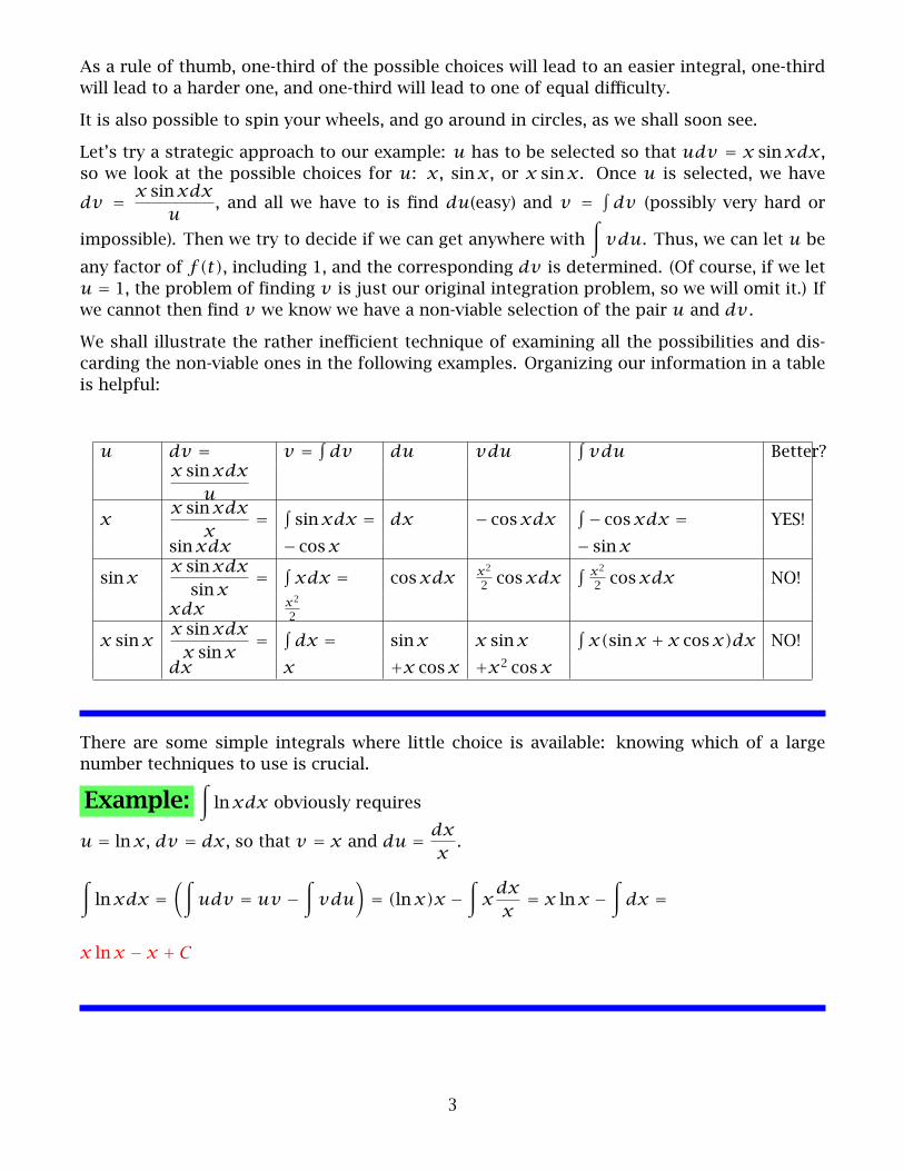
Let’s try a strategic approach to our example: u has to be selected so that udv = x sinxdx,so we look at the possible choices for u: x, sinx, or x sinx. Once u is selected, we have

dv = x sinxdxu

, and all we have to is find du(easy) and v = ∫ dv (possibly very hard or

impossible). Then we try to decide if we can get anywhere with∫

vdu. Thus, we can let u be

any factor of f (t), including 1, and the corresponding dv is determined. (Of course, if we letu = 1, the problem of finding v is just our original integration problem, so we will omit it.) Ifwe cannot then find v we know we have a non-viable selection of the pair u and dv .

We shall illustrate the rather inefficient technique of examining all the possibilities and dis-carding the non-viable ones in the following examples. Organizing our information in a tableis helpful:

u dv = v = ∫ dv du vdu∫

vdu Better?x sinxdx

ux

x sinxdxx

= ∫sinxdx = dx − cosxdx

∫ − cosxdx = YES!

sinxdx − cosx − sinx

sinxx sinxdxsinx

= ∫xdx = cosxdx x2

2 cosxdx∫ x22 cosxdx NO!

xdx x22

x sinxx sinxdx

x sinx= ∫

dx = sinx x sinx∫

x(sinx + x cosx)dx NO!

dx x +x cosx +x2 cosx

There are some simple integrals where little choice is available: knowing which of a largenumber techniques to use is crucial.

Example:∫lnxdx obviously requires

u = lnx, dv = dx, so that v = x and du = dxx.

∫lnxdx =

(∫udv = uv −

∫vdu)= (lnx)x −

∫x

dxx= x lnx −

∫dx =

x lnx − x + C

3

Example:∫arctanxdx also obviously requires

u = arctanx, dv = dx, so that v = x and du = dx1+ x2

∫arctanxdx =

(∫udv = uv −

∫vdu)= (arctanx)x−

∫x

dx1+ x2

= x arctanx−12

∫2xdx1+ x2

=

x arctanx − 12ln(1+ x2)+ C =

x arctanx − ln√1+ x2 + C

Indefinite Integration of ekt times another factor

We now look at a family of integrals which show up in LSD, (Linear Systems Design), particu-larly in the calculation of Laplace Transforms.

We define G(G) = ∫ ektG(t)dt, where G is any function. The types of continuous functionG that arise in practical situations are often sums and products of polynomials, exponentialfunctions, and sinusoidal functions. Fortunately, we know how to evaluate these using thetechnique of integration by parts.

Examples:(1) G(t) = c, a constant. Integration by parts is not needed here. Then G(c) =

∫ektG(t)dt =

ck

ekt + C

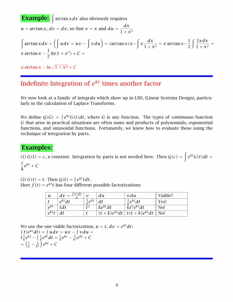
(2) G(t) = t. Then G(t) = ∫ ekttdt.Here f (t) = ektt has four different possible factorizations:

u dv = f (t)dtu v du vdu Viable?

t ektdt 1kekt dt 1

kektdt Yes!ekt tdt t2 kektdt kt2ektdt No!ektt dt t (t + k)ektdt t(t + k)ektdt No!

We use the one viable factorization, u = t, dv = ektdt:∫t(ektdt) = ∫ udv = uv − ∫ vdu =

t 1kekt − ∫ 1kektdt = tkekt − 1

k2ekt + C=(

tk − 1

k2

)ekt + C

4

(3) G(t) = t2. Then G(t2) = ∫ ektt2dt, so f (t) = ektt2. This has four possible factorizations:

u dv = f (t)dtu v du vdu Viable?

t ekttdt(

tk − 1

k2

)ekt dt

(tk − 1

k2

)ektdt Yes, but messy

t2 ektdt 1kekt 2tdt 2

ktektdt Yes!

ekt t2dt 13t3 kektdt k

3t3ektdt No!ektt tdt 1

2t2 (t + k)ektdt 12t2(t + k)ektdt No!

ektt2 dt t (kt2 + 2t)ektdt t(kt2 + 2t)ektdt No!

We see that if we use the factorization u = t2, dv = ektdt, we get∫

t2ektdt = ∫ udv =uv − ∫ vdu = t2

k ekt − 2k

∫tektdt =

t2k ekt − 2

k

(t2k − 2

k

)ekt =(

t2k − 2t

k2 + 2k3

)ekt + C

(4) We notice how the problem of evaluating∫

t2ekt was reduced to the evaluation of∫

ekttdt,which had just been done. We suspect the existence of a reduction formula for

∫ekttndt. Hav-

ing been successful in taking dv = ektdt in the two preceding examples, we decide to do thisagain, and we have u = ekttndt

ektdt = tn. We calculate v = 1kekt and du = ntn−1dt, so that:∫

ekttndt = ∫ udv = uv − ∫ vdu = 1ktnekt − n−1

k

∫ekttn−1dt.

Thus we have G(tn) = 1ktnekt − n−1

k G(tn−1).

(5) G(t) = sinat. We have f (t) = ekt sinat, so there are just three choices for u:

u dv = f (t)dtu v du vdu Viable?

sinat ektdt 1kekt a cosatdt a

k ekt cosatdt Yes

ekt sinatdt − 1a cosat kektdt − k

aekt cosatdt Yesekt sinat dt t (k sinat + a cosat)ektdt t(k sinat + a cosat)ektdt No!

The first two choices are both viable, and we see that they both lead to the evaluation of∫ekt cosatdt. We will examine both cases closely:

First Choice: u1 = sinat, dv1 = ektdtWe get: G(sinat) = ∫ ekt sinatdt = ∫ u1dv1 = u1v1−

∫v1du1 = sinat 1kekt−∫ a

k ekt cosatdt =sinat 1kekt − a

k

∫ekt cosatdt =

sinat 1kekt − akG(cosat)

or

G(sinat) = sinat1k

ekt − akG(cosat)

5

In evaluating∫

ekt cosatdt we again have three choices, two of which are viable:

u dv = f (t)dtu v du vdu Viable?

cosat ektdt 1kekt −a sinatdt −a

k ekt sinatdt Yes

ekt cosatdt 1a sinat kektdt k

aekt sinatdt Yesekt cosat dt t (k cosat − a sinat)ektdt t(k sinat + a cosat)ektdt No!

Again we have two choices. First and Best Choice:We will let U1 = cosat, dV1 = ektdt, and we get:G(cosat) = ∫ cosatektdt = ∫ U1dV1 = U1V1 −

∫V1dU1 =

cosat 1kekt − ∫ 1kekt(−a sinatdt) =1k cosatekt + a

k

∫ekt sinatdt =

1k cosatekt + a

kG(sinat),or

G(cosat) = 1kcosatekt + a

kG(sinat)

so we are back where we started! However, if we substitute this into the equation

G(sinat) = sinat1k

ekt − akG(cosat)

we get G(sinat) = sinat1k

ekt − ak

(1kcosatekt + a

kG(sinat)

)= sinat

1k

ekt − ak2cosatekt −

a2

k2G(sinat)

which can be solved for G(sinat):

(1+ a2

k2)G(sinat) = a2 + k2

k2G(sinat) = sinat

1k

ekt − ak2cosatekt =

ekt(sinatkk2− a

k2cosat) = ekt

k2(k sinat − a cosat) so

G(sinat) = k sinat − a cosata2 + k2

ekt

Last and Worst Choice: We will now let U2 = ekt, dV2 = cosat, and we get:

G(cosat) = ekt(1asinat)−

∫1asinat(ektkdt) = 1

aekt sinat−k

a

∫ekt sinatdt = 1

aekt sinat−k

aG(sinat)

This time, however, if we substitute this into the equation

G(sinat) = sinat1k

ekt − akG(cosat)

we get

G(sinat) = sinat1k

ekt − ak

(1a

ekt sinat − kaG(sinat)

)= G(sinat)

so there is no information gained.

6

Second Choice: u2 = ekt, dv2 = sinatdtWeget: G(sinat) = ∫ ekt sinatdt = ∫ u2dv2 = u2v2−

∫v2du2 = ekt(− 1

a cosat)−∫ kaekt cosatdt =

− 1aekt cosat − k

aG(cosat)

or

G(sinat) = −1a

ekt cosat − kaG(cosat)

Using, from above,

G(cosat) = 1kcosatekt + a

kG(sinat)

we get

G(sinat) = −1a

ekt cosat − ka

(1kcosatekt + a

kG(sinat)

)= G(sinat)

so there is no new information. On the other hand, if we use

G(cosat) = 1a

ekt sinat − kaG(sinat)

we get the same value as before.

(6)G(cosat). This is easily derived from the calculations of the previous example.

G(cosat) = 1kcosatekt+a

kG(sinat) = 1

kcosatekt+a

k

(k sinat − a cosat

a2 + k2ekt)= a sinat + k cosat

a2 + k2ekt

so

G(cosat) = a sinat + k cosata2 + k2

ekt

(7)G(tn sinat) = ∫ tn sinatektdtLet u = tn sinat, dv = ektdt, so that du = (ntn−1 sinat + atn cosat)dt, and v = 1

kekt. ThenG(tn sinat) = ∫ tn sinatektdt = ∫ udv = uv − ∫ vdu =tn sinat(1kekt)− ∫ 1kekt((ntn−1 sinat + atn cosat)dt) =1ktn sinatekt − n

kG(tn−1 sinat)− akG(tn cosat)

or

G(tn sinat) = 1k

tn sinatekt − nkG(tn−1 sinat)− a

kG(tn cosat)

7

(8)G(tn cosat) = ∫ tn cosatektdt. Let U = tn cosat and dV = ektdt,so that dU = (ntn−1 cosat − atn sinat)dt and V = 1

kekt. Then

G(tn cosat) = ∫ tn cosatektdt = ∫ UdV = UV − ∫ Vdu =tn cosat 1kekt − ∫ ekt((ntn−1 cosat − atn sinat)dt) =1ktn cosatekt − n

kG(tn−1 cosat)+ akG(tn sinat).

We can now solve for G(tn sinat):

G(tn sinat) = 1a2 + k2

[(k sinat − a cosat)tnekt −n(G(tn−1(k sinat − a cosat)))

]and hence

G(tn cosat) = 1a2 + k2

[(k cosat − a sinat)tnekt +n(G(tn−1(k cosat − a sinat)))

]

8

Trigonometric Integrals

It is often necessary to evaluate integrals of the form∫(sinx)m(cosx)ndx, where m and n are integers.

If one of the exponents, either m or n is and odd, there is a straightforward simplification.

Case 1: m = 2M + 1 is odd.

Then (sinx)m = (sinx)2M+1 = (sin2 x)M sinx = (1− cos2 x)M sinx,

so our integral becomes

∫(sinx)m(cosx)ndx =

∫(1− cos2 x)M sinx(cosx)ndx

and we may make the substitution u = cosx with du = − sinxdx to get∫(sinx)m(cosx)ndx =

∫(1− cos2 x)M sinx(cosx)ndx = −

∫(1−u2)Mundu

Example:∫

(sinx)11(cosx)10dx = −∫

(1−u2)5u10du =

−∫ [1− 5u2 + 10(u2)2 − 10(u2)3 + 5(u2)4 − (u2)5

]u10du =

−∫

u10 − 5u12 + 10u14 − 10u16 + 5u18 −u20du =

−(

u11

11− 5u13

13+ 10u15

15− 10u17

17+ 5u19

19− u21

21

)+ C =

−cos11 x11

+ 5cos13 x

13− 2cos

15 x5

+ 10cos17 x

17− 5cos19x

19+ cos

21 x21

+ C

9

Example:∫

(sinx)11(cosx)−10dx = −∫

(1−u2)5u−10du =

−∫ [1− 5u2 + 10(u2)2 − 10(u2)3 + 5(u2)4 − (u2)5

]u−10du =

−∫

u−10 − 5u−8 + 10u−6 − 10u−4 + 5u−2 −u0du =

−(

u−9

−9 − 5u−7

−7 + 10u−5

−5 − 10u−3

−3 + 5u−1

−1 −u)+ C =

−(−cos

−9 x9

+ 5cos7 x

7− 2cos−5 x + 10cos

−3 x3

− 5cos−1 x − cosx)+ C =

19sec9x − 5

7sec7x + 2sec5x − 10

3sec3x + 5secx + cosx + C

Example:∫

(sinx)−11(cosx)−10dx =∫

(sinx)−12(cosx)−10 sinxdx = −∫

(1−u2)−6u−10du

can be done, but requires the method of Partial Fractions, which we shall see later.

The situation is similar when the power of cosx is odd.

Example:∫

(sinx)10(cosx)11dx =∫

(sinx)10(cosx)10 cosxdx =∫

(sinx)10(cos2 x)5 cosxdx =∫

(sinx)10(1− sin2 x)5 cosxdx =

( letting u = sinx and du = cosxdx)

∫u10(1−u2)5du =

∫u10[1− 5u2 + 10(u2)2 − 10(u2)3 + 5(u2)4 − (u2)5

]du =

∫u10 − 5u12 + 10u14 − 10u16 + 5u18 −u20du =

u11

11− 5u13

13+ 10u15

15− 10u17

17+ 5u19

19− u21

21+ C =

111sin11 x − 5

13sin13 x + 2

5sin15 x − 10

17sin17 x + 5

19sin19− 1

21sin21 x + C

10

When both powers are odd, it is easiest to select the function with the highest power for sub-stitution:

Good Example:∫

(sinx)11(cosx)3dx =∫

(sinx)11(cosx)2 cosxdx =∫

(sinx)11(1− sin2 x) cosxdx =

( letting u = sinx and du = cosxdx)

∫u11(1−u2)du =

∫u11 −u13du = u11

11− u14

14+ C = 1

11sin11 x − 1

14sin13 x + C

Bad Example:∫

(sinx)11(cosx)3dx =∫

(sinx)10(cosx)3 sinxdx =∫

(1− cos2 x)5(cosx)3 sinxdx =

( letting u = cosx and du = − sinxdx)

∫(1−u2)5u3(−du) =

∫ [−1+ 5u2 − 10(u2)2 + 10(u2)3 − 5(u2)4 + (u2)5

]u3du =

∫ [−u3 + 5u5 − 10u7 + 10u9 − 5u11 +u13

]du =

−u4

4+ 5u6

6− 10u8

8+ 10u10

10− 5u12

12+ u14

14+ C =

−14cos4 x + 5

6cos6 x − 5

4cos8 x + cos10 x − 5

12cos12 x + 1

14cos14 x + C

11

When neither power is odd, we need to use a double angle formula from trigonometry:

cos2x ≡ 2cos2 x − 1 = 1− 2sin2 x

can be solved for cos2 x and sin2 x:

cos2 x = 1+ cos2x2

and sin2 x = 1− cos2x2

Thus, if we want to integrate∫

(sinx)m(cosx)ndx, wherem and n are even integers, we writem = 2M and n = 2N and we have:

∫(sinx)m(cosx)ndx =

∫(sinx)2M(cosx)2Ndx =

∫(sin2 x)M(cos2 x)Ndx =

∫ (1− cos2x

2

)M (1+ cos2x2

)Ndx = 2−(M+N)

∫(1− cos2x)M (1+ cos2x)N dx

12

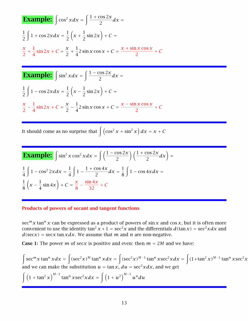
Example:∫cos2 xdx =

∫1+ cos2x

2dx =

12

∫1+ cos2xdx = 1

2

(x + 1

2sin2x

)+ C =

x2+ 14sin2x + C = x

2+ 142sinx cosx + C = x + sinx cosx

2+ C

Example:∫sin2 xdx =

∫1− cos2x

2dx =

12

∫1− cos2xdx = 1

2

(x − 1

2sin2x

)+ C =

x2− 14sin2x + C = x

2− 142sinx cosx + C = x − sinx cosx

2+ C

It should come as no surprise that∫ (cos2 x + sin2 x

)dx = x + C

Example:∫sin2 x cos2 xdx =

∫ (1− cos2x

2

)(1+ cos2x

2dx)=

14

∫1− cos2 2xdx = 1

4

∫1− 1+ cos4x

2dx = 1

8

∫1− cos4xdx =

18

(x − 1

4sin4x

)+ C = x

8− sin4x

32+ C

Products of powers of secant and tangent functions

secmx tann x can be expressed as a product of powers of sinx and cosx, but it is often moreconvenient to use the identity tan2 x+1 = sec2x and the differentials d(tanx) = sec2xdx andd(secx) = secx tanxdx. We assume that m and n are non-negative.

Case 1: The power m of secx is positive and even: then m = 2M and we have:

∫secmx tann xdx =

∫(sec2x)M tann xdx =

∫(sec2x)M−1 tann xsec2xdx =

∫(1+tan2 x)M−1 tann xsec2xd

and we can make the substitution u = tanx, du = sec2xdx, and we get∫ (1+ tan2 x

)M−1tann xsec2xdx =

∫ (1+u2

)M−1undu

13

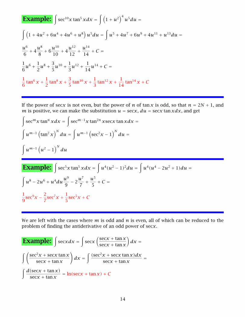
Example:∫sec10x tan5 xdx =

∫ (1+u2

)4u5du =

∫ (1+ 4u2 + 6u4 + 4u6 +u8

)u5du =

∫u5 + 4u7 + 6u9 + 4u11 +u13du =

u6

6+ 4u8

8+ 6u10

10+ 4u12

12+ u14

14+ C =

16

u6 + 12

u8 + 35

u10 + 13

u12 + 114

u14 + C =

16tan6 x + 1

2tan8 x + 3

5tan10 x + 1

3tan12 x + 1

14tan14 x + C

If the power of secx is not even, but the power of n of tanx is odd, so that n = 2N + 1, andm is positive, we can make the substitution u = secx, du = secx tanxdx, and get∫secmx tann xdx =

∫secm−1x tan2n xsecx tanxdx =

∫um−1

(tan2 x

)Ndu =

∫um−1

(sec2x − 1

)Ndu =

∫um−1

(u2 − 1

)Ndu

Example:∫sec5x tan5 xdx =

∫u4(u2 − 1)2du =

∫u4(u4 − 2u2 + 1)du =

∫u8 − 2u6 +u4du

u9

9− 2u7

7+ u5

5+ C =

19sec9x − 2

7sec7x + 1

5sec5x + C

We are left with the cases where m is odd and n is even, all of which can be reduced to theproblem of finding the antiderivative of an odd power of secx.

Example:∫secxdx =

∫secx

(secx + tanxsecx + tanx

)dx =

∫ (sec2x + secx tanxsecx + tanx

)dx =

∫(sec2x + secx tanx)dx

secx + tanx=

∫d(secx + tanx)secx + tanx

= ln(secx + tanx)+ C

14

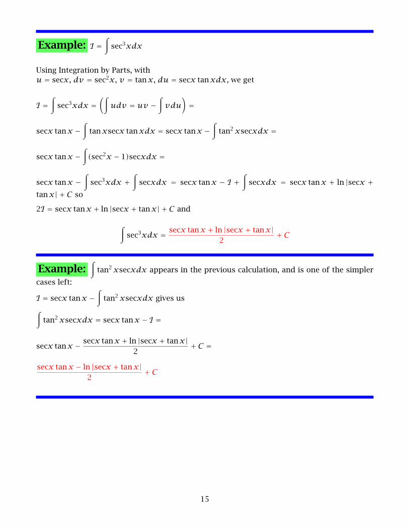
Example: I =∫sec3xdx

Using Integration by Parts, withu = secx, dv = sec2x, v = tanx, du = secx tanxdx, we get

I =∫sec3xdx =

(∫udv = uv −

∫vdu)=

secx tanx −∫tanxsecx tanxdx = secx tanx −

∫tan2 xsecxdx =

secx tanx −∫

(sec2x − 1)secxdx =

secx tanx −∫sec3xdx +

∫secxdx = secx tanx − I +

∫secxdx = secx tanx + ln |secx +

tanx| + C so

2I = secx tanx + ln |secx + tanx| + C and

∫sec3xdx = secx tanx + ln |secx + tanx|

2+ C

Example:∫tan2 xsecxdx appears in the previous calculation, and is one of the simpler

cases left:

I = secx tanx −∫tan2 xsecxdx gives us

∫tan2 xsecxdx = secx tanx − I =

secx tanx − secx tanx + ln |secx + tanx|2

+ C =

secx tanx − ln |secx + tanx|2

+ C

15

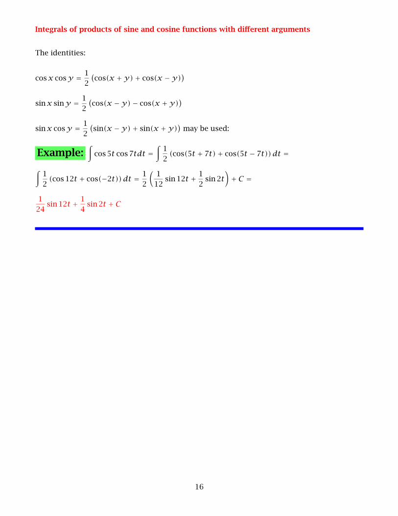
Integrals of products of sine and cosine functions with different arguments

The identities:

cosx cosy = 12

(cos(x +y)+ cos(x −y)

)

sinx siny = 12

(cos(x −y)− cos(x +y)

)

sinx cosy = 12

(sin(x −y)+ sin(x +y)

)may be used:

Example:∫cos5t cos7tdt =

∫12

(cos(5t + 7t)+ cos(5t − 7t)) dt =∫12

(cos12t + cos(−2t)) dt = 12

(112sin12t + 1

2sin2t

)+ C =

124sin12t + 1

4sin2t + C

16

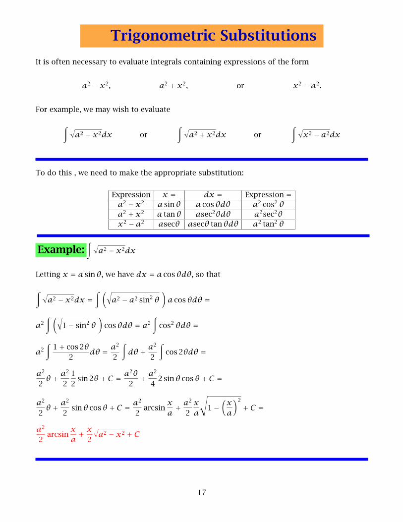
Trigonometric Substitutions

It is often necessary to evaluate integrals containing expressions of the form

a2 − x2, a2 + x2, or x2 − a2.

For example, we may wish to evaluate

∫ √a2 − x2dx or

∫ √a2 + x2dx or

∫ √x2 − a2dx

To do this , we need to make the appropriate substitution:

Expression x = dx = Expression =a2 − x2 a sinθ a cosθdθ a2 cos2 θa2 + x2 a tanθ asec2θdθ a2sec2θx2 − a2 asecθ asecθ tanθdθ a2 tan2 θ

Example:∫ √

a2 − x2dx

Letting x = a sinθ, we have dx = a cosθdθ, so that

∫ √a2 − x2dx =

∫ (√a2 − a2 sin2 θ

)a cosθdθ =

a2∫ (√

1− sin2 θ)cosθdθ = a2

∫cos2 θdθ =

a2∫1+ cos2θ

2dθ = a2

2

∫dθ + a2

2

∫cos2θdθ =

a2

2θ + a2

212sin2θ + C = a2θ

2+ a2

42 sinθ cosθ + C =

a2

2θ + a2

2sinθ cosθ + C = a2

2arcsin

xa+ a2

2xa

√1−(

xa

)2+ C =

a2

2arcsin

xa+ x2

√a2 − x2 + C

17

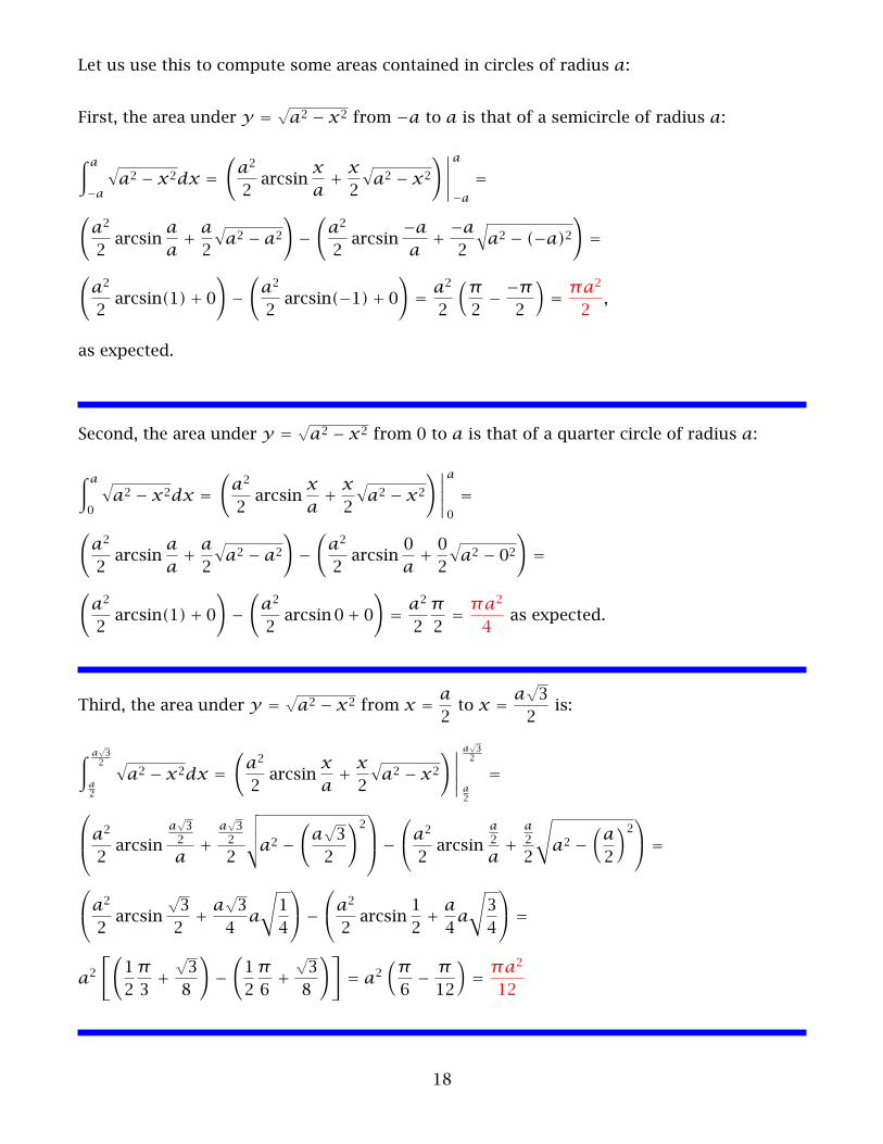
Let us use this to compute some areas contained in circles of radius a:

First, the area under y = √a2 − x2 from −a to a is that of a semicircle of radius a:

∫ a

−a

√a2 − x2dx =

(a2

2arcsin

xa+ x2

√a2 − x2

)∣∣∣∣∣a

−a=

(a2

2arcsin

aa+ a2

√a2 − a2

)−(

a2

2arcsin

−aa+ −a2

√a2 − (−a)2

)=

(a2

2arcsin(1)+ 0

)−(

a2

2arcsin(−1)+ 0

)= a2

2

(π2− −π

2

)= πa2

2,

as expected.

Second, the area under y = √a2 − x2 from 0 to a is that of a quarter circle of radius a:

∫ a

0

√a2 − x2dx =

(a2

2arcsin

xa+ x2

√a2 − x2

)∣∣∣∣∣a

0

=(

a2

2arcsin

aa+ a2

√a2 − a2

)−(

a2

2arcsin

0a+ 02

√a2 − 02

)=

(a2

2arcsin(1)+ 0

)−(

a2

2arcsin0+ 0

)= a2

2π2= πa2

4as expected.

Third, the area under y = √a2 − x2 from x = a2to x = a

√32

is:

∫ a√32

a2

√a2 − x2dx =

(a2

2arcsin

xa+ x2

√a2 − x2

)∣∣∣∣∣a√32

a2

=a2

2arcsin

a√32

a+

a√32

2

√√√√a2 −(

a√32

)2−a2

2arcsin

a2

a+

a2

2

√a2 −

(a2

)2 =a2

2arcsin

√32+ a

√34

a

√14

−a2

2arcsin

12+ a4

a

√34

=

a2[(12

π3+√38

)−(12

π6+√38

)]= a2

(π6− π12

)= πa2

12

18

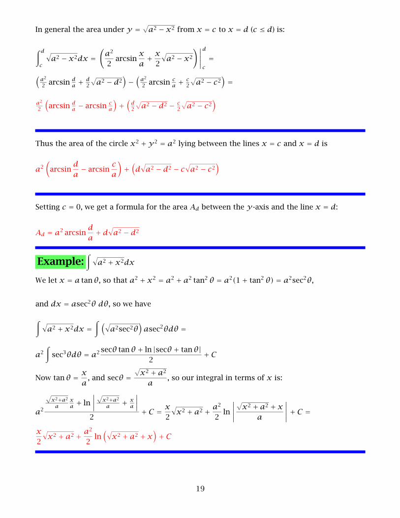
In general the area under y = √a2 − x2 from x = c to x = d (c ≤ d) is:

∫ d

c

√a2 − x2dx =

(a2

2arcsin

xa+ x2

√a2 − x2

)∣∣∣∣∣d

c=

(a22 arcsin

da + d

2

√a2 − d2

)−(

a22 arcsin

ca + c

2

√a2 − c2

)=

a22

(arcsin d

a − arcsin ca

)+(

d2

√a2 − d2 − c

2

√a2 − c2

)

Thus the area of the circle x2 +y2 = a2 lying between the lines x = c and x = d is

a2(arcsin

da− arcsin c

a

)+(d√

a2 − d2 − c√

a2 − c2)

Setting c = 0, we get a formula for the area Ad between the y-axis and the line x = d:

Ad = a2 arcsinda+ d√

a2 − d2

Example:∫ √

a2 + x2dx

We let x = a tanθ, so that a2 + x2 = a2 + a2 tan2 θ = a2(1+ tan2 θ) = a2sec2θ,

and dx = asec2θ dθ, so we have

∫ √a2 + x2dx =

∫ (√a2sec2θ

)asec2θdθ =

a2∫sec3θdθ = a2

secθ tanθ + ln |secθ + tanθ|2

+ C

Now tanθ = xa, and secθ =

√x2 + a2

a, so our integral in terms of x is:

a2

√x2+a2

axa + ln

∣∣∣∣√

x2+a2a + x

a

∣∣∣∣2

+ C = x2

√x2 + a2 + a2

2ln

∣∣∣∣∣√

x2 + a2 + xa

∣∣∣∣∣+ C =

x2

√x2 + a2 + a2

2ln(√

x2 + a2 + x)+ C

19

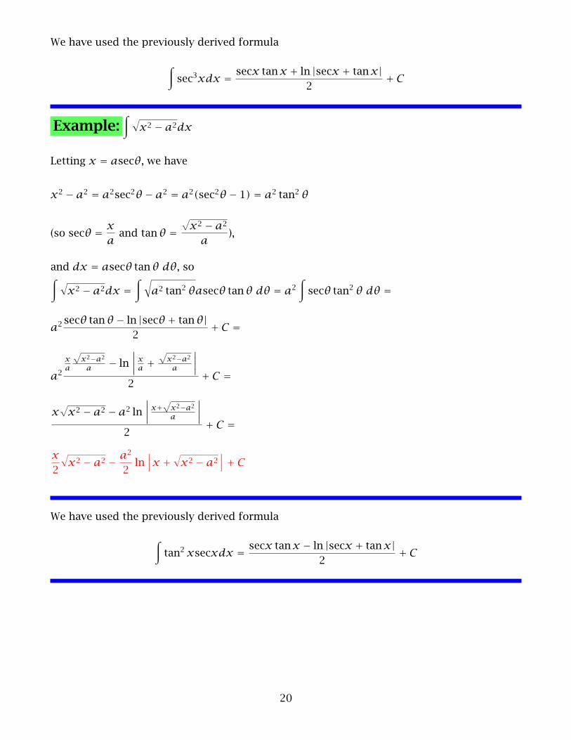
We have used the previously derived formula

∫sec3xdx = secx tanx + ln |secx + tanx|

2+ C

Example:∫ √

x2 − a2dx

Letting x = asecθ, we have

x2 − a2 = a2sec2θ − a2 = a2(sec2θ − 1) = a2 tan2 θ

(so secθ = xaand tanθ =

√x2 − a2

a),

and dx = asecθ tanθ dθ, so∫ √x2 − a2dx =

∫ √a2 tan2 θasecθ tanθ dθ = a2

∫secθ tan2 θ dθ =

a2secθ tanθ − ln |secθ + tanθ|

2+ C =

a2xa

√x2−a2

a − ln∣∣∣∣x

a +√

x2−a2a

∣∣∣∣2

+ C =

x√

x2 − a2 − a2 ln∣∣∣∣x+

√x2−a2a

∣∣∣∣2

+ C =

x2

√x2 − a2 − a2

2ln∣∣∣x + √x2 − a2

∣∣∣+ C

We have used the previously derived formula

∫tan2 xsecxdx = secx tanx − ln |secx + tanx|

2+ C

20

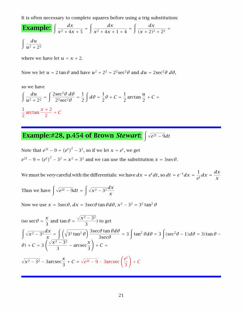
It is often necessary to complete squares before using a trig substitution:

Example:∫

dxx2 + 4x + 5 =

∫dx

x2 + 4x + 1+ 4 =∫

dx(x + 2)2 + 22 =

∫du

u2 + 22

where we have let u = x + 2.

Now we let u = 2 tanθ and have u2 + 22 = 22sec2θ and du = 2sec2θ dθ,

so we have∫du

u2 + 22 =∫2sec2θ dθ22sec2θ

= 12

∫dθ = 1

2θ + C = 1

2arctan

u2+ C =

12arctan

x + 22

+ C

Example:#28, p.454 of Brown Stewart:∫ √

e2t − 9dt

Note that e2t − 9 = (et)2 − 32, so if we let x = et, we get

e2t − 9 = (et)2 − 32 = x2 = 32 and we can use the substitution x = 3secθ.

Wemust be very careful with the differentials: we havedx = etdt, sodt = e−tdx = 1et dx = dx

x

Thus we have∫ √

e2t − 9dt =∫ √

x2 − 32dxx

Now we use x = 3secθ, dx = 3secθ tanθdθ, x2 − 32 = 32 tan2 θ

(so secθ = x3and tanθ =

√x2 − 323

) to get

∫ √x2 − 32dx

x=∫ (√

32 tan2 θ)3secθ tanθdθ

3secθ= 3∫tan2 θdθ = 3

∫(sec2θ − 1)dθ = 3(tanθ −

θ)+ C = 3(√

x2 − 323

− arcsecx3

)+ C =

√x2 − 32 − 3arcsecx

3+ C =

√e2t − 9− 3arcsec

(et

3

)+ C

21

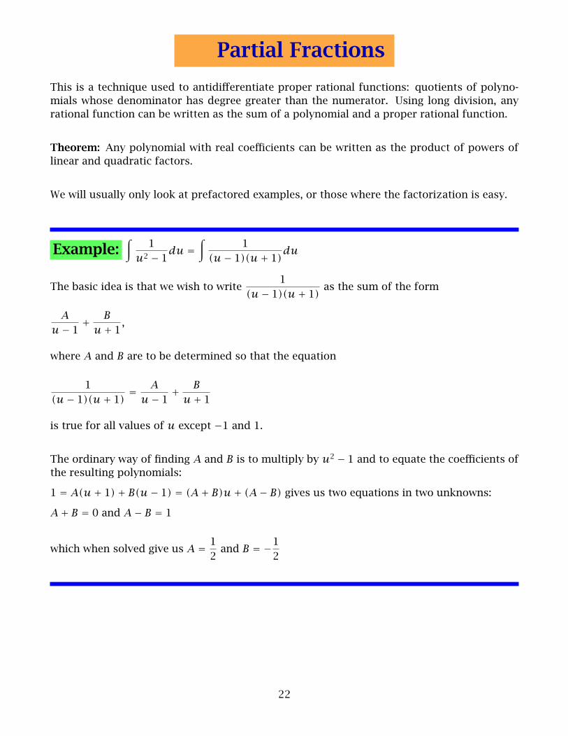
Partial Fractions

This is a technique used to antidifferentiate proper rational functions: quotients of polyno-mials whose denominator has degree greater than the numerator. Using long division, anyrational function can be written as the sum of a polynomial and a proper rational function.

Theorem: Any polynomial with real coefficients can be written as the product of powers oflinear and quadratic factors.

We will usually only look at prefactored examples, or those where the factorization is easy.

Example:∫

1u2 − 1du =

∫1

(u− 1)(u+ 1)du

The basic idea is that we wish to write1

(u− 1)(u+ 1)as the sum of the form

Au− 1 +

Bu+ 1,

where A and B are to be determined so that the equation

1(u− 1)(u+ 1)

= Au− 1 +

Bu+ 1

is true for all values of u except −1 and 1.

The ordinary way of finding A and B is to multiply by u2 − 1 and to equate the coefficients ofthe resulting polynomials:

1 = A(u+ 1)+ B(u− 1) = (A+ B)u+ (A− B) gives us two equations in two unknowns:

A+ B = 0 and A− B = 1

which when solved give us A = 12and B = −1

2

22

A quicker way is to substitute the “illegal” values u = −1 and u = 1 into the equation1 = A(u+ 1)+ B(u− 1)

u = −1: 1 = A(−1+ 1)+ B(−1− 1) = −2B so B = −12

u = 1: 1 = A(1+ 1)+ B(1− 1) = 2A so A = 12

We then have

1(u− 1)(u+ 1)

= 12

1u− 1 −

12

1u+ 1, so∫

1(u− 1)(u+ 1)

du = 12

∫1

u− 1du− 12

∫1

u+ 1du =

12ln |u− 1| − 1

2ln |u+ 1| + C = ln

√∣∣∣∣u− 1u+ 1

∣∣∣∣+ C

Definition: A partial fraction is an expression of the form

A(cx + d)m or

Bx ++C(ax2 + bx + c)n .

At this point we (theoretically) have learned how to antidifferentiate partial fractions, and the

next skill to learn is how to rewrite a proper rational functionP(x)Q(x)

as the sum of partial

fractions.

First Case: Q(x) = (c1x+d1)(c2x+d2) · · · (ckx+dk) is the product of distinct linear factors.

Then we can write

P(x)Q(x)

= P(x)(c1x + d1)(c2x + d2) · · · (akx + dk)

= A1

c1x + d1+ A2

c2x + d2+ · · · + Ak

ckx + dk

Multiplying both sides of the equation by Q(x), we get:

P(x) = A1(c2x + d2) · · · (ckx + dk)+A2(c1x + d1)(c3x + d3) · · · (ckx + dk)+ · · · +Ak(c1x + d1) · · · (ck−1x + dk−1)

which is easily solved by substituting the values xi = −di

ci, i = 1,2,3, . . . , k.

23

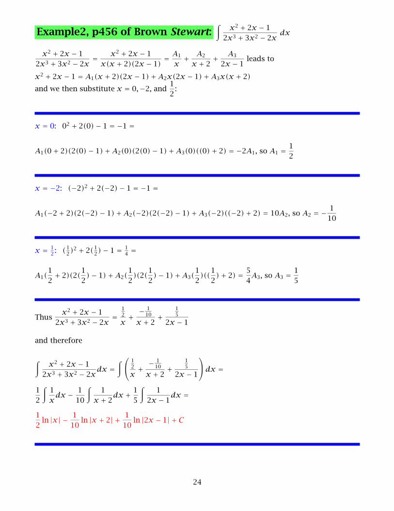
Example2, p456 of Brown Stewart:∫

x2 + 2x − 12x3 + 3x2 − 2x

dx

x2 + 2x − 12x3 + 3x2 − 2x

= x2 + 2x − 1x(x + 2)(2x − 1)

= A1

x+ A2

x + 2 +A3

2x − 1 leads to

x2 + 2x − 1 = A1(x + 2)(2x − 1)+A2x(2x − 1)+A3x(x + 2)

and we then substitute x = 0,−2, and 12:

x = 0: 02 + 2(0)− 1 = −1 =

A1(0+ 2)(2(0)− 1)+A2(0)(2(0)− 1)+A3(0)((0)+ 2) = −2A1, so A1 = 12

x = −2: (−2)2 + 2(−2)− 1 = −1 =

A1(−2+ 2)(2(−2)− 1)+A2(−2)(2(−2)− 1)+A3(−2)((−2)+ 2) = 10A2, so A2 = − 110

x = 12 : (12)2 + 2(12)− 1 = 1

4 =

A1(12+ 2)(2(

12

)− 1)+A2(12

)(2(12

)− 1)+A3(12

)((12

)+ 2) = 54

A3, so A3 = 15

Thusx2 + 2x − 1

2x3 + 3x2 − 2x=

12

x+ − 1

10

x + 2 +15

2x − 1

and therefore

∫x2 + 2x − 1

2x3 + 3x2 − 2xdx =

∫ 12

x+ − 1

10

x + 2 +15

2x − 1

dx =

12

∫1x

dx − 110

∫1

x + 2dx + 15

∫1

2x − 1dx =

12ln |x| − 1

10ln |x + 2| + 1

10ln |2x − 1| + C

24

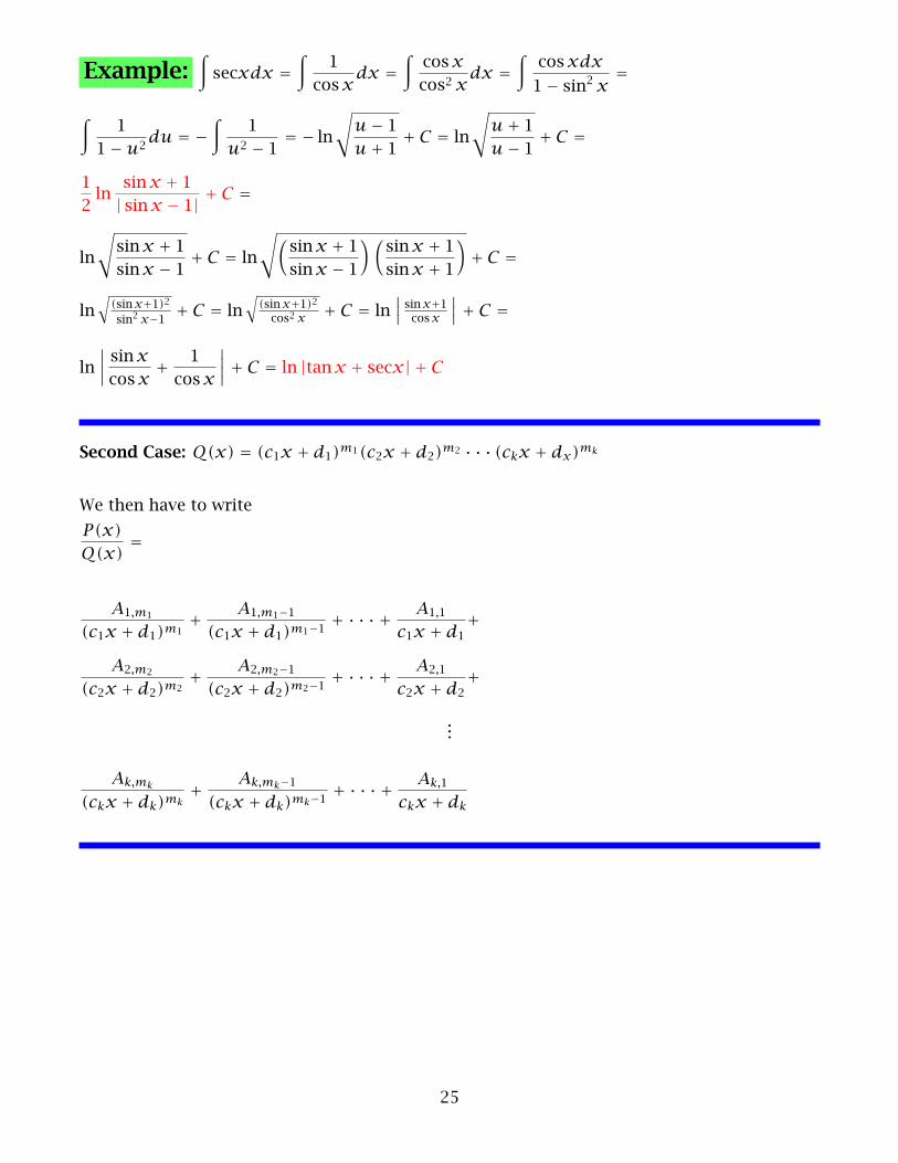
Example:∫secxdx =

∫1

cosxdx =

∫cosxcos2 x

dx =∫cosxdx1− sin2 x

=

∫1

1−u2du = −

∫1

u2 − 1 = − ln√

u− 1u+ 1 + C = ln

√u+ 1u− 1 + C =

12ln

sinx + 1| sinx − 1| + C =

ln

√sinx + 1sinx − 1 + C = ln

√(sinx + 1sinx − 1

)(sinx + 1sinx + 1

)+ C =

ln√

(sinx+1)2sin2 x−1 + C = ln

√(sinx+1)2cos2 x + C = ln

∣∣∣ sinx+1cosx

∣∣∣+ C =

ln∣∣∣∣ sinxcosx

+ 1cosx

∣∣∣∣+ C = ln |tanx + secx| + C

Second Case: Q(x) = (c1x + d1)m1(c2x + d2)m2 · · · (ckx + dx)mk

We then have to write

P(x)Q(x)

=

A1,m1

(c1x + d1)m1+ A1,m1−1

(c1x + d1)m1−1 + · · · +A1,1

c1x + d1+

A2,m2

(c2x + d2)m2+ A2,m2−1

(c2x + d2)m2−1 + · · · +A2,1

c2x + d2+

...

Ak,mk

(ckx + dk)mk+ Ak,mk−1

(ckx + dk)mk−1 + · · · +Ak,1

ckx + dk

25

Example:∫1

(1− x2)2dx =

∫1

(x − 1)2(x + 1)2dx

We write1

(x − 1)2(x + 1)2= A1,2

(x − 1)2+ A1,1

x − 1 +A22

(x + 1)2+ A2,1

x + 1,

and multiply by (x − 1)2(x + 1)2 to get

1 = A1,2(x + 1)2 +A1,1(x − 1)(x + 1)2 +A2,2(x − 1)2 +A2,1(x − 1)2(x + 1)

Substituting x = −1 and x = 1 gets us two constants quickly:x = −1: 1 = A1,2(−1+1)2+A1,1(−1−1)(−1+1)2+A2,2(−1−1)2+A2,1(−1−1)2(−1+1) =4A2,2

so A2,2 = 14

x = 1: 1 = A1,2(1+ 1)2 +A1,1(1− 1)(1+ 1)2 +A2,2(1− 1)2 +A2,1(1− 1)2(1+ 1) = 4A1,2

so A1,2 = 14

The quickest way to get the two remaining coefficients is to insert the coefficients just obtainedinto the original equation:

1 = A1,2(x + 1)2 +A1,1(x − 1)(x + 1)2 +A2,2(x − 1)2 +A2,1(x − 1)2(x + 1)

becomes

1 = 14

(x + 1)2 +A1,1(x − 1)(x + 1)2 + 14

(x − 1)2 +A2,1(x − 1)2(x + 1)

or

1 = (x + 1)2[14+A1,1(x − 1)

]+ (x − 1)2

[14+A2,1(x + 1)

]

Differentiating, we get

0 = 2(x + 1)[14+A1,1(x − 1)

]+ (x + 1)2A1,1 + 2(x − 1)

[14+A2,1(x + 1)

]+ (x − 1)2A2,1

26

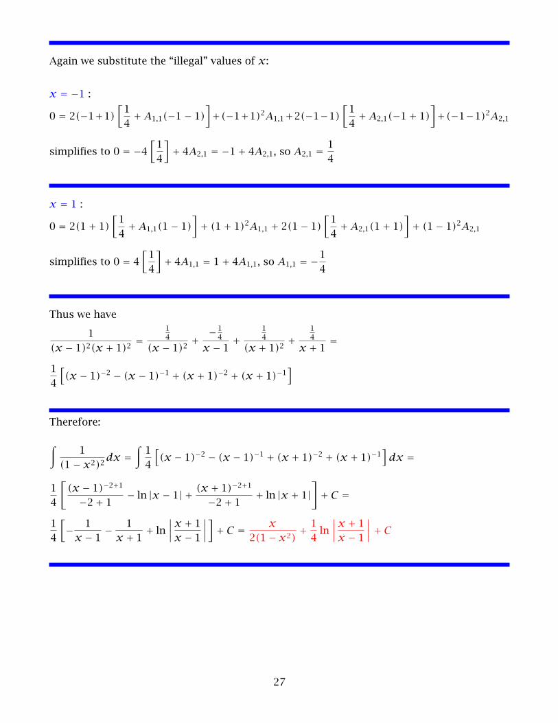
Again we substitute the “illegal” values of x:

x = −1 :0 = 2(−1+1)

[14+A1,1(−1− 1)

]+(−1+1)2A1,1+2(−1−1)

[14+A2,1(−1+ 1)

]+(−1−1)2A2,1

simplifies to 0 = −4[14

]+ 4A2,1 = −1+ 4A2,1, so A2,1 = 14

x = 1 :0 = 2(1+ 1)

[14+A1,1(1− 1)

]+ (1+ 1)2A1,1 + 2(1− 1)

[14+A2,1(1+ 1)

]+ (1− 1)2A2,1

simplifies to 0 = 4[14

]+ 4A1,1 = 1+ 4A1,1, so A1,1 = −14

Thus we have

1(x − 1)2(x + 1)2

=14

(x − 1)2+ −1

4

x − 1 +14

(x + 1)2+

14

x + 1 =

14

[(x − 1)−2 − (x − 1)−1 + (x + 1)−2 + (x + 1)−1

]

Therefore:

∫1

(1− x2)2dx =

∫14

[(x − 1)−2 − (x − 1)−1 + (x + 1)−2 + (x + 1)−1

]dx =

14

[(x − 1)−2+1

−2+ 1 − ln |x − 1| + (x + 1)−2+1

−2+ 1 + ln |x + 1|]+ C =

14

[− 1

x − 1 −1

x + 1 + ln∣∣∣∣x + 1

x − 1∣∣∣∣]+ C = x

2(1− x2)+ 14ln∣∣∣∣x + 1

x − 1∣∣∣∣+ C

27

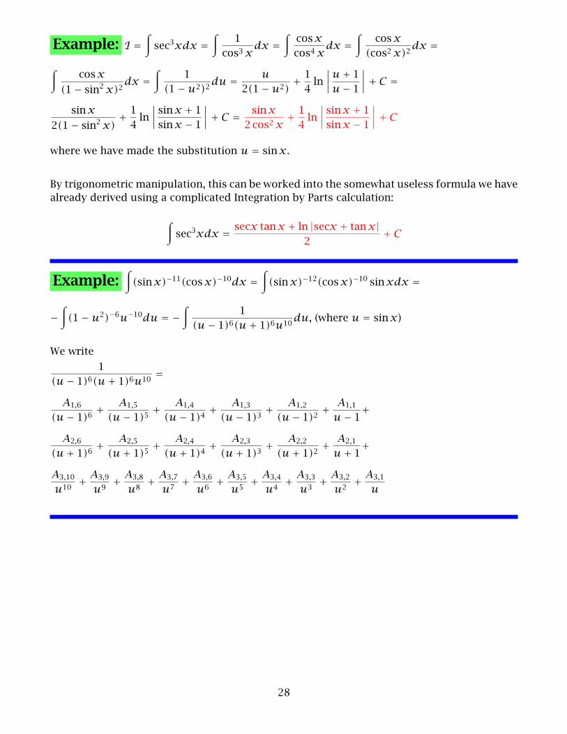
Example: I =∫sec3xdx =

∫1

cos3 xdx =

∫cosxcos4 x

dx =∫

cosx(cos2 x)2

dx =∫

cosx(1− sin2 x)2

dx =∫

1(1−u2)2

du = u2(1−u2)

+ 14ln∣∣∣∣u+ 1

u− 1∣∣∣∣+ C =

sinx2(1− sin2 x)

+ 14ln∣∣∣∣sinx + 1sinx − 1

∣∣∣∣+ C = sinx2cos2 x

+ 14ln∣∣∣∣sinx + 1sinx − 1

∣∣∣∣+ C

where we have made the substitution u = sinx.

By trigonometric manipulation, this can be worked into the somewhat useless formula we havealready derived using a complicated Integration by Parts calculation:

∫sec3xdx = secx tanx + ln |secx + tanx|

2+ C

Example:∫

(sinx)−11(cosx)−10dx =∫

(sinx)−12(cosx)−10 sinxdx =

−∫

(1−u2)−6u−10du = −∫

1(u− 1)6(u+ 1)6u10

du, (where u = sinx)

We write

1(u− 1)6(u+ 1)6u10

=

A1,6

(u− 1)6+ A1,5

(u− 1)5+ A1,4

(u− 1)4+ A1,3

(u− 1)3+ A1,2

(u− 1)2+ A1,1

u− 1+

A2,6

(u+ 1)6+ A2,5

(u+ 1)5+ A2,4

(u+ 1)4+ A2,3

(u+ 1)3+ A2,2

(u+ 1)2+ A2,1

u+ 1+

A3,10

u10+ A3,9

u9+ A3,8

u8+ A3,7

u7+ A3,6

u6+ A3,5

u5+ A3,4

u4+ A3,3

u3+ A3,2

u2+ A3,1

u

28

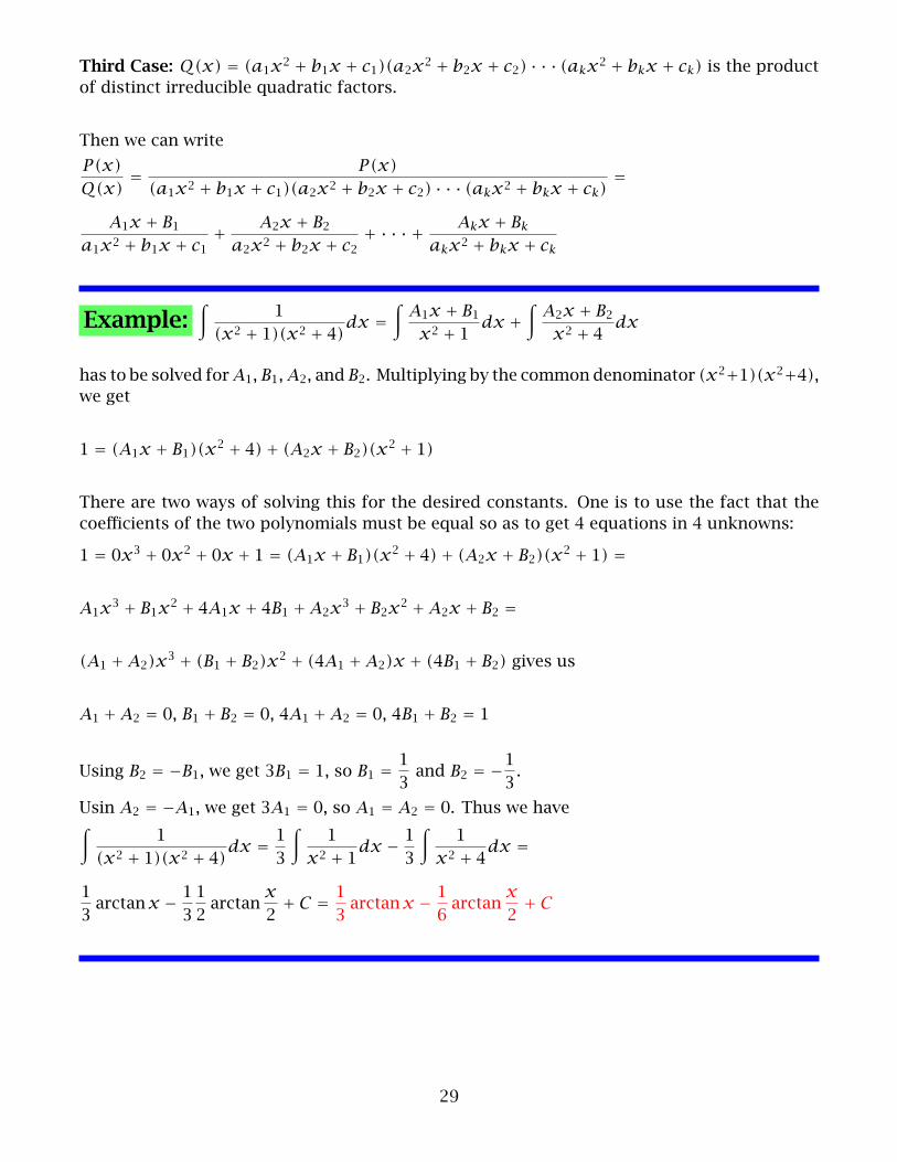
Third Case: Q(x) = (a1x2 + b1x + c1)(a2x2 + b2x + c2) · · · (akx2 + bkx + ck) is the productof distinct irreducible quadratic factors.

Then we can write

P(x)Q(x)

= P(x)(a1x2 + b1x + c1)(a2x2 + b2x + c2) · · · (akx2 + bkx + ck)

=

A1x + B1a1x2 + b1x + c1

+ A2x + B2a2x2 + b2x + c2

+ · · · + Akx + Bk

akx2 + bkx + ck

Example:∫

1(x2 + 1)(x2 + 4)

dx =∫

A1x + B1x2 + 1 dx +

∫A2x + B2

x2 + 4 dx

has to be solved forA1, B1,A2, and B2. Multiplying by the commondenominator (x2+1)(x2+4),we get

1 = (A1x + B1)(x2 + 4)+ (A2x + B2)(x2 + 1)

There are two ways of solving this for the desired constants. One is to use the fact that thecoefficients of the two polynomials must be equal so as to get 4 equations in 4 unknowns:

1 = 0x3 + 0x2 + 0x + 1 = (A1x + B1)(x2 + 4)+ (A2x + B2)(x2 + 1) =

A1x3 + B1x2 + 4A1x + 4B1 +A2x3 + B2x2 +A2x + B2 =

(A1 +A2)x3 + (B1 + B2)x2 + (4A1 +A2)x + (4B1 + B2) gives us

A1 +A2 = 0, B1 + B2 = 0, 4A1 +A2 = 0, 4B1 + B2 = 1

Using B2 = −B1, we get 3B1 = 1, so B1 = 13 and B2 = −13.Usin A2 = −A1, we get 3A1 = 0, so A1 = A2 = 0. Thus we have∫

1(x2 + 1)(x2 + 4)

dx = 13

∫1

x2 + 1dx − 13

∫1

x2 + 4dx =

13arctanx − 1

312arctan

x2+ C = 1

3arctanx − 1

6arctan

x2+ C

29

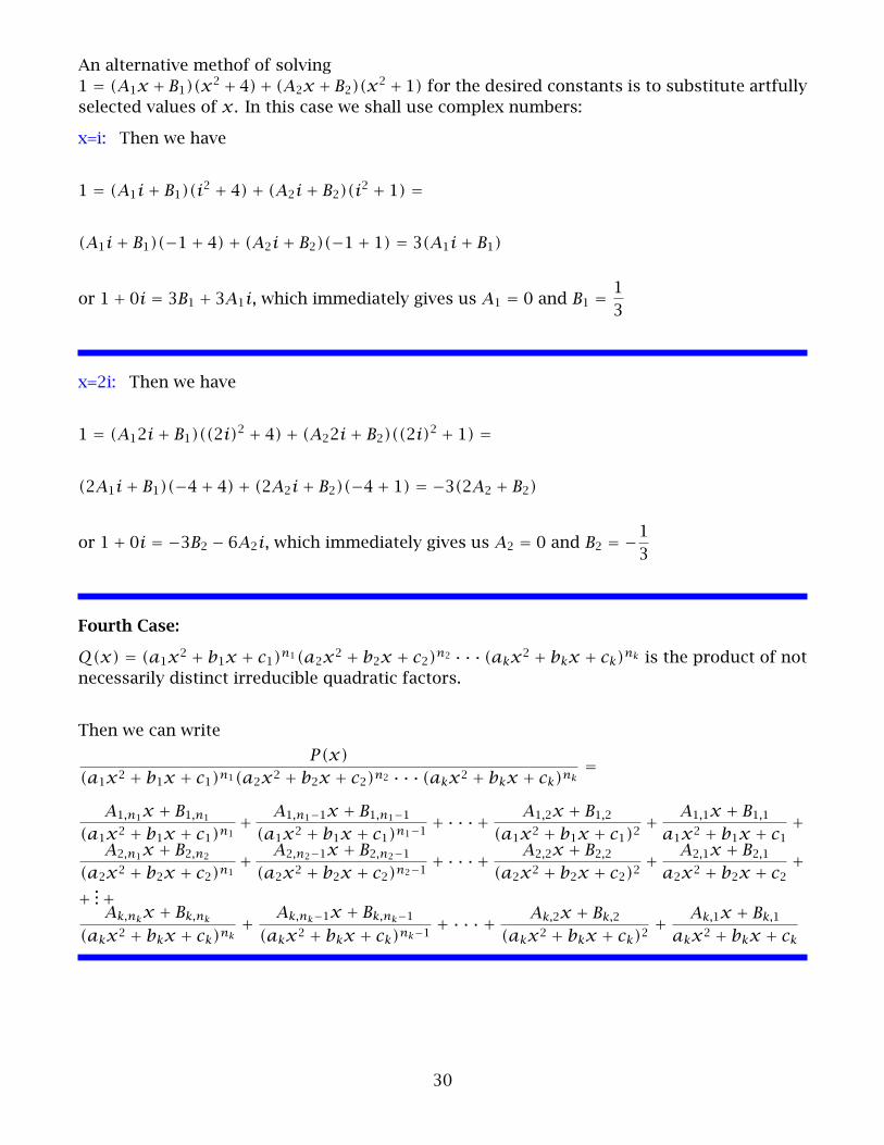
An alternative methof of solving1 = (A1x+ B1)(x2+ 4)+ (A2x+ B2)(x2+ 1) for the desired constants is to substitute artfullyselected values of x. In this case we shall use complex numbers:

x=i: Then we have

1 = (A1i+ B1)(i2 + 4)+ (A2i+ B2)(i2 + 1) =

(A1i+ B1)(−1+ 4)+ (A2i+ B2)(−1+ 1) = 3(A1i+ B1)

or 1+ 0i = 3B1 + 3A1i, which immediately gives us A1 = 0 and B1 = 13

x=2i: Then we have

1 = (A12i+ B1)((2i)2 + 4)+ (A22i+ B2)((2i)2 + 1) =

(2A1i+ B1)(−4+ 4)+ (2A2i+ B2)(−4+ 1) = −3(2A2 + B2)

or 1+ 0i = −3B2 − 6A2i, which immediately gives us A2 = 0 and B2 = −13

Fourth Case:

Q(x) = (a1x2 + b1x + c1)n1(a2x2 + b2x + c2)n2 · · · (akx2 + bkx + ck)nk is the product of notnecessarily distinct irreducible quadratic factors.

Then we can write

P(x)(a1x2 + b1x + c1)n1(a2x2 + b2x + c2)n2 · · · (akx2 + bkx + ck)nk

=

A1,n1x + B1,n1

(a1x2 + b1x + c1)n1+ A1,n1−1x + B1,n1−1

(a1x2 + b1x + c1)n1−1 +· · ·+A1,2x + B1,2

(a1x2 + b1x + c1)2+ A1,1x + B1,1

a1x2 + b1x + c1+

A2,n1x + B2,n2

(a2x2 + b2x + c2)n1+ A2,n2−1x + B2,n2−1

(a2x2 + b2x + c2)n2−1 +· · ·+A2,2x + B2,2

(a2x2 + b2x + c2)2+ A2,1x + B2,1

a2x2 + b2x + c2+

+ ...+Ak,nkx + Bk,nk

(akx2 + bkx + ck)nk+ Ak,nk−1x + Bk,nk−1

(akx2 + bkx + ck)nk−1 + · · · +Ak,2x + Bk,2

(akx2 + bkx + ck)2+ Ak,1x + Bk,1

akx2 + bkx + ck

30

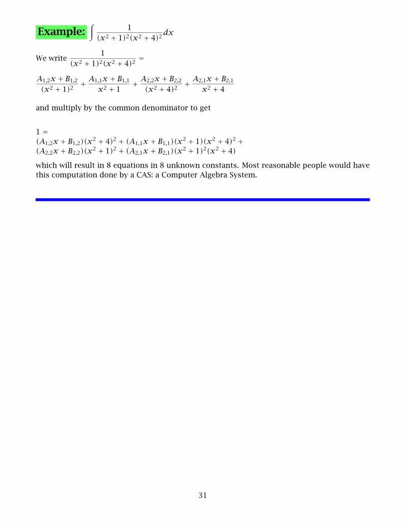
Example:∫

1(x2 + 1)2(x2 + 4)2

dx

We write1

(x2 + 1)2(x2 + 4)2=

A1,2x + B1,2

(x2 + 1)2+ A1,1x + B1,1

x2 + 1 + A2,2x + B2,2

(x2 + 4)2+ A2,1x + B2,1

x2 + 4

and multiply by the common denominator to get

1 =(A1,2x + B1,2)(x2 + 4)2 + (A1,1x + B1,1)(x2 + 1)(x2 + 4)2 +(A2,2x + B2,2)(x2 + 1)2 + (A2,1x + B2,1)(x2 + 1)2(x2 + 4)

which will result in 8 equations in 8 unknown constants. Most reasonable people would havethis computation done by a CAS: a Computer Algebra System.

31

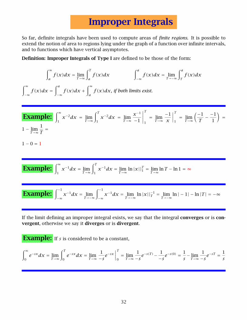
Improper Integrals

So far, definite integrals have been used to compute areas of finite regions. It is possible toextend the notion of area to regions lying under the graph of a function over infinite intervals,and to functions which have vertical asymptotes.

Definition: Improper Integrals of Type I are defined to be those of the form:

∫∞a

f (x)dx = limT→∞

∫ T

af (x)dx

∫ a

−∞f (x)dx = lim

T→−∞

∫ a

Tf (x)dx

∫∞−∞

f (x)dx =∫ a

−∞f (x)dx +

∫∞a

f (x)dx, if both limits exist.

Example:∫∞1

x−2dx = limT→∞

∫ T

1x−2dx = lim

T→∞x−1

−1

∣∣∣∣∣T

1

= limT→∞

−1x

∣∣∣∣T

1= lim

T→∞

(−1T− −11

)=

1− limT→∞

1T=

1− 0 = 1

Example:∫∞1

x−1dx = limT→∞

∫ T

1x−1dx = lim

T→∞ln |x||T1 = lim

T→∞lnT − ln 1 = ∞

Example:∫ −1−∞

x−1dx = limT→−∞

∫ −1−∞

x−1dx = limT→−∞

ln |x||−1T = limT→−∞

ln | − 1| − ln |T | = −∞

If the limit defining an improper integral exists, we say that the integral converges or is con-vergent, otherwise we say it diverges or is divergent.

Example: If s is considered to be a constant,

∫∞0

e−sxdx = limT→∞

∫ T

0e−sxdx = lim

T→∞1−s

e−sx∣∣∣∣

T

0= lim

T→∞1−s

e−s(T)− 1−s

e−s(0) = 1s− lim

T→∞1−s

e−sT = 1s

32

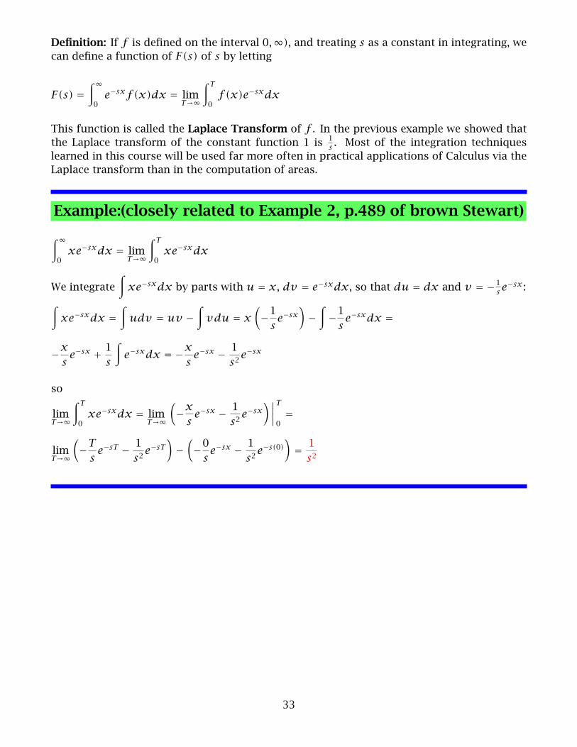
Definition: If f is defined on the interval 0,∞), and treating s as a constant in integrating, wecan define a function of F(s) of s by letting

F(s) =∫∞0

e−sxf (x)dx = limT→∞

∫ T

0f (x)e−sxdx

This function is called the Laplace Transform of f . In the previous example we showed thatthe Laplace transform of the constant function 1 is 1

s . Most of the integration techniqueslearned in this course will be used far more often in practical applications of Calculus via theLaplace transform than in the computation of areas.

Example:(closely related to Example 2, p.489 of brown Stewart)

∫∞0

xe−sxdx = limT→∞

∫ T

0xe−sxdx

We integrate∫

xe−sxdx by parts with u = x, dv = e−sxdx, so that du = dx and v = −1s e−sx:

∫xe−sxdx =

∫udv = uv −

∫vdu = x

(−1

se−sx)−∫−1

se−sxdx =

−xs

e−sx + 1s

∫e−sxdx = −x

se−sx − 1

s2e−sx

so

limT→∞

∫ T

0xe−sxdx = lim

T→∞

(−x

se−sx − 1

s2e−sx)∣∣∣∣

T

0=

limT→∞

(−T

se−sT − 1

s2e−sT)−(−0

se−sx − 1

s2e−s(0)

)= 1

s2

33

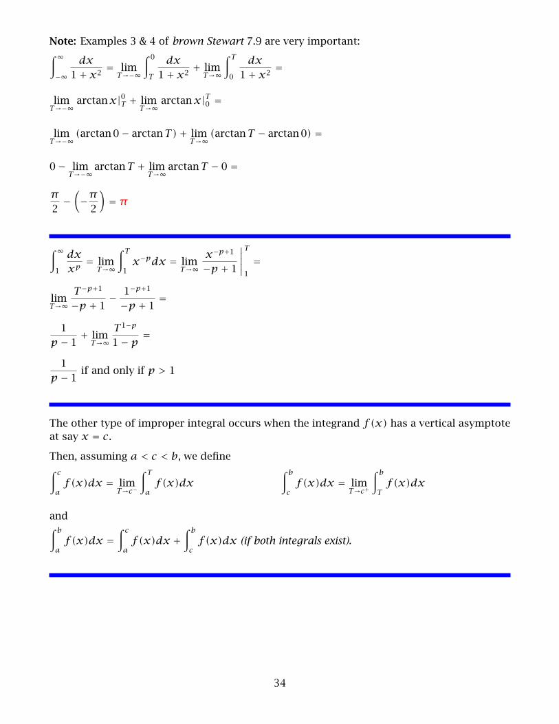
Note: Examples 3 & 4 of brown Stewart 7.9 are very important:∫∞−∞

dx1+ x2

= limT→−∞

∫ 0T

dx1+ x2

+ limT→∞

∫ T

0

dx1+ x2

=

limT→−∞

arctanx|0T + limT→∞arctanx|T0 =

limT→−∞

(arctan0− arctanT)+ limT→∞

(arctanT − arctan0) =

0− limT→−∞

arctanT + limT→∞

arctanT − 0 =

π2−(−π2

)= π

∫∞1

dxxp = lim

T→∞

∫ T

1x−pdx = lim

T→∞x−p+1

−p + 1

∣∣∣∣∣T

1

=

limT→∞

T−p+1

−p + 1 −1−p+1

−p + 1 =

1p − 1 + limT→∞

T 1−p

1− p=

1p − 1 if and only if p > 1

The other type of improper integral occurs when the integrand f (x) has a vertical asymptoteat say x = c.

Then, assuming a < c < b, we define∫ c

af (x)dx = lim

T→c−

∫ T

af (x)dx

∫ b

cf (x)dx = lim

T→c+

∫ b

Tf (x)dx

and∫ b

af (x)dx =

∫ c

af (x)dx +

∫ b

cf (x)dx (if both integrals exist).

34

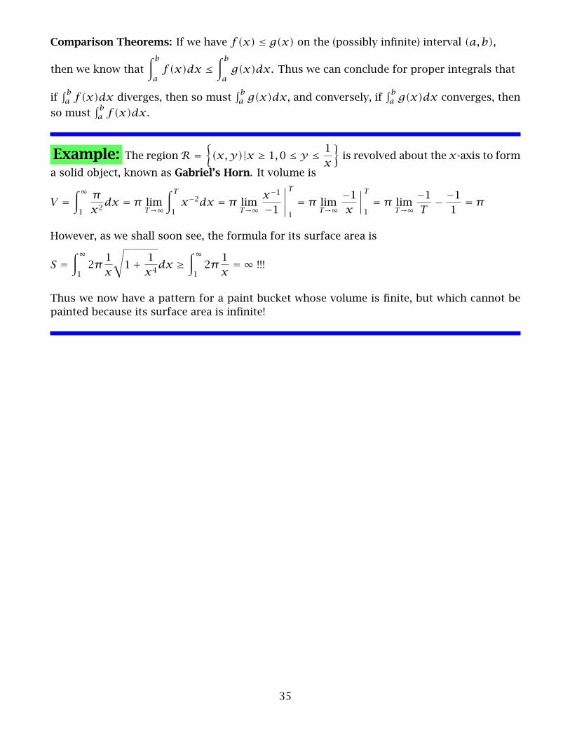
Comparison Theorems: If we have f (x) ≤ g(x) on the (possibly infinite) interval (a, b),

then we know that∫ b

af (x)dx ≤

∫ b

ag(x)dx. Thus we can conclude for proper integrals that

if∫ ba f (x)dx diverges, then so must

∫ ba g(x)dx, and conversely, if

∫ ba g(x)dx converges, then

so must∫ ba f (x)dx.

Example: The regionR ={

(x, y)|x ≥ 1,0 ≤ y ≤ 1x

}is revolved about the x-axis to form

a solid object, known as Gabriel’s Horn. It volume is

V =∫∞1

πx2

dx = π limT→∞

∫ T

1x−2dx = π lim

T→∞x−1

−1

∣∣∣∣∣T

1

= π limT→∞

−1x

∣∣∣∣T

1= π lim

T→∞−1T− −11= π

However, as we shall soon see, the formula for its surface area is

S =∫∞12π

1x

√1+ 1

x4dx ≥

∫∞12π

1x= ∞ !!!

Thus we now have a pattern for a paint bucket whose volume is finite, but which cannot bepainted because its surface area is infinite!

35

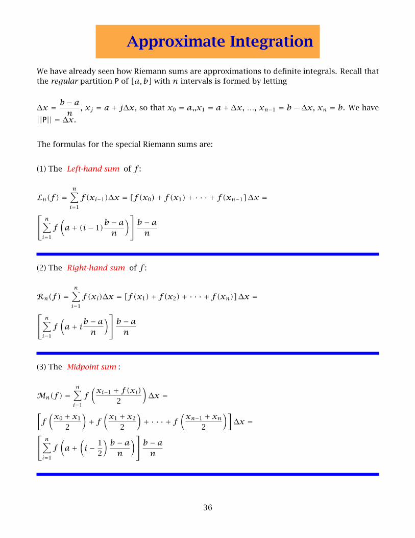
Approximate Integration

We have already seen how Riemann sums are approximations to definite integrals. Recall thatthe regular partition P of [a, b] with n intervals is formed by letting

∆x = b − an

, xj = a+ j∆x, so that x0 = a,,x1 = a+ ∆x, …, xn−1 = b − ∆x, xn = b. We have||P|| = ∆x.

The formulas for the special Riemann sums are:

(1) The Left-hand sum of f :

Ln(f ) =n∑

i=1f (xi−1)∆x = [f (x0)+ f (x1)+ · · · + f (xn−1]∆x =

n∑

i=1f(

a+ (i− 1)b − a

n

) b − an

(2) The Right-hand sum of f :

Rn(f ) =n∑

i=1f (xi)∆x = [f (x1)+ f (x2)+ · · · + f (xn)]∆x =

n∑

i=1f(

a+ ib − a

n

) b − an

(3) The Midpoint sum :

Mn(f ) =n∑

i=1f(

xi−1 + f (xi)2

)∆x =

[f(

x0 + x12

)+ f(

x1 + x22

)+ · · · + f

(xn−1 + xn

2

)]∆x =

n∑

i=1f(

a+(

i− 12

)b − a

n

) b − an

36

(4) The Inscribed sum of f : In(f ) = [m1 +m2 + · · · +mn]∆x

(5) The Exscribed sum of f : En(f ) = [M1 +M2 + · · · +Mn]∆x

The Trapezoidal Estimate or Trapezoidal Rule Tn(f ) = 12

(f (x0)+ 2f (x1)+ 2f (x2)+ · · · +2f (xn − 1)+ f (xn))∆x =f (a)+ 2

n−1∑i=1

f(

a+ ib − a

n

)+ f (b)

b − a

n

which is the sumof the areas of the trapezoids passing (xi−1,0)(xi−1, f (xi−1))(xi, f (xi))(xi,0)turns out to be the average of the left and right hand sums:

Ln(f )+Rn(f ) =n∑

i=1f (xi−1)∆x +

n∑i=1

f (xi)∆x =f (a)+ 2

n−1∑i=1

f(

a+ ib − a

n

)+ f (b)

b − a

n= Tn(f )

We would like to know how close these sums are to the actual value of∫ b

af (x)dx. If A is an

approximation to∫ b

af (x)dx, we define E(A) =

∣∣∣∣∣∫ b

af (x)dx −A)

∣∣∣∣∣So far, we only know the following theorem:

Theorem If f has continuous derivative f ′ on [a, b], and |f ′(x)| < M for all xin [a, b], then En(f )− In(f ) ≤ M (b−a)2

n , so

limn→∞En(f )− In(f ) = 0

This was used to prove part of the Fundamental Theorem of Calculus, but is not particularyuseful because of the difficulty of finding the Incribed and Exscribed Sums. We can make some

use of it by noting that for any Riemann sum Rn(f ) =n∑

i=1f (ti)∆x = b − a

n

n∑

i=1f (ti)

over a

regular partition we have In(f ) ≤≤ En(f ), so the theorem tells us that E(Rn(f )) ≤ M(b − a)2

n.

In terms of the examples just preceding the Substitution Method, we have, letting y = f (x) =x2, a = 0, b = 1, (so that ∫ b

a f (x)dx = 13),

37

Ln(f ) = 13− 12n

+ 16n2

, so E(Ln(f )) = 12n

− 16n2

Rn(f ) = 13+ 12n

+ 16n2

, so E(Rn(f )) = 12n

+ 16n2

Tn(f ) = Ln(f )+Rn(f )2

= 13+ 16n2

, so E(Tn(f )) = 16n2

Mn(f ) = 13− 112n2

, so E(Mn(f )) = 112n2

We state without proof some useful facts: If f ′′ exists and is continuous on [a, b], and ifM2 =max

{|f ′′(x)| : a ≤ x ≤ b}, then

E(Tn(f )) ≤ M2(b − a)3

12n2and E(Mn(f )) ≤ M2

(b − a)3

24n2

In our example, we have f ′′(x) = 2, so we take M2 = 2 and get

E(Tn(f )) ≤ 2(1− 0)3

12n2= 16n2

and E(Mn(f )) ≤ M2(b − a)3

12n2= 2(1− 0)3

24n2= 112n2

Example: Use the Trapezoidal and Midpoint Rules to estimate∫ 30

√42 − x2dx to within

0.001 of the true value.

Solution: We have f (x) =(42 − x2

) 12,

f ′(x) = 12

(16− x2

)− 12 (−2x) = − x

(16− x2)12

,

f ′′(x) = −(16− x2

) 12 (1)− (x)12

(16− x2

)− 12 (−2x)16− x2

= −16− x2 + x2

(16− x2)32

= − 16

(16− x2)32

so M2 =max{∣∣∣∣∣− 16

(16− x2)32

∣∣∣∣∣ : 0 ≤ x ≤ 3}= 16max

{1

(16− x2)32

: 0 ≤ x ≤ 3}= 167√7

Thus E(Tn(f )) ≤ 167√7

(3− 0)3

12n2= 367√7n2

< 0.001 if n2 >360007√7or n >

√360007√7� 44.1. We

taken = 45 and getL45(f ) = 10.797845,R45(f ) = 10.707562, soT45(f ) = 10.797845+ 10.7075622

=10.752704.

For the midpoint rule, we take n = 23 and getM23(f ) = 10.753927. The actual value (to 15decimal places) is 10.753123598448735.

38

Simpson’s Rule

A more sophisticated approach is make n be even and to approximate the graph of y =f (x) on the intervals [xi, xi+2] with the parabolas passing throught the points (xi, f (xi)),(xi+1, f (xi+1), and (xi+2, f (xi+2). The result is the approximation

Sn(f ) = [f (x0)+ 4f (x1)+ 2f (x2)+ 4f (x3)+ · · · + 2f (xn−2)+ 4f (xn−1)+ f (xn)]b − a3n

If f ′′′′ exists and is continuous on [a, b], and if M4 =max{|f ′′′′(x)| : a ≤ x ≤ b

},

E(Sn(f )) ≤ M4(b − a)5

180n4

Simpson’s Rule can be expressed in terms of the Trapezoidal and Midpoint Rules:

Sn(f ) = Tn(f )+ 2Mn(f )3

In our first example, we have f ′′′′(x) = 0, so we take M4 = 0 and get

E(Sn(f )) ≤ M4(b − a)5

180n4= 0

Using Sn(f ) = Tn(f )+ 2Mn(f )3

, we get Sn(f ) =13 + 1

6n2 + 2(13 − 112n2 )

3= 13.

In our second example, we have, using f ′′(x) = −16(16− x2)−32 ,

f ′′′(x) = −16(−32

)(16− x2)−

52 (−2x) = −48 x

(16− x2)52

f ′′′′(x) = −48(16− x2)52 (1)− x 5

2(16− x2)32 (−2x)

(16− x2)5= −4816− x2 + 5x2

(16− x2)72

= −192 4+ x2

(16− x2)72

Thus M4 = max

{∣∣∣∣∣−192 4+ x2

(16− x2)72

∣∣∣∣∣ : 0 ≤ x ≤ 3}= 192max

{∣∣∣∣∣ 4+ x2

(16− x2)72

∣∣∣∣∣ : 0 ≤ x ≤ 3}≤

1924+ 32772

= 2496343

√7� 2.75

Thus E(Sn(f )) ≤ M4(3− 0)5

180n4= M4

920n4

< 2.759

20n4= 1.237

n4< 0.001 ifn4 > 1237 orn > 5.9.

39

We taken = 6 and get: L6(f ) = 11.06815,R6(f ) = 10.39103, soT6(f ) = 11.06815+ 10.391032

=

10.72959. Also,M6(f ) = 10.764584, so S6(f ) = T6(f )+ 2S6(f )3

= 10.72959+ 2(10.764584)3

=32.258758

3= 10.752919

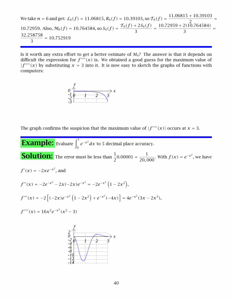
Is it worth any extra effort to get a better estimate of M4? The answer is that it depends ondifficult the expression for f ′′′′(x) is. We obtained a good guess for the maximum value of|f ′′′′(x) by substituting x = 3 into it. It is now easy to sketch the graphs of functions withcomputers:

x

y

-3-2-10

0 1 2 3

The graph confirms the suspicion that the maximum value of |f ′′′′(x)| occurs at x = 3.

Example: Evaluate∫ 10

e−x2dx to 5 decimal place accuracy.

Solution: The error must be less than 120.00001 = 1

20,000. With f (x) = e−x2, we have

f ′(x) = −2xe−x2, and

f ′′(x) = −2e−x2 − 2x(−2x)e−x2 = −2e−x2(1− 2x2

),

f ′′′(x) = −2[(−2x)e−x2

(1− 2x2

)+ e−x2(−4x)

]= 4e−x2(3x − 2x3),

f ′′′′(x) = 16x2e−x2(x2 − 3)

x

y

-14-12-10-8-6-4-202

0 1 2 3

40

We have M4 ≤ 13, so E(Sn(f )) ≤ M4(1− 0)5

180n4=≤ 13

180n4<

120,000

if

n4 >260,000180

= 26,00018

= 13,0009

� 1444.4 or n > 6.16, so we take n = 8.Then L8(f ) � 0.78537315, R8(f ) � 0.7063581,

so T8(f ) = L8(f )+R8(f )2

= 0.74586564.

AlsoM8(f ) = 0.7473036,and S8(f ) = 0.74682426.

As a matter of fact,E(S8(f )) ≤ 13180(10)4

� 0.000007, so we expect six decimal place accuracy

of S8(f ).

Using n = 100, we have

L100(f ) = 0.7499786,

R100(f ) = 0.7436574,

T100(f ) = 0.746818,

M100(f ) = 0.7468272,

S100(f ) = 0.7468242574357303.

We have E(S100(f )) ≤ 13180(100)4

� 0.0000000007, so our first 9 decimal places are accurate,

i.e.,∫ 10

e−x2dx = 0.746824257 is a true statement.

41