1

Motion Planning for Disc-shaped Robots Pushing aPolygonal Object in the Plane

Attawith Sudsang, Fred Rothganger, and Jean Ponce

Abstract—This paper addresses the problem of using three disc-shapedrobots to manipulate a polygonal object in the plane in the presence of ob-stacles. The proposed approach is based on the computation of maximaldiscs (dubbedmaximum independent capture discs, or MICaDs) where therobots can move independently while preventing the object from escapingtheir grasp. It is shown that, in the absence of obstacles, itis always pos-sible to bring a polygonal object from any configuration to any other onewith robot motions constrained to lie in a set of overlappingMICaDs. Thisapproach is generalized to the case where obstacles are present by decom-posing the corresponding motion planning task into (1) the constructionof a collision-free path for a modified form of the object, and(2) the exe-cution of this path by a sequence of simultaneous and independent robotmotions within overlapping MICaDs. The proposed algorithm is guaran-teed to generate a valid plan provided a collision-free pathexists for themodified form of the object. It has been implemented and experiments withNomadic Scout mobile robots are presented.

Keywords—capture regions, object manipulation, pushing, motion plan-ning

I. I NTRODUCTION

This paper addresses the problem of using three disc-shapedrobots to manipulate a polygonal object in the plane in the pres-ence of obstacles. In practice, the robots may be the fingertips ofa gripper or mobile platforms. The proposed approach is basedon the computation of maximal discs (dubbedmaximum inde-pendent capture discs, or MICaDs for short) of the workspacewhere the robots can move independently while guaranteeingthat the object cannot escape their grasp.

We show that, in the absence of obstacles, there is a neigh-borhood of any object configuration such that any other config-uration within it can be reached using robot motions confinedto the associated MICaDs (a property akin to local controlla-bility). This forms the basis for an approach to manipulationplanning where an object’s trajectory is divided into maximalsegments such that the MICaDs associated with the endpointsofeach segment overlap. We generalize this approach to the casewhere obstacles are present by decomposing the correspondingmotion planning task into (1) the construction of a collision-freepath for a modified form of the object, and (2) the execution ofthis path by a sequence of simultaneous and independent robotmotions within overlapping MICaDs. The proposed algorithmis guaranteed to generate a valid plan provided a collision-freepath exists for the modified form of the object. In addition, itdoes not assume that contact is maintained during the execu-tion of the manipulation task, nor does it rely on detailed and apriori unverifiable models of friction or contact dynamics,but itallows the construction of manipulation plans guaranteed to suc-ceed under the weaker assumption that jamming does not occurduring the task execution. We have implemented the proposedapproach and present experiments with Nomadic Scout mobilerobots.

The proposed approach is based on a few lemmas. Proofstoo lengthy to be included in the body of this presentation are

relegated to an appendix, along with the derivation of a few keyequations. A preliminary version of this work appeared in [1].

A. Background

When a hand holds an object at rest, the forces and momentsexerted by the fingers balance each other to achieve equilibrium.For the hand to hold the object securely, it should also be capa-ble of preventing any motion due to external forces and torques.This is captured by the dual notions ofform and force closurethat constitute the traditional theoretical basis for grasp plan-ning [2], [3], [4]. Recently, Rimon and Burdick have introducedthe notion ofsecond-order immobility[5], [6] and shown thatcertain equilibrium grasps of a part which do not achieve formclosure effectively prevent anyfinitemotion of this part throughcurvature effects in configuration space. We introduced in [7],[8] the more general notion ofinescapable configuration spaceregion (orICS): as shown in [5], [6], an object is immobilizedwhen it rests at an isolated point of its free configuration space;moving the fingers in an appropriate way transforms this iso-lated point into a compact region of free space (the ICS) thatcannot be escaped by the object.

ICS regions were introduced in the context of in-hand manip-ulation with a multi-fingered reconfigurable gripper [7], [8] (seethe works of Rimon and Blake [9] and Davidson and Blake [10]for the related notion of acagein two- and three-finger grasp-ing). We showed in [11] that ICS regions can also be used tomanipulate an object by pushing it with three disc-shaped robotsmoving one at a time along straight lines with fixed directions.The object remains at all times in the ICS region associated withthe robots, and the manipulation will succeed as long as the fric-tion forces associated with contacts between the robots, the ob-ject and its supporting plane are not large enough to cause jam-ming.

The methods presented in [10], [9], [11] can only be used togenerate plans where robots move one by one in a fixed direc-tion. This severely limits the extent of each manipulation step,forcing any complex motion to be decomposed into a large num-ber of atomic elements. We introduced in [12] another techniqueallowing the robots to move one by one in two-dimensional re-gions. Here we go further, showing how to construct maximum-radius workspace discs where the robots can move simultane-ously and independently while preventing the object from es-caping their grasp, and use these discs as the basis for a newapproach to motion planning in the presence of obstacles.

The general form of the manipulation planning problem isdiscussed in [13], [14], and [15]. The proposed approach is re-lated to a number of other techniques for manipulation planningwhere the uncertainty in the position of the manipulated partis reduced by exploiting the task mechanics. Work in this area

2

was pioneered by Inoue [16] and Whitney [17], and techniquesfor re-orienting parts through pushing and grasping operationshave been developed by several authors, including Fearing [18],Mason [19], Mani and Wilson [20], Brost [21], Erdmann andMason [22], Peshkin and Sanderson [23], Goldberg [24], Abelland Erdmann [25], Rao and Goldberg [26], Akella et al. [27],and Leveroni and Salisbury [28]. Unlike these methods, thatallassume some predictive model of the contact mechanics, our ap-proach does not require that robot/object contact be maintainedduring grasping or manipulation, nor does it rely on detailedmodels of friction and contact dynamics. In addition, by decom-posing the construction of manipulation plans into the computa-tion of a collision-free path for (a modified form of) the object,followed by the construction of elementary robot motion se-quences for executing this path, we obtain an efficient approachto manipulation planning in the presence of obstacles that is ca-pable of exploiting the effective algorithms that are available formotion planning in low-dimension configuration spaces, such asthe exact motion planner of Avnaimet al. [29], or the approx-imate but very efficient planners of Barraquand and Latombe[30] and Kavrakiet al. [31].

II. M AXIMUM INDEPENDENTCAPTURE DISCS

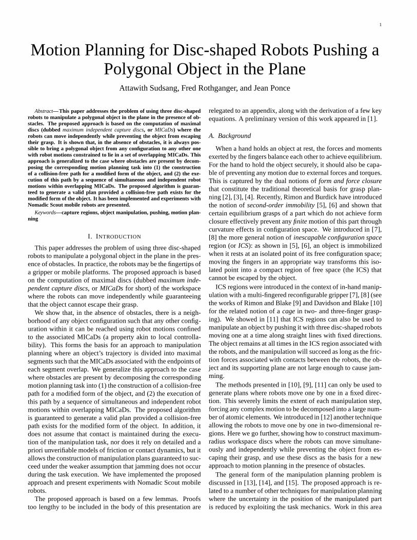
We characterize in this section the configurations of threedisc-shaped robots that capture a polygonal object, i.e., preventit from escaping to infinity. We will assume that all contactsbetween the object, the robots and the supporting plane are fric-tionless. Although this assumption is not verified by most phys-ical systems, robots that capture an object without friction willstill capture it when friction is present, and the motion plan-ning techniques presented in latter parts of this article will beguaranteed to succeed as long as the friction forces are not largeenough to cause jamming. We assume in this section that the ob-ject has been grown by the robots’ radius, while the robots havebeen shrunk into their centers. (This transforms the boundary ofthe object into a generalized polygon with straight and circulararcs.) We consider the grown object and the point-like robotsto be workspace objects. We will restrict our analysis to thestudy of the constraints imposed on the (point) robots by threearbitrarily chosen straight edgesE1, E2 andE3 of the grownobject.

Notation: Given some fixed coordinate system for the plane,we will denote byqi = (xi; yi) (i = 1; 2; 3) the positions of therobotsB1; B2 andB3, and byp = (x; y; ) the configurationof the polygonal objectB being manipulated. The edgesEiare associated with the robotsBi (i = 1; 2; 3), and we denotebyEi() the set of configurations(x; y) for which the robotBitouches the edgeEi when the polygonB is at orientation.

A given configuration of the robots defines the setF of freeconfigurations of the polygon in its configuration space IR2 S1. For polygonal objects, the robots immobilize the object atequilibrium, which occurs when the edge normals at the threecontact points intersect at a single point and positively span theplane [5], [6].

We say that the robotscapturethe object whenF contains acompact connected componentI andp belongs toI. In thiscase the object is free to move inside theinescapable configura-tion space(ICS) regionI, but it cannot escape the robots’ grasp.

(a) B3

BB1 B2

(b)

1 θ

q1

p1

q3

q2

E ( )

E

Fig. 1. Contact between an edge and a robot: (a) the original (ungrown) objectand the three robots; (b) the grown object, the point-like robots, and the c-spaceobstacle induced by the contact. Both (a) and (b) are in workspace, and relevantconfiguration space objects (p andE1()) have been projected onto workspace.

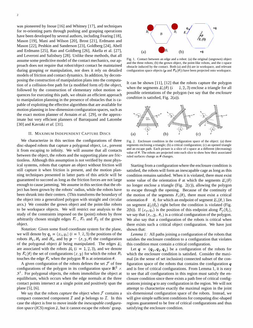
It can be shown [11], [12] that the robots capture the polygonwhen the segmentsEi() (i = 1; 2; 3) enclose a triangle for allpossible orientations of the polygon (we say that theenclosureconditionis satisfied, Fig. 2(a)).

(a)q1

q2q3FreeSpace

(b)q1

q2q3

(c)q1

q2q3

Fig. 2. Enclosure condition in the configuration space of theobject: (a) threesegments enclosing a triangle; (b) a critical configuration; (c) an opened triangleand an escape path. Each picture is a slice of c-space at a different (decreasing)value of. The robots are projected onto each slice to show how their associatedruled surfaces change as changes.

Starting from a configuration where the enclosure conditionissatisfied, the robots will form an inescapable cage as long asthiscondition remains satisfied. When it is violated, there mustexistsome value of the orientation at which the segmentsEi()no longer enclose a triangle (Fig. 2(c)), allowing the polygonto escape through the opening. Because of the continuity ofthe motion of the segmentsEi(), there must exist a criticalorientation = for which an endpoint of segmentEi( ) lieson segmentEj( ) right before the condition is violated (Fig.2(b)). If (x ; y ) is the position of this endpoint alongEj( ),we say that(x ; y ; ) is a critical configuration of the polygon.We also say that a configuration of the robots is critical whenthere exists such a critical object configuration. We have justshown that:

Lemma 1:All paths joining a configuration of the robots thatsatisfies the enclosure condition to a configuration that violatesthis condition must contain a critical configuration.

Let q = (q1; q2; q3) be a configuration of the robots forwhich the enclosure condition is satisfied. Consider the maxi-mal (in the sense of set inclusion) connected subset of the con-figuration space of the robots that contains the configuration qand is free of critical configurations. From Lemma 1, it is easyto see that all configurations in this region must satisfy theen-closure condition since there exists a path free of criticalconfig-urations joiningq to any configuration in the region. We will notattempt to characterize exactly the maximal region in the jointsix-dimensional configuration space of the robots. Instead, wewill give simple sufficient conditions for computing disc-shapedregions guaranteed to be free of critical configurations andthussatisfying the enclosure condition.

3

Definition 1: Three discs1;2 and 3 are independentcapture discs(or ICaDs for short) when, for any configurationq in 1 2 3, the robots capture the object. A triple ofICaDs such that the radius of the smallest disc has maximal sizeis called a triple ofmaximum independent capture discs, or MI-CaDs.

A. Constructing the MICaDs

The rest of this section presents a method for constructing atriple of MICaDs. We assume that an immobilizing configura-tion q0 of the robots exists for the selected triple of edges1 andcharacterize the range of motions that robots starting inq0 mayundergo before reaching a critical configuration.

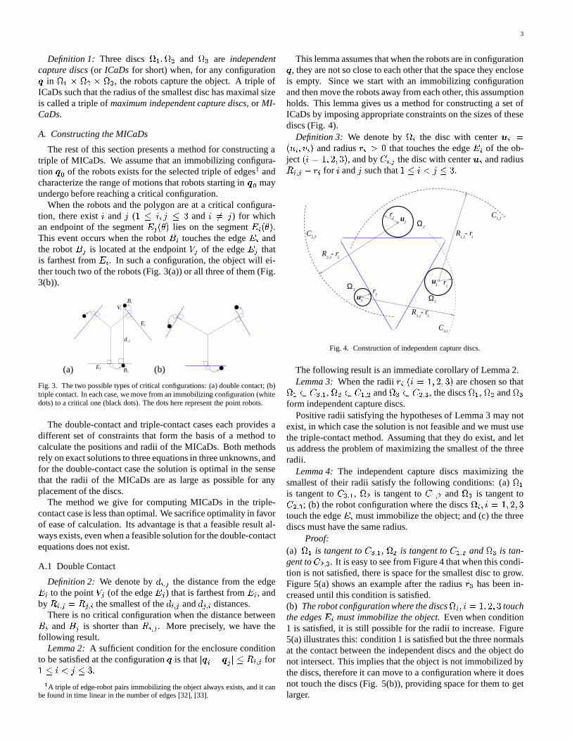
When the robots and the polygon are at a critical configura-tion, there existi andj (1 i; j 3 and i 6= j) for whichan endpoint of the segmentEj() lies on the segmentEi().This event occurs when the robotBi touches the edgeEi andthe robotBj is located at the endpointVj of the edgeEj thatis farthest fromEi. In such a configuration, the object will ei-ther touch two of the robots (Fig. 3(a)) or all three of them (Fig.3(b)).

(a) BiEi

Ej

Bj

Vj

d i,j

(b)

Fig. 3. The two possible types of critical configurations: (a) double contact; (b)triple contact. In each case, we move from an immobilizing configuration (whitedots) to a critical one (black dots). The dots here representthe point robots.

The double-contact and triple-contact cases each providesadifferent set of constraints that form the basis of a method tocalculate the positions and radii of the MICaDs. Both methodsrely on exact solutions to three equations in three unknowns, andfor the double-contact case the solution is optimal in the sensethat the radii of the MICaDs are as large as possible for anyplacement of the discs.

The method we give for computing MICaDs in the triple-contact case is less than optimal. We sacrifice optimality infavorof ease of calculation. Its advantage is that a feasible result al-ways exists, even when a feasible solution for the double-contactequations does not exist.

A.1 Double Contact

Definition 2: We denote bydi;j the distance from the edgeEi to the pointVj (of the edgeEj) that is farthest fromEi, andbyRi;j = Rj;i the smallest of thedi;j anddj;i distances.

There is no critical configuration when the distance betweenBi andBj is shorter thanRi;j . More precisely, we have thefollowing result.

Lemma 2:A sufficient condition for the enclosure conditionto be satisfied at the configurationq is thatjqi qj j Ri;j for1 i < j 3.1A triple of edge-robot pairs immobilizing the object alwaysexists, and it canbe found in time linear in the number of edges [32], [33].

This lemma assumes that when the robots are in configurationq, they are not so close to each other that the space they encloseis empty. Since we start with an immobilizing configurationand then move the robots away from each other, this assumptionholds. This lemma gives us a method for constructing a set ofICaDs by imposing appropriate constraints on the sizes of thesediscs (Fig. 4).

Definition 3: We denote byi the disc with centerui =(ui; vi) and radiusri > 0 that touches the edgeEi of the ob-ject (i = 1; 2; 3), and byCi;j the disc with centerui and radiusRi;j ri for i andj such that1 i < j 3.

R2,3 2

- r

C2,3

r2 u

2 Ω2

C1,2

C3,1

R3,1 3

- r

R1,2 1

- r

Ω3

Ω1

u3

r3

u1 r

1

Fig. 4. Construction of independent capture discs.

The following result is an immediate corollary of Lemma 2.Lemma 3:When the radiiri (i = 1; 2; 3) are chosen so that1 C3;1, 2 C1;2 and3 C2;3, the discs1, 2 and3

form independent capture discs.Positive radii satisfying the hypotheses of Lemma 3 may not

exist, in which case the solution is not feasible and we must usethe triple-contact method. Assuming that they do exist, andletus address the problem of maximizing the smallest of the threeradii.

Lemma 4:The independent capture discs maximizing thesmallest of their radii satisfy the following conditions: (a) 1is tangent toC3;1, 2 is tangent toC1;2 and3 is tangent toC2;3; (b) the robot configuration where the discsi; i = 1; 2; 3touch the edgeEi must immobilize the object; and (c) the threediscs must have the same radius.

Proof:(a) 1 is tangent toC3;1, 2 is tangent toC1;2 and3 is tan-gent toC2;3. It is easy to see from Figure 4 that when this condi-tion is not satisfied, there is space for the smallest disc to grow.Figure 5(a) shows an example after the radiusr3 has been in-creased until this condition is satisfied.(b) The robot configuration where the discsi; i = 1; 2; 3 touchthe edgesEi must immobilize the object.Even when condition1 is satisfied, it is still possible for the radii to increase.Figure5(a) illustrates this: condition 1 is satisfied but the threenormalsat the contact between the independent discs and the object donot intersect. This implies that the object is not immobilized bythe discs, therefore it can move to a configuration where it doesnot touch the discs (Fig. 5(b)), providing space for them to getlarger.

4

(a)

3Ω

u3

r3

Ω

C

C

C

R

R

r

r

2

2

1

1,2

2,3

3,1

1,2

2,3

u

u

1

2

-r

-r

R 3,1-r 3

1

2

Ω1

(b)

3Ω

u3

r3

Ω

C

C

C

R

R

r

r

2

2

1

1,2

2,3

3,1

1,2

2,3

u

u

1

2

-r

-r

R 3,1-r 3

1

2

Ω1

Fig. 5. Proving Lemma 4: (a) independent capture discs wherecondition 1satisfied; (b) when the discs do not immobilize the object, there is some spacefor the smallest disc to grow.

(c) The three radii are equal:r1 = r2 = r3. Consider Fig-ure 6. We denote byLi;j the line segment joining two pointsin the disci and the discj that are farthest from each other.Clearly,Li;j passes through the centers of both discs. For con-dition 1 to be satisfied, the length ofLi;j must be maintainedconstant atRi;j . In Figure 6(a), we assume that the first twoconditions are satisfied andr2 is the smallest radius. To increasethe radiusr2, we change the intersection point betweenL1;2 andL2;3 (which is the location of the center of2). For the discs notto intersect with the object and to maintain the constant lengthof eachLi;j , asr2 increases, the object must move toward1and3 and the radiir1 andr3 must decrease (Fig. 6(b)). Sincethis process can always be applied as long as the radius of thesmallest disc is strictly smaller than the other ones, this radius ismaximized when all three radii are equal.

(a)

1Ω

2

1223

313Ω

L

Ω

L

L

(b)Ω Ω

Ω

L

L L

2

23

3

31

12

1

Fig. 6. Growing the smallest disc.

Lemma 4 allows us to compute the MICaDs. For a given con-figuration of the object, these discs are defined by three param-eters: the position(s; t) of the intersection of the three normalsto the object edges at the points where the discs touch them, andthe common radiusr of the discs. Lemma 4 yields a quadraticequation inr, s andt for each disc (Appendix A), and the max-imum capture discs can be found by solving the correspondingsystem of three equations in three unknowns using homotopycontinuation [34] and picking the solution that yields the max-imum value ofr. The centers of the corresponding discs areeasily determined by the condition that they must be tangenttothe selected object edges.

A.2 Triple Contact

For the double-contact solution to be feasible: 1)r, s andtmust be real numbers (imaginary component equal to zero), 2)r must be positive, and 3)(s; t) must be positioned so that eachdisc is tangent to its respective edge at a point that is actuallyon the line segment that is part of the object. Failing that, we

cannot determine the MICaDs using the double-contact equa-tions. (The reason why this occurs has to do with the shape ofthe configuration space obstacles, and is beyond the scope ofthis paper.) However, we can use the following method, whichis based on constraints derived from the triple-contact case.

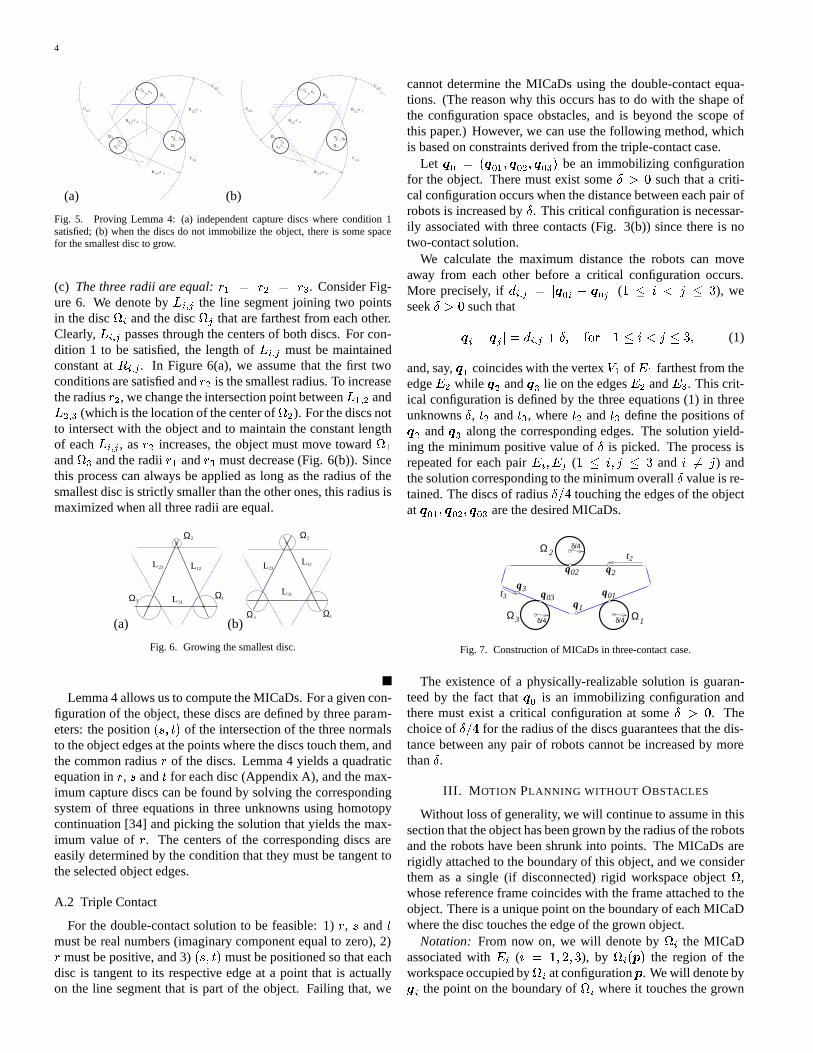
Let q0 = (q01; q02; q03) be an immobilizing configurationfor the object. There must exist someÆ > 0 such that a criti-cal configuration occurs when the distance between each pairofrobots is increased byÆ. This critical configuration is necessar-ily associated with three contacts (Fig. 3(b)) since there is notwo-contact solution.

We calculate the maximum distance the robots can moveaway from each other before a critical configuration occurs.More precisely, ifdi;j = jq0i q0j j (1 i < j 3), weseekÆ > 0 such thatjqi qj j = di;j + Æ; for 1 i < j 3; (1)

and, say,q1 coincides with the vertexV1 of E1 farthest from theedgeE2 while q2 andq3 lie on the edgesE2 andE3. This crit-ical configuration is defined by the three equations (1) in threeunknownsÆ, t2 andt3, wheret2 andt3 define the positions ofq2 andq3 along the corresponding edges. The solution yield-ing the minimum positive value ofÆ is picked. The process isrepeated for each pairEi; Ej (1 i; j 3 and i 6= j) andthe solution corresponding to the minimum overallÆ value is re-tained. The discs of radiusÆ=4 touching the edges of the objectatq01; q02; q03 are the desired MICaDs.

Ω13Ω δ/4 δ/4

q01

δ/42Ω

q02

q1

q03

q3

q2

t2

t3

Fig. 7. Construction of MICaDs in three-contact case.

The existence of a physically-realizable solution is guaran-teed by the fact thatq0 is an immobilizing configuration andthere must exist a critical configuration at someÆ > 0. Thechoice ofÆ=4 for the radius of the discs guarantees that the dis-tance between any pair of robots cannot be increased by morethanÆ.

III. M OTION PLANNING WITHOUT OBSTACLES

Without loss of generality, we will continue to assume in thissection that the object has been grown by the radius of the robotsand the robots have been shrunk into points. The MICaDs arerigidly attached to the boundary of this object, and we considerthem as a single (if disconnected) rigid workspace object,whose reference frame coincides with the frame attached to theobject. There is a unique point on the boundary of each MICaDwhere the disc touches the edge of the grown object.

Notation: From now on, we will denote byi the MICaDassociated withEi (i = 1; 2; 3), by i(p) the region of theworkspace occupied byi at configurationp. We will denote bygi the point on the boundary ofi where it touches the grown

5

object, and bygi(p) the point in workspace occupied bygi atconfigurationp.

The three robots form an inescapable cage if there exists aconfigurationp of such thatqi belongs toi(p) for i =1; 2; 3. According to Lemma 4, when the positions of the robotsareqi = gi(p) (i = 1; 2; 3), the object is immobilized in thecorresponding configurationp.

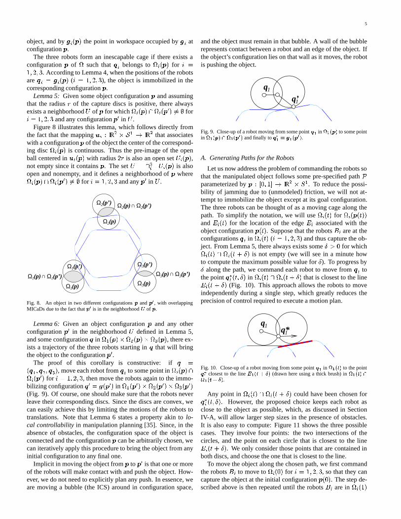
Lemma 5:Given some object configurationp and assumingthat the radiusr of the capture discs is positive, there alwaysexists a neighborhoodU of p for whichi(p)\i(p0) 6= ; fori = 1; 2; 3 and any configurationp0 in U .

Figure 8 illustrates this lemma, which follows directly fromthe fact that the mappingui : IR2 S1 ! IR2 that associateswith a configurationp of the object the center of the correspond-ing disci(p) is continuous. Thus the pre-image of the openball centered inui(p) with radius2r is also an open setUi(p),not empty since it containsp. The setU = \3i=1Ui(p) is alsoopen and nonempty, and it defines a neighborhood ofp wherei(p) \i(p0) 6= ; for i = 1; 2; 3 and anyp0 in U .

∩Ω2(p) Ω2(p’)

Ω1(p) Ω1(p’)∩

Ω1(p)

Ω1(p’) Ω3(p’)

Ω3(p)

∩ Ω3(p’)Ω3(p)

Ω2(p’)

Ω2(p)

Fig. 8. An object in two different configurationsp andp0, with overlappingMICaDs due to the fact thatp0 is in the neighborhoodU of p.

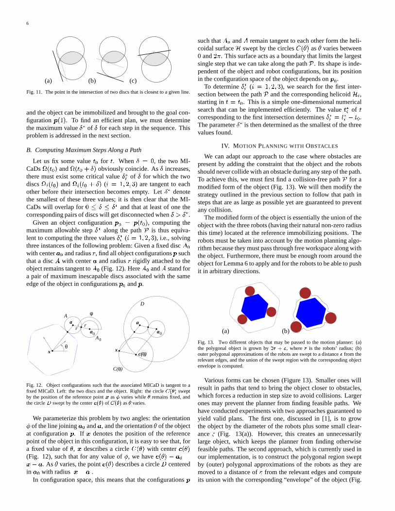
Lemma 6:Given an object configurationp and any otherconfigurationp0 in the neighborhoodU defined in Lemma 5,and some configurationq in 1(p)2(p)3(p), there ex-ists a trajectory of the three robots starting inq that will bringthe object to the configurationp0.

The proof of this corollary is constructive: ifq =(q1; q2; q3), move each robot fromqi to some point ini(p) \i(p0) for i = 1; 2; 3, then move the robots again to the immo-bilizing configurationq0 = g(p0) in 1(p0)2(p0)3(p0)(Fig. 9). Of course, one should make sure that the robots neverleave their corresponding discs. Since the discs are convex, wecan easily achieve this by limiting the motions of the robotstotranslations. Note that Lemma 6 states a property akin tolo-cal controllability in manipulation planning [35]. Since, in theabsence of obstacles, the configuration space of the object isconnected and the configurationp can be arbitrarily chosen, wecan iteratively apply this procedure to bring the object from anyinitial configuration to any final one.

Implicit in moving the object fromp to p0 is that one or moreof the robots will make contact with and push the object. How-ever, we do not need to explicitly plan any push. In essence, weare moving a bubble (the ICS) around in configuration space,

and the object must remain in that bubble. A wall of the bubblerepresents contact between a robot and an edge of the object.Ifthe object’s configuration lies on that wall as it moves, the robotis pushing the object.

q1

q’1

Fig. 9. Close-up of a robot moving from some pointq1 in 1(p) to some pointin 1(p) \ 1(p0) and finally toq01 = g1(p0).A. Generating Paths for the Robots

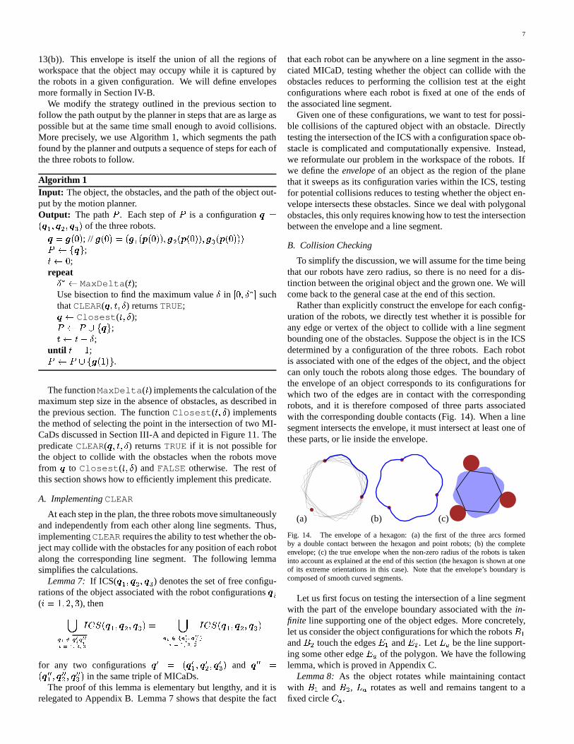
Let us now address the problem of commanding the robots sothat the manipulated object follows some pre-specified pathPparameterized byp : [0; 1 ! IR2 S1. To reduce the possi-bility of jamming due to (unmodeled) friction, we will not at-tempt to immobilize the object except at its goal configuration.The three robots can be thought of as a moving cage along thepath. To simplify the notation, we will usei(t) for i(p(t))andEi(t) for the location of the edgeEi associated with theobject configurationp(t). Suppose that the robotsBi are at theconfigurationsqi in i(t) (i = 1; 2; 3) and thus capture the ob-ject. From Lemma 5, there always exists someÆ > 0 for whichi(t) \ i(t + Æ) is not empty (we will see in a minute howto compute the maximum possible value forÆ). To progress byÆ along the path, we command each robot to move fromqi tothe pointqi (t; Æ) in i(t) \ i(t + Æ) that is closest to the lineEi(t + Æ) (Fig. 10). This approach allows the robots to moveindependently during a single step, which greatly reduces theprecision of control required to execute a motion plan.

q1q*1

Fig. 10. Close-up of a robot moving from some pointq1 in 1(t) to the pointq1 closest to the lineE1(t + Æ) (drawn here using a thick brush) in1(t) \1(t+ Æ).Any point in i(t) \ i(t + Æ) could have been chosen forqi (t; Æ). However, the proposed choice keeps each robot as

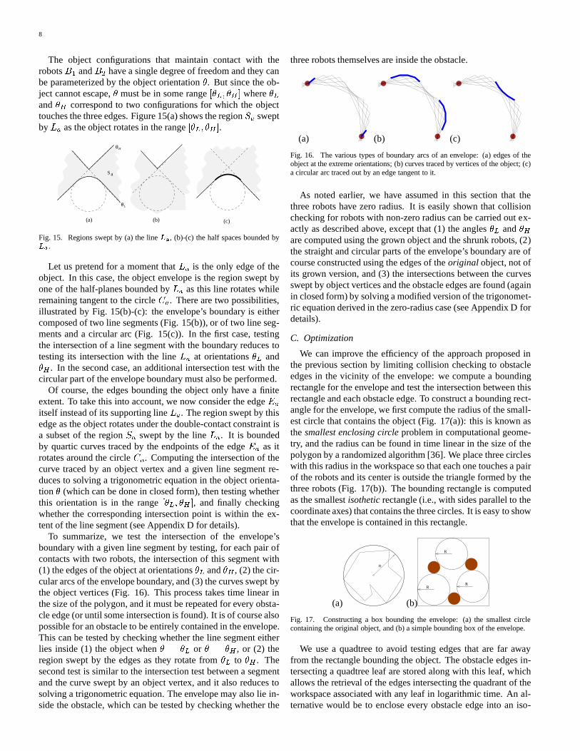
close to the object as possible, which, as discussed in SectionIV-A, will allow larger step sizes in the presence of obstacles.It is also easy to compute: Figure 11 shows the three possiblecases. They involve four points: the two intersections of thecircles, and the point on each circle that is closest to the lineEi(t + Æ). We only consider those points that are contained inboth discs, and choose the one that is closest to the line.

To move the object along the chosen path, we first commandthe robotsBi to move toi(0) for i = 1; 2; 3, so that they cancapture the object at the initial configurationp(0). The step de-scribed above is then repeated until the robotsBi are ini(1)

6

(a) (b) (c)

Fig. 11. The point in the intersection of two discs that is closest to a given line.

and the object can be immobilized and brought to the goal con-figurationp(1). To find an efficient plan, we must determinethe maximum valueÆ of Æ for each step in the sequence. Thisproblem is addressed in the next section.

B. Computing Maximum Steps Along a Path

Let us fix some valuet0 for t. WhenÆ = 0, the two MI-CaDs(t0) and(t0 + Æ) obviously coincide. AsÆ increases,there must exist some critical valueÆi of Æ for which the twodiscsi(t0) andi(t0 + Æ) (i = 1; 2; 3) are tangent to eachother before their intersection becomes empty. LetÆ denotethe smallest of these three values; it is then clear that the MI-CaDs will overlap for0 Æ Æ and that at least of one thecorresponding pairs of discs will get disconnected whenÆ > Æ.

Given an object configurationp0 = p(t0), computing themaximum allowable stepÆ along the pathP is thus equiva-lent to computing the three valuesÆi (i = 1; 2; 3), i.e., solvingthree instances of the following problem: Given a fixed discA0with centera0 and radiusr, find all object configurationsp suchthat a discA with centera and radiusr rigidly attached to theobject remains tangent toA0 (Fig. 12). HereA0 andA stand fora pair of maximum inescapable discs associated with the sameedge of the object in configurationsp0 andp.

a

φ

rr

D

A

c( )θ

C( )θ

θ

a0 0

0

x

a aA

x

Fig. 12. Object configurations such that the associated MICaD is tangent to afixed MICaD. Left: the two discs and the object. Right: the circleC() sweptby the position of the reference pointx as varies while remains fixed, andthe circleD swept by the center () of C() as varies.

We parameterize this problem by two angles: the orientation of the line joininga0 anda, and the orientation of the objectat configurationp. If x denotes the position of the referencepoint of the object in this configuration, it is easy to see that, fora fixed value of, x describes a circleC() with center ()(Fig. 12), such that for any value of, we have () a0 =x a. As varies, the point () describes a circleD centeredin a0 with radiusjx aj.

In configuration space, this means that the configurationsp

such thatA0 andA remain tangent to each other form the heli-coidal surfaceH swept by the circlesC() as varies between0 and2. This surface acts as a boundary that limits the largestsingle step that we can take along the pathP . Its shape is inde-pendent of the object and robot configurations, but its positionin the configuration space of the object depends onp0.

To determineÆi (i = 1; 2; 3), we search for the first inter-section between the pathP and the corresponding helicoidHi,starting int = t0. This is a simple one-dimensional numericalsearch that can be implemented efficiently. The valueti of tcorresponding to the first intersection determinesÆi = ti t0.The parameterÆ is then determined as the smallest of the threevalues found.

IV. M OTION PLANNING WITH OBSTACLES

We can adapt our approach to the case where obstacles arepresent by adding the constraint that the object and the robotsshould never collide with an obstacle during any step of the path.To achieve this, we must first find a collision-free pathP for amodified form of the object (Fig. 13). We will then modify thestrategy outlined in the previous section to follow that path insteps that are as large as possible yet are guaranteed to preventany collision.

The modified form of the object is essentially the union of theobject with the three robots (having their natural non-zeroradiusthis time) located at the reference immobilizing positions. Therobots must be taken into account by the motion planning algo-rithm because they must pass through free workspace along withthe object. Furthermore, there must be enough room around theobject for Lemma 6 to apply and for the robots to be able to pushit in arbitrary directions.

(a) (b)

Fig. 13. Two different objects that may be passed to the motion planner: (a)the polygonal object is grown by2r + ", wherer is the robots’ radius; (b)outer polygonal approximations of the robots are swept to a distance" from therelevant edges, and the union of the swept region with the corresponding objectenvelope is computed.

Various forms can be chosen (Figure 13). Smaller ones willresult in paths that tend to bring the object closer to obstacles,which forces a reduction in step size to avoid collisions. Largerones may prevent the planner from finding feasible paths. Wehave conducted experiments with two approaches guaranteedtoyield valid plans. The first one, discussed in [1], is to growthe object by the diameter of the robots plus some small clear-ance" (Fig. 13(a)). However, this creates an unnecessarilylarge object, which keeps the planner from finding otherwisefeasible paths. The second approach, which is currently used inour implementation, is to construct the polygonal region sweptby (outer) polygonal approximations of the robots as they aremoved to a distance of" from the relevant edges and computeits union with the corresponding “envelope” of the object (Fig.

7

13(b)). This envelope is itself the union of all the regions ofworkspace that the object may occupy while it is captured bythe robots in a given configuration. We will define envelopesmore formally in Section IV-B.

We modify the strategy outlined in the previous section tofollow the path output by the planner in steps that are as large aspossible but at the same time small enough to avoid collisions.More precisely, we use Algorithm 1, which segments the pathfound by the planner and outputs a sequence of steps for each ofthe three robots to follow.

Algorithm 1Input: The object, the obstacles, and the path of the object out-put by the motion planner.Output: The pathP . Each step ofP is a configurationq =(q1; q2; q3) of the three robots.q = g(0); // g(0) = (g1(p(0)); g2(p(0)); g3(p(0)))P fqg;t 0;

repeatÆ MaxDelta (t);Use bisection to find the maximum valueÆ in [0; Æ suchthatCLEAR(q; t; Æ) returnsTRUE;q Closest (t; Æ);P P [ fqg;t t+ Æ;

until t = 1;P P [ fg(1)g.The functionMaxDelta (t) implements the calculation of the

maximum step size in the absence of obstacles, as described inthe previous section. The functionClosest (t; Æ) implementsthe method of selecting the point in the intersection of two MI-CaDs discussed in Section III-A and depicted in Figure 11. ThepredicateCLEAR(q; t; Æ) returnsTRUEif it is not possible forthe object to collide with the obstacles when the robots movefrom q to Closest (t; Æ) andFALSE otherwise. The rest ofthis section shows how to efficiently implement this predicate.

A. ImplementingCLEAR

At each step in the plan, the three robots move simultaneouslyand independently from each other along line segments. Thus,implementingCLEARrequires the ability to test whether the ob-ject may collide with the obstacles for any position of each robotalong the corresponding line segment. The following lemmasimplifies the calculations.

Lemma 7: If ICS(q1; q2; q3) denotes the set of free configu-rations of the object associated with the robot configurationsqi(i = 1; 2; 3), then[qi 2 q0iq00ii = 1; 2; 3ICS(q1; q2; q3) = [qi 2 fq0i; q00i gi = 1; 2; 3 ICS(q1; q2; q3)for any two configurationsq0 = (q01; q02; q03) and q00 =(q001 ; q002 ; q003 ) in the same triple of MICaDs.

The proof of this lemma is elementary but lengthy, and it isrelegated to Appendix B. Lemma 7 shows that despite the fact

that each robot can be anywhere on a line segment in the asso-ciated MICaD, testing whether the object can collide with theobstacles reduces to performing the collision test at the eightconfigurations where each robot is fixed at one of the ends ofthe associated line segment.

Given one of these configurations, we want to test for possi-ble collisions of the captured object with an obstacle. Directlytesting the intersection of the ICS with a configuration space ob-stacle is complicated and computationally expensive. Instead,we reformulate our problem in the workspace of the robots. Ifwe define theenvelopeof an object as the region of the planethat it sweeps as its configuration varies within the ICS, testingfor potential collisions reduces to testing whether the object en-velope intersects these obstacles. Since we deal with polygonalobstacles, this only requires knowing how to test the intersectionbetween the envelope and a line segment.

B. Collision Checking

To simplify the discussion, we will assume for the time beingthat our robots have zero radius, so there is no need for a dis-tinction between the original object and the grown one. We willcome back to the general case at the end of this section.

Rather than explicitly construct the envelope for each config-uration of the robots, we directly test whether it is possible forany edge or vertex of the object to collide with a line segmentbounding one of the obstacles. Suppose the object is in the ICSdetermined by a configuration of the three robots. Each robotis associated with one of the edges of the object, and the objectcan only touch the robots along those edges. The boundary ofthe envelope of an object corresponds to its configurations forwhich two of the edges are in contact with the correspondingrobots, and it is therefore composed of three parts associatedwith the corresponding double contacts (Fig. 14). When a linesegment intersects the envelope, it must intersect at leastone ofthese parts, or lie inside the envelope.

(a) (b) (c)

Fig. 14. The envelope of a hexagon: (a) the first of the three arcs formedby a double contact between the hexagon and point robots; (b)the completeenvelope; (c) the true envelope when the non-zero radius of the robots is takeninto account as explained at the end of this section (the hexagon is shown at oneof its extreme orientations in this case). Note that the envelope’s boundary iscomposed of smooth curved segments.

Let us first focus on testing the intersection of a line segmentwith the part of the envelope boundary associated with thein-finite line supporting one of the object edges. More concretely,let us consider the object configurations for which the robotsB1andB2 touch the edgesE1 andE2. LetLa be the line support-ing some other edgeEa of the polygon. We have the followinglemma, which is proved in Appendix C.

Lemma 8:As the object rotates while maintaining contactwith B1 andB2, La rotates as well and remains tangent to afixed circleCa.

8

The object configurations that maintain contact with therobotsB1 andB2 have a single degree of freedom and they canbe parameterized by the object orientation. But since the ob-ject cannot escape, must be in some range[L; H whereLandH correspond to two configurations for which the objecttouches the three edges. Figure 15(a) shows the regionSa sweptbyLa as the object rotates in the range[L; H .

(b)(a) (c)

Sa

θH

θL

Fig. 15. Regions swept by (a) the lineLa, (b)-(c) the half spaces bounded byLa.

Let us pretend for a moment thatLa is the only edge of theobject. In this case, the object envelope is the region sweptbyone of the half-planes bounded byLa as this line rotates whileremaining tangent to the circleCa. There are two possibilities,illustrated by Fig. 15(b)-(c): the envelope’s boundary is eithercomposed of two line segments (Fig. 15(b)), or of two line seg-ments and a circular arc (Fig. 15(c)). In the first case, testingthe intersection of a line segment with the boundary reducestotesting its intersection with the lineLa at orientationsL andH . In the second case, an additional intersection test with thecircular part of the envelope boundary must also be performed.

Of course, the edges bounding the object only have a finiteextent. To take this into account, we now consider the edgeEaitself instead of its supporting lineLa. The region swept by thisedge as the object rotates under the double-contact constraint isa subset of the regionSa swept by the lineLa. It is boundedby quartic curves traced by the endpoints of the edgeEa as itrotates around the circleCa. Computing the intersection of thecurve traced by an object vertex and a given line segment re-duces to solving a trigonometric equation in the object orienta-tion (which can be done in closed form), then testing whetherthis orientation is in the range[L; H , and finally checkingwhether the corresponding intersection point is within theex-tent of the line segment (see Appendix D for details).

To summarize, we test the intersection of the envelope’sboundary with a given line segment by testing, for each pair ofcontacts with two robots, the intersection of this segment with(1) the edges of the object at orientationsL andH , (2) the cir-cular arcs of the envelope boundary, and (3) the curves sweptbythe object vertices (Fig. 16). This process takes time linear inthe size of the polygon, and it must be repeated for every obsta-cle edge (or until some intersection is found). It is of course alsopossible for an obstacle to be entirely contained in the envelope.This can be tested by checking whether the line segment eitherlies inside (1) the object when = L or = H , or (2) theregion swept by the edges as they rotate fromL to H . Thesecond test is similar to the intersection test between a segmentand the curve swept by an object vertex, and it also reduces tosolving a trigonometric equation. The envelope may also liein-side the obstacle, which can be tested by checking whether the

three robots themselves are inside the obstacle.

(a) (b) (c)

Fig. 16. The various types of boundary arcs of an envelope: (a) edges of theobject at the extreme orientations; (b) curves traced by vertices of the object; (c)a circular arc traced out by an edge tangent to it.

As noted earlier, we have assumed in this section that thethree robots have zero radius. It is easily shown that collisionchecking for robots with non-zero radius can be carried out ex-actly as described above, except that (1) the anglesL andHare computed using the grown object and the shrunk robots, (2)the straight and circular parts of the envelope’s boundary are ofcourse constructed using the edges of theoriginal object, not ofits grown version, and (3) the intersections between the curvesswept by object vertices and the obstacle edges are found (againin closed form) by solving a modified version of the trigonomet-ric equation derived in the zero-radius case (see Appendix Dfordetails).

C. Optimization

We can improve the efficiency of the approach proposed inthe previous section by limiting collision checking to obstacleedges in the vicinity of the envelope: we compute a boundingrectangle for the envelope and test the intersection between thisrectangle and each obstacle edge. To construct a bounding rect-angle for the envelope, we first compute the radius of the small-est circle that contains the object (Fig. 17(a)): this is known asthesmallest enclosing circleproblem in computational geome-try, and the radius can be found in time linear in the size of thepolygon by a randomized algorithm [36]. We place three circleswith this radius in the workspace so that each one touches a pairof the robots and its center is outside the triangle formed bythethree robots (Fig. 17(b)). The bounding rectangle is computedas the smallestisotheticrectangle (i.e., with sides parallel to thecoordinate axes) that contains the three circles. It is easyto showthat the envelope is contained in this rectangle.

(a)

R

(b)

RR

R

Fig. 17. Constructing a box bounding the envelope: (a) the smallest circlecontaining the original object, and (b) a simple bounding box of the envelope.

We use a quadtree to avoid testing edges that are far awayfrom the rectangle bounding the object. The obstacle edges in-tersecting a quadtree leaf are stored along with this leaf, whichallows the retrieval of the edges intersecting the quadrantof theworkspace associated with any leaf in logarithmic time. An al-ternative would be to enclose every obstacle edge into an iso-

9

thetic rectangle, and retrieve all rectangles intersecting the rect-angle bounding the object. In computational geometry, thisproblem is referred to asorthogonal intersection searchingandit can be solved with query timeO(m + logn) and preprocess-ing timeO(n logn), wherem is the number of edge-enclosingrectangles intersecting the object-enclosing rectangle,andn isthe number of obstacle edges [37], [38].

V. I MPLEMENTATION AND RESULTS

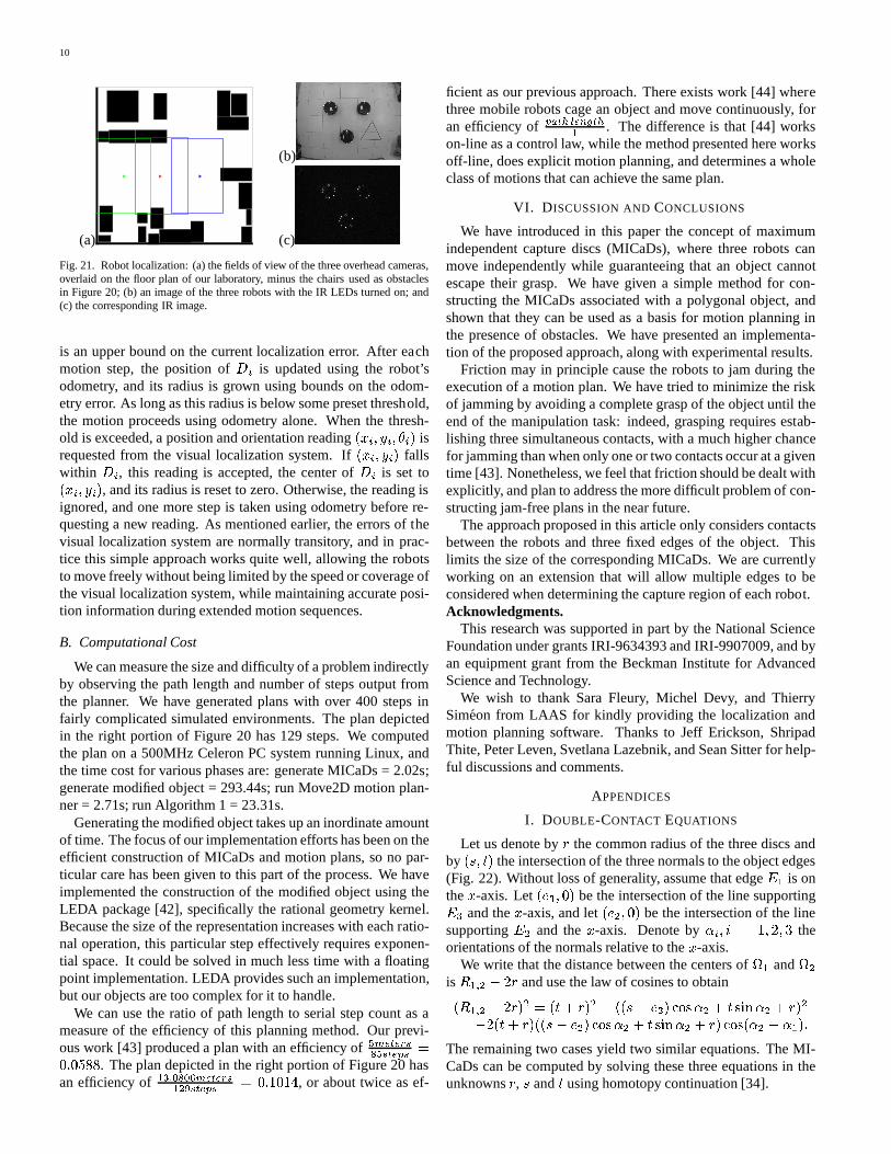
We have implemented the construction of MICaDs for polyg-onal objects. The implementation does not include the triple-contact case (discussed in Section II-A.2), but is still capableof handling most polygons in which we are interested. Figure18 shows some examples of polygons and their associated MI-CaDs.

(a) (b)

(c) (d)

Fig. 18. Examples of MICaDs: (a) the object used in the experiments, (b)-(d)other examples. In each example, the polygonal object and the three robots areportrayed with shaded regions, while the grown generalizedpolygon and thecorresponding MICaDs are portrayed with black lines.

We have also implemented the proposed motion planning al-gorithm, and conducted experiments using three Nomadic Scoutrobots and a styrofoam triangle on casters (Fig. 19). We usethe motion planning library contained in the Move2D pack-age from LAAS to compute collision-free paths for our objects.Move2D is a graphical motion planning package which con-tains a potential-field planner based on the navigation functionmethod discussed in [39].2 For obstacles we have used natu-rally occurring objects in our building, such as chairs and pillars,modeled as simple polygons.

Figure 20 shows still images of two experiments and the cor-responding motion plans. Animations of these plans and ac-tual video footage are available from our web site,http://www-cvr.ai.uiuc.edu/ponce_grp/demos/micad .

A. Closed-Loop Control

As mentioned above, we have conducted experiments withboth open- and closed-loop control, using dead reckoning inthefirst case, and visual feedback from overhead cameras in thesecond one. The open-loop approach has proven insufficient forpaths whose length is greater than about 5 meters, due to imper-fect odometry and drift due to friction and slipping. For closed-loop control, we have implemented a visual localization system2See the web site [40] for details on the software and its implementation.

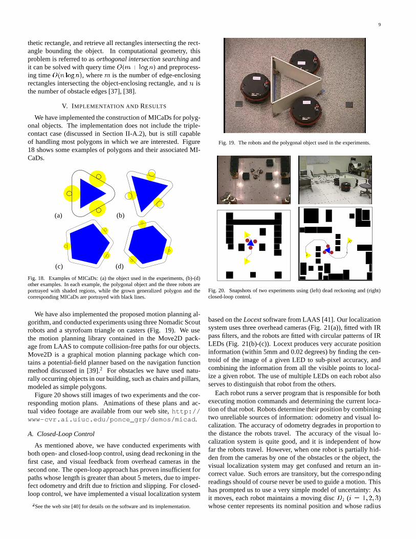
Fig. 19. The robots and the polygonal object used in the experiments.

Fig. 20. Snapshots of two experiments using (left) dead reckoning and (right)closed-loop control.

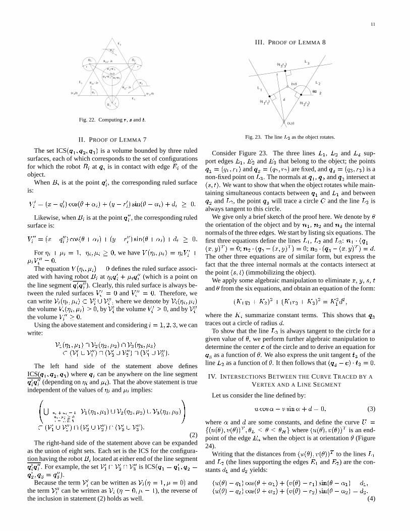
based on theLocextsoftware from LAAS [41]. Our localizationsystem uses three overhead cameras (Fig. 21(a)), fitted withIRpass filters, and the robots are fitted with circular patternsof IRLEDs (Fig. 21(b)-(c)). Locext produces very accurate positioninformation (within 5mm and 0.02 degrees) by finding the cen-troid of the image of a given LED to sub-pixel accuracy, andcombining the information from all the visible points to local-ize a given robot. The use of multiple LEDs on each robot alsoserves to distinguish that robot from the others.

Each robot runs a server program that is responsible for bothexecuting motion commands and determining the current loca-tion of that robot. Robots determine their position by combiningtwo unreliable sources of information: odometry and visuallo-calization. The accuracy of odometry degrades in proportion tothe distance the robots travel. The accuracy of the visual lo-calization system is quite good, and it is independent of howfar the robots travel. However, when one robot is partially hid-den from the cameras by one of the obstacles or the object, thevisual localization system may get confused and return an in-correct value. Such errors are transitory, but the correspondingreadings should of course never be used to guide a motion. Thishas prompted us to use a very simple model of uncertainty: Asit moves, each robot maintains a moving discDi (i = 1; 2; 3)whose center represents its nominal position and whose radius

10

(a)

(b)

(c)

Fig. 21. Robot localization: (a) the fields of view of the three overhead cameras,overlaid on the floor plan of our laboratory, minus the chairsused as obstaclesin Figure 20; (b) an image of the three robots with the IR LEDs turned on; and(c) the corresponding IR image.

is an upper bound on the current localization error. After eachmotion step, the position ofDi is updated using the robot’sodometry, and its radius is grown using bounds on the odom-etry error. As long as this radius is below some preset threshold,the motion proceeds using odometry alone. When the thresh-old is exceeded, a position and orientation reading(xi; yi; i) isrequested from the visual localization system. If(xi; yi) fallswithin Di, this reading is accepted, the center ofDi is set to(xi; yi), and its radius is reset to zero. Otherwise, the reading isignored, and one more step is taken using odometry before re-questing a new reading. As mentioned earlier, the errors of thevisual localization system are normally transitory, and inprac-tice this simple approach works quite well, allowing the robotsto move freely without being limited by the speed or coverageofthe visual localization system, while maintaining accurate posi-tion information during extended motion sequences.

B. Computational Cost

We can measure the size and difficulty of a problem indirectlyby observing the path length and number of steps output fromthe planner. We have generated plans with over 400 steps infairly complicated simulated environments. The plan depictedin the right portion of Figure 20 has 129 steps. We computedthe plan on a 500MHz Celeron PC system running Linux, andthe time cost for various phases are: generate MICaDs = 2.02s;generate modified object = 293.44s; run Move2D motion plan-ner = 2.71s; run Algorithm 1 = 23.31s.

Generating the modified object takes up an inordinate amountof time. The focus of our implementation efforts has been on theefficient construction of MICaDs and motion plans, so no par-ticular care has been given to this part of the process. We haveimplemented the construction of the modified object using theLEDA package [42], specifically the rational geometry kernel.Because the size of the representation increases with each ratio-nal operation, this particular step effectively requires exponen-tial space. It could be solved in much less time with a floatingpoint implementation. LEDA provides such an implementation,but our objects are too complex for it to handle.

We can use the ratio of path length to serial step count as ameasure of the efficiency of this planning method. Our previ-ous work [43] produced a plan with an efficiency of5meters85steps =0:0588. The plan depicted in the right portion of Figure 20 hasan efficiency of13:0806meters129steps = 0:1014, or about twice as ef-

ficient as our previous approach. There exists work [44] wherethree mobile robots cage an object and move continuously, foran efficiency ofpath length1 . The difference is that [44] workson-line as a control law, while the method presented here worksoff-line, does explicit motion planning, and determines a wholeclass of motions that can achieve the same plan.

VI. D ISCUSSION ANDCONCLUSIONS

We have introduced in this paper the concept of maximumindependent capture discs (MICaDs), where three robots canmove independently while guaranteeing that an object cannotescape their grasp. We have given a simple method for con-structing the MICaDs associated with a polygonal object, andshown that they can be used as a basis for motion planning inthe presence of obstacles. We have presented an implementa-tion of the proposed approach, along with experimental results.

Friction may in principle cause the robots to jam during theexecution of a motion plan. We have tried to minimize the riskof jamming by avoiding a complete grasp of the object until theend of the manipulation task: indeed, grasping requires estab-lishing three simultaneous contacts, with a much higher chancefor jamming than when only one or two contacts occur at a giventime [43]. Nonetheless, we feel that friction should be dealt withexplicitly, and plan to address the more difficult problem ofcon-structing jam-free plans in the near future.

The approach proposed in this article only considers contactsbetween the robots and three fixed edges of the object. Thislimits the size of the corresponding MICaDs. We are currentlyworking on an extension that will allow multiple edges to beconsidered when determining the capture region of each robot.Acknowledgments.

This research was supported in part by the National ScienceFoundation under grants IRI-9634393 and IRI-9907009, and byan equipment grant from the Beckman Institute for AdvancedScience and Technology.

We wish to thank Sara Fleury, Michel Devy, and ThierrySimeon from LAAS for kindly providing the localization andmotion planning software. Thanks to Jeff Erickson, ShripadThite, Peter Leven, Svetlana Lazebnik, and Sean Sitter for help-ful discussions and comments.

APPENDICES

I. DOUBLE-CONTACT EQUATIONS

Let us denote byr the common radius of the three discs andby (s; t) the intersection of the three normals to the object edges(Fig. 22). Without loss of generality, assume that edgeE1 is onthex-axis. Let(e3; 0) be the intersection of the line supportingE3 and thex-axis, and let(e2; 0) be the intersection of the linesupportingE2 and thex-axis. Denote byi; i = 1; 2; 3 theorientations of the normals relative to thex-axis.

We write that the distance between the centers of1 and2isR1;2 2r and use the law of cosines to obtain(R1;2 2r)2 = (t+ r)2 + ((s e2) os2 + t sin2 + r)22(t+ r)((s e2) os2 + t sin2 + r) os(2 1):The remaining two cases yield two similar equations. The MI-CaDs can be computed by solving these three equations in theunknownsr, s andt using homotopy continuation [34].

11

α −α2 3

(e ,0)3

Ω

ΩΩ

1

23

E

E

1

2

3E α

α

α1

2

3

α −αα −α1 213

(e , 0)2

R - 2r12

R - 2r23

R - 2r31

(s,t)

r

rr

Fig. 22. Computingr, s andt.II. PROOF OFLEMMA 7

The set ICS(q1; q2; q3) is a volume bounded by three ruledsurfaces, each of which corresponds to the set of configurationsfor which the robotBi at qi is in contact with edgeEi of theobject.

WhenBi is at the pointq0i, the corresponding ruled surfaceis:V 0i = (x q0i) os( + i) + (y r0i) sin( + i) + di 0:

Likewise, whenBi is at the pointq00i , the corresponding ruledsurface is:V 00i = (x q00i ) os( + i) + (y r00i ) sin(+ i) + di 0:

For i + i = 1; i; i 0, we haveV (i; i) = iV 0i +iV 00i = 0.The equationV (i; i) = 0 defines the ruled surface associ-

ated with having robotBi at iq0i + iq00i (which is a point onthe line segmentq0iq00i ). Clearly, this ruled surface is always be-tween the ruled surfacesV 0i = 0 andV 00i = 0. Therefore, wecan writeVi(i; i) V 0i [ V 00i ; where we denote byVi(i; i)the volumeVi(i; i) 0, byV 0i the volumeV 0i 0, and byV 00ithe volumeV 00i 0.

Using the above statement and consideringi = 1; 2; 3, we canwrite: V1(1; 1) \ V2(2; 2) \ V3(3; 3) (V 01 [ V 001 ) \ (V 02 [ V 002 ) \ (V 03 [ V 003 ):

The left hand side of the statement above definesICS(q1; q2; q3) whereqi can be anywhere on the line segmentq0iq00i (depending oni andi). That the above statement is trueindependent of the values ofi andi implies:0S i + i = 1i; i 0i = 1; 2; 3 V1(1; 1) [ V2(2; 2) [ V3(3; 3)1A (V 01 [ V 001 ) \ (V 02 [ V 002 ) \ (V 03 [ V 003 ):

(2)The right-hand side of the statement above can be expanded

as the union of eight sets. Each set is the ICS for the configura-tion having the robotBi located at either end of the line segmentq0iq00i . For example, the setV 01 \ V 02 \ V 003 is ICS(q1 = q01; q2 =q02; q3 = q003 ).

Because the termV 0i can be written asVi( = 1; = 0) andthe termV 00i can be written asVi ( = 0; = 1), the reverse ofthe inclusion in statement (2) holds as well.

III. PROOF OFLEMMA 8

(q ,r )1 1

(x,y)

(s,t)L

1

L 2

L3

d

θ+α 2

(q ,r )

(q ,r )

2 2

3 3

Fig. 23. The lineL3 as the object rotates.

Consider Figure 23. The three linesL1, L2 andL3 sup-port edgesE1, E2 andE3 that belong to the object; the pointsq1 = (q1; r1) andq2 = (q2; r2) are fixed, andq3 = (q3; r3) is anon-fixed point onL3. The normals atq1, q2 andq3 intersect at(s; t). We want to show that when the object rotates while main-taining simultaneous contacts betweenq1 andL1 and betweenq2 andL2, the pointq3 will trace a circleC and the lineL3 isalways tangent to this circle.

We give only a brief sketch of the proof here. We denote bythe orientation of the object and byn1, n2 andn3 the internalnormals of the three edges. We start by listing six equations. Thefirst three equations define the linesL1, L2 andL3: n1 (q1 (x; y)T ) = 0; n2 (q2 (x; y)T ) = 0; n3 (q3 (x; y)T ) = d.The other three equations are of similar form, but express thefact that the three internal normals at the contacts intersect atthe point(s; t) (immobilizing the object).

We apply some algebraic manipulation to eliminatex, y, s, tand from the six equations, and obtain an equation of the form:(K1q3 +K2)2 + (K1r3 +K3)2 = K21d2;where theKi summarize constant terms. This shows thatq3traces out a circle of radiusd.

To show that the lineL3 is always tangent to the circle for agiven value of, we perform further algebraic manipulation todetermine the center of the circle and to derive an equation forq3 as a function of. We also express the unit tangentt3 of thelineL3 as a function of. It then follows that(q3 ) t3 = 0.

IV. I NTERSECTIONSBETWEEN THECURVE TRACED BY A

VERTEX AND A L INE SEGMENT

Let us consider the line defined by:u os+ v sin+ d = 0; (3)

where andd are some constants, and define the curveU =f(u(); v())T ; L Hg where(u(); v())T is an end-point of the edgeEa when the object is at orientation (Figure24).

Writing that the distances from(u(); v())T to the linesL1andL2 (the lines supporting the edgesE1 andE2) are the con-stantsd1 andd2 yields:(u() q1) os( + 1) + (v() r1) sin( + 1) = d1;(u() q2) os( + 2) + (v() r2) sin( + 2) = d2:

(4)

12

(q ,r )1 1

(q ,r )2 2

Eaθ θ(u( ), v( ))

EE

E

12

3

(q ,r )3 3

d

θ+α

θ+α

1

2

d21

LL

12

Fig. 24. Parameterizing the endpoint(u(); v())T . The object is drawn asdotted polygon here.

We want to compute the intersection of the curveU and theline L. Suppose the intersection occurs at(u; v)T . We can thensetu() = u andv() = v in (4), and use the resulting equationsto eliminateu andv in (3). We obtain after some simplification:(r1 r2) os( 1 2 2)+(q1 q2) sin( 1 2 2)2d2 sin( 1 ) + 2d1 sin( 2 ) +K = 0;

(5)whereK = 8<: r2 os( 1 + 2) r1 os(+ 1 2)+2d sin(1 2) + q1 sin( + 1 2)q2 sin( 1 + 2):

Finding the roots of Eq. (5) amounts to solving a trigonomet-ric equation in which can be done in closed form. The inter-section ofU andL are the points(u; v)T at the root values ofthat are within the range[L; H . To compute the intersectionof a line segment supported by the given lineL, an extra stepis needed for testing whether any of the obtained intersectionpoints is between the endpoints of the line segment.

Note that the derivation of (5) assumes that the robots havezero radius. To handle non-zero radii, we simply use the linesL1andL2 supporting the edges of thegrownobject in the deriva-tion, and use ford1 andd2 the distances between the vertex ofinterest of theoriginal, ungrown object and these lines. The restof the derivation remains unchanged.

REFERENCES

[1] A. Sudsang and J. Ponce, “A new approach to motion planning for disc-shaped robots manipulating a polygonal object in the plane,” in IEEE Int.Conf. on Robotics and Automation, San Francisco, CA, 2000, pp. 1068–1075.

[2] R.S. Ball, A treatise on the theory of screws, Cambridge University Press,1900.

[3] M.S. Ohwovoriole, An extension of screw theory and its application tothe automation of industrial assemblies, Ph.D. thesis, Stanford University,Stanford, CA, 1980.

[4] F. Reulaux,The kinematics of machinery, MacMillan, NY, 1876, Reprint,Dover, NY, 1963.

[5] E. Rimon and J. W. Burdick, “Mobility of bodies in contact—i: A new2nd order mobility index for multiple-finger grasps,”IEEE Transactionson Robotics and Automation, vol. 14, no. 5, pp. 696–708, 1998.

[6] E. Rimon and J. W. Burdick, “Mobility of bodies in contact—ii: Howforces are generated by curvature effects,”IEEE Transactions on Roboticsand Automation, vol. 14, no. 5, pp. 709–717, 1998.

[7] A. Sudsang, J. Ponce, and N. Srinivasa, “Grasping and in-hand manipula-tion: Experiments with a reconfigurable gripper,”Advanced Robotics, vol.12, no. 5, pp. 509–533, December 1998.

[8] A. Sudsang, J. Ponce, and N. Srinivasa, “Grasping and in-hand manip-ulation: Geometry and algorithms,”Algorithmica, vol. 26, pp. 466–493,January 2000.

[9] E. Rimon and A. Blake, “Caging 2D bodies by one-parametertwo-fingered gripping systems,” inIEEE Int. Conf. on Robotics and Automa-tion, Minneapolis, MN, April 1996, pp. 1458–1464.

[10] C. Davidson and A. Blake, “Caging planar objects with a three-fingerone-parameter gripper,” inIEEE Int. Conf. on Robotics and Automation,Leuven, Belgium, June 1998, pp. 2722–2727.

[11] A. Sudsang and J. Ponce, “On grasping and manipulating polygonal ob-jects with disc-shaped robots in the plane,” inIEEE Int. Conf. on Roboticsand Automation, Leuven, Belgium, June 1998, pp. 2740–2746.

[12] A. Sudsang and J. Ponce, “On manipulating polygonal objects with three2-dof robots in the plane,” inIEEE Int. Conf. on Robotics and Automation,Detroit, MI, 1999, pp. 2227–2233.

[13] Y. Koga, On Computing Multi-Arm Manipulation Trajectories, Ph.D.thesis, Stanford University, 1994.

[14] R. Alami, J.P. Laumond, and T. Simeon, “Two maipulation planning al-gorithms,” in Proceedings of Workshop on Algorithmic Foundations ofRobotics, Latombe Goldberg, Halperin and Wilson, Eds. 1995, A K Pe-ters.

[15] Juan Manuel Ahuactzin, Kamal Gupta, and Emmanuel Mazer, “Manipu-lation planning for redundant robots: A practical approa ch,” InternationalJournal of Robotics Research, vol. 17, no. 7, pp. 731–747, July 1998.

[16] H. Inoue, “Force feedback in precise assembly tasks,” AI Lab. AIM-308,MIT, 1974.

[17] D.E. Whitney, “Quasi-static assembly of compliantly supported rigidparts,” J. Dyn. Sys., Meas. Contr., vol. 104, pp. 65–77, 1982.

[18] R. S. Fearing, “Simplified grasping and manipulation with dextrous robothands,” IEEE Journal of Robotics and Automation, vol. RA-2, no. 4, pp.188–195, Dec. 1986.

[19] M.T. Mason, “Mechanics and planning of manipulator pushing opera-tions,” International Journal of Robotics Research, vol. 5, no. 3, pp. 53–71, 1986.

[20] M. Mani and E.D.W. Wilson, “A programmable orienting system for flatparts,” inNorth American Mfg. Research Conf. XIII, 1985.

[21] R.C. Brost, “Automatic grasp planning in the presence of uncertainty,”International Journal of Robotics Research, vol. 7, no. 1, pp. 3–17, 1988.

[22] M. Erdmann and M. T. Mason, “An exploration of sensorless manipu-lation.,” IEEE Journal of Robotics and Automation, vol. 4, no. 4, pp.369–379, Aug. 1988.

[23] M.A. Peshkin and A.C. Sanderson, “Planning robotic manipulation strate-gies for workpieces that slide,”IEEE Journal of Robotics and Automation,vol. 4, no. 5, 1988.

[24] K.Y. Goldberg, “Orienting polygonal parts without sensors,” Algorith-mica, vol. 10, no. 2, pp. 201–225, 1993.

[25] T. Abell and M. A. Erdmann, “Stably supported rotationsof a planar poly-gon with two frictionless contacts,”IEEE/RSJ International Conferenceon Robots and Systems, vol. 3, pp. 411–418, August 1995.

[26] A.S. Rao and K.Y. Goldberg, “Manipulating algebraic parts in the plane,”IEEE Transactions on Robotics and Automation, pp. 598–602, 1995.

[27] S. Akella, W. H. Huang, K. M. Lynch, and M. T. Mason, “Planar ma-nipulation on a conveyor with a one joint robot,” inRobotics Research:The Seventh International Symposium, G. Giralt and G. Hirzinger, Eds.,London, UK, 1996, pp. 265–276, Springer.

[28] S. Leveroni and K. Salisbury, “Reorienting objects with a robot hand usinggrasp gaits,” inRobotics Research: The Seventh International Symposium,G. Giralt and G. Hirzinger, Eds., London, UK, 1996, pp. 39–51, Springer.

[29] F. Avnaim, J.-D. Boissonnat, and B. Faverjon, “A practical exact mo-tion planning algorithm for polygonal objects amidst polygonal obstacles,”Tech. Rep. 890, INRIA, 1988.

[30] J. Barraquand and J.-C. Latombe, “Robot motion planning: a distributedrepresentation approach,”International Journal of Robotics Research, vol.10, pp. 628–649, 1991.

[31] Lydia E. Kavraki, PetrSvestka, Jean-Claude Latombe, and Mark H. Over-mars, “Probabilistic roadmaps for path planning in high-dimensional con-figuration spaces,”IEEE Transactions on Robotics and Automation, vol.12, no. 4, pp. 566–580, Aug. 1996.

[32] X. Markenscoff, L. Ni, and C.H. Papadimitriou, “The geometry of grasp-ing,” International Journal of Robotics Research, vol. 9, no. 1, pp. 61–74,February 1990.

[33] B. Mishra, J.T. Schwartz, and M. Sharir, “On the existence and synthesisof multifinger positive grips,”Algorithmica, Special Issue: Robotics, vol.2, no. 4, pp. 541–558, November 1987.

13

[34] A.P. Morgan, Solving Polynomial Systems using Continuation for Engi-neering and Scientific Problems, Prentice Hall, Englewood Cliffs, NJ,1987.

[35] K.M. Lynch and M.T. Mason, “Stable pushing: mechanics,controllabil-ity, and planning,” inAlgorithmic Foundations of Robotics, K.Y. Goldberg,D. Halperin, J.-C. Latombe, and R. Wilson, Eds., pp. 239–262. A.K. Pe-ters, 1995.

[36] E. Welzl, “Smallest enclosing disks (balls and ellipsoids),” in New Resultsand New Trends in Computer Science, LNCS 555, H. Maurer, Ed., pp.359–370. Springer Verlag, 1991.

[37] V. Vaishnavi and D. Wood, “Data structures for the rectangle containmentand enclosure problems,”Computer Graphics and Image Processing, vol.13, pp. 372–384, 1980.

[38] V. Vaishnavi and D. Wood, “Rectilinear line segment intersection, layeredsegment trees, and dynamization,”J. Algorithms, vol. 3, pp. 160–176,1982.

[39] J.-C. Latombe, Robot Motion Planning, Kluwer Academic Publishers,1991.

[40] Nicola Simeon, “Move2D (software),” http://www.laas.fr/˜nic/G2D/RIA-g2d.html .

[41] S. Fleury, T. Baron, and M. Herrb, “Monocular localization of a mobilerobot. LAAS Report 92451,” inInternational Conference on IntelligentAutonomous Systems (IAS-3), Pittsburgh (USA), February 15-18, 1993,pp. 470–479.

[42] LEDA, “Library of Efficient Data types and Algorithms,” Dis-tributed by Algorithmic Solutions, GmbH. http://www.algorithmic-solutions.com .

[43] A. Sudsang, Geometry and algorithms for part fixturing, grasping andmanipulation with modular fixturing elements, a new reconfigurable grip-per and mobile robots, Ph.D. thesis, University of Illinois at Urbana-Champaign, 1999.

[44] J.Spletzer, A.K.Das, R. Fierro, C.J. Taylor, V. Kumar,and J.P. Ostrowski,“Cooperative localization and control for multi-robot manipulation,” inIROS01, 2001.

Attawith Sudsang received the B.Eng. degree incomputer engineering from Chulalongkorn Univer-sity, Thailand, in 1991, the M.S. and Ph.D. degreesin computer science from the University of Illinoisat Urbana-Champaign in 1994 and 1999 respectively.Part of the work presented in this paper was donewhile he was completing his doctoral research atUIUC. He was a research associate at the Departmentof Computer Science, Rice University from 1999 to2000. Since January, 2001, he has been a Lecturerat the Department of Computer Engineering, Chula-

longkorn University. His research interests include distributed manipulation,part fixturing and grasping.

Fred Rothganger received his M.S. degree inComputer Science from University of Massachusetts,Boston, in 1997. He is currently a doctoral studentworking under Jean Ponce at the University of Illi-nois, Urbana-Champaign. His research interests arein vision and mobile robotics. His current work is inautomatic construction of models for recognition.

Jean Ponceis a Professor in the Department of Com-puter Science and the Beckman Institute at the Uni-versity of Illinois at Urbana-Champaign. Dr. Ponce’smain research interests are in Computer Vision andRobotics. His current Computer Vision research fo-cuses on automatic 3D model construction from imagedata, interactive image synthesis from video streams,motion analysis, 3D shape representation and objectrecognition. His Robotics work focuses on fixture,grasp and manipulation planning, and he has recentlydeveloped a novel reconfigurable gripper and a part

feeder that automatically adapts to new part geometry. Dr. Ponce is the author

of over a hundred technical publications and he is finishing,in collaboration withDr. David Forsyth from UC Berkeley, a Computer Vision textbook that will beout in the Summer of 2002. He is an associate editor of the International Jour-nal of Computer Vision and was an area editor of Computer Vision and ImageUnderstanding (1994-2000) and an associate editor of the IEEE Transactions onRobotics and Automation (1996-2001). He was program co-chair of the 1997IEEE Conference on Computer Vision and Pattern Recognitionand served asgeneral co-chair of the year 2000 edition of this conference.