Lefschetz fibrations over the disc
51
Proc. London Math. Soc. (3) 107 (2013) 340–390 C ❡ 2013 London Mathematical Society doi:10.1112/plms/pds078 Lefschetz fibrations over the disc Nikos Apostolakis, Riccardo Piergallini and Daniele Zuddas Abstract We provide a complete set of moves relating any two Lefschetz fibrations over the disc having as their total space the same four-dimensional 2-handlebody up to 2-equivalence. As a consequence, we also obtain moves relating diffeomorphic three-dimensional open books, providing a different approach to an analogous previous result by Harer. 1. Introduction As Harer showed in [11], any four-dimensional 2-handlebody W can be represented by a topological (achiral) Lefschetz fibration over the disc, that is, a smooth map W → B 2 whose generic fibre is an orientable bounded surface and whose singularities are topologically equivalent to complex non-degenerate ones. Harer’s argument is based on Kirby calculus [14]. An alternative approach to the same result was provided in [15, Remark 2.3]. This is based on the characterization of allowable Lefschetz fibrations (see Section 6) as those smooth maps that admit a factorization W p → B 2 × B 2 π → B 2 , where p : W → B 2 × B 2 is a covering simply branched over a braided surface and π is the canonical projection. The two other ingredients of the proof are Montesinos’s representation of four-dimensional 2-handlebodies as coverings of B 4 simply branched over ribbon surfaces [16] and Rudolph’s procedure for isotoping any orientable ribbon surface to a braided surface [20]. In this paper, we use the second approach together with the branched covering interpretation of Kirby calculus given by Bobtcheva–Piergallini in [3], to relate different Lefschetz fibrations representing the same four-dimensional 2-handlebody up to 2-equivalence by means of certain moves S, T and U on their monodromy representation. These monodromy moves are described in Section 7. Move S (Figure 33) is nothing but the well known positive or negative Hopf stabilization, and it corresponds to adding a pair of cancelling 1- and 2-handles to the handlebody, while move T (Figure 36) is new, and roughly speaking it corresponds to a 2-handle sliding. Both such moves are applied only to allowable Lefschetz fibrations (see Section 6). On the contrary, move U (Figure 38) is just used to transform any Lefschetz fibration into an allowable one. Namely, our main result is the following theorem in Section 8. Theorem A. Any two allowable Lefschetz fibrations f : W → B 2 and f : W → B 2 repre- sent 2-equivalent four-dimensional 2-handlebodies H f and H f if and only if they are related by fibred equivalence and the moves S and T . Moreover, the allowability hypothesis can be relaxed by using in addition move U . Received 13 March 2012; revised 26 August 2012; published online 4 February 2013. 2010 Mathematics Subject Classification 55R55, 57N13 (primary), 57M12, 57R65 (secondary). Partially supported by a CUNY Community College Collaborative Incentive Grant and a PSCCUNY Cycle 39 Research Award (Nikos Apostolakis). Supported by Regione Autonoma della Sardegna with funds from PO Sardegna FSE 2007–2013 and L.R. 7/2007 ‘Promotion of scientific research and technological innovation in Sardinia’. Also thanks to ESF for short visit grants within the program ‘Contact and Symplectic Topology’ (Daniele Zuddas).
Transcript of Lefschetz fibrations over the disc

Proc. London Math. Soc. (3) 107 (2013) 340–390 C�2013 London Mathematical Societydoi:10.1112/plms/pds078
Lefschetz fibrations over the disc
Nikos Apostolakis, Riccardo Piergallini and Daniele Zuddas
Abstract
We provide a complete set of moves relating any two Lefschetz fibrations over the disc having astheir total space the same four-dimensional 2-handlebody up to 2-equivalence. As a consequence,we also obtain moves relating diffeomorphic three-dimensional open books, providing a differentapproach to an analogous previous result by Harer.
1. Introduction
As Harer showed in [11], any four-dimensional 2-handlebody W can be represented bya topological (achiral) Lefschetz fibration over the disc, that is, a smooth map W → B2
whose generic fibre is an orientable bounded surface and whose singularities are topologicallyequivalent to complex non-degenerate ones. Harer’s argument is based on Kirby calculus [14].
An alternative approach to the same result was provided in [15, Remark 2.3]. This is basedon the characterization of allowable Lefschetz fibrations (see Section 6) as those smooth mapsthat admit a factorization W
p→ B2 ×B2 π→ B2, where p :W → B2 ×B2 is a covering simplybranched over a braided surface and π is the canonical projection. The two other ingredientsof the proof are Montesinos’s representation of four-dimensional 2-handlebodies as coveringsof B4 simply branched over ribbon surfaces [16] and Rudolph’s procedure for isotoping anyorientable ribbon surface to a braided surface [20].
In this paper, we use the second approach together with the branched covering interpretationof Kirby calculus given by Bobtcheva–Piergallini in [3], to relate different Lefschetz fibrationsrepresenting the same four-dimensional 2-handlebody up to 2-equivalence by means of certainmoves S, T and U on their monodromy representation.
These monodromy moves are described in Section 7. Move S (Figure 33) is nothing butthe well known positive or negative Hopf stabilization, and it corresponds to adding a pair ofcancelling 1- and 2-handles to the handlebody, while move T (Figure 36) is new, and roughlyspeaking it corresponds to a 2-handle sliding. Both such moves are applied only to allowableLefschetz fibrations (see Section 6). On the contrary, move U (Figure 38) is just used totransform any Lefschetz fibration into an allowable one.
Namely, our main result is the following theorem in Section 8.
Theorem A. Any two allowable Lefschetz fibrations f :W → B2 and f ′ :W ′ → B2 repre-sent 2-equivalent four-dimensional 2-handlebodies Hf and Hf ′ if and only if they are relatedby fibred equivalence and the moves S and T . Moreover, the allowability hypothesis can berelaxed by using in addition move U .
Received 13 March 2012; revised 26 August 2012; published online 4 February 2013.
2010 Mathematics Subject Classification 55R55, 57N13 (primary), 57M12, 57R65 (secondary).
Partially supported by a CUNY Community College Collaborative Incentive Grant and a PSCCUNY Cycle39 Research Award (Nikos Apostolakis). Supported by Regione Autonoma della Sardegna with funds from POSardegna FSE 2007–2013 and L.R. 7/2007 ‘Promotion of scientific research and technological innovation inSardinia’. Also thanks to ESF for short visit grants within the program ‘Contact and Symplectic Topology’(Daniele Zuddas).

LEFSCHETZ FIBRATIONS OVER THE DISC 341
Here is a very sketchy outline of the proof of Theorem A. According to [15], the two allowableLefschetz fibrations are realized as simple coverings of B2 ×B2 branched over braided surfaces(see Section 6). Such braided surfaces, endowed with the labelling that encodes the monodromyof the coverings, are special cases of labelled ribbon surfaces representing 2-equivalent, four-dimensional 2-handlebodies as branched coverings of B4 (see Section 5). Therefore, they canbe related by a finite sequence of isotopy and covering moves (Figures 3 and 24) given in [3].Then, we perform on these moves a streamlined version of the Rudolph’s braiding procedure[20], which retracts labelled ribbon surfaces onto labelled braided surfaces (see Section 4).The result is a quite large set of moves on labelled braided surfaces, and the last part of theproof, carried out in Section 8, consists in reducing it, up to braided isotopy, to only two movescorresponding to the monodromy moves S and T .
The same argument also gives the following theorem in Section 9. Here, the extra moveP (Figure 66) corresponds to making connected sum with CP 2, whereas move Q consists inadding a pair contiguous opposite Dehn twists to the monodromy sequence of the Lefschetzfibration.
Theorem B. Two allowable Lefschetz fibrations over B2 represent four-dimensional2-handlebodies with diffeomorphic oriented boundaries if and only if they are related by fibredequivalence, the moves S and T of Section 7, and the moves P and Q.
Theorems A and B can be considered as four-dimensional analogues of the equivalencetheorem for three-dimensional open books proved by Harer in [12]. In fact, such open booksnaturally arise as boundary restrictions of Lefschetz fibrations. Then, by considering theboundary restrictions ∂S, ∂T and ∂P of the moves S, T and P , we also derive the next theoremin Section 9. We remark that, in contrast to Harer’s moves, our moves can be completelydescribed in terms of the open book monodromy.
Theorem C. Two open books are supported by diffeomorphic oriented three-manifolds ifand only if they are related by fibred equivalence and the moves ∂S, ∂T and ∂P .
The paper is organized as follows. Section 2 is devoted to ribbon surfaces and to 1-isotopybetween them. Sections 3 and 4 deal with braided surfaces and the Rudolph’s braidingprocedure. In Section 5, we review the branched covering representation of four-dimensional2-handlebodies and adapt the covering moves to the present aim. In Sections 6 and 7, we recallthe branched covering representation of Lefschetz fibrations and define the equivalence movesfor them. Finally, in Sections 8 and 9 we establish the three equivalence theorems stated above.
2. Ribbon surfaces
A regularly embedded smooth compact surface S ⊂ B4 is called a ribbon surface if theEuclidean norm restricts to a Morse function on S with no local maxima in IntS. Assumingthat S ⊂ R4
+ ⊂ R4+ ∪ {∞} ∼= B4, where ∼= stands for the standard orientation preserving
conformal equivalence, this property is smoothly equivalent to the fact that the fourth Cartesiancoordinate restricts to a Morse height function on S with no local minima in IntS. Sucha surface S ⊂ R4
+ can be horizontally (preserving the height function given by the fourthcoordinate) isotoped to make its orthogonal projection in R3 a self-transversal immersedsurface, whose double points form disjoint arcs as in Figure 1(a). We call the orthogonalprojection π(S) ⊂ R3 a three-dimensional diagram of S.
Actually, any immersed compact surface S ⊂ R3 with all self-intersections as above and noclosed components is the three-dimensional diagram of a ribbon surface. This can be obtained

342 NIKOS APOSTOLAKIS RICCARDO PIERGALLINI AND DANIELE ZUDDAS
Figure 1. Ribbon intersection.
by pushing IntS inside IntR4+ in such a way that all self-intersections disappear. Moreover, it
is uniquely determined up to vertical isotopy.In the following, we will omit the projection π and use the same notation for a ribbon surface
in B4 and its three-dimensional diagram in R3, the distinction between them being clear fromthe context.
Any ribbon surface S admits a handlebody decomposition with only 0- and 1-handles inducedby the height function. Such a 1-handlebody decomposition S = (H0
1 � · · · �H0m) ∪ (H1
1 � · · · �H1n) is called adapted, if each ribbon self-intersection of its three-dimensional diagram involves
an arc contained in the interior of a 0-handle and a proper transversal arc in a 1-handle(cf. [21]). Then, looking at the three-dimensional diagram, we have that the 0-handles H0
i
are disjoint non-singular discs in R3, while the 1-handles H1j are non-singular bands in R3
attached to the 0-handles and possibly passing through them to form ribbon intersections likethe one shown in Figure 1(b). Moreover, we can think of S as a smoothing of the frontier of((H0
1 � · · · �H0m) × [0, 1]) ∪ ((H1
1 � · · · �H1n) × [0, 1/2]) in R4
+.A ribbon surface S ⊂ R4
+ endowed with an adapted handlebody decomposition as above willbe referred to as an embedded two-dimensional 1-handlebody.
A convenient way of representing a ribbon surface S arises from the observation that itsthree-dimensional diagram, considered as a two-dimensional complex in R3, collapses to agraph T . We can choose T = π(P ) for a smooth simple spine P of S (simple means thatall the vertices have valency one or three), which intersects each 1-handle H1
j along its core.Moreover, we can also assume T to meet each ribbon intersection arc of S at exactly one4-valent vertex, as in Figure 1(b) where the fourth edge of T in the back is not visible. Theinverse image of such a 4-valent vertex of T consists of two points, in the interior of two distinctedges of P , while the projection restricted over the complement of all 4-valent vertices of T isinjective.
Therefore, T has vertices of valency 1, 3 or 4. We call singular vertices the 4-valent verticeslocated at the ribbon intersections, and flat vertices all the other vertices. Moreover, we assumeT to have three distinct tangent lines at each flat 3-valent vertex and two distinct tangent linesat each singular vertex.
Up to a further horizontal isotopy of S, we can contract its three-dimensional diagram to anarrow regular neighbourhood of the graph T . Then, by considering a planar diagram of T ,we easily get a new diagram of S, consisting of a number of copies of the local spots shown inFigure 2, and some non-overlapping flat bands connecting those spots. We call this a planardiagram of S.
We emphasize that a planar diagram of S arises as a diagram of the pair (S, T ) and thisis the right way to think about it. However, we omit to draw the graph T in the pictures ofplanar diagrams, since it can be trivially recovered, up to diagram isotopy, as the core of thediagram itself. In particular, the diagram crossings and the singular vertices of T are locatedat the centres of the copies of the two rightmost spots in Figure 2, while the flat vertices of itare located at the centres of copies of the two leftmost spots.

LEFSCHETZ FIBRATIONS OVER THE DISC 343
Figure 2. Local models for planar diagrams.
Figure 3. 1-isotopy moves for planar diagrams.
Of course, a planar diagram determines a ribbon surface S only up to vertical isotopy.Namely, the three-dimensional height function (and the four-dimensional one as well) cannotbe determined from the planar diagram, apart from the obvious constrains imposed by theconsistency with the local configurations of Figure 2.
Ribbon surfaces will be always represented by planar diagrams and considered up to verticalisotopy (in the sense just described above). Moreover, planar diagrams will be always consideredup to planar diagram isotopy, that is ambient isotopy of the plane containing them.
Following [3], two ribbon surfaces S, S′ ⊂ R4+ are said to be 1-isotopic if there exists a
smooth ambient isotopy (ht)t∈[0,1] such that: (1) h1(S) = S′; (2) St = ht(S) is a ribbon surfacefor every t ∈ [0, 1]; (3) the projection of St in R3 is an honest three-dimensional diagramexcept for a finite number of critical t’s. Such equivalence relation between ribbon surfaces canbe interpreted as embedded 1-deformation of embedded two-dimensional 1-handlebodies, andthis is the reason for calling it 1-isotopy. Whether or not 1-isotopy coincides with isotopy isunknown, but this problem is not relevant for our purposes.
All we need to know here is that two ribbon surfaces are 1-isotopic if and only if theirthree-dimensional diagrams are related by three-dimensional isotopies and the moves depictedin Figure 3. This has been proved in [3, Proposition 1.3].
We observe that the moves s1 to s4 are described in terms of planar diagrams. An analogousexpression of three-dimensional isotopies in terms of certain moves of planar diagrams has beenprovided by [4, Proposition 10.1]. Since this aspect will be crucial in the following, we give acomplete account of that result in the proof of Proposition 1.
In order to express three-dimensional isotopy of three-dimensional diagrams of ribbonsurfaces in terms of planar diagrams, it is convenient to consider the special case when allribbon intersections are terminal, that is, they appear only at the ends of the bands (and neverin the middle of them, as in the rightmost spot in Figure 2).
A planar diagram with this property will be called a special planar diagram. Figure 4 depictsthe two different local configurations that replace (f) of Figure 2, when dealing with a specialplanar diagram. Notice that, in the previous context, (g) and (h) can be seen as combinationsof (f) and (a) of Figure 2.
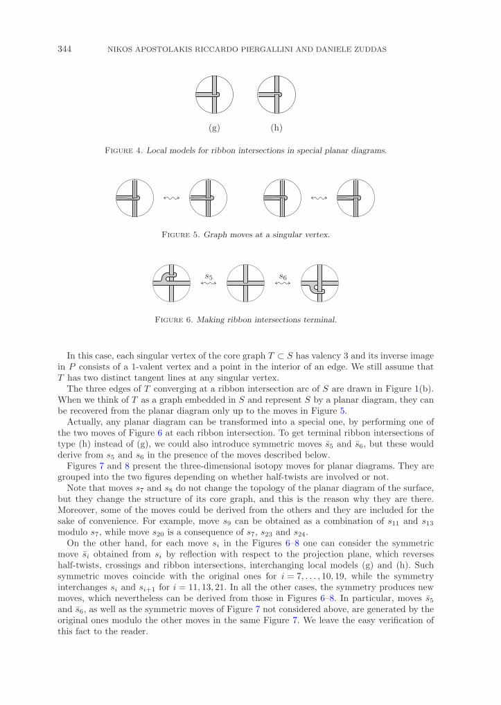
344 NIKOS APOSTOLAKIS RICCARDO PIERGALLINI AND DANIELE ZUDDAS
Figure 4. Local models for ribbon intersections in special planar diagrams.
Figure 5. Graph moves at a singular vertex.
Figure 6. Making ribbon intersections terminal.
In this case, each singular vertex of the core graph T ⊂ S has valency 3 and its inverse imagein P consists of a 1-valent vertex and a point in the interior of an edge. We still assume thatT has two distinct tangent lines at any singular vertex.
The three edges of T converging at a ribbon intersection arc of S are drawn in Figure 1(b).When we think of T as a graph embedded in S and represent S by a planar diagram, they canbe recovered from the planar diagram only up to the moves in Figure 5.
Actually, any planar diagram can be transformed into a special one, by performing one ofthe two moves of Figure 6 at each ribbon intersection. To get terminal ribbon intersections oftype (h) instead of (g), we could also introduce symmetric moves s5 and s6, but these wouldderive from s5 and s6 in the presence of the moves described below.
Figures 7 and 8 present the three-dimensional isotopy moves for planar diagrams. They aregrouped into the two figures depending on whether half-twists are involved or not.
Note that moves s7 and s8 do not change the topology of the planar diagram of the surface,but they change the structure of its core graph, and this is the reason why they are there.Moreover, some of the moves could be derived from the others and they are included for thesake of convenience. For example, move s9 can be obtained as a combination of s11 and s13modulo s7, while move s20 is a consequence of s7, s23 and s24.
On the other hand, for each move si in the Figures 6–8 one can consider the symmetricmove si obtained from si by reflection with respect to the projection plane, which reverseshalf-twists, crossings and ribbon intersections, interchanging local models (g) and (h). Suchsymmetric moves coincide with the original ones for i = 7, . . . , 10, 19, while the symmetryinterchanges si and si+1 for i = 11, 13, 21. In all the other cases, the symmetry produces newmoves, which nevertheless can be derived from those in Figures 6–8. In particular, moves s5and s6, as well as the symmetric moves of Figure 7 not considered above, are generated by theoriginal ones modulo the other moves in the same Figure 7. We leave the easy verification ofthis fact to the reader.

LEFSCHETZ FIBRATIONS OVER THE DISC 345
Figure 7. Flat isotopy moves.
Proposition 1. Two planar diagrams represent 1-isotopic ribbon surfaces if and only ifthey are related by a finite sequence of moves s1 to s26 in Figures 3, 6–8.
Proof. The ‘if’ part is trivial, since all the moves in Figures 6–8 represent specialthree-dimensional diagram isotopies. For the ‘only if’ part, we need to show that these movesdo generate any three-dimensional diagram isotopy between planar diagrams.
Moves s5 and s6 allow us to restrict attention to special planar diagrams. Moreover, allthe moves of Figures 7 and 8 contain only terminal ribbon intersections; hence, they can beperformed in the context of special planar diagrams.
Now, consider two special planar diagrams representing ribbon surfaces S0 and S1, whosethree-dimensional diagrams are isotopic in R3, and let H :R3 × [0, 1] → R3 be a smoothambient isotopy such that h1(S0) = S1.
For i = 0, 1, let Pi be a simple spine of Si, and Ti = π(Pi) be the core of its diagram. Up tomoves, we can assume that h1(T0) = T1. Indeed, by cutting S1 along the ribbon intersectionarcs, we get an embedded surface S1 ⊂ R3 with some marked arcs, one in the interior and twoalong the boundary, for each ribbon intersection. This operation transforms the graphs T1 andh1(T0) into simple spines of S1 relative to the marked arcs. Figure 9 shows the effect of the cutat the ribbon intersections in Figure 4.
From the intrinsic point of view, that is, considering S1 as an abstract surface and forgettingits inclusion in R3, the theory of simple spines implies that moves s7, s8 and the composition

346 NIKOS APOSTOLAKIS RICCARDO PIERGALLINI AND DANIELE ZUDDAS
Figure 8. Half-twisted isotopy moves.
Figure 9. Cutting the three-dimensional diagram at a ribbon intersection.
of the moves s5 and s6 suffice to transform h1(T0) into T1. In particular, the first two movescorrespond to the well known moves for simple spines of surfaces, while the third together withthe moves in Figure 5, which do not change the surface, relates the different positions of thespine with respect to the marked arcs in the interior of S1. It remains only to observe that, upto the other moves in Figures 7 and 8, the portion of the surface involved in each single spinemodification can be isolated in the planar diagram, as needed to perform the above-mentionedmoves.
So, let us suppose that h1(S0, T0) = (S1, T1). Note that the intermediate pairs (St, Tt) =ht(S0, T0) with 0 < t < 1 do not necessarily project into special planar diagrams in R2.
By transversality, we can assume that the graph Tt regularly projects to a diagram in R2
for every t ∈ [0, 1], except a finite number of t’s corresponding to extended Reidemeister movesfor graphs. For such exceptional t’s, the lines tangent to Tt at its vertices are assumed not tobe vertical.
We define Γ ⊂ T0 × [0, 1] as the subspace of pairs (x, t) for which the plane TxtSt tangent
to St at xt = ht(x) is vertical (if x ∈ T0 is a singular vertex, there are two such tangent planesand we require that one of them is vertical).
By a standard transversality argument, we can perturb H in such a way that:
(a) Γ is a graph embedded in T0 × [0, 1] as a smooth stratified subspace of constantcodimension 1 and the restriction η : Γ → [0, 1] of the height function (x, t) → t is aMorse function on each edge of Γ;

LEFSCHETZ FIBRATIONS OVER THE DISC 347
(b) the edges of Γ locally separate regions consisting of points (x, t) for which the projectionof St into R2 has opposite local orientations at xt;
(c) the two planes tangent to any St at a singular vertex of Tt are not both vertical, andif one of them is vertical then it does not contain both the lines tangent to Tt at thatvertex.
As a consequence of (b), for each flat vertex x ∈ T0 of valency one or three there are finitelymany points (x, t) ∈ Γ, all of which have the same valency one or three as vertices of Γ. Similarly,as a consequence of (c), for each singular vertex x ∈ T0 there are finitely many points (x, t) ∈ Γ,all of which have valency one or two as vertices of Γ. Moreover, the above-mentioned verticesof Γ of valency one or three are the only vertices of Γ of valency = 2.
Let 0 < t1 < t2 < · · · < tk < 1 be the critical levels where one of the following holds:
(1) Tti does not project regularly in R2, because there is a point xi along an edge of T0 suchthat the line tangent to Tti at hti(xi) is vertical;
(2) Tti projects regularly in R2, but its projection is not a graph diagram, due to a multipletangency or crossing at some point;
(3) there is a point (xi, ti) ∈ Γ with xi a univalent or a singular vertex of T0;(4) there is a critical point (xi, ti) for the function η along an edge of Γ.
Without loss of generality, we assume that only one of the four cases mentioned above occursat any critical level ti. Note that the points (x, t) of Γ such that x ∈ T0 is a flat tri-valent vertexrepresent a subcase of case 2 and for this reason they are not included in case 3.
For t ∈ [0, 1] − {t1, t2, . . . , tk}, there exists a sufficiently small regular neighbourhood Nt ofTt in St, such that the pair (Nt, Tt) projects to a planar diagram.
We observe that the planar diagram of Nt is uniquely determined up to diagram isotopy by(the diagram of) its core Tt and by the tangent planes of St at Tt. In fact, the half-twists of Ntalong the edges of Tt correspond to the transversal intersections of Γ with T0 × {t} and theirsigns depend only on the local behaviour of the tangent planes of Tt. In particular, the planardiagrams of (N0, T0) and (N1, T1) coincide, up to planar diagram isotopy, with the originalones of (S0, T0) and (S1, T1).
If an interval [t′, t′′] does not contain any critical level ti, then each single half-twist persistsbetween the levels t′ and t′′, hence the planar isotopy relating the diagrams of Tt′ and Tt′′ alsorelate the diagrams of Nt′ and Nt′′ , except for possible slidings of half-twists along ribbonsover/under crossings. These can be realized by using moves s19, s21 and s22.
At this point, the only thing left to show is that Nt′ and Nt′′ are related by moves for [t′, t′′]a sufficiently small neighbourhood of a critical level ti. We do that separately for the fourdifferent types of critical levels.
If ti is of type 1, then a kink is appearing or disappearing along an edge of the core graph.When this kink is positive, the diagrams of Nt′ and Nt′′ are directly related by move s20 if(xi, ti) is a local maximum point for η and the kink is appearing, or if (xi, ti) is a local minimumpoint for η and the kink is disappearing. All the other cases of a positive kink can be reducedto the previous ones, by means of move s19. The case of a negative kink is symmetric, we canjust use moves si in place of the moves si.
If ti is of type 2, then either a regular isotopy move is occurring between Tt′ and Tt′′ or twotangent lines at a tri-valent vertex xi of Tti project to the same line in the plane. In the firstcase, the regular isotopy move occurring between Tt′ and Tt′′ , trivially extends to one of themoves s9 to s16. In the second case, xi may be either a flat or a singular vertex of Tti . If xi isa flat vertex, then the tangent plane to St at H(xi, t) is vertical for t = ti and its projectionreverses the orientation when t passes from t′ to t′′. Moves s24 and s24 (modulo moves s9 ands19) describe the effect on the diagram of such a reversion of the tangent plane. If xi is asingular vertex, then Nt′ changes into Nt′′ by one move s17, s17, s18 or s18.

348 NIKOS APOSTOLAKIS RICCARDO PIERGALLINI AND DANIELE ZUDDAS
If ti is of type 3, then either a half-twist is appearing/disappearing at the tip of the tongueof the surface corresponding to a univalent vertex or one of the two bands at the ribbonintersection corresponding to a singular vertex is being reversed in the plane projection. Thefirst case corresponds to move s23 or s23, while the second case corresponds, up to move s19,to one of moves s25, s25, s26 or s26 (depending on the type of ribbon intersection and on whichband is being reversed).
Finally, if ti is of type 4, a pair of cancelling half-twists is appearing or disappearing alonga band, just as in move s19.
In the following we will focus on flat planar diagrams, meaning planar diagrams withouthalf-twists. In other words, these are planar diagrams locally modelled on the spots (a), (b),(e) and (f) in Figure 2 (and possibly (g) and (h) in Figure 4).
Of course, only orientable ribbon surfaces can be represented by flat planar diagrams. Infact, a ribbon surface with a flat planar diagram has a preferred orientation induced by theprojection in the plane of the diagram, which in this case is a regular map. Actually, anyoriented ribbon surface is known to admit a flat planar diagram. But we will not need this facthere, and we just refer to [20] for its proof.
In contrast, finding a complete set of local moves representing 1-isotopy between orientedribbon surfaces in terms of flat planar diagrams seems not to be so easy. These should includeall the moves s1 to s18 in Figures 3, 6 and 7 and flat versions of some of the moves s19 to s26in Figure 8.
However, this problem can be circumvented when using labelled orientable ribbon surfacesto represent branched coverings of B4, thanks to the presence of the covering moves introducedin Section 5 (cf. Figure 24).
3. Braided surfaces
A regularly embedded smooth compact surface S ⊂ B2 ×B2 is called a (simply) braidedsurface of degree m if the projection π :B2 ×B2 → B2 onto the first factor restricts to asimple branched covering p = π| :S → B2 of degree m.
This means that there exists a finite set A = {a1, a2, . . . , an} ⊂ IntB2 of branch points, suchthat the restriction p| :S − p−1(A) → B2 −A is an ordinary covering of degree m, while overany branch point ai ∈ A there is only one singular point si ∈ p−1(ai) ⊂ S and p has local degree2 at si, being locally smoothly equivalent to the complex map z → z2.
For any singular point si ∈ S, there are local complex coordinates on the two factors centredat si, with respect to which S has local equation z1 = z2
2 . Actually, if we insist that thoselocal coordinates preserve standard orientations, then we have two different possibilities, upto ambient isotopy, for the local equation of S at si, namely z1 = z2
2 or z1 = z22 . We call si a
positive twist point for S in the first case and a negative twist point for S in the second case.By a braided isotopy between the two braided surfaces S, S′ ⊂ B2 ×B2, we mean a smooth
ambient isotopy (ht)t∈[0,1] of B2 ×B2 such that h1(S) = S′ and each ht preserves the verticalfibres (those of the projection π); in other words, there exists a smooth ambient isotopy(kt)t∈[0,1] of B2 such that π ◦ ht = kt ◦ π for every t ∈ [0, 1]. In particular, if such a braidedisotopy exists, then S and S′ are isotopic through braided surfaces. Of course, braided isotopyreduces to vertical isotopy if kt = idB2 for every t ∈ [0, 1].
Now, assume that ∗ ∈ S1 is fixed once and for all as the base point of B2 −A. Then,the classical theory of coverings tells us that the branched covering p :S → B2 is uniquelydetermined up to diffeomorphisms by the monodromy ωp :π1(B2 −A) → Σm of its restrictionover B2 −A (defined only up to conjugation in Σm, depending on the numbering of the sheets).
Similarly, the braided surface S ⊂ B2 ×B2 is uniquely determined up to vertical isotopyby its braid monodromy, that is a suitable lifting ωS :π1(B2 −A) → Bm of ωp to the braid

LEFSCHETZ FIBRATIONS OVER THE DISC 349
Figure 10. The standard Hurwitz system.
group Bm of degree m. This is defined in the following way: we take ∗ = (∗1, ∗2, . . . , ∗m) =p−1(∗) ⊂ {∗} ×B2 ∼= B2 as the base point of the configuration space ΓmB2 of m points inB2, then for any [λ] ∈ π1(B2 −A, ∗) we put ωS([λ]) = [λ] ∈ π1(ΓmB2, ∗) ∼= Bm, where λ is theloop given by λ(t) = p−1(λ(t)) ⊂ {λ(t)} ×B2 ∼= B2 for any t ∈ [0, 1]. We can immediately seethat σ ◦ ωS = ωp, where σ : Bm → Σm is the canonical homomorphism giving the permutationassociated to a braid. Like the monodromy ωp, the braid monodromy ωS is defined only up toconjugation in Bm, depending on the identification π1(ΓmB2, ∗) ∼= Bm.
The local model of the twists points forces the braid monodromy ωS(μ) of any meridianμ ∈ π1(B2 −A) around a branch point a ∈ A to be a half-twist β±1 ∈ Bn around an arc b ⊂B2 between two points ∗j and ∗k. The arc b turns out to be uniquely determined up toambient isotopy of B2 mod ∗, while the half-twist β±1 is positive (right-handed) or negative(left-handed) according to the sign of the twist point si ∈ S.
Conversely, as we will see shortly, any homomorphism ϕ :π1(B2 −A) → Bm that sendsmeridians around the points of A to positive or negative half-twists around intervals in B2
is the braid monodromy of a braided surface S ⊂ B2 ×B2 with branch set A.We recall that π1(B2 −A) is freely generated by any set of meridians α1, α2, . . . , αn around
the points a1, a2, . . . , an, respectively. An ordered sequence (α1, α2, . . . , αn) of such meridiansis called a Hurwitz system for A when the following properties hold: (i) each αi is realizedas a counterclockwise parametrization of the boundary of a regular neighbourhood in B2 of anon-singular arc from ∗ to ai, which we still denote by αi; (ii) except for their end points, thearcs α1, α2, . . . , αn are pairwise disjoint and contained in IntB2 −A; (iii) around ∗ the arcsα1, α2, . . . , αn appear in the counterclockwise order, so that the composition loop α1α2 · · ·αnis homotopic in B2 −A to the usual counterclockwise generator α ∈ π1(S1), and the points ofA are assumed to be indexed accordingly. Up to ambient isotopy of B2 fixing S1 but not A,any Hurwitz system looks like the standard one depicted in Figure 10.
For the sake of convenience, here the disc B2 is drawn as B1 ×B1 with rounded corners.Actually, in all the pictures, we will always draw both the horizontal and the vertical fibres ofB2 ×B2 as B1 ×B1 with rounded corners.
There is a natural transitive action of the braid group Bn∼= π1(Γn IntB2, A) on the set
of Hurwitz systems for A. To any such Hurwitz system (α1, α2, . . . , αn) we associate a setof standard generators ξ1, ξ2, . . . , ξn−1 of Bn, with ξi the right-handed half-twists around theinterval xi αiαi+1 with end points ai and ai+1. Under the action of Bn, each ξi transforms(α1, α2, . . . , αn) into (α′
1, α′2, . . . , α
′n) with α′
i = αiαi+1α−1i , α′
i+1 = αi and α′k = αk for k =
i, i+ 1. This will be referred to as the ith elementary transformation ξi (cf. Figure 11). Itturns out that any two Hurwitz systems for A are related by a finite number of consecutiveelementary transformations ξ±1
i with i = 1, 2, . . . , n− 1.Given a Hurwitz system (α1, α2, . . . , αn) for A, we can represent the braid monodromy
of the braided surface S by the sequence (β1 = ωS(α1), β2 = ωS(α2), . . . , βn = ωS(αn)) ofpositive or negative half-twists in Bm, and the monodromy of the branched covering p :S →B2 by the sequence (τ1 = σ(β1), τ2 = σ(β2), . . . , τn = σ(βn)) of the associated transpositionsin Σm.

350 NIKOS APOSTOLAKIS RICCARDO PIERGALLINI AND DANIELE ZUDDAS
Figure 11. Elementary transformations.
Figure 12. From braid monodromy to braided surfaces.
Conversely, starting from any sequence (β1, β2, . . . , βn) of positive or negative half-twists inBm, we can construct a braided surface S = S(m;β1, β2, . . . , βn) of degree m, whose braidmonodromy is determined by βi = ωS(αi), as follows (cf. [20, Section 2]). First, we fix abase point ∗ = (∗1, ∗2, . . . , ∗m) ∈ ΓmB2 and consider the m horizontal copies of B2 given byB2j = B2 × {∗j} ⊂ B2 ×B2 for any j = 1, 2, . . . ,m. We assume that the points ∗j form an
increasing sequence in B1 ⊂ B2, to let the discs B21 , B
22 , . . . , B
2m appear to be stacked up on
the top of each other in that order, when we look at the three-dimensional picture given bythe canonical projection π :B2 ×B2 → B2 ×B1. Then, we consider the standard generatorsξ1, ξ2, . . . , ξm−1 of Bm
∼= π1(ΓmB2, ∗), with ξi the right-handed half-twist around the verticalinterval xi between ∗i and ∗i+1. Finally, we choose a family δ1, δ2, . . . , δn of disjoint arcs in B2,respectively, joining the points a1, a2, . . . , an to S1, like the dashed ones in Figure 10, whichform a splitting complex for the branched covering p : S → B2, and we do the following foreach i = 1, 2, . . . , n: (i) we express the half-twist βi as η−1ξ±1
jiη, with ξji a standard generator
of Bm and η ∈ Bm such that η(xji) = bi is the arc around which βi is defined, thanks to thetransitive action of Bm on the set of arcs between points of A; (ii) we deform the discs B2
j
by a vertical ambient isotopy supported inside N ×B2 for a small regular neighbourhood Nof δi in B2, which realizes the braid η over each fibre of a collar C ⊂ N of the boundary ofN in B2, while it does not depend on the first component over N − C; (iii) we replace thetwo adjacent discs (N − C) × {∗ji} ⊂ B2
jiand (N − C) × {∗ji+1} ⊂ B2
ji+1 by the local modeldescribed above for a positive or negative twist point, depending on the sign of the half-twistβi (that is on the exponent of ξ±1
ji).
Up to horizontal isotopy, the last construction results in attaching to the horizontal discs anarrow half-twisted vertical band, which we still denote by βi, as the relative half-twist of thestarting sequence. The band βi has a half-twist whose sign is the opposite of that of the originalhalf-twist βi (and of the twist-point si ∈ S), hence it contributes to the boundary braid of thethree-dimensional picture a half-twist having the same sign as the original one. Moreover, thecore of the band βi is the arc bi around which the half-twist βi was defined, translated to thefibre over ai. See Figure 12 for the case when βi is the negative half-twist η−1ξ−1
4 η ∈ B6 aroundthe arc bi = η(x4) with η = ξ3ξ
22ξ3.

LEFSCHETZ FIBRATIONS OVER THE DISC 351
Figure 13. Band presentation and line diagram of a braided surface.
The identification B2 ×B2 − {(0, ∗)} ∼= B4 − {∞} ∼= R4+ given by a suitable rounding
(smoothing the corners) of B2 ×B2 followed by the standard orientation preserving conformalequivalence B4 ∼= R4
+ ∪ {∞}, makes the braided surface S we have just constructed into aribbon surface S ⊂ R4
+. In fact, the projection of S in R3 turns out to be a three-dimensionaldiagram provided that the images of the arcs bi meet transversally those of the discs B2
j ,each ribbon intersection arc being formed by a band βi passing through a disc B2
j , incorrespondence with a transversal intersection point between bi and B2
j . Therefore, the 1-handlebody decomposition of S given by the discs B2
1 , B22 , . . . , B
2m (as the 0-handles) and by
the bands β1, β2, . . . , βn (as the 1-handles), turns out to be an adapted one.We call the ribbon surface S ⊂ R4
+ a band presentation of the braided surface S ⊂ B2 ×B2. For example, on the left side of Figure 13 we see a band presentation of the braidedsurface S(6;β1, β2, β3, β4) of degree 6 arising from the sequence (β1 = ξ1, β2 = ξ−1
3 ξ−12 ξ3, β3 =
ξ−15 ξ4ξ3ξ
−14 ξ5, β4 = ξ−1
3 ξ−22 ξ−1
3 ξ−14 ξ3ξ
22ξ3) of half-twists in B6.
A more economical way to represent braided surfaces in terms of band presentationsis provided by line diagrams. These are just a variation in the charged fence diagramsintroduced by Rudolph [22]. Namely, they consist of m horizontal lines standing for thediscs B2
1 , B22 , . . . , B
2m and n arcs between them given by the cores b1, b2, . . . , bn of the bands
β1, β2, . . . , βn, with the signs of the corresponding half-twists on the top. The right side ofFigure 13 shows the line diagram of the surface depicted on the left side.
Of course, a braided surface S has different band presentations, depending on the choiceof various objects involved in the construction above: (i) the Hurwitz system (α1, α2, . . . , αn);(ii) the base point ∗ ∈ ΓmB2; (iii) the particular realizations of the arcs b1, b2, . . . , bn withintheir isotopy classes.
The choices at points 2 and 3 are not relevant up to vertical isotopy of the braided surfaceS(m;β1, β2, . . . , βm), but still they can affect the ribbon surface diagram of the correspondingband presentation.
Concerning point 1, we observe that different Hurwitz systems lead to different sequences ofhalf-twists. As any two Hurwitz systems are related by elementary transformations and theirinverses, the same holds for the corresponding sequences of half-twists.
Adopting Rudolph’s terminology [20], we call such an elementary transformation of thesequence of half-twists a band sliding. Namely, the sliding of βi+1 over βi changes thesequence (β1, β2, . . . , βn) into (β′
1, β′2, . . . , β
′n), with β′
i = βiβi+1β−1i , β′
i+1 = βi and β′k = βk
for k = i, i+ 1. The inverse transformation is the sliding of β′i over β′
i+1. Actually, thesecan be geometrically interpreted as genuine embedded 1-handle slidings only in the casewhen bi and bi+1 can be realized as arcs whose intersection is one of their end points.On the other hand, it reduces to the interchange of βi and βi+1 if bi and bi+1 canbe realized as disjoint arcs, hence the two half-twists commute. Figure 14 shows a bandinterchange followed by a geometric band sliding, in terms of band presentations and linediagrams.

352 NIKOS APOSTOLAKIS RICCARDO PIERGALLINI AND DANIELE ZUDDAS
Figure 14. Band interchange and sliding.
Figure 15. Isotoping an arc bi.
Recalling that any two Hurwitz systems for a given branch set A are isotopically equivalentto the standard one (if we do not insist on keeping A fixed), when considering braided surfacesup to braided isotopy we can always assume the Hurwitz system to be the standard one.From this point of view, we can say that a sequence of half-twists (β1, β2, . . . , βn) in Bm,without any reference to a specific Hurwitz system, uniquely determines the braided surfaceS(m;β1, β2, . . . , βn) up to braided isotopy. Moreover, the braided surfaces determined by twosuch monodromy sequences are braided isotopic if and only if they are related by simultaneousconjugation of all the βi’s in Bm and band slidings (hence cyclic shift of the βi’s as well).
Proposition 2. All the band presentations of a braided surface S are 1-isotopic. Moreover,if S′ is another braided surface related to S by a braided isotopy, then the band presentationsof S′ are 1-isotopic to those of S.
Proof. We first address the dependence of the band presentation of S on the arcsb1, b2, . . . , bn, assuming that the Hurwitz system is fixed. It is clear from the constructionof S that the ribbon intersections of the band βi with the horizontal discs B2
j arise fromthe (transversal) intersections of bi with the horizontal arcs joining the points ∗j with BdB2
depicted in Figure 15(a). On the other hand, we recall that bi is uniquely determined up toambient isotopy of B2 mod ∗. By transversality, we can assume that such an isotopy essentiallymodifies the intersections of bi with those horizontal arcs only at a finite number of levels,when bi changes to b′i as in Figure 15(b) or (c) up to symmetry. Then, except for thesecritical levels any isotopy of the arc bi induces a three-dimensional diagram isotopy of S,while the modifications induced on S at the critical levels of type (b) and (c) can be realizedby straightforward applications of the 1-isotopy moves s1 and s2,3, respectively.

LEFSCHETZ FIBRATIONS OVER THE DISC 353
Figure 16. Sliding βi+1 over a positive βi (the non-trivial case).
At this point, having proved the independence on the arcs bi, we observe that the verticalisotopy relating the braided surfaces resulting from different choices of the base point ∗ ∈ΓmB2 (subject to the condition the ∗i’s form an increasing sequence in B1 ⊂ B2) inducesthree-dimensional diagram isotopy on the band presentation.
For the dependence of the band presentation on the Hurwitz system and for the secondpart of the proposition, it suffices to consider the case of the elementary transformation of thesequence of half-twists (β1, β2, . . . , βn) given by the sliding of βi+1 over βi. If the arcs bi andbi+1 are disjoint, hence βi and βi+1 commute, the band presentation only changes by a three-dimensional diagram isotopy. In the case when bi ∩ bi+1 consists of one common end point, wehave a true embedded sliding, which can be easily realized by the 1-isotopy moves s2,3. Thecase when bi and bi+1 share both end points and nothing else is similar, being reducible to twoconsecutive true embedded slidings. Then, we are left to consider the case when bi and bi+1
have some transversal intersection point (possibly in addition to some common end point). Inthis case, we first isotope the arc bi+1 so that each transversal intersection is contained in aportion of the arc that runs nearly parallel to all the arc bi. There are essentially two differentways to do that, the right one depending on the sign of the half-twist βi. The first step ofFigure 16(a) shows how to deal with a single transversal intersection for a positive βi (βi+1
should be isotoped in the other way for a negative βi). In any case, according to the firstpart of the proof, isotoping βi+1 induces 1-isotopy on the band presentation S. After that, thedesired elementary transformation amounts to passing the band βi+1 through the band βi inthe band presentation S, as it can be easily realized by looking again at the example describedin Figure 16 (in (b) only the portion of βi+1 parallel to βi is shown). Then, to conclude theproof, it suffices to notice that βi+1 can be passed through βi by means of a sequence of 1-isotopy moves s2,3,4. In particular, move s4 is needed to pass the ribbon intersections of βiwith the discs B2
j .
In the following, we will not distinguish between a braided surface S and any bandpresentation of it, taking into account that there is a canonical identification between themand that the latter is uniquely determined up to 1-isotopy.
A braided surface S of degree m with n twist points can be deformed to a braided surface S′
of degree m+ 1 with n+ 1 twist points, called an elementary stabilization of S, by expandinga new half-twisted band from one of the horizontal discs of S and then a new horizontal discfrom the tip of that band. Looking at the three-dimensional diagram, we see that the bandpresentations of S and S′ are 1-isotopic. In fact, apart from the three-dimensional diagramisotopy only move s2 is needed when the new band is pushed through a disc. The inverseprocess, that is cancelling a band βi and a horizontal disc B2
j from a braided surface S toget an elementary destabilization of it, can be performed when βi is the only band attachedto B2
j and no band is linked with (passes through, in the three-dimensional diagram) B2j . For

354 NIKOS APOSTOLAKIS RICCARDO PIERGALLINI AND DANIELE ZUDDAS
Figure 17. Making bands monotonic.
example, in the braided surface of Figure 13 the band β3 can be cancelled with the disc B26 , and
after that (but not before) the band β4 can be cancelled with the disc B25 . A (de)stabilization
is the result of consecutive elementary (de)stabilizations.We say that a band βi of a braided surface S is a monotonic band, if it has the form
ξ−εk−1k−1 ξ
−εk−2k−2 · · · ξ−εj+1
j+1 ξ±1j ξ
εj+1j+1 · · · ξεk−2
k−2 ξεk−1k−1 for some j < k and εh = ±1. In other words,
βi appears to run monotonically (with respect to the coordinate x3) from B2j to B2
k in thethree-dimensional diagram of S, and its core bi can be drawn as a vertical segment in the linediagram of S (remember that we are assuming the standard generators ξ1, ξ2, . . . , ξm−1 of Bm
to be half-twists around vertical arcs). For example, the bands β1, β2 and β3 in Figure 13 aremonotonic, whereas β4 is not. S is called a braided surface with monotonic bands if all itsbands are monotonic. In the following proposition, we see that stabilization and band slidingenable us to transform any braided surface into one with monotonic bands.
Proposition 3. Any braided surface S admits a positive stabilization S′ with monotonicbands up to braided isotopy. Moreover, since stabilization is realizable by 1-isotopy, S and S′
are 1-isotopic.
Proof. In Figure 17 we see how to eliminate the first extremal point along the core b of aband β (the one having sign ± in the diagrams) by a suitable positive elementary stabilizationand the subsequent sliding of the band β over the new stabilizing band. For the sake of clarity,here all the four possible cases are shown, even if they are symmetric to each other. In all thecases, the new stabilizing band is a monotonic band that runs parallel to the first monotonicportion of β (in particular, it passes through the same horizontal discs).
Iterating this process for all the extremal points along b, we can replace the band β with asequence of monotonic bands. Once this is done for all the bands of S, we get a braided surfacewith monotonic bands.
It remains to observe that all the elementary stabilizations can be performed at the beginningto obtain the desired stabilization S′, while leaving all the band slidings at the end to give abraided isotopy from S′ to a braided surface with monotonic bands.
To conclude this section we observe that any braided surface S is orientable, carryingthe preferred orientation induced by the branched covering p :S → B2. Therefore, any bandpresentation of it admits a flat planar diagram. For a braided surface S with monotonicbands, this can be easily obtained through the three-dimensional diagram isotopy given bythe following simple procedure (cf. [20] and see Figure 18 for an example): first flatten the
LEFSCHETZ FIBRATIONS OVER THE DISC 355
Figure 18. Getting a flat planar diagram of a band presentation.
Figure 19. Local models for rectangular diagrams.
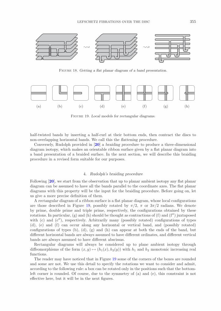
half-twisted bands by inserting a half-curl at their bottom ends, then contract the discs tonon-overlapping horizontal bands. We call this the flattening procedure.
Conversely, Rudolph provided in [20] a braiding procedure to produce a three-dimensionaldiagram isotopy, which makes an orientable ribbon surface given by a flat planar diagram intoa band presentation of a braided surface. In the next section, we will describe this braidingprocedure in a revised form suitable for our purposes.
4. Rudolph’s braiding procedure
Following [20], we start from the observation that up to planar ambient isotopy any flat planardiagram can be assumed to have all the bands parallel to the coordinate axes. The flat planardiagrams with this property will be the input for the braiding procedure. Before going on, letus give a more precise definition of them.
A rectangular diagram of a ribbon surface is a flat planar diagram, whose local configurationsare those described in Figure 19, possibly rotated by π/2, π or 3π/2 radians. We denoteby prime, double prime and triple prime, respectively, the configurations obtained by theserotations. In particular, (g) and (h) should be thought as contractions of (f) and (f′′) juxtaposedwith (c) and (c′′), respectively. Arbitrarily many (possibly rotated) configurations of types(d), (e) and (f) can occur along any horizontal or vertical band, and (possibly rotated)configurations of types (b), (d), (g) and (h) can appear at both the ends of the band, butdifferent horizontal bands are always assumed to have different ordinates, and different verticalbands are always assumed to have different abscissas.
Rectangular diagrams will always be considered up to plane ambient isotopy throughdiffeomorphisms of the form (x, y) → (h1(x), h2(y)) with h1 and h2 monotonic increasing realfunctions.
The reader may have noticed that in Figure 19 some of the corners of the boxes are roundedand some are not. We use this detail to specify the rotations we want to consider and admit,according to the following rule: a box can be rotated only in the positions such that the bottom-left corner is rounded. Of course, due to the symmetry of (a) and (e), this constraint is noteffective here, but it will be in the next figures.
356 NIKOS APOSTOLAKIS RICCARDO PIERGALLINI AND DANIELE ZUDDAS
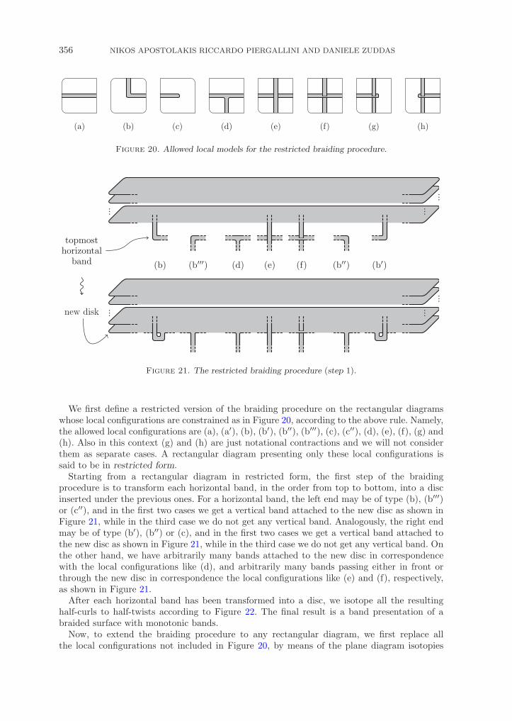
Figure 20. Allowed local models for the restricted braiding procedure.
Figure 21. The restricted braiding procedure (step 1).
We first define a restricted version of the braiding procedure on the rectangular diagramswhose local configurations are constrained as in Figure 20, according to the above rule. Namely,the allowed local configurations are (a), (a′), (b), (b′), (b′′), (b′′′), (c), (c′′), (d), (e), (f), (g) and(h). Also in this context (g) and (h) are just notational contractions and we will not considerthem as separate cases. A rectangular diagram presenting only these local configurations issaid to be in restricted form.
Starting from a rectangular diagram in restricted form, the first step of the braidingprocedure is to transform each horizontal band, in the order from top to bottom, into a discinserted under the previous ones. For a horizontal band, the left end may be of type (b), (b′′′)or (c′′), and in the first two cases we get a vertical band attached to the new disc as shown inFigure 21, while in the third case we do not get any vertical band. Analogously, the right endmay be of type (b′), (b′′) or (c), and in the first two cases we get a vertical band attached tothe new disc as shown in Figure 21, while in the third case we do not get any vertical band. Onthe other hand, we have arbitrarily many bands attached to the new disc in correspondencewith the local configurations like (d), and arbitrarily many bands passing either in front orthrough the new disc in correspondence the local configurations like (e) and (f), respectively,as shown in Figure 21.
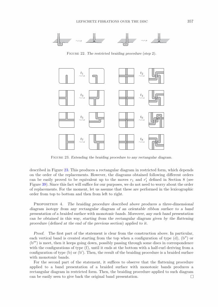
After each horizontal band has been transformed into a disc, we isotope all the resultinghalf-curls to half-twists according to Figure 22. The final result is a band presentation of abraided surface with monotonic bands.
Now, to extend the braiding procedure to any rectangular diagram, we first replace allthe local configurations not included in Figure 20, by means of the plane diagram isotopies
LEFSCHETZ FIBRATIONS OVER THE DISC 357
Figure 22. The restricted braiding procedure (step 2).
Figure 23. Extending the braiding procedure to any rectangular diagram.
described in Figure 23. This produces a rectangular diagram in restricted form, which dependson the order of the replacements. However, the diagrams obtained following different orderscan be easily proved to be equivalent up to the moves r1 and r′1 defined in Section 8 (seeFigure 39). Since this fact will suffice for our purposes, we do not need to worry about the orderof replacements. For the moment, let us assume that these are performed in the lexicographicorder from top to bottom and then from left to right.
Proposition 4. The braiding procedure described above produces a three-dimensionaldiagram isotopy from any rectangular diagram of an orientable ribbon surface to a bandpresentation of a braided surface with monotonic bands. Moreover, any such band presentationcan be obtained in this way, starting from the rectangular diagram given by the flatteningprocedure (defined at the end of the previous section) applied to it.
Proof. The first part of the statement is clear from the construction above. In particular,each vertical band is created starting from the top when a configuration of type (d), (b′′) or(b′′′) is meet, then it keeps going down, possibly passing through some discs in correspondencewith the configurations of type (f), until it ends at the bottom with a half-curl deriving from aconfiguration of type (b) or (b′). Then, the result of the braiding procedure is a braided surfacewith monotonic bands.
For the second part of the statement, it suffices to observe that the flattening procedureapplied to a band presentation of a braided surface with monotonic bands produces arectangular diagram in restricted form. Then, the braiding procedure applied to such diagramcan be easily seen to give back the original band presentation.

358 NIKOS APOSTOLAKIS RICCARDO PIERGALLINI AND DANIELE ZUDDAS
5. Four-Dimensional 2-handlebodies
By a four-dimensional 2-handlebody we mean a compact orientable four-manifold W endowedwith a handlebody structure, whose handles have indices at most 2. We call 2-equivalence theequivalence relation on four-dimensional 2-handlebodies generated by 2-deformations, meaninghandle isotopy, handle sliding and addition/deletion of cancelling pairs of handles of indices lessthan or equal to 2. Of course, 2-equivalent, four-dimensional 2-handlebodies are diffeomorphic,while the converse is not known and likely false.
Here, we consider four-dimensional 2-handlebodies as simple covers of B4 branched overribbon surfaces. We recall that a smooth map p :W → B4 is called a d-fold branched coveringif there exists a smooth two-dimensional subcomplex S ⊂ B4, the branch set, such that therestriction p| :W − p−1(S) → B4 − S is a d-fold ordinary covering. We will always assume thatS is a ribbon surface in R4
+ ⊂ R4+ ∪ {∞} ∼= B4. In this case, p can be completely described
in terms of the monodromy ωp :π1(B4 − S) → Σd, by labelling each region of the three-dimensional diagram of S with the permutation ωp(μ) associated to a meridian μ aroundit, in such a way that the usual Wirtinger relations at the crossings are respected. Conversely,any Σd-labelling of S respecting such relations actually describes a covering of B4 branchedover S. Moreover, p is called a simple branched covering if over any branch point y ∈ Sthere is only one singular point x ∈ p−1(y) and p has local degree 2 at x, being locallysmoothly equivalent to the complex map (z1, z2) → (z1, z2
2). In terms of the correspondinglabelling, this means that each region is labelled by a transposition in Σd. We will referto a ribbon surface with such a labelling by transpositions in Σd as a labelled ribbonsurface.
Proposition 5. A simple covering p :W → B4 branched over a ribbon surface determinesa four-dimensional 2-handlebody decomposition Hp of W, well defined up to 2-deformations.
Proof. Following [16], once an adapted 1-handlebody decomposition S = (D1 � · · · �Dm) ∪ (B1 � · · · �Bn) of S is given, with discs Di as 0-handles and bands Bj as 1-handles, a 2-handlebody decomposition W = (H0
1 � · · · �H0d) ∪ (H1
1 � · · · �H1m) ∪ (H2
1 � · · · �H2n), where d is the degree of p, can be constructed as follows. We put S0 = D1 � · · · �Dm ⊂ B4
and denote by p0 :W1 → B4 the d-fold simple covering branched over S0 with the labellinginherited by S. Then, we put W1 = (H0
1 � · · · �H0d) ∪ (H1
1 � · · · �H1m), where the 0-handles
H01 , . . . , H
0d∼= B4 are the sheets of the covering p0 and we have a 1-handle H1
i between the0-handles H0
k and H0l for each disc Di ⊂ S0 with label (k l). Finally, W can be obtained
by attaching to W1 a 2-handle H2j for each band Bi ⊂ S, whose attaching map is described
by the framed knot given by the unique annular component of p−10 (Bj) ⊂ BdW1 (here we
think Bj ⊂ R3 as a band in the three-dimensional diagram of S). A detailed discussion of thisconstruction in terms of Kirby diagrams can be found in [3, Section 2].
Now, according to [3, Proposition 2.2], the 2-equivalence class of the 2-handlebody decompo-sition ofW we have just described does not depend on the particular choice of the 1-handlebodydecomposition of S.
In light of the above proposition, it makes sense to say that any Σd-labelled ribbon surfaceS ⊂ B4 representing a simple branched covering p, also represents the four-dimensional 2-handlebody Hp up to 2-deformations.
In terms of this representation, the addition of a pair of cancelling 0- and 1-handles to thehandlebody structure of W can be interpreted as the addition of a (d+1)th extra sheet to thecovering and the corresponding addition to S of a separate trivial disc Dm+1 labelled (i d+1)with i � d. We call elementary stabilization this operation, which changes a d-fold branchedcovering into a (d+1)-fold one representing the same handlebody up to 2-deformation, and

LEFSCHETZ FIBRATIONS OVER THE DISC 359
Figure 24. The covering moves.
elementary destabilization its inverse. Also in this context, by a (de)stabilization we mean theresult of consecutive elementary (de)stabilizations.
On the other hand, the addition/deletion of a pair of cancelling 1- and 2-handles in thehandlebody structure of W can be interpreted as the addition/deletion of a correspondingcancelling disc and band in the handlebody structure of S. This leaves essentially unchangedthe labelled ribbon surface S (possibly up to some 1-isotopy moves s2 occurring when the bandpasses through some discs), hence the covering p :W → B4 as well.
The following proposition summarizes results from [3, 16].
Proposition 6. Up to 2-deformations, any connected four-dimensional 2-handlebodycan be represented as a simple 3-fold branched covering of B4, by a Σ3-labelled ribbonsurface in B4. Two labelled ribbon surfaces in B4 represent 2-equivalent connected four-dimensional 2-handlebodies if and only if, after stabilization to the same degree greater thanor equal to 4, they are related by labelled 1-isotopy, meaning 1-isotopy that preserves thelabelling consistently with the Wirtinger relations, and by the covering moves c1 and c2 inFigure 24.
Proof. The first part of the statement is [16, Theorem 6] (see [3, Section 3] for a differentproof based on Kirby diagrams), while the second part is [3, Theorem 1].
We remark that the orientability of a four-dimensional 2-handlebody does not imply theorientability of the labelled ribbon surfaces representing it as a simple branched covering ofB4. Nevertheless, by using the covering moves c1 and c2, any such labelled ribbon surface canbe transformed into an orientable one, representing the same handlebody up to 2-deformations.In fact, those moves together with stabilization will enable us to easily convert any labelledplanar diagram into a flat one.
As we anticipated at the end of Section 2, the covering moves c1 and c2 will also play acrucial role in the interpretation of Proposition 6 in terms of labelled flat planar diagrams. Inthis context, we can still use the moves s5 and s6 in Figure 6 and the flat isotopy moves ofFigure 7, but not the isotopy moves of Figure 8 that involve half-twists.
On the other hand, the 1-isotopy moves of Figure 3, as well as the covering moves c1 andc2 themselves, which arise as three-dimensional moves, can also be thought of as moves of flatplanar diagrams due to their flat presentation. However, when doing so one has to be carefulto use them only accordingly to such fixed flat presentation.
Finally, (de)stabilization makes sense also for flat planar diagrams, being realizable in theelementary case as addition/deletion of a separate flat disc labelled (i d+1) with i � d, to aΣd-labelled flat diagram. We call such a modification a (de)stabilization move.
As we will see shortly, in the presence of covering moves and stabilization all the moves ofFigure 8 can be replaced by a unique move of flat planar diagrams (cf. Figure 27). But first weneed the following lemma (cf. [3, 19]).
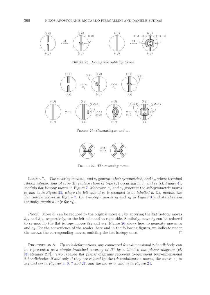
360 NIKOS APOSTOLAKIS RICCARDO PIERGALLINI AND DANIELE ZUDDAS
Figure 25. Joining and splitting bands.
Figure 26. Generating c3 and c4.
Figure 27. The reversing move.
Lemma 7. The covering moves c1 and c2 generate their symmetric c1 and c2, where terminalribbon intersections of type (h) replace those of type (g) occurring in c1 and c2 (cf. Figure 4),modulo flat isotopy moves in Figure 7. Moreover, c1 and c1 generate the self-symmetric movesc3 and c4 in Figure 25, where the left side of c4 is assumed to be labelled in Σd, modulo theflat isotopy moves in Figure 7, the 1-isotopy moves s2 and s3 in Figure 3 and stabilization(actually required only for c4).
Proof. Move c1 can be reduced to the original move c1, by applying the flat isotopy movess18 and s17, respectively, to the left side and to right side. Similarly, move c2 can be reducedto c2 modulo the flat isotopy moves s18 and s11. Figure 26 shows how to generate moves c3and c4. For the convenience of the reader, here and in the following figures, we indicate underthe arrows the corresponding moves, omitting the flat isotopy ones.
Proposition 8. Up to 2-deformations, any connected four-dimensional 2-handlebody canbe represented as a simple branched covering of B4 by a labelled flat planar diagram (cf.[3, Remark 2.7]). Two labelled flat planar diagrams represent 2-equivalent four-dimensional2-handlebodies if and only if they are related by the (de)stabilization moves, the moves s1 tos18 and s27 in Figures 3, 6, 7 and 27, and the moves c1 and c2 in Figure 24.

LEFSCHETZ FIBRATIONS OVER THE DISC 361
Figure 28. Replacing half-twists.
Figure 29. Deriving move s19.
Proof. Proposition 6 tells us that any connected four-dimensional 2-handlebody can berepresented by a labelled planar diagram. This can be made flat by replacing one by one inturn all the half-twist occurring in it as indicated in Figure 28, where d is the degree of thecovering. Of course, the degree of the covering increases by one at a single replacement; hence,we have different degrees d when replacing different half-twists. Then, the final degree dependson the number of the half-twists (a different flattening procedure, which does not increase thedegree, is described in [3, Remark 2.7]), while the final labelling depends on the order of thereplacements and on the choice of i (instead of j) for each one of them. In any case, we obtaina labelled flat planar diagram representing the same four-dimensional 2-handlebody as theoriginal diagram, since each replacement can be thought as a move c4 followed by a move s23or s23. This proves the first part of the proposition.
Now, assume that we have two labelled flat planar diagrams representing the same four-dimensional 2-handlebody up to 2-deformations. Then, by Proposition 6 they are related bya sequence of (de)stabilization moves, 1-isotopy moves s1 to s26 and covering moves c1 andc2. At each step of the sequence, if some half-twist is created by one of the moves s19 to s26,we replace it as described above. Then, we let the replacing configuration follow the originalhalf-twist under the subsequent moves, until it disappears by the effect of one of the movess19 to s26 again. In this way, we get a sequence of flat planar diagrams between the givenones, each related to the previous by the same move as in the original sequence, except thatinstead of the moves s19 to s26 we have their flat versions deriving from the replacement ofhalf-twists. Then, to prove the second part of the proposition, it suffices to derive those flatversions from the moves prescribed in the statement. In doing that, we can also use the movesc1, c2, c3 and c4, thanks to Lemma 7, and all the symmetric moves s5 to s18, according tothe discussion preceding Proposition 1. Moreover, since the labelling resulting from differentchoices in replacing the half-twists can be easily seen to be equivalent up to some moves c4and s27 (possibly after renumbering the sheets of the covering), we can always assume it to bethe most convenient one.
Move s19 is realized in Figure 29, with one move s27 and two moves c4. Moves s21 and s22can be derived in a similar way, with the help of some flat isotopy moves. Move s20 can beskipped, being a consequence of s7, s23 and s24 (in the special case when the bottom band isterminal), as we have already noted.
Moves s23 and s25 are obtained in Figure 30, by using moves c3 and s2 for the former andmoves s27 and c4 for the latter.
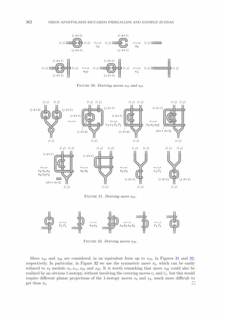
362 NIKOS APOSTOLAKIS RICCARDO PIERGALLINI AND DANIELE ZUDDAS
Figure 30. Deriving moves s23 and s25.
Figure 31. Deriving move s24.
Figure 32. Deriving moves s26.
Move s24 and s26 are considered, in an equivalent form up to s19, in Figures 31 and 32,respectively. In particular, in Figure 32 we use the symmetric move s2, which can be easilyreduced to s2 modulo s5, s11, s23 and s25. It is worth remarking that move s26 could also berealized by an obvious 1-isotopy, without involving the covering moves c1 and c1, but this wouldrequire different planar projections of the 1-isotopy moves s3 and s4, much more difficult toget than s2.

LEFSCHETZ FIBRATIONS OVER THE DISC 363
6. Lefschetz fibrations over B2
A smooth map f :W → B2, with W a smooth oriented compact four-manifold (possibly withcorners), is called a Lefschetz fibration if the following properties hold.
(1) f has a finite set A = {a1, a2, . . . , an} ⊂ IntB2 of singular values and the restrictionf| :W − f−1(A) → B2 −A is a locally trivial fibre bundle, whose fibre is a compact connectedorientable surface F with (possibly empty) boundary, called the regular fibre of f .
(2) For any ai ∈ A the singular fibre Fai= f−1(ai) contains only one singular point wi ∈
Fai∩ IntW and there are local complex coordinates (z1, z2) of W and z of B2 centred at wi
and ai, respectively, such that f : (z1, z2) → z = z21 + z2
2 .
If such coordinates (z1, z2) can be chosen to preserve orientations (no matter whether z doesas well or not), then we call wi a positive singular point, otherwise we call it a negative singularpoint. Obviously, at a negative singular point we can always choose orientation preservingcomplex coordinates (z1, z2) such that f : (z1, z2) → z = z2
1 + z22 .
Two Lefschetz fibrations f :W → B2 and f ′ :W ′ → B2 are said to be fibred equivalent ifthere are orientation preserving diffeomorphisms ϕ :B2 → B2 and ϕ :W →W ′ such that ϕ ◦f = f ′ ◦ ϕ. Of course, in this case ϕ restricts to a bijection ϕ| :A→ A′ between the sets ofsingular values of f and f ′, respectively, while ϕ sends each singular point wi of f into asingular point w′
j of f ′ with the same sign.Note that the locally trivial fibre bundle f| in the definition of Lefschetz fibration f :W →
B2 is oriented. Indeed, each regular fibre Fx = f−1(x) ∼= F with x ∈ B2 −A has a preferredorientation, determined by the following rule: the orientation of W at any point of Fx coincideswith the product of the orientation induced by the standard one of B2 on any smooth localsection of f with the preferred one of Fx in that order. In what follows, we will considerF = F∗ = f−1(∗) endowed with this preferred orientation, for the fixed base point ∗ ∈ S1.
On the other hand, any singular fibre Faiis an orientable surface away from the singular
point wi and the preferred orientation of the regular fibres coherently extends to Fai− {wi}.
Moreover, when BdF = ∅, by putting BdFai= Bd(Fai
− {wi}) for i = 1, 2, . . . , n and T =⋃x∈B2 BdFx ⊂ BdW , we have that f|T :T → B2 is a trivial bundle with fibre BdF . In this
case, corners naturally occur along T ∩ f−1(S1) =⋃x∈S1 BdFx ⊂ BdW .
The structure of f over a small disc Di centred at a singular value ai is given by thefollowing commutative diagram, where: γ±1 :F → F is a Dehn twist along a cycle c ⊂ F , andit is positive (right-handed) or negative (left-handed) according to the sign of the singularpoint wi ∈ Fai
; T (γ±) = F × [0, 1]/((γ±1(x), 0) ∼ (x, 1) ∀x ∈ F ) is the mapping torus of γ±1
and π :T (γ±1) → S1 ∼= [0, 1]/(0 ∼ 1) is the canonical projection; the singular fibre Fai∼= F/c
has a node singularity at wi, which is positive or negative according to the sign of wi; ϕ and ϕare orientation preserving diffeomorphisms such that the cycles cx = ϕ([c, s], t) ⊂ Fx collapseto wi as x = ϕ(s, t) → ai. (cf. [9] or [13])
Because of this collapsing, the cycles cx are called vanishing cycles. We point out that they arewell defined up to ambient isotopy of the fibres Fx, while the cycle c ⊂ F is only defined upto diffeomorphisms of F , depending on the specific identification F ∼= Fx induced by ϕ. Theindeterminacy of the cycle c ⊂ F can be resolved if a Hurwitz system (α1, α2, . . . , αn) for A isgiven. In fact, we can choose ϕ such that the induced identification F ∼= Fx coincides with theone deriving from any trivialization of f| over any arc α′
i joining ∗ to x in B2 −A and running
364 NIKOS APOSTOLAKIS RICCARDO PIERGALLINI AND DANIELE ZUDDAS
along αi outside Di. In this way, we get a cycle ci ⊂ F well defined up to ambient isotopy ofF , which represents the vanishing cycles at wi in the regular fibre F = F∗. We denote by γi,the positive (right-handed) or negative (left-handed) Dehn twists of F along ci correspondingto γ±1 in the above diagram, which is uniquely determined up to ambient isotopy of F as well.We call ci the vanishing cycle of f over ai and γi the mapping monodromy of f over ai (withrespect to the given Hurwitz system).
The Lefschetz fibration f :W → B2 with the set of singular values A ⊂ B2 turns outto be uniquely determined, up to fibred equivalence, by its mapping monodromy sequence(γ1, γ2, . . . , γn) with respect to any given Hurwitz system (α1, α2, . . . , αn) for A. Of course, wecan identify F with the standard compact connected oriented surface Fg,b with genus g � 0and b � 0 boundary components, and think of each γi as a Dehn twist of Fg,b. Actually, wewill represent them as signed cycles in Fg,b.
According to our discussion about Hurwitz systems in Section 3, mapping monodromysequences associated to different Hurwitz systems are related by elementary transformations,changing a given sequence of Dehn twists (γ1, γ2, . . . , γn) into (γ′1, γ
′2, . . . , γ
′n) with γ′i =
γiγi+1γ−1i , γ′i+1 = γi and γ′k = γk for k = i, i+ 1, for some i < n, and their inverses. We call
this transformation the twist sliding of γi+1 over γi, and its inverse the twist sliding of γ′iover γ′i+1.
When considering f up to fibred equivalence, we can always assume (α1, α2, . . . , αn) to be thestandard Hurwitz system and consider (γ1, γ2, . . . , γn) as an abstract sequence of Dehn twistsof Fg,b without any reference to a specific Hurwitz system. In this perspective, twist slidingscan be interpreted as fibred isotopy moves, and two sequences of Dehn twists of Fg,b representfibred equivalent Lefschetz fibrations if and only if they are related by: (1) the simultaneousaction of Mg,b = M+(Fg,b) on the vanishing cycles, where M+ denotes the positive mappingclass group consisting of all isotopy classes of orientation preserving diffeomorphisms fixingthe boundary, to take into account possibly different identifications F ∼= Fg,b; (2) twist slidings(hence cyclic shift of the γi’s as well), to pass from one Hurwitz system to another.
Actually, any sequence (γ1, γ2, . . . , γn) of positive or negative Dehn twists of Fg,b doesrepresent in this way a Lefschetz fibration f :W → B2 with regular fibre F ∼= Fg,b, uniquelydetermined up to fibred equivalence. Such a Lefschetz fibration f can be constructed asdescribed below.
The most elementary non-trivial Lefschetz fibrations over B2 are the Hopf fibrations h± :H± → B2. These are defined as h+(z1, z2) = z2
1 + z22 and h−(z1, z2) = z2
1 + z22 for all (z1, z2) ∈
C2, andH± = {(z1, z2) ∈ C | |z1|2 + |z2|2 � 2 and |h±(z1, z2)| � 1} ∼= B4 (up to smoothing the
corners). Their regular fibre is an annulus F ∼= F0,2 and they have w1 = (0, 0) and a1 = 0 asthe unique singular point and singular value respectively, while the mapping monodromy γ1
is the right-handed Dehn twist along the unique vanishing cycle c1 represented by the coreof F for h+, and the left-handed Dehn twist along c1 for h−. Furthermore, for each x ∈ S1,the regular fibre Fx = h−1
+ (x) or h−1− (x) forms a left- or right-handed, respectively, full twist
as an embedded closed band in BdH± ∼= S3. We call h+ and h−, the positive and negative,respectively, Hopf fibration.
Now we introduce a fibre gluing operation, which will allow us to build up any other non-trivial Lefschetz fibration over B2 by using Hopf fibrations as the basic blocks, and to describethe equivalence moves in Section 7 as well.
Let f1 :W1 → B2 and f2 :W2 → B2 be two Lefschetz fibrations with regular fibres F1 =f−11 (∗) and F2 = f−1
2 (∗), respectively, and let η :G1 → G2 be a diffeomorphism between twosmooth subsurfaces (possibly with corners) G1 ⊂ F1 and G2 ⊂ F2 such that F = F1 ∪η F2 =(F1 � F2)/(x ∼ η(x) ∀x ∈ G1) is a smooth surface (possibly with corners). For i = 1, 2, wecan consider Fi ⊂ F and hence FrF Fi ⊂ BdFi. Moreover, once a trivialization ϕi :Ti =⋃x∈B2 Bd f−1
i (x) → B2 × BdFi of the restriction fi| :Ti → B2 is chosen such that ϕi(x) =(∗, x) for all x ∈ BdFi, we can extend fi to a Lefschetz fibration fi : Wi → B2 with F as

LEFSCHETZ FIBRATIONS OVER THE DISC 365
the regular fibre, in the following way. We put Wi = Wi ∪ϕ′i(B2 × ClF (F − Fi)), where ϕ′
i
is the restriction of ϕi to T ′i = ϕ−1
i (B2 × FrF Fi) ⊂ Ti, and define fi to coincide with theprojection onto the first factor in B2 × ClF (F − Fi). Then, let I1, I2 ⊂ S1 denote two intervals,respectively, ending to and starting from ∗ ∈ S1 (in the counterclockwise orientation) andlet ψi : f−1
i (Ii) → Ii × F be any trivialization of the restrictions fi| : f−1i (Ii) → Ii such that
ψi(x) = (∗, x) for all x ∈ F , with i = 1, 2. Finally, we define a new Lefschetz fibration f1 #η
f2 :W1#ηW2 → B2#B2 ∼= B2, where B2#B2 = B2 ∪ρ B2 is the boundary connected sumgiven by an orientation reversing identification ρ : I1 → I2, by putting W1#ηW2 = W1 ∪ψ W2
and f1 #η f2 = f1 ∪ψ f2, with ψ = ψ−12 ◦ (ρ× idF ) ◦ ψ1 : f−1
1 (I1) → f−12 (I2). A straightforward
verification shows that, this is well defined up to fibred equivalence, depending only on f1, f2and η, but not on the various choices involved in its construction.
We call the Lefschetz fibration f1 #η f2 :W1#ηW2 → B2 the fibre gluing of f1 and f2 throughthe diffeomorphism η :G1 → G2. It has regular fibre F = F1 ∪η F2. Moreover, under theidentification B2#B2 ∼= B2, its set of singular values is the disjoint union A = A1 �A2 ⊂ B2 ofthose of f1 and f2, while a mapping monodromy sequence for it is given by the juxtaposition oftwo given sequences for f1 and f2, with all the Dehn twists thought of as acting on F , throughthe inclusions Fi ⊂ F .
Up to fibred equivalence, fibre gluing is weakly associative in the sense that the equivalencebetween (f1 #η1 f2) #η2 f3 and f1 #η1 (f2 #η2 f3) holds under the assumption (not always true)that all the gluings appearing in both the expressions make sense. This fact easily followsfrom the definition and allows us to write f1 #η1 f2 #η2 · · · #ηn−1 fn without brackets. Still upto fibred equivalence, fibre gluing is also commutative, being the monodromy sequences forf1 #η f2 and f2 #η−1 f1 related by a cyclic shift.
Finally, it is worth noticing that the fibre gluing f1 #η f2 reduces to the usual fibre sum (cf.[9]) when Gi = Fi = F for i = 1, 2 and η = idF . On the other hand, as we will see in the nextsection, it also includes as a special case the Hopf plumbing.
Then, given any sequence of positive or negative Dehn twists (γ1, γ2, . . . , γn) of Fg,b, aLefschetz fibration f :W → B2 with that mapping monodromy sequence is provided by the fibregluing f = f0 #η1h1 #η2 h2 · · · #ηn
hn, where: f0 is the product fibration B2 × Fg,b → B2; hiis a positive or negative Hopf fibration according to the sign of γi; ηi :Ni → Fi is an orientationpreserving diffeomorphism between a regular neighbourhood Ni ⊂ IntFg,b of the cycle ci alongwhich γi occurs and the regular fibre Fi of hi.
The total space W of any Lefschetz fibration f :W → B2 has a natural four-dimensional2-handlebody structure Hf , induced by ‖f‖2 :W → [0, 1] as a Morse function away from 0 (see[9] or [13]). For our aims, it is more convenient to derive such handlebody structure of Wfrom a mapping monodromy sequence representing f , through the corresponding fibre gluingdecomposition. This is the point of view adopted in the next proposition.
Proposition 9. Any Lefschetz fibration f :W → B2 determines a four-dimensional2-handlebody decomposition Hf of W, well defined up to 2-deformations. Moreover, the2-equivalence class of Hf is invariant under fibred equivalence of Lefschetz fibrations.
Proof. Let (γ1, γ2, . . . , γn) be the mapping monodromy sequence of f associated to anyHurwitz system for the set of singular values A = {a1, a2, . . . , an} ⊂ B2. Then, a four-dimensional 2-handlebody decomposition of W based on the corresponding fibre gluingpresentation f = f0 #η1h1 #η2h2 · · · #ηn
hn described above, can be constructed as follows.We start with any handlebody decomposition HF of Fg,b and consider the induced four-
dimensional 2-handlebody decomposition B2 ×HF of the product B2 × Fg,b (actually, thiscan be assumed to have no 2-handles if b > 0). Then, for all i = 1, 2, . . . , n, we define the2-handle H2
i as the total space H± ∼= B4 of the Hopf fibration hi :H± → B2, attached to
366 NIKOS APOSTOLAKIS RICCARDO PIERGALLINI AND DANIELE ZUDDAS
B2 × Fg,b through the map (ρ× ηi)−1 : I2 × Fi → I1 × Fg,b. The attaching sphere of H2i is a
copy {yi} × ci ⊂ S1 × Fg,b of the vanishing cycle ci ⊂ Fg,b, while its attaching framing turnsout to be ±1 with respect to the one given by Fg,b. Namely, we have −1 or +1 if the singularpoint wi, hence the Hopf fibration hi, is positive or negative, respectively, due to the full twistwith the opposite sign formed by the fibre of hi in BdH± ∼= S3. The points y1, y2, . . . , yn areordered along S1 − {∗} according to the counterclockwise orientation.
Now, we let Hf = (B2 ×HF ) ∪H21 ∪H2
2 ∪ · · · ∪H2n be the handlebody decomposition of W
just constructed and observe that, up to handle isotopy, it depends only on the choices of themapping monodromy sequence (γ1, γ2, . . . , γn) and of the handlebody decomposition HF ofFg,b.
The well definedness of Hf up to 2-deformations and its invariance under fibred isotopyof f are immediate consequences of the following facts: (1) diffeomorphic two-dimensionalhandlebodies are always 2-equivalent; (2) any twist sliding in the mapping monodromy sequence(γ1, γ2, . . . , γn) induces a number of 2-handle slidings on the handlebody Hf , one for eachtransversal intersection between the cycles involved in the twist sliding.
As proved by Harer in his thesis [11], up to 2-equivalence any four-dimensional 2-handlebodydecomposition of W can be represented by a Lefschetz fibration f :W → B2 according toProposition 9. This could also be derived from Proposition 8, by applying the braidingprocedure discussed in Section 4 to the labelled flat diagram representing the given handlebodydecomposition (cf. Proposition 10).
The natural question of how to relate any two such representations of 2-equivalent four-dimensional 2-handlebodies will be answered in the next sections, by using the branchedcovering representation of Lefschetz fibrations we are going to describe in the final part ofthis section. As a preliminary step, let us briefly discuss the notion of mapping monodromyhomomorphism of a Lefschetz fibration.
Let f :W → B2 be a Lefschetz fibration with set of singular values A = {a1, a2, . . . , an} ⊂ B2
and regular fibre F ∼= Fg,b. Since π1(B2 −A) is freely generated by any Hurwitz system(α1, α2, . . . , αn) for A, the corresponding mapping monodromy sequence (γ1, γ2, . . . , γn) forf gives rise to a homomorphism ωf :π1(B2 −A) → Mg,b = M+(Fg,b) ∼= M+(F ) such thatωf (αi) = γi for every i = 1, 2, . . . , n (remember that we denote by M+ the positive mappingclass group, consisting of all isotopy classes of orientation preserving diffeomorphisms fixingthe boundary).
We call ωf :π1(B2 −A) → Mg,b the mapping monodromy of f . Note that ωf is defined onlyup to conjugation in Mg,b, depending on the chosen identification F ∼= Fg,b. On the contrary,ωf does not depend on the specific sequence (γ1, γ2, . . . , γn), admitting an intrinsic definitionnot based on the choice of a Hurwitz system.
We outline this definition of ωf , to emphasize that for BdF = ∅ (that is b > 0) it also involvesthe choice of a trivialization ϕ :T ∼= B2 × BdF of the bundle f|T :T → B2, such that ϕ(x) =(∗, x) for all x ∈ BdF . This is used to achieve the condition that ωf ([λ]) fixes BdF for any [λ] ∈π1(B2 −A), as follows. Given the loop λ : [0, 1] → B2 −A, we first consider the commutativediagram below, where the total space of the induced fibre bundle λ∗(f|) is identified with[0, 1] × F by a trivialization of λ∗(f|), in such a way that λ(0, x) = x for all x ∈ F and λ(t, x) =ϕ(λ(t), x) for all x ∈ BdF .

LEFSCHETZ FIBRATIONS OVER THE DISC 367
Then we put ωf ([λ]) = [λ1], with λ1 :F → F the diffeomorphism fixing BdF , defined byλ1(x) = λ(1, x) for all x ∈ F . It is not difficult to see that this definition is independent onthe specific choice of ϕ, since different choices are fibrewise isotopic.
From the classical theory of fibre bundles, we know that ωf uniquely determines therestriction of f| over B2 −A up to fibred equivalence. But, in general, it does not determinethe whole Lefschetz fibration f . In fact, when considering γi as an element of Mg,b the signof it as a Dehn twist gets lost if the cycle ci is homotopically trivial in Fg,b, being in thiscase γi and γ−1
i both isotopic to the identity, while there is no loss of information in the non-trivial cases. Therefore, the mapping monodromy ωf :π1(B2 −A) → Mg,b uniquely determinesthe Lefschetz fibration f :W → B2 up to fibred equivalence only under the assumption thatno vanishing cycle of f is homotopically trivial in Fg,b, in which case f is called a relativelyminimal Lefschetz fibration. While in the presence of trivial vanishing cycles, f turns out tobe determined only up to blow-ups (cf. [9]).
A Lefschetz fibration f :W → B2 is called allowable if its regular fibre F has boundaryBdF = ∅ and all its vanishing cycles are homologically non-trivial in F (hence f is relativelyminimal as well). Of course, since the property of being homologically non-trivial is invariantunder the action of M+(F ), it is enough to verify it for the vanishing cycles ci of any givenmonodromy sequence (γ1, γ2, . . . , γn) for f .
According to Loi and Piergallini [15] and Zuddas [23], allowable Lefschetz fibrations areclosely related to simple covering of B2 ×B2 branched over braided surfaces. This relation isestablished by the next two propositions. But first we recall the notion of lifting braids (cf. [2,17] or [23]).
Let q :F → B2 be a simple covering branched over the finite set ∗ ∈ ΓmB2. Then a braidβ ∈ Bm
∼= π1(ΓmB2, ∗) is said to be liftable with respect to q, when such is the terminaldiffeomorphism h1 : (B2, ∗) → (B2, ∗) of an ambient isotopy (ht)t∈[0,1] of B2 that fixes S1
and realizes β as the loop t → ht(∗) in ΓmB2, meaning that there exists a diffeomorphismh1 :F → F such that q ◦ h1 = h1 ◦ q. We denote by Lq ⊂ Bm the subgroup of the liftablebraids and by λq : Lq → M+(F ) the lifting homomorphism, that sends β to the isotopyclass of h1. It turns out that, if β ∈ Lq is a positive or negative half-twist around an arcb ⊂ B2, then λq(β) is, respectively, the positive or negative Dehn twist along the uniquecycle component of q−1(b) ⊂ F . Actually, every compact connected orientable surface F withboundary BdF = ∅ admits a branched covering q :F → B2, such that any Dehn twist in M+(F )along a homologically non-trivial cycle of F can be represented in this way. This result datesback to the 1970s in the special case when BdF is connected, while it was proved in [23] in thegeneral case.
Proposition 10. Let p :W → B2 ×B2 be a simple covering branched over a braidedsurface S ⊂ B2 ×B2. Then, the composition f = π ◦ p :W → B2, where π :B2 ×B2 → B2 isthe projection onto the first factor, is an allowable Lefschetz fibration. The set A ⊂ B2 ofsingular values of f coincides with the branch set of the branched covering π|S :S → B2, and themapping monodromy of f is the lifting ωf = λq ◦ ωS of the braid monodromy ωS of S, throughthe branched covering q = p| :F ∼= f−1(∗) → π−1(∗) ∼= B2 representing the regular fibre F off (note that ImωS ⊂ Lq). Moreover, the four-dimensional 2-handlebody decompositions Hf
and Hp of W, given by Propositions 9 and 5, respectively, coincide (up to 2-equivalence).
Proof. The first part of the statement is a special case of Proposition 1 of [15]. The proofof the equations ωf = λq◦ ωS and Hf = Hp is just a matter of comparing the definitions.
Proposition 11. Any allowable Lefschetz fibration f :W → B2 factorizes as a compositionf = π ◦ p, where π :B2 ×B2 → B2 is the projection onto the first factor and p :W → B2 ×B2
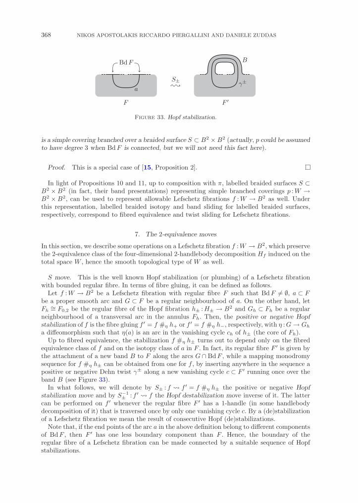
368 NIKOS APOSTOLAKIS RICCARDO PIERGALLINI AND DANIELE ZUDDAS
Figure 33. Hopf stabilization.
is a simple covering branched over a braided surface S ⊂ B2 ×B2 (actually, p could be assumedto have degree 3 when BdF is connected, but we will not need this fact here).
Proof. This is a special case of [15, Proposition 2].
In light of Propositions 10 and 11, up to composition with π, labelled braided surfaces S ⊂B2 ×B2 (in fact, their band presentations) representing simple branched coverings p :W →B2 ×B2, can be used to represent allowable Lefschetz fibrations f :W → B2 as well. Underthis representation, labelled braided isotopy and band sliding for labelled braided surfaces,respectively, correspond to fibred equivalence and twist sliding for Lefschetz fibrations.
7. The 2-equivalence moves
In this section, we describe some operations on a Lefschetz fibration f :W → B2, which preservethe 2-equivalence class of the four-dimensional 2-handlebody decomposition Hf induced on thetotal space W , hence the smooth topological type of W as well.
S move. This is the well known Hopf stabilization (or plumbing) of a Lefschetz fibrationwith bounded regular fibre. In terms of fibre gluing, it can be defined as follows.
Let f :W → B2 be a Lefschetz fibration with regular fibre F such that BdF = ∅, a ⊂ Fbe a proper smooth arc and G ⊂ F be a regular neighbourhood of a. On the other hand, letFh ∼= F0,2 be the regular fibre of the Hopf fibration h± :H± → B2 and Gh ⊂ Fh be a regularneighbourhood of a transversal arc in the annulus Fh. Then, the positive or negative Hopfstabilization of f is the fibre gluing f ′ = f #η h+ or f ′ = f #η h−, respectively, with η :G→ Gha diffeomorphism such that η(a) is an arc in the vanishing cycle ch of h± (the core of Fh).
Up to fibred equivalence, the stabilization f #η h± turns out to depend only on the fibredequivalence class of f and on the isotopy class of a in F . In fact, its regular fibre F ′ is given bythe attachment of a new band B to F along the arcs G ∩ BdF , while a mapping monodromysequence for f #η h± can be obtained from one for f , by inserting anywhere in the sequence apositive or negative Dehn twist γ± along a new vanishing cycle c ⊂ F ′ running once over theband B (see Figure 33).
In what follows, we will denote by S± : f � f ′ = f #η h± the positive or negative Hopfstabilization move and by S−1
± : f ′ � f the Hopf destabilization move inverse of it. The lattercan be performed on f ′ whenever the regular fibre F ′ has a 1-handle (in some handlebodydecomposition of it) that is traversed once by only one vanishing cycle c. By a (de)stabilizationof a Lefschetz fibration we mean the result of consecutive Hopf (de)stabilizations.
Note that, if the end points of the arc a in the above definition belong to different componentsof BdF , then F ′ has one less boundary component than F . Hence, the boundary of theregular fibre of a Lefschetz fibration can be made connected by a suitable sequence of Hopfstabilizations.

LEFSCHETZ FIBRATIONS OVER THE DISC 369
Figure 34. The Lefschetz fibration t.
Looking at the handlebody decomposition Hf , we see that a Hopf stabilization results intoan addition of a cancelling pair of handles of indices 1 and 2. Namely, the 1-handle derives fromthe new band B, and a 2-handle is attached along a parallel copy of c with framing −1 or +1with respect to the fibre, depending on the stabilization being positive or negative, respectively.Thus, the 2-equivalence class of Hf is preserved by Hopf stabilization.
For an allowable Lefschetz fibration f :W → B2 represented by a Σd-labelled braided surfaceS according to Proposition 11, a Hopf (de)stabilization corresponds to an elementary labelled(de)stabilization of S as defined in Section 3. This changes the fibration f , but not the coveringp :W → B2 ×B2 up to smooth equivalence (after smoothing the corners), and it should notbe confused with the covering stabilization obtained by the addition of an extra separate sheetto S with monodromy (i d+ 1) for some i � d, which, on the contrary, changes the covering p,but not the Lefschetz fibration f up to fibred equivalence.
As a consequence, we have that allowability of Lefschetz fibrations is preserved by Hopf(de)stabilization. Moreover, Proposition 3 implies that any allowable Lefschetz fibration admitsa positive stabilization represented by a labelled braided surface with monotonic bands. Finally,it is worth mentioning that the S move has been used by the third author in [24] to constructuniversal Lefschetz fibrations (the analogous of universal bundles).
T move. This is a new move, which corresponds to particular 2-deformations of thehandlebody decomposition Hf of the total space W of a Lefschetz fibration f :W → B2. LikeHopf stabilization, the T move applies only if the regular fibre F of f has non-empty boundary,but an extra condition is required on the mapping monodromy of f . This condition can beexpressed by assuming that f = f0 #η t, where f0 :W0 → B2 is any Lefschetz fibration withbounded regular fibre, while the specific Lefschetz fibration t :B4 → B2 and the gluing map ηare as follows.
Figure 34 describes t :B4 → B2 in terms of its regular fibre Ft ∼= F0,3 and its monodromysequence (γ1, γ2). Here, the Dehn twists γ1 and γ2 are represented by the signed vanishingcycles c1 and c2, respectively, parallel to the inner boundary components. We assume thetwists to have opposite signs, since this is enough for our purposes, but this assumption couldbe relaxed, as we will see later. Moreover, we note that γ1 and γ2 can be interchanged in thesequence, since c1 and c2 are disjoint.
The gluing map η :G0 → Gt is shown in Figure 35. The surface G0 ⊂ F0 is an annulus in theregular fibre F0 of f0, whose core is the oriented cycle a ⊂ IntF0 and whose boundary meetsBdF0 along the four arcs indicated in the figure, in such a way that the oriented transversalarcs r and s are properly embedded in F0. On the left side of the figure, we see the annulusGt ⊂ Ft with the oriented cycle and arcs corresponding to a, r and s under η. While the rightside gives an analogous description of a different gluing map η′ :G0 → Gt. The outer boundarycomponent of Gt coincides with that of Ft, while the inner one meets along two arcs those ofFt. Of course, the given data uniquely determine the rest of η and η′ up to isotopy.
We call a T move the transformation T : f� f ′, with f = f0 #η t :W = W0 #η B4 and f ′ =
f0 #η′ t :W ′ = W0 #η′ B4. A more explicit description of such move is provided in Figure 36.
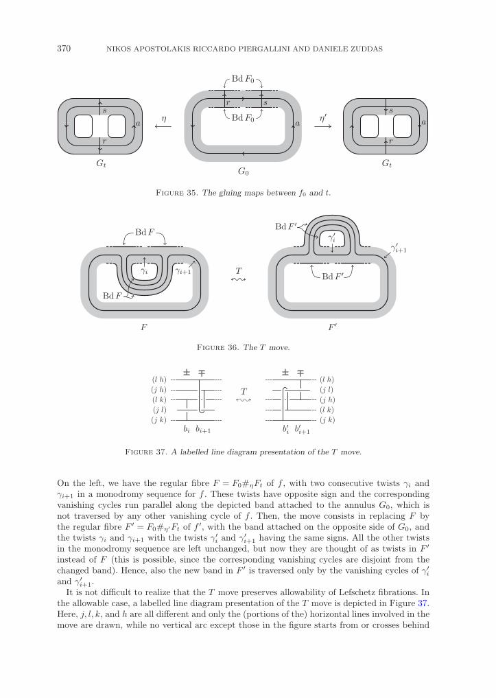
370 NIKOS APOSTOLAKIS RICCARDO PIERGALLINI AND DANIELE ZUDDAS
Figure 35. The gluing maps between f0 and t.
Figure 36. The T move.
Figure 37. A labelled line diagram presentation of the T move.
On the left, we have the regular fibre F = F0#ηFt of f , with two consecutive twists γi andγi+1 in a monodromy sequence for f . These twists have opposite sign and the correspondingvanishing cycles run parallel along the depicted band attached to the annulus G0, which isnot traversed by any other vanishing cycle of f . Then, the move consists in replacing F bythe regular fibre F ′ = F0#η′Ft of f ′, with the band attached on the opposite side of G0, andthe twists γi and γi+1 with the twists γ′i and γ′i+1 having the same signs. All the other twistsin the monodromy sequence are left unchanged, but now they are thought of as twists in F ′
instead of F (this is possible, since the corresponding vanishing cycles are disjoint from thechanged band). Hence, also the new band in F ′ is traversed only by the vanishing cycles of γ′iand γ′i+1.
It is not difficult to realize that the T move preserves allowability of Lefschetz fibrations. Inthe allowable case, a labelled line diagram presentation of the T move is depicted in Figure 37.Here, j, l, k, and h are all different and only the (portions of the) horizontal lines involved in themove are drawn, while no vertical arc except those in the figure starts from or crosses behind
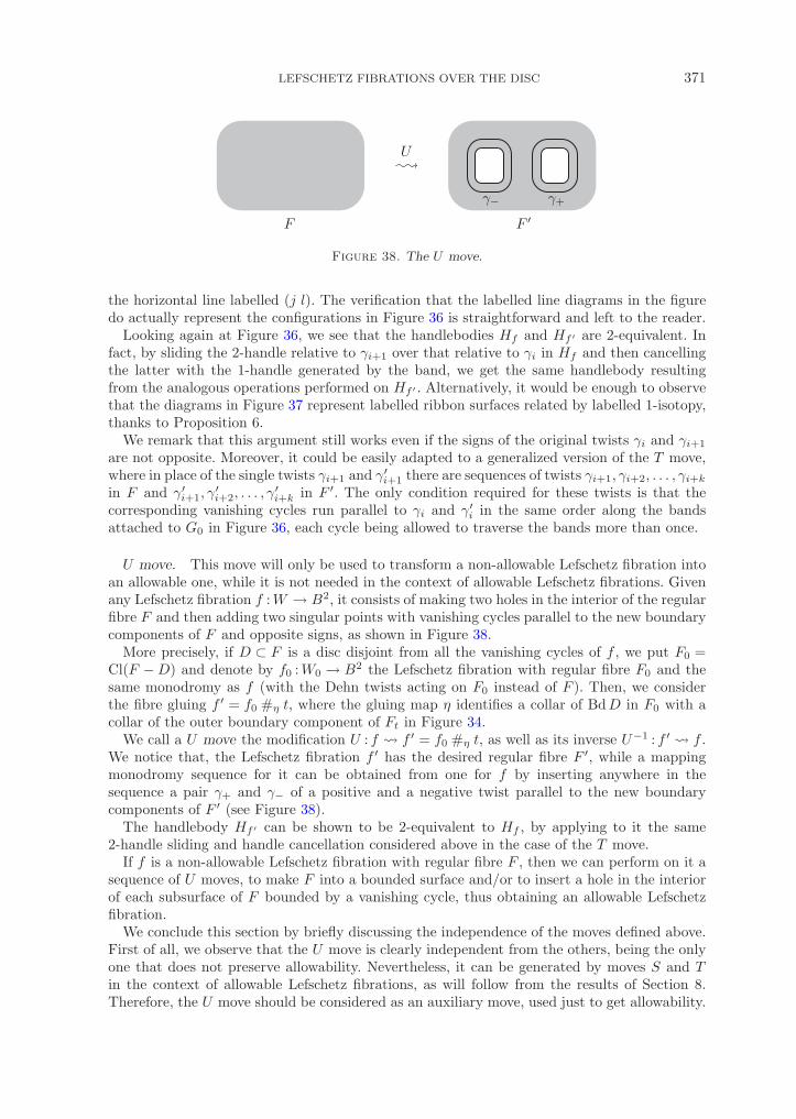
LEFSCHETZ FIBRATIONS OVER THE DISC 371
Figure 38. The U move.
the horizontal line labelled (j l). The verification that the labelled line diagrams in the figuredo actually represent the configurations in Figure 36 is straightforward and left to the reader.
Looking again at Figure 36, we see that the handlebodies Hf and Hf ′ are 2-equivalent. Infact, by sliding the 2-handle relative to γi+1 over that relative to γi in Hf and then cancellingthe latter with the 1-handle generated by the band, we get the same handlebody resultingfrom the analogous operations performed on Hf ′ . Alternatively, it would be enough to observethat the diagrams in Figure 37 represent labelled ribbon surfaces related by labelled 1-isotopy,thanks to Proposition 6.
We remark that this argument still works even if the signs of the original twists γi and γi+1
are not opposite. Moreover, it could be easily adapted to a generalized version of the T move,where in place of the single twists γi+1 and γ′i+1 there are sequences of twists γi+1, γi+2, . . . , γi+kin F and γ′i+1, γ
′i+2, . . . , γ
′i+k in F ′. The only condition required for these twists is that the
corresponding vanishing cycles run parallel to γi and γ′i in the same order along the bandsattached to G0 in Figure 36, each cycle being allowed to traverse the bands more than once.
U move. This move will only be used to transform a non-allowable Lefschetz fibration intoan allowable one, while it is not needed in the context of allowable Lefschetz fibrations. Givenany Lefschetz fibration f :W → B2, it consists of making two holes in the interior of the regularfibre F and then adding two singular points with vanishing cycles parallel to the new boundarycomponents of F and opposite signs, as shown in Figure 38.
More precisely, if D ⊂ F is a disc disjoint from all the vanishing cycles of f , we put F0 =Cl(F −D) and denote by f0 :W0 → B2 the Lefschetz fibration with regular fibre F0 and thesame monodromy as f (with the Dehn twists acting on F0 instead of F ). Then, we considerthe fibre gluing f ′ = f0 #η t, where the gluing map η identifies a collar of BdD in F0 with acollar of the outer boundary component of Ft in Figure 34.
We call a U move the modification U : f � f ′ = f0 #η t, as well as its inverse U−1 : f ′ � f .We notice that, the Lefschetz fibration f ′ has the desired regular fibre F ′, while a mappingmonodromy sequence for it can be obtained from one for f by inserting anywhere in thesequence a pair γ+ and γ− of a positive and a negative twist parallel to the new boundarycomponents of F ′ (see Figure 38).
The handlebody Hf ′ can be shown to be 2-equivalent to Hf , by applying to it the same2-handle sliding and handle cancellation considered above in the case of the T move.
If f is a non-allowable Lefschetz fibration with regular fibre F , then we can perform on it asequence of U moves, to make F into a bounded surface and/or to insert a hole in the interiorof each subsurface of F bounded by a vanishing cycle, thus obtaining an allowable Lefschetzfibration.
We conclude this section by briefly discussing the independence of the moves defined above.First of all, we observe that the U move is clearly independent from the others, being the onlyone that does not preserve allowability. Nevertheless, it can be generated by moves S and Tin the context of allowable Lefschetz fibrations, as will follow from the results of Section 8.Therefore, the U move should be considered as an auxiliary move, used just to get allowability.
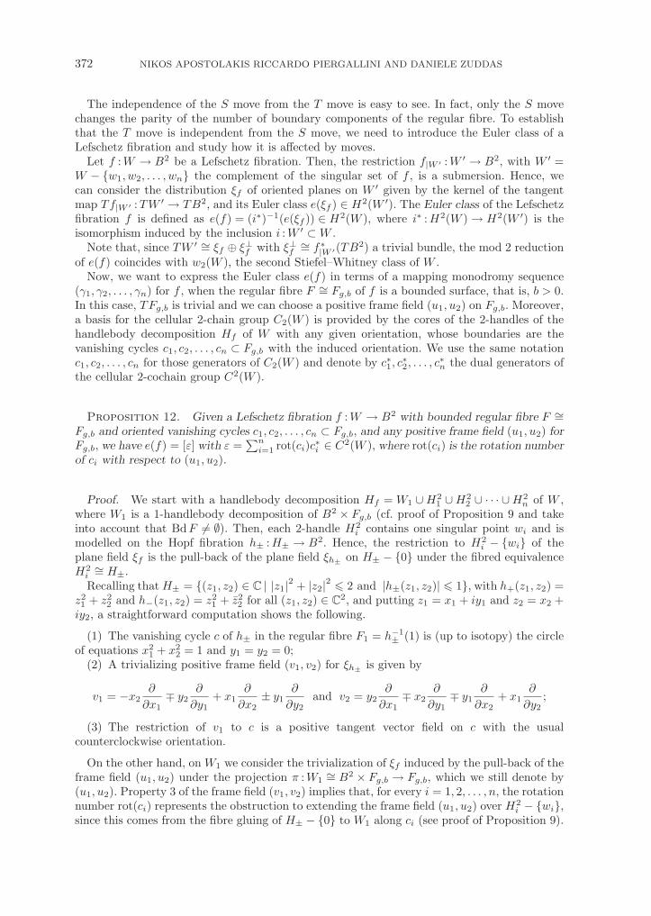
372 NIKOS APOSTOLAKIS RICCARDO PIERGALLINI AND DANIELE ZUDDAS
The independence of the S move from the T move is easy to see. In fact, only the S movechanges the parity of the number of boundary components of the regular fibre. To establishthat the T move is independent from the S move, we need to introduce the Euler class of aLefschetz fibration and study how it is affected by moves.
Let f :W → B2 be a Lefschetz fibration. Then, the restriction f|W ′ :W ′ → B2, with W ′ =W − {w1, w2, . . . , wn} the complement of the singular set of f , is a submersion. Hence, wecan consider the distribution ξf of oriented planes on W ′ given by the kernel of the tangentmap Tf|W ′ :TW ′ → TB2, and its Euler class e(ξf ) ∈ H2(W ′). The Euler class of the Lefschetzfibration f is defined as e(f) = (i∗)−1(e(ξf )) ∈ H2(W ), where i∗ :H2(W ) → H2(W ′) is theisomorphism induced by the inclusion i :W ′ ⊂W .
Note that, since TW ′ ∼= ξf ⊕ ξ⊥f with ξ⊥f ∼= f∗|W ′(TB2) a trivial bundle, the mod 2 reductionof e(f) coincides with w2(W ), the second Stiefel–Whitney class of W .
Now, we want to express the Euler class e(f) in terms of a mapping monodromy sequence(γ1, γ2, . . . , γn) for f , when the regular fibre F ∼= Fg,b of f is a bounded surface, that is, b > 0.In this case, TFg,b is trivial and we can choose a positive frame field (u1, u2) on Fg,b. Moreover,a basis for the cellular 2-chain group C2(W ) is provided by the cores of the 2-handles of thehandlebody decomposition Hf of W with any given orientation, whose boundaries are thevanishing cycles c1, c2, . . . , cn ⊂ Fg,b with the induced orientation. We use the same notationc1, c2, . . . , cn for those generators of C2(W ) and denote by c∗1, c
∗2, . . . , c
∗n the dual generators of
the cellular 2-cochain group C2(W ).
Proposition 12. Given a Lefschetz fibration f :W → B2 with bounded regular fibre F ∼=Fg,b and oriented vanishing cycles c1, c2, . . . , cn ⊂ Fg,b, and any positive frame field (u1, u2) forFg,b, we have e(f) = [ε] with ε =
∑ni=1 rot(ci)c∗i ∈ C2(W ), where rot(ci) is the rotation number
of ci with respect to (u1, u2).
Proof. We start with a handlebody decomposition Hf = W1 ∪H21 ∪H2
2 ∪ · · · ∪H2n of W ,
where W1 is a 1-handlebody decomposition of B2 × Fg,b (cf. proof of Proposition 9 and takeinto account that BdF = ∅). Then, each 2-handle H2
i contains one singular point wi and ismodelled on the Hopf fibration h± :H± → B2. Hence, the restriction to H2
i − {wi} of theplane field ξf is the pull-back of the plane field ξh± on H± − {0} under the fibred equivalenceH2i∼= H±.
Recalling thatH± = {(z1, z2) ∈ C | |z1|2 + |z2|2 � 2 and |h±(z1, z2)| � 1}, with h+(z1, z2) =z21 + z2
2 and h−(z1, z2) = z21 + z2
2 for all (z1, z2) ∈ C2, and putting z1 = x1 + iy1 and z2 = x2 +
iy2, a straightforward computation shows the following.
(1) The vanishing cycle c of h± in the regular fibre F1 = h−1± (1) is (up to isotopy) the circle
of equations x21 + x2
2 = 1 and y1 = y2 = 0;(2) A trivializing positive frame field (v1, v2) for ξh± is given by
v1 = −x2∂
∂x1∓ y2
∂
∂y1+ x1
∂
∂x2± y1
∂
∂y2and v2 = y2
∂
∂x1∓ x2
∂
∂y1∓ y1
∂
∂x2+ x1
∂
∂y2;
(3) The restriction of v1 to c is a positive tangent vector field on c with the usualcounterclockwise orientation.
On the other hand, on W1 we consider the trivialization of ξf induced by the pull-back of theframe field (u1, u2) under the projection π :W1
∼= B2 × Fg,b → Fg,b, which we still denote by(u1, u2). Property 3 of the frame field (v1, v2) implies that, for every i = 1, 2, . . . , n, the rotationnumber rot(ci) represents the obstruction to extending the frame field (u1, u2) over H2
i − {wi},since this comes from the fibre gluing of H± − {0} to W1 along ci (see proof of Proposition 9).

LEFSCHETZ FIBRATIONS OVER THE DISC 373
Thus, the cohomology class of ε in H2(W ′) coincides with e(ξf ), and the proposition followsat once.
Proposition 12 allows us to easily compute the changes in the Euler class e(f) induced byany move performed on f . This is done in the following proposition, which obviously impliesthe independence of the T move from the S move.
Proposition 13. Let f :W → B2 and f ′ :W → B2 be Lefschetz fibrations with boundedregular fibres. If f ′ is obtained from f by an S move, then e(f ′) = e(f). While, if f ′ is obtainedfrom f by a T move or a U move, then e(f ′) = e(f) + 2[δ] for some (generically cohomologicallynon-trivial) cocycle δ ∈ C2(W ).
Proof. We choose trivializing frame fields (u1, u2) and (u′1, u′2) for F and F ′, respectively,
to coincide with the standard one in Figures 33, 36 and 38, and assume all the vanishing cyclesin those figures to be counterclockwise oriented. Then we use Proposition 12 to evaluate thedifference e(f ′) − e(f).
In the case when f ′ is a Hopf-stabilization of f , we have that e(f ′) − e(f) = [c∗], where c∗
is the dual of the generator c of C2(W ) corresponding to the new Dehn twist γ± in Figure 33.But this is cohomologically trivial in W , hence e(f ′) = e(f).
If f and f ′ are related by a T move as in Figure 36, then e(f ′) − e(f) = [(c′i)∗ + (c′i+1)
∗] −[c∗i + c∗i+1]. Since c∗i and (c′i)
∗ are, respectively, cohomologous to c∗i+1 and −(c′i+1)∗ in W , we
can write e(f ′) − e(f) = 2[δ] with δ = −c∗i . Similarly, if f and f ′ are related by a U move asin Figure 38, we have e(f ′) − e(f) = 2[δ] with δ = c∗+.
Remark 14. Any integral lifting of the second Stiefel–Whitney class of a four-dimensional2-handlebody W is the Euler class of a Lefschetz fibration W → B2.
Since any two such liftings differ by an even class (by the universal coefficient theorem),that statement follows once we show that starting from any Lefschetz fibration f : W → B2
with bounded fibre F , one can construct another Lefschetz fibration f ′ : W → B2 such thate(f ′) = e(f) ± 2c∗ for an arbitrary vanishing cycle c ⊂ F of f . Up to isotopy, we can assumethat there is a disc in IntF − c and an arc joining it to BdF , which intersects c transversely ina single point and do not intersect any other vanishing cycles. Then by performing a U moveinside this disc, we get e(f ′) = e(f) − 2c∗. Changing f ′ by two more U moves, performed in asimilar way with the two new vanishing cycles introduced by the former U move in place of c,we get e(f ′) = e(f) + 2c∗.
8. The main theorem
As a preliminary step to prove the equivalence theorem for Lefschetz fibrations, we need totranslate into the language of rectangular diagrams the moves for labelled flat planar diagramsconsidered in Proposition 8. In doing that, we continue to use for rotated moves the ‘primenotation’ and the graphical ‘rounded bottom-left corner’ rule introduced in Section 4.
First of all, we consider the plane isotopy moves in Figure 39. These are intended to relateplanar rectangular diagrams, which are isotopic in the projection plane (crossing and ribbonintersections are assumed to be preserved by the isotopy). We observe that only two rotationsof the moves r1, r3 and r6 are enough, due to their symmetry. Move r1 switches two horizontalbands which are contiguous in the vertical order, under the assumption that the horizontalintervals they span do not overlap. Similarly, move r′1 switches two contiguous vertical bandsunder the analogous assumption. Here we include, as degenerate horizontal or vertical bands,the end points of vertical or horizontal ones, respectively. In all the moves, when a band coming

374 NIKOS APOSTOLAKIS RICCARDO PIERGALLINI AND DANIELE ZUDDAS
Figure 39. Plane isotopy moves for rectangular diagrams.
out from the box is translated, we assume that the translation is small enough to not interferewith the rest of the diagram.
Figures 40–42 provide the rectangular versions of the moves in Figures 3, 6, 7 and 24. Weobserve that, no rotated move is needed here, thanks to the moves in Figure 39 that allow usto rotate by kπ/2 any local configuration in the diagram. Moreover, we put each move in themost convenient form for applying Rudolph’s braiding procedure to it.
Lemma 15. Two labelled rectangular diagrams represent 2-equivalent connected four-dimensional 2-handlebodies as simple branched coverings of B4 if and only if they are relatedby rectangular (de)stabilization and the moves r1 to r25 in Figures 39–42.
Proof. Moves r1 to r7 in Figure 39, together with their allowed rotated versions, sufficeto realize any plane isotopy between rectangular diagrams. In fact, any flat planar diagram isuniquely determined by its planar core graph, together with some extra information on thevertices corresponding to crossings and ribbon intersections. Now, it is not difficult to realizethat any isotopy of the graph, as well as any deformation of its structure, can be approximatedby using the moves in Figure 39. In particular, the two moves r26 and r27 in Figure 43, whichare obviously needed in order to approximate isotopies along an edge, can be obtained from r4and r5 modulo r2.
Then, it suffices to show that the remaining moves r8 to r25 generate all the moves listed inProposition 8, in the presence of moves r1 to r7.
The moves in Figure 40 together with r2 and r3, generate the moves s5 to s18 in Figures 6and 7 and the move s27 in Figure 27. The only non-trivial facts in this respect are the following:(1) move s9, which does not have an explicit representation in Figure 40, can be obtained as acomposition of moves r2, r8 and r10; (2) r14 and r15 completed with the right terminations, gives15 and s16 (after contracting the extra tongue, by using r2, r4, r5, r8 and r9); (3) similarly,r16, r17, r18 and r19 give s5, s6, s17 and s18.
While the moves r20 to r23 in Figure 41 and the moves r24 and r25 in Figure 42 are rectangularversions of the 1-isotopy moves s1 to s4 in Figure 3 and of the covering moves c1 and c2 inFigure 27, respectively.

LEFSCHETZ FIBRATIONS OVER THE DISC 375
Figure 40. Three-dimensional isotopy moves for rectangular diagrams.
Figure 41. 1-isotopy moves for rectangular diagrams.
Figure 42. Covering moves for colored rectangular diagrams.

376 NIKOS APOSTOLAKIS RICCARDO PIERGALLINI AND DANIELE ZUDDAS
Figure 43. Breaking edges.
At this point, we are in a position to prove our main theorem.
Theorem A. Any two allowable Lefschetz fibrations f :W → B2 and f ′ :W ′ → B2 repre-sent 2-equivalent four-dimensional 2-handlebodies Hf and Hf ′ if and only if they are relatedby fibred equivalence and the moves S and T . Moreover, the allowability hypothesis can berelaxed by using in addition move U .
Proof. As we have seen in Section 7, fibred equivalence and moves S, T and U do not changethe 2-equivalence class of the total space of a Lefschetz fibration. This gives the ‘if’ part of thestatement. Concerning the ‘only if’ part, the reduction to the allowable case immediately followsfrom the fact that any Lefschetz fibration can be made into an allowable one by performing Umoves on it (see Section 7).
Now, let f and f ′ be allowable Lefschetz fibrations as in the statement. Thanks to Propo-sition 11 and the consideration following it, they can be represented by band presentations Sand S′ of certain labelled braided surfaces. Moreover, by Proposition 3 (cf. discussion on Smove in Section 7), up to positive stabilization and fibred equivalence of Lefschetz fibrations,the labelled surfaces S and S′ can be assumed to have monotonic bands. Finally, we performon these surfaces the flattening procedure described at the end of Section 3, getting in this waytwo labelled rectangular diagrams, which we still denote by S and S′. Lemma 15 tells us thatS and S′ are related by rectangular (de)stabilization and moves r1 to r25.
Concerning rectangular (de)stabilization, we observe that it can be realized by theaddition/deletion of a separate short horizontal band labelled (i d+1) (cf. Section 5). But,once the braiding procedure has been applied, this band results into a separate sheet labelled(i d+1), which affects the covering but not the Lefschetz fibration (cf. discussion on S move inSection 7).
The rest of the proof is devoted to showing that Rudolph’s braiding procedure makes movesr1 to r25 (including the rotated versions of moves r1 to r7) into modifications of labelled braidedsurfaces, which can be realized by labelled band sliding (that means labelled braided isotopy),(de)stabilization of labelled braided surfaces (which corresponds to the S move) and the labelledbraided surface representation of the T move (see Figure 37). Note that the braiding procedureapplied to the rectangular diagrams S and S′ gives back the original braided surfaces (cf.Proposition 4).
We will include in the argument also the moves r26 and r27 (and their rotated versions).These are not strictly needed, but they help us to simplify the handling of the other moves.Moves will be considered in a convenient order not consistent with the numbering.
In the computations below, we will use the line notation for the rectangular diagrams, as wealready did for the braided surfaces. This consists of a rectangular diagram of the core graphof the represented ribbon surface, with the conventions described in Figure 44 for the terminalbands and the ribbon intersections.
Moves r1, r26 and r27. We observe that the two bands of the rectangular diagram involvedin these moves give rise to two sets of bands in the braided surface, due to the preliminaryreplacements of local configurations that are not in the restricted form for Rudolph’s procedure.

LEFSCHETZ FIBRATIONS OVER THE DISC 377
Figure 44. The line notation for rectangular diagrams.
Figure 45. Sliding a band to the right.
Actually, those replacements make a single move r1 between the original rectangular diagramsinto a finite sequence of moves r1 between the corresponding diagrams in restricted form.Analogously, a single move r26 or r27 is made into a sequence of moves r1 and one move r26 orr27, respectively. Therefore, we can limit ourselves to consider moves r1, r26 and r27 betweendiagrams in restricted form, each horizontal band of which generates a single sheet of thebraided surface.
In the case of move r1, from the two bands on the left we get two sheets of the braidedsurface, such that the upper or the lower one is trivial, respectively, on the right or on the leftof a certain abscissa. We stabilize the braided surface by inserting a trivial sheet immediatelyover those two sheets and connecting it to the lower one by a positive half-twisted band locatedat that abscissa. After that, we make the lower sheet trivial by sliding this band to the rightand then we remove it by destabilizing. The left side of Figure 45 shows the effect of the slidingon the four possible types of bands we can meet. The resulting braided surface is the one givenby the diagram on the right side of move r1.
Move r26 can be treated in a similar way. Here, we just slide to the right the positive half-twisted band of the braided surface corresponding to the vertical band of the diagram on theleft side of the move and then remove the lower sheet by destabilizing. The left side of Figure 45still describes the sliding in this case if we ignore the sheet in the middle.
Move r27 is the up-down symmetric of r26. Hence, the same argument holds for it, exceptfor the half-twisted band being negative and the sliding of it working as in the right side ofFigure 45.
Moves r′1, r′26 and r′27. The reduction to the case of diagrams in restricted form goes as above
(rotate everything in the reasoning). In this case, move r′1 just means a band sliding (we arechanging the order of commuting bands), while moves r′26 and r′27 can be interpreted as asliding followed by a destabilization, as in Figure 46.
From now on, we will implicitly use the above moves to localize the other ones, by breaking allthe bands coming out from the involved local configurations. In this way, we can disregard thesmall translations of those bands needed for the move to take place. Moreover, the replacementsneeded to get configurations in restricted form can be performed in any order (cf. Section 4) andthe moves can be assumed to directly act on diagrams in restricted form, after the replacements.
Moves r2, r′2, r
′′2 , r
′′′2 . Figure 47 shows how to deal with these moves. For r2, we have only
a destabilization, for r′2 and r′′′2 we first need to perform one sliding, while for r′′2 we candestabilize the top sheet and then continue as for r26.

378 NIKOS APOSTOLAKIS RICCARDO PIERGALLINI AND DANIELE ZUDDAS
Figure 46. Moves r′26 and r′27.
Figure 47. Moves r2, r′2, r
′′2 and r′′′2 .
Figure 48. Move r′′′5 .
Moves r4, r′4, r
′′4 , r
′′′4 and r5, r
′5, r
′′5 , r
′′′5 . After the replacements in Figure 23: move r4 follows
from r26; move r′4 follows from r′1 and r′26; move r5 follows from r27; moves r′′′4 , r′5 and r′′5
are tautological. Moreover, moves r′′4 and r′′′5 are equivalent modulo r26. Finally, move r′′′5 isconsidered in Figure 48. Here, a stabilization and a band sliding are performed at the end of thetop and the bottom line respectively, and the two resulting rightmost diagrams are equivalentup to band sliding.
Moves r3, r′3. These moves can be easily seen to be equivalent modulo moves r4, r5, r26, r27
and their rotated versions. Move r′3 is considered in Figure 49. Here, the two rightmost diagramsare equivalent up to band sliding.

LEFSCHETZ FIBRATIONS OVER THE DISC 379
Figure 49. Move r′3.
Figure 50. Move r′6.
Moves r6, r′6. We observe that move r6 is tautological, since it coincides with t2. Move r′6 is
treated in Figure 50. Also in this case band sliding and (de)stabilization suffice. In particular,after the last step in the figure, the band between the two remaining sheets has to be slidedup to the right end (as in Figure 45), to allow a final destabilization.
Moves r8, r9 and r21. For r8 and r21 it suffices to note that, once the replacement t′′1 isapplied to the terminal vertical band, the sheet deriving from this band can be removed bydestabilization on both the sides of the move. Move r9 does not affect at all the resultingbraided surface.
Moves r11, r12, r15, r16, r18 and r20. The local configurations involved in all these moves arein the restricted form (hence, no replacement is required) and it is easy to see that they justchange the braided surface by a sliding of one of the two half-twisted bands which appear overthe other one. In particular, these bands commute for the first three moves. Actually, for mover20 some further band sliding and a destabilization are required, like for r26 and r′′2 .
Moves r17 and r19. In Figure 51, we compare the two braided surfaces originated by the localconfigurations in move r17. Once again we see that they are equivalent up to band slidings andstabilization.
The case of move r19 is symmetric to that of r17 modulo moves r1, r′1, r26, r′26 and r′6. In fact,
in Figure 52, we show how the right side of move r19 can be put in restricted form by usingthose moves (instead of the replacement t2). The result is symmetric to the second diagram inFigure 51.
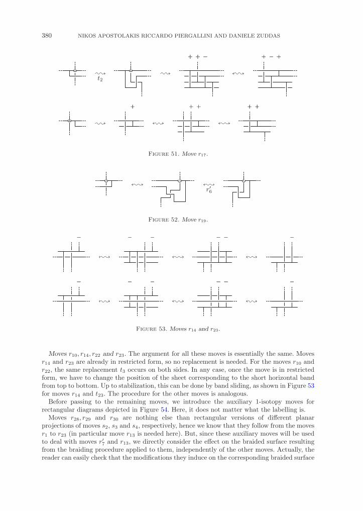
380 NIKOS APOSTOLAKIS RICCARDO PIERGALLINI AND DANIELE ZUDDAS
Figure 51. Move r17.
Figure 52. Move r19.
Figure 53. Moves r14 and r23.
Moves r10, r14, r22 and r23. The argument for all these moves is essentially the same. Movesr14 and r23 are already in restricted form, so no replacement is needed. For the moves r10 andr22, the same replacement t3 occurs on both sides. In any case, once the move is in restrictedform, we have to change the position of the sheet corresponding to the short horizontal bandfrom top to bottom. Up to stabilization, this can be done by band sliding, as shown in Figure 53for moves r14 and t23. The procedure for the other moves is analogous.
Before passing to the remaining moves, we introduce the auxiliary 1-isotopy moves forrectangular diagrams depicted in Figure 54. Here, it does not matter what the labelling is.
Moves r28, r29 and r30 are nothing else than rectangular versions of different planarprojections of moves s2, s3 and s4, respectively, hence we know that they follow from the movesr1 to r23 (in particular move r13 is needed here). But, since these auxiliary moves will be usedto deal with moves r′7 and r13, we directly consider the effect on the braided surface resultingfrom the braiding procedure applied to them, independently of the other moves. Actually, thereader can easily check that the modifications they induce on the corresponding braided surface

LEFSCHETZ FIBRATIONS OVER THE DISC 381
Figure 54. Auxiliary moves.
Figure 55. Move r′7.
Figure 56. Move r′′7 .
are completely analogous to those induced by moves r21, r22 and r23, respectively, and can berealized by (de)stabilization and band sliding as well.
Moves r7, r′7, r
′′7 , r
′′′7 . Concerning r7, we see that once the replacement t8 is applied to the
diagram on the right side of the move, it turns out to be equivalent to that on the left sideup to moves r1, r′1, r27, r
′27. Move r′′′7 is tautological, since it coincides with t4. So, we are left
with moves r′7 and r′′7 . These are, respectively, treated in Figures 55 and 56, where they arederived from the moves considered above after the required replacements. In particular, thethird diagram in the first line of Figure 55 can be proved to be equivalent to the second one,by cancelling the two opposite kinks, once the top one has been moved down passing throughthe horizontal band in the middle. The last operation can be realized in a straightforward way,by using the moves already considered above and the auxiliary moves r28 and r29.
Moves r24 and r25. We consider these moves in Figures 57 and 58. Here, we start with oneside of the move (the right side for r24 and the left side for r25) and end up with the braided
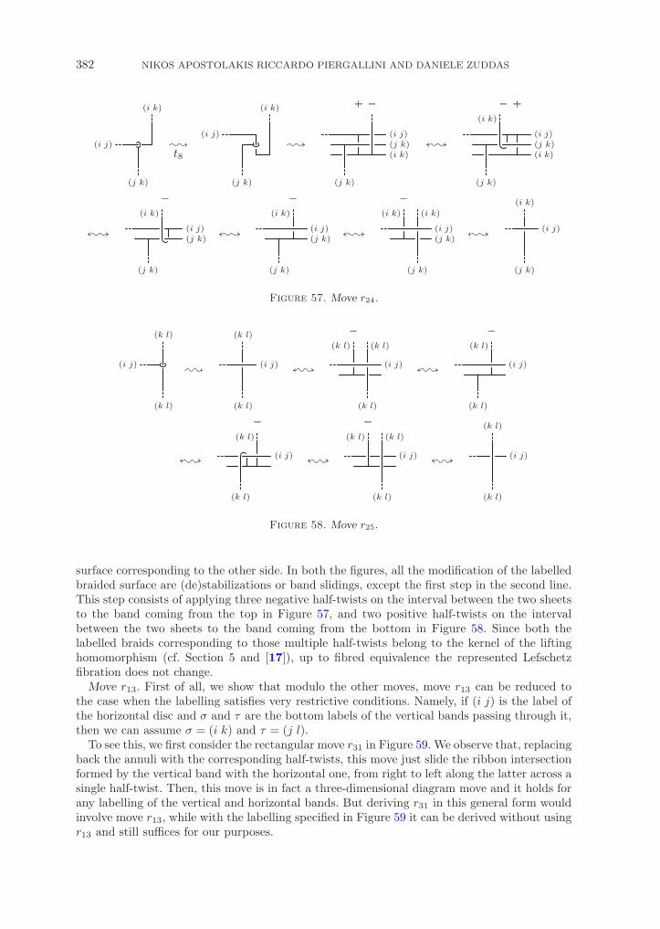
382 NIKOS APOSTOLAKIS RICCARDO PIERGALLINI AND DANIELE ZUDDAS
Figure 57. Move r24.
Figure 58. Move r25.
surface corresponding to the other side. In both the figures, all the modification of the labelledbraided surface are (de)stabilizations or band slidings, except the first step in the second line.This step consists of applying three negative half-twists on the interval between the two sheetsto the band coming from the top in Figure 57, and two positive half-twists on the intervalbetween the two sheets to the band coming from the bottom in Figure 58. Since both thelabelled braids corresponding to those multiple half-twists belong to the kernel of the liftinghomomorphism (cf. Section 5 and [17]), up to fibred equivalence the represented Lefschetzfibration does not change.
Move r13. First of all, we show that modulo the other moves, move r13 can be reduced tothe case when the labelling satisfies very restrictive conditions. Namely, if (i j) is the label ofthe horizontal disc and σ and τ are the bottom labels of the vertical bands passing through it,then we can assume σ = (i k) and τ = (j l).
To see this, we first consider the rectangular move r31 in Figure 59. We observe that, replacingback the annuli with the corresponding half-twists, this move just slide the ribbon intersectionformed by the vertical band with the horizontal one, from right to left along the latter across asingle half-twist. Then, this move is in fact a three-dimensional diagram move and it holds forany labelling of the vertical and horizontal bands. But deriving r31 in this general form wouldinvolve move r13, while with the labelling specified in Figure 59 it can be derived without usingr13 and still suffices for our purposes.

LEFSCHETZ FIBRATIONS OVER THE DISC 383
Figure 59. The auxiliary move r31.
Figure 60. Deriving the auxiliary move r31.
Figure 61. Reducing move r13 to the case σ = (i k) and τ = (jl).
Figure 60 shows how to derive move r31 with that labelling from the other moves exceptr13. Here, the moves indicated under the arrows are intended up to the planar isotopy movesin Figure 39 (in particular up to rotations).
At this point, we are in a position to deal with move r13. We begin by modifying both sidesof the move as in the top line of Figure 61, where the disc and the bands are broken by usingmove c4 in Figure 25 and some 1-isotopy moves are performed (including r28 and r30). In thisway, the original move is changed into two reversing moves involving three ribbon intersections,but now the bottom labels of the vertical bands are all different from each other and from (i j).In the second line of Figure 61, we realize such a reversing move in terms of two moves r13with the same constraints on labelling. This also requires two moves c4 at the first and laststep and a move r31 at the middle step.
By this argument, we can assume that also σ and τ in the original move r13 are differentfrom each other and from (i j). Under such assumption, if σ or τ are disjoint from (i j),then the move can easily be deduced from the covering moves in Figure 42. In the remaining

384 NIKOS APOSTOLAKIS RICCARDO PIERGALLINI AND DANIELE ZUDDAS
Figure 62. Move r13.
cases, up to symmetry we have σ = (i k) while τ can be one of (i l), (j k) or (j l) (here, weassume i, j, k and l all different). At this point, the reduction to the only case when τ = (j l) isimmediate.
Figure 62 shows how to realize move r13 with σ = (i k) and τ = (j l) in terms of the T movedescribed in Section 7. This is needed to relate the two rightmost braided surfaces, once theyare obtained by suitable stabilizations (the sign of the stabilizing band is irrelevant).
Remark 16. According to Theorem A, any U move between allowable Lefschetz fibrationscan be generated by S and T moves. Actually, this could be proved directly by induction onthe number of vanishing cycles that separate the region where the U move is performed fromthe boundary of the fibre. Indeed, this number can be reduced to zero by suitable T moves andslidings, and after that the U move can be trivially realized by two opposite S moves.
9. Open books
Given a closed connected oriented three-manifold M , by an open book structure on M, wemean a smooth map f :M → B2 such that the following properties hold.
(1) The restriction f|T :T = Cl(f−1(IntB2)) → B2 is a (trivial) fibre bundle, with L =f−1(0) ⊂M a smooth link, called the binding of the open book, and T ⊂M a tubularneighbourhood of L;
(2) The composition ρf = ρ ◦ f|M−L :M − L→ S1, with ρ :B2 − {0} → S1 the projectiondefined by ρ(x) = x/‖x‖, is a locally trivial fibre bundle, whose fibre is the interior IntF of acompact connected orientable bounded surface F , called the page of the open book.
Such a map induces an open book decomposition of M into compact connected orientablebounded surfaces Fs = f−1([0, s]) = Cl(ρ−1
f (s)) ⊂M with s ∈ S1, called the pages of thedecomposition. These are all diffeomorphic to F and only meet at their common boundaryBdFs = L. Moreover, Fs has a preferred orientation determined by the following rule: theorientation of M at any point of Fs coincides with the product of the orientation induced bythe standard one of S1 on any smooth local section of ρf with the preferred orientation of Fs,in that order. This makes ρf into an oriented locally trivial fibre bundle. In what follows, wewill consider F = F∗ endowed with this preferred orientation, for the fixed base point ∗ ∈ S1.
Two open books f :M → B2 and f ′ :M ′ → B2 are said to be fibred equivalent if there areorientation preserving diffeomorphisms ϕ :B2 → B2 and ϕ :M →M ′ such that ϕ ◦ f = f ′ ◦ ϕ.
By the monodromy of an open book f :M → B2 with binding L ⊂M and page F , wemean the mapping class γf = ωf (α) ∈ M+(F ), with ωf :π1(S1) → M+(F ) the monodromy

LEFSCHETZ FIBRATIONS OVER THE DISC 385
homomorphism of the F -bundle ρf |M−IntT :M − IntT → S1 and α ∈ π1(S1) the usual coun-terclockwise generator. The monodromy γf uniquely determines ρf and hence f up to fibredequivalence.
Once an identification F ∼= Fg,b is chosen, we can think of γf as an element of Mg,b =M+(Fg,b) ∼= M+(F ). Of course, this is only defined up to conjugation in Mg,b, dependingof the identification F ∼= Fg,b. Actually, two open books f :M → B2 and f ′ :M ′ → B2 arefibred equivalent if and only if they have diffeomorphic pages F ∼= F ′ ∼= Fg,b and conjugatemonodromies γf and γf ′ in Mg,b.
Given any γ ∈ Mg,b, we can construct an open book fγ :Mγ → B2 with page F ∼= Fg,b andmonodromy γ as follows. Let T (γ) = Fg,b × [0, 1]/((γ(x), 0) ∼ (x, 1) ∀x ∈ Fg,b) be the mappingtorus of (any representative of) γ. Since γ restricts to the identity of BdFg,b, there is acanonical identification η : BdFg,b × S1 → T (γ|BdFg,b
) ⊂ T (γ). Then, we put Mγ = T (γ) ∪ηBdFg,b ×B2 and define fγ :Mγ → B2 to coincide with the canonical projection π :T (γ) →S1 ∼= [0, 1]/(0 ∼ 1) on T (γ) and with the projection on the second factor on BdFg,b ×B2.
It is clear from the definitions that any Lefschetz fibration f :W → B2 restricts to an openbook ∂f = f| : BdW → B2 on the boundary of W . The page of ∂f is the regular fibre Fof f and its monodromy homomorphism is ω∂f = ωf ◦ i∗ :π1(S1) → Mg,b, where i∗ is thehomomorphism induced by the inclusion i :S1 ⊂ B2 −A, with A the set of singular valuesof f . Hence, if (γ1, γ2, . . . , γn) is any mapping monodromy sequence for f , the monodromy of∂f is given by the product γ∂f = γ1γ2 · · · γn (usually called the total monodromy of f).
Conversely, any open book f :M → B2 can be easily seen to be fibred equivalent to theboundary restriction ∂f : BdW → B2 of an allowable Lefschetz fibration f :W → B2, which wecall a filling of f . In fact, Mg,b is known to be generated by the Dehn twists along homologicallynon-trivial cycles in Fg,b, and any factorization γf = γ1γ2 · · · γn ∈ Mg,b of the monodromy of finto such Dehn twists gives rise to a mapping monodromy sequence (γ1, γ2, . . . , γn) representinga filling of f . Of course, different factorizations give rise to possibly inequivalent different fillings.
In particular, we consider the standard open book ∂π :S3 ∼= Bd(B2 ×B2) → B2 on S3 asthe boundary of the trivial product fibration π :B4 ∼= B2 ×B2 → B2 given by the projectiononto the first factor.
If f :W → B2 is an allowable Lefschetz fibration and f = π ◦ p is any factorization withp :W → B2 ×B2 a simple covering branched over a braided surface S ⊂ B2 ×B2 as inProposition 11, then the boundary open book ∂f admits an analogous factorization ∂f =∂π ◦ p|, where p| : BdW → S3 ∼= Bd(B2 ×B2) is a simple covering branched over the closedbraid BdS ⊂ S1 ×B2. By the existence of fillings, any open book admits such a factorization,hence it can be represented as the lifting of the standard open book ∂π with respect to a simplecovering of S3 branched over a closed braid.
It is well known since Alexander [1] that any closed oriented three-manifold admits an openbook decomposition (Gonzales-Acuna [10] and Myers [18] independently proved that this canalways be assumed to have connected binding).
Harer in [12] proved that any two open book decompositions of the same three-manifoldare related, up to fibred equivalence, by a sequence of Hopf band (de)plumbing and doubletwistings. The Hopf band (de)plumbing is essentially the restriction to the boundary of theHopf (de)stabilization of Lefschetz fibrations described in Section 7. While the double twistingis a more involved modification defined in terms of surgery as follows.
Given an open book decomposition of M , consider two pages F1 and F2 of it and two cyclesc1 ⊂ F1 and c2 ⊂ F2 which bound an embedded annulus A ⊂M . Let c′i ⊂ Fi and c′′i ⊂ A theframings induced on ci by Fi and A, respectively, and assume that c′′i + (−1)i = c′i + εi, forsome arbitrary independent choices of εi = ±1. Then, surgering M along c1 and c2 with theopposite framings c′′1 − 1 and c′′2 + 1 does not change the manifold M , while it changes theoriginal monodromy γ ∈ Mg,b of the open book into the composition γγε11 γ
ε22 ∈ Mg,b, where γi
is the positive Dehn twists of Fg,b along ci ⊂ Fi ∼= Fg,b for a suitable identification Fi ∼= Fg,b.

386 NIKOS APOSTOLAKIS RICCARDO PIERGALLINI AND DANIELE ZUDDAS
Figure 63. Kirby calculus moves for planar diagrams.
Figure 64. Kirby calculus moves for rectangular diagrams.
Unfortunately, the effect of a double twisting on the open book structure can be quitedestructive, due to the fact that the annulus A can intersect the binding and the pages in arather arbitrary way. However, as conjectured by Harer himself in [12] and later proved byGiroux and Goodman in [8], this second move is not needed when M is S3 (or more generallyan integral homology sphere).
Here, we will provide a different set of moves alternative to the one given by Harer, basedon the results of the previous section, by looking at open books as boundaries of Lefschetzfibrations.
As the first step, we establish how to relate two Lefschetz fibrations on four-dimensional2-handlebodies having diffeomorphic oriented boundaries. In order to do that, let us introducethe moves in Figure 63, which interpret the Kirby calculus moves in terms of labelled planardiagrams, according to next proposition. Here, on the left side of move k2 we assume to havea Σd-labelled diagram.
Proposition 17. Two labelled ribbon surfaces in B4 represent connected four-dimensional2-handlebodies with diffeomorphic boundaries if and only if they are related by labelled1-isotopy, (de)stabilization and the moves c1, c2, k1 and k2 in Figures 24 and 63.
Proof. This is essentially [3, Theorem 2]. In fact: move k1 coincides with move T of [3]; movek2 is equivalent to move P+ of [3] up to stabilization and the covering move c3 in Figure 25;P− of [3] is equivalent to the inverse of P+ modulo k1.
Figure 64 shows rectangular versions of the moves above, in a suitable restricted form forthe application of the braiding procedure.
Lemma 18. Two labelled rectangular diagrams represent connected four-dimensional2-handlebodies with diffeomorphic boundaries if and only if they are related by rectangular(de)stabilization, the moves r1 to r25 in Figures 39–42, and the moves k1 and k2 in Figure 64.
Proof. This is an immediate consequence of Lemma 15 and Proposition 17.

LEFSCHETZ FIBRATIONS OVER THE DISC 387
Figure 65. Braiding the move k2.
Figure 66. The P move.
Figure 67. Braiding the move k1.
Before stating our equivalence theorem for the boundaries of allowable Lefschetz fibrations,we still need to see how moves k1 and k2 look like once the braiding procedure is applied tothem.
P move. We start with move k2 in Figure 64. Since the right side of the move is separatedfrom the rest of the labelled rectangular diagram, we can think of that move as adding (ordeleting) the corresponding labelled braided surface shown in Figure 65 on the top of the othersheets (labelled in Σd).
In terms of the mapping monodromy sequence of the Lefschetz fibration f , this means adding(or deleting) two bands B− and B+ to the regular fibre F , and three Dehn twists γ, γ− andγ+ to the sequence, the first two twists negative and the third one positive, as illustrated inFigure 66. We leave the easy verification of that to the reader. Of course, being those cyclesdisjoint from one another and from all the other ones, it does not matter where they are locatedin the sequence.
We call that modification a P move. Actually, another version of the P move, equivalent tothe inverse of it modulo the Q move below, could be given with γ a positive twist. This wouldcorrespond to inverting the half-twist in the band on the right side of the original move k2 inFigure 63.
Up to U move (used to get allowability), both versions of the P move, with γ negative orpositive, can be thought as adding/deleting a trivial Dehn twist γ to the monodromy sequence.This means performing a blow-up/down in IntW , by adding/deleting a connected sum term+CP 2 or −CP 2, respectively, leaving the boundary open book ∂f unchanged.
Q move. Figure 67 shows the labelled braided surface translation of the diagram of theright side of move k1 in Figure 64. This differs from the analogous translation of the left side,by an extra pair of contiguous opposite Dehn twists.

388 NIKOS APOSTOLAKIS RICCARDO PIERGALLINI AND DANIELE ZUDDAS
We callQmove the insertion (or deletion) in the mapping monodromy sequence of a Lefschetzfibration f of any pair of contiguous opposite Dehn twists along a homologically non-trivialcycle. Obviously, this does not affect the total monodromy, hence it leaves the boundary openbook ∂f unchanged.
At this point, we are ready to conclude with the boundary equivalence theorem and itsinterpretation in terms of open books.
Theorem B. Two allowable Lefschetz fibrations over B2 represent four-dimensional2-handlebodies with diffeomorphic oriented boundaries if and only if they are related by fibredequivalence, the moves S and T of Section 7, and the moves P and Q.
Proof. In light of the above discussion on P and Q moves, this follows from Theorem Aand Lemma 18.
Now, we denote by ∂S, ∂T and ∂P the moves on open books given by the restriction toboundary of the corresponding moves S, T and P on Lefschetz fibrations. In particular, ∂Scoincides with the Hopf plumbing considered by Harer in [12], while ∂T and ∂P are brieflydiscussed below.
Theorem C. Two open books are supported by diffeomorphic oriented three-manifolds ifand only if they are related by fibred equivalence and the moves ∂S, ∂T and ∂P .
Proof. This immediately follows from Theorem B, taking into account that the restrictionof the Q move to the boundary does not affect at all the open book structure.
10. Final remarks
Compared with Harer’s double twisting, our moves ∂T and ∂P seem preferable, since they canbe completely described in terms of the open book monodromy.
Actually, the ∂P move can be easily seen to be a special case of the Harer’s double twisting,up to Hopf plumbing. In fact, referring to Figure 66, once the page F has been stabilized toF ′ with the new Dehn twists γ− and γ+ by two ∂S moves, the cycle γ spans a disc D in theboundary three-manifold M . Moreover, D and F ′ support the same framing on γ, in such away that the Dehn twist along γ can be inserted in the monodromy of the open book by adouble twisting with c1 trivial and c2 = γ (cf. definition at p. 385).
A similar explicit realization of the ∂T move in terms of Hopf plumbing and double twistingshould likely exist, but we were not able to find it. Of course, this would lead to an alternativeproof of the Harer’s equivalence theorem in [12].
As we mentioned when defining the T move, the Dehn twists involved in it could havearbitrary signs. Denote by T+ the move in the case of all positive twists. Then S+ andT+ are moves for positive (allowable) Lefschetz fibrations with bounded fibre. By [15],these fibrations represent compact Stein domains with strictly pseudoconvex boundary upto orientation-preserving diffeomorphisms.
Problem 19. Do S+, T+ and fibred equivalence suffice to relate any two positive Lefschetzfibrations on the same four-dimensional 2-handlebody up to 2-equivalence?

LEFSCHETZ FIBRATIONS OVER THE DISC 389
A similar question can be posed for positive open books (namely those whose monodromyadmits a factorization into positive Dehn twists) by considering the boundary restrictions ∂S+
and ∂T+.
Problem 20. Do ∂S+, ∂T+ and fibred equivalence suffice to relate any two positive openbooks on the same three-manifold?
In [7], Giroux proved that two open books represent the same contact three-manifold if andonly if they are related by positive stabilizations and fibred equivalence (see also [6] for aproof). It is natural to ask if our move ∂T+ preserves properties of contact structures like Steinfillability, symplectic fillability or tightness.
Finally, we note that our Theorems A, B and C are formulated up to fibred equivalence.However, when the ambient four-dimensional 2-handlebody or three-manifold is given, isotopicversions of them would be desirable, with fibred isotopy in place of fibred equivalence (in thespirit of [8]). In order to get such isotopic versions, we just need a careful analysis of how ourmoves can be realized as embedded ones. This will be the object of a forthcoming paper.
References
1. J. W. Alexander, ‘A lemma on systems of knotted curves’, Proc. Natl. Acad. Sci. USA 9 (1923) 93–95.2. N. Apostolakis, ‘On 4-fold covering moves’, Algebr. Geom. Topology 3 (2003) 117–145.3. I. Bobtcheva and R. Piergallini, ‘Covering moves and Kirby calculus’, Preprint, 2004,
arXiv:math/0407032v4 [math.GT], a revised version has been published as a part of [5].4. I. Bobtcheva and R. Piergallini, ‘A universal invariant of four-dimensional 2-handlebodies and three-
manifolds’, Preprint, 2006, arXiv:math/0612806v1 [math.GT], a revised version has been published as apart of [5].
5. I. Bobtcheva and R. Piergallini, ‘On 4-dimensional 2-handlebodies and 3-manifolds’, J. Knot. TheoryRamifications 21 (2012).
6. J. Etnyre, ‘Lectures on open book decompositions and contact structures’, Floer homology, gaugetheory, and low-dimensional topology, Clay Mathematics Proceedings 5 (American Mathematical Society,Providence, RI, 2006) 103–141.
7. E. Giroux, ‘Geometrie de contact: de la dimension trois vers les dimensions superieures’, Proceedings ofthe International Congress of Mathematicians, Vol. II (Beijing, 2002), 405–414, Higher Ed. Press.
8. E. Giroux and N. Goodman, ‘On the stable equivalence of open books in three-mani-folds’, Geom. Topol.10 (2006) 97–114.
9. R. E. Gompf and A. I. Stipsicz, 4-manifolds and Kirby calculus, Graduate Studies in Mathematics 20(American Mathematical Society, Providence, RI, 1999).
10. F. Gonzalez-Acuna, 3-dimensional open books, Lectures (University of Iowa Topology Seminar, 1974/75).11. J. Harer, ‘Pencils of curves on 4-manifolds’, PhD thesis, University of California, Berkeley, 1979.12. J. Harer, ‘How to construct all fibered knots and links’, Topology 21 (1982) 263–280.13. A. Kas, ‘On the handlebody decomposition associated to a Lefschetz fibration’, Pacific J. Math. 89 (1980)
89–104.14. R. Kirby, ‘A calculus for framed links in S3’, Invent. Math. 45 (1978) 35–56.15. A. Loi and R. Piergallini, ‘Compact Stein surfaces with boundary as branched covers of B4’, Invent.
Math. 143 (2001) 325–348.16. J. M. Montesinos, ‘4-manifolds, 3-fold covering spaces and ribbons’, Trans. Amer. Math. Soc. 245 (1978)
453–467.17. M. Mulazzani and R. Piergallini, ‘Lifting braids’, Rend. Ist. Mat. Univ. Trieste, Suppl. 1, XXXII (2001)
193–219.18. R. Myers, ‘Open book decompositions of 3-manifolds’, Proc. Amer. Math. Soc. 72 (1978) 397–402.19. R. Piergallini and D. Zuddas, ‘A universal ribbon surface in B4’, Proc. London Math. Soc. 90 (2005)
763–782.20. L. Rudolph, ‘Braided surfaces and Seifert ribbons for closed braids’, Comment. Math. Helv. 58 (1983)
1–37.21. L. Rudolph, ‘Special position for surfaces bounded by closed braids’, Rev. Mat. Ibero-Americana 1 (1985)
93–133; revised version: preprint 2000.22. L. Rudolph, ‘Constructions of quasipositive knots and links. IV: Quasipositive annuli’, J. Knot Theory
Ramifications 1 (1992) 451–466.23. D. Zuddas, ‘Representing Dehn twists with branched coverings’, Int. Math. Res. Not. 2009 (2009) 387–413.24. D. Zuddas, ‘Universal Lefschetz fibrations over bounded surfaces’, Algebr. Geom. Topology. 12 (2012)
1815–1833.

390 LEFSCHETZ FIBRATIONS OVER THE DISC
Nikos ApostolakisDepartment of Mathematics and Computer
ScienceBronx Community College – CUNY2155 University Avenue
Bronx, NY 10453USA
nikos·ap@gmail·com
Riccardo PiergalliniScuola di Scienze e TecnologieUniversita di Camerinovia Madonna delle CarceriI-62032 CamerinoItaly
riccardo·piergallini@unicam·it
Daniele ZuddasDipartimento di Matematica e InformaticaUniversita di CagliariVia Ospedale 72Andrea LoiI-09124 CagliariItaly
d·zuddas@gmail·com