A unifying framework for LBP and related methods
31
Final draft author manuscript A unifying framework for LBP and related methods Francesco Bianconi and Antonio Fern´ andez Abstract In this chapter we describe a unifying framework for local binary patterns and variants which we refer to as histograms of equivalent patterns (HEP). In pre- senting this concept we discuss some basic issues in texture analysis: the problem of defining what texture is; the problem of classifying the many existing texture de- scriptors; the concept of bag-of-features and the design choices that one has to deal with when designing a texture descriptor. We show how this relates to local binary patterns and related methods and propose a unifying mathematical formalism to ex- press them within the HEP. Finally, we give a geometrical interpretation of these methods as partitioning operators in a high-dimensional space, showing how this representation can propound possible directions for future research. 1 Introduction It is somewhat surprising that, in spite of the wide popularity and the numerous applications of local binary patterns and variants (LBP&V, henceforth), little effort has been devoted to address their theoretical foundations. In this chapter we wish to provide some insight about the rationale behind these methods, hoping that this could help to fill this gap. The overall aim of this chapter is to put LBP&V in the context of related literature and show that such methods actually belong to a wider class of texture descriptors which we refer to as histograms of equivalent patterns (HEP). Francesco Bianconi Department of Industrial Engineering, Universit` a degli Studi di Perugia, Via G. Duranti, 67 – 06125 Perugia (Italy), e-mail: [email protected] Antonio Fern´ andez School of Industrial Engineering, Universidade de Vigo, Campus Universitario – 36310 Vigo (Spain) e-mail: [email protected] 1
-
Upload
khangminh22 -
Category
Documents
-
view
4 -
download
0
Transcript of A unifying framework for LBP and related methods
Final draf
t
author m
anuscr
ipt
A unifying framework for LBP and relatedmethods
Francesco Bianconi and Antonio Fernandez
Abstract In this chapter we describe a unifying framework for local binary patternsand variants which we refer to as histograms of equivalent patterns (HEP). In pre-senting this concept we discuss some basic issues in texture analysis: the problemof defining what texture is; the problem of classifying the many existing texture de-scriptors; the concept of bag-of-features and the design choices that one has to dealwith when designing a texture descriptor. We show how this relates to local binarypatterns and related methods and propose a unifying mathematical formalism to ex-press them within the HEP. Finally, we give a geometrical interpretation of thesemethods as partitioning operators in a high-dimensional space, showing how thisrepresentation can propound possible directions for future research.
1 Introduction
It is somewhat surprising that, in spite of the wide popularity and the numerousapplications of local binary patterns and variants (LBP&V, henceforth), little efforthas been devoted to address their theoretical foundations. In this chapter we wishto provide some insight about the rationale behind these methods, hoping that thiscould help to fill this gap. The overall aim of this chapter is to put LBP&V in thecontext of related literature and show that such methods actually belong to a widerclass of texture descriptors which we refer to as histograms of equivalent patterns(HEP).
Francesco BianconiDepartment of Industrial Engineering, Universita degli Studi di Perugia, Via G. Duranti, 67 – 06125Perugia (Italy), e-mail: [email protected]
Antonio FernandezSchool of Industrial Engineering, Universidade de Vigo, Campus Universitario – 36310 Vigo(Spain) e-mail: [email protected]
1
Final draf
t
author m
anuscr
ipt
2 F. Bianconi and A. Fernandez
Our journey starts with a discussion on some very fundamental issues in textureanalysis, such as the definition of texture itself and the problem of establishing aclear and unequivocal classification of the existing texture descriptors. The lack ofa formal definition of texture, as well as the uncertainty entailed within the classi-fication frameworks proposed thus far, represent, in fact, serious problems when itcomes to deciding whether LBP and related methods belong to one category or an-other. A closer look at LBP&V reveals that a trait common to them all is the idea of‘bag of features’, a concept that proves fundamental to texture analysis in general.In the process of developing a texture descriptor, there are some fundamental issuesone has inevitably to deal with: how should we probe images? What type of localfeatures should we consider? How can we establish a dictionary of local features?In what way should we assign a local feature to an entry in the dictionary? Whattype of global statistical descriptors should we characterize an image with? Of thesequestions, and of the possible answers, we discuss in Sec. 2, with specific empha-sis on the solutions provided by LBP&V. In doing so, we show how these methodscan be easily expressed in a formal way within the wider class of histograms ofequivalent patterns. We show that many texture descriptors such as local binary pat-terns, local ternary patterns, texture spectrum, coordinated clusters representationand many others are all instances of the HEP, which can be considered a general-ization of LBP&V. Finally we present a geometrical interpretation of these methodsas partitioning operators in a high-dimensional space. Since they are expressible assystems of linear equalities and inequalities in the grey-scale intensities, we see thatthey represent convex polytopes: convex figures bounded by hyperplanes which areanalogue of polygons in two dimensions and polyhedra in three dimensions.
2 Fundamental issues in texture analysis
Texture analysis is an area of intense research activity and vast literature. In spiteof this, there are two fundamental matters which have not been solved yet: 1) thedefinition of the concept of texture; and 2) the establishment of a meaningful andunambiguous taxonomy of the existing texture descriptors. The lack of satisfac-tory solutions to these two key issues is a serious point of weakness that limits theprogress of the discipline. We strongly believe that significant advances in the fieldcould be achieved, if these problems could be sorted. In the following subsectionswe discuss the two matters in detail.
2.1 Defining texture
Texture is a widely used term in computer vision, and it is rather surprising thatsuch a ubiquitous concept has not found a general consensus regarding an explicitdefinition. Ahonen and Pietikainen [2] correctly noted that this is perhaps one of the

Final draf
t
author m
anuscr
ipt
A unifying framework for LBP and related methods 3
reasons why neither a unifying theory nor a framework of texture descriptors hasbeen proposed so far.
The root of the word (from Latin texere = to weave) suggests that texture issomewhat related to the interaction, combination and intertwinement of elementsinto a complex whole. The concept of texture as the visual property of a surface,however, is rather subjective and imprecise. We can recognize texture when we seeit, but defining it in a formal way is much more difficult. Certainly there are someattributes of texture which are largely agreed upon: that texture is the property ofan area (and not of a point), that it is related to variation in appearance and thatit strongly depends on the scale of an image and that it is perceived as the combi-nation of some basic patterns. Davies, for instance, states that most people wouldprobably call texture a pattern with both randomness and regularity [13]. Petrouand Garcıa-Sevilla [65] call texture the ‘variation of data at scales smaller than thescale of interest’. Many are, in fact, the definitions that have been proposed in lit-erature: the reader may find a small compendium in Ref. [77]. Unfortunately noneof such definition has elicited general consensus, mainly because there is no formal,mathematical model from which we can infer a quantitative general definition.
2.2 Categorizing texture descriptors
The second critical point – which is actually a direct consequence of the first –concerns the development of a taxonomy of texture descriptors. Several attempts toclassify texture descriptors have been made so far.
To the best of our knowledge the first attempt dates back to the late 70’s andwas proposed by Haralick [26]. He divided texture descriptors into statistical andstructural, though it was soon recognised that it was quite difficult to draw a sharpborder between the two classes [86, 23]. Such a division was inspired on the pio-neering work of Julesz, who conjectured that texture discrimination in the humanvisual system comes in two forms: perceptive and cognitive [36]. The former pro-vides an immediate characterization of texture and is mostly statistical, the latterrequires scrutiny and is mostly structural.
Wu et al. [87] refined this two-class taxonomy by splitting the class of statis-tical methods into five subclasses: spatial gray-level dependence methods, spatialfrequency-based features, stochastic model-based features, filtering methods, andheuristic approaches. Then, in the late 90’s Tuceryan and Jain proposed a classi-fication into four categories (i.e.: statistical, geometrical, model-based and signalprocessing methods) which gathered a good number of followers and strongly in-fluenced literature thereupon. Yet not even this classification has been exempt fromcriticism, due to the fact that some texture descriptors possess distinctive traits thatbelong to more than one class, and therefore a completely crisp separation does nothold in general. Recently, Xie and M. Mirmehdi [88] have suggested that the fourclasses proposed by Tuceryan and Jain should be rather considered as attributes thatone specific method may possess or not. Such a categorization represents, in our
Final draf
t
author m
anuscr
ipt
4 F. Bianconi and A. Fernandez
view, the best attempt to classify texture descriptors so far. Yet, any classificationbased on ‘semantic’ categories will never be completely satisfactory, because ofits intuitive and informal nature. Rather, the correct approach should be based onformal mathematical definitions.
The above mentioned difficulties come up clearly when it comes to find the rightplacement to LBP and related methods. Though LBP was proposed as ‘the unifyingapproach to the traditionally divergent statistical and structural models of textureanalysis’ [51], there is actually no consensus on this point, due to the lack of auniversally accepted taxonomy. Different authors classify LBP in different ways: aspurely statistical [68], purely structural [30], stochastic [72] or even model-based[74, 64].
In this contribution we show that LBP and variants that can be easily defined ina formal way within the HEP. This approach generates no doubt whether a methodpertains to this class or not, and therefore is a step in the direction of defining aunifying taxonomy of texture descriptors. Before presenting the mathematical for-malism of our approach we need to digress a bit on the concept of bag of features,which helps to clarify the ideas presented herein.
3 Bag of features
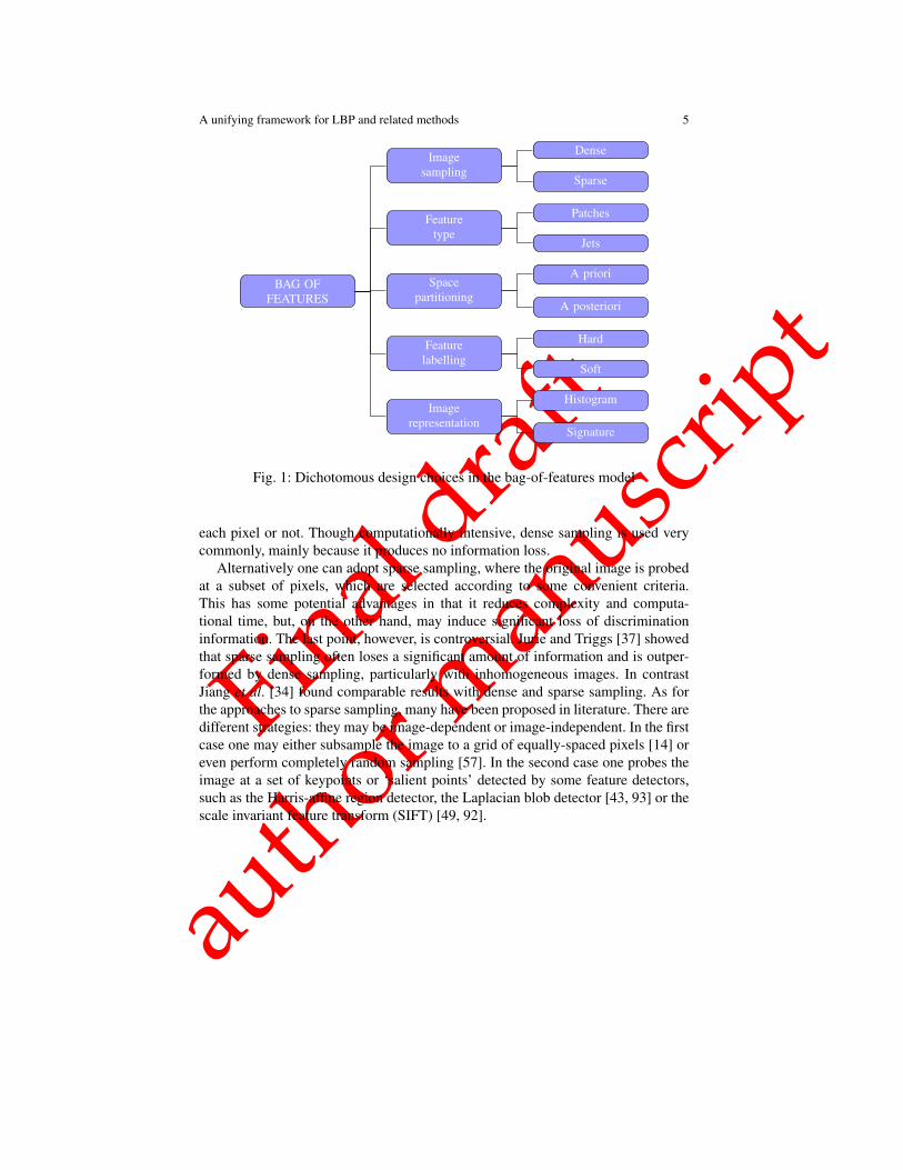
The orderless ‘bag of features’ model (BoF) derives from the ‘bag of words’ model,an approach to natural language processing in which a text is represented throughthe total number of occurrences of each word that appear in it, regardless of theirordering [53]. Thus, in this view, the two texts “Spain plays better soccer than Italy”and “Italy plays better soccer than Spain” are perfectly equivalent. Likewise, theBoF represents images through the probability of occurrence of certain local fea-tures (‘textons’), regardless of their spatial distribution. Such a procedure combinesthe responses of some local feature detectors obtained at different image locationsinto convenient statistical descriptors (e.g.: histograms) that summarize the distribu-tion of the features over the region of interest [9]. Representing images through thefrequency of a discrete vocabulary of local features has proven widely effective forimage classification tasks and object recognition [93, 56]. Fundamental to this ap-proach are the five alternative options that we discuss in the next subsections. Thesecan be viewed as dichotomous design choices and can be conveniently representedthrough a binary tree, as in Fig. 1.
3.1 Image sampling: dense vs. sparse
The first design choice is about the feature sampling mechanism. This can be ei-ther dense or sparse, depending on whether the image is probed exhaustively at
Final draf
t
author m
anuscr
ipt
A unifying framework for LBP and related methods 5
BAG OFFEATURES
Imagerepresentation
Signature
Histogram
Featurelabelling
Soft
Hard
Spacepartitioning
A posteriori
A priori
Featuretype
Jets
Patches
Imagesampling
Sparse
Dense
Fig. 1: Dichotomous design choices in the bag-of-features model
each pixel or not. Though computationally intensive, dense sampling is used verycommonly, mainly because it produces no information loss.
Alternatively one can adopt sparse sampling, where the original image is probedat a subset of pixels, which are selected according to some convenient criteria.This has some potential advantages in that it reduces complexity and computa-tional time, but, on the other hand, may induce significant loss of discriminationinformation. The last point, however, is controversial. Jurie and Triggs [37] showedthat sparse sampling often loses a significant amount of information and is outper-formed by dense sampling, particularly with inhomogeneous images. In contrastJiang et al. [34] found comparable results with dense and sparse sampling. As forthe approaches to sparse sampling, many have been proposed in literature. There aredifferent strategies: they may be image-dependent or image-independent. In the firstcase one may either subsample the image to a grid of equally-spaced pixels [14] oreven perform completely random sampling [57]. In the second case one probes theimage at a set of keypoints or ‘salient points’ detected by some feature detectors,such as the Harris-affine region detector, the Laplacian blob detector [43, 93] or thescale invariant feature transform (SIFT) [49, 92].
Final draf
t
author m
anuscr
ipt
6 F. Bianconi and A. Fernandez
3.2 Feature type: patches vs. jets
The second design choice is related to the type of local data from which features areextracted. These may be either image filter responses – usually referred to as jets –or image patches.
In the first case features are extracted from the output of oriented linear filters[52, 44, 83, 69]. The use of filters has a long history in texture analysis and has beenjustified on the basis of both theoretical and psychophysical considerations. For along time it was believed that any transform of the original image patches satisfyingsome optimality criteria should always improve the efficiency, when compared withthe original representation [79]. The relation between some classes of filters (e.g.:Gabor filters) and the human vision system [12] has also been frequently argued infavour of their use. Theories of sparse representation and compressed sensing haveinspired filtering-based methods too, such as the recently proposed random projec-tions [47]. Yet filtering is not exempt of problems: the design (and implementation)of filter banks is not trivial and is likely to be application-dependent. It is knownthat parameter tuning is critical and may have significant effects on the results [5].Moreover the large support that some filters require may be, in some applications,incompatible with the size of the images.
The supremacy of filter bank-based descriptors for texture analysis has beenquestioned by several authors, most notably Varma and Zissermann [81, 84], whoaffirmed that filter banks are not strictly necessary, and that using directly grey-scaleintensities in local patches with support as small as 3×3 may result in comparableor even superior accuracy. This leads to the second approach, that of image patches.Using image patches is generally faster than using filter responses, and free the userfrom having to design complex filter banks. Conversely, they tend to be more sen-sitive to noise [94], since the change in the value of a single pixel can dramaticallyaffect the response of the feature detector. In a comparison between the two meth-ods, Ghita et al. [22] showed that the performances in texture classification offeredby LBP/C and multi-channel Gabor filtering are comparable.
As for LBP and related methods, these have been traditionally considered asbased on image patches. Recently, Ahonen and Pietikainen, however, correctlynoted that LBP can be viewed as a filter operator based on local derivative filters anda threshold-based vector quantization function [2]. This interpretation in some sensesmooths the traditional distinction between patch-based and jet-based methods – atleast from a theoretical standpoint. From a practical one, however, we believe thatsuch a distinction remains meaningful and useful, especially when we consider thesignificant differences that exist in the design and implementation of the two ap-proaches.
Final draf
t
author m
anuscr
ipt
A unifying framework for LBP and related methods 7
3.3 Partitioning the feature space: a priori vs. a posteriori
The third design choice involves the definition of convenient rules to partition thefeature spaces that arise from either filter responses (jets) or image patches. To thisend there are two alternative strategies, which we refer to as a priori and a posteriori.The difference between the two is that rules are defined independently of data inthe former, whereas they are learnt from data in the latter. This design choice isvery intriguing since it reflects, in our view, the ancient philosophical debate as towhether knowledge is attained apart from experience or arises from it [38].
A priori partitioning has been the basis of many approaches proposed in liter-ature. The simplest of such methods is perhaps regular subdivision of the featurespace into equally-spaced regions (regular binning). The main inconvenience withthis method is that the number of required bins grows exponentially as a functionof space dimensionality and soon far outweighs the number of datapoints avail-able in a single image with which to populate the histogram, with potential over-fitting problems (in an experiment Varma and Zissermann clearly demonstratedthat increasing the number of bins decreases the performance [82]). Hash-codeshave been proposed as a partial workaround to this problem [78]. More commonlya priori partitioning of the feature space is defined through a function that oper-ates on the grey-scale values of the pixels in a neighbourhood. Typically such afunction is based on operators as simple as pairwise comparisons and thresholding[28, 61, 50, 10, 75, 54, 15, 48], though other operators such as ranking [32] havebeen proposed too. This is the idea LBP&V are based upon, as we shall discuss indetail in the forthcoming section. Alternatively one can define partitioning criteriathat operate on filter responses instead of image patches. As for this approach, it isworth mentioning the basic image features (BIF) proposed by Crosier and Griffin[11], which define a mathematical quantisation of a filter response space into seventypes of local image structure. Likewise the approach of Rouco et al. [69] is basedon quantizing the response of some linear filters into three discrete values throughan a priori-defined ternary thresholding function.
In the opposite strategy, a posteriori partitioning, the partitioning scheme is learntfrom training data. The usual procedure involves the definition of sets of represen-tative local image features usually referred to as ‘codebooks’. Typical methods togenerate codebooks are based on clustering, which has been used both with imagepatches [84] and filter responses [81, 47]. Due to its simplicity and good conver-gence properties, the iterative k-means is the most widely used algorithm in thiscontext. Nonetheless, there are some drawbacks with this procedure: it is time con-suming; it requires the number of clusters as input, and it produces non-deterministicresults if random initialization is used (which is often the case). Furthermore, fre-quently appearing patterns are not necessarily the most discriminative [21]: indeedin text analysis, for instance, articles and prepositions are the most frequent words,but they are not particularly discriminative. Alternative approaches to k-means clus-tering include vector quantization through self-organising maps [80, 60], adaptivebinning [45, 39] and sparse coding [19].
Final draf
t
author m
anuscr
ipt
8 F. Bianconi and A. Fernandez
The a priori vs. a posteriori dilemma is a subject where scientific interest is cur-rently high. General considerations suggest that a priori approaches are faster, sincethey do not require codebook generation. They also proved quite accurate in a widerange of practical applications, as demonstrate LBP&V. On the other hand one mayargue that in some specific applications, where features tend to cluster in limited por-tions of the feature space, a priori partitioning schemes may be scarcely efficient,whereas a posteriori schemes may me more convenient, since they can be tuned tothe application. Rouco et al. [69] recently suggested that, in principle, a priori parti-tioning is recommendable for broad-domain applications and large image databases,whereas a posteriori (data-driven) partitioning schemes suit better small databasescontaining few texture classes.
3.4 Feature labelling: hard vs. soft
Once the feature space has been partitioned, one has to label each feature of theimage to process on the basis of the obtained partition. This is the fourth designchoice, which gives rise to two alternative approaches, which we refer to as hardand soft labelling.
The hard approach consist in assigning an image feature to one single partitionof the feature space [28, 52, 61, 81]. When codebooks are used, this is usuallyimplemented through the nearest neighbour rule: a feature is assigned the label ofthe nearest element in the codebook. This results in a Voronoi tessellation of thefeature space. Although computationally simple, hard labelling has some importantdrawbacks, such as sensitivity to noise and limited discriminant power.
The soft approach has emerged as a robust alternative to hard labelling. This isbased on the consideration that, since verbal descriptions of visual characteristicslike colour or a texture are often ambiguous, this ambiguity should be taken intoaccount in the bag-of-features model [21]. The basic idea in soft assignment is thata local feature is assigned to more than one partition, or, equivalently, that parti-tion’s borders are not crisp, but fuzzy. Through convenient membership functions[76, 3, 1, 33] one can in fact consider a local feature as belonging to more than onepartition. Another possible approach is kernel density estimation, the function ofwhich is to smooth the local neighborhood of data samples. In the implementationproposed by Gemert et al. [21] the authors assume that the similarity between animage feature and a codeword is described by a normal function of the distance.Recently, the theory and algorithms of sparse coding and sparse representation havealso been proposed to represent a local feature by a linear combination over a code-book. The ‘weight’ of each element of the codebook on the feature is estimatedthrough suitable minimization procedures [89, 46].
Final draf
t
author m
anuscr
ipt
A unifying framework for LBP and related methods 9
3.5 Image representation: histogram vs. signature
The last design choice is about image representation. This can be based on his-togram or signature. A histogram of a set with respect to a measurement is a fixed-size vector which reports the frequency of quantified values of that measurementamong the samples [73]. The elements of the vector are usually referred to as bins.In the context of this paper histograms report how many times each partition intowhich the feature space is divided is represented in the image to analyse. In con-trast, signatures are variable-size structures which report only the dominant clustersthat are extracted from the original data [70]. Each cluster (or node) is representedby its center and a weight that denotes the size of the cluster. Signatures of differ-ent images may be therefore different in length, and the order in which clusters arelisted does not matter [43]. Consequently, similarity between histograms and sig-natures are measured differently: histogram similarity is usually evaluated throughstandard distance functions such as Manhattan, Euclidean or χ2, whereas signaturesare compared through the earth movers’ distance.
4 Histograms of equivalent patterns
Different combinations of the five design options discussed in the preceding sec-tion have been proposed in literature. We coined the term histograms of equivalentpatterns (HEP) to refer to those BoF descriptors that adopt the following designchoices: a) dense image sampling; b) image patches as input data; c) a priori par-titioning of the features space; d) hard label assignment and e) histogram-basedimage representation. Here below we show that these concepts can be easily ex-pressed in a formal way. The use of a mathematical formalism makes it possible todetermine, unambiguously, whether a texture descriptor belongs to the HEP or not,and therefore removes the inherent uncertainty of semantic taxonomies of whichwe discussed in Sec. 2.2. We also show how LBP and variants can be regarded asinstances of the HEP.
First of all let us introduce the notation to be used henceforth. Let I be an M×Nmatrix representing the raw pixel intensities of an image quantized to G grey levelsranging from 0 to G−1, and Im,n the grey-scale intensity at pixel (m,n).
Definition 1. A texture descriptor is a function F that receives an image I as inputand returns a vector h:
h = F (I) (1)
where h is usually referred to as the feature vector.
Definition 2. Histograms of equivalent patterns (HEP) is a class of texture descrip-tors for which the k-th element of h can be expressed in the following way:
Final draf
t
author m
anuscr
ipt
10 F. Bianconi and A. Fernandez
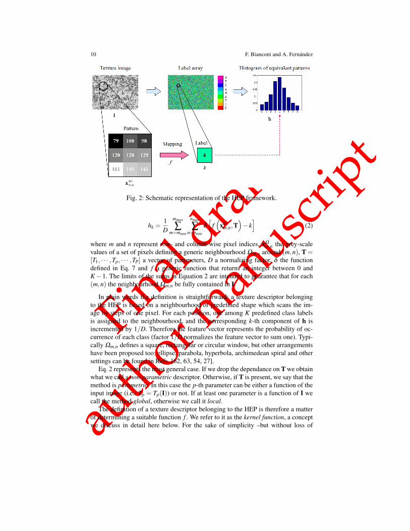
Fig. 2: Schematic representation of the HEP framework.
hk =1D
mmax
∑m=mmin
nmax
∑n=nmin
δ
[f(
xΩm,n,T
)− k]
(2)
where m and n represent row- and column-wise pixel indices, xΩm,n the grey-scale
values of a set of pixels defining a generic neighbourhood Ωm,n around (m,n), T =[T1, · · · ,Tp, · · · ,TP] a vector of parameters, D a normalizing factor, δ the functiondefined in Eq. 7 and f a generic function that returns an integer between 0 andK−1. The limits of the sums in Equation 2 are intended to guarantee that for each(m,n) the neighbourhood Ωm,n be fully contained in I.
In plain words the definition is straightforward: a texture descriptor belongingto the HEP is based on a neighbourhood of predefined shape which scans the im-age by steps of one pixel. For each position, one among K predefined class labelsis assigned to the neighbourhood, and the corresponding k-th component of h isincremented by 1/D. Therefore the feature vector represents the probability of oc-currence of each class (factor 1/D normalizes the feature vector to sum one). Typi-cally Ωm,n defines a square, rectangular or circular window, but other arrangementshave been proposed too: ellipse, parabola, hyperbola, archimedean spiral and othersettings can be found in Refs. [62, 63, 54, 27].
Eq. 2 represents the most general case. If we drop the dependance on T we obtainwhat we call a non-parametric descriptor. Otherwise, if T is present, we say that themethod is parametric. In this case the p-th parameter can be either a function of theinput image (i.e.: Tp = Tp(I)) or not. If at least one parameter is a function of I wecall the method global, otherwise we call it local.
The definition of a texture descriptor belonging to the HEP is therefore a matterof determining a suitable function f . We refer to it as the kernel function, a conceptwe discuss in detail here below. For the sake of simplicity –but without loss of
Final draf
t
author m
anuscr
ipt
A unifying framework for LBP and related methods 11
generality– we restrict the discussion to 3×3 square neighbourhoods. Now considera generic image I and let x3×3
m,n be the set of grey-scale values of a 3× 3 squareneighbourhood centred at (m,n):
x3×3m,n =
Im−1,n−1 Im−1,n Im−1,n+1Im,n−1 Im,n Im,n+1Im+1,n−1 Im+1,n Im+1,n+1
(3)
In this case the parameters in Eq. 2 take the following values: mmin = nmin = 2,mmax = M−1, nmax = N−1 and D = (M−2)(N−2).
Now let M3×3,G be the set of all the possible instances defined by Eq. 3. Thisentity is the feature space we introduced in Sec. 3.2 and represents all the possiblegrey-scale patterns associated to a predefined neighbourhood (3×3 window, in thiscase). In the remainder of this section we use the symbol x to indicate a generic pat-tern of this type. The HEP partitions the feature space through the a priori-definedfunction f , which establishes an equivalence relation ∼ in M3×3,G that acts as fol-lows:
x1 ∼ x2⇔ f (x1) = f (x2) ∀x1,x2 ∈M3×3,G. (4)
This relation induces a partition in M3×3,G that can be expressed in the followingway:
M3×3,G =⋃
0≤k≤K−1
M f ,k (5)
where the family of subsets M f ,k | 0 ≤ k ≤ K− 1 is pairwise disjoint, and eachsubset is defined by:
M f ,k = x ∈M3×3,G | f (x) = k (6)
If we consider a neighbourhood Ω of generic shape and size, the above reasoningequally holds: f still defines a partition of the pattern space MΩ ,G. In this case thenumber of possible patterns is Gω , where ω is the number of pixels in Ω . In princi-ple any function f defines a texture descriptor belonging to the HEP. In practice it isrecommendable that f satisfy some reasonable constraints. A sensible criterion, forinstance, could be that the induced equivalence relation be perceptually meaningful,or, in other words, that similar patterns be mapped into the same equivalence class.For example, in Ref. [20] the authors quantize 3×3 patches according to a modifiedorder statistic, and define equivalence classes based on photometry, complexity andgeometry in image space. Another important condition is that f provide effectivedimensionality reduction, i.e. K G9.
In some cases a texture descriptor can be obtained combining two or more equiv-alence relations. The two combination approaches that we consider here are con-catenation and joint description.
Let f1 and f2 be two mappings, and K1 and K2 the dimensions of the correspond-ing feature vectors. Concatenation generates a new feature vector that contains the

Final draf
t
author m
anuscr
ipt
12 F. Bianconi and A. Fernandez
elements of both f1 and f2, therefore its dimension is K1 +K2. We use the symbol ||to indicate this operation.
Joint description means that each class is uniquely identified by two labels, eachone generated by a different mapping. Conceptually this operation is very similar toa Cartesian product, thus we indicate it with the symbol ×. The number of featuresis K1K2 in this case. In the implementation adopted here, this type of representa-tion is serialized into a one-dimensional feature vector, with the convention that the(k1K2 + k2)-th element corresponds to class labels k1 and k2 of, respectively, f1 andf2.
5 LBP and variants within the HEP
In this section we review a selection of LBP variants and show that these apparentlydivergent texture descriptors are all instances of the HEP. To this end we present a setof LBP&V and provide, for each, the mathematical formulation inside the HEP. Inpresenting the methods we show how this formalization makes it possible to set intoevidence similarities and dissimilarities between the texture descriptors that belongto this family. To keep things simple we limit the review to the M3×3,G patternspace, though the formulations presented henceforth can be effortlessly extended toneighbourhoods of different shape and size.
As a preliminary step we define four functions of the real variable x that areextensively used throughout the paper. These are:
• the δ function
δ (x) =
1, if x = 00, otherwise
(7)
• the binary thresholding function
b(x) =
1, if x≥ 00, if x < 0
(8)
• the ternary thresholding function
t(x,T ) =
0, if x <−T1, if −T ≤ x≤ T2, if x > T
(9)
• the quinary thresholding function
Final draf
t
author m
anuscr
ipt
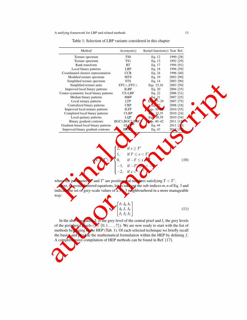
A unifying framework for LBP and related methods 13
Table 1: Selection of LBP variants considered in this chapter
Method Acronym(s) Kernel function(s) Year Ref.
Texture spectrum TS0 Eq. 12 1990 [28]Texture spectrum TS1 Eq. 13 1992 [29]Rank transform RT Eq. 17 1994 [91]
Local binary patterns LBP Eq. 18 1996 [59]Coordinated clusters representation CCR Eq. 24 1996 [40]
Modified texture spectrum MTS Eq. 19 2003 [90]Simplified texture spectrum STS Eq. 14 2003 [90]
Simplified texture units STU+,STU× Eqs. 15,16 2003 [50]Improved local binary patterns ILBP Eq. 20 2004 [35]
Center-symmetric local binary patterns CS-LBP Eq. 22 2006 [31]Median binary patterns MBP Eq. 21 2007 [25]Local ternary patterns LTP Eqs. 27–29 2007 [75]
Centralized binary patterns CBP Eq. 23 2008 [18]Improved local ternary patterns ILTP Eqs. 30–32 2010 [55]Completed local binary patterns CLBP Eqs. 33,35 2010 [24]
Local quinary patterns LQP Eqs. 38,39 2010 [54]Binary gradient contours BGC1,BGC2,BGC3 Eqs. 40–42 2011 [15]
Gradient-based local binary patterns GLBP Eq. 44 2011 [30]Improved binary gradient contours IBGC1 Eq. 43 2012 [17]
q(x,T,T ′) =
2, if x≥ T ′
1, if T ≤ x < T ′
0, if −T ≤ x < T−1, if −T ′ ≤ x <−T−2, if x <−T ′
(10)
where the parameters T and T ′ are positive real numbers satisfying T < T ′.Next, to avoid cluttered equations, let us take out the sub-indices m,n of Eq. 3 and
indicate the set of grey-scale values of a 3×3 neighbourhood in a more manageableway:
x =
I7 I6 I5I0 Ic I4I1 I2 I3
(11)
In the above equation Ic is the grey level of the central pixel and I j the grey levelsof the peripheral pixels ( j ∈ 0,1, . . . ,7). We are now ready to start with the list ofmethods belonging to the HEP (Tab. 1). Of each selected technique we briefly recallthe basics and provide the mathematical formulation within the HEP by defining f .A comprehensive compilation of HEP methods can be found in Ref. [17].
Final draf
t
author m
anuscr
ipt
14 F. Bianconi and A. Fernandez
5.1 Texture spectrum
Texture spectrum, introduced by He and Wang [28], can be considered the precursorof LBP. In its original formulation it is based on the ternary thresholding function(Eq. 9) with T = 0. We refer to this method as TS0. In this model each peripheralpixel of the 3× 3 neighbourhood is assigned a value 0, 1 or 2 when its grey-levelintensity is less, equal or greater than the intensity of the central pixel, respectively.This defines a set of 38 possible ternary patterns. The corresponding kernel functionis:
fTS0(x) =7
∑j=0
t (I j− Ic,0)3 j (12)
Later on the same authors proposed a variation of the method in which T takesa value different than zero [29]. This improvement should be potentially beneficialin presence of noise, since a grey-level variation below T does not change a ternarypattern into another. We indicate this method with the acronym TS1, and the corre-sponding kernel function is formally analogous to Eq. 12:
fTS1(x,T ) =7
∑j=0
t (I j− Ic,T )3 j (13)
5.2 Simplified texture spectrum
Texture spectrum has been the basis of a good number of variations, all with the aimof reducing the rather high dimensionality of the method. Xu et al. [90] proposeda simplified version which we indicate here as simplified texture spectrum (STS).The approach is based on the observation that, as the neighbourhood moves acrossthe image at steps of one pixel, a generic couple of pixels (c, j) switches into thesymmetric ( j,c). Consequently each comparison between the central pixel and eachpixel in the periphery is performed twice. In order to avoid this redundancy andreduce complexity, the authors consider the neighbourhood formed by the centralpixel and the four adjacent peripheral pixels of one quadrant only, specifically thosecorresponding to indices j∈4, · · · ,7 (see Eq. 11). This setting reduces the numberof features from 38 to 34. The kernel function can be expressed as follows:
fSTS(x) =7
∑j=4
t (Ic− I j,0)3 j−4 (14)
Final draf
t
author m
anuscr
ipt
A unifying framework for LBP and related methods 15
5.3 Simplified texture units
Madrid-Cuevas et al. [50] proposed two simplified versions of texture spectrum re-ferred to as simplified texture units. The first one, STU+, considers the neighbour-hood composed of the central pixel and its vertically- and horizontally-connectedperipheral pixels (i.e.: pixels 0, 2, 4 and 6 in Eq. 11). The second one, STU×, oper-ates on the neighbourhood formed by the central pixel and its diagonally-connectedperipheral pixels (i.e.: pixels 1, 3, 5 and 7 in Eq. 11). In both cases dimensionalityis reduced from 38 to 34. The corresponding kernel functions are:
fSTU+(x,T ) =3
∑j=0
t(I2 j− Ic,T
)3 j (15)
fSTU×(x,T ) =3
∑j=0
t(I2 j+1− Ic,T
)3 j (16)
5.4 Rank transform
The rank transform (RT) [91] takes into account the number of pixels in the periph-ery of the 3×3 region the intensity of which is less than the intensity of the centralpixel. Since this number ranges from zero to eight, there are nine possible patterns.The kernel function is:
fRT(x) =7
∑j=0
b(Ic− I j−1) (17)
5.5 Local binary patterns
Local binary patterns (LBP) [59] have received a great deal of attention in the patternrecognition community. In the 3× 3 domain the LBP operator thresholds the eightperipheral pixels of the neighbourhood at the value of the central pixel, thus defininga set of 28 possible binary patterns. The kernel function is:
fLBP(x) =7
∑j=0
b(I j− Ic)2 j (18)
The first appearance of the expression ‘local binary patterns’ dates back to awork published in 1994 [58]. Further studies, however, revealed that an embryonicidea of the method had appeared, under a different name, in earlier works too. The
Final draf
t
author m
anuscr
ipt
16 F. Bianconi and A. Fernandez
interested reader may find further details about the origin of this very influentialmethod in Refs. [66, 17].
5.6 Modified texture spectrum
Modified texture spectrum (MTS) can be considered as a simplified version of LBP,where only a subset of the peripheral pixels (i.e. pixels 4, 5, 6 and 7 in Eq. 11) isconsidered. To be precise the inequality in b is flipped in the original formulation ofMTS [90], but this unimportant difference in no way alters the information that themethod conveys. The kernel function of is:
fMTS(x) =7
∑j=4
b(Ic− I j)2 j−4 (19)
5.7 Improved local binary patterns
Improved local binary patterns (ILBP) are based on an idea similar to LBP, the onlydifference is that the whole 3×3 neighbourhood is thresholded by its average grey-scale value [35]. This gives (29− 1) possible binary patterns (the all 0s pattern isnot possible by definition, hence the subtractive term −1 in the equation below).The kernel function is:
fILBP(x) = b(Ic−Tmean)28 +7
∑j=0
b(I j−Tmean)2 j−1 (20)
where Tmean is the average grey-scale value over the whole neighbourhood.
5.8 Median binary patterns
Median binary patterns (MBP) [25] have much in common with ILBP, the onlydifference is that MBP thresholds the grey-scale values of the 3×3 neighbourhoodat their median value, instead of their average value. The kernel function can beexpressed as follows:
fMBP(x) = b(Ic−Tmedian)28 +7
∑j=0
b(I j−Tmedian)2 j−1 (21)
Final draf
t
author m
anuscr
ipt
A unifying framework for LBP and related methods 17
5.9 Center-symmetric local binary patterns
Center-symmetric local binary patterns (CS-LBP) [31] are similar to LBP, but em-ploy a different scheme to compare the pixel in the neighbourhood. Whereas thecentral pixel plays a pivotal role in LBP, CS-LBP discards it altogether and consid-ers the following centre-symmetric couples of pixel values (Eq. 11): (I0, I4), (I1, I5),(I2, I6) and (I3, I7). Robustness on flat image regions is obtained by thresholdingthe gray level differences with a parameter T . This generates a set of 24 possiblepatterns. The kernel function can be expressed in the following way:
fCS-LBP(x,T ) =3
∑j=0
b(I j− I j+4−T −1
)2 j (22)
5.10 Centralized binary patterns
Centralized binary patterns (CBP) [18] consider the same couples of centre-symmetricpixels used by CS-LBP plus the central pixel. Relative comparison is based on theabsolute difference of grey-scale values, which is thresholded at a predefined smallpositive value T . The kernel function can be formalized as follows:
fCBP(x,T ) = b(|Ic−Tmean|−T )24 +3
∑j=0
b(∣∣I j− I j+4
∣∣−T)
2 j (23)
where Tmean is defined as in Sec. 5.7.
5.11 Coordinated clusters representation
The coordinated clusters representation (CCR) was originally intended as a texturedescriptor for binary images [40]. It was later on extended to grey-scale imagesthrough a preliminary thresholding step [71], and, recently, to colour images too[7]. The method is based on the probability of occurrence of the 29 possible binaryinstances of a 3×3 window. It is similar to LBP and ILBP, though threshold is globalin this case. The global threshold can be computed in various ways. A possibleapproach to estimate it is through isentropic partition [6, 16]. In this case thresholdTisoentr is the value that divides the grey-scale histogram into two parts of equalentropy. The kernel function can be expressed as follows:
fCCR(x,Tisoentr) = b(Ic−Tisoentr)28 +7
∑j=0
b(I j−Tisoentr)2 j (24)
Final draf
t
author m
anuscr
ipt
18 F. Bianconi and A. Fernandez
5.12 Local ternary patterns
Local ternary patterns [75] can be considered a hybrid between texture spectrum andlocal binary patterns. Similarily to texture spectrum, in fact, they make use of theternary thresholding function to obtain ternary binary patterns. Each ternary patternis split in two binary patterns (lower and upper) through the following rules:
b j,LOWER =
1, if t j = 00, otherwise
(25)
b j,UPPER =
1, if t j = 20, otherwise
(26)
where t j and b j represent, respectively, the ternary and binary value correspondingto pixel j. With this convention the kernel functions that define the distributionsof lower (LTPL) and upper (LTPU) local ternary patterns can be expressed in thefollowing way:
fLTPL(x,T ) =7
∑j=0
b(Ic− I j−T )2 j (27)
fLTPU(x,T ) =7
∑j=0
b(I j− Ic−T )2 j (28)
The two descriptors are finally concatenated to form the LTP model:
hLTP = hLTPU||hLTPL (29)
5.13 Improved local ternary patterns
Improved local ternary patterns (ILTP) [55] are an extension of LTP where eachpixel in the neighbourhood is thresholded at the average grey-scale value. Similarlyto LTP the representation is split into a lower and upper part:
fILTPL(x,T ) = b(Tmean− Ic−T )28 +7
∑j=0
b(Tmean− I j−T )2 j (30)
fILTPU(x,T ) = b(Ic−Tmean−T )28 +7
∑j=0
b(I j−Tmean−T )2 j (31)
where Tmean is defined as in Sec. 5.7. The two descriptors are concatenated to givethe ILTP model:
Final draf
t
author m
anuscr
ipt
A unifying framework for LBP and related methods 19
hILTP = hILTPH||hILTPL (32)
5.14 Completed local binary patterns
Completed Local Binary Patterns (CLBP) have been recently introduced by Guo etal. [24] as an extension of local binary patterns. The approach is based on differentcombinations of three basic descriptors: CLBP C, CLBP M and CLBP S. The lastis just an alias for standard LBP, already treated in Sec. 5.5.
CLBP C thresholds the central pixel of the 3× 3 neighbourhood at the averagegrey-scale value of the whole image, and therefore generates only two binary pat-terns. The kernel function is:
fCLBP C(x,TI) = b(Ic−TI) (33)
where
TI =
M
∑m=1
N
∑n=1
Im,n
MN(34)
CLBP M considers the possible binary patterns that are defined by the absolutedifference between the grey-scale value of a pixel in the periphery and that of thecentral pixel when thresholded with a global parameter. In formulas:
fCLBP M(x,T∆ I) =7
∑j=0
b(|I j− Ic|−T∆ I)2 j (35)
where T∆ I is the average value of the difference in grey value between a pixel in theperiphery and the central pixel:
T∆ I =
M−1
∑m=2
N−1
∑n=2
1
∑i=−1
1
∑j=−1|Im−i,n− j− Im,n|
8(M−2)(N−2)(36)
In [24] the authors suggest that the three descriptors can be combined in differentways to give joint and concatenated descriptors, for example: CLBP M× CLBP C,CLBP S × CLBP M, CLBP M × CLBP S × CLBP C and CLBP S || CLBP M ×C.
Final draf
t
author m
anuscr
ipt
20 F. Bianconi and A. Fernandez
5.15 Local quinary patterns
In local quinary patterns (LQP) [54] the grey level difference between the centralpixel and the pixels of the periphery is encoded using five discrete levels (i.e.: −2,−1, 0, 1 and 2) which are computed using two thresholds: T and T ′. LQP is thereforeclosely related to LTP, the only difference being that the number of encoding levelsis five in LQP and three in LTP. The quinary pattern is split into four binary patternsthrough the following rule:
b j,i =
1, if q j = i0, otherwise
(37)
where b j,i and q j are the binary and quinary value corresponding to pixel j and leveli; i ∈ −2,−1,1,2. The kernel function corresponding to each level is:
fLQP,i(x,T,T ′) =7
∑j=0
δ[q(Ic− I j,T,T ′
)− i]
2 j (38)
The feature vector is obtained as follows:
hLQP = hLQP,−2||hLQP,−1||hLQP,1||hLQP,2 (39)
5.16 Binary gradient contours
The recently introduced binary gradient contours (BGC) [15], are a family of de-scriptors based on pairwise comparison of adjacent pixels belonging to one or moreclosed paths traced along the periphery of the 3×3 neighbourhood (hence the namecontours). For each closed path a binary pattern is obtained by assigning each pairof adjacent pixels (i, j) in the path the binary value b(I j− Ii). Since there are severalpaths that one can pick out from the 3×3 neighbourhood, different BGC operatorsexist. In Ref. [15] we proposed three different operators, which are referred to asBGC1, BGC2 and BGC3. Both BCG1 and BCG3 are based on one closed path.In the first case the pixels that define the path are: 0,1,2,3,4,5,6,7,0 (Eq. 11),therefore the corresponding couples from which the binary values are extracted are:(0,1),(1,2), · · · ,(7,0). In the second case the path is defined by the followingsequence of pixels: 0,5,2,7,4,1,6,3,0 (couples are defined in the same way).Both descriptors generate (28− 1) possible different patterns, since, as it happenswith ILBP, the all-0s pattern is, by definition, impossible. In contrast BGC2 em-ploys two closed paths, which are: 1,7,5,3,1 and 0,6,4,2,0. In this case eachpath generates (24−1) possible patterns, therefore the joint combination of the twogives (24− 1)2 = 225 possible patterns. The kernel functions of the three modelsare reported here below:
Final draf
t
author m
anuscr
ipt
A unifying framework for LBP and related methods 21
fBGC1(x) =7
∑j=0
b(I j− I( j+1) mod 8
)2 j−1 (40)
fBGC2(x) = (24−1)3
∑j=0
b(I2 j− I2( j+1) mod 8
)2 j+
3
∑j=0
b(I2 j+1− I(2 j+3) mod 8
)2 j−24
(41)
fBGC3(x) =7
∑j=0
b(I3 j mod 8− I3( j+1) mod 8
)2 j−1 (42)
5.17 Improved binary gradient contours
An extension of BGC1 has been recently proposed [17]. The improved binary gra-dient contour (IBGC1) includes the central pixel and can be easily derived from theoriginal formulation by comparing the central pixel value with the average grey-scale value Tmean over the 3×3 neighbourhood. The kernel function is:
fIBGC1(x) = b(Ic−Tmean)(28−1)+7
∑j=0
b(Ii− I( j+1) mod 8
)2 j−1 (43)
where Tmean is defined as in Sec. 5.7.
5.18 Gradient-based local binary patterns
Another LBP-related method is represented by gradient-based local binary patterns(GLBP) [30]. Here the absolute difference between the central pixel and each pe-ripheral pixel is thresholded at the mean absolute difference between (I0, I4) and(I2, I6). In formulas:
fGLBP(x) =7
∑j=0
b(I+−
∣∣I j− Ic∣∣)2 j (44)
where:
I+ =12(|I0− I4|+ |I2− I6|) (45)
Final draf
t
author m
anuscr
ipt
22 F. Bianconi and A. Fernandez
6 Geometrical interpretation
In the preceding section we have provided an algebraic formulation of LBP andvariants in the framework of the HEP. We show that these methods can be viewedas partitioning operators acting on a high-dimensional space. This is no surprise ifwe consider that, in the end, texture analysis is about modeling and understandingthe distribution of a population in a high-dimensional space. As noted by Pothos etal. [67], many texture descriptors extract different features in number and qualityby providing proper quantization and optimal partitioning of the high-dimensionalspace. So are, for instance, Crosier and Griffin’s basic image features [11], throughwhich the authors establish a direct link between detection of local features andspace partitioning, and the local intensity order pattern (LIOP), recently proposedby Wang et al. [85]. Local binary patterns and variants are clearly based on this ideaas well (as we show here below), though they have been seldom investigated underthis perspective, and rarely studied under a theoretical viewpoint either. Actually,we are only aware of two references on this subject [41, 8]; in both the authorsstudy the probability distribution of local binary patterns and show the high a-prioriprobability of uniform patterns.
Now, we would like to give a geometrical interpretation of LBP&V. If we takea look at the kernel functions of the methods presented in Sec. 5, we soon recog-nise that these define sets of equalities and/or inequalities in the variables Ic andI j, j ∈ 0, · · · ,7 (see Eq. 11). Geometrically they represent polytopes in M3×3,G,i.e.: regions bounded by hyperplanes which are equivalent to polygons in two di-mensions. The good news is that many things about polytopes are known: efficientalgorithms exist to calculate their exact volume [42] and to count how many dis-crete integer points fall inside them [4]. This makes it possible to investigate thetheoretical properties of a texture descriptor through the volume distribution ofits corresponding polytopes. In Ref. [15] we showed how this relates to the theo-retical efficiency of a method: under the assumption of uniformly-distributed andstochastically-independent grey-scale values this is optimal when the feature spaceis partitioned into regions of equal volume.
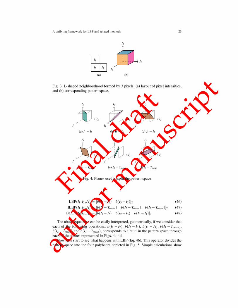
In order to clarify these ideas we present a motivational example in which wereduce the dimensionality of the problem. We consider, to this end, an L-shaped3-pixel neighbourhood like the one depicted in Fig. 3a. Pixel intensities are denotedby I1, I2 and I3. We assume that grey-scale is continuous rather than discrete, and wealso assume the simplifying hypotheses considered in Ref. [8], namely that pixel in-tensities are uniformly distributed in the range [0,1] and stochastically-independent.The feature space is therefore the unitary cube of uniform density represented inFig. 3b.
This 3-dimensional model allows polytopes (polyhedra – in this case) to be easilyvisualized, a thing that would be impossible in a higher-dimensional space. We nowwish to provide a geometrical representation of LBP&V in this model. For the sakeof simplicity we limit the study to three representative examples: LBP, ILBP andBGC. Every part into which each method divides the feature space of Fig. 3b can belabelled through a binary string in the following way:
Final draf
t
author m
anuscr
ipt
A unifying framework for LBP and related methods 23
I1
I2 I3
(a)
I2
I3
I1
(b)
Fig. 3: L-shaped neighbourhood formed by 3 pixels: (a) layout of pixel intensities,and (b) corresponding pattern space.
I2
I3
I1
(a) I1 = I2
I2
I3
I1
(b) I2 = I3
I2
I3
I1
(c) I1 = I3
I2
I3
I1
(d) I1 = Tmean
I2
I3
I1
(e) I2 = Tmean
I2
I3
I1
(f) I3 = Tmean
Fig. 4: Planes used to split the pattern space
LBP(I1, I2, I3) = [b(I1− I2) b(I3− I2)]2 (46)ILBP(I1, I2, I3) = [b(I1−Tmean) b(I2−Tmean) b(I3−Tmean)]2 (47)
BGC1(I1, I2, I3) = [b(I1− I2) b(I2− I3) b(I3− I1)]2 (48)
The above equations can be easily interpreted, geometrically, if we consider thateach of the following operations: b(I1 − I2), b(I2 − I3), b(I1 − I3), b(I1 − Tmean),b(I2−Tmean) and b(I3−Tmean), corresponds to a ‘cut’ in the pattern space througheach of the planes represented in Figs. 4a-4d.
Now let’s start to see what happens with LBP (Eq. 46). This operator divides thepattern space into the four polyhedra depicted in Fig. 5. Simple calculations show
Final draf
t
author m
anuscr
ipt
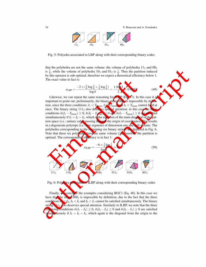
24 F. Bianconi and A. Fernandez
112 102 012 002
Fig. 5: Polyedra associated to LBP along with their corresponding binary codes
that the polyhedra are not the same volume: the volume of polyhedra 112 and 002is 2
6 , while the volume of polyhedra 102 and 012 is 16 . Thus the partition induced
by this operator is sub-optimal, therefore we expect a theoretical efficiency below 1.The exact value in fact is:
eLBP =−2× ( 2
6 log 26 +
16 log 1
6 )
log4=
1.91832
= 0.9591 (49)
Likewise, we can repeat the same reasoning for ILBP (Eq. 47). In this case it isimportant to point out, preliminarily, the binary string 0002 is impossible by defini-tion, since the three conditions: I1 < Tmean, I2 < Tmean and I3 < Tmean cannot hold atonce. The binary string 1112 also deserves special attention: in this case the threeconditions b(I1−Tmean) ≥ 0, b(I2−Tmean) ≥ 0 and b(I3−Tmean) ≥ 0 are satisfiedsimultaneously if I1 = I2 = I3, which is the equation of the main diagonal of the pat-tern space (i.e.: unitary cube) passing through the origin of coordinates. This resultsin a degenerate polytope (i.e.: line segment) of dimension one and null volume. Thepolyhedra corresponding to the remaining six binary strings are depicted in Fig. 6.Note that these six polyhedra have the same volume ( 1
6 ), therefore the partition isoptimal. The corresponding efficiency is in fact 1:
eILBP =−6× 1
6 log 16
log6= 1 (50)
1112 1102 1012 1002 0112 0102 0012
Fig. 6: Polyedra associated to ILBP along with their corresponding binary codes
Finally, we conclude the examples considering BGC1 (Eq. 48). In this case wehave that the string 0002 is impossible by definition, due to the fact that the threeconditions I1 < I2, I2 < I3 and I3 < I1 cannot be satisfied simultaneously. The binarystring 1112 also deserves special attention. Similarly to ILBP, we note that the threefollowing conditions b(I1− I2) ≥ 0, b(I2− I3) ≥ 0 and b(I3− I1) ≥ 0 are satisfiedsimultaneously if I1 = I2 = I3, which again is the diagonal from the origin to the
Final draf
t
author m
anuscr
ipt
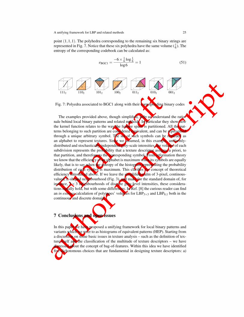
A unifying framework for LBP and related methods 25
point (1,1,1). The polyhedra corresponding to the remaining six binary strings arerepresented in Fig. 7. Notice that these six polyhedra have the same volume ( 1
6 ). Theentropy of the corresponding codebook can be calculated as:
eBGC1 =−6× 1
6 log 16
log6= 1 (51)
1112 1102 1012 1002 0112 0102 0012
Fig. 7: Polyedra associated to BGC1 along with their corresponding binary codes
The examples provided above, though simplified, help us understand the ratio-nale behind local binary patterns and related methods. In particular they show howthe kernel function relates to the way the feature space is partitioned. All the pat-terns belonging to such partition are considered equivalent, and can be representedthrough a unique arbitrary symbol. The set of such symbols can be regarded asan alphabet to represent textures. Since we assumed, in this example, uniformly-distributed and stochastically independent grey-scale intensities, the volume of eachsubdivision represents the probability that a texture descriptor assigns, a priori, tothat partition, and therefore to the corresponding symbol. From information theorywe know that the efficiency of an alphabet is maximum when its symbols are equallylikely, that is to say when the entropy of the histogram representing the probabilitydistribution of each symbol is maximum. This clarifies the concept of theoreticalefficiency introduced above. If we leave the simplified realm of 3-pixel, continous-valued, L-shaped neighbourhood (Fig. 3), and make for the standard domain of, forinstance, 3× 3 neighbourhoods of discrete grey-level intensities, these considera-tions equally hold, but with some differences. In Ref. [8] the curious reader can findan in extenso calculation of polytopes’ volumes for LBP3×3 and LBP8,1 both in thecontinuous and discrete domain.
7 Conclusions and open issues
In this paper we have proposed a unifying framework for local binary patterns andvariants which we refer to as histograms of equivalent patterns (HEP). Starting froma discussion on some basic issues in texture analysis – such as the definition of tex-ture itself and the classification of the multitude of texture descriptors – we havedigressed about the concept of bag-of-features. Within this idea we have identifiedfive dichotomous choices that are fundamental in designing texture descriptors: a)
Final draf
t
author m
anuscr
ipt
26 F. Bianconi and A. Fernandez
image sampling (dense or sparse?); b) type of features (patches or jets?); c) spacepartitioning (a priori or a posteriori?); d) label assignment (hard or soft?) and e)image representation (histogram or signature?). We have shown which choices areadopted by the HEP and how these can be formalized mathematically. This enableslocal binary patterns and variants to be expressed through a common formalism andsets into evidence that they can all be viewed as instances of the HEP. In the last partof the chapter we have given a geometrical reading of these methods showing howthey partition the feature space into polytopes. This interpretation makes it possi-ble to study some intrinsic theoretical properties of the methods, and suggests pos-sible directions for future research: this could be focused on studying partitioningschemes (i.e.: kernel functions) that maximize the theoretical amount of informationconveyed by the descriptor, and, possess, at the same time, some type of invariance,such as robustness against against rotation, grey-scale transformations or viewpointchanges.
Acknowledgements
This work was supported by the Spanish Government under projects no. TRA2011-29454-C03-01 and CTM2010-16573.
References
1. T. Ahonen and M. Pietikainen. Soft histograms for local binary patterns. In Proceedings ofthe Finnish Signal Processing Symposium (FINSIG 2007), Oulu, Finland, 2007.
2. T. Ahonen, J. Matas, C. He, and M. Pietikainen. Rotation invariant image description withlocal binary pattern histogram Fourier features. In Proceedings of the 16th ScandinavianConference (SCIA 2009), volume 5575 of Lecture Notes in Computer Science, pages 61–70.Springer, 2009.
3. A. Barcelo, E. Montseny, and P. Sobrevilla. On fuzzy texture spectrum for natural microtex-tures characterization. In Proceedings EUSFLAT-LFA 2005, pages 685–690, 2005.
4. M. Beck and S. Robins. Computing the Continuous Discretely. Integer-point Enumeration inPolyhedra. Springer, New York, 2007.
5. F. Bianconi and A. Fernandez. Evaluation of the effects of Gabor filter parameters on textureclassification. Pattern Recognition, 40(12):3325–3335, 2007.
6. F. Bianconi, A. Fernandez, E. Gonzalez, and F. Ribas. Texture classification through combina-tion of sequential colour texture classifiers. In Luis Rueda, Domingo Mery, and Josef Kittler,editors, Progress in Pattern Recognition, Image Analysis and Applications. Proceedings of the12th Iberoamerican Congress on Pattern Recognition (CIARP 2007), volume 4756 of LectureNotes in Computer Science, pages 231–240. Springer, 2008.
7. F. Bianconi, A. Fernandez, E. Gonzalez, D. Caride, and A. Calvino. Rotation-invariant colourtexture classification through multilayer CCR. Pattern Recognition Letters, 30(8):765–773,2009.
8. F. Bianconi and A. Fernandez. On the occurrence probability of local binary patterns: a theo-retical study. Journal of Mathematical Imaging and Vision, 40(3):259–268, 2011.
Final draf
t
author m
anuscr
ipt
A unifying framework for LBP and related methods 27
9. Y.-L. Boureau, J. Ponce, and Y. LeCun. A theoretical analysis of feature pooling in vi-sual recognition. In Proceedings of the 27th International Conference on Machine Learning(ICML-10), pages 111–118, Haifa, Israel, June 2010.
10. C.-I. Chang and Y. Chen. Gradient texture unit coding for texture analysis. Optical Engineer-ing, 43(8):1891–1902, 2004.
11. M. Crosier and L. D. Griffin. Using basic image features for texture classification. Interna-tional Journal of Computer Vision, 88:447–460, 2010.
12. J.G. Daugman. Uncertainty relation for resolution in space, spatial frequency, and orientationoptimized by two-dimensional visual cortical filters. Journal of the Optical Society of AmericaA, 2:1160–1169, 1985.
13. E. R. Davies. Introduction to texture analysis. In M. Mirmehdi, X. Xie, and J. Suri, editors,Handbook of texture analysis, pages 1–31. Imperial College Press, 2008.
14. L. Fei-Fei and P. Perona. A bayesian hierarchical model for learning natural scene categories.In Proceedings of the 2005 IEEE Computer Society Conference on Computer Vision and Pat-tern Recognition (CVPR 2005), volume 2, pages 524–531, June 2005.
15. A. Fernandez, M. X. Alvarez, and F. Bianconi. Image classification with binary gradientcontours. Optics and Lasers in Engineering, 49(9-10):1177–1184, 2011.
16. A. Fernandez, O. Ghita, E. Gonzalez, F. Bianconi, and P. F. Whelan. Evaluation of robustnessagainst rotation of LBP, CCR and ILBP features in granite texture classification. MachineVision and Applications, 22(6):913–926, 2011.
17. A. Fernandez, M. X. Alvarez, and F. Bianconi. Texture description through histograms ofequivalent patterns. Journal of Mathematical Imaging and Vision, 2012. to appear.
18. X. Fu and W. Wei. Centralized binary patterns embedded with image euclidean distancefor facial expression recognition. In Proceedings of the Fourth International Conference onNatural Computation (ICNC’08), volume 4, pages 115–119, 2008.
19. M. J. Gangeh, A. Ghodsi, and M. Kamel. Dictionary learning in texture classification. InM. Kamel and A. Campilho, editors, Proceedings of the 8th International Conference on Im-age Analysis and Recognition (ICIAR 2011), volume 6753 of Lecture Notes in Computer Sci-ence, pages 335–343, Burnaby, BC, Canada, June 2011. Springer.
20. D. Geman and A. Koloydenko. Invariant statistics and coding of natural microimages. InProceedings of the First International Workshop on Statistical and Computational Theories ofVision, Fort Collins, CO, USA, June 1999. published on the web.
21. J. C. van Gemert, C. J. Veenman, A. W. M. Smeulders, and J.-M. Geusebroek. Visual wordambiguity. IEEE Transactions on Patterns Analysis and Machine Intelligence, 32(7):1271–1283, 2010.
22. O. Ghita, D. E. Ilea, A. Fernandez, and P. F. Whelan. Local binary patterns versus signal pro-cessing texture analysis. A study from a performance evaluation perspective. Sensor Review,32:149–162, 2012.
23. L. van Gool, P. Dewaele, and A. Oosterlinck. Texture analysis anno 1983. Computer Vision,Graphics, and Image Processing, 29(3):336–357, 1985.
24. Z. Guo, L. Zhang, and D. Zhang. A completed modeling of local binary pattern operator fortexture classification. IEEE Transactions on Image Processing, 19(6):1657–1663, 2010.
25. A. Hafiane, G. Seetharaman, and B. Zavidovique. Median binary pattern for textures classifi-cation. In Proceedings of the 4th International Conference on Image Analysis and Recognition(ICIAR 2007), volume 4633 of Lecture Notes in Computer Science, pages 387–398, Montreal,Canada, August 2007.
26. R. M. Haralick. Statistical and structural approaches to texture. Proceedings of the IEEE,67(5):786–804, 1979.
27. Y. He, N. Sang, and C. Gao. Multi-structure local binary patterns for texture classification.Pattern Analysis and Applications, pages 1–13, 2012. Article in Press.
28. D.-C. He and L. Wang. Texture unit, texture spectrum, and texture analysis. IEEE Transactionson Geoscience and Remote Sensing, 28(4):509–512, 1990.
29. D.-C. He and L. Wang. Unsupervised textural classification of images using the texture spec-trum. Pattern Recognition, 25(3):247–255, 1992.
Final draf
t
author m
anuscr
ipt
28 F. Bianconi and A. Fernandez
30. Y. He and N. Sang. Robust illumination invariant texture classification using gradient localbinary patterns. In Proceedings of 2011 International Workshop on Multi-Platform/Multi-Sensor Remote Sensing and Mapping, pages 1–6, Xiamen, China, January 2011.
31. M. Heikkila, M. Pietikainen, and C. Schmid. Description of interest regions with Local BinaryPatterns. Pattern Recognition, 42:425–436, 2009.
32. L. Hepplewhite and T. J. Stonhamm. Texture classification using N-tuple pattern recogni-tion. In Proceedings of the 13th International Conference on Pattern Recognition (ICPR’96),volume 4, pages 159–163, August 1996.
33. D. K. Iakovidis, E. G. Keramidas, and D. Maroulis. Fuzzy local binary patterns for ultrasoundtexture characterization. In Aurelio Campilho and Mohamed Kamel, editors, Proceedings ofthe 5th International Conference on Image Analysis and Recognition (ICIAR 2008), volume5112 of Lecture Notes in Computer Science, pages 750–759, Povoa de Varzim, Portugal, June2008.
34. Y.-G. Jiang, C.-W. Ngo, and Jun Yang. Towards optimal bag-of-features for object categoriza-tion and semantic video retrieval. In Proceedings of the 6th ACM international conference onImage and Video Retrieval (CIVR’07), pages 494–501, 2007.
35. H. Jin, Q. Liu, H. Lu, and X. Tong. Face detection using improved LBP under bayesianframework. In Proceedings of the 3rd International Conference on Image and Graphics,pages 306–309, 2004.
36. B. Julesz. Experiments in the visual perception of texture. Scientific American, 232(4):34–43,1975.
37. F. Jurie and B. Triggs. Creating efficient codebooks for visual recognition. In Proceedingsof the Tenth IEEE International Conference on Computer Vision (ICCV’05), volume 1, pages604–610, 2005.
38. I. Kant. The Critique of Pure Reason. Pennsylvania State Electronic Classics Series, 2010.Translated by J. M. D. Meiklejoh.
39. S. Konishi and A. L. Yuille. Statistical cues for domain specific image segmentation withperformance analysis. In Proceedings of the 2000 IEEE Computer Society Conference onComputer Vision and Pattern Recognition (CVPR’00), volume 1, pages 125–132, 2000.
40. E. V. Kurmyshev and M. Cervantes. A quasi-statistical approach to digital binary image rep-resentation. Revista Mexicana de Fısica, 42(1):104–116, 1996.
41. O. Lahdenoja. A statistical approach for characterising local binary patterns. Technical Report795, Turku Centre for Computer Science, Finland, 2006.
42. J. Lawrence. Polytope volume computation. Mathematics of Computation, 57(195):259–271,1991.
43. S. Lazebnik, C. Schmid, and J. Ponce. A sparse texture representation using local affineregions. IEEE Transactions on Pattern Analysis and Machine Intelligence, 27(8):1265–1278,2005.
44. T. Leung and J. Malik. Representing and recognizing the visual appearance of materials usingthree-dimensional textons. International Journal of Computer Vision, 43(1):29–44, 2001.
45. X. Liu and D. Wang. Texture classification using spectral histograms. IEEE Transactions onImage Processing, 12(6):661–670, 2003.
46. L. Liu, L. Wang, and X. Liu. In defense of soft-assignment coding. In Proceedings of the 13thIEEE International Conference on Computer Vision (ICCV 2011), pages 2486–2493, 2011.
47. L. Liu and P. W. Fieguth. Texture classification from random features. IEEE Transactions onPattern Analysis and Machine Intelligence, 34(3):574–586, 2012.
48. L. Liu, L. Zhao, Y. Long, G. Kuang, and P. W. Fieguth. Extended local binary patterns fortexture classification. Image and Vision Computing, 30(2):86–99, 2012.
49. D. G. Lowe. Distinctive image features from scale-invariant keypoints. International Journalof Computer Vision, 60(2):91–110, 2004.
50. F. J. Madrid-Cuevas, R. Medina, M. Prieto, N. L. Fernandez, and A. Carmona. Simplifiedtexture unit: A new descriptor of the local texture in gray-level images. In Francisco J. PeralesLopez, Aurelio C. Campilho, Nicolas Perez de la Blanca, and Alberto Sanfeliu, editors, Pat-tern Recognition and Image Analysis, Proceedings of the First Iberian Conference (IbPRIA2003), volume 2652 of Lecture Notes in Computer Science, pages 470–477. Springer, 2003.
Final draf
t
author m
anuscr
ipt
A unifying framework for LBP and related methods 29
51. T. Maenpaa and M. Pietikainen. Texture analysis with local binary patterns. In C. H. Chen andP. S. P. Wang, editors, Handbook of Pattern Recognition and Computer Vision (3rd Edition),pages 197–216. World Scientific Publishing, 2005.
52. J. Malik, S. Belongie, J. Shi, and T. Leung. Textons, contours and regions: cue integration inimage segmentation. In The Proceedings of the Seventh IEEE International Conference onComputer Vision (ICCV’99), volume 2, pages 918–925, 1999.
53. C.D. Manning, P. Raghavan, and H. Schutze. An introduction to information retrieval. Cam-bridge University Press, Cambridge (UK), 2009.
54. L. Nanni, A. Lumini, and S. Brahnam. Local binary patterns variants as texture descriptorsfor medical image analysis. Artificial Intelligence in Medicine, 49(2):117–125, 2010.
55. L. Nanni, S. Brahnam, and A. Lumini. A local approach based on a Local Binary Pat-terns variant texture descriptor for classifying pain states. Expert Systems with Applications,37(12):7888–7894, 2010.
56. L. Nanni, S. Brahnam, and A. Lumini. Random interest regions for object recognition basedon texture descriptors and bag of features. Expert Systems with Applications, 39(1):973–977,2012.
57. E. Nowak, F. Jurie, and B. Triggs. Sampling strategies for bag-of-features image classifica-tion. In Proceedings of European Conference on Computer Vision 2006 (ECCV’06), Part IV,volume 3954 of Lecture Notes in Computer Science, pages 490–503. Springer-Verlag, 2006.
58. T. Ojala, M. Pietikainen, and D. Harwood. Performance evaluation of texture measures withclassification based on Kullback discrimination of distributions. In Proceedings of the 12thIAPR International Conference on Pattern Recognition, volume 1, pages 582–585, 1994.
59. T. Ojala, M. Pietikainen, and D. Harwood. A comparative study of texture measures withclassification based on feature distributions. Pattern Recognition, 29(1):51–59, 1996.
60. T. Ojala, M. Pietikainen, and J. Kyllonen. Gray level cooccurrence histograms via learningvector quantization. In Proceedings of the 11th Scandinavian Conference on Image Analysis(SCIA 1999), pages 103–108, Kangerlussuaq, Greenland, 1999.
61. T. Ojala, M. Pietikainen, and T. Maenpaa. Multiresolution gray-scale and rotation invarianttexture classification with local binary patterns. IEEE Transactions on Pattern Analysis andMachine Intelligence, 24(7):971–987, 2002.
62. D. Patel and T. J. Stonham. A single layer neural network for texture discrimination. In IEEEInternational Symposium on Circuits and Systems, 1991, volume 5, pages 2656–2660, June1991.
63. D. Patel and T. J. Stonham. Texture image classification and segmentation using rank-orderclustering. In Proceedings of the 11th International Conference on Pattern Recognition(ICPR’92), volume 3, pages 92–95. IEEE Computer Society, 1992.
64. O. A. B. Penatti, E. Valle, and R. da Silva Torres. Comparative study of global color andtexture descriptors for web image retrieval. Journal of Visual Communication andImage Rep-resentation, 23:359–380, 2012.
65. M. Petrou and P. Garcıa Sevilla. Image Processing. Dealing with Texture. Wiley Interscience,2006.
66. M. Pietikainen, A. Hadid, G. Zhao, and T. Ahonen. Computer Vision Using Local BinaryPatterns, volume 40 of Computational Imaging and Vision. Springer, London, 2011.
67. V. K. Pothos, C. Theoharatos, E. Zygouris, and G. Economu. Distributional-based textureclassification using non-parametric statistics. Pattern Analysis and Applications, 11:117–129,2008.
68. F. Tajeri pour, M. Rezaei, M. Saberi, and S. F. Ershad. Texture classification approach based oncombination of random threshold vector technique and co-occurrence matrixes. In Proceed-ings of the International Conference on Computer Science and Network Technology, 2011(ICCSNT), volume 4, pages 2303–2306, Harbin, China, December 2011.
69. J. Rouco, A. Mosquera, M. G. Penedo, M. Ortega, and M. Penas. Texture description in localscale using texton histograms with quadrature filter universal dictionaries. IET ComputerVision, 5(4):211–221, 2011.
Final draf
t
author m
anuscr
ipt
30 F. Bianconi and A. Fernandez
70. Y. Rubner, C. Tomasi, and L. J. Guibas. A metric for distributions with applications to im-age databases. In Proceedings of the Sixth International Conference on Computer Vision(ICCV’98), pages 59–66, 1998.
71. R. E. Sanchez-Yanez, E. V. Kurmyshev, and A. Fernandez. One-class texture classifier in theCCR feature space. Pattern Recognition Letters, 24(9-10):1503–1511, 2003.
72. N. Sebe and M. S. Lew. Texture features for content-based retrieval. In M. S. Lew, editor,Principles of visual information retrieval, pages 51–85. Springer-Verlag, London, UK, 2001.
73. F. Serratosa and A. Sanfeliu. Signatures versus histograms: Definitions,distances and algo-rithms. Pattern Recognition, 39(5):921–934, 2006.
74. G. P. Stachowiak, P. Podsiadlo, and G. W. Stachowiak. A comparison of texture feature ex-traction methods for machine condition monitoring and failure analysis. Tribology Letters,20(2):133–147, 2005.
75. X. Tan and B. Triggs. Enhanced local texture feature sets for face recognition under difficultlighting conditions. In Analysis and Modelling of Faces and Gestures, volume 4778 of LectureNotes in Computer Science, pages 168–182. Springer, 2007.
76. J. S. Taur and C.-W. Tao. Texture classification using a fuzzy texture spectrum and neuralnetworks. Journal of Electronic Imaging, 7(1):29–35, 1998.
77. M. Tuceryan and A. K. Jain. Texture analysis. In C. H. Chen, L. F. Pau, and P. S. P. Wang,editors, Handbook of Pattern Recognition and Computer Vision (2nd Edition), pages 207–248.World Scientific Publishing, 1998.
78. T. Tuytelaars and C. Schmid. Vector quantizing feature space with a regular lattice. In Pro-ceedings of the IEEE 11th International Conference on Computer Vision (ICCV’07), pages1–8, Rio de Janeiro, Brazil, October 2007. IEEE.
79. M. Unser. Local linear transforms for texture measurements. Signal Processing, 11(1):61–79,July 1986.
80. K. Valkealahti and E. Oja. Reduced multidimensional co-occurrence histograms in textureclassification. IEEE Transactions on Pattern Analysis and Machine Intelligence, 20(1):90–94,1998.
81. M. Varma and A. Zisserman. Texture classification: Are filter banks necessary? In Proceedingsof the 2003 IEEE Computer Society Conference on Computer Vision and Pattern Recognition(CVPR’03), volume 2, pages 691–698, June 2003.
82. M. Varma and A. Zisserman. Unifying statistical texture classification frameworks. Imageand Vision Computing, 22(14):1175–1183, 2004.
83. M. Varma and A. Zisserman. A statistical approach to texture classification from single im-ages. International Journal of Computer Vision, 62(1-2):61–81, 2005.
84. M. Varma and A. Zisserman. A statistical approach to material classification using image patchexemplars. IEEE Transactions on Pattern Analysis and Machine Intelligence, 31(11):2032–2047, 2009.
85. Z. Wang, B. Fan, and F. Wu. Local intensity order pattern for feature description. In Pro-ceedings of the 13th International Conference on Computer Vision (ICCVı¿ 1
2 2011), pages603–610, Barcelona, Spain, November 2011.
86. H. Wechsler. Texture analysis – A survey. Signal Processing, 2(3):271–282, 1980.87. C.-M. Wu and Y.-C. Chen. Statistical feature matrix for texture analysis. CVGIP: Graphical
Models and Image Processing, 54(5):407–419, 1992.88. X. Xie and M. Mirmehdi. A galaxy of texture features. In M. Mirmehdi, X. Xie, and J. Suri,
editors, Handbook of texture analysis, pages 375–406. Imperial College Press, 2008.89. J. Xie, L. Zhang, J. You, and D. Zhang. Texture classification via patch-based sparse texton
learning. In Proceedings of the International Conference on Image Processing, pages 2737–2740, 2010.
90. B. Xu, P. Gong, E. Seto, and R. Spear. Comparison of gray-level reduction and differenttexture spectrum encoding methods for land-use classification using a panchromatic Ikonosimage. Photogrammetric Engineering and Remote Sensing, 69(5):529–536, 2003.
91. R. Zabih and J. Woodfill. Non-parametric local transforms for computing visual correspon-dence. In Proceedings of the 3rd European Conference on Computer Vision (ECCV 1994),pages 151–158, Stockholm, Sweden, May 1994. Springer-Verlag.

Final draf
t
author m
anuscr
ipt
A unifying framework for LBP and related methods 31
92. H. Zhang, R. Rahmani, S. R. Cholleti, and S. A. Goldman. Local image representationsusing pruned salient points with applications to CBIR. In Proc. of the 14th Annual ACMInternational Conference on Multimedia, Santa Barbara (USA), October 2006.
93. J. Zhang, M. Marszałek, S. Lazebnik, and C. Schmid. Local features and kernels for clas-sification of texture and object categories: A comprehensive study. International Journal ofComputer Vision, 73(2):213–238, 2007.
94. H. Zhou, R. Wang, and C. Wang. A novel extended local-binary-pattern operator for textureanalysis. Information Sciences, 178(22):4314–4325, 2008.