Unifying practical uncertainty representations. II: Clouds
28
arXiv:0808.2747v1 [math.PR] 20 Aug 2008
-
Upload
independent -
Category
Documents
-
view
0 -
download
0
Transcript of Unifying practical uncertainty representations. II: Clouds

arX
iv:0
808.
2747
v1 [
mat
h.PR
] 2
0 A
ug 2
008
UNIFYING PRACTICAL UNCERTAINTY
REPRESENTATIONS: I. GENERALIZED P-BOXES
SÉBASTIEN DESTERCKE, DIDIER DUBOIS, AND ERIC CHOJNACKI
Abstra t. There exist several simple representations of un er-
tainty that are easier to handle than more general ones. Among
them are random sets, possibility distributions, probability inter-
vals, and more re ently Ferson's p-boxes and Neumaier's louds.
Both for theoreti al and pra ti al onsiderations, it is very useful
to know whether one representation is equivalent to or an be ap-
proximated by other ones. In this paper, we dene a generalized
form of usual p-boxes. These generalized p-boxes have interest-
ing onne tions with other previously known representations. In
parti ular, we show that they are equivalent to pairs of possibil-
ity distributions, and that they are spe ial kinds of random sets.
They are also the missing link between p-boxes and louds, whi h
are the topi of the se ond part of this study.
1. Introdu tion
Dierent formal frameworks have been proposed to reason under
un ertainty. The best known and oldest one is the probabilisti frame-
work, where un ertainty is modeled by lassi al probability distribu-
tions. Although this framework is of major importan e in the treat-
ment of un ertainty due to variability, many arguments onverge to
the fa t that a single probability distribution annot adequately a -
ount for in omplete or impre ise information. Alternative theories
and frameworks have been proposed to this end. The three main su h
frameworks, are, in de reasing order of generality, Impre ise probabil-
ity theory[43, Random disjun tive sets [12, 40, 32 and Possibility the-
ory [46, 16. Within ea h of these frameworks, dierent representations
and methods have been proposed to make inferen es and de isions.
This study fo uses on un ertainty representations, regarding the re-
lations existing between them, their respe tive expressiveness and pra -
ti ality. In the past years, several representation tools have been pro-
posed: apa ities [5, redal sets [29, random sets [32, possibility dis-
tributions [46, probability intervals [9, p-boxes [21 and, more re ently,
louds [34, 35. Su h a diversity of representations motivates the study
of their respe tive expressive power.
1
2 S. DESTERCKE, D. DUBOIS, AND E. CHOJNACKI
The more general representations, su h as redal sets and apa ities,
are expressive enough to embed other ones as parti ular instan es, fa-
ilitating their omparison. However, they are generally di ult to
handle, omputationally demanding and not tted to all un ertainty
theories. As for simpler representations, they are useful in pra ti al
un ertainty analysis problems [45, 38, 22. They ome in handy when
trading expressiveness (possibly losing some information) against om-
putational e ien y; they are instrumental in eli itation tasks, sin e
requesting less information[1; they are also instrumental in summariz-
ing omplex results of some un ertainty propagation methods [20, 2.
The obje t of this study is twofold: rst, it provides a short review of
existing un ertainty representations and of their relationships; se ond,
it studies the ill-explored relationships between more re ent simple rep-
resentations and older ones, introdu ing a generalized form of p-box.
Credal sets and random sets are used as the ommon umbrella lar-
ifying the relations between simplied models. Finding su h formal
links fa ilitates a unied handling and treatment of un ertainty, and
suggests how tools used for one theory an eventually be useful in the
setting of other theories. We thus regard su h a study as an important
and ne essary preamble to other studies devoted to omputational and
interpretability issues. Su h issues, whi h still remain a matter of lively
debate, are not the main topi of the present work, but we nevertheless
provide some omments regarding them. In parti ular, we feel that is
important to re all that a given representation an be interpreted and
pro essed dierently a ording to dierent theories, whi h were often
independently motivated by spe i problems.
This work is made of two ompanion papers, one devoted to p-boxes,
introdu ing a generalization thereof that subsumes possibility distribu-
tions. The se ond part onsiders Neumaier's louds, an even more
general representation tool.
This paper rst reviews older representation tools, already onsid-
ered by many authors. A good omplement to this rst part, although
adopting a subje tivist point of view, is provided by Walley [44. Then,
in Se tion 3, we propose and study a generalized form of p-box extend-
ing, among other things, some results by Baudrit and Dubois [1. As
we shall see, this new representation, whi h onsists of two omono-
toni distributions, is the missing link between usual p-boxes, louds
and possibility distributions, allowing to relate these three represen-
tations. Moreover, generalized p-boxes have interesting properties and
are promising un ertainty representations by themselves. In parti ular,

UNIFYING UNCERTAINTY REPRESENTATIONS: GENERALIZED P-BOXES 3
Se tion 3.3 shows that generalized p-boxes an be interpreted as a spe-
ial ase of random sets; Se tion 3.4 studies the relation between prob-
ability intervals and generalized p-boxes and dis usses transformation
methods to extra t probability intervals from p-boxes, and vi e-versa.
In the present paper, we restri t ourselves to un ertainty represen-
tations dened on nite spa es (en ompassing the dis retized real line)
unless stated otherwise. Representations dened on the ontinuous real
line are onsidered in the se ond part of this paper. To make the paper
easier to read, longer proofs have been moved to an appendix.
2. Non-additive un ertainty theories and some
representation tools
To represent un ertainty, Bayesian subje tivists advo ate the use of
single probability distributions in all ir umstan es. However, when the
available information la ks pre ision or is in omplete, laiming that a
unique probability distribution an faithfully represent un ertainty is
debatable
1
. It generally for es to engage in too strong a ommitment,
onsidering what is a tually known.
Roughly speaking, alternative theories re alled here (impre ise prob-
abilities, random sets, and possibility theory) have the potential to
lay bare the existing impre ision or in ompleteness in the information.
They evaluate un ertainty on a parti ular event by means of a pair of
( onjugate) lower and upper measures rather than by a single one. The
dieren e between upper and lower measures then ree ts the la k of
pre ision in our knowledge.
In this se tion, we rst re all basi mathemati al notions used in the
sequel, on erning apa ities and the Möbius transform. Ea h theory
mentioned above is then briey introdu ed, with fo us on pra ti al rep-
resentation tools available as of to-date, like possibility distributions,
p-boxes and probability intervals, their expressive power and omplex-
ity.
2.1. Basi mathemati al notions. Consider a nite spa e X on-
taining n elements. Measures of un ertainty are often represented by
set-fun tions alled apa ities, that were rst introdu ed in Choquet's
work [5.
Denition 1. A apa ity on X is a fun tion µ, dened on the set of
subsets of X, su h that:
1
For instan e, the following statement about a oin: "We are not sure that this
oin is fair, so the probability for this oin to land on Heads (or Tails) lies between
1/4 and 3/4" annot be faithfully modeled by a single probability.

4 S. DESTERCKE, D. DUBOIS, AND E. CHOJNACKI
• µ(∅) = 0, µ(X) = 1,• A ⊆ B ⇒ µ(A) ≤ µ(B).
A apa ity su h that
∀A, B ⊆ X, A ∩ B = ∅, µ(A ∪ B) ≥ µ(A) + µ(B)
is said to be super-additive. The dual notion, alled sub-additivity,
is obtained by reversing the inequality. A apa ity that is both sub-
additive and super-additive is alled additive.
Given a apa ity µ, its onjugate apa ity µcis dened as µc(E) =
µ(X) − µ(Ec) = 1 − µ(Ec), for any subset E of X, Ecbeing its om-
plement. In the following, PX denotes the set of all additive apa ities
on spa e X. We will also denote P su h apa ities, sin e they are
equivalent to probability measures on X. An additive apa ity P is
self- onjugate, and P = P c. An additive apa ity an also be ex-
pressed by restri ting it to its distribution p dened on elements of Xsu h that for all x ∈ X, p(x) = P (x). Then ∀x ∈ X, p(x) ≥ 0,∑
x∈X p(x) = 1 and P (A) =∑
x∈A p(x).When representing un ertainty, the apa ity of a subset evaluates the
degree of onden e in the orresponding event. Super-additive and
sub-additive apa ities are tted to the representation of un ertainty.
The former, being sub-additive, verify ∀E ⊂ X, µ(E) + µ(Ec) ≤ 1and an be alled autious apa ities (sin e, as a onsequen e, µ(E) ≤µc(E), ∀E); they are tailored for modeling the idea of ertainty. The
latter being sub-additive, verify ∀E ⊂ X, µ(E) + µ(Ec) ≥ 1, an be
alled bold apa ities; they a ount for the weaker notion of plausibility.
The ore of a autious apa ity µ is the ( onvex) set of additive apa -
ities that dominate µ, that is, Pµ = P ∈ PX |∀A ⊆ X, P (A) ≥ µ(A).This set may be empty even if the apa ity is autious. We need
stronger properties to ensure a non-empty ore. Ne essary and su-
ient onditions for non-emptiness are provided by Walley [43, Ch.2.
However, he king that these onditions hold an be di ult in general.
An alternative to he king the non-emptiness of the ore is to use spe-
i hara teristi s of apa ities that ensure it, su h as n-monotoni ity.
Denition 2. A super-additive apa ity µ dened on X is n−monotone,where n > 0 and n ∈ N, if and only if for any set A = Ai|0 < i ≤n Ai ⊂ X of events Ai, it holds that
µ(⋃
Ai∈A
Ai) ≥∑
I⊆A
(−1)|I|+1µ(⋂
Ai∈I
Ai)
An n-monotone apa ity is also alled a Choquet apa ity of order
n. Dual apa ities are alled n-alternating apa ities. If a apa ity
UNIFYING UNCERTAINTY REPRESENTATIONS: GENERALIZED P-BOXES 5
is n-monotone, then it is also (n − 1)-monotone, but not ne essar-
ily (n + 1)-monotone. An ∞-monotone apa ity is a apa ity that
is n-monotone for every n > 0. On a nite spa e, a apa ity is ∞-
monotone if it is n-monotone with n = |X|. The two parti ular ases
of 2-monotone (also alled onvex) apa ities and ∞-monotone apa i-
ties have deserved spe ial attention in the literature [4, 43, 31. Indeed,
2-monotone apa ities have a non-empty ore. ∞-monotone apa ities
have interesting mathemati al properties that greatly in rease ompu-
tational e ien y. As we will see, many of the representations studied
in this paper possess su h properties. Extensions of the notion of apa -
ity and of n-monotoni ity have been studied by de Cooman et al. [11.
Given a apa ity µ on X, one an obtain multiple equivalent rep-
resentations by applying various (bije tive) transformations [23 to it.
One su h transformation, useful in this paper, is the Möbius inverse:
Denition 3. Given a apa ity µ on X, its Möbius transform is a
mapping m : 2|X| → R from the power set of X to the real line, whi h
asso iates to any subset E of X the value
m(E) =∑
B⊂E
(−1)|E−B|µ(B)
Sin e µ(X) = 1,∑
E∈X m(E) = 1 as well, and m(∅) = 0. Moreover,
it an be shown [40 that the values m(E) are non-negative for all sub-sets E of X (hen e ∀E ∈ X, 1 ≥ m(E) ≥ 0) if and only if the apa ity
µ is ∞-monotone. Then m is alled a mass assignment. Otherwise,
there are some (non-singleton) events E for whi h m(E) is negative.
Su h a set-fun tion m is a tually the unique solution to the set of 2n
equations
∀A ⊆ X, µ(A) =∑
E⊆A
m(E),
given any apa ity µ. The Möbius transform of an additive apa ity P oin ides with its distribution p, assigning positive masses to singletons
only. In the sequel, we fo us on pairs of onjugate autious and bold
apa ities. Clearly only one of the two is needed to hara terize an
un ertainty representation (by onvention, the autious one).
2.2. Impre ise probability theory. The theory of impre ise proba-
bilities has been systematized and popularized by Walley's book [43.
In this theory, un ertainty is modeled by lower bounds ( alled oherent
lower previsions) on the expe ted value that an be rea hed by bounded
real-valued fun tions on X ( alled gambles). Mathemati ally speaking,
su h lower bounds have an expressive power equivalent to losed on-
vex sets P of (nitely additive) probability measures P on X. In the
6 S. DESTERCKE, D. DUBOIS, AND E. CHOJNACKI
rest of the paper, su h onvex sets will be named redal sets (as is often
done [29). It is important to stress that, even if they share similarities
(notably the modeling of un ertainty by sets of probabilities), Walley's
behavioral interpretation of impre ise probabilities is dierent from the
one of lassi al robust statisti s
2
[25.
Impre ise probability theory is very general, and, from a purely
mathemati al and stati point of view, it en ompasses all represen-
tations onsidered here. Thus, in all approa hes presented here, the
orresponding redal set an be generated, making the omparison of
representations easier. To larify this omparison, we adopt the follow-
ing terminology:
Denition 4. Let F1 and F2 denote two un ertainty representation
frameworks, a and b parti ular representatives of su h frameworks, and
Pa,Pb the redal sets indu ed by these representatives a and b. Then:
• Framework F1 is said to generalize framework F2 if and only if
for all b ∈ F2, ∃a ∈ F1 su h that Pa = Pb (we also say that F2
is a spe ial ase of F1).
• Frameworks F1 and F2 are said to be equivalent if and only if
for all b ∈ F2, ∃a ∈ F1 su h that Pa = Pb and onversely.
• Framework F2 is said to be representable in terms of frame-
work F1 if and only if for all b ∈ F2, there exists a subset
a1, . . . , ak|ai ∈ F1 su h that Pb = Pa1∩ . . . ∩ Pak
• A representative a ∈ F1 is said to outer-approximate (inner-
approximate) a representative b ∈ F2 if and only if Pb ⊆ Pa
(Pa ⊆ Pb)
2.2.1. Lower/upper probabilities. In this paper, lower probabilities (lower
previsions assigned to events) are su ient to our purpose of repre-
senting un ertainty. We dene a lower probability P on X as a super-
additive apa ity. Its onjugate P (A) = 1 − P (Ac) is alled an upper
probability. The (possibly empty) redal set PP indu ed by a given
lower probability is its ore:
PP = P ∈ PX |∀A ⊂ X, P (A) ≥ P (A).
Conversely, from any given non-empty redal set P, one an on-
sider a lower envelope P∗ on events, dened for any event A ⊆ Xby P∗(A) = minP∈P P (A). A lower envelope is a super-additive a-
pa ity, and onsequently a lower probability. The upper envelope
2
Roughly speaking, in Walley's approa h, the primitive notions are lower and
upper previsions or sets of so- alled desirable gambles des ribing epistemi un er-
tainty, and the fa t that there always exists a "true" pre ise probability distribution
is not assumed.

UNIFYING UNCERTAINTY REPRESENTATIONS: GENERALIZED P-BOXES 7
P ∗(A) = maxP∈P P (A) is the onjugate of P∗. In general, a redal
set P is in luded in the ore of its lower envelope: P ⊆ PP∗, sin e PP∗
an be seen as a proje tion of P on events.
Coherent lower probabilities P are lower probabilities that oin ide
with the lower envelopes of their ore, i.e. for all events A of X,
P (A) = minP∈PPP (A). Sin e all representations onsidered in this pa-
per orrespond to parti ular instan es of oherent lower probabilities,
we will restri t ourselves to su h lower probabilities. In other words,
redal sets PP in this paper are entirely hara terized by their lower
probabilities on events and are su h that for every event A, there is aprobability distribution P in PP su h that P (A) = P (A).A redal set PP an also be des ribed by a set of onstraints on
probability assignments to elements of X:
P (A) ≤∑
x∈A
p(x) ≤ P (A).
Note that 2|X| − 2 values (|X| being the ardinality of X), are needed
in addition to onstraints P (X) = 1, P (∅) = 0 to ompletely spe ify
PP .
2.2.2. Simplied representations. Representing general redal sets in-
du ed or not by oherent lower probabilities is usually ostly and deal-
ing with them presents many omputational hallenges (See, for ex-
ample, Walley [44 or the spe ial issue [3). In pra ti e, using simpler
representations of impre ise probabilities often alleviates the eli itation
and omputational burden. P-boxes and interval probabilities are two
su h simplied representations.
P-boxes
Let us rst re all some ba kground on umulative distributions. Let
P be a probability measure on the real line R. Its umulative distri-
bution is a non-de reasing mapping from R to [0, 1] denoted F P, su h
that for any r ∈ R, F P (r) = P ((−∞, r]). Let F1 and F2 be two umu-
lative distributions. Then, F1 is said to sto hasti ally dominate F2 if
only if F1 is point-wise lower than F2: F1 ≤ F2.
A p-box [21 is then dened as a pair of (dis rete) umulative dis-
tributions [F , F ] su h that F sto hasti ally dominates F . A p-box
indu es a redal set P[F,F ] su h that:
(1) P[F,F ]=P ∈ PR|∀r ∈ R, F (r) ≤ P ((−∞, r]) ≤ F (r)
We an already noti e that sin e sets (−∞, r] are nested, P[F,F ] is de-
s ribed by onstraints that are lower and upper bounds on su h nested
sets (as noti ed by Kozine and Utkin [26, who dis uss the problem of

8 S. DESTERCKE, D. DUBOIS, AND E. CHOJNACKI
building p-boxes from partial information). This interesting hara ter-
isti will be ru ial in the generalized form of p-box we introdu e in
se tion 3. Conversely we an extra t a p-box from a redal set P by on-
sidering its lower and upper envelopes restri ted to events of the form
(−∞, r], namely, letting F (r) = P∗((−∞, r]), F (r) = P ∗((−∞, r]).P[F,F ] is then the tightest outer-approximation of P indu ed by a p-
box.
Cumulative distributions are often used to eli it probabilisti knowl-
edge from experts [6. P-boxes an thus dire tly benet from su h
methods and tools, with the advantages of allowing some impre ision in
the representation (e.g., allowing experts to give impre ise per entiles).
P-boxes are also su ient to represent nal results produ ed by im-
pre ise probability models when only a threshold violation has to be
he ked. Working with p-boxes also allows, via so- alled probabilisti
arithmeti [45, for very e ient numeri al methods to a hieve some
parti ular types of ( onservative) inferen es.
Probability intervals
Probability intervals, extensively studied by De Campos et al. [9, are
dened as lower and upper bounds of probability distributions. They
are dened by a set of numeri al intervals L = [l(x), u(x)]|x ∈ X su hthat l(x) ≤ p(x) ≤ u(x), ∀x ∈ X, where p(x) = P (x). A probability
interval indu es the following redal set:
PL = P ∈ PX |∀x ∈ X, l(x) ≤ p(x) ≤ u(x)
A probability interval L is alled rea hable if the redal set PL is
not empty and if for ea h element x ∈ X, we an nd at least one
probability measure P ∈ PL su h that p(x) = l(x) and one for whi h
p(x) = u(x). In other words, ea h bound an be rea hed by a prob-
ability measure in PL. Non-emptiness and rea hability respe tively
orrespond to the onditions [9:
∑
x∈X
l(x) ≤ 1 ≤∑
x∈X
u(x) non-emptiness
u(x) +∑
y∈X\x
l(y) ≤ 1 and l(x) +∑
y∈X\x
u(y) ≥ 1 rea hability
If a probability interval L is non-rea hable, it an be transformed into
a probability interval L′, by letting l′(x) = infP∈PL
(p(x)) and u′(x) =supP∈PL
(p(x)). More generally, oherent lower and upper probabilities
P (A), P (A) indu ed by PL on all events A ⊂ X are easily al ulated

UNIFYING UNCERTAINTY REPRESENTATIONS: GENERALIZED P-BOXES 9
by the following expressions
(2)
P (A) = max(∑
x∈A
l(x), 1−∑
x∈Ac
u(x)), P (A) = min(∑
x∈A
u(x), 1−∑
x∈Ac
l(x)).
De Campos et al. [9 have shown that these lower and upper probabil-
ities are Choquet apa ities of order 2.
Probability intervals, whi h are modeled by 2|X| values, are very on-venient tools to model un ertainty on multinomial data, where they an
express lower and upper onden e bounds. They an thus be derived
from a sample of small size [30. On the real line, dis rete probability
intervals orrespond to impre isely known histograms. Probability in-
tervals an be extra ted, as useful information, from any redal set P on
a nite set X, by onstru ting LP = [P (x), P (x)], x ∈ X. LP
then represents the tightest probability interval outer-approximating
P. Numeri al and omputational advantages that probability intervals
oer are dis ussed by De Campos et al. [9.
2.3. Random disjun tive sets. A more spe ialized setting for rep-
resenting partial knowledge is that of random sets. Formally a random
set is a family of subsets of X ea h bearing a probability weight. Typi-
ally, ea h set represents an in omplete observation, and the probability
bearing on this set should potentially be shared among its elements,
but is not by la k of su ient information.
2.3.1. Belief and Plausibility fun tions. Formally, a random set is de-
ned as a mapping Γ : Ω → ℘(X) from a probability spa e (Ω,A, P )to the power set ℘(X) of another spa e X (here nite). It is also alled
a multi-valued mapping Γ. Insofar as sets Γ(ω) represent in omplete
knowledge about a single-valued random variable, ea h su h set on-
tains mutually ex lusive elements and is alled a disjun tive set
3
. Then
this mapping indu es the following oherent lower and upper probabil-
ities on X for all events A [12 (representing all probability fun tions
on X that ould be found if the available information were omplete):
P (A) = P (ω ∈ Ω|Γ(ω) ⊆ A); P (A) = P (ω ∈ Ω|Γ(ω) ∩ A 6= ∅),
where ω ∈ Ω|Γ(ω) ∩ A 6= ∅ ∈ A is assumed. When X is nite, a
random set an be represented as a mass assignment m over the power
set ℘(X) of X, letting m(E) = P (ω, Γ(ω) = E), ∀E ∈ X. Then,
∑
E⊆X m(E) = 1 and m(∅) = 0. A set E that re eives stri t positive
mass is alled a fo al set, and the mass m(E) an be interpreted as the
3
as opposed to sets as olle tions of obje ts, i.e. sets whose elements are jointly
present, su h as a region in a digital image.
10 S. DESTERCKE, D. DUBOIS, AND E. CHOJNACKI
probability that the most pre ise des ription of what is known about
a parti ular situation is of the form "x ∈ E". From this mass assign-
ment, Shafer [40 dene two set fun tions, alled belief and plausibility
fun tions, respe tively:
Bel(A) =∑
E,E⊆A
m(E); P l(A) = 1 − Bel(Ac) =∑
E,E∩A 6=∅
m(E).
The mass assignment being positive, a belief fun tion is an∞-monotone
apa ity. The mass assignment m is indeed the Möbius transform of
the apa ity Bel. Conversely, any ∞-monotone apa ity is indu ed
by one and only one random set. We an thus speak of the random
set underlying Bel. In the sequel, we will use this notation for lower
probabilities stemming from random sets (Dempster and Shafer de-
nitions being equivalent on nite spa es). Smets [42 has studied the
ase of ontinuous random intervals dened on the real line R, where
the mass fun tion is repla ed by a mass density bearing on pairs of
interval endpoints.
Belief fun tions an be onsidered as spe ial ases of oherent lower
probabilities, sin e they are∞-monotone apa ities. A random set thus
indu es the redal set PBel = P ∈ PX |∀A ⊆ X, Bel(A) ≤ P (A).Note that Shafer [40 does not refer to an underlying probability
spa e, nor does he uses the fa t that a belief fun tion is a lower proba-
bility: in his view, extensively taken over by Smets [41, Bel(A) is sup-posed to quantify an agent's belief per se with no referen e to a proba-
bility. However, the primary mathemati al tool ommon to Dempster's
upper and lower probabilities and to the Shafer-Smets view is the no-
tion of (generally nite) random disjun tive set.
2.3.2. Pra ti al aspe ts. In general, 2|X| − 2 values are still needed to
ompletely spe ify a random set, thus not learly redu ing the omplex-
ity of the model representation with respe t to apa ities. However,
simple belief fun tions dened by only a few positive fo al elements
do not exhibit su h omplexity. For instan e, a simple support belief
fun tion is a natural model of an unreliable testimony, namely an ex-
pert stating that the value of a parameter x belong to set A ⊆ X.
Let α be the reliability of the expert testimony, i.e. the probability
that the information is irrelevant. The orresponding mass assignment
is m(A) = α, m(X) = 1 − α. Impre ise results from some statisti al
experiments are easily expressed by means of random sets, m(A) beingthe probability of an observation of the form x ∈ A.As pra ti al models of un ertainty, random sets present many ad-
vantages. First, as they an be seen as probability distributions over

UNIFYING UNCERTAINTY REPRESENTATIONS: GENERALIZED P-BOXES 11
subsets of X, they an be easily simulated by lassi al methods su h as
Monte-Carlo sampling, whi h is not the ase for other Choquet apa i-
ties. On the real line, a random set is often restri ted to a nite olle -
tion of losed intervals with asso iated weights, and one an then easily
extend results from interval analysis [33 to random intervals [18, 24.
2.4. Possibility theory. The primary mathemati al tool of possibil-
ity theory is the possibility distribution, whi h is a set-valued pie e of
information where some elements are more plausible than others. To
a possibility distribution are asso iated spe i measures of ertainty
and plausibility.
2.4.1. Possibility and ne essity measures. A possibility distribution is a
mapping π : X → [0, 1] from X to the unit interval su h that π(x) = 1for at least one element x in X. Formally, a possibility distribution is
equivalent to the membership fun tion of a normalized fuzzy set [46
4
.
Twenty years earlier, Sha kle [39 had introdu ed an equivalent notion
alled distribution of potential surprise ( orresponding to 1−π(x)) forthe representation of non-probabilisti un ertainty.
Several set-fun tions an be dened from a possibility distribution
π [15:
Possibility measures: Π(A) = supx∈A
π(x).(3)
Ne essity measures: N(A) = 1 − Π(Ac).(4)
Su ien y measures: ∆(A) = infx∈A
π(x).(5)
The possibility degree of an event A evaluates the extent to whi h this
event is plausible, i.e., onsistent with the available information. Ne es-
sity degrees express the ertainty of events, by duality. In this ontext,
distribution π is potential (in the spirit of Sha kle's), i.e. π(x) = 1does not guarantee the existen e of x. Their hara teristi property
are: N(A∩B) = min(N(A), N(B)) and Π(A∪B) = max(Π(A), Π(B))for any pair of events A, B of X. On the ontrary ∆(A) measures the
extent to whi h all states of the world where A o urs are plausible.
Su ien y
5
distributions, generally denoted by δ, express a tual pos-
sibility. They are understood as degree of empiri al support and obey
an opposite onvention: δ(x) = 1 guarantees (= is su ient for) the
existen e of x.
4
The membership fun tion of a fuzzy set ν is a mapping ν : X → [0, 1]5
also alled guaranteed possibility distributions [15.

12 S. DESTERCKE, D. DUBOIS, AND E. CHOJNACKI
2.4.2. Relationships with previous theories. A ne essity measure (resp
a possibility measure) is formally a parti ular ase of belief fun tion
(resp. a plausibility fun tion) indu ed by a random set with nested
fo al sets (already in [40). Given a possibility distribution π and a
degree α ∈ [0, 1], strong and regular α- uts are subsets respe tively de-
ned as Aα = x ∈ X|π(x) > α and Aα = x ∈ X|π(x) ≥ α. Theseα- uts are nested, sin e if α > β, then Aα ⊆ Aβ . On nite spa es, the
set π(x), x ∈ X is of the form α0 = 0 < α1 < . . . < αM = 1. There
are only M distin t α- uts. A possibility distribution π then indu es
a random set having, for i = 1, . . . , M , the following fo al sets Ei with
masses m(Ei):
(6)
Ei = x ∈ X|π(x) ≥ αi = Aαi
m(Ei) = αi − αi−1
In this nested situation, the same amount of information is ontained
in the mass fun tion m and the possibility distribution π(x) = P l(x), alled the ontour fun tion of m. For instan e a simple support belief
fun tion su h that m(A) = α, m(X) = 1 − α forms a nested stru ture,
and yields the possibility distribution π(x) = 1 if x ∈ A and 1 − αotherwise. In the general ase, m annot be re onstru ted only from its
ontour fun tion. Outer and inner approximations of general random
sets in terms of possibility distributions have been studied by Dubois
and Prade in [17.
Sin e the ne essity measure is formally a parti ular ase of belief
fun tion, it is also an∞-monotone apa ity, hen e a parti ular oherent
lower probability. If the ne essity measure is viewed as a oherent lower
probability, its possibility distribution indu es the redal set Pπ = P ∈PX |∀A ⊆ X, P (A) ≥ N(A). We re all here a result, proved by Dubois
et al. [19, 14 and by Couso et al. [8 in a more general setting, whi h
links probabilities P that are in Pπ with onstraints on α- uts, thatwill be useful in the sequel:
Proposition 1. Given a possibility distribution π and the indu ed on-
vex set Pπ, we have for all α in (0, 1], P ∈ Pπ if and only if
1 − α ≤ P (x ∈ X|π(x) > α)
This result means that the probabilities P in the redal set Pπ an
also be des ribed in terms of onstraints on strong α- uts of π (i.e.
1 − α ≤ P (Aα)).
2.4.3. Pra ti al aspe ts. At most |X| − 1 values are needed to fully as-
sess a possibility distribution, whi h makes it the simplest un ertainty

UNIFYING UNCERTAINTY REPRESENTATIONS: GENERALIZED P-BOXES 13
representation expli itly oping with impre ise or in omplete knowl-
edge. This simpli ity makes this representation very easy to handle.
This also implies less expressive power, in the sense that, for any event
A , either Π(A) = 1 or N(A) = 0 (i.e. intervals [N(A), Π(A)] are of theform [0, α] or [β, 1]). This means that, in several situations, possibility
distributions will be insu ient to ree t the available information.
Nevertheless, the expressive power of possibility distributions ts
various pra ti al situations. Moreover, a re ent psy hologi al study [37
shows that sometimes people handle un ertainty a ording to possibil-
ity theory rules. Possibility distributions on the real line an be inter-
preted as a set of nested intervals with dierent onden e degrees [14
(the larger the set, the highest the onden e degree), whi h is a good
model of, for example, an expert opinion on erning the value of a
badly known parameter. Similarly, it is natural to view nested on-
den e intervals oming from statisti s as a possibility distribution.
Another pra ti al ase where un ertainty an be modeled by possibil-
ity distributions is the ase of vague linguisti assessments on erning
probabilities [10.
2.5. P-boxes and probability intervals in the un ertainty land-
s ape. P-boxes, rea hable probability intervals, random sets and pos-
sibility distributions an all be modeled by redal sets and dene oher-
ent lower probabilities. Kriegler and Held [27 show that random sets
generalize p-boxes (in the sense of Denition 4), but that the onverse
do not hold (i.e. redal sets indu ed by dierent random sets an have
the same upper and lower bounds on events of the type (∞, r], andhen e indu e the same p-boxes).
There is no spe i relationship between the frameworks of possibil-
ity distributions, p-boxes and probability intervals, in the sense that
none generalize the other. Some results omparing possibility distribu-
tions and p-boxes are given by Baudrit and Dubois [1. Similarly, there
is no generalization relationship between probability intervals and ran-
dom sets. Indeed upper and lower probabilities indu ed by rea hable
probability intervals are order 2 apa ities only, while belief fun tions
are ∞-monotone. In general, one an only approximate one represen-
tation by the other.
Transforming a belief fun tion Bel into the tightest probability in-
terval L outer-approximating it (i.e. PBel ⊂ PL, following Denition 4)
is simple, and onsists of taking for all x ∈ X:
l(x) = Bel(x) and u(x) = P l(x)
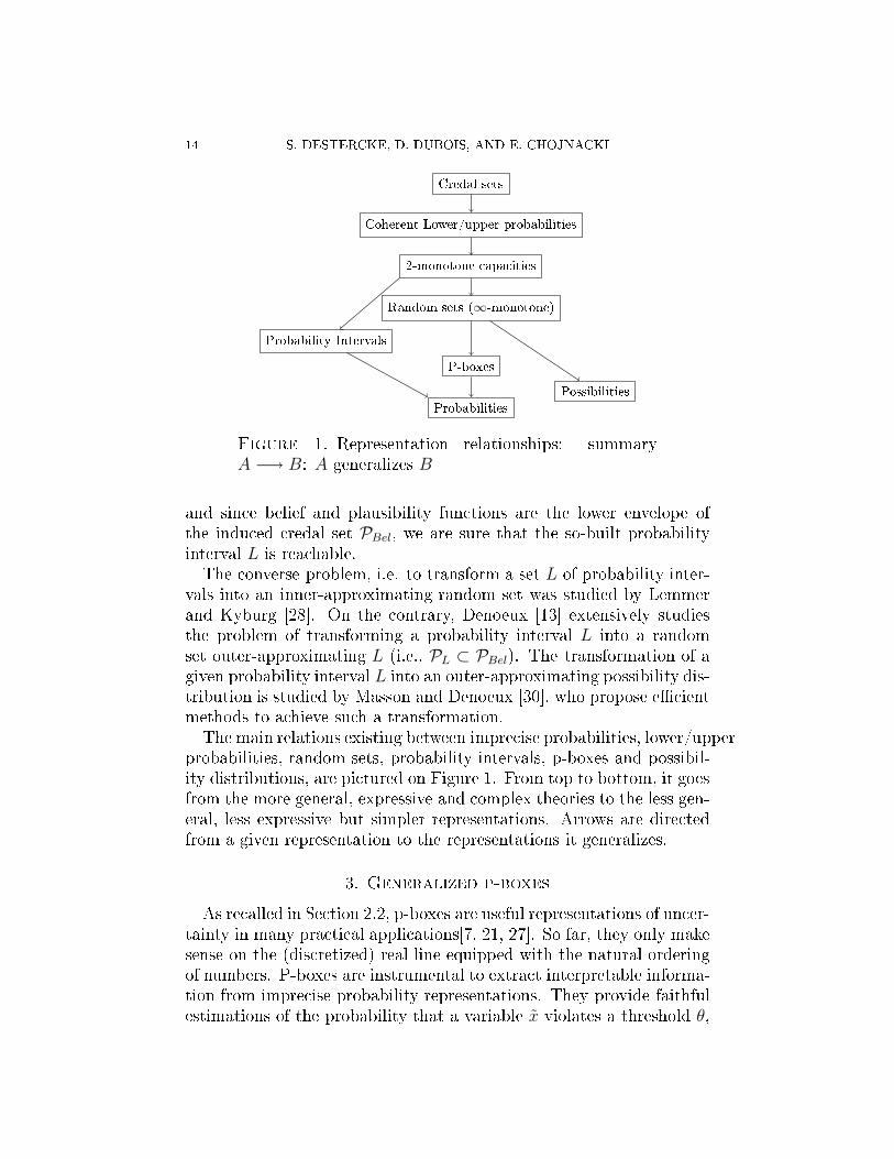
14 S. DESTERCKE, D. DUBOIS, AND E. CHOJNACKI
Credal sets
Coherent Lower/upper probabilities
2-monotone apa ities
Random sets (∞-monotone)
P-boxes
Probabilities
Probability Intervals
Possibilities
Figure 1. Representation relationships: summary
A −→ B: A generalizes B
and sin e belief and plausibility fun tions are the lower envelope of
the indu ed redal set PBel, we are sure that the so-built probability
interval L is rea hable.
The onverse problem, i.e. to transform a set L of probability inter-
vals into an inner-approximating random set was studied by Lemmer
and Kyburg [28. On the ontrary, Denoeux [13 extensively studies
the problem of transforming a probability interval L into a random
set outer-approximating L (i.e., PL ⊂ PBel). The transformation of a
given probability interval L into an outer-approximating possibility dis-
tribution is studied by Masson and Denoeux [30, who propose e ient
methods to a hieve su h a transformation.
The main relations existing between impre ise probabilities, lower/upper
probabilities, random sets, probability intervals, p-boxes and possibil-
ity distributions, are pi tured on Figure 1. From top to bottom, it goes
from the more general, expressive and omplex theories to the less gen-
eral, less expressive but simpler representations. Arrows are dire ted
from a given representation to the representations it generalizes.
3. Generalized p-boxes
As re alled in Se tion 2.2, p-boxes are useful representations of un er-
tainty in many pra ti al appli ations[7, 21, 27. So far, they only make
sense on the (dis retized) real line equipped with the natural ordering
of numbers. P-boxes are instrumental to extra t interpretable informa-
tion from impre ise probability representations. They provide faithful
estimations of the probability that a variable x violates a threshold θ,

UNIFYING UNCERTAINTY REPRESENTATIONS: GENERALIZED P-BOXES 15
i.e., upper and lower estimates of the probability of events of the form
x ≥ θ. However, they are mu h less adequate to ompute the proba-
bility that some output remains lose to a referen e value ρ [1, whi h
orresponds to omputing upper and lower estimates of the probability
of events of the form |x − ρ| ≥ θ. The rest of the paper is devoted to
the study of a generalization p-boxes, to arbitrary (nite) spa es, where
the underlying ordering relation is arbitrary, and that an address this
type of query. Generalized p-boxes will also be instrumental to har-
a terize a re ent representation proposed by Neumaier [34, studied in
the se ond part of this paper.
Generalized p-boxes are dened in Se tion 3.1. We then pro eed
to show the link between generalized p-boxes, possibility distributions
and random sets. We rst show that the former generalize possibility
distributions and are representable (in the sense of Denition 4) by
pairs thereof. Conne tions between generalized p-boxes and probability
intervals are also explored.
3.1. Denition of generalized p-boxes. The starting point of our
generalization is to noti e that any two umulative distribution fun -
tions modelling a p-box are omonotoni . Two mappings f and f ′from
a spa e X to the real line are said to be omonotoni if and only if, for
any pair of elements x, y ∈ X, we have f(x) < f(y) ⇒ f ′(x) ≤ f ′(y). Inother words, given an indexing of X = x1, . . . , xn, there is a permu-
tation σ of 1, 2, . . . , n su h that f(xσ(1)) ≥ f(xσ(2)) ≥ · · · ≥ f(xσ(n))and f ′(xσ(1)) ≥ f ′(xσ(2)) ≥ · · · ≥ f ′(xσ(n)). We dene a generalized
p-box as follows:
Denition 5. A generalized p-box [F , F ] dened on X is a pair of
omonotoni mappings F , F , F : X → [0, 1] and F : X → [0, 1] fromX to [0, 1] su h that F is pointwise less than F (i.e. F ≤ F ) and there
is at least one element x in X for whi h F (x) = F (x) = 1.
Sin e ea h distribution F , F is fully spe ied by |X| − 1 values, it
follows that 2|X| − 2 values ompletely determine a generalized p-box.
Note that, given a generalized p-box [F , F ], we an always dene a
omplete pre-ordering ≤[F,F ] on X su h that x ≤[F ,F ] y if F (x) ≤ F (y)
and F (x) ≤ F (y), due to the omonotoni ity ondition. If X is a subset
of the real line and if ≤[F ,F ] is the natural ordering of numbers, then
we retrieve lassi al p-boxes.
To simplify notations in the sequel, we will onsider that, given a
generalized p-box [F , F ], elements x of X are indexed su h that i < jimplies that xi ≤[F ,F ] xj . We will denote (x][F,F ] the set of the form
xi|xi ≤[F,F ] x. The redal set indu ed by a generalized p-box [F , F ]
16 S. DESTERCKE, D. DUBOIS, AND E. CHOJNACKI
an then be dened as
P[F ,F ] = P ∈ PX |i = 1, . . . , n, F (xi) ≤ P ((xi][F,F ]) ≤ F (xi).
It indu es oherent upper and lower probabilities su h that F (xi) =P ((xi][F,F ]) and F (xi) = P ((xi][F,F ]). When X = R and ≤[F,F ] is the
natural ordering on numbers, then ∀r ∈ R, (r][F,F ] = (−∞, r], and the
above equation oin ides with Equation (1).
In the following, sets (xi][F,F ] are denoted Ai, for all i = 1, . . . , n.
These sets are nested, sin e ∅ ⊂ A1 ⊆ . . . ⊆ An = X6
. For all i =1, . . . , n, let F (xi) = αi and F (xi) = βi. With these onventions, the
redal set P[F,F ] an now be des ribed by the following n onstraints
bearing on probabilities of nested sets Ai:
(7) i = 1, . . . , n αi ≤ P (Ai) ≤ βi
with 0 = α0 ≤ α1 ≤ . . . ≤ αn = 1, 0 = β0 < β1 ≤ β2 ≤ . . . ≤ βn = 1and αi ≤ βi.
As a onsequen e, a generalized p-box an be generated in two dif-
ferent ways:
• By starting from two omonotone fun tions F ≤ F dened on
X, the pre-order being indu ed by the values of these fun tions,
• or by assigning upper and lower bounds on probabilities of a
pres ribed olle tion of nested sets Ai.
Note that the se ond approa h is likely to be more useful in pra ti al
assessments and eli itation of generalized p-boxes.
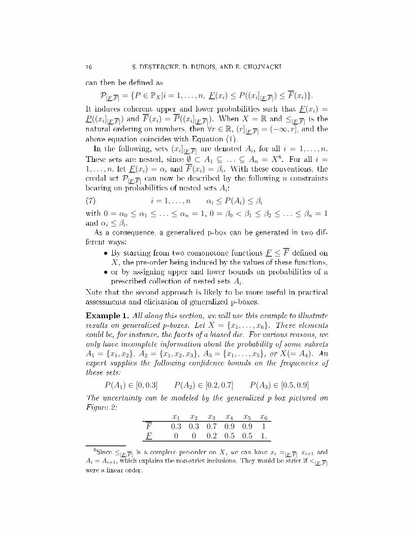
Example 1. All along this se tion, we will use this example to illustrate
results on generalized p-boxes. Let X = x1, . . . , x6. These elements
ould be, for instan e, the fa ets of a biased die. For various reasons, we
only have in omplete information about the probability of some subsets
A1 = x1, x2, A2 = x1, x2, x3, A3 = x1, . . . , x5, or X(= A4). An
expert supplies the following onden e bounds on the frequen ies of
these sets:
P (A1) ∈ [0, 0.3] P (A2) ∈ [0.2, 0.7] P (A3) ∈ [0.5, 0.9]
The un ertainty an be modeled by the generalized p-box pi tured on
Figure 2:
x1 x2 x3 x4 x5 x6
F 0.3 0.3 0.7 0.9 0.9 1F 0 0 0.2 0.5 0.5 1.
6
Sin e ≤[F,F ] is a omplete pre-order on X , we an have xi =[F,F ] xi+1 and
Ai = Ai+1, whi h explains the non-stri t in lusions. They would be stri t if <[F,F ]
were a linear order.

UNIFYING UNCERTAINTY REPRESENTATIONS: GENERALIZED P-BOXES 17
0
xi
1
x1 x2 x3 x4 x5 x6
0.2
0.4
0.6
0.8
: F: F
Figure 2. Generalized p-box [F, F ] of Example 1
3.2. Conne ting generalized p-boxes with possibility distribu-
tions. It is natural to sear h for a onne tion between generallized
p-boxes and possibility theory, sin e possibility distributions an be
interpreted as a olle tion of nested sets with asso iated lower bounds,
while generalized p-boxes orrespond to lower and upper bounds also
given on a olle tion of nested sets. Given a generalized p-box [F , F ],the following proposition holds:
Proposition 2. Any generalized p-box [F , F ] on X is representable by
a pair of possibility distributions πF , πF , su h that P[F ,F ] = PπF∩PπF
,
where:
πF (xi) = βi and πF (xi) = 1 − maxαj|αj < αi; j = 0, . . . , i
for i = 1, . . . , n, with α0 = 0.
Proof of Proposition 2. Consider the set of onstraints given by Equa-
tion (7) and dening the onvex set P[F ,F ]. These onstraints an be
separated into two distin t sets: (P (Ai) ≤ βi)i=1,n and (P (Aci) ≤
1 − αi)i=1,n. Now, rewrite onstraints of Proposition 1, in the form
∀α ∈ (0, 1]: P ∈ Pπ if and only if P (x ∈ X|π(x) ≤ α) ≤ α.The rst set of onstraints (P (Ai) ≤ βi)i=1,n denes a redal set Pπ
F
that is indu ed by the possibility distribution πF , while the se ond set
of onstraints (P (Aci) ≤ 1−αi)i=1,n denes a redal set PπF
that is in-
du ed by the possibility distribution πF , sin e Aci = xk, . . . xn, where
k = maxj|αj < αi. The redal set of the generalized p-box [F , F ],resulting from the two sets of onstraints, namely i = 1, . . . , n, βi ≤P (Ai) ≤ αi, is thus Pπ
F∩ PπF
.
Example 2. The possibility distributions πF , πF for the generalized
p-box dened in Example 1 are:
x1 x2 x3 x4 x5 x6
πF 0.3 0.3 0.7 0.9 0.9 1πF 1 1 1 0.8 0.8 0.5
18 S. DESTERCKE, D. DUBOIS, AND E. CHOJNACKI
Note that, when F is inje tive, <[F,F ] is a linear order, and we have
πF (xi) = 1 − αi−1. So, generalized p-boxes allow to model un ertainty
in terms of pairs of omonotone possibility distributions. In this ase,
ontrary to the ase of only one possibility distribution, the two bounds
en losing the probability of a parti ular event A an be tighter, i.e.
no longer restri ted to the form [0, α] or [β, 1], but ontained in the
interse tion of intervals of this form.
An interesting ase is the one where, for all i = 1, . . . , n−1, F (xi) =0 and F (xn) = 1. Then, πF = 1 and Pπ
F∩ PπF
= PπFand we
retrieve the single distribution πF . We re over πF if we take for all
i = 1, . . . , n, F (xi) = 1. This means that generalized p-boxes also
generalize possibility distributions, and are representable by them in
the sense of Denition 4.
3.3. Conne ting Generalized p-boxes and random sets. We al-
ready mentioned that p-boxes are spe ial ases of random sets, and the
following proposition shows that it is also true for generalized p-boxes.
Proposition 3. Generalized p-boxes are spe ial ases of random sets,
in the sense that for any generalized p-box [F , F ] on X, there exist a
belief fun tion Bel su h that P[F ,F ] = PBel.
In order to prove Proposition 3, we show that the lower probabilities
indu ed by a generalized p-box and by the belief fun tion given by
Algorithm 1 oin ide on every event. To do that, we use the partition
of X indu ed by nested sets Ai, and ompute lower probabilities of
elements of this partition. We then he k that the lower probabilities
on all events indu ed by the generalized p-box oin ide with the belief
fun tion indu ed by Algorithm 1. The detailed proof an be found in
the appendix.
Algorithm 1 below provides an easy way to build the random set
en oding a given generalized p-box. It is similar to existing algo-
rithms [27, 38, and extends them to more general spa es. The main
idea of the algorithm is to use the fa t that a generalized p-box an
be seen as a random set whose fo al sets are obtained by threshold-
ing the umulative distributions (as in Figure 2). Sin e the sets Ai
are nested, they indu e a partition of X whose elements are of the
form Gi = Ai \ Ai−1. The fo al sets of the random set equivalent to
the generalized p-box are made of unions of onse utive elements of
this partition. Basi ally, the pro edure omes down to progressing a
threshold θ ∈ [0, 1]. When αi+1 > θ ≥ αi and βj+1 > θ ≥ βj , then, the
orresponding fo al set is Ai+1 \ Aj, with mass
(8) m(Ai+1 \ Aj) = min(αi+1, βj+1) − max(αi, βj).

UNIFYING UNCERTAINTY REPRESENTATIONS: GENERALIZED P-BOXES 19
Algorithm 1: R-P-box → random set transformation
Input: Generalized p-box [F , F ] and orresponding nested sets
∅ = A0, A1, . . . , An = X, lower bounds αi and upper
bounds βi
Output: Equivalent random set
for i = 1, . . . , n do
Build partition Gi = Ai \ Ai−1
Build set
γl|l = 1, . . . , 2n − 1 = αi|i = 1, . . . , n ∪ βi|i = 1, . . . , nWith γl indexed su h that
γ1 ≤ . . . ≤ γl ≤ . . . ≤ γ2n−1 = βn = αn = 1Set α0 = β0 = γ0 = 0 and fo al set E0 = ∅for k = 1, . . . , 2n − 1 do
if γk−1 = αi then
Ek = Ek−1 ∪ Gi+1
if γk−1 = βi then
Ek = Ek−1 \ Gi
Set m(Ek) = γk − γk−1
We an also give another hara terization of the random set (8): let
us note 0 = γ0 < γ1 < . . . < γM = 1 the distin t values taken by F , Fover elements xi of X (note that M is nite and M < 2n). Then, forj = 1, . . . , M , the random set dened as:
(9)
Ej=xi∈X|(πF
(xi)≥γj)∧(1−πF (xi)<γj)
m(Ej) = γj − γj−1
is the same as the one built by using Algorithm 1, but this formulation
lays bare the link between Equation (6) and the possibility distributions
πF , πF .
Example 3. This example illustrates the appli ation of Algorithm 1,
by applying it to the generalized p-box given in Example 1. We have:
G1 = x1, x2 G2 = x3 G3 = x4, x5 G4 = x6
and
0 ≤ 0 ≤ 0.2 ≤ 0.3 ≤ 0.5 ≤ 0.7 ≤ 0.9 ≤ 1
α0 ≤ α1 ≤ α2 ≤ β1 ≤ α3 ≤ β2 ≤ β3 ≤ α4
γ0 ≤ γ1 ≤ γ2 ≤ γ3 ≤ γ4 ≤ γ5 ≤ γ6 ≤ γ7
20 S. DESTERCKE, D. DUBOIS, AND E. CHOJNACKI
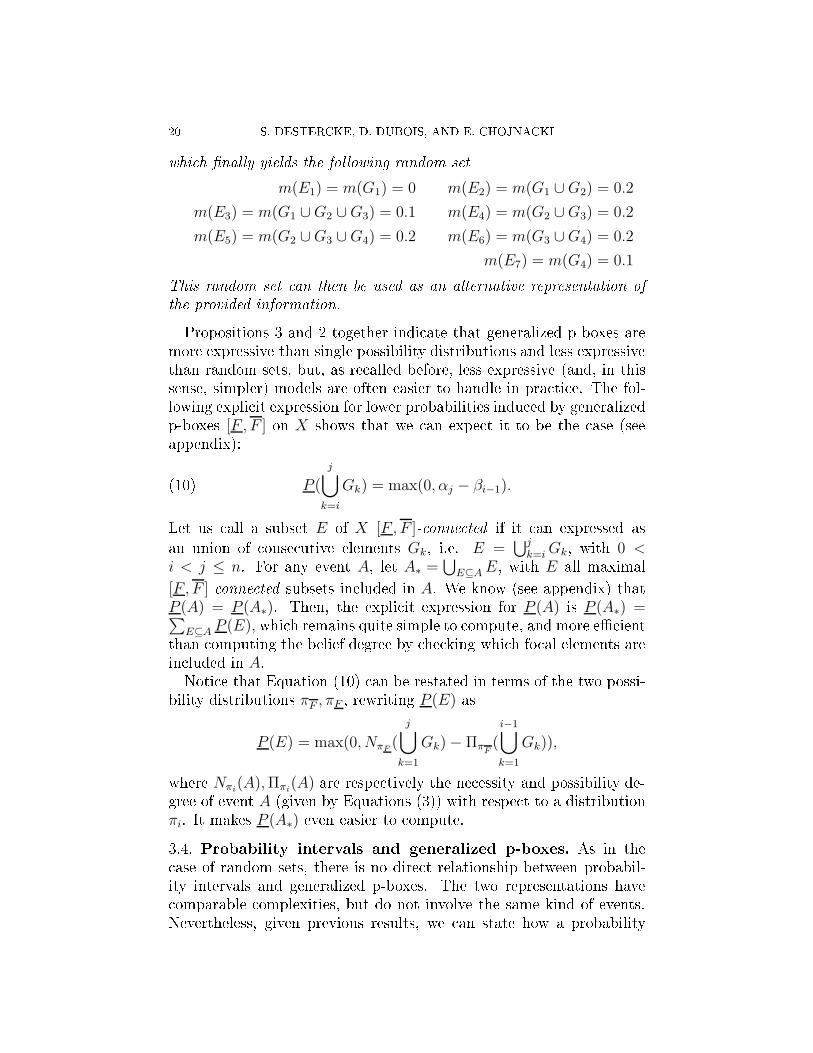
whi h nally yields the following random set
m(E1) = m(G1) = 0 m(E2) = m(G1 ∪ G2) = 0.2
m(E3) = m(G1 ∪ G2 ∪ G3) = 0.1 m(E4) = m(G2 ∪ G3) = 0.2
m(E5) = m(G2 ∪ G3 ∪ G4) = 0.2 m(E6) = m(G3 ∪ G4) = 0.2
m(E7) = m(G4) = 0.1
This random set an then be used as an alternative representation of
the provided information.
Propositions 3 and 2 together indi ate that generalized p-boxes are
more expressive than single possibility distributions and less expressive
than random sets, but, as re alled before, less expressive (and, in this
sense, simpler) models are often easier to handle in pra ti e. The fol-
lowing expli it expression for lower probabilities indu ed by generalized
p-boxes [F , F ] on X shows that we an expe t it to be the ase (see
appendix):
(10) P (
j⋃
k=i
Gk) = max(0, αj − βi−1).
Let us all a subset E of X [F , F ]- onne ted if it an expressed as
an union of onse utive elements Gk, i.e. E =⋃j
k=i Gk, with 0 <i < j ≤ n. For any event A, let A∗ =
⋃
E⊆A E, with E all maximal
[F, F ]- onne ted subsets in luded in A. We know (see appendix) that
P (A) = P (A∗). Then, the expli it expression for P (A) is P (A∗) =∑
E⊆A P (E), whi h remains quite simple to ompute, and more e ient
than omputing the belief degree by he king whi h fo al elements are
in luded in A.Noti e that Equation (10) an be restated in terms of the two possi-
bility distributions πF , πF , rewriting P (E) as
P (E) = max(0, NπF(
j⋃
k=1
Gk) − ΠπF(
i−1⋃
k=1
Gk)),
where Nπi(A), Ππi
(A) are respe tively the ne essity and possibility de-
gree of event A (given by Equations (3)) with respe t to a distribution
πi. It makes P (A∗) even easier to ompute.
3.4. Probability intervals and generalized p-boxes. As in the
ase of random sets, there is no dire t relationship between probabil-
ity intervals and generalized p-boxes. The two representations have
omparable omplexities, but do not involve the same kind of events.
Nevertheless, given previous results, we an state how a probability

UNIFYING UNCERTAINTY REPRESENTATIONS: GENERALIZED P-BOXES 21
interval L an be transformed into a generalized p-box [F , F ], and
vi e-versa.
First onsider a probability interval L and some indexing x1, . . . , xn
of elements in X. A generalized p-box [F ′, F′] outer-approximating the
probability interval L an be omputed by means of Equations (2) as
follows:
F ′(xi) = P (Ai) = α′i = max(
∑
xi∈Ai
l(xi), 1 −∑
xi /∈Ai
u(xi))(11)
F′(xi) = P (Ai) = β ′
i = min(∑
xi∈Ai
u(xi), 1 −∑
xi /∈Ai
l(xi))
where P, P are respe tively the lower and upper probabilities of PL.
Re all that Ai = x1, . . . , xi. Note that ea h permutation of elements
of X provide a dierent generalized p-box and that there is no tightest
outer-approximation among them.
Next, onsider a generalized p-box [F , F ] with nested sets A1 ⊆ . . . ⊆An. The probability interval L′
on elements xi orresponding to [F , F ]is given by:
P (xi) = l′(xi) = max(0, αi − βi−1)(12)
P (xi) = u′(xi) = βi − αi−1
where P, P are the lower and upper probabilities of the redal set P[F ,F ]
on elements of X, αi = F (Ai), βi = F (Ai) and β0 = α0 = 0. This is
the tightest probability interval outer-approximating the generalized
p-box, and there is only su h set.
Of ourse, transforming a probability interval L into a p-box [F , F ]and vi e-versa generally indu es a loss of information. But we an show
that probability intervals are representable (see denition 4) by gener-
alized p-boxes: let Σσ the set of all possible permutations σ of elements
of X, ea h dening a linear order. A generalized p-box a ording to
permutation σ is denoted [F ′, F′]σ and alled a σ-p-box. We then have
the following proposition (whose proof is in the appendix):
Proposition 4. Let L be a probability interval, and let [F ′, F′]σ be
the σ-p-box obtained from L by applying Equations (11). Moreover, let
L′′σ denote the probability interval obtained from the σ-p-box [F ′, F
′]σ
by applying Equations (12). Then, the various redal sets thus dened
satisfy the following property:
(13) PL =⋂
σ∈Σσ
P[F ′,F′
]σ=
⋂
σ∈Σσ
PL′′
σ

22 S. DESTERCKE, D. DUBOIS, AND E. CHOJNACKI
Lower/upper prev.
Lower/upper prob.
2-monotone apa ities
Random sets (∞-monot)
Generalized p-boxes
P-boxes
Probabilities
Probability Intervals
Possibilities
Figure 3. Representation relationships: summary with
generalized p-boxes. A −→ B: A generalizes B. A 99K B:
B is representable by A
This means that the information modeled by a set L of probability in-
tervals an be entirely re overed by onsidering sets of σ-p-boxes. Notethat not all |X|! su h permutations need to be onsidered, and that in
pra ti e, L an be exa tly re overed by means of a redu ed set S of
|X|/2 permutations, provided that xσ(1), σ ∈ S∪xσ(n), σ ∈ S = X.
Sin e P[F ,F ] = PπF∩Pπ
F, then it is immediate from Proposition 4,that,
in terms of redal sets, PL =⋂
σ∈Σσ
(
PπFσ∩ Pπ
F σ
)
, where πF σ, πF σ
are
respe tively the possibility distributions orresponding to F σ and F σ.
4. Con lusion
This paper introdu es a generalized notion of p-box. Su h a gener-
alization allows to dene p-boxes on nite (pre)-ordered spa es as well
as dis retized p-boxes on multi-dimensional spa es equipped with an
arbitrary (pre)-order. On the real line, this preorder an be of the form
x ≤ρ y if and only if |x − ρ| ≤ |y − ρ|, thus a ounting for events of
the form lose to a pres ribed value ρ. Generalized p-boxes are rep-
resentable by a pair of omonotone possibility distributions. They are
spe ial ase of random sets, and the orresponding mass assignment has
been laid bare. Generalized p-boxes are thus more expressive than sin-
gle possibility distributions and likely to be more tra table than general

UNIFYING UNCERTAINTY REPRESENTATIONS: GENERALIZED P-BOXES 23
random sets. Moreover, the fa t that they an be interpreted as lower
and upper onden e bounds over nested sets makes them quite at-
tra tive tools for subje tive eli itation. Finally, we showed the relation
existing between generalized p-boxes and sets of probability intervals.
Figure 3 summarizes the results of this paper, by pla ing generalized
p-boxes inside the graph of Figure 1. New relationships and represen-
tations obtained in this paper are in bold lines. Computational aspe ts
of al ulations with generalized p-boxes need to be explored in greater
detail (as is done by De Campos et al. [9 for probability intervals) as
well as their appli ation to the eli itation of impre ise probabilities.
Another issue is to extend presented results to more general spa es,
to general lower/upper previsions or to ases not onsidered here (e.g.
ontinuous p-boxes with dis ontinuity points), possibly using existing
results [42, 11. Interestingly, the key ondition when representing gen-
eralized p-boxes by two possibility distributions is their omonotoni -
ity. In the se ond part of this paper, we pursue the present study by
dropping this assumption. We then re over so- alled louds, re ently
proposed by Neumaier [34.
Referen es
[1 C. Baudrit, D. Dubois, Pra ti al representations of in omplete probabilisti
knowledge, Computational Statisti s and Data Analysis 51 (1) (2006) 86108.
[2 C. Baudrit, D. Guyonnet, D. Dubois, Joint propagation and exploitation of
probabilisti and possibilisti information in risk assessment, IEEE Trans.
Fuzzy Systems 14 (2006) 593608.
[3 A. Cano, F. Cozman, T. Lukasiewi z (eds.), Reasoning with impre ise proba-
bilities, vol. 44 of I. J. of Approximate Reasoning, 2007 (2007).
[4 A. Chateauneuf, J.-Y. Jaray, Some hara terizations of lower probabilities
and other monotone apa ities through the use of Möbius inversion, Mathe-
mati al So ial S ien es 17 (3) (1989) 263283.
[5 G. Choquet, Theory of apa ities, Annales de l'institut Fourier 5 (1954) 131
295.
[6 R. Cooke, Experts in un ertainty, Oxford University Press, Oxford, UK, 1991.
[7 J. Cooper, S. Ferson, L. Ginzburg, Hybrid pro essing of sto hasti and sub-
je tive un ertainty, Risk Analysis 16 (1996) 785791.
[8 I. Couso, S. Montes, P. Gil, The ne essity of the strong alpha- uts of a fuzzy
set, Int. J. on Un ertainty, Fuzziness and Knowledge-Based Systems 9 (2001)
249262.
[9 L. de Campos, J. Huete, S. Moral, Probability intervals: a tool for un ertain
reasoning, I. J. of Un ertainty, Fuzziness and Knowledge-Based Systems 2
(1994) 167196.
[10 G. de Cooman, A behavioural model for vague probability assessments, Fuzzy
Sets and Systems 154 (2005) 305358.

24 S. DESTERCKE, D. DUBOIS, AND E. CHOJNACKI
[11 G. de Cooman, M. Troaes, E. Miranda, n-monotone lower previsions and
lower integrals, in: F. Cozman, R. Nau, T. Seidenfeld (eds.), Pro . 4th Inter-
national Symposium on Impre ise Probabilities and Their Appli ations, 2005.
[12 A. Dempster, Upper and lower probabilities indu ed by a multivalued mapping,
Annals of Mathemati al Statisti s 38 (1967) 325339.
[13 T. Denoeux, Constru ting belief fun tions from sample data using multinomial
onden e regions, I. J. of Approximate Reasoning 42 (2006) 228252.
[14 D. Dubois, L. Foulloy, G. Mauris, H. Prade, Probability-possibility transforma-
tions, triangular fuzzy sets, and probabilisti inequalities, Reliable Computing
10 (2004) 273297.
[15 D. Dubois, P. Hajek, H. Prade, Knowledge-driven versus data-driven logi s, J.
of Logi , Language and Information 9 (2000) 6589.
[16 D. Dubois, H. Prade, Possibility Theory: An Approa h to Computerized Pro-
essing of Un ertainty, Plenum Press, New York, 1988.
[17 D. Dubois, H. Prade, Consonant approximations of belief fun tions, I.J. of
Approximate reasoning 4 (1990) 419449.
[18 D. Dubois, H. Prade, Random sets and fuzzy interval analysis, Fuzzy Sets and
Systems (42) (1992) 87101.
[19 D. Dubois, H. Prade, When upper probabilities are possibility measures, Fuzzy
Sets and Systems 49 (1992) 6574.
[20 S. Ferson, L. Ginzburg, Hybrid arithmeti , in: Pro . of ISUMA/NAFIPS'95,
1995.
[21 S. Ferson, L. Ginzburg, V. Kreinovi h, D. Myers, K. Sentz, Constru ting prob-
ability boxes and Dempster-Shafer stru tures, Te h. rep., Sandia National Lab-
oratories (2003).
[22 M. Fu hs, A. Neumaier, Potential based louds in robust design optimization,
Journal of statisti al theory and pra ti e To appear.
[23 M. Grabis h, J. Mari hal, M. Roubens, Equivalent representations of set fun -
tions, Mathemati s on operations resear h 25 (2) (2000) 157178.
[24 J. Helton, W. Oberkampf (eds.), Alternative Representations of Un ertainty,
Spe ial issue of Reliability Engineering and Systems Safety, vol. 85, Elsevier,
2004.
[25 P. Huber, Robust statisti s, Wiley, New York, 1981.
[26 I. Kozine, L. Utkin, Constru ting impre ise probability distributions, I. J. of
General Systems 34 (2005) 401408.
[27 E. Kriegler, H. Held, Utilizing random sets for the estimation of future limate
hange, I. J. of Approximate Reasoning 39 (2005) 185209.
[28 J. Lemmer, H. Kyburg, Conditions for the existen e of belief fun tions or-
responding to intervals of belief, in: Pro . 9th National Conferen e on A.I.,
Anaheim, 1991.
[29 I. Levi, The Enterprise of Knowledge, MIT Press, London, 1980.
[30 M. Masson, T. Denoeux, Inferring a possibility distribution from empiri al
data, Fuzzy Sets and Systems 157 (3) (2006) 319340.
[31 E. Miranda, I. Couso, P. Gil, Extreme points of redal sets generated by 2-
alternating apa ities, I. J. of Approximate Reasoning 33 (2003) 95115.
[32 I. Mol hanov, Theory of Random Sets, Springer, London, 2005.
[33 R. Moore, Methods and appli ations of Interval Analysis, SIAM Studies in
Applied Mathemati s, SIAM, Philadelphia, 1979.
UNIFYING UNCERTAINTY REPRESENTATIONS: GENERALIZED P-BOXES 25
[34 A. Neumaier, Clouds, fuzzy sets and probability intervals, Reliable Computing
10 (2004) 249272.
[35 A. Neumaier, On the stru ture of louds, Available on
http://www.mat.univie.a .at/∼neum (2004).
[36 Z. Pawlak, Rough Sets. Theoreti al Aspe ts of Reasoning about Data, Kluwer
A ademi , Dordre ht, 1991.
[37 E. Raufaste, R. Neves, C. Mariné, Testing the des riptive validity of possibility
theory in human judgments of un ertainty, Arti ial Intelligen e 148 (2003)
197218.
[38 H. Regan, S. Ferson, D. Berleant, Equivalen e of methods for un ertainty
propagation of real-valued random variables, I. J. of Approximate Reasoning
36 (2004) 130.
[39 G. L. S. Sha kle, De ision, Order and Time in Human Aairs, Cambridge
University Press, Cambridge, 1961.
[40 G. Shafer, A mathemati al Theory of Eviden e, Prin eton University Press,
New Jersey, 1976.
[41 P. Smets, The normative representation of quantied beliefs by belief fun tions,
Arti ial Intelligen e 92 (1997) 229242.
[42 P. Smets, Belief fun tions on real numbers, I. J. of Approximate Reasoning 40
(2005) 181223.
[43 P. Walley, Statisti al reasoning with impre ise Probabilities, Chapman and
Hall, New York, 1991.
[44 P. Walley, Measures of un ertainty in expert systems, Arti al Intelligen e 83
(1996) 158.
[45 R. Williamson, T. Downs, Probabilisti arithmeti i : Numeri al methods
for al ulating onvolutions and dependen y bounds, I. J. of Approximate
Reasoning 4 (1990) 8158.
[46 L. Zadeh, Fuzzy sets as a basis for a theory of possibility, Fuzzy Sets and
Systems 1 (1978) 328.
Appendix
Proof of Proposition 3. From the nested sets A1 ⊆ A2 ⊆ . . . ⊆An = X we an build a partition s.t. G1 = A1, G2 = A2 \A1, . . . , Gn =An \ An−1. On e we have a nite partition, every possible set B ⊆ X an be approximated from above and from below by pairs of sets B∗ ⊆B∗
[36:
B∗ =⋃
Gi, Gi ∩ B 6= ∅; B∗ =⋃
Gi, Gi ⊆ B
made of a nite union of the partition elements interse ting or on-
tained in this set B. Then P (B) = P (B∗),P (B) = P (B∗), so we only
have to are about unions of elements Gi in the sequel. Espe ially, for
ea h event B ⊂ Gi for some i, it is lear that P (B) = 0 = Bel(B)and P (B) = P (Gi) = P l(B). So, to prove Proposition 3, we have to
show that lower probabilities given by a generalized p-box [F , F ] andby the orresponding random set built through algorithm 1 oin ide on

26 S. DESTERCKE, D. DUBOIS, AND E. CHOJNACKI
unions of elements Gi. We will rst on entrate on unions of ons utive
elements Gi, and then to any union of su h elements.
Let us rst onsider union of onse utive elements
⋃jk=i Gk (when
k = 1, we retrieve the sets Aj). Finding P (⋃j
k=i Gk) is equivalent to
omputing the minimum of
∑jk=i P (Gk) under the onstraints
i = 1, . . . , n αi ≤ P (Ai) =
i∑
k=1
P (Gk) ≤ βi
whi h reads
αj ≤ P (Ai−1) +
j∑
k=i
P (Gk) ≤ βj
so
∑jk=i P (Gk) ≥ max(0, αj − βi−1). This lower bound is optimal,
sin e it is always rea hable: if αj > βi−1, take P s.t. P (Ai−1) = βi−1,
P (⋃j
k=i Gk) = αj − βi−1, P (⋃n
k=j+1 Gk) = 1 − αj . If αj ≤ βi−1, take P
s.t. P (Ai−1) = βi−1, P (⋃j
k=i Gk) = 0, P (⋃n
k=j+1 Ek) = 1 − βi−1. And
we an see, by looking at Algorithm 1, that Bel(⋃j
k=i Gk) = max(0, αj−
βi−1): fo al elements of Bel are subsets of⋃j
k=i Gk if βi−1 < αj only.
Now, let us onsider a union A of non- onse utive elements s.t.
A = (⋃i+l
k=i Gk ∪⋃j
k=i+l+m Gk) with m > 1. As in the previous ase,
we must ompute min(
∑i+lk=i P (Gk) +
∑jk=i+l+m P (Gk)
)
to nd the
lower probability on P (A). An obvious lower bound is given by
min(
i+l∑
k=i
P (Gk)+
j∑
k=i+l+m
P (Gk))
≥ min(
i+l∑
k=i
P (Gk))
+min(
j∑
k=i+l+m
P (Gk))
and this lower bound is equal to
max(0, αi+l − βi−1) + max(0, αj − βi+l+m−1) = Bel(A)
Consider the two following ases with probabilisti mass assignments
showing that bounds are attained:
• αi+l < βi−1, αj < βi+l+m−1 and probability masses:
P (Ai−1) = βi−1, P (⋃i+l
k=i Gk) = αi+l − βi−1, P (⋃i+l+m−1
k=i+l+1 Gk) = βi+l+m−1 − αi+l,
P (⋃j
k=i+l+m Gk) = αj − βi+l+m−1 and P (⋃n
k=j+1 Gk) = 1 − αj.
• αi+l > βi−1, αj > βi+l+m−1 and probability masses:
P (Ai−1) = βi−1, P (⋃i+l
k=i Gk) = 0, P (⋃i+l+m−1
k=i+l+1 Gk) = αj − βi−1,
P (⋃j
k=i+l+m Ek) = 0 and P (⋃n
k=j+1 Gk) = 1 − αj .
The same line of thought an be followed for the two remaining ases.
As in the onse utive ase, the lower bound is rea hable without vio-
lating any of the restri tions asso iated to the generalized p-box. We

UNIFYING UNCERTAINTY REPRESENTATIONS: GENERALIZED P-BOXES 27
have P (A) = Bel(A) and the extension of this result to any number nof "dis ontinuities" in the sequen e of Gk is straightforward. The proof
is omplete, sin e for every possible union A of elements Gk, we have
P (A) = Bel(A)
Proof of Proposition 4. To prove this proposition, we must rst re-
all a result given by De Campos et al. [9: given two probability in-
tervals L and L′dened on a spa e X and the indu ed redal sets PL
and PL′, the onjun tion PL∩L′ = PL ∩ PL′
of these two sets an be
modeled by the set (L ∩ L′) of probability intervals that is su h that
for every element x of X,
l(L∩L′)(x) = max(lL(x), lL′(x)) and u(L∩L′)(x) = min(uL(x), uL′(x))
and these formulas extend dire tly to the onjun tion of any number
of probability intervals on X.
To prove Proposition 4, we will show, by using the above onjun tion,
that PL =⋂
σ∈ΣσPL′′
σ. Note that we have, for any σ ∈ Σσ, PL ⊂
P[F ′,F
′
]σ⊂ PL′′
σ, thus showing this equality is su ient to prove the
whole proposition.
Let us note that the above in lusion relationships alone ensure us
that
PL ⊆⋂
σ∈ΣσP[F ′,F
′
]σ⊆
⋂
σ∈ΣσPL′′
σ. So, all we have to show is that the
in lusion relationship is in fa t an equality.
Sin e we know that both PL and
⋂
σ∈ΣσPL′′
σ an be modeled by
probability intervals, we will show that the lower bounds l on every
element x in these two sets oin ide (and the proof for upper bounds
is similar).
For all x in X, lL′′
Σ(x) = maxσ∈Σσ
lL′′
σ(x), with L′′
Σ the probability
interval orresponding to
⋂
σ∈ΣσPL′′
σand L′′
σ the probability interval
orresponding to a parti ular permutation σ. We must now show that,
for all x in X, lL′′
Σ(x) = lL(x).
Given a ranking of elements of X, and by applying su essively Equa-
tions (11) and (12), we an express the dieren es between bounds
l′′(xi) of the set L′′and l(xi) of the set L in terms of set of bounds L.
This gives, for any xi ∈ X:
l(xi) − l′′(xi) =min(l(xi), 0 +∑
xi∈Ai−1
(u(xi) − l(xi)),
(14)
0 +∑
xi∈Aci
(u(xi) − l(xi)), (l(xi) +∑
xj 6=xi
xj∈X
u(xj)) − 1, 1 −∑
xi∈X
l(xi))
28 S. DESTERCKE, D. DUBOIS, AND E. CHOJNACKI
We already know that, for any permutation σ and for all x in X, we
have lL′′
σ(x) ≤ lL(x). So we must now show that, for a given x in X,
there is one permutation σ su h that lL′′
σ(x) = lL(x). Let us onsider
the permutation pla ing the given element at the front. If x is the rst
element xσ(1), then Equation (14) has value 0 for this element, and we
thus have lL′′
σ(x) = lL(x). Sin e if we onsider every possible ranking,
every element x of X will be rst in at least one of these rankings, this
ompletes the proof.
Institut de Radioprote tion et Sûreté nu léaire, Bât 720, 13115
St-Paul lez Duran e, FRANCE
E-mail address : sdester kegmail. om
Université Paul Sabatier, IRIT, 118 Route de Narbonne, 31062 Toulouse
E-mail address : duboisirit.fr
Institut de Radioprote tion et Sûreté nu léaire, Bât 720, 13115
St-Paul lez Duran e, FRANCE
E-mail address : eri . hojna kiirsn.fr