arX

iv:a

stro

-ph/

0501

573v

2 1

8 Fe

b 20

05

THE FRACTAL DIMENSION OF PROJECTED CLOUDS

Nestor Sanchez,1,2 Emilio J. Alfaro,1 and Enrique Perez1

ABSTRACT

The interstellar medium seems to have an underlying fractal structure which

can be characterized through its fractal dimension. However, interstellar clouds

are observed as projected two-dimensional images, and the projection of a tri-

dimensional fractal distorts its measured properties. Here we use simulated frac-

tal clouds to study the relationship between the tri-dimensional fractal dimension

(Df) of modeled clouds and the dimension resulting from their projected images.

We analyze different fractal dimension estimators: the correlation and mass di-

mensions of the clouds, and the perimeter-based dimension of their boundaries

(Dper). We find the functional forms relating Df with the projected fractal di-

mensions, as well as the dependence on the image resolution, which allow to

estimate the “real” Df value of a cloud from its projection. The application of

these results to Orion A indicates in a self-consistent way that 2.5 . Df . 2.7

for this molecular cloud, a value higher than the result Dper +1 ≃ 2.3 some times

assumed in literature for interstellar clouds.

Subject headings: ISM: structure — ISM: clouds — ISM: general

1. INTRODUCTION

Maps of nearby cloud complexes have shown that the gas and dust are organized into

irregular hierarchical structures which seem similar to each other over a wide range of scales

(Scalo 1990; Falgarone et al. 1992). This self-similarity has been interpreted as a signature of

an underlying fractal geometry that may be related to the physical processes supporting the

generation of structures in the interstellar medium. The origin of this fractal-like structure

seems to be turbulence (Falgarone & Phillips 1990; Kritsuk & Norman 2004; Padoan et al.

2004), although self-gravity could also play an important role (de Vega et al. 1996). A fractal

1Instituto de Astrofısica de Andalucıa, CSIC, Apdo. 3004, E-18080, Granada, Spain; nestor@iaa.es,

emilio@iaa.es, eperez@iaa.es.

2Departamento de Fısica, Universidad del Zulia, Maracaibo, Venezuela.

– 2 –

structure for the interstellar medium is consistent with many observed features, including

the cloud size and cloud mass distribution functions (Elmegreen & Falgarone 1996), the

properties of the intercloud medium (Elmegreen 1997a), and even the stellar initial mass

function (Larson 1992; Elmegreen 1997b, 2002).

Therefore, it is important to measure the degree of fractality and/or complexity of the

ISM. There are several ways this can be done, such as structure tree methods (Houlahan &

Scalo 1992), delta variance techniques (Stutzki et al. 1998), principal components analysis

(Ghazzali et al. 1999), multifractal analysis (Chappell & Scalo 2001), metric space techniques

(Khalil et al. 2004), etc. A simple method consists of calculating the fractal dimension

characterizing structures in the ISM, but it has to be mentioned that quantifying the fractal

dimension of an object is generally not sufficient to characterize it, because objects with

different morphological properties could have the same fractal dimension (Mandelbrot 1983).

In spite of this a number of studies have been done to estimate the fractal dimension of

interstellar clouds. Most of these studies use the so-called perimeter-area method: if the iso-

contours exhibit a power-law perimeter-area relation with a noninteger exponent over certain

range of scales, this exponent may be interpreted in terms of a fractal dimension (Dper) that

characterizes the manner these curves fill space (Mandelbrot 1983). This method was used

by Beech (1987) on a group of selected dark clouds to estimate a fractal dimension of 1.4,

whereas Bazell & Desert (1988) calculated an average fractal dimension of 1.26 for cirrus

regions discovered by IRAS. Dickman et al. (1990) studied five different molecular cloud

complexes (Chamaeleon, R CrA, ρ Oph, Taurus and the Lynds 134/183/1778 group) finding

1.17 . Dper . 1.28. Also for the Taurus complex, Scalo (1990) found Dper = 1.4 and

Falgarone et al. (1991) found Dper = 1.36 over a very wide range of sizes. Hetem & Lepine

(1993) reported 1.3 . Dper . 1.52 for the Chamaeleon complex with an average of 1.44, a

value notoriously higher than the one of Dickman et al. (1990). Vogelaar & Wakker (1994)

also estimate relatively high values for Dper which generally range between 1.35 and 1.5 for

high-velocity clouds and IRAS cirrus.

The observational evidence can be summarized by saying that the boundaries of molecu-

lar clouds appear to be fractal curves with dimension Dper ∼ 1.35 (or some value in the range

1.2 . Dper . 1.5). But the clouds are necessarily recorded as two-dimensional images pro-

jected onto a plane perpendicular to the line-of-sight. The connection between Dper and the

fractal dimension of the tri-dimensional clouds is still an open question. The fractal nature

of the projected boundaries suggests that these clouds may have fractal surfaces with dimen-

sions given by Dper +1 (Mandelbrot 1983). Then, it is usually assumed that Dper +1 ≃ 2.35

should be the fractal dimension of interstellar clouds (e.g. Beech 1992). However, although

it is possible that much of their internal structure is directly reflected in surface features,

there is not necessarily any simple relation between the fractal dimension of the surface of

– 3 –

a cloud and that of its internal structure. On the other hand, it has been proven that the

intersection of a fractal with dimension Df and a plane gives another fractal with dimension

given by Df − 1 (Mandelbrot 1983), but a projection is a totally different operation and the

result Dpro = Df − 1 does not have to be expected for the projected fractal dimension. In

fact, if an object of fractal dimension Df embedded in a tri-dimensional Euclidean space, is

projected on a plane, it is possible to show that the projection has dimension Dpro = Df or

Dpro = 2 depending on whether Df < 2 or Df > 2, respectively (Falconer 1990). Thus, the

projection of a cloud with Df ≃ 2.35 would give rise to a compact shadow that may not be

a fractal, but we want to emphasize that the relationship between the fractal dimension of

this projection and that of its boundary is not clearly established.

The purpose of this work is to investigate the relationship between the fractal dimen-

sion of a tri-dimensional cloud and the fractal dimension of its projection, both for the whole

projected image and for its boundary. To do this we use artificial fractal clouds generated by

using an algorithm which mimics in some way the hierarchical fragmentation process occur-

ring in molecular cloud complexes. Our main goal is to estimate the real fractal dimension of

interstellar clouds from observed images. In § 2, we explain the manner in which we simulate

the clouds and, after a brief review on some definitions of fractal dimension, we calculate

the fractal (correlation and mass) dimensions of the projected clouds. In § 3, we address the

perimeter-area relation of the projected images and its dependence on the image resolution.

This analysis is applied to the Orion A molecular cloud in § 4 and, finally, the main results

are discussed in § 5.

2. FRACTAL DIMENSION OF SIMULATED CLOUDS

We first have to generate tri-dimensional fractal clouds. For convenience we use simple

recursive construction rules based on the Soneira & Peebles (1978) method. Within a sphere

of radius R we place randomly N spheres of radius R/L with L > 1, in each of these spheres

we place again N smaller spheres with radius R/L2, and so on up to level H of hierarchy.

The set of NH points (actually little spherical particles of radius R/LH) in the last level

forms an object with fractal dimension given by Df = log N/ log L. Most simulations were

made using N = 3 fragments in a total of H = 9 levels of hierarchy (∼ 2 × 104 particles

in the last level) with the fractal dimension in the range 1 < Df < 3. However, when the

fractal dimension is too high (Df & 2.6) the filling factor tends to 1 and it becomes difficult

– 4 –

to place randomly the spheres through all the volume without they being superposed1. In

these cases we use N = 8 fragments in H = 5 levels (∼ 3× 104 particles) and each fragment

is placed randomly within the available volume in the direction of each of the eight octants.

This allows us to reach high fractal dimension values (and filling factors) easily. In any case,

several tests showed that our results do not depend (at least within the error bars) on N

and/or H (as long as we have a sufficiently high number of particles in the last level). In

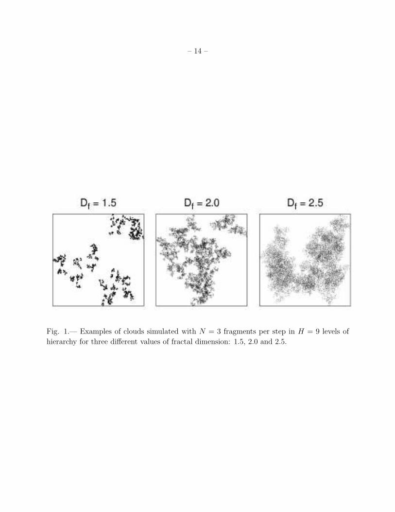
order to illustrate the appearance of the point distributions, Figure 1 shows examples of

projections of tri-dimensional fractals generated by using N = 3, H = 9 and three different

values of fractal dimension (Df = 1.5, 2.0 and 2.5).

2.1. Fractal Dimension Estimation

In the following, we will focus our attention on the empirical determination of the

fractal dimension both for the simulated clouds and for their two-dimensional projections. In

general, a fractal can be defined as a set of points whose Hausdorff dimension DH is strictly

larger than its topological dimension DT (Mandelbrot 1983). To estimate the Hausdorff

dimension authors normally use working definitions which fit their method and needs, and

thus there is not a unique definition of fractal dimension. In general, a fractal quantity is

a number which is connected to some length l in a manner like A ∼ lDA, where DA would

be the (constant) dimension associated to the quantity A. The most straightforward way

to estimate the Hausdorff dimension of a fractal set is through the box-counting method,

based on the fact that the number of boxes, N(r), having side r needed to cover a fractal

object varies as r−DB , being DB an estimation of DH (Mandelbrot 1983) which is called

the “box-counting dimension” (or “capacity”). Then, if we cover the object with a grid and

count the number N(r) of occupied cells of size r, we can compute

DB = − limr→0

log N(r)

log r. (1)

In practice DB corresponds with the slope of the best fit in a log N− log r plot, but obviously

the range where this scale law is valid in real (finite) fractals is limited to the range between

the smallest measurable region (the resolution) and the object size.

The major problem with the box-counting method is that it leads to imprecise results

because of its sensitivity to, for example, the placement and orientation of the grid and

1We avoid superposition because the tests made allowing superposition showed that the properties are

modified in such a way that it appears a multifractal behavior and a unique fractal dimension can not be

defined in a wide scale range

– 5 –

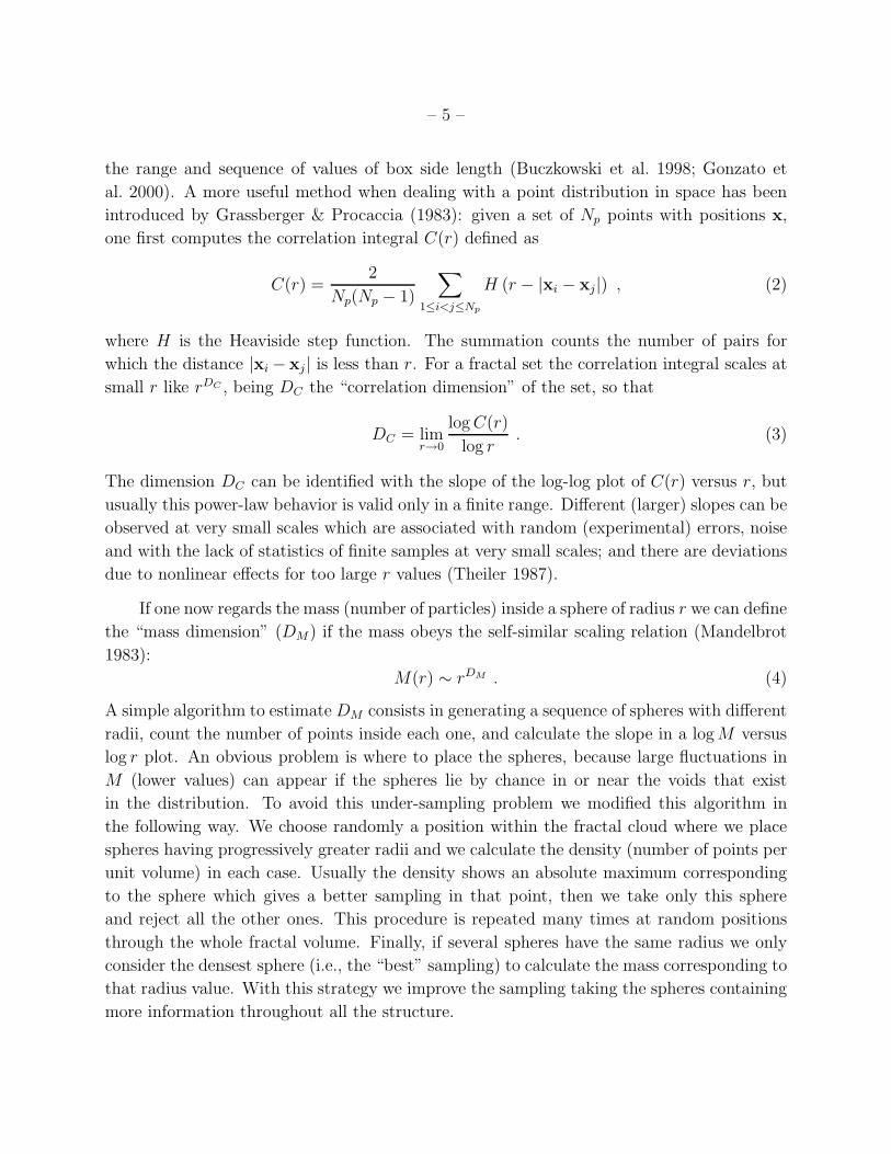
the range and sequence of values of box side length (Buczkowski et al. 1998; Gonzato et

al. 2000). A more useful method when dealing with a point distribution in space has been

introduced by Grassberger & Procaccia (1983): given a set of Np points with positions x,

one first computes the correlation integral C(r) defined as

C(r) =2

Np(Np − 1)

∑

1≤i<j≤Np

H (r − |xi − xj|) , (2)

where H is the Heaviside step function. The summation counts the number of pairs for

which the distance |xi − xj | is less than r. For a fractal set the correlation integral scales at

small r like rDC , being DC the “correlation dimension” of the set, so that

DC = limr→0

log C(r)

log r. (3)

The dimension DC can be identified with the slope of the log-log plot of C(r) versus r, but

usually this power-law behavior is valid only in a finite range. Different (larger) slopes can be

observed at very small scales which are associated with random (experimental) errors, noise

and with the lack of statistics of finite samples at very small scales; and there are deviations

due to nonlinear effects for too large r values (Theiler 1987).

If one now regards the mass (number of particles) inside a sphere of radius r we can define

the “mass dimension” (DM) if the mass obeys the self-similar scaling relation (Mandelbrot

1983):

M(r) ∼ rDM . (4)

A simple algorithm to estimate DM consists in generating a sequence of spheres with different

radii, count the number of points inside each one, and calculate the slope in a log M versus

log r plot. An obvious problem is where to place the spheres, because large fluctuations in

M (lower values) can appear if the spheres lie by chance in or near the voids that exist

in the distribution. To avoid this under-sampling problem we modified this algorithm in

the following way. We choose randomly a position within the fractal cloud where we place

spheres having progressively greater radii and we calculate the density (number of points per

unit volume) in each case. Usually the density shows an absolute maximum corresponding

to the sphere which gives a better sampling in that point, then we take only this sphere

and reject all the other ones. This procedure is repeated many times at random positions

through the whole fractal volume. Finally, if several spheres have the same radius we only

consider the densest sphere (i.e., the “best” sampling) to calculate the mass corresponding to

that radius value. With this strategy we improve the sampling taking the spheres containing

more information throughout all the structure.

– 6 –

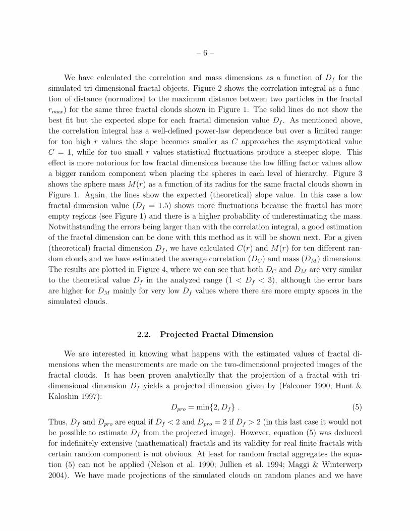
We have calculated the correlation and mass dimensions as a function of Df for the

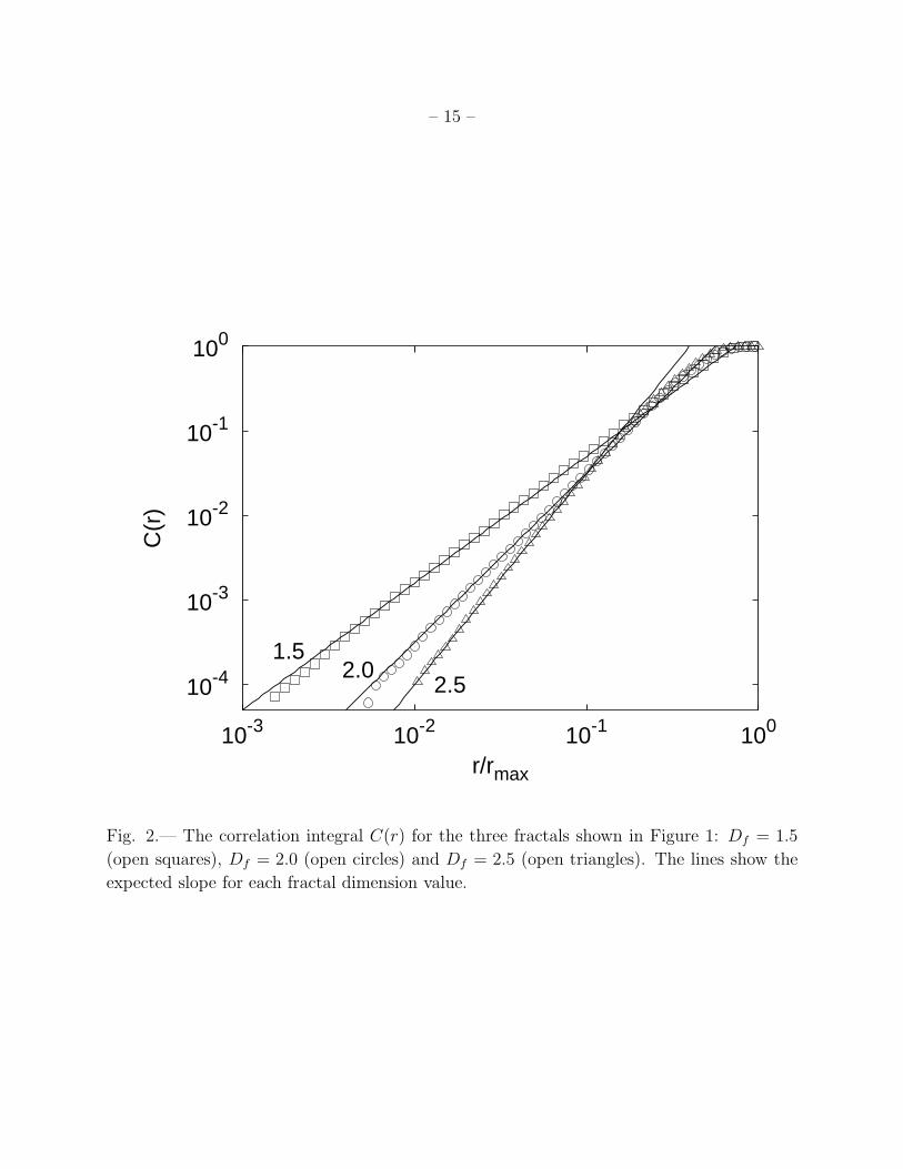
simulated tri-dimensional fractal objects. Figure 2 shows the correlation integral as a func-

tion of distance (normalized to the maximum distance between two particles in the fractal

rmax) for the same three fractal clouds shown in Figure 1. The solid lines do not show the

best fit but the expected slope for each fractal dimension value Df . As mentioned above,

the correlation integral has a well-defined power-law dependence but over a limited range:

for too high r values the slope becomes smaller as C approaches the asymptotical value

C = 1, while for too small r values statistical fluctuations produce a steeper slope. This

effect is more notorious for low fractal dimensions because the low filling factor values allow

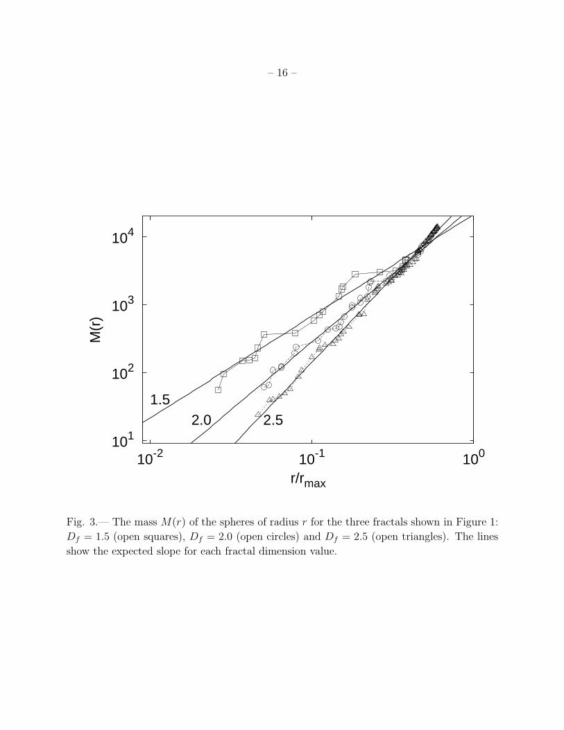
a bigger random component when placing the spheres in each level of hierarchy. Figure 3

shows the sphere mass M(r) as a function of its radius for the same fractal clouds shown in

Figure 1. Again, the lines show the expected (theoretical) slope value. In this case a low

fractal dimension value (Df = 1.5) shows more fluctuations because the fractal has more

empty regions (see Figure 1) and there is a higher probability of underestimating the mass.

Notwithstanding the errors being larger than with the correlation integral, a good estimation

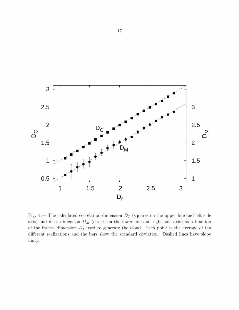
of the fractal dimension can be done with this method as it will be shown next. For a given

(theoretical) fractal dimension Df , we have calculated C(r) and M(r) for ten different ran-

dom clouds and we have estimated the average correlation (DC) and mass (DM) dimensions.

The results are plotted in Figure 4, where we can see that both DC and DM are very similar

to the theoretical value Df in the analyzed range (1 < Df < 3), although the error bars

are higher for DM mainly for very low Df values where there are more empty spaces in the

simulated clouds.

2.2. Projected Fractal Dimension

We are interested in knowing what happens with the estimated values of fractal di-

mensions when the measurements are made on the two-dimensional projected images of the

fractal clouds. It has been proven analytically that the projection of a fractal with tri-

dimensional dimension Df yields a projected dimension given by (Falconer 1990; Hunt &

Kaloshin 1997):

Dpro = min{2, Df} . (5)

Thus, Df and Dpro are equal if Df < 2 and Dpro = 2 if Df > 2 (in this last case it would not

be possible to estimate Df from the projected image). However, equation (5) was deduced

for indefinitely extensive (mathematical) fractals and its validity for real finite fractals with

certain random component is not obvious. At least for random fractal aggregates the equa-

tion (5) can not be applied (Nelson et al. 1990; Jullien et al. 1994; Maggi & Winterwerp

2004). We have made projections of the simulated clouds on random planes and we have

– 7 –

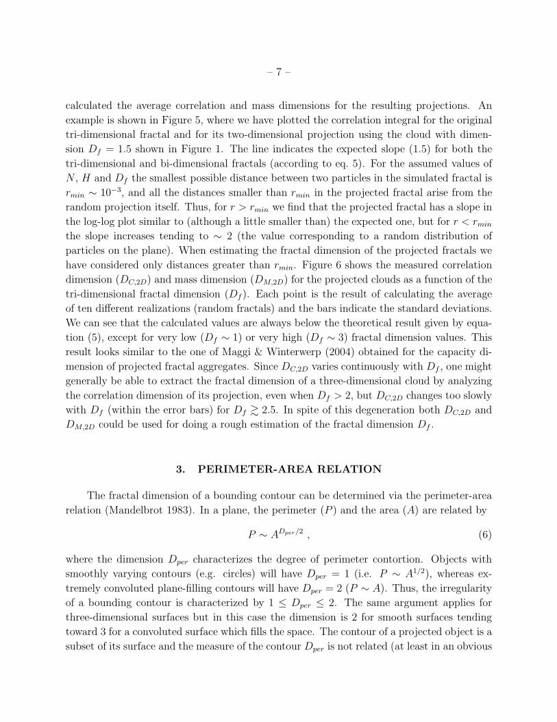
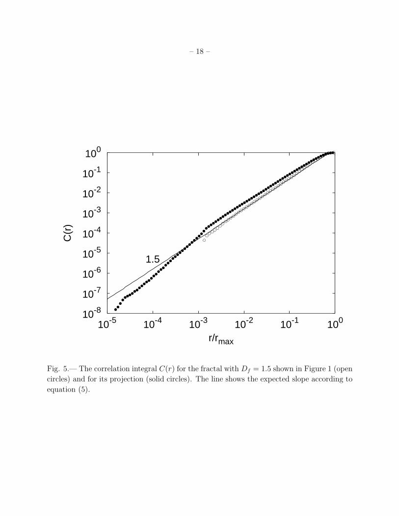
calculated the average correlation and mass dimensions for the resulting projections. An

example is shown in Figure 5, where we have plotted the correlation integral for the original

tri-dimensional fractal and for its two-dimensional projection using the cloud with dimen-

sion Df = 1.5 shown in Figure 1. The line indicates the expected slope (1.5) for both the

tri-dimensional and bi-dimensional fractals (according to eq. 5). For the assumed values of

N , H and Df the smallest possible distance between two particles in the simulated fractal is

rmin ∼ 10−3, and all the distances smaller than rmin in the projected fractal arise from the

random projection itself. Thus, for r > rmin we find that the projected fractal has a slope in

the log-log plot similar to (although a little smaller than) the expected one, but for r < rmin

the slope increases tending to ∼ 2 (the value corresponding to a random distribution of

particles on the plane). When estimating the fractal dimension of the projected fractals we

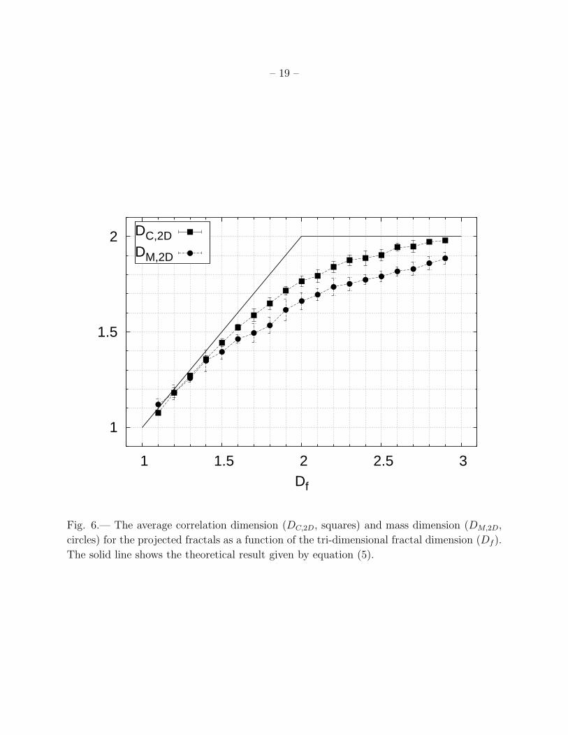
have considered only distances greater than rmin. Figure 6 shows the measured correlation

dimension (DC,2D) and mass dimension (DM,2D) for the projected clouds as a function of the

tri-dimensional fractal dimension (Df ). Each point is the result of calculating the average

of ten different realizations (random fractals) and the bars indicate the standard deviations.

We can see that the calculated values are always below the theoretical result given by equa-

tion (5), except for very low (Df ∼ 1) or very high (Df ∼ 3) fractal dimension values. This

result looks similar to the one of Maggi & Winterwerp (2004) obtained for the capacity di-

mension of projected fractal aggregates. Since DC,2D varies continuously with Df , one might

generally be able to extract the fractal dimension of a three-dimensional cloud by analyzing

the correlation dimension of its projection, even when Df > 2, but DC,2D changes too slowly

with Df (within the error bars) for Df & 2.5. In spite of this degeneration both DC,2D and

DM,2D could be used for doing a rough estimation of the fractal dimension Df .

3. PERIMETER-AREA RELATION

The fractal dimension of a bounding contour can be determined via the perimeter-area

relation (Mandelbrot 1983). In a plane, the perimeter (P ) and the area (A) are related by

P ∼ ADper/2 , (6)

where the dimension Dper characterizes the degree of perimeter contortion. Objects with

smoothly varying contours (e.g. circles) will have Dper = 1 (i.e. P ∼ A1/2), whereas ex-

tremely convoluted plane-filling contours will have Dper = 2 (P ∼ A). Thus, the irregularity

of a bounding contour is characterized by 1 ≤ Dper ≤ 2. The same argument applies for

three-dimensional surfaces but in this case the dimension is 2 for smooth surfaces tending

toward 3 for a convoluted surface which fills the space. The contour of a projected object is a

subset of its surface and the measure of the contour Dper is not related (at least in an obvious

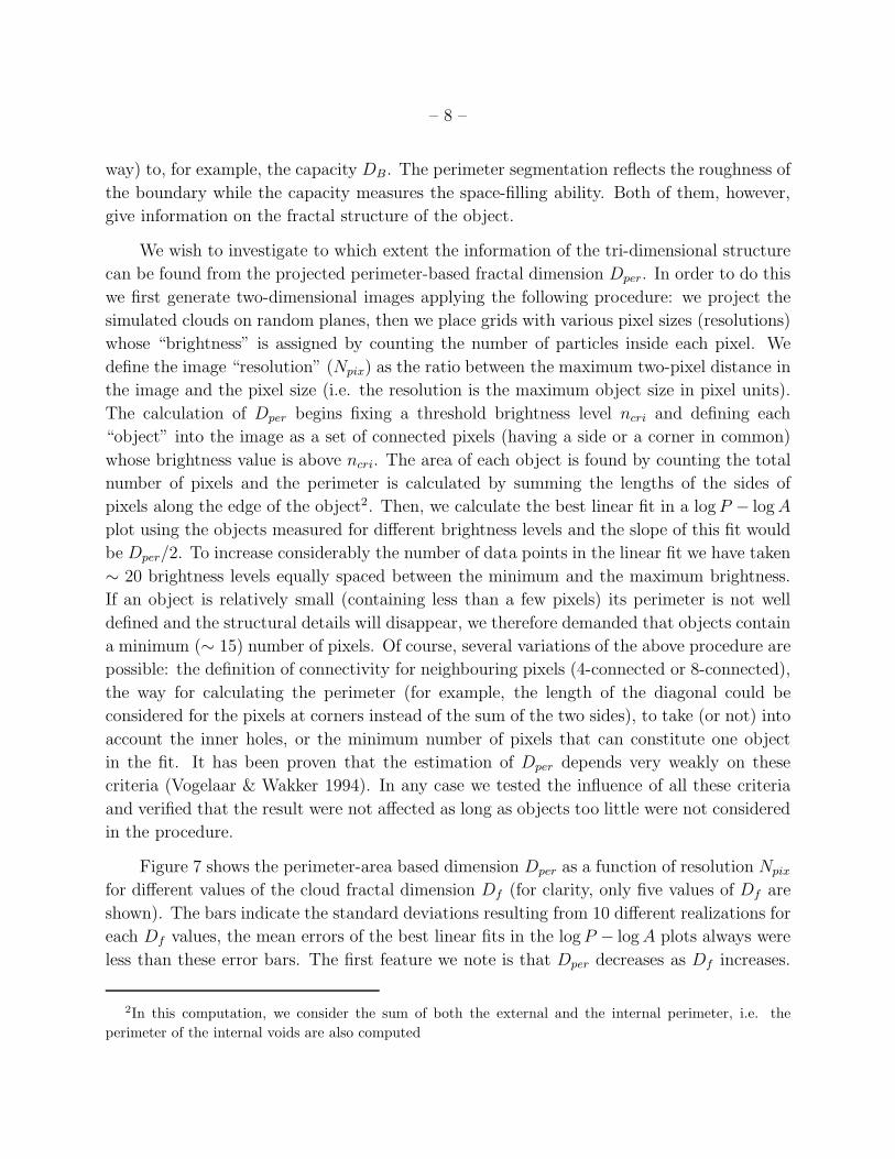
– 8 –

way) to, for example, the capacity DB. The perimeter segmentation reflects the roughness of

the boundary while the capacity measures the space-filling ability. Both of them, however,

give information on the fractal structure of the object.

We wish to investigate to which extent the information of the tri-dimensional structure

can be found from the projected perimeter-based fractal dimension Dper. In order to do this

we first generate two-dimensional images applying the following procedure: we project the

simulated clouds on random planes, then we place grids with various pixel sizes (resolutions)

whose “brightness” is assigned by counting the number of particles inside each pixel. We

define the image “resolution” (Npix) as the ratio between the maximum two-pixel distance in

the image and the pixel size (i.e. the resolution is the maximum object size in pixel units).

The calculation of Dper begins fixing a threshold brightness level ncri and defining each

“object” into the image as a set of connected pixels (having a side or a corner in common)

whose brightness value is above ncri. The area of each object is found by counting the total

number of pixels and the perimeter is calculated by summing the lengths of the sides of

pixels along the edge of the object2. Then, we calculate the best linear fit in a log P − log A

plot using the objects measured for different brightness levels and the slope of this fit would

be Dper/2. To increase considerably the number of data points in the linear fit we have taken

∼ 20 brightness levels equally spaced between the minimum and the maximum brightness.

If an object is relatively small (containing less than a few pixels) its perimeter is not well

defined and the structural details will disappear, we therefore demanded that objects contain

a minimum (∼ 15) number of pixels. Of course, several variations of the above procedure are

possible: the definition of connectivity for neighbouring pixels (4-connected or 8-connected),

the way for calculating the perimeter (for example, the length of the diagonal could be

considered for the pixels at corners instead of the sum of the two sides), to take (or not) into

account the inner holes, or the minimum number of pixels that can constitute one object

in the fit. It has been proven that the estimation of Dper depends very weakly on these

criteria (Vogelaar & Wakker 1994). In any case we tested the influence of all these criteria

and verified that the result were not affected as long as objects too little were not considered

in the procedure.

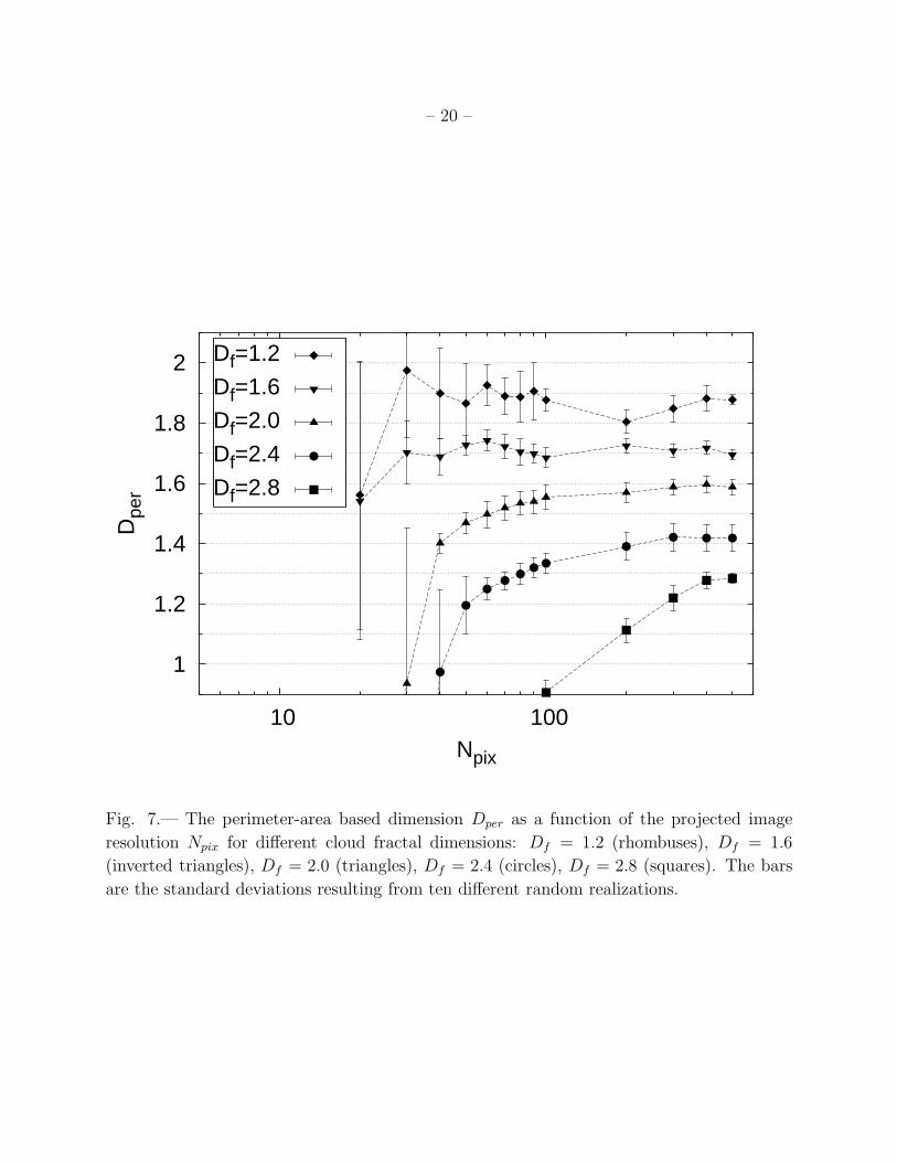
Figure 7 shows the perimeter-area based dimension Dper as a function of resolution Npix

for different values of the cloud fractal dimension Df (for clarity, only five values of Df are

shown). The bars indicate the standard deviations resulting from 10 different realizations for

each Df values, the mean errors of the best linear fits in the log P − log A plots always were

less than these error bars. The first feature we note is that Dper decreases as Df increases.

2In this computation, we consider the sum of both the external and the internal perimeter, i.e. the

perimeter of the internal voids are also computed

– 9 –

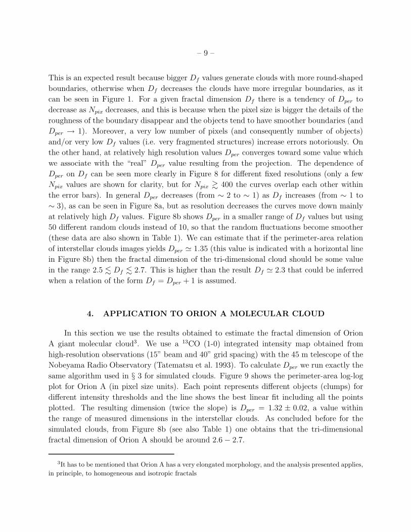
This is an expected result because bigger Df values generate clouds with more round-shaped

boundaries, otherwise when Df decreases the clouds have more irregular boundaries, as it

can be seen in Figure 1. For a given fractal dimension Df there is a tendency of Dper to

decrease as Npix decreases, and this is because when the pixel size is bigger the details of the

roughness of the boundary disappear and the objects tend to have smoother boundaries (and

Dper → 1). Moreover, a very low number of pixels (and consequently number of objects)

and/or very low Df values (i.e. very fragmented structures) increase errors notoriously. On

the other hand, at relatively high resolution values Dper converges toward some value which

we associate with the “real” Dper value resulting from the projection. The dependence of

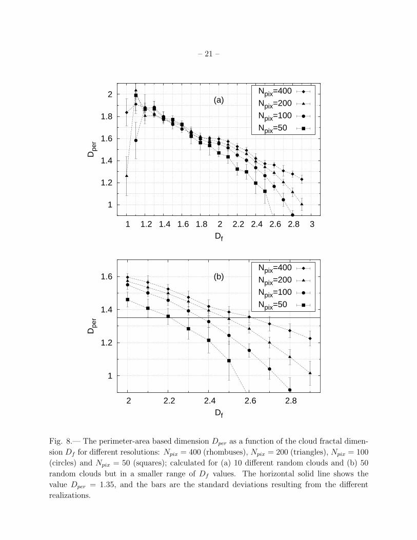
Dper on Df can be seen more clearly in Figure 8 for different fixed resolutions (only a few

Npix values are shown for clarity, but for Npix & 400 the curves overlap each other within

the error bars). In general Dper decreases (from ∼ 2 to ∼ 1) as Df increases (from ∼ 1 to

∼ 3), as can be seen in Figure 8a, but as resolution decreases the curves move down mainly

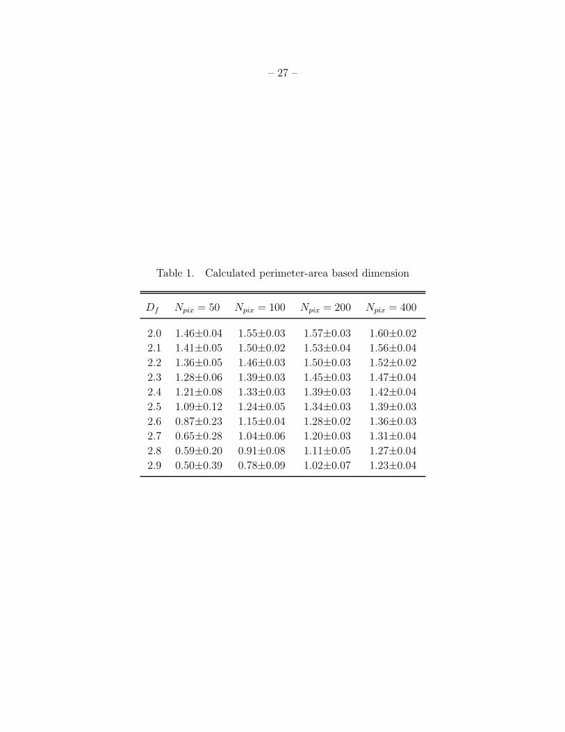
at relatively high Df values. Figure 8b shows Dper in a smaller range of Df values but using

50 different random clouds instead of 10, so that the random fluctuations become smoother

(these data are also shown in Table 1). We can estimate that if the perimeter-area relation

of interstellar clouds images yields Dper ≃ 1.35 (this value is indicated with a horizontal line

in Figure 8b) then the fractal dimension of the tri-dimensional cloud should be some value

in the range 2.5 . Df . 2.7. This is higher than the result Df ≃ 2.3 that could be inferred

when a relation of the form Df = Dper + 1 is assumed.

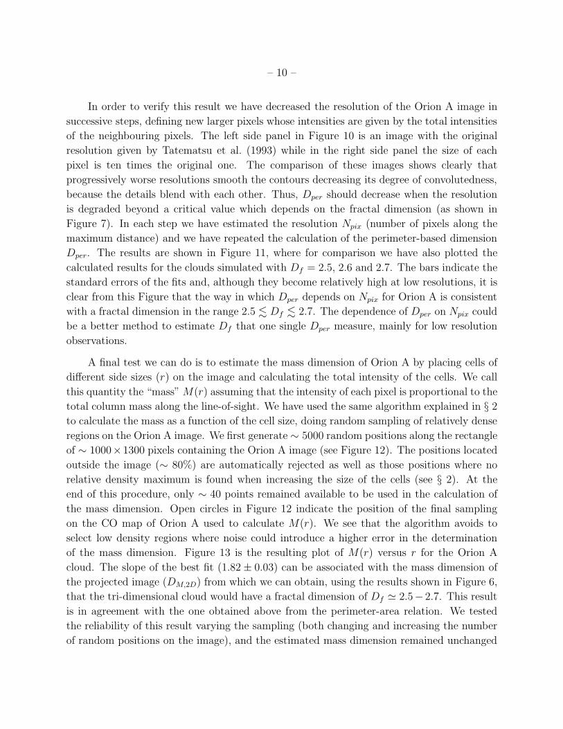
4. APPLICATION TO ORION A MOLECULAR CLOUD

In this section we use the results obtained to estimate the fractal dimension of Orion

A giant molecular cloud3. We use a 13CO (1-0) integrated intensity map obtained from

high-resolution observations (15” beam and 40” grid spacing) with the 45 m telescope of the

Nobeyama Radio Observatory (Tatematsu et al. 1993). To calculate Dper we run exactly the

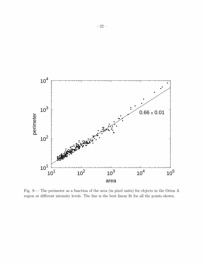
same algorithm used in § 3 for simulated clouds. Figure 9 shows the perimeter-area log-log

plot for Orion A (in pixel size units). Each point represents different objects (clumps) for

different intensity thresholds and the line shows the best linear fit including all the points

plotted. The resulting dimension (twice the slope) is Dper = 1.32 ± 0.02, a value within

the range of measured dimensions in the interstellar clouds. As concluded before for the

simulated clouds, from Figure 8b (see also Table 1) one obtains that the tri-dimensional

fractal dimension of Orion A should be around 2.6 − 2.7.

3It has to be mentioned that Orion A has a very elongated morphology, and the analysis presented applies,

in principle, to homogeneous and isotropic fractals

– 10 –

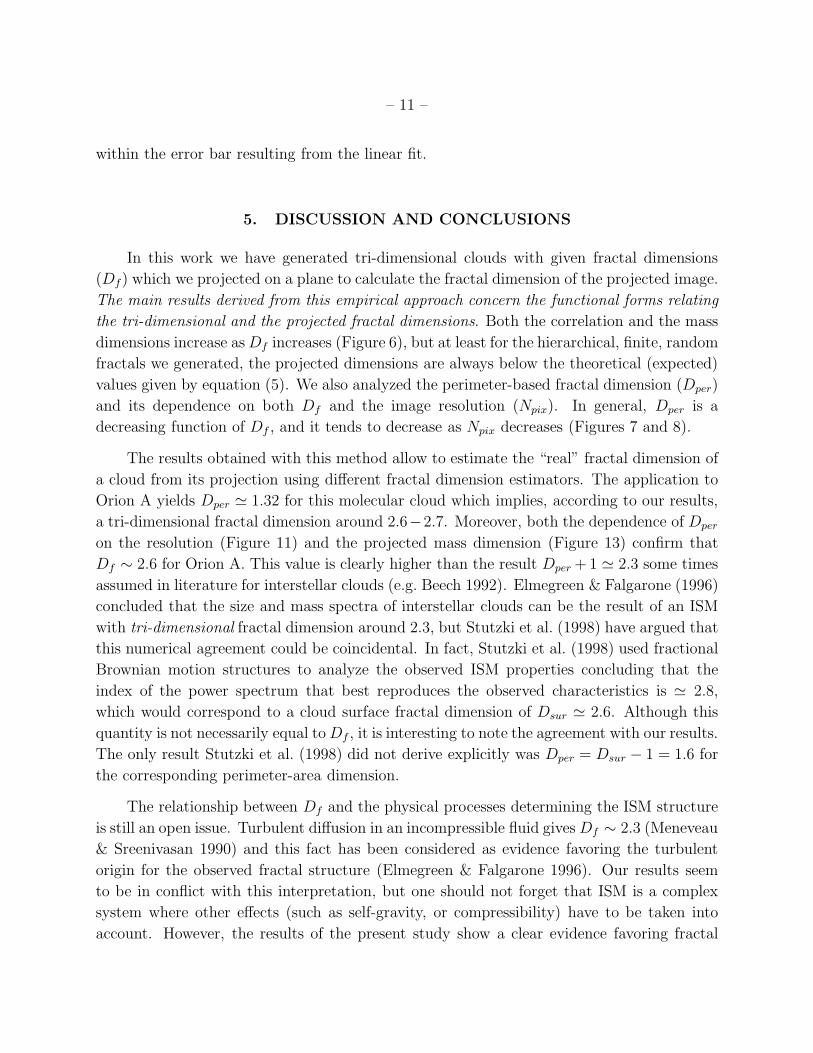
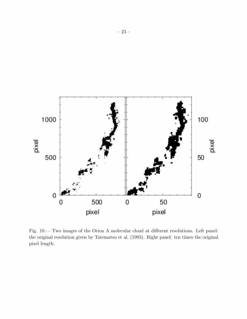
In order to verify this result we have decreased the resolution of the Orion A image in

successive steps, defining new larger pixels whose intensities are given by the total intensities

of the neighbouring pixels. The left side panel in Figure 10 is an image with the original

resolution given by Tatematsu et al. (1993) while in the right side panel the size of each

pixel is ten times the original one. The comparison of these images shows clearly that

progressively worse resolutions smooth the contours decreasing its degree of convolutedness,

because the details blend with each other. Thus, Dper should decrease when the resolution

is degraded beyond a critical value which depends on the fractal dimension (as shown in

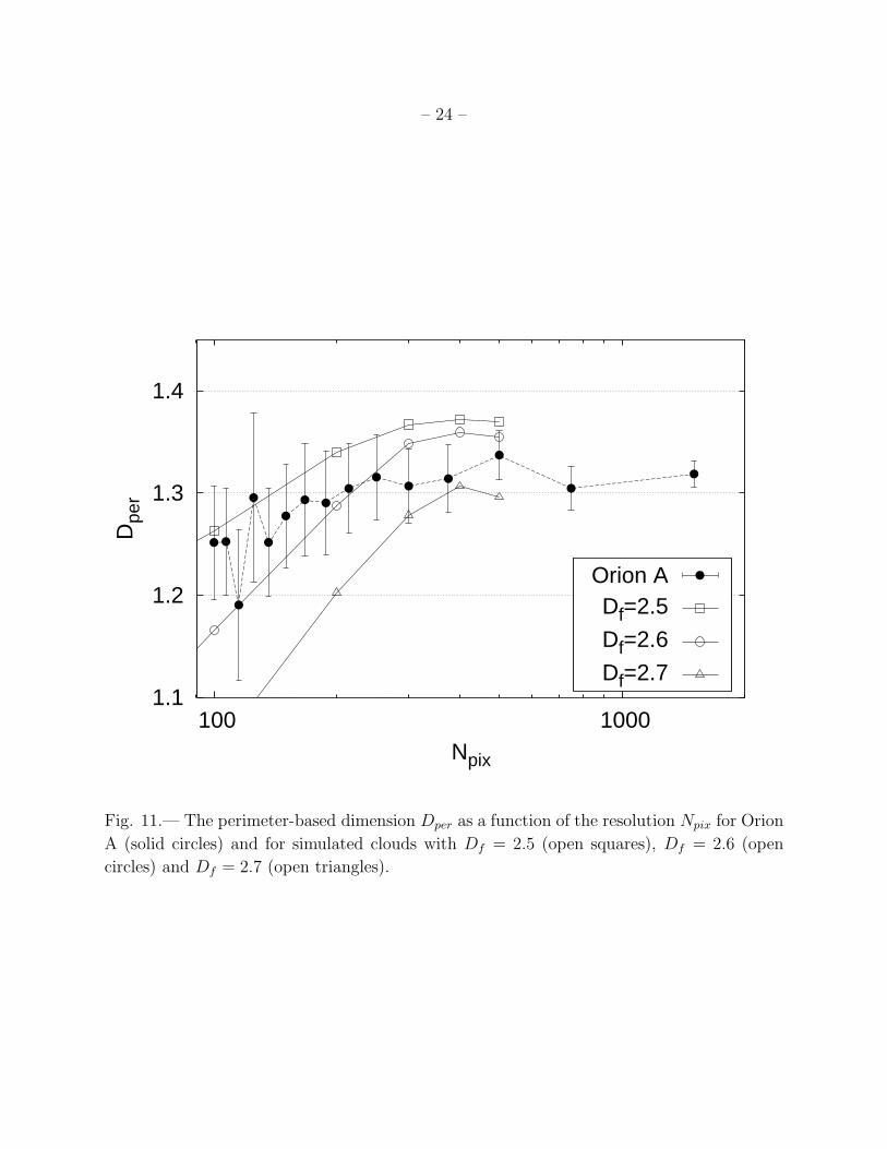
Figure 7). In each step we have estimated the resolution Npix (number of pixels along the

maximum distance) and we have repeated the calculation of the perimeter-based dimension

Dper. The results are shown in Figure 11, where for comparison we have also plotted the

calculated results for the clouds simulated with Df = 2.5, 2.6 and 2.7. The bars indicate the

standard errors of the fits and, although they become relatively high at low resolutions, it is

clear from this Figure that the way in which Dper depends on Npix for Orion A is consistent

with a fractal dimension in the range 2.5 . Df . 2.7. The dependence of Dper on Npix could

be a better method to estimate Df that one single Dper measure, mainly for low resolution

observations.

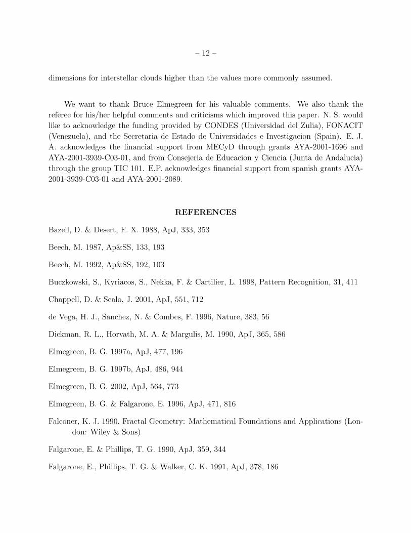
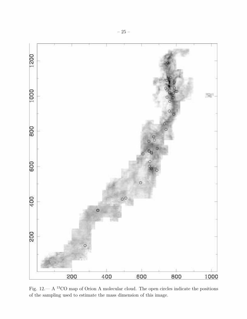
A final test we can do is to estimate the mass dimension of Orion A by placing cells of

different side sizes (r) on the image and calculating the total intensity of the cells. We call

this quantity the “mass” M(r) assuming that the intensity of each pixel is proportional to the

total column mass along the line-of-sight. We have used the same algorithm explained in § 2

to calculate the mass as a function of the cell size, doing random sampling of relatively dense

regions on the Orion A image. We first generate ∼ 5000 random positions along the rectangle

of ∼ 1000×1300 pixels containing the Orion A image (see Figure 12). The positions located

outside the image (∼ 80%) are automatically rejected as well as those positions where no

relative density maximum is found when increasing the size of the cells (see § 2). At the

end of this procedure, only ∼ 40 points remained available to be used in the calculation of

the mass dimension. Open circles in Figure 12 indicate the position of the final sampling

on the CO map of Orion A used to calculate M(r). We see that the algorithm avoids to

select low density regions where noise could introduce a higher error in the determination

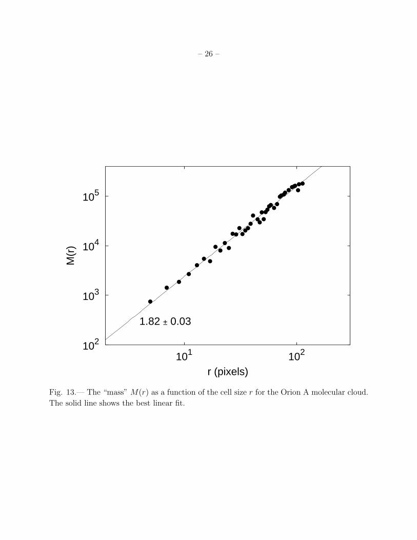
of the mass dimension. Figure 13 is the resulting plot of M(r) versus r for the Orion A

cloud. The slope of the best fit (1.82 ± 0.03) can be associated with the mass dimension of

the projected image (DM,2D) from which we can obtain, using the results shown in Figure 6,

that the tri-dimensional cloud would have a fractal dimension of Df ≃ 2.5− 2.7. This result

is in agreement with the one obtained above from the perimeter-area relation. We tested

the reliability of this result varying the sampling (both changing and increasing the number

of random positions on the image), and the estimated mass dimension remained unchanged

– 11 –

within the error bar resulting from the linear fit.

5. DISCUSSION AND CONCLUSIONS

In this work we have generated tri-dimensional clouds with given fractal dimensions

(Df) which we projected on a plane to calculate the fractal dimension of the projected image.

The main results derived from this empirical approach concern the functional forms relating

the tri-dimensional and the projected fractal dimensions. Both the correlation and the mass

dimensions increase as Df increases (Figure 6), but at least for the hierarchical, finite, random

fractals we generated, the projected dimensions are always below the theoretical (expected)

values given by equation (5). We also analyzed the perimeter-based fractal dimension (Dper)

and its dependence on both Df and the image resolution (Npix). In general, Dper is a

decreasing function of Df , and it tends to decrease as Npix decreases (Figures 7 and 8).

The results obtained with this method allow to estimate the “real” fractal dimension of

a cloud from its projection using different fractal dimension estimators. The application to

Orion A yields Dper ≃ 1.32 for this molecular cloud which implies, according to our results,

a tri-dimensional fractal dimension around 2.6−2.7. Moreover, both the dependence of Dper

on the resolution (Figure 11) and the projected mass dimension (Figure 13) confirm that

Df ∼ 2.6 for Orion A. This value is clearly higher than the result Dper + 1 ≃ 2.3 some times

assumed in literature for interstellar clouds (e.g. Beech 1992). Elmegreen & Falgarone (1996)

concluded that the size and mass spectra of interstellar clouds can be the result of an ISM

with tri-dimensional fractal dimension around 2.3, but Stutzki et al. (1998) have argued that

this numerical agreement could be coincidental. In fact, Stutzki et al. (1998) used fractional

Brownian motion structures to analyze the observed ISM properties concluding that the

index of the power spectrum that best reproduces the observed characteristics is ≃ 2.8,

which would correspond to a cloud surface fractal dimension of Dsur ≃ 2.6. Although this

quantity is not necessarily equal to Df , it is interesting to note the agreement with our results.

The only result Stutzki et al. (1998) did not derive explicitly was Dper = Dsur − 1 = 1.6 for

the corresponding perimeter-area dimension.

The relationship between Df and the physical processes determining the ISM structure

is still an open issue. Turbulent diffusion in an incompressible fluid gives Df ∼ 2.3 (Meneveau

& Sreenivasan 1990) and this fact has been considered as evidence favoring the turbulent

origin for the observed fractal structure (Elmegreen & Falgarone 1996). Our results seem

to be in conflict with this interpretation, but one should not forget that ISM is a complex

system where other effects (such as self-gravity, or compressibility) have to be taken into

account. However, the results of the present study show a clear evidence favoring fractal

– 12 –

dimensions for interstellar clouds higher than the values more commonly assumed.

We want to thank Bruce Elmegreen for his valuable comments. We also thank the

referee for his/her helpful comments and criticisms which improved this paper. N. S. would

like to acknowledge the funding provided by CONDES (Universidad del Zulia), FONACIT

(Venezuela), and the Secretaria de Estado de Universidades e Investigacion (Spain). E. J.

A. acknowledges the financial support from MECyD through grants AYA-2001-1696 and

AYA-2001-3939-C03-01, and from Consejeria de Educacion y Ciencia (Junta de Andalucia)

through the group TIC 101. E.P. acknowledges financial support from spanish grants AYA-

2001-3939-C03-01 and AYA-2001-2089.

REFERENCES

Bazell, D. & Desert, F. X. 1988, ApJ, 333, 353

Beech, M. 1987, Ap&SS, 133, 193

Beech, M. 1992, Ap&SS, 192, 103

Buczkowski, S., Kyriacos, S., Nekka, F. & Cartilier, L. 1998, Pattern Recognition, 31, 411

Chappell, D. & Scalo, J. 2001, ApJ, 551, 712

de Vega, H. J., Sanchez, N. & Combes, F. 1996, Nature, 383, 56

Dickman, R. L., Horvath, M. A. & Margulis, M. 1990, ApJ, 365, 586

Elmegreen, B. G. 1997a, ApJ, 477, 196

Elmegreen, B. G. 1997b, ApJ, 486, 944

Elmegreen, B. G. 2002, ApJ, 564, 773

Elmegreen, B. G. & Falgarone, E. 1996, ApJ, 471, 816

Falconer, K. J. 1990, Fractal Geometry: Mathematical Foundations and Applications (Lon-

don: Wiley & Sons)

Falgarone, E. & Phillips, T. G. 1990, ApJ, 359, 344

Falgarone, E., Phillips, T. G. & Walker, C. K. 1991, ApJ, 378, 186

– 13 –

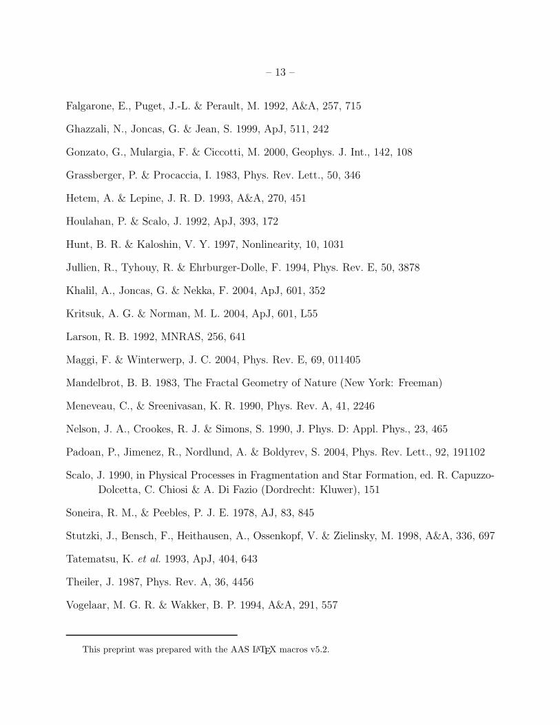
Falgarone, E., Puget, J.-L. & Perault, M. 1992, A&A, 257, 715

Ghazzali, N., Joncas, G. & Jean, S. 1999, ApJ, 511, 242

Gonzato, G., Mulargia, F. & Ciccotti, M. 2000, Geophys. J. Int., 142, 108

Grassberger, P. & Procaccia, I. 1983, Phys. Rev. Lett., 50, 346

Hetem, A. & Lepine, J. R. D. 1993, A&A, 270, 451

Houlahan, P. & Scalo, J. 1992, ApJ, 393, 172

Hunt, B. R. & Kaloshin, V. Y. 1997, Nonlinearity, 10, 1031

Jullien, R., Tyhouy, R. & Ehrburger-Dolle, F. 1994, Phys. Rev. E, 50, 3878

Khalil, A., Joncas, G. & Nekka, F. 2004, ApJ, 601, 352

Kritsuk, A. G. & Norman, M. L. 2004, ApJ, 601, L55

Larson, R. B. 1992, MNRAS, 256, 641

Maggi, F. & Winterwerp, J. C. 2004, Phys. Rev. E, 69, 011405

Mandelbrot, B. B. 1983, The Fractal Geometry of Nature (New York: Freeman)

Meneveau, C., & Sreenivasan, K. R. 1990, Phys. Rev. A, 41, 2246

Nelson, J. A., Crookes, R. J. & Simons, S. 1990, J. Phys. D: Appl. Phys., 23, 465

Padoan, P., Jimenez, R., Nordlund, A. & Boldyrev, S. 2004, Phys. Rev. Lett., 92, 191102

Scalo, J. 1990, in Physical Processes in Fragmentation and Star Formation, ed. R. Capuzzo-

Dolcetta, C. Chiosi & A. Di Fazio (Dordrecht: Kluwer), 151

Soneira, R. M., & Peebles, P. J. E. 1978, AJ, 83, 845

Stutzki, J., Bensch, F., Heithausen, A., Ossenkopf, V. & Zielinsky, M. 1998, A&A, 336, 697

Tatematsu, K. et al. 1993, ApJ, 404, 643

Theiler, J. 1987, Phys. Rev. A, 36, 4456

Vogelaar, M. G. R. & Wakker, B. P. 1994, A&A, 291, 557

This preprint was prepared with the AAS LATEX macros v5.2.

– 14 –

Fig. 1.— Examples of clouds simulated with N = 3 fragments per step in H = 9 levels of

hierarchy for three different values of fractal dimension: 1.5, 2.0 and 2.5.

– 15 –

10-4

10-3

10-2

10-1

100

10-3 10-2 10-1 100

C(r

)

r/rmax

1.52.0

2.5

Fig. 2.— The correlation integral C(r) for the three fractals shown in Figure 1: Df = 1.5

(open squares), Df = 2.0 (open circles) and Df = 2.5 (open triangles). The lines show the

expected slope for each fractal dimension value.

– 16 –

101

102

103

104

10-2 10-1 100

M(r

)

r/rmax

1.52.0 2.5

Fig. 3.— The mass M(r) of the spheres of radius r for the three fractals shown in Figure 1:

Df = 1.5 (open squares), Df = 2.0 (open circles) and Df = 2.5 (open triangles). The lines

show the expected slope for each fractal dimension value.

– 17 –

0.5

1

1.5

2

2.5

3

1 1.5 2 2.5 3

1

1.5

2

2.5

3

DC

DM

Df

DC

DM

Fig. 4.— The calculated correlation dimension DC (squares on the upper line and left side

axis) and mass dimension DM (circles on the lower line and right side axis) as a function

of the fractal dimension Df used to generate the cloud. Each point is the average of ten

different realizations and the bars show the standard deviation. Dashed lines have slope

unity.

– 18 –

10-8

10-7

10-6

10-5

10-4

10-3

10-2

10-1

100

10-5 10-4 10-3 10-2 10-1 100

C(r

)

r/rmax

1.5

Fig. 5.— The correlation integral C(r) for the fractal with Df = 1.5 shown in Figure 1 (open

circles) and for its projection (solid circles). The line shows the expected slope according to

equation (5).

– 19 –

1

1.5

2

1 1.5 2 2.5 3Df

DC,2D

DM,2D

Fig. 6.— The average correlation dimension (DC,2D, squares) and mass dimension (DM,2D,

circles) for the projected fractals as a function of the tri-dimensional fractal dimension (Df).

The solid line shows the theoretical result given by equation (5).

– 20 –

1

1.2

1.4

1.6

1.8

2

10 100

Dpe

r

Npix

Df=1.2

Df=1.6

Df=2.0

Df=2.4

Df=2.8

Fig. 7.— The perimeter-area based dimension Dper as a function of the projected image

resolution Npix for different cloud fractal dimensions: Df = 1.2 (rhombuses), Df = 1.6

(inverted triangles), Df = 2.0 (triangles), Df = 2.4 (circles), Df = 2.8 (squares). The bars

are the standard deviations resulting from ten different random realizations.

– 21 –

1

1.2

1.4

1.6

1.8

2

1 1.2 1.4 1.6 1.8 2 2.2 2.4 2.6 2.8 3

Dpe

r

Df

(a)Npix=400

Npix=200

Npix=100

Npix=50

1

1.2

1.4

1.6

2 2.2 2.4 2.6 2.8

Dpe

r

Df

(b)Npix=400

Npix=200

Npix=100

Npix=50

Fig. 8.— The perimeter-area based dimension Dper as a function of the cloud fractal dimen-

sion Df for different resolutions: Npix = 400 (rhombuses), Npix = 200 (triangles), Npix = 100

(circles) and Npix = 50 (squares); calculated for (a) 10 different random clouds and (b) 50

random clouds but in a smaller range of Df values. The horizontal solid line shows the

value Dper = 1.35, and the bars are the standard deviations resulting from the different

realizations.

– 22 –

101

102

103

104

101 102 103 104 105

perim

eter

area

0.66 ± 0.01

Fig. 9.— The perimeter as a function of the area (in pixel units) for objects in the Orion A

region at different intensity levels. The line is the best linear fit for all the points shown.

– 23 –

Fig. 10.— Two images of the Orion A molecular cloud at different resolutions. Left panel:

the original resolution given by Tatematsu et al. (1993). Right panel: ten times the original

pixel length.

– 24 –

1.1

1.2

1.3

1.4

100 1000

Dpe

r

Npix

Orion ADf=2.5

Df=2.6

Df=2.7

Fig. 11.— The perimeter-based dimension Dper as a function of the resolution Npix for Orion

A (solid circles) and for simulated clouds with Df = 2.5 (open squares), Df = 2.6 (open

circles) and Df = 2.7 (open triangles).

– 25 –

Fig. 12.— A 13CO map of Orion A molecular cloud. The open circles indicate the positions

of the sampling used to estimate the mass dimension of this image.

– 26 –

102

103

104

105

101 102

M(r

)

r (pixels)

1.82 ± 0.03

Fig. 13.— The “mass” M(r) as a function of the cell size r for the Orion A molecular cloud.

The solid line shows the best linear fit.

– 27 –

Table 1. Calculated perimeter-area based dimension

Df Npix = 50 Npix = 100 Npix = 200 Npix = 400

2.0 1.46±0.04 1.55±0.03 1.57±0.03 1.60±0.02

2.1 1.41±0.05 1.50±0.02 1.53±0.04 1.56±0.04

2.2 1.36±0.05 1.46±0.03 1.50±0.03 1.52±0.02

2.3 1.28±0.06 1.39±0.03 1.45±0.03 1.47±0.04

2.4 1.21±0.08 1.33±0.03 1.39±0.03 1.42±0.04

2.5 1.09±0.12 1.24±0.05 1.34±0.03 1.39±0.03

2.6 0.87±0.23 1.15±0.04 1.28±0.02 1.36±0.03

2.7 0.65±0.28 1.04±0.06 1.20±0.03 1.31±0.04

2.8 0.59±0.20 0.91±0.08 1.11±0.05 1.27±0.04

2.9 0.50±0.39 0.78±0.09 1.02±0.07 1.23±0.04