On fractal distribution function estimation and applications

Stefano M. Iacus e Davide La Torre

Working Paper n.07.2002 – marzo

Dipartimento di Economia Politica e AziendaleUniversità degli Studi di Milanovia Conservatorio, 720122 Milanotel. ++39/02/76074534fax ++39/02/76009695

E Mail: dipeco@unimi.it

Pubblicazione depositata presso gli Uffici Stampa della Procura della Repubblica e della Prefettura di Milano

On fractal distribution function estimation andapplications

Stefano M. Iacus∗ Davide La TorreUniversita degli Studi di Milano

Dipartimento di Economia Politica e AziendaleVia Conservatorio 7 - I-20122 Milano

March 8, 2002

Abstract

In this paper we review some recent results concerning the approximations of dis-tribution functions and measures on [0, 1] based on iterated function systems. The twodifferent approaches available in the literature are considered and their relation areinvestigated in the statistical perspective. In the second part of the paper we proposea new class of estimators for the distribution function and the related characteristicand density functions. Glivenko-Cantelli, LIL properties and local asymptotic minimaxefficiency are established for some of the proposed estimators. Via Monte Carlo anal-ysis we show that, for small sample sizes, the proposed estimator can be as efficient oreven better than the empirical distribution function and the kernel density estimatorrespectively. This paper is to be considered as a first attempt in the construction ofnew class of estimators based on fractal objects. Pontential applications to survivalanalysis with random censoring are proposed at the end of the paper.

1 Introduction

Let X1, X2, . . . , Xn be a sequence of i.i.d. random variables, each having a common contin-uous cumulative distribution function F of a real random variable X with values on [0, 1],

∗Address for correspondance: Stefano M. Iacus, Dipartimento di Economia e Politica Aziendale, ViaConservatorio 7, I-20122 Milano, Italy. E-mail: stefano.iacus@unimi.it

1

i.e. F (x) = P (X ≤ x). We let F be such that F (x) = 0, x ≤ 0 and F (x) = 1, x ≥ 1. Theempirical distribution function (e.d.f.)

Fn(x) =1

n

n∑i=1

1(Xi ≤ x)

is one commonly used estimator of the unknown distribution function F . Here 1(·) is theindicator function. The e.d.f. has an impressive set of good statistical properties such as itis first order efficient in the minimax sense (see Dvoretsky et al. 1956, Kiefer and Wolfowitz1959, Beran 1977, Levit 1978 and Millar 1979, Gill and Levit 1995). More or less recently,other second order efficient estimators have been proposed in the literature for special classesof distribution functions F . Golubev and Levit (1996a, b) and Efromovich(2001) are two ofsuch examples.

It is rather curious that a step-wise function can be such a good estimator and, in fact,Efromovich (2001) shows that, for the class of analytic functions, for small sample sizes, thee.d.f. is not the best estimator. Here we study the properties of a new class of distributionfunction estimators based on iterated function systems (IFSs). IFSs have been introduced inHutchinson (1981) and Barnsley and Demko (1985). These are particulary fractal objects,hence the title of this note. The fractal nature of IFSs based estimators implies that theyare nowhere differentiable and cannot be used to estimate density directly as in Efromovich(2001) but, to this end, we will show a Fourier analysis approach to bypass the problem.

The paper is organized as follows. Section 2 is dedicated to the theoretical background oftwo constructive methods of approximating measures and distribution functions respectively,with support on compact sets. The first method essentially consists in the minimizationapproach based on moment matching. This is rather common in the IFS literature. Thesecond approach attacks directly the problem of approximating a distribution function withan IFS, by imposing conditions on the graph of the IFS. In practice, it is imposed to theIFS to pass through a fixed grid of points. IFS for measures are usually used not in astatistical context but mainly for image compression, here the main goal will be the problemof reconstructing a distribution function from sampled data. Even if we do not treat theproblem here, the results are likely to hold for measures in any finite dimension [0, 1]k, k ≥ 1.In particular, the case k = 2 is interesting for image reconstruction.

Section 3 recalls some results on the Fourier transform for affine IFS. These results arerather important for Section 4 where we propose two kinds of IFS estimators and a densityestimator obtained as a Fourier series estimator. We also study the asymptotic propertiesof one of the two estimators. In particular, we will present a Glivenko-Cantelli theorem, alaw of iterated logarithm property and the local asymptotic minimax efficiency. Section 5 isdedicated to the Monte Carlo analysis on small sample sizes.

2

2 Theoretical background for affine IFSs

In this section we recall some of the results from Forte and Vrscay (1995) and Iacus and LaTorre (2001) concerning the IFSs setup on the the space of distribution function. Let M(X)be the set of probability measures on B(X), the σ-algebra of Borel subsets of X where (X, d)is a compact metric space (in our case will be X = [0, 1] and d the Euclidean metric.)

In the IFS literature the following Hutchinson metric plays a crucial role

dH(µ, ν) = supf∈Lip(X)

{∫X

fdµ−∫

X

fdν

}, µ, ν ∈M(X)

whereLip(X) = {f : X → R, |f(x)− f(y)| ≤ d(x, y), x, y ∈ X}

thus (M(X), dH) is a complete metric space (see Hutchinson, 1981).

As usual, we denote by (w,p) an N -maps contractive IFS on X with probabilities or simplyan N -maps IFS, that is, a set of N affine contractions maps, w = (w1, w2, . . . , wN),

wi = si x+ ai, with |si| < 1, si, ai ∈ R, i = 1, 2, . . . , N,

with associated probabilities p = (p1, p2, . . . , pN), pi ≥ 0, and∑N

i=1 pi = 1. The IFS has acontractivity factor defined as

c = max1≤i≤N

|si| < 1

Consider the following (usually called Markov) operator M : M(X) →M(X) defined as

Mµ =N∑

i=1

piµ ◦ w−1i , µ ∈M(X), (1)

where w−1i is the inverse function of wi and ◦ stands for the composition. In Hutchinson

(1981) it was shown that M is a contraction mapping on (M(X), dH): for all µ, ν ∈ (X),dH(Mµ,Mν) ≤ cdH(µ, ν). Thus, there exists a unique measure µ ∈ M(X), the invariantmeasure of the IFS, such that Mµ = µ by Banach theorem.

2.1 Minimization approach

For affine IFS there exist a simple and useful relation between the moments of probabilitymeasures on M(X). Given an N -maps IFS(w,p) with associated Markov operator M , andgiven a measure µ ∈M(X) then, for any continuous function f : X → R,∫

X

f(x)dν(x) =

∫X

f(x)d(Mµ)(x) =N∑

i=1

pi

∫X

(f ◦ wi)(x)dµ(x) , (2)

3

where ν = Mµ. In our case X = [0, 1] ⊂ R so we readly have a relation involving themoments of µ and ν. Let

gk =

∫X

xkdµ, hk =

∫X

xkdν, k = 0, 1, 2, . . . , (3)

be the moments of the two measures, with g0 = h0 = 1. Then, by (2), with f(x) = xk, wehave

hk =k∑

j=0

(k

j

){ N∑i=1

pisjia

k−ji

}gj, k = 1, 2, . . . , .

Recursive relations for the moments and more details on polynomial IFSs can be found inForte and Vrscay (1995). The following theorem is due to Vrscay and can be found in Forteand Vrscay (1995) as well.

Theorem 1. Set X = [0, 1] and let µ and µ(j) ∈ M(X), j = 1, 2, . . . with associatedmoments of any order gk and

g(j)k =

∫X

xkdµ(j) .

Then, the following statements are equivalent (as j →∞ and ∀k ≥ 0):

i) g(j)k → gk,

ii) ∀f ∈ C(X),∫

Xfdµ(j) →

∫Xfdµ , (weak* convergence),

iii) dH(µ(j), µ) → 0.

(here C(X) is the space of continuous functions on X). This theorem gives a way to findand appropriate set of maps and probabilities by solving the so called problem of momentmatching. With the solution in hands, given the convergence of the moments, we also havethe convergence of the measures and then the stationary measure of M approximates withgiven precision (in a sense specified by the collage theorem below) the target measure µ (seeBarnsley and Demko, 1985).

Next theorem, called the collage theorem is a standard result of IFS theory and is a conse-quence of Banach theorem.

Theorem 2 (Collage theorem). Let (Y, dY ) be a complete metric space. Given an y ∈ Y ,suppose that there exists a contractive map f on Y with contractivity factor 0 ≤ c < 1 suchthat dY (y, f(y)) < ε. If y is the fixed point of f , i.e. f(y) = y, then dY (y, y) < ε

1−c.

So if one wishes to approximate a function y with the fixed point y of an unknown contractivemap f , it is only needed to solve the inverse problem of finding f which minimizes the collagedistance dY (y, f(y)).

4

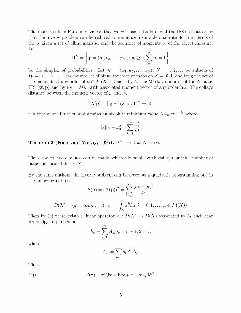
The main result in Forte and Vrscay that we will use to build one of the IFSs estimators isthat the inverse problem can be reduced to minimize a suitable quadratic form in terms ofthe pi given a set of affine maps wi and the sequence of moments gk of the target measure.Let

ΠN =

{p = (p1, p2, . . . , pN) : pi ≥ 0,

N∑i=1

pi = 1

}be the simplex of probabilities. Let w = (w1, w2, . . . , wN), N = 1, 2, . . . be subsets ofW = {w1, w2, . . .} the infinite set of affine contractive maps on X = [0, 1] and let g the set ofthe moments of any order of µ ∈M(X). Denote by M the Markov operator of the N -mapsIFS (w,p) and by νN = Mµ, with associated moment vector of any order hN . The collagedistance between the moment vector of µ and νN

∆(p) = ||g − hN ||l2 : ΠN → R

is a continuous function and attains an absolute minimum value ∆min on ΠN where

||x||l2 = x20 +

∞∑k=1

x2k

k2.

Theorem 3 (Forte and Vrscay, 1995). ∆Nmin → 0 as N →∞.

Thus, the collage distance can be made arbitrarily small by choosing a suitable number ofmaps and probabilities, N∗.

By the same authors, the inverse problem can be posed as a quadratic programming one inthe following notation

S(p) = (∆(p))2 =∞∑

k=1

(hk − gk)2

k2

D(X) = {g = (g0, g1, . . .) : gk =

∫X

xkdµ, k = 0, 1, . . . , µ ∈M(X)}

Then by (2) there exists a linear operator A : D(X) → D(X) associated to M such thathN = Ag. In particular

hk =N∑

i=1

Akipi, k = 1, 2, . . . ,

where

Aki =n∑

j=0

sjia

k−ji gj

Thus

(Q) S(x) = xtQx + btx + c, x ∈ RN ,

5

where

qij =∞∑

k=1

AkiAkj

k2, i, j = 1, 2, . . . , N,

bi = −2∞∑

k=1

gk

k2Aki, i = 1, 2, . . . , N and c =

∞∑k=1

g2k

k2.

The series above are convergent as 0 ≤ Ani ≤ 1 and the minimum can be found by minimizingthe quadratic form on the simplex ΠN . This is the main result in Forte and Vrscay (1995)that can be used straight forwardly in statistical applications as we propose in Section 4.

On the other side Iacus and La Torre (2001) propose a different and direct approach toconstruction on IFSs on the space of distribution function on [0, 1]. Instead of constructingthe IFS by matching the moments, the idea there is to have an IFS that has the same valuesof the target distribution function on a finite number of points.

2.2 Direct approach

We use directly the fractal nature of the IFS. Given a distribution function on [0, 1], the ideais to rescale the whole function in abscissa and ordinate and copying it a number of timesobtaining a function that is again a distribution function. Consider F([0, 1]), the spaceof distribution functions on [0, 1], then (F([0, 1]), d∞) is a complete metric space, whered∞(F,G) = supx∈[0,1] |F (x)−G(x)|.

Let N ∈ N be fixed and let:

i) wi : [ai, bi) → [ci, di) = wi([ai, bi)), i = 1, . . . , N − 1, wN : [aN , bN ] → [cN , dN ], witha1 = c1 = 0 and bN = dN = 1;

ii) wi, i = 1 . . . N , are increasing and continuous;

iii)N−1⋃i=1

[ci, di) ∪ [cN , dN ] = [0, 1];

iv) if i 6= j then [ci, di) ∩ [cj, dj) = ∅.

v) pi ≥ 0, i = 1, . . . , N , δi ≥ 0, i = 1 . . . N − 1,N∑

i=1

pi +N−1∑i=1

δi = 1.

6

On (F([0, 1]), d∞) we define an operator in the following way (see Iacus and La Torre, 2001):

TF (x) =

p1F (w−11 (x)), x ∈ [c1, d1)

piF (w−1i (x)) +

i−1∑j=1

pj +i−1∑j=1

δj , x ∈ [ci, di) , i = 2, . . . , N − 1

pNF (w−1N (x)) +

N−1∑j=1

pj +N−1∑j=1

δj , x ∈ [cN , dN ]

(4)

where F ∈ F([0, 1]). From now on we assume that wi are affine maps of the form wi(x) =six + ai, with 0 < si < 1 and ai ∈ R. Remark that the new distribution function TF isunion of distorted copies of F ; this is the fractal nature of the operator.

TF (x) = piF (w−1i (x)) +

i−1∑j=1

pj +i−1∑j=1

δj , x ∈ wi([ai, bi)) , (5)

where F ∈ F([0, 1]), N ∈ N is fixed and:

i) wi : [ai, bi) → [ci, di) = wi([ai, bi)), i = 1, . . . , N − 1, wN : [aN , bN ] → [cN , dN ], with

a1 = c1 = 0 and bN = dN = 1,N−1⋃i=1

[ai, bi) ∪ [aN , bN ] =k−1⋃i=1

[ci, di) ∪ [cN , dN ] = [0, 1];

ii) wi = si x+ ai, 0 < si < 1, si, ai ∈ R, i = 1 . . . N ;

iii)N⋃

i=1

wi([ai, bi)) = [0, 1);

iv) pi ≥ 0, i = 1, . . . , N , δi ≥ 0, i = 1 . . . N − 1,N∑

i=1

pi +N−1∑i=1

δi = 1;

v) if i 6= j then wi([ai, bi)) ∩ wj([aj, bj)) = ∅;

We limit the treatise to affine maps wi as in Forte and Vrscay (1995), but the general case ofincreasing and continuous maps can be treated as well (see cited reference of the authors).From now on, we consider the sets of maps wi and parameters δi as given, thus the operatordepends only on the probabilities pi and we denote it by Tp.

Theorem 4 (Iacus and La Torre, 2001). Under conditions i) to v):

1. Tp is an operator from F([0, 1]) to itself.

2. Suppose that wi(x) = x, pi = p, and δi ≥ −p, then Tp : F([0, 1]) → F([0, 1]).

3. If c = maxi=1,...,N

pi < 1, then Tp is a contraction on (F([0, 1]), d∞) with contractivity

constant c.

7

4. Let p, p∗ ∈ Rk such that TpF1 = F1 and Tp∗F2 = F2. Then

d∞(F1, F2) ≤1

1− c

N∑j=1

∣∣pj − p∗j∣∣

where c is the contractivity constant of Tp.

The theorem above assures the IFS nature of the operator Tp that can be denoted, as in theprevious section, as a N -maps IFS(w,p) with obvious notation.

The goal is again the solution of the inverse problem in terms of p. Consider the followingconvex set:

CN =

{p ∈ RN : pi ≥ 0, i = 1, . . . , N,

N∑i=1

pi = 1−N−1∑i=1

δi

},

then we have the following results:

Theorem 5 (Iacus and La Torre, 2001). Choose ε > 0 and p ∈ CN such that pi · pj > 0for some i 6= j. If d∞(TpF, F ) ≤ ε, then:

d∞(F, Tp) ≤ε

1− c,

where Tp is the fixed point of Tp on F([0, 1]) and c is the contractivity constant of Tp. More-over, the function D(p) = d∞(TpF, F ), p ∈ RN is convex.

Thus, the following constrained optimization problem:

(P) minp∈CN

d∞(TpF, F )

can always be solved at least numerically.

Another way of choosing the form of Tp is the direct approach, that is the following. Choosen = N+1 points on [0, 1], (x1, . . . , xn), and assume that 0 = x1 < x2 < · · · < xn−1 < xn = 1.The proposed functional is the following

TFu(x) = (F (xi+1)− F (xi))u

(x− xi

xi+1 − xi

)+ F (xi), x ∈ [xi, xi+1),

i = 1, . . . , n−1, where u is any member in the space F([0, 1]). Notice that TF is a particularcase of Tp where pi = F (xi+1)−F (xi), δi = 0 and wi(x) : [0, 1) → [xi, xi+1) = (xi+1−xi)x+xi.This is a contraction and, at each iteration, TF passes exactly through the points F (xi). It isalmost evident that, when n increases the fixed point of the above functional will be “close”to F .

8

For n small, the choice of a good grid of point is critical. So one question arises: how tochoose the n points ? One can proceed case by case but as F is a distribution function one canuse its properties. We propose the following solution: take n points (u1 = 0, u2, . . . , un = 1)equally spaced [0, 1] and define qi = F−1(ui), i = 1, . . . , n. The points qi are just the quantilesof F . In this way, it is assured that the profile of F is followed as smooth as possible. In fact,if two quantiles qi and qi+1 are relatively distant each other, than F is slowly increasing inthe interval (qi, qi+1) and viceversa. This method is more efficient than simply taking equallyspaced points on [0, 1]. With this assumption the functional TF reads as

TNu(x) = TFu(x) =1

Nu

(x− qiqi+1 − qi

)+i− 1

N, x ∈ [qi, qi+1), i = 1, . . . , N .

This form of the estimator proposes an intuitive (possibily) good candidate for distributionfunction estimation. Note that we overcome the problem of moment matching as we don’teven need the existence of the moments.

Corollary 6. As a corollary of the collage Theorem 4 we can anwser to the question: howmany quantiles are needed to approximate a distribution function with a given precision, sayε ? The answer is: take the first integer N such that N =

[1ε

]+2. This value of N is in fact

the one that guarantees that the sup-norm distance between the true F and the fixed pointTF of TF is less than ε. In general, this distance could be considerably smaller as shown inTable 1.

Proof. To estimate d∞(TFF, F ) we can slipt the interval [0,1] as [0 = q0, q1) ∪ [q1, q2) ∪ · · · ∪[qN , qN+1 = 1]. In each of the interval [qi, qi+1) the distance between TFF (x) and F (x) is atmost 1/N . So, by the collage theorem, we have

d∞(TF , F ) <1N

1− c=

1N

1− 1N

=1

N − 1,

since c = maxi=1...n

pi = 1N

. So, given ε > 0, it is sufficient to choose N =[

1ε

]+ 2.

To investigate the asymptotic behaviour of Tp it is worth to show the relation between thisfunctional on the space of distribution function and the one proposed by Forte and Vrscay(1995) on the space of measures.

Assuming that for any F ∈ F([0, 1]) we have F (x) = 0, ∀x ∈ (−∞, 0] and F (x) = 1,∀x ∈ [1,+∞), then Tp can be rewritten as

TpF (x) =

0, x ≤ 0,N∑

i=1

piF (w−1i (x)), x ∈ (0, 1),

1, x ≥ 1 .

letting δi = 0, ∀ i.

9

Theorem 7. Given a set of N maps and probabilities (w,p), satisfying the properties i)-v) along with wi : [0, 1] → [ci, di) then the fixed points of M : M([0, 1]) → M([0, 1]) andTp : F([0, 1]) → F([0, 1]), say µ and F respectively, relate as follows

µ((0, x]) = Mµ((0, x]) = TpF (x) = F (x), ∀x ∈ [0, 1] .

Proof. From the contractivity of M and Tp, there exist µ ∈ M([0, 1]) and F ∈ F([0, 1])fixed points of M and Tp, respectively. Let F ∗(x) = µ((0, x]); the thesis consists of provingF (x) = F ∗(x), ∀x ∈ [0, 1]. So we have:

F ∗(x) = µ((0, x]) = Mµ((0, x]) =N∑

i=1

piµ(w−1i (0, x])

=N∑

i=1

piµ((0, w−1i (x)]) = TpF (x).

By the uniqueness of the fixed points, we get F (x) = F ∗(x).

The previous theorem allows to reuse the results of Forte and Vrscay (1995) and in particulargives another way of finding the solution of (P) in terms of (Q) at least on the simplex ΠN

by letting δi = 0 in CN . This is true in particular if we choose the maps as in TF .

To be more explicit: from now on the functional Tp is intended to have fixed maps w andall δi = 0.

2.3 The choice of affine maps

As we are mostly concerned with estimation, we briefly discuss the problem of choosing themaps. In Forte and Vrscay (1995) the following two sets of wavelet-type maps are proposed.Fixed and index i∗ ∈ N, define

WL1 : ωij =x+ j − 1

2i, i = 1, 2, . . . , i∗ j = 1, 2, . . . , 2i

and

WL2 : ωij =x+ j − 1

i, i = 2, . . . , i∗ j = 2, . . . , i .

Then set N =i∗∑

i=1

2i or N = i∗(i∗ − 1)/2 respectively. To choose the maps, consider the

natural ordering of the maps ωij and operate as follows

W1 = {w1 = ω11, w2 = ω12, w3 = ω21, . . . , w6 = ω24, w7 = ω31, . . . , wN = ωi∗2i∗}

10

and

W2 = {w1 = ω22, w2 = ω32, w3 = ω33, w4 = ω42, . . . , w6 = ω44, . . . , wN = ωi∗i∗}

respectively. Our quantile based maps are of the following type

Wq = {wi(x) = (qi+1 − qi)x+ qi, i = 1, 2, . . . , N}

where qi = F−1(ui), and 0 = u1 < u2 < . . . < uN < uN+1 = 1 are N + 1 equally spacedpoints on [0, 1].

For each given sets of maps w (W1, W2 and Wq) different p’s will be solution of (Q) (or (P)).Whether the corresponding fixed point is closer to a given F in the three cases is not alwaysclear. As an example, in Table 1 we show the relative performance of the approximationbased on the quantity

∆M(p) =M∑

k=1

1

k2

(N∑

i=1

Akipi − gk

)2

(that is an approximation of the collage distance), on the sup-norm d∞ and on the averagemean square error, AMSE. We also report the contractivity constant in both the spaceM([0, 1]) and the space F([0, 1]). Recall that the collage theorem for the moments establishesthat, if g is the vector of moments of a the target measure µ (of a distribution function F )and g is the moment vector of the invariant measure µN of the IFS (w,p) then

||g − g||l2 <∆

1− c.

Table 1 shows that, at least in this classical example of the IFS literature, for a fixed numberof maps N , TN is a better approximator than M relatively to the sup-norm and the AMSEwhile the contrary is true in terms of the approximate collage distance ∆M(p). As notedin Forte and Vrscay (1995), M uses not all the maps, in the sense that N ′, the number ofnon null probabilities, is usually smaller than N . It is evident that, two alternatives seempromising in the perspective of distribution function estimation: M with W1 and TN (i.e.M with maps Wq and pi = 1/N). Note that it is apparently simpler to use TN because thereis no need to calculate moments.

3 Fourier analysis results

The results presented in this section, taken from Forte and Vrscay (1998) Sec. 6, are ratherstraight forward to prove but it is essential to recall them since we will use these in densityestimation later on.

Given a measure µ ∈M(X), the Fourier transform (FT) φ : R → C, where C is the complexspace, is defined by the relation

φ(t) =

∫X

e−itxdµ(x), t ∈ R ,

11

IFS w N N ′ ∆M(p) d∞ AMSE maxp c = max s

M W1 6 5 7.79e-08 0.06253 5.31e-4 0.255 0.500M W2 6 3 3.40e-05 0.25024 9.62e-3 0.483 0.500M Wq 6 6 8.32e-08 0.12718 2.51e-3 0.165 0.259TN Wq 6 6 9.90e-05 0.04550 4.54e-4 0.166 0.259

M W1 10 10 2.45e-07 0.03948 3.45e-4 0.291 0.500M W2 10 6 1.54e-06 0.17870 5.66e-3 0.678 0.500M Wq 10 10 5.00e-08 0.04060 3.55e-4 0.351 0.195TN Wq 10 10 3.34e-05 0.02778 1.46e-4 0.100 0.195

M W1 14 11 5.38e-7 0.02983 1.93e-4 0.266 0.500M W2 14 12 9.56e-7 0.09822 2.17e-3 0.218 0.500M Wq 14 14 2.66e-8 0.02546 1.43e-4 0.106 0.163TN Wq 14 14 1.57e-5 0.01973 6.93e-5 0.100 0.163

Table 1: Approximation results for the different N -maps IFS (w,p) for the targe distributionfunction F (x) = x2(3−2x) as in Forte and Vrscay (1995). N = number of maps used, AMSE= average MSE, max p is the contractivity constant of TN in F([0, 1]), s is the contractivityconstant of M in M([0, 1]). N ′ the number of non null probabilities. For the rest of thenotation see text.

with the well known properties φ(0) = 1 and |φ(t)| ≤ 1, ∀ t ∈ R. We denote by FT (X) theset of all FT’s associated to the measures in M(X). Given two elements φ and ψ in FT (X),the following metric can be defined

dFT (φ, ψ) =

(∫R|φ(t)− ψ(t)|2t−2dt

) 12

and the above integral is always finite (see cited paper). With this metric (FT (X), dFT ) isa complete metric space. Given an N -maps affine IFS(w,p) and its Markov operator M itis possibile to define a new linear operator B : FT (X) → FT (X) as follows

ψ(t) =N∑

k=1

pke−itakφ(skt), t ∈ R ,

where φ is the FT of a measure µ and ψ is the FT of ν = Mµ.

Theorem 8 (Forte and Vrscay, 1998). The operator B is contractive in (FT (X), dFT )and has a unique fixed point. In particular, if φ is the FT of the invariant measure of theMarkov operator M , then the fixed point is

φ(t) =N∑

k=1

pke−itak φ(skt), t ∈ R .

The following final results holds true.

12

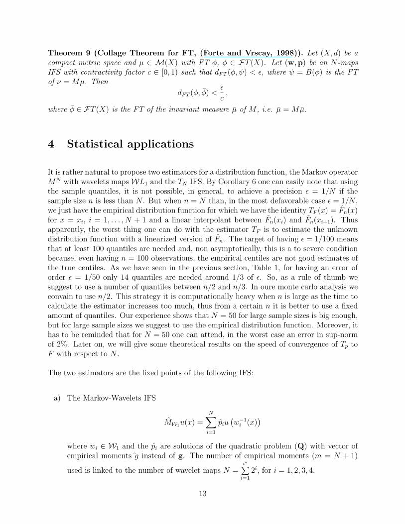
Theorem 9 (Collage Theorem for FT, (Forte and Vrscay, 1998)). Let (X, d) be acompact metric space and µ ∈ M(X) with FT φ, φ ∈ FT (X). Let (w,p) be an N-mapsIFS with contractivity factor c ∈ [0, 1) such that dFT (φ, ψ) < ε, where ψ = B(φ) is the FTof ν = Mµ. Then

dFT (φ, φ) <ε

c,

where φ ∈ FT (X) is the FT of the invariant measure µ of M , i.e. µ = Mµ.

4 Statistical applications

It is rather natural to propose two estimators for a distribution function, the Markov operatorMN with wavelets maps WL1 and the TN IFS. By Corollary 6 one can easily note that usingthe sample quantiles, it is not possible, in general, to achieve a precision ε = 1/N if thesample size n is less than N . But when n = N than, in the most defavorable case ε = 1/N ,we just have the empirical distribution function for which we have the identity TF (x) = Fn(x)for x = xi, i = 1, . . . , N + 1 and a linear interpolant between Fn(xi) and Fn(xi+1). Thusapparently, the worst thing one can do with the estimator TF is to estimate the unknowndistribution function with a linearized version of Fn. The target of having ε = 1/100 meansthat at least 100 quantiles are needed and, non asymptotically, this is a to severe conditionbecause, even having n = 100 observations, the empirical centiles are not good estimates ofthe true centiles. As we have seen in the previous section, Table 1, for having an error oforder ε = 1/50 only 14 quantiles are needed around 1/3 of ε. So, as a rule of thumb wesuggest to use a number of quantiles between n/2 and n/3. In oure monte carlo analysis weconvain to use n/2. This strategy it is computationally heavy when n is large as the time tocalculate the estimator increases too much, thus from a certain n it is better to use a fixedamount of quantiles. Our experience shows that N = 50 for large sample sizes is big enough,but for large sample sizes we suggest to use the empirical distribution function. Moreover, ithas to be reminded that for N = 50 one can attend, in the worst case an error in sup-normof 2%. Later on, we will give some theoretical results on the speed of convergence of Tp toF with respect to N .

The two estimators are the fixed points of the following IFS:

a) The Markov-Wavelets IFS

MW1u(x) =N∑

i=1

piu(w−1

i (x))

where wi ∈ W1 and the pi are solutions of the quadratic problem (Q) with vector ofempirical moments g instead of g. The number of empirical moments (m = N + 1)

used is linked to the number of wavelet maps N =i∗∑

i=1

2i, for i = 1, 2, 3, 4.

13

b) The quantile-based IFS

TNu(x) =N∑

i=1

1

Nu(w−1

i (x))

where (w−1i (x) = (x− qi)/(qi+1 − qi) with qi the empirical quantiles, being q1 = 0 and

qN+1 = 1.

In both cases u is any member of F([0, 1]).

4.1 Asymptotic results for the quantile-based IFS estimator

Asymptotic properties of the fixed points of both M∞ and TN derive as a natural consequence,by the properties of the empirical moments and quantiles. So, one can expect that, for afixed number of N maps, the fixed point of M is a consistent estimator of the fixed point ofM as the sample size increases and that the fixed point of TN converges to the fixed pointof TN as well. But if we let N varying with the sample size n we can have much more, atleast from TN .

The fixed point T ∗N of the above operator, TN , satisfies

T ∗N(x) =1

N

N∑i=1

T ∗N

(x− qiqi+1 − qi

), (6)

for real x. The following (Glivenko-Cantelli) theorem states that T ∗N has the same propertiesof an admissible perturbation of the e.d.f in the sense of Winter (see Winter 1973, 1979 andYukish, 1989). Let us denote by Nn the number of maps and coefficients in the IFS estimatorso to put in evidence the dependency of the sample size n.

Theorem 10. Let T ∗N be as in (6) with Nn →∞ as n→∞. If F is continuous, then

limn→∞

supx∈R

∣∣∣T ∗Nn(x)− F (x)

∣∣∣ a.s.= 0 .

Proof. We can write∣∣∣T ∗Nn(x)− F (x)

∣∣∣ ≤ ∣∣∣T ∗Nn(x)− Fn(x)

∣∣∣+ ∣∣∣Fn(x)− F (x)∣∣∣

and the first term can always be estimated by 1/Nn while the second one converges to 0almost surely by Glivenko-Cantelli theorem.

We can also establish a result of LIL-type. Recall that (Winter, 1979) an estimator Fn of Fis said to have the Chung-Smirnov property if

lim supn→∞

(2n

log log n

) 12

supx∈[0,1]

|Fn(x)− F (x)| ≤ 1 with probability 1.

14

Theorem 11. Let F be continuous and Nn = O(nα), α ∈ (1/2, 1]. Then T ∗Nnhas the

Chung-Smirnov property.

Proof. In fact,

lim supn→∞

(2n

log log n

) 12 1

Nn

= 0

by hypotheses.

We can also establish the local asymptotic minimax optimality of our estimator when Fis in a rich family (in the sense of Levit, 1978 and Millar 1979, see as well Gill and Levit,1995, Section 6) of distribution functions. For any estimator Fn of the unknown distributionfunction F we define the integrated mean square error as follows

Rn(Fn, F ) = nEF

∫ 1

0

(Fn(x)− F (x))2 λ(dx) = EF ||√n(Fn − F )||22

where λ(·) is a fixed probability measure on [0,1] and EF is the expectation under the truelaw F . What follows is the minimax theorem in the version given by Gil and Levit (1995).

Theorem 12 (Gill and Levit, 1995). If F is a rich family, then for any estimator Fn ofF ,

limV ↓F0

lim infn→∞

supF∈V

Rn(Fn, F ) ≥ R0(F0)

where V ↓ F0 denotes the limit in the net of shrinking neighborhoods (with respect to the

variation distance) of F0 and R0(F0) =∫ 1

0F0(x)(1− F0(x))λ(dx).

The above theorem states that, for any fixed F0, it is impossible to do better thatR0(F0) whenwe try to estimate F0. The empirical distribution function Fn is such Rn(Fn, F ) = R0(F ) forall n and so it is asymptotically efficient in the sense above mentioned. The result followsfrom the continuity of Rn in the variation distance topology (see Gill and Levit, 1995). It isalmost trivial to show that also the quantile-based IFS estimator is asymptotically efficientin the sense of the minimax theorem, the only condition to impose is on the number of mapsNn as in the LIL result.

Theorem 13. Let Nn = O(nα), α ∈ (1/2, 1]. Then T ∗Nnis asymptotically efficient under the

hypotheses of Theorem 12.

Proof. Note that R0(F0) is a lower bound on the asymptotic risk of T ∗Nnby Theorem 12.

Moreover,Rn(T ∗Nn

, F ) = EF ||√n(T ∗Nn

− F )||22≤ EF ||

√n(T ∗Nn

− Fn)||22 + EF ||√n(Fn − F )||22

+ 2EF ||√n(T ∗Nn

− Fn)||2EF ||√n(Fn − F )||2

≤ n

N2n

+R0(F ) + 2

√n

Nn

√R0(F )

15

by Chauchy-Schwartz inequality applied to EF ||√n(Fn−F )||2. As Nn = O(nα), α ∈ (1/2, 1],

we have the result. Note that α > 1 is not admissible as at most Nn = n quantiles are ofstatistical interest.

4.2 Characteristic function and Fourier density estimation

Using the results of §3 is now feasible to propose a Fourier expansion estimator of the densityfunction. We assume that all the minimal conditions to proceed in the Fourier analysis ofthis section are fulfilled. Thus, given and N -maps IFS(w,p), we have seen that the IFSestimator is the fixed point of the operator

Tu(x) =N∑

i=1

piu(w−1i (x)), x ∈ [0, 1],

for any u ∈ F([0, 1]) or, equivalently, in the space of measure M([0, 1])

Mµ(A) =N∑

i=1

piµ(w−1i (A)), A ⊂ [0, 1]

with maps and coefficients eventually estimated. Now, let φ be the fixed point of the operatorB in Section 3, i.e.

φ(t) =N∑

k=1

pke−iaktφ(skt), t ∈ R .

Then φ is nothing else that an estimator of the characteristic function of f(·) where f(·) isthe density function of the underlying unknown distribution function F (·) that generates thesample data X1, X2, . . . , Xn. Now (see e.g. Tarter and Lock, 1993) it is possible to derive aFourier expansion density estimator in this way.

φ(t) =

∫ 1

0

f(x)e−itxdx =

∫ 1

0

e−itxdF (x)

and, given φ(t) the density function f(·) can be rewritten as

f(x) =1

2π

+∞∑k=−∞

Bkeikx =

1

2π+

1

π

∞∑i=1

(Re(Bk) cos(kx)− Im(Bk) sin(kx)

)where

Bk =

∫ 1

0

f(x)e−ikxdx = φ(k)

Denoting by φ (the fixed point of) the characteristic function estimator based on quantiles

φ(t) =N∑

k=1

e−iaktφ(skt) , ak = qk, sk = qk+1 − qk , (7)

16

with q0 = 1 and qN+1 = 1, a density function estimator is the following

f(x) =1

2π

+∞∑k=−∞

ckBkeikx (8)

where {ck, k = 0,±1,±2, . . .} is sequence of suitable multipliers not to be estimated andBk = φ(k). One choice for the multipliers is ck = 1 for |k| ≤ m and ck = 0 if |k| > m. Insuch a case the estimator reduces to the raw Fourier expansion estimator

fFT (x) =1

2π

+m∑k=−m

Bkeikx =

1

2π+

1

π

m∑i=1

(Re(Bk) cos(kx)− Im(Bk) sin(kx)

).

A detailed discussion on which family of multipliers is to be choosen can be found in Tarterand Lock (1993) and can be applied to this case as well. As it is well known, the fact thatthe Fourier expansion is a convergent series it is always possible to differentiate or integrateit in order to obtain an estimator for the first derivative of the density

f ′(x) =1

2π

d

dxf(x) =

1

2π

+m∑k=−m

d

dxBke

ikx =+m∑

k=−m, k 6=0

ik

2πBke

ikx

which is a particular case of (8) with ck = ik, |k| ≤ m, k 6= 0 and ck = 0 for k = 0 or|k| > m. We can also propose another distribution function estimator

FFT (x) =1

2π

(x+

+m∑k=−m, k 6=0

Bk

ik

(eikx − 1

))

=1

2π

(x+ 2

m∑k=1

(Re(Bk) sin(kx) + Im(Bk)(cos(kx)− 1)

)) (9)

that can be used as a smooth estimator derived from IFS techinques instead of applyingdireclty the fractal M or TN estimator.

To conclude this section, we have to say that it is still possible to build IFSs in the spaceof density functions but direct application to estimation is less straightforward and this willbe the object of another paper as it requires a different class of IFS systems, namely thelocal-IFS approach.

5 Monte Carlo analysis

Before going into details with simulations results, we want to remark that the IFS estimatorsare fractal objects, this means that they are nowhere differentiable and they are self-similar.In Figure 2 we have represented the distribution function estimator TN of an underlying

17

0.0 0.2 0.4 0.6 0.8 1.0

0.0

0.5

1.0

1.5

2.0

2.5

Kernel vs IFS

x

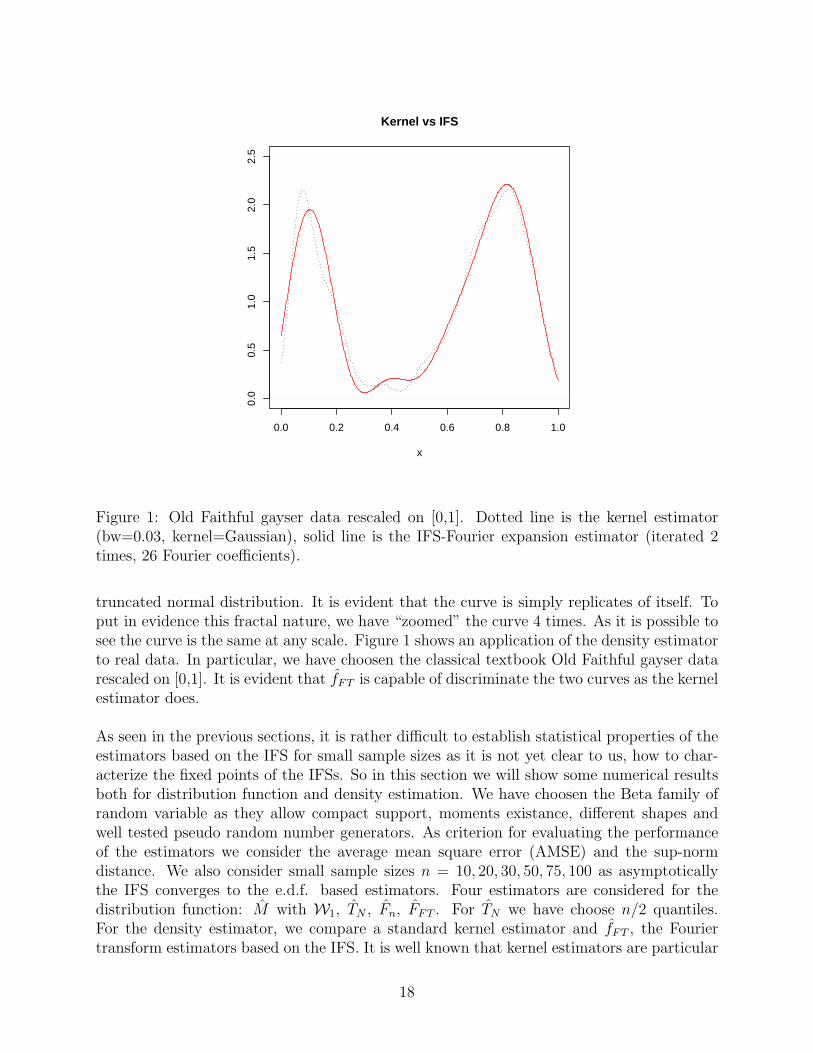
Figure 1: Old Faithful gayser data rescaled on [0,1]. Dotted line is the kernel estimator(bw=0.03, kernel=Gaussian), solid line is the IFS-Fourier expansion estimator (iterated 2times, 26 Fourier coefficients).

truncated normal distribution. It is evident that the curve is simply replicates of itself. Toput in evidence this fractal nature, we have “zoomed” the curve 4 times. As it is possible tosee the curve is the same at any scale. Figure 1 shows an application of the density estimatorto real data. In particular, we have choosen the classical textbook Old Faithful gayser datarescaled on [0,1]. It is evident that fFT is capable of discriminate the two curves as the kernelestimator does.

As seen in the previous sections, it is rather difficult to establish statistical properties of theestimators based on the IFS for small sample sizes as it is not yet clear to us, how to char-acterize the fixed points of the IFSs. So in this section we will show some numerical resultsboth for distribution function and density estimation. We have choosen the Beta family ofrandom variable as they allow compact support, moments existance, different shapes andwell tested pseudo random number generators. As criterion for evaluating the performanceof the estimators we consider the average mean square error (AMSE) and the sup-normdistance. We also consider small sample sizes n = 10, 20, 30, 50, 75, 100 as asymptoticallythe IFS converges to the e.d.f. based estimators. Four estimators are considered for thedistribution function: M with W1, TN , Fn, FFT . For TN we have choose n/2 quantiles.For the density estimator, we compare a standard kernel estimator and fFT , the Fouriertransform estimators based on the IFS. It is well known that kernel estimators are particular

18

0.0 0.2 0.4 0.6 0.8 1.0

0.0

0.2

0.4

0.6

0.8

1.0

x

0.00 0.05 0.10 0.15 0.200.

000.

010.

020.

030.

04x

0.00 0.01 0.02 0.03 0.04 0.05

0.00

000.

0005

0.00

100.

0015

x

0.000 0.002 0.004 0.006 0.008 0.010

0e+

002e

−05

4e−

056e

−05

x

Figure 2: The fractal nature of the IFS distribution function estimator TN . The dotted lineis the underlying truncated Gaussian distribution. The dotted rectangle is to represent thearea zoomed in the next plot (left to right, up to down). The dotted boxes are in the order:[0, q2]× [0, q2], [0, q2

2]× [0, q22] and [0, q3

2]× [0, q32].

19

Fourier expansion estimators by a proper choice of the multiplier ck when the e.d.f is usedin the Fourier transform. The number of terms used in the Fourier series estimators of thedistribution function, is choosen accordingly to the following rule

if∣∣∣Bm+1

∣∣∣2 and∣∣∣Bm+2

∣∣∣2 < 2

n+ 1then use the first m coefficents

as suggested in Tarter and Lock (1993). The rule of thumb we use cannot be consid-ered optimal in any sense but its principle is to minimize the integrated MSE. The soft-ware used is R (Ihaka and Gentleman, 1996) with a beta ‘ifs’ package available on CRANhttp://cran.r-project.org, in the contributed packages directory. Kernel density esti-mation is as in Silverman (1986) and implemented in R with the density() function (seealso Venables and Ripley, 2002) in the R implementation. All the estimates are evaluatedin 512 points in order to calculates AMSE and the sup-norm. For density estimation wecalculate the average of the absolute error (MAE) instead of the sup-norm as this index isinfluenced by the bad performance of density estimators in the endpoints (0 and 1) of thesupport of the distributions.

Tables 2 and 3 are organized as follows: there are five main columns, one for the distributioninvestigated, two for the distribution function estimators and the last two are for densityestimation. Under column AMSE, the MW1 column reports the ratio, in percentage, betweenthe AMSE of MW1 and the AMSE of the Fn and similarly for the entire row. This means thatwe indicate the relative efficiency of the three estimators MW1 , TN anf FFT with respect to Fn.Under the column marked SUP-NORM the same scheme has been applied but consideringthe sup-norm distance.

The last two columns are for density estimation. This time the columns represents the ratioin percentage, of the distance for the Fourier estimator fFT and the kernel estimator.

The tables shows that, in the average the TN estimator is equivalent to to the e.d.f. for uglydistributions like the beta(.1,.9) or beta(.1,.1), while it is somewhat better in the other cases(10 to 20% better). The Fourier series estimator based onf IFS, FFT is preferable to the e.d.fonly for bell shaped distributions and seems unbeatable for simmetric shaped laws. This issomewhat expected by a Fourier expansion estimator. The same argument applies to thedensity estimator: for bell shaped symmetric distributions, it seems as good as the kernelestimator and in some cases even better.

For the beta(.1,.9) or the beta(.1,.1) the density estimators (both kernel and our Fourier)are of no use, we have omitted the corresponding ratios.

5.1 Applications to survival analysis

Let T denote a random lifetime (or time until failure) with distribution function F . Onthe basis of a sample of n independent replications of T the object of inference are usually

20

parameters AMSE SUP-NORM AMSE MAE

n law10 beta(.9,.1)10 beta(.1,.9)10 beta(.1,.1)10 beta( 2, 2)10 beta( 5, 5)10 beta( 5, 3)10 beta( 3, 5)10 beta( 1, 1)

MW1 TN FFT

105260.1 94.86 186.81827.42 99.79 2097.27

34067.84 99.26 560.99153.01 80.99 133.33114.13 89.91 210.0576.14 98.57 163.17142.96 90.70 194.36

58094.14 81.23 88.16

MW1 TN FFT

2179.91 98.10 193.42608.94 100.33 262.185879.58 100.05 190.82102.51 82.18 68.4899.60 89.74 81.6779.46 92.86 71.2499.41 91.34 79.51

2741.62 80.04 80.07

fFT

———

171.16162.46185.88154.86148.71

fFT

———

123.05123.63119.36125.25117.11

parameters AMSE SUP-NORM AMSE MAE

n law20 beta(.9,.1)20 beta(.1,.9)20 beta(.1,.1)20 beta( 2, 2)20 beta( 5, 5)20 beta( 5, 3)20 beta( 3, 5)20 beta( 1, 1)

MW1 TN FFT

80402.60 101.56 216.583156.71 113.31 4028.9930695.03 99.77 999.28

91.73 86.05 100.44154.93 89.27 120.9283.89 92.89 133.44198.84 88.27 116.828601.04 84.89 79.26

MW1 TN FFT

676.97 99.10 251.701265.92 114.50 371.706611.92 98.84 231.8882.46 83.34 61.55114.32 87.49 65.5687.12 89.31 67.28114.82 87.29 67.64751.59 79.27 71.67

fFT

———

121.19120.54123.48132.69153.64

fFT

———

109.07109.30104.81117.18118.69

parameters AMSE SUP-NORM AMSE MAE

n law30 beta(.9,.1)30 beta(.1,.9)30 beta(.1,.1)30 beta( 2, 2)30 beta( 5, 5)30 beta( 5, 3)30 beta( 3, 5)30 beta( 1, 1)

MW1 TN FFT

143440.9 97.17 245.113740.29 118.80 6842.9239983.05 99.62 1352.06

92.86 86.23 86.09191.88 89.54 114.9698.55 91.67 135.96241.12 88.31 108.49483.23 87.16 87.77

MW1 TN FFT

1357.53 92.91 283.571328.19 115.38 486.588086.76 98.57 284.3982.66 84.01 55.83132.21 89.21 67.2797.77 87.90 66.60124.99 88.34 66.76181.99 81.00 75.80

fFT

———

103.84118.48113.78130.77168.50

fFT

———

99.35106.07105.41115.17129.67

Table 2: Relative efficiency of IFS-based estimator with respect to the empirical distributionfunction and the kernel density estimator. Small sample sizes.

21

parameters AMSE SUP-NORM AMSE MAE

n law50 beta(.9,.1)50 beta(.1,.9)50 beta(.1,.1)50 beta( 2, 2)50 beta( 5, 5)50 beta( 5, 3)50 beta( 3, 5)50 beta( 1, 1)

MW1 TN FFT

4462.59 98.59 318.907577.62 107.85 11017.5541958.58 97.77 1740.82

99.40 91.55 75.24279.55 91.57 91.36124.40 97.80 96.04327.86 91.90 84.84548.05 92.84 104.46

MW1 TN FFT

524.57 95.87 361.671875.88 113.85 619.158419.93 99.87 318.4888.29 87.40 54.08158.18 89.64 56.17112.71 92.73 59.33145.24 91.40 60.54144.12 86.24 80.56

fFT

———

93.0688.2589.63115.95173.79

fFT

———

92.6391.6796.36105.87132.25

parameters AMSE SUP-NORM AMSE MAE

n law75 beta(.9,.1)75 beta(.1,.9)75 beta(.1,.1)75 beta( 2, 2)75 beta( 5, 5)75 beta( 5, 3)75 beta( 3, 5)75 beta( 1, 1)

MW1 TN FFT

49097.24 98.85 409.182518.57 122.62 15348.4952407.20 100.37 2460.06109.62 94.77 66.97338.18 97.41 72.95139.85 104.31 111.65407.03 95.14 87.93107.36 98.39 130.28

MW1 TN FFT

853.06 97.66 427.171206.46 122.78 721.8310475.81 106.85 381.39

90.00 90.42 52.11177.11 92.39 53.67120.93 96.29 63.52163.53 91.80 61.7690.23 89.05 83.62

fFT

———

89.9772.7993.45107.14158.01

fFT

———

91.6186.6897.32104.07131.13

parameters AMSE SUP-NORM AMSE MAE

n law100 beta(.9,.1)100 beta(.1,.9)100 beta(.1,.1)100 beta( 2, 2)100 beta( 5, 5)100 beta( 5, 3)100 beta( 3, 5)100 beta( 1, 1)

MW1 TN FFT

322.52 98.22 575.821191.05 114.91 22660.0265060.00 102.02 3901.37113.49 97.03 74.57425.20 95.08 69.37179.28 95.52 100.85489.18 97.59 76.83108.74 101.58 141.98

MW1 TN FFT

425.48 96.65 457.07895.01 152.41 890.919778.29 110.96 455.3497.12 91.68 58.62198.27 93.37 50.80137.34 93.96 60.62176.56 94.23 58.6891.94 92.26 84.65

fFT

———

96.4567.0182.9192.38146.78

fFT

———

95.4880.7592.2598.10125.03

Table 3: Relative efficiency of IFS-based estimator with respect to the empirical distributionfunction and the kernel density estimator. Moderate sample sizes.

22

quantities derived from the so-called survival function S(t) = 1 − F (t) = P (T > t). IfF has a density f then it is possible to define the hazard function h(t) = lim∆t→0 P (t ≤T < t + ∆t|T ≥ T )/∆t = f(t)/S(t) and in particular the cumulative hazard functionH(t) =

∫ t

0h(s)ds = − logS(t). Usually T is thought to take values in [0,∞), but we can

think to consider the estimation conditionally to the last sample failure, say τ , and rescalethe interval [0, τ ] to [0, 1]. So we will assume, from now on, that all the failure times occurin [0,1], being 1 the instant of the last failure when the experiment stops. In this schemeof observation S(t) = 1 − F (t) is a natural estimator of S, with F any estimator of Fand, in particular, the IFS estimator. A more realistic situation is when some censoringoccurs, in the sense that, as time pass by, some of the initial n observations are removedat random times C not because of failure (or death) but for some other reasons. In thiscase, a simple distribution function estimator is obviously not good. Let us denote byt0 = 0 < t1 < · · · < td−1 < td = 1 the observed instants of failure (or death). A well knownestimator of S is the Kaplan-Meyer estimator

S(t) =∏ti<t

r(ti)− di

r(ti)

where r(ti) are the subject exposed to risk of death at time ti and di are the dead in the timeinterval [ti, ti+1) (see the original paper of Kaplan and Meyer, 1958, or for a modern accountFleming and Harrington, 1991). In our case di is always 1 as ti are the instants when failuresoccur. Subjects exposed to risk are those still present in the experiment and not yet dead orcensored. This estimator has good properties whenever T and C are independent. Relatedto the quantities r(ti) and di it is also available the Nelson estimator for the function Hthat is defined as H(t) =

∑ti<t di/r(ti). We assume for simplicity that there are no ties, in

the sense that in each instant ti only one failure occurs. The function H(t) is a increasingstep-function. Now let H(t) = H(t)/H(1). H(t) can be thought as an empirical estimatesof a distribution function H on [0,1]. To derive and IFS estimator for the cumulative hazardfunction H we construct the sample quantiles by simply taking the inverse of H. Supposewe want to deal with N + 1 quantiles, being q1 = 0 and qN+1 = 1. One possible definition ofthe empirical quantile of order k/N is obtained by the formula

qk+1 = ti +ti+1 − ti

H(ti+1)− H(ti)·(k

N− H(ti)

), if H(ti) ≤

k

N< H(ti+1), (10)

for i = 0, 1, . . . , d − 1 and k = 1, 2, . . . , N − 1. Now set pi = 1/N , i = 1, 2, . . . , N and qi,i = 1, 2, . . . , N + 1 as in (10). An IFS estimator of H is H(1) · H(t) where H(t) is thefollowing IFS:

H(t) = Hu(t) =1

N

k∑i=1

u(w−1

i (t))

where w−1i (x) = (x− qi)/(qi+1− qi) and u is any member of the space of distribution function

on [0, 1]. In (10) we have assumed that H is the distribution function of a continuous randomvariable, withH varying linearly between ti and ti+1, but of course any other assumption thanlinearity can be made as well (for example an exponential behaviour). A Fleming-Harrington

23

(or Altshuler) IFS-estimator of S is then

S(t) = exp{−H(1) · H(t)}, t ∈ [0, 1] .

What is the gain in using our S instead of a standard Altshuler estimator. In principle,it is the same as in distribution function estimation: the Altshuler estimator is a functionwith jumps and this jumps are smaller with our IFS estimator. But one other importantconsequence could be the same. Suppose you want to estimate the function h. An estimator isusually given by a discrete density function that gives value di/r(ti) on ti and zero elsewhere.The underlying distribution T is a continuous one so we can propose an estimator of itsdensity f by means of the relation h(t) = f(t)/S(t). In fact, let hFT (t) be the Fouriertransform estimator of the density of H. Then H(1) · hFT (t) is an estimator of h. A densityestimator for f is then

f(t) = H(1) · hFT (t) · S(t)

or, in alternative, using the Kaplan-Meyer estimator of S

f(t) = H(1) · hFT (t) · S(t) .

Final remarks

We haw shown how it is relatively powerful to adopts IFS technique in distribution functionestimation and related quanties (density and Fourier transform). There are several openissues about the estimators themselves. The main open problem is about a better character-ization of the fixed points of the IFS in order to establish non asymptotic properties for theestimators. The second, and commonly not discussed in the IFS literature, is the problem ofchoosing the maps w. There recently appeared some papers that discuss the relationshipsof some class of IFS and wavelets analysis as well as some papers on local IFS (possible can-didates to density functions approximators) but the results there in are not directly usefulto statistics.

References

[1] Barnsley, M.F., Demko, S., “Iterated function systems and the global construction offractals”, Proc. Roy. Soc. London, Ser A, 399, 243-275, 1985.

[2] Beran, R., “Estimating a distribution function”, Ann. Statist., 5, 400-404, 1977.

[3] Dvoretsky, A., Kiefer, J. and Wolfowitz, J., “Asymptotic minimax character of thesample distribution function and of the classical multinomial estimators”, Ann. Math.Statist., 27, 642-669, 1956.

24

[4] Efromovich, S., “Second order efficient estimating a smooth distribution function andits applications”, Meth. Comp. App. Probab., 3, 179-198, 2001.

[5] Kaplan, E. and Meyer, P., “Nonparametric estimator from incomplete observations”, J.Amer. Statist. Ass, 53, 457-81, 1958.

[6] Forte, B., Vrscay, E.R., “Solving the inverse problem for function/image approximationusing iterated function systems, I. Theoretical basis”, Fractal, 2, 3, 325-334, 1995.

[7] Forte, B., Vrscay, E.R., “Inverse problem methods for generalized fractal transforms”,in Fractal Image Encoding and Analysis, NATO ASI Series F, Vol. 159, ed. Y. Fisher,Springer Verlag, Heidelberg, 1998.

[8] Fleming, T.R. and Harrington, D.P. , Counting processes and survival analysis, Wiley,New York, 1991.

[9] Kiefer, J. and Wolfowitz, J., “Asymptotic minimax character of the sample distributionfunction for vector chance variables”, Ann. Math. Stat., 30, 463-489, 1959.

[10] Gill, R. D. and Levit, B. Y., “Applications of the van Trees inequality: A BayesianCramer-Rao bound”, Bernoulli, 1, 59-79, 1995.

[11] Golubev, G. K. and Levit, B. Y., “On the second order minimax estimation of distri-bution functions”, Math. Methods. Statist., 5, 1-31, 1996a.

[12] Golubev, G. K. and Levit, B. Y., “Asymptotic efficient estimation for analytic distri-butions”, Math. Methods. Statist., 5, 357-368, 1996b.

[13] Hutchinson, J., “Fractals and self-similarity”, Indiana Univ. J. Math., 30, 5, 713-747,1981.

[14] Iacus, S.M. and La Torre, D., “Approximating distribution functions by iterated func-tion systems”, submitted, available as Acrobat PDF file athttp://159.149.74.117/~web/R/ifs/ifs.pdf, 2001.

[15] Ihaka, R. and Gentleman, R., “R: A Language for Data Analysis and Graphics”, Journalof Computational and Graphical Statistics, 5, 299-314, 1996.

[16] Levit, B.Y., “Infinite-dimensional information inequalities”, Theory Probab. Applic.,23, 371-377, 1978.

[17] Millar, P.W., “Asymptotic minimax theorems for sample distribution functions”, Z.Warsch. Verb. Geb., 48, 233-252, 1979.

[18] Silverman, B. W., Density Estimation, London, Chapman and Hall, 1986.

[19] Tarter, M.E. and Lock, M.D, Model free curve estimation, Chapman & Hall, New York,1993.

25

[20] Venables, W. N. and Ripley, B. D., Modern Applied Statistics with S-PLUS, New York,Springer, forthcoming, 2002. Springer, New York, 1998.

[21] Winter, B.B., “Strong uniform consistency of integrals of density estimators”, Can. J.Statist., 1, 247–253, 1973.

[22] Winter, B.B., “Convergence rate of perturbed empirical distribution functions”, J. Appl.Prob., 16, 163–173, 1979.

[23] Yukish, J.E. , “A note on limit theorems for perturbed empirical processes”. Stoch.Proc. Appl., 33, 163–173, 1989.

26

La serie dei Working Papers del Dipartimento di Economia Politica e Aziendale può essere richiesta al seguenteindirizzo: Sezione Working Papers - Dipartimento di Economia Politica e Aziendale - Università degli Studi di Milano,Via Conservatorio 7 - 20122 Milano - Italy - fax 39-02-76009695 - Email: Dipeco@unimi.it. A partire dal numero98.01, i working papers sono scaricabili dal sito Internet del dipartimento, all’indirizzo:http://www.eco-dip.unimi.it/index1.htm

The Working Paper Series of the Dipartimento di Economia Politica e Aziendale can be requested at the followingaddress: Sezione Working Papers - Dipartimento di Economia Politica e Aziendale - Università degli Studi di Milano,Via Conservatorio 7 - 20122 Milano - Italy - fax 39-02-76009695 - Email: Dipeco@unimi.it. From number 98.01,working papers are downloadable from the Internet website of the Department at the following location:http://www.eco-dip.unimi.it/index1.htm

Papers già pubblicati/Papers already published

94.01 - D. CHECCHI, La moderazione salariale negli anni 80 in Italia. Alcune ipotesi interpretative basate sul comportamento dei sindacati

94.02 - G. BARBA NAVARETTI, What Determines Intra-Industry Gaps in Technology? A Simple Theoretical Framework for the Analysis of Technological Capabilities in Developing Countries

94.03 - G. MARZI, Production, Prices and Wage-Profit Curves:An Evaluation of the Empirical Results94.04 - D. CHECCHI, Capital Controls and Conflict of Interests94.05 - I. VALSECCHI, Job Modelling and Incentive Design: a Preliminary Study94.06 - M. FLORIO, Cost Benefit Analysis: a Research Agenda94.07 - A. D’ISANTO, La scissione di società e le altre operazioni straordinarie: natura, presupposti economici e

problematiche realizzative94.08 - G. PIZZUTTO, Esistenza dell’ equilibrio economico generale: approcci alternativi94.09 - M.FLORIO, Cost Benefit Analysis of Infrastructures in the Context of the EU Regional Policy94.10 - D.CHECCHI - A. ICHINO - A. RUSTICHINI, Social Mobility and Efficiency - A Re-examination of the Problem of Intergenerational Mobility in Italy94.11 - D.CHECCHI - G. RAMPA - L. RAMPA, Fluttuazioni cicliche di medio termine nell’economia italiana del dopoguerra

95.01 - G. BARBA NAVARETTI, Promoting the Strong or Supporting the Weak? Technological Gaps and Segmented Labour Markets in Sub-Saharan African Industry95.02 - D. CHECCHI, I sistemi di assicurazione contro la disoccupazione: un'analisi comparata95.03 - I. VALSECCHI, Job Design and Maximum Joint Surplus95.04 - M. FLORIO, Large Firms, Entrepreneurship and Regional Policy: "Growth Poles" in the Mezzogiorno over Forty Years95.05 - V. CERASI - S. DALTUNG, The Optimal Size of a Bank: Costs and Benefits of Diversification95.06 - M. BERTOLDI, Il miracolo economico dei quattro dragoni: mito o realtà?95.07 - P. CEOLIN, Innovazione tecnologica ed alta velocità ferroviaria: un'analisi95.08 - G. BOGNETTI, La teoria della finanza a Milano nella seconda metà del Settecento: il pensiero di Pietro Verri95.09 - M. FLORIO, Tax Neutrality in the King-Fullerton Framework, Investment Externalities, and Growth95.10 - D. CHECCHI, La mobilità sociale: alcuni problemi interpretativi e alcune misure sul caso italiano95.11 - G. BRUNELLO - D. CHECCHI , Does Imitation help? Forty Years of Wage Determination in the Italian Private Sector95.12 - G. PIZZUTTO, La domanda di lavoro in condizioni di incertezza95.13 - G. BARBA NAVARETTI - A. BIGANO, R&D Inter-firm Agreements in Developing Countries. Where? Why? How?95.14 - G. BOGNETTI - R. FAZIOLI, Lo sviluppo di una regolazione europea nei grandi servizi pubblici a rete

96.01 - A. SPRANZI, Il ratto dal serraglio di W.A. Mozart. Una lettura non autorizzata96.02 - G. BARBA NAVARETTI - I. SOLOAGA - W. TAKACS, Bargains Rejected? Developing Country Trade Policy on Used Equipment96.03 - D. CHECCHI - G. CORNEO, Social Custom and Strategic Effects in Trade Union Membership: Italy 1951- 199396.04 - V. CERASI, An Empirical Analysis of Banking Concentration96.05 - M. FLORIO, Il disegno dei servizi pubblici locali dal socialismo municipale alla teoria degli incentivi96.06 - G. PIZZUTTO, Piecewise Deterministic Markov Processes and Investment Theory under Uncertainty: Preliminary Notes96.07 - I. VALSECCHI, Job Assignment and Promotion

96.08 - D. CHECCHI, L'efficacia del sistema scolastico in prospettiva storica

97.01 - I. VALSECCHI, Promotion and Hierarchy: A Review97.02 - D. CHECCHI, Disuguaglianza e crescita. Materiali didattici97.03 - M. SALVATI, Una rivoluzione copernicana: l'ingresso nell'Unione Economica e Monetaria97.04 - V. CERASI - B. CHIZZOLINI - M. IVALDI, The Impact of Deregulation on Branching and Entry Costs in the Banking Industry97.05 - P.L. PORTA, Turning to Adam Smith97.06 - M. FLORIO, On Cross-Country Comparability of Government Statistics:OECD National Accounts 1960-9497.07 - F. DONZELLI, Pareto's Mechanical Dream

98.01 - V. CERASI - S. DALTUNG, Close-Relationships between Banks and Firms: Is it Good or Bad?98.02 - M. FLORIO - R. LUCCHETTI - F. QUAGLIA, Grandi e piccole imprese nel Centro-Nord e nel Mezzogiorno: un modello empirico dell'impatto occupazionale nel lungo periodo98.03 – V. CERASI – B. CHIZZOLINI – M. IVALDI, Branching and Competitiveness across Regions in the Italian Banking Industry98.04 – M. FLORIO – A. GIUNTA, Planning Contracts in Southern Italy, 1986-1997: a Prelimary Evaluation98.05 – M. FLORIO – I. VALSECCHI, Planning Agreements in the Mezzogiorno: a Principle Agent Analysis98.06 – S. COLAUTTI, Indicatori di dotazione infrastrutturale: un confronto tra Milano e alcune città europee98.07 – G. PIZZUTTO, La teoria fiscale dei prezzi in un’economia aperta98.08 – M. FLORIO, Economic Theory, Russia and the fading “Washington Consensus”

99.01 – A. VERNIZZI – A. SABA, Alcuni effetti della riforma della legislazione fiscale italiana nei confronti delle famiglie con reddito da lavoro dipendente99.02 – C. MICHELINI, Equivalence Scales and Consumption Inequality: A Study of Household Consumption Patterns in Italy99.03 – S.M. IACUS, Efficient Estimation of Dynamical Systems99.04 – G. BOGNETTI, Nuove forme di gestione dei servizi pubblici99.05 – G.M. BERNAREGGI, Milano e la finanza pubblica negli anni 90: attualità e prospettive

99.06 – M. FLORIO, An International Comparison of the Financial and Economic Rate of Return of Development99.07 – M. FLORIO, La valutazione delle politiche di sviluppo locale99.08 – I. VALSECCHI, Organisational Design: Decision Rules, Operating Costs and Delay99.09 – G. PIZZUTTO, Arbitraggio e mercati finanziari nel breve periodo. Un’introduzione

00.01 – D. LA TORRE – M. ROCCA, A.e. Convex Functions on Rn

00.02 – S.M. IACUS – YU A. KUTOYANTS, Semiparametric Hypotheses Testing for Dynamical Systems with Small Noise00.03 – S. FEDELI – M. SANTONI, Endogenous Institutions in Bureaucratic Compliance Games00.04 – D. LA TORRE – M. ROCCA, Integral Representation of Functions: New Proofs of Classical Results00.05 – D. LA TORRE – M. ROCCA, An Optimization Problem in IFS Theory with Distribution Functions00.06 – M. SANTONI, Specific excise taxation in a unionised differentiated duopoly00.07 – H. GRAVELLE – G. MASIERO, Quality incentives under a capitation regime: the role of patient expectations00.08 – E. MARELLI – G. PORRO, Flexibility and innovation in regional labour markets: the case of Lombardy00.09 – A. MAURI, La finanza informale nelle economie in via di sviluppo00.10 – D. CHECCHI, Time series evidence on union densities in European countries00.11 – D. CHECCHI, Does educational achievement help to explain income inequality?00.12 – G. BOESSO – A. VERNIZZI, Carichi di famiglia nell’Imposta sui Redditi delle Persone Fisiche in Italia e in Europa: alcune proposte per l’Italia

01.01 – G. NICOLINI, A method to define strata boundaries01.02 – S.M. IACUS, Statistical analysis of the inhomogeneous telegrapher’s process01.03 – M. SANTONI, Discriminatory procurement policy with cash limits can lower imports: an example01.04 – D. LA TORRE, L’uso dell’ottimizzazione non lineare nella procedura di compressione di immagini con IFS01.05 – G. MASIERO, Patient movements and practice attractiveness01.06 – S.M. IACUS, Statistic analysis of stochastic resonance with ergodic diffusion noise01.07 – B. ANTONIOLI – G. BOGNETTI, Modelli di offerta dei servizi pubblici locali in Europa01.08 – M. FLORIO, The welfare impact of a privatisation: the British Telecom case-history01.09 – G. P. CRESPI, The effect of economic policy in oligopoly. A variational inequality approach.01.10 – G. BONO – D. CHECCHI, La disuguaglianza a Milano negli anni ’9001.11 – D. LA TORRE, On the notion of entropy and optimization problems01.12 – M. FLORIO – A. GIUNTA, L’esperienza dei contratti di programma: una valutazione a metà percorso01.13 – M. FLORIO – S. COLAUTTI, A logistic growth law for government expenditures: an explanatory analysis01.14 – L. ZANDERIGHI, Town Center Management: uno strumento innovativo per la valorizzazione del centro storico e del commercio urbano

01.15 – ANNA MAFFIOLETTI – MICHELE SANTONI, Do trade union leaders violate subjective expected utility? Some insights from experimental data01.16 – DAVIDE LA TORRE, An inverse problem for stochastic growth models with iterated function systems01.17 – DAVIDE LA TORRE – MATTEO ROCCA, Some remarks on second-order generalized derivatives for C1,1

functions01.18 – ALBERTO BUCCI, Human capital and technology in growth01.19 – RINALDO BRAU – MASSIMO FLORIO, Privatisation as price reforms: an analysis of consumers’ welfare change in the UK01.20 – ALDO SPRANZI, Impresa e consumerismo: la comunicazione consumeristica01.21 – GIUSEPPE BERTOLA – DANIELE CHECCHI, Sorting and private education in Italy01.22 – GIACOMO BOESSO, Analisi della performance ed external reporting: bilanci e dati aziendali on-line in Italia01.23 – GIUSEPPE BOGNETTI, Il processo di privatizzazione nell’attuale contesto internazionale

02.01 – DANIELE CHECCHI – JELLE VISSER, Pattern persistence in european trade union density02.02 – GIOVANNI P. CRESPI – DAVIDE LA TORRE – MATTEO ROCCA, Second order optimality conditions for differentiable functions02.03 – STEFANO M. IACUS – DAVIDE LA TORRE, Approximating distribution functions by iterated function systems02.04 – ALBERTO BUCCI – DANIELE CHECCHI, Crescita e disuguaglianza nei redditi a livello mondiale02.05 – ALBERTO BUCCI, Potere di mercato ed innovazione tecnologica nei recenti modelli di crescita endogena con concorrenza imperfetta02.06 – ALBERTO BUCCI, When Romer meets Lucas: on human capital, imperfect competition and growth02.07 – STEFANO M. IACUS – DAVIDE LA TORRE, On fractal distribution function estimation and applications