Assouad Dimension and Fractal Geometry - arXiv
292
Assouad Dimension and Fractal Geometry Jonathan M. Fraser This material will be published by Cambridge University Press as Assouad Dimension and Fractal Geometry by Jonathan Fraser. This pre-publication version is free to view and download for personal use only. Not for re-distribution, re-sale or use in derivative works. c Jonathan Fraser 2020.
-
Upload
khangminh22 -
Category
Documents
-
view
0 -
download
0
Transcript of Assouad Dimension and Fractal Geometry - arXiv
Assouad Dimension and Fractal Geometry
Jonathan M. Fraser
This material will be published by Cambridge University Press
as Assouad Dimension and Fractal Geometry by Jonathan
Fraser. This pre-publication version is free to view and download
for personal use only. Not for re-distribution, re-sale or use in
derivative works. c© Jonathan Fraser 2020.


For Rayna and Dylan
Contents
Acknowledgements page viii
Preface x
PART ONE THEORY 1
1 Fractal geometry and dimension theory 3
1.1 The emergence of fractal geometry 3
1.2 Dimension theory 5
1.2.1 Dimension theory of measures 9
2 The Assouad dimension 10
2.1 The Assouad dimension and a simple example 10
2.2 A word or two on the definition 13
2.3 Some history 15
2.4 Basic properties: the greatest of all dimensions 17
3 Some variations on the Assouad dimension 22
3.1 The lower dimension 22
3.2 The quasi-Assouad dimension 24
3.3 The Assouad spectrum 25
3.3.1 First observations on the Assouad spectrum 27
3.3.2 A tale of two spectra 32
3.3.3 Recovering the interpolation 36
3.4 Basic properties: revisited 38
3.4.1 Relationships between dimensions 38
3.4.2 Further basic properties 45
3.4.3 Holder distortion 50
3.4.4 An example with non-monotonic Assouad
spectrum 53
iv
Contents v
4 Dimensions of measures 57
4.1 Assouad and lower dimensions of measures 57
4.2 Assouad spectrum and box dimensions of measures 62
5 Weak tangents and microsets 66
5.1 Weak tangents and the Assouad dimension 66
5.2 Weak tangents for the lower dimension? 74
5.3 Weak tangents for spectra? 75
5.4 Weak tangents for measures? 77
PART TWO EXAMPLES 81
6 Iterated function systems 83
6.1 IFS attractors and symbolic representation 83
6.2 Invariant measures 87
6.3 Dimensions of IFS attractors 88
6.4 Ahlfors regularity and quasi-self-similarity 91
7 Self-similar sets 96
7.1 Self-similar sets and the Hutchinson-Moran formula 96
7.2 The Assouad dimension of self-similar sets 98
7.3 The Assouad spectrum of self-similar sets 106
7.4 Dimensions of self-similar measures 109
8 Self-affine sets 113
8.1 Self-affine sets and two strands of research 113
8.2 Falconer’s formula and the affinity dimension 114
8.3 Self-affine carpets 117
8.4 Self-affine sets with a comb structure 127
8.5 A family of worked examples 130
8.6 Dimensions of self-affine measures 133
8.6.1 Another worked example 138
9 Further examples: attractors and limit sets 141
9.1 Self-conformal sets 141
9.2 Invariant sets for parabolic interval maps 144
9.3 Limit sets of Kleinian groups 149
9.4 Mandelbrot percolation 159
10 Geometric constructions 165
10.1 Products 166
10.2 Orthogonal projections 172
10.2.1 Dimension theory of orthogonal projections 172
vi Contents
10.2.2 The Assouad dimension of orthogonal
projections 173
10.2.3 An application to the box dimensions of
projections 178
10.2.4 The lower dimension and projections 182
10.3 Slices and intersections 183
11 Two famous problems in geometric measure theory 187
11.1 Distance sets 187
11.2 Kakeya sets 193
12 Conformal dimension 196
12.1 Lowering the Assouad dimension by quasi-symmetry 196
PART THREE APPLICATIONS 203
13 Applications in embedding theory 205
13.1 Assouad’s embedding theorem 206
13.1.1 Doubling and uniformly perfect metric spaces 206
13.1.2 Assouad’s embedding theorem 208
13.2 The spiral winding problem 210
13.3 Almost bi-Lipschitz embeddings 218
14 Applications in number theory 221
14.1 Arithmetic progressions 221
14.1.1 Discrete Kakeya sets 225
14.2 Diophantine approximation 225
14.3 Definability of the integers 230
15 Applications in probability theory 233
15.1 Uniform dimension results 233
15.2 Dimensions of random graphs 236
16 Applications in functional analysis 237
16.1 Hardy inequalities 237
16.2 Lp → Lq bounds for spherical maximal operators 240
16.3 Connection with Lp-norms 241
17 Future directions 244
17.1 Finite stability of modified lower dimension 244
17.2 Dimensions of measures 245
17.3 Weak tangents 245
17.4 Further questions of measurability 246
17.5 IFS attractors 247
Contents vii
17.6 Random sets 249
17.7 General behaviour of the Assouad spectrum 250
17.8 Projections 253
17.9 Distance sets 254
17.10 The Holder mapping problem and dimension 255
17.11 Dimensions of graphs 255
References 259
List of notation 275
Index 278
Acknowledgements
I am grateful to the Leverhulme Trust and the EPSRC for financial
support during the writing of this book and for supporting much of the
research which I document. I held a Leverhulme Trust Research Fellow-
ship (RF-2016-500) from 2016-2018 for a project entitled Fractal Geom-
etry and Dimension Theory which concerned many problems relating to
the Assouad dimension. In particular, the papers [89, 92] arose directly
from that Fellowship. I also held a Leverhulme Trust Research Project
Grant (RPG-2019-034) from September 2019 for a project entitled New
Perspectives in the Dimension Theory of Fractals. This project concerns
many aspects of this book, most specifically the Assouad spectrum. I
held an EPSRC Standard Grant (EP/R015104/1) from April 2018 for a
project entitled Fourier Analytic Techniques in Analysis and Geometry.
I was also financially supported by the EPSRC during my PhD, which
included the writing of the paper [88], and during my time as a Research
Fellow in Warwick, where I worked on the paper [96], for example.
I am grateful to Cambridge University Press for their assistance during
the writing and publishing process. I thank Tom Harris for carefully
answering many questions, especially early on, and Suresh Kumar for
technical assistance.
I was fortunate to have many friends and colleagues read drafts of this
book. I am especially grateful to Kenneth Falconer for reading the en-
tire manuscript and making numerous detailed suggestions. I also thank
Amlan Banaji, Stuart Burrell, Haipeng Chen, Antti Kaenmaki, Istvan
Kolossvary, Lawrence Lee, Juha Lehrback, Chris Miller, Tuomas Or-
ponen, Pablo Shmerkin, Liam Stuart, and Sascha Troscheit for mak-
ing helpful suggestions. I am also very grateful to Tom Coleman, Ailsa
Fraser, and Iain Fraser for thoroughly proof reading the book. I thank
viii
Acknowledgements ix
Sascha Troscheit for expertly producing the percolation sets depicted in
Figure 9.6.
Finally, I thank my family. Most of all my wife, Rayna, for her support,
encouragement and patience during the writing process. The book is
dedicated to her and our son, Dylan, born 30th November 2018. Maybe
he will read this book someday. I am also extremely grateful to my
mum, Ailsa, my dad, Iain, my sister, Cara, and her partner, Tom, for
their support, especially relating to childcare! Those reading closely will
observe that Cara and Tom did not help with the proof reading.
Preface
I first encountered the Assouad dimension on Wednesday 20th April
2011 whilst attending an EPSRC workshop on Dynamical Systems and
Dimension hosted by the University of Warwick. James Robinson gave
a talk entitled Assouad dimension, cube slicing, and the dynamics on
finite-dimensional attractors, which I remember included a discussion of
the fact that the maximal volume of the intersection of the unit cube
in Rd with an affine hyperplane is√
2 (counter-intuitively independent
of d). I was intrigued by the Assouad dimension, and surprised that I
had not heard of it before, especially given my interest in the box and
Hausdorff dimensions. Following the talk, I found two papers on the
topic, one by Lars Olsen which gave a direct proof of the fact that self-
similar sets satisfying the open set condition have equal Hausdorff and
Assouad dimensions [219], and one by John Mackay which computed the
Assouad dimension of certain self-affine sets [194]. Coincidentally both
of these papers were also published in 2011. Another significant paper on
the topic, which I found shortly after the papers of Mackay and Olsen,
is an article by Jouni Luukkainen [192]. This article established many of
the basic properties of the Assouad dimension, but its main focus was
in proving a ‘Szpilrajn Theorem’ for Assouad dimension: the topological
dimension of a separable metric space X is the infimum of the Assouad
dimension of metric spaces Y such that X and Y are homeomorphic.
Szpilrajn proved this with Assouad dimension replaced by Hausdorff
dimension in 1937 [263].1
Olsen posed two (classically fractal) questions concerning the Assouad
dimension which at the time lay only at the fringes of the fractal geome-
try dialogue, see [219, Questions 1.3 and 1.4]. The first question asked if
1 Szpilrajn later changed his name to Marczewski to avoid persecution in NaziGermany.
x
Preface xi
the Assouad and Hausdorff dimensions could be distinct for self-similar
sets (obviously requiring failure of the open set condition) and the second
asked for the Assouad dimension of the famous self-affine sets introduced
by Bedford and McMullen in the 1980s [26, 210]. The second of these
questions was answered in Mackay’s paper and I was able to answer the
first one (in the affirmative) [88]. All I needed was an example, which I
will describe later in this book in Theorem 7.2.1, but this example led to
fruitful collaboration with James Robinson, Eric Olson and Alexander
Henderson, in which we precisely described the Assouad dimension of
all self-similar sets in R, see Theorem 7.2.4. This work was completed in
2014 and published the following year [96]. I was hooked and ever since
then I have spent a lot of time investigating the Assouad dimension,
learning about its subtle, often counter-intuitive, properties and explor-
ing its connections with dimension theory, fractal geometry and wider
mathematics.
The Assouad dimension is rapidly becoming part of the mainstream
dialogue in fractal geometry and the need for this book is highlighted
by the fact that it is not mentioned in some of the most important and
influential books in the field. For example, it is not mentioned in the
books by Falconer [64, 69, 70, 72], Mattila [205, 207], Bishop and Peres
[34], Edgar [60], Mandelbrot [197], or Barnsley [22, 23]. In many ways I
see this book as a companion to, for example, Kenneth Falconer’s Frac-
tal Geometry: Mathematical Foundations and Applications [70], which
presents a detailed and comprehensive treatment of dimension theory
from a fractal geometry perspective. Many of the examples and prob-
lems I consider will have a similar flavour to those in [70].
The Assouad dimension is mentioned in — and is a central focus of
— some books closely related to fractal geometry. In particular, James
Robinson’s Dimensions, Embeddings, and Attractors [240], and John
Mackay and Jeremy Tyson’s Conformal dimension: Theory and applica-
tion [195]. Robinson’s book focuses on the general embedding theory of
dynamical systems, where the Assouad dimension is a key technical tool
with many applications. We will discuss some examples in this direction
in Section 13.3. Mackay and Tyson’s book focuses on the problem of
lowering dimension (usually Hausdorff or Assouad) via quasi-symmetric
maps. This is a subtle and challenging problem and the Assouad dimen-
sion highlights many key features of this exploration. We will touch on
this area in Chapter 12. Despite the important role played by dimension
theory, these books [240, 195] do not have what I would call classical
fractal geometry at their heart, but rather encounter fractal ideas on
xii Preface
a journey motivated by a different set of problems. As such, this book
serves a different purpose and will consider more classically fractal ques-
tions in the context of Assouad dimension, such as the dimension theory
of iterated functions systems (self-similar, self-affine sets, other dynami-
cal invariants) and geometric constructions (projections, products, slices,
distance sets). As well as developing the theory in the context of fractal
geometry, I will also explore numerous applications to problems in areas
such as embedding theory, arithmetic geometry, Diophantine approxima-
tion, probability theory, and functional analysis. There will inevitably be
some overlap with [240, 195] — for example, Mackay and Tyson’s work
on weak tangents and Assouad dimension has been central to recent
progress in fractal geometry — but I will attempt to keep repetition to
a minimum. Another purpose of this book is to consider various natural
variations on the Assouad dimension, including its natural dual the lower
dimension, the quasi-Assouad dimension, the Assouad spectrum (which
I introduced with my first PhD student, Han Yu) and the corresponding
dimensions of measures. I aim to present these ideas in a unified way
and to inspire future explorations in these directions. As such this book
also contains several new results as I attempt to present a unified and
comprehensive theory.
The book is not meant to be a comprehensive survey and I apologise
in advance for omitting a detailed discussion of much interesting work.
Where appropriate I have tried to include a large set of references and
to indicate where more details could have been included. Often results
are not presented in their most general form. For example, I almost
exclusively restrict my attention to sets and measures in Euclidean space
despite most of the theory applying in more general metric spaces. My
goal here is to present the key ideas in as simple a framework as possible.
Again, where possible, I will indicate where more general results can be
found. Elementary real analysis will be assumed and some familiarity
with fractal geometry and dimension theory would be beneficial, but
should not be required. Some of my favourite introductory books on
analysis include: Howie [138], Rudin [244] and Stewart-Tall [257].
PART ONE
THEORY

1
Fractal geometry and dimension theory
In this introductory chapter we briefly discuss the history and devel-
opment of fractal geometry and dimension theory. We introduce and
motivate some important concepts such as Hausdorff and box dimen-
sion. As part of this discussion we encounter covers and packings, which
are central notions in dimension theory, and introduce the dimension
theory of measures.
1.1 The emergence of fractal geometry
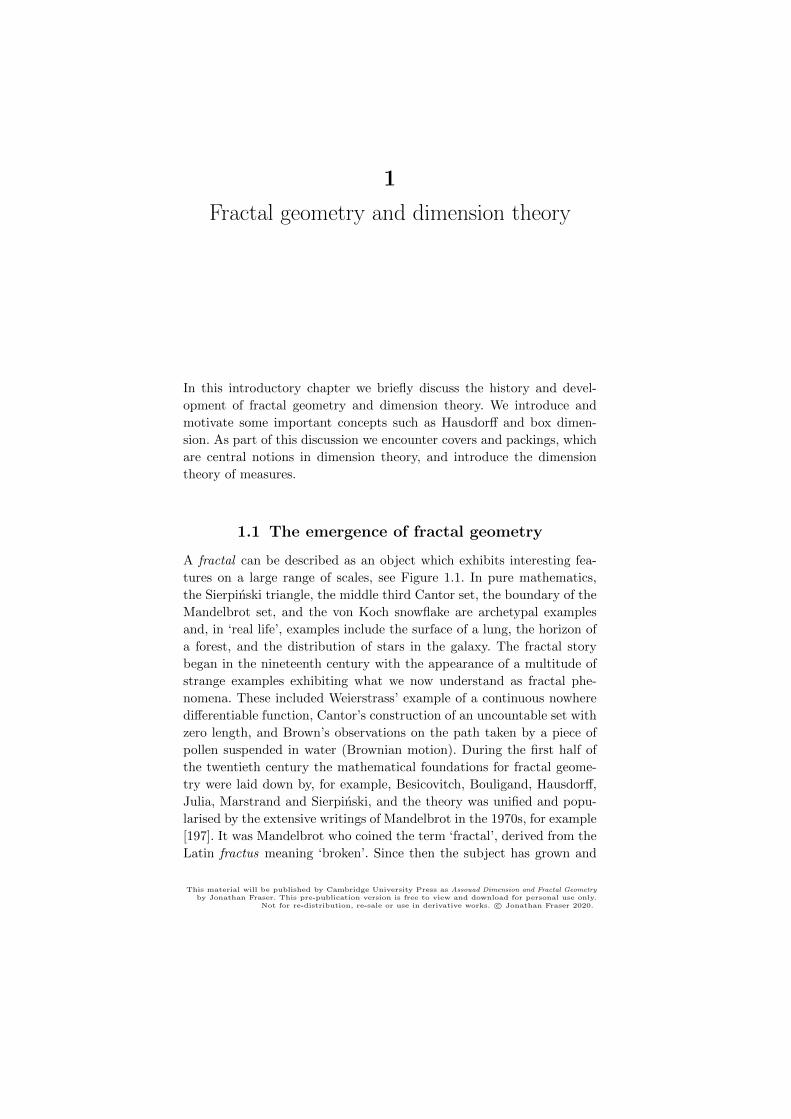
A fractal can be described as an object which exhibits interesting fea-
tures on a large range of scales, see Figure 1.1. In pure mathematics,
the Sierpinski triangle, the middle third Cantor set, the boundary of the
Mandelbrot set, and the von Koch snowflake are archetypal examples
and, in ‘real life’, examples include the surface of a lung, the horizon of
a forest, and the distribution of stars in the galaxy. The fractal story
began in the nineteenth century with the appearance of a multitude of
strange examples exhibiting what we now understand as fractal phe-
nomena. These included Weierstrass’ example of a continuous nowhere
differentiable function, Cantor’s construction of an uncountable set with
zero length, and Brown’s observations on the path taken by a piece of
pollen suspended in water (Brownian motion). During the first half of
the twentieth century the mathematical foundations for fractal geome-
try were laid down by, for example, Besicovitch, Bouligand, Hausdorff,
Julia, Marstrand and Sierpinski, and the theory was unified and popu-
larised by the extensive writings of Mandelbrot in the 1970s, for example
[197]. It was Mandelbrot who coined the term ‘fractal’, derived from the
Latin fractus meaning ‘broken’. Since then the subject has grown and
This material will be published by Cambridge University Press as Assouad Dimension and Fractal Geometryby Jonathan Fraser. This pre-publication version is free to view and download for personal use only.
Not for re-distribution, re-sale or use in derivative works. c© Jonathan Fraser 2020.
4 Fractal geometry and dimension theory
developed as a self-contained discipline in pure mathematics touching on
many other subjects, such as dynamical systems, geometric measure the-
ory, analysis (real and complex), topology, number theory, probability
theory and harmonic analysis. However, the importance of fractals is not
restricted to abstract mathematics, with many naturally occurring phys-
ical phenomena exhibiting a fractal structure, such as graphs of random
processes, percolation models and fluid turbulence. The mathematical
challenge is to understand the mechanisms which generate and under-
pin fractal behaviour and to develop robust and rich theories concerning
the geometric properties that such objects possess.
Figure 1.1 Four fractals. From top left moving clockwise: the boundary of
the Mandelbrot set, the Apollonian circle packing, a (self-affine) leaf and
the Sierpinski triangle.
1.2 Dimension theory 5
1.2 Dimension theory
At the heart of fractal geometry lies dimension theory, the subject dedi-
cated to understanding how to define, interpret, understand, and calcu-
late dimensions of sets in Euclidean space or more general metric spaces.
A dimension is a (usually non-negative real) number which gives geo-
metric information concerning how the object in question fills up space
on small scales. There are many distinct notions of dimension and one of
the joys (and central components) of the subject is in understanding how
these notions relate to each other, and how their behaviour compares in
different settings or when applied to different families of examples.
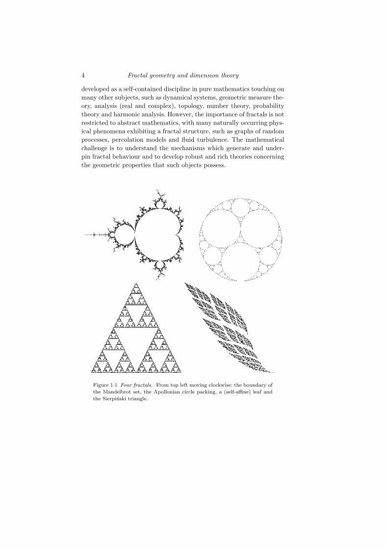
A natural approach to dimension theory is to quantify how large a
set is at a given scale by considering optimal covers by balls whose
diameter is related to the scale. More precisely, given a scale r > 0, a
finite or countable collection of sets Uii is called an r-cover of a set
F if each of the sets Ui has diameter less than or equal to r, and F is
contained in the union⋃i Ui, see Figure 1.2. Throughout the book we
write |U | = supx,y∈U |x−y| for the diameter of a non-empty set U ⊆ Rd.Understanding how to find covers of a set at small scales underpins much
of dimension theory and often the ‘covering strategy’ is specific to the
setting, sometimes driven by dynamical invariance or a priori knowledge
of another, related, set. This book is dedicated to a thorough analysis
of the Assouad dimension and some of its natural variants. However, we
will often attempt to put our discussion in a wider context for which we
require other notions.
The Hausdorff dimension is arguably the most well-studied and im-
portant notion of fractal dimension. It was introduced by Hausdorff
in 1918 [129], greatly developed by Besicovitch, and is considered ex-
tensively in many of the important books on fractal geometry, such as
[34, 69, 70, 205]. It is defined in terms of Hausdorff measure, which can
be viewed as a natural extension of Lebesgue measure to non-integer
dimensions. Given s > 0 and r > 0, the r-approximate s-dimensional
Hausdorff measure of a set F ⊆ Rd is defined by
Hsr(F ) = inf
∑i
|Ui|s : Uii is a countable r-cover of F
and the s-dimensional Hausdorff (outer) measure of F is Hs(F ) =
limr→0Hsr(F ). The limit exists because the sequence Hsr(F ) increases
as r decreases, but it may be infinite. The measures Hs can now be used
to identify the critical exponent or dimension in which it is most appro-
6 Fractal geometry and dimension theory
priate to consider F . First consider the square [0, 1]2, which has infinite
length (length measures objects which are much smaller, such as line
segments or smooth curves), and zero volume (volume measures objects
which are much bigger, such as cubes or spheres). However, the area of
the square is positive and finite (it hardly matters that the precise area
is 1), demonstrating that the natural measure to use when considering
squares is area, that is, 2-dimensional Lebesgue measure. It is no co-
incidence that we think of the square as a 2-dimensional object. Since
we have continuum many Hausdorff measures to choose from, this leads
naturally to the Hausdorff dimension of F being defined as
dimH F = infs > 0 : Hs(F ) = 0
= sup
s > 0 : Hs(F ) =∞
.
It is a useful exercise to show that these two expressions for the Haus-
dorff dimension actually coincide. The value of the Hausdorff measure
in the critical dimension, that is, HdimH F (F ) is often rather hard to
compute exactly and can be any value in [0,∞].
Figure 1.2 Left: a self-affine fractal. Right: a covering of the self-affine frac-
tal using balls of arbitrarily varying radii. Understanding such covers leads
to calculation of the Hausdorff dimension.
A less sophisticated, but nevertheless very useful, notion of dimension
is box dimension. The lower and upper box dimensions of a non-empty
bounded set F ⊆ Rd are defined by
dimBF = lim infr→0
logNr(F )
− log rand dimBF = lim sup
r→0
logNr(F )
− log r,
respectively, where Nr(F ) is the smallest number of open sets required
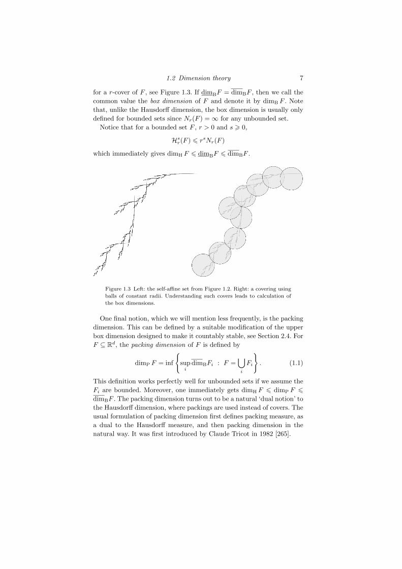
1.2 Dimension theory 7
for a r-cover of F , see Figure 1.3. If dimBF = dimBF , then we call the
common value the box dimension of F and denote it by dimB F . Note
that, unlike the Hausdorff dimension, the box dimension is usually only
defined for bounded sets since Nr(F ) =∞ for any unbounded set.
Notice that for a bounded set F , r > 0 and s > 0,
Hsr(F ) 6 rsNr(F )
which immediately gives dimH F 6 dimBF 6 dimBF .
Figure 1.3 Left: the self-affine set from Figure 1.2. Right: a covering using
balls of constant radii. Understanding such covers leads to calculation of
the box dimensions.
One final notion, which we will mention less frequently, is the packing
dimension. This can be defined by a suitable modification of the upper
box dimension designed to make it countably stable, see Section 2.4. For
F ⊆ Rd, the packing dimension of F is defined by
dimP F = inf
supi
dimBFi : F =⋃i
Fi
. (1.1)
This definition works perfectly well for unbounded sets if we assume the
Fi are bounded. Moreover, one immediately gets dimH F 6 dimP F 6dimBF . The packing dimension turns out to be a natural ‘dual notion’ to
the Hausdorff dimension, where packings are used instead of covers. The
usual formulation of packing dimension first defines packing measure, as
a dual to the Hausdorff measure, and then packing dimension in the
natural way. It was first introduced by Claude Tricot in 1982 [265].
8 Fractal geometry and dimension theory
We write B(x, r) = y ∈ Rd : |y − x| 6 r to denote the closed ball
with centre x ∈ Rd and radius r > 0. A collection of balls B(xi, r)i is
called a (centred) r-packing of a set F if the balls are pairwise disjoint
and, for all i, xi ∈ F . A related notion is that of r-separated sets. A set
X ⊆ F is called an r-separated subset of F if each pair of distinct points
from X are separated by distance at least r. If ri = r for all i, then
the set of centres xii of balls from an r-packing form a 2r-separated
subset of F . It is an elementary but instructive exercise to prove that if
one replaces Nr(F ) in the definition of upper and lower box dimensions
with any of:
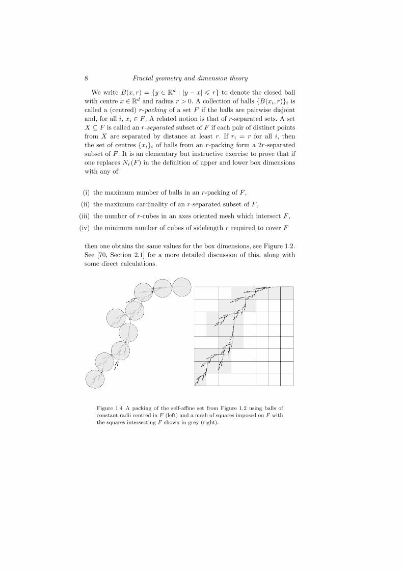
(i) the maximum number of balls in an r-packing of F ,
(ii) the maximum cardinality of an r-separated subset of F ,
(iii) the number of r-cubes in an axes oriented mesh which intersect F ,
(iv) the minimum number of cubes of sidelength r required to cover F
then one obtains the same values for the box dimensions, see Figure 1.2.
See [70, Section 2.1] for a more detailed discussion of this, along with
some direct calculations.
Figure 1.4 A packing of the self-affine set from Figure 1.2 using balls of
constant radii centred in F (left) and a mesh of squares imposed on F with
the squares intersecting F shown in grey (right).
1.2 Dimension theory 9
1.2.1 Dimension theory of measures
An important aspect of dimension theory is the interplay between the
dimensions of sets and the dimensions of measures, see, for example, the
mass distribution principle, Lemma 3.4.2. For this we need analogous
notions of dimension for measures. The (lower) Hausdorff dimension of
a Borel measure µ on Rd is
dimH µ = infdimHE : µ(E) > 0.
Thus the dimension of a measure is conveniently expressible in terms of
dimensions of sets which ‘see’ the measure. We write
supp(µ) = x ∈ Rd : µ(B(x, r)) > 0 for all r > 0 (1.2)
for the support of µ, which is necessarily a closed set, and we say µ is
fully supported on F ⊆ Rd if supp(µ) = F and supported on F ⊆ Rd if
supp(µ) ⊆ F . Straight from the definition one has, for µ supported on
F ,
dimH µ 6 dimH F.
In fact, for Borel sets F ,
dimH F = supdimH µ : supp(µ) ⊆ F. (1.3)
This follows by finding compact subsets E ⊆ F with positive and finite
s-dimensional Hausdorff measure for all s < dimH F , see [70, Theorem
4.10]. Similarly, the (lower) packing dimension of a Borel measure µ on
Rd is
dimP µ = infdimPE : µ(E) > 0.
Again one has, for µ supported on F ,
dimP µ 6 dimP F
and, for Borel sets F ,
dimP F = supdimP µ : supp(µ) ⊆ F.
This final result follows by a similar approach, this time due to Joyce
and Preiss [149]. The box dimension of a measure is a less well-developed
concept. We formulate a definition in Section 4.2 following [75], which
is partially motivated by the Assouad spectrum, see Section 3.3.
2
The Assouad dimension
In this chapter we define the Assouad dimension, which is the central
notion of the book. We discuss its origins in Section 2.3 and establish
many of its basic properties in Section 2.4 such as stability under Lip-
schitz mappings and monotonicity. These are compared with the basic
properties of the Hausdorff and box dimensions.
2.1 The Assouad dimension and a simple example
If the Hausdorff dimension provides fine, but global, geometric informa-
tion, then the Assouad dimension provides coarse, but local, geometric
information. The key difference between the Assouad dimension and the
dimensions discussed in Chapter 1 is that only a small part of the set is
considered at any one time. This is what gives it its ‘local quality’ and
what leads to many of its interesting features, see Figure 2.1
The Assouad dimension of a non-empty set F ⊆ Rd is defined by
dimA F = inf
α : there exists a constant C > 0 such that,
for all 0 < r < R and x ∈ F ,
Nr(B(x,R) ∩ F
)6 C
(R
r
)α .
Recall that Nr(E) is the smallest number of open sets required for an
r-cover of a bounded set E. Note that we can replace Nr in the definition
of the Assouad dimension with any of the standard covering or packing
functions, see the discussion in Chapter 1, and still obtain the same
value for the dimension. For example, Nr(E) could denote the number
This material will be published by Cambridge University Press as Assouad Dimension and Fractal Geometryby Jonathan Fraser. This pre-publication version is free to view and download for personal use only.
Not for re-distribution, re-sale or use in derivative works. c© Jonathan Fraser 2020.
2.1 The Assouad dimension and a simple example 11
of cubes in an r-mesh oriented at the origin which intersect E or the
maximum cardinality of an r-separated subset of E. We also obtain an
equivalent definition if the ball B(x,R) is taken to be open or closed
(although we usually think of it as being closed) or if it is replaced by a
cube of sidelength R centred at x.
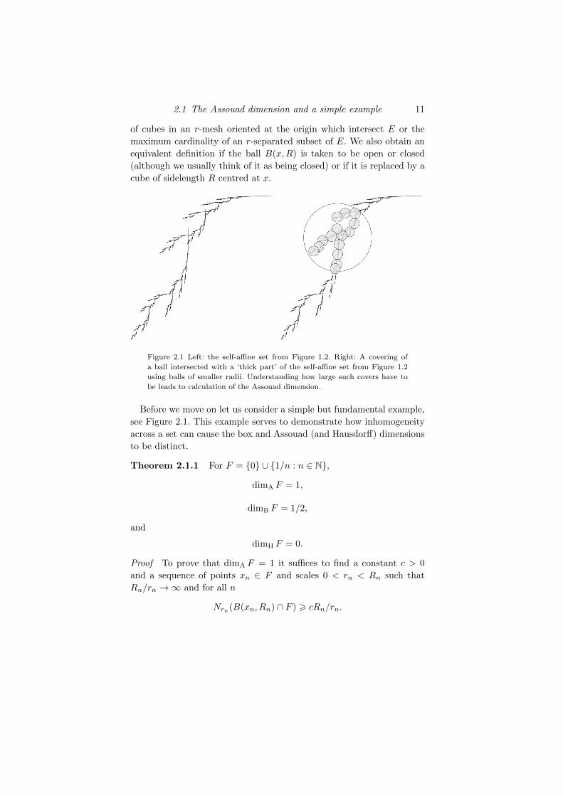
Figure 2.1 Left: the self-affine set from Figure 1.2. Right: A covering of
a ball intersected with a ‘thick part’ of the self-affine set from Figure 1.2
using balls of smaller radii. Understanding how large such covers have to
be leads to calculation of the Assouad dimension.
Before we move on let us consider a simple but fundamental example,
see Figure 2.1. This example serves to demonstrate how inhomogeneity
across a set can cause the box and Assouad (and Hausdorff) dimensions
to be distinct.
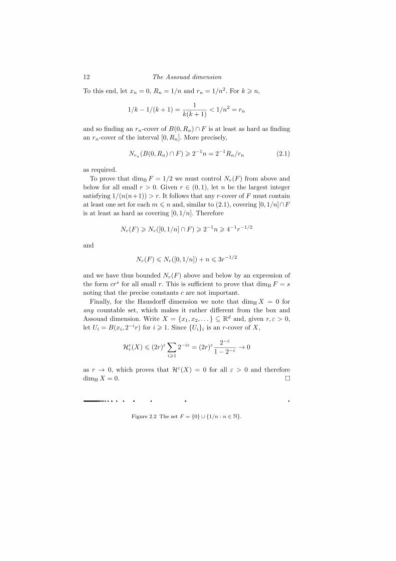
Theorem 2.1.1 For F = 0 ∪ 1/n : n ∈ N,
dimA F = 1,
dimB F = 1/2,
and
dimH F = 0.
Proof To prove that dimA F = 1 it suffices to find a constant c > 0
and a sequence of points xn ∈ F and scales 0 < rn < Rn such that
Rn/rn →∞ and for all n
Nrn(B(xn, Rn) ∩ F ) > cRn/rn.
12 The Assouad dimension
To this end, let xn = 0, Rn = 1/n and rn = 1/n2. For k > n,
1/k − 1/(k + 1) =1
k(k + 1)< 1/n2 = rn
and so finding an rn-cover of B(0, Rn) ∩ F is at least as hard as finding
an rn-cover of the interval [0, Rn]. More precisely,
Nrn(B(0, Rn) ∩ F ) > 2−1n = 2−1Rn/rn (2.1)
as required.
To prove that dimB F = 1/2 we must control Nr(F ) from above and
below for all small r > 0. Given r ∈ (0, 1), let n be the largest integer
satisfying 1/(n(n+1)) > r. It follows that any r-cover of F must contain
at least one set for each m 6 n and, similar to (2.1), covering [0, 1/n]∩Fis at least as hard as covering [0, 1/n]. Therefore
Nr(F ) > Nr([0, 1/n] ∩ F ) > 2−1n > 4−1r−1/2
and
Nr(F ) 6 Nr([0, 1/n]) + n 6 3r−1/2
and we have thus bounded Nr(F ) above and below by an expression of
the form crs for all small r. This is sufficient to prove that dimB F = s
noting that the precise constants c are not important.
Finally, for the Hausdorff dimension we note that dimHX = 0 for
any countable set, which makes it rather different from the box and
Assouad dimension. Write X = x1, x2, . . . ⊆ Rd and, given r, ε > 0,
let Ui = B(xi, 2−ir) for i > 1. Since Uii is an r-cover of X,
Hεr(X) 6 (2r)ε∑i>1
2−iε = (2r)ε2−ε
1− 2−ε→ 0
as r → 0, which proves that Hε(X) = 0 for all ε > 0 and therefore
dimHX = 0.
Figure 2.2 The set F = 0 ∪ 1/n : n ∈ N.
2.2 A word or two on the definition 13
2.2 A word or two on the definition
The first thing one notices about the definition of the Assouad dimension
is that it appears complicated. This is underlined by the fact that we
required three lines to properly express the definition!1 However, despite
its apparent complexity, the underpinning idea is very simple. In fact,
here are five distinct ways of defining the Assouad dimension in one line:
dimA F = sup dimHE : E is a weak tangent of F
dimA F = inf α : F is α-homogeneous
dimA F = inf dimA µ : µ is a Borel measure supported on F
dimA F = inf
α : (∃C > 0) (∀0 < r < R) sup
x∈FNr(B(x,R) ∩ F
)6 C
(R
r
)α
dimA F = inf
α : there exists C > 0 such that, for all 0 < r < R and x ∈ F , Nr
(B(x,R) ∩ F
)6 C
(Rr
)α .
Humour aside, each of these expressions demonstrates an important
principle. The first is a beautiful fact, which was first explicitly stated
by Kaenmaki, Ojala and Rossi [154], but has origins in the work of
Furstenberg [114, 115, 116] and Bishop and Peres [34]. It states that
one may express the Assouad dimension entirely in terms of the Haus-
dorff dimension and entirely at the level of tangents. See Chapter 5 for
more details on this important result, especially Theorem 5.1.3. The sec-
ond expression is how one often explains the notion to an inexperienced
party: suppose we can cover any R-ball in a set F with at most a con-
stant multiple of (R/r)α many r-balls. This is natural since if F is Rdthen one readily covers any R-ball by at most 5 · 2d(R/r)d many r-balls.
We call a set with this property α-homogeneous and clearly this becomes
harder to satisfy as α decreases. The Assouad dimension is simply the
infimum of α such that the set is α-homogeneous. The third expression
brings in the natural interplay between dimensions of sets and dimen-
sions of measures. It is well known that the Hausdorff dimension of a set
is the supremum of the Hausdorff dimension of Borel measures which
it supports, recall (1.3). This duality between sets and measures is a
powerful concept in dimension theory and the fact that one has a paral-
lel dualism for Assouad dimension is appealing — and turns out to be
1 “The problem with the Assouad dimension is that it is impossible to write thedefinition in one line.” - Nick Sharples (in jest), Manchester Dynamics Seminar,October 2015.
14 The Assouad dimension
useful as well. Of course, it depends on how one defines the Assouad di-
mension of a measure. This concept, initially called the upper regularity
dimension, was introduced by Kaenmaki, Lehrback and Vuorinen [153],
and we will discuss it in detail in Chapter 4, especially Theorem 4.1.3.
Hidden in this statement is also the seminal fact that a doubling metric
space always carries a doubling measure. The fourth expression demon-
strates the power of good and efficient notation and the fifth expression
is illustrative of the fact that any mathematical statement, theorem, or
proof, can be reduced to one line if one has a long enough line or a small
enough font!
We conclude this section with some technical remarks on the defini-
tion. In several instances in the literature, for example [219], the follow-
ing subtly different definition of the Assouad dimension is given:
inf
α : there exist constants C > 0, ρ > 0 such that,
for all 0 < r < R < ρ and x ∈ F ,
Nr(B(x,R) ∩ F
)6 C
(R
r
)α . (2.2)
It is easy to check that this definition and our definition coincide for all
bounded F ⊆ Rd but they may differ drastically for unbounded sets.2
For example, our definition assigns the integers dimension 1, whereas
the alternative definition (2.2) assigns them dimension 0. Whether one
wants the integers to have dimension 1 or 0 is perhaps a matter of taste
but at the core of the decision is whether you want to look on large
and small scales for the ‘thickest part’ of the space, or whether you only
want to consider behaviour on small scales. We propose that the integers
should have Assouad dimension 1 and therefore reject the alternative
definition (2.2). This has several theoretical advantages, such as allowing
the Assouad dimension to be invariant under Mobius transformations
and inversions such as z 7→ 1/z, see Section 9.3. It also means we do
not have to specify whether tangents are obtained by ‘zooming out’
or ‘zooming in’ on the fractal. Moreover, the definition we use, see the
beginning of Chapter 2, was also adopted by Robinson [240] and Mackay
and Tyson [195].
In an attempt to simplify the definition, several people have asked us
if the constant C is really necessary. Specifically, does it not get dwarfed
2 It was Chris Miller who first drew my attention to this inconsistency back in2014.
2.3 Some history 15
by (R/r)α−dimA F for all α > dimA F since we should clearly only be
interested in sequences of scales such that R/r → ∞? However, if the
constant C is omitted from the definition, then one does not obtain a
sensible notion of dimension. In particular, the finite set 0, 1 would
have dimension 1 since if we choose x = 0, R = 1 and r = 1/2, then
Nr(B(x,R) ∩ F
)= 2 = (R/r) and so we cannot choose any α < 1 to
satisfy the required condition.
Finally, we point out that the upper box dimension may be expressed
in a similar way to the Assouad dimension, which partially serves to
motivate both definitions and also highlights the potential for interplay
between the two notions. Indeed, for bounded F ⊆ Rd,
dimBF = inf
α : there exists a constant C > 0 such that,
for all 0 < r < 1 and x ∈ F ,
Nr(B(x, 1) ∩ F
)6 C
(1
r
)α .
The reason that one may simplify this expression (for example, the con-
stant C can be removed) is that there is only one scale involved. There-
fore, the upper box dimension may be expressed as an upper limit as
this single scale tends to 0.
2.3 Some history
Although interesting in its own right, and as a notion alongside Haus-
dorff and box dimension in fractal geometry, the Assouad dimension
first came to prominence in other fields. Perhaps most notably, it plays
an important role in quasi-conformal geometry, see [130, 192, 195], and
embedding theory, see [222, 221, 240, 6, 7]. However, there has been an
explosion of activity concerning the Assouad dimension in the fractal
geometry literature in the last few years. We put this down to the pub-
lication of the books by Robinson [240] and Mackay and Tyson [195],
as well as interesting research articles published around the same time
which consider the Assouad dimension in classically fractal settings, such
as [192, 194, 219, 153, 88, 115].
The Assouad dimension takes its name from French mathematician
Patrice Assouad, who used the concept extensively during his doctoral
studies in the 1970s as a tool in embedding problems, see [6, 7, 8]. This
16 The Assouad dimension
work culminated with the seminal Assouad Embedding Theorem, see
Theorem 13.1.3, which served to motivate the Assouad dimension and
popularise it throughout the mathematics community. However, the no-
tion did not quite originate with Assouad and, in fact, appeared (inde-
pendently) at least three times before Assouad’s work in the 1970s.
The earliest reference we are aware of is Bouligand’s 1928 paper [35],
which is best known for the origin of the box dimension, or ‘Minkowski-
Bouligand dimension’. Discussion here is a little vague, but certainly
there is an attempt to consider the volume of the r-neighbourhood of
B(x,R)∩F for sets F ⊆ Rd. Bouligand observes that this may lead to a
different notion of dimension than if the volume of the r-neighbourhood
of the whole of F is considered (this is the box dimension) — not least
since this dimension would depend on the point x. Bouligand writes3
“One must thus give, instead of a dimensional number, a dimensional
order, and also give to the notion of dimensional order a local character”.
He also referred to sets as isodimensional if the ‘local dimensional order’
is the same at all points. In modern day language we might think of this
as sets with equal Assouad and lower dimension.
The next appearance we are aware of is in Larman’s paper [179]
where it is referred to as the dimensional number and denoted by dim-n.
Among many other things, Larman’s work contains the result that, for
fixed p > 0, dimA1/np : n ∈ N = 1 and the fact that the lower dimen-
sion (Larman’s minimal dimensional number m.dim-n) of a compact set
is bounded above by its Hausdorff dimension, see Theorem 3.4.3.
The Assouad dimension also appears implicitly in Furstenberg’s early
work [114]. This was made more explicit in a celebrated article from 2008
[115], see also [116]. We briefly describe some of the results from [115]
to highlight the connection with Assouad dimension. Let F ⊆ [0, 1]d
be a non-empty compact set and say that a non-empty compact set
E ⊆ [0, 1]d is a miniset of F if, for some c > 1 and t ∈ Rd, E ⊆ cF + t.
Moreover, E is called a microset of F if it is a limit of a sequence of
minisets of F in the Hausdorff metric. A family G of non-empty compact
subsets of [0, 1]d is called a gallery if it satisfies:
(i) G is closed with respect to the Hausdorff metric, see (5.1),
(ii) for each E ∈ G, every miniset of E is also in G.
Given a non-empty compact set F ⊆ [0, 1]d, the collection of all microsets
3 I am quoting from the English translation of [35] found in [61]. The translation isdue to Ilan Vardi.
2.4 Basic properties: the greatest of all dimensions 17
of F forms a gallery which Furstenberg denoted by GF . Then the ∗-dimension of F is defined by
dim∗ F = supdimHE : E ∈ GF .
In [115, Theorem 5.1], Furstenberg proved the following.
Theorem 2.3.1 Let G be a gallery. Let
∆(G) = lim supk→∞
1
klog2
(supX∈G
#Q ∈ Dk : X ∩Q 6= ∅),
where Dk denotes the collection of half-open dyadic intervals of side
length 2−k and log2 is the base-2 logarithm. Then there exists a set
A ∈ G such that
dimHA = ∆(G).
It is easy to see that dimHX 6 dimAX 6 ∆(G) for any X ∈ G, and
therefore, for any gallery G,
supdimHX : X ∈ G = supdimAX : X ∈ G = ∆(G),
and, moreover, both these suprema are obtained. In particular, for any
non-empty compact F
dimA F = dim∗ F = ∆(GF )
and there exists a microset E of F such that dimHE = dimA F . Using
our terminology, the gallery GF of a compact set F is the set of all
(subsets of) weak tangents and the coincidence of the ∗-dimension and
the Assouad dimension is manifest in Theorem 5.1.3. See Section 5 for
more details on this topic.
2.4 Basic properties: the greatest of all dimensions
Following [70], in this section we describe some basic properties which
we might hope for a ‘dimension’ to satisfy and then decide which of these
properties are satisfied by the Assouad dimension. To put these results
in context we will frequently compare the behaviour of the Assouad
dimension with that of the box, packing and Hausdorff dimensions.
The following is a list of basic properties which a given notion of
dimension dim may satisfy:
18 The Assouad dimension
• Monotonicity: dim is said to be monotone if E ⊆ F ⇒ dimE 6 dimF
for all E,F ⊆ Rd.• Finite stability: dim is said to be finitely stable if dim(E ∪ F ) =
maxdimE, dimF for all E,F ⊆ Rd.• Countable stability: dim is said to be countably stable if dim
⋃i Fi =
supi dimFi for all countable collections Fii of subsets of Rd.• Lipschitz stability: dim is said to be Lipschitz stable if dimT (F ) 6
dimF for all F ⊆ Rd and all Lipschitz maps T on Rd. Recall that a
map T : F → Rd is Lipschitz if there exists a constant K > 0 such
that, for all x, y ∈ F ,
|T (x)− T (y)| 6 K|x− y|.
• Bi-Lipschitz stability: dim is said to be stable under bi-Lipschitz maps
if dimT (F ) = dimF for all F ⊆ Rd and all bi-Lipschitz maps T on
F . Recall that a map T : F → Rd is bi-Lipschitz if it is Lipschitz with
a Lipschitz inverse (defined on T (F )).
• Stability under closure: dim is said to be stable under closure if dimF =
dimF for all F ⊆ Rd. Here and throughout F denotes the closure of
a set F , which is the intersection of all closed sets containing F .
• Open set property: dim is said to satisfy the open set property if for
any bounded open set U ⊆ Rd, dimU = d.
The proof of the following lemma is left as an exercise, although proofs
can be found in [192]. The proof is straightforward, but the unfamiliar
reader will find it useful to prove it carefully, paying particular attention
to the precise definitions involved.
Lemma 2.4.1 The Assouad dimension is monotone, finitely stable,
stable under closure and satisfies the open set property.
The fact that the Assouad dimension is stable under closure and sat-
isfies the open set property immediately shows that the Assouad dimen-
sion is not countably stable. For example,
dimA([0, 1] ∩Q) = dimA[0, 1] = dimA(0, 1) = 1
but the set [0, 1] ∩ Q is a countable union of singletons, each of which
has Assouad dimension 0.
As an example, and partly to warm us up for future sections, we in-
clude a full proof that the Assouad dimension is stable under bi-Lipschitz
maps. There will be examples later in the book which demonstrate that
2.4 Basic properties: the greatest of all dimensions 19
the Assouad dimension is not stable under Lipschitz maps, see Theorem
3.4.12, Corollary 7.2.2 and also [192, Example A.6 2].
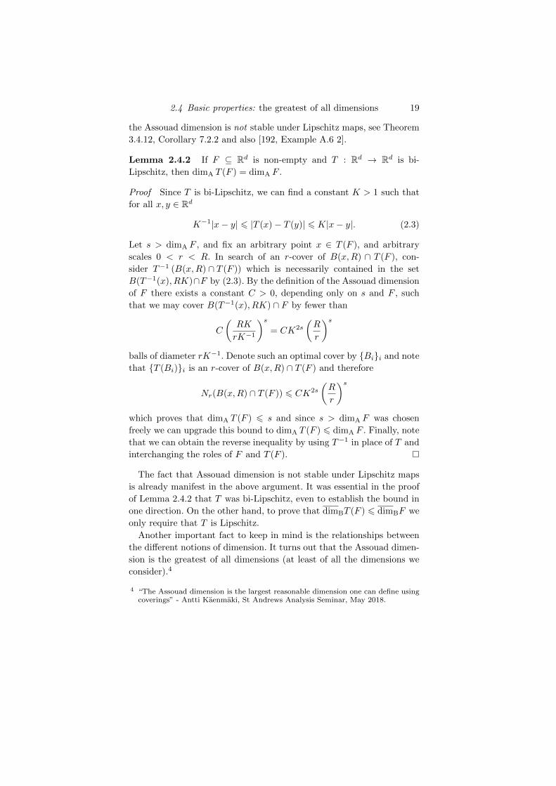
Lemma 2.4.2 If F ⊆ Rd is non-empty and T : Rd → Rd is bi-
Lipschitz, then dimA T (F ) = dimA F .
Proof Since T is bi-Lipschitz, we can find a constant K > 1 such that
for all x, y ∈ Rd
K−1|x− y| 6 |T (x)− T (y)| 6 K|x− y|. (2.3)
Let s > dimA F , and fix an arbitrary point x ∈ T (F ), and arbitrary
scales 0 < r < R. In search of an r-cover of B(x,R) ∩ T (F ), con-
sider T−1 (B(x,R) ∩ T (F )) which is necessarily contained in the set
B(T−1(x), RK)∩F by (2.3). By the definition of the Assouad dimension
of F there exists a constant C > 0, depending only on s and F , such
that we may cover B(T−1(x), RK) ∩ F by fewer than
C
(RK
rK−1
)s= CK2s
(R
r
)sballs of diameter rK−1. Denote such an optimal cover by Bii and note
that T (Bi)i is an r-cover of B(x,R) ∩ T (F ) and therefore
Nr(B(x,R) ∩ T (F )) 6 CK2s
(R
r
)swhich proves that dimA T (F ) 6 s and since s > dimA F was chosen
freely we can upgrade this bound to dimA T (F ) 6 dimA F . Finally, note
that we can obtain the reverse inequality by using T−1 in place of T and
interchanging the roles of F and T (F ).
The fact that Assouad dimension is not stable under Lipschitz maps
is already manifest in the above argument. It was essential in the proof
of Lemma 2.4.2 that T was bi-Lipschitz, even to establish the bound in
one direction. On the other hand, to prove that dimBT (F ) 6 dimBF we
only require that T is Lipschitz.
Another important fact to keep in mind is the relationships between
the different notions of dimension. It turns out that the Assouad dimen-
sion is the greatest of all dimensions (at least of all the dimensions we
consider).4
4 “The Assouad dimension is the largest reasonable dimension one can define usingcoverings” - Antti Kaenmaki, St Andrews Analysis Seminar, May 2018.
20 The Assouad dimension
Property dimH dimP dimB dimB dimA
Monotone X X X X X
Finitely stable X X × X X
Countably stable X X × × ×
Lipschitz stable X X X X ×
Bi-Lipschitz stable X X X X X
Stable under closure × × X X X
Open set property X X X X X
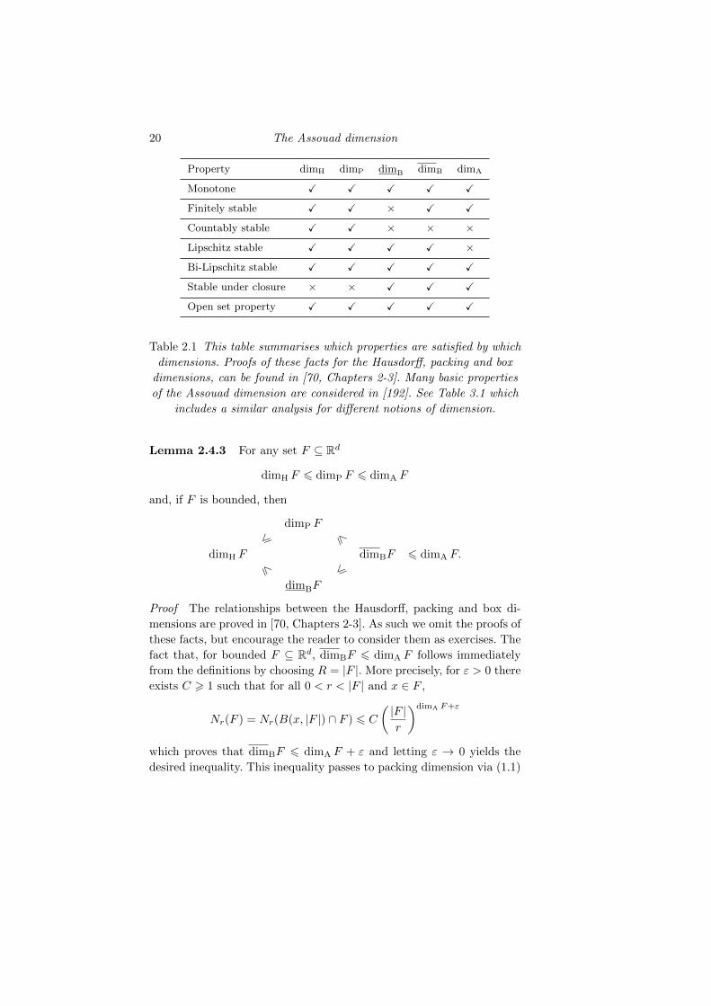
Table 2.1 This table summarises which properties are satisfied by which
dimensions. Proofs of these facts for the Hausdorff, packing and box
dimensions, can be found in [70, Chapters 2-3]. Many basic properties
of the Assouad dimension are considered in [192]. See Table 3.1 which
includes a similar analysis for different notions of dimension.
Lemma 2.4.3 For any set F ⊆ Rd
dimH F 6 dimP F 6 dimA F
and, if F is bounded, then
dimP F
6 6
dimH F dimBF 6 dimA F.6 6
dimBF
Proof The relationships between the Hausdorff, packing and box di-
mensions are proved in [70, Chapters 2-3]. As such we omit the proofs of
these facts, but encourage the reader to consider them as exercises. The
fact that, for bounded F ⊆ Rd, dimBF 6 dimA F follows immediately
from the definitions by choosing R = |F |. More precisely, for ε > 0 there
exists C > 1 such that for all 0 < r < |F | and x ∈ F ,
Nr(F ) = Nr(B(x, |F |) ∩ F ) 6 C
(|F |r
)dimA F+ε
which proves that dimBF 6 dimA F + ε and letting ε → 0 yields the
desired inequality. This inequality passes to packing dimension via (1.1)
2.4 Basic properties: the greatest of all dimensions 21
since
dimP F = infsupi
dimBFi : F =⋃i
Fi, Fi bounded
6 infsupi
dimA Fi : F =⋃i
Fi, Fi bounded
6 dimA F
by monotonicity.
There is no general relationship between the lower box and packing
dimensions.
3
Some variations on the Assouad dimension
In this chapter we introduce several variants of the Assouad dimension,
which will also play a key role in this book. Most importantly, the lower
dimension, see Section 3.1, is the natural dual to the Assouad dimen-
sion, and the Assouad spectrum, see Section 3.3, is a function which
interpolates between the quasi-Assouad dimension and the upper box
dimension. The quasi-Assouad dimension is closely related to the As-
souad dimension and is introduced in Section 3.2. When we say the As-
souad spectrum ‘interpolates’ we mean that it is a continuous function
of θ ∈ (0, 1) which tends to the upper box dimension as θ → 0 and tends
to the quasi-Assouad dimension as θ → 1. Therefore, the Assouad spec-
trum provides more information than the upper box and quasi-Assouad
dimension considered in isolation and serves to explore the gap between
these dimensions, should there be one. In Section 3.4 we develop some of
the basic properties of these notions and in subsequent chapters we will
attempt to present a unified theory of the Assouad dimension together
with all of its natural variants whenever possible.
3.1 The lower dimension
An important theme in dimension theory is that dimensions often come
in pairs. For example, the Hausdorff and packing dimension are a natural
pair, as are the upper and lower box dimensions. See Section 10.1 for
a particularly transparent example of the role of dimension pairs in the
context of product sets. The natural partner of the Assouad dimension
is the lower dimension, which was introduced by Larman [179] where
This material will be published by Cambridge University Press as Assouad Dimension and Fractal Geometryby Jonathan Fraser. This pre-publication version is free to view and download for personal use only.
Not for re-distribution, re-sale or use in derivative works. c© Jonathan Fraser 2020.
3.1 The lower dimension 23
it was called the minimal dimensional number.1 We adopt the name
‘lower dimension’ following an important paper written by Bylund and
Gudayol [40], which will be revisited in Section 4. Just as the Assouad
dimension seeks to quantify the ‘thickest’ part of the set in question, the
lower dimension identifies the ‘thinnest’ part, that is, the part of the set
which is easiest to cover, see Figure 3.1. This leads to the lower dimension
having some strange properties, such as failing to be monotonic.2 The
lower dimension of F is defined by
dimL F = sup
α : there exists a constant C > 0 such that,
for all 0 < r < R 6 |F | and x ∈ F ,
Nr(B(x,R) ∩ F
)> C
(R
r
)α .
Comparing this with the definition of the Assouad dimension, it is clear
that the lower dimension is a dual notion. However, it is worth pointing
out the one asymmetry in the definition which is the inclusion of the
diameter |F | (which may be infinity) as an upper bound on allowable
scales r,R. Sometimes this is included in the definition of the Assouad
dimension, but it leads to an equivalent definition, since for R > |F | it
is just as easy to cover B(x,R) ∩ F as it is to cover B(x, |F |) ∩ F . It
is crucial, however, to include this bound in the definition of the lower
dimension as otherwise all bounded sets would have dimension 0.
If a set has some exceptional points around which it is distributed very
sparsely in comparison with the rest of the set, then the lower dimension
will reflect this. For instance, sets with isolated points always have lower
dimension equal to 0. However, for sets with some degree of homogeneity,
such as attractors of iterated function systems (IFSs) or dynamically
invariant sets, the lower dimension is very suitable and reveals easily
interpreted information about the set. See Theorems 6.3.1 and 7.4.2, as
well as the papers [148, 260]. Since the Assouad and lower dimensions
are extremal, the difference between them provides a crude measure
of inhomogeneity. For example, self-similar sets satisfying the open set
condition and, more generally, Ahlfors-regular sets, have equal Assouad
and lower dimensions, indicating that these sets are as homogeneous as
possible, see Section 6.4. However, for more complicated sets, such as
1 It was referred to as the lower Assouad dimension by Kaenmaki, Lehrback andVuorinen [153] and Tuomas Sahlsten used to call it the uniformity dimension.
2 ‘Thickest’ is monotonic but ‘thinnest’ is not.
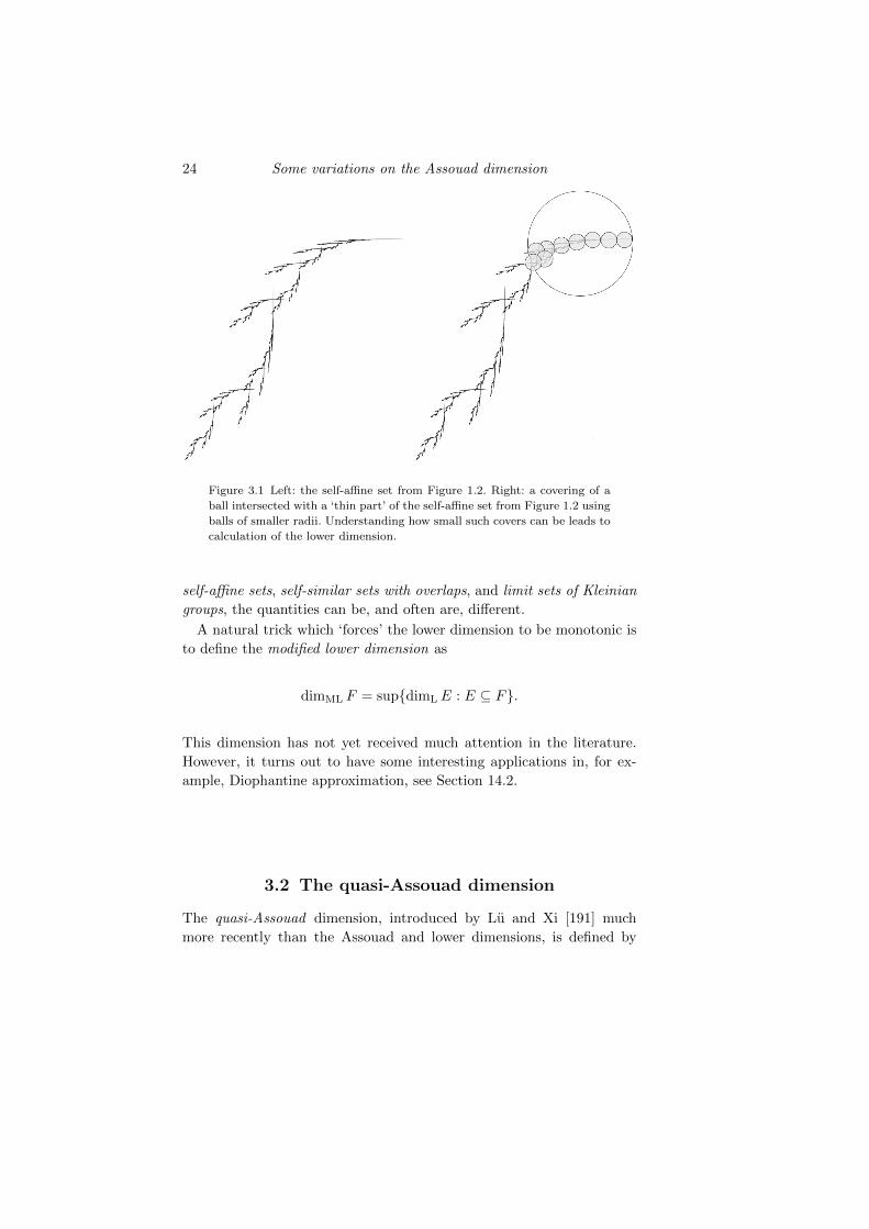
24 Some variations on the Assouad dimension
Figure 3.1 Left: the self-affine set from Figure 1.2. Right: a covering of a
ball intersected with a ‘thin part’ of the self-affine set from Figure 1.2 using
balls of smaller radii. Understanding how small such covers can be leads to
calculation of the lower dimension.
self-affine sets, self-similar sets with overlaps, and limit sets of Kleinian
groups, the quantities can be, and often are, different.
A natural trick which ‘forces’ the lower dimension to be monotonic is
to define the modified lower dimension as
dimML F = supdimLE : E ⊆ F.
This dimension has not yet received much attention in the literature.
However, it turns out to have some interesting applications in, for ex-
ample, Diophantine approximation, see Section 14.2.
3.2 The quasi-Assouad dimension
The quasi-Assouad dimension, introduced by Lu and Xi [191] much
more recently than the Assouad and lower dimensions, is defined by
3.3 The Assouad spectrum 25
dimqA F = limδ→0 hF (δ) where, for δ ∈ (0, 1),
hF (δ) = inf
α : there exists a constant C > 0 such that,
for all 0 < r 6 R1+δ < 1 and x ∈ F ,
Nr(B(x,R) ∩ F
)6 C
(R
r
)α .
The quasi-Assouad dimension leaves an ‘exponential gap’ between the
scales r and R, which in some settings can make a huge difference —
see, for example, Section 9.4.
One of the motivations behind the definition of quasi-Assouad dimen-
sion is that it is preserved under quasi-Lipschitz maps. Given compact
sets X,Y ⊆ Rd, a bijection T : X → Y is called quasi-Lipschitz if
log |T (x)− T (y)|log |x− y|
→ 1
uniformly as |x−y| → 0. The concept of quasi-Lipschitz equivalence was
introduced in [276]. Clearly any bi-Lipschitz map is quasi-Lipschitz. Lu
and Xi [191] proved that for any quasi-Lipschitz map T and F ⊆ Rd
dimqA T (F ) = dimqA F.
This property is shared by the Hausdorff, box and packing dimensions,
but not by the Assouad dimension. We will revisit this concept later,
see Corollary 3.4.15. There is also an analogously defined quasi-lower
dimension, which we will introduce formally below, see (3.3).
3.3 The Assouad spectrum
Motivated by the desire to obtain more nuanced information about the
scaling structure of a fractal set, Fraser and Yu introduced the Assouad
spectrum [111], see also the survey [94]. The idea is to understand which
pairs of scales r < R give rise to the extreme behaviour captured by
the Assouad (and quasi-Assouad) dimension. To each θ ∈ (0, 1), one
associates the appropriate analogue of the Assouad dimension with the
restriction that the two scales r and R used in the definition satisfy R =
rθ. The resulting ‘dimension spectrum’ (as a function of θ) thus gives
finer geometric information regarding the scaling structure of the set
and, in some precise sense, interpolates between the upper box dimension
26 Some variations on the Assouad dimension
and the (quasi-)Assouad dimension. The Assouad spectrum is generally
better behaved than the Assouad dimension and so this interpolation can
lead to a clearer understanding of the Assouad dimension considered in
isolation. More precisely, given θ ∈ (0, 1) we define
dimθA F = inf
α : there exists a constant C > 0 such that,
for all 0 < r < 1 and x ∈ F ,
Nr(B(x, rθ) ∩ F
)6 C
(rθ
r
)α ,
and the dual notion
dimθL F = sup
α : there exists a constant C > 0 such that,
for all 0 < r < 1 and x ∈ F ,
Nr(B(x, rθ) ∩ F
)> C
(rθ
r
)α .
We refer to dimθA F as the Assouad spectrum and dimθ
L F as the lower
spectrum and wish to understand these concepts as functions of θ. Many
properties of these dimension spectra were considered in [111, 95] and
further examples were considered in [112, 108]. Sometimes it is conve-
nient to consider scales expressed as R1/θ < R rather than r < rθ, that
is, the smaller scale as a function of the bigger scale rather than the
bigger scale as a function of the smaller scale. This was how the defi-
nition was originally expressed in [111] but the definition we give here
is clearly equivalent. Since we require r < rθ for θ ∈ (0, 1), it is neces-
sary to restrict our attention to small scale behaviour, that is, r < 1,
which is another notable difference between the Assouad spectrum and
quasi-Assouad dimension in comparison with the Assouad dimension.
As discussed above, this makes no difference for bounded sets, but for
unbounded sets it leads to rather different behaviour. For example, for
all θ ∈ (0, 1), dimθA Z = dimqA Z = 0 < 1 = dimA Z.
We will study many fundamental properties of the Assouad and lower
spectra in the following sections, but we close this introductory discus-
sion by emphasising that these spectra lie in between the Assouad and
lower dimensions and the box dimensions. That is, for bounded F ⊆ Rdand all θ ∈ (0, 1),
dimL F 6 dimθL F 6 dimBF 6 dimBF 6 dimθ
A F 6 dimA F. (3.1)
3.3 The Assouad spectrum 27
See Lemma 3.4.1 and Lemma 3.4.4 for more refined estimates.
3.3.1 First observations on the Assouad spectrum
One of the most important and useful properties of the Assouad and
lower spectra is that they are continuous in θ ∈ (0, 1). This will follow
from the following theorem, which has other useful consequences as well.
This proposition unifies [111, Propositions 3.4 and 3.7], see also [42,
Proposition 2.1].
Theorem 3.3.1 For any set F ⊆ Rd and 0 < θ1 < θ2 < 1,(1− θ2
1− θ1
)dimθ2
A F 6 dimθ1A F
6
(1− θ2
1− θ1
)dimθ2
A F +
(θ2 − θ1
1− θ1
)dim
θ1/θ2A F,
and(1− θ2
1− θ1
)dimθ2
L F 6 dimθ1L F
6
(θ1 − θ1θ2
θ2 − θ1θ2
)dimθ2
L F +
(θ2 − θ1
θ2 − θ1θ2
)dim
θ1/θ2A F.
Proof First consider the Assouad spectrum. Let 0 < θ1 < θ2 < 1,
s < dimθ2A F < t
and
dimθ1/θ2A F < u.
For r ∈ (0, 1), we clearly have
supx∈F
Nr(B(x, rθ2) ∩ F ) 6 supx∈F
Nr(B(x, rθ1) ∩ F ).
Therefore, by applying the definition of the Assouad spectrum directly,
we can find arbitrarily small r > 0 satisfying
supx∈F
Nr(B(x, rθ1) ∩ F ) >
(rθ2
r
)s=(rθ1−1
)s( 1−θ21−θ1
)
which proves
dimθ1A F > s
(1− θ2
1− θ1
)
28 Some variations on the Assouad dimension
and letting s → dimθ2A F yields the desired lower bound. Moving on to
the upper bound for the Assouad spectrum, for r ∈ (0, 1),
supx∈F
Nr(B(x, rθ1) ∩ F ) 6 supx∈F
Nrθ2 (B(x, rθ1) ∩ F ) supx∈F
Nr(B(x, rθ2) ∩ F )
which can be seen by first covering B(x, rθ1) ∩ F by rθ2-balls and then
covering each of these by r-balls. Therefore, for all r ∈ (0, 1),
supx∈F
Nr(B(x, rθ1) ∩ F ) 6
(rθ1
rθ2
)u(rθ2
r
)t=(rθ1−1
)u( θ2−θ11−θ1
)+t(
1−θ21−θ1
)
which proves
dimθ1A F 6 u
(θ2 − θ1
1− θ1
)+ t
(1− θ2
1− θ1
)and letting t → dimθ2
A F and u → dimθ1/θ2A F yields the desired upper
bound.
For the lower spectrum, let
s < dimθ2L F
and
v < dimθ1/θ2L F.
For r ∈ (0, 1),
infx∈F
Nr(B(x, rθ2) ∩ F ) 6 infx∈F
Nr(B(x, rθ1) ∩ F ).
Therefore, by applying the definition of the lower spectrum, for all r ∈(0, 1),
infx∈F
Nr(B(x, rθ1) ∩ F ) >
(rθ2
r
)s=(rθ1−1
)s( 1−θ21−θ1
)
which proves
dimθ1L F > s
(1− θ2
1− θ1
)and letting s→ dimθ2
L F yields the desired lower bound.
The upper bound is a little more complicated. Let
dimθ2L F < t
and
dimθ1/θ2A F < u.
3.3 The Assouad spectrum 29
Then, for r ∈ (0, 1),
infx∈F
Nr(B(x, rθ1) ∩ F )
6 infx∈F
Nrθ1/θ2 (B(x, rθ1) ∩ F ) supx∈F
Nr(B(x, rθ1/θ2) ∩ F )
which comes by first finding an rθ1-ball which minimises
infx∈F
Nrθ1/θ2 (B(x, rθ1) ∩ F ),
covering it efficiently by rθ1/θ2 -balls, and then covering each of these by
r-balls. By applying the definition of the Assouad and lower spectrum,
we can find arbitrarily small r > 0 satisfying
infx∈F
Nr(B(x, rθ1) ∩ F ) 6
(rθ1
rθ1/θ2
)t(rθ1/θ2
r
)u
=
(rθ1
r
)t( θ1−θ1/θ2θ1−1
)+u(θ1/θ2−1θ1−1
)
which proves
dimθ1L F 6 t
(θ1 − θ1θ2
θ2 − θ1θ2
)+ u
(θ2 − θ1
θ2 − θ1θ2
)and letting t → dimθ2
L F and u → dimθ1/θ2A F yields the desired upper
bound.
Using similar ideas, one may establish various other bounds for the
spectra. We omit further details since the estimates above serve our
purpose. See [111, Propositions 3.4 and 3.7] and, in particular, [42,
Proposition 2.1] which establishes a better lower bound for the lower
spectrum than the one we give here.
The most appealing thing about Theorem 3.3.1 is its applications.
The first and most important of these is continuity of the spectra.
Corollary 3.3.2 For a fixed non-empty set F ⊆ Rd, the functions
θ 7→ dimθA F and θ 7→ dimθ
L F are continuous in θ ∈ (0, 1).
One immediately sees that for any set F and all θ ∈ (0, 1), dimθA F 6
dimqA F . Another useful consequence of Theorem 3.3.1 is that if the
Assouad spectrum reaches the quasi-Assouad dimension, then it is con-
stant from that point on. We will see that the Assouad spectrum is not
30 Some variations on the Assouad dimension
necessarily non-decreasing across the whole range, so this information is
a priori useful.
Corollary 3.3.3 Fix a non-empty set F ⊆ Rd. If dimθA F = dimqA F
for some θ ∈ (0, 1), then
dimθ′
A F = dimqA F
for all θ′ ∈ [θ, 1).
Proof This follows from the upper bound on dimθ1A F from Theorem
3.3.1, by choosing θ1 = θ, θ2 = θ′ and bounding dimθ1/θ2A F above by
dimqA F .
As we will see, a typical behaviour for the Assouad spectrum is to
be convex and increasing on (0, ρ) and constantly equal to the quasi-
Assouad dimension on [ρ, 1) for some ρ ∈ (0, 1). Another useful conse-
quence of Theorem 3.3.1 is that, if ρ is known, then we get a simple lower
bound for the increasing part of the spectrum. One reason we mention
this is that ρ turns up again in other contexts, see, for example, Section
17.7.
Corollary 3.3.4 For a fixed non-empty set F ⊆ Rd, suppose
ρ = infθ ∈ (0, 1) : dimθA F = dimqA F
exists and ρ ∈ (0, 1). Then for θ ∈ (0, ρ)
dimθA F >
(1− ρ1− θ
)dimqA F.
Proof This follows from Theorem 3.3.1 with θ1 = θ < θ2 = ρ.
The spectra exhibit stronger regularity properties than just continu-
ity. In fact, [111, Corollary 3.7] shows that the spectra are Lipschitz on
every closed interval strictly contained in (0, 1) and are therefore differ-
entiable almost everywhere by Rademacher’s Theorem. That said, the
set of points for which the spectra are not differentiable may be dense
by the following theorem proved in [95, Theorem 2.5].
Theorem 3.3.5 Let f : [0, 1] → [0, 1] be continuous, concave, non-
decreasing and satisfy f(0) > 0 and f(θ) 6 f(0)(θ + 1) for all θ ∈ [0, 1].
Then there exists a compact set F ⊆ [0, 1] such that
dimθA F = f(θ)
for all θ ∈ (0, 1).
3.3 The Assouad spectrum 31
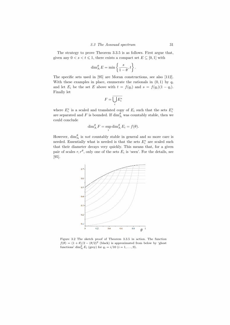
The strategy to prove Theorem 3.3.5 is as follows. First argue that,
given any 0 < s < t 6 1, there exists a compact set E ⊆ [0, 1] with
dimθAE = min
s
1− θ, t
.
The specific sets used in [95] are Moran constructions, see also [112].
With these examples in place, enumerate the rationals in (0, 1) by qiand let Ei be the set E above with t = f(qi) and s = f(qi)(1 − qi).
Finally let
F =⋃i
E∗i
where E∗i is a scaled and translated copy of Ei such that the sets E∗iare separated and F is bounded. If dimθ
A was countably stable, then we
could conclude
dimθA F = sup
idimθ
AEi = f(θ).
However, dimθA is not countably stable in general and so more care is
needed. Essentially what is needed is that the sets E∗i are scaled such
that their diameter decays very quickly. This means that, for a given
pair of scales r, rθ, only one of the sets Ei is ‘seen’. For the details, see
[95].
Figure 3.2 The sketch proof of Theorem 3.3.5 in action. The function
f(θ) = (1 + θ)/2 − (θ/2)2 (black) is approximated from below by ‘ghost
functions’ dimθA Ei (grey) for qi = i/10 (i = 1, . . . , 9).
32 Some variations on the Assouad dimension
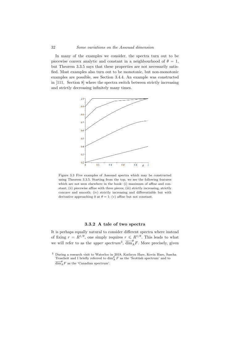
In many of the examples we consider, the spectra turn out to be
piecewise convex analytic and constant in a neighbourhood of θ = 1,
but Theorem 3.3.5 says that these properties are not necessarily satis-
fied. Most examples also turn out to be monotonic, but non-monotonic
examples are possible, see Section 3.4.4. An example was constructed
in [111, Section 8] where the spectra switch between strictly increasing
and strictly decreasing infinitely many times.
Figure 3.3 Five examples of Assouad spectra which may be constructed
using Theorem 3.3.5. Starting from the top, we see the following features
which are not seen elsewhere in the book: (i) maximum of affine and con-
stant; (ii) piecewise affine with three pieces; (iii) strictly increasing, strictly
concave and smooth; (iv) strictly increasing and differentiable but with
derivative approaching 0 at θ = 1; (v) affine but not constant.
3.3.2 A tale of two spectra
It is perhaps equally natural to consider different spectra where instead
of fixing r = R1/θ, one simply requires r 6 R1/θ. This leads to what
we will refer to as the upper spectrum3, dimθ
AF . More precisely, given
3 During a research visit to Waterloo in 2018, Kathryn Hare, Kevin Hare, SaschaTroscheit and I briefly referred to dimθ
A F as the ‘Scottish spectrum’ and to
dimθAF as the ‘Canadian spectrum’.
3.3 The Assouad spectrum 33
θ ∈ (0, 1) we define
dimθ
AF = inf
α : there exists a constant C > 0 such that,
for all 0 < r 6 R1/θ < R < 1 and x ∈ F ,
Nr(B(x,R) ∩ F
)6 C
(R
r
)α
noting that dimθ
AF is equal to hF (δ) in the definition of the quasi-
Assouad dimension, for δ = 1/θ − 1.
It follows immediately from the definition that
dimθA F 6 dim
θ
AF 6 dimqA F 6 dimA F
and, moreover, the upper spectrum is non-decreasing in θ, whereas the
Assouad spectrum is not necessarily non-decreasing. In particular, the
notions are distinct. However, it turns out that the upper spectrum is
determined entirely by the Assouad spectrum. The following result was
proved in [95] and we follow the proof given there.
Theorem 3.3.6 Let F ⊆ Rd. Then, for all θ ∈ (0, 1),
dimθ
AF = sup0<θ′6θ
dimθ′
A F.
Proof We give the proof in the case where F is bounded. The un-
bounded case requires a delicate argument for which we refer the reader
to [95]. We only need to prove
sup0<θ′6θ
dimθ′
A F > dimθ
AF
since the other direction is trivial.
Let θ ∈ (0, 1), s = dimθ
AF which we may assume is strictly positive,
and 0 < ε < s. By definition we can find sequences xi, ri, Ri (i > 1) such
that xi ∈ F , 0 < ri 6 R1/θi < Ri < 1, (ri/Ri)→ 0 and
Nri (B(xi, Ri) ∩ F ) >
(Riri
)s−ε. (3.2)
We can assume that Ri → 0 since otherwise (using (3.1), see Lemma
3.4.1) dimθA F > dimBF > s− ε, which is sufficient.
For each i, let θi be defined by ri = R1/θii , noting that 0 < θi 6 θ for
all i. Using compactness of [0, θ] to extract a convergent subsequence, we
may assume that θi → θ′ ∈ [0, θ] and, by taking a further subsequence
34 Some variations on the Assouad dimension
if necessary, we may assume that |θi − θ′| < δ for all i where δ > 0 can
be chosen arbitrarily. We may also assume that the sequence θi is either
non-increasing or strictly increasing.
First suppose that θ′ = 0. Since F is assumed to be bounded
NR
1/θii
(F ) > NR
1/θii
(B(xi, Ri) ∩ F ) >
(Ri
R1/θii
)s−ε
>
(1
R1/θii
)(s−ε)(1−δ)
by (3.2). Note that the final inequality uses the fact that δ > θi, which
follows since δ > |θi − θ′| = θi. Then (using (3.1), see Lemma 3.4.1)
dimθA F > dimBF > (s− ε)(1− δ). Since δ > 0 and ε > 0 can be chosen
arbitrarily small, this yields the desired result.
From now on suppose θ′ > 0. If the sequence θi is non-increasing, then
θ′ 6 θi, and therefore R1/θii > R
1/θ′
i , for all i. It follows that
NR
1/θ′i
(B(xi, Ri) ∩ F ) > NR
1/θii
(B(xi, Ri) ∩ F )
>
(Ri
R1/θii
)s−εby (3.2)
=
(Ri
R1/θ′
i
)( 1−1/θi1−1/θ′
)(s−ε)
>
(Ri
R1/θ′
i
) θ′(1−θ′−δ)(θ′+δ)(1−θ′) (s−ε)
where the final inequality uses
1− 1/θi1− 1/θ′
=θ′(1− θi)θi(1− θ′)
>θ′(1− θ′ − δ)
(θ′ + δ)(1− θ′)
which holds since θi 6 θ′ + δ. This yields dimθ′
A F > θ′(1−θ′−δ)(θ′+δ)(1−θ′) (s − ε)
and, since δ > 0 can be chosen arbitrarily small (after fixing θ′), we
obtain dimθ′
A F > s− ε.On the other hand, if θi is strictly increasing, then θ′ > θi for all
i. Taking another subsequence if necessary we can also assume that
θi > θ′/2 for all i. Covering by R1/θ′
i -balls and then covering each R1/θ′
i -
3.3 The Assouad spectrum 35
ball by R1/θii -balls we obtain
NR
1/θii
(B(xi, Ri) ∩ F )
6 NR
1/θ′i
(B(xi, Ri) ∩ F )
(supz∈Rd
NR
1/θii
(B(z,R
1/θ′
i
)))
6 NR
1/θ′i
(B(xi, Ri) ∩ F ) c(d)
(R
1/θ′
i
R1/θii
)dwhere c(d) > 1 is a constant depending only on d. Therefore
NR
1/θ′i
(B(xi, Ri) ∩ F ) > c(d)−1NR
1/θii
(B(xi, Ri) ∩ F )R(1/θi−1/θ′)di
> c(d)−1
(Ri
R1/θii
)s−εR
(1/θi−1/θ′)di by (3.2)
= c(d)−1
(Ri
R1/θ′
i
)( 1−1/θi1−1/θ′
)(s−ε)+
(1/θi−1/θ′
1−1/θ′
)d
> c(d)−1
(Ri
R1/θ′
i
)s−ε− δd(1−θ′)θ′/2
,
where the final inequality uses the coefficient bounds(1− 1/θi1− 1/θ′
)> 1
which holds since θ′ > θi and(1/θi − 1/θ′
1− 1/θ′
)= −
(θ′ − θi
(1− θ′)θi
)> − δ
(1− θ′)θ′/2
which holds since 0 < θ′−θi 6 δ and θi > θ′/2. It follows that dimθ′
A F >s− ε− δd
(1−θ′)θ′/2 and since δ > 0 can be chosen arbitrarily small (after
fixing θ′) we obtain dimθ′
A F > s− ε as before. Since ε > 0 was arbitrary
it follows that
sup0<θ′6θ
dimθ′
A F > s
completing the proof.
One of the benefits of Theorem 3.3.6 is that it allows us to focus future
36 Some variations on the Assouad dimension
study on the Assouad spectrum rather than the upper spectrum which
could have a priori contained new information in its own right. Not only
does the Assouad spectrum contain strictly more information than the
upper spectrum, but it is also easier to work with since the family of
scales is 1-parameter, rather than 2-parameter.
A theoretically significant corollary to Theorem 3.3.6, is that we ob-
tain the interpolation result which motivated the introduction of the
Assouad spectrum in the first place, albeit with Assouad dimension re-
placed by quasi-Assouad dimension. In many (but certainly not all) cases
of interest, the quasi-Assouad and Assouad dimensions coincide and so
genuine interpolation between the upper box and Assouad dimension is
achieved.
Corollary 3.3.7 Let F ⊆ Rd. Then dimθA F → dimqA F as θ → 1.
Theorem 3.3.6 only directly implies that lim supθ→1 dimθA F = dimqA F ,
but the fact that the limit of dimθA F as θ → 1 exists follows from [111,
Remark 3.9], see [95, Section 3.2].
The analogous ‘tale of two spectra’ problem for the lower spectrum
was considered in [41, 42]. The quasi-lower dimension, dimqL F , was
introduced in [41] and in [42] it was proved that
dimqL F = limθ→1
dimθL F (3.3)
provided dimL F > 0. The assumption that dimL F > 0 was removed
in [127, Theorem A.2], which allows us to take (3.3) as our definition of
quasi-lower dimension for any set F ⊆ Rd.
3.3.3 Recovering the interpolation
The Assouad spectrum was introduced to understand the ‘gap’ in be-
tween the upper box and Assouad dimensions. This was partially achieved
since, for bounded F ⊆ Rd,
(i) dimθA F → dimBF as θ → 0,
(ii) dimθA F is continuous in θ ∈ (0, 1),
(iii) dimθA F → dimqA F as θ → 1.
In many cases of interest dimqA F = dimA F and so the full range
[dimBF,dimA F ] is ‘witnessed’ by the Assouad spectrum. However, if
dimqA F < dimA F , then there is a gap and the desired interpolation is
not achieved. An approach for ‘recovering the interpolation’ was outlined
in [111], which we briefly explain here.
3.3 The Assouad spectrum 37
Let φ : [0, 1] → [0, 1] be an increasing continuous function such that
φ(R) 6 R for all R ∈ [0, 1]. The φ-Assouad dimension, introduced in
[111], is defined by
dimφA F = inf
α : there exists a constant C > 0 such that,
for all 0 < r 6 φ(R) 6 R < 1 and x ∈ F ,
Nr(B(x,R) ∩ F
)6 C
(R
r
)α .
If φ(R) = R1/θ, then dimφA F recovers the upper Assouad spectrum
(which can be expressed entirely in terms of the Assouad spectrum), and
if φ(R) = R, then dimφA F = dimA F (for bounded F ). Therefore, one
may recover the desired interpolation by identifying precise conditions
on φ which guarantee dimφA F = dimA F . Often dimθ
A F = dimA F for
some θ ∈ (0, 1), in which case the threshold for witnessing the Assouad
dimension is provided by the function φ(R) = R1/θ. The φ-Assouad
dimension has been considered in detail4 by Garcıa, Hare, and Mendivil
[120, 121] and Troscheit [268]. A particular case of interest is Mandelbrot
percolation, see Section 9.4 and Theorem 9.4.4.
Many interesting results pertaining to the φ-Assouad dimension, and
several worthwhile variants, were given in [120]. We highlight some here
but refer the reader to [120] for more detail.
Theorem 3.3.8
(i) If log φ(R)logR → 1 as R→ 0, then, for all sets F ⊆ Rd,
dimφA F > dimqA F.
(ii) If infR>0φ(R)R > 0, then, for all bounded sets F ⊆ Rd,
dimφA F = dimA F.
(iii) There exist sets F ⊆ Rd such that dimqA F < dimA F and for all
s ∈ [dimqA F,dimA F ], there exists φ (with the properties described
above) such that dimφA F = s.
4 Slightly different notation is used in these papers. Instead of writing φ(R) they
write R1+Φ(R). Therefore some care is required when transferring results fromone set of notation to another.
38 Some variations on the Assouad dimension
3.4 Basic properties: revisited
Before we lose track of how many definitions of dimension we are con-
sidering, we briefly return to the topic of basic properties and collect
together some observations on the variants of the Assouad dimension
we have encountered.
3.4.1 Relationships between dimensions
Perhaps the most important facts to establish are how these dimensions
relate to each other. This was already touched on in (3.1) above. The
following should be compared with Lemma 2.4.3 and was observed in
[111].
Lemma 3.4.1 For a bounded set F ⊆ Rd,
dimBF 6 dimθA F 6 dimqA F 6 dimA F
and
dimML F
6 6
dimL F dimBF.6 6
dimθL F
Proof Most of these inequalities follow easily from the definitions and
their proofs are left as exercises. The details can be found in [111]. We
prove dimBF 6 dimθA F here, which is not quite immediate. We may
assume dimBF > 0 and let 0 < t < dimBF < s. By covering F with
rθ-balls and then covering each of these rθ-balls with r-balls we obtain
Nr(F ) 6 Nrθ (F )
(supx∈F
Nr(B(x, rθ) ∩ F )
).
By the definition of upper box dimension, there exist arbitrarily small
r > 0 such that
supx∈F
Nr(B(x, rθ) ∩ F ) >Nr(F )
Nrθ (F )>
r−t
r−θs=
(rθ
r
) θs−tθ−1
which proves that dimθA F > t−θs
1−θ . Since s and t can be made arbitrarily
close to dimBF , the lower bound follows.
3.4 Basic properties: revisited 39
In general the lower dimension and lower spectrum are not comparable
to the Hausdorff dimension. For example, for all θ ∈ (0, 1),
dimL Q = dimθL Q = 1 > 0 = dimH Q
and
dimL[0, 1] ∪ 2 = dimθL[0, 1] ∪ 2 = 0 < 1 = dimH[0, 1] ∪ 2.
However, if F is closed, then one can prove that the lower dimension is
the ‘smallest of all dimensions’. This was first proved by Larman in the
1960s [179, 180]. To prove this result we rely on the mass distribution
principle, Lemma 3.4.2. This is a well-known result in fractal geometry
(for example, see [70]) but we include the proof since it is so simple.
Lemma 3.4.2 Let F ⊆ Rd be a Borel set and suppose that for some
constants C, s > 0 there exists a non-trivial Borel measure on F such
that for all x ∈ F and r > 0
µ(B(x, r)) 6 Crs.
Then dimH F > s.
Proof Let Uii be an arbitrary r-cover of F . Then
0 < µ(F ) 6∑i
µ(Ui) 6∑i
C|Ui|s
and taking infimum over all r-covers we obtain Hsr(F ) > µ(F )/C > 0
and therefore Hs(F ) > µ(F )/C > 0 and dimH F > s as required.
Theorem 3.4.3 If F ⊆ Rd is closed, then
dimL F 6 dimML F 6 dimH F.
Proof We first prove that dimL F 6 dimH F , and we may assume the
lower dimension is strictly positive as otherwise there is nothing to prove.
Fix 0 < s < dimL F . We claim that there exists c ∈ (0, 1) such that,
given any x ∈ F and 0 < ρ < |F |, we can find a collection of c−s points
xi ∈ F such that the closed balls B(xi, cρ) are pairwise disjoint and
B(xi, cρ) ⊆ B(x, ρ). To see this, let s < t < dimL F and note that it
follows directly from the definition of lower dimension that there exists
C > 0 such that, for all x ∈ F and 0 < r < R < |F |, we can find a
collection of C(R/r)t points xi ∈ F such that the closed balls B(xi, r)
are pairwise disjoint and B(xi, r) ⊆ B(x,R). (This is taking advantage
of the relationship between minimal covers and maximal packings.) The
40 Some variations on the Assouad dimension
claim follows by choosing R = ρ and r = cρ such that c ∈ (0, 1) is chosen
small enough to guarantee C(R/r)t = Ccs−tc−s > c−s.
Let B0 be any closed ball centred in F with radius ρ ∈ (0, |F |) and
apply the claim to obtain a collection of c−s pairwise disjoint closed
balls of radius cρ centred in F which are all contained in B0. Apply
this procedure inductively on every ball present at each stage of the
construction to produce a decreasing sequence of sets Bk, (that is, B0 =
B0 ⊃ B1 ⊃ B2 ⊃ . . .), where each Bk consists of c−sk many pairwise
disjoint closed balls of radius ckρ centred in F . The intersection
F ′ =⋂k
Bk (3.4)
is a non-empty compact set and since F is closed we necessarily have
F ′ ⊆ F . Let µ be a Borel probability measure defined on F ′ where each
ball in Bk has mass cks. Given r ∈ (0, 1), let k be the unique integer such
that ckρ 6 r < c(k−1)ρ. By a simple volume argument, for all x ∈ F and
r > 0, the ball B(x, r) can intersect no more than a constant C(d) many
balls from Bk, where C(d) is a constant depending only on the ambient
spatial dimension d. Therefore
µ(B(x, r)) 6 C(d)cks 6 C(d)ρ−srs
and it follows from the mass distribution principle Lemma 3.4.2 that
dimH F > s. Letting s→ dimL F yields dimH F > dimL F , as required.
Moreover, for any E ⊆ F ,
dimLE = dimLE 6 dimHE 6 dimH F = dimH F
where the final inequality uses the fact that F is closed. Therefore
dimML F 6 dimH F .
The lower spectrum is not generally bounded above by the modified
lower dimension or by the Hausdorff dimension, even for closed sets. This
is perhaps a little counter-intuitive because the proof given above almost
looks like it should work with the lower spectrum replacing the lower
dimension. However, the problem is that when we iterate the information
we get from the lower spectrum for a fixed θ the radii of the balls in the
nested sequence Bk decrease super-exponentially, which is not sufficient
to establish the mass distribution estimate. For a concrete example of a
compact set F with
dimθL F > dimH F
for some θ ∈ (0, 1), see the self-affine carpets considered in Section 8.
3.4 Basic properties: revisited 41
Garcıa and Hare proved that the quasi -lower dimension of a closed set is
bounded above by its Hausdorff dimension, that is, for closed F ⊆ Rd,dimqL F 6 dimH F , see [118, Proposition 10]. Therefore, one always has
limθ→1
dimθL F 6 dimH F
for closed F , even if the spectrum is not uniformly bounded above by
the Hausdorff dimension. Slightly more information can be derived from
[120, Proposition 2.12], but we omit the details.
Despite the upper box dimension being a lower bound for the Assouad
spectrum, one can also bound the Assouad spectrum above in terms
of the upper box dimension. The following result, first proved in [111,
Proposition 3.1], will be used throughout the book.
Lemma 3.4.4 For a non-empty bounded set F and θ ∈ (0, 1),
dimBF 6 dimθA F 6 min
dimBF
1− θ, dimqA F
.
Proof The lower bound is from Lemma 3.4.1. The fact that the quasi-
Assouad dimension is an upper bound is trivial, and also from Lemma
3.4.1, and so it remains to prove the ‘other’ upper bound.
Fix θ ∈ (0, 1), s > dimBF and let x ∈ F and r ∈ (0, 1). Appealing to
the definition of the upper box dimension, there exists C > 0 depending
only on s such that
Nr(B(x, rθ) ∩ F ) 6 Nr(F ) 6 Cr−s = C
(rθ
r
)s/(1−θ),
which implies dimθA F 6 s
1−θ . Since s > dimBF was arbitrary, the desired
upper bound follows.
The bounds in Lemma 3.4.4 are sharp. For a family of examples where
the upper bound is obtained, see Theorem 3.4.7, and for a method for
constructing examples where the lower bound is obtained, see Theorem
3.3.5 or Theorem 9.4.2.
The following counter-intuitive result follows from Lemma 3.4.4 and
the fact that the Assouad spectrum approaches the quasi-Assouad di-
mension as θ → 1, see Corollary 3.3.7. We give an alternative direct
proof here, following [118].
Lemma 3.4.5 Let F ⊆ Rd be a non-empty bounded set. Then dimBF =
0 if and only if dimqA F = 0.
42 Some variations on the Assouad dimension
Proof This result was first proved by Garcıa and Hare [118, Proposition
15], and we give their elegant proof, which does not rely on the Assouad
spectrum. Since dimBF 6 dimqA F always holds, it suffices to prove
that if dimBF = 0, then dimqA F = 0. Let ε, δ > 0 and note that
dimBF = 0 means that there exists a constant C > 0 such that for
all r ∈ (0, 1), Nr(F ) 6 Cr−εδ/(1+δ). It follows that, for all x ∈ F and
0 < r 6 R1+δ 6 1,
Nr(B(x,R) ∩ F ) 6 Nr(F ) 6 Cr−εδ/(1+δ) 6 C(R/r)ε
which proves that hF (δ) 6 ε and since ε, δ > 0 are arbitrary the result
follows.
The ‘only if’ part of Lemma 3.4.5 is surprising since we generally
have control in the opposite direction, that is, dimBF 6 dimqA F , and,
moreover, the Assouad dimension can take on any value in [0, d] even in
cases where the box dimension is 0. We are not aware of such a mutual
dependency result holding for any other pair of dimensions.
Corollary 3.4.6 Let F ⊆ Rd be a non-empty bounded set with
dimBF < dimqA F . Suppose
ρ = infθ ∈ (0, 1) : dimθA F = dimqA F = 1− dimBF
dimqA F
noting that this is as small as the phase transition ρ can be by Lemma
3.4.4. Then, for all θ ∈ (0, 1),
dimθA F = min
dimBF
1− θ, dimqA F
.
Proof This follows from Corollary 3.3.4 and Lemma 3.4.4.
To motivate Corollary 3.4.6, we briefly return to the example consid-
ered in Theorem 2.1.1. We take the example a little further by including
an exponent p as well as computing the Assouad spectrum and demon-
strating sharpness of the upper bound from Lemma 3.4.4.
Theorem 3.4.7 For p > 0 and Fp = 0 ∪ 1/np : n ∈ N,
dimθA Fp = min
1
(1 + p)(1− θ), 1
.
Therefore,
dimB Fp =1
1 + p,
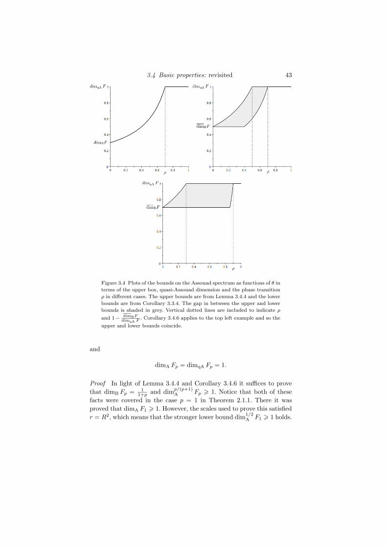
3.4 Basic properties: revisited 43
Figure 3.4 Plots of the bounds on the Assouad spectrum as functions of θ in
terms of the upper box, quasi-Assouad dimension and the phase transition
ρ in different cases. The upper bounds are from Lemma 3.4.4 and the lower
bounds are from Corollary 3.3.4. The gap in between the upper and lower
bounds is shaded in grey. Vertical dotted lines are included to indicate ρ
and 1− dimBFdimqA F
. Corollary 3.4.6 applies to the top left example and so the
upper and lower bounds coincide.
and
dimA Fp = dimqA Fp = 1.
Proof In light of Lemma 3.4.4 and Corollary 3.4.6 it suffices to prove
that dimB Fp = 11+p and dim
p/(p+1)A Fp > 1. Notice that both of these
facts were covered in the case p = 1 in Theorem 2.1.1. There it was
proved that dimA F1 > 1. However, the scales used to prove this satisfied
r = R2, which means that the stronger lower bound dim1/2A F1 > 1 holds.
44 Some variations on the Assouad dimension
The extension of this argument to general p is straightforward and left
to the reader.
Corollary 3.3.4 can be improved if the lower dimension is large.
Theorem 3.4.8 For any set F ⊆ Rd and 0 < θ1 < θ2 < 1,
dimθ1A F >
(θ2 − θ1
1− θ1
)dim
θ1/θ2A F +
(1− θ2
1− θ1
)dimθ2
L F.
In particular, if
ρ = infθ ∈ (0, 1) : dimθA F = dimqA F
exists, ρ ∈ (0, 1) and dimL F = dimBF , then for θ ∈ (0, ρ)
dimθA F > dimBF +
(1− ρ)θ
(1− θ)ρ(dimqA F − dimBF ).
Proof The proof strategy here is similar to Theorem 3.3.1. Given r ∈(0, 1), first choose x ∈ F which maximises
Nrθ2 (B(x, rθ1) ∩ F ) (3.5)
and take a maximal rθ2-packing of B(x, rθ1) ∩ F by balls of radius rθ2 .
We may consider r-covers of each of these balls independently, losing at
most a constant in our estimate for Nr(B(x, rθ1)∩F ). However, we can
only bound the r-covering number for each of these balls from below by
infx∈F
Nr(B(x, rθ2) ∩ F ). (3.6)
Combining (3.5) and (3.6), for arbitrary ε > 0,
Nrθ2 (B(x, rθ1) ∩ F ) > C
(rθ1
rθ2
)dimθ1/θ2A F−ε(
rθ2
r
)dimθ2L F−ε
for a constant C depending only on ε. This proves the result upon letting
ε→ 0.
The lower bound in Theorem 3.4.8 is harder to establish than the
lower bound in Theorem 3.3.1 but — perhaps surprisingly — either
estimate may be better, depending on how relatively large the lower
dimension is. The lower bound from Theorem 3.4.8 turns out to be a
natural candidate for the Assouad spectrum of several examples, both
when the lower dimension is equal to the box dimension and when it is
strictly smaller, see Section 17.7.
Somewhat surprisingly, there does not appear to be an analogue of
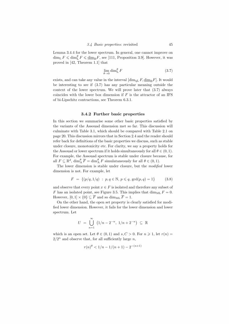
3.4 Basic properties: revisited 45
Lemma 3.4.4 for the lower spectrum. In general, one cannot improve on
dimL F 6 dimθL F 6 dimBF , see [111, Proposition 3.9]. However, it was
proved in [42, Theorem 1.1] that
limθ→0
dimθL F (3.7)
exists, and can take any value in the interval [dimqL F,dimBF ]. It would
be interesting to see if (3.7) has any particular meaning outside the
context of the lower spectrum. We will prove later that (3.7) always
coincides with the lower box dimension if F is the attractor of an IFS
of bi-Lipschitz contractions, see Theorem 6.3.1.
3.4.2 Further basic properties
In this section we summarise some other basic properties satisfied by
the variants of the Assouad dimension met so far. This discussion will
culminate with Table 3.1, which should be compared with Table 2.1 on
page 20. This discussion mirrors that in Section 2.4 and the reader should
refer back for definitions of the basic properties we discuss, such as stable
under closure, monotonicity etc. For clarity, we say a property holds for
the Assouad or lower spectrum if it holds simultaneously for all θ ∈ (0, 1).
For example, the Assouad spectrum is stable under closure because, for
all F ⊆ Rd, dimθA F = dimθ
A F simulataneously for all θ ∈ (0, 1).
The lower dimension is stable under closure, but the modified lower
dimension is not. For example, let
F = (p/q, 1/q) : p, q ∈ N, p 6 q, gcd(p, q) = 1 (3.8)
and observe that every point x ∈ F is isolated and therefore any subset of
F has an isolated point, see Figure 3.5. This implies that dimML F = 0.
However, [0, 1]× 0 ⊆ F and so dimML F = 1.
On the other hand, the open set property is clearly satisfied for modi-
fied lower dimension. However, it fails for the lower dimension and lower
spectrum. Let
U =
∞⋃n=1
(1/n− 2−n, 1/n+ 2−n
)⊆ R
which is an open set. Let θ ∈ (0, 1) and s, C > 0. For n > 1, let r(n) =
2/2n and observe that, for all sufficiently large n,
r(n)θ < 1/n− 1/(n+ 1)− 2−(n+1)
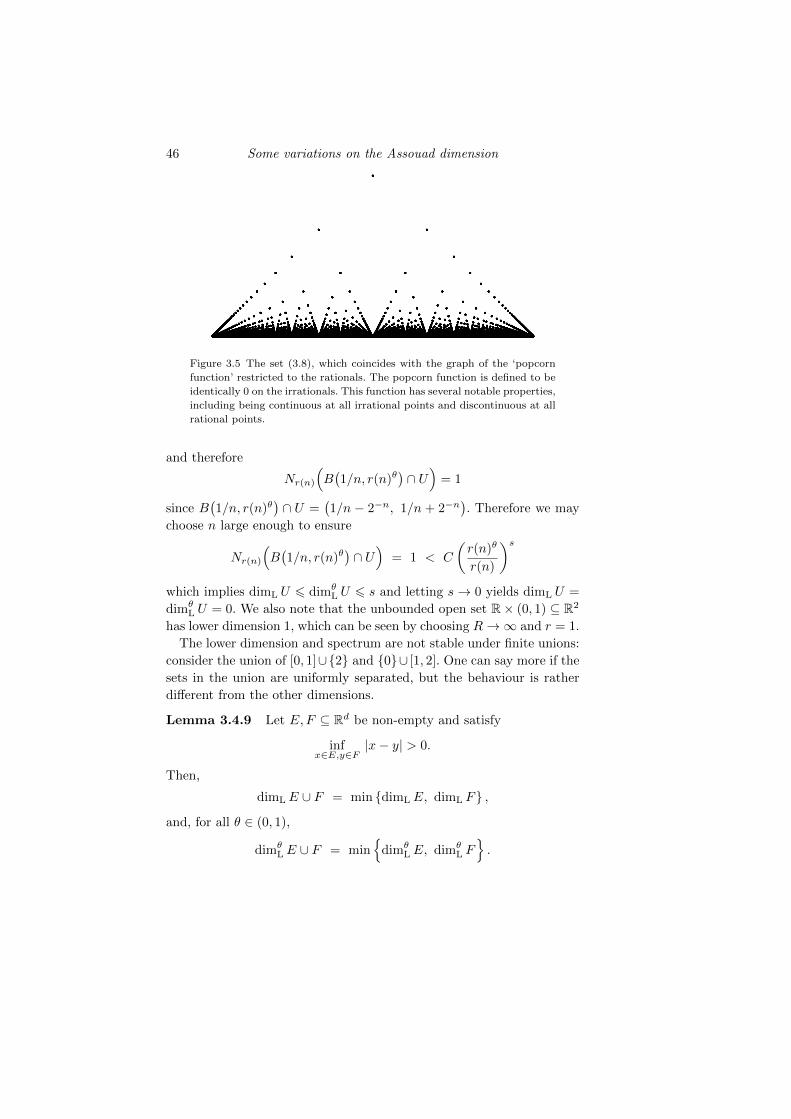
46 Some variations on the Assouad dimension
Figure 3.5 The set (3.8), which coincides with the graph of the ‘popcorn
function’ restricted to the rationals. The popcorn function is defined to be
identically 0 on the irrationals. This function has several notable properties,
including being continuous at all irrational points and discontinuous at all
rational points.
and therefore
Nr(n)
(B(1/n, r(n)θ
)∩ U
)= 1
since B(1/n, r(n)θ
)∩ U =
(1/n − 2−n, 1/n + 2−n
). Therefore we may
choose n large enough to ensure
Nr(n)
(B(1/n, r(n)θ
)∩ U
)= 1 < C
(r(n)θ
r(n)
)swhich implies dimL U 6 dimθ
L U 6 s and letting s→ 0 yields dimL U =
dimθL U = 0. We also note that the unbounded open set R× (0, 1) ⊆ R2
has lower dimension 1, which can be seen by choosing R→∞ and r = 1.
The lower dimension and spectrum are not stable under finite unions:
consider the union of [0, 1]∪2 and 0∪ [1, 2]. One can say more if the
sets in the union are uniformly separated, but the behaviour is rather
different from the other dimensions.
Lemma 3.4.9 Let E,F ⊆ Rd be non-empty and satisfy
infx∈E,y∈F
|x− y| > 0.
Then,
dimLE ∪ F = min dimLE, dimL F ,
and, for all θ ∈ (0, 1),
dimθLE ∪ F = min
dimθ
LE, dimθL F.
3.4 Basic properties: revisited 47
Proof The formulae for the lower dimension and lower spectrum are
proved similarly. The inequalities mindimLE,dimL F 6 dimL(E ∪ F )
and mindimθLE,dimθ
L F 6 dimθL(E ∪ F ) hold without the uniform
separation assumption since, for 0 < r < R < 1,
infx∈E∪F
Nr(B(x,R) ∩ (E ∪ F )
)> min
infx∈E
Nr(B(x,R) ∩ E
), infx∈F
Nr(B(x,R) ∩ F
).
The reverse inequalities hold, assuming the separation assumption, since,
for R < mininfx∈E,y∈F |x−y|, 1, the above inequality can be replaced
by equality. This is because if x ∈ E, then B(x,R) ∩ F = ∅ and vice
versa.
The question of finite stability for the modified lower dimension is a
little tricky. In [111, Proposition 4.3] it was proved that modified lower
dimension is finitely stable for sets E,F which are ‘properly separated’,
in the sense of Lemma 3.4.9, with the general case left as an open ques-
tion [111, Question 9.3]. Here we prove finite stability holds provided the
sets in question are closed. The proof is based on a simple adaptation of
the proof of Lemma 3.4.3.
Lemma 3.4.10 If E,F ⊆ Rd are non-empty and closed, then
dimMLE ∪ F = max dimMLE, dimML F .
Proof The lower bound (>) follows immediately by monotonicity, but
the upper bound (6) is more subtle. We may assume 0 < dimMLE ∪F ,
let 0 < s < dimMLE∪F , and choose a setX ⊆ E∪F with dimLX > s by
applying the definition of modified lower dimension. Since E and F are
closed, the union E ∪ F is closed and therefore the closure X ⊆ E ∪ F .
We now follow the proof of Theorem 3.4.3 with F replaced by X to
obtain a Cantor set
X′
=⋂k
Bk ⊆ X ⊆ E ∪ F
as in (3.4) on page 40 which satisfies dimLX′
= dimHX′> s. There are
now two cases. If X′ ⊆ E, then
dimMLE > dimLX′> s.
On the other hand, if X′
is not contained in E, then, since E is closed,
there must exist x ∈ X ′ and r > 0 such that B(x, r)∩X ′ = F∩X ′. Recall
that the sets Bk are made up of c−sk many pairwise disjoint closed balls
48 Some variations on the Assouad dimension
Biki of radius ckρ. It follows that for some k > 1 and i, Bik ∩X′ ⊆ F .
Therefore
dimML F > dimL(Bik ∩X′) > s
where the final inequality follows due to the homoegeneity of the con-
struction of X′, see the proof of Theorem 3.4.3 for the details. We have
thus established
max dimMLE, dimML F > s
proving the result.
The proof of Lemma 2.4.2 can be suitably adapted to prove that the
other dimensions and spectra we have met in this Chapter are stable
under bi-Lipschitz maps and we leave the details as an exercise.
Lemma 3.4.11 The lower, modified lower and quasi-Assouad dimen-
sions, as well as the Assouad and lower spectra, are stable under bi-
Lipschitz maps.
Despite being bi-Lipschitz stable, none of these notions are stable
under Lipschitz maps. For the lower dimension and spectrum this is
trivial, since the projection of the set [0, 1] × 0 ∪ (0, 1) ⊆ R2 onto
the first coordinate is Lipschitz and easily seen to increase the lower
dimension and spectrum from 0 to 1. For the modified lower dimension,
the graph of the popcorn function again does the job, see Figure 3.5,
where we again consider the projection onto the first coordinate.
Demonstrating that the Assouad spectrum can increase under Lips-
chitz maps is rather more complicated. Since the upper box dimension
cannot increase under Lipschitz maps, using Lemma 3.4.4 we always
have
dimθA T (F ) 6 min
dimBT (F )
1− θ, d
6 min
dimBF
1− θ, d
(3.9)
for bounded sets F ⊆ Rd and Lipschitz maps T . This estimate turns
out to be sharp and shows that there is some control on how badly the
Assouad spectrum can increase under Lipschitz map, but the situation
for the quasi-Assouad and Assouad dimensions are as wild as possible.
Note that if dimBF = 0, then the Assouad spectrum and quasi-Assouad
dimension cannot increase under Lipschitz maps by Corollary 3.4.5, but
the Assouad dimension may still increase arbitrarily, see for example
[103]. An example showing that the quasi-Assouad dimension can in-
crease under Lipschitz maps can be found in [118, Proposition 12]. Here
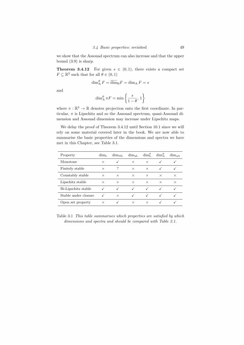
3.4 Basic properties: revisited 49
we show that the Assouad spectrum can also increase and that the upper
bound (3.9) is sharp.
Theorem 3.4.12 For given s ∈ (0, 1), there exists a compact set
F ⊆ R2 such that for all θ ∈ (0, 1)
dimθA F = dimBF = dimA F = s
and
dimθA πF = min
s
1− θ, 1
where π : R2 → R denotes projection onto the first coordinate. In par-
ticular, π is Lipschitz and so the Assouad spectrum, quasi-Assouad di-
mension and Assouad dimension may increase under Lipschitz maps.
We delay the proof of Theorem 3.4.12 until Section 10.1 since we will
rely on some material covered later in the book. We are now able to
summarise the basic properties of the dimensions and spectra we have
met in this Chapter, see Table 3.1.
Property dimL dimML dimqL dimθL dimθ
A dimqA
Monotone × X × × X X
Finitely stable × ? × × X X
Countably stable × × × × × ×
Lipschitz stable × × × × × ×
Bi-Lipschitz stable X X X X X X
Stable under closure X × X X X X
Open set property × X × × X X
Table 3.1 This table summarises which properties are satisfied by which
dimensions and spectra and should be compared with Table 2.1.
50 Some variations on the Assouad dimension
3.4.3 Holder distortion
Bi-Holder maps are a natural generalisation of bi-Lipschitz maps, where
more distortion is allowed. Let X be a domain lying in Rd. We say an
injective map f : X → Rd is (α, β)-Holder, or bi-Holder, for 0 < α 61 6 β <∞ if there exists a constant C > 1 such that, for all x, y ∈ X,
C−1|x− y|β 6 |f(x)− f(y)| 6 C|x− y|α. (3.10)
Notice that (1, 1)-Holder is the same as bi-Lipschitz.
Dimensions are not generally preserved under bi-Holder maps, but one
can often control the distortion in terms of the Holder exponents α and
β. For example, if dim is the Hausdorff, packing, or upper or lower box
dimension, and f is (α, β)-Holder, then
dimX
β6 dim f(X) 6
dimX
α, (3.11)
see [70, Proposition 3.3]. Notably, the Assouad dimension does not sat-
isfy such bounds, see [191, Proposition 1.2], Theorem 10.2.4, or the pa-
pers [103, 106].
The Assouad spectrum, which is inherently more regular than the
Assouad dimension, can be controlled in this context but the control is
more complicated than (3.11). The following lemma was first proved in
[111, Proposition 4.7].
Lemma 3.4.13 Suppose f : X → Rd is (α, β)-Holder. Then, for all
θ ∈ (0, 1),
1− βθ/αβ(1− θ)
dimβθ/αA X 6 dimθ
A f(X) 61− αθ/βα(1− θ)
dimαθ/βA X
and
1− βθ/αβ(1− θ)
dimβθ/αL X 6 dimθ
L f(X) 61− αθ/βα(1− θ)
dimαθ/βL X
where dimβθ/αA X and dim
βθ/αL X are taken to equal 0 if βθ/α > 1.
Proof Fix θ ∈ (0, 1) and let t > dimαθ/βA X. Let x ∈ X and r ∈ (0, 1).
Therefore, by (3.10),
f(B(x, rθ/βC1/β)) ⊇ B(f(x), rθ),
and for every set U ⊆ X with |U | 6 (r/C)1/α
|f(U)| 6 C|U |α 6 r.
3.4 Basic properties: revisited 51
This means that the image of an (r/C)1/α-cover of B(x, rθ/βC1/β))∩Xunder f yields an r-cover of B(f(x), rθ) ∩ f(X). Therefore, applying
the definition of the Assouad spectrum of X, there is a constant C0
depending only on t and C such that
Nr(B(f(x), rθ) ∩ f(X)) 6 N(r/C)1/α(B(x, rθ/βC1/β) ∩X)
6 C0
(rθ/βC1/β
(r/C)1/α
)t
6 C0Ct(1/α+1/β)
(rθ−1
) t(θ/β−1/α)θ−1 .
The dependence of C0 on C is just to account for the fact that the ‘big’
scale rθ/βC1/β is not quite the ‘small’ scale (r/C)1/α to the power αθ/β.
It follows that
dimθA f(X) 6
t(1/α− θ/β)
1− θ=
1− θα/βα(1− θ)
t
and letting t → dimαθ/βA X yields the desired upper bound. The lower
bound for dimθA f(X) can be obtained by applying the upper bound to
the map f−1 : f(X) → X with θ′ = βθ/α for θ < α/β. This uses the
fact that f−1 is (β−1, α−1)-Holder. The estimates for the lower spectrum
are proved in a similar way and we leave the details to the reader.
The following immediate corollary of Lemma 3.4.13 was first recorded
in [111, Theorem 4.11] and allows one to recover some information about
the behaviour of the Assouad dimension under Holder images.
Corollary 3.4.14 Suppose f : X → Rd is (α, β)-Holder. Then
dimA f(X) > dimqA f(X) >(1− ρ)
β − αρdimqAX
where ρ = infθ ∈ (0, 1) : dimθAX = dimqAX.
Another consequence of Lemma 3.4.13 is that the Assouad spectrum
and quasi-Assouad dimension of compact sets are preserved under quasi-
Lipschitz maps. Recall that the quasi-Assouad dimension of a compact
set is preserved under quasi-Lipschitz maps. This was proved in [191],
see Section 3.2. Straight from the definitions, one sees that if a map
f : X → Y is quasi-Lipschitz for compact X,Y , then it is (1− ε, 1 + ε)-
Holder for all ε ∈ (0, 1). This was also observed in [276].
52 Some variations on the Assouad dimension
Corollary 3.4.15 Suppose f : X → Rd is (1− ε, 1 + ε)-Holder for all
ε ∈ (0, 1). Then, for all θ ∈ (0, 1),
dimθA f(X) = dimθ
AX and dimθL f(X) = dimθ
LX
and also
dimqA f(X) = dimqAX and dimqL f(X) = dimqLX.
In particular, this holds if f is quasi-Lipschitz and X is compact.
Proof This follows from Lemma 3.4.13 by letting ε → 0. The quasi-
Assouad invariance then follows by letting θ → 1 and applying Corollary
3.3.7 and, for the quasi-lower dimension, letting ε → 0. If f is quasi-
Lipschitz and X is compact, then Y is compact, f is a bijection and
log |f(x)− f(y)|log |x− y|
→ 1
uniformly as |x − y| → 0. Therefore, for all ε ∈ (0, 1), there exists
δ ∈ (0, 1) such that for |x− y| 6 δ,
|x− y|1+ε 6 |f(x)− f(y)| 6 |x− y|1−ε,
which does not quite prove that f is (1− ε, 1 + ε)-Holder since we need
an estimate like this for all x, y ∈ X, not just x, y which are δ-close.
However, we can ‘upgrade’ the upper bound since if |x− y| > δ, then
|f(x)− f(y)| 6 |f(X)| = |f(X)|δ1−ε δ1−ε 6
|f(X)|δ1−ε |x− y|
1−ε.
For the lower bound, suppose
infx,y∈X:|x−y|>δ
|f(x)− f(y)||x− y|1+ε
= 0.
Therefore, since X is compact, we can find x, y ∈ X with |x − y| > δ
such that f(x) = f(y), which contradicts the assumptions that f is a
bijection. This completes the proof that f is (1− ε, 1 + ε)-Holder for all
ε ∈ (0, 1) and the corollary follows.
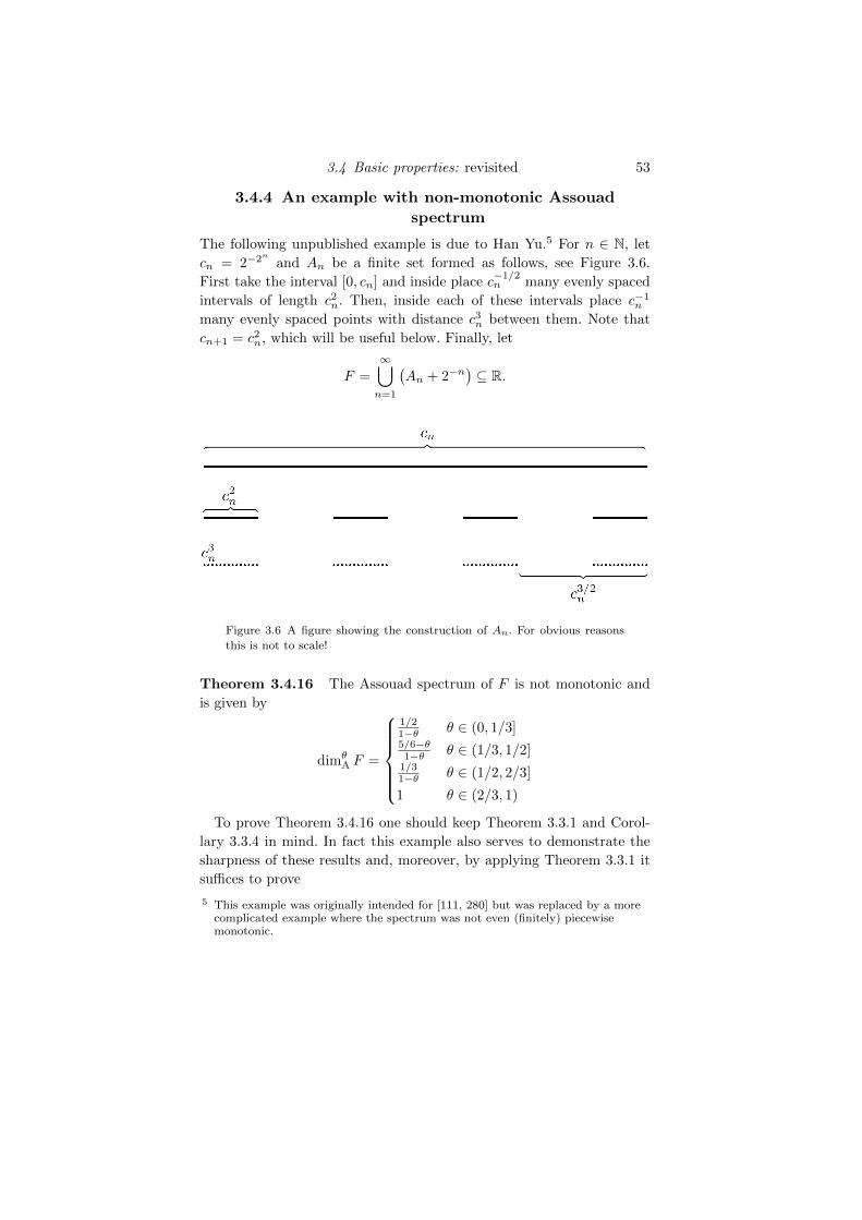
3.4 Basic properties: revisited 53
3.4.4 An example with non-monotonic Assouad
spectrum
The following unpublished example is due to Han Yu.5 For n ∈ N, let
cn = 2−2n and An be a finite set formed as follows, see Figure 3.6.
First take the interval [0, cn] and inside place c−1/2n many evenly spaced
intervals of length c2n. Then, inside each of these intervals place c−1n
many evenly spaced points with distance c3n between them. Note that
cn+1 = c2n, which will be useful below. Finally, let
F =
∞⋃n=1
(An + 2−n
)⊆ R.
Figure 3.6 A figure showing the construction of An. For obvious reasons
this is not to scale!
Theorem 3.4.16 The Assouad spectrum of F is not monotonic and
is given by
dimθA F =
1/21−θ θ ∈ (0, 1/3]5/6−θ1−θ θ ∈ (1/3, 1/2]
1/31−θ θ ∈ (1/2, 2/3]
1 θ ∈ (2/3, 1)
To prove Theorem 3.4.16 one should keep Theorem 3.3.1 and Corol-
lary 3.3.4 in mind. In fact this example also serves to demonstrate the
sharpness of these results and, moreover, by applying Theorem 3.3.1 it
suffices to prove
5 This example was originally intended for [111, 280] but was replaced by a morecomplicated example where the spectrum was not even (finitely) piecewisemonotonic.
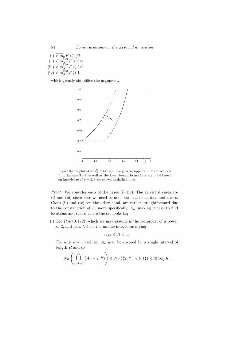
54 Some variations on the Assouad dimension
(i) dimBF 6 1/2
(ii) dim1/3A F > 3/4
(iii) dim1/2A F 6 2/3
(iv) dim2/3A F > 1,
which greatly simplifies the argument.
Figure 3.7 A plot of dimθA F (solid). The general upper and lower bounds
from Lemma 3.4.4 as well as the lower bound from Corollary 3.3.4 based
on knowledge of ρ = 2/3 are shown as dashed lines.
Proof We consider each of the cases (i)–(iv). The awkward cases are
(i) and (iii) since here we need to understand all locations and scales.
Cases (ii) and (iv), on the other hand, are rather straightforward due
to the construction of F , more specifically, An, making it easy to find
locations and scales where the set looks big.
(i) Let R ∈ (0, 1/2), which we may assume is the reciprocal of a power
of 2, and let k > 1 be the unique integer satisfying
ck+1 6 R < ck.
For n > k + 1 each set An may be covered by a single interval of
length R and so
NR
( ∞⋃n=k+1
(An + 2−n
))6 NR
(2−n : n > 1
)6 3| log2R|.
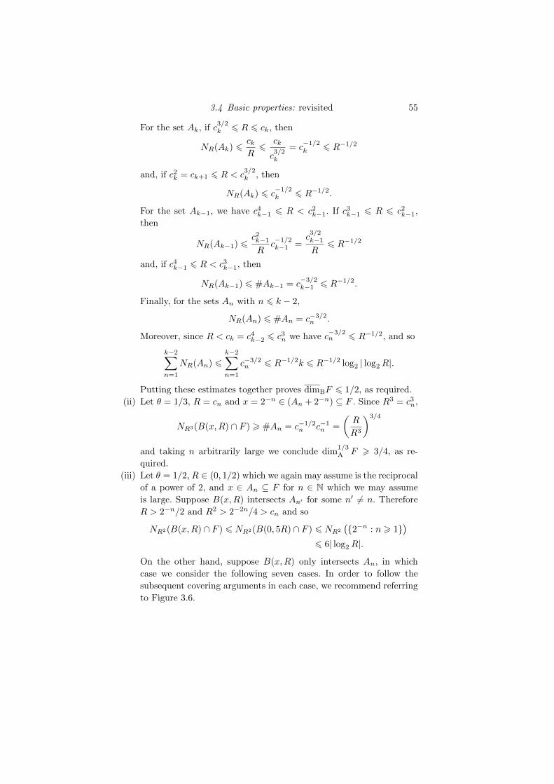
3.4 Basic properties: revisited 55
For the set Ak, if c3/2k 6 R 6 ck, then
NR(Ak) 6ckR
6ck
c3/2k
= c−1/2k 6 R−1/2
and, if c2k = ck+1 6 R < c3/2k , then
NR(Ak) 6 c−1/2k 6 R−1/2.
For the set Ak−1, we have c4k−1 6 R < c2k−1. If c3k−1 6 R 6 c2k−1,
then
NR(Ak−1) 6c2k−1
Rc−1/2k−1 =
c3/2k−1
R6 R−1/2
and, if c4k−1 6 R < c3k−1, then
NR(Ak−1) 6 #Ak−1 = c−3/2k−1 6 R−1/2.
Finally, for the sets An with n 6 k − 2,
NR(An) 6 #An = c−3/2n .
Moreover, since R < ck = c4k−2 6 c3n we have c−3/2n 6 R−1/2, and so
k−2∑n=1
NR(An) 6k−2∑n=1
c−3/2n 6 R−1/2k 6 R−1/2 log2 | log2R|.
Putting these estimates together proves dimBF 6 1/2, as required.
(ii) Let θ = 1/3, R = cn and x = 2−n ∈ (An + 2−n) ⊆ F . Since R3 = c3n,
NR3(B(x,R) ∩ F ) > #An = c−1/2n c−1
n =
(R
R3
)3/4
and taking n arbitrarily large we conclude dim1/3A F > 3/4, as re-
quired.
(iii) Let θ = 1/2, R ∈ (0, 1/2) which we again may assume is the reciprocal
of a power of 2, and x ∈ An ⊆ F for n ∈ N which we may assume
is large. Suppose B(x,R) intersects An′ for some n′ 6= n. Therefore
R > 2−n/2 and R2 > 2−2n/4 > cn and so
NR2(B(x,R) ∩ F ) 6 NR2(B(0, 5R) ∩ F ) 6 NR2
(2−n : n > 1
)6 6| log2R|.
On the other hand, suppose B(x,R) only intersects An, in which
case we consider the following seven cases. In order to follow the
subsequent covering arguments in each case, we recommend referring
to Figure 3.6.
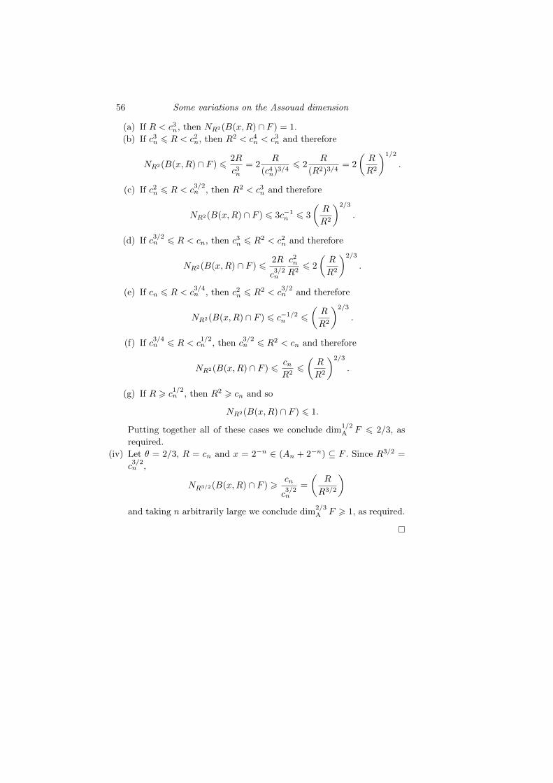
56 Some variations on the Assouad dimension
(a) If R < c3n, then NR2(B(x,R) ∩ F ) = 1.
(b) If c3n 6 R < c2n, then R2 < c4n < c3n and therefore
NR2(B(x,R) ∩ F ) 62R
c3n= 2
R
(c4n)3/46 2
R
(R2)3/4= 2
(R
R2
)1/2
.
(c) If c2n 6 R < c3/2n , then R2 < c3n and therefore
NR2(B(x,R) ∩ F ) 6 3c−1n 6 3
(R
R2
)2/3
.
(d) If c3/2n 6 R < cn, then c3n 6 R2 < c2n and therefore
NR2(B(x,R) ∩ F ) 62R
c3/2n
c2nR2
6 2
(R
R2
)2/3
.
(e) If cn 6 R < c3/4n , then c2n 6 R2 < c
3/2n and therefore
NR2(B(x,R) ∩ F ) 6 c−1/2n 6
(R
R2
)2/3
.
(f) If c3/4n 6 R < c
1/2n , then c
3/2n 6 R2 < cn and therefore
NR2(B(x,R) ∩ F ) 6cnR2
6
(R
R2
)2/3
.
(g) If R > c1/2n , then R2 > cn and so
NR2(B(x,R) ∩ F ) 6 1.
Putting together all of these cases we conclude dim1/2A F 6 2/3, as
required.
(iv) Let θ = 2/3, R = cn and x = 2−n ∈ (An + 2−n) ⊆ F . Since R3/2 =
c3/2n ,
NR3/2(B(x,R) ∩ F ) >cn
c3/2n
=
(R
R3/2
)and taking n arbitrarily large we conclude dim
2/3A F > 1, as required.
4
Dimensions of measures
A key aspect of dimension theory is how dimensions of sets relate to
dimensions of measures. To this end, all the familiar notions of dimen-
sion for sets have natural counterparts in the context of measures, recall
the discussion Section 1.2.1. The Assouad dimension and its many vari-
ants are no different and in this chapter we explore the Assouad type
dimensions and spectra of measures.
4.1 Assouad and lower dimensions of measures
Throughout we assume µ is a locally finite Borel measure on Rd, al-
though much of the theory applies more generally. A measure µ on Rdis locally finite if µ(B(x, r)) <∞ for all x ∈ Rd and r > 0. The Assouad
and lower dimensions of µ describe the optimal global control on the
relative measure of concentric balls. These dimensions were introduced
formally in [153, 152] motivated by previous work on the existence of
doubling measures, see for example [193, 173, 40].1
As usual, we write |E| for the diameter of a non-empty (possibly
unbounded) set E and supp(µ) for the support of a measure µ, which is
1 When they were first introduced, the Assouad and lower dimensions of measureswere referred to as the upper and lower regularity dimensions, respectively. Thisterminology is still popular, but not universally. In fact, when I worked withthese notions in the past I used these names. However, I now favour the Assouadand lower dimension being used. This is for two reasons: firstly, it is importantthat the community agrees on a common set of terminology and notation and,secondly, using the same terminology for sets and measures serves to emphasisethe connection and interplay between the notions.
This material will be published by Cambridge University Press as Assouad Dimension and Fractal Geometryby Jonathan Fraser. This pre-publication version is free to view and download for personal use only.
Not for re-distribution, re-sale or use in derivative works. c© Jonathan Fraser 2020.
58 Dimensions of measures
necessarily closed, see (1.2). The Assouad dimension of µ is defined by
dimA µ = inf
s > 0 : there exists C > 0 such that,
for all 0 < r < R < |supp(µ)| and x ∈ supp(µ),
µ(B(x,R))
µ(B(x, r))6 C
(R
r
)s
and, provided |supp(µ)| > 0, the lower dimension of µ is defined by
dimL µ = sup
s > 0 : there exists C > 0 such that,
for all 0 < r < R < |supp(µ)| and x ∈ supp(µ),
µ(B(x,R))
µ(B(x, r))> C
(R
r
)s
and otherwise it is 0. We adopt the convention that inf ∅ = +∞.
There is a straightforward connection between the Assouad and lower
dimensions of sets and measures, which also provides a powerful method
to estimate the dimensions of sets. This is in some sense dual to the
approach provided by weak tangents (discussed in Chapter 5) since the
estimates are in the opposite direction. Recall that a measure µ is dou-
bling (on its support) if there is a constant c > 1 such that, for all
x ∈ supp(µ) and r > 0,
µ(B(x, 2r)) 6 cµ(B(x, r)).
The following fundamental equivalence was first noted in [147, Lemma
3.2].
Lemma 4.1.1 A measure µ is doubling if and only if dimA µ <∞.
Proof The fact that finite Assouad dimension implies doubling is im-
mediate from the definition. The other implication requires a little more
work. Suppose µ is doubling with doubling constant c > 1. Let x ∈supp(µ) and 0 < r < R. Let n > 0 be the unique integer satisfying
2−nR 6 2r < 2−n+1R,
4.1 Assouad and lower dimensions of measures 59
noting that n 6 log(R/r)/ log 2. Then
µ(B(x,R))
µ(B(x, r))=µ(B(x, 2−nR))
µ(B(x, r))
n−1∏k=0
µ(B(x, 2−kR))
µ(B(x, 2−(k+1)R))
6 cn+1
6 c
(R
r
) log clog 2
which proves dimA µ 6 log clog 2 <∞ as required.
It will be important for us that the Assouad and lower dimensions of
a measure control the Assouad and lower dimensions of its support, see
[153, Section 3].
Lemma 4.1.2 If a measure µ is doubling and fully supported on a
closed set F , then
dimL µ 6 dimL F 6 dimA F 6 dimA µ.
Proof We begin by proving the first inequality. Let t < dimL µ and
consider x ∈ F and R > r > 0. Let UiNi=1 be a minimal r-cover of
B(x,R) ∩ F . Therefore
µ(B(x,R)) 6N∑i=1
µ(Ui) 6 N supy∈B(x,R)∩F
µ(B(y, r)).
Moreover, since µ is assumed to be doubling, for all y ∈ B(x,R) ∩ F ,
µ(B(x,R)) > c−1µ(B(x, 2R)) > c−1µ(B(y,R)), where c is the doubling
constant of µ. Therefore, for all such y,
µ(B(x,R))
µ(B(y, r))> c−1µ(B(y,R))
µ(B(y, r))> C
(R
r
)tfor a constant C which is independent of x, y, r and R. It follows that
Nr(B(x,R) ∩ F ) = N > C
(R
r
)twhich proves dimL F > t and letting t → dimL µ yields the desired
inequality.
The middle inequality is trivial and so it remains to prove the final
inequality. Let s > dimA µ and consider x ∈ F and R > r > 0. Suppose
60 Dimensions of measures
xiNi=1 is a collection of N points in F such that the balls B(xi, r) are
pairwise disjoint and contained in B(x,R). Therefore
µ(B(x,R)) >N∑i=1
µ(B(xi, r)) > N miniµ(B(xi, r)) > 0.
Moreover, for all i, B(x,R) ⊆ B(xi, 2R) and therefore
µ(B(x,R))
µ(B(xi, r))6µ(B(xi, 2R))
µ(B(xi, r))6 C
(R
r
)sfor a constant C which is independent of x, i, r and R. It follows that
N 6 C(Rr
)sand, moreover, that
N6r(B(x,R) ∩ F ) 6 C
(R
r
)ssince if the collection xi is chosen such that N is maximised, then
the collection of balls B(xi, 3r) is a 6r-cover of B(x,R) ∩ F . This is
enough to prove dimA F 6 s and letting s → dimA µ yields the desired
inequality.
A much deeper fact is that the previous lemma is sharp, allowing us to
express the dimensions of sets in terms of the corresponding dimensions
of measures supported on the sets. Recall, for example, that dimH F =
supdimH µ : supp(µ) ⊆ F, see (1.3).
Theorem 4.1.3 For closed F ⊆ Rd,
dimA F = inf dimA µ : supp(µ) = F
and
dimL F = sup dimL µ : supp(µ) = F .
We omit the proof of this result. This Assouad dimension result was
proved by Luukkainen and Saksman [193] (in general) and Konyagin
and Vol’berg [173] (for compact F ) and the lower dimension result was
proved by Bylund and Gudayol [40]. See [152] for further extensions and
clarifications.
It should be clear that the measures µ considered in Theorem 4.1.3
must be fully supported (compare with (1.3) which does not require
this). Given Theorem 4.1.3, it is natural to ask if there always exists
a measure which precisely realises the Assouad and lower dimensions,
that is, with dimA µ = dimA F or dimL µ = dimL F . However, this is
not always possible, at least for the Assouad dimension. Konyagin and
4.1 Assouad and lower dimensions of measures 61
Vol’berg [173, Theorem 4] provided an example of a compact set F for
which dimA µ > dimA F for all doubling measures µ supported on F .
Kaenmaki and Lehrback [152] observed that the example from [173] is
a special case of an inhomogeneous self-similar set, and that this class
of set exhibits this surprising behaviour quite generally. Inhomogeneous
self-similar sets are a generalisation of the self-similar sets we will study
in Chapter 7. They were introduced by Barnsley and Demko [24] (see
also [128]) and their dimension theory has been studied in some de-
tail, see [39, 87, 220, 255]. Kaenmaki and Lehrback [152] also observed
that inhomogeneous self-similar sets with suitable separation conditions
cannot be used to exhibit examples where the lower dimension is not
precisely realised, and it remains an interesting open question to deter-
mine whether or not the lower dimension of a set can always be precisely
realised by a doubling measure, see Question 17.2.1.
Following on from Theorem 4.1.3, another natural question is: given
a set F , what are the possible values of dimA µ for measures supported
on F? We know from Theorem 4.1.3 that this set of values is contained
in [dimA F,∞] and may or may not include the point dimA F . Hare,
Mendivil and Zuberman [126] proved that if F ⊆ R is a compact set
with dimA F > 0, then for all s ∈ (dimA F,∞), there exists a measure
µ on F with dimA µ = s. It was also shown in [126] that if F ⊆ Ris a compact set with dimL F > 0, then for all t ∈ [0,dimL F ), there
exists a measure µ on F with dimL µ = t. Interestingly, the assumption
that dimA F > 0 is necessary for the first result, since they provide an
example of a set E ⊆ R with dimAE = 0 such that
dimA µ : supp(µ) = E = 0,∞.
In fact, one can choose
E = 2−2n : n > 1 ∪ 0.
These results were extended to arbitrary complete metric spaces F by
Suomala [262].
62 Dimensions of measures
4.2 Assouad spectrum and box dimensions ofmeasures
By now it should be obvious how to define the Assouad and lower spectra
of measures and one might even be able to guess some of the relationships
between these spectra and the Assouad and lower dimensions. To make
explicit, for θ ∈ (0, 1), the Assouad spectrum of µ is defined by
dimθA µ = inf
s > 0 : there exists C > 0 such that,
for all 0 < r < |supp(µ)| and x ∈ supp(µ),
µ(B(x, rθ))
µ(B(x, r))6 C
(rθ
r
)s
and, provided |supp(µ)| > 0, the lower spectrum of µ is defined by
dimθL µ = sup
s > 0 : there exists C > 0 such that,
for all 0 < r < |supp(µ)| and x ∈ supp(µ),
µ(B(x, rθ))
µ(B(x, r))> C
(rθ
r
)s
and otherwise it is 0. The following basic properties may be established
following arguments similar to those we have already documented, and
also appear in [75].
Lemma 4.2.1 For any measure µ,
dimL µ 6 dimθL µ 6 dimθ
A µ 6 dimA µ
and if a measure µ is fully supported on a closed set F , then
dimθL µ 6 dimθ
L F 6 dimθA F 6 dimθ
A µ.
An interesting feature of the Assouad spectrum of measures is that, in
searching for an analogue of Lemma 3.4.4, we are led to the appropriate
definition of the upper box dimension of a measure. Specifically, the
4.2 Assouad spectrum and box dimensions of measures 63
upper box dimension of a measure µ is
dimBµ = inf
α : there exists a constant C > 0 such that,
for all 0 < r < |supp(µ)| and x ∈ supp(µ),
µ(B(x, r)) > Crα
.
The upper box dimension for measures was introduced in [75], although
it was referred to as the upper Minkowski dimension. A natural dual
notion is the lower box dimension of µ defined by
dimBµ = inf
α : there exists a constant C > 0 such that,
for all r0 > 0, there exists 0 < r < r0 such that,
for all x ∈ supp(µ), µ(B(x, r)) > Crα
.
If dimBµ = dimBµ, then we refer to the common value as the box
dimension of µ, and denote it by dimB µ. Different definitions of the box
dimensions of measures have been proposed in the past, for example, see
[234, Section 7.1]. However, we favour the definitions above since they
seem consistent with the theory of the Assouad spectrum which we are
developing. The following analogue of Lemma 3.4.4 was proved in [75].
Lemma 4.2.2 For a measure µ supported on a compact set F and
θ ∈ (0, 1),
dimBµ 6 dimθA µ 6
dimBµ
1− θ.
Proof We start by proving the second inequality. Fix 0 < θ < 1 and let
s > dimBµ/(1− θ). This means that there exists a constant C > 0 such
that µ(B(x, r)) > Cr(1−θ)s for all x ∈ F and 0 < r < 1. Therefore,
µ(B(x, rθ))
µ(B(x, r))6 µ(F )C−1r(θ−1)s
for all x ∈ F and 0 < r < 1, which yields dimθA µ 6 s as required.
The first inequality, similar to Lemma 3.4.4, is more awkward. Fix
0 < θ < 1 and let dimθA µ < s < t. This means that there is C > 0 such
that
µ(B(x, rθ))
µ(B(x, r))6 Cr(θ−1)s
64 Dimensions of measures
for all x ∈ F and 0 < r < 1. Since F is compact, we may assume by
rescaling if necessary that |F | < 1/2. Fix 0 < r < 1 and choose k > 1
such that rθk−1
< 1/2 6 rθk
. Therefore
µ(B(x, r)) =µ(B(x, r))
µ(B(x, rθ))
µ(B(x, rθ))
µ(B(x, rθ2))· · · µ(B(x, rθ
k−1
))
µ(B(x, rθk))µ(B(x, rθ
k
))
> C−kr(1−θ)srθ(1−θ)s · · · rθk−1(1−θ)sµ(B(x, 1
2 ))
> C−1(− log 2
log r
) logClog θ
r(1−θk)sµ(F )
> µ(F )C−1( log 2
− log r
) logClog θ 1
r−(s−t) rt
for all x ∈ F . It follows that there is a constant C0 > 0 such that
µ(B(x, r)) > C0rt for all x ∈ F and 0 < r < 1 and hence, dimBµ 6 t
completing the proof.
We may express the upper box dimension of a set in terms of the upper
box dimension of measures fully supported on the set. This is further
motivation for the definition of upper box dimension for measures and
should be compared with (1.3) for Hausdorff dimension and Theorem
4.1.3 for Assouad dimension. One direction follows from Lemma 4.2.1
upon letting θ → 0, and the other direction follows from Tricot’s ‘anti-
Frostman lemma’ [265, Lemma 4], although the proof is only sketched
there (see also [44, Lemma 3.2] and [75]). We prove the upper bound
here directly using an elegant argument due to Kenneth Falconer, see
also [75].
Theorem 4.2.3 For a non-empty compact set F ⊆ Rd,
dimBF = inf
dimBµ : supp(µ) = F.
Proof The upper bound (6) follows from the analogous result for the
Assouad spectrum given in Lemma 4.2.1 and it remains to prove the
upper bound (>). Let t > s > dimBF and for all k ∈ N let xk,iNki=1 be
a maximal 2−k-separated subset of F . We can choose c > 0 such that
for all k
Nk 6 c2ks.
4.2 Assouad spectrum and box dimensions of measures 65
Let
µ =∑k∈N
Nk∑i=1
2−ktδxk,i
noting that this is a finite measure since
µ(Rd) =∑k∈N
Nk∑i=1
2−kt 6∑k∈N
c2ks2−kt <∞
and, moreover, supp(µ) = F . Finally, given x ∈ F and r ∈ (0, 1), choose
the unique k ∈ N such that 2−k < r 6 2−k+1, and observe that there
must exist i ∈ 1, . . . , Nk such that xk,i ∈ B(x, r). Therefore
µ(B(x, r)) > 2−kt > (1/2)trt
proving dimBµ 6 t, as required.
The ‘tale of two spectra’ analysis for measures, including the intro-
duction and discussion of the quasi-Assouad and quasi-lower dimensions
of measures was conducted in [127].
5
Weak tangents and microsets
One of the most effective ways to bound the Assouad dimension of a set
from below is to use weak tangents; an approach pioneered by Mackay
and Tyson [195] with ideas going back to Keith and Laakso [164]. Weak
tangents are tools for capturing the extremal local structure of a set
which should make their connection to Assouad and lower dimensions
evident. In this chapter we explore this connection. We prove Mackay and
Tyson’s estimate, see Theorem 5.1.2, and a stronger result of Fursten-
berg which characterises the Assouad dimension entirely in terms of the
Hausdorff dimension of weak tangents, see Theorem 5.1.3. This latter
theorem has many useful applications, see Theorem 10.2.1 concerning
orthogonal projections in Section 10.2 and Theorem 11.1.3 concerning
distance sets in Section 11.1. We also explore the connections between
weak tangents and the lower dimension in Section 5.2, the Assouad spec-
tra in Section 5.3, and the dimensions of measures in Section 5.4.
5.1 Weak tangents and the Assouad dimension
Let K(Rd) denote the set of all non-empty compact subsets of Rd. This
is a complete metric space when equipped with the Hausdorff metric
dH, see [242, Chapter 2] or [205, Section 4.13], defined by
dH(A,B) = infδ > 0 : A ⊆ Bδ and B ⊆ Aδ (5.1)
where, for any C ∈ K(Rd),
Cδ = x ∈ Rd : |x− y| < δ for some y ∈ C
denotes the open δ-neighbourhood of C. We will also consider the space
K(X) for a fixed non-empty compact set X ⊆ Rd. This is the set of all
This material will be published by Cambridge University Press as Assouad Dimension and Fractal Geometryby Jonathan Fraser. This pre-publication version is free to view and download for personal use only.
Not for re-distribution, re-sale or use in derivative works. c© Jonathan Fraser 2020.
5.1 Weak tangents and the Assouad dimension 67
non-empty compact subsets of X and, importantly, this is a compact
subset of K(Rd).
Definition 5.1.1 Let X ∈ K(Rd) be a fixed reference set (usually the
closed unit ball or cube) and let E,F ⊆ Rd be closed sets with E ⊆ X.
Suppose there exists a sequence of similarity maps Tk : Rd → Rd such
that dH(E, Tk(F )∩X)→ 0 as k →∞. Then E is called a weak tangent
to F .
Recall that a similarity map T : Rd → Rd is a map of the form
x 7→ cO(x) + t where c > 0 is a scalar (called the similarity ratio),
O ∈ O(R, d) is a real orthogonal matrix and t ∈ Rd is a translation.
For example, similarities mapping R to itself are maps of the form
T (x) = cx + t for c ∈ R \ 0 and t ∈ R. We say T is a homothety if O
is the identity. Observe that for all x, y ∈ Rd,
|T (x)− T (y)| = c|x− y|.
The following is a fundamental tool in the study of Assouad dimension
and was proved in [195, Proposition 6.1.5].
Theorem 5.1.2 Let F ⊆ Rd be closed, E ⊆ Rd be compact, and
suppose E is a weak tangent to F . Then dimA F > dimAE.
Proof Let s > dimA F and ck > 0 denote the similarity ratio of Tk.
It follows that there exists a constant C > 0 depending only on s such
that, for all k ∈ N, 0 < r < R and x ∈ Tk(F ),
Nr(B(x,R) ∩ Tk(F )
)6 C
(R
r
)s.
Recall the proof of Lemma 2.4.2 where images of covers under bi-Lipschitz
maps are considered. Fix 0 < r < R and y ∈ E. Choose k ∈ N such that
dH(E, Tk(F ) ∩ X) < r/2. It follows that there exists x ∈ Tk(F ) ∩ Xsuch that B(y,R) ∩ E ⊆ B(x, 2R) and hence, given any r/2-cover of
B(x, 2R) ∩ Tk(F ), we may find an r-cover of B(y,R) ∩ E by the same
number of sets (or fewer). Thus,
Nr(B(y,R) ∩ E
)6 Nr/2
(B(x, 2R) ∩ Tk(F )
)6 C
(2R
r/2
)s
= C 4s(R
r
)swhich proves that dimAE 6 s and therefore dimAE 6 dimA F , as
required.
68 Weak tangents and microsets
Theorem 5.1.2 has a remarkable converse: one can always achieve
the Assouad dimension as the Hausdorff dimension of a weak tangent.
This beautiful fact was first explicitly stated by Kaenmaki, Ojala and
Rossi [154, Proposition 5.7], but has origins in the work of Furstenberg
[114, 115, 116] and Bishop and Peres [34], see the discussion in Section
2.3. It has turned out to be a very useful technical tool and often allows
one to pass a geometrical problem to the level of weak tangents. This
approach provides a mechanism for finding ‘Assouad dimension ana-
logues’ of known results concerning the Hausdorff dimension (and other
dimensions) as well as proving stronger results, not known for other
dimensions, see [89] for examples of this approach in action.
The argument used to prove [154, Proposition 5.7] is based on an
argument of Bishop and Peres [34, Lemma 2.4.4], which in turn takes
inspiration from Furstenberg’s work. Bishop and Peres [34, Lemma 2.4.4]
proved that, given a compact set F ⊆ R, there exists a weak tangent
with Hausdorff dimension equal to the upper box dimension of F . We
present a modification of the proof of Kaenmaki, Ojala and Rossi [154].
See also [155, Corollary 5.2] and [154, Propositions 5.8].
Theorem 5.1.3 Let F ⊆ Rd be closed and non-empty with dimA F =
s ∈ [0, d]. Then there exists a compact set E ⊆ Rd with Hs(E) > 0
which is a weak tangent to F . In particular, dimHE = dimAE = s.
Moreover, one may assume that all of the similarities used to define E
are homotheties.
Proof For integers m, let Q(m) denote the collection of closed dyadic
2−m-cubes imposed on Rd oriented with the coordinate axes. Moreover,
given Q ∈ Q(m) and n > m write
Mn(Q) = # Q′ ∈ Q(n) : Q′ ⊆ Q and Q′ ∩ F 6= ∅ .
Directly from the definition of the Assouad dimension we can find se-
quences mk, nk ∈ N and Qk ∈ Q(mk) such that
Mnk(Qk) > 2(nk−mk)(s−1/k) (5.2)
and nk −mk → ∞ as k → ∞. Let µk be a Borel probability measure
supported on Qk ∩ F such that
µk(Q′) =1
Mnk(Qk)
for all Q′ ∈ Q(nk) such that Q′ ⊆ Qk and Q′ ∩ F 6= ∅.
5.1 Weak tangents and the Assouad dimension 69
Claim: For all t < s and l ∈ N there exists k(l, t) and Q(l, t) ∈ Q(L)
for some L > mk(l,t) + l with Q(l, t) ⊆ Qk(l,t) such that
µk(l,t)(Q′)
µk(l,t)(Q(l, t))6|Q′|t
|Q(l, t)|t
for all Q′ ∈ Q(l′) with L 6 l′ 6 L+ l.
Proof of claim: Suppose the claim does not hold, in which case we can
find t < s and l such that, for all k and Ql ∈ Q(mk + l),
µk(Q1l )
µk(Ql)>|Q1
l |t
|Ql|t
for some Q1l ∈ Q(l1) with mk + l < l1 6 mk + 2l. Fix such a ‘bad cube’
Ql, which, by the pigeonhole principle, we may assume satisfies
µk(Ql) > 2−ld, (5.3)
and Q1l ⊆ Ql. Consider Q1
l and apply the failure of the claim again to
obtain
µk(Q2l )
µk(Q1l )>|Q2
l |t
|Q1l |t
for some Q2l ∈ Q(l2) with l1 < l2 6 l1 + l. Iterating this procedure to
generate a sequence of ‘bad cubes’ Ql ⊃ Q1l ⊃ Q2
l ⊃ · · · ⊃ Qql where q is
chosen to be the largest integer satisfying |Qql | > 2−nk√d. In particular,
nk − l 6 lq 6 nk. (5.4)
Telescoping, and applying (5.3), we obtain
µk(Qql ) >|Qql |t
|Ql|tµk(Ql) >
2−nktdt/2
2−(mk+l)tdt/22−ld
= 2−(nk−mk)t2−l(d−t). (5.5)
Let t < t′ < s and observe that, for large enough k,
Mnk(Qk) > 2(nk−mk)t′
by (5.2). Since Qql contains at most 2dl cubes of level nk (by (5.4)) we
have
µk(Qql ) 62dl
Mnk(Qk)6 2−(nk−mk)t′2dl. (5.6)
70 Weak tangents and microsets
Therefore, combining (5.5) and (5.6), we obtain
2−(nk−mk)t2−l(d−t) 6 2−(nk−mk)t′2dl
which is clearly false for sufficiently large k since nk−mk →∞, proving
the claim.
We are now ready to use the claim to build a suitable weak tangent.
Let tl be a sequence such that tl < s and tl → s. For l ∈ N, let Tl be
the unique homothetic similarity which sends the cube Q(l, tl) from the
claim to [0, 1]d. By taking a subsequence if necessary, we may assume
there is a compact set E ⊆ [0, 1]d such that
Tl(F ) ∩ [0, 1]d → E
in dH and a Borel probability measure µ supported on E such that
µl :=1
µk(l,tl)(Q(l, tl))µk(l,tl) T
−1l → µ
in the weak-∗ topology. Observe that E is a weak tangent to F .
Let r ∈ (0, 1) and Q ∈ Q(n) where n is the largest integer such that
2−n > r. Then, by the claim, for sufficiently large l,
µl(Q) =µk(l,tl)(T
−1l (Q))
µk(l,tl)(Q(l, tl))6|T−1l (Q)|tl|Q(l, tl)|tl
6 2−ntl 6 2srtl .
Moreover, for x ∈ E, the ball B(x, r) can intersect at most 4d cubes
Q ∈ Q(n). Therefore
µ(B(x, r)) 6 lim infl→∞
µl(B(x, r)) 6 lim infl→∞
4d2srtl = 4d2srs.
It follows from the mass distribution principle, Lemma 3.4.2, thatHs(E) >
0, and therefore dimHE > s. Finally, the fact that dimHE = dimAE =
s = dimA F follows from Theorem 5.1.2.
We call E in Definition 5.1.1 a strong tangent to F if X = B(0, 1)
(the closed unit ball), there is a point x0 ∈ F such that the sequence
of similarity maps Tk satisfies Tk(x0) = 0 for all k (we zoom-in to the
specific point x0 ∈ F ), and ck ∞ as k →∞ (we genuinely zoom-in).
Strong tangents are not the right notion to study the Assouad dimension,
as the following theorem shows. This was first demonstrated by Le Donne
and Rajala [182, Example 2.20], see also [89].
5.1 Weak tangents and the Assouad dimension 71
Theorem 5.1.4 There exists a compact set F ⊆ [0, 1] with dimA F =
1, such that all strong tangents to F have Assouad dimension equal to
0.
Proof Let F ⊆ [0, 1] be given by
F = 0 ∪∞⋃k=1
k⋃l=0
2−k + l4−k
.
For each k let Tk be the similarity map defined by Tk(x) = k−14k(x −2−k) and observe that
Tk(F ) ∩ [0, 1] =
k⋃l=0
l/k → [0, 1]
in the Hausdorff metric dH as k →∞. Therefore [0, 1] is a weak tangent
to F and dimA F = 1 by Theorem 5.1.2. Since F has only one accumu-
lation point (at 0), the only non-trivial strong tangents are obtained by
zooming in at this point. As such, suppose E is a strong tangent to F
at 0. Therefore, there exists a sequence of similarity maps Sn (n > 1) of
the form Sn = cnx where 1 < cn ∞ as n→∞ such that
Sn(F ) ∩B(0, 1)→ E
in dH as n → ∞. We have assumed without loss of generality that
cn > 0, which we may do by passing to a subsequence and introducing
a reflection if necessary. Let
F0 = 0 ∪
2−k : k ∈ N.
It is a straightforward exercise to show that dimA F0 = 0. For compari-
son, see Theorem 3.4.7 and note that 2−k is ‘faster’ than 1/kp for any p.
We show that E is also a strong tangent to F0, which will complete the
proof since any strong or weak tangent to F0 necessarily has Assouad
dimension 0 by Theorem 5.1.2. For each n, let
m(n) = min k > 1 : cn2−k 6 1
and note that m(n)→∞ as n→∞. It follows that
Sn(F ) ∩B(0, 1) ⊆ 0 ∪∞⋃
k=m(n)
[cn2−k, cn2−k + cnk4−k
]
72 Weak tangents and microsets
and
Sn(F0) ∩B(0, 1) = 0 ∪∞⋃
k=m(n)
cn2−k
.
Therefore
dH
(Sn(F ) ∩B(0, 1), Sn(F0) ∩B(0, 1)
)6 supk>m(n)
cnk4−k
= cnm(n)4−m(n)
6 m(n)2−m(n) → 0
which yields Sn(F0) ∩B(0, 1)→ E in dH, completing the proof.
If F ⊆ Rd and dimA F = d, that is, the Assouad dimension of F is the
ambient spatial dimension, then even more information can be gleaned
about the weak tangents.
Theorem 5.1.5 If F ⊆ Rd and dimA F = d, then [0, 1]d is a weak
tangent to F .
Proof For a given R > 0, let Q(R) be the natural tiling of Rd consisting
of all translations of [0, R]d by t ∈ RZd. For r > 0 and a given Q ∈ Q(R),
let
Mr(Q) = # Q′ ∈ Q(r) : Q′ ⊆ Q and Q′ ∩ F 6= ∅ .
Since Q ∈ Q(R) are both contained in a ball of radius comparable to R
and contain a ball of radius comparable to R, we may work with cubes
instead of balls in the definition of Assouad dimension. It is also sufficient
just to consider scales R and r which are dyadic, that is, numbers of the
form 2k, for k ∈ Z.
Let F ⊆ Rd be such that dimA F = d. In order to reach a contradic-
tion, assume that [0, 1]d is not a weak tangent to F . This means that
there exists a dyadic ε ∈ (0, 1) such that for all dyadic R > 0 and all
Q ∈ Q(R), there exists a Q′ ∈ Q(εR) such that Q′ ⊆ Q and F ∩Q′ = ∅.
If Q ∈ Q(R) and r > εR, then
Mr(Q) 6 ε−d.
and so we may assume from now on that r < εR. Therefore, for all
5.1 Weak tangents and the Assouad dimension 73
Q ∈ Q(R) and all dyadic r < εR,
Mr(Q) 6 #Q′′ ∈ Q(r) : Q′′ ⊆ Q − #Q′′ ∈ Q(r) : Q′′ ⊆ Q′
=
(R
r
)d−(εR
r
)d
=
(R
r
)d(1− εd). (5.7)
This does not yet contradict the assumption that dimA F = d, and so we
proceed iteratively by cutting out more cubes of increasingly smaller size.
Provided r < ε2R, we may use (5.7) to ‘cut out’ one cube from Q(ε2R)
within each of the cubes from Q(εR) which do intersect F . Therefore
Mr(Q) 6
(R
r
)d (1− εd
)2.
We may continue this process of ‘cutting and reducing’ as long as r <
εkR. Therefore, if we choose m ∈ N such that εm+1R 6 r < εmR, then
we obtain
Mr(Q) 6
(R
r
)d (1− εd
)m6
(R
r
)d (1− εd
)log(r/R)/ log ε−1
=1
1− εd
(R
r
)d− log(1−εd)log ε
.
This proves
dimA F 6 d− log(1− εd)log ε
< d,
a contradiction.
Theorem 5.1.5 is related to the notion of porosity. We say a set F ⊆ Rdis α-porous if there exists α ∈ (0, 1/2) such that for all x ∈ F and all
r > 0 there exists y ∈ B(x, r) such that B(y, αr) ∩ F = ∅. This should
be interpreted as saying that there are uniformly large holes in F at all
locations and scales. We say F is porous if it is α-porous for some α. This
notion goes back to Vaisala [273]. It is straightforward to show that a set
F ⊆ Rd is porous if and only if [0, 1]d is not a weak tangent to the closure
74 Weak tangents and microsets
of F . Therefore Theorem 5.1.5 shows that F ⊆ Rd is porous if and only
if dimA F < d. This fact was proved by Luukkainen [192, Theorem 5.2],
who in fact established the following result, following Salli’s celebrated
results bounding the Hausdorff dimension of porous sets [246].
Theorem 5.1.6 There is a constant ε(α, d) > 0 depending only on α
and d such that if F ⊆ Rd is α-porous, then
dimA F 6 d− ε(α, d).
5.2 Weak tangents for the lower dimension?
There are dual analogues of Theorems 5.1.2, 5.1.3 and 5.1.5 which hold
for the lower dimension, although one has to be careful. Consider the
set F = [0, 1], which has dimL F = 1. However, taking X = [0, 1] and
Tk defined by Tk(x) = (x − 1)/k we find Tk(F ) ∩ X = 0 for all k.
Therefore 0 is a weak tangent to F according to Definition 5.1.1 and
we cannot hope for dimL F 6 dimLE (or even dimL F 6 dimAE) for all
weak tangents E, which would be the naıve analogue of Theorem 5.1.2.
It should be clear that the problem here is that we are restricting the
set Tk(F ) in the ‘wrong way’. This can be rectified by insisting that the
weak tangents intersect the interior of X, see [99, Theorem 1.1] for the
details and proof.
Theorem 5.2.1 Let F ⊆ Rd be closed, E ⊆ Rd be compact and
suppose that E is a weak tangent to F where X = [0, 1]d in the definition
of weak tangent and E ∩ (0, 1)d 6= ∅. Then dimL F 6 dimHE.
Note that one cannot replace dimHE with dimLE in the Theorem
5.2.1 since weak tangents which intersect the interior can still have un-
wanted isolated points on the boundary. There is a way of modifying
the result to force dimLE to appear, see [88, Proposition 7.7]. However,
this is unlikely to yield better applications than Theorem 5.2.1 since the
useful weak tangents tend to have equal lower and Hausdorff dimension.
With this basic inequality established, it is natural to look for an ana-
logue of Theorem 5.1.3. The following was established in [99, Theorem
1.1].
Theorem 5.2.2 Let F ⊆ Rd be closed with dimL F = s ∈ [0, d].
Then there exists a compact set E ⊆ Rd such that E is a weak tangent
intersecting the interior of X as in Theorem 5.2.1 and satisfies dimHE =
dimBE = s.
5.3 Weak tangents for spectra? 75
Despite the utility of Theorem 5.1.2, the dual result for lower di-
mension has not yet provided many applications, but it does paint an
interesting picture of the tangent structure of a given set. For concrete-
ness, given a closed set F ⊆ Rd, let W(F ) be the set consisting of all
weak tangents E to F derived using the reference set X = [0, 1]d, sat-
isfying E ∩ (0, 1)d 6= ∅, and such that the similarity ratios of the maps
Tk monotonically increase without bound, see Definition 5.1.1. That is,
W(F ) is the set of all reasonable weak tangents to F . Note that W(F )
is not quite a gallery as in Section 2.3 but is similar in spirit. Moreover,
write
∆(F ) = dimHE : E ∈ W(F )
for the set of Hausdorff dimensions obtained by reasonable weak tan-
gents. Using this notation, we have already seen that
dimA F = max ∆(F )
and
dimL F = min ∆(F )
noting that the maximum and minimum are indeed attained, see The-
orems 5.1.2, 5.1.3, 5.2.1 and 5.2.2. In particular, ∆(F ) is a singleton if
and only if dimL F = dimA F . Otherwise it contains at least two points,
corresponding to the Assouad and lower dimensions. It was shown in [99,
Theorem 1.3] that if ∆ ⊆ [0, d] is an Fσ set which contains its maximum
and minimum, then there exists a compact set F ⊆ Rd such that
∆(F ) = ∆.
Recall that an Fσ set is a set which can be expressed as a countable
union of closed sets. Finally, the analogue of Theorem 5.1.5, proved in
[99, Theorem 1.4], is that a closed set F ⊆ Rd has dimL F = 0 if and
only if there is a set E ∈ W(F ) which is a singleton.
5.3 Weak tangents for spectra?
Given how readily weak tangents relate to the Assouad dimension, it is
at first sight a little surprising that they do not directly connect with
the Assouad spectrum, or quasi-Assouad dimension. For example, the
polynomial sequence Fp = 1/np : n > 1 has the unit interval [0, 1]
as a weak tangent (even a ‘strong tangent’ at 0), but yet the Assouad
76 Weak tangents and microsets
spectrum is strictly smaller than 1 for all θ < p/(p+ 1). A more striking
example occurs later, where we will see that the limit set of Mandel-
brot percolation in Rd has [0, 1]d as a weak tangent, and so has Assouad
dimension d, but has quasi-Assouad dimension strictly less than d, see
Section 9.4. With these examples in mind, it might seem hopeless to
connect weak tangents to the Assouad spectrum and quasi-Assouad di-
mension. However, Garcıa and Hare [118] observed that if one knows the
speed of convergence to a given weak tangent, then one can get stronger
lower bounds on dimension; that is, one can bound the Assouad spec-
trum, not just the Assouad dimension.
Theorem 5.3.1 Let F ⊆ Rd be closed, E ⊆ Rd be compact, and
suppose E is a weak tangent to F such that there is a constant A > 0
such that
dH(E, Tk(F ) ∩X) 6 Ac(θ−1)/θk (5.8)
where ck > 1 is the similarity ratio of Tk. Then dimθA F > dimBE.
Proof We may assume that ck → ∞ since, if not, then E ⊆ S(F )
for some similarity S and the result is trivial. Moreover, we may assume
dimBE > 0 since otherwise there is nothing to prove. Let 0 < s < dimBE
and, without loss of generality, we further assume |E| = 1.
For k > 1, let rk = Ac(θ−1)/θk and choose y ∈ E. For k sufficiently
large, rk 6 1 and we may find a collection xii of N > r−sk many
points which all lie in E and are 3rk separated. The rate of convergence
condition (5.8) implies that for each i we can find yi ∈ B(xi, rk)∩Tk(F ).
Notice that the points yi are necessarily rk separated. For each i, let
zi = T−1k (yi) which gives us a collection of N points zi ∈ F which are
rk/ck = Ac−1/θk
separated. Moreover, each zi lies in the ball B(z1, 3c−1k ). It follows that
NAc−1/θk
(B(z1, 3c−1k ) ∩ F ) > N > r−sk = As
(c−1k
c−1/θk
)swhich is enough to show dimθ
A F > s and letting s→ dimBE proves the
result.
In the above proof we only needed the extra rate of convergence con-
dition to hold for infinitely many k, not all k as stated. However, one
can always pass to a subsequence of the Tk such that the convergence
5.4 Weak tangents for measures? 77
condition holds for all k, and so this yields no advantage. Several vari-
ants on Theorem 5.3.1 are considered in [118, Theorem 6]. For example,
if one assumes the ck grow at most exponentially, then the result may
be strengthened, and the similarity condition on Tk may be weakened
somewhat. Garcıa and Hare also consider analogous results for the lower
spectrum, where they had to be careful which weak tangents to consider,
as seen in the previous section. We can formulate the result in terms
of the quasi-Assouad dimension, rather than the Assouad spectrum, in
which case we only need the convergence condition with
dH(E, Tk(F ) ∩X) 6 Ac−εk
for some ε > 0, see [118]. Finally, we note we can recover Theorem 3.4.7
using this approach, which also goes some way to proving sharpness of
Theorem 5.3.1. Recall Fp = 1/np : n > 1 for fixed p > 0. Let Tk be
defined by Tk(x) = kpx and observe that
dH([0, 1], Tk(Fp) ∩ [0, 1]) = 1− kp(1/(k + 1)p) 6 k−1 = (kp)−1/p.
Using Theorem 5.3.1 this implies dimθA Fp > 1 for θ satisfying (θ−1)/θ =
−1/p and therefore
dimθA Fp = 1
for all θ > p/(p+ 1) and this, combined with Corollary 3.3.4, yields
dimθA Fp =
1
(1 + p)(1− θ)
for 0 < θ < p/(p+ 1).
5.4 Weak tangents for measures?
The ‘weak tangent’ approach to the Assouad dimension has proved
rather fruitful in tackling several different problems. Indeed, it will show
up throughout this book. The weak tangent approach for measures is
somewhat less developed, partly because it does not work without suit-
able modification. Even once the theory is in place, however, it may still
be less applicable than the theory for sets since understanding tangent
measures is rather harder than understanding tangent sets.
We say that a probability measure ν on Rd is a weak tangent measure
to a measure µ on Rd if there exists a sequence of similarity maps Tk on
78 Weak tangents and microsets
Rd and a sequence of weights pk > 0 such that
pkµ T−1k ν
where denotes weak convergence. Note the key difference between this
and the notion of weak tangents for sets is that we do not restrict to a
fixed compact set X. This means that weak tangent measures typically
have unbounded support. The following analogous result to Theorem
5.1.2 was proved in [98, Theorem 2.2].
Theorem 5.4.1 Suppose ν is a weak tangent measure to a measure µ
on Rd. Then dimA ν 6 dimA µ.
Combining this with Lemma 4.1.1 we see that all weak tangent mea-
sures of doubling measures are doubling.
Corollary 5.4.2 If ν is a weak tangent measure to a doubling measure
µ on Rd, then ν is doubling.
It turns out that, for the conclusions of Theorem 5.4.1 and Corollary
5.4.2 to hold, it is necessary not to restrict the support of the measure.
We demonstrate this using the following example, adapted from [98]. We
construct a doubling measure on the plane which upon restriction to the
unit ball becomes non-doubling, even with infinite box dimension! This
shows that if one restricts the measures pkµ T−1k in the definition of
weak tangent measures to the unit ball, then the analogue of Theorem
5.4.1 fails.
We begin with the square shown on the left of Figure 5.1. Let ri be a
sequence of radii which decay exponentially to 0 and xi be a sequence of
centres moving clockwise on the unit circle S1 which converge polyno-
mially to a point z ∈ S1 as shown. Consider the balls Bi = B(xi, ri) and
remove from the original square the points in the interior of Bi∩B(0, 1)
which are at distance strictly greater than rii from S1 — see the grey
region on the right in Figure 5.1. Label the remaining set, that is, the
square with the grey regions removed, by F .
Let µ be the restriction of 2-dimensional Lebesgue measure to F . It is
straightforward to see that µ is doubling, and even dimL µ = dimA µ = 2.
However, ν = µ|B(0,1) is not doubling and moreover, dimB µ = dimA ν =
∞. For large enough i we have
ν(B(xi, 2ri)) > (π(2ri)2 − πrii)/3 > πr2
i
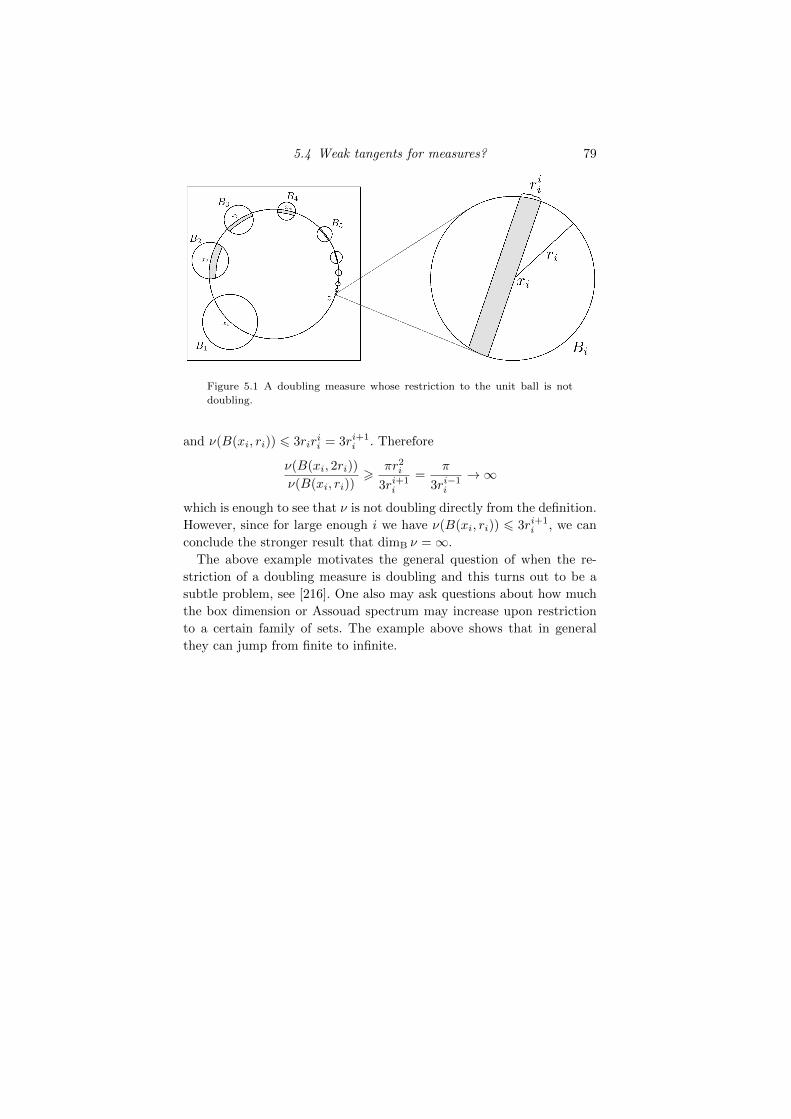
5.4 Weak tangents for measures? 79
Figure 5.1 A doubling measure whose restriction to the unit ball is not
doubling.
and ν(B(xi, ri)) 6 3ririi = 3ri+1
i . Therefore
ν(B(xi, 2ri))
ν(B(xi, ri))>
πr2i
3ri+1i
=π
3ri−1i
→∞
which is enough to see that ν is not doubling directly from the definition.
However, since for large enough i we have ν(B(xi, ri)) 6 3ri+1i , we can
conclude the stronger result that dimB ν =∞.
The above example motivates the general question of when the re-
striction of a doubling measure is doubling and this turns out to be a
subtle problem, see [216]. One also may ask questions about how much
the box dimension or Assouad spectrum may increase upon restriction
to a certain family of sets. The example above shows that in general
they can jump from finite to infinite.


PART TWO
EXAMPLES

6
Iterated function systems
One of the most important and widely used methods for constructing
fractal sets is via iterated function systems. These were introduced in
a celebrated article of Hutchinson [145] and we refer the reader to [70,
Chapter 9] for a thorough overview. We consider the special case of
self-similar sets in Chapter 7, self-affine sets in Chapter 8, and self-
conformal sets in Section 9.1, but in this chapter we introduce the theory
of iterated function systems and their attractors in full generality. We
prove that the lower spectrum of such attractors is surprisingly well-
behaved, see Theorem 6.3.1, and by considering two forms of quasi-self-
similarity we will establish many dimension estimates by extending the
implicit theorems of Falconer and McLaughlin to include the Assouad
and lower dimensions, see Theorem 6.4.3 and Corollary 6.4.4.
6.1 IFS attractors and symbolic representation
An iterated function system (IFS) is a finite collection of contractions
mapping a given compact domain X ⊆ Rd into itself. A contraction on
X is a map S : X 7→ X such that there is a constant c ∈ (0, 1) such that
|S(x)− S(y)| 6 c|x− y| (6.1)
for all x, y ∈ X. The constant c is often referred to as the contraction ra-
tio. The prominence of IFSs in the literature dates back to Hutchinson’s
seminal 1981 paper [145], which contained the following theorem.
This material will be published by Cambridge University Press as Assouad Dimension and Fractal Geometryby Jonathan Fraser. This pre-publication version is free to view and download for personal use only.
Not for re-distribution, re-sale or use in derivative works. c© Jonathan Fraser 2020.
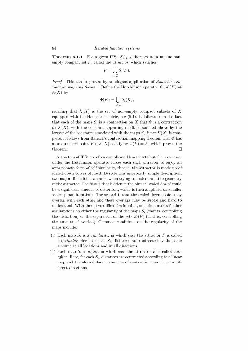
84 Iterated function systems
Theorem 6.1.1 For a given IFS Sii∈I there exists a unique non-
empty compact set F , called the attractor, which satisfies
F =⋃i∈I
Si(F ).
Proof This can be proved by an elegant application of Banach’s con-
traction mapping theorem. Define the Hutchinson operator Φ : K(X)→K(X) by
Φ(K) =⋃i∈I
Si(K),
recalling that K(X) is the set of non-empty compact subsets of X
equipped with the Hausdorff metric, see (5.1). It follows from the fact
that each of the maps Si is a contraction on X that Φ is a contraction
on K(X), with the constant appearing in (6.1) bounded above by the
largest of the constants associated with the maps Si. Since K(X) is com-
plete, it follows from Banach’s contraction mapping theorem that Φ has
a unique fixed point F ∈ K(X) satisfying Φ(F ) = F , which proves the
theorem.
Attractors of IFSs are often complicated fractal sets but the invariance
under the Hutchinson operator forces each such attractor to enjoy an
approximate form of self-similarity, that is, the attractor is made up of
scaled down copies of itself. Despite this apparently simple description,
two major difficulties can arise when trying to understand the geometry
of the attractor. The first is that hidden in the phrase ‘scaled down’ could
be a significant amount of distortion, which is then amplified on smaller
scales (upon iteration). The second is that the scaled down copies may
overlap with each other and these overlaps may be subtle and hard to
understand. With these two difficulties in mind, one often makes further
assumptions on either the regularity of the maps Si (that is, controlling
the distortion) or the separation of the sets Si(F ) (that is, controlling
the amount of overlap). Common conditions on the regularity of the
maps include:
(i) Each map Si is a similarity, in which case the attractor F is called
self-similar. Here, for each Si, distances are contracted by the same
amount at all locations and in all directions.
(ii) Each map Si is affine, in which case the attractor F is called self-
affine. Here, for each Si, distances are contracted according to a linear
map and therefore different amounts of contraction can occur in dif-
ferent directions.
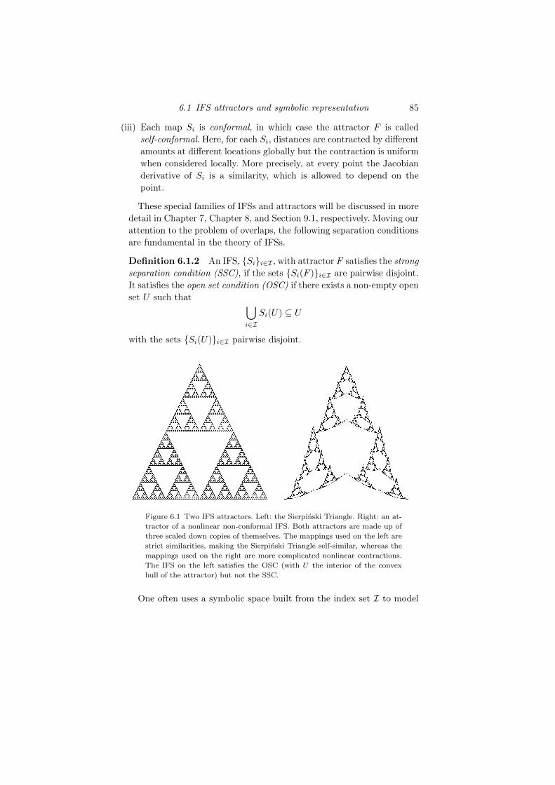
6.1 IFS attractors and symbolic representation 85
(iii) Each map Si is conformal, in which case the attractor F is called
self-conformal. Here, for each Si, distances are contracted by different
amounts at different locations globally but the contraction is uniform
when considered locally. More precisely, at every point the Jacobian
derivative of Si is a similarity, which is allowed to depend on the
point.
These special families of IFSs and attractors will be discussed in more
detail in Chapter 7, Chapter 8, and Section 9.1, respectively. Moving our
attention to the problem of overlaps, the following separation conditions
are fundamental in the theory of IFSs.
Definition 6.1.2 An IFS, Sii∈I , with attractor F satisfies the strong
separation condition (SSC), if the sets Si(F )i∈I are pairwise disjoint.
It satisfies the open set condition (OSC) if there exists a non-empty open
set U such that ⋃i∈I
Si(U) ⊆ U
with the sets Si(U)i∈I pairwise disjoint.
Figure 6.1 Two IFS attractors. Left: the Sierpinski Triangle. Right: an at-
tractor of a nonlinear non-conformal IFS. Both attractors are made up of
three scaled down copies of themselves. The mappings used on the left are
strict similarities, making the Sierpinski Triangle self-similar, whereas the
mappings used on the right are more complicated nonlinear contractions.
The IFS on the left satisfies the OSC (with U the interior of the convex
hull of the attractor) but not the SSC.
One often uses a symbolic space built from the index set I to model
86 Iterated function systems
the attractor of an IFS. It can be more convenient to work with the geom-
etry of the symbolic space and there is a straightforward and canonical
method to transfer information from the symbolic space to the fractal.
We briefly describe this technique and fix some notation which will be
used in later chapters. Let I∗ =⋃k>1 Ik denote the set of all finite
sequences with entries in I and for
i =(i1, i2, . . . , ik
)∈ Ik
write
Si = Si1 Si2 · · · Sik .
Write IN to denote the set of all infinite I-valued sequences and for
i ∈ IN or Il with l > k write i |k ∈ Ik to denote the restriction of i to
its first k entries. Let Π : IN → F be the symbolic coding map from the
symbolic space IN to F defined by
Π(i) =⋂k∈N
Si |k(X).
Then Π(IN) = F , the attractor. For i , j ∈ I∗, we write i ≺ j if j |k = i
for some k 6 |j |, where |j | is the length of the sequence j . That is, i ≺ j
if i is a prefix of j . For
i = (i1, i2, . . . , ik−1, ik) ∈ I∗
let
i− = (i1, i2, . . . , ik−1) ∈ I∗ ∪ ω,
where ω is the empty word. For notational convenience the map Sω is
taken to be the identity. The above establishes a symbolic representation
of F , which is also useful for visualisation purposes. For example, for all
k > 1,
F =⋃i∈Ik
Si (F )
and the ‘pieces’ Si (F ) thus provide a natural cover of F at a scale
which tends to zero as k → ∞. If F is self-similar or self-conformal
and satisfies the OSC, this approach leads to essentially optimal covers.
However, for self-affine sets this is far from true. For i ∈ I∗, we write
[i ] = j ∈ IN : i ≺ j , so that Π([i ]) = Si (F ).
6.2 Invariant measures 87
6.2 Invariant measures
One is often interested in measures supported on attractors of IFSs which
enjoy analogous invariance properties, that is, they are not just arbitrary
measures on the attractor, but measures which are invariant under the
IFS. One natural approach for constructing such measures is to project
Bernoulli measures from the symbolic space onto the attractor. Given
an IFS Sii∈I , with attractor F , associate a probability vector pii∈Iwhere each pi ∈ (0, 1) and
∑i∈I pi = 1. Then, analogously to Theorem
6.1.1, there is a unique Borel probability measure µ satisfying
µ =∑i∈I
piµ S−1i (6.2)
where µS−1i is the pushforward of µ under Si, defined by µS−1
i (E) =
µ(S−1i (E)) for Borel sets E. This can be proved in a similar way to
Theorem 6.1.1 by demonstrating that the associated operator is a con-
traction on the space of Borel probability measures on X equipped with
the Wasserstein distance, or another suitable metric.
We generally refer to measures µ given by (6.2) as Bernoulli measures,
but when the attractor is self-similar, we say µ is self-similar, etc. A
question of interest to us is, given a notion of dimension dim and an
IFS attractor F , when does there exist a Bernoulli measure µ such that
dimµ = dimF , or at least a sequence of Bernoulli measures µk such that
dimµk → dimF? The answer to this question is trivial if one simply
requires µ to be supported on F , see (1.3), Theorems 4.1.3, and 4.2.3.
Therefore, the potential interest in the question concerns the existence of
invariant measures realising the dimension of the attractor. Surprisingly,
the answer to this question is not always positive. For example, Das and
Simmons [49] provided an example of a self-affine set in R3 such that
the supremum of the Hausdorff dimensions of all invariant measures is
strictly smaller than the Hausdorff dimension of the set. This answered
an explicit question of Kenyon and Peres [168].
This interplay between dynamically invariant sets and measures is
central to the dimension theory of dynamical systems. IFSs give rise
to one form of dynamical invariance, although the natural dynamically
invariant measures may not be Bernoulli. The natural measures might
be projections of more general shift invariant measures on the symbolic
space, such as Markov measures, or Gibbs measures, or they could simply
be projections of shift ergodic measures. Moreover, other forms of invari-
ance are possible, such as measures preserved under a dynamical system,
88 Iterated function systems
or a group action. The question of interest becomes: when does a given
invariant set support an invariant measure which realises its dimension?
This question can then take on different flavours depending on the type
of invariance and the dimensions involved. Concerning Hausdorff dimen-
sion, realising the dimension means that there is an invariant measure
of maximal dimension, or at least that the supremum of the Hausdorff
dimensions of invariant measures equals the Hausdorff dimension of the
set, recall (1.3). For the Assouad/lower dimension, realising the dimen-
sion means that there is an invariant measure with minimal/maximal
dimension, or at least that the infimum/supremum of the Assouad/lower
dimension of invariant measures equals the Assouad/lower dimension of
the set. It is particularly interesting to us whether or not an invariant
measure can simultaneously realise the lower, Hausdorff, and Assouad
dimensions, in a situation where they are distinct. We refer to this as
the simultaneous realisation problem, which is deliberately vague at this
point, and will revisit it several times later in the book as our family of
examples grows.
6.3 Dimensions of IFS attractors
As we alluded to above, it is very difficult to say anything about the
dimension theory of IFS attractors in general. One simple but important
fact is that we may estimate the Hausdorff and box dimensions in terms
of the Lipschitz constants of the defining maps. Specifically, if each Si is
bi-Lipschitz, with constants 0 < bi 6 ci < 1 such that for all x, y ∈ X
bi|x− y| 6 |Si(x)− Si(y)| 6 ci|x− y|,
and the IFS satisfies the SSC, then
t 6 dimH F 6 dimBF 6 s (6.3)
where s and t are defined by∑i∈I
bti =∑i∈I
csi = 1.
See [70, Propositions 9.6-9.7]. The upper bound holds without any sep-
aration conditions and the lower bound, somewhat surprisingly, can fail
even if the OSC is assumed. For example, consider the self-affine set
defined by the IFS consisting of the maps (x, y) 7→ (x/2, x/2 + y/2) and
(x, y) 7→ (x/2 + y/2, y/2). This IFS satisfies the OSC with the open set
6.3 Dimensions of IFS attractors 89
given by the open unit square (0, 1)2 but the attractor is the singleton
(0, 0).It is natural to ask if these bounds also apply to the Assouad and lower
dimensions but they do not. We give a simple example of a self-affine
set exhibiting this failure in Section 8.5.
It was proved in [278] that the lower dimension is strictly positive for
any self-affine set (irrespective of overlaps), and it is natural to ask if this
extends to more general IFSs. However, it was also shown in [278] that
this is not true if the defining maps are only assumed to be invertible.
Moreover, it can fail trivially if the maps are not invertible since, for
example, one can force an attractor to have an isolated point by adding
a constant map x 7→ c for some c not already in the attractor.
If the maps are assumed to be bi-Lipschitz, then the lower spectrum
is strictly positive, for at least some range of θ. Moreover, dimθL F →
dimBF as θ → 0. Recall that Lemma 3.4.4 shows that dimθA F → dimBF
as θ → 0 for any set F , but it is not true in general that dimθL F →
dimBF .
Theorem 6.3.1 Let F be the attractor of an IFS consisting of bi-
Lipschitz contractions and assume F is not a singleton. Then there exists
θ0 ∈ (0, 1) such that
dimθL F > 0
for all θ ∈ (0, θ0) and dimθL F → dimBF as θ → 0.
Proof First note that, even without the SSC, (6.3) guarantees that the
lower box dimension of F is strictly positive. Since we assume F is not a
singleton, we can find distinct maps S1 and S2 in the IFS with distinct
fixed points. Therefore, for n sufficiently large the IFS consisting of the
two maps Sn1 , Sn2 satisfies the SSC and therefore the attractor, which
is a subset of F , has strictly positive lower box dimension by (6.3). Since
the lower box dimension is positive, for any 0 < s < dimBF , there exists
C > 0 such that Mr(F ) > Cr−s for all r ∈ (0, 1), where Mr(F ) is the
maximal size of an r-separated subset of F .
Write cmax = maxi∈I ci < 1 and bmin = mini∈I bi > 0. Let r be such
that 0 < rθ < |F | and x ∈ F . Choose i ∈ I∗ such that x ∈ Si (F ) ⊆B(x, rθ) but Si−(F ) * B(x, rθ). This forces
c|i |−1max |F | > |Si−(F )| > rθ
and so |i | 6 log(rθ/|F |)/ log cmax + 1. Let Y be a maximal 2r/b|i |min-
separated subset of F and consider the set Si (Y ) which is necessarily a
90 Iterated function systems
2r-separated subset of B(x, rθ) ∩ F . It follows that
Nr(B(x, rθ) ∩ F ) > #Y > C(2r/b|i |min)−s
> Cbsmin2−s|F |−slog bminlog cmax rθs
log bminlog cmax
−s
which, since s can be chosen arbitrarily close to dimBF , shows that
dimθL F > dimBF
1− θ log bmin
log cmax
1− θ.
Therefore, dimθL F > 0 for 0 < θ < log cmax
log bminand dimθ
L F → dimBF as
θ → 0.
Theorem 6.3.1 combined with the fact that dimqL F 6 dimH F for any
closed set F , see [118, Proposition 10], shows that the lower spectrum of
an attractor of a bi-Lipschitz IFS is non-constant whenever the Hausdorff
and lower box dimension are distinct.
We can adapt the example from [278] to show that the previous the-
orem is not true in general if the bi-Lipschitz condition is relaxed to
invertible. Consider the IFS consisting of two maps acting on [0, 1] given
by
S1(x) = x1/x/3
for x > 0 and S1(0) = 0 and
S2(x) = (x+ 2)/3
and let F be the attractor, see Figure 6.3. This IFS satisfies the SSC
and the defining maps are invertible but S1 is not bi-Lipschitz.
Fix θ ∈ (0, 1), a large integer n > 1, and consider x = 0 and R =
Sn1 (1/2). Then
B(0, R) ∩ F = Sn+11 (F )
but for n sufficiently large |Sn+11 (F )| 6 R1/θ and so
NR1/θ (B(0, R) ∩ F ) = 1
which proves that
dimθL F = 0 (6.4)
for all θ ∈ (0, 1).
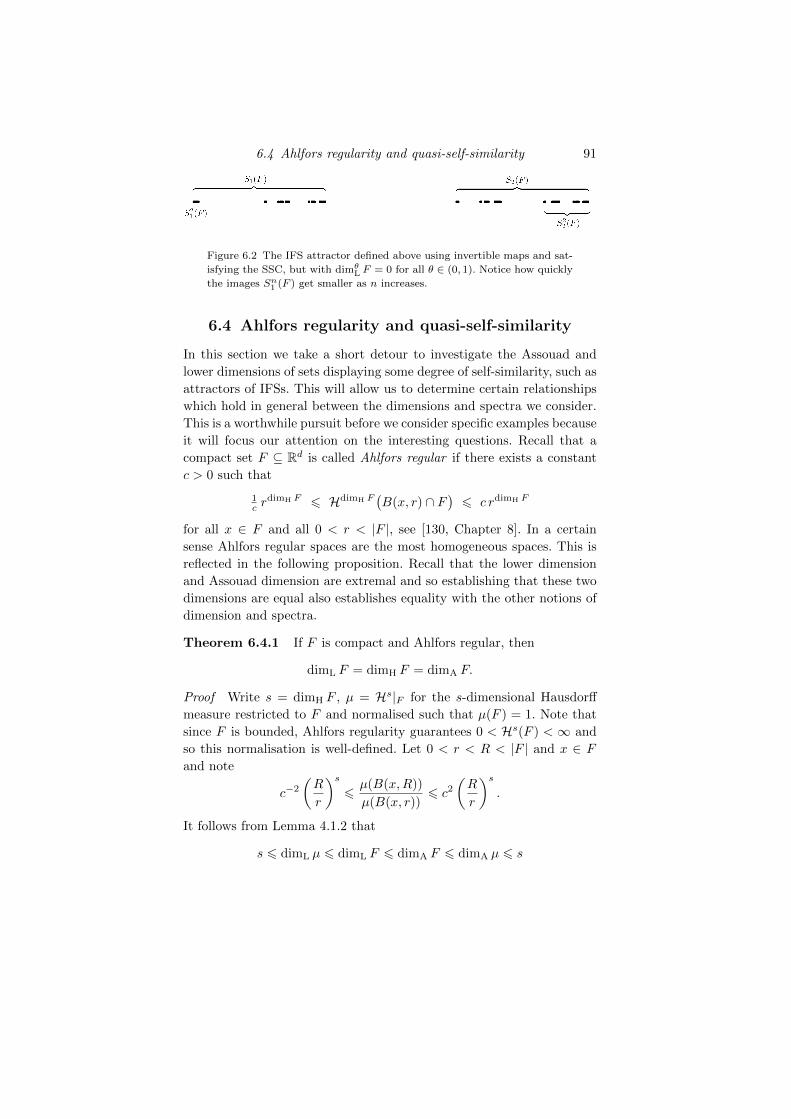
6.4 Ahlfors regularity and quasi-self-similarity 91
Figure 6.2 The IFS attractor defined above using invertible maps and sat-
isfying the SSC, but with dimθL F = 0 for all θ ∈ (0, 1). Notice how quickly
the images Sn1 (F ) get smaller as n increases.
6.4 Ahlfors regularity and quasi-self-similarity
In this section we take a short detour to investigate the Assouad and
lower dimensions of sets displaying some degree of self-similarity, such as
attractors of IFSs. This will allow us to determine certain relationships
which hold in general between the dimensions and spectra we consider.
This is a worthwhile pursuit before we consider specific examples because
it will focus our attention on the interesting questions. Recall that a
compact set F ⊆ Rd is called Ahlfors regular if there exists a constant
c > 0 such that
1c r
dimH F 6 HdimH F(B(x, r) ∩ F
)6 c rdimH F
for all x ∈ F and all 0 < r < |F |, see [130, Chapter 8]. In a certain
sense Ahlfors regular spaces are the most homogeneous spaces. This is
reflected in the following proposition. Recall that the lower dimension
and Assouad dimension are extremal and so establishing that these two
dimensions are equal also establishes equality with the other notions of
dimension and spectra.
Theorem 6.4.1 If F is compact and Ahlfors regular, then
dimL F = dimH F = dimA F.
Proof Write s = dimH F , µ = Hs|F for the s-dimensional Hausdorff
measure restricted to F and normalised such that µ(F ) = 1. Note that
since F is bounded, Ahlfors regularity guarantees 0 < Hs(F ) < ∞ and
so this normalisation is well-defined. Let 0 < r < R < |F | and x ∈ Fand note
c−2
(R
r
)s6µ(B(x,R))
µ(B(x, r))6 c2
(R
r
)s.
It follows from Lemma 4.1.2 that
s 6 dimL µ 6 dimL F 6 dimA F 6 dimA µ 6 s
92 Iterated function systems
proving the result.
The notion of quasi-self-similarity was introduced by Falconer [66] and
McLaughlin [209] and serves to weaken the notion of Ahlfors regularity
whilst maintaining some of the consequences. These results allow one to
deduce facts about the dimensions and measures of a set without having
to calculate them explicitly, which leads to them often being referred to
as implicit theorems. This is done by assuming that either large parts
of the set can be mapped to small parts without too much distortion or
vice versa.
Definition 6.4.2 (Quasi-self-similarity) Let F ⊆ Rd be a non-empty
compact set.
(i) We say F is quasi-self-similar of type (1) if there exists a > 0 and
r0 > 0 such that for every set U that intersects F with |U | 6 r0,
there is a function g : F ∩ U → F satisfying
a |U |−1 |x− y| 6 |g(x)− g(y)| (6.5)
for all x, y ∈ F ∩ U .
(ii) We say F is quasi-self-similar of type (2) if there exists a > 0 and
r0 > 0 such that for every closed ball B with centre in F and radius
R 6 r0, there is a function g : F → F ∩B satisfying
aR |x− y| 6 |g(x)− g(y)| (6.6)
for all x, y ∈ F .
Temporarily write s = dimH F . It was shown in [209, 66] that F
being quasi-self-similar of type (1) guarantees that Hs(F ) > as > 0
and dimBF = dimBF = s. On the other hand, it was shown in [66]
that F being quasi-self-similar of type (2) guarantees Hs(F ) 6 4s a−s <
∞ and dimBF = dimBF = s, also see [69, Chapter 3]. These results
were extended to include the Assouad and lower dimensions in [88].
By considering the relationships between the various dimensions and
spectra discussed in this book, one may also glean implicit theorems
for the other notions by sandwiching them in between the dimensions
considered below.
6.4 Ahlfors regularity and quasi-self-similarity 93
Theorem 6.4.3 Let F ⊆ Rd be compact and non-empty.
(i) If F is quasi-self-similar of type (1), then
dimL F 6 dimH F = dimB F = dimA F.
(ii) If F is quasi-self-similar of type (2), then
dimL F = dimH F = dimB F 6 dimA F.
(iii) If F is quasi-self-similar of type (1) and (2), then
dimL F = dimH F = dimB F = dimA F
and, moreover, F is Ahlfors regular.
Proof Throughout the proof write s = dimH F = dimBF = dimBF .
It follows immediately from the definition of box dimension that for all
ε > 0 there exists a constant C > 1 such that, for all r > 0,
C−1 r−s+ε 6 Nr(F ) 6 C r−s−ε. (6.7)
Proof of (i). Let 0 < r < R 6 r0/2 and x ∈ F . Since F is quasi-self-
similar of type (1), there exists g1 : B(x,R) ∩ F → F satisfying (6.5)
with U = B(x,R). If Uii is an (ar/2R)-cover of g1(B(x,R)∩F ), then
g−11 (Ui)i is an r-cover of B(x,R) ∩ F . Then, applying (6.7),
Nr(B(x,R) ∩ F
)6 Nar/2R
(g1(B(x,R) ∩ F )
)6 Nar/2R(F )
6 C(2/a)s+ε(R
r
)s+εwhich shows dimA F 6 s+ε and letting ε→ 0 completes the proof.
Proof of (ii). Let 0 < r < R 6 r0/2 and x ∈ F . Since F is quasi-
self-similar of type (2), there exists g2 : F → B(x,R)∩F satisfying (6.6)
with B = B(x,R). If Uii is an r-cover of g2(F ), then g−12 (Ui)i is an
(r/aR)-cover of F . Then, applying (6.7),
Nr(B(x,R) ∩ F
)> Nr
(g2(F )
)> Nr/aR(F ) > C−1 as−ε
(R
r
)s−εwhich shows dimL F > s− ε and letting ε→ 0 completes the proof.
Proof of (iii). It remains to prove that F is Ahlfors regular. Let r ∈
94 Iterated function systems
(0, r0/2), x ∈ F and g1 and g2 be maps satisfying (6.5)-(6.6) with
U = B = B(x, r). The results from [66] mentioned above guarantee
as 6 Hs(F ) 6 4s a−s.
Therefore, using the scaling property for Hausdorff measure, see [70,
Proposition 2.2],
Hs(B(x, r) ∩ F ) 6 Hs(g−1
1 (F ))
6 (2r/a)sHs(F ) 6 8s a−2s rs.
and
Hs(B(x, r) ∩ F ) > Hs(g2(F )
)> (ar)sHs(F ) > a2s rs
completing the proof.
The implicit theorems allow us to deduce information about the di-
mensions and spectra of various classes of IFS attractor as well as some
variants, including graph-directed IFSs and sub-self-similar sets. See [69]
for more information on these examples.
Corollary 6.4.4
(a) The following classes of sets are Ahlfors regular and, in particular,
have equal Assouad and lower dimension:
(i) self-similar sets satisfying the OSC,
(ii) self-conformal sets satisfying the OSC,
(iii) graph-directed self-similar or self-conformal sets satisfying the graph-
directed analogue of the OSC.
(b) The following classes of sets have equal Assouad dimension, quasi-
Assouad and Hausdorff dimension, as well as having constant Assouad
spectrum:
(i) sub-self-similar sets satisfying the OSC.
(c) The following classes of sets have equal lower dimension, quasi-lower
dimension and Hausdorff dimension, as well as having constant lower
spectrum, regardless of separation conditions:
(i) self-similar sets,
(ii) self-conformal sets,
(iii) graph-directed self-similar or self-conformal sets.
Proof This follows immediately from Theorem 6.4.3, see [66, 68, 88] for
the details.
6.4 Ahlfors regularity and quasi-self-similarity 95
Theorem 6.4.3 is sharp, in that the inequalities in parts (i) and (ii)
cannot be replaced with equalities in general. To see this, note that the
inequality in part (i) is sharp because the set [0, 1] ∪ 2 is quasi-self-
similar of type (1), but has lower dimension strictly less than Hausdorff
dimension. Also, the inequality in part (ii) is sharp because self-similar
sets can have Assouad dimension strictly larger than Hausdorff dimen-
sion and are quasi-self-similar of type (2), see Theorem 7.2.1.
7
Self-similar sets
Self-similar sets are a special case of IFS attractors and have been studied
extensively in the literature. In this chapter we consider self-similar sets
and measures in detail. Corollary 6.4.4 already implies that self-similar
sets have equal lower, Hausdorff and box dimension, but we will see in
Theorem 7.2.1 that the Assouad dimension may be strictly larger.
7.1 Self-similar sets and the Hutchinson-Moranformula
The key reason why self-similar sets are easier to deal with than self-
affine sets and more general attractors is that the images of the set under
compositions of maps from the IFS form natural covers for the original
set. This leads to simple formulae for the dimensions of a self-similar
set. Recall, a map S : Rd → Rd is called a similarity if there exists a
constant c > 0 such that, for all x, y ∈ Rd,
|S(x)− S(y)| = c|x− y|. (7.1)
The constant c is called the similarity ratio of S. If c ∈ (0, 1) then S
is also a contraction, and we use the term contracting similarity. This
should be compared with the definition of a contraction (6.1), noting that
similarities yield a precise formula for the distortion. Moreover, similari-
ties are bi-Lipschitz with equal upper and lower Lipschitz constants and
so (6.3) immediately yields a precise formula for the dimensions of self-
similar sets when the SSC is satisfied. However, this observation can be
improved.
Given an IFS, Sii∈I , consisting of contracting similarities with simi-
larity ratios cii∈I , the similarity dimension is defined to be the unique
This material will be published by Cambridge University Press as Assouad Dimension and Fractal Geometryby Jonathan Fraser. This pre-publication version is free to view and download for personal use only.
Not for re-distribution, re-sale or use in derivative works. c© Jonathan Fraser 2020.
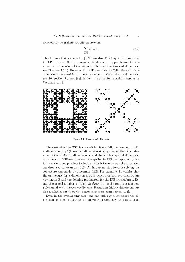
7.1 Self-similar sets and the Hutchinson-Moran formula 97
solution to the Hutchinson-Moran formula∑i∈I
csi = 1. (7.2)
This formula first appeared in [213] (see also [61, Chapter 13]) and later
in [145]. The similarity dimension is always an upper bound for the
upper box dimension of the attractor (but not the Assouad dimension,
see Theorem 7.2.1). However, if the IFS satisfies the OSC, then all of the
dimensions discussed in this book are equal to the similarity dimension,
see [70, Section 9.3] and [88]. In fact, the attractor is Ahlfors regular by
Corollary 6.4.4.
Figure 7.1 Two self-similar sets.
The case when the OSC is not satisfied is not fully understood. In Rd,a ‘dimension drop’ (Hausdorff dimension strictly smaller than the mini-
mum of the similarity dimension, s, and the ambient spatial dimension,
d) can occur if different iterates of maps in the IFS overlap exactly, but
it is a major open problem to decide if this is the only way the dimension
can drop, see, for example, [233]. An important step towards solving this
conjecture was made by Hochman [132]. For example, he verifies that
the only cause for a dimension drop is exact overlaps, provided we are
working in R and the defining parameters for the IFS are algebraic. Re-
call that a real number is called algebraic if it is the root of a non-zero
polynomial with integer coefficients. Results in higher dimensions are
also available, but there the situation is more complicated [133].
Even in the overlapping case, one can still say a lot about the di-
mensions of a self-similar set. It follows from Corollary 6.4.4 that for all
98 Self-similar sets
self-similar sets F one has
dimL F = dimqL F = dimθL F = dimH F = dimP F = dimBF = dimBF
for all θ ∈ (0, 1). However, in the overlapping case the Assouad dimension
can be strictly larger than the box dimension. Whether or not this was
possible was asked by Olsen [219, Question 1.3] and answered in [88,
Section 3.1]. We discuss the Assouad dimension in detail in the following
section.
7.2 The Assouad dimension of self-similar sets
We start with an example from [88], demonstrating that the Assouad di-
mension can strictly exceed the box dimension. We also use this example
to show that Assouad dimension can increase under Lipschitz maps.
Theorem 7.2.1 There exists a self-similar set F ⊆ R such that
dimB F < dimA F .
Proof Let 0 < γ < α < β < 1 be such that log β/ logα /∈ Q and define
similarity maps S1, S2, S3 on [0, 1] by
S1(x) = αx, S2(x) = βx and S3(x) = γx+ (1− γ).
Let F be the self-similar attractor of S1, S2, S3, see Figure 7.2. We
show that [0, 1] is a weak tangent to F . For each integer k > 1 let Tk be
defined by Tk(x) = β−kx and let
Ek = 0 ∪αmβn : m ∈ N, n ∈ Z with n > −k
∩ [0, 1],
noting that Ek ⊆ Tk(F )∩ [0, 1] for each k. Therefore, it suffices to show
that Ek → [0, 1] in the Hausdorff metric dH. Using the fact that the sets
Ek are nested,
Ek →⋃k∈N
Ek ∩ [0, 1]
= αmβn : m ∈ N, n ∈ Z ∩ [0, 1]
= [0, 1],
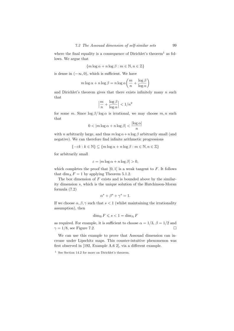
7.2 The Assouad dimension of self-similar sets 99
where the final equality is a consequence of Dirichlet’s theorem1 as fol-
lows. We argue that
m logα+ n log β : m ∈ N, n ∈ Z
is dense in (−∞, 0), which is sufficient. We have
m logα+ n log β = n logα
(m
n+
log β
logα
)and Dirichlet’s theorem gives that there exists infinitely many n such
that ∣∣∣mn
+log β
logα
∣∣∣ < 1/n2
for some m. Since log β/ logα is irrational, we may choose m,n such
that
0 < |m logα+ n log β| < |logα|n
with n arbitrarily large, and thus m logα+n log β arbitrarily small (and
negative). We can therefore find infinite arithmetic progressions
−εk : k ∈ N ⊆ m logα+ n log β : m ∈ N, n ∈ Z
for arbitrarily small
ε = |m logα+ n log β| > 0,
which completes the proof that [0, 1] is a weak tangent to F . It follows
that dimA F = 1 by applying Theorem 5.1.2.
The box dimension of F exists and is bounded above by the similar-
ity dimension s, which is the unique solution of the Hutchinson-Moran
formula (7.2)
αs + βs + γs = 1.
If we choose α, β, γ such that s < 1 (whilst maintaining the irrationality
assumption), then
dimB F 6 s < 1 = dimA F
as required. For example, it is sufficient to choose α = 1/3, β = 1/2 and
γ = 1/8, see Figure 7.2.
We can use this example to prove that Assouad dimension can in-
crease under Lipschitz maps. This counter-intuitive phenomenon was
first observed in [192, Example A.6 2], via a different example.
1 See Section 14.2 for more on Dirichlet’s theorem.
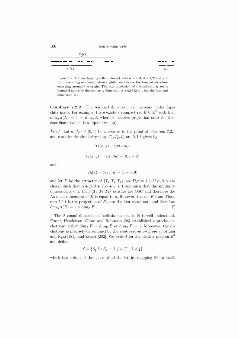
100 Self-similar sets
Figure 7.2 The overlapping self-similar set with α = 1/3, β = 1/2 and γ =
1/8. Stretching our imagination slightly, we can see the tangent structure
emerging around the origin. The box dimension of the self-similar set is
bounded above by the similarity dimension s ≈ 0.9582 < 1 but the Assouad
dimension is 1.
Corollary 7.2.2 The Assouad dimension can increase under Lips-
chitz maps. For example, there exists a compact set E ⊆ R2 such that
dimA π(E) = 1 > dimAE where π denotes projection onto the first
coordinate (which is a Lipschitz map).
Proof Let α, β, γ ∈ (0, 1) be chosen as in the proof of Theorem 7.2.1
and consider the similarity maps T1, T2, T3 on [0, 1]2 given by
T1(x, y) = (αx, αy),
T2(x, y) = (βx, βy) + (0, 1− β)
and
T3(x) = (γx, γy) + (1− γ, 0)
and let E be the attractor of T1, T2, T3, see Figure 7.3. If α, β, γ are
chosen such that α + β, β + γ, α + γ 6 1 and such that the similarity
dimension s < 1, then T1, T2, T3 satisfies the OSC and therefore the
Assouad dimension of E is equal to s. However, the set F from Theo-
rem 7.2.1 is the projection of E onto the first coordinate and therefore
dimA π(E) = 1 > dimAE.
The Assouad dimension of self-similar sets in R is well-understood.
Fraser, Henderson, Olson and Robinson [96] established a precise di-
chotomy: either dimA F = dimH F or dimA F = 1. Moreover, the di-
chotomy is precisely determined by the weak separation property of Lau
and Ngai [181], and Zerner [282]. We write I for the identity map on Rdand define
E = S−1i Sj : i , j ∈ I∗, i 6= j
which is a subset of the space of all similarities mapping Rd to itself.
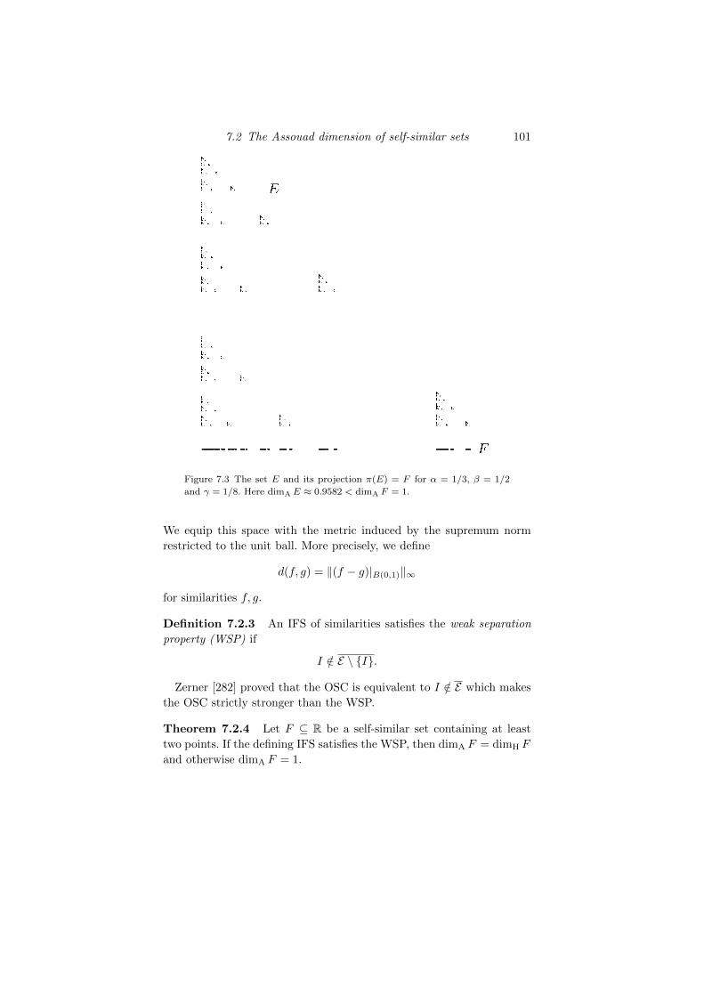
7.2 The Assouad dimension of self-similar sets 101
Figure 7.3 The set E and its projection π(E) = F for α = 1/3, β = 1/2
and γ = 1/8. Here dimA E ≈ 0.9582 < dimA F = 1.
We equip this space with the metric induced by the supremum norm
restricted to the unit ball. More precisely, we define
d(f, g) = ‖(f − g)|B(0,1)‖∞
for similarities f, g.
Definition 7.2.3 An IFS of similarities satisfies the weak separation
property (WSP) if
I /∈ E \ I.
Zerner [282] proved that the OSC is equivalent to I /∈ E which makes
the OSC strictly stronger than the WSP.
Theorem 7.2.4 Let F ⊆ R be a self-similar set containing at least
two points. If the defining IFS satisfies the WSP, then dimA F = dimH F
and otherwise dimA F = 1.
102 Self-similar sets
Using this result, and some work concerning the Hausdorff measure
of self-similar sets, Farkas and Fraser [81, Corollary 3.2] proved the fol-
lowing set of equivalences. A neat consequence of this is that the WSP
is intrinsic to the set F , provided the Hausdorff dimension is not full:
either all IFSs defining F satisfy the WSP or none do. This does not
hold for the OSC or SSC, for example.
Theorem 7.2.5 Let F ⊆ R be a self-similar set containing at least
two points with s = dimH F < 1. Then the following are equivalent:
(i) the defining IFS satisfies the WSP
(ii) Hs(F ) > 0
(iii) 0 < Hs(F ) <∞(iv) F is Ahlfors regular
(v) dimA F = dimH F .
Proof The fact that (i) implies (ii) was proved by Zerner [282, Corollary
of Proposition 2]. It follows from [66] that Hs(F ) <∞ and therefore (ii)
and (iii) are equivalent. The fact that (ii) implies (iv) follows from [81,
Theorem 2.1 and Lemma 1.1] which gives that for any r > 0, Hs(E) =
Hsr(E) for any Hs-measurable subset E ⊆ F . Therefore, for any x ∈ Fand 0 < r 6 |F |,
Hs(F ∩B(x, r)) = Hs2r(F ∩B(x, r)) 6 2srs
where the final inequality comes by considering the trivial cover B(x, r).Moreover, the reverse inequality is straightforward since F ∩B(x, r) con-
tains Si (F ) for some i ∈ I∗ such that the similarity ratio of Si is at least
cr for a uniform constant c > 0 depending only on the IFS. Therefore,
using the scaling property for Hausdorff measure (see [70, Proposition
2.2]),
Hs(F ∩B(x, r)) > Hs(Si (F )) = csrsHs(F ) > 0
which proves that F is Ahlfors regular. Theorem 6.4.1 gives that (iv)
implies (v). Finally, Theorem 7.2.4 and the fact that s < 1 shows that
(v) implies (i), completing the proof.
The self-similar set constructed in Theorem 7.2.1 clearly fails the WSP.
This constitutes one of two well-known methods for constructing such
examples. The other is due to Bandt and Graf [13] and works as follows.
One advantage of the Bandt-Graf approach is that all of the similarity
7.2 The Assouad dimension of self-similar sets 103
ratios can be the same. Let c ∈ (0, 1) be the common similarity ratio
and consider the IFS consisting of the three maps
S1(x) = cx, S2(x) = c(x+ t), S3(x) = cx+ (1− c) (7.3)
acting on [0, 1] where t ∈ (0, (1− c)/c) is
t = t(c) =1− cc
∞∑k=0
c2k
. (7.4)
The elements S−1i Sj where |i | = |j | = n are of the form
x 7→ x+
n∑k=1
c−kak (7.5)
where
ak ∈ 0,±ct,±(1− c),± (ct− (1− c)) .
Consider n = 2m for some large integer m > 1 and choose the coefficients
aknk=1 as
ak =
−(1− c) if k = 2m − 2l for some l = 0, . . . ,m
ct if k = n
0 otherwise
in which case (7.5) becomes
x 7→ x+ c−2m(ct)− (1− c)m∑l=0
c2l−2m = x+ (1− c)
∞∑k=m+1
c2k−2m
using (7.4). Therefore, choosing m large we can approximate the identity
arbitrarily well by non-identity elements, proving the IFS fails the WSP.
Theorem 7.2.4 says that for self-similar sets in R the Assouad dimen-
sion is either equal to the Hausdorff dimension or equal to the ambient
spatial dimension (which in this case is 1). We can use the example of
Bandt and Graf to show that this does not hold in higher dimensions,
following [96]. Consider the IFS acting on [0, 1]2 consisting of the maps
S1(x) = x/5, S2(x) = x/5 + (t/5, 0),
S3(x) = x/5 + (4/5, 0), S4(x) = x/5 + (0, 4/5)
where t = t(1/5), as in (7.4). Let E denote the attractor, see Figure
7.4. Note that E is not contained in any line (and thus the true ambi-
ent dimension is 2) and also satisfies dimHE 6 log 4/ log 5 < 1 by the
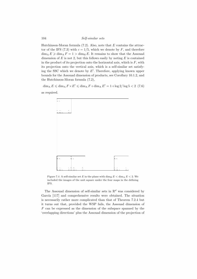
104 Self-similar sets
Hutchinson-Moran formula (7.2). Also, note that E contains the attrac-
tor of the IFS (7.3) with c = 1/5, which we denote by F , and therefore
dimAE > dimA F = 1 > dimHE. It remains to show that the Assouad
dimension of E is not 2, but this follows easily by noting E is contained
in the product of its projection onto the horizontal axis, which is F , with
its projection onto the vertical axis, which is a self-similar set satisfy-
ing the SSC which we denote by E′. Therefore, applying known upper
bounds for the Assouad dimension of products, see Corollary 10.1.2, and
the Hutchinson-Moran formula (7.2),
dimAE 6 dimA F×E′ 6 dimA F+dimAE′ = 1+log 2/ log 5 < 2 (7.6)
as required.
Figure 7.4 A self-similar set E in the plane with dimH E < dimA E < 2. We
included the images of the unit square under the four maps in the defining
IFS.
The Assouad dimension of self-similar sets in Rd was considered by
Garcıa [117] and comprehensive results were obtained. The situation
is necessarily rather more complicated than that of Theorem 7.2.4 but
it turns out that, provided the WSP fails, the Assouad dimension of
F can be expressed as the dimension of the subspace spanned by the
‘overlapping directions’ plus the Assouad dimension of the projection of
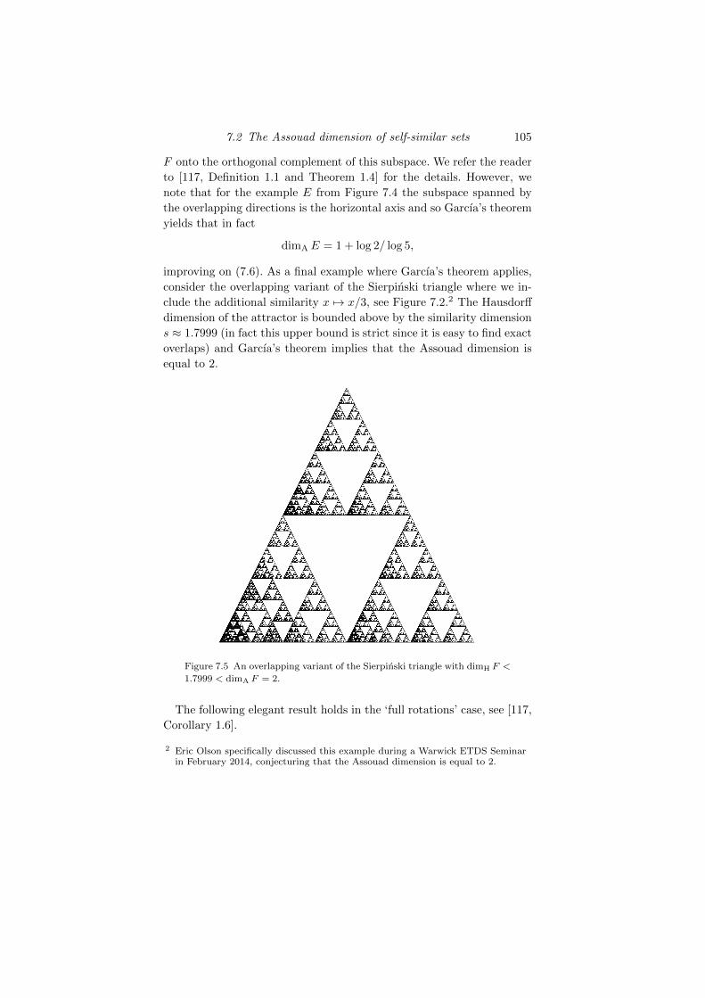
7.2 The Assouad dimension of self-similar sets 105
F onto the orthogonal complement of this subspace. We refer the reader
to [117, Definition 1.1 and Theorem 1.4] for the details. However, we
note that for the example E from Figure 7.4 the subspace spanned by
the overlapping directions is the horizontal axis and so Garcıa’s theorem
yields that in fact
dimAE = 1 + log 2/ log 5,
improving on (7.6). As a final example where Garcıa’s theorem applies,
consider the overlapping variant of the Sierpinski triangle where we in-
clude the additional similarity x 7→ x/3, see Figure 7.2.2 The Hausdorff
dimension of the attractor is bounded above by the similarity dimension
s ≈ 1.7999 (in fact this upper bound is strict since it is easy to find exact
overlaps) and Garcıa’s theorem implies that the Assouad dimension is
equal to 2.
Figure 7.5 An overlapping variant of the Sierpinski triangle with dimH F <
1.7999 < dimA F = 2.
The following elegant result holds in the ‘full rotations’ case, see [117,
Corollary 1.6].
2 Eric Olson specifically discussed this example during a Warwick ETDS Seminarin February 2014, conjecturing that the Assouad dimension is equal to 2.
106 Self-similar sets
Theorem 7.2.6 Let F ⊆ Rd be a self-similar set containing at least
two points. If the defining IFS does not satisfy the WSP and the group
generated by the orthogonal components of the defining similarities is
dense in SO(d) or O(d), then
dimA F = d.
Essentially the rotational components of the defining similarities plus
failure of the WSP guarantee that the span of the overlapping directions
is the whole of Rd.
7.3 The Assouad spectrum of self-similar sets
Compared to the Assouad dimension, the Assouad spectrum is less well-
understood for self-similar sets, even in the line. Some estimates based
on the Lq-spectrum of an associated self-similar measure are provided in
[112] and there is some evidence to suggest that if F ⊆ Rd is self-similar,
then
dimB F = dimθA F = dimqA F
for all θ ∈ (0, 1). Relying on a powerful result of Shmerkin and work of
Hochman, this can be verified in some cases.
Theorem 7.3.1 If F ⊆ R is self-similar such that there are no exact
overlaps in the construction and the defining parameters for the IFS are
algebraic, then
dimB F = dimθA F = dimqA F
for all θ ∈ (0, 1).
Proof In the setting of the theorem, Hochman [132] proved that the
box dimension is given by the similarity dimension, that is dimB F = s,
and we may assume s < 1 since otherwise there is nothing to prove.
Let µ be the self-similar measure supported by F associated to the
Bernoulli weights csi, see (7.2). Shmerkin [254, Theorem 6.6] strength-
ened Hochman’s result by proving that the Lq-spectrum of µ is affine,
that is,
τµ(q) = s(1− q)
for q > 0. This is a strengthening of Hochman’s result since τµ(0) re-
turns the box dimension of F . If the OSC is satisfied, then these results
7.3 The Assouad spectrum of self-similar sets 107
are straightforward, and go back much further, and so the novelty of
Shmerkin’s result (and Theorem 7.3.1) is in the overlapping case. Recall
the (upper) Lq-spectrum is defined by
τµ(q) = lim supr→0
logMqr (µ)
− log r
where
Mqr (µ) = sup
∑i
µ(Ui)q
with the supremum taken over all centred packings Uii of F by balls of
radius r. Let ε ∈ (0, 1) and choose q > 1 large enough so that −(s−ε)q >s(1− q) = τµ(q). It follows that there exists a constant C > 1 such that
Mqr (µ) 6 Cr(s−ε)q
for all r ∈ (0, 1). Then, since B(x, r) is an r-packing for any particular
choice of x and r ∈ (0, 1), we have
µ (B(x, r))q 6 Mq
r (µ) 6 Cr(s−ε)q
and therefore
µ (B(x, r)) 6 C1/qr(s−ε) (7.7)
for all x ∈ F and r ∈ (0, 1).
For i = (i1, i2, . . . , ik) ∈ I∗, we write ci = ci1ci2 · · · cik for the similar-
ity ratio of Si . Let x ∈ F , r > 0 be small, and θ ∈ (0, 1). For δ ∈ (0, 1),
let I(δ) ⊆ I∗ be the δ-stopping, defined by
I(δ) = i ∈ I∗ : ci 6 δ < ci−
and
M(x, rθ) = #i ∈ I(rθ) : Si (F ) ∩B(x, rθ) 6= ∅
.
All of the sets Si (F ) contributing to M(x, rθ) lie completely inside the
ball B(x, arθ
)for some fixed constant a > 1 which is independent of rθ
and x. Moreover, using (7.7) and the definition of µ,
M(x, rθ) csminrθs 6 µ
(B(x, arθ
))6 C1/qa(s−ε)rθ(s−ε)
where cmin = mini∈Ici, and so
M(x, rθ) 6 c−sminC1/qa(s−ε)r−εθ. (7.8)
We wish to cover B(x, rθ) by sets of diameter less than or equal to r
108 Self-similar sets
and to do this we iterate the construction of F inside each of the sets
Si (F ) contributing to M(x, rθ). More precisely, the setsSi j (F ) : i ∈ I(rθ) with Si (F ) ∩B(x, rθ) 6= ∅, j ∈ I
(r1−θ)
all have diameters at most r and form a cover of B(x, rθ). Therefore
N(B(x, rθ) ∩ F, r
)6M(x, rθ)
(#I
(r1−θ)) (7.9)
and so it remains to estimate #I(r1−θ). We have
(#I
(r1−θ)) r(s+ε)(1−θ) 6 c−2
min
∑j∈I(r1−θ)
cs+εj 6 c−2min
∞∑k=1
∑j∈Ik
cs+εj
= c−2min
∞∑k=1
∑j∈I
cs+εj
k
=: b <∞
using the Hutchinson-Moran formula (7.2) and therefore
#I(r1−θ) 6 br(s+ε)(θ−1). (7.10)
Thus, by (7.8), (7.9) and (7.10),
N(B(x, rθ) ∩ F, r
)6M(x, rθ)
(#I
(r1−θ))
6 c−sminC1/qa(s−ε)r−εθ br(s+ε)(θ−1)
6 c−sminC1/qa(s−ε)b
(rθ−1
)s+ ε1−θ
which proves
dimθA F 6 s+
ε
1− θand letting ε→ 0 proves the result.
Following [252], the requirement in Theorem 7.3.1 that there are no
exact overlaps and the defining parameters for the IFS are algebraic can
be replaced with a weaker but more technical assumption that there is
no ‘super-exponential concentration of cylinders’. The super-exponential
concentration condition was first considered in [132] where it was proved
that if the defining parameters are algebraic then super-exponential con-
centration is equivalent to the presence of exact overlaps. In fact, un-
til 2019 the only known mechanism for generating super-exponential
7.4 Dimensions of self-similar measures 109
concentration was via exact overlaps. However, papers by Baker [11]
and Barany-Kaenmaki [20] proved that super-exponential concentration
without exact overlaps is possible. For example, [11] demonstrates this
by constructing an explicit non-algebraic IFS using continued fraction
expansions.
7.4 Dimensions of self-similar measures
The Assouad and box dimensions of self-similar measures satisfying the
SSC were computed in [98, Theorem 2.4] and the lower dimension in
[127, Proposition 2.3]. The fact that such measures are doubling goes
back much further, for example to [217].
Theorem 7.4.1 Let µ be a self-similar measure satisfying the SSC.
Then µ is doubling and
dimA µ = dimB µ = maxi∈I
log pilog ci
and
dimL µ = mini∈I
log pilog ci
.
Proof Let δ be the minimal distance between distinct sets Si(F ) and
Sj(F ), that is,
δ = mini 6=j
infx∈Si(F )y∈Sj(F )
|x− y| > 0
which is strictly positive since the SSC holds. Given x ∈ F with
Π(i1, i2, . . . ) = x
for (i1, i2, . . . ) ∈ IN, which is uniquely defined since the SSC holds,
and r > 0 small, let n(x, r) be the largest integer such that 2r/δ 6ci1ci2 · · · cin(x,r)
and m(x, r) be the smallest non-negative integer such
that
Π([i1, . . . , im(x,r)]) ⊆ B(x, r/2).
Using these definitions,
pi1 · · · pim(x,r)6 µ(B(x, r))
and
Π([i1, . . . , im(x,r)−1]) 6⊆ B(x, r/2)
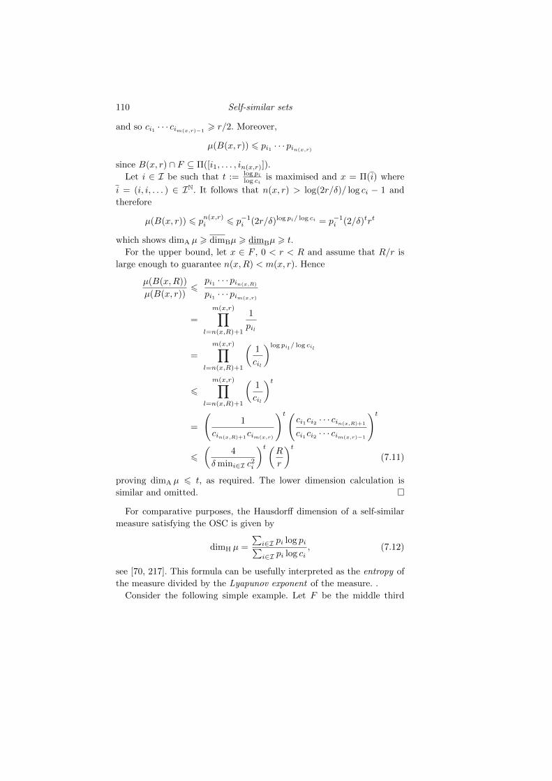
110 Self-similar sets
and so ci1 · · · cim(x,r)−1> r/2. Moreover,
µ(B(x, r)) 6 pi1 · · · pin(x,r)
since B(x, r) ∩ F ⊆ Π([i1, . . . , in(x,r)]).
Let i ∈ I be such that t := log pilog ci
is maximised and x = Π(i) where
i = (i, i, . . . ) ∈ IN. It follows that n(x, r) > log(2r/δ)/ log ci − 1 and
therefore
µ(B(x, r)) 6 pn(x,r)i 6 p−1
i (2r/δ)log pi/ log ci = p−1i (2/δ)trt
which shows dimA µ > dimBµ > dimBµ > t.
For the upper bound, let x ∈ F , 0 < r < R and assume that R/r is
large enough to guarantee n(x,R) < m(x, r). Hence
µ(B(x,R))
µ(B(x, r))6
pi1 · · · pin(x,R)
pi1 · · · pim(x,r)
=
m(x,r)∏l=n(x,R)+1
1
pil
=
m(x,r)∏l=n(x,R)+1
(1
cil
)log pil/ log cil
6m(x,r)∏
l=n(x,R)+1
(1
cil
)t
=
(1
cin(x,R)+1cim(x,r)
)t(ci1ci2 · · · cin(x,R)+1
ci1ci2 · · · cim(x,r)−1
)t
6
(4
δmini∈I c2i
)t(R
r
)t(7.11)
proving dimA µ 6 t, as required. The lower dimension calculation is
similar and omitted.
For comparative purposes, the Hausdorff dimension of a self-similar
measure satisfying the OSC is given by
dimH µ =
∑i∈I pi log pi∑i∈I pi log ci
, (7.12)
see [70, 217]. This formula can be usefully interpreted as the entropy of
the measure divided by the Lyapunov exponent of the measure. .
Consider the following simple example. Let F be the middle third
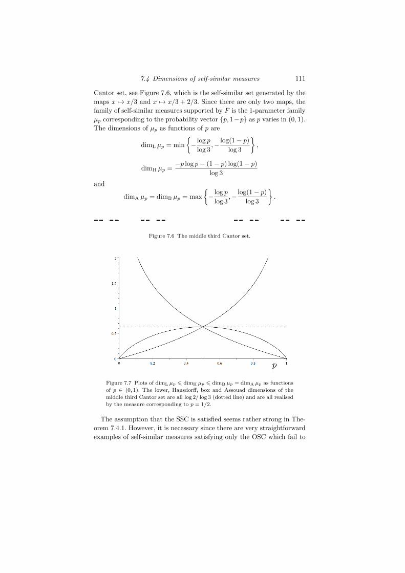
7.4 Dimensions of self-similar measures 111
Cantor set, see Figure 7.6, which is the self-similar set generated by the
maps x 7→ x/3 and x 7→ x/3 + 2/3. Since there are only two maps, the
family of self-similar measures supported by F is the 1-parameter family
µp corresponding to the probability vector p, 1−p as p varies in (0, 1).
The dimensions of µp as functions of p are
dimL µp = min
− log p
log 3,− log(1− p)
log 3
,
dimH µp =−p log p− (1− p) log(1− p)
log 3
and
dimA µp = dimB µp = max
− log p
log 3,− log(1− p)
log 3
.
Figure 7.6 The middle third Cantor set.
Figure 7.7 Plots of dimL µp 6 dimH µp 6 dimB µp = dimA µp as functions
of p ∈ (0, 1). The lower, Hausdorff, box and Assouad dimensions of the
middle third Cantor set are all log 2/ log 3 (dotted line) and are all realised
by the measure corresponding to p = 1/2.
The assumption that the SSC is satisfied seems rather strong in The-
orem 7.4.1. However, it is necessary since there are very straightforward
examples of self-similar measures satisfying only the OSC which fail to
112 Self-similar sets
even be doubling. Note how the coefficient of (R/r)t at the end of the
proof of Theorem 7.4.1 blows up as δ → 0, see (7.11). This gives some
indication that the SSC is playing a key role. For example, consider the
IFS consisting of the maps S1 : x 7→ x/2 and S2 : x 7→ (x + 1)/2 and
the self-similar measure µ associated with p, 1 − p for p > 1/2. The
support of µ is the attractor which in this case is [0, 1]. Let k > 1 be
large and x = 1/2− 2−k ∈ [0, 1] such that
B(x, 2−k) = Π([1, 2, 2, . . . , 2])
where 2 has been chosen k − 2 times. This means
B(x, 3 · 2−k) ⊃ Π([2, 1, 1, . . . , 1])
where this time 1 has been chosen k − 2 times. Therefore
µ(B(x, 3 · 2−k))
µ(B(x, 2−k))>
(1− p)pk−2
p(1− p)k−2=
(p
1− p
)k−3
→∞
proving that µ is not doubling and hence dimA µ = ∞. In fact, this
argument can be adapted to show that dimqA µ = ∞ and so µ is not
even ‘quasi-doubling’, see [125, Example 3.2]. The paper [125] contains
a thorough investigation of the quasi-Assouad dimension of self-similar
measures which fail the SSC and the paper [127] considers the lower
dimension. For example, [127, Corollary 3.5] shows that the lower di-
mension of any self-similar measure which is not an atom is positive.
Recall that a measure is called an atom if it is supported on a single
point. This is perhaps surprising since the analogous statement for As-
souad dimension fails dramatically, since the Assouad dimension can be
infinite very easily.
Theorem 7.4.2 Let µ be a self-similar measure which is not an atom.
Then
dimL µ > 0.
8
Self-affine sets
Self-affine sets are another special case of IFS attractors. Since the defin-
ing maps may contract distance by different amounts in different direc-
tions, the dimension theory of self-affine sets and measures is more com-
plicated, and much richer, than that of self-similar sets. In this chapter
we study self-affine sets in detail, paying particular attention to Bedford-
McMullen carpets where our theory can be developed explicitly. Formu-
lae for the dimensions of Bedford-McMullen carpets are given in The-
orem 8.3.1 and for the Assouad and lower spectra in Theorem 8.3.3.
The dimension theory of self-affine measures is considered in Section
8.6, focusing on several explicit examples.
8.1 Self-affine sets and two strands of research
An affine map is a map consisting of two parts: a linear map and a
translation. An attractor of an IFS is a self-affine set if all the defining
maps are affine. We note that in Rd self-similar sets are a special case of
self-affine sets, since similarity maps are necessarily affine. Even in the
presence of separation properties, self-affine sets are notoriously difficult
to handle in comparison with self-similar sets and there are still many
fascinating open problems in the area. For example, does the box dimen-
sion of a self-affine set necessarily exist? (Recall that the box dimension
of an arbitrary self-similar set always exists by the implicit theorems,
see Corollary 6.4.4.) In the 1980s there were two important results in the
dimension theory of self-affine sets, which began two interconnected but
complementary strands of research. The survey paper [71] describes both
strands of research as well as other areas connected with the dimension
theory of self-affine sets.
This material will be published by Cambridge University Press as Assouad Dimension and Fractal Geometryby Jonathan Fraser. This pre-publication version is free to view and download for personal use only.
Not for re-distribution, re-sale or use in derivative works. c© Jonathan Fraser 2020.
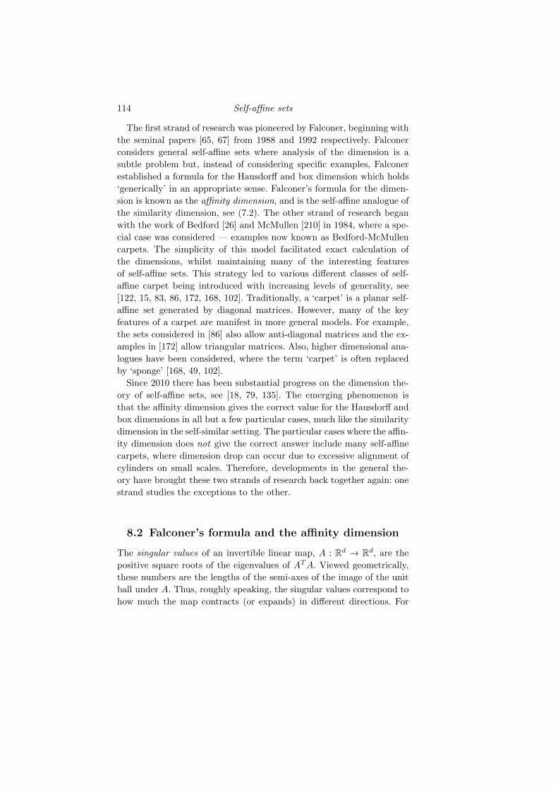
114 Self-affine sets
The first strand of research was pioneered by Falconer, beginning with
the seminal papers [65, 67] from 1988 and 1992 respectively. Falconer
considers general self-affine sets where analysis of the dimension is a
subtle problem but, instead of considering specific examples, Falconer
established a formula for the Hausdorff and box dimension which holds
‘generically’ in an appropriate sense. Falconer’s formula for the dimen-
sion is known as the affinity dimension, and is the self-affine analogue of
the similarity dimension, see (7.2). The other strand of research began
with the work of Bedford [26] and McMullen [210] in 1984, where a spe-
cial case was considered — examples now known as Bedford-McMullen
carpets. The simplicity of this model facilitated exact calculation of
the dimensions, whilst maintaining many of the interesting features
of self-affine sets. This strategy led to various different classes of self-
affine carpet being introduced with increasing levels of generality, see
[122, 15, 83, 86, 172, 168, 102]. Traditionally, a ‘carpet’ is a planar self-
affine set generated by diagonal matrices. However, many of the key
features of a carpet are manifest in more general models. For example,
the sets considered in [86] also allow anti-diagonal matrices and the ex-
amples in [172] allow triangular matrices. Also, higher dimensional ana-
logues have been considered, where the term ‘carpet’ is often replaced
by ‘sponge’ [168, 49, 102].
Since 2010 there has been substantial progress on the dimension the-
ory of self-affine sets, see [18, 79, 135]. The emerging phenomenon is
that the affinity dimension gives the correct value for the Hausdorff and
box dimensions in all but a few particular cases, much like the similarity
dimension in the self-similar setting. The particular cases where the affin-
ity dimension does not give the correct answer include many self-affine
carpets, where dimension drop can occur due to excessive alignment of
cylinders on small scales. Therefore, developments in the general the-
ory have brought these two strands of research back together again: one
strand studies the exceptions to the other.
8.2 Falconer’s formula and the affinity dimension
The singular values of an invertible linear map, A : Rd → Rd, are the
positive square roots of the eigenvalues of ATA. Viewed geometrically,
these numbers are the lengths of the semi-axes of the image of the unit
ball under A. Thus, roughly speaking, the singular values correspond to
how much the map contracts (or expands) in different directions. For
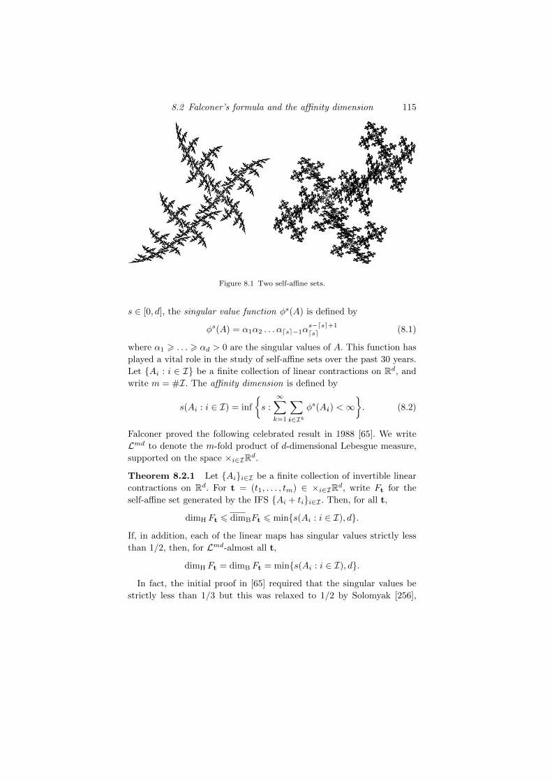
8.2 Falconer’s formula and the affinity dimension 115
Figure 8.1 Two self-affine sets.
s ∈ [0, d], the singular value function φs(A) is defined by
φs(A) = α1α2 . . . αdse−1αs−dse+1dse (8.1)
where α1 > . . . > αd > 0 are the singular values of A. This function has
played a vital role in the study of self-affine sets over the past 30 years.
Let Ai : i ∈ I be a finite collection of linear contractions on Rd, and
write m = #I. The affinity dimension is defined by
s(Ai : i ∈ I) = inf
s :
∞∑k=1
∑i∈Ik
φs(Ai ) <∞. (8.2)
Falconer proved the following celebrated result in 1988 [65]. We write
Lmd to denote the m-fold product of d-dimensional Lebesgue measure,
supported on the space ×i∈IRd.
Theorem 8.2.1 Let Aii∈I be a finite collection of invertible linear
contractions on Rd. For t = (t1, . . . , tm) ∈ ×i∈IRd, write Ft for the
self-affine set generated by the IFS Ai + tii∈I . Then, for all t,
dimH Ft 6 dimBFt 6 mins(Ai : i ∈ I), d.
If, in addition, each of the linear maps has singular values strictly less
than 1/2, then, for Lmd-almost all t,
dimH Ft = dimB Ft = mins(Ai : i ∈ I), d.
In fact, the initial proof in [65] required that the singular values be
strictly less than 1/3 but this was relaxed to 1/2 by Solomyak [256],
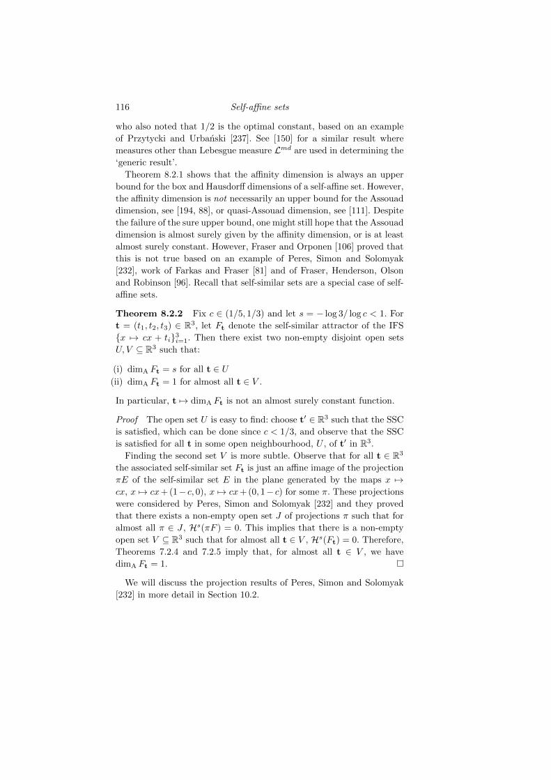
116 Self-affine sets
who also noted that 1/2 is the optimal constant, based on an example
of Przytycki and Urbanski [237]. See [150] for a similar result where
measures other than Lebesgue measure Lmd are used in determining the
‘generic result’.
Theorem 8.2.1 shows that the affinity dimension is always an upper
bound for the box and Hausdorff dimensions of a self-affine set. However,
the affinity dimension is not necessarily an upper bound for the Assouad
dimension, see [194, 88], or quasi-Assouad dimension, see [111]. Despite
the failure of the sure upper bound, one might still hope that the Assouad
dimension is almost surely given by the affinity dimension, or is at least
almost surely constant. However, Fraser and Orponen [106] proved that
this is not true based on an example of Peres, Simon and Solomyak
[232], work of Farkas and Fraser [81] and of Fraser, Henderson, Olson
and Robinson [96]. Recall that self-similar sets are a special case of self-
affine sets.
Theorem 8.2.2 Fix c ∈ (1/5, 1/3) and let s = − log 3/ log c < 1. For
t = (t1, t2, t3) ∈ R3, let Ft denote the self-similar attractor of the IFS
x 7→ cx + ti3i=1. Then there exist two non-empty disjoint open sets
U, V ⊆ R3 such that:
(i) dimA Ft = s for all t ∈ U(ii) dimA Ft = 1 for almost all t ∈ V .
In particular, t 7→ dimA Ft is not an almost surely constant function.
Proof The open set U is easy to find: choose t′ ∈ R3 such that the SSC
is satisfied, which can be done since c < 1/3, and observe that the SSC
is satisfied for all t in some open neighbourhood, U , of t′ in R3.
Finding the second set V is more subtle. Observe that for all t ∈ R3
the associated self-similar set Ft is just an affine image of the projection
πE of the self-similar set E in the plane generated by the maps x 7→cx, x 7→ cx+ (1− c, 0), x 7→ cx+ (0, 1− c) for some π. These projections
were considered by Peres, Simon and Solomyak [232] and they proved
that there exists a non-empty open set J of projections π such that for
almost all π ∈ J , Hs(πF ) = 0. This implies that there is a non-empty
open set V ⊆ R3 such that for almost all t ∈ V , Hs(Ft) = 0. Therefore,
Theorems 7.2.4 and 7.2.5 imply that, for almost all t ∈ V , we have
dimA Ft = 1.
We will discuss the projection results of Peres, Simon and Solomyak
[232] in more detail in Section 10.2.
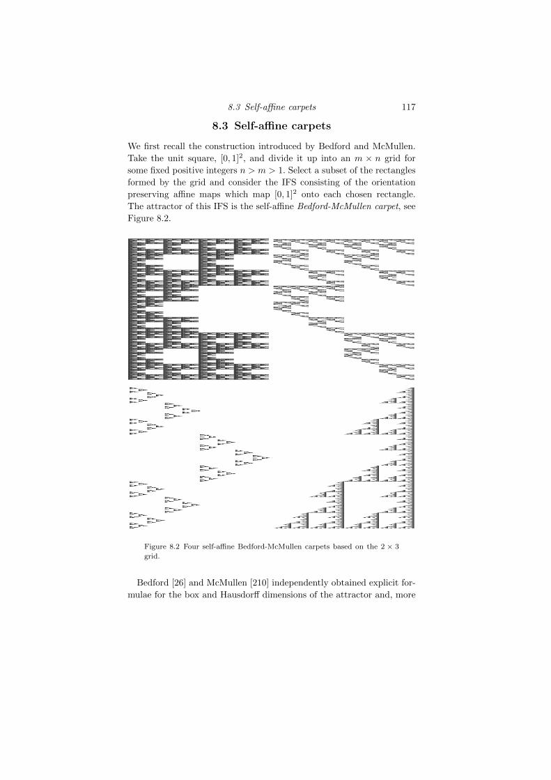
8.3 Self-affine carpets 117
8.3 Self-affine carpets
We first recall the construction introduced by Bedford and McMullen.
Take the unit square, [0, 1]2, and divide it up into an m × n grid for
some fixed positive integers n > m > 1. Select a subset of the rectangles
formed by the grid and consider the IFS consisting of the orientation
preserving affine maps which map [0, 1]2 onto each chosen rectangle.
The attractor of this IFS is the self-affine Bedford-McMullen carpet, see
Figure 8.2.
Figure 8.2 Four self-affine Bedford-McMullen carpets based on the 2 × 3
grid.
Bedford [26] and McMullen [210] independently obtained explicit for-
mulae for the box and Hausdorff dimensions of the attractor and, more
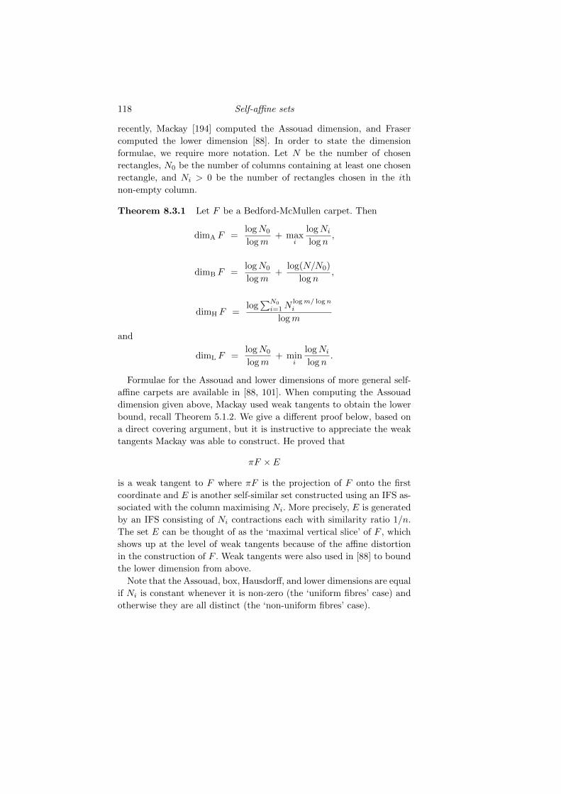
118 Self-affine sets
recently, Mackay [194] computed the Assouad dimension, and Fraser
computed the lower dimension [88]. In order to state the dimension
formulae, we require more notation. Let N be the number of chosen
rectangles, N0 be the number of columns containing at least one chosen
rectangle, and Ni > 0 be the number of rectangles chosen in the ith
non-empty column.
Theorem 8.3.1 Let F be a Bedford-McMullen carpet. Then
dimA F =logN0
logm+ max
i
logNilog n
,
dimB F =logN0
logm+
log(N/N0)
log n,
dimH F =log∑N0
i=1Nlogm/ logni
logm
and
dimL F =logN0
logm+ min
i
logNilog n
.
Formulae for the Assouad and lower dimensions of more general self-
affine carpets are available in [88, 101]. When computing the Assouad
dimension given above, Mackay used weak tangents to obtain the lower
bound, recall Theorem 5.1.2. We give a different proof below, based on
a direct covering argument, but it is instructive to appreciate the weak
tangents Mackay was able to construct. He proved that
πF × E
is a weak tangent to F where πF is the projection of F onto the first
coordinate and E is another self-similar set constructed using an IFS as-
sociated with the column maximising Ni. More precisely, E is generated
by an IFS consisting of Ni contractions each with similarity ratio 1/n.
The set E can be thought of as the ‘maximal vertical slice’ of F , which
shows up at the level of weak tangents because of the affine distortion
in the construction of F . Weak tangents were also used in [88] to bound
the lower dimension from above.
Note that the Assouad, box, Hausdorff, and lower dimensions are equal
if Ni is constant whenever it is non-zero (the ‘uniform fibres’ case) and
otherwise they are all distinct (the ‘non-uniform fibres’ case).
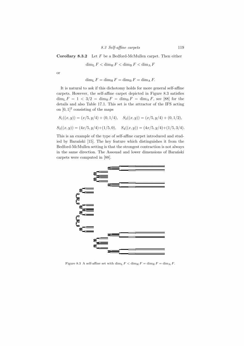
8.3 Self-affine carpets 119
Corollary 8.3.2 Let F be a Bedford-McMullen carpet. Then either
dimL F < dimH F < dimB F < dimA F
or
dimL F = dimH F = dimB F = dimA F.
It is natural to ask if this dichotomy holds for more general self-affine
carpets. However, the self-affine carpet depicted in Figure 8.3 satisfies
dimL F = 1 < 3/2 = dimH F = dimB F = dimA F , see [88] for the
details and also Table 17.1. This set is the attractor of the IFS acting
on [0, 1]2 consisting of the maps
S1((x, y)) = (x/5, y/4) + (0, 1/4), S2((x, y)) = (x/5, y/4) + (0, 1/2),
S3((x, y)) = (4x/5, y/4)+(1/5, 0), S4((x, y)) = (4x/5, y/4)+(1/5, 3/4).
This is an example of the type of self-affine carpet introduced and stud-
ied by Baranski [15]. The key feature which distinguishes it from the
Bedford-McMullen setting is that the strongest contraction is not always
in the same direction. The Assouad and lower dimensions of Baranski
carpets were computed in [88].
Figure 8.3 A self-affine set with dimL F < dimH F = dimB F = dimA F .
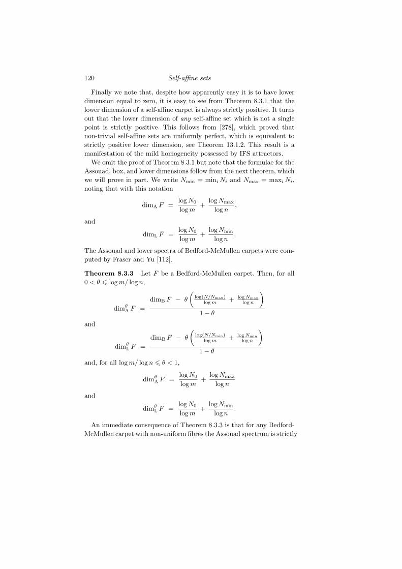
120 Self-affine sets
Finally we note that, despite how apparently easy it is to have lower
dimension equal to zero, it is easy to see from Theorem 8.3.1 that the
lower dimension of a self-affine carpet is always strictly positive. It turns
out that the lower dimension of any self-affine set which is not a single
point is strictly positive. This follows from [278], which proved that
non-trivial self-affine sets are uniformly perfect, which is equivalent to
strictly positive lower dimension, see Theorem 13.1.2. This result is a
manifestation of the mild homogeneity possessed by IFS attractors.
We omit the proof of Theorem 8.3.1 but note that the formulae for the
Assouad, box, and lower dimensions follow from the next theorem, which
we will prove in part. We write Nmin = miniNi and Nmax = maxiNi,
noting that with this notation
dimA F =logN0
logm+
logNmax
log n,
and
dimL F =logN0
logm+
logNmin
log n.
The Assouad and lower spectra of Bedford-McMullen carpets were com-
puted by Fraser and Yu [112].
Theorem 8.3.3 Let F be a Bedford-McMullen carpet. Then, for all
0 < θ 6 logm/ log n,
dimθA F =
dimB F − θ
(log(N/Nmax)
logm + logNmax
logn
)1− θ
and
dimθL F =
dimB F − θ
(log(N/Nmin)
logm + logNmin
logn
)1− θ
and, for all logm/ log n 6 θ < 1,
dimθA F =
logN0
logm+
logNmax
log n
and
dimθL F =
logN0
logm+
logNmin
log n.
An immediate consequence of Theorem 8.3.3 is that for any Bedford-
McMullen carpet with non-uniform fibres the Assouad spectrum is strictly
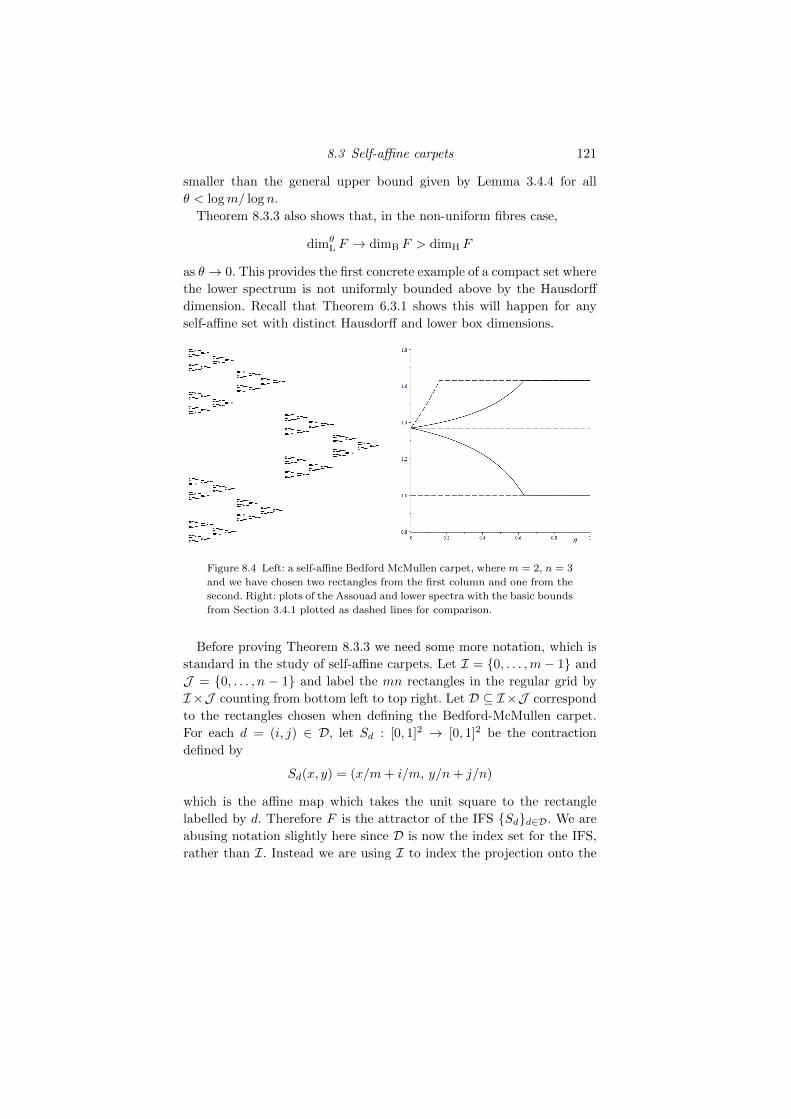
8.3 Self-affine carpets 121
smaller than the general upper bound given by Lemma 3.4.4 for all
θ < logm/ log n.
Theorem 8.3.3 also shows that, in the non-uniform fibres case,
dimθL F → dimB F > dimH F
as θ → 0. This provides the first concrete example of a compact set where
the lower spectrum is not uniformly bounded above by the Hausdorff
dimension. Recall that Theorem 6.3.1 shows this will happen for any
self-affine set with distinct Hausdorff and lower box dimensions.
Figure 8.4 Left: a self-affine Bedford McMullen carpet, where m = 2, n = 3
and we have chosen two rectangles from the first column and one from the
second. Right: plots of the Assouad and lower spectra with the basic bounds
from Section 3.4.1 plotted as dashed lines for comparison.
Before proving Theorem 8.3.3 we need some more notation, which is
standard in the study of self-affine carpets. Let I = 0, . . . ,m− 1 and
J = 0, . . . , n − 1 and label the mn rectangles in the regular grid by
I×J counting from bottom left to top right. Let D ⊆ I×J correspond
to the rectangles chosen when defining the Bedford-McMullen carpet.
For each d = (i, j) ∈ D, let Sd : [0, 1]2 → [0, 1]2 be the contraction
defined by
Sd(x, y) = (x/m+ i/m, y/n+ j/n)
which is the affine map which takes the unit square to the rectangle
labelled by d. Therefore F is the attractor of the IFS Sdd∈D. We are
abusing notation slightly here since D is now the index set for the IFS,
rather than I. Instead we are using I to index the projection onto the
122 Self-affine sets
first coordinate, which is a self-similar set. Let
D∞ = d = (d1, d2, . . . ) : dl = (il, jl) ∈ D
be the set of infinite words over D and let Π : D∞ → [0, 1]2 be the sym-
bolic coding map, recalling that F = Π(D∞) is the Bedford-McMullen
carpet. Let d ∈ D∞ and r > 0 be a small radius. Define l1(r), l2(r) to
be the unique natural numbers satisfying
m−l1(r) 6 r < m−l1(r)+1 (8.3)
and
n−l2(r) 6 r < n−l2(r)+1. (8.4)
The approximate square centred at d = ((i1, j1), (i2, j2), . . . ) ∈ D∞ with
radius r > 0 is defined by
Q(d, r) =
d′ = ((i′1, j′1), (i′2, j
′2), . . . ) ∈ D∞ :
i′l = il for all l 6 l1(r) and j′l = jl for all l 6 l2(r).
The image of this symbolic object on the carpet, Π(Q(d, r)
), is a subset
of F which contains the point Π(d) and naturally sits inside a rectan-
gle which is ‘approximately a square’ of radius r in that it has width
m−l1(r) ∈ (r/m, r] and height n−l2(r) ∈ (r/n, r]. One obtains equivalent
definitions of the Assouad and lower spectra if one replaces B(x,R) by
Π(Q(d, R)
), that is, we may use approximate squares instead of balls.
The following lemma is the first indication that there will be a phase
transition in the spectra at θ = logm/ log n.
Lemma 8.3.4
(i) If θ 6 logm/ log n and r ∈ (0, 1) is small enough, then
l2(rθ) 6 l1(rθ) 6 l2 (r) 6 l1 (r) .
(ii) If θ > logm/ log n and r ∈ (0, 1) is small enough, then
l2(rθ) 6 l2 (r) 6 l1(rθ) 6 l1 (r) .
Proof This follows immediately from the definitions of l1(·) and l2(·).
8.3 Self-affine carpets 123
Proof of Theorem 8.3.3: We will only prove the formula for the Assouad
spectra and leave the lower spectra calculation (which is similar) as an
exercise. First consider 0 < θ < logm/ log n. Let
d = ((i1, j1), (i2, j2), . . . ) ∈ D∞
and r ∈ (0, 1) be small. Consider the approximate square Π(Q(d, rθ))
and observe that it is made up of several horizontal strips with width
m−l1(rθ), which is the same as that of the approximate square, and height
n−l1(rθ), which is smaller, but still larger than r/n since l1(rθ) 6 l2 (r)
by Lemma 8.3.4. These strips contain images of F under l1(rθ)-fold
compositions of maps from Sdd∈D and so to keep track of how many
there are, we count rectangles in the appropriate columns for each map
in the composition. The total number of such strips is therefore
l1(rθ)∏l=l2(rθ)+1
Nil .
We need to cover these strips by sets of diameter r and so we iterate
the construction inside each horizontal strip until the heights of the
construction rectangles are n−l2(r), which is approximately r. This takes
l2(r)− l1(rθ) iterations and, this time, for every iteration we pick up N
smaller rectangles (one for every map in the IFS), rather than just those
inside a particular column. We are left with a collection of rectangles
with height approximately r and width m−l2(r), which is larger than r.
We continue iterating inside each of these rectangles until the widths of
the construction rectangles are m−l1(r), which is roughly r. This takes a
further l1(r)− l2(r) iterations. We can then cover the resulting collection
of rectangles by small sets of diameter r, observing that sets formed
by this last stage of iteration can be efficiently covered simultaneously,
provided they are in the same column. Therefore, for each of the last
iterations we only require a factor of N0 more covering sets (one for each
non-empty column).
Putting all these estimates together, yields a good estimate for
Nr(Π(Q(d, rθ)
)which is accurate up to constants which we can safely ignore. More
precisely, there is a constant C > 0, which may depend on θ but not on
124 Self-affine sets
d or r, such that
Nr(Π(Q(d, rθ)
))
6 C
(l1(rθ)∏
l=l2(rθ)+1
Nil
) (N l2(r)−l1(rθ)
) (Nl1(r)−l2(r)0
)(8.5)
6 C
(Nmax
)l1(rθ)−l2(rθ) (N l2(r)−l1(rθ)
) (Nl1(r)−l2(r)0
)
6 CN3 (Nmax)log rθ/ logn−log rθ/ logm
· N log rθ/ logm−log r/ logn Nlog r/ logn−log r/ logm0
= CN3rθ logNmax/ logn+θ log(N/Nmax)/ logm+log(N0/N)/ logn− logN0/ logm.
This proves
dimθA F 6
(logN0
logm + log(N/N0)logn
)− θ
(log(N/Nmax)
logm + logNmax
logn
)1− θ
,
as required. The lower bound follows similarly by choosing d ∈ D∞,
such that Nil = Nmax for all l. For such d the upper bound established
above is also a lower bound, up to a constant.
Our work so far has shown that for θ = logm/ log n
dimθA F =
logN0
logm+
logNmax
log n
which is the Assouad dimension of F . It therefore follows from Corollary
3.3.3 and Theorem 8.3.1 and that for θ ∈ (logm/ log n, 1)
dimθA F = dimqA F = dimA F.
In fact the above argument requires only a minor modification to prove
Mackay’s result (see Theorem 8.3.1)
dimA F =logN0
logm+
logNmax
log n(8.6)
which would complete the proof of Theorem 8.3.3 without relying on
a priori information about the Assouad dimension. Since dimA F >dimθ
A F , all that remains is to prove the reverse inequality. Consider
8.3 Self-affine carpets 125
d ∈ D∞, chosen such that Nil = Nmax for all l, and 0 < r < R < 1. If
r 6 R1/θ, then the argument above already proves
Nr(Π(Q(d, R)
))6 c
(R
r
) logN0logm + logNmax
logn
for a constant c > 0 and, therefore, we may assume r > R1/θ. Following
the ‘decomposing and covering’ approach from above, with R replacing
rθ, we obtain a family of horizontal strips with height approximately r
after l2(r) steps. This happens before the widths become smaller than
R, since in this case l2(r) 6 l1(R), see Lemma 8.3.4. The effect is that
the ‘middle term’ in (8.5) (concerning powers of N) disappears. This
gives, for a constant c′ > 0,
Nr(Π(Q(d, R)
))
6 c′
(l2(r)∏
l=l2(R)+1
Nil
) (Nl1(r)−l1(R)0
)
= c′
(Nmax
)l2(r)−l2(R)
Nl1(r)−l1(R)0
6 c′N−2 (Nmax)logR/ logn−log r/ logn
NlogR/ logm−log r/ logm0
= c′N−2
(R
r
) logN0logm + logNmax
logn
completing the proof of (8.6) and Theorem 8.3.3.
We can deduce the quasi-Assouad and quasi-lower dimensions imme-
diately from Theorem 8.3.3.
Corollary 8.3.5 Let F be a Bedford-McMullen carpet. Then
dimqA F = dimA F =logN0
logm+
logNmax
log n
and
dimqL F = dimL F =logN0
logm+
logNmin
log n.
We can also compute the modified lower dimension from Theorem
126 Self-affine sets
8.3.3, although it requires one more ingredient. Surprisingly it turns out
to be equal to the Hausdorff dimension, not the lower dimension.
Corollary 8.3.6 Let F be a Bedford-McMullen carpet. Then
dimML F = dimH F =log∑N0
i=1Nlogm/ logni
logm.
Corollary 8.3.6 follows immediately from Theorem 8.3.3 and the fol-
lowing lemma due to Ferguson, Jordan and Shmerkin [84, Lemma 4.3].
This shows how to construct subsets of carpets which have lower dimen-
sion arbitrarily close to the Hausdorff dimension of the original carpet.
This proves the lower bound and, since the modified lower dimension
of a compact set is always bounded above by the Hausdorff dimension
by Theorem 3.4.3, the result follows. We include the proof of the result
of Ferguson, Jordan and Shmerkin, which introduced a useful technique
based on ‘approximating systems from within’ by choosing a subsystem
according to digit frequencies and then applying Stirling’s formula.
Lemma 8.3.7 Given a Bedford-McMullen carpet F and ε > 0, there
exists a subset E ⊆ F that is also a Bedford-McMullen carpet, has
uniform fibres, and satisfies
dimHE = dimLE > dimH F − ε.
Proof Let s = dimH F and, for d = (i, j) ∈ D, let
pd = N(logm/ logn)−1i /ms
noting that∑d∈D pd = 1. The probability weights pd are those defining
the McMullen measure, that is, the unique self-affine measure of maximal
Hausdorff dimension. For k > 1 a large integer, let
l(k) =∑d∈D
bkpdc (8.7)
and
D(k) =d = (d1, . . . , dl(k)) ∈ Dl(k) : for all d ∈ D, #t : dt = d = bkpdc
.
In particular, D(k) selects the subset of l(k) level words whose digits
appear with the ‘correct’ frequency from the point of view of Hausdorff
dimension.
Consider the IFS Sd : d ∈ D(k) and denote its attractor by E(k).
Clearly E(k) is a Bedford-McMullen carpet and, since each element of
8.4 Self-affine sets with a comb structure 127
D(k) is composed of the same collection of maps (just in a different
order), E also has uniform fibres. It follows from Theorem 8.3.1 that
dimLE(k) = dimHE(k) =logN0(k)
logm(k)+
log(N(k)/N0(k))
log n(k)
where m(k) = ml(k) and n(k) = nl(k) are the integer parameters defining
the grid associated with E(k) and N0(k) and N(k) are the number of
non-empty columns and the number of rectangles in the construction of
E(k) respectively. These latter parameters can be computed explicitly
by a simple counting argument and we find
N(k) =l(k)!∏
d∈Dbkpdc!
and
N0(k) =l(k)!∏N0
i=1
(∑Nij=1bkp(i,j)c
)!.
We can therefore estimate the dimension of E(k) from below using Stir-
ling’s approximation
a log a− a 6 log a! 6 a log a− a+ log a (a > 7) (8.8)
and (8.7) to get
dimLE(k) =log l(k)!−
∑N0
i=1 log(∑Ni
j=1bkp(i,j)c)
!
l(k) logm
+
∑N0
i=1 log(∑Ni
j=1bkp(i,j)c)
!−∑d∈D logbkpdc!
l(k) log n
> s− ε(k)
where ε(k)→ 0 as k →∞. This proves the theorem, since we can choose
k arbitrarily large.
8.4 Self-affine sets with a comb structure
A family of planar non-carpet self-affine sets was considered by Barany,
Kaenmaki and Rossi [21]. The phenomenon that the Assouad dimen-
sion is given by the dimension of a projection plus the largest dimension
of an orthogonal slice is again manifest although, as one moves away
128 Self-affine sets
from carpets, it becomes less clear which projections to consider and
the structure of both the projection and maximal slice are more com-
plicated. The paper deals with the extra complexity of the projections
by assuming that all of the projections are intervals. The question then
becomes: over which collection of slices should the dimension be max-
imised? This is a subtle problem in general. Notice that in the case of
Bedford-McMullen carpets one always considers slices in the direction of
the strongest contraction, which is always the vertical direction. When
the matrices associated with the defining maps are non-diagonal matri-
ces, we must consider the slices over a larger family of directions, but
the philosophy is the same.
An IFS of affine maps acting on the plane is said to be reducible if there
is a line which is invariant under the defining matrices (for example,
Bedford-McMullen carpets are generated by reducible IFSs, since the
matrices preserve both the horizontal and vertical axes), irreducible if
there is no such invariant line, and strongly irreducible if there is no finite
union of lines which is invariant under the defining matrices. Moreover, it
is said to be proximal if the semigroup generated by the defining matrices
contains an element which has two real and distinct eigenvalues.
For example, if the defining matrices are all upper-triangular, then
the IFS is reducible. Moreover, a (proximal) IFS defined by a collection
of diagonal and anti-diagonal matrices is irreducible but not strongly
irreducible since the union of the vertical and horizontal axes is invari-
ant but neither the vertical nor horizontal axes are invariant on their
own. In fact, the case where there are both diagonal and anti-diagonal
matrices is the only one which is irreducible but not strongly irreducible,
see [21, Lemma 2.2]. The proximal condition should be interpreted as
guaranteeing that the attractor of the IFS is ‘genuinely self-affine’. For
example, it rules out self-similar sets. We write G(1, 2) for the collec-
tion of 1-dimensional subspaces of R2 and πF for the projection of F
onto π ∈ G(1, 2). The space G(1, 2) is often referred to as the Grass-
mannian manifold, see Chapter 10.2. We also write π⊥ ∈ G(1, 2) for the
1-dimensional subspace perpendicular to π.
The following theorem was proved in [21, Theorem 3.2], although their
result is more general than we state.
Theorem 8.4.1 Let F ⊆ R2 be a self-affine set satisfying the SSC and
such that πF is an interval for all π ∈ G(1, 2). Furthermore, assume that
the defining IFS is either: proximal and reducible; or strongly irreducible
and all the defining matrices have strictly positive entries. Then there
8.4 Self-affine sets with a comb structure 129
exists π ∈ G(1, 2) such that
dimA F = 1 + maxx∈F
dimH
((π⊥ + x) ∩ F
).
The projection π appearing in Theorem 8.4.1 is made more explicit
in [21], but we omit discussion of the details. It turns out that one
needs to consider all Furstenberg projections and then choose π such
that maxx∈F dimH(π⊥ + x) ∩ F is maximised.
The proof of Theorem 8.4.1 relies on many more recent advances in
the theory of self-affine sets. The tangent structure of the self-affine sets
considered is crucial and it turns out that typically the weak tangents
of self-affine sets have a ‘fibred structure’ given by the product of an
interval and a Cantor set. (Here we restrict ourselves to weak tangents
associated to sequences of similarities whose similarity ratios tend to
infinity, that is, we genuinely ‘zoom-in’.) The ‘interval’ here comes from
the projection condition and the Cantor set comes from a slice of F . The
tangent structure of self-affine sets has been developed in, for example,
[14, 151]. Other more recent developments connecting the ergodic theory
of the action of the collection of matrices in the defining IFS on projective
space also play a vital role, see [17, 18, 19, 79].
One simple and well-known family of sets to which Theorem 8.4.1
applies is the family considered by Przytycki-Urbanski [237]. These self-
affine carpets fall into the more general family studied by Feng and
Wang [83] and are related to Bernoulli convolutions. Fix λ ∈ (1/2, 1)
and consider the IFS consisting of S1 and S2 acting on [0, 1]2 defined by
S1(x, y) = (λx, y/2) and S2(x, y) = (λx+ (1− λ), (y + 1)/2)
writing F for the attractor. This IFS is clearly proximal and reducible
and so the formula from Theorem 8.4.1 applies and, moreover, there is
only one ‘Furstenberg direction’ and so the family of slices one has to
consider are simply the vertical slices, yielding
dimA F = 1 + maxx∈[0,1]
dimH Vx ∩ F
where Vx = (x, y) : y ∈ R. This family of self-affine sets was also stud-
ied by Fraser and Jordan [101] and the Assouad dimension was computed
via a different approach. There it was proved, see [101, Corollary 2.3],
that
dimA F = 2 + slog λ
log 2
where s is the infimum over all local dimensions of the associated Bernoulli
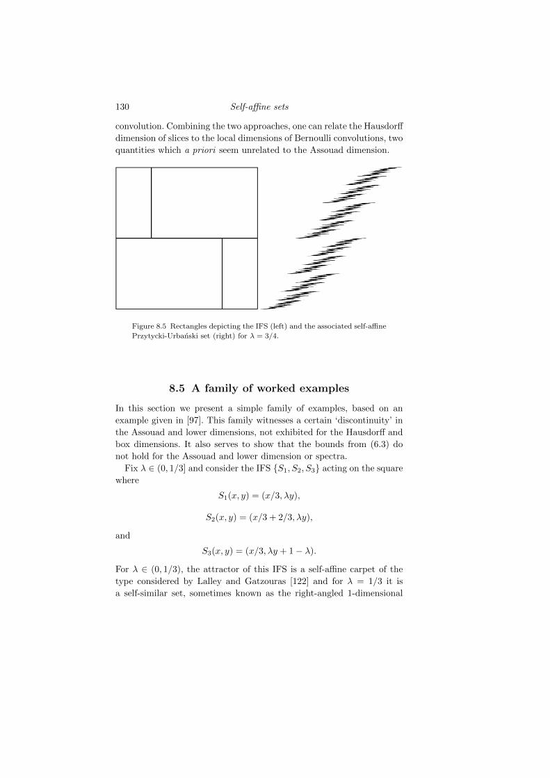
130 Self-affine sets
convolution. Combining the two approaches, one can relate the Hausdorff
dimension of slices to the local dimensions of Bernoulli convolutions, two
quantities which a priori seem unrelated to the Assouad dimension.
Figure 8.5 Rectangles depicting the IFS (left) and the associated self-affine
Przytycki-Urbanski set (right) for λ = 3/4.
8.5 A family of worked examples
In this section we present a simple family of examples, based on an
example given in [97]. This family witnesses a certain ‘discontinuity’ in
the Assouad and lower dimensions, not exhibited for the Hausdorff and
box dimensions. It also serves to show that the bounds from (6.3) do
not hold for the Assouad and lower dimension or spectra.
Fix λ ∈ (0, 1/3] and consider the IFS S1, S2, S3 acting on the square
where
S1(x, y) = (x/3, λy),
S2(x, y) = (x/3 + 2/3, λy),
and
S3(x, y) = (x/3, λy + 1− λ).
For λ ∈ (0, 1/3), the attractor of this IFS is a self-affine carpet of the
type considered by Lalley and Gatzouras [122] and for λ = 1/3 it is
a self-similar set, sometimes known as the right-angled 1-dimensional
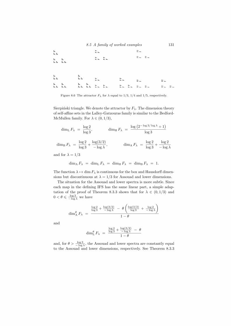
8.5 A family of worked examples 131
Figure 8.6 The attractor Fλ for λ equal to 1/3, 1/4 and 1/5, respectively.
Sierpinski triangle. We denote the attractor by Fλ. The dimension theory
of self-affine sets in the Lalley-Gatzouras family is similar to the Bedford-
McMullen family. For λ ∈ (0, 1/3),
dimL Fλ =log 2
log 3, dimH Fλ =
log(2− log 3/ log λ + 1
)log 3
dimB Fλ =log 2
log 3+
log(3/2)
− log λ, dimA Fλ =
log 2
log 3+
log 2
− log λ
and for λ = 1/3
dimA Fλ = dimL Fλ = dimH Fλ = dimB Fλ = 1.
The function λ 7→ dimFλ is continuous for the box and Hausdorff dimen-
sions but discontinuous at λ = 1/3 for Assouad and lower dimensions.
The situation for the Assouad and lower spectra is more subtle. Since
each map in the defining IFS has the same linear part, a simple adap-
tation of the proof of Theorem 8.3.3 shows that for λ ∈ (0, 1/3) and
0 < θ 6 log 3− log λ we have
dimθA Fλ =
log 2log 3 + log(3/2)
− log λ − θ
(log(3/2)
log 3 + log 2− log λ
)1− θ
and
dimθL Fλ =
log 2log 3 + log(3/2)
− log λ − θ
1− θ
and, for θ > log 3− log λ , the Assouad and lower spectra are constantly equal
to the Assouad and lower dimensions, respectively. See Theorem 8.3.3
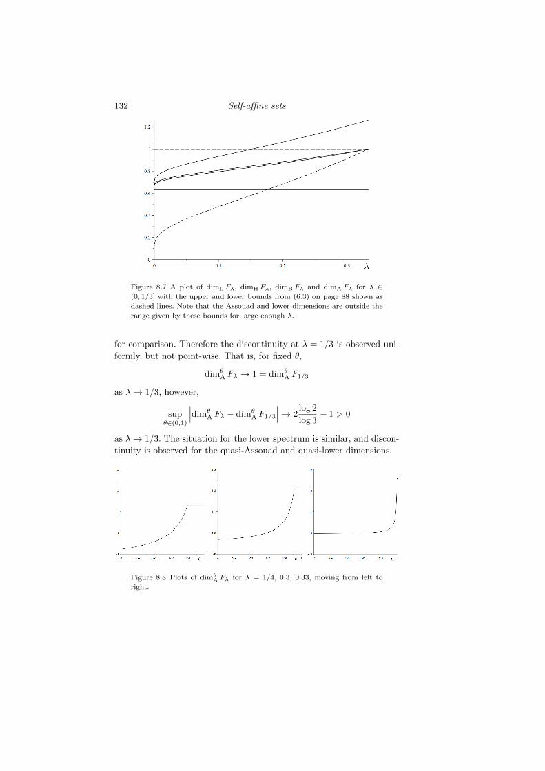
132 Self-affine sets
Figure 8.7 A plot of dimL Fλ, dimH Fλ, dimB Fλ and dimA Fλ for λ ∈(0, 1/3] with the upper and lower bounds from (6.3) on page 88 shown as
dashed lines. Note that the Assouad and lower dimensions are outside the
range given by these bounds for large enough λ.
for comparison. Therefore the discontinuity at λ = 1/3 is observed uni-
formly, but not point-wise. That is, for fixed θ,
dimθA Fλ → 1 = dimθ
A F1/3
as λ→ 1/3, however,
supθ∈(0,1)
∣∣∣dimθA Fλ − dimθ
A F1/3
∣∣∣→ 2log 2
log 3− 1 > 0
as λ→ 1/3. The situation for the lower spectrum is similar, and discon-
tinuity is observed for the quasi-Assouad and quasi-lower dimensions.
Figure 8.8 Plots of dimθA Fλ for λ = 1/4, 0.3, 0.33, moving from left to
right.
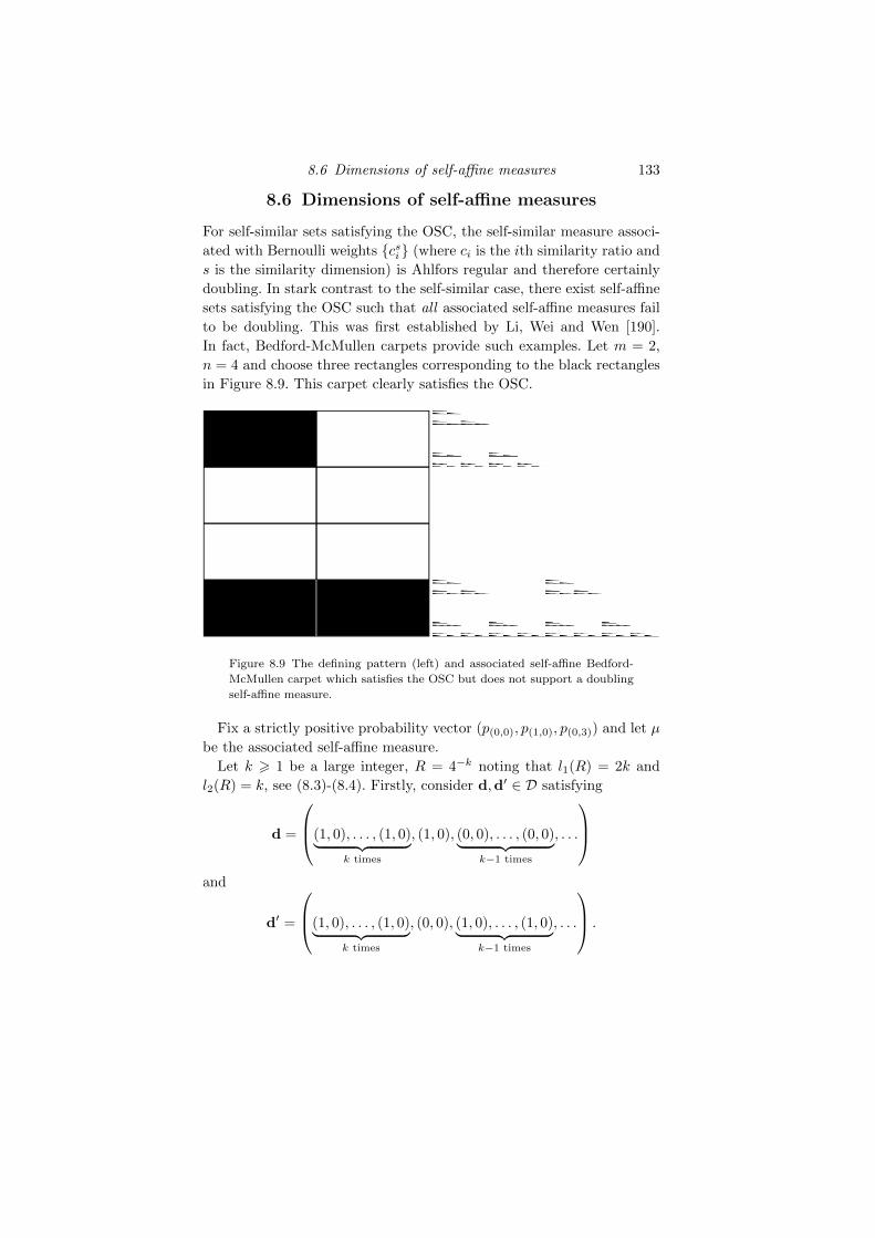
8.6 Dimensions of self-affine measures 133
8.6 Dimensions of self-affine measures
For self-similar sets satisfying the OSC, the self-similar measure associ-
ated with Bernoulli weights csi (where ci is the ith similarity ratio and
s is the similarity dimension) is Ahlfors regular and therefore certainly
doubling. In stark contrast to the self-similar case, there exist self-affine
sets satisfying the OSC such that all associated self-affine measures fail
to be doubling. This was first established by Li, Wei and Wen [190].
In fact, Bedford-McMullen carpets provide such examples. Let m = 2,
n = 4 and choose three rectangles corresponding to the black rectangles
in Figure 8.9. This carpet clearly satisfies the OSC.
Figure 8.9 The defining pattern (left) and associated self-affine Bedford-
McMullen carpet which satisfies the OSC but does not support a doubling
self-affine measure.
Fix a strictly positive probability vector (p(0,0), p(1,0), p(0,3)) and let µ
be the associated self-affine measure.
Let k > 1 be a large integer, R = 4−k noting that l1(R) = 2k and
l2(R) = k, see (8.3)-(8.4). Firstly, consider d,d′ ∈ D satisfying
d =
(1, 0), . . . , (1, 0)︸ ︷︷ ︸k times
, (1, 0), (0, 0), . . . , (0, 0)︸ ︷︷ ︸k−1 times
, . . .
and
d′ =
(1, 0), . . . , (1, 0)︸ ︷︷ ︸k times
, (0, 0), (1, 0), . . . , (1, 0)︸ ︷︷ ︸k−1 times
, . . .
.
134 Self-affine sets
Crucially, the approximate squares Π(Q(d, R)) and Π(Q(d′, R)) are ad-
jacent in that they share a common edge. Moreover,
µ(Π(Q(d, R)))
µ(Π(Q(d′, R)))=
pk+1(1,0)(p(0,0) + p(0,3))
k−1
p2k−1(1,0) (p(0,0) + p(0,3))
=
(p(0,0) + p(0,3)
p(1,0)
)k−2
.
If µ is doubling, this ratio must remain bounded away from zero and
infinity, which is only possible if
p(1,0) = p(0,0) + p(0,3), (8.9)
which we assume from now on. Secondly, consider d,d′ ∈ D satisfying
d =
(1, 0), (0, 0), . . . , (0, 0)︸ ︷︷ ︸2k−1 times
, . . .
and
d′ =
(0, 0), (1, 0), . . . , (1, 0)︸ ︷︷ ︸2k−1 times
, . . .
.
Again, the approximate squares Π(Q(d, R)) and Π(Q(d′, R)) are adja-
cent and this time, using (8.9),
µ(Π(Q(d, R)))
µ(Π(Q(d′, R)))=p(1,0)(p(0,0) + p(0,3))
2k−1(
p(0,0)p(0,0)+p(0,3)
)k−1
(p(0,0) + p(0,3))p2k−1(1,0)
(p(0,0)
p(0,0)+p(0,3)
)=
(p(0,0)
p(0,0) + p(0,3)
)k−2
.
If µ is doubling, this ratio must also remain bounded away from zero
and infinity, which is only possible if p(0,0) = p(0,0) + p(0,3). However,
this is not possible since p(0,3) > 0 and therefore µ cannot be doubling.
This time in parallel with the self-similar setting, the lower dimension
of self-affine measures is rather better behaved than the Assouad dimen-
sion (recall Theorem 7.4.2). For example, [127, Theorem 3.9] shows that
any non-trivial self-affine measure has positive lower dimension.
Theorem 8.6.1 Let µ be a self-affine measure which is not an atom.
Then
dimL µ > 0.
8.6 Dimensions of self-affine measures 135
In order to guarantee that self-affine measures supported on Bedford-
McMullen carpets are doubling, one needs to impose a stronger separa-
tion condition than the SSC. This condition, introduced by King [170],
is known as the very strong separation condition (VSSC) and stipulates
than the SSC is satisfied and, in addition, rectangles cannot be chosen
from adjacent columns. Notably, this rules out the carpet from Figure
8.9. With this condition in place, formulae for the Assouad, lower and
box dimensions of self-affine measures on carpets can be derived. The
Assouad dimension was considered in [98, Theorem 2.6] and the lower di-
mension in [127, Theorem 3.11]. The box dimensions are derivable from
[218, Proposition 3.3.1] (see the discussion in [98]) although they were
not referred to as box dimensions at this time. The results in [98] and
[218] also apply to Bedford-McMullen sponges, the higher dimensional
analogue of Bedford-McMullen carpets.
In order to state the results, it is convenient to write, for d = (i, j) ∈ D,
P (d) =∑
d′=(i,j′)∈D
pd′
which is the sum of the probabilities associated to rectangles in the same
column as d = (i, j), that is, with i fixed and j′ varying.
Theorem 8.6.2 Let µ be a self-affine measure supported on a Bedford-
McMullen carpet satisfying the VSSC. Then
dimA µ = maxd∈D
log(1/P (d))
logm+ max
d∈D
log(P (d)/pd)
log n,
dimL µ = mind∈D
log(1/P (d))
logm+ mind∈D
log(P (d)/pd)
log n
and
dimB µ = maxd∈D
log(1/P (d))
(1
logm− 1
log n
)+ max
d∈D
log(1/pd)
log n.
Comparing this theorem to Theorem 8.3.1 we see that there always
exists a self-affine measure which (simultaneously) realises the Assouad
and lower dimensions of a Bedford-McMullen carpet.
Corollary 8.6.3 Let µ be a self-affine measure supported on a Bedford-
McMullen carpet F with non-uniform fibres. Then
dimA F = dimA µ
136 Self-affine sets
if and only if P (d) = 1/N0 and P (d)/pd 6 Nmax for all d ∈ D, and
dimL F = dimL µ
if and only if P (d) = 1/N0 and P (d)/pd > Nmin for all d ∈ D. Moreover,
there is always at least one self-affine measure µ satisfying
dimA F = dimA µ > dimL F = dimL µ.
The natural measure µ which simultaneously realises the Assouad
and lower dimensions was introduced in [98] and called the coordinate
uniform measure and can be constructed by first distributing weight
equally among all used columns and then, within each column, distribut-
ing weight evenly between the rectangles in the column. There may be
other measures which simultaneously realise the Assouad and lower di-
mensions, provided there exists a column with Nmin < Ni < Nmax.
In this case there is room to distribute the weight not exactly equally
between the rectangles in the intermediate column.
Consider the simultaneous realisation problem, discussed in Section
6.2, which asks if there exists a measure which simultaneously realises
different notions of dimension (in situations when they are distinct). In
the positive direction, the coordinate uniform measure solves this prob-
lem for Bedford-McMullen carpets with non-uniform fibres and satisfy-
ing the VSSC in the setting of Assouad and lower dimension. However,
if we throw the Hausdorff dimension into the mix, then the situation is
not as straightforward. In fact there does not exist a self-affine measure
which simultaneously realises all three notions of dimension. In the case
where the carpet does not have uniform fibres, the Assouad, Hausdorff,
and lower dimensions of Bedford-McMullen carpets are necessarily dis-
tinct by Theorem 8.3.1. Moreover, it is well-known that there exists a
unique invariant probability measure of maximal Hausdorff dimension,
namely, the McMullen measure. The McMullen measure is the self-affine
measure associated with
pd = N(logm/ logn)−1i /mdimH F
for d = (i, j) ∈ D. Therefore, P (d) = Nlogm/ logni /mdimH F varies with i
and it follows from Corollary 8.6.3 that the Assouad and lower dimen-
sions of the McMullen measure are always distinct from the Assouad
and lower dimensions of the carpet, provided the VSSC is satisfied and
the carpet does not have uniform fibres.
In general the Hausdorff dimension of a self-affine measure on a Bedford-
8.6 Dimensions of self-affine measures 137
McMullen carpet is given by
dimH µ =h(µ)
log n+
log n− logm
log ndimH πµ (8.10)
where
h(µ) = −∑d∈D
pd log pd
is the entropy of µ and dimH πµ is the Hausdorff dimension of the pro-
jection of µ onto the first coordinate. This projection is a self-similar
measure satisfying the OSC and therefore the dimension can be com-
puted easily by applying (7.12). Here log n and logm are the Lyapunov
exponents of µ. The formula (8.10) is known as a Ledrappier-Young for-
mula, following [183, 184]. It was proved by Barany and Kaenmaki [19]
that every planar self-affine measure satisfies the appropriate analogue
of the Ledrappier-Young formula, which essentially says the Hausdorff
dimension can be expressed in terms of entropy, Lyapunov exponents
(which are more complicated for general self-affine measures) and di-
mensions of projections. See [17, 82] for further work in this direction.
The situation for box dimension is even worse: there does not exist
a self-affine measure which realises the box dimension. One might have
guessed that the coordinate uniform measure would work due to the
connection between the upper box and (quasi-)Assouad dimensions via
the Assouad spectrum. However, for the coordinate uniform measure µ
dimB µ =logN0
logm+
logNmax
log n= dimA µ = dimA F.
Another reasonable candidate is the uniform measure which gives weight
1/N to each symbol. However, for this measure
dimB F < dimB µ =log(N/Nmin)
logm+
logNmin
log n.
For any self-affine measure
maxd∈D
1/P (d) > N0
and
maxd∈D
1/pd > N
by the pigeonhole principle. If both of these lower bounds could be
simultaneously achieved then the box dimension of F would be re-
alised. However, this is clearly impossible since one cannot uniformly
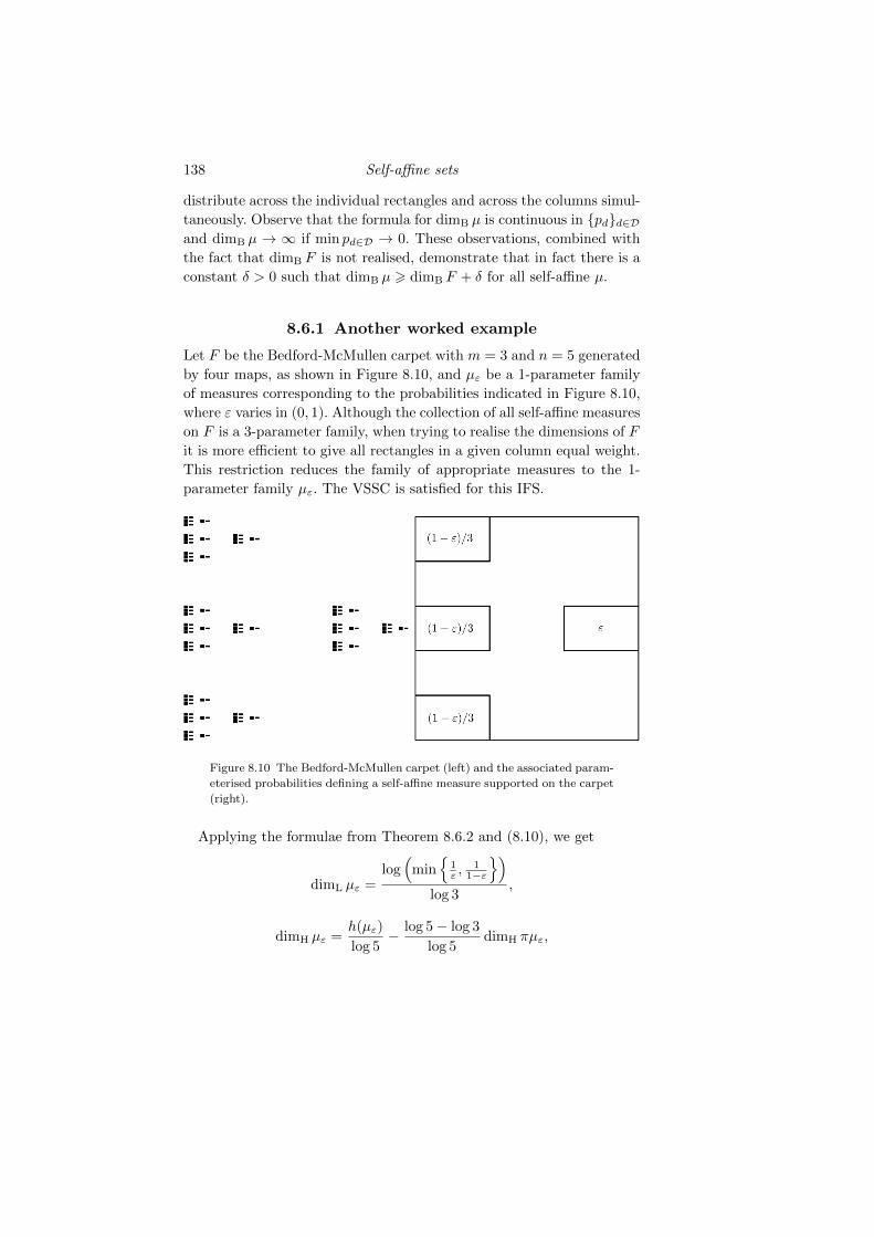
138 Self-affine sets
distribute across the individual rectangles and across the columns simul-
taneously. Observe that the formula for dimB µ is continuous in pdd∈Dand dimB µ → ∞ if min pd∈D → 0. These observations, combined with
the fact that dimB F is not realised, demonstrate that in fact there is a
constant δ > 0 such that dimB µ > dimB F + δ for all self-affine µ.
8.6.1 Another worked example
Let F be the Bedford-McMullen carpet with m = 3 and n = 5 generated
by four maps, as shown in Figure 8.10, and µε be a 1-parameter family
of measures corresponding to the probabilities indicated in Figure 8.10,
where ε varies in (0, 1). Although the collection of all self-affine measures
on F is a 3-parameter family, when trying to realise the dimensions of F
it is more efficient to give all rectangles in a given column equal weight.
This restriction reduces the family of appropriate measures to the 1-
parameter family µε. The VSSC is satisfied for this IFS.
Figure 8.10 The Bedford-McMullen carpet (left) and the associated param-
eterised probabilities defining a self-affine measure supported on the carpet
(right).
Applying the formulae from Theorem 8.6.2 and (8.10), we get
dimL µε =log(
min
1ε ,
11−ε
)log 3
,
dimH µε =h(µε)
log 5− log 5− log 3
log 5dimH πµε,
8.6 Dimensions of self-affine measures 139
dimB µε = log
(max
1
ε,
1
1− ε
)(1
log 3− 1
log 5
)+
log(
max
1ε ,
31−ε
)log 5
and
dimA µε =log(
max
1ε ,
11−ε
)log 3
+log 3
log 5,
see Figure 8.11, and also
dimL F =log 2
log 3≈ 0.6309,
dimH F =log(
1 + 3log 3log 5
)log 3
≈ 1.0347,
dimB F =log 2
log 3+
log 2
log 5≈ 1.0616
and
dimA F =log 2
log 3+
log 3
log 5≈ 1.3135.
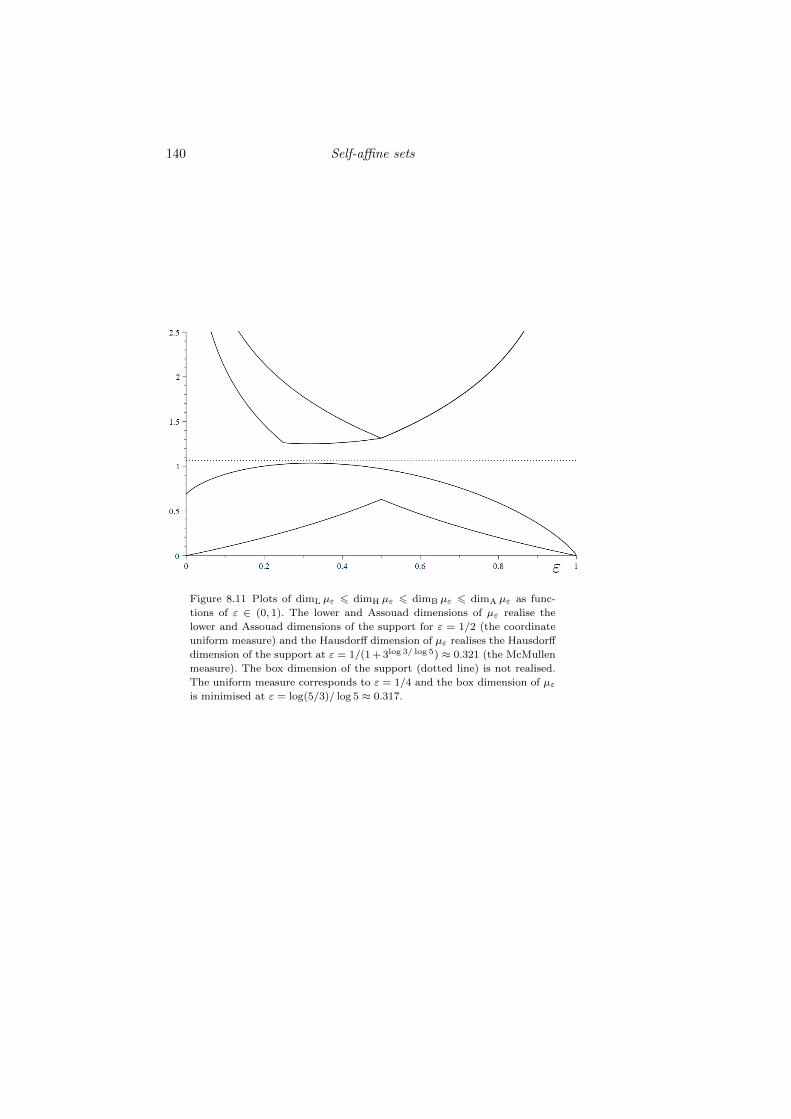
140 Self-affine sets
Figure 8.11 Plots of dimL µε 6 dimH µε 6 dimB µε 6 dimA µε as func-
tions of ε ∈ (0, 1). The lower and Assouad dimensions of µε realise the
lower and Assouad dimensions of the support for ε = 1/2 (the coordinate
uniform measure) and the Hausdorff dimension of µε realises the Hausdorff
dimension of the support at ε = 1/(1 + 3log 3/ log 5) ≈ 0.321 (the McMullen
measure). The box dimension of the support (dotted line) is not realised.
The uniform measure corresponds to ε = 1/4 and the box dimension of µεis minimised at ε = log(5/3)/ log 5 ≈ 0.317.
9
Further examples: attractors and limit sets
In this chapter we collect together discussion of several further families
of fractal sets. In Section 9.1 we consider self-conformal sets, which are
another special case of IFS attractor. In Section 9.2 we consider sets
invariant under parabolic interval maps. While these sets are similar in
spirit to IFS attractors, they are not necessarily attractors of IFSs since
the inverse branches of the associated dynamical system fail to be strict
contractions. The resulting parabolic behaviour greatly influences the
Assouad dimension of such sets, see Theorem 9.2.1. In Section 9.3 we
consider limit sets of Kleinian groups which are invariant sets for the
group action on the boundary of hyperbolic space. Parabolic behaviour
is again the main issue here and the dimension theory is developed in
detail, see Theorem 9.3.3. In Section 9.4 we consider the random limit
sets resulting from Mandelbrot percolation. Here we find a stark differ-
ence between the typical behaviour of the Assouad and quasi-Assouad
dimension. We discuss a result of Troscheit which brings the φ-Assouad
dimensions, discussed in Section 3.3.3, into consideration in order to un-
derstand the gap between the quasi-Assouad and Assouad dimensions,
see Theorem 9.4.4.
9.1 Self-conformal sets
Self-conformal sets are natural generalisations of self-similar sets. The
key property that the cylinder sets Si (F ) give rise to efficient covers of
F is preserved (this is not true for self-affine sets), but the defining maps
need not be similarities. At first sight it seems quite difficult to construct
examples of such IFSs and in fact we must pay careful attention to the
derivatives of the defining maps. For this reason it takes a little more
This material will be published by Cambridge University Press as Assouad Dimension and Fractal Geometryby Jonathan Fraser. This pre-publication version is free to view and download for personal use only.
Not for re-distribution, re-sale or use in derivative works. c© Jonathan Fraser 2020.
142 Further examples: attractors and limit sets
time to set up the theory. Given an open domain U ⊆ Rd (d > 2), a
continuously differentiable (C1) map S : U → Rd is conformal if for all
x ∈ U the Jacobian derivative S′(x) : Rd → Rd is an invertible similarity.
Our intuition that such maps are hard to construct is somewhat sup-
ported by the fact that, at least in high dimensions, there are not many
ways to construct conformal maps. Liouville’s theorem says that confor-
mal maps on R3 are either similarities or compositions of reflections in
spheres or lines.1 In R2 (identified with C) conformal maps correspond
precisely to holomorphic functions with non-zero derivative on U . In Rthe situation is slightly different. Requiring that the derivatives are in-
vertible similarities is not enough to ensure that the cylinders give rise
to good covers and more regularity is necessary. (Indeed, all non-zero
derivatives in R are invertible similarities, since all affine maps are simi-
larities.) The appropriate condition is to impose more regularity on the
derivative. Abusing terminology slightly, given an open interval U , we
say S : U → R is conformal if S is C1+α for some α ∈ (0, 1] with non-
zero derivative. This means that S is continuously differentiable with
|S′(x)| > 0 for all x ∈ U and the derivative is Holder continuous, that
is, there exist constants C > 0 and α ∈ (0, 1] such that
|S′(x)− S′(y)| 6 C|x− y|α
for all x, y ∈ U . We say a set F ⊆ Rd is self-conformal if it is the attractor
of an IFS consisting of contractions on a compact set X ⊆ Rd which
all extend to injective conformal maps on a common bounded convex
open set U ⊃ X. Self-conformal sets in the line are often called ‘cookie-
cutters’, see [69, Chapter 4], where they are sometimes more conveniently
expressed as repellers of uniformly expanding interval maps. Here the
contractions in the defining IFS correspond to the inverse branches of
the expanding map. This is also the case in higher dimensions. Key
examples in the plane include Julia sets for certain hyperbolic rational
functions on C, such as z 7→ z2 +c where c ∈ C with |c| > 2.475, or limit
sets of certain Kleinian groups.
Angelevska, Kaenmaki and Troscheit [5] conducted a thorough inves-
tigation of self-conformal sets, mostly in the line, in an effort to develop
conformal analogues of results from [96, 81] — specifically those pre-
sented here as Theorems 7.2.4 and 7.2.5. There are numerous complica-
tions here, not least with the definition of the weak separation property
(WSP). Recall our definition of the WSP for IFSs of similarities (Defi-
1 See the connection to Mobius maps in Section 9.3.
9.1 Self-conformal sets 143
nition 7.2.3) which said the identity should not be in the closure of
S−1i Sj : i , j ∈ I∗, i 6= j \ I
where I is the identity map. There is a problem applying this definition
to the conformal case since the domain of S−1i generally will not be the
range of Sj and so we cannot compose the maps. The reason this works
so well in the self-similar case is that a similarity on Rd is determined
by its action on d+ 1 points and so one can blindly extend the defining
maps to the whole of Rd. Following [5] we say a conformal IFS satisfies
the WSP if
inf
‖S′i‖−1 sup
x∈F|Si (x)− Sj (x)| : i , j ∈ I∗ and Si |F 6= Sj |F
> 0.
Notice how inverses are not used and instead one normalises by the op-
erator norm of the derivative S′i . Moreover, one must restrict attention
to the action of the maps on F . Also notice that if the maps are simi-
larities, then this is equivalent to the definition of WSP used previously.
Actually this was not the definition of the WSP in [5] but it was proved
to be equivalent to the WSP when F is not a singleton, see [5, Theorem
3.2]. With this definition in place, the following analogues of Theorems
7.2.4 and 7.2.5 were obtained in [5, Theorem 4.1 and Corollary 4.2].
Theorem 9.1.1 Let F ⊆ R be a self-conformal set containing at least
two points. If the defining IFS satisfies the WSP, then dimA F = dimH F
and otherwise dimA F = 1.
Theorem 9.1.2 Let F ⊆ R be a self-conformal set containing at least
two points with s = dimH F < 1. Then the following are equivalent:
(i) the defining IFS satisfies the WSP
(ii) Hs(F ) > 0
(iii) 0 < Hs(F ) <∞(iv) F is Ahlfors regular
(v) dimA F = dimH F .
The ‘best guess’ for the Hausdorff (and box, packing and lower) di-
mension of a self-conformal set is given by the unique solution to Bowen’s
formula, which is the conformal analogue of the Hutchinson-Moran for-
mula (7.2). The pressure P : [0,∞)→ R is defined by
P (s) = limk→∞
1
klog
∑i∈Ik‖Si‖s. (9.1)
144 Further examples: attractors and limit sets
This limit exists by a standard subadditivity argument, recall Fekete’s
lemma. Moreover, P is decreasing, convex and has a unique root. As in
the self-similar case, we expect Bowen’s formula to give the Hausdorff
dimension of the attractor unless there is a ‘good reason’ for this not
to hold, such as exact overlaps. That is, for self-conformal F ⊆ Rd, it
is natural to conjecture that dimH F = mins, d (where s is given by
P (s) = 0) provided there are no exact overlaps. We say the IFS has exact
overlaps if Si |F = Sj |F for some i , j ∈ I∗ with i 6= j . Note that exact
overlaps clearly force dimH F to be smaller than the solution to Bowen’s
formula P (s) = 0, and so the interesting case is when there are no exact
overlaps. As a direct consequence of Theorem 9.1.2, [5, Theorem 4.3]
obtains the following contribution towards the ‘overlaps conjecture’ in
the self-conformal setting.
Theorem 9.1.3 Let F ⊆ R be a self-conformal set with dimH F =
s ∈ (0, 1) and Hs(F ) > 0. Then P (dimH F ) = 0 if and only if there are
no exact overlaps.
This result follows from the previous theorem together with two fun-
damental results regarding self-conformal sets. The first is that the OSC
is equivalent to Hs(F ) > 0 where P (s) = 0, which is a result of Peres,
Rams, Simon and Solomyak [231]. The second is that if an IFS satisfies
the WSP but does not have exact overlaps, then it in fact satisfies the
OSC. This is a result of Deng and Ngai [52, Theorem 1.3].
9.2 Invariant sets for parabolic interval maps
The ‘cookie cutter’ sets mentioned in the previous setting can be viewed
as invariant sets for uniformly expanding full branched interval maps
modelled by the full shift. This is natural in the setting of IFSs (where
the complexity comes from distortion or overlaps, rather than from the
underlying dynamical system) but is quite restrictive if one is interested
in more general dynamically invariant sets. See [69, 234, 283] for more
examples of invariant sets arising from dynamical systems. In this section
we consider parabolic (or non-uniformly expanding) interval maps and
essentially show that the Assouad dimension of any invariant set is 1,
which is maximal.
Let S : [0, 1] → [0, 1] be a contractive interval map with a parabolic
fixed point. By contractive we mean that, for all x, y ∈ [0, 1],
|S(x)− S(y)| < |x− y|
9.2 Invariant sets for parabolic interval maps 145
and by parabolic fixed point we mean a point p ∈ [0, 1] such that S(p) = p
and S is differentiable at p with |S′(p)| = 1. If p = 0 or p = 1, then
we use one-sided derivatives. Note that S is not a strict contraction and
we require no regularity assumptions on S other than differentiability
at p, although it clearly has to be continuous. We are interested in sets
which map into themselves under S. This is a weak form of dynamical
invariance. Recall that x, S(x), S2(x), . . . is the forward orbit of the
point x under S.
Theorem 9.2.1 Let S be a contractive interval map with a parabolic
fixed point p. If F ⊆ [0, 1] contains a point whose forward orbit avoids
p and S(F ) ⊆ F , then dimA F = 1.
Proof Let z ∈ F be such that the forward orbit of z under S avoids p.
Since S is contractive, Sn(z) → p as n → ∞. This follows from a mild
generalisation of Banach’s contraction mapping theorem which holds for
contractive maps on compact spaces (rather than contractions on com-
plete spaces). Moreover, Sn(z) 6= p for all n > 1 and, by the invariance
assumption, F ⊇ Sn(z) : n > 1. Assume that S′(p) = 1, noting that
if S′(p) = −1, then we may replace S with S S. The sequence Sn(z)
is eventually monotonic and we assume that it is eventually decreasing
without loss of generality. Moreover, the gaps Sn(z)− Sn+1(z) > 0 are
decreasing in n since S is contractive and
Sn(z)− Sn+1(z)
Sn(z)− p= 1−
S(Sn(z)
)− S(p)
Sn(z)− p→ 0
since S′(p) = 1. It follows that for similarities Tn : R→ R defined by
Tn(x) =x− p
Sn(z)− p
we have
dH(Tn(F ) ∩ [0, 1], [0, 1]) 6Sn(z)− Sn+1(z)
Sn(z)− p→ 0
where dH is the Hausdorff metric. Therefore [0, 1] is a weak tangent to
F and dimA F = 1, as required.
This theorem is rather abstract but it applies to many dynamically
invariant sets. For example, S could be a member of a finite or in-
finite parabolic iterated function system with F as the attractor, see
Urbanski’s parabolic Cantor sets [272] (these are not to be confused
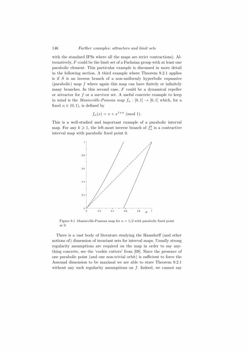
146 Further examples: attractors and limit sets
with the standard IFSs where all the maps are strict contractions). Al-
ternatively, F could be the limit set of a Fuchsian group with at least one
parabolic element. This particular example is discussed in more detail
in the following section. A third example where Theorem 9.2.1 applies
is if S is an inverse branch of a non-uniformly hyperbolic expansive
(parabolic) map f where again this map can have finitely or infinitely
many branches. In this second case, F could be a dynamical repeller
or attractor for f or a survivor set. A useful concrete example to keep
in mind is the Manneville-Pomeau map fα : [0, 1] → [0, 1] which, for a
fixed α ∈ (0, 1), is defined by
fα(x) = x+ x1+α (mod 1).
This is a well-studied and important example of a parabolic interval
map. For any k > 1, the left-most inverse branch of fkα is a contractive
interval map with parabolic fixed point 0.
Figure 9.1 Manneville-Pomeau map for α = 1/2 with parabolic fixed point
at 0.
There is a vast body of literature studying the Hausdorff (and other
notions of) dimension of invariant sets for interval maps. Usually strong
regularity assumptions are required on the map in order to say any-
thing concrete, see the ‘cookie cutters’ from [69]. Since the presence of
one parabolic point (and one non-trivial orbit) is sufficient to force the
Assouad dimension to be maximal we are able to state Theorem 9.2.1
without any such regularity assumptions on f . Indeed, we cannot say
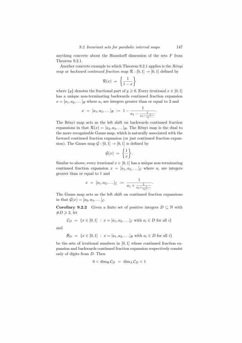
9.2 Invariant sets for parabolic interval maps 147
anything concrete about the Hausdorff dimension of the sets F from
Theorem 9.2.1.
Another concrete example to which Theorem 9.2.1 applies is the Renyi
map or backward continued fraction map R : [0, 1]→ [0, 1] defined by
R(x) =
1
1− x
where y denotes the fractional part of y > 0. Every irrational x ∈ [0, 1]
has a unique non-terminating backwards continued fraction expansion
x = [a1, a2, . . . ]B where ai are integers greater than or equal to 2 and
x = [a1, a2, . . . ]B := 1− 1
a1 − 1a2− 1
a3−...
.
The Renyi map acts as the left shift on backwards continued fraction
expansions in that R(x) = [a2, a3, . . . ]B. The Renyi map is the dual to
the more recognisable Gauss map, which is naturally associated with the
forward continued fraction expansion (or just continued fraction expan-
sion). The Gauss map G : [0, 1]→ [0, 1] is defined by
G(x) =
1
x
.
Similar to above, every irrational x ∈ [0, 1] has a unique non-terminating
continued fraction expansion x = [a1, a2, . . . ]C where ai are integers
greater than or equal to 1 and
x = [a1, a2, . . . ]C :=1
a1 + 1a2+ 1
a3+...
.
The Gauss map acts as the left shift on continued fraction expansions
in that G(x) = [a2, a3, . . . ]C .
Corollary 9.2.2 Given a finite set of positive integers D ⊆ N with
#D > 2, let
CD = x ∈ [0, 1] : x = [a1, a2, . . . ]C with ai ∈ D for all i
and
BD = x ∈ [0, 1] : x = [a1, a2, . . . ]B with ai ∈ D for all i
be the sets of irrational numbers in [0, 1] whose continued fraction ex-
pansion and backwards continued fraction expansion respectively consist
only of digits from D. Then
0 < dimH CD = dimA CD < 1
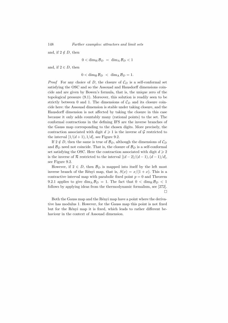
148 Further examples: attractors and limit sets
and, if 2 /∈ D, then
0 < dimH BD = dimA BD < 1
and, if 2 ∈ D, then
0 < dimH BD < dimA BD = 1.
Proof For any choice of D, the closure of CD is a self-conformal set
satisfying the OSC and so the Assouad and Hausdorff dimensions coin-
cide and are given by Bowen’s formula, that is, the unique zero of the
topological pressure (9.1). Moreover, this solution is readily seen to be
strictly between 0 and 1. The dimensions of CD and its closure coin-
cide here: the Assouad dimension is stable under taking closure, and the
Hausdorff dimension is not affected by taking the closure in this case
because it only adds countably many (rational points) to the set. The
conformal contractions in the defining IFS are the inverse branches of
the Gauss map corresponding to the chosen digits. More precisely, the
contraction associated with digit d > 1 is the inverse of G restricted to
the interval [1/(d+ 1), 1/d], see Figure 9.2.
If 2 /∈ D, then the same is true of BD, although the dimensions of CDand BD need not coincide. That is, the closure of BD is a self-conformal
set satisfying the OSC. Here the contraction associated with digit d > 2
is the inverse of R restricted to the interval [(d− 2)/(d− 1), (d− 1)/d],
see Figure 9.2.
However, if 2 ∈ D, then BD is mapped into itself by the left most
inverse branch of the Renyi map, that is, S(x) = x/(1 + x). This is a
contractive interval map with parabolic fixed point p = 0 and Theorem
9.2.1 applies to give dimA BD = 1. The fact that 0 < dimH BD < 1
follows by applying ideas from the thermodynamic formalism, see [272].
Both the Gauss map and the Renyi map have a point where the deriva-
tive has modulus 1. However, for the Gauss map this point is not fixed
but for the Renyi map it is fixed, which leads to rather different be-
haviour in the context of Assouad dimension.
9.3 Limit sets of Kleinian groups 149
Figure 9.2 Left: the Gauss map. Right: the Renyi map.
9.3 Limit sets of Kleinian groups
The key property enjoyed by the examples in the previous section is
non-uniform hyperbolicity, or parabolicity. This phenomenon occurs in
many interesting contexts across dynamics, often leading to complicated
behaviour. In this section we focus on another example, Kleinian limits
sets, where we can take the theory further.
Beautiful fractal sets arise as limit sets of Kleinian groups acting on
hyperbolic space. Here, parabolic elements in the group lead to parabolic
dynamics on the limit set. For integer d > 1, the Poincare ball
Dd+1 =z ∈ Rd+1 : |z| < 1
equipped with the hyperbolic metric d defined by
ds =2|dz|
1− |z|2
is a popular model of (d + 1)-dimensional hyperbolic space. The im-
portant geometric feature of this metric space is that distance blows
up near the boundary, leading to a much ‘larger’ boundary at infin-
ity than that possessed by Euclidean space. The boundary is Sd =z ∈ Rd+1 : |z| = 1
. This ‘extra space’ at infinity leads to a richer
group of isometries, which also has a particularly elegant description: it
is the stabiliser of Dd+1 in the Mobius group acting on Rd+1. The Mobius
group is the group of all maps which can be expressed as compositions
of reflections in spheres. We will mostly be concerned with orientation
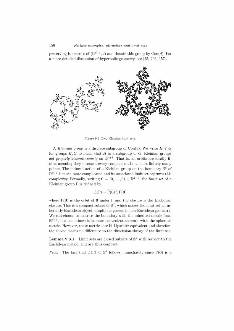
150 Further examples: attractors and limit sets
preserving isometries of (Dd+1, d) and denote this group by Con(d). For
a more detailed discussion of hyperbolic geometry, see [25, 203, 157].
Figure 9.3 Two Kleinian limit sets.
A Kleinian group is a discrete subgroup of Con(d). We write H 6 G
for groups H,G to mean that H is a subgroup of G. Kleinian groups
act properly discontinuously on Dd+1. That is, all orbits are locally fi-
nite, meaning they intersect every compact set in at most finitely many
points. The induced action of a Kleinian group on the boundary Sd of
Dd+1 is much more complicated and its associated limit set captures this
complexity. Formally, writing 0 = (0, . . . , 0) ∈ Dd+1, the limit set of a
Kleinian group Γ is defined by
L(Γ) = Γ(0) \ Γ(0)
where Γ(0) is the orbit of 0 under Γ and the closure is the Euclidean
closure. This is a compact subset of Sd, which makes the limit set an in-
herently Euclidean object, despite its genesis in non-Euclidean geometry.
We can choose to metrise the boundary with the inherited metric from
Rd+1, but sometimes it is more convenient to work with the spherical
metric. However, these metrics are bi-Lipschitz equivalent and therefore
the choice makes no difference to the dimension theory of the limit set.
Lemma 9.3.1 Limit sets are closed subsets of Sd with respect to the
Euclidean metric, and are thus compact.
Proof The fact that L(Γ) ⊆ Sd follows immediately since Γ(0) is a
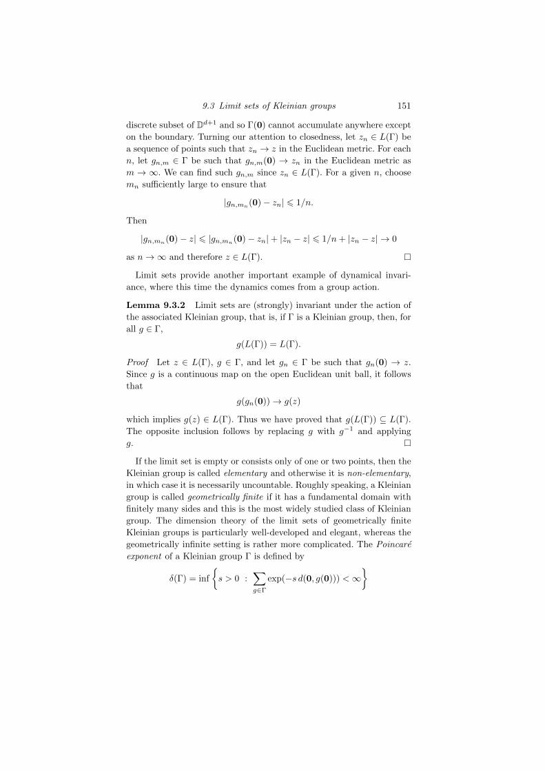
9.3 Limit sets of Kleinian groups 151
discrete subset of Dd+1 and so Γ(0) cannot accumulate anywhere except
on the boundary. Turning our attention to closedness, let zn ∈ L(Γ) be
a sequence of points such that zn → z in the Euclidean metric. For each
n, let gn,m ∈ Γ be such that gn,m(0) → zn in the Euclidean metric as
m → ∞. We can find such gn,m since zn ∈ L(Γ). For a given n, choose
mn sufficiently large to ensure that
|gn,mn(0)− zn| 6 1/n.
Then
|gn,mn(0)− z| 6 |gn,mn(0)− zn|+ |zn − z| 6 1/n+ |zn − z| → 0
as n→∞ and therefore z ∈ L(Γ).
Limit sets provide another important example of dynamical invari-
ance, where this time the dynamics comes from a group action.
Lemma 9.3.2 Limit sets are (strongly) invariant under the action of
the associated Kleinian group, that is, if Γ is a Kleinian group, then, for
all g ∈ Γ,
g(L(Γ)) = L(Γ).
Proof Let z ∈ L(Γ), g ∈ Γ, and let gn ∈ Γ be such that gn(0) → z.
Since g is a continuous map on the open Euclidean unit ball, it follows
that
g(gn(0))→ g(z)
which implies g(z) ∈ L(Γ). Thus we have proved that g(L(Γ)) ⊆ L(Γ).
The opposite inclusion follows by replacing g with g−1 and applying
g.
If the limit set is empty or consists only of one or two points, then the
Kleinian group is called elementary and otherwise it is non-elementary,
in which case it is necessarily uncountable. Roughly speaking, a Kleinian
group is called geometrically finite if it has a fundamental domain with
finitely many sides and this is the most widely studied class of Kleinian
group. The dimension theory of the limit sets of geometrically finite
Kleinian groups is particularly well-developed and elegant, whereas the
geometrically infinite setting is rather more complicated. The Poincare
exponent of a Kleinian group Γ is defined by
δ(Γ) = inf
s > 0 :
∑g∈Γ
exp(−s d(0, g(0))) <∞
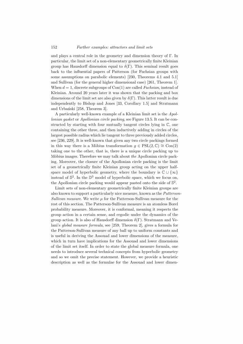
152 Further examples: attractors and limit sets
and plays a central role in the geometry and dimension theory of Γ. In
particular, the limit set of a non-elementary geometrically finite Kleinian
group has Hausdorff dimension equal to δ(Γ). This seminal result goes
back to the influential papers of Patterson (for Fuchsian groups with
some assumptions on parabolic elements) [230, Theorems 4.1 and 5.1]
and Sullivan (for the general higher dimensional case) [261, Theorem 1].
When d = 1, discrete subgroups of Con(1) are called Fuchsian, instead of
Kleinian. Around 20 years later it was shown that the packing and box
dimensions of the limit set are also given by δ(Γ). This latter result is due
independently to Bishop and Jones [33, Corollary 1.5] and Stratmann
and Urbanski [258, Theorem 3].
A particularly well-known example of a Kleinian limit set is the Apol-
lonian gasket or Apollonian circle packing, see Figure 13.5. It can be con-
structed by starting with four mutually tangent circles lying in C, one
containing the other three, and then inductively adding in circles of the
largest possible radius which lie tangent to three previously added circles,
see [236, 229]. It is well-known that given any two circle packings formed
in this way there is a Mobius transformation g ∈ PSL(2,C) ∼= Con(2)
taking one to the other, that is, there is a unique circle packing up to
Mobius images. Therefore we may talk about the Apollonian circle pack-
ing. Moreover, the closure of the Apollonian circle packing is the limit
set of a geometrically finite Kleinian group acting on the upper half-
space model of hyperbolic geometry, where the boundary is C ∪ ∞instead of S2. In the D3 model of hyperbolic space, which we focus on,
the Apollonian circle packing would appear pasted onto the side of S2.
Limit sets of non-elementary geometrically finite Kleinian groups are
also known to support a particularly nice measure, known as the Patterson-
Sullivan measure. We write µ for the Patterson-Sullivan measure for the
rest of this section. The Patterson-Sullivan measure is an atomless Borel
probability measure. Moreover, it is conformal, meaning it respects the
group action in a certain sense, and ergodic under the dynamics of the
group action. It is also of Hausdorff dimension δ(Γ). Stratmann and Ve-
lani’s global measure formula, see [259, Theorem 2], gives a formula for
the Patterson-Sullivan measure of any ball up to uniform constants and
is useful in deriving the Assouad and lower dimensions of the measure,
which in turn have implications for the Assouad and lower dimensions
of the limit set itself. In order to state the global measure formula, one
needs to introduce several technical concepts from hyperbolic geometry
and so we omit the precise statement. However, we provide a heuristic
description as well as the formulae for the Assouad and lower dimen-
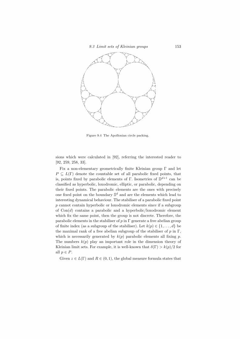
9.3 Limit sets of Kleinian groups 153
Figure 9.4 The Apollonian circle packing.
sions which were calculated in [92], referring the interested reader to
[92, 259, 258, 33].
Fix a non-elementary geometrically finite Kleinian group Γ and let
P ⊆ L(Γ) denote the countable set of all parabolic fixed points, that
is, points fixed by parabolic elements of Γ. Isometries of Dd+1 can be
classified as hyperbolic, loxodromic, elliptic, or parabolic, depending on
their fixed points. The parabolic elements are the ones with precisely
one fixed point on the boundary Sd and are the elements which lead to
interesting dynamical behaviour. The stabiliser of a parabolic fixed point
p cannot contain hyperbolic or loxodromic elements since if a subgroup
of Con(d) contains a parabolic and a hyperbolic/loxodromic element
which fix the same point, then the group is not discrete. Therefore, the
parabolic elements in the stabiliser of p in Γ generate a free abelian group
of finite index (as a subgroup of the stabiliser). Let k(p) ∈ 1, . . . , d be
the maximal rank of a free abelian subgroup of the stabiliser of p in Γ,
which is necessarily generated by k(p) parabolic elements all fixing p.
The numbers k(p) play an important role in the dimension theory of
Kleinian limit sets. For example, it is well-known that δ(Γ) > k(p)/2 for
all p ∈ P .
Given z ∈ L(Γ) and R ∈ (0, 1), the global measure formula states that
154 Further examples: attractors and limit sets
µ(B(z,R)) is given, up to uniform constants independent of z and R, by
Rδ(Γ)Rρ(z,R)(δ(Γ)−k(z,R)) (9.2)
where, roughly speaking, k(z,R) = k(p) if z is ‘near’ the parabolic fixed
point p ∈ P and 0 6 ρ(z,R) 6 1 quantifies ‘near’ in terms of a fixed
standard set of horoballs.2 A horoball is a Euclidean sphere whose in-
terior lies in Dd+1 and is tangent to Sd at a parabolic fixed point. For
more details on standard horoballs and ranks of parabolic elements, see
[258]. A simple initial observation to make here is that if there are no
parabolic elements, then the global measure formula (9.2) simplifies to
Rδ(Γ). (9.3)
Therefore, applying Lemma 4.1.2, for non-elementary geometrically fi-
nite Kleinian groups with no parabolic fixed points,
dimA L(Γ) = dimL L(Γ) = dimA µ = dimL µ = δ(Γ).
In light of this result, we assume from now on that Γ contains a parabolic
element and write 1 6 kmin 6 kmax 6 d to denote the minimal and
maximal ranks of parabolic fixed points, respectively. The main results
from [92] are stated below.
Theorem 9.3.3 Let Γ 6 Con(d) be a non-elementary geometrically
finite Kleinian group with a parabolic element. Then
dimA µ = max kmax, 2δ(Γ)− kmin ,
dimL µ = min kmin, 2δ(Γ)− kmax ,
dimA L(Γ) = maxkmax, δ(Γ)
and
dimL L(Γ) = minkmin, δ(Γ).
Recall that, for any non-elementary geometrically finite Kleinian group
Γ,
dimH L(Γ) = dimP L(Γ) = dimB L(Γ) = dimH µ = δ(Γ).
For d = 2 we can ‘upgrade’ the previous theorem to include finitely
2 Note that this is not how the global measure formula is usually presented, forexample in [259, 92]. It is more common for the radius of the ball to be writtenas R = e−t for t > 0. We chose to express it in this way to make the notationconsistent with the rest of the book. Finally, to simplify exposition, our functionρ has been ‘normalised’ by dividing the usual ρ by | logR|.
9.3 Limit sets of Kleinian groups 155
generated geometrically infinite Kleinian groups thanks to a result of
Bishop and Jones [33]. They proved that if Γ 6 Con(2) is a finitely
generated geometrically infinite Kleinian group, then dimH L(Γ) = 2. In
the geometrically infinite case, we still have δ(Γ) 6 dimH L(Γ), but this
inequality can be strict.
Corollary 9.3.4 Let Γ 6 Con(2) be a finitely generated non-elementary
Kleinian group. Then
dimA L(Γ) = maxkmax, dimH L(Γ).
The full proofs of Theorem 9.3.3 are technical, but to see where the
formulae come from is fairly straightforward. The following discussion
is deliberately very rough and we refer the reader to [92] for the details.
First, consider the Patterson-Sullivan measure µ. If we choose z = p ∈ P ,
then k(z,R) = k(p) for all R > 0 sufficiently small and ρ(z,R) → 1 as
R → 0. Therefore, applying the global measure formula (9.2), for all
ε > 0 there is a constant C > 1 such that
C−1
(R
r
)2δ(Γ)−k(p)−ε
6µ(B(z,R))
µ(B(z, r))6 C
(R
r
)2δ(Γ)−k(p)+ε
which immediately gives
dimL µ 6 2δ(Γ)− kmax 6 2δ(Γ)− kmin 6 dimA µ. (9.4)
Observing the behaviour (R
r
)k(p)
is a little harder, and requires a more careful choice of z. If we choose
z ‘close to p at scale R’ but ‘far away from p at scale r’, then we can
achieve
k(z,R) = k(p), k(z, r) = 0
ρ(z,R) =log(R/r)
| logR|, ρ(z, r) = 0
which, applying (9.2), gives µ(B(z,R))µ(B(z,r)) , up to constants, as
Rδ(Γ)Rlog(R/r)| logR| (δ(Γ)−k(p))
rδ(Γ)=
(R
r
)k(p)
which yields
dimL µ 6 kmin 6 kmax 6 dimA µ. (9.5)
156 Further examples: attractors and limit sets
Combining (9.4) and (9.5) yields the lower bound for dimA µ and the
upper bound for dimL µ from Theorem 9.3.3. The remaining inequalities
are proved by demonstrating that the scaling behaviour witnessed by
the choices of z,R and r above are extremal. This requires more delicate
understanding of the underlying hyperbolic geometry and we omit the
details.
Concerning the Assouad dimension of the limit set L(Γ), we have
the lower bound dimA L(Γ) > dimH L(Γ) = δ(Γ) and the lower bound
dimA L(Γ) > kmax is also fairly straightforward. In fact [−1, 1]k(p) (em-
bedded in Rd+1) is a (weak) tangent to L(Γ) at p ∈ P . This can be seen
by taking the orbit of a point z ∈ L(Γ) with z 6= p under the free abelian
group of rank k(p) lying inside the stabiliser of p, which we denote by Γ′.
Using the fact that Γ is discrete, we find a Zk(p) action with p playing
the role of infinity. This leads to Γ′(z) being an inverted Zk(p)-lattice,
accumulating at p, and letting Tl (l > 1) be a sequence of similarities
which send p → 0 ∈ Rd+1 and have similarity ratio equal to l, we find
(an embedding of) [−1, 1]k(p) is contained in a weak tangent to L(Γ) as
required.
Similarly, the upper bound dimL L(Γ) 6 δ(Γ) is straightforward. The
upper bound dimL L(Γ) 6 kmin seems like it should follow easily too, but
there is an additional complication which does not occur in the Assouad
case since we need to ensure that the weak tangent is precisely [−1, 1]k(p)
(not just a set containing [−1, 1]k(p)). However, a deep result of Bowditch
[36] guarantees that the limit set lies within a bounded neighbourhood of
a k(p)-dimensional affine plane containing p. This allows us to conclude
that the weak tangent constructed above is precisely [−1, 1]k(p).
The upper bound for the Assouad dimension and lower bound for
the lower dimension are rather more difficult to prove and we omit the
details. However, note that if δ(Γ) 6 (kmin + kmax)/2, then
dimA L(Γ) 6 dimA µ = max kmax, 2δ(Γ)− kmin = kmax
and if δ(Γ) > (kmin + kmax)/2, then
dimL L(Γ) > dimL µ = min kmin, 2δ(Γ)− kmax = kmin
and so the difficult bounds can be obtained ‘cheaply’ in these ranges.
Interestingly, one of the tough bounds is always ‘cheap’. Moreover, this
highlights the situation when δ(Γ) = (kmin + kmax)/2 as particularly
interesting (or straightforward). In this case
dimA L(Γ) = dimA µ = kmax > kmin = dimL µ = dimL L(Γ).
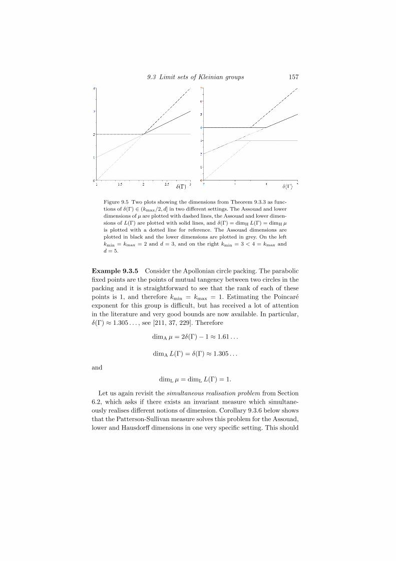
9.3 Limit sets of Kleinian groups 157
Figure 9.5 Two plots showing the dimensions from Theorem 9.3.3 as func-
tions of δ(Γ) ∈ (kmax/2, d] in two different settings. The Assouad and lower
dimensions of µ are plotted with dashed lines, the Assouad and lower dimen-
sions of L(Γ) are plotted with solid lines, and δ(Γ) = dimH L(Γ) = dimH µ
is plotted with a dotted line for reference. The Assouad dimensions are
plotted in black and the lower dimensions are plotted in grey. On the left
kmin = kmax = 2 and d = 3, and on the right kmin = 3 < 4 = kmax and
d = 5.
Example 9.3.5 Consider the Apollonian circle packing. The parabolic
fixed points are the points of mutual tangency between two circles in the
packing and it is straightforward to see that the rank of each of these
points is 1, and therefore kmin = kmax = 1. Estimating the Poincare
exponent for this group is difficult, but has received a lot of attention
in the literature and very good bounds are now available. In particular,
δ(Γ) ≈ 1.305 . . . , see [211, 37, 229]. Therefore
dimA µ = 2δ(Γ)− 1 ≈ 1.61 . . .
dimA L(Γ) = δ(Γ) ≈ 1.305 . . .
and
dimL µ = dimL L(Γ) = 1.
Let us again revisit the simultaneous realisation problem from Section
6.2, which asks if there exists an invariant measure which simultane-
ously realises different notions of dimension. Corollary 9.3.6 below shows
that the Patterson-Sullivan measure solves this problem for the Assouad,
lower and Hausdorff dimensions in one very specific setting. This should
158 Further examples: attractors and limit sets
be compared with the situation for Bedford-McMullen carpets, where
there are no self-affine measures which solve the simultaneous realisa-
tion problem in the non-uniform fibres case. Note that µ always realises
the Hausdorff dimension of L(Γ), but only sometimes realises the As-
souad and lower dimensions.
Corollary 9.3.6 Let Γ 6 Con(d) be a non-elementary geometrically
finite Kleinian group. Then
dimL µ = dimL L(Γ) < dimH µ = dimH L(Γ) < dimA µ = dimA L(Γ)
if and only if kmin < kmax and δ(Γ) = (kmin + kmax)/2.
Another common consideration in dimension theory is to identify pos-
sible relationships between dimensions in particular contexts, see Figure
17.1. Despite the fact that dimH L(Γ) = dimB L(Γ) always holds for geo-
metrically finite Kleinian limit sets, the behaviour regarding the Assouad
and lower dimensions is quite rich. We note that dimH L(Γ) = dimB L(Γ)
does not always hold in the geometrically infinite case. In dimension 1,
that is, when Γ 6 Con(1) is a Fuchsian group, we have a dichotomy
similar to that observed for self-similar (and self-conformal) sets in R,
see Theorems 7.2.4 and 9.1.1.
Corollary 9.3.7 Let Γ 6 Con(1) be a non-elementary geometrically
finite Fuchsian group with L(Γ) 6= S1.
(i) If Γ does not contain any parabolic elements, then
0 < dimL L(Γ) = dimH L(Γ) = dimA L(Γ) = δ(Γ) < 1.
(ii) If Γ contains a parabolic element, then
1/2 < dimL L(Γ) = dimH L(Γ) = δ(Γ) < dimA L(Γ) = 1.
In higher dimensions, more relationships are possible. In fact we can
achieve
dimL L(Γ) < dimH L(Γ) < dimA L(Γ),
dimL L(Γ) = dimH L(Γ) < dimA L(Γ)
or
dimL L(Γ) < dimH L(Γ) = dimA L(Γ).
This should again be compared with the situation for Bedford-McMullen
9.4 Mandelbrot percolation 159
carpets, where we either have the lower, Hausdorff and Assouad dimen-
sions equal to a common value or to three distinct values, see Corollary
8.3.2.
We have seen in this section that the lower dimension of the limit set
of a non-elementary geometrically finite Kleinian group is positive. In
fact this phenomenon has been observed in another context. Jarvi and
Vuorinen [148, Theorem 5.5] proved that limit sets of finitely generated
Kleinian groups are uniformly perfect, which turns out to be equivalent,
see Theorem 13.1.2. Uniform perfectness has been investigated exten-
sively in the context of Kleinian limit sets, see [260] and the references
therein.
9.4 Mandelbrot percolation
Mandelbrot percolation is a random process giving rise to fractals which
are statistically self-similar, see [70, Section 15.2]. The model is simple,
but it captures many key features of randomness and has attracted a lot
of attention in the fractal geometry literature, see for example [238, 239].
We recall the construction, which begins with the unit cube M0 =
[0, 1]d, a fixed integer m > 2, and a probability p ∈ (0, 1). At the first
step we divideM0 intomd (closed) cubes of side lengthm−1 and, for each
cube, we independently choose to keep it with probability p, or remove
it with probability (1 − p). Let M1 be the union of cubes which are
kept and then repeat the first step inside each kept cube independently.
Iterating this procedure leads to a decreasing sequence of closed sets Mk
defined to be the union of cubes of sidelength m−k which are kept at
stage k. The limit set is the random set M = ∩kMk, see Figure 9.6.
It is well-known that if p > m−d, then M is non-empty with positive
probability. We assume from now on that this is the case. To get a feel
for why this is the threshold, note that inside a given cube the expected
number of kept cubes at the next level is pmd. If we condition on M
being non-empty, then almost surely
dimHM = dimBM = d+log p
logm∈ (0, d).
The Assouad dimension behaves rather differently, as seen in the fol-
lowing result of Fraser, Miao and Troscheit [104]. This result can also be
derived from earlier work of Berlinkov and Jarvenpaa on porosity [29].
An immediate and somewhat counter-intuitive consequence of this result
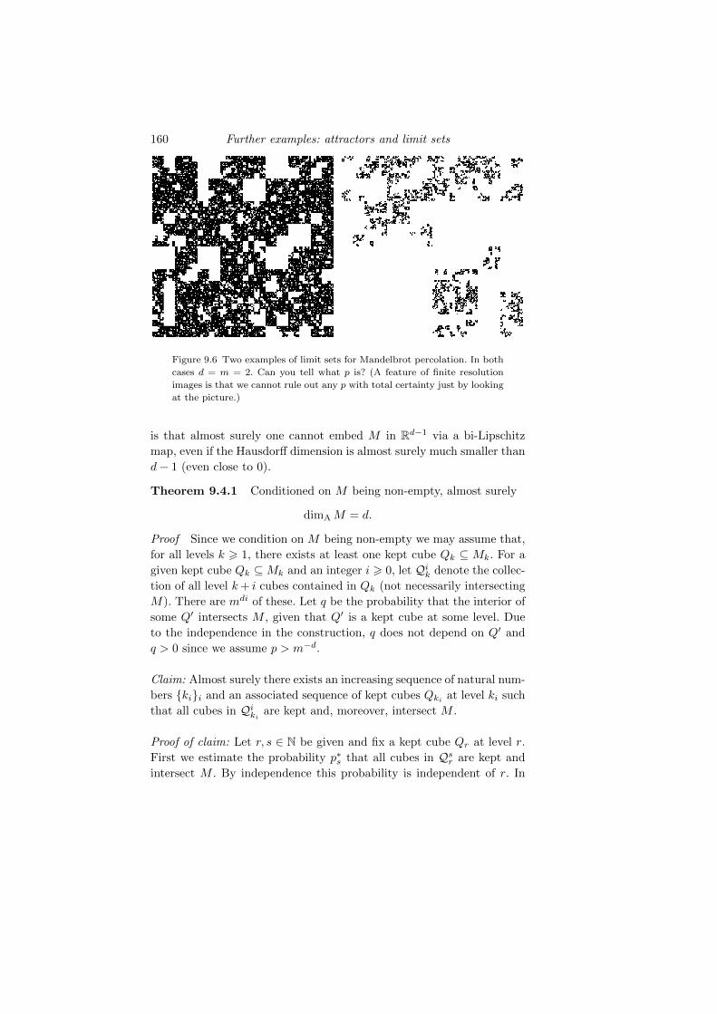
160 Further examples: attractors and limit sets
Figure 9.6 Two examples of limit sets for Mandelbrot percolation. In both
cases d = m = 2. Can you tell what p is? (A feature of finite resolution
images is that we cannot rule out any p with total certainty just by looking
at the picture.)
is that almost surely one cannot embed M in Rd−1 via a bi-Lipschitz
map, even if the Hausdorff dimension is almost surely much smaller than
d− 1 (even close to 0).
Theorem 9.4.1 Conditioned on M being non-empty, almost surely
dimAM = d.
Proof Since we condition on M being non-empty we may assume that,
for all levels k > 1, there exists at least one kept cube Qk ⊆ Mk. For a
given kept cube Qk ⊆Mk and an integer i > 0, let Qik denote the collec-
tion of all level k+ i cubes contained in Qk (not necessarily intersecting
M). There are mdi of these. Let q be the probability that the interior of
some Q′ intersects M , given that Q′ is a kept cube at some level. Due
to the independence in the construction, q does not depend on Q′ and
q > 0 since we assume p > m−d.
Claim: Almost surely there exists an increasing sequence of natural num-
bers kii and an associated sequence of kept cubes Qki at level ki such
that all cubes in Qiki are kept and, moreover, intersect M .
Proof of claim: Let r, s ∈ N be given and fix a kept cube Qr at level r.
First we estimate the probability p∗s that all cubes in Qsr are kept and
intersect M . By independence this probability is independent of r. In
9.4 Mandelbrot percolation 161
order for all cubes to be kept we must first have chosen to keep all cubes
in Q1r, and then all cubes in Q2
r, and so on until finally keeping all cubes
in Qsr. This requires us to choose to keep a total of
L 6s∑
a=1
mda =md(s+1) −md
md − 1
cubes. Since these choices are independent, the probability of keeping
them all is pL. Just because we have kept these cubes at level (s + r),
they may go on to become extinct later in the construction. However,
the probability that the interiors of all of the cubes in Qsr will go on to
intersect M in the limit is at least qmds
. Therefore, the probability we
are looking for is
p∗s > pLqmds
.
Define l(s) inductively by l(s+ 1) = l(s) + k(s) with l(1) = 1 and
k(s) = s
⌈− log 2
log(1− p∗s)
⌉. (9.6)
Let Es be the event that for at least one j ∈ 0, s, 2s, . . . , k(s)− s there
exists a kept cube Ql(s)+j such that all cubes in Qsl(s)+j survive and
intersect M . Applying (9.6),
P(Es) > 1− (1− p∗s)k(s)/s > 1/2.
The claim follows immediately by the Borel-Cantelli Lemma, noting that
the events Es are independent.
To complete the proof we show that, conditioned on M being non-
empty, almost surely X = [0, 1]d is a weak tangent to M . The result then
follows from Theorem 5.1.2. Let Ti be the natural orientation preserving
similarity that maps the cube Qki to X. By the claim we have that,
almost surely, each of the level ki + i cubes inside Qki intersect M .
Therefore
dH(Ti(M) ∩X,X) 6√dm−i
and so dH(Ti(M) ∩X,X)→ 0 as i→∞ as required.
The Assouad spectrum was considered in [112, 266, 280] and the out-
come is rather different. The following result was first proved in [112]
but an alternative and more direct proof was given by Troscheit [266].
We follow Troscheit’s proof below.
162 Further examples: attractors and limit sets
Theorem 9.4.2 Conditioned on M being non-empty, almost surely
dimθAM = dimBM
for all θ ∈ (0, 1).
Proving Theorem 9.4.2, following [266], hinges on the following lemma,
which appears to be fundamental in the study of the Assouad spec-
trum and quasi-Assouad dimension in random settings, see [266, 268]. It
says that the probability of the number of cubes at level k being much
larger than the expectation is very small (super-exponentially small in
k), which allows us to control the number of descendants of a given node
uniformly and with high probability.
Lemma 9.4.3 There exists τ > 0 such that for all ε ∈ (0, 1) and all
k > 1
P(Zk > msk(1+ε)) 6 exp(−τmskε).
This lemma constitutes a ‘large deviations’ estimate for Mandelbrot
percolation. It applies more generally to supercritical Galton-Watson
processes with finitely supported offspring distribution. For us, Zk is a
Galton-Watson process because the construction proceeds independently
inside each kept cube and the supercritical condition translates to p >
m−d. Moreover, the finitely supported offspring condition is satisfied
since m is fixed. The more general result is proved in [9], see also [268].
Write Zk to denote the number of kept cubes comprising Mk and note
that
E(Zk) = (pmd)k = msk
where s is the almost sure Hausdorff dimension of the limit set M .
Proof of Theorem 9.4.2. Fix θ ∈ (0, 1) and ε > 0. Throughout we condi-
tion on non-extinction. In order to prove that almost surely dimθAM 6
s + ε, it is enough to prove that almost surely for all sufficiently large
integers k > 1 and l = dk/θe that
supQ⊆Mk
Z∗k(Q) 6 m(l−k)(s+ε)
where Z∗k(Q) is the number of level l descendants of a given level k cube
Q ⊆Mk. Note the difference between Zk and Z∗k(Q).
Since E(Zk) = (pmd)k = msk, almost surely there is a random con-
stant C1 > 0 such that
Zk 6 C1msk(1+ε) (9.7)
9.4 Mandelbrot percolation 163
for all k > 1. Moreover, using the statistical self-similarity of the process
and applying Lemma 9.4.3, for all level k cubes Q,
P(Z∗k(Q) > ms(l−k)(1+ε)) = P(Zl−k > ms(l−k)(1+ε))
6 C exp(−τms(l−k)ε). (9.8)
Therefore, combining (9.7) and (9.8),
P(
supQ⊆Mk
Z∗k(Q) > ms(l−k)(1+ε)
)6 C1m
sk(1+ε)C exp(−τms(l−k)ε)
6 C1C exp(k logms(1+ε) − τmsk(1/θ−1)ε
)6 C1C exp
(−(τ/2)msk(1/θ−1)ε
)(9.9)
for large enough k. Therefore∑k>1
P(
supQ⊆Mk
Z∗k(Q) > m(l−k)(s+ε)
)<∞
and by the Borel-Cantelli lemma
supQ⊆Mk
Z∗k(Q) 6 m(l−k)(s+ε)
for all but finitely many k almost surely, completing the proof.
Theorems 9.4.1 and 9.4.2 show that genuine interpolation between the
box dimension and Assouad dimension is not achieved by the Assouad
spectrum for Mandelbrot percolation. However, using the finer analysis
provided by the φ-Assouad dimensions dimφAM , the interpolation can be
recovered, recall Section 3.3.3. Troscheit proved the following dichotomy
in [268].
164 Further examples: attractors and limit sets
Theorem 9.4.4 Iflog(R/φ(R))
log | logR|→ 0
as R→ 0, then, conditioned on M being non-empty, almost surely
dimφAM = d = dimAM.
On the other hand, if
log(R/φ(R))
log | logR|→ ∞
as R→ 0, then, conditioned on M being non-empty, almost surely
dimφAM = dimBM = d+
log p
logm.
The proof follows a similar strategy to the proof of Theorem 9.4.2
— especially the second part. Indeed, an inspection of the proof reveals
that (9.9) is a very crude estimate and would also be possible for φ
with φ(R) much larger than R1/θ. Also, note that Theorem 9.4.4 im-
plies Theorem 9.4.2 by considering φ(R) = R1/θ and Theorem 9.4.1 by
considering φ(R) = R. A similar dichotomy, with the same threshold
on φ, was obtained in a different random setting based on ‘complemen-
tary intervals’ in [121], see also [119]. The Assouad spectrum of random
self-affine carpets was considered in [108].
10
Geometric constructions
In this chapter we consider how the dimension theory we have devel-
oped behaves in the context of three classical constructions in geometric
measure theory: products, projections, and slices. In Section 10.1 we ex-
amine the relationship between the dimensions of sets E, F with the
product set E ×F . In Section 10.2 we consider how the dimensions of a
set behave under orthogonal projection onto linear subspaces. The typ-
ical behaviour of the Hausdorff dimension under orthogonal projection
is described in the celebrated Marstrand-Mattila projection theorems
(10.3) and we find that there is no such result describing the Assouad
dimension, see Theorem 10.2.4. However, one can obtain a one-sided
Marstrand-Mattila type result, see Theorem 10.2.1, which turns out to
have a very small set of exceptions due to a result of Orponen, see The-
orem 10.2.2. In Section 10.2.3 we provide an application of the Assouad
dimension and spectra to the box dimensions of orthogonal projections,
see Corollary 10.2.8. Finally, in Section 10.3 we consider how the di-
mensions of the slices of a set relate to the dimensions of the set itself.
We construct an example of a set with maximal box (and Assouad)
dimension which has very small slices, see Theorem 10.3.2.
This material will be published by Cambridge University Press as Assouad Dimension and Fractal Geometryby Jonathan Fraser. This pre-publication version is free to view and download for personal use only.
Not for re-distribution, re-sale or use in derivative works. c© Jonathan Fraser 2020.
166 Geometric constructions
10.1 Products
Given sets E ⊆ Rd1 and F ⊆ Rd2 , it is a natural question to consider
how the dimensions of E and F relate to the dimensions of the product
set
E × F = (x, y) : x ∈ E, y ∈ F ⊆ Rd1 × Rd2 ≡ Rd1+d2 .
Consider, for example, E = F = [0, 1], in which case E×F = [0, 1]2 and
we have
dim(E × F ) = 2 = dimE + dimF.
Perhaps we can expect this additive behaviour more generally? This
turns out to depend crucially on the notion of dimension used and the
structure of E and F . The theory is well-understood and the general
phenomenon is that dimensions behave in pairs. It is a good exercise to
prove that, for bounded sets E,F ,
dimBE + dimBF 6 dimB(E × F ) 6 dimBE + dimBF
and
dimBE + dimBF 6 dimB(E × F ) 6 dimBE + dimBF.
Here upper and lower box dimensions behave as a pair and this pattern
repeats for other dimension pairs. Marstrand proved that dimHE +
dimH F 6 dimH(E ×F ) for Borel sets E,F [202] and Howroyd proved
that the Hausdorff and packing dimension are a natural pair in this
setting [142]. That is, for Borel sets E,F ,
dimHE + dimH F 6 dimH(E × F ) 6 dimHE + dimP F
and
dimHE + dimP F 6 dimP(E × F ) 6 dimPE + dimP F.
The lower and Assouad dimensions also behave as a pair, see [88]. How-
ever, it is more natural to use the modified lower dimension when bound-
ing the Assouad dimension of a product set from below, see Corollary
10.1.2. We prove the analogous statement for measures, from which the
statement for sets will (at least partially) follow. This is an example of
how results for sets are often obtained as corollaries to stronger results
for measures. Given locally finite measures µ supported on E and ν sup-
ported on F , the product measure µ×ν is defined to be the unique Borel
measure satisfying
(µ× ν)(E′ × F ′) = µ(E′)ν(F ′)
10.1 Products 167
for all Borel sets E′ ⊆ E and F ′ ⊆ F .
Theorem 10.1.1 Let µ and ν be locally finite Borel measures on Rd1and Rd2 , respectively. Then
dimL µ + dimA ν 6 dimA(µ× ν) 6 dimA µ + dimA ν
and, if µ and ν are either both compactly supported or both have un-
bounded support, then
dimL µ + dimL ν 6 dimL(µ× ν) 6 dimL µ + dimA ν.
Proof We prove the result for dimA(µ× ν). The lower dimension ana-
logue is proved similarly and left as an exercise. To see why the product
of a compactly supported measure and a measure with unbounded sup-
port behaves differently, see Example 10.1.3.
The upper bound is straightforward. Let ε > 0. For all (x, y) ∈ E×Fand 0 < r < R < 1,
µ× ν(B((x, y), R))
µ× ν(B((x, y), r))6
µ× ν(B(x,R)×B(y,R))
µ× ν(B(x, r/√
2)×B(y, r/√
2))
=µ(B(x,R))ν(B(y,R))
µ(B(x, r/√
2))ν(B(y, r/√
2))
6 C
(R
r
)dimA µ+ dimA ν+ε
for a constant C > 1 independent of x, y, r and R. This proves that
dimA(µ× ν) 6 dimA µ + dimA ν + ε
and letting ε→ 0 gives the desired upper bound.
Turning our attention to the lower bound, let ε > 0 and choose se-
quences yk ∈ F , rk, Rk ∈ (0, 1) satisfying
ν(B(yk, Rk/√
2))
ν(B(yk, rk))>
(Rkrk
)dimA ν−ε
(10.1)
for all k and Rk/rk → ∞. Such sequences exist by the definition of
168 Geometric constructions
dimA ν. For x ∈ E arbitrary,
µ× ν(B((x, yk), Rk))
µ× ν(B((x, yk), rk))>µ× ν(B(x,Rk/
√2)×B(yk, Rk/
√2))
µ× ν(B(x, rk)×B(yk, rk))
=µ(B(x,Rk/
√2))ν(B(yk, Rk/
√2))
µ(B(x, rk))ν(B(yk, rk))
> C ′(Rkrk
)dimL µ−ε+ dimA ν−ε
for a constant C ′ > 0 independent of x and k. The final inequality above
follows from (10.1) and the definition of dimL µ. This proves that
dimA(µ× ν) > dimL µ + dimA ν − 2ε
and letting ε→ 0 gives the desired lower bound.
We obtain the analogous result for sets as a corollary. The fact that the
Assouad dimension is subadditive on products, that is, dimA(E×F ) 6dimAE + dimA F was observed in [192, Theorem A.5], see also [240,
Lemma 9] and [88, Proposition 2.1]. Sharpness of these product formulae
was considered in [224, 223].
Corollary 10.1.2 For non-empty sets E,F
dimMLE + dimA F 6 dimA(E × F ) 6 dimAE + dimA F
and, if E and F are either both bounded or both unbounded, then
dimLE + dimL F 6 dimL(E × F ) 6 dimLE + dimA F.
Proof Again, we only consider the statement for dimA(E×F ). The up-
per bound follows immediately from Theorem 10.1.1 and Theorem 4.1.3
by choosing a sequence of measures µ and ν supported on E and F ,
respectively, whose Assouad dimensions approach the Assouad dimen-
sions of E and F . For the lower bound, we first obtain the statement
with dimMLE replaced by dimLE by a similar approach to that used in
the proof of the lower bound in Theorem 10.1.1. Let ε > 0 and choose
sequences yk ∈ F , rk, Rk ∈ (0, 1) satisfying
Mrk(B(yk, Rk/√
2) ∩ F ) >
(Rkrk
)dimA F−ε
(10.2)
for all k and Rk/rk → ∞, where Mrk(·) is the maximum cardinality
10.1 Products 169
of an rk-separated subset of a given set. Such sequences exist by the
definition of dimA F . For x ∈ E arbitrary,
Mrk(B((x, yk), Rk) ∩ (E × F ))
>Mrk
((B(x,Rk/
√2) ∩ E
)×(B(yk, Rk/
√2) ∩ F
))>Mrk(B(x,Rk/
√2) ∩ E)Mrk(B(yk, Rk/
√2) ∩ F )
> C ′′(Rkrk
)dimL E−ε+ dimA F−ε
for a constant C ′′ > 0 independent of x and k, using (10.2) and the defi-
nition of dimLE. This proves that dimA(E×F ) > dimLE + dimA F−2ε
and letting ε→ 0 gives the desired lower bound. Finally, we can upgrade
this lower bound by replacing dimLE by dimMLE by passing to a subset
of E (and therefore a subset of E × F ) with lower dimension close to
dimMLE.
The following example shows that if we take the product of a bounded
set with an unbounded set, then the bounds for lower dimension from
Theorem 10.1.1 and Corollary 10.1.2 do not hold. The only inequality
which can go wrong is the first one.
Example 10.1.3 There exist sets E,F ⊆ R such that
dimLE + dimL F > dimL(E × F )
and measures µ, ν on R such that
dimL µ + dimL ν > dimL(µ× ν).
For example, let E = [0, 1] and F = R, which both have lower dimension
1. However, considering r = 1 and R→∞ to obtain the upper bound,
dimL(E × F ) = 1.
For an example with measures, let µ and ν be Lebesgue measure on E
and F respectively.
The product formulae presented above are useful in many contexts,
particularly when constructing examples. We give an application of this
here, which also relies on an understanding of self-similar sets — another
very useful collection of objects for constructing examples! Specifically,
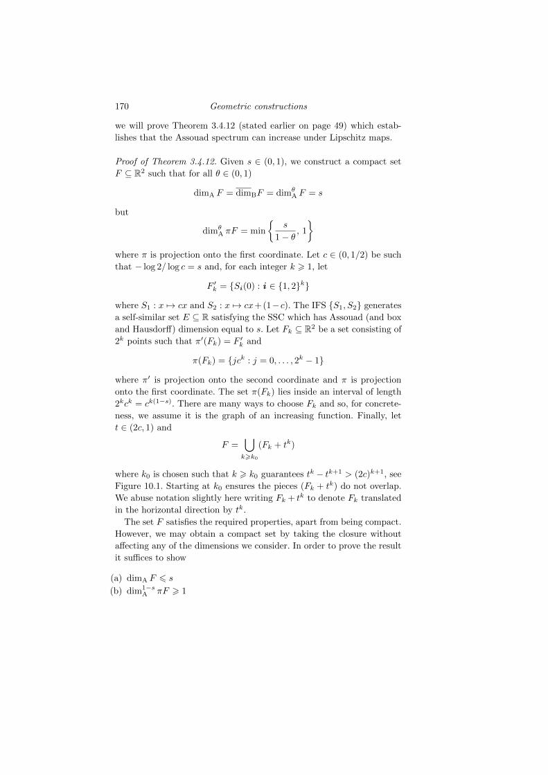
170 Geometric constructions
we will prove Theorem 3.4.12 (stated earlier on page 49) which estab-
lishes that the Assouad spectrum can increase under Lipschitz maps.
Proof of Theorem 3.4.12. Given s ∈ (0, 1), we construct a compact set
F ⊆ R2 such that for all θ ∈ (0, 1)
dimA F = dimBF = dimθA F = s
but
dimθA πF = min
s
1− θ, 1
where π is projection onto the first coordinate. Let c ∈ (0, 1/2) be such
that − log 2/ log c = s and, for each integer k > 1, let
F ′k = Si (0) : i ∈ 1, 2k
where S1 : x 7→ cx and S2 : x 7→ cx+(1−c). The IFS S1, S2 generates
a self-similar set E ⊆ R satisfying the SSC which has Assouad (and box
and Hausdorff) dimension equal to s. Let Fk ⊆ R2 be a set consisting of
2k points such that π′(Fk) = F ′k and
π(Fk) = jck : j = 0, . . . , 2k − 1
where π′ is projection onto the second coordinate and π is projection
onto the first coordinate. The set π(Fk) lies inside an interval of length
2kck = ck(1−s). There are many ways to choose Fk and so, for concrete-
ness, we assume it is the graph of an increasing function. Finally, let
t ∈ (2c, 1) and
F =⋃k>k0
(Fk + tk)
where k0 is chosen such that k > k0 guarantees tk − tk+1 > (2c)k+1, see
Figure 10.1. Starting at k0 ensures the pieces (Fk + tk) do not overlap.
We abuse notation slightly here writing Fk + tk to denote Fk translated
in the horizontal direction by tk.
The set F satisfies the required properties, apart from being compact.
However, we may obtain a compact set by taking the closure without
affecting any of the dimensions we consider. In order to prove the result
it suffices to show
(a) dimA F 6 s
(b) dim1−sA πF > 1
10.1 Products 171
Figure 10.1 Left: the construction of F with c = 1/5 and t = 1/2. Rect-
angles containing the finite sets Fk + tk are shown along with the points
comprising Fk+tk. Right: the associated set Z×E, which contains a subset
which is bi-Lipschitz equivalent to F .
and apply Lemma 3.4.4 and Corollary 3.4.6 to both F and πF , recalling
that the upper box dimension cannot increase under Lipschitz maps and
so dimBπF 6 dimBF 6 dimA F .
To prove (a), let F0 be the set formed from F by projecting each
piece Fk + tk onto the vertical line passing through (tk, 0). The induced
bijection between F and F0 is bi-Lipschitz, since the horizontal spacing of
points in Fk+ tk is ck and the vertical spacing is (at least) ck. Moreover,
F0 ⊆ Z × E where Z = tk : k > 1 and E is the self-similar set
mentioned above. Therefore, using Theorem 10.1.2 and Lemma 2.4.2,
dimA F = dimA F0 6 dimA Z × E 6 dimA Z + dimAE = s.
It is a short exercise to show that dimA Z = 0, which we leave to the
reader.
To prove (b), let x = tk ∈ πF and r = ck. Since r1−s = ck(1−s) = 2kck,
π(Fk + tk) ⊆ B(x, r1−s) and therefore
Nr(B(x, r1−s) ∩ πF ) > 2k−1 = 12
r1−s
r.
Since we can take k arbitrarily large, we conclude dim1−sA πF > 1.
172 Geometric constructions
10.2 Orthogonal projections
10.2.1 Dimension theory of orthogonal projections
How dimension behaves under orthogonal projection is a classical prob-
lem in geometric measure theory. It was first considered by Marstrand
in a seminal article from 1954 [201], although Besicovitch considered the
Lebesgue measure of projections of planar sets with positive and finite
1-dimensional Hausdorff measure somewhat earlier, see for example [31].
Consider, for example, a line segment L embedded in R3. Then for all
but one 2-dimensional hyperplane V ⊆ R3, the orthogonal projection of
L onto V is also a line segment and therefore the dimension of L (which is
1) is typically preserved under projection onto 2-dimensional subspaces.
Conversely, consider the unit sphere S2 ⊆ R3 (which is a 2-dimensional
set). Then for all 1-dimensional subspaces V ⊆ R3, the projection of
S2 onto V is a line segment and so the dimension of S2 is not typically
preserved under projection onto 1-dimensional subspaces, but does typ-
ically attain the largest value possible. Despite the simplicity of these
examples, these phenomena occur much more generally.
For integers k, d with 1 6 k < d, consider projections of Rd onto
k-dimensional subspaces V . The k-dimensional subspaces of Rd come
with a natural k(d − k) dimensional manifold structure, and so come
equipped with a k(d − k) dimensional analogue of Lebesgue measure
(this may be formally expressed in terms of the Haar measure on the
d-dimensional orthogonal group O(d)). We identify each k-dimensional
subspace V with the orthogonal projection π : Rd → V and denote the
set of all such projections as G(k, d). We can thus make statements about
‘almost all’ orthogonal projections π ∈ G(k, d). The manifold G(k, d) is
usually called the Grassmannian manifold, see [205, Chapter 3]. We are
abusing notation slightly, writing G(k, d) for both the collection of k-
dimensional subspaces of Rd and for the space of associated projections
onto these subspaces.
The classical result concerning Hausdorff dimension (often referred to
as Marstrand’s projection theorem or the Marstrand-Mattila projection
theorem), is that, for a fixed Borel set F ⊆ Rd, almost all π ∈ G(k, d)
satisfy
dimH πF = mink, dimH F. (10.3)
This was first proved by Marstrand in the case d = 2 [201] and later
by Mattila [204] in the general case, based on a potential-theoretic ap-
proach of Kaufman [160]. Similar results exist for the packing and upper
10.2 Orthogonal projections 173
and lower box dimensions in that for almost all π ∈ G(k, d) the di-
mension of πF is equal to a constant. These results were proved by
Falconer and Howroyd [78]. Unlike the Hausdorff dimension result, the
constants are not as simple as mink, dimF and are given by dimen-
sion profiles. Dimension profiles were introduced by Howroyd [143] and
Falconer-Howroyd [78] in the 1990s. We refer the reader to the survey
articles [74, 206] for an overview of the dimension theory of projections.
10.2.2 The Assouad dimension of orthogonal projections
Compared to the Hausdorff, box and packing dimensions, a striking
difference in the case of Assouad dimension is that the dimension of πF
need not be almost surely constant. This was first observed by Fraser
and Orponen [106, Theorem 2.5] who constructed a compact set in the
plane which projects to sets with two different Assouad dimensions in
positively many directions π ∈ G(1, 2). We recall the construction below.
Despite the Assouad dimension not necessarily taking a constant value
almost surely, it turns out that it can be almost surely bounded from
below in a meaningful way.
Theorem 10.2.1 Let F ⊆ Rd be any non-empty set and k < d be a
positive integer. Then
dimA πF > mink, dimA F
for almost all π ∈ G(k, d).
The case when k = 1 and d = 2 was proved by Fraser and Orponen,
see [106, Theorem 2.1], and the general case was proved by Fraser [89].
Interestingly, Theorem 10.2.1 is false if one replaces Assouad dimension
by upper box dimension. The upper box dimension of πF is almost surely
constant, but this constant can be strictly smaller than the minimum of
k and the upper box dimension of F , see [77] or the surveys [74, 206].
Theorem 10.2.1 establishes that for a nonempty set F ⊆ Rd, the set
π ∈ G(k, d) : dimA πF < mink, dimA F (10.4)
is a null set with respect to the Grassmannian measure. One can ask for
more precise information here by, for example, estimating the Hausdorff
dimension of the exceptional set (10.4). This problem has attracted much
interest in the context of Marstrand’s projection theorem for Hausdorff
dimension, see [74, 206]. For example, given a Borel set F ⊆ Rd with
174 Geometric constructions
dimH F 6 k and 0 < s 6 dimH F ,
dimHπ ∈ G(k, d) : dimH πF < s 6 k(d− k) + s− k.
Moreover, Kaufman and Mattila [162] constructed a compact set F ⊆ Rdwith any given Hausdorff dimension in [0, k] such that
dimHπ ∈ G(k, d) : dimH πF < dimH F = k(d− k) + dimH F − k
exhibiting sharpness of the estimate above in the case of largest s. In
particular, the set of exceptions can be large in the sense of dimen-
sion, despite being a null set. Orponen [226] established a striking result
concerning the exceptional set of dimensions in the context of Assouad
dimension.
Theorem 10.2.2 Let F ⊆ R2 be any non-empty set. Then
dimHπ ∈ G(1, 2) : dimA πF < min1,dimA F = 0.
We are able to give a full and self-contained proof of Theorem 10.2.1
below. Theorem 10.2.2 is rather harder to prove and relies on deep mod-
ern advances, including Shmerkin’s inverse theorem for Lq-norms [254].
Proof of Theorem 10.2.1: We follow the proof from [89, Section 3.3.1].
For all π ∈ G(k, d), π(F ) ⊆ π(F ) and therefore we may assume that F is
closed. It follows from Theorem 5.1.3 that there exists a compact set E ⊆Rd which is a weak tangent to F such that dimHE = dimA F . Examining
the proof of Theorem 5.1.3, we may assume that the similarity maps
generating E are homotheties. Therefore we may choose a sequence of
homothetic similarity maps Tk on Rd and a compact set X ⊆ Rd such
that
Tk(F ) ∩X → E (10.5)
in dH as k → ∞. For k > 1, write Tk(x) = ckx + tk for a real constant
ck > 0 and a translation tk ∈ Rd.In the following, we identify π(Rd) with Rk for each π ∈ G(k, d).
Define a map π Tk π−1 from π(Rd) to itself by
π Tk π−1(x) = π(Tk(y)) : π(y) = x.
Since Tk is homothetic the set π(Tk(y)) : π(y) = x is a singleton and
so this map is well-defined. For x ∈ π(Rd),
π Tk π−1(x) = π(ckπ−1(x) + tk) = ckx+ π(tk)
10.2 Orthogonal projections 175
and so π Tk π−1 is also a homothetic similarity. Since π : K(Rd) →K(Rk) is continuous, it follows from (10.5) that( (
π Tk π−1)
(π(F )))∩ π(X) = π(Tk(F )) ∩ π(X) ⊇ π (TkF ∩X)
→ π(E) (10.6)
in dH as k → ∞. Note that π(X) is a compact subset of π(Rd) and
K(π(X)) is compact and so we may assume, by taking a subsequence if
necessary, that (π Tk π−1)(π(F )) ∩ π(X) converges to a compact set
E′ ⊆ π(X) in dH as k →∞. In particular, E′ is a weak tangent to π(F )
and it follows from (10.6) that E′ ⊇ π(E).
We have established that for all π ∈ G(k, d), the set π(E) is a subset of
a weak tangent to π(F ). It therefore follows from Theorem 5.1.2 and the
Marstrand-Mattila projection theorem that, for almost all π ∈ G(k, d),
dimA π(F ) > dimA π(E) > dimH π(E) = mink, dimHE= mink, dimA F
completing the proof of Theorem 10.2.1.
In order to construct a set F such that dimA πF is not almost surely
constant, we first consider projections of self-similar sets, recall Chapter
7. The following is a special case of [106, Theorems 2.3-2.4].
Theorem 10.2.3 Let F ⊆ R2 be a self-similar set containing at least
two points and suppose the defining maps are homotheties. Then, for all
π ∈ G(1, 2),
(i) if HdimH πF (πF ) > 0, then dimA πF = dimH πF ,
(ii) if HdimH πF (πF ) = 0, then dimA πF = 1.
Moreover, provided F is not contained in a line, there is at least one
π ∈ G(1, 2) such that dimA πF = 1.
Proof The first part of this result follows from Theorems 7.2.4 and 7.2.5
since the projections πF are self-similar. This relies on the fact that the
maps are homotheties. The observation that there is at least one π such
that dimA πF = 1 was proved in [106, Theorem 2.4] using a variant of
the example of Bandt and Graf, see (7.3).
Theorem 10.2.3 provides a family of examples where dimA πF is not
almost surely constant. The following was proved in [106, Theorem 2.5],
and we sketch their argument below.
176 Geometric constructions
Theorem 10.2.4 For any s satisfying log5 3 < s < 1, there exists a
compact set F ⊆ R2 with Hausdorff and Assouad dimensions equal to s
for which there are two non-empty disjoint open sets I, J ⊆ G(1, 2) such
that:
(i) dimA πF = s for all π ∈ I(ii) dimA πF = 1 for almost all π ∈ J .
Proof Fix c ∈ (1/5, 1/3) and let F be the self-similar attractor of the
IFS on [0, 1]2 given by x 7→ cx, x 7→ cx+(0, 1−c), x 7→ cx+(1−c, 0),see Figure 10.2. Observe that F satisfies the OSC and so dimH F =
dimA F = − log 3/ log c =: s ∈ (log5 3, 1). It follows from Theorem 10.2.3
that:
(i) dimA πF = dimH πF if and only if HdimH πF (πF ) > 0
(ii) dimA πF = 1 if and only if HdimH πF (πF ) = 0.
Marstrand’s projection theorem guarantees that dimH πF = s < 1 al-
most surely. Therefore, in light of the above dichotomy, it is sufficient to
show that there is a non-empty open interval1 of projections π for which
Hs(πF ) > 0, and a non-empty open interval of projections π within
which Hs(πF ) = 0 almost surely. The first of these tasks is straightfor-
ward because one can easily find a non-empty open interval of projec-
tions π for which πF is a self-similar set satisfying the OSC and therefore
dimH πF = s and Hs(πF ) > 0, see Section 6.4. The existence of such
an interval relies on the assumption c < 1/3 since (after rescaling) the
problem reduces to positioning three pairwise disjoint closed intervals of
length c inside the unit interval.
The second task is more delicate, but was solved by Peres, Simon
and Solomyak [232]. They defined the set of intersection parameters
IP = π : π is not injective on F and proved that IP contains a non-
empty interval provided c > 1/5 and, moreover, for almost every π ∈ IPwe have Hs(πF ) = 0. This can be found in [232, Theorem 1.2(i) and
Example 2.8], see Figure 10.2.
The examples in Theorem 10.2.4 were the first examples demonstrat-
ing that the Assouad dimension need not be almost surely constant un-
der projection. However, it is conjectured (but not proved, see Theorem
7.3.1 and Question 17.5.3), that for these examples, the quasi-Assouad
dimension and Assouad spectrum are almost surely constant, since the
projections are self-similar.
1 We identify G(1, 2) with [0, 1) so we may talk about ‘intervals’ of projections π.
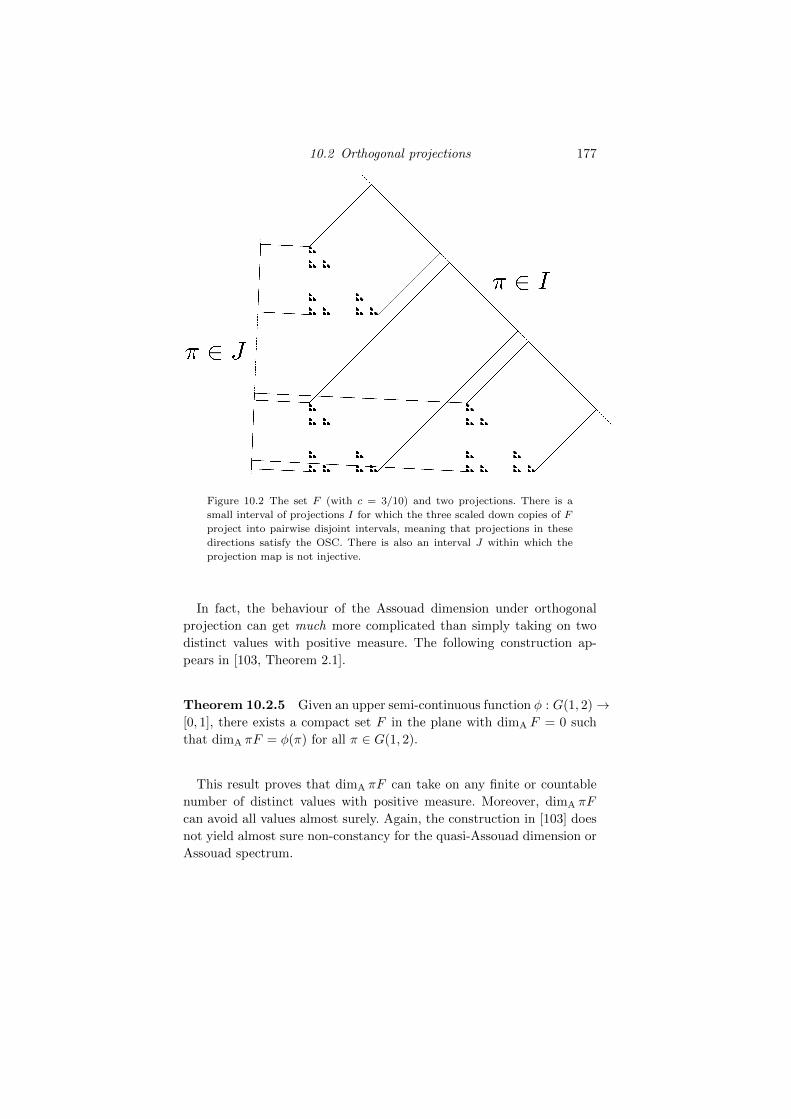
10.2 Orthogonal projections 177
Figure 10.2 The set F (with c = 3/10) and two projections. There is a
small interval of projections I for which the three scaled down copies of F
project into pairwise disjoint intervals, meaning that projections in these
directions satisfy the OSC. There is also an interval J within which the
projection map is not injective.
In fact, the behaviour of the Assouad dimension under orthogonal
projection can get much more complicated than simply taking on two
distinct values with positive measure. The following construction ap-
pears in [103, Theorem 2.1].
Theorem 10.2.5 Given an upper semi-continuous function φ : G(1, 2)→[0, 1], there exists a compact set F in the plane with dimA F = 0 such
that dimA πF = φ(π) for all π ∈ G(1, 2).
This result proves that dimA πF can take on any finite or countable
number of distinct values with positive measure. Moreover, dimA πF
can avoid all values almost surely. Again, the construction in [103] does
not yield almost sure non-constancy for the quasi-Assouad dimension or
Assouad spectrum.
178 Geometric constructions
10.2.3 An application to the box dimensions of
projections
As mentioned above, there is a Marstrand-type theorem for the box di-
mensions. That is, for a bounded set F ⊆ Rd, the dimensions dimBπF
take a common value for almost all π ∈ G(k, d) with a similar statement
for the lower box dimensions. The common value is given by a dimension
profile, which is a little more complicated than the almost sure constant
in Marstrand’s theorem, which is simply mink,dimH F. Recall, that
dimension profiles first appeared in [78, 143] and the almost sure con-
stancy for the box dimensions of projections was established in [143].
A capacity approach to dimension profiles was introduced much more
recently in [73]. Given the kernel
φkr (x) = min
1,( r
|x|
)k(10.7)
the capacity of a bounded set F with respect to this kernel is
1
Ckr (F )= inf
µ∈M(F )
∫ ∫φkr (x− y)dµ(x)dµ(y).
Here M(F ) denotes the collection of Borel probability measures sup-
ported by F . The double integral inside the infimum is called the energy
of µ and the inner integral is called the potential of µ at y.
It was shown in [73] that the box dimension profiles are given by
dimkBF = lim inf
r→0
logCkr (F )
− log r, dim
k
BF = lim supr→0
logCkr (F )
− log r
and, as mentioned above, these give the almost sure box dimensions of
projections, see [73, Theorem 1.1].
Theorem 10.2.6 Let F ⊆ Rd be a non-empty compact set. Then for
almost all π ∈ G(k, d)
dimBπF = dimkBF and dimBπF = dim
k
BF.
Interestingly the dimension profiles are not necessarily given by a sim-
ple expression analogous to the Hausdorff dimension case. However, they
always satisfy
dimBF
1 + (1/k − 1/d)dimBF6 dim
k
BF 6 mink,dimBF (10.8)
with the same bounds holding for dimkBF with lower box dimension
10.2 Orthogonal projections 179
replacing upper box dimension. Moreover, these bounds are the best
possible, as shown in [77, 146].
Work of Falconer, Fraser and Shmerkin [76] demonstrated that the As-
souad spectrum can be used to estimate the box dimension profiles and
this leads to the following application in the context of the box dimen-
sions of projections. More transparent corollaries will follow. The result
is more efficiently expressed in terms of the upper Assouad spectrum,
see Section 3.3.2.
Theorem 10.2.7 Let 1 6 k < d, F ⊆ Rd bounded and θ ∈ (0, 1).
Then, for almost all π ∈ G(k, d),
dimBπF > dimBF −max0, dimθ
AF − k, (dimA F − k)(1− θ)
and
dimBπF > dimBF −max0, dimθ
AF − k, (dimA F − k)(1− θ).
Proof We follow the proof in [76]. By rescaling if necessary, we may
assume that |F | < 1/2. Fix θ ∈ (0, 1), s > dimθ
AF , t > dimA F and let
C > 0 be a constant such that, for all 0 < r < R < 1 and x ∈ F ,
Nr(B(x,R) ∩ F ) 6 C
(R
r
)tand, for all 0 < r 6 R1/θ < R < 1 and x ∈ F ,
Nr(B(x,R) ∩ F ) 6 C
(R
r
)s.
Also let u < dimBF . Let 0 < r < 1 be small and let xiMi=1 be a
maximal r-separated set of points in F . For small enough r, we can
guarantee M > r−u by applying the definition of lower box dimension.
Place a point mass of weight 1/M at each xi and let µ be the sum of
these point masses, that is,
µ =
M∑i=1
1
Mδxi .
Write A = dlog2(2|F |r−1)e and a = d(1−θ) log2(r−1)e and observe that,
180 Geometric constructions
for sufficiently small r, a < A. The potential of µ at xi is∫φkr (xi − y)dµ(y) 6
A∑n=0
2−(n−1)kµ(B(xi, 2nr)) (applying (10.7))
6A∑n=0
2−(n−1)k 1
MNr(B(xi, 2
nr) ∩ F)
6 2kru( A∑n=a
2−nkC(2nr
r
)s
+
a−1∑n=0
2−nkC(2nr
r
)t)6 c ru max
1, r−(s−k), r−(t−k)(1−θ)
where c > 0 is a constant independent of r. Summing over i, the energy
of µ can be bounded as∫ ∫φkr (x− y)dµ(x)dµ(y) 6 c ru max
1, r−(s−k), r−(t−k)(1−θ)
and therefore the capacity Ckr (F ) satisfies
Ckr (F ) > c−1r−u min
1, r(s−k), r(t−k)(1−θ).
Thus, by Theorem 10.2.6, for almost all π ∈ G(k, d),
dimBπF = dimkBF
= lim infr→0
logCkr (F )
− log r
> lim infr→0
log(c−1r−u min1, r(s−k), r(t−k)(1−θ)
)− log r
= u−max0, s− k, (t− k)(1− θ)
which completes the proof for lower box dimension. The proof for upper
box dimension is similar and omitted.
Theorem 10.2.7 yields simple conditions guaranteeing that the box
dimension profiles are given by an expression analogous to that in the
statement of the Marstrand-Mattila projection theorem. The following
is an adaptation of [76, Corollary 1.3].
10.2 Orthogonal projections 181
Corollary 10.2.8 Let 1 6 k < d and F ⊆ Rd be a non-empty bounded
set. Then for almost all π ∈ G(k, d)
dimBπF > dimBF −max0, dimqA F − k.
In particular, if dimqA F 6 maxk, dimBF, then for almost all π ∈G(k, d)
dimBπF = mink, dimBF.
Proof This follows immediately from Theorem 10.2.7 by letting θ →1.
A natural question is when Theorem 10.2.7 improves on the general
lower bounds from (10.8). Based on knowledge of the Assouad dimension,
we get the following improvement, which first noted in [76, Corollary 1.5].
Corollary 10.2.9 Let 1 6 k < d, F ⊆ Rd be a non-empty bounded
set and suppose dimBF 6 k and
maxk, dimBF 6 dimA F <(kd+ 2dimBF (d− k))k
kd+ dimBF (d− k).
Then, for almost all π ∈ G(k, d),
dimBπF > dimBF −(dimA F − k)dimBF
k>
dimBF
1 + (1/k − 1/d)dimBF.
Proof This follows immediately from Theorem 10.2.7. If dimBF = k,
then the bound follows by letting θ → 0. If dimBF < k, then choose θ as
large as possible such that dimθ
AF 6 k. By Lemma 3.4.4 this can always
be done for
θ > 1− dimBF
k
and so, for almost all π ∈ G(k, d),
dimBπF > dimBF−(dimA F−k)(1−θ) > dimBF−(dimA F − k)dimBF
k.
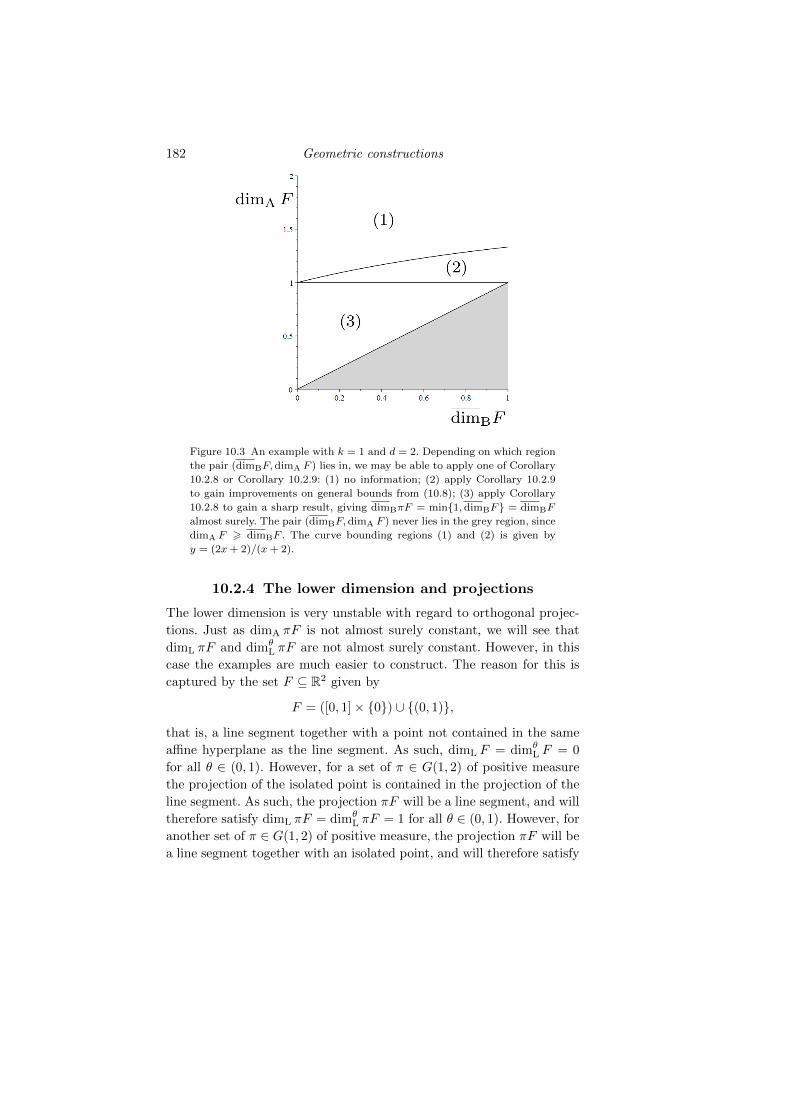
182 Geometric constructions
Figure 10.3 An example with k = 1 and d = 2. Depending on which region
the pair (dimBF, dimA F ) lies in, we may be able to apply one of Corollary
10.2.8 or Corollary 10.2.9: (1) no information; (2) apply Corollary 10.2.9
to gain improvements on general bounds from (10.8); (3) apply Corollary
10.2.8 to gain a sharp result, giving dimBπF = min1, dimBF = dimBF
almost surely. The pair (dimBF,dimA F ) never lies in the grey region, since
dimA F > dimBF . The curve bounding regions (1) and (2) is given by
y = (2x+ 2)/(x+ 2).
10.2.4 The lower dimension and projections
The lower dimension is very unstable with regard to orthogonal projec-
tions. Just as dimA πF is not almost surely constant, we will see that
dimL πF and dimθL πF are not almost surely constant. However, in this
case the examples are much easier to construct. The reason for this is
captured by the set F ⊆ R2 given by
F = ([0, 1]× 0) ∪ (0, 1),
that is, a line segment together with a point not contained in the same
affine hyperplane as the line segment. As such, dimL F = dimθL F = 0
for all θ ∈ (0, 1). However, for a set of π ∈ G(1, 2) of positive measure
the projection of the isolated point is contained in the projection of the
line segment. As such, the projection πF will be a line segment, and will
therefore satisfy dimL πF = dimθL πF = 1 for all θ ∈ (0, 1). However, for
another set of π ∈ G(1, 2) of positive measure, the projection πF will be
a line segment together with an isolated point, and will therefore satisfy
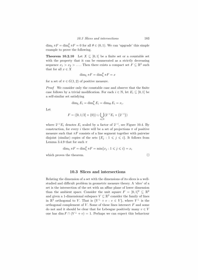
10.3 Slices and intersections 183
dimL πF = dimθL πF = 0 for all θ ∈ (0, 1). We can ‘upgrade’ this simple
example to prove the following.
Theorem 10.2.10 Let X ⊆ [0, 1] be a finite set or a countable set
with the property that it can be enumerated as a strictly decreasing
sequence x1 > x2 > . . . . Then there exists a compact set F ⊆ R2 such
that for all x ∈ XdimL πF = dimθ
L πF = x
for a set of π ∈ G(1, 2) of positive measure.
Proof We consider only the countable case and observe that the finite
case follows by a trivial modification. For each i ∈ N, let Ei ⊆ [0, 1] be
a self-similar set satisfying
dimLEi = dimθLEi = dimHEi = xi.
Let
F = ([0, 1/2]× 0) ∪⋃i∈N
(2−iEi × 2−i)
where 2−iEi denotes Ei scaled by a factor of 2−i, see Figure 10.4. By
construction, for every i there will be a set of projections π of positive
measure such that πF consists of a line segment together with pairwise
disjoint (similar) copies of the sets Ej : 1 6 j 6 i. It follows from
Lemma 3.4.9 that for such π
dimL πF = dimθL πF = minxj : 1 6 j 6 i = xi
which proves the theorem.
10.3 Slices and intersections
Relating the dimension of a set with the dimensions of its slices is a well-
studied and difficult problem in geometric measure theory. A ‘slice’ of a
set is the intersection of the set with an affine plane of lower dimension
than the ambient space. Consider the unit square F = [0, 1]2 ⊆ R2
and given a 1-dimensional subspace V ⊆ R2 consider the family of lines
in R2 orthogonal to V . That is V ⊥ + v : v ∈ V , where V ⊥ is the
orthogonal complement of V . Some of these lines intersect F and some
do not and it should be clear that for Lebesgue positively many v ∈ Vone has dimF ∩ (V ⊥ + v) = 1. Perhaps we can expect this behaviour
184 Geometric constructions
Figure 10.4 The set F together with a projection πF where only the sets
πE1, πE2 and πE3 are ‘visible’. For the purpose of illustration, the self-
similar sets have been replaced by line segments.
more generally. That is, given compact F ⊆ R2, then perhaps for ‘most’
V ∈ G(1, 2) and ‘many’ v ∈ V
dimF ∩ (V ⊥ + v) > dimF − 1.
This is formalised by Marstrand’s slicing theorem which was first es-
tablished in the plane [201], and for the higher dimensional result see
[205, 70]. One version of the theorem is as follows, see [205, Theorem
10.10].
Theorem 10.3.1 Let d > k > 1 be integers and F ⊆ Rd be a Borel set
withHs(F ) > 0 for some s > (d−k). Then, for almost all V ∈ G(d−k, d),
dimH
(F ∩ (V ⊥ + v)
)> s− (d− k)
for positively many v ∈ V .
Here “almost all” V ∈ G(d−k, d) refers to the Grassmannian measure
on G(d− k, d) and “positively many” v ∈ V refers to Lebesgue measure
on V .
It turns out that this result is very much measure-theoretic and relies
on the fact that the Hausdorff dimension cannot be large on a (measure
theoretically) small set. This is not the case for the box dimensions,
Assouad dimension and everything in between. We construct a set below
10.3 Slices and intersections 185
with full box, quasi-Assouad and Assouad dimension such that all slices
of the set have dimension 0 — we can even arrange for all the slices to
be finite!
Theorem 10.3.2 Given d > 1, there exists a compact set F ⊆ Rdsuch that dimBF = d but for all integers 1 6 k < d, all V ∈ G(d− k, d),
and all v ∈ V , the slice F ∩ (V ⊥ + v) consists of at most k + 1 points.
Note that the upper bound of k + 1 on the cardinality of the slices
here is sharp since any set F ⊆ Rd with at least k + 1 points intersects
at least one k-dimensional affine plane in a set of at least k + 1 points.
Proof Fix d > 1 and let E0 = 1/ log(n) : n = 2, 3, 4, . . . . It is straight-
forward to show that dimBE0 = 1 and we leave the details as an exercise.
For comparison, see Theorem 3.4.7 and note that 1/ log(n) is ‘slower’
than 1/np for any p. Let
E = (E0)d = E0 × · · · × E0 ⊆ Rd
which, by the formulae from Section 10.1, has lower box dimension d.
Note that every point in E is isolated and therefore, for every x ∈ E,
ε(x) = inf|x− y| : y ∈ E, y 6= x > 0.
Let
E′ =⋃x∈E
B(x, ε(x)/10)
which by the definition of ε(·) is a pairwise disjoint union of balls. Note
that any set consisting of precisely one point from each of the balls
B(x, ε(x)/10) is bi-Lipschitz equivalent to E and, therefore, has lower
box dimension d. Our set F will be (the closure of) one of these sets.
Since E is countable we can enumerate the balls in the construction of
E′ as B1, B2, . . . and we construct F by placing one point inside each
ball B1, B2, . . . in turn. Place a point x1 in B1 arbitrarily and then, once
we have placed the first n points, the (n+ 1)th point xn+1 is placed in
Bn+1 such that, for all 1 6 k < d, xn+1 does not lie in any k-dimensional
affine plane (V ⊥ + v) which already contains k + 1 points from the set
0 ∪ x1, x2, . . . , xn. To see why such placement of xn+1 is possible,
observe that there are only finitely many such affine planes because
every collection of k + 1 points is contained in a unique k-dimensional
affine plane. Therefore, the union of all affine planes we must avoid has
zero d-dimensional Lebesgue measure, whereas the set of possible choices
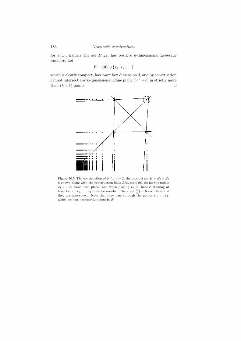
186 Geometric constructions
for xn+1, namely the set Bn+1, has positive d-dimensional Lebesgue
measure. Let
F = 0 ∪ x1, x2, . . .
which is clearly compact, has lower box dimension d, and by construction
cannot intersect any k-dimensional affine plane (V ⊥+v) in strictly more
than (k + 1) points.
Figure 10.5 The construction of F for d = 2: the product set E = E0 ×E0
is shown along with the construction balls B(x, ε(x)/10). So far the points
x1, . . . , x4 have been placed and when placing x5 all lines containing at
least two of x1, . . . , x4 must be avoided. There are(42
)= 6 such lines and
they are also shown. Note that they pass through the points x1, . . . , x4,
which are not necessarily points in E.
11
Two famous problems in geometric measuretheory
In this chapter we discuss the Assouad dimension in the context of two
famous conjectures in geometric measure theory: Falconer’s distance set
conjecture, and the Kakeya conjecture. In Section 11.1 we prove the
Assouad dimension version of one variant of the distance set problem in
the plane, see Theorem 11.1.3. In Section 11.2 we discuss the Kakeya
conjecture and give an elementary proof that ‘extended Kakeya sets’
have maximal Assouad dimension, see Theorem 11.2.2.
11.1 Distance sets
Given a set F ⊆ Rd, the distance set of F is defined by
D(F ) = |x− y| : x, y ∈ F.
The distance set problem, which stems from a seminal paper of Falconer
[63], is to relate the dimensions of F with the dimensions of D(F ).
Falconer’s distance set conjecture refers to several related conjectures,
one version of which is as follows.
Conjecture 11.1.1 Let d > 2 and F ⊆ Rd be an analytic set. If
dimH F > d/2, then D(F ) has positive Lebesgue measure (or even non-
empty interior). In particular, dimHD(F ) = 1.
There are numerous partial results in support of this conjecture, but
the problem is still open, even in the plane. See [207, Conjecture 4.5] and
the subsequent discussion. That said, since 2010 the problem has been
receiving a lot of attention in the literature, and significant progress is
being made, see for example, [252, 253, 225, 167, 124].
If we only consider the dimension (not measure) of the distance set,
This material will be published by Cambridge University Press as Assouad Dimension and Fractal Geometryby Jonathan Fraser. This pre-publication version is free to view and download for personal use only.
Not for re-distribution, re-sale or use in derivative works. c© Jonathan Fraser 2020.
188 Two famous problems in geometric measure theory
then dimension equal to d/2 should suffice. We may also replace the
Hausdorff dimension with Assouad dimension, and obtain a different
conjecture.
Conjecture 11.1.2 Let dim denote either the Hausdorff or Assouad
dimension, let d > 2 and F ⊆ Rd be an analytic set. If dimF > d/2,
then dimD(F ) = 1.
It may also be interesting to consider further variants of the problem
with dim replaced by other notions of dimension or spectra. The planar
Assouad dimension version of the conjecture was resolved in [89], apart
from the case dimA F = 1. This remaining case was later resolved in
[90]. To the best of our knowledge, all other versions of this conjecture
are open for all values of d > 2.
Theorem 11.1.3 If F ⊆ R2 with dimA F > 1, then dimAD(F ) = 1.
A result of Shmerkin [253] resolves the planar Hausdorff dimension
version of the problem with some additional assumptions.
Theorem 11.1.4 If F ⊆ R2 is a Borel set with dimH F = dimP F > 1,
then dimHD(F ) = 1.
Here we show how to obtain Theorem 11.1.3 from Theorem 11.1.4, al-
though this was not how Theorem 11.1.3 was originally proved because
Shmerkin’s result was not available at the time. The key technical obser-
vation is that one can pass questions on distance sets to weak tangents.
The following lemma is from [89, Lemma 3.1].
Lemma 11.1.5 Let F ⊆ Rd be a non-empty closed set and suppose
E is a weak tangent to F . Then
dimAD(F ) > dimAD(E).
Proof We follow the proof from [89, Section 3.2.1]. Since E is a weak
tangent to F , we may find a non-empty compact set X ⊆ Rd with
|X| > 0 and a sequence of similarity maps Tk : Rd → Rd such that
Tk(F ) ∩X → E (11.1)
in dH as k → ∞. Write ck ∈ (0,∞) for the similarity ratio of the map
Tk. Consider the sequence of compact sets given by
ckD(F ) ∩ [0, |X|]
11.1 Distance sets 189
where
ckD(F ) = ckz : z ∈ D(F ).
Using compactness of (K([0, |X|]), dH), we can find a strictly increasing
infinite sequence of integers (kn)n>1 such that cknD(F ) ∩ [0, |X|] con-
verges to a compact set B in the Hausdorff metric dH. In particular, the
set B is a weak tangent to D(F ) and therefore Theorem 5.1.2 gives
dimAD(F ) > dimAB.
It therefore suffices to show that D(E) ⊆ B. Let z = |x− y| ∈ D(E) for
some x, y ∈ E. It follows from (11.1) that we can find sequences xk, yk ∈Tk(F )∩X such that xk → x and yk → y. For each k, T−1
k (xk), T−1k (yk) ∈
F and so
c−1k |xk − yk| = |T
−1k (xk)− T−1
k (yk)| ∈ D(F ).
Moreover, |xk − yk| 6 |X| and therefore
|xk − yk| ∈ ckD(F ) ∩ [0, |X|].
It follows that
z = |x− y| = limk→∞
|xk − yk| = limn→∞
|xkn − ykn | ∈ B
as required.
Proof of Theorem 11.1.3: Let F ⊆ R2 be a closed set with dimA F =
s > 1. We will deal with the non-closed case at the end of the proof. It
follows from Theorem 5.1.3 that F has a weak tangent E such that
dimHE = dimPE = dimAE = s > 1.
It follows that dimAD(F ) > dimAD(E) > dimHD(E) by Lemma 11.1.5
and, moreover, since dimPE = dimHE > 1, Theorem 11.1.4 implies
dimHD(E) = 1.
All that remains is the case when F is not closed. However, dimA F =
dimA F > 1 and D(F ) ⊇ D(F ). Therefore, using the result in the closed
case,
dimAD(F ) = dimAD(F ) > dimAD(F ) = 1
as required.
Clearly, dimA F > 1 does not guarantee that D(F ) has non-empty
190 Two famous problems in geometric measure theory
interior since such sets may be countable, but it does guarantee the ex-
istence of a weak tangent to D(F ) with non-empty interior, by applying
Theorem 5.1.5.
Corollary 11.1.6 If F ⊆ R2 is any set with dimA F > 1, then D(F )
has a weak tangent with non-empty interior.
In the higher dimensional setting, Lemma 11.1.5 yields partial results
and also shows that the Hausdorff dimension version of Conjecture 11.1.2
implies the Assouad dimension version, see [89, Theorem 2.5]. Moreover,
partial results for Hausdorff dimension may be ‘converted’ into analogous
partial results for Assouad dimension. See the survey [207] for some
history and discussion of various partial results in higher dimensions,
such as the well-known Falconer-Erdogan-Wolff bounds. These bounds
were recently improved in [55, 56].
Theorem 11.1.7 Let d > 2 be an integer and F ⊆ Rd be any non-
empty set. Then
dimAD(F ) > infE ∈K(Rd):
dimH E= dimA F
dimAD(E).
For example, if d = 3 and dimA F > 9/5, then dimAD(F ) = 1.
The non-quantitative part of Theorem 11.1.7 was proved in [89, Theo-
rem 2.5] and provides a recipe for directly transferring any bounds con-
cerning the Hausdorff dimension version of the distance set problem into
analogous bounds concerning the Assouad dimension version. The quan-
titative example with d = 3 follows by applying the non-quantitative
part to the Hausdorff dimension results from [55]. Higher dimensional
analogues of these bounds can also be derived by considering [56]. It ap-
pears that the appropriate analogues of these bounds are not known to
hold for other notions of dimension, such as box or packing dimension.
As for sets with small Assouad dimension, it was proved in [100, The-
orem 2.9] that if F ⊆ Rd satisfies 0 < dimA F < d, then
dimAD(F ) > dimA F/d, (11.2)
which improves on estimates from Theorem 11.1.7 when dimA F is small.
Observe that the distance set D(F ) consists of the norms of points in
the difference set F−F . By relating the difference set and an appropriate
orthogonal projection of the product set F ×F , the results from Section
10.1 show
dimBD(F ) 6 dimB(F × F ) 6 2dimBF
11.1 Distance sets 191
for any bounded F ⊆ Rd. However, there exist compact sets in Rd with
Hausdorff dimension 0, but whose distance set contains an interval. For
example, [166, Proposition 3.1] provides a compact set F ⊆ Rd with
Hausdorff dimension 0 but for which F ∩ (F + t) 6= ∅ for all t ∈ [0, 1]d.
This shows that [0,√d] ⊆ D(F ) and so dimAD(F ) = 1. That said, the
product-projection argument above guarantees dimHD(F ) 6 dimH F +
dimP F for F ⊆ Rd and so the size of the distance set can be controlled
by the size of F in some sense. The situation for Assouad dimension is
rather different since Assouad dimension can increase under orthogonal
projection. In fact, arbitrarily small sets can have distance sets with full
Assouad dimension. Such examples are provided by simple self-similar
sets, requiring only an irrationality condition. This shows that for every
s ∈ (0, 1), there exists an Ahlfors regular set with dimension s but
dimAD(F ) = 1. The following is from [89, Theorem 2.7].
Theorem 11.1.8 Let F ⊆ Rd be a self-similar set which is not a single
point and suppose that two of the defining similarity ratios are given by
α, β ∈ (0, 1) satisfying logα/ log β /∈ Q. Then dimAD(F ) = 1.
Proof We follow the argument from [89, Section 3.2.3]. Let x, y ∈ F be
distinct points and let ∆ := |x− y| > 0. Let Sα be a defining similarity
map with similarity ratio α and Sβ be a defining similarity map with
similarity ratio β. Using invariance under the defining IFS, for integers
m,n > 0, the points Smα Snβ (x), Smα Snβ (y) ∈ F . Therefore
|Smα Snβ (x)− Smα Snβ (y)| = αmβn∆ ∈ D(F ).
The proof of Theorem 11.1.8 is now similar to Theorem 7.2.1. For inte-
ger k > 1, let Tk : [0, 1] → [0, 1] be the similarity defined by Tk(x) =
∆−1β−kx and, using compactness of K([0, 1]), extract a convergent sub-
sequence of Tk(D(F )) ∩ [0, 1] in the Hausdorff metric. The limit of this
subsequence is a weak tangent to D(F ). Moreover,
0 ∪αmβn : m,n ∈ Z, m > 0, n > −k
∩ [0, 1] ⊆ Tk(D(F )) ∩ [0, 1]
for all k > 1 and therefore the weak tangent contains
αmβn : m ∈ N, n ∈ Z ∩ [0, 1] = [0, 1]
with this equality following from Dirichlet’s theorem and the irrational-
ity of logα/ log β.
By changing the contraction ratios at each stage in the construc-
tion, Theorem 11.1.8 can be used to find a compact set F ⊆ [0, 1] with
dimA F = 0 and dimAD(F ) = 1. See [89, Example 2.6] for the details.
192 Two famous problems in geometric measure theory
Despite the previous examples, Theorem 11.1.3 is sharp in the sense
that one cannot guarantee that the distance set has full Assouad dimen-
sion for sets F with dimA F > s for any s < 1. The next result follows
[89, Example 2.8].
Theorem 11.1.9 For every s ∈ [0, 1), there exists a compact set F ⊆[0, 1] with dimA F = dimH F > s but dimAD(F ) < 1.
Proof Let s ∈ [0, 1), choose an integer N > 2 satisfying (N + 1)/2 −Ns > 1, and another integer K satisfying Ns 6 K < (N + 1)/2. For
i ∈ 0, . . . ,K − 1, let Si : [0, 1]→ [0, 1] be the similarity defined by
Si(x) = (x+ 2i)/N
and F ⊆ [0, 1] be the self-similar set which is the attractor of the IFS
SiK−1i=0 . By construction, this IFS satisfies the OSC, and therefore
dimA F = dimH F =logK
logN> s.
Let π denote orthogonal projection onto the subspace of R2 spanned by
the vector (1,−1) and consider the set π(F × F ). This set turns out to
also be a self-similar set satisfying the OSC, this time defined by 2K−1
similarities with common similarity ratio 1/N . The map g defined by
g(x) = |x| is bi-Lipschitz on (−∞, 0) and [0,∞) and so cannot increase
Assouad dimension. The fact that g is Lipschitz on the whole of R is
not sufficient here since Assouad dimension is not stable under Lipschitz
maps. Since g(π(F × F )) = D(F ) we obtain
dimAD(F ) 6 dimA π(F × F ) 6log(2K − 1)
logN< 1
as desired.
There are many variants on the distance set problem. For example,
[281] considers triples of distances between triples of points instead of
distances between pairs of points. The resulting ‘triangle set’ is a subset
of R3 and the problem is to understand the dimension of the triangle
set, given the dimension of the original set. Partial results concerning
the Assouad dimension version of the problem can be found in [281].
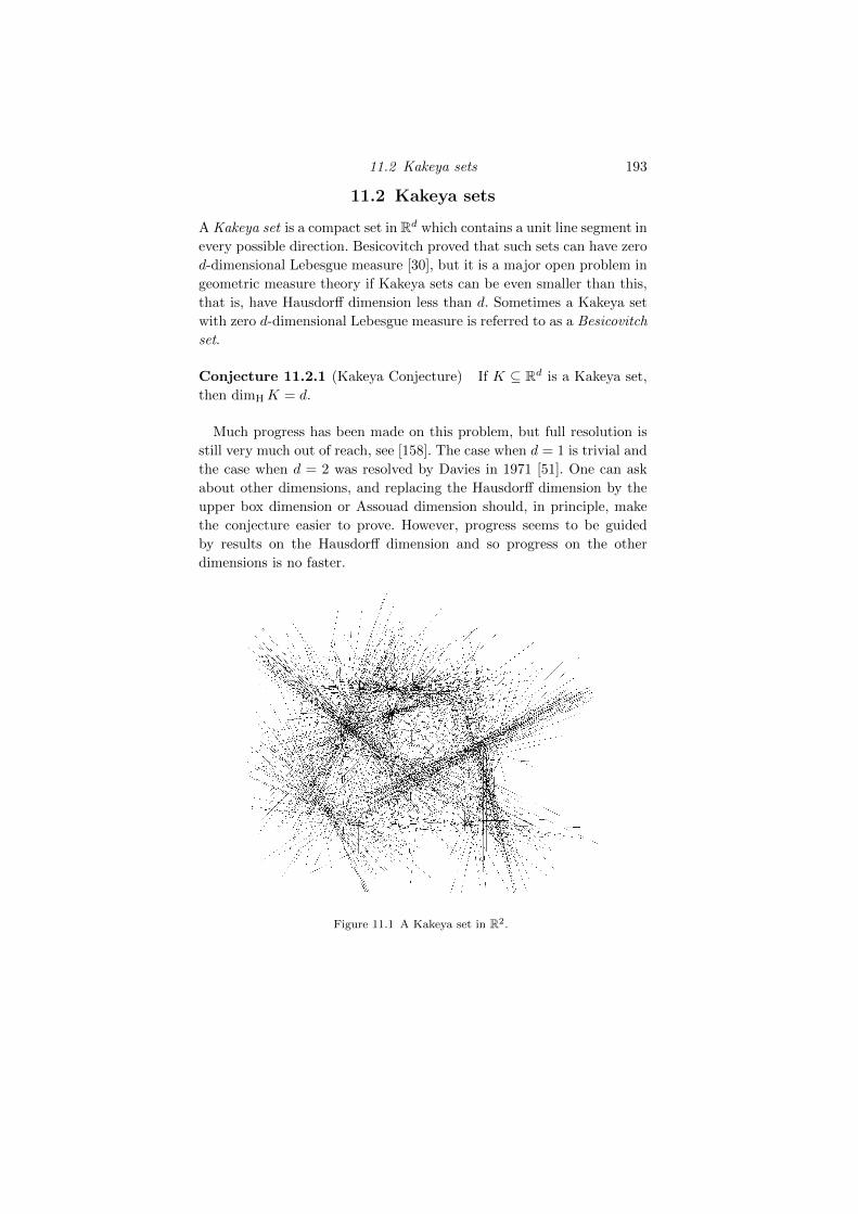
11.2 Kakeya sets 193
11.2 Kakeya sets
A Kakeya set is a compact set in Rd which contains a unit line segment in
every possible direction. Besicovitch proved that such sets can have zero
d-dimensional Lebesgue measure [30], but it is a major open problem in
geometric measure theory if Kakeya sets can be even smaller than this,
that is, have Hausdorff dimension less than d. Sometimes a Kakeya set
with zero d-dimensional Lebesgue measure is referred to as a Besicovitch
set.
Conjecture 11.2.1 (Kakeya Conjecture) If K ⊆ Rd is a Kakeya set,
then dimHK = d.
Much progress has been made on this problem, but full resolution is
still very much out of reach, see [158]. The case when d = 1 is trivial and
the case when d = 2 was resolved by Davies in 1971 [51]. One can ask
about other dimensions, and replacing the Hausdorff dimension by the
upper box dimension or Assouad dimension should, in principle, make
the conjecture easier to prove. However, progress seems to be guided
by results on the Hausdorff dimension and so progress on the other
dimensions is no faster.
Figure 11.1 A Kakeya set in R2.
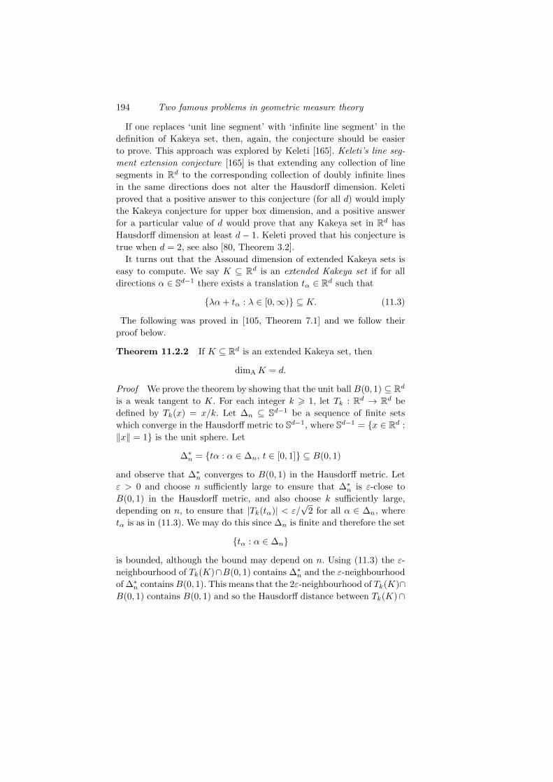
194 Two famous problems in geometric measure theory
If one replaces ‘unit line segment’ with ‘infinite line segment’ in the
definition of Kakeya set, then, again, the conjecture should be easier
to prove. This approach was explored by Keleti [165]. Keleti’s line seg-
ment extension conjecture [165] is that extending any collection of line
segments in Rd to the corresponding collection of doubly infinite lines
in the same directions does not alter the Hausdorff dimension. Keleti
proved that a positive answer to this conjecture (for all d) would imply
the Kakeya conjecture for upper box dimension, and a positive answer
for a particular value of d would prove that any Kakeya set in Rd has
Hausdorff dimension at least d− 1. Keleti proved that his conjecture is
true when d = 2, see also [80, Theorem 3.2].
It turns out that the Assouad dimension of extended Kakeya sets is
easy to compute. We say K ⊆ Rd is an extended Kakeya set if for all
directions α ∈ Sd−1 there exists a translation tα ∈ Rd such that
λα+ tα : λ ∈ [0,∞) ⊆ K. (11.3)
The following was proved in [105, Theorem 7.1] and we follow their
proof below.
Theorem 11.2.2 If K ⊆ Rd is an extended Kakeya set, then
dimAK = d.
Proof We prove the theorem by showing that the unit ball B(0, 1) ⊆ Rdis a weak tangent to K. For each integer k > 1, let Tk : Rd → Rd be
defined by Tk(x) = x/k. Let ∆n ⊆ Sd−1 be a sequence of finite sets
which converge in the Hausdorff metric to Sd−1, where Sd−1 = x ∈ Rd :
‖x‖ = 1 is the unit sphere. Let
∆∗n = tα : α ∈ ∆n, t ∈ [0, 1] ⊆ B(0, 1)
and observe that ∆∗n converges to B(0, 1) in the Hausdorff metric. Let
ε > 0 and choose n sufficiently large to ensure that ∆∗n is ε-close to
B(0, 1) in the Hausdorff metric, and also choose k sufficiently large,
depending on n, to ensure that |Tk(tα)| < ε/√
2 for all α ∈ ∆n, where
tα is as in (11.3). We may do this since ∆n is finite and therefore the set
tα : α ∈ ∆n
is bounded, although the bound may depend on n. Using (11.3) the ε-
neighbourhood of Tk(K)∩B(0, 1) contains ∆∗n and the ε-neighbourhood
of ∆∗n containsB(0, 1). This means that the 2ε-neighbourhood of Tk(K)∩B(0, 1) contains B(0, 1) and so the Hausdorff distance between Tk(K)∩
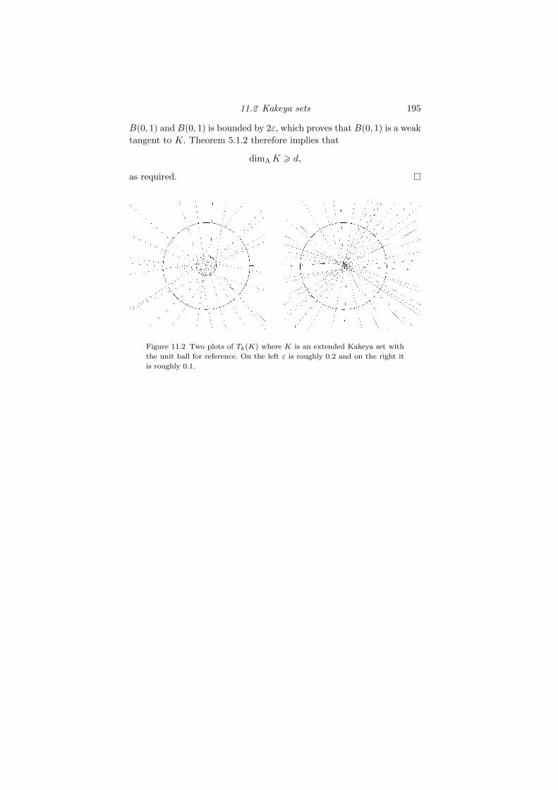
11.2 Kakeya sets 195
B(0, 1) and B(0, 1) is bounded by 2ε, which proves that B(0, 1) is a weak
tangent to K. Theorem 5.1.2 therefore implies that
dimAK > d,
as required.
Figure 11.2 Two plots of Tk(K) where K is an extended Kakeya set with
the unit ball for reference. On the left ε is roughly 0.2 and on the right it
is roughly 0.1.
12
Conformal dimension
In this chapter we briefly discuss conformal dimension and highlight
some particular areas of interest in connection with the topics covered
in this book. The concept of conformal dimension considers how much
a given notion of dimension can drop under quasi-symmetric deforma-
tion. This is often a very challenging problem and we refer the reader
to Mackay and Tyson’s book [195] for a thorough treatment. We give
a proof that equicontractive self-similar sets have conformal Assouad
dimension 0, see Theorem 12.1.1.
12.1 Lowering the Assouad dimension byquasi-symmetry
Consider a notion of dimension, dim, which in what follows will most
often be Hausdorff or Assouad dimension. Then the conformal variant of
this dimension, written Cdim, measures how small the dimension can be
made under quasi-symmetric deformation. This concept was introduced
by Pansu [228] and has given rise to many useful invariants used in
classifying, for example, boundaries of hyperbolic groups. See [195] for
a detailed treatment.
More formally, we say a homeomorphism φ between two sets E,F ⊆Rd is a quasi-symmetry if there exists a homeomorphism η : [0,∞) →[0,∞) such that
|φ(x)− φ(y)||φ(x)− φ(z)|
6 η
(|x− y||x− z|
)for all x, y, z ∈ E with x 6= z. Note that if φ is bi-Lipschitz, then it is
easily seen to be a quasi-symmetry, but quasi-symmetries certainly need
This material will be published by Cambridge University Press as Assouad Dimension and Fractal Geometryby Jonathan Fraser. This pre-publication version is free to view and download for personal use only.
Not for re-distribution, re-sale or use in derivative works. c© Jonathan Fraser 2020.
12.1 Lowering the Assouad dimension by quasi-symmetry 197
not be bi-Lipschitz. Given a notion of dimension dim, the conformal
dimension of F ⊆ Rd is defined by
CdimF = infdimφ(F ) : φ is quasi-symmetric.
Immediately we see CdimF 6 dimF but this inequality can be strict.
For example, if F ⊆ Rd is a self-similar set satisfying the SSC, then
the conformal Assouad dimension of F is 0. This shows that there is no
limit on how much the conformal dimension can drop from the original
dimension. See Chapter 7 for background on self-similar sets.
Theorem 12.1.1 If F ⊆ Rd is a self-similar set satisfying the SSC,
then CdimA F = 0.
Proof We prove the result in the equicontractive case. That is, where F
is the attractor of an IFS of similarities Sii∈I which share a common
similarity ratio c ∈ (0, 1), see (7.1). The general case follows from [195,
Theorem 2.1.2], see also [270]. Let
δ = mini 6=j
infx∈Si(F )y∈Sj(F )
|x− y| > 0
which is strictly positive since the SSC holds. Let λ ∈ (0, 1) and Fλ be
the self-similar set defined by the IFS Sλi i∈I where Sλi is a similarity
with the same (unique) fixed point as Si but with similarity ratio λc.
Since the original IFS satisfies the SSC, the IFS defining Fλ satisfies the
SSC for sufficiently small λ. Moreover, for sufficiently small λ,
mini 6=j
infx∈Sλi (Fλ)
y∈Sλj (Fλ)
|x− y| > δ/2.
We assume from now on that λ is small enough for both of the previous
statements to hold. By Corollary 6.4.4, the Assouad dimension of Fλ is
dimA Fλ =log #I− log(λc)
which can be made arbitrarily small by letting λ → 0. We will show
that F and Fλ are quasi-symmetric equivalent, that is, there is a quasi-
symmetry φ : F → Fλ, which proves the result.
Let φ : F → Fλ be defined by φ(Π(i)) = Πλ(i) for i ∈ IN where Π is
the symbolic coding map associated with the original IFS and Πλ is the
symbolic coding map for Fλ, see Section 6.1. This map is well-defined
198 Conformal dimension
since the SSC guarantees that the symbolic coding maps are bijective.
For all i , j ∈ IN with i 6= j
c|i∧j |δ|F | 6 |Π(i)−Π(j )| 6 c|i∧j ||F | (12.1)
and
(λc)|i∧j |(δ/2)|Fλ| 6 |Πλ(i)−Πλ(j )| 6 (λc)|i∧j ||Fλ| (12.2)
where i ∧ j ∈ I∗ is the longest common prefix of i and j . Consider
x, y, z ∈ F with x = Π(i), y = Π(j ), z = Π(k) for i , j , k ∈ IN with
i 6= k . It follows from (12.1)–(12.2) that
|φ(x)− φ(y)||φ(x)− φ(z)|
6(λc)|i∧j |
(λc)|i∧k |(δ/2)
= 2δ−1− log(λc)log c
(c|i∧j |δ
c|i∧k |
) log(λc)log c
6 2δ−1− log(λc)log c
(|x− y||x− z|
) log(λc)log c
.
Therefore φ is a quasi-symmetry with η : [0,∞)→ [0,∞) given by
η(t) = 2δ−1− log(λc)log c t
log(λc)log c
which completes the proof.
The topological dimension, dimT F , of a non-empty set F ⊆ Rd is
the minimal integer n > 0 such that for every r > 0 there exists an
r-cover of F by open sets such that every x ∈ F lies in at most n + 1
of the covering sets. As such, totally disconnected sets have topological
dimension 0, and dimT ψ([0, 1]k) = k for all k and homeomorphisms
ψ : [0, 1]k → Rd. Moreover, dimT F 6 dimH F for all sets F . Since the
Assouad and Hausdorff dimensions are bounded below by the topological
dimension, which is preserved under homeomorphism, one always has
CdimA F > CdimH F > dimT F
and Theorem 12.1.1 shows that this lower bound can be realised in
non-trivial situations. Conformal Assouad dimension behaves well in the
context of weak tangents, due to the following result of Mackay and
Tyson [195, Proposition 6.1.7], which should be compared with Theorem
5.1.2.
12.1 Lowering the Assouad dimension by quasi-symmetry 199
Theorem 12.1.2 Let F ⊆ Rd be closed, E ⊆ Rd be compact, and
suppose E is a weak tangent to F . Then CdimA F > CdimAE.
This is particularly useful if a given set has easily understood tan-
gents. For example, this result combined with Theorem 5.1.5 yields the
following equivalence.
Corollary 12.1.3 For F ⊆ Rd, dimA F = d if and only if CdimA F =
d.
Proof The non-trivial implication follows since dimA F = d guaran-
tees that [0, 1]d is a weak tangent to F by Theorem 5.1.5. Therefore,
CdimA F > dimT[0, 1]d = d.
Theorem 12.1.2 was used by Mackay [194] to compute the conformal
Assouad dimension of Bedford-McMullen carpets; recall the notation
and setup for these in Section 8.3. There turns out to be a simple di-
chotomy, showing that the conformal Assouad dimension of a Bedford-
McMullen carpet is either the Assouad dimension or zero. See [154,
Theorems A and B] for further results in this direction.
Theorem 12.1.4 Let F be a Bedford-McMullen carpet. If bothNmax <
n and N0 < m, then
CdimA F = 0,
and, otherwise,
CdimA F = dimA F =logN0
logm+
logNmax
log n.
Proof sketch. In the first case, it is shown that F is uniformly discon-
nected, and then the conformal Assouad dimension is 0 by [195, Theorem
2.1.2]. In the second case, a weak tangent is constructed with maximal
Assouad dimension which is of the form [0, 1] × E where E is a self-
similar set. It is known that the Assouad dimension of such product sets
cannot be lowered by quasi-symmetric deformation, see [228, Lemma
6.3], and therefore Theorem 12.1.2 implies that the conformal Assouad
and Assouad dimensions coincide.
In general it is a notoriously difficult problem to compute the con-
formal dimension. Self-similar sets have attracted a large amount of
attention and still very little is known outside of the SSC case. A cele-
brated result of Tyson and Wu [271] shows that the Sierpinski triangle
has conformal Assouad and conformal Hausdorff dimension equal to 1
200 Conformal dimension
(its topological dimension), see Figure 12.1. Recall that the Hausdorff
and Assouad dimensions of the Sierpinski triangle are both given by
log 3/ log 2. To prove the upper bound they construct an explicit family
of IFS attractors which are all quasi-symmetric equivalent to each other
and have dimensions approaching 1. Another famous example, this time
for more nefarious reasons, is the Sierpinski carpet, see Figure 12.1. This
is another self-similar set satisfying the OSC but this time the conformal
(Assouad or Hausdorff) dimension is unknown. The Sierpinski carpet is
the attractor of the IFS formed by dividing the unit square into a 3× 3
grid, removing the middle square and taking orientation preserving sim-
ilarities mapping the square onto the remaining 8 pieces. Therefore, for
F the Sierpinski carpet
dimT F = 1 <log 8
log 3= dimH F = dimA F.
It is known that
1 +log 2
log 36 CdimH F 6 CdimA F <
log 8
log 3.
The first bound follows since
[0, 1]× E ⊆ F
where E is the middle third Cantor set and therefore by [228, Lemma
6.3] the conformal Hausdorff dimension of F cannot be lowered below the
dimension of this product set, see also [269]. The fact that CdimA F <
dimA F is due to Keith and Laakso [164, Corollary 1.0.5], see also [195,
Example 6.2.3]. For other more recent developments on this problem,
see [169, 176].
Rossi and Suomala [243] investigated the conformal Hausdorff di-
mension of the Mandelbrot percolation sets, recall Section 9.4. They
proved that there exists a t such that almost surely, conditioned on non-
extinction,
CdimHM = t < dimHM.
In contrast, Theorem 9.4.1 and Corollary 12.1.3 show that almost surely,
conditioned on non-extinction,
CdimAM = dimAM = d.
Therefore Mandelbrot percolation sets are typically minimal for Assouad
dimension but not for Hausdorff dimension.
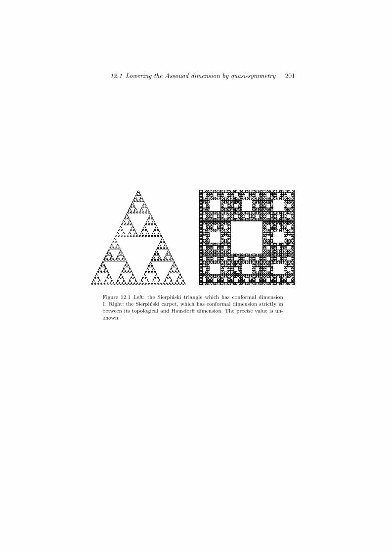
12.1 Lowering the Assouad dimension by quasi-symmetry 201
Figure 12.1 Left: the Sierpinski triangle which has conformal dimension
1. Right: the Sierpinski carpet, which has conformal dimension strictly in
between its topological and Hausdorff dimension. The precise value is un-
known.

PART THREE
APPLICATIONS

13
Applications in embedding theory
Even though the Assouad dimension appeared in other contexts, see
Section 2.3, it was the pioneering work of Assouad in the 1970s [6, 7, 8],
which served to popularise the notion and establish its deep connections
with several areas of mathematics, most notably embedding theory. In
this chapter we discuss various problems in embedding theory, all of
which can be understood as asking for conditions on a metric space
X guaranteeing the existence of an injection (the embedding) mapping
X into Euclidean space. We will often insist that the embeddings pos-
sess some sort of ‘metric regularity’, such as being bi-Lipschitz. In Sec-
tion 13.1 we discuss Assouad’s embedding theorem, see Theorem 13.1.3,
which begins with a discussion of doubling and uniformly perfect metric
spaces and the connection between these notions and the Assouad and
lower dimensions in Section 13.1.1. In Section 13.2 we consider the ‘spi-
ral winding problem’, following [85, 93, 159], which asks: given a planar
spiral, how regular can a homeomorphism be which maps a line segment
onto the spiral? Thus, the spiral winding problem is a specific example
of an embedding problem, where the ‘embedding’ is the inverse of the
solution; that is, we ask for regular embeddings of spirals into the line.
The Assouad spectrum plays a key role here, see (13.7) and Figure 13.5.
Finally, in Section 13.3 we discuss further applications of the Assouad
dimension in embedding theory, as studied by Robinson [240]. Here we
are interested in embeddings of subsets of Banach space into Euclidean
space which are more regular than those provided by Assouad’s embed-
ding theorem.
This material will be published by Cambridge University Press as Assouad Dimension and Fractal Geometryby Jonathan Fraser. This pre-publication version is free to view and download for personal use only.
Not for re-distribution, re-sale or use in derivative works. c© Jonathan Fraser 2020.
206 Applications in embedding theory
13.1 Assouad’s embedding theorem
13.1.1 Doubling and uniformly perfect metric spaces
Even though we work largely in Euclidean space throughout this book,
much of the theory applies in arbitrary metric spaces. One of the funda-
mental facts concerning Assouad dimension is that it precisely charac-
terises doubling metric spaces. Recall that a metric space X is doubling
if there exists a constant K > 1 such that any ball in X may be cov-
ered by fewer than K balls with half the radius. Moreover, the Assouad
dimension of a metric space X is defined by
dimAX = inf
α : there exists a constant C > 0 such that,
for all 0 < r < R and x ∈ X,
Nr(B(x,R)
)6 C
(R
r
)α
where Nr(E) is the minimum number of balls of diameter r required to
cover E ⊆ X.
Theorem 13.1.1 A metric spaceX is doubling if and only if dimAX <
∞.
Proof If dimAX < ∞ then it follows immediately from the definition
that X is doubling. For the reverse implication, assume that X is dou-
bling. Therefore, for all x ∈ X and ρ > 0 we can cover B(x, ρ) by K balls
of radius ρ/2. Fix 0 < r < R and let n be the unique integer such that
21−nR 6 r < 22−nR. Seeking a cover of B(x,R) by balls of diameter r,
first cover B(x,R) by K balls of radius R/2. Then cover these balls by
K balls of radius R/4 and continue inductively until we obtain a cover
by balls of radius 2−nR 6 r/2. This yields
Nr(B(x,R)) 6 Kn 6 K2
(R
r
) logKlog 2
,
which proves that dimAX 6 logKlog 2 <∞ as required.
Recall Lemma 4.1.1 which states that a measure is doubling if and
only if it has finite Assouad dimension. This also holds for measures
supported on general metric spaces and combining Theorem 4.1.3 with
the characterisation of doubling in terms of Assouad dimension, one sees
13.1 Assouad’s embedding theorem 207
that every doubling metric space supports a doubling measure. The spe-
cial case of this fact which implies that every closed subset of Euclidean
space supports a doubling measure was known as Dynkin’s conjecture
[59], until it was resolved by Konyagin and Vol’berg [173].
Just as the Assouad dimension characterises the doubling property,
the lower dimension characterises the property of being uniformly per-
fect. Recall that a metric space is perfect if every point in the space is an
accumulation point. Expressed differently, this means that for all points
x in X and 0 < R we have
B(x,R) \ x 6= ∅.
Uniform perfectness is a quantified version of this where the accumu-
lation can always be taken to be no faster than exponential. A metric
space X is uniformly perfect if there exists a constant κ ∈ (0, 1) such
that, for all points x in X and 0 < R < |X|,
B(x,R) \B(x, κR) 6= ∅
where |X| denotes the diameter of X. The lower dimension of a metric
space X is defined by
dimLX = sup
α : there exists a constant C > 0 such that,
for all 0 < r < R 6 |X| and x ∈ X,
Nr(B(x,R)
)> C
(R
r
)α
where d is the metric on X and |X| = supx,y∈X d(x, y) is the diameter
of X. The following equivalence was proved in [153, Lemma 2.1].
Theorem 13.1.2 A metric space X is uniformly perfect if and only if
dimL F > 0.
Proof If dimLX > s > 0, then there is a constant C > 0 such that for
all x ∈ X and 0 < R < |X|
Nr(B(x,R)) > C
(R
r
)s.
Choose κ ∈ (0, 1) such that Cκ−s > 2 and it follows that
B(x,R) \B(x, (κ/2)R) 6= ∅
208 Applications in embedding theory
since otherwise
1 = NκR(B(x,R)) > C
(R
κR
)s> 2.
Therefore X is uniformly perfect.
In the other direction, suppose X is uniformly perfect with constant κ.
Let x1 ∈ X, 0 < r < R < |X| and let n be the unique integer such that
(κ/3)n+1R < r 6 (κ/3)nR. Since X is uniformly perfect, there exists a
point
x2 ∈ B(x1, R) \B(x1, κR)
where, in particular, the balls B(x1, (κ/3)R) and B(x2, (κ/3)R) are dis-
joint. Repeat the above process within each of these balls to obtain points
x1, x2, x3, x4 such that the balls B(xi, (κ/3)2R) are pairwise disjoint for
i = 1, 2, 3, 4. Repeat this process inductively to obtain 2n points xi such
that the balls B(xi, (κ/3)nR) are pairwise disjoint for i = 1, . . . , 2n . It
follows that any set of diameter r cannot contain more than one of the
points xi and therefore
Nr(B(x1, R)) > 2n > (κ/3)
(R
r
) log 2log(3/κ)
which proves that dimLX > log 2log(3/κ) > 0 as required.
13.1.2 Assouad’s embedding theorem
The theorem which first threw the Assouad dimension into the lime-
light is Assouad’s embedding theorem, proved during Assouad’s doctoral
studies [6, 7, 8]. The question Assouad was considering is: when can a
given metric space be embedded into Euclidean space? The ideal notion
of embedding would be via a bi-Lipschitz map — thus preserving all of
the metric properties up to universal constants. It turns out that the
Assouad dimension almost precisely characterises this problem.
Recall from Lemma 2.4.2 that Assouad dimension is preserved un-
der bi-Lipschitz maps. This already makes the Assouad dimension very
useful in studying embedding problems. For example, if we want a bi-
Lipschitz embedding into Rd (or any space with finite Assouad dimen-
sion), then having finite Assouad dimension or, equivalently, satisfying
the doubling property, see Theorem 13.1.1, is a necessary condition. This
is true of other dimensions but, since Assouad dimension is the largest
among those we consider, it is the most useful. For example, Troscheit
13.1 Assouad’s embedding theorem 209
used this approach to prove that the Brownian map cannot be embed-
ded in Rd using a bi-Lipschitz (or even quasi-symmetric) embedding, see
[267]. This was achieved by proving that the Assouad dimension of the
Brownian map is almost surely infinite despite the Hausdorff dimension
being almost surely 4. The Assouad dimension is also useful in studying
purely Euclidean embedding problems. Recall Theorem 9.4.1 which im-
plies that Mandelbrot percolation in Rd cannot be embedded in Rd−1
even if the parameters are such that the Hausdorff and box dimension
are almost surely very close to 0.
Assouad’s embedding theorem says that being doubling is almost suf-
ficient to guarantee a bi-Lipschitz embedding into Euclidean space.
Theorem 13.1.3 If (X, d) is a metric space with dimAX < ∞, then
for all ε ∈ (0, 1) the space (X, dε) embeds into Rn via a bi-Lipschitz map
for some n > 1 depending on dimAX and ε.
Note that the metric space (X, dε) is known as an ε-snowflaking of
X and is simply the set X equipped with the snowflaked metric dε
defined by dε(x, y) = d(x, y)ε. The requirement ε < 1 guarantees the
metric dε satisfies the triangle inequality. The snowflaking in Theorem
13.1.3 is necessary, unfortunately, and this is the reason that the Assouad
dimension does not precisely characterise the bi-Lipschitz embedding
problem. The Heisenberg group H equipped with the Carnot metric is
an example of a doubling metric space which cannot be embedded in
Euclidean space of any ambient dimension, see [227, 250]. Another well-
known example of a doubling space which cannot embed into Euclidean
space via a bi-Lipschitz mapping is a construction of Lang and Plaut
[178] based on Laakso graphs, see [177].
Naor and Neiman [215] proved that for ε ∈ (1/2, 1), one may choose
the n in Theorem 13.1.3 depending only on dimAX and not on the
snowflaking constant ε. The cost of this improvement was in the depen-
dency on ε of the distortion constant of the bi-Lipschitz embedding. Tao
[264] considered the embedding properties of the Heisenberg group in
detail, proving that the ε-snowflakings of H can be embedded into Rnwith n independent of ε and with the optimal distortion constant.
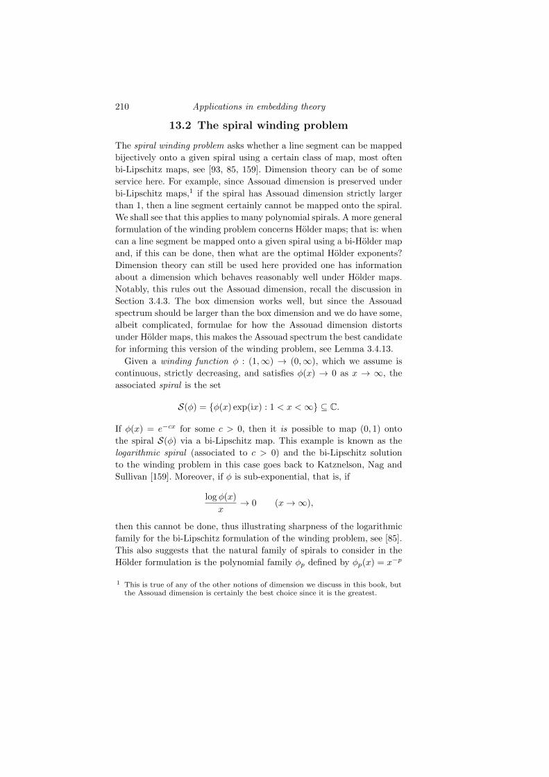
210 Applications in embedding theory
13.2 The spiral winding problem
The spiral winding problem asks whether a line segment can be mapped
bijectively onto a given spiral using a certain class of map, most often
bi-Lipschitz maps, see [93, 85, 159]. Dimension theory can be of some
service here. For example, since Assouad dimension is preserved under
bi-Lipschitz maps,1 if the spiral has Assouad dimension strictly larger
than 1, then a line segment certainly cannot be mapped onto the spiral.
We shall see that this applies to many polynomial spirals. A more general
formulation of the winding problem concerns Holder maps; that is: when
can a line segment be mapped onto a given spiral using a bi-Holder map
and, if this can be done, then what are the optimal Holder exponents?
Dimension theory can still be used here provided one has information
about a dimension which behaves reasonably well under Holder maps.
Notably, this rules out the Assouad dimension, recall the discussion in
Section 3.4.3. The box dimension works well, but since the Assouad
spectrum should be larger than the box dimension and we do have some,
albeit complicated, formulae for how the Assouad dimension distorts
under Holder maps, this makes the Assouad spectrum the best candidate
for informing this version of the winding problem, see Lemma 3.4.13.
Given a winding function φ : (1,∞) → (0,∞), which we assume is
continuous, strictly decreasing, and satisfies φ(x) → 0 as x → ∞, the
associated spiral is the set
S(φ) = φ(x) exp(ix) : 1 < x <∞ ⊆ C.
If φ(x) = e−cx for some c > 0, then it is possible to map (0, 1) onto
the spiral S(φ) via a bi-Lipschitz map. This example is known as the
logarithmic spiral (associated to c > 0) and the bi-Lipschitz solution
to the winding problem in this case goes back to Katznelson, Nag and
Sullivan [159]. Moreover, if φ is sub-exponential, that is, if
log φ(x)
x→ 0 (x→∞),
then this cannot be done, thus illustrating sharpness of the logarithmic
family for the bi-Lipschitz formulation of the winding problem, see [85].
This also suggests that the natural family of spirals to consider in the
Holder formulation is the polynomial family φp defined by φp(x) = x−p
1 This is true of any of the other notions of dimension we discuss in this book, butthe Assouad dimension is certainly the best choice since it is the greatest.
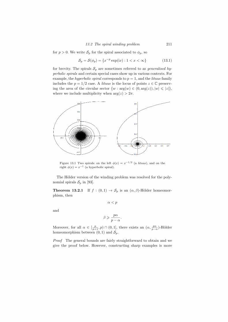
13.2 The spiral winding problem 211
for p > 0. We write Sp for the spiral associated to φp, so
Sp = S(φp) = x−p exp(ix) : 1 < x <∞ (13.1)
for brevity. The spirals Sp are sometimes referred to as generalised hy-
perbolic spirals and certain special cases show up in various contexts. For
example, the hyperbolic spiral corresponds to p = 1, and the lituus family
includes the p = 1/2 case. A lituus is the locus of points z ∈ C preserv-
ing the area of the circular sector w : arg(w) ∈ (0, arg(z)), |w| 6 |z|,where we include multiplicity when arg(z) > 2π.
Figure 13.1 Two spirals: on the left φ(x) = x−1/2 (a lituus), and on the
right φ(x) = x−1 (a hyperbolic spiral).
The Holder version of the winding problem was resolved for the poly-
nomial spirals Sp in [93].
Theorem 13.2.1 If f : (0, 1) → Sp is an (α, β)-Holder homeomor-
phism, then
α < p
and
β >pα
p− α.
Moreover, for all α ∈ [ pp+1 , p) ∩ (0, 1], there exists an (α, pα
p−α )-Holder
homeomorphism between (0, 1) and Sp.
Proof The general bounds are fairly straightforward to obtain and we
give the proof below. However, constructing sharp examples is more
212 Applications in embedding theory
involved but can be achieved using the map gt : (0, 1)→ Sp given by
gt(x) = xtp exp(i/xt)
where
t =α
p− α.
To obtain the bounds, decompose Sp into the disjoint union of ‘full
turns’
Sp =⋃k>1
Skp
where
Skp = x−p exp(ix) : 1 + 2π(k − 1) < x 6 1 + 2πk (13.2)
for each integer k > 1. Also, given a homeomorphism f : (0, 1) → Sp,we decompose (0, 1) into the corresponding half-open intervals
Ik = f−1(Skp ). (13.3)
It is convenient to extend f continuously such that the domain includes
0 and 1 and we assume without loss of generality that f(0) = 0. We have
1
8pk−p 6 |Skp | = |f(Ik)| 6 C|Ik|α (13.4)
where C > 1 is the constant coming from the Holder condition on f , see
(3.10). Therefore
1 =
∞∑k=1
|Ik| > 1
8p/αC1/α
∞∑k=1
k−p/α (13.5)
which forces α < p.
For each integer l > 1, let
xl =
∞∑k=l
|Ik|
as in Figure 13.2. Combining this with (13.4) and (13.5) yields
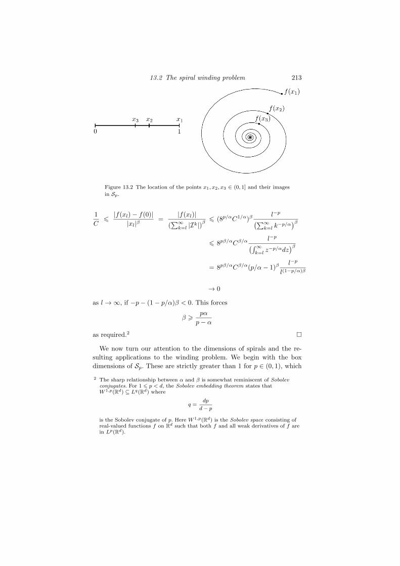
13.2 The spiral winding problem 213
Figure 13.2 The location of the points x1, x2, x3 ∈ (0, 1] and their images
in Sp.
1
C6|f(xl)− f(0)||xl|β
=|f(xl)|
(∑∞k=l |Ik|)
β6 (8p/αC1/α)β
l−p(∑∞k=l k
−p/α)β
6 8pβ/αCβ/αl−p(∫∞
k=lz−p/αdz
)β= 8pβ/αCβ/α(p/α− 1)β
l−p
l(1−p/α)β
→ 0
as l→∞, if −p− (1− p/α)β < 0. This forces
β >pα
p− α
as required.2
We now turn our attention to the dimensions of spirals and the re-
sulting applications to the winding problem. We begin with the box
dimensions of Sp. These are strictly greater than 1 for p ∈ (0, 1), which
2 The sharp relationship between α and β is somewhat reminiscent of Sobolevconjugates. For 1 6 p < d, the Sobolev embedding theorem states thatW 1,p(Rd) ⊆ Lq(Rd) where
q =dp
d− p
is the Sobolev conjugate of p. Here W 1,p(Rd) is the Sobolev space consisting ofreal-valued functions f on Rd such that both f and all weak derivatives of f arein Lp(Rd).
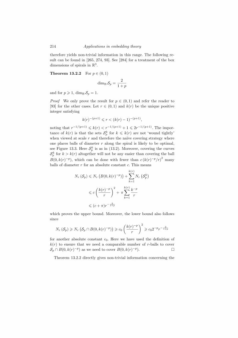
214 Applications in embedding theory
therefore yields non-trivial information in this range. The following re-
sult can be found in [265, 274, 93]. See [284] for a treatment of the box
dimensions of spirals in R3.
Theorem 13.2.2 For p ∈ (0, 1)
dimB Sp =2
1 + p
and for p > 1, dimB Sp = 1.
Proof We only prove the result for p ∈ (0, 1) and refer the reader to
[93] for the other cases. Let r ∈ (0, 1) and k(r) be the unique positive
integer satisfying
k(r)−(p+1) 6 r < (k(r)− 1)−(p+1),
noting that r−1/(p+1) 6 k(r) < r−1/(p+1) + 1 6 2r−1/(p+1). The impor-
tance of k(r) is that the sets Skp for k 6 k(r) are not ‘wound tightly’
when viewed at scale r and therefore the naıve covering strategy where
one places balls of diameter r along the spiral is likely to be optimal,
see Figure 13.3. Here Skp is as in (13.2). Moreover, covering the curves
Skp for k > k(r) altogether will not be any easier than covering the ball
B(0, k(r)−p), which can be done with fewer than c (k(r)−p/r)2
many
balls of diameter r for an absolute constant c. This means
Nr (Sp) 6 Nr(B(0, k(r)−p)
)+
k(r)∑k=1
Nr(Skp)
6 c
(k(r)−p
r
)2
+ π
k(r)∑k=1
k−p
r
6 (c+ π)r−2
1+p
which proves the upper bound. Moreover, the lower bound also follows
since
Nr (Sp) > Nr(Sp ∩B(0, k(r)−p)
)> c0
(k(r)−p
r
)2
> c02−pr−2
1+p
for another absolute constant c0. Here we have used the definition of
k(r) to ensure that we need a comparable number of r-balls to cover
Sp ∩B(0, k(r)−p) as we need to cover B(0, k(r)−p).
Theorem 13.2.2 directly gives non-trivial information concerning the
13.2 The spiral winding problem 215
Figure 13.3 An efficient cover for part of a spiral which is not wound as
tightly as the covering scale.
winding problem: if f : (0, 1) → Sp is an onto α-Holder map and p ∈(0, 1), then
α 6p+ 1
2< 1 (13.6)
and therefore f cannot be Lipschitz.
Next we consider the Assouad spectrum. The following result was
proved in [93], although the case when p ∈ (0, 1) is derivable from [111,
Theorem 7.2], which also included more general sub-exponential spirals.
Note that for p 6 1, the Assouad spectrum is given by the general upper
bound from Lemma 3.4.4 but, for p > 1, it is not.
Theorem 13.2.3 For p ∈ (0, 1) and θ ∈ (0, 1),
dimθA Sp = min
2
(1 + p)(1− θ), 2
and, for p > 1 and θ ∈ (0, 1),
dimθA Sp = min
1 +
θ
p(1− θ), 2
.
Proof We prove the result for p > 1, and refer the reader to [93] for the
p ∈ (0, 1] case. It suffices to consider 0 < θ < p1+p since, for θ′ = p
1+p ,
1 +θ′
p(1− θ′)= 2,
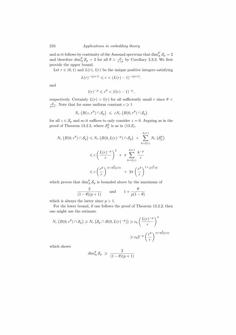
216 Applications in embedding theory
and so it follows by continuity of the Assouad spectrum that dimθ′
A Sp = 2
and therefore dimθA Sp = 2 for all θ > p
1+p by Corollary 3.3.3. We first
provide the upper bound.
Let r ∈ (0, 1) and L(r), l(r) be the unique positive integers satisfying
L(r)−(p+1) 6 r < (L(r)− 1)−(p+1).
and
l(r)−p 6 rθ < (l(r)− 1)−p,
respectively. Certainly L(r) > l(r) for all sufficiently small r since θ <pp+1 . Note that for some uniform constant c > 1
Nr(B(z, rθ) ∩ Sp
)6 cNr
(B(0, rθ) ∩ Sp
)for all z ∈ Sp and so it suffices to only consider z = 0. Arguing as in the
proof of Theorem 13.2.2, where Skp is as in (13.2),
Nr(B(0, rθ) ∩ Sp
)6 Nr
(B(0, L(r)−p) ∩ Sp
)+
L(r)∑k=l(r)
Nr(Skp)
6 c
(L(r)−p
r
)2
+ π
L(r)∑k=l(r)
k−p
r
6 c
(rθ
r
) 2(1−θ)(p+1)
+ 2π
(rθ
r
)1+ θp(1−θ)
which proves that dimθA Sp is bounded above by the maximum of
2
(1− θ)(p+ 1)and 1 +
θ
p(1− θ)which is always the latter since p > 1.
For the lower bound, if one follows the proof of Theorem 13.2.2, then
one might use the estimate
Nr(B(0, rθ) ∩ Sp
)> Nr
(Sp ∩B(0, L(r)−p)
)> c0
(L(r)−p
r
)2
> c02−p(rθ
r
) 2(1−θ)(p+1)
which shows
dimθA Sp >
2
(1− θ)(p+ 1)
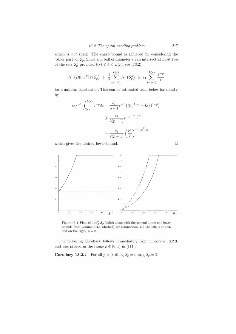
13.2 The spiral winding problem 217
which is not sharp. The sharp bound is achieved by considering the
‘other part’ of Sp. Since any ball of diameter r can intersect at most two
of the sets Skp provided l(r) 6 k 6 L(r), see (13.2),
Nr(B(0, rθ) ∩ Sp
)>
1
2
L(r)∑k=l(r)
Nr(Skp)
> c1
L(r)∑k=l(r)
k−p
r
for a uniform constant c1. This can be estimated from below for small r
by
c1r−1
∫ L(r)
l(r)
z−pdz =c1
p− 1r−1
(l(r)1−p − L(r)1−p)
>c1
2(p− 1)r−1− θ(1−p)p
=c1
2(p− 1)
(rθ
r
)1+ θp(1−θ)
which gives the desired lower bound.
Figure 13.4 Plots of dimθA Sp (solid) along with the general upper and lower
bounds from Lemma 3.4.4 (dashed) for comparison. On the left, p = 1/2,
and on the right, p = 2.
The following Corollary follows immediately from Theorem 13.2.3,
and was proved in the range p ∈ (0, 1) in [111].
Corollary 13.2.4 For all p > 0, dimA Sp = dimqA Sp = 2.
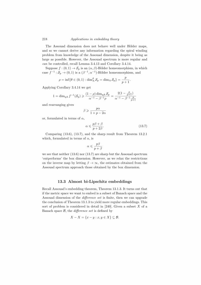
218 Applications in embedding theory
The Assouad dimension does not behave well under Holder maps,
and so we cannot derive any information regarding the spiral winding
problem from knowledge of the Assouad dimension, despite it being as
large as possible. However, the Assouad spectrum is more regular and
can be controlled, recall Lemma 3.4.13 and Corollary 3.4.14.
Suppose f : (0, 1)→ Sp is an (α, β)-Holder homeomorphism, in which
case f−1 : Sp → (0, 1) is a (β−1, α−1)-Holder homeomorphism, and
ρ = infθ ∈ (0, 1) : dimθA Sp = dimA Sp =
p
p+ 1.
Applying Corollary 3.4.14 we get
1 = dimqA f−1(Sp) >
(1− ρ) dimqA Spα−1 − β−1ρ
=2(1− p
p+1 )
α−1 − β−1 pp+1
and rearranging gives
β >pα
1 + p− 2α
or, formulated in terms of α,
α 6pβ + β
p+ 2β. (13.7)
Comparing (13.6), (13.7), and the sharp result from Theorem 13.2.1
which, formulated in terms of α, is
α 6pβ
p+ β
we see that neither (13.6) nor (13.7) are sharp but the Assouad spectrum
‘outperforms’ the box dimension. However, as we relax the restrictions
on the inverse map by letting β → ∞, the estimates obtained from the
Assouad spectrum approach those obtained by the box dimension.
13.3 Almost bi-Lipschitz embeddings
Recall Assouad’s embedding theorem, Theorem 13.1.3. It turns out that
if the metric space we want to embed is a subset of Banach space and the
Assouad dimension of the difference set is finite, then we can upgrade
the conclusion of Theorem 13.1.3 to yield more regular embeddings. This
sort of problem is considered in detail in [240]. Given a subset X of a
Banach space B, the difference set is defined by
X −X = x− y : x, y ∈ X ⊆ B.
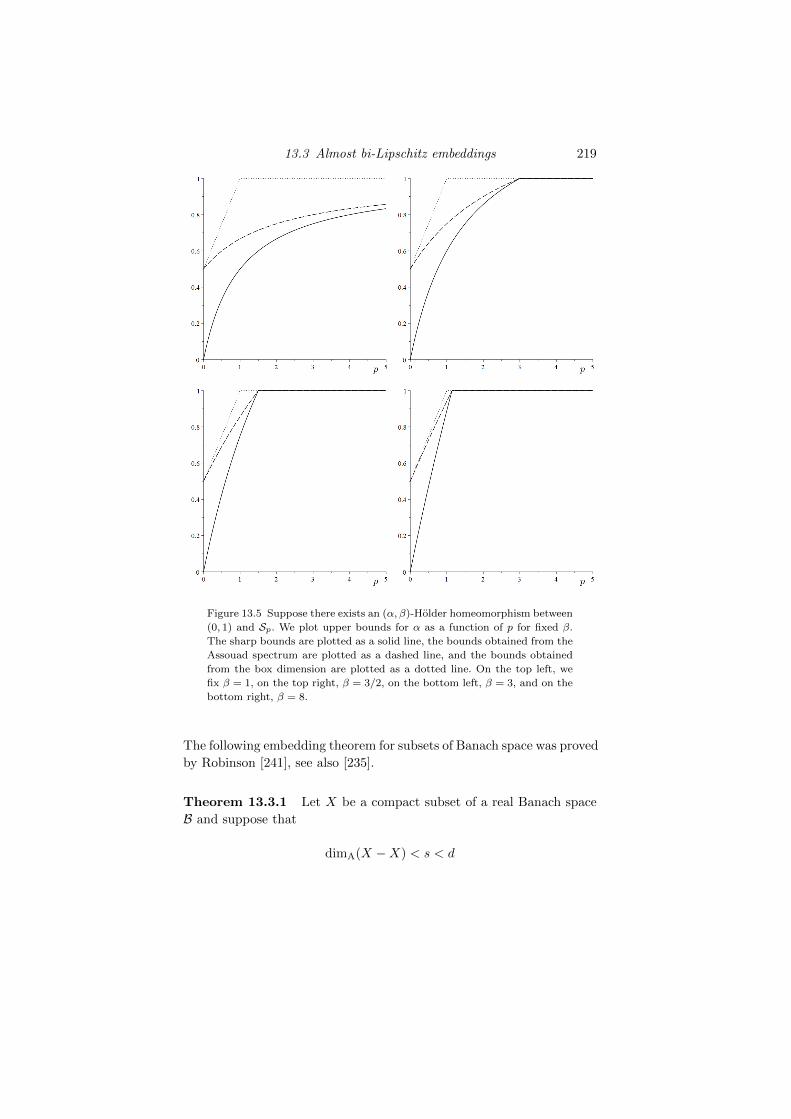
13.3 Almost bi-Lipschitz embeddings 219
Figure 13.5 Suppose there exists an (α, β)-Holder homeomorphism between
(0, 1) and Sp. We plot upper bounds for α as a function of p for fixed β.
The sharp bounds are plotted as a solid line, the bounds obtained from the
Assouad spectrum are plotted as a dashed line, and the bounds obtained
from the box dimension are plotted as a dotted line. On the top left, we
fix β = 1, on the top right, β = 3/2, on the bottom left, β = 3, and on the
bottom right, β = 8.
The following embedding theorem for subsets of Banach space was proved
by Robinson [241], see also [235].
Theorem 13.3.1 Let X be a compact subset of a real Banach space
B and suppose that
dimA(X −X) < s < d
220 Applications in embedding theory
with d ∈ N and
γ >d+ 1
d− s.
Then there exists a linear map f : B → Rd which is injective and γ-
almost bi-Lipschitz on X; that is, there exists c, ρ > 0 such that
c−1 ‖x− y‖| log ‖x− y‖|γ
6 |f(x)− f(y)| 6 c‖x− y‖
for all x, y ∈ X with ‖x− y‖ 6 ρ.
In fact, this theorem can be strengthened in several ways, for example
to almost homogeneous X−X and the existence of the embedding f can
be upgraded to a generic statement, see [240, Theorem 9.18]. Note that
the difference set X−X is an orthogonal projection, see Section 10.2, of
the product X×X and if dimAX <∞, then dimAX×X = 2 dimAX <
∞ by results in Section 10.1. However, despite orthogonal projections
being Lipschitz, the Assouad dimension of X − X may be larger than
that of X × X. In fact, [240, Lemma 9.12] constructs an example of a
set X in a Banach space such that dimAX = 0 but dimA(X −X) =∞.
This highlights the fact that the assumption that the difference set is
doubling in Theorem 13.3.1 is much stronger than the assumption that
X is doubling in Theorem 13.1.3. Then again, the conclusion that there is
a linear almost bi-Lipschitz embedding into Euclidean space is stronger
than the conclusion of Theorem 13.1.3 that every snowflaking embeds
via a bi-Lipschitz map.
Margaris [199, 200] later observed that the assumption that X − Xis doubling in Theorem 13.3.1 can be weakened in a meaningful way. In
fact, all that is needed is that X−X be ‘doubling near the origin’. Given
s > 0, we say X −X is s-doubling near the origin if there exists C > 1
such that for all 0 < r < R
Nr
(B(0, R) ∩ (X −X)
)6 C
(R
r
)s.
Theorem 13.3.2 Let X be a compact subset of a real Banach space
B and suppose X − X is s-doubling near the origin. Then, given any
γ > 1, there exists d ∈ N and a linear map f : B → Rd which is injective
and γ-almost bi-Lipschitz on X, that is, there exists c > 0, ρ > 0 such
that
c−1 ‖x− y‖| log ‖x− y‖|γ
6 |f(x)− f(y)| 6 c‖x− y‖
for all x, y ∈ X with ‖x− y‖ 6 ρ.
14
Applications in number theory
Given the origins and motivation for studying the Assouad dimension,
applications in embedding theory are perhaps expected. In this chap-
ter we discuss a collection of, perhaps more surprising, applications to
several distinct problems in number theory. In Section 14.1 we consider
the problem of finding arithmetic progressions inside sets of integers.
Recall, for example, the Erdos conjecture on arithmetic progressions, of
which the celebrated Green-Tao Theorem [123] is a special case. It turns
out that the Assouad dimension can be used to prove a weak ‘asymp-
totic’ version of this conjecture, first proved in [110]. In Section 14.2 we
discuss some problems in Diophantine approximation, the general area
concerned with how well real numbers can be approximated by rationals.
Here there is a well-developed connection between estimating the Haus-
dorff dimension of sets of badly approximable numbers and the lower
dimension, see work of Das, Fishman, Simmons and Urbanski [45]. Fi-
nally, in Section 14.3 we discuss an elegant use of the Assouad dimension
in problems of definability of the integers due to Hieronymi and Miller
[131].
14.1 Arithmetic progressions
Arithmetic progressions are among the most natural and well-studied
mathematical objects. Determining whether a given set contains an
arithmetic progression is often a subtle problem and has been stud-
ied in many contexts. Perhaps the most famous example of this is Sze-
meredi’s theorem, which states that a set of positive integers with pos-
itive upper natural density contains arbitrarily long arithmetic pro-
gressions. The upper natural density of a set X ⊆ Z+ is defined as
This material will be published by Cambridge University Press as Assouad Dimension and Fractal Geometryby Jonathan Fraser. This pre-publication version is free to view and download for personal use only.
Not for re-distribution, re-sale or use in derivative works. c© Jonathan Fraser 2020.
222 Applications in number theory
lim supn→∞#X∩1,...,n
n . The Erdos conjecture on arithmetic progres-
sions suggests that more should be true.
Conjecture 14.1.1 If X ⊆ Z+ is such that∑x∈X
1/x =∞,
then X should contain arbitrarily long arithmetic progressions.
This conjecture is sometimes attributed to Erdos-Turan, following
[62]. A celebrated breakthrough in this direction is the Green-Tao theo-
rem [123], which asserts that the primes contain arbitrarily long arith-
metic progressions. Recall that the reciprocals of the primes form a di-
vergent series, and so this is a special case of the Erdos conjecture. It
turns out that the Assouad dimension is intimately related to ‘approx-
imate’ arithmetic structure, and in this section we show how it can be
used to prove an approximate version of the Erdos conjecture, following
[110].
An arithmetic progression of length k > 1 and gap size ∆ > 0 is a set
of the form
x, x+ ∆, x+ 2∆, . . . , x+ (k − 1)∆,
for some x ∈ R, that is, a collection of k points each separated from the
next by a common distance ∆. We consider the following weakening of
the property of containing arithmetic progressions, which was introduced
and studied in [110, 107].
Definition 14.1.2 A set of positive integers X ⊆ Z+ gets arbitrarily
close to arbitrarily long arithmetic progressions if, for all k ∈ N and
ε > 0, there exists an arithmetic progression P of length k and gap size
∆ > 0 such that
supp∈P
infx∈X|p− x| 6 ε∆.
This definition should be understood as saying that, for arbitrarily
large k and arbitrarily small ε > 0, X gets within ε of an arithmetic
progression of length k. The fact that ε∆ appears instead of ε is the
necessary normalization. This is based on the observation that all arith-
metic progressions of length k are essentially the same: they are all equal
to 1, 2, . . . , k upon rescaling and translation.
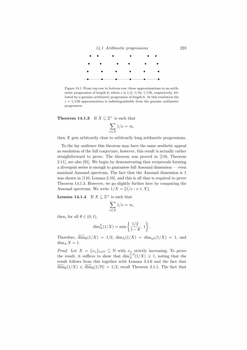
14.1 Arithmetic progressions 223
Figure 14.1 From top row to bottom row: three approximations to an arith-
metic progression of length 6, where ε is 1/3, 1/10, 1/150, respectively, fol-
lowed by a genuine arithmetic progression of length 6. At this resolution the
ε = 1/150 approximation is indistinguishable from the genuine arithmetic
progression.
Theorem 14.1.3 If X ⊆ Z+ is such that∑x∈X
1/x =∞,
then X gets arbitrarily close to arbitrarily long arithmetic progressions.
To the lay audience this theorem may have the same aesthetic appeal
as resolution of the full conjecture, however, this result is actually rather
straightforward to prove. The theorem was proved in [110, Theorem
2.11], see also [91]. We begin by demonstrating that reciprocals forming
a divergent series is enough to guarantee full Assouad dimension — even
maximal Assouad spectrum. The fact that the Assouad dimension is 1
was shown in [110, Lemma 2.10], and this is all that is required to prove
Theorem 14.1.3. However, we go slightly further here by computing the
Assouad spectrum. We write 1/X = 1/x : x ∈ X.
Lemma 14.1.4 If X ⊆ Z+ is such that∑x∈X
1/x =∞,
then, for all θ ∈ (0, 1),
dimθA(1/X) = min
1/2
1− θ, 1
.
Therefore, dimB(1/X) = 1/2, dimA(1/X) = dimqA(1/X) = 1, and
dimAX = 1.
Proof Let X = xnn∈N ⊆ N with xn strictly increasing. To prove
the result, it suffices to show that dim1/2A (1/X) > 1, noting that the
result follows from this together with Lemma 3.4.6 and the fact that
dimB(1/X) 6 dimB(1/N) = 1/2, recall Theorem 2.1.1. The fact that
224 Applications in number theory
dimAX = 1 follows since the Assouad dimension is preserved under the
inversion x 7→ 1/x, see [192, Theorem A.10 (1)].
In order to reach a contradiction, suppose that this is false, that is,
dim1/2A (1/X) < s < 1 for some s. It follows that there exists C > 0 such
that, for all integer k > 0,
N4−k(B(0, 2−k) ∩ 1/X
)6 C
(2−k
4−k
)s= C2ks.
If xn, xn+1 6 2k+1 for some k, then
1/xn − 1/xn+1 > 4−(k+1)
and so no open set of diameter 4−k can cover the reciprocals of more
than four distinct points in Xk := X ∩ [2k, 2k+1]. It follows that
|Xk| 6 4N4−k(B(0, 2−k) ∩ 1/X
)6 4C 2ks.
Therefore∑x∈X
1/x 6∞∑k=0
∑n:xn∈Xk
1/xn 6∞∑k=0
|Xk|2−k 6 4C
∞∑k=0
2(s−1)k < ∞,
a contradiction.
Having full Assouad dimension is a strong property, which, in partic-
ular, guarantees that [0, 1] is a weak tangent to X by Theorem 5.1.5.
This is enough information to approximate arithmetic structure.
Lemma 14.1.5 If [0, 1] is a weak tangent to X ⊆ Z+, then X gets
arbitrarily close to arbitrarily long arithmetic progressions.
Proof Let k > 1 be an integer and ε ∈ (0, 1). Since [0, 1] is a weak
tangent to X we can find an interval [n, n + k∆] for integers n,∆ > 1
such that
dH((k∆)−1[n, n+ k∆] ∩X − (k∆)−1n, [0, 1]
)6 ε/k
and therefore, upon rescaling and translating,
dH ([n, n+ k∆] ∩X, [n, n+ k∆]) 6 ε∆.
It follows that for each p ∈ P = n, n + ∆, n + 2∆, . . . , n + k∆ there
must exist a point x ∈ X such that |p − x| 6 ε∆, which proves the
result.
14.2 Diophantine approximation 225
Theorem 14.1.3 then follows from Lemma 14.1.4, Theorem 5.1.5, and
Lemma 14.1.5.
One may bound the Assouad dimension of a set above in terms of
how far away it is from approximating arithmetic progressions of a given
length. This is explored in detail in [107]. A quantitative improvement
of Theorem 14.1.3 was proved in [113] where the error o(∆) is replaced
with O(∆α) for any α ∈ (0, 1).
14.1.1 Discrete Kakeya sets
Lemma 14.1.5 shows that full Assouad dimension guarantees the exis-
tence of almost arithmetic progressions. This also holds for arbitrary
subsets of R and even in higher dimensions or finite dimensional Banach
spaces with ‘arithmetic progression’ replaced by ‘arithmetic patch’, see
[110]. Rather than looking for arithmetic patches, one may consider a
discrete analogue of the Kakeya problem, recall the (continuous) Kakeya
problem which was discussed in Section 11.2. For example, say K ⊆ Rdis a discrete approximate Kakeya set if for all ε > 0, k > 1 and direc-
tions e ∈ Sd−1, there exists an isometric embedding S : R→ Rd and an
arithmetic progressions P ⊆ R of length k and gap ∆ such that
supp∈P
infx∈K|S(p)− x| 6 ε∆
and S(R) is in direction e. We say an isometric embedding V ⊆ Rdof R is in direction e ∈ Sd−1 if V is a translate of the span of e. One
may ask, see [107, 245], whether or not being a discrete approximate
Kakeya set guarantees full Assouad dimension, that is, dimAK = d.
However, Saito [245] proved that this is false. In fact, Saito constructed
a compact discrete approximate Kakeya set K ⊆ Rd with dimAK = 1.
This is clearly sharp, since such sets must have a line segment as a weak
tangent.
14.2 Diophantine approximation
Diophantine approximation concerns how well real numbers can be ap-
proximated by rationals. One of the fundamental results is Dirichlet’s
theorem, which states that for all x ∈ Rd there exist infinitely many
p = (p1, . . . , pd) ∈ Zd and q ∈ N such that
‖x− p/q‖ < 1
q1+1/d(14.1)
226 Applications in number theory
where ‖ · ‖ is the supremum norm on Rd. Importantly, the entries in
the rational approximants p/q share a common denominator q ∈ Nwhich quantifies the level of approximation. Certain numbers can be
approximated much better than (14.1), but others cannot. The badly
approximable numbers are the collection of points x ∈ Rd such that
there is a constant c > 0 such that for all p = (p1, . . . , pd) ∈ Zd and
q ∈ N
‖x− p/q‖ > c
q1+1/d.
We denote the set of badly approximable numbers in Rd by BA(d). Some
authors include the rational numbers in BA(d) and others do not.1 Our
definition does not include them. The set BA(d) has been widely studied
in a variety of contexts. For example, it is known to be a set of zero d-
dimensional Lebesgue measure, but yet has full Hausdorff dimension, see
[248, Chapter III].
A common problem is to investigate the Hausdorff dimension of the
intersection of BA(d) with a given set. The hope is that, since BA(d) is
large from a dimension point of view, for a given set F ⊆ Rd
dimH F ∩ BA(d) = dimH F. (14.2)
This clearly cannot be true for arbitrary F . For example, take F =
Rd \ BA(d), which is a set of full Hausdorff dimension which does not
intersect BA(d) at all. Alternatively, take F = [0, 1]× 0 ⊆ R2. Again,
this set does not intersect BA(d) at all, which can be seen by applying
Dirichlet’s theorem in dimension 1. However, if F is somehow chosen in
a more ‘representative’ way, for example without deliberately trying to
avoid BA(d), then perhaps (14.2) will hold. This kind of problem has
been studied in two main contexts: when F is chosen to be a smooth
submanifold of Rd, or when F is a fractal set. The setting where F is
a manifold is motivated by work of Davenport [50]2 and has developed
into a broad research area, see [27] for some background. The second
context, where F is a fractal set, has gained a lot of attention in the
literature, see [45, 46, 171]. It is in this second context that a surprising
connection to the lower dimension has emerged.
1 Rational numbers are surprisingly hard to approximate by rational numbers(other than themselves).
2 In his 1964 paper, Davenport writes ‘I do not know whether there is a set of αwith the cardinal of the continuum such that the pair (α, α2) is badlyapproximable for simultaneous approximation’. Badziahin and Velani [10]answered this specific question in the affirmative.
14.2 Diophantine approximation 227
A set F ⊆ Rd is hyperplane diffuse if there exists β > 0 such that, for
all R ∈ (0, 1), x ∈ F and affine hyperplanes V ⊆ Rd,
B(x,R) ∩ F \ VβR 6= ∅
where Vε denotes the ε neighbourhood of V . The idea behind this concept
is that hyperplane diffuse sets uniformly avoid all affine hyperplanes at
all locations and scales. For example, any differentiable curve or smooth
manifold fails to be hyperplane diffuse. The following result was obtained
by Das, Fishman, Simmons and Urbanski [45, Corollary 2.6].
Theorem 14.2.1 If F ⊆ Rd is closed and hyperplane diffuse, then
dimH F ∩ BA(d) > dimL F.
We give the proof of Theorem 14.2.1 below, at least the part of the
proof where the lower dimension comes into play. There are two subtly
different ways of applying this result to concrete examples. Firstly, we
can look for hyperplane diffuse sets which already have equal Hausdorff
and lower dimension.
Corollary 14.2.2 If F ⊆ Rd is a self-similar set, a self-conformal set
or the limit set of a Kleinian group with no parabolic elements which,
in addition, is not contained in a hyperplane, then
dimH F ∩ BA(d) = dimH F.
One might also hope to apply this theorem directly to Kleinian limit
sets where kmin > δ(Γ), since here dimL L(Γ) = dimH L(Γ), see Theorem
9.3.3. However, digging into the proof of this fact in [92] demonstrates
that [0, 1]kmin (embedded in Rd) is a weak tangent to such sets, which
prevents them from being hyperplane diffuse if kmin < d. The theorem
does apply to Kleinian groups with parabolic elements if kmin = d, and
to any Fuchsian limit set.
The second approach is to upgrade the lower bound by replacing the
lower dimension with modified lower dimension. Although here one must
be careful that the subsets of F which are used to witness the modified
lower dimension are themselves hyperplane diffuse. One then looks for
sets with equal modified lower and Hausdorff dimension, which are more
common and include Bedford-McMullen carpets, for example, see Sec-
tion 8.3.
228 Applications in number theory
Corollary 14.2.3 If F ⊆ R2 is a Bedford-McMullen carpet con-
structed such that at least two columns and at least two rows are used,
then
dimH F ∩ BA(d) = dimH F.
Proof This follows immediately from Theorem 14.2.1 and Lemma 8.3.7
together with the observation that the subsystems constructed in the
proof of Lemma 8.3.7 are hyperplane diffuse under the additional as-
sumptions regarding used columns and rows.
Before proving Theorem 14.2.1, we need to introduce Schmidt games,
which often play a role in Diophantine approximation. These games were
introduced by Schmidt in [247] and are played in a complete metric
space (X, d) . For us the metric space will always be a closed subset of
Euclidean space. The game is played by two players, Alice and Bob.
Given 0 < α, β < 1, Alice and Bob play the (α, β)-game as follows:
(i) Bob begins by choosing r0 > 0 and x0 ∈ X and we write B0 =
B (x0, r0) and rn = (αβ)nr0 for all n ∈ N.
(ii) On Alice’s nth turn, she chooses yn such that d (xn, yn) + αrn 6 rn.
(iii) On Bob’s (n+ 1)st turn, he chooses xn+1 such that d (yn, xn+1) +
αβrn 6 αrn.
(iv) The inequalities above ensure that the closed balls
Bn = B (xn, rn)
and
An = B(yn, αr(n−1)
)form an interlaced decreasing sequence
B0 ⊇ A1 ⊇ B1 ⊇ A2 ⊇ · · · ⊇ Bn ⊇ An+1 ⊇ Bn+1 ⊇ · · · , (14.3)
and hence intersect at a unique point which is called the outcome of
the game.
Given a set S ⊆ X, if Alice has a strategy guaranteeing that the outcome
lies in S, then S is called (α, β)-winning. If for some fixed α, the set S
is (α, β)-winning for all 0 < β < 1, then S is called α-winning. If S is
α-winning for some 0 < α < 1, then S is called winning.
We quote the following result from [45, Proposition 2.3] which follows
by piecing together results from [38].
14.2 Diophantine approximation 229
Lemma 14.2.4 Let F ⊆ Rd be closed and hyperplane diffuse. Then
BA(d) ∩ F is winning on F .
First, [38, Theorem 2.5] establishes that BA(d) is hyperplane absolute
winning, which just means winning for a different variant of Schmidt’s
game. Second, [38, Proposition 4.7] proves that if F is hyperplane dif-
fuse and E is hyperplane absolute winning on F , then E is winning on F .
Proof of Theorem 14.2.1. We follow the proof of [45, Proposition 2.5]. Let
s = dimL F , and ε > 0. Therefore there is a constant C > 0 such that,
for all x ∈ F , β ∈ (0, 1/4) and R ∈ (0, 1], we can find a 3βR-separated
subset of B(x, (1− β)R) ∩ F of size at least
N := Cβ−(s−ε).
Let α ∈ (0, 1) and β ∈ (0, 1/4) be chosen such that BA(d) ∩ F is (α, β)-
winning on F . We know such an α exists since BA(d)∩F is winning on
F by Lemma 14.2.4 and β can be arbitrarily small.
For each ball A = B(x,R), let yi(A) (for i = 1, . . . , N) be a 3βR-
separated subset and write fi(A) = B(yi(A), βR). Suppose Alice is play-
ing a winning strategy for the (α, β)-game such that the outcome of the
game always ends up in BA(d) ∩ F . In response to Alice playing the
ball An, Bob can play any of the balls fi(An), which are legal moves
by construction. Moreover, suppose Bob begins with an arbitrary ball
B0 = B(x0, 1). Since the balls fi(An) are pairwise disjoint, this array of
plausible strategies for Bob gives rise to a Cantor set
E =⋃
(i0,i1,... )∈1,...,NN
⋂n
fin(An)
of plausible outcomes for the game, all of which must lie in BA(d) ∩ F .
Let µ be the uniform measure on E chosen such that, for i ∈ 1, . . . , N,µ(fi(An)∩E) = N−n. Since the balls fi(An) have radius (αβ)n and are
separated by (αβ)n, there is a constant c > 0 such that for any r ∈ (0, 1)
and x ∈ Eµ(B(x, r)) 6 cr
logN− log(αβ)
which, by the mass distribution principle Lemma 3.4.2, shows that
dimHE >logN
− log(αβ)=
(s− ε) log β − logC
log β + logα→ (s− ε)
as β → 0. Letting ε → 0, proves dimH BA(d) ∩ F > dimHE > s =
dimL F .
230 Applications in number theory
Finally, we briefly highlight another connection between Diophantine
approximation and the lower dimension, this time of measures. Following
[28], a measure µ is said to be weakly absolutely α-decaying for α > 0 if
there exist constants C, r0 > 0 such that for all ε > 0
µ(B(x, εr)) 6 Cεαµ(B(x, r))
for all x ∈ supp(µ) and r 6 r0. It was proved in [140, Proposition 2.6]
that
dimL µ = supα > 0 : µ is weakly absolutely α-decaying.
In particular, there exists weakly absolutely α-decaying measures with
support equal to F if and only if dimL F > 0 by virtue of Theorem
4.1.3. In [28] the notion of weakly absolutely α-decaying was used to
study Diophantine properties of limit sets of Kleinian groups. For exam-
ple, [28, Corollary 1] proves that if Γ is a non-elementary, geometrically
finite Kleinian group and µ is a weakly absolutely α-decaying measure
supported on K ⊆ L(Γ), then K is µ-extremal. Here µ-extremal refers
to a Diophantine property which, roughly speaking, means that the µ
measure of the set of very well-approximable points is zero. In the Eu-
clidean setting x ∈ Rd is called very well-approximable if there exists
ε > 0 such that there exist infinitely many p = (p1, . . . , pd) ∈ Zd and
q ∈ N such that
‖x− p/q‖ < 1
q1+1/d+ε(14.4)
where ‖ · ‖ is the supremum norm on Rd. This should be compared with
(14.1). In the setting of limit sets of Kleinian groups, ‘approximation
by rationals’ is replaced by ‘approximation by Γ-orbits’; see [28] for the
details and [47, 48] for more variants on ‘decaying’ properties of measures
and application to Diophantine approximation.
14.3 Definability of the integers 231
14.3 Definability of the integers
In this section we very briefly remark upon an application of the Assouad
dimension in an area rather far from the topic of this book: definability
in first-order expansions of the real field. We made no attempt to make
this section self-contained and refer the reader to [54, 131, 196] for more
details and [137] for the necessary background in model theory. In what
follows R = (R, ·,+) denotes the field of real numbers.
In first order logic, the subsets of Rd which are definable in R are
the semialgebraic sets, that is, the sets which can be written as a fi-
nite union of sets expressed in terms of a finite collection of polynomial
equations or (strict) inequalities. In particular, the semialgebraic sets in
R are precisely the sets which are a finite union of singletons and open
intervals. Therefore, N is not definable in R. This is representative of
the simplicity or ‘tameness’ of R. More generally, and following [131],
we think of expansions R of R as being ‘tame’ if they do not define Nand ‘wild’ if they do define N as a first-order structure. This should be
thought of in the context of o-minimality, a notion which characterises
the simplest expansions. An expansion R of R is o-minimal if the only
definable subsets of R are the semialgebraic sets and, as such, expansions
which define N are certainly not o-minimal. The following theorem was
proved in [131, Theorem A] and uses the Assouad dimension to charac-
terise which expansions of R fail to define N and are therefore ‘tame’ in
the above sense.
Theorem 14.3.1 An expansion R of R does not define N if and only
if dimTE = dimAE for all images E of closed definable sets under
definable continuous functions.
Note here that a function is definable if its graph is a definable set.
One direction of the equivalence in Theorem 14.3.1 is straightforward
since dimA N = 1 > 0 = dimT N. The Assouad dimension is favoured
in this analysis (instead of upper box dimension, say), since it is the
largest available notion of metric dimension and therefore provides the
most striking result. However, beyond the aesthetic appeal, the fact that
the Assouad dimension appears specifically has useful consequences in
other definability questions, see [212] and [275].
Following [131], given a set E ⊆ R, R = (R, E) denotes a minimal
expansion which defines E and all of the definable sets in R. For example,
(R,N) necessarily defines all Borel sets, see [163, (37.6)]. This is yet
further evidence of the ‘wildness’ of expansions which define N: once you
232 Applications in number theory
have N you also have all Borel sets. Interesting further examples along
these lines include (R, 2−k : k ∈ N) which does not define N (this was
proved by van den Dries [53]) and (R, 2−√k : k ∈ N) which does define
N (by Theorem 14.3.1). It is a straightforward but worthwhile exercise
to verify that
dimA2−k : k ∈ N = dimT2−k : k ∈ N = 0,
but
dimA2−√k : k ∈ N = 1 > 0 = dimT2−
√k : k ∈ N.
15
Applications in probability theory
Understanding how the dimensions of sets change under distortion by a
random function is an old problem in dimension theory. There is a gen-
eral principle that ‘Brownian motion doubles dimension’, that is, given a
compact set F ⊆ R with Hausdorff dimension at most 1/2, the Hausdorff
dimension of F will almost surely double under distortion by Brownian
motion, see (15.1). Motivated by a series of ‘uniform dimension results’
by Kaufman [161] and others, Balka and Peres proved that this dimen-
sion doubling phenomenon can be made uniform over all Borel subsets
of a given set, provided the quasi-Assouad dimension of the given set is
small enough, see Theorem 15.1.1. In Section 15.2, we consider the As-
souad dimensions of sets and measures generated by random functions,
following [141, 140].
15.1 Uniform dimension results for fractionalBrownian motion
Brownian motion1 is a fundamental example of a random process and
gives rise to many interesting (random) fractals via graphs, images and
level sets. It can be characterised as the unique random function B :
[0,∞)→ R satisfying
(i) B(0) = 0
(ii) B is almost surely continuous
(iii) B has independent increments, that is, B(t1) − B(s1) and B(t2) −B(s2) are independent for 0 6 s1 < t1 < s2 < t2
1 Some authors refer to the precise mathematical formulation of this process as theWiener process, reserving the term Brownian motion to describe the trajectoryof a piece of pollen suspended in water.
This material will be published by Cambridge University Press as Assouad Dimension and Fractal Geometryby Jonathan Fraser. This pre-publication version is free to view and download for personal use only.
Not for re-distribution, re-sale or use in derivative works. c© Jonathan Fraser 2020.
234 Applications in probability theory
(iv) the increments are normally distributed with
B(t)−B(s) ∼ N (0, |s− t|).
Fractional Brownian motion Bα (with index α ∈ (0, 1)) is a natural
variant of Brownian motion.2 This process was introduced by Mandel-
brot and van Ness [198] and can be characterised as the unique random
function Bα : [0,∞)→ R satisfying
(i) Bα(0) = 0
(ii) Bα is a Gaussian process
(iii) Bα is almost surely continuous
(iv) Bα has stationary increments with the covariance condition
E(Bα(s)Bα(t)) = (|s|2α + |t|2α − |s− t|2α)/2
(v) the increments are normally distributed with
Bα(t)−Bα(s) ∼ N (0, |s− t|2α).
When α = 1/2, fractional Brownian motion recovers classical Brownian
motion and as α decreases the process becomes ‘more fractal’, see [1, 70,
214, 156] for more details. Many interesting dimension questions arise.
Given a fixed Borel set F ⊆ [0, 1], Kahane [156] proved that almost
surely
dimHBα(F ) = min
1,
dimH F
α
. (15.1)
In fact, Bα is almost surely γ-Holder for any γ ∈ (0, α) and so the upper
bound follows from (3.11). A similar result holds for packing dimension
but with dimH F replaced with the α-dimensional packing profile of F ,
see Section 10.2. This result is due to Xiao [277]. Higher dimensional
analogues of these results are also given in [156, 277].
An interesting and challenging problem is to try to obtain these results
uniformly ; that is, almost surely the conclusion holds for all Borel sets
F simultaneously. However, it is easy to see that this cannot be true
since the zero set of Bα, that is, the set
x ∈ [0, 1] : Bα(x) = 0
is known to have Hausdorff dimension 1 − α almost surely. Therefore,
almost surely there is always a Borel set with positive dimension which
gets mapped to a set with dimension 0 under Bα. Surprisingly, one can
2 α is often called the ‘Hurst parameter’ or ‘Hurst index’.
15.1 Uniform dimension results 235
obtain a uniform dimension result for planar Brownian motion, that is
B : R → R2 defined by B(x) = (B1(x), B2(x)) where B1 and B2 are
independent Brownian motions. It was proved by Kaufman [161] that
almost surely
dimH B(F ) = 2 dimH F and dimP B(F ) = 2 dimP F
simultaneously for all Borel sets F ⊆ [0, 1], see also [214]. Balka and Peres
[12] investigated the question of when a uniform result can be recovered
in the 1-dimensional setting, where a surprising and elegant connection
to the Assouad dimension was unearthed. The idea is to replace [0, 1]
with a ‘small enough’ set D ⊆ [0, 1] such that a uniform dimension result
can be obtained for all subsets of D.
Theorem 15.1.1 If D ⊆ [0, 1] satisfies dimqAD 6 α, then almost
surely
dimHBα(F ) =dimH F
α
simultaneously for all F ⊆ D.
Balka and Peres also obtain this result with Hausdorff dimension re-
placed by packing dimension and their result is stronger than stated
since they use a modification of the quasi-Assouad dimension, which is
bounded above by the quasi-Assouad dimension. In fact their notion of
dimension turns out to be sharp for the packing dimension problem.
First, they define the modified Assouad dimension by
dimMA F = limδ→1
inf
supihFi(δ) : F =
⋃i
Fi
where hF (δ) is the function used to define the quasi-Assouad dimen-
sion in Section 3.2. To get a better feel for this definition, notice the
similarity between this and how the upper box dimension is ‘modi-
fied’ in order to obtain the packing dimension, see (1.1). In particular,
dimP F 6 dimMA F 6 dimqA F . The following is [12, Theorem 1.8].
Theorem 15.1.2 For an analytic set D ⊆ [0, 1], the following are
equivalent:
(i) dimMAD 6 α
(ii) almost surely
dimPBα(F ) =dimP F
α
simultaneously for all F ⊆ D.
236 Applications in probability theory
Note the philosophical connection between this result and Corollary
10.2.8. Both results say that if the quasi-Assouad dimension is small
enough, then the dimension profile under consideration is maximal.
Many other related results are proved and discussed in [12]. Balka and
Peres specifically ask if dimMA F = dimH F for any self-similar set F ,
see [12, Problem 1.16]. This would follow from a positive answer to the
question of whether dimqA F = dimH F for every self-similar set F , see
Question 17.5.3.
15.2 Dimensions of random graphs
Another interesting random fractal arising from (fractional) Brownian
motion is the graph, defined by
G(Bα) = (x,Bα(x)) : x ∈ [0, 1].
This set is known to have Hausdorff, packing and box dimension almost
surely given by 2− α, see [1] or [70, Section 16.3]. It was shown in [141]
that the Assouad dimension of G(Bα) is almost surely 2 (independent
of α). Notice the parallel between this result and the dimension results
for Mandelbrot percolation, see Theorem 9.4.1. The fact that the graph
of classical Brownian motion has Assouad dimension 2 can be derived
from results in [43].
Howroyd [140, Theorem 2.5] proved that for all doubling measures µ
supported on [0, 1], the pushforward of µ onto the graph G(Bα) is almost
surely not doubling. By virtue of Theorem 4.1.3 the graph G(Bα) nec-
essarily supports doubling measures, but the result of Howroyd shows
that almost surely these measures cannot be the pushforward of a de-
terministic measure on [0, 1]. This is rather different from the Hausdorff
dimension case, where the pushforward of Lebesgue measure onto G(Bα)
is almost surely a measure of Hausdorff dimension 2−α, that is, a mea-
sure which realises the Hausdorff dimension of the graph.
16
Applications in functional analysis
In this final applications chapter, we consider a range of problems in
functional and harmonic analysis. In Section 16.1 we begin with a well-
established connection between the Assouad and lower dimensions and
Hardy inequalities, following work of Lehrback [186] and others. The ba-
sic connection is that conditions on a domain, in terms of the Assouad
and lower dimensions of the codomain, determine whether the domain
admits a Hardy inequality. In Section 16.2 we explore a different problem
involving maximal operators averaged over spheres, considered by An-
derson, Hughes, Roos and Seeger [4], where the Assouad dimension plays
a role in determining whether certain Lp improving estimates are satis-
fied. Moreover, the Assouad spectrum makes an appearance in examin-
ing the sharpness of the Assouad dimension results. Finally, in Section
16.3 we consider the relationship between Lp smoothness of measures
and the Assouad and lower spectra, following [109].
16.1 Hardy inequalities
Hardy’s inequality states that for a sequence of non-negative real num-
bers an and p > 1
∞∑n=1
(a1 + a2 + · · ·+ an
n
)p6
(p
p− 1
)p ∞∑n=1
apn.
Various continuous analogues of this inequality are known to hold. For
example, we say an open domain Ω ⊆ Rd admits a p-Hardy inequality if
there exists a constant C > 1 such that∫Ω
(|f(x)|d(x,Ωc)
)pdx 6 C
∫Ω
Lipx(f)pdx
This material will be published by Cambridge University Press as Assouad Dimension and Fractal Geometryby Jonathan Fraser. This pre-publication version is free to view and download for personal use only.
Not for re-distribution, re-sale or use in derivative works. c© Jonathan Fraser 2020.
238 Applications in functional analysis
for all Lipschitz f : Rd → R with compact support contained in Ω,
where d(x,Ωc) = infy/∈Ω |x − y| is the distance from x to the codomain
Ωc = Rd \ Ω and
Lipx(f) = supy 6=x
|f(x)− f(y)||x− y|
is the (upper) Lipschitz constant of f at x ∈ Rd. Often the family
of Lipschitz functions is replaced by smooth functions with compact
support, in which case Lipx(f) is replaced by |∇f(x)|.Not all domains admit a p-Hardy inequality and it turns out that the
Assouad and lower dimensions of the codomain play a key role. The
following result can be found in [186, Corollary 1.3].
Theorem 16.1.1 If Ω ⊆ Rd is an open set and either dimA Ωc < d−por Ωc is unbounded and dimL Ωc > d − p, then Ω admits a p-Hardy
inequality.
Theorem 16.1.1 follows as a corollary to a more general result con-
cerning weighted Hardy inequalities, which we do not consider here but
refer the reader to [186] for more information, including an extensive
bibliography. There are many other connections between the Assouad
dimension and inequalities in functional analysis. We refer the reader
to the survey [187] for more details but briefly mention a few highlights
here. Connections between the Assouad dimension and Sobolev inequali-
ties are considered in [189, 57]. In [188] it is established that (for subsets
of Euclidean space) the Assouad and Aikawa dimensions coincide, see [2].
This latter result connects the Assouad dimension to yet another fam-
ily of integral inequalities, see [188, Definition 3.2]. Finally, connections
between the Assouad dimension and Muckenhoupt weights are given in
[58], see also [187].
Returning to Theorem 16.1.1, it was proved in [174] that, for open
domains Ω ⊆ Rd, dimL Ωc > 0 is equivalent to Ω admitting a d-Hardy
inequality. We prove one direction of this equivalence to give some intu-
ition as to how the lower dimension plays a role.
Theorem 16.1.2 If Ω ⊆ Rd is an open domain with dimL Ωc = 0,
then Ω does not admit a d-Hardy inequality.
Proof Suppose dimL Ωc = 0, in which case Ωc is not uniformly perfect
by Theorem 13.1.2. Therefore, for an arbitrary κ ∈ (0, 1/2) which we fix,
we can find y ∈ Ωc and 0 < R < 1/d such that B(y,R) \B(y, κR) ⊆ Ω.
Consider f defined by f(x) = max1−|y−x|, 0 for x ∈ Ω and f(x) = 0
16.1 Hardy inequalities 239
otherwise. Then∫Ω
(|f(x)|d(x,Ωc)
)ddx >
∫B(y,R/2)\B(y,κR)
(1− |y − x||x− y|
)ddx
=
∫B(0,R/2)\B(0,κR)
(1− |x||x|
)ddx
= ωd
∫ R/2
κR
(1− xx
)dxd−1dx (16.1)
where ωd > 0 is a constant depending only on d. This final equality is
via a standard reduction for the integral of a radial function in spherical
coordinates. Continuing, we may bound (16.1) below by
cd
∫ R/2
κR
x−1dx = cd log(1/(2κ))
for another constant cd > 0. In particular, this lower bound grows with-
out bound as κ→ 0. However,∫Ω
Lipx(f)ddx 6∫B(y,1)
dx <∞
is bounded independently of κ and so Ω does not admit a d-Hardy in-
equality.
Sometimes in the literature one can find analogues of Theorem 16.1.1
where the codomain Ωc is replaced by the boundary ∂Ω. Essentially, this
subtle difference only plays a role in the case of weighted Hardy inequal-
ities, which we do not discuss here. Note that if dimA ∂Ω < d− 1, then
Ωc = ∂Ω. To see this, observe that if Ωc has interior, then we can find
x, y ∈ Rd and r > 0 such that B(x, r) ⊆ Ω and B(y, r) ⊆ Ωc. Therefore,
the projection of ∂Ω onto the (d − 1)-dimensional hyperplane perpen-
dicular to the line joining x and y has non-empty interior, which forces
dimH ∂Ω > d − 1. In the context of Theorem 16.1.1, this observation
means that the alternative assumption that dimA ∂Ω < d− p is actually
equivalent to the (a priori stronger) assumption that dimA Ωc < d− p.The situation for lower dimension is more subtle, see [185].
240 Applications in functional analysis
16.2 Lp → Lq bounds for spherical maximal operators
A connection between the Assouad dimension and certain Lp → Lq
inequalities was established in [4]. Moreover, the Assouad spectrum is
used in order to examine sharpness of the results. Let d > 2 and f :
Rd → R be a locally integrable function and consider the average of f
over the sphere centred at x ∈ Rd with radius t > 0, that is,
Atf(x) =
∫f(x− ty)dσ
where σ is the normalised surface measure on the unit sphere in Rd.Given a set E ⊂ [1, 2], consider the maximal function
MEf(x) = supt∈E|Atf(x)|.
A common problem in harmonic analysis is to examine when a given
maximal function is an embedding from Lp into Lq for some p, q > 1.
The maximal function is called Lp improving if q > p. The following
Lp → Lq embedding result was proved in [4, Theorem 1].
Theorem 16.2.1 If (1/p, 1/q) ∈ Rd(E), then there is a constant C > 1
such that
‖MEf‖q 6 C‖f‖p
for all locally integrable f : Rd → R, where Rd(E) is a quadrilateral
region determined by dimAE, dimBE and d. Specifically, Rd(E) is the
interior of the convex hull of the four points:
(0, 0),
(d− 1
d− 1 + dimBE,
d− 1
d− 1 + dimBE
),
(d− dimBE
d− dimBE + 1,
1
d− dimBE + 1
),
and (d(d− 1)
d2 + 2 dimAE − 1,
d− 1
d2 + 2 dimAE − 1
)together with the diagonal line segment joining the first two points with
the first point included and the second point not included.
If d = 2 and dimAE > 1/2, then the proof of the above theorem is
not given in [4] but deferred to a later paper. The portion of Rd(E)
intersecting the diagonal p = q only depends on dimBE and d and this
connection with the upper box dimension was observed earlier [249].
16.3 Connection with Lp-norms 241
Theorem 16.2.1 is pretty close to being sharp and the sharpness was
investigated in [4, Theorem 2] using the Assouad spectrum. An example
of what is proved in [4] is that if E is such that
dimθAE = min
dimBE
1− θ,dimAE
, (16.2)
for all θ ∈ (0, 1) — that is, the Assouad spectrum of E is as large as
possible given the basic bounds in Lemma 3.4.4 — then the conclusion
of Theorem 16.2.1 is false for (1/p, 1/q) /∈ R(E). This can be interpreted
as showing that, for E satisfying (16.2), Theorem 16.2.1 is sharp up to
boundary points.
16.3 Connection with Lp-norms
There is a simple connection between the Assouad and lower spectra
and Lp norms, which was observed in [109]. Recall a measure µ on R is
absolutely continuous if all Lebesgue null sets are given zero µ measure.
If µ is absolutely continuous, then there is a Lebesgue integrable function
f , the density or Radon-Nikodym derivative, such that
µ(E) =
∫E
f(x) dx
for all Borel sets E. Given p > 1, we write Lp[0, 1] for the set of all
integrable functions g : [0, 1]→ R such that
‖g‖p :=
(∫ 1
0
g(x)p dx
)1/p
<∞
and we say µ ∈ Lp[0, 1] if µ is absolutely continuous with density f ∈Lp[0, 1]. As such, we are restricting our attention to measures with sup-
port in [0, 1]. We write f ∈ L−p[0, 1] if the set E = x ∈ [0, 1] : f(x) = 0is of Lebesgue measure zero and(∫
[0,1]\E1/f(x)pdx
)1/p
<∞,
and µ ∈ L−p[0, 1] if µ is absolutely continuous with density f ∈ L−p[0, 1].
The smoothness of µ can then be characterised by which Lp[0, 1] and
L−p[0, 1] spaces the measure belongs to — the larger the exponents p,
the smoother the measure is. Absolutely continuous measures on R im-
mediately satisfy dimH µ = 1 and it is natural to consider other notions
242 Applications in functional analysis
of dimension. The main result in [109, Theorem 2.1] establishes a sharp
one-way implication between smoothness and regularity, as characterised
by Lp properties and dimensions respectively. More general results than
those we present below are available in [109].
Theorem 16.3.1 Suppose µ is an absolutely continuous measure and
p1, p2 > 1 are such that µ ∈ Lp1 [0, 1]∩L−p2 [0, 1]. Then, for all θ ∈ (0, 1),
1− θp1 + p2
p1p2(1− θ)6 dimθ
L µ 6 dimθA µ 6 1 +
p1 + θp2
p1p2(1− θ).
Proof Recall Holder’s inequality for measurable functions f, g:
‖fg‖1 6 ‖f‖p‖g‖q,
where q = p/(p−1) is the Holder conjugate of p, and the reverse Holder
inequality, assuming in addition that f(x) 6= 0 for almost every x,
‖fg‖1 > ‖f‖−p‖g‖p/(p+1).
Here ‖f‖−p and ‖g‖p/(p+1) are not norms but convenient notation for
‖f‖−p =
(∫ 1
0
f(x)−pdx
)−1/p
and
‖g‖p/(p+1) =
(∫ 1
0
f(x)p/(p+1)dx
)(p+1)/p
.
Write f for the density of µ and χA for the indicator function on a set
A. Fix θ ∈ (0, 1), x ∈ supp(µ) and r ∈ (0, 1). Write q1 ∈ (1,∞) for the
Holder conjugate of p1. Applying Holder’s inequality and the reverse
Holder inequality,
µ(B(x, rθ))
µ(B(x, r))=‖fχB(x,rθ)‖1‖fχB(x,r)‖1
6‖f‖p1‖χB(x,rθ)‖q1
‖f‖−p2‖χB(x,r)‖p2/(1+p2)
=
(‖f‖p1‖f‖−p2
) (2rθ)1/q1
(2r)1+1/p2
=
(‖f‖p121/q1
‖f‖−p221+1/p2
)(rθ
r
) θ/q1−1−1/p2θ−1
,
which proves
dimθA µ 6
θ/q1 − 1− 1/p2
θ − 1= 1 +
p1 + θp2
p1p2(1− θ),
16.3 Connection with Lp-norms 243
as required. We omit the proof of the estimate for dimθL µ.
The inequalities in Theorem 16.3.1 are sharp, see [109], and estimates
are also available for p1, p2 =∞.
17
Future directions
In this chapter we briefly outline what we believe are some of the key
questions for the future and discuss some of the challenges which this
book has unearthed. We pose several open problems and, in order for
this list to remain up to date, an active list will be maintained on the
author’s personal homepage. In 2020 this page was hosted here: http:
//www.mcs.st-andrews.ac.uk/~jmf32/. The questions are presented
roughly in the same order as the relevant topics are encountered in the
book.
17.1 Finite stability of modified lower dimension
Modified lower dimension is known to be finitely stable in two situations:
when the sets in question are closed, see Lemma 3.4.10, or when the
sets in question are ‘properly separated’, see [111, Proposition 4.3]. The
general case remains unknown.
Question 17.1.1 Is it true that, for arbitrary E,F ⊆ Rd,
dimMLE ∪ F = max dimMLE, dimML F?
It follows from monotonicity and Lemma 3.4.10 that
max dimMLE, dimML F 6 dimMLE ∪ F6 max
dimMLE, dimML F
. (17.1)
This material will be published by Cambridge University Press as Assouad Dimension and Fractal Geometryby Jonathan Fraser. This pre-publication version is free to view and download for personal use only.
Not for re-distribution, re-sale or use in derivative works. c© Jonathan Fraser 2020.
17.2 Dimensions of measures 245
17.2 Dimensions of measures
Theorem 4.1.3 shows that one can approximate the Assouad and lower
dimensions of a compact set by the Assouad and lower dimensions of
doubling measures supported on the set (from above and below, respec-
tively). However, it is not always possible to find a measure with Assouad
dimension precisely equal to that of the set, see [152, 173]. The analogous
problem for lower dimension remains open, and was posed explicitly in
[152, Question 5.4].
Question 17.2.1 Does there exist a compact set F ⊆ Rd such that
dimL µ < dimL F for all doubling measures fully supported on F?
In the context of box dimension, it was proved in [75, Proposition 3.4]
that there exists a compact set F ⊆ Rd such that
dimBF < dimBµ
for all doubling measures supported on F . This should be compared
to Theorem 4.2.3. It was proved in [75, Theorem 2.1] that the word
‘doubling’ cannot be dropped here.
17.3 Weak tangents
The fact that the Assouad dimension is always realised by the Haus-
dorff dimension of a weak tangent is a powerful theoretical tool, recall
Theorem 5.1.3. It is natural to ask if this can be strengthened by re-
placing the Hausdorff dimension with something smaller. It is easy to
construct examples showing that the Hausdorff dimension cannot be re-
placed by the lower dimension (or even the lower spectrum) in general.
Consider the middle third Cantor set and add a point in the middle of
every complementary interval. The resulting set F is compact (in fact
it is an inhomogeneous self-similar set, see [87, 152, 255]) and it is a
short exercise to show that dimA F = log 2log 3 but that every weak tan-
gent has an isolated point. Therefore, all weak tangents E of F satisfy
dimLE = dimθLE = 0 for all θ ∈ (0, 1). However, it is not known if the
modified lower dimension can be used.
Question 17.3.1 Is it true that for all closed sets F ⊆ Rd there exists
a weak tangent E of F such that dimMLE = dimA F?
A slightly weaker version of this question would be to ask if there

246 Future directions
exist weak tangents with modified lower dimension arbitrarily close to
dimA F . On the other hand, a slightly stronger version of the question
would be to ask if there exists a weak tangent which contains an Ahlfors-
regular subset of dimension dimA F . An affirmative answer to the strong
version of the question would have powerful applications. For example,
it would allow Theorem 11.1.3 to be extended to the dimA F = 1 case,
see Question 17.9.1 below. This would follow by applying Lemma 11.1.5
and the main result of [225].
Given a closed set F ⊆ Rd, recall the set of Hausdorff dimensions
attained at the level of weak tangents is
∆(F ) = dimHE : E ∈ W(F ),
where W(F ) denotes the set of ‘reasonable’ weak tangents of F , see
Section 5.2. It is known that ∆(F ) always contains its maximum and
minimum and, subject to this constraint, any Fσ set can be realised
as ∆(F ) for some F . However, not much more is known about the set-
theoretic complexity of ∆(F ).
Question 17.3.2 Given a closed set F ⊆ Rd, is the set ∆(F ) always
analytic or Borel and, if so, does it always belong to a particular finite
Borel class?
It is certainly not true that for any set ∆ ⊆ [0, d] containing its
maximum and minimum there is a compact set F such that ∆(F ) = ∆.
This can be seen by a simple cardinality argument, since the collection of
possible ∆ has cardinality #P(R) (that is, the cardinality of the power
set of R), but the collection of possible choices for F has cardinality #R(that is, the cardinality of R), which is strictly smaller.
17.4 Further questions of measurability
Motivated by the discussion in Section 17.3, we note that a simpler mea-
surability question was considered in [88, 111]. It was shown that the
function dim : K(Rd)→ R is Borel measurable (even of Baire class pre-
cisely 2) if dim is the Assouad or lower dimension and K(Rd) is the set of
non-empty compact subsets of Rd equipped with the Hausdorff metric,
see (5.1). Similar measurability results hold for the Assouad and lower
spectra, see [111, Theorems 5.1 and 5.2]. For comparison, the Hausdorff
and upper and lower box dimensions were shown to be measurable (and
17.5 IFS attractors 247
of Baire class 2) in [208] but there it was also proved that the pack-
ing dimension is not measurable. It is not known if the modified lower
dimension is measurable, see [111, Question 9.4].
Question 17.4.1 Is the function dimML : K(Rd) → R Borel measur-
able? If so, does it belong to a particular Baire class?
17.5 IFS attractors
The Assouad and lower dimension are well-understood in the case of pla-
nar self-affine sets with a grid structure. Bedford-McMullen and Lalley-
Gatzouras type carpets were considered in [194], Baranski type carpets
were considered in [88], higher dimensional sponges in [97, 139, 45], and
restricted families of planar self-affine sets without a grid structure were
considered in [21, 101]. It seems the most natural examples to consider
next are either more general planar self-affine carpets without a grid
structure or higher dimensional versions of these sets. Alternatively, the
Assouad and lower spectra are not as well understood, even in the plane.
The following question is motivated by Theorem 8.4.1 proved in [21] as
well as the typical formula for the Assouad dimension of carpet type
self-affine sets.
Question 17.5.1 Let F ⊆ R2 be a self-affine set satisfying the SSC
and which is not self-similar. Does there always exist π ∈ G(1, 2) such
that
dimA F = dimA πF + maxx∈πF
dimA(π⊥ + x) ∩ F?
It is interesting to examine the relationship between the various dif-
ferent notions of dimension in a given setting. For a given class of
sets one can ask what relationships are possible between the dimen-
sions and spectra? For example, all the dimensions and spectra are
necessarily equal for Ahlfors regular sets. Interestingly, the configura-
tion dimL F < dimB F = dimA F is possible for self-affine carpets,
but not for self-similar sets (even with overlaps) and the configuration
dimL F = dimB F < dimA F is not possible for self-affine carpets, but
is possible for self-similar sets with overlaps. Roughly speaking, the rea-
son for this is as follows. The non-uniform scaling present in self-affine
carpets allows one to ‘spread’ the set out making certain locations easier
to cover and thus making the lower dimension drop. Whereas, one can
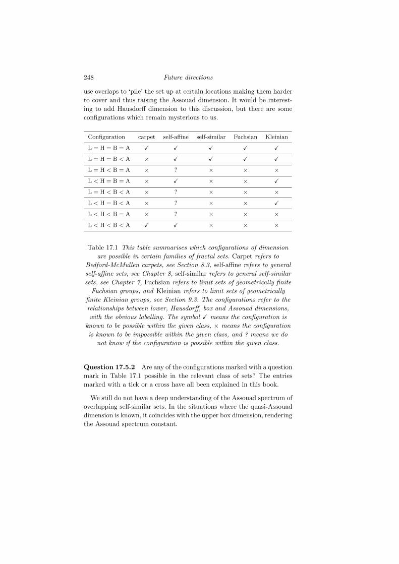
248 Future directions
use overlaps to ‘pile’ the set up at certain locations making them harder
to cover and thus raising the Assouad dimension. It would be interest-
ing to add Hausdorff dimension to this discussion, but there are some
configurations which remain mysterious to us.
Configuration carpet self-affine self-similar Fuchsian Kleinian
L = H = B = A X X X X X
L = H = B < A × X X X X
L = H < B = A × ? × × ×
L < H = B = A × X × × X
L = H < B < A × ? × × ×
L < H = B < A × ? × × X
L < H < B = A × ? × × ×
L < H < B < A X X × × ×
Table 17.1 This table summarises which configurations of dimension
are possible in certain families of fractal sets. Carpet refers to
Bedford-McMullen carpets, see Section 8.3, self-affine refers to general
self-affine sets, see Chapter 8, self-similar refers to general self-similar
sets, see Chapter 7, Fuchsian refers to limit sets of geometrically finite
Fuchsian groups, and Kleinian refers to limit sets of geometrically
finite Kleinian groups, see Section 9.3. The configurations refer to the
relationships between lower, Hausdorff, box and Assouad dimensions,
with the obvious labelling. The symbol X means the configuration is
known to be possible within the given class, × means the configuration
is known to be impossible within the given class, and ? means we do
not know if the configuration is possible within the given class.
Question 17.5.2 Are any of the configurations marked with a question
mark in Table 17.1 possible in the relevant class of sets? The entries
marked with a tick or a cross have all been explained in this book.
We still do not have a deep understanding of the Assouad spectrum of
overlapping self-similar sets. In the situations where the quasi-Assouad
dimension is known, it coincides with the upper box dimension, rendering
the Assouad spectrum constant.
17.6 Random sets 249
Question 17.5.3 Is it true that, for all self-similar sets F ⊆ Rd,
dimqA F = dimB F?
An affirmative answer to this question would also answer a question
posed by Balka and Peres [12, Problem 1.16], which asks the same ques-
tion but with quasi-Assouad dimension replaced by their modified As-
souad dimension (which is bounded above by quasi-Assouad dimension).
In all cases where the quasi-Assouad and Assouad dimensions are
both known for an attractor of an IFS satisfying the OSC or SSC, they
coincide. On the other hand, they are often distinct in the overlapping
case, recall Theorem 7.3.1, or in the random case, recall Theorems 9.4.1-
9.4.2.
Question 17.5.4 Does there exist a self-affine set F ⊆ Rd which
satisfies the SSC and is such that dimqA F < dimA F?
Note that the answer to this question is yes if one does not assume
separation conditions, for example, the self-similar sets from Theorem
7.2.1. Moreover, it is no if one replaces self-affine with self-similar or
self-conformal (whilst maintaining the SSC).
Theorem 6.3.1 proved that the lower spectrum of the attractor of a
non-trivial IFS of bi-Lipschitz contractions is always strictly positive,
at least for some range of θ. We do not know if the lower dimension is
necessarily strictly positive. Recall, it was proved in [278] that the lower
dimension of any self-affine set is strictly positive and the example (6.4)
on page 90 shows that the lower dimension can be zero if the contractions
are not bi-Lipschitz.
Question 17.5.5 Let F ⊆ Rd be the attractor of an IFS consisting
of bi-Lipschitz contractions and assume F is not a singleton. Is it true
that dimL F > 0?
17.6 Random sets
Recall Theorem 9.4.4 which established a dichotomy for determining
the almost sure value of dimφAM for different functions φ, where M is
the limit set of Mandelbrot percolation, see Sections 3.3.3 and 9.4. We
condition on non-extinction of M . The situation is understood when
log(R/φ(R))
log | logR|(17.2)
250 Future directions
either converges to 0 or diverges as R → 0, but otherwise remains un-
clear.
Question 17.6.1 Suppose (17.2) neither converges to 0 nor diverges.
Then what is the almost sure value of dimφAM?
Note that dimφAM may be expressed in terms of tail events (we only
care about small scale behaviour), and so there is an almost sure value
of dimφAM by Kolmogorov’s 0-1 law. Moreover, for any φ, the almost
sure value of dimφAM must be in the interval [s, d] where s is the almost
sure Hausdorff dimension of M and d is the ambient spatial dimension.
Question 17.6.2 Is it true that for all t ∈ [s, d], there exists φ such
that almost surely dimφAM = t?
17.7 General behaviour of the Assouad spectrum
An example was constructed in [111, Section 8] demonstrating that the
Assouad spectrum can be strictly decreasing on infinitely many disjoint
intervals accumulating at θ = 0. However, we believe this behaviour is
not possible at θ = 1.
Question 17.7.1 Is it true that for any set F ⊆ Rd, there exists
θF ∈ (0, 1) such that dimθA F is non-decreasing on the interval (θF , 1)?
Recall that dimθA F is often constant in a neighbourhood of θ = 1, but
may be strictly increasing in certain special cases, see Theorem 3.3.5.
We have seen that the Assouad spectrum can exhibit many different
features. However, for sets which exhibit a certain ‘rough homogene-
ity’, such as dynamical invariance or statistical self-similarity, then the
Assouad spectrum tends to take on one of two forms. It is either con-
stant (recall Mandelbrot percolation or self-similar sets with overlaps)
or consists of a convex increasing part followed by a constant part (recall
self-affine carpets, spirals, polynomial sequences). It turns out that there
is even more similarity between the examples in this latter situation than
meets the eye. Suppose the phase transition between the increasing and
constant parts of the spectrum occurs at θ = ρ ∈ (0, 1). Following some
non-trivial algebraic manipulation1, we find that for F a (non-uniform
fibre) Bedford-McMullen carpet (Theorem 8.3.3), a polynomial spiral
1 “but isn’t all algebraic manipulation trivial?” - Anon
17.7 General behaviour of the Assouad spectrum 251
(Theorem 13.2.3), or a polynomial sequence (Theorem 3.4.7),
dimθA F = min
dimB F +
(1− ρ)θ
(1− θ)ρ(dimqA F − dimB F ) , dimqA F
.
(17.3)
We note that in each of these examples dimqA F = dimA F but we chose
to use dimqA in the formula since it is perhaps more representative of
what is really going on. The formula (17.3) shows that in each of these
examples the Assouad spectrum is determined by the box dimension,
the (quasi-)Assouad dimension, and the phase transition ρ. It is per-
haps disappointing for an object with so many degrees of freedom to be
determined by such a small set of values, but we believe this is indica-
tive of the simplicity of these examples rather than the simplicity of the
Assouad spectrum as a concept. Lemma 3.4.4 guarantees that
ρ > 1− dimBF
dimqA F. (17.4)
For the polynomial sequences (17.4) is always an equality, for the poly-
nomial spirals (17.4) is an equality if and only if p 6 1, and for the
Bedford-McMullen carpets (17.4) is never an equality.
It seems from this observation that the phase transition ρ merits
deeper investigation. Indeed, in these three examples ρ is a constant
which holds particular geometric significance for the set in question,
capturing some fundamental scaling property. For carpets, the kth level
rectangles in the standard construction of F are of size m−k × n−k and
therefore ρ = logmlogn is the ‘logarithmic eccentricity’. For spirals, the kth
revolution, given by
x−p exp(ix) : 1 + 2π(k − 1) < x 6 1 + 2πk,
has diameter comparable to k−p, while the distance between the end
points (or, outer radius minus inner radius) is comparable to k−(p+1).
These are fundamental measurements considered in the winding prob-
lem, see [93], and measure how big the kth revolution is and how tightly
it is wound, respectively. Again the ‘logarithmic eccentricity’ is
log (k−p)
log(k−(p+1)
) =p
p+ 1= ρ.
It is probably naıve to expect (17.3) to be the ‘rule of thumb’ for sets
exhibiting ‘rough homogeneity’, but it would certainly be interesting to
identify other natural classes of set for which this formula holds for a
particular choice of ‘fundamental ratio’ ρ. Natural examples to consider
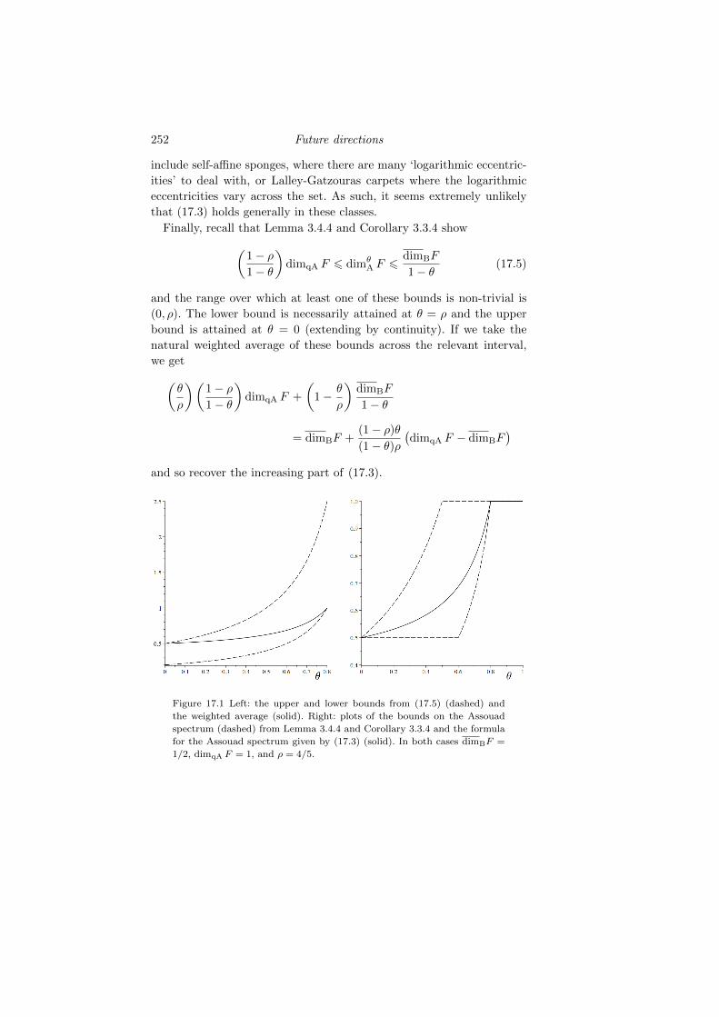
252 Future directions
include self-affine sponges, where there are many ‘logarithmic eccentric-
ities’ to deal with, or Lalley-Gatzouras carpets where the logarithmic
eccentricities vary across the set. As such, it seems extremely unlikely
that (17.3) holds generally in these classes.
Finally, recall that Lemma 3.4.4 and Corollary 3.3.4 show(1− ρ1− θ
)dimqA F 6 dimθ
A F 6dimBF
1− θ(17.5)
and the range over which at least one of these bounds is non-trivial is
(0, ρ). The lower bound is necessarily attained at θ = ρ and the upper
bound is attained at θ = 0 (extending by continuity). If we take the
natural weighted average of these bounds across the relevant interval,
we get(θ
ρ
)(1− ρ1− θ
)dimqA F +
(1− θ
ρ
)dimBF
1− θ
= dimBF +(1− ρ)θ
(1− θ)ρ(dimqA F − dimBF
)and so recover the increasing part of (17.3).
Figure 17.1 Left: the upper and lower bounds from (17.5) (dashed) and
the weighted average (solid). Right: plots of the bounds on the Assouad
spectrum (dashed) from Lemma 3.4.4 and Corollary 3.3.4 and the formula
for the Assouad spectrum given by (17.3) (solid). In both cases dimBF =
1/2, dimqA F = 1, and ρ = 4/5.
17.8 Projections 253
17.8 Projections
Theorem 10.2.1 establishes an almost sure lower bound for the Assouad
dimension of projections of sets in Rd onto k-dimensional subspaces.
Theorem 10.2.2 upgrades this fact in the case d = 2 and k = 1 by estab-
lishing that the lower bound in fact holds for all projections outside of
a set of exceptions of Hausdorff dimension 0. It is natural to ask about
the higher dimensional setting. One cannot hope for a 0-dimensional
set of exceptions in general. Suppose F is contained in a 1-dimensional
subspace V ⊆ Rd and consider projections of F onto k-dimensional sub-
spaces. Then there is a k(d−1−k)-dimensional family of k-dimensional
subspaces (those transversal to V ) onto which the projection of F is
singleton.
Question 17.8.1 Is it true that, for any non-empty set F ⊆ Rd and
1 6 k < d,
dimHπ ∈ G(k, d) : dimA πF < mink, dimA F 6 k(d− 1− k)?
There is also the question of possible refinements of the conclusion
that the Hausdorff dimension of the exceptional set is 0. The following
question was asked in [226], and there are obvious analogous questions
in higher dimensions.
Question 17.8.2 Is it true that, for any non-empty set F ⊆ R2,
dimPπ ∈ G(1, 2) : dimA πF < min1,dimA F = 0?
One could also consider different gauge functions to further refine the
Hausdorff dimension result.
Theorem 10.2.5 revealed that the function π 7→ dimA πF may realise
any upper semi-continuous function φ : G(1, 2) → [0, 1] upon careful
selection of a compact set F ⊆ R2. Note, however, that π 7→ dimA πF
is not necessarily upper semi-continuous (for example, consider a line
segment). On the other hand, π 7→ dimA πF cannot realise all functions
φ : G(1, 2) → [0, 1]. This can be seen by another simple cardinality
argument. The set of possible functions φ has cardinality #P(R) (that
is, the cardinality of the power set of R), but the collection of possible
choices for compact F has cardinality #R (that is, the cardinality of R),
which is strictly smaller. Recall the connection between this issue and
that following Question 17.3.2.
Question 17.8.3 Given a compact set F ⊆ R2, is the function π 7→dimA πF Borel measurable? If so, does it lie in a finite Borel class?
254 Future directions
17.9 Distance sets
The planar version of the distance set problem for Assouad dimension
was resolved in [90], but progress in higher dimensions so far is tied
to the Hausdorff dimension problem, which is still wide open. The first
question we ask is very concrete, and the second is a little more open
ended, motivated by the fact that the Assouad dimension problem is
‘ahead’ of the Hausdorff dimension problem in the plane.
Question 17.9.1 Is it true that if F ⊆ Rd with d > 3, then
dimAD(F ) >2
ddimA F?
Question 17.9.2 For sets F ⊆ Rd with d > 3, can we move the
Assouad dimension version of the distance set problem ‘ahead’ of the
Hausdorff or box dimension version? For example, can we prove that
dimA F > s guarantees dimAD(F ) = 1 for some s for which we do not
yet have the corresponding Hausdorff or box dimension result?
A popular variant of the distance set problem is to consider pinned
distance sets. Given F ⊆ Rd and x ∈ F , the pinned distance set (of F
at x) is defined by
Dx(F ) = |x− y| : y ∈ F.
Note that pinned distance sets are subsets of the distance set. Many
natural questions arise, but generally speaking if the distance set is large,
we expect there to be a large pinned distance set; or even many large
pinned distance sets, see [253]. For example, we can ask for a pinned
version of Theorem 11.1.3.
Question 17.9.3 Is it true that if F ⊆ R2 is a set with dimA F > 1,
then there exists x ∈ F such that dimADx(F ) = 1?
Finally, a more general question, which equally applies to any of the
Hausdorff, box, packing or Assouad dimensions.
Question 17.9.4 Let dim denote one of the Hausdorff, box, packing
or Assouad dimensions. Given s ∈ (0, d], what is
infdimD(F ) : dimF = s?
Is the function
s 7→ infdimD(F ) : dimF = s
independent of the specific choice of dim?
17.10 The Holder mapping problem and dimension 255
17.10 The Holder mapping problem and dimension
Motivated by the spiral winding problem discussed in Section 13.2, con-
sider the following general problem. Fix bounded sets X,Y ⊆ Rd which
are homeomorphic to each other, for example, the line segment (0, 1)
and the spiral Sp. First, ask if there exists a bi-Holder homeomorphism
between X and Y . If the answer to this is yes, then ask for sharp esti-
mates on the forward and backwards Holder exponents α and β. Second,
compute the dimensions and dimension spectra of X and Y and consider
the estimates on α and β which come directly from this information (by
applying results from Section 3.4.3, for example). It seems interesting
to develop a thorough understanding of how good this information is:
when do the sharp estimates come from dimension theory and when
do they not? Moreover, it would also be interesting to know which di-
mensions or dimension spectra generally provide better information. For
example, the polynomial spirals we considered in Section 13.2 provide
examples where sharp information is not provided by dimension the-
ory, and where the Assouad spectrum performs best. This discussion is
deliberately rather vague so that it can be applied in many situations.
Rather than get too hung up on a particular version of the problem, a
better overall strategy is to unearth general phenomena using elegant
examples.
17.11 Dimensions of graphs
One of the earliest examples of what is now known as a fractal is the
graph of the Weierstrass function. Discovered in 1872 by Carl Weier-
strass, it was the first example of a continuous real-valued function which
is nowhere differentiable.2 Given integer b > 2 and a ∈ (1/b, 1), the
Weierstrass function Wa,b : R→ R is defined by
Wa,b(x) =
∞∑n=0
an cos(2πbnx).
It was a long-standing open problem to compute the Hausdorff dimen-
sion of the graph of Wa,b, that is, the set3
G(Wa,b) = (x,Wa,b(x)) : x ∈ [0, 1],2 Bolzano had an example of such a function as early as 1830 but it was only
published posthumously in 1922.3 the domain is not important here, but it is convenient to assume it is bounded.
256 Future directions
see, for example, [32]. The conjecture was that the Hausdorff dimension
should equal
2 +log a
log b∈ (1, 2). (17.6)
This was resolved by Shen [251] in full generality and for certain ranges
of parameters a little earlier by Baranski, Barany and Romanowska [16].
The box and packing dimensions of the graph are also given by (17.6),
but this was known somewhat earlier, see for example [144]. We do not
know the Assouad or quasi-Assouad dimension of the graph, but there is
some heuristic evidence, provided by Yu, to suggest that it is not given
by (17.6) in general. More precisely, a related question was considered
by Yu [279] where the cosine function appearing in the definition of the
Weierstrass function is replaced by the ‘distance to the nearest integer’
function T : R → R given by T (x) = min|x − n| : n ∈ Z. The only
important difference here is that the smooth oscillations provided by cos
are replaced with sawtooth type oscillations. The resulting functions are
known as Takagi functions and are easier to handle than the Weierstrass
function, see the survey [3], and the Hausdorff, box and packing dimen-
sions are also known to be given by the formula (17.6). Yu showed that
the Assouad dimension of the graph of the Takagi function can exceed
the box dimension [279, Theorem 1.1]. He was able to bound the Assouad
dimension from below by 1 + 1/k if ab > 1 is the root of a Littlewood
polynomial of degree k − 1. Recall that a Littlewood polynomial is a
polynomial all of whose coefficients are ±1. In particular, fixing ab and
thus k, the box dimension of the graph can be made arbitrarily close to
1 by increasing b (and decreasing a accordingly).
Question 17.11.1 What are the Assouad dimensions, quasi-Assouad
dimensions, and Assouad spectra of the graphs of the Weierstrass and
Takagi functions?
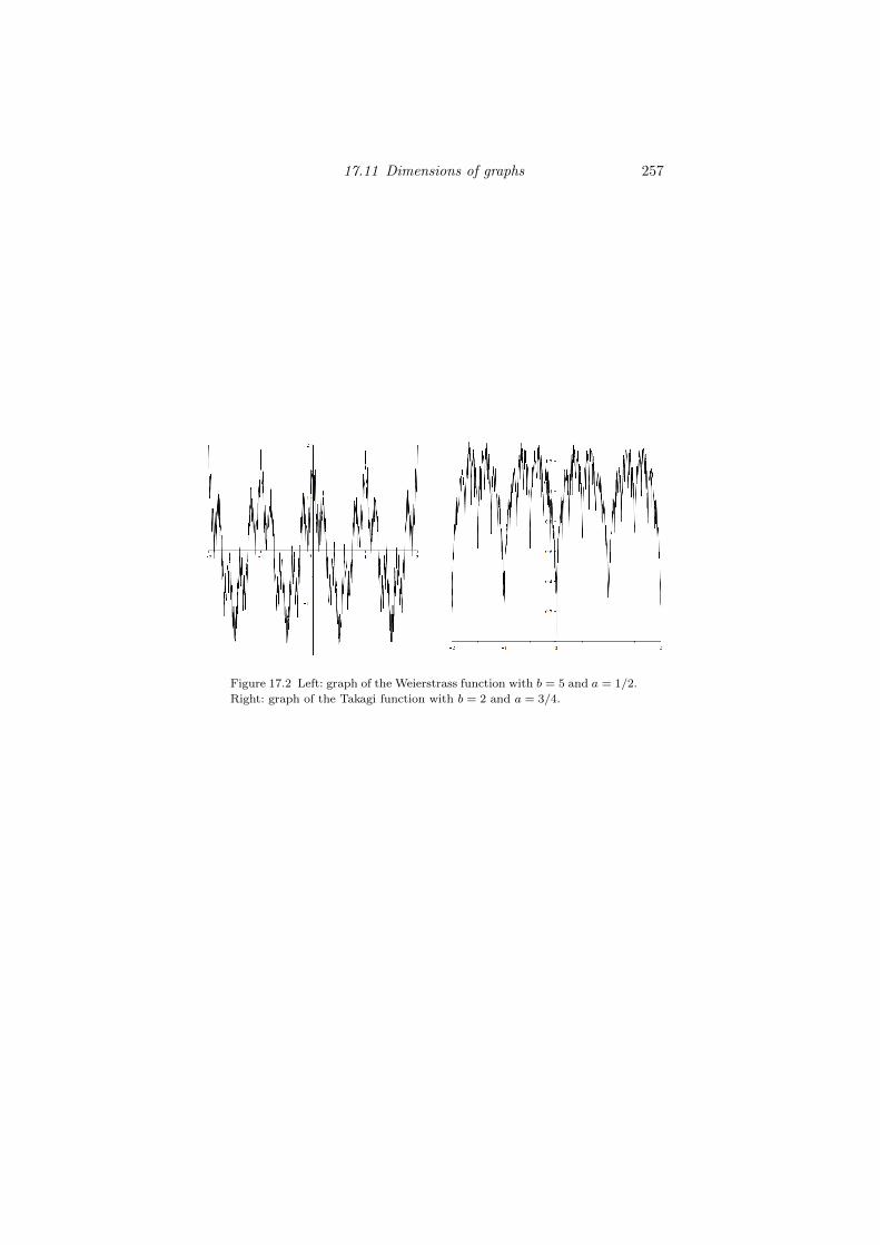
17.11 Dimensions of graphs 257
Figure 17.2 Left: graph of the Weierstrass function with b = 5 and a = 1/2.
Right: graph of the Takagi function with b = 2 and a = 3/4.

References
[1] R. J. Adler. The geometry of random fields, John Wiley & Sons, (1981).
[2] H. Aikawa. Quasiadditivity of Riesz capacity, Math. Scand., 69, (1991),15–30.
[3] P. Allaart and K. Kawamura. The Takagi function: a survey, Real Anal.Ex., 37, (2011), 1–54.
[4] T. C. Anderson, K. Hughes, J. Roos and A. Seeger. Lp →Lq bounds for spherical maximal operators, preprint, available at:https://arxiv.org/abs/1909.05389
[5] J. Angelevska, A. Kaenmaki and S. Troscheit. Self-conformal sets withpositive Hausdorff measure, Bull. Lond. Math. Soc., 52, (2020), 200–223.
[6] P. Assouad. Espaces metriques, plongements, facteurs, These de doctoratd’Etat, Publ. Math. Orsay 223–7769, Univ. Paris XI, Orsay, (1977).
[7] P. Assouad. Etude d’une dimension metrique liee a la possibilite deplongements dans Rn, C. R. Acad. Sci. Paris Ser. A-B, 288, (1979),731–734.
[8] P. Assouad. Plongements lipschitziens dans Rn, Bull. Soc. Math. France,111, (1983), 429–448.
[9] K. B. Athreya. Large deviation rates for branching processes. I. Singletype case, Ann. Appl. Probab., 4, (1994), 779–790.
[10] D. Badziahin and S. Velani. Badly approximable points on planar curvesand a problem of Davenport, Math. Ann., 359, (2014), 969–1023.
[11] S. Baker. Iterated function systems with super-exponentially close cylin-ders, preprint, available at: https://arxiv.org/pdf/1909.04343
[12] R. Balka and Y. Peres. Uniform dimension results for fractional Brownianmotion, J. Fractal Geom., 4, (2017), 147–183.
[13] C. Bandt and S. Graf. Self-similar sets VII. A characterization of self-similar fractals with positive Hausdorff measure, Proc. Amer. Math. Soc.114, (1992), 995–1001.
[14] C. Bandt and A. Kaenmaki. Local structure of self-affine sets, ErgodicTh. Dynam. Syst., 33, (2013), 1326–1337.
[15] K. Baranski. Hausdorff dimension of the limit sets of some planar geo-metric constructions, Adv. Math., 210, (2007), 215–245.
259
260 References
[16] K. Baranski, B. Barany and J. Romanowska. On the dimension of thegraph of the classical Weierstrass function, Adv. Math., 265, (2014), 32–59.
[17] B. Barany. On the Ledrappier-Young formula for self-affine measures,Math. Proc. Cambridge Philos. Soc., 159, (2015), 405–432.
[18] B. Barany, M. Hochman and A. Rapaport. Hausdorff dimension of planarself-affine sets and measures, Invent. Math., 216, (2019), 601–659.
[19] B. Barany and A. Kaenmaki. Ledrappier-Young formula and exact di-mensionality of self-affine measures, Adv. Math., 318, (2017), 88–129.
[20] B. Barany and A. Kaenmaki. Superexponential condensation without ex-act overlaps, preprint, available at: https://arxiv.org/abs/1910.04623
[21] B. Barany, A. Kaenmaki and E. Rossi. Assouad dimension of planar self-affine sets, preprint, available at: https://arxiv.org/pdf/1906.11007
[22] M. F. Barnsley. Fractals Everywhere, Academic Press, (1988).
[23] M. F. Barnsley. Superfractals, Cambridge University Press, Cambridge,(2006).
[24] M. F. Barnsley and S. Demko. Iterated function systems and the globalconstruction of fractals, Proc. R. Soc. Lond. Ser. A, 399, (1985), 243–275.
[25] A. F. Beardon. The geometry of discrete groups, Graduate Texts in Math-ematics, vol. 91, Springer-Verlag, New York, (1983).
[26] T. Bedford. Crinkly curves, Markov partitions and box dimensions in self-similar sets, PhD thesis, University of Warwick, (1984).
[27] V. Beresnevich. Badly approximable points on manifolds, Invent. Math.,202, (2015), 1199–1240.
[28] V. Beresnevich, A. Ghosh, D. Simmons and S. Velani. Diophantine ap-proximation in Kleinian groups: singular, extremal,and bad limit points,J. London Math. Soc., 98, (2018), 306–328.
[29] A. Berlinkov and E. Jarvenpaa. Porosities of Mandelbrot percolation, J.Theoret. Probab., 32, (2019), 608–632.
[30] A.S. Besicovitch. On Kakeya’s problem and a similar one, Math. Z., 27,(1928), 312–320.
[31] A.S. Besicovitch. On the fundamental geometrical properties of linearlymeasurable plane sets of points, III, Math. Ann., 116, (1939), 349–357.
[32] A.S. Besicovitch and H.D. Ursell. Sets of fractional dimensions (V): Ondimensional numbers of some continuous curves, J. London Math. Soc.,12, (1937), 18–25.
[33] C. J. Bishop and P. W. Jones. Hausdorff dimension and Kleinian groups,Acta Math., 179, (1997), 1–39.
[34] C. J. Bishop and Y. Peres. Fractals in Probability and Analysis, Cam-bridge studies in advanced mathematics, 162, Cambridge, (2017).
[35] M.G. Bouligand. Ensembles Impropres et Nombre Dimensionnel, Bull.Sci. Math. 52, (1928), 320–344, 361–376.
[36] B. H. Bowditch. Geometrical finiteness for hyperbolic groups, J. Funct.Anal., 113, (1993), 245–317.
[37] D. W. Boyd. The residual set dimension of the Apollonian packing, Math-ematika, 20, (1973), 170–174.
References 261
[38] R. Broderick, L. Fishman, D. Kleinbock, A. Reich and B. Weiss. The setof badly approximable vectors is strongly C1 incompressible, Math. Proc.Cambridge Philos. Soc., 153, (2012), 319–339.
[39] S. A. Burrell. On the dimension and measure of inhomogeneous attrac-tors, Real Anal. Ex., 44, (2019), 199–216.
[40] P. Bylund and J. Gudayol. On the existence of doubling measures withcertain regularity properties, Proc. Amer. Math. Soc., 128, (2000), 3317–3327.
[41] H.-P. Chen, Y.-L. Du and C. Wei. Quasi-Lower Dimension and Quasi-Lipschitz Mapping, Fractals, (2017).
[42] H.-P. Chen, M. Wu and Y. Chang. Lower Assouad type dimensions ofuniformly perfect sets in doubling metric spaces, preprint, available at:https://arxiv.org/abs/1807.11629
[43] J. T. Cox and P. S. Griffin. How porous is the graph of Brownian motion,Trans. Amer. Math. Soc., 325, (1991), 119–140.
[44] C. D. Cutler. Strong and weak duality principles for fractal dimensionin Euclidean space, Math. Proc. Cambridge Philos. Soc., 118, (1995),393–410.
[45] T. Das, L. Fishman, D. Simmons and M. Urbanski. Badly approximablepoints on self-affine sponges and the lower Assouad dimension, ErgodicTh. Dynam. Syst., 39, (2019), 638–657.
[46] T. Das, L. Fishman, D. Simmons and M. Urbanski. Badly approximablevectors and fractals defined by conformal dynamical systems, Math. Res.Lett., 25, (2018), 437–467.
[47] T. Das, L. Fishman, D. Simmons and M. Urbanski. Extremality anddynamically definedmeasures, part I: Diophantine properties of quasi-decaying measures, Selecta Math., 24, (2017), 2165–2206.
[48] T. Das, L. Fishman, D. Simmons and M. Urbanski. Extremality and dy-namically defined measures, part II: Measures from conformal dynamicalsystems, preprint, available at: https://arxiv.org/pdf/1508.05592
[49] T. Das and D. Simmons. The Hausdorff and dynamical dimensions ofself-affine sponges: a dimension gap result, Invent. Math., 210, (2017),85–134.
[50] H. Davenport. A note on Diophantine approximation. II, Mathematika,11, (1964), 50–58.
[51] R. O. Davies. Some remarks on the Kakeya problem, Math. Proc. Cam-bridge Philos. Soc., 69, (1971), 417–421.
[52] Q.-R. Deng and S.-M. Ngai. Conformal iterated function systems withoverlaps, Dyn. Syst., 26, (2011), 103–123.
[53] L. van den Dries. The field of reals with a predicate for the powers oftwo, Manuscripta Math., 54, (1985), 187–195.
[54] L. van den Dries and C. Miller. Geometric categories and o-minimal struc-tures, Duke Math. J., 84, (1996), 497–540.
[55] X. Du, L. Guth, Y. Ou, H. Wang, B. Wilson and R. Zhang. Weightedrestriction estimates and application to Falconer distance set problem,preprint, available at: https://arxiv.org/abs/1802.10186
262 References
[56] X. Du and R. Zhang. Sharp L2 estimate of Schrodinger max-imal function in higher dimensions, preprint, available at:https://arxiv.org/abs/1805.02775
[57] B. Dyda, J. Lehrback and A. Vahakangas. Fractional Hardy-Sobolev typeinequalities for half spaces and John domains, Proc. Amer. Math. Soc.,146, (2018), 3393–3402.
[58] B. Dyda, L. Ihnatsyeva, J. Lehrback, H. Tuominen and A. Vahakangas.Muckenhoupt Ap-properties of distance functions and applications toHardy-Sobolev-type inequalities, Potential Anal., 50, (2019), 83–105.
[59] E. M. Dynkin. Free interpolation by functions with derivatives in H1, J.Soviet Math., 27, (1984), 2475–2481.
[60] G. A. Edgar. Measure, Topology and Fractal Geometry, Springer-Verlag,(1990).
[61] G. A. Edgar. Classics on Fractals, Addison-Wesley, (1993).[62] P. Erdos and P. Turan. On some sequences of integers, J. Lond. Math.
Soc., 11, (1936), 261–264.[63] K. J. Falconer. On the Hausdorff dimensions of distance sets, Mathe-
matika, 32, (1985), 206–212.[64] K. J. Falconer. The Geometry of Fractal Sets, Cambridge University
Press, (1985).[65] K. J. Falconer. The Hausdorff dimension of self-affine fractals, Math. Proc.
Camb. Phil. Soc., 103, (1988), 339–350.[66] K. J. Falconer. Dimensions and measures of quasi self-similar sets, Proc.
Amer. Math. Soc., 106, (1989), 543–554.[67] K. J. Falconer. The Hausdorff dimension of self-affine fractals II, Math.
Proc. Camb. Phil. Soc., 111, (1992), 169–179.[68] K. J. Falconer. Sub-self-similar sets, Trans. Amer. Math. Soc., 347,
(1995), 3121–3129.[69] K. J. Falconer. Techniques in Fractal Geometry, John Wiley, (1997).[70] K. J. Falconer. Fractal Geometry: Mathematical Foundations and Appli-
cations, John Wiley & Sons, Hoboken, NJ, 3rd. ed., (2014).[71] K. J. Falconer. Dimensions of Self-affine Sets - A Survey, Further De-
velopments in Fractals and Related Fields, Birkhauser, Boston, (2013),115–134.
[72] K. J. Falconer. Fractals - A Very Short Introduction, Oxford UniversityPress, (2013).
[73] K. J. Falconer. A capacity approach to box and packing dimensions ofprojections of sets and exceptional directions, J. Fractal Geom., to ap-pear.
[74] K. J. Falconer, J. M. Fraser and X. Jin. Sixty Years of Fractal Projections,Fractal geometry and stochastics V, (Eds. C. Bandt, K. J. Falconer andM. Zahle), Birkhauser, Progress in Probability, (2015).
[75] K. J. Falconer, J. M. Fraser and A. Kaenmaki. Minkowski dimension formeasures, preprint, available at: https://arxiv.org/abs/2001.07055
[76] K. J. Falconer, J. M. Fraser and P. Shmerkin. Assouad dimension in-fluences the box and packing dimensions of orthogonal projections, J.Fractal Geom., to appear, available at: https://arxiv.org/abs/1911.04857
References 263
[77] K. J. Falconer and J. D. Howroyd. Projection theorems for box and pack-ing dimensions, Math. Proc. Cambridge Philos. Soc., 119, (1996), 287–295.
[78] K. J. Falconer and J. D. Howroyd. Packing dimensions of projectionsand dimension profiles, Math. Proc. Cambridge Philos. Soc., 121, (1997),269–286.
[79] K. J. Falconer and T. Kempton. Planar self-affine sets with equal Haus-dorff, box and affinity dimensions, Ergodic Th. Dynam. Syst., 38, (2018),1369–1388.
[80] K. J. Falconer and P. Mattila. Strong Marstrand theorems and dimensionsof sets formed by subsets of hyperplanes, J. Fractal Geom., 3, (2016),319–329.
[81] A. Farkas and J. M. Fraser. On the equality of Hausdorff measure andHausdorff content, J. Fractal. Geom., 2, (2015), 403–429.
[82] D.-J. Feng. Dimension of invariant measures for affine iterated functionsystems, preprint, available at: https://arxiv.org/abs/1901.01691
[83] D.-J. Feng and Y. Wang. A class of self-affine sets and self-affine measures,J. Fourier Anal. Appl., 11, (2005), 107–124.
[84] A. Ferguson, T. Jordan and P. Shmerkin. The Hausdorff dimension of theprojections of self-affine carpets, Fund. Math., 209, (2010), 193–213.
[85] A. Fish and L. Paunescu. Unwinding spirals, preprint, available at:https://arxiv.org/pdf/1603.03145
[86] J. M. Fraser. On the packing dimension of box-like self-affine sets in theplane, Nonlinearity, 25, (2012), 2075–2092.
[87] J. M. Fraser. Inhomogeneous self-similar sets and box dimensions, StudiaMath., 213, (2012), 133–156.
[88] J. M. Fraser. Assouad type dimensions and homogeneity of fractals,Trans. Amer. Math. Soc., 366, (2014), 6687–6733.
[89] J. M. Fraser. Distance sets, orthogonal projections, and passing to weaktangents, Israel J. Math., 226, (2018), 851–875.
[90] J. M. Fraser. A nonlinear projection theorem for Assouad dimension andapplications, preprint, available at: https://arxiv.org/pdf/2004.12001
[91] J. M. Fraser. Almost arithmetic progressions in the primes and otherlarge sets, Amer. Math. Monthly, 126, (2019), 553–558.
[92] J. M. Fraser. Regularity of Kleinian limit sets and Patterson-Sullivanmeasures, Trans. Amer. Math. Soc., 372, (2019), 4977–5009.
[93] J. M. Fraser. On Holder solutions to the spiral winding problem, preprint,available at: https://arxiv.org/pdf/1905.07563
[94] J. M. Fraser. Interpolating between dimensions, Fractal geometry andstochastics VI, to appear, Birkhauser, Progress in Probability, (2019),available at: https://arxiv.org/abs/1905.11274
[95] J. M. Fraser, K. E. Hare, K. G. Hare, S. Troscheit and H. Yu. The Assouadspectrum and the quasi-Assouad dimension: a tale of two spectra, Ann.Acad. Sci. Fenn. Math., 44, (2019), 379–387.
[96] J. M. Fraser, A. M. Henderson, E. J. Olson and J. C. Robinson. On theAssouad dimension of self-similar sets with overlaps, Adv. Math., 273,(2015), 188–214.
264 References
[97] J. M. Fraser and D. C. Howroyd. Assouad type dimensions for self-affinesponges, Ann. Acad. Sci. Fenn. Math., 42, (2017), 149–174.
[98] J. M. Fraser and D. C. Howroyd. On the upper regularity dimensions ofmeasures, Indiana Univ. Math. J., 69, (2020), 685–712.
[99] J. M. Fraser, D. C. Howroyd, A. Kaenmaki and H. Yu. On the Hausdorffdimension of microsets, Proc. Amer. Math. Soc., 147, (2019), 4921–4936.
[100] J. M. Fraser, D. C. Howroyd and H. Yu. Dimension growth for iteratedsumsets, Math. Z., 293, (2019), 1015–1042.
[101] J. M. Fraser and T. Jordan. The Assouad dimension of self-affine carpetswith no grid structure, Proc. Amer. Math. Soc., 145, (2017), 4905–4918.
[102] J. M. Fraser and N. Jurga. The packing dimension of exceptional self-affine sets in R3, preprint, available at: https://arxiv.org/abs/1907.07593
[103] J. M. Fraser and A. Kaenmaki. Attainable values for the Assouad di-mension of projections, Proc. Amer. Math. Soc., to appear, available at:https://arxiv.org/pdf/1811.00951
[104] J. M. Fraser, J. J. Miao and S. Troscheit. The Assouad dimension ofrandomly generated fractals, Ergodic Th. Dynam. Syst., 38, (2018), 982–1011.
[105] J. M. Fraser, E. J. Olson and J. C. Robinson. Some results in supportof the Kakeya conjecture, Real Anal. Ex., 42, (2017), 253–268.
[106] J. M. Fraser and T. Orponen. The Assouad dimensions of projections ofplanar sets, Proc. Lond. Math. Soc., 114, (2017), 374–398.
[107] J. M. Fraser, K. Saito and H. Yu. Dimensions of sets which uniformlyavoid arithmetic progressions, Int. Math. Res. Not., (2019), 4419–4430.
[108] J. M. Fraser and S. Troscheit. The Assouad spectrum of random self-affine carpets, preprint, available at: https://arxiv.org/abs/1805.04643
[109] J. M. Fraser and S. Troscheit. Smoothness versus regularity of measures,preprint, available at: https://arxiv.org/abs/1912.07292
[110] J. M. Fraser and H. Yu. Arithmetic patches, weak tangents, and dimen-sion, Bull. Lond. Math. Soc., 50, (2018), 85–95.
[111] J. M. Fraser and H. Yu. New dimension spectra: finer information onscaling and homogeneity, Adv. Math., 329, (2018), 273–328.
[112] J. M. Fraser and H. Yu. Assouad type spectra for some fractal families,Indiana Univ. Math. J., 67, (2018), 2005–2043.
[113] J. M. Fraser and H. Yu. Approximate arithmetic structure in large setsof integers, preprint, available at: https://arxiv.org/abs/1905.05034
[114] H. Furstenberg. Intersections of Cantor sets and transversality ofsemigroups, Problems in Analysis (Princeton Mathematical Series, 31).(1970), 41–59.
[115] H. Furstenberg. Ergodic fractal measures and dimension conservation,Ergodic Th. Dynam. Syst., 28, (2008), 405–422.
[116] H. Furstenberg. Ergodic theory and fractal geometry, CBMS RegionalConference Series in Mathematics, 120, American Mathematical Society,Providence, RI, (2014).
[117] I. Garcıa. Assouad dimension and local structure of self-similar sets withoverlaps in Rd, preprint, available at: https://arxiv.org/abs/1909.03148
References 265
[118] I. Garcıa and K. E. Hare. Properties of Quasi-Assouad dimension,preprint, available at: https://arxiv.org/abs/1703.02526
[119] I. Garcıa, K. E. Hare and F. Mendivil. Assouad dimensions of com-plementary sets, Proc. Roy. Soc. Edin. , to appear, available at:https://arxiv.org/abs/1604.01234
[120] I. Garcıa, K. E. Hare and F. Mendivil. Intermediate Assouad-like di-mensions, preprint, available at: https://arxiv.org/abs/1903.07155
[121] I. Garcıa, K. E. Hare and F. Mendivil. Almost sure Assouad-like dimensions of complementary sets, preprint, available at:https://arxiv.org/abs/1903.07800
[122] D. Gatzouras and S. P. Lalley. Hausdorff and box dimensions of certainself-affine fractals, Indiana Univ. Math. J., 41, (1992), 533–568.
[123] B. Green and T. Tao. The primes contain arbitrarily long arithmeticprogressions, Ann. Math., 167, (2008), 481–547.
[124] L. Guth, A. Iosevich, Y. Ou and H. Wang. On Falconer’s distance setproblem in the plane, Invent. Math., 219, (2020), 779–830.
[125] K. E. Hare, K. G. Hare and S. Troscheit. Quasi-doubling of self-similar measures with overlaps, J. Fractal Geom., to appear, availableat arXiv:1807.09198
[126] K. E. Hare, F. Mendivil and L. Zuberman. Measures with speci-fied support and arbitrary Assouad dimensions, preprint, available at:https://arxiv.org/abs/1908.04592
[127] K. E. Hare and S. Troscheit. Lower Assouad dimension of measuresand regularity, Math. Proc. Camb. Phil. Soc., to appear, available at:https://arxiv.org/abs/1812.05573
[128] M. Hata. On some properties of set-dynamical systems, Proc. JapanAcad. Ser. A, 61, (1985), 99–102.
[129] F. Hausdorff. Dimension und außeres Maß, Math. Ann., 79, (1918), 157–179.
[130] J. Heinonen. Lectures on Analysis on Metric Spaces, Springer-Verlag,New York, (2001).
[131] P. Hieronymi and C. Miller. Metric dimensions and tameness in expan-sions of the real field, Trans. Amer. Math. Soc., 373, (2019), 849–874.
[132] M. Hochman. On self-similar sets with overlaps and inverse theoremsfor entropy, Ann. Math., 180, (2014), 773–822.
[133] M. Hochman. On self-similar sets with overlaps and inverse theoremsfor entropy in Rd, Mem. Amer. Math. Soc., to appear, available at:https://arxiv.org/abs/1503.09043
[134] M. Hochman. Dynamics on fractals and fractal distributions, preprint,available at: https://arxiv.org/abs/1008.3731
[135] M. Hochman and A. Rapaport. Hausdorff dimension of planarself-affine sets and measures with overlaps, preprint, available athttps://arxiv.org/abs/1904.09812
[136] M. Hochman and P. Shmerkin. Local entropy averages and projectionsof fractal measures, Ann. Math., 175, (2012), 1001–1059.
[137] W. Hodges. Model theory, Encyclopedia of Mathematics and its Appli-cations, 42, Cambridge University Press, Cambridge, 1993.
266 References
[138] J. M. Howie. Real analysis, Springer Undergraduate Mathematics Series.Springer-Verlag London, Ltd., London, (2001).
[139] D. C. Howroyd. Assouad type dimensions for certain sponges with aweak coordinate ordering condition, J. Fractal Geom., 6, (2019), 67–88.
[140] D. C. Howroyd. Regularity dimensions: quantifying doubling and uni-form perfectness, preprint, available at: https://arxiv.org/abs/1910.14074
[141] D. C. Howroyd and H. Yu. Assouad dimension of random processes,Proc. Edin. Math. Soc., 62, (2019), 281–290.
[142] J. D. Howroyd. On Hausdorff and packing dimension of product spaces,Math. Proc. Cambridge Philos. Soc., 119, (1996), 715–727.
[143] J. D. Howroyd. Box and packing dimensions of projections and dimen-sion profiles, Math. Proc. Cambridge Philos. Soc., 130, (2001), 135–160.
[144] T.Y. Hu and K.S. Lau. Fractal dimensions and singularities of the Weier-strass type functions, Trans. Amer. Math. Soc., 335, (1993), 649–665.
[145] J. E. Hutchinson. Fractals and self-similarity, Indiana Univ. Math. J.,30, (1981), 713–747.
[146] M. Jarvenpaa. On the upper Minkowski dimension, the packing dimen-sion, and orthogonal projections, Ann. Acad. Sci. Fenn. A Dissertat., 99,(1994).
[147] E. Jarvenpaa, M. Jarvenpaa, A. Kaenmaki, T. Rajala, S. Rogovin andV. Suomala. Packing dimension and Ahlfors regularity of porous sets inmetric spaces, Math. Z., 266, (2010), 83–105.
[148] P. Jarvi and M. Vuorinen. Uniformly perfect sets and quasiregular map-pings, J. London Math. Soc., 54, (1996), 515–529.
[149] H. Joyce and D. Preiss. On the existence of subsets of finite positivepacking measure, Mathematika, 42, (1995), 15–24.
[150] T. Jordan and N. Jurga. Self-affine sets with non-compactly supportedrandom perturbations, Ann. Acad. Sci. Fen. Math., 39, (2014), 771–785.
[151] A. Kaenmaki, H. Koivusalo and E. Rossi. Self-affine sets with fibredtangents, Ergodic Th. Dynam. Syst., 37, (2017), 1915–1934.
[152] A. Kaenmaki and J. Lehrback. Measures with predetermined regularityand inhomogeneous self-similar sets, Ark. Mat., 55, (2017), 165–184.
[153] A. Kaenmaki, J. Lehrback and M. Vuorinen. Dimensions, Whitney cov-ers, and tubular neighborhoods, Indiana Univ. Math. J., 62, (2013),1861–1889.
[154] A. Kaenmaki, T. Ojala, and E. Rossi. Rigidity of quasisymmetric map-pings on self-affine carpets, Int. Math. Res. Not. IMRN, 12, (2018), 3769–3799.
[155] A. Kaenmaki and E. Rossi. Weak separation condition, Assouad dimen-sion, and Furstenberg homogeneity, Ann. Acad. Sci. Fenn. Math., 41,(2016), 465–490.
[156] J.-P. Kahane. Some random series of functions, Second edition. Cam-bridge Studies in Advanced Mathematics, 5. Cambridge University Press,Cambridge, (1985).
[157] M. Kapovich. Kleinian groups in higher dimensions, Geometry and dy-namics of groups and spaces, 487–564, Progr. Math., 265, Birkhauser,Basel, (2008).
References 267
[158] N. H. Katz and T. Tao. Recent progress on the Kakeya conjecture,Publ. Mat., Proceedings of the 6th International Conference on HarmonicAnalysis, (2002), 161–179.
[159] Y. Katznelson, N. Subhashis and D. Sullivan. On conformal weldinghomeomorphisms associated to Jordan curves, Ann. Acad. Sci. Fenn.Math., 15, (1990), 293–306.
[160] R. Kaufman. On Hausdorff dimension of projections, Mathematika, 15,(1968), 153–155.
[161] R. Kaufman. Une propriete metrique du mouvement brownien, C. R.Acad. Sci. Paris Ser. A-B, 268, (1969), A727–A728.
[162] R. Kaufman and P. Mattila. Hausdorff dimension and exceptional sets oflinear transformations, Ann. Acad. Sci. Fenn. Math., 1, (1975), 387–392.
[163] A. Kechris. Classical descriptive set theory, Graduate Texts in Mathe-matics, 156, Springer-Verlag, New York, (1995).
[164] S. Keith and T. Laakso. Conformal Assouad dimension and modulus,Geom. Funct. Anal., 14, (2004), 1278–1321.
[165] T. Keleti. Are lines much bigger than line segments? Proc. Amer. Math.Soc., 144, (2016), 1535–1541.
[166] T. Keleti, D. Nagy and P. Shmerkin. Squares and their centers, J. Anal.Math., 134, (2018), 643–669.
[167] T. Keleti and P. Shmerkin. New bounds on the dimensions of planardistance sets, Geom. Funct. Anal., 29, (2019), 1886–1948.
[168] R. Kenyon and Y. Peres. Measures of Full dimension on Affine-InvariantSets, Ergodic Th. Dynam. Syst., 16, (1996), 307–323.
[169] J. Kigami. Quasisymmetric modification of metrics on self-similar sets,Geometry and analysis of fractals, 88, Springer Proc. Math. Stat., 253–282, Springer, Heidelberg, (2014).
[170] J. F. King. The singularity spectrum for general Sierpinski carpets, Adv.Math., 116, (1995), 1–11.
[171] D. Kleinbock and B. Weiss. Badly approximable vectors on fractals,Israel J. Math., 149, (2005), 137–170.
[172] I. Kolossvary and K. Simon. Triangular Gatzouras-Lalley-type planarcarpets with overlaps, Nonlinearity, 32, (2019), 3294–3341.
[173] S.V. Konyagin and A.L. Vol’berg. On measures with the doubling con-dition, Math. USSR-Izv., 30, (1988), 629–638.
[174] R. Korte and N. Shanmugalingam. Equivalence and self-improvement ofp-fatness and Hardy’s inequality, and association with uniform perfect-ness, Math. Z., 264, (2010), 99–110.
[175] P. Koskela and X. Zhong. Hardy’s inequality and the boundary size,Proc. Amer. Math. Soc., 131, (2003), 1151–1158.
[176] J. Kwapisz. Conformal dimension via p-resistance: Sierpinski carpet,preprint, (2017).
[177] T. Laakso. Plane with A∞-weighted metric not bi-Lipschitz embeddableto Rn, Bull. London Math. Soc., 34, (2002), 667–676.
[178] U. Lang and C. Plaut. Bilipschitz embeddings of metric spaces into spaceforms, Geom. Dedicata, 87, (2001), 285–307.
268 References
[179] D. G. Larman. A new theory of dimension, Proc. London Math. Soc.(3), 17, (1967), 178–192.
[180] D. G. Larman. On Hausdorff measure in finite dimensional compactmetric spaces, Proc. London Math. Soc. (3), 17, (1967), 193–206.
[181] K.-S. Lau and S.-M. Ngai. Multifractal measures and a weak separationproperty, Adv. Math., 141, (1999), 45–96.
[182] E. Le Donne and T. Rajala. Assouad dimension, Nagata dimension, anduniformly close metric tangents, Indiana Univ. Math. J., 64, (2015),21–54.
[183] F. Ledrappier and L.-S. Young. The metric entropy of diffeomorphisms.I. Characterization of measures satisfying Pesin’s entropy formula, Ann.Math., 122, (1985), 509–539.
[184] F. Ledrappier and L.-S. Young.The metric entropy of diffeomorphisms.II. Relations between entropy, exponents and dimension, Ann. Math.,122, (1985), 540–574.
[185] J. Lehrback. Pointwise Hardy inequalities and uniformly fat sets, Proc.Amer. Math. Soc., 136, (2008), 2193–2200.
[186] J. Lehrback. Hardy inequalities and Assouad dimensions, J. Anal.Math., 131, (2017), 367–398.
[187] J. Lehrback. Assouad type dimensions and applications, Fractal geom-etry and stochastics VI, to appear, Birkhauser, Progress in Probability,(2019).
[188] J. Lehrback and H. Tuominen. A note on the dimensions of Assouadand Aikawa, J. Math. Soc. Japan, 65, (2013), 343–356.
[189] J. Lehrback and A. Vahakangas. In between the inequalities of Sobolevand Hardy, J. Funct. Anal., 271, (2016), 330–364.
[190] H. Li, C. Wei and S. Wen. Doubling Property of Self-affine Measures onCarpets of Bedford and McMullen, Indiana Univ. Math. J., 65, (2016),833–865.
[191] F. Lu and L. Xi. Quasi-Assouad dimension of fractals, J. Fractal Geom.,3, (2016), 187–215.
[192] J. Luukkainen. Assouad dimension: antifractal metrization, porous sets,and homogeneous measures, J. Korean Math. Soc., 35, (1998), 23–76.
[193] J. Luukkainen and E. Saksman. Every complete doubling metric spacecarries a doubling measure, Proc. Amer. Math. Soc., 126, (1998), 531–534.
[194] J. M. Mackay. Assouad dimension of self-affine carpets, Conform. Geom.Dyn. 15, (2011), 177–187.
[195] J. M. Mackay and J. T. Tyson. Conformal dimension: Theory and ap-plication, University Lecture Series, 54. American Mathematical Society,Providence, RI, (2010).
[196] D. Macpherson. Notes on o-minimality and variations. Model theory, al-gebra, and geometry, 97–130, Math. Sci. Res. Inst. Publ., 39, CambridgeUniv. Press, Cambridge, 2000.
[197] B. B. Mandelbrot. The Fractal Geometry of Nature, Freeman, (1982).[198] B. B. Mandelbrot and J. W. van Ness. Fractional Brownian motions,
fractional noises and applications, SIAM Review, 10, (1968), 422–437.
References 269
[199] A. Margaris. Dimensions, Embeddings, and Iterated Function Systems,PhD thesis, The University of Warwick, (2019).
[200] A. Margaris. Almost bi-Lipschitz embeddings using cov-ers of balls centred at the origin, preprint, available at:https://arxiv.org/abs/2001.02607
[201] J. M. Marstrand. Some fundamental geometrical properties of plane setsof fractional dimensions, Proc. London Math. Soc.(3), 4, (1954), 257–302.
[202] J. M. Marstrand. The dimension of Cartesian product sets. Proc. Cam-bridge Philos. Soc., 50, (1954), 198–202.
[203] B. Maskit. Kleinian groups, Grundlehren der Mathematischen Wis-senschaften [Fundamental Principles of Mathematical Sciences], 287,Springer-Verlag, Berlin, (1988).
[204] P. Mattila. Hausdorff dimension, orthogonal projections and intersec-tions with planes, Ann. Acad. Sci. Fenn. A Math. 1 (1975), 227–244.
[205] P. Mattila. Geometry of sets and measures in Euclidean spaces, Cam-bridge studies in advanced mathematics, 44, Cambridge University Press,(1995).
[206] P. Mattila. Recent progress on dimensions of projections, in Geometryand Analysis of Fractals, D.-J. Feng and K.-S. Lau (eds.), pp 283–301,Springer Proceedings in Mathematics & Statistics. 88, Springer-Verlag,Berlin Heidelberg, (2014).
[207] P. Mattila. Fourier analysis and Hausdorff dimension, Cambridge stud-ies in advanced mathematics, 150, Cambridge, (2015).
[208] P. Mattila and R. D. Mauldin. Measure and dimension functions: mea-surability and densities, Math. Proc. Camb. Phil. Soc., 121, (1997), 81–100.
[209] J. McLaughlin. A note on Hausdorff measures of quasi-self-similar sets,Proc. Amer. Math. Soc., 100, (1987), 183–186.
[210] C. McMullen. The Hausdorff dimension of general Sierpinski carpets,Nagoya Math. J., 96, (1984), 1–9.
[211] C. McMullen. Hausdorff dimension and conformal dynamics. III. Com-putation of dimension, Amer. J. Math., 120, (1998), 691–721.
[212] C. Miller and P. Speissegger. Expansions of the real field bycanonical products, Canadian Math. Bull., to appear, available at:https://arxiv.org/abs/1812.05547
[213] P. A. P. Moran. Additive functions of intervals and Hausdorff measure,Math. Proc. Camb. Phil. Soc., 42, (1946), 15–23.
[214] P. Morters and Y. Peres. Brownian Motion, with an appendix by O.Schramm and W. Werner, Cambridge University Press, (2010).
[215] A. Naor and O. Neiman. Assouad’s theorem with dimension independentof the snowflaking, Rev. Mat. Iberoamercana, 28, (2012), 1–21.
[216] T. Ojala. Thin and Fat sets: geometry of doubling measures in metricspaces, PhD thesis, University of Jyvaskyla, (2014).
[217] L. Olsen. A multifractal formalism, Adv. Math., 116, (1995), 82–196.
[218] L. Olsen. Self-affine multifractal Sierpinski sponges in Rd, Pacific J.Math, 183, (1998), 143–199.
270 References
[219] L. Olsen. On the Assouad dimension of graph directed Moran fractals,Fractals, 19, (2011), 221–226.
[220] L. Olsen and N. Snigireva. Lq spectra and Renyi dimensions of in-homogeneous self-similar measures, Nonlinearity, 20, (2007), 151–175.
[221] E. Olson. Bouligand dimension and almost Lipschitz embeddings, Pa-cific J. Math., 202, (2002), 459–474.
[222] E. J. Olson and J. C. Robinson. Almost bi-Lipschitz embeddings andalmost homogeneous sets, Trans. Amer. Math. Soc., 362, (2010), 145–168.
[223] E. Olson and J. C. Robinson. A simple example concerning the upperbox-counting dimension of a cartesian product, Real Anal. Ex., to appear.
[224] E. Olson, J. C. Robinson and N. Sharples. Generalised Cantor sets andthe dimension of products, Math. Proc. Camb. Phil. Soc., 160, (2016),51–75.
[225] T. Orponen. On the distance sets of Ahlfors-David regular sets, Adv.Math., 307, (2017), 1029–1045.
[226] T. Orponen. On the Assouad dimension of projections, Proc. Lond.Math. Soc., to appear, available at: https://arxiv.org/abs/1902.04993
[227] P. Pansu. Metriques de Carnot-Caratheodory et quasiisometries des es-paces symetriques de rang un, Ann. Math., 129, (1989), 1–60.
[228] P. Pansu. Dimension conforme et sphere a l’infini des varietes a courburenegative, Ann. Acad. Sci. Fenn. Math., 14, (1989), 177–212.
[229] J. R. Parker. Kleinian circle packings, Topology, 34, (1995), 489–496.[230] S. J. Patterson. The limit set of a Fuchsian group, Acta Math., 136,
(1976), 241–273.[231] Y. Peres, M. Rams, K. Simon and B. Solomyak. Equivalence of positive
Hausdorff measure and the open set condition for self-conformal sets,Proc. Amer. Math. Soc., 129, (2001), 2689–2699.
[232] Y. Peres, K. Simon and B. Solomyak. Self-similar sets of zero Hausdorffmeasure and positive packing measure, Israel J. Math., 117, (2000), 353–379.
[233] Y. Peres and B. Solomyak Problems on self-similar sets and self-affine sets: an update, Fractal geometry and stochastics, II (Greif-swald/Koserow, 1998), 95–106, Progr. Probab., 46, Birkhauser, Basel,(2000).
[234] Y. B. Pesin. Dimension Theory in Dynamical Systems: ContemporaryViews and Applications, Univ. of Chicago Press, (1997).
[235] E. Pinto de Moura and J. C. Robinson. Orthogonal sequences and regu-larity of embeddings into finite-dimensional spaces, J. Math. Anal. Appl.,368, (2010), 254–262.
[236] M. Pollicott. Apollonius circle counting, London Math. Soc. Newsletter,478, (2018), 31–34.
[237] F. Przytycki and M. Urbanski. On the Hausdorff dimension of somefractal sets, Studia Math., 93, (1989), 155–186.
[238] M. Rams and K. Simon. The geometry of fractal percolation, Geom-etry and analysis of fractals, 303–323, Springer Proc. Math. Stat., 88,Springer, Heidelberg, (2014).
References 271
[239] M. Rams and K. Simon. Projections of fractal percolations, Ergodic Th.Dynam. Syst., 35, (2015), 530–545.
[240] J. C. Robinson. Dimensions, Embeddings, and Attractors, CambridgeUniversity Press, (2011).
[241] J. C. Robinson. Log-Lipschitz embeddings of homogeneous sets withsharp logarithmic exponents and slicing products of balls, Proc. Amer.Math. Soc., 142, (2014), 1275–1288.
[242] C. A. Rogers. Hausdorff Measures, Cambridge University Press, (1998).[243] E. Rossi and V. Suomala. Fractal percolation and quasisymmetric map-
pings, preprint, available at: https://arxiv.org/abs/1905.11080[244] W. Rudin. Principles of Mathematical Analysis, Third edition. Interna-
tional Series in Pure and Applied Mathematics. McGraw-Hill Book Co.,New York-Auckland-Dusseldorf, (1976).
[245] K. Saito. Construction of a one-dimensional set which asymptoti-cally and omnidirectionally contains arithmetic progressions, J. Fractal.Geom., to appear, available at: https://arxiv.org/abs/1805.12063
[246] A. Salli. On the Minkowski dimension of strongly porous fractal sets inRn, Proc. London Math. Soc., 62, (1991), 353–372.
[247] W. M. Schmidt. On badly approximable numbers and certain games,Trans. Amer. Math. Soc., 123, (1966), 178–199.
[248] W. M. Schmidt. Diophantine approximation, Lecture Notes in Mathe-matics, 785, Springer-Verlag, Berlin, (1980).
[249] A. Seeger, S. Wainger and J. Wright. Pointwise convergence of sphericalmeans, Math. Proc. Cambridge Philos. Soc., 118, (1995), 115–124.
[250] S. Semmes. On the nonexistence of bi-Lipschitz parameterizations andgeometric problems about A∞-weights, Rev. Mat. Iberoamericana, 12,(1996), 337–410.
[251] W.-X. Shen. Hausdorff dimension of the graphs of the classical Weier-strass functions, Math. Z., 289, (2017), 1–44.
[252] P. Shmerkin. On distance sets, box-counting and Ahlfors-regular sets,Discrete Analysis, 9, (2017).
[253] P. Shmerkin. On the Hausdorff dimension of pinned distance sets, IsraelJ. Math., 230, (2019), 949–972.
[254] P. Shmerkin. On Furstenberg’s intersection conjecture, self-similar mea-sures, and the Lq norms of convolutions, Ann. Math., 189, (2019), 319–391.
[255] N. Snigireva. Inhomogeneous self-similar sets and measures, PhD thesis,University of St Andrews, (2008).
[256] B. Solomyak. Measure and dimension for some fractal families, Math.Proc. Camb. Phil. Soc., 124, (1998), 531–546.
[257] I. Stewart and D. Tall. The Foundations of Mathematics, Oxford Uni-versity Press, (1997).
[258] B. O. Stratmann and M. Urbanski. The box-counting dimension forgeometrically finite Kleinian groups, Fund. Math., 149, (1996), 83–93.
[259] B. O. Stratmann and S. L. Velani. The Patterson measure for geomet-rically finite groups with parabolic elements, new and old, Proc. Lond.Math. Soc., 71, (1995), 197–220.
272 References
[260] T. Sugawa. Uniform perfectness of the limit sets of Kleinian groups,Trans. Amer. Math. Soc., 353, (2001), 3603–3615.
[261] D. Sullivan. Entropy, Hausdorff measures old and new, and limit sets ofgeometrically finite Kleinian groups, Acta Math., 153, (1984), 259–277.
[262] V. Suomala. Intermediate value property for the Assouad dimension ofmeasures, preprint, available at: https://arxiv.org/abs/2001.11306
[263] E. Szpilrajn (Marczewski). La dimension et la mesure, Fund. Math., 27,(1937), 81–89.
[264] T. Tao. Embedding the Heisenberg group into a bounded dimen-sional Euclidean space with optimal distortion, preprint, available at:https://arxiv.org/abs/1811.09223
[265] C. Tricot. Two definitions of fractional dimension, Math. Proc. Camb.Phil. Soc., 91, (1982), 57–74.
[266] S. Troscheit. The quasi-Assouad dimension of stochastically self-similarsets, Proc. Roy. Soc. Edinburgh Sect. A, to appear, (2017), available at:https://arxiv.org/abs/1709.02519
[267] S. Troscheit. On quasisymmetric embeddings of the Brownian map andcontinuum trees, preprint, available at: https://arxiv.org/abs/1912.07291
[268] S. Troscheit. Assouad spectrum thresholds for some randomconstructions, Canadian Math. Bull., to appear, available at:https://arxiv.org/abs/1906.02555
[269] J. T. Tyson. Sets of minimal Hausdorff dimension for quasiconformalmaps, Proc. Amer. Math. Soc., 128, (2000), 3361–3367.
[270] J. T. Tyson. Lowering the Assouad dimension by quasisymmetric map-pings, Illinois J. Math., 45, (2001), 641–656.
[271] J. T. Tyson and J.-M. Wu. Quasiconformal dimensions of self-similarfractals, Rev. Mat. Iberoamericana, 22, (2006), 205–258.
[272] M. Urbanski. Parabolic Cantor sets, Fund. Math., 151, (1996), 241–277.[273] J. Vaisala. Porous sets and quasisymmetric maps, Trans. Amer. Math.
Soc., 299, (1987), 525–533.[274] J. C. Vassilicos and J. C. R. Hunt. Fractal dimensions and spectra of
interfaces with application to turbulence, Proc. Roy. Soc. London Ser. A,435, (1991), 505–534.
[275] E. Walsberg. Externally definable quotients and NIP expan-sions of the real ordered additive group, preprint, available at:https://arxiv.org/abs/1910.10572
[276] L.-F. Xi. Quasi-Lipschitz equivalence of fractals, Israel J. Math., 160,(2007), 1-21.
[277] Y. Xiao. Packing dimension of the image of fractional Brownian motion,Statist. Probab. Lett., 33, (1997), 379–387.
[278] F. Xie, Y. Yin and Y. Sun. Uniform perfectness of self-affine sets, Proc.Amer. Math. Soc., 131, (2003), 3053–3057.
[279] H. Yu. Weak tangents and level sets of Takagi functions, preprint, avail-able at: https://arxiv.org/abs/1611.04172
[280] H. Yu. Assouad type dimensions and dimension spectra for some fractalfamilies, PhD thesis, The University of St Andrews, (2019).
[281] H. Yu. Dimensions of triangle sets, Mathematika, 65, (2019), 311–332.
References 273
[282] M. P. W. Zerner. Weak separation properties for self-similar sets, Proc.Amer. Math. Soc., 124, (1996), 3529–3539.
[283] M. Zinsmeister. Thermodynamic Formalism and Holomorphic Dynami-cal Systems, SMF/AMS Texts and Monographs, 2, (1996).
[284] D. Zubrinic and V. Zupanovic. Box dimension of spiral trajectories ofsome vector fields in R3, Qual. Theory Dyn. Syst., 6, (2005), 251–272.

List of notation
Dimensions and spectra
dimφA φ-Assouad dimension
dim an unspecified dimension
dimA Assouad dimension
dimθA Assouad spectrum
dimθA upper (Assouad) spectrum
dimB lower box dimension
dimB upper box dimension
dimB box dimension
CdimA conformal Assouad dimension
CdimH conformal Hausdorff dimension
dimH Hausdorff dimension
dimL lower dimension
dimθL lower spectrum
dimML modified lower dimension
dimP packing dimension
dimqA quasi-Assouad dimension
dimqL quasi-lower dimension
dimT topological dimension
275
276 List of notation
General notation
|x| the absolute value of a real or complex number x
B(x, r) a (usually closed) ball centred at x with radius r
#F cardinality of a set F , which may be finite or infinite
E × F Cartesian product of sets E and F
F closure of a set F
F c complement of a set F (usually with Rd as the ambient space)
C the complex numbers, often identified with the complex plane
Con(d) isometry group of Dd+1
|F | the diameter |F | = supx,y∈F
|x− y| of a set F , which may be finite or infinite
Dd+1 Poincare disk model of d+ 1 dimensional hyperbolic space
D(F ) the distance set D(F ) = |x− y| : x, y ∈ F of a set F
G(k, d) Grassmannian manifold consisting of k-dimensional subspaces of Rd
Hs s-dimensional Hausdorff measure
Hsr r-approximate s-dimensional Hausdorff measure
dH Hausdorff metric
K(X) set of all non-empty compact subsets of a set X
L(Γ) the limit set of a Kleinian group Γ
Ld d-dimensional Lebesgue measure
µ a locally finite Borel measure
Mr(F ) maximum number of points in an r-separated subset of F
N the natural numbers (which do not include 0)
Nr(F ) minimum number of open sets of diameter r required to cover F
O(d) d-dimensional orthogonal group
π an element of G(k, d), which may be identified with an orthogonal projection
π⊥ orthogonal complement of π ∈ G(k, d)
Q the rational numbers
R the real numbers, often identified with the real line
Rd d-dimensional Euclidean space
SO(d) d-dimensional special orthogonal group
supp(µ) support supp(µ) = x : µ(B(x, r)) > 0 for all r > 0 of a measure µ
Z the integers
List of notation 277
Notation relating to iterated function systems
I the identity map
I a finite index set for an iterated function system (IFS)
Ik the set of all sequences of length k with entries in II∗ the set of all finite sequences with entries in I
IN the set of all infinite sequences with entries in I
i− the sequence (i1, i2, . . . , ik−1) for i =(i1, i2, . . . , ik
)∈ Ik
[i ] the cylinder j ∈ IN : i ≺ j for i ∈ Ik
IFS iterated function system
OSC open set condition
Π symbolic coding map associated with an IFS
≺ ‘is a prefix of’, e.g. i ≺ j for i , j ∈ I∗
Q(d, r) approximate square centred at d with radius r
Si the composition Si1 Si2 · · · Sik for i =(i1, i2, . . . , ik
)∈ Ik
SSC strong separation condition
VSSC very strong separation condition
WSP weak separation property
Index
Lp improving, 239
Lp-space, 240
Lq-spectrum, 106
φ-Assouad dimension, 37
p-Hardy inequality, 237
r-separated set, 8
absolute continuity, 240
affine map (affinity), 113
affinity dimension, 115
Ahlfors regularity, 91
Aikawa dimension, 237
almost bi-Lipschitz embedding, 218
Apollonian circle packing, 4, 152
approximate square, 122
arithmetic progression, 221
Assouad dimension, 10
of a measure, 58
of a metric space, 206
Assouad spectrum, 26
of a measure, 62
Assouad’s embedding theorem, 209
badly approximable numbers, 226
Bedford-McMullen carpet, 117
Besicovitch set, 193
bi-Lipschitz function, 18
bi-Lipschitz stability, 18
Bowen’s formula, 143
box dimension, 6
of a measure, 62
Brownian motion, 232
conformal dimension, 197
conformal map, 142
continued fraction, 147
backwards continued fraction, 147
contraction, 83
contraction ratio, 83contractive map, 145
coordinate uniform measure, 136
countable stability, 18cover, 5
definability, 231
difference set, 218
dimension drop, 97dimension profile, 172, 177
capacity approach, 178
Diophantine approximation, 225Dirichlet’s theorem, 98, 191, 225
distance set, 187
conjecture, 187doubling measure, 58
doubling metric space, 206
doubling near the origin, 220Dynkin’s conjecture, 207
entropy, 110
Erdos conjecture, 222
extremality, 230
Falconer’s formula, 115finite stability, 18
fractional Brownian motion, 233
Fuchsian group, 152fully supported measure, 9
gallery, 16Galton-Watson process, 162
Gauss map, 147global measure formula, 153
Grassmannian manifold, 172
Green-Tao theorem, 222
Holder function, 50Holder mapping problem, 254Holder’s inequality, 241
278
Index 279
Hardy’s inequality, 236
Hausdorff dimension, 6
of a measure, 9
Hausdorff measure, 5
Hausdorff metric, 66
Heisenberg group, 209
Hutchinson operator, 84
Hutchinson-Moran formula, 97
hyperbolic metric, 149
hyperbolic space, 149
hyperplane diffuse, 226
implicit theorems, 92
inhomogeneous self-similar set, 61, 244
interval maps, 144
iterated function system (IFS), 83
attractor, 84
invariant measure, 87
Kakeya set, 193
conjecture, 193
discrete Kakeya set, 225
extended Kakeya set, 194
Kleinian group, 149
limit set, 150, 227
Poincare exponent, 151
Kolmogorov’s 0-1 law, 249
Laakso graphs, 209
large deviations, 162
Ledrappier-Young formula, 137
Lipschitz function, 18
Lipschitz stability, 18
Littlewood polynomial, 255
lituus, 211
locally finite (measure), 57
logarithmic spiral, 210
lower dimension, 23
of a measure, 58
of a metric space, 207
lower spectrum, 26
of a measure, 62
Lyapunov exponent, 110
Mobius group, 149
Mandelbrot percolation, 159
Mandelbrot set, 4
Manneville-Pomeau map, 146
Marstrand’s slicing theorem, 184
Marstrand-Mattila projection theorem,
172
mass distribution principle, 39
McMullen measure, 126, 136
measurability, 246
microset, 16middle third Cantor set, 111
modified Assouad dimension, 234
modified lower dimension, 24monotonicity, 17
Muckenhoupt weights, 237
neighbourhood (of a set), 66
o-minimality, 231open set condition, 85
open set property, 18
orthogonal projection, 171
packing (centred) , 8
packing dimension, 7of a measure, 9
parabolic Cantor set, 146
parabolic point, 145, 153rank, 153
Patterson-Sullivan measure, 153
percolation, 159, 200pinned distance set, 253
popcorn function, 46
porosity, 73pressure, 143
product, 165measures, 166
quasi-Assouad dimension, 25quasi-Lipschitz function, 25
quasi-lower dimension, 36
quasi-self-similarity, 92quasi-symmetry, 196
Renyi map, 147Radon-Nikodym derivative, 240
regularity dimension, 57
reverse Holder inequality, 241
Schmidt games, 228
self-affine set, 113Baranski carpet, 119
Przytycki-Urbanski carpet, 129
self-affine carpet, 117, 199, 227self-affine measure, 133
uniform fibres, 118
self-conformal set, 141self-similar set, 96
self-similar measure, 109
semialgebraic set, 230Sierpinski carpet, 97, 201
Sierpinski triangle, 4, 85, 201similarity, 67
similarity ratio, 67, 96
similarity dimension, 96
280 Index
simultaneous realisation problem, 88
for Kleinian groups, 157
for self-affine sets, 136singular value function, 115
slice, 183
snowflaking, 209Sobolev inequality, 237
spherical maximal function, 239
spiral winding problem, 210stability under closure, 18
Stirling’s approximation, 127
strong separation condition, 85support (of a measure), 9
symbolic coding map, 86symbolic space, 86
Szemeredi’s theorem, 221
Takagi function, 255topological dimension, 198
uniformly perfect, 207upper natural density, 222
upper spectrum, 33
very strong separation condition, 135
weak separation property, 101for self-conformal sets, 143
weak tangent, 67
of a measure, 77Weierstrass function, 254